Advanced Architectures and Control Concepts for MORE MICROGRIDS · · 2010-05-25Advanced...
171
Advanced Architectures and Control Concepts for MORE MICROGRIDS Specific Targeted Project Contract No: PL019864 DH2. Report on economic, technical and environmental benefits of Microgrids in typical EU electricity systems WPH. Impact on the Development of Electricity Infrastructure TH2. Quantifying the impact of Microgrids on investment and replacement strategies of future national electricity infrastructure December 2009 Final Version
Transcript of Advanced Architectures and Control Concepts for MORE MICROGRIDS · · 2010-05-25Advanced...

Advanced Architectures and
Control Concepts for
MORE MICROGRIDS
Specific Targeted Project
Contract No: PL019864
DH2. Report on economic, technical and
environmental benefits of Microgrids in
typical EU electricity systems
WPH. Impact on the Development of
Electricity Infrastructure
TH2. Quantifying the impact of Microgrids on investment
and replacement strategies of future national electricity
infrastructure
December 2009
Final Version

MORE MICROGRIDS – WPH, Deliverable DH2
WPH/TH2 Page 2
Document Information
Deliverable: DH2. Report on economic, technical and environmental benefits of
Microgrids in typical EU electricity systems
Task Title: TH2. Quantifying the impact of Microgrids on investment and replacement
strategies of future national electricity infrastructure
Date: December 2009
Coordinator: Goran Strbac [email protected]
Author: Pierluigi Mancarella [email protected]
Contributors Dimitrios Papadaskalopoulos [email protected]
Efthymios Manitsas [email protected]
Chin Kim Gan [email protected]
Danny Pudjianto [email protected]
Marko Aunedi [email protected]
Vladimir Stanojevic [email protected]
Vera Silva [email protected]
Paulo Moisés [email protected]
Manuel Matos [email protected]
João Peças Lopes [email protected]
André Madureira [email protected]
Chiara Michelangeli [email protected]
Nikos Hatziargyriou [email protected]
Anestis Anastasiadis [email protected]
Access:
x
Project Consortium
European Commission PUBLIC
Status: For Information
Draft Version Final Version (internal document)
Submission for Approval (deliverable)
Final Version (deliverable, approved on…)
x

MORE MICROGRIDS – WPH, Deliverable DH2
WPH/TH2 Page 3
Executive Summary
This Deliverable report contains the main findings from the work carried out for Task
TH2: “Quantifying the impact of Microgrids on investment and replacement strategies of
future national electricity infrastructure”, which is the core of Work Package H (WPH) of
the More Microgrids project. In particular, a number of models and relevant studies have
been carried out to investigate the potential impact and benefits of Microgrid operation
on different power system areas of interest, ranging from distribution networks to
conventional generation operation and expansion, with specific reference to typical
European scenarios.
The Deliverable is composed of a main body (the present document) and four Annexes.
The types of analysis performed, the models and tools developed, and the results obtained
are synthetically presented below.
Distribution network studies
In order to quantify the distribution network capacity that could be displaced by micro-
generation operating in Microgrids, Imperial has developed the so called Generic
Distribution System (GDS) model, enabling to represent typical European distribution
networks designed in top-down hierarchical structure. In particular, by analysing multiple
voltage levels, technical, economic and environmental impacts of Microgrids on a system
level can be studied. The tool is based on radial load flow analysis based on typical
generation and load patterns, which allows a better understanding of the relevant drivers
for benefits. The models has been populated by real network data provided by partners
for selected Northern and Central European countries, namely, FYROM, Germany,
Netherlands, Poland, UK, with DG largely characterized by Combined Heat and Power
(CHP) systems. Given the large variety of characteristics, comparison among the
different networks has enabled to strategically highlight common trends and differences.
The main focus of the analysis has been on estimating the reinforcement requirements to
accommodate Distributed Generation (DG) due to voltage, thermal or fault level issues,
as well as the potential benefits owing to postponing the need for upgrading network
capacity to accommodate load growth. Within this scope, different strategies for Active
Management (AM) of the network at different voltage levels have also been considered,
consisting of coordinated control of on-load tap changers, reactive power control and
generation curtailment where needed. In particular, AM strategies have been compared to
a classical fit & forget (passive management - PM) approach, so as to highlight the need
and benefits of controllability both in Microgrids and at higher voltage levels. This type
of studies have been carried out through a Cost Benefit Analysis (CBA) approach,
whereby potential benefits have been evaluated against potential additional operational
cost (namely, losses) and the cost of infrastructure required to implement intelligent
control strategies (communication infrastructure, automatisms, and so on). In this regard,
typical cost for the needed communication infrastructure has been identified. A crucial
outcome of the comparison among different networks and network management
strategies in the presence of DG has been that benefits and impacts, as well as mitigation

MORE MICROGRIDS – WPH, Deliverable DH2
WPH/TH2 Page 4
actions and further benefits brought by AM actions, are strongly related to the strength of
the network.
The studies based on the GDS model have been divided into two groups according to the
scenarios examined, the temporal basis and the methodology undertaken for network
development evaluation.
The first stream of analyses has been based on the data provided by the project partners
regarding the envisaged demand and DG penetration at all voltage levels in a number of
future snapshots. In this case, a dynamic assessment for network development has been
carried out taking optimal decisions on network investment including selection of AM
strategies at different milestone times across the provided scenarios. A schematic flow of
the methodology comparing the case with and without DG is shown in Figure A.1.
Figure A.1. Dynamic network assessment model.
The second stream of analyses is more specific to Microgrids (consisting of a mix of
Micro-CHP and Micro-PV systems) and has involved studies of the impacts of micro-DG
and AM based on the current distribution networks (static assessment). This allows a
straightforward quantification of the sensitivity of Microgrids impacts with respect to the
level of micro-DG penetration (high and low) and of demand (high and low) at LV has
been quantified.
From the different types of analysis run, some key outcomes have been identified, as
summarised below:
- The contribution of micro-generation to decreasing upstream power flows leads to:
substantial value (in terms of capacity release) in the Polish, FYROM, and UK
networks, where reinforcement is demand-driven; zero value in the very strong
Dutch network; negative value in the (also quite strong) German network, where the
envisaged DG penetration is likely to create fault level problems.
- In a similar manner, although the effect of DG on losses was beneficial in most
cases, there are situations in the Dutch network where DG creates significant reverse
power flows and increases distribution losses.
- For relatively weaker networks (Poland, FYROM, UK), in those cases where a part
of the required reinforcement is related to voltage problems the application of active
management reduces significantly the reinforcement cost (in Figure A.2 the case
with PM is even negative since voltage rise due to DG calls for network
reinforcement relative to the case without DG), at the expense of higher losses in the
network (Figure A.3). This is due to the higher network exploitation enabled by AM,
while in the PM case the feeders are upgraded and thus the losses decrease.
MORE MICROGRIDS – WPH, Deliverable DH2
WPH/TH2 Page 5
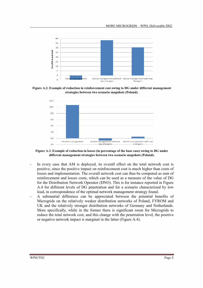
Figure A.2. Example of reduction in reinforcement cost owing to DG under different management
strategies between two scenario snapshots (Poland).
Figure A.3. Example of reduction in losses (in percentage of the base case) owing to DG under
different management strategies between two scenario snapshots (Poland).
- In every case that AM is deployed, its overall effect on the total network cost is
positive, since the positive impact on reinforcement cost is much higher than costs of
losses and implementation. The overall network cost can thus be computed as sum of
reinforcement and losses costs, which can be used as a measure of the value of DG
for the Distribution Network Operator (DNO). This is for instance reported in Figure
A.4 for different levels of DG penetration and for a scenario characterized by low
load, in correspondence of the optimal network management strategy found.
- A substantial difference can be appreciated between the potential benefits of
Microgrids on the relatively weaker distribution networks of Poland, FYROM and
UK and the relatively stronger distribution networks of Germany and Netherlands.
More specifically, while in the former there is significant room for Microgrids to
reduce the total network cost, and this change with the penetration level, the positive
or negative network impact is marginal in the latter (Figure A.4).

MORE MICROGRIDS – WPH, Deliverable DH2
WPH/TH2 Page 6
Figure A.4. Comparative impact of Microgrids on total network cost (reinforcement and losses).
Analyses relevant to Southern European scenarios, with large presence of PV systems,
have been carried out by NTUA for Greece and by ERSE for Italy to complete a
comprehensive picture of different scenarios across Europe. In particular, in the Italian
case the impact of PV-based Microgrids on MV network investment has been assessed at
the design stage through different planning strategies, namely: a) PM; b) probabilistic,
with load and generation hourly profiles; c) considering AM options at a design stage.
The results from the analysis confirm the GDS results for the other countries, yielding
that conventional PM planning approaches lead to higher investment costs due to (worst
case-driven) over-sizing of lines and transformers. On the other hand, if the possibility to
resort to AM options (in this case based on Demand Side Management – DSM – actions)
is considered during the planning process, reduction in investment costs can be observed,
although at the cost of energy losses. If a completely energy-autonomous Microgrids
(resulting in zero active and reactive power flows at the MV/LV substation transformer),
can be set up, further reduction in network upgrading costs and electricity losses can be
achieved. These results are summarised in Figure A.5.
0%
10%
20%
30%
40%
50%
60%
70%
80%
90%
100%
110%
0% 180% 180% with microgrids (100%)
DG penetration [% of residential peak loads]
Costs
[%
of to
tal costs
of re
fere
nce c
ase]
Figure A.5. Comparison of total costs under different planning strategies.
Further network development studies have been run by Imperial through a generic
distribution network model based on fractal topology generation in order to assess the
potential contribution and value of micro-DG for greenfield network design of typical
Daily
patterns
F&F
AM

MORE MICROGRIDS – WPH, Deliverable DH2
WPH/TH2 Page 7
urban areas and rural areas in the UK. The results show that a large number of micro-
sources whose after-diversity production profile is well correlated with the network
demand can contribute significantly to reduce the need for network asset. More
specifically, it clearly emerges how the main driver for benefits is the correlation between
local generation and demand. Therefore, CHP systems can bring substantial benefits in
Northern scenarios to help support local demand and saving upstream network asset,
while the potential of PV is restricted in this sense, due to the scarce correlation with
peak load (typically occurring in winter). Controlling dispatchable DG such as micro-
CHP to modulate their generation pattern to adapt to the electrical demand can bring
further benefits.
The order of magnitude of the overall network benefits (network asset and losses) relative
to a base case in which the distribution network is designed without DG is shown in
Table A.1, pointing out that while PV can contribute to network cost reduction by some
10% only (mostly owing to losses reduction), controllable systems can reduce the
network cost by up to one third (corresponding to an annual network cost of about 11
£/kW of peak load). In particular, controllability can bring additional benefits up to 13%
or some 4 £/kW of peak load, as further illustrated in Figure A.6, with the breakdown of
cost reduction per voltage level. The network infrastructure savings due to reduced power
flows can be substantial, with prevailing influence on transformers in urban areas and
overhead lines in rural areas.
Table A.1. Overall value of DG in percentage of the no-DG case (urban network).
Scenarios 0 10 20 30 50 100
PV 0.0 2.8 4.2 6.1 8.4 10.6
Uncontrolled CHP 0.0 4.7 8.3 12.0 17.3 23.7
Controlled CHP 0.0 5.5 8.7 12.7 20.1 36.3
DG penetration levels (%)
0
2
4
6
8
10
12
14
0 10 20 30 50 100
£/k
W/y
ea
r
DG penetration level (%)
33kV 11kV LV
0
2
4
6
8
10
12
14
0 10 20 30 50 100
£/k
W/
ye
ar
DG penetration level (%)
33kV 11kV LV
Figure A.6. Network value of uncontrolled (left) and controlled (right) CHP (UK urban networks).
While the absolute value of DG increases with the penetration (defined here as dwellings
with micro-DG relative to overall dwellings in the network) level, its specific value
normalized with respect to DG installed capacity decreases and saturates relatively soon
(Figure A.7). It is however interesting to show how the value of controllability changes
for different penetration levels, with the maximum value of controllability in the order of

MORE MICROGRIDS – WPH, Deliverable DH2
WPH/TH2 Page 8
50 £/kWDG in urban areas for 100% penetration level, while for rural areas the figure is in
the order of 30 £/kWDG for penetration higher than 30%.
0
50
100
150
200
250
10 20 30 50 100
£/k
W_
DG
ca
pa
city
DG penetration level (%)
100% Controllable CHP
Uncontrollable CHP
PV
Figure A.7. Total network value of DG in urban areas per installed DG capacity.
Given the utmost role envisaged for CHP systems to meet European environmental
targets, specific analyses have been run by Imperial to gain more insights on the drivers
for benefits in the interaction between local electricity and heat demand and production in
cogeneration. From the analysis on a UK urban reference network it has emerged that the
main driver for environmental benefits is the adoption of technologies with high electrical
efficiency and run under heat following mode. On the other hand, if these technologies
are sized to satisfy the heat demand, it is likely that substantial electricity exports to the
grid occur, whereas for technologies with smaller electrical efficiency a better
compromise between network and environmental benefits can be expected. More
specifically, for small penetration levels only benefits for both environmental and
network criteria are likely to arise. For network deferral benefits, in particular, the annual
value is in the order of 10÷15 £/kW of peak load for small penetration and rises to about
40÷45 £/kW for 50% penetration level, with minor impact of controllability. The upper
level for network investment deferral is in the order of 55 £/kW, which reflects the value
of the transformer asset at LV, and would further rise if network deferral for the upstream
feeders were taken into account as well. However, for larger penetration levels counter-
flows could potentially lead to need for network reinforcement. In this case, the adoption
of controllability can help mitigate the need for network reinforcement by reducing the
electricity export, although this would come at the cost of reduced environmental benefits
due to cogeneration (which corresponds to passing from internalized environmental
benefits of about 7÷14 £/MWhe to 4÷8 £/MWhe, based on a carbon cost of 10÷20 £/ton).
From the different analyses conducted, a number of general conclusions can be drawn
about the impact of micro-generation and Microgrids on distribution network
development:
- Benefits arise at low penetration levels of DG without significant drawbacks, while
for higher penetration levels of DG losses can sometimes increase due to counter-
flows, which could even lead to overtake circuit thermal ratings. In addition, voltage
rise issues might arise as well in the presence of long (rural) feeders and high
generation level uncorrelated with demand.

MORE MICROGRIDS – WPH, Deliverable DH2
WPH/TH2 Page 9
- Therefore, strong networks with overrated circuits and relatively short feeders can
accommodate DG without significant problems while operation benefits hold,
although sometimes not significant. On the other hand, weak networks with smaller
circuit capacities and longer feeders may exhibit problems that might be significantly
mitigated by DG (when problem are demand-driven), whereas on the other hand
local generation might exacerbate voltage rise issues calling for network upgrade.
- For weak networks, at most penetration levels AM of different forms (generation
curtailment, load controllability, adoption of on-line tap changer coordinated with
reactive power control, and so forth), including in the Microgrid operational options,
can help put off network reinforcement.
- Active network operation, which generally also includes coordination between
Microgrids and the upper voltage level when problems occur at MV, typically leads
to higher operational (mainly losses-related) costs due to higher (and more efficient)
deployment of the existing asset. The trade-off of additional losses and cost of
implementation of (optimal) AM strategies against network upgrade cost needs to be
thoroughly assessed, according to the models illustrated. In the analyses run, the cost
balance is always in favour of AM implementation.
- In terms of environmental benefits, the contribution of DG is significant owing to the
clean technologies used, with the benefits due to clean energy production being at
least one order of magnitude more than network benefits in terms of losses.
Transmission network studies
In order to identify the potential costs and benefits of Microgrids in terms of transmission
network development, a general framework based on a CBA approach has been
developed by Imperial to include DG into transmission planning, under the rationale that
transmission investment should be optimised in the long run against the cost of
congestion. In addition, an optimal generation/load scheduling model has been developed
to identify the value of controllable loads aggregated within Microgrids for transmission
purposes according to different criteria. Illustrative examples have been run based on the
UK system. In this respect, although the results found are by nature case specific, the
qualitative trend can be generalised to other cases. In particular, the models developed
provide a solid ground to run CBA-based studies to assess the value of controllability of
Microgrids for transmission, to be assessed against the cost of the relevant
communication infrastructure needed.
Regarding the impact of DG within Microgrids for transmission development, a first
realistic analysis has shown that, compared to the base case with no DG, intermittent DG
(wind) could increase transmission cost by about £33/kWDG. However, a combination of
wind and CHP (with penetration of about one seventh of the network peak demand)
compared with the base case could reduce the transmission cost substantially, by some
£54/kWDG. The impact of CHP on transmission is therefore even larger if wind scenario
is compared with wind plus CHP scenario, with benefit of CHP translating into a value of
£160/kWCHP. This means that the CHP production profiles bring benefits in terms of
transmission capacity and congestion release. The additional value brought by CHP
increases by about one fifth if CHP can be optimally controlled within Microgrids, but

MORE MICROGRIDS – WPH, Deliverable DH2
WPH/TH2 Page 10
does not change significantly after enabling 60% controllability, as shown in Figure A.8.
The value of controllability is relatively modest compared with the benefits brought by
CHP itself, but this could be expected since the network flows are still dominantly
controlled using conventional generators.
0
5
10
15
20
25
30
0 20 40 60 80 100
va
lue
of
DG
co
ntr
oll
ab
ilit
y [
£/k
W]
number of controlled units [%]
Figure A.8. Value of Microgrid-enabled micro-CHP controllability for transmission capacity release.
As far as controllable loads are concerned, the results in the case study run show that
DSM enabled by Microgrids has an overall positive impact on network operation by
reducing the total generation re-dispatch cost owing to congestion release, with an annual
value attached to controllability varying from 34 to 9 £/kW of controllable load when the
dispatchable load changes from about 2% to 8% of the peak load (Figure A.9). The
decrease in the specific value per installed capacity of controllable load is due to the fact
that there is saturation in the amount of energy that can be managed. This is a key
characteristic of controllable loads with certain time-constraints, whose application is
case specific and whose extent is limited by the relevant conditions.
Figure A.9. Cost reduction from DSM enabled by controllable loads in Microgrids.
Generation studies
Different analyses have been performed to address the impact and the benefits brought by
Microgrids with respect to conventional generation systems.
More specifically, two general types of analysis have been carried out, namely, relevant
to identify the potential of Microgrids to support generation adequacy while keeping

MORE MICROGRIDS – WPH, Deliverable DH2
WPH/TH2 Page 11
given level of security of supply, and to identify the value of Microgrids to support
system operation and provide in case load balancing services.
In terms of capacity adequacy, detailed modelling has been performed by INESC, with
an illustrative numerical example performed for the Portuguese case. The analysis
confirms the previous network analyses, whereby the main driver for benefits is the
correlation between micro-DG supply and (peak) demand. This leads to relatively high
value of capacity credit (CC) for micro-CHP, in the order of 60%, which is consistent
with values obtained in an estimate performed by Imperial for the UK for similar
penetration levels. On the other hand, the CC of PV and micro-wind is relatively limited,
equal to about 16% and 4%, respectively, due to the scarce correlation of their output
with the occurrence of peak load. A further key conclusion from the results is related to
the limited influence that the rated power and unavailability of the micro-generators has
on the CC value.
Regarding more specifically Microgrids, the results show that integration of controllable
micro-CHP systems within MG increases their CC, for example passing from 69% to
75% if 20% of these generators may be controlled by the action of Microgrids (Figure
A.10). Similarly, significant CC may be obtained by load controllability. For instance,
the control of 5% of the total system load enables to remove roughly 5% of the
conventional generation capacity installed in the system. This confirms the strategic role
that DSM actions enabled Microgrids could play in future system development.
0%
20%
40%
60%
80%
100%
0 400 800 1200 1600 2000 2400
Micro-CHP (MW)
CC
(%
)
0% controllable 5% controllable
10% controllable 20% controllable
Figure A.10. Influence of Microgrid on the CC of micro-CHP systems.
From an operational perspective, if the level of clean intermittent (wind) and inflexible
(nuclear and carbon capture and storage (CCS) plants) generation increases as expected,
more value could be attached to flexible DG with high capacity credit. Therefore, a
scheduling modeling has been developed by Imperial and has been specifically adapted to
include micro-CHP, intermittent sources and must-run plants. A number of analyses have
then been carried out to explore the value of micro-CHP, to be potentially controlled
within Microgrids, in providing balancing services within systems with different
flexibility levels. The key aspect of the model developed is the ability to capture the
interaction among response, reserve and energy provision from different generators,
including micro-CHP, taking into account their cost and emission characteristics.

MORE MICROGRIDS – WPH, Deliverable DH2
WPH/TH2 Page 12
The potential impact and value of Microgrids on the overall system performance was
investigated with a number of different assumptions regarding the flexibility that
Microgrids are able to provide to the system. More specifically, four different service
provision regimes have been investigated, adding up on top of the other, moving from
inflexible operation (heat following micro-CHP seen as negative load), to flexible energy
balancing, to reserve provision, and ending with a regime where Microgrids are capable
of providing a full range of system services, including frequency response. The resulting
four operating regimes were simulated as part of the system scheduling model, varying
certain parameters such as Microgrid penetration, wind penetration and system flexibility,
to investigate the sensitivity of the impact of Microgrids on system operation under a
range of circumstances that could occur across Europe.
As a common point, it has emerged that Microgrid-related benefits, expressed per unit of
micro-CHP capacity, decrease with increasing Microgrid penetration because of a
saturation effect. This discrepancy, which is consistent with the network analyses
described above, becomes more evident with more flexible Microgrid operating regimes.
For a highly flexible system, the system value of Microgrids for systems with significant
wind capacity is higher if Microgrids are able to provide flexible reserve and response
services. Annual values for substituting electricity normally provided by conventional
plants with distributed generation achieves around £80/kWe, and this remains the largest
component of the overall savings, even for more flexible operating regimes. In the most
flexible regime, the total annual savings can reach levels of around £100-£120/kWe to
£120-£140/kWe for cases without and with wind, respectively. The main difference
between the two cases appears upon introducing reserve provision from Microgrids,
which provides higher value in the high-wind case.
For a medium flexible system, trends are rather similar as for the highly flexible case,
although the level of savings is markedly lower here (roughly a half of the value for
highly-flexible system), as a consequence of the cost assumptions made for conventional
generators in the two system types. In relative terms, adding flexibility to Microgrids
(especially balancing and reserve) adds more value in the case with wind, compared with
the highly flexible system. In that case, total value in the most flexible Microgrid
operating regime can reach almost double of the value of using Microgrids only to
substitute electricity from conventional units. Starting from the annual value of around
£40/kWe for the non-flexible case, the value climbs to £50-60/kWe for the no-wind case
and to £60-70/kWe for the case with 20 GW of wind.
When looking at the cost saving profile for the low-flexibility case, most of the added
value comes from Microgrids providing reserve services. In fact, because of a very low
flexibility in the system (due to large must-run and wind capacities), adding inflexible
micro-CHP profiles as a negative demand helps the system only slightly, since the
remaining less flexible conventional units have an even more variable net demand profile
to follow. The largest benefit for the system occurs when reserve provision from
Microgrids is considered as an option. Providing reserve from Microgrids increases their
system value by a factor of 2 to 3.5 (Fig. A.11). This largely results from releasing a large

MORE MICROGRIDS – WPH, Deliverable DH2
WPH/TH2 Page 13
amount of conventional capacity which is normally used to provide this reserve, and this
enables a more efficient operation of the rest of the system.
Figure A.11. Cost savings for the low-flexibility system.
Trends in emission savings are very similar to the ones for cost savings, since both cost
and emission savings come from avoiding the usage of fossil fuels in conventional plants.
Emission reduction in a highly flexible system is around 0.5-1 kg CO2/kWe per annum.
In the medium-flexibility case the emission reduction ranges between 2-3 kg CO2/kWe,
largely as a result of a higher emission factor assumed for medium-flexibility
conventional generation (by a factor of around 2.5). In the low-flexible system, this value
grows from around 1 to almost 5 kg CO2/kWe, as flexibility of Microgrids operating
regime increases.
As a further key point, it is of particular interest to investigate how the flexibility
provided by Microgrids can contribute to reducing the need to curtail wind output in
periods of high wind and low demand. This issue is especially important for situations
with very high wind capacity present in the system, exemplified in the low-flexibility
system (Figure A.12). In this regard, when operating in an inflexible operating regime
(i.e., heat following), micro-CHPs can actually aggravate the situation regarding wind
curtailment, as their fixed output profile, when combined with high wind in periods of
low demand, further reduces the net demand to be covered by conventional units in the
system. This situation improves slightly with adding balancing flexibility to Microgrids,
while a major improvement appears when Microgrids are allowed to provide reserve
services (and replace reserve provided by conventional units). In their most flexible
operating regime, Microgrids can contribute to reduce curtailed wind output by 0.3-0.8
kWh/kWe, and enable more efficient integration of intermittent wind output.

MORE MICROGRIDS – WPH, Deliverable DH2
WPH/TH2 Page 14
Figure A.12. Wind curtailment reduction for the low-flexibility system.
By focusing on the incremental value brought by adding flexible service capabilities to
Microgrids operation, for instance for a highly flexible power system with 5%
penetration rate of Microgrids, the majority of the system value is contributed by using
electricity from micro-CHPs in the first place. The reserve component of the value
becomes significant in case with higher wind penetration (Figure A.13), passing from
about 20 to about 40 £/kWDG/year, due to higher reserve requirements to conventional
generators in such conditions that are displaced by micro-CHP. For a medium flexible
system, the overall level of savings is lower (due to overall lower fuel cost from the
generation portfolio), but the weight of the additional value components for system
services provision is comparable to the highly flexible case.
Figure A.13. Incremental components of system savings for the highly flexible system.
In the low-flexibility system, the majority of the value comes from providing reserve
services. Indeed, flexible reserve provision is of great value in this kind of system, since
the generation portfolio exhibits relatively inexpensive energy, but very little operating
flexibility. This additional flexibility also allows higher deployment of intermittent

MORE MICROGRIDS – WPH, Deliverable DH2
WPH/TH2 Page 15
renewable sources. In fact, while an inflexible operating regime (i.e., heat following) for
micro-CHPs can actually exacerbate the volume of wind curtailed to provide system
balancing, the situation improves slightly with adding balancing flexibility to Microgrids,
and a major improvement appears when Microgrids are allowed to provide reserve
services (and replace reserve provided by conventional units). In this regard,
controllability of small-scale flexible units does not only provide cheaper alternative to
conventional generators to provide flexibility, but also allows larger integration of
renewable sources, as mentioned above.
Figure A.14. Incremental components of system savings for the low-flexibility system.
Using Microgrids replaces a portion of electricity otherwise generated by conventional
units, but it also reduces the need for conventional capacity in the system. Hence, by
observing the maximum utilised conventional capacity within one year in cases with and
without Microgrids, it is possible to provide a rough estimate of how much conventional
capacity could be displaced by Microgrids in particular configurations.
The results generally indicate that no significant discrepancies exist in terms of how
much conventional capacity could be displaced by Microgrids for different system types
and with or without wind. As a representative example, Figure A.15 indicates how much
capacity the Microgrids could displace in a system with no wind, for a range of operating
regimes and Microgrid penetrations. The displacements are shown along with the actual
total capacity of micro-CHPs, for the sake of comparison. The ratio of displaced
conventional capacity to installed CHP capacity could thus be somehow interpreted as
“economic capacity credit” as opposed to the classical capacity credit from security
studies. According to the figure, the inflexible operating mode of Microgrids is only able
to displace conventional generation for a part of the installed micro-CHP capacity (some
45-60% of it, depending on the penetration), with larger penetrations displacing relatively
less capacity due to the saturation effect. When flexible energy provision by Microgrids
is introduced, the displaced capacity increases approximately to the level of installed
micro-CHP capacity. This is mainly because in this regime the flexibility of Microgrids
allows for the flattening of the load diagram seen by conventional units, i.e., reducing the
net peak to be covered by large-scale generators. Adding further flexible services to
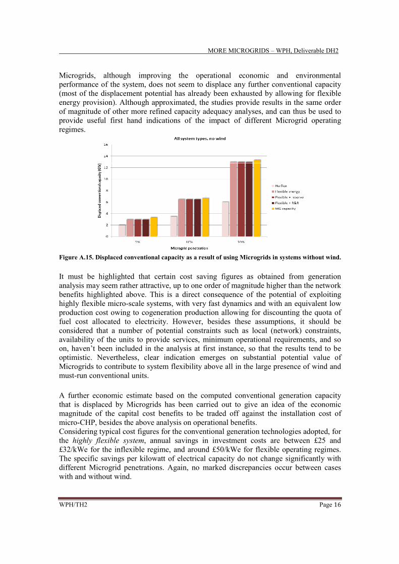
MORE MICROGRIDS – WPH, Deliverable DH2
WPH/TH2 Page 16
Microgrids, although improving the operational economic and environmental
performance of the system, does not seem to displace any further conventional capacity
(most of the displacement potential has already been exhausted by allowing for flexible
energy provision). Although approximated, the studies provide results in the same order
of magnitude of other more refined capacity adequacy analyses, and can thus be used to
provide useful first hand indications of the impact of different Microgrid operating
regimes.
Figure A.15. Displaced conventional capacity as a result of using Microgrids in systems without wind.
It must be highlighted that certain cost saving figures as obtained from generation
analysis may seem rather attractive, up to one order of magnitude higher than the network
benefits highlighted above. This is a direct consequence of the potential of exploiting
highly flexible micro-scale systems, with very fast dynamics and with an equivalent low
production cost owing to cogeneration production allowing for discounting the quota of
fuel cost allocated to electricity. However, besides these assumptions, it should be
considered that a number of potential constraints such as local (network) constraints,
availability of the units to provide services, minimum operational requirements, and so
on, haven’t been included in the analysis at first instance, so that the results tend to be
optimistic. Nevertheless, clear indication emerges on substantial potential value of
Microgrids to contribute to system flexibility above all in the large presence of wind and
must-run conventional units.
A further economic estimate based on the computed conventional generation capacity
that is displaced by Microgrids has been carried out to give an idea of the economic
magnitude of the capital cost benefits to be traded off against the installation cost of
micro-CHP, besides the above analysis on operational benefits.
Considering typical cost figures for the conventional generation technologies adopted, for
the highly flexible system, annual savings in investment costs are between £25 and
£32/kWe for the inflexible regime, and around £50/kWe for flexible operating regimes.
The specific savings per kilowatt of electrical capacity do not change significantly with
different Microgrid penetrations. Again, no marked discrepancies occur between cases
with and without wind.
MORE MICROGRIDS – WPH, Deliverable DH2
WPH/TH2 Page 17
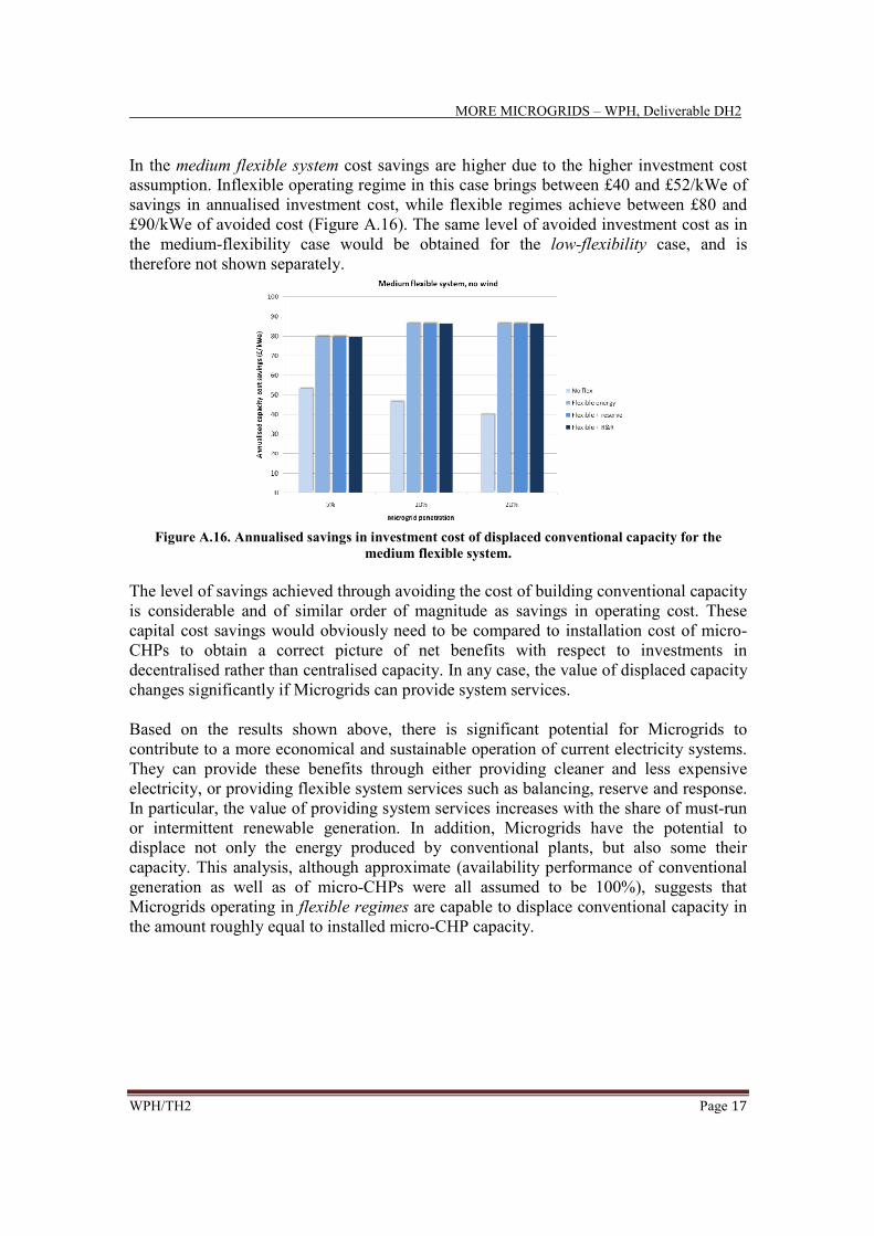
In the medium flexible system cost savings are higher due to the higher investment cost
assumption. Inflexible operating regime in this case brings between £40 and £52/kWe of
savings in annualised investment cost, while flexible regimes achieve between £80 and
£90/kWe of avoided cost (Figure A.16). The same level of avoided investment cost as in
the medium-flexibility case would be obtained for the low-flexibility case, and is
therefore not shown separately.
Figure A.16. Annualised savings in investment cost of displaced conventional capacity for the
medium flexible system.
The level of savings achieved through avoiding the cost of building conventional capacity
is considerable and of similar order of magnitude as savings in operating cost. These
capital cost savings would obviously need to be compared to installation cost of micro-
CHPs to obtain a correct picture of net benefits with respect to investments in
decentralised rather than centralised capacity. In any case, the value of displaced capacity
changes significantly if Microgrids can provide system services.
Based on the results shown above, there is significant potential for Microgrids to
contribute to a more economical and sustainable operation of current electricity systems.
They can provide these benefits through either providing cleaner and less expensive
electricity, or providing flexible system services such as balancing, reserve and response.
In particular, the value of providing system services increases with the share of must-run
or intermittent renewable generation. In addition, Microgrids have the potential to
displace not only the energy produced by conventional plants, but also some their
capacity. This analysis, although approximate (availability performance of conventional
generation as well as of micro-CHPs were all assumed to be 100%), suggests that
Microgrids operating in flexible regimes are capable to displace conventional capacity in
the amount roughly equal to installed micro-CHP capacity.

MORE MICROGRIDS – WPH, Deliverable DH2
WPH/TH2 Page 18
Contents
ACRONYM LIST ............................................................................................... 21
LIST OF FIGURES ............................................................................................. 22
LIST OF TABLES .............................................................................................. 25
1. Introduction ................................................................................................. 26
2. Impact of Microgrids on European distribution network development .......... 30
2.1 Generalities ............................................................................................ 30
2.2 Network investment strategies and value of active management within
Microgrids based on Generic Distribution System (GDS) models ........................... 32
2.2.1 GDS model ......................................................................................... 32
2.2.2 Active management modelling .............................................................. 35
2.2.3 Cost of Active Management implementation ........................................... 38
2.2.4 Optimisation of Active Management controls ......................................... 41
2.2.5 Outputs of analysis with the GDS model ................................................ 43
2.2.6 Benefits related to losses ...................................................................... 43
2.2.7 Benefits related to reinforcement .......................................................... 44
2.2.8 Benefits related to total network cost ..................................................... 46
2.2.9 Benefits related to local power generation ............................................. 46
2.2.10 Scenarios and types of analysis examined .......................................... 47
2.3 Northern and central European scenario analyses: Poland ........................... 52
2.3.1 Dynamic assessment of DG and AM based on partners’ scenarios ........... 52
2.3.2 Parametric assessment of micro DG and AM on current networks............ 55
2.4 Northern and central European scenario analyses: FYROM ........................ 57
2.4.1 Parametric assessment of micro DG and AM on current networks............ 57
2.5 Northern and central European scenario analyses: UK ................................ 61
2.5.1 Parametric assessment of micro DG and AM on current networks............ 61
2.6 Northern and central European scenario analyses: Germany ........................ 64
2.6.1 Dynamic assessment of DG and AM based on partners’ scenarios ........... 64
2.6.2 Parametric assessment of micro DG and AM on current networks............ 66
2.7 Northern and central European scenario analyses: Netherlands .................... 68
2.7.1 Dynamic assessment of DG and AM based on partners’ scenarios ........... 68
2.7.2 Parametric assessment of micro DG and AM on current networks............ 69
2.8 Northern and central European scenario analyses: Comparative analysis ...... 71
2.8.1 Dynamic assessment of DG and AM based on partners’ scenarios ........... 71
2.8.2 Parametric assessment of micro DG and AM on current networks............ 75
2.9 Southern European scenario analyses: Greece ............................................ 82
2.9.1 Impact of DG on system flows and investment deferral economic benefits . 82
2.9.2 Case study application ......................................................................... 82
2.9.3 Synthesis of the main results ................................................................. 83
2.10 Southern European scenario analyses: Italy ............................................... 85
2.10.1 Network design strategies in the presence of DG................................. 85
2.10.2 Test network.................................................................................... 85

MORE MICROGRIDS – WPH, Deliverable DH2
WPH/TH2 Page 19
2.10.3 Scenarios and planning strategies ..................................................... 86
2.10.4 Assessment of the impact of totally autonomous Microgrids on network
planning 86
2.10.5 Conclusions on the Italian network analyses ...................................... 90
2.11 Impact on Microgrids on network replacement scenarios through generic
distribution system fractal model ......................................................................... 91
2.11.1 Multi-voltage fractal model, LCC network design criteria and value of DG
91
2.11.2 DG technologies and control strategies for network replacement analysis
92
2.11.3 Urban network design ...................................................................... 93
2.11.4 Rural network design ....................................................................... 97
2.11.5 Losses result comparison with other studies ....................................... 97
2.11.6 Concluding remarks on the fractal network replacement assessment ..... 98
2.12 Fractal network-based analysis of economic and environmental impact of
micro-CHP systems in Microgrids ....................................................................... 99
2.12.1 Network, environmental and DG modelling ........................................ 99
2.12.2 Generation scenarios and analyses .................................................. 100
2.12.3 Synthesis of the network deferral results .......................................... 100
2.12.4 Environmental performance ........................................................... 102
2.12.5 Concluding remarks on Distributed CHP studies .............................. 105
2.13 Considerations on network security contribution from DG and Microgrids . 106
2.14 Final considerations on Microgrids impact on distribution network operation
and development ............................................................................................. 108
3. System-wide impact of Microgrids on transmission networks ...................... 110
3.1 Generalities: rationales for transmission investment and impact of Microgrids
110
3.2 Methodology for assessment of optimal transmission investment considering
the impact of Microgrids .................................................................................. 112
3.2.1 Network operation synthesis ............................................................... 112
3.2.2 Transmission capacity planning .......................................................... 112
3.2.3 Cost benefit transmission design in the presence of DG and Microgrids . 113
3.3 Case study application for the UK transmission system ............................. 114
3.3.1 Case study description ....................................................................... 114
3.3.2 Value of wind and uncontrolled CHP .................................................. 115
3.3.3 Value of CHP controllability within Microgrids ................................... 116
3.4 Utilisation of controllable loads in Microgrids for transmission congestion
release 118
3.4.1 Generalities on controllable loads for transmission impact assessment ... 118
3.4.2 Model of controllable loads for network congestion release ................... 119
3.4.3 Inputs and outputs to the DSM model .................................................. 120
3.4.4 Case study application to the simplified UK transmission system ........... 121
3.4.5 Case study results and discussion ....................................................... 123
3.5 Final considerations on the value of Microgrids for transmission investment
127
4. System-level impact of Microgrids on central generation operation and

MORE MICROGRIDS – WPH, Deliverable DH2
WPH/TH2 Page 20
development ...................................................................................................... 129
4.1 Generation capacity contribution of microgeneration and Microgrids ......... 129
4.1.1 Generalities on security of supply and contribution from Microgrids ...... 129
4.2 General discussion on DG contribution to security of supply in a Northern
European country case ..................................................................................... 131
4.2.1 Combined Heat and Power (CHP) ...................................................... 131
4.2.2 Wind Power ...................................................................................... 132
4.2.3 Photovoltaics (PV) ............................................................................ 133
4.3 Main findings of the studies on generation adequacy in the Portuguese case 133
4.3.1 Generalities on the methodology developed for Microgrid contribution to
security of supply ......................................................................................... 133
4.3.2 Capacity credit contribution from different micro-generation technologies
133
4.3.3 Specific results for Microgrids ............................................................ 137
4.3.4 Concluding remarks on the Portuguese studies on generation adequacy with
Microgrids .................................................................................................. 138
4.4 Role of flexibility provided by controllable generation in Microgrids and
dynamic impact on centralized generation .......................................................... 140
4.4.1 Synthesis of dynamic operation of power systems ................................. 140
4.4.2 Generalities on the impact of intermittent sources on frequency services
requirements and results from previous studies ............................................... 141
4.4.3 The role of flexibility that can be provided by Microgrids ...................... 143
4.4.4 Scheduling model for system-level impact assessment of Microgrids on
conventional generation ............................................................................... 143
4.4.5 Case study examples .......................................................................... 147
4.4.6 Discussion of the results .................................................................... 149
4.4.7 Estimate of cost savings for conventional generation displacement ........ 160
4.4.8 Conclusive remarks on system-level impact of Microgrids ..................... 163
4.5 Role of flexibility provided by controllable loads in Microgrids ................. 165
4.6 Final considerations on Microgrids impact on conventional generation
operation and development ............................................................................... 166
5. Concluding remarks on Task TH2 of WPH ................................................ 168
REFERENCES ................................................................................................. 170

MORE MICROGRIDS – WPH, Deliverable DH2
WPH/TH2 Page 21
ACRONYM LIST
AM Active Management
BAU Business As Usual
CBA Cost-Benefit Analysis
CC Capacity Credit
CCGT Combined Cycle Gas Turbine
CCS Carbon Capture and Storage
CHP Combined Heat and Power
CO2ER CO2 Emission Reduction
DG Distributed Generator
DH District Heating
DNO Distribution Network Operator
DSM Demand Side Management
DSO Distribution System Operator
ESP Electrical Separate Production
FC Fuel Cell
FESR Fuel Energy Savings Ratio
F&F Fit-and-Forget approach (or passive management – PM – approach)
FL Fault Level (short circuit capacity)
GDS Generic Distribution System
GSP Grid Supply Point
GT Gas Turbine
HV High Voltage
ICE Internal Combustion Engine
ICT Information and Communication Technology
LCC Life Cycle Cost
LHV Lower Heating Value
LV Low Voltage
MG Microgrids
MX Mixed (cables/lines)
MT Microturbine
MV Medium Voltage
NPV Net Present Value
OH Overhead (lines)
PM Passive Management
PV Photovoltaic
PW Present Worth
RES Renewable Energy Sources
SP Separate Production
TSO Transmission System Operator
TSP Thermal Separate Production
UG Under-Ground (cables)
VPP Virtual Power Plant

MORE MICROGRIDS – WPH, Deliverable DH2
WPH/TH2 Page 22
LIST OF FIGURES
Figure 1.1. Representation of a generic distribution network. ........................................... 33
Figure 1.2. Representation of a GDS module. ................................................................... 34
Figure 1.3. Illustration of voltage problems....................................................................... 35
Figure 1.4. Active Management of voltage drop problems ............................................... 36
Figure 1.5. Limitations imposed on the action of OLTC by adjacent feeders ................... 37
Figure 1.6. Active Management of voltage rise problems ................................................. 37
Figure 1.7. Control and measurement system for reactive power compensation .............. 39
Figure 1.8. Control and measurement system for generation curtailment ......................... 40
Figure 1.9. Control and measurement system at the substation ......................................... 41
Figure 1.10. Measurement system at each feeder .............................................................. 41
Figure 1.11. Model for the calculation of total network cost............................................. 49
Figure 1.12. Dynamic network assessment model............................................................. 50
Figure 1.13. Reinforcement deferral by the deployment of active management ............... 53
Figure 1.14. Losses reduction in 2015 under different strategies ...................................... 54
Figure 1.15. Reduction in total network cost in 2015-2020 under different strategies ..... 54
Figure 1.16. Parametric analysis of the reduction in reinforcement cost........................... 55
Figure 1.17. Parametric analysis of the reduction in losses ............................................... 56
Figure 1.18. Parametric analysis of the reduction in reinforcement cost........................... 57
Figure 1.19. Parametric analysis of the reduction in losses ............................................... 58
Figure 1.20. Parametric analysis of the reduction in total network cost ............................ 59
Figure 1.21. Parametric analysis of the changes in the aggregate demand curve .............. 59
Figure 1.22. Parametric analysis of the environmental benefits of micro DG .................. 60
Figure 1.23. Parametric analysis of the reduction in reinforcement cost........................... 61
Figure 1.24. Parametric analysis of the reduction in losses ............................................... 62
Figure 1.25. Parametric analysis of the reduction in total network cost ............................ 62
Figure 1.26. Parametric analysis of the incremental benefit of micro DG ........................ 63
Figure 1.27. Increase in reinforcement cost in each time window .................................... 64
Figure 1.28. Losses reduction in each yearly snapshot ...................................................... 65
Figure 1.29. Reduction in total network cost in each time window .................................. 65
Figure 1.30. Parametric analysis of the increase in reinforcement cost............................. 66
Figure 1.31. Parametric analysis of the reduction in losses ............................................... 67
Figure 1.32. Parametric analysis of the changes in the aggregate demand curve .............. 67
Figure 1.33. Losses reduction in each yearly snapshot ...................................................... 68
Figure 1.34. Losses reduction per voltage level in each yearly snapshot .......................... 68
Figure 1.35. Changes in the aggregate demand curve ....................................................... 69
Figure 1.36. Parametric analysis of the reduction in losses ............................................... 70
Figure 1.37. Parametric analysis of the reduction in losses per network component ........ 70
Figure 1.38. Comparison of the reduction in reinforcement cost ...................................... 72
Figure 1.39. Comparison of the reduction in losses........................................................... 73
Figure 1.40. Comparison of the reduction in total network cost ....................................... 74
Figure 1.41. Comparison of the incremental benefit of DG .............................................. 74
Figure 1.42. Comparison of the reduction in reinforcement cost in low load scenario ..... 76
Figure 1.43. Comparison of the reduction in reinforcement cost in high load scenario .... 76

MORE MICROGRIDS – WPH, Deliverable DH2
WPH/TH2 Page 23
Figure 1.44. Comparison of the reduction in losses in low load scenario ......................... 77
Figure 1.45. Comparison of the reduction in losses in high load scenario ........................ 78
Figure 1.46. Comparison of the reduction in total network cost in low load scenario ...... 79
Figure 1.47. Comparison of the reduction in total network cost in high load scenario ..... 80
Figure 1.48. Comparison of the incremental benefit of micro DG in low load scenario... 81
Figure 1.49. Comparison of the incremental benefit of micro DG in high load scenario . 81
Figure 1.50. Hellenic 17-bus test distribution network. ..................................................... 83
Figure 1.51. Deferral time benefits due to DG in the Hellenic test network. .................... 84
Figure 1.52. Overall cost benefits due to DG network deferral in the Hellenic test
network.84
Figure 1.53. Costs of the network designed considering daily profiles for loads and
generators ........................................................................................................................... 87
Figure 1.54. Costs of the network designed based on the traditional fit&forget approach87
Figure 1.55. Costs of the network designed considering daily curves and possible load
shedding (DSM) actions .................................................................................................... 88
Figure 1.56. Comparison of total costs under different planning strategies ...................... 88
Figure 1.57. Comparison of investment costs under different planning strategies ............ 89
Figure 1.58. Comparison of energy losses under different planning strategies ................. 89
Figure 1.59. Network value of DG for PV in UK urban networks. ................................... 94
Figure 1.60. Network value of DG for uncontrolled (left) and 100% controlled (right)
CHP in urban networks. ..................................................................................................... 94
Figure 1.61. Total network value of DG in urban areas per installed DG capacity. .......... 95
Figure 1.62. Total network losses in urban areas for PV ................................................... 96
Figure 1.63. Total network losses in urban areas for uncontrolled (left) and 100%
controlled (right) CHP ....................................................................................................... 96
Figure 1.64. Contribution of micro-CHP and PV on the reduction in distribution network
losses in rural areas in Northern European characteristic systems. ................................... 97
Figure 1.65. Contribution of micro-CHP and PV on the reduction in distribution network
losses in urban areas in Northern European characteristic systems. .................................. 97
Figure 1.66. Zoom-out of substation maximum loading profile for a 100 kWe unit. ..... 101
Figure 1.67. Network overall NPV (normalised with respect to the network peak demand)102
Figure 1.68. Network overall NPV (normalised with respect to the DG installed electrical
capacity) of transformer capacity release. ....................................................................... 102
Figure 1.69. Cogeneration energy saving performance of the overall network (separate
production parameters refer to average marginal plant electrical efficiency). ................ 104
Figure 1.70. Cogeneration emission reduction performance of the overall network
(separate production parameters refer to average marginal plant .................................... 104
Figure 1.71. Cogeneration environmental-related potential economic savings for the
overall network for generation mix 2 (separate production parameters refer to average
marginal plant electrical efficiency, cost of carbon equal to 20£/tonCO2). ....................... 104
Figure 1.72. Wired and non-wired solutions to distribution network security of supply.106
Figure 2.1. Ratio of demand for transmission and installed generating capacity as a
function of its capacity credit. .......................................................................................... 111
Figure 2.2. Simplified transmission model of the UK. .................................................... 114
Figure 2.3. Value of microgrid-enabled micro-CHP controllability for transmission
capacity release. ............................................................................................................... 117
MORE MICROGRIDS – WPH, Deliverable DH2
WPH/TH2 Page 24
Figure 2.4. Algorithm for transmission network congestion management through
controllable loads. ............................................................................................................ 120
Figure 2.5. Sixteen bus-bar representation of the UK transmission system. ................... 122
Figure 2.6. Load patterns for the three controllable load types used in the analysis. ...... 122
Figure 2.7. Reduction in wind spilled and reduction in congested energy. ..................... 124
Figure 2.8. Reduction in cost obtained with controllable loads (compared to the base
case).124
Figure 2.9. Rescheduled generation energy: base case vs. DSM enabled by aggregated
controllable loads in Microgrids. ..................................................................................... 125
Figure 2.10. Yearly reduced energy due to controllable loads for each bus. ................... 126
Figure 2.11. Line utilization for 3 GW of controllable loads. ......................................... 126
Figure 3.1. Conventional generation capacity displaced by micro-CHP. ........................ 132
Figure 3.2. Conventional generation capacity displaced by wind power. ....................... 132
Figure 3.3. CC of different micro-generation technologies ............................................. 134
Figure 3.4. Influence of the unavailability of micro-generation technologies on the CC135
Figure 3.5. Comparison of the CC values for different micro-generation technologies .. 136
Figure 3.6. CC values adjusted to energy ........................................................................ 136
Figure 3.7. Influence of Microgrid on the CC of micro-CHP systems ............................ 137
Figure 3.8. CC of Microgrid due to load control ............................................................. 138
Figure 3.9. Probability Density Function (PDF) of fluctuations in wind power output. . 141
Figure 3.10. PDF of hourly variations in wind output from diverse and non-diverse wind
source.142
Figure 3.11. Heat demand profiles for micro-CHPs ........................................................ 146
Figure 3.12. Cost savings for the highly flexible system with no wind .......................... 150
Figure 3.13. Cost savings for the highly flexible system with 20 GW of wind .............. 150
Figure 3.14. Cost savings for the medium flexible system with no wind ........................ 151
Figure 3.15. Cost savings for the medium flexible system with 20 GW of wind ............ 151
Figure 3.16. Cost savings for the low-flexibility system ................................................. 152
Figure 3.17. Carbon emission reduction for the highly flexible system .......................... 153
Figure 3.18. Carbon emission reduction for the medium flexible system ....................... 154
Figure 3.19. Carbon emission reduction for the low-flexibility system .......................... 155
Figure 3.20. Wind curtailment reduction for the low-flexibility system ......................... 156
Figure 3.21. Incremental components of system savings for the highly flexible system 157
Figure 3.22. Incremental components of system savings for the medium flexible system158
Figure 3.23. Incremental components of system savings for the low-flexibility system 159
Figure 3.24. Displaced conventional capacity as a result of using Microgrids in systems
without wind .................................................................................................................... 161
Figure 3.25. Displaced conventional capacity as a result of using Microgrids in systems
with 20 GW wind ............................................................................................................. 161
Figure 3.26. Annualised savings in investment cost of displaced conventional capacity for
the highly flexible system ................................................................................................ 163
Figure 3.27. Annualised savings in investment cost of displaced conventional capacity for
the medium flexible system ............................................................................................. 163

MORE MICROGRIDS – WPH, Deliverable DH2
WPH/TH2 Page 25
LIST OF TABLES
Table 1.1. Electrical and thermal efficiency for different CHP sizes ................................ 47
Table 1.2. CHP and PV shares in the micro DG scenarios. ............................................... 50
Table 1.3. Urban network characteristics used in the case study. ...................................... 93
Table 1.4. Overall value of DG (for LV, MV and HV) in percentage with respect to the
base case (no DG) urban network cost. ............................................................................. 94
Table 2.1. Estimated regional distribution of DG in 2010. .............................................. 115
Table 2.2. Estimated annual generation cost and transmission cost. ............................... 115
Table 2.3. Estimated value of DG controllability for the case study system. .................. 117
Table 2.4. Input parameters to the DSM model. .............................................................. 120
Table 2.5. Impact of controllable load on the transmission system operation. ................ 123
Table 3.1. Microgrids case studies for system-level impact on generation ..................... 148
Table 3.2. Capacity breakdown for different system types ............................................. 148

MORE MICROGRIDS – WPH, Deliverable DH2
WPH/TH2 Page 26
1. Introduction
Power systems were originally developed in the form of local generation supplying local
demands, the individual systems being built and operated by independent companies.
During the early years of development, this proved quite sufficient. However, it was soon
recognized that an integrated system, planned and operated by a specific organization,
was needed to create an effective system that was both reasonably secure and
economical. This led to the development in most European countries of centrally located
generation feeding the demands via transmission and distribution systems. Back to that
time, a significant amount of local generation was left isolated within the developing
distribution systems, but this was gradually mothballed and subsequently
decommissioned so that, by the 1970s, most of it had disappeared from the electricity
supply industry. This trend may well have continued for the need to minimize energy use,
particularly the one believed to create environmental pollution. Consequently,
governments and energy planners have more recently been actively developing
alternative and cleaner forms of energy production, these being dominated by renewable
(wind, solar, etc.), local CHP plant, and the use of waste products. Paradoxically,
economics and the location of the fuel and/or energy sources have meant that these newer
sources have had to be mainly connected into distribution networks rather than at the
transmission level. A full circle has therefore evolved with generation being ‘embedded’
in distribution systems and ‘dispersed’ around the systems rather than being located and
dispatched centrally or globally [1]. Over the past decades, models, techniques and
application tools have been developed that recognized the central nature of generation.
However, some very specific features of local Distributed Generation (DG), namely,
those relatively small amounts of generation dispersed around the system and connected
to (often relatively weak) distribution networks, need to be adequately addressed. In
particular, the fact that DG is not usually dispatched by the network operator has meant
that existing techniques and practices have had to be reviewed and updated to take these
features into account [2]. In this outlook, while mostly benefits may arise for a small
penetration level of DG whereby small generators can be seen as negative loads from the
network perspective, larger shares of uncontrolled embedded generators in distribution
networks, with different load pattern characteristics and often intermittent, may pose
serious challenges for the operation and infrastructure development of power systems, as
already partly explored in Deliverable DH1 [3] and detailed in the sequel of this work.
In a centrally planned (“conventional”) power system, demand and supply balance is
typically maintained through provision of sufficient flexible/controllable generation that
keeps the system frequency within desired limits to ensure the correct operation of the
system. However, in the future the maintenance of system integrity may become more
challenging due to the reduced presence of conventional (flexible) large scale generation
leaving room to more intermittent Renewable Energy Sources (RES), above all wind and
Photovoltaic (PV), as well as “clean” but inflexible large-scale generation such as nuclear
and Carbon Capture and Storage (CCS) power plants. Therefore, a crucial point of the
development of electricity infrastructure in terms of frequency-related ancillary service
MORE MICROGRIDS – WPH, Deliverable DH2
WPH/TH2 Page 27
provision (namely, reserve and response) is to understand how and to what extent part of
the system control measures could come from new non-conventional dispersed
generation units as well as from active and controllable demand. Indeed, without the
contribution of DG and responsive demand into the system operation activities, a larger
proportion of conventional generation will have to be retained as system reserve, leading
to increasingly uneconomic solutions to mitigate the impact of a large percentage of clean
but uncontrollable generation in the system. At the same time, the question arise as to
what extent Distributed Energy Resources (DER) could contribute to long-term
generation adequacy, so as to postpone, for instance, conventional generation investment
in the presence of load growth.
From a network standpoint, the spread of generation connected across the distribution
network has substantial implications for power flow configurations and then again on the
all network operation and development. In particular, as widely discussed in Deliverable
DH1 [3], in a system where bulk of electricity supply comes from large scale
transmission-connected generators, there are unidirectional power flows through
transmission to distribution networks, and then on to end consumers via a series of
voltage transformations. With penetration of small-scale generation even at low voltage
(LV) level, these power flow patterns will change. Reverse flows may be expected as
well, caused by uncontrolled generation connected to the distribution network producing
more output than can be consumed by local demand. In some instances, these reverse
flows may occur at the transmission-distribution boundaries resulting in export from the
distribution network back to the transmission grid. In this respect, being sited in close
proximity to demand, DG will reduce the distribution network import requirements, thus
reducing the requirement for transmission capacity. While it is important to understand
the magnitude of network capacity contribution from DG allowing decrease or postpone
in transmission investment, similarly to generation adequacy, it is likely that a future low-
carbon system will be constrained in its choice of generation location by availability of
primary resources, so that transmission will still play a key role in long-distance bulk
transportation of power from remote RES.
With specific regard to distribution networks where small-scale DG is being installed, for
relatively small penetration levels mainly network benefits such as losses reduction and
voltage support are likely to arise, which top up benefits such as emission reduction for
instance due to utilization of distributed cogeneration close to the final heat users. Hence,
having scattered DG popping up in the network as negative loads does not affect
remarkably the network operation. However, with the main driver for benefits being
correlation between demand and generation, with increasing share of uncontrolled and
intermittent DG not correlated with demand the operating philosophy of the distribution
networks needs to be changed. Indeed, with bi-directional power flows and increasing
influx of generation into the network it will be more and more difficult for the
distribution network operator to maintain a passive operation approach (DG equal to
negative load) without investing heavily in network reinforcement [4] [5]. In this outlook,
Active Management (AM) of the network will become a key approach to enable
integration of local generation and higher network utilisation without resorting to
MORE MICROGRIDS – WPH, Deliverable DH2
WPH/TH2 Page 28
network reinforcements, which could on the other hand hinder further integration of
DER.
The Microgrids (MG) concept is to be framed within the context outlined above. More
specifically, MG represent a form of LV networks (as well as medium voltage (MV)
networks as aggregation of LV ones) where microgeneration and loads (and in general
DER) can be controlled in order to reach predefined objectives. In particular, the scope of
the analyses in Work Package (WP) H of the More Microgrids project, and particularly of
this Deliverable, is to evaluate and quantify the potential contribution of MG in terms of
network support and infrastructure development. In fact, while other aspects of MG are
relatively better known (for instance, related to reliability improvements, for which the
reader can find insights in WPG), the impact on electricity infrastructure evolution is to
be thoroughly addressed yet. This report aims to cover this knowledge gap, and provides
a number of quantitative analyses that follow up the introductory models illustrated in
Deliverable DH1 which can inform policy makers and relevant stakeholders on the
potential role of microgrids in system-wide impact and electrical infrastructure
development. Among other issues, it is important to highlight how the need for this
research is highly timely, considering that EU transmission and distribution networks
were significantly expanded in the ‘60s and the assets then installed are approaching the
end of their useful life and will need to be replaced. On the other hand, the need for
coping with the climate chance challenges has brought an abrupt change in the generation
philosophy, with the subsequent challenges to manage the system, as mentioned above.
This Deliverable summarizes the analyses carried out by several partners within Task
TH2 of WPH. As such, it contains a substantial amount of work that, for the sake of
readability, is organized in this main text accompanied by a number of Annexes with
more details on specific studies (namely, on distribution networks and generation
adequacy) that are summarized in the main part.
More specifically, the report is organized as follows:
• Chapter 2 describes the impact of Microgrids on distribution network replacement
scenarios, based on the foreseen scenarios of DG and load evolution and different
strategies. The studies are based on different approaches undertaken by the partners
involved. In particular, northern and central European network scenarios have been
analysed by Imperial on the basis of specific network data provided by partners,
namely, FYROM, Germany, Netherlands, UK, and Poland. The analyses have been
carried out by means of the Generic Distribution System (GDS) tool specifically
developed to quantify the capacity of distribution network assets (as well as
transmission assets) that can be displaced by Microgrids, as described in Deliverable
DH1. In addition, while the GDS analyses mainly focus on CHP-dominated
generation scenarios, southern European scenarios, with widespread use of PV, have
been analysed by NTUA for Greece and by ERSE (former CESI Ricerca) for Italy.
All the details of the studies are reported in Annex H2.A for GDS analyses and
Annex H2.B for southern Europe analyses.
• Chapter 3 discusses the impact of Microgrids from a point of view of transmission
investment. In particular, after discussing the general issues of the relation between
MORE MICROGRIDS – WPH, Deliverable DH2
WPH/TH2 Page 29
transmission investment and DG, the impact of DG controllability within MG is
estimated through a UK case study, and relevant general considerations are carried
out. A further case study example illustrates the utilisation of controllable loads
within MG to increase the utilisation of transmission corridors and decrease the level
of congestion, thus postponing the need for network reinforcements and decreasing
the volume of intermittent renewable energy to be curtailed owing to capacity
release.
• Chapter 4 contains studies carried out to analyse the impact and role of Microgrids
relative to centralised conventional generation systems. More specifically, the
concept of capacity credit, relative to generation adequacy and expansion planning,
is discussed. Detailed probabilistic models, with illustrative studies relevant to a
Portuguese case, have been elaborated by INESC1 and are reported in Annex H2.C.
In addition, the contribution of Microgrids to provide frequency response and reserve
is assessed for different generation scenarios and levels of generation flexibility,
pointing out the main drivers and providing quantitative indications about economic
and environmental value that MG can bring in providing ancillary services to the
system. This includes economic savings in terms of conventional generation
expansion, and environmental savings owing to additional share of intermittent
renewable sources (namely, wind) that can be economically and securely integrated
in the system. Relevant analyses of the contribution to system services are carried out
in terms of both controllable DG and controllable loads.
• Chapter 5 contains the concluding remarks on the work carried out within the Task.
1 INESC work on security of supply was originally scheduled for WPG but then it has been moved to WPH
and is presented in this report based on its relevance to system development.

MORE MICROGRIDS – WPH, Deliverable DH2
WPH/TH2 Page 30
2. Impact of Microgrids on European distribution network
development
This chapter illustrates a number of different analyses run to assess the impact of DG
integrated within Microgrids on distribution network infrastructure development.
More specifically, a set of system-level impact studies has been run by Imperial College
through the Generic Distribution System (GDS) model developed in this project. The
model is capable to appraise the impact of DG and various Active Management (AM)
strategies on the entire distribution network from a Grid Supply Point (GSP). Specific
methodologies for static and dynamic replacement strategies have been developed, taking
into account both investment and operational costs. Northern/Central networks and
generation scenarios (dominated by CHP) have been used to populate the model based on
data provided by project partners, to be representative of typical network configurations.
In addition, specific Microgrids scenarios have been studied to identify the main drivers
for impact and benefits in terms of infrastructure investment and replacement strategies.
Relevant environmental analyses have also been carried out to crate a full picture of the
costs and the benefits owing to Microgrids. The diversity of the networks and scenarios
studied enables to get valuable insights on the potential impact of Microgrids for network
replacement in Europe. Details on the Northern/Central scenario analyses are reported in
Annex H2.A.
In addition to the GDS analyses, specific studies have been carried out for Southern
networks and generation scenarios. More specifically, NTUA has run a case study to
quantify the investment deferral benefits due to DG to a typical Microgrid test network,
while ERSE has explored the benefits of PV-dominated Microgrids (in case operating
autonomously) on MV network planning according to different design strategies. Details
on the Southern scenario analyses are reported in Annex H2.B.
Further analyses by Imperial College have addressed greenfield distribution network
replacement strategies to identify the value of DG and controllability for system
development. Such analyses are based on a fractal model specifically developed for
system-wide assessments. The same model has also been used to run a merge of network
and environmental studies in CHP-dominated Microgrids, providing insights on the
interaction between power systems and the heat sector, which is gaining increasing
attention in the last years in order to develop more sustainable energy systems. Details on
the fractal-based analyses are reported in Annex H2.C.
2.1 Generalities
Modern distribution systems were designed to accept power coming from the
transmission system at the Bulk Supply Transformers of the Grid Supply Point (GSP) and
to further distribute it to customers. Thus the flow of both real power (P) and reactive
power (Q) was always from the higher to the lower voltage levels (Fig. 1).
However, as mentioned in the Introduction, with significant penetration of DG and
Microgrids the power flows may become reversed, with the distribution network no
longer being a passive circuit supplying loads but an active system with power flows and

MORE MICROGRIDS – WPH, Deliverable DH2
WPH/TH2 Page 31
voltages determined by the generation as well as the loads (Fig.2). The change in real and
reactive power flows caused by Microgrids generation has important technical and
economic implications for the power system [1].
The main reason is that DG is connected primarily within distribution networks, designed
under the paradigm that consumer loads are passive and power flows only from
substations to consumers and not in the opposite direction. In order to address this point,
many studies on the interconnection of DG with distribution networks have been carried
out, ranging from control and protection to voltage stability and power quality (for
instance, [6][7][8], among many others). There have also been discussions about the
environmental impact of widespread use of DG, in terms of pollutant emissions and
noise. Notwithstanding the disadvantages of DG, important benefits have been
acknowledged. These benefits are not only technical, such as the improvement of end-
user power quality and reliability. In fact, there are a number of economic benefits of DG,
the most important of which being the end-user electricity bill reduction, especially for
gas-fired technologies (peaking internal combustion engines (ICEs) or microturbines
(MTs)). This is especially valid in those regions where the so-called “spark spread”, that
is, the difference between the local electricity rates and the gas prices, is high. The
quantification of this benefit is relatively straightforward as the technology costs (upfront
investment, taxes, utility rates, and fuel) can be weighed against annual expenditures in
electricity purchases, and the financial returns can therefore be estimated without much
effort by the end-user. On the other hand, utilities have recognized the importance of the
utilization of DG solutions to defer the investment on distribution wires and power
transformers. In some cases, DG has even been the only viable solution found to supply
growing demands on certain neighborhoods, due to environmental opposition and
aesthetical concerns.
This work then targets the quantification of one of the most important benefits of DG and
Microgrids, which is the capability to defer planned or required investments in wires and
transformers by distribution utilities. In fact, if the capacity deferral benefit of DG can be
quantified, utilities can find new opportunities to implement “non-wires” solutions to
tackle necessary network upgrades and internalize all benefits. Regulators have also more
opportunities to better design credits for third-party owned DG investments that benefit
not only the owner itself but the local utility altogether. Indeed, governments are devoted
to provide the owners of renewable DG with credits of different sorts as a way of
encouraging the installation of clean technologies. However, there has been some
criticism regarding the way these credits are defined. We argue here that in an open
market for DG deployment and incentives, such credits should be based on the real
benefits produced by the particular DG solution and not in governmental policies in the
form of flat production credits or tax benefits. The DG industry will only mature as a
viable market alternative for consumers and utilities when all the benefits produced by a
particular DG system are accounted for and credited to its owners.
In the sequel a number of analyses are run to identify the benefits and the costs that DG
could bring about in terms of infrastructure development and expansion. The analyses
will be mostly based on real scenarios provided by consortium partners. In addition,
sensitivity studies will be carried out to examine the impact of a number of key factors on
the overall benefits of microgrids, including micro generation technology, level of
penetration, levels of integration of micro-generation within Microgrids (controllability

MORE MICROGRIDS – WPH, Deliverable DH2
WPH/TH2 Page 32
level), seasonal operating patterns, correlation with demand, and so forth. As a major
aspect within the Microgrids framework, we will highlight the potential additional
benefits that controllability of DER and AM will be able to provide relative to a business-
as-usual (BAU) case with DG but no microgrids. In fact, significant penetration of DG in
distribution may create issues such as voltage rise effect in rural distribution and
increased fault levels in urban distribution networks. Without proper management, they
increase the cost of DG connection due to network reinforcement requirements, which
ultimately influences the amount of additional DG that can penetrate the distribution
system. Active management in Microgrids will thus enable maximization of the use of
the existing circuits by taking full advantage of generator dispatch, control of transformer
taps, voltage regulators, reactive power management, and system reconfiguration in an
integrated manner. In order to have a full unbiased picture of positive and negative
impacts, we’ll run a full cost benefit analysis (CBA) aimed at identifying the cost optimal
tradeoff between infrastructure replacement postponing and additional costs for instance
due to need for supporting Information and Communication Technology (ICT)
infrastructure.
2.2 Network investment strategies and value of active management within
Microgrids based on Generic Distribution System (GDS) models
2.2.1 GDS model
The first tool developed for assessing microgrids and more in general DG impact on
distribution networks is the so called Generic Distribution System (GDS) model [8].
Such tool allows the investigation of typical (generic) networks, with specified
characteristics that change area by area and country by country, but that are still able to
provide general results without going into detailed assessment of whole power systems.
Indeed, the tool is simple enough yet capable to be used for accurate investigations
involving a variety of operating conditions in order to capture the temporal and spatial
impacts of DG on the network.
The input parameters of the networks analyzed are tuned to fit the distribution network
characteristics for the specific countries, according to the data requested and provided by
the partners (see Annexes of Deliverable DH1 [3] for the description of the template
through which relevant data were requested). Then, the GDS model enables to run hourly
load flow analyses (on an annual time frame and on the basis of typical seasonal
characteristic days) on these distribution networks, and to provide relevant results on the
impact of alternative microgrids penetration and operation scenarios (including different
typologies of DG equipment involved) on losses, power flows, and voltage profiles.
Thereby, sensible conclusions can be drawn on the need for network reinforcement rather
than on the possibility of adopting active management schemes to increase the network
performance and the penetration of DG. Such AM schemes range from coordinated
voltage control policies to curtailment of distributed generation output, if necessary.

MORE MICROGRIDS – WPH, Deliverable DH2
WPH/TH2 Page 33
The complexity of modeling individual distribution networks can be mitigated with the
development of a generic model, which enables us to represent typical European
networks. The basic topology and design philosophy of distribution networks is common
in most EU countries, with multi-voltage networks and substations with transformers
between these networks. Regardless the variety of networks it is possible to encounter, all
of them are characterized by a limited number of overhead line (OH) and underground
(UG) cable typologies to convey power from the transmission system through the
different voltage levels and eventually to end users. OH lines prevail for the higher
voltage levels, whereas UG cables are more used in the lower voltage levels, above all in
high-density urban areas. Transformers may vary in capacity and number per substation,
whereas cables and lines may vary in capacity and length. Of course, the specific design
in a specific area may affect resistance and reactance values (the main parameters for
power flow assessment), but, to a large extent, for each country it is possible to draw
generic networks that at first approximation resemble the typical ones from the various
Distribution System Operators (DSOs) in that country. Such networks, in particular, are
similar enough in topology and design philosophy so as to allow the adoption of a
common modeling approach on a Grid Supply Point (GSP) basis (boundary between the
meshed transmission and the radial distribution network), as described in [9] and [10].
The networks analysed in the GDS tool are operated radially, which is the typical
approach in most countries. However, some networks might be operated in (weakly)
meshed configuration. Meshed network modelling would require the implementation of
advanced load flow calculations that go beyond the scope of the tool developed and
might hinder the possibility of running general although simplified analyses. In addition,
for strategic assessments (and not detailed design) of MG, as is the purpose of WPH, the
difference in the impact on radial or weakly-meshed networks can be reasonably
neglected. It is therefore assumed here that each distribution network is operated radially
from the GSP point to the end users. Furthermore, it is assumed that the model is
composed of well-balanced three-phase circuits and transformers. A graphical
representation of a generic distribution network with various loads and distributed
generators connected is shown in Figure 2.1.
Figure 2.1. Representation of a generic distribution network.

MORE MICROGRIDS – WPH, Deliverable DH2
WPH/TH2 Page 34
Each voltage level in the GDS tool is modelled trough different modules [9]. A module is
composed of a substation with the relevant transformers, the low voltage bus-bar of that
substation, and a number of feeders (with loads and distributed generators connected to
them) connected to that bus-bar, as depicted in Figure 2.2. Thus, when modelling a
distribution network it is possible either to define as many modules as substations in the
real network in order to obtain a totally precise but large model, or to define a smaller
number of modules that would capture the key characteristics of the network. The latter
approach is the most suitable for strategic analyses of large microgrid deployment in
different countries. However, more accurate studies for targeted networks can be run in
order to refine some specific details.
Figure 2.2. Representation of a GDS module.
The design of a module is flexible, as it is possible to choose the characteristics of the
transformers (capacity, impedance, no-load losses at rated power and load losses at rated
power, break rating of switchboards), the number of feeders connected to the bus-bar,
their type (overhead line, cable or mixed), their length and size (and consequently their
resistance, reactance and thermal capacity) -as well as different tapering configurations-,
and the load/DG distribution among the different feeders and along each feeder. Apart
from the technical parameters, the user can also choose the economic parameters of the
network components (reinforcement price of feeders, transformers and switchboards).
Finally, the structure of the connection between different voltage levels should be
specified; the type and number of lower voltage modules allocated along each higher
voltage feeder is defined by the user.
Owing to the differences existing between each voltage level, particularly with regard to
the connection of load, DG and lower voltage substations to the feeders, the main
configuration of the modules is typically slightly dissimilar for each voltage level.
Data on load and generation are organized according to typical hourly load profiles in
nine characteristic days, representative of the overall year. Hence, hourly, daily
(weekday, Saturdays and Sundays) and seasonal load and generation profile variations
can be captured and used for load flow analyses that could cover the whole year time

MORE MICROGRIDS – WPH, Deliverable DH2
WPH/TH2 Page 35
span. In addition, different load types (residential with and without electric heating,
industrial, commercial and agricultural) and generation types (wind, PV, hydro, CHP,
biomass, landfill gas, industrial waste) can be considered according to the specific
country case. The distribution of loads and generators at each voltage level, among
different modules of the same voltage level, among different feeders of the same module
and along each feeder is also modeled [9]. Finally, the user can specify the power factor
of the different loads and DG.
2.2.2 Active management modelling
Under the Passive Management regime, the distribution networks are designed to be
able to operate with minimum real-time management and automatically deal with the
worst-case expected situations. The adoption of this regime yields high investment on
network components and a low network utilization, since these worst case situations
occur very rarely. Under the -recently proposed- Active Management regime [11][12],
instead of planning and operating the network in anticipation of worst case scenarios, the
operator deals with constraints during different system conditions by exercising real-time
management of voltage, power flows and fault level through a number of different
components. In this work, we have focused on Voltage Active Management by utilizing
reactive compensation, online tap changers and generation curtailment.
Figure 2.3. Illustration of voltage problems
The voltage at busbar 2 ( ) of Figure 2.3 can be approximately calculated as follows:
(1)
Every DNO has an obligation to supply its customers at a voltage within specified limits
( and which are country- and voltage level- specific parameters). If the
values , , , for the generation and load are such that < or > , a
voltage drop or a voltage rise constraint arises. Under the Passive Management regime,
the feeder will be replaced with one of smaller resistance R and reactance X (a feeder
with larger cross section and capacity) in order to mitigate the voltage drop/rise between
the two buses.

MORE MICROGRIDS – WPH, Deliverable DH2
WPH/TH2 Page 36
Under the Active Management regime, the high investment cost of reinforcing the feeder
can be avoided by utilizing different control alternatives:
Voltage drop constraints:
Injecting reactive power at bus 2, by connecting a capacitive reactive compensator
(e.g. a STATCOM) , as depicted in Figure 2.4. The voltage at bus 2 will be
increased at:
(2)
It is important to observe from this equation that the effectiveness of this control action is
greatly influenced by the value of line reactance X: reactive compensation is considerably
more effective in overhead networks (with typical reactance of ≈0.4Ω/km), than on
cable networks (with typical reactance of ≈0.1Ω/km).
Figure 2.4. Active Management of voltage drop problems
Increasing voltage at bus 1 by changing the tap position of the On Load Tap Changer
(OLTC) at the transformer, as depicted in Figure 2.4. However, a limit is imposed on this
control alternative by adjacent feeders connected to the same substation, as it can be seen
in Figure 2.5. Increasing in order to increase (to mitigate a voltage drop constraint)
will also increase the voltage at bus 2, as the following equation indicates:
(3)
and a voltage rise problem will arise if > . This problem can be solved by
implementing a coordinated area-based control scheme which takes into account the
voltage at every feeder connected at the substation to keep in a certain range in order to
keep both and between the permissible limits ([11] and [12]).
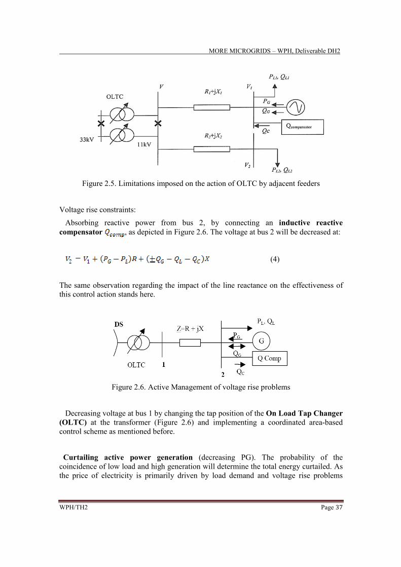
MORE MICROGRIDS – WPH, Deliverable DH2
WPH/TH2 Page 37
Figure 2.5. Limitations imposed on the action of OLTC by adjacent feeders
Voltage rise constraints:
Absorbing reactive power from bus 2, by connecting an inductive reactive
compensator , as depicted in Figure 2.6. The voltage at bus 2 will be decreased at:
(4)
The same observation regarding the impact of the line reactance on the effectiveness of
this control action stands here.
Figure 2.6. Active Management of voltage rise problems
Decreasing voltage at bus 1 by changing the tap position of the On Load Tap Changer
(OLTC) at the transformer (Figure 2.6) and implementing a coordinated area-based
control scheme as mentioned before.
Curtailing active power generation (decreasing PG). The probability of the
coincidence of low load and high generation will determine the total energy curtailed. As
the price of electricity is primarily driven by load demand and voltage rise problems

MORE MICROGRIDS – WPH, Deliverable DH2
WPH/TH2 Page 38
occur typically during periods of low demand, the value of the curtailed energy is likely
to be relatively low [12].
Another possible means of voltage management could be the control of the reactive
power generation (control of the generator’s power factor) of the units operating in
the Microgrid. However, this option is not included in the model, and a single value for
the power factor of each DG was specified at the data received from our European
partners. Thus, the only modification in occurs when active power generation
curtailment takes place and the power factor of the generator is not equal to one.
Nevertheless, it has to be considered that in practice reactive support could be provided
by distributed generators connected at LV in the Microgrids. This is particularly relevant
when voltage drop issues due to large loads occur. In this case, the model developed
calculates reactive compensation needed at the end of the feeders where voltage drop
problems arise. This reactive compensation could in case be provided by changing the
DG power factor of the units operating in the Microgrid, with subsequent benefits mainly
at voltage levels higher that LV (the weight of reactance at LV is negligible, so that
reactive flows do not support voltage profiles substantially, differently from MV where
the weight of reactance is relatively higher).
2.2.3 Cost of Active Management implementation
In this section, the cost incurred by the distribution network operator (DNO) for the
implementation of each control option is presented. This data is the result of a survey that
was carried with 3 DNOs in the UK and is presented in detail in [12]. Since similar data
for other countries was not available, these values were used for the calculation of the
implementation cost of active management in the networks of every country (the
exchange rate used was 1£=1.11€).
Reactive power compensation: The cost of this control option can be divided into two
components:
1a) The capacity cost of the compensator, which is £30,000 per MVar. We have assumed
that this cost is infinitely modular, meaning that when the capacity of an already installed
compensator needs to be increased, the capacity cost incurred is given by the extra
capacity needed times the above mentioned value per MVar.
1b) The fixed cost of implementing this option (Figure 2.7), which includes the cost of: a
voltage transformer (£1000) which transforms the high network voltage to smaller
values, suitable for measurement and control purposes, a transducer (£200) which
converts the output of the voltage transformer to a voltage measurement suitable for
communication with the network operator, a Supervisory Control And Data Acquisition
(SCADA) system which processes the voltage measurements and the instructions it
receives from the network operator and controls the operation of the compensator

MORE MICROGRIDS – WPH, Deliverable DH2
WPH/TH2 Page 39
according to these instructions and a Remote Telemetry Unit (RTU) which constitutes the
interface between the control and measurement system at the reactive compensator and
the chosen communication circuit, used for sending field measurements to and receiving
instructions from the network operator (total cost of the SCADA and the RTU is £2500 –
it is assumed that power line communication is used, so no additional cost for the
communication is incurred by the network operator). According to the previous values,
the total fixed cost is £3700 (per compensator).
Figure 2.7. Control and measurement system for reactive power compensation
Generation Curtailment: The cost of this control option is divided into two
components as well:
2a) The cost of the curtailed energy in the electricity market, which is equal to the price
of energy (country- and voltage level- specific, given in £/MWh or €/MWh) times the
curtailed energy in MWh
2b) The fixed cost of implementing this option (Figure 2.8), which is equal to the
respective cost of the reactive power compensation option (£3700 per DG)
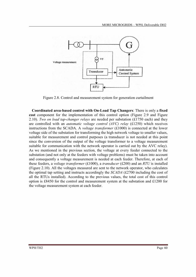
MORE MICROGRIDS – WPH, Deliverable DH2
WPH/TH2 Page 40
Figure 2.8. Control and measurement system for generation curtailment
Coordinated area-based control with On-Load Tap Changers: There is only a fixed
cost component for the implementation of this control option (Figure 2.9 and Figure
2.10). Two on load tap-changer relays are needed per substation (£1750 each) and they
are controlled with an automatic voltage control (AVC) relay (£1250) which receives
instructions from the SCADA. A voltage transformer (£1000) is connected at the lower
voltage side of the substation for transforming the high network voltage to smaller values,
suitable for measurement and control purposes (a transducer is not needed at this point
since the conversion of the output of the voltage transformer to a voltage measurement
suitable for communication with the network operator is carried out by the AVC relay).
As we mentioned in the previous section, the voltage at every feeder connected to the
substation (and not only at the feeders with voltage problems) must be taken into account
and consequently a voltage measurement is needed at each feeder. Therefore, at each of
these feeders, a voltage transformer (£1000), a transducer (£200) and an RTU is installed
(Figure 2.10). All the voltages measured are sent to the network operator, who calculates
the optimal tap setting and instructs accordingly the SCADA (£2700 including the cost of
all the RTUs installed). According to the previous values, the total cost of this control
option is £8450 for the control and measurement system at the substation and £1200 for
the voltage measurement system at each feeder.

MORE MICROGRIDS – WPH, Deliverable DH2
WPH/TH2 Page 41
Figure 2.9. Control and measurement system at the substation
Figure 2.10. Measurement system at each feeder
2.2.4 Optimisation of Active Management controls
An optimisation method is required in order to determine the least-cost combination of
the above control options resolving the voltage problems arising in the distribution
network. Since the control with OLTC has only a fixed cost component (installing tap
changers is a discrete decision), two alternative active management strategies were
considered:
Active management without tap changers. A capacitive compensator with the
relevant control and measurement system presented above is connected to each feeder
facing a voltage drop problem; on the other hand, an inductive compensator with the
relevant control and measurement system is connected to each feeder with a voltage rise
problem and the relevant control and measurement system enabling generation

MORE MICROGRIDS – WPH, Deliverable DH2
WPH/TH2 Page 42
curtailment is connected to each generator (if any) on this feeder. An optimisation
algorithm embedded in the GDS model determines the least-cost combination of
generation curtailment ( ) and reactive compensation ( ) resolving each voltage
problem in the network. Since the fixed cost of these two control options is the same,
only the annual cost of the curtailed energy in the electricity market ( ) and the
annualised capacity cost of the compensator ( ) are included in the objective
function:
(5)
Active management with tap changers. The relevant control and measurement system
presented in Figure 2.9 is connected to each substation where at least one feeder with a
voltage problem is connected and the measurement system presented in Figure 2.10 is
connected to each feeder connected to this substation. The tap changers alone might not
be able to resolve the problems arising due to the following limitations: i) the minimum
and maximum limits imposed on the tap position (country- and voltage- level specific
parameters) ii) the need to keep the voltage at every feeder connected to the substation
within the permissible limits (as explained in Section 2.2.2 and illustrated on Figure 2.5).
If this is the case, reactive compensation and generation curtailment is deployed as
explained in strategy a). The objective function of the optimization algorithm is the same
as in strategy a), but apart from the generation curtailment and the reactive compensation,
the tap position of the tap changers ( ) is optimised:
(6)
The implementation cost of strategy a) is highly proportional to the number of feeders
suffering from voltage problems and the severity of these problems (deviation from the
acceptable voltage limits) while the implementation cost of strategy b) is much less
affected by a change in these parameters (once tap changers are installed in a substation,
they can deal with voltage problems in every feeder connected to the substation and
irrespectively of their severity if the above mentioned limitations are not reached).
Therefore, the relation between the cost of strategies a) and b) depends on the nature of
the voltage problems in the network. In a network with a small number of feeders
suffering from voltage problems and moderate violations of the voltage limits (small
deviation from the minimum or maximum voltage limit), the cost of the required
compensation and generation curtailment under strategy a) is lower than the fixed cost of
installing tap changers and strategy a) is more economic. In a network with a large
number of feeders suffering from voltage problems and severe violations of the voltage
limits (big deviation from the minimum or maximum voltage limit), the cost of the
required compensation and generation curtailment under strategy a) becomes very high
and strategy b) becomes more economic.

MORE MICROGRIDS – WPH, Deliverable DH2
WPH/TH2 Page 43
2.2.5 Outputs of analysis with the GDS model
Each GDS simulation runs on an annual time frame and provides us with certain
technical results regarding the examined distribution network:
-Total annual losses (in MWh), annual losses per voltage level and annual losses per
network component (losses on transformers – losses on feeders)
-Total energy production per type of DG (in MWh)
-Maximum power flow on each network component and consequently determination
of thermal problems in the network
-Maximum voltage drop/rise on each feeder and consequently determination of
voltage problems in the network
-Contribution from each DG at the fault level of the terminal busbar they are
connected to and consequently determination of fault level problems in the
network
-Energy curtailment of each generator (in MWh) and capacity of reactive
compensation installed at each feeder facing voltage problems (in MVar) when
Active Management is deployed
By processing these results with suitable models, we were able to assess the technical,
economic and environmental benefits of Microgrids (Distributed Generation and Active
Management), as presented in the next subsections.
2.2.6 Benefits related to losses
For each scenario analysed, the losses reduction by the installation of DG is calculated
as:
(7)
(where the annual energy losses without DG connected at the network and
the annual energy losses with DG connected at the network). This reduction is calculated
for the total losses in the network, the losses at each voltage level and the losses at each
type of network component (feeders-transformers), and for the different operating
strategies (passive management, active management without tap changers and active
management with tap changers).
MORE MICROGRIDS – WPH, Deliverable DH2
WPH/TH2 Page 44
The annual cost of losses can be calculated by the product of the losses and the price
of energy (country-specific parameter) at each voltage level ( is the number of
voltage levels in the network):
(8)
Therefore, for each scenario analysed and each of the operating strategies, the cost of
losses reduction by the installation of DG is calculated as:
(9)
(where the cost of losses without DG connected at the network and the
cost of losses with DG connected at the network)
The reduction of losses by the installation of DG results in emissions reduction
calculated as:
(10)
(where the emission factor of the marginal plant of central generation). This model
was followed since we have assumed that losses in the distribution network are covered
from the central generation and more specifically by the last plant in the unit commitment
list. Since the development of a model which would estimate the changes in unit
commitment and economic dispatch of the central generation due to the connection of
DG (and would enable us to identify the marginal plant every hour) is out of the scope of
this work, we have carried out a parametric analysis for the emissions reduction, using
different values for .
2.2.7 Benefits related to reinforcement
Based on the technical results from the GDS simulation, we can calculate the
reinforcement cost required for resolving the various problems arising, under passive
and active management. We need to stress that: i) only reinforcement costs (and not
expansion costs) were taken into account and ii) the reinforcement strategy we used took
into account the indivisibility of assets (a certain number of standard types and sizes of
feeders, transformers and switchboards are available in each country) and the
reinforcement policy defined by the DNO of each network we have analysed (e.g. in
Germany, the type and size of feeders that will be used when reinforcement of
underground cables is needed is defined in the data we received from our partners).

MORE MICROGRIDS – WPH, Deliverable DH2
WPH/TH2 Page 45
Passive management: feeders are reinforced when they face a thermal (maximum
power flow on them is greater than their thermal capacity) or voltage problem (maximum
voltage drop/rise on them is greater than the voltage drop/rise limit imposed on the DNO;
this limit is country- and voltage level- specific), transformers are reinforced when they
face a thermal problem (maximum power flow on them is greater than their thermal
capacity) and switchboards at substations are reinforced when they face a fault level
problem (the fault level contribution of DGs connected to these substations is higher than
the available break rating headroom of the switch board; a parametric analysis was
carried out using a 10%,20% and 30% headroom). Consequently, the total reinforcement
cost is
(11)
where the cost of reinforcing feeders with thermal problems, the cost of
reinforcing feeders with voltage problems, the cost of reinforcing transformers and
the cost of reinforcing switchboards.
Active management: as under passive management, feeders and transformers are
reinforced when they face a thermal problem and switchboards are reinforced when they
face a fault level problem. Voltage problems of feeders are resolved by the deployment of
generation curtailment, reactive compensation and coordinated control of tap changers,
according to the active management strategy followed (with or without tap changers).
The deployment of each of these controls has specific cost components (presented
above). Consequently, the total reinforcement cost is:
(12)
(13)
where , , the cost of deploying generation curtailment, reactive
compensation and coordinated control with tap changers respectively.
For each scenario analysed and each of the operating strategies, the reinforcement cost
reduction by the installation of DG is calculated as:
(14)
(where the reinforcement cost without DG connected at the network and
the reinforcement cost with DG connected at the network). This reduction is calculated
for the total reinforcement cost, the reinforcement cost of each voltage level and the
reinforcement cost of each type of network component (feeders-transformers).

MORE MICROGRIDS – WPH, Deliverable DH2
WPH/TH2 Page 46
2.2.8 Benefits related to total network cost
In order to evaluate the total network cost for each examined scenario and each
operating strategy, it is necessary to transfer the two components of this cost
(reinforcement cost and cost of losses) to a common temporal basis. The models followed
to achieve this depend on the scope and the inputs of the analysis carried out and
consequently will be presented in Section 2.2.10. After this step, we will be able to
calculate the total network cost reduction by the installation of DG as:
(15)
where the network cost without DG connected at the network and the
network cost with DG connected at the network.
2.2.9 Benefits related to local power generation
Generation at the distribution level contributes to supply demand that should otherwise be
supplied by central generation; hence, the equivalent residual demand as seen at the GSP
from the transmission network is reduced [3]. This reduction can be expressed by the
reduction in the maximum power (in MVA) flowing on the boundary between the
examined distribution network and the upward transmission network (transformers of the
highest voltage level of the examined distribution network), which has a beneficial
impact on transmission investment decisions. Moreover, the installation of DG
modifies the shape of the aggregate demand curve of the distribution network (profile of
the power flowing on the boundary), which has an impact on central generation
scheduling decisions. We need to stress that the development of models quantifying
these two impacts is out of the scope of this work.
Since local energy production displaces part of the central one and is characterized by
much lower (or even zero in cases of renewable generators) emissions, the
installation of DG results in emissions reduction. The calculation of this reduction
is based on the marginal plant model presented in Section 2.2.6 and is different for
different types of DG [3]:
Renewable Generators: these generators do not produce ; thus the annual
reduction in CO2 due to renewable generation is
(16)

MORE MICROGRIDS – WPH, Deliverable DH2
WPH/TH2 Page 47
where is the annual renewable energy production and is the emission factor of
the marginal plant of central generation
Combined Heat and Power Generators: the emissions reduction from the operation
of these generators is not only due to the displacement of central electricity production
but also due to the displacement of useful heat produced by conventional boilers; thus it
is calculated as:
(17)
with
and
where and the annual electricity and heat production of the CHP respectively,
and the electrical and thermal efficiency of the CHP (the values used in our
analysis for different CHP sizes/technologies are given in Table 2.1), the emission
factor of the fuel used by the CHP (natural gas with 200g/kWh was considered in our
analysis) and the emission factor of the standalone boiler (assumed 240g/kWh in our
analysis) displaced by the CHP.
Table 2.1. Electrical and thermal efficiency for different CHP sizes
Micro
CHP
Small
CHP
Medium
CHP
Large
CHP
ηW 0.2 0.3 0.35 0.4
ηQ 0.7 0.55 0.5 0.45
2.2.10 Scenarios and types of analysis examined
Our analysis on the technical, economic and environmental benefits of Microgrids is
divided into two parts: i) dynamic assessment of the impacts of Distributed Generation
and Active Management on European distribution systems over different network
scenarios based on the foreseen DG and demand evolution as provided from our partners
and ii) parametric assessment of the impacts of micro DG and AM on today’s European
distribution networks.

MORE MICROGRIDS – WPH, Deliverable DH2
WPH/TH2 Page 48
Dynamic assessment of DG and AM based on partners’ scenarios
Our partners from Northern and Central European countries have provided us with the
expected demand and installed DG capacity on typical distribution networks of their
countries in four future yearly snapshots. Our task in this part of the analysis was to
assess the benefits of DG and AM on these networks in a dynamic fashion.
Since the data concerning the DG penetration evolution were given for these 4 snapshots
t0, t1, t2 and t3, we have assumed that connection of new DG and network reinforcement
will only take place in these snapshots (and consequently we have run GDS simulations
only for these snapshots), in order to simplify the analysis (a year by year assessment
would need extremely more GDS simulations and would require a number of uncertain
assumptions about the DG penetration evolution in intermediate years).
In each snapshot, we run GDS simulations for two cases: i) base case, where no DG is
connected at the network and the network problems arising are solved by deploying
passive management and ii) test case, where the foreseen for this snapshot DG is
connected at the network and all the possible reinforcement strategies (passive
management, active management without tap changers, active management with tap
changers) are examined and compared, based on their network cost (reinforcement cost
and cost of losses).
As we stressed in Section 2.2.8, in order to evaluate the total network cost for each of the
above cases, we need to bring its two components in the same temporal basis. Since
network reinforcement takes place in specific snapshots, the time window between two
consecutive snapshots can constitute this common basis. Since the economic parameters
of the assets (inputs of the analysis) correspond to the current value of their total capital
cost, the reinforcement cost calculated in the first place ( ) refers to a temporal basis
equal to the life cycle of the distribution assets (assumed 20 years in this work); it can be
brought to the common basis by subtracting the (present value of the) residual (or
salvage) value of the assets at the end of the time window. For example (Figure 2.11),
the cost of reinforcing the network in the time window t0 to t1 is equal to the present
value of the reinforcement cost incurred in t0 minus the present value of the residual
value of this investment in t1. We have assumed that the residual value of the assets
depends only on the number of years they have been used, in a linear fashion. Thus, in
the same example, the residual value of the investment will be:
, since the life cycle of the assets is 20 years and the length of the examined
time window is t1-t0 years. Moreover, we have assumed that the cost of assets increases
with the annual inflation rate (g=3% for every country in this work).

MORE MICROGRIDS – WPH, Deliverable DH2
WPH/TH2 Page 49
Figure 2.11. Model for the calculation of total network cost
On the other hand, the cost of losses for each case is brought to this common basis by
calculating the present value of the annual cost of losses for each of the years of the
examined time window. For example (Figure 2.11), the cost of losses in the time window
t0 to t1 is equal to the sum of the present value of the cost of losses in t0 and each of the
intermediate years between t0 and t1. Since the GDS simulation with the t0 demand and
DG data gives us the annual losses for t0, we have used an interpolation method in
order to project the losses in each of the subsequent years, by taking into account the
annual increase rate of the load (provided by our partners). Moreover, we have assumed
that the price of energy at each voltage level (which is used in order to calculate the cost
of losses) increases with the annual inflation rate.
Hence, the total network cost in the time window t0 to t1 in the above example will be:
(18)
where the present value of the reinforcement cost incurred in t0, the present
value of the residual value of this reinforcement in t1 and the sum of
the present value of the cost of losses in each of the years included in this time window.
In the test case (case with DG), the reinforcement strategy which gives the lowest total
network cost in the next time window is the one that will be selected; in the previous
example, the strategy which gives the lowest network cost for the time window t0 to t1
will be selected for the reinforcement of the network in t0 (optimal reinforcement
strategy in t0). This decision will affect the future structure of the network since this
optimally reinforced network will constitute the input network for the GDS simulation for
t1 etc, as depicted in Figure 2.12. By following this model, we are able to assess the

MORE MICROGRIDS – WPH, Deliverable DH2
WPH/TH2 Page 50
dynamic impacts of DG and AM on distribution network evolution, like cases of
reinforcement deferral.
Figure 2.12. Dynamic network assessment model
Parametric assessment of micro DG and AM on current networks
In this part of the work, our task was to assess the benefits of micro DG (DG at the Low
Voltage level) and AM on typical distribution networks (in their current form – no
dynamic assessment was investigated in this case) of 5 countries (UK, Germany,
Netherlands, Poland and FYROM). In order to do that, we have carried out a parametric
analysis investigating 3 scenarios for the micro DG penetration (50%, 100%, 150% of
current load at LV) and two scenarios for the load at LV (110% and 150% of current load
at LV). In the rest of the voltage levels, the load was considered fixed and equal to its
current value and no DG was connected. Only Combined Heat and Power (CHP)
generators and Photovoltaic (PV) panels were considered as micro Distributed Generators
(since these are currently the most mature technologies for connection at LV), with
country-specific shares presented in Table 2.2:
Table 2.2. CHP and PV shares in the micro DG scenarios.
UK Germany Netherlands Poland FYROM
CHP 95% 60% 60% 60% 20%
PV 5% 40% 40% 40% 80%
The above-mentioned scenarios refer to a single snapshot (current year) and consequently
the model used in this part of the analysis is much simpler than the dynamic model
presented in the previous section. The common temporal basis for the evaluation of the
total network cost of each DG penetration and each reinforcement strategy was simply
the year which the simulation refers to. The reinforcement cost can be brought to this
common basis by annualising it:
(19)

MORE MICROGRIDS – WPH, Deliverable DH2
WPH/TH2 Page 51
where d the discount rate (assumed 7% in our analysis) and N the recovery period of the
capital investment needed (assumed 20 years in our analysis). Hence, the total network
cost for the examined snapshot will be:
(20)
where the annual cost of losses. Based on this network cost, the optimal
reinforcement strategy and the optimal DG capacity for each load scenario can be
identified.

MORE MICROGRIDS – WPH, Deliverable DH2
WPH/TH2 Page 52
2.3 Northern and central European scenario analyses: Poland
2.3.1 Dynamic assessment of DG and AM based on partners’ scenarios
Our dynamic analysis on the Polish distribution network shows that the large majority of
the required reinforcement in each of the examined time windows is related to
violations of voltage limits caused by demand (voltage drop), with the most severe
problems arising at the medium voltage level, since it is characterized by many long,
overhead lines. Reinforcement driven by the installation of DG is only encountered in
2010, when some large wind turbines are connected to weak 15kV feeders; in the rest of
the examined time windows, since the problems arising are caused by demand, DG
reduces reinforcement cost, by mitigating these problems. The dynamic nature of our
analysis enables us to witness not only reinforcement cost reduction, but also
reinforcement deferral by the installation of DG: in the base case (no DG), the 110kV
transformers need reinforcement in 2020 while in the test case (with DG), they need
reinforcement in 2030.
The deployment of active management reduces further the reinforcement cost in each
time window, since the cost of implementing the active controls is much lower than the
cost of replacing the feeders suffering from voltage problems. The active management
strategy giving the lowest reinforcement cost in each of the examined time windows is
AM without tap changers. Active management in the time window 2010-2015 includes
curtailment of the production of the generators causing voltage rise problems; however,
the total curtailed energy of each involved generator is less than 2% of its total energy
production during this time window. The dynamic nature of our analysis enables us to
witness not only reinforcement cost reduction, but also reinforcement deferral by the
deployment of active management: in the base case the replacement of certain heavy-
loaded feeders is needed in 2010 because they face voltage problems; in the test case this
replacement in 2010 is avoided (since active controls are used in order to resolve these
problems) and it is deferred in 2015 when the same feeders face thermal problems (that is
why in the test case, there is an increase in the reinforcement cost related to feeders’
thermal problems in the time window 2015-2020, as shown on Figure 2.13).
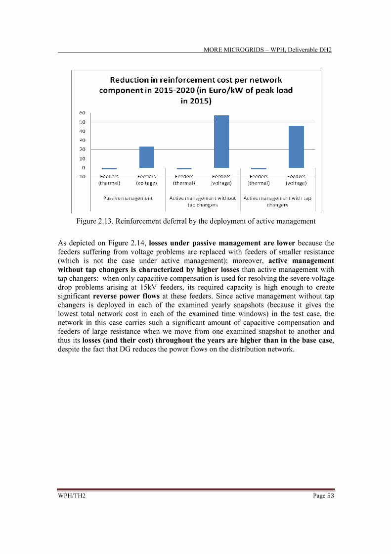
MORE MICROGRIDS – WPH, Deliverable DH2
WPH/TH2 Page 53
Figure 2.13. Reinforcement deferral by the deployment of active management
As depicted on Figure 2.14, losses under passive management are lower because the
feeders suffering from voltage problems are replaced with feeders of smaller resistance
(which is not the case under active management); moreover, active management
without tap changers is characterized by higher losses than active management with
tap changers: when only capacitive compensation is used for resolving the severe voltage
drop problems arising at 15kV feeders, its required capacity is high enough to create
significant reverse power flows at these feeders. Since active management without tap
changers is deployed in each of the examined yearly snapshots (because it gives the
lowest total network cost in each of the examined time windows) in the test case, the
network in this case carries such a significant amount of capacitive compensation and
feeders of large resistance when we move from one examined snapshot to another and
thus its losses (and their cost) throughout the years are higher than in the base case,
despite the fact that DG reduces the power flows on the distribution network.

MORE MICROGRIDS – WPH, Deliverable DH2
WPH/TH2 Page 54
Figure 2.14. Losses reduction in 2015 under different strategies
Even though the cost of losses is generally higher in the DG case than in the base case,
the reinforcement cost is much lower in the former and thus DG brings a benefit with
regard to the total network cost. Active management reduces further the total
network cost, because its positive impact on the reinforcement cost is much more
significant than its negative impact on the (cost of) losses; more specifically, active
management without tap changers is the optimal strategy in each of the examined time
windows (Figure 2.15).
Figure 2.15. Reduction in total network cost in 2015-2020 under different strategies

MORE MICROGRIDS – WPH, Deliverable DH2
WPH/TH2 Page 55
2.3.2 Parametric assessment of micro DG and AM on current networks
Our snapshot-based analysis on the Polish distribution network shows that the whole
required reinforcement in both low and high load scenarios is related to voltage drop
problems and -as in the previous part of the analysis- the installation of micro DG and
the deployment of active management reduce reinforcement cost. Our parametric analysis
has demonstrated that as the micro DG penetration increases, the reinforcement cost
is reduced; moreover the benefits of active management (in comparison with passive
management) become less apparent when the micro DG penetration increases and
the demand decreases, as the emerging voltage drop problems become less severe
(Figure 2.16). The active management strategy giving the lowest reinforcement cost on
each micro DG penetration-demand scenario depends on the relative severity of the
emerging voltage problems.
Figure 2.16. Parametric analysis of the reduction in reinforcement cost
As the micro DG penetration increases, the losses reduction with respect to the base
case becomes more significant, as larger part of the power required by the load is
supplied locally, and thus the power flows on the network are reduced. The two
differences in losses between the different strategies (described in Section 2.3.1) become
less apparent as micro DG penetration is increased and load is decreased, since less
voltage drop problems occur and thus fewer feeders are replaced under passive
management and less capacitive compensation is connected at the suffering feeders under
active management without tap changers (Figure 2.17).
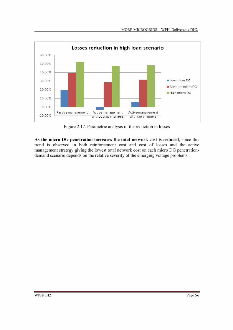
MORE MICROGRIDS – WPH, Deliverable DH2
WPH/TH2 Page 56
Figure 2.17. Parametric analysis of the reduction in losses
As the micro DG penetration increases the total network cost is reduced, since this
trend is observed in both reinforcement cost and cost of losses and the active
management strategy giving the lowest total network cost on each micro DG penetration-
demand scenario depends on the relative severity of the emerging voltage problems.

MORE MICROGRIDS – WPH, Deliverable DH2
WPH/TH2 Page 57
2.4 Northern and central European scenario analyses: FYROM
2.4.1 Parametric assessment of micro DG and AM on current networks
Our analysis on the FYROM distribution network shows that very significant
reinforcement is required in both low and high load scenarios, related to violations of
both voltage and thermal limits (almost equally significant) caused by demand, with
the most severe problems arising at the very weak low voltage level. Since this
reinforcement is driven by demand, as the micro DG penetration increases, the
reinforcement cost is reduced; evidence of the weakness of the network is the fact that a
low micro DG penetration cannot extenuate at all the arising problems in the low load
scenario under passive management (Figure 2.18).
The deployment of active management reduces further the reinforcement cost (since
the cost of implementing the active controls is much lower than the cost of replacing the
feeders suffering from voltage problems) but this benefit becomes less apparent when
the micro DG penetration increases and the demand decreases, as the emerging
voltage drop problems become less severe. Active management with tap changers gives
the least reinforcement cost in scenarios where the severity of the voltage problems is
relatively high (low micro DG scenario on Figure 2.18) and active management without
tap changers constitutes the least- reinforcement cost option in scenarios where the
severity of the voltage problems is relatively low (medium and high load scenarios on
Figure 2.18).
Figure 2.18. Parametric analysis of the reduction in reinforcement cost

MORE MICROGRIDS – WPH, Deliverable DH2
WPH/TH2 Page 58
As the micro DG penetration increases, the losses reduction with respect to the base
case becomes more significant, as larger part of the power required by the load is
supplied locally, and thus the power flows on the network are reduced. Losses under
passive management are lower because the feeders suffering from voltage problems are
replaced with feeders of smaller resistance (which is not the case under active
management); this difference becomes less apparent as micro DG penetration is increased
and load is decreased, since the severity of the arising voltage problems is reduced, and
thus the replacement of feeders under passive management becomes less significant
(Figure 2.19).
Figure 2.19. Parametric analysis of the reduction in losses
As the micro DG penetration increases the total network cost is reduced, since this
trend is observed in both reinforcement cost and cost of losses; active management
reduces further the total network cost, since its positive impact on the reinforcement
cost is much more significant than its negative impact on the (cost of) losses (Figure
2.20).

MORE MICROGRIDS – WPH, Deliverable DH2
WPH/TH2 Page 59
Figure 2.20. Parametric analysis of the reduction in total network cost
The installation of micro DG reduces the maximum power flow on the GSP and
alters the shape of the aggregate demand curve of the FYROM distribution network (Figure 2.21): micro PV generators (which constitute the largest part of micro DG)
change radically the shape of the curve at morning and afternoon hours (as a result the
time that the morning peak occurs in a spring/autumn weekday is altered) and micro CHP
generators change slightly the shape of the curve at evening hours (as a result the time
that the night peak occurs in a spring/autumn weekday is altered in the high micro DG
case), due to the characteristics of their generation profile. These effects have potential
impacts on transmission investment and central generation scheduling decisions.
Figure 2.21. Parametric analysis of the changes in the aggregate demand curve

MORE MICROGRIDS – WPH, Deliverable DH2
WPH/TH2 Page 60
Micro DG reduces emissions since it reduces losses and it displaces part of the
central electricity production (micro CHP generators also displace part of the heat
production by conventional boilers). For a certain emission factor of the marginal plant of
central generation, the emissions reduction with respect to the base case (no DG)
increases with the micro DG penetration, as the losses reduction and the micro DG
energy production become more significant (Figure 2.22).
Figure 2.22. Parametric analysis of the environmental benefits of micro DG

MORE MICROGRIDS – WPH, Deliverable DH2
WPH/TH2 Page 61
2.5 Northern and central European scenario analyses: UK
2.5.1 Parametric assessment of micro DG and AM on current networks
Just as in the Polish and FYROM networks, the whole reinforcement in both low and
high load scenarios is demand-driven, and consequently as the micro DG penetration
increases, the reinforcement cost is reduced; in the low load case, no reinforcement is
required with a high micro DG penetration and thus the deployment of different strategies
does not affect the reinforcement cost (Figure 2.23). The deployment of active
management reduces further the reinforcement cost under each of the rest demand-
micro DG combinations and more specifically the active management strategy giving the
lowest reinforcement cost is AM with tap changers, because the voltage problems
arising are severe enough to economically justify the installation of tap changers.
Figure 2.23. Parametric analysis of the reduction in reinforcement cost
In the low load scenario, when we move from low to medium micro DG penetration, the
power flow from the GSP to the demand decreases (as more of the power required by the
load is supplied by micro DG) and thus losses are reduced; on the other hand, when we
move from medium to high micro DG penetration, the power flows are reversed (since
DG capacity is higher than the load) and these reverse flows are so high that the losses
are increased (Figure 2.24).

MORE MICROGRIDS – WPH, Deliverable DH2
WPH/TH2 Page 62
Figure 2.24. Parametric analysis of the reduction in losses
In the low load scenario, even though high micro DG penetration gives zero
reinforcement cost, medium micro DG penetration is characterized by the lowest total
network cost since it gives the lowest (cost of) losses (Figure 2.25); in the high load
scenario, high micro DG penetration is characterized by the lowest total network cost
because it gives both the lowest reinforcement cost and the lowest (cost of) losses. Active
management reduces further the total network cost in both load scenarios, because its
positive impact on the reinforcement cost is much more significant than its negative
impact on the (cost of) losses.
Figure 2.25. Parametric analysis of the reduction in total network cost

MORE MICROGRIDS – WPH, Deliverable DH2
WPH/TH2 Page 63
While in the low load scenario the incremental benefit of micro DG on the total
network cost (value of the next kW of micro DG) decreases as its penetration increases
for every operating strategy , in the high load scenario the saturation effect on this
incremental benefit is observed (Figure 2.26) under passive management: it increases
when we move from low to medium micro DG penetration (because the benefits from a
low penetration are so limited that there is significant room for beneficial impacts from
extra micro DG capacity) and it decreases when we move from medium to high micro
DG penetration (because the benefits from a medium penetration are so significant that
the room for beneficial impacts from extra micro DG capacity is limited).
Figure 2.26. Parametric analysis of the incremental benefit of micro DG

MORE MICROGRIDS – WPH, Deliverable DH2
WPH/TH2 Page 64
2.6 Northern and central European scenario analyses: Germany
2.6.1 Dynamic assessment of DG and AM based on partners’ scenarios
The German distribution network is a strong network with low losses and able to
accommodate the envisaged DG penetration and demand evolution without thermal and
voltage problems. On the other hand, depending on the short circuit capacity headroom
available in the existing switchgear, reinforcement due to increased short circuit levels
(caused by DG) is likely. Figure 2.27 presents the network investment required to
overcome short circuit problems in each of the examined time windows, with 10%
headroom requiring 20kV and 110kV switchgear replacement, and the rest of the
headroom requiring only replacement of 20kV switchgear.
Figure 2.27. Increase in reinforcement cost in each time window
As shown in Figure 2.28, losses decrease with the installation of DG since part of the
power required by the load is supplied locally, and thus the power flows on the network
are reduced; this reduction in losses increases in the future as DG penetration increases
much faster than the demand. It is noted that circuit losses decrease dramatically
compared to transformer losses.

MORE MICROGRIDS – WPH, Deliverable DH2
WPH/TH2 Page 65
Figure 2.28. Losses reduction in each yearly snapshot
Overall, network cost decreases by the installation of DG (Figure 2.29), thank to losses
reduction, although DG penetration is likely to require switchgear reinforcement because
of increased short circuit levels.
Figure 2.29. Reduction in total network cost in each time window
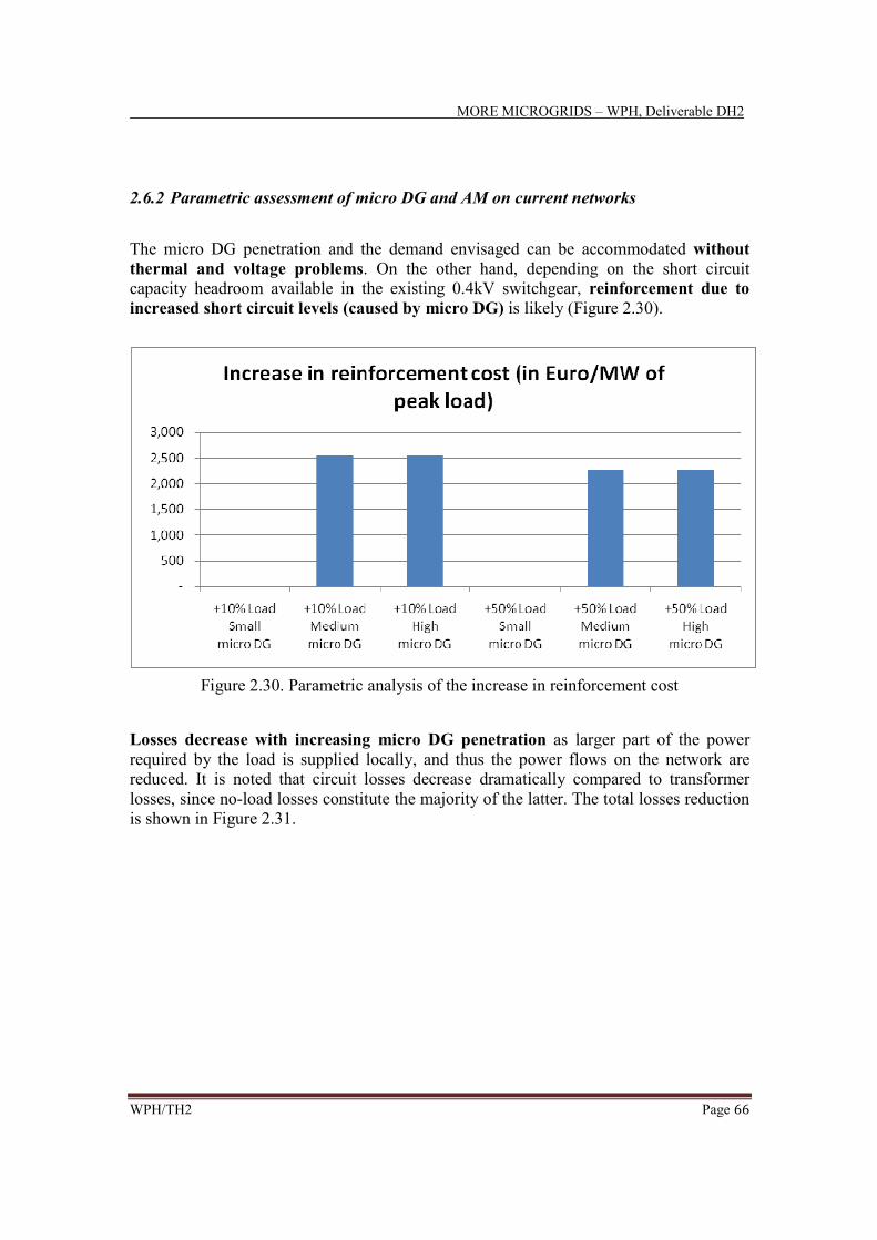
MORE MICROGRIDS – WPH, Deliverable DH2
WPH/TH2 Page 66
2.6.2 Parametric assessment of micro DG and AM on current networks
The micro DG penetration and the demand envisaged can be accommodated without
thermal and voltage problems. On the other hand, depending on the short circuit
capacity headroom available in the existing 0.4kV switchgear, reinforcement due to
increased short circuit levels (caused by micro DG) is likely (Figure 2.30).
Figure 2.30. Parametric analysis of the increase in reinforcement cost
Losses decrease with increasing micro DG penetration as larger part of the power
required by the load is supplied locally, and thus the power flows on the network are
reduced. It is noted that circuit losses decrease dramatically compared to transformer
losses, since no-load losses constitute the majority of the latter. The total losses reduction
is shown in Figure 2.31.

MORE MICROGRIDS – WPH, Deliverable DH2
WPH/TH2 Page 67
Figure 2.31. Parametric analysis of the reduction in losses
Overall, network cost decreases by the installation of micro DG thank to losses
reduction, although increased micro DG penetration is likely to require switchgear
reinforcement because of increased short circuit levels.
Finally, the installation of micro DG reduces the maximum GSP power flow and alters
the shape of the aggregate demand curve of the German distribution network (as a
result the time that the peak occurs in a winter weekday is changed), as shown in Figure
2.32, with potential impacts on transmission investment and central generation
scheduling decisions.
Figure 2.32. Parametric analysis of the changes in the aggregate demand curve
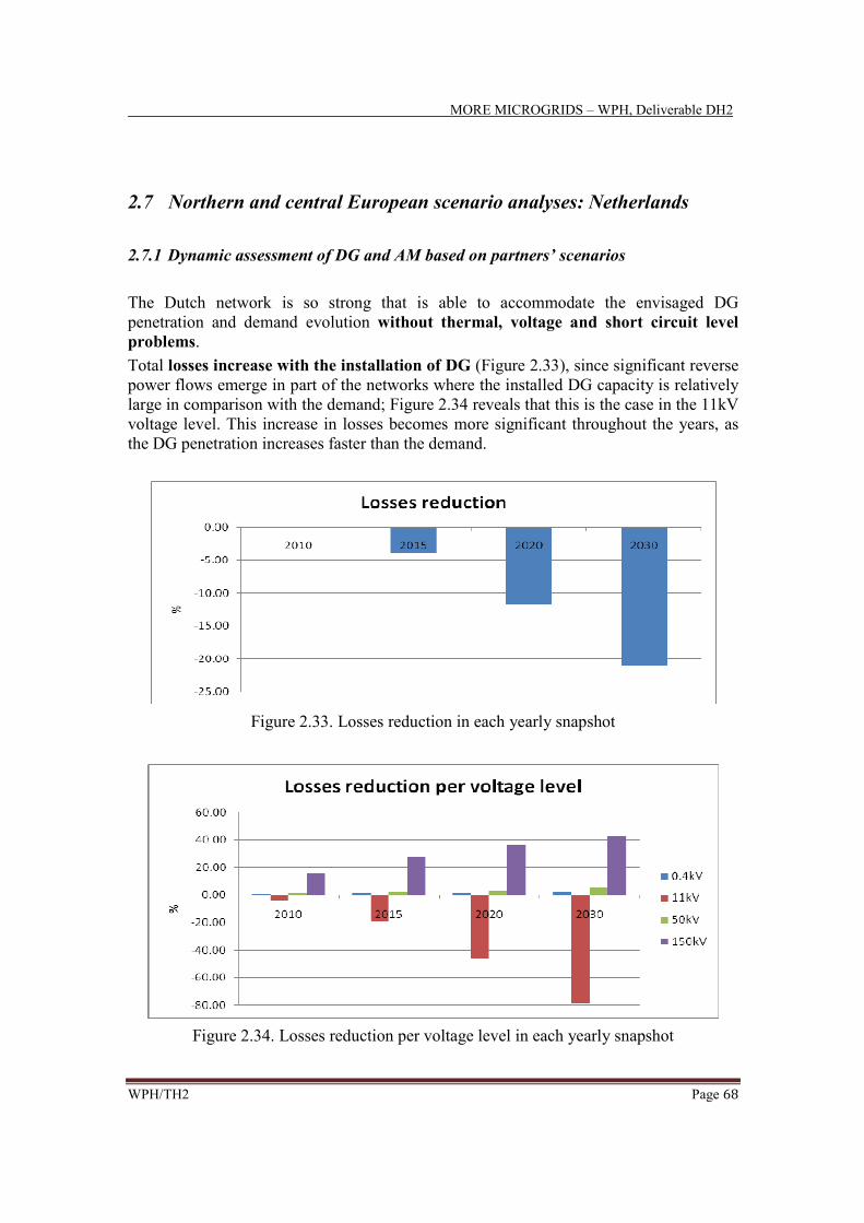
MORE MICROGRIDS – WPH, Deliverable DH2
WPH/TH2 Page 68
2.7 Northern and central European scenario analyses: Netherlands
2.7.1 Dynamic assessment of DG and AM based on partners’ scenarios
The Dutch network is so strong that is able to accommodate the envisaged DG
penetration and demand evolution without thermal, voltage and short circuit level
problems.
Total losses increase with the installation of DG (Figure 2.33), since significant reverse
power flows emerge in part of the networks where the installed DG capacity is relatively
large in comparison with the demand; Figure 2.34 reveals that this is the case in the 11kV
voltage level. This increase in losses becomes more significant throughout the years, as
the DG penetration increases faster than the demand.
Figure 2.33. Losses reduction in each yearly snapshot
Figure 2.34. Losses reduction per voltage level in each yearly snapshot

MORE MICROGRIDS – WPH, Deliverable DH2
WPH/TH2 Page 69
Overall, the foreseen DG penetration increases the total network cost, since it
increases the (cost of) losses while it does not affect the reinforcement cost.
The foreseen DG penetration reduces the maximum GSP power flow and alters the
shape of the aggregate demand curve of the Dutch distribution network (Figure
2.35), with potential impacts on transmission investment and central generation
scheduling decisions.
Figure 2.35. Changes in the aggregate demand curve
2.7.2 Parametric assessment of micro DG and AM on current networks
The Dutch network is able to accommodate the envisaged micro DG penetration and
demand without thermal, voltage and short circuit problems.
As shown in Figure 2.36, losses decrease with increasing micro DG penetration, as
larger part of the power required by the load is supplied locally, and thus the power flows
on the network are reduced. It is noted that circuit losses decrease dramatically compared
to transformer losses since no-load losses constitute the majority of the latter (Figure
2.37).

MORE MICROGRIDS – WPH, Deliverable DH2
WPH/TH2 Page 70
Figure 2.36. Parametric analysis of the reduction in losses
Figure 2.37. Parametric analysis of the reduction in losses per network component
The total network cost is reduced when micro DG penetration is increased, since the
cost of losses follows the same trend while the reinforcement cost is not affected.

MORE MICROGRIDS – WPH, Deliverable DH2
WPH/TH2 Page 71
2.8 Northern and central European scenario analyses: Comparative
analysis
2.8.1 Dynamic assessment of DG and AM based on partners’ scenarios
In this section, a comparison of the results acquired from our dynamic analysis on
distribution networks of three different countries is carried out. More specifically, these
three distribution networks are compared on the basis of the impacts of (the foreseen in
each network) DG and the implementation of AM with respect to the base case (no DG
and passive management) over the next 20 years. Our analysis on the distribution
network of Poland has included the deployment of different operating strategies (passive
management, active management without tap changers and active management with tap
changers), since voltage problems emerge in this network; for simplicity reasons, only the
results which correspond to the optimal operating strategy (the one giving the lowest total
network cost) are presented, and thus the impact of AM is inherently included in the
following results. Moreover, our analysis on the distribution network of Germany has
showed that the installation of DG causes fault level problems and the cost of the
required reinforcement depends on the available break rating headroom of the existing
switchboards; for simplicity reasons, only the results which correspond to the worst case
scenario (10% headroom) are presented.
1.Benefits related to reinforcement
The reduction in the reinforcement cost by the installation of DG for the different
distribution networks in each of the examined time windows is presented on Figure 2.38.
We can observe that the installation of DG has different impacts on the reinforcement
cost of different networks:
i) DG has a very significant positive impact on the reinforcement cost of the
Polish network, since most of the required reinforcement is driven by demand
(thus there is ground for DG to mitigate the reinforcement cost) and its largest
part is related to violations of voltage limits (thus there is ground for active
management to mitigate the reinforcement cost)
ii) DG has no impact on the reinforcement cost of the Dutch network since this
network is so strong that no reinforcement is required without or with DG
installed
iii) DG has a marginal negative impact on the reinforcement cost of the strong
German network in the time windows 2010-2015 and 2030-2040 since the
installation of DG causes fault level problems and thus drives the replacement
of some switchboards; on the other hand, it has no impact on the
reinforcement cost in the time windows 2015-2020 and 2020-2030

MORE MICROGRIDS – WPH, Deliverable DH2
WPH/TH2 Page 72
Figure 2.38. Comparison of the reduction in reinforcement cost
2.Benefits related to losses
The losses reduction by the installation of DG for the different distribution networks in
each of the examined yearly snapshots is depicted on Figure 2.39. We can observe that
the installation of DG has different impacts on the losses of different networks:
i) DG has a positive impact on the losses of the German network, as part of the
power required by the load is supplied locally and consequently the power
flows from the GSP to the demand are reduced; this positive impact increases
as years pass by, since DG penetration increases much faster than the demand
and consequently greater part of the demand is supplied locally
ii) DG has a negative impact on the losses of the Dutch network, since
significant reverse power flows emerge in parts of the network where the
installed DG capacity is relatively large in comparison with the load; this
negative impact increases as the years pass by since DG penetration increases
much faster than the demand and consequently the emerging reverse power
flows become more significant
iii) DG has a negative impact on the losses of the Polish network, because the
strategy deployed in the DG case (active management without tap changers) is
characterized by very high losses because it involves the connection of very
large capacitive compensation which creates significant reverse power flows;

MORE MICROGRIDS – WPH, Deliverable DH2
WPH/TH2 Page 73
this negative impact increases as the years pass by since this capacitive
compensation increases faster than the demand and consequently the
emerging reverse power flows become more significant
Figure 2.39. Comparison of the reduction in losses
3.Benefits related to total network cost
The reduction in total network cost (sum of the reduction in reinforcement cost and the
reduction in the cost of losses) by the installation of DG for the different distribution
networks in each of the examined time windows is presented on Figure 2.40. We can
observe that the installation of DG has different impacts on the total network cost of
different networks:
i) DG has a significant positive impact on the total network cost of the Polish
network, since its positive impact on reinforcement cost is extremely higher
than its negative impact on (the cost of) losses
ii) DG has a moderate positive impact on the total network cost of the German
network, since its positive impact on (the cost of) losses is much higher than
its marginal negative impact on reinforcement cost
iii) DG has a marginal negative impact on the total network cost of the Dutch
network, since it increases (the cost of) losses and it does not affect
reinforcement cost

MORE MICROGRIDS – WPH, Deliverable DH2
WPH/TH2 Page 74
Figure 2.40. Comparison of the reduction in total network cost
The network which is benefited the most by the installation of DG is the Polish one,
where there is significant ground for DG and AM to mitigate the required reinforcement.
The incremental benefit of DG on the total network cost (value of the next kW of DG) for
the different distribution networks in each of the examined time windows is presented on
Figure 2.41; similar trends are observed here, with the highest value of DG being
observed in the Polish network.
Figure 2.41. Comparison of the incremental benefit of DG

MORE MICROGRIDS – WPH, Deliverable DH2
WPH/TH2 Page 75
2.8.2 Parametric assessment of micro DG and AM on current networks
In this section, a comparison of the results acquired from our parametric analysis on
distribution networks of five different countries is carried out. More specifically, these
five distribution networks are compared on the basis of the impacts of micro DG and AM
with respect to the base case (no micro DG and passive management). Our analysis on
the distribution networks of Poland, FYROM and UK has included the deployment of
different operating strategies (passive management, active management without tap
changers and active management with tap changers), since voltage problems emerge in
these networks; for simplicity reasons, only the results which correspond to the optimal
operating strategy (the one giving the lowest total network cost) are presented, and thus
the impact of AM is inherently included in the following results. Moreover, our analysis
on the distribution network of Germany has showed that the installation of micro DG
causes fault level problems and the cost of the required reinforcement depends on the
available break rating headroom of the existing switchboards; for simplicity reasons, only
the results which correspond to the worst case scenario (10% headroom) are presented.
1.Benefits related to reinforcement
The reduction in the annualized reinforcement cost by the installation of micro DG for
the different distribution networks in the low and the high load scenario is presented on
Figures 2.42 and 2.43 respectively. We can observe that the installation of micro DG has
different impacts on the reinforcement cost of different networks:
i) in the Polish, FYROM and UK networks micro DG has a positive impact on the
reinforcement cost since reinforcement is driven by demand (thus there is ground
for micro DG to mitigate the reinforcement cost) and its largest part is related to
violations of voltage limits (thus there is ground for active management to
mitigate the reinforcement cost); the network which is benefited the most by the
installation of micro DG in the low load scenario is the Polish one, while the
greatest benefit by the installation of micro DG in the high load scenario is
observed in the UK network
ii) in the Dutch network micro DG has no impact on the reinforcement cost since
this network is so strong that no reinforcement is required without or with micro
DG installed
iii) in the German network micro DG has a negative impact on the reinforcement
cost since the installation of micro DG causes fault level problems and thus
drives the replacement of some switchboards
As expected, for a specific demand, the positive (Poland, FYROM, UK) and negative
(Germany) impact of micro DG generally increases with its penetration.

MORE MICROGRIDS – WPH, Deliverable DH2
WPH/TH2 Page 76
Figure 2.42. Comparison of the reduction in reinforcement cost in low load scenario
Figure 2.43. Comparison of the reduction in reinforcement cost in high load scenario
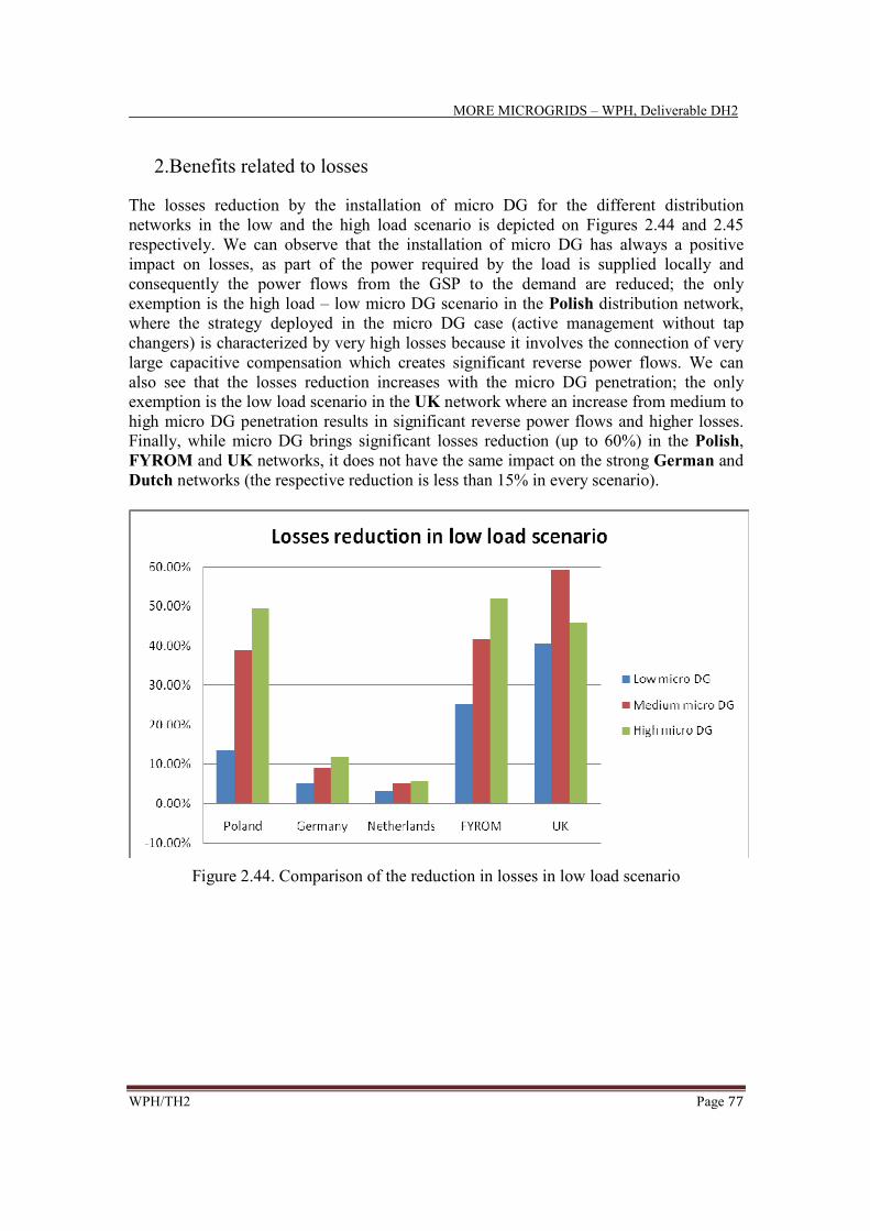
MORE MICROGRIDS – WPH, Deliverable DH2
WPH/TH2 Page 77
2.Benefits related to losses
The losses reduction by the installation of micro DG for the different distribution
networks in the low and the high load scenario is depicted on Figures 2.44 and 2.45
respectively. We can observe that the installation of micro DG has always a positive
impact on losses, as part of the power required by the load is supplied locally and
consequently the power flows from the GSP to the demand are reduced; the only
exemption is the high load – low micro DG scenario in the Polish distribution network,
where the strategy deployed in the micro DG case (active management without tap
changers) is characterized by very high losses because it involves the connection of very
large capacitive compensation which creates significant reverse power flows. We can
also see that the losses reduction increases with the micro DG penetration; the only
exemption is the low load scenario in the UK network where an increase from medium to
high micro DG penetration results in significant reverse power flows and higher losses.
Finally, while micro DG brings significant losses reduction (up to 60%) in the Polish,
FYROM and UK networks, it does not have the same impact on the strong German and
Dutch networks (the respective reduction is less than 15% in every scenario).
Figure 2.44. Comparison of the reduction in losses in low load scenario

MORE MICROGRIDS – WPH, Deliverable DH2
WPH/TH2 Page 78
Figure 2.45. Comparison of the reduction in losses in high load scenario
3.Benefits related to total network cost
The reduction in total network cost (sum of the reduction in the annualized reinforcement
cost and the reduction in the annual cost of losses) by the installation of micro DG for the
different distribution networks in the low and the high load scenario is presented on
Figures 2.46 and 2.47 respectively. We can observe that the installation of micro DG has
always a positive impact on the total network cost:
i) in the Polish, FYROM and UK networks, micro DG reduces both the
reinforcement cost (Figures 2.42 and 2.43) and the cost of losses (since it
reduces losses as shown on Figures 2.44 and 2.45; the only exemption is the
high load-low micro DG scenario in the Polish network but the increase in the
cost of losses is extremely smaller than the reduction in the reinforcement
cost),
ii) in the Dutch network, micro DG reduces the cost of losses (since it reduces
losses), while it has no impact on the reinforcement cost and
iii) in the German network, even though micro DG has a negative impact on the
reinforcement cost it has a much higher positive impact on the cost of losses
(since it reduces losses).
Regarding the impacts of different micro DG penetrations, we can see that:
i) in the Polish and FYROM networks, the total network cost is decreased when the
micro DG penetration is increased, since both the reinforcement cost and the cost
of losses follow the same trend,
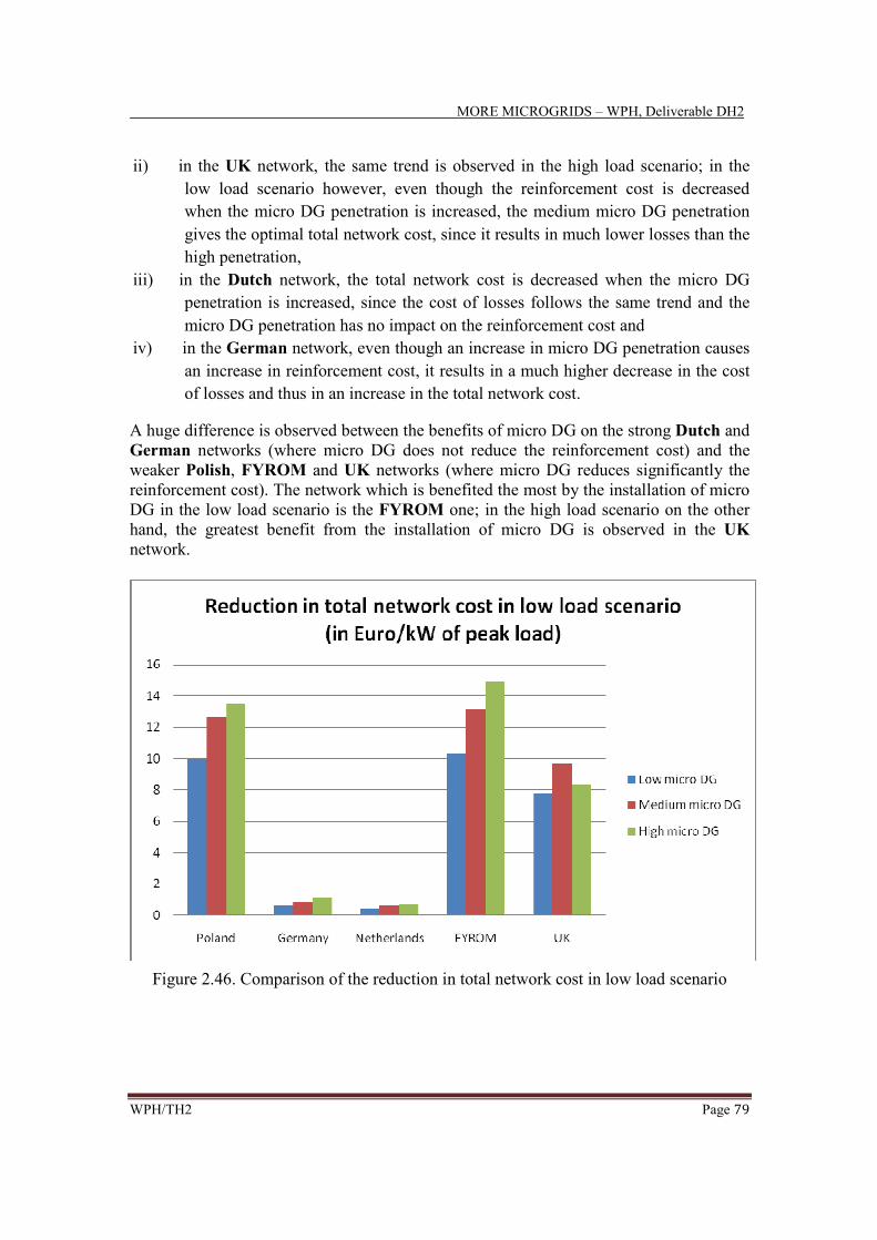
MORE MICROGRIDS – WPH, Deliverable DH2
WPH/TH2 Page 79
ii) in the UK network, the same trend is observed in the high load scenario; in the
low load scenario however, even though the reinforcement cost is decreased
when the micro DG penetration is increased, the medium micro DG penetration
gives the optimal total network cost, since it results in much lower losses than the
high penetration,
iii) in the Dutch network, the total network cost is decreased when the micro DG
penetration is increased, since the cost of losses follows the same trend and the
micro DG penetration has no impact on the reinforcement cost and
iv) in the German network, even though an increase in micro DG penetration causes
an increase in reinforcement cost, it results in a much higher decrease in the cost
of losses and thus in an increase in the total network cost.
A huge difference is observed between the benefits of micro DG on the strong Dutch and
German networks (where micro DG does not reduce the reinforcement cost) and the
weaker Polish, FYROM and UK networks (where micro DG reduces significantly the
reinforcement cost). The network which is benefited the most by the installation of micro
DG in the low load scenario is the FYROM one; in the high load scenario on the other
hand, the greatest benefit from the installation of micro DG is observed in the UK
network.
Figure 2.46. Comparison of the reduction in total network cost in low load scenario

MORE MICROGRIDS – WPH, Deliverable DH2
WPH/TH2 Page 80
Figure 2.47. Comparison of the reduction in total network cost in high load scenario
The incremental benefit of micro DG on the total network cost (value of the next kW of
micro DG) for the different distribution networks in the low and the high load scenario is
depicted on Figures 2.48 and 2.49 respectively. For each network, as the micro DG
penetration is increased (for a specific level of demand) and as the demand is decreased
(for a specific level of micro DG penetration), the available room for beneficial effects of
extra micro DG capacity is reduced and thus the value of the next kW of micro DG is
decreased. The networks with the highest value of micro DG in the low and the high load
scenario are the Polish and the UK network respectively.
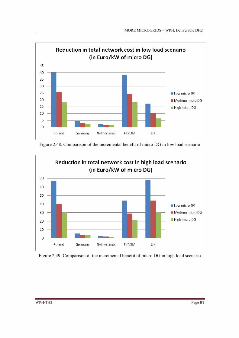
MORE MICROGRIDS – WPH, Deliverable DH2
WPH/TH2 Page 81
Figure 2.48. Comparison of the incremental benefit of micro DG in low load scenario
Figure 2.49. Comparison of the incremental benefit of micro DG in high load scenario

MORE MICROGRIDS – WPH, Deliverable DH2
WPH/TH2 Page 82
2.9 Southern European scenario analyses: Greece
This Section briefly summarizes the main findings by NTUA about the infrastructure
impact of Microgrids on a typical distribution network in Greece, characterised by a
number of micro-PV units spread across the network coupled with relatively larger
dispatchable generators. The details of the methodology, assumptions and calculations
can be found in Annex H2.B.
2.9.1 Impact of DG on system flows and investment deferral economic benefits
As discussed above, by using DG technologies to supply locally the demand needs,
investment on strategic expensive network upgrades (above all in metropolitan areas) can
be deferred. The value of the deferral of these investments depends on the equipment
costs and the time by which these investments are deferred. This deferral time depends, in
turn, on the size of the DG being installed and the rate at which the local load grows.
More specifically, when a new DG system is installed and operates, the currents in some
of the network feeders may be reduced, according to the size of DG and its location
throughout the network. If the demand across the network continues to grow, certain time
will pass before the feeder currents reach the values found before the DG started to
operate. The benefit to the distribution utility is immediate: it will take more time for the
current on those loaded transformers or feeders to reach the technical limits at which new
investments have to be put in place. The benefit is even more evident when the current
reduction defers or avoids already scheduled investments. Therefore, the first step
towards the quantification of the benefit of transformers or feeders investment deferral is
to measure the impact of the DG output on the currents across the distribution network,
which can be assessed by running power flow analyses across the network. Once power
flows have been run and the impact of DG outputs on network flows has been quantified,
it is possible to estimate the time span τk by which the presence of DG postpones the need
for investment on certain portions of the network. The methodology is detailed in Annex
H2.B. As a result, the economic benefits to the utility can be quantified through the
temporal value of money. More specifically, the time by which a given investment on a
feeder or a group of feeders is delayed is given by the lowest (minimum) deferral time of
the feeder or any of the feeders belonging to that particular group. Thereby, the total
benefit Bi to the utility given by the Microgrid located at bus i is the sum of all benefits
obtained in all groups of feeders owing to time value of money [14], namely
∑
−=g
gi gieCB ρτ
11 (8)
2.9.2 Case study application
The methodology presented was applied to the typical Hellenic LV network shown
below, characterised by three feeders, one serving a primarily residential area, one

MORE MICROGRIDS – WPH, Deliverable DH2
WPH/TH2 Page 83
serving a small workshop, and one commercial feeder. A variety of DER, such as one
MT, one FC, one directly coupled Wind Turbine and several PV units are installed in the
residential feeder. It is assumed that all DER produce active power at unity power factor.
17
Unit
ID Unit Name
Minimum
Capacity
(kW)
Maximum
Capacity
(kW)
1 Microturbine 2 30
2 Fuel Cell 1 30
3 WT 1 0.1 15
4 PV 1 0.05 3
5 PV 2 0.05 2.5
6 PV 3 0.05 2.5
7 PV 4 0.05 2.5
8 PV 5 0.05 2.5
Figure 2.50. Hellenic 17-bus test distribution network.
2.9.3 Synthesis of the main results
Many scenarios have been analysed to assess the benefits from DG on investment
deferral. In particular, among the other results detailed in Annex H2.B, next pictures
show the deferral time and the total network benefit increase with DG penetration.
In terms of strategic considerations, it can be concluded that the deferral time and total
economic benefits increase when the DG production of a Microgrid is installed near load
pockets and during peak load period. This almost obvious result was not only confirmed
but also quantified. In particular, investments on expensive network upgrades can be
deferred. The value of the deferral of these investments depends on the investment costs
and the time by which these investments are deferred. This deferral time depends, in turn,
on the size of the DG being installed and the rate at which the local load grows. Although
a quantification of the deferral benefits is extremely complex, the results in the test case
show that the relevant correlations are linear.
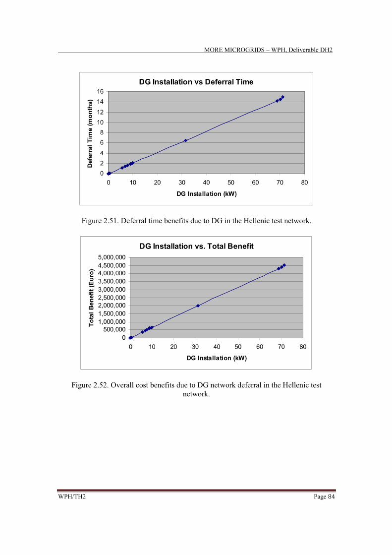
MORE MICROGRIDS – WPH, Deliverable DH2
WPH/TH2 Page 84
DG Installation vs Deferral Time
0
2
4
6
8
10
12
14
16
0 10 20 30 40 50 60 70 80
DG Installation (kW)
Defe
rral Tim
e (m
onth
s)
Figure 2.51. Deferral time benefits due to DG in the Hellenic test network.
DG Installation vs. Total Benefit
0
500,000
1,000,000
1,500,000
2,000,000
2,500,000
3,000,000
3,500,000
4,000,000
4,500,000
5,000,000
0 10 20 30 40 50 60 70 80
DG Installation (kW)
Tota
l B
enefit (E
uro
)
Figure 2.52. Overall cost benefits due to DG network deferral in the Hellenic test
network.

MORE MICROGRIDS – WPH, Deliverable DH2
WPH/TH2 Page 85
2.10 Southern European scenario analyses: Italy
This Section briefly summarizes the main findings by ERSE about the infrastructure
impact of PV-based Microgrids on a typical MV distribution network in Italy. The details
of the methodology, assumptions and calculations can be found in Annex H2.B.
2.10.1 Network design strategies in the presence of DG
A specific tool has been developed by ERSE for assessment of MV infrastructure
development in the presence of DG. The tool designs the network topology and sizes the
circuits by minimizing (through heuristic optimization) the overall cost of network
investment, maintenance, upgrade and losses, for both normal and emergency conditions,
subject to classical network constraints. In order to take into account the uncertainties
introduced by DG in the planning process, a probabilistic approach is adopted and a
probabilistic load flow (PLF) is implemented that takes into account the probability
density function (pdf) of loads and DG production. For typical distribution planning
studies, both loads and generators are represented by means of normal distributions.
As a major feature, the tool allows the planner to consider some of the most important
functions of Active Management, namely generation curtailment (in analogy to the GDS
analyses illustrated above), load shedding and network reconfiguration.
Resorting to active management is dealt with through a probabilistic approach, whereby
the DSO gives customers or producers a certain probability to be shed or disconnected
during the most critical hours, guaranteeing normal operation in the rest of the day.
However, in many cases the use of active controls is limited to emergency conditions
(line faults), that implies a reduced probability of occurrence.
The simulation of AM in the planning methodology allows postponement of investments
thanks to the maximum exploitation of the existing assets. On the other hand, as already
observed in the GDS analyses above, by maintaining the network close to its thermal
capacity limits AM generally results in an increase in losses.
For comparison purposes, simulations are run also with a conventional “fit and forget”
(F&F) planning policy, that implies the sizing of the distribution system so as to meet
technical constraints in the most onerous conditions, both in steady state and emergency
conditions: minimum load/maximum generation and maximum load/no generation.
2.10.2 Test network
The test network is a portion of a real 20 kV MV distribution network supplied by one
primary substation with two HV/MV transformers rated 16 MVA, feeding 118 MV/LV
nodes (52 feeder nodes and 66 lateral nodes). Two main areas can be identified, roughly
corresponding to low-density rural centres (4.5 MW of peak load) with long overhead
lines and high-density urban/industrial loads (11.9 MW of peak load) with underground
cables. The total length of the network is 62.8 km, of which about 80% overhead lines
MORE MICROGRIDS – WPH, Deliverable DH2
WPH/TH2 Page 86
and 20% underground cables. Five typologies of loads have been considered: residential,
industrial, tertiary, agricultural and public lighting. Details are provided in Annex H2.B.
2.10.3 Scenarios and planning strategies
The effect of different DG penetration levels and planning approaches on network
upgrade costs and losses have been analyzed.
Several scenarios have been considered with increasing levels of penetration of PV
generation on residential nodes. This choice is due to the fact that PV generation is
presently strongly supported in Italy, with high feed-in tariffs for small plants connected
to the LV level, so a significant development is expected in areas with predominant
residential characteristics. The percent level of DG penetration has been defined as the
ratio of installed capacity to peak load, referred to residential nodes only.
Different planning strategies have been adopted:
A probabilistic planning approach, taking into account load and generation daily
profiles discretized into 24 hourly intervals.
A conventional F&F, or worst-case, criterion; daily power profiles and the
coincidence factor between loads and DG are not considered.
A probabilistic planning approach with the possibility to consider at a design stage
the resort to Active Management options (DSM) to solve violations; it has been
assumed that residential customers participate to a load control program by
accepting a maximum demand reduction of 50%.
2.10.4 Assessment of the impact of totally autonomous Microgrids on network
planning
Among other analyses (detailed in Annex H2.B) relevant to DG operation within a Multi-
Microgrids framework (in which active control actions are carried out at the MV level),
specific analyses have been run for Microgrids assumed to be totally autonomous in
terms of energy balance, thanks to the integration of responsive loads, controllable
generators and storage systems. Each LV MG has been ideally represented, at the MV
level, as a node behaving as a load coupled with a generator, in such as way that each
Microgrid results in zero net power flow (both active and reactive) at the corresponding
MV/LV substation transformer. A totally autonomous Microgrid requires a DG
penetration level of 100% in energy terms. Given the assumed daily profiles, this implies
an installed DG capacity of about 180% of peak load; consequently, the assessment of the
benefits of Microgrids has been made with comparison to the scenario of 180% DG
penetration.
The following pictures show the comparison of investment costs, losses costs, and energy
losses (in percentage of total energy delivered to loads) for three different scenarios:
base case without DG,
180% of “simple” DG power penetration,
180% of DG power penetration (100% in energy terms) in the form of integrated
microgrids;
and for three different planning strategies:

MORE MICROGRIDS – WPH, Deliverable DH2
WPH/TH2 Page 87
probabilistic approach with daily profiles,
fit&forget,
DSM.
0%
10%
20%
30%
40%
50%
60%
70%
80%
90%
100%
110%
0% 180% 180% with microgrids (100%)
DG penetration [% of residential peak loads]
Costs
[%
of to
tal costs
of re
fere
nce c
ase]
Figure 2.53. Costs of the network designed considering daily profiles for loads and
generators
0%
10%
20%
30%
40%
50%
60%
70%
80%
90%
100%
110%
0% 180% 180% with microgrids (100%)
DG penetration [% of residential peak loads]
Costs
[%
of to
tal costs
of re
fere
nce c
ase]
Figure 2.54. Costs of the network designed based on the traditional fit&forget approach
losses cost
investment cost
losses cost
investment cost

MORE MICROGRIDS – WPH, Deliverable DH2
WPH/TH2 Page 88
0%
10%
20%
30%
40%
50%
60%
70%
80%
90%
100%
110%
0% 180% 180% with microgrids (100%)
DG penetration [% of residential peak loads]
Costs
[%
of to
tal costs
of re
fere
nce c
ase]
Figure 2.55. Costs of the network designed considering daily curves and possible load
shedding (DSM) actions
0%
10%
20%
30%
40%
50%
60%
70%
80%
90%
100%
110%
0% 180% 180% with microgrids (100%)
DG penetration [% of residential peak loads]
Costs
[%
of to
tal costs
of re
fere
nce c
ase]
Figure 2.56. Comparison of total costs under different planning strategies
losses cost
investment cost
Daily
patterns
F&F
DSM

MORE MICROGRIDS – WPH, Deliverable DH2
WPH/TH2 Page 89
0%
10%
20%
30%
40%
50%
60%
70%
80%
90%
100%
110%
0% 180% 180% with microgrids (100%)
DG penetration [% of residential peak loads]
Costs
[%
of to
tal costs
of re
fere
nce c
ase]
Figure 2.57. Comparison of investment costs under different planning strategies
It is worth noticing that in the presence of completely autonomous Microgrid operation,
load shedding actions are never necessary even in emergency conditions, so investment
costs and losses are the same as in the case of planning with daily profiles (the resultant
optimal network configuration is identical).
0.0%
0.1%
0.2%
0.3%
0.4%
0.5%
0.6%
0.7%
0.8%
0.9%
1.0%
1.1%
1.2%
1.3%
1.4%
1.5%
0% 180% 180% with microgrids (100%)
DG penetration [% of residential peak loads]
Losses [%
of energ
y d
elivere
d]
Figure 2.58. Comparison of energy losses under different planning strategies
Daily
patterns
F&F
DSM
Daily
patterns
F&F
DSM
MORE MICROGRIDS – WPH, Deliverable DH2
WPH/TH2 Page 90
2.10.5 Conclusions on the Italian network analyses
This Section has illustrated an analysis of the impact of DG and Microgrids on
investments in electricity distribution infrastructures conducted on a typical Italian MV
network, by making use of a software tool for optimal planning developed by ERSE for
research purposes. The effect on network upgrade costs and losses of an increasing
degree of penetration of PV generators in residential areas have been analyzed.
Different planning strategies have been adopted, namely: a) probabilistic, with load and
generation hourly profiles; b) conventional “fit & forget” (worst case); c) considering
active management options at a design stage. The comparison has been based on different
parameters, namely, investment costs for network upgrading, cost of losses, energy
losses, and voltage profiles.
The conventional “fit & forget” planning approach, based on a worst case scenario, leads
to higher investment costs, due to the oversizing of lines and transformers. On the other
hand, when the presence of DG is correctly taken into account at a design stage, benefits
can be obtained, at least until a certain degree of penetration, in terms of reduction in
investment costs for network upgrading – required to face load growth – and in cost of
losses. If the possibility to resort to active management options is considered during the
planning process, a further reduction in investment costs can be observed. However, the
higher exploitation of existing network asset causes an increase in energy losses. These
findings are completely in line with the findings by Imperial College for Northern and
Central European networks with different types of DG, which highlights the generality of
the results reached from different studies.
Finally, the effect of the integration, at the LV level, of loads, generators and storage in
the form of completely autonomous Microgrids has been considered, resulting in zero
active and reactive power flows at the MV/LV substation transformer. This configuration
leads to a further reduction in network upgrading costs and electricity losses.
As a further final general comment, it is crucial to underline that active management
options and Microgrid operation must be considered at the planning stage in order to take
full advantage of their benefits for network development.

MORE MICROGRIDS – WPH, Deliverable DH2
WPH/TH2 Page 91
2.11 Impact on Microgrids on network replacement scenarios through
generic distribution system fractal model
This Section shows some of the work carried out by Imperial College, detailed in Annex
H2.C, for optimal greenfield distribution network replacement scenario analysis in the
presence of Microgrids.
2.11.1 Multi-voltage fractal model, LCC network design criteria and value of DG
As widely described in Deliverable DH1 [3], Imperial has developed a specific
methodology to assess the impact and the potential value of Microgrids on distribution
network design strategies (greenfield design). The model is based on fractal algorithms
that generate generic distribution networks mimicking realistic consumer settlements and
network paths, thus enabling to get deeper insights on actual network topological
characteristics with respect to other simplified geometric models [15].
In order to evaluate system-level network replacement strategies, different voltage levels
are modelled for distribution systems, namely, LV, MV and HV. Indeed, only by
modelling the whole distribution cost chain is possible to fully capture the benefits
associated to Microgrids, even if operating at the LV level only.
Optimal economic design strategy (based on minimum Life Cycle Cost - LCC) [16] is
carried out as a benchmark design to be adopted in the future, which is consistent with
the information on replacement strategies received from the partners. This design
approach trades off operational cost (mainly due to losses, with minor contribution from
maintenance, above all in rural overhead lines) against cost of investment, so that key
network performance indicators are the network costs (infrastructure and loss-related)
with relevant breakdown.
The value of DG in Microgrids is then assessed by comparing the relevant output metrics
(mainly cost of investment and cost of losses) with and without microgeneration. For
these purposes, the network design exercise has been carried out for a base case with no
DG, and for a number of different penetration cases in which the presence of DG is taken
into account when evaluating the upstream flows at MV.
In terms of circuit design, based on the LCC model illustrated above, it can be expected
that the impact of DG will be such that potential reduced flows in MV and HV network
branches (the net flows in the branches are the driver for LCC circuit design) might imply
deployment of smaller circuits due to lower cost of losses. However, smaller circuits
might also mean higher losses at the design stage with respect to the case without DG
(where higher losses would lead to larger circuits). The presence of reduced flows
owning to DG is not considered to size laterals and feeders at LV. In fact, while it is
realistic to assume a certain degree of diversity provided by a large number of small-scale
units aggregated at LV when it comes to sizing the upper voltage levels, sizing also the
LV branches might be unrealistic. As a result, the value of DG at LV will be purely from
the value of losses reduction contributed by DG.

MORE MICROGRIDS – WPH, Deliverable DH2
WPH/TH2 Page 92
For the sake of simplicity full availability is considered here for the DG units, in order to
have an estimate of the potential effects of DG for different penetration levels and control
strategies. This somehow leads to an upper boundary of the potential contribution of DG
for network capacity support at upper voltage levels, while actual benefits in terms of
capacity support might be slightly less, as also discussed below.
Large-scale typical urban areas and rural areas in the UK have been considered for
exemplificative purposes of system level analyses. However, although the specific
numerical results are of course case-specific, the general outputs and considerations
stemming from the analysis are expected to be applicable to most networks and cases
across Europe.
2.11.2 DG technologies and control strategies for network replacement analysis
Different technologies are considered for the analysis, namely, CHP and PV, and are
assumed to be only connected at LV level. More specifically:
• Heat following for uncontrolled CHP whereby CHP generator follows the thermal
load and electricity is produced according to its co-generation ratio;
• Electricity following for 100% CHP whereby CHP generator follows the local
electrical load and heat is produced according to its co-generation ratio;
• Uncontrolled PV whereby electricity is produced as a result of solar power.
For CHP systems, the controllability issue is addressed here by assuming that the CHP
unit is running under electricity following strategy as opposed to the classical
“uncontrolled” strategy in which heat demand is followed, corresponding to intermittent
generation from a network outlook. Indeed, it can be expected that by controlling DG in
order to follow the electrical load the negative network impact will be minimized and on
the contrary network benefits will be maximized. In this way, “impact boundaries” can be
drawn by assessing the impact for the two limit control strategies, providing indications
on the additional potential value of controlling DG within Microgrids. Although these
boundaries do not envelope the maximum benefits that controllability can bring, which
would be related to optimize specific objective function and each single case (see WPG
for these specific types of analyses), the approach followed enables to get insights from a
system-level strategic perspective on the value of different operability configurations and
of increasing the correlation between local supply and demand, which has proven to be
one of the main drivers for benefits.
In the analyses considered in the sequel, penetration level is defined as number of LV
customers equipped with DG. Therefore, 100% penetration means all the customers have
a DG unit installed at their premises. Typical electrical and thermal load patterns have
been used to populate the networks with different types and number of realistic
consumers, whose details are reported in Annex H2.C.

MORE MICROGRIDS – WPH, Deliverable DH2
WPH/TH2 Page 93
2.11.3 Urban network design
Typical UK urban load density has been used to populate the relevant network
characteristics, as shown in Table 2.3.
Table 2.3. Urban network characteristics used in the case study.
Urban network characteristic LV MV
Peak demand [MVA] 5 370
Load density [MVA/km2] 5 3.7
Number of 11/0.4kV subst. 25 1,800
Number of 33/11kV subst. - 12
Network area [km2] 1 100
Network length [km] 27 322
Number of LV consumers 2,000 150,000
Figure 2.59 shows the overall value of DG (capitalized value of losses plus investment,
given in £/year per kW of network peak demand and based on 30 years network life and
7% discount rate) for different penetration levels of PV connected at LV system, with
breakdown of value per voltage level. Similarly, Figure 2.60 shows the value of DG in
the case of CHP systems (in both uncontrolled and controlled cases). As mentioned
above, the value of DG has been calculated as difference between base case (network
designed without DG) and the DG case.
It can be easily observed that controlled CHP provides the highest value for avoided
network cost with least network impact, since perfect match is achieved between local
demand and supply, minimizing the flows required from the upper network as well as
possible counter-flows due to load/generation un-correlation and then exporting energy.
However, it has to be noticed that even when perfect local match (full controllability)
occurs, it is not possible to decrease the network below certain thresholds (that also
depend on the penetration levels). In fact, the circuits need to be able to stand the relevant
short-circuit currents, which leads to install minimum circuit size. In addition, for at MV
and HV voltage levels the circuits are typically doubled due to security constraints and
need for guaranteeing that enough capacity is available for network reconfiguration in the
presence of downstream faults.
As for the uncontrolled CHP, the value of DG is still quite substantial owing to the good
correlation between load and generation. As expected, the highly uncorrelated PV
generation to load profile (peak production occurs in summer daytime, while
consumption in the UK is prevailing in winter evenings) results in the lowest network
value. For Southern countries, PV could instead provide suitable network support, as for
instance exemplified in the Italian distribution network analyses reported in Section 2.10.
The potential cost contribution of DG for infrastructure replacement is summarized in
Table 2.4 with respect to the base case network cost with no DG. It can be appreciated
that potentially up to one-third of network cost can be avoided for 100% controllable

MORE MICROGRIDS – WPH, Deliverable DH2
WPH/TH2 Page 94
CHP scenario with 100% of DG penetration. However, also uncontrolled CHP can give a
substantial contribution owing to relatively good electricity and heat demand correlation,
which translates into good generation and demand correlation even for the heat following
strategy. On the other hand, the extent of cost contribution from PV is more limited, and
it is mostly due to cost reduction, which in turn drives towards smaller circuits according
to the minimum LCC methodology adopted. However, this effect is relatively small.
0
2
4
6
8
10
12
14
0 10 20 30 50 100
£/k
W/y
ea
r
DG penetration level (%)
33kV 11kV LV
Figure 2.59. Network value of DG for PV in UK urban networks.
0
2
4
6
8
10
12
14
0 10 20 30 50 100
£/k
W/y
ea
r
DG penetration level (%)
33kV 11kV LV
0
2
4
6
8
10
12
14
0 10 20 30 50 100
£/k
W/
ye
ar
DG penetration level (%)
33kV 11kV LV
Figure 2.60. Network value of DG for uncontrolled (left) and 100% controlled (right)
CHP in urban networks.
Table 2.4. Overall value of DG (for LV, MV and HV) in percentage with respect to the
base case (no DG) urban network cost.
Scenarios 0 10 20 30 50 100
PV 0.0 2.8 4.2 6.1 8.4 10.6
Uncontrolled CHP 0.0 4.7 8.3 12.0 17.3 23.7
Controlled CHP 0.0 5.5 8.7 12.7 20.1 36.3
DG penetration levels (%)
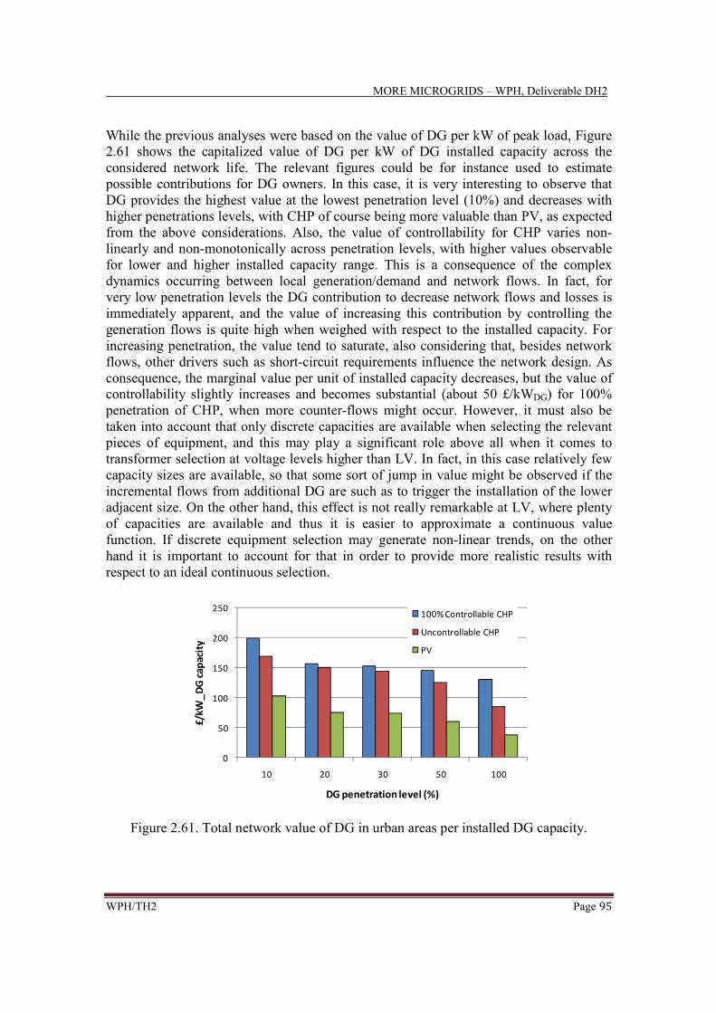
MORE MICROGRIDS – WPH, Deliverable DH2
WPH/TH2 Page 95
While the previous analyses were based on the value of DG per kW of peak load, Figure
2.61 shows the capitalized value of DG per kW of DG installed capacity across the
considered network life. The relevant figures could be for instance used to estimate
possible contributions for DG owners. In this case, it is very interesting to observe that
DG provides the highest value at the lowest penetration level (10%) and decreases with
higher penetrations levels, with CHP of course being more valuable than PV, as expected
from the above considerations. Also, the value of controllability for CHP varies non-
linearly and non-monotonically across penetration levels, with higher values observable
for lower and higher installed capacity range. This is a consequence of the complex
dynamics occurring between local generation/demand and network flows. In fact, for
very low penetration levels the DG contribution to decrease network flows and losses is
immediately apparent, and the value of increasing this contribution by controlling the
generation flows is quite high when weighed with respect to the installed capacity. For
increasing penetration, the value tend to saturate, also considering that, besides network
flows, other drivers such as short-circuit requirements influence the network design. As
consequence, the marginal value per unit of installed capacity decreases, but the value of
controllability slightly increases and becomes substantial (about 50 £/kWDG) for 100%
penetration of CHP, when more counter-flows might occur. However, it must also be
taken into account that only discrete capacities are available when selecting the relevant
pieces of equipment, and this may play a significant role above all when it comes to
transformer selection at voltage levels higher than LV. In fact, in this case relatively few
capacity sizes are available, so that some sort of jump in value might be observed if the
incremental flows from additional DG are such as to trigger the installation of the lower
adjacent size. On the other hand, this effect is not really remarkable at LV, where plenty
of capacities are available and thus it is easier to approximate a continuous value
function. If discrete equipment selection may generate non-linear trends, on the other
hand it is important to account for that in order to provide more realistic results with
respect to an ideal continuous selection.
0
50
100
150
200
250
10 20 30 50 100
£/k
W_
DG
ca
pa
city
DG penetration level (%)
100% Controllable CHP
Uncontrollable CHP
PV
Figure 2.61. Total network value of DG in urban areas per installed DG capacity.

MORE MICROGRIDS – WPH, Deliverable DH2
WPH/TH2 Page 96
Figure 2.62 and Figure 2.63 shows the total network losses for the considered scenarios
for PV and CHP, respectively. It can be observed that the higher is the correlation
between DG generation and demand profile, the greater is the network losses reduction.
In particular, the losses decrease is substantial at LV, where the great majority of losses
within the distribution system occur. Relative losses reduction with respect to the base
case can be as high as 50% when uncontrolled CHP is used for the 100% penetration
level, and in the same condition controllability can further decrease losses by an
additional 15%. Hence, total distribution losses may pass from about 3.7% without DG to
as little as 1.4% in the case of controlled CHP for all LV customers. On the other hand, it
is very interesting to observe the effects of PV generation. For low penetration levels, the
contribution to losses reduction is similar to the one from CHP. However, this reduction
starts to saturate at higher PV penetrations (>50%), as apparent from Figure 2.62,
whereby there reverse flows occur (PV production becomes substantial at times of low
demand in the central hours of summer days).
Further analyses relevant to cost breakdown per equipment and voltage levels are
reported in Annex H2.C.
0.0%
0.5%
1.0%
1.5%
2.0%
2.5%
3.0%
3.5%
4.0%
0 10 20 30 50 100
Loss
es
(%)
DG penetration level (%)
33kV
11kV
LV
Figure 2.62. Total network losses in urban areas for PV
0.0%
0.5%
1.0%
1.5%
2.0%
2.5%
3.0%
3.5%
4.0%
0 10 20 30 50 100
Loss
es
(%)
DG penetration level (%)
33kV
11kV
LV
0.0%
0.5%
1.0%
1.5%
2.0%
2.5%
3.0%
3.5%
4.0%
0 10 20 30 50 100
Loss
es
(%)
DG penetration level (%)
33kV
11kV
LV
Figure 2.63. Total network losses in urban areas for uncontrolled (left) and 100%
controlled (right) CHP

MORE MICROGRIDS – WPH, Deliverable DH2
WPH/TH2 Page 97
2.11.4 Rural network design
In order to have a full picture of the potential of Microgrids for network design
contribution, studies on typical rural networks have been carried out in addition to the
above urban analyses. The full set of studies performed for rural areas, analogous to the
urban studies, is reported in Annex H2.C.
2.11.5 Losses result comparison with other studies
The impact of RES and DG especially micro generation (micro-CHP and PV) had also
been previously studied through the UK GDS model in [17], which is recalled here for
the sake of comparison. In that case, two different network characteristics, rural and
urban were used, again taking into account peak and off-peak demand conditions and
temporal variation (hourly and seasonal) of loads and DG output for different penetration
levels of DG. Characteristic simplified profiles of micro-CHP and PV were used. The
results of the studies are summarised in Figure 2.64 for rural areas and Figure 2.65 for
urban areas.
0
1
2
3
4
5
6
7
8
9
10
0% 8% 16% 20% 24% 32% 39% 59% 80% 80% 90% 100%
Installed capacity in % of the GSP peak load
Losses (%
)
CHP-Rural PV-Rural
Figure 2.64. Contribution of micro-CHP and PV on the reduction in distribution network
losses in rural areas in Northern European characteristic systems.
0
1
2
3
4
5
6
7
8
9
10
0% 8% 16% 20% 24% 32% 39% 59% 80% 80% 90% 100%
Installed capacity in % of the GSP peak load
Losses (%
)
CHP-Urban PV-Urban
Figure 2.65. Contribution of micro-CHP and PV on the reduction in distribution network
losses in urban areas in Northern European characteristic systems.

MORE MICROGRIDS – WPH, Deliverable DH2
WPH/TH2 Page 98
Losses are given in percentage of annual energy consumption. In the UK, the average
distribution losses are about 7% with losses in rural networks significantly higher (mostly
doubled) than losses in urban (city) areas. This can be understood since customers in
rural areas are more clustered and connected via longer and smaller conductors compared
with customers in town and cities. Thus, the effect of deploying micro-CHP and PV is
more apparent in rural systems. The level of losses can be reduced by 41% from 8.5% to
5% of annual energy consumption by micro-CHP with total installed capacity of 50% of
the total Grid Supply Point (GSP) peak load. In urban areas, the same capacity of micro-
CHP only reduces the level of losses from 4.5% to 3% (33% reduction). Application of
PV also shows similar trends but with significantly less impact in magnitude; in fact, with
the same installed capacity (50% of peak demand), the reduction of losses is about 1.5%.
This is less than half of the benefits obtained by micro-CHP. Given that the peak output
of PV is not correlated with peak demand especially in the UK, PV contribution to loss
reduction will not be as significant as micro-CHP.
It is therefore interesting to notice how the analyses run for future network development
through the fractal model are consistent with the impact assessment analyses run with the
GDS system. However, besides that, it is also interesting to notice how in the fractal
expansion analyses the figures found for losses were quite lower than the actual ones,
above all for rural areas (see Annex H2.C). This is due to the LCC methodology used for
network design, which, by explicitly taking into account the cost of losses, implicitly
leads to set up an energy-efficient network, benchmark for future power systems.
2.11.6 Concluding remarks on the fractal network replacement assessment
The studies carried out with the fractal model for greenfield network design show that
correlation between load and generation is a key factor for network development
contribution of DG and the relevant value of control micro-generation within Microgrids,
confirming the impact assessment studies run above for different European countries. In
this light, uncontrolled CHP could potentially provide network support owing to good
correlation, with a substantial value brought by DG in both urban and rural areas. Up to
one-third of network cost can be avoided for 100% controllable CHP (corresponding to
an annual network cost of about 11 £/kW), with the maximum value of controllability in
the order of 50 £/kWDG in urban areas for 100% penetration level and 30 £/kWDG in rural
areas for penetration higher than 30% (see Annex H2.C for rural-related assessment). On
the other hand, PV has poor correlation with the load in the UK systems analysed, and
can only provide up to 10% of network avoided cost, mostly in terms of losses. The
network infrastructure savings due to reduced power flows is substantial at MV, with
prevailing influence on transformers in urban areas and overhead lines in rural areas.
Equipment capacity saving is also significant at higher level of penetration, where the
smaller number of pieces of equipment available may induce form of nonlinearities in the
DG value for different penetration levels, though.
7
7

MORE MICROGRIDS – WPH, Deliverable DH2
WPH/TH2 Page 99
2.12 Fractal network-based analysis of economic and environmental
impact of micro-CHP systems in Microgrids
This Section reports the main findings of the work carried out by Imperial College,
detailed in Annex H2.C, about comprehensive network and environmental benefits for
distributed CHP (DCHP) systems operated within Microgrids according to different
control strategies, and of the relevant impact of controllability actions. This is
fundamental to identify all the costs and benefits from DER not only in terms of electrical
networks but for the overall energy system chain.
2.12.1 Network, environmental and DG modelling
Potential costs and benefits in terms of network impact from DCHP operated within
Microgrids are calculated on the basis of a reference network whose topology and circuit
sizing is generated through the fractal model and the LCC methodology described in the
previous Section. Again, a typical UK urban network model is specifically used for the
analysis, but the methodology could be applied to more general situations for system-
wide assessments.
The energy performance of CHP prime movers are represented by their electrical efficiency
and thermal efficiency. In addition, the cogeneration ratio, ratio of heat to electricity output
as well as of thermal to electrical efficiency, is used to characterise the DG behaviour.
Details on the modelling can be found in Deliverable DH1 [3].
Different penetration levels are analysed, indicated with the index p, defined as the
relative number of customers with a CHP unit out of the overall LV customers. In
addition, as in the previous Section two control strategies for DCHP have been defined
here, namely, Heat Following (HF) and Electricity Following (EF). As mentioned above,
from the electrical outlook heat following mode may be considered as uncontrolled or
intermittent generation, whereby cogeneration benefits are maximised. On the other hand,
if the CHP generator follows the local electrical load, heat is produced accordingly
(regardless of the actual thermal load), as resulting from the characteristics cogeneration
ratio. In this case, an auxiliary boiler is assumed to be put in operation to supply the
thermal load if the thermal production is not sufficient (no storage is modelled here). On
the other hand, if the heat cogenerated is higher than the actual local thermal demand,
heat is wasted. Therefore, this strategy brings smaller environmental benefits relative to
the thermal load following. Environmental benefits are defined according to the PES
(primary energy saving) and CO2ER (CO2 emission reduction) indicators introduced in
Deliverable DH1 and detailed in Annex H2.C.
For each penetration level p of DCHP, controllability within Microgrids is addressed by
changing the number of units operated following the local electrical load rather than the
thermal one (assumed to be the base case). This is indicated through the index cp,
pointing out the ratio of electricity-driven CHP units with respect to overall ones (the
remaining units are supposed to operate with classical thermal following).

MORE MICROGRIDS – WPH, Deliverable DH2
WPH/TH2 Page 100
Network benefits of DG are based on identifying the investment deferral benefits and
losses change owing to DCHP generation for different scenarios with respect to a bas
case without DG. Hence, the main difference with the analyses run in the above Section
is that here no network design is carried out, but the impact on a (reference) network is
assessed.
2.12.2Generation scenarios and analyses
Starting from the network and demand characteristics detailed in Annex H2.C, two
generation mixes (also detailed in the Annex) have been considered, which lead to a
number of scenarios obtained by changing the DG penetration and controllability indices.
In the generation mix 1, terrace houses equipped with DCHP can in principle cover both
electricity and heat peak (if the two peaks occurred simultaneously); this is line with
currently envisaged applications of micro-CHP systems mainly aimed at substituting
residential boilers. On the other hand, regardless of the control strategy adopted, flat
buildings equipped with the MT1 in any case needs support from the grid to cover the
electrical demand and from auxiliary boilers to cover the heat demand. Again, this sizing
approach is in line with typical design strategies for relatively larger CHP systems aimed
at covering a certain part of the electrical/thermal load to maximize the plant profitability.
In the generation mix 2, again terrace houses with DCHP can potentially cover both
electricity and heat peak, with a major difference relative to the previous case, namely,
that electricity can be exported to the grid owing to the larger electrical capacity of the
ICE unit. Similarly, flat buildings equipped with the MT2 will be able to export
electricity when following the heat demand. It is also important to highlight that the
overall DG electric capacity installed in generation mix 2 is such that all LV networks
considered can in principle operate isolated from the MV network as energy autonomous
Microgrids, while isolated operation for generation mix 1 could occur only through
resorting to load control actions.
2.12.3 Synthesis of the network deferral results
A number of nonlinearities arise in the operation of DCHP systems in different
penetration and controllability scenarios, which highlight the complexity of the concepts
studied. In this respect, Figure 2.66 illustrates some typical nonlinearity that may
characterize the peak loading analysis (relevant to investment deferral benefits) for a
representative case of 100 kVA transformer. In particular, it can be seen how for
generation mix 1 while moving from p = 10% to p = 50% the loading level halves, with
negligible impact of controllability for 10% penetration and relatively small for 50%
penetration. On the other hand, increasing the penetration level to p = 100% does not
change substantially the substation peak loading level, due to some sort of saturation in
the correlation between generation and loads. However, the loading level further
decreases when the share of generation units in electricity following mode increases.
Contrarily, the higher installed electrical capacity in generation mix 2 is such that
counter-flows occur for high penetration levels, leading to even higher loading level than

MORE MICROGRIDS – WPH, Deliverable DH2
WPH/TH2 Page 101
in the base case (without DG) for p=0 and all CHP units in heat following mode. In this
case, the effects of controllability to mitigate counter-flows are apparent, with the LV
network that can operate isolated as an autonomous Microgrid for cp=100% (transformer
loading level equal to zero in Figure 2.66 (b)).
0
20
40
60
80
100
NO DG 0% 10% 50% 100% 0% 10% 50% 100% 0% 10% 50% 100%
loading, %
Percentage of units in electricity following mode
10% DG penetration
50% DG penetration 100% DG penetration
substation ID 11
0
20
40
60
80
100
NO
DG
0% 10% 50% 100% 0% 10% 50% 100% 0% 10% 50% 100%
loading, %
Percentage of units in electricity following mode
10% DG penetration
50% DG penetration
100% DG penetrationsubstation ID 11
a) Generation mix 1 b) Generation mix 2
Figure 2.66. Zoom-out of substation maximum loading profile for a 100 kWe unit.
The analysis regarding the substation maximum loading level directly translates into
ability of DG to defer investment, as opposed to potential negative effects of anticipating
investment. A synthetic economic view on the effects of penetration and controllability
levels of DG is provided in Figure 2.67 that shows the potential economic value
(normalized to the network peak load) of network capacity release for the overall
network. For generation mix 1, Figure 2.67(a) confirms that there is some sort of
saturation effect in terms of network deferral value while increasing p, mainly due to the
generation/load correlation. In all cases, controllability can increase the economic value
of the network asset. Again, it is even more interesting to analyse what happens for
generation mix 2. In fact, in this case for low penetration (p = 10%) the value is about
50% higher than for generation mix 1, owing to local generation/load balance. On the
other hand, there are only marginal benefits from generation mix 2 relative to generation
mix 1 for p = 50%, due to the increasing uncorrelated energy between generation and
load. The situation is exacerbated for large DG penetration (p = 100%) of generation mix
2, for which no economic value arise at all due to uncorrelated flows as exemplified in
Figure 2.67(b) unless DG is operated under electricity following mode. However, even in
this latter case the value is less than from generation mix 1, apart from marginal benefits
in the extreme case with p = 100% and cp = 100% (isolated energy autonomous
Microgrid operation).

MORE MICROGRIDS – WPH, Deliverable DH2
WPH/TH2 Page 102
0
10
20
30
40
50
60
0% 10% 50% 100% 0% 10% 50% 100% 0% 10% 50% 100%
£/kWp
Percentage of units in electricity following mode
10% DG penetration
50% DG penetration
100% DG penetration
-10
0
10
20
30
40
50
60
0% 10% 50% 100% 0% 10% 50% 100% 0% 10% 50% 100%
£/kWp
Percentage of units in electricity following mode
10% DG penetration
50% DG penetration
100% DG penetration
a) Generation mix 1 b) Generation mix 2
Figure 2.67. Network overall NPV (normalised with respect to the network peak demand)
of transformer capacity release.
In terms of network value brought by DCHP normalised with respect to DG installed
capacity (potentially useful to formulate rewards for the prosumers), it can be appreciated
how the specific value of DG decreases with the penetration level, that is, the marginal
value of DG is a negative slope function with respect to the penetration level as shown in
Figure 2.68. In fact, the benefits brought by local balancing are maximised when the DG
production is relatively low (all produced electricity displaces peak flows), and decreases
with an increase of (in part uncorrelated) production. For the same reason, the value for
generation mix 1 is higher than for generation mix 2 by about 20 £/kWDG regardless of
the control strategy for penetration level of 10% and 50%. The value is even higher for p
= 100% when part of the units in generation mix 2 are run following the heat, for the
reasons explained above.
0
10
20
30
40
50
60
70
80
0% 10% 50% 100% 0% 10% 50% 100% 0% 10% 50% 100%
£/kWD G
Percentage of units in electricity following mode
10% DG penetration
50% DG penetration
100% DG penetration
0
10
20
30
40
50
60
70
80
0% 10% 50% 100% 0% 10% 50% 100% 0% 10% 50% 100%
£/kWDG
Percentage of units in electricity following mode
10% DG penetration
50% DG penetration
100% DG penetration
a) Generation mix 1 b) Generation mix 2
Figure 2.68. Network overall NPV (normalised with respect to the DG installed electrical
capacity) of transformer capacity release.
2.12.4Environmental performance
While the previous analyses have focused on network impact, Figure 2.69 and Figure
2.70 show the potential environmental benefits that DCHP systems can bring owing to
cogeneration of electricity and heat in terms of energy saving and emission reduction for
the overall network, respectively. Besides for different values of p and cp, also different
average power system electrical generation efficiencies and emission factors are

MORE MICROGRIDS – WPH, Deliverable DH2
WPH/TH2 Page 103
considered as parameters, while for heat generation the base case refer to the thermal
energy balances calculated in the case of no DG.
The environmental benefits increase with DG penetration, as expected since a higher
share of overall generation is achieved through high efficiency combined production.
This is also apparent from the comparison between generation mixes 1 and 2, with the
latter bringing higher benefits in all cases owing to the higher overall electrical and
thermal capacities installed. In addition, the benefits increase substantially if the
comparison is carried out with respect to relatively lower efficiency and higher emission
marginal plants. Typical electrical efficiency reference values for marginal plants can be
in the order of 30÷35% (open cycle gas turbines and coal plants), with relevant emission
factors in the order of 700÷800 g/kWhe.
A further key point is that the environmental benefits are dramatically influenced by the
control strategy, with heat following mode yielding much better performance with respect
to electricity following mode. Again, this is due to the fact that the benefits of
cogeneration are maximized when the heat load is followed, as the electrical network is
available as a sink for excess production or as a source for covering demand in excess of
generation. On the contrary, when electricity is followed, heat generation comes along
and the non perfect correlation between electrical and thermal load may generate either
heat in excess of the demand (to be wasted off) or insufficient to cover demand (so that
auxiliary boiler production is needed). Either way, the benefits of cogeneration are
decreased relative to the heat following strategy.
In order to get an idea of what the environmental benefits might mean in economic terms,
a possible way is to transform the emission reduction into economic flows by costing the
emissions, for instance based on the prevailing cost of emission trading scheme. This
corresponds to internalize the external environmental effects according to the external
cost framework discussed in Deliverable DH1 [3]. The results from such an exercise are
reported in Figure 2.71 with reference to generation mix 2, based on a carbon cost of 20
£/tonCO2, highlighting that the environmental benefits if properly internalized lead to
substantial economic savings for the society (the environmental cost savings are
normalized with respect to overall electric energy demand). In particular, for the largest
penetration of CHP and marginal emission factor around 700 g/kWhe, the environmental
cost savings are in the order of 14 £/MWhe for heat following CHP and drop to 8
£/MWhe for completely controlled CHP units (and autonomous operation of the LV
Microgrids). These benefits should be taken into account too when analyzing the overall
costs and benefits for the entire energy system owing to Microgrids development.

MORE MICROGRIDS – WPH, Deliverable DH2
WPH/TH2 Page 104
-5
0
5
10
15
20
25
30
0%10%50%100%0%10%50%100%0%10%50%100%
FESR, %
Percentage of units in electricity following mode
0.3 0.4 0.5
p=50%
p=100%
p=10%
0
5
10
15
20
25
30
35
40
45
0%10%50%100%0%10%50%100%0%10%50%100%
FESR, %
Percentage of units in electricity following mode
0.3 0.4 0.5
p=50%
p=100%
p=10%
a) Generation mix 1 b) Generation mix 2
Figure 2.69. Cogeneration energy saving performance of the overall network (separate
production parameters refer to average marginal plant electrical efficiency).
-5
0
5
10
15
20
25
30
35
0%10%50%100%0%10%50%100%0%10%50%100%
CO2ER, %
Percentage of units in electricity following mode
800 700 600 500 400
p=50%p=100%
p=10%
0
10
20
30
40
50
60
0%10%50%100%0%10%50%100%0%10%50%100%
CO2ER, %
Percentage of units in electricity following mode
800 700 600 500 400
p=50%p=100%
p=10%
a) Generation mix 1 b) Generation mix 2
Figure 2.70. Cogeneration emission reduction performance of the overall network
(separate production parameters refer to average marginal plant
CO2 emission factor, in g/kWhe).
0
2
4
6
8
10
12
14
16
18
0%10%50%100%0%10%50%100%0%10%50%100%
£/MWhe
Percentage of units in electricity following mode
800 700 600 500 400
p=50%p=100%
p=10%
Figure 2.71. Cogeneration environmental-related potential economic savings for the
overall network for generation mix 2 (separate production parameters refer to average
marginal plant electrical efficiency, cost of carbon equal to 20£/tonCO2).

MORE MICROGRIDS – WPH, Deliverable DH2
WPH/TH2 Page 105
2.12.5 Concluding remarks on Distributed CHP studies
By taking into account electricity and heat aspects at the same time, more insights on the
drivers for benefits have been gained in this Section, whose results are detailed in Annex
H2.C. From the analyses it has emerged that the main driver for environmental benefits is
the adoption of DCHP technologies with high electrical efficiency and run under heat
following mode. On the other hand, if these technologies are sized to satisfy the heat
demand, it is likely that substantial electricity exports to the grid occur. More specifically,
the grid impact from the second generation mix could be much higher than from the first
one when following the thermal load. In fact, owing to the lower cogeneration ratio, for a
given unit of produced heat much more electricity is now produced. On the other hand,
the possibility of controlling the units according to an electricity following strategy could
lead to decrease the environmental benefits due to cogeneration (which corresponds to
passing from an external cost benefits of about 14 £/MWhe to 8 £/MWhe, based on a
carbon cost of 20 £/ton). For the generation mix 1, owing to the better match between
production and demand cogeneration ratio, a better compromise between network and
environmental benefits can be expected. In general, small penetrations are not going to
lead to a substantial impact in any case, and benefits for both environmental and network
criteria are likely to arise. For network deferral benefits, in particular, the value is in the
order of 10÷15 £/kWp for small penetration and rises to about 40÷45 £/kWp for both
micro-generation scenarios and 50% penetration level, with minor impact of
controllability. However, for larger penetration levels problem might arise in terms of
network impact, as apparent from generation mix 2, p=100% and cp=0, needing network
reinforcement (negative NPV) In this case, the adoption of controllability by reducing the
electricity export can help mitigate the need for network reinforcement, although this
would come at the above cost of environmental benefit loss. In any case, the upper level
for network investment deferral is in the order of 55 £/kWp, which reflects the value of
the transformer asset at LV. This value would further rise if the network deferral for the
feeders at upper voltage levels were taken into account as well.

MORE MICROGRIDS – WPH, Deliverable DH2
WPH/TH2 Page 106
2.13 Considerations on network security contribution from DG and
Microgrids
In the above studies, economics has been considered as the main driver for network
investment analysis. In addition, in order to estimate to potential value of DG and
Microgrids to network development, full availability of DG has been considered in the
analysis. However, this is not the case in practical situations, when some DG units might
not be available for network support and then security, and further considerations need to
be carried out in terms of network design to guarantee security. Hence, although this
aspect is primary focus of WPG, in the sequel few and mostly qualitative considerations
are illustrated for the sake of completing the impact assessment of Microgrids on
distribution network investment.
It has been shown [18] that DG could effectively deployed to contribute to network
security, intended as provision of sufficient network resources to secure load in the event
of network failure. A simple example is illustrated in Figure 2.72, where a DNO that
traditionally ensures security of supply in a 33/11 kV demand group through network
design (double circuit), ignoring the presence of the DG, needs to decide between a wired
and a non-wired solution in the event of load growth. In particular, if no security
contribution is allocated to DG, a new transformer needs to be added to maintain the
same level of n-1 security. Alternatively, the DNO could exploit the contribution of the
generator. In this case, assuming an availability of the 30 MW generator equal to 60%, an
overall security contribution of 18 MW could be recognised for network planning
purposes, and the network reinforcement need is mitigated.
OR
Figure 2.72. Wired and non-wired solutions to distribution network security of supply.
Recently a methodology for updating the previous network security standard [18] has
been developed and adopted in the UK to take into consideration new distributed
generation technologies. The methodology proposes a calculation of the capacity of a
perfect circuit, which, when substituted for the DG, gives the same level of expected
energy not supplied. The capacity of this ideal circuit is thus a measure of the capacity
contribution of DG.
For the purposes of this work, it is interesting to know that the standard developed
addresses non-intermittent (conventional generators) and intermittent (wind and hydro)
generation technologies. In particular, for non intermittent generation availability of
individual units and the number of units are key driving factors of the contribution that

MORE MICROGRIDS – WPH, Deliverable DH2
WPH/TH2 Page 107
DG can make. As expected, units with higher availabilities make larger contributions to
security than units with lower availability, and a single unit makes less contribution than
a capacity-equivalent group of multiple units. A further key point is that correlation
between local generation and network demand represents the main driver for DG to
provide security, besides benefits, as also discussed in the following Chapters for
transmission and generation. Therefore, it can be expected that the capacity contribution
of a large number of aggregated micro-generators within Microgrids can be quite
substantial in those cases when generation and network peak demand are well correlated,
as for instance for micro-CHP in the UK case. On the other hand, PV systems cannot
contribute to network security in Northern European countries, but can certainly do so to
a certain extent in Southern countries. These considerations are also in line with models
that are based on probabilistic load flows to assess the capacity contribution of DG to
network design [19], including the Italian case reported above, and with the detailed
model developed by INESC for generation security of supply and illustrated in Annex
H2.D.
With specific regard to the network design analyses run above, it can be expected that
small scale CHP systems have availability in the order of 0.9, which corresponds to
capacity contribution around 0.8 if more than 10 units are aggregated. These are the
figures that can be expected for Microgrids operating with a large number of small CHP
units, as in the examples shown in Section 2.11 for fractal model of system development.
Therefore, also from a security standpoint it is reasonable to consider reduced flows at
upper voltage level, also considering that in any case the LCC methodology for circuit
sizing would lead to circuit utilization quite low (below 50%) and that short-circuit
requirements would further increase this capacity, so that the final network design with
reduced flows will be consistent in most cases with the DG capacity contribution
calculated. In any case, the fractal analyses and the GDS analyses illustrated should be
considered from a strategic standpoint in terms of giving general directions, while
specific situations should be considered case by case. In this respect, the possibility of
controlling micro-generators within Microgrids could lead to specific DG design aimed at
providing some sort of reserve network contribution in those cases when micro-
generation production were to fail. For these purposes, optimization models such as the
ones developed in WPG for operational analyses could be adopted for network design
analyses as well.

MORE MICROGRIDS – WPH, Deliverable DH2
WPH/TH2 Page 108
2.14 Final considerations on Microgrids impact on distribution network
operation and development
In this Chapter, a number of models have been presented and relevant analyses have been
run to assess the impact of micro-generation and Microgrids on electrical distribution
network development. In particular, GDS-based studies have been conducted for northern
and central European scenarios dominated by CHP systems, while specific studies have
been run for Southern scenarios with prevailing PV generation. In addition, different
analyses have conducted through generic distribution networks based on fractal topology
generation in terms of current network impact assessment as well as network planning in
the presence of DG and controllable sources.
Notwithstanding the differences in the models adopted, the input data, and the analyses
run, some common points have emerged (through quantitative results) that are
summarised below:
The contribution of microgeneration to decreasing upstream power flows leads to
substantial potential decrease in losses and network utilisation, further allowing network
investment deferral and subsequent economic savings for network operators.
The main driver for such benefits is the correlation between local generation and
demand. Therefore, CHP systems can bring substantial benefits in northern scenarios to
help accommodate growing loads without network reinforcements, while the potential of
PV is restricted in this sense, due to the scarce correlation with peak load (typically
occurring in winter). On the other hand, PV can bring network benefits in southern
climates.
Benefits arise at low penetration levels of DG without significant drawbacks, while for
higher penetration levels of DG losses can increase due to counter-flows, which could
even lead to overtake circuit thermal ratings, above all if the load growth is not
significant. In addition, voltage rise issues might arise as well in the presence of long
(rural) feeders and high generation level uncorrelated with demand.
Strong networks with overrated circuits and relatively short feeders can accommodate
DG without significant problems while operation benefits hold, although sometimes not
significant. On the other hand, weak networks with smaller circuit capacities and longer
feeders may exhibit problems that might be significantly mitigated by DG (when problem
are demand-driven), whereas on the other hand local generation might exacerbate voltage
rise issues calling for network upgrade.
For weak networks, therefore, at most penetration levels with respect to demand active
management strategies of different forms (generation curtailment, load controllability,
adoption of on-line tap changer coordinated with reactive power control, and so forth)
can help put off network reinforcement and decrease the volume of asset to be reinforced.
However, active network operation, which generally also includes coordination between
Microgrids and the upper voltage level when problems occur at MV, typically leads to

MORE MICROGRIDS – WPH, Deliverable DH2
WPH/TH2 Page 109
higher operational (mainly losses-related) costs due to higher (and more efficient)
deployment of the existing asset. The trade-off of additional losses and cost of
implementation of (optimal) active management strategies against network upgrade cost
needs to be thoroughly assessed, according to the models illustrated.
For network expansion purposes, a large number of micro-sources whose after-diversity
production profile is well correlated with the network demand can contribute
significantly to reduce the need for new asset with a good degree of reliability.
Controlling generation in dispatchable sources such as micro-CHP to modulate their
generation pattern to adapt to the electrical demand can bring further benefits. However,
unless accepting a general decrease in generation overall efficiency, suitable storage
systems should be coupled to micro-CHP to conserve the ability to meet the thermal
demand of dwellings.
In terms of environmental benefits, the contribution of DG is significant owing to the
clean technologies used, with the benefits due to clean energy production being at least
one order of magnitude more than network benefits in terms of losses.
MORE MICROGRIDS – WPH, Deliverable DH2
WPH/TH2 Page 110
3. System-wide impact of Microgrids on transmission networks
This chapter discusses the main aspects relevant to the impact of Microgrids on
transmission network development. More specifically, after discussing the economic and
security rationales for transmission system design, specific analyses are run through a
Cost Benefit Analysis (CBA) model developed by Imperial College to assess the impact
of DG and generation controllability within Microgrids on transmission development. In
addition, the value of controllable loads (namely, water heaters) aggregated within
Microgrids is also analysed through a model developed by Imperial College for Demand
Side Management (DSM) integration into system operation and development. The
benefits from controllable loads are assessed in terms of congestion release and network
capacity increase, also allowing a larger integration of intermittent large-scale renewable
sources. The concepts developed have been exemplified through transmission analyses in
a UK network test case.
3.1 Generalities: rationales for transmission investment and impact of
Microgrids
As introduced in Deliverable DH1 [3], control of the output of despachable (and normally
uncontrolled) DG systems together with responsive loads within Microgrids can be
carried out to provide support to system operation and development. Besides the impacts
on distribution networks discussed above, operation of Microgrids can influence the
power system operation and development on the transmission level, namely, generation
asset and transmission network. The extent to which MGs can influence transmission
investment depends foremost on their penetration level, besides the specific generation
characteristics of each technology and the correlation with demand, and the
controllability level of DER sources, as explored below.
The primary function of transmission in a power system is to ensure efficient transport of
electrical energy from generators to demand centres while maintaining required standards
of security and quality of supply. The underlying philosophy of existing transmission
networks was indeed centred on the requirement that transmission capacity should be
sufficient to ensure that generators in remote areas are not unduly restricted from
contributing to security of supply of local loads. With respect to system security, the
impact of RES and DG on transmission requirement is a function on their ability to
displace capacity of remote generators and their contribution to system security.
Methods described for instance in [20] for interconnected systems can be employed to
assess the risk posed by transmission. The results show that the ratio of demand for
transmission driven by security and the installed capacity of DG is quite linear to its
capacity credit. In this respect, an illustrative example is shown in Figure 3.1, which has
been obtained by computing the required transmission capacity for a remote equivalent
generator with different capacity credit (see also Chapter 4 and Annex H2.D) to access a
local load. More specifically, the values have been calculated by running capacity

MORE MICROGRIDS – WPH, Deliverable DH2
WPH/TH2 Page 111
adequacy studies based on a two bus-bar system, interconnected by finite transmission
line. The capacity of the interconnector has been computed so that the risk posed by finite
transmission capacity does not add up more than 5% to the overall system risk (largely
determined by generation availability). In this way, the additional system risk posed by
finite transmission is capped to 5% of the risk posed by finite generation capacity.
Figure 3.1. Ratio of demand for transmission and installed generating capacity as a
function of its capacity credit.
Beside security issues, transmission is also built to allow access to merit but remote
generators. As discussed in Deliverable DH1 [3], in the operational time scale this
requires efficient dispatch of generation that minimises generation costs while
maximising use of the existing transmission capacity. In the long term this requires that
the system follows the path of least cost development that ensures efficient transmission
investment. Therefore, putting together economic and security rationales, in Northern and
Central countries uncontrolled DG with relatively high capacity credit such as micro-
CHP [21] (see also Chapter 4 and Annex H2.D for exploration and quantification of this concept) is likely to remove out of merit local generation. Thus, it will not raise demand
for new transmission but, in contrast, will release capacity of existing transmission so it
can accommodate more load that can be served in the most cost effective way. On the
other hand, in exporting areas increase in local generation will increase demand for
transmission to allow more access to merit generation taking place in Microgrids.
Optimal capacity of transmission in the presence of MG can therefore be optimised
taking into account critical operating snapshots which cover the variability and
intermittency of RES and DG technologies, their controllability level, and the interaction
with given generation system. These aspects of transmission network operation and
capacity planning are discussed below in the context of MG. In particular, the aim of the
studies is to assess the impact of large scale microgrid deployment and operation on the
transmission network especially on the development of transmission capacity (deferral of
capacity reinforcement) and the impact of improving controllability of uncontrolled DG
or loads on the system operation costs.

MORE MICROGRIDS – WPH, Deliverable DH2
WPH/TH2 Page 112
3.2 Methodology for assessment of optimal transmission investment
considering the impact of Microgrids
3.2.1 Network operation synthesis
Network operation is concerned with management of network constraints in an efficient
and cost effective manner to achieve minimum production costs. Management of
constraints is primarily achieved through re-dispatch of generation. Regarding the
potential of microgeneration for transmission constraint management, let us analyse for
example the role of CHP and RES. In the case of CHP it might not be viable to constrain
this generation off or on for purposes of relieving network constraints since heat demand
would override the electrical network considerations especially in cases where storage is
either limited or non existent as is presently often the case. As far as RES are concerned,
renewable generation has a short run marginal cost of zero and therefore it is very costly
to constrain off this type of generation diminishing the role of renewable sources in
constraint management. Therefore, the scope for microgeneration contribution seems
relatively limited. Nevertheless, it is worth analysing the potential value of controllable
DG in microgrids for transmission network management purpose, even if it is only to a
limited extent as discussed above. Apart from this, even under a scenario where the
impact of DG in transmission constraint management is limited, it is still valuable for the
TSO to have knowledge of the net impact of DG on the transmission system in real time.
Better knowledge of variability of the DG output in real time would indeed enable the
TSO to make more informed and therefore more cost effective arrangements for system
reserve as well as constraint management, as better discussed below.
3.2.2 Transmission capacity planning
As mentioned above and in Deliverable DH1 [3], in the ideal case network capacity
should be determined from an optimisation process that minimises the network
investment and system operating costs. System operating costs largely consist of the cost
of constraints, the cost of losses and the cost of unsupplied energy as dictated by
particular security standards. The cost of constraints (or “out of merit order generation
cost”) is in essence the cost associated with dispatching more expensive generation
instead of cheaper generation due to network capacity constraints. Optimal transmission
capacity is therefore obtained by minimising operating costs and transmission
investment, that is, by balancing the transmission investment cost and the benefit derived
from this investment by way of reduction in out of merit generation cost. As illustrated in
Deliverable DH1, out of merit generation cost is inversely proportional to transmission
capacity. Therefore, while it is in principle possible to run a system with zero congestion,
this comes at high cost, which leads to the notion of optimal congestion. It has to be
pointed out that this cost Benefit Analysis (CBA) approach steps beyond traditional

MORE MICROGRIDS – WPH, Deliverable DH2
WPH/TH2 Page 113
security-driven approaches as typically envisaged in national grid codes. These would
typically base transmission capacity calculation on the rationale of being able to meet
peak demand with given installed capacity margin. However, this approach reflects
conventional generation schemes, whereas since DG has different technologies (and, in
particular, intermittent ones) the issue of the capacity that should be used in the
determination of transmission capacity is critical. This is in turn primarily related to
correlation of generation and demand when peak demand occurs, which does not
necessarily correspond to peak generation or installed generation capacity. For example,
in a Northern country with peak demand occurring in a winter evening, the output of PV
based generation for purposes of transmission capacity planning should be zero given that
at the time of the system peak the output of PV is likely to be zero. The output of DG and
renewable generation at time of system peak demand is therefore central to determination
of contribution for transmission capacity. This brings into focus the operating patterns of
the DG and hence time of use of the transmission networks becomes critical.
3.2.3 Cost benefit transmission design in the presence of DG and Microgrids
On the above premises, it emerges how optimisation of network capacity according to the
most economically efficient solution enables a better picture and quantification of the
impact from non-conventional DG generators. Hence, the CBA model illustrated can be
used to determine how much additional or deferred capacity would be driven through
installation and operation of Microgrids. In particular, the potential value of
controllability of microgrids (for instance, by controlling micro-CHP output) can be
assessed.
Based on this concept, in terms of numerical analyses for illustrating the drivers and the
impact of DG and MG on transmission infrastructures, a specific tool has been developed
(see Deliverable DH1 [3] for details) by Imperial, which balances the cost of transmission
constraints with the cost of increasing the transfer capability of transmission system, that
is, transmission capacity increase can be justified only if the congestion relief benefits are
higher than the capital investment costs. For each operating scenario (with and without
Microgrids) the schedule of conventional and renewable generation outputs is determined
by using economic dispatch calculation. Of course, the accuracy of the results depends on
the accuracy of the modelling process and on the reliability of the input data. However,
once reasonable assumptions are taken, the methodology allows an unbiased comparative
assessment of alternative MG scenarios, which is the main objective of this work. In this
outlook, since the methodology looks for the optimum in all the scenarios analysed
(without microgrids, and with microgrids with different characteristics and penetration
levels), comparison of the results lead to an unbiased evaluation of the actual impact of
microgrids on the transmission infrastructure on a “like for like” basis.

MORE MICROGRIDS – WPH, Deliverable DH2
WPH/TH2 Page 114
3.3 Case study application for the UK transmission system
3.3.1 Case study description
A simple model of the UK transmission network (Figure 3.2) has been developed to
exemplify the methodology formulated for assessment of the impact of Microgrids on
network congestion management and transmission capacity.
N-E&W
NW- SHETL
N-SHETL
Sloy Scheme
S- SHETL
S-SPTL
NW-E&W
M-E&WME- E&W
SE-E&WS-E&W
SW-E&W
UN-E&W
NE-E&W
MW- E&W
N- SPTL
Figure 3.2. Simplified transmission model of the UK.
The studies use estimated generation and demand in 2010 as from the Great Britain
Seven Year Statement (GB SYS) [22]. The total installed wind generation is considered
equal to 12.1 GW. In addition to wind and other renewables, 10 GW of small and micro
CHP is supposed to be installed, with a regional distribution estimated based on previous
studies [23].
The resulting figures for each node used in the transmission model are summarised in

MORE MICROGRIDS – WPH, Deliverable DH2
WPH/TH2 Page 115
Table 3.1.
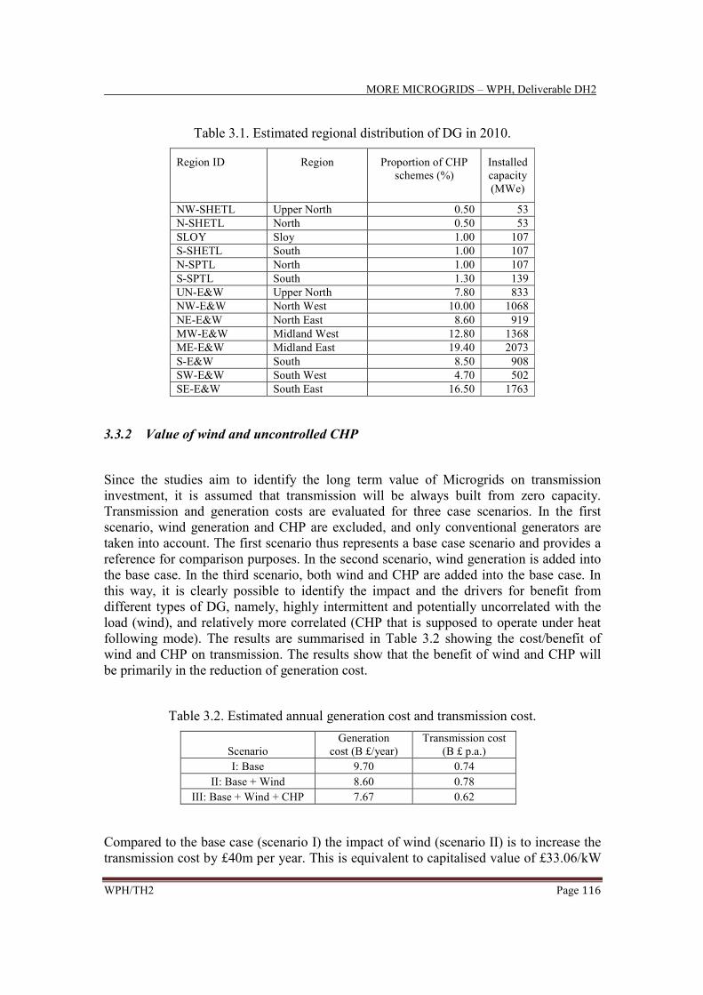
MORE MICROGRIDS – WPH, Deliverable DH2
WPH/TH2 Page 116
Table 3.1. Estimated regional distribution of DG in 2010.
Region ID Region Proportion of CHP
schemes (%)
Installed
capacity
(MWe)
NW-SHETL Upper North 0.50 53
N-SHETL North 0.50 53
SLOY Sloy 1.00 107
S-SHETL South 1.00 107
N-SPTL North 1.00 107
S-SPTL South 1.30 139
UN-E&W Upper North 7.80 833
NW-E&W North West 10.00 1068
NE-E&W North East 8.60 919
MW-E&W Midland West 12.80 1368
ME-E&W Midland East 19.40 2073
S-E&W South 8.50 908
SW-E&W South West 4.70 502
SE-E&W South East 16.50 1763
3.3.2 Value of wind and uncontrolled CHP
Since the studies aim to identify the long term value of Microgrids on transmission
investment, it is assumed that transmission will be always built from zero capacity.
Transmission and generation costs are evaluated for three case scenarios. In the first
scenario, wind generation and CHP are excluded, and only conventional generators are
taken into account. The first scenario thus represents a base case scenario and provides a
reference for comparison purposes. In the second scenario, wind generation is added into
the base case. In the third scenario, both wind and CHP are added into the base case. In
this way, it is clearly possible to identify the impact and the drivers for benefit from
different types of DG, namely, highly intermittent and potentially uncorrelated with the
load (wind), and relatively more correlated (CHP that is supposed to operate under heat
following mode). The results are summarised in Table 3.2 showing the cost/benefit of
wind and CHP on transmission. The results show that the benefit of wind and CHP will
be primarily in the reduction of generation cost.
Table 3.2. Estimated annual generation cost and transmission cost.
Scenario
Generation
cost (B £/year)
Transmission cost
(B £ p.a.)
I: Base 9.70 0.74
II: Base + Wind 8.60 0.78
III: Base + Wind + CHP 7.67 0.62
Compared to the base case (scenario I) the impact of wind (scenario II) is to increase the
transmission cost by £40m per year. This is equivalent to capitalised value of £33.06/kW

MORE MICROGRIDS – WPH, Deliverable DH2
WPH/TH2 Page 117
of wind, calculated as difference between the transmission cost in scenario I and scenario
II, divided by total wind installed capacity (12.1 GW) and multiplied by ten in order to
get the capitalised value. On the other hand, the simultaneous presence of wind and CHP
(scenario III) compared to the base case (scenario I) reduces the transmission cost
substantially, by £120m per year. This is equivalent to a capitalised value of £54.30/kW
of total DG (wind plus CHP), calculated as the transmission cost of scenario I minus the
transmission cost of scenario III divided by total DG installed capacity (22.1 GW) and
multiplied by ten in order to get the capitalised value. Therefore, CHP close to demand
has a tremendous impact on transmission investment, and this impact is even larger if we
compare scenario II and scenario III, with the benefit of CHP being £160m per annum,
translating to capitalised value of £160/kW of CHP. This value is equal to the
transmission cost of scenario II minus the transmission cost of scenario III divided by the
total CHP installed capacity (10.0 GW) and multiplied by ten in order to get the
capitalised value. While the figures are rough estimates and should be viewed for
exemplificative purposes and are case specific, the framework and methodology applied
in making these assessments are however robust and can be used to evaluate alternative
scenarios based on credible data inputs. In the specific case analysed, the indications
from the study are that wind generation cannot displace effectively transmission capacity
and may require, on the contrary, additional network investment. On the other hand, CHP
systems relatively well correlated to loads may replace transmission capacity.
3.3.3 Value of CHP controllability within Microgrids
In the previous studies, although the installed capacity of CHP represented about 12% of
total installed generating capacity, CHP generators were supposed to be uncontrolled,
which reflects the current arrangements of DG nor being controlled nor dispatched by the
TSO due to their small scale. However, as stems from the above analyses, the presence of
a large number of CHP plants will certainly have an impact on transmission system
power flows (as well as system balancing costs, as discussed in the next Chapter). The
question arises as to whether controllability of DER within Microgrids, made visible to
TSOs, could in the future bring benefits to transmission planning. In this respect, this
Section illustrates how the results from the previous studies would be modified if CHP
systems were controlled in such a way to optimise transmission flow managing and peak
generation costs. For these studies, it is assumed that there is no constraint in distribution
networks which hinder the use of DG for controlling flows in transmission network.
The studies were carried out assuming that the output profile of CHP can be optimised
with a predefined degree of flexibility to reduce generation and transmission cost, and
scenario analyses are run by increasing the number of controllable units (controllability
level) with respect to the base case of heat-following (uncontrolled) output. It is
important to note that the optimisation will modify the dispatch of CHP while preserving
the amount of energy generated by DG on daily basis. This can be consistent with
assuming, for instance, that storage systems are available to deliver in any case the
required amount of heat to local users.
The overall results of the studies are shown in Table 3.3. These results demonstrate the
value of DG controllability for various level of controllability, being namely comprised
between 0 and £30/kW of CHP installed capacity. These values are relatively modest

MORE MICROGRIDS – WPH, Deliverable DH2
WPH/TH2 Page 118
compared with the values obtained above from Table 3.2, but these results were expected
since the network flows are still dominantly controlled using conventional generators.
Table 3.3. Estimated value of DG controllability for the case study system.
Controllability
(%)
Reduction of
transmission
cost
(M £/year)
Capitalised
value of
controllability
(£/kW)
Reduction
of
generation
cost (M
£/year)
Capitalised
value of
controllability
(£/kW)
Total value of DG
controllability
(£/kW)
0 0 0.00 0 0.00 0.00
10 6 6.36 1 1.00 7.37
20 16 15.68 -1 -1.23 14.45
40 25 25.04 0 -0.29 24.75
60 22 21.68 6 5.88 27.57
80 23 22.63 6 6.31 28.95
100 21 20.96 9 8.78 29.74
It is important to note that the capitalised value of controllability obtained in these studies
depends on the assumption used in the studies with reference to generation and
transmission cost. The marginal costs of generation used for this study are as follows:
wind (zero marginal cost) and DG (£ 10/MWh), nuclear and hydro (£20/MWh), coal
(£25/MWh), CCGT (£30/MWh), oil and other peak plants (£50/MWh). Conventional
generators in Scotland are set to be cheaper by £2/MWh than the generators in England
and the incremental transfer capacity cost is assumed to be 175 £/MW/km/year.
Apart from the absolute values (necessarily depending on the specific system topology
and cost assumption for network asset and generation marginal cost), it is interesting to
point out that the incremental reduction in demand of new transmission capacity and
generation costs is not linear with the increase in number of controlled units, with a
saturation showing up after about 60% controllability, as clearly shown by Figure 3.3.
0
5
10
15
20
25
30
0 20 40 60 80 100
va
lue
of
DG
co
ntr
oll
ab
ilit
y [
£/k
W]
number of controlled units [%]
Figure 3.3. Value of microgrid-enabled micro-CHP controllability for transmission
capacity release.

MORE MICROGRIDS – WPH, Deliverable DH2
WPH/TH2 Page 119
3.4 Utilisation of controllable loads in Microgrids for transmission
congestion release
3.4.1 Generalities on controllable loads for transmission impact assessment
In the previous Sections we have explored how DG in Microgrids can impact at the
transmission level. However, besides generation, controllable loads enabled by
Microgrids could play a key role in transmission system development and congestion
release (and thus potential investment deferral), and for larger deployment of intermittent
sources. In addition, as better discussed in the next Chapter, controllable loads can bring
substantial benefits in terms of system balancing, as already discussed in Deliverable
DH1 [3], particularly in systems with significant contribution of intermittent and
unpredictable Renewable Energy Sources (RES) in combination with inflexible
conventional generation (nuclear, Carbon Capture and Storage - CCS).
A number of controllable loads could be adopted within Demand Side Management
(DSM) schemes enabled by Microgrids, from water heaters and other household
appliances to, more recently, electric vehicles. In particular, there are two general classes
of loads whose characteristics lend themselves well for controllability purposes, namely:
• Loads whose time of use can be shifted or altered without changing the final
outcomes, such as washing machines, dish washers and tumble dryers.
• Thermal loads, which rely on the availability of thermal storage systems or intrinsic
storage characteristics as for instance providing by buildings. Water heaters, air
conditioning systems and heat pumps belong to this kind of appliances.
A specific methodology [24] has been developed by Imperial in order to study the
potential impact of DSM on transmission network management as well as, more
specifically, of aggregated controllable loads enabled by Microgrids. In particular, the
methodology enables to identify in which transmission points controllable loads should
be placed, and to what extent. Hence, it is possible to identify the characteristics and the
siting of those Microgrids that should aggregate controllable loads and perform the
required DSM activities. Although not detailed here (for more details see for instance
[25]), the developed also described the scheduling of the different appliances considered
in the load control schemes, so that the Microgrid Central Controller (MGCC) could
actually dispatch control signals. The benefits of controllable loads are established as the
difference between the total costs of traditional network operation based solutions
without DSM and the costs of the system that includes DSM technologies. As for the
methodology for transmission planning in the presence of DG described above, in order
to develop a network congestion management model the network operation costs
associated with network congestion need to be taken into account.

MORE MICROGRIDS – WPH, Deliverable DH2
WPH/TH2 Page 120
3.4.2 Model of controllable loads for network congestion release
The controllable load model for network congestion release is built according to a two
step optimization procedure. This is necessary in order to allow the quantification of the
additional operation cost due to network congestion:
1. Economic dispatch of the available generation is performed in order to minimize the
system operation cost based on the relevant generation marginal cost (€/MW) for
each unit and for each time interval. The presence of wind generation is modeled
through zero production cost in order to prioritize the usage of wind energy. The
constraints considered are the generation/demand power-balance at every time step
and the minimum and maximum limits on power output for each generator. Network
constraints are ignored at this stage (network is assumed to be of infinite capacity) to
obtain the total dispatch cost with single bus-bar system.
2. An Optimal Power Flow (OPF) is performed considering the actual network capacity
limits and the output of the generators yielded from previous step. A DC model is
used for the sake of simplicity (actually, transmission lines usually have high X/R
ratio, so this assumption is justified in case of transmission networks), so that the
formulation does not include losses. Whenever the generation schedule obtained in
the previous algorithm step leads to violation of network constraints, the generation
outputs are re-dispatched according to an objective function that minimizes the cost
of these re-adjustments. Positive and negative adjustment costs are modeled for each
generator, as usual in typical balancing mechanism markets.
It is clear that the goal of the algorithm is to minimize the additional operation cost
caused by network constraints, and for this purpose controllable load (DSM) models are
included in the OPF formulation. Available controllable loads can indeed lead to a lower
value for the objective function, meaning less expensive network operation obtained by
maximization of the utilization of the existing network capacity. When wind is taken into
account, with its intermittent characteristics, overall cost reduction is accompanied and
driven by reduction in wind curtailment.
The schematic presentation of the two-step algorithm is shown in Figure 3.4.
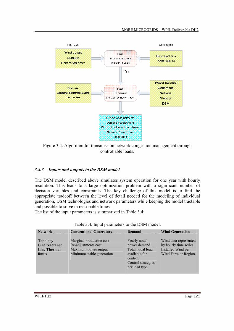
MORE MICROGRIDS – WPH, Deliverable DH2
WPH/TH2 Page 121
Figure 3.4. Algorithm for transmission network congestion management through
controllable loads.
3.4.3 Inputs and outputs to the DSM model
The DSM model described above simulates system operation for one year with hourly
resolution. This leads to a large optimization problem with a significant number of
decision variables and constraints. The key challenge of this model is to find the
appropriate tradeoff between the level of detail needed for the modeling of individual
generation, DSM technologies and network parameters while keeping the model tractable
and possible to solve in reasonable times.
The list of the input parameters is summarized in Table 3.4:
Table 3.4. Input parameters to the DSM model.
Network Conventional Generators Demand Wind Generation
Topology
Line reactance
Line Thermal
limits
Marginal production cost
Re-adjustments cost
Maximum power output
Minimum stable generation
Yearly nodal
power demand
Total nodal load
available for
control.
Control strategies
per load type
Wind data represented
by hourly time series
Installed Wind per
Wind Farm or Region

MORE MICROGRIDS – WPH, Deliverable DH2
WPH/TH2 Page 122
As outputs from the algorithm, generator output power changes, load changes due to
DSM, power flows across network branches, potential load shed, wind curtailment, and
so on, are obtained. In particular, the value of controllable loads is measured using the
following set of metrics to capture different types of potential benefits:
• Reduction in congestion (or re-dispatching) cost;
• Reduction in the wind spilled in the system;
• Reduction in the volume of constrained energy from merit generation.
As apparent from the list of metrics, benefits are computed as the differences between the
value of the base case where DSM is not available and the same scenarios with DSM.
3.4.4 Case study application to the simplified UK transmission system
In order to exemplify the model developed for system-level impact of controllable loads
on transmission networks, a case study application has been run for the UK. The system
under analysis is a simplified model, conveniently divided in 16 areas defined by
boundaries, each represented by one equivalent bus, as already illustrated above. The 16
bus-bar system obtained, with also relevant information on generation, demand and lines,
is shown in Figure 3.5.
As general considerations, in the north part of the system (buses 1 to 6) there is less
generation and less demand, the generation has lower marginal cost, and there is high
wind penetration. This corresponds to realistic conditions occurring in Scotland. Wind
generators are attached at buses 1, 2, 4, 6 and 15. In the south part of the UK (buses from
6 to 16) there is much more generation, but also huge demand centers are located in the
south (particularly in London area). Under such conditions, congestion problems arise.
The problem is emphasized when it is required to ship the intermittent energy produced
by wind generation from north to south. Line 6 (L6) becomes highly congested.
Microgrids could therefore play a prominent role in the mitigation of such congestion
problems by aggregating suitable controllable loads. The maximum total amount of load
available for DSM within Microgrids is assumed to be 6 GW, and sensitivity analyses are
run to check the impact of different controllable load capacities. In terms of types of
controllable loads, water heaters have been considered in the analysis, with the three load
pattern characteristics given in Figure 3.6. These control schemes represent the demand
side flexibility and incorporate the payback phenomenon of thermal loads (more
information can be found in [27]). The left part of each control scheme represents load
reduction and is described by negative values, while the right part (positive values)
represents the payback phenomenon.

MORE MICROGRIDS – WPH, Deliverable DH2
WPH/TH2 Page 123
bottle-
neckload
centre
load
centre
Figure 3.5. Sixteen bus-bar representation of the UK transmission system.
Figure 3.6. Load patterns for the three controllable load types used in the analysis.
General system data: - 80 generators, ~95 GW
- Generator capacity range: 8-7874 MW
- Wind generators in buses 1, 2, 4, 6, 15
- Wind generation: 15 GW, 40 TWh
- Peak demand ~68 GW

MORE MICROGRIDS – WPH, Deliverable DH2
WPH/TH2 Page 124
3.4.5 Case study results and discussion
The impact of using controllable loads compared to the base case without them is
summarized in Table 3.5. The “value” attached to controllable loads is calculated by
dividing the reduction in annual re-dispatch cost by the total load capacity available for
controllability.
Looking at Table 3.5, controllable loads have an overall positive impact on network
operation by reducing the total re-dispatch cost, the total wind spilled, and the total
volume of congestion. All these metrics augment for increasing available capacity of
controllable loads. In particular, Figure 3.7 highlights how the amount of controllable
load has a big impact to the reduction of congested energy, while the impact on the
reduction of wind spilled is relatively small, mostly due to the specific siting of the wind
mills. On the other hand, it is interesting to point out that the value per kW of load
decreases. In fact, after a certain level the amount of energy that can be managed
saturates, and thus the specific value decreases, as it can be clearly observed from Figure
3.8. Understanding of this behavior is fundamental for carrying out an appropriate Cost
Benefit Analysis (CBA), as controllability also comes at the cost of the relevant
communication infrastructure needed.
Table 3.5. Impact of controllable load on the transmission system operation.
Controllable
load
available
capacity
Annuatised
Value
Reduction in
re-dispatch cost
Reduction in
wind spilled
Reduction in
volume of
congestion
[GW] [£/kW/year] [×106 £/year] [GWh/year] [TWh/year]
1.5 34.3 51.5 57.4 0.6
3 17.9 53.8 66.4 1.1
4.5 12.2 55.1 69.5 1.5
6 9.32 55.9 71.1 1.8

MORE MICROGRIDS – WPH, Deliverable DH2
WPH/TH2 Page 125
Figure 3.7. Reduction in wind spilled and reduction in congested energy.
Figure 3.8. Reduction in cost obtained with controllable loads (compared to the base
case).
Figure 3.9 shows the total yearly increased energy “Pg_plus” and the total decreased
energy “Pg_minus” due to re-dispatching of generators for each bus in the system and in
the case with and without controllable loads. It is obvious that the generators in north
decrease their outputs, while those in south increase. This is the consequence of the fact
that the marginal cost of northern generators is lower than the southern, so during
economic dispatch (1st step of the algorithm) engaged were mostly the generators in the
north. However, due to network congestion, electricity cannot be transmitted from north
to south, so the generators in the south must increase their production, and those in the
north, due to power balance between generation and demand, must decrease their outputs.
Controllability of loads can clearly lead to change the generation re-dispatching patterns
aimed to avoid tie line bottlenecks, with an eventual overall congestion cost decrease.
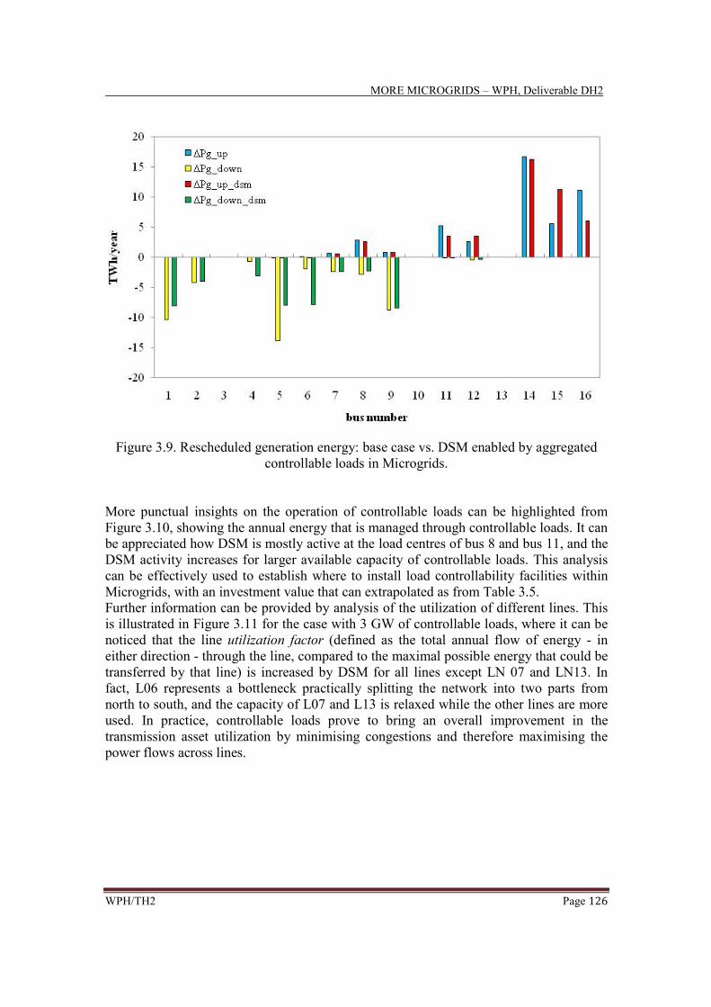
MORE MICROGRIDS – WPH, Deliverable DH2
WPH/TH2 Page 126
Figure 3.9. Rescheduled generation energy: base case vs. DSM enabled by aggregated
controllable loads in Microgrids.
More punctual insights on the operation of controllable loads can be highlighted from
Figure 3.10, showing the annual energy that is managed through controllable loads. It can
be appreciated how DSM is mostly active at the load centres of bus 8 and bus 11, and the
DSM activity increases for larger available capacity of controllable loads. This analysis
can be effectively used to establish where to install load controllability facilities within
Microgrids, with an investment value that can extrapolated as from Table 3.5.
Further information can be provided by analysis of the utilization of different lines. This
is illustrated in Figure 3.11 for the case with 3 GW of controllable loads, where it can be
noticed that the line utilization factor (defined as the total annual flow of energy - in
either direction - through the line, compared to the maximal possible energy that could be
transferred by that line) is increased by DSM for all lines except LN 07 and LN13. In
fact, L06 represents a bottleneck practically splitting the network into two parts from
north to south, and the capacity of L07 and L13 is relaxed while the other lines are more
used. In practice, controllable loads prove to bring an overall improvement in the
transmission asset utilization by minimising congestions and therefore maximising the
power flows across lines.
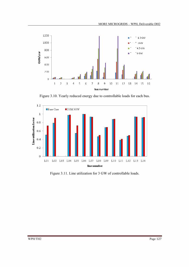
MORE MICROGRIDS – WPH, Deliverable DH2
WPH/TH2 Page 127
Figure 3.10. Yearly reduced energy due to controllable loads for each bus.
Figure 3.11. Line utilization for 3 GW of controllable loads.
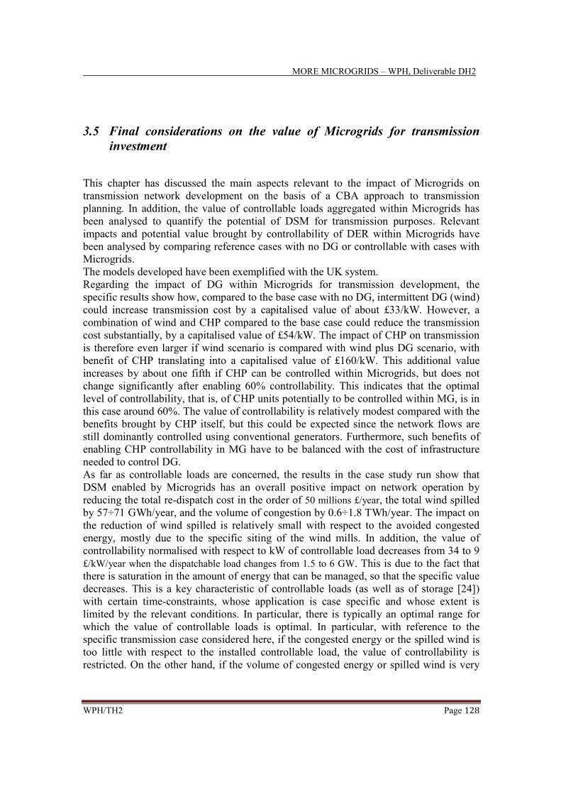
MORE MICROGRIDS – WPH, Deliverable DH2
WPH/TH2 Page 128
3.5 Final considerations on the value of Microgrids for transmission
investment
This chapter has discussed the main aspects relevant to the impact of Microgrids on
transmission network development on the basis of a CBA approach to transmission
planning. In addition, the value of controllable loads aggregated within Microgrids has
been analysed to quantify the potential of DSM for transmission purposes. Relevant
impacts and potential value brought by controllability of DER within Microgrids have
been analysed by comparing reference cases with no DG or controllable with cases with
Microgrids.
The models developed have been exemplified with the UK system.
Regarding the impact of DG within Microgrids for transmission development, the
specific results show how, compared to the base case with no DG, intermittent DG (wind)
could increase transmission cost by a capitalised value of about £33/kW. However, a
combination of wind and CHP compared to the base case could reduce the transmission
cost substantially, by a capitalised value of £54/kW. The impact of CHP on transmission
is therefore even larger if wind scenario is compared with wind plus DG scenario, with
benefit of CHP translating into a capitalised value of £160/kW. This additional value
increases by about one fifth if CHP can be controlled within Microgrids, but does not
change significantly after enabling 60% controllability. This indicates that the optimal
level of controllability, that is, of CHP units potentially to be controlled within MG, is in
this case around 60%. The value of controllability is relatively modest compared with the
benefits brought by CHP itself, but this could be expected since the network flows are
still dominantly controlled using conventional generators. Furthermore, such benefits of
enabling CHP controllability in MG have to be balanced with the cost of infrastructure
needed to control DG.
As far as controllable loads are concerned, the results in the case study run show that
DSM enabled by Microgrids has an overall positive impact on network operation by
reducing the total re-dispatch cost in the order of 50 millions £/year, the total wind spilled
by 57÷71 GWh/year, and the volume of congestion by 0.6÷1.8 TWh/year. The impact on
the reduction of wind spilled is relatively small with respect to the avoided congested
energy, mostly due to the specific siting of the wind mills. In addition, the value of
controllability normalised with respect to kW of controllable load decreases from 34 to 9
£/kW/year when the dispatchable load changes from 1.5 to 6 GW. This is due to the fact that
there is saturation in the amount of energy that can be managed, so that the specific value
decreases. This is a key characteristic of controllable loads (as well as of storage [24])
with certain time-constraints, whose application is case specific and whose extent is
limited by the relevant conditions. In particular, there is typically an optimal range for
which the value of controllable loads is optimal. In particular, with reference to the
specific transmission case considered here, if the congested energy or the spilled wind is
too little with respect to the installed controllable load, the value of controllability is
restricted. On the other hand, if the volume of congested energy or spilled wind is very

MORE MICROGRIDS – WPH, Deliverable DH2
WPH/TH2 Page 129
high, there is little room for time-constrained controllability to bring benefits, and further
actions (such as network reinforcements) are needed.
Although the results found are by nature case specific, the qualitative trend can be
generalised to other cases. In particular, the models developed provide a solid ground to
run CBA-based studies to assess the value of controllability of Microgrids for
transmission, as controllability also comes at the cost of the relevant communication
infrastructure needed.

MORE MICROGRIDS – WPH, Deliverable DH2
WPH/TH2 Page 130
4. System-level impact of Microgrids on central generation operation and development
This chapter provides overall views and studies of the impact of Microgrids entailing
controllable DG and loads on the development of the central generation system
(conventional generators and large scale renewables). More specifically, after discussing
the general concept of capacity value of micro-CHP, wind power and PV systems with
reference to typical northern situations (UK), a detailed methodology for the evaluation
of security of supply in the presence of microgeneration and Microgrids is provided. This
comprehensive theoretical and practical analysis (whose details are reported in Annex
H2.D) has been run by INESC with reference to the Portuguese case. Then, by using a
scheduling model developed by Imperial and explicitly adapted to take into account
distributed energy resources, the system-level impact of Microgrids on the economic and
environmental performance of different types of power systems with different levels of
flexibility (and, in particular, low-flexible systems with plenty of must-run units and wind
power) has been assessed. Among other results, the analysis considers the possibility
from distributed resources aggregated within Microgrids to support system operation
through provision of energy flexibility (load following), reserve and response services,
which leads not only to assess the relevant potential benefits on operational cost, but also
to estimate the potential value in displacing cost intensive generation and delaying their
expansions in case of demand growth, as well as simply displacing old and inefficient
central generators.
4.1 Generation capacity contribution of microgeneration and Microgrids
4.1.1 Generalities on security of supply and contribution from Microgrids
In Deliverable DH1 [3] it was generally discussed how, depending on the timeframe
considered, microgrid operation could influence short-term balancing (from seconds to
days) and long-term capacity provision (from months to years) in order to keep the
system reliability and energy supply power quality levels within the permissible limits.
Focusing on generation adequacy contribution, the challenging aspect relevant to
microgeneration operation is that power output of most of RES and in general DG
technologies is intermittent, which is caused either by the natural variability of primary
energy sources or by their operational mode (for instance, the heat following mode of
CHP systems). This affects their capacity value which is linked to the concepts of overall
adequacy of the generation capacity and the long-term reliability of the system.
Reliability based generation capacity adequacy assessment techniques [20] are generally
employed to determine the conventional generating capacity requirements in systems
with and without RES and DG. The difference between the conventional generation
capacity amounts needed between the two alternative scenarios indicates the capacity
credit (CC) of RES and DG.

MORE MICROGRIDS – WPH, Deliverable DH2
WPH/TH2 Page 131
More in general, the security of supply is defined as the ability of a power system to serve
the forecasted load, with a specified reliability level. It is a primary objective of any
power system, because of the important costs (security, economical, social and political)
that result from an inadequate level of security. There are two main components affecting
the security of supply, namely:
1. Generation adequacy, which has to do with the ability of the generation assets to cover
the expected values of load, including the system losses.
2. Transmission adequacy, which is related to the ability of the transmission system to
ensure the needed power flows between the generation and the load points.
Because of its location in the electrical system (LV networks), micro-DG and Microgrids
contribute to improve both components of the security of supply. In addition, a number of
(mostly economic) factors contributing for the reluctance to the investment on
conventional power plants tend not to exist in the micro-generation case. Therefore, the
expected dissemination of these systems may result on a valuable contribution to the
security of supply. Moreover, this contribution tends to increase when the transmission
adequacy decreases, as generation is situated on the distribution network side. It is
interesting to notice how this is an opposite situation to the one occurring for
conventional generation, where the limitations of the transmission system influence
negatively generation contribution to the satisfaction of the system load. However, once
the transmission networks exhibit high reliability, their influence on the security of
supply tends to be low. On the other hand, the reliability of the distribution networks may
influence negatively DG contribution. Therefore, in this work it is assumed that the
contribution of DG to security of supply is limited to the improvements on generation
adequacy.
The specific contribution of a Microgrid to the security of supply is a result of the ability
of those structures to manage (or partially manage) their internal load and generation.
Thus, the contribution of a Microgrid is influenced by the characteristics of
controllability of their internal DG systems and loads. Concerning DG, only micro-CHP
systems with ability to store the thermal energy may be assumed as controllable. In fact,
only those units may respond to the needs of the electrical system without wasting the
thermal energy (preserving the principle of combined heat and power generation). As a
consequence of such control, those microgenerators tend to be always available to
respond to capacity scarcity situations. In alternative, micro-CHP systems could operate
coupled to an auxiliary boiler, although this would lead to smaller overall generation
efficiency. Regarding PV and micro-wind systems it is important to stress that those units
are not controllable, since their generation is influenced by the availability of the primary
resources.
Concerning the load, it is important to emphasise that the contribution of Microgrids to
generating adequacy comes from the ability of those entities to interrupt part of it when a
situation of generation scarcity exists. Microgrids are indeed in excellent position to
participate in mechanisms of active load management, namely through their ability to
interrupt internal load. Once those structures may be used to interrupt the less important
loads (heat load, cooling, etc...), the interruption may be done, sometimes, without

MORE MICROGRIDS – WPH, Deliverable DH2
WPH/TH2 Page 132
noticeable effects on consumers (reducing the potential economic cost that results from
the load interruption).
4.2 General discussion on DG contribution to security of supply in a
Northern European country case
4.2.1 Combined Heat and Power (CHP)
As widely discussed in Deliverable DH1 [3], micro-CHP units are generally adopted for
domestic applications ranging between 1 and 10 kWe and are normally connected at
230V. Larger CHP units, although still connected to MV, could be used in small
commercial and industrial centres and could be for instance based on MTs.
At this scale, CHP systems operating at individual buildings are typically driven by heat
demand, with electricity somehow being a by-product. The capacity credit of small-scale
CHP units mostly depends on their flexibility to supply system peak demand. If we
consider Northern countries such as the UK, heat demand has a strong correlation with
electricity consumption especially in the cold weather condition. Therefore, CHP can be
used to reduce peak demand during winter peak. On the contrary, during hot weather
condition there is a little need of heat generation which inhibits the use of CHP for
capacity provision.
Figure 4.1 exemplifies the conventional capacity that can be displaced by micro-CHP.
The studies were conducted on the UK system and for different penetration levels of DG,
by overlapping the overall system demand profile under peak conditions with typical
electricity production schedules from CHP following heating domestic load profiles.
Although no reliability aspects were taken into account in estimating the capacity credit
of micro-CHP, it has to be highlighted that the availability factor of domestic CHP is
typically quite high (even above 90%), so it is less relevant compared to the diversity of
its utilization during peak demand, which has been taken into account although in an to
an approximate way.
In terms of numerical results, it can be appreciated how relatively small penetration of
micro-CHP, e.g. 2 GW can displace about 1.4 GW conventional capacity (capacity credit
of 70%), owing to the good correlation between heat-driven generation patterns and
system demand. However, once the penetration level increases, the ability to displace
conventional generation capacity reduces. At 10 GW, which is a likely estimate for the
UK in the upcoming year, the capacity credit reduces to some 40%. At the point where
the peak demand on the system minus the output of micro-CHP (that is, the net demand
as seen by conventional generation) is driven no longer by winter peak demand but by
summer peak demand, increasing further the installed capacity of micro-CHP will not
reduce conventional generation capacity which is needed to secure summer peak load.
This leads to the saturation that can be appreciated for about 35 GW of installed CHP,
which roughly corresponds to 50% of the current demand, for which the relative capacity
credit is only 25%.

MORE MICROGRIDS – WPH, Deliverable DH2
WPH/TH2 Page 133
0
1
2
3
4
5
6
7
8
9
10
0 10 20 30 40 50
Dis
pla
ced
Co
nv
en
tio
na
l Ca
pa
city
(GW
)
Installed Capacity of Micro CHP (GW)
Figure 4.1. Conventional generation capacity displaced by micro-CHP.
However, if micro-CHP can be controlled within Microgrids to respond to electricity
demand without being constrained by heat requirement, it could increase its capacity
credit, although this will lead to additional costs due to the reduction in overall
cogeneration efficiency, in case cost of storage systems and/or auxiliary boilers, and the
cost of enhancing its controllability. More details on these aspects are provided below
and in Annex H2.D.
4.2.2 Wind Power
In [28] the capacity credit of wind power in the UK was calculated for two different
scenarios of geographical distribution of wind power. In this respect, Figure 4.2 shows
the results of analyses carried out for a range of wind penetrations to examine the
generating capacity of conventional plant that can be displaced by wind, while
maintaining the risk of loss of supply at the historical level of 9%. The results indicate a
limited capability of wind power to displace conventional capacity. 10 GW of non-
diverse wind source can displace only 2 GW conventional generators, corresponding to
20% of capacity credit.
0
2,0 00
4,0 00
6,0 00
8,0 00
0 10 2 0 3 0 40
Wind capacity (GW)
Displaced conventional
capacity (MW) Divers e wind source
Non-divers e wind source
Figure 4.2. Conventional generation capacity displaced by wind power.

MORE MICROGRIDS – WPH, Deliverable DH2
WPH/TH2 Page 134
4.2.3 Photovoltaics (PV)
Like other RES, the capacity credit of PV is strongly linked to the correlation of its
output with peak demand. In a system where peak loads occur during summer daytime,
PV has a potential to reduce the capacity of conventional plant resulting in significant
capacity credit of this RES. This could be the case in Southern Europe countries. On the
other hand, in a system where peak loads occur during winter nights, like in the UK, the
capacity credit of PV is practically zero. Details on the capacity contribution of PV in a
Portuguese scenario are reported in Annex H2.D.
4.3 Main findings of the studies on generation adequacy in the
Portuguese case
This Section reports a short synthesis of the main findings by INESC Porto on generation
security of supply and adequacy. Details on methodology, models and calculations can be
found in Annex H2.D.
4.3.1 Generalities on the methodology developed for Microgrid contribution to
security of supply
In order to evaluate the contribution from Microgrids to security of supply, a probabilistic
approach based on a non-chronological Monte-Carlo Simulation process is presented
here. To account for the potential dependencies between the seasonal and daily load and
generation profiles of the DG units (function of weather conditions) several scenarios
were defined. Those scenarios make it acceptable to consider that the random variables
(load level and capacity factor of the DG) present an independent behaviour in each
scenario.
The developed methodology was applied to a system that has the size of the Portuguese
one, namely concerning the load level. The adequacy indices of a base case, without DG,
were compared with the indices associated to various penetrations of different micro-
generation technologies (CHP, PV, micro-wind) and the existence of Microgrids.
Moreover, the contribution of those entities to the generating adequacy of the Portuguese
power system was measured by using the concept of capacity credit (CC). As mentioned
above, this concept is defined as the conventional generation that may be removed from
the system, after adding DG and Microgrids, while maintaining the initial reliability of
the system unchanged (detailed on the metrics used are reported in Annex H2.D).
4.3.2 Capacity credit contribution from different micro-generation technologies
Figure 4.3 shows the CC obtained for the different micro-generation technologies
considered in the study, assuming an unavailability factor f=10%. The CC values
expressed in MW correspond to the amount of conventional generation that can be
removed, after the addition of the micro-generation capacity, while maintaining the initial

MORE MICROGRIDS – WPH, Deliverable DH2
WPH/TH2 Page 135
reliability of the system. The percentage values of the CC correspond to the ratio between
the CC in MW and the total micro-generation installed capacity.
0
50
100
150
200
250
0 250 500 750 1000 1250 1500 1750 2000
PV (MW)
CC
(M
W)
1 kW - f=0.10 3 kW - f = 0.10 10 kW - f = 0.10
0%
3%
6%
9%
12%
15%
18%
21%
0 250 500 750 1000 1250 1500 1750 2000
PV (MW)
CC
(%
)
1 kW - f=0.10 3 kW - f = 0.10 10 kW - f = 0.10
0
200
400
600
800
1000
1200
0 250 500 750 1000 1250 1500 1750 2000
uCHP (MW)
CC
(M
W)
1 kW - f=0.10 3 kW - f = 0.10 10 kW - f = 0.10
0%
10%
20%
30%
40%
50%
60%
70%
0 250 500 750 1000 1250 1500 1750 2000
uCHP (MW)
CC
(%
)
1 kW - f=0.10 3 kW - f = 0.10 10 kW - f = 0.10
0
20
40
60
80
100
0 250 500 750 1000 1250 1500 1750 2000
uWind (MW)
CC
(M
W)
1 kW - f=0.10 3 kW - f = 0.10 10 kW - f = 0.10
0%
2%
4%
6%
8%
10%
0 250 500 750 1000 1250 1500 1750 2000
uWind (MW)
CC
(%
)
1 kW - f=0.10 3 kW - f = 0.10 10 kW - f = 0.10
Figure 4.3. CC of different micro-generation technologies
The analysis of the results enables to conclude that the rated power of the micro-
generation units does not influence significantly the CC to be allocated to those units.
Another important conclusion that may be extracted from the results has to do with the
behaviour of the percentage value of the CC. At the initial stage (up to approximately 500
MW), the CC increases with the increase of the micro-generation installed power,
declining afterwards.

MORE MICROGRIDS – WPH, Deliverable DH2
WPH/TH2 Page 136
The influence of the micro-generation unavailability on the CC is illustrated in Figure
4.4. This influence is more significant than the one of the rated power of the micro-
generation units, however still limited.
0
50
100
150
200
250
0 250 500 750 1000 1250 1500 1750 2000
PV (MW)
CC
(M
W)
3 kW - f=0.05 3 kW - f = 0.10 3 kW - f = 0.25
0%
3%
6%
9%
12%
15%
18%
21%
0 250 500 750 1000 1250 1500 1750 2000
PV (MW)
CC
(M
W)
3 kW - f=0.05 3 kW - f = 0.10 3 kW - f = 0.25
0
200
400
600
800
1000
1200
0 250 500 750 1000 1250 1500 1750 2000
uCHP (MW)
CC
(M
W)
3 kW - f=0.05 3 kW - f = 0.10 3 kW - f = 0.25
0%
10%
20%
30%
40%
50%
60%
70%
0 250 500 750 1000 1250 1500 1750 2000
uCHP (MW)
CC
(M
W)
3 kW - f=0.05 3 kW - f = 0.10 3 kW - f = 0.25
0
20
40
60
80
100
0 250 500 750 1000 1250 1500 1750 2000
uWind (MW)
CC
(M
W)
3 kW - f=0.05 3 kW - f = 0.10 3 kW - f = 0.25
0%
2%
4%
6%
8%
10%
0 250 500 750 1000 1250 1500 1750 2000
uWind (MW)
CC
(M
W)
3 kW - f=0.05 3 kW - f = 0.10 3 kW - f = 0.25
Figure 4.4. Influence of the unavailability of micro-generation technologies on the CC
Figure 4.5 allows comparison of the CC to be allocated to each of the micro-generation
technologies considered. An important conclusion that can be drawn from this figure is
that the influence of the micro-generation penetration level on the CC tends to be limited.
This is an important feature, namely from the regulation point of view (once it allows
establishing CC values that are not significantly affected by the uncertainty on the micro-
generation penetration level). Also, comparison of CHP and PV confirm also in the
Portuguese case the findings relevant to UK distribution networks in terms of capcity
support.

MORE MICROGRIDS – WPH, Deliverable DH2
WPH/TH2 Page 137
0%
10%
20%
30%
40%
50%
60%
70%
0 250 500 750 1000 1250 1500 1750 2000
Pinst (MW)
CC
(%
)
uCHP 3 kW - f = 0.10 uWind 3 kW - f = 0.10 PV 3 kW - f = 0.10
Figure 4.5. Comparison of the CC values for different micro-generation technologies
The CC of each micro-generation technology is influenced by the amount of energy it
generates and by the periods where this generation takes place. Dividing the CC of each
micro-generation technology by its average annual CF we eliminate the first influence,
highlighting the second one. Figure 4.6 shows the CC adjusted to energy (assuming that
all technologies generate the same energy). This figure confirms the tendency of the
micro-CHP systems to inject power into the grid when it is more needed (from the point
of view of the security of supply).
0%
50%
100%
150%
200%
250%
0 250 500 750 1000 1250 1500 1750 2000
Pins (MW)
CC
(%
)
uCHP 3 kW - f = 0.10 uWind 3 kW - f = 0.10 PV 3 kW - f = 0.10
Figure 4.6. CC values adjusted to energy

MORE MICROGRIDS – WPH, Deliverable DH2
WPH/TH2 Page 138
4.3.3 Specific results for Microgrids
As mentioned above, the major characteristics of Microgrids, namely, their ability to
control internal loads and generators, also enable them to contribute to generation
adequacy. That contribution depends on the magnitude of load and of mico-generation
that can be actively managed by the central controller of the Microgrids. Concerning
micro-generation it is important to stress that only micro-CHP systems may be effectively
controllable, since the production of PV and micro-wind systems is imposed by the
availability of the primary resources. Even for micro-CHP systems, not all units might be
easily controlled without waste of thermal energy. As a consequence, only the systems
with aptitude to store thermal energy should be accounted for when assessing the
generation adequacy, unless at the cost of lower environmental efficiency. Regarding
load management, the benefits depend on the share of the internal load that may be shed
or shifted from peak period to non-peak periods, similarly to the analysis run in Section
3.4 for transmission congestion release.
Figure 4.7 shows an example of the influence of Microgrids on the CC of micro-CHP
systems when different percentages of such systems are assumed as controllable. The
increase in CC due to controllability is quite impressive.
0%
20%
40%
60%
80%
100%
0 400 800 1200 1600 2000 2400
Micro-CHP (MW)
CC
(%
)
0% controllable 5% controllable
10% controllable 20% controllable
Figure 4.7. Influence of Microgrid on the CC of micro-CHP systems
Concerning load control, Figure 4.8 shows the CC to be attributed to Microgrids when
assuming increasing quantities of the total system load as controllable load by Microgrids
action. Note that the CC refers to the total capacity of the conventional generation system
(10800 MW is this case). Again, the contribution is quite impressive, basically linear with
the amount of controllable load.

MORE MICROGRIDS – WPH, Deliverable DH2
WPH/TH2 Page 139
0.0%
2.0%
4.0%
6.0%
8.0%
10.0%
0% 1% 2% 3% 4% 5% 6% 7% 8% 9% 10%
% Total load of the system
CC
(%
)
Figure 4.8. CC of Microgrid due to load control
4.3.4 Concluding remarks on the Portuguese studies on generation adequacy with
Microgrids
This Section has described methodology and results (whose comprehensive details can be
found in Annex H2.D) to evaluate the CC of micro-generation systems and of
Microgrids. The methodology was applied to the Portuguese system (with some
simplifications) and the results were shown and discussed. First, the results show that
different DG technologies contribute differently to the security of supply. For instance, a
CC = 64% was obtained by a set of 160,000 micro-CHP systems with rated power of 3
kW and unavailability f = 10%. Therefore, the addition of 480 MW of micro-CHP to the
Portuguese system enables to remove some 307 MW of conventional generation, keeping
the initial reliability of the system. In the same conditions, the CC values of the PV and
micro-wind systems are 16% and 4%, respectively. The performance of micro-CHP
systems is justified by the fact that these generators have propensity to inject power in
periods of higher system loads.
Another important conclusion that can be drawn from the results is related to the limited
influence that the rated power and unavailability of the micro-generators has on the CC
value. For example, the CC of the 160,000 micro-CHP systems mentioned above
increases to 67% if an unavailability of 5% is assumed for the generators. Therefore,
halving the unavailability of the generators only increases the CC in 4.7%. If the
unavailability is increased by 500% (f = 25%) the CC decreases by 17% to a value of
53%. Similar results can be obtained for the other DG technologies studied. From the
regulatory point of view, this is an important feature, once the regulator may adopt
reasonable values for those parameters without incurring in significant errors when
assessing the CC.
The initial reliability of the electrical system also influences the CC of the micro-
generation technologies. In fact, the CC of the micro-CHP units tends to increase when
the system has higher initial reliability. The opposite situation occurs in the case of PV
and micro-wind systems, whose CC appears more sensitive to the initial reliability of the
system then for micro-CHP systems.
Regarding more specifically Microgrids, the results show that the integration of
controllable micro-CHP systems within MG increases their CC. For example, the CC

MORE MICROGRIDS – WPH, Deliverable DH2
WPH/TH2 Page 140
obtained by a set of 160,000 micro-CHP systems with rated power of 3 kW and f = 10%
is CC = 69%. However, if 20% of these generators may be controlled by the action of
Microgrids, the CC increases by 9%, reaching the value CC = 75%. Similarly, significant
CC may be obtained by load controllability within Microgrids. For instance, the control
of 5% of the total system load enables to remove 500 MW of conventional generation,
that is, roughly 5% of the conventional generation capacity installed in the system. This
confirms the strategic role that DSM actions enabled by aggregating Microgrids could
play in future system development, as also described elsewhere in this work.

MORE MICROGRIDS – WPH, Deliverable DH2
WPH/TH2 Page 141
4.4 Role of flexibility provided by controllable generation in Microgrids
and dynamic impact on centralized generation
The relatively limited capacity contribution of RES and DG as from above will need
support of conventional generation to maintain system security at desired levels, which
impacts on the utilization of other technologies present in the system and in retaining
greater proportion of conventional generation in the system with reduced utilization.
Greater impact on the utilization of the incumbent technologies will translate into higher
additional generation capacity costs attributed to these sources [29]. From this
perspective, the possibility of controlling DER within Microgrids for ancillary services
system support, mainly for reserve and response traditionally provided by conventional
generation, will be crucial to minimise the additional costs incurred by conventional
generators due to intermittent DG. On these premises, this Section outlines the potential
benefits brought by Microgrids providing flexibility and controllability necessary for
maintaining secure operation of the system such as load following and frequency control.
4.4.1 Synthesis of dynamic operation of power systems
As introduced in detail in Deliverable DH1 [3], for static analyses of the power system
MG can be seen as negative demand, similarly to large-scale RES (wind) that is not
specifically considered for system balancing purposes. However, for a realistic evaluation
of the costs on power system operation and development from DG technologies, dynamic
characteristics need to be taken into account. In particular, a power system must be able
to respond to rapid and large fluctuations in supply and demand while maintaining given
levels of system security and reliability. Conventional generation does traditionally
provide the needed frequency control services, with a level of flexibility (ability of
ramping up and down, start up or shut down, and so on) that varies from plant to plant. In
particular, reserve services are generally provided by plants rotating in synchronism with
the bulk system (spinning reserve), to be deployed within 5÷10 minutes, as well as by
non-synchronised alternatives (standing reserve), such as stand-by generators, to be
deployed within some 20 minutes. Normally, spinning reserve is called in action first
since it exhibits lower utilisation cost and is thus used to target relatively more frequent
and smaller imbalances. On the other hand, standing reserve exhibits lower holding costs
but has higher utilisation ones, so it is typically deployed for less frequent but more
substantial imbalances.
The amount of reserve required is related to the probability of unbalances between
generation and demand. Since the outputs of RES and in general small-scale DG are
relatively less controllable and less predictable, additional operating reserve will be
needed to cover the uncertainty and variability of their output. This depends on the level
of their penetration and the variability of their output over different time horizons. As for
the other issues described earlier in this work, for a relatively small penetration of
microgeneration additional amount of reserve is negligible. The amount will increase
with the level of penetration since the magnitude of the uncertainty increases. Different
types of RES impose different types and magnitudes of reserve requirements due to the

MORE MICROGRIDS – WPH, Deliverable DH2
WPH/TH2 Page 142
different level of their output fluctuation and its correlation with demand. These aspects
need to be thoroughly understood to assess the impact of Microgrids operation on power
systems and the potential benefits from controlling DER to provide system services
support.
4.4.2 Generalities on the impact of intermittent sources on frequency services
requirements and results from previous studies
Statistical techniques [30][31] can be applied to estimate the operating reserve
requirements due to the penetration of RES and DG. In particular, the variations of wind
and PV output follows a distribution which is close to a Normal distribution. Therefore,
typical approaches are based on estimating additional reserve requirements due to RES as
3 times the relevant standard deviation. In some cases this reserve figure can be extended
to 3.5 or 4 to cover the longer tails of the actual distributions. An example is reported in
Figure 4.9, illustrating typical fluctuations in wind power output over four hour time
horizon.
0.00
0.02
0.04
0.06
-30 -20 -10 0 10 20 30
Output variation (% of installed capacity)
Probability σ3σ3-
Figure 4.9. Probability Density Function (PDF) of fluctuations in wind power output.
In order to determine the overall reserve requirements, the variations in RES and DG
need to combined with the forecast errors in demand and conventional generation across
the same considered time horizon. This calculation is performed by using standard
statistical approaches to combine errors. It is important to highlight that the diversity
occurring among different RES reduces the variation in their cumulative output. A typical
example is shown in Figure 4.10, showing the results (in the form of the PDFs of hourly
variation) from statistical analysis of the time series data of wind generation for both non-
diverse (correlated) and diverse (uncorrelated) UK wind farms. It can be easily observed
that the magnitude of power output fluctuations is significantly reduced in the diverse
case.

MORE MICROGRIDS – WPH, Deliverable DH2
WPH/TH2 Page 143
0.00
0.04
0.08
0.12
0.16
0.20
-30 -20 -10 0 10 20 30
Output variation (% of installed capacity)
Diverse wind source Non-diverse wind source
Probability
Figure 4.10. PDF of hourly variations in wind output from diverse and non-diverse wind
source.
From previous studies run by Imperial College [28][29][32], on the time scale of primary
frequency control the estimates for increased reserve requirements have resulted in a very
small impact. This is due to the smoothing effect of short-term variations of DG and RES
power production, uncorrelated with each other and with other fast variations of loads
and generation units.
On the time scale of secondary and tertiary frequency control, increasing penetration of
intermittent sources, and in particular wind, will increase the impact on the net
imbalances of the power system. The estimates for the extra reserve requirements due to
wind power for UK is in the order of 2-8% of the installed wind power capacity at 10%
penetration of gross consumption [33]. Another study [34] also analysed balancing power
with respect to the accuracy of wind power forecasting to determine the amount of
regulating power that can be reduced by improved forecasting. At 20% capacity
penetration, 7% of wind power capacity is needed for balancing, if persistence is
assumed. In the hypothesis of a perfect forecast, only 2% additional capacity would be
needed at this penetration level. The values shown are only indicative relative and intend
to illustrate the beneficial effect of forecasting on additionally required reserve capacity.
In the case of micro-CHP, the additional reserve requirement is expected to be less due to
better predictability of its output when aggregated.
As discussed in Deliverable DH1 [3], since generators need to be part loaded and
conditioned to provide spinning reserve and stand-by (standing) reserve, additional
reserve requirements will increase the operating cost of such generators that need to be
recovered through ancillary service charges. Additional operating costs may also occur
since those generators that provide reserve may come from out of merit generation and
need to produce electricity at least at minimum stable generation.
Focus on wind studies in recent years, according to [32] with wind supplying 10% of the
electricity demand, the required additional reserve capacity for the UK is in the range of
3% to 6% of the rated capacity of wind plant. With 20% wind, the range is approximately
4 to 8%. Accommodating 10% wind in the UK system would therefore increase

MORE MICROGRIDS – WPH, Deliverable DH2
WPH/TH2 Page 144
balancing costs by some 3.9 €/MWh of wind and 20% wind would increase those costs
by around 4.6 €/MWh of wind.
These costs are of course dependent upon the technology that is employed to provide
these operating reserves. Systems that have sufficient flexibility and low/zero marginal
cost generation such as hydro power can incur lower additional operating reserve costs
compared to thermal generation based systems.
4.4.3 The role of flexibility that can be provided by Microgrids
On the above premises, the question to be addressed in this work is therefore how
microgeneration technologies within Microgrids would impact on the system operational
requirements, and whether such technologies can contribute to frequency support to the
system. In fact, the scenarios that are envisaged for most EU countries lead to consider an
increasing level of inflexibility of the overall system, whether due to additional base-load
nuclear or Carbon Capture and Storage (CCS) systems, or intermittent large-scale wind
resources. This will eventually mean additional reserve costs, above all for spinning
reserve (see Deliverable DH1 [3] for more detailed overview). Therefore, it is crucial to
seek for additional means of flexibility. Focusing on microgeneration, in particular, CHP
systems that normally are operated under thermal load-following mode could be
deployed for grid-related services, above all if equipped with heat storage systems
capable to decouple the electrical and thermal loads. Therefore, MG with controllable
microgenerators could represent a valuable source of flexibility and provision of system
ancillary services that otherwise would be provided by the marginal central generating
units. If not, it will be possible to displace only a reduced amount of central generation
capacity, needed for system services, and such capacity will operate more frequent in part
loaded mode, with far higher costs than currently. Besides microgeneration, support
could be provided by controllable loads as well. In this respect, examples of energy
balancing support in the presence of intermittent sources and variable flexibility
portfolios are discussed in Section 4.5. For system-level applications, indeed, it is
expected that the value of controllable sources (DG or DSM) in microgrids will be
strongly related to the flexibility of the conventional generation mix, besides the
penetration of RES such as wind and further inflexible generation such as CCS. This
value is also expected to increase with the increase of the penetration of wind and
inflexible sources.
Quantitative analyses in this respect are provided below.
4.4.4 Scheduling model for system-level impact assessment of Microgrids on
conventional generation
In order to assess the impact of coordinated Microgrid operation on system performance,
a large-scale system scheduling model was used that has been developed by Imperial, and
modified to accommodate a range of studies performed within this Deliverable. The
model carries out an annual assessment of generation system operation. It optimally
allocates generation resources to provide energy, reserve and response services. The
model is able to incorporate various generation technologies and their respective

MORE MICROGRIDS – WPH, Deliverable DH2
WPH/TH2 Page 145
capabilities, daily and seasonal changes in demand and different levels of penetration of
intermittent renewable electricity. In order to investigate the interaction between
Microgrids and the power system, the model was extended to incorporate various levels
of Microgrid controllability that could be used by the system.
The key aspect of the model is the ability to capture the interaction between response,
reserve and energy provision from generators, taking into account their cost
characteristics and dynamic capabilities. Considering response services in isolation from
reserve and energy would indeed provide unrealistic results. Conventional generation
units are represented through generic units of different technologies most widespread
across Europe, namely, CCGT, coal, and nuclear. In addition, also CCS plants are
simulated as must-run units, so that future generation mixes as envisaged in low-carbon
strategies of several governments can be analysed as well. The data on generator physical
parameters, cost, efficiency and emission characteristics were taken as typical for
particular technologies.
Following are the key features of the model:
• Commitment and dispatch of large-scale generation units is done through minimising
operation costs, considering: generation start-up, incremental production costs, and
cost of holding standing reserve in stand-by plants. Generator cost characteristics are
modelled in a way that allows accounting for decreased operating efficiency when
operating part-loaded.
• Consideration of generators’ technical limits and capability to change the output:
o Generation technical limits;
o Ramp rates;
o Minimum up and down times;
o Must-run status (mostly relevant to nuclear or CCS plants).
• Demand balance constraint based on the criterion that the generation schedule needs
to supply the net demand (system demand minus wind output) at all times, where net
demand is the difference between demand and wind generation.
• Deterministic requirements constraining the minimum levels of:
o Primary response: provided by part-loaded conventional generation plants, and
potentially Microgrids;
o Spinning reserve: provided by part loaded plants and set according to an optimal
allocation obtained off-line;
o Standing reserve: provided by stand-by plants and set to provide the difference
between total reserve required and the spinning reserve allocated.
• The model captures the interaction between provision of response and spinning
reserve by the same unit. The capacity available for spinning reserve is taken into
account when setting the generator’s available response capacity.
The system operation is simulated for one year with half-hourly time resolution, resulting
in 17,520 values of system demand and wind output profile, both of which are based on
UK system data. However, in terms of strategic information provided by the model and
the analysis, the results can be reasonably generalised to other countries. The results
obtained for each scenario represent the minimum operation cost to supply net demand

MORE MICROGRIDS – WPH, Deliverable DH2
WPH/TH2 Page 146
and ensure pre-defined levels of response and reserve. Additionally, the model provides
information on CO2 emissions and wind curtailment necessary to balance generation and
demand. The latter may occur in certain time instances when there is excess energy in the
system, due to certain conventional plants being kept part-loaded to provide reserve or
response services, supplying at the same time electricity at the level of at least their
minimum stable generation.
The optimal economic operation of the system is calculated taking into consideration
daily and seasonal demand variations and variations in wind output over the year. To
properly simulate system operation, and capture all relevant parameters, the methodology
includes the following considerations:
• Modified system response requirements were generated through adjusting system
primary response requirements to incorporate the uncertainty of wind. Statistical
properties of actual wind data were incorporated into calculations of new system
response requirements which capture the additional uncertainty introduced by
various penetration levels of wind generation, as mentioned in Section 4.4.2. The
new response requirements ensure that the risk of violating frequency limits remains
unchanged.
• Reserve requirements are defined taking into account wind and demand forecast
errors and generation outages within operational reserve time scales. This was
incorporated into calculations of the additional reserves (the forecast lead time used
is 4 hours, corresponding to the expected time required to start a new plant). This
process was carried out for different wind penetration scenarios. The reserve
requirements ensure that wind uncertainty is taken into account without changing the
operational risk accepted by the system operator. The allocation between spinning
and standing reserve is optimised externally to minimise expected imbalance costs
for different structures of the generation system.
• CO2 emissions from fossil fuel-based electricity generation are modelled considering
International Panel on Climate Changes (IPCC) emission factors for different fuels.
The emission factors establish a proportional relationship between primary energy
used for generating electricity and the CO2 emissions caused by the process. This
implies that CO2 emissions per unit of electricity output depend on the efficiency of
the technology, i.e., that emissions per megawatt-hour of electricity generated
increase when power plants are part-loaded.
• The variation of wind generation over the year is taken into account by using an
appropriately constructed wind time series based on typical UK values, which
allowed for simulating the wind outputs for different wind penetration levels.
Microgrids are incorporated into the scheduling model by assuming they cover a part of
the electricity demand. Their electricity output profile is related to their heat output
requirements in a manner that depends on the level of controllability of micro-CHPs (this
is elaborated in the following section). In this analysis one representative heat consumer
type was assumed with nine representative heat demand profiles used to model weekly
and seasonal oscillations in heat demand that needs to be covered by Microgrids. Nine
profiles refer to particular combinations of day types (workday, Saturday or Sunday) and

MORE MICROGRIDS – WPH, Deliverable DH2
WPH/TH2 Page 147
seasons of the year (summer, winter or spring/autumn), for which characteristic profiles
were available. The half-hourly profiles are depicted in Figure 4.11.
Figure 4.11. Heat demand profiles for micro-CHPs
The heat-to-electricity output ratio of micro-CHPs was assumed to be 6.5, so that the
maximum electricity output for one CHP unit would be 1 kW. The number of micro-
CHPs in the system, i.e., the penetration of Microgrids, was scaled up to account for
different penetration levels. Cases considered in this analysis included the total electrical
capacity of CHP-based Microgrids in the amount of 5%, 10% and 20% of peak system
electricity demand (which in this case was 66.7 GW).
Another important micro-CHP parameter was its cost, which was assumed to be
£20/MWh. This cost is significantly lower than conventional generation plants, ensuring
that micro-CHPs are always included in the dispatch. This low figure is justified by the
fact that the actual cost of gas for electricity generation from CHP can be discounted by
an equivalent amount needed to produce heat. For example, this cost allocation procedure
can be based on incremental efficiencies (see for instance [35][36]).

MORE MICROGRIDS – WPH, Deliverable DH2
WPH/TH2 Page 148
4.4.5 Case study examples
The impact of Microgrids on the overall system performance was investigated with a
number of different assumptions regarding the flexibility that Microgrids are able to
provide to the system. These assumptions are added gradually, starting from the least
flexible operation, and ending with the regime where Microgrids are capable of providing
a full range of system services. More specifically, here is the description of the four
distinctive operating regimes considered in this analysis:
1. Non-flexible operation. In this regime it is assumed that micro-CHPs follow their
respective heat load patterns, i.e., their electricity output is not flexible. From the
system-level point of view, micro-CHP electrical output can be considered as
negative demand, which displaces some of the electricity, but almost none of the
capacity provided by conventional generation.
2. Flexible energy balancing. In the second regime, micro-CHPs are assumed to be
allowed to shift their heat and electricity production within a day, provided that the
total delivered heat energy is equal to the total daily heat requirements of the
consumer for that particular day. Decoupling heat delivery from electricity
generation is assumed to have been made possible by installing an appropriate heat
storage, which can be managed in order to accurately follow consumer’s heat load
profiles2.
3. Flexible balancing with reserve provision. In addition to balancing energy delivery
within a day, this regime further assumes that micro-CHPs are able to provide
reserve capacity to the system. By using the non-utilised part of their capacity,
micro-CHPs are able to offer upward and downward reserve capability to the system
operator. Micro-CHPs therefore effectively compete with large-scale conventional
generation in providing reserve services to the system, resulting in a more efficient
system operation.
4. Flexible balancing with reserve and response provision. On top of providing energy
balancing and reserve services, micro-CHPs are here assumed to be able to
contribute to frequency response services as well. This contribution is again
delivered from the unused part of micro-CHP capacity at a given time instance,
which is now allocated between reserve and response provision (the model ensures
that no part of the unused capacity can be used to provide both types of services, but
at most one of them, depending on what is optimal from the system point of view).
In this regard, in analogy to large conventional generators it was assumed that: i)
micro-CHPs would provide frequency response only up to a certain percentage of
their capacity (e.g. 10%), as currently required by Grid Code; and ii) because of
dynamic behaviour of generators providing response, offloading by 1 MW results in
response contribution of less than 1 MW (typically 0.5-0.6 MW).
All four operating regimes were simulated as part of the system scheduling model,
varying certain parameters, such as Microgrid penetration, wind penetration and system
2 Although charging and discharging losses are inherent to any storage system, they were not considered in
this analysis for simplicity reasons.

MORE MICROGRIDS – WPH, Deliverable DH2
WPH/TH2 Page 149
flexibility, to investigate the sensitivity of the impact of Microgrids on system operation
under a range of circumstances. A summary of cases considered is given in Table 2.1.
Table 4.1. Microgrids case studies for system-level impact on generation
System parameter Values considered
Microgrid operating regime Non-flexible
Flexible energy balancing
Flexible balancing with reserve
Flexible balancing with reserve and response
Microgrid penetration 5% of system peak
10% of system peak
20% of system peak
Wind capacity 0 GW
20 GW
System flexibility Highly flexible system
Medium flexible system
Low-flexibility system
The system flexibility parameter primarily refers to the ability of conventional plants to
change their output, expressed through their ramp rates, minimum up and down times,
etc. In this analysis, highly flexible system is based on faster-ramping units (such as e.g.
CCGT units), and medium flexible system is based on units with slower ramping
capability, but with lower variable operating cost (such as e.g. coal-fired units). Both of
the two systems have a certain moderate quantity of inflexible must-run units (such as
e.g. nuclear or CCS plants). Low-flexibility system on the other hand has a higher share
of must-run generation, as well as a very high level of installed wind capacity (30 GW).
Details on the composition of each system type are laid out in Table 4.2.
Table 4.2. Capacity breakdown for different system types
System type High-flexibility
units
Medium-
flexibility units
Must-run
units
Wind capacity
Highly
flexible
60 GW - 12 GW 0 or 20 GW
Medium
flexible
- 60 GW 12 GW 0 or 20 GW
Low-
flexibility
- 60 GW 15 GW 30 GW
The effect of introducing Microgrids into the electricity system is evaluated by
comparing system performance indicators in cases with Microgrids with a reference case
where no Microgrids exist in the system. This permits the quantification of the effect on
system cost, carbon emissions, curtailed wind energy, and conventional capacity needed
on the system.

MORE MICROGRIDS – WPH, Deliverable DH2
WPH/TH2 Page 150
The following section presents the numerical results and discusses the main drivers for
the system-level value arising from the usage of Microgrids within the electricity system.
4.4.6 Discussion of the results
In order to provide a uniform platform for comparing performance parameters for
different Microgrid penetration levels, the results obtained through simulations are
normalised and expressed per kilowatt of micro-CHP electrical capacity. In other words,
system savings will be expressed in pounds sterling per kWe, carbon emission savings in
kilograms of CO2 per kWe, and wind curtailment reduction in kWh of wind energy saved
per kWe of micro-CHP capacity.
Cost savings
Figure 4.12 and Figure 4.13 show system cost savings for a highly flexible system from
using Microgrids for different operating regimes, with Microgrid penetration as
parameter. The two figures represent cases without wind and with 20 GW of wind,
respectively.
It is clearly visible that Microgrid-related benefits, expressed per unit of micro-CHP
capacity, decrease with increasing Microgrid penetration. In other words, because of a
saturation effect, first installations of Microgrid capacity bring higher benefits than the
capacity added later on. This discrepancy becomes more evident with more flexible
Microgrid operating regimes.
One can also notice that the system value of Microgrids for systems with significant wind
capacity is higher if Microgrids are able to provide flexible reserve and response services.
Values for less flexible operating regimes do not differ notably between no-wind and
wind-rich cases. The least operating regime (which is effectively substitution of
electricity normally provided by conventional plants with Microgrid generation) achieves
around £80/kWe of system value, and this remains the largest component of the overall
savings, even for more flexible operating regimes. In the most flexible regime, the total
savings can reach the levels of around £100-£120/kWe, i.e. £120-£140/kWe for cases
without wind and with wind, respectively. The main difference between the two cases
appears upon introducing reserve provision from Microgrids, which provides higher
value in the high-wind case.

MORE MICROGRIDS – WPH, Deliverable DH2
WPH/TH2 Page 151
Figure 4.12. Cost savings for the highly flexible system with no wind
Figure 4.13. Cost savings for the highly flexible system with 20 GW of wind
Cost savings in the case of a medium flexible system are depicted in Figure 4.14 and
Figure 4.15. Trends are rather similar as for the highly flexible case, the main difference
being the overall level of savings, which is markedly lower here (roughly a half of the
value for highly-flexible system). This is a consequence of the cost assumptions made for
conventional generators in two system types (medium-flexibility system is assumed to
consist of cheaper generation units). Again, value expressed per kWe of micro-CHP
decreases with higher Microgrid penetration.

MORE MICROGRIDS – WPH, Deliverable DH2
WPH/TH2 Page 152
Figure 4.14. Cost savings for the medium flexible system with no wind
Figure 4.15. Cost savings for the medium flexible system with 20 GW of wind
Finally, when looking at the cost saving profile for the low-flexibility case in Figure 4.16,
one can notice that most of the added value comes from Microgrids providing reserve
services in such a system. Because of a very low flexibility in the system (due to large
must-run and wind capacities), adding inflexible micro-CHP profiles as a negative
demand helps the system only slightly, since the remaining less flexible conventional
units have an even more variable net demand profile to follow.

MORE MICROGRIDS – WPH, Deliverable DH2
WPH/TH2 Page 153
The largest benefit for the system occurs when reserve provision from Microgrids is
considered as an option. Providing reserve from Microgrids increases their system value
by a factor of 2 to 3.5. This largely results from releasing a large amount of conventional
capacity which is normally used to provide this reserve, and this enables a more efficient
operation of the rest of the system.
Figure 4.16. Cost savings for the low-flexibility system
Carbon emission reduction
Figure 4.17, Figure 4.18 and Figure 4.19 show the savings in CO2 emissions achieved
through Microgrids operation within the electricity system, for all three system types.
Trends in emission savings are very similar to the ones for cost savings, which is not
surprising, given that both cost and emission savings come from avoiding the usage of
fossil fuels in conventional plants. The only difference is the relative level of these
savings for different system types, which results from assumptions made with respect to
emission factors from different technologies.
Emission reduction in a highly flexible system is around 0.5-1 kg CO2/kWe per annum.
The same saturation effect as with cost savings is visible for higher Microgrid
penetrations, where benefits per unit of capacity diminish. In the medium-flexibility case
the emission reduction ranges between 2-3 kg CO2/kWe, largely as a result of a higher
emission factor assumed for medium-flexibility conventional generation (by a factor of
around 2.5). In the low-flexible system, this value grows from around 1 to almost 5 kg
CO2/kWe, as flexibility of Microgrids operating regime increases.

MORE MICROGRIDS – WPH, Deliverable DH2
WPH/TH2 Page 154
Figure 4.17. Carbon emission reduction for the highly flexible system

MORE MICROGRIDS – WPH, Deliverable DH2
WPH/TH2 Page 155
Figure 4.18. Carbon emission reduction for the medium flexible system

MORE MICROGRIDS – WPH, Deliverable DH2
WPH/TH2 Page 156
Figure 4.19. Carbon emission reduction for the low-flexibility system
Reducing wind curtailment
It is of particular interest to investigate how the flexibility provided by Microgrids can
contribute to reducing the need to curtail wind output in periods of high wind and low
demand. This issue is especially important for situations with very high wind capacity
present in the system; therefore, only the results for the low-flexibility system are
discussed here (Figure 4.20), since in the other two the effects are of minor magnitude.
When operating in an inflexible operating regime (i.e. heat load following), micro-CHPs
can actually aggravate the situation regarding wind curtailment. Their fixed output
profile, when combined with high wind in periods of low demand, further reduces the net
demand to be covered by conventional units in the system. This situation improves
slightly with adding balancing flexibility to Microgrids, while a major improvement
appears when Microgrids are allowed to provide reserve services (and replace reserve
provided by conventional units). In their most flexible operating regime, Microgrids can
contribute to reduce curtailed wind output by 0.3-0.8 kWh/kWe, and enable more
efficient integration of intermittent wind output.

MORE MICROGRIDS – WPH, Deliverable DH2
WPH/TH2 Page 157
Figure 4.20. Wind curtailment reduction for the low-flexibility system
A valuable insight into the results of this analysis can be made by looking at the
incremental value brought about by adding flexible service capabilities to Microgrids
operation. In order to illustrate this, Figure 4.21 shows incremental components of system
cost savings for the highly flexible system, with 5% penetration rate of Microgrids. It
suggests that the majority of the system value is contributed by using electricity from
micro-CHPs in the first place (even in an inflexible regime). The reserve component of
the value becomes significant in case with higher wind penetration, due to higher reserve
requirements in such conditions.

MORE MICROGRIDS – WPH, Deliverable DH2
WPH/TH2 Page 158
Figure 4.21. Incremental components of system savings for the highly flexible system
Figure 4.22 depicts a similar behaviour for the medium flexible system. The overall level
of savings is lower (due to lower assumption on generator fuel cost), but the weight of the
components is comparable to the highly flexible case.

MORE MICROGRIDS – WPH, Deliverable DH2
WPH/TH2 Page 159
Figure 4.22. Incremental components of system savings for the medium flexible system
Finally, in the low-flexibility system, as indicated in Figure 4.23, the majority of the
value comes from providing reserve services. Flexible reserve provision is of great value
in this kind of system, since it has a lot of relatively inexpensive energy, but little
operating flexibility.

MORE MICROGRIDS – WPH, Deliverable DH2
WPH/TH2 Page 160
Figure 4.23. Incremental components of system savings for the low-flexibility system
It must be highlighted that certain cost saving figures as obtained from the analysis may
seem rather attractive, and are a direct consequence of the potential of exploiting highly
flexible small scale systems with an equivalent low production cost owing to
cogeneration discounting. However, the potential savings need to be balanced against
costs that would need to be incurred in order to enable the Microgrids to provide
operational flexibility.
In particular, in order to provide flexible energy balancing within a day, micro-CHPs
need to be equipped with appropriate storage devices. Cost of installing and maintaining
storage facilities needs to be compared to the potential savings that could be achieved
from providing flexible electricity generation to accommodate the needs of the system.
Alternatively, auxiliary boilers could be installed, in which case both investment cost and
operational cost of the overall cogeneration system (micro-CHP plus boiler) would
increase, since the benefits from cogeneration gas discounting (which is relevant to both
cost and emission) would decrease.
Similarly, if a micro-CHP needs to provide reserve and frequency response, it needs to be
fitted with adequate real-time communication and control equipment, which would allow
it to flexibly respond to automatic or instructed commands from the system operator.
Therefore, as in the previous cases analysed in the previous chapters, a full CBA need to
be run in order to indicate whether using controllability option would provide net overall
benefits. In particular, the cost of additional equipment such as storage, auxiliary boilers,
communication systems, and so forth, together with potential additional costs, need to be
lower than the projected benefits, in order for these operating regimes to become
economically justifiable.

MORE MICROGRIDS – WPH, Deliverable DH2
WPH/TH2 Page 161
4.4.7 Estimate of cost savings for conventional generation displacement
Using Microgrids replaces a portion of electricity otherwise generated by conventional
units, but it also reduces the need for conventional capacity in the system. In the analysis
carried out here, this impact was estimated by observing the maximum utilised
conventional capacity within one year in cases with and without Microgrids being used in
the system. The difference between the two cases then provides a rough estimate of how
much conventional capacity could be displaced if Microgrids operated in a particular
regime at a particular penetration level.
Studies performed for different system types indicated that no significant discrepancies
exist in terms of how much conventional capacity could be displaced by Microgrids.
Therefore, the results shown in the following figures refer to all system types.
Figure 4.24 indicates how much capacity the Microgrids could displace in a system with
no wind, for a range of operating regimes and Microgrid penetrations. The displacements
are shown along with the actual total capacity of micro-CHPs, for the sake of
comparison. According to the figure, the inflexible operating mode of Microgrids is only
able to displace a part of the installed micro-CHP capacity (some 45-60% of it,
depending on the penetration), with larger penetrations displacing relatively less capacity
due to the saturation effect. When flexible energy provision by Microgrids is introduced,
the displaced capacity increases approximately to the level of installed micro-CHP
capacity. This is mainly because in this regime the flexibility of Microgrids allows for the
flattening of the load diagram seen by conventional units, i.e. reducing the net peak to be
covered by large-scale generators.
Adding further flexible services to Microgrids, although improving the economic and
environmental performance of the system, does not seem to displace any further
conventional capacity (most of the displacement potential has already been exhausted by
allowing for flexible energy provision).
In a system with 20 GW of wind, as suggested by Figure 4.25, the capacity displaced
would change only marginally compared to the no-wind case. It would again reach
roughly the level of installed micro-CHP capacity for the flexible operating regimes of
the Microgrids.

MORE MICROGRIDS – WPH, Deliverable DH2
WPH/TH2 Page 162
Figure 4.24. Displaced conventional capacity as a result of using Microgrids in systems
without wind
Figure 4.25. Displaced conventional capacity as a result of using Microgrids in systems
with 20 GW wind
A further economic estimate based on the computed conventional generation capacity
that is displaced by Microgrids can be carried out. However, again it is not
straightforward to move directly from displaced capacity to economics, mainly because
investments in generation are no longer a centralized issue but depend on several factors
related to promoters, market, etc. Nevertheless, just to give an idea of the economic

MORE MICROGRIDS – WPH, Deliverable DH2
WPH/TH2 Page 163
magnitude of the benefits, in order to put this effect of displacing conventional capacity
in perspective with operating cost savings, the investment cost that would be needed to
construct the displaced capacity has been annualised and divided with total installed
micro-CHP capacity. This makes it possible to monetise the capacity displacement, and
to express it relative to Microgrid electrical capacity again, in a similar fashion to
operational benefits discussed earlier.
The investment cost avoided now differs between highly flexible and medium flexible
systems, since different investment costs were assumed for the two types of conventional
generation units. The overnight investment cost for the highly flexible units was
supposed to be £630/kW with a life time of 25 years, while the medium flexible units
were assumed to cost £1180/kW with expected life time of 40 years. Assuming 7% for
the discount rate, the annualised investment cost for the two technologies would then be
equal to £54/kW/yr (highly flexible units) and £89/kW/yr (medium flexible units).
With the above cost assumptions, the avoided annualised investment cost for a range of
Microgrid penetrations and operating regimes is shown in Figure 4.26 and Figure 4.27.
For the highly flexible system, annual savings in investment costs are between £25 and
£32/kWe for the inflexible regime, and around £50/kWe for flexible operating regimes.
The specific savings per kilowatt of electrical capacity do not change significantly with
different Microgrid penetrations. Again, no marked discrepancies occur between cases
with and without wind.
In the medium flexible system cost savings are higher due to the higher investment cost
assumption. Inflexible operating regime in this case brings between £40 and £52/kWe of
savings in annualised investment cost, while flexible regimes achieve between £80 and
£90/kWe of avoided cost. The same level of avoided investment cost as in the medium-
flexibility case would be obtained for the low-flexibility case, and is therefore not shown
separately.
The level of savings achieved through avoiding the cost of building conventional capacity
is considerable and of similar order of magnitude as savings in operating cost. These
capital cost savings would obviously need to be compared to installation cost of micro-
CHPs to obtain a correct picture of net benefits with respect to investments in capacity.
Without going into detail of this comparative analysis, the order of magnitude of the
findings suggests that conventional generation capacity could be economically displaced
by Microgrids. In particular, the value of the displaced capacity could change
significantly if Microgrids can provide system services, so that in this sense the CBA
analysis of centralised towards decentralised energy is a function of the level of
additional flexibility that can be brought by DG.

MORE MICROGRIDS – WPH, Deliverable DH2
WPH/TH2 Page 164
Figure 4.26. Annualised savings in investment cost of displaced conventional capacity for
the highly flexible system
Figure 4.27. Annualised savings in investment cost of displaced conventional capacity for
the medium flexible system
Conclusively, it needs to be stressed that this estimate is rather rough, and in order to
obtain better estimates a detailed capacity adequacy analysis would be necessary. This
would need to include the availability performance of conventional generation, as well as
of micro-CHPs, which were assumed to be 100% reliable in this analysis. In other words,
the results presented here are likely to err slightly on the optimistic side. Nevertheless,
they can still provide a reasonable first estimate of the impact of different regimes of
Microgrid operation on the capacity needed from the rest of the system.
4.4.8 Conclusive remarks on system-level impact of Microgrids
Based on the results shown above, there is significant potential for Microgrids to
contribute to a more economical and sustainable operation of current electricity systems.
They can provide these benefits through either providing cleaner and less expensive
electricity, or providing flexible system services such as balancing, reserve and response.
One of the key drivers for reaping benefits from Microgrids is its operation cost, or more
precisely, the differential between its cost and the cost of alternative large-scale

MORE MICROGRIDS – WPH, Deliverable DH2
WPH/TH2 Page 165
generation in the system. Obviously, with cheaper electricity generated by Microgrids,
the value it provides to the system grows larger.
Another key driver for the value of Microgrids is the flexibility of the system they are
embedded into. This refers to both the flexibility of the conventional generation
predominating in the system, and the share of must-run or intermittent renewable
generation. With these shares reaching non-negligible levels the value of Microgrids, in
terms of providing flexibility-related services such as reserve and response, increases
rapidly.
Lastly, Microgrids have the potential to displace not only the energy produced by
conventional plants, but also some of their capacity. This analysis, although quite
approximate, suggests that Microgrids operating in flexible regimes are capable to
displace conventional capacity in the amount roughly equal to installed micro-CHP
capacity.

MORE MICROGRIDS – WPH, Deliverable DH2
WPH/TH2 Page 167
4.6 Final considerations on Microgrids impact on conventional
generation operation and development
Different analyses have been performed in this Chapter to address the impact and the
benefits brought by Microgrids with respect to the conventional generation system.
More specifically, two general types of analysis have been carried out, namely, relevant
to identify the (long term) potential of Microgrids to provide generation adequacy while
keeping given level of reliability, and to identify the value of Microgrids if capable to
provide load balancing ancillary services to the system.
In terms of capacity adequacy, the detailed modelling and analysis performed in the
Portuguese case confirms the previous network analyses of Chapter 2, whereby the main
driver for benefits is the correlation between micro-DG supply and (peak) demand. This
leads to relatively high value of capacity credit for micro-CHP, in the order of 60%,
which is consistent with values obtained in the UK analysis for similar penetration levels.
On the other hand the CC values of the PV and micro-wind systems are quite limited,
namely, 16% and 4%, respectively. Another key conclusion from the results is related to
the limited influence that the rated power and unavailability of the micro-generators has
on the CC value.
Regarding more specifically Microgrids, the results show that the integration of
controllable micro-CHP systems within MG increases their CC, for example passing
from 69% to 75% if 20% of these generators may be controlled by the action of
Microgrids. Similarly, significant CC may be obtained by load controllability within
Microgrids. For instance, the control of 5% of the total system load enables to remove
roughly 5% of the conventional generation capacity installed in the system. This confirms
the strategic role that DSM actions enabled by aggregating Microgrids could play in
future system development.
In terms of operational analysis, a detailed scheduling model developed by Imperial has
been used to quantify the potential value of Microgrids in providing system-level services
and benefits. In particular, different levels of balancing services have been analysed
within different generation portfolio flexibility frameworks, in order to understand the
conditions whereby benefits would arise. By looking at the incremental value brought by
adding flexible service capabilities to Microgrids operation, for highly flexible system
with 5% penetration rate of Microgrids the majority of the system value is contributed by
using electricity from micro-CHPs in the first place. The reserve component of the value
becomes significant in case with higher wind penetration, due to higher reserve
requirements to conventional generators in such conditions that are displaced by micro-
CHP.
For a medium flexible system, the overall level of savings is lower (due to overall lower
fuel cost from the generation portfolio), but the weight of the additional value
components for system services provision is comparable to the highly flexible case.

MORE MICROGRIDS – WPH, Deliverable DH2
WPH/TH2 Page 168
In the low-flexibility system, the majority of the value comes from providing reserve
services. Indeed, flexible reserve provision is of great value in this kind of system, since
the generation portfolio exhibits relatively inexpensive energy, but very little operating
flexibility. This additional flexibility also allows higher deployment of intermittent
renewable sources. In fact, while an inflexible operating regime (i.e. heat load following)
for micro-CHPs can actually exacerbate the volume of wind curtailed to provide system
balancing, the situation improves slightly with adding balancing flexibility to Microgrids,
and a major improvement appears when Microgrids are allowed to provide reserve
services (and replace reserve provided by conventional units). In this regard,
controllability of small-scale flexible units do not only provide a cheaper alternative to
conventional generators to provide flexibility, but also allows larger integration of
renewable sources.
From the scheduling analysis carried out it has emerged how Microgrids have the
potential to displace not only the energy produced by conventional plants, but also some
of their capacity. In particular, while the capacity displaced for inflexible regimes (i.e.,
heat following mode for CHP) is in the same order of magnitude of the capacity credit as
computed from security models, the results, although approximate, suggest that
Microgrids operating in flexible regimes are capable to displace conventional capacity in
the amount roughly equal to the installed micro-CHP capacity.
In terms of economic savings attached to conventional generation capacity displacement,
the level of savings achieved through avoiding the cost of building conventional capacity
is considerable and of similar order of magnitude as savings in operating cost. These
capital cost savings would obviously need to be compared to installation cost of micro-
CHPs to obtain a correct picture of net benefits with respect to investments in capacity.
Without going into detail of this comparative analysis, the order of magnitude of the
findings suggests that conventional generation capacity could be economically displaced
by Microgrids. In particular, the value of the displaced capacity could change
significantly if Microgrids can provide system services, so that in this sense the CBA
analysis of centralised towards decentralised energy is a function of the level of
additional flexibility that can be brought by DG.

MORE MICROGRIDS – WPH, Deliverable DH2
WPH/TH2 Page 169
5. Concluding remarks on Task TH2 of WPH
This report has described the results of the investigations performed in WPH, Task 2 of
the MORE MICROGRIDS Project.
The overall objective of the Task has been to quantify the impact of Microgrid scenarios
on investment and replacement strategies of future national electricity infrastructure
across Europe.
To these purposes, a number of models and tools have been developed and relevant
studies have been conducted by several partners led by Imperial to investigate the
potential impact and benefits of Microgrid operation on different power system areas of
interest. More specifically, the impact of various Microgrid scenarios with uncontrolled
and controlled DG and loads has been analysed for the development of:
- Distribution networks;
- Transmission networks;
- Centralised conventional generation.
For distribution networks, a number of typical networks, representative of different types
of distribution systems it is possible to encounter across Europe, have been analysed,
namely, for FYROM, Germany, Greece, Italy, Netherlands, Poland, Portugal, and UK.
Notwithstanding the differences in the models used as well as in the types of networks
and load and generations scenarios envisaged by the partners, the results found convey
the basic information that distributed generation embedded in Microgrids enabling some
sort of generation/load controllability can bring substantial benefits for the development
of distribution infrastructures. Such benefits tend to be more apparent in the presence of
relatively weak networks and extreme situations such as high load/low DG and low
load/high DG, as quantified in the different studies performed, with the main driver for
benefits being the correlation between local supply and demand. In addition, distributed
generation in Microgrids is capable to bring further environmental benefits owing to the
possibility of integrating small-scale renewable resources such as PV or high efficiency
cogeneration systems through micro-CHP.
For transmission networks, it has been shown how local generation can support
congestion relieves and capacity release and can thus contribute to a more economic
efficient system development. Controllability of transmission flows through aggregated
DG enabled by Microgrids can bring further benefits although to a limited extent, since
the great majority of flows are still controlled by conventional units. In addition, spot
benefits may arise from deployment of controllable loads that, besides helping release
capacity and reduce congestion volumes, with overall economic benefits in terms of
energy cost, can contribute to additional integration of intermittent and clean renewable
sources such as wind.

MORE MICROGRIDS – WPH, Deliverable DH2
WPH/TH2 Page 170
In terms of impact on conventional generation, the findings from the studies highlight
how benefits in terms of operational cost of the system arise owing to local generation
correlated with demand (e.g., micro-CHP in northern countries). In addition, if DG
controllable within Microgrids can provide system services such as energy flexibility,
reserve and response, the overall benefits get substantial, above all in the presence of
relatively inflexible systems with nuclear and CCS plants as well as intermittent wind
power. In this respect, the flexibility provided by Microgrids can help further integration
of renewable and clean sources while mitigating the cost for additional spinning and
standing reserve from conventional power plants. This can also contribute to reduction of
installed conventional generation capacity. In this regard, the economic analyses run with
the developed scheduling model lead to similar conclusions in terms of capacity credit
from Microgrids as obtained from more advanced security of supply models. In
particular, with both approaches, the possibility of controlling generation/load can
increase the capacity contribution from distributed energy sources.
The analyses carried out in this work have highlighted the value of Microgrids for the
system according to the different areas explored above. Such benefits need to be assessed
against the cost of installing microgrids, namely, provided that DG is already in place, the
cost of communication, responsive automatisms, additional equipment needed for
efficient operation (e.g., heat storage systems allowing decoupling heat and electricity
production), and so forth. In addition, a pre-requisite for the effective development of
Microgrids, and for such benefits to manifest, is that adequate commercial and regulatory
frameworks are in place to acknowledge the system benefits found. This aspect is
discussed in Deliverable DH3.

MORE MICROGRIDS – WPH, Deliverable DH2
WPH/TH2 Page 171
REFERENCES
[1] N. Jenkins, R. Allan, P. Crossley, D. Kirschen, G. Strbac, Embedded Generation, IEE,
Cambridge University Press, 2000.
[2] G.Strbac, N.Jenkins, and T.Green, Future Network Technologies, Report to DTI Centre for
Distributed Generation and Sustainable Electrical Energy, UK, June 2006.
[3] P. Mancarella et al., Deliverable DH1, Work Package H, More Microgrids project, Contract
no. PL019864, April 2009.
[4] P. Djapic, C. Ramsay, D. Pudjianto, G. Strbac, J. Mutale, N. Jenkins, R. Allan, ”Taking an
active approach”, IEEE Power and Energy Magazine, vol.5, July-August, 2007, pp. 68-77.
[5] H.A. Gil and G. Joos, “On the quantification of the network capacity deferral value of
distributed generation”, IEEE Trans. Power Syst., Vol. 21, No 4, pp. 1592-1599, Nov. 2006.
[6] Papathanassiou S., Hatziargyriou N., Strunz K., 2005. A Benchmark LV Microgrid for
steady state and transient analysis. Proceedings of the Cigre Symposium on Power Systems
with Dispersed Generation”, Athens, April 2005.
[7] “More Microgrids”, WPG - Task TG3, DG4. Report on the social, economic and
environmental benefits provided by Microgrids on power system operation, Coordinator:
Nikos Hatziargyriou.
[8] “More Microgrids”, WPG - Task TG2, DG3. Report on the technical benefits provided by
Microgrids on power system operation, Authors: Nikos Hatziargyriou, Anestis Anastasiadis.
[9] Pudjanto D., Cao D.M., Grenard S. and Strbac G., “Method for Monetarisation of Cost and
Benefits of DG Options”, Report for DG-GRID Project, January 2006
[10] Grenard S., “Optimal Investment in Distribution Systems Operating in a Competitive
Environment”, PhD Thesis, University of Manchester, June 2005
[11] Cao D.M., “Investigation of Economic Indicators of Distribution Network Operation and
Development”, PhD Thesis, Imperial College London, May 2008
[12] Liew S.N., “Technical and Economic Assessments of Active Distribution Networks”, PhD
Thesis, University of Manchester, June 2002
[13] Strbac G., Jenkins N., Hird M., Djapic P. and Nicholson G., “Integration of operation of
embedded generation and distribution networks”, Manchester Centre of Electrical Energy,
May 2002
[14] D. Short and G. R. Chesley, Fundamentals of Financial Accounting, 3rd Canadian ed. Homewood, IL: Richard D. Irwin, 1994.
[15] J.P.Green, S.A.Smith, G.Strbac, Evaluation of electricity distribution system design
strategies, IEE Proc.-Gener. Transm. Distrib.. Vol. 146, 1999, pp. 53-60.
[16] S.Curcic, G.Strbac, and X.-P.Zhang, Effect of losses in design of distribution circuits, IEE Proc.-Gener. Transm. Distrib., Vol. 148, 2001, pp. 343-349.
[17] Grenard, S., Pudjianto, D. and Strbac, G (2005). “Benefits of active management of
distribution network in the UK”, CIRED 2005, Turin, Italy.
[18] R Allan, G Strbac, P Djapic, K Jarrett(2004), “Developing the P2/6 Methodology”,
www.ensg.gov.uk/assets/ methodology.pdf
[19] V.H. Mendez, J. Rivier , J.I. de la Fuente, T. Gomez , J. Arceluz, J. Marı, A. Madurga,
Impact of distributed generation on distribution investment deferral, Electrical Power and
Energy Systems 28 (2006) 244–252.
[20] R. Billinton and R. N. Allan (1984), „Reliability Evaluation of Power Systems.“Plenum
Press: New York and London.
[21] A.D. Hawkes, M.A. Leach, The capacity credit of micro-combined heat and power, Energy
Policy 36 (2008) 1457–1469.
[22] Great Britain Seven Year Statement”, National Grid Company plc, May 2005.

MORE MICROGRIDS – WPH, Deliverable DH2
WPH/TH2 Page 172
[23] G Strbac, N. Jenkins, et al, “Integrating Renewables and CHP into the UK electricity system”, Tyndall Centre, technical report 13, March 2004.
[24] V. Silva, V. Stanojević, D. Pudjianto, G. Strbac: Benefits of Storage and DSM in
Transmission Congestion Management in Systems with High Wind Penetration, 7th
International Workshop on Large-Scale Integration of Wind Power into Power Systems as
well as on Transmission Networks for Offshore Wind Farms, 26 - 27 May, 2008, Madrid,
Spain.
[25] Inigo Cobelo: Active control of Distribution Networks, PhD thesis, The University of Manchester, UK, 2005.
[26] www.nationalgrid.com
[27] Lee, S.H. and C.L. Wilkins, A practical approach to appliance load control analysis: water
heater case study, IEEE Transaction on Power Apparatus and Systems, 1983. VOL PAS -
102(4): p. 1007-1013.
[28] G. Strbac, A. Shakoor, M. Black, D. Pudjianto, T. Bopp, Impact of wind generation on the
operation and development of the UK electricity systems, Electric Power System Research
77 (2007) 1214-1227.
[29] A. A. Shakoor (2005), “Security and Cost Evaluation of Power Generation Systems with
Intermittent Energy Sources”, PhD Thesis in Department of Electrical and Electronic
Engineering: The University of Manchester.
[30] Doherty,R., O’Malley, M. (2005),”A New Approach to Quantify Reserve Demand in
Systems With Significant Installed Wind Capacity” , IEEE Transactions on Power Systems,
vol. 20, no. 2, May 2005
[31] Eric Hirst, Jeffery Hild (2004),”Integrating Large amounts of wind energy with a small
electric-power system”, Harvard Electricity Policy Group, John F. Kennedy School of
Government.
[32] ILEX, Strbac, G. (2002) Quantifying the System Costs of Additional Renewables. London,
Department for Trade and Industry.
[33] Holttinen, H. (2004) The impact of large scale wind power production on the Nordic
electricity system”. Department of Engineering, Physics and Mathematics. Helsinki,
Helsinki University of Technology.
[34] Milligan (2003) “Wind Power Plants and System Operation in the Hourly Time Domain”,
AWEA Wind Power 2003 Conference.
[35] J.H. Horlock, 1997. Cogeneration-Combined Heat and Power (CHP). Krieger, Malabar, FL.
[36] P.Mancarella and G.Chicco, Distributed multi-generation systems. Energy models and
analyses, Nova Science Publishers, Hauppauge, NY, 2009.