Advertising, Learning, and Consumer Choice in

Experience Good Markets: A Structural

Empirical Examination

Daniel A. Ackerberg�

This version: June 28, 1998

Abstract

This paper empirically analyzes di�erent e�ects of advertising in a non-

durable, experience good market. A dynamic learning model of consumer

behavior is presented in which we allow both \informative" e�ects of adver-

tising and \prestige" or \image" e�ects of advertising. This learning model

is estimated using consumer level panel data tracking grocery purchases

and advertising exposures over time. Empirical results suggest that in this

data, advertising's primary e�ect was that of informing consumers. The

estimates are used to quantify the value of this information to consumers

and evaluate welfare implications of an alternative advertising regulatory

regime.

JEL Classi�cations: D12, M37, D83

�' Economics Dept., Boston University, Boston, MA 02115 (ackerber@bu.edu). This paper isa revised version of the second and third chapters of my doctoral dissertation at Yale University.Many thanks to my advisors: Steve Berry and Ariel Pakes, as well as Lanier Benkard, RussellCooper, Gautam Gowrisankaran, Sam Kortum, Mike Riordan, John Rust, Roni Shachar, andmany seminar participants, including most recently those at the NBER 1997Winter IO meetings,for advice and comments. I thank the Yale School of Management for gratefully providing thedata used in this study. Financial support from the Cowles Foundation in the form of the ArvidAnderson Dissertation Fellowship is acknowledged and appreciated. All remaining errors in thispaper are my own.

1. Introduction

Theoretical work in economics has long been concerned with di�erent in uences of advertising on

consumer behavior. Marshall (1919) praised \constructive" advertising, which he described as adver-

tising that conveys economically relevant information to consumers. On the other hand, he termed the

\incessant iteration of the name of a product" as \combative" advertising, and criticized the \social

waste" of engaging in such behavior. More recently, economists have developed formal models of ad-

vertising's possible e�ects. Stigler (1961), Butters (1977), and Grossman and Shapiro (1984) examine

models in which �rms send consumers advertising messages to explicitly inform them of their brand's

existence or observable characteristics. In contrast to this explicit provision of information, Nelson

(1974), Schmalensee (1977), Kihlstrom and Riordan (1984), and Milgrom and Roberts (1986) analyze

models in which �rms producing non-durable experience goods use advertising to implicitly signal

information on their brand's experience characteristics (e.g. unobserved quality or taste). In these

equilibria, brands with higher unobserved quality advertise more and consumers rightfully interpret

these high advertising levels as signaling information on this higher quality.

Stigler and Becker (1977) and Becker and Murphy (1993) examine models in which a brand's

advertising level interacts in a consumer's utility function with consumption of that brand. They

posit that this might occur through prestige e�ects whereby, all else equal, a consumer derives more

utility from consuming a more advertised good (analogous to the excess utility some might derive from

dining in a \prestigious" restaurant). One could make similar arguments where consumers derive direct

utility from the content of advertisements such as images or personalities. In contrast to the above

\informative" e�ects of advertising, we term these \prestige" or \image" e�ects of advertising. As

these prestige and image e�ects involve advertising in itself changing demand for a brand, we feel

that the framework provides a way of capturing the ideas behind Marshall's \combative" advertising

and Galbraith's (1958) \persuasive" advertising that is fully consistent with rational consumers and

utility maximization. Evidence of such e�ects might be Coca-Cola and Pepsi television advertising.

We doubt that this level of advertising would be optimal if its sole purpose was to provide product

information to the very few consumers who do not already know the existence or characteristics of the

brands.

One �nding of this theoretical literature is that the way (or ways) in which advertising a�ects

consumers is an important component of the functioning of a market. Advertising that provides

information on a brand's search or experience characteristics is likely to have di�erent implications

on market structure, evolution, and performance than advertising which creates prestige or image

associations that give direct utility to consumers1. Unfortunately, the theoretical literature cannot

tell us which of these e�ects exist or predominate in a particular market. In certain markets, casual

empiricism may suggest an answer2. On the other hand, we feel that there is a wide range of markets,

some in which advertising expenditures reach more than 10% of revenues, where the answer is not

clear. Past formal empirical literature addressing this question has su�ered from a variety of problems.

Telser (1964) and Boyer (1974) correlate advertising levels and measures of pro�tability at the industry

level. Though interesting, their identifying hypothesis, that informative e�ects should reduce entry

barriers and pro�tability while non-informative e�ects should raise them, su�ers from acknowledged

endogeneity problems3. Benham (1972) provides a fascinating study of the consequences of removing

legal restrictions on eyeglass advertising, but this relies on a unique natural experiment. Nelson (1974)

includes some interesting empirical work that seems to suggest the existence of signaling information

in advertising, but his methods cannot formally measure or separate di�erent e�ects. Resnik and Stern

(1978) examine actual advertisements to assess informational content. Unfortunately, information that

a product exists or implicit signaling information need not be embodied in explicit verbal or visual

content.

This study follows Ackerberg (1996) in capitalizing on recently collected consumer level panel data

1One example is entry. If advertising purely provides information, ability to advertise may decrease \informational"barriers to entry in an industry (see e.g Tirole (1988) pg. 289). On the other hand, prestige e�ects that persist overtime might increase barriers to entry , perhaps also creating product di�erentiation and market power. Of course, wemust also realize that advertising content is endogenous and chosen by �rms. But the way in which advertising works ina particular market may re ect how \prestige" prone a product is, as well as the extent to which imperfect informationexists in a market.

2Consider the Coke and Pepsi example above. At the opposite extreme, consider classi�ed ads, which clearly providea great deal of product information.

3For example, one might expect informative advertising to be more common in markets with higher existing \infor-mative" barriers to entry.

2

to distinguish and measure di�erent e�ects of advertising. We have data following consumers' gro-

cery purchases and television advertising exposures for a newly introduced brand of Yogurt over a 15

month period. The goal is to determine whether these advertisements provided product information

to consumers (on either product existence, search, or experience characteristics), whether these ad-

vertisements generated Becker-like prestige or image e�ects, or whether there was some combination

of both types of e�ects. Ackerberg (1996) addresses this question using a reduced form empirical

approach, looking for a di�erential e�ect of these advertisements on experienced and inexperienced

consumers of the brand (experienced consumers being those who have tried the brand at some point

in the past). Since experienced consumers presumably already know of the brand's existence and its

observable and unobservable characteristics, he argues that they should not be a�ected by exposures

to informative advertising4. On the other hand, he hypothesizes that Becker-like prestige or image

e�ects of advertising should generally a�ect both inexperienced and experienced users of the brand5.

Simple reduced form discrete choice models indicate that, all else equal, the advertisements did af-

fect consumers who had never experienced the brand of yogurt before but did not a�ect experienced

consumers. He concludes that the data are consistent with these particular advertisements a�ecting

consumers primarily by providing information.

The present study applies a similar empirical identi�cation argument from a more structural per-

spective. To more rigorously examine these informational arguments, we formally model consumer

information, introducing a model of consumer behavior that explicitly includes both informative and

prestige e�ects of advertising. We proceed with an introduction to and simple example of our model,

4One of the noted exceptions to this argument is if advertising provides information on changing search characteristics,e.g. price. Price information, however, is not typically mentioned in the advertisements like those considered here, i.e.national television advertisements for non-durables. Also noted is the possibility that experience characteristics arenot learned perfectly with one consumption experience, in which case signaling information in advertising could a�ectexperienced consumers. See Ackerberg (1996) for other exceptions and more discussion.

5The idea here is that if, for example, a consumer obtains an extra z utils from consuming a product that is associated(by advertising) with a particular image, seeing such an ad will increase the utility he obtains from consuming the productby z regardless of whether he has purchased the product in the past. Clearly there is a bit of speculation in formulatingthese intangible image and prestige e�ects, so we try to be as general as possible in specifying such e�ects. On theother hand, a key to empirically distinguishing these prestige or image e�ects from informative e�ects is the assumptionthat they do not somehow interact in the utility function with measures of past consumption. An example of such aninteraction is a consumer who gets less prestige utility from current consumption of a brand the more he has consumedthe brand in the past. In this case prestige or image advertising would also relatively a�ect inexperienced consumers.Again, Coke and Pepsi may provide evidence that these e�ects can exist (without such an interaction), as these ads mustbe a�ecting experienced consumers.

3

then detail its important empirical advantages over the afore-mentioned reduced form approach.

The model which we present and estimate is similar to Eckstein, Horsky, and Raban's (1989)

dynamic learning model of experience goods with the addition of these two e�ects of advertising. In

each period of our model, dynamically optimizing consumers choose between di�erentiated brands of

a non-durable, experience good. Consumers start the model with imperfect information on a brand's

characteristics. They learn about these characteristic both through consumption of the brand and

through informative advertising. Our Becker-like prestige or image e�ect of advertising enters directly

in the utility function, in uencing utility independently of beliefs on inherent product characteristics6.

A related model is estimated in Erdem and Keane (1996). They also extend the model of Eckstein,

et. al. to include informative advertising, but are primarily concerned with the demand implications

of this single e�ect and do not try to distinguish di�erent e�ects of advertising7.

The most basic representation of the important empirical components of our model is as follows.

Consider a consumer who purchases a brand if the utility he expects to obtain from consuming the

brand is greater than some threshold k, i.e. i�

E [U (�; a) j a] > k

The utility function U contains �, representing the brand's inherent characteristics (e.g. calories, fat

content, taste), and a, some measure of what the consumer knows about the brand's advertising level

and/or content. The expectation is over � as the consumer doesn't necessarily know all the brand's

characteristics perfectly. Note that a enters in two places into this expected utility. First, it directly

enters the utility function. This is our prestige or image e�ect of advertising - advertising in uencing

6We stress that these prestige/image e�ects constitute completely rational behavior on the part of consumers. Termingthese \persuasive" e�ects of advertising might be somewhat of a misnomer, as our consumers are not somehow persuadedor fooled by advertising into making bad purchase decisions. We give the consumer more credit than that.

7There are a number of other signi�cant di�erences between the two empirical models. One is in the extent to whichconsumer heterogeneity is allowed. Our model focuses on one particular brand and allows consumers to di�er in bothinitial perceptions of the brand and �nal (post-information) perceptions of the brand. In other words, some consumerslearn that they really enjoy the yogurt, while others �nd out that they do not. In Erdem and Keane, there is noheterogeneity in what is learned. Consumers all converge to the same belief about the utility they will obtain from abrand. On the other hand, they are able to examine learning and advertising for multiple (8) brands. Also, they examinelaundry detergent, where idiosyncratic tastes may be less of a factor than in food products. The models also di�er inthe way that informative advertising is modelled (see below) and in the policy analysis that is performed. They examineand evaluate alternative �rm advertising strategies while we measure the value of information contained in advertising.

4

utility given inherent product characteristics. Secondly, the expectation over � is conditioned on a.

This is our informative e�ect of advertising - we allow advertising to \tell" the consumer something

about the brand's characteristics �8. As consumption of the brand also provides information to the

consumer on the brand's characteristics, we obtain the result that informative advertising impacts the

expected utility of inexperienced consumers more than that of experienced consumers. In the case

where consumption of one unit provides perfect information on �, informative advertising does not

a�ect the expected utility or behavior of experienced users at all. On the other hand, our prestige or

image e�ect of advertising a�ects utility regardless of whether a consumer is experienced or not. This

distinction is what separately identi�es these two e�ects of advertising in our empirical work, similar

to but in a more structural and formal fashion than the reduced form models above.

Formalizing this model involves specifying the process through which informative advertising a�ects

a consumer's information set. As noted above, there are a number of di�erent types of information

advertising can provide: explicit information on product existence or observable characteristics, or

signaling information on experience characteristics. It would be optimal to write down and estimate

a consumer model including all these possible informative e�ects. Unfortunately, such a model would

likely be computationally intractable, and more importantly, these separate informative e�ects would

be hard, if not impossible, to empirically distinguish given our dataset. We therefore choose just one

of these informative e�ects to include in our structural model, a signaling e�ect of advertising9. Rea-

sons for this particular choice include: (1) the recent focus on signaling arguments in the theoretical

literature to explain the lack of explicit information in many television advertisements, (2) some very

casual empirical evidence from Ackerberg (1996), and (3) convenience and exibility in computation

and estimation10. Given the necessity of making such a choice, it is very important to note that this

8An intuitive way of thinking about these two e�ects within the framework of Lancaster's (1971) characteristics-basedproduct di�erentiation is that our informative advertising tells the consumer where a product lies in characteristic space;our prestige or image advertising involves advertising actually constituting a dimension in characteristic space.

9The e�ect of advertising modeled in Erdem and Keane (1996) is a di�erent type of informative advertising, one whereeach advertisement a consumer sees tells him some explicit information about the product.

10Regarding (2), one hypothesis is that information on existence or explicit characteristic information should dependmore on the absolute number of advertising exposures a consumers sees than advertising \intensity" (i.e. advertisementsseen per hours of TV watched) . On the other hand, signaling information might depend more on advertising intensities,the consumer wants to know how much a brand is spending on advertising. In the reduced form models of Ackerberg(1996) advertising intensities �t the data better than the absolute number of advertising exposures. This could besuggestive of signaling (on the other hand, it also might indicate that the intensity variables have less measurement error

5

empirical work does not take a stand on which types of informative e�ects of advertising are actually

occurring in our market. However, we believe that these di�erent informative e�ects of advertis-

ing should in some sense be observationally equivalent in our data: all tend to a�ect inexperienced

rather than experienced consumers of the brand. As a result, we feel that our empirical analysis and

conclusions regarding signi�cance or insigni�cance of our informative and prestige e�ects would not

substantially change if we had instead modeled one of the other informative e�ects of advertising. In

summary, we interpret a statistically signi�cant signaling e�ect of advertising not as empirical support

for signaling per se, but as support for the more general hypothesis that advertising is providing some

kind of product information to consumers.

There are important advantages of this structural approach to distinguishing di�erent e�ects of

advertising as compared to the reduced form models of Ackerberg (1996)11. If consumers learn from

consumption of a brand (and the data suggest they do), we expect to see discrete (and likely per-

sistent) changes in consumer behavior after consumption experiences. More speci�cally, if consumers

obtain idiosyncratic information from consumption, we might expect prior experience and the resulting

accumulation of information to generate relatively higher variance (across consumers) in experienced

consumers' behaviors (e.g. some consumers �nd out they like the brand, some �nd out they do not).

This increased dispersion in behavior is not captured in standard discrete choice models where ex-

planatory variables, e.g. \prior experience", shift means and not variances. This contrasts with our

structural learning model, which does accommodate such dispersion by allowing heterogeneous con-

sumer tastes for the brand that are not realized (learned) by a consumer until after having experienced

the brand12. Not only will ignorance of this dispersion be ine�cient, but it can potentially generate

than the absolute ones). Regarding (3), we also speculate that prestige e�ects might depend on advertising intensitiesrather than a consumer's absolute number of exposures (prestige may be generated by the amount of advertising a branddoes, image e�ects may depend on how intensely a product is associated with an image). Thus, with a signaling e�ect,we only have to keep track of one advertising variable per consumer (intensity) rather than two (both intensity andnumber of exposures), and identi�cation comes from the more robust implications of the model rather than by de�nitionof two di�erent advertising measures.

11There are also notable disadvantages, including 1) more structural assumptions, including the restriction to onlyexplicitly including one informative e�ect of advertising, and 2) increased computational complexity, which prevents asexploratory an analysis as one might like.

12In the reduced form models, adding an unobserved interaction term (e.g. a persistent random coe�cient) on adummy variable \prior experience" might be able to partially replicate this dispersion. However, such models begin tolook a lot like the myopic structural models used in this paper.

6

spurious results13. These types of issues illuminate the need to consider structural models in future

empirical studies of information.

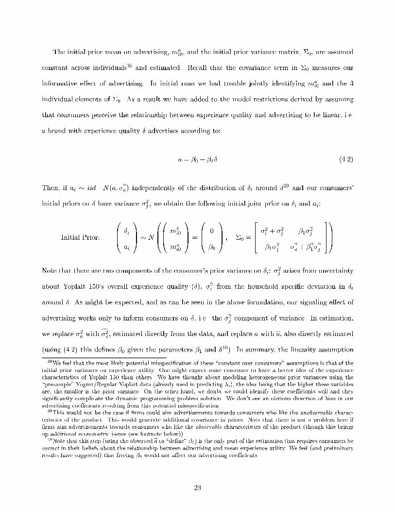
A second major advantage of the structural approach is that it allows for interesting policy analysis

that is simply not possible with the reduced form analysis. If, for example, advertising provides

consumers with information, we would like to know the value of this information. In order to compute

such a value, we need to be able to adjust optimal consumer behavior when the source of information

is eliminated. With a structural model this is possible. In our case we ban advertising and are able to

adjust consumer behavior appropriately so that the resulting zero advertising levels are not interpreted

as a \bad" signal. We stress both here and later that, unlike our main empirical conclusions, the welfare

analysis we perform is probably highly dependent on our choice to model informative advertising as

a signaling e�ect. Though this limits the applicability of the welfare results, we feel that it is still an

interesting and enlightening exercise.

Estimates of our structural learning model support two main conclusions. First, we can easily

reject the hypothesis of perfect information. The data suggest that consumers do learn from their

consumption experiences with the brand. Second, we �nd a strong, positive informative e�ect of

advertising and an economically and statistically insigni�cant prestige e�ect of advertising. This

supports the reduced form conclusion that the advertisements in this data primarily a�ected consumers

through the provision of information. Again, we stress that since we include only one informative

e�ect, we are prevented from drawing any conclusions about the nature of informative e�ect, i.e.

whether it is in fact signaling information or perhaps information on product existence or observable

characteristics. Under the strong assumption that it is in fact signaling information, our policy analysis

13As Ackerberg (1996) notes, their argument regarding di�erent empirical implications of informative and prestigeadvertising is made conditional on a consumer's expected utility (EU) from consuming the brand. In other words, em-pirically one wants to compare the e�ects of a brand's advertising on two consumers with the same EU from consumption,but di�erent levels of experience with the brand (e.g. one experienced, the other inexperienced). The argument needs tobe conditional because of potential correlations in the data between prior experience and current expected utility fromconsumption (see Ackerberg (1996) for a simple example). Though such positive correlation between prior experienceand expected utility is likely adequately conditioned on in the reduced form models, the increased dispersion in behavior(EU) mentioned in the text above is not. For example, consider a situation where both experienced and inexperiencedconsumers have EU 's centered at zero (assume consumers purchase if EU > 0), but experienced consumers EU 's havemore dispersion (a higher variance) (see Figure 1). In this case, a burst of prestige advertising that shifts all consumersEU 's up by a certain amount will induce a higher proportion of inexperienced consumers than experienced consumersto purchase. Without conditioning on this increased dispersion, one would incorrectly conclude that this advertisingrelatively a�ects inexperienced consumers.

7

indicates that the value of this information to consumers is signi�cantly less than the resources spent

on advertising. This at least suggests that advertising signaling may be a very ine�cient way of

transferring information. Section 2 introduces our general model of consumer behavior and Section 3

describes the data used in this study. Section 4 details our empirical speci�cation and presents our

results. In Section 5 we perform our welfare experiments and Section 6 concludes.

2. The Model

Consider a market in which there are J di�erentiated brands of a non-durable experience good. In

each time period t, consumer i observes prices, pijt, and advertising intensities, aijt, of each brand j.

Advertising intensity refers to some measure of the number of advertisements of brand j that consumer

i is exposed to in period t, perhaps divided by units of possible exposure time (e.g. TV watching or

radio listening time). Note that prices are allowed to vary across both consumers and time. It is

assumed that the good is non-durable enough so that a brand purchased at t is completely consumed

before t+ 1.

After observing prices and advertising intensities in a given period, the consumer decides whether

to purchase one unit of one of the brands or nothing. Consumers are assumed to make this discrete

choice to maximize their expected discounted sum of future utilities conditional on their information

set at t:

maxc� (Ii� ) �>=t

E

"1X�=t

���tUic�� j Iit

#(2.1)

where ct 2 f0; ::::; Jg is the consumer's choice at t (0 represents no purchase) and � is the per-period

discount factor14.

As is now relatively common in the empirical analysis of di�erentiated products, we take a Lan-

casterian, characteristics-based approach to consumer theory, assuming the utility a consumer derives

from a brand is a function of the brand's characteristics and the consumer's tastes for these character-

14Note that we consider an in�nite horizon problem. As consumers have �nite lives, there is obviously some �nitehorizon, but because the time frame of the empirical work will be a consumer shopping trip, the number of periods willbe very large and approach the in�nite horizon solution. Also, note that because the consumer's information may changethrough time, the consumer maximization problem is over a sequence of choice functions mapping future realizations ofinformation sets into choices.

8

istics. Speci�cally, we assume the utility consumer i obtains from purchase and consumption of brand

j in period t is:

Uijt = U(pijt;Xj ; yi; �ijt;maijt; �ijt+1) (2.2)

where Xj contains observable characteristics of brand j, and yi are consumer i's tastes for these

characteristics. �ijt represents idiosyncratic, time-varying shocks to the utility the consumer derives

from consuming brand j that are known prior to the purchase decision. Though we defer its formal

de�nition until later, maijt is a measure of what consumer i currently knows about how much brand j is

advertising. Its entry into the utility function will represent our image or prestige e�ect of advertising.

The term �ijt+1, which we call \experience utility", captures the experience nature of the good.

It is a scalar measure of the utility that consumer i derives from brand characteristics that are not

directly observable to him (i.e. experience characteristics). It is dated t + 1 because in contrast to

the other elements of the utility function, it is not necessarily known to the consumer at the time

of purchase. For food products, Xj might contain observable characteristics such as calories or fat

content, while �ijt+1 might represent how the brand actually tastes to the consumer (conditional on

Xj). Although �ijt+1 is not observable before purchase, it is observed if good j is purchased and

consumed at t because total utility is realized and all other components of the utility function are

known. Thus, in the simplest case where �ijt+1 is constant over time we have a \one-consumption"

learning process. In this case, if the consumer purchases and consumes the brand once, he observes

�ijt+1 and knows its value for all future t:

As in Eckstein et.al. (1988), we allow for a more general learning process in which it may take

more than one consumption to ascertain the experience utility to expect from future consumption of

a brand. Speci�cally, it is assumed that:

�ijt+1 = �ij + �ijt+1 where �ijt+1 � iid N(0; �2�) (2.3)

Although �ijt+1 is realized (observed) by the consumer after consumption, its components, �ij and

�ijt+1; are never individually observed. �ij is the mean experience utility consumer i obtains from

9

brand j. �ijt+1 are i.i.d. confounding variables that cannot be distinguished from this mean. In the

case of food products, variance in �ijt+1 may result from variation in product quality, combination

with other products, the existence of di�erent avors of a brand that the consumer must learn to

optimize over, or even di�erent moods or situations at time of consumption15. In contrast to the

i.i.d. �ijt+1, �ij is persistent over time. It is thus bene�cial for the consumer to use information

contained in observed �ijt+1's to learn about its value. In the degenerate case where �2� = 0, we have

the one-consumption learning process described above where �ij (and thus �ijt+1 8t) is learned after

one consumption experience. In the non-degenerate case, consumption and subsequent realization of

�ijt+1 does not exactly reveal �ij , but it does provide information about it. This information will be

consistently modeled in a Bayesian learning framework.

In a similar formulation, we assume that consumers' observed advertising intensities, aijt, follow

the process:

aijt = aj + �ijt where �ijt � iidN(0; �2� ) (2.4)

and where aj is the mean advertising intensity of brand j. Deviations in aijt around aj may be

caused by variation in consumers' television or reading habits or variation in where or when a brand

is advertised16. Although consumers do not directly observe a brand's mean advertising intensity aj ,

we allow them to be interested in it for two reasons: (1) Possible prestige, image or status e�ects of

advertising where the consumer, all else equal, obtains more utility from consuming a more advertised

brand or a brand more associated (through advertising) with a particular image, and/or (2) a belief

that �rms use aj to implicitly signal information on the mean experience utility they obtain from the

brand �ij , as would be the case in a Nelson type signaling equilibrium. In either of these cases, an

optimizing consumer will use observed aijt's to learn about aj . Note that in this model there is no

15In all these cases the important thing is that the �ijt are indistinguishable from �ij , e.g. the consumer is in a happymood, enjoys the product more than usual, but cannot distinguish exactly what component of the extra enjoyment wasdue to his mood and what component was due to the product's experience characteristics. Note that one could also addrandomness to the utility function that is not known prior to purchase but is distinguishable (from �ij and �ijt) afterconsumption. As long as such error is additive and i.i.d., only its expectation has an e�ect on decision making.

16One can easily generalize to having advertising exposures distributed around an individual speci�c mean (i.e. aijt =aij + �ijt). It is also possible to allow brands' advertising levels to vary randomly over time. However, these levels neednot be serially correlated to ensure that per-period deviations from an individual's mean are independently distributed(this is necessary for the Bayesian updating formulas below).

10

explicit information about the product obtained through advertisements: consumers are assumed to

know of the existence of all brands and know all the observable characteristics of each brand17.

We consistently model information provided by the observed aijt's and �ijt+1's on the relevant

unknowns aj and �ij as a bivariate Bayesian learning process. In matrix notation, equations (2.3) and

(2.4) become: �ijt+1

aijt

!� i.i.d. N

�ij

aj

!;�ij

!where �ij =

2664 �2� 0

0 �2�

3775 (2.5)

The assumed diagonality of �ij implies that there is no correlation between �ijt+1 and aijt conditional

on their means. In other words, deviations around mean experience utility due to quality variation,

consumption situations, avors, etc. are assumed uncorrelated with the deviations around mean

advertising level due to variation in television watching or brand advertising levels. Appealing to the

theory of conjugate distributions (DeGroot (1970)), this equation, along with an initial (t = 0) prior

on aj and �ij :

Initial Prior:

�ij

aj

!� N

m�

ij0

maij0

!;�ij0

!(2.6)

generates a learning process in which a consumer's posterior on brand j after a history of observed

advertising intensities, faij1; :::; aijtg, and consumption experiences, f�ij1; :::; �ijKijtg, is given by18:

�ij

aj

!� N( mijt ; �ijt ) (2.7)

where: mijt =�m�

ijt

maijt

�= (��1ij0 + �ijt�

�1ij )

�1(��1ij0mij0 + �ijt��1ij zijt);

17As mentioned and discussed in the introduction, complexity and identi�cation issues necessitated the inclusion ofonly one informative e�ect of advertising in our model. There are clearly alternative speci�cations of informative e�ects.Erdem and Keane's (1996) similar dynamic model has advertising explicitly informing the consumer on characteristicsof the brand. In their model, each advertisement a consumer sees gives them an iid draw from a distribution centeredat �ij . Another alternative would be to allow advertising to inform consumers of a product's existence. Modeling thiswould likely involve introducing an indicator function of product existence knowledge that is in uenced by advertising aswell as other things. See the introduction for arguments why we chose our particular e�ect and why we feel that alteringthis choice would not signi�cantly a�ect our primary empirical results.

18The derivation of the following conjugate result is a fairly simple extension of the derivation for a multivariate normalwith equal draws in DeGroot. Note that use of these conjugates (and all the (in our case normality) assumptions that gowith it) is necessary because it allows us to express posterior distributions with a �nite number of parameters. As theconsumer's state space will need to include their current posterior, this reduces the state space from an entire functionto a simple set of parameters, allowing the dynamic program to be numerically solvable.

11

�ijt = (��1ij0 + �ijt��1ij )

�1 ; zijt =� 1

Kijt

PKijtk=1

�ijk

1

t

Pt

�=1aij�

�; and �ijt =

2664 Kijt 0

0 t

3775and where Kijt equals the number of consumption experiences consumer i has had with brand j up to

period t. As the consumer observes an advertising intensity for each brand in each period, the number

of observed advertising intensities is t.

The consumer's period t posterior mean for brand j, mijt =�m�

ijt

maijt

�, is a matrix weighted average

of initial priors and observed realizations of �ijt+1 and aijt. An important result of Bayesian learning

is that these posterior means and variances summarize all the consumer's information on �ij and aj .

Thus, under the i.i.d. assumption of (2.5); the current posterior (mijt, �ijt) is su�cient to de�ne

perceived distributions over both future �ijt+1's and aijt's as well as future posteriors19.

Of particular interest at this point is the composition of the variance matrix of the consumer's

initial priors. If the covariance term of �ij0 is zero, then the updating processes on �ij and aj are

completely independent. On the other hand, a non-zero covariance term indicates a perception by

consumers that �ij and aj are correlated. This links the two learning processes - in this case, observed

levels of advertising that provide direct information on aj will, through this covariance term, provide

indirect information on �ij . Such a correlation in priors would arise from a belief that advertising is

used by �rms to signal information on a brand's experience utility. As an example, suppose there is a

Nelson type signaling equilibrium in which �rms set brand advertising levels according to:

aj = �0 + �1�j

where �j is brand j's mean experience utility level over the population. Then, assuming (1) a

normal population distribution of �ij around �j (�ij � N(�j ; �2i )) and (2) a normal prior on �j

(�j � N(m�ij0; �

2j )), a Bayesian consumer's initial prior variance matrix will have covariance element

�1�2j : This covariance term captures the informative signaling e�ect of advertising in our model. In

19Note that in this formulation �ij is assumed known to the consumer. One implication of this is that the posteriorvariance matrix evolves deterministically in the number of consumption experiences and time. It is possible to deriveupdating rules in cases where these variances are not known. Unfortunately, this leads to a structure too complicatedfor empirical work.

12

the case where it is positive, consumers interpret high levels of advertising as a signal of a higher �ij20:

In addition to this informative e�ect of advertising, we accommodate prestige or image e�ects of

advertising by allowing the consumer's current posterior mean on aj ; maijt, to enter directly into the

utility function (2.2). A positive derivative of (2.2) with respect to maijt indicates that, all else equal (in

particular expectations over �ijt+1), the consumer receives more utility from consuming a product that

he believes has a higher advertising intensity. Again, the interpretation is as in Becker and Murphy

(1993), i.e. advertising itself or images in advertising bestow some \coolness" or \prestige" on the

product that is directly valued by consumers21.

Given the learning process as speci�ed in (2.7), we can move back to the consumer's dynamic

choice problem. Because the posterior (mijt, �ijt) is su�cient to de�ne all the consumer's current

information on �ij and aj ; the sequential maximization problem of (2.1) can be transformed into the

following Bellman's equation:

Vi(pit;mit;�it; �it) = maxcit2f0;::;Jg

E[U(pictt;Xj ; yi; �ictt;maictt

; �ictt+1)

+ �Vi(pit+1;mit+1;�it+1; �it+1) j (pit;mit;�it; �it); cit]

(2.8)

where the state space (pit;mit;�it; �it) contains prices, current posterior distributions for each of the J

brands, and time-varying preference shocks for all J brands22. The expectation is over current period

20For the most part (particularly in the welfare analysis that follows estimation), we take the view that consumers arerational in their beliefs, i.e. that a positive covariance term in priors is actually generated by a signaling equilibrium,not just spurious beliefs by consumers. A less restrictive, alternative interpretation is that in estimating

Pij0; we are

simply estimating consumer beliefs, without assuming anything about where they come from or whether or not they arecorrect. In this case, a positive covariance term simply means that consumers think more advertised products will bebetter, perhaps rightly, perhaps wrongly - making the description of this e�ect as \information" a rather loose one.

21As we are essentially putting \the amount the consumer thinks the brand is advertised" in the utility function, theprestige interpretation is a bit more natural than the image interpretation. At �rst take, one might consider an imagee�ect of advertising more discrete - a consumer either knows or doesn't know that a brand is associated with a particularimage (e.g. Michael Jordan). On the other hand, image e�ects may arise from a consumer wanting (i.e. deriving utilityfrom) other people associating them with particular images. As the amount of other people who are aware of the brand'simage association will depend on the amount the brand advertises the association, one can justify this use of this term.Clearly we are in somewhat murky waters regarding the speci�cation of these image and prestige e�ects. To partiallycompensate, in empirical work we try to be as general as possible with the speci�cation. We also consider the possibilitythat these e�ects are heterogeneous across the population (i.e. consumers have di�erent valuations of prestige or di�erentattitudes towards particular images). The most critical thing that we are not exible with is that ma

ijt doesn't somehowinteract in the current period utility function with measures of past consumption. As mentioned in the introduction andshould be clear in a moment, such interactions can eliminate our source of separate identi�cation of the informative andprestige e�ects of advertising.

22Note three strong assumptions of the model: 1) We assume J independent learning processes for the di�erent brandsof the product. Such would not be the case if one were learning about preferences for experience characteristics of the

13

experience utility �ictt+1 as well as next period's state. For consumer i with posterior (mit;�it) facing

prices pit and shocks �it, Vi(�) is the perceived expected discounted value of future utilities23. This

value function has an associated policy function, cit = ci(pit;mit;�it; �it), which maps the consumer's

current state into an optimal choice of brand. Ackerberg (1996b) provides more details of this Bellman's

equation including the corresponding state evolution equations.

To summarize, we have a dynamic model of behavior in which a consumer learns from both

consumption and advertising exposures. Purchase and consumption of a brand provides the consumer

with direct information on the utility he derives from the brand's experience characteristics. Observed

advertising intensities have two e�ects on a consumer: First, they may provide indirect, signaling

information on these experience characteristics. Second, they are a direct indication of a brand's

advertising intensity, which may through image or prestige e�ects provide a direct utility the consumer.

The consumer decides between brands based on the information learned from past consumption and

advertising while realizing the e�ect that current decisions will have on future information.

Unfortunately, the above dynamic model is not analytically solvable. However, we have used

numeric solution methods to solve and generate predictions of the model. These general predictions

are made through characterization of the value function and simulation of the model at reasonable

sets of parameters. The range of parameters tried as well as the intuitive nature of the predictions

suggests that they should hold at most if not all parameter values, but this is not necessarily the case.

Ackerberg (1996b) contains a more thorough comparative static analysis of this model.

One implication of the learning process is that consumers are likely to change their purchasing

general product (e.g. if one has never tried yogurt before, consumption of one particular brand of yogurt will surelyprovide information on what to expect from consuming a di�erent brand of yogurt), 2) The model ignores potentialspillovers of information between consumers. Consumers are unable converse with each other about observed advertisinglevels or experience utilities. If this were the case, it clearly would provide additional information to consumers on ajand �j , and possibly on their own speci�c �ij 's (As might be the case if two consumers knew themselves to have similarpreferences for experience characteristics or if experience characteristics were easily describable (e.g. That brand is verysweet).), and 3) The model assumes that there is no signaling information in price. In theory, there is no reason why onecouldn't add price signaling to the model in an analogous fashion to the way advertising signaling is modeled.

23Vi(�) is indexed by i because of consumer speci�c, time invariant variables such as yi and �i that are not explicitlyincluded in the state space. It is the perceived value because this is what the consumer believes his expected discountedvalue of future utilities to be (given his information). There is also a \true" value function, the \true" expected discountedvalue of future utilities, which is additionally a function of the unknown �ij 's. This true value function captures theextent to which posteriors di�er from the true �ij , and the \mistakes" that might result.

14

patterns24 over time as a result of obtaining new information. The parameters of the learning process

determine how long these purchasing patterns will be changing. In a one brand, no advertising, model

with a one-consumption learning process (�2� = 0; [�ij0]11 > 0), purchase patterns change after the

�rst purchase but not thereafter. If there is variance in �ijt+1 (0 < �2� < 1), purchasing patterns

do change after the second or more purchases, the extent and length depending on �2� and [�ij0]11.

On the other hand, if there is no learning (�2� = 1 or [�ij0]11 = 0), we obtain constant purchasing

patterns through time.

A second characteristic of the model is that if there is learning, there is a value of information to

consumers. Consumers may be willing to experiment with new brands that do not maximize expected

current utility in order to obtain information on that brand and make more educated decisions in

the future. The extent of this willingness depends on the consumer's discount rate, prior variances,

and per-period variances in advertising intensities and experience utility. The more the consumer

discounts the future, the less likely he is to experiment as the information bene�t to future utilities

is weighed less. If advertising is more informative (a large covariance term in �ij0) or more precise

(�2� is smaller), the consumer is also be less likely to experiment, relying on informative advertising

for information rather than trying the new product. On the other hand, the quicker the experience

learning process (�2� smaller) or the more information there is to be learned ([�ij0]11 larger), the more

likely the consumer is to experiment with a new product that does not maximize current expected

utility.

The most important implication of the model for the current empirical study concerns the two

di�erent e�ects of advertising in the model. Both consumption and informative advertising can provide

information to the consumer on the mean experience utility he will obtain from future consumption.

However, while consumption provides direct information on this experience utility, advertising only

provides indirect information through a consumer's prior beliefs that the two variables are correlated.

24Purchasing patterns generally refer to the number of purchases of a brand in a given time interval. By allowingvariance in either �ijt's or prices, consumers in our model exhibit non-degenerate (i.e. not either always purchase ornever purchase) purchase patterns even in the case where there is no learning (Learning itself (without variance in either�ijt's or prices) will generate purchasing pattern changes, but in a very binary way (e.g. without advertising we have asimple optimal stopping time model)).

15

The more direct information the consumer has obtained through consumption experiences, the less he

needs to rely on the indirect advertising information. As a result, all else equal, the more consumption

experiences a consumer has had, the less informative advertising will a�ect his expected utility from

consumption. Under one-consumption learning, for example, informative advertising will not a�ect a

consumer after one consumption experience with the brand. At that point, the consumer will have

already learned �ij and have no use for the information on experience utility contained in advertising. In

contrast, our direct, prestige or image e�ect of advertising a�ects the expected utility of inexperienced

and experienced users of a brand equally. This is the behavioral implication that we take to the data

to distinguish between these two e�ects of advertising.

3. The Data

Consumer level panel data on grocery purchases is used in estimation of the model of section 2.

This data, collected by A.C. Nielsen, is commonly referred to as \scanner panel data" because it

was recorded by supermarket UPC scanners25. In each of two geographically isolated markets (Sioux

Falls, South Dakota and Spring�eld, Missouri), shopping trips and purchases of approximately 2000

households at 80% of area supermarkets and drugstores were followed for three years (1986-1988).

There is also data on weekly prices at each store, so we essentially know prices on each household's

shopping trips26. In addition to containing this extremely detailed data on household purchases over

time, A.C. Nielsen TV meters were used to collect information on household TV advertising exposures

for about half the households in the last year of the data. We thus know, along with when and what

each household bought, when members of the household were potentially exposed to TV advertisements

for each brand.

The publicly available Nielsen data contains data on four product categories: ketchup, laundry

25This type of data has primarily been analyzed in the marketing literature (e.g. Guadagni and Little (1983), Pedrickand Zufryden (1991), Deighton, et. al. (1994), Russell and Kamakura (1994), McCulloch and Rossi (1994)). Withthe exception of Erdem and Keane (1996), these studies have used static, more \reduced form", discrete choice modelsof consumer behavior. As in Erdem and Keane, the studies that examine advertising focus on assessing \how much"advertising a�ects behavior, not distinguishing \how" it a�ects behavior.

26It is important to note that data on prices in a particular store on a given day is not through direct observation, butrather imputed from purchases by other consumers in the sample (see Ackerberg (1996) for more detail on this issue).

16

detergent, soup, and yogurt. Ackerberg (1996) chose to focus on the yogurt data for reasons that are

just as relevant for this study. First, the inability to even parsimoniously include inventory behav-

ior and purchase quantity choice in the model suggests the choice of the least durable of the above

products. Second, empirical identi�cation in both models relies on distinguishing experienced from

inexperienced users of a brand. This generates a serious initial condition problem unless one has

data from a product's initial introduction on the market. The yogurt data includes such a product:

Yoplait 150, a lowfat yogurt introduced in April, 1987, about 15 months before the end of the Nielsen

data. As computational issues are even more binding here than in that paper, we again focus speci�-

cally on Yoplait 150, modeling competing brands in a informationally static and unfortunately sparse

framework.

Table 3.1 gives some summary statistics for the data following Yoplait 150's introduction27. Com-

paring advertising shares to market shares suggests that it was, at least initially, a heavily advertised

yogurt. The large di�erence in market shares between markets 1 and 2 may be due to the existence

of two, high-share, local brands in market 1 and the signi�cant number of manufacturer coupons that

seem to have been available in market 2. We urge the reader to consult Ackerberg (1996, 1996b) for

a more thorough data description, including samples of particular consumer's purchase patterns, an

examination of the time paths of prices, advertising, and sales, and a discussion of data problems

relating to manufacturers coupons28 and advertising29.

27Only households whose television viewing was recorded are included both here and in estimation. We also limit thedata to shopping trips in supermarkets (rather than drugstores) and those in which $10 or more was spent.

28Brie y, since we only observe manufacturers coupons that are redeemed, this cannot be used as an explanatoryvariable due to correlation with any unobservables determining purchases. Because of their relative prevalence in market2, we use a market dummy as a proxy for the \availability of manufacturers coupons" (this is the variable we reallywant). In contrast, we do know when store coupons (coupons typically distributed in the store) were available (in thedata this was only for one week in two stores), so we do include this as an explanatory variable.

29A signi�cant problem with advertising is that advertising exposures were only measured in the last year of theNielsen study. This leaves about three months when Yoplait 150 was on the market but advertising was not measured.We use zero advertising exposures for this period, a potential justi�cation being that for almost three weeks after TVmeasurement started, there were no Yoplait 150 advertisements observed. We hope this may indicate that Yoplait didnot begin advertising the product until this time. In any case, evidence in Ackerberg (1996) suggests that alternativetreatments of this time period do not a�ect the identi�cation of di�erent e�ects of advertising. Other problems with ouradvertising variable include unreliability of TV meters (we eliminated consumers with extremely large viewing gaps - anindication that their meter may not have been working), and a problem inherent in data such as this that we are notsure exactly sure who in a household (if anybody, for that matter) watched or paid attention to an advertisement.

17

4. Estimation

We now move to estimation of our model using this data, starting with a detailed discussion of our

empirical speci�cation. We begin with precise formulations of the utility function and the learning

process. As the model contains a signi�cant degree of unobserved consumer heterogeneity, we feel

it important to emphasize which variables are econometric observables, which are econometric un-

observables, and which are assumed constant over consumers and estimated. It is also important to

consider what is known to consumers at particular points of time. Because the empirical model is

fairly complicated and non-linear, we intuitively discuss how our data should identify the parameters

of the learning process, followed by a description of the likelihood function. We then mention issues

regarding solution of the dynamic programming problem generated by the model before concluding

with a discussion of our estimates. Two general sets of estimates are presented. The �rst assumes

myopic consumers who learn and update according to the above model but maximize only current

expected utility, not the expected discounted sum of all future utilities. Although this model iden-

ti�es the parameters of the learning process, it does not require solving the dynamic programming

model of section 2, signi�cantly reducing computational burden. Note, however, that this rules out

the experimentation behavior generated by the dynamic model. The second set of estimates are of

the full dynamic problem in which consumers are forward-looking in their behavior. This does require

solution of the dynamic programming problem.

4.1. Empirical Speci�cation

In all empirical work, we assume that the time frame of our model is the consumer (i.e. household)-

shopping trip. Speci�cally, we model consumer i's purchase decision on each of their shopping trips

t through the 15 months of data. Because of computational issues, we restrict ourselves to modeling

the simple binary choice whether or not to purchase Yoplait 150 on each shopping trip. As such, the

choice to purchase a di�erent brand of yogurt is included in the \outside alternative" along with the

18

decision not to buy any brand of yogurt30. We assume the following parametric speci�cation of our

consumers' single period utility functions:

Uit =

8>><>>:Ui1t = �i + �1pit + �2scit + �it+1 + �3m

ait + �i1t if Yoplait 150 purchased & consumed at t

Ui2t = �4pothit + �i2t otherwise (outside alternative)

The variables pit; scit; and pothit measure price of Yoplait 150, value of a possible store coupon available

for Yoplait 150, and a scalar measure of other yogurts' prices31 respectively on shopping trip t of

consumer i. Note that these variables vary over both time and consumers, as supermarkets change

prices over time and consumers shop at di�erent supermarkets. The parameters �1, �2, and �4 measure

marginal e�ects of these variables on utility.

The time-invariant �i represents consumer i's individual-speci�c preferences for the observable

characteristics of Yoplait 150. �i is thus known to consumer i for all t. Econometrically, we model

�i as a linear combination of observable consumer characteristics plus a normally distributed random

variable with variance �2�. These observable consumer characteristics (yi) include a market dummy,

the consumer's income and family size, and the number of yogurt, lowfat yogurt, and regular Yoplait

purchases made by the consumer in the data prior to Yoplait 150's introduction on the market32.

The \random e�ect" component of �i allows for persistent di�erences in consumers' known tastes for

Yoplait 150 that are not observed by us as econometricians.

�i1t and �i2t capture time-varying shocks to the utility derived from each alternative. These are also

assumed known to the consumer at the time of purchase. To ease computation in both the dynamic

30In more preliminary speci�cations we compared these 2 choice models to 3 choice models (with the choices: Yoplait150, a di�erent brand of yogurt, or no yogurt) and obtained very similar results. Note that we also completely ig-nore the number of yogurts purchased on a particular shopping occasion, avoiding what is in actuality a complicateddiscrete/continuous choice. Regarding the learning process, our assumption is that purchase quantities and variablespossibly a�ecting the length of the learning process (in particular, family size) scale together so that one purchase occa-

sion provides the same information across households. We note that this purchase quantity data may be a potentiallyinteresting source of information on learning for future work.

31This is measured as minjf(pijt � pj)=pjg; the minimum (over all other brands of Yogurt j) percentage currentdeviation from the average price of that brand.

32This \presample" purchase data is assumed exogenous to our model, and as might be expected are very goodpredictors of �i. In the reduced form models of Ackerberg(1996) other household characteristics such as ages and sexeswere not signi�cant. Note that because they do not change over time, coe�cients on individual Yoplait 150 observablecharacteristics Xj such as calories or fat content (in a linear utility, binary choice model) would not be separatelyidenti�ed. WLOG, �i represents the sum of the utilities from these characteristics for consumer i.

19

programming problem and estimation, these econometric unobservables are assumed i.i.d. Type 1

Extreme Value deviates. As in a standard discrete choice model, we cannot identify relative levels or

variances of the utility function. The lack of a constant term in the outside alternative utility is our

additive normalization; the �xed variance of the �it's the multiplicative.

As in the theoretical model, �it+1 represents the utility consumer i obtains from the experience

characteristics of Yoplait 150 if it is purchased and consumed in period t. Again, this term is generally

not known before the period t purchase decision. As such (given our linear utility formulation), what is

relevant to this decision is the expectation of �it+1, which is determined by the consumer's information,

i.e. what they have observed in the past. Recall that a consumer in period t has observed advertising

levels of Yoplait 150 in each past period (the sequence fai1; ::::::; aitg), and has observed realizations of

experience utility in past periods in which Yoplait 150 was purchased and consumed (f�i1; ::::::; �iKitg).

The consumer combines these observations with his priors (as per eqs. (2.7)) to compute his period t

posterior means (m�it and ma

it) on the mean experience utility he obtains from consuming Yoplait 150

(�i) and how much Yoplait 150 is advertising (a). As the per-period experience utility draws �it+1 are

distributed around �i, the period t expectation of �it+1 is simply the consumer's period t posterior

mean on �i, m�it33. Importantly, recall that it is through this posterior on experience utility (m�

it)

that our informative, signaling e�ect of advertising in uences expected utility. A positive covariance

term in initial priors implies that past advertising observations fai1; ::::::; aitg positively a�ect m�it (as

well as mait). In this case the consumer associates or interprets high advertising levels as signaling

information on good experience characteristics.

Lastly, note that consumer i's period t posterior mean on Yoplait 150's advertising intensity, mait,

enters directly into the utility derived from consuming the brand. The parameter on this term, �3

(and in some cases �3i) captures our direct, \prestige" e�ect of advertising on utility. �3i > 0 indicates

that all else equal, the consumer obtains more utility the more he thinks Yoplait is being advertised.

In summary, our informative e�ect of advertising enters expected utility through m�it (E[�it+1]), our

33This is just the combination of two normal distributions. The consumer knows �it+1 � N(�i, [�]11) (but doesn'tknow �i) and \perceives" (has the posterior) that �i � N(m�

it; [�]11). Therefore, he sees �it+1 as coming from the\combination" of the two distributions, i.e. �it+1 � N(m�

it; [�]11+ [�]11).

20

prestige e�ect of advertising through mait.

From an econometrician's point of view, a consumer's two sources of information (past �it+1's and

ait's) di�er considerably because while we observe a consumer's advertising exposures, we clearly do

not observe his realizations of experience utility. In our model, consumers want to determine how much

advertising a brand is engaging in. Thus we de�ne ait, consumer i's observed advertising intensity in a

given period t, as the number of advertisements seen by i between the current (t) and previous (t� 1)

shopping trip divided by the amount of television watched during that period34. This controls for

the fact that di�erent consumers watch di�erent amounts of television. Our econometric assumption

on the realized �it+1's matches our theoretical one, i.e. that they are assumed distributed normally

around �i. The variance of this distribution, �2� , is assumed constant over consumers and time (recall

that this variance determines the length of the learning process, e.g. �2� =0 implies a one-consumption

learning process). For the Bayesian updating formulas, we also need to know the per-period variance

in ait. This is computed for a particular consumer and time period as a function of the amount

of television watched since the last shopping trip and the measured sample variance of advertising

intensity in the data35. This allows the precision of an advertising observation ait to increase in the

number of hours of television watched between t � 1 and t. While our formulation directly controls

for the obvious fact that consumers watch di�erent amounts of television, the data also indirectly

suggests that consumers di�er in the type of programming they watch (we �nd statistically signi�cant

34As mentioned in the introduction, there are a number of reasons why we de�ne our advertising variables as ad-vertisements per TV hour. First, we think that this de�nition best corresponds to the speci�c e�ects of advertisingincluded in the model. One could argue that both signaling and prestige e�ects should depend on how much the brand isadvertising, not how many advertisements the consumer sees (in contrast, if advertising informed consumers of existenceor characteristics, we would expect it to depend more on the absolute number of ads seen by the consumer). Second, thisde�nition may alleviate measurement error resulting from TV meter problems. Third, and perhaps a result of the �rst orsecond, Ackerberg (1996) found intensities to do better at explaining the data than absolute number of advertisements.Also note that we are assuming that we observe advertising exposures exactly. We would have preferred to explicitlyinclude advertising measurement error as an unobservable in the model (this method could also be used to deal with theproblem of initial advertising in the �rst 3 months). Unfortunately, as advertising in any given period a�ects decisionsin all future periods, this results in a rather nightmarish integration problem in estimation.

35Because the advertising process is inherently binary (either you see or don't see an advertisement for Yoplait 150in a given minute (or quarter-hour)) this variance computation is a simple function of the probability of seeing an adin the time segment (assumed constant over time) and the amount of time segments. It should be noted that becauseait is essentially the sum of binary random variables , it takes a rather large stretch of the imagination to invoke aCLT and assume its normality in the Bayesian updating rules, particularly in light of the extremely low frequency ofadvertising exposures (on average one every three or four weeks, although this varies signi�cantly across households).Unfortunately, this is a necessary assumption in developing feasible Bayesian updating rules (Since we need a conjugatebivariate distribution with correlation, we are pretty much forced to use normals) . We hope the fact that this is athird-order problem prevents it from a�ecting the results signi�cantly.

21

di�erences in consumers' mean (over time) ait's , i.e. how many total Yoplait 150 advertisements they

saw divided by total hours of television watched over the sample). To accommodate this, we add an

additional, consumer level of variance to the advertising exposure process. Speci�cally, we assume

that the ait's are distributed normally around a consumer-speci�c advertising intensity ai (in some

sense measuring the type of programming consumer i watches) which in turn are distributed normally

around the brand's advertising intensity a36.

The mean experience utilities of each consumer, �i (what the �it+1's are distributed around) are

themselves econometric unobservables. Because of the linearity of the utility function, we merge any

initial expectations the consumer has on �i into �i, essentially treating consumer i's initial expected

value of Yoplait 150's unobservable characteristics as an \observable" characteristic. This normalizes

each consumers initial prior on �i to zero (m�i0 = 0) and gives �i the nice interpretation of being

prediction error by the consumer on the utility obtained from consuming Yoplait 150. �i > 0 indicates

that consumer i is unexpectedly surprised by the quality/taste of Yoplait 150. These �i are assumed

to be distributed across the population as:

�i � iid N(�; �2i ) (4.1)

independently of �i. This independence disallows, for example, the experience characteristics of Yoplait

150 to be (on average) more or less unexpectedly preferred by those who like its observable character-

istics37. Note that we do not �x the mean of �i across the population (�) at 0 - this is a parameter

which we estimate and can be interpreted as the overall experience \quality" of Yoplait 150. A �>0

indicates that on average (across consumers), Yoplait 150 was better than initially expected.

36As the ait are observables this does nothing to estimation or the model except that now mait is the consumer's

posterior on ai (rather than on a). Literally, this changes slightly the interpretation of the \prestige" e�ect as now it'sa high belief on ai that generates utility. Practically, as consumers are using the same information (ait's) to learn abouta and ai, the posterior on a is just going to follow the posterior of ai around, so plugging into utility the posterior on airather than a should make virtually no di�erence (in fact, we believe that the period t posterior on a may be a linearfunction the posterior on ai (one can fairly easily show the linear relation holds for 0,1,and 1 observations of ait) -if this is the case, plugging in the posterior on a makes exactly no di�erence). On the other hand, the empirical factthat ai seems to vary across our consumers raises the question of whether ai may be correlated with consumer speci�cunobservables in the model. This is discussed below.

37We have also chosen not to model �i as a function of consumer observables (as is done with �i). Both this and theprevious assumption (�i independent of �i) could in theory be relaxed. Identi�cation and computation issues associatedwith the increase in parameters have prevented this.

22

The initial prior mean on advertising, mai0, and the initial prior variance matrix, �0, are assumed

constant across individuals38 and estimated. Recall that the covariance term in �0 measures our

informative e�ect of advertising. In initial runs we had trouble jointly identifying mai0 and the 3

individual elements of �0. As a result we have added to the model restrictions derived by assuming

that consumers perceive the relationship between experience quality and advertising to be linear, i.e.

a brand with experience quality � advertises according to:

a = �0 + �1� (4.2)

Then, if ai � iid N(a; �2a) independently of the distribution of �i around �39 and our consumers'

initial priors on � have variance �2j , we obtain the following initial joint prior on �i and ai:

Initial Prior:

0BB@ �i

ai

1CCA � N

0BB@0BB@ m�

i0

mai0

1CCA =

0BB@ 0

�0

1CCA ; �0 =

2664 �2i + �2j �1�2j

�1�2j �2a + �21�

2j

37751CCA

Note that there are two components of the consumer's prior variance on �i: �2j arises from uncertainty

about Yoplait 150's overall experience quality (�), �2i from the household speci�c deviation in �i

around �. As might be expected, and as can be seen in the above formulation, our signaling e�ect of

advertising works only to inform consumers on �, i.e. the �2j component of variance. In estimation,

we replace �2a withc�2a, estimated directly from the data, and replace a with ba, also directly estimated

(using (4.2) this de�nes �0 given the parameters �1 and �40). In summary, the linearity assumption

38We feel that the most likely potential misspeci�cation of these \constant over consumers" assumptions is that of theinitial prior variances on experience utility. One might expect some consumer to have a better idea of the experiencecharacteristics of Yoplait 150 than others. We have thought about modeling heterogeneous prior variances using the\presample" Yogurt/Regular Yoplait data (already used in predicting �i), the idea being that the higher these variablesare, the smaller is the prior variance. On the other hand, we doubt we could identify these coe�cients well and theysigni�cantly complicate the dynamic programming problem solution. We don't see an obvious direction of bias in ouradvertising coe�cients resulting from this potential misspeci�cation.

39This would not be the case if �rms could aim advertisements towards consumers who like the unobservable charac-teristics of the product. This would generate additional covariance in priors. Note that there is not a problem here if�rms aim advertisements towards consumers who like the observable characteristics of the product (though this bringsup additional econometric issues (see footnote below)).

40Note that this step (using the observed ba to \de�ne" �0) is the only part of the estimation that requires consumers becorrect in their beliefs about the relationship between advertising and mean experience utility. We feel (and preliminaryresults have suggested) that freeing �0 would not a�ect our advertising coe�cients.

23

on consumer beliefs reduces the parameters �;ma0 ; �

2i ; and 3 elements of �0 to the parameters �; �

2i ; �

2j ;

and �1(Instead of �1, we actually estimate �, the correlation coe�cient implied by �1).

Given that this is a fairly complicated econometric model, it is important to discuss how these

learning parameters are identi�ed by the data. Identi�cation comes primarily from examining how

consumers' purchase behaviors change through the time frame of the sample, in particular after the po-

tential acquisition of information (either through consumption experiences or advertising exposures).

If there is no learning, we would see constant (but likely heterogeneous over consumers) purchasing

patterns over time (conditional on covariates such as price). With learning, consumption experiences

(and the resulting accumulation of information) will change a consumer's purchasing patterns. Even-

tually, everything about the brand is learned and a consumer's purchase patterns will converge to some

\post-information" level. �2�, the variance in the unobserved component of consumers' known tastes

for Yoplait 150, is identi�ed by unobserved heterogeneity in consumers' \pre-information" (pre-�rst

purchase) behavior. On the other hand, �2i , the variance of the unknown taste �i across the pop-

ulation, is identi�ed by the variance of \post-information" heterogeneity41. �; the mean experience

utility of Yoplait 150, is assessed by a comparison of the means of these two distributions, i.e. whether

\post-information", consumers (on average) purchase Yoplait 150 more or less than \pre-information"

(net of experimentation behavior due to dynamic optimization). �2� , the per-period variance in ex-

perience utility, is identi�ed by the number of consumption experiences it takes for consumers to

learn �i, i.e. how many consumption experiences it takes for purchasing patterns to converge to the

\post-information" level. If, for example, purchase patterns change after initial purchases, but not

thereafter, it is indicative that �2� = 0, i.e. a one-consumption learning process. The advertising-related

coe�cients, �1 and �3, are identi�ed generally by the e�ects of advertising exposures on purchasing

patterns. Again, the two are separately distinguished by the relative e�ects of advertising exposures

on inexperienced and experienced consumers42.

41More precisely, one wants to compare the variance of post-information heterogeneity to that of pre-informationheterogeneity. Under our assumptions (in particular that the random component of �i and �i are independent and thatutility is additive in the two terms), the di�erence in these variances is �2i .

42The last \learning process" parameter, �2j , is identi�ed through its appearance in the prior variance matrix. Adjustingthis a�ects 1) experimentation behavior in the dynamic model, and 2) the shape of learning (how posteriors evolve overtime).

24

Moving to estimation, the primary issue is the large amount of consumer heterogeneity and the

resulting number of econometric unobservables. Besides the per-period logit errors, we do not observe

a consumer's �i, his random component of �i, and his realizations of experience utility (�it+1) at each

purchase occasion. Recall that these unobservables are assumed mutually uncorrelated except for the

fact that experience utility realizations are distributed around �i. In addition, these unobservables

are assumed independent of our observables yi; ait; pit; scit; and pothit43. Because of the persistent

unobservables and the dependence of purchase probabilities on lagged endogenous variables (through

posteriors), we use Maximum Likelihood, integrating the persistent unobservables over the entire

sequence of a consumer's choices to derive the probability of that consumer's observed data44. This

results in the following likelihood function (for consumer i) :

Li(�) = Pr

�ncit = c(mit(�

tit; a

tit; c

t�1it ; �); zit;�it; �i; �it; �)

oTit=1

j zTiit ; aTiit ; yi

�=RPr

�ncit = c(mit(�

tit; a

tit; c

t�1it ; �); zit;�it; �i; �it; �)

oTit=1

j zTiit ; aTiit ; �i; �

Tiit

�p(d�Tiit j �i; �)p(d�i j �)p(d�i j yi; �)

=R QTi

t=1 Prhcit = c(mit(�

tit; a

tit; c

t�1it ; �); zit;�it; �i; �it; �) j zit; a

tit; �i; �

tit; c

t�1it

ip(d�Tiit j �i; �)p(d�i j �)p(d�i j yi; �)

where cit is the consumer's observed choice in period t, c(�) is the model's predicted choice, zit =

43We think that the most likely violation of this assumption would be due to the endogeneity of supermarket choiceand shopping trip timing. We cannot have consumers getting high �i1t draws and searching out low Yoplait 150 prices.Hopefully Yogurt is a small enough component of consumers' purchases to prevent signi�cant amounts of such behaviorfrom occurring. Another potential endogeneity problem arises if �rms are able to focus advertising towards consumerswho like Yoplait 150 more than our observables predict (i.e. ait is correlated with the random component of �i or �i) .In Ackerberg (1996), this possibility was tested by including a consumer's mean advertising exposure level (� 1

T

Pait )

as a consumer characteristic. This obtained a positive but insigni�cant coe�cient.44With the exception of the logit errors, the integrals generated by these unobservables are not analytically computable

and we rely on either simulation or discrete approximations to evaluate them. As is well known, simulation of theseintegrals combined with Maximum Likelihood estimation results in inconsistent estimates for a �nite number of simulationdraws. We do use some crude importance sampling techniques to reduce simulation error and inconsistencies. Note thatan alternative to this SML procedure would be to use a simulated GMM framework, using moments in either sequenceprobabilities (McFadden (1989)) or transition probabilities (Keane (1994)). Because of the large number of potentialchoice sequences (given about 60 time periods per individual), the feasible version of McFadden's estimator wouldrequire numerically simulating the logit errors in addition to the other unobservables. Though in this case one wouldobtain consistent estimates regardless of the number of simulation draws, this would greatly increase both computationalburden (the estimator is not continuous in the parameters) and simulation error, a trade-o� we think may not be worthit. Keane's transition probability estimator solves this problem, but like SML, is not consistent for a �xed number ofsimulation draws. While Keane (1994) shows that small sample bias is small (relative to SML) for short panels (T = 8),it is not clear what happens in very long panels when the denominators in his estimator will likely contain much moresimulation error.

25

(pit; pothit ; scit), Ti is the total number of shopping trips of consumer i, and superscripts indicate histories

of a variable through that point (e.g. atit = fai1; ::::; aitg). The Pr [�] in the last line is the probability

that the period t logit errors (�it) are such that the model's predicted choice equals our observed choice,

conditioned in particular on �i, past choices cit, and past realized �it+1's45. The predicted choice

function c(�) is de�ned by either myopic utility maximization (i.e. I(EUi1t > EUi2t)) or the optimal

policy function generated by the dynamic programming problem. Note that this choice function is

a function of current posterior means mit(�), which in turn are a function of past realizations of

experience utility and past advertising intensities. Under the i.i.d. logit assumption on the �it's, the

last Pr [�] has a closed form solution in both the myopic and fully dynamic cases (see Rust (1987)).

4.2. Dynamic Programming Solution

In estimating the full dynamic model, we must solve the consumer's dynamic programming problem

to obtain the predicted choice function c(�). As this solution depends on the majority of the model's

parameters, it needs to be embedded into the routine used to maximize the likelihood function. Our

utility speci�cation and the assumed learning process generate the Bellman's equation:

V (sit; �) = max fE[Ui1t + �V (sit+1; �) j sit; ct = 1]; Ui2t + �E[V (sit+1; �) j sit; ct = 2]g

where the state space sit = (�i;mit;�it; pit; scit; pothit ; �iot; �i1t). Although this state space appears to be

quite large, there are a number of simpli�cations and assumptions that we use to signi�cantly reduce

the dimensionality of the problem and allow for relatively quick numeric solution. First, conditional

on �0 and �, Kit (the number of purchases up to t) and TVit (total hours of television watched up to

t) are su�cient to de�ne the posterior variance matrix �it. Therefore, our assumption that �0 and �

are constant across consumers46 allows us to replace �it in the state space by Kit and TVit: Second,

45Note that formally we are integrating over the Ti potential �it+1's on every shopping trip of consumer i (not justtrips in which a Yoplait 150 purchase was made). In practice, since the �it+1's on non-purchase trips are not observedby the consumer and don't a�ect anything, these integrals disappear, leaving just integrals over the �it+1's associatedwith actual purchases.

46For dynamic programming purposes (to get � constant), we assume that all consumers anticipate watching the sameamount of television between the current and next shopping (�xing this amount at the sample mean). Note that thisassumption only a�ects perceptions of the future - in the actual Bayesian updating formulas used in likelihood evaluation,

26

because �it+1 enters the utility function linearly, �i can be merged into the learning process (so our

consumer Bayesian updates on the sum �i + �i). Third, state variables whose realizations only a�ect

current utility need not be solved for explicitly as state variables (Pakes (1986), Rust (1987), Keane

and Wolpin (1994)). This removes the i.i.d. �'s from the e�ective state space, and as we assume that

consumers perceive pit; scit;and pothit to be non-serially correlated47, we end up with a four dimensional

problem where st, the \e�ective" state space, equals (mit;Kit; TVit):

A second major simpli�cation results from the existence of an analytic solution for the expected

value of the maximum of logit errors. As a result, the expectation over future �'s in the Bellman

equation can be computed analytically (Rust(1987)). This, along with the assumption of discrete

perceived distributions of future pit; scit;and pothit ; implies that to compute the expectations in the

value function we need only numerically integrate over the distribution of next period's posterior

means:

Because the elements of st are either continuous variables (mit) or take on a large number of

discrete values (Kit and TVit), the state space must be discretized in order to apply the Method of

Successive Approximations and numerically solve the above dynamic programming problem. Note

that we do not discretize the entire dynamic problem, but choose points at which we will solve for the

(approximate) value function. In the following estimation results we have discretized the state space

into 10 to 20 points in each dimension. Because the numerical integration mentioned above is only two

dimensional we chose to use quadrature type methods rather than Monte-Carlo. Since the quadrature

points generate future states that are not our discretized ones, we use linear interpolation to evaluate

the value function at these states. Unfortunately, the computation burden of even this simpli�ed

problem is large enough to prevent a detailed exploration of either alternative numeric methods or the

� depends on the amount of television watched between t� 1 and t. A similar assumption involves the discount factor.Although time between shopping trips varies signi�cantly over consumers and time, we assume that consumers use thesame per-shopping trip discount factor to weight the future. Again, this only a�ects perceptions of the future. Relaxingeither of these assumptions would at the very least add an extra \state" variable to the model (i.e. the time until yournext shopping trip, the amount of TV you will watch between now and then)

47We assume a 4-point (estimated from the data) perceived distribution of future pit, and 1-point expectations ofscit and pothit . We note that the assumption that the pit are iid is easily rejected by the data, and is only adopted forcomputational reasons. We believe that this e�ect of this on estimation should be small, as this distribution only entersinto expectations of the future in the dynamic program (and it doesn't enter the myopic estimation results at all). SeeAckerberg (1996b) for a more thorough development of the concepts of this section in the context of our model.

27

sensitivity of the parameter estimates to the current discretization process48.

4.3. Results

Table 4.1 presents maximum likelihood estimates of the above model. In initial runs we had trouble

obtaining reasonable estimates of �2� , the per-period variance in experience utility. In particular, our

estimates were unreasonably high, indicating that consumers were learning (through consumption)

about the unobservable characteristics of Yoplait 150 very slowly. As this parameter is identi�ed

by changes in consumer purchasing patterns after consumption experiences, it is likely that it picks

up variables unobserved by us that cause such changes (e.g. learning about other brands or prod-

ucts)49. As a result, the majority of our estimates assume a one-period learning process (�2� = 0)

where one consumption experience with Yoplait 150 informs the consumer exactly the value of its

experience characteristics to him. This assumption has the added bene�t of greatly reducing both the

computational burden of the dynamic programming problem and the dimensionality of the integrals

in likelihood evaluation. We have capitalized on this computational reduction to increase the preci-

sion and accuracy of our discretization and integral evaluation over what would have otherwise been

possible50.

The �rst two columns of Table 4.1 contain results under the myopic assumption on behavior,

with and without a time trend51 on the outside alternative. The last three columns are results from

48For example, one could move to higher order interpolations, as perhaps this can obtain more accuracy with a lessernumber of discretized points (Rust(1995), Johnson et. al.(1993)). Rust (1997) also suggests randomly picking state spacediscretization points in order to break the curse of dimensionality. One could also move to pure Monte-Carlo simulationor importance sampled Monte-Carlo for the expectation. We felt that conditional on having only ~50 pts to work with,discretized normals would be better. Informal experimentation with our number and choice of discretized points resultsin slightly di�erent estimates, but found no evidence to alter the conclusions of this study.

49We leave the investigation of potential misspeci�cation due to not allowing such e�ects to future work.50With this assumption, the state variable \number of previous Yoplait 150 purchases" becomes a simple indicator

variable whether the consumer has ever bought Yoplait 150. For likelihood evaluation, we now only need to numericallyevaluate a two dimensional integral for each household (rather than 2+ KiT ). Then, with the following discretization ofthe state space ( m�

it- 20 points, mait- 10 points, Kit- 2 points (either purchased or never purchased), TVit- 10 points), 49

draws on the Bellman's equation integral (for a total of 196,000 3-dimensional interpolations per contraction iteration),and each of the distributions of �i and the random component of �i discretized into a 26 point normal for likelihoodevaluation (for a total of 26^2 draws), one function evaluation with a discount rate of .98 on an UltraSparc in highlyoptimized C code takes about 7 minutes (�5.5 min. for the contraction mapping to converge (�1 sec. per contractioniteration), 1.5 min. for likelihood evaluation). Even with good starting parameters, the entire maximization procedurecan take up to a month.

51This time trend, for example, might capture e�ects of new entrants into the yogurt market over the period. Addinga linear time trend to the dynamic problem does not increase computation as the trend can be merged into posteriormeans. With linearity, expectations of future means look the same from any point in time. This would not be the case

28

estimation of the full dynamic model. In all �ve models, the price, other price, and store coupon

coe�cients are very similar, signi�cant and the hypothesized sign. The price coe�cients generate

price elasticities of demand for Yoplait 150 (over the entire time frame of the sample) of approximately

3.3. The estimates and signi�cance of �� indicates that there is signi�cant unexplained heterogeneity

in consumers' initial valuations of Yoplait 150. The very large signi�cance of the estimates of �i

strongly support the existence of imperfect information and learning, indicating that consumers' have

heterogeneous components of utility that are not realized until after their �rst consumption experience

with Yoplait 150.

Moving from the myopic to the fully dynamic models corresponds to allowing the consumers'

discount factors to di�er from zero. In the model without the time trend, this results in a signi�cant

increase in likelihood and an estimated discount factor of .981. As this is a discount factor for the time

between shopping trips, which averages only a little more than a week, this estimate is low, though not

necessarily unreasonable. It may be capturing consumer uncertainty on how long Yoplait 150 might

remain on the market or the possibility of newer, better Yogurts being introduced. In the dynamic

models including a time trend, reasonable values of the discount factor result in worse likelihoods than

the corresponding myopic model. This is likely the result of the positive time trend on the outside

good generating behavior similar to the experimental behavior generated by a higher discount factor.

We therefore �x the discount factor at its point estimate from the dynamic model without the time

trend.

Of particular interest in comparing the myopic and fully dynamic results are the estimates of �, the

mean experience quality of Yoplait 150. While the negative estimates in the myopic models suggest that

consumers (on average) liked Yoplait 150 less than expected, the positive dynamic estimates indicate

that consumers (on average) were pleasantly surprised by the experience quality of the brand. Although

these coe�cients are not generally signi�cant, this points out a possible bias in the myopic assumption.

Experimentation behavior generated by a true dynamic decision process is likely interpreted in a

myopic model as overpredictions of experience utility by consumers.

if we had, for example, a quadratic time trend.

29

The estimated coe�cients pertaining to advertising strongly support the hypothesis that adver-

tising is a�ecting consumers only through the informational structure of the model. Our \prestige"

coe�cient on advertising directly in the utility function, �3, is actually signi�cantly negative in the

models without a time trend, though this may be due to an upward time trend in posterior advertising

means. In the models including a time-trend, the coe�cients are virtually zero and insigni�cant. On

the other hand, the estimates of �, the correlation coe�cient corresponding to �0, are all signi�cantly

positive, suggesting that advertising is providing consumers with information. The di�ering levels of

the estimates of � across the columns do not re ect di�erences in the magnitude of this informative

e�ect of advertising. � is not as orthogonal a measure of the informative advertising elasticity of

demand as we would like. This elasticity depends heavily on the relation of � to the overall magnitude

of �0; which is not identi�ed particularly well and varies over the sets of estimates. The parameters

at the bottom of the table provide a better indicator of this informative e�ect of advertising. These

indicate the percent increase in purchase probability of a representative inexperienced consumer after

a doubling of advertising exposures for 1, 5, and 20 week periods (To focus on the informative e�ect

we do not double the advertising level that enters the prestige e�ect). These informative advertising

\elasticities" are all signi�cant and fairly consistent across the models, the only anomaly being in

the myopic, time trend model where information seems to be conveyed quicker, but asymptotes to a

lesser magnitude. The overall advertising elasticities generated by the models including time trends

are approximately .1552. These are very similar to those found in Ackerberg (1996) and along with

the estimated price elasticity imply an advertising to sales ratio of 4.5% in a static, single-product

�rm, advertising and price-setting model53.

52That is, doubling Yoplait's advertising level over the entire time frame of the data results in a 15% increase in sales.We don't approximate standard errors here because the derivatives needed for the delta method are extremely hard tosimulate accurately for the entire sample (in contrast to those for a representative consumer above). We expect thatthese overall elasticities (as well as overall informative elasticities) would also be signi�cant.

53One can obtain this result by di�erentiating the pro�t function �(p; a) = q(p; a)(p � mc) � caa where q(p; a) isdemand as a function of price and advertising, mc is the marginal cost of the product, and ca is the cost per \unit" ofadvertising intensity. This simple model combined with our estimates also predicts a price-cost markup of 30%. Thoughthese seem to be reasonable results (According to Advertising Age, in 1988 total Yoplait advertising expenditures wereabout 7% of total sales) and provide ballpark �gures, this simple �rm side model is obviously de�cient. First, with ourdemand environment, �rm behavior should be dynamic in nature. Second, this is not a single-product �rm. Third, aswe don't model consumer's purchase amounts, these elasticities are not necessarily the elasticity of total quantity (units)purchased with respect to price (or advertising).

30

Table 4.2 examines three perturbations of the myopic model (these perturbations make the dynamic

model infeasible to estimate). In the �rst column we allow for a more exible speci�cation of the

persuasive e�ect of advertising by including dummies for mait lying in di�erent regions. The estimates

are generally imprecise and don't follow any general trend. We have also tried this simultaneously

estimating regions and using non-linear functional forms, but haven't found much. The estimates in the

second column include a random coe�cient on persuasive advertising, addressing the possibility that

there may be heterogeneity in prestige or image e�ects across the population. This random coe�cient

is constant for a given consumer through the time frame of the model and assumed independent of

the observables and other unobservables54. Although the estimated standard deviation of the random

coe�cient is economically large it is insigni�cant even when simulation error is neglected55. Note

that the mean prestige e�ect stays at essentially zero. We hesitate to make any strong conclusions

about these results because the random coe�cient may be picking up measurement error in our

advertising variable. The third column relaxes our assumption of a one-period learning process, �xing

�2� arbitrarily at 1 (This results in a path of posterior experience quality variances (in # of prior

purchases) of 2.882, .742, .426. .299, .230, .187,....). Note that in this model our informative e�ect

of advertising can in uence a consumer's behavior after their �rst consumption experience (though

its e�ect diminishes in number of prior consumption experiences). Although the parameters of the

learning process change signi�cantly in this set of estimates, we still obtain an insigni�cant prestige

e�ect and a positive, signi�cant informative e�ect.

Before proceeding, we reiterate some important points that arise from our inability to include or

empirically distinguish more than one informative e�ect of advertising in our model. First, we feel

alternative models with di�erent formulations of the informative e�ect of advertising discussed in the

introduction would produce similar empirical results, i.e. a signi�cant informative e�ect, insigni�cant

54With more data, it might be interesting to allow this random coe�cient to depend on consumer characteristics. Notethat in the dynamic programming problem, this random coe�cient would be an additional \e�ective state variable" (i.e.the value and choice functions would depend on it).

55For a consumer whose prestige random e�ect is 1 standard deviation away from the mean, a doubling of advertisingat the mean has the same e�ect on purchase probability as a 5 cent price decrease. Because there are 3 unobservables tointegrate out over in this model, we switch from discretizing the integrals to using Monte-Carlo with crude importancesampling. We also use this technique in the next set estimates, where there are (2+kiT ) dimensional integrals to evaluate.As a result of this, the likelihood values in the last two columns are not directly comparable with the previous likelihoods.

31

prestige e�ect. Underlying this point is a strong belief that the di�erential e�ect advertising on

inexperienced and experienced consumers that separately identi�es the informative and prestige e�ects

of advertising in the current model would provide similar distinction of informative and prestige e�ects

under alternative informative e�ect formulations. As a result, we interpret our results as strong

empirical support for: (1) the conclusion that there were no Becker-like prestige e�ects generated by

these advertisements, and (2) the hypothesis that these advertisements provided consumers with some

type of product information, not that this was necessarily signaling information.

5. Welfare Analysis

We now move to a welfare analysis of the above results, examining the social welfare consequences of

advertising in this market. In contrast to the above, this analysis is highly conditional on the assump-

tion that the informative e�ect of advertising we have found is in fact pure signaling information56.

There is a relatively clear cost-bene�t trade o� with our signaling e�ect of advertising: costs

the cost of resources devoted to advertising, bene�ts the information conveyed to consumers by the

advertising (we ignore potential bene�ts (or costs) of advertising outside this market, in particular its

subsidization of media.) On the other hand, for possible prestige e�ects, there is a serious question

as to how to measure potential bene�ts of advertising. Because utility is a latent variable, a positive

prestige e�ect only indicates that advertising increases the utility of consuming Yoplait 150 relative to

other yogurts. We cannot distinguish whether it adds to the utility obtained from consuming Yoplait

150 or subtracts (i.e. dis-prestige) from the utility derived from consuming the outside alternative57.

As this distinction would clearly be relevant to any welfare analysis, our conclusion that there is no

56Not only is it dependent on this strong assumption, but also on numerous and likely simplistic �rm behavioralassumptions and equilibrium extrapolations that will follow. As a result we certainly do not take this to be anywherenear an \end all" conclusion on the welfare e�ects of advertising in this market. On the other hand, we do feel is thatit is an interesting exploration of the structural estimates and illuminate interesting (and typically ignored) possibilitiesconcerning the welfare e�ects of informative advertising. Essentially, we push our structural model to the \bitter end".What is additionally of interest is just how far this \bitter end" is.

57Nor anything in between, nor for that matter if it adds to or subtracts from both utilities in di�erent amounts. Thisresult is in theory true in any discrete choice model, for example, one might attempt a similar argument with price orproduct characteristics. In that case, however, there is no reason why the price or characteristics of Yoplait 150 shouldhave any e�ect on the utility obtained from not consuming Yoplait 150. With the intangibility of prestige e�ects, thisline of argument is much more believable.

32

prestige e�ect of advertising in this market is quite facilitating here58.

Our �rst step is to combine the �nal dynamic estimates of the demand for Yoplait 150 (the

last column of Table 4.1) with pro�t maximizing �rst order conditions of Yoplait to \back-out" the

production cost of Yoplait 150 and costs of advertising. Unfortunately, the �rst-order conditions which

we would like to have, those arising from Yoplait's dynamic price and advertising setting problem, are

not feasibly obtainable within the context of the fairly complicated consumer side model presented

here. Even ignoring other products, the �rm's state space for such a dynamic model would need to

contain the joint distribution of consumer tastes and experience. This is far too complicated for the

present work and we proceed using a major simpli�cation of producer behavior: one in which the �rm

sets one price and one advertising level in order to maximize pro�ts in some \introductory period"59.

Another problem is that we do not observe a single price, but rather a distribution of prices. Again

in order to simplify things, we assume that the �rm chooses a mean price with the price distribution

around that mean price �xed (as per our sample - perhaps due to retailer behavior). Importantly, note

that this mean price is the average price observed by a consumer on any given shopping trip, not the

average price paid for Yoplait 150 (which is presumably lower). While we concentrate on reporting how

p changes under alternative policies, our welfare calculations depend on optimal consumer response

to these prices and thus depend more directly on the prices actually paid.

The above assumptions result in Yoplait setting its mean price p and advertising intensity a to

maximize total pro�ts over the introductory period:

�(p; a) = TR(p; a)� q(p; a) �mc� caa

58Were this not the case we might do something like the following: Suppose we estimated a positive prestige e�ect� of Yoplait 150 advertising. It might be reasonable to assume that this positive relative e�ect could not decrease theabsolute utility from consuming Yoplait 150 and could not increase the absolute utility from consuming the outsidealternative. This puts bounds on the e�ects on un-normalized utility at (0,�) on Yoplait 150 (respectively (-�;0) onthe outside alternative). One could then do a welfare analysis on di�erent points in this range (in particular the bestand worst case scenarios for advertising). This is somewhat reminiscent of the procedure in Dixit and Norman's (1987)theoretical work on advertising, but actually quite di�erent. Their range corresponds to the degree to which consumer'sare rational in their decision-making ( In our model the bottom of this range would entail a consumer making decisionsbased on U 's but receiving utility U� �ma

it). They do not address the possibility that a brand's advertising might a�ectthe utility derived from not consuming a product.

59We take this introductory period to be the length of our data. One possible justi�cation for this could be thatproduct qualities are somehow revealed to consumers after the introductory period, essentially removing any dynamice�ects of current price and advertising setting on pro�ts after this period.

33

where q(p; a) and TR(p; a) are total sales and total sales revenue, mc is the assumed constant marginal

cost of a unit of Yoplait 150, and ca is the cost per \unit" of advertising intensity. TR(p; a) and

q(p; a) are quantities which we can simulate using our estimated structural model. This involves

drawing consumers from the estimated distribution of consumer heterogeneity, simulating prices and

advertising exposures, and computing information paths and optimal purchase decisions through the

time frame of the model. Note that TR cannot be decomposed (into p � q) because of the distribution

of prices. Di�erentiating with respect to both p and a and manipulating the two F.O.C.'s gives:

mc =

@TR(p;a)@p

@q(p;a)@p

ca =@TR(p; a)

@a�

@q(p; a)

@amc

Using our estimates we simulate these four derivatives and solve these equations, obtaining a marginal

cost of Yoplait 150 of $0.422 (p = $0.653) and a cost per unit of advertising intensity of $373260 ;61.

With these costs in hand, we can analyze the welfare e�ects of a ban on advertising62. We �rst

eliminate the covariance term in consumers' priors (i.e. set �0 = �1 = 0) . This constitutes rational

consumer behavior under the new regime, as the resulting advertising intensity of 0 should not be

60This advertising cost is not normalized (i.e. not per consumer) and thus scales with our simulated dataset of1.2 million consumers over 20 periods. More generally, because of our assumptions of 1) a constant marginal cost ofproduction and 2) that the �rm faces a constant price per unit of advertising intensity (TC(a) = caa), changing thesize of the simulated dataset would change nothing (except for the scale) of our calculations (if we double population,then q; TR; and their derivatives all double, mc remains the same, and thus ca doubles). Note that one could argue thatdue to supply side conditions (i.e. the \zero marginal cost" nature of the literal production of advertising exposures),the advertising market equilibrium ca per person could actually change as population changes (e.g. because of its largepopulation, advertising in the US may cost less per exposure than in a smaller country). Even if this is the case, the(presumed optimal) advertising we observe is Yoplait's U.S. national advertising. Thus, the ca per person we actuallyback out using our estimates is the correct cost for U.S. national advertising, and our welfare calculations are correct(scaled appropriately) for a country the size of the U.S. (though perhaps not for a smaller country where ca per person

could be di�erent). Obviously these results also rely on the demand curves of consumers in Sioux Falls and Spring�eldbeing representative of the U.S. population in general.

61In contrast to the simulations in the previous section to obtain price and advertising elasticities, here we redrawadvertising exposures according to the estimated advertising process. This smooths out the advertising exposures andsurely increases our projected value of the advertising information (The problem in the actual data is the fact that thereis no advertising for the �rst three months drives consumer's priors incorrectly downward, in some cases driving the valueof the information negative).

62We focus on a total ban (rather than intermediate policies such as taxes or subsidies) because it is the most straight-forward analysis. With the structure on the consumer side, we can easily adjust consumer beliefs for any alternativesignaling equilibria (i.e. any combination of �0 and �1 ). What we don't have (without a complete structural model of�rm behavior) is the map from alternative tax policy into a new signaling equilibrium (except for the case of a ban onadvertising where clearly �0 and �1 must become zero).

34

telling consumers anything about Yoplait 150's experience quality. Note that because of the dynamics,

this loss of advertising information also results in consumers who are more inclined to \experiment"

with Yoplait 150 in order to learn about its experience characteristics. With �0 = �1 = 0 we obtain

a new demand system (TR(�) and q(�) functions), which is used to numerically �nd the new p which

solves the above �rst order conditions (unfortunately, we cannot optimally adjust competitors' prices

because we have no model of demand for competing products). We �nd a new pro�t maximizing mean

price of Yoplait 150 of $0.646. The near one cent reduction in optimal price results from Yoplait 150's

better than average mean experience characteristics (� = :899 > 0). The advertising ban prevents

Yoplait from signaling this through advertising and reduces their ability to price this quality.

The �rst two columns of Table 5.1 exhibit some welfare measures of the two equilibria. Both �rm

pro�ts and compensating variation (CV) increase under the advertising ban. Yoplait does make less

variable pro�ts, but this is overcome by saved advertising expenditures63. The change in CV measures

two e�ects on consumers: 1) the loss of the signaling information contained in advertising and 2) the

equilibrium change in price. To separate the two e�ects, the third column additionally considers the

case when Yoplait is not allowed to optimally adjust mean price. The change in CV from the �rst

column to here measures the pure value of the advertising information. Though this information value

is positive, its loss is more than outweighed by Yoplait 150's price cut. In sum, this analysis suggests

that the costs of advertising Yoplait 150 far exceeded its signaling information bene�ts.

On the other hand, this is only part of the story. Yoplait 150 is just one product introduction

with one particular �. The linear signaling equilibrium we have assumed and estimated is really

an equilibrium over many possible new products with many di�erent experience qualities �64. The

bene�ts of signaling information should di�er for di�erent �'s. Intuitively, the bene�t should be

greatest for products with experience qualities far away from consumers' initial priors on �, as these

63The increase in pro�ts under the ban suggests that in equilibrium ability to advertise might dissuade entry. This goesagainst the standard argument (see, e.g., Tirole (1988) pg. 288 ) that informative e�ects of advertising should promoteentry by reducing natural information barriers.

64Again, we acknowledge the signi�cant degree of extrapolation going on in this exercise and that our results dependcrucially on this (as well as our other very stringent assumptions on �rm behavior). In essence, we have estimated anentire equilibrium over potential entrants from data on just one entrant. On the other hand, we �nd it intriguing how(under our assumptions) this entire equilibrium (or a least the local slope of it) can be identi�ed by the variance inadvertising exposures we observe over consumers .

35

are the products for which our advertising can provide the \most" information. Thus, to completely

assess the welfare consequences of this signaling equilibrium, what we really want to do integrate out

welfare bene�ts over the distribution of all possible product introductions (i.e. all possible experience

qualities)65. Note that assuming consumers are \correct" (in a probabilistic sense) in their priors,

the distribution of possible experience qualities that we want to integrate over is actually part of our

consumer model - it is the consumers' initial prior on � (which we have assumed normal, normalized

its mean to 0, and estimated the standard deviation �j = :593).

At this point, one might think we are stuck, as we have no direct data on these other \products"

with di�erent �'s. On the other hand, given (p; a), we can compute (simulate) demand for alternate

experience qualities (TR(p; a; �), q(p; a; �))66. In addition, although we do not know marginal costs and

optimal mean prices for alternative experience qualities (mc(�) and p(�)), our signaling equilibrium

equation does tell us how much they should optimally advertise (a(�) = �0 + �1�). Therefore, as

we have two �rst order conditions and just two unknowns (mc and p), we can numerically solve out

these unknowns for each �. Knowing mc(�); we can also invert out optimal mean prices for each

experience quality under an advertising ban and the resulting adjusted demand system,. Figure 5.1

plots the results: p(�) ;mc(�); and pnoad(�) - all increase in experience quality67. Of particular note is

the result that under the ban, prices become more equalized. Due to the lessened information, higher

quality products are less able to price their quality while lower quality products can extract more

\dis-information" rents.

Figure 5.2 plots CV under the two regimes, as well as for the case where the �rms do not change

65One can interpret this either of two ways: 1) that this is the a-priori expectation (over the realization of the exogenous,random experience quality � of Yoplait 150) of the bene�ts of Yoplait 150's introduction, or (2) that new products withrandom, exogenous experience qualities are entering the market consecutively and this is an integral of bene�ts overtime/products.

66Note that in the interpretation of consecutive product introductions, demand also depends on potentially di�erentobservable characteristics of these products. In this case we assume that the other products have the same observablecharacteristics (encompassed in the �i's) as Yoplait 150. We also need to assume that the distribution of prices around�p is �xed.

67The fact that prices vary over experience quality raises the question of why consumers can't simply infer quality fromprice. One possibility is that there is too much variation in the price distribution (although there is variance in advertisingalso). Another is that, as in Milgrom and Roberts, �rms in equilibrium need to set both prices and advertising levelsappropriately for a credible signal. A more logistical problem is that our linear advertising equilibrium equation indicateslow �j 's (those more than 1.54 standard deviations below the mean) should advertise negative amounts. In simulatingwelfare for these qualities, we assume that no money is spent on advertising but that consumers get the correct signalsanyway, again likely biasing our results slightly in favor of advertising.

36

price under the ban (again to separate out information e�ects from price e�ects ). As expected, the

further experience quality is away from their prior mean the more consumers bene�t from the adver-

tising information (Figure 5.2b). In fact, for experience qualities close to 0, the e�ect of advertising

information on compensating variation is negative because the variance in the advertising signal moves

consumers away from initially close-to-correct priors68. The price increases coming with the ban at

the low end of the spectrum accentuate the loss in CV, while the price decreases at the high end more

than compensate for it (Though it appears that above � =1.4 they may not).

Figures 5.3 - 5.6 indicate �rm sales, revenues, costs, and pro�ts under the two regimes. Most notable

is the fact that pro�ts go up under the advertising ban over the entire range of qualities. Again this

suggests that this equilibrium between consumers and �rms is such that �rms are hurt by the ability

to advertise, at least when we only account for pro�ts in this \introductory" period69. Also of note

is the fact that �rm pro�ts decrease in experience quality. Again these are only introductory period

pro�ts, and there may be compensating positive returns to experience quality after the introductory

period, but this result is somewhat unappealing70. More appealing is the fact that the advertising ban

slightly accentuates the slope of the pro�t curve. This suggests that the ability to advertise increases

incentives (or at least decreases disincentives!) to invest in experience quality in a model where such

choices were endogenized. Figure 5.7 plots total surplus under the two regimes; only in the very

68It appears that the lack of symmetry of the \value of information" function (the minimum being at experience quality.2) arises from a somewhat inconsistent treatment of the discount factor. In adding our welfare measures over periodswe use discount factor above the estimated .98 (Otherwise things die out very quickly). This means that consumers areactually not behaving to exactly maximize our CV measure (They are behaving to optimize CV according to a discountfactor of .98). This lower discount factor implies less experimentation behavior, and therefore from our social plannerstandpoint it is better to fool the consumers into a bit more experimentation.

69This increase in pro�ts under the ban exempli�es the dependence of these results on the information being signalinginformation. Suppose that instead, Yoplait 150's advertisements solely informed consumers of its existence on the market.Using the same F.O.C.'s as above, we would never obtain the increase in pro�ts resulting from an advertising ban thatwe �nd above. The reason is that such a ban wouldn't a�ect the \zero advertising" demand curve (as long as consumersdon't, for example, increase search) so Yoplait 150's optimal (though now unacheivable) advertising level would remainthe same with the ban (i.e. it would still want to advertise a positive amount). Therefore, pro�ts must be lower underthe ban. This contrasts with the situation above in which the ban on advertising changes consumers' equilibrium beliefsand thus changes the demand curve the �rm is facing.

70Generating this result is the fact that lower experience quality products' lower prices generate many more �rst-timepurchases and many more idiosyncratic taste draws from a fairly high variance distribution. We suspect that this slopemight disappear or change sign if we allowed �rms some exibility in changing prices over time. This would allow higherquality �rms to start with a lower prices to stimulate experimentation, then charge a higher price to reap pro�ts. Ofcourse it would also allow low quality �rms more exibility also, but we anticipate the increase in pro�ts would beproportionately less. We are currently attempting to invert out optimal choices when we allow �rms to choose two prices(this involves simultaneously solving 3 F.O.C.'s)

37

negative range do consumer losses outweigh pro�t gains. The approximate value of the integral of the

welfare gain over the �i distribution divided by total revenues (similarly weighted) implies a welfare

gain to the ban of slightly more than 4% of industry sales, suggesting that if this is in fact signaling

information, it is not providing the information very e�ciently.

6. Conclusions

In summary, we feel our structural estimation results are strong and interesting. We present a model in

which we explicitly include two e�ects of advertising: an informative e�ect which enters the information

structure of our dynamic consumer learning model, and a prestige or image e�ect entering directly into

consumers' utility functions. Structural estimation of this model �nds a large, signi�cant, and robust

informative e�ect of advertising and an insigni�cant prestige e�ect, suggesting that these Yoplait

150 television advertisements a�ected consumers primarily through the provision of information, not

through prestige or image e�ects. These results support the conclusions of Ackerberg (1996) and

strengthen them by explicitly allowing and controlling for experience characteristics and consumer

learning. We feel that together the two approaches provide a broad framework within which one can

analyze e�ects of advertising for other products, given the appropriate data. Of particular interest

might be comparing estimates across di�erent types of products, seeing if one can �nd the existence

of prestige or image e�ects.

An important next step is to ascertain what the implications are of such �ndings on the functioning

of markets. We feel that knowledge of how advertising a�ects or potentially a�ects a market should

be an important consideration in policy decisions with respect to that market. We take a brief stab

at such questions in our welfare examination, albeit in a somewhat unsatisfying way as the analysis

rests on some very simple and strong assumptions on �rm behavior and our particular modeling of

informative advertising. The lack of a realistic �rm side model is also problematic because it creates

an inability to convincingly consider dynamic decisions such as entry and innovation. These are two

very interesting and policy relevant variables that are likely to depend on the way or ways in which

advertising works in a market.

38

These de�ciencies point to further research. One direction is moving to consumer levels models

incorporating multiple informative e�ects of advertising. As suggested in Ackerberg (1996), di�erent

informative e�ects can potentially be distinguished with the proper data71. Perhaps more challenging

is developing realistic empirical models of �rm behavior in markets with imperfect information and

advertising. Such models would need to be dynamic, as decisions such as price have dynamic e�ects

though their e�ects on consumer information. We also would want such models to endogenize entry

and innovation. Unfortunately, it is likely not feasible to embed a consumer demand model as rich as

the above into a dynamic model of �rm behavior. Therefore, the challenge is to develop a demand

side rich enough to accommodate such decisions and e�ects but parsimonious enough to be able to

solve and estimate.

71Identi�cation might come from two sources - �rst, as mentioned earlier, one could exploit the di�erence betweenadvertising exposures and advertising intensities, hypothesizing that more direct forms of information depend on absolutenumber of exposures, indirect forms of information such as signaling depending on intensities. A second source could beheterogeneity in response to advertising. Explicit information on characteristics might result in heterogenous responses,depending on whether the consumer is favorable towards the explicit information being conveyed.

39

Table 3.1: Summary Statistics

Variable Market 1 Market 2

Households 950 825

Total Shopping Trips 67051 54308

Average Shopping Trips per Household 70.58 65.82(33.39) (31.82)

Average Price of Yoplait 150 (Cents) 0.645 0.663(0.060) (0.079)

Shopping Trips with Yoplait 150 Purchase 302 656

Manufacturers Coupons Redeemed 16 238for Yoplait 150Shopping Trips with Other Yogurt Purchase 5432 3863

Households Trying Yoplait 150 123 184

Households Trying Other Yogurts 648 512

Commercial Exposures 12918 12563

Commercial Exposures per Household 13.60 15.22(10.81) (9.96)

Advertising Share of Yoplait 150 0.35 0.37

Market Share of Yoplait 150 0.05 0.14

Note: Standard Errors in parentheses where applicable

Table 4.1: Myopic and Full Dynamic Estimates

Parameter Myopic Myopic Dynamic Dynamic No PrestigeModel Model w/ Model Model w/ Advertising

Time Trend Time Trend

�1 - Price -5.26140 -5.54170 -5.29690 -5.49230 -5.48930(0.31620) (0.32557) (0.31454) (0.33230) (0.32980)

�2 - Store Coupon 3.11930 3.11540 3.04760 3.11030 3.09590(0.82961) (0.80984) (0.83679) (0.81199) (0.80927)

�3 - Prestige Advertising -0.10537 0.00281 -0.15855 -0.02469 0(0.03751) (0.03886) (0.04117) (0.04415)

�4 - Competitor's Price -0.74010 -0.69667 -0.77747 -0.69536 -0.70704(0.22169) (0.22243) (0.22154) (0.22136) (0.21827)

�5 - Time Trend on 0 1.16370 0 0.94299 0.98856Outside Alternative (0.17081) (0.16134) (0.13694)

�i - Variance of �i 1.76690 1.77900 1.86030 1.83750 1.81620around � (0.13582) (0.13985) (0.13924) (0.13319) (0.13261)

�j - Consumer's percieved 0.92348 1.65730 1.88830 0.64559 0.59278variance of � (0.23840) (1.57685) (1.33743) (0.32074) (0.27870)

� - Correlation Coe�cient 0.36563 0.67287 0.14273 0.13258 0.12347of �0 - Informative Advertising (0.12444) (0.36086) (0.09219) (0.04054) (0.03619)

� - Mean Experience Quality -1.24190 -0.71716 0.67938 0.89500 0.89878of Yoplait 150 (0.72998) (0.99348) (0.78308) (0.28409) (0.27600)

Discount Factor 0 0 0.98139 0.98 0.98(0.01885)

�i - Constant -4.45980 -3.41110 -4.88810 -4.51520 -4.60370(0.97585) (1.08139) (0.53794) (0.46500) (0.46387)

�i - Market Dummy 1.65010 1.49190 1.22720 1.25530 1.27340(0.19015) (0.17476) (0.23433) (0.17639) (0.17298)

�i - Income 0.08351 0.07467 0.05884 0.06475 0.05995(0.03342) (0.03114) (0.02958) (0.02679) (0.02658)

�i - Family Size -0.07470 -0.06929 -0.08792 -0.06254 -0.02484(0.08044) (0.07055) (0.06345) (0.06048) (0.06061)

�i - Presample 0.01494 0.01380 0.01185 0.01148 0.01087Yogurt Purchases (0.01485) (0.01326) (0.01124) (0.01113) (0.01113)

�i - Presample -0.00014 -0.00012 -0.00011 -0.00010 -0.00010Yogurt Purchases2 (0.00002) (0.00002) (0.00002) (0.00002) (0.00002)

�i - Presample 0.05463 0.04687 0.04216 0.04100 0.04129Yoplait Purchases (0.01583) (0.01410) (0.01319) (0.01195) (0.01195)

�i - Presample 0.04221 0.03549 0.03272 0.03090 0.03136Lowfat Purchases (0.01667) (0.01487) (0.01322) (0.01252) (0.01256)

�� 2.13160 1.76610 1.62990 1.51500 1.51040(0.17652) (0.16045) (0.28756) (0.22596) (0.21967)

Log Likelihood -3958.3624 -3942.3477 -3955.6524 -3943.6655 -3944.0053

Note: Below parameters not estimated, standard errors obtained by delta method

Informative Advertising 0.20384 0.39247 0.17026 0.18841 0.17477E�ect - 1 Week (0.11962) (0.17159) (0.08390) (0.07528) (0.06206)

Informative Advertising 0.38684 0.43850 0.35706 0.37724 0.34987E�ect - 5 Weeks (0.17380) (0.16671) (0.18483) (0.14463) (0.12727)

Informative Advertising 0.69631 0.46575 0.62958 0.57476 0.52950E�ect - 20 Weeks (0.23173) (0.18467) (0.32990) (0.17113) (0.14201)

[�]1=211

= (�2i + �2j )1=2 1.99367 2.43135 2.65073 1.94761 1.91048

(0.16888) (1.08192) (0.99821) (0.17032) (0.15449)

Table 4.2: Additional Estimates

Parameter Myopic w/ Flexible Myopic w/ Random Myopic w/ multi-Prestige Advertising Coe�cient on period learning

Prestige Advertising ([�]11 = 1)

�1 - Price -5.52580 -5.62280 -5.72480(0.33081) (0.32840) (0.33384)

�2 - Store Coupon 3.12930 3.06820 3.11890(0.81223) (0.82226) (0.81513)

�3 - Prestige Advertising -0.00803 -0.03285(0.05651) (0.04685)

�4 - Competitor's Price -0.69068 -0.71465 -0.72726(0.22560) (0.22015) (0.22448)

�5 - Time Trend on 1.23630 1.07650 1.28130Outside Alternative (0.16740) (0.17547) (0.19354)

�i - Variance of �i 1.76940 1.48520 2.30260around � (0.14222) (0.14672) (2.59952)

�j - Consumer's percieved 1.45280 1.70980 4.90710variance of � (0.14235) (1.38625) (1.64029)

� - Correlation Coe�cient 0.62582 0.74675 0.79062of �0 - Informative Advertising (0.04930) (0.27701) (0.34281)

� - Mean Experience Quality -0.75524 -0.84418 1.72740of Yoplait 150 (0.09484) (0.76762) (0.15174)

Discount Factor 0 0 0

�i - Constant -3.43571 -3.22620 -3.01320(0.44095) (0.85789) (1.30272)

�� 1.76680 1.74530 1.73290(0.15519) (0.11035) (0.12572)

I(1 <= mait < 2) 0.15037

(0.09829)

I(2 <= mait < 3) 0.06883

(0.14448)

I(3 <= mait < 4) 0.19758

(0.15790)

I(4 <= mait < 5) 0.23300

(0.16749)

I(5 <= mait < 6) -0.04442

(0.21307)

I(6 <= mait) -0.32607

(0.32196)

S.D. of Random 0.11258Coe�cient on �3 (0.07562)

Log Likelihood -3940.0390 -3939.6724 -3921.7334

Note: Below parameters not estimated, standard errors obtained by delta method

Informative Advertising 0.34616 0.38097 0.53471E�ect - 1 Week (0.03477) (0.17062) (0.23470)

Informative Advertising 0.38876 0.41891 0.58903E�ect - 5 Weeks (0.04632) (0.18613) (0.21620)

Informative Advertising 0.41421 0.44082 0.62047E�ect - 20 Weeks (0.05497) (0.20523) (0.23471)

[�]1=211

= (�2i + �2j )1=2 2.28941 2.26478 2.88182

(0.14028) (1.04530) (2.08098)

Note: Standard Errors in parentheses. In columns 2 and 3 these are not adjusted

for simulation error. Because of di�erent simulation methods, likelihoods in

columns 2 and 3 not directly comparable to those in column 1 and Table 4.1. Not

all �i terms shown.

Table 5.1: Yoplait 150 Welfare Results

Variable Estimated Ad Ban Adjusting Ad Ban w/oEquilibrium Price Optimally Adjusting Price

Mean Price 0.6527 0.6458 0.6527Marginal Cost 0.4221 0.4221 0.4221Total Sales 236371.00 225498.00 218377.00Total Revenue 148360.93 140129.22 137047.13Production Costs 99762.744 95173.686 92168.197Advertising Costs 9329.996 0 0Total Costs 109092.74 95173.686 92168.197Pro�ts 39268.186 44955.529 44878.933Compensating Variation 45541.838 46554.529 44962.923Total Welfare 84810.024 91510.058 89841.856

Figure 5.1

Prices and Marginal Costs

0

0.1

0.2

0.3

0.4

0.5

0.6

0.7

0.8

-1.4 -1.2 -1 -0.8 -0.6 -0.4 -0.2 0 0.2 0.4 0.6 0.8 1 1.2 1.4

Experience Quality

$

Marginal CostMean PriceMean Price w/Ad Ban

Figure 5.2

Compensating Variation

-20000

-10000

0

10000

20000

30000

40000

50000

60000

70000

80000

-1.4 -1.2 -1 -0.8 -0.6 -0.4 -0.2 0 0.2 0.4 0.6 0.8 1 1.2 1.4

Experience Quality

$

CVCV w/Ad BanCV w/Ad Ban (No Price Change)

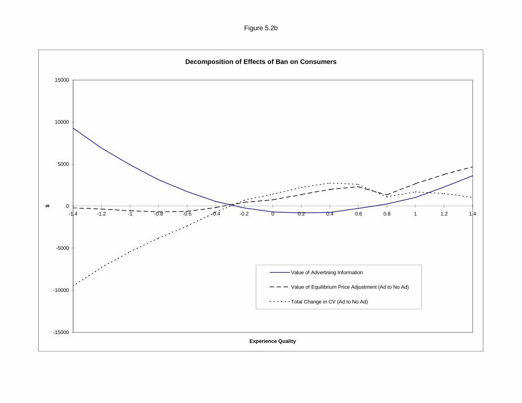
Figure 5.2b

Decomposition of Effects of Ban on Consumers

-15000

-10000

-5000

0

5000

10000

15000

-1.4 -1.2 -1 -0.8 -0.6 -0.4 -0.2 0 0.2 0.4 0.6 0.8 1 1.2 1.4

Experience Quality

$

Value of Advertising Information

Value of Equilibrium Price Adjustment (Ad to No Ad)

Total Change in CV (Ad to No Ad)

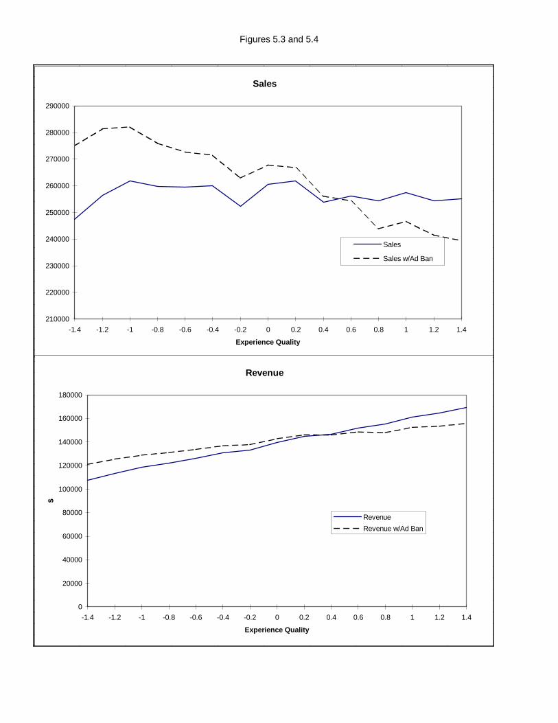
Figures 5.3 and 5.4

Sales

210000

220000

230000

240000

250000

260000

270000

280000

290000

-1.4 -1.2 -1 -0.8 -0.6 -0.4 -0.2 0 0.2 0.4 0.6 0.8 1 1.2 1.4

Experience Quality

Sales

Sales w/Ad Ban

Revenue

0

20000

40000

60000

80000

100000

120000

140000

160000

180000

-1.4 -1.2 -1 -0.8 -0.6 -0.4 -0.2 0 0.2 0.4 0.6 0.8 1 1.2 1.4

Experience Quality

$

RevenueRevenue w/Ad Ban

Figures 5.5 and 5.6

Costs

0

20000

40000

60000

80000

100000

120000

140000

-1.4 -1.2 -1 -0.8 -0.6 -0.4 -0.2 0 0.2 0.4 0.6 0.8 1 1.2 1.4

Experience Quality

$

Production Costs

Advertising Costs

Total Costs

Production (= Total) Costs w/Ad Ban

Profits

0

10000

20000

30000

40000

50000

60000

70000

80000

-1.4 -1.2 -1 -0.8 -0.6 -0.4 -0.2 0 0.2 0.4 0.6 0.8 1 1.2 1.4

Experience Quality

$

ProfitsProfits w/o Ad CostsProfits w/Ad Ban

Figure 5.7

Total Surplus

0

20000

40000

60000

80000

100000

120000

140000

-1.4 -1.2 -1 -0.8 -0.6 -0.4 -0.2 0 0.2 0.4 0.6 0.8 1 1.2 1.4

Experience Quality

$

Total SurplusTotal Surplus w/Ad Ban

References

Ackerberg D. (1996) “Empirically Distinguishing Informative and Prestige Effects of Advertising”mimeo, Boston University

Ackerberg, D. (1996b) “Advertising, Information, and Consumer Choice in Experience GoodMarkets” Doctoral Dissertation, Yale University.

Advertising Age, Serial, Chicago, Ill. , Crane Communications

Becker, G.S. and Murphy, K.M. (1993) “A Simple Theory of Advertising as a Good or Bad”,Quarterly Journal of Economics, 942-964

Benham, L. (1972) “The Effect of Advertising on the Price of Eyeglasses” Journal of Law andEconomics 337-352

Berry, S. , Levinsohn, J., and Pakes, A. (1995) “Automobile Prices in Market Equilibrium”Econometrica., 63, 841-890

Boyer, K.D. (1974) “Informative and Goodwill Advertising” The Review of Economics andStatistics 541-548

Butters, G. (1977) “Equilibrium Distributions of Sales and Advertising Prices” Review ofEconomic Studies 44:465-491

DeGroot, M. (1970) Optimal Statistical Decisions New York, McGraw Hill

Deighton, J., Henderson, C. and Neslin, S. (1994) “The Effects of Advertising on BrandSwitching and Repeat Purchasing” Journal of Marketing Research, 31:28-41.

Dixit, A. and Norman, V. (1978) “Advertising and Welfare” Bell Journal of Economics 9:1-17

Erdem, T. and Keane, M. (1996) “Decision-Making Under Uncertainty: Capturing DynamicBrand Choices in Turbulent Consumer Goods Markets” Marketing Science 15:1-20

Eckstein, Z., Horsky, D., and Raban, Y. (1988) “An Empirical Dynamic Model of Optimal BrandChoice”, Mimeo, Tel-Aviv University.

Eckstein, Z. and Wolpin, K. (1991) “The Specification and Estimation of Dynamic StochasticDiscrete Choice Models” The Journal of Human Resources, 24:563-597.

Galbraith, J.K. (1958) The Affluent Society Houghton-Mifflin, Boston, MA

Gonul, F. and Srinivasan, K. (1993) “Modeling Multiple Sources of Heterogeneity in MultinomialLogit Models: Methodological and Managerial Issues” Marketing Science 12:213-230

Grossman, G. and Shapiro, C. (1984) “Informative Advertising with Differentiated Products”Review of Economic Studies, 63-81

Guadagni, P. and Little J., (1983) “A Logit Model of Brand Choice Calibrated on Scanner Data”Marketing Science, 2:206-238

Johnson, S., Stedinger, J., Shoemaker, C., Li, Y. Tejada-Guibert, J. (1993) “Numeric Solution ofContinuous State Dynamic Programs Using Linear and Spline Interpolation”, OperationsResearch, 41-3 484-500

Keane, M. (1994) “A Computationally Practical Simulation Estimator for Panel Data”Econometrica 62:95-116

Keane, M. and Wolpin, K. (1994) “The Solution and Estimation of Discrete Choice DynamicProgramming Models by Simulation and Interpolation: Monte Carlo Evidence” Review ofEconomics and Statistics 648-672

Kihlstrom and Riordan (1984) “Advertising as a Signal” Journal of Political Economy 92:427-450

Lancaster, K. (1971) Consumer Demand: A New Approach New York, Columbia UniversityPress

Lucas, R. (1976) Econometric Policy Evaluation:A Critique, in K. Brunner and A. Meltzer ThePhillips Curve and Labor Markets, Amsterdam, North Holland Pub.

Marshall, A. (1919) Industry and Trade; a Study of Industrial Technique and BusinessOrganization London, MacMillan

McCulloch, R. and Rossi, P. (1994) “An Exact Likelihood Analysis of the Multinomial ProbitModel” Journal of Econometrics 64:207-240

McFadden, D. (1973) “Conditional Logit Analysis of Qualitative Choice Behavior” in P.Zarembka (ed.) Frontiers in Econometrics New York, Academic Press

McFadden, D. (1989) “A Method of Simulated Moments for Estimation of Discrete ResponseModels without Numerical Integration” Econometrica 57:995-1026

Milgrom, P. and Roberts, J. (1986) “Price and Advertising Signals of Product Quality” Journal ofPolitical Economy 94:796-821

Nelson, P (1970) “Information and Consumer Behavior”, Journal of Political Economy 78:311-329

Nelson, P. (1974) “Advertising as Information” Journal of Political Economy 82:729-753

Pakes, A. (1986) “Patents as Options: Some Estimates of the Value of Holding European PatentStocks” Econometrica 54:755-85

Pakes, A. and Pollard, D. (1989) “Simulation and the Asymptotics of Optimization Estimators”Econometrica 57:1027-57

Pedrick, J. aand Zufryden, F. (1991) “Evaluating the Impact of Advertising Media Plans: A Modelof Consumer Purchase Dynamics using Single Source Data” Marketing Science 10:111-129

Resnick, A. and Stern, B. “An Analysis of the Information Content in Television Advertising”Journal of Marketing 41:50-53

Russell, G. and Kamakura, W. (1994) “Understanding Brand Competition Using Micro andMacro Scanner Data” Journal of Marketing Research 31:289-307

Rust, J. (1987) “Optimal Replacement of GMC Bus Engines: An Empirical Model of HaroldZurcher” Econometrica 55:999-1035

Rust, J. (1995) “Numerical Dynamic Programming in Economics” Draft for Handbook ofComputational Economics

Rust, J. (1997) “Using Randomization to Break the Curse of Dimensionality” ForthcomingEconometrica

Schmalensee R. (1972) The Economics of Advertising Amsterdam, North Hollland Publishers

Schmalensee R. (1978) “A Model of Advertising and Product Quality” Journal of PoliticalEconomy, 86

Shapiro, Carl (1982) “Consumer Information, Product Quality, and Seller Reputation” BellJournal of Economics, 20-35

Stigler, G.L. (1961) “The Economics of Information” Journal of Political Economy 71:213-225

Stigler, G and Becker, G. (1977) “De Gustibus Non Est Disputandum” American EconomicReview, 471-99

Telser, L.G. (1964) “Advertising and Competition”, Journal of Political Economy, 72:537-562

Tirole, J. (1988) The Theory of Industrial Organization Cambridge, MA, MIT Press