Adv ances in Di - projecteuclid.org

Advances in Differential Equations Volume 10, Number 11 (2005), 1261–1300

WEAK SOLUTIONS TO THE CAUCHY PROBLEMOF A SEMILINEAR WAVE EQUATION

WITH DAMPING AND SOURCE TERMS

Petronela RaduDepartment of Mathematics, University of Nebraska-Lincoln, NE 68588

(Submitted by: Viorel Barbu)

Abstract. In this paper we prove local existence of weak solutions fora semilinear wave equation with power-like source and dissipative termson the entire space Rn. The main theorem gives an alternative proofof the local in time existence result due to J. Serrin, G. Todorova andE. Vitillaro, and also some extension to their work. In particular, ourmethod shows that sources that are not locally Lipschitz in L2 can becontrolled without any damping at all. If the semilinearity involving thedisplacement has a “good” sign, we obtain global existence of solutions.

1. Introduction

In this paper we study the following semilinear wave equation:

utt − ∆u + f(x, t, u) + g(x, t, ut) = 0 a.e. in Rn × [0,∞);u|t=0 = u0 ; ut|t=0 = u1 .

(SW)

We will refer to the f nonlinearity as the source term, while g will be calledthe dissipative term. The initial data u0 and u1 are given.

In order to facilitate the presentation, we next list the hypotheses thatgovern our results.Assumptions. Suppose that the nonlinearities f and g satisfy the following:

(A0) f is measurable in x, differentiable in t almost everywhere, differen-tiable in u almost everywhere, and there exists a continuous function k suchthat for almost every x, t

|fu(x, t, u)| ≤ k(r) for a.e. |u| ≤ r;

(A1) Growth conditions on the source term f :(i) f(x, t, 0) = 0;(ii) |f(x, t, u)| ≤ m1|u|p+m2|u|q such that 1 < q < p < 2∗−1, m1, m2 > 0,

where 2∗ = 2nn−2 ;

Accepted for publication: May 2005.AMS Subject Classifications: 35L05, 35L15, 35L70; 35L20.

1261

1262 Petronela Radu

(A2) |ft(x, t, u)| ≤ K for some K > 0;(A2)* f does not depend on t and F (x, u) =

∫ u0 f(x, v)dv ≥ 0;

(A3) g = g(x, t, v) is measurable in t, differentiable in x, and continuousin v;

(A4) for every x, t the function v → g(x, t, v) is increasing andg(x, t, 0) = 0;

(A5) vg(x, t, v) ≥ C1|v|m+1 and |g(x, t, v)| ≤ C2|v|m for some m ≥ 0;(A6) |∇xg(x, t, v)| ≤ C|v|;(A7) |gt(x, t, v)| ≤ C|v|;(A8) either (a) 1 < p < 2∗

2 , m > 0, (b) p + pm < 2∗, m > 0, or

(c) 1 < p < 2∗−1, m ∈ 0, 1, where p and m are given by (A1), respectively,(A5) above.

In the above assumptions, C, C1, C2 represent nonnegative constants whichmay change from line to line.

The model equation with nonlinearities that satisfy the assumptions (A0)-(A8) is:

utt − ∆u ± u|u|p−1 ± u|u|q−1 + ut|ut|m−1 = 0,

where 1 < q < p < 2∗−1 and m ≥ 0. The “-” sign corresponds to assumption(iii) (a), whereas the “+” sign gives us a model that satisfies (iii)(b).

The following definition gives a precise description of the type of solutionswhich are studied in this paper.

Definition 1.1. Let ΩT := Ω × (0, T ), where Ω ⊂ Rn is an open connectedset with smooth boundary ∂Ω. Suppose the functions f and g satisfy theassumptions (A1) and (A5), and further suppose that u0 ∈ H1

0 (Ω)∩Lp+1(Ω)and u1 ∈ L2(Ω) ∩ Lm+1(Ω).

A weak solution on ΩT of the boundary-value problem

utt − ∆u + f(x, t, u) + g(x, t, ut) = 0 in Ω × (0, T );(u, ut)|t=0 = (u0, u1);u = 0 on ∂Ω × (0, T ).

(SWB)

is any function u satisfying

u ∈ C(0, T ; H10 (Ω)) ∩ Lp+1(ΩT ), ut ∈ L2(ΩT ) ∩ Lm+1(ΩT ),

and∫

ΩT

(u(x, s)φtt(x, s) + ∇u(x, s) ·∇φ(x, s) + f(x, s, u)φ(x, s)

+ g(x, s, ut)φ(x, s))

dxds =∫

Ω

(u1(x)φ(x, 0) − u0(x)φt(x, 0)

)dx

Weak solutions to the Cauchy problem 1263

for every φ ∈ C∞c (Ω × (−∞, T )).

Remark. The above definition remains the same for the Cauchy problem(SW); take Ω = Rn with no boundary conditions.

The literature on semilinear wave equations is vast, yet we have completeexistence results for only some special cases of semilinearities. First, theexistence of weak solutions for the equation with either a power of u or apower of ut has been studied (see [5, 6, 8, 11]). Even this case presentednumerous challenges, and it has been shown that the equation can exhibitblow-up phenomenon when the semilinearity has a “bad” sign. One of thefirst works on the subject, where the interaction between a power of u anda power of ut is treated, is the landmark paper authored by J.-L. Lionsand W. Strauss [12]. In a series of papers [7, 17, 21, 22], V. Georgiev, J.Serrin, G. Todorova, and E. Vitillaro have brought significant contributionsto the study of the wave equation with damping and source terms. Roughlyspeaking, they prove, for some ranges of exponents, that if the exponent ofthe source term is higher than the exponent of the damping, one expectsblow up of solutions; otherwise, the solutions exist globally. More recently,other semilinearities have been considered; among them, the problem witha degenerate damping term |u|k|ut|m−1ut [2, 14].

The work presented here provides an alternative proof, based on energymethods, to the local existence result by J. Serrin, G. Todorova and E. Vi-tillaro in [17], and we also obtain a slight improvement for the range ofexponents p and m. More precisely, we can show local existence for theCauchy problem (SW), even when there is no damping (i.e. m = 0) for all1 < p < 2∗−1 (2∗ = 2n

n−2), since our proof does not make use of the smooth-ing effect of the damping. The restriction p + p

m < 2∗ for 2∗

2 < p < 2∗ − 1found in [17] appears in our work as well, but we are able to allow p to goall the way up to 2∗ − 1 in the case of Lipschitz damping (m = 1).

The result that we obtain holds for finite energy initial data, not necessar-ily with compact support as is assumed in [17]. The assumption (A7) aboveis more restrictive than (Q4) (page 8 in [17]), but our work has the advan-tage of allowing some dependence on t for f , and of having no assumptionson gv for m ≥ 2 ((Q5)-(Q6) page 8 in [17]). Regarding global existence,the arguments used in this paper yield global existence results in the specialsituation when f does not depend on time and F (u) =

∫ u0 f(x, v)dv ≥ 0

(assumption (A2)* - in this case f does not behave as a true source term forthe equation).

Some of the tools that we use are the potential well method which goesback to L. E. Payne and D. H. Sattinger in [13, 15], and an idea used by

1264 Petronela Radu

p

!

p"

m m!

"

M. Crandall and L. Tartar in [19] which allows us to solve the problem onthe entire space Rn with arbitrarily large initial data.

In the sequel, we denote by B(x, R) the open ball centered at x, of radiusR, and by B(R) the open ball centered at the origin of radius R. |Ω| isthe Lebesgue measure of a measurable set Ω ⊂ Rn. For the norms in theLebesgue and Sobolev spaces we will use the following notation:

| · |q,Ω is the norm in Lq(Ω) and | · |q is the norm in Lq(Rn);|| · ||k,Ω is the norm in Hk(Ω) and || · ||k is the norm in Hk(Rn);|| · ||H1

0 (Ω) is denoted by || · ||Ω.The paper is organized as follows. In Section 2 we focus on the boundary-

value problem (SWB) with Lipschitz source terms and general damping,for which existence and uniqueness results are known. Section 3 is devotedto obtaining local existence of weak solutions for the Cauchy problem withsource terms and damping that satisfy the assumptions (A0)-(A8). We con-clude with some remarks and generalizations which can be obtained by usingthe arguments of this paper.

2. Preliminary results on a bounded domain

This section contains some of the results that we will use in order toprove our main theorem. We record here two existence theorems, that areavailable in the literature, which deal with a simplified case of the problem(SWB), when the source term f(x, t, u) is a globally Lipschitz function in theu argument, and the dissipative term g(x, t, ut) is a monotone function in ut.The first theorem yields existence of strong solutions, while the second dealswith weak solutions (see [1], [3], [12] and the Appendix for more discussion


of these results). For these solutions we prove finite speed of propagationwhich will play an important role in the next section when we present ourmain theorem. We begin by stating the theorem regarding strong solutions(see the Appendix for a proof):

Theorem 2.1. (Existence and uniqueness of strong solutions for dissipativewave equations with Lipschitz source terms) Let Ω ⊂ Rn be a bounded do-main with smooth boundary ∂Ω, and the functions f(x, t, u) and g(x, t, v) beunder the assumptions (A0),(A2),(A3)-(A7), and additionally:

|f(x, t, u) − f(x, t, v)| ≤ L|u − v|,

for almost every x ∈ Rn and for all t, u, v ∈ R. Let u0, u1 ∈ H10 (Ω) with u0 ∈

H2(Ω), G(x, 0, u1) ∈ L1(Ω), where G is defined by the formula G(x, t, v) =∫ v0 g(x, t, y)dy. Then the initial boundary-value problem:

utt − ∆u + f(x, t, u) + g(x, t, ut) = 0 in Ω × (0, T );(u, ut)|t=0 = (u0, u1);u = 0 on ∂Ω × (0, T ).

(SWB)

admits a unique solution u on the time interval [0, T ] in the sense of Defi-nition 1.1; i.e., u ∈ C(0, T ; H1

0 (Ω)) ∩ Lp+1(ΩT ), ut ∈ L2(ΩT ) ∩ Lm+1(ΩT ),with the additional regularity

u ∈ C1([0, T ];L2(Ω)) with utt, ∆u ∈ L2(0, T ; L2(Ω)).

Remark. A solution with the above additional regularity is usually calleda strong solution.

A classical technique that we will use is the approximation of the initialdata with smooth functions and then passing to the limit in the sequence ofapproximate solutions. The following theorem will justify this argument.

Theorem 2.2. (Convergence of a sequence of smooth solutions) Under theassumptions of Theorem 2.1, if (u0η , u1η)η≥1 is a sequence of smooth func-tions such that (u0η , u1η) → (u0, u1) in H1

0 (Ω) × L2(Ω), then the solutionsuη provided by Theorem 2.3 with initial data (u0η , u1η) satisfy

uη(t) → u(t) in H10 (Ω), uηt(t) → ut(t) in L2(Ω)

for every t > 0, where u is the solution of (SWB) with initial data (u0, u1).

Proof. We use the same techniques that are used in the proof of Theorem2.1; i.e. multiply the equation by uηt −ut, integrate with respect to the spaceand then the time variables, and use the Lipschitz assumption for f and the

1266 Petronela Radu

monotonicity for g. Doing so yields:∫

Ω|uηt(x, t) − ut(x, t)|2 + |∇uη(x, t) −∇u(x, t)|2dx

≤∫

Ω

[(u1η(x) − u1(x))2 +|∇u0η(x) −∇u0(x)|2

]dx

+∫ t

0

∫

ΩL

(|(uη(x, s) − u(x, s))t|2 +|∇uη(x, s) −∇u(x, s)|2

)dxds.

Poincare’s inequality followed by Gronwall’s inequality will show the claimedconvergences. In order to finish the proof, we need to show that the limitfunction u is a solution of (SWB). To this end we invoke the celebratedmonotonicity argument due to Lions and Strauss. (A detailed discussion ofthis can be found in Section 3, page 18 of this paper.) !

The next theorem is basically the statement of Theorem 2.1 under weakerassumptions (less differentiability) for initial data.Theorem 2.3. (Existence and uniqueness of solutions for dissipative waveequations with Lipschitz source terms) Let Ω ⊂ Rn be a bounded domainwith smooth boundary ∂Ω, and the functions f(x, t, u) and g(x, t, v) sat-isfy assumptions (A0), (A2), (A3)-(A7), and f is globally Lipschitz in thelast argument with Lipschitz constant L. Let u0, u1 ∈ H1

0 (Ω) × L2(Ω) withG(x, 0, u1) ∈ L1(Ω), where G is defined by the formula

G(x, t, v) =∫ v

0g(x, t, y)dy.

Then (SWB) admits a unique solution u on the time interval [0, T ] in thesense of the Definition 1.1; i.e.,

u ∈ C(0, T ; H10 (Ω)) ∩ Lp+1(ΩT ), ut ∈ L2(ΩT ) ∩ Lm+1(ΩT ).

Proof. For the pair of initial data u0, u1 ∈ H10 (Ω) × L2(Ω), we take a se-

quence of approximations uε0, u

ε1 ∈ C∞

c (Ω). The regularized sequence satisfiesthe hypotheses of Theorem 2.1, so we obtain a sequence of smooth solutionsuε. From Theorem 2.2 we have the existence of a solution u as the limit ofuε. The uniqueness follows the same way as in Theorem 2.1. !

Two crucial ingredients for the proof of our main existence theorem are afinite speed of propagation result and an energy identity, which are statedand proved below. The energy identity is well known, but the novelty of thefinite speed of propagation result consists in the fact that we obtained it forLipschitz source terms of arbitrary sign and general damping which can evenbe a non-differentiable function.


Theorem 2.4. (Finite speed of propagation) Consider the problem (SWB)under the hypothesis of Theorem 2.3. Then

(1) if the initial data u0, u1 is compactly supported inside the ball B(x0, R)⊂ Ω, then u(x, t) = 0 outside B(x0, R + t);

(2) if (u0, u1), (v0, v1) are two pairs of initial data with compact support,with the corresponding solutions u(x, t), respectively v(x, t), and u0(x) =v0(x) for x ∈ B(x0,R) ⊂ Ω, then u(x, t) = v(x, t) inside B(x0, R − t) forany t < R.

Proof. Part (1) The proof presented here extends an argument used forthe linear wave equation by L. Tartar [20].

Assume for now that f(x, t, u) = 0 for |x − x0| ≥ R + t. Since theequation is invariant under translations, without loss of generality we cantake x0 = 0. First we approximate the initial data uniformly by smoothfunctions (u0η , u1η) with compact support inside B(Rη), with Rη R asη → 0. By Theorem 2.1, for any T > 0, the solution of:

uηtt − ∆uη + f(x, t, uη) + g(x, t, uηt) = 0 in Ω × (0, T );(uη, uηt)|t=0 = (uη0 , uη1);uη = 0 on ∂Ω × (0, T )

(SWBη)

exists on [0, T ] and it has the regularity of a strong solution.Consider a function φη with φη(r) = 0 on (−∞, Rη], φη(r) > 0 on (Rη,∞),

such that φ′(r) ≥ 0 on R. Since uηt ∈ L∞(0, T ; H10 (B(Rη))), we are allowed

to multiply (SWη) by uηt(t, x)φη(|x|− t), for any 0 < t < T . The quantity:

Iη(t) :=∫

Rn(|uηt(x, t)|2 + |∇uη(x, t)|2)φη(|x|− t) dx

is well defined and assume for now that dIη

dt ≤ 0. It can be easily seen thatIη(0) = 0, since

Iη(0) =∫

|x|<Rη

(|u1η(x)|2 + |∇u0η(x)|2)φη(|x|) dx

+∫

|x|>Rη

(|u1η(x)|2 + |∇u0η(x)|2)φη(|x|) dx.

The first integral is 0 since φη(|x|) = 0 for |x| < Rη. The initial data hassupport inside the domain |x| < Rη, so the second integral is zero.

The assumption that the mapping t → Iη(t) is decreasing leads us toIη(t) ≤ Iη(0) = 0, which means that uη(x, t) = 0 if |x|− t > Rη . We pass to

1268 Petronela Radu

the limit in η (see Theorem 2.2) to obtain u(x, t) = 0 for |x| − t > R, andthis concludes the proof.

It suffices then to prove that dIη

dt ≤ 0. For the regularized initial datawe have uη ∈ L∞(0, T ; H1

0 (B(Rη))), uηt ∈ L∞(0, T ; H10 (B(Rη))), uηtt ∈

L1(0, T ; L2(B(Rη))), which enables us to compute (we drop the subscriptη in the remainder of the proof)

dI

dt(t) =

∫

Rn2φ(|x|− t)(ututt +

n∑

i=1

uxiutxi)(x, t) dx

−∫

Rnφ′(|x|− t)(u2

t + |∇u|2)(x, t) dx =∫

Rn2φ(|x|− t)(ututt)(x, t) dx

−∫

Rn

n∑

i=1

((2φ(|x|− t)uxi)xiut) (x, t) dx−∫


t + |∇u|2)(x, t) dx

=∫

Rn2φ(|x|−t)((utt−∆u)ut)(x, t) dx−

∫

Rn

n∑

i=1

2φ′(|x|−t)xi

r(uxiut)(x, t) dx

−∫


t + |∇u|2)(x, t) dx.

By (SWB)utt − ∆u = −f(x, t, u) − g(x, t, ut),

hence the assumptions on the support of φ and f , together with the factthat g is nondecreasing, make the first term of the last equality negative.We factor out φ′(|x|−t) in the other two terms, and since φ′(r) ≥ 0 for everyr, it is enough to show that

u2t + |∇u|2 + 2

n∑

i=1

xi

|x|uxiut ≥ 0, (2.1)

which is obtained by summing the inequalities:( xi

|x|ut + uxi

)2≥ 0 for all i = 1, ..., n.

It remains to show that the function f vanishes for |x − x0| ≥ R + t.A fixed-point argument will establish this fact now. Consider the iterativeequation:

uk+1tt − ∆uk+1 + f(x, t, uk) + g(x, t, uk+1

t ) = 0(uk+1, uk+1

t )|t=0 = (u0, u1)uk+1 = 0 on ∂Ω × (0, T ),


for every k ∈ N, with (u0, u0t ) = (u0, u1). The existence of a unique weak so-

lution is guaranteed by Theorem 2.3. An induction argument, together withthe first part of the proof, will show that uk(x, t) = 0 for |x−x0| > R+ t, forevery k ∈ N. It is enough then to show that uk(x, t) → u(x, t) almost every-where as k → ∞. Since f is Lipschitz we obtain that f(x, t, uk(x, t)), whichis zero for |x − x0| ≥ R + t, converges almost everywhere to f(x, t, u(x, t)),hence f vanishes outside the cone |x−x0| < R+t. The sequence of differencefunctions vk(x, t) := uk(x, t) − u(x, t) satisfies:

vk+1tt − ∆vk+1 + f(x, t, vk + u) − f(x, t, u)

+g(x, t, vk+1t + ut) − g(x, t, ut) = 0

(vk+1, vk+1t )|t=0 = (0, 0)

vk+1 = 0 on ∂Ω × (0, T ).

Upon multiplication by vk+1t and integration over (0, t) × Rn, we use the

monotonicity of g to derive the following inequality:∫

Rn(vk+1

t (x, t))2 + |∇vk+1(x, t)|2 dx

≤∫ t

0

∫

Rn2|f(x, t, vk + u) − f(x, t, u)||vk+1

t (x, s)|dx ds,

which by the Lipschitz assumption on f is

≤∫ t

02L|vk(s)|2|vk+1

t (s)|2 ds ≤ L

∫ t

0|vk(s)|22 + |vk+1

t (s)|22 ds.

We now need a bound for∫ t

0|vk(s)|22ds, which we obtain by writing:

|vk(t)|22 = 2∫ t

0

∫

Rnvk(x, s)vk

t (x, s)dx ds

≤∫ t

0

∫

Rn(vk(x, s))2 + (vk

t (x, s))2dx ds.

Gronwall’s inequality for the function |vk(s)|22 will give us for any t < T thebound:

|vk(t)|22 ≤ eT∫ t

0|vk

t (s)|22ds.

At this point, to simplify the writing let

φk(t) :=∫ t

0|vk

t (s)|22 + |∇vk(t)|22ds.

1270 Petronela Radu

By summarizing the estimates above, we have that φk+1 satisfies the in-equality:

φk+1t (t) ≤ Lφk+1(t) + Cφk(t),

which after integration becomes:

φk+1(t) ≤ C

∫ t

0eL(t−s)φk(s)ds ≤ CeLT

∫ t

0φk(s)ds.

A simple induction argument will show that:

φk+1(t) ≤ KCk+1eLT (k+1)tk+1

(k + 1)!,

where K is a bound on |φ1(t)| for all t in [0, T ]. Thus we proved the conver-gence for uk(x, t) almost everywhere (x, t), so u(x, t) = 0 outside the domainof dependence, i.e. for |x − x0| ≥ R + t. Recall that this actually is provenfor the sequence of approximated solutions uη. By Theorem 2.2 we have theconvergence uη(t) → u(t) ∈ H1

0 (Ω), hence uη(t) → u(t) almost everywhere.This concludes the proof of Part (1).Part (2). We follow here a similar argument as in Part (1). Initially, wework under the assumption that

f(x, t, u(x, t)) = f(x, t, v(x, t)) (2.2)

for |x| < R − t (again, take x0 = 0). The difference u − v satisfies:

(u − v)tt − ∆(u − v) + f(x, t, u) − f(x, t, v) + g(x, t, ut) − g(x, t, vt) = 0;((u − v), (u − v)t) |t=0 = (0, 0)u − v = 0 on ∂Ω × (0, T ).

Consider a function ψ strictly positive on (−∞, R), such that ψ(r) = 0 on[R,∞) and ψ′(r) ≤ 0 everywhere. Define the function J(t) by

J(t) :=∫

Rn

((ut(x, t) − vt(x, t))2 + |∇(u(x, t) − v(x, t))|2

)ψ(|x|− t)dx.

We will show thatdJ

dt≤ 0. As before, this will show that u(x, t) = v(x, t)

on the support of ψ(|x| + t), i.e. if |x| < R − t. The proof here is similar tothat in (1):

dJ

dt=

∫

Rn2ψ(|x| + t)[((u − v)tt − ∆(u − v))(u − v)t](x, t) dx

+∫

Rn

n∑

i=1

2ψ′(|x| + t)xi

r[(u − v)xi(u − v)t](x, t) dx


+∫

Rnψ′(|x| + t)[(u − v)2t + |∇(u − v)|2](x, t) dx.

We use the equality

(u − v)tt − ∆(u − v) = −f(x, t, u) + f(x, t, v) − g(x, t, ut) + g(x, t, vt),

(2.1), (2.2), and the assumptions on the support of ψ to obtain that J isdecreasing. In order to prove (2.2), we use the following iterative schemeswith u1 = u0 and v1 = v0 :

uk+1tt − ∆uk+1 + f(x, t, uk) + g(x, t, uk+1

t ) = 0(uk+1, uk+1

t )|t=0 = (u0, u1)uk+1 = 0 on ∂Ω × (0, T ),

and

vk+1tt − ∆vk+1 + f(x, t, vk) + g(x, t, vk+1

t ) = 0(vk+1, vk+1

t )|t=0 = (v0, v1)vk+1 = 0 on ∂Ω × (0, T ).

Again, the existence and uniqueness of the solutions uk+1 and vk+1 is guaran-teed by Theorem 2.1. By the first part of the proof, since (u0, u1) = (v0, v1)we have that uk = vk, which implies that uk+1 = vk+1 on the desired do-main. Since we also have that u1 = v1, by the induction principle, theequality uk = vk holds true for all k’s. The argument will be complete aftershowing uk − vk → 0 almost everywhere as k → ∞. We subtract the aboveiterative schemes and obtain:

(uk+1 − vk+1)tt − ∆(uk+1 − vk+1) + f(x, t, uk) − f(x, t, vk)+g(x, t, uk+1

t ) − g(x, t, vk+1t ) = 0

(uk+1 − vk+1, (uk+1 − vk+1)t)|t=0 = (0, 0)uk+1 − vk+1 = 0 on ∂Ω × (0, T ).

An argument identical to the one used in (1) for the sequence vk concludesthe proof. !

The proof of the following proposition is nontrivial, but it can be obtainedby a modification of the argument in Lemma 8.3 in [10]. Note that for strongsolutions, the proof is immediate.

Proposition 2.5. (The energy identity) If u is a weak solution of (SWB),under the assumptions of Theorem 2.3 we have the following equality:

E(t) +∫

ΩF (x, t, u(x, t)) dx −

∫ t

0

∫

Ωft(x, s, u(x, s)) dx ds

1272 Petronela Radu

+∫ t

0

∫

Ωg(x, s, ut(x, s))ut(x, s) dx ds = E(0), (2.3)

where E(t) := 12 |ut(t)|22,Ω + 1

2 |∇u(t)|22,Ω.

3. The Cauchy Problem

In this section we state and prove the main result of this paper. In com-parison with the existence theorem from the previous section, we remarkthat here the bounded set Ω is replaced by Rn, and the source term f is notrequired to be Lipschitz.

Theorem 3.1. (Existence of weak solutions) Let (u0, u1) ∈ H10 (Rn)×L2(Rn)

and consider the Cauchy problem

utt − ∆u + f(x, t, u) + g(x, t, ut) = 0 a.e. in Rn × [0,∞);u|t=0 = u0 ; ut|t=0 = u1 .

(SW)

Assume G(x, 0, u1) ∈ L1(Rn), where G(x, t, v) =∫ v0 g(x, t, u)du, and the

validity of assumptions (A0)-(A8). Then, there exists a time 0 < T < 1such that (SW) admits a weak solution on [0, T ] in the sense of Definition1.1. In addition, if (A2)* is satisfied, then the solution is global, so T can betaken arbitrarily.

Remark. The bound T < 1 is artificially imposed; the true restriction forthe time of existence is due to the interaction of the semilinearities f and gand it will be presented in more detail in the proof.

Proof. With or without assumption (A2)*, the proof follows the same ar-gument, so we will make the necessary adjustments when needed and showhow the assumption (A2)* gives a stronger result.

We start by assuming that f is globally Lipschitz in the last argument;i.e., there exists a constant L > 0 such that:

|f(x, t, u) − f(x, t, v)| ≤ L|u − v|. (3.1)

Also, in the beginning we take u0, u1 with compact support inside a ball ofradius R, so that we deal with the problem on a bounded domain. With suchf, g, u0, u1 the existence and regularity results of Section 2 are available.

As part of a compactness argument, our goal is to obtain bounds for|∇u(t)|Ω, where Ω is a bounded domain which contains the support of theinitial data. This is straightforward from the energy identity if we assumethe positivity conditions (A2)* on the antiderivative F . If we work under theassumption (A1)(a), in a first step we additionally impose some “smallness”assumptions in order to prove that |∇u(t)|Ω < α for any t < 1.


Next, we construct Lipschitz approximations fε for the general nonlinear-ity f that satisfies the assumptions (A0)-(A2). We apply the results obtainedin the first step (where the bounds will not depend on ε) to the sequence ofsolutions uε and pass to the limit to get a solution of the problem (SW) on abounded domain. We will eliminate the “smallness” restrictions imposed inthe case of (A1)(a), and the fact that the initial data has compact supportthrough a “patching” argument.Step 1. As mentioned above, we start by assuming that f is Lipschitz, sothat (3.1) holds. Fix x0 ∈ Rn, and consider the initial data of (SW) sup-ported inside the ball B(x0, R), with zero boundary conditions on a domainsufficiently large that contains B(x0, R). Without loss of generality, we canassume that x0 = 0, since the equation is invariant under translations inspace.

First, we will discuss the case when f satisfies (A1)(a).Due to the finite speed of propagation property (Theorem 2.4), we have

that u(x, t) is zero outside B(R + t); hence, for t < 1, u(x, t) is supportedinside the set Ω := B(R+1). In this case we impose the following “smallness”conditions on the initial data:

|∇u0|Ω < α,12|u1|2Ω+

12|∇u0|2Ω+

∫

ΩF (x, 0, u0(x)) dx+K|Ω| < Φ(α), (3.2)

where α and Φ will be chosen later, K is the constant in (A2), and Ω =B(R + 1).

For p < 2∗ and any v ∈ H10 (Ω) we will need the following inequality:

|v|p,Ω ≤ C(R + 1)n 2∗−p2∗p |∇v|Ω. (3.3)

This is a consequence of the Holder inequality:

|v|p,Ω ≤( ∫

Ω|v|

2∗p pdx

) 12∗

( ∫

Ωdx

) 2∗−p2∗p ≤ |v|2∗(

ωn

n(R + 1)n)

2∗−p2∗p ,

and of the Sobolev imbedding theorem:

|v|2∗ ≤ C∗|∇v|Ω,

where C∗ depends only on n, and in (3.3) we take C = C∗(ωnn )

2∗−p2∗p , where

ωnn is the volume of the unit sphere in Rn.

Since u(t) ∈ H10 (B(R + t)) implies u(t) ∈ H1

0 (Ω) for t < 1, the inequality(3.3) will hold for any u(t) with 0 < t < 1.

By (A4) and the energy identity we obtain:

1274 Petronela Radu

12|ut(t)|2Ω +

12|∇u(t)|2Ω +

∫

ΩF (x, t, u(x, t)) dx

≤ K|Ω| + 12|u1|2Ω +

12|∇u0|2Ω +

∫

ΩF (x, 0, u0(x)) dx = K|Ω| + E(0). (3.4)

The growth assumption for F given in (A1)(iii)(a), followed by an applicationof the inequality (3.3) yields:

12|∇u(t)|2Ω +

∫

ΩF (x, t, u(x, t)) dx ≥ 1

2|∇u(t)|2Ω − m1|u(t)|pp,Ω − m2|u(t)|qq,Ω

≥ 12|∇u(t)|2Ω − m1C

p|∇u(t)|pΩ(R + 1)n 2∗−p2∗

− m2Cq|∇u(t)|qΩ(R + 1)n 2∗−q

2∗ . (3.5)

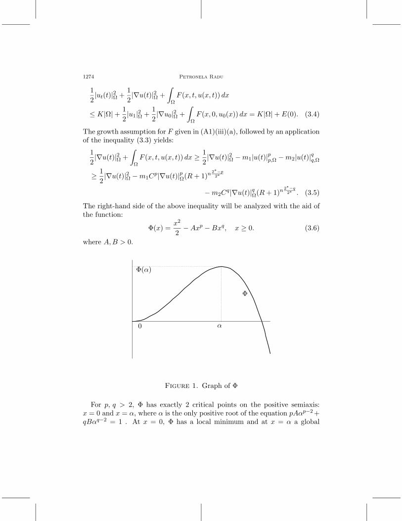
The right-hand side of the above inequality will be analyzed with the aid ofthe function:

Φ(x) =x2

2− Axp − Bxq, x ≥ 0. (3.6)

where A, B > 0.

α0

Φ

Φ(α)

Figure 1. Graph of Φ

For p, q > 2, Φ has exactly 2 critical points on the positive semiaxis:x = 0 and x = α, where α is the only positive root of the equation pAαp−2 +qBαq−2 = 1 . At x = 0, Φ has a local minimum and at x = α a global


maximum. In (3.6) we take:

A = m1Cp(R + 1)n 2∗−p

2∗ , B = m2Cq(R + 1)n 2∗−q

2∗ .

(R + 1 is related to the restriction t < 1.) We point out that the root αdepends on R, which measures the size of the support of the initial data.

Assume that |∇u(s)|Ω < α for all s ∈ [0, s0), for some s0 (s0 > 0, as|∇u0|Ω < α and t → |∇u(t)|Ω is continuous). With the new notation, (3.5)becomes:

12|∇u(t)|2Ω +

∫

ΩF (x, t, u(x, t)) dx ≥ 1

2|∇u(t)|2Ω − A|∇u(t)|pΩ − B|∇u(t)|qΩ,

which combined with (3.4) gives us:12|ut(t)|2Ω+

12|∇u(t)|2Ω − A|∇u(t)|pΩ − B|∇u(t)|qΩ (3.7)

≤ 12|ut(t)|2Ω +

12|∇u(t)|2Ω +

∫

ΩF (x, t, u(x, t)) dx

≤ K|Ω| + 12|u1|2Ω +

12|∇u0|2Ω +

∫

ΩF (x, 0, u0(x)) dx < Φ(α),

the last inequality being part of the “smallness” hypothesis which we as-sumed in Step 1. Therefore

12|∇u(t)|2Ω − A|∇u(t)|pΩ − B|∇u(t)|qΩ = Φ(|∇u(t)|Ω) < Φ(α) (3.8)

so, by the continuity in time of |∇u(t)|Ω we get:

|∇u(t)|Ω < α (3.9)

for any t < 1. Otherwise, Φ(|∇u(t)|Ω) ≥ Φ(α) for the times t which do notsatisfy (3.9), but this would contradict (3.8). (In other words, if we start inthe well of the graph of Φ at time t = 0 with |∇u0|Ω < α, we cannot get out,so |∇u(t)|Ω remains bounded by α. ) We make the remark that the boundt < 1 is related to the choice of the domain Ω = B(R + 1).

If f satisfies (A2)*, we easily obtain the bound |∇u(t)|Ω < C(u0, u1) fromthe energy identity, since we have that F ≥ 0.

The time t was artificially bounded by 1; the true restriction is a conse-quence of the arguments above, and it will be explained more in the last step.This will give us only a local result in time under the hypothesis (A1)(a).There will be no constraints if assumptions (A2)* are satisfied, hence weobtain global existence of solutions.Step 2. In this step we will construct truncations for the initial data, forwhich the “smallness” assumptions are satisfied. First consider a pair of

1276 Petronela Radu

initial data (u0, u1) such that u0 ∈ H2(Rn), u1 ∈ H1(Rn), and G(x, 0, u1) ∈L1(Rn) (recall that G(x, t, v) =

∫ v0 g(x, t, y) dy). The higher differentiability

assumptions on the initial data will be later removed. For now, we keep theLipschitz assumptions for f .

Fix x0 ∈ Rn. We will find a domain Ω around x0, small enough, andconstruct a new pair of initial data (u∗

0, u∗1) such that they satisfy (3.2)

inside Ω. We apply the results of Step 1 to obtain bounds for times t < 1for the new solution u∗ generated by the initial data (u∗

0, u∗1).

Again, we first analyze the case when (A1)(a) is satisfied. From now onlet α be the critical point of the function Φ from Step 1, with the coefficientsA, B corresponding to R = 1. Hence, in the sequel α will depend only onthe norm of the initial data.

We find ρ < 1 small enough such that

ρ <( Φ(α)

4Kωn

)1/n, |∇u0|B(x0,ρ) <

α

2, and |∇u0|2B(x0,ρ) ≤

Φ(α)8

,

2(C∗ωn)1n

(|∇u0|B(x0,ρ) + |u0|B(x0,ρ)

)≤ α

2, and

4C∗2ω

2∗−22∗

n |u0|2B(x0,ρ) ≤Φ(α)

8,

12|u1|2B(x0,ρ) ≤

Φ(α)4

,

m1(C∗)p(|∇u0|B(x0,ρ) + |u0|B(x0,ρ)

(2ρ

+ 1))p

≤ Φ(α)8

,

m2(C∗)q(|∇u0|B(x0,ρ) + |u0|B(x0,ρ)

(2ρ

+ 1))q

≤ Φ(α)8

, (3.10)

where C∗ is the constant from the Sobolev inequality. To have these condi-tions satisfied, it is enough to take ρ < ( Φ(α)

4Kωn)1/n such that

|∇u0|B(x0,ρ) < minα

2,

√Φ(α)

8,

α

4(C∗ωn)1n

,1

2C∗

(Φ(α)8m1

)1/p,

12C∗

(Φ(α)8m2

)1/q, (3.11)

|u0|B(x0,ρ) < min α

4(C∗ωn)1n

,1

ωnC∗

√Φ(α)

32ω2∗−22∗

n

,1

8C∗

(Φ(α)8m1

)1/p

,

18C∗

(Φ(α)8m2

)1/q, (3.12)


and

|u1|2B(x0,ρ) ≤√

Φ(α)8

. (3.13)

The existence of such a ρ, independent of x0 ∈ Rn, is motivated by theequi-integrability of the functions u0,∇u0, u1. More precisely, for each ofthe functions u0,∇u0, u1 we apply the following result of classical analysis:

If f ∈ L1(A), with A a measurable set, then for every given ε > 0, thereexists a δ > 0 such that

∫E |f(x)|dx < ε, for every measurable set E ⊂ A of

measure less than δ (see [4]). Note that δ does not depend on E, hence ρdoes not vary with x0.

It is possible that u0 /∈ H10 (B(x0, ρ)) since it does not necessarily have

zero trace on the boundary, so in order to apply the results of Step 1, wemultiply u0 by a cutoff function. For ε sufficiently small (to be chosen later),choose θε, a twice differentiable cutoff function, obtained by smoothing theLipschitz graph:

θ0ε(x) =

1, |x − x0| ≤ ρ − ερ − |x − x0|

ε, ρ − ε ≤ |x − x0| ≤ ρ

0, |x − x0| ≥ ρ.

Choose an appropriate smoothing operator for θ0ε such that we have:

|θε|∞,B(x0,ρ) ≤ 1, |∇θε|∞,B(x0,ρ) ≤1ε. (3.14)

The product θεu0 =: u∗0 belongs to H1

0 (B(x0, ρ)) ∩ H2(B(x0, ρ)), but ourgoal is to also have the inequality (3.2) satisfied by the new pair of initialdata (u∗

0, u∗1) (note that u1 already enjoys all the desired smoothness, so we

can take u∗1 = u1). As the computations below will show, the domain over

which the integrals in the inequality (3.2) are considered will have to betaken smaller. Mainly, this is due to the fact that the gradient of the newinitial data may increase when multiplied by the cutoff function.

We have∇u∗

0 = θε∇u0 + u0∇θε.

Hence,

|∇u∗0|B(x0,ρ) ≤ |θε|∞,B(x0,ρ)|∇u0|B(x0,ρ) + |∇θε|∞,B(x0,ρ)|u0|B(x0,ρ).

By (3.14) and by Holder’s inequality, the above quantity is:

<α

2+ |u0|2∗,B(x0,ρ)|B(x0, ρ)|

1n

1ε.

1278 Petronela Radu

Choose ε < ρ, so the above inequality, with the aid of Sobolev’s inequality,becomes:

|∇u∗0|B(x0,ρ) ≤

α

2+(C∗ωn)

1n

(|∇u0|B(x0,ρ) + |u0|B(x0,ρ)

) (3.11),(3.12)≤ α

2+

α

2= α.

This proves that for any ρ∗ < ρ we have

|∇u∗0|B(x0,ρ∗) < α.

We claim that (u∗0, u

∗1) satisfies the second inequality of (3.2) on the smaller

ball of radius ρ∗ (ρ∗ < ρ will be found later); i.e.

12|u∗

1|2B(x0,ρ∗) +12|∇u∗

0|2B(x0,ρ∗) +∫

B(x0,ρ∗)F (x, 0, u∗

0(x)) dx

+ K|B(x0, ρ∗)| < Φ(α). (3.15)

We prove this inequality by estimating each term. For the first term wehave:

12|u∗

1|2B(x0,ρ∗) ≤12|u∗

1|2B(x0,ρ) =12|u1|2B(x0,ρ) <

Φ(α)4

.

Also,

12|∇u∗

0|2B(x0,ρ∗) ≤12|∇u∗

0|2B(x0,ρ) ≤ |θ|2∞,B(x0,ρ)|∇u0|2B(x0,ρ)+

+ |∇θ|2∞,B(x0,ρ)|u0|2B(x0,ρ) <Φ(α)

8+

1ε2

|u0|2B(x0,ρ). (3.16)

Choose ρ∗ < ρ2 such that

4ρ2

|u0|2B(x0,ρ∗) <Φ(α)

8. (3.17)

Take ε := ρ − ρ∗ (this satisfies the earlier restriction that ε < ρ). Sinceε > ρ

2 , we have that1ε2

|u0|2B(x0,ρ∗) <Φ(α)

8.

Therefore,12|∇u∗

0|2B(x0,ρ∗) <Φ(α)

4.

For the third term, we use the fact that ρ∗ < ρ, the assumption (A1)(a),the Sobolev embedding theorem and the restrictions for ρ in (3.11), (3.12)to obtain:∫

B(x0,ρ∗)F (x, 0, u∗

0(x)) dx ≤∫

B(x0,ρ)F (x, 0, u∗

0(x)) dx


≤∫

B(x0,ρ)(m1|u∗

0(x)|p + m2|u∗0(x)|q) dx

≤ m1(C∗)p(|∇u∗

0|B(x0,ρ) + |u∗0|B(x0,ρ)

)p + m2(C∗)q(|∇u∗

0|B(x0,ρ)

+ |u∗0|B(x0,ρ)

)q

≤ m1(C∗)p(|∇u0|B(x0,ρ) + |u0|B(x0,ρ)

(2ρ

+ 1))p

+ m2(C∗)q(|∇u0|B(x0,ρ) + |u0|B(x0,ρ)

(2ρ

+ 1))q

<Φ(α)

8+

Φ(α)8

=Φ(α)

4.

We also have that K|B(x0, ρ∗)| < Φ(α)4 , so by summing the above inequalities

we have (3.15). Next, we approximate initial data u0 ∈ H1(Rn), u1 ∈ L2(Rn)by smooth functions and pass to the limit in (3.15) to obtain the conclusionsof this step for general initial data.Step 3. At this time we approximate the source term f by Lipschitz func-tions fε such that fε satisfy the assumptions (A0) with a new function kε

instead of k, and (A1), (A2) with constants m1, m2, p, q, 1 + K. Obviously,the Lipschitz constants for each of the functions fε may depend on ε. Theexact procedure of approximation will be presented at the end of Step 3.We note that the estimates regarding the functions fε that follow from theenergy identity will basically remain unaffected (replace K by 1 + K).

In the case when (A1)(a) is assumed, since the growth condition uses thesame m1, m2, p, q for fε as for f , the coefficients A, B from (3.6), correspond-ing to fε, as well as the root α, and the radius ρ, chosen in Step 1, will notdepend on ε.

With the notation of the previous sections, we solve the problem with theinitial data (u∗

0, u∗1) (where (u∗

0, u∗1) are obtained in Step 2) and nonlinearities

fε, g, and zero boundary conditions on a domain large enough that includesB(x0, ρ∗). We obtain that the solution u∗ enjoys the regularity stated inTheorem 2.3, and furthermore, u∗ satisfies the estimate:

|∇u∗ε(t)|B(x0,ρ∗) < α, (3.18)

for 0 ≤ t ≤ ρ∗/2. From the energy identity (2.3), hypothesis (A2), and thefact that g is increasing, the following inequality results:

|u∗εt

(t)|22,B(x0,ρ∗) + |∇u∗ε(t)|22,B(x0,ρ∗) +

∫

B(x0,ρ∗)Fε(x, t, u∗

ε(x, t))dx

≤ 2K|B(x0, ρ∗)| + E(0),

1280 Petronela Radu

so, with the growth condition (A1)(a) on F ε, Sobolev’s inequality and (3.18),we obtain the bound:

|u∗εt

(t)|22,B(x0,ρ∗) + |∇u∗ε(t)|22,B(x0,ρ∗) (3.19)

≤ 2K|B(x0, ρ∗)| + E(0) +

∫

B(x0,ρ∗)(m1|u∗

ε(x, s)|p + m2|u∗ε(x, s)|q)dx

≤ 2K|B(x0, ρ∗)| + E(0) + C(ρ∗, m1)|∇u∗

ε(t)|p2,B(x0,ρ∗)

+ C(ρ∗, m2)|∇u∗ε(t)|

q2,B(x0,ρ∗) < C, if 0 ≤ t ≤ ρ2/2.

By integrating in time (3.19) up to ρ∗/2, we deduce from Alaoglu’s theoremthe existence of a subsequence, denoted also by u∗

ε, for which we have theconvergences:

u∗ε → u∗ weak star in L∞(0, ρ∗/2; H1

0 (B(x0, ρ∗)))

u∗εt→ u∗

t weak star in L∞(0, ρ∗/2; L2(B(x0, ρ∗))).

(3.20)

Also, by Aubin’s theorem and the Rellich-Kondrachov compactness embed-ding theorem we have the convergence

u∗ε → u∗ strongly in L2((0, ρ∗/2) × B(x0, ρ

∗))

so for a subsequence we have

u∗ε(x, t) → u∗(x, t) a.e. (x, t) ∈ B(x0, ρ

∗) × (0, ρ∗/2). (3.21)

We will show after the construction of the Lipschitz approximations fε thatthis is enough to obtain fε(x, t, u∗

ε(x, t)) → f(x, t, u∗(x, t)) in L1(B(x0, ρ∗)×(0, ρ∗/2)), hence, also in the sense of distributions.

A monotonicity argument will be applied in order to pass to the limit inthe nonlinear dissipative term g(x, t, u∗

εt). From (A4), the energy identity

and the bounds on Fε obtained above, we have:

|u∗εt

(t)|22,B(x0,ρ∗) + |∇u∗ε(t)|22,B(x0,ρ∗) +

∫ t

0

∫

B(x0,ρ∗)|u∗

εt(x, s)|m+1dxds

≤ |u∗εt

(t)|22,B(x0,ρ∗) + |∇u∗ε(t)|22,B(x0,ρ∗) +

∫ t

0

∫

B(x0,ρ∗)g(x, s, u∗

εt(x, s))

· u∗εt

(x, s)dxds ≤ C. (3.22)

Therefore, we can again extract a subsequence u∗ε such that:

u∗εt

u∗t in Lm+1((0, ρ∗/2) × B(x0, ρ

∗))

g(x, t, u∗εt

) ξ in L(m+1)′((0, ρ∗/2) × B(x0, ρ∗)).

(3.23)


Passing to the limit in ε we obtain (we drop the ∗ symbol for u in the sequel)

utt − ∆u + f(x, t, u) + ξ = 0 in the sense of distributions. (3.24)

We need to verify that ξ = g(x, t, ut). By (3.20) and (3.22),

|ut(t)|22,B(x0,ρ∗) + |∇u(t)|22,B(x0,ρ∗)

+ lim infε→0

∫ t

0

∫

B(x0,ρ∗)g(x, s, uεt(x, s))uεt(x, s)dxds ≤ C. (3.25)

By the monotonicity of g we also have that:∫ t

0

∫

B(x0,ρ∗)(g(x, s, uεt(x, s)) − g(x, s, φ(x, s)))(uεt(x, s) − φ(x, s))dxds ≥ 0

(3.26)for every φ ∈ Lm+1((0, t) × B(x0, ρ∗)). The following inequality is provenbelow:

lim infε→0

∫ t

0

∫

B(x0,ρ∗)g(x, s, uεt(x, s))uεt(x, s)dxds

≤∫ t

0

∫

B(x0,ρ∗)ξut(x, s)dxds. (3.27)

At the moment assume that (3.27) is valid. Then we have that

lim infε→0

∫ t

0

∫

B(x0,ρ∗)(g(x, s, uεt(x, s)) − g(x, s, φ(x, s)))(uεt − φ(x, s))dxds

≤∫ t

0

∫

B(x0,ρ∗)(ξ(x, s) − g(x, s, φ(x, s)))(ut(x, s) − φ(x, s))dxds. (3.28)

By combining (3.26) and (3.28) we obtain:∫ t

0

∫

B(x0,ρ∗)(ξ(x, s) − g(x, s, φ(x, s)))(ut(x, s) − φ(x, s))dxds ≥ 0,

for all t < ρ∗/2, so by passing to the limit as t → ρ∗/2, it holds also fort = ρ∗/2. We choose φ appropriately (φ± := ut ± λv for λ > 0) and takev arbitrary in C∞

c (B(x0, ρ∗)). Let λ → 0 for both choices, φ+, respectivelyφ−, to obtain the desired equality ξ = g(ut).

Remark: One can also use Lemma 1.3 page 42 in [1] to obtain ξ = g(ut)from (3.27).Proof of inequality (3.27). We mention here that this is the only placein this work where the range of the exponents p and m has to be restricted

1282 Petronela Radu

by p + pm < 2∗ or by p < 2∗/2 (except in the cases m = 0 or m = 1 when p

belongs to the full subcritical interval (1, 2∗ − 1)).In order to obtain (3.27), it is enough to show

lim infε→0

∫ t

0

∫

B(x0,ρ∗)(g(x, s, uεt(x, s)) − ξ(x, s))

· (uεt(x, s) − ut(x, s))dxds ≤ 0, (3.29)

due to (3.20)2 and (3.23)2.Note now that in order to prove (3.29) it is enough to have the similar

equality for the source terms; i.e.,

lim infε→0

∫ t

0

∫

B(x0,ρ∗)(fε(x, s, uε(x, s)) − f(x, s, u(x, s)))

· (uεt(x, s) − ut(x, s))dxds = 0. (3.30)

This is motivated by the following argument. By the energy identity we have∫ t

0

∫

B(x0,ρ∗)(fε(uε) − f(u))(uεt − ut)dxds

+∫ t

0

∫

B(x0,ρ∗)(g(uεt) − ξ)(uεt − ut)dxds

= −∫ t

0

∫

B(x0,ρ∗)

(|uεt − ut|2 + |∇uε −∇u|2

)dxds ≤ 0

where the right-hand side above is bounded below due to (3.19), and it isnon-positive. We deduce that

lim infε→0

∫ t

0

∫


+ lim infε→0

∫ t

0

∫


≤ lim infε→0

( ∫ t

0

∫


+∫ t

0

∫


)≤ 0,

so if one has (3.30), then (3.29) follows.


In order to prove (3.30) we multiply out the quanitities in the integrandand show convergence for each of them. We start with the study of the“non-mixed” product fε(uε)uεt . We have the equality

∫ t

0

∫

B(x0,ρ∗)fε(x, s, uε(x, s))uεt(x, s)dxds

=∫

B(x0,ρ∗)Fε(x, s, uε(x, s))dx|s=t

s=0 −∫ t

0

∫

B(x0,ρ∗)Fεt(x, s, uε(x, s))dxds,

where we notice that we can pass to the limit in the first term of the right-hand side by (3.19) combined with the condition of subcritical growth forF . For the second term, by (A2), we have |Fεt(uε)| ≤ K|uε|, and sinceuε is bounded in L1 (as a consequence of the Sobolev embedding theorem)by the Lebesgue dominated convergence we get fε(x, t, uε) → f(x, t, u) inL1((0, t) × B(x0, ρ∗)).

The analysis of the “mixed” terms (which are fε(uε)ut and f(u)uεt) will,however, impose some restrictions on the exponents p and m. We firstanalyze fε(uε)ut which converges almost everywhere to f(u)ut by (3.34).By Egoroff’s theorem for every δ > 0 there exists a set A ⊂ (0, t)×B(x0, ρ∗)with |A| < δ such that fε(uε)ut → f(u)ut uniformly (hence, in L1) on(0, t) × B(x0, ρ∗)\A. We write

∫ t

0

∫

B(x0,ρ∗)fε(uε)utdxds =

∫

(0,t)×B(x0,ρ∗)\Afε(uε)utdxds

+∫

Afε(uε)utdxds. (3.31)

Due to the uniform convergence of fε(uε)ut → f(u)ut on (0, t)×B(x0, ρ∗)\A,we have

limε→0

∫

(0,t)×B(x0,ρ∗)\Afε(uε)utdxds =

∫

(0,t)×B(x0,ρ∗)\Af(u)utdxds. (3.32)

In order to analyze the integral on A from (3.31) we apply Holder’s inequalitywith conjugate exponents α, β, and γ:

∫

A|fε(uε)ut|dxds ≤ C

( ∫

A|uε|αpdxds

) 1α( ∫

A|ut|βdxds

) 1β |A|

1γ . (3.33)

Our goal is to bound the first two factors on the right-hand side above, andto this end we have two options for choosing α, β, and γ. First we take

α =2∗

p, β = 2, γ =

2 · 2∗

2∗ − 2p,

1284 Petronela Radu

and by the Sobolev embedding theorem and by (3.18) we have the desiredbounds in (3.33) if γ > 0. The positivity of γ amounts to p < 2∗

2 which iscondition (a) in (A8). The second choice is

α =m + 1

m − (m + 1)η, β = m + 1, γ =

1η,

for some 0 < η < 1. We need to impose that αp ≤ 2∗ and by lettingη → 0 (η -= 0), we get the restriction p + p

m < 2∗ (condition (b) in (A8)).Now we go back in (3.31) and take limδ→0 limε→0 on both sides. First,

in (3.32) take limδ→0 and notice that we can bound the integrand the sameway as in (3.33), and since we have the convergence of the sets (0, t) ×B(x0, ρ∗)\A → (0, t) × B(x0, ρ∗) as δ → 0, by the Lebesgue dominatedconvergence theorem we have

limδ→0

limε→0

∫

(0,t)×B(x0,ρ∗)\Afε(uε)utdxds =

∫

(0,t)×B(x0,ρ∗)f(u)utdxds.

From (3.33) we have that

limδ→0

limε→0

∫

A|fε(uε)ut|dxds ≤ lim

δ→0C|A|

1γ lim

ε→0M = 0,

where M is a bound for the first two factors on the right-hand side of (3.33).Thus we obtained:

limε→0

∫ t

0

∫

B(x0,ρ∗)fε(uε)utdxds =

∫ t

0

∫

B(x0,ρ∗)f(u)utdxds.

For the analysis of the second “mixed” term f(x, t, u)uεt we first integrateby parts :

∫ t

0

∫

B(x0,ρ∗)f(x, t, u)uεtdxds =

∫

B(x0,ρ∗)f(x, t, u)uεdxds|s=t

s=0

−∫ t

0

∫

B(x0,ρ∗)ft(x, t, u)uεdxds −

∫ t

0

∫

B(x0,ρ∗)fu(x, t, u)utuεdxds.

In the first two terms on the right-hand side above we use the fact thatuε → u strongly in L2 and (A2) to obtain convergence of the integrals withno additional restrictions. For the third term we use the same argumentinvolving Egoroff’s theorem as we did above in the proof of convergence offε(uε)ut. The analysis is similar and yields the same conditions, so we omitit.

If m = 0 (no damping) or m = 1 (Lipschitz damping) then one does notneed the monotonicity argument in order to obtain g(ut) = ξ, only (3.20)2


and (3.23)1. Since there is no other restriction imposed on p, these valuesfor p and m cover the case (c) in (A8).

If we assume (A2)*, then (3.19):

|u∗εt

(t)|22,B(x0,ρ) + |∇u∗ε(t)|22,B(x0,ρ) ≤ C

holds for every ρ > 0 (note that we do not need Sattinger’s argument,therefore no smallness conditions are imposed). The positivity of Fε andthe energy identity give us Lp+1 bounds for the solution which will yieldconvergence of the source terms by Lemma 1.3 page 13 in [11] (this argumentdoes not require Sobolev’s embedding theorem, hence we could apply it forany p if we were able to eliminate the bound p < 2∗ − 1 in the monotonicityargument above). We cut the initial data only so that we can work ona bounded domain where the compactness arguments allow us to pass tothe limit in our sequence of approximations. The argument that followsis identical to the one used before. In the next section we will show howthe local time of existence ρ∗/2 is replaced by any time T under hypothesis(A2)*, thus obtaining global existence.Construction of the Lipschitz approximations fε. Take ηε a smoothcutoff function with

(1) 0 ≤ ηε(v) ≤ 1;(2) ηε(v) = 1, if |v| < 1

ε ;(3) ηε(v) = 0, if |v| > 2

ε ;(4) |η′ε(v)| ≤ Cε.

Construct fε(x, t, u) := f(x, t, u)ηε(u). Then

fεu(x, t, u) =

fu(x, t, , u), if |u| <1ε

fu(x, t, u)ηε(u) + f(x, t, u)η′ε(u), if1ε

< |u| <2ε

0, otherwise.

By the assumption (A0) we get that(1) if |u| < 1

ε , then |fεu | ≤ |fu| ≤ k(

2ε

);

(2) if 1ε < |u| < 2

ε , then |fεu | ≤ |fu| + |f |Cε ≤ k(

2ε

)+ Cεk

(2ε

)2ε

= (2C + 1)k(

2ε

);

(3) if |u| > 2ε , then |fεu | = 0.

Therefore, fε is Lipshitz in u with the Lipschitz constant (2C + 1)k(

2ε

).

We prove that if uε(x, t) → u(x, t) almost everywhere as ε → 0 then:

fε(x, t, uε(x, t)) → f(x, t, u(x, t)) a.e..

1286 Petronela Radu

We have that (we drop the x, t arguments for the functions u and uε):

|fε(x,t, uε) − f(x, t, u)| ≤ |fε(x, t, uε) − fε(x, t, u)| + |fε(x, t, u) − f(x, t, u)|≤|f(x, t, uε)ηε(uε) − f(x, t, uε)ηε(u)| + |f(x, t, uε)ηε(u) − f(x, t, u)ηε(u)|

+ |f(x, t, u)ηε(u) − f(x, t, u)|≤|f(x, t, uε)||ηε(uε) − ηε(u)| + |ηε(u)||f(x, t, uε) − f(x, t, u)|

+ |f(x, t, u)||ηε(u) − 1|≤|f(x, t, uε)|max

v|η′ε(v)||uε − u| + |f(x, t, uε) − f(x, t, u)|

+ |f(x, t, u)||ηε(u) − 1|.

We conclude that

fε(x, t, uε(x, t)) → f(x, t, u(x, t)) a.e., (3.34)

since f and ηε are continuous in u, uε(x, t) → u(x, t) almost everywhere, andηε → 1 almost everywhere.

Since fε(x, t, u) = ηε(u)f(x, t, u), then from the assumption (A1) on f , wehave that |fε(x, t, uε)| ≤ m1|uε|p + m2|uε|q.

By (3.19)) and the Rellich-Kondrachov embedding theorem, since 1 <q < p < 2∗ − 1 we have that up

ε and uqε converge strongly in L1 (up to

a subsequence), hence by the Lebesgue dominated convergence theoremfε(x, t, uε) → f(x, t, u) strongly in L1. As an immediate consequence wehave convergence in the sense of distributions for the source terms.

Thus, we proved that our approximations have the desired properties.Step 4. We now consider the problem on the entire space Rn. In order toeliminate the restriction of working with “small” initial data with compactsupport, we use a “patching” of solutions argument due to M. Crandall andL. Tartar who applied it in [19] to show global existence of a solution forthe Broadwell model. This step will require us to carefully assemble all theresults obtained in the previous steps.

Let (u0, u1) be a pair of initial data on Rn that satisfies the assumptions ofTheorem 3.1. The recipe for constructing our solutions from general initialdata is as follows:Step 4.1. Cut the initial data in small pieces on bounded domains and foreach piece obtain global existence of solutions for the approximate problemswith Lipschitz source terms fε.Step 4.2. For each bounded domain, obtain bounds for |∇uε|2 and pass tothe limit in the approximate solutions; hence, we obtain existence for theproblem with a general source term.


Step 4.3. Up to some time T < 1, “patch all solutions” obtained in Step 4.2to obtain a solution for the problem with a general source term with initialdata on Rn.Step 4.4. Show that the solution defined in Step 4.3 is a well-definedfunction and it is the solution generated by the initial data (u0, u1).

Here is a detailed discussion of the above construction.Step 4.1. Let d > 0. Consider a lattice of points xk, k ∈ N in Rn situatedat a distance d away from each other, such that in every ball of radius d wefind at least one xk. With ρ∗ given by (3.15) and (3.11) (where ρ∗ dependsonly on the norms of the initial data), construct the balls Bk of radius ρ∗/2centered at xk. The procedure outlined in Step 2 for truncating the initialdata around x0 to obtain a “small piece” denoted by (u∗

0, u∗1), will be used

now to construct around each xk the truncations (u∗0,k, u

∗1,k) which will satisfy

the “smallness” assumptions

|∇u∗0,k|Bk < α,

12|u∗

1,k|2Bk+

12|∇u∗

0,k|2Bk+

∫

Bk

F (x, 0, u∗0,k(x)) dx + K|Bk|

< Φ(α).

On each of the balls Bk we apply Theorem 2.3 to obtain global existence ofsolutions u∗

ε,k for the problem (SWB) with initial data (u∗0,k, u

∗1,k) and with

the Lipschitz approximations fε for the source term (see the construction fε

at the end of Step 3).Step 4.2. At this point, the arguments of Step 3 for passing to the limitas ε → 0 in the sequence of approximate problems are applied, where x0 issuccessively replaced by xk. First, we apply Sattinger’s argument to estimate|∇uε|2 on each of the balls B(xk, ρ∗/2). (Note that we need to make use ofthe smallness assumptions written in Step 4.1.) The convergence u∗

ε,k → u∗k

takes place on every domain Bk × (0, ρ∗/2), so we obtain a global solutionto the boundary-value problem (SWB) for Ω = Bk, for every k.Step 4.3. The solutions u∗

k found in Step 4.2 will now be “patched” togetherto obtain our general solution. First, we need to introduce the followingnotation. For k ∈ N, let Ck := (y, s) ∈ R3 × [0,∞); |y − xk| ≤ ρ∗/2 − sbe the backward cones which have their vertices at (xk, ρ∗/2). For d smallenough (i.e., for 0 < d < ρ∗/2) any two neighboring cones Ck and Cj willintersect. For every set of intersection Ik,j := Ck ∩ Cj the maximum valuefor time contained in it is equal to (ρ∗ − d)/2 (see Figure 3 below).

For t < ρ∗/2 we define the piecewise function:

u(x, t) := u∗k(x, t), if (x, t) ∈ Ck. (3.35)

1288 Petronela Radu

This solution is defined only up to time (ρ∗ − d)/2, since the cones do notcover the entire strip Rn × (0, ρ∗/2). By letting d → 0 we can obtain asolution well defined up to time ρ∗/2. Thus, we have u defined up to timeρ∗/2, which is the height of all cones Ck. Every pair (x, t) ∈ Rn × (0, ρ∗/2)belongs to at least one Ck, so in order to show that this function from (3.35)is well defined, we need to check that it is single valued on the intersectionof two cones. Also, we need to show that the above function is the solutiongenerated by the pair of initial data (u0, u1). Both proofs will be done inthe next step.

"

!

"d

"

#

ρ∗/2#

t

x

Ik,jCk Cj

xk xj

(ρ∗ − d)/2

ρ∗/2

!!

!!

!!

!!""

""

""

""!!

!!

!!

!!""

""

""

""

Figure 3: The intersection of the cones Ck and Cj

Step 4.4. In order to prove the properties that we set out to do in this step,we will go back and look at the solutions u∗

k as limits of the approximationsolutions u∗

k,ε.For each k ∈ N we have (u∗

0,k, u∗1,k) = (u0, u1) for every x ∈ Bk = y ∈ Rn :

|y − xk| < ρ∗/2 (see the construction of the truncations (u∗0,k, u

∗1,k) in Step

2). Therefore, u∗ε,k (defined in Step 4.1) is an approximation of the solution

generated by the initial data (u0, u1) on Ck (from the uniqueness propertygiven by Part 2 of Proposition 2.4). We let ε → 0 (use the argument fromStep 3) to show that the solution u on each Ck is generated by the initialdata (u0, u1).

To show that u defined by (3.35) is a proper function, we use the sameresult of uniqueness given by the finite speed of propagation. First note thatfor n ≥ 3 the intersection Ik,j is not a cone, but it is contained by the coneCk,j with the vertex at ((xk +xj)/2, (ρ∗− d)/2) of height (ρ∗− d)/2. In thiscone we use the uniqueness asserted by the finite speed of propagation asfollows. First note that the cones Ck,j contain the sets Ik,j , but Ck,j ⊂ Ck ∪Cj . In Ck and Cj we have the two solutions u∗

k,ε and u∗j,ε (see construction


in 4.1); hence, in Ck,j we now have defined two solutions. Since u∗k,ε and

u∗j,ε start with the same initial data ((u∗

0,k, u∗1,k) = (u0, u1) = (u∗

0,j , u∗1,j) on

Bk ∩ Bj), they are equal. We let ε → 0 to obtain u∗k = u∗

j in Ck,j , andsince Ik,j ⊂ Ck,j we proved u∗

k = u∗j on Ik,j . Therefore, u is a single-valued

(proper) function.Finally, the fact that this constructed function u is a solution to the

Cauchy problem (SW) is immediate since it satisfies both the wave equationand the initial conditions.

The above method of using cutoff functions and “patching” solutionsbased on uniqueness will work the same way in the case when we addition-ally assume (A2)*. Since we can choose the height of the cones as large aswe wish, the solutions exist globally in time under the positivity hypothesisfor F . !

Remark 1. This proof works in the variable coefficient case, i.e., for theequation

utt −n∑

i,j=1

(aij(x)uxi(x, t))xj + f(x, t, u) + g(x, t, ut) = 0, (3.36)

where to the assumptions (A0)-(A7), we add the following assumptions con-cerning the coefficients aij . For every 1 ≤ i, j ≤ n, we impose that aij

are

(1) bounded: aij ∈ L∞(Rn);(2) symmetric: aij = aji;(3) elliptic:

∑ni,j=1 aij(x)ξiξj ≥ k|ξ|2, k > 0, for every ξ ∈ Rn with

components ξi.

This generalization is mainly possible due to the fact that the arguments usedin the proof of Theorem 2.1 and in the finite propagation speed property donot critically rely on the fact that the coefficients are constant. The rest ofthe proof can be easily adjusted.

Remark 2. The local existence result obtained under the assumption(A1)(a) can not be extended to a global existence theorem, as blow-up re-sults in the non-coercive case show that the solution may go to infinity inL∞ norm in finite time (see [5], [7]). More precisely, in [7] it was shown thatif 1 < m < p < n

n−2 , the solution of the equation:

utt − ∆u − u|u|p−1 + ut|ut|m−1 = 0

1290 Petronela Radu

will exist only locally in time if its initial data has sufficiently large negativeenergy.

Remark 3. The assumption (A0) for f can be relaxed in the sense that weonly need a function k such that

if |x|, t, |u| ≤ r, then |fu(x, t, u)| ≤ k(r).

Remark 4. In the case of (A2)* the bound p < 2∗ − 1 can be replaced bythe less restrictive p+ p

m < 2∗ (see the discussion following the monotonicityargument for (A2)*).Remark 5. In the growth assumption (A1)(ii) we can allow 2 ≤ q < p,instead of 2 < q < p, if m2 < C∗, where C∗ is the constant from Sobolev’sinequality, so the potential well function Φ will have a quadratic term witha positive coefficient in front.

4. Appendix

This section is dedicated to obtaining global existence of weak solutionsfor semilinear wave equations with Lipschitz source terms and monotonedamping. Such a result can be obtained via semigroup theory (see for ex-ample [3]), but in order to make the results of this paper self contained, weinclude a proof based solely on estimates. The ideas of this proof can befound in the classical works of V. Barbu [1], and J.-L. Lions [12].

At first, we present a lemma that collects a series of properties of theYosida approximation. Given a function g(x, t, v) that satisfies (A3)-(A7)we define the Yosida approximation of g in the third argument, v, by :

gλ(x, t, v + λg(x, t, v)) = g(x, t, v). (4.1)

With the aid of the function

Hλ,x,t(v) = v + λg(x, t, v)

we can writegλ(x, t, v) = g(x, t, H−1

λ,x,t(v)), (4.2)

where H−1 denotes the inverse of H. We denote by:

Gλ(x, t, v) =∫ v

0gλ(x, t, y)dy.

Then, we have the following:

Lemma 4.1. (Properties of the Yosida approximation) For g(x, t, v), a func-tion which is increasing and differentiable in v, let gλ be given as in (4.2).Then, the following hold


(i) (A4)λ : gλ is increasing;(ii) gλ is a Lipschitz function in v of constant 1

λ ; i.e.,

|gλ(x, t, v1) − gλ(x, t, v2)| ≤1λ|v1 − v2|;

(iii) λgλ(x, t, v) = v − H−1λ,x,t(v);

(iv) Gλ ≥ 0;(v) (A6) implies

(A6)λ : |∇xgλ(x, t, v)| ≤ C|v|;(vi) (A7) implies

(A7)λ : |Gλt (x, t, v)| ≤ C|v|2;

(vii) Gλ(x, t, v) ≤ G(x, t, v), for every x, t, v; hence

||Gλ(t, v)||L1(Ω) ≤ ||G(t, v)||L1(Ω).

Proof. In the equations below the arguments x and t will be suppressedwhenever they do not play a significant role.

(i) First note that H−1 is an increasing function, being the inverse of anincreasing function. By (4.2) gλ is a composition of increasing functions,therefore it inherits the same monotonicity.

(ii) We differentiate with respect to v the equality (4.1) and obtain:

gλv (v + λg(v)) =

gv(v)1 + λgv(v)

. (4.3)

Since gv(v) ≥ 0 for every v, we get 0 ≤ gλv ≤ 1

λ .The fact that 0 ≤ gλ

v ≤ 1λ implies:

|gλ(x, t, v1) − gλ(x, t, v2)| ≤∫ v2

v1

|gλv (x, t, y)|dy ≤ 1

λ|v1 − v2|.

(iii) It is enough to show that H−1λ,x,t = (I + λg)−1 = I − λgλ, where

I : R → R is the identity function; i.e. I(v) = v and the inverse functionsare taken only with respect to the v argument. This equality is true, since(I − λgλ)(I + λg) = I is the same as g = gλ(I + λg), which is equivalent to(4.2).

(iv) We have gλ(x, t, 0) = 0 (by the definition of gλ and by g(x, t, 0) = 0).Therefore, by (i) gλ(v) ≥ 0, if v ≥ 0 and gλ(v) < 0, if v < 0, and this impliesGλ ≥ 0.

(v) For simplicity, denote by vλ(x, t, v) := (I + λg(x, t))−1(v), so that

vλ(x, t, v) + λg(x, t, vλ) = v. (4.4)

1292 Petronela Radu

Then, by the definition of gλ

gλ(x, t, v) = g(x, t, vλ). (4.5)

We differentiate (4.4) with respect to x and obtain

∇xvλ + λ∇xg(vλ) + λgv(vλ)∇xvλ = 0.

So∇xvλ(1 + λgv(vλ)) = −λ∇xg(vλ).

Hence, by (4.5), (A6) and λ, gv ≥ 0 we have:

|∇xgλ(v)| ≤ |∇xg(vλ)| + |gv(vλ)∇xvλ|by (A6)≤ C|vλ| + λgv(vλ)|∇xg(vλ)|

1 + λgv(vλ)≤ C|vλ| + |∇xg(vλ)| ≤ C|vλ|.

The facts that g is increasing and g(x, t, 0) = 0 imply that vλg(vλ) ≥ 0, soby squaring (4.4), we obtain |vλ| ≤ |v|, which together with the previousinequality and the hypothesis conclude the proof.

(vi) As in the previous case, we prove that |gλt (x, t, v)| ≤ C|v|. By inte-

grating with respect to v, we obtain (A7)λ.(vii) In the notation of (v), since gλ is increasing and gλ(0) = 0, we have

that if v ≤ 0 then gλ(v) = g(vλ) ≤ 0. This implies that vλ ≤ 0 since g isincreasing with g(0) = 0. Hence v and vλ have the same sign (the case v ≥ 0can be treated in an analogous way). Recall that |vλ| ≤ |v|. In the case0 ≤ vλ ≤ v, by the monotonicity of g, we have that 0 ≤ g(vλ) = gλ(v) ≤g(v). By integration with respect to v we obtain Gλ(x, t, v) ≤ G(x, t, v), forv ≥ 0. In an analogous way we treat the case v ≤ vλ ≤ 0. By integrationwith respect to the x variable, we obtain the desired inequality of the L1

norms. !Remark. The above properties hold for g only continuous and increasing.Approximate such a function with differentiable functions (by taking convo-lutions with mollifiers) for which the above statements are true. Pass to thelimit to obtain the same conclusions for g.

Next we present the proof of Theorem 2.1.

Proof. Existence: Under the assumptions of Theorem 2.1 consider theapproximate problem:

uλtt − ∆uλ + f(x, t, uλ) + gλ(x, t, uλ

t ) = 0 in Ω × (0, T );(uλ, uλ

t )|t=0 = (u0, u1);uλ = 0 on ∂Ω × (0, T ),

(SWBλ)


where gλ is the Yosida approximation of g defined for λ > 0 by (4.1).The approximate problem (SWBλ) can be seen as a Lipschitz perturbation

of a linear semigroup, so it has a unique weak solution for sufficiently regularinitial data (see [1]). For this problem, the regularity of the initial data ispropagated in time. Since for the following estimates we need sufficientlyregular solutions, we approximate the initial data by C∞

0 functions u0ε , u1ε .Then we pass to the limit as ε → 0 in the estimates obtained, and this yieldsthe estimates for the problem with initial data u0, u1 ∈ H1

0 (Ω), u0 ∈ H2(Ω).This argument allows us to use the multipliers below and establishes thevalidity of the following computations, where we drop the subscript ε.A priori estimates. The following estimates are needed for the proof:

|uλt (t)|2L2(Ω) + ||uλ(t)||2H1

0 (Ω) ≤ C; (4.6)

||uλt (t)||2H1

0 (Ω) + |∆uλ(t)|2L2(Ω) ≤ C; (4.7)∫ T

0|uλ

tt(t)|2L2(Ω)dt ≤ C; (4.8)

∫ T

0|gλ(t, uλ

t )|2L2(Ω) dt ≤ C, (4.9)

for all t ∈ [0, T ], and where C is a generic constant, independent of λ.These estimates are obtained by multiplying the equation (SWBλ) by

appropriate quantities. In order to obtain (4.6) we use the multiplier uλt ,

integrate over the space Ω and obtain:12

d

dt

∫

Ω

(|uλ

t (x, t)|2 + |∇uλ(x, t)|2)dx ≤ −

∫

Ωf(x, t, uλ)uλ

t (x, t)dx,

by the monotonicity of gλ. Integration in t and the Lipschitz assumptionson f yield:∫

Ω

(|uλ

t (x, t)|2 + |∇uλ(x, t)|2)dx

≤∫

Ω

(u2

1(x) + |∇u0(x)|2)dx + 2L

∫ t

0

∫

Ω|uλ(x, s)||uλ

t (x, s)|dxds

≤∫

Ω

(u2

1(x) + |∇u0(x)|2)dx + L

∫ t

0

∫

Ω

(|uλ(x, s)|2 + |uλ

t (x, s)|2)dx ds,

which by Poincare’s inequality is

≤∫

Ω

(u2

1(x) + |∇u0(x)|2)dx + L

∫ t

0

∫

Ω

(C|∇uλ(x, s)|2 + |uλ

t (x, s)|2)dx ds.

1294 Petronela Radu

These inequalities hold for any t ∈ (0, T ), so by Gronwall we get:

|uλt (t)|2L2(Ω) + ||uλ(t)||2H1

0 (Ω) ≤ eCT∫

Ω

(u2

1(x) + |∇u0(x)|2)dx = Const.

Estimate (4.7) is obtained by multiplying the equation by −∆uλt and inte-

grating in x. We omit the x, t arguments for the function u to write:∫

Ω

[−uλ

tt∆uλt + ∆uλ∆uλ

t − f(x, t, uλ)∆uλt −gλ(x, t, uλ

t )∆uλt

]dx = 0.

(4.10)We have ∫

Ωgλ(x, t, uλ

t )∆uλt dx ≤ −

∫

Ω∇xgλ(x, t, uλ

t ) ·∇uλt dx. (4.11)

To show (4.11), we mollify gλ, so that its approximations are increasingand differentiable. For the approximations (denoted still gλ) we use Green’sformula where all the boundary terms are zero to write:

∫

Ωgλ(x, t, uλ

t )∆uλt dx = −

∫

Ωgλv (x, t, uλ

t )|∇uλt |2dx

−∫

Ω∇xgλ(x, t, uλ

t ) ·∇uλt dx ≤ −

∫

Ω∇xgλ(x, t, uλ

t ) ·∇uλt dx.

By passing to the limit in the sequence of approximations, we have (4.11)for gλ.

Therefore, by (A6)λ (the consequence of (A6) for gλ) and by (4.11) weget: ∫

Ωgλ(x, t, uλ

t )∆uλt dx ≤ C

∫

Ω

(|∇uλ

t (x, t)|2 + |uλt (x, t)|2

)dx,

hence, by (4.10) and the above inequality:

12

d

dt

∫

Ω

(|∇uλ

t |2 + |∆uλ|2)dx ≤

∫

Ωf(x, t, uλ)∆uλ

t dx

+ C

∫

Ω

(|∇uλ

t |2 + |uλt |2

)dx.

We integrate in time to obtain∫

Ω

(|∇uλ

t (x, t)|2 + |∆uλ(x, t)|2)dx ≤

∫

Ω

(|∇u1(x)|2 + |∆u0(x)|2

)dx

+∫ t

0

∫

Ω

(2f(x, t, uλ)∆uλ

t (x, s) + C|∇uλt (x, s)|2 + C|uλ

t (x, s)|2)

dxds.

1296 Petronela Radu

where we made use of Young’s inequality with coefficients ε, 1ε , η, 1

η . Bychoosing ε and η small enough, Poincare’s inequality combined with thebounds from (4.6) and (4.7) yields :

C

∫ T

0|uλ

tt(s)|2L2(Ω)ds +∫

ΩGλ(x, T, uλ

t (x, T ))dx ≤∫

ΩGλ(x, 0, u1(x))dx + C.

Gλ is a positive function by Lemma 4.13 and ||Gλ(0, u1)||L1(Ω) ≤ C by thehypothesis and Lemma 4.14. These facts will imply (4.8).

We follow the same kind of argument for the last estimate in (4.9), mul-tiplying by gλ(x, t, uλ

t ) and integrating over (0, T ) × Ω.∫ T

0

∫

Ω|gλ(x, s, uλ

t )|2dxds =∫ T

0

∫

Ω

(∆uλ(x, s)gλ(x, s, uλ

t )

−uλtt(x, s)gλ(x, s, uλ

t ) − f(x, s, uλ)gλ(x, s, uλt )

)dxds

≤∫ T

0

∫

Ω

(12ε

|∆uλ(x, s)|2 +ε

2|gλ(x, s, uλ

t )|2 +12η

|uλtt(x, s)|2

+η

2|gλ(x, s, uλ

t )|2 +L

2ζ|uλ(x, s)|2 +

ζ

2|gλ(x, s, uλ

t )|2)

dxds.

Again, choose ε, η, ζ small enough in Young’s inequality and use (4.6),(4.7)and (4.8) to obtain (4.9). At this point, the estimates hold for regularsolutions uλ

ε , where we omitted the subscript ε. We let ε → 0, so (4.6-4.9)take place for solutions uλ.

Next, we will show that (uλ)λ≥0 is a Cauchy sequence in H10 (Ω) and

(uλt )λ≥0 is Cauchy in L2(Ω). We subtract the equation (SWBµ) from (SWBλ),

multiply the result by the difference uλt −uµ

t , and integrate over Ω to obtain:

12

d

dt

(∫

Ω(uλ

t (x, t) − uµt (x, t))2 + |∇uλ(x, t) −∇uµ(x, t)|2dx

)(4.12)

+∫

Ω(f(x, t, uλ) − f(x, t, uµ))(uλ

t (x, t) − uµt (x, t))dx

+∫

Ω(gλ(x, t, uλ

t ) − gµ(x, t, uµt ))(uλ

t (x, t) − uµt (x, t))dx = 0.

By Lemma 4.12 we have the identity

uλt = λgλ(uλ

t ) + (1 + λg)−1(uλt ),

and a similar relation for uµ. We drop the x, t arguments to write:

(gλ(uλt ) − gµ(uµ

t ))(uλt − uµ

t ) = (gλ(uλt ) − gµ(uµ

t ))(λgλ(uλt ) − µgµ(uµ

t )


+ (I + λg)−1(uλt ) − (I + µg)−1(uµ

t )). (4.13)

We denote ζ := (I + λg)−1(uλt ), η := (I + µg)−1(uµ

t ), and use the definitionof the Yosida approximations to get:

gλ(uλt ) = g(I + λg)−1(uλ

t ) = g(ζ), gµ(uµt ) = g(I + µg)−1(uµ

t ) = g(η).

We employ the above relations and the monotonicity of g in (4.13):

(gλ(uλt ) − gµ(uµ

t ))(uλt − uµ

t ) = (gλ(uλt ) − gµ(uµ


t ))

+ (g(ζ) − g(η))(ζ − η) ≥ (gλ(uλt ) − gµ(uµ


t )).

We integrate (4.12) with respect to time and use the Lipschitz assumptionon f to arrive at the following inequalities:

|uλt (t) − uµ

t (t)|2L2(Ω) + ||uλ(t) − uµ(t)||2H10 (Ω)

≤ 2L

∫ t

0

∫

Ω|uλ(x, s) − uµ(x, s)| · |uλ

t (x, s)uµt (x, s)|dxds

− 2∫ t

0

∫

Ω(gλ(x, s, uλ

t ) − gµ(x, s, uµt ))(λgλ(x, s, uλ

t ) − µgµ(x, s, uµt ))dxds

≤ L

∫ t

0

∫

Ω

(|uλ(x, s) − uµ(x, s)|2 + |uλ

t (x, s) − uµt (x, s)|2

)dxds + C|λ − µ|

≤ C

∫ t

0

(|uλ

t (s) − uµt (s)|2L2(Ω) + ||uλ(s) − uµ(s)||2H1

0 (Ω)

)ds + C|λ − µ|,

where Poincare’s inequality was used to obtain the last inequality. An appli-cation of Gronwall’s inequality shows that our sequence is Cauchy. Furtherexplanation is due in the above argument where we used that

−∫ t

0

∫

Ω(gλ(x, s, uλ

t ) − gµ(x, s, uµt ))(λgλ(x, s, uλ

t ) − µgµ(x, s, uµt ))dxds

≤ C(λ − µ).

For simplicity, let us denote by a and b the following quantities: a :=gλ(x, s, uλ

t ), b := gµ(x, s, uµt ) Then, it will be enough to show that:

−(λa − µb)(a − b) ≤ C(λ − µ) (4.14)

for some C, which can be positive or negative. There are two cases: eitherλ = µ, which is trivial, or λ -= µ. In this second case, we can chooseC = b2−a2

2 , so the following inequalities hold: a2−ab+C ≥ 0, b2−ab−C ≥ 0,which implies

−λ(a2 − ab + C) − µ(b2 − ab − C) ≤ 0,

1298 Petronela Radu

which is (4.14) rearranged. The argument is finished as we observe that∫ T0

∫Ω a2dxds, respectively

∫ T0

∫Ω b2dxds, are finite due to (4.9).

Thus, we have the following convergences for the Cauchy sequences:

uλ(t) → u(t) uniformly on [0, T ] in H10 (Ω)

uλt (t) → ut(t) uniformly on [0, T ] in L2(Ω).

(4.15)

In order to conclude the proof of existence (and regularity) of the solution,we remark that also the following convergences take place for a subsequence(not relabeled) of uλ:

uλtt → utt weakly in L2(0, T ; L2(Ω)) due to (4.8);

∆uλ → ∆u weakly in L2(0, T ; L2(Ω)) due to (4.7);

f(x, t, uλ) → f(x, t, u) in L2(0, T ; L2(Ω)) due to the Lipschitz assumptions;

gλ(x, t, uλt ) → ξ weakly in L2(0, T ; L2(Ω)) for some ξ ∈ L2(0, T ; L2(Ω)),

due to (4.9).

Finally, (4.15)2 implies ξ = g(ut) in L2(0, T ; L2(Ω)).Uniqueness. Suppose that u and v are two solutions of (SWB), then thedifference u − v satisfies the equation:

(u − v)tt − ∆(u − v) + f(x, t, u) − f(x, t, v) + g(x, t, ut) − g(x, t, vt) = 0,

with initial and boundary data identically zero. As usual, we multiply theequation by (u− v)t, which is allowed due to the regularity obtained above,and integrate in space and time. Therefore:

∫

Ω[(ut − vt)(t, x)]2 + |∇(u − v)(t, x)|2dx ≤ −

∫ t

0

∫

Ω(f(x, t, u) − f(x, t, v))

· (ut(x, s) − vt(x, s)) + (g(x, s, ut) − g(x, s, vt))(ut(x, s) − vt(x, s))dsdx.

The same ingredients that we used before, the Lipschitz assumptions on f ,the monotonicity of g, and the Cauchy and Gronwall inequalities give usu − v = 0. Thus, the solutions of (SWB) are unique. !

Acknowledgements. I wish to express my gratitude to my thesis advisor,Luc Tartar, for his advice and patience while working on this result. I wouldlike to thank Mohammad Rammaha for his careful reading of the manuscript.My most sincere gratitude goes to Irena Lasiecka whose valuable commentsled to a significant improvement of this paper.


References

[1] V. Barbu, “ Nonlinear Semigroups and Differential Equations in Banach Spaces,” Ed-itura Academiei, Bucuresti Romania and Noordhoff International Publishing, LeydenNetherlands (1976).

[2] V. Barbu, I. Lasiecka, and M. A. Rammaha, On nonlinear wave equations with de-generate damping and source terms, Trans. Amer. Math. Soc., 357 (2005), 2571–2611.

[3] I. Chueshov, M. Eller, and I. Lasiecka, On the attractor for a semilinear wave equationwith critical exponent and nonlinear boundary dissipation, Communications in PartialDifferential Equations, 27 (2002), 1901–1951.

[4] L. C. Evans and R. F. Gariepy, “Measure Theory and Fine Properties of Functions,”Studies in Advanced Mathematics, (1992).

[5] R. T. Glassey, Blow-up theorems for nonlinear wave equations, Math.Z., 132 (1973),183–203.

[6] R. T. Glassey, Existence in the large for !u = F (u) in 2 dimensions, Math. Z., 178(1981), 233–261.

[7] V. Georgiev and G. Todorova, Existence of a solution of the wave equation withnonlinear damping and source terms, J.Differential Equations, 109 (1994), 295–308.

[8] F. John, Blow-up of solutions of nonlinear wave equations in three space dimensions,Manuscripta Math., 28 (1979), 235–268.

[9] I. Lasiecka and D. Tataru, Uniform boundary stabilization of semilinear wave equa-tions with nonlinear boundary damping, Differential and Integral Equations, 6 (1993),507–533.

[10] J. L. Lions and E. Magenes, “Non-Homogeneous Boundary Value Problems and Ap-plications,” vol. 1, Springer-Verlag, New York-Heidelberg (1972).

[11] J.-L. Lions, “Quelques methodes de resolution de problemes aux limites non lineaires,”Dunod , Paris 1969

[12] J.-L. Lions and W. A. Strauss, On some nonlinear evolution equations, Bull.Soc.Math. France, 93 (1965), 43–96.

[13] L. E. Payne and D. H. Sattinger, Saddle points and instability of nonlinear hyperbolicequations, Israel J. Math., 22 (1975), 273–303.

[14] D. R. Pitts and M. A. Rammaha, Global existence and non-existence theorems fornonlinear wave equations, Indiana University Math. Journal, 51 (2002), 3621–3637.

[15] D. H. Sattinger, On global solution of non linear hyperbolic equations, Arch. Rat.Mech. Anal., 28 (1968), 148–172.

[16] J. Schaeffer, The equation utt − ∆u = |u|p for the critical value of p, Proc. Roy. Soc.Edinburgh Sect. A, 101A (1985), 31–44.

[17] J. Serrin, G. Todorova, and E. Vitillaro, Existence for a nonlinear wave equation withdamping and source terms, Differential Integral Equations, 16 (2003), 13–50.

[18] W. A. Strauss, “ Nonlinear Wave Equations,” CBMS Lecture Notes, No. 73, Amer.Math. Soc. (1989).

[19] L. Tartar, Existence globale pour un systeme hyperbolique semi lineaire de la theoriecinetique des gaz, Seminaire Goulaouic-Schwartz (1975/1976), Equations auxderivees partielles et analyse fonctionnelle, Exp. No. 1, 11 pp. Centre Math., EcolePolytech., Palaiseau, 1976.

[20] L. Tartar, “ Topics in Nonlinear Analysis,” Publications Mathematiques d’Orsay, 78,13, Universite de Paris-Sud, Departement de Mathematiques, Orsay, 1978, ii+271 pp.

1300 Petronela Radu

[21] G. Todorova, Cauchy problems for a nonlinear wave equation with nonlinear dampingand source terms, Nonlinear Anal., 41 (2000), 891–905.

[22] E. Vitillaro, Global existence for the wave equation with nonlinear boundary dampingand source terms, J. Differential Equations, 186, (2002), 259–298.

Adv ances in Di - projecteuclid.org

Documents

Transcript of Adv ances in Di - projecteuclid.org