Adrian Mander - Institute for Mathematical...
56
Adaptive Biomarker Trial Designs Adrian Mander MRC Biostatistics Unit, University of Cambridge Jul 2017 July 3, 2017 1/45
Transcript of Adrian Mander - Institute for Mathematical...

Adaptive Biomarker Trial Designs
Adrian Mander
MRC Biostatistics Unit, University of Cambridge
Jul 2017
July 3, 2017 1/45

Overview
1 Designs
2 Adaptive enrichment single-arm trial
3 Multiple treatments
July 3, 2017 2/45

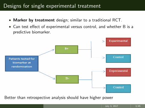
Designs for single experimental treatment
• Marker by treatment design; similar to a traditional RCT.
• Can test effect of experimental versus control, and whether B is apredictive biomarker.
Better than retrospective analysis should have higher power
July 3, 2017 3/45
Designs for single experimental treatment
• Marker by treatment design; similar to a traditional RCT.
• Can test effect of experimental versus control, and whether B is apredictive biomarker.
Better than retrospective analysis should have higher power
July 3, 2017 3/45
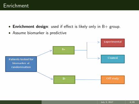
Enrichment
• Enrichment design: used if effect is likely only in B+ group.
• Assume biomarker is predictive
July 3, 2017 4/45

Adaptive Enrichment
• Adaptive enrichment designs recruit all patients, then have interimanalysis to decide if recruitment should be restricted.
• Has a chance to find treatment effect in everyone if it is present, or toenrich if not.
July 3, 2017 5/45
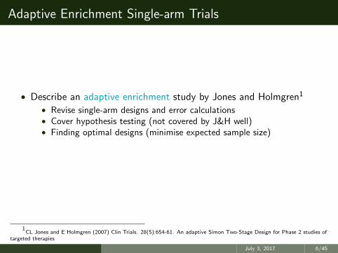
Adaptive Enrichment Single-arm Trials
• Describe an adaptive enrichment study by Jones and Holmgren1
• Revise single-arm designs and error calculations• Cover hypothesis testing (not covered by J&H well)• Finding optimal designs (minimise expected sample size)
1CL Jones and E Holmgren (2007) Clin Trials. 28(5):654-61. An adaptive Simon Two-Stage Design for Phase 2 studies of
targeted therapies
July 3, 2017 6/45
Jones and Holmgren
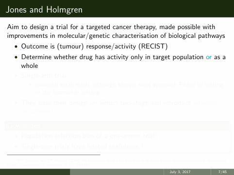
Aim to design a trial for a targeted cancer therapy, made possible withimprovements in molecular/genetic characterisation of biological pathways
• Outcome is (tumour) response/activity (RECIST)
• Determine whether drug has activity only in target population or as awhole
• Single-arm trial• powerful small study although sample sizes approach Phase III setting
in the biomarker setting
• They base their design on Simon two-stage and introduce adaptiveenrichment
Downsides• Population selection bias of a one-armed trial!
• Single-arm trials have limited usefulness 1
1MJ Grayling and AP Mander (2016) Do single-arm trials have a role in drug development plans incorporating randomised
trials? Pharmaceutical statistics 15 (2), 143-151
July 3, 2017 7/45

Jones and Holmgren
Aim to design a trial for a targeted cancer therapy, made possible withimprovements in molecular/genetic characterisation of biological pathways
• Outcome is (tumour) response/activity (RECIST)
• Determine whether drug has activity only in target population or as awhole
• Single-arm trial• powerful small study although sample sizes approach Phase III setting
in the biomarker setting
• They base their design on Simon two-stage and introduce adaptiveenrichment
Downsides• Population selection bias of a one-armed trial!
• Single-arm trials have limited usefulness 1
1MJ Grayling and AP Mander (2016) Do single-arm trials have a role in drug development plans incorporating randomised
trials? Pharmaceutical statistics 15 (2), 143-151
July 3, 2017 7/45
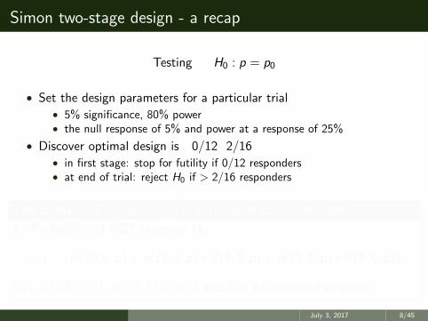
Simon two-stage design - a recap
Testing H0 : p = p0
• Set the design parameters for a particular trial• 5% significance, 80% power• the null response of 5% and power at a response of 25%
• Discover optimal design is 0/12 2/16• in first stage: stop for futility if 0/12 responders• at end of trial: reject H0 if > 2/16 responders
The probability of rejecting H0 in terms of p the response
1 - Probability of NOT rejecting H0
= 1 − (B(12, 0, p) + b(12, 1, p) ∗ B(4, 1, p) + b(12, 2, p) ∗ B(4, 0, p))
B() is P(X ≤ x), b() is P(X = x) and X is a Binomial distribution
July 3, 2017 8/45
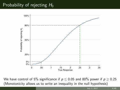
Probability of rejecting H0
0%5%
20%
50%
80%
100%
Prob
abilit
y of
reje
ctin
g H
0
0 .05 .1 .15 .2 .25 .3 .35True Response
We have control of 5% significance if p ≤ 0.05 and 80% power if p ≥ 0.25(Monotonicity allows us to write an inequality in the null hypothesis)
July 3, 2017 9/45

The expected sample size of the trial
12
13
14
15
16Ex
pect
ed S
ampl
e Si
ze
0 .05 .1 .15 .2 .25 .3 .35True Response
July 3, 2017 10/45

Jones and Holmgren Design
Tests the two null hypotheses for the positive and the unselectedpopulation
H−0 : p− = p0 & H+
0 : p+ = p0
• If you reject H−0
• Conclude efficacy in unselected population
• If you reject H+0
• Conclude efficacy in biomarker positive population
They assume that the response p+ > p−
Our design parameters
• p0 = 0.05 (under null biomarker is not prognostic)
• 5% significance and 80% power
July 3, 2017 11/45

J&H schematic
Unselected
Recruit
ResponseLarge
NO Efficacy
Unselected
EfficacyUnselected
YES YES
Positives
NO NO
UnselectedResponse
YES
ResponseNO
ResponsePositives
Some
Positives
YES
Some
Positives
Efficacy
Yes, recruitPositives
YES
NO
Large
UnselectedSTOPYes, recruit
July 3, 2017 12/45

Route 1 - conclusions for the unselected populationPositives not looked at
ROUTE 1
Unselected
Recruit
ResponseLarge
NO EfficacyPositives
Unselected
Unselected
YES YES
YES
NO
Efficacy
UnselectedResponse
SomeResponse
NONO
Positives
EfficacyPositives
YES
SomeResponse
Large
Yes, recruitPositives
YES
NOPositives
UnselectedSTOPYes, recruit
July 3, 2017 13/45

Route 2 - conclusions in positive populationvia unselected recruitment
Unselected
Unselected
ResponseLarge
NO Efficacy
Recruit
EfficacyUnselected
YES YES
YES Positives
NO
UnselectedResponse
SomeResponse
NOResponsePositives
EfficacyPositives
YES
NO
Positives
Large
Yes, recruitPositives
YES
Some
Yes, recruitUnselected
STOP
ROUTE 2
NO
July 3, 2017 14/45
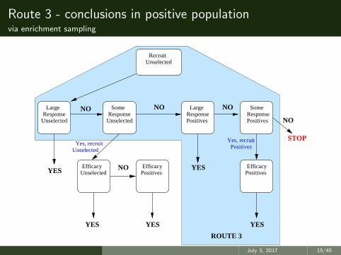
Route 3 - conclusions in positive populationvia enrichment sampling
Unselected
Unselected
ResponseLarge
NO Efficacy
Recruit
EfficacyUnselected
YES YES
YES Positives
NO
UnselectedResponse
SomeResponse
NOResponsePositives
EfficacyPositives
YES
NO
Positives
Large
Yes, recruitPositives
YES
Some
NO
Yes, recruitUnselected
ROUTE 3
STOP
July 3, 2017 15/45

An actual designH−
0 : p = 0.05 H+0 : p = 0.05
(37−, 2+)(25+)
Unselected
RecruitUnselected
Large
NO Efficacy
Response
EfficacyUnselected
YES
PositivesYES
NO NO
YES
ResponseSome
ResponseUnselected
ResponsePositives
Efficacy
NO
YES
Some
Positives
Positives
Yes, recruitPositives
YES
Large
STOP
(30−, 13+)
>6 R−
NO
>5 R+ >1 R+
>5 R+>2 R+
>2 R−
Yes, recruitUnselected
>6 R−
July 3, 2017 16/45

Shorthand for the design
We characterise all the design parameters as
• Stage 1• (3 2)/(30 13)
• Stage 2• (6/38) OR (7 3)/(67 15)
There are 10 numbers to find
• with 5 choices for each gives 10 million designs.
• We have fast programs to search a huge design space (Colin) to findbest design searching 10 billion designs
July 3, 2017 17/45

The rejection probabilities for Route 1
0
.2
.4
.6
.8
1
Res
pons
e in
+ p
op
0 .2 .4 .6 .8 1Response in - pop
0
.1
.2
.4
.6
.8
.9
1
Rej
ect H
0- and
H0+
Route 1: R1()
July 3, 2017 18/45
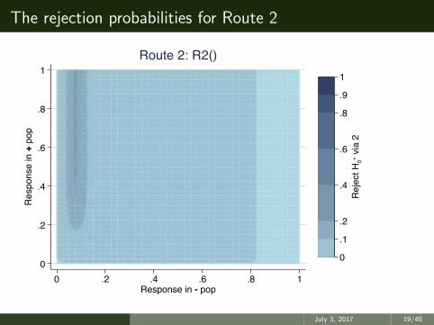
The rejection probabilities for Route 2
0
.2
.4
.6
.8
1
Res
pons
e in
+ p
op
0 .2 .4 .6 .8 1Response in - pop
0
.1
.2
.4
.6
.8
.9
1
Rej
ect H
0+ via
2
Route 2: R2()
July 3, 2017 19/45
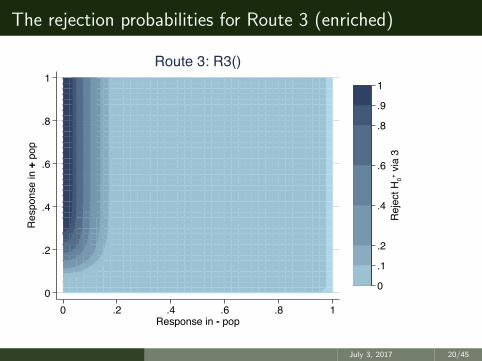
The rejection probabilities for Route 3 (enriched)
0
.2
.4
.6
.8
1
Res
pons
e in
+ p
op
0 .2 .4 .6 .8 1Response in - pop
0
.1
.2
.4
.6
.8
.9
1
Rej
ect H
0+ via
3
Route 3: R3()
July 3, 2017 20/45

The rejection probabilities
0
.1
.2
.3
.4
Res
pons
e in
+ p
op
0 .1 .2 .3 .4Response in - pop
0.1.2
.4
.6
.8
.91
Rej
ect H
0- and
H0+
Route 1: R1()
0
.1
.2
.3
.4
Res
pons
e in
+ p
op
0 .1 .2 .3 .4Response in - pop
0.1.2
.4
.6
.8
.91
Rej
ect H
0+ via
2
Route 2: R2()
0
.1
.2
.3
.4
Res
pons
e in
+ p
op
0 .1 .2 .3 .4Response in - pop
0.1.2
.4
.6
.8
.91
Rej
ect H
0+ via
3Route 3: R3()
0
.1
.2
.3
.4R
espo
nse
in +
pop
0 .1 .2 .3 .4Response in - pop
0.1.2
.4
.6
.8
.91
Rej
ect a
ny
ANY Route: R123()
July 3, 2017 21/45

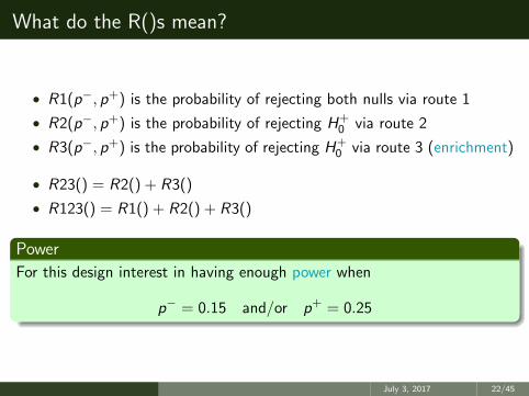
What do the R()s mean?
• R1(p−, p+) is the probability of rejecting both nulls via route 1
• R2(p−, p+) is the probability of rejecting H+0 via route 2
• R3(p−, p+) is the probability of rejecting H+0 via route 3 (enrichment)
• R23() = R2() + R3()
• R123() = R1() + R2() + R3()
Power
For this design interest in having enough power when
p− = 0.15 and/or p+ = 0.25
July 3, 2017 22/45
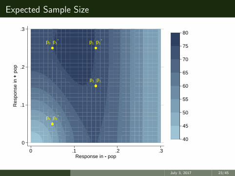
Expected Sample Size
p0- p1
+ p1- p1
+
p1- p1
-
p0- p0
+
0
.1
.2
.3
Res
pons
e in
+ p
op
0 .1 .2 .3Response in - pop
40
45
50
55
60
65
70
75
80
July 3, 2017 23/45
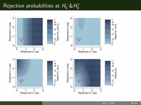
Rejection probabilities at H−0 &H
+0
3.7%
0
.1
.2
.3
Res
pons
e in
+ p
op
0 .1 .2 .3Response in - pop
0.1.2
.4
.6
.8
.91
Rej
ect H
0- and
H0+
0.5%
0
.1
.2
.3
Res
pons
e in
+ p
op
0 .1 .2 .3Response in - pop
0.1.2
.4
.6
.8
.91
Rej
ect H
0+ via
2
0.6%
0
.1
.2
.3
Res
pons
e in
+ p
op
0 .1 .2 .3Response in - pop
0.1.2
.4
.6
.8
.91
Rej
ect H
0+ via
3
4.8%
0
.1
.2
.3
Res
pons
e in
+ p
op
0 .1 .2 .3Response in - pop
0.1.2
.4
.6
.8
.91
Rej
ect a
ny
July 3, 2017 24/45

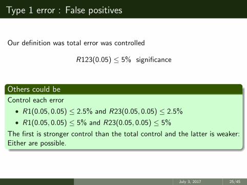
Type 1 error : False positives
Our definition was total error was controlled
R123(0.05) ≤ 5% significance
Others could be
Control each error
• R1(0.05, 0.05) ≤ 2.5% and R23(0.05, 0.05) ≤ 2.5%
• R1(0.05, 0.05) ≤ 5% and R23(0.05, 0.05) ≤ 5%
The first is stronger control than the total control and the latter is weaker:Either are possible.
July 3, 2017 25/45

Rejection probabilities at some alternatives
3.7% 80.1%
80.1%
0
.1
.2
.3
Res
pons
e in
+ p
op
0 .1 .2 .3Response in - pop
0.1.2
.4
.6
.8
.91
Rej
ect H
0- and
H0+
11.5% 3.6%
1.9%
0
.1
.2
.3
Res
pons
e in
+ p
op
0 .1 .2 .3Response in - pop
0.1.2
.4
.6
.8
.91
Rej
ect H
0+ via
2
68.5% 12.8%
6.2%
0
.1
.2
.3
Res
pons
e in
+ p
op
0 .1 .2 .3Response in - pop
0.1.2
.4
.6
.8
.91
Rej
ect H
0+ via
3
83.7% 96.5%
88.2%
0
.1
.2
.3
Res
pons
e in
+ p
op
0 .1 .2 .3Response in - pop
0.1.2
.4
.6
.8
.91
Rej
ect a
ny
July 3, 2017 26/45
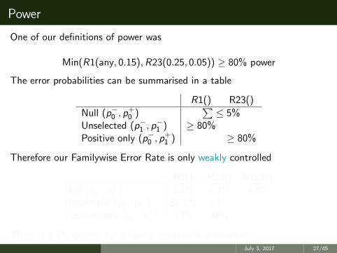
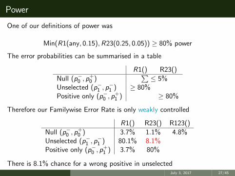
Power
One of our definitions of power was
Min(R1(any, 0.15),R23(0.25, 0.05)) ≥ 80% power
The error probabilities can be summarised in a table
R1() R23()
Null (p−0 , p+0 )
∑≤ 5%
Unselected (p−1 , p−1 ) ≥ 80%
Positive only (p−0 , p+1 ) ≥ 80%
Therefore our Familywise Error Rate is only weakly controlled
R1() R23() R123()
Null (p−0 , p+0 ) 3.7% 1.1% 4.8%
Unselected (p−1 , p−1 ) 80.1% 8.1%
Positive only (p−0 , p+1 ) 3.7% 80%
There is 8.1% chance for a wrong positive in unselectedJuly 3, 2017 27/45

Other possible error controls
The main one is Familywise Error Rate being strongly controlled
R1() R23()
Null (p−0 , p+0 )
∑≤ 5%
Unselected (p−1 , p−1 ) ≥ 80% ≤ 5%
Positive only (p−0 , p+1 ) ≤ 5% ≥ 80%
With stronger false positive control we get
R1() R23() R123()
Null (p−0 , p+0 ) ≤ 2.5% ≤ 2.5% ≤ 5%
Unselected (p−1 , p−1 ) ≥ 80% ≤ 5%
Positive only (p−0 , p+1 ) ≤ 5% ≥ 80%
July 3, 2017 28/45

Conclusions
• We belief you want to control the wrong positive error
• We optimised with respect to the expected sample size under theglobal null
• We have software that used massive parallelisation
• Future — want to understand whether there is a role for single-armtrials in biomarker trials
July 3, 2017 29/45
Multiple experimental treatments
• If there are several experimental treatments available for testing, thenthere are substantial advantages of including several arms in a single‘umbrella’ trial.
• A shared control group means more statistical efficiency: test moretreatments with the same number of centres.
• Administratively and logistically easier compared to separate trials.
• For targeted treatments: more enrolled patients will receive atreatment targeted at their biomarker profile.
• However, also these types of trials are also more complicated.
July 3, 2017 30/45

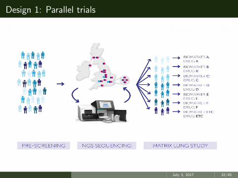
Design 1: Parallel trials
• One type of platform trial consists of a set of parallel trials.
• A patient is allocated to a trial on the basis of their biomarker profile.
• A couple of UK examples:• National lung matrix trial• FOCUS 4
• Both of these also use adaptive design approaches to stop sub-trialswhere the treatment is not showing sufficient signs of efficacy.
July 3, 2017 31/45
Design 1: Parallel trials
July 3, 2017 32/45
Design 2: Bayesian adaptive randomisation
• A second type of umbrella trial does not make assumptions of linksbetween biomarkers and treatments.
• Example: BATTLE, ISPY2
• Both of these use Bayesian adaptive randomisation (BAR) to changethe randomisation probability:
• A patient is more likely to receive treatments that have previouslyworked well on patients with similar biomarker profiles.
July 3, 2017 33/45
Design 3: Linked BAR design
• When the links between treatment and biomarker are plausible butunsure, neither design seems completely appropriate.
• Intermediate choice: linked-BAR design1.
• Combines initial stage of parallel-trials design then uses BAR toupdate allocation in case alternative links are present.
1Wason J, Abraham J, Baird R, Gournaris J, Vallier A, Brenton J, Earl H, Mander A. (2015) A Bayesian adaptive design
for biomarker trials with linked treatments. British Journal of Cancer 113, 699-705
July 3, 2017 34/45
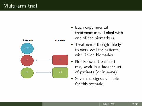
Multi-arm trial
• Each experimentaltreatment may ‘linked’withone of the biomarkers.
• Treatments thought likelyto work well for patientswith linked biomarker.
• Not known: treatmentmay work in a broader setof patients (or in none).
• Several designs availablefor this scenario
July 3, 2017 35/45

Motivating clinical example - post-adjuvant breast cancer
• Japanese trial has recently shown that capecitabine can improvelong-term disease-free survival after breast surgery in poor prognosisgroups.
• Clinical collaborators in University of Cambridge oncology departmentwanted phase II design that would test whether targeted agents wouldoffer advantages over capecitabine.
• Patient population is women who have residual circulating tumourDNA after tumour removal operation — data shows this group haspoor prognosis.
July 3, 2017 36/45
Motivating clinical example - post-adjuvant breast cancer
• Primary endpoint — log percentage change in circulating tumourDNA level from baseline to six months. Immunology and cycle cellgene panels used as the biomarkers.
• Moderately prevalent biomarkers ( 30% for each).
• Treatment arms include capecitabine (control) and two targetedagents that would be thought to work in patients who have highlevels of the relevant gene panel.
July 3, 2017 37/45

Linked BAR design
• Stage 1: 100 patients recruited and randomised between control andexperimental arm linked with a biomarker the patient is positive for.Control arm randomisation is always 1/3.
• E.g. if patient is positive for biomarker 1, randomised between controland treatment 1 in 1:2 ratio.
• If patient positive for both biomarkers or neither, randomised 1:1:1between control and experimental treatments.
July 3, 2017 38/45

Model used for BAR
• Stage 2 (200 patients): at a series of interim analyses, recommendedallocation probabilities get updated according to results so far.
• Bayesian linear model fitted at each interim. Model containsintercept, marginal effects of each experimental treatment (β),marginal effect of each biomarker (γ), and interactions betweenbiomarkers and treatment (δ).
log
(yi1yi0
)= µ+ βT (i) +
2∑j=1
γjxij +2∑
j=1
δT (i)jxij + εi εi ∼ N(0, σ2)
where yi0 and yi1 are ctDNA measurements at baseline and six monthsrespectively, T (i) is allocated treatment of patient i , xij is 1 if patient i ispositive for biomarker j .
July 3, 2017 39/45
Linked BAR model
• Model uses normal-inverse gamma form for conjugacy.
• All parameters except δ11 and δ22 have non-informative priors.
• δ11 and δ22 have moderately informative priors chosen to continuefavouring allocation of patients to linked treatments (until there issufficient evidence that they are not working).
• Model gives posterior probability of each experimental treatmentbeing superior to control for each possible biomarker profile.
• These posterior probabilities are then transformed into allocationprobabilities for future patients (see Wason et al. for more details).
July 3, 2017 40/45
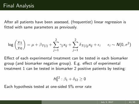
Final Analysis
After all patients have been assessed, (frequentist) linear regression isfitted with same parameters as previously.
log
(yi1yi0
)= µ+ βT (i) +
2∑j=1
γjxij +2∑
j=1
δT (i)jxij + εi εi ∼ N(0, σ2)
Effect of each experimental treatment can be tested in each biomarkergroup (and biomarker negative group). E.g. effect of experimentaltreatment 1 can be tested in biomarker 2 positive patients by testing:
H120 : β1 + δ12 ≥ 0
Each hypothesis tested at one-sided 5% error rate
July 3, 2017 41/45
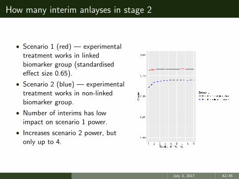
How many interim anlayses in stage 2
• Scenario 1 (red) — experimentaltreatment works in linkedbiomarker group (standardisedeffect size 0.65).
• Scenario 2 (blue) — experimentaltreatment works in non-linkedbiomarker group.
• Number of interims has lowimpact on scenario 1 power.
• Increases scenario 2 power, butonly up to 4.
July 3, 2017 42/45

Comparison of designs (50000 replicates)
Scenario Parallel trials power BAR power Linked-BAR power
Trt 1 worksin all patients 0.949 0.977 0.976
Trt 1 works inbiomarker 1
positive patients 0.831 0.798 0.833
Trt 1 works inbiomarker 2
positive patients 0.428 0.796 0.699
Parallel trials BAR Linked-BAR
Maximumtype I error rate 0.248 0.214 0.212
July 3, 2017 43/45
Conclusions
• Wason et al. shows comparisons for large number of scenarios.
• Generally:• When biomarker-treatment links are correct: parallel trials best, linked
BAR very close. BAR loses moderate amount of power but still prettygood.
• When links are incorrect: BAR best, linked BAR loses moderateamount of power; parallel trials low power.
July 3, 2017 44/45

Acknowledgements
All members of the MRC Biostatistics Unit
• Deepak Parashar (Warwick Uni)
• Colin Starr
• Jack Bowden (Bristol Uni)
• Lorenz Wernisch
• James Wason
July 3, 2017 45/45


![⃝₪[jerry mander] four arguments for the elimination](https://static.fdocuments.us/doc/165x107/568ca8e71a28ab186d9b46b7/jerry-mander-four-arguments-for-the-elimination.jpg)