CREATE Research Archive

Published Articles & Papers

2005

Adjusting to Natural DisastersKerry SmithArizona State University, kerry.smith@asu.edu

Jared C. Carbone

Daniel G. Hallstrom

Jaren C. Pope

Michael E. Darden

Follow this and additional works at: http://research.create.usc.edu/published_papers

This Article is brought to you for free and open access by CREATE Research Archive. It has been accepted for inclusion in Published Articles & Papersby an authorized administrator of CREATE Research Archive. For more information, please contact gribben@usc.edu.

Recommended CitationSmith, Kerry; Carbone, Jared C.; Hallstrom, Daniel G.; Pope, Jaren C.; and Darden, Michael E., "Adjusting to Natural Disasters"(2005). Published Articles & Papers. Paper 163.http://research.create.usc.edu/published_papers/163

ADJUSTING TO NATURAL DISASTERS

Smith, V., Carbone, J., Hallstrom, D., Pope, J. & Darden, M.

CREATE REPORT Under FEMA Grant EMW-2004-GR-0112

March 15 , 2005

Center for Risk and Economic Analysis of Terrorism Events

University of Southern California Los Angeles, California

3710 McClintock Avenue, RTH 314 Los Angeles, CA 90089-2902 ~ (213) 740-5514 ~ www.usc.edu/create

Report #05-005 DRAFT

1

Adjusting to Natural Disasters

V. Kerry Smith, Jared C. Carbone, Daniel G. Hallstrom, Jaren C. Pope, and Michael E. Darden*

March 15, 2005

Abstract

People can answer the risks presented by natural disasters in a number of ways; they can move out of harms way, they can self protect, or they can insure. This paper uses the largest U.S. natural disaster on record, Hurricane Andrew, to evaluate how people and housing markets respond to a large disaster. Our analysis combines a unique ex post database on the storm’s damage along with information from the 1990 and 2000 Censuses as well as information on housing sales in Dade County, Florida where the storm hit. The results suggest that the economic capacity of households to adjust explains most of the differences in demographic groups’ patterns of adjustment to the hurricane damage. Low income households respond primarily by moving into low-rent housing in areas that experienced heavy damage. Middle income households move away to avoid risk, and the wealthy, for whom insurance and self-protection is most affordable, remain. This pattern of adjustment is roughly mean neutral, so an analysis based on summary measures would miss these important adjustments. Our analysis of the housing sales record indicates that the new risk information provided by the event reduced the rate of appreciation in prices by about fifty percent for the zones with the highest FEMA flood risk ratings. This finding is corroborated at the qualitative level by the Census data. JEL Classification Nos: Q51,Q54

Key Words: Natural Hazards, Economic Adjustment, Hurricanes

* University Distinguished Professor, North Carolina State University, and Resources for the Future University Fellow; Postdoctoral Fellow, CEnREP, North Carolina State University; Affiliated Economist, CEnREP, North Carolina Sate University; Graduate Fellow; and Undergraduate Fellow, CEnREP, North Carolina State University, respectively. Smith’s research was partially supported by the United States Department of Homeland Security through the Center for Risk and Economic Analysis of Terrorism Events (CREATE), grant number EMW-2004-GR-0112. However, any opinion, findings, and conclusions or recommendations in this document are those of the author(s) and do not necessarily reflect views of the U.S. Department of Homeland Security. Thanks are due to H. Spencer Banzhaf, Kathleen Bell, David Card, and Richard Ready for very helpful comments on earlier summaries of this and related research. Thanks are also due Alex Boutaud and Susan Hinton for assistance in preparing the manuscript.

DRAFT

2

Adjusting to Natural Disasters

I. Introduction

Natural disasters force adjustment. The Indian Ocean tsunami, severe storms in the

western U.S. and hurricanes in Florida made 2004 a year for renewing our collective

awareness of this fact. This paper uses Hurricane Andrew, the largest U.S. natural

disaster on record, to investigate two questions.1 We first consider how people adjust.

People can answer the risks presented by natural disasters in a number of ways: they can

move out of harms way; they can self-protect, building structures less vulnerable to

damage; or they can insure. This paper provides a snapshot of the socio-economic forces

that reshaped Dade County, Florida after Andrew made landfall and destroyed a large

portion of the private housing and commenrcial facilities. The second part of the analysis

looks at the net effect of these adjustments on the value of homes in areas that were

perceived to be subject to increased risk after this natural disaster. Both aspects of the

analysis bear directly on our ability to design policies that facilitate people’s ability to

return to their everyday activities after disasters.

We take advantage of a unique ex post evaluation of Andrew’s damage conducted

by the National Oceanic and Atmospheric Administration (NOAA) and published in the

1 Robert Hartwig, Senior Vice President and Chief Economist of the Insurance Information Institute, used this characterization in describing the impact of hurricanes on economic activity in hurricane prone counties. He observed that: “Hurricane Andrew, until September 11, 2001, was the global insurance

industry’s event of record. For nearly a decade it was the disaster against which all other disasters worldwide were compared….Andrew struck Florida in August 1992 with 140 mile-per-hour winds and produced insured losses of $15.5 billion – about $20 billion in current (2001) dollars. …Although Andrew has now been eclipsed as the largest insurance event in world history (by September 11)…It remains the largest natural disaster on record in terms of insured losses, not only in the United States but world- wide…” (Hartwig [2002] pp.1-2, parenthetical phrase added).

DRAFT

3

Miami Herald on December 20, 1992 (referred to later as the NOAA/Miami Herald data).

This summary includes information on 420 subdivisions or condominium developments

in the area affected by Andrew. To evaluate how people adjusted after the storm, we use

the 1990 and 2000 Censuses to compare the demographic and economic attributes of the

populations in Dade County at the block group level before and after the storm. When

matched with the NOAA/Miami Herald data on the damages and the FEMA flood maps

that identify areas subject to differentiated risks of coastal flooding, these records

produce a picture of the spatial adjustments that took place.

Our findings confirm some prior beliefs about this hurricane and overturn others.

In contrast to the popular views of the storm’s impact, white, middle-income households

were more likely to experience significant damage than poor minority households.

Financial capacity, as reflected by home ownership and education, are key factors in who

adjusted to the damage. In the eight years after Andrew the population in areas with 50

percent or more of the homes damaged so seriously as to be rated uninhabitable grew

faster than areas with less damage. White and black homeowners and white renters

moved away from damaged areas. Hispanic households, both owners and renters, moved

into the areas with hurricane damage. Lower income households tended to move into

damaged areas while middle income moved out. In general, the storm’s damage did not

affect higher income households. In 2000, households with annual incomes over 150,000

were the only group likely to be attracted to areas with a comparable “type” of household

– i.e. to areas where the same income level households lived in 1990.

More broadly, the analysis also highlights the potential importance of household

heterogeneity on the meaurement of spatially-delineated environmental impacts; the

DRAFT

4

changes to the income distribution that we find are roughly mean neutral, so a

comparable study based on summary measures would miss much of the story.2

The second half of the analysis – the evaluation the economic consequences of

these adjustments – makes use of two different strategies. The first evaluates the changes

in the distributions of rents and homeowners’ beliefs about their homes’ values between

the 1990 and 2000 Censuses in response to average damage and the fraction of a block

group in a FEMA risk zone. The second matches the damage information to a repeat

sales hedonic property value data set for residential properties in Dade County. Both

analyses confirm that these types of adjustments have implications for markets. The

repeat sales findings indicate that, after controlling for damage, the information conveyed

by Andrew caused the prices of homes in high risk areas to appreciate more slowly than

their counterparts throughout Dade County. Our estimates imply a fifty to sixty percent

reduction in the average increase in home prices for homes located in areas perceived to

be higher risk as a result of the storm. The change in the Census median measures over

the decade also suggests slower appreciation. However, the estimate is smaller.

Section two describes the unique configuration of spatially delineated data

required to undertake the analysis. The third section develops the hypotheses

motivating our expectation for differences in households’ adjustments. Our results are

developed in Section four in two parts. First we describe the changing features of

neighborhoods based on the 1990 and 2000 Censuses for the county. After that we

summarize the highlights of the repeat sales analysis of residential home sales in Dade 2Recently, quasi-experiments (such as the one performed here) have raised questions about the the viability of earlier hedonic studies on the value of air quality improvements and superfund clean up (see Chay and Greenstone [forthcoming] and Greenstone and Gallagher [2004]). The current paper bears on this discussion as well. To the extent that changes in these other environmental amenities result in large distributional changes like those found here, quasi-experiments based on summary data may be biased.

DRAFT

5

County. This model uses the spatial location and timing of the most recent and the

immediately preceding sales of homes in areas with varying flood risks to identify the

market responses to Andrew’s damage and any risk information homebuyers associate

with the hurricane. At the micro level, adjustment in home prices for locations with

higher fractions of damaged properties likely reflects the net impact of repairs and

market perceptions of the construction quality of homes. Our comparison of the

results from a repeat sales analysis using actual transactions with the same logic

applied to changes in the median home values from the 1990 and 2000 Censuses finds

that both strategies would conclude that Andrew caused homebuyers to revise their

assessment of the risks from buying homes in FEMA’s Special Flood Hazard Zones.

II. Data

In December 1992 the Miami Herald published a special report analyzing the

factors responsible for areas with significant damage that were far from the storm’s

strongest winds. As part of the report, the newspaper included the full documentation for

the NOAA damage assessment by subdivision. Using the map included with the Miami

Herald’s feature article it was possible to align the roadways in the Miami Herald map

with an Arcview map of the primary roads within the county. A set of 306 grids was

DRAFT

6

defined to match the subdivision records to our two other databases. The first task linked

the grids to Census block groups. Each block group was assigned the average (area

weighted if a subdivision crossed Census boundaries) damage measure for the

subdivision falling within its boundary. The second used the latitude and longitude of

each home in the repeat sales data to identify its grid and assign an average damage

estimate.

These damage estimates serve two roles. For our analysis of the composition of

the block groups they are proxies for the extent to which neighborhoods offer

opportunities for nearly complete replacement of residential structures. When one

hundred percent of the homes in a neighborhood are judged to be uninhabitable, then we

expect that there is the opportunity to transform completely the composition of the area.

The impact of smaller amounts of damage on changes in the composition of a block

group depends on the relative importance of quality filtering versus the externalities

effects attributed to different demographic and economic groups.

When the damage measure is used with our repeat sales model that is based on

individual home sales, the interpretation of the variable is somewhat different. In this

case, two effects are being represented simultaneously. The first is as a control for the

likelihood of damage to that structure as a result of the hurricane and with it the prospects

that the house may have been altered as part of the repair. The damage measure serves as

a proxy variable because our micro level housing data only include information on the

home attributes as of the most recent sale. As a result, it is not possible to control for

alterations due to the repairs of any storm damage. This effect could be especially

important for sales that bracket the storm. The second influence stems from the overall

DRAFT

7

pattern of Andrew’s damage. It was not perceived to be consistently associated with

wind damage.5 An important motivation for the special report published in the Miami

Herald was explaining the heterogeneity in storm impacts by subdivision. Thus, at the

micro level, these measures may also be reflecting changes in perceived structural

integrity of the homes within a subdivision as a result of the reports of storm damage.6

Our estimates of the effects of the storm on price changes describe the net effect of these

two influences.

Between the 1990 and 2000 Censuses, the definition of block groups for the

county changed, expanding from 1048 in 1990 to 1222 in 2000. This change reflects the

increase in population in the county and the need to re-align Census summaries to match

the new population distribution. The expansion in the number of block groups is a

response to population growth. Thus, how it is treated could be important to the way any

of the demographic changes are measured. To avoid mixing the potential for endogeneity

in the neighborhood definition with the event being studied (i.e. Andrew’s damage) we

focus on the 1990 definition of block groups.

Our analysis considers two different samples. First, we construct area weighted

averages of Census statistics from the 2000 block groups so that each record can be

matched to its 1990 counterpart. As a cross check to these results, we repeat the analysis

5 We obtained the original Wakimoto and Black [1994] maps describing the wind patterns for Andrew with the assistance of Roger Wakimoto. A cross tabular analysis of the Miami Herald damage survey data with an approximate wind based delineator of the damage suggests higher wind areas were more likely to experience damage. Nonetheless, the Miami Herald story “Less Winds, Lots of Damage,” December 20, 1992, documents a large number of exceptions. 6 We do not have access at the micro level to the repair history of properties, building permits, or other information that would allow distinguishing individual properties that were damaged. Thus these average measures are assumed to serve as a proxy for damage. At the same time they also signal that a subdivision may be of lower construction quality. The Miami Herald feature clearly documents problems in the county’s building inspections, noting that “Unsupervised and understaffed, with civil service rules that give them job protection, Dade’s building inspectors were no match for the development of the 1980s.” Lisa Getter, “Inspections: A Breakdown in the System,” Miami Herald, December 20, 1992.

DRAFT

8

using the sample of block groups that did not change between the two Censues. Table 1

reports an overall summary of the demographic and economic patterns in 1990 and 2000

using the full sample of area weighted estimates based on the 1990 block groups. The

average proportion of each demographic and economic category across block groups is

reported for three samples. The last two columns labeled “overall” provide these average

proportions for all the block groups between 1990 and 2000. The first two sets of

columns decompose this set into block groups experiencing 50% or greater of their

homes as uninhabitable based on the NOAA-Miami Herald survey. The number of block

groups in this category is 27. The second group includes those with less than 50%

uninhabitable. The number of observations in this category ranges from 968 to 997

depending on the variable selected.

This decomposition suggests the hurricane’s damage was not disproportionately

experienced by minority or poor households. In 1990 block groups with 50% or over

damage were largely white (both owner and rental households) in the income range from

25,000 to 60,000. When we consider the proportions in 2000, white households moved

out (both owners and renters). Hispanic households moved in. The changes in the

relative number of Hispanic households in damaged areas partially reflects the overall

growth in their share in the county. However this is not the full story. If we consider the

white, African American, and hispanic households who report they migrated into the

county in the last five years from elsewhere, then we would find white households are the

largest share of these new residents -- 46.4 percent of the toal for these three groups.

Hispanic households account for next largest share at 41.5 percent.

DRAFT

9

Middle income households moved out and the lower (15,000-25,000) and high

income groups moved in. Of course, these summaries are simple averages and do not

take account of initial conditions in each area. In addition, they would change somewhat

if we modify the threshold used to isolate the high damage block groups. This separation

at 50% leads to a relatively small sample of block groups that underlies the means used to

characterize who is adjusting to extensive damage. In section four we use regression

models to evaluate how the difference in damage at block groups affect changes in their

composition.

The second component of our analysis uses a repeat sales database for residential

properties in the county. Our housing data include records for all sales of residential

properties in Dade County, Florida from 1983 to 2000. They were purchased from a

commercial vendor (First American Real Estate Solutions) and provide the characteristics

of the properties at the time of the most recent sale, the date of each sale (year, month,

and day), the sales price, the latitude and longitude coordinates, and a variety of variables

describing the homes. Our focus is on a subset of the sales – properties that sold at least

twice – and we consider the two most recent sales. These sales data were cleaned to

remove several types of transactions, including: properties that sold for less than $100;

properties that were bought and sold within a period of several months and had a price

difference exceeding $500,000; and properties where the first sale was for land only and

the second sale included land and a structure. We limited the sample to properties built

after 1982 because of changes in federal legislation grandfathering subsidized insurance

for older properties and other state level insurance changes that may have special

implications for homes built before this date.

DRAFT

10

Each record in our sample was merged with the Federal Emergency Management

Agency’s G3 flood map for the county. Information about the Special Flood Hazard

Area (SFHA) is in the public domain. The Coastal Barrier Act of 1982 required lenders

to notify homebuyers about a property’s flood risk due to location in an SFHA. The geo-

coded sales were also merged with a spatially delineated map of the path of Hurricane

Andrew as well as the grid cells for the NOAA-Miami Herald data.

Three areas with differing flood hazard risks can be distinguished from the FEMA

maps for Dade County – AE, AH, and X500 designations. AE corresponds to the highest

risk category. Homes built after 1974 in these locations have the highest rates for flood

insurance.7 The rates in AE zones range from $0.16 to $0.39 per $100 of coverage

depending on base floor elevation (BFE). The AH areas are somewhat lower risk,

generally corresponding to higher elevations of about – one to three BFE. X500 are

usually described as areas with negligible risk.

The primary sources of damage in a hurricane are often wind and storm surge.

These impacts need not correspond to the areas designated by the SFHA as most

hazardous. In the case of Andrew, damage was also not readily predicted by sustained

wind and gusts. Andrew’s wind speeds were estimated to be above 133 miles per hour

(mph) with gusts over 175 mph in some areas. Yet some subdivisions experiencing

substantially lower winds were completely destroyed. This inconsistent pattern of

damage was responsible for the Miami Herald investigation and special series of articles.

Their conclusion was that damage in areas not experiencing strong winds or storm surges

was due to poor housing construction and lax standards.

7 The Federal flood insurance program provides for subsidized rates for homes built before 1974.

DRAFT

11

From our perspective this record is an advantage for a quasi-experiment – the

structural properties of individual neighborhoods could not be known in advance. They

are revealed by damage caused by Andrew. Initial location decisions would not be able

to take account of the expected structural integrity of the homes. Before the storm, the

FEMA hazard areas were the only signals available to homebuyers. After the storm we

hypothesize that these same FEMA areas and the reported damage are interpreted

differently. Our data allows consideration of both the pattern of damage and the FEMA

risk classes. By using grids to assign the Miami-Herald damage measure we assure that

any stigma to undamaged homes in housing subdivisions that experience substantial

damage as well as specific effects on damaged homes are taken into account in measuring

the effects of risk information.

We hypothesize that this construction effect will be known as a result of the

Miami Herald report. Thus, the only other basis for using the storm to separately

delineate areas with risk is based on the FEMA hazard categories. Our analysis of repeat

sales focuses on the SFHA risk designations because they align with insurance rates and

are the most consistent risk information available to homebuyers in making ex ante

location choices.

III. Non-Market and Market Responses

A. Background

When a large share of the private and public capital supporting daily activities is

significantly damaged, decisions must be made about how to respond. The larger the

impact of a disaster, the greater, in principle, is the opportunity to observe social and

DRAFT

12

economic adjustment. Most of the available economic models of household adjustment

to exogenous changes in community attributes are intended to describe responses to

relatively small changes in features of a home or a neighborhood. In the empirical tests

of these models the attributes of interest are assumed to be conveyed to homeowners

through their locational choices. Households are assumed to be heterogeneous with

different preferences for location specific amenities. As a rule, they assume there is one

or more endogenous (to the adjustment process) attributes of neighborhoods that can

reinforce or retard responses to an exogenous change in the location specific attribute.

For example, in the externality/filtering models (Coulson and Bond [1990]) average

neighborhood income is hypothesized to be a factor that influences household

preferences for a neighborhood. It also changes as people alter their choices for

neighborhoods. As a result, changes in mean income can enhance or reduce the effects of

an exogenous change in a neighborhood attribute. The overall outcome on composition

of an area depends on the size and direction of the effect of neighborhood mean income

on the marginal willingness to pay for the attribute that changes. A comparable set of

influences can be found in the sorting models that would have consistent predictions for

large changes in neighborhood attributes and indeterminant implications for small (see

Banzhaf and Walsh [2004]).8

8 The externality/filtering and sorting models rely on common formal structure. The first identifies two types of households who must select among locations with continuous variation in an exogenous attribute. Sorting models assume a finite set of communities and continuous variation in household taste. Banzhaf and Walsh illustrate their analysis with two communities varying in an exogenous attribute and describe sorting among communities. In both structures an equilibrium is defined. With filtering it is the law of one price whereas with sorting it is boundary indifference. Comparative statics with each relation given constraints linking household heterogeneity to endogenous outcomes yields the results implying how heterogeneity affects the impact of a change in the exogenous attribute. Both models require some version of the single cross condition and a large change to derive unambiguous hypotheses about outcomes. This requirement for a large change is a key advantage for analysis of outcomes after natural disasters.

DRAFT

13

This research has two implications for our analysis. First, it implies that the larger

the damage in a neighborhood, the greater the prospects for a change in measures of its

demographic and economic composition. Such changes offer the opportunity, given

individuals have the resources to pay for adjustment, to observe whether the exogenous

change offsets any endogenous retarding (or enhancing) effects of the changes in the

existing composition of a neighborhood. Second, they suggest we are more likely to

uncover effects of damage by comparing changes in the distributions of the household

types with the 1990 and 2000 Censuses rather than changes in measures of the central

tendencies for these distributions.

B. Models

Our strategy for keeping track of who adjusts uses a simple regression format.

We estimates how ( )( )jttj yy −+10 varies with the average proportion of homes that are

judged uninhabitable. jty is the proportion of households (or individuals depending on

the measure being summarized) in category j for t = 1990. For example this could be the

proportion in a racial group or it could be the proportion born in Florida. This simple

specification is estimated using a variety of additional control variables, including the

baseline (i.e. 1990) proportion of households (or individuals) in each group, the location

of block groups in relation to FEMA flood zones, and the potential effects of a

neighborhood bordering Homestead Air Force Base. This facility was closed after the

hurricane due to extensive damage. Our basic model is given in equation (1) with jd

designating the Miami Herald damage measure and jkz a set of variables that correspond

DRAFT

14

to the different controls investigated as part of evaluating the robustness of our

conclusions.

( )( ) jk

jkkjjttj zdyy εταα +++=− ∑+ 1010 (1)

jε is a random error assumed to be classically well behaved

kταα and , , 10 are parameters to be estimated

For some of the economic variables, such as the distributions of incomes, rents,

and housing values, the cell definitions used in reporting each distribution changed

between the two Censuses. These changes in the 2000 expand the resolution in the

middle categories and change the upper censoring point. We redefined the 2000

categories for rents, housing values, and income so they matched the 1990 categories.

For property values and rents these models generalize the logic proposed by Chay

and Greenstone [forthcoming] to use quasi-random experiments to avoid bias in

estimating the incremental value of changes in site specific amenities. That is, in a

hedonic model the process assuring that the estimated differences in the equilibrium

prices with amenities will reflect incremental willingness to pay relies on sorting

behavior on the part of those buying the homes. People select the best locations they can

afford. Nonetheless, there may be unobserved differences in the households selecting

locations with low amenity levels in comparison to those with high levels. Use of an

exogenous instrument and a difference-in-difference framework allows the effect of

interest and the influence of unobserved heterogeneity to be distinguished.

Applications of this logic for environmental effects have generally relied on

county (or Census tract) level mean or median housing values across Censuses. To the

extent there is a change in the composition of the housing available as a result of the

DRAFT

15

amenity differences, the “average” may not be distinguishing a marginal value for the

change in the amenity. Instead it bundles an induced change in the structural attributes of

what constitutes the average housing with the amenity change. Use of changes in the

distributions of housing values or rents allows greater control over the “types” of housing

through the value and rent brackets. Unfortunately it does not provide a basis for

measuring the marginal willingness to pay for amenities. Thus, a final stage in our

analysis compares our estimates of changes in the distribution with what would have

been concluded if we used the median rents and housing values in 1990 and 2000 with

the 1990 block group definition.

Ideally one would have data on individual home sales and the ability to observe

how prices changed before and after the hurricane. As we noted in the previous section,

we purchased data to meet this ideal -- a transactions-based set of home sales for Dade

County. So, it is possible to develop a repeat sales model based on these micro data and

compare the two strategies for evaluating the effects of Andrew.

The repeat sales model alters the focus of our attention from the block group, as a

proxy for a neighborhood, to the individual property. The sales price (Rit, i identifies

each property and t the time of sale) is assumed to be a function of each home’s

characteristics (xik) including locational attributes. These locational features distinguish

the three FEMA flood hazard areas – AE, AH, and X500. For each area we hypothesize

a different subjective belief about the risk of damage due to coastal storms. Equation (2)

outlines the model.

( )

( )( )∑

∑∑

=

=

+++−

+++++=

3

1

3

1

1

ln

litiltltli

litiltltli

kikkit

eF

epbFxcR

ηβφγ

ηβ (2)

DRAFT

16

The first term, ∑k

ikk xc , captures the effect of the housing characteristics. These

attributes describe the features of the home and its lot. They would generally include its

size, the lot size, age, the number of baths, presence of pool, carport, etc. iη is an

idiosyncratic, time invariant effect due to unobserved heterogeneity. liF is a qualitative

variable identifying the location of properties inside the lthe zone (l =1) versus outside

the zone, (l = 0). The sample also includes homes in areas without any of these flood

zone designations. We assume households have different subjective probabilities of a

hurricane strike causing damage within each of these areas. In our example with l = 1,

they might be designated as ltp and ltφ , respectively. ltb and ltγ are the time effects for

properties inside and outside each flood zone. ite is assumed to be a well-behaved error

(i.e. independent and identically distributed).

Andrew’s extensive damage to Dade County required households to adjust.9

Even if a home was not damaged as a result of the hurricane, we hypothesize that owners

at the time of the hurricane and potential buyers thereafter would perceive the risks of

coastal hazards damaging each location differently. These different perceptions imply

the initial sales prices would be based on one set of subjective beliefs in each FEMA

zone; after the hurricane they are based on another.

For example, if we assume before Andrew 0llt pp = and 0llt φφ = , then after

Andrew, households have received the new information and adjust their risk assessments

to 1llt pp = and 0llt φφ = for the two areas. Defining 1=tA if Andrew occurred and 9 See West and Lenz [1994] for background. David Lenz provided us an unpublished report on the damage after Andrew conducted using American Red Cross estimates of damage by the Metropolitan Dade County Planning Department (Kerr [1993]). This summary suggests a loss of 47,100 housing units in South Dade County. 101,000 individuals, according to these estimates, were dislocated in the four months after Andrew and about 57,000 of these people moved out of the county.

DRAFT

17

0=tA otherwise, ltp and ltφ can be defined recognizing this hypothesized discrete

change in risks for the two locations by equations (3) and (4), respectively.

( ) 01 1 ltltlt pApAp −+= (3)

( ) 011 1 lttlt AA φφφ −+= (4)

Substituting (3) and (4) into equation (2) yields equation (5).

( )( )( )

( ) ( )( )( )∑

∑∑

=

=

++−++−

+++−+++=

3

101

3

101

11

1ln

litiltltltli

litiltltltli

kikkit

eAAF

epApAbFxcR

ηφφβγ

ηβ (5)

To evaluate how adjustment is displayed through markets and the importance of

these altered expectations we need to be able to distinguish these effects from the

heterogeneity in individual properties. We use a difference-in-difference framework to

control for this heterogeneity. Our housing sales sample is limited to houses that sold at

least twice between 1983 and 2000. We base our analysis on the two most recent sales.

Differencing equation (5) for the same property i for sales in years t and s , we

have equation (6).

( ) ( ) ( )( ) ( )( )

( ) ( )( ) ( ) ( )isitl

stlillll

lstll

llsltlsltli

llslt

is

it

eeAAFpp

AAbbFRR

−+−⋅−−−⋅

+−−+−−−+−=⎟⎠⎞⎜

⎝⎛

∑

∑∑∑

=

===3

10101

3

101

3

1

3

1ln

φφβ

φφβγγγγ (6)

To derive equation (6) the structural characteristics are assumed to remain

constant so that these terms cancel from the estimating equation. The interaction term

indicating the sales bracketed Andrew and that a property is in the lth hazard zone for our

example measures ( ) ( )[ ]0101 llll pp φφβ −−− . To estimate this effect we assume that: (a)

there are no significant changes in housing attributes between the two time periods (e.g.

DRAFT

18

the kx ’s remain the same); (b) the partial effects of structural attributes on the log of the

sale prices are constant (i.e. the kc ’s do not change); and (c) the unobserved

heterogeneity is not differentially influenced by the event.

The sum of the term identifying sales that bracket Andrew and the one identifying

those in each of the flood risk zones estimates how the market evaluated the new risk for

these areas (i.e. ( )01 ll pp −β ; for l = 1, 2, 3). When the Miami-Herald damage measure is

introduced into the model and interacted with variables identifying sales bracketing the

storm, we can estimate the net effect of hurricane stigma for subdivisions with significant

damage as well as modifications to damaged properties as part of their repairs.. It is also

possible to include variables reflecting different aspects of the market adjustment,

including the time since Andrew (i.e. the time between August 23-24, 1992 and the most

recent sale of each home in the sample) and the time between the two sales for each price

difference.

Another change to our simple description of the model involves including fixed

effects to account for the changes in insurance arising with the 1994 federal flood

insurance legislation. These variables are distinguished by zone and the date of the most

recent sale in relationship to the implementation data for the changes in the federal flood

insurance program (i.e. 1996). Florida’s response to the insurance crisis created by

Andrew was to create two state run property and casualty underwriting associations.

During the period of our sample, popular descriptions of the program suggest that the

property insurance was under-priced and did not signal the risks of coastal locations.10

We hypothesize the changes in the federal program, both increasing rates and enforcing a

10 Longman [1994].

DRAFT

19

requirement for insurance, may have been especially important if the two sales bracketed

Andrew and the second sale fell after the policy change. We also include an inverse

Mills ratio to evaluate the potential for selection effects that arises by limiting the sample

to properties with at least two sales.11

Finally, our application permits the first comparison of two strategies for using

the hedonic logic together with a quasi-random experiment to isolate the effects of

locationally delineated attributes. Chay and Greenstone [forthcoming] demonstrated the

importance of using exogenous instruments in testing the effects of site specific amenities

and disamenities. Their analysis relies on Census measures for property values, medians

or means for counties. Our unit is the block group. We have micro and aggregate data

for the same external event so it is possible to evaluate the performance of a Census-

based comparison.

IV. Results

A. Who Adjusts

Our analysis of the changes in the composition of the Census blocks in Dade

County between 1990 and 2000 is divided into three components. First we consider

simple models describing whether the proportionate change in a demographic or

economic variable describing the population changes with the NOAA/Miami Herald

damage measure assigned to each block group. These analyses include such variables as

the counts of white, black, and Hispanic homeowners or the households in the 40 to

60,000 dollar income bracket, and so forth. We report models with two samples. With

11 These estimates are the two-step Heckman [1979] approach using Huber’s [1967] robust estimates for the standard errors. The selection model was estimated using fixed effects for each of the sale years for each of the properties. See Appendix A for the estimates.

DRAFT

20

the full sample of block groups we collapse the 2000 block groups to 1990 definitions.

We use two sets of area weights in this process. When the variable being summarized is

a count we apply the fraction of the 2000 block group that is from the original 1990

definition. Assuming uniform density of the relevant population in each 2000 block

group this process assigns the correct weight to each component.

For continuous measures, such as the median income or the median value for

homeowners’ reports for their home’s sale price, the appropriate weight is the fraction of

the 1990 block group that is in the 2000 block group. These weights sum to unity when

we collapse the 2000 summary statistics to the 1990 map for block groups.

We also evaluate whether the relationships between the proportionate changes and

the NOAA/Miami Herald damage measure depend on the initial (i.e. in 1990) fraction of

each group in each 1990 block group. To evaluate the potential effect of the area weights

used to reconstruct our sample, we repeat these analyses using samples with only the

block groups that did not change between 1990 and 2000. Finally we also consider

whether the FEMA flood zones influence the locational choices of different groups.

Table 2 reports the first simple analysis, considering in the top panel whether the

fraction of households reporting that they stayed in the same house was influenced by the

NOAA/Miami Herald damage measure assigned to each block group. Damage did not

affect leaving one’s house or county. It does appear to influence the relocation patterns

of those households born outside Florida. These groups avoid areas with damage. Native

Floridians are then a disproportionately higher share of the population. None of these

results is affected by the sample.

DRAFT

21

Table 3 reports the simple models for demographic variables, income, rents, and

housing values. Each entry in the table corresponds to a different model where the

dependent variable is the proportionate change between the 1990 and 2000 Censuses and

the independent variable is the NOAA/Miami Herald damage measure ( jd in equation

(1)) or this measure along with the 1990 proportion of the relevant group in each block

group (WI for ‘with initial conditions’). We do not report estimates for the parameters

associated with this baseline proportion. The table entries indicate its sign and

significance as a gauge for the robustness of the estimates for the damage measure.

White owners and renters appear to avoid damaged areas. It appears that black

households with home equity adopt the same adjustments in qualitative terms as the

white households. The size of their responses coefficient is smaller and its significance is

sensitive to the sample used. Black renters and Hispanic households, both owners and

renters, increase in the damaged areas. While some of the Hispanic increase reflects an

overall increase in this demographic group, as suggested in the average proportionate

growth measures by demographic groups for the county as a whole (in Table 1), there is

also a disproportionate growth in the damaged areas. Considering the results for groups

based on the various educational levels achieved, the proportions with less than high

school along those with graduate degrees are consistently significant and negatively

related to the damage measure.12

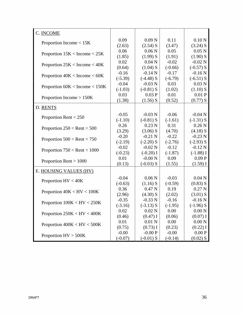
Use of the proportionate changes in the groups in the income cells allows more

direct consideration of the heterogeneity arguments associated with the tipping/sorting

models used to describe how the composition of a community changes in response to an 12 In interpreting estimates it might seem implausible to have all negative estimates. However, both the numerator and the denominator in each ratio for each educational category are changing between census years. Moreover we are not including all educational categoreies in the decompostion.

DRAFT

22

exogenous shock. When we used the median income, the difference in the log of the

median income in the two Census is negatively related to damage, but not significant at

the ten percent level (p-value is 0.11). The results in table 3 help to explain why.

The proportion of households in the lowest two income categories (less than 15K

and 15K to 25K) grows while the middle income group (40K to 60K) declines. Upper

income groups do not significantly change in response to the damage areas. This pattern

is broadly consistent with the expectations of sorting models. In a Tiebout model

households adjust to local public goods (and bads) based on their ability to pay. The

middle income group may have the ability to pay for adjustment. Moving to avoid risk is

the way they appear to adjust. Lower income groups may be taking advantage of the

lower rents in these areas. They do not have the ability to pay for moving out to another

lower risk area as an adjustment. The damage and re-construction creates an opportunity

when the replacement of residential structures is with lower cost units.

Higher income households have the ability to self protect and to insure. As a

result, it seems reasonable to expect a wider array of adjustment possibilities. Moving

out of an area may be the last alternative for this group. Thus, there is a reasonable

explanation for a lack of any changes with this group. The high coastal risk areas also

correspond to areas with high coastal amenities. High income households in these zones

may have already self protected.

Rents and housing values adapt to support the changing composition of

households in the damaged block groups. The proportion of lower rent units increased in

damaged areas and the higher rent decreased. The same effects can be traced in the signs

and significance of the owner reported housing values. The proportion in the range 40K

DRAFT

23

to 100K increased with damage while those in the 100K to 250K decreased. There was

no change in the proportions in the higher valued categories with respect to damage.

Table 4 considers whether the adjustments are affected by the ability to avoid

risky areas. That is, controlling for the average NOAA-Miami damage in a block group

we consider whether the fraction in the block group in different FEMA risk categories

influenced the proportionate changes in each demographic group and income category.

These estimates are based on the full sample of block groups. As noted earlier AE is

classified the highest risk category for coastal flooding, AH next highest, and X500

minimal risk. Homestead is a dummy variable to indicate whether the block group

bordered the Homestead Air Force Base (=1 and 0 otherwise). This facility was closed

after being completely destroyed by the hurricane. We might expect two influences with

this variable. The first is associated with initial land uses around the base and the second

with the scale of the effects of damage along with the base closing to depress land values

and reduce economic activity.

White owners and renters, tend to avoid block groups with the highest risk (AE).

Hispanic owners and renters and black renters seem to disproportionately increase in

block groups with the highest risk. The results for income groups are not as clear-cut as

they are for the demographic categories. Low income groups decrease in the block

groups with the largest fraction of their area in the high risk FEMA category and increase

in the AH category. Other income groups have largely insignificant coefficients for the

area variables. There are a few exceptions with the most intriguing of these estimates

associated with the over 150K group increasing with the area of the block group in the

high risk category. This seemingly counter-intuitive result likely reflects the higher

DRAFT

24

amenity levels associated with these same locations and the ability of this group to self

protect and insure against the risks posed in these areas.

Overall, these results confirm the importance of models that account for

heterogeneity in describing the patterns of household adjustment to disasters. As

expected, ability to pay appears to be important to understanding why we observe

differences in demographic groups’ responses to damage caused by natural disasters.

Comparing the responses of black homeowners and renters we find the former behaves

more comparably with white households. Ethnic attachment to neighborhoods, as

hypothesized in social interaction models and as proxied in our analysis by the 1990

proportion of Hispanic households, does not overturn the results suggesting these groups,

both owners and renters, are more likely to move into damaged areas. In their case

treating home ownership as a proxy for ability to pay would not allow us to reconcile

these findings with what was estimated for other groups.

There appears to be an especially interesting story in the changes in the income

distributions. Lower income groups increase in damaged areas and the proportion of

middle income groups decreases, suggesting there is adjustment to both damage and

potentially the perception of increased risk. The lower income groups may be taking

advantage of lower rents. Thus, this finding contrasts with Breen’s (1997) results

suggesting little change in demographics in response decisions to use new areas for

facilities with increased environmental risk.13

Our analysis suggests higher income groups do not adjust to damage and, if

anything, tend to move to coastal locations with higher risks of flooding damage. Had

13 Breen [1997] and Banzhaf and Walsh [2004] find comparable results for Hispanic populations’ responses to other sources of environmental risks.

DRAFT

25

we used the change in the median income between the two Censuses, our conclusion

would have been much different. That is, analysis of the change in the log of the median

income leads to the mistaken impression that the hurricane’s damage was not an

influence on the proportionate change in average income of households in Dade County’s

block groups. It would have suggested the size of the area in high risk zones was

negative and significant influence. Equation (7) provides these estimates (with t ratios in

parentheses).14

( ) ( )( )

( ) ( ) ( )500

58.110.0

29.002.0

95.211.0

60.119.0

14.13298.0~ln~ln 10

XAHAE

DamageNOAAmm tt

−−

−−

−−

⋅−

−=−⎟⎠⎞⎜

⎝⎛

+

(7)

n = 1022

R2 = 0.01

The significant negative coefficient for the proportion of the block group in the AE zone

would miss the likely amenity effect we found through a more detailed examination of

the income distribution changes. Recall the highest income groups increased in block

groups based on analysis of the proportionate changes in the cells of the income

distribution.

Finally the rent and homeowners’ stated home values also present a complex set

of changes with proportionate growth in the fraction in the lowest categories for areas

where Andrew’s damage was greatest and declines in the intermediate values for these

same areas. These changes add to the challenges faced by the use of summary measures

to isolate an exogenous effect. We return to this issue below.

14 tm~ designates median income in t = 1990 and t+10 = 2000; NOAA Damage is the average proportion uninhabitable; AE, AH, and X500 are the proportion of area in each block group in the specific flood zone designation.

DRAFT

26

B. Market Responses to Damage and Risk information

Table 5 report the results from our repeat sales model based on the transactions

database described earlier. Using latitude and longitude it is possible to locate each

property into FEMA flood zones as well as the grids for storm damage. The dependent

variable is the difference in the log of the sales prices for the two most recent sales of

each property as implied by equation (6) earlier. Our zone variables are dummy variables

identifying whether or not each home is in each FEMA flood risk area. The variables

measuring the time between sales and the time since Andrew, as well as a qualitative

variable identifying whether the two sales bracket Andrew, are used to control for the

various implications of the timing of the events represented in the model. We also

include the average value for the NOAA/Miami Herald damage variable assigned to each

home for those cases with sales that bracket Andrew (zero is assigned for those that do

not).

Two aspects of our findings are especially important to understanding the role of

market adjustment. The hurricane did appear to lead to significant discounting in the rate

of appreciation of homes in the FEMA coastal risk zones. The estimated magnitude of

the impacts for AE and AH zones is consistent with their relative risks. While the

estimated effects of the two zones would not be judged to be significantly different

( ( ) 14.29907,1 =F ), this is a relatively close call. The p-value for equality of these two

effects would imply the effect of AE is greater than AH with a one sided test. Including

the damage estimate suggests the stigma associated with using storm damage to judge

construction quality may offset any improvements made to damaged homes as part of the

DRAFT

27

post hurricane repairs. Overall, the hurricane had dramatic effects on market

expectations. The pace of appreciation of homes in the highest risk areas was reduced by

50 to 60 percent.

The market impact of Andrew’s damage was considerable. For those areas

experiencing complete damage, property values decline by about thirty-four percent. It is

important to acknowledge that this result is based on average damage to an area, not

specific damage to individual properties. Moreover, the properties used to estimate this

effect were no longer damaged at the time they were sold and entered our sample. The

reason the contribution of the damage coefficient does not have a large impact on the

overall measure of the capitalization of the revised risk information is that the average

damage measures for the properties in our sample are small. The properties in the repeat

sales sample were in areas where approximately 16 percent were uninhabitable as a result

of damage from the storm.

The last aspect of our analysis re-visits the Census block data and uses the median

home values (as evaluated by owners) and the median rents to evaluate the extent of the

risk information and damage effects of the hurricane. Tables 6 and 7 report our

estimates. In table 6 the proportionate changes in median housing value and rent display

some consistency with the transactions data.15 Column (1) evaluates the effect of the

Miami Herald damage measure and FEMA risk zones on the change in housing values.

There are no apparent effects of the hurricane damage on median housing values. There

is some consistency with the risk information effect with the proportion of a block

group’s area in either the AE or the AH zones reducing the appreciation in median

15 These models rely on the difference in the log of the median values of homeowners’ assessments of what their homes would sell for between the 1990 and 2000 Censuses.

DRAFT

28

housing values. These effects are not significantly different. Column (2) evaluates the

sensitivity of these findings to including measures of the change in the characteristics of

owner occupied housing over the same period, and we see there is no difference in the

general conclusions one would draw from the analysis.

When we compare these estimates to the results from individual housing sales, it

is clear there are challenges in interpreting both the damage and risk zone measures. At

the block group level both measure the spatial extent of their respective influence and

can, as a result, be interpreted in several ways. For example, the Miami Herald damage

measure could be interpreted as a proxy for the extent of loss in the housing stock as well

as potential stigma associated with poor construction. The proportionate area measures

for the FEMA flood zones may reflect supply of locations and risk of coastal flooding.

Without the ability to observe actual housing sales that bracket Andrew, we cannot

“control” how these effects are allowed to influence the change in housing values. At

best the Census analysis reflects the permanence of each set of effects. In this context

damage appears to have no permanent effect on “average” values while risk does.

Columns (3) and (4) parallel the models for homeowner values, with (3) as the

simple model and (4) including controls for the changing composition of rental housing.

In the case of the proportionate change in median rent, only the area in the highest FEMA

risk zone has a significant negative effect on the change in rents between the two

Censuses.

Table 7 describes how the effects of damage and areas in risk zones influence

changes in the proportion of the homes in each home value interval and in each rent

category. These groupings offer another strategy for controlling for all the housing

DRAFT

29

attributes that could have been included in the models in table 6 using means. The

distributional approach may well offer a better control because of the likely narrower

difference in attributes across the housing units in each cell.

Overall the results using the Census data are mixed – they isolate the increase in

the proportions in the low home value and low rent categories with damage, as we

discussed in the case of the simple models earlier, though the significance of these effects

is somewhat lower. The high risk FEMA zones tend to reduce the number of homes in

the middle value group and increase those in the lowest housing value group as well as

those in the 400,000 to 500,000 home value group. The change in the composition of the

distribution from middle values to the lowest value category seems to dominate the effect

at the highest end of the distribution. It is likely what drives the overall negative effect

observed for the medians. The effects estimated for NOAA damage are comparable to

what we found with the simple models.

Thus, this comparative assessment suggests the task of detecting quasi-

experimental effects on market responses using Census aggregates is challenging. The

heterogeneous behavior that sorting models seek to depict is real. It affects changes in

the demographics as well as the ability of summary statistics such as medians to isolate

the role of the spatially delineated changes in the amenities. It is usually asserted that

these effects are most reliably uncovered with the quasi experimental designs

To the extent our hurricane example is representative, the analysis of changes in

medians based on spatial areas would best be interpreted as tests of the effect of an

amenity (or disamenity) rather than as estimates of the magnitude of its incremental

value. There are simply too many changes in the composition of the distribution of

DRAFT

30

homes (or rental units) that can be taking place. This is especially true for a large scale

event. With smaller sources of impact the discrepancies may be smaller, but in these

cases the ability to detect them reliably may also be diminished.

V. Implications

This analysis has implications for three areas of ongoing research. The first

involves insights into who adjusts to large scale disasters. Most of differences in

adjustment across groups differing in educational and racial background are likely to be

due to their economic capacity to undertake changes in their residential locations. The

pattern no doubt reflects differences in these groups’ available income and wealth.

Whites, both homeowners and renters, are likely to have access to greater resources to

permit their adaptation than Hispanics or black households who don’t own their homes.

Several authors’ concerns about the confounding effects of household

heterogeneity for the composition of communities after exogenous changes in amenities

are confirmed with the large scale damage associated with Andrew. Our analysis of the

distributions of income, housing values, and rents indicate that the underlying shifts in

these distributions can yield ambiguous results for the medians. Nonetheless, the pattern

of change in each of these distributions is consistent with the low income groups being

least able to adjust to natural disasters. It seems reasonable to conclude that this lack of

responsiveness is due largely to economic capacity and not ethnic influences. Indeed, the

hypothesis that the social interaction effect associated with attachment to neighborhoods

with “like” groups was only supported for the highest income households. All other

DRAFT

31

groups’ patterns of adjustment implied movement away from areas with a large fraction

of “their group” in 1990.

The second area where our analyses offer some new results concerns the change

in market prices for housing. Our repeat sales analysis documents that the hurricane’s

damage serves, on net, as an ex post signal of poor quality housing construction for

residential properties. Moreover, the hurricane appears to have caused re-consideration

of the risk designations implied by FEMA’s flood hazard areas. Market price changes for

sales that bracket Andrew are consistent with the risk ordering of the FEMA zones.

A comparison of Census based estimates of the market capitalization of the

signals provided by hurricane Andrew’s risk information confirms in qualitative terms

the lessons derived from the analysis of individual transactions. The contrast between the

potential interpretations for the variables we used to control for the damage and risk

information associated with the storm highlights the challenges in using summary

statistics to implement a quasi-experimental design. Sorting models imply that

heterogeneity in preferences and unobservable features of constraints can have large

effects on the adjustments households can make in response to large, exogenous shocks.

These differences are likely to show up as changes in the distribution of housing values

that may not be easily detected with measures of changes in the central tendency.

Our findings of consistent qualitative results between our analyses of the micro

level repeat sales outcomes and the changes between the 1990 and 2000 Censuses

medians may reflect the long term nature of the change in perceptions of the hazards of

coastal locations. The distribution changes suggest that the highest income groups appear

DRAFT

32

to be self protecting and insuring. For the other groups the results suggest that their

actions depend on whether they have the economic capacity to adjust their locations.

Finally, it is difficult to draw transferable lessons from one analysis of adjustment

to a large scale disaster for other disastrous events, both natural and manmade. It is clear

that economic circumstances of households seem to be the most important factor in

understanding responses. Perhaps the best lesson is that there is a great deal that can be

recovered from ex post studies of asset prices. A better mapping of the spatial effects of

the disasters to residential and other sales prices together with more explicit treatment of

neighborhood features offers a research strategy with considerable potential. It will

require more detailed and immediate record keeping after disasters. Our analysis was

possible because there was a controversy after Andrew over the performance of Dade

County’s building inspectors. This public outrage lead to a special study of the features

of damaged areas and the records that permit our study. More systematic record-keeping

creates opportunities to learn how to improve the public role in ex post adjustment.

DRAFT

33

Table 1: The Composition of Dade County by Damage Class from Andrew: 1990 and 2000 Censuses Greater Than 50% Less Than 50% Overall Summary

1990 2000 1990 2000 1990 2000

I. Demographic Composition

Owner Occupied

White 0.663 0.499 0.489 0.417 0.494 0.419

Black 0.122 0.122 0.213 0.221 0.211 0.218

Hispanic 0.149 0.298 0.267 0.309 0.264 0.309

Renters

White 0.589 0.388 0.410 0.369 0.415 0.370

Black 0.166 0.220 0.256 0.248 0.254 0.246

Hispanic 0.185 0.293 0.290 0.315 0.288 0.315

II. Income Distribution

Less than 15,000 0.189 0.175 0.317 0.247 0.313 0.245

15,000 – 25,000 0.138 0.167 0.178 0.148 0.177 0.149

25,000 – 40,000 0.229 0.198 0.196 0.177 0.197 0.178

40,000 – 60,000 0.284 0.174 0.151 0.159 0.155 0.159

60,000 – 150,000 0.149 0.256 0.131 0.216 0.132 0.217

over 150,000 0.011 0.031 0.026 0.052 0.026 0.052

DRAFT

34

Table 2: Types of Adjustments in Response to Andrew’s Damagea

Model Same Block Group

Area Weighted 2000 to 1990

A. STAYING PUT

Proportion – Same House -0.04 (-0.88)

0.00 (0.03)

Proportion – Same County 0.04 (1.00)

0.04 (1.37)

B. CHANGES IN COMPOSITION BASED ON BIRTH AREA

Midwest -0.03 (-2.54)

-0.04 (-4.75)

Northeast -0.02 (-1.16)

-0.03 (-1.61)

South -0.10 (-4.97)

-0.08 (-4.37)

West -0.01 (-0.79)

-0.00 (-0.30)

Florida 0.06 (1.84)

0.06 (2.36)

a The numbers in parentheses are t-ratios for the null hypothesis of no association.

DRAFT

35

Table 3: Demographic and Economic Adjustments to Andrew’s Damagea

Model Same Block Group Area Weighted 2000 to 1990

S WIb S WIb

A. DEMOGRAPHIC

1. Owner Occupied

Proportion – White -0.12 (-3.29)

-0.06 N (-1.92) S

-0.14 (-4.56)

-0.07 N(-2.89) S

Proportion – Black -0.09 (-2.83)

-0.09 N (-2.90) S

-0.03 (-0.98)

-0.03 N(-1.26) S

Proportion – Hispanic 0.17 (8.29)

0.13 N (6.46) S

0.16 (8.39)

0.11 N(6.35) S

2. Renters

Proportion – White -0.16 (-3.36)

-0.10 N (-2.58) S

-0.20 (-5.20)

-0.12 N(-3.79) S

Proportion – Black 0.07 (1.71)

0.06 N (1.68) S

0.07 (1.97)

0.06 N(1.79) S

Proportion – Hispanic 0.11 (3.29)

0.05 N (1.85) S

0.14 (5.17)

0.08 N(3.44) S

B. EDUCATION

Proportion less than H.S. -0.21 (-2.99)

-0.21 P (-2.98) S

-0.21 (-3.63)

-0.20 P(-3.57) I

Proportion with H.S. -0.05 (-1.49)

-0.06 N (-1.91) S

-0.04 (-1.73)

-0.03 N(-1.40) S

Proportion with Some College -0.00 (-0.18)

-0.03 N (-1.30) S

-0.01 (-0.63)

-0.02 N(-1.17) S

Proportion with College -0.04 (-2.00)

-0.04 P (-1.87) I

-0.03 (-1.72)

-0.03 P(-1.57) S

Proportion with Graduate School -0.06 (-2.10)

-0.07 N (-2.30) S

-0.05 (-2.44)

-0.06 N(-2.66) S

a The numbers in parentheses are t-ratios for the null hypothesis of no association. b This column corresponds to models that include the damage measure for Andrew along with the initial count of the group being modeled in each block group in 1990. The letters refer to the sign and significance of a term included to reflect the count of households in the relevant group in 1990. N= negative, P = positive, S = significant, I = insignificant.

DRAFT

36

C. INCOME

Proportion Income < 15K 0.09 (2.63)

0.09 N(2.54) S

0.11 (3.47)

0.10 N(3.24) S

Proportion 15K < Income < 25K 0.06 (1.85)

0.06 N(1.99) S

0.05 (1.91)

0.05 N(1.90) S

Proportion 25K < Income < 40K 0.02 (0.64)

0.04 N(1.04) S

-0.02 (-0.66)

-0.02 N(-0.57) S

Proportion 40K < Income < 60K -0.16 (-5.39)

-0.14 N(-4.48) S

-0.17 (-6.79)

-0.16 N(-6.51) S

Proportion 60K < Income < 150K -0.04 (-1.03)

-0.03 N(-0.81) S

0.03 (1.02)

0.03 N(1.10) S

Proportion Income > 150K 0.03 (1.38)

0.03 P(1.56) S

0.01 (0.52)

0.01 P(0.77) S

D. RENTS

Proportion Rent < 250 -0.05 (-1.10)

-0.03 N(-0.81) S

-0.06 (-1.61)

-0.04 N(-1.31) S

Proportion 250 < Rent < 500 0.26 (3.29)

0.23 N(3.06) S

0.31 (4.70)

0.26 N(4.18) S

Proportion 500 < Rent < 750 -0.20 (-2.19)

-0.21 N(-2.20) S

-0.22 (-2.76)

-0.23 N(-2.93) S

Proportion 750 < Rent < 1000 -0.02 (-0.23)

-0.02 N(-0.20) I

-0.12 (-1.87)

-0.12 N(-1.88) I

Proportion Rent > 1000 0.01 (0.13)

-0.00 N(-0.03) S

0.09 (1.55)

0.09 P(1.59) I

E. HOUSING VALUES (HV)

Proportion HV < 40K -0.04 (-0.63)

0.06 N(1.16) S

-0.03 (-0.59)

0.04 N(0.83) S

Proportion 40K < HV < 100K 0.36 (2.96)

0.47 N(4.30) S

0.19 (2.02)

0.27 N(3.01) S

Proportion 100K < HV < 250K -0.35 (-3.16)

-0.33 N(-3.13) S

-0.16 (-1.95)

-0.16 N(-1.96) S

Proportion 250K < HV < 400K 0.02 (0.46)

0.02 N(0.47) I

0.00 (0.06)

0.00 N(0.07) I

Proportion 400K < HV < 500K 0.01 (0.75)

0.01 N(0.73) I

0.00 (0.23)

0.00 N(0.22) I

Proportion HV > 500K -0.00 (-0.07)

-0.00 P(-0.01) S

-0.00 (-0.14)

0.00 P(0.02) S

DRAFT

37

Table 4: Adjustment and Risk Informationa

FEMA Flood Zones

NOAA / Miami Herald

Damage AE AH X500 Homestead

Air Force Base

A. DEMOGRAPHIC

1. Owner Occupied

Proportion – White -0.13 (-4.05)

-0.03 (-3.10)

-0.01 (-0.46)

0.04 (2.10)

-0.12 (-1.34)

Proportion – Black -0.04 (-1.28)

0.01 (1.51)

-0.01 (-0.60)

-0.03 (-2.00)

0.13 (1.61)

Proportion – Hispanic 0.15 (8.03)

0.02 (3.67)

0.02 (1.99)

0.01 (0.57)

-0.01 (-0.25)

2. Renter

Proportion – White -0.20 (-4.95)

-0.04 (-3.08)

0.00 (0.10)

0.01 (0.49)

-0.07 (-0.82)

Proportion – Black 0.07 (1.86)

0.03 (2.39)

0.02 (0.88)

-0.00 (-0.25)

-0.06 (-0.75)

Proportion – Hispanic 0.13 (4.77)

0.02 (1.98)

0.01 (0.49)

0.01 (0.42)

0.10 (1.69)

a The numbers in parentheses are t-ratios for the null hypothesis of no association.

DRAFT

38

3. Income

Proportion Income < 15K 0.10 (3.39)

-0.02 (-1.58)

0.06 (2.88)

0.06 (3.37)

-0.03 (-0.34)

Proportion 15K < Income < 25K 0.05 (1.95)

0.00 (0.32)

-0.03 (-1.69)

-0.03 (-2.19)

-0.01 (-0.16)

Proportion 25K < Income < 40K -0.02 (-0.58)

0.01 (0.91)

-0.02 (-1.01)

-0.01 (-0.82)

-0.01 (-0.15)

Proportion 40K < Income < 60K -0.17 (-6.52)

-0.00 (-0.46)

-0.04 (-2.37)

-0.02 (-1.32)

0.04 (0.55)

Proportion 60K < Income < 150K 0.02 (1.71)

-0.00 (-0.26)

0.03 (1.84)

0.00 (0.29)

0.05 (0.60)

Proportion Income > 150K 0.01 (0.64)

0.01 (2.21)

-0.00 (-0.55)

0.00 (0.03)

-0.03 (-0.78)

DRAFT

39

Table 5: Micro Level Repeat Sales Models for Andrew’s Effects on Residential Housing Pricesa

Independent Variables (1) ZONE EFFECTS

In Zone AE 0.035 (0.56)

In Zone AH 0.040 (0.74)

In Zone X500 0.558 (5.44)

In Zone AE * time between sales -0.012 (-3.72)

In Zone AH * time between sales -0.014 (-4.41)

In Zone X500 * time between sales -0.010 (-4.42)

ANDREW EFFECTS

Sales Bracket Andrew -0.555 (-8.50)

Sales Bracket Andrew * time since Andrew -0.007 (-1.36)

Sales Bracket Andrew * In Zone AE -0.001 (-0.01)

Sales Bracket Andrew * In Zone AH -0.129 (-1.60)

Sales Bracket Andrew * In Zone X500 0.635 (3.66)

Sales Bracket Andrew * In Zone AE * time since Andrew -0.012 (-3.72)

Sales Bracket Andrew * In Zone AH * time since Andrew -0.014 (-4.41)

Sales Bracket Andrew * In Zone X500 * time since Andrew -0.010 (-4.42)

Sales Bracket Andrew * In Zone AE * After Federal Flood Insurance -0.266 (-2.44)

Sales Bracket Andrew * In Zone AH * After Federal Flood Insurance -0.187 (-2.40)

Sales Bracket Andrew * In Zone X500 * After Federal Flood Insurance 0.242 (1.18)

NOAA / Miami Herald Percent Uninhabitable * Sales Bracket Andrew -0.336 (-7.70)

a The numbers in parenthesis below the estimated coefficients are the ratios of these coefficients to robust estimates of their standard errors.

DRAFT

40

OTHER VARIABLES

Time between sales 0.010 (12.44)

Time between sales * Located in SFHA 0.010 (3.55)

Inverse Mills Ratio -1.154 (-33.67)

Intercept 0.657 (12.45)

R2 0.205

Number of Observations 9,929

Proportional Effect on Appreciation in Housing Prices

WITHOUT DAMAGE ADJUSTMENT

In Zone AE -0.560 (p-value=0.00)

In Zone AH -0.447 (p-value=0.00)

In Zone X500 -0.297 (p-value=0.43)

WITH DAMAGE ADJUSTMENT

In Zone AE -0.614 (p-value=0.00)

In Zone AH -0.501 (p-value=0.00)

In Zone X500 -0.350 (p-value=0.64)

DRAFT

41

Table 6: Census Based Estimates of Andrew’s Effects on Median Housing Values and

Rents, 1900-2000a

Independent Variable Home Owner Values Rents (1) (2)b (3) (4)c

NOAA / Miami Herald Damage -0.014 (-0.12)

-0.014 (-0.12)

0.071 (0.58)

0.058 (0.49)

Proportion in AE Zone -0.110 (-2.61)

-0.111 (-2.62)

-0.085 (-2.15)

-0.108 (-3.21)

Proportion in AH Zone -0.175 (-2.22)

-0.178 (-2.26)

0.074 (0.95)

0.020 (0.29)

Proportion in X500 Zone 0.044 (0.64)

0.052 (0.75)

-0.076 (-1.15)

-0.006 (-0.10)

Constant 0.349 (14.43)

0.342 (13.78)

0.237 (10.30)

0.260 (13.07)

Other Controls for Attributes No Yes No Yes

No. of Observations 945 945 977 803

R2 0.012 0.017 0.008 0.041

a The numbers in parentheses are t-ratios for the null hypothesis of no association. b The controls for the homeowners’ equation include the change in the proportion of owner occupied homes with 5 rooms or less, the change in the proportion of one family homes, the change in the proportion of owner occupied mobile homes, the change in the proportion of homes with 2 or more bedrooms, and the change in the proportion of homes with complete kitchens. c The controls for the rental equation include the change in the proportion of rental mobile homes and the change in the proportion of rental units with 2 or more bedrooms.

DRAFT

42

Table 7: Census Based Estimates of Andrew’s Effect on Distribution of Housing Values and Rentsa

FEMA Flood Zones

NOAA / Miami Herald

Damage Zone AE Zone AH Zone X500

Homeowner Values

Proportion HV < 40K -0.04 (-0.80)

0.06 (3.78)

0.04 (1.24)

0.02 (0.91)

Proportion 40K < HV < 100K 0.18 (1.89)

-0.01 (-0.40)

0.00 (0.06)

-0.08 (-1.49)

Proportion 100K < HV < 250K -0.13 (-1.59)

-0.06 (-2.02)

-0.07 (-1.32)

0.07 (1.52)

Proportion 250K < HV < 400K -0.00 (-0.11)

-0.01 (-0.60)

0.02 (0.99)

-0.01 (-0.90)

Proportion 400K < HV < 500K 0.00 (0.03)

0.01 (2.52)

0.01 (0.72)

-0.00 (-0.54)

Proportion HV > 500K -0.00 (-0.23)

0.00 (0.82)

0.01 (0.59)

0.00 (0.05)

Rents

Proportion Rent < 250 -0.05 (-1.54)

0.00 (0.29)

0.02 (0.80)

0.05 (2.71)

Proportion 250 < Rent < 500 0.31 (4.74)

-0.08 (-4.05)

0.02 (0.42)

0.00 (0.11)

Proportion 500 < Rent < 750 -0.21 (-2.60)

0.06 (2.58)

-0.10 (-2.01)

-0.04 (-0.94)

Proportion 750 < Rent < 1000 -0.11 (-1.79)

0.00 (0.19)

-0.01 (-0.18)

0.02 (0.60)

Proportion Rent > 1000 0.06 (1.16)

0.01 (0.66)

0.07 (2.01)

-0.04 (-1.22)

a The numbers in parentheses are t-ratios for the null hypothesis of no association.

DRAFT

43

References

Banzhaf, H. Spencer and Randall P. Walsh, (2004), ‘Testing for Environmental

Gentrification: Migratory Responses to Changes in Environmental Quality’ Paper

presented to the 2004 AERE Workshop, Estes Park, CO, May.

Breen, Vicki and Francis Gupta, (1997), ‘Coming to the Nuisance or Going to the

Barrios? A Longitudinal Analysis of Environmental Justice Claims’ Ecology Law

Quarterly, 24: 3-56.

Chay, Kenneth and Michael Greenstone, (forthcoming), ‘Does Air Quality Matter?

Evidence From the Housing Market’ Journal of Political Economy, (in press).

Chivers, James and Nicholas E. Flores (2002), ‘Market failure in information: the

national flood insurance program’, Land Economics, 78 (4), 515-521.

Coulson, N. Edward and Eric W. Bond, (1990), ‘A Hedonic Approach to Residential

Succession’ Review of Economics and Statistics, 72 (August): 483-444.

Greenstone, Michael and Justin Gallagher, (2004), ‘Does Hazardous Waste Matter?

Evidence from the Housing Market and the Superfund Program’ Unpublished paper,

MIT Department of Economics, July.

Hartwig, R.P. (2002), ‘Florida case study: economic impacts of business closures in

hurricane prone counties’, working paper, Insurance Information Institute (June).

Heckman, James, (1979), ‘Sample selection as a specification error’, Econometrica, 47,

153-162.

Huber, Peter J. (1967), ‘The behavior of maximum likelihood estimates under non-

standard conditions’, in Proceedings of the Fifth Symposium on Mathematical

Statistics and Probability, Berkeley, CA: University of California Press.

DRAFT

44

Kerr, Oliver, (1993), ‘Population Estimates and Projections Post-Hurricane Andrew:

Dade County, Florida, 1993’ Unpublished report, Metropolitan Dade County

Planning Department, May.

Longman, P. (1994), ‘The politics of wind’, Florida Trend, 37 (5), 30-39.

Wakimoto, R.M. and P.G. Black (1994), ‘Damage survey of Hurricane Andrew and its

relationship to the eyewall’, Bulletin of the American Meteorological Society, 75

(February), 189-200.

DRAFT

45

Appendix A: Probit Selection Models for Housing Sales

Estimator Parameter Year Built

Fixed Effect Dade County

1983 0.101 (0.87)

1984 -0.010 (-0.09)

1985 -0.078 (-0.70)

1986 -0.055 (-0.50)

1987 -0.186 (-1.73)

1988 -0.179 (-1.68)

1989 -0.303 (-2.91)

1990 -0.236 (-2.27)

1991 -0.290 (-2.71)

1992 -0.450 (-4.01)

1993 -0.864 (-8.26)

1994 -0.884 (-8.36)

1995 -0.916 (-8.42)

1996 -0.952 (-8.77)

1997 -1.237 (-10.78)

1998 -1.118 (-9.85)

1999 -- --

Intercept 0.320 (3.36)

Number of Observations 10,534

Pseudo R2 0.0712

DRAFT