Adiabatic Processes in Quantum Computation · Geometric phases in open tripod systems. Phys. Rev. A...
136
Adiabatic Processes in Quantum Computation -Experimental and theoretical studies -1 0 1 2 3 -200 -100 0 100 200 A 1 A r Energy eigenvalue [MHz] t [ s] Ditte Møller PhD Thesis May 2008 Lundbeck Foundation Theoretical Center for Quantum System Research Department of Physics and Astronomy, University of Aarhus
Transcript of Adiabatic Processes in Quantum Computation · Geometric phases in open tripod systems. Phys. Rev. A...

Adiabatic Processes inQuantum Computation
-Experimental and theoretical studies
-1 0 1 2 3
-200
-100
0
100
200
A1
Ar
Ener
gy e
igen
val
ue
[MH
z]
t [ s]
Ditte Møller
PhD ThesisMay 2008
Lundbeck Foundation Theoretical Center for Quantum System ResearchDepartment of Physics and Astronomy, University of Aarhus

This thesis is submitted to the Faculty of Science at the Universityof Aarhus, Denmark, in order to fulfil the requirements for obtaining thePhD degree in Physics. The studies were carried out under supervision ofAssociate Professor Lars Bojer Madsen and Professor Klaus Mølmer in theLundbeck Foundation Theoretical Center for Quantum System Researchat the Department of Physics and Astronomy.

Preface
This thesis is based on four years of PhD studies at the Department of Physicsand Astronomy, University of Aarhus. The first years were spent in theIon Trap Group under the supervision of Michael Drewsen and Jens LykkeSørensen. The investigations considered quantum logic with trapped lasercooled 40Ca+-ions with the main focus on internal state detection using adia-batic processes. Theoretical studies of adiabatic processes were the subject ofthe final two PhD years and took place under the supervision of Lars BojerMadsen and Klaus Mølmer. My supervisors deserve the greatest thank forsharing their insight in, and enthusiasm for the complexity of the quantumworld.
I have had the privilege of being a part of the experimental ion trap groupas well as the Lundbeck Foundation Theoretical Center for Quantum Re-search and I would like to thank all friends and colleagues at the Departmentfor fruitful scientific discussions and excellent company. Finally, I would liketo acknowledge Uffe Vestergaard Poulsen, Peter Fønss Herskind and AndersPeter Sloth for proofreading this thesis.
Ditte MøllerMay, 2008
i


List of publications
[I] Jens L. Sørensen, Ditte Møller, Theis Iversen, Jakob B. Thomsen, FrankJensen, Peter Staanum, Dirk Voigt, and Michael DrewsenEfficient coherent internal state transfer in trapped ions using stimulatedRaman adiabatic passage.New J. Phys. 8, 261 (2006).
[II] Ditte Møller, Lars Bojer Madsen, and Klaus MølmerGeometric phase gates based on stimulated Raman adiabatic passage intripod systems.Phys. Rev. A 75, 062302 (2007).
[III] Ditte Møller, Jens L. Sørensen, Jakob B. Thomsen, and Michael DrewsenEfficient qubit detection using alkaline-earth-metal ions and a doublestimulated Raman adiabatic process.Phys. Rev. A 76, 062322 (2007).
[IV] Ditte Møller, Lars Bojer Madsen, and Klaus MølmerGeometric phases in open tripod systems.Phys. Rev. A 77, 022306 (2008).
[V] Ditte Møller, Lars Bojer Madsen, and Klaus MølmerQuantum gates and multi-particle entanglement by Rydberg excitationblockade and adiabatic passage.Phys. Rev. Lett. 100, 170504 (2008).
iii


Contents
1 Introduction 11.1 Quantum computation . . . . . . . . . . . . . . . . . . . . . . . 11.2 Outline . . . . . . . . . . . . . . . . . . . . . . . . . . . . . . . 5
2 Adiabatic processes 72.1 Geometric phases . . . . . . . . . . . . . . . . . . . . . . . . . . 82.2 Stimulated Raman adiabatic passage . . . . . . . . . . . . . . . 112.3 Optimising the STIRAP efficiency . . . . . . . . . . . . . . . . 162.4 Summary . . . . . . . . . . . . . . . . . . . . . . . . . . . . . . 21
3 Geometric phase gates 233.1 Geometric phase and STIRAP . . . . . . . . . . . . . . . . . . 233.2 Geometric phase gates . . . . . . . . . . . . . . . . . . . . . . . 243.3 Conclusion . . . . . . . . . . . . . . . . . . . . . . . . . . . . . 36
4 Geometric phases of an open system 374.1 Evolution of an open system . . . . . . . . . . . . . . . . . . . . 374.2 Non-Hermitian no-jump evolution . . . . . . . . . . . . . . . . 404.3 Jump evolution . . . . . . . . . . . . . . . . . . . . . . . . . . . 444.4 Fidelity of Hadamard gate . . . . . . . . . . . . . . . . . . . . . 464.5 Conclusion . . . . . . . . . . . . . . . . . . . . . . . . . . . . . 50
5 Entangling Rydberg atoms 515.1 Rydberg atoms . . . . . . . . . . . . . . . . . . . . . . . . . . . 515.2 Entangling two atoms . . . . . . . . . . . . . . . . . . . . . . . 555.3 Many-particle entanglement . . . . . . . . . . . . . . . . . . . . 605.4 Conclusion . . . . . . . . . . . . . . . . . . . . . . . . . . . . . 64
6 Quantum computation with 40Ca+ 656.1 Requirements . . . . . . . . . . . . . . . . . . . . . . . . . . . . 656.2 Internal state detection . . . . . . . . . . . . . . . . . . . . . . 686.3 Summary . . . . . . . . . . . . . . . . . . . . . . . . . . . . . . 69
v

7 Experimental setup 717.1 Overview . . . . . . . . . . . . . . . . . . . . . . . . . . . . . . 717.2 Laser cooling of 40Ca+ . . . . . . . . . . . . . . . . . . . . . . . 737.3 Photoionisation . . . . . . . . . . . . . . . . . . . . . . . . . . . 757.4 Laser systems . . . . . . . . . . . . . . . . . . . . . . . . . . . . 767.5 Imaging system . . . . . . . . . . . . . . . . . . . . . . . . . . . 827.6 Ion storage . . . . . . . . . . . . . . . . . . . . . . . . . . . . . 827.7 Magnetic fields . . . . . . . . . . . . . . . . . . . . . . . . . . . 87
8 STIRAP experiments 898.1 Optical pumping . . . . . . . . . . . . . . . . . . . . . . . . . . 898.2 Setup and timing of STIRAP experiments . . . . . . . . . . . . 918.3 Delay scan . . . . . . . . . . . . . . . . . . . . . . . . . . . . . . 938.4 Frequency scan . . . . . . . . . . . . . . . . . . . . . . . . . . . 968.5 The first STIRAP process . . . . . . . . . . . . . . . . . . . . . 978.6 Conclusion . . . . . . . . . . . . . . . . . . . . . . . . . . . . . 98
9 Summary and Outlook 999.1 Dansk resume . . . . . . . . . . . . . . . . . . . . . . . . . . . . 100
Appendices 101
A Principles of numerical simulations 103A.1 The Schrodinger equation . . . . . . . . . . . . . . . . . . . . . 103A.2 Density matrix . . . . . . . . . . . . . . . . . . . . . . . . . . . 105
B Properties of 40Ca+ 109B.1 Characteristics . . . . . . . . . . . . . . . . . . . . . . . . . . . 109B.2 Rabi frequencies . . . . . . . . . . . . . . . . . . . . . . . . . . 110
C Measurements of laser phase fluctuations 113
Bibliography 117

Chapter 1
Introduction
The non-local and non-deterministic nature of quantum mechanics challengesour classical intuition, but it also opens the door to a magically well-definedmathematical description of the microscopic world, and enables us to explainphenomena which can not be understood classically. Despite its success indescribing what we measure in the laboratories, the counter-intuitive natureof quantum mechanics has provoked decades of debate about its interpreta-tion. Experimentalists now perform experiments on small quantum systemslike a single atom or photon and thereby investigate the intriguing quantumworld. Recent progress is so great that the non-classical correlations of quan-tum mechanics can be exploited for a wide range of applications with impactoutside the laboratories. Quantum cryptography guarantees secure exchangeof information and quantum computation brings algorithms which outshinetheir classical counterparts. This first introductory chapter briefly presentsthe key concepts of quantum computation and describe the experimental andtheoretical progress on implementations in various physical systems. Basedon the introduction, we outline the contents of the thesis.
1.1 Quantum computation
While the computer industry is discovering the limits of classical computation,the quantum computer brings new and more efficient algorithms using the par-allelism of quantum superposition. The development of quantum computersstarted in the nineteen-eighties with the first ideas for exploiting the paral-lelism of quantum mechanics for computations [1,2], and gained strength withthe proposals of quantum algorithms which could outperform their classicalcounterparts [3,4]. During the last decades many different physical implemen-tations of a large scale quantum computer have been suggested and experi-mental progress has been achieved in various schemes. Here, we give a briefintroduction to the concepts, but a careful review of quantum computationcan be found in [5].
1

2 Introduction
1.1.1 Qubits, quantum gates and algorithms
The fundamental unit of information in a classical computer, the bit, is rep-resented as either 0 or 1. In a quantum computer the bits are replaced bya quantum system with two states, |0〉 and |1〉, which for instance could bedifferent energy levels in an atom. In a classical computer the bits are ei-ther 0 or 1, but quantum mechanics allows for the existence of superpositionstates c0|0〉 + c1|1〉, where the coefficients are complex numbers that fulfills|c0|2 + |c1|2 = 1. The basic unit in quantum information is these superposi-tion states, called qubits. They open for a dramatic increase in computationalpower because with N qubits the computer can be in a superposition of 2N
classical states which in principle can process in parallel.The catch, though, is the read out of the qubit state. When we measure
the state we will find that it is in either |0〉 or |1〉 with probability |c0|2 or |c1|2,respectively, and the system collapses onto the measured state. This impliesthat even though the N qubits allow for calculation with 2N classical statessimultaneously, a measurement collapses the system onto one of the 2N states.In order to exploit the parallelism of quantum mechanics, algorithms must be
0
>1=c 0
0+c 1
1Y
>
> >>Figure 1.1: The state of the qubit,c0|0〉+ c1|1〉, can be represented as anarrow on the Bloch sphere.
created in a clever way such that the power achieved by the parallelism is notlost when a result is read out of the computer. Today only a few efficientquantum algorithms have been proposed including the famous Grover searchalgorithm [3], which efficiently searches for elements in an unordered database,and Shor’s algorithm for factorising large composite numbers into primes [4].
As in classical computation the quantum algorithms can be decomposedinto gates acting on either one or two qubits. A set of gates, from which allalgorithms can be created, is called universal and could for example consistof one-qubit phase gates, a one-qubit Hadamard gate and either a two-qubitcontrolled-not or a two-qubit controlled phase gate. The actions of thesegates are sketched in Fig. 1.2.
1.1.2 Entanglement
The two-qubit gates rely on the existence of entanglement - a pure quantumresource. A composite quantum system of two qubits, A and B, is entangled

1.1. Quantum computation 3
|0〉 → |0〉|1〉 → eiϕ1|1〉
(a) One-qubit phase gate.
|0〉 → 1√2(|0〉+ |1〉)
|1〉 → 1√2(|0〉 − |1〉)
(b) One-qubit Hadamard gate.
|00〉 → |00〉|01〉 → |01〉|10〉 → |11〉|11〉 → |10〉
(c) Two-qubit C-not gate.
|00〉 → |00〉|01〉 → |01〉|10〉 → |10〉|11〉 → eiϕ2|11〉
(d) Two-qubit controlled phase gate.
Figure 1.2: Quantum gates in the one-qubit basis |0〉, |1〉 or two-qubit basis|00〉, |01〉, |10〉, |11〉.
when their wave function cannot be separated in a product of wave func-tions of each system, |ψ〉AB 6= |ψ〉A|ψ〉B. Entanglement means a correlationbetween physical observables of the two qubits. As an example, the state|ψ〉AB = |0〉A|0〉B + |1〉A|1〉B is maximal entangled. If we measure the stateof qubit A we will get either |0〉A or |1〉A with probability 1/2 and the wavefunction of the composite system will collapse to |0〉A|0〉B or |1〉A|1〉B. A subse-quent measurement of the state of system B will with certainty yield the sameoutcome as the measurement of system A. These non-classical correlations arean essential property of quantum mechanics and have led to discussion withinthe physics community about the completeness of the theory. The studies ofentanglement are of fundamental interest, and during the recent decades en-tanglement has also been used as a resource in many fields of physics, amongothers quantum cryptography, teleportation, metrology and computation [5].
1.1.3 Building a large scale quantum computer
Building a large scale quantum computer is not trivial, since it requires veryprecise control over small quantum systems. Various systems have been pro-posed and are being explored as physical implementations. These systemsinclude nuclear- magnetic-resonances (NMR) [6, 7], linear optics [8], trappedatoms [9, 10] or ions [11] and solid states system including quantum dots [12]and super conducting devices [13]. To enable a comparison of the differentsystems David DiVincenzo defined five criteria, that a system must fulfil to

4 Introduction
ensure implementation of quantum computation [14].
1. A scalable system with well characterised qubits.
2. Ability to initialise the system in a fiducial state.
3. A universal set of quantum gates.
4. A coherence time of the qubit, which is much longer than gate operationtimes.
5. Qubit-specific measurement.
Scalablephysical system Initialization
Long coherence time
Universal set of gates Read out
Trapped Ions Electronic or hyperfine statesQuantised vibrational or cavity field modes
NMRNuclear spins of atoms in a designer molecule
RF pulses and chemical bonds between atoms
Neutral Atoms Hyperfine statesDipole-dipole interaction or cavity field modes
Linear opticsPolarisation of a single photon
Beam splitters and measurements
Quantum dot Electron spin Magnetic field and columb blockade
Super conductingQuantised flux or charge in superconducting circuit
Currents and/or magnetic fields
Demonstrated experimentally Theory proposals available No proposals available
DiVincenzo Criteria
CouplingQubit
Figure 1.3: Scheme showing the present state of different physical implementationsof quantum computation.
Fig. 1.3 shows the progress of some of the most advanced physical implemen-tations. A more detailed discussion of the different implementations can befound in the quantum computation roadmap [15]. Each physical system hasadvantages and disadvantages. The implementations based on trapped atoms(ions or neutrals) have the advantage of isolated systems with long coherencetime and gates with high fidelity are achieved in these well-controlled systems.However, the scaling is very challenging for trapped ions or neutrals. The solidstate systems may be easier to scale, but there is at present problems achievinga sufficient coherence time. It is an open question which system will be supe-rior and it is likely that a large scale quantum computer will be a combinationof different physical systems.
1.2. Outline 5
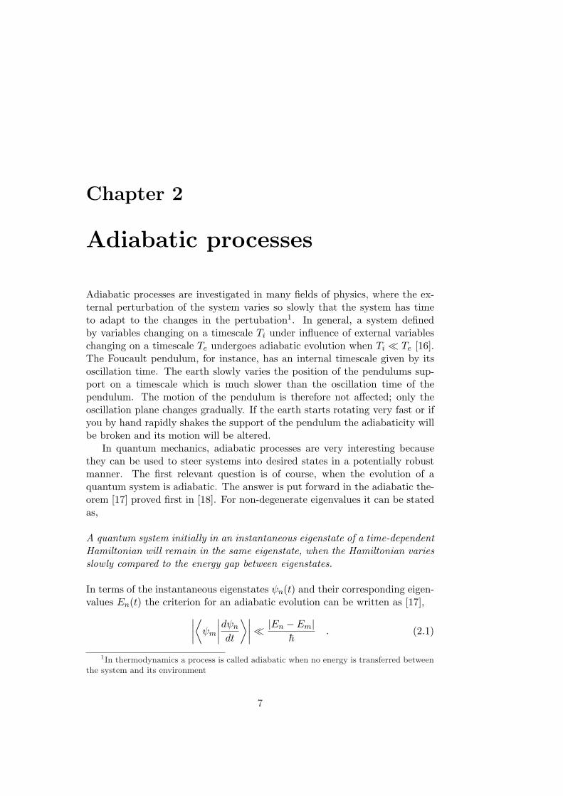
1.2 Outline
This concludes the brief introduction to quantum computation. The topic ofthe thesis is adiabatic processes and the advances they may bring to quantumcomputation. A system controlled by slowly varying external parameters hastime to adapt to the changes. A process fulfilling this is said to be adiabaticand in chapter 2 we will describe the concept of adiabaticity more preciselyand present a criterion for determining when a quantum process is adiabatic.Further more, the geometric phases acquired during an adiabatic evolution willbe defined and the adiabatic process used throughout this thesis, stimulatedRaman adiabatic passage (STIRAP), is described.
The first part of the thesis presents theoretical studies. Chapter 3 showshow the geometric phase acquired by a quantum system subject to STIRAPcan be used to create a universal set of quantum gates. In chapter 4 oneof these gates, the Hadamard gate, is considered when the quantum systemis open and therefore subject to dephasing. In chapter 5 we focus on aspecific implementation of quantum computation and describe how neutralatoms with a highly excited electron, so-called Rydberg atoms, can be usedfor quantum computation. We present a method to create two-qubit gates aswell as many-particle entanglement.
In the second part we turn to experimental studies and in chapter 6 an-other candidate for implementation of quantum computation, namely trappedlaser cooled ions, is presented. We describe a scheme for detection of internalspin states in 40Ca+. The detection scheme is based on two STIRAP pro-cesses and the experimental studies in chapter 7 and 8 show how one ofthese transfers population efficiently between two internal states. Chapter 7gives a view over the experimental setup and chapter 8 presents the results.
The main ideas and results of the thesis are summarised in the conclusionand Danish summary (Dansk resume) of chapter 9.

Chapter 2
Adiabatic processes
Adiabatic processes are investigated in many fields of physics, where the ex-ternal perturbation of the system varies so slowly that the system has timeto adapt to the changes in the pertubation1. In general, a system definedby variables changing on a timescale Ti under influence of external variableschanging on a timescale Te undergoes adiabatic evolution when Ti ¿ Te [16].The Foucault pendulum, for instance, has an internal timescale given by itsoscillation time. The earth slowly varies the position of the pendulums sup-port on a timescale which is much slower than the oscillation time of thependulum. The motion of the pendulum is therefore not affected; only theoscillation plane changes gradually. If the earth starts rotating very fast or ifyou by hand rapidly shakes the support of the pendulum the adiabaticity willbe broken and its motion will be altered.
In quantum mechanics, adiabatic processes are very interesting becausethey can be used to steer systems into desired states in a potentially robustmanner. The first relevant question is of course, when the evolution of aquantum system is adiabatic. The answer is put forward in the adiabatic the-orem [17] proved first in [18]. For non-degenerate eigenvalues it can be statedas,
A quantum system initially in an instantaneous eigenstate of a time-dependentHamiltonian will remain in the same eigenstate, when the Hamiltonian variesslowly compared to the energy gap between eigenstates.
In terms of the instantaneous eigenstates ψn(t) and their corresponding eigen-values En(t) the criterion for an adiabatic evolution can be written as [17],
∣∣∣∣⟨
ψm
∣∣∣∣dψn
dt
⟩∣∣∣∣ ¿|En − Em|
~. (2.1)
1In thermodynamics a process is called adiabatic when no energy is transferred betweenthe system and its environment
7

8 Adiabatic processes
When the eigenvalues are degenerate, adiabaticity only ensures that the sys-tem stays within the eigenspace of the initial eigenvalue. The evolution withinthis eigenspace is then derived by applying the Schrodinger equation as dis-cussed below.
2.1 Geometric phases
When the adiabatic criterion is fulfilled, the evolution of a quantum systemwith non-degenerate eigenvalues can be described by a following of the eigen-states and a calculation of the phases acquired by each eigenstate. In thedegenerate case we must calculate the evolution within the eigenspace pop-ulated. In both scenarios, two contributions can be distinguished. Dynamicphases which depend explicitly on the time evolution of the Hamiltonian andgeometric phases which depend on the geometry of the space spanned by thecontrolling parameters.
2.1.1 Non-degenerate eigenvalues
We first consider a system in an eigenstate ψn(t) corresponding to the non-degenerate eigenvalue En(t). The adiabatic theorem states that the systemwill remain in ψn(t), but may acquire a phase. One contribution to this is thedynamic phase, which is simply given by the time integral of the energy,
θn(t) = −1~
∫ t
ti
En(t′)dt′. (2.2)
For adiabatic processes an additional geometric phase contribution was broughtinto focus in 1984 by M. Berry [19]. Berry proved its existence by assumingthat a phase, γn(t), is acquired in addition to the dynamic one,
Ψ(ti) = ψn(ti) → Ψ(t) = ψn(t)ei(θn(t)+γn(t)). (2.3)
The evolution is given by the Schrodinger equation,
Hψnei(θn+γn) = i~d
dt
(ψnei(θn+γn)
)⇒
Enψnei(θn+γn) = (i~ψn − ~θnψn − ~γnψn)ei(θn+γn) ⇒Enψn = (i~ψn − ~θnψn − ~γnψn), (2.4)
where the dot denotes a derivative with respect to time. From (2.2) we findθn = −En/~ and (2.4) reduces to,
γnψn = iψn. (2.5)
Taking the inner product with ψn then yields,
γn = i〈ψn|ψn〉. (2.6)

2.1. Geometric phases 9
If the inner product 〈ψn|ψn〉 is non-zero an additional phase will be acquired.This phase is called Berry’s phase or the geometric phase, because the phasehas a geometric interpretation as seen from the following convenient rewriting:The time dependence of ψn(t) can be viewed as a dependence of time varyingparameters, R(t), controlling the Hamiltonian and we write ψn(R(t)). Thetime derivative is now expressed as,
∂ψn(R(t))∂t
= ∇RψndR
dt, (2.7)
and the phase is found by integrating (2.6),
γn(t) = i
∫ t
ti
〈ψn|∇Rψn〉∂R
∂t′dt′ = i
∫ R(t)
R(ti)〈ψn|∇Rψn〉dR. (2.8)
While the dynamic phase in (2.2) depends strongly on the elapsed time, theadditional phase γn, on the contrary, is independent of the time and only relieson the path traversed in the parameter space spanned by R(t). This geometricnature of Berry’s phase is particularly apparent for a cyclic evolution, wherethe system returns to the initial state after some time T and the geometricphase is a path integral around a closed loop,
γn(T ) = i
∮〈ψn|∇Rψn〉dR. (2.9)
The three dimensional cyclic geometric phase has a classical analogue,called the Hannay angle [20], acquired for instance by the Foucault pendulum.
q
Figure 2.1: Parallel transport of a pendulum oscillating in the direction of the redarrows around the blue cyclic route on the earth. Initially, the pendulum swings inthe direction of the light red arrow on the North Pole, but when it returns to theNorth Pole again it swings in the direction of the dark red arrow and the oscillationplane has been rotated an angle Θ = A/R2 defined by the enclosed area, A, and theradius of the earth, R.

10 Adiabatic processes
If we first imagine a pendulum swinging in some direction at the North Poleindicated by the light red arrow in Fig. 2.1 and then move its support aroundthe earth following for example the closed blue loop the oscillation plane willfollow the red arrows. When the pendulum returns to the North Pole it nolonger swing in its original plane - the oscillation plane is rotated an angledetermined by the area enclosed by the loop, or more precisely the solid anglesubtended. This is exactly an example of the Hannay angle [16]. The Foucaultpendulum does not move, but instead the earth rotates making the pendulumacquire a Hannay angle, rotating the oscillation plane of the pendulum.
2.1.2 Degenerate eigenvalues
For degenerate eigenvalues transfer may occur between eigenstates with thesame eigenvalue even when adiabaticity is maintained and the Berry phaseis replaced by a unitary transformation between the degenerate eigenstates[21, 22]. A system initially in the eigenspace spanned by eigenstates ψk cor-responding to the eigenvalue E will remain in the same eigenspace when theevolution is adiabatic and the wave function can be written,
Ψ = eiθ∑
k
ckψk, (2.10)
where all eigenstates acquire the same dynamic phase, θ. Inserting (2.10) intothe Schrodinger equation yields the evolution,
HΨ = i~Ψ ⇒eiθE
∑
k
ckψk =∑
k
eiθ(i~ckψk − ~θckψk + i~ψkck
)⇒ (2.11)
E∑
k
ckψk =∑
k
(i~ckψk + Eckψk + i~ψkck
)⇒
∑
k
ckψk =∑
k
−ψkck.
Taking the inner product with ψm gives the differential equations,
cm = −∑
k
ck
⟨ψm
∣∣∣ψk
⟩. (2.12)
The single phase acquired in the non-degenerate case derived in (2.6) is thusreplaced by a matrix connecting the initial and final state.
2.1.3 Geometric quantum computation
Geometric phases only depend on the path traversed in the parameter space.They are therefore expected to be less sensitive to noise than the dynamic

2.2. Stimulated Raman adiabatic passage 11
phases, but to what extend this holds true is still an open question. As anillustration we consider the closed loop phase (2.9) in the three dimensionalcase, where it can be rewritten as a surface integral,
γn(T ) = i
∫∇R × 〈ψn|∇Rψn〉da. (2.13)
The first thing to note is that the integral does not depend on the speed of theprocess. In addition, as long as the area enclosed is kept constant, the integralwill be insensitive to small variations in the path traversed. This leads to theconclusion that geometric phases are typically robust with respect to fluctua-tions in the controlling parameters [23,24]. Robustness against environmentalnoise leading to decoherence is less obvious and proof has only been given forcertain kinds of noises and systems [25,26].
The robust features of the geometric phases, anticipated by the theoret-ical investigations discussed above, may be used to improve the fidelities ofquantum gates. So-called geometric or holonomic quantum computation [27]is build of gates relying on geometric phases. Proposals for holonomic quan-tum computation is available in trapped ion [28–30], neutral atom [31], linearoptics [32], NMR [33] and solid state [34] systems. Experimentally, gateshave been implemented in ion traps [35], NMR [33] and super conductingsystems [36].
2.2 Stimulated Raman adiabatic passage
Stimulated Raman adiabatic passage (STIRAP) is a robust way of adiabati-cally transferring population from one quantum state to another and enablesus to make the transfer state selective, coherent and efficient. The adiabaticityalso ensures controllable geometric phases making STIRAP a promising toolfor creation of robust geometric gates in quantum computation. We presentthe STIRAP theory that will be used throughout the thesis as a basis for thegeometric gate suggestions as well as in a proposal for detection of the internalstate of a trapped ion. A thorough review of STIRAP was presented in [37].
2.2.1 STIRAP theory
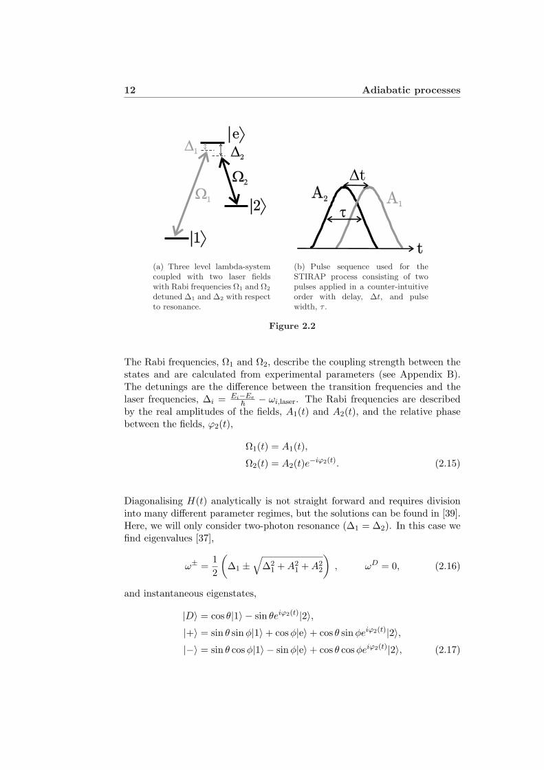
STIRAP is performed by application of two laser fields to a system with alambda level structure as shown in Fig. 2.2(a). Two coherent laser pulsestransfer the population from one quantum state, |1〉, via an intermediate state|e〉 to another state, |2〉. In the Rotating Wave Approximation (RWA) wecan express the instantaneous Hamiltonian of the system in the |1〉,|e〉,|2〉-basis [37,38] as
H(t) =~2
0 Ω∗1(t) 0Ω1(t) 2∆1 Ω2(t)
0 Ω∗2(t) 2(∆1 −∆2)
. (2.14)
12 Adiabatic processes
W1
W2
D1 D
2
>2
>1
>e
(a) Three level lambda-systemcoupled with two laser fieldswith Rabi frequencies Ω1 and Ω2
detuned ∆1 and ∆2 with respectto resonance.
Dt
t
A2 A
1
t
(b) Pulse sequence used for theSTIRAP process consisting of twopulses applied in a counter-intuitiveorder with delay, ∆t, and pulsewidth, τ .
Figure 2.2
The Rabi frequencies, Ω1 and Ω2, describe the coupling strength between thestates and are calculated from experimental parameters (see Appendix B).The detunings are the difference between the transition frequencies and thelaser frequencies, ∆i = Ei−Ee
~ − ωi,laser. The Rabi frequencies are describedby the real amplitudes of the fields, A1(t) and A2(t), and the relative phasebetween the fields, ϕ2(t),
Ω1(t) = A1(t),
Ω2(t) = A2(t)e−iϕ2(t). (2.15)
Diagonalising H(t) analytically is not straight forward and requires divisioninto many different parameter regimes, but the solutions can be found in [39].Here, we will only consider two-photon resonance (∆1 = ∆2). In this case wefind eigenvalues [37],
ω± =12
(∆1 ±
√∆2
1 + A21 + A2
2
), ωD = 0, (2.16)
and instantaneous eigenstates,
|D〉 = cos θ|1〉 − sin θeiϕ2(t)|2〉,|+〉 = sin θ sinφ|1〉+ cosφ|e〉+ cos θ sinφeiϕ2(t)|2〉,|−〉 = sin θ cosφ|1〉 − sinφ|e〉+ cos θ cosφeiϕ2(t)|2〉, (2.17)

2.2. Stimulated Raman adiabatic passage 13
with tan θ(t) = A1(t)A2(t) defining the mixing angle, θ, and tanφ =
√−ω−
ω+. |D〉
is called a dark state because it does not absorb or emit photons. In terms ofRabi frequencies the dark state reads,
|D(t)〉 =A2(t)√
A21(t) + A2
2(t)|1〉 − A1(t)√
A21(t) + A2
2(t)eiϕ2(t)|2〉. (2.18)
With all population initially in |1〉 and only field 2 applied we start out in |D〉.Changing the amplitudes of the fields A1(t) and A2(t) adiabatically ensuresthat all population remains in |D〉. Increasing A1(t) while decreasing A2(t)transfers the population from |1〉 to |2〉. A counter-intuitive pulse sequence,where the pulse of the second field arrives before the pulse of the first, is shownin Fig. 2.2(b) and does exactly as we request. If the evolution is not perfectlyadiabatic, population will be lost to |+〉 and |−〉 and therefore to the excitedstate |e〉, from where it could be lost due to spontaneous emission. To avoidthis diabatic transfer the adiabatic criterion (2.1) states that the couplingbetween |D〉 and |+〉 or |−〉 must be small compared to the energy-splittingof the states, ∣∣∣∣
⟨±
∣∣∣∣d
dt
∣∣∣∣D
⟩∣∣∣∣ ¿ |ω± − ωD|. (2.19)
The coupling,∣∣⟨± ∣∣ d
dt
∣∣D⟩∣∣, corresponds to
∣∣dθdt
∣∣ [40], which can be averagedfor smooth laser pulses to give [37],
∣∣∣∣dθ
dt
∣∣∣∣av
=π
2T(2.20)
where T is the duration of the pulse sequence from θ = 0 until θ = π/2.Combining (2.20) and (2.19) yields the criterion,
∣∣ω±∣∣T =12
∣∣∣∣∆± 12
√∆2
1 + A21 + A2
2
∣∣∣∣T À 1. (2.21)
The criterion can be fulfilled by many different pulse shapes and in this workwe use either Gaussian
A1(t) = A1,maxe−“
tτ/2
”2
(2.22)
A2(t) = A2,maxe−“
t+∆tτ/2
”2
or sin2 pulses
A1(t) =
A1,max sin2
(πt2τ
)if 0 < t < 2τ
0 otherwise(2.23)
A2(t) =
A2,max sin2
(π(t+∆t)
2τ
)if −∆t < t < 2τ −∆t
0 otherwise

14 Adiabatic processes
In both cases ∆t is the delay between the two pulses while the pulse width τis defined as the full width at 1/e of maximum for the Gaussian pulses andthe full width at half maximum (FWHM) for sin2 pulses.
2.2.2 Maintaining adiabaticity
Adiabatic processes are obtained by a large energy splitting and slowly varyingpulses. Fig. 2.3 considers two pulse sequences. One, where the peak Rabifrequencies are A1,max = A2,max/2π =20 MHz and the duration of the sequenceis T ≈12 µs (left column) and another with weaker Rabi frequencies A1,max =A2,max/2π =10 MHz, and shorter pulses with T ≈6 µs (right column). Thelaser fields are on resonance, the pulses are Gaussian and their time variationis shown in Fig. 2.3(a). The energy difference between the eigenvalues iscalculated directly from (2.16) with ∆1 = 0 and depends only on the Rabifrequency amplitudes. The splitting is halved when the Rabi frequencies arehalved as shown in Fig. 2.3(c). The shorter pulses influence the duration of thesequence and cause the slope of the mixing angle, θ, in Fig. 2.3(b) to becomesteeper. The splitting of the eigenvalues is smaller and the time variation isfaster in the right column implying that this situation is less adiabatic. Thisis also what we see when we propagate the Schrodinger equation and plotthe populations in the atomic states in Fig. 2.3(d). To the left no populationof |e〉 is visible, while the situation in the right column populates |e〉 slightlyand the transfer efficiency is reduced by a factor of 10−3. The violation ofadiabaticity is more apparent when we look at the population of the dark statein Fig. 2.3(e). We see that even though the diabatic transfer is present duringthe process, the population of the dark state is almost fully restored. If decayfrom |e〉 is introduced diabatic transfer to the bright states are more severe,because they decay and population of the dark state is no longer restored.
2.2.3 Adiabatic elimination
STIRAP can also be understood from adiabatic elimination of the excitedstate. The Schrodinger equation for the lambda system yields the differentialequations for the population amplitudes on two-photon resonance with realRabi frequencies,
c1 = −12Ω1ce,
ce = −12Ω1c1 − 1
2Ω2c2 + ∆1ce,
c2 = −12Ω2ce. (2.24)
Now assuming ce = 0 leads to
ce =(Ω1c1 + Ω2c2)
2∆1, (2.25)

2.2. Stimulated Raman adiabatic passage 15
0
5
10
15
20
0.0
0.2
0.4
0.6
0.8
1.0
-6 -4 -2 0 2 4 60.99
1.00
-10
-5
0
5
10
0
5
10
15
20
0.0
0.2
0.4
0.6
0.8
1.0
-6 -4 -2 0 2 4 60.99
1.00
-10
-5
0
5
10
A2
A1
A/2
[M
Hz]
P1
Pe
P2
Popula
tion o
fato
mic
sta
tes
PD
Popula
tion o
fdark
sta
te
t [ s]
(b)
(c)
(d)
(e)
(a)
/2
[M
Hz]
D
+
-
A2 A
1
A/(2
) [M
Hz]
Popula
tion
P1
Pe
P2
PD
Popula
tion
t [ s]
/2
[M
Hz]
D
+
-
0
/2
0
/2
Figure 2.3: Time evolution of the field amplitudes (panel (a)), the mixing angle(panel (b)), the eigenenergies (panel (c)), population in the atomic states (panel(d)), and population in the dark state (panel(e)). The left column shows results forparameters, A1,max = A2,max/2π =20 MHz, ∆t = 4.2 and τ = 4, while the rightcolumn shows results for parameters A1,max = A2,max/2π =10 MHz, ∆t = 2 andτ = 2.
16 Adiabatic processes
and substituting (2.25) into (2.24) yields,(
c1
c2
)= − 1
4∆1
(Ω2
1 Ω1Ω2
Ω1Ω2 Ω22
)(c1
c2
). (2.26)
Diagonalising (2.26) gives eigenvalues
ωB = − 14∆1
(Ω21 + Ω2
2) , ωD = 0, (2.27)
and corresponding eigenstates,
|D〉 = cos θ|1〉 − sin θ|2〉,|B〉 = sin θ|1〉+ cos θ|2〉, (2.28)
where θ is the mixing angle from the previous section. The dark state, |D〉,is exactly the dark state found from the full solution, while the bright state,|B〉, is the superposition of |+〉 and |−〉 of (2.17), where |e〉 is not populated,|B〉 = sinφ|+〉+cos φ|−〉. As long as adiabaticity is maintained using adiabaticelimination is a good approach, but as soon as we have some diabatic transferwe need to turn to the full solution to analyse the effect of populating thebright states.
2.3 Optimising the STIRAP efficiency
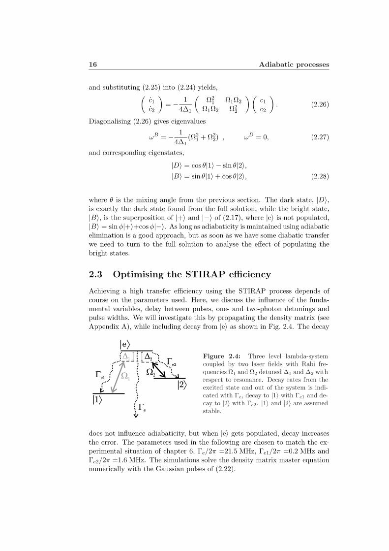
Achieving a high transfer efficiency using the STIRAP process depends ofcourse on the parameters used. Here, we discuss the influence of the funda-mental variables, delay between pulses, one- and two-photon detunings andpulse widths. We will investigate this by propagating the density matrix (seeAppendix A), while including decay from |e〉 as shown in Fig. 2.4. The decay
W1
W2
D1
D2
Ge
Ge1
Ge2
>e
>2
>1
Figure 2.4: Three level lambda-systemcoupled by two laser fields with Rabi fre-quencies Ω1 and Ω2 detuned ∆1 and ∆2 withrespect to resonance. Decay rates from theexcited state and out of the system is indi-cated with Γe, decay to |1〉 with Γe1 and de-cay to |2〉 with Γe2. |1〉 and |2〉 are assumedstable.
does not influence adiabaticity, but when |e〉 gets populated, decay increasesthe error. The parameters used in the following are chosen to match the ex-perimental situation of chapter 6, Γe/2π =21.5 MHz, Γe1/2π =0.2 MHz andΓe2/2π =1.6 MHz. The simulations solve the density matrix master equationnumerically with the Gaussian pulses of (2.22).

2.3. Optimising the STIRAP efficiency 17
2.3.1 Optimal pulse delay and width
The first parameter we investigate is the delay between the two pulses. Weshow the transfer efficiency as a function of ∆t for various peak Rabi fre-quencies A1,max = A2,max in Fig. 2.5. Both laser fields are on resonance. Fornegative delay corresponding to the intuitive pulse sequence, the pulse of field1 arrives first and may excite some population but when the pulse of field2 subsequently arrives the population is repumped from |2〉 and the transferefficiency is zero. When the pulses begin to overlap the Raman resonancecreated induces Rabi oscillations and the transfer efficiency increases. Forcounter-intuitive pulse sequences the transfer efficiency approaches 1 and anoptimal delay is reached at a value depending on the Rabi frequency. For largepositive delays the pulses are separated but the Ω1 pulse arrives last, and itcan therefore excite some population to |e〉, from where some will decay to |2〉explaining the plateau in Fig. 2.5. The efficiency at the plateau is determined
-1 0 1 2 3 4 50.0
0.2
0.4
0.6
0.8
1.0
A2 A
1A2
A1A
2A
1
Tra
nsf
er e
ffic
iency
t [ s]
Figure 2.5: Transfer efficiency as a function of delay between pulses for differ-ent choices of peak Rabi frequencies, A1,max/2π = A2,max/2π =10 MHz (—),A1,max/2π = A2,max/2π =20 MHz (—), A1,max/2π = A2,max/2π =100 MHz (—)and A1,max/2π = A2,max/2π =300 MHz (—). Positive delay corresponds to thecounter-intuitive pulse sequence, where the laser pulse of field 2 arrives before the laserpulse of field 1. The optimal delay is indicated by crosses. Parameters; τ1 = τ2 =2 µsand ∆1 = ∆2 = 0. The three pulse sequences on top illustrate the pulse positions atthe delays indicated by the small arrows.

18 Adiabatic processes
by the branching ratio between the different decay rates. The simulationsshow that for peak Rabi frequencies above A1,max/2π = A2,max/2π =100 MHzthe transfer efficiency is close to unity and insensitive to fluctuations in thedelay. For smaller Rabi frequencies the transfer efficiency decreases and thesensitivity to fluctuations in delay increases.
The crosses in Fig. 2.5 indicate the optimal delay for each Rabi frequencyand show that the optimal delay increases when the Rabi frequency increases.This is due to the tails of the Gaussian pulses and the finite simulation time.All population is transferred when θ = π/2 and for Gaussian pulses
tan θ =A1(t)A2(t)
=A1,maxe
−( tτ/2
)2
A2,maxe−( t+∆t
τ/2)2
=A1,max
A2,maxe
“∆t2+2t∆t
(τ/2)2
”. (2.29)
For a simulation terminated at some fixed time t = tf a larger ∆t implies θcloser to π/2 and therefore a higher transfer efficiency. On the other hand, alarge delay will make it more difficult to obtain adiabaticity, but this can becompensated by large Rabi frequencies. The optimal pulse delay is thereforethe largest possible not violating adiabaticity, favouring large delays for largeRabi frequencies. It should be noted, however, that inclusion of decoherencemechanisms as for example laser linewidth, tends to make the optimal delaysmaller.
A longer pulse width, will of course strengthen the adiabaticity, but inexperiments decoherence is also an issue imposing an upper limit on the timeused and therefore on the pulse widths. Choosing the pulse width will thusbe a trade-off between the effect of decoherence and diabatic transfer.
2.3.2 Laser detunings
In experiments one-photon excitations may reduce the efficiency and it isadvantageous to introduce large one-photon detunings to diminish this effect.We have simulated the effect in Fig. 2.6. It shows that increasing the one-photon detuning does not limit the transfer efficiency as long as we are close tothe two-photon resonance, ∆2−∆1 = 0, but also that this criterion gets stricteras we increase the one-photon detuning. If we require a transfer efficiencyabove 0.99 the demand on two-photon detuning is found from the green curveof Fig. 2.6 to be |∆2 −∆1| ≤ 2π × 0.5 MHz, when ∆1 = 2π × 1200 MHz. For∆1 = 2π× 600 MHz, maintaining a two-photon resonance within 2π× 1 MHzis sufficient as found from the red curve. An efficient transfer can in this waybe maintained in spite of a small drift from two-photon resonance.
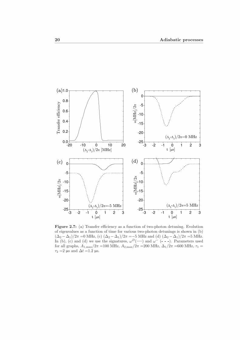
A closer look at Fig. 2.6 reveals that the spectra are not exactly symmetricwith respect to the sign of the two-photon detuning. With unbalanced Rabifrequencies, A2,max = 2A1,max, the asymmetry becomes more evident as seen inFig. 2.7(a). For small negative two-photon detunings the transfer efficiency ismuch higher than for the corresponding positive two-photon detunings. This

2.3. Optimising the STIRAP efficiency 19
-20 -10 0 10 200.0
0.2
0.4
0.6
0.8
1.0T
ransf
er e
ffic
iency
(2 1
)/2 [MHz]
Figure 2.6: Transfer efficiency as a function of two-photon detuning (∆2 − ∆1).The curves correspond to different one-photon detunings, ∆1/2π =0 MHz (—),∆1/2π =300 MHz (—), ∆1/2π =600 MHz (—) and ∆1/2π =1200 MHz (—). Pa-rameters, A1,max/2π = A2,max/2π =100 MHz, τ1 = τ2 =2 µs and ∆t =1.2 µs.
effect is due to diabatic transfer between |D〉 and the energetically closestbright state |−〉. As discussed previously, this is likely when |D〉 and |−〉 arenearly degenerate. The eigenvalues found in (2.16) are valid only on two-photon resonance. A more complicated general expression for the eigenvalueshas as mentioned been derived in [39] and is plotted in Fig. 2.7(b-d), wherewe show the eigenvalues of |D〉 (solid curves) and |−〉 (dashed curves) as afunction of time for three different choices of two-photon detuning. In thecase where ∆2 −∆1 = 0 MHz (Fig. 2.7(b)) the eigenvalues of course coincidewhen the Rabi frequencies are zero before and after the pulses, but in thiscase no diabatic transfer will occur as no coupling is present. For a positivetwo-photon detuning, (∆2−∆1)/2π = 5MHz ( Fig. 2.7(d)), we see an avoidedcrossing leading to a probability for diabatic transfer to the |−〉-state. Sucha transfer leads to population of the |e〉-state which decays rapidly. For anegative two-photon detuning, (∆2 − ∆1)/2π = −5MHz in Fig. 2.7(c), anenergy splitting of |D〉 and |−〉 is present through the whole evolution andthe probability for diabatic transfer is much smaller. It is this difference thatgives rise to the asymmetry of the two-photon spectrum in Fig. 2.7(a).
20 Adiabatic processes
-3 -2 -1 0 1 2 3-25
-20
-15
-10
-5
0
-3 -2 -1 0 1 2 3-25
-20
-15
-10
-5
0
-3 -2 -1 0 1 2 3-25
-20
-15
-10
-5
0
-20 -10 0 10 200.0
0.2
0.4
0.6
0.8
1.0
[MH
z]/2
t [ s] t [ s]
(2-
1)/2 =-5 MHz (
2-
1)/2 =5 MHz
(d)(c)
(b)(a)
(2-
1)/2 =0 MHz
[MH
z]/2
t [ s]
[MH
z]/2
Tra
nsf
er e
ffic
iency
(2-
1)/2 [MHz]
Figure 2.7: (a) Transfer efficiency as a function of two-photon detuning. Evolutionof eigenvalues as a function of time for various two-photon detunings is shown in (b)(∆2−∆1)/2π =0 MHz, (c) (∆2−∆1)/2π =−5 MHz and (d) (∆2−∆1)/2π =5 MHz.In (b), (c) and (d) we use the signatures, ωD(—) and ω− (- - -). Parameters usedfor all graphs, A1,max/2π =100 MHz, A2,max/2π =200 MHz, ∆1/2π =600 MHz, τ1 =τ2 =2 µs and ∆t =1.2 µs.

2.4. Summary 21
2.4 Summary
In quantum mechanics adiabaticity can be used to ensure that a system remainin some desired eigenstate. STIRAP is a well-documented method for popula-tion transfer between selected states in a robust manner. Small fluctuations inthe controlling parameters do not influence the efficiency and the variables (de-tuning, pulse width and delay between pulses) discussed above can be chosensuch that perfect transfer is achieved as shown in chapter 2.3. Unfortunatelythey are not the only variables to be considered in experiments. The atomwill move, the phase of the laser will fluctuate, light might be present beforeand after the STIRAP process due to imperfect shutters, and external fieldscould influence the process. In chapter 7 and 8 we discuss these experimentallimitations in relation to the work with trapped ions.
In this chapter we have only considered STIRAP for population transfer,but the adiabatic processes also have the nice feature that eigenstates acquirecontrollable geometric phases that are expected to be robust with respect toparameter fluctuations and certain kinds of noise as discussed in chapter 2.1.3.In chapter 3 and 5 we utilise the geometric phases acquired in a STIRAPprocess to create robust entanglement and quantum gates. In chapter 4 wetake a closer look at one of the gates, when decoherence is present.

Chapter 3
Geometric phase gates
Quantum gates based on geometric phases can be employed to improve therobustness of quantum computation. In order to create a desired controllablegeometric phase the system must undergo an adiabatic evolution, preferablein a dark state with eigenenergy zero such that no dynamic phase is acquired.One suitable candidate fulfilling these requirements is STIRAP where thesystem evolves adiabatically in the dark state found in (2.17). We show howthis dark state acquires a geometric phase, which is used to create a one-qubitphase gate. We present a complete set of gates based on similar dark statesacquiring geometric phases. The work described here was published in [II].
3.1 Geometric phase and STIRAP
As discussed in chapter 2.2, STIRAP can be described as a rotation of theadiabatic dark state in the |1〉, |e〉, |2〉 basis for the lambda system,
|D(t)〉 = cos θ(t)|1〉 − sin θ(t)eiϕ2(t)|2〉, (3.1)
where tan θ = A1A2
is the fraction of the two Rabi frequency amplitudes and ϕ2
the relative phase between the two laser fields as defined in (2.15). Initially(cos θ = 1 and |ψ(ti)〉 = |1〉), only |D〉 is populated and in the adiabaticlimit all population remains in the |D〉-state through the whole process. Thedark state has zero energy eigenvalue and hence does not acquire any dynamicphase, but may acquire a geometric phase γ1(t), and we can write the wavefunction as
|ψ(t)〉 = eiγ1(t)|D(t)〉. (3.2)
In order to find the geometric phase we apply Berry’s formula (2.8),
γ1 = i
∫ Rf
Ri
〈D|∇R|D〉 · dR, (3.3)
23
24 Geometric phase gates
with R-vector, R =(
θϕ2
). We find the gradient of the dark state
∇R|D〉 =(− sin θ|1〉 − cos θeiϕ2 |2〉
− sin θieiϕ2 |2〉)
, (3.4)
calculate the inner product
〈D|∇R|D〉 =(
0i sin2 θ
)⇒ 〈D|∇R|D〉 · dR = i sin2 θdϕ2, (3.5)
and find the geometric phase
γ1(t) = −∫ ϕ2(t)
ϕ2(ti)sin2 θdϕ2. (3.6)
This yields the wave function
ψ(t) = eiγ1(t)|D(t)〉 = eiγ1(t) cos θ(t)|1〉 − ei(γ1(t)+ϕ2(t)) sin θ(t)|2〉,
which after the whole STIRAP pulse sequence (sin θ = 1) simply reads
ψ(tf ) = −ei(γ1(tf )+ϕ2(tf ))|2〉.
3.2 Geometric phase gates
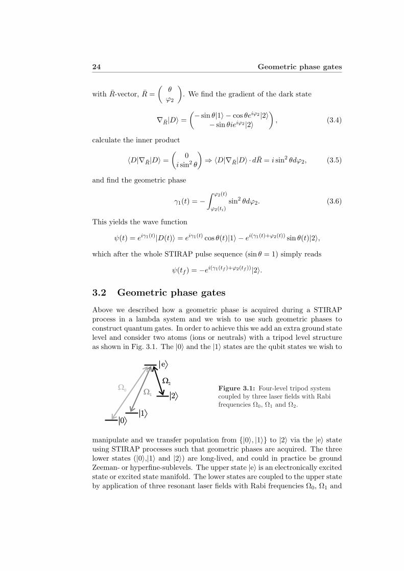
Above we described how a geometric phase is acquired during a STIRAPprocess in a lambda system and we wish to use such geometric phases toconstruct quantum gates. In order to achieve this we add an extra ground statelevel and consider two atoms (ions or neutrals) with a tripod level structureas shown in Fig. 3.1. The |0〉 and the |1〉 states are the qubit states we wish to
W1
W2
W0
>2
>1
>e
>0
Figure 3.1: Four-level tripod systemcoupled by three laser fields with Rabifrequencies Ω0, Ω1 and Ω2.
manipulate and we transfer population from |0〉, |1〉 to |2〉 via the |e〉 stateusing STIRAP processes such that geometric phases are acquired. The threelower states (|0〉,|1〉 and |2〉) are long-lived, and could in practice be groundZeeman- or hyperfine-sublevels. The upper state |e〉 is an electronically excitedstate or excited state manifold. The lower states are coupled to the upper stateby application of three resonant laser fields with Rabi frequencies Ω0, Ω1 and
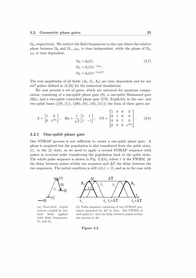
3.2. Geometric phase gates 25
Ω2, respectively. We restrict the Rabi frequencies to the case where the relativephase between Ω0 and Ω1, ϕ01, is time independent, while the phase of Ω2,ϕ2, is time dependent,
Ω0 =A0(t), (3.7)
Ω1 =A1(t)e−iϕ01 ,
Ω2 =A2(t)e−iϕ2(t).
The real amplitudes of all fields (A0, A1, A2) are time dependent and we usesin2-pulses defined in (2.23) for the numerical simulations.
We now present a set of gates, which are universal for quantum compu-tation, consisting of a one-qubit phase gate (S), a one-qubit Hadamard gate(Ha), and a two-qubit controlled phase gate (CS). Explicitly in the one- andtwo-qubit bases (|0〉, |1〉, |00〉, |01〉, |10〉, |11〉) the form of these gates are
S =[1 00 eiφ1
], Ha =
1√2
[1 11 −1
], CS =
1 0 0 00 1 0 00 0 1 00 0 0 eiφ2
. (3.8)
3.2.1 One-qubit phase gate
One STIRAP process is not sufficient to create a one-qubit phase gate. Aphase is acquired but the population is also transferred from the qubit state,|1〉, to the |2〉 state, so we need to apply a second STIRAP sequence withpulses in reversed order transferring the population back to the qubit state.The whole pulse sequence is shown in Fig. 3.2(b), where τ is the FWHM, ∆tthe delay between pulses within one sequence and ∆T the delay between thetwo sequences. The initial condition is still ψ(ti) = |1〉 and as in the case with
W1
W2
>2
>1
>e
>0
(a) Four-level tripodsystem coupled by twolaser fields appliedwith Rabi frequenciesΩ1 and Ω2.
t
Dt
t
A2
A2 A
1
DT
ta t
bt
a+DT t +DT
b
A1
(b) Pulse sequence consisting of two STIRAP pro-cesses separated by ∆T in time. The FWHM ofeach pulse is τ and the delay between pulses withinone process is ∆t.
Figure 3.2
26 Geometric phase gates
one sequence the wave function is as derived above
ψ(t) = eiγ1(t)|D(t)〉 = eiγ1(t) cos θ(t)|1〉 − ei(γ1(t)+ϕ2(t)) sin θ(t)|2〉, (3.9)
but now the final state after the whole pulse sequence is
ψ(tf ) = eiγ1 |1〉. (3.10)
This corresponds to a one-qubit phase gate |1〉 → eiγ1 |1〉 and the geometricphase is integrated over the whole pulse sequence from ti = ta to tf = tb +∆T
γ1 = −∫ ϕ2(tb+∆T )
ϕ2(ta)sin2 θ(t)dϕ2(t), (3.11)
where
sin2 θ(t) =A2
1(t)A2
1(t) + A22(t)
. (3.12)
The integral in (3.11) can be solved analytically when we assume that all fourpulses are described by the common function A(t). The instants of time ta andtb in Fig. 3.2(b) are defined such that sin2 θ(t) ≈ 0 for t < ta and t > tb + ∆Tand sin2 θ(t) ≈ 1 for tb < t < ta + ∆T . With these definitions we obtain from(3.11) and (3.12)
γ1 =−∫ ϕ2(tb)
ϕ2(ta)
A2(t)A2(t) + A2(t + ∆t)
dϕ2 (3.13)
−∫ ϕ2(ta+∆T )
ϕ2(tb)1dϕ2
−∫ ϕ2(tb+∆T )
ϕ2(ta+∆T )
A2(t + ∆t−∆T )A2(t + ∆t−∆T ) + A2(t−∆T )
dϕ2.
Substituting t′ = t−∆T in the last integral and assuming that ϕ2 is a mono-tonic function we obtain
γ1 =−∫ tb
ta
A2(t)A2(t) + A2(t + ∆t)
dϕ2
dtdt (3.14)
−∫ ta+∆T
tb
dϕ2
dtdt
−∫ tb
ta
A2(t′ + ∆t)A2(t′ + ∆t) + A2(t′)
dϕ2
dtdt′
=−∫ ta+∆T
ta
dϕ2
dtdt = ϕ2(ta)− ϕ2(ta + ∆T ).
The geometric phase thus only depends on the laser field phases and requirescontrol of ∆T and similarity of the four pulses. All these quantities are rou-tinely controlled to high precision in present-day laboratories. The population

3.2. Geometric phase gates 27
0.0
0.2
0.4
0.6
0.8
1.0
-1 0 1 2 3 4 5 6 7
Pulses
Population
0
-
/2
- /2Phases
t/
Figure 3.3: The centre panel shows the evolution of the population in states |1〉(black), |e〉 (red), and |2〉 (blue). The lower panel shows the evolution of the phases,φ1 of state |1〉 (grey, black) and φ2 of state |2〉 (cyan, blue). Analytical resultsare shown with cyan or grey curves and numerical with blue or black curves. Thenumerically calculated phases are only shown when the corresponding population isnon-zero. The calculations were made with sin2-pulses, Eq. (2.23), and parametersin units of the pulse width τ , ϕ2 = t/τ , Amax,1τ/2π = Amax,2τ/2π = 100, ∆t/τ = 1,∆T/τ = 5.
and the phases of the three states |1〉, |e〉 and |2〉 can be found numerically bysolving the time-dependent Schrodinger equation (See details in appendix A).An example of this is shown in the centre panel of Fig. 3.3. All population isinitially in the |1〉-state (black curve). During the first STIRAP-process thepopulation is transferred from |1〉 to |2〉 (blue curve) while the second STIRAP-process transfers the population back to |1〉. The |e〉-state (red curve) is neverpopulated and hence no loss of population occurs due to spontaneous emis-sion from |e〉. The evolution of the phases can be found numerically as wellas analytically, as shown with the cyan/grey and the blue/black curves in thelower panel of Fig. 3.3. In the time-spans where the states in question arepopulated, the direct numerical solution of the time-dependent Schrodingerequation gives results for the phases in agreement with the above analyticalresults. The grey curve shows the phase of |1〉, φ1. This phase is the geomet-ric phase (φ1 = γ1) and it remains zero until the first set of STIRAP pulsesarrive (ta in Fig. 3.2(b)). It then accumulates a phase until the second pair

28 Geometric phase gates
of pulses has passed (tb + ∆T in Fig. 3.2(b)). The total acquired phase is asshown in (3.14), γ1 = ϕ2(ta) − ϕ2(ta + ∆T ). The phase of the |2〉-state (φ2)(cyan curve) contains not only the geometric phase γ1 but also the additionalϕ2 − π [see Eq. (3.1)] yielding a total phase φ2 = γ1 + ϕ2 − π. The |2〉-statetherefore accumulates a phase before the first and after the second STIRAPprocess -but none in between where γ1 and ϕ2 cancel each other.
3.2.2 Hadamard gate
Creating a Hadamard gate takes a little more effort than the one-qubit phasegate but relies on the same principles now involving two dark states. It isimplemented using all three laser fields with Rabi frequencies Ω0, Ω1 and Ω2 asdefined in (3.7) and shown in Fig. 3.4(a). In the rotating wave approximation
W1
W2
W0
>2
>1
>e
>0
(a) Four-level tripodsystem coupled bythree laser fields withRabi frequencies Ω0,Ω1 and Ω2.
t
Dt
t
A2
A2 A
1
DT
ta t
bt
a+DT t +DT
b
A1
A0
A0
(b) Pulse sequence consisting of two STIRAP pro-cesses separated by ∆T in time. The FWHM ofeach pulse is τ and the delay between pulses withinone process is ∆t.
Figure 3.4
we derive the Hamiltonian
H(t) =~2
0 0 A0(t) 00 0 A1(t)eiϕ01 0
A0(t) A1(t)e−iϕ01 0 A2(t)e−iϕ2(t)
0 0 A2(t)eiϕ2(t) 0
(3.15)
expressed in the |0〉, |1〉, |e〉, |2〉 basis. We parameterise the complex Rabifrequencies
Ω0(t) = sin θ01
√A0(t)2 + A1(t)2, (3.16)
Ω1(t) = cos θ01
√A0(t)2 + A1(t)2e−iϕ01 , (3.17)
Ω2(t) = cos θH(t)√
A0(t)2 + A1(t)2 + A2(t)2e−iϕ2(t), (3.18)
where the two angles are defined as tan θ01 = A0(t)/A1(t) and tan θH(t) =√A2
0(t) + A21(t)/A2(t). A diagonalisation of (3.15) gives the four energy eigen-
valuesω± = ±1
2
√A2
0 + A21 + A2
2 , ωDi = 0 (i = 1, 2), (3.19)

3.2. Geometric phase gates 29
and eigenvectors
|+〉 =1√2
[sin θH(t)(sin θ01|0〉+ cos θ01e
iϕ01 |1〉)− |e〉+ cos θH(t)eiϕ2(t)|2〉],
|−〉 =1√2
[sin θH(t)(sin θ01|0〉+ cos θ01e
iϕ01 |1〉) + |e〉+ cos θH(t)eiϕ2(t)|2〉],
|D1〉 = − cos θH(t)(sin θ01|0〉+ cos θ01eiϕ01 |1〉) + sin θH(t)eiϕ2(t)|2〉, (3.20)
|D2〉 = cos θ01|0〉 − sin θ01eiϕ01 |1〉.
We assume that the system is initially (t = ti) in a superposition of the darkstates and that the evolution is adiabatic. Then the population stays withinthe space spanned by the two dark states and the wave function at later timesis given by
|D(t)〉 = CD1(t)|D1(t)〉+ CD2(t)|D2(t)〉. (3.21)
In order to determine the time evolution of the coefficients CD1(t), CD2(t)we use the method for degenerate eigenvalues described in chapter 2.1.2. Thetime evolution is given by the Schrodinger equation i~|D(t)〉 = H(t)|D(t)〉 = 0and yields two coupled differential equations
CD1 = −CD1〈D1|D1〉 − CD2〈D1|D2〉, (3.22)
CD2 = −CD1〈D2|D1〉 − CD2〈D2|D2〉.
Only one coefficient is non-zero, 〈D1|D1〉 = iϕ2 sin2 θH and hence the differ-ential equations just read
CD1 = −iϕ2 sin2 θHCD1 (3.23)
CD2 = 0,
yielding the simple evolution
CD1(t) = eiγH CD1(ti), (3.24)CD2(t) = CD2(ti).
The phase
γH = −∫ t
ti
ϕ2 sin2 θHdt′, (3.25)
acquired by |D1〉 is purely geometric because the dark states do not acquireany dynamic phases, ωDi = 0. Since no population is transferred between thetwo dark states the geometric phase acquired by |D1〉 could also be calculatedusing Berry’s original formula (2.8). This approach was used in Refs. [22] and[II].

30 Geometric phase gates
The geometric phase is only acquired by one of the dark states and it cantherefore be used to control the superposition
|D(t)〉 = eiγH CD1(ti)|D1(t)〉+ CD2(ti)|D2(t)〉. (3.26)
For the Hadamard gate, like for the one-qubit gate, the pulse sequence con-sists of two STIRAP processes, but this time with both Ω0 and Ω1 appliedsimultaneous with different amplitudes as shown in Fig. 3.4(b). This createsa constant θ01, while θH is varied according to
cos θH(t) =A2(t)√
A0(t)2 + A1(t)2 + A2(t)2. (3.27)
Initially, with all population in |0〉 or |1〉 and cos θH = 1 only the dark statesare populated [See Eq. (3.20)]. The first set of pulses transfers populationpartially from |0〉 and |1〉 to |2〉 while the second transfers all population backto |0〉 and |1〉. Only population in |D1〉 will be transferred, while |D2〉 isunaffected. After the whole pulse sequence (sin θH = 1) the system ends upin the final state
|D(tf )〉 =CD1(ti)eiγH(tf )|D1(tf )〉+ CD2(ti)|D2(tf )〉 (3.28)
=[− sin θ01CD1(ti)eiγH(tf ) + cos θ01CD2(ti)]|0〉
+ [− cos θ01CD1(ti)eiγH(tf ) + sin θ01CD2(ti)]|1〉,
where we have used (3.20) in the second line. In the |0〉, |1〉-basis, an initialstate |ψi〉 = ai|0〉+ bi|1〉 is transferred to a final state |ψf 〉 = af |0〉+ bf |1〉 =U |ψi〉, with the unitary transformation
U =[
cos2 θ01 + eiγH sin2 θ01 cos θ01 sin θ01e−iϕ01(eiγH − 1)
cos θ01 sin θ01eiϕ01(eiγH − 1) sin2 θ01 + eiγH cos2 θ01
]. (3.29)
By carefully adjusting the amplitudes and phases of the laser fields, the val-ues of θ01, ϕ01 and γH can be controlled and thus generate rotations in the|0〉, |1〉-basis. We note that U is the identity when no geometric phase isacquired, γH = 0. As a special case θ01 = π
8 , φ01 = π and γH = −π implementa Hadamard gate
U =1√2
[1 11 −1
]. (3.30)
More specifically, θ01 = π8 can be obtained by choosing the relative laser
field strengths such that Amax,0 = Amax,1(√
2− 1). Furthermore, Amax,2 =√A2
max,0 + A2max,1, ϕ2 = t/τ and ∆T/τ = π assure γH = −π.

3.2. Geometric phase gates 31
3.2.3 Two-qubit phase gate
STIRAP processes are well suited for creating arbitrary one-qubit rotations,but quantum computation requires gates acting on two or more qubits andthese are typically more difficult to implement because they necessitate acontrollable coupling between the qubits. We consider a coupling E|22〉〈22|between two atoms with the tripod level structure shown in Fig. 3.5. We apply
W1
W2
W1
W2
>
>
>
>0 b
1b
2b
eb
>
>
>
>0 a
1a
2a
ea
Figure 3.5: Two atoms with a four-level tripod structure with two laser fields appliedwith Rabi frequencies Ω1 and Ω2.
only two laser fields Ω1 and Ω2, assume no relative phase between the two Rabifrequencies and without loss of generality write them as real, Ω1 = A1 andΩ2 = A2. The Hamiltonian in the two atomic basis |ji〉 = |j〉a|i〉bj,i=0,1,e,2
reads
H =− ~2Ω1 [(|1〉a〈e|+ |e〉a〈1|)⊗ Ib + Ia ⊗ (|1〉b〈e|+ |e〉b〈1|)] (3.31)
− ~2Ω2 [(|2〉a〈e|+ |e〉a〈2|)⊗ Ib + Ia ⊗ (|2〉b〈e|+ |e〉b〈2|)]
+ E|2〉a|2〉b〈2|a〈2|.
In order to solve (3.31) it is advantageous to go into the interaction picturewith respect to the coupling term in the Hamiltonian, H0 = E|22〉〈22|. Herethe Hamiltonian is solved analytically yielding eigenvalues
ω =
0 multiplicity 62√
Ω21 + Ω2
2 multiplicity 4−2
√Ω2
1 + Ω22 multiplicity 4√
Ω21 + Ω2
2 multiplicity 1−
√Ω2
1 + Ω22 multiplicity 1
, (3.32)

32 Geometric phase gates
and an orthonormal basis for the 6-dimensional null space,
|D1〉 = |00〉,|D2〉 = − cos θ|10〉+ sin θ|20〉,|D3〉 = − cos θ|01〉+ sin θ|02〉, (3.33)
|D4〉 = 1/√
2(sin θ(|1e〉 − |e1〉) + cos θ(|2e〉 − |e2〉)),|D5〉 = cos2 θ|11〉 − sin θ cos θ(|12〉+ |21〉) + sin2 θeiEt|22〉,|D6〉 = 1/
√2(− sin2 θ|11〉 − sin θ cos θ(|12〉+ |21〉) + |ee〉 − cos2 θeiEt|22〉),
where tan θ = A1A2
. We note that |D2〉 and |D3〉 are exactly the single atomdark states used for the one-qubit phase gate. With six degenerate stateswe once more use the method of chapter 2.1.2. We assume that we startwith all population in |11〉, only Ω2 applied (cos θ = 1) and write ψ(ti) =|D5(ti)〉. Initially, the Schrodinger and the interaction picture coincides andhence ψI(ti) = ψ(ti), where I indicates the interaction picture. We assumean adiabatic evolution and hence no population transfer between the six darkstates and the bright states will occur. The interaction picture wave functionat later times is
|DI(t)〉 =∑
b
Bb(t)|Db(t)〉. (3.34)
The time evolution of the coefficients is given by the Schrodinger equation
|DI(t)〉 =−i
~(H(t)−H0(t))|DI(t)〉 ⇒
∑
b
Bb(t)Db(t)〉+ Bb(t)|Db(t)〉 =−i
~∑
b
Bb(t)(H(t)−H0(t))|Db(t)〉 = 0 ⇒∑
b
Bb(t)|Db(t)〉 = −∑
b
Bb(t)|Db(t)〉, (3.35)
where we have used that [H(t)−H0(t)]|Db(t)〉 = 0 for all dark states. Takingthe inner product with 〈Dc(t)| gives the coupled differential equations,
Bc(t) = −∑
b
Bb(t)〈Dc(t)|Db(t)〉. (3.36)

3.2. Geometric phase gates 33
The only non-zero 〈Dc|Db〉-elements are,
〈D5|D5〉 = iE sin4 θ, (3.37)
〈D5|D6〉 =i√2E cos2 θ sin2 θ,
〈D6|D5〉 =i√2E cos2 θ sin2 θ,
〈D6|D6〉 =i
2E cos4 θ,
and the differential equations for the B-coefficient reduce to,
B1 = 0, B2 = 0, B3 = 0, B4 = 0, (3.38)
B5 = −iE sin4 θB5 − i√2E cos2 θ sin2 θB6,
B6 = − i√2E cos2 θ sin2 θB5 − i
12E cos4 θB6.
All population is initially in |D5〉 and (3.38) shows that only when cos2 θ sin2 θis non-vanishing, population can be transferred from |D5〉 to |D6〉. Keepingthe time when cos2 θ sin2 θ 6= 0 short ensures that effectively all populationstays in |D5〉 while accumulating a phase. In this regime where B6(t) ≈ 0 wemay readily solve (3.38) and obtain the wave function
|DI(t)〉 =e−iE
R tti
sin4 θdt|D5〉 (3.39)
= cos2 θe−iE
R tti
sin4 θdt|11〉− sin θ cos θe
−iER t
tisin4 θdt(|12〉+ |21〉)
+ sin2 θe−iE
R tti
sin4 θdt+iEt|22〉.
Going back to the Schrodinger picture an extra phase is added to the |22〉state,
|D〉 =e−iE|22〉〈22|t|DI〉 (3.40)
=e−iE
R tti
sin4 θdt[cos2 θ|11〉 − sin θ cos θ(|12〉+ |21〉) + sin2 θ|22〉].
We stay in |D5〉 during the whole sequence acquiring the geometric phase
γ2 = −E
∫ t
−∞sin4 θdt, (3.41)

34 Geometric phase gates
and the two STIRAP sequences thus transfers |11〉 → eiγ2 |11〉. When only oneatom is in the |1〉-state the evolution is exactly as described for the one-qubitphase gate, but here no geometric phase is accumulated because the phases ofthe laser fields are kept fixed (ϕ2 = 0), i.e.,
|00〉 → |00〉 (3.42)|01〉 → |01〉|10〉 → |10〉|11〉 → eiγ2 |11〉.
Maintaining adiabaticity limits our choice of parameters and now we addition-ally need to ensure a small population transfer to |D6〉. In order to achievethis we need to keep
∫E cos2 θ sin2 θdt small. On the other hand we wish to
acquire a geometric phase γ2 = −E∫ t−∞ sin4 θdt. Fortunately, these require-
ment are not contradictory because γ2 is mainly acquired between the two setof pulses, where sin4 θ = 1, while cos2 θ sin2 θ is only non-zero during the over-lap of pulses. Therefore the smallest pulse width not violating adiabaticityshould be used. For this pulse width the optimal delay, ∆t, will be a trade off.A large delay will decrease the time where cos2 θ sin2 θ is non-zero, but makeit more difficult to maintain adiabaticity. With an optimal pulse delay, E and∆T must be chosen such that
∫E cos2 θ sin2 θdt is small while γ2 ≈ E∆T is
equal to, e.g., π. This will be a trade off between fidelity and gate time. Asan example the parameters Amax,iτ/2π = 100, ∆t/τ = 1.35, ∆T/τ = 2.7,Eτ/2π = 0.1 lead to a phase γ2 = π and a fidelity |〈D(tf )|ψ(tf )〉|2 = 0.99,where |ψ(tf )〉 was found propagating the Schrodinger equation with initialstate |11〉 and projected onto the idealised final state |D(tf )〉 = eiγ2 |11〉. Thesimulations are made with decay rate Γeτ/2π = 1 in order to enhance theeffect of population transfer to |D6〉 populating |e〉.
The two-qubit gate exploits the small energy shift, when two particlesoccupy the same state, to create a conditional geometric phase. Alternatively,a large energy shift could have been employed to block certain states frombeing populated and hence alter the dark states followed by the system steeringit through different dark states depending on the number of particles present.The different dark states acquire different geometric phases and thus a phasegate is achieved. This method is explored in chapter 5.
3.2.4 Experimental realisation
The one-qubit gates are implemented choosing an atom with three stablestates and one excited state. The demands for laser and pulse sequence pa-rameters are basically the same as for a single STIRAP process described inchapter 2.3. In addition the relative phase of the two laser fields needs to becontrolled. This could be achieved implementing the gates in systems where
3.2. Geometric phase gates 35
the three laser frequencies lie so close that all fields can be generated from thesame source and hence the relative phases of the fields are easily controllable.Encoding |0〉, |1〉, |2〉 in atomic Zeeman- or hyperfine-substates would fulfilthis. These requirements can be achieved in various atomic systems such asoptically trapped neutral atoms, trapped ions and rare-earth ions doped intocrystals.
To provide the coupling E|22〉〈22| for the two-qubit gate we need to bea little more specific, and we suggest in the case of trapped atoms or ionsto exploit the long-range dipole-dipole interaction between Rydberg excitedatoms [41] (described in chapter 5) and in the case of doped crystals to use theinteraction between excited states with permanent dipole moments [42]. Howto use this interaction to create E|22〉〈22| is an open question. One suggestioncould be to apply an off-resonant laser field between |2〉 and an excited statewith large dipole moment. As shown in [43], this off-resonant excitation causesenergy shifts (AC Stark shifts) of the |2〉 states, and due to the dipole-dipoleinteraction, this shift will have a non-separable component of precisely thedesired form for suitable choices of the laser detunings and strengths. Theproblem with this approach is that in order to create a sufficiently large energyshift without populating the excited state the interaction time must be verylong because the interaction is off-resonant.
Decoherence due to spontaneous emission from the upper state |e〉 is negli-gible, because all population transfers are done without populating this state,with the possible exception of the undesirable population of |D6〉 for the two-qubit gate. Other decoherence mechanisms could influence the gates and toavoid this fast processes are preferable. The exact values depend on the sys-tem. With trapped ions, Rabi frequencies of some hundred MHz are easilyachievable and the adiabatic gates can be performed in a few microseconds.On this timescale decoherence will not limit the STIRAP efficiency as shownexperimentally as well as theoretically [I, III]. In neutral atoms interactingvia Rydberg excited state dipole moments, Rabi frequencies may exceed MHz.A dephasing time of 870 µs between two hyperfine states in Rubidium atomsin an optical dipole trap was measured using Ramsey spectroscopy [44] andalso here decoherence is not expected to be a limiting factor for the proposedgates. This is supported by an experiment where population was transferredefficiently in Rydberg atoms using adiabatic passage [45]. Rare-earth-ionshave coherence lifetimes exceeding ms and also here adiabatic transfer wasdemonstrated with pulses well below ms [46,47]. In chapter 4 we show how adephasing will affect the geometric phases and the fidelity of the Hadamardgate.

36 Geometric phase gates
3.3 Conclusion
We have shown that in the adiabatic limit population transfer in tripod sys-tems introduces purely geometric phases. These phases can be used to forma set of robust geometric gates. The performance of the three gates dependson the robustness of the geometric phases. The population transfers are donewithout ever populating the upper state |e〉 in the tripod system, which ensuresthat the gates are insensitive to spontaneous emission and STIRAP allows forsome fluctuations in the controlling parameters. Pulse shapes, delay betweensequences and ratio between Rabi frequencies are routinely controlled exper-imentally without drift in the laboratory and using systems where the threelaser fields are generated from the same source, the relative laser phases arealso controllable.
In the two-qubit gate the product of the coupling strength, E, and thetime when the pulses overlap must be kept small, while the product of E andthe time spent between pulse pairs should yield the desired phase. This im-plies that the latter time interval must be an order of magnitude longer thanthe duration of the STIRAP pulses. In the mentioned examples the coherencetimes of the systems are indeed sufficiently long to fulfil this constraint. Inconclusion, the one-qubit gates are governed by parameters that are achiev-able in present-day laboratories and can be performed on timescales wheredecoherence is not a limiting factor. The two-qubit gate is only feasible if arealistic implementation of the coupling is found. In chapter 5 we present analternative geometric two-qubit gate in Rydberg atoms.

Chapter 4
Geometric phases of an opensystem
Chapter 3 presented an universal set of gates based on dark states that acquiregeometric phases. The geometric phases are expected to be robust againstsome sources of decoherence as discussed in chapter 2.1.3. To study decoher-ence we need to generalise the concept of geometric phase to open quantumsystems. Various proposals have been made [48–50] and they all point to theproblem that phase information tends to be lost when the system is open anddecoheres for instance due to spontaneous emission. The full system includingdecoherence can still be described, for example, by the density matrix ap-proach, which predicts the relative phases between the involved basis states.The information about the phases acquired by each eigenstate, however, isnot available nor is the information about the geometric or dynamic natureof the phase. We will here use the Monte Carlo wave function (MCWF) ap-proach [51, 52] and we consider as an example the Hadamard gate of chapter3.2.2. For the open system we calculate geometric phases and show how thegate fidelity is affected. This work was published in [IV].
4.1 Evolution of an open system
4.1.1 Lindblad master equation
The evolution of an open system can be found by solving the Lindblad masterequation [53],
ρ = − i
~[H, ρ]− 1
2
∑m
(C†mCmρ + ρC†
mCm) +∑m
CmρC†m, (4.1)
where H is the Hamiltonian for the closed system and the decoherence isdescribed by the Lindblad operators, Cm. The Lindblad master equationdescribes the evolution of a system coupled to some environment. It is derived
37

38 Geometric phases of an open system
as the reduced trace over the environment variables assuming the Markovapproximation, that is ρ(t) only depends on ρ(t) at the same time. TheCm operators are not uniquely defined and have not necessarily any physicalinterpretation.
4.1.2 Quantum Monte Carlo approach
The Lindblad master equation results in an ensemble average of the evolution,but does not reveal a clear distinction between the geometric and dynamicphases. Instead we use the quantum jump approach, where the wave functionis evolved stochastically [51,52]. Here we can follow the evolution of the wavefunctions as well as the acquired geometric and dynamic phases. We see howthe population in the atomic states and the relative phases between them areaffected by the decoherence.
For a small time step, δt, the evolution of the wave function is describedas either a jump, that is a projection by one of the Lindblad operators,
|ψnn(t + δt)〉 = Cm|ψ(t)〉 (4.2)
or by a no-jump evolution with the non-Hermitian Hamiltonian
H = H + H,′
H ′ =−i~2
∑m
C†mCm, (4.3)
which for a sufficiently small δt yields
|ψnn(t + δt)〉 =
(1− iHδt
~
)|ψ(t)〉. (4.4)
The propagated wave function is not normalised as denoted by .nn. Theprobability for the system to follow the no-jump evolution is given by thesquared norm of the wave function.
〈ψnn(t + δt)|ψnn(t + δt)〉 =〈ψ(t)|(
1 +iH†δt~
)(1− iHδt
~
)|ψ(t)〉 (4.5)
=1− i
~〈ψ(t)|C†
mCm|ψ(t)〉≡1− δp ≡ 1−
∑m
δpm
where δpm = δt〈ψ(t)|C†mCm|ψ(t)〉 is the probability for the mth jump to occur
within the time step δt. For the method to be valid, δt has to be so small that

4.1. Evolution of an open system 39
δp ¿ 1 and the evolution is therefore to a good approximation given by thenon-Hermitian Hamiltonian.
Numerically, different methods can be employed to determine when a jumpoccurs. One method is for each time step to choose a random number between0 and 1, propagate the wave function one time step with the non-HermitianHamiltonian, calculate the square of the wave function norm and if it is lessthan the random number a jump occurs. Finally, the wave function is nor-malised after each time step and a new random number chosen. A moreefficient method is to choose one random number and then propagate thewave function until its norm squared is less than the number - at this instanta jump occurs. When we average over many different traces we reproduce thedensity matrix calculation. For further details see for example [51,52].
4.1.3 Decoherence model
We consider the Hadamard gate described in chapter 3.2.2. Decoherence dueto spontaneous emission has little effect because |e〉 is never populated, butdephasing of the state |0〉 due to, e.g., collisions or phase fluctuation of thefield Ω0 will influence the evolution. We consider for simplicity only dephasingof one state and describe this by including relaxation terms in the masterequation
ρ = − i
~[H, ρ]−
0 Γ0ρ01 Γ0ρ0e Γ0ρ02
Γ0ρ10 0 0 0Γ0ρe0 0 0 0Γ0ρ20 0 0 0
. (4.6)
One can verify that (4.6) is on the Lindblad form [Eq. (4.1)] with a singleLindblad operator, C0 =
√2Γ0|0〉〈0|. The operator is not unique and it is
possible to choose other operators yielding (4.6), but working with just oneoperator simplifies the analysis. Given C0 we find H ′ = −i~Γ0|0〉〈0| andwith the closed system Hamiltonian in (3.15) we write the non-HermitianHamiltonian
H(t) =~2
−2iΓ0 0 A0(t) 00 0 A1(t)eiϕ01 0
A0(t) A1(t)e−iϕ01 0 A2(t)e−iϕ2(t)
0 0 A2(t)eiϕ2(t) 0
. (4.7)
Propagating (4.7) yields the no-jump evolution, which we describe in chapter4.2. Jump traces, where the system is projected onto the state C0|ψ(tj)〉 ∝ |0〉at the instant of time tj , are considered in chapter 4.3.

40 Geometric phases of an open system
4.2 Non-Hermitian no-jump evolution
We first aim to solve the no-jump evolution and to this end it is advantageousto rewrite (4.7) in the interaction picture with respect to H ′ = −i~Γ0|0〉〈0|,
HI(t) =~2
0 0 A0(t)eΓ0(t−ti) 00 0 A1(t)eiϕ01 0
A0(t)e−Γ0(t−ti) A1(t)e−iϕ01 0 A2(t)e−iϕ2(t)
0 0 A2(t)eiϕ2(t) 0
.
(4.8)
The subscript I indicates that the evolution is described in the interactionpicture. The Hamiltonian is non-Hermitian due to the Γ0-exponents and inorder to determine the geometric phases we follow the procedure of [54]. Wediagonalise HI and find the eigenvalues
ω±I = ±12
√A2
0 + A21 + A2
2 , ωDiI = 0 (i = 1, 2), (4.9)
and the right (subscript r) and left (subscript l) eigenvectors
|±r〉I =1√2
[sin θH(t)(sin θ01e
Γ0(t−ti)|0〉+ cos θ01eiϕ01 |1〉) (4.10)
∓|e〉+ cos θH(t)eiϕ2(t)|2〉],
|D1r〉I = − cos θH(t)(sin θ01eΓ0(t−ti)|0〉+ cos θ01e
iϕ01 |1〉) + sin θH(t)eiϕ2(t)|2〉,|D2r〉I = cos θ01e
Γ0(t−ti)|0〉 − sin θ01eiϕ01 |1〉,
I〈±l| = 1√2
[sin θH(t)(sin θ01e
−Γ0(t−ti)〈0|+ cos θ01e−iϕ01〈1|)
∓〈e|+ cos θH(t)e−iϕ2(t)〈2|],
I〈D1l| = − cos θH(t)(sin θ01e−Γ0(t−ti)〈0|+ cos θ01e
−iϕ01〈1|) + sin θH(t)e−iϕ2(t)〈2|,I〈D2l| = cos θ01e
−Γ0(t−ti)〈0| − sin θ01e−iϕ01〈1|,
where θ01, θH , ϕ01 and ϕ2 are as in the closed system case, see (3.16)-(3.18).The left and right eigenvectors fulfil the biorthonormal condition 〈il|jr〉I = δi,j
[55].Initially (t = ti) the eigenvectors of the open system (4.10) coincide with
the eigenvectors of the closed system (3.20), and the initial state of the opensystem is simply the initial state of the closed system,
|ψ(ti)〉I = CoD1
(ti)|D1r(ti)〉I + CoD2
(ti)|D2r(ti)〉I (4.11)= CD1(ti)|D1(ti)〉+ CD2(ti)|D2(ti)〉,
4.2. Non-Hermitian no-jump evolution 41
where .o denotes the open system coefficients. The adiabatic STIRAPevolution ensures that the system remains within the subspace spanned by|D1r(t)〉I , |D2r(t)〉I. Inserting (4.11) into the time-dependent Schrodingerequation gives a set of differential equations for the coefficients
CoD1
= −(Γ0 cos2 θH sin2 θ01 + iϕ2 sin2 θH)CoD1
+ Γ0 cos θH sin θ01 cos θ01CoD2
CoD2
= Γ0 cos θH sin θ01 cos θ01CoD1− Γ0 cos2 θ01C
oD2
(4.12)
These can be solved numerically for CoD1
and CoD2
and without loss of generalitywe write the solutions as
CoD1
(t) =e−Γ0α(t)eiγ1,nj(t)CoD1
(ti), (4.13)
CoD2
(t) =e−Γ0β(t)eiγ2,nj(t)CoD2
(ti),
and expand the wave function as
|ψnn(t)〉I = e−Γ0α(t)eiγ1,nj(t)CoD1
(ti)|D1r(t)〉I+e−Γ0β(t)eiγ2,nj(t)CoD2
(ti)|D2r(t)〉I .(4.14)
The two dark states each acquire a complex geometric phase composed by realparts (γ1,nj and γ2,nj) and imaginary parts (Γ0α(t) and Γ0β(t)) parameterisedby the dephasing rate, Γ0. When Γ0 → 0 the differential equation in (4.12)reduces to the closed system equations in (3.22).
As an example we choose an initial state |ψi〉 = |0〉 and apply the pulsesequence in Fig. 3.1(b) with parameters leading to θ01 = π
8 , φ01 = π andγH = −π (see details in caption of Fig. 4.1). As discussed in chapter 3.2.2 thisevolution corresponds to the Hadamard gate (3.30) for the closed system. InFig. 4.1 we show the evolution of the phases as a function of time for differentvalues of the dephasing rate, Γ0. The real geometric phases γ1,nj (black)and γ2,nj (blue) are unaffected by the dephasing and their values are, on thescale of the figure, identical to the analytical result for the closed system(γ1,nj = γH , γ2,nj = 0), which are marked with crosses in Fig. 4.1. Theexponents α (green) and β (red) are also almost unaffected by the dephasingrate. The results for Γ0τ = 10−5 and Γ0τ = 10−3 (solid) are identical whileincreasing the dephasing to Γ0τ = 10−1 (dashed) gives only a small deviation.Experimentally, dephasing rates can be kept below Γ0τ = 10−3 and for thesevalues of Γ0, α and β are unaffected by the dephasing rate and hence theimaginary parts of the phases Γ0α and Γ0β scale linearly with the dephasingrate. It should be noted that the values of α and β depend on the initial statewhile γ1,nj and γ2,nj are independent. Going back to the Schrodinger pictureyields
|ψnn(t)〉 = e−Γ0(t−ti)|0〉〈0|[e−Γ0αeiγ1,njCoD1
(ti)|D1r〉I (4.15)
+e−Γ0βeiγ2,njCoD2
(ti)|D2r〉I ].

42 Geometric phases of an open system
0 1 2 3 4 5
-3
-2
-1
0
1
2
3
4
Phas
e
t/
0 10-5/10-3 10-1 0
1,nj
2,nj
Figure 4.1: Time evolution of γ1,nj , γ2,nj , α and β for different dephasing rates, Γ0.The calculations were made with sin2 pulses (2.23) and all parameters are given inunits of the pulse width, τ : ϕ2 = t/τ , Amax,0τ/2π = 300, Amax,1 = Amax,0/(
√2− 1),
A2max,2 = A2
max,0 + A2max,1, ∆t/τ = 1, and ∆T/τ = π. These parameters lead to
θ01 = π8 , φ01 = π and γH = −π. Dephasing rates of Γ0τ = 10−5 and Γ0τ = 10−3
(solid) yield identical results, while Γ0τ = 10−1 (dashed) shows a small deviation att/τ & 3.5.
In the |0〉, |1〉-basis an initial state in the Schrodinger picture |ψ(ti)〉 =ai|0〉+bi|1〉 is transferred to a final non-normalised state |ψnn(tf )〉 = Li|ψ(ti)〉 =af |0〉+ bf |1〉 with
Li =[Li,00 Li,01
L∗i,01 Li,11
], (4.16)
where
Li,00 = cos2 θ01e−Γ0βeiγ2,nj + sin2 θ01e
−Γ0αeiγ1,nj ,
Li,01 = cos θ01 sin θ01e−iϕ01(eiγ1,nje−Γ0α − eiγ2,nje−Γ0β), (4.17)
Li,11 = sin2 θ01e−Γ0βeiγ2,nj + cos2 θ01e
−Γ0αeiγ1,nj .
(4.18)
We note that the phases α and β and therefore also Li depends on the initialstate of the system. The normalisation constant
Ni = |CD1(ti)|2e−2Γ0α + |CD2(ti)|2e−2Γ0β, (4.19)

4.2. Non-Hermitian no-jump evolution 43
also depends on the initial state, and the final state reads |ψ(tf )〉 = 1√Ni
Li|ψ(ti)〉.While the phases γ1,nj and γ2,nj are robust with respect to dephasing, the ap-pearance of the imaginary phases α and β affects the populations. Figure 4.2
0 1 2 3 4 50.0
0.2
0.4
0.6
0.8
1.0
P0
P1
Pe
P2
t/
Population
(a) Closed system evolution. The popu-lations evolve to P0 = 1/2 and P1 = 1/2when no dephasing is present.
4.00 4.05 4.10 4.15 4.20 4.25 4.30
0.499
0.500
0.501
Population
t/
(b) Final part of the populations when nodephasing is present (black) and with de-phasing (Γ0τ = 10−3) calculated from themaster equation (green) as well as the no-jump evolution (red).
Figure 4.2 Evolution of the population in the |0〉-state (P0, solid), the |1〉-state(P1, dashed), the |e〉-state (Pe, dashed-dotted) and the |2〉-state (P2, dotted) withall population initially in the |0〉-state. The calculations were made with sin2 pulses[Eq. (2.23)] and all parameters are given in units of the pulse width, τ : ϕ2 = t/τ ,Amax,0τ/2π = 300, Amax,1 = Amax,0/(
√2− 1), A2
max,2 = A2max,0 + A2
max,1, ∆t/τ = 1,and ∆T/τ = π. These parameters lead to θ01 = π
8 , φ01 = π and γH = −π.
shows the evolution of the population in the four atomic states (|0〉, |1〉, |e〉, |2〉)with initial state |ψi〉 = |0〉 and application of the pulse sequence in Fig. 3.1(b)with parameters θ01 = π/8, ϕ01 = π and γH = −π. In the closed system theseparameters lead to an implementation of the Hadamard gate and hence finalpopulations
P0 = (cos2 θ01 − sin2 θ01)2 =12, (4.20)
P1 = 4 sin2 θ01 cos2 θ01 =12,
as shown in Fig. 4.2(a). When we introduce dephasing, |ψi〉 = |0〉 leads tofinal populations found from the no-jump evolution in (4.16) with the approx-imations γ1,nj = −π and γ2,nj = 0,
P0 =(cos2 θ01e
−Γ0β − sin2 θ01e−Γ0α)2
sin2 θ01e−2Γ0α + cos2 θ01e−2Γ0β, (4.21)
P1 =(sin θ01 cos θ01(e−Γ0β + e−Γ0α))2
sin2 θ01e−2Γ0α + cos2 θ01e−2Γ0β.

44 Geometric phases of an open system
The deviation from the closed system case is thus determined by the two imag-inary geometric phases, Γ0α and Γ0β. Figure 4.2(b) shows how the evolutionis modified. The no-jump traces (red) predict too little population in the |0〉state compared to the full solution calculated by the Lindblad master equation(green), because the jump traces, where the population at some instant of timeis projected onto the |0〉 state, is neglected. In order to find the whole solu-tion we therefore need to calculate the jump traces, but for realistic dephasingrates the no-jump calculation predicts the evolution to a good approximation.
4.3 Jump evolution
For the present choice of parameters the system jumps in a small fraction ofthe Monte Carlo traces to the |0〉-state due to C0 =
√2Γ0|0〉〈0|. If a jump
occurs at tj we expand the wave function (|0〉) in the adiabatic basis of theinstantaneous eigenstates
|ψ(tj)〉I =|0〉 (4.22)=− cos θH(tj) sin θ01|D1r(tj)〉I + cos θ01|D2r(tj)〉I
+1√2
sin θH(tj) sin θ01(|+r (tj)〉I + | −r (tj)〉I).
After the jump the evolution is described by the no-jump non-HermitianHamiltonian in (4.8). In the adiabatic basis we can describe this evolutionby calculating the geometric and dynamic phases acquired by the four states.Adiabaticity ensures that population is only transferred between adiabaticeigenstates with same eigenvalue. The bright eigenstates (|+r〉, |−r〉) are sep-arated in energy from each other and from the dark states, such that thereis only population transfer between the two dark states. Each bright state istherefore uncoupled to other states and they each acquire a dynamic phase aswell as a complex geometric phase that can be calculated directly from (2.8).The complex geometric phase is the same for the two bright states
γB =i
∫ R(tf )
R(tj)〈±l|∇R|±r〉 · dR (4.23)
=12iΓ0 sin θ2
01
∫ t
tj
sin2 θHdt′ − 12
∫ t
tj
ϕ2 cos2 θHdt′
≡iΓ0δ + γb,
while the dynamic phase is different for the |+r〉I and |−r〉I states,
ϑ± = ∓12
∫ t
tj
√A2
0 + A21 + A2
2dt′.

4.3. Jump evolution 45
The two dark states |D1r〉, |D2r〉 are coupled and the phases they acquireare found from (4.12) with the initial conditions,
CoD1
(ti) = CoD1
(tj) = − cos θH(tj) sin θ01, (4.24)Co
D2(ti) = Co
D2(tj) = cos θ01.
The phases are denoted −Γ0αa + iγ1a and −Γ0βa + iγ2a, where .a indicatesphases acquired by the dark states after the jump. The wave function at latertimes in the interaction picture is then written
|ψ(t)〉I =− cos θH(tj) sin θ01e−Γ0αaeiγ1a |D1r〉I (4.25)
+ cos θ01e−Γ0βaeiγ2a|D2r〉I
+1√2
sin θH(tj) sin θ01e−Γ0δeiγbeiϑ+ |+r〉I
+1√2
sin θH(tj) sin θ01e−Γ0δeiγbeiϑ− |−r〉I ,
Going back to the Schrodinger picture and calculating the final populationsin the atomic states yields
P0 =1N| cos2 θ01e
−Γ0βaeiγ2a + sin2 θ01 cos θH(tj)e−Γ0αaeiγ1a |2, (4.26)
P1 =1N
sin2 θ01 cos2 θ01|e−Γ0βaeiγ2a − cos θH(tj)e−Γ0αaeiγ1a |2,
Pe =1N
sin2 θ01 sin2 θH(tj)e−2Γ0δ sin2 ϑ−,
P2 =1N
sin2 θ01 sin2 θH(tj)e−2Γ0δ cos2 ϑ−,
where the normalisation constant is given as
N = sin2 θ01 cos2 θH(tj)e−2Γ0α + cos2 θ01e−2Γ0β + sin2 θ01 sin2 θH(tj)e−2Γ0δ,
(4.27)and phases are only acquired from the latest jump time, tj . The final pop-ulations can in this way be calculated after each Monte Carlo trace and thedeviations from the closed system case can be explained by the complex geo-metric phases acquired by the adiabatic states.
When all complex geometric phases are carefully taken into account anaverage over many traces reproduces the numerical solution of the masterequation in (4.6). Figure 4.2(b) showed how the final populations calculatedusing only the no-jump evolution deviated from the full density matrix solu-tion. In Fig. 4.3 we show how this can be corrected taking into account alsojump traces. The calculations are made with parameters which implement

46 Geometric phases of an open system
4.00 4.05 4.10 4.15 4.20 4.25 4.30
0.499
0.500
0.501Population
t/
Figure 4.3: Population in the |0〉-state (solid) and the |1〉-state (dashed), when thesystem is subject to dephasing, Γ0τ = 10−3. The graph shows only the final partof the time evolution, where the differences can be distinguished. The green curveshows the solution of the master equation [Eq. (4.6)], the red curve the no-jump trace,while the last two curves are averages over 10000 (blue) and 200000 (black) jump andno-jump traces. The calculations were made with sin2 pulses [Eq. (2.23)] and allparameters are given in units of the pulse width, τ : ϕ2 = t/τ , Amax,0τ/2π = 300,Amax,1 = Amax,0/(
√2− 1), A2
max,2 = A2max,0 + A2
max,1, ∆t/τ = 1, and ∆T/τ = π.
the Hadamard gate in the closed system and a dephasing rate Γ0τ = 10−3
(see details in the caption of Fig. 4.3). The no-jump trace (red) deviates fromthe density matrix calculation (green) on the order of 10−3. An average over10000 jump and no-jump Monte Carlo traces (blue) reduces the deviation toan order of 10−4, while averaging over 200000 traces (black) reduces it furtherto an order of 10−5.
4.4 Fidelity of Hadamard gate
The calculated Monte Carlo traces can be used to find the fidelity of theHadamard gate. For a given initial state |ψi〉 we can determine the fidelityas the overlap between the target (closed-system) wave function |ψ0〉 and thefinal Monte Carlo wave functions (no-jump |ψnj〉 or one jump at tj |ψj(tj)〉)weighed by the probability for each trace to occur (no-jump Pnj or one jumpPj(tj)). The contribution to the fidelity from traces with more than one jump

4.4. Fidelity of Hadamard gate 47
is negligible for realistic dephasing rates. The fidelity, accordingly reads
Fi = Pnj |〈ψ0|ψnj〉|2 +∫
Pj(tj)|〈ψ0|ψj(tj)〉|2dtj . (4.28)
As a first approximation the fidelity can be calculated neglecting the jumptraces
Fi,nj = Pnj |〈ψ0|ψnj〉|2. (4.29)
The no-jump probability is just the norm of the non-normalised no-jump wavefunction [see Eq. (4.5)] and the fidelity reduces to
Fi,nj = |〈ψ0|ψnj,nn〉|2. (4.30)
The wave functions are found from (3.29), |ψ0〉 = U |ψi〉 and (4.16) combinedwith a transformation to the Schrodinger picture, |ψnj,nn〉 = e−Γ0(t−ti)|0〉〈0|L|ψi〉.The overlap between these leads to
Fi,nj =|〈ψiU†0 |e−Γ0(t−ti)|0〉〈0|Lψi〉|2 (4.31)
=e−2Γ0αnj |CiD1|4 + e−2Γ0βnj |Ci
D2|4
+ 2e−Γ0(αnj+βnj)|CiD1|2|Ci
D2|2 cos(γ1,nj − γ2,nj − γH),
where we write the initial coefficients, CoD1
(ti) = CiD1
and CoD2
(ti) = CiD2
.The second part of the fidelity comes from traces with one jump at the
instant tj . Also here the fidelity can be calculated directly from the non-normalised wave function,
Fi,j = |〈ψ0|ψj,nn〉|2. (4.32)
|ψj,nn〉 is calculated as described in (4.25) with the modification that the wavefunction is not normalised after a jump, and both the norm-loss before thejump as well as the
√2Γ0 factor obtained in the jump are kept in order to get
the true probability distribution. The overlap is calculated in the Schrodingerpicture and is determined by the geometric phases acquired by |D1r〉I (−Γ0αb+iγ1b, −Γ0αa + iγ1a) and |D2r〉I (−Γ0βb + iγ2b, −Γ0βa + iγ2a) before the jumpdenoted by .b and after denoted by .a. The fidelity from the jump tracesis proportional to
√2Γ0
2 because this factor is obtained by the wave functionduring a jump,
Fi,j = 2Γ0
∫ξi,j(αb, γ1b, αa, γ1a, βb, γ2b, βa, γ2a)dtj , (4.33)
where ξi,j(αb, γ1b, αa, γ1a, βb, γ2b, βa, γ2a) depends on the geometric phases inthe jump traces with a jump at tj . Traces with more than one jump willcontribute with terms proportional to higher orders of Γ0 and are thereforeneglected. Also Fi,j will contain terms proportional to higher orders of Γ0 and

48 Geometric phases of an open system
keeping only terms to first order in Γ0 we approximate e−Γ0αi ≈ 1, e−Γ0βi ≈ 1.The fidelity thus only depends on the real phases,
Fi,j = 2Γ0
∫ξi,j(γ1b, γ1a, γ2b, γ2a)dtj , (4.34)
and to first order in Γ0 only zeroth order terms in γ1b, γ1a γ2b and γ2a con-tribute. These can be found analytically by solving the imaginary part of(4.12),
γ(0)1b = −
∫ tj
ti
sin θH(tj)ϕ2dt, (4.35)
γ(0)1a = −
∫ tf
tj
sin θH(tj)ϕ2dt,
γ(0)2b = γ
(0)2a = 0,
and we write the the jump fidelity,
Fi,j = 2Γ0
∫ξi,j(γ0
1b, γ01a)dtj . (4.36)
The no-jump fidelity in (4.31) is also simplified keeping only first order terms.This corresponds to, e−Γ0αnj ≈ 1−Γ0αnj , e−Γ0βnj ≈ 1−Γ0βnj and cos(γ1,nj−γ2,nj − γH) ≈ cos(γ0
1,nj − γ02,nj − γH) = 1, because the same calculation that
gave (4.35) yields γ01,nj = γH and γ0
2,nj = 0. With these approximations (4.31)reduces to,
Fi,nj = 1− 2Γ0(αnj |CiD1|2 + βnj |Ci
D2|2), (4.37)
and we write the total fidelity for a given initial state
Fi = Fi,nj + Fi,j (4.38)
= 1− 2Γ0(αnj |CiD1|2 + βnj |Ci
D2|2) + 2Γ0
∫ξi,j(γ0
1b, γ01a)dtj .
The fidelity determined from the Monte Carlo traces can be comparedto the Uhlmann state fidelity calculated from the final closed system densitymatrix ρ0 and the final open system density matrix ρ(Γ0) [56],
Fρ,i =(
Tr√
ρ1/20 ρ(Γ0)ρ
1/20
)2
. (4.39)
Both Fi and Fρ,i give the fidelity for a given initial state and the averagefidelity can be found by integrating over the surface of the Bloch sphere
F =14π
∫FidΩ. (4.40)
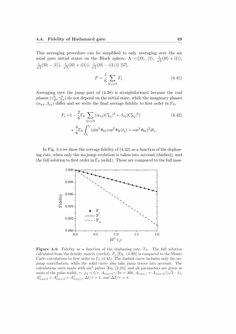
4.4. Fidelity of Hadamard gate 49
This averaging procedure can be simplified to only averaging over the sixaxial pure initial states on the Bloch sphere, Λ =|0〉, |1〉, 1√
2(|0〉+ |1〉),
1√2(|0〉 − |1〉), 1√
2(|0〉+ i|1〉), 1√
2(|0〉 − i|1〉) [57],
F =16
∑
|ψi〉εΛFi. (4.41)
Averaging over the jump part of (4.38) is straightforward because the realphases (γ0
1b, γ01a) do not depend on the initial state, while the imaginary phases
(αnj , βnj) differ and we write the final average fidelity to first order in Γ0,
Fi =1− 26Γ0
∑
|ψi〉εΛ(αnj |Ci
D1|2 + βnj |Ci
D2|2) (4.42)
+46Γ0
∫ tf
ti
(sin2 θ01 cos2 θH(tj) + cos2 θ01)2dtj .
In Fig. 4.4 we show the average fidelity of (4.42) as a function of the dephas-ing rate, when only the no-jump evolution is taken into account (dashed), andthe full solution to first order in Γ0 (solid). These are compared to the full mas-
0.0 0.5 1.0 1.5 2.00.990
0.992
0.994
0.996
0.998
1.000
F
F F
nj
Fid
elity
10-3
0
Figure 4.4: Fidelity as a function of the dephasing rate, Γ0. The full solutioncalculated from the density matrix (circles), Fρ [Eq. (4.39)] is compared to the MonteCarlo calculations to first order in Γ0 (4.42). The dashed curve includes only the no-jump contribution, while the solid curve also take jump traces into account. Thecalculations were made with sin2 pulses [Eq. (2.23)] and all parameters are given inunits of the pulse width, τ : ϕ2 = t/τ , Amax,0τ/2π = 300, Amax,1 = Amax,0/(
√2−1),
A2max,2 = A2
max,0 + A2max,1, ∆t/τ = 1, and ∆T/τ = π.

50 Geometric phases of an open system
ter equation solution (circles). All fidelities are calculated for the Hadamardgate implemented by the parameters θ01 = π/8, ϕ01 = π and γH = −π as inall previous numerical results. The fidelity decreases as expected when thedephasing rate increases, but is still acceptable when the system is subjectto realistic dephasing rates. The no-jump results set a lower bound on thefidelity but it is necessary to include traces with one jump in order to geta satisfactory accuracy for realistic dephasing rates. Equation (4.42) showsexplicitly how the average fidelity depends on the geometric phases acquiredduring the no-jump evolution.
4.5 Conclusion
We have shown how the evolution of a system acquiring geometric phases canbe described also when dephasing is present. Modifying the closed systemanalysis to a jump and a no-jump evolution under which the wave functionacquires complex geometric phases. This method has the advantage that weretain the analytical insight given by the adiabatic following of eigenstates andthe phases they acquire. The no-jump trace gives a first approximation to theevolution, but jump traces has to be included in order to achieve a sufficientaccurate result consistent with a density matrix calculation.

Chapter 5
Entangling Rydberg atoms
Rydberg atoms are neutrals with a highly excited electron in so-called Ryd-berg states. The Rydberg atoms have played an important role in atomicphysics, because they possess a range of interesting properties. The electroncan be in states that resemble classical orbits, the Rydberg states have largetransition dipole moments and the Rydberg atoms are easily manipulatedby external magnetic or electric fields [58]. From a quantum informationpoint of view the Rydberg states are interesting since they have relativelylong lifetimes and because the large dipole moments induce a dipole-dipoleinteraction inhibiting excitation of more than one atom to the Rydberg state.This Rydberg excitation blockade can be used as the coupling between qubitsrequired to implement two-qubit gates.
In this chapter we will combine the Rydberg blockade and the rapid adia-batic laser pulse sequence known from STIRAP. We show how the adiabaticpassage in the presence of the Rydberg blockade can be used to steer two atomsinto a maximally entangled state and implement two-bit quantum gates. Formany atoms, the excitation blockade leads to an effective implementation ofcollective-spin and Jaynes-Cummings-like Hamiltonians, and we show thatthe adiabatic passage can be used to generate collective Jx = 0 states andGreenberger-Horne-Zeilinger states of tens of atoms. The work presented inthis chapter was published in [V].
5.1 Rydberg atoms
Progress in trapping and manipulating neutral atoms in dipole traps has madeit possible to work towards a quantum computer using the hyperfine sublevelof the ground state in alkali atoms (typically Caesium or Rubidium) to encodequbits. The atoms are confined in optical dipole traps and can be prepared inarrays with access to individual addressing of each atom [44,59]. The opticaltraps can be moved and by overlapping two traps the atoms can be transferred
51

52 Entangling Rydberg atoms
from one trap to another without loss of coherence [60]. Single qubit rotationsare performed driving two-photon Raman transitions [61,62].
The single valence electron in a trapped alkali atom is excited to a Ryd-berg state with large principal quantum number, n. Two or more atomswill experience the Rydberg excitation blockade, which we discuss in furtherdetail below. Experimentally, the challenge at this point is demonstrating atwo-qubit gate relying on the Rydberg blockade and most recent an importantprogress was made, when the excitation of one atom to a Rydberg state withn = 79 was seen to block excitation of another [63]. The next step is nowto use the blockade to implement a two-qubit gate. The first proposals forthis type of gate [41, 64] were dynamic, while the work presented here relieson adiabatic evolution and geometric phases. Before describing our schemeto create two-qubit gates as well as many-atom entanglement we will brieflydiscuss the level structure of the Rydberg atoms considered, the applicationof the STIRAP pulse sequence, and the Rydberg excitation blockade.
5.1.1 STIRAP applied to ladder-systems in Rydberg atoms
We consider atoms with two lower levels and a Rydberg state in a ladderstructure coupled by two resonant laser fields with Rabi frequencies Ω1 andΩr as shown in Fig. 5.1(a). The STIRAP process applies the counter-intuitivepulse sequence of Fig. 5.1(b) and the mathematics is exactly as describedfor the lambda system in chapter 2.2.1 [38]. For a single atom the processtherefore transfers the population from the ground state |1〉 to the Rydberg
>r
>2
>1
Wr
W1
(a) Three-level ladder system andtwo laser fields with Rabi frequenciesΩ1 and Ωr.
t
t
Dt
Ar
A1
(b) STIRAP pulse sequence.The FWHM of each pulse is τand the delay between pulseswithin one process is ∆t.
Figure 5.1

5.1. Rydberg atoms 53
state |r〉 by adiabatically following the usual dark state
|D1〉 = cos θ|1〉 − sin θeiφr |r〉, (5.1)
where tan θ = A1/Ar expresses the relative strength and φr the relative phaseof the two laser fields. We assume that |1〉 and |2〉 are long lived states, but |r〉has a finite lifetime, which may affect the gate fidelity. This could for examplebe achieved by implementing |1〉 and |2〉 as hyperfine states in Rubidium orCaesium. The lifetime of the Rydberg state, τr, increases with n as shown inFig. 5.2 for Rubidium1. Here n > 70 ensures τr &100 µs implying that gatesshould last only a few microseconds.
1.0
0.8
0.4
0.6
0.0
0.2
t[m
s]r
0 25 1007550n
t =0.1 msr
Figure 5.2: Lifetime of the excited S,P,D and F states of Rubidium as a function ofprincipal quantum number, n. The red curves show results for atoms in a cryogenicenvironment (T=0 K) while the blue curves show results at room temperature (T=300K). The figure is reproduced from [65] by courtesy of Mark Saffman.
5.1.2 Rydberg excitation blockade
The large transition dipole moments of the highly excited Rydberg stateslead to strong interactions between atoms a few micrometres apart. Whenthe interaction is present, double excited states are shifted in energy, and alaser field resonant with a single atom transition can not excite two atomsbecause it will be off-resonant. A single excitation will therefore suppressexcitation of other atoms within reach of the dipole-dipole interaction. Cal-culating the exact value of the energy shift is not an easy task because itinvolves many states. Experimentally, it is important to choose proper states
1The lifetimes of Rydberg states in Caesium are similar.
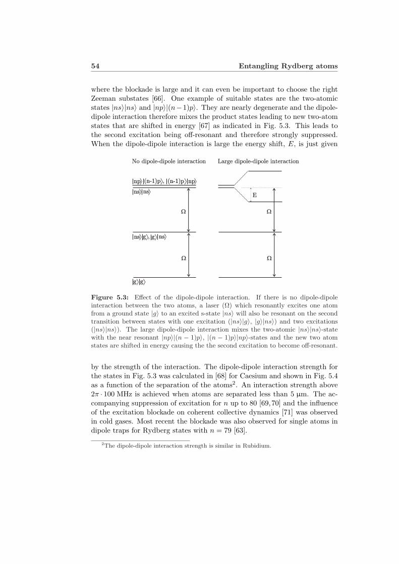
54 Entangling Rydberg atoms
where the blockade is large and it can even be important to choose the rightZeeman substates [66]. One example of suitable states are the two-atomicstates |ns〉|ns〉 and |np〉|(n−1)p〉. They are nearly degenerate and the dipole-dipole interaction therefore mixes the product states leading to new two-atomstates that are shifted in energy [67] as indicated in Fig. 5.3. This leads tothe second excitation being off-resonant and therefore strongly suppressed.When the dipole-dipole interaction is large the energy shift, E, is just given
>
W
ns>
g
>g , ns>>g
(n-1)p ,np> > (n-1)p> np>
ns> >ns
W
>g
W
W
E
No dipole-dipole interaction Large dipole-dipole interaction
Figure 5.3: Effect of the dipole-dipole interaction. If there is no dipole-dipoleinteraction between the two atoms, a laser (Ω) which resonantly excites one atomfrom a ground state |g〉 to an excited s-state |ns〉 will also be resonant on the secondtransition between states with one excitation (|ns〉|g〉, |g〉|ns〉) and two excitations(|ns〉|ns〉). The large dipole-dipole interaction mixes the two-atomic |ns〉|ns〉-statewith the near resonant |np〉|(n − 1)p〉, |(n − 1)p〉|np〉-states and the new two atomstates are shifted in energy causing the the second excitation to become off-resonant.
by the strength of the interaction. The dipole-dipole interaction strength forthe states in Fig. 5.3 was calculated in [68] for Caesium and shown in Fig. 5.4as a function of the separation of the atoms2. An interaction strength above2π · 100 MHz is achieved when atoms are separated less than 5 µm. The ac-companying suppression of excitation for n up to 80 [69,70] and the influenceof the excitation blockade on coherent collective dynamics [71] was observedin cold gases. Most recent the blockade was also observed for single atoms indipole traps for Rydberg states with n = 79 [63].
2The dipole-dipole interaction strength is similar in Rubidium.
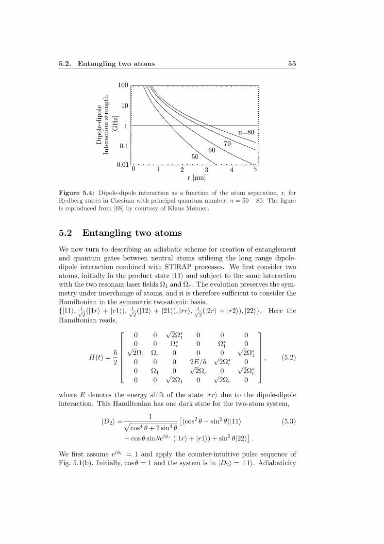
5.2. Entangling two atoms 55
0 1 2 3 4 50.01
0.1
1
10
100
5060
70
n=80
Dip
ole
-dip
ole
Inte
ract
ion
stre
ngth
[GH
z]
r [mm]
Figure 5.4: Dipole-dipole interaction as a function of the atom separation, r, forRydberg states in Caesium with principal quantum number, n = 50− 80. The figureis reproduced from [68] by courtesy of Klaus Mølmer.
5.2 Entangling two atoms
We now turn to describing an adiabatic scheme for creation of entanglementand quantum gates between neutral atoms utilising the long range dipole-dipole interaction combined with STIRAP processes. We first consider twoatoms, initially in the product state |11〉 and subject to the same interactionwith the two resonant laser fields Ω1 and Ωr. The evolution preserves the sym-metry under interchange of atoms, and it is therefore sufficient to consider theHamiltonian in the symmetric two-atomic basis,|11〉, 1√
2(|1r〉 + |r1〉), 1√
2(|12〉 + |21〉), |rr〉, 1√
2(|2r〉 + |r2〉), |22〉. Here the
Hamiltonian reads,
H(t) =~2
0 0√
2Ω∗1 0 0 00 0 Ω∗r 0 Ω∗1 0√2Ω1 Ωr 0 0 0
√2Ω∗1
0 0 0 2E/~√
2Ω∗r 00 Ω1 0
√2Ωr 0
√2Ω∗r
0 0√
2Ω1 0√
2Ωr 0
, (5.2)
where E denotes the energy shift of the state |rr〉 due to the dipole-dipoleinteraction. This Hamiltonian has one dark state for the two-atom system,
|D2〉 =1√
cos4 θ + 2 sin4 θ
[(cos2 θ − sin2 θ)|11〉 (5.3)
− cos θ sin θeiφr (|1r〉+ |r1〉) + sin2 θ|22〉] .
We first assume eiφr = 1 and apply the counter-intuitive pulse sequence ofFig. 5.1(b). Initially, cos θ = 1 and the system is in |D2〉 = |11〉. Adiabaticity
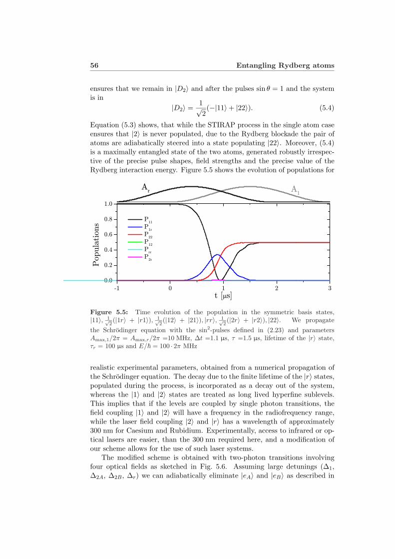
56 Entangling Rydberg atoms
ensures that we remain in |D2〉 and after the pulses sin θ = 1 and the systemis in
|D2〉 =1√2(−|11〉+ |22〉). (5.4)
Equation (5.3) shows, that while the STIRAP process in the single atom caseensures that |2〉 is never populated, due to the Rydberg blockade the pair ofatoms are adiabatically steered into a state populating |22〉. Moreover, (5.4)is a maximally entangled state of the two atoms, generated robustly irrespec-tive of the precise pulse shapes, field strengths and the precise value of theRydberg interaction energy. Figure 5.5 shows the evolution of populations for
-1 0 1 2 30.0
0.2
0.4
0.6
0.8
1.0
Popula
tions
t [ s]
P11
P1r
P22
P12
Prr
P2r
A1
Ar
Figure 5.5: Time evolution of the population in the symmetric basis states,|11〉, 1√
2(|1r〉 + |r1〉), 1√
2(|12〉 + |21〉), |rr〉, 1√
2(|2r〉 + |r2〉), |22〉. We propagate
the Schrodinger equation with the sin2-pulses defined in (2.23) and parametersAmax,1/2π = Amax,r/2π =10 MHz, ∆t =1.1 µs, τ =1.5 µs, lifetime of the |r〉 state,τr = 100 µs and E/~ = 100 · 2π MHz
realistic experimental parameters, obtained from a numerical propagation ofthe Schrodinger equation. The decay due to the finite lifetime of the |r〉 states,populated during the process, is incorporated as a decay out of the system,whereas the |1〉 and |2〉 states are treated as long lived hyperfine sublevels.This implies that if the levels are coupled by single photon transitions, thefield coupling |1〉 and |2〉 will have a frequency in the radiofrequency range,while the laser field coupling |2〉 and |r〉 has a wavelength of approximately300 nm for Caesium and Rubidium. Experimentally, access to infrared or op-tical lasers are easier, than the 300 nm required here, and a modification ofour scheme allows for the use of such laser systems.
The modified scheme is obtained with two-photon transitions involvingfour optical fields as sketched in Fig. 5.6. Assuming large detunings (∆1,∆2A, ∆2B, ∆r) we can adiabatically eliminate |eA〉 and |eB〉 as described in

5.2. Entangling two atoms 57
>r
>2>1
Wr
W1
>eA
D1
>eB
W2A
D2A
W2B
D2B
Dr
Figure 5.6: Five-level system coupled by four infrared or optical laser fields.
chapter 2.2.3 and find the Hamiltonian for the reduced three level system,
H(t) =~2
|Ω1|22∆2A
− 2(∆2A −∆1)Ω1Ω∗2A2∆2A
0Ω∗1Ω2A
2∆2A
|Ω2A|22∆2A
+ |Ω2B |22∆2B
ΩrΩ∗2B2∆2B
0 Ω∗rΩ2B
2∆2B
|Ωr|22∆2B
− 2(∆2B −∆r)
.
(5.5)
If the two-photon detunings are now varied such that,
2(∆2A −∆1) =|Ω1|22∆2A
and 2(∆2B −∆r) =|Ωr|22∆2B
, (5.6)
the Hamiltonian reduces to the familiar three level Hamilton (see (2.14) forcomparison)
H(t) =~2
0 Ω12 0Ω∗12
|Ω2A|22∆2A
+ |Ω2B |22∆2B
Ω∗r20 Ωr2 0
, (5.7)
with the dark state
|Dad〉 =Ar2(t)√
A212(t) + A2
r2(t)|1〉 − A12(t)√
A212(t) + A2
r2(t)eiϕad(t)|r〉, (5.8)
where A12 and Ar2 are the field strengths and ϕad the relative phase of theRaman Rabi frequencies,
Ω12 =Ω1Ω∗2A
2∆2Aand Ωr2 =
ΩrΩ∗2B
2∆2B. (5.9)
The five level scheme of course has the disadvantage that it involves fourlaser fields and in addition the two-photon detuning must be controlled time

58 Entangling Rydberg atoms
dependent, but it should be straight forward to implement using for exampleacusto optical modulators. The advantage is the easier access to the necessarylaser wavelengths. Both implementations require that the laser phases arestable.
To investigate the criterion of adiabaticity and the role of the Rydberginteraction energy E, in Fig. 5.7, we show the fidelity of the creation of theentangled state, F = |〈D2|ψf 〉|2, where |ψf 〉 is the final state calculated bypropagation of the state vector with the time-dependent Hamiltonian (5.2).The simulations show that, as long as E is large enough to prevent populationof states with more than one Rydberg excitation, the exact value of E is notimportant. With peak Rabi frequencies Amax,1/2π = Amax,r/2π = 10 MHz, aRydberg energy shift of E/~ = 50 · 2π MHz is sufficient. The time span where|r〉 is populated is determined by the pulse width and it is desirable to usethe smallest possible width that does not violate adiabaticity, yielding a totaltime of entanglement generation of 3-4 µs, which is short compared with theradiative lifetime of the highly excited Rydberg state & 100 µs.
1.0 1.2 1.4 1.6 1.8 2.0 2.2 2.4
0.986
0.988
0.990
0.992
0.994
0.996
0.998
1.000
Df
2
[ s]
E/h=10 MHz E/h=50 MHz E/h=100 MHz E/h=1000 MHz
Figure 5.7: Fidelity of the entanglement creation as a function of pulse width fordifferent values of dipole-dipole interaction, E. |ψf 〉 was found by propagating (5.2)with initial state |11〉. We show the norm square of the overlap with the target state|D2〉. The laser pulses are modelled by the sin2-pulses in (2.23) and with parametersAmax,1/2π = Amax,r/2π = 10 MHz, ∆t = 1.1 MHz and τr = 100 MHz.

5.2. Entangling two atoms 59
5.2.1 Two-qubit phase gate
The two-atom entanglement scheme can be modified to create a two-qubitphase gate. To this end we apply a second STIRAP sequence with pulses inreversed order as shown in Fig. 5.8. The second pulse pair transfers populationback to |11〉. The Rabi frequencies now have a non-vanishing relative phaseφr(t) between Ω1 and Ωr and the dark state (5.3) acquires the geometricphase [19]
γ2 = −∫
cos2 θ sin2 θ
cos4 θ + 2 sin4 θφrdt. (5.10)
t
Ar
A1t
DTDt
Ar
A1
Figure 5.8: Two STIRAP processes separated by ∆T in time.
When we supplement the atomic level scheme with another qubit state |0〉,which is decoupled from the STIRAP pulses, only the two-qubit register state|11〉 will acquire the geometric phase, γ2. The |00〉 state will be unaffectedwhile for the |01〉 and |10〉 states the atom in |1〉 will follow the single atomdark state (5.1) and acquire the geometric phase found in chapter 3.1,
γ1 = −∫
sin2 θφrdt. (5.11)
This implies the evolution,
|00〉 → |00〉 (5.12)
|01〉 → eiγ1 |01〉|10〉 → eiγ1 |10〉|11〉 → eiγ2 |11〉
corresponding to a controlled two-qubit phase gate with phase ∆ϕ = γ2 −2γ1. γ2 is only acquired when the pulses overlap (sin θ cos θ 6= 0), while γ1
is acquired primarily between the two pulse sequences (sin θ 6= 0), and ∆ϕcan, e.g., be controlled by adjusting ∆T . This is seen in Fig. 5.9 where theentangling phase, ∆ϕ is shown as a function of the delay between the two pulsesequences when the relative phase is φr(t) = t · 2 MHz. To achieve ∆ϕ = π inthis case it is sufficient to set ∆T ≈ 2.1 µs corresponding to a gate time below10 µs.

60 Entangling Rydberg atoms
1.5 2.0 2.5 3.0 3.5
0
-
T [ s]
Figure 5.9: Entangling phase as a function of the delay between the two pulsesequences. The laser pulses are modeled by sin2-pulses and parameters Amax,1/2π =Amax,r/2π =10 MHz, ∆t =1.1 µs, τ =1.5 µs, φr(t) = t · 2 MHz, τr =100 µs andE/~ = 100 · 2π MHz
5.3 Many-particle entanglement
We now show that when more than two atoms in |1〉 are subject to the STIRAPpulse sequence they also become entangled. Provided all atoms are localisedwithin a region of a few µm, the transition towards the Rydberg states isrestricted to the coupling of collective states with either zero or one Rydbergatom and we implement this by truncating the basis so it only includes stateswith zero or one atom in the |r〉 state. We write the symmetric basis states ofthe system as
|n1, n2 = N − n1, 0〉, (5.13)|n1, n2 = N − n1 − 1, 1〉,
where N is the total number of atoms, n1 and n2 the number of atoms in |1〉and |2〉 and 0 or 1 indicates whether |r〉 is populated with zero or a singleatom. The basis consists of N + 1 states with no Rydberg excitation and Nwith a single excitation. The interaction with the radiation fields Ω1 and Ωr,∑N
j=1−12(Ω1(t)|2〉j〈1|+ Ωr(t)|r〉j〈2|+ h.c.), can now be rewritten
H(t) = HJx(t) + HJC(t), (5.14)
with variable strengths, representing the coupling by the fields driving thelower and the upper transition, respectively. The dynamics of the lower levelscan be rewritten in a collective spin description and in the accompanyingSchwinger oscillator description,
HJx(t) = −~Ω1(t)Jx(t) = −12~Ω1(t)(a
†1a2 + a1a
†2), (5.15)

5.3. Many-particle entanglement 61
where a(†)i are annihilation (creation) operators for the number of atoms in
|i〉. The upper transition is described by
HJC(t) = −12~Ωr(t)(a2σ
+ + a†2σ−) (5.16)
where we use Pauli matrices σ+ and σ− to describe the transfer of populationbetween states with zero and one Rydberg excitation in the atomic ensemble.The Rydberg blockade is assumed in both the truncation of the basis and inthe use of the two-level Pauli matrix description of the population in |r〉. TheHJC is the quantum optical Jaynes-Cummings (JC) Hamiltonian, introducedoriginally to describe the resonant interaction between a two-level atom andquantised light [72]. JC dynamics has been implemented in strong couplingcavity QED experiments, where non-classical states of light, such as Fockstates and quantum superposition states, are produced efficiently [73]. HJC
also describes the motion of laser driven trapped ions, where it has been usedto generate various non-classical states [74,75]. Following these proposals, JCdynamics is sufficient to produce a variety of interesting states of an atomicensemble by the Rydberg blockade. In this work we will use the advantagesof the robust STIRAP process to produce entangled states.
The Hamiltonian in (5.14) has a dark state with zero valued eigenenergythroughout the STIRAP process. This follows because the operator Θ =(−1)n2 , which inverts the sign of the operators a2 and a†2, anti-commutes withH, HΘ = −ΘH. Any eigenstate |ψ〉 of H with energy eigenvalue E, thenhas a partner, Θ|ψ〉 with eigenvalue -E and the energy eigenvalue spectrum issymmetric around zero. The number of eigenstates is odd because N atomsinduce N +1 different states with no atoms in |r〉 and N states with one atomin |r〉, and hence there must always be a state with eigenvalue zero. The fullcurves in Fig. 5.10 show the 13 energy eigenvalues for 6 atoms found from anumerical diagonalisation of (5.14), and they clearly confirm the existence ofthe dark state throughout the pulse sequence.
The STIRAP process starts with Ω1 = 0 and hence initially H(t) =HJC(t) = −1
2~Ωr(t)(a2σ+ + a†2σ
−). The Jaynes-Cummings Hamiltonian haseigenvalues 0,±1
2~Ωr(t)√
n2 + 1 and these are shown as blue curves in Fig.5.10, where they match the full solution as long as Ω1 = 0. In this regimethe dark state is |n1 = N, n2 = 0, nr = 0〉 corresponding to our initial statewith all atoms in |1〉. Adiabaticity ensures that we remain in the dark stateof the full Hamiltonian and when Ω1 is increased and Ωr reduced, the systemends up in the dark state of H(t) = HJx(t) = −~Ω1(t)Jx. The final statewith Jx = 0 have either no or a single Rydberg excitation leaving K = N orK = N − 1 atoms in the |1〉 and |2〉 states. The eigenvalues of −Ω1(t)Jx are−Ω1(t)−K/2,−K/2+1, ..., K/2− 1,K/2 and E = 0 occurs for K even. ForN even, the dark state does not populate |r〉, while for N odd, the final darkstate is the state with one Rydberg excitation and N − 1 atoms in the Jx = 0
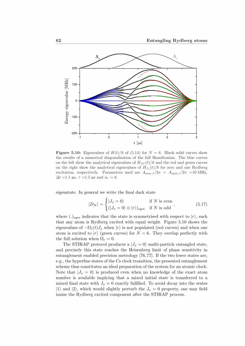
62 Entangling Rydberg atoms
-1 0 1 2 3
-200
-100
0
100
200
A1A
r
Ener
gy e
igen
val
ue
[MH
z]
t [ s]
Figure 5.10: Eigenvalues of H(t)/~ of (5.14) for N = 6. Black solid curves showthe results of a numerical diagonalisation of the full Hamiltonian. The blue curveson the left show the analytical eigenvalues of HJC(t)/~ and the red and green curveson the right show the analytical eigenvalues of HJx(t)/~ for zero and one Rydbergexcitation, respectively. Parameters used are Amax,1/2π = Amax,r/2π =10 MHz,∆t =1.1 µs, τ =1.5 µs and φr = 0.
eigenstate. In general we write the final dark state
|DN 〉 =
|Jx = 0〉 if N is even(|Jx = 0〉 ⊗ |r〉)sym if N is odd
, (5.17)
where (.)sym indicates that the state is symmetrised with respect to |r〉, suchthat any atom is Rydberg excited with equal weight. Figure 5.10 shows theeigenvalues of −Ω1(t)Jx when |r〉 is not populated (red curves) and when oneatom is excited to |r〉 (green curves) for N = 6. They overlap perfectly withthe full solution when Ωr = 0.
The STIRAP protocol produces a |Jx = 0〉 multi-particle entangled state,and precisely this state reaches the Heisenberg limit of phase sensitivity inentanglement enabled precision metrology [76,77]. If the two lower states are,e.g., the hyperfine states of the Cs clock transition, the presented entanglementscheme thus constitutes an ideal preparation of the system for an atomic clock.Note that |Jx = 0〉 is produced even when no knowledge of the exact atomnumber is available implying that a mixed initial state is transferred to amixed final state with Jx = 0 exactly fulfilled. To avoid decay into the states|1〉 and |2〉, which would slightly perturb the Jx = 0 property, one may fieldionise the Rydberg excited component after the STIRAP process.
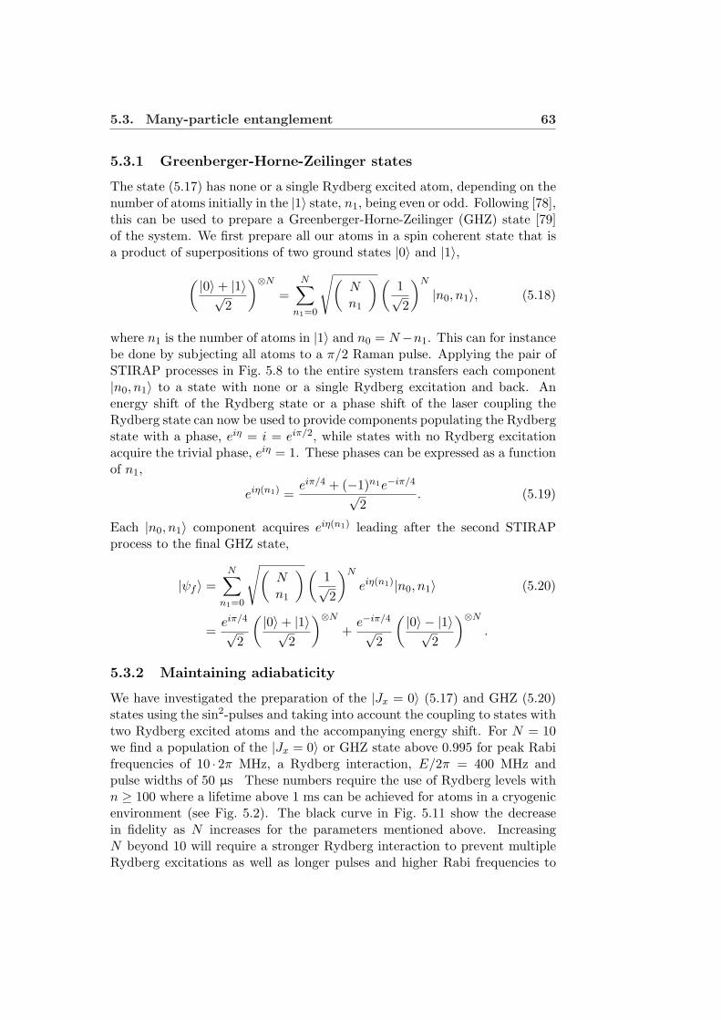
5.3. Many-particle entanglement 63
5.3.1 Greenberger-Horne-Zeilinger states
The state (5.17) has none or a single Rydberg excited atom, depending on thenumber of atoms initially in the |1〉 state, n1, being even or odd. Following [78],this can be used to prepare a Greenberger-Horne-Zeilinger (GHZ) state [79]of the system. We first prepare all our atoms in a spin coherent state that isa product of superpositions of two ground states |0〉 and |1〉,
( |0〉+ |1〉√2
)⊗N
=N∑
n1=0
√(Nn1
)(1√2
)N
|n0, n1〉, (5.18)
where n1 is the number of atoms in |1〉 and n0 = N−n1. This can for instancebe done by subjecting all atoms to a π/2 Raman pulse. Applying the pair ofSTIRAP processes in Fig. 5.8 to the entire system transfers each component|n0, n1〉 to a state with none or a single Rydberg excitation and back. Anenergy shift of the Rydberg state or a phase shift of the laser coupling theRydberg state can now be used to provide components populating the Rydbergstate with a phase, eiη = i = eiπ/2, while states with no Rydberg excitationacquire the trivial phase, eiη = 1. These phases can be expressed as a functionof n1,
eiη(n1) =eiπ/4 + (−1)n1e−iπ/4
√2
. (5.19)
Each |n0, n1〉 component acquires eiη(n1) leading after the second STIRAPprocess to the final GHZ state,
|ψf 〉 =N∑
n1=0
√(Nn1
)(1√2
)N
eiη(n1)|n0, n1〉 (5.20)
=eiπ/4
√2
( |0〉+ |1〉√2
)⊗N
+e−iπ/4
√2
( |0〉 − |1〉√2
)⊗N
.
5.3.2 Maintaining adiabaticity
We have investigated the preparation of the |Jx = 0〉 (5.17) and GHZ (5.20)states using the sin2-pulses and taking into account the coupling to states withtwo Rydberg excited atoms and the accompanying energy shift. For N = 10we find a population of the |Jx = 0〉 or GHZ state above 0.995 for peak Rabifrequencies of 10 · 2π MHz, a Rydberg interaction, E/2π = 400 MHz andpulse widths of 50 µs These numbers require the use of Rydberg levels withn ≥ 100 where a lifetime above 1 ms can be achieved for atoms in a cryogenicenvironment (see Fig. 5.2). The black curve in Fig. 5.11 show the decreasein fidelity as N increases for the parameters mentioned above. IncreasingN beyond 10 will require a stronger Rydberg interaction to prevent multipleRydberg excitations as well as longer pulses and higher Rabi frequencies to

64 Entangling Rydberg atoms
ensure adiabaticity. This is shown with the grey curve in Fig. 5.11 where thepeak Rabi frequencies, the pulse widths and Rydberg interaction strength aredoubled and the fidelity is increased from 0.43 to 0.98 for N = 20. Full insightinto the parameter requirements for large N will necessitate further numericalstudies. As indicated by the energy spectra in Fig. 5.10, there is a criticalcrossing region at t ' 0.5 µs, where special care should be taken, and weanticipate that control theory may be used to find optimal pulse shapes thatmay improve the fidelities and make it possible to reach higher atom number.
6 8 10 12 14 16 18 20
0.4
0.5
0.6
0.7
0.8
0.9
1.0
Jx
f
N
Figure 5.11: Fidelity of the |Jx = 0〉 creation as a function of the number of atomsfor two different sets of parameters. The laser pulses are modelled by the sin2-pulsesin (2.23) and the black curve is the result for parameters Amax,1/2π = Amax,r/2π =10 MHz, ∆t = 30 µs, τ = 50 µs and E/2π =400 MHz, while the grey corresponds toAmax,1/2π = Amax,r/2π = 20 MHz, ∆t = 70 µs, τ = 100 µs and E/2π =800 MHz.
5.4 Conclusion
In conclusion, we have demonstrated that the Rydberg excitation blockademechanism in conjunction with rapid adiabatic passages provide rich oppor-tunities to prepare two- and multi-atom entangled states with confined sam-ples of atoms in for example optical dipole traps or small lattice arrays. Ourcalculations indicate the possibility of high fidelity generation of entangledstates and quantum superposition states with tens of atoms. To achieve im-plementations in larger systems, higher Rabi frequencies and Rydberg stateswith longer coherence times must be available for experimentalist. In additioncontrol theory may be used to optimise pulse shapes.

Chapter 6
Quantum computation with40Ca+
Trapped laser cooled ions are one of the most promising candidates for im-plementing quantum computation. They represent well isolated systems withlong coherence times and by applying available laser sources population of theinternal states can be controlled to high precision. In the first part of thischapter we briefly discuss the progress in implementing the ion trap quantumcomputer going through the DiVinzenco criteria presented in chapter 1.1.3.We focus on the ion specie (40Ca+) and the qubit encoding (Zeeman sub-levels) considered experimentally here in Arhus, but also point out the keyresults of whole ion trap community. In the second part, we propose a schemefor internal state detection that we will use to detect our qubit. This detectionscheme is also the subject of the experimental investigations in chapter 7 and8.
6.1 Requirements
6.1.1 A scalable qubit system
We intend to use the two Zeeman-sublevels of the |S1/2〉 ground state of 40Ca+
as our qubit states and denote them by |↑〉(m = 1/2) and |↓〉(m = −1/2).The five relevant energy states |S1/2〉, |P1/2〉, |D3/2〉, |P3/2〉 and |D5/2〉 areshown in Fig. 6.1 and we indicate their Zeeman structure. We will couplethe states by four laser fields with wavelengths 397 nm, 866 nm, 850 nm and854 nm. The |D3/2〉 and |D5/2〉 states are metastable with lifetimes ≈1 s [80]and their decay can thus be neglected. The |P1/2〉 and |P3/2〉 states decay asindicated in Fig. 6.1(b). The physical properties of the 40Ca+ ion is describedin appendix B.
Other advanced qubit encodings are based on either a combination of the|S1/2〉 and the |D5/2〉 states in 40Ca+ [81] or encodings in hyperfine states of
65

66 Quantum computation with 40Ca+
W397
W866
W850
D397 D866
D850D854
G21
G41
G23
G43
G45 W854
>2
>3
>5
>4
> >
1 =
>P1/2
>2
>
>3D3/2
>
>5D5/2
>
>4P3/2
>S1/2>
397
nm 86
6nm 85
0nm
854
nm
393
nm
732
nm
729
nm
(a) (b)
Figure 6.1: Relevant energy levels of 40Ca+. In (a) we indicate their terms (LJ),|1〉 = |S1/2〉, |2〉 = |P1/2〉, |3〉 = |D3/2〉, |4〉 = |P3/2〉 and |5〉 = |D5/2〉 and showthe wavelengths of the transitions. In (b) only the four couplings used in this work isshown with Rabi frequencies Ωi and detunings ∆i. Here, we also indicate the Zeemansublevels and the qubit encoding in the electronic ground state, (|↑〉(m = 1/2) and|↓〉(m = −1/2)). The non-negligible decay rates from |i〉 to |j〉 (Γij) are shown aswell.
9Be+ or 111Cd+ [82, 83]. The advantage of the implementations in Ca is thatlaser sources of the right wavelengths are readily available, while the hyperfinequbits of 9Be+ or 111Cd+ are less sensitive to magnetic field fluctuations. Theexperimental advances are similar for the two approaches and research is alsodevoted to combining the strengths of the two using the isotope 43Ca+, whichhave non-zero nuclear spin and encode the qubit in the hyperfine sublevels ofthe |S1/2〉 ground state [84,85].
For all the ion trap proposals scaling the system is a challenging task.Scaling by just adding more ions to a string has a natural limit [86] andexperiments entangling 6-8 ions [87,88] are reaching this limit. Further scalingmust rely on more clever designs. One promising design for a large-scale iontrap quantum computer [89] consists of several connected ion traps with theability to transfer ions from one trap area to another. One area is used forinteraction between ions using laser manipulation while other areas are usedas memory units, where the ions are stored when they are not involved ingate operations in the interaction area. This requires control of the transportof ions in complex structures [90] and especially shuttling around corners ischallenging [91].
6.1.2 Initialisation
The ion can be initialised in either the |↓〉 or |↑〉 state by optical pumping andthe vibrational ground state of the quantised ion motion, |0〉 can be reached,e.g, by applying sideband cooling as discussed in chapter 7.2.

6.1. Requirements 67
6.1.3 Universal gates
Performing a one-qubit gate corresponds to an arbitrary rotation on the Blochsphere (Fig. 1.1), which for ions can be done by applying a laser pulse and con-trolling the phase of the light field and the pulse area. This requires individualaddressing of the ions which has been demonstrated experimentally [92]. In oursystem Raman transitions between the two Zeeman sublevels of |S1/2〉 via the|P1/2〉-state will be used for these quantum logic operations as demonstratedfor the hyperfine qubits [82]. It will then be the pulse area of the effectiveRaman Rabi frequency we need to control. Alternatively, the geometric gatespresented in chapter 3 could be implemented.
There are many different proposals for the implementation of a universaltwo-qubit gate. The first proposal was given by Cirac and Zoller when theysuggested the ion trap quantum computer [11]. The gate is realised by cou-pling the qubits through their common vibrational motion and requires coolingto the vibrational ground state. Mølmer and Sørensen [93] made another pro-posal using the same coupling. The advantage of their gate is that it worksfor ions, which are not cooled to the exact vibrational ground state. Addi-tionally, different implementations of geometric two-qubit phase gates was pro-posed [29,30]. The Cirac-Zoller gate [11], the Mølmer-Sørensen gate [93] and ageometric phase gate [30] have all been demonstrated experimentally [94–96].The highest fidelity with hyperfine qubits was demonstrated implementingthe phase gate in 9Be+-ions yielding a fidelity of approximately 97% [96]. Re-cently, this result was exceeded with the optical qubit in 40Ca+ implementingthe Mølmer-Sørensen gate with a 99.3% fidelity [97]. This fidelity approachesthe error thresholds required for fault tolerant quantum computation1. Smallalgorithms using trapped ions have been implemented experimentally; Groverssearch algorithm [100], the Deutsch-Jozsa algorithm [101] and the semiclas-sical quantum fourier transform [102], which is an important ingredient inShor’s factoring algorithm.
6.1.4 Coherence time
In the experimental realisation of the Cirac and Zoller gate [11] the operationtime was ≈ 500 µs, while the the Mølmer-Sørensen gate and the controlledphase gate is as fast as ≈ 20 µs [94, 96]. This sets the requirements for thecoherence time of our qubit. Coherence times of tens of seconds of two Zee-man substates of 40Ca+ encoded in a decoherence free subspace [103] has beenobserved [104]. Using the field insensitive hyperfine qubits [105] a similar co-herence time is reached without going into a decoherence free subspace and anorder of magnitude longer is expected for a decoherence free subspace of hy-
1Different error correction codes estimate allowed error rates between 10−5 and 10−2
[98, 99]. However, high error rates require a large overhead of qubits to encode the errorcorrection.

68 Quantum computation with 40Ca+
perfine qubits [103]. The coherence time of the ion trap quantum computer istherefore at present three orders of magnitude longer than the gate operationtime. Since we are using the Zeeman-sublevels as our qubit the decoherencewill mainly be due to external magnetic fields and to achieve a sufficient co-herence time we will need a good control of magnetic fields combined withencoding in a decoherence free subspace.
6.2 Internal state detection
We determine whether the ion is in the | ↑〉 or | ↓〉-state by performing aprojection measurement in three steps as shown in Fig. 6.2.
+W (s )397
W866
D397 D866>P1/2
>D3/2
>D5/2
>P3/2
>
>S1/2
>
W850
D850D854
>P1/2
W854
>D3/2
>D5/2
>P3/2
>
>S1/2
>
W397
W866
D397 D866>P1/2
>D3/2
>D5/2
>P3/2
>
>S1/2
>
ShelvingFirst STIRAP sequence Second STIRAP sequence
Fluorescence detection
Figure 6.2: Laser fields applied in the three steps of the qubit detection scheme,first STIRAP process, second STIRAP process and fluorescence detection.
1. The first STIRAP process applies Ω397 and Ω866 transferring populationfrom |S1/2〉 to |D3/2〉. The polarisation of the 397 nm pulse is chosen sothat only the population in |↓〉 is transferred, while |↑〉 remains unaf-fected.
2. The second STIRAP process with Ω850 and Ω854 applied transfers allpopulation in |D3/2〉 to |D5/2〉.
3. After shelving, the population remaining in |↑〉 can be observed applyingΩ397 and Ω866 and monitoring the fluorescence at 397 nm.
A weak externally applied magnetic field defines the quantisation axis andcreates a Zeeman splitting of | ↓〉 and | ↑〉. Another detection scheme waspresented in [106] with a 86% efficiency and relies on angular momentumselection rules combined with coherent population trapping. The STIRAPprocess used is described in chapter 2.2 and we use the Gaussian pulses definedin (2.22).

6.3. Summary 69
6.3 Summary
The ion trap quantum computer is no longer a theoretical idea since all Di-Vincenzo criteria except scalability are met. Scaling the computer requiresnew trap designs with, e.g., segmented traps as well as a reduction of all errorrates. This means that all gates as well as the state detections have to beperformed with very high fidelities and requires long coherence time. In thefollowing two chapters we will focus on the experimental implementation ofthe internal state detection, as outlined above.


Chapter 7
Experimental setup
In this chapter we introduce the experimental equipment and setup used inthe STIRAP experiments.
7.1 Overview
The experimental setup consists of a segmented linear Paul trap placed in thecentre of a vacuum chamber accessible by laser beams from several directions.A sketch of the setup is shown in Fig. 7.1 and a picture of the vacuum chamberand its components in Fig. 7.2. Ultra high vacuum is obtained by baking out
Image intensifier
BeamsplitterPMT
CCD-camera
Objective Lens
Ionisinglaser beam (272 nm)
Shutter
Oven
Imaging system:
Trap Electrodes
yz
x
y
zx
866 nm
397 nm
397 nm
850 nm
854 nm397 nm
Figure 7.1: Sketch of the experimental setup including the imaging system. Theapplied laser fields are indicated.
the chamber at 150 C during a few days while applying a turbo molecularpump1. After bakeout a pressure around 4 · 10−11 Torr is maintained by an
1Leybold Trivac
71

72 Experimental setup
Coilfeedthrough
Ca oven
Oven shutter
Trapfeed-
through
Optical fiber mountMg oven
Trap
Coil
Deflection plates Electron gun10 cm
Figure 7.2: Picture of the vacuum chamber and its constituents. The applied laserfields are indicated.
ion pump2 and a sublimation pump3. A beam of calcium atoms is releasedfrom an oven (heated to ≈ 500 C) and ionised by a 272 nm uv-laser beam asdescribed in chapter 7.3. The beam of calcium atoms intersects the ionisinglaser beam in the centre of the linear Paul trap. Alternatively, the calciumcan be ionised using an Electron gun which can be steered through the trapcentre using deflection plates. This method has not been used in this worksince it is not isotope selective and more dirty than photoionisation. RF- andDC-voltages are applied to the trap electrodes, confining the ions in the centreof the trap.
In addition to the ionisation beam the ions are addressed by four laserbeams (with wavelengths 397 nm, 866 nm, 850 nm and 854 nm) passing throughviewports of the vacuum chamber as shown in Fig. 7.1 and 7.2. All laser fieldsintersect at the trap centre. As a guidance an optical fibre (125 µm diameter)mounted inside the chamber can be placed in the trap centre and detectionof scattered light using the imaging system will ensure that the lasers passthrough the centre. Above the trap an imaging system collects the 397 nmphotons and we detect the fluorescence with a CCD camera and a photo mul-
2Varian VacIon Plus 300 Starcell pump (240L/s) with a Midivac 929-5002 controller3Constructed at the Department

7.2. Laser cooling of 40Ca+ 73
tiplier tube (PMT). Before entering the chamber the laser beams pass severallenses, waveplates, EOMs and AOMs, that control their waist, polarisation,frequency and shape.
Two coils are placed in a Helmholtz configuration on each side of thetrap and used for creating a magnetic field along the trap axis. The vacuumchamber and all parts mounted inside it have been described in detail in [29].In the following the laser systems (chapter 7.4), the imaging system (chapter7.5), the ion trap (chapter 7.6), and external magnetic fields (chapter 7.7) willbe described in further detail. The laser systems are used for STIRAP, Dopplercooling and photoionisation. STIRAP was discussed in detail in chapter 2.2and we will, before giving the details on the setup of the laser systems, describeDoppler cooling (chapter 7.2) and photoionisation (chapter 7.3) of 40Ca+.
7.2 Laser cooling of 40Ca+
Laser cooling is a method used to reduce the velocity of for example a trappedion. In Doppler laser cooling the ion interacts with a near resonant laserof frequency, ωL. An ion with a velocity v with respect to the laser lightexperiences a shifted frequency: ω(v) = ωL(1 − v
c ). Ions moving towards thelaser field will therefore experience a higher frequency, while ions moving awayfrom the light experiences a lower.
IonLaser Laser
vw wL 12< w w
L 12>w
12
Figure 7.3: The Doppler cooling principle.
Doppler cooling takes place in what is effectively a two-level system (withresonance frequency, ω12), where the laser field ωL is red-detuned from theatomic resonance frequency, so ions moving towards the laser field with avelocity that match the Doppler shift (kv = ∆12 = ω12 − ωL) is exactly onresonance and have the largest possible absorption cross section. Absorptionof a photon gives the ion an additional momentum ~k in the direction oflight propagation and subsequent decay gives another momentum kick. If theemission is stimulated it will effectively cancel the absorption. Spontaneousemission gives on average no contribution to the ion momentum, because theradiation pattern is spatially symmetric. This leaves an effective momentumkick in the direction of light propagation from absorption, which slows downthe ion. The frequency of the absorbed photon is slightly lower than thefrequency of the emitted and therefore energy is taken out of the system.Doppler cooling is described in further mathematical detail in [107].
In 40Ca+, Doppler cooling is performed with a 397 nm laser on the |S1/2〉-|P1/2〉 transition, and since some of the population in |P1/2〉 decays to |D3/2〉

74 Experimental setup
w=
397
nm
L
866
nm
G21
G23
E1
E2
>P1/2
>D3/2
>S1/2
Figure 7.4: Doppler cooling using a two-level system with resonance frequency ω12
coupled with a laser at frequency ωL. An additional laser at 866 nm is necessary in40Ca+ to repump from the |D3/2〉-state.
an additional laser at 866 nm is applied to repump the population in |D3/2〉into the cooling-cycle again (see Fig. 7.4). Laser cooling of free ions in three di-mensions can be achieved using six pairwise counter-propagating laser beams4.For trapped ions this is not necessary because the velocity reverses in a con-fined system and one laser beam is sufficient if applied in a direction thatcools both radial and axial motion. In the experiment we use two counterpropagating beams parallel to the ion string and one beam in a 45 anglewith respect to the string as shown in Fig. 7.1. The continuous process wherean ion absorbs and emits a photon sets a lower boundary for the velocity ofthe ion. With optimal detuning an average kinetic energy, 〈Ek〉 = ~Γ
4 can beobtained, where for simplicity only one dimension was considered [108]. Fromthe kinetic energy a temperature can be defined from 1
2kBT = 〈Ek〉, which foroptimal Doppler cooling gives the so-called Doppler temperature,
TD =~Γ2kB
. (7.1)
For the |S1/2〉-|P1/2〉 cooling transition Γ21/2π = 20.7 MHz. This correspondsto a Doppler temperature TD =0.5 mK, when we neglect the |P1/2〉-|D3/2〉transition. This approximation is allowed because only 8% of the populationin |P1/2〉 decay through this channel. Doppler cooling gives the additionaladvantage that emitted 397 nm photons allow for detection of the ions usinga CCD-camera or a photo-multiplier tube (PMT).
Recently, Doppler cooling on the dipole forbidden |S1/2〉-|D5/2〉 transitionwas demonstrated [109]. The 854 nm and 866 nm lasers were applied to re-pump population from |D3/2〉 and |D5/2〉 to |P3/2〉 and |P1/2〉, from where itdecays back to |S1/2〉 and emits the 393 nm and 397 nm photons used for de-tection. This has the advantage that photons are detected on a transition,where no lasers are applied and therefore improves the signal to noise ratio.
4Actually only 4 laser beams are required when applied in a clever configuration.
7.3. Photoionisation 75
Additionally, it allows for quantum logic experiments in 40Ca+ using onlyinfrared laser sources.
The ion is confined in the linear Paul trap and it experiences as we willdiscuss in chapter 7.6 a harmonic potential. The quantised ion motion istherefore described by the vibrational eigenstates |n〉 of the harmonic oscilla-tor, where n is the vibrational quantum number corresponding to the energy(12 +n)~ωz, where ωz/2π ≈ 0.5 MHz is the axial oscillation frequency of the ion
in the trap. With more than one ion in the trap different vibrational modescan be excited [110]. Ions cooled to the Doppler temperature TD =0.5 mKhave a mean vibrational quantum number, 〈n〉 = 20, found from the relationkBTD = (1
2 + n)~ωz. Confining the ion stronger by an increment of ωz willdecrease 〈n〉, but to reach the vibrational ground state, |0〉, Doppler coolingis not sufficient.
One efficient method is sideband cooling [35, 111] relying on the resolvedsidebands appearing in the absorption profile of an internal transition, whenits linewidth is much smaller than the trap oscillation frequency, Γ ¿ ωz. Inthis regime the sidebands can by application of clever laser combinations beused to cool the ion to the vibrational ground state. Using dipole transitionsfor sideband cooling is not feasible because Γ is on the order of MHz and willtherefore require extremely strong confinement of the ions. Instead dipole-forbidden quadrupole transitions [112–114] or two-photon Raman transitions[115,116] have been used in experimental implementations. In our experimentswe intend to use Raman transitions between the two Zeeman sublevel of |S1/2〉for sideband cooling of the trapped ions. This scheme was implemented in[116] and thoroughly described for our experiments in [29]. An alternativeto sideband cooling relies on electromagnetically induced transparency [117]and cools the ion to nearly the vibrational ground state, 〈n〉 = 0.1 [118, 119].For large scale quantum computation and to avoid decoherence, sympatheticcooling can be applied [120, 121]. The ion used for quantum logic is now notlaser cooled, but cooled via its Coulomb interaction with another ion, whichis laser cooled. The other ion can be either a different ion specie [122] or adifferent ion isotope [123].
7.3 Photoionisation
Ionising the calcium loaded into the trap can be done using either electronbombardment or a two-photon ionisation process. As mentioned, only thelatter was used in this work, because it is a very clean process that makesit possible to load ions in small ion traps, as the one used for our experi-ments, without depositing calcium on the electrodes. It furthermore has theadvantage that the ionisation and thus the loading is isotope selective. Thisresonance-enhanced two-photon ionisation was presented in [124] and is shownschematically in Fig. 7.5. One 272 nm photon excites an electron from the

76 Experimental setup
4s2 1S0-state to the 4s5p 1P1-state. Subsequently, the atom can be ionised byeither a 272 nm or 397 nm (applied for doppler cooling) photon transferringthe excited electron to the continuum. If the electron decays to the metastable4s3d 1D2-state a 272 nm photon can still ionise the atom. Another two-photon
2 14s S0
14s5p P1
14s3d D2
272nm
272nm272nm
397nm
Figure 7.5: Simplified energy levels of neutral calcium. The hatched area indicatesthe continuum.
ionisation scheme was presented in [125] exciting to the 4s4p 1P1-state with a423 nm and subsequently exciting an auto-ionising state with a 389 nm pho-ton. This process has the advantage of a higher loading rate because of ahigh oscillation strength of the first excitation, but has the disadvantage ofless isotope selectivity.
7.4 Laser systems
The STIRAP experiments require five laser systems. The calcium atoms areionised in a process where two 272 nm photons are absorbed. For Doppler cool-ing and the first STIRAP sequence we use two lasers at 866 nm and 397 nmwhile the second STIRAP process is done by two lasers with wavelengths850 nm and 854 nm. Figure 7.6 sketches the configuration of the beams onthe trap table. For all lasers the wavelengths can be measured with a waveme-ter5 with a seven-digit precision and the resonance frequencies can be foundusing optogalvanic spectroscopy with a hollow-cathode discharge lamp [127].After measuring the power and waists of the lasers the Rabi frequency of eachtransition can be calculated from the formulas derived in Appendix B. Wedo not consider the phase of the Rabi frequencies and simply denote theirstrength by Ω(t).
5Standard tool for measuring laser wavelengths based on the interferometer designdemonstrated first in [126].

7.4. Laser systems 77
854nm850nm
397nm
Translatorfor fibre
Oven
Shutter
EOM
AOM
600MHz
AOM80MHz
-1. order
0. order
Frequencyquadrupledfibre laser
272nm
FrequencydoubledTi:Sa laser
1500mm
1500m
m
397nm272nm
RGA
Ion gauge
Ovenconnections
Trap supplies
Leak v
alve
854nm850nm
RamanBeams
866nm
l/2
l/2
l/2
l/2
l/2
397nm866nm
397nm
l/2
l/4
Figure 7.6: Sketch of beam configuration on the trap table. Only beams used inthe experiments presented in this work are drawn.

78 Experimental setup
7.4.1 397 nm lasersystem
In Fig. 7.7 a sketch of the 397 nm laser setup is seen. It consists of a Coherent899 Titanium-Sapphire Ringlaser pumped by a Coherent Verdi V8 laser andfrequency-doubled in a 12 mm LBO crystal placed in an external bowtie cavity.The Verdi laser has a maximal 8 W output power at 532 nm and usually pumpsthe Titanium-Sapphire laser with 6 W, which then produces approximately400 mW at 794 nm. The 400 mW 794 nm light is then frequency doubled inthe cavity creating ≈30 mW 397 nm light6. The cavity-length is locked using aHansch-Couillaud polarisation lock [129]. Frequency stabilisation is obtainedby splitting of a small part of the Titanium-Sapphire laser to a temperaturestabilised cavity and locking using the Pound-Drever-Hall technique [130,131].The stabilisation cavity has a drift of ≈ 1 MHz/h [131]. The laser frequencycan be scanned using an 220 MHz AOM in a double pass configuration placedin the beam used for frequency-locking. The 397 nm light is brought to thetrap-table through air with negligible losses. In this work the 397 nm laserhas only been used for Doppler cooling and for this purpose we split the beamin three parts. Two beams access the trap counter-propagating along the trapaxis and one beam in a 45 angle with respect to the trap axis as sketched inFig. 7.6. In future experiments a 600 MHz AOM will split the beam and thelight on resonance (0. order) will be used for Doppler cooling, while the lightshifted 600 MHz (1. order) will be used for the first STIRAP sequence as wellas Raman beams for sideband cooling and gates.
7.4.2 Infrared lasersystems
The three diode lasers (850 nm, 854 nm and 866 nm) are anti-reflection coateddiodes in homebuilt external cavities with gratings (1800 lines/mm) in Littrowconfigurations. Frequency locking and control are obtained as in the case ofthe 397 nm laser described above.
The 866 nm laser (Fig. 7.7) is sent through an optical fibre to the trap table.At the trap table (Fig. 7.6) the beam is split into two. One part is used torepump population that decays to the D3/2-state during Doppler cooling backinto the S1/2 ↔P1/2-cooling cycle. In order to avoid Zeeman sublevels in D3/2
that do not couple to the 866 nm laser this part of the beam passes throughan Electro Optical Modulator (EOM) used to scramble the polarisation. Theother beam is used for optical pumping so we can force population into desiredZeeman sublevels of D3/2. The two beams can be blocked independently bymechanical shutters.
The 850 nm and 854 nm lasers are pulsed using two 70 MHz AOM’s andsubsequently overlapped on a grating and sent to the trap table through thesame fibre ensuring perfect overlap. The 850 nm and 854 nm lasers are locked
6With a new crystal and an optimised cavity 500 mW 794 nm-light has been shown togenerate 150 mW 397 nm-light [128].

7.4. Laser systems 79
854nm
850nm AOM
70MHz
To l-meter and opto-galvanic lamp
Diode Laser
Diode Laser
To
traptab
le
l/2
l/2
AOM
70MHz
AOM
220MHz
l/4
AOM
220MHz
l/4
l/2
To PDH locksame cavity
l/2
866nmDiode Laser
l/2 To l-meter and opto-galvanic lamp
To trap table
AOM
220MHz
l/4
To PDHcavity lock
794nmTi:Sa LaserVerdi Laser
l/2LBO
397nm
l/2
To l-meter and opto-galvanic lamp
Cavity lock
AOM
220MHz
l/4
To PDHcavity lock
397 nm laser system
866 nm laser system
850 nm and 854 nm laser systems
To trap table
l/2
l/4
Polarisingbeamsplitter
Mirror
Dichroic mirror
Mechanical shutter
eam dumpB
Half-wave plate
Optical fibre
Flip mirror
Grating
Quarter-wave plate
Faraday isolator
Figure 7.7: Sketch of the setup of the four laser systems used for Doppler coolingand STIRAP.

80 Experimental setup
to the same reference cavity with a drift below 1 MHz/h, and when we useco-propagating beams the drift in two-photon detuning will be well below1 MHz/h. The laser detunings will in the experiments be a whole free spectrumrange of the reference cavity, which is approximately 2π · 600 MHz.
7.4.3 272 nm lasersystem
Until recently 544 nm light was produced by a Coherent CR-699 ring laserusing the dye Pyrromethene and pumped by a Spectra Physics Argon Ionlaser. The laser was frequency locked to a commercial stabilisation cavity.This system has been replaced by a frequency-doubled fibre laser system. Thefibre laser is an ytterbium doped germanosilicate glass distributed feedbacklaser7 producing 1088 nm light coupled through a polarisation maintaining fi-bre. 544 nm light is then produced by second harmonic generation in a 15 mmLiNbO3 crystal placed in an external bowtie cavity. To achieve non-criticalphase matching the crystal is placed in a homebuilt oven where T≈161 C ismaintained. The cavity is frequency locked using the Pound-Drever-Hall tech-nique. The fibre laser produces at most 2 W which is converted to 845 mW544 nm light. Power levels above 700 mW are stable over several hours. The544 nm light is frequency-doubled to achieve 272 nm light. This second har-monic generation takes place in another Bowtie cavity with a 8 mm BBOcrystal locked with a Hansch-Couillaud technique. 730 mW of 544 nm lightgives rise to 115 mW at 272 nm. For further details on the setup and perfor-mance of the fibre laser system see [132].
7.4.4 Residual light
In the first generation of STIRAP experiments beams of atoms passed throughtwo stationary laser beams [37, 40]. Here, the detection region was spatiallywell separated from the STIRAP region and no residual light was present.When we consider the situation with stationary ions and pulsed laser beams,the situation is less favourable. In the case of a constant background level oflaser light, the ions do not start out in an exact dark state and hence popula-tion transfer may be limited by the resulting finite population of the short livedstates |P1/2〉 and |P3/2〉. Moreover, since the residual light is able to excitethe Raman resonance between the states |D3/2〉 and |D5/2〉, repumping of thetransferred population can take place after the STIRAP pulse sequence. Witha small background level of light this Raman resonance will be narrow andhence the limitation of population transfer is most severe near two-photon res-onance and it may therefore be most efficient to perform STIRAP experimentsslightly off two-photon resonance if residual light is present. One-photon exci-tations will not be severe because we use large one-photon detunings. In theexperiments it is important to reduce the residual light and we do this in two
7Koheras BoostikTM

7.4. Laser systems 81
steps. The laser pulses are generated using AOM’s as mentioned previouslyand to ensure a fast and efficient shut down of the RF-power delivered to theAOM’s, an electronic RF-switch is build into the AOM RF-sources. With theswitch the RF-power delivered to the AOM is suppressed with 100 dB. TheRF-switch is fast, but it still allows for generation of a small amount of resid-ual 1.order light. In addition, 0.order light scattered in the crystal also reachthe ions, and we therefore shut the beams using two mechanical shutters (onefor opening and one for shutting). These have an opening/closing time as wellas a time jitter, such that they are open approximately 200 µs during whichexperiments take place in ≈10 µs.
7.4.5 Laser phase fluctuations
Laser phase fluctuations lead to dephasing between the three states involvedand may affect STIRAP. We have therefore measured the phase fluctuations ofthe involved lasers and explain the method and the results in appendix C. Onsmall time scales (a few µs ) the fluctuations were measured to be a few kHzincreasing to a few hundred kHz on a 22 µs time scale. These measurementsshowed that the linewidth to a good approximation had a Lorentzian profile.The fluctuations can therefore be included as decay terms in the off-diagonalelements of the density matrix (see appendix A). Such simulations of thepopulation in |D5/2〉 after a STIRAP process from |D3/2〉 when disturbed byphase fluctuations are shown in Fig. 7.8 (dashed and dotted curves).
0 50 100 1500.3
0.4
0.5
0.6
0.7
0.8
0.9
1.0
0 1 2 3 4 5
0.980
0.985
0.990
0.995
1.000PD
5/2
Laser linewidth [kHz]
Figure 7.8: Transfer efficiency as a function of the linewidth of the 850 nmand 854 nm laser fields for different choices of Rabi frequencies. The simulationsuse Gaussian pulses (2.22) with τ850 = τ854 =2 µs, ∆t =1.2 µs and ∆850/2π =∆850/2π =600 MHz and Rabi frequencies Ω850,max/2π = Ω854,max/2π=300 MHz(- - -) or Ω850,max/2π = Ω854,max/2π=100 MHz ( · · · ). Initially, all populationis in |D3/2〉. The simulations are compared with PD5/2 from (7.2) (—).

82 Experimental setup
The dephasing effect was also studied in [133], where the STIRAP transferefficiency was shown to depend only on the dephasing rate between |D3/2〉 and|D5/2〉, γD,
PD5/2=
13
+23e−3γDτ2/16∆t, (7.2)
for Gaussian pulses within the adiabatic limit, not taking decay from |P3/2〉into account. We show this approximate result as the solid curve in Fig. 7.8,but it underestimates the effect of laser phase fluctuations because decay isnot included. The curves show that the transfer efficiency is strongly limitedby the laser phase fluctuations. The duration of experiments must thereforebe only a few microseconds to ensure phase fluctuations below 1.5 · 2π kHz(see appendix C). In this case the transfer efficiency will remain above 0.99of the population.
7.5 Imaging system
The imaging system is constructed to measure the rate of 397 nm photonsemitted by the ions. A sketch of the imaging system is shown in Fig. 7.9. Theobjective lens8 is mounted on a 3D translation stage about 5 cm above thechamber. It collects and focuses the emitted light from the ions. The collectedphotons are split on a 50/50 beamsplitter. One part is amplified by an imageintensifier9 and detected on a charged coupled device (CCD) camera10. Theprinciple of the image intensifier is that photons hit a photocathode wherethey cause the emission of electrons. These electrons are accelerated by a DCvoltage towards a phosphorscreen where the electron signal is converted backinto light. Between the photocathode and the phosphor-screen the electronspass microchannel plates that increases the number of electrons that reach thescreen. The CCD-camera yields a position dependent picture of the emittedphotons. The other part of the photons are detected by a photo multipliertube (PMT)11 measuring the total 397 nm fluorescence. With the camera wedetect the fluorescence of the single ions individually while the PMT has theadvantage that the signal can be analysed fast and efficient during experi-ments.
7.6 Ion storage
In the theoretical description so far the manipulations of single ions are sim-plified by considering ions that do not move and are not subject to external
8Nikon, 10x magnification and f-number ≈1.7.9Proxitronic, model BV 2581 BY-V 1N.
10Sensicam system from PCO.11Hamamatsu H5783P-06.

7.6. Ion storage 83
BeamsplitterPMT
CCD-camera
Objective Lens
Trap
Image intensifierPhosphorscreenMCPPhotocathode
Figure 7.9: Sketch of imaging system.
forces beside the applied laser fields. Experimentally, we prefer a similar sit-uation. This is obtained by confining the ions using electromagnetic fieldsand slowing them down using laser cooling. In all experiments presentedhere the ions are confined in the linear Paul trap [107,134] and Doppler lasercooled as described previously in chapter 7.2. The Paul traps are based on thequadrupole mass filter [135] invented by Wolfgang Paul, and the linear ver-sion makes it possible to confine many ions strongly on strings and even createlarge crystals of ions [136–138]. For the linear Paul trap the three dimensionalharmonic pseudo potential created by the trap and the very well isolated ionsare important features for quantum logic. As shown in the following the ionmotion is not strictly harmonic. The harmonic motion is superimposed bya small-amplitude motion, due to the RF-field used to trap the ions, calledmicromotion. This chapter describes the theory of ion storage in the linearPaul trap used for the experiments. For large scale quantum computation seg-mented traps [89], ion traps integrated on a chip [139] and surface traps [140]are being developed.
Figure 7.10: Fluorescence from ionstring confined in the linear Paul trap andDoppler laser cooled.
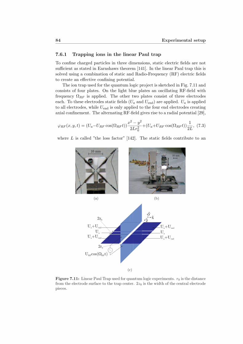
84 Experimental setup
7.6.1 Trapping ions in the linear Paul trap
To confine charged particles in three dimensions, static electric fields are notsufficient as stated in Earnshaws theorem [141]. In the linear Paul trap this issolved using a combination of static and Radio-Frequency (RF) electric fieldsto create an effective confining potential.
The ion trap used for the quantum logic project is sketched in Fig. 7.11 andconsists of four plates. On the light blue plates an oscillating RF-field withfrequency ΩRF is applied. The other two plates consist of three electrodeseach. To these electrodes static fields (Ua and Uend) are applied. Ua is appliedto all electrodes, while Uend is only applied to the four end electrodes creatingaxial confinement. The alternating RF-field gives rise to a radial potential [29],
ϕRF (x, y, t) = (Ua−URF cos(ΩRF t))x2 − y2
2Lr20
+(Ua+URF cos(ΩRF t))1
2L, (7.3)
where L is called ”the loss factor” [142]. The static fields contribute to an
10 mm
(a)
10 mm
(b)
Ua+Uend
$x
$y
$z
U cos(W t)RF RF
Ua+Uend
Ua
Ua+Uend
Ua+Uend
Ua
2z0
2r0
(c)
Figure 7.11: Linear Paul Trap used for quantum logic experiments. r0 is the distancefrom the electrode surface to the trap center. 2z0 is the width of the central electrodepieces.

7.6. Ion storage 85
axial as well as a radial potential [29],
ϕend(x, y, z) = κUend(z2 − 12(1− χ)x2 − 1
2(1 + χ)y2), (7.4)
where the geometric factor κ ≈ (2z0)−2. χ is an asymmetry parameter thataccounts for Uend only being applied to the dark blue plates thus creating anasymmetry. For an ion of mass, m, and charge, Q, we can describe the motionin the resulting potential. On the z-axis the potential is static and harmonicat frequency,
ωz =
√2QκUend
m. (7.5)
The resulting radial potential gives rise to equations of motion on Mathieuform [143],
∂2x
∂τ2+ [a + az(1− χ)− 2q cos(2τ)] = 0,
∂2y
∂τ2+ [−a + az(1 + χ) + 2q cos(2τ)] = 0, (7.6)
where the following dimensionless parameters have been introduced
q =2QURF
mLr20ΩRF
, a =4QUa
mLr20ΩRF
, τ =ΩRF t
2and az = −2(
wz
ΩRF)2. (7.7)
Mathieu equations defined by ∂2x∂τ2 + [a − 2q cos(2τ)] = 0 have stable and
unstable solutions depending on a and q as shown in Fig. 7.12(a) [144]. Thereexists an infinite number of configurations allowing for stable motion. Inthe experiments the trap is operated in the region depicted in Fig. 7.12(b).Defining ax = a + az(1 − χ) and ay = −a + az(1 + χ) (7.6) is brought onMathieu form,
∂2x
∂τ2+ [ax − 2q cos(2τ)] = 0,
∂2y
∂τ2+ [ay + 2q cos(2τ)] = 0. (7.8)
Since the stability diagram is symmetric around the a-axis, the Mathieu equa-tions have stable solutions for both ax, q and ay, q in the shaded regionof Fig. 7.12(b),
x(t) = x0[1− q
2cos(ΩRF t)] cos(ωxt),
y(t) = y0[1 +q
2cos(ΩRF t)] cos(ωyt),
z(t) = z0 cos(ωzt), (7.9)

86 Experimental setup
0 2 4 6 8 10 12
-2
0
2
4
6
8
10
a
q0 2 4 6 8 10 12
-2
0
2
4
6
8
10
Stable
solutions
(a) Regimes where the Mathieu equationshave stable solutions from [145].
0.0 0.5 1.0 1.5 2.0
-1.0
-0.5
0.0
0.5
1.0
a
q0.0 0.5 1.0 1.5 2.0
-1.0
-0.5
0.0
0.5
1.0
0.0 0.5 1.0 1.5 2.0
-1.0
-0.5
0.0
0.5
1.0
(b) Stable region for the linear Paul trapused in experiments from [145]. The dotrepresents typical parameters.
Figure 7.12
where x(t) and y(t) are 1.order solutions to (7.8) assuming |ax|, |ay|, |q| ¿ 1[29, 145] and z(t) completes the picture. The radial ion-motion is thus de-scribed by a secular motion along the x-axis and y-axis with frequencies,
ωx =12
√q
2+ a + az(1− χ)ΩRF , ωy =
12
√q
2− a + az(1 + χ)ΩRF (7.10)
superimposed by a fast oscillation at the RF-frequency of small amplitude, theion micromotion. Neglecting micromotion, the ion undergoes harmonic motionin all three dimensions with frequencies ωx, ωy, ωz. The trap is operated atΩRF /2π = 11.5 MHz or ΩRF /2π = 16.7 MHz and is constructed to haveχ = 0.269 and L = 1.23 [29]. For ΩRF /2π = 16.7, a typical choice of voltages(URF = 400V , Uend = 7V and Ua = 0V ) leads to parameters q = 0.26,az = −0.0016, ax = −0.0012, ay = −0.0020 and frequencies ωz/2π = 0.47MHz, ωy/2π = 1.51 MHz and ωx/2π = 1.53 MHz. For more than one ion inthe trap, the equations of motion and the stability regions are modified. Fora detailed discussion see [145].
7.6.2 Micromotion
Ion micromotion induces time dependent Doppler-shifts in the rest frame ofthe ion and thereby alter the excitation spectrum of its atomic transitions.Experiments may therefore be affected by micromotion. In the descriptionabove the RF-field only modulates the radial motion, but if a small amount ofRF-field is also produced on the end electrodes, axial micromotion can occur.The amplitude of axial micromotion, though, will be much smaller than theradial.
In the experiments presented in this thesis only course micromotion com-pensation was used, placing the ion in the centre of the trap where micromotion
7.7. Magnetic fields 87
is minimal. The coarse adjustment is done radially by observing the positionof the ion on the CCD-camera when the RF-potential is lowered and movingthe ion with the compensations voltages until its position is independent of thestrength of the RF-potential. The same procedure with Uend places the ion inthe centre of the axial confining potential. Fine compensation of micromotionwill be implemented using the correlation method presented in [146]. Here ameasurement of the correlation between the emission of photons and the RF-field is made. The correlations arise from the time dependent Doppler-shiftsin the rest frame of the ion and can be used to estimate the micromotionvelocity.
In the STIRAP experiments the laser beams are parallel to the axis andSTIRAP is only sensitive to axial micromotion. The Doppler shift induced bya micromotion velocity, v (∆i/2π = 1
λiv) will imply a change in two-photon de-
tuning. For the second STIRAP sequence the two wavelengths lie very closeand the induced two-photon detuning will always will be negligible. In thefirst, allowing for two-photon detunings below 0.5 MHz, we require an axialvelocity below 0.4 m/s. This should be possible to reach even without finecompensation, but to ensure that this is the case, the correlation method willbe used to measure the micromotion velocity. In future experiments with side-band cooling and gates, Raman transitions between the two Zeeman sublevelsof |S1/2〉 will be used. As described in [29] this will be achieved with lasersperpendicular to the trap axis. In this case radial micromotion will also becritical and fine compensation of micromotion necessary.
7.7 Magnetic fields
An external magnetic field will shift the Zeeman sublevels of the ion. It isdesirable to be able to control this splitting and we try to minimise the mag-netic fields from the environment experienced by the ions. The experimentalchamber is therefore shielded by µ-metal12. The µ-metal does not shield ex-ternal magnetic fields completely and in order to control the magnetic field,a Hall-probe placed just outside the chamber, but inside the µ-metal shieldmeasures the magnetic field in three dimensions. A non-zero field can becompensated with three coils placed outside the chamber. A time-dependentmagnetic field is compensated by a continuous measurement of the magneticfield and a subsequent feedback-current to the coils. This enables us to main-tain zero field within 1 mG, corresponding to a Larmor-frequency ωL = gi · 1.4kHz, where the Lande factors (gi) for Ca can be found in appendix B. Thehighest Larmor frequency is found for the S1/2 with gi = 2 and ωL = 2.8 kHz,which should not be critical for STIRAP. With the coils we can also create anon-zero magnetic field in any given direction.
12 nickel-iron alloy with very high magnetic permeability


Chapter 8
STIRAP experiments
The first STIRAP experiments were presented in 1990 [40], where a beamof atoms, as mentioned earlier, passed two stationary laser beams effectivelycreating laser pulses seen by the atom. These experiments showed high trans-fer efficiencies and had the advantage that no residual light was present.When considering using STIRAP for different aspects of quantum logic sin-gle non-moving atoms are preferable. Experiments with non-moving atoms ormolecules have been demonstrated [45,147,148], but all with ensembles of par-ticles. This chapter describes an experiment where single ions are transferredwith high efficiency using STIRAP. We present results on the second STIRAPsequence in the internal state detection scheme described in chapter 6.2, wherepopulation is transferred from the |D3/2〉 state to the |D5/2〉 state in 40Ca+.Instead of the first STIRAP sequence we optically pump the population from|S1/2〉 to |D3/2〉(m = ±3/2). The results were published in [I].
8.1 Optical pumping
The population initially in the ground state is optically pumped to the extremeZeeman sublevels (m = ±3/2) of the |D3/2〉 state, which is then the startingpoint for the experiments. We have chosen the Zeeman sublevels yielding thehighest Clebsch-Gordan coefficients. As shown in Fig. 8.1 the 397 nm laserexcites all population from |S1/2〉 to |P1/2〉, from where it decays either back to|S1/2〉 or to |D3/2〉. Population in |D3/2〉(m = ±1/2) is then pumped out withthe 866 nm laser polarised along the direction of an applied magnetic field (thex-direction in Fig. 8.1). After some cycles all population therefore ends up in|D3/2〉(m = ±3/2). We investigate our ability to optically pump by loadinga small Coulomb crystal into the trap. We apply the 397 nm and 866 nmlasers as described above in order to achieve that only |D3/2〉(m = ±3/2) ispopulated and we turn on the 850 nm and 854 nm with low power during100 µs with polarisations along the direction of the magnetic field, so thatonly π-transitions are coupled as shown in Fig. 8.1. We use a magnetic field
89

90 STIRAP experiments
Figure 8.1: Laser fields applied during optical pumping from |S1/2〉 to |D3/2〉(m =±3/2). The 866 nm laser is polarised along the direction of a bias magnetic field, B,ensuring that the population is optically pumped to the |D3/2〉(m = ±3/2) Zeemansublevels, because only two transitions are coupled. Subsequently, the 850 nm and854 nm lasers are also applied with polarisations along the magnetic field and thereforeonly π transitions between |D3/2〉, |P3/2〉 and |D5/2〉 are coupled.
of approximately 3 G and the Zeeman sublevels are therefore split, such thatwe can control which Zeeman level the lasers couple by an adjustment ofthe two photon resonance ∆two = ∆854 −∆850. Finally, we measure if somepopulation is transferred from |D3/2〉 to |D5/2〉, by applying the 397 nm laser
-4 -2 0 2 40.80
0.84
0.88
0.92
0.96
1.00
Rel
ativ
e fluor
esce
nce
two/2 [MHz]
Figure 8.2: Relative fluorescence measured by the PMT as a function of the two-photon detuning ∆two in the case where we populate all Zeeman sublevels in |D3/2〉(black) and in the case where we optically pump to the |D3/2〉(m = ±3/2)(red). Thesolid lines show a fit to Gaussian line-shapes. The smaller line width in the case withoptical pumping is due to a smaller Rabi frequency. The strengths of the lines arenot symmetric because the 397 nm laser does not populate the Zeeman sublevels ofP1/2 equally.

8.2. Setup and timing of STIRAP experiments 91
and the 866 nm laser with its polarisation scrambled to drive all |D3/2〉-|P1/2〉transitions. Simultaneously, we measure fluorescence.
We see a drop in fluorescence if population was transferred to the |D5/2〉state and show this as a function of the two-photon detuning in Fig. 8.2.The results show that when we do not optically pump (black dots) all fourZeeman sublevels are populated, while optical pumping (red dots) reduces thepopulation in the (m = ±1/2) sublevels significantly and we estimate that lessthan 15% of the population is in (m = ±1/2) after optical pumping.
8.2 Setup and timing of STIRAP experiments
After optical pumping we perform STIRAP experiments with both laserspolarised along the bias magnetic field so we have effectively only two π-transitions as shown in Fig. 8.1. To analyse the results using the PMT weneed three detection periods - one with all ions non-fluorescent, one with allions fluorescent and one after the STIRAP experiment. The whole sequenceused is shown in Fig. 8.3 and consists of four parts:
• In the first detection period we apply the Doppler cooling lasers (397 nmand polarisation scrambled 866 nm) and for repumping shelved popula-
10 ms PMT detection (B)10 ms PMT detection (D)8 ms CCD detection
10 ms PMT detection (L) Stirap-sequence
(20 ms)
Opticalpump(4ms)
854 nm
850 nm
866 nmpolarisationscrambled
397 nm
866 nmpolarised
Figure 8.3: Laser sequence used in STIRAP experiments. First period is a detectionperiod where all ions are in the fluorescent cooling cycle. This is followed by opticalpumping, the two STIRAP pulses and then another period with the cooling lasersapplied measuring fluorescent population remaining in the |D3/2〉-state. The finalperiod is used to measure the background level of scattered light when all populationis trapped in the |D3/2〉 state, because the 866 nm laser is not applied to repumppopulation back into the cooling cycle.
92 STIRAP experiments
tion in |D5/2〉 also the 854 nm is applied. In this period all ions willtherefore be fluorescent (L).
• We then optically pump with the π-polarised 866 nm laser and the397 nm laser and apply two STIRAP pulses. If the process is efficientall population is now in the |D5/2〉 state.
• The second detection period again applies the two Doppler cooling lasersand ions remaining in |D3/2〉 will fluoresce (D).
• To measure a background fluorescence level from for example scatteredlight, we apply only the 397 nm laser. Ions that are not already in |D5/2〉are then shelved in |D3/2〉 and no ions fluoresce (B).
We name the three measured levels of fluorescence L (light), D (dark), B
(background) and calculate the transfer efficiency as D−BL−B .
Experimental parametersThe 850 nm and 854 nm lasers are focused to a 60 µm waist in the trap centre.We measure their power level, P850 =2.4 mW, P854 =3.6 mW and calculatethe Rabi frequencies on the m = ±3/2 → m = ±3/2 transitions from theformula derived in appendix B,
Ω850,3/2/2π ≈ 100 MHz,
Ω854,3/2/2π ≈ 250 MHz.
With the RF-switch in the AOM open, the residual Rabi frequencies weremeasured to
Ω850,3/2,off/2π ≈ 0.9 MHz,
Ω854,3/2,off/2π ≈ 4.4 MHz
With the RF-switch in the AOM closed, the residual Rabi frequencies weremeasured to
Ω850,3/2,off/2π ≈ 0.2 MHz,
Ω854,3/2,off/2π ≈ 0.3 MHz.
The RF-switch suppresses the RF-power with 100 dB, but a part of the resid-ual light originates from scattered 0.order light in the AOM crystal and istherefore not reduced by the RF-switch. Both lasers are red-detuned fromresonance to avoid one-photon excitations: ∆850/2π ≈ ∆854/2π ≈600 MHzand we use Gaussian pulses as defined in (2.22). The magnetic field in allSTIRAP experiments was Bx ≈ 1G.
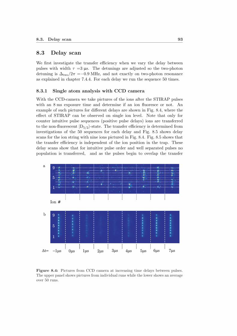
8.3. Delay scan 93
8.3 Delay scan
We first investigate the transfer efficiency when we vary the delay betweenpulses with width τ =3 µs. The detunings are adjusted so the two-photondetuning is ∆two/2π =−0.9 MHz, and not exactly on two-photon resonanceas explained in chapter 7.4.4. For each delay we run the sequence 50 times.
8.3.1 Single atom analysis with CCD camera
With the CCD-camera we take pictures of the ions after the STIRAP pulseswith an 8 ms exposure time and determine if an ion fluoresce or not. Anexample of such pictures for different delays are shown in Fig. 8.4, where theeffect of STIRAP can be observed on single ion level. Note that only forcounter intuitive pulse sequences (positive pulse delays) ions are transferredto the non-fluorescent |D5/2〉-state. The transfer efficiency is determined frominvestigations of the 50 sequences for each delay and Fig. 8.5 shows delayscans for the ion string with nine ions pictured in Fig. 8.4. Fig. 8.5 shows thatthe transfer efficiency is independent of the ion position in the trap. Thesedelay scans show that for intuitive pulse order and well separated pulses nopopulation is transferred, and as the pulses begin to overlap the transfer
1
5
9
Ion #
1
5
9
-1ms 0ms 1ms 3ms2ms 4ms 5ms 6ms 7msDt=
a
b
Figure 8.4: Pictures from CCD camera at increasing time delays between pulses.The upper panel shows pictures from individual runs while the lower shows an averageover 50 runs.

94 STIRAP experiments
-2 -1 0 1 2 3 4 5 6 7
0.0
0.1
0.2
0.3
0.4
0.5
0.6
0.7
0.8
0.9
1.0
[ s]
Tra
nsf
er e
ffic
iency
Ion # 1 2 3 4 5 6 7 8 9
Figure 8.5: STIRAP transfer efficiency as a function of delay between pulses forindividual ions analysed with CCD-camera and averaged over 50 sequences.
efficiency increases because of the creation of a Raman transition, but firstwhen the pulse order is counter intuitive the transfer rises above 0.5 becauseSTIRAP becomes efficient. For counter intuitive but separated pulses theefficiency drops to a constant level at 0.05 due to a off-resonant one-photonexcitation induced by the 850 nm pulse.
8.3.2 Average of more atoms
Averaging over and finding the standard deviation of the nine ions in Fig. 8.5gives a final estimation of the transfer efficiency as depicted with blue circles inFig. 8.6(a). The results obtained from the CCD-pictures are compared withthe PMT measurements. The PMT measures the fluorescence level in thethree periods indicated in Fig. 8.3. For each experiment with 50 sequences wefind the transfer efficiency, D−B
L−B , and from the 50 sequences we calculate theaverage and standard deviation as shown with the green circles in Fig. 8.6(a).The PMT and CCD results show good agreement.
The experimental results are compared with a theoretical simulation solv-ing the density matrix master equation for the five level system in Fig. 6.1neglecting the Zeeman structure. The simulations are made with Rabi frequen-cies, laser phase fluctuations and residual light levels that optimises the agree-ment between theory and experiment. We find Ω850/2π =90 MHz, Ω854/2π =225 MHz, 10 kHz phase fluctuations for both lasers and residual Rabi frequen-cies at 1% of the peak value for the 850 nm laser and 2% for the 854 nm when

8.3. Delay scan 95
-2 -1 0 1 2 3 4 5 6 70.0
0.2
0.4
0.6
0.8
1.0
Tra
nsf
er e
ffic
iency
t [ s]
(a) Average and standard deviation of 50sequences and 9 ions measured with CCD(blue) and PMT (green). The solid blackline is a numerical simulation with laserphase fluctuations and residual light in-cluded.
-2 -1 0 1 2 3 4 5 6 70.0
0.2
0.4
0.6
0.8
1.0
Tra
nsf
er e
ffic
iency
t [ s]
(b) Comparison between measured re-sults (blue circles and green triangles) andnumerical simulations. The black curveis as in (a). The efficiency is optimisedby first neglecting the laser phase fluc-tuations (red) and further by disregard-ing the residual light as well (light greencurve).
Figure 8.6: STIRAP transfer efficiency as a function of delay between pulsesmeasured with CCD camera, PMT and compared with the a numerical propaga-tion of the density matrix master equation using parameters Ω850,3/2/2π =90 MHz,Ω854,3/2/2π =225 MHz, ∆850/2π=600 MHz, ∆854/2π = 600 − 0.9 MHz and 2 kHzphase fluctuations of all lasers. The residual light levels used were 1% of the peakvalue for the 850 nm laser and 2% for the 854 nm during the 20 µs where the RF-switch is open and 0.1% for both lasers during the 200 µs where the RF-switch isclosed. All simulations are with Ω397/2π =100 MHz. The light green curve in (b)where residual light is neglected is calculated on two-photon resonance where theefficiency then is optimal.
the RF-switch is open and 0.1% for both lasers when the RF-switch is closed.There is a discrepancy between the Rabi frequencies measured and the onesused in the simulations, which we explain by a non-perfect overlap betweenthe ion-string and the focused laser beam as well as the fact that the opticalpumping was not perfect and therefore a part of the transfer takes place onthe m = ±1/2 ↔ m = ±1/2 transitions, where the coupling is weaker. Theresidual light levels are approximately as measured. The 3 µs wide pulses usedin the experiment indicate that coherence must be kept for approximately tenmicroseconds and hence longer than the 2 µs timescale, where 2 kHz phasefluctuations were measured as shown in appendix C. The 10 kHz phase fluc-tuations are thus a realistic assumption.
The optimal delay between the pulses is approximately 3.0 µs where weachieve a transfer efficiency of 93 ± 2%. The two main error sources are thelaser phase fluctuations and the residual light. We show this in Fig. 8.6(b),where the red curve neglects the laser phase fluctuations and the light greencurve also disregards residual light. The transfer efficiency can be improved

96 STIRAP experiments
-2 0 2 4 60.0
0.2
0.4
0.6
0.8
1.0
0.95
Tra
nsf
er e
ffic
iency
Pulse delay [ s]
Figure 8.7: Delay scan with two ions. The transfer efficiency is measured with thePMT. The average and standard deviation is found from 50 sequences.
significantly by a better phase stabilisation of the lasers combined with a moreefficient shut down of the laser light. We achieve a higher transfer efficiencywith only two ions in the string, where 95 ± 2% was obtained as shown inFig. 8.7. The slightly lower transfer efficiency in the nine ion case may be dueto a higher RF-heating rate.
8.4 Frequency scan
The STIRAP efficiency depends significantly on the two-photon detuning andwith a fixed delay (∆t =2 µs) between pulses with pulse width, τ =3 µs wemeasure the dependence scanning the frequency of the 854 nm laser as shownin Fig. 8.8. The experimental results arise from eight scans (each averagedover 50 sequences) of ion strings with between one and ten ions measuredwith the PMT. The average and the standard deviation are calculated fromthese eight results and compared with a simulation solving the density matrixmaster equation with the same parameters as in the simulations presentedin Fig. 8.6. The asymmetry of the spectrum is due to the unbalanced Rabifrequencies as described in chapter 2.3.2. The residual light gives rise to aparasitic Raman resonance (see chapter 7.4.4) and the best transfer efficiency istherefore not achieved on two-photon resonance, but with a small negative two-photon detuning, ∆two/2π =−0.9 MHz. Here we achieve a transfer efficiencyof 91.8± 0.7%.
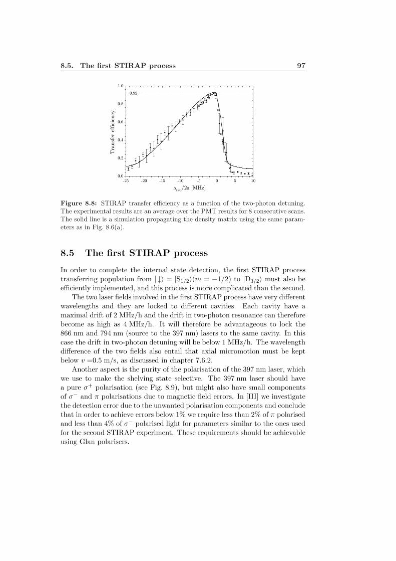
8.5. The first STIRAP process 97
-25 -20 -15 -10 -5 0 5 100.0
0.2
0.4
0.6
0.8
1.0
0.92
Tra
nsf
er e
ffic
iency
two/2 [MHz]
Figure 8.8: STIRAP transfer efficiency as a function of the two-photon detuning.The experimental results are an average over the PMT results for 8 consecutive scans.The solid line is a simulation propagating the density matrix using the same param-eters as in Fig. 8.6(a).
8.5 The first STIRAP process
In order to complete the internal state detection, the first STIRAP processtransferring population from | ↓〉 = |S1/2〉(m = −1/2) to |D3/2〉 must also beefficiently implemented, and this process is more complicated than the second.
The two laser fields involved in the first STIRAP process have very differentwavelengths and they are locked to different cavities. Each cavity have amaximal drift of 2 MHz/h and the drift in two-photon resonance can thereforebecome as high as 4 MHz/h. It will therefore be advantageous to lock the866 nm and 794 nm (source to the 397 nm) lasers to the same cavity. In thiscase the drift in two-photon detuning will be below 1 MHz/h. The wavelengthdifference of the two fields also entail that axial micromotion must be keptbelow v =0.5 m/s, as discussed in chapter 7.6.2.
Another aspect is the purity of the polarisation of the 397 nm laser, whichwe use to make the shelving state selective. The 397 nm laser should havea pure σ+ polarisation (see Fig. 8.9), but might also have small componentsof σ− and π polarisations due to magnetic field errors. In [III] we investigatethe detection error due to the unwanted polarisation components and concludethat in order to achieve errors below 1% we require less than 2% of π polarisedand less than 4% of σ− polarised light for parameters similar to the ones usedfor the second STIRAP experiment. These requirements should be achievableusing Glan polarisers.
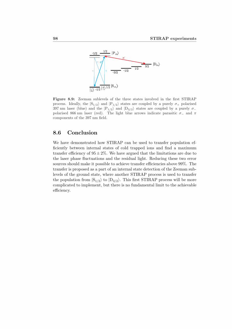
98 STIRAP experiments
Figure 8.9: Zeeman sublevels of the three states involved in the first STIRAPprocess. Ideally, the |S1/2〉 and |P1/2〉 states are coupled by a purely σ+ polarised397 nm laser (blue) and the |P1/2〉 and |D3/2〉 states are coupled by a purely σ−polarised 866 nm laser (red). The light blue arrows indicate parasitic σ− and πcomponents of the 397 nm field.
8.6 Conclusion
We have demonstrated how STIRAP can be used to transfer population ef-ficiently between internal states of cold trapped ions and find a maximumtransfer efficiency of 95± 2%. We have argued that the limitations are due tothe laser phase fluctuations and the residual light. Reducing these two errorsources should make it possible to achieve transfer efficiencies above 99%. Thetransfer is proposed as a part of an internal state detection of the Zeeman sub-levels of the ground state, where another STIRAP process is used to transferthe population from |S1/2〉 to |D3/2〉. This first STIRAP process will be morecomplicated to implement, but there is no fundamental limit to the achievableefficiency.

Chapter 9
Summary and Outlook
Quantum computation is still far from the goal of implementing algorithmswith a large number of qubits that can outperform their classical counterparts.An important challenge is not only to implement initialisation, gates and readout, but also to perform each step with high fidelity. To achieve this, it may beadvantageous to use adiabatic processes with their potential robustness. Thisthesis have considered different ways of employing adiabaticity in quantumcomputation as well as for creation of many-particle entangled states.
Chapter 3 and 5 presented quantum gates based on adiabatic following ofdark states acquiring geometric phases. The system remains in the dark stateswhen STIRAP processes are used and adiabaticity maintained. The gates arequite insensitive to fluctuations in the controlling parameters and are in thatrespect robust. Robustness against noise is a more complicated question.Chapter 4 showed how the geometric phases acquired in the implementationof the Hadamard gate become complex and cause a decrease in fidelity. Thefidelity, though, is still above 0.99 for realistic experimental dephasing ratesand apart from the influence of noise it depends on our ability to maintainadiabaticity and on the robustness of the geometric phases. Adiabaticity isachieved using high Rabi frequencies and long pulses, but it is on the otherhand preferable to use the shortest possible pulses to achieve fast gates thatare less sensitive to decoherence. Choosing the optimal pulse width will be atrade-off. When adiabaticity is ensured, the pulse shapes, the delay betweenpulses, the relative field strengths and relative phases of the applied laserfields must be controlled in order to achieve the desired geometric phases. Ofthese only control of the relative phase is challenging and it is preferable toimplement the gates in systems where all involved lasers originate from thesame source implying the use of Zeeman or hyperfine sublevels coupled to thesame excited state.
The one-qubit gates can be implemented in various systems such as op-tically trapped neutral atoms, trapped ions and rare-earth ions doped intocrystals, while the two-qubit gate presented in chapter 5 is based on the long
99

100 Summary and Outlook
range dipole-dipole interaction in Rydberg atoms. It is an open questionto what extend the geometric gates are more robust than the dynamic andfurther theoretical investigations including comparative studies are needed toshed light on the benefits of geometric gates. In spite of this, we conclude thatthe one-qubit gate of chapter 3 and the two-qubit gate of chapter 5 combinedyield a universal set of quantum gates that can be implemented experimentallywith high fidelities.
The experimental investigations of adiabatic transfer between internal statesof trapped laser cooled 40Ca+ ions in chapter 8 showed a 95% efficiency andcomparison with numerical studies revealed that the limiting factor was acombination of residual light and laser phase fluctuations. These are not fun-damental limitations, but must be improved in order to achieve an efficiencyof the qubit detection scheme proposed in chapter 6 that is high enough tomake it a true candidate for read out of the ion trap quantum computer.
The Rydberg atoms are not only a candidate for quantum computation,but as we show in chapter 5 a single STIRAP sequence applied to tens ofatoms will entangle them with high fidelity. Apart from being of fundamentalinterest the produced entangled states are important for precision metrology.The work showed how the Rydberg blockade in conjunction with the adiabaticprocesses produces a Jaynes-Cummings dynamics, that is sufficient to producea variety of interesting states and it could be interesting to investigate thisfurther.
9.1 Dansk resume
Kvantecomputeren begyndte som en fascinerende ide, hvor smarte algoritmerudnytter kvantemekanikkens parallelitet til at løse problemer, som er utilgæn-gelige pa klassiske computere. I løbet af de sidste artier har eksperimentellefremskridt muliggjort manipulation af enkelte atomer og ioner, som bruges tilat realisere kvantegates. Udfordringen i dag er at skalere computeren, hvilketkræver at alle manipulationer skal udføres med høj præcision, fordi fejleneellers vil akkumulere og ødelægge slutresultatet. For at opna dette kan detvære en fordel at bruge adiabatiske processer.
I den teoretiske del af afhandlingen præsenteres kvantegates baseret paadiabatiske processer, som er robuste i forhold til fluktuationer i parametre ogdet diskuteres, hvordan de pavirkes af støj. De adiabatiske processer anvendesogsa til at entangle mange neutrale atomer, som vekselvirker pa grund afderes store dipolmomenter. Den eksperimentelle del viser, hvordan populationeffektivt kan overføres fra en intern tilstand til en anden i fangede laserkølede40Ca+-ioner og vi demonstrerer en effektivitet pa 95%. Afvigelsen fra 100%effektivitet tilskrives fluktuationer i lasernes relative fase, og at ioner utilsigtetbliver belyst af laserne ogsa før og efter den adiabatiske proces, hvilket kanødelægge sluttilstanden.

Appendices
101


Appendix A
Principles of numericalsimulations
The purpose of this appendix is to give an overview of the different numericalsimulations used throughout the thesis. We demonstrate the methods on thethree level lambda system shown in Fig. A.1, but the principles are directlyextended to systems with more than three levels as well as more than oneatom.
WA
WB
DA D
B
Ge
Ge1
Ge2
>e
>2
>1
Figure A.1: Three level lambda-systemcoupled by two laser fields with Rabi fre-quencies ΩA and ΩB detuned ∆A and ∆B
with respect to resonance. Decay rates fromthe excited state and out of the system is in-dicated with Γe, decay to |1〉 with Γe1 anddecay to |2〉 with Γe2. |1〉 and |2〉 are as-sumed stable.
A.1 The Schrodinger equation
We first describe only the Schrodinger equation neglecting decay and otherdecoherence sources. We consider external laser fields as plane monochromaticwaves and in the dipole approximation the field interacts with an electron viathe potential,
V = −er(12εE0e
−iωt + c.c.), (A.1)
103

104 Principles of numerical simulations
Using the enumeration of the levels and laser fields shown in Fig. A.1 we canwrite all nonzero couplings,
V1e = −er1e(12εE0e
−iωt + c.c.)A,
Ve1 = −ere1(12εE0e
−iωt + c.c.)A,
V2e = −er2e(12εE0e
−iωt + c.c.)B,
Ve2 = −ere2(12εE0e
−iωt + c.c.)B. (A.2)
Solving the Schrodinger equation corresponds to solving a set of coupled equa-tions for the probability amplitudes ai,
i~a1 = E1a1 − 12er1e(εE0e
−iωt + c.c.)Aae,
i~ae = Eeae − 12ere1(εE0e
−iωt + c.c.)Aa1 − 12ere2(εE0e
−iωt + c.c.)Ba2,
i~a2 = E2a2 − 12er2e(εE0e
−iωt + c.c.)Bae, (A.3)
where Ei are energies of the atomic levels. We define Rabi frequencies,
ΩA =eE0
~re1 · ε, (A.4)
ΩB =eE0
~re2 · ε,
and detunings,
∆A =E1 −Ee
~− ωA, (A.5)
∆B =E2 −Ee
~− ωB.
Choosing E1 = 0 and introducing convenient phase shifted probability ampli-tudes,
a1 = c1,
ae = cee−iωAt,
a2 = c2e−i(ωA−ωB)t, (A.6)

A.2. Density matrix 105
we can rewrite (A.3) in the rotating wave approximation,
ic1 = −12Ω∗Ace,
ice = ∆Ace − 12ΩAc1 − 1
2ΩBc2,
ic2 = (∆A −∆B)c2 − 12Ω∗Bce. (A.7)
These differential equations correspond exactly to the Hamiltonian in (2.14)and when we in the thesis show numerical solutions of the Schrodinger equa-tion we refer to propagating these equations using a Runge-Kutta routine inMatlab. When the systems become large, as in the many-atom calculationsin chapter 5.3, it is convenient to calculate the propagation by,
|ψ(t + dt)〉 = exp(−iHdt
~
)|ψ(t)〉, (A.8)
where H is assumed constant during the small time step, dt.Spontaneous emission out of the system can be included as imaginary
decay terms in (A.7), but when we wish to investigate decay and decoherencethe density matrix is more suitable.
A.2 Density matrix
For the closed system the density matrix is defined as ρij = cic∗j and its time
evolution given by ρij = cic∗j + cic∗j and we find,
ρ11 =− 12i(ΩAρ1e − Ω∗Aρe1),
ρee =12i(ΩBρ2e − Ω∗Bρe2) +
12i(ΩBρ2e − Ω∗Bρe2),
ρ22 =− 12i(ΩBρ2e − Ω∗Bρe2),
ρ1e =i∆Aρ1e +12iΩ∗A(ρee − ρ11)− 1
2iΩ∗Bρ12,
ρ12 =i(∆A −∆B)ρ12 +12iΩ∗Aρe2 − 1
2iΩ∗Bρ1e,
ρ2e =i∆Bρ2e +12iΩ∗B(ρee − ρ22)− 1
2iΩ∗Aρ21. (A.9)
The diagonal elements now directly display the population in the three atomicstates, while the off-diagonal elements express the coherence among the dif-ferent states and give the relative phases between them. The closed atomic
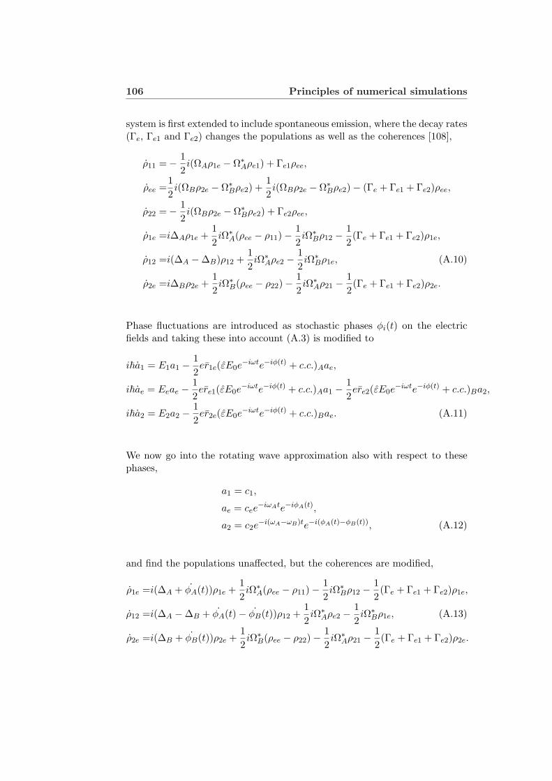
106 Principles of numerical simulations
system is first extended to include spontaneous emission, where the decay rates(Γe, Γe1 and Γe2) changes the populations as well as the coherences [108],
ρ11 =− 12i(ΩAρ1e − Ω∗Aρe1) + Γe1ρee,
ρee =12i(ΩBρ2e − Ω∗Bρe2) +
12i(ΩBρ2e − Ω∗Bρe2)− (Γe + Γe1 + Γe2)ρee,
ρ22 =− 12i(ΩBρ2e − Ω∗Bρe2) + Γe2ρee,
ρ1e =i∆Aρ1e +12iΩ∗A(ρee − ρ11)− 1
2iΩ∗Bρ12 − 1
2(Γe + Γe1 + Γe2)ρ1e,
ρ12 =i(∆A −∆B)ρ12 +12iΩ∗Aρe2 − 1
2iΩ∗Bρ1e, (A.10)
ρ2e =i∆Bρ2e +12iΩ∗B(ρee − ρ22)− 1
2iΩ∗Aρ21 − 1
2(Γe + Γe1 + Γe2)ρ2e.
Phase fluctuations are introduced as stochastic phases φi(t) on the electricfields and taking these into account (A.3) is modified to
i~a1 = E1a1 − 12er1e(εE0e
−iωte−iφ(t) + c.c.)Aae,
i~ae = Eeae − 12ere1(εE0e
−iωte−iφ(t) + c.c.)Aa1 − 12ere2(εE0e
−iωte−iφ(t) + c.c.)Ba2,
i~a2 = E2a2 − 12er2e(εE0e
−iωte−iφ(t) + c.c.)Bae. (A.11)
We now go into the rotating wave approximation also with respect to thesephases,
a1 = c1,
ae = cee−iωAte−iφA(t),
a2 = c2e−i(ωA−ωB)te−i(φA(t)−φB(t)), (A.12)
and find the populations unaffected, but the coherences are modified,
ρ1e =i(∆A + φA(t))ρ1e +12iΩ∗A(ρee − ρ11)− 1
2iΩ∗Bρ12 − 1
2(Γe + Γe1 + Γe2)ρ1e,
ρ12 =i(∆A −∆B + φA(t)− φB(t))ρ12 +12iΩ∗Aρe2 − 1
2iΩ∗Bρ1e, (A.13)
ρ2e =i(∆B + φB(t))ρ2e +12iΩ∗B(ρee − ρ22)− 1
2iΩ∗Aρ21 − 1
2(Γe + Γe1 + Γe2)ρ2e.

A.2. Density matrix 107
Now, if we assume that the process leading to the phase fluctuations is Marko-vian the spectrum of the laser will be Lorentzian and its first order correlationfunction is [149]
〈eφi(t)eφi(t′)〉 = e−Γi(t−t′), (A.14)
where Γi is the bandwidth of the Lorentzian spectrum for the i’th laser field.It was shown in [149] that in this situation (A.13) can be averaged over thestochastic fluctuations of the phase to yield,
ρ11 =− 12i(ΩAρ1e − Ω∗Aρe1) + Γe1ρee,
ρee =12i(ΩBρ2e − Ω∗Bρe2) +
12i(ΩBρ2e − Ω∗Bρe2)− (Γe + Γe1 + Γe2)ρee,
ρ22 =− 12i(ΩBρ2e − Ω∗Bρe2) + Γe2ρee,
ρ1e =(i∆A − ΓA)ρ1e +12iΩ∗A(ρee − ρ11)− 1
2iΩ∗Bρ12 − 1
2(Γe + Γe1 + Γe2)ρ1e,
ρ12 =(i∆A − i∆B − ΓA − ΓB)ρ12 +12iΩ∗Aρe2 − 1
2iΩ∗Bρ1e, (A.15)
ρ2e =(i∆B − ΓB)ρ2e +12iΩ∗B(ρee − ρ22)− 1
2iΩ∗Aρ21 − 1
2(Γe + Γe1 + Γe2)ρ2e.
As discussed in chapter 4.1.1 the density matrix including decay and decoher-ence as described above can be written as a Lindblad master equation, withsuitable Lindblad operators, and with these operators the quantum MonteCarlo method introduced in chapter 4.1.2 can also be used.


Appendix B
Properties of 40Ca+
B.1 Characteristics
The five dipole allowed transitions in 40Ca+ are characterised by the wave-lengths and linewidths [110], from which the saturation intensities can becalculated.
Transition λ [nm] Isat [mW/cm2] Γ/2π
S1/2 − P1/2 396.847 43.3 20.7S1/2 − P3/2 393.366 46.2 21.5D3/2 − P1/2 866.241 0.34 1.69D3/2 − P3/2 849.802 0.038 0.177D5/2 − P3/2 854.209 0.33 1.58
The D5/2 and D3/2 states are metastable and their lifetimes have beeninvestigated in several experiments. The most precise measurements havebeen performed with a single trapped ion yielding: τD3/2
= 1176± 11 ms andτD5/2
= 1168± 9 ms [80].
B.1.1 Zeeman structure
A magnetic field introduces a Zeeman structure of the energy levels. TheZeeman splitting in 40Ca+ is given by
∆i/2π =gimiµBB
~= gimiB× 1.4 MHz/G (B.1)
where the Lande factors are:
State S1/2 P1/2 P3/2 D3/2 D5/2
g 2 2/3 4/3 4/5 6/5
109

110 Properties of 40Ca+
B.2 Rabi frequencies
In a two-level atom with transition frequency ω coupled by a laser field withfield strength E0 and decay rate from the upper level Γ, the Rabi frequency(χ) is simply [108],
χ2 =Γ2
2I
Isat, (B.2)
where the intensity I = 12cε0E
20 and the saturation intensity
Isat =~Γω3
12πc2, (B.3)
yields
χ2 =3πΓc3ε0E
20
~ω3. (B.4)
This Rabi frequency only describes the coupling in a two-level atom and andwe call it the two-level Rabi frequency.
In an atom with fine structure, the Rabi frequency for a one-photon tran-sition between a lower state |J,m〉 and an upper state |J ′,m′〉 is defined fromthe atomic dipole moment operator coupled to the electric field
Ωf,i =eE0
~〈J ′,m′|ε · r|J,m〉 (B.5)
where ε represents the polarisation of the electric field. In order to calculatethe dipole matrix elements we expand in polarisation components denoted byq = 0,±1, where q = 0 corresponds to linear polarised light and q = ±1 tocircular polarised light,
〈J ′,m′|ε · r|J,m〉 =∑
q=0,±1
〈J ′, m′|rq|J,m〉, (B.6)
and calculate the matrix element for a given polarisation of the light using theWigner-Eckart theorem [150]
〈J ′,m′|rq|J,m〉 = (−1)J ′−m′(
J ′ 1 J−m′ q m
)(J ′||r||J)
= (−1)J ′−m′(−1)J ′+J+1
(J 1 J ′
m q −m′
)(J ′||r||J).
(B.7)
where we have used the symmetries of the 3j-symbols. The reduced matrixelements are connected to the decay rates [150]
Γ =ω3e2
3πε0~c3
12J ′ + 1
|〈J ′||r||J〉|2, (B.8)

B.2. Rabi frequencies 111
and the 3j-symbol can be rewritten as Clebsch-Gordan coefficients,(
J 1 J ′
m q −m′
)= (−1)J−1+m′ 1√
2J ′ + 1〈Jm1q|J ′m′〉. (B.9)
Substituting (B.7), (B.8) and (B.9) into (B.5) we find the Rabi frequency fora given polarisation,
Ωq = χ〈Jm1q|J ′m′〉(−1)2J+2J ′
= χ〈Jm1q|J ′m′〉, (B.10)
as a modification of the two-level Rabi frequency. Below we show the Clebsch-Gordan coefficient for selected transitions.
m′ = −1/2 m′ = 1/2
m = −1/2 −√
1/3 −√
2/3m = 1/2
√2/3
√1/3
Table B.1: Clebsch-Gordan coefficients for the S1/2−P1/2 transition withJ = J ′ = 1/2 coupled with the 397 nm laser.
m′ = −1/2 m′ = 1/2
m = −3/2√
1/2 -m = −1/2 −
√1/3
√1/6
m = 1/2√
1/6 −√
1/3m = 3/2 -
√1/2
Table B.2: Clebsch-Gordan coefficients for the D3/2−P1/2 transition with J = 3/2and J ′ = 1/2 coupled with the 866 nm laser.
m′ = −3/2 m′ = −1/2 m′ = 1/2 m′ = 3/2
m = −3/2 −√
3/5 −√
2/5 - -m = −1/2
√2/5 −
√1/15 −
√8/15 -
m = 1/2 -√
8/15√
1/15 −√
2/5m = 3/2 - -
√2/5
√3/5
Table B.3: Clebsch-Gordan coefficients for the D3/2−P3/2 transition withJ = J ′ = 3/2 coupled with the 850 nm laser.

112 Properties of 40Ca+
m′ = −3/2 m′ = −1/2 m′ = 1/2 m′ = 3/2m = −5/2
√2/3 - - -
m = −3/2 −√
4/15√
2/5 - -m = −1/2
√1/15 −
√2/5
√1/5 -
m = 1/2 -√
1/5 -√
2/5√
1/15m = 3/2 - -
√2/5 −
√4/15
m = 5/2 - - -√
2/3
Table B.4: Clebsch-Gordan coefficients for the D5/2−P3/2 transition with J = 5/2and J ′ = 3/2 coupled with the 854 nm laser.

Appendix C
Measurements of laser phasefluctuations
Phase fluctuations of the lasers involved in STIRAP lead to a decay of thecoherences and thereby limits the transfer efficiency. The phase fluctuationsare measured with a delayed self-heterodyne interferometer as first proposed in[151]. The laser beam is split on a 50/50 beamsplitter, changing the frequencyof one beam with an AOM and delaying the other in a fibre. The delay timeis nL/c, where L is the fibre length and n = 1.5 the typical refraction indexfor an optical fibre. The two beams are subsequently superimposed in a fibre
Laser AOM PhotoDetector
SpectrumAnalyser
Fibre delay line
NPBS NPBS
Figure C.1: Setup for measurement of laser phase fluctuations. The laser beam issplit on a non-polarising beamsplitter (NPBS). One part pass through an AOM, theother is delayed in a fibre. Subsequently, they are reunited on another non-polarisingbeamsplitter and the interference beat-note between them is measured.
coupled beamsplitter creating a beat-signal, which is analysed in a spectrumanalyser. If two lasers with optical frequencies ω1 and ω2 are superimposed ona photodetector a beat-note can be observed at the difference in the opticalfrequencies of the two laser beams - in our case the frequency change made bythe AOM is around 400 MHz.
In our setup both beams have the same source so in order to considerthese as two independent laser sources we need to delay one beam beyond thecoherence time (τcoh = 1
2πδl) of the laser. To make measurements far beyond
113

114 Measurements of laser phase fluctuations
the coherence time of the lasers we use a 4.3 km optical fibre1 corresponding toa 22µs delay time. This was done for the 850 nm and 854 nm lasers as shownin Fig. C.2. A fit of the results to a Lorentz distribution yields FWHM of390 kHz and 208 kHz, respectively, and assuming the laser phase fluctuationsare Lorentz-distributed, the FWHM width of the measured beat-notes aretwice the FWHM-Lorentz linewidth of the lasers [152,153] yielding linewidthsδ850 = 195 kHz and δ854 = 104 kHz.
-1000 -500 0 500 10000.2
0.3
0.4
0.5
0.6
0.7
0.8
0.9
1.0
Nor
mal
ised
inte
nsi
ty
Frequency [kHz]
(a) Beat note of 850 nm laser withFWHM=390 kHz.
-1000 -500 0 500 1000
0.5
0.6
0.7
0.8
0.9
1.0
Nor
mal
ised
inte
nsi
ty
Frequency [kHz]
(b) Beat note of 854 nm laser withFWHM=208 kHz.
Figure C.2: Linewidth measurements with 4.3 km fibre delay line. Both measure-ments are assumed to be Lorentzian.
For all four lasers (850 nm, 854 nm, 866 nm and 794 nm, which is frequencydoubled to 397 nm), measurements were also done with fibre lengths2 300m and 518 m corresponding to 1.5 µs and 2.6 µs delay between the twobeams. This gives us measurements of the dephasing rates due to laser phasefluctuations on the time scales we use in the STIRAP-sequences. In this casethe two beams can not be considered independent and the measured phasefluctuations are estimates of the phase fluctuations experienced by the ionsduring a STIRAP process. The results are shown for all four lasers witha 518 m fibre delay in Fig. C.3 yielding phase fluctuations below 1.5 kHzfor all lasers involved in STIRAP - measured as the FWHM of a fit to aLorentz distribution. For a 300 m delay line the fluctuations are just a littlebelow the 518 m result as shown in the same figure for the 854 nm laser.The measurements of the phase fluctuations are to a good approximationLorentzian and can therefore be included as decay terms in the off-diagonaldensity matrix elements as in the simulations presented in chapter 7.4.5.
14300 m optical telecom fibre.2300 m single mode optical fibre with operating wavelength at 830 nm (sm800-5.6-125
from Thorlabs). The 518 m fibre consists of the 300 m fibre connected with a 218 m telecomfibre single mode at 1089 nm.

Measurements of laser phase fluctuations 115
-4 -2 0 2 4
0.7
0.8
0.9
1.0
Norm
alise
d inte
nsi
ty
Frequency [kHz]
(a) Beat note of 866 nm laser withFWHM=1.5 kHz measured with 518 mfibre delay line.
-4 -2 0 2 4
0.2
0.4
0.6
0.8
1.0
Nor
mal
ised
inte
nsi
ty
Frequency [kHz]
(b) Beat note of 794 nm laser withFWHM=0.9 kHz measured with 518 mfibre delay line.
-4 -2 0 2 4
0.2
0.3
0.4
0.5
0.6
0.7
0.8
0.9
1.0
Nor
mal
ised
inte
nsi
ty
Frequency [kHz]
(c) Beat note of 866 nm laser withFWHM=0.7 kHz measured with 518 mfibre delay line.
-4 -2 0 2 4
0.2
0.4
0.6
0.8
1.0
Nor
mal
ised
inte
nsi
ty
Frequency [kHz]
(d) Beat notes of 854 nm laser delayedwith 518 m fibre delay line (grey) yieldingFWHM=1.2 kHz and 300 m fibre (black)yielding FWHM=1.1 kHz.
Figure C.3: Measurements of phase fluctuations with 300 m and 518 m fibre delaylines. The solid lines are fits to Lorentz distributions.


Bibliography
[1] R. P. Feynman, Quantum-Mechanical Computers, Found. Phys. 16, 507(1986).
[2] P. Benioff, Quantum-Mechanical Hamiltonian Models of Turing-Machines, J. Stat. Phys. 29, 515 (1982).
[3] L. K. Grover, Quantum mechanics helps in searching for a needle in ahaystack, Phys. Rev. Lett. 79, 325 (1997).
[4] P. W. Shor, Polynomial-time algorithms for prime factorization and dis-crete logarithms on a quantum computer, SIAM J. Comput. 26, 1484(1997).
[5] M. A. Nielsen and I. L. Chuang, Quantum Computation and QuantumInformation (Cambridge University Press, 2000).
[6] N. A. Gershenfeld and I. L. Chuang, Bulk Spin-Resonance QuantumComputation, Science 275, 350 (1997).
[7] L. M. K. Vandersypen and I. L. Chuang, NMR techniques for quantumcontrol and computation, Rev. Mod. Phys. 76, 1037 (2004).
[8] P. Kok, W. J. Munro, K. Nemoto, T. C. Ralph, J. P. Dowling and G. J.Milburn, Linear optical quantum computing with photonic qubits, Rev.Mod. Phys. 79, 135 (2007).
[9] H. J. Briegel, T. Calarco, D. Jaksch, J. I. Cirac and P. Zoller, Quantumcomputing with neutral atoms, J. Mod. Optic. 47, 415 (2000).
[10] I. H. Deutsch, G. K. Brennen and P. S. Jessen, Quantum Computing withNeutral Atoms in an Optical Lattice, Fortschr. Phys. 48, 925 (2000).
[11] J. I. Cirac and P. Zoller, Quantum Computations with Cold TrappedIons, Phys. Rev. Lett. 74, 4091 (1995).
[12] A. Imamoglu, Quantum Computation Using Quantum Dot Spins andMicrocavities, Fortschr. Phys. 48, 987 (2000).
117

118 Bibliography
[13] Y. Makhlin, G. Schon and A. Shnirman, Quantum-state engineering withJosephson-junction devices, Rev. Mod. Phys. 73, 357 (2001).
[14] D. P. DiVincenzo, The Physical Implementation of Quantum Computa-tion, Fortschr. Phys. 48, 771 (2000).
[15] R. Hughes and T. Heinrichs, A Quantum Information Science and Tech-nology Roadmap (2004), http://qist.lanl.gov/qcomp_map.shtml.
[16] D. J. Griffiths, Introduction to Quantum Mechanics (Prentice-Hall,1995).
[17] A. Messiah, Quantum Mechanics, volume 2 (North-Holland publishingcompany, 1961).
[18] M. Born and V. Fock, Beweis des Adiabatensatzes, Z. Phys. 51, 165(1928).
[19] M. V. Berry, Quantal Phase-Factors Accompanying Adiabatic Changes,Proc. R. Soc. London, Ser. A 392, 45 (1984).
[20] J. H. Hannay, Angle variable holonomy in adiabatic excursion of anintegrable Hamiltonian, J. Phys. A 18, 221 (1985).
[21] F. Wilczek and A. Zee, Appearance of Gauge Structure in SimpleDynamical-Systems, Phys. Rev. Lett. 52, 2111 (1984).
[22] R. G. Unanyan, B. W. Shore and K. Bergmann, Laser-driven populationtransfer in four-level atoms: Consequences of non-Abelian geometricaladiabatic phase factors, Phys. Rev. A 59, 2910 (1999).
[23] P. Solinas, P. Zanardi and N. Zanghı, Robustness of non-Abelian holo-nomic quantum gates against parametric noise, Phys. Rev. A 70, 042316(2004).
[24] S.-L. Zhu and P. Zanardi, Geometric quantum gates that are robustagainst stochastic control errors, Phys. Rev. A 72, 020301 (2005).
[25] G. De Chiara and G. M. Palma, Berry Phase for a Spin 1/2 Particle ina Classical Fluctuating Field, Phys. Rev. Lett. 91, 090404 (2003).
[26] A. Nazir, T. P. Spiller and W. J. Munro, Decoherence of geometric phasegates, Phys. Rev. A 65, 042303 (2002).
[27] P. Zanardi and M. Rasetti, Holonomic quantum computation, Phys.Lett. A 264, 94 (1999).
[28] L. M. Duan, J. I. Cirac and P. Zoller, Geometric manipulation of trappedions for quantum computation, Science 292, 1695 (2001).
Bibliography 119
[29] P. Staanum, Quantum Optics with Trapped Calcium Ions, Ph.D. thesis,University of Aarhus (2004).
[30] A. Sørensen and K. Mølmer, Entanglement and quantum computationwith ions in thermal motion, Phys. Rev. A 62, 022311 (2000).
[31] A. Recati, T. Calarco, P. Zanardi, J. I. Cirac and P. Zoller, Holonomicquantum computation with neutral atoms, Phys. Rev. A 66, 032309(2002).
[32] J. Pachos and S. Chountasis, Optical holonomic quantum computer,Phys. Rev. A 62, 052318 (2000).
[33] J. A. Jones, V. Vedral, A. Ekert and G. Castagnoli, Geometric quantumcomputation using nuclear magnetic resonance, Nature 403, 869 (2000).
[34] P. Solinas, P. Zanardi, N. Zanghı and F. Rossi, Nonadiabatic geometricalquantum gates in semiconductor quantum dots, Phys. Rev. A 67, 052309(2003).
[35] D. Leibfried, R. Blatt, C. Monroe and D. Wineland, Quantum dynamicsof single trapped ions, Rev. Mod. Phys. 75, 281 (2003).
[36] G. Falci, R. Fazio, G. M. Palma, J. Siewert and V. Vedral, Detectionof geometric phases in superconducting nanocircuits, Nature 407, 355(2000).
[37] K. Bergmann, H. Theuer and B. W. Shore, Coherent population transferamong quantum states of atoms and molecules, Rev. Mod. Phys. 70,1003 (1998).
[38] B. W. Shore, The Theory of Coherent Atomic Excitation (Wiley, NewYork, 1990).
[39] M. P. Fewell, B. W. Shore and K. Bergmann, Coherent population trans-fer among three states: Full algebraic solutions and the relevance of nonadiabatic processes to transfer by delayed pulses, Aust. J. Phys. 50, 281(1997).
[40] U. Gaubatz, P. Rudecki, S. Schiemann and K. Bergmann, PopulationTransfer between Molecular Vibrational Levels by Stimulated Raman-Scattering with Partially Overlapping Laserfields - a New Concept andExperimental Results, J. Chem. Phys. 92, 5363 (1990).
[41] D. Jaksch, J. I. Cirac, P. Zoller, S. L. Rolston, R. Cote and M. D. Lukin,Fast quantum gates for neutral atoms, Phys. Rev. Lett. 85, 2208 (2000).
120 Bibliography
[42] N. Ohlsson, R. K. Mohan and S. Kroll, Quantum computer hardwarebased on rare-earth-ion-doped inorganic crystals, Opt. Commun. 201,71 (2002).
[43] I. Bouchoule and K. Mølmer, Spin squeezing of atoms by the dipole in-teraction in virtually excited Rydberg states, Phys. Rev. A 65, 041803(2002).
[44] D. D. Yavuz, P. B. Kulatunga, E. Urban, T. A. Johnson, N. Proite,T. Henage, T. G. Walker and M. Saffman, Fast ground state manipula-tion of neutral atoms in microscopic optical traps, Phys. Rev. Lett. 96,063001 (2006).
[45] J. Deiglmayr, M. Reetz-Lamour, T. Amthor, S. Westermann, A. L.de Oliveira and M. Weidemuller, Coherent excitation of Rydberg atomsin an ultracold gas, Opt. Commun. 264, 293 (2006).
[46] F. de Seze, F. Dahes, V. Crozatier, I. Lorgere, F. Bretenaker and J. L.Le Gouet, Coherent driving of Tm3+: YAG ions using a complex hyper-bolic secant optical field, Eur. Phys. J. D 33, 343 (2005).
[47] H. Goto and K. Ichimura, Expectation-value approach to photon statis-tics in cavity QED, Phys. Rev. A 74, 069901 (2006).
[48] E. Sjoqvist, On geometric phases for quantum trajectories, Acta Phys.Hung. B 26, 195 (2006).
[49] S. Dasgupta and D. A. Lidar, Decoherence-induced geometric phase ina multilevel atomic system, J. Phys. B 40, S127 (2007).
[50] A. Carollo, I. Fuentes-Guridi, M. F. Santos and V. Vedral, GeometricPhase in Open Systems, Phys. Rev. Lett. 90, 160402 (2003).
[51] K. Mølmer, Y. Castin and J. Dalibard, Monte-Carlo Wave-FunctionMethod in Quantum Optics, J. Opt. Soc. Am. B 10, 524 (1993).
[52] K. Mølmer and Y. Castin, Monte Carlo wavefunctions in quantum op-tics, Quantum Semiclass. Opt. 8, 49 (1996).
[53] S. Haroche and J.-M. Raimond, Exploring the Quantum (Oxford Uni-versity Press, Oxford, 2006), chapter 4.
[54] J. C. Garrison and E. M. Wright, Complex Geometrical Phases for Dis-sipative Systems, Phys. Lett. A 128, 177 (1988).
[55] F. H. M. Faisal, Theory of multiphoton processes (Plenum Press, NewYork, 1987), chapter 11.2.

Bibliography 121
[56] A. Uhlmann, The ”transition probability” in the state space of a∗-algebra,Rep. Math. Phys. 9, 273 (1976).
[57] M. D. Bowdrey, D. K. L. Oi, A. J. Short, K. Banaszek and J. A. Jones,Fidelity of single qubit maps, Phys. Lett. A 294, 258 (2002).
[58] T. F. Gallagher, Rydberg atoms (University Press, Cambridge, 1994).
[59] R. Dumke, M. Volk, T. Muther, F. B. J. Buchkremer, G. Birkl andW. Ertmer, Micro-optical Realization of Arrays of Selectively Address-able Dipole Traps: A Scalable Configuration for Quantum Computationwith Atomic Qubits, Phys. Rev. Lett. 89, 097903 (2002).
[60] J. Beugnon, C. Tuchendler, H. Marion, A. Gaetan, Y. Miroshnychenko,Y. R. P. Sortais, A. M. Lance, M. P. A. Jones, G. Messin, A. Browaeysand P. Grangier, Two-dimensional transport and transfer of a singleatomic qubit in optical tweezers, Nat. Phys. 3, 696 (2007).
[61] M. P. A. Jones, J. Beugnon, A. Gaetan, J. Zhang, G. Messin,A. Browaeys and P. Grangier, Fast quantum state control of a singletrapped neutral atom, Phys. Rev. A 75, 040301 (2007).
[62] T. A. Johnson, E. Urban, T. Henage, L. Isenhower, D. D. Yavuz, T. G.Walker and M. Saffman, Rabi Oscillations between Ground and RydbergStates with Dipole-Dipole Atomic Interactions, Phys. Rev. Lett. 100,113003 (2008).
[63] M. Saffman, Private communication (2008).
[64] M. D. Lukin, M. Fleischhauer, R. Cote, L. M. Duan, D. Jaksch, J. I.Cirac and P. Zoller, Dipole Blockade and Quantum Information Pro-cessing in Mesoscopic Atomic Ensembles, Phys. Rev. Lett. 87, 037901(2001).
[65] M. Saffman and T. G. Walker, Analysis of a quantum logic device basedon dipole-dipole interactions of optically trapped Rydberg atoms, Phys.Rev. A 72, 022347 (2005).
[66] T. G. Walker and M. Saffman, Consequences of Zeeman degeneracy forthe van der Waals blockade between Rydberg atoms, Phys. Rev. A 77,032723 (2008).
[67] I. E. Protsenko, G. Reymond, N. Schlosser and P. Grangier, Operationof a quantum phase gate using neutral atoms in microscopic dipole traps,Phys. Rev. A 65, 052301 (2002).
[68] E. Brion, K. Mølmer and M. Saffman, Quantum Computing with Col-lective Ensembles of Multilevel Systems, Phys. Rev. Lett. 99, 260501(2007).

122 Bibliography
[69] D. Tong, S. M. Farooqi, J. Stanojevic, S. Krishnan, Y. P. Zhang, R. Cote,E. E. Eyler and P. L. Gould, Local Blockade of Rydberg Excitation in anUltracold Gas, Phys. Rev. Lett. 93, 063001 (2004).
[70] K. Singer, M. Reetz-Lamour, T. Amthor, L. G. Marcassa and M. Wei-demuller, Suppression of Excitation and Spectral Broadening Inducedby Interactions in a Cold Gas of Rydberg Atoms, Phys. Rev. Lett. 93,163001 (2004).
[71] R. Heidemann, U. Raitzsch, V. Bendkowsky, B. Butscher, R. Low,L. Santos and T. Pfau, Evidence for coherent collective Rydberg excita-tion in the strong blockade regime, Phys. Rev. Lett. 99, 163601 (2007).
[72] F. W. Cummings, Stimulated Emission of Radiation in a Single Mode,Phys. Rev. 140, A1051 (1965).
[73] A. Auffeves, P. Maioli, T. Meunier, S. Gleyzes, G. Nogues, M. Brune,J. M. Raimond and S. Haroche, Entanglement of a Mesoscopic Fieldwith an Atom Induced by Photon Graininess in a Cavity, Phys. Rev.Lett. 91, 230405 (2003).
[74] D. M. Meekhof, C. Monroe, B. E. King, W. M. Itano and D. J. Wineland,Generation of Nonclassical Motional States of a Trapped Atom, Phys.Rev. Lett. 76, 1796 (1996).
[75] D. Leibfried, D. M. Meekhof, B. E. King, C. Monroe, W. M. Itano andD. J. Wineland, Experimental Determination of the Motional QuantumState of a Trapped Atom, Phys. Rev. Lett. 77, 4281 (1996).
[76] M. J. Holland and K. Burnett, Interferometric Detection of Optical-Phase Shifts at the Heisenberg Limit, Phys. Rev. Lett. 71, 1355 (1993).
[77] P. Bouyer and M. A. Kasevich, Heisenberg-limited spectroscopy with de-generate Bose-Einstein gases, Phys. Rev. A 56, R1083 (1997).
[78] B. Yurke and D. Stoler, Generating quantum mechanical superpositionsof macroscopically distinguishable states via amplitude dispersion, Phys.Rev. Lett. 57, 13 (1986).
[79] D. Greenberger, M. Horne and A. Zeilinger, Bell’s theorem, QuantumTheory, and Conceptions of the Universe (Kluwer Academics, Dor-drecht, The Netherlands, 1989), pp. 73-76.
[80] A. Kreuter, C. Becher, G. P. T. Lancaster, A. B. Mundt, C. Russo,H. Haffner, C. Roos, W. Hansel, F. Schmidt-Kaler, R. Blatt and M. S.Safronova, Experimental and theoretical study of the 3d2D-level lifetimesof 40Ca+, Phys. Rev. A 71, 032504 (2005).

Bibliography 123
[81] H. C. Nagerl, C. Roos, D. Leibfried, H. Rohde, G. Thalhammer, J. Es-chner, F. Schmidt-Kaler and R. Blatt, Investigating a qubit candidate:Spectroscopy on the S1/2 to D5/2 transition of a trapped calcium ion ina linear Paul trap, Phys. Rev. A 61, 023405 (2000).
[82] C. Monroe, D. M. Meekhof, B. E. King, W. M. Itano and D. J. Wineland,Demonstration of a Fundamental Quantum Logic Gate, Phys. Rev. Lett.75, 4714 (1995).
[83] L. Deslauriers, P. C. Haljan, P. J. Lee, K. A. Brickman, B. B. Blinov,M. J. Madsen and C. Monroe, Zero-point cooling and low heating oftrapped 111Cd+ ions, Phys. Rev. A 70, 043408 (2004).
[84] J. Benhelm, G. Kirchmair, U. Rapol, T. Korber, C. F. Roos and R. Blatt,Measurement of the hyperfine structure of the S1/2 −D5/2 transition in43Ca+, Phys. Rev. A 75, 032506 (2007).
[85] D. M. Lucas, B. C. Keitch, J. P. Home, G. Imreh, M. J. McDonnell, D. N.Stacey, D. J. Szwer and A. M. Steane, A long-lived memory qubit on alow-decoherence quantum bus, arXiv: quant-ph/0710.4421v1 (2008).
[86] R. J. Hughes, D. F. V. James, E. H. Knill, R. Laflamme and A. G.Petschek, Decoherence Bounds on Quantum Computation with TrappedIons, Phys. Rev. Lett. 77, 3240 (1996).
[87] D. Leibfried, E. Knill, S. Seidelin, J. Britton, R. B. Blakestad, J. Chi-averini, D. B. Hume, W. M. Itano, J. D. Jost, C. Langer, R. Ozeri,R. Reichle and D. J. Wineland, Creation of a six-atom ‘Schrodinger cat’state, Nature 438, 639 (2005).
[88] H. Haffner, W. Hansel, C. F. Roos, J. Benhelm, D. Chek-al kar,M. Chwalla, T. Korber, U. D. Rapol, M. Riebe, P. O. Schmidt,C. Becher, O. Guhne, W. Dur and R. Blatt, Scalable multiparticle en-tanglement of trapped ions, Nature 438, 643 (2005).
[89] D. Kielpinski, C. Monroe and D. J. Wineland, Architecture for a large-scale ion-trap quantum computer, Nature 417, 709 (2002).
[90] D. Hucul, M. Yeo, W. Hensinger, J. Rabchuk, S. Olmschenk and C. Mon-roe, On the Transport of Atomic Ions in Linear and MultidimensionalIon Trap Arrays, arXiv:quant-ph/0702175v3 (2007).
[91] W. K. Hensinger, S. Olmschenk, D. Stick, D. Hucul, M. Yeo, M. Acton,L. Deslauriers, C. Monroe and J. Rabchuk, T-junction ion trap array fortwo-dimensional ion shuttling, storage, and manipulation, Appl. Phys.Lett. 88, 034101 (2006).

124 Bibliography
[92] H. C. Nagerl, D. Leibfried, H. Rohde, G. Thalhammer, J. Eschner,F. Schmidt-Kaler and R. Blatt, Laser addressing of individual ions in alinear ion trap, Phys. Rev. A 60, 145 (1999).
[93] A. Sørensen and K. Mølmer, Quantum Computation with Ions in Ther-mal Motion, Phys. Rev. Lett. 82, 1971 (1999).
[94] C. A. Sackett, D. Kielpinski, B. E. King, C. Langer, V. Meyer, C. J.Myatt, M. Rowe, Q. A. Turchette, W. M. Itano, D. J. Wineland andI. C. Monroe, Experimental entanglement of four particles, Nature 404,256 (2000).
[95] F. Schmidt-Kaler, H. Haffner, M. Riebe, S. Gulde, G. P. T. Lancaster,T. Deuschle, C. Becher, C. F. Roos, J. Eschner and R. Blatt, Realiza-tion of the Cirac-Zoller controlled-NOT quantum gate, Nature 422, 408(2003).
[96] D. Leibfried, B. DeMarco, V. Meyer, D. Lucas, M. Barrett, J. Brit-ton, W. M. Itano, B. Jelenkovic, C. Langer, T. Rosenband and D. J.Wineland, Experimental demonstration of a robust, high-fidelity geomet-ric two ion-qubit phase gate, Nature 422, 412 (2003).
[97] J. Benhelm, G. Kirchmair, C. F. Roos and R. Blatt, Towards fault-tolerant quantum computing with trapped ions, Nature Physics 4 (2008).
[98] A. M. Steane, Efficient fault-tolerant quantum computing, Nature 399,124 (1999).
[99] E. Knill, Quantum computing with realistically noisy devices, Nature434, 39 (2005).
[100] K. A. Brickman, P. C. Haljan, P. J. Lee, M. Acton, L. Deslauriers andC. Monroe, Implementation of Grover’s quantum search algorithm in ascalable system, Phys. Rev. A 72, 050306 (2005).
[101] S. Gulde, M. Riebe, G. P. T. Lancaster, C. Becher, J. Eschner,H. Haffner, F. Schmidt-Kaler, I. L. Chuang and R. Blatt, Implementa-tion of the Deutsch-Jozsa algorithm on an ion-trap quantum computer,Nature 421, 48 (2003).
[102] J. Chiaverini, J. Britton, D. Leibfried, E. Knill, M. D. Barrett, R. B.Blakestad, W. M. Itano, J. D. Jost, C. Langer, R. Ozeri, T. Schaetz andD. J. Wineland, Implementation of the Semiclassical Quantum FourierTransform in a Scalable System, Science 308, 997 (2005).
[103] D. Kielpinski, V. Meyer, M. A. Rowe, C. A. Sackett, W. M. Itano,C. Monroe and D. J. Wineland, A Decoherence-Free Quantum MemoryUsing Trapped Ions, Science 291, 1013 (2001).

Bibliography 125
[104] H. Haffner, F. Schmidt-Kaler, W. Hansel, C. F. Roos, T. Korber,M. Chwalla, M. Riebe, J. Benhelm, U. D. Rapol, C. Becher and R. Blatt,Robust entanglement, Appl. Phys. B 81, 151 (2005).
[105] C. Langer, R. Ozeri, J. D. Jost, J. Chiaverini, B. DeMarco, A. Ben-Kish,R. B. Blakestad, J. Britton, D. B. Hume, W. M. Itano, D. Leibfried,R. Reichle, T. Rosenband, T. Schaetz, P. O. Schmidt and D. J.Wineland, Long-Lived Qubit Memory Using Atomic Ions, Phys. Rev.Lett. 95, 060502 (2005).
[106] M. J. McDonnell, J. P. Stacey, S. C. Webster, J. P. Home, A. Ramos,D. M. Lucas, D. N. Stacey and A. M. Steane, High-Efficiency Detectionof a Single Quantum of Angular Momentum by Suppression of OpticalPumping, Phys. Rev. Lett. 93, 153601 (2004).
[107] P. K. Ghosh, Ion Traps (Oxford University Press Inc., New York, 1995).
[108] H. J. Metcalf and P. Straten, Laser Cooling and Trapping (Springer,2002).
[109] R. J. Hendricks, J. L. Sørensen, C. Champenois, M. Knoop andM. Drewsen, Doppler cooling of calcium ions using a dipole-forbiddentransition, Phys. Rev. A 77, 021401 (2008).
[110] D. F. V. James, Quantum dynamics of cold trapped ions with applicationto quantum computation, Appl. Phys. B 66, 181 (1998).
[111] D. Wineland and H. Dehmelt, Proposed 1014 Delta Upsilon Less ThanUpsilon Laser Fluorescence Spectroscopy on T1+ Mono-Ion OscillatorIii, Bull. Am. Phys. Soc. 20, 637 (1975).
[112] F. Diedrich, J. C. Bergquist, W. M. Itano and D. J. Wineland, LaserCooling to the Zero-Point Energy of Motion, Phys. Rev. Lett. 62, 403(1989).
[113] C. Roos, T. Zeiger, H. Rohde, H. C. Nagerl, J. Eschner, D. Leibfried,F. Schmidt-Kaler and R. Blatt, Quantum State Engineering on an Op-tical Transition and Decoherence in a Paul Trap, Phys. Rev. Lett. 83,4713 (1999).
[114] E. Peik, J. Abel, T. Becker, J. von Zanthier and H. Walther, Sidebandcooling of ions in radio-frequency traps, Phys. Rev. A 60, 439 (1999).
[115] C. Monroe, D. M. Meekhof, B. E. King, S. R. Jefferts, W. M. Itano,D. J. Wineland and P. Gould, Resolved-Sideband Raman Cooling of aBound Atom to the 3D Zero-Point Energy, Phys. Rev. Lett. 75, 4011(1995).
126 Bibliography
[116] S. Webster, Raman Sideband Cooling and Coherent Manipulation ofTrapped Ions, Ph.D. thesis, Oxford University (2005).
[117] G. Morigi, J. Eschner and C. H. Keitel, Ground State Laser CoolingUsing Electromagnetically Induced Transparency, Phys. Rev. Lett. 85,4458 (2000).
[118] C. F. Roos, D. Leibfried, A. Mundt, F. Schmidt-Kaler, J. Eschner andR. Blatt, Experimental Demonstration of Ground State Laser Coolingwith Electromagnetically Induced Transparency, Phys. Rev. Lett. 85,5547 (2000).
[119] F. Schmidt-Kaler, J. Eschner, G. Morigi, C. F. Roos, D. Leibfried,A. Mundt and R. Blatt, Laser cooling with electromagnetically inducedtransparency: application to trapped samples of ions or neutral atoms,Appl. Phys. B 73, 807 (2001).
[120] D. J. Larson, J. C. Bergquist, J. J. Bollinger, W. M. Itano and D. J.Wineland, Sympathetic Cooling of Trapped Ions - a Laser-Cooled 2-Species Nonneutral Ion Plasma, Phys. Rev. Lett. 57, 70 (1986).
[121] D. Kielpinski, B. E. King, C. J. Myatt, C. A. Sackett, Q. A. Turchette,W. M. Itano, C. Monroe, D. J. Wineland and W. H. Zurek, Sympa-thetic cooling of trapped ions for quantum logic, Phys. Rev. A 61, 032310(2000).
[122] M. D. Barrett, B. DeMarco, T. Schaetz, V. Meyer, D. Leibfried, J. Brit-ton, J. Chiaverini, W. M. Itano, B. Jelenkovic, J. D. Jost, C. Langer,T. Rosenband and D. J. Wineland, Sympathetic cooling of 9Be+ and24Mg+ for quantum logic, Phys. Rev. A 68, 042302 (2003).
[123] B. B. Blinov, L. Deslauriers, P. Lee, M. J. Madsen, R. Miller andC. Monroe, Sympathetic cooling of trapped Cd+ isotopes, Phys. Rev.A 65, 040304 (2002).
[124] N. Kjærgaard, L. Hornekær, A. M. Thommesen, Z. Videsen andM. Drewsen, Isotope selective loading of an ion trap using resonance-enhanced two-photon ionization, Appl. Phys. B 71, 207 (2000).
[125] S. Gulde, D. Rotter, P. Barton, F. Schmidt-Kaler, R. Blatt andW. Hogervorst, Simple and efficient photo-ionization loading of ions forprecision ion-trapping experiments, Appl. Phys. B 73, 861 (2001).
[126] J. L. Hall and S. A. Lee, Interferometric real-time display of cw dye laserwavelength with sub-Doppler accuracy, Appl. Phys. Lett. 29, 367 (1976).
[127] R. Ohmukai, M. Watanabe, H. Imajo, K. Hayasaka and S. Urabe,Doppler-Free Optogalvanic Spectroscopy of Ca+ and Ca, Japan. J. Appl.Phys. 33, 311 (1994).

Bibliography 127
[128] C. D. Bruun, Effektiv anden harmonisk generation i ekstern kavitet,Master thesis, University of Aarhus (1998).
[129] T. W. Hansch and B. Couillaud, Laser frequency stabilization by polar-ization spectroscopy of a reflecting reference cavity, Opt. Commun. 35,441 (1980).
[130] R. W. P. Drever, J. L. Hall, F. V. Kowalski, J. Hough, G. M. Ford, A. J.Munley and H. Ward, Laser Phase and Frequency Stabilization Usingan Optical-Resonator, Appl. Phys. B 31, 97 (1983).
[131] F. K. Jensen, Laser Frequency Stabilization for use in STIRAP Experi-ments, Master thesis, University of Aarhus (2004).
[132] P. Herskind, J. Lindballe, C. Clausen, J. L. Sørensen and M. Drewsen,Second-harmonic generation of light at 544 and 272 nm from anytterbium-doped distributed-feedback fiber laser, Opt. Lett. 32, 268(2007).
[133] P. A. Ivanov, N. V. Vitanov and K. Bergmann, Effect of dephasing onstimulated Raman adiabatic passage, Phys. Rev. A 70, 063409 (2004).
[134] J. D. Prestage, G. J. Dick and L. Maleki, New ion trap for frequencystandard applications, J. Appl. Phys. 66, 1013 (1989).
[135] W. Paul, Electromagnetic traps for charged and neutral particles, Rev.Mod. Phys. 62, 531 (1990).
[136] D. J. Wineland, J. C. Bergquist, W. M. Itano, J. J. Bollinger and C. H.Manney, Atomic-Ion Coulomb Clusters in an Ion Trap, Phys. Rev. Lett.59, 2935 (1987).
[137] F. Diedrich, E. Peik, J. M. Chen, W. Quint and H. Walther, Observationof a Phase Transition of Stored Laser-Cooled Ions, Phys. Rev. Lett. 59,2931 (1987).
[138] M. Drewsen, C. Brodersen, L. Hornekær, J. S. Hangst and J. P. Schifffer,Large Ion Crystals in a Linear Paul Trap, Phys. Rev. Lett. 81, 2878(1998).
[139] D. Stick, W. K. Hensinger, S. Olmschenk, M. J. Madsen, K. Schwab andC. Monroe, Ion trap in a semiconductor chip, Nat. Phys. 2, 36 (2006).
[140] S. Seidelin, J. Chiaverini, R. Reichle, J. J. Bollinger, D. Leibfried, J. Brit-ton, J. H. Wesenberg, R. B. Blakestad, R. J. Epstein, D. B. Hume, W. M.Itano, J. D. Jost, C. Langer, R. Ozeri, N. Shiga and D. J. Wineland,Microfabricated Surface-Electrode Ion Trap for Scalable Quantum Infor-mation Processing, Phys. Rev. Lett. 96, 253003 (2006).
128 Bibliography
[141] C. J. Foot, Atomic Physics (Oxford University Press, New York, 2005).
[142] C. A. Schrama, E. Peik, W. W. Smith and H. Walther, Novel miniatureion traps, Opt. Commun. 101, 32 (1993).
[143] M. Abramowitz and I. A. Stegun, Handbook of Mathematical Functions(Dover Publications, New York, 1965), 9th edition.
[144] M. Drewsen and A. Brøner, Harmonic linear Paul trap: Stability dia-gram and effective potentials, Phys. Rev. A 62, 045401 (2000).
[145] A. Brøner, Molekylær dynamiske simulationer af fa-ion Coulomb krys-taller i radiofrekvente fælder, Master thesis, University of Aarhus (2000).
[146] D. J. Berkeland, J. D. Miller, J. C. Bergquist, W. M. Itano and D. J.Wineland, Minimization of ion micromotion in a Paul trap, J. Appl.Phys. 83, 5025 (1998).
[147] B. Broers, H. B. van Linden van den Heuvell and L. D. Noordam, Ef-ficient population transfer in a three-level ladder system by frequency-swept ultrashort laser pulses, Phys. Rev. Lett. 69, 2062 (1992).
[148] T. Cubel, B. K. Teo, V. S. Malinovsky, J. R. Guest, A. Reinhard,B. Knuffman, P. R. Berman and G. Raithel, Coherent population trans-fer of ground-state atoms into Rydberg states, Phys. Rev. A 72, 023405(2005).
[149] T. Haslwanter, H. Ritsch, J. Cooper and P. Zoller, Laser-noise-inducedpopulation fluctuations in two- and three-level systems, Phys. Rev. A 38,5652 (1988).
[150] I. I. Sobelman, Atomic Spectra and Radiative Transitions (Springer,1992), 2nd edition.
[151] T. Okoshi, K. Kikuchi and A. Nakayama, Novel Method for High-Resolution Measurement of Laser Output Spectrum, Electron. Lett. 16,630 (1980).
[152] M. Han and A. Wang, Analysis of a loss-compensated recirculating de-layed self-heterodyne interferometer for laser linewidth measurement,Appl. Phys. B 81, 53 (2005).
[153] P. B. Gallion and G. Debarge, Quantum Phase Noise and Field Correla-tion in Single Frequency Semiconductor-Laser Systems, IEEE J. Quan-tum Electron. 20, 343 (1984).