Additional Evidence

on Information

Variables

and Equity Premium

Predictability

002-17

par

Stéphane Chrétien Frank Coggins

CAHIER DE RECHERCHE

Préambule

La gestion financière responsable vise la maximisation de la richesse relative au risque dans le

respect du bien commun des diverses parties prenantes, actuelles et futures, tant de l’entreprise que

de l’économie en général. Bien que ce concept ne soit pas en contradiction avec la définition de la

théorie financière moderne, les applications qui en découlent exigent un comportement à la fois

financièrement et socialement responsable. La gestion responsable des risques financiers, le cadre

réglementaire et les mécanismes de saine gouvernance doivent pallier aux lacunes d’un système

parfois trop permissif et naïf à l’égard des actions des intervenants de la libre entreprise.

Or, certaines pratiques de l’industrie de la finance et de dirigeants d’entreprises ont été sévèrement

critiquées depuis le début des années 2000. De la bulle technologique (2000) jusqu’à la mise en

lumière de crimes financiers [Enron (2001) et Worldcom (2002)], en passant par la mauvaise

évaluation des titres toxiques lors de la crise des subprimes (2007), la fragilité du secteur financier

américain (2008) et le lourd endettement de certains pays souverains, la dernière décennie a été

marquée par plusieurs événements qui font ressortir plusieurs éléments inadéquats de la gestion

financière. Une gestion de risque plus responsable, une meilleure compréhension des

comportements des gestionnaires, des modèles d’évaluation plus performants et complets intégrant

des critères extra-financiers, l’établissement d’un cadre réglementaire axé sur la pérennité du bien

commun d’une société constituent autant de pistes de solution auxquels doivent s’intéresser tant les

académiciens que les professionnels de l’industrie. C’est en mettant à contribution tant le savoir

scientifique et pratique que nous pourrons faire passer la finance responsable d’un positionnement

en périphérie de la finance fondamentale à une place plus centrale. Le développement des

connaissances en finance responsable est au cœur de la mission et des intérêts de recherche des

membres du Groupe de Recherche en Finance Appliquée (GReFA) de l’Université de Sherbrooke.

Cette étude traite de l’un des enjeux les plus fondamentaux en évaluation des prix des titres

financiers, soit la prévisibilité de la prime de risque de marché. Nous proposons d’étudier un large

éventail de variables de prévision dans un contexte canadien, ce qui permet de nous distinguer des

nombreuses études réalisées à l’aide de données américaines. Ceci permet de vérifier si le pouvoir

explicatif de certaines variables jugées performantes avec des données américaines persiste dans

un contexte canadien, ou s’il s’agit plutôt de liens statistiques faussés par le recours à un échantillon

spécifique. Nos résultats confirment que la prime de risque canadienne est prévisible, mais

remettent néanmoins en question le succès de certaines variables jugées performantes avec des

données américaines.

Additional Evidence on Information Variables

and Equity Premium Predictability

Stéphane Chrétien a,*, Frank Coggins b

a Investors Group Chair in Financial Planning

Professor of Finance, Finance, Insurance and Real Estate Department

Faculty of Business Administration, Laval University, CRREP, GReFA and LABIFUL

Pavillon Palasis-Prince, 2325, rue de la Terrasse, Quebec City, QC, Canada, G1V 0A6

b Professor of Finance, Department of Finance

Faculté d’administration, Université de Sherbrooke, Chaire Desjardins en finance responsable and GReFA,

2500 Boul.Université, Sherbrooke, QC, Canada, J1K 2R1

April 2017

Abstract

This paper presents the most comprehensive out-of-U.S.-sample examination of information

variables and equity premium predictability by focusing on Canada to reassess the growing

U.S.-based evidence casting doubt on predictability. Using monthly data for 36 variables from

1950 to 2013, we test their individual predictive ability and provide a new empirical assessment

of the related econometric issues. We find conclusive and robust evidence of in-sample, out-of-

sample and economically meaningful predictability of the Canadian equity premium, providing

guidance on each variable as a market indicator. Our results nevertheless raise questions on

some variables that have been successful U.S. predictors.

JEL Classification: G11, G12, G14, C53

Keywords: Predictability; Equity Premium; Information Variables

We would like to thank Claudia Champagne, Marie-Hélène Gagnon, Philippe Grégoire, Jean-François Guimond, Wenjin Kang,

Alexandre Kopoin, Pierre-Vincent Shehyn-Plante and participants at the Mathematical Finance Days and the Asian Finance

Association International Conference for helpful comments, and Leticia Eugenia Corona Callejas, Frédéric Gagnon and David

Légaré for excellent research assistance. We gratefully acknowledge financial support from the Social Sciences and Humanities

Research Council (Chrétien), the Investors Group Chair in Financial Planning and Faculty of Business Administration at Laval

University (Chrétien) and the Chaire Desjardins en finance responsible and Faculté d’administration, Université de Sherbrooke

(Coggins). Stéphane Chrétien is also grateful to Kalok Chan (Department Head) and the Department of Finance at the Hong Kong

University of Science and Technology, where part of this research was conducted while he was a Visiting Associate Professor of

Finance. * Corresponding author. Voice: 1 418 656-2131, ext. 3380. Fax: 1 418 656 2624. Email: stephane.chretien@fsa.ulaval.ca.

Additional Evidence on Information Variables

and Equity Premium Predictability

Abstract

This paper presents the most comprehensive out-of-U.S.-sample examination of information

variables and equity premium predictability by focusing on Canada to reassess the growing

U.S.-based evidence casting doubt on predictability. Using monthly data for 36 variables from

1950 to 2013, we test their individual predictive ability and provide a new empirical assessment

of the related econometric issues. We find conclusive and robust evidence of in-sample, out-of-

sample and economically meaningful predictability of the Canadian equity premium, providing

guidance on each variable as a market indicator. Our results nevertheless raise questions on

some variables that have been successful U.S. predictors.

JEL Classification: G11, G12, G14, C53

Keywords: Predictability; Equity Premium; Information Variables

1

1. Introduction

The predictability of the equity premium is a topic of high importance in economics and finance. A large

number of empirical studies conclude that the equity premium is predictable with information variables

(also called predictive/state variables or market indicators) like inflation, the Treasury bill yield, the term

premium, the credit (or default) premium, the dividend yield or the dividend price ratio, etc.1 A common

impression that predictability is significant has led to the use of information variables in numerous

financial applications. In particular, the role of time-varying economic conditions in conditional

investigations of asset pricing and testing (e.g., Shanken, 1990; Ferson and Harvey, 1991), performance

evaluation (e.g., Ferson and Schadt, 1996) and asset allocation (e.g., Kandel and Stambaugh, 1996;

Campbell and Viceira, 1998) have now become prevalent. In practice, the topic has also the utmost

relevance for investors using market timing strategies and economists interested in the business cycle.

More recently, a literature has developed casting doubt on the evidence and usefulness of

predictability. Arguments include data mining, small sample bias, spurious regression, model instability,

structural breaks, poor predictive ability, low economic value and real time availability of data and

statistical methods (see, among others, Nelson and Kim, 1993; Pesaran and Timmermann, 1995; Bossaerts

and Hillion, 1999; Stambaugh, 1999; Sullivan et al., 1999; Pesaran and Timmermann, 2002; Ferson et al.,

2003; Goyal and Welch, 2003; Cooper et al., 2005; Paye and Timmermann, 2006; Rapach and Wohar,

2006; Ang and Bekaert, 2007; Timmermann, 2008; Welch and Goyal, 2008; Powell et al., 2009; Turner,

2015; McLean and Pontiff, 2016). For examples, Ferson et al. (2003) conclude that “many of the

regressions in the literature, based on individual predictor variables, may be spurious,” and Welch and

Goyal (2008) add that “these models would not have helped an investor with access only to available

information to profitably time the market.” This literature is not without its own critics (see, among others,

1 The literature is too voluminous to cover fully as it goes back to Dow (1920). Some classic studies include Nelson

(1976), Fama and Schwert (1977), Fama (1981), Keim and Stambaugh (1986), Campbell (1987), Campbell and

Shiller (1988), Fama and French (1988, 1989), and Breen et al. (1989).

2

Lewellen, 2004; Marquering and Verbeek, 2004; Campbell and Yogo, 2006; Campbell and Thompson,

2008; Cochrane, 2008; Rapach et al., 2010; Maio, 2013, 2016; Pettenuzzo et al., 2014; Li and Tsiakas,

2016). Given this debate and the overall importance of the topic, new evidence on the issue is needed.

This paper presents the most comprehensive examination of information variables and equity

premium predictability outside the U.S. by focusing on Canada. Specifically, we identify 36 potential

information variables and test their individual predictive ability for the Canadian monthly equity premium.

The information variables include market characteristics, interest rate levels, changes and spreads,

macroeconomic indicators and Canadian-specific variables. We provide in-sample (IS), out-of-sample

(OOS) and economic value evidence using common estimation techniques and performance measures, as

well as a long time series covering the period from 1950 to 2013. Our analysis has two motivations.

First and foremost, given that the current debate on predictability concentrates almost exclusively on

the U.S. case, our Canadian examination provides a robustness check to shed a new light on the current

doubts on predictability. As most of our 36 potential information variables have been shown as useful

predictors in the U.S., our results provide out-of-U.S.-sample evidence that alleviates the data mining

issue. Our sample is interesting as the Canadian and U.S. economic environments are relatively similar so

that commonly-used information variables are expected to be relevant, yet the variables’ measurement

errors and other noise should be partly unrelated. Along with our large and unique dataset, we also

carefully choose our estimation techniques and performance measures to mitigate known econometric

issues and hence are able to give an out-of-U.S.-sample assessment of the importance of small sample

bias, spurious regression, model instability, structural breaks, poor predictive ability, low economic value

and real time data availability. Our findings provide the most in-depth look at information variables and

predictability issues in any single country outside the U.S.

Second, despite the importance of predictability for Canadian academics and practitioners, there is

currently little evidence of relevant information variables and equity premium predictability in Canada.

Our review of the literature using Canadian data shows that existing studies are characterized by the

examination of a small number of variables, the use of a short time series and a focus on IS results. For

3

example, in contrast to the comprehensive nature of our investigation, no existing article documents IS

and OOS results in Canada for more than five variables using a sample period of more than 30 years.2

Furthermore, the Canadian evidence is often not conclusive, with contradictory results on the significance

of predictability for six out of the eight variables investigated by more than one article. Overall, out of our

36 potential information variables, 19 variables are studied for the first time in Canada.

We reach the following conclusions from our empirical results. First, we find conclusive evidence of

IS and OOS predictability of the Canadian equity premium. Using simulated cut-offs to account for the

small sample bias and the spurious regression concern, 17 of the 36 information variables we investigate

are IS significant at the 10% level and seven of these variables are OOS significant as well: the previous

equity premium, the variation in the Treasury bill yields, the variation in the long-term government bond

yields, the long-term government bond yield relative to its one-year moving average, the gross domestic

product growth, the composite leading indicator growth and the variation in the CAD/USD exchange rate.

Although the predictive power of the information variables is typically low, we establish that the

predictions are economically meaningful for a mean-variance investor.

Second, we find many cases where, similar to the findings of Welch and Goyal (2008), the predictive

ability of the information variables does not appear to be stable using a sub-period analysis. While the

predictive ability might have disappeared for some variables, there is also evidence suggesting that the

predictive ability of numerous variables differs in the inflationary context of the 1970-1989 sub-period

versus the low-inflation context of the other sub-periods we investigate. If we focus more specifically on

the results of the last sub-period, perhaps the most relevant for current investors and economists, we

2 We are able to identify ten articles with some Canadian equity predictability evidence: Solnik (1993), Ferson and

Harvey (1994), Carmichael and Samson (1996), Korkie and Turtle (1998), Rapach et al. (2005), Guo (2006b), Paye

and Timmermann (2006), Deaves et al. (2008), Hjalmarsson (2010), and Rapach et al. (2013). Rapach et al. (2005)

and Hjalmarsson (2010) are the two studies with Canadian contents the most related to ours in terms of methodology,

although the country is just one of the many countries they examine. For Canada, they consider six predictive

variables with data from 1975 to 2001 and four predictive variables with data from 1952 to 2004, respectively.

4

document eight information variables that are both IS and OOS significant, i.e. the previous equity

premium, the Treasury bill yield, the term premium, the return-based credit premium, the gross domestic

product growth, the Bank of Canada prime rate, the composite leading indicator growth and the variation

in the CAD/USD exchange rate. The Canadian equity premium has thus also been predictable from 1990

to 2013. To investigate the statistical significance of the instability, we implement the tests for multiple

structural breaks of Bai and Perron (1998, 2003a, 2003b). We find that the predictive relations are stable

enough to accept the null hypothesis of no break for most information variables.

Overall, in contrast to Welch and Goyal (2008) and other doubters, our findings support the evidence

in favor of significant and useful predictability. They also suggest that predictability might be robust to the

econometric issues raised in the literature. Hence, they reinforce the use of information variables as

market indicators for investors and as conditioning instruments in empirical asset pricing investigations of

conditional models. However, they also raise questions on the forecasting ability of some variables that

have been successful predictors for the U.S. equity premium. In particular, the widely-used dividend yield,

dividend-price ratio and credit premium (or default spread) variables, as well as the cross-sectional beta

price of risk variable of Polk et al. (2006), the stock variance variable of Guo (2006a) and the issuing

activity variable of Boudoukh et al. (2007) show little significant predictive ability in a Canadian context.

The rest of the paper is divided as follows. The next section provides the methodology for estimating

and measuring the performance of the IS and OOS predictions, and for establishing their economic value.

Section 3 summarizes the data, including the sources for the variables and their descriptive statistics.

Section 4 presents and interprets the empirical results. Section 5 concludes. Appendix A gives a detailed

description of the construction of the information variables. Appendix B identifies and characterizes the

existing Canadian evidence on the predictive ability of the information variables under investigation.

2. Methodology

We examine the monthly predictive ability of information variables for the Canadian equity premium with

an in-sample (IS) and an out-of-sample (OOS) analysis covering the period from 1950 to 2013. We also

assess the economic value of the predictions for a mean-variance investor.

5

2.1 IN-SAMPLE (IS) PREDICTABILITY

We first estimate the coefficients of a predictive regression for each information variable with the full

available sample. Our goal is to document, with a common technique and time period, which variables in

our list contribute significantly to explain the Canadian equity premium in sample.

Specifically, let tEQP be the equity premium at time t and let 1itZVAR be the information variable i at

time t–1. The t–1 time indicator of the variable explicitly reminds that it is predetermined compare to the

equity premium. Then, for each information variable, we estimate the following regression:

titt ZVARbaEQP 1 (1)

The estimation is done using the generalized method of moments of Hansen (1982) with the independent

variable as instrument. This results in a just identified system and produces OLS estimates for the

parameters. Heteroskedasticity and autocorrelation consistent (HAC) Newey and West (1987) standard

errors are used to form t-statistics on the significance of the coefficient.3 We also compute the adjusted

coefficient of determination2R of the predictive regression and test its significance with the F-statistic.

In order to analyse the stability of the full-period predictive relations, we also estimate the IS

regressions in three sub-periods (1950 to 1969, 1970 to 1989 and 1990 to 2013). By verifying if the

information variables present a change of significance from the full period to the sub-periods, these results

are useful in detecting potential structural changes in the relationship. We also implement the tests for

multiple structural breaks developed by Bai and Perron (1998, 2003a, 2003b, 2006). We consider a pure

structural change model that allows for m breaks (m + 1 regimes):

titjjt ZVARbaEQP 1 , ,,,11 jj TTt for .1,,1 mj (2)

In this model, the break dates ),( 1 mTT are unknown and, by convention, 00 T and .1 TTm The

minimum number of observations in a regime is given by ,T where is the trimming. As show by Bai

and Perron (1998, 2003a), the model can be estimated efficiently by least-squares principle.

3 The number of lags is set according to the formula Int{4(T/100)1/4} following Granger et al. (2001).

6

To determine the number and date of the breaks, we follow the sequential approach recommended by

Bai and Perron (2006). First, we use the double maximum tests U DmaxF and W DmaxF to test the null

hypothesis of no break versus an unknown number of breaks given some upper bound.4 When the null

hypothesis is rejected, we use the test supF(l + 1|l) to test for the null hypothesis of l versus l + 1 breaks,

increasing l sequentially from 0 to the value for which supF(l + 1|l) first fails to reject the null hypothesis.

The number of breaks is equal to the number of rejections. See Bai and Perron (1998, 2003a, 2003b) for

the detailed specifications and properties of the tests. In our implementation, the tests allow for

heteroscedasticity and autocorrelation, and for heterogeneity of distribution across regimes in the residuals

and the regressors. Following Bai and Perron (2006), we use the HAC estimator based on the Quadratic

Spectral kernel and optimal bandwidth of Andrews (1991) to estimate the covariance matrices. We

furthermore select a trimming of = 0.15, which results in at most five breaks, following the analysis of

Bai and Perron (2006) that at least 15% of the total number of observations may be needed to correctly

implement the HAC estimator.5 The critical values for the tests are available in Bai and Perron (2003b).

One concern is that some information variables are highly persistent and thus can lead to spurious IS

regression results in small sample similar to the ones documented by Stambaugh (1999), Granger et al.

(2001) and Ferson et al. (2003), even when using autocorrelation-consistent standard errors. To address

this issue, we use a simulation to determine the appropriate significance level of the t-statistic of our

estimates and the F-statistic of the regressions. The bootstrap simulation procedure is similar to the one

4 These tests are based on the conventional F-statistic for testing that the coefficients are equal across regimes. For

each possible number of breaks up to the upper bound, an individual F-statistic using the break dates that maximize

its value is formed. The double maximum tests are then based on the maximum F-statistic across all possible choices

of number of breaks, with weights on the individual tests that are either equal (for the U DmaxF test) or set such that

the marginal p-values are equal across values of m (for the W DmaxF test, assuming a significance level of 5%).

5 Depending on the data generating process and the number of observations, Bai and Perron (2006) find that a

trimming of 0.15 or 0.20 may be needed. We thus verify that our empirical results are robust to the choice of η = 0.20

with at most three breaks. We also check the robustness to the use of the Newey and West (1987) HAC estimator.

7

proposed by Mark (1995) and Welch and Goyal (2008). Specifically, we use a data generating process that

imposes the null of no predictability for the equity premium and assume an AR(1) process for the

information variable:

ZVARttt

EQPtt

ZVARZVAR

EQP

1

(3)

We compute OLS parameter estimates using the full sample and store the residuals for sampling. We then

generate bootstrapped time series by drawing with replacement from the residuals, hence preserving the

autocorrelation structure of the information variable and the cross-correlation structure of the residuals.

We finally estimate the predictive regression as described previously with the simulated variables. 10,000

simulation runs are performed for each information variable and used to establish the significance level of

the t-statistics and the F-statistics.6 The OOS analysis described below is another way to alleviate this

concern as a spurious IS relation should lead to no OOS forecasting power.

2.2 OUT-OF-SAMPLE (OOS) PREDICTABILITY

Examining the OOS predictability of the information variables is a natural complement to the IS analysis.

From a statistical viewpoint, as argued by Welch and Goyal (2008), it represents a useful model diagnostic

for IS significant information variables. Perhaps more importantly, from an economic viewpoint, it is

relevant for decision makers working in real time, like investors interested market timing, economists

focusing on time-varying economic conditions, etc. The OOS exercise consists of predicting the equity

premium with a lagged information variable by using a model estimated only from data available at the

time of the forecast. Specifically, for each prediction month, we estimate the previously described

regression using a data window that ends in the preceding month and compute the forecast from the

estimated model. We follow two different methods for specifying the estimation window. The rolling

6 The initial observation of each run is selected by picking one date at random. It is then discarded before the

estimation. The size of each time series corresponds either to the full-sample number of observations or to 240

observations (representative of the sub-periods).

8

method estimates the predictive models from data inside a fixed-size window of 240 months.7 In other

words, each OOS forecast is made from a model estimated with the previous 240 months of data. The

recursive method, followed by Welch and Goyal (2008), involves instead using all observations available

at the time of the forecast. The estimation window therefore grows over time.

Once we obtain the OOS predictions, we follow Welch and Goyal (2008) to compute a number of

OOS statistics to examine if the squared forecast errors of the predictive model are significantly smaller

than those of a model based simply on the historical mean in the estimation window. Let Nt be the

forecast error at time t of the historical mean model (the Null model) and let At be the forecast error at

time t of the predictive model (the Alternative model). We can then compute the following OOS statistics:

Mean squared errors:

T

t

NtNT

MSE1

21

T

t

AtAT

MSE1

21 (4)

Coefficients of determination: N

A

MSE

MSER 12

2

1)1(1 22

T

TRR (5)

F-statistic of the predictive model: MSE-F A

AN

MSE

MSEMSET

(6)

t-statistic of the predictive model: MSE-T

T

MSEMSE

T

T

AtNt

AN

22

1

(7)

MSE-F is a F-statistic proposed by McCracken (2007). MSE-T is a t-statistic developed by Diebold and

Mariano (1995) and modified by Harvey et al. (1997). Both statistics follow non-standard distributions as

the asymptotic difference in squared forecast errors has zero variance under the Null. We assess their

statistical significance from the asymptotic critical values tabulated by McCracken (2007) as well as from

the simulated critical values using the bootstrapped time series described in the previous section.

According to Clark and McCracken (2001), the MSE-F statistic has higher power than the MSE-T statistic.

7 This window size is the minimum advocated statistically by McCracken (2007) and the minimum used by Welch

and Goyal (2008) in their American study.

9

Given the 240-month estimation window before the first forecast, the full sample for the OOS

analysis goes from February 1970 to December 2013.8 In order to analyse the OOS stability of the

predictive relations, we also compute the OOS statistics in two sub-periods (1970 to 1989 and 1990 to

2013) that correspond to the last two sub-periods of the IS results. To allow a diagnosis of the

performance of the predictions through time, we finally provide a graphical analysis of the results based

on the cumulative squared forecast errors differences t AtNt

22 . Following Welch and Goyal (2008),

we obtain 95% confidence intervals in the figures from the MSE-T critical values.

2.3 ECONOMIC VALUE OF THE PREDICTIONS

As stressed by Campbell and Thompson (2008), statistical evidence can be misleading in determining the

value of information variables for investors, as predictions with low explanatory power can still produce

economically meaningful results. Following Marquering and Verbeek (2004), Campbell and Thompson

(2008), Welch and Goyal (2008) and Rapach et al. (2010), we examine the economic value of the

predictions by calculating the realized utility gains on a real-time basis for a mean-variance investor with

risk aversion parameter γ who allocates his portfolio monthly between the equity market and the risk-free

asset using the predictive model.

Let NtEQP be the forecast at time t of the equity premium based on the historical mean model (the Null

model) and let AtEQP be the forecast at time t of the equity premium based on the predictive model (the

Alternative model). Let ˆt be a forecast at time t of the standard deviation of the equity returns. Then, for

the mean-variance investor using the forecasts, the equity market allocation at time t are given by the

following portfolio weights:

Equity allocations: 1

21

1

ˆ

NtNt

t

EQPX

1

21

1

ˆ

AtAt

t

EQPX

(8)

8 For the information variables with less than 240 months of historical observations before September 1970, we still

compute their OOS forecasts as long as at least 36 observations are available.

10

Let N and N be the sample mean and standard deviation, respectively, of the returns on the portfolio

with equity allocation NtX and let A and A be the sample mean and standard deviation, respectively, of

the returns on the portfolio with equity allocation AtX . Over the OOS period, the realized average utility

levels of the mean-variance investor are given by:

Utility levels: 21

2N N NU 21

2A A AU (9)

The utility gain (or certainty equivalent return) A NU U can be interpreted as the portfolio management

fee that an investor would be willing to pay to have access to the additional information available in the

predictive model. Following Campbell and Thompson (2008), Welch and Goyal (2008) and Rapach et al.

(2010), we use a ten-year rolling window to estimate ˆt , constrain the equity allocations between 0% and

150% to prevent extreme investments and rule out negative equity premium predictions, and select 3 ,

although other reasonable values lead to qualitatively similar results.

3. Data: Construction and Descriptive Statistics

In the predictive regressions, the dependent variable is always the Canadian equity premium (the excess

return a Canadian stock market index over the risk-free rate). The independent variable is one of the 36

information variables described below. These variables are predetermined as they are lagged by one

period compare to the equity premium. They are further identified by a name beginning with "Z". All

variables are sampled at monthly frequency and the dataset covers the period from February 1950 to

December 2013. We first provide details on the sources and construction of the variables and then present

their descriptive statistics. Finally, we briefly characterize the existing Canadian evidence.

3.1 SOURCES AND CONSTRUCTION

3.1.1 Equity Premium

Equity Market Return: The equity market returns from February 1950 to January 1956 are the total returns

(including dividends) on the value-weighted equity market index from the Canadian Financial Markets

Research Centre (CFMRC). From February 1956, we use the total returns on the S&P/TSX Composite

11

Index (previously known as the TSE Composite Index) from the CFMRC or Datastream databases. We

switch to the S&P/TSX Composite Index as soon as data are available as we have access to its dividend

yield and price-earnings ratio.

Risk-Free Rate: The risk-free rate is the one-month return on the three-month Government of Canada

Treasury bills, taken from the CFMRC database.

Equity Premium (EQP): The equity premium is the difference between the equity market return and

the risk-free rate. Figure 1 shows the monthly EQP from February 1950 to December 2013. We can easily

locate the important Canadian crisis since 1950, including the recession-linked corrections of August-

October 1957 and April-May 1970, the oil shock of 1973-1974, the sharp decline associated with high

interest rates and inflation concerns of the early 1980s, the October 1987 crash, the Russian debt default

and associated Long Term Capital Management bankruptcy of August 1998, the burst of the tech bubble

at the end of 2000 and the start of 2001 (lead by the decline in Nortel Networks Inc.), the September 2001

terrorism attack and the intensification of the subprime crisis in September-October 2008.

3.1.2 Information Variables

We identify 36 potential information variables that can be classified into four categories: market

characteristic variables (based on equity valuation ratios and market-related variables), interest rate

variables (based on interest rates and yield spreads), macroeconomic variables (based on aggregate

economic indicators) and Canadian-specific variables (based on the Canada-U.S. exchange rate and

commodity price indexes). Table I presents an overview of the variables by giving their category, name,

short description, sample start date and data sources. The initial goal was to consider the information

variables that have already been used or could make sense in a Canadian context, or that are common in

U.S. studies. However, we encounter some difficulties regarding availability of data. We thus sometimes

end up with shorter time series than desired. In a few cases, we also had to construct the information

variable from the combination of up to three underlying variables to obtain longer time series. We relegate

to appendix A the construction details and precise sources of the variables, as well as a correlation

analysis between closely related variables. In appendix B, we discuss the existing Canadian evidence on

12

the predictive ability of the information variables. In summary, the existing literature shows no

comprehensive examination of information variables and equity premium predictability in Canada.

3.2 DESCRIPTIVE STATISTICS

Table II shows the full-sample mean, standard deviation, minimum, maximum, excess kurtosis, skewness,

and autocorrelation (with significance) as well as the sub-period means of the variables in the study. The

Canadian equity premium has a monthly average of 0.45% (an annualized value of 5.44%) and a standard

deviation of 4.37% for the full sample, 1950 to 2013. The annualized mean EQP is 8.32% from 1950 to

1969, 3.52% from 1970 to 1989 and 4.65 % from 1990 to 2013. The minimum is -23.53% in October

1987 and the maximum is 15.84% in January 1975 as the market recovers from the oil shock recession.

The excess kurtosis of 2.61 and skewness of -0.7 are similar to the ones in the American equity premium.

The information variables also have typical descriptive statistics. The most interesting element is

perhaps the various economic environments provided by the three sup-periods. For example, the different

means for the 1970-1989 sub-period are revealing of the inflationary context of the times as the mean

inflation rate is about three times higher than the ones in the other two sub-periods. This is compatible

with significantly higher means for the money supply growth, the Bank of Canada prime rate, the

Treasury bill yield and the long-term yield from 1970 to 1989. Similar to U.S. variables, numerous

Canadian information variables are strongly autocorrelated. In particular, ZDY, ZDYf, ZDP, ZPE, ZEP,

ZCSBETA, ZTBILL, ZTBILLr, ZLTGOV, ZLTGOVr, ZTERM, ZCREDIT, ZCREDITs, ZUNEMP,

ZPRIME, ZPRIMEr, ZFX and ZFXr have an autocorrelation coefficient greater than 0.80. Similar to the

U.S., the Canadian market needs attention on the spurious regression concern.

4. Empirical Results

Tables 3 to 9 present the empirical results for the 36 information variables. Tables 3 and 4 show

respectively the IS and OOS results for the full sample. Tables 5 and 6 give respectively the IS and OOS

results by sub-periods. In the tables with IS results, for each information variable, we report the estimate

of the regression coefficient b and its Newey-West adjusted t-statistic, as well as the2R and the F-statistic

of the predictive regression. The significance level of the t-statistic and F-statistic is determined using

13

simulated critical cut-offs. In the tables with OOS results, for each information variable, we report the

MSE-T statistic, the MSE-F statistics and the OOS2R for the rolling and recursive methods. For

comparison, we also provide the corresponding IS2R . The significance of the MSE-T and MSE-F

statistics is determined from simulated critical values. Table VII presents the findings for the multiple

structural break tests. Table VIII examines the results of predictive regressions that consider the

publication delays of macroeconomic variables. Table IX assesses the economic value of the predictions.

Our analysis of the empirical results proceeds as follows. First, we present our general findings on the

predictability of the equity premium in Canada. Second, we provide a detailed variable-by-variable

analysis of the predictive ability of the information variables under consideration. Third, we study the

impact of publication delays. Fourth, we give some evidence on the economic value of the predictions.

4.1 GENERAL FINDINGS

4.1.1 In-Sample Significance of the Information Variables

Table III shows evidence that numerous information variables are individually able to predict the

Canadian equity premium in sample. Based on the F-statistic, 6, 14 and 17 variables are significant at the

1%, 5% and 10% levels, respectively. Based on the t-statistic, 4, 8 and 13 variables are significant at the

1%, 5% and 10% levels, respectively. While many significant variables are interest rate variables

(ZTBILL, ZTBILLv, ZTBILLr, ZLTGOV, ZLTGOVv, ZLTGOVr, ZTERM), we also find some

predictive ability in market characteristic variables (ZEQP, ZSVAR, ZJAN), macroeconomic variables

(ZGDPG, ZPRIME, ZPRIMEv, ZPRIMEr, ZLEAD) and a Canadian-specific variable (ZFXv).

Given the large number of variables investigated, it may not be surprising to find some significant

relations just by chance, and there is the possibility that our results may be attributed to data mining.

However, the large proportion of significant variables suggests true IS predictability. For example,

assuming that the 36 predictive regressions are independent, we would expect to incorrectly find (or

making a type I error) at most 1 (0.01×36 < 1), 2 (0.05×36 < 2) and 4 (0.1×36 < 4) significant variables at

the 1%, 5% and 10% levels, respectively. Furthermore, the high significance levels of the results provide

14

some evidence against the concern of data mining. A conservative way to demonstrate this is by

considering modified cut-off statistics that use Bonferroni correction intervals. Given the 36 variables

investigated, this modification is equivalent in an operational sense to requiring 0.028% (1%/36), 0.139%

(5%/36) and 0.278% (10%/36) levels of significance rather than 1%, 5% and 10% levels. Using these

modified (and conservative) levels, three variables are still significant based on both the t-statistic and the

F-statistic (ZEQP, ZLTGOVr, ZLEAD). Overall, the results in Table III suggest that the Canadian equity

premium is IS predictable and thus provide an out-of-U.S.-sample validation of the U.S. evidence.

4.1.2 Out-of-Sample Significance of the Information Variables

Table IV reports conclusive evidence of OOS predictability of the Canadian equity premium. Based on the

MSE-F statistic and the recursive window schemes, the case with the highest statistical power according to

Clark and McCracken (2001), 3, 6 and 7 variables are significant at the 1%, 5% and 10% levels,

respectively. The significant variables include a market characteristic variable (ZEQP), interest rate

variables (ZTBILLv, ZLTGOVv, ZLTGOVr), macroeconomic variables (ZGDPG, ZLEAD), and a

Canadian-specific variable (ZFXv). Six of these variables (ZEQP, ZTBILLv, ZLTGOVv, ZLTGOVr,

ZGDPG, ZLEAD) are significant whether we consider the results from the MSE-T or MSE-F statistics, or

from the rolling or recursive window schemes. Given the difficulty reported by Welch and Goyal (2008)

in their comprehensive study of finding significant OOS predictability, our results suggest that the

evidence on the predictability of the equity premium in Canada might be stronger than in the U.S.

4.1.3 Predictive Power

While we find evidence of IS and OOS predictability, it should be emphasized that the predictive power of

the information variables is very low. In the IS results reported in Table III, only three variables present

2R greater than 1%: ZEQP (2R = 1.41%), ZLTGOVr (

2R = 1.88%) and ZLEAD (2R = 1.61%). In the

OOS results reported in Table IV, they are the only variables with2R greater than 0.5% and most

variables obtain negative2R . These low values are not surprising as they are similar to those in U.S.

studies. They nevertheless demonstrate that the monthly equity premium is difficult to predict accurately.

15

4.1.4 Stability

Tables 5 and 6 provide sub-period results to assess the stability of the predictive relationships. Similar to

the findings of Welch and Goyal (2008), the predictive ability of the information variables does not appear

to be stable. For example, in Table V, while many variables are significant in at least one sub-period, no

variable presents a significant predictive ability in all three sub-periods. Three hypotheses can be raised to

explain these results.

A first hypothesis is that the predictability documented by older studies is spurious or irrational, in

which case it should not appear in the more recent sub-period as it might have been the result of chance or

arbitraged away. Some variables (like ZDP, ZJAN, ZTBILLr and ZLTGOVr) seem to have in fact lost

their predictive ability over time. However, there are almost as many significant variables in the 1990-

2013 sub-period than in the 1950-1969 sub-period, and many variables (like ZEQP, ZTBILL, ZTERM,

ZPRIME and ZLEAD) have remarkably similar predictive ability in the two sub-periods.

Another hypothesis is that the predictive ability is time-varying and depends on the economic

conditions. We can provide some indicative evidence on this hypothesis by looking at the results in the

1970-1989 sub-period versus the other two sub-periods. As discussed previously, the 1970-1989 sub-

period is particular for its inflationary context. The results in Table V show that the predictive ability of

many interest rate and macroeconomic variables is different in this sub-period than in the other two sub-

periods. First, there are a smaller number of information variables with predictive ability in the

inflationary sub-period than in the other two sub-periods. Second, variables that are significant predictors

in the inflationary sub-period tend to lose their significance in the other two sub-periods, and vice versa.9

Similar conclusions can be reached from the OOS results in Table VI.

9 While beyond the scope of this paper, this finding suggests that a multivariate approach that combines variables

with complementary predictive ability in different contexts should be more successful in predicting the Canadian

equity premium. Rapach et al. (2010) argue that such an approach works well in the U.S.

16

A last hypothesis is that instability appears in the predictive relationships due to the reduced power of

the statistics in smaller samples. If predictive ability is truly stable, then more observations should lead to

higher statistical power. While this hypothesis cannot be rule out, and the usual advice that sub-period

statistics should be interpreted with caution applies, Tables 5 and 6 find numerous cases of significant

predictive regressions, suggesting that the statistics are powerful enough in the sub-periods.

Overall, Tables 5 and 6 show that the results are relatively unstable. While the predictive ability

might have disappeared for some variables, there is also evidence suggesting that the predictive ability of

numerous variables differs in the inflationary context of the 1970-1989 sub-period versus the low-inflation

context of the other sub-periods. If we focus more specifically on the results of the last sub-period,

perhaps the most relevant for current investors and economists, Tables 5 and 6 document seven

information variables (ZEQP, ZTBILL, ZTERM, ZGDPG, ZPRIME, ZLEAD, ZFXv) that are both IS and

OOS significant. The Canadian equity premium has thus been predictable from 1990 to 2013.

4.1.5 Structural Breaks

While the previous subsection uncovers some instability, Table VII finds conclusive evidence of the IS

presence of a structural break for only two variables, i.e., the dividend-price ratio (ZDP) and the long-term

Government bond yield (ZLTGOV). For ZDP, the break date is December 1964 and the predictive

coefficient is significantly positive before the break (b = 2.841) and insignificant after the break (b =

0.033). For ZLTGOV, the break date is April 1960 and the predictive coefficient is significantly negative

in the first regime (b = -1.670) and insignificant in the second regime (b = -0.104). These findings are

robust to the use of the Newey and West (1987) HAC estimator instead of the Quadratic Spectral kernel

HAC estimator of Andrews (1991). When the trimming is set at = 0.20 (with at most three breaks),

instead of = 0.15 (with at most five breaks), ZLTGOV does not present a significant break anymore, but

the results for the other variables are similar. Overall, the tests for multiple structural breaks of Bai and

17

Perron (1998, 2003a, 2003b, 2006) indicate that the predictive relations appear stable enough to accept the

null hypothesis of no break for most information variables.10

4.1.6 Spurious Regression Concern

Given the high autocorrelation of the information variables and the associated spurious regression

concern, we assess the significance levels of the statistics in Tables 3 to 6 from simulated critical values

using the procedure described in section 2. To understand the importance of the spurious regression

concern in our Canadian context, in unreported results, we examine if the significance levels of the

statistics change when we use the asymptotic critical values rather than the simulated ones.11 In the full-

sample results of Tables 3 and 4, we find that spurious regression results are not an important concern, in

accordance with the relatively large number of observations.12 Not surprisingly, the issue is a bigger

concern in the smaller samples of the sub-periods. For the results in Table V, we count eight cases where a

statistic goes from significant at the 10% level with the asymptotic critical values to insignificant with the

simulated ones. However, in Table VI, we obtain only one change of significance, suggesting that the

MSE-T and MSE-F statistics are less concerned by spurious results.

4.1.7 Out-of-Sample Methodology and Statistics

In Tables 4 and 6, we provide OOS results for two estimation window schemes (rolling and recursive) and

two OOS statistics (MSE-T and MSE-F). A comparison of the results for these different possibilities

10 It is possible to account for structural breaks in OOS predictability results. For example, Pesaran and Timmermann

(2002) propose a strategy based on structural break tests with data available at the time of the forecast. When at least

one break is detected, they make the OOS forecast using data from the last break date up to the forecast date, instead

of using a rolling or recursive estimation window scheme. Since we find little IS significant evidence of structural

breaks, we do not empirically examine OOS predictability in the presence of structural breaks.

11 McCracken (2007) provides asymptotic critical values for the MSE-T and MSE-F statistics.

12 Specifically, there is only one change of decision in Table III when we use the simulated critical values rather than

the asymptotic ones: the t-statistic for ZSVAR changes from significant at the 10% level to insignificant. In Table

IV, there is no change of decision.

18

suggests that the choice does not matter in most cases. In Table IV, for example, there is no case where the

MSE-T and MSE-F statistics does not agree on whether the predictive relation is significant at least at the

10% level. Similarly, there are only three cases where insignificant evidence is found with one window

scheme while significant evidence, albeit at the 10% level, is obtained with the other.13

4.2 VARIABLE-BY-VARIABLE RESULTS

In this section, we present a detailed variable-by-variable analysis of our results. Such analysis is

insightful for two main reasons. First, it provides a comprehensive robustness check as many of the

variables studied are believed to be successful predictors in the U.S. and sometimes in Canada. Second, it

provides guidance on the value of each variable as conditioning information in financial applications or as

market timing signal for investors. As mentioned previously, a good OOS performance is a useful

statistical and economic complement to a statistically significant IS relationship when establishing the

quality of a predictive model. For this reason, in our variable-by-variable analysis, we split the variables

into two groups based on their full-sample IS significance and discuss their results separately.

For the IS significant variables, our analysis focuses on the following criteria that a good

predictive model should meet: 1- Significant OOS performance for the full sample; 2- Generally

significant IS and OOS performances in sub-periods; 3- Relatively stable IS regression coefficient

estimates in sub-periods. Using the same criteria, the goal for IS insignificant variables is to establish if

instability or structural changes occur in the relationship and hence detect environments in which the

information variables could be significant predictors. Throughout the analysis, we examine particularly

the most recent sub-period (1990-2013). Its results represent not only a useful data snooping check given

that most information variables were uncovered in earlier years, but they might also be the most relevant

for current investors and economists.

13 We also consider a rolling window scheme with a five-year estimation period rather than the 20-year period

advocated by McCracken (2007). In unreported results, we find no significant OOS statistics with this alternative.

19

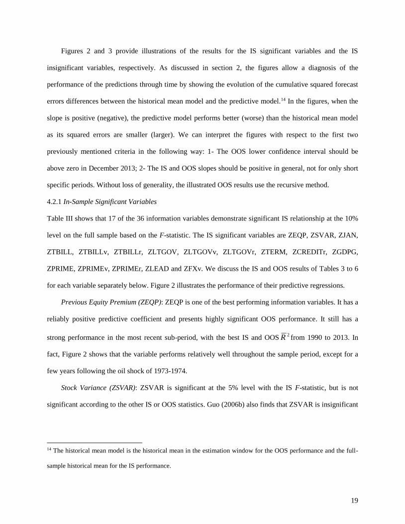
Figures 2 and 3 provide illustrations of the results for the IS significant variables and the IS

insignificant variables, respectively. As discussed in section 2, the figures allow a diagnosis of the

performance of the predictions through time by showing the evolution of the cumulative squared forecast

errors differences between the historical mean model and the predictive model.14 In the figures, when the

slope is positive (negative), the predictive model performs better (worse) than the historical mean model

as its squared errors are smaller (larger). We can interpret the figures with respect to the first two

previously mentioned criteria in the following way: 1- The OOS lower confidence interval should be

above zero in December 2013; 2- The IS and OOS slopes should be positive in general, not for only short

specific periods. Without loss of generality, the illustrated OOS results use the recursive method.

4.2.1 In-Sample Significant Variables

Table III shows that 17 of the 36 information variables demonstrate significant IS relationship at the 10%

level on the full sample based on the F-statistic. The IS significant variables are ZEQP, ZSVAR, ZJAN,

ZTBILL, ZTBILLv, ZTBILLr, ZLTGOV, ZLTGOVv, ZLTGOVr, ZTERM, ZCREDITr, ZGDPG,

ZPRIME, ZPRIMEv, ZPRIMEr, ZLEAD and ZFXv. We discuss the IS and OOS results of Tables 3 to 6

for each variable separately below. Figure 2 illustrates the performance of their predictive regressions.

Previous Equity Premium (ZEQP): ZEQP is one of the best performing information variables. It has a

reliably positive predictive coefficient and presents highly significant OOS performance. It still has a

strong performance in the most recent sub-period, with the best IS and OOS2R from 1990 to 2013. In

fact, Figure 2 shows that the variable performs relatively well throughout the sample period, except for a

few years following the oil shock of 1973-1974.

Stock Variance (ZSVAR): ZSVAR is significant at the 5% level with the IS F-statistic, but is not

significant according to the other IS or OOS statistics. Guo (2006b) also finds that ZSVAR is insignificant

14 The historical mean model is the historical mean in the estimation window for the OOS performance and the full-

sample historical mean for the IS performance.

20

in Canada. Figure 2 shows that, apart from performing very well in predicting the equity premium during

the 2008 subprime crisis, ZSVAR has not been a reliable predictor.

January Dummy (ZJAN): As in the U.S., ZJAN is positively related to the equity premium in Canada,

a finding that confirms the results from multivariate regressions in the literature (Solnik, 1993; Carmichael

and Samson, 1996; Korkie and Turtle, 1998). But as in the U.S., the January effect has mostly disappeared

since it was first documented by Rozeff and Kinney (1976), as shown by the IS and OOS results in the

1990-2013 sub-period and the graph in Figure 2.

Treasury Bill Yields (ZTBILL, ZTBILLv, ZTBILLr): The Treasury bill yields variables obtain a

negative predictive coefficient in the full sample and in the sub-periods, a sign that corresponds to the one

found in the existing Canadian literature and in most U.S. studies. Future excess equity returns are higher

when the T-bill yield is low and has decreased compare to the previous month and to the previous year

average. Of the three variables, ZTBILL has the best IS and OOS performances in the most recent sub-

period, but the worst in the second sub-period. On the contrary, the significant performance of ZTBILLv

comes mainly from the second sub-period. Figure 2 illustrates how the performance of the two variables

differ greatly in the inflationary context of the late 1970s and the 1980s, where the T-bill yields were at

their highest historical levels, but constantly declining, which translates into opposite predictions for

ZTBILL and ZTBILLv. Based on U.S. predictability results, the T-bill yields variables are some of the

most commonly used information variables. Our significant performance thus provides an important

robustness check to the U.S. results.

Long-Term Government Bond Yields (ZLTGOV, ZLTGOVv, ZLTGOVr): The IS and OOS results for

ZLTGOV, ZLTGOVv and ZLTGOVr are qualitatively similar to their respective short term equivalent

ZTBILL, ZTBILLv and ZTBILLr, as can be observed from Figure 2. The main noteworthy difference is

that the relative variable (ZLTGOVr) now presents the most significant IS and OOS performances. For

long-term bond yields, this version thus works generally better than the level variable (ZLTGOV) or the

variation variable (ZLTGOVv).

21

Term Premium (ZTERM): Similar to the findings reported in the existing literature, ZTERM has a

reliably positive predictive coefficient. It has also performed well recently, as the IS and OOS results are

significant at least at the 5% level in the last sub-period. Its insignificant full-sample OOS performance

can be explained by its poor ability during the inflationary context of the late 1970s and the 1980s.

Otherwise, as seen in Figure 2, the variable predicts consistently well. Overall, ZTERM is thus a relatively

good predictor in Canada, confirming the predictive ability of the term premium in U.S. data.

Return-Based Credit Premium (ZCREDITr): The return-based credit premium variable is significant

at the 10% level with the IS F-statistic, but is not significant according to the other IS or OOS statistics. It

has a positive, but insignificant, predictive coefficient in all sub-periods. Figure 2 shows that, apart from

performing very well in predicting the equity premium during the 2008 subprime crisis, ZCREDITr has

not been a reliable predictor.

Gross Domestic Product Growth (ZGDPG): ZGDPG is positively associated with the equity

premium. Its IS and OOS performances are particularly good in the most recent sub-period and are

sufficiently good overall to obtain significant full-sample IS and OOS results. Figure 2 reveals that the

performance has been especially good since the end of the 1990s, making ZGDPG a potentially interesting

information variable going forward.

Bank of Canada Prime Rates (ZPRIME, ZPRIMEv, ZPRIMEr): Not surprisingly, the IS and OOS

performance results for ZPRIME, ZPRIMEv and ZPRIMEr are similar to their respective T-bill

equivalents ZTBILL, ZTBILLv and ZTBILLr, as can be seen in Figure 2. However, the variables do not

predict as well as their T-bill counterparts, perhaps because the T-bill yields reflect market conditions

more rapidly and more completely than the prime rates, which indicate mainly the monetary conditions.

Composite Leading Indicator Growth (ZLEAD): According to the full-sample IS or OOS2R ,

ZLEAD is one of the best performing information variables. It has a reliably positive predictive

coefficient and its IS and OOS results are significant at the 1% level. It has also the second best

performance in the most recent sub-period, with an IS2R equal to 1.46% and a recursive OOS

2R equal to

22

1.28% in the period from 1990 to 2013. Similar to ZEQP, Figure 2 shows that ZLEAD performs relatively

well throughout the sample period, except for a few years following the oil shock of 1973-1974. This

similarity is not unexpected as the TSX Composite Index is one of the components of the Composite

Leading Indicator.

CAD/USD Exchange Rate Variation (ZFXv): ZFXv is negatively related to the equity premium, so

that an appreciation of the Canadian dollar leads to an increase in the excess return of equity. This

predictive relation is IS significant at the 5% level and is OOS significant at the 10% level with a recursive

estimation window scheme. Figure 2 shows that, apart from performing very well in predicting the equity

premium during the 2008 subprime crisis, ZFXv has not been a reliable predictor.

4.2.2 In-Sample Insignificant Variables

Table III shows that 19 of the 36 information variables demonstrate insignificant IS relationship on the

full sample based on the F-statistic. The IS insignificant variables are ZDY, ZDYf, ZDP, ZPE, ZEP,

ZVOLG, ZVOLGd, ZISSUE, ZCSBETA, ZCREDIT, ZCREDITs, ZINF, ZPRODG, ZUNEMP,

ZMONEYG, ZFX, ZFXr, ZENERG and ZMMG. We discuss the IS and OOS results of Tables 3 to 6 for

each variable separately below. If a model has no IS performance, its OOS performance is not interesting.

However, because some of these variables are so prominent, it is useful to examine their results. The

analysis could further identify sub-periods of success, which could help identify variables that have lost

their predictive power over the years or that have just recently become valuable predictor. Figure 3

illustrates the performance of their predictive regressions.

Dividend Yields (ZDY, ZDYf), Dividend-Price Ratio (ZDP), Price-Earnings Ratio (ZPE) and

Earnings-Price Ratio (ZEP): As expected from the literature, these market valuation ratios have generally

positive predictive coefficients (except for ZPE). However, they show little evidence of ability in

predicting the equity premium. In fact, their upper confidence intervals in Figure 3 indicate that their OOS

predictions are significantly worse than the historical mean model, with prediction errors especially large

around the oil shock of 1973-1974. These results are of particular importance for ZDP, which is one of the

most commonly used information variable in U.S. studies. The results in Table V show that ZDP loses its

23

predictive power in the last two sub-periods after being a significant IS predictor in first sub-period. The

structural break tests in Table VII confirm that it is significant only in the first regime that ends in

December 1964. These findings are consistent with the U.S. evidence of Boudoukh et al. (2007), who

argue that dividends do not capture well anymore the payouts of firms due to the explosion of share

repurchase transactions.

Volume Growths (ZVOLG, ZVOLGd): The volume of shares growth ZVOLG and the dollar volume

growth ZVOLGd are not helpful in predicting the equity premium. While volume indicators are regularly

part of technical analysis predictive system, their usefulness might be greater in forecasting the volatility

of the equity premium.

Issuing Activity (ZISSUE): The net equity expansion variable ZISSUE should better reflect the payout

yield of firms (Boudoukh et al., 2007). However, contrary to the U.S. findings of Welch and Goyal

(2008), ZISSUE presents no evidence of predictive ability in full sample or in sub-periods in Canada.

Figure 3 shows that it has an especially large OOS prediction errors around the oil shock of 1973-1974.

Cross-Sectional Beta Price of Risk (ZCSBETA): ZCSBETA should have a positive predictive

coefficient according to Polk et al. (2006), which is what we find, although we obtain no significant

performance statistics in our (relatively short) Canadian sample. In fact, Figure 3 demonstrates that

ZCSBETA is one of the worst OOS performers in our information variables.

Yield Spread Credit Premium (ZCREDIT, ZCREDITs): The credit premium variables based on yield

spreads are not useful in predicting the equity premium in Canada. The long-term default yield spread

ZCREDIT obtains a negative and insignificant predictive coefficient. This finding is in contrast to the U.S.

results, where ZCREDIT has typically a significantly positive coefficient and is one of the most

commonly used information variables. While this difference suggests an issue with robustness, it could

more likely reflect problems in constructing ZCREDIT for Canada. The credit premium in the U.S. is

defined as the difference between BAA and AAA-rated corporate bond yields. We are unfortunately

unable to construct such a variable with the available Canadian data. In fact, to construct ZCREDIT, we

compare long-term government yields to the long-term corporate yields obtained from a combination of

24

three different series. The resulting yield spread is thus influenced by differences in important factors such

as duration, liquidity, etc. between the government and corporate sectors. It is further affected by the

changing average ratings of the corporate sector through time, as the rating is not held fixed at BAA for

the corporate bonds. Our attempt to obtain a cleaner variable by forming a short-term credit premium

variable ZCREDITs proves unsuccessful, as ZCREDITs also obtains a negative and insignificant

predictive coefficient.

Inflation Rate (ZINF): ZINF does not forecast the equity premium in any significant way, although

the sign of its predictive relation is constantly negative in the sub-periods. No lasting favorable

predictability pattern emerges from Figure 3 either.

Industrial Production Growth (ZPRODG): ZPRODG presents no significant forecasting power and

obtains predictive coefficients that change sign across the sub-periods. Figure 3 shows that it briefly works

very well in the oil shock period of 1973-1974, but has a sharp decline in its performance around the

market correction of the early 1980s.

Unemployment Rate (ZUNEMP): ZUNEMP is positively associated with the equity premium, but is

never a significant predictor. The scale of its graph in Figure 3 indicates that its squared forecast errors are

highly similar to the ones of the historical mean model.

Money Supply Growth (ZMONEYG): ZMONEYG presents significant IS performance from 1950 to

1969, with a positive predictive coefficient. However, it loses its predictive ability in the second and

especially the third sub-periods, where it also sees its coefficient changes sign. Its graph in Figure 3

illustrates well its relatively favorable performance until the end of the 1980s and its bad performance

since then, consistent with money supply becoming a less useful indicator of monetary policy.

CAD/USD Exchange Rates (ZFX, ZFXr): While the variation in the CAD/USD exchange rates

presents some predictability evidence due to its performance during the 2008 subprime crisis, the level of

the exchange rate (ZFX) and its relative value (ZFXr) have no significant forecasting ability. As Figure 3

illustrates, ZFX even underperforms significantly the historical mean model since the first half of the

1980s with its OOS predictions.

25

Commodity Price Growths (ZENERG, ZMMG): ZENERG and ZMMG are positively associated with

the equity premium in the 1990-2013 sub-period, although the relations are insignificant. Figure 3

illustrates that their OOS performances are particularly poor around the market correction of the early

1980s. While the energy and metals and minerals sectors weight heavily in the Canadian economy, the

growths in their associated commodity price indexes do not represent useful information variables.

4.3 PUBLICATION DELAYS FOR MACROECONOMIC VARIABLES

One concern with some macroeconomic variables is that they are published with a delay. Obviously, any

variable not yet known publicly is not useful in real time, even though evidence of its predictive ability is

still indicative of its informational content. Furthermore, it is possible that a variable with insignificant

results in our regressions could still have predictive ability if we consider its publication delay adequately,

as its impact on the equity premium might be related to its announcement. Complicating matters more, the

publication delays are not the same across variables and have likely been reduced through time from 1950

to 2013. To consider this issue, we examine the results of predictive regressions that use the value of a

macroeconomic variable two, three or four months before the equity premium as a predictor. These results

thus assume implicitly that a delay of two, three or four months between the value of the predictive

variable and the equity premium is sufficient to account for the publication delays.15

Table VIII examines the IS and OOS results of predictive regressions that consider the publication

delays of six macroeconomic variables in our sample, i.e., ZINF, ZPRODG, ZUNEMP, ZMONEYG,

ZGDPG and ZLEAD. The three macroeconomic variables related to the Bank of Canada prime rates are

not relevant for this exercise as they are available in real time. The significant forecasting power

documented in Tables 3 and 4 for ZGDPG and ZLEAD is diminished once we consider publication

delays. The significantly positive relation for ZGDPG at the one-month delay becomes insignificant at the

15 A related concern for real time predictability is the availability of statistical methods and computer technology.

Pesaran and Timmermann (1995) consider this concern in their choice of model selection criteria through time and

find that their results are generally similar across techniques. In this paper, we do not examine this issue.

26

two- and three-month delays and significantly negative at the four-month delay. ZLEAD still predicts

positively and significantly the equity premium with a three-month delay, although the predictive

coefficient is reduced by approximately 50%. Oppositely, while Tables 3 and 4 document little forecasting

power for ZINF, ZPRODG, ZUNEMP and ZMONEYG, Table VIII finds evidence of predictive ability at

the three- and four-month delays for ZINF, at the four-month delay for ZPRODG and at the two-month

delay for ZMONEYG. The strongest findings are for ZINF using a four-month delay, where the IS and

OOS results are significant at the 1% level with2R approximately equal to 0.8%. Inflation has thus a

significantly negative relation to the equity premium once a reasonable publication delay is considered.

4.4 ECONOMIC VALUE

To go beyond the statistical significance of the results, Table IX presents results on the economic value of

the predictions by using the methodology outlined in section 2.3. For each information variable and its

associated OOS predictive model, the table first reports results on the portfolio of a mean-variance

investor using the forecasts from the predictive model, namely the average equity allocation, the

proportions of allocation equal to 0% or 150% (the limits allowed), the annualized values of the mean

return, standard deviation of returns and average utility level of the portfolio and the end-of-sample value

of a 1$ beginning-of-sample investment in the portfolio.16 It then gives differences with the portfolio using

forecasts from the historical mean model in terms of average utility level, mean return, standard deviation

of returns and value of a 1$ investment. Without loss of generality, we report the results using the

recursive OOS predictions.

Despite the statistical evidence of low explanatory power and only 7 full-sample IS and OOS

significant predictions, the results in Table IX indicate that the information variables provide individual

forecasts that are generally economically meaningful, supporting the argument of Campbell and

Thompson (2008). Focusing on the average utility gain (or certainty equivalent return) A NU U , a mean-

16 The annualized values are obtained by multiplying the monthly results by 12 for the mean return and average

utility level, and by 12 for the standard deviation of returns.

27

variance investor would be willing to pay an average annualized portfolio management fee of 0.49% to

have access to the additional information available in the predictive model. The fees are positive for 19

out of 36 information variables, greater than 0.5% for 16 variables, greater than 1% for 10 variables and

greater than 2% for 4 variables (ZEQP, ZTBILL, ZLTGOVv, ZLEAD).17 Compare to a portfolio based on

the historical mean forecast, the portfolios based on the predictive model produce higher mean return in 16

cases and lower standard deviation of returns in 22 cases. This latter result is consistent with the findings

of Breen et al. (1989) that an important factor in the contribution of a predictive model to an investment

strategy is the reduction of volatility.

The most economically meaningful variable is by far the composite leading indicator growth ZLEAD

with an average utility gain of 4.77%. ZLEAD obtains the highest annualized mean return increase (

A N = 4.20%), even though it produces a portfolio with an average equity allocation (Mean XA =

73.0%) similar to the average across information variables of 68.2%, and lower than the one of 81.4% for

the portfolio based on the historical mean model. For comparison, ZLTGOVv ( A N = 3.10%) and

ZLTGOVr ( A N = 3.01%) obtains the second and third highest mean return increases by allocating

respectively 84.0% and 91.4% of their portfolio to equities. The best information variables in terms of

annualized volatility reduction are ZDY ( A N = -5.28%) and ZGDPG ( A N = -4.43%). While

their portfolio allocates less than 50% to equities, ZGDPG further generates a positive utility gain for the

mean-variance investor, even producing a positive mean return difference over the 81.4%-equity-weighted

historical mean portfolio.

5. Conclusion

There is currently an important debate on the evidence and usefulness of equity premium predictability

results, a debate with far reaching implications for both researchers and practitioners. Despite the

international relevancy of the issue, this debate is mainly based on evidence from U.S. data. For example,

17 Similar to Campbell and Thompson (2008), our results do not take into account transaction costs, but we note that

utility gains of more than 50 basis points per year should be sufficient to cover substantial costs.

28

in Canada, where this topic is as important as elsewhere, there is currently no comprehensive evidence of

relevant information variables and equity premium predictability. The main objective of this paper is to

document such Canadian evidence, which is not only useful on its own, but also serves as an out-of-U.S.-

sample assessment of the predictability debate.

Specifically, we construct 36 potential information variables and test their individual predictive

ability for the Canadian monthly equity premium from 1950 to 2013. The information variables include

market characteristics, interest rate levels, changes and spreads, macroeconomic indicators and Canadian-

specific variables. We provide IS, OOS and economic value evidence using common estimation

techniques and performance measures, which are carefully chosen to mitigate known econometric issues.

The four principal findings from our results are as follows. First, we find conclusive evidence of IS

and OOS predictability of the Canadian monthly equity premium, providing an out-of-U.S.-sample

robustness check of the U.S. evidence. Second, we provide a new empirical assessment of the issues of

small sample bias, spurious regression, model instability, structural breaks, poor predictive ability, low

economic value and real time data availability. We show that our results are generally robust to these

econometric issues that have been raised in the literature. While we uncover some instability in the results

related to the 1973-1974 oil shock and the inflationary concern of the 1980s, we implement multiple

structural break tests and do not obtain any significant break for most information variables. We also

document strong evidence that the equity premium is still predictable from 1990 to 2013. Third, we show

that forecasts from the information variables are economically meaningful for a mean-variance investor.

Fourth, we provide guidance on the usefulness of each information variable as a market indicator,

raising questions on the forecasting ability of some variables that have been successful predictors for the

U.S. equity premium. Table X provides a summary of the significance of the complete set of IS and OOS

results documented in the paper. The table makes it easy to identify the information variables with the best

predictive ability, namely the previous equity premium, the Treasury bill yield and long-term government

bond yield variables, the gross domestic product growth and the composite leading indicator growth. The

table also shows that the dividend yield, the dividend-price ratio, the credit premium, the cross-sectional

29

beta price of risk of Polk et al. (2006), the stock variance of Guo (2006a) and the issuing activity of

Boudoukh et al. (2007) show little significant predictive ability in a Canadian context.

While our results show significant predictability of the Canadian equity premium, there are numerous

possible ways to improve the forecasting ability of the information variables. A straightforward extension,

examined by Campbell and Thompson (2008) in U.S. data, is to impose economic restrictions on the sign

of the predictions so that the equity premium is predicted to be non-negative. Another interesting

extension is to combine the individual forecasts from information variables to improve the predictive

performance. Rapach et al. (2010) show that such a combination approach improves the OOS performance

of U.S. predictions. Finally, we can extend our predictive approach from individual models to multivariate

models. For example, the general-to-specific approach of Hendry (1995) provides a way to identify a set

of significant variables that can be useful in a multivariate forecasting model. Champagne et al. (2017)

examine these extensions and find stronger predictability evidence for the Canadian equity premium.

30

Appendix A. Construction Details and Sources of the Information Variables

This appendix gives a detailed description of the construction and sources of the information variables,

regrouped by their category, as well as a correlation analysis between the closely related variables.

A.1 MARKET CHARACTERISTIC VARIABLES

Twelve information variables are related to equity valuation ratios and market-related variables (ZDY,

ZDYf, ZDP, ZPE, ZEP, ZEQP, ZVOLG, ZVOLGd, ZSVAR, ZISSUE, ZCSBETA and ZJAN):

Dividend Yields (ZDY, ZDYf): We consider two annual dividend yield variables for the S&P/TSX

Composite Index. The realized dividend yield (ZDY) is computed from the difference between the one-

year total return of the index and its one-year price return. The data come from the CFMRC database and

start in February 1957. We also obtain a forward-looking dividend yield variable (ZDYf) available as

series V122628 in the CANSIM database from Statistics Canada. This series is described as “taking the

indicated dividend to be paid per share of stock over the next 12 months and dividing it by the current

price of the stock.”18 The data begin in February 1956. The correlation between ZDY and ZDYf is 0.62.

Dividend-Price Ratio (ZDP): We calculate the dividend-price ratio as the realized dividend yield

multiplied by the value of the index one year ago and divided by the current value of the index. The data

go back to February 1957. The correlation between ZDP and ZDY is 0.87.

Price-Earnings Ratio (ZPE): The price-earnings ratio of the S&P/TSX Composite Index is obtained

from the CANSIM database as series V122629. It is available starting in February 1956. It corresponds to

the current market price divided by the earnings in the latest fiscal year.19

Earnings-Price Ratio (ZEP): The earnings-price ratio is one over the price-earnings ratio. The

correlation between ZEP and ZPE is -0.54.

18 See the Notes to the Tables for Table F3 in the Bank of Canada Banking and Financial Statistics, May 2010.

19 From August 2001 to July 2002, the ratio was not listed due to negative earnings. We replace the missing value

with the maximum value of the price-earnings ratio prior to August 2001.

31

Previous Equity Premium (ZEQP): Canadian equity market returns are slightly positively

autocorrelated, perhaps due to non synchronous or thin trading (see Fowler et al., 1979). ZEQP is simply

the lagged EQP and attempts to capture the predictive information in the premium of the previous month.

Volume Growths (ZVOLG, ZVOLGd): We consider two volume growth variables for the TSX

exchange. The volume of shares growth variable (ZVOLG) is the growth in the monthly number of shares

transacted while the dollar volume growth is the growth in the monthly value of shares traded. The data

come from the CANSIM database as series V37413 and V37412, respectively, and start in March 1953.

The correlation between ZVOLG and ZVOLGd is 0.75.

Stock Variance (ZSVAR): We compute the realized stock variance as the sum of squared daily returns

on the Canadian stock market. The data are from the CFMRC or Datastream databases. ZSVAR is

computed from the daily returns of the value-weighted CFMRC equity market index from February 1975

to January 1977 and the S&P/TSX Composite Index thereafter. Guo (2006a) documents a positive relation

between ZSVAR and future market returns in the U.S.

Issuing Activity (ZISSUE): To compute the corporate issuing activity, we first compute the dollar

amount of net equity issuing activity, following Welch and Goyal (2008) as: Net Issue at month t =

Market Capitalisation at month t – Market Capitalisation at month t-1 × (1 + Market Capital Gain Return

at month t). The issuing activity variable (ZISSUE) is the net equity expansion defined as the ratio of the

twelve-month moving sums of net issues divided by the current market capitalisation. The data come from

the CFMRC database. From February 1951 to September 2000, the price and number of shares for each

individual stock is used to obtain the total market capitalisation. From October 2000, we take the total

market capitalisation of the S&P/TSX Composite Index from Datastream. ZISSUE is related to a variable

proposed by Boudoukh et al. (2007) in the U.S. They show that since the adoption of SEC rule 10b-18 in

1982, there has been an explosion of share repurchase transactions. They argue that this newly important

distribution channel has caused the dividend yield to lose its predictive power, but a more largely defined

payout yield that includes share repurchases still provides significant predictions. This analysis could be

32

relevant for Canada as well as Kooli and L’Her (2010) similarly find a decline in dividend paying firms

and a significant increase in share repurchase programs.

Cross-Sectional Beta Price of Risk (ZCSBETA): The cross-sectional beta premium is the difference in

betas between value and growth portfolios. Polk et al. (2006) show that it predicts the equity premium for

the U.S. and a group of international countries (excluding Canada). From January 1980, we follow Polk et

al. (2006) to construct ZCSBETA from the Canadian value and growth portfolios available on Kenneth R.

French’s Web page (http://mba.tuck.dartmouth.edu/pages/faculty/ken.french/data_library.html).20

Specifically, ZCSBETA is equal to the 36-month average rolling beta of the four value portfolios minus

the 36-month average rolling beta of the four growth portfolios.

January Dummy (ZJAN): This dummy variable (not lagged) is set to 1 in January and 0 for the other

months and captures the so-called January effect predicting higher returns in January.

A.2 INTEREST RATE VARIABLES

Ten information variables are related to interest rates (ZTBILL, ZTBILLv, ZTBILLr, ZLTGOV,

ZLTGOVv, ZLTGOVr, ZTERM, ZCREDIT, ZCREDITs, ZCREDITr).

Treasury Bill Yields (ZTBILL, ZTBILLv, ZTBILLr): The Treasury bill yield is the annualized yield-to-

maturity of the three-month Government of Canada Treasury bill. It is taken from the CFMRC database

and is also available as series V122541 in the CANSIM database. We use the lagged value directly as an

information variable (ZTBILL). But as ZTBILL is highly persistent, we also consider its lagged monthly

variation (ZTBILLv) and its lagged value relative to its twelve-month moving average (ZTBILLr).

Long-Term Government Bond Yields (ZLTGOV, ZLTGOVv, ZLTGOVr): The long-term government

yield is the average yield-to-maturity of the Government of Canada Treasury bonds with a maturity of ten

years or more. It is available in the CFMRC database and in the CANSIM database as series V122487. As

for ZTBILL, we use its lagged value (ZLTGOV), its lagged variation (ZLTGOVv) and its lagged value

20 These portfolios are the top 30% and bottom 30% portfolios of stocks sorted on four Morgan Stanley Capital

International value measures: Dividend yield, book-to-market ratio, Earnings-price ratio and cash flows-price ratio.

33

relative to its twelve-month moving average (ZLTGOVr). The correlations with their corresponding

Treasury bill variable are 0.94 for ZLTGOV, 0.45 for ZLTGOVv, and 0.64 for ZLTGOVr.

Term Premium (ZTERM): The term premium is the difference between ZLTGOV and ZTBILL.

Credit Premium (ZCREDIT, ZCREDITs, ZCREDITr): We consider three credit premium (or default

spread) variables. The first credit premium is the difference between the yield on long-term corporate

bonds and ZLTGOV. To construct a long history of the corporate yields, we combine three different

series. From February 1950 to October 1977, we use the series V35752 from the CANSIM database, the

Scotia-McLeod Canada Long-Term All-Corporate Yield Index. From November 1977 to June 2007, we

take the Scotia Capital Canada All-Corporations Long-Term bond yield series from CFMRC, also

available as series V122518 in the CANSIM database. From July 2007, we take the yield from the Bank

of America Merrill Lynch Canada Corporate Bond 10Y+ Index (series MLCCTPL) from Datastream. In

an effort to avoid mixing three different series, a second yield spread variable is computed as the

difference between the yield on the three-month prime corporate paper (series V122491) and ZTBILL.

This short-term credit premium variable (ZCREDITs) goes back to February 1956 and has a correlation of

0.05 with ZCREDIT. Finally, we form a return-based credit premium variable (ZCREDITr) as the

difference between long-term corporate bond and long-term government bond returns. For the corporate

bond returns, we use series V35754 (the Scotia-McLeod Canada Long-Term All-Corporate Total Return

Index) from December 1950 to October 2002. From November 2002, we take the total returns from the

Bank of America Merrill Lynch Canada Corporate Bond 10Y+ Index (series MLCCTPL). We obtain the

government bond returns from the CFMRC database. ZCREDITr has correlations of -0.06 with ZCREDIT

and -0.07 with ZCREDITs.

A.3 MACROECONOMIC VARIABLES

Nine information variables are based on macroeconomic indicators (ZINF, ZPRODG, ZUNEMP,

ZMONEY, ZGDPG, ZPRIME, ZPRIMEv, ZPRIMEr, ZLEAD).

Inflation Rate (ZINF): The inflation rate is the monthly growth in the Consumer Price Index (CPI)

obtained from the CANSIM database as series V41690973.

34

Industrial Production Growth (ZPRODG): The monthly industrial production growth is the monthly

growth in the Industrial Production Index (IPI) extracted from the CANSIM database as series V53384745

or Datastream. It is available from March 1956.

Unemployment Rate (ZUNEMP): The unemployment rate data are collected from Datastream (code

CNOUN014R) and go back to February 1960. It is also available as series V2064894 from the CANSIM

database from January 1975.

Money Supply Growth (ZMONEYG): The money supply growth is the monthly growth of the Money

Supply Index obtained as series V37173 from the CANSIM database. The money supply variable

represents the unadjusted currency outside banks.

Gross Domestic Product Growth (ZGDPG): The gross domestic product (GDP) growth is the

monthly growth in the seasonally adjusted GDP for all industries. We construct the ZGDPG variable with

two series (V329529 and V65201483) from the CANSIM database. The first one, the GDP at factor cost

in 1992 constant prices, allows going back to March 1961, but is now discontinued. The second one, the

GDP at basic prices in 2007 constant prices, is used as soon as possible so that it is behind the ZGDPG

variable from March 1997. Although they differ slightly in their methodology, the series produce growths

correlated at 0.90 in their common time span.

Bank of Canada Prime Rates (ZPRIME, ZPRIMEv, ZPRIMEr): Series V122530 from the CANSIM

database is the source for the Bank of Canada prime or discount rate. As it is highly persistent (like

ZTBILL), we use its lagged value (ZPRIME), its lagged variation (ZPRIMEv) and its lagged value

relative to its twelve-month moving average (ZPRIMEr). The correlations with their corresponding

Treasury bill variable are 0.995 for ZPRIME, 0.84 for ZPRIMEv, and 0.97 for ZPRIMEr.

Composite Leading Indicator Growth (ZLEAD): The composite leading indicator (CLI) growth is

mainly the monthly growth of the unsmoothed CLI available as series V7687 from the CANSIM database.

According to Statistics Canada, the CLI is “comprised of ten components which lead cyclical activity and

together represent all major categories of GDP. It thus reflects a variety of mechanisms that can cause

35

business cycles.”21 The components are an housing index, the business and personal services employment,

the TSE 300 Index, the money supply M1, the U.S. Composite Leading Indicator, the average work week

hours, the new orders in durable goods, the shipments/inventories of finished goods, the furniture and

appliance sales and other durable goods sales. The series starts in May 1952, but is discontinued since

April 2012. Thereafter, we use a CLI from the OECD Main Economic Indicators, available in Datastream

as series CNCYLEADT. The CLIs have a correlation of 0.97 in their common time span.

A.4 CANADIAN-SPECIFIC VARIABLES

The last five information variables are particularly relevant for the Canadian economy (ZFX, ZFXv,

ZFXr, ZENERG, ZMMG).

CAD/USD Exchange Rates (ZFX, ZFXv, ZFXr): Canada’s largest trading partner is by far the U.S.

The spot exchange rate in Canadian dollars per U.S. dollar is collected from the CFMRC database and is

also available as series V37426 from the CANSIM database. As it is highly persistent, we use its lagged

value (ZFX), its lagged variation (ZFXv) and its lagged value relative to its twelve-month moving average

(ZFXr).22 ZFX, ZFXv and ZFXr start in November 1950, December 1950 and October 1951, respectively.

Commodity Price Growths (ZENERG, ZMMG): We consider two commodity price index growth

variables that are associated with two important sectors of the Canadian economy. The energy index

growth is the monthly growth in the Fisher Commodity Energy Price Index. The metals and minerals

index growth is the monthly growth in the Fisher Commodity Metals and Minerals Price Index. The data

come from the CANSIM database as series V52673498 and V52673499, respectively, and start in March

1972. The correlation between ZENERG and ZMMG is 0.23.

21 For this explanation and more details on the CLI series, see the Statistics Canada website at the following address:

www.statcan.gc.ca/cgi-bin/imdb/p2SV.pl?Function=getSurvey&SDDS=1601&lang=fr&db=imdb&adm=8&dis=2.

22 We also considered the three-month forward CAD/USD exchange rate (series V37437) used by Korkie and Turtle

(1998). However, given its correlation of 0.9997 with the spot exchange rate, we discard it from further analysis.

36

Appendix B. Existing Canadian Evidence

This appendix identifies and characterizes the existing Canadian evidence on the predictive ability of the

36 information variables under investigation. Table B1 provides a summary of this evidence. Specifically,

for each variable covered in the literature, it gives the article reference, the IS data period, the sign of the

predictive coefficient estimate, the IS 2R (or

2R if 2R is unavailable), as well as whether or not the IS and

OOS results are significant if available. The table includes articles that look at the individual predictive

performance of the information variables, as we do in this paper. As a complement, the table also includes

articles that present variable-specific predictive coefficient estimates taken from a multivariate predictive

model. This last set of articles, for which we only report the sign and significance of the predictive

coefficient estimates, provides indirect evidence on the predictive relation of the information variables.

A number of conclusions can be drawn from the Canadian evidence we uncover. First, while

American evidence exists on most of the information variables considered in this study, the predictive

ability of 19 of our 36 variables is not examined in a Canadian context. Furthermore, the individual

predictive performance of some of the variables covered in the literature is undocumented as only

multivariate results are available. Second, the results for most variables are not confirmed by an extensive

body of works. Out of the 17 variables covered in the Canadian literature, nine variables are examined by

one article and two variables are studied by two articles, hardly definitive evidence. Only three variables

(ZDP, ZTBILL, ZTERM) are investigated by more than three papers. Third, the sample sizes of many

existing Canadian studies are relatively small. Out of the ten articles found with Canadian evidence, only

one recent article (Hjalmarsson, 2010) use more than 40 years of monthly data. Seven of the ten articles

have a sample size less than half the one we have.

Fourth, the Canadian evidence is often not conclusive. There are contradictory results on the

significance of IS predictability for six (ZDP, ZJAN, ZTBILL, ZTBILLv, ZLTGOV, ZTERM) of the

variables with evidence from more than one article. Only two variables have similar IS evidence from

multiple sources: ZDY (significant performance) and ZEP (insignificant performance). There is also little

OOS Canadian evidence as only two articles (Rapach et al., 2005; Hjalmarsson, 2010) have reported

37

results on OOS performance. Thus, in contrast to the comprehensive nature of our investigation, no

existing article documents IS and OOS results in Canada for more than five information variables using a

sample period of more than 30 years.

Rapach et al. (2005) and Hjalmarsson (2010) are perhaps the two studies included in Table B1 that

are the most related to ours in terms of methodology. Both studies look at international equity premium IS

and OOS predictability from individual country-specific information variables. While they do not focus

specifically on Canada, the country is included as part of the large number of countries they examine. For

Canada, Rapach et al. (2005) consider six variables with data from 1975 to 2001 while Hjalmarsson

(2010) studies four variables with data from 1952 to 2004. Rapach et al. (2005) find significant IS

relations for ZLTGOVr (negative) and ZPRODG (positive), and insignificant relations for ZTBILLr

(negative), ZTERM (positive), INF (positive) and ZMONEYG (positive). Hjalmarsson (2010) find

significant IS relations for ZTBILL (negative) and ZTERM (positive), and insignificant relations for ZDP

(positive) and ZEP (positive). ZLTGOVr and ZTERM present significant OOS performance as well.

Other than the articles included in Table B1, we can also mention some additional evidence from

related literature on the Canadian market. For example, in a multivariate conditional APT context,

Koutoulas and Kryzanowski (1994, 1996) show that market returns are negatively related to innovations

on the variation of the exchange rate (a variable similar to ZFXv) and on the term premium (a variable

similar to ZTERM), and positively related to innovations on the leading indicator growth (a variable

similar to ZLEAD) and on the industrial production growth (a variable similar to ZPRODG). In a similar

context, Carmichael and Samson (2003) estimate that market returns are positively related to the lagged

term premium (a variable similar to ZTERM), the lagged equity premium (a variable similar to ZEQP)

and the January dummy ZJAN, while the relation with the lagged GDP growth (a variable similar to

ZGDPG), the lagged inflation (a variable similar to ZINF) and the lagged real short-term interest rate (a

variable similar to ZTBILL) depends on their specification.

Using a cointegration technique, Cheung and Ng (1998) show that quarterly market returns are

related positively to the lagged equity premium (a variable similar to ZEQP) and negatively to the lagged

38

real oil price index growth (a variable related to ZENERG), while not significantly related to the lagged

growth in money supply (a variable similar to ZMONEYG) and the lagged gross national product growth

(a variable related to ZGDPG). More recently, in a study on the exposures of returns in the G7 economies,

Bredin and Hyde (2011) obtain that Canadian returns are positively exposed to the lagged appreciation of

the Canadian dollar (a variable inversely related to ZFXv) and the lagged variation in the Treasury bill

yield (a variable similar to ZTBILLv). While the evidence presented in these articles is suggestive of the

relevancy of some information variables, it comes from different contexts and does not provide an

assessment of their individual predictive ability.

Finally, there exists a literature on the predictability of the Canadian equity premium from

international information variables. For example, Ferson and Harvey (1993, 1994) show that Canadian

excess returns in U.S. dollars can be predicted by world information variables. Interestingly, they also

reject the hypothesis that country information variables have no explanatory power when global variables

are included. Harvey (1991) and Carmichael and Samson (1996) find that some commonly used U.S.

information variables are IS significant in predicting the Canadian equity premium. More recently, Rapach

et al. (2013) look at the role of the U.S. in international stock return predictability and show that the

lagged U.S. equity premium produces significant IS and OOS predictions for the Canadian equity

premium. In this paper, similar to the comprehensive studies of U.S. predictability, we focus exclusively

on local information variables.

39

References

Andrews, D.W.K. (1991) Heteroskedasticity and autocorrelation consistent covariance matrix estimation,

Econometrica 59, 817–858.

Ang, A. and Bekaert, G. (2007) Stock return predictability: is it there? Review of Financial Studies 20,

651–707.

Bai, J. and Perron, P. (1998) Estimating and testing linear models with multiple structural changes,

Econometrica 66, 47–78.

Bai, J. and Perron, P. (2003a) Computation and analysis of multiple structural change models, Journal of

Applied Econometrics 18, 1–22.

Bai, J. and Perron, P. (2003b) Critical values for multiple structural change tests, Econometrics Journal 6,

72–78.

Bai, J. and Perron, P. (2006) Multiple structural change models: a simulation analysis, in: D. Corbae, S.N.

Durlauf and B.E. Hansen (eds.), Econometric Theory and Practice: Frontiers of Analysis and Applied

Research, Cambridge: Cambridge University Press, 212–237.

Bossaerts, P. and Hillion, P. (1999) Implementing statistical criteria to select return forecasting models:

what do we learn? Review of Financial Studies 12, 405–428.

Boudoukh, J., Michely, R., Richardson, M. and Roberts, M. (2007) On the importance of measuring

payout yield: implications for empirical asset pricing, Journal of Finance 62, 877–915.

Bredin, D. and Hyde, S. (2011) Investigating sources of unanticipated exposure in industry stock returns,

Journal of Banking and Finance 35, 1128–1142.

Breen, W., Glosten, L.R. and Jagannathan, R. (1989) Economic significance of predictable variations in

stock index returns, Journal of Finance 64, 1177–1189.

Campbell, J.Y. (1987) Stock returns and the term structure, Journal of Financial Economics 18, 373–399.

Campbell, J.Y. and Shiller, R. (1988) Stock prices, earnings, and expected dividends, Journal of Finance

43, 661–676.

Campbell, J.Y. and Thompson, S.B. (2008) Predicting the equity premium out of sample: can anything

beat the historical average? Review of Financial Studies 21, 1509–1531.

Campbell, J.Y. and Viceira, L. (1998) Consumption and portfolio decisions when expected returns are

time varying, Quarterly Journal of Economics 114, 433–495.

Campbell, J.Y. and Yogo, M. (2006) Efficient tests of stock return predictability, Journal of Financial

Economics 81, 27–60.

Carmichael, B. and Samson, L. (1996) The determination of risk premiums and the integration of the

Canadian and American stock markets (in French), Canadian Journal of Economics 24, 595–614.

Carmichael, B. and Samson, L. (2003) Expected returns and economic risk in Canadian financial markets,

Applied Financial Economics 13, 177–189.

Champagne, C., Chrétien, S. and Coggins, F. (2017) Equity premium predictability: combination forecasts

versus multivariate regression predictions, Working Paper, Laval University.

Cheung, Y-W. and Ng, L.K. (1998) International evidence on the stock market and aggregate economic

activity, Journal of Empirical Finance 5, 281–296.

Clark, T.E. and McCracken, M.W. (2001) Tests of equal forecast accuracy and encompassing for nested

models, Journal of Econometrics 105, 85–110.

40

Cochrane, J.H. (2008) The dog that did not bark: a defense of return predictability, Review of Financial

Studies 21, 1533–1575.

Cooper, M., Gutierrez Jr., R.C. and Marcum, B. (2005) On the predictability of stock returns in real time,

Journal of Business 78, 469–499.

Deaves, R., Miu, P. and White, C.B. (2008) Canadian stock market multiples and their predictive content,

International Review of Economics and Finance 17, 457–466.

Diebold, F.X. and Mariano, R.S. (1995) Comparing predictive accuracy, Journal of Business and

Economic Statistics 13, 253–263.

Dow, C.H. (1920) Scientific stock speculation, The Magazine of Wall Street.

Fama, E.F. (1981) Stock returns, real activity, inflation, and money, American Economic Review 71, 545–

565.

Fama, E.F. and French, K.R. (1988) Dividend yields and expected stock returns, Journal of Financial

Economics 22, 3–25.

Fama, E.F. and French K.R. (1989) Business conditions and expected returns on stocks and bonds,

Journal of Financial Economics 25, 23–49.

Fama, E.F. and Schwert, G.W. (1977) Asset returns and inflation, Journal of Financial Economics 5, 115–

146.

Ferson, W.E. and Harvey, C.R. (1991) The variation of economic risk premiums, Journal of Political

Economy 99, 385–415.

Ferson, W.E. and Harvey, C.R. (1993) The risk and predictability of international equity returns, Review

of Financial Studies 6, 527–566.

Ferson, W.E. and Harvey, C.R. (1994) An exploratory investigation of the fundamental determinants of

national equity market returns, in: J.A. Frankel (ed), Internationalization of Equity Markets, Chicago:

University of Chicago Press, 59–148.

Ferson, W.E., Sarkissian, S. and Simin, T.S. (2003) Spurious regression in financial economics, Journal of

Finance 58, 1393–1413.

Ferson,W.E. and Schadt, R.W. (1996) Measuring fund strategy and performance in changing economic

conditions, Journal of Finance 51, 425–461.

Fowler, D.J., Rorke, C.H. and Jog, V. (1979), Heteroscedasticity, R² and thin trading on the Toronto stock

exchange, Journal of Finance 34, 1201–1210.

Goyal, A. and Welch, I. (2003) Predicting the equity premium with dividend ratios, Management Science

49, 639–654.

Granger, C.W.J., Hyung, N. and Jeon, Y. (2001) Spurious regressions with stationary series, Applied

Economics 33, 899–904.

Guo, H. (2006a) On the out-of-sample predictability of stock market returns, Journal of Business 79, 645–

670.

Guo, H. (2006b) The risk-return relation in international stock markets, The Financial Review 41, 565–

587.

Hansen, L.P. (1982) Large sample properties of generalized method of moments estimators, Econometrica

50, 1029–1054.

Harvey, C.R. (1991) The world price of covariance risk, Journal of Finance 46, 111–157.

41

Harvey, D.I., Leybourne, S.J. and Newbold, P. (1997) Testing the equality of prediction mean squared

errors, International Journal of Forecasting 13, 281–291.

Hendry, D.F. (1995) Dynamic Econometrics, Oxford: Oxford University Press.

Hjalmarsson, E. (2010) Predicting global stock returns, Journal of Financial and Quantitative Analysis 45,

49–80.

Kandel, S. and Stambaugh, R.F. (1996) On the predictability of stock returns: an asset allocation

perspective, Journal of Finance 51, 385–424.

Keim, D. and Stambaugh, R.F. (1986) Predicting returns in the stock and bond markets, Journal of

Financial Economics 17, 357–390.

Kooli, M. and L’Her, J.-F. (2010) Dividends versus share repurchases evidence from Canada: 1985-2003,

The Financial Review 45, 57–81.

Korkie, B. and Turtle, H. (1998) The Canadian investment opportunity set, 1967-1993, Canadian Journal

of Administrative Science 15, 213–229.

Koutoulas, G. and Kryzanowski, L. (1994) Integration or segmentation of the Canadian stock market:

evidence based on the APT, Canadian Journal of Economics 27, 329–351.

Koutoulas, G. and Kryzanowski, L. (1996) Macrofactor conditional volatilities, time-varying risk premia

and stock return behavior, The Financial Review 31, 169–195.

Lewellen, J. (2004) Predicting returns with financial ratios, Journal of Financial Economics 74, 209–237.

Li, J. and Tsiakas, I. (2016) Equity premium prediction: the role of economic and statistical constraints,

Journal of Financial Markets, forthcoming.

Maio, P. (2013) The “Fed model” and the predictability of stock returns, Review of Finance 17, 1489–

1533.

Maio, P. (2016) Cross-sectional return dispersion and the equity premium, Journal of Financial Markets

29, 87–109.

Mark, N.C. (1995) Exchange rates and fundamentals: evidence on long-horizon predictability, American

Economic Review 85, 201–218.

Marquering, W. and Verbeek, M. (2004) The economic value of predicting stock index returns and

volatility, Journal of Financial and Quantitative Analysis 39, 407–429.

McCracken, M.W. (2007) Asymptotics for out-of-sample tests of Granger causality, Journal of

Econometrics 140, 719–752.

McLean, R.D. and Pontiff, J. (2016) Does academic research destroy stock return predictability?, Journal

of Finance 71, 5–32.

Nelson, C.R. (1976) Inflation and the rates of return on common stock, Journal of Finance 31, 471–483.

Nelson, C. and Kim, M. (1993) Predictable stock returns: the role of small sample bias, Journal of

Finance 48, 641–661.

Newey, W.K. and West, K.D. (1987) A simple, positive semi-definite, heteroskedasticity and

autocorrelation consistent covariance matrix, Econometrica 55, 703–808.

Paye, B.S. and Timmermann, A. (2006) Instability of return prediction models, Journal of Empirical

Finance 13, 274–315.

Pesaran, M.H. and Timmermann, A. (1995) Predictability of stock returns: robustness and economic

significance, Journal of Finance 50, 1201–1228.

42

Pesaran, M.H. and Timmermann, A. (2002) Market timing and return prediction under model instability,

Journal of Empirical Finance 9, 495–510.

Pettenuzzo, D., Timmermann, A. and Valkanov, R. (2014) Forecasting stock returns under economic

constraints, Journal of Financial Economics 114, 517–553.

Polk, C., Thompson, S. and Vuolteehaho, T. (2006) Cross-sectional forecasts of the equity premium,

Journal of Financial Economics 81, 101–141.

Powell, J., Shi, J., Smith, T. and Whaley, R. (2009) Common divisors, payout persistence, and return

predictability, International Review of Finance 9, 335–357.

Rapach, D., Strauss, J. and Zhou, G. (2010) Out-of-sample equity premium prediction: combination

forecasts and links to the real economy, Review of Financial Studies 23, 821–862.

Rapach, D., Strauss, J. and Zhou, G. (2013) International stock return predictability: what is the role of the

United States? Journal of Finance 68, 1633–1662.

Rapach, D. and Wohar, M. (2006) Structural breaks and predictive regression models of aggregate U.S.

stock returns, Journal of Financial Econometrics 4, 238–274.

Rapach, D., Wohar, M. and Rangvid, J. (2005) Macro variables and international return predictability,

International Journal of Forecasting 21, 137–166.

Rozeff, M. and Kinney W. (1976) Capital market seasonality: the case of stock returns, Journal of

Financial Economics 3, 379–402.

Shanken, J. (1990) Intertemporal asset pricing: an empirical investigation, Journal of Econometrics 45,

99–120.

Solnik, B. (1993) The performance of international asset allocation strategies using conditioning

information, Journal of Empirical Finance 1, 33–55.

Stambaugh, R.F. (1999) Predictive regressions, Journal of Financial Economics 54, 375–421.

Sullivan, R., Timmermann, A. and White, A. (1999) Data-snooping, technical trading rule performance,

and the bootstrap, Journal of Finance 54, 1647–1691.

Timmermann, A. (2008) Elusive return predictability, International Journal of Forecasting 20, 15–27.

Turner, J.A. (2015) Casting doubt on the predictability of stock returns in real time: Bayesian model

averaging using realistic priors, Review of Finance 19, 785–821.

Welch, I. and Goyal, A. (2008) A comprehensive look at the empirical performance of equity premium

prediction, Review of Financial Studies 21, 1455–1508.

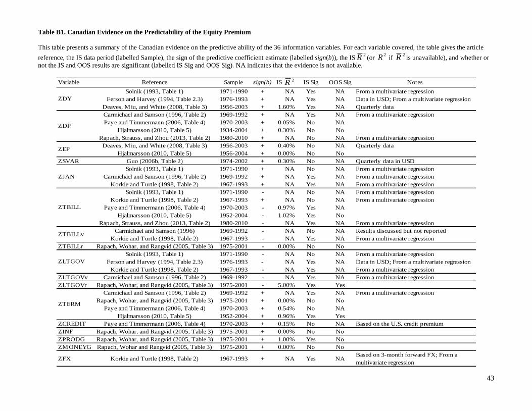
43

Table B1. Canadian Evidence on the Predictability of the Equity Premium

This table presents a summary of the Canadian evidence on the predictive ability of the 36 information variables. For each variable covered, the table gives the article

reference, the IS data period (labelled Sample), the sign of the predictive coefficient estimate (labelled sign(b)), the IS2R (or

2R if 2R is unavailable), and whether or

not the IS and OOS results are significant (labelled IS Sig and OOS Sig). NA indicates that the evidence is not available.

Variable Reference Sample sign(b) IS IS Sig OOS Sig Notes

Solnik (1993, Table 1) 1971-1990 + NA Yes NA From a multivariate regression

Ferson and Harvey (1994, Table 2.3) 1976-1993 + NA Yes NA Data in USD; From a multivariate regression

Deaves, Miu, and White (2008, Table 3) 1956-2003 + 1.60% Yes NA Quarterly data

Carmichael and Samson (1996, Table 2) 1969-1992 + NA Yes NA From a multivariate regression

Paye and Timmermann (2006, Table 4) 1970-2003 + 0.05% No NA

Hjalmarsson (2010, Table 5) 1934-2004 + 0.30% No No

Rapach, Strauss, and Zhou (2013, Table 2) 1980-2010 + NA No NA From a multivariate regression

Deaves, Miu, and White (2008, Table 3) 1956-2003 + 0.40% No NA Quarterly data

Hjalmarsson (2010, Table 5) 1956-2004 + 0.00% No No

ZSVAR Guo (2006b, Table 2) 1974-2002 + 0.30% No NA Quarterly data in USD

Solnik (1993, Table 1) 1971-1990 + NA No NA From a multivariate regression

ZJAN Carmichael and Samson (1996, Table 2) 1969-1992 + NA Yes NA From a multivariate regression

Korkie and Turtle (1998, Table 2) 1967-1993 + NA Yes NA From a multivariate regression

Solnik (1993, Table 1) 1971-1990 - NA No NA From a multivariate regression

Korkie and Turtle (1998, Table 2) 1967-1993 + NA No NA From a multivariate regression

Paye and Timmermann (2006, Table 4) 1970-2003 - 0.97% Yes NA

Hjalmarsson (2010, Table 5) 1952-2004 - 1.02% Yes No

Rapach, Strauss, and Zhou (2013, Table 2) 1980-2010 - NA Yes NA From a multivariate regression

Carmichael and Samson (1996) 1969-1992 - NA No NA Results discussed but not reported

Korkie and Turtle (1998, Table 2) 1967-1993 - NA Yes NA From a multivariate regression

ZTBILLr Rapach, Wohar, and Rangvid (2005, Table 3) 1975-2001 - 0.00% No No

Solnik (1993, Table 1) 1971-1990 - NA No NA From a multivariate regression

Ferson and Harvey (1994, Table 2.3) 1976-1993 - NA Yes NA Data in USD; From a multivariate regression

Korkie and Turtle (1998, Table 2) 1967-1993 - NA Yes NA From a multivariate regression

ZLTGOVv Carmichael and Samson (1996, Table 2) 1969-1992 - NA Yes NA From a multivariate regression

ZLTGOVr Rapach, Wohar, and Rangvid (2005, Table 3) 1975-2001 - 5.00% Yes Yes

Carmichael and Samson (1996, Table 2) 1969-1992 + NA Yes NA From a multivariate regression

Rapach, Wohar, and Rangvid (2005, Table 3) 1975-2001 + 0.00% No No

Paye and Timmermann (2006, Table 4) 1970-2003 + 0.54% No NA

Hjalmarsson (2010, Table 5) 1952-2004 + 0.96% Yes Yes

ZCREDIT Paye and Timmermann (2006, Table 4) 1970-2003 + 0.15% No NA Based on the U.S. credit premium

ZINF Rapach, Wohar, and Rangvid (2005, Table 3) 1975-2001 + 0.00% No No

ZPRODG Rapach, Wohar, and Rangvid (2005, Table 3) 1975-2001 + 1.00% Yes No

ZMONEYG Rapach, Wohar and Rangvid (2005, Table 3) 1975-2001 + 0.00% No No

ZFX Korkie and Turtle (1998, Table 2) 1967-1993 + NA Yes NABased on 3-month forward FX; From a

multivariate regression

ZDY

ZDP

ZLTGOV

ZTERM

ZEP

ZTBILL

ZTBILLv

2R

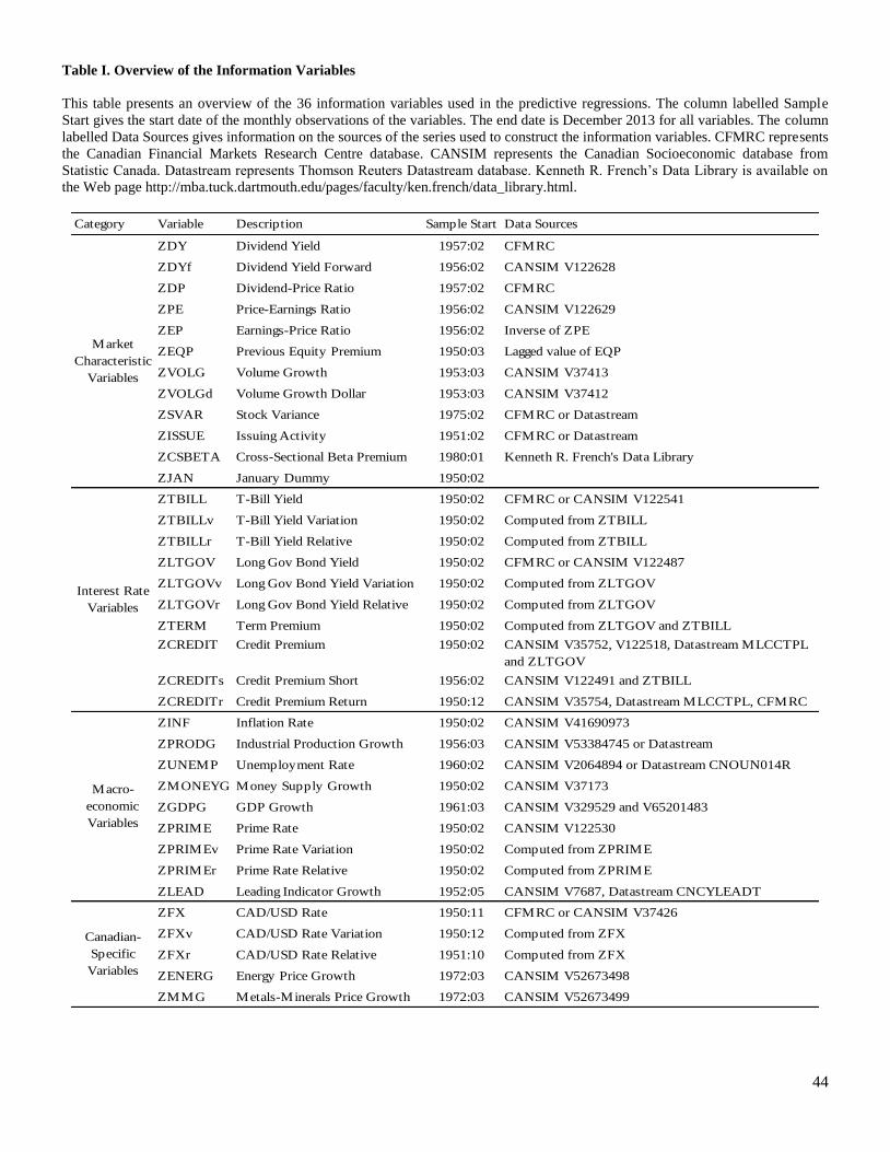
44

Table I. Overview of the Information Variables

This table presents an overview of the 36 information variables used in the predictive regressions. The column labelled Sample

Start gives the start date of the monthly observations of the variables. The end date is December 2013 for all variables. The column

labelled Data Sources gives information on the sources of the series used to construct the information variables. CFMRC represents

the Canadian Financial Markets Research Centre database. CANSIM represents the Canadian Socioeconomic database from

Statistic Canada. Datastream represents Thomson Reuters Datastream database. Kenneth R. French’s Data Library is available on

the Web page http://mba.tuck.dartmouth.edu/pages/faculty/ken.french/data_library.html.

Category Variable Description Sample Start Data Sources

ZDY Dividend Yield 1957:02 CFMRC

ZDYf Dividend Yield Forward 1956:02 CANSIM V122628

ZDP Dividend-Price Ratio 1957:02 CFMRC

ZPE Price-Earnings Ratio 1956:02 CANSIM V122629

ZEP Earnings-Price Ratio 1956:02 Inverse of ZPE

ZEQP Previous Equity Premium 1950:03 Lagged value of EQP

ZVOLG Volume Growth 1953:03 CANSIM V37413

ZVOLGd Volume Growth Dollar 1953:03 CANSIM V37412

ZSVAR Stock Variance 1975:02 CFMRC or Datastream

ZISSUE Issuing Activity 1951:02 CFMRC or Datastream

ZCSBETA Cross-Sectional Beta Premium 1980:01 Kenneth R. French's Data Library

ZJAN January Dummy 1950:02

ZTBILL T-Bill Yield 1950:02 CFMRC or CANSIM V122541

ZTBILLv T-Bill Yield Variation 1950:02 Computed from ZTBILL

ZTBILLr T-Bill Yield Relative 1950:02 Computed from ZTBILL

ZLTGOV Long Gov Bond Yield 1950:02 CFMRC or CANSIM V122487

ZLTGOVv Long Gov Bond Yield Variation 1950:02 Computed from ZLTGOV

ZLTGOVr Long Gov Bond Yield Relative 1950:02 Computed from ZLTGOV

ZTERM Term Premium 1950:02 Computed from ZLTGOV and ZTBILL

ZCREDITs Credit Premium Short 1956:02 CANSIM V122491 and ZTBILL

ZCREDITr Credit Premium Return 1950:12 CANSIM V35754, Datastream MLCCTPL, CFMRC

ZINF Inflation Rate 1950:02 CANSIM V41690973

ZPRODG Industrial Production Growth 1956:03 CANSIM V53384745 or Datastream

ZUNEMP Unemployment Rate 1960:02 CANSIM V2064894 or Datastream CNOUN014R

ZMONEYG Money Supply Growth 1950:02 CANSIM V37173

ZGDPG GDP Growth 1961:03 CANSIM V329529 and V65201483

ZPRIME Prime Rate 1950:02 CANSIM V122530

ZPRIMEv Prime Rate Variation 1950:02 Computed from ZPRIME

ZPRIMEr Prime Rate Relative 1950:02 Computed from ZPRIME

ZLEAD Leading Indicator Growth 1952:05 CANSIM V7687, Datastream CNCYLEADT

ZFX CAD/USD Rate 1950:11 CFMRC or CANSIM V37426

ZFXv CAD/USD Rate Variation 1950:12 Computed from ZFX

ZFXr CAD/USD Rate Relative 1951:10 Computed from ZFX

ZENERG Energy Price Growth 1972:03 CANSIM V52673498

ZMMG Metals-Minerals Price Growth 1972:03 CANSIM V52673499

CANSIM V35752, V122518, Datastream MLCCTPL

and ZLTGOV

Canadian-

Specific

Variables

Macro-

economic

Variables

Interest Rate

Variables

Market

Characteristic

Variables

1950:02Credit PremiumZCREDIT

45

Table II. Descriptive Statistics of the Equity Premium and Information Variables

This table presents the full-sample mean, standard deviation, minimum, maximum, excess kurtosis, skewness, and autocorrelation

(with significance), as well as the mean in three sub-periods of the variables in the study. The data are at monthly frequency and

cover the period from February 1950 to December 2013. The variable EQP is the Canadian equity premium. The variables

beginning by Z are the information variables and have been lagged by one month. The information variables are described in Table

I. ***, ** and * indicate significance at the 1%, 5% and 10% levels, respectively.

Variable Mean Std Dev Min MaxExcess

Kurt

Skew-

nessMean Mean Mean

EQP 0.0045 0.044 -0.235 0.158 2.607 -0.697 0.124 *** 0.0069 0.0029 0.0039

ZDY 0.0345 0.013 0.009 0.085 0.933 0.740 0.882 *** 0.0369 0.0435 0.0259

ZDYf 0.0308 0.009 0.010 0.063 0.028 0.128 0.985 *** 0.0335 0.0375 0.0235

ZDP 0.0324 0.011 0.009 0.086 0.517 0.275 0.862 *** 0.0350 0.0401 0.0246

ZPE 24.652 35.437 6.580 254.98 31.450 5.434 0.911 *** 17.024 12.978 38.802

ZEP 0.0626 0.028 0.004 0.152 0.539 0.664 0.986 *** 0.0596 0.0870 0.0441

ZEQP 0.0045 0.044 -0.235 0.158 2.600 -0.695 0.124 *** 0.0070 0.0029 0.0038

ZVOLG 0.0297 0.236 -0.577 1.885 7.107 1.513 -0.237 *** 0.0370 0.0345 0.0206

ZVOLGd 0.0323 0.233 -0.606 1.791 6.199 1.485 -0.187 *** 0.0276 0.0420 0.0274

ZSVAR 0.0019 0.004 0.000 0.055 91.074 8.335 0.577 *** 0.0014 0.0022

ZISSUE 0.0276 0.083 -0.223 0.543 14.126 2.517 0.780 *** 0.0259 0.0401 0.0184

ZCSBETA -0.2789 0.308 -1.463 0.249 3.752 -1.588 0.987 *** -0.288 -0.275

ZJAN 0.0821 0.275 0.000 1.000 7.320 3.050 -0.090 ** 0.0795 0.0833 0.0833

ZTBILL 0.0539 0.038 0.002 0.208 0.988 1.041 0.992 *** 0.0325 0.0913 0.0405

ZTBILLv 0.0000 0.005 -0.036 0.033 13.285 0.099 0.248 *** 0.0003 0.0002 -0.0004

ZTBILLr 0.0000 0.011 -0.039 0.045 2.114 0.098 0.913 *** 0.0016 0.0011 -0.0021

ZLTGOV 0.0681 0.030 0.021 0.177 0.116 0.762 0.995 *** 0.0466 0.1010 0.0585

ZLTGOVv 0.0000 0.003 -0.023 0.020 12.249 -0.176 0.065 * 0.0002 0.0001 -0.0002

ZLTGOVr 0.0000 0.006 -0.026 0.032 5.903 0.596 0.874 *** 0.0011 0.0005 -0.0013

ZTERM 0.0141 0.014 -0.043 0.044 1.590 -0.892 0.955 *** 0.0141 0.0097 0.0179

ZCREDIT 0.0103 0.005 0.002 0.037 4.608 1.606 0.975 *** 0.0070 0.0104 0.0128

ZCREDITs 0.0050 0.006 -0.002 0.039 5.688 2.154 0.878 *** 0.0077 0.0064 0.0023

ZCREDITr 0.0005 0.013 -0.067 0.092 5.949 0.038 -0.043 0.0006 0.0005 0.0004

ZINF 0.0030 0.005 -0.013 0.026 1.785 0.639 0.244 *** 0.0021 0.0056 0.0017

ZPRODG 0.0028 0.006 -0.029 0.038 4.102 0.359 0.370 *** 0.0012 0.0055 0.0014

ZUNEMP 0.0753 0.022 0.024 0.141 -0.181 0.197 0.962 *** 0.0506 0.0803 0.0814

ZMONEYG 0.0054 0.016 -0.051 0.053 1.749 -0.668 -0.049 0.0043 0.0076 0.0045

ZGDPG 0.0027 0.005 -0.015 0.022 1.099 -0.019 -0.079 ** 0.0045 0.0028 0.0019

ZPRIME 0.0580 0.037 0.005 0.210 0.952 1.022 0.992 *** 0.0368 0.0964 0.0437

ZPRIMEv 0.0000 0.005 -0.038 0.042 18.563 0.121 0.270 *** 0.0003 0.0002 -0.0004

ZPRIMEr 0.0000 0.011 -0.037 0.048 2.479 0.175 0.914 *** 0.0014 0.0011 -0.0021

ZLEAD 0.0032 0.010 -0.028 0.035 0.611 -0.196 0.134 *** 0.0027 0.0033 0.0036

ZFX 1.1540 0.169 0.948 1.600 -0.400 0.802 0.996 *** 1.0235 1.1510 1.2608

ZFXv 0.0000 0.014 -0.074 0.126 10.271 0.477 0.255 *** 0.0001 0.0004 -0.0004

ZFXr -0.0002 0.034 -0.158 0.170 4.540 -0.073 0.922 *** 0.0005 0.0024 -0.0028

ZENERG 0.0074 0.063 -0.241 0.282 2.469 -0.027 0.264 *** 0.0078 0.0071

ZMMG 0.0042 0.036 -0.134 0.172 2.504 0.283 0.326 *** 0.0060 0.0028

1950-

1969

1970-

1989

1990-

2013

Autocor-

relation

Full Sample

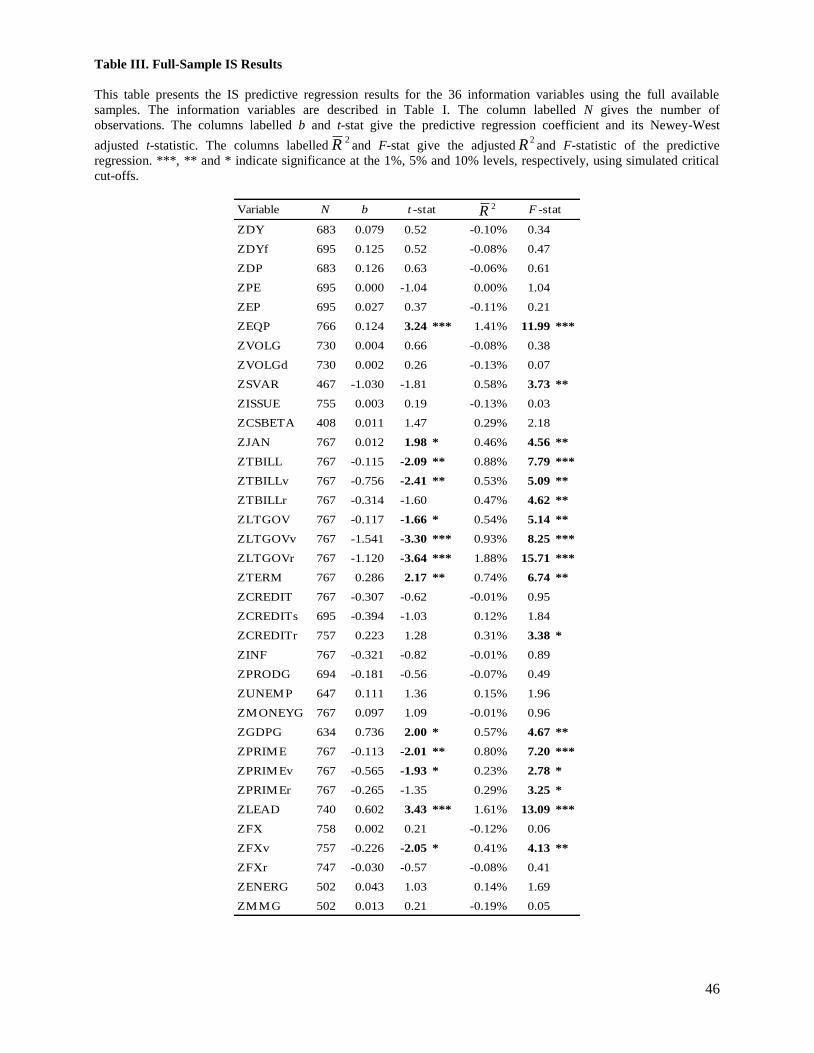
46

Table III. Full-Sample IS Results

This table presents the IS predictive regression results for the 36 information variables using the full available

samples. The information variables are described in Table I. The column labelled N gives the number of

observations. The columns labelled b and t-stat give the predictive regression coefficient and its Newey-West

adjusted t-statistic. The columns labelled2R and F-stat give the adjusted

2R and F-statistic of the predictive

regression. ***, ** and * indicate significance at the 1%, 5% and 10% levels, respectively, using simulated critical

cut-offs.

Variable N b

ZDY 683 0.079 0.52 -0.10% 0.34

ZDYf 695 0.125 0.52 -0.08% 0.47

ZDP 683 0.126 0.63 -0.06% 0.61

ZPE 695 0.000 -1.04 0.00% 1.04

ZEP 695 0.027 0.37 -0.11% 0.21

ZEQP 766 0.124 3.24 *** 1.41% 11.99 ***

ZVOLG 730 0.004 0.66 -0.08% 0.38

ZVOLGd 730 0.002 0.26 -0.13% 0.07

ZSVAR 467 -1.030 -1.81 0.58% 3.73 **

ZISSUE 755 0.003 0.19 -0.13% 0.03

ZCSBETA 408 0.011 1.47 0.29% 2.18

ZJAN 767 0.012 1.98 * 0.46% 4.56 **

ZTBILL 767 -0.115 -2.09 ** 0.88% 7.79 ***

ZTBILLv 767 -0.756 -2.41 ** 0.53% 5.09 **

ZTBILLr 767 -0.314 -1.60 0.47% 4.62 **

ZLTGOV 767 -0.117 -1.66 * 0.54% 5.14 **

ZLTGOVv 767 -1.541 -3.30 *** 0.93% 8.25 ***

ZLTGOVr 767 -1.120 -3.64 *** 1.88% 15.71 ***

ZTERM 767 0.286 2.17 ** 0.74% 6.74 **

ZCREDIT 767 -0.307 -0.62 -0.01% 0.95

ZCREDITs 695 -0.394 -1.03 0.12% 1.84

ZCREDITr 757 0.223 1.28 0.31% 3.38 *

ZINF 767 -0.321 -0.82 -0.01% 0.89

ZPRODG 694 -0.181 -0.56 -0.07% 0.49

ZUNEMP 647 0.111 1.36 0.15% 1.96

ZMONEYG 767 0.097 1.09 -0.01% 0.96

ZGDPG 634 0.736 2.00 * 0.57% 4.67 **

ZPRIME 767 -0.113 -2.01 ** 0.80% 7.20 ***

ZPRIMEv 767 -0.565 -1.93 * 0.23% 2.78 *

ZPRIMEr 767 -0.265 -1.35 0.29% 3.25 *

ZLEAD 740 0.602 3.43 *** 1.61% 13.09 ***

ZFX 758 0.002 0.21 -0.12% 0.06

ZFXv 757 -0.226 -2.05 * 0.41% 4.13 **

ZFXr 747 -0.030 -0.57 -0.08% 0.41

ZENERG 502 0.043 1.03 0.14% 1.69

ZMMG 502 0.013 0.21 -0.19% 0.05

t -stat F -stat2R

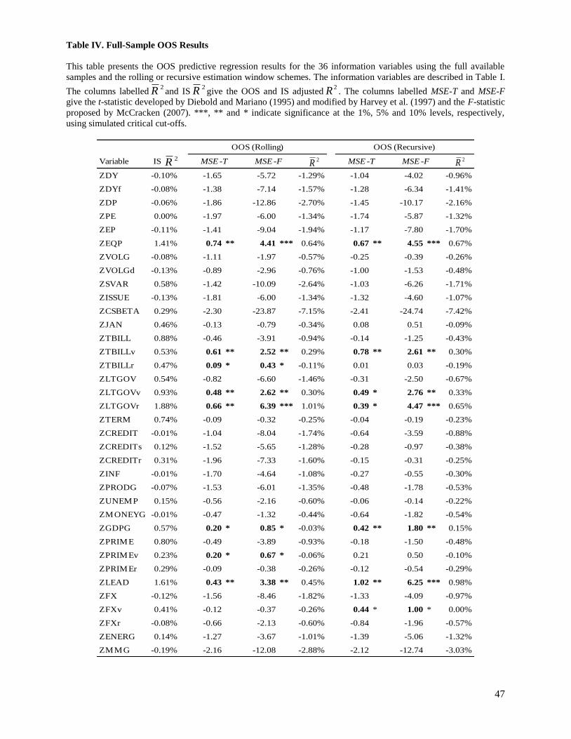
47

Table IV. Full-Sample OOS Results

This table presents the OOS predictive regression results for the 36 information variables using the full available

samples and the rolling or recursive estimation window schemes. The information variables are described in Table I.

The columns labelled2R and IS

2R give the OOS and IS adjusted2R . The columns labelled MSE-T and MSE-F

give the t-statistic developed by Diebold and Mariano (1995) and modified by Harvey et al. (1997) and the F-statistic

proposed by McCracken (2007). ***, ** and * indicate significance at the 1%, 5% and 10% levels, respectively,

using simulated critical cut-offs.

Variable IS

ZDY -0.10% -1.65 -5.72 -1.29% -1.04 -4.02 -0.96%

ZDYf -0.08% -1.38 -7.14 -1.57% -1.28 -6.34 -1.41%

ZDP -0.06% -1.86 -12.86 -2.70% -1.45 -10.17 -2.16%

ZPE 0.00% -1.97 -6.00 -1.34% -1.74 -5.87 -1.32%

ZEP -0.11% -1.41 -9.04 -1.94% -1.17 -7.80 -1.70%

ZEQP 1.41% 0.74 ** 4.41 *** 0.64% 0.67 ** 4.55 *** 0.67%

ZVOLG -0.08% -1.11 -1.97 -0.57% -0.25 -0.39 -0.26%

ZVOLGd -0.13% -0.89 -2.96 -0.76% -1.00 -1.53 -0.48%

ZSVAR 0.58% -1.42 -10.09 -2.64% -1.03 -6.26 -1.71%

ZISSUE -0.13% -1.81 -6.00 -1.34% -1.32 -4.60 -1.07%

ZCSBETA 0.29% -2.30 -23.87 -7.15% -2.41 -24.74 -7.42%

ZJAN 0.46% -0.13 -0.79 -0.34% 0.08 0.51 -0.09%

ZTBILL 0.88% -0.46 -3.91 -0.94% -0.14 -1.25 -0.43%

ZTBILLv 0.53% 0.61 ** 2.52 ** 0.29% 0.78 ** 2.61 ** 0.30%

ZTBILLr 0.47% 0.09 * 0.43 * -0.11% 0.01 0.03 -0.19%

ZLTGOV 0.54% -0.82 -6.60 -1.46% -0.31 -2.50 -0.67%

ZLTGOVv 0.93% 0.48 ** 2.62 ** 0.30% 0.49 * 2.76 ** 0.33%

ZLTGOVr 1.88% 0.66 ** 6.39 *** 1.01% 0.39 * 4.47 *** 0.65%

ZTERM 0.74% -0.09 -0.32 -0.25% -0.04 -0.19 -0.23%

ZCREDIT -0.01% -1.04 -8.04 -1.74% -0.64 -3.59 -0.88%

ZCREDITs 0.12% -1.52 -5.65 -1.28% -0.28 -0.97 -0.38%

ZCREDITr 0.31% -1.96 -7.33 -1.60% -0.15 -0.31 -0.25%

ZINF -0.01% -1.70 -4.64 -1.08% -0.27 -0.55 -0.30%

ZPRODG -0.07% -1.53 -6.01 -1.35% -0.48 -1.78 -0.53%

ZUNEMP 0.15% -0.56 -2.16 -0.60% -0.06 -0.14 -0.22%

ZMONEYG -0.01% -0.47 -1.32 -0.44% -0.64 -1.82 -0.54%

ZGDPG 0.57% 0.20 * 0.85 * -0.03% 0.42 ** 1.80 ** 0.15%

ZPRIME 0.80% -0.49 -3.89 -0.93% -0.18 -1.50 -0.48%

ZPRIMEv 0.23% 0.20 * 0.67 * -0.06% 0.21 0.50 -0.10%

ZPRIMEr 0.29% -0.09 -0.38 -0.26% -0.12 -0.54 -0.29%

ZLEAD 1.61% 0.43 ** 3.38 ** 0.45% 1.02 ** 6.25 *** 0.98%

ZFX -0.12% -1.56 -8.46 -1.82% -1.33 -4.09 -0.97%

ZFXv 0.41% -0.12 -0.37 -0.26% 0.44 * 1.00 * 0.00%

ZFXr -0.08% -0.66 -2.13 -0.60% -0.84 -1.96 -0.57%

ZENERG 0.14% -1.27 -3.67 -1.01% -1.39 -5.06 -1.32%

ZMMG -0.19% -2.16 -12.08 -2.88% -2.12 -12.74 -3.03%

MSE -T MSE -F MSE -T MSE -F

OOS (Recursive)OOS (Rolling)

2R2R

2R

48

Table V. Sub-Period IS Results

This table presents the IS predictive regression results for the 36 information variables in three sub-periods. The information variables are described in Table I. The column

labelled N gives the number of observations. The columns labelled b and t-stat give the predictive regression coefficient and its Newey-West adjusted t-statistic. The columns

labelled2R and F-stat give the adjusted

2R and F-statistic of the predictive regression. ***, ** and * indicate significance at the 1%, 5% and 10% levels, respectively, using

simulated critical cut-offs.

Variable N b N b N b

ZDY 155 0.551 0.90 -0.10% 0.86 240 0.197 0.84 -0.13% 0.69 288 -0.019 -0.05 -0.35% 0.00

ZDYf 167 1.527 1.49 1.28% 3.19 240 0.621 1.24 0.52% 2.26 288 -0.216 -0.42 -0.22% 0.38

ZDP 155 3.729 4.18 *** 6.02% 11.01 *** 240 0.331 0.94 0.03% 1.08 288 -0.026 -0.06 -0.35% 0.01

ZPE 167 -0.002 -0.91 0.19% 1.33 240 0.000 -0.09 -0.42% 0.01 288 0.000 -1.11 0.11% 1.32

ZEP 167 0.378 0.75 -0.01% 1.00 240 0.058 0.45 -0.31% 0.26 288 0.055 0.33 -0.29% 0.18

ZEQP 238 0.160 2.71 ** 2.16% 6.28 ** 240 0.078 1.35 0.19% 1.47 288 0.153 2.23 ** 1.98% 6.86 ***

ZVOLG 202 0.005 0.60 -0.30% 0.41 240 0.003 0.30 -0.39% 0.06 288 0.003 0.18 -0.34% 0.04

ZVOLGd 202 -0.008 -0.65 -0.26% 0.49 240 0.000 0.04 -0.42% 0.00 288 0.011 0.85 -0.05% 0.88

ZSVAR 179 -0.167 -0.37 -0.55% 0.02 288 -1.294 -2.20 * 1.41% 5.15 **

ZISSUE 227 -0.119 -1.01 0.15% 1.36 240 -0.003 -0.15 -0.41% 0.01 288 0.042 1.10 0.02% 1.06

ZCSBETA 120 0.045 0.74 -0.01% 1.01 288 0.010 1.31 0.30% 1.89

ZJAN 239 0.018 2.07 * 1.43% 4.49 ** 240 0.021 1.49 0.91% 3.22 * 288 0.000 0.02 -0.35% 0.00

ZTBILL 239 -0.303 -2.30 ** 1.82% 5.46 ** 240 -0.133 -1.19 0.43% 2.05 288 -0.172 -2.12 ** 0.99% 3.89 **

ZTBILLv 239 0.007 0.01 -0.42% 0.00 240 -1.006 -2.46 ** 1.25% 4.06 ** 288 -0.639 -1.06 -0.01% 0.97

ZTBILLr 239 -0.517 -1.85 * 0.56% 2.36 240 -0.368 -1.28 0.80% 2.94 * 288 -0.128 -0.45 -0.29% 0.18

ZLTGOV 239 -0.358 -1.90 ** 1.06% 3.59 * 240 -0.233 -1.26 0.68% 2.66 288 -0.120 -1.15 0.05% 1.16

ZLTGOVv 239 -0.855 -0.33 -0.35% 0.17 240 -1.702 -2.92 ** 1.74% 5.27 ** 288 -1.341 -1.67 0.21% 1.62

ZLTGOVr 239 -2.480 -2.52 ** 1.98% 5.86 ** 240 -1.290 -3.39 *** 3.98% 10.99 *** 288 -0.582 -1.15 -0.02% 0.94

ZTERM 239 0.668 2.17 * 1.76% 5.30 ** 240 0.134 0.62 -0.20% 0.52 288 0.409 2.50 ** 1.46% 5.29 **

ZCREDIT 239 -0.801 -0.79 -0.02% 0.96 240 0.057 0.05 -0.42% 0.00 288 -0.206 -0.27 -0.27% 0.23

ZCREDITs 167 -0.470 -0.68 -0.24% 0.61 240 -0.360 -0.70 -0.12% 0.72 288 -1.425 -0.65 0.23% 1.68

ZCREDITr 229 0.245 1.08 -0.01% 1.00 240 0.044 0.13 -0.41% 0.03 288 0.330 1.32 1.00% 3.94 **

ZINF 239 -0.118 -0.27 -0.40% 0.06 240 -0.757 -0.93 -0.03% 0.94 288 -0.021 -0.03 -0.35% 0.00

ZPRODG 166 0.162 0.25 -0.58% 0.04 240 -0.322 -0.49 -0.25% 0.40 288 -0.124 -0.35 -0.31% 0.12

ZUNEMP 119 0.124 0.66 -0.35% 0.60 240 0.260 1.53 0.74% 2.81 * 288 0.101 0.57 -0.20% 0.43

ZMONEYG 239 0.254 2.34 ** 0.84% 3.05 * 240 0.179 1.32 0.03% 1.08 288 -0.253 -1.20 0.18% 1.52

ZGDPG 106 0.604 1.10 0.43% 1.48 240 0.648 1.06 0.14% 1.34 288 1.145 1.55 0.60% 2.74 *

ZPRIME 239 -0.304 -2.08 ** 1.53% 4.73 ** 240 -0.138 -1.10 0.35% 1.84 288 -0.179 -2.29 ** 1.08% 4.18 **

ZPRIMEv 239 0.343 0.58 -0.32% 0.24 240 -0.865 -2.22 ** 0.82% 3.01 * 288 -0.440 -0.79 -0.22% 0.38

ZPRIMEr 239 -0.391 -1.51 0.20% 1.49 240 -0.336 -1.12 0.54% 2.31 288 -0.081 -0.31 -0.32% 0.08

ZLEAD 212 0.571 2.47 ** 2.74% 7.00 *** 240 0.560 1.61 0.74% 2.80 288 0.710 1.98 * 1.46% 5.29 **

ZFX 230 0.012 0.20 -0.41% 0.06 240 0.016 0.66 -0.26% 0.39 288 0.005 0.31 -0.30% 0.14

ZFXv 229 -0.249 -0.64 -0.28% 0.36 240 -0.075 -0.31 -0.39% 0.07 288 -0.264 -2.08 * 1.18% 4.46 **

ZFXr 219 0.093 0.60 -0.31% 0.33 240 0.085 0.82 -0.23% 0.46 288 -0.067 -1.07 0.21% 1.62

ZENERG 214 -0.008 -0.11 -0.47% 0.01 288 0.052 1.12 0.53% 2.55

ZMMG 214 -0.044 -0.49 -0.37% 0.23 288 0.066 0.75 -0.07% 0.79

1950-1969 1970-1989 1990-2013

F -statt -stat F -stat t -stat F -stat t -stat2R 2R 2R

49

Table VI. Sub-Period OOS Results

This table presents the OOS predictive regression results for the 36 information variables in two sub-periods and using the rolling or recursive estimation window

schemes. The information variables are described in Table I. The columns labelled2R and IS

2R give the OOS and IS adjusted2R . The columns labelled MSE-T and

MSE-F give the t-statistic developed by Diebold and Mariano (1995) and modified by Harvey et al. (1997) and the F-statistic proposed by McCracken (2007). ***, **

and * indicate significance at the 1%, 5% and 10% levels, respectively, using simulated critical cut-offs.

Variable IS IS

ZDY -0.13% -1.06 -2.62 -1.53% -0.76 -2.17 -1.34% -0.35% -1.40 -3.09 -1.44% -0.75 -1.71 -0.95%

ZDYf 0.52% -0.72 -2.64 -1.54% -0.58 -1.92 -1.24% -0.22% -1.43 -4.73 -2.03% -1.36 -4.79 -2.05%

ZDP 0.03% -1.31 -7.06 -3.48% -1.16 -6.37 -3.17% -0.35% -1.76 -5.29 -2.23% -1.07 -3.05 -1.42%

ZPE -0.42% -1.68 -3.44 -1.89% -1.54 -3.39 -1.87% 0.11% -1.04 -2.28 -1.15% -0.86 -2.18 -1.11%

ZEP -0.31% -1.21 -6.30 -3.14% -1.12 -6.08 -3.04% -0.29% -0.98 -1.81 -0.99% -0.36 -0.60 -0.56%

ZEQP 0.19% 0.01 0.05 -0.40% -0.05 -0.22 -0.51% 1.98% 1.18 ** 5.19 *** 1.43% 1.22 ** 5.76 *** 1.62%

ZVOLG -0.39% -0.94 -0.40 -0.59% -0.14 -0.15 -0.49% -0.34% -0.88 -1.76 -0.97% -0.22 -0.24 -0.44%

ZVOLGd -0.42% -0.82 -1.40 -1.02% -0.70 -0.80 -0.76% -0.05% -0.49 -1.53 -0.89% -0.83 -0.68 -0.59%

ZSVAR -0.55% -1.13 -5.04 -4.39% -1.23 -5.26 -4.55% 1.41% -0.86 -4.20 -1.83% 0.25 0.71 -0.10%

ZISSUE -0.41% -1.69 -4.47 -2.34% -1.26 -3.67 -1.99% 0.02% -0.65 -0.79 -0.63% -0.62 -0.27 -0.44%

ZCSBETA -0.01% -2.29 -18.00 -28.8% -2.43 -18.15 -29.1% 0.30% -0.51 -1.77 -0.97% -0.56 -2.50 -1.23%

ZJAN 0.91% 0.23 1.13 * 0.05% 0.60 * 2.77 ** 0.73% -0.35% -1.11 -2.49 -1.22% -1.05 -3.21 -1.48%

ZTBILL 0.43% -0.51 -3.09 -1.74% -0.34 -2.44 -1.46% 0.99% -0.05 -0.28 -0.45% 0.60 * 1.99 ** 0.34%

ZTBILLv 1.25% 0.64 * 2.00 ** 0.41% 0.73 * 1.79 ** 0.33% -0.01% 0.09 0.19 -0.28% 0.29 0.58 -0.15%

ZTBILLr 0.80% 0.25 0.94 * -0.03% 0.17 0.73 -0.12% -0.29% -0.46 -0.80 -0.63% -0.45 -0.98 -0.69%

ZLTGOV 0.68% -0.60 -3.13 -1.76% -0.34 -2.17 -1.34% 0.05% -0.55 -3.41 -1.55% 0.04 0.10 -0.32%

ZLTGOVv 1.74% 0.34 1.42 * 0.17% 0.35 1.50 * 0.21% 0.21% 0.38 * 1.10 * 0.03% 0.41 1.15 * 0.05%

ZLTGOVr 3.98% 0.76 ** 5.93 *** 2.01% 0.54 * 5.06 *** 1.66% -0.02% -0.18 -0.64 -0.57% -0.41 -1.70 -0.95%

ZTERM -0.20% -0.97 -2.33 -1.41% -0.74 -2.62 -1.54% 1.46% 1.07 ** 2.94 ** 0.66% 1.06 ** 3.54 *** 0.87%

ZCREDIT -0.42% -1.32 -2.32 -1.41% -0.62 -1.49 -1.05% -0.27% -0.71 -6.23 -2.57% -0.38 -2.15 -1.11%

ZCREDITs -0.12% -0.49 -1.26 -0.95% -0.38 -1.07 -0.87% 0.23% -1.93 -4.89 -2.08% 0.39 0.36 -0.23%

ZCREDITr -0.41% -1.84 -3.48 -1.90% -1.14 -1.65 -1.12% 1.00% -1.07 -3.80 -1.69% 1.40 ** 1.97 ** 0.33%

ZINF -0.03% -0.22 -0.45 -0.61% 0.14 0.20 -0.34% -0.35% -3.18 -4.81 -2.05% -0.79 -0.94 -0.68%

ZPRODG -0.25% -0.82 -2.32 -1.41% -0.37 -1.09 -0.88% -0.31% -1.57 -3.84 -1.71% -0.35 -0.58 -0.55%

ZUNEMP 0.74% 0.08 0.17 -0.35% -0.10 -0.16 -0.49% -0.20% -0.80 -2.77 -1.32% 0.06 0.07 -0.33%

ZMONEYG 0.03% -0.03 -0.07 -0.45% 0.09 0.19 -0.34% 0.18% -1.28 -1.46 -0.86% -1.79 -2.40 -1.19%

ZGDPG 0.14% -0.09 -0.25 -0.53% 0.07 0.20 -0.34% 0.60% 0.47 * 1.36 * 0.12% 0.72 * 1.85 ** 0.29%

ZPRIME 0.35% -0.61 -3.39 -1.87% -0.40 -2.67 -1.56% 1.08% 0.04 0.18 -0.29% 0.63 * 2.02 ** 0.35%

ZPRIMEv 0.82% 0.25 0.65 -0.15% 0.21 0.37 -0.27% -0.22% -0.06 -0.11 -0.39% 0.05 0.08 -0.32%

ZPRIMEr 0.54% 0.13 0.42 -0.25% 0.09 0.30 -0.30% -0.32% -0.66 -1.02 -0.71% -0.55 -1.05 -0.72%

ZLEAD 0.74% 0.01 0.06 -0.40% 0.47 * 1.89 ** 0.36% 1.46% 0.55 * 3.93 *** 1.00% 1.05 ** 4.76 *** 1.28%

ZFX -0.26% -1.06 -3.62 -1.97% -0.98 -2.44 -1.46% -0.30% -1.14 -4.93 -2.10% -1.35 -1.41 -0.84%

ZFXv -0.39% -1.60 -1.96 -1.25% -0.97 -0.95 -0.82% 1.18% 0.76 ** 2.34 ** 0.46% 1.08 ** 2.54 ** 0.53%

ZFXr -0.23% -0.82 -0.84 -0.78% -0.25 -0.31 -0.55% 0.21% -0.38 -1.34 -0.82% -0.87 -1.88 -1.01%

ZENERG -0.47% -1.90 -3.92 -2.83% -1.44 -3.75 -2.73% 0.53% 0.72 ** 1.21 * 0.07% -0.29 -0.62 -0.57%

ZMMG -0.37% -2.17 -9.67 -6.35% -2.01 -9.51 -6.25% -0.07% -0.20 -0.25 -0.44% -0.72 -1.25 -0.79%

OOS (Rolling) OOS (Recursive) OOS (Rolling) OOS (Recursive)

1970-1989 1990-2013

MSE -F MSE -T MSE -FMSE -T MSE -F MSE -T MSE -F MSE -T 2R2R 2R2R 2R2R

50

Table VII. Results of Multiple Structural Break Tests

This table presents the results for the multiple structural break tests developed by Bai and Perron (1998, 2003a, 2003b, 2006) for

the 36 information variables using the full sample. The information variables are described in Table I. The columns labelled U

DmaxF and W DmaxF give the double maximum tests of the null hypothesis of no break versus an unknown number of breaks

given some upper bound. The columns labelled N and Break Dates give the number and date of the breaks identified using the

sequential approach described in section 2.1. The columns labelled b give the predictive regression coefficient in each regime when

a break is identified. ***, ** and * indicate significance at the 1%, 5% and 10% levels, respectively, using the critical values of Bai

and Perron (2003a) for the double maximum tests and asymptotic critical values for the t-statistic associated with the predictive

regression coefficient.

Variable N b b b

ZDY 4.50 6.08 0

ZDYf 5.34 8.64 0

ZDP 15.44 ** 18.23 *** 1 196412 2.841 *** 0.033

ZPE 8.64 9.63 0

ZEP 6.00 9.69 0

ZEQP 3.60 4.86 0

ZVOLG 2.96 4.98 0

ZVOLGd 5.42 9.18 0

ZSVAR 6.71 9.06 0

ZISSUE 3.82 5.19 0

ZCSBETA 7.13 8.80 0

ZJAN 5.87 7.01 0

ZTBILL 8.43 10.20 0

ZTBILLv 6.84 9.49 0

ZTBILLr 6.90 6.90 0

ZLTGOV 13.08 ** 13.52 ** 0 196004 -1.67 *** -0.1

ZLTGOVv 2.64 3.49 0

ZLTGOVr 5.88 8.34 0

ZTERM 4.30 5.10 0

ZCREDIT 4.31 5.85 0

ZCREDITs 6.42 10.38 0

ZCREDITr 5.96 8.49 0

ZINF 6.90 8.23 0

ZPRODG 3.83 5.69 0

ZUNEMP 5.45 7.12 0

ZMONEYG 4.53 5.81 0

ZGDPG 4.88 6.11 0

ZPRIME 7.56 10.19 0

ZPRIMEv 5.34 5.34 0

ZPRIMEr 4.80 4.80 0

ZLEAD 2.03 3.60 0

ZFX 7.96 15.91 ** 0

ZFXv 9.04 12.59 * 0

ZFXr 5.57 7.82 0

ZENERG 5.67 7.13 0

ZMMG 6.61 9.42 0

U DmaxF W DmaxF Break Dates

Test of No Break vs Unknown

Number of Breaks

Number of Breaks and

Break Dates

Coefficient b per Regime

Regime 1 Regime 2 Regime 3

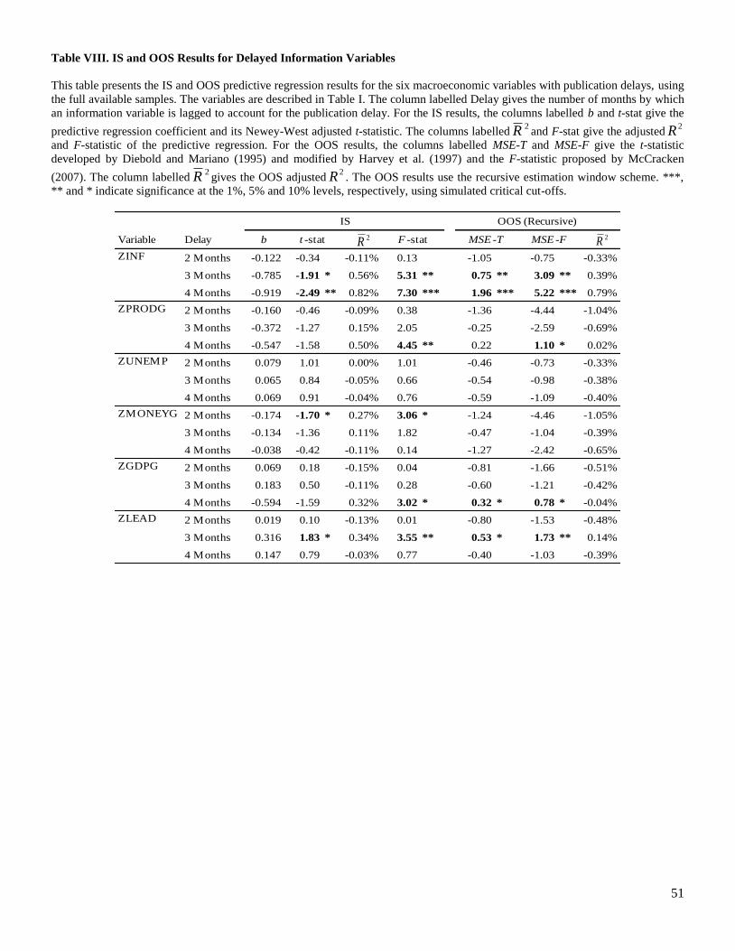
51

Table VIII. IS and OOS Results for Delayed Information Variables

This table presents the IS and OOS predictive regression results for the six macroeconomic variables with publication delays, using

the full available samples. The variables are described in Table I. The column labelled Delay gives the number of months by which

an information variable is lagged to account for the publication delay. For the IS results, the columns labelled b and t-stat give the

predictive regression coefficient and its Newey-West adjusted t-statistic. The columns labelled2R and F-stat give the adjusted

2Rand F-statistic of the predictive regression. For the OOS results, the columns labelled MSE-T and MSE-F give the t-statistic

developed by Diebold and Mariano (1995) and modified by Harvey et al. (1997) and the F-statistic proposed by McCracken

(2007). The column labelled2R gives the OOS adjusted

2R . The OOS results use the recursive estimation window scheme. ***,

** and * indicate significance at the 1%, 5% and 10% levels, respectively, using simulated critical cut-offs.

Variable Delay b

2 Months -0.122 -0.34 -0.11% 0.13 -1.05 -0.75 -0.33%

3 Months -0.785 -1.91 * 0.56% 5.31 ** 0.75 ** 3.09 ** 0.39%

4 Months -0.919 -2.49 ** 0.82% 7.30 *** 1.96 *** 5.22 *** 0.79%

2 Months -0.160 -0.46 -0.09% 0.38 -1.36 -4.44 -1.04%

3 Months -0.372 -1.27 0.15% 2.05 -0.25 -2.59 -0.69%

4 Months -0.547 -1.58 0.50% 4.45 ** 0.22 1.10 * 0.02%

2 Months 0.079 1.01 0.00% 1.01 -0.46 -0.73 -0.33%

3 Months 0.065 0.84 -0.05% 0.66 -0.54 -0.98 -0.38%

4 Months 0.069 0.91 -0.04% 0.76 -0.59 -1.09 -0.40%

2 Months -0.174 -1.70 * 0.27% 3.06 * -1.24 -4.46 -1.05%

3 Months -0.134 -1.36 0.11% 1.82 -0.47 -1.04 -0.39%

4 Months -0.038 -0.42 -0.11% 0.14 -1.27 -2.42 -0.65%

2 Months 0.069 0.18 -0.15% 0.04 -0.81 -1.66 -0.51%

3 Months 0.183 0.50 -0.11% 0.28 -0.60 -1.21 -0.42%

4 Months -0.594 -1.59 0.32% 3.02 * 0.32 * 0.78 * -0.04%

2 Months 0.019 0.10 -0.13% 0.01 -0.80 -1.53 -0.48%

3 Months 0.316 1.83 * 0.34% 3.55 ** 0.53 * 1.73 ** 0.14%

4 Months 0.147 0.79 -0.03% 0.77 -0.40 -1.03 -0.39%

ZGDPG

ZLEAD

IS

ZINF

ZPRODG

ZUNEMP

ZMONEYG

OOS (Recursive)

t -stat F -stat MSE -T MSE -F 2R2R

52

Table IX. Economic Value of the Predictions

This table examines the economic value of the predictions for a mean-variance investor who forms his portfolio based on the

forecasts from the OOS predictive regressions using the recursive estimation window scheme. The information variables are

described in Table I. The methodology is described in section 2.3. The columns labelled Portfolio Based on Predictive Model give

statistics on the portfolios constructed with the forecasts from the information variables, namely their average equity allocation

(Mean XA), their proportions of allocation equal to the limits allowed of 0% (%XA = 0) or 150% (%XA = 1.5), their annualized

values of the mean return (μA), standard deviation of returns (σA) and average utility level (UA), and their end-of-sample value of a

1$ beginning-of-sample investment ($VA). The columns labelled Differences with Portfolio Based on Historical Mean give

statistics on the differences with a portfolio constructed with the forecasts from the historical mean model, namely their differences

in utility level (UA-UN), mean return (μA-μN), standard deviation of returns (σA-σN) and value of a 1$ investment ($VA-$VN).

Variable Mean X A % X A = 0 % X A =1.5 μ A σ A U A $V A U A -U N μ A -μ N σ A -σ N $V A -$V N

ZDY 37.4% 12.7% 1.9% 6.65% 9.02% 5.43% 15.27 $ -0.48% -2.32% -5.28% -16.83 $

ZDYf 44.2% 32.3% 8.9% 7.65% 12.27% 5.39% 20.54 $ -0.52% -1.33% -2.02% -11.56 $

ZDP 37.5% 21.8% 5.3% 6.93% 9.19% 5.66% 17.28 $ -0.24% -2.04% -5.11% -14.81 $

ZPE 60.1% 6.1% 4.4% 7.45% 12.19% 5.22% 18.64 $ -0.69% -1.53% -2.11% -13.45 $

ZEP 54.4% 4.9% 3.8% 7.50% 11.68% 5.45% 19.62 $ -0.46% -1.48% -2.61% -12.48 $

ZEQP 77.0% 16.9% 18.4% 11.84% 14.32% 8.76% 112.10 $ 2.85% 2.87% 0.03% 80.01 $

ZVOLG 68.0% 0.2% 2.1% 8.20% 12.45% 5.87% 25.56 $ -0.04% -0.78% -1.84% -6.53 $

ZVOLGd 68.3% 0.9% 3.4% 7.95% 12.75% 5.51% 22.51 $ -0.40% -1.03% -1.55% -9.59 $

ZSVAR 62.2% 3.9% 3.5% 8.53% 12.92% 6.03% 15.55 $ -1.35% -1.24% 0.30% -9.01 $

ZISSUE 68.1% 3.6% 3.4% 8.39% 13.14% 5.80% 26.63 $ -0.11% -0.58% -1.15% -5.46 $

ZCSBETA 62.3% 17.2% 9.7% 7.57% 11.88% 5.45% 8.22 $ -0.74% -0.79% -0.13% -2.27 $

ZJAN 66.0% 0.0% 8.7% 8.90% 12.79% 6.45% 34.44 $ 0.54% -0.07% -1.50% 2.35 $

ZTBILL 72.4% 31.3% 18.4% 11.18% 14.73% 7.92% 80.97 $ 2.01% 2.20% 0.43% 48.87 $

ZTBILLv 83.7% 4.7% 11.2% 11.17% 15.54% 7.55% 77.24 $ 1.64% 2.20% 1.25% 45.15 $

ZTBILLr 83.0% 11.8% 19.5% 10.69% 14.84% 7.38% 66.08 $ 1.47% 1.71% 0.55% 33.98 $

ZLTGOV 60.0% 33.4% 11.0% 9.59% 13.65% 6.80% 43.33 $ 0.89% 0.62% -0.65% 11.24 $

ZLTGOVv 84.0% 12.1% 17.5% 12.07% 15.86% 8.30% 113.26 $ 2.39% 3.10% 1.57% 81.17 $

ZLTGOVr 91.4% 17.6% 32.3% 11.99% 16.61% 7.85% 102.31 $ 1.94% 3.01% 2.32% 70.22 $

ZTERM 82.2% 14.4% 20.9% 10.85% 14.44% 7.72% 72.61 $ 1.82% 1.88% 0.14% 40.51 $

ZCREDIT 59.0% 9.9% 2.8% 8.42% 11.98% 6.26% 28.60 $ 0.36% -0.56% -2.32% -3.49 $

ZCREDITs 71.1% 2.7% 0.4% 8.75% 12.00% 6.59% 33.21 $ 0.68% -0.23% -2.30% 1.12 $

ZCREDITr 74.4% 2.5% 5.9% 8.79% 13.47% 6.07% 31.03 $ 0.16% -0.18% -0.83% -1.07 $

ZINF 79.9% 2.1% 6.6% 9.00% 14.64% 5.78% 31.41 $ -0.13% 0.02% 0.34% -0.68 $

ZPRODG 54.6% 8.7% 1.3% 7.70% 10.95% 5.91% 22.22 $ 0.00% -1.27% -3.35% -9.87 $

ZUNEMP 83.8% 0.0% 5.1% 9.55% 14.20% 6.53% 41.47 $ 0.62% 0.58% -0.10% 9.37 $

ZMONEYG 80.5% 4.6% 11.8% 8.85% 15.51% 5.24% 28.15 $ -0.67% -0.12% 1.22% -3.94 $

ZGDPG 49.8% 14.0% 3.4% 9.13% 9.87% 7.67% 43.91 $ 1.76% 0.16% -4.43% 11.82 $

ZPRIME 70.4% 30.2% 16.7% 10.71% 14.32% 7.63% 67.75 $ 1.72% 1.73% 0.02% 35.66 $

ZPRIMEv 83.2% 3.0% 9.1% 9.73% 14.76% 6.47% 43.49 $ 0.56% 0.76% 0.46% 11.40 $

ZPRIMEr 83.5% 8.2% 17.3% 9.98% 14.33% 6.90% 50.11 $ 0.99% 1.01% 0.04% 18.01 $

ZLEAD 73.0% 15.7% 17.5% 13.17% 12.90% 10.68% 220.50 $ 4.77% 4.20% -1.39% 188.41 $

ZFX 87.7% 0.4% 14.0% 8.79% 16.84% 4.53% 24.48 $ -1.38% -0.19% 2.54% -7.61 $

ZFXv 77.2% 2.1% 8.0% 9.40% 14.19% 6.38% 39.14 $ 0.48% 0.43% -0.11% 7.05 $

ZFXr 72.4% 3.2% 3.2% 8.25% 13.16% 5.66% 25.07 $ -0.25% -0.72% -1.14% -7.02 $

ZENERG 43.6% 15.0% 1.1% 7.08% 8.33% 6.04% 13.51 $ -1.07% -2.37% -4.15% -14.84 $

ZMMG 47.1% 13.1% 3.4% 6.99% 9.99% 5.50% 12.32 $ -1.61% -2.45% -2.49% -16.03 $

Portfolio Based on Predictive ModelDifferences with Portfolio Based on

Historical Mean

53

Table X. Summary of the F-Statistic and MSE-F Statistic Significance Level

This table presents a summary of the significance levels obtained IS or OOS with the F-statistics in Tables 3 to 6, in full sample or

in three sub-periods and with the rolling or recursive estimation window schemes. The information variables are described in Table

I. The IS F-statistic is the F-statistic of the predictive regression. The OOS F-statistic is the MSE-F statistic proposed by

McCracken (2007). ***, ** and * indicate significance at the 1%, 5% and 10% levels, respectively, using simulated critical cut-

offs. NA indicates that the evidence is not available.

Variable Name ISOOS

(Roll)

OOS

(Recu)IS IS

OOS

(Roll)

OOS

(Recu)IS

OOS

(Roll)

OOS

(Recu)

ZDY Dividend Yield

ZDYf Dividend Yield Forward

ZDP Dividend-Price Ratio ***

ZPE Price-Earnings Ratio

ZEP Earnings-Price Ratio

ZEQP Previous Equity Premium *** *** *** ** *** *** ***

ZVOLG Volume Growth

ZVOLGd Volume Growth Dollar

ZSVAR Stock Variance ** NA **

ZISSUE Issuing Activity

ZCSBETA Cross-Sectional Beta Premium NA

ZJAN January Dummy ** ** * * **

ZTBILL T-Bill Yield *** ** ** **

ZTBILLv T-Bill Yield Variation ** ** ** ** ** **

ZTBILLr T-Bill Yield Relative ** * * *

ZLTGOV Long Gov Bond Yield ** *

ZLTGOVv Long Gov Bond Yield Variation *** ** ** ** * * * *

ZLTGOVr Long Gov Bond Yield Relative *** *** *** ** *** *** ***

ZTERM Term Premium ** ** ** ** ***

ZCREDIT Credit Premium

ZCREDITs Credit Premium Short

ZCREDITr Credit Premium Return * ** **

ZINF Inflation Rate

ZPRODG Industrial Production Growth

ZUNEMP Unemployment Rate *

ZMONEYG Money Supply Growth *

ZGDPG GDP Growth ** * ** * * **

ZPRIME Prime Rate *** ** ** **

ZPRIMEv Prime Rate Variation * * *

ZPRIMEr Prime Rate Relative *

ZLEAD Leading Indicator Growth *** ** *** *** ** ** *** ***

ZFX CAD/USD Rate

ZFXv CAD/USD Rate Variation ** * ** ** **

ZFXr CAD/USD Rate Relative

ZENERG Energy Price Growth NA *

ZMMG Metals-Minerals Price Growth NA

Full Sample1950-

19691970-1989 1990-2013

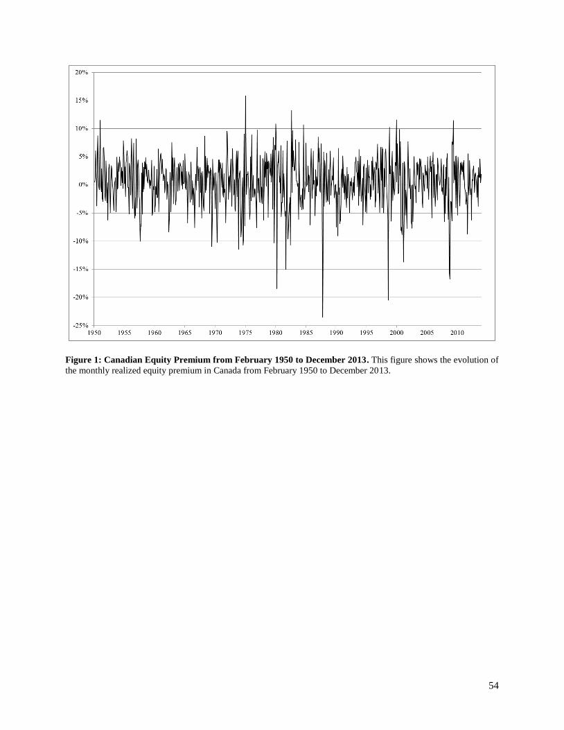
54

Figure 1: Canadian Equity Premium from February 1950 to December 2013. This figure shows the evolution of

the monthly realized equity premium in Canada from February 1950 to December 2013.

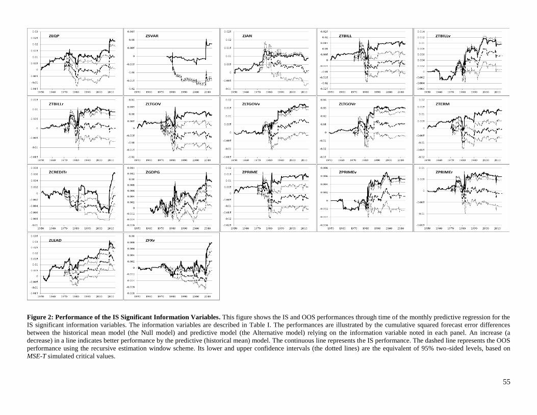
55

Figure 2: Performance of the IS Significant Information Variables. This figure shows the IS and OOS performances through time of the monthly predictive regression for the

IS significant information variables. The information variables are described in Table I. The performances are illustrated by the cumulative squared forecast error differences

between the historical mean model (the Null model) and predictive model (the Alternative model) relying on the information variable noted in each panel. An increase (a

decrease) in a line indicates better performance by the predictive (historical mean) model. The continuous line represents the IS performance. The dashed line represents the OOS

performance using the recursive estimation window scheme. Its lower and upper confidence intervals (the dotted lines) are the equivalent of 95% two-sided levels, based on

MSE-T simulated critical values.

56

Figure 3: Performance of the IS Insignificant Information Variables. This figure shows the IS and OOS performances through time of the monthly predictive regression for

the IS insignificant information variables. The information variables are described in Table I. The performances are illustrated by the cumulative squared forecast error

differences between the historical mean model (the Null model) and predictive model (the Alternative model) relying on the information variable noted in each panel. An

increase (a decrease) in a line indicates better performance by the predictive (historical mean) model. The continuous line represents the IS performance. The dashed line

represents the OOS performance using the recursive estimation window scheme. Its lower and upper confidence intervals (the dotted lines) are the equivalent of 95% two-sided

levels, based on MSE-T simulated critical values.