Addition Ripple Carry Adder - University of Hong...

10.4.14

1

Computer Arithmetic (2)

ELEC8106/ELEC6102

Spring 2010

Hayden Kwok-Hay So

Arithmetic Units  How do we carry out +, −, ×, ÷ in

FPGA?

 How do we perform sin, cos, e, etc?

H. So, Sp10 Lecture 7 - ELEC8106/6102 2

Addition  Two +ve integers can be added similar

to the way decimal numbers are added in “long addition”

 The same addition can be implemented in hardware (ASIC), and FPGA.


2 3 1 9 +

2 1

4 1 +

1 1 1 0 1 1 1 0 0 1

1 0 0 1 0 1 1 1 1

Ripple Carry Adder  Mimic the working of a long addition

 Each bit of addition handled by one “Full-Adder”

 Full Adder •  Add two 1-bit numbers AND a carry in •  i.e. Add THREE 1-bit numbers •  Produce 1 sum bit and 1 carry bit


Half Adder   Add two 1-bit numbers   Produce 1 sum bit and 1 carry bit


S

Cout

A

B

A B C S

0 0 0 0

0 1 0 1

1 0 0 1

1 1 1 0

Full Adder   A full adder handles a carry

input as well as the two input data bits •  All together there are 3 inputs,

and 2 outputs


A B Cin Cout S 0 0 0 0 0

0 0 1 0 1

0 1 0 0 1

0 1 1 1 0

1 0 0 0 1

1 0 1 1 0

1 1 0 1 0

1 1 1 1 1

€

S = A⊕ B⊕Cin

Cout = AB + Cin (A⊕ B)

10.4.14

2

Ripple Carry Adder (1)  A ripple-carry adder is formed by chaining

series of full adders (FAs) •  1 FA for each input bit •  Carry-out from a bit i is connected as the

carry-input for bit (i +1)


FA FA FA FA

A0 B0 A1 B1 A2 B2 A3 B3

S0 S1 S2 S3

Cout 0

Ripple Carry Adder (2)   Delay through a ripple-carry adder is

proportional to the width of data input   O(n) delay, where n is the width of the input


FA FA FA FA

A0 B0 A1 B1 A2 B2 A3 B3

S0 S1 S2 S3

Cout 0

0

0 0 0 0 0 0 0 0

1

1

2

2

3

3

4

4

Carry Look Ahead Adder   In a ripple carry adder, each bit must wait for

the result of carry from previous bit before its calculation may start

  A carry look ahead (CLA) adder looks ahead in the input to figure out the carry

  Define two functions: •  Generate •  Propagate

  If Gi = 1, then ci+1 = 1   If Pi = 1, then ci+1 = ci

•  Bit i propagate the carry from bit (i-1) to bit (i+1)


€

Gi ≡ AiBi

Pi ≡ Ai + Bi

CLA adder  Both generate and propagate can be

calculated in constant time •  They depend only on the input bits

 Using the definition of P and G, carry bits can be calculated in constant time as well:


€

ci+1 =Gi + Pici=Gi + Pi(Gi−1 + Pi−1ci−1)=Gi + PiGi−1 + PiPi−1(Gi−2 + Pi−2ci−2)

=Gi + PiGi−1 + PiPi−1Gi−2 + PiPi−1Pi−2Gi−3++ PiPi−1…P0c0

CLA Adder

  Looking at how a carry is calculated, we can interpret it as:

 Carry bit i+1 is set if •  (1) a carry is generated at bit i OR •  (2) if a carry is generated in any of the

previous position AND can be propagated all the way to position i.

 How long does it take to calculate carry?


€

ci+1 =Gi + PiGi−1 + PiPi−1Gi−2 + PiPi−1Pi−2Gi−3++ PiPi−1…P0c0

CLA Adder

 Constant delay!

 Caveat?


C4

Carry Lookahead Logic

A0 B0

G0

C0

P0 S0

A1 B1

G1

C1

P1 S1

A2 B2

G2

C2

P2 S2

A3 B3

G3

C3

P3 S3

0

0 0 0 0 0 0 0 0

1 1 1 1 1 1 1 1

2 2 2

1 3 3 3

3

10.4.14

3

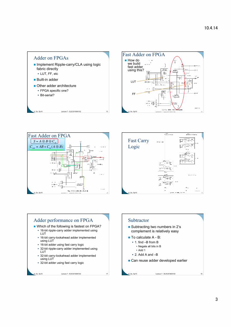
Adder on FPGAs   Implement Ripple-carry/CLA using logic

fabric directly •  LUT, FF, etc

 Built-in adder

 Other adder architecture •  FPGA specific one? •  Bit-serial?


Fast Adder on FPGA


 How do we build fast adder using this?

LUT

FF

Fast Adder on FPGA


€

S = A⊕ B⊕Cin

Cout = AB + Cin (A⊕ B)Fast Carry Logic


Adder performance on FPGA  Which of the following is fastest on FPGA? •  16-bit ripple-carry adder implemented using

LUT •  16-bit carry-lookahead adder implemented

using LUT •  16-bit adder using fast carry logic •  32-bit ripple-carry adder implemented using

LUT •  32-bit carry-lookahead adder implemented

using LUT •  32-bit adder using fast carry logic


Subtractor  Subtracting two numbers in 2’s

complement is relatively easy

 To calculate A - B: •  1. find –B from B

•  Negate all bits in B •  Add 1

•  2. Add A and –B

 Can reuse adder developed earlier


10.4.14

4

Subtractor


FA FA FA FA

A0 A1 A2 A3

S0 S1 S2 S3

Cout Subtract

B0 B1 B2 B3

Multiplication


× 1 1 1 0 1 1 1 0 0 1 1 1 1 0 1

1 1 1 0 1 0 0 0 0 0

0 0 0 0 0 1 1 1 0 1

0 1 1 0 1 1 0 1 1

Multiplication  Multiplication is a form of repeated

addition

 Multiplying two n-bit numbers can be achieved by adding n partial results

 Produce a result of 2n bits


Multiplier - Iterative   Start from basic definition of multiplication, do

“shift and conditional add”   Requires n cycles


1

+

A

CLK

>>

0

>> 0

S

B

Multiplier - Parallel   Use n adders to perform all partial sum addition in

parallel   Requires 1 cycle – but long cycle…


+

+

+

+

Simple Parallel Multiplier  Critical path

scales with 2n


FA FA FA FA

FA FA FA FA

FA FA FA FA

FA FA FA FA

10.4.14

5

Multiplier - Carry Save Adders   Carry save adder tree   Critical path scales

with 2n   Fast adder at the end


FA FA FA FA

FA FA FA FA

FA FA FA FA

FA FA FA FA

+

Fast Multiplier on FPGA  Reuse carry logic for adders for partial

result calculation


Source: xapp215

Dedicated DSP Block in V6


Constant Multiplication   If one of the input to a multiplier is

constant, circuit can be simplified

  IF one of the input is a power of 2, then multiplication becomes shift •  A * 2n is equivalent to A << n

 What if the constant is not power of 2? •  Number decomposition


Constant Multiplier – Decomposition  When multiplying a constant in fixed point,

recall that the value represented by the bit string is:

  Therefore, ALL representable fixed point numbers can be represented as a sum of power of 2

 Can decompose the constant multiplier into multiple shifts


€

−2n−k bn−1 + 2i−k bii= 0

n−1

∑

Decomposition

  Compared to standard multiplier, all 0 terms are eliminated

  Can we do better?


€

B = kA A B k

A B

2n-2

21

2n-1

20

+ A B +

<< n-1

<< n-2

<< 1

<< 0

10.4.14

6

Canonic Signed Digit  Signed digit (SD) representation: •  Similar to binary representation except the

set {-1, 0, 1} is used for the digits

 Representation is not unique

 E.g. In 4-bit SD number rep: 3 = 0011 = 0101 = 0111 = 1101 = 1111

 Canonic representation has minimum number of nonzero digits •  Not unique


Canonic Signed Digit  Use CSD to minimize number of

nonzero

 E.g. 125 = 01111101 = 10000011


A B

25

22

26

20

+ A B

21

27

20 +

-

Division  Division is substantially more

complicated than multiplication

 2 main methods: •  Bit-by-bit calculation

•  Calculate each bit similar to manual division •  Mathematical approximation

•  Start with an approximation and iteratively refine the solution until desired precision is reached

 Use as few as possible!


Signal Flow Graph Manipulations


FIR as an Example


z-1

×

+

z-1

+

× ×

x[n]

y[n]

z-1 FF = Delay for 1 sample (clock cycle) =

h0 h1 h2

Signal Flow Graph  Simplify the block diagram with more

efficient notation:


k

z-1 z-1

×

k

+

z-1 z-1

h0 h1 h2

x[n]

y[n]

FIR filter

10.4.14

7

Dataflow system Remember:   In most digital signal processing system with a

continuous stream of data input, the overall latency “usually” doesn’t matter.

  Therefore, it is ok to put extra delay at I/O without changing the function of the design


z-1 z-1

h0 h1 h2

x[n]

y[n] z-20

z-5

But why?

Nodal Delay Transfer


k0 z-2

k1

k0 z-1

k1

z-1

z-1

k z-1 k z-1

z-1

z-1 z-1

(a)

(b)

(c)

z-1 (e)

z-1

z-1 (d) k0

k1

k0

k1 z+1

z+1

Nodal Delay Transfer  Remember, z+1 is non-causal •  Not implementable on hardware

 Must eliminate any z+1 in the final graph before going to hardware implementation •  Pushing delay within the graph •  Inserting delay at I/O •  Reorganizing the graph


Cutset  Separate the

SFG into two disjoint graphs

 Example:


z-1 z-1

h0 h1 h2

x[n]

y[n]

z-1

h2

y[n]

z-1

h0 h1

x[n]

Cutset Retiming  Generalization of the nodal delay

transfer primitives


Delay can be added to all incoming edges to a cutset if advances are added to all outgoing edges, and vice-versa

Cutset Retiming


z-1

h2

y[n]

z-1

h0 h1

x[n] z-1

z-1

z+1

z-1 z-1

h0 h1 h2

x[n]

y[n] z-1

z-1

z+1

10.4.14

8

Use of retiming  Reduce critical path •  Pipelining

 Decrease number of registers  Reduce Power

 Reduce clock rate

 …


In Summary…   Review basic computer arithmetic

•  + － × ÷   Add/sub easiest to implement

•  Highly optimized in FPGAs   Multiplier more complex

•  VLSI has many optimized multipliers •  FPGAs design may use the fast carry logic •  Dedicated multiplier / DSP blocks

  Divisor very complex •  Use IP cores

  Signal flow graph and retiming helps to lay out signal processing systems


Addition Ripple Carry Adder - University of Hong...

Documents

Transcript of Addition Ripple Carry Adder - University of Hong...