Adaptively Sampled Distance Fields: A General Representation of Shape for Computer Graphics

Sarah F. Frisken, Ronald N. Perry, Alyn P. Rockwood, and Thouis R. Jones MERL – Mitsubishi Electric Research Laboratory

Figure 1. An ADF showing fine detail carved on a rectangular slab with a flat-edged chisel.

Figure 2. Artistic carving of a high order surface with a rounded chisel.

Figure 3. A semi-transparent electron probability distribution of a cyclohexane molecule.

ABSTRACT Adaptively Sampled Distance Fields (ADFs) are a unifyingrepresentation of shape that integrate numerous concepts incomputer graphics including the representation of geometry andvolume data and a broad range of processing operations such asrendering, sculpting, level-of-detail management, surfaceoffsetting, collision detection, and color gamut correction. Itsstructure is uncomplicated and direct, but is especially effectivefor quality reconstruction of complex shapes, e.g., artistic andorganic forms, precision parts, volumes, high order functions, andfractals. We characterize one implementation of ADFs,illustrating its utility on two diverse applications: 1) artisticcarving of fine detail, and 2) representing and rendering volumedata and volumetric effects. Other applications are brieflypresented. CR Categories: I.3.6 [Computer Graphics]: Methodology andtechniques – Graphics data structures; I.3.5 ComputationalGeometry and Object Modeling – Object modeling Keywords: distance fields, carving, implicit surfaces, rendering, volume rendering, volume modeling, level of detail, graphics. {frisken,perry,rockwood,jones}@merl.com

1. INTRODUCTION In this paper we propose adaptively sampled distance fields(ADFs) as a fundamental graphical data structure. A distance fieldis a scalar field that specifies the minimum distance to a shape,where the distance may be signed to distinguish between theinside and outside of the shape. In ADFs, distance fields areadaptively sampled according to local detail and stored in a spatialhierarchy for efficient processing. We recommend ADFs as asimple, yet consolidating form that supports an extensive varietyof graphical shapes and a diverse set of processing operations.Figures 1, 2, and 3 illustrate the quality of object representationand rendering that can be achieved with ADFs as well as thediversity of processing they permit. Figures 1 and 2 show finedetail carved on a slab and an artistic carving on a high ordercurved surface. Figure 3 depicts an electron probabilitydistribution of a molecule that has been volume rendered with aglowing aura that was computed using a 3D noise function.

ADFs have advantages over several standard shaperepresentations because as well as representing a broad class offorms, they can also be used for a number of important operationssuch as locating surface points, performing inside/outside andproximity tests, Boolean operations, blending and filleting,determining the closest points on a surface, creating offsetsurfaces, and morphing between shapes.

It is important to note that by shape we mean more than justthe 3D geometry of physical objects. We use it in a broad contextfor any locus defined in a metric space. Shape can have arbitrarydimension and can be derived from measured scientific data,computer simulation, or object trajectories through time andspace. It may even be non-Euclidean. 2. BACKGROUND Commonly used shape representations for geometric designinclude parametric surfaces, subdivision surfaces, and implicitsurfaces. Parametric representations include polygons, splinepatches, and trimmed NURBs. Localizing (or generating) surfacepoints on parametric surfaces is generally simpler than with other

Permission to make digital or hard copies of part or all of thiswork or personal or classroom use is granted without feeprovided that copies are not made or distributed for profit orcommercial advantage and that copies bear this notice and thefull citation on the first page. To copy otherwise, to republish, topost on servers, or to redistribute to lists, requires prior specificpermission and/or a fee. SIGGRAPH 2000, New Orleans, LA USA © ACM 2000 1-58113-208-5/00/07 ...$5.00

representations and hence they are easier to draw, tessellate,subdivide, and bound [3]. Parametric surfaces typically needassociated data structures such as B-reps or space partitioningstructures for representing connectivity and for more efficientlocalization of primitives in rendering, collision detection, andother processing. Creating and maintaining such structures adds tothe computational and memory requirements of therepresentation. Parametric surfaces also do not directly representobject interiors or exteriors and are subsequently more difficult toblend and use in Boolean operations. While subdivision surfacesprovide an enhanced design interface, e.g., shapes aretopologically unrestricted, they still suffer from many of the samelimitations as parametric representations, e.g., the need forauxiliary data structures [8], the need to handle extraordinarypoints, and the difficulty in controlling fine edits.

Implicit surfaces are defined by an implicit function f(x∈Rn)= c, where c is the constant value of the iso-surface. Implicitfunctions naturally distinguish between interior and exterior andcan be used to blend objects together and to morph betweenobjects. Boolean operations defined for implicit functions providea natural sculpting interface for implicit surfaces [3, 18]; however,when many operations are combined to generate a shape thecomputational requirements for interactive rendering or otherprocessing become prohibitive. Furthermore, it is difficult todefine an implicit function for an arbitrary object, or to chartpoints on its surface for rendering and other processing.

Volumetric data consists of a regular or irregular grid ofsampled data, frequently generated from 3D image data ornumerical simulation. Object surfaces can be represented as iso-surfaces of the sampled values and data between sample pointscan be reconstructed from local values for rendering or otherprocessing. Several systems have been developed for sculptingvolumetric data using Boolean operations on sample densityvalues [1, 2]. However, in these systems, iso-surfaces lack sharpcorners and edges because the density values are low-pass filterednear object surfaces to avoid aliasing artifacts in rendering. Inaddition, the need to pre-select volume size and the use of regularsampling force these systems to limit the amount of detailachievable. Sensable DevicesTM has recently introduced acommercial volume sculpting system [21]. To create detailedmodels, very large volumes are required (a minimum of 512Mbytes of RAM) and the system is advertised for modeling only“organic” forms, i.e. shapes with rounded edges and corners.

Additional representations of shape for computer graphicsinclude look-up tables, Fourier expansions, particle systems,grammar-based models, and fractals (iterated function systems),all of which tend to have focused applications [10].

The ADF representation, its applications, and theimplementation details presented in this paper are new. Sampleddistance fields have, however, been used previously in a numberof specific applications. They have been used in robotics for pathplanning [12, 13] and to generate swept volumes [20]. Incomputer graphics, sampled distance fields were proposed forvolume rendering [11], to generate offset surfaces [4, 17], and tomorph between surface models [7, 17]. Level sets can either begenerated from distance fields or they can be used to generatesampled distance fields [15, 22]. As with regularly sampledvolumes, regularly sampled distance fields suffer from largevolume sizes and a resolution limited by the sampling rate. Theselimitations are addressed by ADFs. 3. ADAPTIVE DISTANCE FIELDS A distance field is a scalar field that specifies the minimum

distance to a shape, where the distance may be signed todistinguish between the inside and outside of the shape. As simpleexamples, consider the distance field of the unit sphere S in R3

given by h(x) = 1 – (x2 + y2 + z2) ½, in which h is the Euclideansigned distance from S, or h(x) = 1 – (x2 + y2 + z2), in which h isthe algebraic signed distance from S, or h(x) = (1 – (x2 + y2 + z2))2,in which h is an unsigned distance from S.

The distance field is an effective representation of shape.However, regularly sampled distance fields have drawbacksbecause of their size and limited resolution. Because fine detailrequires dense sampling, immense volumes are needed toaccurately represent classical distance fields with regularsampling when any fine detail is present, even when the finedetail occupies only a small fraction of the volume. To overcomethis limitation, ADFs use adaptive, detail-directed sampling, withhigh sampling rates in regions where the distance field containsfine detail and low sampling rates where the field varies smoothly.Adaptive sampling permits arbitrary accuracy in the reconstructedfield together with efficient memory usage. In order to process theadaptively sampled data more efficiently, ADFs store the sampleddata in a hierarchy for fast localization. The combination of detail-directed sampling and the use of a spatial hierarchy for datastorage allows ADFs to represent complex shapes to arbitraryprecision while permitting efficient processing.

In summary, ADFs consist of adaptively sampled distancevalues organized in a spatial data structure together with a methodfor reconstructing the underlying distance field from the sampledvalues. One can imagine a number of different instantiations ofADFs using a variety of distance functions, reconstructionmethods, and spatial data structures. To provide a clearelucidation of ADFs, we focus on one specific instance for theremainder of this paper. This instance is simple, but results inefficient rendering, editing, and other processing used byapplications developed in this paper. Specifically, we demonstratean ADF which stores distance values at cell vertices of an octreedata structure and uses trilinear interpolation for reconstructionand gradient estimation. The wide range of research in adaptiverepresentations suggest several other ADF instantiations based on,for example, wavelets [5] or multi-resolution Delaunaytetrahedralizations [6]. 3.1 Octree-based ADFs Octree data structures are well known and we assume familiarity(see [19]). For purposes of instruction, we demonstrate theconcepts in 2D (with quadtrees), which are easily generalized tohigher dimensions. In a quadtree-based ADF, each quadtree cellcontains the sampled distance values of the cell’s 4 corners andpointers to parent and child cells.

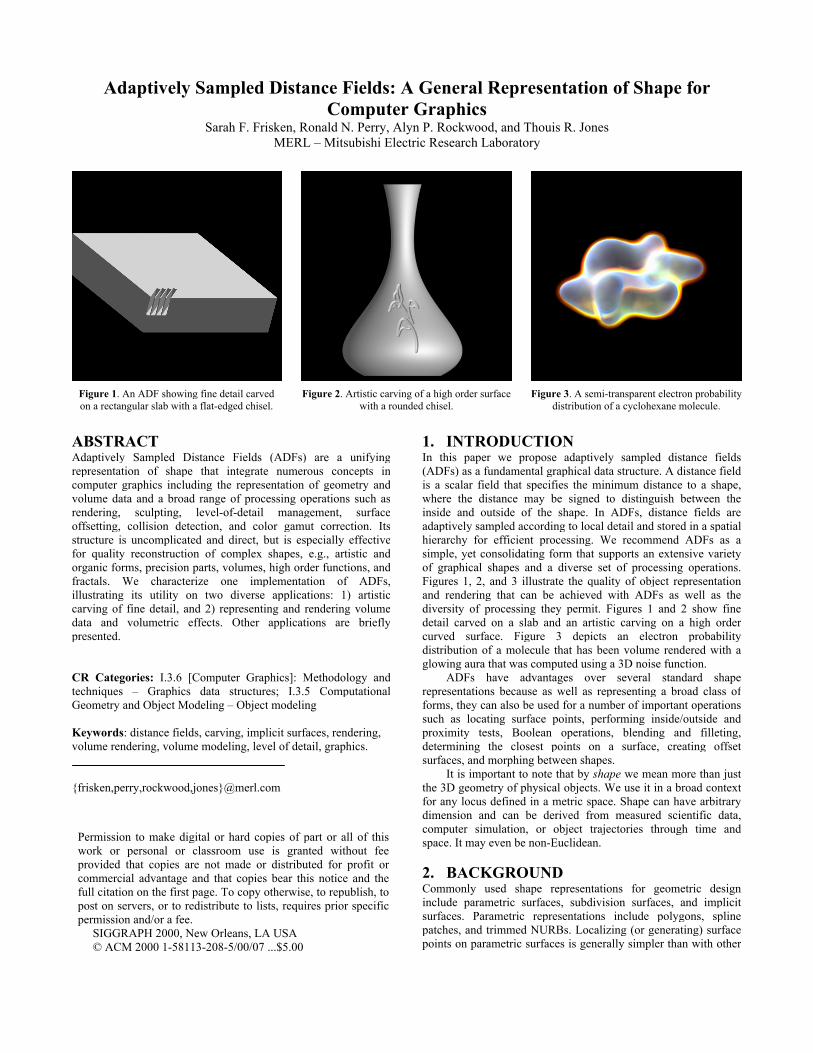
Given a shape as in Figure 4a, subdivision of a cell in thequadtree depends on the variation of the distance field (shown inFigure 4c) over the parent cell. This differs from 3-color quadtrees[19] which represent object boundaries by assigning one of threetypes to each cell in the quadtree: interior, exterior, and boundary.In 3-color quadtrees, all boundary cells are subdivided to apredetermined highest resolution level. In contrast, boundary cellsof ADFs are only subdivided when the distance field within a cellis not well approximated by bilinear interpolation of its cornervalues. Hence, large cells can be used to represent edges inregions where the shape is relatively smooth, resulting insignificantly more compression than 3-color quadtrees. This isillustrated in Figures 4b and 4d where the ADF of 4d requiresonly 1713 cells while the 3-color quadtree of 4b requires 23,573cells. In the ADF quadtree, straight edges of the “R” arerepresented by large cells; only corners provoke repeated

subdivision. Figure 4d also shows that even highly curved edges can be

efficiently represented by ADFs. Because bilinear interpolationrepresents curvature reasonably well, cells with smoothly curvededges do not require many levels in the ADF hierarchy. Cells thatdo require many levels in the hierarchy are concentrated atcorners and cusps.

These are typical statistics for 2D objects. As anotherindication of ADF size, Table 1 compares the number of trianglesrequired to represent a sphere of radius 0.4 to the number of cellsand distance (sample) values of the corresponding ADF whenboth the triangles and the interpolated distance values are within agiven error tolerance from the true sphere.

Higher order reconstruction methods and better predicatesfor subdivision might be employed to further increasecompression, but the numbers already suggest a point ofdiminishing returns for the extra effort. 3.2 Generating ADFs The generation of an ADF requires a procedure or function toproduce the distance function, h(x) at x ∈ Rn, where distance isinterpreted very broadly as in Section 3. Continuity,differentiability, and bounded growth of the distance function canbe used to advantage in rendering or other processing, but are notrequired. Some of the images in this paper utilize distancefunctions that are non-differentiable (Figure 8) and highly non-Euclidean with rapid polynomial growth (Figures 2 and 3).

One example of a distance function is the implicit form of anobject, for which the distance function can correspond directly tothe implicit function. A second example includes procedures thatdetermine the Euclidean distance to a parametric surface. For

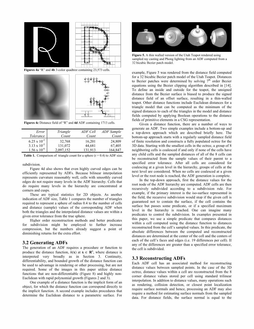
example, Figure 5 was rendered from the distance field computedfor a 32 bicubic Bezier patch model of the Utah Teapot. Distancesto Bezier patches were determined by solving 7th order Bezierequations using the Bezier clipping algorithm described in [14].To define an inside and outside for the teapot, the unsigneddistance from the Bezier surface is biased to produce the signeddistance field of an offset surface, resulting in a thin-walledteapot. Other distance functions include Euclidean distances for atriangle model that can be computed as the minimum of thesigned distances to each of the triangles in the model and distancefields computed by applying Boolean operations to the distancefields of primitive elements in a CSG representation.

Given a distance function, there are a number of ways togenerate an ADF. Two simple examples include a bottom-up anda top-down approach which are described briefly here. Thebottom-up approach starts with a regularly sampled distance fieldof finite resolution and constructs a fully populated octree for the3D data. Starting with the smallest cells in the octree, a group of 8neighboring cells is coalesced if and only if none of the cells haveany child cells and the sampled distances of all of the 8 cells canbe reconstructed from the sample values of their parent to aspecified error tolerance. After all cells are considered forcoalescing at a given level in the hierarchy, groups of cells at thenext level are considered. When no cells are coalesced at a givenlevel or the root node is reached, the ADF generation is complete.

In the top-down approach, first the distance values for theroot node of the ADF hierarchy are computed. ADF cells are thenrecursively subdivided according to a subdivision rule. Forexample, if the primary interest is the iso-surface represented inthe field, the recursive subdivision would stop if the given cell isguaranteed not to contain the surface, if the cell contains thesurface but passes some predicate, or if a specified maximumlevel in the hierarchy is reached. One can imagine manypredicates to control the subdivision. In examples presented inthis paper, we use a simple predicate that compares distanceswithin a cell computed using the distance function to distancesreconstructed from the cell’s sampled values. In this predicate, theabsolute differences between the computed and reconstructeddistances are determined at the center of the cell and the centers ofeach of the cell’s faces and edges (i.e. 19 differences per cell). Ifany of the differences are greater than a specified error tolerance,the cell is subdivided. 3.3 Reconstructing ADFs Each ADF cell has an associated method for reconstructingdistance values between sampled points. In the case of the 3Doctree, distance values within a cell are reconstructed from the 8corner distance values stored per cell using standard trilinearinterpolation. In addition to distance values, many operations suchas rendering, collision detection, or closest point localizationrequire surface normals and hence, processing an ADF may alsorequire a method for estimating surface normals from the sampleddata. For distance fields, the surface normal is equal to the

Figures 4a “R” and 4b 3-color quadtree containing 23,573 cells.

Figures 4c Distance field of “R” and 4d ADF containing 1713 cells.

Figure 5. A thin walled version of the Utah Teapot rendered using sampled ray casting and Phong lighting from an ADF computed from a 32 bicubic Bezier patch model.

Error Tolerance

Triangle Count

ADF Cell Count

ADF Sample Count

6.25 x 10-5 32,768 16,201 24,809 3.13 x 10-5 131,072 44,681 67,405 1.56 x 10-6 2,097,152 131,913 164,847

Table 1. Comparison of triangle count for a sphere (r = 0.4) to ADF size.

normalized gradient of the distance field at the surface. There areseveral methods for estimating the gradient of sampled data. Weuse the analytic gradient of the trilinear reconstruction within eachcell: grad(x,y,z) = (h(xr,y,z) - h (xl,y,z), h(x,yu,z) - h(x,yd,z), h(x,y,zf)- h(x,y,zb)), where (xr,y,z), (xl,y,z), (x,yu,z), etc. are projections of(x,y,z) onto the right, left, up, down, front, and back faces of thecell, respectively. In theory, this cell-localized gradient estimationcan result in C1 discontinuities at cell boundaries but as can beseen from the figures, these artifacts are not noticeable withsufficient subdivision. 4. APPLICATIONS AND

IMPLEMENTATION DETAILS ADFs have application in a broad range of computer graphicsproblems. We present two examples below to illustrate the utilityof ADFs and to provide some useful implementation details onprocessing methods such as rendering and sculpting ADF models.This section ends with short descriptions of several otherapplications to give the reader an idea of the diverse utility ofADFs. 4.1 Precise carving Figures 1, 2, and 6 show examples of objects represented andcarved as ADFs. Because objects are represented as distancefields, the ADF can represent and reconstruct smooth surfacesfrom sampled data. Because the ADF efficiently samples distancefields with high local curvature, it can represent sharp surfacecorners without requiring excessive memory. Carving is intuitive;the object is edited simply by moving a tool across the surface. Itdoes not require control point manipulation, remeshing thesurface, or trimming. By storing sample points in an octree, bothlocalizing the surface for editing and determining ray-surfaceintersections for rendering are efficient.

Like implicit surfaces, ADFs can be sculpted using simpleBoolean operations applied to the object and tool distance fields.Figures 1, 2, and 6 show carving using the difference operator,hcarved(x) = min(hobject(x), -htool(x)). Other operators includeaddition, hcarved(x) = max(hobject(x), htool(x)), and intersection,hcarved(x) = min(hobject(x), htool(x)). Blending or filleting can alsobe defined for shaping or combining objects (as was done for themolecules of Figures 3 and 7). While these Boolean operationsapply to the entire distance field, for systems where only surfacesare important, application of the operations can be limited inpractice to a region within a slightly extended bounding box of thetool.

The basic edit operation is much like a localized ADFgeneration. The first step in the editing process is to determine thesmallest ADF cell, or set of cells, entirely containing the tool’sextended bounding box (obvious consideration of the ADFboundaries apply). The containing cell is then recursivelysubdivided, applying the difference operator to the object and toolvalues to obtain new values for the carved ADF. During therecursive subdivision, cell values from the object are obtainedeither from existing sampled values or by reconstruction if anedited cell is subdivided beyond its original level. Subdivisionrules similar to those of top-down generation are applied, with theexception that the containing cell must be subdivided to someminimum level related to the tool size.

The carving examples were rendered using ray casting withanalytic surface intersection. In this method, a surface point isdetermined by finding the intersection between a ray cast into theADF octree from the eye and the zero-value iso-surface of theADF. Local gradients are computed at surface points using the

gradient estimation described above (the figures were renderedwith simple Phong lighting). When the traversing ray passesthrough a leaf node of the octree, intersection between the ray andthe surface reconstructed from the 8 cell sample values is tested.We have used two different methods to find the ray-surfaceintersection; a cubic root solver that finds the exact intersection ofthe ray with the trilinear surface defined by the distance values atthe cell corners (as in [16]), and a linear approximation whichdetermines the distance values where the ray enters and exits thecell and computes the linear zero-crossing if the two values have adifferent sign. Both methods work well but the linearapproximation has proven to be faster and its rendered images arenot visibly different from those rendered with the cubic solver.When solving for intersections, we set the distance at the entrypoint of a cell to be equal to the distance at the exit from theprevious cell. This avoids the crack problem discussed in [24] forrendering hierarchical volume data, preventing C0 discontinuitiesin the surface where ADF cells of different size abut. Most of theimages shown in this paper were rendered using a supersamplingof 16 rays per pixel followed by the application of a Mitchell filterof radius 2.0.

The octree promotes efficient ray traversal even for verycomplicated scenes. Rendering the Menger Sponge (Figure 8)takes approximately the same amount of time as rendering lesscomplex ADF models. As in most rendering methods based onspatial decomposition, rendering time is determined more byscreen coverage than by model complexity. Current renderingrates are fast enough for interactive updating of the carving regionduring editing. Preliminary tests indicate that an order ofmagnitude improvement in the rendering speed of the entireimage can be achieved by adaptive supersampling. 4.2 Volume data ADFs are also amenable to volume rendering and can be used toproduce interesting effects. For example, offset surfaces can beused to render thick, translucent surfaces. Adding volume texturewithin the thick surface in the form of variations in color ortransparency is relatively easy. In addition, distance values fartheraway from the zero-valued iso-surface can be used for specialeffects. Figure 7 shows a cocaine molecule volume rendered in ahaze of turbulent mist. The mist was generated using a colorfunction based on distance from the molecule surface. To achievethe turbulence the distance value input to the color function ismodulated by a noise function based on position [9].

We use a ray casting volume renderer to demonstrate someof these effects. Colors and opacities are accumulated at equallyspaced samples along each ray using a back-to-front renderingalgorithm. Sample points that lie near the zero-value iso-surfaceare shaded with Phong lighting.

Our sampled ray caster is not optimized for speed. However,properties of the ADF data structure can be used to greatlyincrease the rendering rate. For example, the octree allows us toquickly skip regions of the volume that are far from the surface. In

Figure 6. A close up of the carved slab in Figure 1.

addition, because distances to the closest surface are available ateach sample point, space-leaping methods can be used to speed uprendering [26].

4.3 Other application areas 4.3.1 Representing complexity Complexity may be considered from several viewpoints. Firstly,the visual complexity of an object might include factors such assurface variation and topology. Secondly, the representationcomplexity is determined by the size and intricacy of the datastructure needed to represent the object. The third measure ofcomplexity considers the algebraic complexity of the object,which includes such factors as polynomial degree, transcendentalfunctions, and numerical routines required to define the object’sshape. Such routines are pertinent especially when algebraicdistance is employed for the distance field.

Figure 8 shows a good example of the first two types ofcomplexity, the Menger Sponge, which is a fractal createdrecursively by subtracting smaller and smaller crossing cuboidsfrom an initial cube. In the limit there is no neighborhood of thesurface that is not punctured regardless of how small theneighborhood is chosen. It is an infinite perforation, a 3D versionof the famous Cantor set.

After each level of subtraction there are 20 self-similarsubcuboids generated. An artless approach to maintaining the datastructure would generate order O (20n) faces for n iterations. Evenif shared faces were combined and interior faces culled, anapproach that keeps a boundary representation (B-rep) withouttroublesome T-junctions would have O (12n) faces. To be moreexact, after seven iterations there would be 26 million+ faces in aB-rep data structure. Consider the difficulty of performingproximity tests, collision detection, or inside/outside tests withsuch a representation. In contrast, these tests are much simplerusing ADFs. Far from being a contrived case, the complexity ofthe distance field of the Menger Sponge is representative of thedistance fields of many naturally occurring shapes which wouldpresent similar problems for traditional methods.

Figures 2 and 7 both demonstrate ADFs’ ability to handlealgebraic complexity. While Figure 7 reconstructs an approximateprobability density field for a molecule of 43 atoms (C17H21NO4),the vase in Figure 2 is defined first as a rotation of a quinticBezier curve. Mathematically, it is posed as a rational implicitfunction with a square root of a (total) degree 16 over 2. CubicBezier curves are then mapped onto the surface as paths for thecarving tool. In this case, the carver is a curved chisel, resulting ina very high degree tubular surface on the vase. This carving pathand vase create an algebraically very complex distance field,which is nevertheless cleanly reconstructed and rendered.

4.3.2 Level-of-detail models There are at least two approaches for representing ADF models atdifferent levels of detail for rendering and progressivetransmission of models. The simplest approach is to truncate theADF at fixed levels in the octree. The truncation can either bedone during rendering or transmission, during generation, or to anexisting high resolution ADF. A second method uses the errorgenerated in the test for cell subdivision during top-downgeneration of the ADF. By storing this error within the cell, anLOD model can be generated by truncating ADF cells with errorsless than that specified for the given LOD. This provides a morecontinuously varying parameter for selecting the LOD andprovides degradation of the object shape that is consistent for bothsmooth and highly curved portions of the surface as the level ofthe LOD model decreases. This second method is illustrated inFigure 9 where four LOD models with varying amounts of errorare rendered from an ADF octree. 4.3.3 Collision detection Distance fields have been used for collision avoidance in roboticsand for detecting collisions and computing penetration forces inhaptics [12, 13]. Octrees or other hierarchies of bounding boxeshave also been used successfully to accelerate collision detectionalgorithms. The combination of these two representations in theADF as well as the ability to represent offset surfaces and surfacesat different levels of detail suggest that ADFs have significantpotential for applications that require collision detection. 4.3.4 Color gamut representation Devices such as color printers and monitors have unique colorcharacteristics. Each can represent colors within their ownparticular color gamut, which is restricted, for example, by thetypes of dyes used by the printer. When an image is acquired ordesigned on one system and then displayed or printed on another,it is often important to match colors as closely as possible. This

Figure 7. An ADF cocaine molecule volume rendered in a haze of turbulent mist. The mist was generated using a color function dependent on distance from the molecule surface.

Figure 8. An ADF of the Menger Sponge, a fractal created recursively by subtracting smaller and smaller crossing cuboids from an initial cube. Four levels of recursion are shown.

Figure 9. Four LOD models with varying amounts of error rendered from an ADF octree.

involves correcting colors that fall outside of the device’s gamutand sometimes requires a complicated mapping to warp the gamutof one system onto that of another [23].

Most color devices represent their color gamuts in largelook-up-tables (LUTs). Usually, a binary table is used to testcolors against the device’s gamut to see if they fall in or out ofgamut. If a color falls out of gamut, a set of model coefficientsand look-up tables are used to map the color onto the ‘closest’device color. Using ADFs to represent a device’s gamut hasseveral advantages over the LUT approach. First, out-of-gamuttests are easily performed with ADFs and edge-sampling errorsthat occur with the use of binary tables are avoided. Second, anADF out-of-gamut test provides more information than isavailable with binary tables; the distance indicates how far out ofgamut a color lies and the gradient indicates the direction to thenearest in-gamut color. Third, since ADFs use adaptive sampling,they should provide significant compression over LUTrepresentations. Finally, since distance fields can be used to warpbetween shapes, ADFs may prove to be a useful representation formapping between device gamuts. 4.3.5 Machining ADFs provide powerful tools for computer aided machining. Theuse of a distance function for representing surfaces allows therepresentation of the surface, the interior of the object, and thematerial that must be removed. Knowledge of the object interiorcan be used for part testing (e.g., part thickness tests [25]). Arepresentation of the volume outside of the surface as well asdistances to the closest surface can be used for planning tool pathsand tool sizes for the machining process. Offset surfaces can beused to plan rough cutting for coarse-to-fine machining or fordesigning part molds for casting. The size of cells at the surfaceand the object normal near the surface can be used to select toolsize and orientation. Finally, as illustrated in Figure 6, ADFs canrepresent fine surfaces and sharp corners efficiently, making itpossible to represent machining precision in the ADF model. 5. CONCLUSIONS Although distance fields have been used in certain specificapplications as mentioned above, the breadth and flexibility oftheir application to problems in computer graphics has not beenappreciated, in part due to their large memory requirements.ADFs address this issue by adaptively sampling the distance fieldand storing sampled values in a spatial hierarchy. For 2D shapes,we typically achieve better than 20:1 reductions overstraightforward boundary (3-color) quadtrees. Nevertheless, ADFsmaintain the reconstruction quality of the original distance field asseen in the examples presented; shapes, even those with highfrequency components such as edges or corners, are reconstructedaccurately.

Distance fields can embody considerable information about ashape, not just the critical zero-valued iso-surface, but alsoinformation about the volume in which it sits, an indication ofinside vs. outside, and gradient and proximity information.

Operations on a shape can often be achieved by operationson its distance field. For example, Boolean set operations becomesimple max/min operations on the field; edges and corners can berounded by low-pass filtering; and so forth.

ADFs tend to separate generation of shapes into a preprocessstep that may require complex and time-consuming methods, anda process for graphical operations that is fast and tolerant ofvarious types of complexity. Indeed, fractals and mathematicallysophisticated or carved shapes can be processed as quickly as

much simpler shapes. The wide diversity of such manipulationsinclude, for example, proximity testing (for collision detection,haptics, color gamut correction, milling), efficient ray-surfaceintersection for rendering, localized reconstruction, surface andvolume texturing, blending, filleting, offset surfaces, and shapewarping. 6. FUTURE WORK The introduction of ADFs opens up a wide range of futuredirections. Considerable research is left to investigate the possibletransformations between shape and its distance field. Differenthierarchical structures and reconstruction methods await testingand experience. For example, wavelets show particular promise[5], and Delaunay tetrahedralizations have been successfully usedfor multiresolution representation of volume data [6]. The relativecompactness for very complex shapes has implications for level ofdetail management and progressive transmission. Efficientconversion between ADFs and standard (e.g. triangle and NURB)models is a valuable undertaking. Finally, we look forward tocombining ADFs with more powerful rendering methods; forexample, we envision hierarchical radiosity using form factorsbased on the ADF cells. 7. ACKNOWLEDGEMENTS We gratefully acknowledge the help of Mars Brimhall, John Ford,and Stephan Roth in generating some of the images in this paper. 8. REFERENCES [1] R. Avila and L. Sobierajski, “A haptic interaction method for volume visualization”, Proc.

IEEE Visualization’96, pp. 197-204, 1996. [2] J. Baerentzen, “Octree-based volume sculpting”, Proc. Late Breaking Hot Topics, IEEE

Visualization’98, pp. 9-12, 1998. [3] J. Bloomenthal, Introduction to Implicit Surfaces, Morgan Kaufman Publishers, 1997. [4] D. Breen, S. Mauch and R. Whitaker, “3D scan conversion of CSG models into distance

volumes”, Proc. 1998 IEEE Symposium on Volume Visualization, pp. 7-14, 1998. [5] M. Chow and M. Teichmann, “A Wavelet-Based Multiresolution Polyhedral Object

Representation”, Visual Proc. SIGGRAPH ’97, p. 175, 1997. [6] P. Cignoni, L. De Floriani, C. Montani, E. Puppo, R. Scopigno, “Multiresolution Modeling

and Rendering of Volume Data based on Simplicial Complexes”, 1994 ACM Volume Visualization Conference Proceedings, 1994, pp.19-26.

[7] D. Cohen-Or, D. Levin, and A. Solomovici, “Three-dimensional distance field metamorphosis”, ACM Transactions on Graphics, 1997.

[8] T. DeRose, M. Kass, T. Truong, “Subdivision surfaces in character animation”, Proc. SIGGRAPH ’98, pp. 85-94, 1998.

[9] D. Ebert, F.K. Musgrave, D. Peachy, K. Perlin, S. Worley, Texturing and Modeling a Procedural Approach, Academic Press, 1998.

[10] J. Foley, A. van Dam, S. Feiner, and J. Hughes, Computer Graphics: Principles and Practice, Addison-Wesley, 1992.

[11] S. Gibson, “Using DistanceMaps for smooth surface representation in sampled volumes”, Proc. 1998 IEEE Volume Visualization Symposium, pp. 23-30, 1998.

[12] R. Kimmel, N. Kiryati and A. Bruckstein, “Multi-valued distance maps for motion planning on surfaces with moving obstacles”, IEEE Trans. on Robotics & Automation, 14, pp. 427-436, 1998.

[13] J. Lengyel, M. Reichert, B. Donald and D. Greenberg, “Real-time robot motion planning using rasterizing computer graphics hardware”, Proc. SIGGRAPH ’90, pp. 327-335, 1990.

[14] T. Nishita, T.W. Sederberg and M. Kakimoto, “Ray tracing trimmed rational surface patches”, Proc. SIGGRAPH ’90, pp. 337-345, 1990.

[15] S. Osher and J. Sethian, “Fronts propagating with curvature-dependent speed: algorithms based on Hamilton-Jacobi formulation”, J. Computational Physics, 79, pp. 12-49, 1988.

[16] S. Parker, M. Parker, Y. Livnat, P. Sloan, C. Hansen, and P. Shirley, “Interactive ray tracing for volume visualization” IEEE Transactions On Visualization and Computer Graphics, Vol. 5 (3), pp. 238-250, 1999.

[17] B. Payne and A. Toga, “Distance field manipulation of surface models”, IEEE Computer Graphics and Applications, pp. 65-71, 1992.

[18] A. Ricci, “A constructive geometry for computer graphics”, Computer Journal, Vol. 16, No. 2, pp. 157-160, 1973.

[19] H. Samet, The Design and Analysis of Spatial Data Structures, Addison-Wesley, 1989. [20] W. Schroeder, W. Lorensen, and S. Linthicum, "Implicit modeling of swept surfaces and

volumes," Proc. Visualization '94, pp. 40-45, 1994. [21] Sensable Devices’ FreeForm modeling software. http://www.sensable.com/freeform. [22] J. Sethian, Level Set Methods: Evolving Interfaces in Geometry, Fluid Mechanics,

Computer Vision, and Material Science, Cambridge University Press, 1996. [23] M. Stone, W. Cowan, J. Beatty, “Color gamut mappings and the printing of digital color

images”, ACM Transaction on Graphics, Vol. 7, pp. 249-292, 1988. [24] R. Westermann, O. Sommer, T. Ertl, “Decoupling polygon rendering from geometry using

rasterization hardware”, in Proc. Eurographics Rendering Workshop '99, pp. 45-56, 1999. [25] R. Yagel, S. Lu, A. Rubello, R. Miller, “Volume-based reasoning and visualization of

dicastability” In Proc. IEEE Visualization ‘95, pp. 359-362, 1995. [26] K. Zuiderveld, A. Koning, and M. Viergever, “Acceleration of ray-casting using 3D

distance transforms”, in Proc. Visualization in Biomedical Computing ’92, pp. 324-335, 1992.