Adaptive step edge model for self-consistent training of neural network for probabilistic edge labelling

W.C. Chen N .A. Thacker P.I. Rockett

Indexing term: Edge labelling, Neural networks, Monte Carlo methods

Abstract: The authors present a robust neural network edge labelling strategy in which a network is trained with data from an imaging model of an ideal step edge. They employ the Sobel operator and other preprocessing steps on image data to exploit the known invariances due to lighting and rotation and so reduce the complexity of the mapping which the network has to learn. The composition of the training set to achieve labelling of the image lattice with Bayesian posterior probabilities is described. The back propagation algorithm is used in network training with a novel scheme for constructing the desired training set; results are shown for real images and comparisons are made with the Canny edge detector. The effects of adding zero- mean Gaussian image noise are also shown. Several training sets of different sizes generated from the step edge model have been used to probe the network generalisation ability and results for both training and testing sets are shown. To elucidate the roles of the Sobel operator and the network, a probabilistic Sobel labelling strategy has been derived; its results are inferior to those of the neural network.

1 Introduction

Artificial neural networks have previously been applied to low-level feature detection in images [ 1 4 ] but with limited success. The attraction of neural networks for this application lies in their potential for: (a) Removing the need for an arbitrary threshold strength to effect reliable labelling (b) Simple impIementation in real-time hardware. A correctly trained network can be shown to approximate Bayes probabilities for classification [5 ] , thus producing an optimal labelling which can be considered as a robust technique for feature extraction.

When considering the application of neural networks to research in machine vision there are several limita- tions of these algorithms which need to be considered. 0 IEE, 1996 IEE Proceedings online no. 19960161 Paper fxst received 28th March and in revised form 31st October 1995 The authors are with the Department of Electronic & Electrical Engineer- ing, University of Sheffield, Mappin Street, Sheffield S1 3JD, UK

IEE Proc-Vis. Image Signal Process., Vol. 143, No. 1, February 1996

Feed-forward neural networks are simply a high- dimensional interpolation system and can only repro- duce one-to-one or many-to-one mappings. As a conse- quence, use of these methods can give no advantage over standard techniques if there is an accurate func- tional mapping for the system. Where no functional mapping for the system is known then neural networks can be expected to work only as well as other nonpara- metric methods. They can only be expected to perform better than parametric methods if the assumptions of the selected parametric mapping are inadequate. Con- ventional architectures do not generate meaningful internal representations due to a limitation caused by the initial selection of network architecture and they are therefore not effective at extracting relevant invari- ant relationships between conjunctions of input fea- tures. Traditional neural network architectures are notoriously difficult to train efficiently. The other problem is that the training time required for a particu- lar mapping task grows as approximately the cube of the complexity of the problem. Functional mapping networks can currently be of value in limited complex- ity problems where most of the required output map- ping (invariance) characteristics have already been built into the input data.

We believe the disappointing performance of much previous neural network edge detectors is due in the main to insufficient consideration being given to the training data presented to the network. For a 3 x 3 patch and assuming pixel intensities in the range [0..255] the total number of patterns in the space is 2569 or -5 x 1021. Since training by back propagation is a 0 ( N 3 ) problem it is likely that previously published edge labelling neural networks have been trained with an inadequate sampling of this pattern space leading to poor generalisation and labelling performance.

In this paper we report a simple feed-forward neural network trained by conventional error back propaga- tion for edge labelling trained on data constructed from a model of a step edge in image grey level. Not only does our approach enable us to accurately control the coverage of the pattern space in which learning is to performed but, very importantly, it also provides a tool for assessing the generalisation ability of the trained network. In contrast to the conventional approach of obtaining a labelled set of edge exemplars from an image and testing with a leave-one-out strategy, our approach enables us to explore sufficiency criteria of the training set and of the network architecture. Key to our success has been preprocessing to remove known invariances from the raw image data to reduce the scale

41

of the problem to be learned. In addition to presenting results on generalisation ability with respect to the size and composition of the training set, we also show results obtained from real images and compare these with the results obtained from the well known Canny edge detector [6].

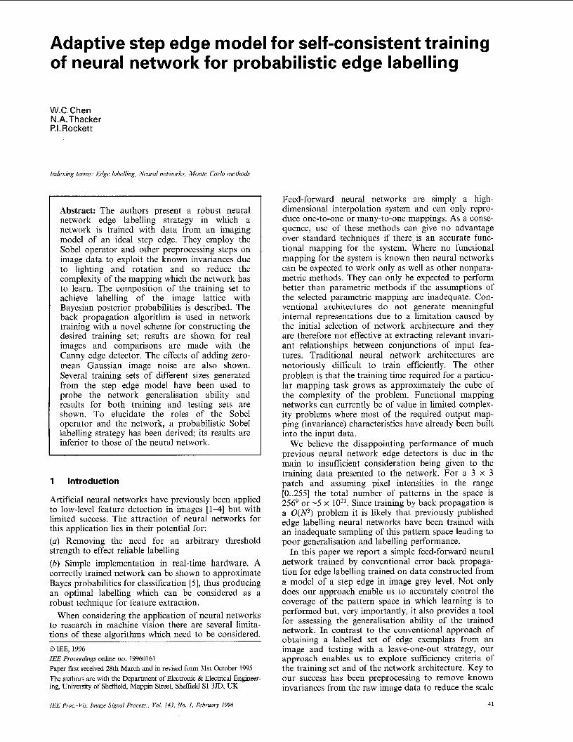
2 Hierarchical system architecture

There are three units of this edge labelling system: the edge modelling, the invariance data 'filtering' and the traininghesting network. The overall hierarchical net- work architecture is shown in Fig. 1.

I

I step edgemodei j edge modelling unit

training/testing network

I .................. 1 .'I Overall system architecture

log I

\ t Y

I

I I I

'.G+'

3x3 Sobel mask 1 datainvariance preprocessing

k- pixel width(-1 -4 Step edge model illustrating the model parameters Fig. 2

: patchrotate I

2.7 Edge modelling unit The objective of this unit is to generate an A4xM array (where A4 is odd) of real values which correspond to the light intensity values integrated over the light-sensi- tive regions of the pixels of a CCD array. We have considered a (p, 8) parameterisation of the straight line of the step edge and started with a function which returns an array of pixel intensities, and which takes the following arguments: p: perpendicular distance of the line from the origin 8: slope of the normal of the line Xp, Yp: dimensions of the pixel in X and Y directions, respectively

j

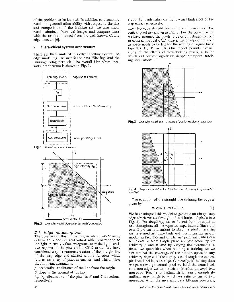
IL, I,: light intensities on the low and high sides of the step edge, respectively. The step edge straight line and the dimensions of the central pixel are shown in Fig. 2. For the present work we have assumed the pixels to be of unit dimension but in general, for real CCD arrays, the pixels do not abut as space needs to be left for the routing of signal lines: typically Xp, Yp -- 0.8. Our model permits explicit study of the effects of non-abutting pixels, a factor which will become significant in spatiotemporal track- ing applications.

tY

Fig.3 Step edge model in 5 x 5 lattice ofpixels: member of edge class

t Y

Fig.4 non-edge

Step edge model in 5 x 5 lattice ofpixels: example of unobvious

The equation of the straight line defining the edge is given by

We have adopted this model to generate an abrupt step edge which passes through a 5 x 5 lattice of pixels (see Fig. 3). For simplicity, we set Xp and Yp both equal to one throughout all the reported experiments. Since our overall system is invariant to absolute pixel intensities we have used arbitrary high and low intensities in our model; in fact 255 and 0. The net pixel intensities can be calculated from simple plane analytic geometry for arbitrary p and 0, and by varying the increments in these two quantities when building a training set we can control the coverage of the pattern space to any arbitrary degree. If the step passes through the central pixel we label it as an edge. Contrarily, if the step does not pass through central pixel we label the central cell as a non-edge; we term such a situation an unobvious non-edge (Fig. 4) to distinguish it from a completely uniform grey patch to which we refer as an obvious non-edge. After the invariant data filtering processes,

zcos8 +ys in8 = p (1)

42 IEE Proc-Vis. Image Signal Pvocess., Vol. 143, No. I , February 1996

the 5 x 5 patch has rotational symmetry so we can sim- ply define the range of 8 in [0..7~/2] and [7~..37~/2] and ignore the reversed grey level case of the 5 x 5 patch. For a 5 x 5 patch the range of p is [0 ..d2 x 5/21.

Therefore, to determine if a given patch is an edge pattern the distance p must satisfy the following condi- tion:

where

( 3 )

i.e. the step needs to pass through the central lattice site.

2.2 Data invariance preprocessing From the edge modelling unit, a training set of 5 x 5 image patches is generated. In this preprocessing stage our objective is to remove known invariances from the data before feeding them to the neural network to reduce the complexity of the problem to be learned. First we take the (common) logarithm of the grey level so that steps in image intensity are invariant to the absolute grey levels involved. This preprocessing step alone reduces the number of patterns to be learned by an order of magnitude. Secondly we compute the edge orientation of the (candidate) patch using a 5 x 5 Sobel operator and rotate the patch such that the candidate edge lies in the first quadrant; this stage again reduces the number of patterns to be learned by a factor of four. Thirdly, we compute the image gradients using a

3 x 3 Sobel operator so that the input vector to the neural network classifier is a 3 x 3 patch of image gra- dient magnitudes.

2.3 Trainingbesting network The neural network architecture used in this work is a conventional multilayer perceptron (MLP) with sigmoi- dal neuron nonlinearities. The error back propagation algorithm [7] is used in network training. Nine input nodes are required for the training sets and single out- put node for the edge probability. Eight hidden nodes are adopted in our neural network.

3

Different ways of generating the training sets in neural network edge detection are shown in literature [l-4, 8- 131. Here we present construction of the training sets from our edge imaging model. For comparison, we also present results from networks trained using exemplars derived from real images in the following subsection.

3. I Real image exemplars One possible method of obtaimng a training set is to take a real image (or series of images) and label the edges by hand or with an existing edge detector such as Canny. We have tried the approach of using Canny- labelled data but a number of problems arise. First and foremost is the sheer size of the training set produced. We have used a real image with 256 x 256 size to get the training set. Using the ‘house’ image (Fig. 5a) and after preprocessing to remove invariances, each training pattern consists of nine (3 x 3) element input vectors and the Canny-labelled data of the centre pixel is the desired output. For this image a total of 252 times 252 (= 63 504) input patterns was generated (3167 edges

Construction of the training set

U b

Fig. 5 a Original picture (256 x 256); b Neural network output after training c After taking threshold = 0.75; d The desired output map in training (from Canny)

IEE Proc.-Vis. Image Signal Process., Vol. 143, No. 1, February 1996

Experimental results using image exemplars

43

a

C

a Original image (512 x 512); b Neural network output c After taking threshold = 0.75; d The desired output map for comparison

and 60 337 non-edges). The error back propagation feed-forward neural network which comprises nine input nodes, eight hidden nodes and one output node was used. This was selected by the standard technique of varying the number of hidden nodes and choosing the network architecture giving the smallest mean- squared error for the validation set. Fig. 5 shows the training results; some slanting lines and details in Fig. 5c of neural network outputs appear more reliably labelled than those of the desired training output map from the Canny detector in Fig. 5d although the net- work output is missing some lines which are detected by Canny. To evaluate this trained network, we used another real image but the results are unsatisfactory (Fig. 6).

We have attempted to cluster these training sets by using a Euclidean distance scheme in the vector space to reduce the size, i.e. reduce the training time. In addi- tion, we also adopted parts of three different real images to cover more patterns and in an attempt to increase training information, another input vector of the central pixel grey level in 3 x 3 mask was added as the tenth input in network training. The results from the subsequently trained network were still unsatisfac- tory due, we suspect, to the fact that the coverage of the pattern space was largely random resulting in weak or incorrect classification. In principle this deficiency could be remedied by taking more exemplars but at the cost of increased training time.

3.2 Step edge imaging model Motivated by the desire to guarantee proper coverage of the pattern space while keeping the size of training set as small as possible, we have adopted the step edge imaging model to generate edges and non-edges train- ing sets in a 5 x 5 lattice of pixels. A major question

44

b

d

regarding the composition of the training set is what proportion should be edge examples and what propor- tion non-edges. Richards and Lippmann [5] and others have demonstrated that, subject to certain sufficiency conditions, neural network classifiers approximate the Bayesian posterior probability so the training set needs to be constructed to reflect the Bayesian prior probabil- ities of the edge and non-edge classes; we also present a modified proof in the Appendix. For a typical image, we observe that the ratio of non-edge-to-edges k is in the range 5-1OO:l. For n edge exemplars, within the class of kn non-edges we require 4n unobvious non- edges since if a step is moved by uniform increments across the 5 x 5 image patch only one-fifth of the pat- terns so generated will be edges, i.e. fall within the cen- tral pixel. Thus the remaining (k - 4)n of our non-edge examples need to be patches of uniform grey level, namely obvious non-edges. (In a related setting, Davies [14] has pointed out the need for the correct weighting in the training set of conventional pattern classifiers.)

By choosing increments for p and e, Ap and A @ we can generate an arbitrarily large training set (of edges and unobvious non-edges) to which we can add the necessary number of obvious non-edges to complete the set. Since, however, we wish to minimise training time we only require a set just sufficient to train the network to a required degree of generalisation. For p in the range [-p,,, ... pmaJ and 0 in the range [0 ... OmX] the numbers of uniform steps in p and 0, respec- tively are

U P and

+1 (5) omaz No - ae

and the total number of edgeslunobvious non-edges is

IEE Proc.-Vis. Image Signal Process., Vol. 143, No. I, February 1996

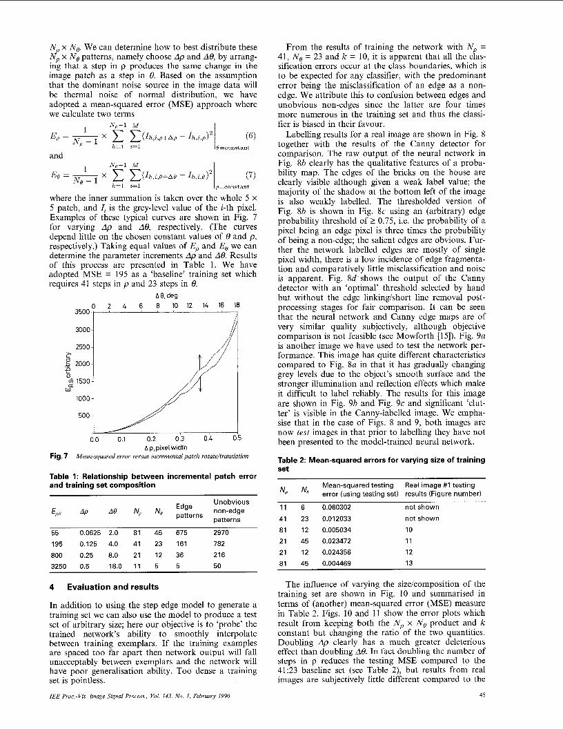
Np x Ne. We can determine how to best distribute these Np x Ne patterns, namely choose A p and A8, by arrang- ing that a step in p produces the same change in the image patch as a step in 8. Based on the assumption that the dominant noise source in the image data will be thermal noise of normal distribution, we have adopted a mean-squared error (MSE) approach where we calculate two terms

and N a - l M I

where the inner summation is taken over the whole 5 x 5 patch, and Ii is the grey-level value of the i-th pixel. Examples of these typical curves are shown in Fig. 7 for varying Ap and A6, respectively. (The curves depend little on the chosen constant values of 8 and p , respectively.) Taking equal values of Ep and E, we can determine the parameter increments Ap and A8. Results of this process are presented in Table 1. We have adopted MSE = 195 as a ‘baseline’ training set which requires 41 steps in p and 23 steps in 8.

A 8, deg 0 2 4 6 8 IO 12 14 16 18

3000 1

0.0 0.1 0.2 0 3 0.4 0.5 Ap,pixelwidth

Fig. 7 Mean-squared error versus incremental patch rotate/tranrlation

Table 1 : Relationship between incremental patch error and training set composition

Unobvious

patterns EP.0 AP A* NP No Edge patterns non-edge

55 0.0625 2.0 81 45 675 2970 195 0.125 4.0 41 23 161 782 800 0.25 8.0 21 12 36 216 3250 0.5 18.0 1 1 5 5 50

4 Evaluation and results

In addition to using the step edge model to generate a training set we can also use the model to produce a test set of arbitrary size; here our objective is to ‘probe’ the trained network’s ability to smoothly interpolate between training exemplars. If the training examples are spaced too far apart then network output will fall unacceptably between exemplars and the network will have poor generalisation ability. Too dense a training set is pointless.

IEE Proc.-Vis. Image Signal Process., Vol. 143, No. I , February 1996

From the results of training the network with N p = 41, Ne = 23 and k = 10, it is apparent that all the clas- sification errors occur at the class boundaries, which is to be expected for any classifier, with the predominant error being the misclassification of an edge as a non- edge. We attribute this to confusion between edges and unobvious non-edges since the latter are four times more numerous in the training set and thus the classi- fier is biased in their favour.

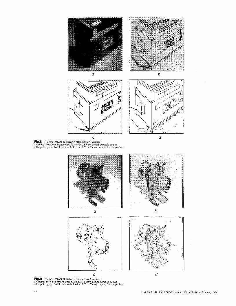
Labelling results for a real image are shown in Fig. 8 together with the results of the Canny detector for comparison. The raw output of the neural network in Fig. 8b clearly has the qualitative features of a proba- bility map. The edges of the bricks on the house are clearly visible although given a weak label value; the majority of the shadow at the bottom left of the image is also weakly labelled. The thresholded version of Fig. 8b is shown in Fig. 8c using an (arbitrary) edge probability threshold of 2 0.75, i.e. the probability of a pixel being an edge pixel is three times thc probability of being a non-edge; the salient edges are obvious. Fur- ther the network labelled edges are mostly of single pixel width, there is a low incidence of edge fragmenta- tion and comparatively little misclassification and noise is apparent. Fig. 8d shows the output of the Canny detector with an ‘optimal’ threshold selected by hand but without the edge linkinghhort line removal post- processing stages for fair comparison. It can be seen that the neural network and Canny edge maps are of very similar quality subjectively, although objective comparison is not feasible (see Mowforth [15]). Fig. 9a is another image we have used to test the network per- formance. This image has quite different characteristics compared to Fig. 8a in that it has gradually changing grey levels due to the object’s smooth surface and the stronger illumination and reflection effects which make it difficult to label reliably. The results for this image are shown in Fig. 9b and Fig. 9c and significant ‘clut- ter’ is visible in the Canny-labelled image. We empha- sise that in the case of Figs. 8 and 9, both images are now test images in that prior to labelling they have not been presented to the model-trained neural network.

Table 2: Mean-squared errors for varying size of training set

Mean-squared testing Np No error (using testing set)

1 1 6 0.060302 41 23 0.012033 81 12 0.005034 21 45 0.023472 21 12 0.024356 81 45 0.004469

Real image #I testing results (Figure number)

not shown

not shown

10 1 1 12 13

The influence of varying the sizelcomposition of the training set are shown in Fig. 10 and summarised in terms of (another) mean-squared error (MSE) measure in Table 2. Figs. 10 and 11 show the error plots which result from keeping both the N p x No product and k constant but changing the ratio of the two quantities. Doubling Ap clearly has a much greater deleterious effect than doubling de. In fact doubling the number of steps in p reduces the testing MSE compared to the 41:23 baseline set (see Table 2), but results from real images are subjectively little different compared to the

45

a . . .... . . ... .,. .. . ......... ............... . . . .

- . - I C

Fig.8 a Original grey-level image (size: 256 x 256); b Raw neural network output c Output edge probabilities thresholded at 0.75; d Canny output, for comparison

Testing results of image 1 after network trained

U

C Fig.9 a Original grey-level image (size: 512 x 512); b Raw neural network output c Output edge probabilities thresholded at 0.75; d Canny output, for comparison

Testing results of image 2 after network trained

b

b

d

46 IEE Proc.-Vis. Image Signal Process., Vol. 143, No. 1, February 1996

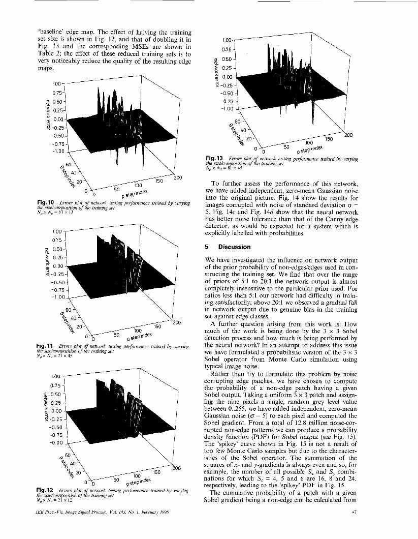
‘baseline’ edge map. The effect of halving the training set size is shown in Fig. 12, and that of doubling it in Fig. 13 and the corresponding MSEs are shown in Table 2; the effect of these reduced training sets is to very noticeably reduce the quality of the resulting edge maps.

1.00 _____I\ 0.751

0

Fig. 10 the size/composition of the training set No x Na = 81 x 12

Errors plot of network testing performance trained by varying

1.00 1 0.75

-0.501 -0.75 7 -l.OO&--

Fig. 11 the size/composition of t A training set No x Na = 21 x 45

Errors plot o network testing performance trained by varying

1.00 ___c_?\

-0.50 -0.75 1 -0.00 &---

\ I

Fig. 12 the size/composition of the training set Np x No = 21 x 12

Errors plot of network testing pevformance trained by varying

0.75 4

-0.50 -0.75 1 7 -1.00 &---

Fig. 13 the size/composition of tle training set N , x N a = 8 1 x 4 5

Errors plot o network testing performance trained by varying

To further assess the performance of this network, we have added independent, zero-mean Gaussian noise into the original picture. Fig. 14 show the results for images corrupted with noise of standard deviation CY = 5. Fig. 14c and Fig. 14d show that the neural network has better noise tolerance than that of the Canny edge detector, as would be expected for a system which is explicitly labelled with probabilities.

5 Discussion

We have investigated the influence on network output of the prior probability of non-edgesledges used in con- structing the training set. We find that over the range of priors of 5:l to 20:l the network output is almost completely insensitive to the particular prior used. For ratios less than 5:l our network had difficulty in train- ing satisfactorily; above 20:1 we observed a gradual fall in network output due to genuine bias in the training set against edge classes.

A further question arising from this work is: How much of the work is being done by the 3 x 3 Sobel detection process and how much is being performed by the neural network? In an attempt to address this issue we have formulated a probabilistic version of the 3 x 3 Sobel operator from Monte Carlo simulation using typical image noise.

Rather than try to formulate this problem by noise corrupting edge patches, we have chosen to compute the probability of a non-edge patch having a given Sobel output. Taking a uniform 3 x 3 patch and assign- ing the nine pixels a single, random grey level value between 0..255, we have added independent, zero-mean Gaussian noise (0 = 5) to each pixel and computed the Sobel gradient. From a total of 12.8 million noise-cor- rupted non-edge patterns we can produce a probability density function (PDF) for Sobel output (see Fig. 15). The ‘spikey’ curve shown in Fig. 15 is not a result of too few Monte Carlo samples but due to the character- istics of the Sobel operator. The summation of the squares of x- and y-gradients is always even and so, for example, the number of all possible S, and Sy combi- nations for which S, = 4, 5 and 6 are 16, 8 and 24, respectively, leading to the ‘spikey’ PDF in Fig. 15.

The cumulative probability of a patch with a given Sobel gradient being a non-edge can be calculated from

IEE Proc-Vis. Image Signal Process., Vol. 143, No. 1, February 1996 41

a b

C Fig. 14 a Original grey-level image; b Raw neural network output c Output edge probabilities thresholded at 0.75; d Canny output for comparison

Experimental results of adding independent zero-mean Gaussian noise of B = 5

Sobel output Fig.15 Monte-Carlo simulation using 3 x 3 Sobel detector with zero mean inde endent Gaussian noise of B = 5: probability density function (PDF) ofiobel output

d

its PDF by integration where the lower limit of the integration is the impossible event (i.e. maximum Sobel gradient). The cumulative non-edge probability is shown in Fig. 16 as a dotted line; the edge probability is simply the complement of the non-edge probability for this two-class problem and is shown as a solid line in Fig. 16. Figs. 17 and 18 show the experimental results for a grey-level image. This probabilistic Sobel operator appears more satisfactory than using a hard, heuristic threshold but it still suffers from the well known Sobel problem of producing ‘thick’ edges rather than edges of unit width. Consequently, we infer that the neural network is doing more than just learning a probabilistic threshold for the Sobel operator. We believe our network is estimating the joint probability of occurrence of statistically dependent events associ- ated with the existence of an edge within the central cell of the mask and thus is performing probabilistic data fusion. In this light the role of the network can be visualised in the following manner: If we have a 3 x 3 patch of edge gradients, G = {g!,,g2 ..., g9} our network approximates the Bayes probability P(C,IG) where C, is the class label. Each event g, is distinct and so

where gl, g2, ... are correlated random variables. Thus we believe the neural network is learning an estimate of the probability of the conjunction of a set of correlated events and is thus performing a data fusion role.

6 Conclusions

P(C,IG) = p(C,Igl n g2 n . . . n g9)

0 20 40 60 80 100

Monte-Carlo simulation using 3 x 3 Sobel detector with zero Sobel output

.16 mean independent Gaussian noise of 0 = 5: Probabilistic model __ edge . . . . . . . . . non-edge

48

The main motivations behind the use of neural net- works for feature extraction are to develop a robust, sensibly thresholded approach which is suitable for hardware implementation. Hopefully, we will be able to

IEE Proc -Vis Image Signal Process, Vol 143, No I , February 1996

design a single computational architecture capable of efficiently labelling a wide range of different features in an image. To achieve this we have found that the first requirement is to reduce the complexity of the learning problem so that both network training and size are manageable. In addition we have demonstrated the benefits of generating a simulated traininghesting set. This gives us the opportunity to analyse the coverage of the functional mapping provided by the network in a self-consistent manner. Currently our model for edge labelling does not include sensor noise or effects due to the active area of an image pixel but these effects can be easily included. These modifications would be impossible with conventional feature extraction tech- niques such as Canny.

Fig.17 mean independent Gaussian noise of (r = 5: real image testing result

Monte-Carlo simulation using 3 x 3 Sobel detector with zero

level intensities are mean values integrated across the camera pixels, and not available as a continuous func- tion. Thus account could be taken of the fact that in CCD cameras, the light-sensitive areas of adjacent pix- els do not abut but rather have ‘dead zones’ which are used for routing interconnects.

7 Acknowledgments

One of us (Wan-Ching Chen) is grateful to the Taiwan- ese Government for a research scholarship. N. Thacker acknowledges the financial support of SERC/EPSRC Contract No. GR/J104464.

8 References

1 CASABURI, S., PETROSINO, A., and TAGLIAFERRI, R.: ‘A neural network approach to robust edge detection’, Proceedings 5th Italian Workshop on Neural networks, Wirn-Vietri, 1992, pp. 266-212

2 PHAM, D.T., and BAYRO-CORROCHANO, E.J.: ‘Neural net- works for low-level image processing’, Proceedings of ICANN-92,

~~

1992, pp. 809-812 3 CHANG. C.-H.. CHANG. C.-C., and HWANG, S.-Y.: ‘Connec-

tionist learning urocedure ’for edge detection’. Proc. SPIE - Int. .. . ~~~. . ~ ~ ~ ~ ~~~ ~

Soc. Opt. Engt i991, 1607, pp. 255-236 4 PAIK, J.K., BRAILEAN, J,.C. and KATSAGGELOS, A.K.: ‘An

edge detection algorithm using multi-state adalines’, Pattern Rec- ogiit., 1992, 25, 02), pp. 1497-1504

5 RICHARDS, M.D., and LIPPMANN, R.P.: ‘Neural network classifiers estimate Bayesian a posteriori probabilities’, Neural Cnmnvt 1991 3. f4). nn 461483 r - - - - , - - - -, -, , ,,

6 CANNY, J.F.: ‘A computational approach to edge detection’, IEEE Trans., 1986, PAMI-8, pp. 679498

7 RUMMELHART, D., HINTON, G., and WILLIAMS, R.: ‘Learning representations by back propagation of errors’, Nature, 1986, 323, pp. 533-536 MADIRAJU. S.V.R., LIU, Z.-O., and CAELLI, T.M.: ‘Feature 8

Fig. 18 Monte-Carlo simulation using 3 x 3 Sobel detector with zero mean independent Gaussian noise of (r = 5: output edge probabilities thresh- olded at 0.75

There are several advantages of the present neural network implementation (a) Computational effort is small compared to Canny and thus is suitable for real-time processing. (b) The outputs approximate the Bayes posterior prob- abilities and so a principled threshold can be applied to segment edges. This is in distinct contrast to conven- tional edge detectors which require an empirically determined threshold on the gradient, generally differ- ent for each processed image. (c) Direct construction of a training set from an imag- ing model rather than learning examples from real images allows a minimal training set to be constructed for the problem, thus minimising network training time. The trade-offs between training time and network performance are explicit. (d) The imaging model accounts for the fact that grey-

IEE Proc.-Vis. Image Signal Process., Vol. 143, No. I , February 1996

extraction using neural network$, Proceedings of the 4th Austral- ian conference on Neural networks, 1993, pp. 224221

9 ENAB, Y.M.: ‘Neural edge detector’, Proc. SPIE - Int. Soc. Opt. Eng., 1990, 1382, pp. 292-303

10 SHIH, F.Y., MOH, J., and BOURNE, H.: ‘A neural architecture applied to the enhancement of noisy binary images’, Eng. Appl. Art$ Intell., 1992, 5, (3), pp. 215-222

11 WELLER, S.: ‘Artificial neural net learns the Sobel operators (and more)’, Proc. SPIE - Int. Soc. Opt. Eng., 1991, 1469, pp. 2 19-224

12 SPREEUWERS, L.J.: ‘A neural network edge detector’, Proc. SPIE - Int. Soc. Opt. Eng., 1991, 1451, pp. 204-215

13 KERR, D.A., and BEZDEK, J.C.: ‘Edge detection using a fuzzy neural network‘, Proc. SPIE - Int. Soc. Opt. Eng., 1992, 1710, pp. 5 10-52 1

14 DAVIES, E.R.: ‘Training sets and a priori probabilities with the nearest neighbour method of pattern recognition’, Pattern Recog- nit. Lett., 1988, 8, pp. 11-13

15 MOWFORTH, P., and GILLESPIE, L.: ‘Edge detection as an ill- posed specification task‘, Research report, The Turing Institute and the Computer Science Department, University of Strathclyde, Glasgow, UK, 1987, pp. 1-1 1

9 Appendix

The optimisation function is the least-squares error cri- teria which, summed over the entire data set for output k, gives

Ek = C(o(1n) - t n k ) 2 (8) n

where t,k is the nth training output and o is the output from the network for a particular input I,. The obvious interpretation for this training algorithm is that our training outputs are Gaussian-distributed random vari- ables. However, we can also show that there is another link with probability theory which is broader in scope and therefore much more powerful.

Provided that we are training with data which defines a l-from-K coding of the output (i.e. classification) we can partition the error measure across the K classes according to their relative conditional probabilities

49

p(Cklr> so that

(9)

n

where <air> is the expectation operator of a at I,,. By completing the square this can now be rewritten as

n n

The last term is purely data-dependent so that the only effect that training can have is to minimise the first term which is clearly a minimum when o(IJ = <tklln>. For a l-from-K coding of the output and in the limit of an infmite number of samples <tklIn> = P(CklIn). Thus under these conditions neural net- works trained with the least-squares error function will approximate conditional probabilities of classifi- cation. Notice that the error function itself E is not necessarily defined as an expectation value as it is in [5] and the output will estimate conditional probabil- ities provided that the ratio of output samples neces- sary to define <tklI,> at each point I, in the data set is preserved.

50 IEE Proc.-Vis. Image Signal Process., Vol. 143, No. I , February 1996