Adaptive space-time finite element

methods for non-autonomous parabolic

problems with distributional sources

Ulrich Langer Andreas Schafelner

DK-Report No. 2020-03 03 2020

A–4040 LINZ, ALTENBERGERSTRASSE 69, AUSTRIA

Supported by

Austrian Science Fund (FWF) Upper Austria

Editorial Board: Bruno BuchbergerEvelyn BuckwarBert JuttlerUlrich LangerManuel KauersPeter PauleVeronika PillweinSilviu RaduRonny RamlauJosef Schicho

Managing Editor: Diego Dominici

Communicated by: Bert JuttlerVeronika Pillwein

DK sponsors:

• Johannes Kepler University Linz (JKU)

• Austrian Science Fund (FWF)

• Upper Austria

Adaptive space-time finite element methods

for non-autonomous parabolic problems

with distributional sources

Ulrich Langer, Andreas Schafelner

Abstract

We consider locally stabilized, conforming finite element schemes oncompletely unstructured simplicial space-time meshes for the numericalsolution of parabolic initial-boundary value problems with variable coef-ficients that are possibly discontinuous in space and time. Distributionalsources are also admitted. Discontinuous coefficients, non-smooth bound-aries, changing boundary conditions, non-smooth or incompatible initialconditions, and non-smooth right-hand sides can lead to non-smooth so-lutions. We present new a priori and a posteriori error estimates forlow-regularity solutions. In order to avoid reduced rates of convergencethat appear when performing uniform mesh refinement, we also consideradaptive refinement procedures based on residual a posteriori error indi-cators and functional a posteriori error estimators. The huge system ofspace-time finite element equations is then solved by means of GMRESpreconditioned by space-time algebraic multigrid. In particular, in the 4dspace-time case, simultaneous space-time parallelization can considerablyreduce the computational time. We present and discuss numerical resultsfor several examples possessing different regularity features.

Keywords: Non-autonomous Parabolic Initial-Boundary Value Problem,Distributional Sources, Space-Time Finite Element Methods, Unstruc-tured Meshes, Adaptivity

MSC 2010: 35K20, 65M60, 65M50, 65M15, 65Y05

1 Introduction

Time-parallel and space-time methods, in particular, space-time finite elementmethods have a long history. We refer the interested reader to the survey articles[14] and [36] for a comprehensive review of time-parallel and space-time meth-ods, respectively. We here only mention the Streamline Upwind Petrov-Galerkin(SUPG) finite element method (sometimes also called Streamline Diffusion (SD)method), that was originally proposed by Hughes and Brooks for solving sta-tionary convection-dominated convection-diffusion problems [16], and was later

1

used by Johnson and Saranen [9] to construct stable finite element schemesfor time-dependent convection-diffusion problems, discretizing space and timesimultaneously in time-slices. Similarly, in [17], Hughes, Franca and Hulbertproposed and analyzed the more general Galerkin/Least-Squares Finite Ele-ment Method (FEM) for stationary and instationary problems including time-dependent convection-diffusion problems. Both techniques were then used inmany publications to stabilize finite element schemes.

The revival of space-time methods is certainly connected with the availabil-ity of massively parallel computers with thousands or even millions of cores, butalso with the simultaneous adaptivity in space and time, the easy handling ofmoving spatial domains and interfaces that are fixed in the space-time domainQ, and the all-at-once treatment of first-order optimality conditions (KKT sys-tem) in optimal control problems with parabolic or hyperbolic PDE constraints.Recently, time-upwind stabilizations have been used to construct and analyze co-ercive space-time Isogeometric Analysis (IGA) schemes in [23], partial low-ranktensor IGA schemes [26], and space-time hp-finite element schemes combinedwith mesh-grading in time to treat singularities in time [11]. These papers relyon a tensor-product structure of space and time. Results related to methods thatdo not assume a tensor-product structure were presented, e.g., in [34], where theauthor proposes and analyzes a inf-sup-stable space-time FEM on completelyunstructured decompositions of the space-time domain, and in [1], where anarbitrary dimension convection-diffusion scheme for space-time problems is pro-posed, with two different discretizations. Unstructured space-time finite elementand IGA methods have also been used to solve involved engineering problems;see, e.g., [2, 18], and the references therein, where mostly unstructured meshesare used within time slabs into which the space-time cylinder Q is decomposed.

Following our previous work [24], we will derive, analyze and test space-time finite element methods on completely unstructured simplicial space-timemeshes for non-autonomous parabolic initial-boundary value problems with dis-tributional right-hand sides of the form: find u such that

∂tu− divx(ν∇xu) = f − divx(f) in Q = Ω× (0, T ), (1)

u = uD := 0 on Σ = ∂Ω× (0, T ), (2)

u = u0 on Σ0 = Ω× 0, (3)

where the spatial domain Ω ⊂ Rd, d = 1, 2, 3, is bounded and Lipschitz,T > 0 denotes the final time, ν ∈ L∞(Q) is a given uniformly bounded andpositive coefficient that may discontinuously depend on the spatial variablex = (x1, . . . , xd) and the time variable t, f ∈ L2(Q), and f ∈ [L2(Q)]d. Iff = 0 and ν is of bounded variation in t for almost all x, then the weak so-lution u of (1)–(3) has maximal parabolic regularity, i.e., ∂tu ∈ L2(Q) andLxu := −divx(ν∇xu) ∈ L2(Q), see [12]. Thus, in the maximal parabolic reg-ularity setting, the PDE ∂tu − divx(ν∇xu) = f makes sense in L2(Q), andthis setting was the starting point for deriving the consistent space-time finiteelement schemes in [24]. If f 6= 0 and it is not smooth enough, i.e., f creates adistribution that is not in L2(Q), then maximal parabolic regularity does not

2

hold. However, in many applications, the vector field f has a special structure.For instance, in 2d eddy current problems, ν denotes the reluctivity, f is nothingbut the impressed current in the coils, and f represents the magnetization in thepermanent magnets. In such a way, we can model a rotating electrical machine,see, e.g., [29]. Motivated by such applications, we can assume that there is adecomposition of the space-time cylinder Q =

⋃mi=1Qi into m non-overlapping,

sufficiently smooth subdomains Q1, . . . , Qm such that f is sufficiently smoothin Qi but may have jumps across the boundaries of these subdomains. Thesejumps create distributions located on the interfaces between the subdomains. Inthis paper, we consider exactly this case of such a special right-hand side witha piecewise smooth vector-field f leading to a distribution that is located onthe interfaces. We again derive a consistent space-time finite element scheme,for which we prove a best-approximation (Cea-like) estimate that immediatelyyields convergence rate estimates in terms of the mesh-size h under additionalregularity assumptions. In the case of low-regularity solutions, say, u ∈ H1+s(Q)with some s ∈ (0, 1], and uniform mesh refinement, we can only expect a con-vergence rate of O(hs) in the corresponding energy norm independent of thepolynomial order p of the finite element shape functions used. To circumventthis loss in the convergence rate, we also consider full space-time adaptive finiteelement procedures based on residual indicators or functional error estimators.We compare the efficiency of these adaptive approaches in a series of numericalexperiments.

The remainder of the paper is organized as follows. In Section 2, we recallthe standard space-time variational formulation and solvability results includingmaximal parabolic regularity and other regularity results. Section 3 is devotedto the derivation of consistent space-time finite element schemes. New a priorierror estimates are presented in Section 4. Section 5 deals with a posteriori errorestimates, which are used to control the adaptive finite element procedures inour numerical experiments. In Section 6, we present various numerical resultsfor uniform and adaptive mesh refinement in space and time. Finally, we drawsome conclusions in Section 7.

2 Space-time variational formulation and solv-ability results

We start with Ladyzhenskaya’s space-time variational formulation of the para-bolic initial-boundary value problem (1)–(3) in space-time Sobolev spaces, see[20] and the classical monographs [22, 21]: find u ∈ H1,0

0 (Q) := v ∈ L2(Q) :∇xu ∈ [L2(Q)]d, u = 0 on Σ such that

a(u, v) :=

∫Q

(−u∂tv + ν∇xu · ∇xv) dQ =∫Q

(f v + f · ∇xv) dQ+

∫Ω

u0(x) v(x, 0) dx =: l(v), ∀v ∈ H1,1

0,0(Q),

(4)

3

where H1,1

0,0(Q) := v ∈ L2(Q) : ∇xu ∈ [L2(Q)]d, ∂tu ∈ L2(Q), u = 0 on Σ, u =

0 on ΣT = Ω× T. If f ∈ L2,1(Q) := v : Q→ R :∫ T

0‖v(·, t)‖L2(Ω) dt <∞,

f ∈ [L2(Q)]d, u0 ∈ L2(Ω), and the coefficient ν ∈ L∞(Q) is uniformly boundedand positive, i.e., there exist positive constants ν and ν such that

ν ≤ ν(x, t) ≤ ν for almost all (x, t) ∈ Q, (5)

then the space-time variational formulation (4) has a unique solution u that evenbelongs to the space V 1,0

2 (Q) ⊂ H1,00 (Q); see [21], Chapter III, Paragraph 3,

Theorem 3.2. In particular, this means that ‖u(·, t)‖L2(Ω) is continuous with re-spect to (wrt) t. Therefore, the initial condition makes sense in L2(Ω). The sameresult can be obtained if we consider the solvability of (1)–(3) in the Bochnerspace W (0, T ) := v ∈ L2(0, t;H1

0 (Ω)) : ∂tu ∈ L2(0, t;H−1(Ω)) of abstractfunctions u mapping the time interval [0, T ] to some Hilbert or Banach spaceX(Ω). Indeed, the parabolic initial-boundary value problem is uniquely solv-able in W (0, T ), and W (0, T ) is continuously embedded into C([0, T ], L2(Ω));see, e.g., [25]. This view at parabolic initial-boundary value is closely connectedwith the so-called line variational formulations and the corresponding opera-tor ordinary differential equations, and is the starting point for time-steppingmethods.

If f ∈ L2(Q), f = 0, u0 ∈ H10 (Ω), and ν = 1, then the solution u ∈ H1,0

0 (Q)

of (4) belongs to the space H∆,10 (Q) = v ∈ H1

0 (Q) : ∆xv ∈ L2(Q), andcontinuously depends on t in the norm of the space H1

0 (Ω); see [21], Chap-ter III, Paragraph 2, Theorem 2.1. This property is called maximal parabolicregularity. If ν = ν(x, t) depends on x and t (non-autonomous case) possiblyin discontinuous way (like in electrical machines, moving interfaces), then it ismore involved to specify the most general conditions for ν such that maximalparabolic regularity happens, i.e. the solution u ∈ H1,0

0 (Q) of (4) belongs to thespace

HL,10 (Q) = v ∈ H10 (Q) : Lxv := divx(ν∇xu) ∈ L2(Q).

Recently, Dier [12] proved maximal parabolic regularity provided that the cor-responding elliptic form is of bounded variation. In our case, this means that νis of bounded variation in t for almost all x. In the case of maximal parabolicregularity, we have ∂tu− Lxu = f in L2(Q) that was the starting point for thederivation of consistent space-time finite element schemes in [24].

In general, for non-trivial f ∈ [L2(Q)]d (with jumps), we cannot expectmaximal parabolic regularity. Motivated by applications, we assume that thereexist a decomposition of the space-time cylinder Q =

⋃mi=1Qi into m non-

overlapping Lipschitz domains Q1, . . . , Qm such that the restriction of f to Qibelongs to H(divx, Qi) for all i = 1, 2, . . . ,m, but may have jumps across theboundaries of these subdomains. Now, taking an arbitrary test function v ∈H1,1

0,0(Q) with a compact support in Qi, we immediately get∫

Qi

(−u∂tv + ν∇xu · ∇xv) dQ =

∫Qi

(f v + f · ∇xv) dQ. (6)

4

from the space-time variational formulation (4). Rewriting the left-hand sideand applying integration by parts on the right-hand side in (6), we obtain∫

Qi

(ν∇xu−u

)· ∇v dQ =

∫Qi

(f − divxf)v dQ, (7)

where ∇ =(∇>x ∂t

)>is the space-time gradient. This is nothing but the

definition of the weak space-time divergence, i.e., we have

div

(−ν∇xu

u

)= f − divxf in L2(Qi). (8)

The solution u ∈ V 1,02 (Q) of (4) also satisfies the integral identity; see [21],

Chapter 3, identity (3.20) on p. 120,∫Q

(−u∂tv + ν∇xu · ∇xv) dQ+

∫Ω

u(x, T ) v(x, T ) dx =∫Q

(f v + f · ∇xv) dQ+

∫Ω

u0(x) v(x, 0) dx, ∀v ∈ H10 (Q),

(9)

from which one can derive the space-time flux relationm∑i=1

∫∂Qi

(ν∇xu−u

)·(nxnt

)v ds+

∫Ω

u(x, T ) v(x, T ) dx

=

m∑i=1

∫∂Qi

f · nx v ds+

∫Ω

u0 v(x, 0) dx, ∀v ∈ H10 (Q).

(10)

Indeed, in (9), we can rewrite the integrals over Q as sum of integrals over Qi.Then we have the variational identity

m∑i=1

∫Qi

(ν∇xu−u

)· ∇v dQ+

∫Ω

u(x, T ) v(x, T ) dx

=

m∑i=1

∫Qi

(f v + f · ∇xv) dQ+

∫Ω

u0 v(x, 0) dx

for all v ∈ H10 (Q) = H1,1

0 (Q). Integrating by parts in the left-hand side and inthe right-hand side gives the identity

m∑i=1

(∫Qi

div

(−ν∇xu

u

)v dQ+

∫∂Qi

(ν∇xu−u

)·(nxnt

)v ds

)+

∫Ω

u(x, T ) v(x, T ) dx

=

m∑i=1

(∫Qi

(f − divxf)v dQ+

∫∂Qi

f · nx v ds

)+

∫Ω

u0 v(x, 0) dx, (11)

that holds for all v ∈ H10 (Q). We mention that the integral over ∂Qi have to be

understood as duality products on H−1/2(∂Qi)×H1/2(∂Qi). Using (8) in (11),we arrive at the space-time flux relation (10).

5

3 Space-time finite element methods

Next, we need a decomposition (triangulation) Th of Q into shape-regular finiteelements K such that Q =

⋃K∈Th K and K ∩K ′ = ∅ for all K and K ′ from Th

with K 6= K ′; see [4, 5, 8] for a precise definition of shape-regular triangulations.We assume that the triangulation is aligned with Qi, i.e. Qi = ∪K∈Ti,hK canbe represented by a subset Ti,h of the triangulation Th = ∪mi=1Ti,h.

On the basis of the shape-regular triangulation Th, we define the space-timefinite element space

V0h = v ∈ C(Q) : v(xK(·)) ∈ Pp(K), ∀K ∈ Th, v = 0 on Σ (12)

as usual [4, 5, 8], where xK(·) denotes the map from the reference element Kto the finite element K ∈ Th, and Pp(K) is the space of polynomials of the

degree p on the reference element K. The space-time finite elements space V0h

is obviously a finite dimensional subspace of the space H10 (Q) ⊂ V 1,0

2 (Q). Let usdenote the dimension of V0h by Nh. For simplicity, throughout this paper and,in particular, in our numerical experiments in Section 6, we use affine-linearmappings xK(·) and simplicial elements K.

Following [24], we first multiply (8), that is valid in L2(K) for all K ∈ Thsince the triangulation Th is align with Qi, by a locally scaled upwind testfunction

vh,K(x, t) := vh(x, t) + θKhK∂tvh(x, t), vh ∈ V0h,

then integrate over K, and finally sum over all K ∈ Th, giving the identity∑K∈Th

∫K

div

(−ν∇xu

u

)(vh + θKhK∂tvh) dQ

=∑K∈Th

∫K

(f − divxf)(vh + θKhK∂tvh) dQ

Integration by parts yields∑K∈Th

∫K

[ν∇xu · ∇xvh − u∂tvh + θKhKdiv

(−ν∇xu

u

)∂tvh dQ

]+∑K∈Th

∫∂K

(−ν∇xu

u

)·(nxnt

)vh ds

=∑K∈Th

∫K

[fvh + f · ∇xvh + θKhKf∂tvh − θKhKdivxf∂tvh] dQ

−∑K∈Th

∫∂K

f · nxvh ds

Since the triangulation Th is aligned with the interfaces generated by the decom-position of Q into the space-time subdomains Q1, Q2, . . . , Qm, the space-time

6

flux identity (10) is also valid if one replaces the subdomains Qi by the finite ele-ments K. Using (10) with Qi replaced by K in the last identity, we immediatelyobtain the consistency relation

ah(u, vh) = lh(vh) ∀vh ∈ V0h, (13)

with

ah(u, vh) :=∑K∈Th

∫K

[ν∇xu · ∇xvh − u∂tvh + θKhKdiv

(−ν∇xu

u

)∂tvh

]dQ

(14)

+

∫Ω

u(x, T )vh(x, T )dx,

lh(vh) :=∑K∈Th

∫K

[fvh + f · ∇xvh + θKhKf∂tvh − θKhKdivx(f) ∂tvh] dQ

+

∫Ω

u0(x)vh(x, 0)dx.

Therefore, we arrive at the following consistent space-time finite element schemefor solving the initial-boundary value problem (4): find uh ∈ V0h such that

ah(uh, vh) = lh(vh) ∀vh ∈ V0h. (15)

Subtracting the space-time finite element scheme (15) form the consistency re-lation (13), we get the Galerkin orthogonality relation

ah(u− uh, vh) = 0 ∀vh ∈ V0h, (16)

that is crucial for deriving a priori discretization error estimates in the nextsection. We now show that the bilinear form ah(·, ·) is coercive on V0h withrespect to the norm

‖vh‖2h :=∑K∈Th

[‖ν1/2∇xvh‖2L2(K) + θKhK‖∂tvh‖2L2(K)

]+‖vh(·, T )‖2L2(Ω) + ‖vh(·, 0)‖2L2(Ω). (17)

Lemma 1. If θK is chosen sufficiently small, then there exist a positive constantµc such that

ah(vh, vh) ≥ µc ‖vh‖2h, ∀vh ∈ V0h. (18)

More precisely, if θK ≤ hK/c2I,K,ν for all K ∈ Th, then µc can be chosen 1/2,

where cI,K(ν) denotes the constant from the inverse inequality

‖divx(ν∇xvh)‖L2(K) ≤ cI,K,ν h−1k ‖ν

1/2∇xvh‖L2(K) (19)

that holds for all vh ∈ V0h and K ∈ Th; see [24].

7

Proof. For all vh ∈ V0h, we have the following representation of the bilinearform ah(vh, vh):

ah(vh, vh) =∑K∈Th

∫K

[|ν1/2∇xvh|2 −

1

2∂tv

2h + θKhKdiv

(−ν∇xvh

vh

)∂tvh

]dQ

+

∫Ω

|vh(x, T )|2 dx

=∑K∈Th

∫K

[|ν1/2∇xvh|2 + θKhK |∂tvh|2

]dQ+

1

2

∫Ω

|vh(x, T )|2 dx

+1

2

∫Ω

|vh(x, 0)|2 dx−∑K∈Th

θKhK

∫K

divx(ν∇xvh)∂tvh dQ (20)

Estimating the last term by Cauchy’s inequality, Young’s inequality, and theinverse inequality (19), we immediately get

ah(vh, vh) ≥∑K∈Th

[(1−

εθKc2I,K,ν

2hK)‖ν1/2∇xvh‖2L2(K) + (1− 1

2ε)θKhK‖∂tvh‖2L2(K)

]

+1

2‖vh(·, T )‖2L2(Ω) +

1

2‖vh(·, 0)‖2L2(Ω), ∀vh ∈ V0h,

from which (1) follows for ε = 1 and θK ≤ hk/c2I,K,ν for all K ∈ Th.

Remark 2. For the special case that p = 1 (linear shape functions) and ν =νK = const for all K ∈ Th, the last term in (20) vanishes since divx(ν∇xvh) =νK∆xvh = 0 on K. Therefore, we have

ah(vh, vh) =∑K∈Th

∫K

[|ν1/2∇xvh|2 + θKhK |∂tvh|2

]dQ+

1

2

∫Ω

|vh(x, T )|2 dx

+1

2

∫Ω

|vh(x, 0)|2 dx =: ‖|vh‖|2h, ∀vh ∈ V0h, (21)

i.e. the bilinear form ah(·, ·) is coercive on V0h wrt the norm ‖| · ‖|h with theconstant µc = 1.

The coercivity of the bilinear form ah(·, ·) on V0h yields uniqueness, and, inthe finite-dimensional case, uniqueness implies existence. Thus, the space-timefinite element scheme (15) has a unique solution uh ∈ V0h that can be foundby solving one linear system of algebraic equations. Once the basis is chosen,the space-time finite element scheme (15) is nothing but one system of linearalgebraic equations. Indeed, let p(j) : j = 1, . . . , Nh be the finite elementnodal basis of V0h, i.e., V0h = spanp(1), . . . , p(Nh), where Nh is the number ofall space-time unknowns (dofs). Then we can express the approximate solution

uh in terms of this basis, i.e., uh(x, t) =∑Nh

j=1 uj p(j)(x, t). Inserting this ansatz

into (15) and testing with p(i), we get the linear system

Khuh = fh, (22)

8

for determining the unknown coefficient vector uh = (uj)j=1,...,Nh∈ RNh , where

Kh = (ah(p(j), p(i)))i,j=1,...,Nhand f

h= (lh(p(i)))i=1,...,Nh

. The system matrixKh is non-symmetric, but positive definite due to Lemma 1.

4 A priori error estimates

We now introduce the norm

‖u‖2h,∗ :=∑K∈Th

[‖ν1/2∇xu‖2L2(K) + (θKhK)−1‖u‖2L2(K)

+ θKhK‖div

(−ν∇xu

u

)‖2L2(K)

]+ ‖u(·, T )‖2L2(Ω)

that is defined on V0h,∗ = HL0 (Q) + V0h to which the solution u and the dis-cretization error u − uh belong. The solution space HL0 (Q) can be chosen asv ∈ H1,0

0 (Q) : Lu := div(−ν∇xu, u) ∈ L2(Qi), i = 1, . . . ,m.

Lemma 3. The bilinear form (14) is bounded on V0h,∗ × V0h, i.e.,

|ah(u, vh)| ≤ µb ‖u‖h,∗‖vh‖h, ∀u ∈ V0h,∗, vh ∈ V0h (23)

with µb = 1.

Proof. Using Cauchy’s inequalities, we immediately get

ah(u, vh) =∑K∈Th

∫K

ν∇xu · ∇xvh − u∂tvh + θKhKdiv

(−ν∇xu

u

)∂tvhdQ

+

∫Ω

u(x, T )vh(x, T )dx

≤∑K∈Th

[(‖ν1/2∇xu‖2L2(K)

)1/2 (‖ν1/2∇xvh‖2L2(K)

)1/2

+(

(θKhK)−1‖u‖2L2(K)

)1/2 (θKhK‖∂tvh‖2L2(K)

)1/2

+

(θKhK‖div

(−ν∇xu

u

)‖2L2(K)

)1/2 (θKhK‖∂tvh‖2L2(K)

)1/2]

+(‖u(·, T )‖2L2(Ω)

)1/2 (‖vh(·, T )‖2L2(Ω)

)1/2

≤µb‖u‖h,∗‖vh‖h

with µb = 1.

The Galerkin orthogonality (16) together with the coercivity (18) and thegeneralized boundedness (23) of the bilinear form ah(·, ·) immediately yield abest-approximation (Cea-like) discretization error estimate in the correspondingnorms.

9

Lemma 4. Let u ∈ HL0 (Q) and uh ∈ V0h be the solutions of the parabolicIBVP (4) and the space-time finite element scheme (15), respectively, and letthe assumptions of Lemma 1 (coercivity) Lemma 3 (boundedness) hold. Thenthe discretization error estimate

‖u− uh‖h ≤ infvh∈V0h

(‖u− vh‖h +

µbµc‖u− vh‖h,∗

)(24)

holds.

Proof. Using (18), (16), and (23), we immediately get the estimates

µc‖vh−uh‖2h ≤ ah(vh−uh, vh−uh) = ah(u−uh, vh−uh) ≤ µb‖u−uh‖h‖u−vh‖h,∗

for any vh ∈ V0h, from which (24) follows by triangle inequality.

In order to obtain a convergence rate estimate from (24), we have to inserta suitable interpolation or quasi-interpolation Iph(u) ∈ V0h of the solution u intothe infimum. If u is sufficiently smooth, then we can use the nodal Lagrangeinterpolation that leads to completely local estimates. More precisely, let u ∈HL0 (Q) ∩ Hk(Q) ∩ H l(Th) with some l ≥ k > (d + 1)/2. Since in this caseHk(Q) ⊂ C(Q), the nodal Lagrange interpolation is well defined. Then thestandard finite element interpolation error estimates (see, e.g., [5, Theorem4.4.4] or [8, Theorem 3.1.6]) and the best-approximation error estimate (24)lead to the a priori discretization error estimate

‖u− uh‖h ≤ c

( ∑K∈Th

h2(s−1)K |u|2Hs(K)

)1/2

(25)

with s = minl, p + 1 and some generic positive constant c; see [24, Theorem13.3]. If the nodal Lagrange interpolation is not well defined due to the lowregularity of the solution u, we can make use of the quasi-interpolation operatorsproposed by Clement [10] or Scott and Zhang [33]. Let v ∈ Hk(Q), with somek > 1. Then, for instance, the Scott-Zhang quasi-interpolation operator ISZh :H1(Q)→ V0h provides the local interpolation error estimate

‖v − ISZh v‖Hm(K) ≤ chs−mK |v|Hs(SK), m = 0, 1, (26)

where s = mink, p + 1, c is again a generic positive constant, and SK :=

K ′ ∈ Th : K ∩ K ′ 6= ∅ denotes the neighborhood of the simplex K ∈ Th;see monograph [5, (4.8.10)]) or the original paper [33], and space interpolationresults [3, 15].

Theorem 5. Beside the assumptions imposed on the data ν, f , f and Q, andthe triangulation Th, we assume that the solution u of the space-time variationalproblem (4) belongs to HL0 (Q) ∩ Hk(Q), (d + 1)/2 ≥ k > 1, and ν∇x(u) ∈

10

(Hk−1(K))d for all K ∈ Th. Furthermore, let the assumptions of Lemma 4 befulfilled. Then the a priori discretization error estimate

‖u−uh‖2h ≤ c∑K∈Th

[h

2(s−1)K

(|u|2Hs(SK) + |ν∇xu|2Hs−1(K)

)+ h2

K‖divx(ν∇xu)‖2L2(K)

](27)

holds, with s = mink, p + 1 = k ≤ (d + 1)/2 for d = 1, 2, 3 and a positivegeneric constant c.

Proof. Inserting vh = ISZh u ∈ V0h into the infimum of the right-hand side of thebest-approximation error estimate (24), we immediately get

‖u− uh‖2h ≤(‖u− ISZh u‖h +

µ2b

µ2c

‖u− ISZh u‖h,∗)2

≤ 2‖eh‖2h + 2µ2b

µ2c

‖eh‖2h,∗

≤∑K∈Th

[2(1 +

µ2b

µ2c

)‖ν1/2∇xeh‖2L2(K) + 2θKhK‖∂teh‖2L2(K)

+ 2µ2b

µ2c

(θKhK)−1‖eh‖2L2(K) + 2µ2b

µ2c

θKhK‖div

(−ν∇xeh

eh

)‖2L2(K)

]+ 2(1 +

µ2b

µ2c

)‖eh(·, T )‖2L2(Ω) + 2‖eh(·, 0)‖2L2(Ω), (28)

where eh = u−ISZh u denotes the interpolation error. The first three terms in thesum can directly be estimated by means of the local interpolation error estimate(26). The fourth term needs special treatment. Inserting and subtracting theaverage

I0hq(x) =

1

|K|

∫K

q(y)dy ∈ Rd+1 forx ∈ K (29)

of the space-time flux q = (−ν(∇xu)T , u)T over K ∈ Th and using the inverseinequalities ‖divx(ch+ν∇xvh)‖L2(K) ≤ ch−1

K ‖ch+ν∇xvh‖L2(K) for all (ch, vh) ∈Rd×V0h and ‖∂t(ch−vh)‖L2(K) ≤ ch−1

K ‖ch−vh‖L2(K) for all (ch, vh) ∈ R×V0h,we can estimate this term as follows:

‖div

(−ν∇xeh

eh

)‖L2(K) = ‖div(q − I0

hq + I0hq −

(−ν∇x(ISZh u)

ISZh u

))‖L2(K)

≤‖divq‖L2(K) + ‖div(I0hq −

(−ν∇x(ISZh u)

ISZh u

))‖L2(K)

≤‖divq‖L2(K) + ch−1K ‖I

0hq −

(−ν∇x(ISZh u)

ISZh u

)‖L2(K).

Now, the last term can be estimated by means of the local approximation prop-erties of I0

h and ISZh . Indeed, inserting and subtracting q in the last term of the

11

above estimate, we get

‖I0hq −

(−ν∇x(ISZh u)

ISZh u

)‖2L2(K) ≤ 2‖I0

hq − q‖2L2(K) + 2‖q −(−ν∇x(ISZh u)

ISZh u

)‖2L2(K)

≤ c(h

2(s−1)K |ν∇x(u)|2Hs−1(K) + h2

K |u|2H1(K) + h2(s−1)K |u|2Hs(SK) + h2s

K |u|2Hs(SK)

),

where we have used the Poincare inequality for estimating the first term and(26) for the second term. Finally, we have to estimate the last two terms in(28). The trace theorem and the local interpolation error estimate (26) yieldthe estimates

‖eh(·, T )‖2L2(Ω) ≤ c ‖eh‖2H1(Q) ≤ c

∑K∈Th

‖eh‖2H1(K) ≤ c∑K∈Th

h2(s−1)K |u|2Hs(SK)

that is obviously also valid for the last term ‖eh(·, 0)‖2L2(Ω) in (28). Combining

these estimates, we arrive at (27).

5 A posteriori error estimates and adaptivity

In contrast to elliptic boundary value problems, there are not so many resultson space-time a posteriori error estimates and simultaneous space-time adap-tivity driven by the corresponding error indicators for finite element schemeson unstructured simplicial meshes that treat time t as just another variable,say, xd+1, like in this paper; cf. also survey paper [36]. As in the elliptic case,Steinbach and Yang [35] have recently proposed to use the local residual errorindicator

ηK :=(h2K‖Rh(uh)‖2L2(K) + hK‖Jh(uh)‖2L2(∂K)

)1/2

(30)

for driving the adaptivity, where uh is the space-time finite element solution,Rh(uh) := f + divx(ν∇xuh)− ∂tuh denotes the residual on K ∈ Th, Jh(uh) :=[ν∇xuh]e represents the jump of the space flux across one face e ⊂ ∂K ofthe boundary ∂K of an element K ∈ Th. Here, we assume that there are nodistributional sources, i.e., f = 0. While one has complete theoretical controlon the adaptive process (reliability, efficiency, convergence, optimality) in theelliptic case, see [7] and the references therein, similar theoretical results arenot available for adaptive processes based on the residual error indicator (30).Even the reliability is not shown theoretically, although the numerical resultspresented in [35, 36] show the same behavior as in the elliptic case.

Repin proposed functional a posteriori discretization error estimates for theinstationary heat equation in [30], see also Repin’s monograph [31][Section 9.3,pp. 229–242]. Repin’s first form of the error majorant

M2

1(β, δ, v,y) :=

∫Ω

|v(x, 0)− u0(x)|2 dx

+1

δ

∫Q

[(1 + β)|f + y − ν∇xv|2 + c2FΩ(1 +

1

β)|f − ∂tv + divxy|2

]dQ

12

provides a guaranteed upper bound of the error u− v with respect to the norm

|||u−v|||2(1,2−δ) := (2−δ)‖∇x(u−v)‖2L2(Q) +‖u−v‖2L2(ΣT ) ≤M2

1(β, δ, v,y) (31)

for any approximation v ∈ H10 (Q) to the solution u of (4), for any flux y ∈

H(divx, Q) := y ∈ (L2(Q))d : divx(y) ∈ L2(Q), and for any weight functionβ ∈ L∞µ (0, T ) := β ∈ L∞(0, T ) : β(t) ≥ µ for almost all t ∈ (0, T ). Hereδ ∈ (0, 2] and µ ∈ (0, 1) are fixed parameters, and cFΩ is the Friedrichs constantfor the space domain Ω. Estimate (31) is proven in Theorem 9.6 from [31] for thecase f = 0, but the proof remains unchanged in the presence of distributionalsources. In particular, we can choose our finite element solution uh ∈ V0h ⊂H1

0 (Q) as v in (31). The parameter δ ∈ (0, 2] can be chosen to weight thetwo parts of the norm ||| · |||(1,2−δ), e.g., the choice δ = 1 equilibrates both parts,whereas the choice δ = 2 provides a L2 error estimate at the final time t = T . Inorder to compute an upper bound on the discretization error u−uh via estimate(31), we have to choose appropriate fluxes y ∈ H(divx, Q) and weight functionsβ ∈ L∞µ (0, T ). We cannot choose y = ν∇xuh − f since the finite element fluxν∇xuh does not belong to H(divx, Q) in general. Thus, we have to postprocessthe finite element flux in such a way that the postprocessed finite element fluxPh(ν∇xuh) belongs to some Yh ⊂ H(divx, Q). In our numerical experimentsin Section 6, we simply average the finite element flux in the vertices; see e.g.[37, 38]. Then one can calculate β from the minimization of the majorant. Ifwe choose β as a positive constant, then we get

β(0) = cFΩ Meq(uh,y(0)h ) /Mflux(uh,y

(0)h ) (32)

where y(0)h = Ph(ν∇xuh)− f , Meq(uh,y

(0)h ) =

∫Q|f − ∂tuh + divxy

(0)h |2dQ, and

Mflux(uh,y(0)h ) =

∫Q|f + y

(0)h − ν∇xuh|2dQ. If one is not satisfied with the

bound M2

1(β(0), δ, uh,y(0)h ), then one can start an alternating minimization of

the majorant M2

1(β, δ, uh,yh) with respect to yh and β, where one has to solve

the auxiliary problem: find y(k+1)h ∈ Yh such that

Ak(y(k+1)h ,wh) = Fk(wh) ∀wh ∈ Yh (33)

for improving the fluxes followed by calculating improved weights β(k+1) viaformula (32), where Yh ⊂ H(divx, Q) is a suitable finite element space for thefluxes,

Ak(yh,wh) :=∑K∈Th

∫K

((1 + β(k))yh ·wh

+ c2FΩ(1 + 1/β(k))divx(yh)divx(wh))

dQ,

Fk(wh) :=∑K∈Th

∫K

((1 + β(k))(ν∇xuh − f) ·wh

− c2FΩ(1 + 1/β(k))(f − ∂tuh) divx(wh))

dQ,

13

In the numerical experiments presented in Section 6, we choose δ = 1, and,as already mentioned above, v = uh. Furthermore, we use the nodal averagingprocedure to post-process the finite element flux ν∇xuh. We use the finiteelement space Yh = (Vh)d ⊂ (H1(Q))d ⊂ H(divx, Q) for the fluxes. Notethat this choice might be too restrictive since it excludes fluxes that are onlycontinuous in their normal component. We apply one iteration of the alternatingminimization described above, i.e., we have to solve the auxiliary problem (33)once, which is symmetric and positive definite. Hence, we can apply a fewiterations of the (preconditioned) Conjugate Gradient (CG) method, where the

post-processed flux y(0)h is used as initial guess. We then use the first part of

the majorant

ηK(uh) = ‖f + y(1)h − ν∇xuh‖L2(K),

as an error indicator, where y(1)h results from the improvement of y

(0)h by a few

CG iterations. We proceed by using Dorfler marking [13] as a marking strategy,i.e., we determine a set M⊆ Th of (almost) minimal cardinality such that

Ξ η(uh)2 ≤∑K∈M

ηK(uh)2,

with a suitable bulk parameter Ξ ∈ (0, 1]. In particular, we use the imple-mentation recently proposed by Pfeiler et al. [28], which is straightforward toparallelize. We will also survey the efficiency index of the a posteriori errorestimator, that is defined as

Ieff2 =

∑K∈Th ηK(uh)2

‖u− uh‖2h,

with the exact solution u and its finite element approximation uh.

6 Numerical results

In this section, we present the results of an extensive set of numerical experi-ments. We realized the space-time FEM in our C++ code “SpTmFEM”, usingthe fully parallelized finite element library MFEM [27], where we implementedarbitrary-order finite elements in 4D. The large linear systems arising from thediscretized variational problem are solved by means of a flexible GeneralizedMinimal Residual (GMRES) method [32], preconditioned by an algebraic multi-grid V-cycle. In particular, we use the BoomerAMG, provided by the solverlibrary hypre1. We start the iterative solver with the initial guess zero, andstop once the initial residual is reduced by a factor of 10−8. However, especiallyin an adaptive procedure, it may be better to interpolate the solution from theprevious refinement level to the current one and use it as an initial guess forthe iterative solver. In addition, we relax the stopping criterion, i.e., we stop

1https://computing.llnl.gov/projects/hypre-scalable-linear-solvers-multigrid-methods

14

once the initial residual is reduced by a factor of e.g. 10−2. This approach issometimes referred to as Nested Iterations (NI).

All numerical experiments were performed on the distributed memory clusterQuartz2, located at the Lawrence Livermore National Laboratory.

6.1 Moving peak

For our first example, we consider the four dimensional hyper-cube Q = (0, 1)4

as space-time cylinder, the diffusion coefficient ν ≡ 1, and we use the manu-factured solution

u(x, t) =

3∏i=1

(x2i − xi)(t2 − t)e−100((x1−t)2+(x2−t)2+(x3−t)2).

We then compute the right-hand side and boundary data accordingly. Thissolution is very smooth. Thus, we would expect optimal convergence rates foruniform mesh refinement. However, the solution is also very localized and hassteep gradients. In order to recover the optimal convergence rate quickly, we willapply adaptive mesh refinement based on the error estimator from the previoussection. Moreover, we compare the efficiency index Ieff of the functional errorestimator with that of the residual-based error indicator proposed by Steinbachand Yang [36]. In Figure 1, we present the relative error in the energy norm(17), using both uniform and adaptive refinement, as well as different polyno-mial degrees for the finite element shape functions. We can observe the expectedbehavior, i.e., even a sufficiently uniformly refined mesh results in an (almost)optimal convergence rate wrt the polynomial degree. However, adaptive refine-ment results in optimal convergence rates, and, moreover, reduces the numberof dofs needed to obtain an error below a certain threshold, e.g., for p = 3, arelative error below 1% needs only 4 742 845 adaptive space-time dofs, comparedto more than 81 044 161 dofs using uniform refinement. In the left of Figure 2,we plot the efficiency indices of the functional estimator and the residual indi-cator for different polynomial degrees. For the functional estimator, we observeefficiency indices Ieff ∼ 1.4, independently of the polynomial degree p. Theefficiency index of the residual indicator depends on p. For p = 1, we observeefficiency indices around 1 whereas the efficiency indices are much worse forhigher polynomial degrees p.

6.2 Circular Arc Scan Track

The next example was introduced in [6] as a simplified model for simulating in-stationary heat transfer in additive manufacturing processes. We again have avery localized right-hand side, but this time we do not know the exact solution.Hence, we will compare the finite element solutions produced by adaptive refine-ment with a finite element solution obtained on a very fine, uniformly refined

2https://hpc.llnl.gov/hardware/platforms/Quartz

15

103 104 105 106 107 108 109

1%

10%

100%

#dofs

‖u− uh‖h

uniform, p = 1

uniform, p = 2

uniform, p = 3

adaptive, p = 1

adaptive, p = 2

adaptive, p = 3

Figure 1: Example 6.1: Convergence rates of uniform and adaptive refinements,using the functional estimator, for d = 3 with marking threshold Ξ = 0.25.

104 105 106 107

1

10

100

#dofs

Ieff

residual, p = 1 functional, p = 1

residual, p = 2 functional, p = 2

residual, p = 3 functional, p = 3

residual, p = 4 functional, p = 4

residual, p = 5 functional, p = 5

Figure 2: Example 6.1: Efficiency indices (lower left); and the mesh after 20adaptive refinements, cut at t = 0.5 (lower right); for d = 3, and Ξ = 0.25.

mesh. We consider the space-time cylinder Q = (0, 10)2 × (0, 5), the thermalconductivity coefficient ν ≡ 1, the right hand side

f(x, t) = 2.97× 105 exp(−100

((x1 − x1(t))2 + (x2 − x2(t))2

)),

16

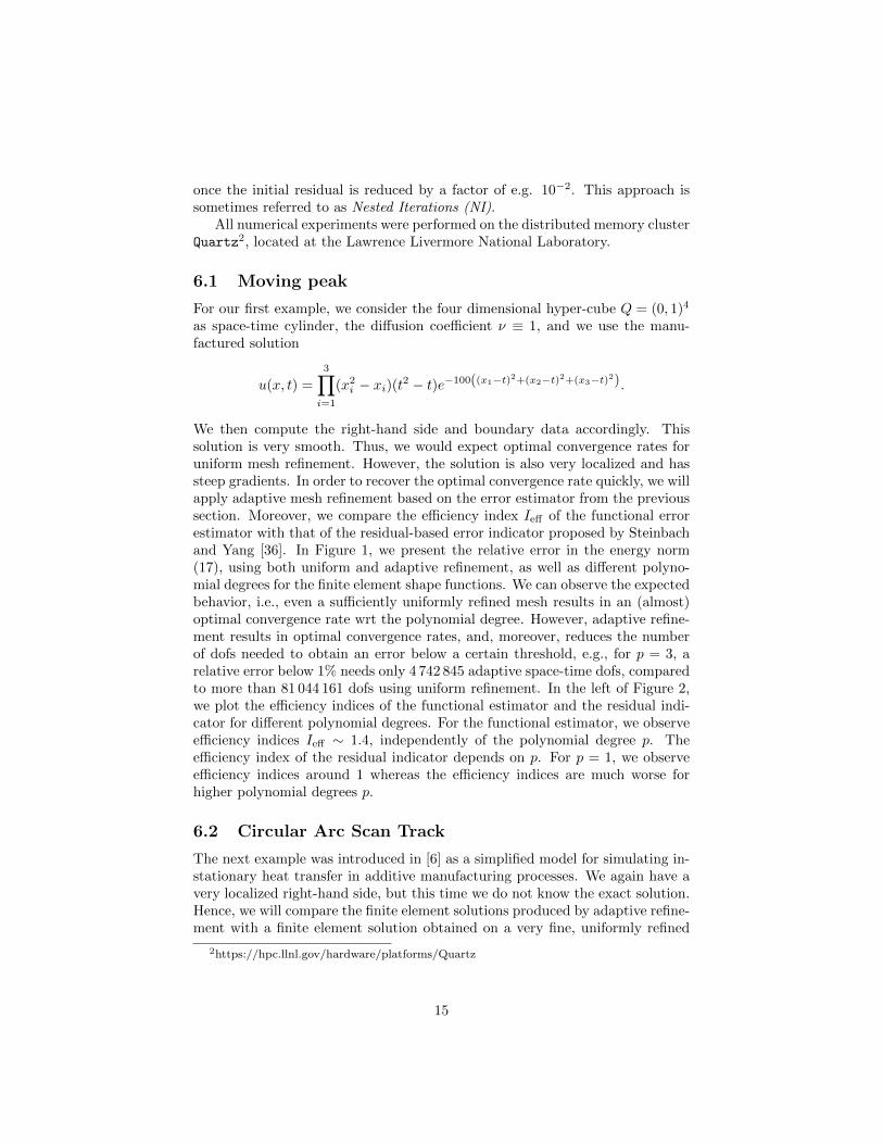
with (x1(t), x2(t)) = (5(1+cos(π(5+2t)/20)), 3+5 sin(π(5+2t)/20)), the initialcondition u0 ≡ 20 on Σ0, and the Neumann boundary condition ν∇xu · ~nx = 0on Σ; see also [6]. In the left plot of Figure 3, we present the convergencerates in the energy-norm ‖.‖h, for different combinations of polynomial degreep and a posteriori error indicators/estimators. The stagnation at the end ofeach line is due to the local mesh resolution of the adaptively refined meshthat is getting smaller than the mesh resolution of the reference solution. Interms of convergence rates, the functional error estimator gives clearly betterrates for linear elements, whereas the rates for quadratic and cubic elementsare almost indistinguishable. However, when we compare the efficiency indexIeff , we observe a notable difference. While Ieff ∼ 1 for the functional estimatorindependently of p, the efficiency index for the residual indicator is also close to 1for linear elements, but much worse when we increase the polynomial degree. In

functional, p = 1 functional, p = 2 functional, p = 3

residual, p = 1 residual, p = 2 residual, p = 3

103 104 105 106

10%

100%

#dofs

103 104 105 106

1

10

#dofs

Figure 3: Convergence rates in the energy norm (left); Efficiency indices Ieff

(right); for different polynomial degrees p, and bulk parameter Ξ = 0.25.

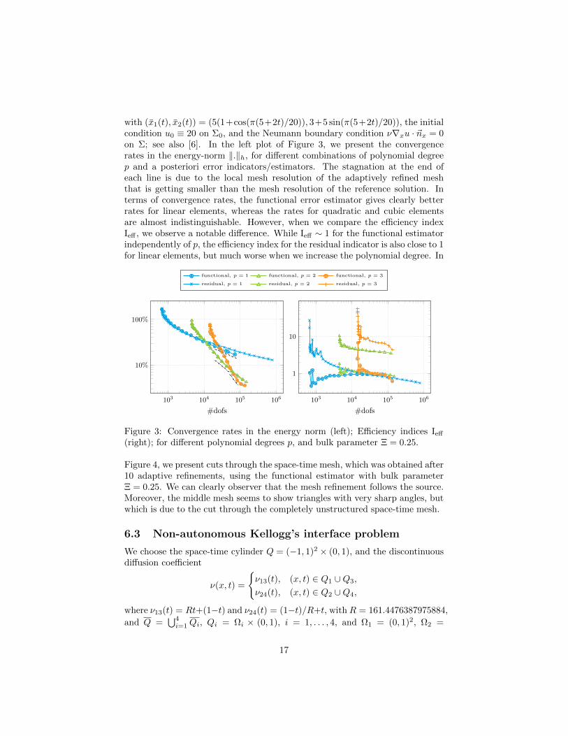
Figure 4, we present cuts through the space-time mesh, which was obtained after10 adaptive refinements, using the functional estimator with bulk parameterΞ = 0.25. We can clearly observer that the mesh refinement follows the source.Moreover, the middle mesh seems to show triangles with very sharp angles, butwhich is due to the cut through the completely unstructured space-time mesh.

6.3 Non-autonomous Kellogg’s interface problem

We choose the space-time cylinder Q = (−1, 1)2 × (0, 1), and the discontinuousdiffusion coefficient

ν(x, t) =

ν13(t), (x, t) ∈ Q1 ∪Q3,

ν24(t), (x, t) ∈ Q2 ∪Q4,

where ν13(t) = Rt+(1−t) and ν24(t) = (1−t)/R+t, withR = 161.4476387975884,

and Q =⋃4i=1Qi, Qi = Ωi × (0, 1), i = 1, . . . , 4, and Ω1 = (0, 1)2, Ω2 =

17

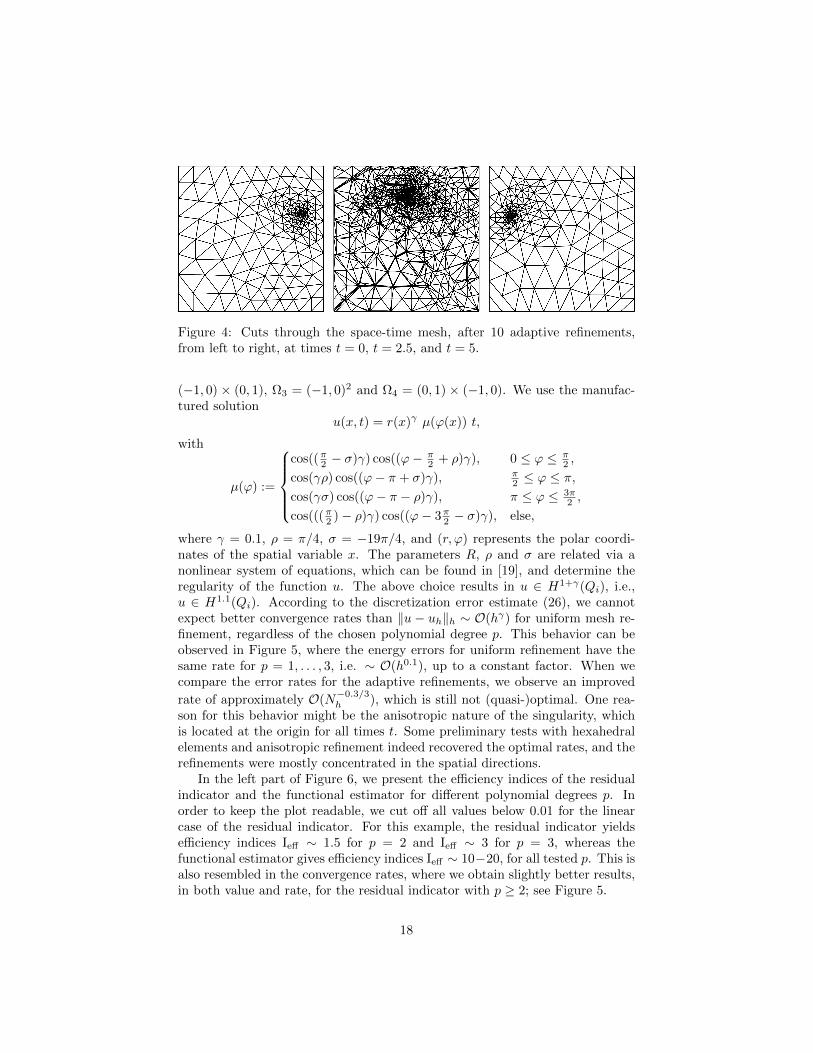
Figure 4: Cuts through the space-time mesh, after 10 adaptive refinements,from left to right, at times t = 0, t = 2.5, and t = 5.

(−1, 0) × (0, 1), Ω3 = (−1, 0)2 and Ω4 = (0, 1) × (−1, 0). We use the manufac-tured solution

u(x, t) = r(x)γ µ(ϕ(x)) t,

with

µ(ϕ) :=

cos((π2 − σ)γ) cos((ϕ− π

2 + ρ)γ), 0 ≤ ϕ ≤ π2 ,

cos(γρ) cos((ϕ− π + σ)γ), π2 ≤ ϕ ≤ π,

cos(γσ) cos((ϕ− π − ρ)γ), π ≤ ϕ ≤ 3π2 ,

cos(((π2 )− ρ)γ) cos((ϕ− 3π2 − σ)γ), else,

where γ = 0.1, ρ = π/4, σ = −19π/4, and (r, ϕ) represents the polar coordi-nates of the spatial variable x. The parameters R, ρ and σ are related via anonlinear system of equations, which can be found in [19], and determine theregularity of the function u. The above choice results in u ∈ H1+γ(Qi), i.e.,u ∈ H1.1(Qi). According to the discretization error estimate (26), we cannotexpect better convergence rates than ‖u − uh‖h ∼ O(hγ) for uniform mesh re-finement, regardless of the chosen polynomial degree p. This behavior can beobserved in Figure 5, where the energy errors for uniform refinement have thesame rate for p = 1, . . . , 3, i.e. ∼ O(h0.1), up to a constant factor. When wecompare the error rates for the adaptive refinements, we observe an improved

rate of approximately O(N−0.3/3h ), which is still not (quasi-)optimal. One rea-

son for this behavior might be the anisotropic nature of the singularity, whichis located at the origin for all times t. Some preliminary tests with hexahedralelements and anisotropic refinement indeed recovered the optimal rates, and therefinements were mostly concentrated in the spatial directions.

In the left part of Figure 6, we present the efficiency indices of the residualindicator and the functional estimator for different polynomial degrees p. Inorder to keep the plot readable, we cut off all values below 0.01 for the linearcase of the residual indicator. For this example, the residual indicator yieldsefficiency indices Ieff ∼ 1.5 for p = 2 and Ieff ∼ 3 for p = 3, whereas thefunctional estimator gives efficiency indices Ieff ∼ 10−20, for all tested p. This isalso resembled in the convergence rates, where we obtain slightly better results,in both value and rate, for the residual indicator with p ≥ 2; see Figure 5.

18

104 105 106 107 108

0.1

0.158

0.251

#dofs

‖u− uh‖h

p = 1, uniform p = 2, uniform p = 3, uniform

p = 1, residual p = 2, residual p = 3, residual

p = 1, functional p = 2, functional p = 3, functional

Figure 5: Example 6.3: Convergence rates for uniform and adaptive refine-ment, with bulk parameter Ξ = 0.25. The line corresponds to a rate of

O(N−0.1/3h ), and the line to O(N

−0.3/3h ).

104 105 106

0.01

0.1

1

10

#dofs

Ieff

residual, p = 1

residual, p = 2

residual, p = 3

functional, p = 1

functional, p = 2

functional, p = 3

Figure 6: Example 6.3: Efficiency indices (left); and plot of the solution at t = 1(right); with marking threshold Ξ = 0.25.

7 Conclusions

We presented and analyzed locally stabilized, consistent, conforming finite ele-ment schemes on completely unstructured simplicial space-time meshes for non-

19

autonomous parabolic initial-boundary value problems. We admitted specialdistributional right-hand sides and (diffusion) coefficients which can be discon-tinuous in space and time. Such data can lead to low-regularity solutions. Wederived a priori estimates for solutions belonging to Hk(Q) with some k ∈ (1, 2].In this case, uniform mesh refinement leads to low convergence rates. More pre-cisely, in the energy norm ‖·‖h, we get O(hk−1) independently of the polynomialdegree p of the shape functions used on the reference element. This theoreticalresult is confirmed by all numerical experiments performed. The convergencerate can drastically be improved by adaptivity. In order to devise an adap-tive finite element scheme, one needs an local error indicator derived from aposteriori discretization error estimators. In contrast to elliptic boundary-valueproblems where adaptive finite element schemes are well established in theoryand practice, the picture is different with respect to fully adaptive space-timefinite element methods. We numerically studied the residual indicator proposedby O. Steinbach and H. Yang, and indicators based on functional a posterioriestimators proposed by S. Repin, where we only used the first part of the ma-jorant as local error indicator. This choice already yields an indicator that isreliable and provides an upper bound with efficiency indices that are close to1 for the first two examples, whereas the residual indicator is only reliable forhigher polynomial degrees, with efficiency indices much bigger than 1. However,for the third example, the residual indicator results in much better efficiency in-dices than the functional estimator/indicator. The reduced performance of thelatter is most likely due to two reasons: first, we only use the continuous finiteelement spaces (Vh)d for flux recovering that do not reflect the right behavior ofthe fluxes across material interfaces that arise in the third example, and second,the singularity is highly anisotropic in space and time, i.e., we would need avery high spatial resolution, but relatively coarse one in time. Anisotropic re-finement techniques, in particular, on simplicial space-time meshes is certainlya challenge that will be a topic of our future research on space-time adaptivity.

8 Acknowledgment

The authors would like to thank the Austrian Science Fund (FWF) for the fi-nancial support under the grant DK W1214-04. Furthermore, we would like tothank Sergey Repin for discussing with us the use of functional error estimatesduring his visits at Linz. Andreas Schafelner wants to thank Panayot Vassilevskifor the support during his visits at the Lawrence Livermore National Labora-tory, for many fruitful discussions, and for the possibility to compute on thedistributed memory cluster Quartz in Livermore.

References

[1] Bank, R. E., Vassilevski, P. S., and Zikatanov, L. T. Arbitrarydimension convection-diffusion schemes for space-time discretizations. J.

20

Comput. Appl. Math. 310 (2017), 19–31.

[2] Behr, M. Simplex space-time meshes in finite element simulations. Inter-nat. J. Numer. Methods Fluids 57 (2008), 1421–1434.

[3] Bergh, J., and Lofstrom, J. Interpolation spaces. An Introduction,vol. 223. Springer, Berlin, 1976.

[4] Braess, D. Finite Elemente. Theorie, schnelle Loser und Anwendungenin der Elastizitatstheorie, 5th revised ed. Springer Spektrum, Berlin, 2013.

[5] Brenner, S. C., and Scott, L. R. The mathematical theory of finite ele-ment methods, third ed., vol. 15 of Texts in Applied Mathematics. Springer,New York, 2008.

[6] Carraturo, M., Giannelli, C., Reali, A., and Vazquez, R. Suit-ably graded THB-spline refinement and coarsening: Towards an adaptiveisogeometric analysis of additive manufacturing processes. Comput. Meth-ods Appl. Mech. Engrg. 348 (2019), 660–679.

[7] Carstensen, C., Feischl, M., Page, M., and Praetorius, C. Ax-ioms of adaptivity. Comput. Methods Appl. Math. 67 (2014), 1195–1253.

[8] Ciarlet, P. G. The Finite Element Method for Elliptic Problems. North-Holland Publishing Co., Amsterdam-New York-Oxford, 1978.

[9] C.Johnson, and Saranen, J. Streamline diffusion methods for the in-compressible Euler and Navier-Stokes equations. Math. Comp. 47, 175(1986), 1–18.

[10] Clement, P. Approximation by finite element functions using local reg-ularization. Rev. Francaise Automat. Informat. Recherche OperationnelleSer. 9, R-2 (1975), 77–84.

[11] Devaud, D., and Schwab, C. Space–time hp-approximation of parabolicequations. Calcolo 55, 3 (2018), 35.

[12] Dier, D. Non-autonomous maximal regularity for forms of bounded vari-ation. J. Math. Anal. Appl. 425 (2015), 33–54.

[13] Dorfler, W. A convergent adaptive algorithm for Poisson’s equation.SIAM J. Numer. Anal. 33, 3 (1996), 1106–1124.

[14] Gander, M. J. 50 years of time parallel integration. In Multiple Shoot-ing and Time Domain Decomposition. Springer Verlag, Heidelberg, Berlin,2015, pp. 69–114.

[15] Heuer, N. On the equivalence of fractional-order Sobolev semi-norms. J.Math. Anal. Appl. 417, 2 (2014), 505–518.

21

[16] Hughes, T., and Brooks, A. A multidimensional upwind scheme withno crosswind diffusion. In Finite Element Methods for Convection Domi-nated Flows (New York, 1979), T. Hughes, Ed., vol. 34 of AMD, ASME.

[17] Hughes, T., Franca, L., and Hulbert, G. A new finite element formu-lation for computational fluid dynamics: VIII. The Galerkin/least-squaresmethod for advection-diffusive equations. Comput. Methods Appl. Mech.Engrg. 73 (1989), 173–189.

[18] Karyofylli, V., Wendling, L., Make, M., Hosters, N., and Behr,M. Simplex space-time meshes in thermally coupled two-phase flow simu-lations of mold filling. Computers and Fluids (2019), 104261.

[19] Kellogg, R. B. On the Poisson equation with intersecting interfaces.Appl. Anal. 4 (1974), 101–129.

[20] Ladyzhenskaya, O. On solvability of the basic boundary value problemsof parabolic and hyperbolic type. Dokl. Alad. Nauk SSSR 97 (1954), 395–398. (in Russian).

[21] Ladyzhenskaya, O. A. The boundary value problems of mathematicalphysics, vol. 49 of Applied Mathematical Sciences. Springer-Verlag, NewYork, 1985. Translated from the Russian edition, Nauka, Moscow, 1973.

[22] Ladyzhenskaya, O. A., Solonnikov, V. A., and Uraltseva, N. Lin-ear and quasilinear equations of parabolic type. Nauka, Moscow, 1967.

[23] Langer, U., Moore, S., and Neumuller, M. Space-time isogeometricanalysis of parabolic evolution equations. Comput. Methods Appl. Mech.Engrg. 306 (2016), 342–363.

[24] Langer, U., Neumuller, M., and Schafelner, A. Space-time FiniteElement Methods for Parabolic Evolution Problems with Variable Coeffi-cients. In Advanced Finite Element Methods with Applications - SelectedPapers from the 30th Chemnitz Finite Element Symposium 2017, T. Apel,U. Langer, A. Meyer, and O. Steinbach, Eds., vol. 128 of Lecture Notes inComputational Science and Engineering (LNCSE). Springer, Berlin, Hei-delberg, New York, 2019, ch. 13, pp. 247–275.

[25] Lions, J. L. Optimal control of systems governed by partial differentialequations., vol. 170. Springer, Berlin, 1971.

[26] Mantzaflaris, A., Scholz, F., and Toulopoulos, I. Low-rank space-time decoupled isogeometric analysis for parabolic problems with varyingcoefficients. Comput. Methods Appl. Math. 19, 1 (2019), 123–136.

[27] MFEM: Modular finite element methods library. mfem.org.

[28] Pfeiler, C.-M., and Praetorius, D. Dorfler marking with minimalcardinality is a linear complexity problem, 2019. arXiv:1907.13078.

22

[29] Pyrhonen, J., Jokinen, T., and Hrabovcova, V. Design of RotatingElectrical Machines. John Wiley & Sons, 2008.

[30] Repin, S. Estimates of deviations from exact solutions of initial-boundaryvalue problem for the heat equation. Rend. Mat. Acc. Lincei 13, 9 (2002),121–133.

[31] Repin, S. A posteriori estimates for partial differential equations, vol. 4of Radon Series on Computational and Applied Mathematics. de Gruyter,Berlin, 2008.

[32] Saad, Y. A flexible inner-outer preconditioned GMRES algorithm. SIAMJ. Sci. Comput. 14, 2 (1993), 461–469.

[33] Scott, L. R., and Zhang, S. Finite element interpolation of nonsmoothfunctions satisfying boundary conditions. Math. Comput. 54, 190 (1990),483–493.

[34] Steinbach, O. Space-time finite element methods for parabolic problems.Comput. Methods Appl. Math. 15, 4 (2015), 551–566.

[35] Steinbach, O., and Yang, H. Comparison of algebraic multigrid meth-ods for an adaptive space-time finite-element discretization of the heatequation in 3d and 4d. Numer. Linear Algebra Appl. 25, 3 (2018), e2143nla.2143.

[36] Steinbach, O., and Yang, H. Space–time finite element methods forparabolic evolution equations: Discretization, a posteriori error estimation,adaptivity and solution. In Space-Time Methods: Application to PartialDifferential Equations, vol. 25 of Radon Series on Computational and Ap-plied Mathematics. de Gruyter, 2019, pp. 207–248.

[37] Zienkiewicz, O. C., and Zhu, J. Z. The superconvergent patch recoveryand a posteriori error estimates. I: The recovery technique. Int. J. Numer.Methods Eng. 33, 7 (1992), 1331–1364.

[38] Zienkiewicz, O. C., and Zhu, J. Z. The superconvergent patch recoveryand a posteriori error estimates. II: Error estimates and adaptivity. Int.J. Numer. Methods Eng. 33, 7 (1992), 1365–1382.

23

Technical Reports of the Doctoral Program

“Computational Mathematics”

2020

2020-01 N. Smoot: A Single-Variable Proof of the Omega SPT Congruence Family Over Powers of 5Feb 2020. Eds.: P. Paule, S. Radu

2020-02 A. Schafelner, P.S. Vassilevski: Numerical Results for Adaptive (Negative Norm) ConstrainedFirst Order System Least Squares Formulations March 2020. Eds.: U. Langer, V. Pillwein

2020-03 U. Langer, A. Schafelner: Adaptive space-time finite element methods for non-autonomousparabolic problems with distributional sources March 2020. Eds.: B. Juttler, V. Pillwein

2019

2019-01 A. Seiler, B. Juttler: Approximately C1-smooth Isogeometric Functions on Two-Patch Do-mains Jan 2019. Eds.: J. Schicho, U. Langer

2019-02 A. Jimenez-Pastor, V. Pillwein, M.F. Singer: Some structural results on Dn-finite functions

Feb 2019. Eds.: M. Kauers, P. Paule

2019-03 U. Langer, A. Schafelner: Space-Time Finite Element Methods for Parabolic Evolution Prob-lems with Non-smooth Solutions March 2019. Eds.: B. Juttler, V. Pillwein

2019-04 D. Dominici, F. Marcellan: Discrete semiclassical orthogonal polynomials of class 2 April

2019. Eds.: P. Paule, V. Pillwein

2019-05 D. Dominici, V. Pillwein: A sequence of polynomials generated by a Kapteyn series of thesecond kind May 2019. Eds.: P. Paule, J. Schicho

2019-06 D. Dominici: Mehler-Heine type formulas for the Krawtchouk polynomials June 2019. Eds.:

P. Paule, M. Kauers

2019-07 M. Barkatou, A. Jimenez-Paster: Linearizing Differential Equations Riccati Solutions as Dn-Finite Functions June 2019. Eds.: P. Paule, M. Kauers

2019-08 D. Dominici: Recurrence coefficients of Toda-type orthogonal polynomials I. Asymptotic anal-ysis. July 2019. Eds.: P. Paule, M. Kauers

2019-09 M. Neumuller, M. Schwalsberger: A parallel space-time multigrid method for the eddy-currentequation Nov 2019. Eds.: U. Langer, R. Ramlau

2019-10 N. Smoot: An Implementation of Radus Ramanujan-Kolberg Algorithm Nov 2019. Eds.:

P. Paule, S. Radu

2019-11 S. Radu, N. Smoot: A Method of Verifying Partition Congruences by Symbolic ComputationDec 2019. Eds.: P. Paule, V. Pillwein

2019-12 J. Qi: How to avoid collision of 3D-realization for moving graphs Dec 2019. Eds.: J. Schicho,

M. Kauers

The complete list since 2009 can be found at

https://www.dk-compmath.jku.at/publications/

Doctoral Program

“Computational Mathematics”

Director:Dr. Veronika PillweinResearch Institute for Symbolic Computation

Deputy Director:Prof. Dr. Bert JuttlerInstitute of Applied Geometry

Address:Johannes Kepler University LinzDoctoral Program “Computational Mathematics”Altenbergerstr. 69A-4040 LinzAustriaTel.: ++43 732-2468-6840

E-Mail:office@dk-compmath.jku.at

Homepage:http://www.dk-compmath.jku.at

Submissions to the DK-Report Series are sent to two members of the Editorial Boardwho communicate their decision to the Managing Editor.