1

Adaptive Signal Processing

Adaptiivne signaalitöötlus

Leon H. Sibul

Kevadsemester, 2007

2

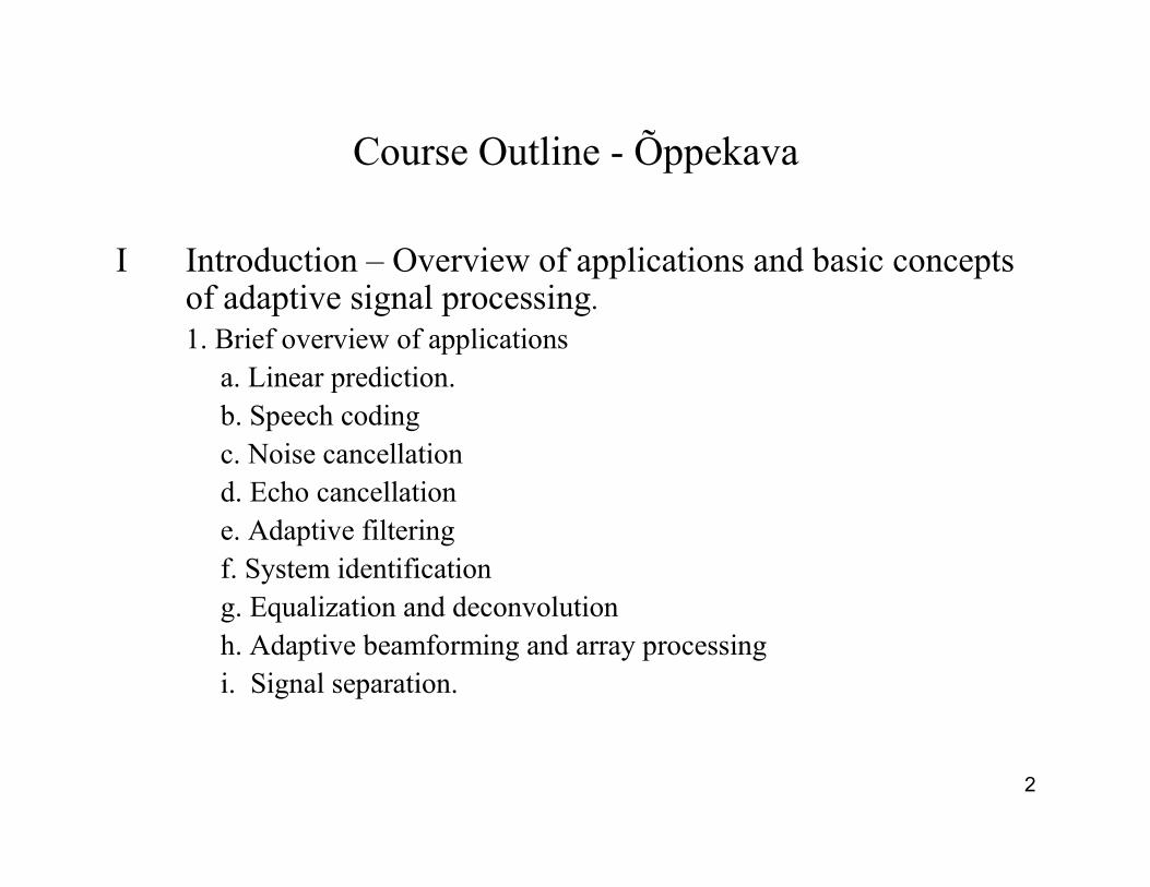
Course Outline - Õppekava

I Introduction – Overview of applications and basic concepts of adaptive signal processing.1. Brief overview of applications

a. Linear prediction.b. Speech codingc. Noise cancellationd. Echo cancellatione. Adaptive filteringf. System identificationg. Equalization and deconvolutionh. Adaptive beamforming and array processingi. Signal separation.

3

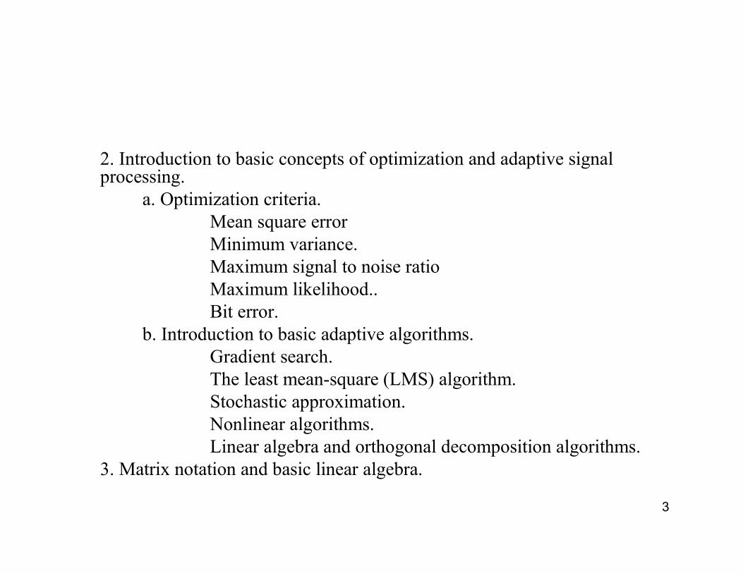
2. Introduction to basic concepts of optimization and adaptive signal processing.

a. Optimization criteria.Mean square errorMinimum variance.Maximum signal to noise ratioMaximum likelihood..Bit error.

b. Introduction to basic adaptive algorithms.Gradient search. The least mean-square (LMS) algorithm.Stochastic approximation.Nonlinear algorithms.Linear algebra and orthogonal decomposition algorithms.

3. Matrix notation and basic linear algebra.

4

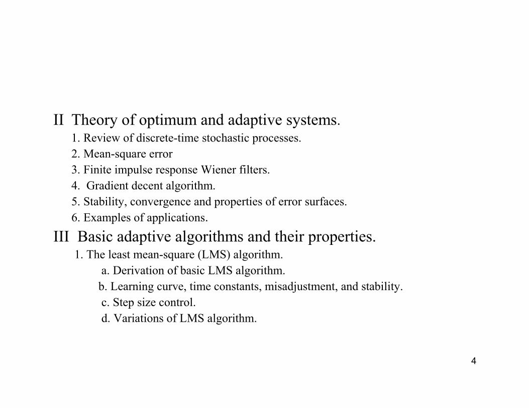
II Theory of optimum and adaptive systems.1. Review of discrete-time stochastic processes.

2. Mean-square error

3. Finite impulse response Wiener filters.

4. Gradient decent algorithm.

5. Stability, convergence and properties of error surfaces.

6. Examples of applications.

III Basic adaptive algorithms and their properties.1. The least mean-square (LMS) algorithm.

a. Derivation of basic LMS algorithm.

b. Learning curve, time constants, misadjustment, and stability.

c. Step size control.

d. Variations of LMS algorithm.

5

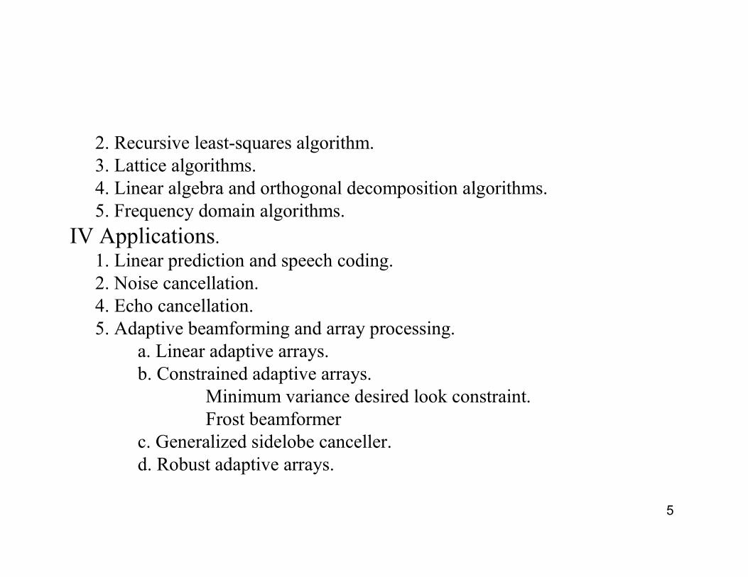
2. Recursive least-squares algorithm.3. Lattice algorithms.4. Linear algebra and orthogonal decomposition algorithms.5. Frequency domain algorithms.

IV Applications.1. Linear prediction and speech coding.2. Noise cancellation.4. Echo cancellation.5. Adaptive beamforming and array processing.

a. Linear adaptive arrays.b. Constrained adaptive arrays.

Minimum variance desired look constraint.Frost beamformer

c. Generalized sidelobe canceller.d. Robust adaptive arrays.

6

Bibliography

1. Vary, P. and Martin, R., Digital Speech Transmission- Enhancement, Coding and Error Concealment, John Wiley & Sons, LTD., Chichester, England, 2006.

2. Schobben, D. W. E., Real Time Concepts in Acoustics, KluwerAcademic Publishers, Dordrecht, The Netherlands, 2001.

3. Poularikas, A. D. and Ramadan, z. M., Adaptive Filter Primer with MATLAB, CRC, Taylor & Francis, Boca Raton, FL., USA, 2006.

4. Haykin, S., Adaptive Filter Theory, Third Ed., Prentice Hall, Upper Saddle River, NJ, USA, 1996.

5. Alexander, S.T., Adaptive Signal Processing, Theory and Applications, Springer-Verlag, New York, USA, 1986.

6. Widrow, B. and Sterns, S.D., Adaptive Signal Processing, Prentice-Hall, Englewood Cliffs, NJ, USA, 1985.

7

7. Adaptive Signal Processing, Edited by L.H Sibul, IEEE Press, New York, USA 1987.

8. Manzingo R.A. and Miller, T.W., Introduction to Adaptive Arrays, John Wiley-Interscience, New York, USA, 1980.

9. Swanson C. D., Signal Processing for Intelligent Sensors, Marcel Dekker, New York, USA, 2000.

10. Colub,G.H., and Van Loan, Matrix Computations, The Johns Hopkins University Press, Baltimore, MD, USA, 1983.

11. Tammeraid, Ivar, Lineaaaralgebra rakendused, TTÜ Kirjastus, Tallinn, Estonia, 1999. 2. Lineaaralgebra avutusmeetodid. 2.3 Singulaarlahutus.

12. Van Trees, H.L., Optimum Array Processing, Part IV of Detetection, Estimation and Modulation Theory, Wiley-Interscience, New York, USA, 2002. Chapter 6 – Optimum Waveform Estimation, Chapter 7-Adaptive Beamformers, A- Matrix Operations.

8

13. Allen, B., and Ghavami, M., Adaptive Array Systems; Fundamentals and Applications,Wiley, Chichester, England, 2005.

14. Cichocki, A., and Amari, S-I, Adaptive Blind Signal and Image Processing, Wiley,West Sussex, England, 2002.

9

Õppenõuded ja hindamine:

1. Semestri töö ja aruanne: Rakendusülesandelahendus kasutades adaptiivset signaalitöötlust jaMATLABi. Teema valik oleneb õpilase huvidest jaoskustest. 60% hindest.

2. Kodutööd ja harjutused. 20% hindest Kodutööd jaharjutused peavad olema sooritatud, et lõppeksamile pääseda.

3. Suuline lõppeksam. Käsitab peamiselt semestri töödja põhiteooriat. Õpilane võib kasutada kuni 20 lehekülge enda tehtud märkmeid. 20% hindest.

10

Semestritöö ja aruande nõuded.

1. Sissejuhastus- Ülesande definitsioon, selle rakendus, selletähtsus ja lühike aruande ülevaade.

2. Teooria ja algoritmi tuletus.

3. Kasutatud algoritm ja kuidas see lahendab käesolevarakendusülesande.

4. MATLABIi programm.

5. Graafikud ja nende selgitus.

6. Tulemuste analüüs, selgitused ja järeldused.

7. Kokkuvõte.

8. Kirjandus.Märkused: Word, Powerpoint, PDF, umbes 10 kuni 15 lehekülge, eesti või inglise

keeles.

11

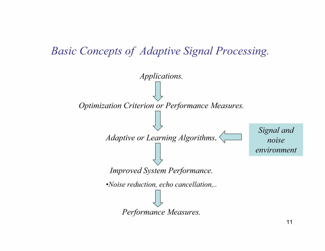
Basic Concepts of Adaptive Signal Processing.

Applications.

Optimization Criterion or Performance Measures.

Adaptive or Learning Algorithms.

Improved System Performance.

•Noise reduction, echo cancellation,..

Performance Measures.

Signal and

noise

environment

12

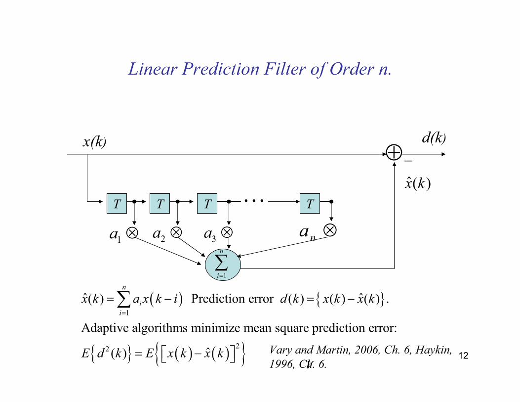
Linear Prediction Filter of Order n.

T T T T

1a ⊗

1

n

i=∑

2a ⊗ 3a ⊗ na ⊗

⊕d(k)x(k)

…ˆ( )x k

−

( ) { }

{ } ( ) ( ){ }

1

22

ˆ ˆ( ) Prediction error ( ) ( ) ( ) .

Adaptive algorithms minimize mean square prediction error:

ˆ( )

n

i

i

x k a x k i d k x k x k

E d k E x k x k

=

= − = −

= −

∑

V

Vary and Martin, 2006, Ch. 6, Haykin,

1996, Ch. 6.

13

Optimum Linear Prediction.

{ } ( )( ){ }{ }

( ) ( ) ( ) ( ){ }

{ }( ){ }

( ) ( ){ } ( ) ( ) ( )

22

2

2 2

2

2

1

ˆMinimize mean square error: ( ) ( ) .

( )2 2 0 1,2,... .

( )2 0 Minimum.

=

n

i

i

E d k E x k x k

E d k d kE d k E d k x k n

a a

E d kE x k

a

E d k x k E x k a x k i x k

E

λ λ

λ

λ λ

λ

λ λ=

= −

∂ ∂ = = − − = =

∂ ∂

∂= − ≥

∂

− = − − −

∑

( ) ( ){ } ( ) ( )1

1

{ }

( ) ( ) 0

n

i

i

n

xx xx

i

x k x k a E x k i x k

R R i

λ λ

λ λ

=

=

− − − −

= − − =

∑

∑

14

Optimum Linear Prediction.

1

2

(1) (0) ( 1) (1 )

(2) (1) (0) (2 )

( ) ( 1) ( 2) (0)

In vector matrix notation:

is a positive defi

xx xx xx xx

xx xx xx xx

xx xx xx xx n

R R R R n a

R R R R n a

R n R n R n R a

ϕ ϕ−

− − − =

− −

= = 1

xx xx opt xx xx xxR a a R R

⋯

⋯

⋮ ⋮ ⋮ ⋮ ⋮

⋯

( )

1 2

2 2 2

2 2

2

2

nite, Toeplitz matrix.

ˆ( ) ( 1) ( 1) ( 1), ( 2),..., ( )

( , ,..., )

2 2

prediction gain

T

T

n

d x x

x x

xp

d

x k k k x k x k x k n

a a a

G

σ σ ϕ σ ϕ ϕ ϕ ϕ

σ ϕ ϕ σ ϕ

σσ

− − −

−

= − − − − −

= − + = − +

= − = −

=

T

T T T 1 T 1 1

xx xx xx xx xx xx xx xx xx xx

T 1 T

xx xx xx xx

a x x

a

a a R a R R R R

R a

≜

≜

.

15

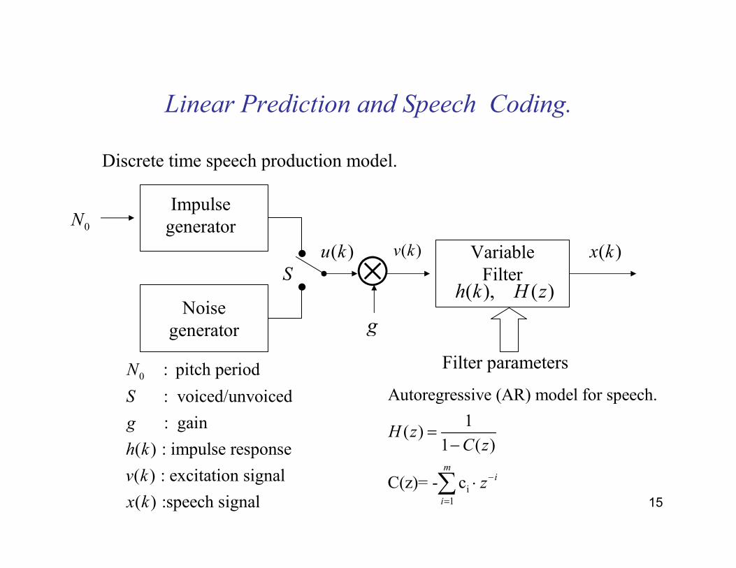
Linear Prediction and Speech Coding.

0N

Noisegenerator

•

• ⊗VariableFilter

Impulse generator

( ), ( )h k H z

Filter parameters

Discrete time speech production model.

( )u k ( )v k ( )x k

g

S

0 : pitch period

: voiced/unvoiced

: gain

( ) : impulse response

( ) : excitation signal

( ) :speech signal

N

S

g

h k

v k

x ki

1

Autoregressive (AR) model for speech.

1( )

1 ( )

C(z)= - cm

i

i

H zC z

z−

=

=−

⋅∑

16

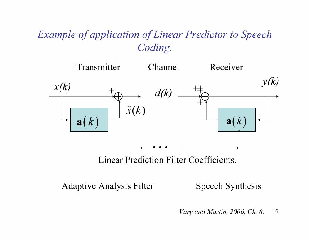
Example of application of Linear Predictor to Speech

Coding.

Transmitter Channel Receiver

⊕ ⊕-+

++++

( )ka ( )ka

Linear Prediction Filter Coefficients.

Adaptive Analysis Filter Speech Synthesis

x(k)

ˆ( )x k

d(k)y(k)

⋯

Vary and Martin, 2006, Ch. 8.

17

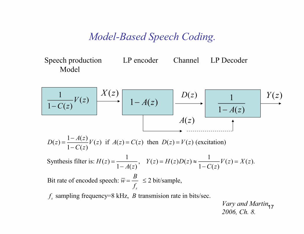
Model-Based Speech Coding.

Speech production LP encoder Channel LP DecoderModel

1( )

1 ( )V z

C z−

( )X z1 ( )A z−

( )D z 1

1 ( )A z−

( )Y z

( )A z

1 ( )( ) ( ) if ( ) ( ) then ( ) ( ) (excitation)

1 ( )

1 1Synthesis filter is: ( ) , ( ) ( ) ( ) ( ) ( ).

1 ( ) 1 ( )

Bit rate of encoded speech: 2 bit/sample,

sampling frequencs

s

A zD z V z A z C z D z V z

C z

H z Y z H z D z V z X zA z C z

Bw

f

f

−= = =

−

= = ≈ =− −

= ≤

y=8 kHz, transmision rate in bits/sec.B

Vary and Martin,

2006, Ch. 8.

18

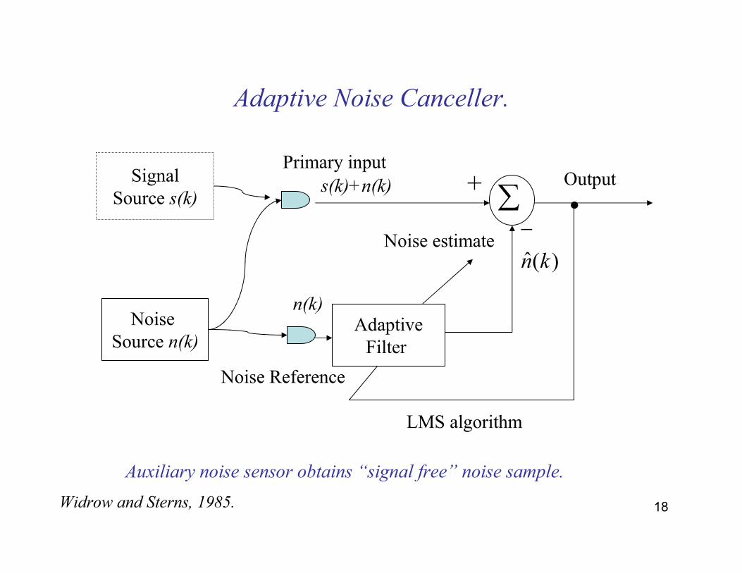
Adaptive Noise Canceller.

Primary inputSignal

Source s(k)

Noise Source n(k)

∑∑+

AdaptiveFilter

LMS algorithm

Noise Reference

Noise estimateˆ( )n k

−•Outputs(k)+n(k)

n(k)

Auxiliary noise sensor obtains “signal free” noise sample.

Widrow and Sterns, 1985.

19

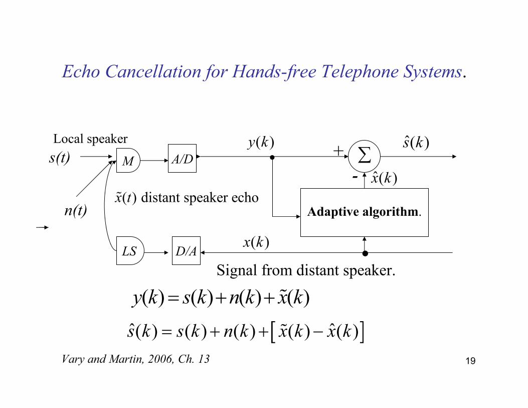
Echo Cancellation for Hands-free Telephone Systems.

Local speaker

M

LS

A/D

D/A

( ) distant speaker echox tɶ

s(t)

n(t)

∑

Adaptive algorithm.

Signal from distant speaker.

( ) ( ) ( ) ( )y k s k n k x k= + + ɶ

ˆ( )x k

( )x k

-

ˆ( )s k

[ ]ˆ ˆ( ) ( ) ( ) ( ) ( )s k s k n k x k x k= + + −ɶ

( )y k+•

•

Vary and Martin, 2006, Ch. 13

20

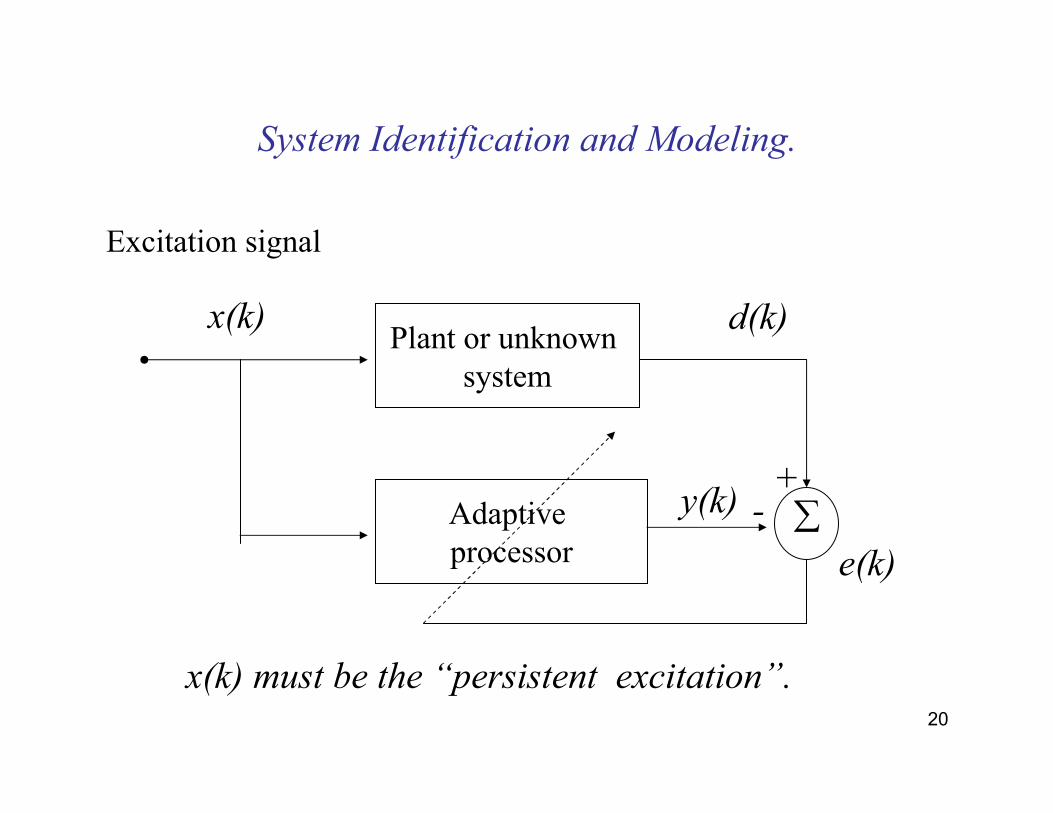
System Identification and Modeling.

Excitation signal

Plant or unknown system

Adaptive processor

∑

x(k) d(k)

e(k)

+-y(k)

x(k) must be the “persistent excitation”.

21

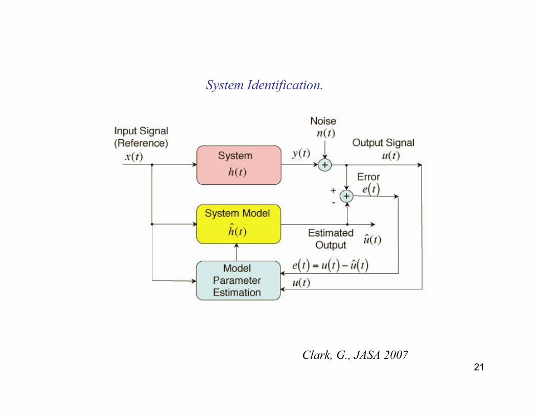
System Identification.

Clark, G., JASA 2007

22

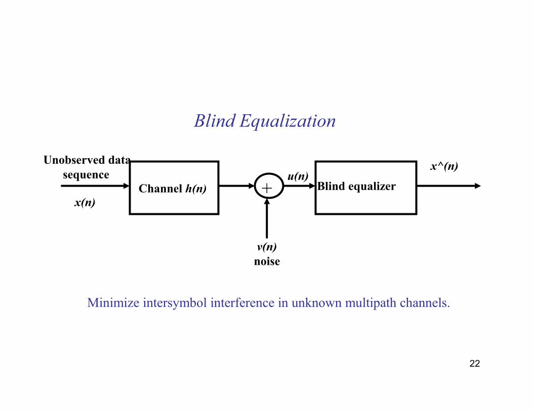
Blind Equalization

Channel h(n)

Unobserved data

sequenceBlind equalizer

x(n)

v(n)

noise

u(n)

Minimize intersymbol interference in unknown multipath channels.

x^(n)

+

23

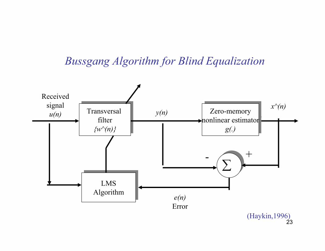
Bussgang Algorithm for Blind Equalization

Transversal filter{w^(n)}

Transversal filter{w^(n)}

Zero-memorynonlinear estimator

g(.)

Zero-memorynonlinear estimator

g(.)

LMSAlgorithmLMS

Algorithm

∑

Received signal u(n) y(n)

x^(n)

+-

e(n)

Error(Haykin,1996)

24

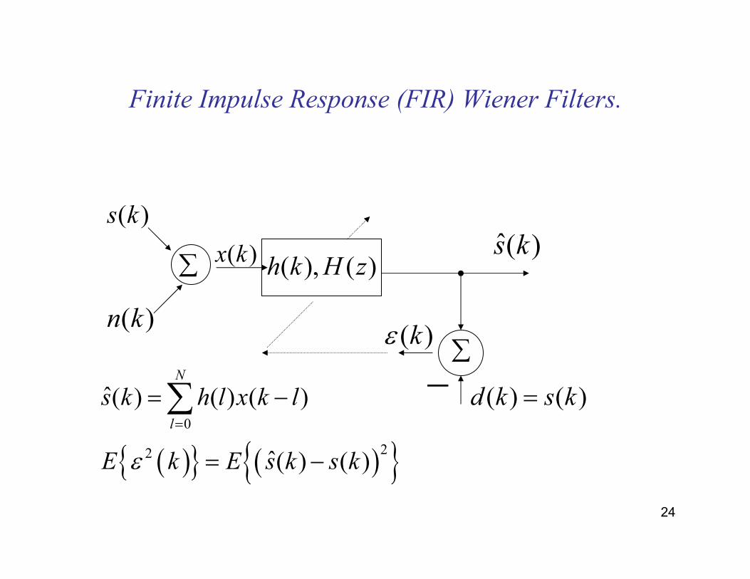
Finite Impulse Response (FIR) Wiener Filters.

( )s k

( )n k

∑ ( )x k ( ), ( )h k H z

∑

ˆ( )s k

( ) ( )d k s k=−( )kε

( ){ } ( ){ }0

22

ˆ( ) ( ) ( )

ˆ( ) ( )

N

l

s k h l x k l

E k E s k s kε

=

= −

= −

∑

25

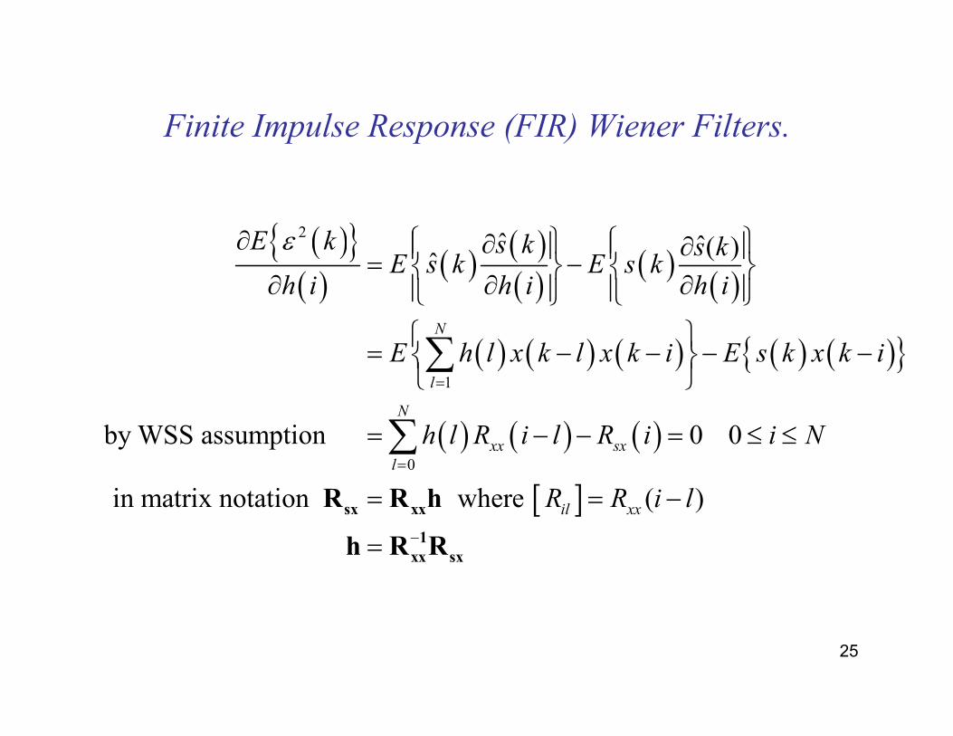
Finite Impulse Response (FIR) Wiener Filters.

( ){ }( )

( ) ( )( )

( )( )

( ) ( ) ( ) ( ) ( ){ }

( ) ( ) ( )

[ ]

2

1

0

ˆ ˆ( )ˆ

by WSS assumption 0 0

in matrix notation where ( )

N

l

N

xx sx

l

il xx

E k s k s kE s k E s k

h i h i h i

E h l x k l x k i E s k x k i

h l R i l R i i N

R R i l

ε

=

=

−

∂ ∂ ∂ = −

∂ ∂ ∂

= − − − −

= − − = ≤ ≤

= = −

=

∑

∑

sx xx

1

xx sx

R R h

h R R

26

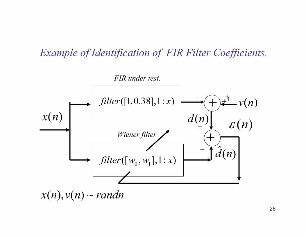
Example of Identification of FIR Filter Coefficients.

( )x n

0 1([ , ],1: )filter w w x

([1,0.38],1: )filter x + ( )v n

+

+ +++

+

_ ˆ( )d n

( )nε( )d n

( ), ( )x n v n randn∼

FIR under test.

Wiener filter

+

+

27

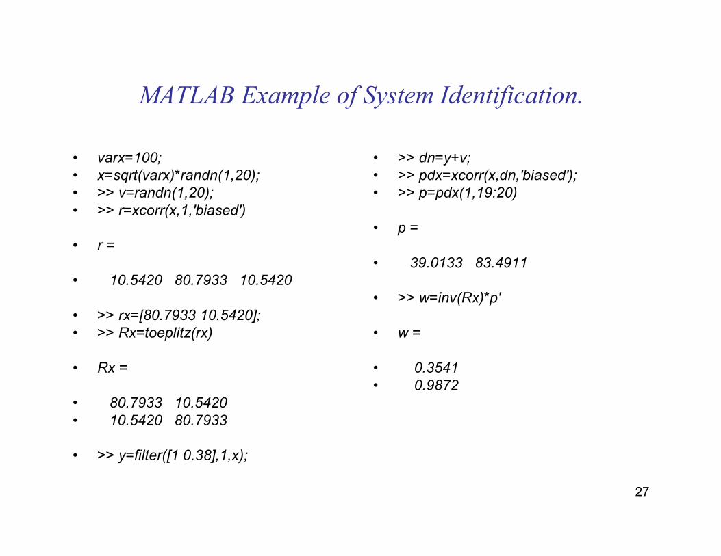
MATLAB Example of System Identification.

• varx=100;• x=sqrt(varx)*randn(1,20); • >> v=randn(1,20);• >> r=xcorr(x,1,'biased')

• r =

• 10.5420 80.7933 10.5420

• >> rx=[80.7933 10.5420];• >> Rx=toeplitz(rx)

• Rx =

• 80.7933 10.5420• 10.5420 80.7933

• >> y=filter([1 0.38],1,x);

• >> dn=y+v;• >> pdx=xcorr(x,dn,'biased');• >> p=pdx(1,19:20)

• p =

• 39.0133 83.4911

• >> w=inv(Rx)*p'

• w =

• 0.3541• 0.9872

28

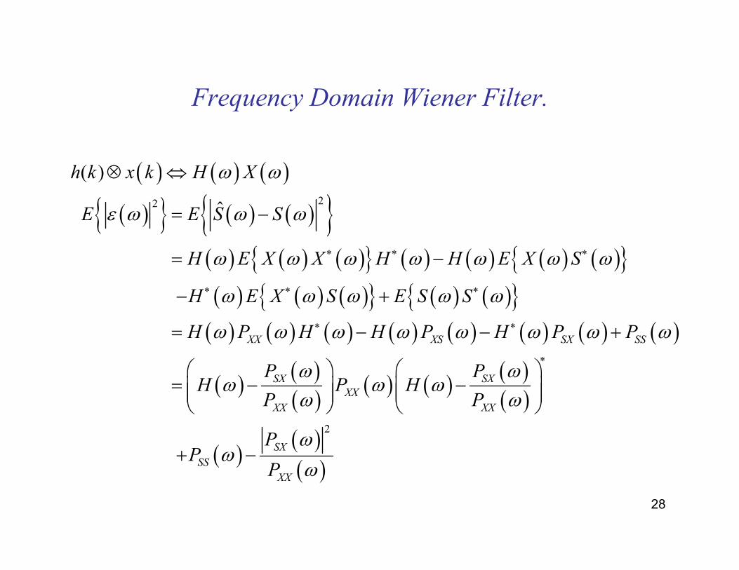
Frequency Domain Wiener Filter.

( ) ( ) ( )

( ){ } ( ) ( ){ }( ) ( ) ( ){ } ( ) ( ) ( ) ( ){ }( ) ( ) ( ){ } ( ) ( ){ }( ) ( ) ( ) ( ) ( ) ( ) ( ) ( )

( ) ( )( )

( ) ( ) ( )( )

( )( )( )

22

2

( )

ˆ

XX XS SX SS

SX SX

XX

XX XX

SX

SS

XX

h k x k H X

E E S S

H E X X H H E X S

H E X S E S S

H P H H P H P P

P PH P H

P P

PP

P

ω ω

ε ω ω ω

ω ω ω ω ω ω ω

ω ω ω ω ω

ω ω ω ω ω ω ω ω

ω ωω ω ω

ω ω

ωω

ω

∗ ∗ ∗

∗ ∗ ∗

∗ ∗

∗

⊗ ⇔

= −

= −

− +

= − − +

= − −

+ −

29

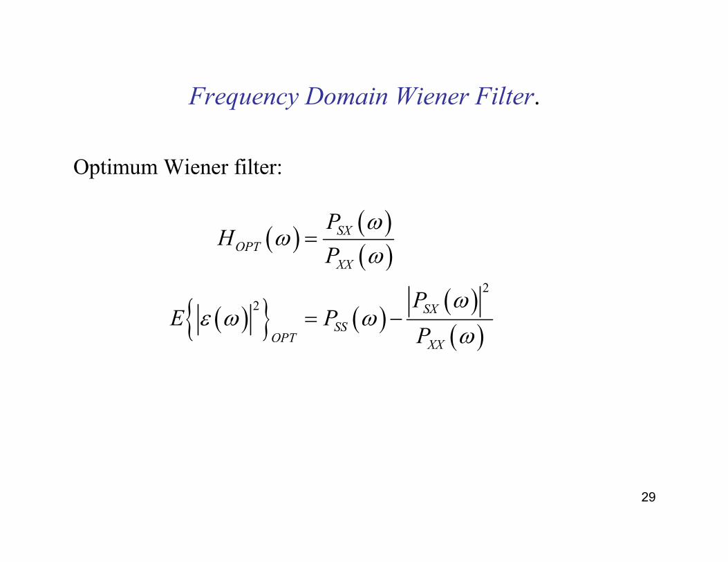
Frequency Domain Wiener Filter.

Optimum Wiener filter:

( ) ( )( )

( ){ } ( )( )( )

2

2

SX

OPT

XX

SX

SSOPT

XX

PH

P

PE P

P

ωω

ω

ωε ω ω

ω

=

= −

30

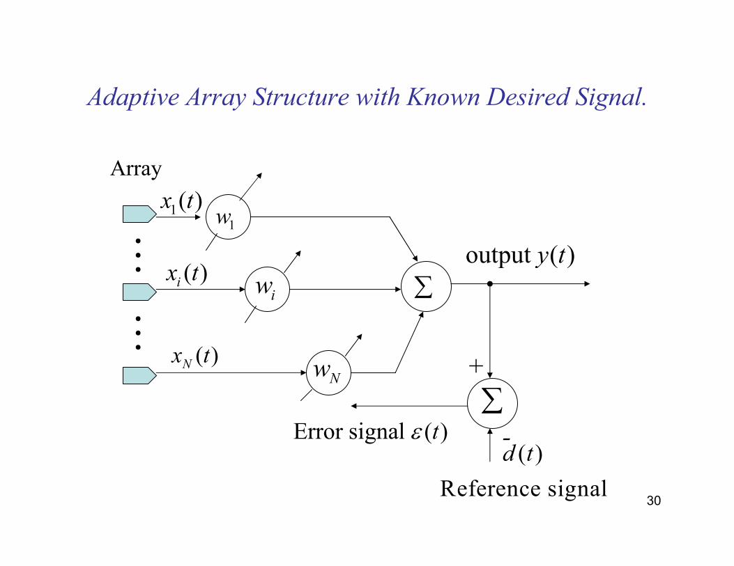
Adaptive Array Structure with Known Desired Signal.

Array

⋮

⋮

1( )x t

( )ix t

( )Nx t

1w

iw

Nw

∑output ( )y t

∑

( )

Reference signal

d tError signal ( )tε

+

-

31

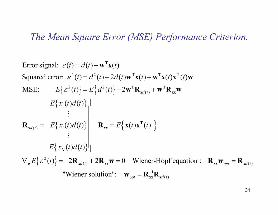
The Mean Square Error (MSE) Performance Criterion.

{ } { }{ }

{ }

{ }

{ }

2 2

2 2( )

1

( )

2

Error signal: ( ) ( ) ( )

Squared error: ( ) ( ) 2 ( ) ( ) ( ) ( )

MSE: ( ) ( ) 2

( ) ( )

( ) ( ) ( ) ( )

( ) ( )

d t

d t i

N

t d t t

t d t d t t t t

E t E d t

E x t d t

E x t d t E t t

E x t d t

E

ε

ε

ε

ε

= −

= − +

= − +

= =

∇

T

T T T

T T

x xx

T

x xx

w

w x

w x w x x w

w R w R w

R R x x

⋮

⋮

{ } ( ) ( )

( )

( ) 2 2 0 Wiener-Hopf equation :

"Wiener solution":

d t opt d t

opt d t

t

−

= − + = =

=

x xx xx x

1

xx x

R R w R w R

w R R

32

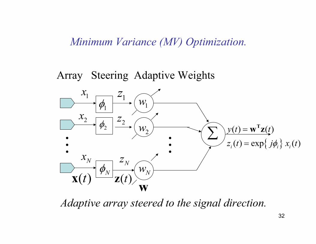
Minimum Variance (MV) Optimization.

Array Steering Adaptive Weights

⋮ ⋮∑

1φ

2φ

Nφ

1w

2w

Nw

1x 1z

2x 2z

Nx Nz

{ }( ) ( )

( ) exp ( )i i i

y t t

z t j x tφ

=

=

Tw z

( )tx ( )tzw

Adaptive array steered to the signal direction.

33

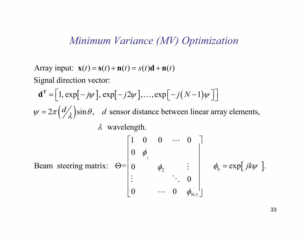
Minimum Variance (MV) Optimization

[ ] [ ] ( )

( )

Array input: ( ) ( ) ( ) ( ) ( )

Signal direction vector:

1, exp , exp 2 , ,exp 1

2 sin , sensor distance between linear array elements,

wavelength.

Beam steering matri

t t t s t t

j j j N

d d

ψ ψ ψ

ψ π θλλ

= + = +

= − − − −

=

T

x s n d n

d …

[ ]1

k2

N-1

1 0 0 0

0

x: = exp .0

0

0 0

jk

φ

φ ψφ

φ

Θ =

⋯

⋮

⋮ ⋱

⋯

34

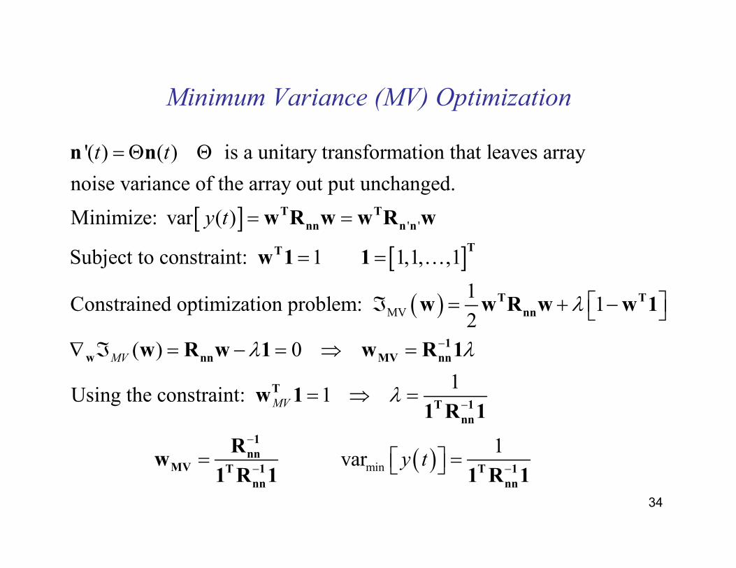
Minimum Variance (MV) Optimization

[ ][ ]

' '

'( ) ( ) is a unitary transformation that leaves array

noise variance of the array out put unchanged.

Minimize: var ( )

Subject to constraint: 1 1,1, ,1

Constrained optimizatio

t t

y t

= Θ Θ

= =

= =

T T

nn n n

TT

n n

w R w w R w

w 1 1 …

( )

( )

MV

min

1n problem: 1

2

( ) 0

1Using the constraint: 1

1var

MV

MV

y t

λ

λ λ

λ

−

−

−

− −

ℑ = + −

∇ ℑ = − = ⇒ =

= ⇒ =

= =

T T

nn

1

w nn MV nn

T

T 1

nn

1

nnMV T 1 T 1

nn nn

w w R w w 1

w R w 1 w R 1

w 11 R 1

Rw

1 R 1 1 R 1

35

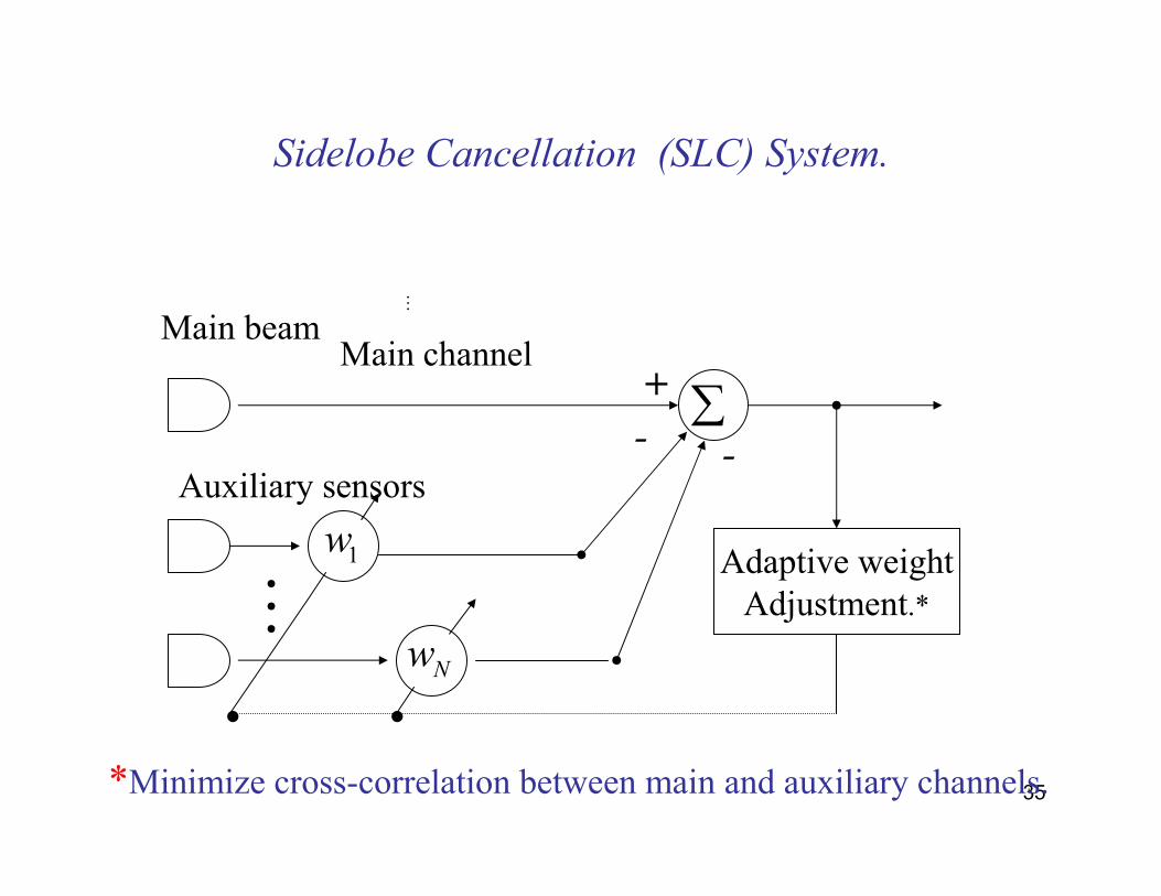
Sidelobe Cancellation (SLC) System.

Main channelMain beam

Auxiliary sensors

⋮

⋮1w

Nw

+ ∑

Adaptive weightAdjustment.*

- -

• •

*Minimize cross-correlation between main and auxiliary channels.

36

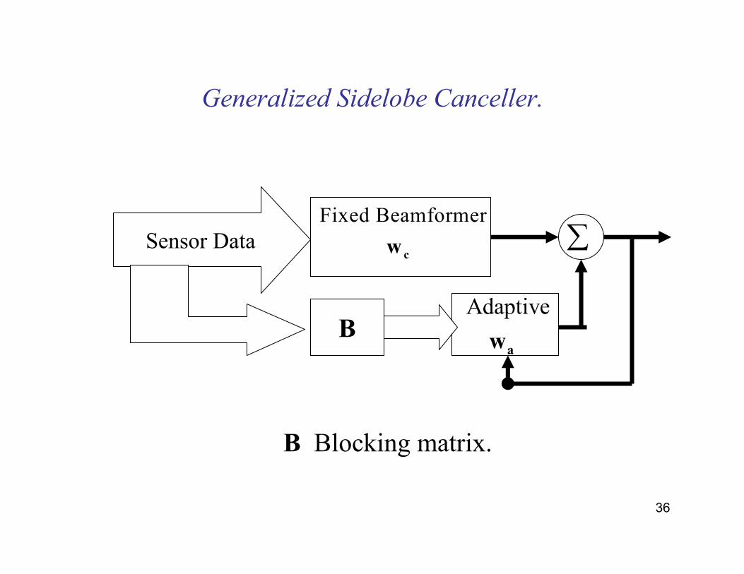
Generalized Sidelobe Canceller.

Sensor Data

B

∑

Adaptive

aw

Fixed Beamformer

cw

B Blocking matrix.

37

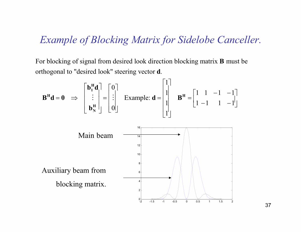
Example of Blocking Matrix for Sidelobe Canceller.

-2 -1.5 -1 -0.5 0 0.5 1 1.5 20

2

4

6

8

10

12

14

16

Main beam

Auxiliary beam from

blocking matrix.

For blocking of signal from desired look direction blocking matrix must be

orthogonal to "desired look" steering vector .

10

1 1 1 1 1 Example:

10

1

− − = ⇒ = = =

H

1

H H

H

N

B

d

b d

B d 0 d B

b

⋮ ⋮1 1 1 1

− −

38

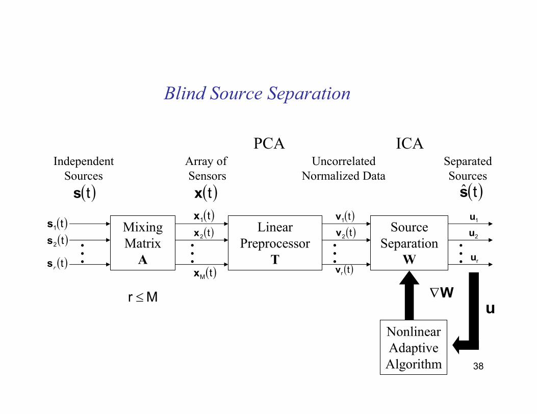
Blind Source Separation

IndependentSources

Array of Sensors

UncorrelatedNormalized Data

SeparatedSources

MixingMatrixA

LinearPreprocessor

T

SourceSeparation

W. . .

. . .

. . .

. . .

NonlinearAdaptiveAlgorithm

PCA ICA

( )t1s

( )t2s

( )ts( )ts ( )tx( )t1x

( )t2x

( )t1v

( )t2v

1u

2u

u

( )trs

∇WM r ≤

( )tMx( )trv

ru

39

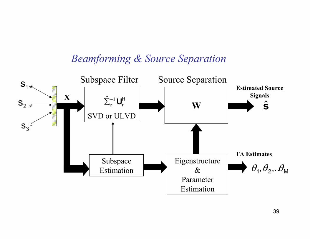
Beamforming & Source Separation

SVD or ULVD

ˆ −∑ 1

r

H

rU

W

Subspace Filter Source Separation

SubspaceEstimation

Eigenstructure&

Parameter Estimation

TA Estimates

1s

2s

3s

Estimated Source

Signals

sX

M21 ,.. , θθθ

40

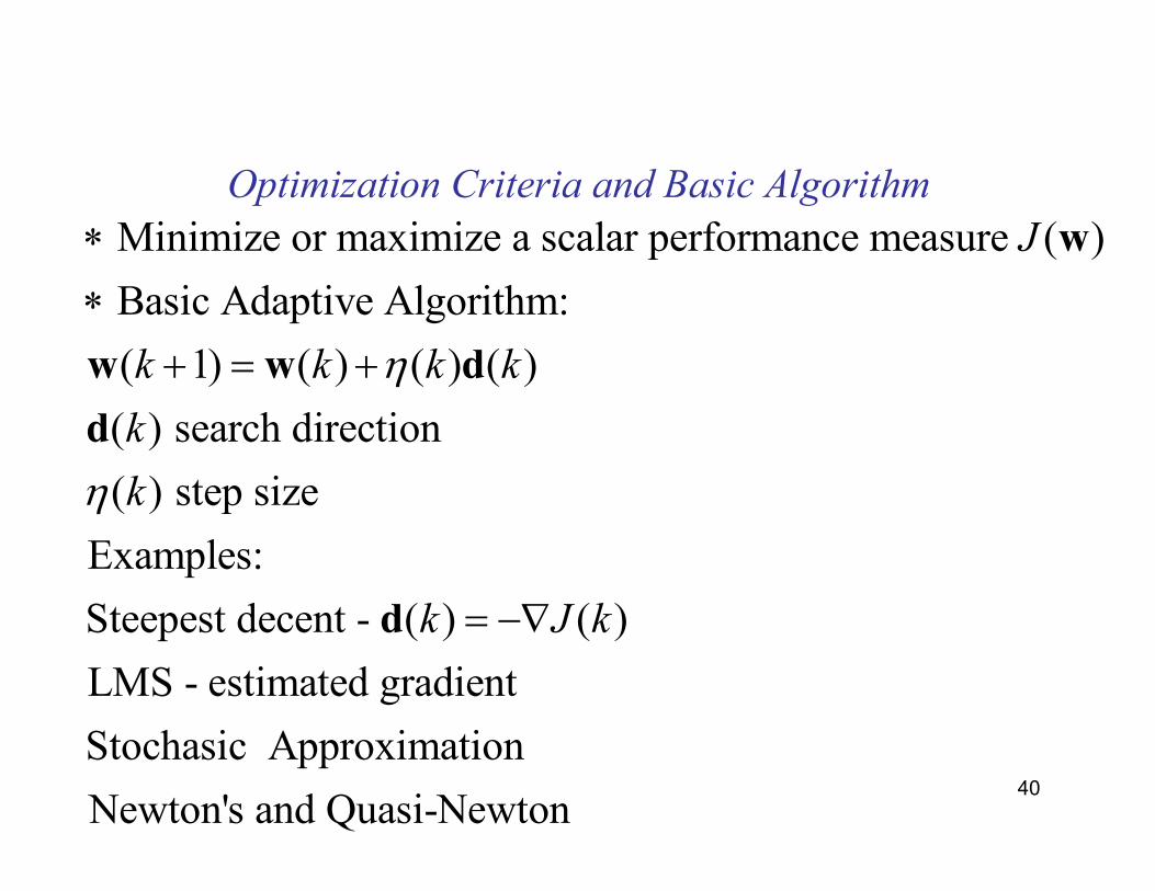
Optimization Criteria and Basic Algorithm

Minimize or maximize a scalar performance measure ( )

Basic Adaptive Algorithm:

( 1) ( ) ( ) ( )

( ) search direction

( ) step size

Examples:

Steepest decent - ( ) ( )

LMS - estimated gradient

J

k k k k

k

k

k J k

η

η

∗

∗

+ = +

= −∇

w

w w d

d

d

Stochasic Approximation

Newton's and Quasi-Newton

41

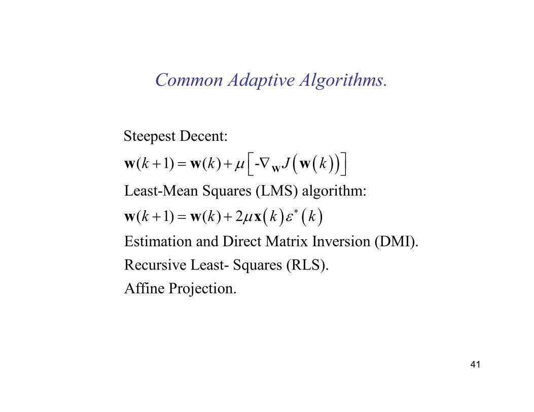
Common Adaptive Algorithms.

( )( )

( ) ( )

Steepest Decent:

( 1) ( ) -

Least-Mean Squares (LMS) algorithm:

( 1) ( ) 2

Estimation and Direct Matrix Inversion (DMI).

Recursive Least- Squares (RLS).

Affine Projection.

k k J k

k k k k

µ

µ ε ∗

+ = + ∇

+ = +

Ww w w

w w x

42

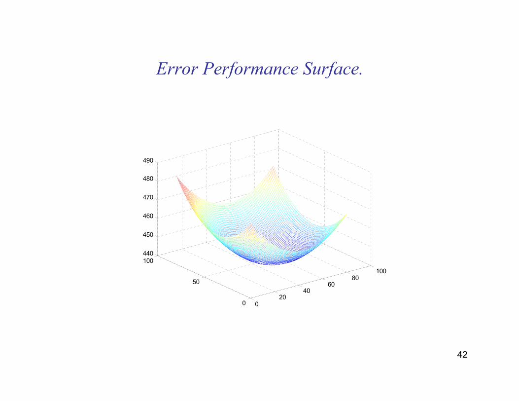
Error Performance Surface.

020

4060

80100

0

50

100440

450

460

470

480

490

43

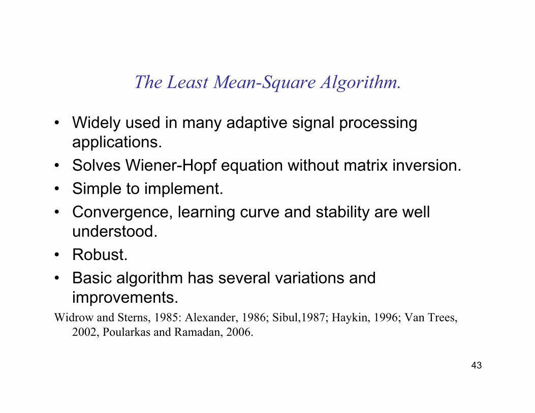
The Least Mean-Square Algorithm.

• Widely used in many adaptive signal processing

applications.

• Solves Wiener-Hopf equation without matrix inversion.

• Simple to implement.

• Convergence, learning curve and stability are well

understood.

• Robust.

• Basic algorithm has several variations and

improvements.Widrow and Sterns, 1985: Alexander, 1986; Sibul,1987; Haykin, 1996; Van Trees,

2002, Poularkas and Ramadan, 2006.

44

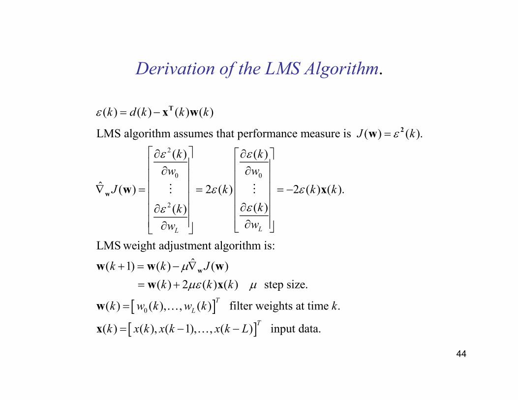
Derivation of the LMS Algorithm.

2

0 0

2

( ) ( ) ( ) ( )

LMS algorithm assumes that performance measure is ( ) ( ).

( ) ( )

ˆ ( ) 2 ( ) 2 ( ) ( ).

( )( )

LMS weight adjustment alg

LL

k d k k k

J k

k k

w w

J k k k

kk

ww

ε

ε

ε ε

ε εεε

= −

=

∂ ∂ ∂ ∂ ∇ = = = − ∂∂ ∂∂

T

2

w

x w

w

w x⋮ ⋮

[ ][ ]

0

orithm is:

ˆ( 1) ( ) ( )

( ) 2 ( ) ( ) step size.

( ) ( ), , ( ) filter weights at time .

( ) ( ), ( 1), , ( ) input data.

T

L

T

k k J

k k k

k w k w k k

k x k x k x k L

µ

µε µ

+ = − ∇

= +

=

= − −

ww w w

w x

w

x

…

…

45

The LMS Algorithm for M-th Order Adaptive

Filter.

Inputs: M=filter length

=step-size factor

( ) input data to the adaptive filter

(0) int alize the

n

µ=

=

x

w weight vector=0

ˆOutputs: ( ) adaptive filter output= ( ) ( ) ( )

( ) ( ) ( ) error

Algorithm: ( 1) ( ) 2 ( ) ( )

y n n n d n

n d n y n

n n n n

εµε

= =

= − =

+ = +

Tw x

w w x

46

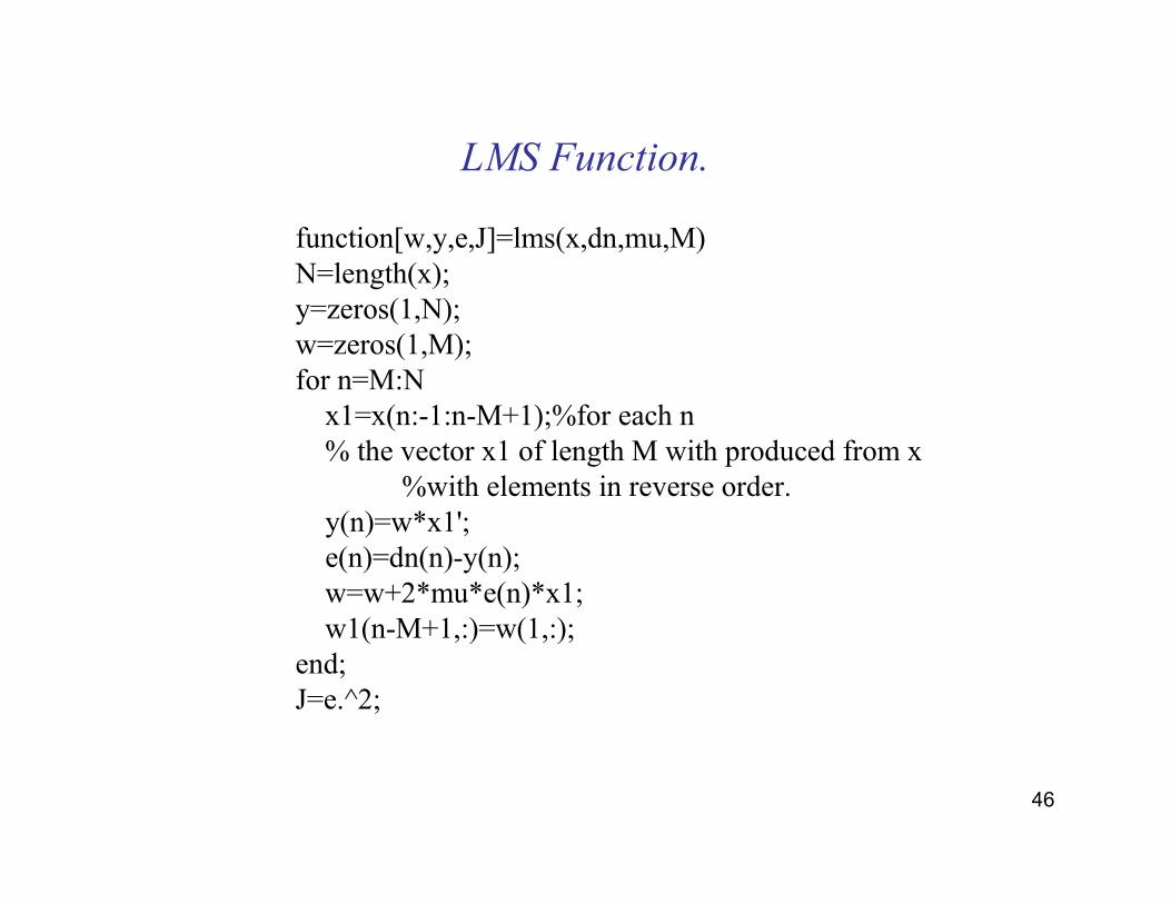
LMS Function.

function[w,y,e,J]=lms(x,dn,mu,M)N=length(x);y=zeros(1,N);w=zeros(1,M);for n=M:Nx1=x(n:-1:n-M+1);%for each n% the vector x1 of length M with produced from x

%with elements in reverse order.y(n)=w*x1';e(n)=dn(n)-y(n);w=w+2*mu*e(n)*x1;w1(n-M+1,:)=w(1,:);

end;J=e.^2;

47

Convergence of the Mean Weight Vector of LMS

{ } { } ( ) ( ){ }{ } ( ) ( ) ( )( ) ( ){ }{ } ( ){ } ( ) ( ){ } { }

( ){ } { }( )

( ) { }( ){ } ( )

( 1) ( ) 2

( ) 2

( ) 2 ( ) 2 ( ) !

! Assumed that ( ) and are independent.

( ) 2 ( )

2 ( ) 2

Define ( ) 1

d

OPT OPT d

OPT

E k E k E k k

E k E d k k k k

E k E d k k E k k E k

k k

E k E k

E k

k E k k

µ ε

µ

µ µ

µ

µ µ −

+ = +

= + −

= + −

= + −

= − + =

= − + =

T T

T

x xx

1

xx xx xx x

w w x

w w x x

w x x x w

x w

w R R w

I R w R w w R R

v w w v ( ) ( )

( ) ( ) ( )( ) ( ) ( )

2

1 2

1 2 ( ) ( )

k

k k

k k k k

µ

µ

µ

−

+ = − Λ = = Λ

+ = − Λ =

xx

T T T T T

xx xx xx

T

xx

I R v

UU v UU U U v UU I R U U

h I h U v h

48

Convergence of the Mean Weight Vector of LMS

( ) ( ) ( )

( ) ( ) ( ) ( ) ( )

( ) ( ) ( )

( )

( )

( )( ) [ ] [ ]

{ }

2

1

1 2 0

2 2 1 2 0

1 2 0

1 2 0 0

0

1 2

0

0 0 0 1 2

1lim 0 if 1 1 2 1 0

lim ( /

k

k

k

m

k

L

MAX MAXk MAX

OPTk

k

k tr tr

E k

µ

µ µ

µ

µλ

µλ

µλ

µλ µ λλ→∞

→∞

= − Λ

= − Λ = − Λ

+ = − Λ

−

−= −

= − < − < < < ≤ Λ =

∴ =

xx

xx xx

xx

xx

h I h

h I h I h

h I h

h R

w w

⋮ ⋮

⋯ ⋯

⋱ ⋮

⋮ ⋮

⋮ ⋱

⋯

49

Convergence Rate of the LMS Algorithm.

( )

( )

2

maxmax

max min

2

LMS weight convergence is geometric with geometric ratio

for coordinate:

1 1 11 2 exp 1

2!

For large

Conditio

:

1

n number) o

11

f

2 12

1 (

p

p p

p p p

p

p p p

p p

r

p th

r

r

µλτ τ τ

τ

µλ ττ µλ

λµ τ

λ λ

−

= − − ≈ − +

= − ≈ − ∴ ≈

∝ ∝

⋯

xx

R

50

Learning Curve and Misadjustment.

{ } { }{ } { }{ } { }

1

2 2

2 2min min

2 2

MSE: 2

Minimum MSE: 2

=

opt d

opt opt opt

d d d opt

E E d

E E d

E d E d

ε

ξ ε

−

−

−

−

=

= − +

= = − +

− = −

xx x

T T 1

xd xx

T T 1

xd xx

1

x xx x x

w R R

w R w R w

w R w R w

R R R R w

( ) ( )( ) ( )

( )( )

min

min min

min

Excess MSE: EMSE

( )

( ) ( ) ( ) ( )

( ) ( )

note:

= ( )

opt opt

d

pt

d

o

k k

k

k

k

k

k

k

k

k

k

ξ

ξ ξ

ξ

ξ + − −

= + = +

=

=

=

Λ

= + Λ

−

Λ

T

xx

T

T

x

T T

xx

T

x x

T

xx

T

x

w w R

R R

w w

v R v v U U v

h h

R

R

w w w

U U

( ) = ( ) ( ) ( ) ( )

opt

k k k k

−

= ΛT T

xx

w

v R v h h

51

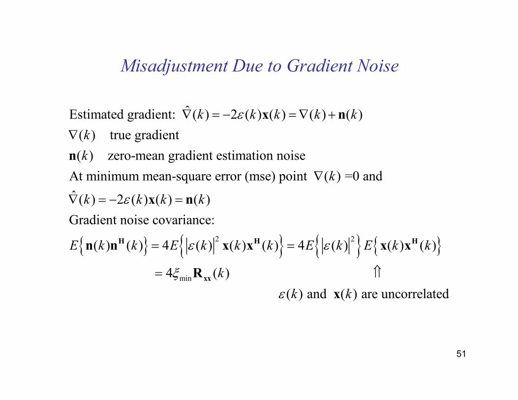
Misadjustment Due to Gradient Noise

ˆEstimated gradient: ( ) 2 ( ) ( ) ( ) ( )

( ) true gradient

( ) zero-mean gradient estimation noise

At minimum mean-square error (mse) point ( ) =0 and

ˆ ( ) 2 ( ) ( ) ( )

Gradient noise

k k k k k

k

k

k

k k k k

ε

ε

∇ = − = ∇ +

∇

∇

∇ = − =

x n

n

x n

{ } { } { } { }2 2

min

covariance:

( ) ( ) 4 ( ) ( ) ( ) 4 ( ) ( ) ( )

4 ( )

( ) and ( ) ar

E k k E k k k E k E k k

k

k k

ε ε

ξ

ε

= =

= ⇑

H H H

xx

n n x x x x

R

x e uncorrelated

52

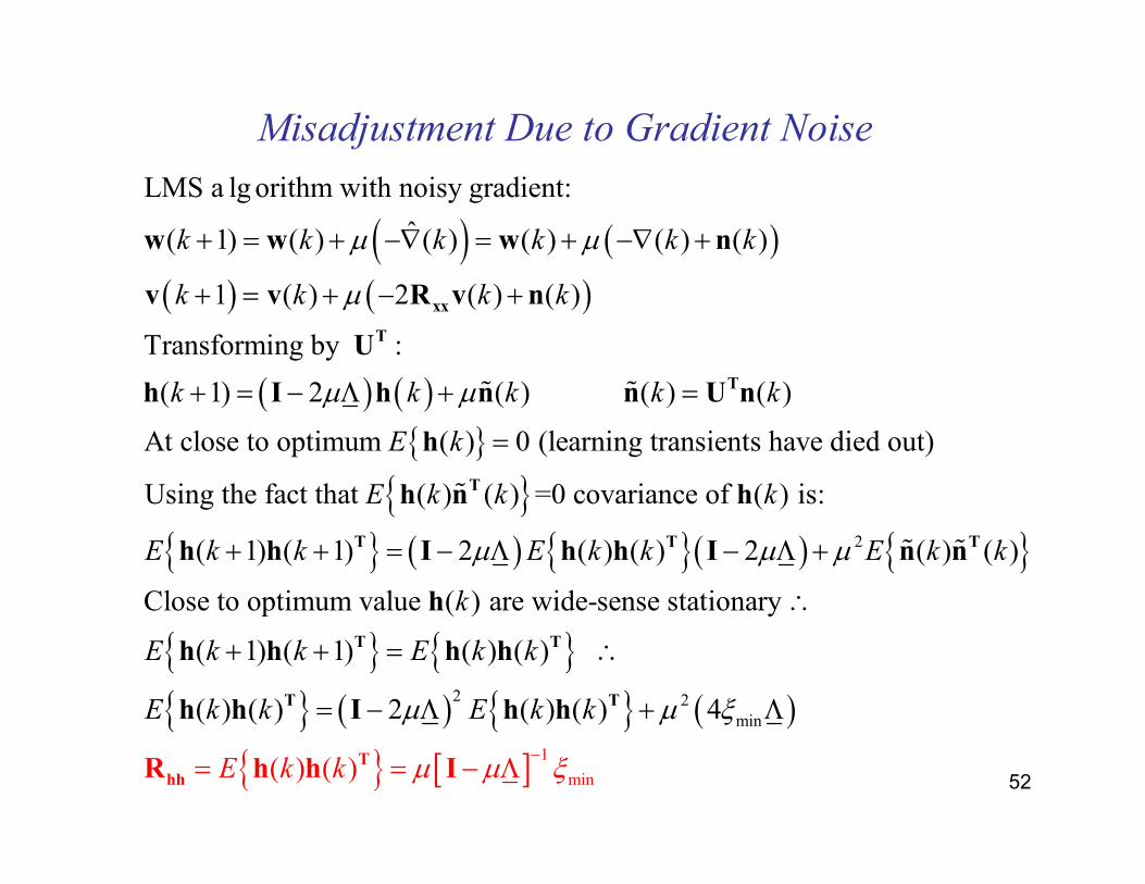
Misadjustment Due to Gradient Noise

( ) ( )

( ) ( )

( ) ( ){ }

LMS a lgorithm with noisy gradient:

ˆ( 1) ( ) ( ) ( ) ( ) ( )

1 ( ) 2 ( ) ( )

Transforming by :

( 1) 2 ( ) ( ) ( )

At close to optimum ( ) 0 (learning transients hav

k k k k k k

k k k k

k k k k k

E k

µ µ

µ

µ µ

+ = + −∇ = + −∇ +

+ = + − +

+ = − Λ + =

=

xx

T

T

w w w n

v v R v n

U

h I h n n U n

h

ɶ ɶ

{ }{ } ( ) { }( ) { }

{ } { }

2

e died out)

Using the fact that ( ) ( ) =0 covariance of ( ) is:

( 1) ( 1) 2 ( ) ( ) 2 ( ) ( )

Close to optimum value ( ) are wide-sense stationary

( 1) ( 1) ( ) ( )

E k k k

E k k E k k E k k

k

E k k E k k

µ µ µ+ + = − Λ − Λ +

∴

+ + = ∴

T

T T T

T T

h n h

h h I h h I n n

h

h h h h

ɶ

ɶ ɶ

{ } ( ) { } ( )

{ } [ ] 1

mi

2

n

2

min( ) ( ) 2

( ) )

( ( )

(

) 4E k k E

E k

k

k

kµ µ ξ

µ µ ξ−

= − Λ + Λ

= = − ΛT

T T

hh

h h I

h I

h h

R h

53

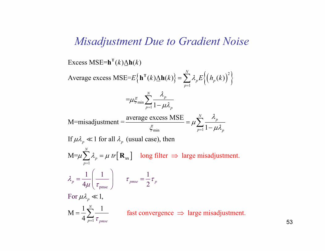
Misadjustment Due to Gradient Noise

{ } ( ){ }21

min1

1min

Excess MSE= ( ) ( )

Average excess MSE= ( ) ( ) ( )

=1

average excess MSEM=misadjustment =

1

If 1 for all (usual cas

N

p p

p

Np

p p

Np

p p

p p

k k

E k k E h kλ

λµξ

µλ

λµ

ξ µλ

µλ λ

=

=

=

Λ

Λ =

−

=−

∑

∑

∑

T

T

h h

h h

≪

[ ]

pmse

1

1

1 1 1

4

e), th

long filter large misadjustment.

fast convergence large m

en

M=

isadjustment.

1,

1 1

2

F

M

4

or

N

p

p

p

p pmse p

pmse

N

p

tr

λ τ τ

µ λ µ

µλ

µ τ

τ

=

=

= =

⇒=

=

⇒

∑

∑

xxR

≪

54

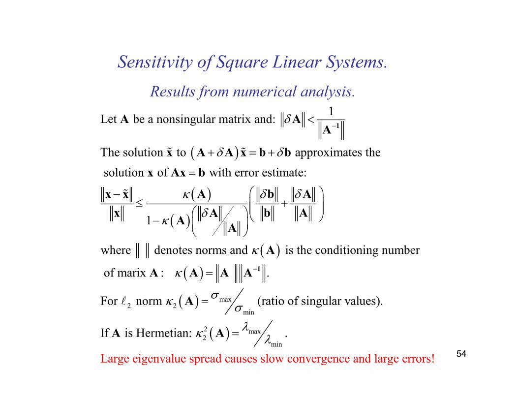
Sensitivity of Square Linear Systems.

Results from numerical analysis.

( )

( )

( )

( )

1Let be a nonsingular matrix and:

The solution to approximates the

solution of with error estimate:

1

where denotes norms and is the

δ

δ δ

δ δκδκ

κ

−<

+ = +

=

−≤ + −

1A A

A

x A A x b b

x Ax b

x x b AA

x b AAA

A

A

ɶ ɶ

ɶ

( )

( )

( )

max2 2

min

2 max2

min

conditioning number

of marix : .

For norm (ratio of singular values).

If

Large eigenvalue spread causes

is Hermeti

slow convergence and large errors

an: .

!

κ

σκ σ

λκ λ

−=

=

=

1A A A A

A

A A

ℓ

55

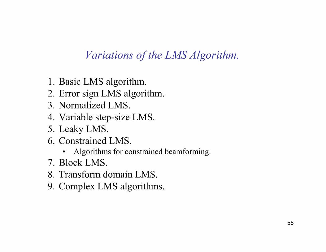
Variations of the LMS Algorithm.

1. Basic LMS algorithm.2. Error sign LMS algorithm.3. Normalized LMS.4. Variable step-size LMS.5. Leaky LMS.6. Constrained LMS.

• Algorithms for constrained beamforming.

7. Block LMS.8. Transform domain LMS.9. Complex LMS algorithms.

56

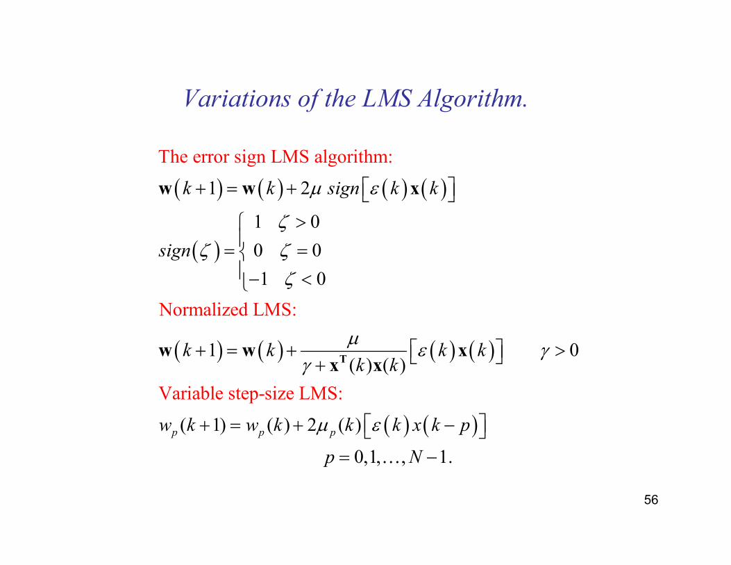
Variations of the LMS Algorithm.

( ) ( ) ( ) ( )

( )

( ) ( ) ( ) ( )

( ) ( )

1 2

1 0

0 0

1 0

1 0( ) ( )

( 1) ( ) 2 ( )

The error sign LMS algorithm:

No

rmalized LMS:

Varia

ble step-size LMS:

p p p

k k sign k k

sign

k k k kk k

w k w k k k x k p

µ ε

ζζ ζ

ζ

µε γ

γ

µ ε

+ = + >

= =− <

+ = + > +

+ = + −

T

w w x

w w xx x

0,1, , 1.p N= −…

57

Time Varying Step Size

1

2

b

( ) 0

( )

( )

These conditions are satisfied by sequences:

c(k)= 0.5 1.0

kExample:

1 1 1{ (k)}=c{1, , ,... ,...}

2 3

k

k

k

k

b

k

η

η

η

η

η

∞

=

>

= ∞

< ∞

< ≤

∑

∑

58

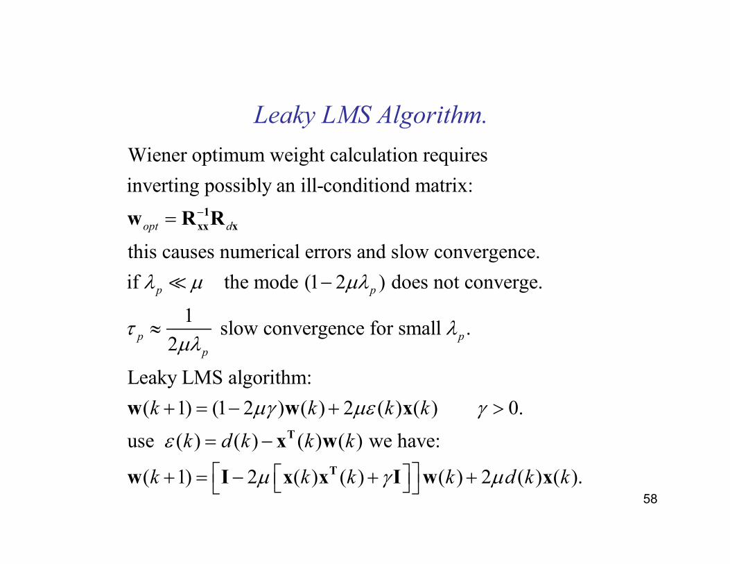
Leaky LMS Algorithm.

Wiener optimum weight calculation requires

inverting possibly an ill-conditiond matrix:

this causes numerical errors and slow convergence.

if the mode (1 2 ) does not converge.

1

2

opt d

p p

p

p

λ µ µλ

τµλ

−=

−

≈

1

xx xw R R

≪

slow convergence for small .

Leaky LMS algorithm:

( 1) (1 2 ) ( ) 2 ( ) ( ) 0.

use ( ) ( ) ( ) ( ) we have:

( 1) 2 ( ) ( ) ( ) 2 ( ) ( ).

p

k k k k

k d k k k

k k k k d k k

λ

µγ µε γ

ε

µ γ µ

+ = − + >

= −

+ = − + +

T

T

w w x

x w

w I x x I w x

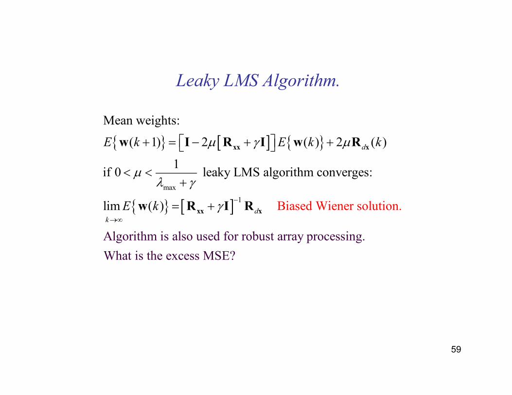
59

Leaky LMS Algorithm.

{ } [ ] { }

{ } [ ]max

1

Mean weights:

( 1) 2 ( ) 2 ( )

1if 0 leaky LMS algori

Algorithm is also used for

thm converges:

lim ( ) Biased Wiener

robust array processi

solution.

ng.

What

d

d

k

E k E k k

E k

µ γ µ

µλ γ

γ −

→∞

+ = − + +

< <+

= +

xx x

xx x

w I R I w R

w R I R

is the excess MSE?

60

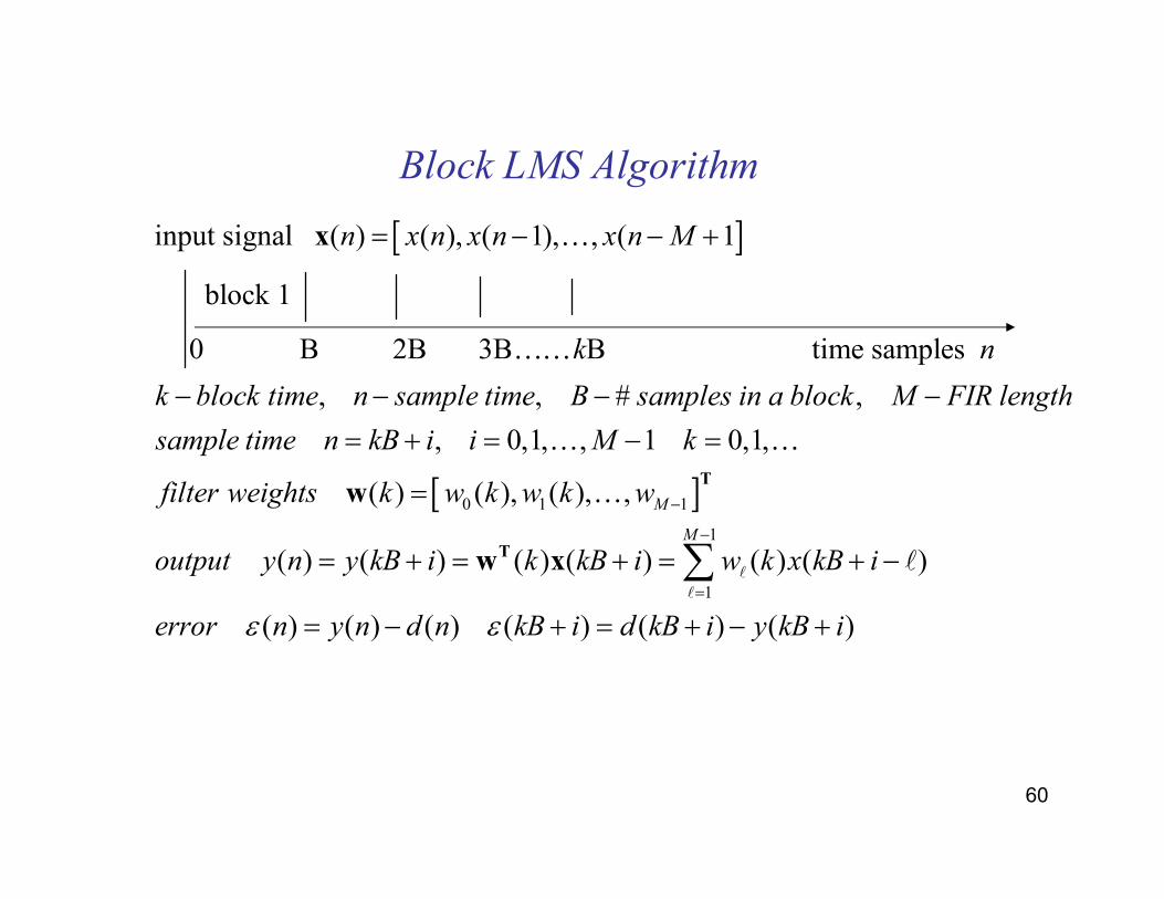
Block LMS Algorithm

[ ]input signal ( ) ( ), ( 1), , ( 1

block 1

0 B 2B 3B B time samples

n x n x n x n M

k

= − − +x …

……

[ ]0 1 1

1

1

, , # ,

, 0,1, , 1 0,1,

( ) ( ), ( ), ,

( ) ( ) ( ) ( ) ( ) ( )

( ) ( ) (

M

M

n

k block time n sample time B samples in a block M FIR length

sample time n kB i i M k

filter weights k w k w k w

output y n y kB i k kB i w k x kB i

error n y n d nε

−

−

=

− − − −

= + = − =

=

= + = + = + −

= −

∑

T

T

w

w x ℓ

ℓ

… …

…

ℓ

) ( ) ( ) ( )kB i d kB i y kB iε + = + − +

61

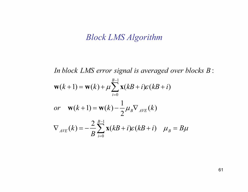
Block LMS Algorithm

1

0

1

0

:

( 1) ( ) ( ) ( )

1( 1) ( ) ( )

2

2( ) ( ) ( )

B

i

B AVE

B

AVE B

i

In block LMS error signal is averaged over blocks B

k k kB i kB i

or k k k

k kB i kB i BB

µ ε

µ

ε µ µ

−

=

−

=

+ = + + +

+ = − ∇

∇ = − + + =

∑

∑

w w x

w w

x

62

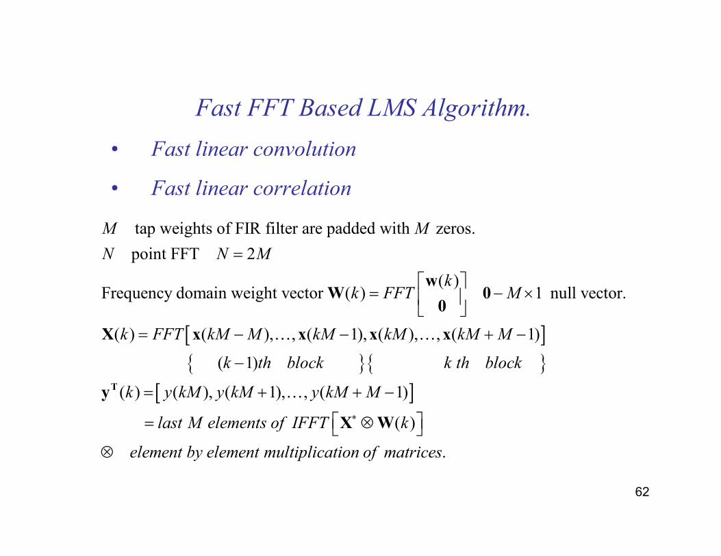
Fast FFT Based LMS Algorithm.

• Fast linear convolution

• Fast linear correlation

[ ]

tap weights of FIR filter are padded with zeros.

point FFT 2

( )Frequency domain weight vector ( ) 1 null vector.

( ) ( ), , ( 1), ( ), , ( 1)

M M

N N M

kk FFT M

k FFT kM M kM kM kM M

=

= − ×

= − − + −

wW 0

0

X x x x x… …

{ }{ }[ ]

( 1)

( ) ( ), ( 1), , ( 1)

( )

.

k th block k th block

k y kM y kM y kM M

last M elements of IFFT k

element by element multiplication of matrices

∗

−

= + + −

= ⊗ ⊗

Ty

X W

…

63

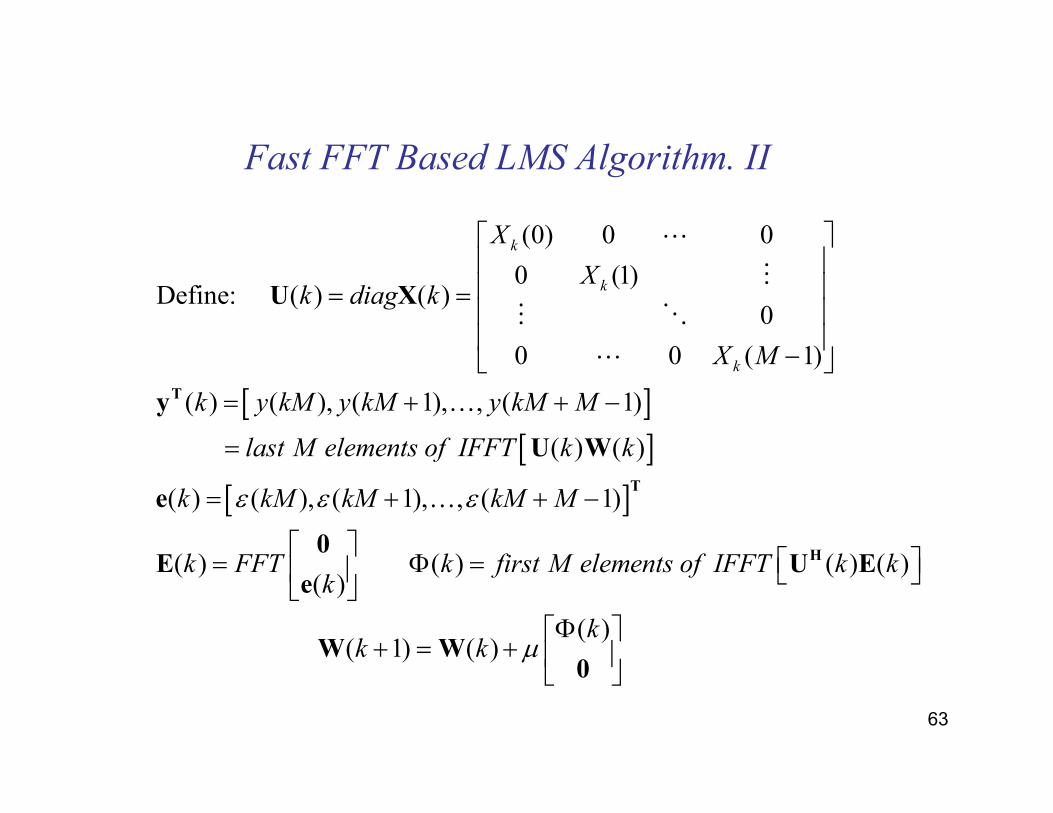
Fast FFT Based LMS Algorithm. II

[ ][ ]

[ ]

(0) 0 0

0 (1)Define: ( ) ( )

0

0 0 ( 1)

( ) ( ), ( 1), , ( 1)

( ) ( )

( ) ( ), ( 1), , ( 1)

( ) ( )( )

k

k

k

X

Xk diag k

X M

k y kM y kM y kM M

last M elements of IFFT k k

k kM kM kM M

k FFT k first M elements of IFFTk

ε ε ε

= =

−

= + + −

=

= + + −

= Φ =

T

T

U X

y

U W

e

0E

e

⋯

⋮

⋮ ⋱

⋯

…

…

( ) ( )

( )( 1) ( )

k k

kk k µ

Φ + = +

HU E

W W0

64

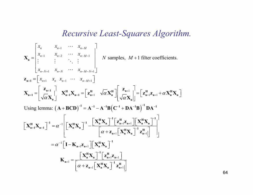
Recursive Least-Squares Algorithm.

1

1 2 1

1 1

1 1 1

1

1 1 1

samples, 1 filter coefficients.

n n n M

n n n M

n N n N n M N

n n n n M

x x x

x x xN M

x x x

x x x x

α αα α

− −

− − − −

− + − − − +

+ + − − +

+ ++ + + + + +

= +

=

= = = +

n

n 1

n 1 nH H H H H

n 1 n 1 n 1 n n n n n n

n n

X

z

z zX X X z X z z X X

X X

⋯

⋯

⋮ ⋮ ⋱ ⋮

⋯

⋯

( ) ( )

1 11

1 1

11 1

1

1

Using lemma:

αα

α

−− − − − − −

− −

− − + +−+ + −

+ +

−−+ +

−

+

+

+ = − +

= − +

= −

=

11 1 1 1 1 1

1 1H H H

1 1 n n n n n nH H

n 1 n 1 n n 1H H

n n n n

1H

n n n n

1H

n n n

n

A BCD A A B C DA B DA

X X z z X XX X X X

z X X z

I K z X X

X X zK

1

1 1α

+

−

+ +

+

H

n

1H H

n n n n

z

z X X z

65

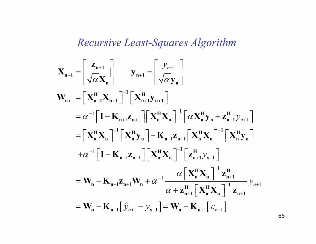
Recursive Least-Squares Algorithm

1

1

11 1 1

1 1

11 1

n

n

y

y

α α

α α

α

+ +

+ +

−

+ + + + +

−−+ + + +

− −

+ +

−−+ + +

= =

=

= − +

= −

+ −

n 1

n 1 n 1

n n

1H H

n n 1 n 1 n 1 n 1

1H H H

n n n n n n n 1

1 1H H H H

n n n n n n n n n n

1H

n n n n n

zX y

X y

W X X X y

I K z X X X y z

X X X y K z X X X y

I K z X X z

[ ] [ ]

1

11 1 1

1 1 1 1 1ˆ

n

n

n n n

y

y

y y

αα

α

ε

+

−

+−+ + +−

+ +

+ + + + +

= − + +

= − − = −

H

1

1H H

n n n 1

n n n n 1H H

n 1 n n n 1

n n n n

X X zW K z W

z X X z

W K W K

66

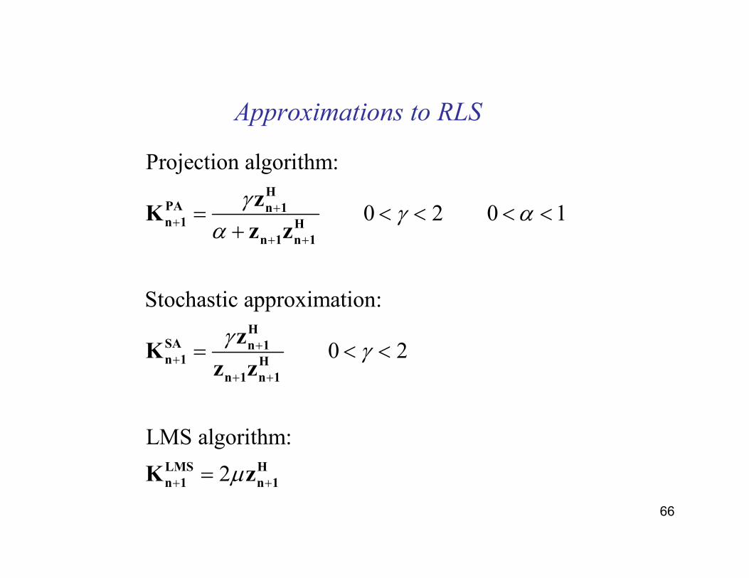
Approximations to RLS

Projection algorithm:

0 2 0 1

Stochastic approximation:

0 2

LMS algorithm:

2

γγ α

α

γγ

µ

++

+ +

++

+ +

+ +

= < < < <+

= < <

=

HPA n 1n 1 H

n 1 n 1

HSA n 1n 1 H

n 1 n 1

LMS H

n 1 n 1

zK

z z

zK

z z

K z

67

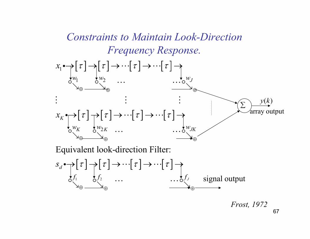
Constraints to Maintain Look-Direction

Frequency Response.

[ ] [ ] [ ] [ ]

[ ] [ ] [ ] [ ]

1

1 2

2

Equivalent look-direction Filt

K

J

JKK K

w w w

w ww

x

x

τ τ τ τ

τ τ τ τ

⊕ ⊕ ⊕

⊕ ⊕ ⊕

→ → → → →

→ → → → →

ց ց ց

ց ց ց

i ⋯ ⋯

⋯ ⋯

⋮ ⋮ ⋮

i ⋯ ⋯

⋯ ⋯

� � �

� � �

[ ] [ ] [ ] [ ]1 2

er:

J

d

f f f

s τ τ τ τ

⊕ ⊕ ⊕

→ → → → →

ց ց ց

i ⋯ ⋯

⋯ ⋯� � �

∑

signal output

( )

array output

y k

Frost, 1972

68

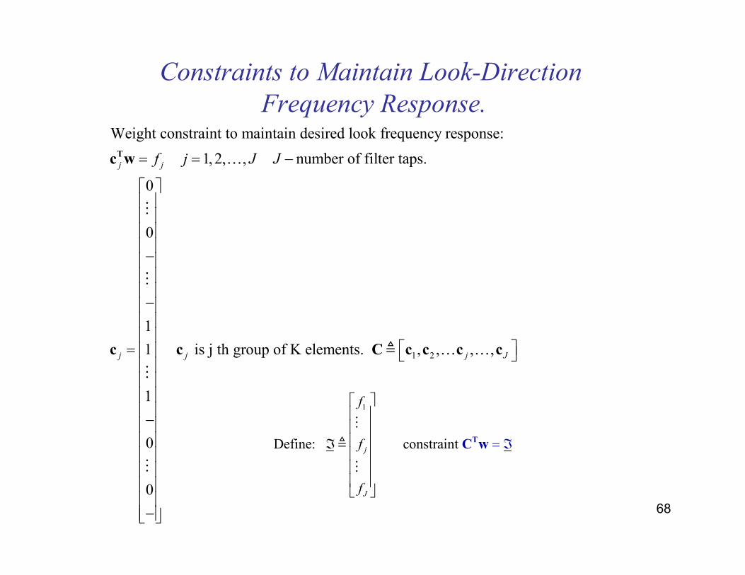
Constraints to Maintain Look-Direction

Frequency Response.Weight constraint to maintain desired look frequency response:

1,2, , number of filter taps.

0

0

1

1 is j th group of K elements.

1

0

0

j j

j j

f j J J= = −

− −

= − −

Tc w

c c

…

⋮

⋮

⋮

⋮

1 2 , , , ,j J C c c c c≜ … …

1

Define: constraint j

J

f

f

f

ℑ

= ℑ

TC w

⋮

≜

⋮

69

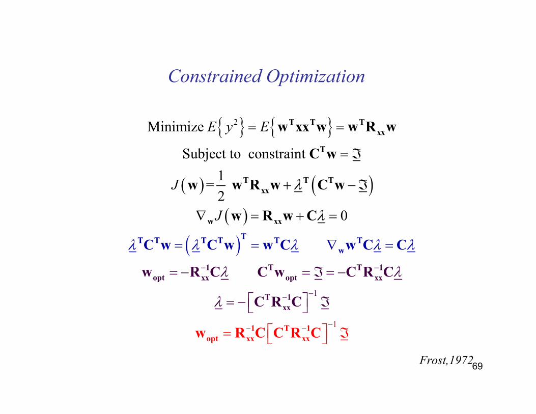
Constrained Optimization

{ } { }

( ) ( )( )

( )

1

2

1

Minimize

Subject to constraint

1= 2

0

E y E

J

J

λ λ

λ λ

λ

λ

λ λ

λ

λ

− −

−−

−−

−

= − = ℑ =

= =

= ℑ

+ −ℑ

∇ = +

−

= − ℑ

= = ∇

= ℑ

=

=T

T T T T T T

1 T

T T T

xx

T

T 1

opt xx opt

w

1 T 1

op

x

T T T

xx

w x

x

T 1

xx

x

x

x

t x

x

w xx w w R w

C w

w

C w C w w C

w R C C R

w R C C w C R C

C

C R

w R w C w

w R w C

w

C

C C

Frost,1972

70

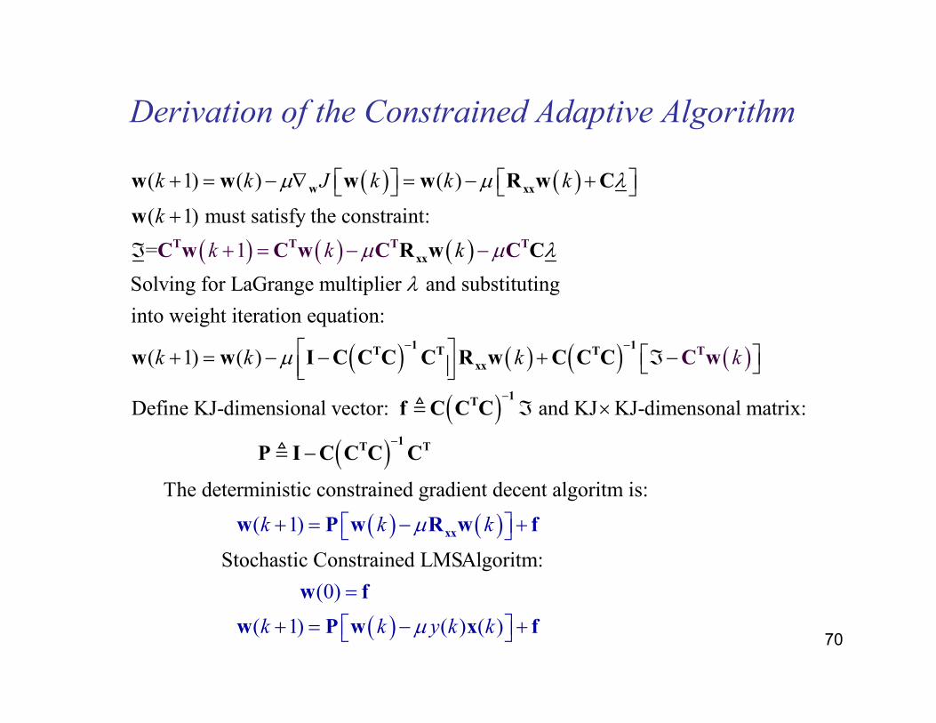
Derivation of the Constrained Adaptive Algorithm

( ) ( )

( ) ( ) ( )

( 1) ( ) ( )

( 1) must satisfy the constraint:

=

Solving for LaGrange multiplier and substituting

into weight iteration equatio

1

n:

( 1) ( )

k

k k J k k k

k

k

k

k

k

µ µ λ

λ

µ λ

µ

µ

+ = − ∇ = − + +

ℑ + =

+ = − −

− −T T T

w xx

xx

TC w C w C C

w w w w R w C

w

R w C

w w I ( ) ( ) ( ) ( )

( )( )

( ) ( )

Define KJ-dimensional vector: and KJ KJ-dimensonal matrix:

The deterministic constrained gradient decent algoritm

( 1)

is:

k k k

k k

µ

− −

−

−

+ ℑ−

ℑ ×

−

+ = −

1 1T T T

xx

T

xx

1T

1T T

w

C C C C R w C C C

f C C C

P I C

P w R

C

w

C C

C

w

≜

≜

( )

Stochastic Constrained L

(0)

(

MSAlgoritm:

1) ( ) ( )k k y k kµ

+

=

+ = − +

f

w f

w P w x f

71

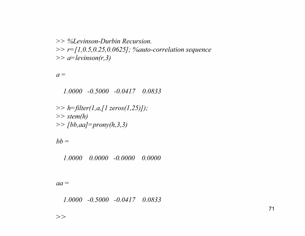
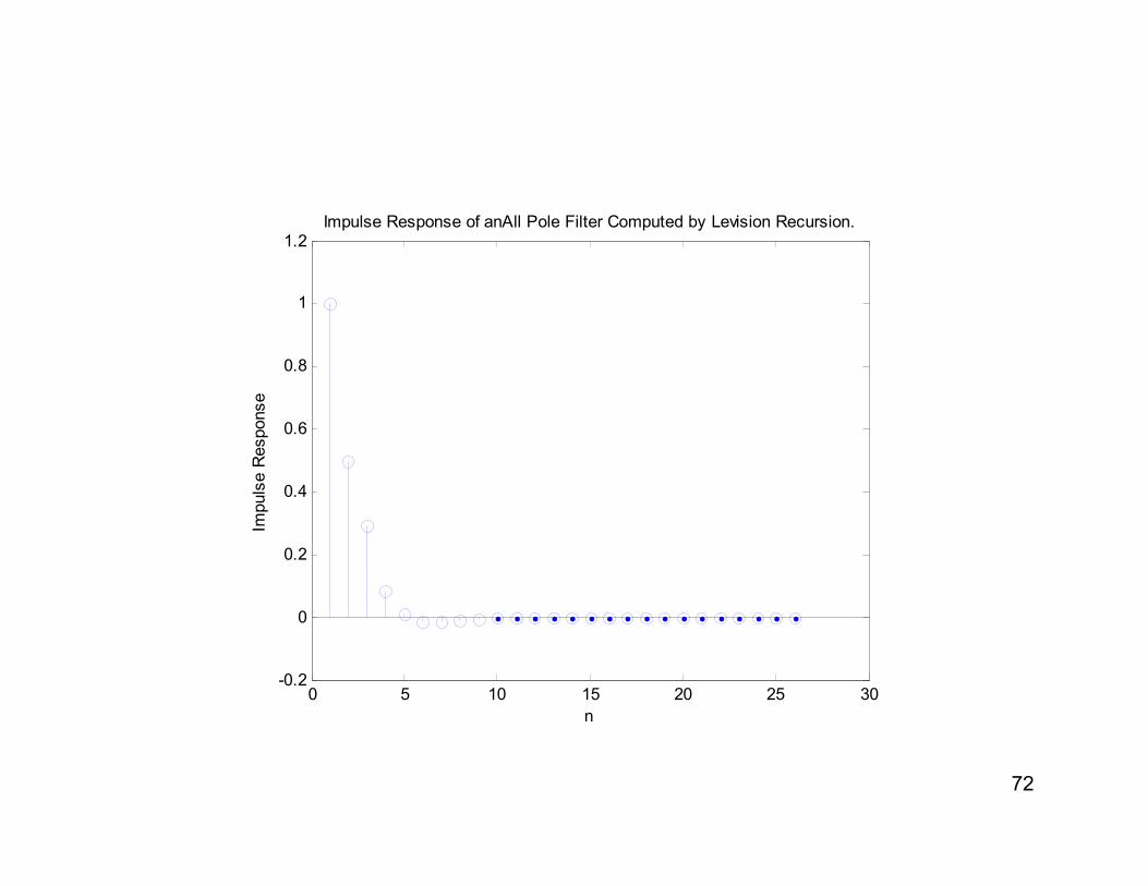
>> %Levinson-Durbin Recursion.

>> r=[1,0.5,0.25,0.0625]; %auto-correlation sequence

>> a=levinson(r,3)

a =

1.0000 -0.5000 -0.0417 0.0833

>> h=filter(1,a,[1 zeros(1,25)]);

>> stem(h)

>> [bb,aa]=prony(h,3,3)

bb =

1.0000 0.0000 -0.0000 0.0000

aa =

1.0000 -0.5000 -0.0417 0.0833

>>

72

0 5 10 15 20 25 30-0.2

0

0.2

0.4

0.6

0.8

1

1.2Impulse Response of anAll Pole Filter Computed by Levision Recursion.

Impulse Response

n