Adaptive Routing in Ad Hoc Wireless Multi-hop Networks · Frederick Ducatelle Adaptive Routing in...
197
Adaptive Routing in Ad Hoc Wireless Multi-hop Networks Doctoral Dissertation submitted to the Faculty of Informatics of the University of Lugano in partial fulfillment of the requirements for the degree of Doctor of Philosophy presented by Frederick Ducatelle under the supervision of Prof. Luca Maria Gambardella September 2007
Transcript of Adaptive Routing in Ad Hoc Wireless Multi-hop Networks · Frederick Ducatelle Adaptive Routing in...
Adaptive Routing in Ad Hoc WirelessMulti-hop Networks
Doctoral Dissertation submitted to the
Faculty of Informatics of the University of Lugano
in partial fulfillment of the requirements for the degree of
Doctor of Philosophy
presented by
Frederick Ducatelle
under the supervision of
Prof. Luca Maria Gambardella
September 2007

Dissertation Committee
Prof. Luca M. Gambardella IDSIA, Switzerland
Prof. Dr. Antonio Carzaniga USI, Switzerland
Prof. Dr. Amy L. Murphy USI, Switzerland
Prof. Dr. Patrick Thiran EPFL, Switzerland
Dissertation accepted on 10 September 2007
Supervisor PhD program director
Prof. Luca Maria Gambardella Prof. Dr. Fabio Crestani


To Lili and Delphine


Abstract
Ad hoc wireless multi-hop networks (AHWMNs) are communication networks that con-sist entirely of wireless nodes, placed together in an ad hoc manner, i.e. with minimalprior planning. All nodes have routing capabilities, and forward data packets for othernodes in multi-hop fashion. Nodes can enter or leave the network at any time, and maybe mobile, so that the network topology continuously experiences alterations duringdeployment. AHWMNs pose substantially different challenges to networking protocolsthan more traditional wired networks. These challenges arise from the dynamic andunplanned nature of these networks, from the inherent unreliability of wireless com-munication, from the limited resources available in terms of bandwidth, processing ca-pacity, etc., and from the possibly large scale of these networks. Due to these differentchallenges, new algorithms are needed at all layers of the network protocol stack.
We investigate the issue of adaptive routing in AHWMNs, using ideas from artificialintelligence (AI). Our main source of inspiration is the field of Ant Colony Optimization(ACO). This is a branch of AI that takes its inspiration from the behavior of ants innature. ACO has been applied to a wide range of different problems, often giving state-of-the-art results. The application of ACO to the problem of routing in AHWMNs isinteresting because ACO algorithms tend to provide properties such as adaptivity androbustness, which are needed to deal with the challenges present in AHWMNs. Onthe other hand, the field of AHWMNs forms an interesting new application domainin which the ideas of ACO can be tested and improved. In particular, we investigatethe combination of ACO mechanisms with other techniques from AI to get a powerfulalgorithm for the problem at hand.
We present the AntHocNet routing algorithm, which combines ideas from ACO rout-ing with techniques from dynamic programming and other mechanisms taken frommore traditional routing algorithms. The algorithm has a hybrid architecture, combin-ing both reactive and proactive mechanisms. Through a series of simulation tests, weshow that for a wide range of different environments and performance metrics, AntHoc-Net can outperform important reference algorithms in the research area. We provide anextensive investigation of the internal working of the algorithm, and we also carry outa detailed simulation study in a realistic urban environment. Finally, we discuss theimplementation of ACO routing algorithms in a real world testbed.
i

Acknowledgments
I would like to thank in the first place my supervisor, Luca Maria Gambardella, whohas given me the opportunity to work on this project and has assisted me in any waypossible. Then, I want to thank my colleague, Gianni A. Di Caro, who has been likea second supervisor to me, and has been an invaluable help throughout this project.Other people who have been of scientific importance for my work on this thesis include(in order of appearance) John Levine, who has first introduced me to the field of antcolony optimization, Marco Dorigo, who initiated this interesting research field and alsobrought me in contact with IDSIA, Patrick Thiran, who brought us in contact with thefield of ad hoc networks, and Martin Roth, who gave me the opportunity to work withhim at Deutsche Telekom Laboratories in Berlin. Furthermore, I would like to thankall the people at IDSIA for all scientific input, in the form of presentations, discussions,etc..
Apart from the scientific input, of equal importance to me has been the personalsupport I have received throughout the years that I have spent on this thesis. I want tothank a number of people without whom this work would never have been completed. Inthe first place, I thank my wife, Liliana Carrillo, and my daughter, Delphine, who arrivedjust in time to give me the final support I needed to finish the work. Then I want to thankmy family, my mother, my father and my sisters, Caroline and Barbara, who have been,from distance, a great support. Next, I thank Alex Graves and Matteo Gagliolo, partnersin crime during all those years in Lugano. Friends back home, Pieter Vandenbosscheand family, Kobe Lootens, Dieter Herregodts, Pieter Orbie, Frederik Demilde, KatelijneCarbonez, Tom Ghyselinck, and many others. And all other friends, wherever they are,Matthew Davies, Elaine Boyd, Jesper Salomon, Olga Chrysanthopoulou, Ola Svenson,Nikos Mutsanas, Shane Legg, Maciej Kurant, etc..
iii

Contents
1 Introduction 11.1 General introduction . . . . . . . . . . . . . . . . . . . . . . . . . . . . . . . 11.2 Contributions of this thesis . . . . . . . . . . . . . . . . . . . . . . . . . . . . 31.3 Outline of the thesis . . . . . . . . . . . . . . . . . . . . . . . . . . . . . . . . 4
2 Ad hoc wireless multi-hop networks 72.1 A definition of ad hoc wireless multi-hop networks . . . . . . . . . . . . . . 72.2 Types of ad hoc wireless multi-hop networks . . . . . . . . . . . . . . . . . 8
2.2.1 Mobile ad hoc networks . . . . . . . . . . . . . . . . . . . . . . . . . . 82.2.2 Wireless mesh networks . . . . . . . . . . . . . . . . . . . . . . . . . . 92.2.3 Sensor networks . . . . . . . . . . . . . . . . . . . . . . . . . . . . . . 112.2.4 Algorithms for different types of AHWMNs . . . . . . . . . . . . . . . 11
2.3 Issues in ad hoc wireless multi-hop networking . . . . . . . . . . . . . . . . 112.3.1 Network topology and node mobility . . . . . . . . . . . . . . . . . . . 122.3.2 The physical layer . . . . . . . . . . . . . . . . . . . . . . . . . . . . . 132.3.3 The data link layer . . . . . . . . . . . . . . . . . . . . . . . . . . . . . 142.3.4 The transport layer . . . . . . . . . . . . . . . . . . . . . . . . . . . . 16
2.4 Routing in ad hoc wireless multi-hop networks . . . . . . . . . . . . . . . . 172.4.1 Proactive versus reactive routing algorithms . . . . . . . . . . . . . . 172.4.2 Important routing algorithms for AHWMNs . . . . . . . . . . . . . . 182.4.3 Other techniques for AHWMN routing . . . . . . . . . . . . . . . . . . 23
2.5 Conclusion . . . . . . . . . . . . . . . . . . . . . . . . . . . . . . . . . . . . . 28
3 Adaptive routing and learning 313.1 Adaptive routing in the internet . . . . . . . . . . . . . . . . . . . . . . . . . 31
3.1.1 Distance vector routing . . . . . . . . . . . . . . . . . . . . . . . . . . 323.1.2 Link state routing . . . . . . . . . . . . . . . . . . . . . . . . . . . . . 36
3.2 Ant Colony Optimization routing algorithms . . . . . . . . . . . . . . . . . . 383.2.1 Ants in nature . . . . . . . . . . . . . . . . . . . . . . . . . . . . . . . 383.2.2 The Ant Colony Optimization metaheuristic . . . . . . . . . . . . . . 403.2.3 AntNet: an ACO algorithm for routing in telecommunication networks 423.2.4 ACO routing principles . . . . . . . . . . . . . . . . . . . . . . . . . . 443.2.5 Existing ACO routing algorithms for wired networks . . . . . . . . . 453.2.6 Existing ACO routing algorithms for AHWMNs . . . . . . . . . . . . 48
3.3 Routing and machine learning . . . . . . . . . . . . . . . . . . . . . . . . . . 503.3.1 The reinforcement learning framework . . . . . . . . . . . . . . . . . 503.3.2 Elementary solution methods for reinforcement learning: dynamic
programming and Monte Carlo sampling . . . . . . . . . . . . . . . . 533.3.3 Temporal-difference learning and Q-routing . . . . . . . . . . . . . . 55
3.4 Conclusion . . . . . . . . . . . . . . . . . . . . . . . . . . . . . . . . . . . . . 56
v
Frederick Ducatelle Adaptive Routing in Ad Hoc Wireless Multi-hop Networks
4 AntHocNet: an adaptive routing algorithm for ad hoc wireless multi-hopnetworks 574.1 General overview of the AntHocNet routing algorithm . . . . . . . . . . . . 57
4.1.1 Algorithm description . . . . . . . . . . . . . . . . . . . . . . . . . . . 584.1.2 Schematic representation . . . . . . . . . . . . . . . . . . . . . . . . . 60
4.2 Detailed descriptions . . . . . . . . . . . . . . . . . . . . . . . . . . . . . . . 624.2.1 Data structures in AntHocNet . . . . . . . . . . . . . . . . . . . . . . 624.2.2 Reactive route setup . . . . . . . . . . . . . . . . . . . . . . . . . . . . 634.2.3 Proactive route maintenance . . . . . . . . . . . . . . . . . . . . . . . 654.2.4 Data packet forwarding . . . . . . . . . . . . . . . . . . . . . . . . . . 694.2.5 Link failures . . . . . . . . . . . . . . . . . . . . . . . . . . . . . . . . 694.2.6 Routing metrics . . . . . . . . . . . . . . . . . . . . . . . . . . . . . . 72
4.3 Further Discussions . . . . . . . . . . . . . . . . . . . . . . . . . . . . . . . . 744.3.1 AntHocNet and reinforcement learning . . . . . . . . . . . . . . . . . 744.3.2 Challenges for routing in AHWMNs . . . . . . . . . . . . . . . . . . . 754.3.3 AntHocNet related to other routing algorithms . . . . . . . . . . . . . 764.3.4 Older versions of AntHocNet . . . . . . . . . . . . . . . . . . . . . . . 77
4.4 Conclusion . . . . . . . . . . . . . . . . . . . . . . . . . . . . . . . . . . . . . 79
5 An evaluation study of AntHocNet 815.1 Setup of the evaluation study . . . . . . . . . . . . . . . . . . . . . . . . . . 81
5.1.1 On the use of simulation . . . . . . . . . . . . . . . . . . . . . . . . . 815.1.2 The QualNet network simulator . . . . . . . . . . . . . . . . . . . . . 835.1.3 Simulation scenarios . . . . . . . . . . . . . . . . . . . . . . . . . . . 835.1.4 Algorithms used for comparison . . . . . . . . . . . . . . . . . . . . . 845.1.5 Evaluation measures . . . . . . . . . . . . . . . . . . . . . . . . . . . 85
5.2 Comparisons to other routing algorithms . . . . . . . . . . . . . . . . . . . 855.2.1 Varying the maximum node speed for RWP mobility . . . . . . . . . 865.2.2 Varying the pause time for RWP mobility . . . . . . . . . . . . . . . . 885.2.3 Varying the speed for GM mobility . . . . . . . . . . . . . . . . . . . . 905.2.4 Varying the data send rate . . . . . . . . . . . . . . . . . . . . . . . . 935.2.5 Varying the number of data sessions . . . . . . . . . . . . . . . . . . 955.2.6 Varying the network area size . . . . . . . . . . . . . . . . . . . . . . 975.2.7 Varying the number of nodes . . . . . . . . . . . . . . . . . . . . . . . 995.2.8 Summary . . . . . . . . . . . . . . . . . . . . . . . . . . . . . . . . . . 100
5.3 Analysis of AntHocNet’s internal working . . . . . . . . . . . . . . . . . . . 1015.3.1 Switching off proactive actions and local repair . . . . . . . . . . . . 1025.3.2 Using different routing metrics . . . . . . . . . . . . . . . . . . . . . . 1045.3.3 Varying the proactive ant send interval . . . . . . . . . . . . . . . . . 1055.3.4 Varying the number of entries in the pheromone diffusion messages 1065.3.5 Varying the routing coefficient for ants . . . . . . . . . . . . . . . . . 1075.3.6 Varying the routing coefficient for data . . . . . . . . . . . . . . . . . 1105.3.7 Summary . . . . . . . . . . . . . . . . . . . . . . . . . . . . . . . . . . 111
5.4 Conclusion . . . . . . . . . . . . . . . . . . . . . . . . . . . . . . . . . . . . . 111
6 Simulation of an urban scenario 1136.1 Design of the simulation study . . . . . . . . . . . . . . . . . . . . . . . . . . 113
6.1.1 General description of the simulation study . . . . . . . . . . . . . . 1136.1.2 The urban environment and node mobility . . . . . . . . . . . . . . . 1146.1.3 Radio propagation . . . . . . . . . . . . . . . . . . . . . . . . . . . . . 1166.1.4 Data traffic . . . . . . . . . . . . . . . . . . . . . . . . . . . . . . . . . 1186.1.5 Related work on the simulation of AHWMNs in urban environments 118
6.2 Test results . . . . . . . . . . . . . . . . . . . . . . . . . . . . . . . . . . . . . 1206.2.1 General network properties . . . . . . . . . . . . . . . . . . . . . . . . 120
vi

Frederick Ducatelle Adaptive Routing in Ad Hoc Wireless Multi-hop Networks
6.2.2 Data send rate . . . . . . . . . . . . . . . . . . . . . . . . . . . . . . . 1226.2.3 Number of data sessions . . . . . . . . . . . . . . . . . . . . . . . . . 1236.2.4 Node density . . . . . . . . . . . . . . . . . . . . . . . . . . . . . . . . 1256.2.5 Node speed . . . . . . . . . . . . . . . . . . . . . . . . . . . . . . . . . 1276.2.6 Supporting VoIP traffic data loads . . . . . . . . . . . . . . . . . . . . 129
6.3 Conclusion . . . . . . . . . . . . . . . . . . . . . . . . . . . . . . . . . . . . . 129
7 Towards the implementation of adaptive routing in AHWMNs 1337.1 On the deployment of AHWMNs . . . . . . . . . . . . . . . . . . . . . . . . . 133
7.1.1 AHWMN testbeds . . . . . . . . . . . . . . . . . . . . . . . . . . . . . . 1347.1.2 Implementations of AHWMN routing algorithms . . . . . . . . . . . . 135
7.2 The MagAntA routing system . . . . . . . . . . . . . . . . . . . . . . . . . . . 1377.2.1 The program structure . . . . . . . . . . . . . . . . . . . . . . . . . . 1387.2.2 The control module . . . . . . . . . . . . . . . . . . . . . . . . . . . . 1397.2.3 The routing interface . . . . . . . . . . . . . . . . . . . . . . . . . . . 1397.2.4 The routing module . . . . . . . . . . . . . . . . . . . . . . . . . . . . 1407.2.5 The MagAntA adaptive routing algorithm . . . . . . . . . . . . . . . . 140
7.3 Integration with the Linux kernel . . . . . . . . . . . . . . . . . . . . . . . . 1427.3.1 Ana4 . . . . . . . . . . . . . . . . . . . . . . . . . . . . . . . . . . . . . 1437.3.2 Current state of the system . . . . . . . . . . . . . . . . . . . . . . . . 1457.3.3 Other approaches . . . . . . . . . . . . . . . . . . . . . . . . . . . . . 146
7.4 Conclusion . . . . . . . . . . . . . . . . . . . . . . . . . . . . . . . . . . . . . 147
8 Conclusions 1498.1 Contributions and findings of this thesis . . . . . . . . . . . . . . . . . . . . 1498.2 Future research directions . . . . . . . . . . . . . . . . . . . . . . . . . . . . 151
vii

List of Figures
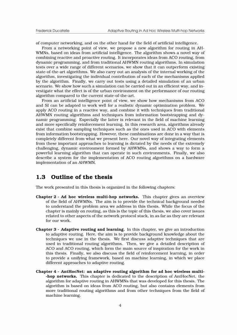
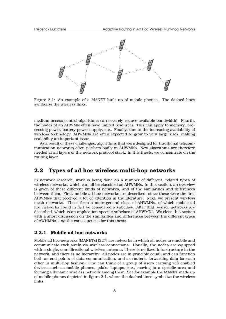
2.1 An example of a MANET built up of mobile phones. The dashed linessymbolize the wireless links. . . . . . . . . . . . . . . . . . . . . . . . . . . . 8
2.2 An example of a WMN, in which five static wireless nodes (in this exam-ple, these are WiFi access points) act as mesh routers and a number ofheterogeneous mobile devices play the role of mesh clients. . . . . . . . . . 10
2.3 The hidden and exposed terminal problems (figure adapted from [254]) . . 152.4 The working of OLSR. The dashed lines symbolize wireless links (not all
links are drawn in order not to overload the picture). Node j chooses i, k,l and m as MPR nodes, since they are sufficient to reach all its two-hopneighbors. Figure adapted from [61]. . . . . . . . . . . . . . . . . . . . . . . 20
3.1 An example of the working of RIP. The figure shows the routing table main-tained in node 2, and one of the update messages that are periodicallysent out by this node. The trajectories of the update messages are given indashed lines. The cost of each link is given in milliseconds. . . . . . . . . . 33
3.2 The counting to infinity problem. After the failure of the link between node2 and node 3, node 1 and node 2 adapt their estimate of the cost of theroute to node 4 based on the updates they receive from each other. Figureadapted from [254]. . . . . . . . . . . . . . . . . . . . . . . . . . . . . . . . . 34
3.3 An example of the working of OSPF. The figure shows the topologicaldatabase maintained in node 2 (this should be the same for each nodein the network), and a link state advertisements sent out by node 2. Thelink state advertisements are flooded over the network, as is indicated bythe dashed lines. . . . . . . . . . . . . . . . . . . . . . . . . . . . . . . . . . . 36
3.4 The shortest path mechanism used by ants. The different colors indicateincreasing levels of pheromone intensity. From left to right and then fromtop to bottom, we see the situation in successive time steps. Figure takenfrom [70]. . . . . . . . . . . . . . . . . . . . . . . . . . . . . . . . . . . . . . . 39
3.5 Data structures for the AntNet routing algorithm. We show for node 2the pheromone routing table, with one row for each next hop and onecolumn for each destination, and the local traffic statistics table, with theaverage, variance and best value for the trip time to each destination. Thevalues given along each link are the expected delay of a data packet on thislink. The line thickness for the outgoing links of node 2 indicate differentpreferences for ants going towards destination 7. . . . . . . . . . . . . . . . 43
3.6 An example of a reinforcement learning problem. A learning agent A entersthe gridworld at position S. It can move to different positions by takingone of four possible actions: north, south, east or west. The reward is 0 ineach position, except for position G, where the reward is 10. After reachingposition G, the agent is automatically moved back to S. The agent shouldlearn by trial and error to find which movements maximize its total reward. 51
ix
Frederick Ducatelle Adaptive Routing in Ad Hoc Wireless Multi-hop Networks
3.7 A formal model for the RL problem. The agent interacts with its environ-ment. At time step t, the agent is in state st in the environment, andreceives the corresponding reward rt. In response, it takes action at. Theenvironment, in turn, responds to the action in time step t + 1, providingthe agent with a new state st+1 and reward rt+1. Figure taken from [252]. 52
4.1 A finite state machine representation of the AntHocNet routing algorithm. 604.2 An example of available pheromone in an AHWMN. Node 1 is running a
communication session with node 8 as destination. Regular pheromoneis indicated by solid arrows. The route over the nodes 3, 6 and 7 is theresult of a reactive route setup. The one-hop route from node 5 to node8 is there independent of the running session: node 5 is aware that node8 is its neighbor and therefore knows it has a one hop path to node 8.Virtual pheromone is indicated by dashed arrows. It forms a field pointingtowards the destination node 8. Virtual pheromone is the result of thepheromone diffusion process. . . . . . . . . . . . . . . . . . . . . . . . . . . 66
5.1 Results for AntHocNet, AODV, OLSR and ANSI using different values forthe maximum speed in the RWP mobility model: (a) delivery ratio, (b) av-erage end-to-end delay, (c) average delay jitter, (d) overhead in number ofpackets, and (e) overhead in number of bytes. . . . . . . . . . . . . . . . . . 86
5.2 Results for AntHocNet, AODV, OLSR and ANSI using different values forthe pause time in the RWP mobility model: (a) delivery ratio, (b) averageend-to-end delay, (c) average delay jitter, (d) overhead in number of pack-ets, and (e) overhead in number of bytes. . . . . . . . . . . . . . . . . . . . . 88
5.3 A node moving according to the RWP mobility model. The node starts ina randomly chosen initial point (A). It chooses a random destination point(B) and moves to it in a straight line. Then, it pauses for a fixed amountof time. After that, it repeats this sequence of actions till the end of thesimulation (leading to the points C, D, E, and F). . . . . . . . . . . . . . . . 89
5.4 Results for AntHocNet, AODV, OLSR and ANSI using different values forthe maximum speed using the GM mobility model: (a) delivery ratio, (b)average end-to-end delay, (c) average delay jitter, (d) overhead in numberof packets, and (e) overhead in number of bytes. . . . . . . . . . . . . . . . 91
5.5 Results for AntHocNet, AODV, OLSR and ANSI using different values forthe data send rate: (a) delivery ratio, (b) average end-to-end delay, (c) av-erage delay jitter, (d) overhead in number of packets, and (e) overhead innumber of bytes. . . . . . . . . . . . . . . . . . . . . . . . . . . . . . . . . . . 94
5.6 Results for AntHocNet, AODV, OLSR and ANSI using different values forthe number of data sessions: (a) delivery ratio, (b) average end-to-enddelay, (c) average delay jitter, (d) overhead in number of packets, and (e)overhead in number of bytes. . . . . . . . . . . . . . . . . . . . . . . . . . . 96
5.7 Results for AntHocNet, AODV, OLSR and ANSI using different sizes for thenetwork area surface. The length of the long edge in meters is given onthe x-axis, while the length of the short edge is always one third of this.We report (a) delivery ratio, (b) average end-to-end delay, (c) average delayjitter, (d) overhead in number of packets, and (e) overhead in number ofbytes. . . . . . . . . . . . . . . . . . . . . . . . . . . . . . . . . . . . . . . . . 98
5.8 Results for AntHocNet, AODV, OLSR and ANSI using different networksizes. The number of nodes in the network is indicated on the x-axis. Thenetwork area size is incremented proportionally so that the node densityremains the same as in the base scenario. We report (a) delivery ratio, (b)average end-to-end delay, (c) average delay jitter, (d) overhead in numberof packets, and (e) overhead in number of bytes. . . . . . . . . . . . . . . . 100
x
Frederick Ducatelle Adaptive Routing in Ad Hoc Wireless Multi-hop Networks
5.9 Results for AntHocNet, AntHocNet without proactive route maintenanceprocess (“AntHocNetnp”), AntHocNet without local route repair (“AntHocNetnr”)and AntHocNet with neither proactive route maintenance nor route repair(“AntHocNetnpnr”). The tests are carried out in scenarios with increasingnumber of nodes, as in subsection 5.2.7. We report (a) delivery ratio, (b)average end-to-end delay, (c) average delay jitter, and (d) overhead in num-ber of packets. . . . . . . . . . . . . . . . . . . . . . . . . . . . . . . . . . . . 102
5.10The average number of hops for different versions of AntHocNet in scenar-ios with increasing number of nodes. . . . . . . . . . . . . . . . . . . . . . . 103
5.11Results for AntHocNet using different routing metrics: signal-to-interference-and-noise ratio (“SINR”), number of hops (“Hops”), delay (“Delay”), and thecombination of hops and delay (“Delay+Hops”). The tests are carried out inscenarios with increasing number of nodes, as in subsection 5.2.7. We re-port (a) delivery ratio, (b) average end-to-end delay, (c) average delay jitter,and (d) overhead in number of packets. . . . . . . . . . . . . . . . . . . . . 104
5.12The average number of hops for AntHocNet using different routing metricsin scenarios with increasing number of nodes. . . . . . . . . . . . . . . . . 105
5.13Results for AntHocNet using different send intervals for the proactive ants.We send 1 ant every 0.5, 1, 2, 5, 10, 20, and 50s. This is indicated onthe x-axis. We use scenarios with varying mobility: we apply RWP withmaximum speeds of 2, 5, 10 and 20m/s. The results for different speedvalues are represented with different curves. We report (a) delivery ratio,(b) average end-to-end delay, (c) average delay jitter, and (d) overhead innumber of packets. . . . . . . . . . . . . . . . . . . . . . . . . . . . . . . . . 106
5.14Results for AntHocNet using different send intervals for the proactive ants.We send 1 ant every 0.5, 1, 2, 5, 10, 20, and 50s. This is indicated on thex-axis. We use scenarios with varying data load: we use data sessionssending 1, 4 and 8 packets per second. The results for different data sendrates are represented with different curves. We report (a) delivery ratio,(b) average end-to-end delay, (c) average delay jitter, and (d) overhead innumber of packets. . . . . . . . . . . . . . . . . . . . . . . . . . . . . . . . . 107
5.15Results for AntHocNet using different number of entries in the pheromonediffusion messages. The number of entries used are 0, 2, 5, 10 and 20, andare indicated on the x-axis. We do experiments with varying node mobility:we apply RWP with maximum speeds of 2, 5, 10 and 20m/s. The resultsfor different speed values are represented with different curves. We report(a) delivery ratio, (b) average end-to-end delay, (c) average delay jitter, and(d) overhead in number of packets. . . . . . . . . . . . . . . . . . . . . . . . 108
5.16Results for AntHocNet using different values for the proactive ant routingexponent. The exponent values that we use are 2, 5, 10, 20 and ∞ (thelatter represents deterministic forwarding of proactive forward ants alongthe best path). The tests are carried out in scenarios with varying dataload: we use data sessions sending 1, 4 and 8 packets per second. Theresults for different data send rates are represented with different curves.We report (a) delivery ratio, (b) average end-to-end delay, (c) average delayjitter, and (d) overhead in number of packets. . . . . . . . . . . . . . . . . . 109
5.17Results for AntHocNet using different values for the data routing expo-nent. The exponent values that we use are 2, 5, 10, 20 and ∞ (the latterrepresents deterministic forwarding of data along the best path). The testsare carried out in scenarios with varying data load: we use data sessionssending 1, 4 and 8 packets per second. The results for different data sendrates are represented with different curves. We report (a) delivery ratio,(b) average end-to-end delay, (c) average delay jitter, and (d) overhead innumber of packets. . . . . . . . . . . . . . . . . . . . . . . . . . . . . . . . . 110
xi
Frederick Ducatelle Adaptive Routing in Ad Hoc Wireless Multi-hop Networks
6.1 The setting of our simulation study: an area of 1561 × 997m2 in the centerof the Swiss town of Lugano. . . . . . . . . . . . . . . . . . . . . . . . . . . 115
6.2 A graph representing street patterns in our urban environment. The graphis indicated by the red lines in the figure. This graph was used to calculatelocations and movements for the network nodes. . . . . . . . . . . . . . . 116
6.3 For the modeling of radio wave propagation, we make use of precalculatedsignal strength data. In order to calculate this data, we choose discretesample points at regular intervals in the areas where the nodes move, andmake ray propagation calculations for each pair of points. In the map, thelocations of the sample points are indicated with red circles. . . . . . . . . 118
6.4 Graph properties of AHWMNs with increasing number of nodes in the ur-ban setting versus in an open space environment. We report here (a) theaverage number of neighbors per node, (b) the average fraction of nodepairs between which a path exists, (c) the average length of the shortestpath between nodes (measured in number of hops), and (d) the averagelink duration. . . . . . . . . . . . . . . . . . . . . . . . . . . . . . . . . . . . . 121
6.5 Results for AntHocNet and AODV with increasing data send rates in theurban scenario. We report (a) delivery ratio, (b) average end-to-end delay,(c) average delay jitter, (d) overhead in number of packets, and (e) overheadin number of bytes. . . . . . . . . . . . . . . . . . . . . . . . . . . . . . . . . 122
6.6 Results for AntHocNet and AODV with increasing number of data sessionsin the urban scenario. We use data rates of 5 and 10 packets/s, indicated bydifferent curves in the figure. We report (a) delivery ratio, (b) average end-to-end delay, (c) average delay jitter, (d) overhead in number of packets,and (e) overhead in number of bytes. . . . . . . . . . . . . . . . . . . . . . . 124
6.7 Results for AntHocNet and AODV with increasing number of nodes in theurban scenario. We use data rates of 0.033, 2 and 25packets/s, indicated bydifferent curves in the figure. We report (a) delivery ratio, (b) average end-to-end delay, (c) average delay jitter, (d) overhead in number of packets,and (e) overhead in number of bytes. . . . . . . . . . . . . . . . . . . . . . . 126
6.8 Results for AntHocNet and AODV with increasing maximum node speedin the urban scenario. We use data rates of 0.033, 2 and 25packets/s,indicated by different curves in the figure. We report (a) delivery ratio, (b)average end-to-end delay, (c) average delay jitter, (d) overhead in numberof packets, and (e) overhead in number of bytes. . . . . . . . . . . . . . . . 128
6.9 Results for AntHocNet and AODV with VoIP level data rates (25packets/s)and varying numbers of data sessions in the urban scenario. We report(a) delivery ratio, (b) average end-to-end delay, (c) average delay jitter, (d)overhead in number of packets, and (e) overhead in number of bytes. . . . 130
6.10Sessions reaching VoIP quality requirements in terms of delivery ratio,delay and jitter: (a) as a fraction of the total number of started sessionsand (b) in absolute numbers. . . . . . . . . . . . . . . . . . . . . . . . . . . . 131
7.1 The layout of the Magnets backbone network in the center of Berlin. Thefigure shows the name and the location of the buildings on which thebackbone nodes are placed, and indicates the wireless links that existbetween them, with their lengths. Figure taken from [148]. . . . . . . . . . 134
7.2 The structure of the MagAntA routing system. . . . . . . . . . . . . . . . . 1387.3 Declaration of the routing interface structure. Some details were left out
to improve readability; e.g., the parameters taken by each of the functionsare left out here. . . . . . . . . . . . . . . . . . . . . . . . . . . . . . . . . . . 140
7.4 The integration of MagAntA with the Linux kernel using Ana4. . . . . . . . 1437.5 The Ana4 ad hoc layer, (a) as seen from layer 3, and (b) as seen from layer 2.144
xii

Frederick Ducatelle Adaptive Routing in Ad Hoc Wireless Multi-hop Networks
7.6 The different tables used for routing in Ana4: (a) the ARP table maps IPaddresses to ad hoc addresses, (b) the COM table maps destination adhoc addresses to next hop ad hoc addresses, and (c) the ATP table mapsnext hop ad hoc addresses to MAC addresses and outgoing device names.Example adapted from [38]. . . . . . . . . . . . . . . . . . . . . . . . . . . . 145
xiii

List of Tables
5.1 Different control packets used by AntHocNet and AODV in the experimentswith increasing RWP pause times. We report the number of route setups,route retries and route repairs per session. . . . . . . . . . . . . . . . . . . 90
5.2 The average link duration for RWP and GM mobility over a 900 secondscenario using increasing maximum speeds. . . . . . . . . . . . . . . . . . 92
xv

Glossary
ABC Ant-Based Control, 41ABR Associativity-Based Routing, 25ACK ACKnowledgement, 15ACO Ant Colony Optimization, 31ACS Ant Colony System, 41ADRA Ant-based Distributed Routing Algorithm,
49AHWMN Ad Hoc Wireless Multi-hop Network, 1AI Artificial Intelligence, 39AMQR Ant colony based Multi-path QoS-aware
Routing, 49ANSI Ad hoc Networking with Swarm Intelli-
gence, 48AODV Ad-hoc On-demand Distance Vector rout-
ing, 17ARA Ant-colony-based Routing Algorithm, 48ARP Address Resolution Protocol, 135AS Ant System, 40AS Autonomous System, 31ASR Adaptive Swarm-based Routing, 46ATM Asynchronous Transfer Mode, 47
BGP Border Gateway Protocol, 18, 31
CAF Co-operative Asymmetric Forward, 46CBR Constant Bit Rate, 83CE Cross-Entropy, 47CGSR Clusterhead Gateway Switched Routing,
23CTS Clear To Send, 15
DCF Distributed Coordination Function, 15DSDV Destination-Sequenced Distance-Vector
routing, 17DSR Dynamic Source Routing, 17DTL Deutsche Telekom Laboratories, 9DTN Delay Tolerant Network, 13
ETT Expected Transmission Time, 25ETX Expected Transmission Count, 25
FSR Fisheye State Routing, 24
xvii
Frederick Ducatelle Adaptive Routing in Ad Hoc Wireless Multi-hop Networks
GA Genetic Algorithm, 46GM Gauss-Markov, 85GPS Global Positioning System, 24GSM Global System for Mobile Communica-
tions, 1
IETF Internet Engineering Task Force, 9
LAN Local Area Network, 25LEACH Low Energy Adaptive Clustering Hierar-
chy, 24LoS Line of Sight, 116LQSR Link Quality Source Routing, 21LSA Link State Advertisement, 36
MABR Mobile Ants Based Routing, 26MAC Medium Access Control, 14MANET Mobile Ad hoc NETwork, 8MCL Mesh Connectivity Layer, 21MIT Massachusetts Institute of Technology, 9MMAS MAX-MIN Ant System, 41MPLS Multiprotocol Label Switching, 137MPR Multi-Point Relays, 19
NoC Networks-on-Chip, 47
OLSR Optimized Link State Routing, 17OSPF Open Shortest Path First, 19, 31
PERA Probabilistic Emergent Routing Algorithm,48
QoS Quality of Service, 36
RBA Routing By Ants, 46RERR Route ERRor message, 21RIP Routing Information Protocol, 18, 31RL Reinforcement Learning, 50RREP Route REPly message, 21RREQ Route REQuest message, 21RTS Request To Send, 15RTT Round Trip Time, 16RWP Random WayPoint, 13
SELA Stochastic Estimator Learning Automata,47
SINR signal-to-interference-and-noise ratio, 73SMS Short Messaging Service, 113
TCP Transmission Control Protocol, 16TORA Temporally-Ordered Routing Algorithm,
22
xviii
Frederick Ducatelle Adaptive Routing in Ad Hoc Wireless Multi-hop Networks
TSP Traveling Salesman Problem, 40
UDP User Datagram Protocol, 16UWB Ultra Wide Band, 1
VoIP Voice-over-IP, 113
WAN Wide Area Network, 26WDM Wavelength-Division Multiplexing, 47WiFi Wireless-Fidelity, 1WiMax Worldwide Interoperability for Microwave
Access, 1WLAN Wireless Local Area Network, 1WMN Wireless Mesh Network, 9
ZRP Zone Routing Protocol, 18
xix

Chapter 1
Introduction
In this thesis, we investigate the development of adaptive routing algorithms for adhoc wireless multi-hop networks using techniques from artificial intelligence, and inparticular from swarm intelligence. The aim of the thesis is two-fold. From the point ofview of networking, we want to take advantage of promising techniques from the areaof artificial intelligence to develop a strong algorithm to solve the challenging task ofrouting in ad hoc wireless multi-hop networks. From the point of view of artificial intel-ligence, we want to show how the basic ideas from swarm intelligence can be adaptedto work well for a realistic, very challenging dynamic problem.
In what follows, we first give a general introduction to the problem that is investi-gated in the thesis. Then we list the contributions of the thesis, and finally, we providean outline of its content.
1.1 General introduction
One of the most important developments in recent years in the field of telecommu-nication networks is the increased use of wireless communication. A wide range ofdifferent wireless technologies and standards have been developed, including Wireless-Fidelity [3] (WiFi, IEEE 802.11), Bluetooth [33] (IEEE 802.15.1), Zigbee [13] (IEEE802.15.4), Ultra Wide Band [4, 282] (UWB, IEEE 802.15.3), Worldwide Interoperabil-ity for Microwave Access [5] (WiMax, IEEE 802.16), etc.. These technologies are beingmade available on an ever increasing number of devices such as laptops, mobile phones,palmtops, etc., allowing them to connect to a variety of different networks. This explo-sive growth has made wireless communication networks one of the most importantareas of research in computer science.
Within the field of wireless networks, one can make a distinction between infrastruc-tured networks and infrastructureless networks [227]. In infrastructured networks, afixed, wired backbone infrastructure is available, and all communication is directedover this backbone. This approach is followed in traditional wireless network systemssuch as the Global System for Mobile Communications (GSM) [222] and Wireless LocalArea Networks (WLANs) [110]. In infrastructureless networks, such a backbone doesnot exist, and wireless devices communicate directly with one another through point-to-point connections. An important aspect in infrastructureless wireless networks isthe use of multi-hop data forwarding: since direct point-to-point connections are onlypossible between wireless nodes that are in immediate radio range of each other, com-munication between nodes that are remote from each other needs to be supported byother nodes in the network, which function as relay points, effectively substituting themissing wired backbone infrastructure. Infrastructureless wireless networks are also
1
Frederick Ducatelle Adaptive Routing in Ad Hoc Wireless Multi-hop Networks
referred to as ad hoc networks, since they can be deployed on-the-fly, without the needfor prior planning (as opposed to infrastructured networks, where considerable effortsand investments are needed before communication can take place). In this thesis, wewill use the term ad hoc wireless multi-hop networks (AHWMNs).
Different types of AHWMNs exist. Examples are mobile ad hoc networks, wirelessmesh networks and sensor networks. Mobile ad hoc networks (MANETs) [227] arenetworks that are made up of a set of homogeneous mobile devices. These devicescommunicate exclusively through wireless connections, normally using a single, omni-directional antenna. All nodes in the network are equal, and there are no designatedrouters, meaning that all nodes can serve both as end points of data communicationand as intermediate relay points or routers. Wireless mesh networks (WMNs) [16] dif-fer from MANETs mainly because they are more heterogeneous. They consist of meshclient nodes, which are similar to MANET nodes, and mesh router nodes, which areusually less mobile, have more resources (e.g. more powerful processors, more batterypower, etc..), and support a variety of different wireless technologies. The availability ofmesh routers allows the creation of a structured organization and can greatly improvethe applicability and the capacities of the network. Finally, sensor networks [17] areAHWMNs that consist of wireless sensor nodes. Each sensor node is a small unit con-taining one or more sensors, a small processing unit and a wireless radio. Problemsspecific to sensor networks stem from the fact that sensor nodes are small and havevery limited capacities, that usually vast numbers of nodes are deployed, and that datatraffic patterns show certain characteristic regularities.
In this thesis, we focus on the problem of routing in AHWMNs. Routing is the taskof constructing and maintaining the paths that connect remote source and destinationnodes of data. This task is particulary hard in AHWMNs due to issues that result fromthe particular characteristics of these networks. A first important issue is the fact thatAHWMNs are dynamic networks. This is due to their ad hoc nature: connections be-tween nodes in the network are set up in an unplanned manner, and are often changedwhile the network is in use. Especially when mobile nodes are used, such changes cantake place continuously. An AHWMN routing algorithm should be adaptive in order tokeep up with such dynamics. A second issue is the unreliability of wireless commu-nication. Data and control packets can easily get lost during transmission, especiallywhen mobile nodes are involved, and when multiple transmissions take place simul-taneously and interfere with each other. A routing algorithm should be robust withrespect to such losses. A third issue is caused by the often limited capabilities of theAHWMN nodes. There are limitations in terms of network bandwidth, node processingpower, memory, battery power, etc.. It is therefore important for a routing algorithmto work in an efficient way. Finally, a last important issue is the network size. Withthe ever growing numbers of portable wireless devices, many AHWMNs are expected togrow to very large sizes. Routing algorithms should be scalable to keep up with suchevolutions.
To solve the challenging problem of routing in AHWMNs, we apply methods from thefield of artificial intelligence. Specifically, we are interested in the use of techniquesfrom swarm intelligence (SI) [34,151] and ant colony optimization (ACO) [83,87]. SI isthe branch of artificial intelligence that is focused on the design of algorithms inspiredby the collective behavior of social insects and other animal societies. ACO is a subsetof SI that takes its inspiration from the foraging behavior of ants living in colonies. Ithas been observed from experiments that ants in a colony are able to find the shortestpath between their nest and a food source, even though this task is well outside thecapabilities of each individual ant. The key to this colony level shortest path behavioris the use of a volatile chemical substance called pheromone. Ants going between theirnest and a food source leave a trail of pheromone behind, and also preferentially move inthe direction of higher pheromone intensities. Shorter paths can be completed quickerand more frequently by the ants, and therefore get marked with a higher pheromone
2
Frederick Ducatelle Adaptive Routing in Ad Hoc Wireless Multi-hop Networks
intensity. These paths then attract more ants, which in turn increases their pheromonelevel, until there is a convergence of the majority of the ants onto the shortest paths.The ants completing paths can be seen as repetitive samples of possible paths, whilethe laying and following of pheromone results in a collective learning process guidedby implicit reinforcement of good solutions. ACO algorithms inspired by this shortestpath behavior have been developed in recent years for many different problems. Themain areas of application have been on the one hand the field of static combinatorialoptimization problems (see e.g. [84,107,169]), and on the other hand the field of routingin telecommunication networks (see e.g. [235,71,70]).
ACO algorithms for routing in telecommunication networks differ substantially frommore traditional routing algorithms. They gather routing information through the repet-itive sampling of possible paths between source and destination nodes using artificialant packets. Probabilistic distance vector tables, called pheromone tables, fulfill therole of pheromone in nature, with artificial ants being forwarded along them in a hop-by-hop way using stochastic forwarding decisions. Also data packets are forwardedstochastically using similar tables, resulting in automatic data load balancing. ACOrouting algorithms boast some of the properties that we have outlined earlier as beingimportant for AHWMN routing, such as adaptivity and robustness. This is mainly dueto the continuous exploration of the network by stochastically forwarded ant probingpackets. However, existing ACO routing algorithms have mainly been designed for wirednetworks. They are not able to deal with the high levels of change that are present inAHWMNs, nor do they offer the efficiency needed to work in AHWMNs. For example,the same repetitive sampling of paths using ant agents that ensures continued adap-tivity and robustness, can easily generate high levels of overhead that can clutter thenetwork.
In this thesis, we investigate how ideas from ACO routing can be used efficiently tobuild an adaptive routing algorithm for AHWMNs. Our aim with this work is twofold.On the one hand, we want to develop a routing algorithm for AHWMNs that containsthe advantages of adaptivity and robustness that are present in ACO routing. In thisway, we want to obtain an algorithm that can deliver a better service than currentlyexisting algorithms for these networks. On the other hand, we want to use AHWMNsas a testbed for the use of SI and ACO: it forms an interesting problem domain to seehow principles from SI and ACO can be applied to a realistic and challenging dynamicoptimization problem. This will lead to the development of new practices in the use ofACO and ACO routing.
One important aspect in the work presented here is the hybridization between differ-ent technologies. Since ACO routing as it exists now is not fit to work well in AHWMNs,we combine it with techniques from other fields. On the one hand, we include tech-niques that are present in existing AHWMN routing algorithms, such as e.g. floodingand local repair mechanisms. On the other hand, we also consider the integration withother methods from artificial intelligence. In particular, we use ideas from informationbootstrapping [252] and dynamic programming [26], which in artificial intelligence areimportant for the field of reinforcement learning [252], and in networking have beenused as the basis for the development of distance vector routing algorithms [27] suchas RIP [123]. This novel combination of the techniques from ACO, which are primarilybased on repeated sampling and are therefore related to Monte Carlo methods, withtechniques from dynamic programming gives a fruitful interaction and allows to builda powerful algorithm.
1.2 Contributions of this thesis
The contributions of the work presented in this thesis can be considered from twodifferent points of view. On the one hand, the thesis contains contributions for the field
3
Frederick Ducatelle Adaptive Routing in Ad Hoc Wireless Multi-hop Networks
of computer networking, and on the other hand for the field of artificial intelligence.From a networking point of view, we propose a new algorithm for routing in AH-
WMNs, based on ideas from artificial intelligence. The algorithm shows a novel way ofcombining reactive and proactive routing. It incorporates ideas from ACO routing, fromdynamic programming, and from traditional AHWMN routing algorithms. In simulationtests over a wide range of different scenarios, we show that it can outperform existingstate-of-the-art algorithms. We also carry out an analysis of the internal working of thealgorithm, investigating the individual contribution of each of the mechanisms appliedby the algorithm. Finally, we carry out tests using a detailed simulation of an urbanscenario. We show how such a simulation can be carried out in an efficient way, and in-vestigate what the effect is of the urban environment on the performance of our routingalgorithm compared to the current state-of-the-art.
From an artificial intelligence point of view, we show how mechanisms from ACOand SI can be adapted to work well for a realistic dynamic optimization problem. Weapply ACO routing in a reactive way, and combine it with techniques from traditionalAHWMN routing algorithms and techniques from information bootstrapping and dy-namic programming. Especially the latter is relevant in the field of machine learningand more specifically reinforcement learning. In this research area, algorithms alreadyexist that combine sampling techniques such as the ones used in ACO with elementsfrom information bootstrapping. However, these combinations are done in a way that iscompletely different from what we present here. Our novel way of integrating elementsfrom these important approaches to learning is dictated by the needs of the extremelychallenging, dynamic environment formed by AHWMNs, and shows a way to form apowerful learning algorithm that can operate in such environments. Finally, we alsodescribe a system for the implementation of ACO routing algorithms on a hardwareimplementation of an AHWMN.
1.3 Outline of the thesis
The work presented in this thesis is organized in the following chapters:
Chapter 2 - Ad hoc wireless multi-hop networks. This chapter gives an overviewof the field of AHWMNs. The aim is to provide the technical background neededto understand the problem area we address in this thesis. While the focus of thechapter is mainly on routing, as this is the topic of this thesis, we also cover issuesrelated to other aspects of the network protocol stack, in as far as they are relevantfor our work.
Chapter 3 - Adaptive routing and learning. In this chapter, we give an introductionto adaptive routing. Here, the aim is to provide background knowledge about thetechniques we use in the thesis. We first discuss adaptive techniques that areused in traditional routing algorithms. Then, we give a detailed description ofACO and ACO routing, which form the main source of inspiration for the work inthis thesis. Finally, we also discuss the field of reinforcement learning, in orderto provide a unifying framework, based on machine learning, in which we placedifferent approaches to adaptive routing.
Chapter 4 - AntHocNet: an adaptive routing algorithm for ad hoc wireless multi--hop networks. This chapter is dedicated to the description of AntHocNet, thealgorithm for adaptive routing in AHWMNs that was developed for this thesis. Thealgorithm is based on ideas from ACO routing, but also contains elements frommore traditional routing algorithms and from other techniques from the field ofmachine learning.
4
Frederick Ducatelle Adaptive Routing in Ad Hoc Wireless Multi-hop Networks
Chapter 5 - An evaluation study of AntHocNet. In this chapter, we present results ofan extensive set of simulation studies in which we evaluate the AntHocNet routingalgorithm. The chapter is divided in two parts, with the first part dedicated toa comparison with current state-of-the-art AHWMN routing algorithms, and thesecond part focused on investigating the internal working of AntHocNet itself.
Chapter 6 - Simulation of an urban scenario. Here, we describe a different set ofsimulation tests, carried out in an urban environment. We first describe how wegot a detailed simulation of such an environment in an efficient way, and thenevaluate the behavior of AntHocNet in this environment.
Chapter 7 - Towards the implementation of adaptive routing in AHWMNs. In thisfinal chapter, we discuss a system for the implementation of ACO routing algo-rithms in real AHWMN testbeds. The system is based on a set of kernel modulesand a routing daemon running in user space.
5

Chapter 2
Ad hoc wireless multi-hopnetworks
The work presented in this thesis is focused on ad hoc wireless multi-hop networks(AHWMN). This chapter gives an overview of existing research on this kind of networks.Section 2.1 provides a definition for AHWMNs. Section 2.2 describes which differenttypes exist. Section 2.3 lists a number of networking issues in AHWMNs, related to dif-ferent levels of the network protocol stack. Finally, we dedicate the whole of section 2.4to routing in AHWMNs, since that is the main focus of this thesis.
2.1 A definition of ad hoc wireless multi-hop networks
In recent years, a growing number of devices are getting equipped with networkingcapabilities. Many of these devices are mobile and communicate using a variety ofwireless technologies, such as Bluetooth, WiFi, etc., which allow them to connect toexisting telecommunication networks and to each other. If these devices also supportrouting, they can forward data for each other. One can then combine a number of suchdevices with minimal planning to form a network. Such a network would be an adhoc wireless multi-hop network. Formally, we can say that an AHWMN is a networkconsisting of nodes that communicate solely through wireless connections, in whichdata can be forwarded over multiple hops, and which is at least partly deployed in adhoc manner. Ad hoc deployment entails that little or no planning is needed, and thatchanges in the network (such as adding, moving or removing nodes) can be done withminimal extra work.
From the above definition, it is clear that there are some substantial differencesbetween AHWMNs and traditional telecommunication networks. Probably the most im-portant difference is that the topology of an AHWMN is not the result of careful planning,but instead emerges from the placement of the nodes: there is a link between nodes ifthey are in range of each other’s wireless radio signal. As a consequence, the topologyis essentially dynamic: it can be extended by adding new wireless nodes, reduced byremoving nodes, or changed in a continuous way if some of the nodes are mobile. Suchdynamic behavior presents an important new challenge in networking technology, sincein traditional networks, changes happen relatively infrequently. A second important dif-ference is that AHWMNs rely exclusively on wireless links. This means that data trans-port is less reliable, and that there is less available bandwidth. Thirdly, AHWMNs areusually highly decentralized, lacking hierarchy or central control. This makes it moredifficult to optimize the use of network resources (e.g., 2.3.3 explains how decentralized
7
Frederick Ducatelle Adaptive Routing in Ad Hoc Wireless Multi-hop Networks
Figure 2.1: An example of a MANET built up of mobile phones. The dashed linessymbolize the wireless links.
medium access control algorithms can severely reduce available bandwidth). Fourth,the nodes of an AHWMN often have limited resources. This can apply to memory, pro-cessing power, battery power supply, etc.. Finally, due to the increasing availability ofwireless technology, AHWMNs are often expected to grow to very large sizes, makingscalability an important issue.
As a result of these challenges, algorithms that were designed for traditional telecom-munication networks often perform badly in AHWMNs. New algorithms are thereforeneeded at all layers of the network protocol stack. In this thesis, we concentrate on therouting layer.
2.2 Types of ad hoc wireless multi-hop networks
In network research, work is being done on a number of different, related types ofwireless networks, which can all be classified as AHWMNs. In this section, an overviewis given of these different kinds of networks, and of the similarities and differencesbetween them. First, mobile ad hoc networks are described, since these were the firstAHWMNs that received a lot of attention in the literature. Next, we present wirelessmesh networks. These form a more general class of AHWMNs, of which mobile adhoc networks could in fact be considered a subclass. After that, sensor networks aredescribed, which is an application specific subclass of AHWMNs. We close this sectionwith a short discussion on the similarities and differences between the different typesof AWHMNs, and the consequences for this thesis.
2.2.1 Mobile ad hoc networks
Mobile ad hoc networks (MANETs) [227] are networks in which all nodes are mobile andcommunicate exclusively via wireless connections. Usually, the nodes are equippedwith a single, omnidirectional wireless antenna. There is no fixed infrastructure in thenetwork, and there is no hierarchy: all nodes are in principle equal, and can functionboth as end points of data communication, and as routers, forwarding data for eachother in multi-hop fashion. One can think of a group of users carrying wifi enableddevices such as mobile phones, pda’s, laptops, etc., moving in a specific area andforming a dynamic wireless network among them. See for example the MANET made upof mobile phones depicted in figure 2.1, where the dashed lines symbolize the wirelesslinks.
8
Frederick Ducatelle Adaptive Routing in Ad Hoc Wireless Multi-hop Networks
As a consequence of the above mentioned properties, MANETs are dynamic, flat,fully decentralized networks without central control or overview. This gives rise to anumber of tough challenges for networking algorithms. MANET algorithms should behighly adaptive to the ever changing environment. They should be robust in order todeal with unreliable wireless transmissions. They should work in a fully distributedway. Finally, they should be efficient in their use of the limited network resources,such as bandwidth, battery power in the mobile nodes, etc..
The idea for MANETs stems from research into DARPA packet radio networks [142,145]. Starting from the publication of the Destination-Sequenced Distance-Vector rout-ing algorithm [211] in 1994, MANETs were the first type of AHWMNs to be investigated.The specific challenges that are encountered in these networks have called the atten-tion of many researchers and have made this a very active research area. Also, theInternet Engineering Task Force (IETF) has set up a MANET working group to guidelinestandardizations. However, when it comes to implementation, the MANET challengeshave proven to be very hard to deal with, so that there is now also a growing interest inAHWMNs with less mobility and more hierarchy and organization, such as the wirelessmesh networks described in 2.2.2.
2.2.2 Wireless mesh networks
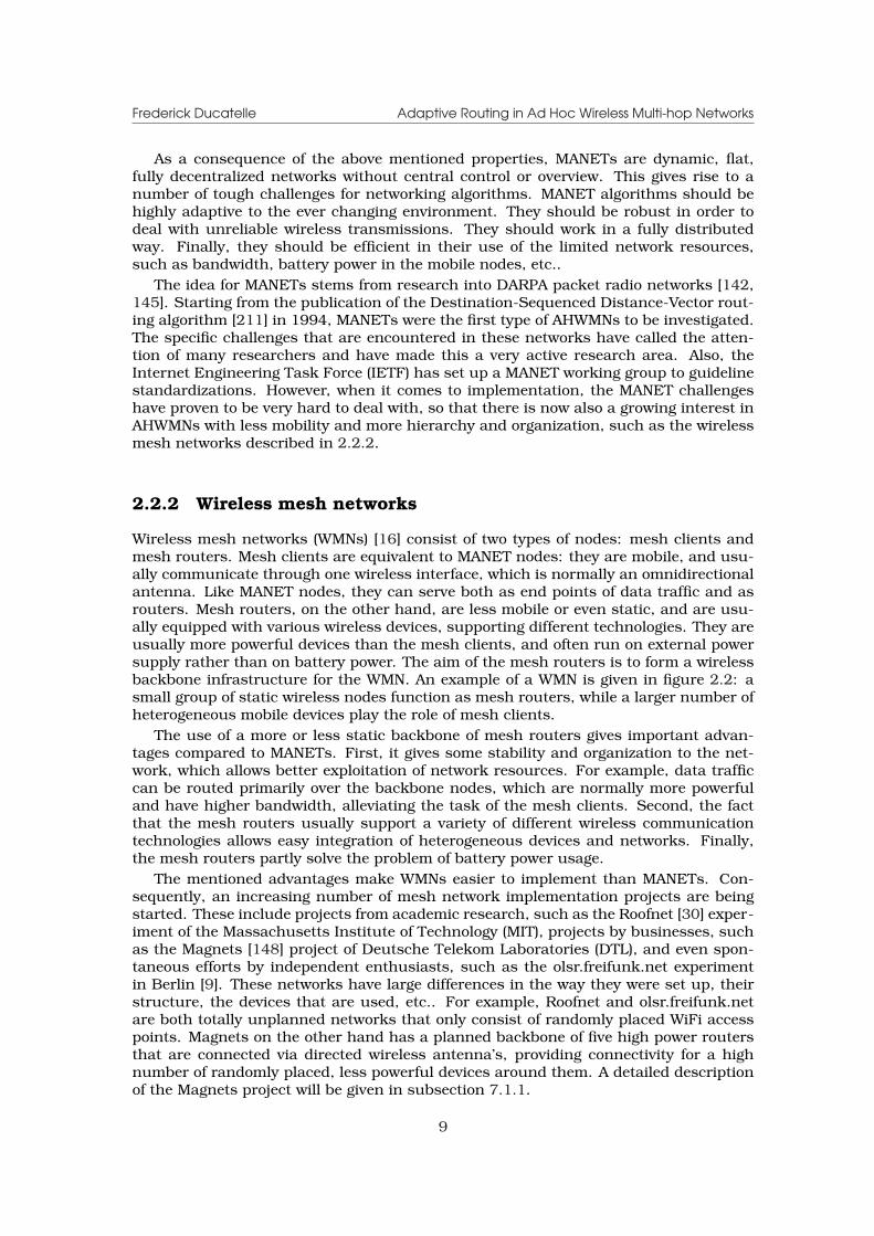
Wireless mesh networks (WMNs) [16] consist of two types of nodes: mesh clients andmesh routers. Mesh clients are equivalent to MANET nodes: they are mobile, and usu-ally communicate through one wireless interface, which is normally an omnidirectionalantenna. Like MANET nodes, they can serve both as end points of data traffic and asrouters. Mesh routers, on the other hand, are less mobile or even static, and are usu-ally equipped with various wireless devices, supporting different technologies. They areusually more powerful devices than the mesh clients, and often run on external powersupply rather than on battery power. The aim of the mesh routers is to form a wirelessbackbone infrastructure for the WMN. An example of a WMN is given in figure 2.2: asmall group of static wireless nodes function as mesh routers, while a larger number ofheterogeneous mobile devices play the role of mesh clients.
The use of a more or less static backbone of mesh routers gives important advan-tages compared to MANETs. First, it gives some stability and organization to the net-work, which allows better exploitation of network resources. For example, data trafficcan be routed primarily over the backbone nodes, which are normally more powerfuland have higher bandwidth, alleviating the task of the mesh clients. Second, the factthat the mesh routers usually support a variety of different wireless communicationtechnologies allows easy integration of heterogeneous devices and networks. Finally,the mesh routers partly solve the problem of battery power usage.
The mentioned advantages make WMNs easier to implement than MANETs. Con-sequently, an increasing number of mesh network implementation projects are beingstarted. These include projects from academic research, such as the Roofnet [30] exper-iment of the Massachusetts Institute of Technology (MIT), projects by businesses, suchas the Magnets [148] project of Deutsche Telekom Laboratories (DTL), and even spon-taneous efforts by independent enthusiasts, such as the olsr.freifunk.net experimentin Berlin [9]. These networks have large differences in the way they were set up, theirstructure, the devices that are used, etc.. For example, Roofnet and olsr.freifunk.netare both totally unplanned networks that only consist of randomly placed WiFi accesspoints. Magnets on the other hand has a planned backbone of five high power routersthat are connected via directed wireless antenna’s, providing connectivity for a highnumber of randomly placed, less powerful devices around them. A detailed descriptionof the Magnets project will be given in subsection 7.1.1.
9
Frederick Ducatelle Adaptive Routing in Ad Hoc Wireless Multi-hop Networks
Figure 2.2: An example of a WMN, in which five static wireless nodes (in this example,these are WiFi access points) act as mesh routers and a number of heterogeneousmobile devices play the role of mesh clients.
10
Frederick Ducatelle Adaptive Routing in Ad Hoc Wireless Multi-hop Networks
2.2.3 Sensor networks
Sensor networks [17] are AHWMNs that consist of wireless sensor nodes. Those aresmall devices equipped with one or more sensors, some small processing capacity, anda radio transmitter. The aim of sensor networks is to deploy a large number of suchsensor devices to measure a certain phenomenon. This can be geological activity, hu-man body functioning, etc.. By forming a multi-hop network among them, the sensornodes have a means to send the data they have measured to a ”sink” node, where theycan be processed. The fact that the network is ad-hoc allows to set it up with minimalplanning. One can for example throw sensors from a boat into the sea so that they canform a network at the bottom, or drop them from a plane.
Sensor networks come with their own specific challenges. First of all, they are usu-ally very large networks, possibly consisting of thousands of nodes or more, so thatalgorithms need to scale well. Next, the sensor nodes are normally designed to be verycheap, light devices. This means that they have very limited resources for storage, pro-cessing and transmission, so that highly efficient algorithms are needed. This problemis acerbated by the fact that sensor batteries can often not be replaced (e.g., when thesensors are thrown at the bottom of the ocean). Moreover, the use of cheap, low powerradio technology also means that communication is highly unreliable and irregular. Forexample, changing radio ranges can give rise to unidirectional connections [290]. Soalgorithms have to be robust and should be able to deal with unidirectional links. An-other issue in sensor networks is that their topology is usually very dynamic. Differentfrom MANETs, this is not so much due to mobility of the sensor nodes (they are in factoften static), but rather to the easy failure of lightweight devices with limited power, andthe fact that often new sensor devices are added. Finally, the communication patternsin sensor networks are quite specific: each sensor node acquires data at regular inter-vals, and needs to send this data to the sink node. It is important to take these patternsinto account when designing network protocols, in order to obtain better usage of thelimited available resources.
2.2.4 Algorithms for different types of AHWMNs
All three types of networks described above possess the typical properties of AHWMNs:they have an ad hoc, dynamic topology, they use unreliable connections, they arehighly decentralized, and they have limited network resources. Also, they might allgrow to large sizes, although this aspect is more pronounced in sensor networks thanin MANETs and WMNs. Due to these similarities, networking algorithms for differenttypes of AHWMNs should have similar properties, such as adaptivity to a changing en-vironment, robustness with respect to packet corruption or loss, a highly distributedorganization, efficiency and scalability. As a result, there is often a large overlap be-tween algorithms used for the different types of AHWMNs. Especially for MANETs andWMNs this is the case. MANETs were the first AHWMNs that received a lot of researchattention, and WMNs can in a way be seen as the follow up of MANETs. Therefore,WMNs use to a large extent the algorithms that have been proposed for MANETs. Sen-sor networks have been developed more or less in parallel with MANETs, and have morespecific algorithms. The work in this thesis is in the first place focused on MANETs andWMNs.
2.3 Issues in ad hoc wireless multi-hop networking
This section builds on the general description provided in section 2.2 to investigateimportant issues for networking in AHWMNs. We start with aspects of network con-nectivity and node mobility, and then move up the network protocol stack discussing
11
Frederick Ducatelle Adaptive Routing in Ad Hoc Wireless Multi-hop Networks
issues related to the physical layer, the data link layer, and the transport layer. Specificattention is given to how these issues have consequences for the task of routing. Rout-ing itself is not discussed in this section: since it is the main focus of attention of thisdissertation, it is treated in more detail in section 2.4.
2.3.1 Network topology and node mobility
As stated in 2.2, the topology of an AHWMN is normally not the result of careful plan-ning, but arises from the placement of the nodes. In what follows, we first comment onhow this affects network connectivity, and then on how it relates to node mobility.
Network connectivity
There is a link between two nodes of an AHWMN if they can receive each other’s radiosignals. Therefore, the topology of the network is directly defined by the relative place-ment of the nodes and the range of their radio transmitters. Since the placement of thenodes in an AHWMN is done in ad hoc manner, with minimal planning, it can be con-sidered as a random process, from which the network topology emerges. An importantfactor in this process is the node density, since it directly influences the connectivity inthe resulting network topology. In [89,88], the theory of percolation is used to investi-gate this relationship between node density and network connectivity analytically. Theauthors show that there is a quite clear cut off point in node density, called the criticaldensity, under which the network falls apart into small, internally connected islands,and above which there is connectivity between the majority of the nodes in the network.For densities that are just above the critical density, this network wide connectivity isquite sparse, so that paths between most pairs of nodes depend on the availability of afew critical links. The failure of any of these critical links has a large impact on the rout-ing possibilities in the network. This is in contrast with densely connected networks,where often many alternatives are available to route around a failed link. This meansthat in sparse networks, it is more difficult for a routing algorithm to provide adaptivityto changes in the network topology. So, we can conclude that the node density of anAHWMN directly affects the difficulty of the routing task.
Node density only has meaning when treated relative to the transmission range ofthe nodes’ radio equipment: if this range is reduced while the number of nodes perunit of area stays the same, the connectivity of the network decreases. This means thatvariations of the radio range influence network connectivity as much as node density.Radio range variations can happen accidently, for example because of random varia-tions in the environment or because of changes in the available power in each node (seealso explanations in 2.3.2), or can be induced intentionally, for example in order to savebattery power or to reduce radio interference between different transmitters [195,150].Some work treats the problem of defining a minimal power usage for each node un-der the explicit constraint that there needs to be at least one path between each pairof nodes in the network [114, 196]. This is particularly relevant in sensor networks,where, as mentioned in 2.2.3, batteries can sometimes not be replaced. Clearly, theapplication of such schemes can give rise to difficult topologies to maintain routing in.
Node mobility
Since the network topology is defined by the placement of the nodes, it changes whenthe nodes move. As a consequence, the difficulty of the routing task is also stronglyinfluenced by the characteristics of the node mobility. These characteristics includethe speed of the movements, and the specific patterns followed by the nodes. Thelatter defines for example how the nodes move relative to each other, and can give rise
12

Frederick Ducatelle Adaptive Routing in Ad Hoc Wireless Multi-hop Networks
to temporary differences in node density. The impact of node mobility is especiallyimportant in MANETs, where all nodes are mobile.
Node mobility depends on the usage of the network. Unfortunately, most research onAHWMNs is done in academic context, without a clear understanding of their purpose.Mobility is therefore usually simulated with artificial models, of which the RandomWaypoint model (RWP) [140] is by far the most popular. Under this model, each nodepicks a random destination, and a random speed, and moves in a straight line to thisdestination with the chosen speed. Then the node pauses for a certain time, after whichit picks a new destination and speed. Other models use different approaches, or modelspecific behaviors such as e.g. group movements. An overview of mobility models usedin the literature is given in [46]. In recent years, there is a growing suspicion towardsthese artificial mobility models, because they do not reflect real movements very well,and because they may artificially give rise to certain node distributions. For example,under RWP, nodes tend to cluster more in the center of the AHWMN area, so that thereis higher density there, giving better connectivity [29]. There is now a lot of interest incollecting traces of real movements of people (e.g., see [55]), but so far very few suchinformation is available.
An interesting side remark can be made here with respect to the relationship be-tween mobility, connectivity and network capacity. If applications can tolerate highdelays, communication between remote nodes in the network can profit from node mo-bility by letting packets be temporarily stored in moving nodes, so that they can travelcloser to their destination this way. This can increase the capacity of the network, sinceless wireless retransmissions need to be done [118]. It can also allow communication innetworks where there is no direct connectivity between source and destination nodes.This is the area of delay tolerant networking (DTN) [44]. DTN was in the first placedeveloped as a solution for interplanetary telecommunications, where some links canincur enormous delays, and some recipients can temporarily be out of range for com-munication, e.g. a space station that is circling around a remote planet. Recently, theterm DTN has also been adopted to describe AHWMNs with intermittent connectivity,such as e.g. MANETs consisting of people carrying short-range bluetooth devices. Alsothe terms opportunistic networking or pocket switched networking are used [246,133].While these “terrestrial” DTNs could be seen as a new type of AHWMNs, they are usuallystill considered MANETs, operating in the extreme case where there is very limited con-nectivity. Nevertheless, they need specific networking algorithms, which can deal withthese difficult circumstances. Such algorithms are outside the scope of this dissertationthough.
2.3.2 The physical layer
The physical layer is concerned with issues regarding the physical transmission of databetween two nodes. While a lot could be said about different radio transmission tech-nologies that can be used, we will here limit the discussion to some issues that havedirect implications for routing. First, we discuss about the occurrence of unidirectionallinks, and next, we comment on how choices at the physical layer are defining for net-work capacity.
Unidirectional links
Most networking algorithms for AHWMNs assume all links in the network to be bidirec-tional: if node i can hear node j, then node j can also hear node i. In reality however,an AHWMN can also contain unidirectional links. These can occur for various reasons.One reason can be a difference in radio range between the nodes: if i has a higher rangethan j, it is possible that j can hear i while i cannot hear j. Such a difference in radiorange can be chosen deliberately, or can be the result of a difference in available battery
13
Frederick Ducatelle Adaptive Routing in Ad Hoc Wireless Multi-hop Networks
power in the nodes (see subsection 2.3.1). Another, related reason for the occurrenceof unidirectional links is radio irregularity. It has been observed that the radio range ofwireless nodes does not form a perfect circle around the node, but instead shows quiteirregular patterns [290]. This is mainly due to differences in radio wave propagation indifferent directions. A third reason for unidirectional links can be interference by othertransmitters. It is possible that the level of interference is different at i and j, so thatone of the two can temporarily not receive data from the other. The negative impact onnetwork performance due to the presence of unidirectional links has been documentedin various works [219,187].
Network capacity
Choices at the physical layer are defining for the network capacity. Most work on AH-WMNs relies on WiFi technology (IEEE 802.11) [3], which can in theory provide a rela-tively high throughput of up to 54 Mbps. Other, newer technologies, such as UWB (IEEE802.15.3) [4, 282] and WiMax (IEEE 802.16) [5], promise even much higher through-put. Despite these high bandwidth values, however, the actual available capacity inan AHWMN is much lower. This is due to interference between different transmitters.Different pairs of nodes in the network can only communicate simultaneously if theyare situated far enough from each other, so that they do not disrupt each other’s signal.This is also referred to with the term “spatial reuse”: the wireless channel can be usedfor multiple simultaneous communications if there is spatial separation. In [120], theauthors investigate how much capacity is actually available in an AHWMN if spatialreuse is optimally used. They conclude that the available capacity per node in bit-meters per second is inversely correlated with the square root of the total number ofnodes in the network, which means that for large AHWMNs, the available capacity pernode tends to zero. This result is not very encouraging for AHWMN research, but needsto be read with some caution. The investigation was done for networks using single-channel, omnidirectional antennas. If more than one channel is used, or other antennasystems, such as directional antennas [284] or multi-antenna systems [179], better ca-pacity can be obtained. Nevertheless, when developing algorithms for AHWMNs, oneneeds to be aware that the total available bandwidth is much lower than what wirelesstechnologies can in theory provide, so that efficiency is important.
2.3.3 The data link layer
The data link layer is concerned with the organization of transmission and retransmis-sion of data between two nodes. Often, the data link layer is identified with its mostimportant component, the medium access control (MAC) sublayer. This componentdeals with the coordination of the access of different nodes to a shared communica-tion medium. In AHWMNs, this comes down to avoiding interference while maximizingspatial reuse. A different goal, which is mainly important in sensor networks, is powersaving [19]. In what follows, we first describe general issues related to MAC organiza-tion in AHWMNs, and then discuss the most popular AHWMN MAC protocol, namelythe IEEE 802.11 DCF protocol.
Medium access control in AHWMNs
Since AHWMNs are usually highly decentralized, MAC protocols need to work in a dis-tributed way. This makes it difficult to organize the sharing of the wireless mediumin an efficient way via the creation of multiple channels through frequency or code di-vision multiplexing, or via the assignment of time slots. Research is therefore mainlyconcentrated on single channel, contention based algorithms.
14
Frederick Ducatelle Adaptive Routing in Ad Hoc Wireless Multi-hop Networks
A B C D
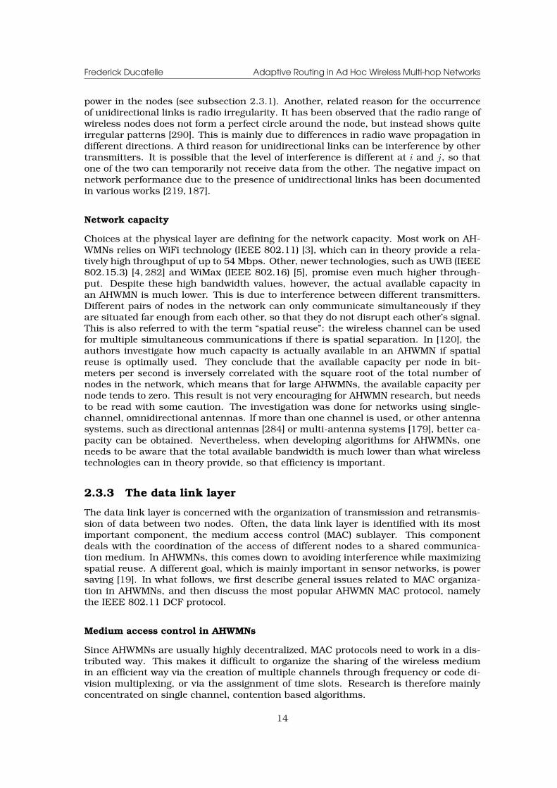
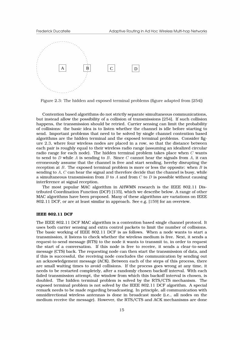
Figure 2.3: The hidden and exposed terminal problems (figure adapted from [254])
Contention based algorithms do not strictly separate simultaneous communications,but instead allow the possibility of a collision of transmissions [254]. If such collisionhappens, the transmission should be retried. Carrier sensing can limit the probabilityof collisions: the basic idea is to listen whether the channel is idle before starting tosend. Important problems that need to be solved by single channel contention basedalgorithms are the hidden terminal and the exposed terminal problems. Consider fig-ure 2.3, where four wireless nodes are placed in a row, so that the distance betweeneach pair is roughly equal to their wireless radio range (assuming an idealized circularradio range for each node). The hidden terminal problem takes place when C wantsto send to D while A is sending to B. Since C cannot hear the signals from A, it canerroneously assume that the channel is free and start sending, hereby disrupting thereception at B. The exposed terminal problem is more or less the opposite: when B issending to A, C can hear the signal and therefore decide that the channel is busy, whilea simultaneous transmission from B to A and from C to D is possible without causinginterference at signal reception.
The most popular MAC algorithm in AHWMN research is the IEEE 802.11 Dis-tributed Coordination Function (DCF) [135], which we describe below. A range of otherMAC algorithms have been proposed. Many of these algorithms are variations on IEEE802.11 DCF, or are at least similar in approach. See e.g. [159] for an overview.
IEEE 802.11 DCF
The IEEE 802.11 DCF MAC algorithm is a contention based single channel protocol. Ituses both carrier sensing and extra control packets to limit the number of collisions.The basic working of IEEE 802.11 DCF is as follows. When a node wants to start atransmission, it listens to check whether the wireless medium is free. Next, it sends arequest-to-send message (RTS) to the node it wants to transmit to, in order to requestthe start of a conversation. If this node is free to receive, it sends a clear-to-sendmessage (CTS) back. The requesting node can then start the transmission of data, andif this is successful, the receiving node concludes the communication by sending outan acknowledgement message (ACK). Between each of the steps of this process, thereare small waiting times to avoid collisions. If the process goes wrong at any time, itneeds to be restarted completely, after a randomly chosen backoff interval. With eachfailed transmission attempt, the window from which this backoff interval is chosen, isdoubled. The hidden terminal problem is solved by the RTS/CTS mechanism. Theexposed terminal problem is not solved by the IEEE 802.11 DCF algorithm. A specialremark needs to be made regarding broadcasting. In principle, all communication withomnidirectional wireless antennas is done in broadcast mode (i.e., all nodes on themedium receive the message). However, the RTS/CTS and ACK mechanisms are done
15
Frederick Ducatelle Adaptive Routing in Ad Hoc Wireless Multi-hop Networks
with just one node and assure the implementation of unicasting. Therefore, if a nodewants to broadcast a message to all its neighbors, it cannot use these mechanisms. Asa consequence, broadcast transmissions are less protected and therefore less reliablethan unicast transmissions.
A lot of research has been done to assess the efficiency of the IEEE 802.11 DCFalgorithm. First of all, due to the sending of extra control packets around each datapacket, and the small delays between each of these sendings, the theoretical maximumthroughput using IEEE 802.11 DCF is a lot lower than the actual capacity of the radiotransmitters [143] (down to 50% or less depending on the size of the transmitted datapackets). More problematic is the use of the exponentially growing random backoff in-terval: if there are a lot of collisions, e.g. when there is a lot of data traffic in the network,it is possible that some communications are suspended for a longer time, or even getcompletely starved [28]. This problem can be acerbated in multi-hop communications,where subsequent hops in a path can actually interfere with each other [170,280].
As a consequence of all this, the use of IEEE 802.11 DCF puts further severe limita-tions on the already compromised capacity of AHWMNs (the capacity limitations basedon spatial reuse calculations described in 2.3.2 assumed a perfect MAC layer protocol).Some improvements have been proposed in other MAC protocols (see [159]), but thebasic problems stay the same. The main cause of inefficiency in MAC layer organiza-tion is the decentralized nature of AHWMNs, which commands a distributed approach.Improvements are possible if there is some structure in the network, such as betweenbackbone nodes in a WMN (see 2.2.2), or if node mobility is low enough so that thereis time to set up a different MAC organization, as is sometimes done in sensor net-works [19,161]. In other cases, however, we need to be aware that the MAC layer limitsthe capacity of the network, and increases the need for efficiency at the routing layer.
2.3.4 The transport layer
The transport layer is situated above the routing layer. It is concerned with the organi-zation of the transport of data between the source and destination nodes of a commu-nication session over the path provided by the routing algorithm [254]. The two maintransport protocols in the internet are the User Datagram Protocol (UDP) [217] and theTransmission Control Protocol (TCP) [218]. TCP offers a secure transport service: atriple handshake mechanism is used to establish a connection at the start of the trans-port session, the arrival of each data packet is acknowledged by the receiver, warningsare sent from the destination to the source if packets arrive out of order, lost packetsare retransmitted, and a congestion control mechanism is used to adapt the speed ofthe data flow in case there is packet loss. UDP, on the other hand, offers a servicewithout any guarantees: it just sends packets on their way from source to destination,without using any of the mentioned mechanisms. UDP can be preferred over TCP forshort data transports when the underlying network is very reliable. In what follows, wecomment on the use of TCP and UDP in AHWMNs.
TCP versus UDP in AHWMNs
AHWMNs are inherently unreliable networks, due to their use of wireless links and theirdynamic nature. So it makes sense to use a secure service like TCP, rather than UDP.However, there are problems with the use of TCP in AHWMNs, stemming from variouscauses.
A first problem for TCP in AHWMNs is that its various mechanisms cause a lot ofextra overhead [111]. For example, for each data packet going from source to des-tination, an acknowledgement is sent back from destination to source. This goes inconflict with the typically low capacity of AHWMNs, as described in 2.3.2 and 2.3.3.This problem can be acerbated due to interactions with the MAC layer algorithm, as
16

Frederick Ducatelle Adaptive Routing in Ad Hoc Wireless Multi-hop Networks
TCP uses exponentially growing random backoff timers for retransmission, just likeIEEE 802.11 DCF (see 2.3.3). A second problem is caused by TCP’s congestion man-agement mechanism [22,250]. TCP was designed with wired networks in mind, wheredata transmissions are quite reliable. Therefore, when TCP detects a problem with datadelivery (out of order delivery or packet loss), it assumes that the cause is congestionof the network, and consequently reduces the data flow. In AHWMNs, however, packetloss is often caused by the use of unreliable wireless links or mobility induced path loss.TCP will therefore lower its throughput unnecessarily and reduce the throughput of thenetwork. A third problem has to do with TCP timers. To define whether a packet waslost, TCP uses timers, which are based on an estimate of the time it takes for a packetto go to a destination and for an acknowledgement to come back to the source. Thisis the so-called round trip time (RTT). In an AHWMN, which is an inherently dynamicenvironment, the RTT can vary greatly, making its estimation difficult. This causesTCP to detect false packet losses, which are again interpreted as caused by congestion,with a reduction of the data throughput as a consequence. A final problem has to dowith the frequent path failures that occur in AHWMNs [130]. In these situations, thereis again packet loss, but the destination will not be able to warn the source about it.Therefore, the source only detects the loss when its timer for the acknowledgement runsout, causing extra delay.
The above problems make the use of TCP in AHWMNs problematic. Therefore, manyvariations of TCP have been proposed, in an attempt to deal with these difficulties.See [268] for an overview. Nevertheless, many AHWMN research studies avoid theseproblems altogether by using the UDP transport protocol. For the routing layer, theimportant message is that correct data delivery is an important evaluation criterium,as the transport layer above it has difficulties providing reliability.
2.4 Routing in ad hoc wireless multi-hop networks
Routing is the task of directing data flows from source nodes to destination nodes whilemaximizing network performance. This is particularly hard in AHWMNs. Due to the adhoc and dynamic nature of the network, the topology can change constantly, and pathsbetween sources and destinations that were initially efficient can quickly become inef-ficient or even infeasible. This means that routing information should be updated moreregularly than in traditional wired telecommunication networks. However, this can be aproblem in AHWMNs, with their limited bandwidth and node resources, and their possi-bly unreliable communication channels. New routing algorithms are therefore needed,which can give adaptivity in an efficient and robust way.
A lot of research has been done on routing in AHWMNs in the past few years. In thissection, we give an overview of the research in this area. The aim is not to present anexhaustive list of existing protocols (for this, we refer to existing surveys, such as [227,14]), but rather to describe the most important ones and to give insight into interestingideas and techniques that have been developed in this area. We start the section with anexplanation of the distinction between proactive and reactive routing protocols, whichis the most used criterium to classify AHWMN routing algorithms. Next, we describein detail a number of representative routing algorithms. Finally, we give an overview ofimportant techniques used in other AHWMN routing algorithms.
2.4.1 Proactive versus reactive routing algorithms
Traditionally, AHWMN routing protocols are classified as proactive or reactive protocols.Under proactive routing protocols, all nodes of the network try to maintain consistentrouting information about all other nodes at all times. This means that routing informa-tion needs to be updated after each change in the network. Data are routed by a simple
17
Frederick Ducatelle Adaptive Routing in Ad Hoc Wireless Multi-hop Networks
lookup in the tables which store the routing information, and proactive routing algo-rithms are therefore also called table-driven [227]. Examples of proactive algorithmsare Destination-Sequenced Distance-Vector Routing (DSDV) [211] and Optimized LinkState Routing (OLSR) [61] (see subsection 2.4.2 for descriptions of both algorithms). Un-der reactive routing protocols, nodes only gather the routing information that is strictlyneeded. This is the case when a new data session is started, or when a currently usedpath fails. Gathering routing information usually involves a route discovery or a routerepair phase. Reactive algorithms are also called on-demand algorithms [227]. Exam-ples are Dynamic Source Routing (DSR) [140] and Ad-Hoc On-Demand Distance VectorRouting (AODV) [213] (see subsection 2.4.2).
Proactive algorithms have the advantage that routing information is always readilyavailable when data needs to be sent. Also, all changes in the network are taken intoaccount, so that new routing opportunities can be exploited, and backup paths can beprovided when primary paths fail. On the downside, these algorithms can become quiteinefficient or even break down completely when a lot of changes need to be tracked.This is the case when the topology is highly dynamic, or when the network is large.Reactive algorithms only focus on the routing information that is strictly necessary.This way, they can greatly reduce the overhead they create, so that they are in generalmore efficient. The disadvantage is that they are never prepared for disruptive events,and that some data packets can therefore incur large delays, e.g. during the routesetup phase at the start of a communication session. In MANETs, where all nodes aremobile, so that there are a lot of topology changes, the general preference is for reactivealgorithms [42]. However, in WMNs, which are less dynamic, and in sensor networks,where nodes are often not mobile, proactive algorithms can also be a good choice.
So far we have used the terms proactive and reactive routing in a rather strict sense.We can define reactive behavior in a more general way as the gathering of routing in-formation in reaction to an event, and proactive behavior as the gathering of routinginformation at all other times. Algorithms which combine both reactive and proactiveelements are called hybrid algorithms. They try to combine the advantages of both ap-proaches. The classic example is the Zone Routing Protocol (ZRP) [121] (see subsection2.4.2). In practice, a lot of AHWMN routing algorithms can be labeled hybrid, since theycontain some combination of reactive and proactive behavior.
2.4.2 Important routing algorithms for AHWMNs
In what follows we describe in detail some of the most representative routing algorithmsfor AHWMNs. For routing in MANETs and WMNs, which largely use the same protocols,we describe two proactive algorithms, DSDV and OLSR, two reactive algorithms, DSRand AODV, and one hybrid algorithm, ZRP. For sensor networks, we describe directeddiffusion, which is a reactive protocol.
Destination-Sequenced Distance-Vector Routing
DSDV, published in 1994 [211], was the first routing algorithm for AHWMNs. It isa direct adaptation of distance vector routing, which is at the basis of internet routingprotocols such as Routing Information Protocol (RIP) [123] and Border Gateway Protocol(BGP) [178] (see also subsection 3.1.1).
In distance vector routing algorithms, every node i keeps for every destination x aset of distances {dx
ij}, indicating the distance to reach x from i when neighbor j is usedas the next hop in the path. The distance metric can be the number of hops or the end-to-end delay. Data that need to be routed for destination x are sent to the neighbor withthe lowest value for the distance. In order to keep the distance vector tables up to date,each node periodically broadcasts an update of its shortest routes to its neighbors. Aneighbor k receiving from i the update dx
i , which is the shortest distance from i to x,
18
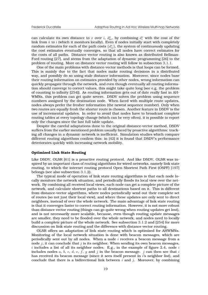
Frederick Ducatelle Adaptive Routing in Ad Hoc Wireless Multi-hop Networks
can calculate its own distance to x over i, dxki, by combining dx
i with the cost of thelink from k to i (which it monitors locally). Even if nodes initially start with completelyrandom estimates for each of the path costs {dx
ij}, the system of continuously updatingthe cost estimates eventually converges, so that all nodes have correct estimates forthe costs of all paths. Distance vector routing is also known as distributed Bellman-Ford routing [27], and stems from the adaptation of dynamic programming [26] to theproblem of routing. More on distance vector routing will follow in subsection 3.1.1.
One of the main problems with distance-vector methods is that loops can be formed.This is mainly due to the fact that nodes make routing decisions in a distributedway, and possibly do so using stale distance information. Moreover, since nodes basetheir routing information on estimates provided by other nodes, wrong information canquickly propagate through the network, and even though eventually all routing informa-tion should converge to correct values, this might take quite long (see e.g. the problemof counting to infinity [254]). As routing information gets out of date really fast in AH-WMNs, this problem can get quite severe. DSDV solves the problem using sequencenumbers assigned by the destination node. When faced with multiple route updates,nodes always prefer the fresher information (the newest sequence number). Only whentwo routes are equally fresh the shorter route is chosen. Another feature in DSDV is theuse of incremental updates. In order to avoid that nodes have to broadcast completerouting tables at every topology change (which can be very often), it is possible to reportonly the changes since the last full table update.
Despite the careful adaptations done to the original distance-vector method, DSDVsuffers from the earlier mentioned problem usually faced by proactive algorithms: track-ing all changes in a dynamic network is inefficient. Simulation studies which comparedifferent routing algorithms confirm this: in [42] it is found that DSDV’s performancedeteriorates quickly with increasing network mobility.
Optimized Link State Routing
Like DSDV, OLSR [61] is a proactive routing protocol. And like DSDV, OLSR was in-spired by an important class of routing algorithms for wired networks, namely link staterouting, to which the internet routing protocol Open Shortest Path First (OSPF) [197]belongs (see also subsection 3.1.2).
The typical mode of operation of link state routing algorithms is that each node lo-cally monitors the network situation, and periodically floods its local view over the net-work. By combining all received local views, each node can get a complete picture of thenetwork, and calculate shortest paths to all destinations based on it. This is differentfrom distance-vector algorithms, where nodes periodically send out their complete setof routes (so not just their local view), and where these updates are only sent to directneighbors, instead of over the whole network. The main advantage of link state routingis that it converges faster to correct routing information. However, it is not more robustthan distance vector routing (things can go quite wrong when routing updates get lost),and is not necessarily more scalable, because, even though routing update messagesare smaller, they need to be flooded over the whole network, and nodes need to locallybuild a complete picture of the whole network. See subsection 3.1.2 and [254] for morediscussion on link state routing and the difference with distance vector routing.
OLSR offers an adaptation of link state routing which is optimized for AHWMNs.Monitoring of the local network situation is done with beacon messages, which areperiodically sent out by all nodes. When a node i receives a beacon message from anode j, it can conclude that j is its neighbor. When sending its own beacon messages,i includes a list of all its neighbor nodes. E.g., in the example of figure 2.4, node iincludes nodes a, b, c, d, e, f , g and j in the beacon message. j can then see that ihas received its beacon message (since it sees itself present in i’s neighbor list), andconclude that there is a bidirectional link between i and j. Moreover, by combining
19
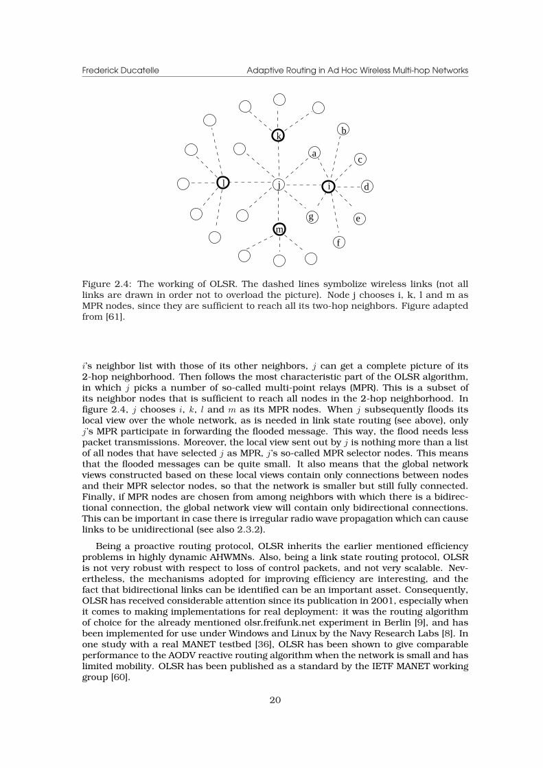
Frederick Ducatelle Adaptive Routing in Ad Hoc Wireless Multi-hop Networks
i d
eg
a
l
k b
c
f
j
m
Figure 2.4: The working of OLSR. The dashed lines symbolize wireless links (not alllinks are drawn in order not to overload the picture). Node j chooses i, k, l and m asMPR nodes, since they are sufficient to reach all its two-hop neighbors. Figure adaptedfrom [61].
i’s neighbor list with those of its other neighbors, j can get a complete picture of its2-hop neighborhood. Then follows the most characteristic part of the OLSR algorithm,in which j picks a number of so-called multi-point relays (MPR). This is a subset ofits neighbor nodes that is sufficient to reach all nodes in the 2-hop neighborhood. Infigure 2.4, j chooses i, k, l and m as its MPR nodes. When j subsequently floods itslocal view over the whole network, as is needed in link state routing (see above), onlyj’s MPR participate in forwarding the flooded message. This way, the flood needs lesspacket transmissions. Moreover, the local view sent out by j is nothing more than a listof all nodes that have selected j as MPR, j’s so-called MPR selector nodes. This meansthat the flooded messages can be quite small. It also means that the global networkviews constructed based on these local views contain only connections between nodesand their MPR selector nodes, so that the network is smaller but still fully connected.Finally, if MPR nodes are chosen from among neighbors with which there is a bidirec-tional connection, the global network view will contain only bidirectional connections.This can be important in case there is irregular radio wave propagation which can causelinks to be unidirectional (see also 2.3.2).
Being a proactive routing protocol, OLSR inherits the earlier mentioned efficiencyproblems in highly dynamic AHWMNs. Also, being a link state routing protocol, OLSRis not very robust with respect to loss of control packets, and not very scalable. Nev-ertheless, the mechanisms adopted for improving efficiency are interesting, and thefact that bidirectional links can be identified can be an important asset. Consequently,OLSR has received considerable attention since its publication in 2001, especially whenit comes to making implementations for real deployment: it was the routing algorithmof choice for the already mentioned olsr.freifunk.net experiment in Berlin [9], and hasbeen implemented for use under Windows and Linux by the Navy Research Labs [8]. Inone study with a real MANET testbed [36], OLSR has been shown to give comparableperformance to the AODV reactive routing algorithm when the network is small and haslimited mobility. OLSR has been published as a standard by the IETF MANET workinggroup [60].
20
Frederick Ducatelle Adaptive Routing in Ad Hoc Wireless Multi-hop Networks
Dynamic Source Routing
DSR [140] was in 1996 the first reactive routing algorithm to be published. As in otherreactive algorithms, nodes only actively look for routing information when it is strictlyneeded, i.e. when data needs to be sent to a destination for which no valid route exists.Important features of the algorithm are that it uses source routing, and that it makesextensive use of caching to increase the available routing information.
Under DSR, nodes that need to send data first check whether they have any routinginformation available for the requested destination. If this is not the case, a routediscovery process is started, in which a route request message (RREQ) is flooded overthe network. Once the RREQ reaches the destination, a route reply message (RREP) issent back to the source, either following the same path of the RREQ back, or followinga different path from the destination to the source. At the return of the RREP, the routediscovery process is complete, and the source can start sending data. If later, duringthe communication, one of the links on the path fails, a route error message (RERR) issent from the node where the error was detected back to the source, which can thenstart a new route discovery process.
An important aspect of DSR is that it uses source routing. This means that dataare not routed hop by hop, as is common practice in most routing algorithms, butthat instead the source node decides about the complete path to the destination, andadds it to each data packet. While this means extra overhead per data packet, sourcerouting has as an advantage that the source has complete control over the path, sothat e.g. loops can be avoided. Another advantage is that all nodes that receive adata packet on its way to its destination can extract information about the topology ofthe network. This last property is exploited extensively in DSR, which allows nodes tocache all routes they can extract from passing data packets (if promiscuous mode ispossible, this includes also data packets that were not destined for the current node,but could somehow be overheard). This allows to build a database of existing routes,which can be used to avoid the need for a route discovery process, to provide backuppaths in case of failure, etc.. However, caching can also be dangerous. Overheardroutes often stay in cache unused for a while before they are actually needed, at whichpoint they might have expired already. As a consequence, data packets can be sentonto erroneous routes, leading to extra delay and overhead. Moreover, these erroneousroutes can be overheard by other nodes, so that wrong information can actually spreadover the network. This phenomenon is called “cache pollution” [183,186].
DSR is an important reference algorithm in the field. A number of studies compareit to AODV, the other important reactive algorithm, which is described below, howeverwith few conclusive results [42, 65]. Recently, DSR formed the inspiration for LinkQuality Source Routing (LQSR) [92], which is the routing algorithm used in the MeshConnectivity Layer (MCL) architecture developed by Microsoft Research labs, and for theSrcr routing algorithm, which was developed for use in MIT’s Roofnet WMN testbed [30].
Ad-Hoc On-Demand Distance Vector Routing
AODV [213] was published as the on-demand version of DSDV. Like DSDV, it uses hopby hop data routing based on distance vector tables. Also, it uses the destination basedsequence numbers of DSDV to distinguish old from new routing information. Being areactive algorithm however, AODV is in its general working more similar to DSR.
Under AODV, nodes that have data to send to a destination that they have no infor-mation about, start a route discovery process. This process is similar to the one of DSR:a RREQ is flooded over the network, and when it reaches the destination, a RREP issent back to the source, which can then start sending data over the newly establishedpath. The difference with DSR lies in the way routes are identified: the RREQ does notstore the full path that it has traveled, but instead leaves in the routing table of each
21

Frederick Ducatelle Adaptive Routing in Ad Hoc Wireless Multi-hop Networks
intermediate node a pointer towards the source. The RREP follows these pointers backto the source, and changes them into pointers towards the destination. Data packetsare routed from source to destination following these pointers, and do not have to carryfull paths. When there is a failure anywhere along the path, a RERR is used to warnthe source, which can start a new route discovery process. A possible improvement,which was studied together with some other optimizations of AODV in [165], allows forintermediate nodes to try to locally rebuild failed routes, i.e. to find a route around afailed link. This is called local repair.
The use of hop by hop rather than source routing has as most important advantagethat there is no extra overhead for each data packet. A disadvantage is that nodes can-not extract routes from passing data packets, so that caching like in DSR is impossible.However, as was explained before, caching can also have a negative impact.
AODV is by far the most cited and studied AHWMN routing protocol. It forms themost important benchmark algorithm for the evaluation of other routing protocols, andhas been standardized by the IETF [212].
Zone Routing Protocol
ZRP [121] was the first hybrid routing algorithm. It is less used than other routingalgorithms presented in this section, but is described here because it provides a simpleexample of how reactive and proactive routing can be combined.
Under ZRP, proactive routing is used within a certain zone around each node (soeach node keeps up-to-date routes to nodes in a k hop radius, where k can be equalto 2 or 3 e.g.), and reactive routing is used for destinations further away. Data fordestinations within the zone can therefore be delivered straight away. For destinationsfurther away, a route discovery process is needed. The use of the zones allows todesign a route discovery process that is more efficient than those of AODV and DSR:the source node sends the RREQ to the nodes at the outer edges of its zone, and thosenodes forward it to their zone’s outer edges and so on, so that the RREQ travels injumps. The discovered paths consist of a list of zone edge nodes, and do not containinformation about the nodes between them. This means that the paths can be smallerto store, and that they can in principle be more robust (since they are not affected bythe movement of nodes between the zone edge nodes).
Directed diffusion
Directed diffusion [137] is a reactive routing protocol for sensor networks. It addressesissues of scalability, robustness and efficiency, and was designed specifically to sup-port the typical communication patterns of sensor networks, where the sensor nodesperiodically need to forward their sensed data to one or more sink nodes. Directed dif-fusion has similarities to Temporally-Ordered Routing Algorithm (TORA) [209], which isa reactive routing algorithm that was developed for MANETs.
In directed diffusion, the setup of data paths is initiated from the sink node whendata are needed. To this end, an interest message is formulated, which describeswhich data are needed, for which period they are needed, and with which frequency.This interest is subsequently propagated through the network to all sensor nodes. Eachnode that receives it sets up a gradient, which is a pointer to the node it received theinterest from, and starts looking for the requested data with the requested frequency.When a node obtains data that fit the interest message, it forwards them along thecorresponding gradient. Data coming from different parts of the sensor network can beaggregated when they meet in an intermediate node while traveling to the sink. Thisway, forwarding can be done more efficiently, which is very important given the strictpower limitations in sensor networks. Once the sink node starts receiving data, it starts
22
Frederick Ducatelle Adaptive Routing in Ad Hoc Wireless Multi-hop Networks
to regularly resend its interest, in order to reinforce and repair the existing paths. Thisway, higher robustness is provided.
2.4.3 Other techniques for AHWMN routing
The algorithms described in 2.4.2 represent the most cited ones in the area of AHWMNrouting. In what follows, we give a broader overview of this research area. In particular,we describe a number of interesting techniques that have been developed, explain howthey are used in different algorithms, and comment on advantages and disadvantages ofeach of them. In particular, we talk about the use of multipath routing, about creatinga hierarchical structure in the network, about the use of geographical location informa-tion, about different routing metrics, about techniques for large scale AHWMNs, aboutmulticasting, geocasting and broadcasting, and about data-centric routing, which isimportant in sensor networks.
Single path versus multipath routing
Most routing algorithms use single path routing: at all times, only one path is main-tained between source and destination. The alternative is to maintain multiple pathssimultaneously. Advantages of multipath routing include higher throughput, becausedata can be spread over the different paths, and higher robustness, because backuppaths are available in case of a failure and because multiple copies of the data can besent in parallel over different paths. Both of these are important features in the faceof the low capacity and reliability that are typical for AHWMNs. Disadvantages of mul-tipath routing are mainly due to the fact that more than one path needs to be set upand maintained. This leads to more complex algorithms, and more overhead. A con-firmation of the advantages and disadvantages of multipath routing in AHWMNs, bothvia analysis and simulation, is given in [214]. On the other hand, a similar analyticalstudy in [109] shows how a bad spreading of the multiple paths can negatively affectthe throughput advantage.
A large number of multipath routing algorithms have been proposed in AHWMN re-search. See [198] for an overview. These algorithms differ in the way multiple pathsare set up, maintained and used. During path setup, a number of different paths areselected. Some algorithms allow braided multiple paths [108], whereas others look forlink [186] or node [283] disjoint paths, or even paths which are outside each other’s in-terference range [278]. This is important in AHWMNs, where the augmented throughputoffered by the use of multiple paths can only be realized if these paths do not interferewith each other. Once the paths are set up, they need to be maintained. Most al-gorithms manage the paths in a reactive way: they remove paths when a link breakoccurs, and only take action when no valid path to the destination is left. A few al-gorithms use probing to obtain up-to-date information about the paths and to detectfailures [108,269]. Finally, the way the multiple paths are used differs strongly amongalgorithms. In many of them, only one of the paths is used for data transport, whilethe others are only used in case of a failure in the primary path [163, 201]. Some al-gorithms also explore the idea of spreading data over the multiple paths to increasethe throughput [164, 108, 269]. An interesting way of spreading data to increase ro-bustness is presented in [261]: diversity coding allows to encode N blocks of data intoM + N blocks in such a way that any subset of size N of these M + N blocks allows toreconstruct the original data. By using this encoding and spreading data over multiplepaths, robustness of data delivery can be greatly improved.
23
Frederick Ducatelle Adaptive Routing in Ad Hoc Wireless Multi-hop Networks
Network structure
Many AHWMN routing algorithms, including the algorithms DSDV, OLSR, AODV andDSR described in 2.4.2, consider all nodes in the network as equal and perform routingin an essentially flat space. These are called uniform protocols. A different approach isto try to make the routing task easier by giving some structure to the routing space. Thisis the strategy used by partitioning protocols. A classic example is Clusterhead Gate-way Switched Routing (CGSR) [59]. This algorithm organizes the AHWMN in clusters,each with a clusterhead and a number of gateways, and organizes all communicationbetween nodes of different clusters via the clusterheads and the gateways.
The advantage of partitioning algorithms is that they simplify routing, so that inprinciple better efficiency and scalability can be achieved. In practice, however, thereare also some important disadvantages. First, if mobility is high, the maintenance ofthe network partitioning can cause a lot of overhead. Second, attributing roles such asclusterhead or gateway to certain nodes means that the network is more dependent onthem, and that they have to perform more work than other nodes (this can be a problemif there is limited battery power e.g.). Finally, although partitioning leads to faster routediscovery in large networks, the discovered routes are not always the shortest: nodescould be close to each other in the network, but still have to communicate through theirrespective clusterheads. In sensor networks, where nodes are often static and scalabil-ity is a very important factor, partitioning algorithms are relatively more popular thanin MANETs and WMNs. An example is the Low Energy Adaptive Clustering Hierarchyprotocol (LEACH) [125].
A middle way between uniform and partitioning protocols is given by neighbor selec-tion protocols [102]. In these protocols, each node gives some structure to the networkfrom its own point of view. An example is the previously mentioned ZRP (see 2.4.2),in which each node uses a proactive protocol to maintain routing information aboutnodes within a certain number of hops, and a reactive protocol for nodes further away.Another example is Fisheye State Routing (FSR) [210], in which updating of routinginformation is done frequently for nearby nodes, and less frequently for nodes furtheraway. This results in a blurred vision of the network: for faraway nodes only a vaguerouting direction is known, but as the data packet approaches its destination, moreprecise routing information is available. The advantage of neighbor selection protocolsis that there is some structure in the network, which improves scalability and efficiency,without there being an overall structure that needs to be maintained.
Using location information
Some AHWMN routing algorithms use geographic location information for routing (e.g.[146]). In such location based algorithms, source nodes add the geographic coordinatesof the destination to each data packet, and forwarding decisions are based on whichnext hop brings the data packet closest to its destination. This approach exploits thefact that the network topology is defined by the placement of the nodes (see 2.3.1),so that geographical proximity is closely related to proximity on the network topologygraph. A good overview of existing location based algorithms can be found in [113].
Advantages of location based routing are that no explicit path setup is necessary,that paths are flexible (here, a path is not a list of nodes to be visited, but instead resultsfrom the location based decisions at each intermediate node), and that very little routinginformation needs to be maintained. This makes the system more efficient, scalable androbust. There are, however, also a number of problems that need to be solved in thisapproach to AHWMN routing. First of all, each node has be able to obtain its ownlocation coordinates. This is normally done through the use of the Global PositioningSystem (GPS) [129]. However, use of GPS can be expensive, and is not always possible(e.g. indoors). In [47], the authors present a rather complicated method for GPS free
24
Frederick Ducatelle Adaptive Routing in Ad Hoc Wireless Multi-hop Networks
location detection. A second problem is that source nodes need a way to figure outthe location coordinates of the destination node, and maintain them in the face ofmobility. This is usually done using some form of location server. However, the use of asingle location server is in conflict with the distributed and ad hoc nature of AHWMNs,and creates a single point of failure. Some solutions to this problem are describedin [171, 31]. Finally, location based algorithms can experience difficulties when thereis a big gap in the graph that stops greedy forwarding from finding the destination.Approaches to get around wholes in the network graph are presented in [157,31].
Routing metrics
Routing algorithms need a metric to evaluate different routes and choose one (or several)among them. The most straightforward choices are the end-to-end delay and the hopcount. The end-to-end delay can however be quite unstable in AHWMNs. One reason isthat there is often only one wireless device, with one queue that is shared for all wirelesslinks, so that the traffic for one neighbor also suffers from high delays for the trafficfor other neighbors. Another reason is that differences in wireless connection qualitycan lead to high delay variations, e.g. due to the exponential backoff interval used forretransmissions at the MAC layer as explained in 2.3.3. Compared to delay, the hopcount is a very simple and stable metric. It has therefore been used by a lot of AHWMNrouting algorithms. Nevertheless, there is a growing awareness that hop count is notnecessarily a good metric [67]. This is because paths with a low number of hops usuallyconsist of long hops, which can be of low quality and break easily as a consequence ofnode movement, and because short paths tend to go through the center of the AHWMNarea, where congestion and wireless channel contention is higher.
A number of other metrics have been proposed to evaluate paths. In Associativity-Based Routing (ABR) [257], nodes periodically broadcast beacon messages, and theycount how many of these messages they have received from each of their neighbors.These are called “associativity ticks”. Links with a high number of associativity ticksare considered more stable, and are therefore preferred.
Power aware routing algorithms (e.g. [247]) evaluate paths based on their power us-age. Apart from saving on limited power resources, lowering power usage also reducesinterference and increases the possibility for spatial reuse. Different power based met-rics are possible. One can e.g. choose the path which uses minimal power, or thepath going over nodes with most power left (so that the remaining lifetime of the pathis maximized). A number of power based routing metrics are discussed in [240]. Ageneral survey on power aware networking (not just routing) is given in [141]. Poweraware networking is especially important in sensor networks, where power resourcesare usually more limited and can often not be replaced (see also 2.2.3).
An interesting newly proposed metric is the Expected Transmission Count (ETX) [66].This metric estimates the expected number of transmissions that will be needed to suc-cessfully conclude the transfer of a data packet over a link. This includes possibleretransmissions of the data packet due to failures, and the transmission of the ac-knowledgment packet in backward direction. The estimate is obtained by measuringthe transmission success of regularly sent probe messages. An important reason forthe development of ETX was the observation that MAC layer mechanisms such as theRTS/CTS and ACK messages of IEEE 802.11 DCF allow to send data packets over lossylinks, making it difficult to assess the real link quality. The ETX measure was devel-oped based on experiences from real AHWMN deployment, and formed the basis forthe Expected Transmission Time (ETT) metric used in the Roofnet testbed [30]. In [93],the ETX metric was compared to hop count and end-to-end delay. It was found to givesignificantly better performance in static networks (although producing longer paths),but was outperformed by hop count in dynamic networks because the probe basedtransmission estimation was too slow to adapt.
25

Frederick Ducatelle Adaptive Routing in Ad Hoc Wireless Multi-hop Networks
Large AHWMNs
In the field of MANET and WMN routing, most of the work is done on the scale of alocal area network (LAN), with simulation and implementation tests carried out withnetworks of up to maximally 100 nodes. An exception is the scalability study of AODVdescribed in [162], which evaluates the performance of AODV in a network of up to10000 nodes. This paper proposes a number of extensions to AODV to improve itsperformance in such large networks: expanding ring search, query localization andlocal repair. With expanding ring search, the flooding of the RREQ message for initialpath setup is limited in size in order to improve the efficiency of the process: the floodedmessage is forwarded for a maximum number of hops, and only if this limited flooddoes not result in a path to the destination, it is gradually increased in size. Also querylocalization and local repair are meant to make the path setup more efficient, but onlyin the case of the failure of an existing path. With query localization (originally proposedin [53]), the RREQ flood is only allowed to propagate in the neighborhood of a previouslyknown path to the destination. With local repair, path failures are resolved with alimited flooding of a repair message around the area where the failure was detected.Despite these adaptations, AODV’s performance was found to degrade quickly for largenetworks, due to the long path lengths. For example, throughput was down to 50% at1000 nodes.
A few algorithms were proposed specifically for MANETs and WMNs of wide areanetwork (WAN) scale. An example is the Terminodes routing algorithm [31]. It uses ge-ographic location information for scalable routing, and maintains a small world overlaynetwork to support efficient route detection [32]. The algorithm performed well in largescale simulation tests that went up to 600 nodes. Also the Mobile Ants Based Rout-ing (MABR) algorithm [126, 127] aims at supporting routing in large AHWMNs. LikeTerminodes, MABR uses geographical information to increase scalability. Also, it di-vides the whole area of the AHWMN into zones to make the system more manageable.In a large simulation study with 10000 nodes, it compared favorably to Terminodesrouting [127]. The MABR algorithm is partly based on the Ant Colony Optimizationmeta-heuristic described in chapter 3.
In the field of sensor network routing, scalability is very important, since the ex-pected size of such networks is typically very large. To provide such scalability, sensornetwork routing protocols often use location based routing [281], and/or network parti-tioning techniques [125]. Sometimes, sensor networks are considered so large that it isimpossible to assign a unique identifier to each node. In that case, a possible solutionis to apply data centric routing, where data is routed based on their content, ratherthan based on a destination node identifier [18]. Data-centric routing is described inmore detail later in this section.
Unicasting versus multicasting, geocasting and broadcasting
So far, we have only discussed unicast routing protocols, in which a sender sends toone particular receiver. Some protocols also support communication between a senderand a group of receivers. Based on characteristics of the group of receivers, one candistinguish between multicasting, geocasting and broadcasting.
In multicast protocols, the group of receivers is a subset of the nodes of the network,where each member needs to be explicitly identified. Many of the often cited applica-tions of AHWMNs, like disaster recovery and battlefield communication, typically needsupport for this form of communication. Multicasting could be provided via the useof parallel unicast sessions between the source and each of the destinations. Such anapproach would however be quite inefficient. A commonly used alternative is to builta routing structure between the members of the multicast receiver group, so that mes-sages from the source can efficiently be forwarded between them. This routing structure
26
Frederick Ducatelle Adaptive Routing in Ad Hoc Wireless Multi-hop Networks
can in principle have any shape. E.g., the approach described in [279] proposes to use atree structure. In [166], several multicast routing protocols for AHWMNs are described,and their performances are compared in a simulation study. One conclusion of thepaper is that multicast protocols using a mesh routing structure are to be preferredover those using a tree structure, since they provide multiple paths between each pairof receivers.
Geocasting can be seen as a special case of multicasting, whereby the group of re-ceivers is defined as all the nodes that are currently in a certain geographical area.The term was first proposed in [203]. Typical applications of geocasting could be localadvertising or service provisioning, finding out who is in your neighborhood, or geo-graphic message delivery (e.g., sending an emergency message to all nodes in a certainarea). In sensor networks, where the relation between the sensed data and their lo-cation is often important, geocasting is often needed. In [154], three different geocastrouting protocols, all adapted from existing multicast routing protocols, are describedand compared.
In broadcasting, the group of receivers contains all the nodes in the network. Itis important to understand the difference between broadcasting at the MAC level andbroadcasting at the network level. At the MAC level, a broadcast reaches all nodesthat are in radio range of the sender. Some details about MAC level broadcasting inAHWMNs are given in 2.3.3. At the network level, a broadcast reaches all nodes in theAHWMN, some of which possibly after multi-hop relaying. Network level broadcastingis also often referred to as flooding. Many existing AHWMN unicast routing algorithmsrely on flooding to spread or gather routing information. Examples are AODV’s andDSR’s flooding of RREQ messages to set up paths, and OLSR’s flooding of local net-work views via MPR nodes (see 2.4.2). Due to the need for multi-hop forwarding offlooded messages, flooding can get quite inefficient. In fact, in reactive algorithms suchas AODV and DSR, flooding is the most important source of control overhead. Somemechanisms have been proposed to make flooding more efficient, such as OLSR’s use ofMPR nodes. An overview and comparison of efficient flooding protocols is given in [285].
Address-centric versus data-centric routing
Address-centric routing is the normal way of operation in computer networks: dataare routed through the network based on the address of their destination node. Data-centric routing provides a radically different approach: destination addresses are notused, and data are instead forwarded based on their contents. Under data-centricrouting, routing information does not indicate the next hop corresponding to a spe-cific destination address, but corresponding to certain data properties. An importantexample is the directed diffusion algorithm described in 2.4.2. In terms of operation,data-centric protocols can be classified as query based or negotiation based. In querybased algorithms, such as directed diffusion [137] and rumor routing [41], the desti-nation node defines the properties of the data it is interested in, and the sensor nodesforward the requested data. In negotiation based algorithms, such as sensor protocolsfor information via negotiation (SPIN) [158], sensor nodes advertise which data theyhave available, and destination nodes can register to receive this data. Closely relatedto data-centric routing is the more general framework of content-based networking [52].
Data-centric routing was in the first place developed for sensor networks, to supportthe typical communication patterns of such networks, where data measured by sensorsspread over a wide area need to be drawn to one or more sink nodes. In this context,data-centric routing has some important advantages. These are in the first place relatedto the fact that data forwarding is made more efficient: sensor nodes only send the datathat are requested by the sink node, and similar data coming from different sensors canbe aggregated at intermediate nodes to travel more efficiently till the sink. The efficiencyadvantages due to aggregation have been confirmed via analytical modeling in [156].
27
Frederick Ducatelle Adaptive Routing in Ad Hoc Wireless Multi-hop Networks
Other advantages of data-centric routing come from the fact that no destination nodeaddress is used in the routing. This can help reduce the need for network wide topologyinformation, as in directed diffusion [137], and eliminates the need for a global space ofunique addresses. These are important elements to improve scalability and efficiencyin very large sensor networks.
2.5 Conclusion
In this chapter, we have described the context in which the work for this thesis issituated. We have explained what AHWMNs are, which different types exist, what issuesneed to be dealt with in AHWMN networking, and what the current state-of-the-artis in the area of AHWMN routing. Throughout this chapter, we have explained howthe properties of AHWMNs define in a direct or indirect way the characteristics of therouting task in such networks. Specifically, we have formulated a number of differentchallenges that will need to be addressed by the algorithms developed in this thesis. Thefirst of these is adaptivity. An AHWMN routing algorithm needs to provide adaptivity todeal with the dynamic nature of these networks. We have shown how the placementof the nodes and their movements affect the topology and its changes, and how thenode density and radio transmission range influence this. The second challenge isrobustness. Wireless transmissions are often unreliable, and mobility induced pathfailures can cause extra packet loss. AHWMN routing algorithms should be able towork correctly and provide a reliable service in such a challenging environment. Thisis especially important since, as we described, the traditional approach of providingservice level guarantees at the transport layer encounters difficulties in AHWMNs. Thethird challenge is efficiency: the needed adaptivity and robustness have to be obtainedin an efficient way, wasting as little as possible of the limited network resources. Theseresources refer in the first place to network capacity. Network capacity is mainly limiteddue to the need to share the wireless channel among the nodes of the network, and thedifficulties that are encountered at the MAC layer when trying to organize this sharingeffectively. Other limited resources are the battery power of the nodes, their processingpower, etc.. Finally, the last challenge is scalability. In the flat AHWMN environmentwith limited capacity, AHWMN routing algorithms should provide a service that canscale to large numbers of nodes.
We have in this chapter also described a number of techniques that have been de-veloped by different researchers in the field of AHWMN routing to deal with the abovechallenges. We have first described multipath routing, and have explained how it canimprove throughput, adaptivity and reliability. Then, we have explained how the use ofstructure and organization can help scalability. Next, we have described how locationinformation can be used in routing, and how it can increase scalability and efficiency.We have also given an overview of different path evaluation metrics that can be used,and have discussed their respective advantages and disadvantages. Then, we havediscussed some routing algorithms for large scale AHWMNs, and have explained thetechniques that they use. Next, we have discussed techniques used for multicasting,geocasting and broadcasting. Finally, we have described the possibility to use data-centric routing to improve scalability and efficiency in sensor networks. Many of thetechniques described in this chapter are used in the algorithms developed in this thesis,or in the algorithms we compare with.
The focus in the rest of this thesis will be on routing in MANETs and WMNs. Sen-sor networks have slightly different properties, as has been explained throughout thischapter, and command therefore a different approach. Nevertheless, since they arealso types of AHWMNs, there are a lot of similarities with MANETs and WMNs, so thatthe techniques developed in this thesis can to some extent also serve in them. Ona related note, we expect that also research in other types of networks could benefit
28
Frederick Ducatelle Adaptive Routing in Ad Hoc Wireless Multi-hop Networks
from the ideas developed in this thesis. We think hereby of more traditional, wired net-works, and of application layer overlay networks, such as peer-to-peer networks [243]or resilient overlay networks [20]. Also in these kinds of networks, properties suchas adaptivity, robustness, efficiency, etc. can be very useful. In wired networks, forexample, algorithms need to be adaptive to deal with link failures, or to change theirbehavior depending on the network load. In overlay networks, where nodes are con-nected through virtual links, the topology is at least as dynamic as in AHWMNs, so thatalso there adaptivity is important. On the other hand, robustness and efficiency couldbe less important, both in wired and in overlay networks.
29

Chapter 3
Adaptive routing and learning
In this chapter, we discuss existing approaches to adaptive routing. The aim is tomake the reader acquainted with some important core techniques behind these algo-rithms, and their advantages and disadvantages, so that the choices made for the workpresented in this thesis can be better understood. Where possible, we will commenton how the adaptive techniques discussed here score with respect to the importantchallenges in AHWMN routing that were outlined in the previous chapter, namely adap-tivity, robustness, efficiency and scalability. We will also point out how and where thesetechniques are used in the AHWMN routing algorithms described before.
In what follows, we first discuss adaptivity in internet routing algorithms. Due tothe large size of the internet, it is impossible for human operators to keep track of allchanges in its network topology. Therefore, internet routing algorithms contain built-inmechanisms for adaptivity. Some of these mechanisms will be used further on in thisthesis. Next, we discuss Ant Colony Optimization (ACO) routing algorithms. This is arelatively new class of routing algorithms, which was inspired by the mechanisms usedby ant colonies to find the shortest path between their nest and a food source, and bythe ACO metaheuristic which was derived from this. ACO routing algorithms form themain source of inspiration for the work in this thesis. In the final section, we provide adeeper discussion on those of the described techniques that are most relevant for thisthesis, and on their relationship with the field of machine learning.
3.1 Adaptive routing in the internet
The internet today can be considered as a collection of subnetworks, commonly referredto as autonomous systems (ASs) [254]. For routing inside an AS, intra-domain routingprotocols such as the Routing Information Protocol (RIP) [123] and Open Shortest PathFirst (OSPF) [197] are used. For routing between ASs, which is called inter-domainrouting, the standard is the Border Gateway Protocol (BGP) [178]. Underlying these dif-ferent algorithms are two basic approaches to routing: distance vector routing and linkstate routing. While RIP is a direct implementation of the basic ideas behind distancevector routing, OSPF is the most important instantiation of link state routing. BGP isbased on distance vector routing, but it follows a significantly different approach fromRIP, in order to allow the implementation of internet policies and to overcome someof the shortcomings of RIP. Recently, a new approach to routing, ant colony optimiza-tion (ACO) routing, has been proposed as an alternative to both distance vector and linkstate routing. ACO routing is a class of highly adaptive algorithms, which was developedbased on artificial intelligence techniques, and in particular on the ACO metaheuristicfor optimization.
31
Frederick Ducatelle Adaptive Routing in Ad Hoc Wireless Multi-hop Networks
In what follows, we describe the working of distance vector routing and link staterouting, using the mentioned internet routing algorithms as examples, and discussadvantages and disadvantages of both approaches. ACO routing is described separatelylater in section 3.2; since it forms the most important source of inspiration for the workin this thesis, a full separate section is devoted to it.
3.1.1 Distance vector routing
Distance vector routing is also known as Bellman-Ford routing [27] or Ford-Fulkersonrouting [103], after the authors of the earliest work on this approach. Below, we firstdescribe RIP as an example of the basic working of distance vector routing. Then, wediscuss advantages and disadvantages of this approach. Next, we describe BGP, whichimplements distance vector routing differently from RIP. Finally, we comment on the useof distance vector routing in AHWMNs. A short description of distance vector routinghas also been provided in the description of DSDV in subsection 2.4.2.
RIP: basic distance vector routing
Distance vector routing was originally derived from the principles of dynamic program-ming, which is a general solution method for optimization problems proposed by Bell-man in 1957 [26]. The basic idea behind dynamic programming is to split an opti-mization problem into subproblems, and use the solutions to these subproblems toconstruct an optimal solution for the main problem. The subproblems themselves arerecursively split into smaller subproblems, until an elementary case is reached that iseasy to solve. In routing, the optimization problem is to find the shortest path from asource node s to a destination node d. This problem is split into the subproblems offinding the shortest path from each of the neighbors of s to the destination d. Each ofthese subproblems is recursively split up further, until they are reduced to the simplecase of finding the one hop path between one of d’s neighbors and d. As an example,consider the network of figure 3.1. The shortest path from node 1 to node 7 is foundby calculating the shortest path from node 2 to node 7 and that from node 3 to node7, adding the cost of the one hop link from node 1 to respectively node 2 and node 3,and comparing the results. In turn, the shortest path from node 2 to node 7 is foundby comparing the shortest paths from the nodes 1, 3 and 4 to node 7, and the shortestpath from node 3 to node 7 by comparing the shortest paths from the nodes 1, 2 and 5to node 7. Finally, finding the shortest path from the nodes 4 and 5 to node 7 is trivial,since they are one hop paths.
Distance vector routing is an asynchronous, distributed implementation of this ap-proach, and RIP is a more or less direct implementation of the basic distance vectoralgorithm. Under RIP, each node keeps routing information in a table that has oneentry for each destination. In this entry, it stores the estimated cost of the best path tothis destination, and the outgoing link over which this best path goes. In the exampleof figure 3.1, the routing table of node 2 is shown. Periodically, each node broadcasts toall its neighbors a route update message containing a list with the cost estimates for alldestinations in its routing table. A node n which receives from its neighbor m a messagethat m can reach destination d with cost cd
m, can calculate the cost cmdn of going from n
over m to destination d. It does this by adding together the locally observed cost cmn to
go to its neighbor m and the reported cost cdm. So, in the example of figure 3.1, node
1 calculates that the cost of going over node 2 to reach node 7 is 5ms: it is the cost oftaking the link to node 2 (which is observed to be 2ms), and the cost of going from node2 to node 7 (which is reported by node 2 to be 3ms). Node n calculates in this way thecost of the path over each of its outgoing links, and chooses the best one to put in itsrouting table and report in its own periodic update messages.
32
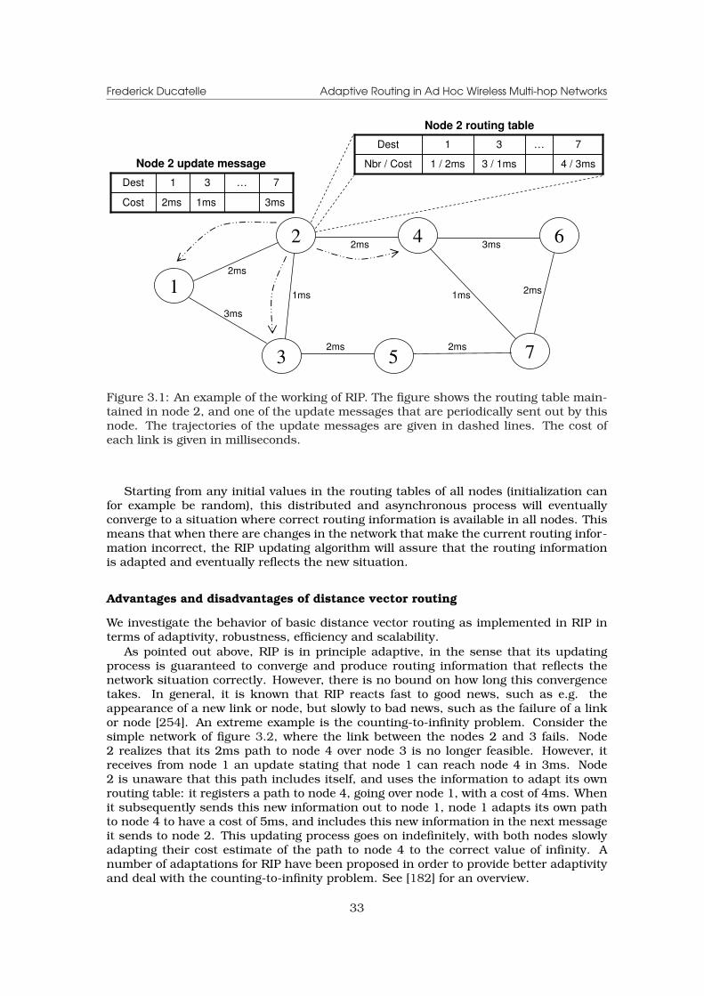
Frederick Ducatelle Adaptive Routing in Ad Hoc Wireless Multi-hop Networks
Nbr / Cost
Dest
4 / 3ms3 / 1ms1 / 2ms
7…31
1
2
3 5
4 6
7
Cost
Dest
3ms1ms2ms
7…31
2ms
Node 2 routing table
Node 2 update message
3ms
1ms
2ms
2ms
2ms
1ms
3ms
2ms
Figure 3.1: An example of the working of RIP. The figure shows the routing table main-tained in node 2, and one of the update messages that are periodically sent out by thisnode. The trajectories of the update messages are given in dashed lines. The cost ofeach link is given in milliseconds.
Starting from any initial values in the routing tables of all nodes (initialization canfor example be random), this distributed and asynchronous process will eventuallyconverge to a situation where correct routing information is available in all nodes. Thismeans that when there are changes in the network that make the current routing infor-mation incorrect, the RIP updating algorithm will assure that the routing informationis adapted and eventually reflects the new situation.
Advantages and disadvantages of distance vector routing
We investigate the behavior of basic distance vector routing as implemented in RIP interms of adaptivity, robustness, efficiency and scalability.
As pointed out above, RIP is in principle adaptive, in the sense that its updatingprocess is guaranteed to converge and produce routing information that reflects thenetwork situation correctly. However, there is no bound on how long this convergencetakes. In general, it is known that RIP reacts fast to good news, such as e.g. theappearance of a new link or node, but slowly to bad news, such as the failure of a linkor node [254]. An extreme example is the counting-to-infinity problem. Consider thesimple network of figure 3.2, where the link between the nodes 2 and 3 fails. Node2 realizes that its 2ms path to node 4 over node 3 is no longer feasible. However, itreceives from node 1 an update stating that node 1 can reach node 4 in 3ms. Node2 is unaware that this path includes itself, and uses the information to adapt its ownrouting table: it registers a path to node 4, going over node 1, with a cost of 4ms. Whenit subsequently sends this new information out to node 1, node 1 adapts its own pathto node 4 to have a cost of 5ms, and includes this new information in the next messageit sends to node 2. This updating process goes on indefinitely, with both nodes slowlyadapting their cost estimate of the path to node 4 to the correct value of infinity. Anumber of adaptations for RIP have been proposed in order to provide better adaptivityand deal with the counting-to-infinity problem. See [182] for an overview.
33
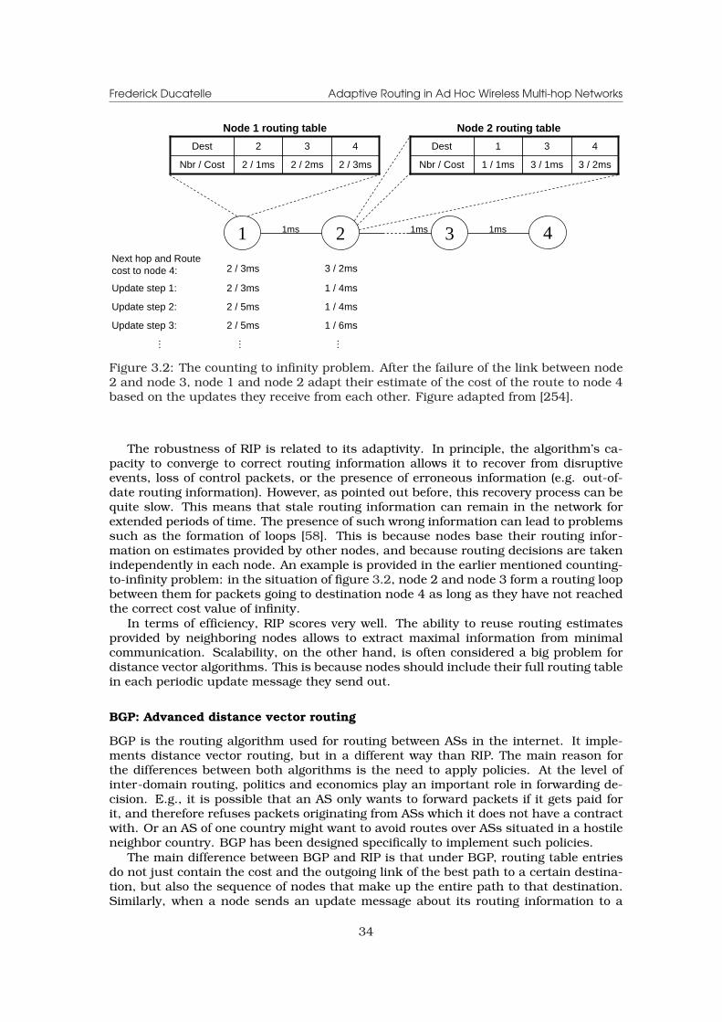
Frederick Ducatelle Adaptive Routing in Ad Hoc Wireless Multi-hop Networks
Nbr / Cost
Dest
3 / 2ms3 / 1ms1 / 1ms
431
1 2 3 4
Node 2 routing table
1ms 1ms 1ms
Nbr / Cost
Dest
2 / 3ms2 / 2ms2 / 1ms
432
Node 1 routing table
…
1 / 6ms
1 / 4ms
1 / 4ms
3 / 2ms
…
2 / 5ms
2 / 5ms
2 / 3ms
2 / 3ms
…
Update step 3:
Update step 2:
Update step 1:
Next hop and Route cost to node 4:
Figure 3.2: The counting to infinity problem. After the failure of the link between node2 and node 3, node 1 and node 2 adapt their estimate of the cost of the route to node 4based on the updates they receive from each other. Figure adapted from [254].
The robustness of RIP is related to its adaptivity. In principle, the algorithm’s ca-pacity to converge to correct routing information allows it to recover from disruptiveevents, loss of control packets, or the presence of erroneous information (e.g. out-of-date routing information). However, as pointed out before, this recovery process can bequite slow. This means that stale routing information can remain in the network forextended periods of time. The presence of such wrong information can lead to problemssuch as the formation of loops [58]. This is because nodes base their routing infor-mation on estimates provided by other nodes, and because routing decisions are takenindependently in each node. An example is provided in the earlier mentioned counting-to-infinity problem: in the situation of figure 3.2, node 2 and node 3 form a routing loopbetween them for packets going to destination node 4 as long as they have not reachedthe correct cost value of infinity.
In terms of efficiency, RIP scores very well. The ability to reuse routing estimatesprovided by neighboring nodes allows to extract maximal information from minimalcommunication. Scalability, on the other hand, is often considered a big problem fordistance vector algorithms. This is because nodes should include their full routing tablein each periodic update message they send out.
BGP: Advanced distance vector routing
BGP is the routing algorithm used for routing between ASs in the internet. It imple-ments distance vector routing, but in a different way than RIP. The main reason forthe differences between both algorithms is the need to apply policies. At the level ofinter-domain routing, politics and economics play an important role in forwarding de-cision. E.g., it is possible that an AS only wants to forward packets if it gets paid forit, and therefore refuses packets originating from ASs which it does not have a contractwith. Or an AS of one country might want to avoid routes over ASs situated in a hostileneighbor country. BGP has been designed specifically to implement such policies.
The main difference between BGP and RIP is that under BGP, routing table entriesdo not just contain the cost and the outgoing link of the best path to a certain destina-tion, but also the sequence of nodes that make up the entire path to that destination.Similarly, when a node sends an update message about its routing information to a
34
Frederick Ducatelle Adaptive Routing in Ad Hoc Wireless Multi-hop Networks
neighbor, it includes full paths. By combining the paths for different destinations re-ported by all neighbors, each node can construct a view of the network, on which itbases its own routing decisions. Thanks to the availability of full path information, it iseasy to implement policies such as the ones mentioned above. BGP is sometimes alsocalled a path vector routing algorithm, since its routing table is a vector of paths, ratherthan distances.
In terms of adaptivity, BGP scores better than RIP. The availability of full path in-formation allows to solve the counting to infinity problem, and to avoid loop forma-tion [254]. Nevertheless, observations of internet behavior have shown that BGP canstill be slow to converge to correct routing information after a failure, in the order of tensof minutes [160]. Also robustness remains a problem, since the loss of control packetsor the presence of erroneous information still leads to instabilities (see e.g. [270] for astudy of the behavior of BGP in a stressful situation). Finally, in terms of efficiency andscalability, BGP scores worse than RIP, since the algorithm is more complex, and morerouting information needs to be exchanged between nodes. The growing size of routingtables in the internet has become an important problem, and different strategies havebeen developed to deal with it [134,43].
Distance vector routing in AHWMNs
The first routing algorithm that was developed for AHWMNs, DSDV, is a distance vec-tor algorithm. It follows quite closely the basic approach described for RIP. The mainreasons for adopting the distance vector approach for AHWMN routing are its relativesimplicity and efficiency, which are important properties in resource constrained envi-ronments such as an AHWMNs. To deal with problems that stem from slow adaptivityand low robustness, such as loop formation, DSDV contains an elegant solution basedon sequence numbers. All routing table entries are labeled with a sequence numberthat is assigned by the destination. A node i only accepts new routing information for adestination d if the new information has a higher sequence number than what is alreadyavailable in i, or when it has the same sequence number but a better routing metric.For an example of how this solves the problem of loop formation, consider again thecounting-to-infinity problem depicted in figure 3.2. After the failure of the link betweennode 2 and node 3, updates about the route to destination node 4 sent out by node1 or node 2 always have the same sequence number. This is because assigning newsequence numbers is the responsibility of the destination, node 4, and all connectiv-ity to this node is lost. Moreover, the updates sent back and forth between the twonodes have increasing routing metrics, and are therefore not accepted. Details aboutthe DSDV algorithm are given in subsection 2.4.2 and in [211].
Despite the use of the destination based sequence number mechanism, DSDV wasfound to be insufficiently adaptive and robust to work in AHWMNs, especially as net-work size or dynamism increased (see e.g. [42,180]). Therefore, a few years later, AODVwas proposed as a follow up to DSDV. AODV is labeled a distance vector algorithm,since its routing tables hold the cost and next hop of the best route for each desti-nation, and are therefore distance vectors just like the tables used in DSDV and RIP.However, AODV’s approach to gathering and updating routing information has noth-ing in common with the distributed algorithm described in this subsection. One couldtherefore say that AODV is a distance vector algorithm but not a Bellman-Ford algo-rithm. However, since these two terms have always been associated with each other,this can create some confusion. For details about AODV we refer to subsection 2.4.2and to [213].
35

Frederick Ducatelle Adaptive Routing in Ad Hoc Wireless Multi-hop Networks
2ms
6 - 7
2ms
2 - 1
Cost
Link
2ms3ms2ms …
7 - 6…1 - 31 - 2
1
2
3 5
4 6
7
Cost
Nbr
2ms1ms2ms
431
2ms
Node 2 topological database
Node 2 link state advertisement
3ms
1ms
2ms
2ms
2ms
1ms
3ms
2ms
Figure 3.3: An example of the working of OSPF. The figure shows the topologicaldatabase maintained in node 2 (this should be the same for each node in the network),and a link state advertisements sent out by node 2. The link state advertisements areflooded over the network, as is indicated by the dashed lines.
3.1.2 Link state routing
Link state routing was in the first place developed to overcome problems of slow conver-gence and scalability that are present in distance vector protocols. Its basic approachto spreading and calculating routing information is fundamentally different. In whatfollows, we first describe OSPF, which is the main representant of link state routing,then discuss advantages and disadvantages of this approach, and finally comment onthe use of link state routing in AHWMNs. A short description of link state routing wasalso provided earlier, in the discussion of the OLSR protocol in 2.4.2.
OSPF
The basic working of link state routing algorithms is depicted in figure 3.3. Each nodelocally monitors the cost to go to each of its neighbors. This forms the node’s local state.Whenever a node detects a change in its local state, it floods it to all other nodes in thenetwork in a link state advertisement (LSA) message. LSA messages contain sequencenumbers in order to distinguish old from new routing information. By combining theLSAs received from all nodes in the network, each node can get a complete view of thecurrent network situation. This is stored in the node’s topological database. Usingthis database, each node runs the Dijkstra shortest path algorithm [208] to constructa shortest path tree with itself as root, and uses the result to fill its routing table. Interms of the mechanism used to spread routing information, the difference with dis-tance vector routing could be summarized as follows: while in distance vector routing,nodes send their global network information out locally to their neighbors, in link staterouting, they send their local network view out globally to all other nodes.
The OSPF algorithm implements the above scheme. However, it has a lot of addedfeatures to make it better suited to the specific properties of the internet. Some ofthese are aimed at improving scalability. OSPF allows to split the network into so-called areas, so that inside each area, nodes only maintain routing information aboutthat area. For routing between areas, a backbone is set up. Note that these areas
36
Frederick Ducatelle Adaptive Routing in Ad Hoc Wireless Multi-hop Networks
are subnetworks inside the earlier mentioned ASs (which are themselves subnetworksof the internet). Another scalability related feature of OSPF is the possibility to rep-resent a group of directly connected routers by one node in the OSPF network. Tothis end, one of the routers, called the designated router, acts on behalf of the wholegroup. This is for example relevant in LANs where all nodes are connected through anEthernet bus; it would be inefficient to let each of these nodes run OSPF separately.Other features of OSPF, which are not related to scalability, include the fact that allmessage exchanges are authenticated, in order to improve security, and the possibilityto route packets distinctly based on their IP Type of Service field, so that in principledifferentiated Quality-of-Service (QoS) routing [153] can be supported.
Advantages and disadvantages of link state routing
Link state routing offers good adaptivity: any detected change is flooded through thenetwork in LSAs, and as soon as the nodes in the network have received all updates,they can recalculate the shortest paths to all destinations so that their routing tablesreflect the new network situation. This is faster than the slowly converging distributedupdating process used in distance vector routing.
Robustness, on the other hand, can be a problem for link state routing algorithms.If LSAs get lost, or stale LSAs are used for updates, nodes end up with erroneoustopological databases, and calculate wrong paths. In OSPF, a number of measureshave been taken to alleviate these problems. In order to avoid the loss of LSAs, each LSAtransmission needs to be acknowledged, and duplicate transmissions are done in caseof failure. Also, each node periodically sends out refresh LSAs, which repeat previouslytransmitted information. In order to avoid the use of stale routing information, eachLSA is given a sequence number, so that receiving nodes can figure out the relative ageof different LSAs coming from the same source node. Furthermore, LSAs are given atimestamp, so that they can be discarded when they get too old.
In terms of efficiency, link state routing should in principle score quite well. How-ever, the previously mentioned measures to improve robustness compromise this: extraoverhead is created by LSA acknowledgements, duplicate LSAs and refresh LSAs. More-over, in the presence of links of unstable quality, a large number of new LSAs can becreated in reaction to repeated changes in link availability [236].
Finally, also scalability might be an issue for link state routing protocols. This isslightly ironic, since the need for scalability improvement was one of the reasons fordeveloping link state routing as a replacement for distance vector routing. However, thefact that each node needs to build a map of the entire network, and that each LSA needsto be flooded to all other nodes, can be problematic in large networks. These problemsare partly alleviated in OSPF by the earlier described mechanisms of using areas anddesignated routers.
Link state routing in AHWMNs
The link state approach has been applied to routing in AHWMNs in the OLSR routingprotocol. OLSR follows the basic ideas of link state routing in terms of the spreadingof routing information and the calculation of shortest paths. It does not include anyof the specific features of OSPF such as the use of areas and designated routers toimprove scalability. Instead, OLSR obtains improved adaptivity and scalability throughthe use of multi-point relays. Detailed descriptions of this mechanism and of OLSR ingeneral are given in subsection 2.4.2 and in [61]. Despite the limitations in terms of ro-bustness and scalability that come with the link state approach, OLSR gives acceptableperformance in AHWMNs, at least when the network is not too large or dynamic [36].
37
Frederick Ducatelle Adaptive Routing in Ad Hoc Wireless Multi-hop Networks
3.2 Ant Colony Optimization routing algorithms
In this section we describe ACO routing. This is a class of adaptive routing algorithmsthat form an alternative to the more traditional approaches to routing described above.ACO routing was originally inspired by mechanisms found in biology: it is based onprinciples that are present in the foraging behavior of ants in nature, and on the ACOframework for optimization that was derived from these principles. ACO routing al-gorithms work in a highly distributed way, and have properties such as adaptivity,robustness and scalability. This makes them particularly interesting to deal with thechallenges in AHWMN routing that were described in chapter 2. ACO routing forms animportant source of inspiration for the work described further on in this thesis.
In what follows, we first describe the mechanisms behind the food gathering processof ants in nature that was the original inspiration behind ACO and ACO routing. Then,in subsection 3.2.2, we present the ACO metaheuristic for the solution of optimizationproblems that was derived from this process and formed the basis for the develop-ment of ACO routing. Next, in subsection 3.2.3, we introduce ACO routing throughthe description of an example, the AntNet routing algorithm. Subsequently, in subsec-tion 3.2.4, we provide a deeper analysis of the given example in order to identify whichare the main principles and properties of ACO routing. Finally, in subsections 3.2.5and 3.2.6, we give an overview of existing ACO routing algorithms, respectively forwired networks and for AHWMNs.
3.2.1 Ants in nature
The main source of inspiration behind ACO and ACO routing is a behavior that is dis-played by certain species of ants in nature during foraging. It has been observed thatants from e.g. the family of Argentine ants Linepithema Humile are able to find theshortest path between their nest and a food source [115]. This is remarkable becauseeach individual ant is a rather simple creature, with very limited vision and comput-ing power, and finding the shortest among several available paths is certainly beyondits capabilities. The only way that this difficult task can be realized is through thecooperation between the individuals in the colony.
The key behind the colony level shortest path behavior is the use of pheromone. Thisis a volatile chemical substance that is secreted by the ants in order to influence thebehavior of other ants and of itself. Pheromone is not only used by ants to find shortestpaths, but is in general an important tool that is used by many different species ofants (and also by a lot of other social animals) for a wide variety of tasks that involvecoordinated behavior [131].
In the case of the path finding task we describe here, the ants use pheromone torecruit subsequent ants to the paths they have followed. Ants moving between theirnest and a food source leave a trail of pheromone behind, and they also preferably go inthe direction of high intensities of pheromone. We use the example situation depicted infigure 3.4 to explain how this simple behavior leads to the discovery of shortest paths.In our example, there are two possible paths between the ant nest and the food source,one of which is considerably shorter than the other. The first ants leaving the nest haveno information available. They therefore choose their movements randomly. This leadsto approximately 50% of the ants choosing the short path and 50% choosing the longpath. All moving ants leave a trail of pheromone behind. The ants going over the shortpath reach the destination earlier than those going over the long path. Moreover, theycan return faster. This leads temporarily to a higher pheromone concentration on theshortest path. Subsequent ants leaving the nest are attracted by this higher intensity,and go therefore preferably also over the shortest path. As this process continues, themajority of the ants eventually concentrate on the shortest path. It needs to be pointed
38

Frederick Ducatelle Adaptive Routing in Ad Hoc Wireless Multi-hop Networks
Nest
Food
Pheromone Intensity Scale
t = 2 t = 3
t = 1
Nest
Food
Nest
FoodFood
Nest
t = 0
Figure 3.4: The shortest path mechanism used by ants. The different colors indicateincreasing levels of pheromone intensity. From left to right and then from top to bottom,we see the situation in successive time steps. Figure taken from [70].
out however, that the behavior of the ants is never deterministic, so that there willalways remain a minority of ants that explore the longer path.
The use of pheromone is an example of a form of indirect communication that isoften referred to as stigmergy [116,256]. We speak of stigmergy when concurrent agentscommunicate through local adaptations of the environment: agents make local changesto the environment, and in turn locally sense the environment for this kind of changes.The environment’s properties that are changed and sensed by the agents are calledstigmergic variables. In the case of the above described shortest path mechanism, thestigmergic variable is the pheromone. Ants change the pheromone intensity locallyby dropping their own pheromone, and they sense the environment in their immediateneighborhood for variations in pheromone intensity, to which they adapt their behavior.In processes such as the ant colony shortest path behavior, stigmergy is a key elementto provide self-organization in a system consisting of highly independent distributedagents.
The shortest path finding process of the ants has a number of interesting proper-ties. First of all, it is highly distributed and self-organized. There is no central controlmechanism; instead, the organization of the behavior emerges from the simple rulesof stigmergic communication that are followed by the individual ants. Second, it ishighly robust. This is related to the property of self-organization: the system has nosingle point of failure, but instead consists of a high number of individually unimpor-tant agents, so that even significant agent losses do not have a large impact on theperformance. Third, the process is adaptive. Since none of the ant behavior is deter-ministic, and some individuals keep exploring also longer paths, the system can adaptto changes in the environment. In [115], the authors describe how ants are able to startusing a new shorter path when it is presented to them at a later point in the experiment.Finally, the process is scalable: the process can be scaled to arbitrarily large colonies.
39

Frederick Ducatelle Adaptive Routing in Ad Hoc Wireless Multi-hop Networks
3.2.2 The Ant Colony Optimization metaheuristic
The distributed shortest path finding process of foraging ants described above has beenan important source of inspiration for artificial intelligence (AI) researchers. In par-ticular, it was the basis for the development of the ACO metaheuristic [83, 87]. Thisis a general framework for the development of algorithms to solve optimization prob-lems. The main idea behind ACO is the use of a colony of artificial ants and a matrixof artificial pheromone. ACO algorithms work in an iterative way. In each iteration,all artificial ants build a solution to the problem at hand in parallel, using the artificialpheromone matrix. Then, the pheromone matrix is updated based on the solutions thatwere found. This way, the pheromone matrix reflects information about good solutionsthat have been found so far, and allows ants in subsequent generations to use thisinformation when building new solutions.
The first applications of ACO were for the traveling salesman problem (TSP). An in-stance of the TSP is defined by a fully connected weighted graph G = (V, E), where theset of vertices V corresponds to a number of cities, and the set of edges E representsthe connections between the cities. With each of the edges (i, j), a distance d(i, j) isassociated. The distances can be symmetric (in which case d(i, j) = d(j, i) for all pairsof cities i and j), or asymmetric. The aim is to find a closed tour that visits all citiesexactly once while minimizing the total traveled distance. This combinatorial optimiza-tion problem is NP-hard. The TSP can very easily be seen as a shortest path findingproblem, which makes it an obvious first choice for the implementation of ACO.
The first ACO algorithm that was developed for the TSP is Ant System (AS), whichwas originally proposed by Dorigo in his PhD thesis in 1992 [82] and first published inEnglish in 1996 [85]. In AS, an artificial pheromone value τ(i, j) is associated with eachedge (i, j). The algorithm maintains a colony of artificial ants, which build solutionsusing this artificial pheromone, and afterwards update the pheromone based on thequality of the solution they obtain. The algorithm works in an iterative way. At thestart of each iteration, each ant is placed in a randomly chosen initial city. Startingfrom there, it moves from city to city, building a solution to the TSP. When choosing thenext city to move to, an ant considers all cities that it has not visited yet. It picks oneof these using the random-proportional rule given in equation 3.1. This rule calculatesthe probability pk(i, j) that ant k in city i chooses city j to move to next.
pk(i, j) =
{[τ(i,j)]α[η(i,j)]β∑
l∈Nki
[τ(i,l)]α[η(i,l)]βif j ∈ Nk
i
0 otherwise(3.1)
In this equation, Nki represents the set of cities that ant k has not yet visited before
reaching city i. η(i, j) is equal to 1/d(i, j), the inverse of the distance between i and j. Itserves as a heuristic value that helps guiding the construction of solutions. Using therule of equation 3.1, the probability of choosing city j after city i increases when thepheromone between i and j is higher and when the distance between i and j is lower.The parameters α and β define the relative weight given to respectively the pheromoneand the distance heuristic in the decision process: with β = 0, the decision is purelybased on the pheromone, meaning the experience gathered in previous iterations, whilewith α = 0, the decision is purely based on the heuristic, so that AS comes down to arandomized local search.
At the end of each iteration, the solutions constructed by the ants are evaluated,and the pheromone values are updated. Pheromone updating includes pheromoneevaporation and pheromone deposition. Pheromone evaporation refers to the decreaseof all pheromone values. It is done using equation 3.2. In this equation, 0 ≤ ρ ≤ 1 isthe pheromone evaporation rate. Pheromone evaporation allows to forget old solutions.Pheromone deposition refers to the increase of pheromone on edges that have beenused in the solutions constructed by the ants. It is done using equation 3.3. In this
40
Frederick Ducatelle Adaptive Routing in Ad Hoc Wireless Multi-hop Networks
equation, m is the total number of ants, and ∆τ(i, j)k is the inverse of the cost of thesolution constructed by ant k if edge (i, j) is part of this solution, and is 0 otherwise.Pheromone deposition serves to reinforce good solutions.
τ(i, j) = (1− ρ)τ(i, j), ∀(i, j) ∈ E (3.2)
τ(i, j) = τ(i, j) +m∑
k=1
∆τ(i, j)k, ∀(i, j) ∈ E (3.3)
The algorithm is run until a given number of iterations is reached, or until no solu-tion improvement has been obtained for a number of iterations.
AS was found to work well for small instances of the TSP, but failed to compete withstate-of-the-art methods on large instances. However, its publication raised a generalinterest in the approach, and inspired the development of a number of similar algo-rithms for the TSP that were more powerful and did manage to provide state-of-the-artperformance. These algorithms include Elitist AS [85], Ant-Q [105], Ant Colony System(ACS) [84] and MAX-MIN AS (MMAS) [245]. All of these algorithms are based on thesame basic principles as AS: a number of artificial ants each build their own solutionto the TSP. They do this in a constructive way, starting from a random initial city andadding new cities until a full solution is reached. Each decision to add a new city ismade stochastically, using probabilities that depend partly on a pheromone value andpartly on a heuristic value. Pheromone is updated according to the quality of the solu-tions provided by the ants. The main difference between these new algorithms and theoriginal AS lies in the balance between the exploitation of information that has beenlearnt so far and the exploration of new possibilities. In general, AS’s successors aremore aggressive to exploit. For example, in Elitist AS, pheromone updating is only donefor the ants that found the best solutions in the current iteration, and for the best so-lution found so far over all past iterations. In ACS, exploitation is also increased byusing the selection rule for cities (equation 3.1) deterministically in a certain percent-age of cases. Also, AS’s successors provide mechanisms to balance exploration andexploitation, so that the algorithms can be better tweaked for the problem at hand.Apart from these differences, some of AS’s successors, namely ACS and MMAS, havebeen combined with local search: to each of the solutions found by the ants, a localsearch procedure is applied to bring it to a local optimum. Then, pheromone is updatedbased on the improved solution. This hybrid approach was found to be very powerful.
After the applications to the TSP, ACO has in recent years also been adapted forthe solution of a wide range of other problems. These include the quadratic assign-ment problem [184, 107], the vehicle routing problem [106], the graph coloring prob-lem [63], the shortest common super-sequence problem [193], the multiple knapsackproblem [168], the bin packing problem [99, 169], the 2D HP protein folding prob-lem [239], etc.. Most of these problems are very different from the TSP and have astructure that is much less easy to reduce to a shortest path finding problem. ACOalgorithms for these problems use therefore often quite different approaches, which ismainly reflected in the way pheromone is stored, updated and used. The core ideasalways remain the same however: to produce multiple parallel solutions in each iter-ation, using a high degree of stochasticity, and to store information about previouslyfound good solutions in an artificial pheromone matrix, which is used to produce newsolutions in subsequent iterations. Overviews of applications of ACO can be foundin [34,86,87].
ACO has also been applied to networking problems. Some of these are off-line com-binatorial problems, such as the problem of routing and wavelength-allocation in anoptical fibre network [202] or the problem of finding disjoint paths in a telecommuni-cation network [267]. ACO algorithms for these problems follow a similar pattern asthe other ACO algorithms for combinatorial problems described earlier. A very different
41
Frederick Ducatelle Adaptive Routing in Ad Hoc Wireless Multi-hop Networks
problem is that of adaptive routing in telecommunication networks. This is an onlinedynamic problem: the properties of the problem change continuously and the optimiza-tion algorithm has to adapt its solution online. Applications of ACO for routing, such asAnt-Based Control (ABC) [235] and AntNet [71], are therefore very different from thosefor static off-line problems. The rest of this section is dedicated to the description ofthese algorithms.
3.2.3 AntNet: an ACO algorithm for routing in telecommunicationnetworks
A number of different ACO algorithms for adaptive routing in networks have been pro-posed. The first of these were ABC [235] for connection oriented telecommunicationnetworks, and AntNet [71, 70] for packet switched data networks. Both of these algo-rithms were developed for wired networks. Here, we describe AntNet as a prototypeexample of ACO routing.
In AntNet, every node in the network keeps two data structures: a routing table anda local traffic statistics table. This is illustrated in figure 3.5. The routing tables containthe artificial pheromone, and are therefore also called pheromone tables. Pheromonetables contain for every destination a vector with one entry per outgoing link. Theentry T d
ij of node i’s pheromone table Ti contains the pheromone value τdij, which is
a floating point number indicating the relative goodness of taking outgoing link j onthe way to destination d. Pheromone values are normalized per destination. The localtraffic statistics tables contain three entries for each destination. The first two keep amoving average of the estimated average and variance of the trip time to the destination.The third keeps the best trip time experienced over a moving observation window. Thestatistics are updated using the traffic times experienced by ants, and are used toevaluate the trip time experienced on new routes.
Every node s in the network sends small control packets out at regular intervals, toa randomly chosen destination d (the probability of choosing a particular destination ddepends on the amount of data traffic that is currently being generated in the node ford). These control packets play the role of artificial ants, and are called forward ants.They are similar to probing packets. Their aim is to find a path to the destination andevaluate it. While traveling to d, the forward ant records the times that elapse goingfrom node to node until the destination. As the forward ants are placed in the samequeues as data packets, these time recordings are similar to the delays experienced bydata packets.
The route chosen by each ant is the result of stochastic routing decisions taken atevery hop: in each intermediate node, the ant chooses a next hop according to the ruleof equation 3.4. This rule gives the probability that an ant in node i chooses node j asnext hop on its way to d. It is partly based on the pheromone value τd
ij, which representsinformation learned from previous ants, and the heuristic value ηij, which is based onthe length of the queue for the link to j in node i. The role of ηij is to provide anestimate of local traffic, in order to help guide the ant routing process. The value α inequation 3.4 is a parameter used to balance the relative importance of the pheromoneand the heuristic value in the routing decision, and |Ni| is the number of neighbors,used in the denominator for normalization purposes. Using this approach, forwardants build paths like the artificial ants in AS build solutions to the TSP: constructing thepath hop by hop in a stochastic way using both pheromone and heuristic information.Through the use of probabilistic decision making, different paths are explored and madeavailable for data routing.
P dij =
τdij + αηij
1 + α(|Ni| − 1)(3.4)
42
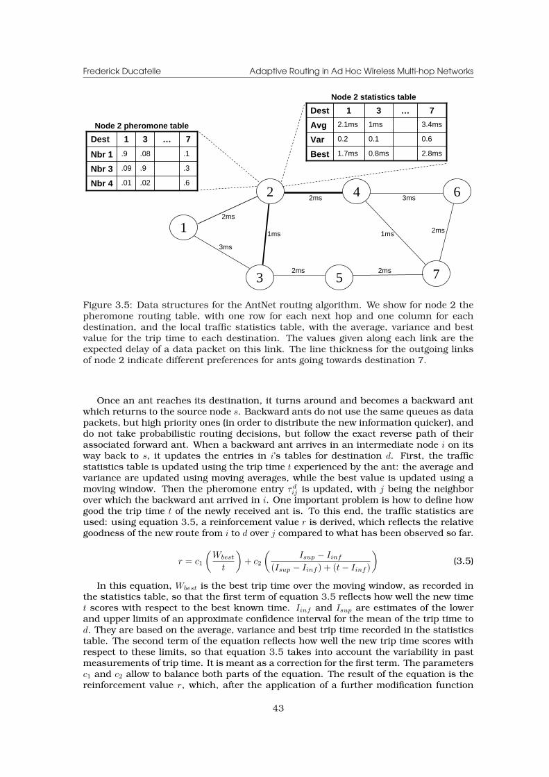
Frederick Ducatelle Adaptive Routing in Ad Hoc Wireless Multi-hop Networks
1
2
3 5
4 6
7
2ms
3ms
1ms
2ms
2ms
2ms
1ms
3ms
2ms
Node 2 pheromone table
.6.02.01Nbr 4
.3.9.09Nbr 3
.1.08.9Nbr 1
7…31Dest
2.8ms0.8ms1.7msBest
0.60.10.2Var
3.4ms1ms2.1msAvg
7…31Dest
Node 2 statistics table
Figure 3.5: Data structures for the AntNet routing algorithm. We show for node 2 thepheromone routing table, with one row for each next hop and one column for eachdestination, and the local traffic statistics table, with the average, variance and bestvalue for the trip time to each destination. The values given along each link are theexpected delay of a data packet on this link. The line thickness for the outgoing linksof node 2 indicate different preferences for ants going towards destination 7.
Once an ant reaches its destination, it turns around and becomes a backward antwhich returns to the source node s. Backward ants do not use the same queues as datapackets, but high priority ones (in order to distribute the new information quicker), anddo not take probabilistic routing decisions, but follow the exact reverse path of theirassociated forward ant. When a backward ant arrives in an intermediate node i on itsway back to s, it updates the entries in i’s tables for destination d. First, the trafficstatistics table is updated using the trip time t experienced by the ant: the average andvariance are updated using moving averages, while the best value is updated using amoving window. Then the pheromone entry τd
ij is updated, with j being the neighborover which the backward ant arrived in i. One important problem is how to define howgood the trip time t of the newly received ant is. To this end, the traffic statistics areused: using equation 3.5, a reinforcement value r is derived, which reflects the relativegoodness of the new route from i to d over j compared to what has been observed so far.
r = c1
(Wbest
t
)+ c2
(Isup − Iinf
(Isup − Iinf ) + (t− Iinf )
)(3.5)
In this equation, Wbest is the best trip time over the moving window, as recorded inthe statistics table, so that the first term of equation 3.5 reflects how well the new timet scores with respect to the best known time. Iinf and Isup are estimates of the lowerand upper limits of an approximate confidence interval for the mean of the trip time tod. They are based on the average, variance and best trip time recorded in the statisticstable. The second term of the equation reflects how well the new trip time scores withrespect to these limits, so that equation 3.5 takes into account the variability in pastmeasurements of trip time. It is meant as a correction for the first term. The parametersc1 and c2 allow to balance both parts of the equation. The result of the equation is thereinforcement value r, which, after the application of a further modification function
43
Frederick Ducatelle Adaptive Routing in Ad Hoc Wireless Multi-hop Networks
(for which we refer to [71]), is used to update the pheromone value τdij through a moving
average. This way, the new pheromone value incorporates the latest reported trip time.If enough ants are used, all pheromone values can be kept up-to-date so that they givean accurate image of the current network situation.
Data packets are routed in a similar way as forward ants, choosing a next hopstochastically at every hop. Stochastic forwarding of data packets allows per packetdata load balancing. The probability Rd
ij for a data packet in node i with destination dto take node j as a next hop is given in equation 3.6. Like the probability for forwardants, it is based on pheromone values. However, there are two important differences.First of all, the local heuristic ηij based on the queue lengths is not used here. Second,the pheromone is raised to a power ε, which is normally larger than 1. This increasesthe probability of taking paths with higher pheromone values, so that data packets areonly routed over the best paths, and are not used for exploration like the forward ants.
Rdij =
(τdij)
ε
∑l∈Ni
(τdil)ε
(3.6)
In simulation studies using the Omnet++ simulator [265], AntNet was comparedto traditional routing algorithms such as OSPF and distance vector routing, and toother adaptive routing algorithms, such as Q-routing (see subsection 3.3.3 and [39]).In a wide range of test scenarios, using different networks such as NSFNET and theJapanese NTTnet, and using different patterns in terms of data load, AntNet was shownto be superior to all other algorithms in terms of packet throughput and end-to-enddelay. It did produce more overhead than traditional static routing algorithms, but notmore than other adaptive routing algorithms.
3.2.4 ACO routing principles
In the previous subsection, we took a detailed look at AntNet, an example of an ACOrouting algorithm. Now, we take a more general point of view, and extract the mainprinciples behind ACO routing with their properties. The material presented here hasalso been described in [76], in a slightly different form.
A first important characteristic of ACO routing algorithms is that they gather rout-ing information through the repeated sampling of full paths. This is in line with thebehavior of ants in nature, where a large number of ants continuously move betweentheir nest and the food source, and with the working of ACO algorithms for combina-torial optimization, where multiple artificial ants repeatedly and in parallel constructsample solutions for the problem at hand. The ACO approach to routing is quite dif-ferent from the distance vector approach, where routing information is derived frominformation provided by neighboring nodes, and from the link state approach, whererouting information is calculated based on the update messages received from all othernodes in the network. Due to the use of redundant probing packets such as the for-ward ants in AntNet, the ACO approach to the gathering of routing information is quiterobust: each ant is individually unimportant and loss of control packets can be tol-erated. An important aspect of the whole process is the fact that ants always samplefull paths between source and destination. At no point is routing information derivedfrom information provided by other nodes. This is in stark contrast to the distancevector approach, where all routing information is derived from estimates provided byneighbor nodes. Relying only on direct experiences from full path samples adds furtherto the robustness of the algorithm, as updates are not dependent on the correctnessof the routing information available in other nodes. More about this will follow also insubsection 3.3.2. On the downside, the constant use of probing also leads to increasedoverhead, which can negatively influence the efficiency of ACO routing.
44
Frederick Ducatelle Adaptive Routing in Ad Hoc Wireless Multi-hop Networks
A second characteristic is the way ants choose a path to sample: they construct thepath hop by hop in a stochastic way using pheromone information. The relation withthe foraging behavior of ants in nature and with ACO for combinatorial optimizationis again evident, as also there ants follow their path or construct their solution stepby step using pheromone in a non-deterministic way. The use of the pheromone in-formation allows to build on experiences gathered by previous ants. It is the key tothe stigmergic process that guides the coordinated working of a highly distributed pro-cess. The fact that ants build their paths in a probabilistic way allows the explorationof multiple paths. This makes the algorithm adaptive to changes in the network envi-ronment. Moreover, it leads to the availability of multiple paths for data routing, eachwith an associated goodness value. This increases robustness, through the availabilityof backup paths, and allows to spread data over the multiple paths, increasing networkthroughput (see also subsection 2.4.3).
A third characteristic is the stochastic forwarding of data packets based on thepheromone information. This relates to the issue of using multiple paths discussedabove. By forwarding data probabilistically, the data load is spread over the multipleavailable paths on a per packet basis. This allows to make better use of available net-work resources and obtain better throughput. The use of pheromone in this processensures that data is focused on the best paths. If pheromone is always kept up-to-date,by using sufficient ants, data load balancing automatically follows the changes in thenetwork. An important aspect in the stochastic forwarding of data is that it uses a dif-ferent formula than the ants, focusing more on the best pheromone. This way, ants aremore explorative, while data packets concentrate on exploiting the routing informationprovided by the ants. Here, the relation with ant foraging behavior in nature and ACOfor combinatorial problems is less obvious: in those processes, the same ants need totake care of exploration of the solution space and exploitation of previously found infor-mation in order to find the best solution. Using separate mechanisms for explorationand exploitation allows to build a more flexible system.
3.2.5 Existing ACO routing algorithms for wired networks
Apart from the AntNet algorithm described in subsection 3.2.3, a wide range of differentACO routing algorithms have been proposed. Here, we give an overview of existing ACOrouting algorithms for wired networks, while in the next subsection, we discuss ACOrouting algorithms for AHWMNs.
ABC [235] was developed before AntNet, in 1996, and takes a significantly differentapproach, mainly because it was developed for a different type of networks: it assumesa network with symmetric path travel costs, in which data communication is organizedthrough virtual circuits (rather than using the packet switched approach supported byAntNet). Like in AntNet, each node s periodically sends out ants to randomly chosendestinations. Each ant has an associated age, which is increased proportionally tothe load of each visited node (the age is increased more when heavily loaded nodesare passed, so that it reflects the free space on the followed route). While travelingfrom its source s to its destination d, the ant updates the pheromone for the pathbackward to s, based on its age. This is an important difference with AntNet: antsupdate pheromone about the path to their source while going forward, and no backwardants are used. This is possible because of the assumption of symmetric path costs.Other major differences compared to AntNet are that no path statistics are used toevaluate path quality measurements reported by the ants, and that no local heuristicis used to help guide the ants (in AntNet, the local queue lengths are used). Finally, inABC, it is not data packets that are routed according to the pheromone, but call setupmessages. Moreover, these messages do not follow pheromone probabilistically, butgreedily choose the directions with the highest pheromone level. Once a call has been
45

Frederick Ducatelle Adaptive Routing in Ad Hoc Wireless Multi-hop Networks
set up successfully, data packets follow its circuit deterministically. ABC was tested insimulation on a model of the British Telecom network and was shown to give superiorperformance compared to other approaches.
The algorithm proposed in [248], called Ants Routing, builds on ABC. It is meant fornetworks with frequent node and link failures. The main difference compared to ABC isthe use of so-called uniform ants. These are different from the regular ABC ants in thesense that they do not have a specific destination and do not follow pheromone infor-mation. Instead, they wander through the network choosing each next hop accordingto a uniform distribution, until they have reached a maximum time-to-live, after whichthey are discarded. The use of uniform ants improves exploration. This is particularyimportant when dealing with frequent topology changes; the algorithms AntNet andABC were designed to be adaptive with respect to data traffic changes, rather than withrespect to topology changes. Another advantage of the uniform ants is that they do nothave a specific destination, so that they can be used in case a node does not know allpossible destinations in the network. A disadvantage is that uniform ants can lead toinefficiencies, due to the overhead they cause and the suboptimal paths they follow.
A number of papers propose further adaptations to ABC. The algorithm proposedin [35] allows ants in ABC to update pheromone not only for their source node s, butalso for all intermediate nodes on their path. The authors of [226] describe ABC-backward, which combines ABC with elements from AntNet, such as the use of for-ward and backward ants and the use of the ants’ trip time for pheromone updating.In [230], the authors extend ABC with probabilistic routing of call setups and the useof anti-pheromone, which allows ants to decrease pheromone in some cases, instead ofincreasing it.
AntNet-FA [72] is an adaptation of AntNet, proposed by the same authors of theoriginal algorithm. It is very similar to the original AntNet, but contains an improvementin the behavior of the forward ants: AntNet-FA’s forward ants do not use the samequeues as data packets, but instead take high priority queues like backward ants.The trip times experienced by the forward ants are therefore no longer representativefor what can be expected for data packets; the trip time for data packets are insteadcalculated by the backward ants as the sum of local estimates maintained in each ofthe intermediate nodes. The main advantage of this approach is that ants can travelfaster so that updates are done more in real-time.
Other papers propose further improvements to AntNet. In [80] and [205] some mech-anisms to enhance the exploratory behavior of AntNet are presented. In [23], the au-thors propose other improvements to AntNet such as the possibility to explicitly takelink and node failures into account, and a better initialization of the pheromone ta-bles. In [149], adaptive-SDR is proposed. The main difference with AntNet is that inadaptive-SDR, the network is divided into clusters, and a distinction is made betweeninter-cluster and intra-cluster routing. This improves scalability, since routing tablesdo not have to maintain entries for all possible destinations. Scalability issues of AntNetwere also investigated in [51]. Finally, in [286], the authors present Adaptive Swarm-based Routing (ASR). Differences with AntNet include the use of a momentum termin pheromone updating, and the fact that pheromone is updated for all intermediatenodes as destinations. In simulation, ASR was shown to outperform AntNet in terms ofpacket delay and throughput.
In [274] and other papers from the same authors, Routing By Ants (RBA) is pro-posed. It uses virtual circuits and supports both unicast and multicast routing. RBAhas similarities both with ABC and AntNet. An interesting difference with these twoalgorithms is the fact that the parameters which define how routing decisions are de-rived from pheromone values are carried inside the ants, so that they can be differentfor each ant. These parameters are assigned to ants in their source node and are calcu-lated using a genetic algorithm (GA). Some small improvements to this algorithm wereproposed by different authors in [249].
46
Frederick Ducatelle Adaptive Routing in Ad Hoc Wireless Multi-hop Networks
The authors of [128] propose the Co-operative Asymmetric Forward (CAF) mecha-nism. It shows how forward ants can update routing information about the path totheir source without sending a backward ant and without assuming symmetric pathcosts. In CAF, each data packet hopping from a node i to a node j leaves at j an esti-mate cij of the queuing and transmission time it has experienced while traveling from i.Later, ants traveling in the opposite direction read this estimate and store it. By addingall estimates over their forward path from their source node s till intermediate node i,the ants obtain a good estimate of the delay on the backward path from i to s, so thatthey can correctly update pheromone information about their full backward path.
ACO has also been applied to QoS routing. A first example is AntNet+SELA [78], anadaptation of AntNet for QoS routing in asynchronous transfer mode (ATM) networks.It integrates AntNet with stochastic estimator learning automata (SELA) [266], a frame-work for QoS provisioning in ATM networks that uses static reinforcement learningagents to derive routing and application admission strategies. The original SELA usesa link state approach to gather routing information. AntNet+SELA, on the other hand,uses ant based probing for the collection of routing information. An interesting featureof AntNet+SELA is that nodes have the possibility to reactively send out extra ants inorder to search specific information that they need. For details about the AntNet+SELAsystem, we refer to [78, 70]. A number of other adaptations of ACO routing for QoShave also been proposed. Most of these aim to provide hard QoS guarantees, followingthe IntServ approach to QoS [40]. This is the case for Agent-based Routing System,proposed in [206], and for Q-Colony, proposed in [253]. Other approaches, such as thealgorithm proposed in [192] and AntNet-QoS, presented in [50], combine ACO with asoft approach to QoS routing. The latter proposes an integration of AntNet with theDiffServ framework for QoS [153].
Recently, ACO routing has also been used for routing problems in new kinds ofnetworks (other that the applications to the equally new field of AHWMNs, which aredescribed separately in subsection 3.2.6). One interesting example is its use for theproblem of dynamic routing and wavelength assignment in wavelength-division multi-plexing (WDM) networks, where the aim is to set up a primary path between sourceand destination and one or more disjoint backup paths, in on-demand fashion. Thiswork is described in [204] and other papers by the same authors. Another very inter-esting new application is the use of ACO routing in the domain of Networks-on-Chip(NoC). These are sub-micron scale networks that connect the elements on an integratedcircuit. NoC have many characteristics in common with traditional wired networks,but pose additional challenges that mainly arise from the extremely limited availableresources. In [64], the authors propose an AntNet based approach to routing in NoC.
Finally, we want to mention some algorithms that use biological metaphors that aredifferent from the ant foraging behavior, but reference ACO routing and have elementsin common with this approach. In [273], the BeeHive algorithm is proposed. This algo-rithm is inspired by the behavior of honey bees. Like AntNet, however, it gathers routinginformation using path probing packets (called bee agents here), and it builds stochas-tic routing tables for data forwarding. Different from ants in AntNet, bees are flooded(with a maximum number of hops) instead of unicast along a stochastically chosen pathto a specific destination. Also different from AntNet, the network is divided into regions,so that not all destinations need to be put in the routing table of each node and betterscalability can be provided. The authors of [173] also address this issue of scalabilityin AntNet. They propose GA-agents, which is based on the use of a distributed GA.In GA-agents, each node maintains a GA population, in which each individual repre-sents a path in the network. Paths are encoded as a sequence of turns (rather than asequence of nodes). Individuals are evaluated by letting them probe the path they rep-resent. This way, they are similar to the ants in AntNet. Typical GA operations such asmutation and selection are executed to find the best paths. Finally, in [276] and otherpapers by the same authors, the CE-ants approach is presented. This algorithm is in-
47
Frederick Ducatelle Adaptive Routing in Ad Hoc Wireless Multi-hop Networks
spired by the cross-entropy (CE) metaheuristic for combinatorial optimization proposedby Rubinstein [228]. The CE method is in principle quite different from ACO, since itwas originally derived from techniques for rare event simulation. However, due to theiruse of repeated sampling, many CE algorithms have in practice strong similarities withACO algorithms. The same is true for CE-ants: in overall architecture it is quite similarto ACO routing algorithms like AntNet. The main difference lies in the formulas usedfor pheromone updating, which bear the signature of the CE method. CE-ants hasbeen applied to a variety of routing related problems, such as the problem of findingprotection cycles [277], and the problem of finding primary and backup paths [275].
3.2.6 Existing ACO routing algorithms for AHWMNs
Due to its properties of adaptivity and robustness, ACO has also attracted attention asa paradigm for routing in AHWMNs. Here, we give an overview of algorithms that havebeen proposed in recent years.
A number of the ACO routing algorithms for AHWMNs that have been proposedhave a structure that is quite similar to that of the ACO algorithms for wired net-works described in subsection 3.2.5. The Accelerated Ants Routing algorithm describedin [191, 104], is derived from the Ants Routing algorithm for wired networks. It con-tains small adaptations to this algorithm, such as the no-return rule (which simplystates that ants cannot pick their previous hop as next hop, so that simple loops areavoided), and is shown in simulation to perform better than AntNet in MANETs. TheABC-AdHoc algorithm [255] on the other hand is based both on ABC and AntNet. Whileit uses forward ants that update pheromone for the path to their source, as in done inABC, it uses formulas of AntNet to calculate pheromone updates and to make proba-bilistic routing decisions. In a simulation with rather limited mobility, the ABC-AdHocalgorithm was shown to perform better than AntNet. In [288], the authors proposeadaptations of AntNet for use in sensor networks. These include an informed initializa-tion of pheromone values at node activation, the possibility to flood forward ants, ratherthan unicast them to their destination, and to piggyback these flooded forward ants ontop of data packets. The adaptations of AntNet are shown to perform better than theoriginal algorithm in sensor networks.
The problem with following the design of ACO routing algorithms for wired networkstoo closely is that it results in proactive routing algorithms, which, as has been ex-plained in subsection 2.4.1, is not always the best approach to routing in AHWMNs.This problem and a solution to it are well illustrated in [24]. In this work, the authorsfirst propose an algorithm that is very similar to AntNet. The main differences are thatsome uniform ants are used to improve exploration (see also the Ants Routing algo-rithm described in subsection 3.2.5), and that data are routed deterministically overthe path with the best pheromone. In simulation tests, this algorithm was found toperform worse than AODV, mainly due to inefficient route discovery and large amountsof overhead. Then, the authors propose a new algorithm, called Probabilistic Emer-gent Routing Algorithm (PERA). This is a purely reactive algorithm: forward ants areonly sent out at the start of a communication session, or when all existing routing in-formation is out of date. They are flooded towards the destination. For every copy ofthe forward ant that reaches the destination, a backward ant is sent to the source, sothat multiple paths are created at route setup. It is not clear whether data are routedstochastically or not. In simulation studies, PERA is found to have a performance thatis comparable to AODV. Unfortunately, it is also clear from the description of the al-gorithm that this is mainly due to the fact that PERA is quite similar to AODV, withforward ants and backward ants replacing respectively RREQ and RREP messages. Ofthe original ACO ideas, not much is left.
The approach of building a reactive kind of ACO routing algorithm has been fol-
48
Frederick Ducatelle Adaptive Routing in Ad Hoc Wireless Multi-hop Networks
lowed by several other researchers in the field. Ant-Colony-Based Routing Algorithm(ARA) [119] is quite similar to PERA (and hence to AODV). One difference is that bothforward and backward ants leave pheromone behind: forward ants update pheromoneabout the path to the source, while backward ants update pheromone about the pathto the destination. Another difference is that also data packets update pheromone, sothat paths which are in use are also reinforced while the data session is going on. Thiscomes down to repeated path sampling, so that ARA keeps more of the original ACOcharacteristics than PERA. In simulation, ARA was found to perform better than AODVbut worse than DSR in highly dynamic environments. Also the Termite algorithm [224]follows a reactive approach. Important differences with ARA and PERA are that forwardants are not flooded, but follow a random walk. And backward ants do not necessarilyfollow the exact same path of the RREQ back to the source, but are themselves routedstochastically (this can be an advantage if unidirectional links are present; see subsec-tion 2.3.2). Pheromone updating is done by all packets (also by data), and is alwaysdone with respect to the source that a packet is coming from. This means that costsymmetric paths are assumed. In a small set of simulation tests, Termite was shownto perform better than AODV for varying values of node speed [225]. Ad hoc Network-ing with Swarm Intelligence (ANSI) [220] is again a variation on the same approach. Itonly uses ants at route setup time. A mechanism using forward and backward ants isapplied, and like in Termite and ARA, data packets also deposit pheromone, in orderto reinforce the paths they use. Data are routed deterministically over the best paths.ANSI evaluates paths based on the congestion rates (defined by the free versus occu-pied space in the node IP queues) of nodes along the path. ANSI was shown to performbetter than AODV in simulation. Finally, also Emergent Ad Hoc Routing Algorithm(EARA) [177] follows a similar approach. Different in EARA is that during the courseof a data session, paths are reinforced by ants that are sent out from the destination.New paths are detected using ants that do random walks through the network.
A number of other algorithms use ants in a different way. The authors of [194] pro-pose to use a set of mobile agents that are quite independent from network nodes ordata sessions: these agents are generated at network setup time, and they stay aroundindefinitely. They perform a continuous random walk through the network, keepinga history of the last N nodes they have visited. At each new node they arrive, pathsare extracted from this history list in order to update routing information. The algo-rithm proposed in [190] is a combination between this approach and AODV. Also here, anumber of ant agents keep going through the network indefinitely, performing a randomwalk and keeping a history list of the last N visited nodes. However, here the networknodes also run AODV. They are therefore not solely dependent on the information givento them by the randomly moving ants. Instead, the ants only provide possibilities toimprove on routing information gathered by AODV, or to avoid AODV route setups. Theauthors show that their Ant-AODV method performs better than Ants Routing or AODVseparately. In [45], the authors propose an algorithm that combines geographic rout-ing (see subsection 2.4.3) with ants. In their approach, each node keeps a databaseof the positions of all other nodes. To keep these databases up-to-date, informationis exchanged locally among neighbors, and globally by sending ants to nodes furtheraway. The destination nodes for the ants are chosen according to a probabilistic mech-anism, and nodes can copy the routing information from ants that pass by. So, inthis approach, ants replace flooding as a way to spread routing information over thenetwork. The Mobile Ants-Based Routing Protocol (MABR),proposed in [126, 127] wasdesigned for WAN scale AHWMNs. The algorithm divides the AHWMN area in rectan-gular zones, corresponding to geographical areas. All nodes of a zone together makeup a logical router. Long distance routing is done between logical routers, with theaid of location information. Ants are used at this level, to proactively update routingtables between logical routers. In simulation, MABR compared favorably to Terminodesrouting, a different algorithm for WAN scale AHWMNs.
49
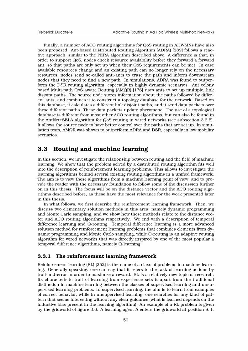
Frederick Ducatelle Adaptive Routing in Ad Hoc Wireless Multi-hop Networks
Finally, a number of ACO routing algorithms for QoS routing in AHWMNs have alsobeen proposed. Ant-based Distributed Routing Algorithm (ADRA) [289] follows a reac-tive approach, similar to the PERA algorithm described above. A difference is that, inorder to support QoS, nodes check resource availability before they forward a forwardant, so that paths are only set up when their QoS requirements can be met. In caseavailable resources change and an existing path can no longer rely on the necessaryresources, nodes send so-called anti-ants to erase the path and inform downstreamnodes that they need to find a new path. In simulations, ADRA was found to outper-form the DSR routing algorithm, especially in highly dynamic scenarios. Ant colonybased Multi-path QoS-aware Routing (AMQR) [176] uses ants to set up multiple, linkdisjoint paths. The source node stores information about the paths followed by differ-ent ants, and combines it to construct a topology database for the network. Based onthis database, it calculates n different link disjoint paths, and it send data packets overthese different paths. These data packets update pheromone. The use of a topologicaldatabase is different from most other ACO routing algorithms, but can also be found inthe AntNet+SELA algorithm for QoS routing in wired networks (see subsection 3.2.5).It allows the source node to have better control over the paths that are set up. In simu-lation tests, AMQR was shown to outperform ADRA and DSR, especially in low mobilityscenarios.
3.3 Routing and machine learning
In this section, we investigate the relationship between routing and the field of machinelearning. We show that the problem solved by a distributed routing algorithm fits wellinto the description of reinforcement learning problems. This allows to investigate thelearning algorithms behind several existing routing algorithms in a unified framework.The aim is to view these algorithms from a machine learning point of view, and to pro-vide the reader with the necessary foundation to follow some of the discussion furtheron in this thesis. The focus will be on the distance vector and the ACO routing algo-rithms described before, as these have the most relevance for the work presented laterin this thesis.
In what follows, we first describe the reinforcement learning framework. Then, wediscuss two elementary solution methods in this area, namely dynamic programmingand Monte Carlo sampling, and we show how these methods relate to the distance vec-tor and ACO routing algorithms respectively. We end with a description of temporaldifference learning and Q-routing. Temporal difference learning is a more advancedsolution method for reinforcement learning problems that combines elements from dy-namic programming and Monte Carlo sampling, while Q-routing is an adaptive routingalgorithm for wired networks that was directly inspired by one of the most popular atemporal difference algorithms, namely Q-learning.
3.3.1 The reinforcement learning framework
Reinforcement learning (RL) [252] is the name of a class of problems in machine learn-ing. Generally speaking, one can say that it refers to the task of learning actions bytrail-and-error in order to maximize a reward. RL is a relatively new topic of research.Its characteristic trait of learning from experience sets it apart from the traditionaldistinction in machine learning between the classes of supervised learning and unsu-pervised learning problems. In supervised learning, the aim is to learn from examplesof correct behavior, while in unsupervised learning, one searches for any kind of pat-tern that seems interesting without any clear guidance (what is learned depends on theinductive bias present in the learning algorithm). An example of a RL problem is givenby the gridworld of figure 3.6. A learning agent A enters the gridworld at position S. It
50
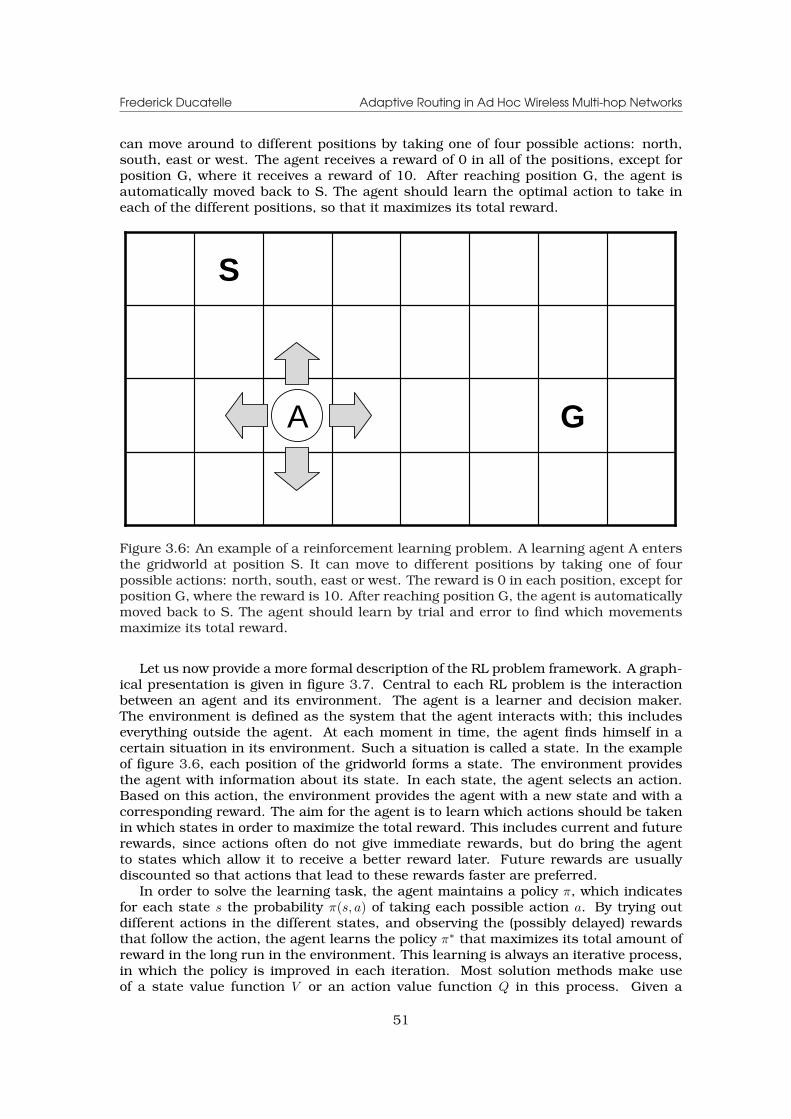
Frederick Ducatelle Adaptive Routing in Ad Hoc Wireless Multi-hop Networks
can move around to different positions by taking one of four possible actions: north,south, east or west. The agent receives a reward of 0 in all of the positions, except forposition G, where it receives a reward of 10. After reaching position G, the agent isautomatically moved back to S. The agent should learn the optimal action to take ineach of the different positions, so that it maximizes its total reward.
GA
S
Figure 3.6: An example of a reinforcement learning problem. A learning agent A entersthe gridworld at position S. It can move to different positions by taking one of fourpossible actions: north, south, east or west. The reward is 0 in each position, except forposition G, where the reward is 10. After reaching position G, the agent is automaticallymoved back to S. The agent should learn by trial and error to find which movementsmaximize its total reward.
Let us now provide a more formal description of the RL problem framework. A graph-ical presentation is given in figure 3.7. Central to each RL problem is the interactionbetween an agent and its environment. The agent is a learner and decision maker.The environment is defined as the system that the agent interacts with; this includeseverything outside the agent. At each moment in time, the agent finds himself in acertain situation in its environment. Such a situation is called a state. In the exampleof figure 3.6, each position of the gridworld forms a state. The environment providesthe agent with information about its state. In each state, the agent selects an action.Based on this action, the environment provides the agent with a new state and with acorresponding reward. The aim for the agent is to learn which actions should be takenin which states in order to maximize the total reward. This includes current and futurerewards, since actions often do not give immediate rewards, but do bring the agentto states which allow it to receive a better reward later. Future rewards are usuallydiscounted so that actions that lead to these rewards faster are preferred.
In order to solve the learning task, the agent maintains a policy π, which indicatesfor each state s the probability π(s, a) of taking each possible action a. By trying outdifferent actions in the different states, and observing the (possibly delayed) rewardsthat follow the action, the agent learns the policy π∗ that maximizes its total amount ofreward in the long run in the environment. This learning is always an iterative process,in which the policy is improved in each iteration. Most solution methods make useof a state value function V or an action value function Q in this process. Given a
51
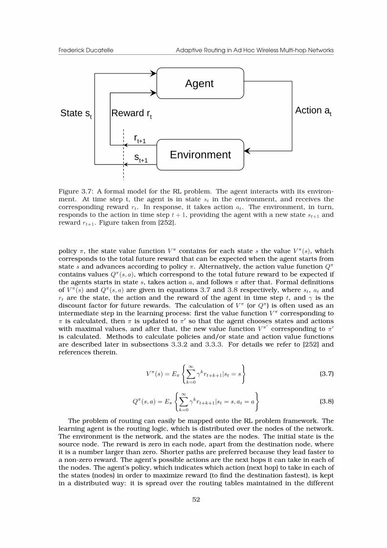
Frederick Ducatelle Adaptive Routing in Ad Hoc Wireless Multi-hop Networks
Agent
Environment
Action atReward rtState st
st+1
rt+1
Figure 3.7: A formal model for the RL problem. The agent interacts with its environ-ment. At time step t, the agent is in state st in the environment, and receives thecorresponding reward rt. In response, it takes action at. The environment, in turn,responds to the action in time step t + 1, providing the agent with a new state st+1 andreward rt+1. Figure taken from [252].
policy π, the state value function V π contains for each state s the value V π(s), whichcorresponds to the total future reward that can be expected when the agent starts fromstate s and advances according to policy π. Alternatively, the action value function Qπ
contains values Qπ(s, a), which correspond to the total future reward to be expected ifthe agents starts in state s, takes action a, and follows π after that. Formal definitionsof V π(s) and Qπ(s, a) are given in equations 3.7 and 3.8 respectively, where st, at andrt are the state, the action and the reward of the agent in time step t, and γ is thediscount factor for future rewards. The calculation of V π (or Qπ) is often used as anintermediate step in the learning process: first the value function V π corresponding toπ is calculated, then π is updated to π′ so that the agent chooses states and actionswith maximal values, and after that, the new value function V π′ corresponding to π′
is calculated. Methods to calculate policies and/or state and action value functionsare described later in subsections 3.3.2 and 3.3.3. For details we refer to [252] andreferences therein.
V π(s) = Eπ
{ ∞∑
k=0
γkrt+k+1|st = s
}(3.7)
Qπ(s, a) = Eπ
{ ∞∑
k=0
γkrt+k+1|st = s, at = a
}(3.8)
The problem of routing can easily be mapped onto the RL problem framework. Thelearning agent is the routing logic, which is distributed over the nodes of the network.The environment is the network, and the states are the nodes. The initial state is thesource node. The reward is zero in each node, apart from the destination node, whereit is a number larger than zero. Shorter paths are preferred because they lead faster toa non-zero reward. The agent’s possible actions are the next hops it can take in each ofthe nodes. The agent’s policy, which indicates which action (next hop) to take in each ofthe states (nodes) in order to maximize reward (to find the destination fastest), is keptin a distributed way: it is spread over the routing tables maintained in the different
52
Frederick Ducatelle Adaptive Routing in Ad Hoc Wireless Multi-hop Networks
nodes. The relationship between the task of routing and the RL framework was firstpointed out in [39].
3.3.2 Elementary solution methods for reinforcement learning: dy-namic programming and Monte Carlo sampling
A wide range of different solution methods have been developed for RL problems. Thetwo most elementary ones are dynamic programming and Monte Carlo sampling. Here,we describe these approaches, and discuss how they relate to strategies used in routing.Later, in subsection 3.3.3, we describe another solution method, temporal-differencelearning, and discuss how one of its instances, namely Q-learning, formed the basis fora different adaptive routing algorithm, called Q-routing.
A first solution method for RL problems is dynamic programming. This is a generaltechnique for solving optimization problems proposed in [26], and has been in use fora long time before it was applied to RL. Dynamic programming has been discussedbefore in 3.1.1, as it was at the basis of the development of distance vector routingalgorithms. The basic idea behind this method is to split an optimization probleminto subproblems, and use the solutions to these subproblems to construct an optimalsolution for the main problem. A straightforward way of using dynamic programmingin RL is policy iteration. The agent starts with a random initial policy π0, and usesdynamic programming to calculate the state value function V π0 corresponding to it.Then π0 is updated to π1 by choosing in each state the actions that optimize the valuesof the states visited by the agent with respect to V π0 . Then, dynamic programming isused again to calculate V π1 . The formula for calculating each state value V π(s) usingdynamic programming is given in equation 3.9, where Pa
ss′ is the probability of reachingstate s′ after taking action a in state s, and Ra
ss′ is the expected reward when reachingstate s′ after taking action a from state s. Compared to the formula of equation 3.7, theinfinite sum of future rewards is replaced by the sum of the expected immediate rewardand the estimated values of the neighbor states s′. This is the trademark approachof dynamic programming: the task of calculating the value of a state is solved basedon the solution of a number of subtasks, namely the values of the neighboring states.This characteristic approach of calculating estimates based on other estimates is in thecontext of RL also called information bootstrapping.
V π(s) ←∑
a
π(s, a)∑
s′Pa
ss′ [Rass′ + γV π(s′)] (3.9)
Dynamic programming formed the inspiration for distance vector routing algorithmssuch as RIP. Details about this have been given before in subsection 3.1.1. Here, weonly want to point out how this approach to routing is affected by the use of the char-acteristic technique of information bootstrapping. This provides high efficiency, dueto the reuse of solutions that were calculated for different subproblems (routing esti-mates calculated for neighboring nodes). However, it is not very robust or adaptive: ifestimates are wrong in one node (e.g. due to changes in the environment), they arepropagated over the network since other estimates are based on them, and it can takea long time until the error is fixed and all the routing information converges again tocorrect values. This limits the usability of a pure dynamic programming approach foradaptive routing in AHWMNs.
A second elementary solution method for RL is Monte Carlo sampling. Also thismethod has been around long before RL itself was a topic. In fact, the term Monte Carlorefers to any problem solving method in which solutions are learned from experiencesobtained by repeated sampling. In the field of RL, Monte Carlo sampling can be usedto calculate value functions in a policy iteration approach, like the one described fordynamic programming above. One difference is that in Monte Carlo learning usually
53
Frederick Ducatelle Adaptive Routing in Ad Hoc Wireless Multi-hop Networks
the action values Qπ(s, a) are used rather than the state values V π(s). To calculatethe value Qπ(s, a) of action a in state s, the agent tries it out: it runs a full episodeof the task (i.e. until it reaches the goal state), starting from state s with action aand then following policy π after that. By executing repeated samples and taking theaverage of the total rewards experienced in each of these samples, a good estimate ofthe expected value of the total future reward can be obtained. In practice, a movingaverage can be used, applying the formula of equation 3.10 after each newly collectedsample experience. In this formula, Rπ(s, a) is the total reward experienced when takingaction a in state s and following π after that, and α is a constant factor used for themoving average. A special case of Monte Carlo sampling is the off-policy version, inwhich the agent collects sample experiences following a different policy than the oneit is actually learning about. This allows more freedom (e.g. to do exploration), but iscomputationally more complicated, as one has to make an adjustment to the averageexperienced rewards in order to find the correct value for the other policy.
Qπ(s, a) ← Qπ(s, a) + α[Rπ(s, a)−Qπ(s, a)] (3.10)
It is easy to see how the ACO approach to routing relies in its process for gatheringrouting information on the same ideas as the Monte Carlo approach to learning in RL.Ants learn action values (the value of taking a next hop in a certain node) by execut-ing complete samples of solutions to the task (by sampling a path to the destination).The final pheromone values are the result of taking a sufficiently high number of sam-ples. ACO routing algorithms in which different forwarding policies are used for antsand data forwarding are similar to off-policy Monte Carlo learning. The fact that thepheromone values do not always correspond to the average of the values experiencedby the ants, but are instead the result of more complicated evaluations of these values(e.g. in AntNet, described in subsection 3.2.3, the experienced delay is manipulatedusing the local traffic statistics), is reminiscent of actor-critic methods, which are moreadvanced RL learning methods [25]. The most important advantage of Monte Carlosampling compared to information bootstrapping is that all estimates are based on di-rect experiences. This makes the estimates more reliable than when they are basedon other estimates, giving increased robustness to the algorithm. This is particularlyimportant in a changing and unreliable environment like AHWMNs. Adaptivity can inprinciple be a problem in Monte Carlo learning, namely when on-policy learning is ap-plied and the policy has converged. In ACO routing, this problem is solved by using anoff-policy approach in which ants follow a slightly different policy from data packets.
It is interesting to note that more traditional routing algorithms for AHWMNs, suchas AODV, DSR and other reactive algorithms (see subsection 2.4.2), also rely on sam-pling. They construct a path based on a single sample. This is of course quite differentfrom taking the average value obtained from repeated sampling such as in ACO rout-ing. Nevertheless, it is a confirmation of the usefulness in AHWMNs of the increasedrobustness obtained through path sampling. This is especially clear in the developmentof AODV. This algorithm is presented as a distance vector algorithm as it was conceivedas a successor to DSDV, a routing algorithm that relies purely on information boot-strapping. However, the only elements it still contains of distance vector routing is theshape of the routing tables. The information bootstrapping approach used in DSDV isdeemed unworkable in the highly dynamic and unreliable AHWMN environment, andis replaced by a strategy that relies on sampling. However, it needs to be noted thatthe sampling in AODV and other reactive routing algorithms is not always done in aconsequent way. E.g., AODV RREQ messages do not always go all the way until thedestination, but return to the source as soon as they find a node that has routing in-formation about the destination. At that point, the source node’s routing informationis again based on an estimate provided by another node.
54
Frederick Ducatelle Adaptive Routing in Ad Hoc Wireless Multi-hop Networks
3.3.3 Temporal-difference learning and Q-routing
Here we describe a more advanced class of solution methods for RL problems, namelytemporal-difference learning. This approach combines elements of dynamic program-ming and Monte Carlo sampling, in order to get advantages from both methods. It isat this point important to point out that the AntHocNet algorithm for routing in AH-WMNs presented in chapter 4 of this thesis also combines elements of both dynamicprogramming and Monte Carlo sampling. It does so in a completely different way thantemporal-difference learning though, as will become clear later.
The simplest version of temporal-difference learning is the one step temporal-differencemethod, referred to as TD(0). The main idea behind this method is for the agent to takea sample of just one step, and then bootstrap information. Concretely, in TD(0), theagents calculates Q(s, a) by taking action a in state s, observing the immediately re-ceived reward r, and bootstrapping on the value of the new state it arrives in. Anexample update formula is given in equation 3.11, where α is a constant factor forcalculating the moving average, and γ is a constant factor to discount rewards thatare received in a future time step. The difference with the update formula for MonteCarlo learning (equation 3.10) is that only one step of experienced reward is used. Thedifference with the update formula for dynamic programming (equation 3.9) is that anexperience is used for the one-step reward, rather than the expected value. Variationsare possible in the choice of the action a′ in the new state s′ on the basis of which thebootstrapped value Q(s′, a′) is chosen. E.g., the most popular TD(0) method, Q-learning,uses the action a′ that gives the maximal value for Q(s′, a′) [272]. This corresponds toan off-policy form of temporal-difference learning, and allows fast convergence to theoptimal policy π∗. The one-step form of temporal difference learning found in TD(0) canbe extended to an n-step algorithm, in which the agent takes a sample of n steps beforebootstrapping the local state value. If n is equal to infinity or to the number of stepsneeded to reach the goal, this comes down to Monte Carlo sampling. Finally, when theresults from several n-step samples are combined, with different values for n, we getthe TD(λ) methods, which are also referred to as eligibility traces [271].
Qπ(s, a) ← Qπ(s, a) + α[r + γQ(s′, a′)−Qπ(s, a)] (3.11)
Just like dynamic programming and Monte Carlo sampling, temporal-differencelearning has been applied to routing. In particular, the Q-learning algorithm men-tioned above has lead to the development of Q-routing [39]. In Q-routing, nodes keeprouting tables that are similar to those in AntNet, with one entry per combination ofnext hop and destination. The routing table entry cd
ij indicates the cost of going from iover neighbor j to destination d. Each time node i sends a data packet to a neighbor jfor a destination d, j sends a control packet back to i. This packet contains the valuesttot, the total queueing and transmission delay experienced by the data packet to reachj from i, and cd
j , the cost of the best path to destination d present in j’s routing table.In node i, ttot and cd
j are summed to get an estimate of the cost from i to d over j, andthe value cd
ij in i’s routing table is updated accordingly. When compared to Q-learning,ttot corresponds to the immediate reward experienced in the one step sample, and cd
j
corresponds to the value of the next state. Like in dynamic programming approachesto routing, such as the basic distance vector routing algorithm, routing updates arebased on the best paths reported by neighboring nodes. The main difference is that inQ-routing the cost of the single hop to the neighbor is taken from a sample, while indistance vector routing, it is an estimate of the expected value, obtained via local mon-itoring. In direct comparisons with the AntNet adaptive routing algorithm, Q-routingscored less well [70].
Another RL inspired approach to routing is SAMPLE [90]. This is an adaptive algo-rithm for MANETs. Similarly to Q-routing, it does an update of routing information with
55
Frederick Ducatelle Adaptive Routing in Ad Hoc Wireless Multi-hop Networks
the transmission of each data packet. Also like Q-routing and dynamic programming,the best path available in neighboring nodes is used for information bootstrapping inthe update process. For the calculation of the cost of the one hop to the neighbor, SAM-PLE relies on a model of the environment. Model-based RL [91] is not presented here,as it would lead us to far. However, the end result is an algorithm that is similar toboth Q-routing and distance vector routing. Important for MANETs, SAMPLE uses anestimate of link qualities with similarities to the ETX measure (see subsection 2.4.3) todefine path costs.
3.4 Conclusion
In this chapter we have described existing adaptive routing algorithms. The aim of thechapter was on the one hand to provide information about other algorithms in the field,and on the other hand to get the reader acquainted with the techniques and terminologythat will be used further in this thesis.
In a first section, we have described adaptive routing algorithms in the internet. Twomain approaches were discussed, namely distance vector routing and link state routing.For either of these approaches, we have investigated how they perform in terms of themajor challenges for AHWMN routing: adaptivity, robustness, efficiency and scalability.We have also indicated to what extent both approaches to routing have been adapted towork in AHWMNs.
Then, in a second section, we have described ACO and ACO routing. ACO is a meta-heuristic for the solution of optimization problems that was inspired by the shortestpath finding behavior of ant colonies in nature. ACO routing is an approach to routingthat is based on the ACO framework. It forms an important source of inspiration forthe work presented in this thesis. Here, we have described the major characteristicsof ACO routing in detail, and have given an extensive overview of existing ACO routingalgorithms, both for wired networks and for AHWMNs.
In a last section, we have treated adaptive routing from a machine learning point ofview. To that end, we have described RL, an important class of learning problems. Wehave shown that the problem of routing in telecommunication networks fits well intothis problem framework. Then, we have investigated how the strategies for the gatheringof routing information used by distance vector and ACO routing algorithms correspondto two important learning methods for RL problems, namely dynamic programming andMonte Carlo learning. Finally, we have described temporal difference learning, a moreadvanced solution method for RL problems that combines elements of both dynamicprogramming and Monte Carlo learning, and we have explained the Q-routing algorithmthat was derived from it. The AntHocNet routing algorithm for AHWMNs described inthe next chapter also combines elements from both of these learning methods, but inquite a different way.
56
Chapter 4
AntHocNet: an adaptive routingalgorithm for ad hoc wirelessmulti-hop networks
In this chapter, we describe AntHocNet, an adaptive routing algorithm for AHWMNs.AntHocNet is a hybrid routing algorithm, in the sense that it contains elements fromboth reactive and proactive routing. Specifically, it combines a reactive route setup pro-cess with a proactive route maintenance and improvement process. AntHocNet was inthe first place inspired by the ACO approach to routing. This is evident in the way thatit gathers, stores and uses routing information. Consequently, the terminology usedin this chapter is mostly related to the ACO routing literature. Nevertheless, AntHoc-Net also contains elements from distance vector routing. In particular, the informationgathering process used in its proactive route maintenance and improvement processcombines the route sampling strategy from ACO routing with an information bootstrap-ping process that is similar to the one used in distance vector routing algorithms. Theway both approaches are combined is novel and allows the algorithm to get the bestof both worlds. AntHocNet was in the first place developed for MANETs and WMNs.Descriptions of the AntHocNet algorithm have been published in [73,94,75,95,74,98].
The rest of this chapter is organized as follows. First, we give a general overviewof the AntHocNet routing algorithm. This includes a high level description of the algo-rithm in words, and a schematic representation. Then, we give a detailed description ofeach of the algorithm’s components. Finally, we provide further discussions on the pre-sented material, such as an investigation of the relations between AntHocNet and otherAHWMN routing algorithms, a discussion of how AntHocNet relates to the RL solutionmethods presented in chapter 3, and a description of elements that were present inolder versions of AntHocNet. Evaluations of AntHocNet and experimental comparisonswith other routing algorithms will be provided in the following chapters.
4.1 General overview of the AntHocNet routing algo-rithm
In this section, we give an overview of the algorithm. We start with a general descriptionin words. Then, we also provide a schematic representation in the form of a finite statemachine.
57

Frederick Ducatelle Adaptive Routing in Ad Hoc Wireless Multi-hop Networks
4.1.1 Algorithm description
AntHocNet is a hybrid algorithm, containing both reactive and proactive elements. Thealgorithm is reactive in the sense that it only gathers routing information about desti-nations that are involved in communication sessions. It is proactive in the sense thatit tries to maintain and improve information about existing paths while the commu-nication session is going on (unlike purely reactive algorithms, which do not searchfor routing information until the currently known routes are no longer valid). Routinginformation is stored in pheromone tables that are similar to the ones used in otherACO routing algorithms. Forwarding of control and data packets is done in a stochasticway, using these tables. Link failures are dealt with using specific reactive mecha-nisms, such as local route repair and the use of warning messages. Below, we describethe general working of the AntHocNet routing algorithm. Details will follow later insection 4.2.
In AntHocNet, routing information is organized in pheromone tables, similar to theones used in other ACO routing algorithms such as the earlier described AntNet (seesubsection 3.2.3). Each node i maintains one pheromone table Ti, which is a two-dimensional matrix. An entry T d
ij of this pheromone table contains information aboutthe route from node i to destination d over neighbor j. This information includes thepheromone value τd
ij, which is a value indicating the relative goodness of going over nodej when traveling from node i to destination d, as well as statistics information aboutthe path, and possibly virtual pheromone (see later). Apart from a pheromone table,each node also maintains a neighbor table, in which it keeps track of which nodes ithas a wireless link to. Details about the data structures maintained under AntHocNetare described in subsection 4.2.1.
At the start of a communication session, the source node of the session controlsits pheromone table, to see whether it has any routing information available for therequested destination. If it does not, it starts a reactive route setup process, in which itsends an ant packet out over the network to find a route to the destination. Such an antpacket is called a reactive forward ant. Each intermediate node receiving a copy of thereactive forward ant forwards it. This is done via unicasting in case the node has routinginformation about the ant’s destination in its pheromone table, and via broadcastingotherwise. Reactive forward ants store the full array of nodes that they have visitedon their way to the destination. The first copy of the reactive forward ant to reachthe destination is converted into a reactive backward ant, while subsequent copies aredestroyed. The reactive backward ant retraces the exact path that was followed by theforward ant back to the source. On its way, it collects quality information about eachof the links of the path. At each intermediate node and at the source, it updates therouting tables based on this quality information. This way, a first route between sourceand destination is established at completion of the reactive route setup process. Thefull process is repeated later if the source node falls without valid routing informationfor the destination of the session while data still need to be sent. Details about thereactive route setup process are provided in subsection 4.2.2.
Once the first route is constructed via the reactive route setup process, the algo-rithm starts the execution of the proactive route maintenance process, in which it triesto update, extend and improve the available routing information. This process runs foras long as the communication session is going on. It consists of two different subpro-cesses: pheromone diffusion and proactive ant sampling. The aim of the pheromonediffusion subprocess is to spread out pheromone information that was placed by theants. Nodes periodically broadcast messages containing the best pheromone infor-mation they have available. Using information bootstrapping, neighboring nodes canthen derive new pheromone for themselves and further forward it in their own periodicbroadcasts. Details about this process will be given later, in subsection 4.2.3. Here,it is sufficient to know that the pheromone diffusion process is similar to the dynamic
58
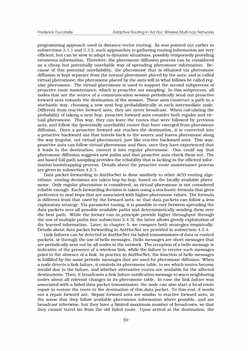
Frederick Ducatelle Adaptive Routing in Ad Hoc Wireless Multi-hop Networks
programming approach used in distance vector routing. As was pointed out earlier insubsections 3.1.1 and 3.3.2, such approaches to gathering routing information are veryefficient, but can be slow to adapt to dynamic situations, possibly temporarily providingerroneous information. Therefore, the pheromone diffusion process can be consideredas a cheap but potentially unreliable way of spreading pheromone information. Be-cause of this potential unreliability, the pheromone that is obtained via pheromonediffusion is kept separate from the normal pheromone placed by the ants, and is calledvirtual pheromone; the pheromone placed by the ants will in what follows be called reg-ular pheromone. The virtual pheromone is used to support the second subprocess ofproactive route maintenance, which is proactive ant sampling. In this subprocess, allnodes that are the source of a communication session periodically send out proactiveforward ants towards the destination of the session. These ants construct a path in astochastic way, choosing a new next hop probabilistically at each intermediate node.Different from reactive forward ants, they are never broadcast. When calculating theprobability of taking a next hop, proactive forward ants consider both regular and vir-tual pheromone. This way, they can leave the routes that were followed by previousants, and follow the (potentially unreliable) routes that have emerged from pheromonediffusion. Once a proactive forward ant reaches the destination, it is converted intoa proactive backward ant that travels back to the source and leaves pheromone alongthe way (regular, not virtual pheromone), just like reactive backward ants. This way,proactive ants can follow virtual pheromone and then, once they have experienced thatit leads to the destination, convert it into regular pheromone. One could say thatpheromone diffusion suggests new paths and that proactive ants check them out. Theant based full path sampling provides the reliability that is lacking in the efficient infor-mation bootstrapping process. Details about the proactive route maintenance processare given in subsection 4.2.3.
Data packet forwarding in AntHocNet is done similarly to other ACO routing algo-rithms: routing decisions are taken hop-by-hop, based on the locally available phero-mone. Only regular pheromone is considered, as virtual pheromone is not consideredreliable enough. Each forwarding decision is taken using a stochastic formula that givespreference to next hops that are associated with higher pheromone values. The formulais different from that used by the forward ants, so that data packets can follow a lessexploratory strategy. Via parameter tuning, it is possible to vary between spreading thedata packets over all possible available paths and deterministically sending them overthe best path. While the former can in principle provide higher throughput throughthe use of multiple paths (see subsection 2.4.3), the latter allows greedy exploitation ofthe learned information. Later, in chapter 5, we compare both strategies empirically.Details about data packet forwarding in AntHocNet are provided in subsection 4.2.4.
Link failures can be detected in AntHocNet via failed transmissions of data or controlpackets, or through the use of hello messages. Hello messages are short messages thatare periodically sent out by all nodes in the network. The reception of a hello message isindicative of the presence of a wireless link, while the failure to receive such messagespoint to the absence of a link. In practice in AntHocNet, the function of hello messagesis fulfilled by the same periodic messages that are used for pheromone diffusion. Whena node detects a link failure, it controls its pheromone table, to see which routes becomeinvalid due to the failure, and whether alternative routes are available for the affecteddestinations. Then, it broadcasts a link failure notification message to warn neighboringnodes about all relevant changes in its pheromone table. In case the link failure wasassociated with a failed data packet transmission, the node can also start a local routerepair to restore the route to the destination of this data packet. To this end, it sendsout a repair forward ant. Repair forward ants are similar to reactive forward ants, inthe sense that they follow available pheromone information where possible, and arebroadcast otherwise, but they have a limited maximum number of broadcasts, so thatthey cannot travel far from the old failed route. Upon arrival at the destination, the
59
Frederick Ducatelle Adaptive Routing in Ad Hoc Wireless Multi-hop Networks
Send reactive forward ant
Route data packets
Send repair forward ant
Repair timeout
Initial state
Process reactive forward ant
Process link failure notification
Process Hello
Process proactive forward ant
Process unicast warning
Process received control packet
Process repair forward ant
Process backward ant
Link failure notification
Backward ant
Repair forward ant
Proactive forward ant
Reactive forward ant
Hello message
Unicast warning
Final state
Send Hello
Receive control packetIdle state
Send unicast warning
No route at source Link failure
Send link failure notification
Receive data
No route at intermediate, data
No route at intermediate, no data
Hello timer
Reactive ant timeout
No route at source
No route at intermediateReactive ant timer
Repair ant timer
Adapt pheromone table
Send proactive ant
Proactive ant timer
Figure 4.1: A finite state machine representation of the AntHocNet routing algorithm.
repair forward ant is converted into a repair backward ant that travels back to the nodethat started the repair process and sets up the pheromone for the repaired route. Alast tool in dealing with link failures is the use of unicast warning messages. Theseare needed when data packets for a lost destination still arrive at the node after a linkfailure notification has already been broadcast. This can be due to bad reception of thebroadcast notification message. In this case, the node unicasts a warning to the nodeit received the data from, in order to inform it that it can no longer forward data forthis destination. Details about how AntHocNet deals with link failures are described insubsection 4.2.5.
4.1.2 Schematic representation
Figure 4.1 gives a schematic representation of the AntHocNet routing algorithm. It con-tains a finite state machine showing the most important components of the algorithm.Below we explain the structure of the finite state machine. For details about each of thecomponents, we refer to section 4.2.
The algorithm is started up in its initial state, in which internal variables are initial-ized. Then, it moves to its idle state, where it waits for events to happen. The eventsthat can take place are the arrival of a data packet, the arrival of a control packet, thedetection of a link failure, and a number of timer events.
60
Frederick Ducatelle Adaptive Routing in Ad Hoc Wireless Multi-hop Networks
In case of a data reception event, the algorithm tries to route the data. Detailsabout data forwarding are given in subsection 4.2.4. This might be impossible, dueto the lack of routing information about the destination. If the current node is thesource node of the data packet, the unavailability of routing information can be becausethe data packet is the first of a new communication session, or because it belongs toa session for which all routing information has become invalid. In both cases, thenode starts a reactive route setup process. Details about this process are given insubsection 4.2.2. If the current node is not the source of the data packet, it concludesthat the upstream node of the data has wrong routing information, and sends it aunicast warning message. This is further explained in subsection 4.2.5, which talksabout link failures.
In case of a control packet reception event, the algorithm checks which type of con-trol packet it is dealing with. In case it is a hello message, the node needs to take notein its neighbor table that it has a wireless link with the packet’s sender, and it needs toextract the routing information inside to update its own virtual pheromone information.This is part of the proactive route maintenance process described in subsection 4.2.3.In case it is a reactive, proactive or repair forward ant, the node needs to execute thecorrect forwarding action, or, if it is the final destination of the ant, create a backwardant and send it back towards the source. In case the control packet is a backward ant(reactive, proactive and repair backward ants have essentially the same behavior, andare therefore collapsed here), the node needs to adapt its pheromone table, and forwardthe ant if it is not its final destination. Details about the treatment of reactive, proactiveand repair forward and backward ants are given respectively in subsections 4.2.2, 4.2.3and 4.2.5. In case the control packet is a link failure notification, the node needs to up-date its pheromone table, and possibly forward the notification. Finally, if it is a unicastwarning, it needs to update its pheromone table, removing the erroneous route. Detailsabout link failure notifications and unicast warnings are given in subsection 4.2.5.
In case of a link failure event, the node first of all adapts the information in itspheromone table to reflect the changed situation. Then, if destinations have becomeunreachable due to the link failure, it needs to take action. If the current node isthe source of a session to one of the lost destinations, it starts a reactive route setupprocess. If, on the other hand, it is an intermediate node on the lost route, it controlswhether the link failure event involved the unsuccessful transmission of a data packet.If this is the case, it starts a local route repair process. Otherwise, it broadcasts a linkfailure notification message. Details on how link failures are dealt with are given insubsection 4.2.5.
The different timers are events that are scheduled by the node itself, in order toplan delayed actions. Hello timer events are scheduled at regular intervals, from themoment the node is switched on and for as long as it is up and running. Receptionof a hello timer event provokes the node to send a hello message, in which it includesits best pheromone information. This is part of the proactive route maintenance pro-cess described in subsection 4.2.3. Proactive ant timer events are also scheduled atregular intervals, but only from the moment a session is started, and until the endof it. Reception of a proactive ant timer event leads the node to send out a proactiveforward ant. Details about this are given in subsection 4.2.3. Repair timer events arescheduled after a repair forward ant has been sent out. At reception of a repair timerevent, the node checks whether a repair backward ant was received, and in case not,it broadcasts a link failure notification. This is part of the process of dealing with linkfailures, described in 4.2.5. Finally, reactive ant timer events are similarly sent outafter the transmission of a reactive forward ant. At reception of a reactive ant timerevent, the node controls whether it has already received a reactive backward ant. Incase not, it can send out a new reactive forward ant (in case the maximum numberof retransmissions has not yet been reached), or conclude that the destination is cur-rently unreachable, and drop queued data packets for it. This is described in detail in
61
Frederick Ducatelle Adaptive Routing in Ad Hoc Wireless Multi-hop Networks
subsection 4.2.2, which explains the reactive route setup phase.
4.2 Detailed descriptions
In this section, we give a detailed description of the different components of the Ant-HocNet routing algorithm. We follow the same structure as in subsection 4.1.1. Firstwe describe the data structures that are maintained in each node. Then, we give detailsabout the reactive route setup process. Subsequently, we discuss the proactive routemaintenance process. Next, we talk about data packet forwarding. After that, we dis-cuss the algorithm’s behavior with respect to link failures. Finally, we talk about therouting metrics used in AntHocNet.
4.2.1 Data structures in AntHocNet
Here, we describe the different data structures that are maintained by each of thenetwork nodes under AntHocNet. In particular, we talk about pheromone tables andneighbor tables.
Pheromone tables
Under AntHocNet, each node i maintains a pheromone table Ti, which is a two-dimen-sional matrix. An entry T d
ij of this matrix contains information about the route fromnode i to destination d over neighbor j. This includes a regular pheromone valueτdij, a virtual pheromone value ωd
ij, and an average number of hops hdij. The regular
pheromone value τdij is an estimate of the goodness of the route from i to d over j. Good-
ness is expressed as the inverse of a cost. Exact values depend on the metric that isused to evaluate the cost of routes. More about the use of different metrics will followin subsection 4.2.6. Regular pheromone is updated by backward ants. These can bereactive, proactive or repair backward ants. Details about the updating process for reg-ular pheromone are given in subsection 4.2.2. The virtual pheromone value ωd
ij formsan alternative estimate of the goodness of the route from i to d over j. Differently fromτdij, it is obtained through information bootstrapping using goodness values reported
by neighbor nodes during the proactive route maintenance process. The updating ofvirtual pheromone is discussed in subsection 4.2.3. The average number of hops hd
ij
is, like the regular pheromone, updated by backward ants. This updating process isdescribed in subsection 4.2.2. hd
ij is used when deciding how long to wait for repairbackward ants (see subsection 4.2.5).
Nodes do not necessarily always have values available for τdij, ωd
ij, and hdij for each
possible combination of destination and next hop. This is in the first place becausenodes do not maintain routing information about all possible destinations in the net-work (they only gather routing information for destinations which communication ses-sions are going on with), and because for a specific destination, nodes do not necessarilyhave a route available over each of their possible neighbors (for instance, during a re-active route setup phase only one route is set up, so that the source node has exactlyone outgoing next hop for the involved destination). Also, since regular and virtualpheromone are obtained through different processes, it is possible that a node has avalue for τd
ij, but not for ωdij, or vice versa. On the other hand, since τd
ij and hdij are both
obtained from backward ants, nodes that have a value for one of the two will also havea value for the other.
62
Frederick Ducatelle Adaptive Routing in Ad Hoc Wireless Multi-hop Networks
Neighbor tables
Apart from the pheromone table, each node also maintains a neighbor table. The neigh-bor table Ni kept by node i is a one-dimensional vector with one entry for each of i’sneighbors. The entry Nij corresponding to i’s neighbor j contains a time value thij in-dicating when i last heard from j. Node i uses this time value to derive whether thereis a wireless link with node j, and to detect link failures. More on the detection andhandling of link failures will follow later in subsection 4.2.5.
4.2.2 Reactive route setup
The reactive route setup process is triggered whenever a node receives a data packetthat was locally generated (i.e., the current node is the packet’s source) for a destinationfor which no routing information is available. This lack of routing information canhappen either because the data packet in question is the first of a new communicationsession, and no routing information for its destination is available from a different orprevious session, or because the data packet belongs to an ongoing session for whichall routes have become invalid (e.g., due to node movements). The reactive route setupprocess involves the sending of a reactive forward ant from source to destination, anda reactive backward ant from destination to source. Below, we discuss each of theseseparately.
Reactive forward ants
At the start of the reactive route setup process, the source node s creates a reactiveforward ant. This is a control packet that has as a goal to find a path from s to anassigned destination d. At the start, the ant contains just the addresses of s and d.Later, as it proceeds through the network, it collects a list P = [1, 2, . . . , d − 1] of all thenodes that it has visited on its way from s to d.
After its creation at s, the reactive forward ant is broadcast, so that all of s’s neigh-bors receive a copy of it. At each subsequent node, the ant is either unicast or broad-cast, depending on whether the current node has routing information for d. If routinginformation is available, the node chooses a next hop for the ant probabilistically, basedon the different pheromone values associated with next hops for d. Concretely, a nodei chooses node n as next hop for the ant with probability P d
in, as calculated by equa-tion 4.1. In this equation, Nd
i is the set of neighbors of i over which a path to d is known,and β1 is a parameter value which can control the exploratory behavior of the ants. Inour experiments, we keep β1 relatively high, on 20. This is because we want to obtainthe initial route as fast as possible, and limit the time we spend on exploration at thisstage.
P din =
(τdin)β1
∑j∈Nd
i(τd
ij)β1, β1 ≥ 1, (4.1)
In case the intermediate node i does not have routing information for d, it broadcaststhe reactive forward ant. Due to this broadcasting (and also the initial broadcasting ats), a reactive forward ant can proliferate quickly over the network, with different copiesof the ant following different paths to the destination. In order to limit the amount ofoverhead that is created this way, nodes only forward the first copy of the ant that theyreceive. Subsequent copies are simply discarded. In previous versions of AntHocNet,nodes were to some extent allowed to forward multiple copies of the same ant, in orderto improve the creation of multiple paths (see also subsection 4.3.4). However, this leadto a lot of overhead.
At the destination, the reactive forward ant is converted into a reactive backwardant, which follows the list of nodes P visited by the forward ant back to s. If more than
63
Frederick Ducatelle Adaptive Routing in Ad Hoc Wireless Multi-hop Networks
one copy of the forward ant is received, only the first is accepted and converted intoa backward ant, while subsequent copies are discarded. This way, only one route isset up during the reactive route setup process. The reason is again to reduce over-head created during this procedure. For the creation of multiple routes, AntHocNetrelies on the proactive route maintenance process, which extends the initially createdroute into a full mesh of routes during the course of the communication session (seesubsection 4.2.3).
Reactive backward ants
The reactive backward ant created by the destination node in response to a reactiveforward ant contains the addresses of the forward ant’s source node s and destinationnode d, as well as the full list of nodes P that the forward ant has visited. The reactivebackward ant is unicast from d and between the nodes of P back to s.
The aim of the reactive backward ant is to update routing information in each ofthe nodes of P and in s. At each node i that it visits, it updates the number of hopshd
in and the regular pheromone value τdin in the pheromone table entry T d
in, where n isthe node that it visited before i on its way from d. The updating of hd
in is done using amoving average, as shown in equation 4.2. In this equation, h is the number of hopsthat the backward ant has traveled between d and i, and α is a parameter regulatinghow quickly the formula adapts to new information. In our experiments, α is alwayskept on 0.7.
hdin ← αhd
in + (1− α)h, α ∈ [0, 1] (4.2)
Updating of the regular pheromone τdin is done based on the cost of the route from i to
d. This cost can be calculated using different metrics, such as the number of hops, theend-to-end delay, etc.. Later on, in subsection 4.2.6, we comment on different metricsused in AntHocNet. Here, we talk in terms of a generic cost c, where cd
i is the cost of theroute from i to d, and cj
i is the cost of the link from i to its neighbor j (it is the cost of aone-hop route). Under AntHocNet, each node maintains a local estimate of the cost cj
i
to go to each of its neighbors j. Details about how these local estimates are calculateddepend on the metric and are discussed in subsection 4.2.6. The reactive backwardant reads at each node i the local estimate cn
i of the cost to go from i to the next hop nthat the ant is coming from. It adds this cost to the total cost cd
n of the route from n tod (which it has been calculating on its way back from d), which is stored inside the ant.The new cost cd
i is used to update the pheromone value τdin in node i, using the moving
average formula of equation 4.3. In this equation, γ is a parameter regulating the speedof adaptation of the pheromone to new cost values. In our experiments, γ was kept on0.7. The cost value cd
i is inverted to calculate the pheromone value τdij, as pheromone
indicates the goodness of a route, rather than its cost.
τdij ← γτd
ij + (1− γ)(cdi )−1, γ ∈ [0, 1] (4.3)
It is interesting to note that in terms of gathering route cost information, there is animportant difference here with the AntNet algorithm described in subsection 3.2.3 andother ACO routing algorithms. Rather than relying on the cost values experienced bythe forward ants, AntHocNet uses the estimates cj
i calculated locally by the nodes. Thisis in order to improve reliability of the measured values. Depending on the cost metricused, the high variability of the wireless medium can cause large differences betweenvalues measured by subsequent samples. For example, the delay incurred on a linkcan vary strongly in case of congestion if IEEE 802.11 is used as a MAC layer protocol(see subsection 2.3.3). Using local estimates that are based on more than one samplecan take away some of this variability.
64
Frederick Ducatelle Adaptive Routing in Ad Hoc Wireless Multi-hop Networks
4.2.3 Proactive route maintenance
The proactive route maintenance process serves to update and extend available routinginformation. In particular, it allows to build a mesh of multiple routes around the initialroute created during the reactive route setup process. The proactive route maintenanceprocess consists of two subprocesses: pheromone diffusion and proactive ant sampling.Pheromone diffusion is aimed at spreading available pheromone information over thenetwork through the use of periodic update messages and information bootstrapping.Proactive ant sampling is aimed at controlling and updating pheromone informationthrough path sampling using proactive forward ants. While proactive ant sampling isstarted by the source node of a communication session at the start of the session andcontinues for as long as the session is going on, pheromone diffusion is executed by allnodes throughout their whole lifetime, and is not particulary bound to the occurrenceof a single session. Below, we describe each of the two subprocesses of proactive routemaintenance separately.
Pheromone diffusion
The reactive route setup process described in subsection 4.2.2 leads to the availabilityof a single route from the source of a communication session to its destination, indi-cated by regular pheromone values in the pheromone tables of the nodes. Moreover,each neighbor node of the destination also has a one-hop route to the destination. Thisis independent of the running session, and is simply due to the fact that neighboringnodes are aware of each other’s presence, as is explained further in subsection 4.2.5.The aim of the pheromone diffusion process is to spread all this pheromone informationout, so that a field of pheromone pointing towards the destination becomes available inthe network. This field of pheromone is indicated in the virtual pheromone values inthe pheromone tables of the nodes. The fact that pheromone is spread out is similar tothe normal diffusion of real pheromone in nature [185], which allows ants further awayto sense it. In the example of figure 4.2, a communication session is going on betweennode 1 and node 8. Regular pheromone is indicated by solid arrows. It consists of a sin-gle route from 1 to 8 over the nodes 3, 6 and 7 that is the result of reactive route setup,and a one-hop route from 5 to 8 that is there independently of the running session,because 5 is aware of the presence of its neighbor 8. The field of virtual pheromone thatis the result of pheromone diffusion is indicated with dashed arrows.
A crucial role in the pheromone diffusion process is played by hello messages. Theseare short messages broadcast every thello seconds asynchronously by all the nodes ofthe network throughout their whole lifetime. In AntHocNet, thello is set to 1 second.Hello messages are used in many existing protocols, such as ABR [257] and OLSR [61](see subsection 2.4.2), to allow nodes to find out which are their immediate neighbors,and to detect link failures. While also in AntHocNet hello messages are used for thispurpose (as is explained in subsection 4.2.5), they also serve a different goal, namely tocarry information in the pheromone diffusion process. They serve as the periodic up-date messages that are needed in the information bootstrapping process of pheromonediffusion. The idea to convey extra routing information inside hello messages has beenused in some other routing algorithms, such as the earlier mentioned OLSR.
Nodes include in each hello message that they send out routing information theyhave available. In particular, a node i constructing a hello message consults its phero-mone table, and picks a maximum number k of destinations it has routing informationfor. k is normally kept on 10, but in chapter 5 we also present results varying thisparameter. If more than k destinations are available, k of them are picked out ran-domly. For each one of these destinations d, the hello message contains the addressof d, the best pheromone value that i has available for d, υd
i , and a bit flag. This bestpheromone value υd
i is taken over all possible values for regular pheromone τdij and vir-
65
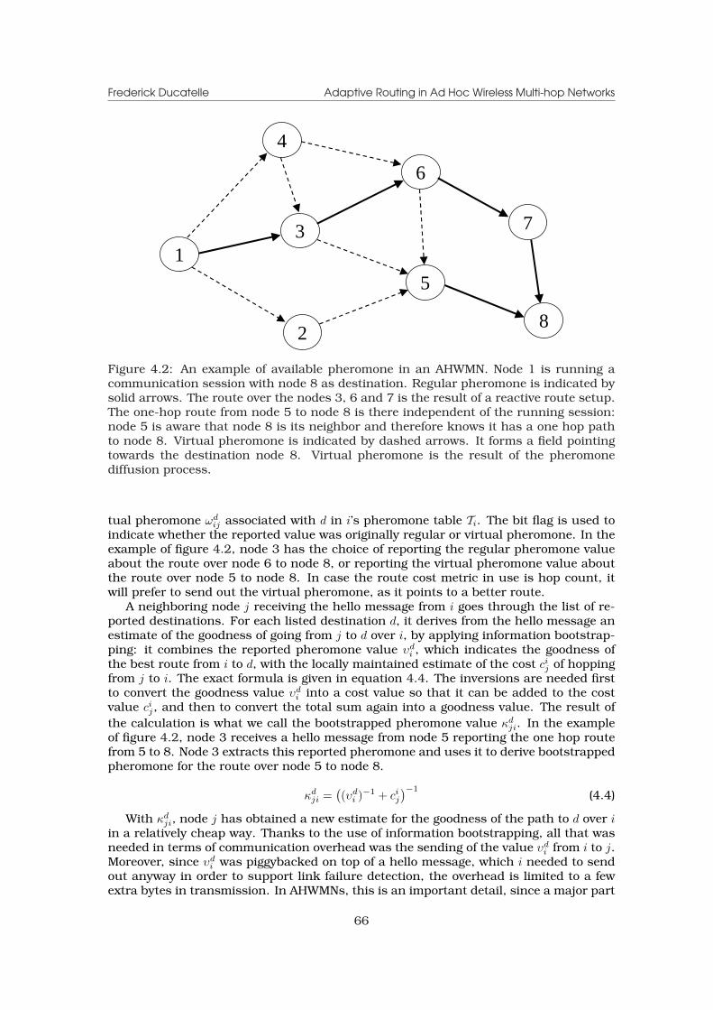
Frederick Ducatelle Adaptive Routing in Ad Hoc Wireless Multi-hop Networks
3
2
4
6
7
8
5
1
Figure 4.2: An example of available pheromone in an AHWMN. Node 1 is running acommunication session with node 8 as destination. Regular pheromone is indicated bysolid arrows. The route over the nodes 3, 6 and 7 is the result of a reactive route setup.The one-hop route from node 5 to node 8 is there independent of the running session:node 5 is aware that node 8 is its neighbor and therefore knows it has a one hop pathto node 8. Virtual pheromone is indicated by dashed arrows. It forms a field pointingtowards the destination node 8. Virtual pheromone is the result of the pheromonediffusion process.
tual pheromone ωdij associated with d in i’s pheromone table Ti. The bit flag is used to
indicate whether the reported value was originally regular or virtual pheromone. In theexample of figure 4.2, node 3 has the choice of reporting the regular pheromone valueabout the route over node 6 to node 8, or reporting the virtual pheromone value aboutthe route over node 5 to node 8. In case the route cost metric in use is hop count, itwill prefer to send out the virtual pheromone, as it points to a better route.
A neighboring node j receiving the hello message from i goes through the list of re-ported destinations. For each listed destination d, it derives from the hello message anestimate of the goodness of going from j to d over i, by applying information bootstrap-ping: it combines the reported pheromone value υd
i , which indicates the goodness ofthe best route from i to d, with the locally maintained estimate of the cost ci
j of hoppingfrom j to i. The exact formula is given in equation 4.4. The inversions are needed firstto convert the goodness value υd
i into a cost value so that it can be added to the costvalue ci
j, and then to convert the total sum again into a goodness value. The result ofthe calculation is what we call the bootstrapped pheromone value κd
ji. In the exampleof figure 4.2, node 3 receives a hello message from node 5 reporting the one hop routefrom 5 to 8. Node 3 extracts this reported pheromone and uses it to derive bootstrappedpheromone for the route over node 5 to node 8.
κdji =
((υd
i )−1 + cij
)−1(4.4)
With κdji, node j has obtained a new estimate for the goodness of the path to d over i
in a relatively cheap way. Thanks to the use of information bootstrapping, all that wasneeded in terms of communication overhead was the sending of the value υd
i from i to j.Moreover, since υd
i was piggybacked on top of a hello message, which i needed to sendout anyway in order to support link failure detection, the overhead is limited to a fewextra bytes in transmission. In AHWMNs, this is an important detail, since a major part
66
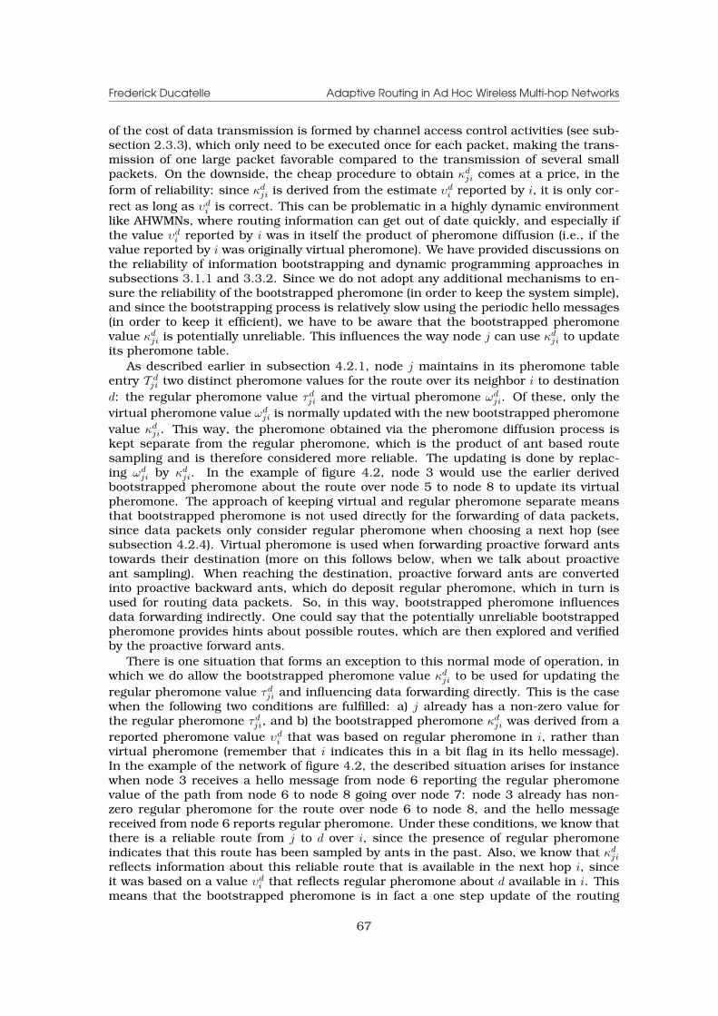
Frederick Ducatelle Adaptive Routing in Ad Hoc Wireless Multi-hop Networks
of the cost of data transmission is formed by channel access control activities (see sub-section 2.3.3), which only need to be executed once for each packet, making the trans-mission of one large packet favorable compared to the transmission of several smallpackets. On the downside, the cheap procedure to obtain κd
ji comes at a price, in theform of reliability: since κd
ji is derived from the estimate υdi reported by i, it is only cor-
rect as long as υdi is correct. This can be problematic in a highly dynamic environment
like AHWMNs, where routing information can get out of date quickly, and especially ifthe value υd
i reported by i was in itself the product of pheromone diffusion (i.e., if thevalue reported by i was originally virtual pheromone). We have provided discussions onthe reliability of information bootstrapping and dynamic programming approaches insubsections 3.1.1 and 3.3.2. Since we do not adopt any additional mechanisms to en-sure the reliability of the bootstrapped pheromone (in order to keep the system simple),and since the bootstrapping process is relatively slow using the periodic hello messages(in order to keep it efficient), we have to be aware that the bootstrapped pheromonevalue κd
ji is potentially unreliable. This influences the way node j can use κdji to update
its pheromone table.As described earlier in subsection 4.2.1, node j maintains in its pheromone table
entry T dji two distinct pheromone values for the route over its neighbor i to destination
d: the regular pheromone value τdji and the virtual pheromone ωd
ji. Of these, only thevirtual pheromone value ωd
ji is normally updated with the new bootstrapped pheromonevalue κd
ji. This way, the pheromone obtained via the pheromone diffusion process iskept separate from the regular pheromone, which is the product of ant based routesampling and is therefore considered more reliable. The updating is done by replac-ing ωd
ji by κdji. In the example of figure 4.2, node 3 would use the earlier derived
bootstrapped pheromone about the route over node 5 to node 8 to update its virtualpheromone. The approach of keeping virtual and regular pheromone separate meansthat bootstrapped pheromone is not used directly for the forwarding of data packets,since data packets only consider regular pheromone when choosing a next hop (seesubsection 4.2.4). Virtual pheromone is used when forwarding proactive forward antstowards their destination (more on this follows below, when we talk about proactiveant sampling). When reaching the destination, proactive forward ants are convertedinto proactive backward ants, which do deposit regular pheromone, which in turn isused for routing data packets. So, in this way, bootstrapped pheromone influencesdata forwarding indirectly. One could say that the potentially unreliable bootstrappedpheromone provides hints about possible routes, which are then explored and verifiedby the proactive forward ants.
There is one situation that forms an exception to this normal mode of operation, inwhich we do allow the bootstrapped pheromone value κd
ji to be used for updating theregular pheromone value τd
ji and influencing data forwarding directly. This is the casewhen the following two conditions are fulfilled: a) j already has a non-zero value forthe regular pheromone τd
ji, and b) the bootstrapped pheromone κdji was derived from a
reported pheromone value υdi that was based on regular pheromone in i, rather than
virtual pheromone (remember that i indicates this in a bit flag in its hello message).In the example of the network of figure 4.2, the described situation arises for instancewhen node 3 receives a hello message from node 6 reporting the regular pheromonevalue of the path from node 6 to node 8 going over node 7: node 3 already has non-zero regular pheromone for the route over node 6 to node 8, and the hello messagereceived from node 6 reports regular pheromone. Under these conditions, we know thatthere is a reliable route from j to d over i, since the presence of regular pheromoneindicates that this route has been sampled by ants in the past. Also, we know that κd
ji
reflects information about this reliable route that is available in the next hop i, sinceit was based on a value υd
i that reflects regular pheromone about d available in i. Thismeans that the bootstrapped pheromone is in fact a one step update of the routing
67
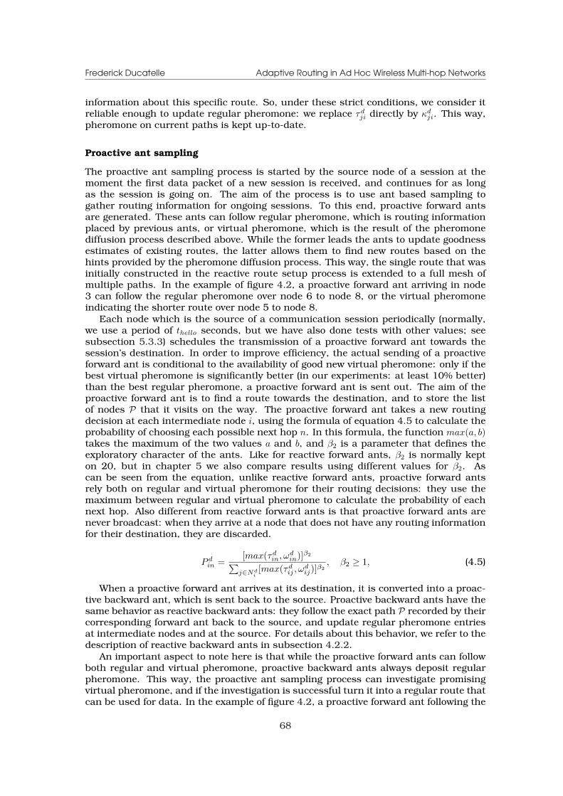
Frederick Ducatelle Adaptive Routing in Ad Hoc Wireless Multi-hop Networks
information about this specific route. So, under these strict conditions, we consider itreliable enough to update regular pheromone: we replace τd
ji directly by κdji. This way,
pheromone on current paths is kept up-to-date.
Proactive ant sampling
The proactive ant sampling process is started by the source node of a session at themoment the first data packet of a new session is received, and continues for as longas the session is going on. The aim of the process is to use ant based sampling togather routing information for ongoing sessions. To this end, proactive forward antsare generated. These ants can follow regular pheromone, which is routing informationplaced by previous ants, or virtual pheromone, which is the result of the pheromonediffusion process described above. While the former leads the ants to update goodnessestimates of existing routes, the latter allows them to find new routes based on thehints provided by the pheromone diffusion process. This way, the single route that wasinitially constructed in the reactive route setup process is extended to a full mesh ofmultiple paths. In the example of figure 4.2, a proactive forward ant arriving in node3 can follow the regular pheromone over node 6 to node 8, or the virtual pheromoneindicating the shorter route over node 5 to node 8.
Each node which is the source of a communication session periodically (normally,we use a period of thello seconds, but we have also done tests with other values; seesubsection 5.3.3) schedules the transmission of a proactive forward ant towards thesession’s destination. In order to improve efficiency, the actual sending of a proactiveforward ant is conditional to the availability of good new virtual pheromone: only if thebest virtual pheromone is significantly better (in our experiments: at least 10% better)than the best regular pheromone, a proactive forward ant is sent out. The aim of theproactive forward ant is to find a route towards the destination, and to store the listof nodes P that it visits on the way. The proactive forward ant takes a new routingdecision at each intermediate node i, using the formula of equation 4.5 to calculate theprobability of choosing each possible next hop n. In this formula, the function max(a, b)takes the maximum of the two values a and b, and β2 is a parameter that defines theexploratory character of the ants. Like for reactive forward ants, β2 is normally kepton 20, but in chapter 5 we also compare results using different values for β2. Ascan be seen from the equation, unlike reactive forward ants, proactive forward antsrely both on regular and virtual pheromone for their routing decisions: they use themaximum between regular and virtual pheromone to calculate the probability of eachnext hop. Also different from reactive forward ants is that proactive forward ants arenever broadcast: when they arrive at a node that does not have any routing informationfor their destination, they are discarded.
P din =
[max(τdin, ωd
in)]β2
∑j∈Nd
i[max(τd
ij , ωdij)]β2
, β2 ≥ 1, (4.5)
When a proactive forward ant arrives at its destination, it is converted into a proac-tive backward ant, which is sent back to the source. Proactive backward ants have thesame behavior as reactive backward ants: they follow the exact path P recorded by theircorresponding forward ant back to the source, and update regular pheromone entriesat intermediate nodes and at the source. For details about this behavior, we refer to thedescription of reactive backward ants in subsection 4.2.2.
An important aspect to note here is that while the proactive forward ants can followboth regular and virtual pheromone, proactive backward ants always deposit regularpheromone. This way, the proactive ant sampling process can investigate promisingvirtual pheromone, and if the investigation is successful turn it into a regular route thatcan be used for data. In the example of figure 4.2, a proactive forward ant following the
68

Frederick Ducatelle Adaptive Routing in Ad Hoc Wireless Multi-hop Networks
virtual pheromone from node 3 over node 5 to node 8 is at its arrival in 8 converted intoa backward ant, which deposits regular pheromone on the link from node 3 to node5. The process of proactive ant sampling increases in this way the number of routesavailable for data routing, which can grow to a full mesh, and allows the algorithmto exploit new routing opportunities in the ever changing AHWMN topology. As statedearlier, the proactive ants provide through their full path sampling the necessary controlto verify the reliability of new routes obtained through the information bootstrappingprocess of pheromone diffusion.
4.2.4 Data packet forwarding
Data packets are forwarded from their source to their destination in hop-by-hop fash-ion, taking a new routing decision at each intermediate node. Routing decisions for datapackets are based only on regular pheromone. This means that they only follow the re-liable routes that are the result of ant based sampling, and leave the virtual pheromoneinformation that is the result of information bootstrapping out of consideration. Thecombination of the reactive route setup and the proactive route maintenance processesleads to the availability of a full mesh of such reliable routes between the source anddestination of each session.
Nodes in AntHocNet forward data packets stochastically, based on the relative valuesof the different regular pheromone entries they have available for the packet’s destina-tion. The probability P d
in for a node i to pick next hop n when forwarding a packet withdestination d is given in the formula of equation 4.6. This formula is very similar to theone used for reactive forward ants (see equation 4.1), but uses a different parameter,β3, for the power function of the pheromone values. This way, the relative preference forthe best routes can be adapted separately for data and for ants (as is common practicein ACO routing algorithms, see section 3.2).
Pnd =(τd
in)β3
∑j∈Nd
i(τd
ij)β3, β3 ≥ 1 (4.6)
By adapting the β3 parameter, one can make data forwarding less or more greedywith respect to the best available routes. By setting β3 low, data is spread over multipleroutes, considering also low quality ones. Using multiple routes for data forwarding canimprove throughput, as the data load is spread more evenly over the available networkresources (see also subsection 2.4.3). By setting β3 high, on the other hand, data isconcentrated on the best routes. This can also be a good choice, since the routes thataccording to the ant sampling give the best performance, are exploited as much aspossible. In our experiments, we normally keep β3 on 20, which is relatively high andonly allows data load spreading when there are several good routes of more or less equalquality. In chapter 5, we also compare results when using different values for β3.
4.2.5 Link failures
In AHWMNs, link failures can occur due to physical changes such as the movement ordisappearance of a node, or due to changes that influence the connectivity of the wire-less communication, such as an increase of radio interference or a decrease in the usedtransmission power. Since AHWMNs are usually highly dynamic, such events are ex-pected to occur frequently, and AHWMN routing algorithms should be prepared to dealwith them effectively. The components of AntHocNet described so far already offer somebasic protection against link failures. The reactive route setup process allows sourcenodes to rebuild entire routes if needed, and the proactive route maintenance processoffers protection in a proactive way through the creation of new paths, which can serve
69

Frederick Ducatelle Adaptive Routing in Ad Hoc Wireless Multi-hop Networks
as backup routing possibilities. In this subsection, we outline further mechanisms inAntHocNet that are specifically aimed at dealing with link failures.
The first step in dealing with link failures is their detection. In AntHocNet, link fail-ures are detected if lower layer protocols report the failure of the unicast transmissionof a control or data packet, or if a node fails to receive periodic hello messages from itsneighbors. Once a failure is detected, the next step is to take action to neutralize its ef-fect. In AntHocNet, the action to be taken depends on the way the failure was detected.If the detection was through the failed transmission of a control packet or through themissed reception of hello messages, the node that detected the link failure broadcasts alink failure notification message, in which it warns downstream nodes about changedroutes. If the detection was through the failed transmission of a data packet, the nodestarts a local route repair process in order to repair the route to the destination of thefailed data packet. A final action that can be taken is the sending of a unicast warn-ing message. These are messages that are used when an earlier broadcast link failurenotification message got lost. Below, we first discuss the detection of link failures, thenthe use of link failure notification messages, next the process of local route repair, andfinally the use of unicast warning messages.
Detecting link failures
Link failures can be detected through the failed unicast transmission of control or datapackets, or via the use of hello messages. Detection through a failed unicast transmis-sion is straightforward. MAC layer protocols usually have mechanisms that inform itabout the success or failure of a unicast transmission. For instance, the IEEE 802.11DCF protocol, which is often used in AHWMNs (see subsection 2.3.3), requires receivingnodes to send an acknowledgement upon successful reception of a unicast transmis-sion. AntHocNet gives MAC layer protocols the possibility to report the failure of atransmission, and assumes in that case that the corresponding link has failed.
Relying solely on this mechanism to detect link failure is not satisfactory however.First of all, it does not allow to detect a link failure in advance, but only at the momentthat it causes damage. Second, on a more technical note, many implementations ofMAC layer protocols do not include the possibility to warn higher layers about a failedtransmission. Therefore, AntHocNet also uses hello messages to detect link failures.These are messages that are sent out by all the nodes of the network asynchronouslyat a fixed interval of thello seconds. When a node i receives a hello message from a newnode j, it can assume that j is its neighbor, and create an entry Nij for j in its neighbortable, indicating in it the last time that it has heard from j. It also makes an entry T j
ij inits pheromone table, indicating that there is a one-hop route from i to j over next hopj. After this, i expects to receive a message from j at least every thello seconds. If i doesnot hear from j for a certain number of thello second intervals (set to 2 intervals here), iassumes that the wireless connection to j has disappeared.
In AntHocNet, hello messages are not only used to detect link failures, but also tocarry pheromone information in the pheromone diffusion process (see subsection 4.2.3).This means that hello messages in AntHocNet are larger than those used in many otherrouting algorithms (such as e.g. in AODV [213], see subsection 2.4.2). For link failuredetection, this can actually be an advantage. It has been pointed out in [56] that sincehello messages are usually smaller than data packets, they can more easily be receivedcorrectly over shaky wireless connections, and therefore give a false image of link avail-ability for data packets. The authors propose exactly the use of larger hello messagesto get a better image of the real network topology.
70
Frederick Ducatelle Adaptive Routing in Ad Hoc Wireless Multi-hop Networks
Link failure notifications
When a node i detects that the link with a neighboring node j is lost, it removes jfrom its neighbor table. Then, it updates its pheromone table Ti, building a link failurenotification message in the process. It scans its pheromone table to control whichdestinations d have a non-zero regular pheromone value τd
ij (i.e., for which destinationsd neighbor node j is used as a next hop from i). For each such destination, i setsτdij to 0. Furthermore, it checks whether the lost pheromone τd
ij was the best or onlyregular pheromone value available for d. If this is the case, it adds the address of thedestination d to the link failure notification message, together with the new best regularpheromone it has available for d. If τd
ij was the only non-zero regular pheromone entryfor d, this is also indicated in the link failure notification message.
Once the link failure notification message is fully constructed, it is broadcast. All ofi’s neighbors receive the message, and update their routing tables for the routes goingover i to the involved destinations, using the new estimates reported in the message.To this end, they use the same formula that is applied for information bootstrapping inthe pheromone diffusion process, as given in equation 4.4. In case they in turn loosetheir best or only route to one of the involved destinations due to the reported failure,they in turn construct their own link failure notification message, in the same way asi did, and broadcast it further. This way, all involved nodes eventually get warned andcan update their pheromone tables.
Local route repair
When a node i detects a link failure through the failed transmission of a data packet,and i does not have any alternative routing information available for the destinationd of this data packet, i does not include d in the link failure notification it sends out.Instead, it starts a local route repair process to try to repair the route to d, so that thedata packet can still be delivered.
At the start of the local route repair process, i creates a repair forward ant. Repairforward ants are identical to reactive forward ants, and are forwarded in the same way:they are broadcast when no routing information is available, and are otherwise unicastto a stochastically chosen next hop using the formula of equation 4.1. The only realdifference with reactive forward ants is that repair forward ants can only be broadcasta limited maximum number of times (we set this number to 2). Therefore, they can onlytravel far if they are unicast over existing pheromone. Concretely, this means that repairforward ants need to stay close to existing routes in order to reach the destination, sothat they really focus on the repair of the lost route. Upon arrival at the destination d,the repair forward ant is converted into a repair backward ant, which travels back to thenode i that launched the local route repair process. It does so in exactly the same wayas a reactive backward ant traveling back to its source (see subsection 4.2.2), updatingregular pheromone entries on the way. Once the repair backward ant is back at theoriginal node i, this node can send its stored data packet to d.
Node i uses a timer to decide how long to wait for a repair backward ant. The valueof this timer is an estimate of the time it takes to go from i to d and come back, and iscalculated as shown in equation 4.7. In this equation, thop is a fixed delay value per hop(set to 50 milliseconds), and hd
ij is the number of hops to the destination as reported bythe backward ants and stored in i’s pheromone table (see subsections 4.2.1 and 4.2.2).The multiplication with 2 is to account for the way to go to the destination and comeback. If no backward ant has been received before the timer runs out, i discards thestored data packet, and broadcasts a link failure notification about destination d.
timer = 2 ∗ thop ∗ hdij (4.7)
71

Frederick Ducatelle Adaptive Routing in Ad Hoc Wireless Multi-hop Networks
Unicast warning messages
A final aspect of dealing with link failures in AntHocNet is the use of unicast warningmessages. These are emergency messages that are needed when link failure notificationmessages are not delivered correctly. This can happen because link failure notificationsare broadcast. The IEEE 802.11 DCF MAC layer protocol, which is very often used inAHWMNs, does not provide any guarantees for the delivery of broadcast messages. Thismakes broadcast transmission a lot less reliable than unicast transmissions, which aresupported with extra mechanisms to improve reliability (see subsection 2.3.3). Supposenow that a node i has lost its only route to a destination d due to a link failure, andwarns other nodes about this in a link failure notification message as described above.If a neighboring node n, which has a route to d using i as next hop, does not receivethis message correctly, it will continue sending data packets for d to i. At this point,i cannot forward the data packets. It therefore answers to the data packet by unicas-ting a short warning message to n, indicating that it has no routing information for d.Upon reception of this message, n removes the erroneous routing information from itspheromone table.
4.2.6 Routing metrics
So far, we have not given any details about how paths are evaluated in AntHocNet, andhave instead talked in terms of a generic cost value. In principle, this generic cost valuecan be replaced by any possible route cost metric. Concretely, we have explored the useof the following ones: the number of hops, the end-to-end delay, a combination of hopsand end-to-end delay, and a metric based on the signal-to-interference-and-noise ratioof links along the route. While the calculation of the number of hops is trivial, the otherthree are a bit more complicated. Therefore, we explain in what follows for each of thesemetrics how a node i locally estimates the cost cj
i of the link to its neighbor j. How localestimates of link costs are then combined into full route costs has been explained earlierin the description of the working of reactive backward ants (see subsection 4.2.2). Inthe experimental results reported in chapters 5 and 6, we normally use the signal-to-interference-and-noise ratio metric, as this gave the best results. Comparisons withversions of AntHocNet using the other metrics will also be reported in chapter 5.
End-to-end delay
When using the end-to-end delay cost metric, the cost estimate cji maintained locally
by node i reflects the expected delay incurred by a data packet when following thewireless link from i to its neighbor j. Concretely, cj
i is calculated by the formula given inequation 4.8. In this formula, qi
mac is the number of packets that are currently in queueat the node to be sent, and timac is an estimate of the time it takes to send one packetvia unicasting. timac is calculated as a moving average of the time elapsed between thearrival of a packet at the MAC layer and the end of a successful transmission, whichis indicated by an acknowledgement received from the next hop. This is shown inequation 4.9, where timac is the latest observed send time, and η is a parameter defininghow quickly the moving average adapts to new observations (η is kept on 0.7).
cji = (qi
mac + 1)timac (4.8)
timac ← ηtimac + (1− η)timac, η ∈ [0, 1] (4.9)
As can be seen from equations 4.8 and 4.9, the calculation of cji here is in fact inde-
pendent of j. This is because we assumed network nodes that have only one wirelessinterface which is an omnidirectional antenna. In this case, the data traffic for all next
72
Frederick Ducatelle Adaptive Routing in Ad Hoc Wireless Multi-hop Networks
hops needs to go over the same outgoing queue, and needs to access the same wirelesschannel, so that a packet queuing to be sent to a node j might need to wait behindpackets for any other neighboring node, experiencing also their delays.
End-to-end delay combined with number of hops
We also considered the possibility to combine the end-to-end delay with the numberof hops. While the end-to-end delay is adaptive to the local traffic situation, it canbe quite unstable, showing large oscillations due to variations in the quality of thewireless channel and local interference. The number of hops, on the other hand, is notadaptive, but is a stable metric. The goal of combining both is to have a metric that isboth adaptive and stable.
The formula for the calculation of cji using the combined metric is given in equa-
tion 4.10. The first part of this formula corresponds to the calculation of the delay, andis identical to the formula of equation 4.8. The second part of the formula reflects thenumber of hops. While the number of hops to reach neighbor j from node i is obviouslyalways 1, here we use a different constant value, namely thop. This is a fixed estimateof the time needed to take one hop in unloaded conditions (we kept thop on 0.003 sec).Using the constant thop, rather than 1, allows to scale the number of hops to the sameorder of magnitude as the time estimation.
cji = (qi
mac + 1)timac + thop (4.10)
Signal-to-interference-and-noise ratio
The signal-to-interference-and-noise ratio (SINR) between a node i and a node j is theratio between the strength of the signal received by node i from node j and the generalnoise and interference from other radio signals present around i. This value can becalculated at the physical layer of the node. SINR is a crucial factor defining the successof a wireless reception. When SINR is high, reception has a high probability of beingsuccessful, whereas when it is low, reception is impossible. In between there is a rangefor which reception is possible with some probability. Note that also factors other thanSINR can influence reception, so that it is sometimes also possible to have bad receptionwhen SINR is high (see e.g. [15]). Nevertheless, SINR is an important indicator of linkquality.
When using SINR to define cji in AntHocNet, we are not interested in fine variations
in the SINR level, but rather in a coarse grained distinction between “good” and “bad”wireless links: we want to capture the difference between links on which reception hasa high probability of being successful, and links on which reception is possible but witha lower probability of success. Therefore, we apply a simple approach using a criticalSINR value SINRc as threshold, in which links with an SINR value lower than SINRc
are penalized. Concretely, we use the formula of equation 4.11, where cji is set to 1
for links with SINR higher than SINRc (this corresponds to using normal hop countas a metric), and to a constant value cconst > 1 for links with SINR lower than SINRc.In simulation tests using IEEE 802.11b radios sending at 2Mbps, we empirically setSINRc to 17dB and cconst to 3. The value of 17dB for SINRc is in line with criticalvalues of SINR found in empirical research on wireless LANs using the same radiotechnology [200].
cji =
{1, if SINR > SINRc
cconst, if SINR ≤ SINRc(4.11)
73
Frederick Ducatelle Adaptive Routing in Ad Hoc Wireless Multi-hop Networks
4.3 Further Discussions
In this section, we provide further discussions related to the AntHocNet routing al-gorithm. First, we consider AntHocNet in the light of the RL framework presentedin chapter 3, and discuss its particular strategies for information gathering from thispoint of view. Then, we take a look at the different challenges for AHWMN routing thatwere pointed out in chapter 2, and investigate qualitatively how AntHocNet deals withthese. Next, we discuss how AntHocNet relates to other existing routing algorithms.In particular, we search in how far components of AntHocNet are also used elsewhere.Finally, we write a few words about mechanisms that were present in older versions ofAntHocNet, and about why they were discarded.
4.3.1 AntHocNet and reinforcement learning
In chapter 3 we have described RL, an important class of problems in machine learning,and we have explained how the problem of routing fits into this framework. Then, wehave discussed two basic solution methods for RL problems, namely dynamic program-ming and Monte Carlo sampling, each with their own advantages and disadvantages,and we have shown how existing routing algorithms relate to them, with distance vec-tor routing being a direct implementation of dynamic programming, and ACO routingrelying mainly on Monte Carlo sampling. Subsequently, we have also described a moreadvanced learning method, temporal difference learning, which combines elements ofboth basic methods, and we have shown the Q-routing algorithm that was based onit. In what follows, we investigate how the AntHocNet routing algorithm proposed inthis chapter relates to all of this. In particular, we describe how AntHocNet uses boththe Monte Carlo sampling and dynamic programming learning methods, but combinesthem in a way that is different from temporal difference learning.
Monte Carlo sampling is used extensively in AntHocNet, since it is the learningmethod applied in ACO routing, which was the main source of inspiration of our al-gorithm. This is most evident in the proactive ant sampling subprocess of the proactiveroute maintenance process (see subsection 4.2.3). In this subprocess, ants are regu-larly sent out by the source node of each session in order to sample a path towards thedestination of the session. This is very much in line with the continuous path samplingdone in other ACO routing algorithms. Apart from this, also the reactive route setupprocess (see subsection 4.2.2) and the local route repair process (see subsection 4.2.5)use a form of Monte Carlo sampling: the reactive and repair forward ants used in theseprocesses each take a single sample of a path through the network, and use it to setup a new route. As was explained earlier in subsection 3.3.2, this approach of usingMonte Carlo sampling by taking a single sample of a path through the network is alsoapplied in many existing reactive routing algorithms. An important point to note here isthat AntHocNet is more consistent in its use of sampling, since both reactive and repairforward ants always go all the way till the destination. In most existing reactive routingalgorithms, including the AODV and DSR protocols described in subsection 2.4.2, thisis not the case: RREQ messages that are searching for a path to the destination canbe returned by intermediate nodes that have routing information about the destinationavailable. At that point, the obtained routing information relies on the estimate pro-vided by the intermediate node, so that a form of information bootstrapping is applied.
The most important advantage of using Monte Carlo sampling here is that it pro-vides a high level of reliability. This is because all routing information is the result ofdirect experiences, giving a certain guarantee about its correctness. A disadvantage isthat it can be inefficient. The need to send sampling packets from source to destinationcan lead to high levels of overhead. The use of IEEE 802.11 DCF as MAC layer mech-anism can deteriorate this problem, because this protocol creates a lot of overhead for
74
Frederick Ducatelle Adaptive Routing in Ad Hoc Wireless Multi-hop Networks
each sent packet, making the transmission of multiple small packets particulary prob-lematic. Traditional reactive routing algorithms deal with the efficiency issue by usingjust a single sample. AntHocNet, on the other hand, improves efficiency by combiningMonte Carlo sampling with a supporting dynamic programming process.
AntHocNet uses dynamic programming in the pheromone diffusion subprocess ofits proactive route maintenance process (see subsection 4.2.3). This subprocess worksmore or less in the same way as distance vector routing algorithms do, using informa-tion bootstrapping in each node to derive routing information from estimates calculatedby neighboring nodes. Such an approach has as an advantage that it is highly efficient,as the information obtained by each node is optimally reused in the calculation of theinformation needed by other nodes. In AntHocNet, this efficiency is further increasedby piggybacking routing updates on top of hello messages, which avoids the transmis-sion of multiple small control packets. An important disadvantage of using dynamicprogramming and information bootstrapping is that it can lead to processes that areslow to converge, so that routing information can be temporarily unreliable. This is es-pecially a problem in dynamic situations. In existing distance vector routing algorithmsfor AHWMNs, such as DSDV (see subsection 2.4.2), extra techniques are applied to en-sure reliability in the face of the highly dynamic network environment. Unfortunately,these techniques introduce extra overhead, and can severely reduce the efficiency ofthe process. Therefore, in AntHocNet, we have chosen a different strategy: the dy-namic programming part of AntHocNet is kept very simple and lightweight, and is notexpected to provide information that is 100% reliable. This way, we focus maximally onits efficiency, and do not worry about its unreliability. Instead, we are aware that theinformation produced by the process can contain errors and therefore we do not use itdirectly for routing. We use it as a guideline for the Monte Carlo sampling of the proac-tive ant sampling subprocess. Using this guideline, the ants do not have to explorethe whole network, but can concentrate on routes that are suggested by pheromonediffusion. This reduction in the need for exploration makes the sampling process moreeffective, so that less ants are needed, leading to better efficiency. This way, we obtainan adaptive algorithm that combines the efficiency of dynamic programming with thereliability and robustness of Monte Carlo sampling.
Note that the way Monte Carlo sampling and dynamic programming are combinedhere is very different from temporal difference learning methods. In n-step temporaldifference learning (see subsection 3.3.3), the learning agent takes a sample of a fewsteps, after which it arrives in an intermediate state i, where it reads the local valueestimate, which it uses to bootstrap on. This approach can be highly efficient, butdoes not avoid the potential unreliability of dynamic programming, since it still usesinformation bootstrapping. It is interesting to see that the temporal difference learningapproach to information gathering is similar to the returning of RREQ messages byintermediate nodes in reactive routing algorithms as described above: the RREQ sam-ples a path till an intermediate node that has routing information available about thedestination, at which point it bootstraps on this information and returns to the source.In AntHocNet, we aimed to be more consistent, and keep sampling and informationbootstrapping strictly separate.
4.3.2 Challenges for routing in AHWMNs
In chapter 2, we have defined a number of challenges for routing in AHWMNs. Theseincluded adaptivity, robustness, efficiency and scalability. Here, we investigate qualita-tively how AntHocNet is equipped to deal with each of these.
Adaptivity is very important in AHWMNs, as the dynamic network environment con-stantly presents the routing algorithms with new changes. Adaptivity is in AntHocNetprovided in two different ways. On the one hand, the algorithm has a wide range of re-
75
Frederick Ducatelle Adaptive Routing in Ad Hoc Wireless Multi-hop Networks
active mechanisms at its disposal. These include the reactive route setup process andthe different mechanisms to deal with link failures, such as link failure notifications,local route repair, and unicast warning messages. These provide the algorithm withtools to react immediately in case a disruptive event takes place. On the other hand,AntHocNet applies also proactive mechanisms, in its proactive route maintenance pro-cess. These allow the algorithm to take adaptive actions without the need for beingprompted by an event. Proactive actions can avoid problems with disruptive events inthe future, by providing backup routes, or exploit new possibilities that arise from thechanges in the environment.
Robustness is in general obtained from the extensive use of ant based full pathsampling, a practice that is taken over from ACO routing. As was explained in chapter 3,using full path sampling as a method to gather routing information leads to increasedrobustness in two ways. First of all, each individual sample is unimportant, so that theloss of control packets only has a marginal effect, not immediately leading to erroneousrouting information. Second, since ants always sample full paths, they provide a certainguarantee that the path actually exists and the reported information is correct. Thisis in contrast with distance vector routing and link state routing, which are both inprinciple more vulnerable in a highly dynamic environment.
Efficiency is taken care of in AntHocNet in two ways. First of all, the algorithm’shybrid architecture combining reactive and proactive components allows to concentrateon the routing information that is most needed. Second, the use of a highly efficientdynamic programming approach, which uses piggybacking on top of hello messages, asa way to guide ant based sampling in the proactive route maintenance process allowsto improve efficiency during the gathering of routing information.
Good scalability is expected to arise from the provided efficiency, adaptivity androbustness. We refer here to the empirical results in chapter 5 that show the scalabilityof the algorithm compared to other, state-of-the-art routing algorithms for AHWMNs.
4.3.3 AntHocNet related to other routing algorithms
In this subsection we take a look at routing algorithms that are related to AntHocNet.We isolate mechanisms that are used in AntHocNet, and investigate to what extent theyare also applied in other AHWMN routing algorithms. In particular we will talk aboutmultipath routing, the use of path sampling, and the approach to combine reactiveroute setup with proactive route improvement.
Multipath routing is used in many AHWMN routing algorithms. An overview hasbeen given earlier in subsection 2.4.3. The main objectives when using multipath rout-ing is to improve failure resilience by providing backup paths, and to improve through-put. The former is inherent to all algorithms that set up multiple paths. The latter canonly be obtained when data traffic is spread over the multiple paths. In AntHocNet,this is possible by choosing a low value for the parameter β3 in equation 4.6, whichleads to a stochastic spreading of the data load according to the relative quality of thedifferent available paths. Such an approach is typical for ACO routing algorithms, andcan therefore also be found in some of the other algorithms that apply ACO routingfor AHWMNs, such as ARA [119] and Termite [225] (nevertheless, many ACO routingalgorithms also forward data deterministically over the best path; see subsection 3.2.6for an overview). Outside the area of ACO routing, adaptive data load spreading is farless common. Most algorithms that do spread data over multiple paths do so in a sim-ple, even way (see e.g. [164]). A few algorithms explore the idea of adaptive data loadspreading depending on the estimated quality of the paths (e.g. [108,269]). Stochasticdata load spreading is to the best of our knowledge unexplored outside the area of ACOrouting.
The use of path sampling as a strategy for obtaining routing information has been
76
Frederick Ducatelle Adaptive Routing in Ad Hoc Wireless Multi-hop Networks
discussed amply in chapter 3 and in subsection 4.3.1. AntHocNet applies sampling bothreactively, using a single sample to set up a route between source and destination, andproactively, using repeated samples to update existing routing information and explorenew possibilities. As was mentioned before, reactive use of single path samples is quitecommon in AHWMNs. It is at the basis of the working of some important algorithms,such as AODV [213] and DSR [140] (see subsection 2.4.2). Proactive use of repeatedpath sampling is far less common. Some algorithms apply it in a limited way, usingsampling to get up-to-date information about existing routes, but not to explore newones. This is the case in [108, 269], and in many of the ACO routing algorithms forAHWMNs (see subsection 3.2.6). The use of sampling to proactively find new routinginformation is quite rare in AHWMNs, even for ACO routing algorithms. Exceptions arethe Termite [225] and EARA [177] algorithms, in which ants (or in the case of Termiteany kind of packets) can take random routing decisions, so that they leave existingroutes, and start exploring new ones. Such random exploration is quite blind. A systemwhere the exploration is guided such as in AntHocNet’s proactive route maintenanceprocess has to our knowledge not been explored outside the work presented in thisthesis.
A hybrid strategy of combining reactive route setup with proactive route improve-ment like the one used in AntHocNet is not very common in AHWMN routing. It isapplied in some ACO routing algorithms such as Termite and EARA through the use ofrandom exploration decisions during the path sampling process, as is explained above.Outside the area of ACO routing, the approach can to some extent be found in thereactive routing protocol DSR. As was explained in subsection 2.4.2, DSR uses sourcerouting, which means that each data packet carries the full route from its source to itsdestination, as a list of addresses. Nodes that are not on this route can overhear thedata packet, and extract the routing information it is carrying. This allows these nodesto discover new routes. Unlike AntHocNet, however, DSR does not include any mech-anism to verify the reliability of these new routes, and in experiments this mechanismhas often been found ineffective, as it allows erroneous routing information to be copiedby other nodes, leading to a quick “pollution” of routing tables throughout the network.Nevertheless, DSR’s approach to route improvement has recently been taken over intwo new routing algorithms: LQSR [92, 93] and Srcr [30]. Quite interestingly, bothalgorithms have been developed specifically for use in real WMN deployment projects:LQSR for Microsoft’s MCL architecture, and Srcr for MIT’s Roofnet project. A very dif-ferent approach to proactive route improvement is found in the LUNAR algorithm [259],which is in essence a reactive algorithm in which improvements are obtained by re-peating the route setup phase every 3 seconds. For efficiency reasons, the algorithm islimited to networks of maximally 3 hops. Like LQSR and Srcr, also LUNAR was devel-oped based on experiences with a real WMN deployment project. The fact that proactiveroute improvement was chosen as the approach in several WMN deployment studies isan indication of its usefulness in realistic settings.
4.3.4 Older versions of AntHocNet
In the first papers about AntHocNet [73, 74], an older version of the algorithm wasdescribed. This version contains some important differences compared to the versiondescribed in this chapter. Specifically, it uses different mechanisms in the reactiveroute setup process and in the proactive route maintenance process. Here, we describethese different mechanisms, and explain why we dropped them.
The main difference in the reactive route setup process of the older version of Ant-HocNet is that not one but multiple routes are set up. To this end, nodes that receivemultiple reactive forward ants belonging to the same route setup process do not imme-diately discard these duplicate ants. Instead, they compare the path traveled by each
77
Frederick Ducatelle Adaptive Routing in Ad Hoc Wireless Multi-hop Networks
ant to that of the previously received ants of this route setup. If the number of hopsand travel time of a newly received ant are both within an acceptance factor a1 of thoseof the best previously received ant of the same route setup, the new ant is accepted andforwarded; otherwise, it is discarded. a1 is set quite low (to 0.9), in order to only allowthe best ants through and avoid too much proliferation of forward ants in the network.The multiple reactive forward ants arriving in the destination are converted into back-ward ants, which return to the source, so that a number of multiple, good paths areset up simultaneously. A problem with the approach is that due to the use of strictacceptance criteria when comparing to the best previously received ant (using the lowacceptance factor a1), the process can lead to a situation where the different resultingpaths are all just small variations of the best one. In general, it is better to have moredisjoint paths, as this gives better protection in case of link failures. To boost the cre-ation of disjoint paths, a different mechanism is applied, which takes into account thefirst hop taken by each ant. If this first hop is different from those taken by previouslyaccepted ants, we apply a higher (less restrictive) acceptance factor a2 than in the casethe first hop was already seen before (a2 was set to 2). A similar strategy can be foundin [186].
The strategy of setting up multiple routes during the reactive route setup processhas as an obvious advantage that multiple routes are available from the start of thecommunication session, so that the session is better protected against link failures andcan start data load spreading immediately. However, through experiments we expe-rienced that it is hard to get a good balance between the number of routes that areobtained and the overhead that is created. High levels of overhead were often experi-enced. Therefore, we decided to restrict reactive route setup to the creation of just onesingle route, and to rely on proactive route maintenance to obtain multiple routes.
The proactive route maintenance process of the older version of AntHocNet is con-siderably different from the new one. It consists of only the proactive ant samplingsubprocess, and does not apply pheromone diffusion. Proactive forward ants can beforwarded through unicasting or through broadcasting. The unicasting is done in thesame way as in the current version of AntHocNet: a next hop is chosen probabilisticallyaccording to available pheromone information. However, since no pheromone diffusionis done, no virtual pheromone is spread out, and the only available pheromone infor-mation for the proactive forward ants is regular pheromone. This means that throughpheromone guided unicasting, ants can check out existing routes, but not explore newones. This is where the broadcasting comes into play. At each node, proactive forwardants have a small probability (set to 10%) of being broadcast. After such a broadcastthe ant arrives in all the neighbors of the broadcasting node. This way, it can leavethe currently existing paths and start the exploration of new ones. It is possible that inthese neighbors it does not find pheromone pointing towards the destination, in whichcase it is broadcast again. The ant will then quickly proliferate and flood the network,like reactive forward ants do. In order to avoid this, the number of broadcasts is limitedto nb (nb was set to 2). If the ant does not find routing information within nb hops, it isdeleted.
Compared to the route exploration done in the current version of AntHocNet, thisolder mechanism has some important shortcomings. First of all, its exploration iscompletely blind: the broadcasts are done randomly, without using any informationabout whether it would be possible to find new good routes there. Second, it createsa lot of overhead. Due to the nb possible broadcasts, each proactive forward ant canmultiply quickly, leading to a lot of extra control packets in the network. Therefore, nb
needs to be kept quite low. As a consequence, however, exploration is more limited,and the number of exploratory moves cannot be more than nb. The proactive routemaintenance process adopted in the current version of AntHocNet is both more effectiveand more efficient.
78
Frederick Ducatelle Adaptive Routing in Ad Hoc Wireless Multi-hop Networks
4.4 Conclusion
In this section we have presented the AntHocNet routing algorithm for AHWMNs. Ant-HocNet is a hybrid algorithm that combines a reactive route setup process with a proac-tive route maintenance process. The reactive route setup is carried out at the start of acommunication session or whenever the source of a current session has no more rout-ing information available for the destination. It creates a single route for the session.The proactive route maintenance is run for the entire duration of the session. Its aim isto keep information about existing routes up to date and to explore new routes. Underimpulse of this process, the initial single route created during reactive route setup isextended to a full mesh, and improved to exploit new possibilities in the changing AH-WMN environment. Other features of AntHocNet are the possibility to do probabilisticdata load spreading, and the use of a number of reactive components to deal with linkfailure, such as the transmission of failure notification messages and the possibility toexecute local route repair.
Considered from a machine learning point of view, AntHocNet relies on two distinctstrategies for information gathering, namely Monte Carlo sampling and dynamic pro-gramming. The Monte Carlo sampling approach is inherited from ACO routing, whichwas the main source of inspiration for AntHocNet. It is applied extensively through-out the different components of the algorithm. Collecting routing information throughthe sampling of full paths leads in general to reliable routing information. Dynamicprogramming is only used during proactive route maintenance. It is the basis of thepheromone diffusion subprocess, which uses information bootstrapping to spread ear-lier obtained routing information over the network. Using a dynamic programmingapproach allows to gather routing information in an efficient way. However, it cansometimes temporarily lead to erroneous information. Therefore, it is in AntHocNetcombined with full path sampling in order to improve reliability. The way ideas fromdynamic programming and Monte Carlo sampling are combined in AntHocNet is novelin the area of machine learning.
The different mechanisms used in AntHocNet help the algorithm to deal with someof the important challenges of AHWMN routing that were pointed out in chapter 2,such as adaptivity, robustness and efficiency. Adaptivity is on the one hand providedby the availability of reactive algorithms such as the reactive route setup and the dif-ferent mechanisms to deal with link failures, which make sure that disruptive eventscan always be dealt with. On the other hand, the use of proactive route maintenanceallows to adapt to change in the environment before they cause disruptions. Robust-ness is in general provided through the use of full path sampling to establish routesfor data traffic. Efficiency is obtained by combining the path sampling with a dynamicprogramming approach which allows to spread routing information in an efficient way.
79

Chapter 5
An evaluation study ofAntHocNet
In this chapter, we present an evaluation study of the AntHocNet routing algorithm.We show results of an extensive set of simulation tests, in which we compare AntHocNetto a number of state-of-the-art AHWMN routing algorithms under a wide variety ofdifferent scenarios. We also present results of tests in which we introduce variations tothe parameters and components of AntHocNet, in order to get a better understanding ofthe internal working of the algorithm. Since AntHocNet was in the first place developedfor working in MANETs, we organized our simulation experiments according to commonpractice in the area of MANET routing research. In particular, we use open spacescenarios in which nodes move according to typical MANET mobility patterns. Thisallows us to compare to existing algorithms on a fair basis. Later, in chapter 6, wepresent results of a different study, in which we use a WMN in an urban scenario.
The rest of this chapter is organized as follows. First, in section 5.1, we describe thesetup of the evaluation study. Next, in section 5.2, we present the tests in which wecompare AntHocNet to existing AHWMN routing algorithms. Finally, in section 5.3, wepresent results of the experimental investigation of the internal working of AntHocNet.The work presented in this chapter has been published in part in the earlier mentionedpapers [73,94,75,95,74], as well as in [96] and in project deliverable [77].
5.1 Setup of the evaluation study
In this section, we describe the organization of the evaluation study presented in thischapter. First, we provide a general discussion regarding the use of simulation for theevaluation of AHWMN routing algorithms. Then, we talk about the simulator softwarewe use. Next, we give specific details about the setup of the simulation studies wecarry out. Then, we give a brief overview of the routing algorithms we use for compari-son. Finally, we discuss the measures we use to evaluate the results of the simulationstudies.
5.1.1 On the use of simulation
For the evaluation of network algorithms, one can can consider two different options:an analytical study or an experimental one. For traditional telecommunication net-works, analytical performance evaluation is a well studied topic [122]. Also for AH-WMNs, there have been a number of interesting analytical studies, e.g. investigating
81
Frederick Ducatelle Adaptive Routing in Ad Hoc Wireless Multi-hop Networks
physical properties such as the maximum possible throughput of a MANET [120], orthe relationship between node density and connectivity [89] (see section 2.3 for descrip-tions of both studies). For AHWMN routing algorithms, analytical studies have beenused for instance to compare load balancing properties of single path and multipathrouting [214, 109] (see subsection 2.4.3), or to study the scalability of routing algo-rithms [231]. Such studies give interesting insights into some properties of algorithms,but are necessarily limited in scope. This is because AHWMNs are very complex envi-ronments. Mobility of network elements and interferences and loss of connectivity overwireless links cause constant changes in the network. Moreover, algorithms at differ-ent levels in the protocol stack are often quite complex (e.g. MAC protocols), preciselyto deal with the dynamically changing environment, and can have unexpected interac-tions with each other. Analytical studies can therefore only be carried out under strictassumptions (e.g., no mobility, or perfect MAC mechanisms), which can have a strongimpact on the obtained results.
Most of the research on AHWMNs therefore follows the second approach, in whichnew algorithms are evaluated through experiments. The basic idea in experimentalresearch is to run the system under investigation and observe its behavior. When it isdifficult to obtain sufficient observations from the real system, a possible alternative isto run the experiments in simulation. Generally speaking, simulation can be definedas the process of designing a model of a real system and conducting experiments withthis model [237, 136]. Simulation is often used in computer network research, andhas been particulary popular in AHWMN research. This is because it is expensiveand technologically difficult to develop a real AHWMN testbed for research purposes,and because in simulation it is easier to carry out large and repeatable sets of tests.Nevertheless, in recent years, there has been a growing interest in real implementationtests as a way to validate and complement the results obtained in simulation. Moreabout this will follow later in chapter 7.
An important issue when setting up experiments, be it in simulation or using a realimplementation, is to choose the scenarios to be used in the study. Designing a scenarioincludes the definition of a number of variables, such as the size of the network, themovement patterns of the nodes, the data traffic between the nodes, the network proto-cols to be used, etc.. Each choice has an important impact on the network environmentand on the measured performances, and it is therefore important that the scenariosare sufficiently representative for the applications that the network will eventually beused for. This is a problem in AHWMN research, and especially in the field of MANETs.Until recently, the community remained rather vague about possible applications forthis kind of networks, so that it was difficult to figure out what would be a realistic sce-nario. Hence, MANET algorithms have mainly been evaluated in experimental setupsthat make minimal assumptions about the environment and the use of the network:they use very simple scenarios, in which nodes move according to random patterns ina rectangular, open area and send data packets to each other at fixed rates. Only in thelast few years there has been an increasing interest in experiments that use scenar-ios that are more complex and possibly more realistic. Especially urban scenarios arepopular, as recently a number of real WMNs have been set up in urban environments,such as e.g. the public WMNs in San Francisco and Philadelphia. However, there arestill considerably less studies available that use these different scenarios compared tothose using simpler scenarios.
In the current chapter, our aim is to carry out a detailed evaluation study of Ant-HocNet, comparing it to existing state-of-the-art routing algorithms for MANETs andWMNs, and investigating its internal working. In order to obtain a better and more faircomparison with existing work in the research area, we decided to stick here with thecommon practice in the research community, and use simulation studies with simplescenarios that are similar to those used by other researchers. Later, in chapter 6, wewill take a different approach and investigate the behavior of AntHocNet in a realis-
82
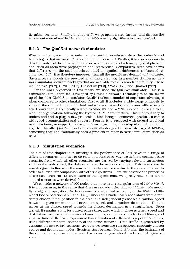
Frederick Ducatelle Adaptive Routing in Ad Hoc Wireless Multi-hop Networks
tic urban scenario. Finally, in chapter 7, we go again a step further, and discuss theimplementation of AntHocNet and other ACO routing algorithms in a real testbed.
5.1.2 The QualNet network simulator
When simulating a computer network, one needs to create models of the protocols andtechnologies that are used. Furthermore, in the case of AHWMNs, it is also necessary todevelop models of the movement of the network nodes and of relevant physical phenom-ena, such as radio wave propagation and interference. Comparative tests have shownthat differences in the used models can lead to significant differences in observed re-sults (see [54]). It is therefore important that all the models are detailed and accurate.Such accurate models are provided in an integrated way in a number of different net-work simulator software packages that are available to the research community. Theseinclude ns-2 [262], OPNET [207], GloMoSim [263], SWAN [175] and QualNet [232].
For the work presented in this thesis, we used the QualNet simulator. This is acommercial simulation tool developed by Scalable Network Technologies as the followup of the older GloMoSim simulator. QualNet offers a number of important advantageswhen compared to other simulators. First of all, it includes a wide range of models tosupport the simulation of both wired and wireless networks, and comes with an exten-sive library that is specifically related to MANETs and WMNs. Second, it uses a clear,modular organization, following the layered TCP/IP architecture. This makes it easy tounderstand and to plug in new protocols. Third, being a commercial product, it comeswith good documentation and support. Fourth, it is equipped with several graphicaluser interfaces, to support the design of new algorithms, the setup of simulation stud-ies, etc.. Finally, QualNet has been specifically designed to simulate large AHWMNs,something that has traditionally been a problem in other network simulators such asns-2.
5.1.3 Simulation scenarios
The aim of this chapter is to investigate the performance of AntHocNet in a range ofdifferent scenarios. In order to do tests in a controlled way, we define a common basescenario, from which all other scenarios are derived by varying relevant parameterssuch as the node speed, the data send rate, the network size, etc.. This base scenariowas designed in line with the most commonly used scenarios in the research area, inorder to allow a fair comparison with other algorithms. Here, we describe the propertiesof the base scenario. Later, in each of the experiments, we specify how the differentapplied scenarios were derived from it.
We consider a network of 100 nodes that move in a rectangular area of 2400× 800m2.It is an open area, in the sense that there are no obstacles that could limit node mobil-ity or signal propagation. Node movements are defined according to the RWP mobilitymodel (see subsection 2.3.1 and [140]). Under this model, each node starts from a ran-domly chosen initial position in the area, and independently chooses a random speedbetween a given minimum and maximum speed, and a random destination. Then, itmoves at the chosen speed towards the chosen destination in a straight line. Uponarrival, it remains static for a fixed pause time, after which it chooses a new speed anddestination. We use a minimum and maximum speed of respectively 0 and 10m/s, anda pause time of 30s. Each experiment has a duration of 900s, and is repeated 20 times,using different random instances of the same scenario. Data traffic is generated byconstant bit rate (CBR) sessions: 20 data sessions are run between randomly chosensource and destination nodes. Sessions start between 0 and 180s after the beginning ofthe simulation, and run till the end. Each session generates 4 packets of 64 bytes persecond.
83
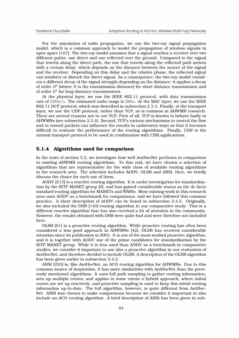
Frederick Ducatelle Adaptive Routing in Ad Hoc Wireless Multi-hop Networks
For the simulation of radio propagation, we use the two-ray signal propagationmodel, which is a common approach to model the propagation of wireless signals inopen space [167]. The two-ray model assumes that a signal reaches a receiver over twodifferent paths: one direct and one reflected over the ground. Compared to the signalthat travels along the direct path, the one that travels along the reflected path arriveswith a certain delay, which depends on the distance between the source of the signaland the receiver. Depending on this delay and the relative phase, the reflected signalcan reinforce or disturb the direct signal. As a consequence, the two-ray model consid-ers a different decay of the signal strength depending on the distance: it applies a decayof order R2 (where R is the transmission distance) for short distance transmission andof order R4 for long distance transmissions.
At the physical layer, we use the IEEE 802.11 protocol, with data transmissionrate of 2Mbit/s. The estimated radio range is 250m. At the MAC layer, we use the IEEE802.11 DCF protocol, which was described in subsection 2.3.3. Finally, at the transportlayer, we use the UDP protocol, rather than TCP, as is common in AHWMN research.There are several reasons not to use TCP. First of all, TCP is known to behave badly inAHWMNs (see subsection 2.3.4). Second, TCP’s various mechanisms to control the flowand to resend packets can influence the results in unforeseen ways so that it becomesdifficult to evaluate the performance of the routing algorithms. Finally, UDP is thenormal transport protocol to be used in combination with CBR applications.
5.1.4 Algorithms used for comparison
In the tests of section 5.2, we investigate how well AntHocNet performs in comparisonto existing AHWMN routing algorithms. To this end, we have chosen a selection ofalgorithms that are representative for the wide class of available routing algorithmsin the research area. The selection includes AODV, OLSR and ANSI. Here, we brieflydiscuss the choice for each one of them.
AODV [213] is a reactive routing algorithm. It is under investigation for standardiza-tion by the IETF MANET group [6], and has gained considerable status as the de factostandard routing algorithm for MANETs and WMNs. Most existing work in this researcharea uses AODV as a benchmark for comparisons, and we have followed this commonpractice. A short description of AODV can be found in subsection 2.4.2. Originally,we also included the DSR [140] routing algorithm in our comparative study. This is adifferent reactive algorithm that has also received a lot of attention in the community.However, the results obtained with DSR were quite bad and were therefore not includedhere.
OLSR [61] is a proactive routing algorithm. While proactive routing has often beenconsidered a less good approach in AHWMNs [42], OLSR has received considerableattention since its publication in 2001. It is one of the most studied proactive algorithm,and it is together with AODV one of the prime candidates for standardization by theIETF MANET group. While it is less used than AODV as a benchmark in comparativestudies, we consider it important to use also a proactive algorithm in our evaluation ofAntHocNet, and therefore decided to include OLSR. A description of the OLSR algorithmhas been given earlier in subsection 2.4.2.
ANSI [220] is, like AntHocNet, an ACO routing algorithm for AHWMNs. Due to thiscommon source of inspiration, it has more similarities with AntHocNet than the previ-ously mentioned algorithms. It uses full path sampling to gather routing information,sets up multiple routes, and applies to some extent a hybrid approach, where initialroutes are set up reactively, and proactive sampling is used to keep this initial routinginformation up-to-date. The full algorithm, however, is quite different from AntHoc-Net. ANSI was chosen to make comparisons because we consider it important to alsoinclude an ACO routing algorithm. A brief description of ANSI has been given in sub-
84
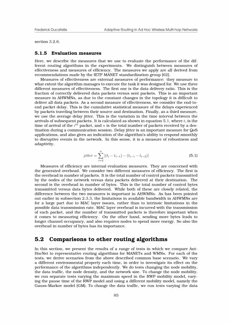
Frederick Ducatelle Adaptive Routing in Ad Hoc Wireless Multi-hop Networks
section 3.2.6.
5.1.5 Evaluation measures
Here, we describe the measures that we use to evaluate the performance of the dif-ferent routing algorithms in the experiments. We distinguish between measures ofeffectiveness and measures of efficiency. The measures we apply are all derived fromrecommendations made by the IETF MANET standardization group [62].
Measures of effectiveness are external measures of performance: they measure towhat extent the algorithm manages to execute the task it was designed for. We use threedifferent measures of effectiveness. The first one is the data delivery ratio. This is thefraction of correctly delivered data packets versus sent packets. This is an importantmeasure in AHWMNs, as due to the constant changes in the topology it is difficult todeliver all data packets. As a second measure of effectiveness, we consider the end-to-end packet delay. This is the cumulative statistical measure of the delays experiencedby packets traveling between their source and destination. Finally, as a third measure,we use the average delay jitter. This is the variation in the time interval between thearrivals of subsequent packets. It is calculated as shown in equation 5.1, where ti is thetime of arrival of the ith packet, and n is the total number of packets received by a des-tination during a communication session. Delay jitter is an important measure for QoSapplications, and also gives an indication of the algorithm’s ability to respond smoothlyto disruptive events in the network. In this sense, it is a measure of robustness andadaptivity.
jitter =n∑
i=2
|(ti − ti−1)− (ti−1 − ti−2)| (5.1)
Measures of efficiency are internal evaluation measures. They are concerned withthe generated overhead. We consider two different measures of efficiency. The first isthe overhead in number of packets. It is the total number of control packets transmittedby the nodes of the network versus data packets delivered at their destination. Thesecond is the overhead in number of bytes. This is the total number of control bytestransmitted versus data bytes delivered. While both of these are closely related, thedifference between the two measures is important in AHWMNs. As has been pointedout earlier in subsection 2.3.3, the limitations in available bandwidth in AHWMNs arefor a large part due to MAC layer issues, rather than to intrinsic limitations in thepossible data transmission rate. MAC layer overhead is incurred with the transmissionof each packet, and the number of transmitted packets is therefore important whenit comes to measuring efficiency. On the other hand, sending more bytes leads tolonger channel occupancy, and also requires nodes to spend more energy. So also theoverhead in number of bytes has its importance.
5.2 Comparisons to other routing algorithms
In this section, we present the results of a range of tests in which we compare Ant-HocNet to representative routing algorithms for MANETs and WMNs. For each of thetests, we derive scenarios from the above described common base scenario. We varya different environmental property each time, in order to investigate its effect on theperformance of the algorithms independently. We do tests changing the node mobility,the data traffic, the node density, and the network size. To change the node mobility,we run separate tests varying the maximum speed in the RWP mobility model, vary-ing the pause time of the RWP model and using a different mobility model, namely theGauss-Markov model (GM). To change the data traffic, we run tests varying the data
85
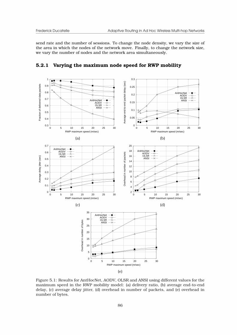
Frederick Ducatelle Adaptive Routing in Ad Hoc Wireless Multi-hop Networks
send rate and the number of sessions. To change the node density, we vary the size ofthe area in which the nodes of the network move. Finally, to change the network size,we vary the number of nodes and the network area simultaneously.
5.2.1 Varying the maximum node speed for RWP mobility
0.3
0.4
0.5
0.6
0.7
0.8
0.9
1
0 5 10 15 20 25 30
Fra
ctio
n of
del
iver
ed d
ata
pack
ets
RWP maximum speed (m/sec)
AntHocNetAODVOLSRANSI
0
0.05
0.1
0.15
0.2
0.25
0.3
0 5 10 15 20 25 30
Ave
rage
end
-to-
end
pack
et d
elay
(se
c)
RWP maximum speed (m/sec)
AntHocNetAODVOLSRANSI
(a) (b)
0
0.1
0.2
0.3
0.4
0.5
0.6
0.7
0 5 10 15 20 25 30
Ave
rage
del
ay ji
tter
(sec
)
RWP maximum speed (m/sec)
AntHocNetAODVOLSRANSI
2
4
6
8
10
12
14
16
18
20
0 5 10 15 20 25 30
Ove
rhea
d in
num
ber
of p
acke
ts
RWP maximum speed (m/sec)
AntHocNetAODVOLSRANSI
(c) (d)
0
5
10
15
20
25
30
35
0 5 10 15 20 25 30
Ove
rhea
d in
num
ber
of b
ytes
RWP maximum speed (m/sec)
AntHocNetAODVOLSRANSI
(e)
Figure 5.1: Results for AntHocNet, AODV, OLSR and ANSI using different values for themaximum speed in the RWP mobility model: (a) delivery ratio, (b) average end-to-enddelay, (c) average delay jitter, (d) overhead in number of packets, and (e) overhead innumber of bytes.
86
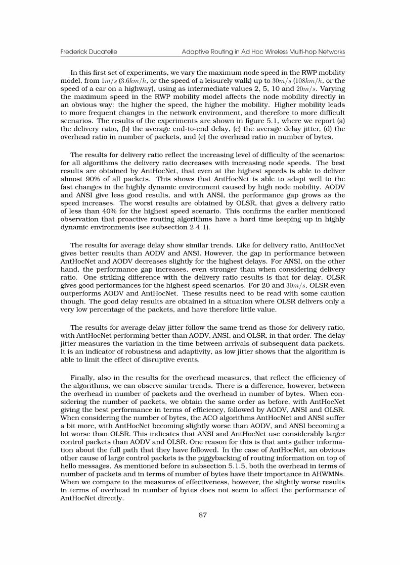
Frederick Ducatelle Adaptive Routing in Ad Hoc Wireless Multi-hop Networks
In this first set of experiments, we vary the maximum node speed in the RWP mobilitymodel, from 1m/s (3.6km/h, or the speed of a leisurely walk) up to 30m/s (108km/h, or thespeed of a car on a highway), using as intermediate values 2, 5, 10 and 20m/s. Varyingthe maximum speed in the RWP mobility model affects the node mobility directly inan obvious way: the higher the speed, the higher the mobility. Higher mobility leadsto more frequent changes in the network environment, and therefore to more difficultscenarios. The results of the experiments are shown in figure 5.1, where we report (a)the delivery ratio, (b) the average end-to-end delay, (c) the average delay jitter, (d) theoverhead ratio in number of packets, and (e) the overhead ratio in number of bytes.
The results for delivery ratio reflect the increasing level of difficulty of the scenarios:for all algorithms the delivery ratio decreases with increasing node speeds. The bestresults are obtained by AntHocNet, that even at the highest speeds is able to deliveralmost 90% of all packets. This shows that AntHocNet is able to adapt well to thefast changes in the highly dynamic environment caused by high node mobility. AODVand ANSI give less good results, and with ANSI, the performance gap grows as thespeed increases. The worst results are obtained by OLSR, that gives a delivery ratioof less than 40% for the highest speed scenario. This confirms the earlier mentionedobservation that proactive routing algorithms have a hard time keeping up in highlydynamic environments (see subsection 2.4.1).
The results for average delay show similar trends. Like for delivery ratio, AntHocNetgives better results than AODV and ANSI. However, the gap in performance betweenAntHocNet and AODV decreases slightly for the highest delays. For ANSI, on the otherhand, the performance gap increases, even stronger than when considering deliveryratio. One striking difference with the delivery ratio results is that for delay, OLSRgives good performances for the highest speed scenarios. For 20 and 30m/s, OLSR evenoutperforms AODV and AntHocNet. These results need to be read with some cautionthough. The good delay results are obtained in a situation where OLSR delivers only avery low percentage of the packets, and have therefore little value.
The results for average delay jitter follow the same trend as those for delivery ratio,with AntHocNet performing better than AODV, ANSI, and OLSR, in that order. The delayjitter measures the variation in the time between arrivals of subsequent data packets.It is an indicator of robustness and adaptivity, as low jitter shows that the algorithm isable to limit the effect of disruptive events.
Finally, also in the results for the overhead measures, that reflect the efficiency ofthe algorithms, we can observe similar trends. There is a difference, however, betweenthe overhead in number of packets and the overhead in number of bytes. When con-sidering the number of packets, we obtain the same order as before, with AntHocNetgiving the best performance in terms of efficiency, followed by AODV, ANSI and OLSR.When considering the number of bytes, the ACO algorithms AntHocNet and ANSI suffera bit more, with AntHocNet becoming slightly worse than AODV, and ANSI becoming alot worse than OLSR. This indicates that ANSI and AntHocNet use considerably largercontrol packets than AODV and OLSR. One reason for this is that ants gather informa-tion about the full path that they have followed. In the case of AntHocNet, an obviousother cause of large control packets is the piggybacking of routing information on top ofhello messages. As mentioned before in subsection 5.1.5, both the overhead in terms ofnumber of packets and in terms of number of bytes have their importance in AHWMNs.When we compare to the measures of effectiveness, however, the slightly worse resultsin terms of overhead in number of bytes does not seem to affect the performance ofAntHocNet directly.
87

Frederick Ducatelle Adaptive Routing in Ad Hoc Wireless Multi-hop Networks
0.55
0.6
0.65
0.7
0.75
0.8
0.85
0.9
0.95
1
0 50 100 150 200 250 300 350 400 450 500
Fra
ctio
n of
del
iver
ed d
ata
pack
ets
RWP pause time (sec)
AntHocNetAODVOLSRANSI
0
0.05
0.1
0.15
0.2
0.25
0.3
0.35
0.4
0.45
0 50 100 150 200 250 300 350 400 450 500
Ave
rage
end
-to-
end
pack
et d
elay
(se
c)
RWP pause time (sec)
AntHocNetAODVOLSRANSI
(a) (b)
0.05
0.1
0.15
0.2
0.25
0.3
0.35
0 50 100 150 200 250 300 350 400 450 500
Ave
rage
del
ay ji
tter
(sec
)
RWP pause time (sec)
AntHocNetAODVOLSRANSI
3
4
5
6
7
8
9
10
11
12
0 50 100 150 200 250 300 350 400 450 500
Ove
rhea
d in
num
ber
of p
acke
ts
RWP pause time (sec)
AntHocNetAODVOLSRANSI
(c) (d)
4
6
8
10
12
14
16
18
20
22
0 50 100 150 200 250 300 350 400 450 500
Ove
rhea
d in
num
ber
of b
ytes
RWP pause time (sec)
AntHocNetAODVOLSRANSI
(e)
Figure 5.2: Results for AntHocNet, AODV, OLSR and ANSI using different values for thepause time in the RWP mobility model: (a) delivery ratio, (b) average end-to-end delay,(c) average delay jitter, (d) overhead in number of packets, and (e) overhead in numberof bytes.
5.2.2 Varying the pause time for RWP mobility
Here, we vary the pause time of the RWP mobility model, from 0s up to 480s, withas intermediate values 15, 30, 60, 120 and 240s. The results of the experiments areshown in figure 5.2. Increasing the pause time has two different effects on the generalproperties of the scenario that are relevant for routing. The first of these is a decrease
88
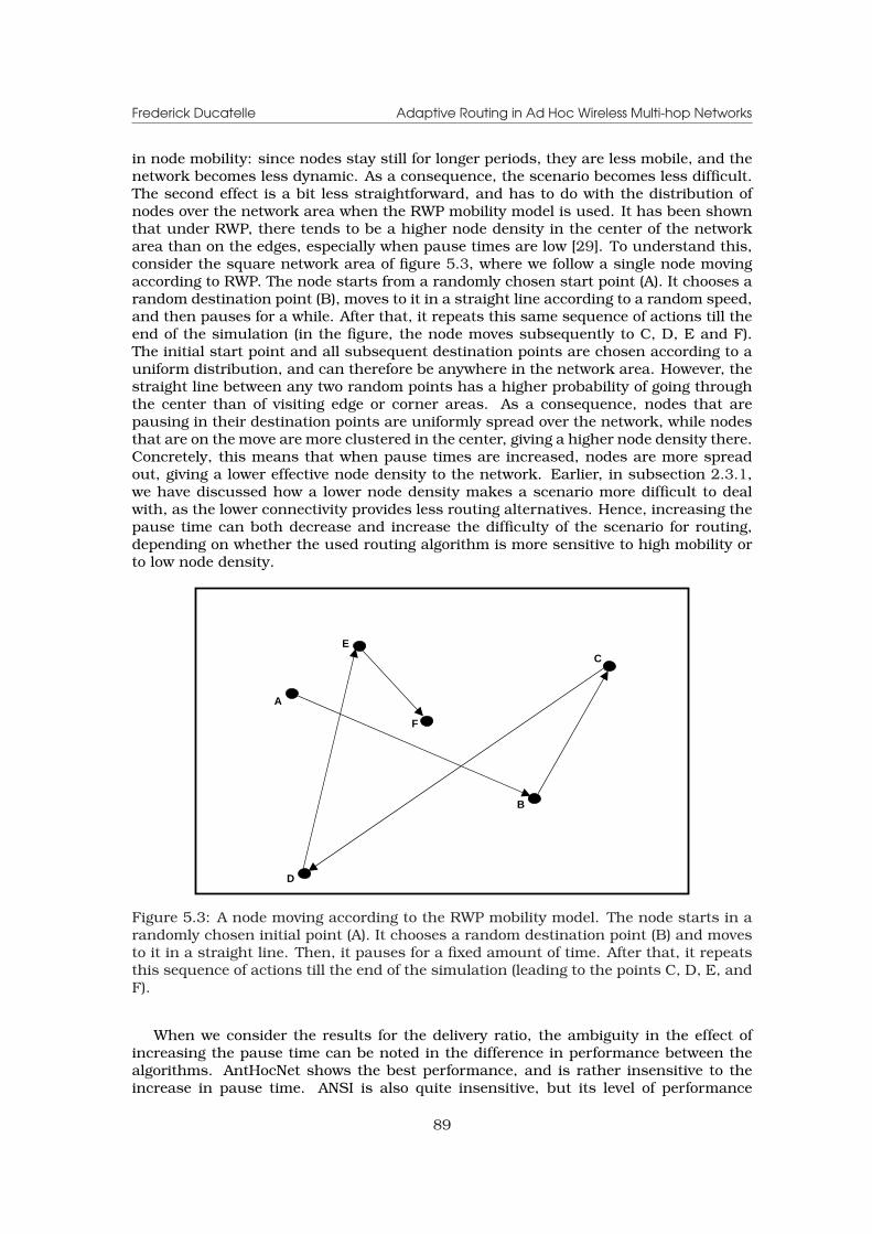
Frederick Ducatelle Adaptive Routing in Ad Hoc Wireless Multi-hop Networks
in node mobility: since nodes stay still for longer periods, they are less mobile, and thenetwork becomes less dynamic. As a consequence, the scenario becomes less difficult.The second effect is a bit less straightforward, and has to do with the distribution ofnodes over the network area when the RWP mobility model is used. It has been shownthat under RWP, there tends to be a higher node density in the center of the networkarea than on the edges, especially when pause times are low [29]. To understand this,consider the square network area of figure 5.3, where we follow a single node movingaccording to RWP. The node starts from a randomly chosen start point (A). It chooses arandom destination point (B), moves to it in a straight line according to a random speed,and then pauses for a while. After that, it repeats this same sequence of actions till theend of the simulation (in the figure, the node moves subsequently to C, D, E and F).The initial start point and all subsequent destination points are chosen according to auniform distribution, and can therefore be anywhere in the network area. However, thestraight line between any two random points has a higher probability of going throughthe center than of visiting edge or corner areas. As a consequence, nodes that arepausing in their destination points are uniformly spread over the network, while nodesthat are on the move are more clustered in the center, giving a higher node density there.Concretely, this means that when pause times are increased, nodes are more spreadout, giving a lower effective node density to the network. Earlier, in subsection 2.3.1,we have discussed how a lower node density makes a scenario more difficult to dealwith, as the lower connectivity provides less routing alternatives. Hence, increasing thepause time can both decrease and increase the difficulty of the scenario for routing,depending on whether the used routing algorithm is more sensitive to high mobility orto low node density.
A
B
C
D
E
F
Figure 5.3: A node moving according to the RWP mobility model. The node starts in arandomly chosen initial point (A). It chooses a random destination point (B) and movesto it in a straight line. Then, it pauses for a fixed amount of time. After that, it repeatsthis sequence of actions till the end of the simulation (leading to the points C, D, E, andF).
When we consider the results for the delivery ratio, the ambiguity in the effect ofincreasing the pause time can be noted in the difference in performance between thealgorithms. AntHocNet shows the best performance, and is rather insensitive to theincrease in pause time. ANSI is also quite insensitive, but its level of performance
89
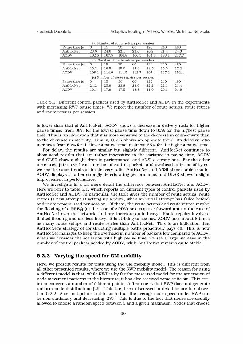
Frederick Ducatelle Adaptive Routing in Ad Hoc Wireless Multi-hop Networks
(a) Number of route setups per sessionPause time (s) 0 15 30 60 120 240 480AntHocNet 23.0 24.6 22.1 22.6 20.2 21.4 24.3AODV 162.5 167.5 164.8 166.3 164.8 183.1 217.7
(b) Number of route retries per sessionPause time (s) 0 15 30 60 120 240 480AntHocNet 15.2 16.5 15.0 14.9 13.5 15.0 17.2AODV 108.1 114.9 111.5 112.7 107.4 127.2 152.4
(c) Number of route repairs per sessionPause time (s) 0 15 30 60 120 240 480AntHocNet 24.2 25.9 23.8 24.0 22.2 22.1 21.4AODV 16.1 17.9 17.5 18.7 21.0 25.1 31.8
Table 5.1: Different control packets used by AntHocNet and AODV in the experimentswith increasing RWP pause times. We report the number of route setups, route retriesand route repairs per session.
is lower than that of AntHocNet. AODV shows a decrease in delivery ratio for higherpause times: from 88% for the lowest pause time down to 80% for the highest pausetime. This is an indication that it is more sensitive to the decrease in connectivity thanto the decrease in mobility. Finally, OLSR shows an opposite trend: its delivery ratioincreases from 60% for the lowest pause time to almost 65% for the highest pause time.
For delay, the results are similar but slightly different. AntHocNet continues toshow good results that are rather insensitive to the variance in pause time, AODVand OLSR show a slight drop in performance, and ANSI a strong one. For the othermeasures, jitter, overhead in terms of control packets and overhead in terms of bytes,we see the same trends as for delivery ratio: AntHocNet and ANSI show stable results,AODV displays a rather strongly deteriorating performance, and OLSR shows a slightimprovement in performance.
We investigate in a bit more detail the difference between AntHocNet and AODV.Here we refer to table 5.1, which reports on different types of control packets used byAntHocNet and AODV. In particular, the table gives the number of route setups, routeretries (a new attempt at setting up a route, when an initial attempt has failed before)and route repairs used per session. Of these, the route setups and route retries involvethe flooding of a RREQ (in the case of AODV) or a reactive forward ant (in the case ofAntHocNet) over the network, and are therefore quite heavy. Route repairs involve alimited flooding and are less heavy. It is striking to see how AODV uses about 8 timesas many route setups and route retries than AntHocNet. This is an indication thatAntHocNet’s strategy of constructing multiple paths proactively pays off. This is howAntHocNet manages to keep the overhead in number of packets low compared to AODV.When we consider the scenarios with high pause time, we see a large increase in thenumber of control packets needed by AODV, while AntHocNet remains quite stable.
5.2.3 Varying the speed for GM mobility
Here, we present results for tests using the GM mobility model. This is different fromall other presented results, where we use the RWP mobility model. The reason for usinga different model is that, while RWP is by far the most used model for the generation ofnode movement patterns in the literature, it has also received some criticism. This crit-icism concerns a number of different points. A first one is that RWP does not generateuniform node distributions [29]. This has been discussed in detail before in subsec-tion 5.2.2. A second point of criticism is that the average node speed under RWP canbe non-stationary and decreasing [287]. This is due to the fact that nodes are usuallyallowed to choose a random speed between 0 and a given maximum. Nodes that choose
90
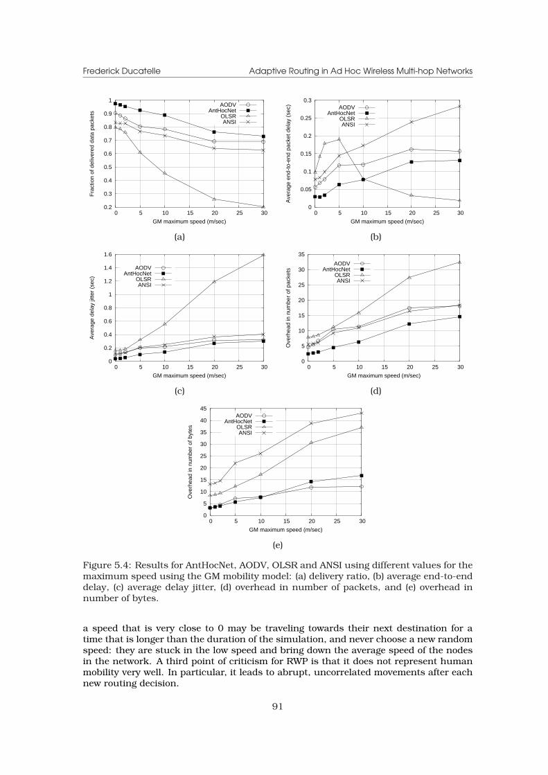
Frederick Ducatelle Adaptive Routing in Ad Hoc Wireless Multi-hop Networks
0.2
0.3
0.4
0.5
0.6
0.7
0.8
0.9
1
0 5 10 15 20 25 30
Fra
ctio
n of
del
iver
ed d
ata
pack
ets
GM maximum speed (m/sec)
AODVAntHocNet
OLSRANSI
0
0.05
0.1
0.15
0.2
0.25
0.3
0 5 10 15 20 25 30
Ave
rage
end
-to-
end
pack
et d
elay
(se
c)
GM maximum speed (m/sec)
AODVAntHocNet
OLSRANSI
(a) (b)
0
0.2
0.4
0.6
0.8
1
1.2
1.4
1.6
0 5 10 15 20 25 30
Ave
rage
del
ay ji
tter
(sec
)
GM maximum speed (m/sec)
AODVAntHocNet
OLSRANSI
0
5
10
15
20
25
30
35
0 5 10 15 20 25 30
Ove
rhea
d in
num
ber
of p
acke
ts
GM maximum speed (m/sec)
AODVAntHocNet
OLSRANSI
(c) (d)
0
5
10
15
20
25
30
35
40
45
0 5 10 15 20 25 30
Ove
rhea
d in
num
ber
of b
ytes
GM maximum speed (m/sec)
AODVAntHocNet
OLSRANSI
(e)
Figure 5.4: Results for AntHocNet, AODV, OLSR and ANSI using different values for themaximum speed using the GM mobility model: (a) delivery ratio, (b) average end-to-enddelay, (c) average delay jitter, (d) overhead in number of packets, and (e) overhead innumber of bytes.
a speed that is very close to 0 may be traveling towards their next destination for atime that is longer than the duration of the simulation, and never choose a new randomspeed: they are stuck in the low speed and bring down the average speed of the nodesin the network. A third point of criticism for RWP is that it does not represent humanmobility very well. In particular, it leads to abrupt, uncorrelated movements after eachnew routing decision.
91
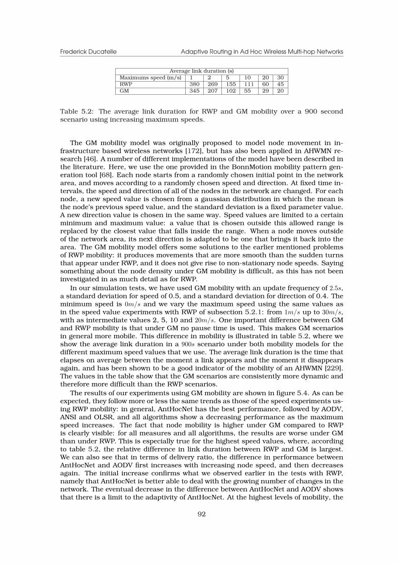
Frederick Ducatelle Adaptive Routing in Ad Hoc Wireless Multi-hop Networks
Average link duration (s)Maximums speed (m/s) 1 2 5 10 20 30RWP 380 269 155 111 60 45GM 345 207 102 55 29 20
Table 5.2: The average link duration for RWP and GM mobility over a 900 secondscenario using increasing maximum speeds.
The GM mobility model was originally proposed to model node movement in in-frastructure based wireless networks [172], but has also been applied in AHWMN re-search [46]. A number of different implementations of the model have been described inthe literature. Here, we use the one provided in the BonnMotion mobility pattern gen-eration tool [68]. Each node starts from a randomly chosen initial point in the networkarea, and moves according to a randomly chosen speed and direction. At fixed time in-tervals, the speed and direction of all of the nodes in the network are changed. For eachnode, a new speed value is chosen from a gaussian distribution in which the mean isthe node’s previous speed value, and the standard deviation is a fixed parameter value.A new direction value is chosen in the same way. Speed values are limited to a certainminimum and maximum value: a value that is chosen outside this allowed range isreplaced by the closest value that falls inside the range. When a node moves outsideof the network area, its next direction is adapted to be one that brings it back into thearea. The GM mobility model offers some solutions to the earlier mentioned problemsof RWP mobility: it produces movements that are more smooth than the sudden turnsthat appear under RWP, and it does not give rise to non-stationary node speeds. Sayingsomething about the node density under GM mobility is difficult, as this has not beeninvestigated in as much detail as for RWP.
In our simulation tests, we have used GM mobility with an update frequency of 2.5s,a standard deviation for speed of 0.5, and a standard deviation for direction of 0.4. Theminimum speed is 0m/s and we vary the maximum speed using the same values asin the speed value experiments with RWP of subsection 5.2.1: from 1m/s up to 30m/s,with as intermediate values 2, 5, 10 and 20m/s. One important difference between GMand RWP mobility is that under GM no pause time is used. This makes GM scenariosin general more mobile. This difference in mobility is illustrated in table 5.2, where weshow the average link duration in a 900s scenario under both mobility models for thedifferent maximum speed values that we use. The average link duration is the time thatelapses on average between the moment a link appears and the moment it disappearsagain, and has been shown to be a good indicator of the mobility of an AHWMN [229].The values in the table show that the GM scenarios are consistently more dynamic andtherefore more difficult than the RWP scenarios.
The results of our experiments using GM mobility are shown in figure 5.4. As can beexpected, they follow more or less the same trends as those of the speed experiments us-ing RWP mobility: in general, AntHocNet has the best performance, followed by AODV,ANSI and OLSR, and all algorithms show a decreasing performance as the maximumspeed increases. The fact that node mobility is higher under GM compared to RWPis clearly visible: for all measures and all algorithms, the results are worse under GMthan under RWP. This is especially true for the highest speed values, where, accordingto table 5.2, the relative difference in link duration between RWP and GM is largest.We can also see that in terms of delivery ratio, the difference in performance betweenAntHocNet and AODV first increases with increasing node speed, and then decreasesagain. The initial increase confirms what we observed earlier in the tests with RWP,namely that AntHocNet is better able to deal with the growing number of changes in thenetwork. The eventual decrease in the difference between AntHocNet and AODV showsthat there is a limit to the adaptivity of AntHocNet. At the highest levels of mobility, the
92
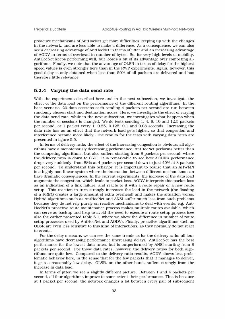
Frederick Ducatelle Adaptive Routing in Ad Hoc Wireless Multi-hop Networks
proactive mechanisms of AntHocNet get more difficulties keeping up with the changesin the network, and are less able to make a difference. As a consequence, we can alsosee a decreasing advantage of AntHocNet in terms of jitter and an increasing advantageof AODV in terms of overhead in number of bytes. So, for very high levels of mobility,AntHocNet keeps performing well, but looses a bit of its advantage over competing al-gorithms. Finally, we note that the advantage of OLSR in terms of delay for the highestspeed values is even stronger here than in the RWP experiments. Again, however, thisgood delay is only obtained when less than 50% of all packets are delivered and hastherefore little relevance.
5.2.4 Varying the data send rate
With the experiments described here and in the next subsection, we investigate theeffect of the data load on the performance of the different routing algorithms. In thebase scenario, 20 data sessions each sending 4 packets per second are run betweenrandomly chosen start and destination nodes. Here, we investigate the effect of varyingthe data send rate, while in the next subsection, we investigates what happens whenthe number of sessions is changed. We do tests sending 1, 4, 8, 10 and 12.5 packetsper second, or 1 packet every 1, 0.25, 0.125, 0.1 and 0.08 seconds. Increasing thedata rate has as an effect that the network load gets higher, so that congestion andinterference become more likely. The results for the tests with varying data rates arepresented in figure 5.5.
In terms of delivery ratio, the effect of the increasing congestion is obvious: all algo-rithms have a monotonously decreasing performance. AntHocNet performs better thanthe competing algorithms, but also suffers starting from 8 packets per second, wherethe delivery ratio is down to 66%. It is remarkable to see how AODV’s performancedrops very suddenly: from 88% at 4 packets per second down to just 40% at 8 packetsper second. To understand this behavior, it is important to realize that an AHWMNis a highly non-linear system where the interaction between different mechanisms canhave dramatic consequences. In the current experiments, the increase of the data loadaugments the congestion, which leads to packet loss. AODV interprets this packet lossas an indication of a link failure, and reacts to it with a route repair or a new routesetup. This reaction in turn strongly increases the load in the network (the floodingof a RREQ creates a large amount of extra overhead) and makes the situation worse.Hybrid algorithms such as AntHocNet and ANSI suffer much less from such problemsbecause they do not rely purely on reactive mechanisms to deal with events; e.g. Ant-HocNet’s proactive route maintenance process makes multiple routes available, whichcan serve as backup and help to avoid the need to execute a route setup process (seealso the earlier presented table 5.1, where we show the difference in number of routesetup processes used by AntHocNet and AODV). Finally, proactive algorithms such asOLSR are even less sensitive to this kind of interactions, as they normally do not reactto events.
For the delay measure, we can see the same trends as for the delivery ratio: all fouralgorithms have decreasing performance (increasing delay). AntHocNet has the bestperformance for the lowest data rates, but is outperformed by ANSI starting from 8packets per second. For those data rates, however, the delivery ratios for both algo-rithms are quite low. Compared to the delivery ratio results, AODV shows less prob-lematic behavior here, in the sense that for the few packets that it manages to deliver,it gets a reasonably low delay. OLSR, on the other hand, suffers strongly from theincrease in data load.
In terms of jitter, we see a slightly different picture. Between 1 and 4 packets persecond, all four algorithms improve to some extent their performance. This is becauseat 1 packet per second, the network changes a lot between every pair of subsequent
93
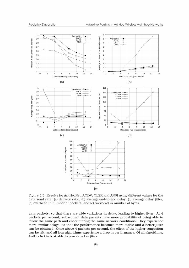
Frederick Ducatelle Adaptive Routing in Ad Hoc Wireless Multi-hop Networks
0.1
0.2
0.3
0.4
0.5
0.6
0.7
0.8
0.9
1
0 2 4 6 8 10 12 14
Fra
ctio
n of
del
iver
ed d
ata
pack
ets
Data send rate (packets/sec)
AntHocNetAODVOLSRANSI
0
1
2
3
4
5
6
7
8
9
0 2 4 6 8 10 12 14
Ave
rage
end
-to-
end
pack
et d
elay
(se
c)
Data send rate (packets/sec)
AntHocNetAODVOLSRANSI
(a) (b)
0
0.1
0.2
0.3
0.4
0.5
0.6
0.7
0.8
0.9
1
0 2 4 6 8 10 12 14
Ave
rage
del
ay ji
tter
(sec
)
Data send rate (packets/sec)
AntHocNetAODVOLSRANSI
0
20
40
60
80
100
120
140
160
0 2 4 6 8 10 12 14
Ove
rhea
d in
num
ber
of p
acke
ts
Data send rate (packets/sec)
AntHocNetAODVOLSRANSI
(c) (d)
0
10
20
30
40
50
60
70
80
90
100
0 2 4 6 8 10 12 14
Ove
rhea
d in
num
ber
of b
ytes
Data send rate (packets/sec)
AntHocNetAODVOLSRANSI
(e)
Figure 5.5: Results for AntHocNet, AODV, OLSR and ANSI using different values for thedata send rate: (a) delivery ratio, (b) average end-to-end delay, (c) average delay jitter,(d) overhead in number of packets, and (e) overhead in number of bytes.
data packets, so that there are wide variations in delay, leading to higher jitter. At 4packets per second, subsequent data packets have more probability of being able tofollow the same path and encountering the same network conditions. They experiencemore similar delays, so that the performance becomes more stable and a better jittercan be obtained. Once above 4 packets per second, the effect of the higher congestioncan be felt, and all four algorithms experience a drop in performance. Of all algorithms,AntHocNet is best able to provide a low jitter.
94

Frederick Ducatelle Adaptive Routing in Ad Hoc Wireless Multi-hop Networks
For the remaining two measures, overhead in number of packets and overhead innumber of bytes, the results bear resemblance to those for jitter. Also here, the fact thatat high data rates subsequent packets are sent closer after each other has a positiveeffect on the performance. This is because the information gathered by the routingalgorithms can get used for more packets before it gets out of date, so that the routingalgorithm can work in a more efficient way. This effect is especially visible for the OLSRalgorithm, that has a monotonously improving performance. This is because OLSRworks in a proactive way and does not react to changes in the data rate: the amount ofcontrol packets or bytes it generates is quite stable, and increasing the data rate justmeans that more data packets are available to be delivered, so that the denominator ofthe overhead measures increases. Also the other algorithms profit to some extent fromthe possibility to work more efficiently when data packets are sent at a higher rate:AODV, ANSI and AntHocNet all have a decreasing amount of overhead for the lowestdata rates. However, for the higher data rates, the effect of the increased congestionbecomes stronger. Especially AODV suffers a lot: while it has the lowest overheadboth in terms of packets and bytes for the lowest data rate, it increases rapidly andis outperformed by all other algorithms for higher data rates. The reason for this hasbeen explained before, when we commented on the results for delivery ratio: AODV’spurely reactive nature makes it extra sensitive to the arrival of disruptive events. Forthe highest data rates, AntHocNet has the lowest overhead.
5.2.5 Varying the number of data sessions
Here, we present results of tests with a varying number of data sessions: we use from10 up to 100 sessions, with an increment of 10 each time. Each data session sends4 packets per second, and source and destination nodes are chosen randomly. Whenincreasing the number of sessions, we increment the total data load in the network, justlike we did when increasing the data send rate in the experiments of subsection 5.2.4.In particular, in terms of number of generated data packets, the scenarios with 40sessions presented here are equivalent to those with 8 packets per second in the ex-periments of subsection 5.2.4, and the scenarios with 50 sessions to those with 10packets per second (other approximate points of comparison between both sets of ex-periments are at 10 sessions, which corresponds to sending 2 packets per second, andat 60 sessions, which corresponds to sending 12 packets per second). Nevertheless,increasing the data load by augmenting the number of sessions can have a differenteffect than increasing it by sending at a higher rate. This is because the increased dataload is spread over multiple sessions. When extra actions need to be performed on aper-session basis, as is the case for reactive routing algorithms, increasing the numberof sessions can be more challenging. The results of the experiments with the numberof sessions are shown in figure 5.8.
When considering the delivery ratio, we see a picture that is very similar to thatfor the data rate experiments: all four algorithms have a decreasing performance forincreasing data load, AntHocNet shows the best results, and AODV has a more suddendrop in performance than the other algorithms. When comparing results directly, wecan see that for AODV they are even lower here than in the data rate experiments (at40 sessions, AODV delivers only 5% of all packets, compared to 25% when sending 8packets per second in the data rate experiments). Apparently the higher number ofroute setups needed due to the presence of more sessions makes the algorithm evenmore sensitive to the increase in data load and congestion. Also ANSI suffers a bitmore than in the data rate experiments: its delivery ratio even drops below that ofOLSR when 40 or more data sessions are used. For AntHocNet, the difference with thedata rate experiments is much smaller. Apparently its lower need for route setups (seetable 5.1) protects its performances sufficiently. Finally, for OLSR there is practically
95
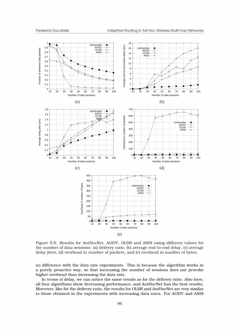
Frederick Ducatelle Adaptive Routing in Ad Hoc Wireless Multi-hop Networks
0
0.1
0.2
0.3
0.4
0.5
0.6
0.7
0.8
0.9
1
10 20 30 40 50 60 70 80 90 100
Fra
ctio
n of
del
iver
ed d
ata
pack
ets
Number of data sessions
AntHocNetAODVOLSRANSI
0
2
4
6
8
10
12
14
16
18
10 20 30 40 50 60 70 80 90 100
Ave
rage
end
-to-
end
pack
et d
elay
(se
c)
Number of data sessions
AntHocNetAODVOLSRANSI
(a) (b)
0
0.2
0.4
0.6
0.8
1
1.2
1.4
1.6
1.8
10 20 30 40 50 60 70 80 90 100
Ave
rage
del
ay ji
tter
(sec
)
Number of data sessions
AntHocNetAODVOLSRANSI
0
100
200
300
400
500
600
700
10 20 30 40 50 60 70 80 90 100
Ove
rhea
d in
num
ber
of p
acke
ts
Number of data sessions
AntHocNetAODVOLSRANSI
(c) (d)
0
50
100
150
200
250
300
350
400
450
10 20 30 40 50 60 70 80 90 100
Ove
rhea
d in
num
ber
of b
ytes
Number of data sessions
AntHocNetAODVOLSRANSI
(e)
Figure 5.6: Results for AntHocNet, AODV, OLSR and ANSI using different values forthe number of data sessions: (a) delivery ratio, (b) average end-to-end delay, (c) averagedelay jitter, (d) overhead in number of packets, and (e) overhead in number of bytes.
no difference with the data rate experiments. This is because the algorithm works ina purely proactive way, so that increasing the number of sessions does not provokehigher overhead than increasing the data rate.
In terms of delay, we can notice the same trends as for the delivery ratio. Also here,all four algorithms show decreasing performance, and AntHocNet has the best results.Moreover, like for the delivery ratio, the results for OLSR and AntHocNet are very similarto those obtained in the experiments with increasing data rates. For AODV and ANSI
96

Frederick Ducatelle Adaptive Routing in Ad Hoc Wireless Multi-hop Networks
on the other hand, the performance is worse than in the data rate experiments, witha larger difference for the purely reactive AODV algorithm and a smaller difference forthe hybrid ANSI algorithm.
In terms of jitter, all four algorithms have decreasing performance, with AntHoc-Net showing the best results. The overall trends are considerably different from thoseobtained in the tests with increasing data rates, where all algorithms first showed animprovement in performance, and then a slow deterioration. In section 5.2.4, we ex-plained that the performance improvement was due to the fact that at higher data rates,subsequent packets come closer after each other and therefore experience more sim-ilar conditions, leading to lower variations in interarrival times. When increasing thenumber of sessions, this positive effect is not present.
Considering the last two measures, the overhead in number of packets and in num-ber of bytes, we can see that the performance of OLSR improves with the numberof sessions, while that of AntHocNet and ANSI is relatively stable and that of AODVshows a dramatic deterioration. Overall, AntHocNet shows the best performance. Theimprovement in overhead results of OLSR is again due to the fact that it is a proac-tive algorithm and therefore does not use extra control packets when more sessionsare started; therefore, more data packets are delivered correctly while using the samenumber of control packets. Different from the data rate experiments, the other threealgorithms do not show an improvement in overhead at the low end of the range of thedata load. In the data rate experiments, such an improvement was possible because thehigher send frequency of data packets allowed to use reactively obtained routing infor-mation for more data packets, thus improving efficiency. When increasing the numberof sessions, this effect does not exist.
5.2.6 Varying the network area size
In this subsection, we present results of tests in which we vary the size of the area inwhich the nodes move. The sizes we use are 1200 × 400m2, 1500 × 500m2, 1800 × 600m2,2100×700m2, 2400×800m2, 2700×900m2, 3000×1000m2, 3300×1100m2, and 3600×1200m2.Increasing the size of the network area increases the average path length between nodesand decreases the node density. Both make the scenario more difficult. The importanceof the node density in AHWMNs has been discussed before in subsection 2.3.1. Sparsernetworks form a more difficult environment because they are less well connected. Inthe best case, this means that there are few routing alternatives between the sourceand destination nodes of a session so that link failures are difficult to repair. In theworst case, there is just no connectivity, and data packets cannot be sent. The resultsfor the network area tests are shown in figure 5.7.
When considering delivery ratio, we can see that for the scenarios with smallest net-work area, AntHocNet and AODV perform equally well, while the result is slightly worsefor ANSI and a lot worse for OLSR. The similarity in performance between AntHocNetand AODV is to be expected. In a dense scenario on a small surface area, paths areshort and many alternatives are available, and it is therefore relatively easy to rebuildroutes after a link failure. As a result, the proactive route maintenance and the re-active route repair processes of AntHocNet, which are aimed at improving routes andavoiding the need for new route setups, create extra overhead without adding muchvalue. Moreover, the large hello messages sent out by all nodes in AntHocNet can causemore interference than in sparse scenarios, since each node has many neighbors. Forincreasing area sizes, the scenarios become more sparse, and all algorithms show de-creasing performance. AntHocNet is better able to deal with the difficulties of sparsescenarios than the other three algorithms, because here its different mechanisms dopay off. Especially with AODV there is a growing difference in performance.
When considering delay, the image is similar. Now, for the smallest network areas,
97
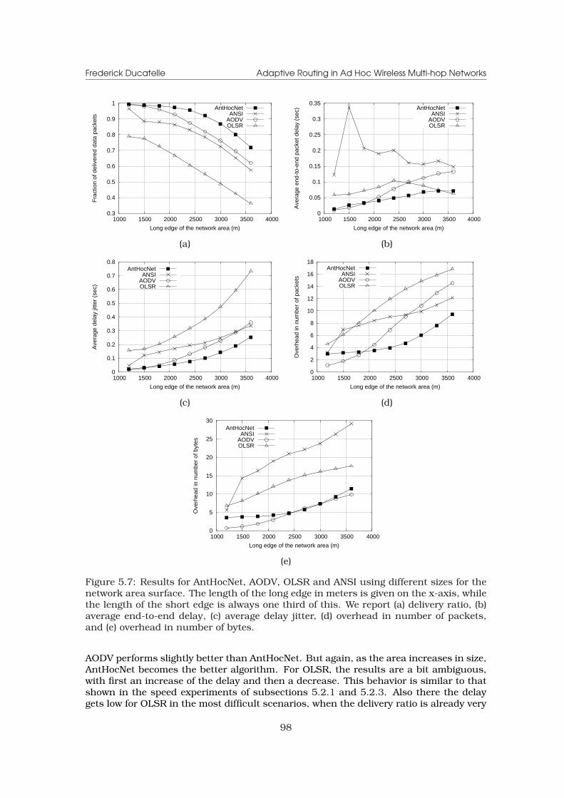
Frederick Ducatelle Adaptive Routing in Ad Hoc Wireless Multi-hop Networks
0.3
0.4
0.5
0.6
0.7
0.8
0.9
1
1000 1500 2000 2500 3000 3500 4000
Fra
ctio
n of
del
iver
ed d
ata
pack
ets
Long edge of the network area (m)
AntHocNetANSI
AODVOLSR
0
0.05
0.1
0.15
0.2
0.25
0.3
0.35
1000 1500 2000 2500 3000 3500 4000
Ave
rage
end
-to-
end
pack
et d
elay
(se
c)
Long edge of the network area (m)
AntHocNetANSI
AODVOLSR
(a) (b)
0
0.1
0.2
0.3
0.4
0.5
0.6
0.7
0.8
1000 1500 2000 2500 3000 3500 4000
Ave
rage
del
ay ji
tter
(sec
)
Long edge of the network area (m)
AntHocNetANSI
AODVOLSR
0
2
4
6
8
10
12
14
16
18
1000 1500 2000 2500 3000 3500 4000
Ove
rhea
d in
num
ber
of p
acke
ts
Long edge of the network area (m)
AntHocNetANSI
AODVOLSR
(c) (d)
0
5
10
15
20
25
30
1000 1500 2000 2500 3000 3500 4000
Ove
rhea
d in
num
ber
of b
ytes
Long edge of the network area (m)
AntHocNetANSI
AODVOLSR
(e)
Figure 5.7: Results for AntHocNet, AODV, OLSR and ANSI using different sizes for thenetwork area surface. The length of the long edge in meters is given on the x-axis, whilethe length of the short edge is always one third of this. We report (a) delivery ratio, (b)average end-to-end delay, (c) average delay jitter, (d) overhead in number of packets,and (e) overhead in number of bytes.
AODV performs slightly better than AntHocNet. But again, as the area increases in size,AntHocNet becomes the better algorithm. For OLSR, the results are a bit ambiguous,with first an increase of the delay and then a decrease. This behavior is similar to thatshown in the speed experiments of subsections 5.2.1 and 5.2.3. Also there the delaygets low for OLSR in the most difficult scenarios, when the delivery ratio is already very
98
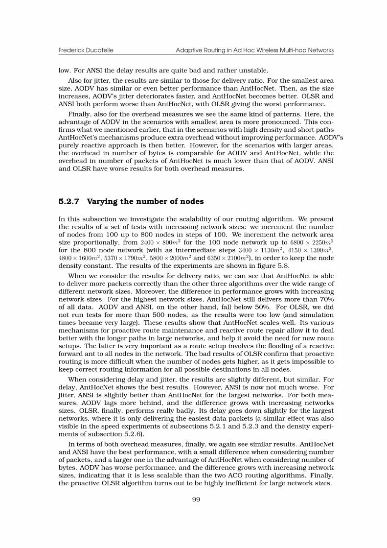
Frederick Ducatelle Adaptive Routing in Ad Hoc Wireless Multi-hop Networks
low. For ANSI the delay results are quite bad and rather unstable.
Also for jitter, the results are similar to those for delivery ratio. For the smallest areasize, AODV has similar or even better performance than AntHocNet. Then, as the sizeincreases, AODV’s jitter deteriorates faster, and AntHocNet becomes better. OLSR andANSI both perform worse than AntHocNet, with OLSR giving the worst performance.
Finally, also for the overhead measures we see the same kind of patterns. Here, theadvantage of AODV in the scenarios with smallest area is more pronounced. This con-firms what we mentioned earlier, that in the scenarios with high density and short pathsAntHocNet’s mechanisms produce extra overhead without improving performance. AODV’spurely reactive approach is then better. However, for the scenarios with larger areas,the overhead in number of bytes is comparable for AODV and AntHocNet, while theoverhead in number of packets of AntHocNet is much lower than that of AODV. ANSIand OLSR have worse results for both overhead measures.
5.2.7 Varying the number of nodes
In this subsection we investigate the scalability of our routing algorithm. We presentthe results of a set of tests with increasing network sizes: we increment the numberof nodes from 100 up to 800 nodes in steps of 100. We increment the network areasize proportionally, from 2400 × 800m2 for the 100 node network up to 6800 × 2250m2
for the 800 node network (with as intermediate steps 3400 × 1130m2, 4150 × 1390m2,4800× 1600m2, 5370× 1790m2, 5800× 2000m2 and 6350× 2100m2), in order to keep the nodedensity constant. The results of the experiments are shown in figure 5.8.
When we consider the results for delivery ratio, we can see that AntHocNet is ableto deliver more packets correctly than the other three algorithms over the wide range ofdifferent network sizes. Moreover, the difference in performance grows with increasingnetwork sizes. For the highest network sizes, AntHocNet still delivers more than 70%of all data. AODV and ANSI, on the other hand, fall below 50%. For OLSR, we didnot run tests for more than 500 nodes, as the results were too low (and simulationtimes became very large). These results show that AntHocNet scales well. Its variousmechanisms for proactive route maintenance and reactive route repair allow it to dealbetter with the longer paths in large networks, and help it avoid the need for new routesetups. The latter is very important as a route setup involves the flooding of a reactiveforward ant to all nodes in the network. The bad results of OLSR confirm that proactiverouting is more difficult when the number of nodes gets higher, as it gets impossible tokeep correct routing information for all possible destinations in all nodes.
When considering delay and jitter, the results are slightly different, but similar. Fordelay, AntHocNet shows the best results. However, ANSI is now not much worse. Forjitter, ANSI is slightly better than AntHocNet for the largest networks. For both mea-sures, AODV lags more behind, and the difference grows with increasing networkssizes. OLSR, finally, performs really badly. Its delay goes down slightly for the largestnetworks, where it is only delivering the easiest data packets (a similar effect was alsovisible in the speed experiments of subsections 5.2.1 and 5.2.3 and the density experi-ments of subsection 5.2.6).
In terms of both overhead measures, finally, we again see similar results. AntHocNetand ANSI have the best performance, with a small difference when considering numberof packets, and a larger one in the advantage of AntHocNet when considering number ofbytes. AODV has worse performance, and the difference grows with increasing networksizes, indicating that it is less scalable than the two ACO routing algorithms. Finally,the proactive OLSR algorithm turns out to be highly inefficient for large network sizes.
99
Frederick Ducatelle Adaptive Routing in Ad Hoc Wireless Multi-hop Networks
0.1
0.2
0.3
0.4
0.5
0.6
0.7
0.8
0.9
1
100 200 300 400 500 600 700 800
Fra
ctio
n of
del
iver
ed d
ata
pack
ets
Number of nodes
AntHocNetANSI
AODVOLSR
0
1
2
3
4
5
6
7
100 200 300 400 500 600 700 800
Ave
rage
end
-to-
end
pack
et d
elay
(se
c)
Number of nodes
AntHocNetANSI
AODVOLSR
(a) (b)
0
0.2
0.4
0.6
0.8
1
1.2
1.4
1.6
1.8
100 200 300 400 500 600 700 800
Ave
rage
del
ay ji
tter
(sec
)
Number of nodes
AntHocNetANSI
AODVOLSR
0
200
400
600
800
1000
1200
1400
1600
1800
100 200 300 400 500 600 700 800
Ove
rhea
d in
num
ber
of p
acke
ts
Number of nodes
AntHocNetANSI
AODVOLSR
(c) (d)
0
100
200
300
400
500
600
700
100 200 300 400 500 600 700 800
Ove
rhea
d in
num
ber
of b
ytes
Number of nodes
AntHocNetANSI
AODVOLSR
(e)
Figure 5.8: Results for AntHocNet, AODV, OLSR and ANSI using different network sizes.The number of nodes in the network is indicated on the x-axis. The network area sizeis incremented proportionally so that the node density remains the same as in the basescenario. We report (a) delivery ratio, (b) average end-to-end delay, (c) average delayjitter, (d) overhead in number of packets, and (e) overhead in number of bytes.
5.2.8 Summary
In the results presented in this section, we have compared AntHocNet to a numberof representative routing algorithms. We have varied many different environmentalparameters, in order to investigate how each of these affects the performance of the
100
Frederick Ducatelle Adaptive Routing in Ad Hoc Wireless Multi-hop Networks
algorithms in absolute and relative terms. In general, we could observe that AntHocNetshows very good behavior over the wide range of scenarios, and often outperforms theother three algorithms.
When considering the mobility experiments, we can see that AntHocNet can dealbetter than the other algorithms with increasing mobility. It is better able to deal withthe network changes induced by mobility. In the RWP tests with increasing maximumnode speed, we can see that as the network gets more dynamic, AntHocNet’s advantageover the other routing algorithms grows. In the pause time tests, results are rather am-biguous, due to the various conflicting trends that are caused by changes in the pausetime. In the test with increasing speed under GM mobility, we can see similar trends asunder RWP mobility, but we can also see that there is a limit to AntHocNet’s adaptivity:for the highest speed values AntHocNet’s advantage over AODV becomes smaller. Thisis because mobility under GM gets higher than under RWP, and under the extrememobility of these scenarios, it becomes hard for AntHocNet’s proactive mechanisms tokeep up and make a difference.
When considering the data load experiments, we can see that none of the consideredalgorithms are really able to deal with high data send rates or high numbers of sessions.The AHWMN capacity is just too limited. Nevertheless, we can see that AntHocNet keepsbetter up with the increasingly challenging environment. Only for the delay resultsin the data rate experiments, it is slightly worse than ANSI. So we can say that theperformance of AntHocNet scales well with increasing data load. On the other hand,the purely reactive approach of AODV turns out to be quite sensitive to changes in thedata load, since it creates too much overhead in reaction to disruptive events.
When considering the experiments with varying node density, we can observe thatall algorithms suffer from the longer path lengths and lower connectivity as scenariosget sparser. However, AntHocNet deals better with these challenges, and especiallycompared to AODV there is a growing gap in performance as node density decreases.On the downside, we can observe that AntHocNet has more difficulties in the densestscenarios. Its proactive route maintenance and reactive route repair mechanisms arerather useless there, as in those scenarios reactively rebuilding a route like AODV doescan be more efficient than continuously trying to extend, improve and repair routes.This is most visible in the overhead results, where AODV clearly outperforms AntHocNetwhen the network is small and dense.
Finally, when we consider the experiments with increasing network sizes, we seesimilar patterns. Again, all algorithms suffer from the increasing scale, and especiallyOLSR turns out to be unable to cope with large AHWMNs. In terms of delivery ratio,we see again the same trend as before, with an increasing performance gap betweenAntHocNet on the one hand and AODV and ANSI on the other hand, showing thatAntHocNet is better able to deal with the difficulties that arise in larger networks. Interms of the other performance measures, the same growing performance gap betweenAntHocNet and AODV remains visible, but ANSI’s performance is more similar to thatof AntHocNet. In general, the results of the tests with increasing network sizes showthat AntHocNet is able to maintain its good performance as the network size increases,thereby showing its good scalability.
5.3 Analysis of AntHocNet’s internal working
In this section, we present a number of tests in which we try to get a better understand-ing of the working of AntHocNet. To this aim, we make variations in the parameters andcomponents used by the algorithm and observe the effect of these changes. In particu-lar, we do tests switching off the proactive components and the local repair mechanism,using different routing metrics, varying the send frequency of proactive forward ants,varying the number of entries in the pheromone diffusion messages, varying the routing
101
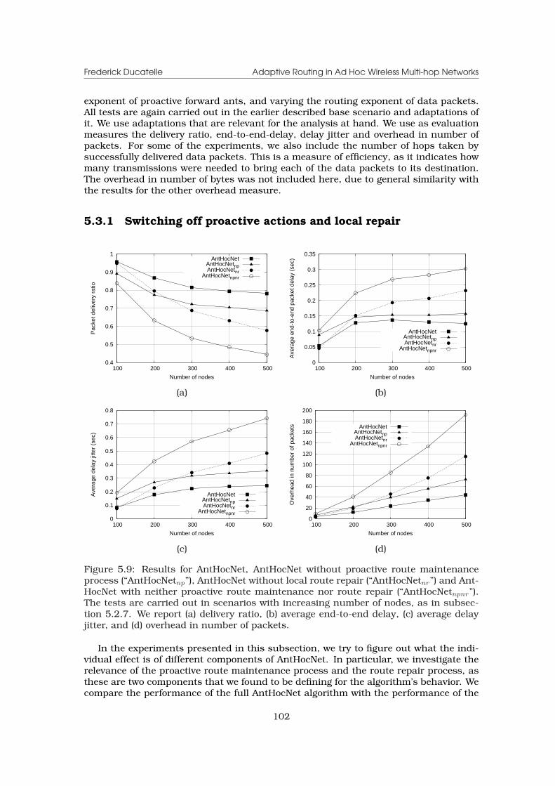
Frederick Ducatelle Adaptive Routing in Ad Hoc Wireless Multi-hop Networks
exponent of proactive forward ants, and varying the routing exponent of data packets.All tests are again carried out in the earlier described base scenario and adaptations ofit. We use adaptations that are relevant for the analysis at hand. We use as evaluationmeasures the delivery ratio, end-to-end-delay, delay jitter and overhead in number ofpackets. For some of the experiments, we also include the number of hops taken bysuccessfully delivered data packets. This is a measure of efficiency, as it indicates howmany transmissions were needed to bring each of the data packets to its destination.The overhead in number of bytes was not included here, due to general similarity withthe results for the other overhead measure.
5.3.1 Switching off proactive actions and local repair
0.4
0.5
0.6
0.7
0.8
0.9
1
100 200 300 400 500
Pac
ket d
eliv
ery
ratio
Number of nodes
AntHocNetAntHocNetnpAntHocNetnr
AntHocNetnpnr
0
0.05
0.1
0.15
0.2
0.25
0.3
0.35
100 200 300 400 500
Ave
rage
end
-to-
end
pack
et d
elay
(se
c)
Number of nodes
AntHocNetAntHocNetnpAntHocNetnr
AntHocNetnpnr
(a) (b)
0
0.1
0.2
0.3
0.4
0.5
0.6
0.7
0.8
100 200 300 400 500
Ave
rage
del
ay ji
tter
(sec
)
Number of nodes
AntHocNetAntHocNetnpAntHocNetnr
AntHocNetnpnr 0
20
40
60
80
100
120
140
160
180
200
100 200 300 400 500
Ove
rhea
d in
num
ber
of p
acke
ts
Number of nodes
AntHocNetAntHocNetnpAntHocNetnr
AntHocNetnpnr
(c) (d)
Figure 5.9: Results for AntHocNet, AntHocNet without proactive route maintenanceprocess (“AntHocNetnp”), AntHocNet without local route repair (“AntHocNetnr”) and Ant-HocNet with neither proactive route maintenance nor route repair (“AntHocNetnpnr”).The tests are carried out in scenarios with increasing number of nodes, as in subsec-tion 5.2.7. We report (a) delivery ratio, (b) average end-to-end delay, (c) average delayjitter, and (d) overhead in number of packets.
In the experiments presented in this subsection, we try to figure out what the indi-vidual effect is of different components of AntHocNet. In particular, we investigate therelevance of the proactive route maintenance process and the route repair process, asthese are two components that we found to be defining for the algorithm’s behavior. Wecompare the performance of the full AntHocNet algorithm with the performance of the
102
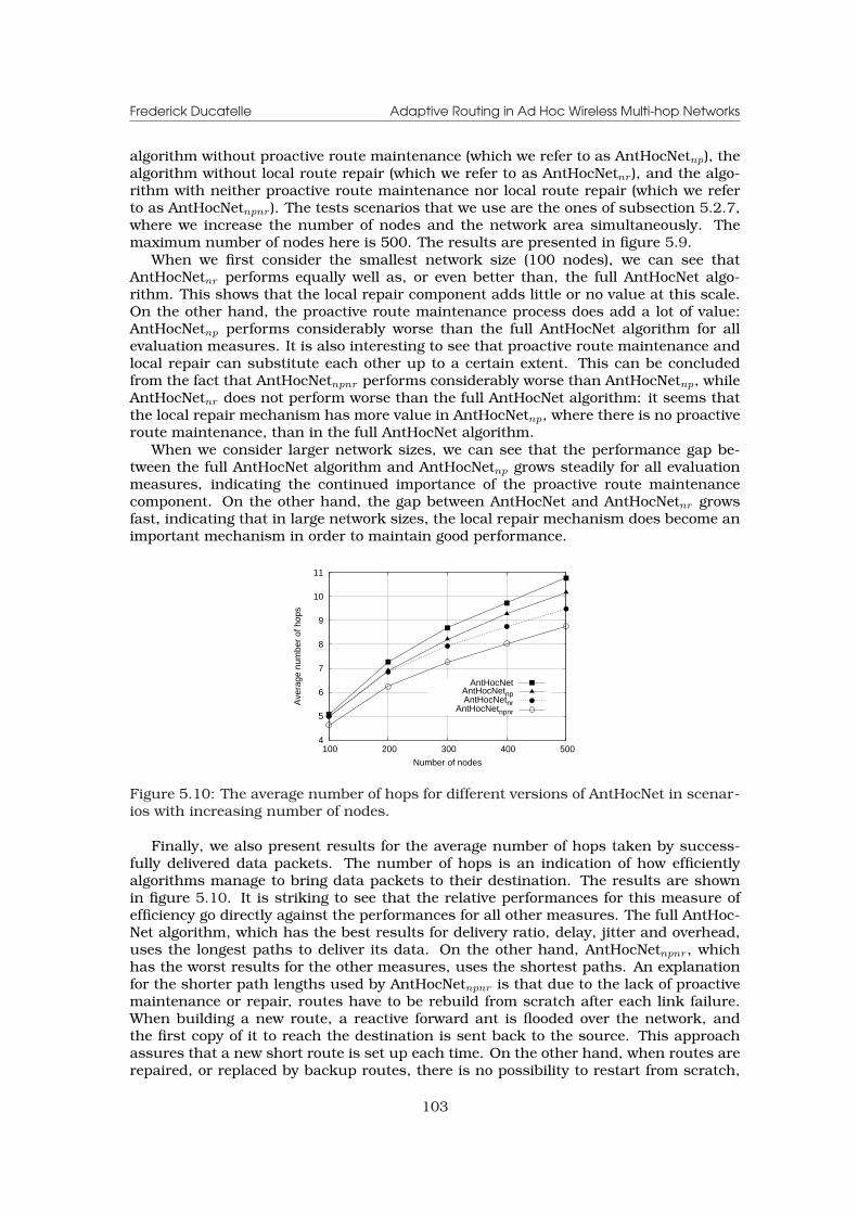
Frederick Ducatelle Adaptive Routing in Ad Hoc Wireless Multi-hop Networks
algorithm without proactive route maintenance (which we refer to as AntHocNetnp), thealgorithm without local route repair (which we refer to as AntHocNetnr), and the algo-rithm with neither proactive route maintenance nor local route repair (which we referto as AntHocNetnpnr). The tests scenarios that we use are the ones of subsection 5.2.7,where we increase the number of nodes and the network area simultaneously. Themaximum number of nodes here is 500. The results are presented in figure 5.9.
When we first consider the smallest network size (100 nodes), we can see thatAntHocNetnr performs equally well as, or even better than, the full AntHocNet algo-rithm. This shows that the local repair component adds little or no value at this scale.On the other hand, the proactive route maintenance process does add a lot of value:AntHocNetnp performs considerably worse than the full AntHocNet algorithm for allevaluation measures. It is also interesting to see that proactive route maintenance andlocal repair can substitute each other up to a certain extent. This can be concludedfrom the fact that AntHocNetnpnr performs considerably worse than AntHocNetnp, whileAntHocNetnr does not perform worse than the full AntHocNet algorithm: it seems thatthe local repair mechanism has more value in AntHocNetnp, where there is no proactiveroute maintenance, than in the full AntHocNet algorithm.
When we consider larger network sizes, we can see that the performance gap be-tween the full AntHocNet algorithm and AntHocNetnp grows steadily for all evaluationmeasures, indicating the continued importance of the proactive route maintenancecomponent. On the other hand, the gap between AntHocNet and AntHocNetnr growsfast, indicating that in large network sizes, the local repair mechanism does become animportant mechanism in order to maintain good performance.
4
5
6
7
8
9
10
11
100 200 300 400 500
Ave
rage
num
ber
of h
ops
Number of nodes
AntHocNetAntHocNetnpAntHocNetnr
AntHocNetnpnr
Figure 5.10: The average number of hops for different versions of AntHocNet in scenar-ios with increasing number of nodes.
Finally, we also present results for the average number of hops taken by success-fully delivered data packets. The number of hops is an indication of how efficientlyalgorithms manage to bring data packets to their destination. The results are shownin figure 5.10. It is striking to see that the relative performances for this measure ofefficiency go directly against the performances for all other measures. The full AntHoc-Net algorithm, which has the best results for delivery ratio, delay, jitter and overhead,uses the longest paths to deliver its data. On the other hand, AntHocNetnpnr, whichhas the worst results for the other measures, uses the shortest paths. An explanationfor the shorter path lengths used by AntHocNetnpnr is that due to the lack of proactivemaintenance or repair, routes have to be rebuild from scratch after each link failure.When building a new route, a reactive forward ant is flooded over the network, andthe first copy of it to reach the destination is sent back to the source. This approachassures that a new short route is set up each time. On the other hand, when routes arerepaired, or replaced by backup routes, there is no possibility to restart from scratch,
103
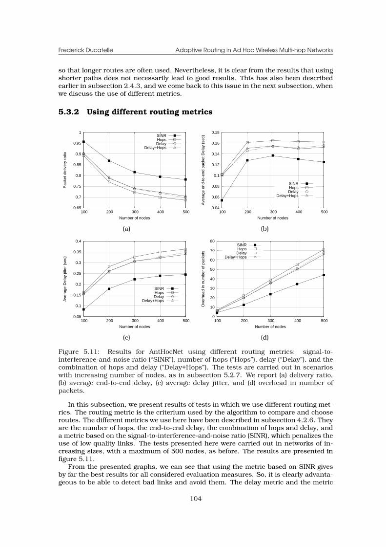
Frederick Ducatelle Adaptive Routing in Ad Hoc Wireless Multi-hop Networks
so that longer routes are often used. Nevertheless, it is clear from the results that usingshorter paths does not necessarily lead to good results. This has also been describedearlier in subsection 2.4.3, and we come back to this issue in the next subsection, whenwe discuss the use of different metrics.
5.3.2 Using different routing metrics
0.65
0.7
0.75
0.8
0.85
0.9
0.95
1
100 200 300 400 500
Pac
ket d
eliv
ery
ratio
Number of nodes
SINRHopsDelay
Delay+Hops
0.04
0.06
0.08
0.1
0.12
0.14
0.16
0.18
100 200 300 400 500
Ave
rage
end
-to-
end
pack
et D
elay
(se
c)
Number of nodes
SINRHopsDelay
Delay+Hops
(a) (b)
0.05
0.1
0.15
0.2
0.25
0.3
0.35
0.4
100 200 300 400 500
Ave
rage
Del
ay ji
tter
(sec
)
Number of nodes
SINRHopsDelay
Delay+Hops
0
10
20
30
40
50
60
70
80
100 200 300 400 500
Ove
rhea
d in
num
ber
of p
acke
ts
Number of nodes
SINRHopsDelay
Delay+Hops
(c) (d)
Figure 5.11: Results for AntHocNet using different routing metrics: signal-to-interference-and-noise ratio (“SINR”), number of hops (“Hops”), delay (“Delay”), and thecombination of hops and delay (“Delay+Hops”). The tests are carried out in scenarioswith increasing number of nodes, as in subsection 5.2.7. We report (a) delivery ratio,(b) average end-to-end delay, (c) average delay jitter, and (d) overhead in number ofpackets.
In this subsection, we present results of tests in which we use different routing met-rics. The routing metric is the criterium used by the algorithm to compare and chooseroutes. The different metrics we use here have been described in subsection 4.2.6. Theyare the number of hops, the end-to-end delay, the combination of hops and delay, anda metric based on the signal-to-interference-and-noise ratio (SINR), which penalizes theuse of low quality links. The tests presented here were carried out in networks of in-creasing sizes, with a maximum of 500 nodes, as before. The results are presented infigure 5.11.
From the presented graphs, we can see that using the metric based on SINR givesby far the best results for all considered evaluation measures. So, it is clearly advanta-geous to be able to detect bad links and avoid them. The delay metric and the metric
104
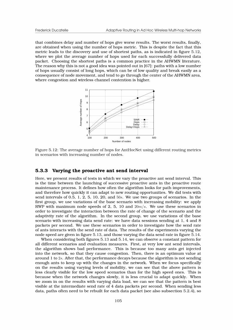
Frederick Ducatelle Adaptive Routing in Ad Hoc Wireless Multi-hop Networks
that combines delay and number of hops give worse results. The worst results, finally,are obtained when using the number of hops metric. This is despite the fact that thismetric leads to the discovery and use of shortest paths, as is indicated in figure 5.12,where we plot the average number of hops used for each successfully delivered datapacket. Choosing the shortest paths is a common practice in the AHWMN literature.The reason why this is not a good idea was pointed out in [67]: paths with a low numberof hops usually consist of long hops, which can be of low quality and break easily as aconsequence of node movement, and tend to go through the center of the AHWMN area,where congestion and wireless channel contention is higher.
4
5
6
7
8
9
10
11
100 200 300 400 500
Ave
rage
num
ber
of H
ops
Number of nodes
SINRHopsDelay
Delay+Hops
Figure 5.12: The average number of hops for AntHocNet using different routing metricsin scenarios with increasing number of nodes.
5.3.3 Varying the proactive ant send interval
Here, we present results of tests in which we vary the proactive ant send interval. Thisis the time between the launching of successive proactive ants in the proactive routemaintenance process. It defines how often the algorithm looks for path improvements,and therefore how quickly it can adapt to new routing opportunities. We did tests withsend intervals of 0.5, 1, 2, 5, 10, 20, and 50s. We use two groups of scenarios. In thefirst group, we use variations of the base scenario with increasing mobility: we applyRWP with maximum node speeds of 2, 5, 10 and 20m/s. We use these scenarios inorder to investigate the interaction between the rate of change of the scenario and theadaptivity rate of the algorithm. In the second group, we use variations of the basescenario with increasing data send rate: we have data sessions sending at 1, 4 and 8packets per second. We use these scenarios in order to investigate how the send rateof ants interacts with the send rate of data. The results of the experiments varying thenode speed are given in figure 5.13, and those varying the data send rate in figure 5.14.
When considering both figures 5.13 and 5.14, we can observe a constant pattern forall different scenarios and evaluation measures. First, at very low ant send intervals,the algorithm shows bad performance. This is because too many ants get injectedinto the network, so that they cause congestion. Then, there is an optimum value ataround 1 to 2s. After that, the performance decays because the algorithm is not sendingenough ants to keep up with the changes in the network. When we focus specificallyon the results using varying levels of mobility, we can see that the above pattern isless clearly visible for the low speed scenarios than for the high speed ones. This isbecause when the network changes slowly, it is less crucial to adapt quickly. Whenwe zoom in on the results with varying data load, we can see that the pattern is bestvisible at the intermediate send rate of 4 data packets per second. When sending lessdata, paths often need to be rebuilt for each data packet (see also subsection 5.2.4), so
105
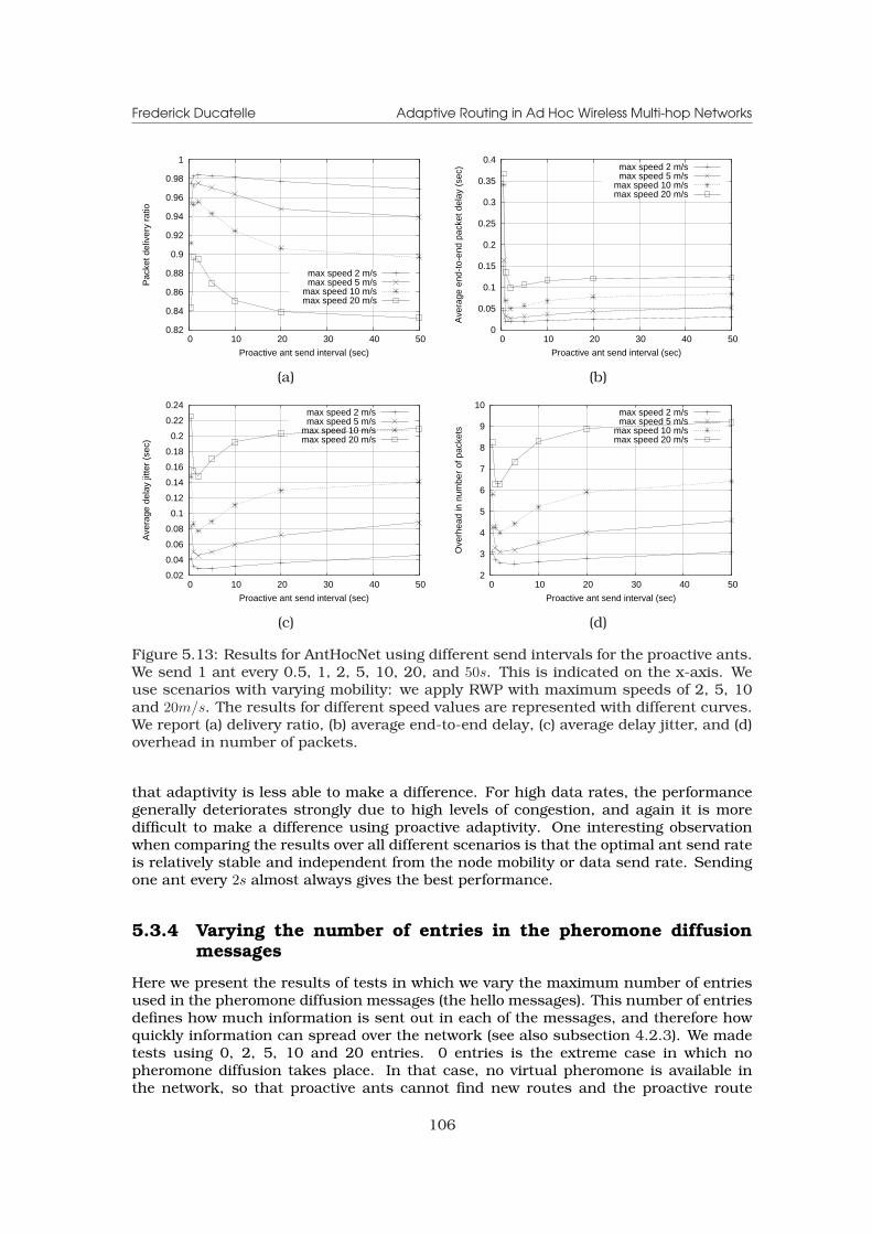
Frederick Ducatelle Adaptive Routing in Ad Hoc Wireless Multi-hop Networks
0.82
0.84
0.86
0.88
0.9
0.92
0.94
0.96
0.98
1
0 10 20 30 40 50
Pac
ket d
eliv
ery
ratio
Proactive ant send interval (sec)
max speed 2 m/smax speed 5 m/s
max speed 10 m/smax speed 20 m/s
0
0.05
0.1
0.15
0.2
0.25
0.3
0.35
0.4
0 10 20 30 40 50
Ave
rage
end
-to-
end
pack
et d
elay
(se
c)
Proactive ant send interval (sec)
max speed 2 m/smax speed 5 m/s
max speed 10 m/smax speed 20 m/s
(a) (b)
0.02
0.04
0.06
0.08
0.1
0.12
0.14
0.16
0.18
0.2
0.22
0.24
0 10 20 30 40 50
Ave
rage
del
ay ji
tter
(sec
)
Proactive ant send interval (sec)
max speed 2 m/smax speed 5 m/s
max speed 10 m/smax speed 20 m/s
2
3
4
5
6
7
8
9
10
0 10 20 30 40 50
Ove
rhea
d in
num
ber
of p
acke
ts
Proactive ant send interval (sec)
max speed 2 m/smax speed 5 m/s
max speed 10 m/smax speed 20 m/s
(c) (d)
Figure 5.13: Results for AntHocNet using different send intervals for the proactive ants.We send 1 ant every 0.5, 1, 2, 5, 10, 20, and 50s. This is indicated on the x-axis. Weuse scenarios with varying mobility: we apply RWP with maximum speeds of 2, 5, 10and 20m/s. The results for different speed values are represented with different curves.We report (a) delivery ratio, (b) average end-to-end delay, (c) average delay jitter, and (d)overhead in number of packets.
that adaptivity is less able to make a difference. For high data rates, the performancegenerally deteriorates strongly due to high levels of congestion, and again it is moredifficult to make a difference using proactive adaptivity. One interesting observationwhen comparing the results over all different scenarios is that the optimal ant send rateis relatively stable and independent from the node mobility or data send rate. Sendingone ant every 2s almost always gives the best performance.
5.3.4 Varying the number of entries in the pheromone diffusionmessages
Here we present the results of tests in which we vary the maximum number of entriesused in the pheromone diffusion messages (the hello messages). This number of entriesdefines how much information is sent out in each of the messages, and therefore howquickly information can spread over the network (see also subsection 4.2.3). We madetests using 0, 2, 5, 10 and 20 entries. 0 entries is the extreme case in which nopheromone diffusion takes place. In that case, no virtual pheromone is available inthe network, so that proactive ants cannot find new routes and the proactive route
106
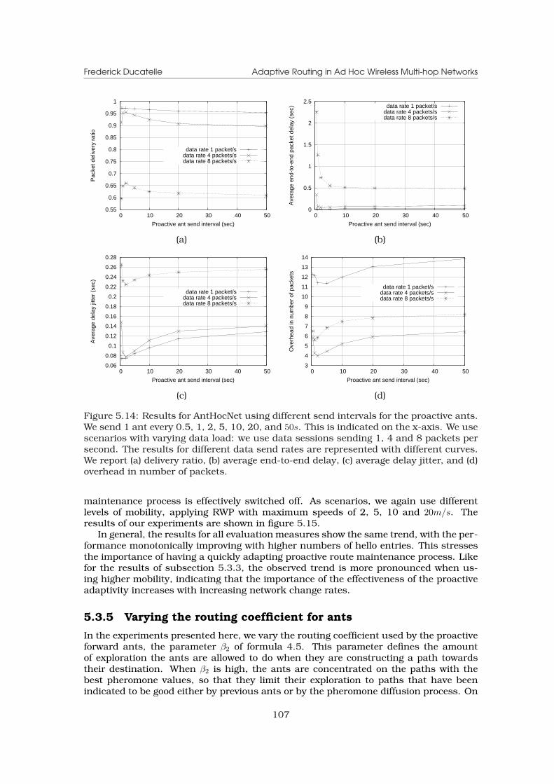
Frederick Ducatelle Adaptive Routing in Ad Hoc Wireless Multi-hop Networks
0.55
0.6
0.65
0.7
0.75
0.8
0.85
0.9
0.95
1
0 10 20 30 40 50
Pac
ket d
eliv
ery
ratio
Proactive ant send interval (sec)
data rate 1 packet/sdata rate 4 packets/sdata rate 8 packets/s
0
0.5
1
1.5
2
2.5
0 10 20 30 40 50
Ave
rage
end
-to-
end
pack
et d
elay
(se
c)
Proactive ant send interval (sec)
data rate 1 packet/sdata rate 4 packets/sdata rate 8 packets/s
(a) (b)
0.06
0.08
0.1
0.12
0.14
0.16
0.18
0.2
0.22
0.24
0.26
0.28
0 10 20 30 40 50
Ave
rage
del
ay ji
tter
(sec
)
Proactive ant send interval (sec)
data rate 1 packet/sdata rate 4 packets/sdata rate 8 packets/s
3
4
5
6
7
8
9
10
11
12
13
14
0 10 20 30 40 50
Ove
rhea
d in
num
ber
of p
acke
ts
Proactive ant send interval (sec)
data rate 1 packet/sdata rate 4 packets/sdata rate 8 packets/s
(c) (d)
Figure 5.14: Results for AntHocNet using different send intervals for the proactive ants.We send 1 ant every 0.5, 1, 2, 5, 10, 20, and 50s. This is indicated on the x-axis. We usescenarios with varying data load: we use data sessions sending 1, 4 and 8 packets persecond. The results for different data send rates are represented with different curves.We report (a) delivery ratio, (b) average end-to-end delay, (c) average delay jitter, and (d)overhead in number of packets.
maintenance process is effectively switched off. As scenarios, we again use differentlevels of mobility, applying RWP with maximum speeds of 2, 5, 10 and 20m/s. Theresults of our experiments are shown in figure 5.15.
In general, the results for all evaluation measures show the same trend, with the per-formance monotonically improving with higher numbers of hello entries. This stressesthe importance of having a quickly adapting proactive route maintenance process. Likefor the results of subsection 5.3.3, the observed trend is more pronounced when us-ing higher mobility, indicating that the importance of the effectiveness of the proactiveadaptivity increases with increasing network change rates.
5.3.5 Varying the routing coefficient for ants
In the experiments presented here, we vary the routing coefficient used by the proactiveforward ants, the parameter β2 of formula 4.5. This parameter defines the amountof exploration the ants are allowed to do when they are constructing a path towardstheir destination. When β2 is high, the ants are concentrated on the paths with thebest pheromone values, so that they limit their exploration to paths that have beenindicated to be good either by previous ants or by the pheromone diffusion process. On
107
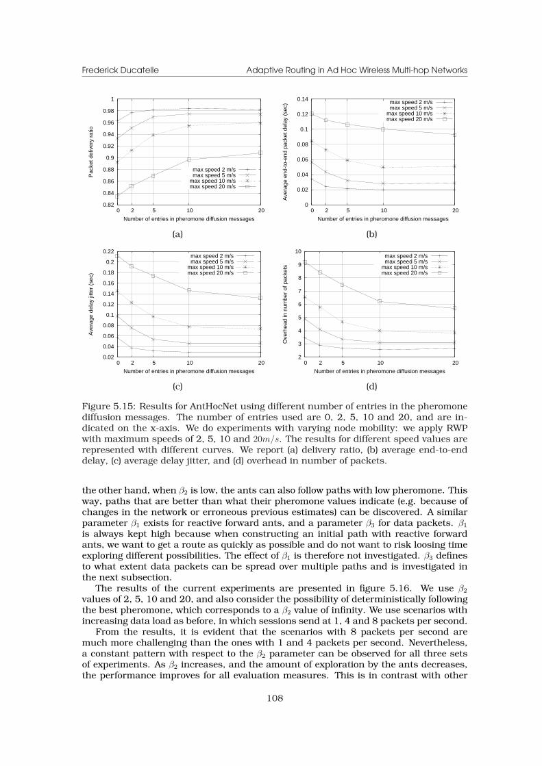
Frederick Ducatelle Adaptive Routing in Ad Hoc Wireless Multi-hop Networks
0.82
0.84
0.86
0.88
0.9
0.92
0.94
0.96
0.98
1
20 10 5 2 0
Pac
ket d
eliv
ery
ratio
Number of entries in pheromone diffusion messages
max speed 2 m/smax speed 5 m/s
max speed 10 m/smax speed 20 m/s
0
0.02
0.04
0.06
0.08
0.1
0.12
0.14
20 10 5 2 0
Ave
rage
end
-to-
end
pack
et d
elay
(se
c)
Number of entries in pheromone diffusion messages
max speed 2 m/smax speed 5 m/s
max speed 10 m/smax speed 20 m/s
(a) (b)
0.02
0.04
0.06
0.08
0.1
0.12
0.14
0.16
0.18
0.2
0.22
20 10 5 2 0
Ave
rage
del
ay ji
tter
(sec
)
Number of entries in pheromone diffusion messages
max speed 2 m/smax speed 5 m/s
max speed 10 m/smax speed 20 m/s
2
3
4
5
6
7
8
9
10
20 10 5 2 0
Ove
rhea
d in
num
ber
of p
acke
ts
Number of entries in pheromone diffusion messages
max speed 2 m/smax speed 5 m/s
max speed 10 m/smax speed 20 m/s
(c) (d)
Figure 5.15: Results for AntHocNet using different number of entries in the pheromonediffusion messages. The number of entries used are 0, 2, 5, 10 and 20, and are in-dicated on the x-axis. We do experiments with varying node mobility: we apply RWPwith maximum speeds of 2, 5, 10 and 20m/s. The results for different speed values arerepresented with different curves. We report (a) delivery ratio, (b) average end-to-enddelay, (c) average delay jitter, and (d) overhead in number of packets.
the other hand, when β2 is low, the ants can also follow paths with low pheromone. Thisway, paths that are better than what their pheromone values indicate (e.g. because ofchanges in the network or erroneous previous estimates) can be discovered. A similarparameter β1 exists for reactive forward ants, and a parameter β3 for data packets. β1
is always kept high because when constructing an initial path with reactive forwardants, we want to get a route as quickly as possible and do not want to risk loosing timeexploring different possibilities. The effect of β1 is therefore not investigated. β3 definesto what extent data packets can be spread over multiple paths and is investigated inthe next subsection.
The results of the current experiments are presented in figure 5.16. We use β2
values of 2, 5, 10 and 20, and also consider the possibility of deterministically followingthe best pheromone, which corresponds to a β2 value of infinity. We use scenarios withincreasing data load as before, in which sessions send at 1, 4 and 8 packets per second.
From the results, it is evident that the scenarios with 8 packets per second aremuch more challenging than the ones with 1 and 4 packets per second. Nevertheless,a constant pattern with respect to the β2 parameter can be observed for all three setsof experiments. As β2 increases, and the amount of exploration by the ants decreases,the performance improves for all evaluation measures. This is in contrast with other
108
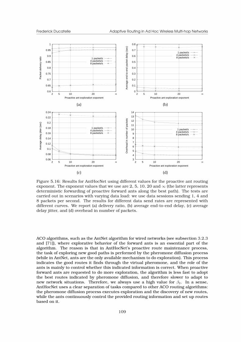
Frederick Ducatelle Adaptive Routing in Ad Hoc Wireless Multi-hop Networks
0.6
0.65
0.7
0.75
0.8
0.85
0.9
0.95
1
∞201052
Pac
ket d
eliv
ery
ratio
Proactive ant exploration exponent
1 packet/s4 packets/s8 packets/s
0
0.1
0.2
0.3
0.4
0.5
0.6
0.7
0.8
∞201052
Ave
rage
end
-to-
end
pack
et d
elay
(se
c)
Proactive ant exploration exponent
1 packet/s4 packets/s8 packets/s
(a) (b)
0.06
0.08
0.1
0.12
0.14
0.16
0.18
0.2
0.22
0.24
∞201052
Ave
rage
del
ay ji
tter
(sec
)
Proactive ant exploration exponent
1 packet/s4 packets/s8 packets/s
3
4
5
6
7
8
9
10
11
12
13
14
∞201052
Ove
rhea
d in
num
ber
of p
acke
ts
Proactive ant exploration exponent
1 packet/s4 packets/s8 packets/s
(c) (d)
Figure 5.16: Results for AntHocNet using different values for the proactive ant routingexponent. The exponent values that we use are 2, 5, 10, 20 and ∞ (the latter representsdeterministic forwarding of proactive forward ants along the best path). The tests arecarried out in scenarios with varying data load: we use data sessions sending 1, 4 and8 packets per second. The results for different data send rates are represented withdifferent curves. We report (a) delivery ratio, (b) average end-to-end delay, (c) averagedelay jitter, and (d) overhead in number of packets.
ACO algorithms, such as the AntNet algorithm for wired networks (see subsection 3.2.3and [71]), where explorative behavior of the forward ants is an essential part of thealgorithm. The reason is that in AntHocNet’s proactive route maintenance process,the task of exploring new good paths is performed by the pheromone diffusion process(while in AntNet, ants are the only available mechanism to do exploration). This processindicates the good routes it finds through the virtual pheromone, and the role of theants is mainly to control whether this indicated information is correct. When proactiveforward ants are requested to do more exploration, the algorithm is less fast to adoptthe best routes indicated by pheromone diffusion, and therefore slower to adapt tonew network situations. Therefore, we always use a high value for β2. In a sense,AntHocNet uses a clear separation of tasks compared to other ACO routing algorithms:the pheromone diffusion process executes exploration and the discovery of new routes,while the ants continuously control the provided routing information and set up routesbased on it.
109
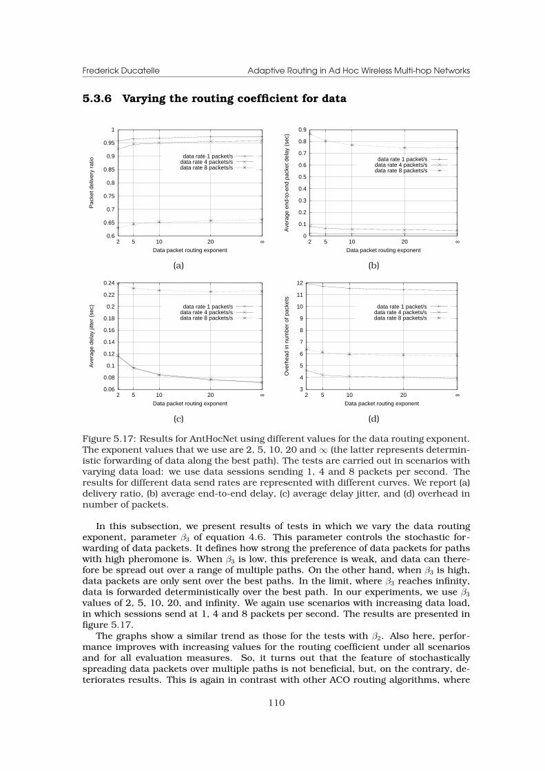
Frederick Ducatelle Adaptive Routing in Ad Hoc Wireless Multi-hop Networks
5.3.6 Varying the routing coefficient for data
0.6
0.65
0.7
0.75
0.8
0.85
0.9
0.95
1
∞201052
Pac
ket d
eliv
ery
ratio
Data packet routing exponent
data rate 1 packet/sdata rate 4 packets/sdata rate 8 packets/s
0
0.1
0.2
0.3
0.4
0.5
0.6
0.7
0.8
0.9
∞201052
Ave
rage
end
-to-
end
pack
et d
elay
(se
c)
Data packet routing exponent
data rate 1 packet/sdata rate 4 packets/sdata rate 8 packets/s
(a) (b)
0.06
0.08
0.1
0.12
0.14
0.16
0.18
0.2
0.22
0.24
∞201052
Ave
rage
del
ay ji
tter
(sec
)
Data packet routing exponent
data rate 1 packet/sdata rate 4 packets/sdata rate 8 packets/s
3
4
5
6
7
8
9
10
11
12
∞201052
Ove
rhea
d in
num
ber
of p
acke
ts
Data packet routing exponent
data rate 1 packet/sdata rate 4 packets/sdata rate 8 packets/s
(c) (d)
Figure 5.17: Results for AntHocNet using different values for the data routing exponent.The exponent values that we use are 2, 5, 10, 20 and ∞ (the latter represents determin-istic forwarding of data along the best path). The tests are carried out in scenarios withvarying data load: we use data sessions sending 1, 4 and 8 packets per second. Theresults for different data send rates are represented with different curves. We report (a)delivery ratio, (b) average end-to-end delay, (c) average delay jitter, and (d) overhead innumber of packets.
In this subsection, we present results of tests in which we vary the data routingexponent, parameter β3 of equation 4.6. This parameter controls the stochastic for-warding of data packets. It defines how strong the preference of data packets for pathswith high pheromone is. When β3 is low, this preference is weak, and data can there-fore be spread out over a range of multiple paths. On the other hand, when β3 is high,data packets are only sent over the best paths. In the limit, where β3 reaches infinity,data is forwarded deterministically over the best path. In our experiments, we use β3
values of 2, 5, 10, 20, and infinity. We again use scenarios with increasing data load,in which sessions send at 1, 4 and 8 packets per second. The results are presented infigure 5.17.
The graphs show a similar trend as those for the tests with β2. Also here, perfor-mance improves with increasing values for the routing coefficient under all scenariosand for all evaluation measures. So, it turns out that the feature of stochasticallyspreading data packets over multiple paths is not beneficial, but, on the contrary, de-teriorates results. This is again in contrast with other ACO routing algorithms, where
110
Frederick Ducatelle Adaptive Routing in Ad Hoc Wireless Multi-hop Networks
stochastic data forwarding allows to improve performance by spreading the data loadover multiple paths and making better use of the full network resources. An expla-nation of why this is not working in the case of AntHocNet can be found in the factthat in AHWMNs different paths between source and destination nodes are not verywell separated: due to radio interference, data packets traveling over parallel pathscan hinder each other, so that it is difficult to obtain any advantages. This issue canpossibly be dealt with if specific mechanisms are used during the construction of thedifferent paths, e.g. choosing paths that go over nodes that are outside each other’stransmission range (see also subsection 2.4.3). However, such mechanisms would bequite complex, especially if we take into account the fact that nodes move, and pathsthat were originally sufficiently apart could move into each other’s transmission range.In AntHocNet, we did not use such an approach. Instead, we keep the data routingcoefficient high, and only use the very best paths. This way, we maximally exploit thebest routes available.
5.3.7 Summary
In this section we have presented results of tests in which we switched on and off differ-ent components of the AntHocNet routing algorithm and varied its internal parameters.The aim was to investigate AntHocNet’s internal working.
First, we have looked at the individual contribution to the algorithm’s performanceof the proactive route maintenance process and the reactive route repair mechanism.We have shown that the proactive route maintenance process has a strong positiveinfluence on the performance over a range of different scenarios. On the other hand,the reactive route repair mechanism turned out to have a large positive contribution inlarge networks but very little or no contribution in small networks.
Next, we have investigated the use of different routing metrics. From the results, itwas clear that the metric using the SINR was superior. The metric using delay and theone using a combination of delay and hops gave worse results. The worst results werefor the number of hops metric, despite the fact that this metric lead to the use of theshortest paths and is very often used for routing in AHWMNs.
Then, we have investigated two parameters that are related to the speed of workingof the proactive route maintenance process: we have done tests varying the send rateof proactive forward ants and varying the number of entries in the pheromone diffusionmessages. Both tests indicated that a faster working proactive route maintenance pro-cess is better: sending ants more regularly and spreading out more information in eachmessage during pheromone diffusion gave better results. Limits are present only whentoo much overhead is created. For example, sending more ants than one per secondlead to rather bad results.
Finally, we have done tests varying the routing coefficient of proactive forward antsand data packets. In both cases, it turned out that increasing the coefficient lead tomonotonically improving results. In the case of proactive forward ants, this shows thatit is better to leave the task of exploring new paths to the pheromone diffusion process,and let the ants focus on the task of controlling the obtained information and turn itinto routes that can be used for data. In the case of data packets, it shows that it isdifficult to get throughput advantage from spreading data over multiple paths, and thatinstead it is better to fully exploit the best routes found by the ants.
5.4 Conclusion
In this chapter we have provided an evaluation study of the AntHocNet routing algo-rithm. Tests were carried out in scenarios that are similar to those commonly used inthe literature on MANET routing.
111
Frederick Ducatelle Adaptive Routing in Ad Hoc Wireless Multi-hop Networks
In a first set of tests, we compared AntHocNet to existing state-of-the-art rout-ing algorithms. These included AODV, a reference reactive routing algorithm, OLSR,an important proactive routing algorithm, and ANSI, which is a representative of theclass of ACO routing algorithms. Results showed that AntHocNet could outperform theother three algorithms over a wide range of different scenarios. Specifically, AntHocNetturned out to perform well in tests with increasing levels of mobility, to deal better thanthe other algorithms with different levels of data load, to cope well with sparse networksituations, and to scale well to networks of increasing sizes. On the downside, Ant-HocNet’s advantage was decreased when mobility got very high, and the algorithm wasoutperformed by AODV when very dense scenarios were used.
In a second set of tests, we investigated the internal working of AntHocNet. Weswitched on and off the use of different components of the algorithm, and varied variousinternal parameters. We found that the proactive maintenance process has a highcontribution to the algorithm’s performance over a range of scenarios, while the localrepair mechanism did not have a positive effect in small networks, but was increasinglyvaluable in large ones. We also found that it is important that the proactive maintenanceprocess works as fast as possible, as long as it does not produce excessive overhead.Among the possible routing metrics, we discovered that the SINR based metric lead tothe best results. Finally, we saw that exploration in the proactive route maintenanceprocess should be left to the pheromone diffusion process rather than to the ants, andthat data packets should be forwarded over the best paths, with minimal data loadspreading.
112
Chapter 6
Simulation of an urban scenario
In the previous chapter we have presented the results of a number of tests in whichwe evaluate the performance of the AntHocNet routing algorithm. All of those testsused scenarios that were derived from a common base scenario, in which a numberof nodes move in an open, rectangular area along straight line segments, and dataare sent at fixed rates. The reason to use this type of scenarios was to stay in linewith the common practice in the literature, so that comparisons with other algorithmsare easier and more fair. However, as was pointed out already in subsection 5.1.1,these scenarios are rather simple, and might not give a correct image of situationsthat occur in reality. Therefore, observed results are not necessarily representativefor what can be expected when the network is deployed for a practical application.The aim of the current chapter is to complement the previous tests with new onesthat use more realistic scenarios. For these new scenarios, we have chosen an urbanenvironment, as the development of recent projects with public WMNs in some citiessuch as Philadelphia [12] and Taipei [10] indicate that this will be an important area ofapplication for AHWMN technology. We take special care to simulate this environmentand the use of an AHWMN in it in an accurate way. We use this detailed simulation tomake new evaluations of AntHocNet’s performance.
The rest of this chapter is organized as follows. First, we describe the simulationsetup, giving special attention to the way we obtained a model of wireless communica-tion in the urban environment and how we were able to simulate it in an efficient way.Then, we present results of a simulation study, in which we first investigate networkproperties of the AHWMN in the urban environment, and then perform a comparativetest of the AntHocNet and AODV routing algorithms. The work presented here has beendescribed in [97] and in project deliverable [49].
6.1 Design of the simulation study
In this section we describe the design of the simulation study. In what follows we firstprovide a general overview of the study. Then, we give detailed descriptions of the urbanenvironment and the implementation of node mobility, of the used radio propagationmodels and their implementation, and of the simulated data traffic. Finally, we reviewrelated literature on the topic of simulations of AHWMNs in urban settings.
6.1.1 General description of the simulation study
The aim of the study presented in this chapter is to evaluate the behavior of the AntHoc-Net routing protocol in an urban environment through simulation. We have chosen the
113
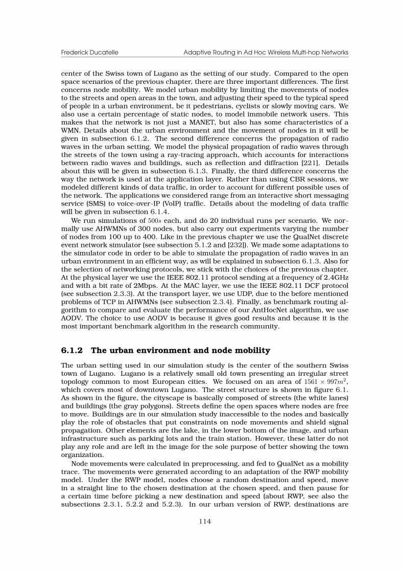
Frederick Ducatelle Adaptive Routing in Ad Hoc Wireless Multi-hop Networks
center of the Swiss town of Lugano as the setting of our study. Compared to the openspace scenarios of the previous chapter, there are three important differences. The firstconcerns node mobility. We model urban mobility by limiting the movements of nodesto the streets and open areas in the town, and adjusting their speed to the typical speedof people in a urban environment, be it pedestrians, cyclists or slowly moving cars. Wealso use a certain percentage of static nodes, to model immobile network users. Thismakes that the network is not just a MANET, but also has some characteristics of aWMN. Details about the urban environment and the movement of nodes in it will begiven in subsection 6.1.2. The second difference concerns the propagation of radiowaves in the urban setting. We model the physical propagation of radio waves throughthe streets of the town using a ray-tracing approach, which accounts for interactionsbetween radio waves and buildings, such as reflection and diffraction [221]. Detailsabout this will be given in subsection 6.1.3. Finally, the third difference concerns theway the network is used at the application layer. Rather than using CBR sessions, wemodeled different kinds of data traffic, in order to account for different possible uses ofthe network. The applications we considered range from an interactive short messagingservice (SMS) to voice-over-IP (VoIP) traffic. Details about the modeling of data trafficwill be given in subsection 6.1.4.
We run simulations of 500s each, and do 20 individual runs per scenario. We nor-mally use AHWMNs of 300 nodes, but also carry out experiments varying the numberof nodes from 100 up to 400. Like in the previous chapter we use the QualNet discreteevent network simulator (see subsection 5.1.2 and [232]). We made some adaptations tothe simulator code in order to be able to simulate the propagation of radio waves in anurban environment in an efficient way, as will be explained in subsection 6.1.3. Also forthe selection of networking protocols, we stick with the choices of the previous chapter.At the physical layer we use the IEEE 802.11 protocol sending at a frequency of 2.4GHzand with a bit rate of 2Mbps. At the MAC layer, we use the IEEE 802.11 DCF protocol(see subsection 2.3.3). At the transport layer, we use UDP, due to the before mentionedproblems of TCP in AHWMNs (see subsection 2.3.4). Finally, as benchmark routing al-gorithm to compare and evaluate the performance of our AntHocNet algorithm, we useAODV. The choice to use AODV is because it gives good results and because it is themost important benchmark algorithm in the research community.
6.1.2 The urban environment and node mobility
The urban setting used in our simulation study is the center of the southern Swisstown of Lugano. Lugano is a relatively small old town presenting an irregular streettopology common to most European cities. We focused on an area of 1561 × 997m2,which covers most of downtown Lugano. The street structure is shown in figure 6.1.As shown in the figure, the cityscape is basically composed of streets (the white lanes)and buildings (the gray polygons). Streets define the open spaces where nodes are freeto move. Buildings are in our simulation study inaccessible to the nodes and basicallyplay the role of obstacles that put constraints on node movements and shield signalpropagation. Other elements are the lake, in the lower bottom of the image, and urbaninfrastructure such as parking lots and the train station. However, these latter do notplay any role and are left in the image for the sole purpose of better showing the townorganization.
Node movements were calculated in preprocessing, and fed to QualNet as a mobilitytrace. The movements were generated according to an adaptation of the RWP mobilitymodel. Under the RWP model, nodes choose a random destination and speed, movein a straight line to the chosen destination at the chosen speed, and then pause fora certain time before picking a new destination and speed (about RWP, see also thesubsections 2.3.1, 5.2.2 and 5.2.3). In our urban version of RWP, destinations are
114
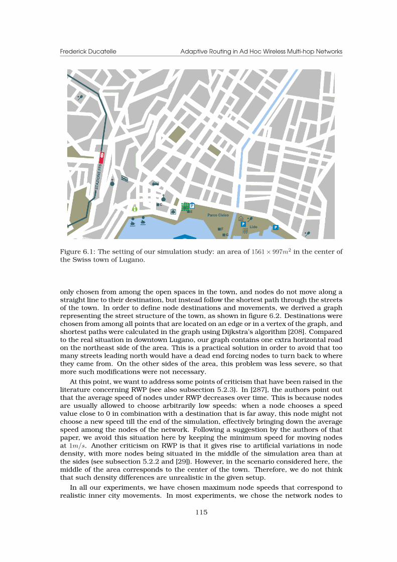
Frederick Ducatelle Adaptive Routing in Ad Hoc Wireless Multi-hop Networks
Figure 6.1: The setting of our simulation study: an area of 1561× 997m2 in the center ofthe Swiss town of Lugano.
only chosen from among the open spaces in the town, and nodes do not move along astraight line to their destination, but instead follow the shortest path through the streetsof the town. In order to define node destinations and movements, we derived a graphrepresenting the street structure of the town, as shown in figure 6.2. Destinations werechosen from among all points that are located on an edge or in a vertex of the graph, andshortest paths were calculated in the graph using Dijkstra’s algorithm [208]. Comparedto the real situation in downtown Lugano, our graph contains one extra horizontal roadon the northeast side of the area. This is a practical solution in order to avoid that toomany streets leading north would have a dead end forcing nodes to turn back to wherethey came from. On the other sides of the area, this problem was less severe, so thatmore such modifications were not necessary.
At this point, we want to address some points of criticism that have been raised in theliterature concerning RWP (see also subsection 5.2.3). In [287], the authors point outthat the average speed of nodes under RWP decreases over time. This is because nodesare usually allowed to choose arbitrarily low speeds: when a node chooses a speedvalue close to 0 in combination with a destination that is far away, this node might notchoose a new speed till the end of the simulation, effectively bringing down the averagespeed among the nodes of the network. Following a suggestion by the authors of thatpaper, we avoid this situation here by keeping the minimum speed for moving nodesat 1m/s. Another criticism on RWP is that it gives rise to artificial variations in nodedensity, with more nodes being situated in the middle of the simulation area than atthe sides (see subsection 5.2.2 and [29]). However, in the scenario considered here, themiddle of the area corresponds to the center of the town. Therefore, we do not thinkthat such density differences are unrealistic in the given setup.
In all our experiments, we have chosen maximum node speeds that correspond torealistic inner city movements. In most experiments, we chose the network nodes to
115

Frederick Ducatelle Adaptive Routing in Ad Hoc Wireless Multi-hop Networks
Figure 6.2: A graph representing street patterns in our urban environment. The graphis indicated by the red lines in the figure. This graph was used to calculate locationsand movements for the network nodes.
be pedestrians or cyclists, with a maximum speed of 3m/s (10.8km/h). Only for theset of experiments with increased mobility, we allow nodes to go up to 15m/s (54km/h),which is a reasonable maximum speed for cars in an urban environment. The pausetime of our RWP model is always 30s. Finally, in all experiments, we keep 20% of thenodes static, to represent immobile network users in the town. These can for examplebe wireless access points placed by shop or restaurant owners, or mesh infrastructurenodes provided by the town authorities. Due to the presence of these static nodes, thenetworks considered here have more similarities with WMNs than those studied in theexperiments of chapter 5, which could be considered pure MANETs.
6.1.3 Radio propagation
Wireless communication in an urban environment is strongly conditioned by the wayradio waves interact with the objects they encounter. The most basic effect is thatwaves produced at street level are blocked by buildings, so that connectivity in urbanwireless networks is restricted compared to open space scenarios. Some urban simula-tion studies for AHWMNs in the literature only account for this effect, using open spacepropagation models along the line of sight (LoS) and blocking any non-LoS communica-tion (see e.g. [188]). In our study, we use a more detailed approach, which incorporatesalso other propagation effects. The most important of these effects is reflection off build-ings: as radio rays bounce off building walls, they can travel around corners into sidestreets. Also, reflection allows a signal to travel further along the LoS through a streetthan it would in open space, since multiple reflected rays are tunneled in the same di-rection. This means that crude approximation models that do not account for reflectionare too restrictive. Another important effect is diffraction, which allows rays to bendaround corners to a certain extent. This further improves connectivity into side streets.
116
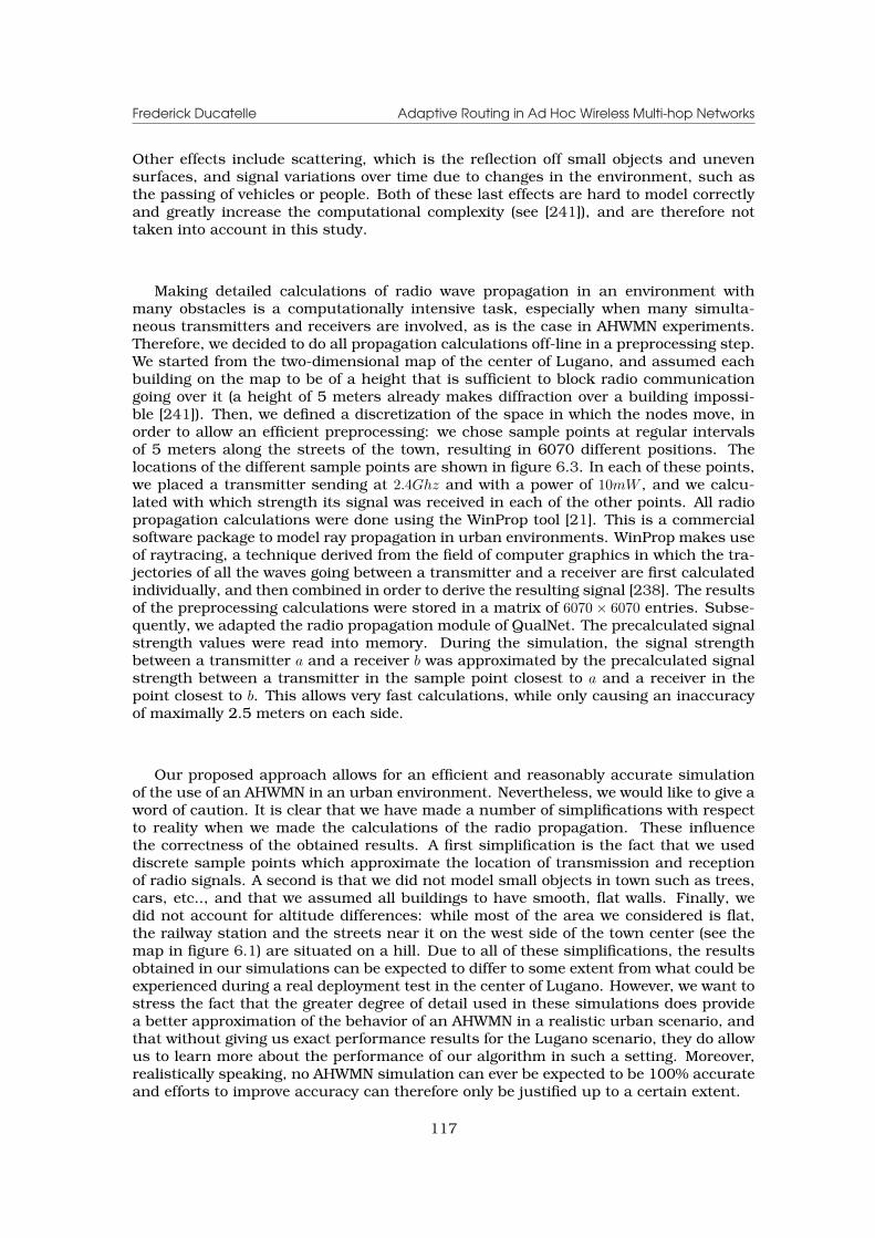
Frederick Ducatelle Adaptive Routing in Ad Hoc Wireless Multi-hop Networks
Other effects include scattering, which is the reflection off small objects and unevensurfaces, and signal variations over time due to changes in the environment, such asthe passing of vehicles or people. Both of these last effects are hard to model correctlyand greatly increase the computational complexity (see [241]), and are therefore nottaken into account in this study.
Making detailed calculations of radio wave propagation in an environment withmany obstacles is a computationally intensive task, especially when many simulta-neous transmitters and receivers are involved, as is the case in AHWMN experiments.Therefore, we decided to do all propagation calculations off-line in a preprocessing step.We started from the two-dimensional map of the center of Lugano, and assumed eachbuilding on the map to be of a height that is sufficient to block radio communicationgoing over it (a height of 5 meters already makes diffraction over a building impossi-ble [241]). Then, we defined a discretization of the space in which the nodes move, inorder to allow an efficient preprocessing: we chose sample points at regular intervalsof 5 meters along the streets of the town, resulting in 6070 different positions. Thelocations of the different sample points are shown in figure 6.3. In each of these points,we placed a transmitter sending at 2.4Ghz and with a power of 10mW , and we calcu-lated with which strength its signal was received in each of the other points. All radiopropagation calculations were done using the WinProp tool [21]. This is a commercialsoftware package to model ray propagation in urban environments. WinProp makes useof raytracing, a technique derived from the field of computer graphics in which the tra-jectories of all the waves going between a transmitter and a receiver are first calculatedindividually, and then combined in order to derive the resulting signal [238]. The resultsof the preprocessing calculations were stored in a matrix of 6070× 6070 entries. Subse-quently, we adapted the radio propagation module of QualNet. The precalculated signalstrength values were read into memory. During the simulation, the signal strengthbetween a transmitter a and a receiver b was approximated by the precalculated signalstrength between a transmitter in the sample point closest to a and a receiver in thepoint closest to b. This allows very fast calculations, while only causing an inaccuracyof maximally 2.5 meters on each side.
Our proposed approach allows for an efficient and reasonably accurate simulationof the use of an AHWMN in an urban environment. Nevertheless, we would like to give aword of caution. It is clear that we have made a number of simplifications with respectto reality when we made the calculations of the radio propagation. These influencethe correctness of the obtained results. A first simplification is the fact that we useddiscrete sample points which approximate the location of transmission and receptionof radio signals. A second is that we did not model small objects in town such as trees,cars, etc.., and that we assumed all buildings to have smooth, flat walls. Finally, wedid not account for altitude differences: while most of the area we considered is flat,the railway station and the streets near it on the west side of the town center (see themap in figure 6.1) are situated on a hill. Due to all of these simplifications, the resultsobtained in our simulations can be expected to differ to some extent from what could beexperienced during a real deployment test in the center of Lugano. However, we want tostress the fact that the greater degree of detail used in these simulations does providea better approximation of the behavior of an AHWMN in a realistic urban scenario, andthat without giving us exact performance results for the Lugano scenario, they do allowus to learn more about the performance of our algorithm in such a setting. Moreover,realistically speaking, no AHWMN simulation can ever be expected to be 100% accurateand efforts to improve accuracy can therefore only be justified up to a certain extent.
117
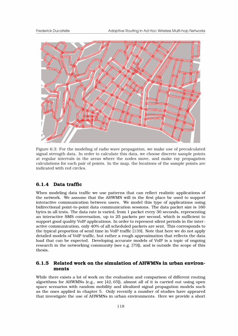
Frederick Ducatelle Adaptive Routing in Ad Hoc Wireless Multi-hop Networks
Figure 6.3: For the modeling of radio wave propagation, we make use of precalculatedsignal strength data. In order to calculate this data, we choose discrete sample pointsat regular intervals in the areas where the nodes move, and make ray propagationcalculations for each pair of points. In the map, the locations of the sample points areindicated with red circles.
6.1.4 Data traffic
When modeling data traffic we use patterns that can reflect realistic applications ofthe network. We assume that the AHWMN will in the first place be used to supportinteractive communication between users. We model this type of applications usingbidirectional point-to-point data communication sessions. The data packet size is 160bytes in all tests. The data rate is varied, from 1 packet every 30 seconds, representingan interactive SMS conversation, up to 25 packets per second, which is sufficient tosupport good quality VoIP applications. In order to represent silent periods in the inter-active communication, only 40% of all scheduled packets are sent. This corresponds tothe typical proportion of send time in VoIP traffic [139]. Note that here we do not applydetailed models of VoIP traffic, but rather a rough approximation that reflects the dataload that can be expected. Developing accurate models of VoIP is a topic of ongoingresearch in the networking community (see e.g. [79]), and is outside the scope of thisthesis.
6.1.5 Related work on the simulation of AHWMNs in urban environ-ments
While there exists a lot of work on the evaluation and comparison of different routingalgorithms for AHWMNs (e.g., see [42, 65]), almost all of it is carried out using openspace scenarios with random mobility and idealized signal propagation models suchas the ones applied in chapter 5. Only recently a number of studies have appearedthat investigate the use of AHWMNs in urban environments. Here we provide a short
118
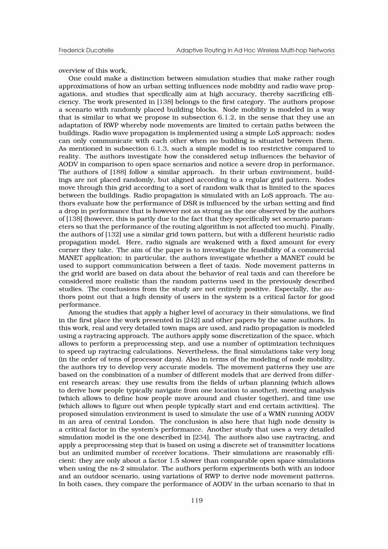
Frederick Ducatelle Adaptive Routing in Ad Hoc Wireless Multi-hop Networks
overview of this work.One could make a distinction between simulation studies that make rather rough
approximations of how an urban setting influences node mobility and radio wave prop-agations, and studies that specifically aim at high accuracy, thereby sacrificing effi-ciency. The work presented in [138] belongs to the first category. The authors proposea scenario with randomly placed building blocks. Node mobility is modeled in a waythat is similar to what we propose in subsection 6.1.2, in the sense that they use anadaptation of RWP whereby node movements are limited to certain paths between thebuildings. Radio wave propagation is implemented using a simple LoS approach: nodescan only communicate with each other when no building is situated between them.As mentioned in subsection 6.1.3, such a simple model is too restrictive compared toreality. The authors investigate how the considered setup influences the behavior ofAODV in comparison to open space scenarios and notice a severe drop in performance.The authors of [188] follow a similar approach. In their urban environment, build-ings are not placed randomly, but aligned according to a regular grid pattern. Nodesmove through this grid according to a sort of random walk that is limited to the spacesbetween the buildings. Radio propagation is simulated with an LoS approach. The au-thors evaluate how the performance of DSR is influenced by the urban setting and finda drop in performance that is however not as strong as the one observed by the authorsof [138] (however, this is partly due to the fact that they specifically set scenario param-eters so that the performance of the routing algorithm is not affected too much). Finally,the authors of [132] use a similar grid town pattern, but with a different heuristic radiopropagation model. Here, radio signals are weakened with a fixed amount for everycorner they take. The aim of the paper is to investigate the feasibility of a commercialMANET application; in particular, the authors investigate whether a MANET could beused to support communication between a fleet of taxis. Node movement patterns inthe grid world are based on data about the behavior of real taxis and can therefore beconsidered more realistic than the random patterns used in the previously describedstudies. The conclusions from the study are not entirely positive. Especially, the au-thors point out that a high density of users in the system is a critical factor for goodperformance.
Among the studies that apply a higher level of accuracy in their simulations, we findin the first place the work presented in [242] and other papers by the same authors. Inthis work, real and very detailed town maps are used, and radio propagation is modeledusing a raytracing approach. The authors apply some discretization of the space, whichallows to perform a preprocessing step, and use a number of optimization techniquesto speed up raytracing calculations. Nevertheless, the final simulations take very long(in the order of tens of processor days). Also in terms of the modeling of node mobility,the authors try to develop very accurate models. The movement patterns they use arebased on the combination of a number of different models that are derived from differ-ent research areas: they use results from the fields of urban planning (which allowsto derive how people typically navigate from one location to another), meeting analysis(which allows to define how people move around and cluster together), and time use(which allows to figure out when people typically start and end certain activities). Theproposed simulation environment is used to simulate the use of a WMN running AODVin an area of central London. The conclusion is also here that high node density isa critical factor in the system’s performance. Another study that uses a very detailedsimulation model is the one described in [234]. The authors also use raytracing, andapply a preprocessing step that is based on using a discrete set of transmitter locationsbut an unlimited number of receiver locations. Their simulations are reasonably effi-cient: they are only about a factor 1.5 slower than comparable open space simulationswhen using the ns-2 simulator. The authors perform experiments both with an indoorand an outdoor scenario, using variations of RWP to derive node movement patterns.In both cases, they compare the performance of AODV in the urban scenario to that in
119

Frederick Ducatelle Adaptive Routing in Ad Hoc Wireless Multi-hop Networks
an open space scenario, and observe a large drop in performance.The work presented in the current chapter of this thesis is in approach and level
of detail similar to the last described work. It allows to get a reasonable feel for whatthe effects can be of an urban environment, while making enough abstraction to getan efficient simulation. This allows us to run a number of different tests in order tosee how the approach followed by AntHocNet deals with the challenges of the urbansetting, and compare this to the different strategy adopted by AODV. None of the urbanscenario simulations we found in the literature provides a performance comparisonbetween different routing algorithms.
6.2 Test results
In this section we describe the results of a range of tests that we ran with the simulationsetup described above. The aim is to investigate how AntHocNet performs in an urbanenvironment, and to compare it to AODV. In what follows, we first describe in sub-section 6.2.1 results of tests in which we investigate general properties of the AHWMNnetwork in the urban scenario, as compared to an open space scenario. These tests aremeant to aid in the understanding of the results observed further on. Then, we presentresults of comparative tests, in which we vary similar parameters as in the tests of sub-section 5.2: we present results with varying data send rates in subsection 6.2.2, withvarying numbers of data sessions in subsection 6.2.3, with varying node densities insubsection 6.2.4 and with varying maximum node speeds in subsection 6.2.5. Finally,in subsection 6.2.6, we also investigate whether it is possible to support VoIP level dataloads with the different routing algorithms in the given urban scenario.
6.2.1 General network properties
In this subsection, we study how the properties of the network formed between theMANET nodes are affected by the fact that we work in an urban environment. The datashown here were obtained by running simulations with an increasing number of nodesin both the urban scenario and an open space scenario of the same dimensions. In theopen space scenario we use the two-ray radio propagation model (see subsection 5.1.3).During these simulations, no data traffic was sent, but all nodes were periodicallybroadcasting beacon messages. We recorded all receptions of these beacon messages,and constructed a network graph for each beaconing period, counting a link between apair of nodes i and j if during the period of the beaconing interval i received a beaconfrom j and j received one from i. This way we got a picture of the network connectivityas experienced by the nodes in the network. In these experiments, all nodes weremoving between 1 and 3m/s. We report results for the average number of neighbors,the connectivity (i.e., the fraction of node pairs between which a path exists), the averagelength of the shortest path between each pair of nodes, and the average link duration.The results are shown in the graphs of figure 6.4.
The average number of neighbors per node are shown in figure 6.4a. We can see thatthis number is always a lot lower in the urban scenario than in the open space scenario.This is due to the limited radio propagation caused by the shadowing by the buildings ofthe town. Also, we can see that, while the number of neighbors grows linearly with thenumber of nodes in the network in both scenarios, the increase is steeper in the openspace scenario. This means that for an equal number of nodes per square meter, nodesin the urban scenario locally experience a lower density. As a consequence, connectivityis worse in the urban scenario, but interference between nodes is also lower.
The lower connectivity in the urban scenario is confirmed by the results of fig-ure 6.4b, where we report the fraction of node pairs between which a path exists in theAHWMN network topology. While the open space scenario is always fully connected,
120
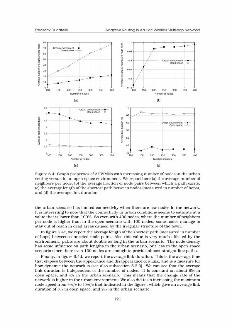
Frederick Ducatelle Adaptive Routing in Ad Hoc Wireless Multi-hop Networks
0
10
20
30
40
50
60
70
80
100 150 200 250 300 350 400
Ave
rage
num
ber
of n
eigh
bors
per
nod
e
Number of nodes
Urban environmentOpen space
0.75
0.8
0.85
0.9
0.95
1
100 150 200 250 300 350 400
Ave
rage
frac
tion
of c
onne
cted
nod
e pa
irs
Number of nodes
Urban environmentOpen space
(a) (b)
2
2.5
3
3.5
4
4.5
5
5.5
100 150 200 250 300 350 400
Ave
rage
pat
h le
ngth
(ho
ps)
Number of nodes
Urban environmentOpen space
40
45
50
55
60
65
70
100 150 200 250 300 350 400
Ave
rage
link
dur
atio
n (s
)
Number of nodes
Urban environmentOpen space
(c) (d)
Figure 6.4: Graph properties of AHWMNs with increasing number of nodes in the urbansetting versus in an open space environment. We report here (a) the average number ofneighbors per node, (b) the average fraction of node pairs between which a path exists,(c) the average length of the shortest path between nodes (measured in number of hops),and (d) the average link duration.
the urban scenario has limited connectivity when there are few nodes in the network.It is interesting to note that the connectivity in urban conditions seems to saturate at avalue that is lower than 100%. So even with 400 nodes, where the number of neighborsper node is higher than in the open scenario with 100 nodes, some nodes manage tostay out of reach in dead areas caused by the irregular structure of the town.
In figure 6.4c, we report the average length of the shortest path (measured in numberof hops) between connected node pairs. Also this value is very much affected by theenvironment: paths are about double as long in the urban scenario. The node densityhas some influence on path lengths in the urban scenario, but less in the open spacescenario since there even 100 nodes are enough to provide almost straight line paths.
Finally, in figure 6.4d, we report the average link duration. This is the average timethat elapses between the appearance and disappearance of a link, and is a measure forhow dynamic the network is (see also subsection 5.2.3). We can see that the averagelink duration is independent of the number of nodes. It is constant on about 65s inopen space, and 43s in the urban scenario. This means that the change rate of thenetwork is higher in the urban environment. We also did tests increasing the maximumnode speed from 3m/s to 10m/s (not indicated in the figure), which gave an average linkduration of 56s in open space, and 28s in the urban scenario.
121
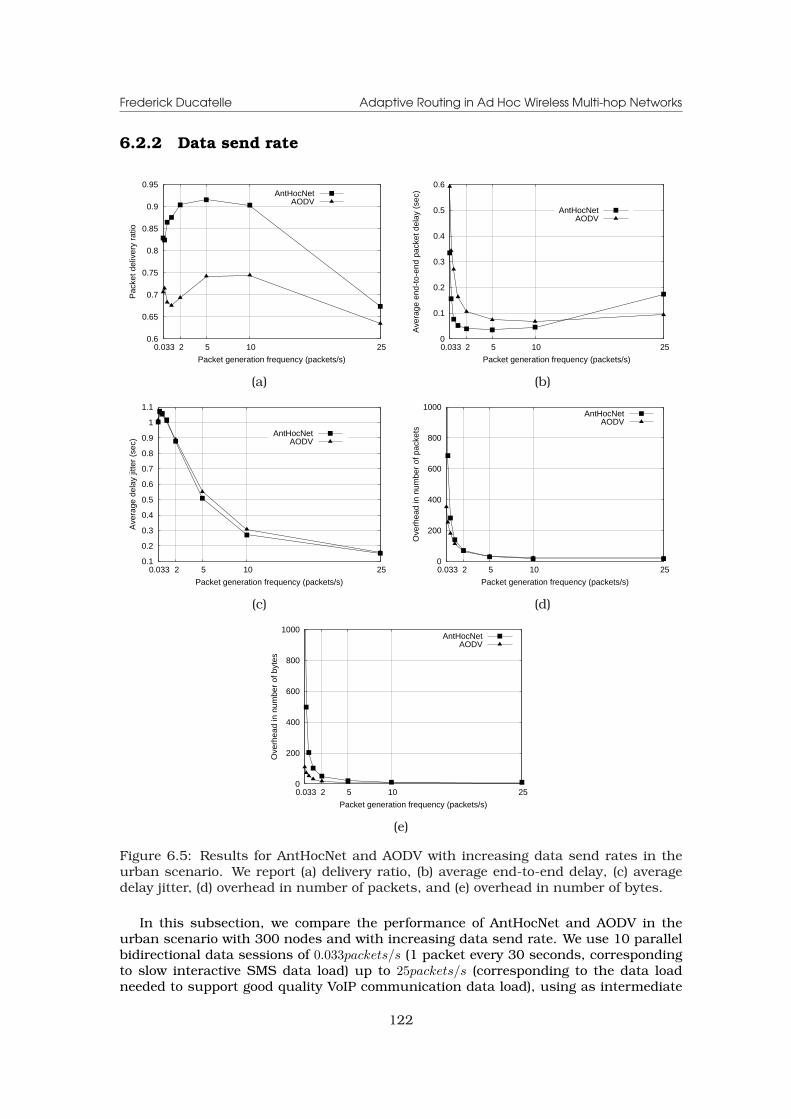
Frederick Ducatelle Adaptive Routing in Ad Hoc Wireless Multi-hop Networks
6.2.2 Data send rate
0.6
0.65
0.7
0.75
0.8
0.85
0.9
0.95
0.033 2 5 10 25
Pac
ket d
eliv
ery
ratio
Packet generation frequency (packets/s)
AntHocNetAODV
0
0.1
0.2
0.3
0.4
0.5
0.6
0.033 2 5 10 25
Ave
rage
end
-to-
end
pack
et d
elay
(se
c)
Packet generation frequency (packets/s)
AntHocNetAODV
(a) (b)
0.1
0.2
0.3
0.4
0.5
0.6
0.7
0.8
0.9
1
1.1
0.033 2 5 10 25
Ave
rage
del
ay ji
tter
(sec
)
Packet generation frequency (packets/s)
AntHocNetAODV
0
200
400
600
800
1000
0.033 2 5 10 25
Ove
rhea
d in
num
ber
of p
acke
ts
Packet generation frequency (packets/s)
AntHocNetAODV
(c) (d)
0
200
400
600
800
1000
0.033 2 5 10 25
Ove
rhea
d in
num
ber
of b
ytes
Packet generation frequency (packets/s)
AntHocNetAODV
(e)
Figure 6.5: Results for AntHocNet and AODV with increasing data send rates in theurban scenario. We report (a) delivery ratio, (b) average end-to-end delay, (c) averagedelay jitter, (d) overhead in number of packets, and (e) overhead in number of bytes.
In this subsection, we compare the performance of AntHocNet and AODV in theurban scenario with 300 nodes and with increasing data send rate. We use 10 parallelbidirectional data sessions of 0.033packets/s (1 packet every 30 seconds, correspondingto slow interactive SMS data load) up to 25packets/s (corresponding to the data loadneeded to support good quality VoIP communication data load), using as intermediate
122

Frederick Ducatelle Adaptive Routing in Ad Hoc Wireless Multi-hop Networks
values 0.2, 0.5, 1, 2, 5 and 10packets/s. Like in the comparative tests of section 5.2,we report the delivery ratio, the average end-to-end delay, the average delay jitter, theoverhead ratio in number of packets, and the overhead ratio in number of bytes. Allresults are shown in figure 6.5.
When considering delivery ratio and delay (figure 6.5a and 6.5b), we can see thatboth algorithms have bad performance for the lowest data rates, better performanceat intermediate rates, and worse performance again for the highest rates. The badperformance at the lowest rates is due to the fact that both AntHocNet and AODV needto set up a route between source and destination prior to communication. When datapackets are sent sporadically, previously constructed routes can rarely be reused, andnew route setups are often necessary. As data rates increase, subsequent packetscan profit from previous route setups. In AntHocNet, where routes are proactivelymaintained and therefore remain valid for longer, this effect is visible at lower ratesthan for AODV. For the highest rates, both algorithms have a decrease in performance,because the high load of data packets starts to interfere with the control packets. Ingeneral, we can see that AntHocNet outperforms AODV for most data rates (except forthe delay at the highest data rate). Considering that the urban scenario has longerpaths and less good connectivity than a comparable open space scenario, this resultwas to be expected, as it was shown in subsections 5.2.6 and 5.2.7 that AntHocNetperforms well under such conditions. When we compare directly with the results forvarying data send rates in open space scenarios presented in subsection 5.2.4, wecan see that both algorithms are better able to deliver the highest data rates in theurban scenario (especially for AODV the difference is large). This is on the one handbecause we use only 10 sessions here (see also further in subsection 6.2.3), and on theother hand because there is less interference due to the shadowing by the buildings.Nevertheless, it must be noted that neither of the algorithms is able to provide a deliveryratio that is sufficient to support a VoIP application (see also further in subsection6.2.6).
When considering average delay jitter, we can see more or less monotonically de-creasing values for both algorithms, with a slight advantage for AntHocNet. The factthat jitter improves with increasing data rates is due to the fact that as data pack-ets are sent more frequently, subsequent packets travel closer after each other, andtherefore encounter more similar conditions. Hence, the differences in their delays aresmaller. A similar effect was visible in the comparative tests in the open space scenariosof subsection 5.2.4. However, in those tests, jitter values only decreased for the lowestvalues for the data rate, and then started to increase. It must be pointed out that in ab-solute terms, the jitter values in the city scenario are much higher for the lowest datarates (due to the worse connectivity and the longer path lengths), and that thereforemore improvement is possible.
In terms of both overhead measures, we can observe monotonically improving per-formances for both algorithms. This is because of the earlier mentioned effect thatat low data rates, routes practically need to be rebuilt for each data packet, whereasat higher rates, subsequent packets can profit from earlier route setups. EspeciallyAntHocNet produces high overhead for the lowest data rates. This is because its mech-anisms to proactively maintain routes create a lot of overhead compared to the numberof packets that are delivered. For the higher data rates, both algorithms have simi-lar overhead ratios. AntHocNet slightly outperforms AODV in overhead in number ofpackets, but not in overhead in number of bytes.
6.2.3 Number of data sessions
Here, we report the results of test in which we vary the number of data sessions, from5 up to 25 sessions, with as intermediate values 10, 15 and 20 sessions. All data
123
Frederick Ducatelle Adaptive Routing in Ad Hoc Wireless Multi-hop Networks
0.4
0.5
0.6
0.7
0.8
0.9
1
5 10 15 20 25
Pac
ket d
eliv
ery
ratio
Number of bidirectional data sessions
AntHocNet 10AODV 10
AntHocNet 5AODV 5
0
0.1
0.2
0.3
0.4
0.5
0.6
0.7
0.8
0.9
5 10 15 20 25
Ave
rage
end
-to-
end
pack
et d
elay
(se
c)
Number of bidirectional data sessions
AntHocNet 10AODV 10
AntHocNet 5AODV 5
(a) (b)
0.25
0.3
0.35
0.4
0.45
0.5
0.55
0.6
5 10 15 20 25
Ave
rage
del
ay ji
tter
(sec
)
Number of bidirectional data sessions
AntHocNet 10AODV 10
AntHocNet 5AODV 5
0
50
100
150
200
250
300
350
400
5 10 15 20 25
Ove
rhea
d in
num
ber
of p
acke
ts
Number of bidirectional data sessions
AntHocNet 10AODV 10
AntHocNet 5AODV 5
(c) (d)
0
20
40
60
80
100
120
5 10 15 20 25
Ove
rhea
d in
num
ber
of b
ytes
Number of bidirectional data sessions
AntHocNet 10AODV 10
AntHocNet 5AODV 5
(e)
Figure 6.6: Results for AntHocNet and AODV with increasing number of data sessionsin the urban scenario. We use data rates of 5 and 10 packets/s, indicated by differentcurves in the figure. We report (a) delivery ratio, (b) average end-to-end delay, (c) averagedelay jitter, (d) overhead in number of packets, and (e) overhead in number of bytes.
sessions are bidirectional. We did tests with two different values for the data send rate:5 and 10packets/s. In figure 6.6, we report delivery ratio, delay, jitter, overhead ratio innumber of packets and overhead ratio in number of bytes.
When considering delivery ratio (figure 6.6a) we can see that AntHocNet outperformsAODV for all scenarios. Apart from that, we observe a common trend for both algorithmsunder both data rates: performance monotonically deteriorates when we increase the
124
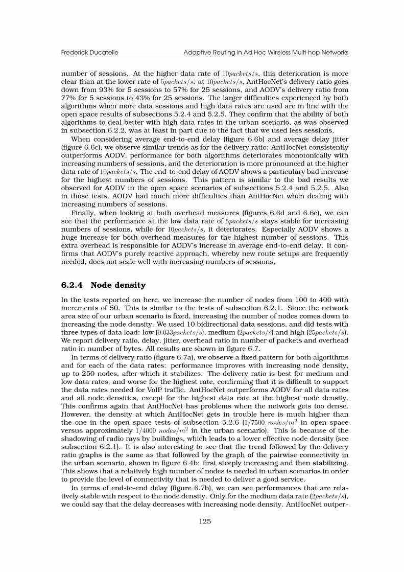
Frederick Ducatelle Adaptive Routing in Ad Hoc Wireless Multi-hop Networks
number of sessions. At the higher data rate of 10packets/s, this deterioration is moreclear than at the lower rate of 5packets/s: at 10packets/s, AntHocNet’s delivery ratio goesdown from 93% for 5 sessions to 57% for 25 sessions, and AODV’s delivery ratio from77% for 5 sessions to 43% for 25 sessions. The larger difficulties experienced by bothalgorithms when more data sessions and high data rates are used are in line with theopen space results of subsections 5.2.4 and 5.2.5. They confirm that the ability of bothalgorithms to deal better with high data rates in the urban scenario, as was observedin subsection 6.2.2, was at least in part due to the fact that we used less sessions.
When considering average end-to-end delay (figure 6.6b) and average delay jitter(figure 6.6c), we observe similar trends as for the delivery ratio: AntHocNet consistentlyoutperforms AODV, performance for both algorithms deteriorates monotonically withincreasing numbers of sessions, and the deterioration is more pronounced at the higherdata rate of 10packets/s. The end-to-end delay of AODV shows a particulary bad increasefor the highest numbers of sessions. This pattern is similar to the bad results weobserved for AODV in the open space scenarios of subsections 5.2.4 and 5.2.5. Alsoin those tests, AODV had much more difficulties than AntHocNet when dealing withincreasing numbers of sessions.
Finally, when looking at both overhead measures (figures 6.6d and 6.6e), we cansee that the performance at the low data rate of 5packets/s stays stable for increasingnumbers of sessions, while for 10packets/s, it deteriorates. Especially AODV shows ahuge increase for both overhead measures for the highest number of sessions. Thisextra overhead is responsible for AODV’s increase in average end-to-end delay. It con-firms that AODV’s purely reactive approach, whereby new route setups are frequentlyneeded, does not scale well with increasing numbers of sessions.
6.2.4 Node density
In the tests reported on here, we increase the number of nodes from 100 to 400 withincrements of 50. This is similar to the tests of subsection 6.2.1. Since the networkarea size of our urban scenario is fixed, increasing the number of nodes comes down toincreasing the node density. We used 10 bidirectional data sessions, and did tests withthree types of data load: low (0.033packets/s), medium (2packets/s) and high (25packets/s).We report delivery ratio, delay, jitter, overhead ratio in number of packets and overheadratio in number of bytes. All results are shown in figure 6.7.
In terms of delivery ratio (figure 6.7a), we observe a fixed pattern for both algorithmsand for each of the data rates: performance improves with increasing node density,up to 250 nodes, after which it stabilizes. The delivery ratio is best for medium andlow data rates, and worse for the highest rate, confirming that it is difficult to supportthe data rates needed for VoIP traffic. AntHocNet outperforms AODV for all data ratesand all node densities, except for the highest data rate at the highest node density.This confirms again that AntHocNet has problems when the network gets too dense.However, the density at which AntHocNet gets in trouble here is much higher thanthe one in the open space tests of subsection 5.2.6 (1/7500 nodes/m2 in open spaceversus approximately 1/4000 nodes/m2 in the urban scenario). This is because of theshadowing of radio rays by buildings, which leads to a lower effective node density (seesubsection 6.2.1). It is also interesting to see that the trend followed by the deliveryratio graphs is the same as that followed by the graph of the pairwise connectivity inthe urban scenario, shown in figure 6.4b: first steeply increasing and then stabilizing.This shows that a relatively high number of nodes is needed in urban scenarios in orderto provide the level of connectivity that is needed to deliver a good service.
In terms of end-to-end delay (figure 6.7b), we can see performances that are rela-tively stable with respect to the node density. Only for the medium data rate (2packets/s),we could say that the delay decreases with increasing node density. AntHocNet outper-
125
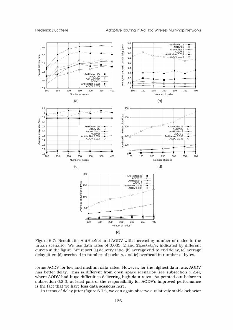
Frederick Ducatelle Adaptive Routing in Ad Hoc Wireless Multi-hop Networks
0.4
0.5
0.6
0.7
0.8
0.9
100 150 200 250 300 350 400
Pac
ket d
eliv
ery
ratio
Number of nodes
AntHocNet 25AODV 25
AntHocNet 2AODV 2
AntHocNet 0.033AODV 0.033
0
0.1
0.2
0.3
0.4
0.5
0.6
0.7
0.8
0.9
100 150 200 250 300 350 400
Ave
rage
end
-to-
end
pack
et d
elay
(se
c)
Number of nodes
AntHocNet 25AODV 25
AntHocNet 2AODV 2
AntHocNet 0.033AODV 0.033
(a) (b)
0.1
0.2
0.3
0.4
0.5
0.6
0.7
0.8
0.9
1
1.1
100 150 200 250 300 350 400
Ave
rage
del
ay ji
tter
(sec
)
Number of nodes
AntHocNet 25AODV 25
AntHocNet 2AODV 2
AntHocNet 0.033AODV 0.033
0
100
200
300
400
500
100 150 200 250 300 350 400
Ove
rhea
d in
num
ber
of p
acke
ts
Number of nodes
AntHocNet 25AODV 25
AntHocNet 2AODV 2
AntHocNet 0.033AODV 0.033
(c) (d)
0
50
100
150
200
100 150 200 250 300 350 400
Ove
rhea
d in
num
ber
of b
ytes
Number of nodes
AntHocNet 25AODV 25
AntHocNet 2AODV 2
AntHocNet 0.033AODV 0.033
(e)
Figure 6.7: Results for AntHocNet and AODV with increasing number of nodes in theurban scenario. We use data rates of 0.033, 2 and 25packets/s, indicated by differentcurves in the figure. We report (a) delivery ratio, (b) average end-to-end delay, (c) averagedelay jitter, (d) overhead in number of packets, and (e) overhead in number of bytes.
forms AODV for low and medium data rates. However, for the highest data rate, AODVhas better delay. This is different from open space scenarios (see subsection 5.2.4),where AODV had huge difficulties delivering high data rates. As pointed out before insubsection 6.2.3, at least part of the responsibility for AODV’s improved performanceis the fact that we have less data sessions here.
In terms of delay jitter (figure 6.7c), we can again observe a relatively stable behavior
126

Frederick Ducatelle Adaptive Routing in Ad Hoc Wireless Multi-hop Networks
with respect to node density. Moreover, both algorithms have more or less the sameperformance. In general, we can see that jitter is highest for the lowest data rate, lowerfor the medium data rate, and lowest for the highest data rate. This is in line with theearlier results of subsection 6.2.2.
Finally, in terms of both overhead measures (figures 6.7d and 6.7e), we can see thatperformance is worse for the low data rate (the results for AntHocNet for the lowest datarate are off the chart), and better for the medium and high data rates. When lookingat the overhead in number of bytes, AntHocNet does always worse than AODV. Whenlooking at overhead in number of packets, AntHocNet does worse than AODV for thelowest data rate, but comparable or better for the medium and high data rates. Thebad results for both algorithms at low data rates is due to the earlier mentioned factthat when data packets are sent sporadically, a route setup is almost always needed foreach new data packet. AntHocNet’s strategy to proactively maintain routes then leadsto extra overhead without giving much advantage. At higher data rates, packets canprofit from earlier route setups, so that the overhead ratio can be reduced. AntHocNet’smechanisms to proactively maintain paths augments this effect, so that the algorithmcan get a lower overhead ratio when measured in number of packets. However, the factthat AntHocNet uses larger hello messages as well as larger control messages (forwardand backward ants carry full paths, whereas AODV’s RREQ and RREP messages do not)causes a higher overhead when measured in number of bytes. Finally, we would like topoint out that both algorithms experience increasing overhead for increasing numbersof nodes. This is because in networks with more nodes flooded control packets areforwarded more times, and more hello messages are produced.
6.2.5 Node speed
In the experiments presented here, we vary the maximum node speed. We increase itfrom the 3m/s used in the previous tests up to 15m/s, which is a reasonable maximumspeed for cars in an urban environment. As intermediate values we use 6, 10 and12.5m/s. We keep using 10 bidirectional data sessions and again do tests with differentdata rates: a low rate of 0.033 packets per second, a medium rate of 2 packets persecond, and a high rate of 25 packets per second. In figure 6.8, we report delivery ratio,end-to-end delay, delay jitter, overhead in number of packets and overhead in numberof bytes.
As can be expected, delivery ratios (figure 6.8a) go down with increasing node speedsunder all data send rates for both algorithms. Apart from that, we get a confirmation ofearlier results. Delivery ratios are highest for medium and low data rates, and lowestfor the highest data rate. AntHocNet delivers more packets than AODV, except for thehighest data rate, where delivery ratios are comparable.
In terms of delay (figure 6.8b), we get a similar picture. Delay goes up with increasingnodes speeds, although the effect is minimal. The best delays are obtained for the lowand medium data rates, and the worst for the highest rates. AntHocNet outperformsAODV at low and medium data rates, while AODV is the best at the highest data rate.
In terms of jitter (figure 6.8c), the effect of the node speed is again minimal: bothalgorithms give more or less stable jitter for increasing node speeds at all data rates.As in previous tests, jitter is highest for the lowest data rates and lower for the mediumand high data rates. The performances of both algorithms in terms of jitter are verycomparable.
Finally, also for both overhead measures, we get familiar patterns. For both mea-sures, performances get slightly worse with increasing node speeds. For overhead innumber of bytes, AODV outperforms AntHocNet at all data rates (the curve for the low-est data rate for AntHocNet is outside the range of the graph). For overhead in numberof packets, AODV outperforms AntHocNet for the low and medium data rates, but not
127
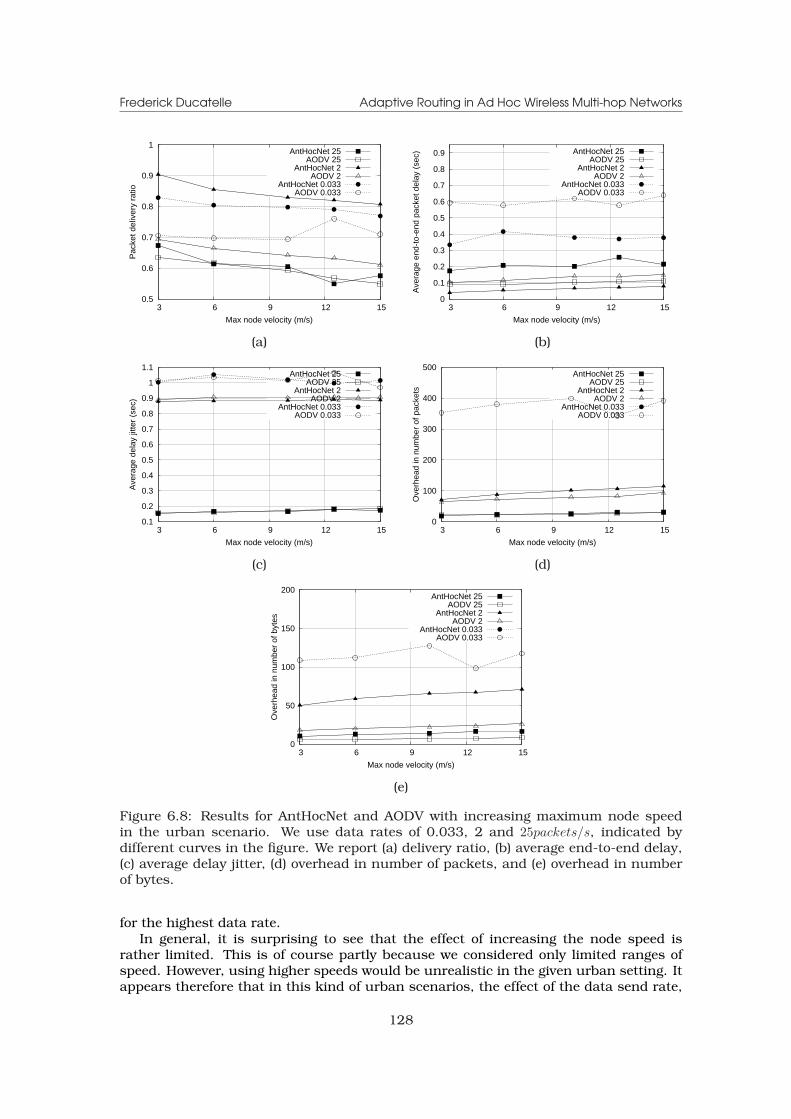
Frederick Ducatelle Adaptive Routing in Ad Hoc Wireless Multi-hop Networks
0.5
0.6
0.7
0.8
0.9
1
15 12 9 6 3
Pac
ket d
eliv
ery
ratio
Max node velocity (m/s)
AntHocNet 25AODV 25
AntHocNet 2AODV 2
AntHocNet 0.033AODV 0.033
0
0.1
0.2
0.3
0.4
0.5
0.6
0.7
0.8
0.9
15 12 9 6 3
Ave
rage
end
-to-
end
pack
et d
elay
(se
c)
Max node velocity (m/s)
AntHocNet 25AODV 25
AntHocNet 2AODV 2
AntHocNet 0.033AODV 0.033
(a) (b)
0.1
0.2
0.3
0.4
0.5
0.6
0.7
0.8
0.9
1
1.1
15 12 9 6 3
Ave
rage
del
ay ji
tter
(sec
)
Max node velocity (m/s)
AntHocNet 25AODV 25
AntHocNet 2AODV 2
AntHocNet 0.033AODV 0.033
0
100
200
300
400
500
15 12 9 6 3
Ove
rhea
d in
num
ber
of p
acke
ts
Max node velocity (m/s)
AntHocNet 25AODV 25
AntHocNet 2AODV 2
AntHocNet 0.033AODV 0.033
(c) (d)
0
50
100
150
200
15 12 9 6 3
Ove
rhea
d in
num
ber
of b
ytes
Max node velocity (m/s)
AntHocNet 25AODV 25
AntHocNet 2AODV 2
AntHocNet 0.033AODV 0.033
(e)
Figure 6.8: Results for AntHocNet and AODV with increasing maximum node speedin the urban scenario. We use data rates of 0.033, 2 and 25packets/s, indicated bydifferent curves in the figure. We report (a) delivery ratio, (b) average end-to-end delay,(c) average delay jitter, (d) overhead in number of packets, and (e) overhead in numberof bytes.
for the highest data rate.In general, it is surprising to see that the effect of increasing the node speed is
rather limited. This is of course partly because we considered only limited ranges ofspeed. However, using higher speeds would be unrealistic in the given urban setting. Itappears therefore that in this kind of urban scenarios, the effect of the data send rate,
128
Frederick Ducatelle Adaptive Routing in Ad Hoc Wireless Multi-hop Networks
the number of data sessions and the number of nodes in the network is much moreimportant than the effect of the node speed.
6.2.6 Supporting VoIP traffic data loads
In a final set of experiments, we investigate the issue of delivering sessions with VoIPlevel data rates. In 6.2.2, we saw that both algorithms have trouble when data rates goup to VoIP levels: AntHocNet drops to a delivery ratio of 67% and a delay of 0.19s, whileAODV has a delivery of 63% and a delay of 0.1s. Jitter is for both algorithms around0.15s. To support good quality VoIP, a delivery ratio of 90% is needed, and end-to-enddelay should not exceed 0.15s (see [189]). Jitter is normally considered in conjunctionwith delay, as applications deal with jitter by keeping packets in buffer for a short timebefore delivering them; jitter can therefore be added to delay to count towards the delaylimit [189]. Using this approach, we can see that both in terms of delivery ratio anddelay, the standards needed to deliver good quality VoIP conversations are not met byeither of the algorithms. Here, we investigate this in more detail.
We do tests varying the number of data sessions from 1 to 10. All sessions arebi-directional and send 25packets/s. The results are show in figure 6.9. When fewsessions are started, we can see that AntHocNet manages to reach the formulated VoIPrequirements both in terms of delivery ratio and delay (when delay and jitter are addedtogether). AODV on the other hand falls short on both requirements. Then, when thenumber of sessions is increased, also AntHocNet fails to reach the VoIP requirements.
These reported results are averages over all the started communication sessionsthough. In order to get a more precise view, we investigate for each scenario how manyof the individual sessions reach the cited requirements. In figure 6.10, we show thisnumber (a) as a fraction of the total number of started sessions, and (b) in absoluteterms. We can see that using AntHocNet, at least a few of the sessions can obtain VoIPquality. When only one session is started, it almost always gets the required quality(in 90% of the cases, as shown in figure 6.10a). Then, as more sessions are started,the fraction of them that receive VoIP quality decreases. However, in absolute terms,the total number of sessions that receive the required quality grows up to almost 2.5when 4 sessions are started, and then remains more or less stable. Finally, when morethan 7 sessions are started, the absolute number also decreases. When 10 sessionsare started, on average about only 1 receives VoIP quality. This is because too manysessions are interfering with each other. For AODV, the number of sessions receivingthe required service quality always remains low.
The results show that using AntHocNet it is in principle possible to support VoIPin the given urban scenario. However, not all sessions can get the required levels ofservice, and when too many sessions are started, all of them suffer. This indicates thatit might be useful to refuse some sessions to start (e.g., sessions that would likely notreceive the required quality anyway, because they need paths that go through highlycongested or poorly connected parts of the network) in order to be able to deliver a goodservice to other sessions. This points to the importance of the use of admission controlor some other system for Quality-of-Service support in resource limited urban MANETs:if only sessions that are likely to get the levels of service they need are allowed to start,less bandwidth is wasted. For existing work on admission control in AHWMNs, seee.g. [81].
6.3 Conclusion
In this chapter, we have studied the behavior of AntHocNet in an urban scenario. First,we have given a detailed description of how we obtained a good and efficient simulationof the working of an AHWMN in an urban environment. Then, we have presented results
129
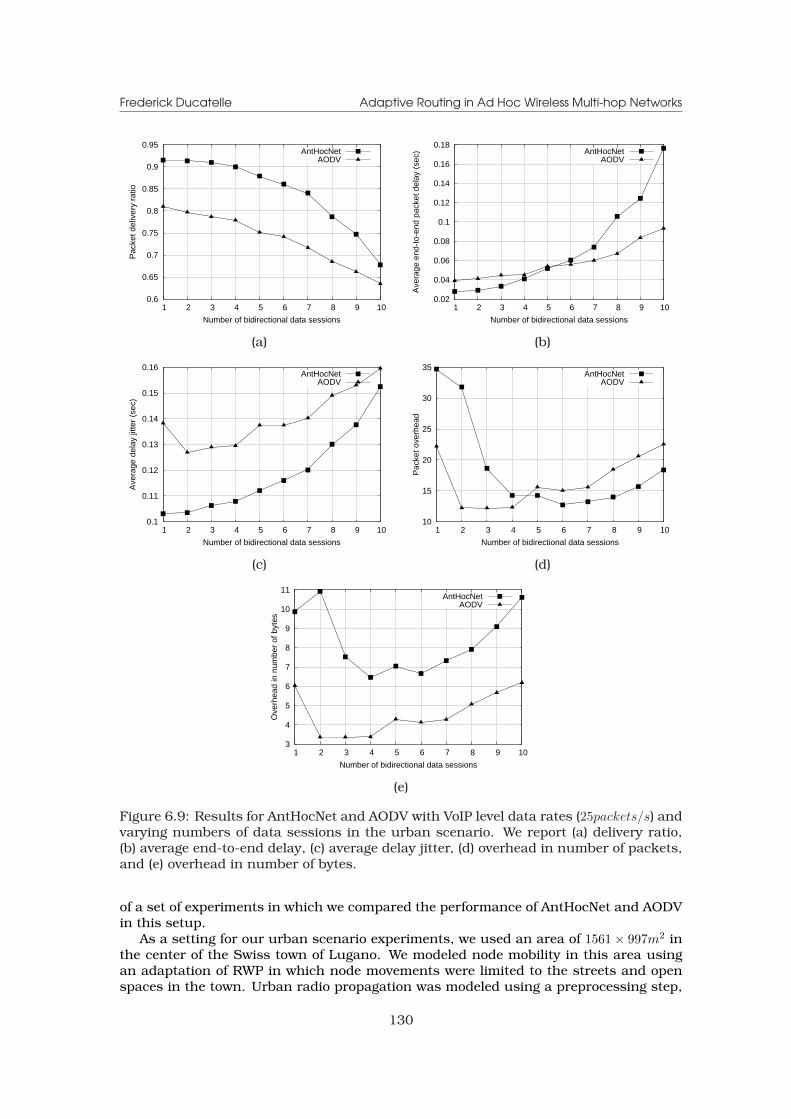
Frederick Ducatelle Adaptive Routing in Ad Hoc Wireless Multi-hop Networks
0.6
0.65
0.7
0.75
0.8
0.85
0.9
0.95
1 2 3 4 5 6 7 8 9 10
Pac
ket d
eliv
ery
ratio
Number of bidirectional data sessions
AntHocNetAODV
0.02
0.04
0.06
0.08
0.1
0.12
0.14
0.16
0.18
1 2 3 4 5 6 7 8 9 10
Ave
rage
end
-to-
end
pack
et d
elay
(se
c)
Number of bidirectional data sessions
AntHocNetAODV
(a) (b)
0.1
0.11
0.12
0.13
0.14
0.15
0.16
1 2 3 4 5 6 7 8 9 10
Ave
rage
del
ay ji
tter
(sec
)
Number of bidirectional data sessions
AntHocNetAODV
10
15
20
25
30
35
1 2 3 4 5 6 7 8 9 10
Pac
ket o
verh
ead
Number of bidirectional data sessions
AntHocNetAODV
(c) (d)
3
4
5
6
7
8
9
10
11
1 2 3 4 5 6 7 8 9 10
Ove
rhea
d in
num
ber
of b
ytes
Number of bidirectional data sessions
AntHocNetAODV
(e)
Figure 6.9: Results for AntHocNet and AODV with VoIP level data rates (25packets/s) andvarying numbers of data sessions in the urban scenario. We report (a) delivery ratio,(b) average end-to-end delay, (c) average delay jitter, (d) overhead in number of packets,and (e) overhead in number of bytes.
of a set of experiments in which we compared the performance of AntHocNet and AODVin this setup.
As a setting for our urban scenario experiments, we used an area of 1561× 997m2 inthe center of the Swiss town of Lugano. We modeled node mobility in this area usingan adaptation of RWP in which node movements were limited to the streets and openspaces in the town. Urban radio propagation was modeled using a preprocessing step,
130
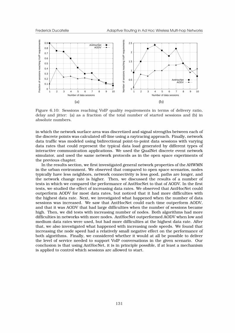
Frederick Ducatelle Adaptive Routing in Ad Hoc Wireless Multi-hop Networks
0
0.1
0.2
0.3
0.4
0.5
0.6
0.7
0.8
0.9
1 2 3 4 5 6 7 8 9 10Fra
ctio
n of
ses
sion
s re
achi
ng V
oIP
req
uire
men
ts
Number of data sessions
AntHocNetAODV
0
0.5
1
1.5
2
2.5
1 2 3 4 5 6 7 8 9 10Num
ber
of s
essi
ons
reac
hing
VoI
P r
equi
rem
ents
Number of data sessions
AntHocNetAODV
(a) (b)
Figure 6.10: Sessions reaching VoIP quality requirements in terms of delivery ratio,delay and jitter: (a) as a fraction of the total number of started sessions and (b) inabsolute numbers.
in which the network surface area was discretized and signal strengths between each ofthe discrete points was calculated off-line using a raytracing approach. Finally, networkdata traffic was modeled using bidirectional point-to-point data sessions with varyingdata rates that could represent the typical data load generated by different types ofinteractive communication applications. We used the QualNet discrete event networksimulator, and used the same network protocols as in the open space experiments ofthe previous chapter.
In the results section, we first investigated general network properties of the AHWMNin the urban environment. We observed that compared to open space scenarios, nodestypically have less neighbors, network connectivity is less good, paths are longer, andthe network change rate is higher. Then, we discussed the results of a number oftests in which we compared the performance of AntHocNet to that of AODV. In the firsttests, we studied the effect of increasing data rates. We observed that AntHocNet couldoutperform AODV for most data rates, but noticed that it had more difficulties withthe highest data rate. Next, we investigated what happened when the number of datasessions was increased. We saw that AntHocNet could each time outperform AODV,and that it was AODV that had large difficulties when the number of sessions becamehigh. Then, we did tests with increasing number of nodes. Both algorithms had moredifficulties in networks with more nodes. AntHocNet outperformed AODV when low andmedium data rates were used, but had more difficulties at the highest data rate. Afterthat, we also investigated what happened with increasing node speeds. We found thatincreasing the node speed had a relatively small negative effect on the performance ofboth algorithms. Finally, we considered whether it would at all be possible to deliverthe level of service needed to support VoIP conversations in the given scenario. Ourconclusion is that using AntHocNet, it is in principle possible, if at least a mechanismis applied to control which sessions are allowed to start.
131

Chapter 7
Towards the implementation ofadaptive routing in AHWMNs
Most existing work on the development of routing algorithms for AHWMNs is carriedout in simulation, rather than in real deployment studies. This is also the case for thework that has been presented in this thesis. An important factor that influences thechoice for simulation as a research tool is that building an AHWMN testbed is expen-sive and requires a substantial effort, in which many technological issues need to beresolved. Simulation is often the only real option for researchers who want to inves-tigate a specific aspect of AHWMNs such as routing. Moreover, simulation also givesother advantages, such as the ease with which different and large test scenarios can beinvestigated, and the possibility to easily repeat previous tests. Nevertheless, since afew years there is a growing awareness in the AHWMN research community that simu-lation experiments have their limitations [54,124,117,260]. The main concern is thatthe abstractions and simplifications used in simulation studies can have a significantimpact on the network behavior, so that observed results can diverge from what canbe expected in reality. Consequently, researchers are increasingly interested in the useof real world testbeds to support research in AHWMNs. Several such testbeds havebeen set up, such as the Roofnet experiment of MIT [30] and the Magnets project ofDTL [148].
In the current chapter, we describe work that we have done regarding the implemen-tation of adaptive routing in AHWMNs. We have developed a system, called MagAntA1,that is aimed at supporting adaptive routing in Linux based AHWMNs. MagAntA runsas a daemon in user space. It is written in C, and possesses a modular structure, whichmakes it easy to adapt and extend with new algorithms.
In what follows, we first describe related work on AHWMN testbeds and the im-plementation of AHWMN routing algorithms. Then, we describe our MagAntA routingsystem. Finally, we discuss how MagAntA integrates with the network protocol stack inthe Linux kernel. The material described in this chapter was based on work carried outduring an internship at DTL. It has been presented in [101].
7.1 On the deployment of AHWMNs
Here, we provide a general discussion on the deployment of AHWMNs. We first discussexisting AHWMN testbeds. In particular, we give details about the Magnets testbed of
1The name MagAntA is derived from the Magnets testbed set up at DTL, the color magenta of the DTL logo,and the ants that formed the initial inspiration for the adaptive routing algorithms we study.
133

Frederick Ducatelle Adaptive Routing in Ad Hoc Wireless Multi-hop Networks
DTL, in order to give a concrete example of the kind of networks that MagAntA wasdeveloped for. Then, we discuss the implementation of AHWMN routing algorithms. Wefirst describe in general the kind of issues that need to be addressed when implementinga routing algorithm for AHWMNs. Then, we discuss existing implementations that haveappeared in the literature.
7.1.1 AHWMN testbeds
A number of AHWMN testbeds have been developed for research purposes and de-scribed in the literature. These include the Roofnet project of MIT [30], the Magnetsproject of DTL [148], the BerlinRoofNet project run by students of Humboldt Universityin Berlin [1], the APE testbed of Uppsala University in Sweden [181], etc.. Most of thesetestbeds are WMNs, although the APE testbed is meant for the deployment of MANETs.Apart from these research testbeds, a number of WMNs have also been deployed bylocal authorities in order to provide services to the general public. These include WMNprojects in Taipei [10] and Philadelphia [12]. Finally, some WMNs are arising in trulyad hoc fashion from the voluntary efforts of computer enthusiasts. Examples of suchnetworks are the olsr.freifunk.net experiment in Berlin [9], and the FeuerFunk experi-ment in Vienna and other Austrian cities [2]. Here, we discuss details of the Magnetsresearch testbed of DTL. Magnets was the network that MagAntA was in the first placedeveloped for. Its description will help the reader to get a concrete idea of the kind ofenvironment we are working in.
Figure 7.1: The layout of the Magnets backbone network in the center of Berlin. Thefigure shows the name and the location of the buildings on which the backbone nodesare placed, and indicates the wireless links that exist between them, with their lengths.Figure taken from [148].
The Magnets network is a WMN that is deployed in the center of Berlin. It contains awireless backbone network of 5 nodes and a wireless mesh of 50 nodes. The structure of
134
Frederick Ducatelle Adaptive Routing in Ad Hoc Wireless Multi-hop Networks
the backbone network is shown in figure 7.1. It consists of 5 mesh routers, with point-to-point links between them. The mesh routers are placed on top of tall buildings, sothat they are in line of sight of each other. The links between them are realized usingdirectional antennas and are based on 802.11 technology. Two of the links (the onebetween the T-Systems and ETF buildings, and the one between the T-Labs and TCbuildings) work at a frequency of 5Ghz, while the others work at a frequency of 2.4GHz.Between two of the nodes (the HHI and T-Labs buildings), there are two parallel links.Thanks to the spatial reuse of the directional antennas, these links can be consideredindependent, so that they offer possibilities for data load balancing. The backbonenetwork provides reliable data transport at high rates (in experiments, throughputs ofup to 55Mbps have been measured). A detailed study of the properties and performanceof the backbone network has been described in [147]. The mesh part of the Magnetsnetwork consists of 50 nodes that are routerboards with multiple Mini PCI cards. Theyuse omnidirectional antennas and run 802.11a/g technology. While the organizationof the backbone nodes is the result of careful planning and tuning, the mesh nodesare placed in ad hoc manner, and their number can easily be extended. The combineduse of backbone and mesh nodes gives the magnets network a strongly heterogeneouscharacter. This heterogeneity will be increased in a later stadium, when the multipleMini PCI slots of the mesh nodes will be used to integrate different technologies, such asGPRS [112], UMTS [11], WiMax [5], Bluetooth [33] and Zigbee [13]. Moreover, the planis to also investigate the integration with other WMNs that exist in the city of Berlin,namely olsr.freifunk.net and BerlinRoofNet. All this heterogeneity is the main differencebetween Magnets and other WMN testbeds, such as Roofnet and BerlinRoofNet, whichare flat networks consisting of only one type of nodes.
7.1.2 Implementations of AHWMN routing algorithms
When implementing a routing algorithm for AHWMN deployment, one has to deal witha number of important issues [38]. A first of these is addressing. WMN nodes should beable to identify themselves even before IP addresses are assigned. This is not so much aproblem for mesh routers such as the nodes in the Magnets backbone network, but it isfor mesh nodes that are connected to the network in ad hoc fashion. For these nodes,connectivity to a server providing IP addresses cannot always be guaranteed. More-over, some form of routing will need to be performed to reach such a server. Therefore,address auto-configuration is important. A second issue is the integrated use of thedifferent wireless interfaces available on each node. A node that has for example abluetooth interface and an 802.11 interface will have different neighbors on each ofthese two interfaces, so that it in fact takes part in two different networks. These differ-ent networks should be integrated to form one AHWMN. A third issue is the integrationwith the existing TCP/IP network protocol stack and the routing protocols therein. AH-WMNs often need to connect to other networks (e.g., the Internet), running traditionalrouting protocols such as OSPF or RIP (see section 3.1). It is important that these proto-cols integrate smoothly with the AHWMN routing protocol. Finally, an important aspectfor any system addressing these issues is that it should require minimal or no changesto existing operating systems and firmware, in order to provide easy installation andportability.
A number of approaches to implement AHWMN routing functionality have appearedin the literature. Here, we give a short description of the most interesting ones. We givespecial attention to how they deal with the different issues listed above.
The first implementation of an AHWMN routing protocol that was made publiclyavailable is Mad-hoc AODV [174], an implementation of AODV for use under Linux. Inthis implementation, all code runs in user space, and no modifications whatsoever aremade to the Linux kernel. This means that Mad-hoc AODV can get only limited feed-
135
Frederick Ducatelle Adaptive Routing in Ad Hoc Wireless Multi-hop Networks
back about what is going on inside the kernel and in particular inside the routing layerin the network protocol stack. It deals with this problem by making use of snooping: itmonitors what kind of packets are being sent out by the kernel and derives from thatwhich routing information is needed and which actions should be taken. For example,to find out that a new route setup is needed, Mad-hoc AODV checks for request pack-ets sent out by the Address Resolution Protocol (ARP) [215]. ARP is a protocol used inbroadcast type networks such as Ethernet in order to map IP addresses to MAC ad-dresses: when a node does not know the MAC address that corresponds to a give IPaddress, it uses ARP to find this out. Therefore, when Mad-hoc AODV observes thatthe local node is sending out an ARP request message, it infers that the node does notknow how to reach a certain destination, and reacts to this with the transmission ofan AODV RREQ. Once it has obtained a route, it updates the routing tables in IP. Ina similar way, all other AODV events are derived from packet snooping. The functionsneeded to perform snooping, as well as the functions to update IP routing tables, existin the kernel and are available to user space programs. The approach of making ab-solutely no modifications to the kernel gives Mad-hoc AODV the advantages that codedevelopment and installation are easy, and that it is portable across different systems.There are however several disadvantages. In the first place, the approach is quite inef-ficient. In the example of the snooping of ARP requests to define the need for a routesetup, it is clear that the sending of the ARP request is not needed and leads to ex-tra overhead. A second disadvantage is that the system is dependent on the working ofARP and IP and the synchronization between them. Apart from these disadvantages, wepoint out that also other issues, including address auto-configuration, the integrationof different network views, and the integration with other networks, are not dealt within this system. Moreover, Mad-hoc AODV was found to contain several severe bugs (seee.g. [199]). Now, it is no longer supported or distributed.
In [57], the authors present an different implementation of the AODV routing algo-rithm, called AODV-UCSB. This implementation makes use of Netfilter [144], a packetfiltering framework that is available inside Linux. Netfilter consists of a number of hooksthat are present at various points in the Linux network protocol stack. Data packetstraversing any of these hooks are diverted to functions in user defined kernel modules,where they can be examined, modified, queued or dropped. In the case of AODV-UCSB,a kernel module is defined that stores incoming and outgoing data packets until a rout-ing decision is taken for them. The actual routing is done by a daemon running in userspace, which acts upon the stored data packets. This way, the use of other routingalgorithms is circumvented. An advantage of this approach is that the routing coderunning in user space can easily be adapted and modified, while the necessary kernelcode is limited to the definition of a kernel module, which is easier to install and portthan a kernel modification [216]. A disadvantage of the approach is that it does notinclude solutions for integration with other networks, for address auto-configuration,and for the integrated use of different network interfaces. A different implementation ofAODV that follows a similar approach to AODV-UCSB is AODV-UU [181]. In its newestversions, this system does include solutions for addressing and integration with othernetworks.
In [69], yet another implementation of AODV is described. Here, AODV is imple-mented as an extension inside ARP. As explained before, the ARP protocol allows nodesin broadcast networks to find out the MAC address that is associated with a certainIP address. In the normal mode of operation, a requesting node A broadcasts an ARPrequest message with the IP address of a node B. If B receives the message (i.e., a nodewith the requested IP address exists on the same broadcast network), it sends backan ARP reply message containing its MAC address, and A can start sending to B. Aspecial case is when B exists in a different network that is connected to A’s network viaa gateway node G. G can then answer to A’s ARP request, and A maps B’s IP address toG’s MAC address, indicating that all packets for B need to be sent to G. This technique
136
Frederick Ducatelle Adaptive Routing in Ad Hoc Wireless Multi-hop Networks
is called Proxy ARP [48]. It allows communication with remote nodes in a way thatis transparent to the routing algorithm at the IP layer: to IP, it seems that the remotenode B is reachable in one hop and that no routing is needed. The authors of [69] adaptthe working of Proxy ARP to integrate AODV in it. ARP requests are replaced by AODVrequests, and they can be forwarded over multiple hops. ARP replies are replaced byAODV replies. Routes are set up by associating the IP address of the destination nodeto the MAC addresses of the different next hops along the path between source anddestination. This approach has as an advantage that it allows a smooth integrationwith the TCP/IP protocol stack and with traditional routing protocols. This is becausethe AHWMN routing is done completely inside ARP, transparent from the IP layer andits routing algorithms. An important disadvantage is that it requires a change in theARP protocol, which is not straightforward to implement and not easily portable. Otherdisadvantages are that the system relies on the availability of IP addresses (and thusdoes not solve the address auto-configuration issue), and that it does not provide inte-gration between the network views provided by the different network interfaces that arepresent in a node.
An interesting property that makes the latter implementation different from the for-mer ones, is that it is not implemented at layer 3 (the IP layer), but below it: since ARPfunctions as some kind of glue between the IP layer and the MAC layer, it can be seenas residing at layer 2.5. The main advantage of working at layer 2.5 is the possibil-ity to offer AHWMN functionality in a way that is transparent to the IP layer and therouting algorithms therein. This transparency makes it easier to integrate with othernetworks and to allow coexistence with traditional Internet routing protocols. A numberof other AHWMN routing implementations follow a layer 2.5 approach. A first exampleis LUNAR [259], which also integrates AHWMN routing with ARP. Like the AODV im-plementation described above, it replaces ARP requests by route requests which canbe forwarded to set up paths. LUNAR has as an interesting feature that it repeatsroute setups every three seconds in order to proactively deal with changes in the net-work (in this way, it can be considered a hybrid approach like AntHocNet; see alsosubsection 4.3.3). The system also provides solutions for address auto-configurationand integration with other networks. A different example of a layer 2.5 approach isLilith [264]. Here, the routing algorithm is not implemented inside ARP, but inside Mul-tiprotocol Label Switching (MPLS) [223]. MPLS is a protocol for constructing paths atlayer 2.5, transparent to IP. In Lilith, MPLS path setups are replaced by route setupsof a simple reactive routing protocol. Like LUNAR, also Lilith can deal with addressauto-configuration and integration with different networks. Finally, two other ad hocrouting implementations that work at layer 2.5 are MCL [7], which runs under Win-dows, and Ana4 [37, 38]. They both follow an approach that uses an ad hoc virtualinterface. The idea is to define an extra, virtual interface next to the interfaces that arealready present in the nodes. This virtual interface contains all the functionality relatedto ad hoc networking, including the routing algorithm. For details about this approach,we refer to subsection 7.3.1, where we describe Ana4.
7.2 The MagAntA routing system
In this section, we describe the MagAntA routing system. First, we present the generalstructure of the system. Then, we discuss each of its different components separately.These are the control module, the routing interface and the routing module. We con-clude the section with a description of the adaptive routing algorithm that is currentlyimplemented in MagAntA.
137
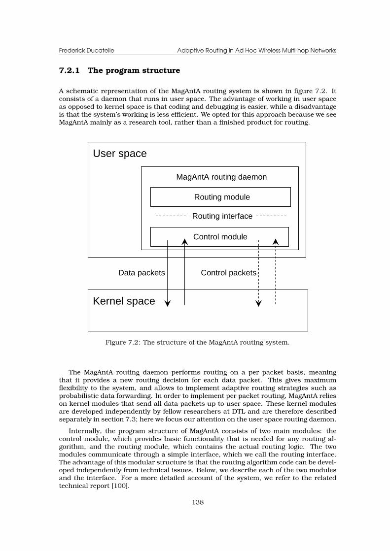
Frederick Ducatelle Adaptive Routing in Ad Hoc Wireless Multi-hop Networks
7.2.1 The program structure
A schematic representation of the MagAntA routing system is shown in figure 7.2. Itconsists of a daemon that runs in user space. The advantage of working in user spaceas opposed to kernel space is that coding and debugging is easier, while a disadvantageis that the system’s working is less efficient. We opted for this approach because we seeMagAntA mainly as a research tool, rather than a finished product for routing.
User space
Kernel space
MagAntA routing daemon
Routing module
Control module
Routing interface
Data packets Control packets
Figure 7.2: The structure of the MagAntA routing system.
The MagAntA routing daemon performs routing on a per packet basis, meaningthat it provides a new routing decision for each data packet. This gives maximumflexibility to the system, and allows to implement adaptive routing strategies such asprobabilistic data forwarding. In order to implement per packet routing, MagAntA relieson kernel modules that send all data packets up to user space. These kernel modulesare developed independently by fellow researchers at DTL and are therefore describedseparately in section 7.3; here we focus our attention on the user space routing daemon.
Internally, the program structure of MagAntA consists of two main modules: thecontrol module, which provides basic functionality that is needed for any routing al-gorithm, and the routing module, which contains the actual routing logic. The twomodules communicate through a simple interface, which we call the routing interface.The advantage of this modular structure is that the routing algorithm code can be devel-oped independently from technical issues. Below, we describe each of the two modulesand the interface. For a more detailed account of the system, we refer to the relatedtechnical report [100].
138
Frederick Ducatelle Adaptive Routing in Ad Hoc Wireless Multi-hop Networks
7.2.2 The control module
The function of the control module is to sustain the working of the daemon and to pro-vide basic functionality to the routing module. The daemon is implemented using aninfinite for-loop, in which the program waits for different events to take place. In par-ticular, it waits for data packets coming from the kernel, for incoming control packets,for routing events timing out, and for user interrupts (which can be used to pause thedaemon). When either of these happen, it takes the appropriate actions.
The functionality provided by the control module to the routing module includes fourbasic services. The first is to gather information about the local host, such as the avail-able network interfaces and their MAC addresses, the local IP address (if it is available),etc.. It presents this information to the routing module, so that it can be used by therouting algorithm. The second service is the transfer of data packets to and from thekernel. For this part, it communicates with kernel modules that send packets up touser space. Details about these kernel modules are given in section 7.3. The controlmodule deals with the technical issues involved in interacting with the kernel modulesand hides these from the routing module. Upon reception of a data packet, it stores thepacket in a static buffer, and provides the routing module with pointers to fields in thepacket headers that are relevant for routing, such as the destination address, the nexthop address, the outgoing interface, etc.. The routing algorithm can then work directlywith these pointers without being aware of the structure of the data packets or theirheaders. The third service is the sending and receiving of control packets. For this ser-vice, the control module communicates directly with the device drivers of the differentnetwork interfaces in the kernel. This is done through the use of raw packet socketsthat are standard available in the kernel [244]; no kernel modules or modificationsare needed. To the routing module, several different possibilities to transmit controlpackets are provided. These include unicast and broadcast transmission, as well asdelayed broadcast transmission, in which the control packet is broadcast after a shortrandom jitter (this is useful for the implementation of flooding). The fourth service isevent scheduling. The control module keeps an event list, to which the routing modulecan add any event that it needs. Whenever an event times out, the control module callsthe event handling function of the routing module.
7.2.3 The routing interface
The function of the routing interface is to form a bridge between the control module,which provides basic functionality, and the routing module, which contains the rout-ing protocol logic. Its most important component is the routing interface structure,which defines all communication possibilities between the two modules. Apart fromthis structure, the routing interface code contains also a number of other structuresand functions that provide useful functionalities for the routing module. These includefunctions to copy and compare addresses and time structures.
The contents of the routing interface structure are shown in figure 7.3 (some details,such as the parameters taken by each of the functions, are left out here to improvereadability). It contains a pointer to a local data structure and a number of functionpointers. The local data structure contains information about the local host, and isfilled in by the control module. It contains the name of the local host, its IP address,the IP, ad hoc and MAC broadcast addresses, and the list of devices available for adhoc routing, with their names and MAC addresses. This is basic information that isneeded by the routing module. The function pointers of routing interface are used forthe communication between the control module and the routing module. The firsthalf of these pointers are filled in by the control module, in order to allow the routingmodule to make use of the functionality it provides. They include a function to senddata packets to the kernel (either to be delivered locally or to be forwarded), different
139
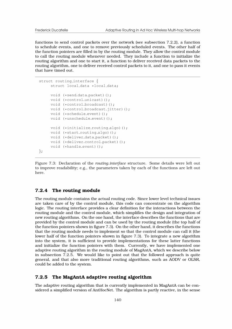
Frederick Ducatelle Adaptive Routing in Ad Hoc Wireless Multi-hop Networks
functions to send control packets over the network (see subsection 7.2.2), a functionto schedule events, and one to remove previously scheduled events. The other half ofthe function pointers are filled in by the routing module. They allow the control moduleto call the routing module whenever needed. They include a function to initialize therouting algorithm and one to start it, a function to deliver received data packets to therouting algorithm, one to deliver received control packets to it, and one to pass it eventsthat have timed out.
struct routing interface {struct local data *local data;
void (*send data packet)();void (*control unicast)();void (*control broadcast)();void (*control broadcast jitter)();void (*schedule event)();void (*unschedule event)();
void (*initialize routing algo)();void (*start routing algo)();void (*deliver data packet)();void (*deliver control packet)();void (*handle event)();
};
Figure 7.3: Declaration of the routing interface structure. Some details were left outto improve readability; e.g., the parameters taken by each of the functions are left outhere.
7.2.4 The routing module
The routing module contains the actual routing code. Since lower level technical issuesare taken care of by the control module, this code can concentrate on the algorithmlogic. The routing interface provides a clear definition for the interactions between therouting module and the control module, which simplifies the design and integration ofnew routing algorithms. On the one hand, the interface describes the functions that areprovided by the control module and can be used by the routing module (the top half ofthe function pointers shown in figure 7.3). On the other hand, it describes the functionsthat the routing module needs to implement so that the control module can call it (thelower half of the function pointers shown in figure 7.3). To integrate a new algorithminto the system, it is sufficient to provide implementations for these latter functionsand initialize the function pointers with them. Currently, we have implemented oneadaptive routing algorithm in the routing module of MagAntA, which we describe belowin subsection 7.2.5. We would like to point out that the followed approach is quitegeneral, and that also more traditional routing algorithms, such as AODV or OLSR,could be added to the system.
7.2.5 The MagAntA adaptive routing algorithm
The adaptive routing algorithm that is currently implemented in MagAntA can be con-sidered a simplified version of AntHocNet. The algorithm is partly reactive, in the sense
140
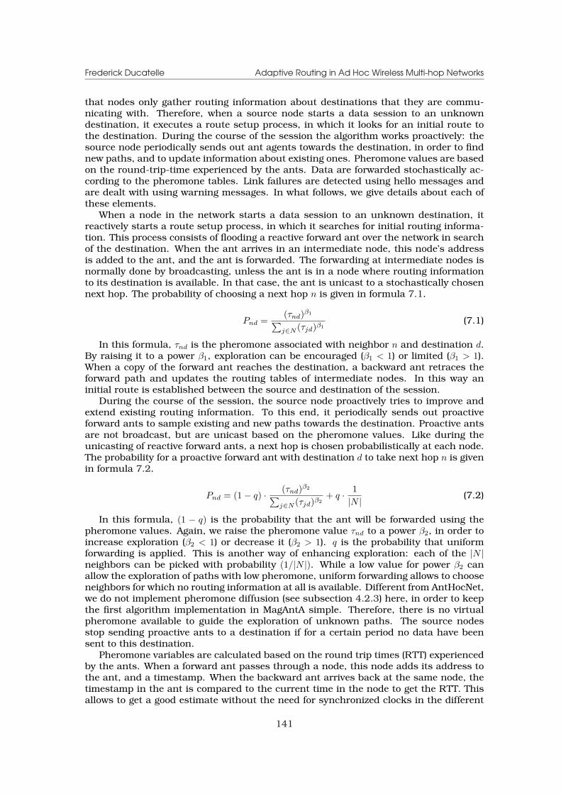
Frederick Ducatelle Adaptive Routing in Ad Hoc Wireless Multi-hop Networks
that nodes only gather routing information about destinations that they are commu-nicating with. Therefore, when a source node starts a data session to an unknowndestination, it executes a route setup process, in which it looks for an initial route tothe destination. During the course of the session the algorithm works proactively: thesource node periodically sends out ant agents towards the destination, in order to findnew paths, and to update information about existing ones. Pheromone values are basedon the round-trip-time experienced by the ants. Data are forwarded stochastically ac-cording to the pheromone tables. Link failures are detected using hello messages andare dealt with using warning messages. In what follows, we give details about each ofthese elements.
When a node in the network starts a data session to an unknown destination, itreactively starts a route setup process, in which it searches for initial routing informa-tion. This process consists of flooding a reactive forward ant over the network in searchof the destination. When the ant arrives in an intermediate node, this node’s addressis added to the ant, and the ant is forwarded. The forwarding at intermediate nodes isnormally done by broadcasting, unless the ant is in a node where routing informationto its destination is available. In that case, the ant is unicast to a stochastically chosennext hop. The probability of choosing a next hop n is given in formula 7.1.
Pnd =(τnd)β1
∑j∈N (τjd)β1
(7.1)
In this formula, τnd is the pheromone associated with neighbor n and destination d.By raising it to a power β1, exploration can be encouraged (β1 < 1) or limited (β1 > 1).When a copy of the forward ant reaches the destination, a backward ant retraces theforward path and updates the routing tables of intermediate nodes. In this way aninitial route is established between the source and destination of the session.
During the course of the session, the source node proactively tries to improve andextend existing routing information. To this end, it periodically sends out proactiveforward ants to sample existing and new paths towards the destination. Proactive antsare not broadcast, but are unicast based on the pheromone values. Like during theunicasting of reactive forward ants, a next hop is chosen probabilistically at each node.The probability for a proactive forward ant with destination d to take next hop n is givenin formula 7.2.
Pnd = (1− q) · (τnd)β2
∑j∈N (τjd)β2
+ q · 1|N | (7.2)
In this formula, (1 − q) is the probability that the ant will be forwarded using thepheromone values. Again, we raise the pheromone value τnd to a power β2, in order toincrease exploration (β2 < 1) or decrease it (β2 > 1). q is the probability that uniformforwarding is applied. This is another way of enhancing exploration: each of the |N |neighbors can be picked with probability (1/|N |). While a low value for power β2 canallow the exploration of paths with low pheromone, uniform forwarding allows to chooseneighbors for which no routing information at all is available. Different from AntHocNet,we do not implement pheromone diffusion (see subsection 4.2.3) here, in order to keepthe first algorithm implementation in MagAntA simple. Therefore, there is no virtualpheromone available to guide the exploration of unknown paths. The source nodesstop sending proactive ants to a destination if for a certain period no data have beensent to this destination.
Pheromone variables are calculated based on the round trip times (RTT) experiencedby the ants. When a forward ant passes through a node, this node adds its address tothe ant, and a timestamp. When the backward ant arrives back at the same node, thetimestamp in the ant is compared to the current time in the node to get the RTT. Thisallows to get a good estimate without the need for synchronized clocks in the different
141
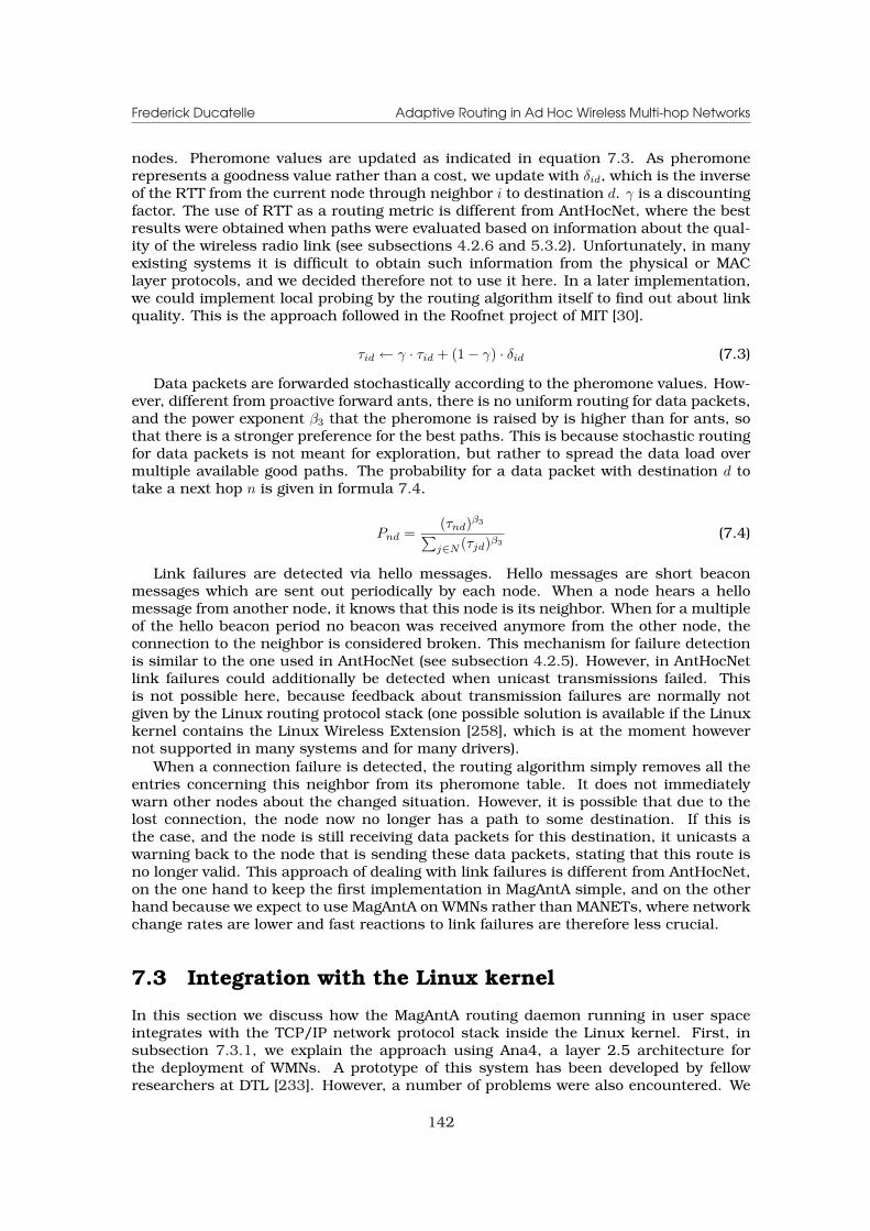
Frederick Ducatelle Adaptive Routing in Ad Hoc Wireless Multi-hop Networks
nodes. Pheromone values are updated as indicated in equation 7.3. As pheromonerepresents a goodness value rather than a cost, we update with δid, which is the inverseof the RTT from the current node through neighbor i to destination d. γ is a discountingfactor. The use of RTT as a routing metric is different from AntHocNet, where the bestresults were obtained when paths were evaluated based on information about the qual-ity of the wireless radio link (see subsections 4.2.6 and 5.3.2). Unfortunately, in manyexisting systems it is difficult to obtain such information from the physical or MAClayer protocols, and we decided therefore not to use it here. In a later implementation,we could implement local probing by the routing algorithm itself to find out about linkquality. This is the approach followed in the Roofnet project of MIT [30].
τid ← γ · τid + (1− γ) · δid (7.3)
Data packets are forwarded stochastically according to the pheromone values. How-ever, different from proactive forward ants, there is no uniform routing for data packets,and the power exponent β3 that the pheromone is raised by is higher than for ants, sothat there is a stronger preference for the best paths. This is because stochastic routingfor data packets is not meant for exploration, but rather to spread the data load overmultiple available good paths. The probability for a data packet with destination d totake a next hop n is given in formula 7.4.
Pnd =(τnd)β3
∑j∈N (τjd)β3
(7.4)
Link failures are detected via hello messages. Hello messages are short beaconmessages which are sent out periodically by each node. When a node hears a hellomessage from another node, it knows that this node is its neighbor. When for a multipleof the hello beacon period no beacon was received anymore from the other node, theconnection to the neighbor is considered broken. This mechanism for failure detectionis similar to the one used in AntHocNet (see subsection 4.2.5). However, in AntHocNetlink failures could additionally be detected when unicast transmissions failed. Thisis not possible here, because feedback about transmission failures are normally notgiven by the Linux routing protocol stack (one possible solution is available if the Linuxkernel contains the Linux Wireless Extension [258], which is at the moment howevernot supported in many systems and for many drivers).
When a connection failure is detected, the routing algorithm simply removes all theentries concerning this neighbor from its pheromone table. It does not immediatelywarn other nodes about the changed situation. However, it is possible that due to thelost connection, the node now no longer has a path to some destination. If this isthe case, and the node is still receiving data packets for this destination, it unicasts awarning back to the node that is sending these data packets, stating that this route isno longer valid. This approach of dealing with link failures is different from AntHocNet,on the one hand to keep the first implementation in MagAntA simple, and on the otherhand because we expect to use MagAntA on WMNs rather than MANETs, where networkchange rates are lower and fast reactions to link failures are therefore less crucial.
7.3 Integration with the Linux kernel
In this section we discuss how the MagAntA routing daemon running in user spaceintegrates with the TCP/IP network protocol stack inside the Linux kernel. First, insubsection 7.3.1, we explain the approach using Ana4, a layer 2.5 architecture forthe deployment of WMNs. A prototype of this system has been developed by fellowresearchers at DTL [233]. However, a number of problems were also encountered. We
142
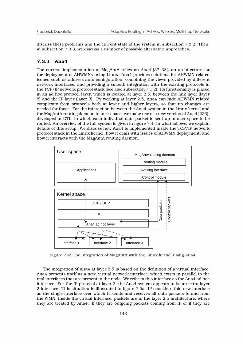
Frederick Ducatelle Adaptive Routing in Ad Hoc Wireless Multi-hop Networks
discuss these problems and the current state of the system in subsection 7.3.2. Then,in subsection 7.3.3, we discuss a number of possible alternative approaches.
7.3.1 Ana4
The current implementation of MagAntA relies on Ana4 [37, 38], an architecture forthe deployment of AHWMNs using Linux. Ana4 provides solutions for AHWMN relatedissues such as address auto-configuration, combining the views provided by differentnetwork interfaces, and providing a smooth integration with the existing protocols inthe TCP/IP network protocol stack (see also subsection 7.1.2). Its functionality is placedin an ad hoc protocol layer, which is located at layer 2.5, between the link layer (layer2) and the IP layer (layer 3). By working at layer 2.5, Ana4 can hide AHWMN relatedcomplexity from protocols both at lower and higher layers, so that no changes areneeded for those. For the interaction between the Ana4 system in the Linux kernel andthe MagAntA routing daemon in user space, we make use of a new version of Ana4 [233],developed at DTL, in which each individual data packet is sent up to user space to berouted. An overview of the full system is given in figure 7.4. In what follows, we explaindetails of this setup. We discuss how Ana4 is implemented inside the TCP/IP networkprotocol stack in the Linux kernel, how it deals with issues of AHWMN deployment, andhow it interacts with the MagAntA routing daemon.
User space
Kernel space
MagAntA routing daemon
Routing module
Control module
Routing interface
Dat
a pa
cket
s
Con
trol
pac
kets
Applications
TCP / UDP
IP
Ana4 ad hoc layer
Interface 1 Interface 2 Interface 3
Figure 7.4: The integration of MagAntA with the Linux kernel using Ana4.
The integration of Ana4 at layer 2.5 is based on the definition of a virtual interface:Ana4 presents itself as a new, virtual network interface, which exists in parallel to thereal interfaces that are present in the node. We refer to this interface as the Ana4 ad hocinterface. For the IP protocol at layer 3, the Ana4 system appears to be an extra layer2 interface. This situation is illustrated in figure 7.5a. IP considers this new interfaceas the single interface over which it sends and receives all data packets to and fromthe WMN. Inside the virtual interface, packets are in the layer 2.5 architecture, wherethey are treated by Ana4. If they are outgoing packets coming from IP or if they are
143
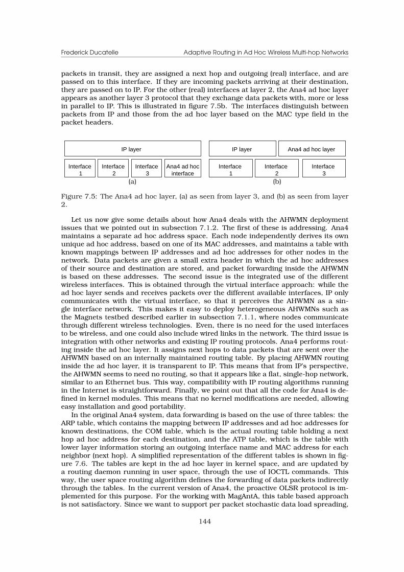
Frederick Ducatelle Adaptive Routing in Ad Hoc Wireless Multi-hop Networks
packets in transit, they are assigned a next hop and outgoing (real) interface, and arepassed on to this interface. If they are incoming packets arriving at their destination,they are passed on to IP. For the other (real) interfaces at layer 2, the Ana4 ad hoc layerappears as another layer 3 protocol that they exchange data packets with, more or lessin parallel to IP. This is illustrated in figure 7.5b. The interfaces distinguish betweenpackets from IP and those from the ad hoc layer based on the MAC type field in thepacket headers.
Interface1
Interface2
Interface3
Ana4 ad hoc interface
IP layer IP layer Ana4 ad hoc layer
Interface1
Interface2
Interface3
(a) (b)
Figure 7.5: The Ana4 ad hoc layer, (a) as seen from layer 3, and (b) as seen from layer2.
Let us now give some details about how Ana4 deals with the AHWMN deploymentissues that we pointed out in subsection 7.1.2. The first of these is addressing. Ana4maintains a separate ad hoc address space. Each node independently derives its ownunique ad hoc address, based on one of its MAC addresses, and maintains a table withknown mappings between IP addresses and ad hoc addresses for other nodes in thenetwork. Data packets are given a small extra header in which the ad hoc addressesof their source and destination are stored, and packet forwarding inside the AHWMNis based on these addresses. The second issue is the integrated use of the differentwireless interfaces. This is obtained through the virtual interface approach: while thead hoc layer sends and receives packets over the different available interfaces, IP onlycommunicates with the virtual interface, so that it perceives the AHWMN as a sin-gle interface network. This makes it easy to deploy heterogeneous AHWMNs such asthe Magnets testbed described earlier in subsection 7.1.1, where nodes communicatethrough different wireless technologies. Even, there is no need for the used interfacesto be wireless, and one could also include wired links in the network. The third issue isintegration with other networks and existing IP routing protocols. Ana4 performs rout-ing inside the ad hoc layer. It assigns next hops to data packets that are sent over theAHWMN based on an internally maintained routing table. By placing AHWMN routinginside the ad hoc layer, it is transparent to IP. This means that from IP’s perspective,the AHWMN seems to need no routing, so that it appears like a flat, single-hop network,similar to an Ethernet bus. This way, compatibility with IP routing algorithms runningin the Internet is straightforward. Finally, we point out that all the code for Ana4 is de-fined in kernel modules. This means that no kernel modifications are needed, allowingeasy installation and good portability.
In the original Ana4 system, data forwarding is based on the use of three tables: theARP table, which contains the mapping between IP addresses and ad hoc addresses forknown destinations, the COM table, which is the actual routing table holding a nexthop ad hoc address for each destination, and the ATP table, which is the table withlower layer information storing an outgoing interface name and MAC address for eachneighbor (next hop). A simplified representation of the different tables is shown in fig-ure 7.6. The tables are kept in the ad hoc layer in kernel space, and are updated bya routing daemon running in user space, through the use of IOCTL commands. Thisway, the user space routing algorithm defines the forwarding of data packets indirectlythrough the tables. In the current version of Ana4, the proactive OLSR protocol is im-plemented for this purpose. For the working with MagAntA, this table based approachis not satisfactory. Since we want to support per packet stochastic data load spreading,
144
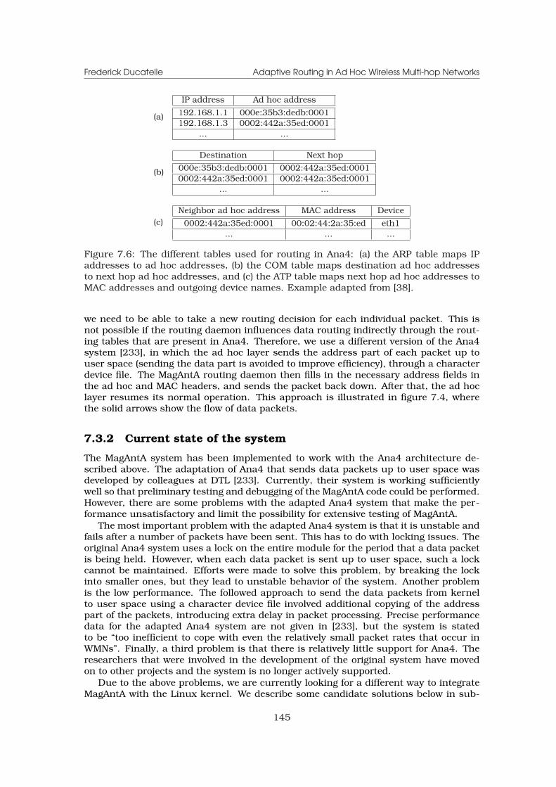
Frederick Ducatelle Adaptive Routing in Ad Hoc Wireless Multi-hop Networks
(a)
IP address Ad hoc address
192.168.1.1 000e:35b3:dedb:0001192.168.1.3 0002:442a:35ed:0001
... ...
(b)
Destination Next hop
000e:35b3:dedb:0001 0002:442a:35ed:00010002:442a:35ed:0001 0002:442a:35ed:0001
... ...
(c)Neighbor ad hoc address MAC address Device
0002:442a:35ed:0001 00:02:44:2a:35:ed eth1... ... ...
Figure 7.6: The different tables used for routing in Ana4: (a) the ARP table maps IPaddresses to ad hoc addresses, (b) the COM table maps destination ad hoc addressesto next hop ad hoc addresses, and (c) the ATP table maps next hop ad hoc addresses toMAC addresses and outgoing device names. Example adapted from [38].
we need to be able to take a new routing decision for each individual packet. This isnot possible if the routing daemon influences data routing indirectly through the rout-ing tables that are present in Ana4. Therefore, we use a different version of the Ana4system [233], in which the ad hoc layer sends the address part of each packet up touser space (sending the data part is avoided to improve efficiency), through a characterdevice file. The MagAntA routing daemon then fills in the necessary address fields inthe ad hoc and MAC headers, and sends the packet back down. After that, the ad hoclayer resumes its normal operation. This approach is illustrated in figure 7.4, wherethe solid arrows show the flow of data packets.
7.3.2 Current state of the system
The MagAntA system has been implemented to work with the Ana4 architecture de-scribed above. The adaptation of Ana4 that sends data packets up to user space wasdeveloped by colleagues at DTL [233]. Currently, their system is working sufficientlywell so that preliminary testing and debugging of the MagAntA code could be performed.However, there are some problems with the adapted Ana4 system that make the per-formance unsatisfactory and limit the possibility for extensive testing of MagAntA.
The most important problem with the adapted Ana4 system is that it is unstable andfails after a number of packets have been sent. This has to do with locking issues. Theoriginal Ana4 system uses a lock on the entire module for the period that a data packetis being held. However, when each data packet is sent up to user space, such a lockcannot be maintained. Efforts were made to solve this problem, by breaking the lockinto smaller ones, but they lead to unstable behavior of the system. Another problemis the low performance. The followed approach to send the data packets from kernelto user space using a character device file involved additional copying of the addresspart of the packets, introducing extra delay in packet processing. Precise performancedata for the adapted Ana4 system are not given in [233], but the system is statedto be “too inefficient to cope with even the relatively small packet rates that occur inWMNs”. Finally, a third problem is that there is relatively little support for Ana4. Theresearchers that were involved in the development of the original system have movedon to other projects and the system is no longer actively supported.
Due to the above problems, we are currently looking for a different way to integrateMagAntA with the Linux kernel. We describe some candidate solutions below in sub-
145
Frederick Ducatelle Adaptive Routing in Ad Hoc Wireless Multi-hop Networks
section 7.3.3.
7.3.3 Other approaches
Here, we explore other possibilities to integrate the MagAntA routing daemon with theLinux kernel. We look for systems that allow as much as possible to stick to the originaldesign architecture laid out for MagAntA. We first discuss an approach that builds onan existing implementation of the AODV routing protocol, and then one that uses Clickrouter.
In subsection 7.1.2, we have described several existing implementations of the AODVrouting protocol. Of these, the AODV-UCSB [57] implementation has a design thatis similar to the one that we are following with MagAntA. It uses a routing daemonthat runs in user space and that makes routing decisions on a per packet basis. Theintegration with the kernel is obtained through Netfilter and a kernel module. Eachpacket entering or leaving the node passes through the Netfilter hooks, from where itis redirected to a kernel module. This kernel module temporarily queues the packet.The user space daemon then takes a routing decision for each queued data packet.The main difference with the approach we have been following is that data packetsdo not go up to user space. Instead, the routing module manipulates the packets inthe kernel space. Nevertheless, per packet routing is still possible, and all routingcode remains in user space. This means that limited changes would be needed toMagAntA in order to work with this system; it would suffice to adapt the functions in thecontrol module that deal with receiving and sending data packets. The changes couldbe made transparent from the routing module. Disadvantages of using the AODV-UCSBapproach is that, different from Ana4, this system does not provide ready solutions forsome important AHWMN related issues such as address auto-configuration, integrationof heterogeneous interfaces, and a smooth integration with other networks runningtraditional IP routing algorithms.
A different approach, which is also proposed in [233] in response to the problemswith Ana4, is to use a Click router. Click [155] is a flexible, modular software ar-chitecture for building configurable routers under Linux. The Click system defines anumber of modules, called elements, which carry out basic functionality that is neededin a router. Examples of existing elements are Queue, which queues data packets,LookupIPRoute, which looks for the destination of a packet in a static routing table,ToDevice, which hands packets to a Linux device driver for transmission, etc.. To build aClick router, one needs to select a combination of these elements that together performthe required functionality, and define connections between them. If the functionality ofexisting elements is not sufficient, one can also program new elements: all elements arewritten in C++ and are subclasses of the class Element. Once a Click router has beenput together, it can be placed in the Click system to function as a Linux router. Onehas the choice between running the router using a Linux in-kernel driver, or using auser-level driver. While the former gives better performance, the latter allows easier de-bugging and fast prototyping. For MagAntA, the advantage of working with Click wouldbe that we can continue working in user space, and maintain a modular and flexiblestructure for the program. Another advantage is that Click is widely used and welldocumented and supported, which makes it an easy to use developing environment. Adisadvantage is that we would need to make considerable changes to the structure ofMagAntA, in order to make it adhere to the typical structure of a Click router in whichthe code is organized according to the flow of packets through a connected system ofelements. Moreover, we would need to program a number of new Click elements tosupport functions that are needed in adaptive routing. Another disadvantage is that,unlike Ana4, Click does not support ready solutions for AHWMN related issues such asaddress auto-configurations and the like. Since, however, Click allows flexible routing
146

Frederick Ducatelle Adaptive Routing in Ad Hoc Wireless Multi-hop Networks
design, such solutions could be implemented.When comparing the two possibilities described above, it seems that the approach
using the AODV-UCSB implementation would be the easiest solution to continue withthe work implemented so far. However, the approach using Click gives more flexibilityand is better documented and supported, so that in the long run, it might be moreinteresting to invest the extra effort needed to migrate to Click.
7.4 Conclusion
In this chapter, we have described efforts that we have made towards the implementa-tion of adaptive routing in AHWMNs. We have presented the MagAntA system, a userspace routing daemon for adaptive routing. MagAntA has a modular structure, con-sisting of a control module, a routing module, and a routing interface between thesetwo. This structure, together with the fact that the system runs entirely in user space,makes it easily extendible and adaptable, so that it is an easy to use research tool.For integration with the Linux kernel, the MagAntA system relies on Ana4, a layer 2.5architecture for the deployment of AHWMNs. The interaction between MagAntA andAna4 is established through packet forwarding: we use an adapted version of Ana4,developed by colleagues at DTL, in which each data packet is sent up to user space tobe routed. The fact that each data packet can be routed individually by the MagAntArouting daemon provides the flexibility that is needed to perform adaptive routing.
The work presented in this chapter is still in progress. While MagAntA has beensubjected to preliminary tests, these were only sufficient to do debugging and verifybasic functionality. Thorough tests of the system to get performance data have notbeen carried out yet. This is due to programming problems that were encounteredby the developers of the adapted Ana4 system. This system is currently still unstableand gives poor performance. We have described some possible alternatives for theintegration of Ana4 with the kernel, using the existing AODV-UCSB system and usingClick. Further developments will be needed to find out which approach is best suitedfor our work.
147

Chapter 8
Conclusions
In this thesis, we have addressed the problem of adaptive routing in AHWMNs usingtechniques from AI and ACO. We have first given an introduction to the fields of AH-WMNs and adaptive routing. Then, we have described the AntHocNet routing algorithm,and next, we have presented a range of experimental tests in which we investigated thebehavior and performance of this algorithm. The tests were carried out both in tradi-tional open space scenarios and in an urban setting. Finally, we have also described asystem for the implementation of ACO algorithms in real world testbeds.
In what follows, we first give an overview of the contributions and findings of thisthesis, and then discuss possible future research directions.
8.1 Contributions and findings of this thesis
The main contribution of this thesis is the development of the AntHocNet routing al-gorithm. AntHocNet has a hybrid architecture, whereby a reactive route setup processis used at the start of each new communication session in order to obtain an initialpath for data forwarding, and a proactive route maintenance process is run through-out the duration of the session with the objective to keep information about existingpaths up-to-date and to explore new and possibly better paths, continuously adaptingto the changing network environment. AntHocNet also possesses a number of reactivemechanisms to deal with link failures, such as the transmission of failure notificationmessages and the possibility to execute local route repairs.
A distinct feature of AntHocNet is that it is based on methods from AI. In particu-lar, it uses elements from ACO and from dynamic programming. From ACO it inheritsthe use of continuous Monte Carlo sampling of full paths, and the use of stochasticdecision making. From dynamic programming, it adopts the use of information boot-strapping. Both Monte Carlo sampling and information bootstrapping are importantparadigms in the field of reinforcement learning. In AntHocNet, Monte Carlo samplingis applied extensively throughout the different components of the algorithm, while in-formation bootstrapping is the basis of the pheromone diffusion process that is part ofthe proactive route maintenance process. While the continuous sampling of full pathsprovides adaptivity and reliability, information bootstrapping gives a highly efficientbut potentially unreliable way of spreading routing information. In the combination ofboth techniques, the sampling practices can be considered a way to confirm the infor-mation suggested earlier by the information bootstrapping process. This approach tocombining Monte Carlo sampling and information bootstrapping is inherently differentfrom other ways of integrating these two important learning paradigms in the field ofreinforcement learning.
149
Frederick Ducatelle Adaptive Routing in Ad Hoc Wireless Multi-hop Networks
We have evaluated the AntHocNet routing algorithm in a wide range of differenttests. A first set of tests was based on standard, open space scenarios. This is a com-mon approach in the field AHWMN research, and was adopted here in order to allow faircomparisons. In these tests, we first compared AntHocNet to existing state-of-the-artAHWMN routing algorithms, including AODV, an important reactive routing algorithm,OLSR, a representative proactive routing algorithm, and ANSI, which is like AntHocNetbased on ACO. Results showed that AntHocNet could outperform the other three algo-rithms over a wide range of different scenarios. Specifically, AntHocNet turned out toperform well in tests with increasing levels of mobility, to deal better than the other al-gorithms with different levels of data load, to cope well with sparse network situations,and to scale well to networks of increasing sizes. On the downside, AntHocNet’s advan-tage was decreased when mobility got very high, and the algorithm was outperformedby AODV when node density got high. In the same test scenarios, we also investigatedthe internal working of AntHocNet. We alternatively enabled and disabled various com-ponents of the algorithm, and investigated their influence. We found that the proactivemaintenance process always has a high contribution to the algorithm’s performance,and that this process should work as fast as possible (i.e., producing large and frequentupdate messages), as long as no excessive levels of overhead are reached. The localroute repair mechanism was found to give important advantages in large networks, butto have a negative impact in small networks. Among the different routing metrics, theSINR based measure gave best results. Finally, we found that, contrary to results inwired networks, stochastic forwarding of forward ants and data did not give advantages;it is better to exploit the best available information.
A second set of tests was based on an urban scenario. We proposed a simulationsetup providing a detailed and at the same time computationally efficient modeling ofoutdoor radio propagation, node mobility, and user traffic. We applied this model usingthe street map of Lugano as a reference. We first investigated properties of the urbannetwork graph and compared them to those of equivalent open space environments. Wefound that nodes have less neighbors, that network connectivity is worse, that paths arelonger, and link durations shorter. Next, we compared the behavior of AntHocNet withthat of AODV in this setup, applying tests in which we varied data send rate, numberof data sessions, node density, and node speed. We found that AntHocNet profits fromthe lower local density in urban settings to let its proactive mechanism work efficiently.However, at high rates, it suffers from interference. At very low rates, both algorithmshave difficulties due to their approach to construct initial routing information reactively.We found that node density has a strong impact on the delivery ratio, while the nodespeed has relatively little impact. Finally, we also found that using AntHocNet, it ispossible to deliver VoIP levels of service, but only for a limited number of sessions. Thispoints to the need for call admission control mechanisms in urban MANETs.
Finally, we investigated the implementation of ACO routing in a Linux based testbed.We presented the MagAntA system, which is a user space routing daemon that imple-ments ACO routing. MagAntA has a modular structure, consisting of a control module,a routing module, and a routing interface between these two. Thanks to this modularapproach and the system’s location in user space, MagAntA is easily extendible andadaptable. For the communication with the Linux kernel, the system relies on Ana4,a layer 2.5 architecture for the deployment of AHWMNs that is defined in a number ofkernel modules. We use a version of Ana4 developed by colleagues at DTL, in which allpackets going to and from the AHWMN are sent up to user space to be treated for rout-ing by MagAntA. This version of Ana4 is in its current state unfortunately still unstable,and MagAntA can therefore not fully be used. We investigated some possible alternativedeployment plans for our system.
150
Frederick Ducatelle Adaptive Routing in Ad Hoc Wireless Multi-hop Networks
8.2 Future research directions
Here we point out some future research directions that are relevant for the work pre-sented in this thesis. These concern the deployment and testing of AntHocNet in hard-ware testbeds, the support of QoS issues in AntHocNet, the use of the ideas behindAntHocNet in other types of networks, the application of other ideas from artificial in-telligence in the field of computer networking, and finally the support of autonomicnetworking.
In chapter 7, we have described a system for the implementation of AntHocNet ina Linux testbed. However, further work is needed in this direction. Implementationand testing in real testbeds is important in the field of networking and especially inthe area of AHWMNs. Real deployment tests can bring up issues that did not come upin simulation. To work well in real implementations, changes might be needed to theAntHocNet algorithm. However, it is encouraging to see that the few other algorithmsthat take into account link quality and use it to proactively improve paths during thecourse of communication sessions, namely LQSR, Srcr and LUNAR, have come out ofresearch on real testbeds.
In chapter 6, we have investigated the use of AntHocNet in a detailed simulation ofan urban environment. One of the tests was concerned with the support of VoIP traffic.Our finding was that VoIP data traffic can in principle be supported by AntHocNet, ifthe number of data sessions with such demands is limited. This brings up the issueof admission control and QoS support. Such mechanisms should be integrated withAntHocNet. An interesting aspect is the fact that AntHocNet uses extensive probing,which could provide the information needed to support QoS. Admission control couldbe carried out during the reactive route setup process.
Interesting future work would also be to apply the ideas behind AntHocNet in dif-ferent kinds of networks. One could in the first place target packet switched wirednetworks. Existing ACO routing algorithms developed for such networks provide adap-tivity with respect to variations in data load, and often ignore the effect of topologychanges. While such changes are less frequent in wired networks compared to AH-WMNs, they can still occur, e.g. due to link or node failures, and the mechanismsdeveloped in AntHocNet could be used to deal with this. Other types of networks inwhich AntHocNet’s mechanisms could be useful are application layer overlay networks.In such networks, nodes are connected at the application layer through virtual links,that are implemented as paths in the underlying physical network. Overlay networkscan have very dynamic topologies. Examples of application layer overlay networks arepeer-to-peer networks [243] and resilient overlay networks [20].
Another interesting direction for future research is to elaborate further on the rela-tionship between the problem of routing and the field of reinforcement learning. In thereinforcement learning literature, one can find more approaches to learning that canbe useful for network routing. One aspect that seems interesting is the possibility toperform off-policy Monte Carlo learning [252]. In off-policy learning the policy used tosample paths is different from the one that information is gathered for. A routing algo-rithm could then use a rather explorative policy for sampling, but gather informationfor a data packet routing policy that is more exploitative or even radically different (e.g.in the case of differentiated QoS routing [153]). Another interesting approach would beto use intermediate bootstrapping, as is done in temporal difference learning [251].
Finally, our work on AntHocNet could be extended in the direction of autonomiccomputing [152]. The main idea behind autonomic computing is that computer sys-tems are getting too complex for human operators to manage, and that they shouldbecome more “self-organized”. For the area of networking, this means that the networkshould be self-configuring, self-optimizing, self-protecting and self-healing. While theseproperties are to some extent already present in the adaptivity, robustness and scala-bility of AntHocNet, further developments would be needed to get to a fully autonomic
151

Frederick Ducatelle Adaptive Routing in Ad Hoc Wireless Multi-hop Networks
routing algorithm. E.g., the algorithm should be able to tune its parameters, and toadapt its working automatically to different types of networks and different types ofdata traffic to be served. Nevertheless, AntHocNet’s approach to constantly gather in-formation about the network through sampling and pheromone diffusion gives a goodbasis to build such a system.
152
Bibliography
[1] Berlinroofnet. Available from: http://sarwiki.informatik.hu-berlin.de/BerlinRoofNet.
[2] Funkfeuer. Available from: http://www.funkfeuer.at/.
[3] IEEE 802.11 standard group website. Available from: http://www.ieee802.org/11/.
[4] IEEE 802.15 standard group website. Available from: http://www.ieee802.org/15/.
[5] IEEE 802.16 standard group website. Available from: http://www.ieee802.org/16/.
[6] The internet engineering task force mobile ad-hoc networking page (MANET).Available from: http://www.ietf.org/html.charters/manet-charter.html.
[7] Microsoft Mesh Networks. Available from: http://research.microsoft.com/mesh/.
[8] The NRL OLSR routing protocol implementation. Available from: http://pf.itd.nrl.navy.mil/olsr/.
[9] olsr.freifunk.net. Available at: http://olsrexperiment.de.
[10] Taipei-wlan. Available from: http://wlan.taipei-elife.net/english/main.html.
[11] Technical specifications and technical reports for a utran-based 3gpp system.Available from: http://www.3gpp.org/ftp/Specs/html-info/21101.htm.
[12] Wireless philadelphia. Available from: http://www.wirelessphiladelphia.org.
[13] The zigbee alliance. Available from: http://www.zigbee.org/en/index.asp.
[14] M. Abolhasan, T. Wysocki, and E. Dutkiewicz. A review of routing protocols formobile ad hoc networks. Ad Hoc Networks, 2:1–22, 2004.
[15] D. Aguayo, J. Bicket, S. Biswas, G. Judd, and R. Morris. Link-level measurementsfrom an 802.11b mesh network. SIGCOMM Computer Commununication Review,34(4):121–132, 2004.
[16] I. F. Akyildiz, X. Wang, and W. Wang. Wireless mesh networks: a survey. Com-puter Networks Journal, 47:445–487, March 2005.
[17] I. F. Akyildiz, S. Weilian, Y. Sankarasubramaniam, and E. Cayirci. A survey onsensor networks. IEEE Communications Magazine, 40(8):102–116, August 2002.
153

Frederick Ducatelle Adaptive Routing in Ad Hoc Wireless Multi-hop Networks
[18] J. N. Al-Karaki and A. E. Kamal. Routing techniques in wireless sensor networks:a survey. IEEE Wireless Communications, 11(6):6–28, December 2004.
[19] M. Ali, U. Saif, A. Dunkels, T. Voigt, K. Romer, K. Langendoen, J. Polastre, andZ. A. Uzmi. Medium access control issues in sensor networks. ACM SIGCOMMComputer Communication Review, 36(2), April 2006.
[20] D. G. Andersen, H. Balakrishnan, M. F. Kaashoek, and R. Morris. Resilient over-lay networks. In Proceedings of the 18th ACM Symposium on Operating SystemsPrinciples, Banff, Canada, October 2001.
[21] AWE Communications. WinProp software suite.
[22] H. Balakrishnan, V. N. Padmanabhan, S. Seshan, and R. H. Katz. A comparisonof mechanisms for improving TCP performance over wireless links. In Proceedingsof ACM SIGCOMM ’96, August 1996.
[23] B. Baran and R. Sosa. A new approach for AntNet routing. In Proceedings of the9th International Conference on Computer Communications Networks, Las Vegas,USA, 2000.
[24] J. S. Baras and H. Mehta. A probabilistic emergent routing algorithm for mobilead hoc networks. In WiOpt03: Modeling and Optimization in Mobile, Ad Hoc andWireless Networks, 2003.
[25] A. G. Barto, R. S. Sutton, and C. W. Anderson. Neuronlike adaptive elements thatcan solve difficult learning control problems. IEEE Transaction on Systems, Manand Cybernetics, SMC-13:834–846, 1983.
[26] R. Bellman. Dynamic Programming. Princeton University Press, 1957.
[27] R. Bellman. On a routing problem. Quarterly of Applied Mathematics, 16(1):87–90, 1958.
[28] B. Bensaou, Y. Wang, and C. C. Ko. Fair medium access in 802.11 based wirelessad hoc networks. In Proceedings of Mobile Ad Hoc Networking and Computing(MobiHoc 2000), pages 99–106, 2000.
[29] C. Bettstetter, G. Resta, and P. Santi. The node distribution of the random way-point mobility model for wireless ad hoc networks. IEEE Transactions on MobileComputing, 2(3):257–269, 2003.
[30] J. Bicket, D. Aguayo, S. Biswas, and R. Morris. Architecture and evaluation of anunplanned 802.11b mesh network. In Proceedings of Mobicom, August 2005.
[31] L. Blazevic, L. Buttyan, S. Capkun, S. Giordano, J.-P. Hubaux, and J.-Y. LeBoudec. Self-organization in mobile ad-hoc networks: the approach of termin-odes. IEEE Communications Magazine, 39(6), June 2001.
[32] L. Blazevic, S. Giordano, and J.-Y. Le Boudec. Anchored path discovery in ter-minode routing. In Proceedings of The Second IFIP-TC6 Networking Conference(Networking 2002), May 2002.
[33] Bluetooth Special Interest Group. Specification of bluetooth system, February2002. Version 1.1.
[34] E. Bonabeau, M. Dorigo, and G. Theraulaz. Swarm Intelligence: From Natural toArtificial Systems. Oxford University Press, 1999.
154

Frederick Ducatelle Adaptive Routing in Ad Hoc Wireless Multi-hop Networks
[35] E. Bonabeau, F. Henaux, S. Guerin, D. Snyers, P. Kuntz, and G. Theraulaz. Rout-ing in telecommunication networks with ”Smart” ant-like agents. In Proceedingsof IATA’98, Second Int. Workshop on Intelligent Agents for Telecommunication Ap-plications, volume 1437 of Lecture Notes in Artificial Intelligence. Springer Verlag,1998.
[36] E. Borgia, M. Conti, F. Delmastro, and E. Gregori. Experimental comparison ofrouting and middleware solutions for mobile ad hoc networks: legacy vs cross-layer approach. In Proceedings of the ACM SIGCOMM Workshop on ExperimentalApproaches to Wireless Network Design and Analysis (E-WIND), August 2005.
[37] N. Boulicault, G. Chelius, and E. Fleury. Experiments of ana4: An implementa-tion of a 2.5 framework for deploying real multi-hop ad hoc and mesh networks.In Proceedings of the IEEE ICPS Workshop on Multi-hop Ad hoc Networks: fromtheory to reality, Santorini, Greece, July 2005.
[38] N. Boulicault, G. Chelius, and E. Fleury. Ana4: a 2.5 framework for deployingreal multi-hop ad hoc and mesh networks. Ad Hoc & Sensor Wireless Networks:an International Journal (AHSWN), 2006. To appear.
[39] J. A. Boyan and M. L. Littman. Packet routing in dynamically changing networks:A reinforcement learning approach. In J. D. Cowan, G. Tesauro, and J. Alspector,editors, Advances in Neural Information Processing Systems 6 (NIPS6), pages 671–678. Morgan Kaufmann, San Francisco, CA, USA, 1994.
[40] R. Braden, D. Clark, and S. Shenker. Integrated services in the Internet architec-ture: an overview. Request For Comments (RFC) 1633, Network Working Group,1994.
[41] D. Braginsky and D. Estrin. Rumor routing algorithm for sensor networks. InProceedings of the First Workshop on Sensor Networks and Applications (WSNA),Atlanta, GA, USA, October 2002.
[42] J. Broch, D. A. Maltz, D. B. Johnson, Y.-C. Hu, and J. Jetcheva. A performancecomparison of multi-hop wireless ad hoc network routing protocols. In Proceed-ings of the Fourth Annual ACM/IEEE International Conference on Mobile Computingand Networking (MobiCom), 1998.
[43] T. Bu, L. Gao, and D. Towsley. On characterizing bgp routing table growth. InProceedings of the IEEE Global Internet Symposium, Taipei, Taiwan, November2002.
[44] S. Burleigh, A. Hooke, L. Torgerson, K. Fall, V. Cerf, B. Durst, K. Scott, andH. Weiss. Delay-tolerant networking: An approach to interplanetary internet.IEEE Communications Magazine, June 2003.
[45] D. Camara and A. Loureiro. Gps/ant-like routing in ad hoc networks. Telecom-munication Systems, 18(1–3):85–100, 2001.
[46] T. Camp, J. Boleng, and V. Davies. A survey of mobility models for ad hoc networkresearch. Wireless Communications & Mobile Computing: Special issue on MobileAd Hoc Networking: Research, Trends and Applications, 2002.
[47] S. Capkun, M. Hamdi, and J.-P. Hubaux. Gps-free positioning in mobile ad-hocnetworks. In Proceedings of the 34th Hawaii International Conference on SystemSciences (HICSS), January 2001.
[48] S. Carl-Mitchell and J. S. Quarterman. Using ARP to Implement Transparent Sub-net Gateways. Network Working Group, October 1987. RFC 1027.
155
Frederick Ducatelle Adaptive Routing in Ad Hoc Wireless Multi-hop Networks
[49] G. D. Caro, F. Ducatelle, and L. M. Gambardella. Demonstrator for mobile ad hocnetworks. Internal Deliverable D12-D13 of FET Project BISON (IST-2001-38923),2004.
[50] L. Carrillo, C. Guadall, J. L. Marzo, G. Di Caro, F. Ducatelle, and L. M. Gam-bardella. Differentiated quality of service scheme based on the use of multi-classes of ant-like mobile agents. In CoNEXT’05: Proceedings of the 2005 ACMconference on Emerging network experiment and technology, Toulouse, France,2005.
[51] L. Carrillo, J. Marzo, D. Harle, and P. Vila. A review of scalability and its ap-plication in the evaluation of the scalability measure of antnet routing. In C. P.Salvador, editor, Proceedings of the IASTED Conference on Communication Sys-tems and Networks (CSN’03), pages 317–323. ACTA Press, 2003.
[52] A. Carzaniga, M. J. Rutherford, and A. L. Wolf. A routing scheme for content-based networking. In Proceedings of IEEE Infocom, Hong Kong, China, March2004.
[53] R. Castaneda and S. R. Das. Query localization techniques for on-demand routingprotocols in ad hoc networks. In Proceedings of the ACM/IEEE MobiCom, pages186–194, Seattle, WA, USA, August 1999.
[54] D. Cavin, Y. Sasson, and A. Schiper. On the accuracy of manet simulators. InProceedings of the Workshop on Principles of Mobile Computing (POMC), 2002.
[55] A. Chaintreau, P. Hui, J. Crowcroft, C. Diot, R. Gass, and J. Scott. Impact ofhuman mobility on the design of opportunistic forwarding algorithms. In Pro-ceedings of 25th IEEE Conference on Computer Communications (INFOCOM), April2006.
[56] I. D. Chakeres and E. M. Belding-Royer. The utility of hello messages for deter-mining link connectivity. In Proceedings of the 5th International Symposium onWireless Personal Multimedia Communications (WPMC), Honolulu, HI, USA, Octo-ber 2002.
[57] I. D. Chakeres and E. M. Belding-Royer. Aodv implementation design and perfor-mance evaluation. 2/3, 2005.
[58] C. Cheng, R. Riley, S. P. R. Kumar, and J. J. Garcia-Luna-Aceves. A loop-freeextended bellman-ford routing protocol without bouncing effect. In Proceedingsof the Symposium on Communications architectures & protocols (SIGCOMM), pages224–236, 1989.
[59] C.-C. Chiang, H. Wu, W. Liu, and M. Gerla. Routing in clustered multihop, mobilewireless networks with fading channel. In Proceedings of IEEE SICON’97, pages197–211, April 1997.
[60] T. Clausen and P. Jacquet. Optimized Link State Routing Protocol (OLSR). IETF,October 2003. RFC 3626.
[61] T. Clausen, P. Jacquet, A. Laouiti, P. Muhlethaler, A. Qayyum, and L. Viennot.Optimized link state routing protocol. In Proceedings of IEEE INMIC, 2001.
[62] S. Corson and J. Macker. Mobile ad hoc networking (MANET): Routing protocolperformance issues and evaluation considerations. Network Working Group, Re-quest for Comments 2501, January 1999. Available from: http://www.ietf.org/rfc/rfc2501.txt.
156
Frederick Ducatelle Adaptive Routing in Ad Hoc Wireless Multi-hop Networks
[63] D. Costa and A. Hertz. Ants can colour graphs. Journal of the Operational Re-search Society, 48:295–305, 1997.
[64] M. Daneshtalab, A. A. Kusha, A. Sobhani, Z. Navabi, M. D. Mottaghi, andO. Fatemi. Ant colony based routing architecture for minimizing hot spots inNoCs. In Proceedings of the 19th annual symposium on Integrated circuits andsystems design (SBCCI), pages 56–61, Ouro Preto, MG, Brazil, 2006.
[65] S. R. Das, C. E. Perkins, and E. M. Royer. Performance comparison of two on-demand routing protocols for ad hoc networks. In Proceedings of the IEEE Con-ference on Computer Communications (INFOCOM), March 2000.
[66] D. S. J. De Couto, D. Aguayo, J. Bicket, and R. Morris. A high-throughput pathmetric for multi-hop wireless routing. In Proceedings of the 9th ACM InternationalConference on Mobile Computing and Networking (MobiCom), September 2003.
[67] D. S. J. De Couto, D. Aguayo, B. A. Chambers, and R. Morris. Performance ofmultihop wireless networks: Shortest path is not enough. In Proceedings of theFirst Workshop on Hot Topics in Networks (HotNets-I). ACM SIGCOMM, 2002.
[68] C. de Waal. Bonnmotion: A mobility scenario generation and analy-sis tool, 2002. Available from: http://web.informatik.uni-bonn.de/IV/Mitarbeiter/dewaal/BonnMotion/.
[69] S. Desilva and S. R. Das. Experimental evaluation of a wireless ad hoc network.In Proceedings of the 9th International Conference on Computer Communicationsand Networks (IC3N), 2000.
[70] G. Di Caro. Ant Colony Optimization and its application to adaptive routing intelecommunication networks. PhD thesis, Faculte des Sciences Appliquees, Uni-versite Libre de Bruxelles, Brussels, Belgium, 2004.
[71] G. Di Caro and M. Dorigo. AntNet: Distributed stigmergetic control for commu-nications networks. Journal of Artificial Intelligence Research (JAIR), 9:317–365,1998.
[72] G. Di Caro and M. Dorigo. Two ant colony algorithms for best-effort routing indatagram networks. In Proceedings of the Tenth IASTED International Conferenceon Parallel and Distributed Computing and Systems (PDCS’98), pages 541–546.IASTED/ACTA Press, 1998.
[73] G. Di Caro, F. Ducatelle, and L. M. Gambardella. AntHocNet: an ant-based hybridrouting algorithm for mobile ad hoc networks. In Proceedings of Parallel ProblemSolving from Nature (PPSN) VIII, volume 3242 of Lecture Notes in Computer Science,pages 461–470. Springer-Verlag, 2004.
[74] G. Di Caro, F. Ducatelle, and L. M. Gambardella. AntHocNet: an adaptive nature-inspired algorithm for routing in mobile ad hoc networks. European Transactionson Telecommunications (ETT), 16(5), 2005.
[75] G. Di Caro, F. Ducatelle, and L. M. Gambardella. Swarm intelligence for routingin mobile ad hoc networks. In Proceedings of the 2005 IEEE Swarm IntelligenceSymposium (SIS), June 2005.
[76] G. Di Caro, F. Ducatelle, and L. M. Gambardella. Reflecting Interfaces: The Com-plex Coevolution of Information Technology Ecosystems, chapter Theory and prac-tice of Ant Colony Optimization for routing in dynamic telecommunications net-works. Idea Group Inc., 2008. To appear.
157
Frederick Ducatelle Adaptive Routing in Ad Hoc Wireless Multi-hop Networks
[77] G. Di Caro, F. Ducatelle, P. Heegarden, M. Jelasity, R. Montemanni, and A. Mon-tresor. Evaluation of basic services in ad-hoc, peer-to-peer and grid networks.Internal Deliverable D7 of FET Project BISON (IST-2001-38923), 2004.
[78] G. Di Caro and T. Vasilakos. Ant-SELA: Ant-agents and stochastic automatalearn adaptive routing tables for QoS routing in ATM networks. ANTS’2000 -From Ant Colonies to Artificial Ants: Second International Workshop on Ant ColonyOptimization, Brussels (Belgium), September 8-9, 2000.
[79] T. Dinh Dang, B. Sonkoly, and S. Molnar. Fractal analysis and modeling of voiptraffic. In Proceedings of the 11th International Telecommunications Network Strat-egy and Planning Symposium (NETWORKS 2004), June 2004.
[80] S. Doi and M. Yamamura. Bntnetl and its evaluation on a situation of congestion.Electronics and Communications in Japan (Part I: Communications), 85(9):31–41,April 2002.
[81] Y. Dong, D. Makrakis, and T. Sullivan. Effective admission control in multihopmobile ad hoc networks. In Proc. of the International Conference on CommunicationTechnology (ICCT), 2003.
[82] M. Dorigo. Optimization, Learning and Natural Algorithms (in Italian). PhD thesis,Dipartimento di Elettronica e Informazione, Politecnico di Milano, IT, 1992.
[83] M. Dorigo, G. Di Caro, and L. M. Gambardella. Ant algorithms for distributeddiscrete optimization. Artificial Life, 5(2):137–172, 1999.
[84] M. Dorigo and L. M. Gambardella. Ant colony system: A cooperative learningapproach to the traveling salesman problem. IEEE Transactions on EvolutionaryComputation, 1(1):53–66, 1997.
[85] M. Dorigo, V. Maniezzo, and A. Colorni. The ant system: Optimization by a colonyof cooperating agents. IEEE Transactions on Systems, Man, and Cybernetics–PartB, 26(1):29–41, 1996.
[86] M. Dorigo and T. Stutzle. The ant colony optimization metaheuristic: Algorithms,applications, and advances. In F. Glover and G. Kochenberger, editors, Handbookof Metaheuristics, volume 57 of International Series in Operations Research andManagement Science. Kluwer Academic Publishers, 2003.
[87] M. Dorigo and T. Stutzle. Ant Colony Optimization. MIT Press, Cambridge, MA,2004.
[88] O. Dousse, F. Baccelli, and P. Thiran. Impact of interferences on connectivity inad hoc networks. In Proceedings of IEEE INFOCOM 2003, San Francisco, April2003.
[89] O. Dousse, P. Thiran, and M. Hasler. Connectivity in ad-hoc and hybrid networks.In Proceedings of IEEE INFOCOM 2002, pages 1079–1088, New York, June 2002.
[90] J. Dowling, E. Curran, R. Cunningham, and V. Cahill. Using feedback in collab-orative reinforcement learning to adaptively optimize manet routing. IEEE Trans-actions on Systems, Man, and Cybernetics - Part A: Systems and Humans, 35(3),May 2005.
[91] K. Doya, K. Samejima, K. Katagiri, and K. Kawato. Multiple model-based rein-forcement learning. Neural Computing, 14(6):1347–1369, 2002.
158
Frederick Ducatelle Adaptive Routing in Ad Hoc Wireless Multi-hop Networks
[92] R. Draves, J. Padhye, and B. Zill. The architecture of the link quality sourcerouting protocol. Technical report MSR-TR-2004-57, Microsoft Research, 2004.
[93] R. Draves, J. Padhye, and B. Zill. Comparison of routing metrics for static multi-hop wireless networks. In Proceedings of ACM SIGCOMM, pages 133–144, Port-land, Oregon, USA, 2004.
[94] F. Ducatelle, G. Di Caro, and L. M. Gambardella. Ant agents for hybrid multipathrouting in mobile ad hoc networks. In Proceedings of the Second Annual Confer-ence on Wireless On demand Network Systems and Services (WONS), St. Moritz,Switzerland, January 18–19 2005.
[95] F. Ducatelle, G. Di Caro, and L. M. Gambardella. Using ant agents to combinereactive and proactive strategies for routing in mobile ad hoc networks. Interna-tional Journal of Computational Intelligence and Applications (IJCIA), 5(2), 2005.
[96] F. Ducatelle, G. Di Caro, and L. M. Gambardella. An analysis of the differentcomponents of the anthocnet routing algorithm. In Proceedings of the Fifth In-ternational Workshop on Ant Colony Optimization and Swarm Intelligence (ANTS),September 2006.
[97] F. Ducatelle, G. Di Caro, and L. M. Gambardella. A study on the use of MANETsin urban environments. Technical Report IDSIA-01-07, Istituto Dalle Molle diStudi Sull’Intelligenza Artificiale (IDSIA), 2007.
[98] F. Ducatelle, L. M. Gambardella, M. Kurant, H. X. Nguyen, and P. Thiran. Depend-able Systems: Software, Computing, Networks, volume 4028 of Lecture Notes inComputer Science, chapter Algorithms for failure detection in large IP-over-Fiberand Wireless Ad Hoc Networks. Springer, 2006.
[99] F. Ducatelle and J. Levine. Ant colony optimisation for bin packing and cuttingstock problems. In Proceedings of the UK Workshop on Computational Intelligence,Edinburgh, UK, September 2001.
[100] F. Ducatelle and M. Roth. Documentation for the maganta routing package. Tech-nical report, Deutsche Telekom Laboratories, July 2006.
[101] F. Ducatelle, M. Roth, and L. M. Gambardella. Design of a user space softwaresuite for probabilistic routing in ad-hoc networks. In Proceedings of the FourthEuropean Workshop on the application of Nature-inspired techniques to Telecom-munication Networks and other Connected Systems (EvoCOMNET2007), Valencia,Spain, April 2007. Poster presentation.
[102] L. M. Feeney. A taxonomy for routing protocols in mobile ad hoc networks. Tech-nical Report T99-07, Swedish Institute of Computer Science, 1 1999.
[103] L. Ford and D. Fulkerson. Flows in Networks. Prentice-Hall, 1962.
[104] K. Fujita, A. Saito, T. Matsui, and H. Matsuo. An adaptive ant-based routingalgorithm used routing history in dynamic networks. In Proc. of the 4th Asia-Pacific Conf. on Simulated Evolution and Learning, 2002.
[105] L. M. Gambardella and M. Dorigo. Ant-Q: A reinforcement learning approachto the traveling salesman problem. In Proceedings of the Twelfth InternationalConference on Machine Learning, ML-95, pages 252–260. Palo Alto, CA: MorganKaufmann, 1995.
159
Frederick Ducatelle Adaptive Routing in Ad Hoc Wireless Multi-hop Networks
[106] L. M. Gambardella, E. Taillard, and G. Agazzi. Ant colonies for vehicle routingproblems. In D. Corne, M. Dorigo, and F. Glover, editors, New Ideas in Optimiza-tion, pages 63–76. London,UK: McGraw-Hill, 1999.
[107] L. M. Gambardella, E. D. Taillard, and M. Dorigo. Ant colonies for thequadratic assignment problem. Journal of the Operational Research Society(JORS), 50(2):167–176, 1999. Also TR-IDSIA-4-97.
[108] D. Ganesan, R. Govindan, S. Shenker, and D. Estrin. Highly-resilient, energy-efficient multipath routing in wireless sensor networks. Mobile Computing andCommunications Review, 1(2), 2002.
[109] Y. Ganjali and A. Keshavarzian. Load balancing in ad hoc networks: Single-pathrouting vs. multi-path routing. In Proceedings of IEEE INFOCOM, March 2004.
[110] M. Gast. 802.11 Wireless Networks: The Definitive Guide. O’Reilly Media, Inc., 2edition, April 2005.
[111] M. Gerla, K. Tang, and R. Bagrodia. TCP performance in wireless multihop net-works. In 2nd IEEE Workshop on Mobile Computing Systems and Applications,pages 41–50, 1999.
[112] B. Ghribi and L. Logrippo. Understanding gprs: The gsm packet radio service.Computer Networks, 34:763–779, 2000.
[113] S. Giordano, I. Stojmenovic, and L. Blazevic. Ad Hoc Wireless Networking, chapterPosition based routing algorithms for ad hoc networks: A taxonomy. Kluwer,2003.
[114] I. Glauche, W. Krause, R. Sollacher, and M. Greiner. Continuum percolation ofwireless ad hoc communication networks. Physica A, 325:577–600, 2003.
[115] S. Goss, S. Aron, J. L. Deneubourg, and J. M. Pasteels. Self-organized shortcutsin the Argentine ant. Naturwissenschaften, 76:579–581, 1989.
[116] P. P. Grasse. La reconstruction du nid et les coordinations interindividuelleschez bellicositermes natalensis et cubitermes sp. La theorie de la stigmergie: essaid’interpretation du comportement des termites constructeurs. Insectes Sociaux,6:41–81, 1959.
[117] R. S. Gray, D. Kotz, C. Newport, N. Dubrovsky, A. Fiske, J. Liu, C. Masone, S. Mc-Grath, and Y. Yuan. Outdoor experimental comparison of four ad hoc routing al-gorithms. In Proceedings of the ACM/IEEE International Symposium on Modeling,Analysis and Simulation of Wireless and Mobile Systems (MSWiM), pages 220–229,October 2004.
[118] M. Grossglauser and D. N. C. Tse. Mobility increases the capacity of ad-hocwireless networks. In Proceedings of INFOCOM, 2001.
[119] M. Gunes, U. Sorges, and I. Bouazizi. ARA - The ant-colony based routing algo-rithm for MANETs. In Proceedings of the ICPP International Workshop on Ad HocNetworks (IWAHN), 2002.
[120] P. Gupta and P. R. Kumar. The capacity of wireless networks. IEEE Transactionson Information Theory, March 2000.
[121] Z. J. Haas. A new routing protocol for the reconfigurable wireless networks. InProceedings of the IEEE International Conference on Universal Personal Communi-cations, 1997.
160
Frederick Ducatelle Adaptive Routing in Ad Hoc Wireless Multi-hop Networks
[122] J. F. Hayes and T. V. J. Ganesh Babu. Modeling and Analysis of Telecommunica-tions Networks. John Wiley & Sons, Inc., 2004.
[123] C. Hedrick. Routing Information Protocol. IETF, 1988. RFC 1058.
[124] J. Heidemann, N. Bulusu, J. Elson, C. Intanagowiwat, K. Lan, Y. Xu, W. Ye,D. Estrin, and R. Govindan. Effects of detail in wireless network simulation.In Proceedings of the SCS Multiconference on Distributed Simulation, pages 3–11,January 2001.
[125] W. Heinzelman, A. Chandrakassan, and H. Balakrishnan. Energy-efficient com-munication protocol for wireless microsensor networks. In Proceedings of the 33rdHawaii International Conference on System Sciences (HICSS), January 2000.
[126] M. Heissenbuttel and T. Braun. Ants-based routing in large scale mobile ad-hocnetworks. In Kommunikation in verteilten Systemen (KiVS03), March 2003.
[127] M. Heissenbuttel, T. Braun, D. Jorg, and T. Huber. A framework for routing inlarge ad-hoc networks with irregular topologies. International Journal of Ad Hoc &Sensor Wireless Networks, Special Issue on the Fourth Annual Mediterranean AdHoc Networking Workshop, 2(2), June 2006.
[128] M. Heusse, D. Snyers, S. Guerin, and P. Kuntz. Adaptive agent-driven routingand load balancing in communication networks. Advances in Complex Systems,1(2):237–254, 1998.
[129] B. Hoffmann-Wellenhof, H. Lichtenegger, and J. Collins. GPS: Theory and Practice.Springer-Verlag, 2001.
[130] G. Holland and N. H. Vaidya. Analysis of TCP performance over mobile ad hocnetworks. In Proceedings of IEEE/ACM MOBICOM ’99, pages 219–230, August1999.
[131] B. Holldobler and E. Wilson. The Ants. Springer-Verlag, Berlin, Germany, 1990.
[132] E. Huang, W. Hu, J. Crowcroft, and I. Wassell. Towards commercial mobile ad hocnetwork applications: A radio dispatch system. In Proceedings of the sixth ACMSymposium on Mobile Ad Hoc Networking and Computing (MobiHoc), May 2005.
[133] P. Hui, A. Chaintreau, R. Gass, J. Scott, J. Crowcroft, and C. Diot. Pocketswitched networking: Challenges, feasibility and implementation issues. In Pro-ceedings of the Second IFIP Workshop on Autonomic Communications, October2005.
[134] G. Huston. Analyzing the internet’s BGP routing table. Internet Protocol Journal,4(1), March 2001.
[135] IEEE 802.11 working group. ANSI/IEEE std. 802.11, 1999 edition: Wireless LANmedium access control (MAC) and physical layer (PHY) specifications. Technicalreport, ANSI/IEEE, 1999.
[136] R. G. Ingalls. Introduction to simulation. In Proceedings of the 2002 Winter Sim-ulation Conference, 2002.
[137] C. Intanagonwiwat, R. Govindan, and D. Estrin. Directed diffusion: A scalableand robust communication paradigm for sensor networks. In Proceedings of theACM/IEEE International Conference on Mobile Computing and Networks (Mobicom),pages 56–67, Boston, MA, USA, 2000.
161
Frederick Ducatelle Adaptive Routing in Ad Hoc Wireless Multi-hop Networks
[138] A. Jardosh, E. M. Belding-Royer, K. C. Almeroth, and S. Suri. Towards realisticmobility models for mobile ad hoc networks. In Proceedings of MobiCom, 2003.
[139] W. Jiang and H. Schulzrinne. Analysis of on-off patterns in voip and their effecton voicetraffic aggregation. In Proceedings of the Ninth International Conferenceon Computer Communications and Networks, 2000.
[140] D. B. Johnson and D. A. Maltz. Mobile Computing, chapter Dynamic Source Rout-ing in Ad Hoc Wireless Networks. Kluwer, 1996.
[141] C. E. Jones, K. M. Sivalingam, P. Agrawal, and J. C. Chen. A survey of energyefficient network protocols for wireless networks. Wireless Networks, 7:343–358,2001.
[142] J. Jubin and J. D. Tornow. The darpa packet radio network protocols. Proceed-ings of the IEEE, 1987.
[143] J. Jun, P. Peddabachagari, and M. Sichitiu. Theoretical maximum throughput ofIEEE 802.11 and its applications. In Proceedings of the 2nd IEEE InternationalSymposium on Network Computing and Applications (NCA), April 2003.
[144] J. Kadlecsik, H. Welte, J. Morris, M. Boucher, and R. Russel. The netfil-ter/iptables project. http://www.netfilter.org.
[145] R. E. Kahn, S. A. Gronemeyer, J. Burchfiel, and R. C. Kunzelman. Advances inpacket radio technology. Proceedings of the IEEE, 1978.
[146] B. Karp and H. T. Kung. Gpsr: Greedy perimeter stateless routing for wirelessnetworks. In Proceedings of the 6th Annual ACM/IEEE International Conferenceon Mobile Computing and Networking (MobiCom ’00), 2000.
[147] R. Karrer, I. Matyasovszki, A. Botta, and A. Pescape. Experimental evaluation andcharacterization of the magnets wireless backbone. In Proceedings of the 1st ACMInternational Workshop on Wireless Network Testbeds, Experimental evaluationand CHaracterization (WiNTECH), Los Angeles, CA, USA, September 2006.
[148] R. Karrer, P. Zerfos, and N. Piratla. Magnets - a next generation access network.In Proceedings of IEEE INFOCOM, April 2006.
[149] I. Kassabalidis, M. A. El-Sharkawi, R. J. Marks II, P. Arabshahi, and A. A. Gray.Swarm intelligence for routing in communication networks. In Proceedings ofthe IEEE World Congress on Computational Intelligence, Hawaii, May 12–17 2002,2002.
[150] V. Kawadia and P. R. Kumar. Power control and clustering in ad hoc networks.2003.
[151] J. Kennedy, R. C. Eberhart, and Y. Shi. Swarm Intelligence. Morgano Kaufmann,2001.
[152] J. Kephart and D. Chess. The vision of autonomic computing. IEEE Computermagazine, pages 41–50, January 2003.
[153] K. Kilkki. Differentiated Services for the Internet. Macmillan Technology Series.Sams, 1999.
[154] Y. B. Ko and N. H. Vaidya. Flooding-based geocasting protocols for mobile ad hocnetworks. Mobile Networks and Applications, 7(6):471–480, 2002.
162
Frederick Ducatelle Adaptive Routing in Ad Hoc Wireless Multi-hop Networks
[155] E. Kohler, R. Morris, B. Chen, J. Jannotti, and M. F. Kaashoek. The click modularrouter. ACM Transactions on Computer Systems, 18(3), 2000.
[156] B. Krishnamachari, D. Estrin, and S. Wicker. Modelling data-centric routing inwireless sensor networks. In Proceedings of IEEE Infocom, 2002.
[157] F. Kuhn, R. Wattenhofer, and A. Zollinger. Worst-case optimal and average-case efficient geometric ad-hoc routing. Technical report, Distributed ComputingGroup, ETH Zurich, December 2002.
[158] J. Kulik, W. Heinzelman, and H. Balakrishnan. Adaptive Protocols for Infor-mation Dissemination in Wireless Sensor Networks. In Proceedings of the FifthAnnual ACM/IEEE International Conference on Mobile Computing and Networking(MobiCom), Seattle, WA, USA, August 1999.
[159] S. Kumar, V. S. Raghavan, and J. Deng. Medium access control protocols forad-hoc wireless networks: A survey. Elsevier Ad-Hoc Networks Journal, 4(3):326–358, May 2006.
[160] C. Labovitz, A. Ahuja, A. Bose, and F. Jahanian. Delayed internet routing con-vergence. In Proceedings of ACM SIGCOMM, pages 175–187, Stockholm, Sweden,2000.
[161] K. Langendoen and G. Halkes. Embedded Systems Handbook, chapter Energy-Efficient Medium Access Control. CRC Press, August 2005.
[162] S.-J. Lee, E. M. Belding-Royer, and C. E. Perkins. Ad hoc on-demand distance-vector routing scalability. ACM SIGMOBILE Mobile Computing and Communica-tions Review, July 2002.
[163] S.-J. Lee and M. Gerla. AODV-BR: Backup routing in ad hoc networks. InProceedings of the IEEE Wireless Communications and Networking Conference(WCNC), 2000.
[164] S.-J. Lee and M. Gerla. Split multipath routing with maximally disjoint paths inad hoc networks. In Proceedings of IEEE ICC, 2001.
[165] S.-J. Lee, E. M. Royer, and C. E. Perkins. Scalability study of the ad hoc on-demand distance vector routing protocol. ACM/Wiley International Journal ofNetwork Management, 13(2):97–114, 2003.
[166] S.-J. Lee, W. Su, J. Hsu, M. Gerla, and R. Bagrodia. A performance comparisonstudy of ad hoc wireless multicast protocols. In Proceedings of IEEE INFOCOM2000, March 2000.
[167] W. C. Y. Lee. Mobile Communications Engineering: Theory and Applications. Mc-Graw Hill Professional, 1997.
[168] G. Leguizamon and Z. Michalewicz. A new version of Ant System for subset prob-lems. In Proceedings of the 1999 Congress on Evolutionary Computation, pages1459–1464. IEEE Press, Piscataway, NJ, USA, 1999.
[169] J. Levine and F. Ducatelle. Ant colony optimisation and local search for binpacking and cutting stock problems. Journal of the Operational Research Society,Special Issue on Local Search, 55(7), July 2004.
[170] J. Li, C. Blake, D. S. J. De Couto, H. I. Lee, and R. Morris. Capacity of ad hocwireless networks. In Proceedings of the 7th ACM International Conference onMobile Computing and Networking (Mobicom), pages 61–69, July 2001.
163
Frederick Ducatelle Adaptive Routing in Ad Hoc Wireless Multi-hop Networks
[171] J. Li, J. Jannotti, D. De Couto, D. R. Karger, and R. Morris. A scalable locationservice for geographic ad-hoc routing. In Proceedings of the 6th Annual ACM/IEEEInternational Conference on Mobile Computing and Networking (MobiCom), pages120–130, August 2000.
[172] B. Liang and Z. J. Haas. Predictive distance-based mobility management for PCSnetworks. In Proceedings of Annual IEEE Conference on Computer Communications(INFOCOM), 1999.
[173] S. Liang, A. N. Zincir-Heywood, and M. I. Heywood. Adding more intelligenceto the network routing problem: Antnet and ga-agents. Applied Soft Computing,2006.
[174] F. Lilieblad, O. Mattsson, P. Nylund, D. Ouchterlony, and A. Roxenhag. Mad-HocAODV Implementation and Documentation. http://mad-hoc.flyinglinux.net.
[175] J. Liu, L. F. Perrone, Y. Yuan, and D. Nicol. The simulator for wireless ad hocnetworks (SWAN). Bucknell University, 2005. Available from: http://www.eg.bucknell.edu/swan.
[176] L. Liu and G. Feng. A novel ant colony based QoS-aware routing algorithm forMANETs. In Proceedings of the First International Conference on advances in Nat-ural Computation (ICNC), pages 457–466, August 2005.
[177] Z. Liu, M. Kwiatkowska, and C. Constantinou. A self-organised emergent routingmechanism for mobile ad hoc networks. European Transactions on Telecommuni-cations (ETT), 16(5):457–470, 2005.
[178] K. Lougheed and Y. Rekhter. A border gateway protocol. IETF, June 1990. RFC1163.
[179] A. Lozano, F. R. Farrokhi, and R. A. Valenzuela. Lifting the limits on high-speedwireless data access using antenna arrays. IEEE Communications Magazine,39:156–162, 2001.
[180] Y. Lu, W. Wang, Y. Zhong, and B. Bhargava. Study of distance vector routingprotocols for mobile ad hoc networks. In Proceedings of the First IEEE InternationalConference on Pervasive Computing and Communications (PERCOM), 2003.
[181] H. Lundgren, D. Lundberg, J. Nielsen, E. Nordstrom, and C. Tschudin. A large-scale testbed for reproducible ad hoc protocol evaluations. In 3rd annual IEEEWireless Communications and Networking Conference (WCNC 2002), pages 412–418. IEEE, March 2002.
[182] G. S. Malkin and M. E. Steenstrup. Distance-vector routing. In M. E. Steenstrup,editor, Routing in Communications Networks, chapter 3, pages 83–98. Prentice-Hall, 1995.
[183] D. A. Maltz, J. Broch, J. Jetcheva, and D. B. Johnson. The effects of on-demandbehavior in routing protocols for multi-hop wireless ad hoc networks. IEEE Jour-nal on Selected Areas in Communications, special issue on mobile and wirelessnetworks, August 1999.
[184] V. Maniezzo, A. Colorni, and M. Dorigo. The ant system applied to the quadraticassignment problem. Technical Report IRIDIA/94-28, Universite Libre de Brux-elles, Belgium, 1994.
164
Frederick Ducatelle Adaptive Routing in Ad Hoc Wireless Multi-hop Networks
[185] R. Mankin, R. Arbogast, P. Kendra, and D. Weaver. Active spaces of pheromonetraps for Plodia interpunctella in enclosed environments. Environmental Entomol-ogy, 28(4):557–565, 1999.
[186] M. Marina and S. Das. On-demand multipath distance vector routing in ad hocnetworks. In Proceedings of IEEE International Conference on Network Protocols(ICNP), pages 14–23, 2001.
[187] M. Marina and S. Das. Routing performance in the presence of unidirectionallinks in multihop wireless networks. In Proceedings of ACM MobiHoc, pages 12–23, 2002.
[188] S. Marinoni and H. H. Kari. Ad hoc routing protocol performance in a realisticenvironment. In Proceedings of IEEE ICN, April 2006.
[189] I. Marsh, F. Li, and G. Karlsson. Wide area measurements of voip quality. In Pro-ceedings of the 4th International Workshop on Quality of Future Internet Services,2003.
[190] S. Marwaha, C. K. Tham, and D. Srinivasan. Mobile agents based routing protocolfor mobile ad hoc networks. In Proc. of IEEE Globecom, 2002.
[191] H. Matsuo and K. Mori. Accelerated ants routing in dynamic networks. In 2ndInt. Conf. on Software Engineering, Artificial Intelligence, Networking and Paral-lel/Distributed Computing, 2001.
[192] T. Michalareas and L. Sacks. Stigmergic techniques for solving multi-constraintrouting for packet networks. In P. Lorenz, editor, Networking - ICN 2001, Proceed-ings of the First International Conference on Networking, Part II, Colmar, FranceJuly 9-13, 2001, volume 2094 of Lecture Notes in Computer Science, pages 687–697. Springer-Verlag, 2001.
[193] R. Michel and M. Middendorf. An ACO algorithm for the shortest supersequenceproblem. In D. Corne, M. Dorigo, and F. Glover, editors, New Ideas in Optimiza-tion, pages 51–61. London,UK: McGraw-Hill, 1999.
[194] N. Minar, K. H. Kramer, and P. Maes. Cooperating mobile agents for dynamicnetwork routing. In A. Hayzelden and J. Bigham, editors, Software Agents forFuture Communication Systems, chapter 12. Springer-Verlag, 1999.
[195] J. P. Monks, V. Bhargavan, and W.-M. Hwu. A power controlled multiple accessprotocol for wireless packet networks. pages 219–228, 2001.
[196] R. Montemanni and L. M. Gambardella. Exact algorithms for the minimum powersymmetric connectivity problem in wireless networks. Computers and OperationsResearch, 32(11):2891–2904, November 2005.
[197] J. Moy. OSPF version 2. Request For Comments (RFC) 1583, Network WorkingGroup, 1994.
[198] S. Mueller, R. Tsang, and D. Ghosal. Multipath routing in mobile ad hoc net-works: Issues and challenges. In Performance Tools and Applications to NetworkedSystems, volume 2965 of LNCS. Springer-Verlag, 2004.
[199] M. Musuvathi, D. Y. W. Park, A. Chou, D. R. Engler, and D. L. Dill. CMC: Apragmatic approach to model checking real code. In Proceedings of the Fifth Sym-posium on Operating Systems Design and Implementation (OSDI), 2002.
165
Frederick Ducatelle Adaptive Routing in Ad Hoc Wireless Multi-hop Networks
[200] C. Na, J. K. Chen, and T. S. Rappaport. Measured traffic statistics and through-put of IEEE 802.11b public WLAN hotspots with three different applications. IEEETransactions on Wireless Communications, 5(11), November 2006.
[201] A. Nasipuri, R. Castaneda, and S. R. Das. Performance of multipath routing foron-demand protocols in mobile ad hoc networks. Mobile Networks and Applica-tions, August 2001.
[202] G. Navarro Varela and M. C. Sinclair. Ant colony optimisation for virtual-wavelength-path routing and wavelength allocation. In Proceedings of the 1999Congress on Evolutionary Computation, pages 1809–1816. IEEE Press, Piscat-away, NJ, USA, 1999.
[203] J. C. Navas and T. Imielinski. Geocast geographic addressing and routing. InProceedings of the 3rd annual ACM/IEEE international conference on Mobile com-puting and networking (MobiCom), pages 66–76, Budapest, Hungary, 1997.
[204] S. Ngo, X. Jiang, V. Le, and S. Horiguchi. Ant-based survivable routing in dynamicWDM networks with shared backup paths. Journal of Supercomputing, 36(3):297–307, June 2006.
[205] K. Oida and A. Kataoka. Lock-free AntNet and its evaluation for adaptiveness.Journal of IEICE B (in Japanese), J82-B(7):1309–1319, 1999.
[206] K. Oida and M. Sekido. ARS: an efficient agent-based routing system for QoSguarantees. Computer communications, 23:1437–1447, 2000.
[207] OPNET Technologies, Inc. OPNET Users’ Manual. Avilable from: http://www.opnet.com.
[208] C. H. Papadimitriou and K. Steiglitz. Combinatorial Optimization. Prentice-Hall,New Jersey, 1982.
[209] V. D. Park and M. S. Corson. A highly adaptive distributed routing algorithm formobile wireless networks. In Proceedings of INFOCOM’97, April 1997.
[210] G. Pei, M. Gerla, and T.-W. Chen. Fisheye state routing: A routing scheme forad hoc wireless networks. In Proceedings of the IEEE International Conference onCommunications, pages 70–74, June 2000.
[211] C. Perkins and P. Bhagwat. Highly dynamic destination-sequenced distance-vector routing (DSDV) for mobile computers. In ACM SIGCOMM’94 Conference onCommunications Architectures, Protocols and Applications, pages 234–244, 1994.
[212] C. E. Perkins. Ad hoc On-Demand Distance Vector (AODV) Routing. IETF, July2003.
[213] C. E. Perkins and E. M. Royer. Ad-hoc on-demand distance vector routing. InProc. of the 2nd IEEE Workshop on Mobile Computing Systems and Applications,1999.
[214] P. Pham and S. Perreau. Performance analysis of reactive shortest path andmulti-path routing mechanism with load balance. In Proceedings of IEEE INFO-COM, March 2003.
[215] D. C. Plummer. An Ethernet Address Resolution Protocol, or: Converting NetworkProtocol Addresses to 48.bit Ethernet Address for Transmission on Ethernet Hard-ware. Network Working Group, November 1982. RFC 826.
166
Frederick Ducatelle Adaptive Routing in Ad Hoc Wireless Multi-hop Networks
[216] O. Pomerantz. The Linux Kernel Module Programming Guide. iUniverse Inc, 2000.
[217] J. Postel. User Datagram Protocol. IETF, August 1980. RFC 768.
[218] J. Postel. Transmission Control Protocol. IETF, September 1981. RFC 793.
[219] R. Prakash. Unidirectional links prove costly in wireless ad hoc networks. InProceedings of the 3rd International Workshop on Discrete Algorithms and Methodsfor Mobile Computing and Communications, 1999.
[220] S. Rajagopalan and C.-C. Shen. ANSI: A unicast routing protocol for mobile ad hocnetworks using swarm intelligence. In Proceedings of the International Conferenceon Artificial Intelligence (ICAI), June 2005.
[221] T. Rappaport. Wireless communications, principles and practice. Prentice Hall,1999.
[222] S. M. Redl, M. K. Weber, and M. W. Oliphant. An Introduction to GSM. ArtechHouse, March 1995.
[223] E. Rosen, A. Viswanathan, and R. Callon. Multiprotocol Label Switching Architec-ture. Network Working Group, January 2001. RFC 3031.
[224] M. Roth and S. Wicker. Termite: Ad-hoc networking with stigmergy. In Proceed-ings of Globecom, 2003.
[225] M. Roth and S. Wicker. Swarm Intelligence and Data Mining, chapter Termite:A Swarm Intelligence Routing Algorithm for Mobile Wireless Ad-Hoc Networks.Springer, 2005.
[226] L. Rothkrantz and R. van der Put. Routing in packet switched networks usingagents. In First International Workshop on Ant Colony Optimization (ANTS), 1998.
[227] E. M. Royer and C.-K. Toh. A review of current routing protocols for ad hoc mobilewireless networks. IEEE Personal Communications, 1999.
[228] R. Y. Rubinstein. Combinatorial optimization, cross-entropy, ants and rareevents. In S. Uryasev and P. Pardalos, editors, Stochastic Optimization: Algorithmsand Applications. Kluwer Academic Publisher, 2000.
[229] N. Sadagopan, F. Bai, B. Krishnamachari, and A. Helmy. PATHS: analysis ofPATH duration statistics and their impact on reactive MANET routing protocols.In Proceedings of MobiHoc’03, pages 245–256, 2003.
[230] H. Sandalidis, K. Mavromoustakis, and P. Stavroulakis. Ant-based probabilisticrouting with pheromone and antipheromone mechanisms. International Journalof Communication Systems (IJCS), 17:55–62, January 2004.
[231] C. Santivanez, B. McDonald, I. Stavrakakis, and R. Ramanathan. On the scalabil-ity of ad hoc routing protocols. In Proceedings of the 21st Annual Joint Conferenceof the IEEE Computer and Communications Societies (Infocom), 2002.
[232] Scalable Network Technologies, Inc. QualNet Simulator, Version 3.8, 2005. Avail-able from: http://www.scalable-networks.com.
[233] H. Schioberg. A performance evaluation framework for wireless mesh routingprotocols. Master’s thesis, Technische Universitat Munchen, Fakultat fur Infor-matik, December 2006.
167
Frederick Ducatelle Adaptive Routing in Ad Hoc Wireless Multi-hop Networks
[234] A. Schmitz and M. Wenig. The effect of the radio wave propagation model inmobile ad hoc networks. In Proceedings of ACM MSWiM, October 2006.
[235] R. Schoonderwoerd, O. Holland, J. Bruten, and L. Rothkrantz. Ant-based loadbalancing in telecommunications networks. Adaptive Behavior, 5(2):169–207,1996.
[236] A. Shaikh, C. Isett, A. Greenberg, M. Roughan, and J. Gottlieb. A case study ofOSPF behavior in a large enterprise network. In Proceedings of the 2nd ACM SIG-COMM Internet Measurement Workshop (IMW), pages 217–230, Marseille, France,2002.
[237] R. E. Shannon. Systems Simulation - The Art and Science. Prentice-Hall, 1975.
[238] P. Shirley and R. M. Keith. Realistic Ray Tracing. A.K. Peters, 2001.
[239] A. Shmygelska and H. H. Hoos. An ant colony optimisation algorithm for the 2dand 3d hydrophobic polar protein folding problem. BMC Bioinformatics, 6(30),February 2005.
[240] S. Singh, M. Woo, and C. S. Raghavendra. Power-aware routing in mobile ad hocnetworks. In Proceedings of Mobicom, Dallas, TX, USA, October 1998.
[241] V. Sridhana and S. Bohacek. Realistic propagation simulation of urban meshnetworks. Technical report, University of Delaware, Department of Electrical andComputer Engineering, 2006.
[242] V. Sridhara, J. Kim, and S. Bohacek. Performance of urban mesh networks. InProceedings of ACM MSWiM, October 2005.
[243] R. Steinmetz and K. Wehrle. Peer-to-Peer Systems and Applications, volume 3485of Lecture Notes in Computer Scienc. Springer Publishing, September 2005.
[244] W. R. Stevens, B. Fenner, and A. M. Rudoff. Unix Network Programming, Vol.1: The Sockets Networking API. Addison-Wesley Professional, 3 edition, October2003.
[245] T. Stutzle and H. Hoos. MAX–MIN Ant System. Future Generation ComputerSystems, 16(8), 2000.
[246] J. Su, A. Chin, A. Popivanova, A. Goel, and E. de Lara. User mobility for oppor-tunistic ad-hoc networking. In Proceedings of the Sixth IEEE Workshop on MobileComputing Systems and Applications, pages 41–50, 2004.
[247] M. W. Subbarao. Dynamic power-conscious routing for MANET’s: an initial ap-proach. Journal of Research of the National Institute of Standards and Technology,1999.
[248] D. Subramanian, P. Druschel, and J. Chen. Ants and reinforcement learning:A case study in routing in dynamic networks. In Proceedings of IJCAI-97, Inter-national Joint Conference on Artificial Intelligence, pages 832–838. Morgan Kauf-mann, 1997.
[249] J. Sum, H. Shen, G. Young, and J. Wu. Analysis on extended ant routing algo-rithms for network routing and management. Journal of Supercomputing, 24(3),March 2003.
[250] D. Sun and H. Man. Performance comparison of transport control protocols overmobile ad hoc networks. In The 12th IEEE International Symposium on Personal,Indoor and Mobile Radio Communication (PIMRC), September 2001.
168
Frederick Ducatelle Adaptive Routing in Ad Hoc Wireless Multi-hop Networks
[251] R. Sutton. Learning to predict by the methods of temporal differences. MachineLearning, 3:9–44, 1988.
[252] R. S. Sutton and A. G. Barto. Reinforcement Learning: An Introduction. MIT Press,1998.
[253] S. Tadrus and L. Bai. A QoS network routing algorithm using multiple pheromonetables. In Proceedings of the IEEE/WIC International Conference on Web Intelli-gence, Halifax, Canada, October.
[254] A. Tanenbaum. Computer Networks. Prentice-Hall, 4th edition, 2002.
[255] B. Tatomir and L. Rothkrantz. Dynamic routing in mobile wireless networksusing ABC-AdHoc. In Proceedings of the fourth International Workshop on AntColony Optimization and Swarm Intelligence (ANTS), September 2004.
[256] G. Theraulaz and E. Bonabeau. A brief history of stigmergy. Artificial Life, SpecialIssue on Stigmergy, 5:97–116, 1999.
[257] C.-K. Toh. Associativity-based routing for ad-hoc mobile networks. Wireless Per-sonal Communications, pages 1–36, March 1997.
[258] J. Tourrilhes. Wireless tools for linux. http://www.hpl.hp.com/personal/Jean_Tourrilhes/Linux/Tools.html, 1996.
[259] C. Tschudin, R. Gold, O. Rensfelt, and O. Wibling. LUNAR: a lightweight underlaynetwork ad-hoc routing protocol and implementation. In Proceedings of Next Gen-eration Teletraffic and Wired/Wireless Advanced Networking (NEW2AN), February2004.
[260] C. Tschudin, P. Gunningberg, H. Lundgren, and E. Nordstrom. Lessons fromexperimental MANET research. Elsevier Ad Hoc Networks Journal, 3(2), 2005.
[261] A. Tsirigos and Z. J. Haas. Multipath routing in the presence of frequent topolog-ical changes. IEEE Communications Magazine, 39, November 2001.
[262] UC Berkeley, LBL, USC/ISI, and Xerox PARC. The ns Manual. Available from:http://www.isi.edu/nsnam/ns/ns-documentation.html.
[263] UCLA Parallel Computing Laboratory. GloMoSim Manual, 1999. Available from:http://pcl.cs.ucla.edu/projects/glomosim/.
[264] V. Untz, M. Heusse, F. Rousseau, and A. Duda. Lilith: an interconnection archi-tecture based on label switching for spontaneous edge networks. In Proceedingsof the First Annual International Conference on Mobile and Ubiquitous Systems:Networking and Services (MOBIQUITOUS), pages 146–151, August 2004.
[265] A. Varga. OMNeT++, Discrete event simulation system, Version 2.2. Technical Uni-versity of Budapest, Department of Telecommunications, 2002. Available from:http://www.hit.bme.hu/phd/vargaa/omnetpp.htm.
[266] A. V. Vasilakos and G. A. Papadimitriou. A new approach to the design of re-inforcement scheme for learning automata: Stochastic Estimator Learning Algo-rithms. Neurocomputing, 7(275), 1995.
[267] P. Vrancx and A. Nowe. Using pheromone repulsion to find disjoint paths. In Fifthinternational workshop on ant colony optimization and swarm intelligence (ANTS),2006.
169
Frederick Ducatelle Adaptive Routing in Ad Hoc Wireless Multi-hop Networks
[268] F. Wang and Y. Zhang. Ad Hoc and Sensor Networks, chapter A Survey on TCPover Mobile Ad-Hoc Networks, pages 267–281. Nova Science Publishers, 2005.
[269] L. Wang, Y. T. Shu, O. W. W. Yang, M. Dong, and L. F. Zhang. Adaptive multipathsource routing in wireless ad hoc networks. In Proc. of the IEEE Int. Conf. onCommunications, 2001.
[270] L. Wang, Z. Zhao, D. Pei, R. Bush, D. Massey, A. Mankin, S. Wu, and L. Zhang.Observation and analysis of bgp behavior under stress. In Proceedings of the 2nd
ACM Workshop on Internet Measurement, 2002.
[271] C. J. Watkins. Learning with Delayed Rewards. PhD thesis, Psychology Depart-ment, University of Cambridge, UK, 1989.
[272] C. J. Watkins and P. Dayan. Q-learning. Machine Learning, 8:279–292, 1992.
[273] H. F. Wedde, M. Farooq, and Y. Zhang. BeeHive: An efficient fault tolerant routingalgorithm under high loads inspired by honey bee behavior. In M. Dorigo, M. Bi-rattari, L. Gambardella, F. Mondada, and T. Stutzle, editors, Ants Algorithms -Proceedings of ANTS 2004, Fourth International Workshop on Ant Algorithms, Lec-ture Notes in Computer Science. Springer-Verlag, 2004. To appear.
[274] T. White, B. Pagurek, and F. Oppacher. Connection management using adaptivemobile agents. In H. Arabnia, editor, Proceedings of the International Conferenceon Parallel and Distributed Processing Techniques and Applications (PDPTA’98),pages 802–809. CSREA Press, 1998.
[275] O. Wittner and B. E. Helvik. Cross entropy guided ant-like agents finding depend-able primary/backup path patterns in networks. In Proceedings of the Congresson Evolutionary Computation (CEC), Honolulu, HI, USA, May 2002.
[276] O. Wittner and B. E. Helvik. Ce-ants: Ant-like agents for path management inthe next-generation internet. Ercim News, (64):31–32, January 2006.
[277] O. Wittner, B. E. Helvik, and V. Nicola. Internet failure protection using hamil-tonian p-cycles found by ant-like agents. In Proceedings of The 5th InternationalWorkshop on Design of Reliable Communication Networks (DRCN), Island of Ischia(Naples), Italy, October 2005.
[278] K. Wu and J. Harms. On-demand multipath routing for mobile ad hoc networks.In Proceedings of EPMCC, 2001.
[279] J. Xie, R. R. Talpade, A. McAuley, and M. Liu. Amroute: Ad hoc multicast routingprotocol. Mobile Networks and Applications, 7:429–439, 2002.
[280] S. Xu and T. Saadawi. Does the IEEE 802.11 mac protocol work well in multihopwireless ad hoc networks? IEEE Communications Magazine, 111:130–137, June2001.
[281] Y. Xu, J. Heidemann, and D. Estrin. Geography-informed energy conservationfor ad-hoc routing. In Proceedings of the Seventh Annual ACM/IEEE InternationalConference on Mobile Computing and Networking (MobiCom), pages 74–80, 2001.
[282] L. Yang and G. B. Giannakis. Ultra-wideband communications: An idea whosetime has come. IEEE Signal Processing Magazine, 21(6):26–54, November 2004.
[283] Z. Ye, S. V. Krishnamurthy, and S. K. Tripathi. A framework for reliable routingin mobile ad hoc networks. In Proceedings of IEEE INFOCOM, 2003.
170
Frederick Ducatelle Adaptive Routing in Ad Hoc Wireless Multi-hop Networks
[284] S. Yi, Y. Pei, and S. Kalyanaraman. On the capacity improvement of ad hocwireless networks using directional antennas. In Proceedings of the fourth ACMSymposium on Mobile Ad Hoc Networking and Computing (MobiHoc), Annapolis,MD, USA, June 2003.
[285] Y. Yi, M. Gerla, and T.-J. Kwon. Efficient flooding in ad hoc networks: a compar-ative performance study. In Proceedings of IEEE ICC, 2003.
[286] L. Yong, Z. Guang-zhou, S. Fan-jun, and L. Xiao-run. Adaptive swarm-basedrouting in communication networks. Journal of Zhejiang University SCIENCE,5(7):867–872, 2004.
[287] J. Yoon, M. Liu, and B. Noble. Random waypoint considered harmful. In Proceed-ings of IEEE INFOCOM, 2003.
[288] Y. Zhang, L. D. Kuhn, and M. P. J. Fromherz. Improvements on ant routingfor sensor networks. In Proceedings of the fourth International Workshop on AntColony Optimization and Swarm Intelligence (ANTS), September 2004.
[289] X. Zheng, W. Guo, and R. Liu. An ant-based distributed routing algorithm for ad-hoc networks. In Proceedings of the International Conference on Communications,Circuits and Systems (ICCCAS), pages 412–417, June 2004.
[290] G. Zhou, T. He, and J. A. Stankovic. Impact of radio irregularity on wirelesssensor networks. In Proceedings of The Second International Conference on MobileSystems, Applications, and Services (MobiSys), June 2004.
171