Adaptive Monitoring of Bursty Data Streams

Brian Babcock, Shivnath Babu, Mayur Datar, and Rajeev Motwani

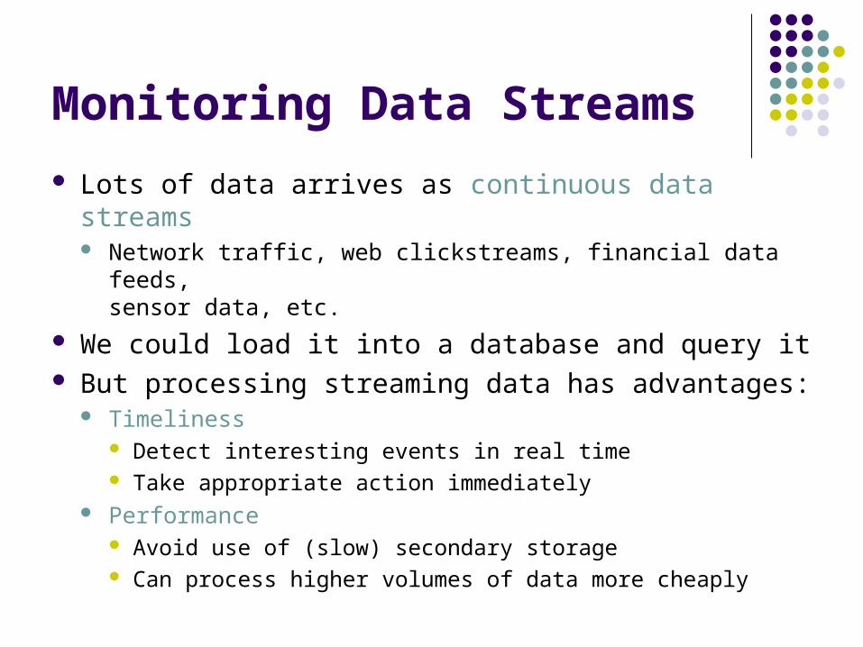
Monitoring Data Streams

Lots of data arrives as continuous data streams Network traffic, web clickstreams, financial data feeds,

sensor data, etc.

We could load it into a database and query it But processing streaming data has advantages:

Timeliness Detect interesting events in real time Take appropriate action immediately

Performance Avoid use of (slow) secondary storage Can process higher volumes of data more cheaply

Network Traffic Monitoring

Security (e.g. intrusion detection) Network performance troubleshooting

Traffic management (e.g. routing policy)

InternetInternet

Data Streams are Bursty

Data stream arrival rates are often: Fast Irregular

Examples: Network traffic (IP, telephony, etc.) E-mail messages Web page access patterns

Peak rate much higher than average rate 1-2 orders of magnitude

Impractical to provision system for peak rate

Bursts Create Backlogs

Arrival rate temporarily exceeds throughput Queues of unprocessed elements build up Two options when memory fills up

Page to disk Slows system, lowers throughput

Admission control (i.e. drop packets) Data is lost, answer quality suffers

Neither option is very appealing

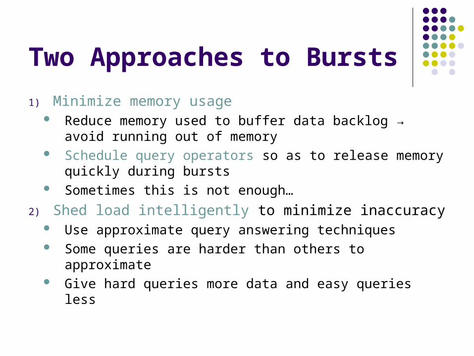
Two Approaches to Bursts

1) Minimize memory usage Reduce memory used to buffer data backlog →

avoid running out of memory Schedule query operators so as to release memory

quickly during bursts Sometimes this is not enough…

2) Shed load intelligently to minimize inaccuracy Use approximate query answering techniques Some queries are harder than others to approximate Give hard queries more data and easy queries less

Outline

Operator Scheduling Load Shedding

Problem Formalization Intuition Behind the Solution Chain Scheduling Algorithm Near-Optimality of Chain Scheduling Experimental Results

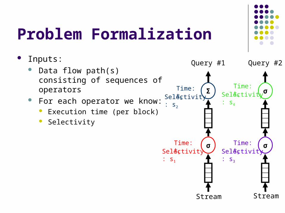
Problem Formalization Inputs:

Data flow path(s) consisting of sequences of operators

For each operator we know: Execution time (per block) Selectivity

σ

Σ

Query #1

σ

σ

Query #2

Stream Stream

Time: t1

Selectivity: s1

Time: t2

Selectivity: s2

Time: t3

Selectivity: s3

Time: t4

Selectivity: s4

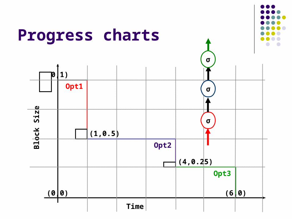
Progress charts

(0,0) (6,0)

Time

Blo

ck S

ize

(0,1)

(1,0.5)

(4,0.25)

Opt1

Opt2

Opt3

σ

σ

σ

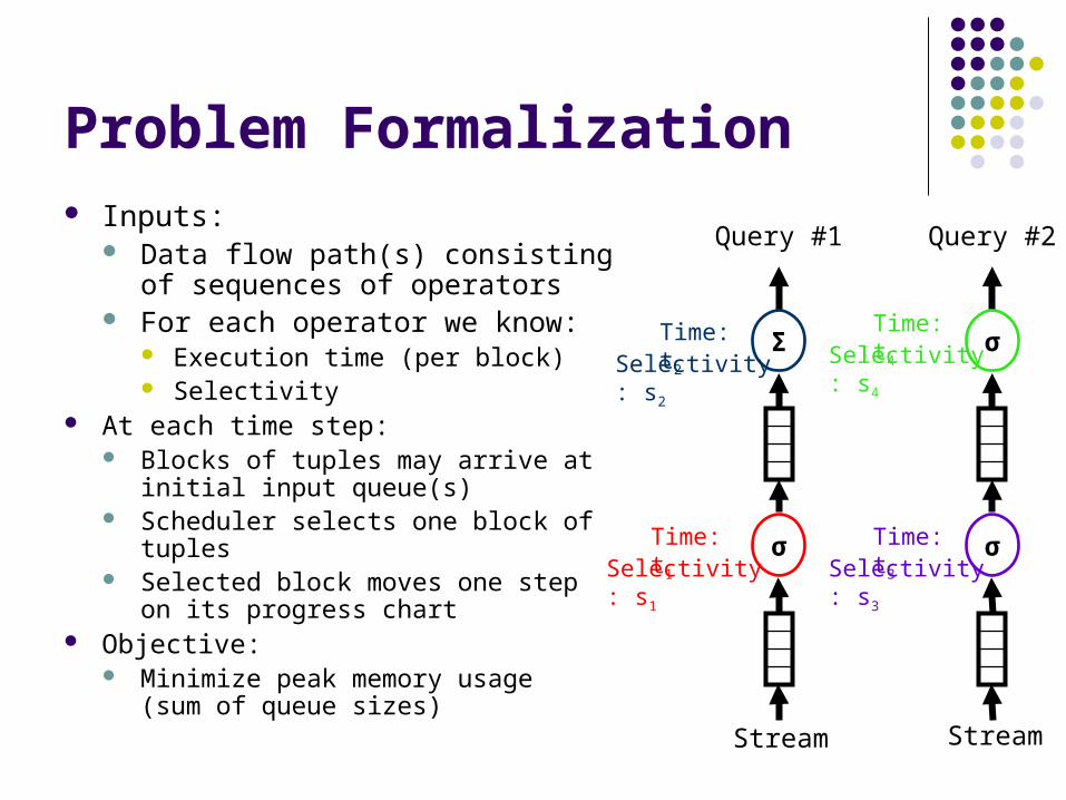
Problem Formalization Inputs:

Data flow path(s) consisting of sequences of operators

For each operator we know: Execution time (per block) Selectivity

At each time step: Blocks of tuples may arrive at initial

input queue(s) Scheduler selects one block of tuples Selected block moves one step on its

progress chart Objective:

Minimize peak memory usage(sum of queue sizes)

σ

Σ

Query #1

σ

σ

Query #2

Stream Stream

Time: t1

Selectivity: s1

Time: t2

Selectivity: s2

Time: t3

Selectivity: s3

Time: t4

Selectivity: s4

Main Solution Idea

Fast, selective operators release memory quickly Therefore, to minimize memory:

Give preference to fast, selective operators Postpone slow, unselective operators

Greedy algorithm: Operator priority = selectivity per unit time (si/ti) Always schedule the highest-priority available operator

Greedy doesn’t quite work… A “good” operator that follows a “bad” operator rarely runs The “bad” operator doesn’t get scheduled Therefore there is no input available for the “good” operator

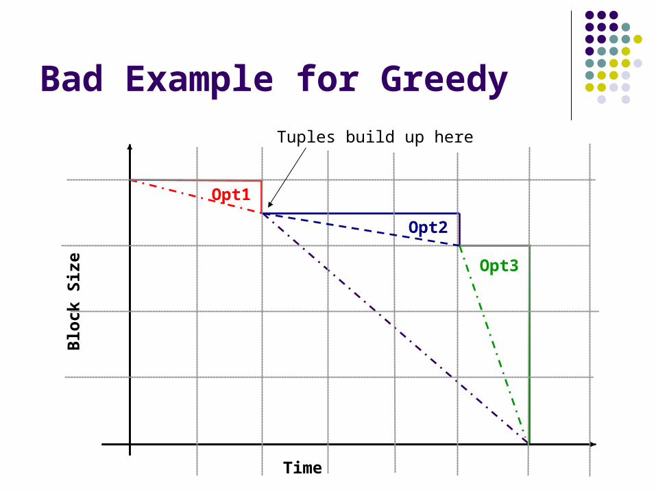
Bad Example for Greedy

Opt1

Opt2

Opt3

Time

Blo

ck S

ize

Tuples build up here

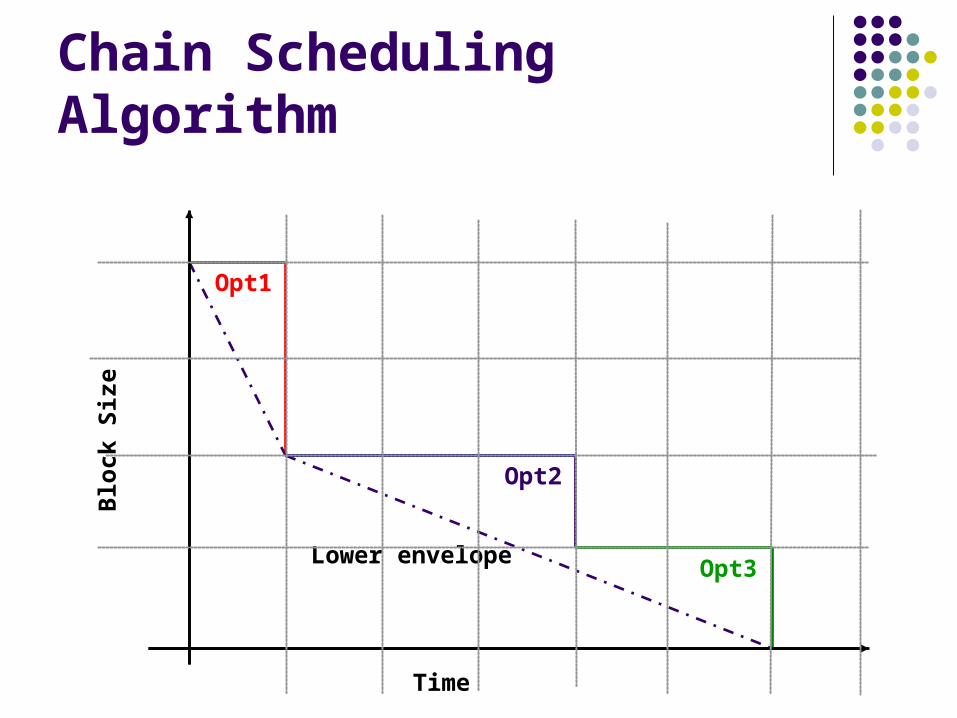
Chain Scheduling Algorithm

Opt1

Opt2

Opt3Lower envelope

Time

Blo

ck S

ize

Chain Scheduling Algorithm

Calculate lower envelope Priority = slope of lower envelope segment Always schedule highest-priority available

operator Break ties using operator order in pipeline

Favor later operators

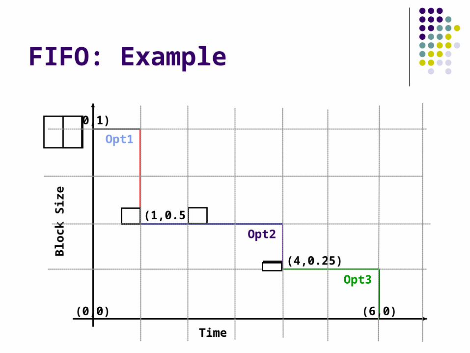
FIFO: Example

(0,0) (6,0)

(0,1)

(1,0.5)

(4,0.25)

Opt1

Opt2

Opt3

Time

Blo

ck S

ize

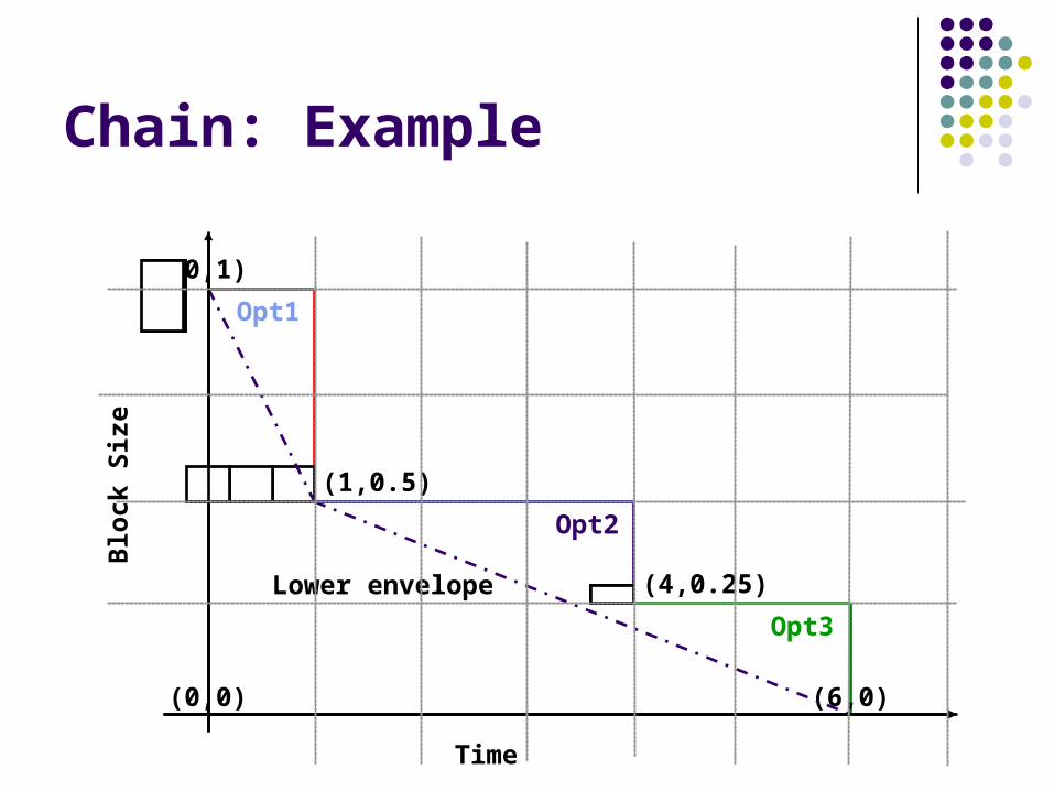
Chain: Example

(0,0) (6,0)

(0,1)

(1,0.5)

(4,0.25)

Opt1

Opt2

Opt3

Lower envelope

Time

Blo

ck S

ize

Memory Usage

Memory Usage

0

0.5

1

1.5

2

2.5

3

0 2 4 6 8

10

12

14

16

18

Time

Blo

ck

Siz

e

FIFO

Chain

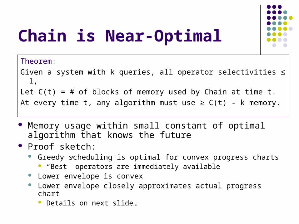
Chain is Near-Optimal

Memory usage within small constant of optimal algorithm that knows the future

Proof sketch: Greedy scheduling is optimal for convex progress charts

“Best” operators are immediately available Lower envelope is convex Lower envelope closely approximates actual progress chart

Details on next slide…

Theorem:

Given a system with k queries, all operator selectivities ≤ 1,

Let C(t) = # of blocks of memory used by Chain at time t.

At every time t, any algorithm must use ≥ C(t) - k memory.

Lemma: Lower Envelope is Close to Actual Progress Chart

At most one block in the middle of each lower envelope segment Due to tie-breaking rule

(Lower envelope + 1) gives upper bound on actual memory usage

Additive error of 1 block per query

Difference

Difference

Performance Comparison

Performance

0

2

4

6

8

10

12

14

0 80

160

240

320

400

480

560

640

720

800

880

960

Time (msecs)

To

tal

Mem

ory

(K

Bs)

Chain

FIFO

spike in memory due to burst

Outline

Operator Scheduling Load Shedding

Motivation for Load Shedding Problem Formalization Load Shedding Algorithm Experimental Results

Why Load Shedding?

Data rate during the burst can be too fast for the system to keep up

Chain Scheduling helps to minimize memory usage, but CPU may be the bottleneck

Timely, approximate answers are often more useful than delayed, exact answers

Solution: When there is too much data to handle, process as much as possible and drop the rest

Goal: Minimize inaccuracy in answers while keeping up with the data

Related Approaches

Our focus: sliding window aggregation queries Goal is minimizing inaccuracy in answers Previous work considered related questions:

Maximize output rate from sliding window joinsKang, Naughton, and Viglas - ICDE 03

Maximize quality of service function for selection queriesTatbul, Cetintemel, Zdonik, Cherniak, Stonebraker-VLDB 03

Problem Setting

Σ Σ

Σ

S1 S2

R

Sliding Window Aggregate Queries(SUM and COUNT)

OperatorSharing

Filters, UDFs, and Joins w/ Relations

Q1 Q2 Q3

Inputs to the Problem

Σ Σ

Σ

S1 S2

R

Std Dev σMean μ

Q1 Q2 Q3

Stream Rate r

Processing Time tSelectivity s

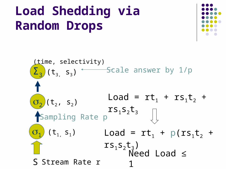
Load Shedding via Random Drops

Stream Rate r

1

2

Σ3

S

(t1, s1)

(t2, s2)Load = rt1 + rs1t2 + rs1s2t3

(t3, s3)

Sampling Rate p

(time, selectivity)

Load = rt1 + p(rs1t2 + rs1s2t3)

Scale answer by 1/p

Need Load ≤ 1

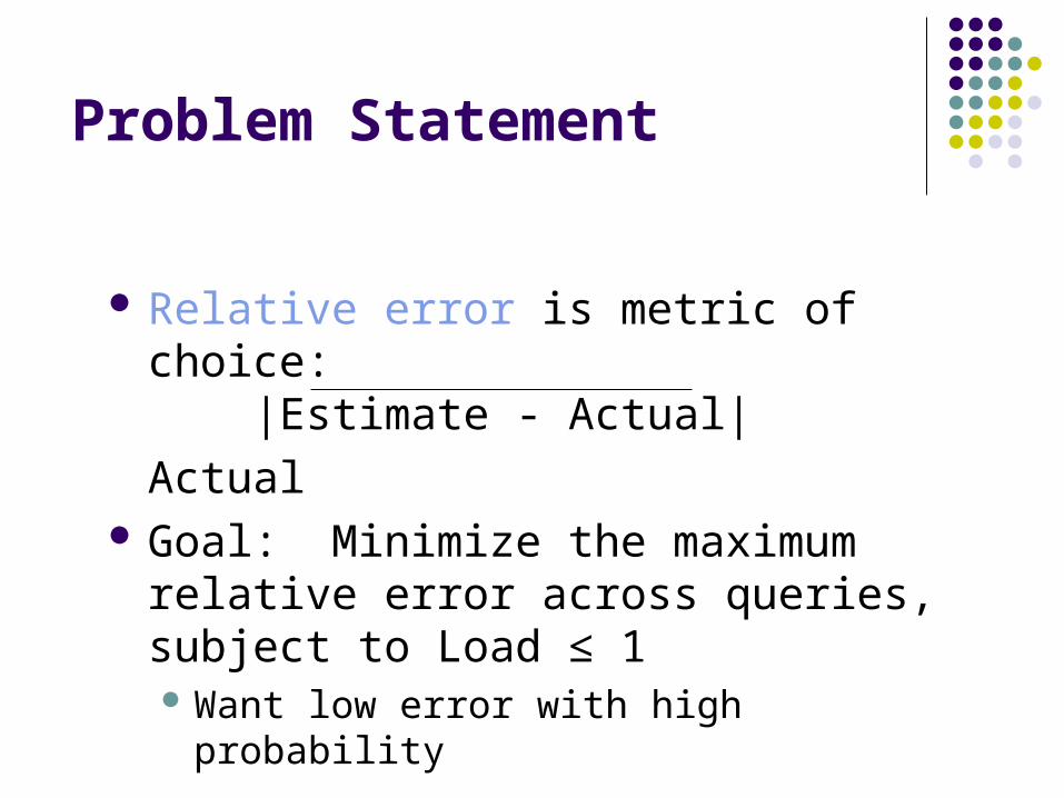
Problem Statement

Relative error is metric of choice:|Estimate - Actual|

Actual Goal: Minimize the maximum relative

error across queries, subject to Load ≤ 1 Want low error with high probability

Quantifying Effects of Load Shedding

1

2

Σ3

Sampling Rate p1

Sampling Rate p2

Scale answer by 1/(p1p2)

Product of sampling rates determines answer quality

1

2

Σ3

Sampling Rate p1p2

Scale answer by 1/(p1p2)

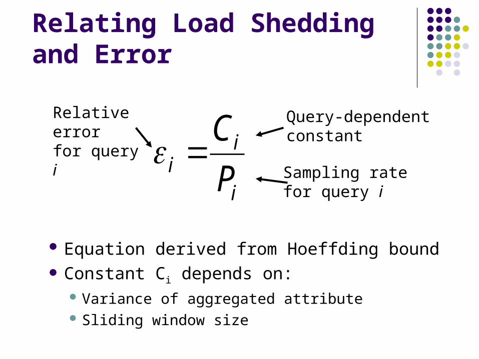
Relating Load Shedding and Error

i

ii P

C

Relative errorfor query i

Sampling ratefor query i

Query-dependentconstant

Equation derived from Hoeffding bound Constant Ci depends on:

Variance of aggregated attribute Sliding window size

Choosing Target Sampling Rates

2

log2

112

22

NP

Sampling ratefor query

Variance ofaggregatedattribute

Slidingwindowsize

RelativeError

Calculate Ratio of Sampling Rates

Minimize maximum relative error →Equal relative error across queries

Express all sampling rates in terms of common variable λ

n

n

P

C

P

C

P

C

2

2

1

1 ii CP

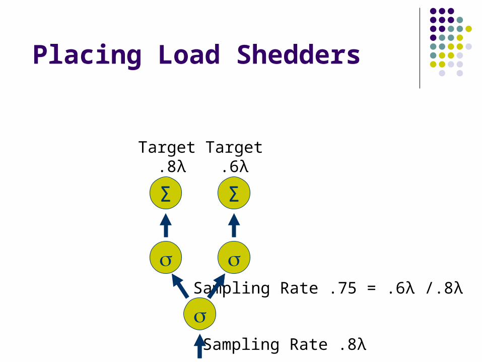
Placing Load Shedders

ΣΣ

Target .8λ

Target.6λ

Sampling Rate .8λ

Sampling Rate .75 = .6λ /.8λ

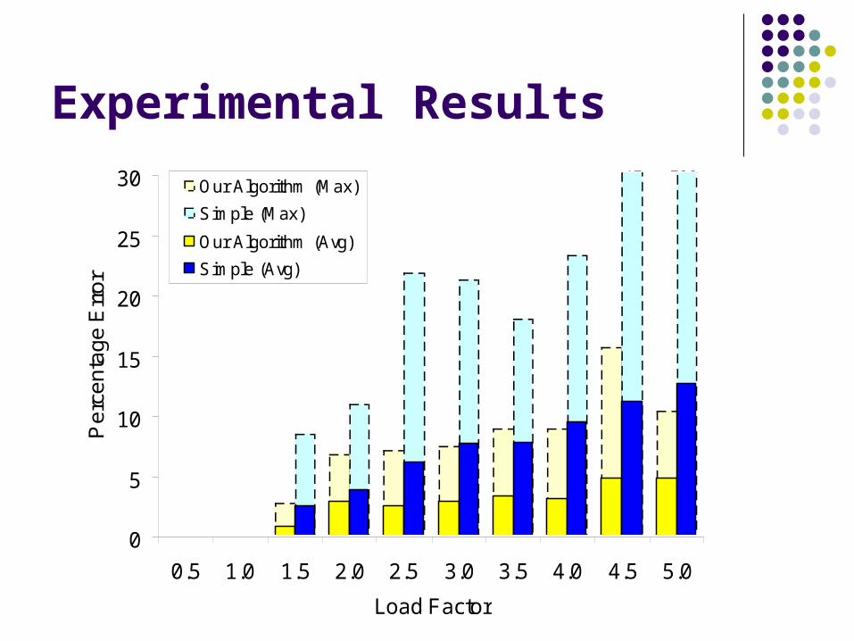
Experimental Results

0

5

10

15

20

25

30

0.5 1.0 1.5 2.0 2.5 3.0 3.5 4.0 4.5 5.0

Load Factor

Pe

rce

nta

ge

Err

or

Our Algorithm (Max)

Simple (Max)

Our Algorithm (Avg)

Simple (Avg)

41 100

Experimental Results

Conclusion

Fluctuating data stream arrival rates create challenges Temporary system overload during bursts

Chain scheduling helps minimize memory usage Main idea: give priority to fast, selective operators

Careful load shedding preserves answer quality Relate target sampling rates for all queries Place random drop operators based on target sampling rates Adjust sampling rates to achieve desired load

Thanks for Listening!

http://www-db.stanford.edu/stream