ADAPTIVE MESHING AND DETAIL-REDUCTION OF 3D-POINT CLOUDS FROM LASER SCANS

Christoph Hoppe a and Susanne Krömker a

a Interdisciplinary Center for Scientific Computing, Numerical Geometry and Visualization Group University of Heidelberg

INF 368, 69120 Heidelberg, Germanychristoph.hoppe@iwr.uni-heidelberg.de, kroemker@iwr.uni-heidelberg.de

KEY WORDS: Laser Scanning, Point Cloud, Cultural Heritage, Modelling, Graphics, Resolution, Method

ABSTRACT:

3D laser scanners become more and more popular especially for measuring construction sites, in the field of architecture and for preservation of monuments. As these scanners can only record discrete data sets (point clouds), it is necessary to mesh these sets for getting closed 3D models and take advantage of 3D graphics acceleration of modern graphics hardware. The meshing process is a complex issue and in the last years there were lots of algorithms developed to solve this problem. In this work a continuous Level-of-Detail (LOD) algorithm will be presented, from which a simplified 3D surface model can be created, which uses only as much triangles as needed. The grade of simplification is user-defined by an error tolerance similar to the Hausdorff distance. This algorithm is not a dynamic (view-dependent) LOD mesh simplification, but a non-redundant approximation of point clouds. It is a simple and extendable meshing algorithm, which is made up of a mixture of some techniques adapted from popular terrain LOD algorithms. The algorithm has been implemented in an OpenGL based editing tool for 3D point clouds called PointMesh, which will be explained in detail. We present examples from an excavation site (church rest of Lorsch Abbey, Germany), the inner part of the Heidelberg Tun (German: Großes Fass, an extremely large wine vat) and the Old Bridge gate, Heidelberg. For different cut-outs a performance comparison of the regular mesh to various adaptive 4-8-meshes with different error tolerances is given in terms of frame rates.

1. INTRODUCTION

All digital measures can only record discrete data sets of reality. As the hardware gets more accurate and the amount of data gets even larger, it is more and more necessary to visualize the measurement for a better understanding.Measuring construction with reflection light laser scanners become more and more popular in the fields of architecture, urban planning, navigation, as well as for documentation and preservation of monuments. The process of visualizing large data sets in 3D costs enormous computing power. In the process of laser scanning it is necessary to directly display the data sets in 3D on non-high performance computers like laptops.Our solution is to automatically generate a textured closed surface model from a user-selected projected rectangular region of the existing point cloud data. While the amount of data will be significantly reduced, the properties of the scanned object, particularly the shape and color, will still be preserved.

The meshing of approximated data in such rectangular cut-outs with an automated texturing with surface details is especially useful for documentation purposes in e.g. medieval archaeology where the user wants to keep track of the details of brickwork without generating a grid for each of the bricks.The presented algorithm is implemented in our OpenGL based editing tool for 3D point clouds called PointMesh. After meshing, it allows to export the generated surface model in VRML-format for further editing.

2. DATA ACQUISITION

We deal with data, which is combined from up to ten or twenty sets of 360-degree full scans in order to avoid shadows in complex buildings and archeological excavations. Due to

simultaneously taking photos while scanning the scene, true color RGB-values can be assigned to the geometric XYZ-data.

Each of the 360-degree full scans has a local coordinate system. These local systems fit into a global one adjusted to a geodesic grid. Thereby a global orientation due to the point of the compass is given. Furthermore the data of each single scan has a functional relation to a spherical domain. By referring to adjacent points while scanning, normal directions for virtual surfaces are determined. These normal vectors are encoded as so-called compass colors at each point in the cloud. Literally the compass color indicates the orientation of a virtual surface at each point and provides this information otherwise lost in a combined 3D data set. This loss of information about surface orientation is due to the process of matching, which leads to a mergence of point data from all scans and therefore results in an unordered final data set. Another advantage of compass colors is a better perception in comparison to a true color representation especially in shadow regions, where true colors do not differ so much.

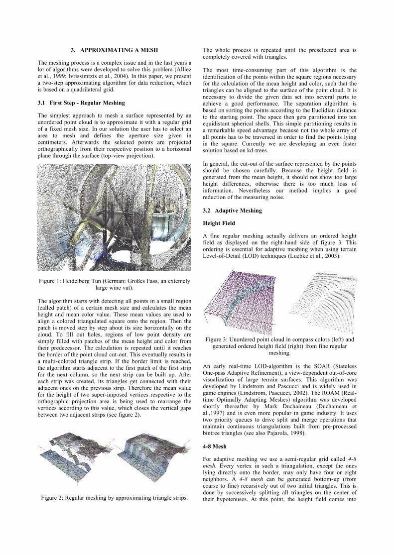
Our data shows two major characteristics:1. The data points are not distributed uniformly. Their density lowers with higher distance to the scanner position and is dependent on the total number of scans.2. Point clouds exhibit holes, which means areas of abrupt change in point density of imaginary surface. They result either from shadows with respect to the scanner location, specular reflections or exceeding the maximum distance along the laser beam. For an example of a merged point cloud of several 360-degree full scans of a complicated environment see figure 1. It shows the interior view of the Heidelberg Tun, an extremely large wine vat with a lot of shadowing due to the inner construction. The circular white spots on the ground show the various positions of the scanner.

3. APPROXIMATING A MESH

The meshing process is a complex issue and in the last years a lot of algorithms were developed to solve this problem (Alliez et al., 1999; Ivrissimtzis et al., 2004). In this paper, we present a two-step approximating algorithm for data reduction, which is based on a quadrilateral grid.

3.1 First Step - Regular Meshing

The simplest approach to mesh a surface represented by an unordered point cloud is to approximate it with a regular grid of a fixed mesh size. In our solution the user has to select an area to mesh and defines the aperture size given in centimeters. Afterwards the selected points are projected orthographically from their respective position to a horizontal plane through the surface (top-view projection).

Figure 1: Heidelberg Tun (German: Großes Fass, an extemely large wine vat).

The algorithm starts with detecting all points in a small region (called patch) of a certain mesh size and calculates the mean height and mean color value. These mean values are used to align a colored triangulated square onto the region. Then the patch is moved step by step about its size horizontally on the cloud. To fill out holes, regions of low point density are simply filled with patches of the mean height and color from their predecessor. The calculation is repeated until it reaches the border of the point cloud cut-out. This eventually results in a multi-colored triangle strip. If the border limit is reached, the algorithm starts adjacent to the first patch of the first strip for the next column, so the next strip can be built up. After each strip was created, its triangles get connected with their adjacent ones on the previous strip. Therefore the mean value for the height of two super-imposed vertices respective to the orthographic projection area is being used to rearrange the vertices according to this value, which closes the vertical gaps between two adjacent strips (see figure 2).

Figure 2: Regular meshing by approximating triangle strips.

The whole process is repeated until the preselected area is completely covered with triangles.

The most time-consuming part of this algorithm is the identification of the points within the square regions necessary for the calculation of the mean height and color, such that the triangles can be aligned to the surface of the point cloud. It is necessary to divide the given data set into several parts to achieve a good performance. The separation algorithm is based on sorting the points according to the Euclidian distance to the starting point. The space then gets partitioned into ten equidistant spherical shells. This simple partitioning results in a remarkable speed advantage because not the whole array of all points has to be traversed in order to find the points lying in the square. Currently we are developing an even faster solution based on kd-trees.

In general, the cut-out of the surface represented by the points should be chosen carefully. Because the height field is generated from the mean height, it should not show too large height differences, otherwise there is too much loss of information. Nevertheless our method implies a good reduction of the measuring noise.

3.2 Adaptive Meshing

Height Field

A fine regular meshing actually delivers an ordered height field as displayed on the right-hand side of figure 3. This ordering is essential for adaptive meshing when using terrain Level-of-Detail (LOD) techniques (Luebke et al., 2003).

Figure 3: Unordered point cloud in compass colors (left) and generated ordered height field (right) from fine regular

meshing.

An early real-time LOD-algorithm is the SOAR (Stateless One-pass Adaptive Refinement), a view-dependent out-of-core visualization of large terrain surfaces. This algorithm was developed by Lindstrom and Pascucci and is widely used in game engines (Lindstrom, Pascucci, 2002). The ROAM (Real-time Optimally Adapting Meshes) algorithm was developed shortly thereafter by Mark Duchaineau (Duchaineau et al.,1997) and is even more popular in game industry. It uses two priority queues to drive split and merge operations that maintain continuous triangulations built from pre-processed bintree triangles (see also Pajarola, 1998).

4-8 Mesh

For adaptive meshing we use a semi-regular grid called 4-8 mesh. Every vertex in such a triangulation, except the ones lying directly onto the border, may only have four or eight neighbors. A 4-8 mesh can be generated bottom-up (from coarse to fine) recursively out of two initial triangles. This is done by successively splitting all triangles on the center of their hypotenuses. At this point, the height field comes into

play: If we would just refine a mesh without using a height field, the result would be completely flat. Using a height field the height of the new vertex at the split point is determined by the nearest point in the height field.In comparison to other triangulation methods (face split / vertex split) a 4-8 mesh offers the great advantage of a valid 4-8 mesh after every step of refinement (see figure 4).

Figure 4: The first four refinement steps of a 4-8 mesh. The numbers indicate the newly inserted vertices in the

particular steps.

In such an unrestrictive refinement the mesh is refined equally at all places. But our aim is to mainly refine the mesh only at places where the surface is uneven, i.e. where the difference between the surface represented by the height field and the present triangulation is too high.

Error Calculation - Establishing a Restriction

To reach this aim, we need an effective limitation to decide a further subdivision of a triangle. That means we need to estimate the difference between the current and an optimal triangulation. In an optimal triangulation every point in the ordered height field would be directly connected to its neighbor points, so every point not lying on the edge would become a new vertex for four triangles.There are several possibilities to calculate this difference, which is commonly called error. One of the more popular variants is the Hausdorff distance.

Hausdorff Distance

For two given sets of points A and B, the Hausdorff distance H(A,B) is defined as the maximum of the minimal distances between both sets. In other words: for every point in set A we search the nearest neighbor in B and vice versa.Afterwards, we calculate the distances between all those points and take the maximum.

Expressed in formulas it reads

H(A,B) = max (h(A,B), h(B,A)) (1)

where

h(A,B) = maxa ∈A min b ∈B || a – b || . (2)

Figure 5: Hausdorff distances between two point sets.The one-sided Hausdorff distances are

h(A,B) = ||v|| and h(B,A) = ||w||. The two-sided Haussdorff distance is

H(A,B) = max (||v||, ||w||) = ||v||.

The function h(A,B), also called one-sided Hausdorff distance, is not symmetric. Every point in A is allocated a single point in B, but there cannot stay allocated (and thereby be multiply allocated) points in set B. Thus h(A,B) ≠ h(B,A). This is illustrated in figure 5.However, the both-sided Hausdorff distance H(A,B) is constructed in such a way that it gets symmetric, by looking at both one-sided Hausdorff distances and returning the maximum value of both.For error estimation in PointMesh we only use an approximation of the Hausdorff distance. If we would calculate the exact Hausdorff distance, we would need to calculate the distance between the including height points and all intersection points with the current triangulation. To simplify and speed up the process, we just compare the heights of the vertices and the center point of the triangle with all height field points overlapped by the triangle. If this difference goes below a user-defined threshold (given in centimeters) the refinement of the triangle is stopped.

3.3 Topological Inconsistencies: Cracks and T-Junctions

If we examine a mesh generated in such a way more closely, we notice cracks at certain places.Cracks develop at such places, where triangles of detail levels differing in more than one level are adjoined (see figure 6). In this case it is possible that the higher detailed triangles insert an additional vertex on the edge of the lower detailed triangle. Because the vertex is using another height field point, its height is different to the edge, so the background peaks through in the finally rendered image.Another unwanted artifact is the T-junction. It is almost the same as a crack, with the slight difference that the height of the inserted vertex does not differ visibly from the height of the edge of the lower detailed triangle.

Figure 6: Cracks and T-junctions occur at places where the mesh resolution changes.

As a simple solution, we could say we just move the inserted vertices to the height of the edge and we would be fine. However, this rather unaesthetic solution is only applicable for static images. If we rotate the view around the mesh, we see bleeding edges at such places, due to a kind of flickering between the edges, caused by minimal floating point rounding differences.The most popular solution for getting a continuous surface mesh is to recursively split all triangles lying directly next to the crack. Though the mesh gets additional triangles, which do not account for more detail, this method eventually delivers the most pleasing results.A consequent recursive splitting can be quite complex, as every split operation may insert a new T-junction at which another triangle needs to be split again and so forth. In other words after every split we would need to check the adjacent triangles again for inconsistencies.Another more simple method to solve this problem would be to merge the two triangles causing the T-junction to a single larger one. The clear downside of this procedure is that this results in a significant loss of detail.

In the following, we present a combination of both, the split and merge methods. Then with the so-called tree pruning an effective speed-up can be achieved (see Balmelli et al., 2003).

Creating Order From Chaos - Vertex Set and Triangle Set

While the 4-8 mesh is being built up, the triangles get structured in a dynamic vector called Vertex Set. In this vector there is no redundancy, i.e. a vertex of a triangle is only stored once although it is generally used by more than one triangle. To take all these triangles into account and to create connections between them, the Vertex Set entries are consecutively updated during the meshing process. All of the three triangle points get stored in a separate array called Triangle Set. The Triangle Set indices of all triangles using the same vertex are added to the Vertex Set. Furthermore, we store two types of special points in the Vertex Set, which we call Split Points and Forbidden Points.

Split Points and Forbidden Points

Already during the generation of the mesh for every finally drawn triangle additional data is being saved. A Split Point of a triangle defines the midpoint of the hypotenuse, at which the triangle would be subdivided further, even though if it is not always necessary to do this.Moreover, the midpoints of each cathetus are stored. At these points there should not be placed a vertex of another triangle, otherwise this would induce a T-junction. Therefore, we decided to call these points Forbidden Points.

Figure 7: Forbidden Points and Split Points.

In figure 7 these points are shown exemplarily. The smaller pale triangles are in a two times higher refinement step than the dark gray triangles. On the left drawing, two shared vertices of the pale triangles are located at a Forbidden Point of the gray triangle marked in white. In this case we would merge both triangles to a triangle, which is located one refinement step lower in order to prevent the T-junction. Even though we are dealing here with a loss of detail, we save the multiple subdivision of the gray triangle and its possible neighbors.On the right side of the drawing, two vertices of the smaller triangles are located at a Split Point of the gray triangle. Here we split the gray triangle along the dotted line into two new triangles of one refinement step higher to eliminate the T-junction.In both cases, the merge and split operations, the newly created (or restored) triangles are checked again in the same way as the gray triangles in order to secure their integration with respect to their other neighbors.

4. GENERATING TEXTURES

To gain a more realistic impression of a surface, textures are commonly used to replace the loss of detail due to simplification. As we already have true color information for

every measurement point in our input data, we basically have two options for generating a texture.The first would be to display the point cloud directly on the screen and take a screenshot from user-defined direction and section. As we firstly implemented this solution we quickly figured out its drawbacks. It is only applicable with an expanded point size, so that holes between the points get eliminated, as now most of the points are overlapping each other. Which point is visible in front is defined by its offset from the surface and the current viewing angle. Although points with high offset are often outliers, they still get preferred. So the overlapping reduces the number of points, which get into account to the final image and it can still be strewn by holes. We can surely say that this solution is rather unaesthetic and only for provisional use.As we already use the point colors in our regular meshing step, we can just perform a very fine meshing (e.g. see figure 8 with a fine regular grid in white (for demonstration purposes only) on top of a Gouraud-shaded surface). The triangle colors are in fact local mean colors of all points within the meshing square. We finally create the texture by saving the triangle colors in a certain order as pixels into a bitmap file. Afterwards, we continue with the adaptive meshing to create a coarser mesh and map the texture onto it.

Figure 8: Arcades of Lorsch Abbey - textured regular mesh.

4.1 Mapping a Texture

As we are able to create suitable textures for our model in the BMP format, we need to map them on our model.In a mapping pixel coordinates of an image are mapped onto the triangles of a 3D-model. For this linear mapping a texture coordinate list (UV coordinates) needs to be supplied. It is rather easy to create such a list for a regular mesh, because all triangles are of the same size. In a 4-8 mesh the sizes of the triangles differ dependent on their refinement level. This poses a problem, which we have not addressed by now.The texturing can be done manually by importing the model to a 3D rendering software. We used a popular open source 3D modeling and rendering software called Blender.

The mapping is done here in the way by firstly loading the mesh and the according image to be uses as texture. By the UV-image editor one can match the image to the surface by simultaneously viewing the result in a separate viewport.The according texture coordinate list is calculated internally by Blender, so that the user doesn't need to complain with that.

Figure 9: Arcades of Lorsch Abbey as a textured adaptive meshed model.

The final model appears as complex as a fine regular meshed one, such that there is almost no loss in information during the grid simplification step while the number of triangles reduces by a factor of five. Figure 9 shows the result with a coarse adaptive grid in white (again for demonstration purposes only) on top of a textured surface.

5. EXPORTING THE MODELS

To use the complete meshed model outside of PointMesh it has to be saved in an appropriate format. We chose to use the VRML format. Because it is ASCII-format, it offers the great advantage to be easily usable and extendable. Besides that, models can be displayed online in all common web browsers by installing a browser-plugin.The big disadvantage is the high memory usage and the relatively low read and write performance compared to other (mostly binary) formats.For saving the model it is possible to choose between VRML-1.0 and VRML-2.0 (VRML97) formats via the GUI. For future versions we plan to implement our own binary file format, which stores the data more compact and may save additional information, such as different adaptive meshing levels.

6. COMPARISION BETWEEN REGLUAR AND ADAPTIVE MESHES

As we are able to save both, the regular and the adaptive meshed model as VRML file, we can compare the different results directly. The comparison of both techniques should not be focused on the visual impression only. The adaptive

triangulation by 4-8 meshes also saves memory and is displayed faster by the graphics hardware.In the presented cut-outs (see figures 9, 10 and 11) we used a fixed patch size of 4 cm for both meshing methods. The error threshold is varied between 2, 4, 6, 8 and 10 cm. Additionally, we took a measure of the mean frame rate, to get a comparison of the display speed. Here it is important to notice that, in contrast to the regular meshing, the results of the 4-8 meshing are still not optimal, because we do not use triangle strips or triangle fans here to speed up the display performance.

Figure 10: Cut-out from the towers of the Old Bridge Heidelberg. Regular mesh (left) and adaptive mesh (right) in wireframe graphics (above) and textured view (below).

Our testing platform:• Intel(R) Pentium(R) Dual CPU T2330 @1.60GHz,

3GB RAM• NVIDIA G86GL-850 Graphics Card

All FPS values are rounded mean values taken over 60 seconds. They have been captured by the application FRAPS (beepa, 2008) and VRMLView (Kongsberg, 2009) running under MS Windows Vista. The results are shown in table 12 and graphically displayed in figures 13 and 14.

Figure 11: Small cut-out from an excavation site at Lorsch.

7. CONCLUSION

According to the true color values a texture is automatically produced on the basis of the finest grid. Coarser grids use the same texture and appear as complex such that there is almost no loss in information during the grid simplification step while the number of triangles reduces by a factor of five. As an outlook, automated texturing even for extremely complicated surfaces will be possible due to the color-coded normal field stored in the so-called compass colors. They allow for a meaningful projection of curved surfaces onto a plane. This forms the basis for a screenshot of the texture to be mapped onto this part of the surface via classical UV-mapping. In the future an implementation of the algorithm

directly on the GPU is promising (see Schneider, Westermann, 2006) due to the highly parallel tasks within our algorithm.

Table 12: Comparision in terms of frame rates and number of triangles.

Figure 13: Comparision of number of triangles for different cut-outs.

Figure 14: Comparision of frame rates for different cut-outs.

ACKNOWLEDGEMENTS

We would like to thank the Interdisciplinary Center for Scientific Computing (IWR) of the University of Heidelberg for technical and computational support. Our thanks also go to Karsten Leuthold, Survey Service, CALLIDUS-Competence Center, for generously let us use the data from the scans of the excavations at Lorsch Abbey and several locations in Heidelberg.

REFERENCES

Alliez, P.; Laurent, N.; Sanson, H.; Schmitt, F., 1999. Mesh approximation using a volume-based metric.Computer Graphics and Applications. Proceedings. Seventh Pacific Conference on Volume, Issue, pp. 292 – 301.

Balmelli, L.; Vetterli, M.; Liebling, T.; 2003. Mesh optimization using global error with application to geometry simplification, Journal of Graphical Models.

beepa® P/L - ACN 106 989 815, © 2008, Real time video capture and benchmarking, http://www.fraps.com/ (accessed 29 Jan. 2009)

Duchaineau, Wolinsky, Sigeti, Miller, Aldrich, Mineev-Weinstein, 1997. ROAMing Terrain: RealTime Optimally Adapting Meshes, Proceedings of IEEE Visualization '97, pp. 81 – 88.

Ivrissimtzis, I.; Yunjin Lee; Seungyong Lee; Jeong, W.-K.; Seidel, H.-P., 2004. Neural mesh ensembles,3D Data Processing, Visualization and Transmission, 3DPVT 2004. Proceedings. 2nd International Symposium onVolume, Issue, 6-9 Sept. 2004, pp. 308 – 315.

Kongsberg Maritim AS, Systems in motion, © 2009, VRMLview, http://www.km.kongsberg.com/sim (accessed 29 Jan. 2009)

Lindstrom, P.; Pascucci, V., 2002. Terrain Simplification Simplified: A General Framework for View Dependent OutofCore Visualization, IEEE Transactions on Visualization and Computer Graphics.

Large Cut-out „Arcades“

Mesh Type Error tol. [cm] # Triangles FPS

regular n/a 70295 24

4-8-mesh 2 9060 35

4-8-mesh 4 6003 37

4-8-mesh 6 4999 40

4-8-mesh 8 3287 44

4-8-mesh 10 3130 45

Cut-out „Old Bridge“

Mesh Type Error tol. [cm] # Triangles FPS

regular n/a 24049 70

4-8-mesh 2 6823 69

4-8-mesh 4 5245 82

4-8-mesh 6 4284 94

4-8-mesh 8 3770 99

4-8-mesh 10 3281 121

Small Cut-out „Excavation“

Mesh Type Error tol. [cm] # Triangles FPS

regular n/a 3677 167

4-8-mesh 2 1677 151

4-8-mesh 4 967 136

4-8-mesh 6 738 149

4-8-mesh 8 607 160

4-8-mesh 10 437 174

n/a 2 4 6 8 10

0

10000

20000

30000

40000

50000

60000

70000

Large Cut-out „Arcades“

Cut-out „Old Bridge“

Small Cut-out „Excavation“

Error tol. [cm]

# T

riang

les

n/a 2 4 6 8 10

0

20

40

60

80

100

120

140

160

180

Large Cut-out „Arcades“

Cut-out „Old Bridge“

Small Cut-out „Excavation“

Error tol. [cm]

FP

S

Luebke, D.; Reddy, M.; Cohen, D.; Varshney, A.; Watson, B.; Huebner, R., 2003. Level of Detail for 3DGraphics, Morgan Kaufmann, ISBN: 9781558608389

Pajarola, R., 1998. Large Scale Terrain Visualization Using The Restricted Quadtree Triangulation, Institute of Theoretical Computer Science, ETH Zürich.

Schneider, J.; Westermann, R.; 2006. GPU-Friendly High-Quality Terrain Rendering, 2006, Journal of WSCG, Vol. 14.