904

Bulletin of the Seismological Society of America, Vol. 92, No. 3, pp. 904–912, April 2002

Adaptive Kernel Estimation and Continuous Probability

Representation of Historical Earthquake Catalogs

by Christian Stock and Euan G. C. Smith

Abstract To develop spatially continuous seismicity models (earthquake proba-bility distributions) from a given earthquake catalog, the method of kernel estimationhas been suggested. Kernel estimations with a global (spatially invariant) bandwidthdeal poorly with earthquake hypocenter distributions that have different spatiallylocal features. For example, a typical earthquake catalog has several areas of highactivity (clusters) and areas of low-background seismicity. An alternative approachis adaptive kernel estimation, which uses a bandwidth parameter that is spatiallyvariable. Its performance compared to kernel estimations with spatially invariantbandwidths suggests that (discrete) earthquake distributions require different degreesof local smoothing to provide useful spatial seismicity models. Using adaptive kernelestimation, the (local) indices of temporal dispersion of any earthquake probabilitydistribution can be estimated and used to model the spatial probability distributionof mainshocks. The application of these methods to New Zealand and Australianearthquake catalogs shows that the spatial features (earthquake clusters) in which themainshocks occurred have been reasonably stable throughout the observation period.The observed regions of higher activity persisted throughout the observation period,and none of these regions decreased to background activity during that time. Thissuggests that these regions will continue to represent higher risk for the occurrenceof moderate to large earthquakes within the next few years or decades. Furthermore,it has been observed that shallow earthquakes are mostly part of temporal sequences(e.g., aftershocks or swarms), whereas the earthquakes within the subduction zonesin New Zealand showed only small temporal variation during the observation period.

Introduction

Probabilistic seismic hazard analysis is, in general,based on an appropriate model for the occurrence of earth-quakes in space and time. Such models often use historicalearthquake catalogs or other representations of discrete hy-pocenter distributions. Any seismicity catalog for some re-gion represents a sample in time drawn from an (unknown)parent distribution of seismicity. Thus, any appropriatemodel for the parent distribution must pass the test that theactual earthquake catalog has a reasonable probability of be-ing drawn from the modeled parent distribution. Our goal isto develop a model that is inferred from the data rather thanto construct a model with the help of external parameters,such as the use of prior seismic zoning, which dictates theboundaries of seismic activity in the model. The advantageof such a model is its independence from subjective deci-sions. Furthermore, external parameters may be wrongly as-sumed to be controlling the observed seismicity. Also, com-monly used seismic zoning has unnatural sharp borders ofactivity that are not to be expected in actual earthquake oc-currence.

There are several different ways to develop earthquakeoccurrence models. The first possibility is the use of para-metric regression, which implies that all the parametersneeded to develop an earthquake occurrence model areknown. Since those parameters are currently not very wellknown, nonparametric estimation seems to be a betterchoice. The three most commonly used nonparametric esti-mations are orthogonal series estimations, kernel estima-tions, and spline estimations (e.g., Hardle, 1990). In orthog-onal series estimation the model is estimated by estimatingthe coefficients of its Fourier expansion, and in spline esti-mation the local variation of the model is minimized by theintroduction of a roughness penalty. Some work on splineestimation in connection with earthquake occurrence modelshas been done by Ogata et al. (1991). Also, there are otherforms of nonparametric estimations that might be used forthe estimation of occurrence models (e.g., Papazachos,1999).

Kernel estimation has been suggested and used in sev-eral studies to transform discrete earthquake distributions

Adaptive Kernel Estimation and Continuous Probability Representation of Historical Earthquake Catalogs 905

into spatially continuous probability distributions (e.g.,Vere-Jones, 1992; Frankel 1995; Cao et al., 1996; Woo,1996; Jackson and Kagan, 1999). In kernel estimation thehypocenters of earthquakes are redistributed in space, wherethe kernel function and its bandwidth dictate the shape andthe amount of the redistribution of each hypocenter. Differ-ent kernels produce qualitatively similar results, whereas thechoice of an appropriate bandwidth is critical for good re-sults (e.g., Silverman, 1986). For the development of seis-micity models, kernel estimation has been mostly used withglobal (spatially invariant) bandwidths. Due to the spatiallyclustered nature of earthquake occurrence it has to be ex-pected that the optimal bandwidth is dependent on earth-quake frequencies and locations. Hence, a local (spatiallyvarying) bandwidth may give a better representation of thedistribution of seismic activity in space. Most earthquakeoccurrence models developed in the past using kernel esti-mation suffer from ignoring the rather important effect ofthe bandwidth, and the resulting occurrence models reflectthe particular choice of bandwidth.

In this study, adaptive kernel estimation, which is onespecific type of kernel estimation using a local bandwidth,has been developed for use with earthquake hypocenter dis-tributions and it is qualitatively compared to kernel estima-tion with a global bandwidth. (We have developed a quan-titative test and used it for comparing the performance ofboth kernel estimations in Stock and Smith [2002].) Thebandwidth has been chosen to be independent of time andearthquake magnitude, which has the advantage of permit-ting the identification of non-Poissonian time behaviorand deviations from the Gutenberg–Richter magnitude-frequency law in the earthquake data set. Once a spatiallycontinuous data representation has been calculated for agiven time interval, the data can be further analyzed for localactivity fluctuations in time. For this purpose, local indicesof dispersion have been calculated, which enables differen-tiation between earthquake clusters in time (e.g., aftershocks,swarms), Poisson time behavior and temporal earthquakerepulsion (inhibition), which could be caused by stress re-lease (i.e., the absence of earthquakes after a large earth-quake). The indices of dispersion can be used to filter theoriginal continuous earthquake frequency representation andproduce a spatial representation of mainshock occurrenceprobabilities, where multiple events (e.g., swarms) are ef-fectively reduced to single events.

To demonstrate the performance of this method, it hasbeen applied to New Zealand and Australian historical earth-quake catalog. The method has been developed for the usein two dimensions to produce planar seismicity representa-tions based on epicenters. In principle, it should also workfor the production of three-dimensional representations us-ing hypocenters, although the method might have to be al-tered to achieve a similar performance because specific ker-nels perform differently in different dimensions.

Methods

Adaptive Kernel Estimation

Kernel estimation is commonly used for nonparametricdensity estimation, namely, to estimate the parent distribu-tion of a sample without the use of a parametric model. Itredistributes the sample data using a kernel function, whichcontrols the shape of the redistribution of each data point,and a bandwidth, which controls how much of each datapoint is redistributed over space—it controls the degree ofsmoothness (i.e., amount of high frequency) of the estimatedcontinuous probability distribution. The two-dimensionalkernel model (e.g., Silverman, 1986, p. 76) is given by

N1 1g(x) � K (x�x ) , (1)� i2 � �Nc ci�1

where K is the chosen kernel function, c is the bandwidth,N is the total number of earthquakes, xi is the location ofeach earthquake, and x is the location in the spatial seismic-ity representation. Different kernels have been suggested forthe construction of representations of earthquake occur-rences (e.g., Vere-Jones, 1992; Cao et al., 1996; Woo, 1996;Jackson and Kagan, 1999). In general, the choice of kernelshould reflect the properties of spatial earthquake hypocenterdistributions, but little research has been done in this field.For example, Woo (1996) suggested the use of studies ofthe fractal distributions of hypocenters (e.g., Robertson etal., 1995). The detection of fractal distributions is, however,problematic (e.g., Marzocchi et al., 1997). Another problemcan be the choice of a rotationally invariant kernel, whichassumes that the earthquake activity has no preferred direc-tion. This is not the case for earthquakes located on well-defined long narrow fault systems, for example, plate bound-aries.

Much more critical than the choice of kernel functionis the choice of an appropriate bandwidth (e.g., Silverman,1986). Bandwidths that are too high lead to very smoothrepresentations, that is, the sample data (earthquake catalog)is redistributed strongly over space. This can lead to blurringof local seismicity clusters (oversmoothing), that is, mainfeatures that are present in the sample data cannot be iden-tified in the estimated parent distribution. In representationsgenerated by bandwidths that are too low, very small seis-micity features are preserved, even if these features are gen-erated by single earthquakes, which would not be expectedto be strongly represented in the parent distribution (under-smoothing). Earthquake occurrence is commonly character-ized by areas consisting of local clusters of high activity andother regions consisting of more uniform activity. Such be-havior is better modeled with different degrees of localsmoothness, which a global bandwidth does not allow for.In the spatial frequency domain, a local bandwidth allowsfor sharp transitions between high- and low-activity levelsin space (i.e., rapidly increasing or decreasing activity over

906 C. Stock and E. G. C. Smith

short distances), whereas sharp transitions are filtered(smoothed) in regions where the data suggests a more uni-form probability distribution (for example, in areas with veryfew individual earthquakes). Hence, a local bandwidth maygive a better representation of the distribution of seismicactivity in space.

Since the aim of this study is to illustrate the differencebetween the performances of global and local bandwidths,the choice of kernel is not very important and the commonlyused Gaussian function has been selected here:

1 1 2K(x) � exp � (x�x ) . (2)i� �2p 2

Adaptive kernel estimation is a three-step process (see Sil-verman, 1986, p. 101):

N 21 (x�x )i1. g (x) � exp � ,1 �2 � 2 �2pNc 2ci�11 1

l2. c (x) � , (3)2 �g (x)1

N 21 1 (x�x )i3. g (x) � exp � ,2 �2 2 � 2 2�2pNc c (x ) 2c c (x )i�11 2 i 1 2 i

where c1 is a global parameter and l is the global mean ofearthquake activity per area during the observation period.In step 1 the pilot estimate g1(x) is calculated, which is usedto determine the local bandwidth c2(x) in step 2. The prob-ability distribution of earthquake occurrences g2(x) is esti-mated in step 3, by relating c2(x) to the location of eachearthquake xi.

When the region of interest has no seismic activity onits borders, locations with no activity should be excludedwhen calculating l, otherwise c2(x) is dependent on regionsize. A c1 value of 1.0 (in units of x) worked very well forthe examples presented in this article and seems to be a goodinitial choice. For other cases another value may give betterresults. Other ways of calculating c2(x) are possible and mayimprove the performance of this method.

Index of Dispersion

A typical, unmodified historical earthquake catalog in-cludes short time activity features such as aftershocks andswarms, which are still present in the continuous represen-tation g2(x). For earthquake hazard analysis, it is importantto distinguish such sequences from regions of high activitythat remain constant throughout the observed time period.To detect temporal activity fluctuations in g2(x), the kernelestimates gt(x) of individual years can be compared to thekernel estimate gT(x) of the whole time period T, and thevariance can be calculated. The index of dispersion is de-fined by the variance over the mean:

T2(g (x) � g (x))� T t

t�12V (x) � . (4)T T •g (x)T

In the examples presented in this article each gt(x) is esti-mated using the local parameter c2(x) obtained from the ker-nel estimate of gT(x) to avoid a spurious time dependencyof c2(x), that is, c2(x) is the same for each individual year.We judge that there are not enough earthquake data in ourdata sets to estimate a reliable c2(x) for each year. For aPoisson process, the expected value of VT(x) is 1 (Johnsonet al. 1992, p. 157). Thus, the measured index of dispersiongives the deviation from a Poisson process, with a valueabove 1 indicating temporal clustering. Values below 1 areexpected in regions where earthquakes decreased the prob-ability of subsequent earthquakes, which could be caused bystress relaxation. In statistical terms, such a condition is re-ferred to as being repulsive in time. In this context, seismic-ity patterns related to decreased probabilities of subsequentearthquakes can be more adequately referred to as inhibitivein time. Regions of low numbers of events usually have ahigh bandwidth c2(x) (see equation 3) and thus are highlyinfluenced by neighboring regions, which leads to a similarlevel of activity for every year throughout the observationperiod. In this case kernel estimation usually leads to lowtemporal variances (i.e., small fluctuations of earthquake ac-tivity) and thus to a low index of dispersion during the ob-servation time. For longer observation times, more data be-come available, and it has to be expected that the temporalvariance will increase. For these regions the small numberof observed earthquakes is not sufficient to decide if theregion behaves in a Poissonian or non-Poissonian way be-cause of the high uncertainty in the estimate of VT(x).

Filtering Sequences

The main interest of hazard studies is the probability ofthe occurrence of main events in the investigated region.With mainshock occurrence we mean the representation ofmultiple sequences (i.e., aftershocks, foreshocks, swarms)by one main event. Multiple sequences can distort this prob-ability distribution because they produce transient local ac-tivity features. Thus it is an advantage if such sequences aretaken out of the analysis. After the probability distributionof mainshocks is known, the hazard due to related earth-quakes can be incorporated using an appropriate occurrencemodel for these sequences (e.g., Omori’s law for after-shocks; see Reasenberg and Jones, 1989).

Removal of individual earthquakes belonging to a se-quence is often problematic (e.g., Davis and Frohlich, 1991;Savage and dePolo, 1993) because it is often not clear if anearthquake belongs to a sequence or not. An alternative wayto estimate probability distributions of mainshocks can beachieved by dividing the continuous representation g2(x) bythe index of dispersion VT(x)2:

Adaptive Kernel Estimation and Continuous Probability Representation of Historical Earthquake Catalogs 907

Table 1Magnitude Completeness

Year Magnitude

New Zealand 1962–1990 4.0(crust) 1991–1997 3.0

New Zealand 1963–1997 4.5(subduction)

Australia 1978–1990 4.01991–1996 3.0

g (x)2g (x)� � . (5)3 2V (x)T

In regions with an index of variation above 1, the index ofdispersion lowers the activity in these regions. For an indexof dispersion smaller than 1 the probability of earthquakesrises. However, as previously discussed, an index of disper-sion below 1 indicates that earthquake occurrence is inhib-ited. Therefore, the mainshock activity should not be in-creased. Hence, equation (5) has been amended to

g (x)2g (x) � c • . (6)3 2(V (x) � 1)T

Now the effective index of dispersion, (VT(x) � 1)2, cannotbe less than 1 no matter how small VT(x) is. For indices ofdispersion much larger than 1 the expression (VT(x) � 1)2

behaves asymptotically to VT(x)2, and thus c should be 1.For an index of dispersion of 1, g3(x) � 1/4 g2(x). As westated before, an index of dispersion of 1 indicates Poisson-ian (cluster free) behavior and thus should not be changed.However, because shallow earthquakes generally produceaftershocks it has to be expected that locations with an indexof dispersion of 1 are not free of temporal clusters, and theprobability of mainshock occurrence has to be downweighted, as this approach does. Nevertheless, a connectionto physical earthquake behavior (e.g., Musmeci and Vere-Jones [1986] attempted to relate spatial aftershocks featuresto the inverse-binomial distribution) would be helpful to jus-tify g3(x) as a model for probability distribution of main-shock occurrence. In the following section, we show that themethod produces very similar representations for indepen-dent time intervals for New Zealand and Australia. We havetried other variations of this method (for example amendingVT(x)2 to (VT(x)2 � 1)), but the form of filtering in equation(6) gives the best results.

ExamplesData

The earthquake catalogs of the New Zealand Seismo-logical Observatory (e.g., Maunder, 1999) and the Austra-lian Seismological Centre (e.g., McCue and Gregson, 1994)have been used for this work. To generate useful probabilitydistributions for a chosen magnitude interval, the earthquakecatalogs have to be complete for the considered magnitudes.For a chosen time interval, the lowest magnitude for whichthe data set is still complete (cutoff magnitude) can be iden-tified by a change of the slope in the graph of the magnitudefrequencies. Such graphs have been generated and evaluated(Stock, 2001). The resulting cutoff magnitudes and corre-sponding years of completeness are given in Table 1.

The earthquake locations have been binned into 0.1� �0.1� and 0.5� � 0.5� cells for New Zealand and Australianshallow earthquakes, respectively. For the two New Zealandsubduction zones (Anderson and Webb, 1994) a depth pro-

file has been generated by projecting the hypocenters of theearthquakes onto a vertical plane along the main seismicactivity trend running from southwest to northeast. The datahave been binned into cells that are 12 km along strike and5 km in depth. Within each cell, the number of earthquakesabove the cutoff magnitude has been summed and dividedby the number of years to calculate an annual rate of activity.These data sets can be readily used for adaptive kernel es-timation.

The probability densities of earthquake activity havebeen plotted as the probability of one or more earthquakesin one year, assuming a Poisson process. This probability isgiven by

P (x) � 1 � exp(�g (x)). (7)�1 3

New Zealand: Shallow

Figure 1 shows the different performance of kernel es-timation with global bandwidth g1(x) compared to adaptivekernel estimation g2(x). Whereas a small global bandwidth(Fig. 1b) preserves high-activity clusters, low activity off-shore (e.g., around latitude �46�, longitude 171�), which inFigure 1a appears to be regular in space, is clustered as well(undersmoothing). A greater bandwidth (Fig. 1c) generatesa higher degree of smoothness in low-activity regions, butthe high-activity clusters are now distributed over a widerspace, leading to a decrease of activity in their centers andan increase in activity in their immediate neighborhood(oversmoothing). The adaptive kernel estimation separateshigh-activity clusters from low-background seismicity, andclusters of high activity can be readily identified. Anotherimportant improvement lies in the reduction of the uniformcircularity of the activity features in the kernel estimationwith global bandwidth, which is artificially imposed by thechoice of a rotationally invariant kernel.

Figure 2 shows the spatial index of dispersion VT(x)between two different time intervals. Temporal activity clus-tering (Fig. 2a) can be mostly matched to spatial clusters ofhigh activity (Fig. 1d). Although the exact location of mostof the individual temporal sequences is different between thetwo different time intervals (compare Fig. 2a and b), mosttemporal sequences of the later time interval are located nearthe temporal sequences of the earlier time interval. This sug-

908 C. Stock and E. G. C. Smith

Figure 1. (a) Probability inferred from the cumulative number of crustal earth-quakes (above 40 km, from 1962 to 1997) in New Zealand in 0.1� squares. (b) and (c)Corresponding probability distribution generated by kernel estimation with globalbandwidths 1.0 and 2.5, respectively. (d) For comparison, the probability distributiongenerated by the adaptive kernel estimation is shown.

gests that the area generating these temporal clusters is big-ger than the spatial extent of any temporal cluster. Somespatial clusters of medium activity in Figure 1d (e.g., aroundlatitude �39�, longitude 176�) indicate little or no temporalclustering in Figure 2a. They probably represent centres ofpersistent medium-rate activity.

Figure 3 shows the seismicity probability distributionsg3(x), with sequences filtered out, during two different timeintervals. The two distributions reveal very similar spatialseismicity features (Fig. 3a and b), although they are inde-pendent, representing the activity of different time intervals

and magnitudes. There are a few differences in detail, whichcould be explained by the shorter observation time for Figure3b compared with Figure 3a. Whereas the uncertainty in-creases for shorter observation times, mainshock activity isexpected to undergo real fluctuations over a time interval ofdecades (e.g., latitude �40�, longitude 174�). Nevertheless,the similarity of Figure 3a and b suggests that these temporalfluctuations are only of secondary order. Some differencesmay be due to the use of better instrumentation in the lateryears, which leads to more accurate hypocenters in Figure3b. The similarity of the two figures suggests that the main

Adaptive Kernel Estimation and Continuous Probability Representation of Historical Earthquake Catalogs 909

Figure 2. The index of dispersion of crustal earthquakes in New Zealand (a) from1962 to 1990 above magnitude 4.0 and (b) from 1991 to 1999 above magnitude 3.0.

seismicity features in New Zealand have been stable overthe last 40 yr.

New Zealand: Subduction Zone

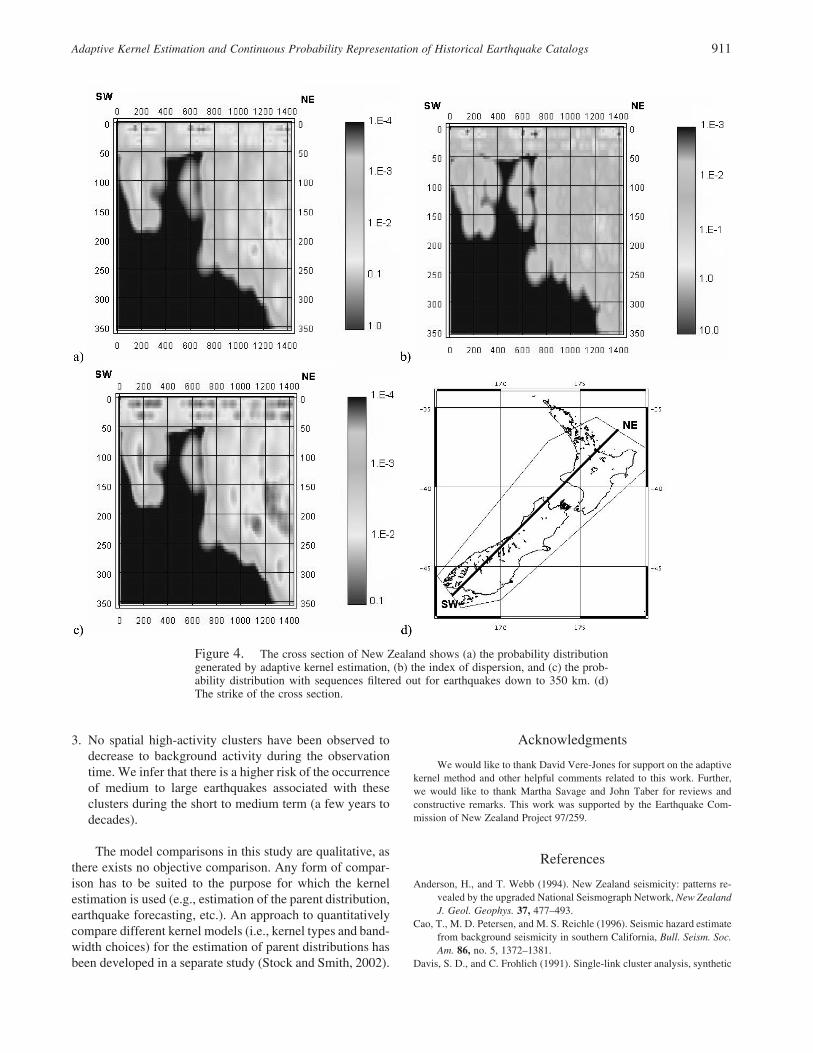
Figure 4 shows a depth profile of the seismicity prob-ability distribution g2(x), the spatial index of dispersionVt(x), and the seismicity probability distribution with earth-quake sequences filtered out g3(x). In contrast to the shallowactivity, temporal clustering was nearly absent for the deepearthquakes in the subducted slabs during the observationperiod (compare Fig. 4a and b), and the index of dispersionof the deep earthquakes looks very uniform. Hence there isno need to filter temporal sequences out of the representationof earthquake occurrence probability (Fig. 4a and c lookalike). One explanation for this result would be that deepearthquakes do not produce many temporally clustered se-quences, such as aftershocks and swarms, as it has been ob-served for large deep earthquakes in the past. The low tem-poral variation further suggests that the spatial earthquakeoccurrence features have been very stable during the obser-vation period.

Australia

Figure 5 shows the seismicity probability distributiong3(x), with earthquake sequences filtered out, during differ-ent time intervals. The two probability distributions (Fig. 5aand b) reveal similar seismicity features, although they donot match as well as the corresponding figures for New Zea-land. This is not surprising because the activity in Australiais much lower and a higher uncertainty in g3(x) is to beexpected due to the lower sample size.

The region of highest activity occurred at the locationof the Tennant Creek earthquake sequence (latitude �20�,

longitude 134�) on 22 January 1988, which had one eventabove magnitude 6.5 and two other events above magnitude6.0 (Gaull et al., 1990). Before these events, the area aroundthis earthquake has been reasonably inactive (Fig. 5c). Thereis little doubt that this earthquake started a spatial cluster ofhigh activity, which persists today. It is possible that otherclusters of persistent high activity, which have producedlarge earthquakes in historical times, have been started byone or a few large events. On the other hand, no spatialclusters of persistent high activity in New Zealand and Aus-tralia decreased to background activity during the observa-tion time.

Discussion

In probabilistic seismic hazard analysis, the main inter-est lies in the occurrence of damaging earthquakes. The pre-sented analysis includes earthquakes below magnitude five,which (in most cases) do not cause great damage. TheGutenberg–Richter law predicts power-law behavior be-tween small and large earthquakes and justifies the extrap-olation from small to large earthquakes. In contrast, the char-acteristic earthquake model (e.g., Wesnousky, 1994; Stirlinget al., 1996) predicts a proportionally larger number of largeearthquakes in regions dominated by long faults. It is pos-sible that some spatial high-activity clusters only producemedium and small size earthquakes but no large earth-quakes. Examples of such clusters can be seen in the TaupoVolcanic Zone in New Zealand (latitude �39�, longitude176�), where no earthquakes above magnitude 7.0 have beenobserved during historical times (e.g., Smith and Webb,1986; Reyners, 1989). The Australian cluster at latitude�34� and longitude 122� is mining induced (Gaull et al.,

910 C. Stock and E. G. C. Smith

Figure 3. The probability distribution of crustalearthquakes in New Zealand with sequences filteredout (a) from 1962 to 1990 above magnitude 4.0 and(b) from 1991 to 1997 above magnitude 3.0.

1990) and has not produced any large earthquakes since in-ception.

Kagan and Jackson (1999) found that the recurrencetimes of doublets of large earthquakes (above magnitude7.0) show power-law behavior and conclude that large earth-quakes cluster in time and space, similar to smaller-sizeearthquakes. Combined with our result, that no spatial clus-ters of persistent high activity in New Zealand and Australiadecreased to background activity during the observationtime, such clusters appear to be potential sources of futuremoderate to large earthquakes for at least a few decades.Currently, work is in progress to incorporate longer-term

data, including geological data (e.g., faults), into the seis-micity models.

For the procedures introduced in this article to workwell, a minimum number of earthquakes are needed. Unfor-tunately, the number of historically observed large earth-quakes (e.g., above magnitude 6) is often too low to producegood results. The more data that are available, the better thedetection and resolution of activity structures will be and thebetter the sequence filtering will work. For example, Aus-tralia has a relatively higher apparent rate of earthquakesoccurring in high-activity regions inferred from magnitude4 and above (Fig. 5a) compared to the activity inferred frommagnitude 3 and above (Fig. 5b). This might be due to alower temporal variance in the first representation, whichprobably results from the low number of counted aftershocksabove magnitude 4. This would lead in turn to a higher un-certainty in the index of dispersion. There are more after-shocks counted above magnitude 3, which thus leads togreater filtering and lower estimated probability densities inthe high-activity clusters.

We suggest that one should generate earthquake prob-ability distributions with the lowest possible cutoff magni-tude to identify spatial and temporal earthquake distributionfeatures. The additional consideration of probability distri-butions with a higher cutoff magnitude may help to identifyimportant differences from the seismicity features of smallerearthquakes (e.g., the identification of high-activity clustersthat have not produced large earthquakes in historical times).The generated representations of earthquake occurrenceprobabilities should not be used for the prediction of earth-quakes for a time period longer than the observation periodbecause activity fluctuations on timescales that exceed theobservation time cannot be predicted with this approach.

Conclusions

Adaptive kernel estimation can better resolve local seis-mic features in distributions of earthquake activity than ker-nel estimations with global bandwidths because of its abilityto adapt the degree of smoothing to the data. The introducedlocal index of dispersion and procedure to filter temporalearthquake sequences has revealed the following results inNew Zealand and Australian earthquake distributions:

1. Whereas shallow earthquakes are mostly part of temporalearthquake sequences (such as mainshocks with after-shocks), the subducting slab in New Zealand has beennearly free from temporal activity variations for the last40 yr, suggesting that deep earthquakes do not producemany multiple events, as observed in the past.

2. The probability distribution of main events has been sta-ble in New Zealand during the last 40 yr. Apart from theTennant Creek earthquake, which introduced a new spa-tial high-activity cluster, the probability distribution ofmain events in Australia has been reasonably stable overthe last 20 yr.

Adaptive Kernel Estimation and Continuous Probability Representation of Historical Earthquake Catalogs 911

Figure 4. The cross section of New Zealand shows (a) the probability distributiongenerated by adaptive kernel estimation, (b) the index of dispersion, and (c) the prob-ability distribution with sequences filtered out for earthquakes down to 350 km. (d)The strike of the cross section.

3. No spatial high-activity clusters have been observed todecrease to background activity during the observationtime. We infer that there is a higher risk of the occurrenceof medium to large earthquakes associated with theseclusters during the short to medium term (a few years todecades).

The model comparisons in this study are qualitative, asthere exists no objective comparison. Any form of compar-ison has to be suited to the purpose for which the kernelestimation is used (e.g., estimation of the parent distribution,earthquake forecasting, etc.). An approach to quantitativelycompare different kernel models (i.e., kernel types and band-width choices) for the estimation of parent distributions hasbeen developed in a separate study (Stock and Smith, 2002).

Acknowledgments

We would like to thank David Vere-Jones for support on the adaptivekernel method and other helpful comments related to this work. Further,we would like to thank Martha Savage and John Taber for reviews andconstructive remarks. This work was supported by the Earthquake Com-mission of New Zealand Project 97/259.

References

Anderson, H., and T. Webb (1994). New Zealand seismicity: patterns re-vealed by the upgraded National Seismograph Network, New ZealandJ. Geol. Geophys. 37, 477–493.

Cao, T., M. D. Petersen, and M. S. Reichle (1996). Seismic hazard estimatefrom background seismicity in southern California, Bull. Seism. Soc.Am. 86, no. 5, 1372–1381.

Davis, S. D., and C. Frohlich (1991). Single-link cluster analysis, synthetic

912 C. Stock and E. G. C. Smith

Figure 5. The probability distribution of crustalearthquakes in Australia (above 50 km) above mag-nitude 4.0 in 0.5� squares with sequences filtered out(a) from 1978 to 1996 above magnitude 4.0, (b) from1991 and 1996 above magnitude 3.0, and (c) from1978 to 1986.

earthquake catalogues, and aftershock identification, Geophys. J. Int.104, no. 2, 289–306.

Frankel, A. (1995). Mapping seismic hazard in the central and easternUnited States, Seism. Res. Lett. 66, 8–21.

Gaull, B. A., M. O. Michael-Leiba, and J. M. W. Rynn (1990). Probabilisticearthquake risk maps of Australia, Aust. J. Earth Sci. 37, 169–87.

Hardle, W. (1990). Applied Nonparametric Regression, Cambridge, Cam-bridge University Press.

Jackson, D. D., and Y. Y. Kagan (1999). Testable earthquake forecasts for1999, Seism. Res. Lett. 70, no. 4, 393–403.

Johnson, N. L., S. Kotz, and A. W. Kemp (1992). Univariate DiscreteDistributions, Second Ed., in Probability and Mathematical Statistics,Wiley series in probability and mathematical statistics, Wiley, NewYork.

Kagan, Y. Y., and D. D. Jackson (1999). Worldwide doublets of largeshallow earthquakes, Bull. Seism. Soc. Am. 89, no. 5, 1147–1155.

Marzocchi, W., F. Mulargia, and G. Gonzato (1997). Detecting low-dimensional chaos in geophysical time series, J. Geophys. Res. 102,no. B2, 3195–3209.

Maunder, D. E. (Editor) (1999). New Zealand seismological report 1997,Seismological Observatory Bulletin E-180, Institute of Geological &Nuclear Sciences Science Report 99/20, Lower Hutt.

McCue, K. and P. Gregson (Editor) (1994). Australian Seismological Re-port, 1991, Australian Geological Survey Organisation Record 1994/10, Australian Geological Survey, Canberra.

Musmeci, F., and D. Vere-Jones (1986). A variable-grid algorithm forsmoothing clustered data, Biometrics 42, 483–494.

Ogata, Y. M. Imoto, and K. Katsura (1991). 3D spatial variation of b-valuesof magnitude frequency distribution beneath the Kanto District, Japan,Geophys. J. Int. 104, no. 1, 135–146.

Papazachos, P. (1999). An alternative method for a reliable estimation ofseismicity with an application in Greece and the surrounding area,Bull. Seism. Soc. Am. 89, no. 1, 111–119.

Reasenberg, P. A., and L. M. Jones (1989). Earthquake hazard after a main-shock in california, Science 243, 1173–1176.

Reyners, M. (1989). New Zealand seismicity 1964–87: an interpretation,New Zealand J. Geol. Geophys. 32, 307–315.

Robertson, M. C., C. G. Sammis, M. Sahimi, and A. J. Martin (1995).Fractal analysis of three-dimensional spatial distributions of earth-quakes with a perlocation interpretation, J. Geophys. Res. 100, no.B1, 609–620.

Savage, M. K., and D. M. dePolo (1993). Foreshock probabilities in thewestern Great-Basin Eastern Sierra Nevada, Bull. Seism. Soc. Am. 83,no. 6, 1910–1938.

Silverman, B. W. (1986). Density Estimation for Statistics and Data Anal-ysis, Monographs on Statistics and Applied Probability, Chapman andHall, London.

Smith, E. G. C., and T. H. Webb (1986). The seismicity and related defor-mation of the central volcanic region, North Island, New Zealand, inLate Cenozoic Volcanism in New Zealand, Ian E. M. Smith (Editor),R. Soc. New Zealand Bull. 23, 112–133.

Stirling, M. W., S. G. Wesnousky, and K. Shimazaki (1996). Fault tracecomplexity, cumulative slip, and the shape of the magnitude-frequency distribution for strike-slip faults: a global survey, Geophys.J. Int. 124, no. 3, 833–868.

Stock, C. (2001). A consistent geological-seismological model for earth-quake occurrence in New Zealand, Ph.D. Thesis, Victoria Universityof Wellington, Wellington, New Zealand.

Stock, C. and E. G. C. Smith (2002). Comparison of seismicity modelsgenerated by different kernel estimations, Bull. Seism. Soc. Am. 92,no. 3, 913–922.

Vere-Jones, D. (1992). Statistical methods for the description and displayof earthquake catalogs, in Statistics in the Environmental and EarthSciences, A. T. Walden and P. Guttorp (Editors), Arnold Publishers,London, 220–246.

Wesnousky, S. G. (1994). The Gutenberg-Richter or characteristic earth-quake distribution, which is it? Bull. Seism. Soc. Am. 84, no. 6, 1940–1959.

Woo, G. (1996). Kernel estimation methods for seismic hazard area sourcemodeling, Bull. Seism. Soc. Am. 86, no. 2, 353–362.

School of Earth SciencesVictoria University of WellingtonPO Box 600Wellington, New Zealand

Manuscript received 30 August 2000.