ADAPTIVE ECHO

CANCELLATION:

A simulation based study of LMS adaptation in

a generalized feed-forward architecture 1 2

Arun ’Nayagam

Dept. of Electrical and Computer Engineering

UFID: 6271− 7860

1Submitted in partial fulfillment of the requirements of the course, EEL 6502:

Adaptive Signal Processing2A basic knowledge of adaptive filtering and The Matrix Trilogy is assumed in

the writing of this manuscript

Chapter 1

Prologue

Figure 1.1: Design Scenario.

Morpheus, commander of the Nebuchadnezzar, receives an important call

from inside the Matrix. It is Neo. He does not believe in his capabilities as

the savior. Morpheus tries to calm Neo. Since Neo is inside the Matrix,

the two-four hybrid on his end is perfect (the Matrix can emulate a perfect

world1). Hence Morpheus can hear Neo clearly. He also hears loud back-

ground music and guesses Neo must be in some kind of public facility like a

1Glitches in the matrix can cause erratic and often chaotic behavior in the matrix

affecting the “perfectness” of the Matrix world. We assume that a glitch in the matrix

does not occur during the conversation between Neo and Morpheus

3

bar. However, the two-four hybrid aboard the Nebuchadnezzar is imperfect.

Thus, Neo is not able to hear Morpheus. All he can hear is an echo of the

load music that is playing around him.

We are a group of DSP engineers who were rescued and brought out of

the Matrix. While connected to the Matrix, the machines had us believe that

we were pursuing graduate studies in Signal Processing at the University of

Florida. Morpheus gives us all a chance to put the skills we learnt in the

Matrix to use. He assigns us the task of designing an adaptive system that

can cancel out the echo that is caused by the near-end hybrid. If we succeed

Morpheus can talk to Neo and make him believe that he is The One. And

then Neo can destroy the Matrix. The future of the rest of mankind depends

on our skills. Its payback time............

4

Chapter 2

Introduction

In this project we study the effectiveness of the least-mean-squares (LMS)

algorithm in a generalized feed-forward structure when applied to a echo can-

cellation application. The report is organized as follows. We begin by first

presenting an introduction to echo cancellation and generalized feed-forward

structures. In the next chapter, we present the theory behind gamma filters.

In Chapter 4, we study the performance of the LMS algorithm in both the

FIR and gamma filter architectures. We demonstrate that the gamma filter

can provide the same performance as the FIR filter with a much smaller

filter order. The report is concluded in Chapter 5.

2.1 Echo Cancellation

Echoes are a common problem in any communication system. Echoes are

present in every day direct conversations between people and also conver-

sations over cell phones or IP telephony. If the delay between the original

speech and the echo is very small (less than 10 milliseconds), the echo is not

noticeable. However in applications like long distance telephony, hands-free

telephones and packet based communication applications like IP telephony,

5

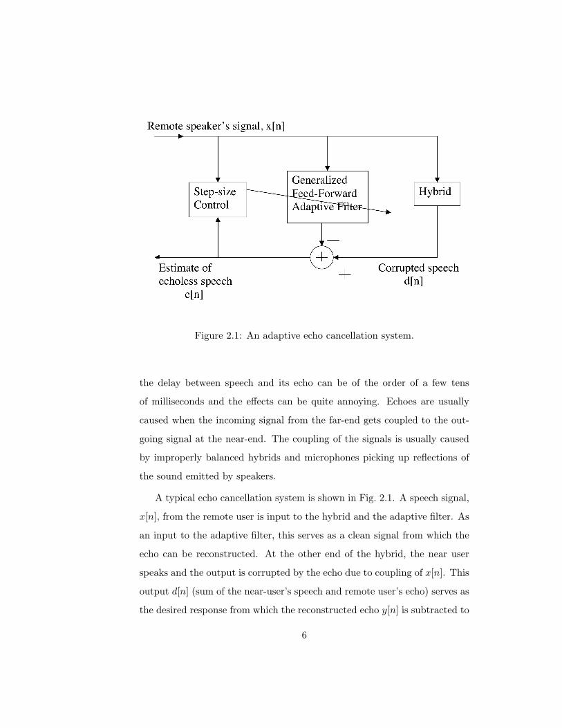
Figure 2.1: An adaptive echo cancellation system.

the delay between speech and its echo can be of the order of a few tens

of milliseconds and the effects can be quite annoying. Echoes are usually

caused when the incoming signal from the far-end gets coupled to the out-

going signal at the near-end. The coupling of the signals is usually caused

by improperly balanced hybrids and microphones picking up reflections of

the sound emitted by speakers.

A typical echo cancellation system is shown in Fig. 2.1. A speech signal,

x[n], from the remote user is input to the hybrid and the adaptive filter. As

an input to the adaptive filter, this serves as a clean signal from which the

echo can be reconstructed. At the other end of the hybrid, the near user

speaks and the output is corrupted by the echo due to coupling of x[n]. This

output d[n] (sum of the near-user’s speech and remote user’s echo) serves as

the desired response from which the reconstructed echo y[n] is subtracted to

6

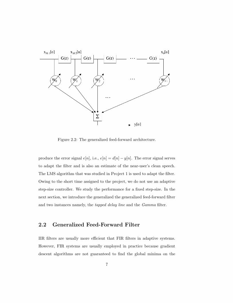
Figure 2.2: The generalized feed-forward architecture.

produce the error signal e[n], i.e., e[n] = d[n]− y[n]. The error signal serves

to adapt the filter and is also an estimate of the near-user’s clean speech.

The LMS algorithm that was studied in Project 1 is used to adapt the filter.

Owing to the short time assigned to the project, we do not use an adaptive

step-size controller. We study the performance for a fixed step-size. In the

next section, we introduce the generalized the generalized feed-forward filter

and two instances namely, the tapped delay line and the Gamma filter.

2.2 Generalized Feed-Forward Filter

IIR filters are usually more efficient that FIR filters in adaptive systems.

However, FIR systems are usually employed in practice because gradient

descent algorithms are not guaranteed to find the global minima on the

7

non-convex performance surface of IIR systems. Also stability of adaptive

IIR filters is a hard problem to which only heuristic solutions have been pro-

posed. The generalized feed-forward (GFF) filter was introduced by Principe

et. al. [1] as an alternative that combines the attractive features of both FIR

and IIR systems.. The structure of the GFF filter is shown in Figure 2.2.

The filter output is given by

Y (z) =M∑

k=0

wkXk(z), where (2.1)

Xk(z) = G(z)Xk−1(z), k = 1, . . . ,M. (2.2)

G(z) is called the generalized delay operator and can have a recursive or

non-recursive structure. A recursive structure for G(z) leads to an overall

IIR structure. The GFF reduces to a tapped delay line or an FIR filter when

G(z) = z−1. The overall transfer function of the GFF filter is given by

H(z) =Y (z)X(z)

=M∑

k=0

wkGk(z). (2.3)

Thus, it is clear that H(z) is stable whenever G(z) is stable. The gamma

filter is obtained is obtained when G(z) = µz−(1−µ) , where µ is a feedback

parameter. The gamma filter is introduced in detail in the next chapter.

8

Chapter 3

The Theory of Gamma

Filters

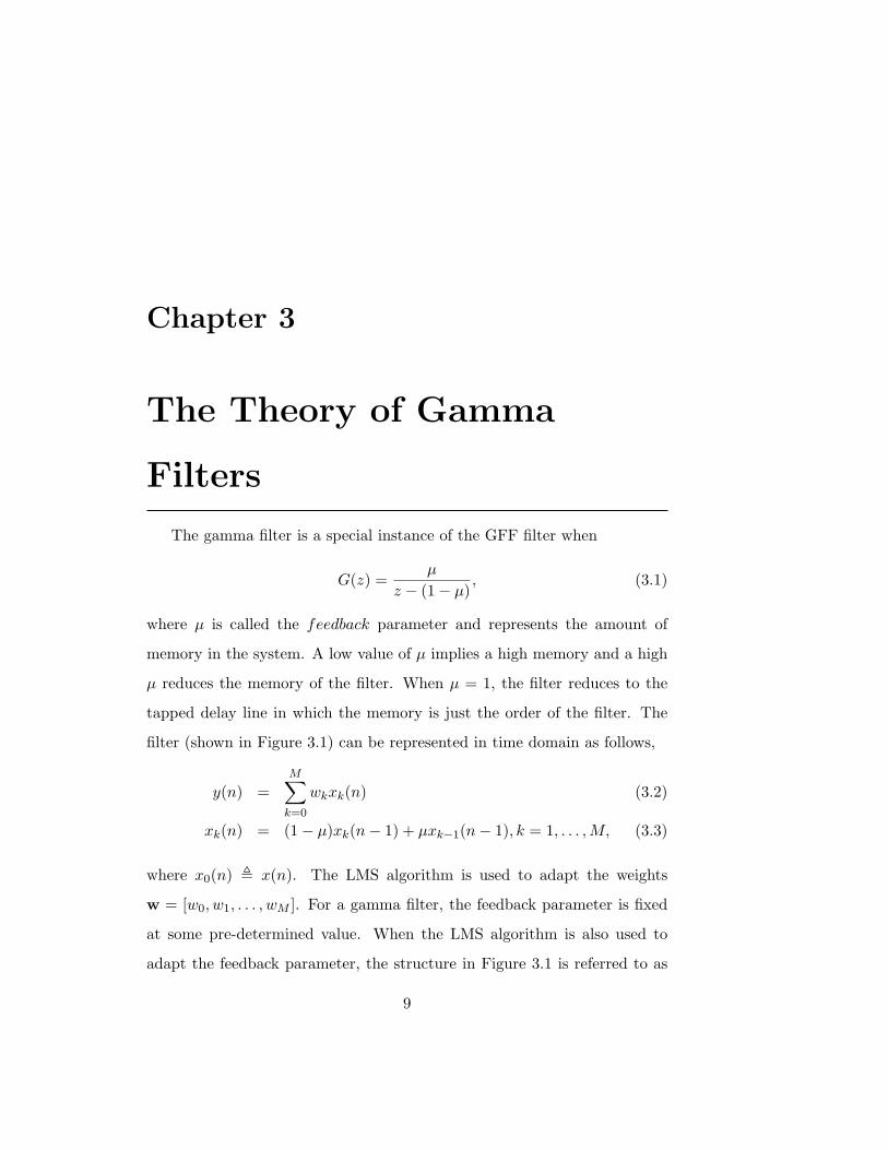
The gamma filter is a special instance of the GFF filter when

G(z) =µ

z − (1− µ), (3.1)

where µ is called the feedback parameter and represents the amount of

memory in the system. A low value of µ implies a high memory and a high

µ reduces the memory of the filter. When µ = 1, the filter reduces to the

tapped delay line in which the memory is just the order of the filter. The

filter (shown in Figure 3.1) can be represented in time domain as follows,

y(n) =M∑

k=0

wkxk(n) (3.2)

xk(n) = (1− µ)xk(n− 1) + µxk−1(n− 1), k = 1, . . . ,M, (3.3)

where x0(n) , x(n). The LMS algorithm is used to adapt the weights

w = [w0, w1, . . . , wM ]. For a gamma filter, the feedback parameter is fixed

at some pre-determined value. When the LMS algorithm is also used to

adapt the feedback parameter, the structure in Figure 3.1 is referred to as

9

Figure 3.1: The gamma filter.

the adaptive gamma filter. It can easily be shown that the filter is stable

whenever G(z) is stable i.e., whenever 0 < µ < 2 the gamma filter is always

stable.

3.1 LMS adaptation of the gamma filter

Let us use the power of the total error as the performance metric (E) that

the gamma filter attempts to minimize. The total power is defined as

E =T∑

n=0

12e2(n) =

T∑n=0

12(d(n)− y(n))2, (3.4)

where y(n) is the output of the gamma filter defined in (3.2) and (3.3) and

d(n) is a desired signal (a corrupted version of the near user’s signal in our

10

application). The LMS algorithm updates the filter weights in a direction

that is opposite to the local gradient, i.e.,

∆wk = −η∂E∂wk

(3.5)

∆µ = −η∂E∂µ

, (3.6)

where η is a step-size parameter. A local time (iterative) approximation of

the above equations can be expressed as

∆wk(n) = ηe(n)xk(n), k = 0, . . . ,M (3.7)

∆µ = η

M∑k=0

e(n)αk(n), (3.8)

where

αk(n) =∂xk(n)

∂µ= (1−µ)αk(n−1)+µαk−1(n−1)+µ[xk−1(n−1)−xk(n−1)].

(3.9)

Note that eqn. (3.9) is defined for k = 0, . . . ,M and α0(n) = 0. Note that

the LMS update equations given in (3.7) and (3.8) work well only when

the step size η is sufficiently small. We show in the next chapter that the

feebdack parameter update in eqn. (3.8) is more sensitive than the weight

update equation (3.7). This is because a large step size causes the values

of µ to go outside the stability region (0, 2) and this causes the IIR filter

to become unstable and the value of µ keeps growing without bound. Note

that the complexity for adaptation is the same as that of adapting an FIR

filter (O(n)). For general IIR filters, the complexity is O(n2). Thus, the

gamma filters harness the power of IIR with low computational complexity.

11

12

Chapter 4

Simulation Results

In this section we present simulation results for the tapped delay line and

the gamma filter when applied to our echo cancellation problem. A key

issue in this application is the selection of the step-size (η) used in the LMS

algorithm. Usually an adaptive step-size is used in practical applications.

Owing to the short-duration assigned to the project, we use various fixed

step-sizes to compare different filter architectures. However, the selection of

step-size is a critical step in the design procedure. We begin by discussing

our approach in the selection of step-size.

4.1 LMS step-size selection

The weight update equation for the LMS algorithm is given by

w(n + 1) = w(n) + ηe(n)u(n), (4.1)

where u(n) is the input to the tapped delay line, e(n) = d(n) − y(n) is

the error signal (difference between the desired signal and filter output).

Convergence analysis has proved that the maximum value of step-size (µ) is

related to the maximum eigenvalue (λmax) of the autocorrelation matrix of

13

the input signal as follows

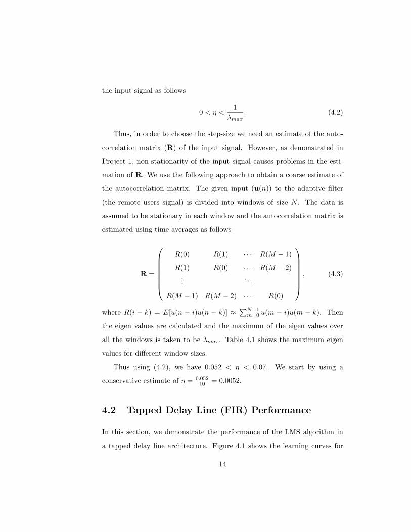
0 < η <1

λmax. (4.2)

Thus, in order to choose the step-size we need an estimate of the auto-

correlation matrix (R) of the input signal. However, as demonstrated in

Project 1, non-stationarity of the input signal causes problems in the esti-

mation of R. We use the following approach to obtain a coarse estimate of

the autocorrelation matrix. The given input (u(n)) to the adaptive filter

(the remote users signal) is divided into windows of size N . The data is

assumed to be stationary in each window and the autocorrelation matrix is

estimated using time averages as follows

R =

R(0) R(1) · · · R(M − 1)

R(1) R(0) · · · R(M − 2)...

. . .

R(M − 1) R(M − 2) · · · R(0)

, (4.3)

where R(i − k) = E[u(n − i)u(n − k)] ≈∑N−1

m=0 u(m − i)u(m − k). Then

the eigen values are calculated and the maximum of the eigen values over

all the windows is taken to be λmax. Table 4.1 shows the maximum eigen

values for different window sizes.

Thus using (4.2), we have 0.052 < η < 0.07. We start by using a

conservative estimate of η = 0.05210 = 0.0052.

4.2 Tapped Delay Line (FIR) Performance

In this section, we demonstrate the performance of the LMS algorithm in

a tapped delay line architecture. Figure 4.1 shows the learning curves for

14

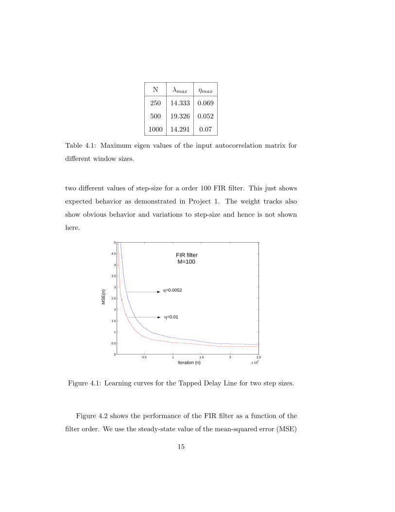
N λmax ηmax

250 14.333 0.069

500 19.326 0.052

1000 14.291 0.07

Table 4.1: Maximum eigen values of the input autocorrelation matrix for

different window sizes.

two different values of step-size for a order 100 FIR filter. This just shows

expected behavior as demonstrated in Project 1. The weight tracks also

show obvious behavior and variations to step-size and hence is not shown

here.

0.5 1 1.5 2 2.5

x 104

0

0.5

1

1.5

2

2.5

3

3.5

4

4.5

5

FIR filter M=100

MS

E(n

)

Iteration (n)

η=0.0052

η=0.01

Figure 4.1: Learning curves for the Tapped Delay Line for two step sizes.

Figure 4.2 shows the performance of the FIR filter as a function of the

filter order. We use the steady-state value of the mean-squared error (MSE)

15

denoted by J(∞) as the performance metric. As expected an increase in

the filter order leads to an improvement in performance. Note that our

conservative step-size of 0.0052 causes slower convergence (refer Figure 4.1)

leading to a higher J(∞). For step-sizes of the order of 10−2, lower step-sizes

usually lead to slower convergence but had a lower J(∞).

100 110 120 130 140 150 160 170 180 190 2000

0.05

0.1

0.15

0.2

0.25

0.3

0.35

η=0.0052

η=0.01

J(∞

)

Filter Order (M)

FIR Filter

Figure 4.2: Performance of the Tapped Delay Line as a function of filter

order.

4.3 Gamma Filter Performance

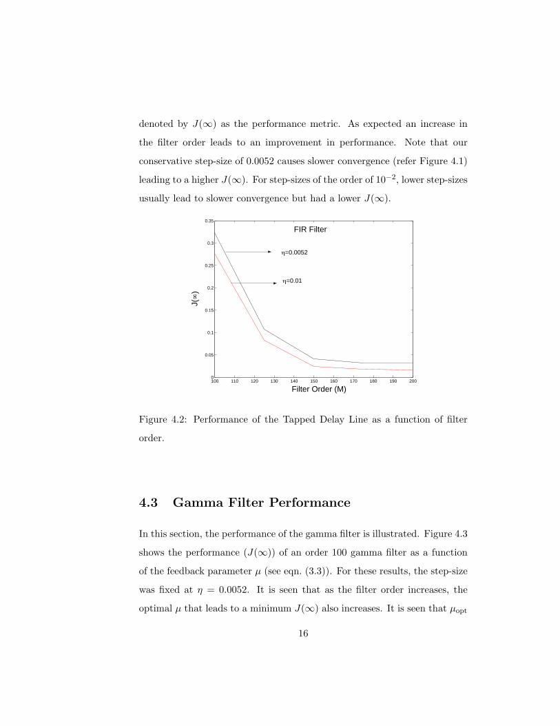
In this section, the performance of the gamma filter is illustrated. Figure 4.3

shows the performance (J(∞)) of an order 100 gamma filter as a function

of the feedback parameter µ (see eqn. (3.3)). For these results, the step-size

was fixed at η = 0.0052. It is seen that as the filter order increases, the

optimal µ that leads to a minimum J(∞) also increases. It is seen that µopt

16

0.1 0.2 0.3 0.4 0.5 0.6 0.7 0.8 0.9 10

0.1

0.2

0.3

0.4

0.5

0.6

0.7

0.8

Feedback Parameter (µ)

J(∞

)M=60

M=100

M=120

M=150

M=80

Figure 4.3: Performance of the gamma filter as a function of the feedback

parameter(µ).

tends to 1 for filter orders greater than 150. This implies that increasing

filter order leads to a reduction in memory in order to achieve the least MSE,

i.e., for very high filter orders µopt ≈ 1 and hence there is no feedback in

the system. Hence, the use of feedback becomes redundant with very high

filter orders. That is, for very large filter orders, the gamma filter tends to

an FIR filter and there is no advantage in using the IIR structure of the

generalized delay blocks (G(z)). Table 4.3 shows the approximate µopt for

different filter orders.

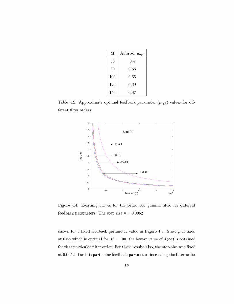
Learning curves for the order 100 filter are shown in Figure 4.4. From

Table 4.3, we note the optimal value for µ = 0.65. Among the learning

curves shown in Figure 4.4, it is seen that µ = 0.65 produces the lowest

steady state MSE (though it converges slower than µ = 0.85).

The performance of the gamma filter as a function of the filter order is

17

M Approx. µopt

60 0.4

80 0.55

100 0.65

120 0.69

150 0.87

Table 4.2: Approximate optimal feedback parameter (µopt) values for dif-

ferent filter orders

0.5 1 1.5 2 2.5

x 104

0

0.5

1

1.5

2

2.5

3

3.5

4

4.5

5

Iteration (n)

MS

E(n

)

µ=0.3

µ=0.6

µ=0.65

µ=0.85

M=100

Figure 4.4: Learning curves for the order 100 gamma filter for different

feedback parameters. The step size η = 0.0052

shown for a fixed feedback parameter value in Figure 4.5. Since µ is fixed

at 0.65 which is optimal for M = 100, the lowest value of J(∞) is obtained

for that particular filter order. For these results also, the step-size was fixed

at 0.0052. For this particular feedback parameter, increasing the filter order

18

beyond 120 produces negligible performance improvement.

80 90 100 110 120 130 140 1500.04

0.05

0.06

0.07

0.08

0.09

0.1

0.11J(∞

)

Filter Order (M)

µ=0.65 (Optimum for M=100)

Figure 4.5: Performance of the gamma filter as a function of the filter order

(M) for a fixed feedback parameter (µ).

4.4 Comparison of LMS and Gamma filter

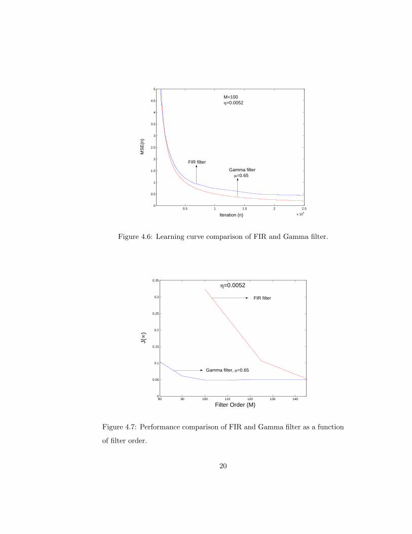
In this section we present performance comparison of the LMS and gamma

filter. Figure 4.6 compares the learning curves for the FIR and gamma filter

for a fixed filter order (M = 100) and LMS step size (η = 0.0052). The

optimal feedback parameter (µ = 0.65) for the gamma filter of order 100 is

used. It is seen that the gamma filter produces a lower MSE for the same

order filter.

Figure 4.7 compares the performance (J(∞)) of the tapped delay line

and the gamma filters with respect to filter order. It is seen that the gamma

filter outperforms the FIR filter for all the shown filter orders (80 − 150).

19

0.5 1 1.5 2 2.5

x 104

0

0.5

1

1.5

2

2.5

3

3.5

4

4.5

5

M=100 η=0.0052

Iteration (n)

MS

E(n

)

FIR filter

Gamma filter µ=0.65

Figure 4.6: Learning curve comparison of FIR and Gamma filter.

80 90 100 110 120 130 1400

0.05

0.1

0.15

0.2

0.25

0.3

0.35

J(∞

)

Filter Order (M)

FIR filter

Gamma filter, µ=0.65

η=0.0052

Figure 4.7: Performance comparison of FIR and Gamma filter as a function

of filter order.

20

Note that a J(∞) = 0.05 is achieved with a FIR filter of order 150 but just

requires a gamma filter order of 90 with feedback parameter µ = 0.65.

4.5 LMS adaptation of the feedback parameter

In the previous sections, the performance of gamma filters with a fixed

feedback parameter is studied. In this section, we present results for adaptive

gamma filters wherein the feedback parameter is adapted using the LMS

algorithm (see eqn. (3.8)). Throughout the discussion in this section we use

η to refer to the step-size for feedback parameter adaptation and ηw to refer

to the step-size for weight adaptation. For all the results in this section,

we use the highest value of ηw that showed convergence behavior for fixed

values of µ in the previous section. The maximum value of ηw is around

0.07 for this application. Thus we fix the value of ηw = 0.07 and study the

behavior of the adaptive gamma filter.

In Figure 4.8, we show the tracking of the feedback parameters for differ-

ent values of η for an order 100 adaptive gamma filter. From Table 4.3, the

optimum value of µ ≈ 0.65. It is seen that with a step-size of η = 1−5, con-

vergence is very slow and does not converge to the optimum value. However

with a larger step-size of η = 5× 10−5, the feedback parameter converges to

around 0.63. For both these results, the step-size is initialized to µ0 = 1 be-

fore adaptation begins. Results are also shown for a step-size of η = 1×10−5

and µ0 = 0.7. It is seen that this particular choice of η and µ0 converges to

around 0.66 which is near the optimal value. Thus, we see that the feedback

parameter adaptation is sensitive to both the step size η and the initial value

of µ.

The learning curves for the choice of η and µ0 used in the previous set of

21

0 2 4 6 8 10 12

x 104

0.6

0.65

0.7

0.75

0.8

0.85

0.9

0.95

1

1.05

Iteration

Fee

dbac

k P

aram

eter

(µ)

η=1x10−5, µ0=1.0

η=5x10−5, µ0=1.0

M=100, ηw

=0.07

η=1x10−5, µ0=0.7

Figure 4.8: LMS tracks of the feedback parameter for an order 100 adaptive

gamma filter.

0 0.5 1 1.5 2 2.5

x 104

0

0.5

1

1.5

Iteration

MS

E(n

)

M=100, ηw

=0.07

η=1x10−5, µ0=1.0

η=5x10−5, µ0=1.0

η=1x10−5, µ0=0.7

Figure 4.9: Learning curves for an order 100 adaptive gamma filter.

22

results are shown in Figure 4.9. It is seen that the choice of η that converges

to a value that is closer to the optimal value has a lower steady-state MSE

and converges faster. It also serves to mention that values of η > 5 × 10−5

cause µ to lie outside the convergence region of (0, 2). This causes the filter

to become unstable and the values of µ start diverging without bound.

Figure 4.10 shows the tracking performance for different filter orders.

From the values given in Table 4.3, it is seen that the adaptive gamma

filter converges to the vicinity of the optimum step-size. As mentioned in

Project 1, the LMS algorithm requires the step-size to be decreased with an

increase in filter order. This is true even for the case of feedback parameter

adaptation. For example, though η = 5 × 10−5 produces convergence in µ

for M = 80, 100, 120, it causes the filter to become unstable if M = 150 and

produces unbounded µ updates.

0 1 2 3 4 5 6 7 8 9 10 11

x 104

0.5

0.55

0.6

0.65

0.7

0.75

0.8

0.85

0.9

0.95

1

Iteration (n)

Fee

dbac

k P

aram

eter

(µ)

M=120

M=100

M=80

η=5x10−5, ηw

=0.07, µ0=1

Figure 4.10: LMS tracking of the feedback parameters for an adaptive

gamma filter with various filter orders.

23

The value of J(∞) as a function of filter order for the adaptive gamma

filter is shown in Figure 4.11. Unlike Figure 4.5, a flooring/saturation is not

seen in the performance. This is because the optimal feedback parameters

are adaptively tracked and hence performance keeps improving with the

filter order. When compared with Figure 4.5 which has a near optimal µ

for M = 100, the adaptive filter produces a lower J(∞) even for M = 100.

This is because the feedback adaptation tracks the actual µopt (µopt ≈ 0.65)

is only an approximation. Thus, when the LMS step-size is properly chosen,

the adaptive gamma filter leads to better performance.

80 85 90 95 100 105 110 115 120 125 1300.003

0.004

0.005

0.006

0.007

0.008

0.009

0.01

J(∞

)

Filter Order (M)

η=5x10−5, ηw

=0.07

Figure 4.11: Performance of the adaptive gamma filter as a function of filter

order.

24

Chapter 5

Concluding Remarks

Based on our simulation based study, the following conclusions can be made

about the two LMS-based adaptive filter architectures discussed in this

project. Since the FIR filter was already exhaustively studied in Project 1,

we will not comment on its performance in detail. The usual behavior

wherein tracking time is inversely proportional to the step size while the

minimum MSE (and therefore the misadjustment) is directly proportional

to the step size, and the step size that achieves optimum performance de-

creases with an increase in filter order were observed. It just serves to say

that with a filter order of around 200 and η = 0.005, we were able to decipher

the speech from Morpheus.

The following observations are made about the gamma filter.

• As the feedback parameter µ → 1 the gamma filter reduces to the

tapped delay line.

• As the filter order is increased, the feedback parameter that achieves

optimum performance increases (see Table 4.3). This implies that the

25

role of the feedback decreases as the filter order increases. In other

words, for very large filter orders feedback does not play a role and all

the performance benefits of the gamma filter can be achieved by using

a simple FIR filter.

• The presence of feedback causes the performance surface to be non-

convex. This can be inferred from Figure 4.3 where the presence of a

local and a global minima can be seen for the filter of order 60.

• It is seen that the gamma filter outperforms the FIR filter (has a lower

J(∞)) and converges faster). Note that a J(∞) = 0.05 is achieved

with a FIR filter of order 150 but just requires a gamma filter order

of 90 with feedback parameter µ = 0.65. Lower MSE is possible if the

feedback parameter is also adapted using LMS.

• The speech can be reconstructed with a gamma filter of order M =

100, a fixed feedback parameter of µ = 0.65 and a step size ηw = 0.07.

(Compare with M = 200 required for the LMS filter). All the words

except one can be recovered with M = 80, µ = 0.55 and ηw = 0.07.

The word that is lost is Morpheus saying “Neo”. This is not very

important in conveying the meaning of the rest of the sentence.

• The feedback parameter can also be adapted using the LMS algo-

rithm. However extreme care must be taken to ensure convergence.

The feedback adaptation is much more sensitive to adaptation than

the weights. This is because a small change in the feedback produces

a disturbance in the signals that are scaled by the weights. This can

produce a large change at the output.

• In general, the step size (η) for feedback adaptation should be much

26

smaller than the step-size (ηw) for weight adaptation. A rule of thumb

is η < ηw

10 . However, for this particular application we required much

smaller step sizes.

• For a filter orders of 80 − 120, η > 5 × 10−5 caused divergence of µ.

That is, as the iterations progressed µ could take a value above 2 or

below 0. This causes the gamma filter to become unstable and µ grows

without bound leading unbounded MSE.

• The adaptive gamma filter is also vulnerable to the initial value that

the feedback parameter is initialized to. If the initial value is close to

the optimal value, all step-sizes that have 0 < µ(n) < 2 converge to

the optimal value.

• The adaptive gamma filter has better performance than the gamma

filter with fixed feedback (compare Figure 4.5 and Figure 4.11).

• Morpheus’s speech can be recovered with an adaptive gamma filter of

order z.

• Epilogue:

After designing the adaptive filter, the design team cross their fingers

and hope Neo can hear Morpheus. The adaptive gamma filter works

very well and Neo hears Morpheus say, “You have to let it all go

Neo: fear, doubt, disbelief”. And by saying this, Morpheus frees

Neo’s mind. This is just the beginning of the end of The Matrix ...

27

28

Bibliography

[1] J. C. Principe, D. de Vries, P. G. de Oliveira, “The Gamma Filter-

A new class of adaptive IIR filters with restricted feedback”, IEEE

Transactions on Signal Proc., vol. 41 no.2, pp 649-656.

[2] J. C. Principe, Adaptive Signal Processing. EEL 6502: Class Notes,

Spring 2004.

[3] S. Haykin, Adaptive filter theory. 4th ed., Prentice Hall, 2001.

29