Adaptive Code Modulation for Rainfall Fade Mitigation in ...

Adaptive Code Modulation for Rainfall Fade Mitigation inEthiopia

Eyob Mersha Woldamanuel

A Thesis submitted to

The department of Electronics and Communication Engineering

School of Electrical Engineering and Computing

Presented in Partial Fulfillment of the Requirement for the Degree of Master’s in

Electronics and Communication Engineering

Office of Graduate Studies

Adama Science and Technology University

Adama

July 2019

Adaptive Code Modulation for Rainfall Fade Mitigation inEthiopia

Eyob Mersha Woldamanuel

Advisor: Feyisa Debo (PhD)

A Thesis submitted to

The department of Electronics and Communication Engineering

School of Electrical Engineering and Computing

Presented in Partial Fulfillment of the Requirement for the Degree of Master’s in

Electronics and Communication Engineering

Office of Graduate Studies

Adama Science and Technology University

Adama

July 2019

Approval of Board of ExaminersWe, the undersigned, members of the Board of Examiners of the final open defense by

——————————————————- have read and evaluated his/her thesis entitled

”————————————————————————————-” and examined the can-

didate. This is, therefore, to certify that the thesis has been accepted in partial fulfillment of the

requirement of the Degree of. . . . . . . . . . . . . . . . . . . . . . . . . . . . . . . . . . . . . . . . . . . . . ............................

———————————————- —————————— ————————–

Advisor Signature Date

———————————————- —————————— ————————–

Chairperson Signature Date

———————————————- —————————— ————————–

Internal Examiner Signature Date

———————————————- —————————— ————————–

External Examiner Signature Date

i

DeclarationI hereby declare that this MSc Thesis is my original work and has not been presented for a

degree in any other university, and all sources of material used for this thesis have been duly

acknowledged.

Name:

Signature:

This MSc Thesis has been submitted for examination with my approval as thesis advisor.

Name:

Signature:

Date of submission ............................................................................

ii

Advisor’s Approval SheetTo: ..................................................................................................................Department

Subject: Thesis Submission

This is to certify that the thesis entitled ......................................................................................

...................................................................submitted in partial fulfillment of the requirements

for the degree of Master’s in .................. ...........................................................................,the

Graduate program of the department of ................................................................................., and

has been carried out by ..............................................................................................................

Id. No. . . . . . . . . . . . . . . . . . . . . . . . . . . . . . under my supervision. Therefore, I recommend that the

student has fulfilled the requirements and hence hereby he/she can submit the thesis/dissertation

to the department.

———————————————- —————————— ————————–

Name of major Advisor Signature Date

iii

ACKNOWLEDGMENT

First and foremost, I would like to thank my almighty God for his immeasurable support and

care. My sincere gratitude goes to my advisor Feyisa Debo (PhD) for his immense guidance and

support. It is with his motivations and follow up that I come up with the completion of this thesis.

In addition, I am greatly indebted to Haramaya University for the chance that gave me to purse

my postgraduate study in Adama Science and Technology University.My gratitude also goes to

Adama Science and Technology Uniiversity as an institute and its Electrical Engineering and

computing school staffs specially the Electronics and Communication Engineering department

staff for their integrity in facilitating the program.

Finally, I would like to take this opportunity to forward my deep hearted thanks to all who

gave me their precious time and effort, specially for Tsegu Kiros and Temsgen Achamo for

moral support, and being with me in time of need.

iv

Contents

APPROVAL OF BOARD OF EXAMINERS i

DECLARATION ii

ADVISOR’S APPROVAL SHEET iii

ACKNOWLEDGMENT iv

TABLE OF CONTENTS viii

LIST OF FIGURES ix

LIST OF TABLES xi

LIST OF ABBREVIATIONS xii

ABSTRACT xiv

1 INTRODUCTION 11.1 Background . . . . . . . . . . . . . . . . . . . . . . . . . . . . . . . . . . . . 1

1.2 Statement of the Problem . . . . . . . . . . . . . . . . . . . . . . . . . . . . . 4

1.3 Significance of the study . . . . . . . . . . . . . . . . . . . . . . . . . . . . . 5

1.4 General and specific objectives . . . . . . . . . . . . . . . . . . . . . . . . . . 6

1.4.1 General Objective . . . . . . . . . . . . . . . . . . . . . . . . . . . . 6

1.4.2 Specific Objectives . . . . . . . . . . . . . . . . . . . . . . . . . . . . 6

1.5 Scope of the study . . . . . . . . . . . . . . . . . . . . . . . . . . . . . . . . . 6

1.6 Organization of the thesis . . . . . . . . . . . . . . . . . . . . . . . . . . . . . 6

v

2 LITERATURE REVIEW 82.1 Line-of Sight Communication Above 5GHz . . . . . . . . . . . . . . . . . . . 8

2.2 Rainfall Attenuation . . . . . . . . . . . . . . . . . . . . . . . . . . . . . . . . 9

2.2.1 Rainfall Rate . . . . . . . . . . . . . . . . . . . . . . . . . . . . . . . 10

2.2.2 Rainfall rate distribution model . . . . . . . . . . . . . . . . . . . . . 10

2.2.3 Rain attenuation models . . . . . . . . . . . . . . . . . . . . . . . . . 12

2.3 Rain Attenuation Mitigation Techniques . . . . . . . . . . . . . . . . . . . . . 16

2.3.1 Diversity . . . . . . . . . . . . . . . . . . . . . . . . . . . . . . . . . 16

2.3.1.1 Frequency diversity (FD) . . . . . . . . . . . . . . . . . . . 16

2.3.1.2 Site Diversity (SD) FMT . . . . . . . . . . . . . . . . . . . 17

2.3.1.3 Satellite Diversity (SatD) . . . . . . . . . . . . . . . . . . . 17

2.3.2 Power control (PC) . . . . . . . . . . . . . . . . . . . . . . . . . . . 17

2.3.3 Adaptive waveform . . . . . . . . . . . . . . . . . . . . . . . . . . . . 18

2.3.3.1 Adaptive modulation . . . . . . . . . . . . . . . . . . . . . 18

2.3.3.2 Adaptive Coding and Modulation . . . . . . . . . . . . . . 18

2.3.4 Adaptive Techniques . . . . . . . . . . . . . . . . . . . . . . . . . . . 19

2.3.5 Non-adaptive Techniques . . . . . . . . . . . . . . . . . . . . . . . . 20

2.4 Performance Analysis of Adaptive Coding and Modulation Schemes . . . . . . 22

2.4.1 SNR estimation . . . . . . . . . . . . . . . . . . . . . . . . . . . . . . 22

2.4.2 Channel model . . . . . . . . . . . . . . . . . . . . . . . . . . . . . . 23

2.4.2.1 AWGN . . . . . . . . . . . . . . . . . . . . . . . . . . . . . 23

2.4.3 Channel coding . . . . . . . . . . . . . . . . . . . . . . . . . . . . . 24

2.4.3.1 Convolutional encoder . . . . . . . . . . . . . . . . . . . . 24

2.4.3.2 Viterbi decoding . . . . . . . . . . . . . . . . . . . . . . . 25

2.4.4 Modulation type . . . . . . . . . . . . . . . . . . . . . . . . . . . . . 26

2.4.5 Bit error rate (BER) performance . . . . . . . . . . . . . . . . . . . . 27

2.4.6 Capacity in AWGN channel . . . . . . . . . . . . . . . . . . . . . . . 28

2.5 Soft computing Techniques for Adaptive Modulation and

Coding Schemes . . . . . . . . . . . . . . . . . . . . . . . . . . . . . . . . . 28

2.5.1 Fuzzy Logic System . . . . . . . . . . . . . . . . . . . . . . . . . . . 29

2.5.1.1 Fuzzy inference system structure . . . . . . . . . . . . . . . 29

vi

2.5.1.2 Types of Fuzzy inference system . . . . . . . . . . . . . . . 30

2.5.1.3 Membership function (MF) . . . . . . . . . . . . . . . . . . 31

2.6 Neural Network Based Algorithms . . . . . . . . . . . . . . . . . . . . . . . . 33

2.6.1 Neuro-Fuzzy Approach . . . . . . . . . . . . . . . . . . . . . . . . . 33

2.6.1.1 Adaptive Network based Fuzzy Inference System . . . . . . 34

2.6.1.2 Neuro-fuzzy (ANFIS) structure . . . . . . . . . . . . . . . . 34

2.6.1.3 Hybrid learning algorithm . . . . . . . . . . . . . . . . . . . 36

2.7 Research Gaps . . . . . . . . . . . . . . . . . . . . . . . . . . . . . . . . . . 38

3 METHODOLOGY 393.1 Introduction . . . . . . . . . . . . . . . . . . . . . . . . . . . . . . . . . . . . 39

3.2 Rain Measurements and Data Processing . . . . . . . . . . . . . . . . . . . . . 39

3.3 Determination of Rain Attenuation . . . . . . . . . . . . . . . . . . . . . . . . 40

3.3.1 The ITU-R Rain Attenuation Model . . . . . . . . . . . . . . . . . . . 40

3.3.2 SNR Calculation . . . . . . . . . . . . . . . . . . . . . . . . . . . . . 43

3.4 Implementation of Adaptive Coding and Modulation . . . . . . . . . . . . . . 44

3.4.1 Neuro-Fuzzy Based Adaptive Coding and Modulation Design . . . . . 45

3.4.1.1 Generation of Input / Output data pairs . . . . . . . . . . . . 46

3.4.1.2 Spectral Efficiency Optimization . . . . . . . . . . . . . . . 48

3.4.2 ANFIS Architecture for Adaptive Coding and Modulation . . . . . . . 48

3.4.2.1 ANFIS System for Training Process . . . . . . . . . . . . . 49

4 RESULT AND DISCUSSION 554.1 Rain Attenuation Results . . . . . . . . . . . . . . . . . . . . . . . . . . . . . 55

4.1.1 Signal Level Analysis . . . . . . . . . . . . . . . . . . . . . . . . . . 58

4.2 Simulation Result of ACM Performance . . . . . . . . . . . . . . . . . . . . . 59

4.2.1 BER Performance Results . . . . . . . . . . . . . . . . . . . . . . . . 59

4.2.2 Effect of Channel Coding . . . . . . . . . . . . . . . . . . . . . . . . 62

4.2.3 Spectral Efficiency Results . . . . . . . . . . . . . . . . . . . . . . . . 66

4.2.4 Parameter Selection to Maximize Spectral Efficiency . . . . . . . . . . 68

4.3 Neuro-Fuzzy Based System Results . . . . . . . . . . . . . . . . . . . . . . . 69

vii

4.3.1 Performance Comparison of the ANFIS to Various Schemes . . . . . . 73

5 CONCLUSION AND RECOMMENDATION 755.1 Conclusion . . . . . . . . . . . . . . . . . . . . . . . . . . . . . . . . . . . . 75

5.2 Recommendations and Future Work . . . . . . . . . . . . . . . . . . . . . . . 76

REFERENCES 77

APPENDICES 83

viii

LIST OF FIGURES

1.1 Coding and Modulation scheme selection mechanism . . . . . . . . . . . . . . 3

2.1 ACM system model. . . . . . . . . . . . . . . . . . . . . . . . . . . . . . . . 18

2.2 Convolutional Encoder[47] . . . . . . . . . . . . . . . . . . . . . . . . . . . . 25

2.3 K=3, k=1 and n=3 convolutional encoder[54] . . . . . . . . . . . . . . . . . . 26

2.4 Structure of fuzzy logic system . . . . . . . . . . . . . . . . . . . . . . . . . . 30

2.5 Type-3 ANFIS structure . . . . . . . . . . . . . . . . . . . . . . . . . . . . . . 34

3.1 Neuro-Fuzzy based ACM block diagram . . . . . . . . . . . . . . . . . . . . . 45

3.2 Neuro-Fuzzy based system model flow chart . . . . . . . . . . . . . . . . . . . 46

3.3 Generation of I/O pairs for different modulation schemes with 1/3 code . . . . 47

3.4 ANFIS structure with four inputs and one output . . . . . . . . . . . . . . . . 50

3.5 Sugeno type FIS with 4 inputs and one output . . . . . . . . . . . . . . . . . . 52

3.6 SNR membership functions . . . . . . . . . . . . . . . . . . . . . . . . . . . . 53

3.7 Input BER membership functions . . . . . . . . . . . . . . . . . . . . . . . . 53

3.8 Membership functions of input modulation . . . . . . . . . . . . . . . . . . . 54

3.9 Membership functions of code rate . . . . . . . . . . . . . . . . . . . . . . . . 54

4.1 Rain rate versus percentage of time exceeded(R0.01) . . . . . . . . . . . . . . . 56

4.2 Frequency of operation versus specific attenuation(ϒR) . . . . . . . . . . . . . 56

4.3 Rain Attenuation at a R0.01 versus frequency of operation above 10 GHz . . . . 57

4.4 Link distance Vs Rain Attenuation at rain rate R0.01 and frequency of operation

11GHz . . . . . . . . . . . . . . . . . . . . . . . . . . . . . . . . . . . . . . . 57

4.5 BER Vs SNR for different M-ary QAM with 1/4 code rate . . . . . . . . . . . 59


ix




4.10 Code rate Vs SNR for different modulation schemes for target bit error rate of

10−2 . . . . . . . . . . . . . . . . . . . . . . . . . . . . . . . . . . . . . . . . 63

4.11 Code rate Vs SNR for different modulation schemes for target bit error rate of

10−5 . . . . . . . . . . . . . . . . . . . . . . . . . . . . . . . . . . . . . . . . 64

4.12 BER Vs SNR for 16QAM for different coding rate . . . . . . . . . . . . . . . 65

4.13 BER Vs SNR for 256QAM for different coding rate . . . . . . . . . . . . . . . 65

4.14 Spectral efficiency Vs SNR for BER of 10−2 for fixed and adaptive coding and

modulation schemes . . . . . . . . . . . . . . . . . . . . . . . . . . . . . . . . 67

4.15 Spectral efficiency Vs SNR for BER of 10−5 for fixed and adaptive coding and

modulation schemes . . . . . . . . . . . . . . . . . . . . . . . . . . . . . . . . 67

4.16 Rule editor of fuzzy inference system . . . . . . . . . . . . . . . . . . . . . . 69

4.17 Rule viewer of fuzzy inference system . . . . . . . . . . . . . . . . . . . . . . 70

4.18 ANFIS surface view for BER Vs SNR . . . . . . . . . . . . . . . . . . . . . . 70

4.19 ANFIS surface view for BER Vs Code-Rate . . . . . . . . . . . . . . . . . . . 71

4.20 ANFIS surface view for MOD Vs Code-Rate . . . . . . . . . . . . . . . . . . 72

4.21 ANFIS surface view for BER Vs MOD . . . . . . . . . . . . . . . . . . . . . 72

4.22 ANFIS surface view for SNR Vs Code-Rate . . . . . . . . . . . . . . . . . . . 72

4.23 ANFIS surface view for SNR Vs Modulation . . . . . . . . . . . . . . . . . . 73

4.24 Performance comparison of Neuro-Fuzzy based ACM with Fuzzy logic based

ACM and threshold ACM . . . . . . . . . . . . . . . . . . . . . . . . . . . . . 74

x

LIST OF TABLES

3.1 Coefficients for Kv and αv for indicated frequency of operation . . . . . . . . . 41

3.2 Link parameters for terrestrial line of sight networks . . . . . . . . . . . . . . 44

3.3 System parameters and values . . . . . . . . . . . . . . . . . . . . . . . . . . 45

3.4 Sample of I/O data pairs obtained from graph resulted from simulation . . . . . 47

4.1 Specific rain attenuation and Total rain attenuation values at R0.01 and path

distance 13.4 km . . . . . . . . . . . . . . . . . . . . . . . . . . . . . . . . . 55

4.2 Rain attenuation related results . . . . . . . . . . . . . . . . . . . . . . . . . . 58

4.3 Required SNR for a set of code rates for target BER=0.01 . . . . . . . . . . . . 63

4.4 Required SNR for a set of code rates for target BER=0.00001 . . . . . . . . . . 64

4.5 Range of SNR values that give a target BER of 10−2 and 10−5 . . . . . . . . . 66

4.6 Neuro-fuzzy parameters and their corresponding values . . . . . . . . . . . . . 68

4.7 Data rate comparison of the proposed scheme to different existing models at

atarget BER=10−2 . . . . . . . . . . . . . . . . . . . . . . . . . . . . . . . . 73

xi

LIST OF ABBREVIATIONS

ACM Adaptive Coding and Modulation

ANFIS Adaptive Network Fuzzy Inference System

AWGN Additive White Gaussian Noise

BER Bit Error Rate

CSI Channel State Information

DE Differential Evolution

DLPC Down-Link Power Control

DPSK Differential Phase Shift Keying

EEPC End-to End Power Control

EHF Extremely High Frequency

FD Frequency Diversity

FEC Forward Error Correction

FIS Fuzzy Inference System

FMT Fade Mitigation Technique

FRBS Fuzzy Rule-Base System

GHz Giga Hertz

GRBF-NN Gaussian Radial Bases Function -Neural Network

I/O Input /Output

ITU International Telecommunication Union

ITU-R International Telecommunication Union-Recommendations

LOS Line-of-Sight

MCP Modulation Code Pair

xii

MF Membership Function

ModCod Modulation and Coding

MPSK M-ary Phase Shift Keying

MQAM M-ary Quadrature Amplitude Modulation

NN Neural Network

OBBS On Board beam Shaping

OFDM Orthogonal Frequency Division Multiplexing

OPV Optimum Power Vector

PAM Phase Amplitude Modulation

PER Packet error Rate

PSK Phase Shift Keying

QAM Quadrature Amplitude Modulation

QoS Quality of Service

QPSK Quadrature Phase Shift keying

RBFNN Rule-Base Fuzzy Neural Network

RIA Rain Induced Attenuation

SatD Satellite Diversity

SD Satellite Diversity

SHF Super High Frequency

SNR Signal-to Noise Ratio

ULPC Up-Link Power Control

xiii

ABSTRACTThe massive demand for efficient, and reliable wireless communication systems has motivated

researchers, and network designers to study communication systems that operate at microwave

and millimetric wave bands. This is due to congestion in the lower frequency spectrum and

increasing demand for large bandwidth and high channel capacity. However, the reliability of

radio communication systems at the higher operation frequency spectrum can be affected by

various atmospheric elements. Of all atmospheric constituent, rainfall is the major cause of

impairment at higher frequency band bringing about scattering, attenuation and depolarization

of signals at the receiver. Rain attenuation, is considerably noticed above 7 GHz and 10

GHz in tropical equatorial and temperate climates, respectively. It causes attenuation in the

transmitted signal and reduction of the link availability. In order to satisfy the Quality of

Service QoS specifications and to achieve high levels of link availability, rain fade counter

measures are required. Adaptive coding and modulation technique (ACM) is one of the several

Fade Mitigation techniques employed to mitigate the effects of time-varying channel conditions

imposed by fading, interference, and noise on wireless communications. The International

Telecommunication Union -Recommendation ITU-R, through Recommendation P 530-16 and

P 618-13, provides basic Line-of-Sight (LOS) link design assumptions based on propagation

prediction methods which are not suitable for tropical regions and at high rainfall rate since

average radius of raindrop in tropical region is greater than that in non-tropical and data for

ITU model is based on data collected from temperate regions. Thus, ITU-R recommends to

use locally measured rain data to predict the rain attenuation for this reason. Unfortunately,

a rain fade mitigation technique based on local rain data has not been adequately studied.

This situation is more prevalent when it comes to African equatorial and tropical countries. In

addition to this, since the condition of the wireless channel is varying with time, an intelligent

adaptive technique, which is good in decision making, is required. In other words, due to

complexity, uncertainty and adaptive nature of the wireless channel, the conventional non-

intelligent systems cannot cope with an adaptive environment. Soft computing techniques such

as fuzzy logic, neural networks, and neuro-fuzzy systems are preferred over the adaptive and

fixed coding and modulation techniques in decision-making. In this thesis, a one-minute rain

rate data collected using a measuring device installed at Jimma University,Ethiopia is used

to determine the rain attenuation. Then, based on this calculated rain attenuation Neuro-

xiv

Fuzzy based Adaptive Coding and Modulation technique is employed to mitigate rain fade in

a particular microwave link between Jimma and Muja.SNR,BER,modulation orde and coding

rate are the input parameters that are used to enhance ACM using Neuro-Fussy based decision

making system. Furthermore, the performance of this Neuro-Fuzzy based adaptive coding

and modulation scheme is compared with non-adaptive technique, and fuzzy-based adaptive

modulation and coding technique.The rain data analysis depicts that the signal-to-noise ratio

at clear sky is 32.5dB for this particular microwave link.Where as ,as the rain rate is above

130 mm/hr ,signal-to-noise ratio drops to 0dB and network outage will occurred.Thus,lower

order modulation scheme with lower coding rate,such as 4QAM-1/3,8QAM-1/4,16QAM-1/4,

is better in maintaining link availability.However,when the channel is not affected by rain

spectral efficiency is improved by utilizing larger constellation size modulation scheme such

as 256QAM,512QAM and 1024 QAM with higher coding rate like 3/4. .In addition to this,

MATLAB simulation result showed that adaptation of channel condition using Neuro-Fuzzy

based adaptive coding and modulation is better than fuzzy logic based adaptation and threshold

adaptive coding and modulation techniques.

Key Words:ITU-R, Rain Attenuation, fade Mitigation Tecchnique,Adaptive Cod-

ing and Moddulation ,Spectral Efficiency,Fuzzy Logic based ACM, Neuro-Fuzzy bassed

ACM

xv

CHAPTER 1

INTRODUCTION

This chapter provides a brief introduction to the background of the study, problem statement and

objectives of the research work. In addition, significance, scope and organization of the thesis

are also presented.

1.1 BackgroundThe enormous need for high speed, reliable and smooth connectivity of high capacity, wireless

communication systems has motivated researchers, communication engineers and network

designers to study communication systems that operate at microwave and millimetric wave

bands. This is due to congestion in the lower frequency spectrum and increasing demand for

large bandwidth and high channel capacity to accommodate ever growing customer services

[1, 2]. However, the reliability of radio communication systems at the higher operation fre-

quency spectrum can be affected by various atmospheric elements such as rainfall, temperature,

pressure, humidity and gases [1, 3]. Of all atmospheric constituent, rainfall is the major cause of

impairment at higher frequency bands bringing about scattering, attenuation and depolarization

of signals at the receiver[2–4].

Generally, at frequencies below 7 GHz, excess attenuation due to rainfall and atmospheric

gaseous, frozen particles such as snow, ice crystals is very small and can be neglected in radio

system design .Rain fade, also referred to rain attenuation, is the dominant factor in path loss

variation above 7 GHz and 10 GHz in tropical equatorial and temperate climates, respectively[1,

3, 5]. Attenuation experienced in these areas is caused by considerably higher rainfall rates and

bigger size of raindrops compared to other parts of the world [6]. Droplets of rain that are found

anywhere along the transmission path in between the transmitter and receiver absorb and diffuse

1

radio frequency. This absorption and diffusion of radio waves cause attenuation in the transmitted

signal and reduction of the link availability. Thus,the occurrence of rain along the transmission

path is considered as the main impairment factor for microwave system degradation. It limits

the transmission distance of radio communication systems and the use of higher frequencies for

line-of-sight microwave links and satellite communications. Consequently, awareness of the

rain fade at the desired frequency of operation is a critical necessity for the design of a reliable

terrestrial and/or earth space communications.

Wireless communications network performance analysis at higher radio frequencies mainly

depends on the assessment of rain attenuation. The fade margin, that is, the system gain ensuring

the necessary Quality of Service (QoS) against various transmission and other impairments,

must be considerably increased to compensate for the severe signal fading occurring at fre-

quencies above 10GHz. The larger fade margins required are not feasible either technically or

economically. Under these conditions, it is more difficult for microwave and millimeter band

communication systems to satisfy the availability and QoS specifications recommended by the

Radio Communications Sector of the International Telecommunications Union (ITU-R)[7].In

order to satisfy the QoS specifications and to achieve high levels of link availability, rain fade

counter measures are required. The technique used to overcome this problem is known as Fade

Mitigation Technique (FMT) [8, 9]. The use of fade mitigation technique to permit operations

under lower fade margins is imperative.

Adaptive coding and modulation technique (ACM) is one of the several Fade Mitigation

techniques employed to combat the effects of time-varying channel conditions imposed by fading,

interference, and noise on wireless communications. The performance of coding and modulation

techniques can be enhanced by adapting the transmission parameters such as code rate and

modulation order to the time-varying channel conditions. The purpose of this transmission

adaption is to increase reliability (reduce BER), spectral efficiency, and conserve the transmitted

power. The quality of the channel should be estimated first to identify the best coding rate and

modulation order[10].

When the estimated signal-to-noise ratio (SNR) is high, then a higher modulation order

with a higher coding rate can be used to increase spectral efficiency[11]. In other words, if the

BER is low and SNR is high, a higher coding rate and modulation order such as 3/4 coding

rate and 512QAM can be employed. On the other hand, during worst channel condition, lower

2

coding rate and modulation order like QAM4 and 1/4 code rate are used to maintain link avail-

ability. Thus, the purpose of adaptive transmission method is to improve the spectral efficiency

and transmission link availability by increasing the channel capacity over the communication

channel and to reduce the propagation impairment effect such as rain fades and environmental

interferences.

In ACM techniques, the desired coding rate and modulation order is selected based on the

estimated SNR and/or calculated BER as shown in Figure 1.1. In a wireless communication

Figure 1.1: Coding and Modulation scheme selection mechanism

system, adapting transmission parameters is done based on the quality of the channel. In a

fixed coding and modulation scheme, the communication system uses single coding rate and

modulation order so that either spectral efficiency or BER is improved. However, adaptive

modulation is advantageous than fixed modulation scheme since it responds to time-varying

channel condition by dynamically varying both modulation order and coding rate to maintains

good performance (Bit Error Rate) and provide better speed (capacity).

Since the condition of the wireless channel is varying with time, an intelligent adaptive

technique, which is good in decision making, is required. In other words, due to complexity,

uncertainty and adaptive nature of the wireless channel, the conventional non-intelligent systems

cannot cope with an adaptive environment. Soft computing techniques such as fuzzy logic,

neural networks, and neuro-fuzzy systems are preferred over the adaptive and fixed coding and

modulation techniques in decision-making to approximate and improve real-world problems.

The conventional adaptive coding and modulation techniques use the if-else statements

to select the desired modulation order and coding rate based on the received SNR and/or BER.

3

Nevertheless, the ordinary hardware decision-making techniques have limitations in predicting

the exact quality of the channel and selecting the appropriate transmission parameters. Using

soft computing technique like fuzzy logic in decision making is a good choice because the

ordinary (non -fuzzy) system is controlled by plain if and else. For instance, if for poor SNR

range is set to 0 - 3 and input is 3.1 then the input is not considered as poor SNR (But it is

poor). If fuzzy logic is used in above case 3.1 is also considered as poor SNR. Hence, enhanced

adaptive modulation is obtained by applying Fuzzy logic-based control system. Neuro-fuzzy

(N-F) controller combines the advantages of fuzzy logic and neural networks. N-F controller

provides automatic adaption procedure to the fuzzy logic controller[12].

Hence, ACM can be varied efficiently with the time changing conditions of the channel by

implementing it along with the neuro-fuzzy based approach in decision-making system. In this

research work, adaptive coding and modulation technique and its capability are investigated to

mitigate rain fade in Ethiopia, which is a tropical country, using measured rain data. In addition

to this, a neuro-fuzzy based decision-making system is implemented along with adaptive coding

and modulation schemes to improve the performance of single frequency carrier communication

systems that takes estimated SNR, BER, modulation order and coding rate as inputs to select the

desired modulation order and coding rate as output.

1.2 Statement of the Problem

The radio wave traveling through the lower atmospheric layer of earth is degraded because of

the presence of atmospheric particles, such as water vapor, water drops, and the ice particles.

The atmospheric gases and rain both absorb and scatter the radio waves and consequently

degrade the performance of the microwave link. Microwave and Millimeter-wave (mm-Wave)

is todays breakthrough frontier for emerging wireless mobile cellular networks, wireless local

area networks, personal area networks, and vehicular communications. However, for tropical

countries like Ethiopia, the data link reliability is affected by atmospheric particles. Among

these atmospheric constituents, rainfall is the major cause of impairment at higher frequency

bands[1].

The ITU-R, through Recommendation P 530-16[5] and P 618-13[13], provides basic Line-

of-Sight (LOS) link design assumptions based on propagation prediction methods which are not

suitable for tropical regions and at high rainfall rate since average radius of raindrop in tropical

4

region is greater than that in non-tropical and data for ITU model is based on data collected

from temperate region of the world [14].It is evident that from research work[2], the rainfall rate

values at different percentages of time for various locations of Ethiopia do not correspond to

ITU-R classifications. It is therefore imperative that for these regions, experimentally determined

parameters are obtained to modify or refine these propagation prediction methods.

Most of the researches that have done on mitigation techniques of rain fade on microwave

terrestrial Line-of-Sight communication for tropical regions was based on the ITU-R propagation

and prediction method which is not practical for the reason mentioned above. This implies

that a rain fade mitigation technique based on local rain data has not been adequately studied.

This situation is more prevalent when it comes to African equatorial and tropical countries.

Thus, a rain attenuation countermeasure based on local rain data model must be investigated

for microwave and millimeter wave radio links especially for African tropical countries like

Ethiopia where there are high rainfall rate and intensity. Investigation of mitigation technique of

rain fade on microwave and millimeter wave Line-of-Sight terrestrial communication in Ethiopia

based on local data is the main motivation to this proposed work.

Even though, several works have been done to investigate mitigation of rain fades in

[15-18], most of the studies were focused on satellite links and not based on the local rain data.

In addition to this one can encounter several studies in the area of adapting OFDM wireless

links using fuzzy and Neuro-Fuzzy techniques[19-21]. However, the adapting capability of soft

computing based adaptive coding and modulation technique has not been adequately studied for

single frequency carrier communication links. This is also another motivation for this study.

1.3 Significance of the study

This thesis has aimed at making substantial contributions to this topic. Some of the benefits of

this research work are listed as follows:

• As have been discussed above, rain attenuation determination in the tropical region needs

local rain data. However, there is no enough study in these tropical countries. Thus, this

proposed work will be an additional asset in this study area.

• It is crucial to know the atmospheric impairment especially rain attenuation effect for the

microwave link designer. Thus, the result of this proposed work can be taken as input

before planning to deploy microwave link in Ethiopia.

5

• The result of this investigation will be useful for microwave terrestrial Line-of-Sight

communication researcher.

• The use of artificial intelligence techniques, for instance, neural networks, fuzzy logic, and

neuro-fuzzy have shown great potential in adapting time-varying channel conditions for

wireless communications. Thus, in this work the neuro-fuzzy system is used to maximize

spectral efficiency and improve QoS for a time- varying wireless systems.

1.4 General and specific objectives

1.4.1 General ObjectiveThe main objective of this thesis is to mitigate rain attenuation over Line - of- Sight terrestrial

microwave communication using Adaptive Coding and Modulation (ACM).

1.4.2 Specific ObjectivesThe specific objectives of this proposed thesis are listed below:

• To make an assessment study of the different rain attenuation mitigation technique in

tropical regions.

• To determine the rain rate and percentage of exceedance

• To determine specific rain attenuation and total rain attenuation

• To implement Adaptive coding and modulation technique to mitigate the rain fade in

Ethiopia using MATLAB simulation software

• To further enhance the adapting capability of ACM by applying the Neuro-Fuzzy system

1.5 Scope of the studyThe main focus of this research is to develop a Neuro-Fuzzy system based adaptive coding

and modulation for mitigation of rain fades over microwave and millimetric wave radio links

in Ethiopia based on locally measured rain data. Perfect knowledge of the AWGN channel is

assumed. The research is done to mitigate single frequency carrier radio links. This thesis is

limited to developing and simulating a model using MATLAB toolboxes.

1.6 Organization of the thesisThe thesis is organized in the following way: Chapter one presents a brief introduction of the

study, the motivation of the study, the significance of the study, objective of the thesis, scope of

the work.

6

Chapter two presents the literature review and brief introduction of rain fade, rain fade

mitigation techniques, adaptive coding and modulation techniques. In addition, soft computing-

based techniques such as fuzzy logic, neural networks and neuro-fuzzy in relation to adaptive

coding and modulation for wireless systems are discussed in this chapter.

In chapter 3 the methodology of proposed neuro-fuzzy based adaptive coding and modu-

lation to mitigate rain attenuation over terrestrial Line- of-Sight radio links are explained.The

model used to determine rain attenuation and the procedures included in the model are clar-

ified.Then procedures that are used to implement Neuro-Fuzzy based adaptive coding and

modulation scheme are explained briefly.

Chapter 4 present the result and discussion of the simulation results. Performance compar-

ison of the simulation results of the proposed scheme to other existing models such as fuzzy

logic and adaptive techniques, and discussion of the results are explained.

Chapter 5 gives the conclusion and recommendation of the thesis.Finally,references that

are used in this research work are presented.

7

CHAPTER 2

LITERATURE REVIEW

2.1 Line-of Sight Communication Above 5GHz

Line- of- Sight propagation is considered as the easiest wireless transmission mode. It can

also be considered as a microwave radio link in which its transmission path from transmitter to

receiver is free from any obstacle[1, 22]. Even though, a satellite link along with its terminals is

a Line-of-Sight communication, Line- of- Sight communication is mostly mean terrestrial radio

link. In some books, it is termed as hops with a path length ranging from 10 km to 100 km. It

offers a broadband telecommunication service with carrier frequency above 900MHz.

A dramatic increase of telecommunication service demand has made the traditional lower

frequency usage congested. This crowding of lower frequency band led scientists and network

designers to shift their interest from low frequency to higher frequency spectrum usage, more

specifically to centimeter and millimeter wave bands[22]. These higher frequency spectrum

are suitable for point-to-point and point-to-multi point Line-of-Sight radio links due to their

capability to handle higher data rate radio links. However, these frequency spectrum are

susceptible to degradation due to the presence of atmospheric particles along its transmission

path.

At higher frequencies, frequencies which are found in microwave and millimetric wave

bands, the interaction of electromagnetic waves with atmospheric gases and with different

metrological phenomena such as hydrometers is increased. This interaction of electromagnetic

waves like rain, snow ,and hail cause absorption and scattering of energy which result in

transmitted signal attenuation[22].

Fading is defined as “the variation with time of the intensity or relative phase, or both, of

any of the frequency components of a received radio signal due to changes in the characteristics

8

of the propagation path with time.” During a fade the received signal level( RSL) decreases.

This results in a degradation of CrN, thus a reduction of signal-to-noise ratio in the demodulated

signal,and, finally, an increase in noise in the derived voice channel. On digital systems, fading

degrades the BER, causing burst errors.The fading or attenuation caused by rainfall is the main

topic of this research work which is discussed briefly in subsequent sections.

2.2 Rainfall Attenuation

From all atmospheric particles, rainfall is the major natural phenomenon which cause sever

propagation degradation in the microwave and millimetric-wave bands[1, 23-25].The severity of

rain fade becomes considerable at millimeter-wave frequencies. This is due to the comparable

size of the raindrops with the wavelength of these spectrum frequencies. Since the rain intensity

and the size of rain drop differ from place to place, the frequency at which rain attenuation be-

come sever is dependent on the geographical area. This is the reason why several scientists have

not common starting frequency at which rain fade become catastrophic for signal transmission.

In [26] 5GHz is the frequency at which rain fade becomes a problem and 20-30GHz a major

propagation impairment depending on the location and link distance. Some put 10GHz [22, 23,

27, 28] as the lower frequency margins for rain become an important factor in the design of

Line-of-Sight communication. However, ITU-R[5] recommends considering rain attenuation in

the design computation of radio links above 5GHz.Furthermore it becomes the dominant factor

in path loss variation above 7 GHz and 10 GHz in tropical and temperate climates, respectively.

Therefore, Line-of-Sight radio link designers should have a prediction method which predicts

the impact of rain attenuation at higher frequencies so as to provide a reliable communication

system at any environmental conditions.

The literature on rain fade above 10GHz is very rich. Since the tropical regions have

high rainfall rate and rain intensity than other parts of the world, rain attenuation must be a

model based on local rain data. Even if the ITU-R recommends[5] to use a local rain data for

propagation modeling of tropical regions, much of the African continent including its equatorial

and tropical area is still not investigated adequately in this context. However, there are few

researches that have been carried out which model rain attenuation from data collected over the

location from a different place in Nigeria [29], Sudan[30], and Ethiopia [31].

9

2.2.1 Rainfall Rate

Determination of rain fades basically depend on the rain rate R(mm/hr), raindrop size and shape,

and volume density (number of drops per m3). Of these factors, only rain rate is readily measured

unless a radar system is available; for this reason, rain rate is most often used parameter for rain

fade characterization[27].

Rain attenuation can be predicted by collecting and analyzing data over a period of time[29,

32]. It is universally accepted that for accurate prediction of rainfall attenuation, rain data with

lower sampling time is necessary. Therefore, recorded rainfall data at one minute or lower

integration time can be applied for effective radio links design. Based on the recommendation

of ITU-R[5], prediction of rain attenuation requires rainfall rate at an integration time of one

minute. However, one-minute integration time rain data is rare in many regions of the world.

This is the only reason that force the radio system engineers and designers to use a rain rate

conversion method. This conversion method converts rainfall rate from the higher integration

times available in the rainfall dataset to the ITU-R recommended one-minute integration time.

There are several methods of rainfall rate conversion developed by researchers. Some of

the methods are dependent on regional factors. Some researchers divided rainfall rate conversion

techniques into three: empirical, physical and analytical. ITU-R P 837.7[33]and Segal[34]

employ an empirical conversion technique depending on the power-law relationship. This

method was used by Ajayi and Ofoche [32] to convert rainfall rate in many locations of Nigeria.

Afullo and Owolawi[29] developed rainfall rate contour maps for South Africa’s locations for

5-minute to one-minute integration times. Fashuyi et al [35], using 60-minute and one-minute

integration time for Durban, developed conversion factors that could be applied by other sites in

South Africa to convert their 60-minute data to their equivalent one-minute data.Feyisa D. et

al[36], proposed the rainfall rate conversion factors from 15-minute to 1-minute integration time;

the development of rainfall rate and fade margin contour maps for Ethiopia sites. Fortunately,

for this research works a rain rate of one-minute integration time is obtained from a rain rate

measurement device installed at Jimma University, Ethiopia.

2.2.2 Rainfall rate distribution model

To determine the total path attenuation, the microwave path loss due to rain attenuations must

be added with the free-space loss (FSL) while considering the anticipated rain rates. The rain

10

rate is usually measured in millimeters per hour. According to, rain at a rate of 100 mm (4

inches) per hour or greater is considered as heavy rain. The rain rate is generally governed by

the size and shape of the raindrops. The path loss normally varies with both the raindrop size

distribution (RSD) and rain rate. In addition to this, the rain rate has a non-uniformity profile.

Moreover, the size of the rain cell (area occupied by rain) considered as it is found in the path of

the microwave link. The heavier the raindrops, the smaller will be the rain cells. Rainfall is a

time-varying random process varying over different locations of the world[5]. The statistical

distribution of rainfall rate is used to understand its effect on radio wave propagation. The

important parameter for rain attenuation is R0.01 obtained from the cumulative distribution of

rainfall rate at 0.01%-time exceedance.

Many authors have conducted research on the prediction of rain fading, as detailed in [3,

5, 24, 36-38]. Most of these authors proposed models for the prediction of rain attenuation,

particularly in circumstances where satisfactory measurements are unavailable. Due to the

stochastic nature of rain process in time and space, it is challenging to get a model that adequately

predicts the dynamic behavior of propagation in the rain. However, there is a requirement for

accurate propagation estimation due to the fact that over-prediction results in costly over-design,

whereas, under-prediction can result the unreliability of the systems.

Efforts have been made initially by the ITU-R 837[33] and then by Crane[37] to classify

the world into rain climatic zones to expand the existing propagation data to a broader range.

These models have however, resulted in much inaccuracy in tropical and equatorial regions

because of the fact that most of the recorded dataset was developed for temperate zones[25].It

observed that the current ITU-R rain attenuation estimation technique is not as precise for the

tropical zone as it has been observed in the temperate zone.

According to ITU-R P 837[33] the world divided in to zones of global rainfall rate de-

pending on experimental measurements from various areas of the world. It classifies the globe

into 15 rainfall climate zones at different percentages of time exceedance. Accordingly, the

important parameters for the determination of rainfall rate for the location under consideration

at any percentage of exceedance are longitude and latitude. Using ITU-R P 837-1 recommen-

dation, Ethiopia has four rainfall climate zones namely, C, D, E, and J. However, the ITU-R

classifications are not necessarily sufficient designations[5]. From this work, the rainfall rate

values at different percentages of time for different locations of Ethiopia do not correspond to

11

ITU-R classifications.

Crane [37] categorized the earth into eight zones, designated A to H with varying amounts

of dryness to wetness. Label H is the tropical wet while A implies arctic dry. Using measured

datasets, there were differences in rainfall rate at lower percentages of exceedance that leads to

the formation of more designations. D zone was then classified into D1- D3, where D1 and D3

stand for driest and wettest seasons respectively. Additionally, this zone of rainfall rate world

map gave further designations of B region such as B1 and B2. As a case in point, Feyisa, Afullo

and Tunde [36] have conducted investigative studies on the analysis and modeling of rainfall

and clear-air atmospheric parameters that contribute wireless network outage in the horn of

Africa for the first time. Continuing from that, the current research proposed rain fade mitigation

technique based on local rain data.

2.2.3 Rain attenuation models

In the planning of terrestrial Line-of Sight systems, a fairly precise rainfall-rate statistics data is

essential for the proper prediction of rain-induced attenuation on propagation paths. A number

of models have been proposed for the prediction of rain attenuation on terrestrial radio links.

These models are intended for the estimation of rain attenuation in cases when adequate direct

measurements are not available. Most of the methods proposed for predicting rain-induced

attenuation make use of the long-term cumulative distribution of point rainfall measurement[40].

There are two broad sorts of rain attenuation predictions on any microwave link:

1. The analytical models which are based on physical laws governing electromagnetic wave

propagation and which attempt to reproduce the actual physical behavior in the attenuation

process;

2. The empirical models which are based on measurement databases from stations in different

climatic zones within a given region.

Various rain attenuation estimation models are available depending on the climatic and

geographical conditions. The important models are Crane global model, Two-component

model, Simple Attenuation model, Garcia model, International Telecommunication Union Radio

Communication sector (ITU-R) model, Bryant model and Moupfouma model.

Rain attenuation over a terrestrial path is defined as the product of specific attenuation

(dB/km) and the effective propagation path length (km). The effective path length is determined

12

from the knowledge of the link length and the horizontal distribution of the rain along the path.

The rain attenuation A (dB) exceeded p % of the time is calculated as:

A =ϒ (R)de f f =ϒ (R)dr (2.1)

ITU-R P.838-3 [35] gives the method for the analyses of specific attenuation,ϒ (R)(dB/km), from

the rain rate R (mm/hr) exceeded at P percent of the time, where the two quantities are related

as,

ϒ (R) = KRα (2.2)

where K and α rely on the frequency and polarization of the electromagnetic wave. These can be

calculated by interpolation considering a logarithmic scale for k and linear for α . The frequency

range is considered from 1 to 1,000 GHz. Similarly, the path reduction factor is r and d is the

radio link path length in km for p time percentage.

A. ITU-R P.530-16 Model

The ITU-R P.530-17[5] gives a simple technique that may be used for estimating the long-term

statistics of rain attenuation. The following simple procedure is presented in this model for

estimating the long-term statistics of rain attenuation:

Step 1: - Rain rate R0.01 exceeded for 0.01% of the time (with an integration time of 1 min) is

calculated.

Step 2:- Specific attenuation specified in equation (2.2), (dB/km) is computed for desired

frequency, polarization and rain rate based on Recommendation ITU-R P.838-3[41].

Step 3: - Calculate the effective path length,de f f , of the link by multiplying the actual path

length d by a distance factor r. An estimate of this factor is given by:

r =1

0.477d0.633R0.073α0.01 f 0.123−10.579(1− exp(−0.024d))

(2.3)

where f (GHz) is the frequency and α is the exponent in the specific attenuation model from

Step 2. The maximum recommended r is 2.5, so if the denominator of equation (3) is less than

0.4, use r = 2.5.

13

Step 4: - An estimate of the path attenuation exceeded for 0.01% of the time is given by:

A =ϒ (R)de f f =ϒ (R)dr (2.4)

Step 5: - The attenuation exceeded for other percentages of time p in the range 0.001% to 1%

may be deduced from the following power law:

Ap

A0.001=C1P−(C2+C3 log10 P) (2.5)

C1 = (0.007C0)[0.121−C0] (2.6)

C2 = 0.855C0 +0.546(1−C0) (2.7)

C3 = 0.139C0 +0.043(1−C0) (2.8)

C0 = {0.12+0.4[log10(

f10 )

0.8], f610GHz0.12, f<10GHz (2.9)

Step 6: - If worst-month statistics are desired, calculate the annual time percentages p cor-

responding to the worst-month time percentages p−w using climate information specified in

Recommendation ITU-R P.841-5[42]. The values of A exceeded for percentages of the time p on

an annual basis will be exceeded for the corresponding percentages of time pw on a worst-month

basis.

B. Moupfouma’s Model

The space between the two ground stations, L, determines a terrestrial microwave link. As the

first step, this model takes the rainfall rate value at 0.01% of the time for the determination of rain

attenuation exceeded for the same percentage of time. The rain attenuation is defined as[21]:

A0.01 = KRα0.01Leq(R0.01,L) (2.10)

whereR0.01 andA0.01 A0.01 are the rainfall rate and path attenuation at 0.01% of time. Leq is the

propagation path length given as:

Leq(R0.01,L) = Lexp(−R0.01

1+ζ (L)R0.01) (2.11)

14

where ζ (L) =−100 for any L 6 7 km; and ζ (L) = (44.2L)0.78 for anyL < 7km. Additionally,

this model gives a method to determine the occurrence of attenuation due to rain on a given

microwave link as:

P(A0.01)> α = 0.01(A0.01

α +1)φ(α)exp(9.21(1− (

α

A0.01))η(α)) (2.12)

whereφ(α) = ( α

A0.01) ln( α

A0.01+1)

C. Crane Global Rain Attenuation Model

The Crane Global model[37] was developed for use on terrestrial paths. The model is based

entirely on geophysical observations of the rain rate, the rain structure and the vertical variation

of atmospheric temperature. The model was developed based on data analyzed for path lengths

of 5, 10 and 22.5 km. To obtain a sufficient sample size at 22.5 km, Crane assumed that for

point rates in excess of 25 mm/h, their occurrence probabilities were independent over distances

greater than 10 km. This assumption was based upon experience with weather radar data. The

assumption was also in an agreement between observations at path lengths of 10, 15, 20 and

22.5 km and with the power law approximation.

Crane accomplished this model by a piecewise representation of the path profile by

exponential functions. An adequate model results when two exponential functions are used to

span the 0–22.5 km distance range, one from 0 toδ (R) km and the other from δ (R) to 22.5 km.

The resulting attenuation model for a given rain rate is given by:

AT =ϒ (R)(exp(yδ (R))

y)exp(zD)− exp(zδ (R))

yexp(αβ ),δ (R)< D < 22.5 (2.13)

AT (R,D) =ϒ (R)(expϒ yδ (R)

y),0 < D < δ (R) (2.14)

whereAT is the horizontal path attenuation (dB), R the rain rate (mm/h), D the path length (km)

and ϒ (R) the specific attenuation. The remaining coefficients are empirical constants of the

15

piecewise exponential model.

B = ln(b) = 0.83−0.17ln(R) (2.15)

C = 0.26−0.03ln(R) (2.16)

δ (R) = 3.8−0.6ln(R) (2.17)

U =B

δ (R)+C (2.18)

y = δ (U) (2.19)

z = δ (C) (2.20)

2.3 Rain Attenuation Mitigation TechniquesSome of the existing rain fades mitigation techniques are discussed below. Almost all fade miti-

gation techniques are reviewed [8, 18] for tropical regions. The key objective for implementing

Fade Mitigation Technique (FMT) system should be the avoidance of static channel parameters

and the design of adaptive systems that compensates for channel effects only when required,

while at the same time providing the desired minimum QoS (quality of service) under clear-sky

conditions. Fade Mitigation Technique (FMT) for the physical layer can be divided into[43]:

1. Diversity:- is the fade avoided by the use of another less impaired link

2. Power Control:- is to transmit power level fitted to propagation impairments.

3. Adaptive waveform :- is the process of fade compensated by a more effective modulation

technique and coding scheme,

2.3.1 DiversityThe objective of these techniques is to re-route information in the network in order to avoid

impairments due to an atmospheric perturbation. Here three types of diversity techniques can be

considered: site (SD), satellite (SatD) and frequency (FD) diversity.

2.3.1.1 Frequency diversity (FD)

Frequency Diversity is a technique which is based on the fact that payloads using two different

frequency bands are available onboard. When a fade is occurring, links are rerouted using

the lowest frequency band payload, less sensitive to atmospheric propagation impairments.

FD was employed in [8]. They used frequency domain separation (in closed loop control) of

16

propagation factors based on the fact that lower frequency components of the attenuation power

spectrum are associated with gaseous absorption, mid frequencies with clouds and rain, and

higher frequencies with scintillations. This makes it possible to achieve the necessary separation

through appropriate filtering.

2.3.1.2 Site Diversity (SD) FMT

It is based on the premise that the probability of attenuation being exceeded simultaneously

at two sites is less than the probability of the same attenuation being exceeded at one of the

sites by a factor which decreases with increasing distance between the sites and with increasing

attenuation. Intense rain cells cause large attenuation values on an earth-space link and often

have horizontal dimensions of no more than a few kilometers.

SD systems can re-route traffic to alternate earth stations with consequent considerable

improvements in the system reliability. A balanced SD system (with attenuation thresholds on

the two links equal) uses a prediction method that computes the joint probability of exceeding

attenuation thresholds and is considered the most accurate and is preferred by ITU[13] .

SD is based on the change of the network routes; so, it applies only for the Fixed Satellite

and terrestrial Service. SD takes advantage that two fades experienced by two Earth Stations

separated by a distance (at least 10km) higher than the size of a convective rain cell and are

statistically independent. The Earth station affected by a weaker event is used and the information

is transmitted to the original destination through a separated terrestrial network.

2.3.1.3 Satellite Diversity (SatD)

Satellite Diversity is regarded in two different ways: on one hand, when designing the system,

by optimizing the size of the constellation (that is the number of satellites) in order to prevent

communications at low elevation angles. On the other hand, in allowing Earth Stations to

choose between various satellites, the one for which the most favorable link with respect to the

propagation conditions exists.

2.3.2 Power control (PC)It is the process of varying transmits power on a satellite link, in the presence of path attenuation,

to maintain a desired power level at the receiver. Power control attempts to restore the link by

increasing the transmit power during a fade event, and then reducing power after the event is

back to its non-fade value. There are four types of Power Control FMT concept: Up-Link Power

17

Control (ULPC), End-to-End Power Control (EEPC), Down-Link Power Control (DLPC) and

On-Board Beam Shaping (OBBS).

2.3.3 Adaptive waveformThese FMTs could be split into three types. These types are Adaptive Coding (AC) technique,

Adaptive Modulation (AM) technique and Data Rate Reduction (DRR) technique. The introduc-

tion of redundant bits to the information bits when a link is experiencing fading, allows detection

and correction of the errors caused by propagation impairments and it leads to a reduction of

the required energy per information bit. Adaptive coding technique consists in implementing a

variable coding rate matched to impairments originating from propagation conditions.

2.3.3.1 Adaptive modulation

In adaptive modulation scheme, the constellation size is allowed to vary depending on the

conditions of the wireless channel. Higher modulation orders are used to maximize the spectral

efficiency during good channel condition. However, the higher modulation schemes such

as 64QAM have higher BER that lower modulation order schemes such as 4QAM. When

the channel condition is bad, a lower modulation order should be used to maintain the link

availability.

2.3.3.2 Adaptive Coding and Modulation

It is an adaptive FMT type in which this thesis mainly focus on. Adaptive Coding and Modulation

is a channel condition adaptation mechanism which combines the advantage of changing

modulation order and coding rate. It dynamically tracks the channel conditions by estimating

Figure 2.1: ACM system model.

18

the wireless channel at the receiver and then feeding back estimated data to the transmitter as

shown in Figure 2.1. Based on the quality of the channel, the transmitter adapts its coding and

modulation schemes to improve throughput and maintain link availability.

2.3.4 Adaptive Techniques

The basic principle that govern adaptive transmission is to secure a constant Eb/N0 by varying the

transmission parameter such as, power level, symbol rate, modulation order, coding rate/scheme,

or any combination of these parameters. Thus, without increasing probability of error(BER)

these schemes offer high average spectral efficiency by transmitting at high speeds under

favorable channel conditions, and reducing throughput as the channel degrades[46].

There are several practical constraints which determine when adaptive coding and modu-

lation should be used. If the channel is changing faster than it can be estimated and fed back

to the transmitter, adaptive techniques will perform poorly, and other means of mitigating the

effects of fading should be used.In our case we have assumed that there is a perfect knowledge

of channel at the receiver.This assumption makes that the fed backing system is instantaneous

and delay free.

In addition to this ,since the transmitter and receiver knows the channel gain we compensate

deep fades by changing the coding rate so that the BER remains small.Hence, burst errors will

not typically occur due to deep fading.Thus, channel interleaving is not required.

To efficiently exploit the time-varying fading channel, the proposed mitigation technique

transmitter should adjust its modulation and coding rate (defining the so-called Adaptive Coded

Modulation) on the basis of the channel state information (CSI), i.e., the set of parameters

characterizing well the quality of the transmission. The main issue in such adaptive coding

and modulation (ACM) schemes is to translate the CSI into a transmission performance metric.

Commonly, the transmitter chooses the modulation and coding scheme (MCS) depending on

the signal to noise ratio (SNR), which defines the performance measured by the bit error rates

(BER).

ACM is one of the various techniques that the satellite industry is utilizing to help reduce

bandwidth costs for customers and improve network performance. It may be a solution that can

provide advantages for your network implementation, or it may have limitations given hardware

costs at each site and other factors[44].

19

S. S. Das et al [18], have made a mitigation technique comparison for Ka-band satellite

links.In this research work, methods to implement FMT through AMC described. From their

comparison, it is known that all other mitigation schemes require data samples at the base-

band(I/Q), whereas AMC operates on bits at the receiver which are generated at the output of

the forward error control decoder (i.e. the AMC is controlled from the application layer).

In another research work L.Castanet et al [45], adaptive modulation/coding described

as of high interest as they allow the performance of individual links to be optimized, and the

transmission characteristics to be adapted to the propagation channel conditions and to the

service requirements for the given link. Those techniques are expected to be promising in

particular in point-to-point service scenario.

2.3.5 Non-adaptive Techniques

In a communication environment where the estimated SNR is sufficiently high and constant, the

general strategy to improve spectral efficiency is to employ fixed transmission mechanism. These

non-adaptive mechanisms are developed for worst-case transmission medium situation. They

need a fixed link margin to maintain the target BERB performance when the channel quality

is poor. Thus, these systems are effectively designed for the worst-case channel conditions,

resulting in insufficient utilization of the full channel capacity[46].

In a fixed modulation scheme, a single modulation scheme is used to enhance data rate.

In addition, by employing forward error correcting (FEC) codes, the amount of error that may

be introduced in the wireless system can be minimized. For a fixed modulation and coding, a

single code rate and modulation order pair such as 64QAM and 2/3 Rc is employed. However,

SNR cannot be kept constant for the whole duration of transmission as the wireless medium by

itself is varying with time. These dynamically varying of SNR may lower the performance of

wireless communication. Hence, fixed techniques are usually employed to improve either the

throughput or BER.

Sriram Vishwanath and Andrea Goldsmith[48] indicates that by assuming instantaneous

and error-free channel gain and phase knowledge at the transmitter and the receiver, it is possible

to determine the optimal adaptation strategy that maximizes the throughput of this system, while

achieving a given bit-error rate under an average power constraint.

In comparison to communication systems designed using fixed coding, ACM can increase

20

the throughput of a robust link by allowing it to dynamically adjust to a less robust modulation/-

coding resulting in a higher throughput under clear sky conditions. Conversely, when compared

to a modestly robust fixed rate coded link, ACM can provide increased link availability by

dynamically adjusting to lower order MODCOD under rain fade conditions. Utilization of

ACM considerably improve link throughput and/or link availability when compared to a fixed

adaptation system service.

Researchers have studied the use of Adaptive coding and Modulation (ACM) for satellite

Line-of-Sight communication to mitigate rain fades[15, 49]. I. Abubakar et al [15] studied

the implementation of adaptive modulation and coding (ACM) for the real operating satellite-

based internet protocol (IP) communication system from the Nigeria communication satellite

(NigComSat-1R) very small aperture terminal (VSAT) network. In this research work, different

modulation schemes are chosen according to the weather conditions in order to achieve the

highest available data rate and preserve the link availability. The results of the experiment they

had conducted indicated that at least a 24% bandwidth reduction can be achieved with the same

data rate by implementing the ACM technique.

J. Petranovich [17] proposed ACM as a powerful tool for mitigating the large weather

induced fades experienced in Ka-band. A sufficiently large set of MODCOD points can

accommodate very deep fades.

Telsat [44] has extensive experience designing, and operating ACM systems at both Ku-

band and Ka-band and proved that ACM can significantly increase link throughput and/or link

availability when compared to a fixed MODCOD service.

Sami H. O. Salih and Mamoun M. A. Suliman [50] implement an Adaptive Modulation

and Coding (AMC) features of the WiMAX and LTE access layer using Software Defined

Radio (SDR) technologies in MATLAB. Even though this paper mainly focuses on the physical

layer design (i.e. Modulation), it emphasized the requirement of better SNRs to overcome

any Intersymbol Interference (ISI) and maintain certain bit error ratio (BER) when modulation

technique such as 64- QAM with fewer overhead bits are used.

E. Alberty et al. [51] numerically showed that adaptive coding and modulation techniques

could significantly increase the average system throughput and availability, thus making the

system economically more attractive for DVB-S2 interactive applications.

G. Albertazzi et al. [52] has simulated WCDMA turbo code with several coding rates

21

and modulation formats in a satellite environment with flat and time selective Ricean fading

channel and in the presence of strong non-linear distortion. The conclusion drawn in this paper

showed that increasing the coding rates or the modulation order the packet Error Rate( PER)

performance decreases with respect to the AWGN channel condition, but is never dramatic.

Andrea J. Goldsmith and Soon-Ghee Chua[10] apply coset codes to adaptive modulation

in fading channels to improve the energy efficiency and increase the data rate over a fading

channel. Assuming flat-fade channel they have showed an effective coding gain of 3 dB relative

to uncoded adaptive MQAM for a simple four-state trellis code, and an effective 3.6-dB coding

gain for an eight-state trellis code.

Andrea J. Goldsmith, and Soon-Ghee Chua [53] has proposed a variable-rate variable-

power M-ary quadrature amplitude modulation (MQAM) scheme to mitigate fading chan-

nels.This scheme has shown to exhibit a 20-dB power gain over non adaptive modulation on a

flat Rayleigh fading channel. This scheme did not consider coding, and this resulted in an 11-dB

gap from the Shannon capacity of the Rayleigh fading channel with transmitter and receiver side

information. Trellis codes can be superimposed on the adaptive modulation for a coding gain of

around 5 dB [47], but the resulting scheme is still more than 6 dB away from capacity.

To summarize the fade mitigation techniques , the power control technique requires high

power capacity if the rain fade lasts long. Diversity techniques are also very expensive because

of associated equipment have to be redundant. Due to its high-cost diversity techniques are less

attractive to network operators. Even though any conventional technique for rain fade mitigation

is not fully efficient, Adaptive Coding and Modulation scheme is preferable than others for

mitigating rain fade in terrestrial Line-of-Sight microwave and millimetric band links.

2.4 Performance Analysis of Adaptive Coding and Modula-

tion Schemes

2.4.1 SNR estimationFor an additive white Gaussian noise (AWGN) channel model, a randomly generated noise is

added to the transmitted signal before its reception. In any communication system, the noise

power should not be excessively large compared to the signal power in order to have a good

quality of service signal reception. The signal-to-noise ratio is defined as the ratio of signal

power Pr to noise power Pn within the spectrum/bandwidth of transmitted signal (2B) and noise

22

power spectral density of No/2. The SNR in dB is given by:

SNR(dB) = 10log10(Pr

Pn) (2.21)

It can also be expressed as

SNR =Pr

BNo(2.22)

2.4.2 Channel model

To examine the performance of any communication system, a precise description of the wireless

channel is vital to address the environment in which the transmission is made. Practical

assumption for a fixed, LOS wireless channel is the additive white Gaussian noise (AWGN)

channel [54] which is flat and not “frequency-selective” as in the case of the fading channel.

Rayleigh fading channel is modeled by several multipath components having compara-

tively similar signal level, and uniformly dispersed phase, which implies there is no Line-of-Sight

(LOS) route between sending and receiving end.Another most frequently employed fading chan-

nel model, which is called the Rician fading model, is adopted when there is a dominant LOS

path and a number of weak multipath components in the propagation environment. These two

fading models are mostly applicable for modeling mobile communication [55] which is not the

communication link this research work based on.

Furthermore, this research work showed that the performance of AWGN channel is the

best of all channels as it has the lowest bit error rate (BER) under QAM, 16-QAM and 64-QAM

modulation schemes. Consequently, this research work exploits additive white Gaussian noise

(AWGN) as a channel model. The flat fading assumption of in our model implies that the

channel coherence bandwidth is greater than the signal bandwidth

2.4.2.1 AWGN

The additive white Gaussian noise (AWGN) channel model is a channel whose sole effect is

the addition of a white Gaussian noise process to the transmitted signal. The term “additive”

means that the noise is simply superimposed or added to the transmitted signal, that there

are no multiplicative mechanisms at work. Since white light contains an equal amount of all

frequencies within the visible and electromagnetic radiation, it is used here to depict that the

23

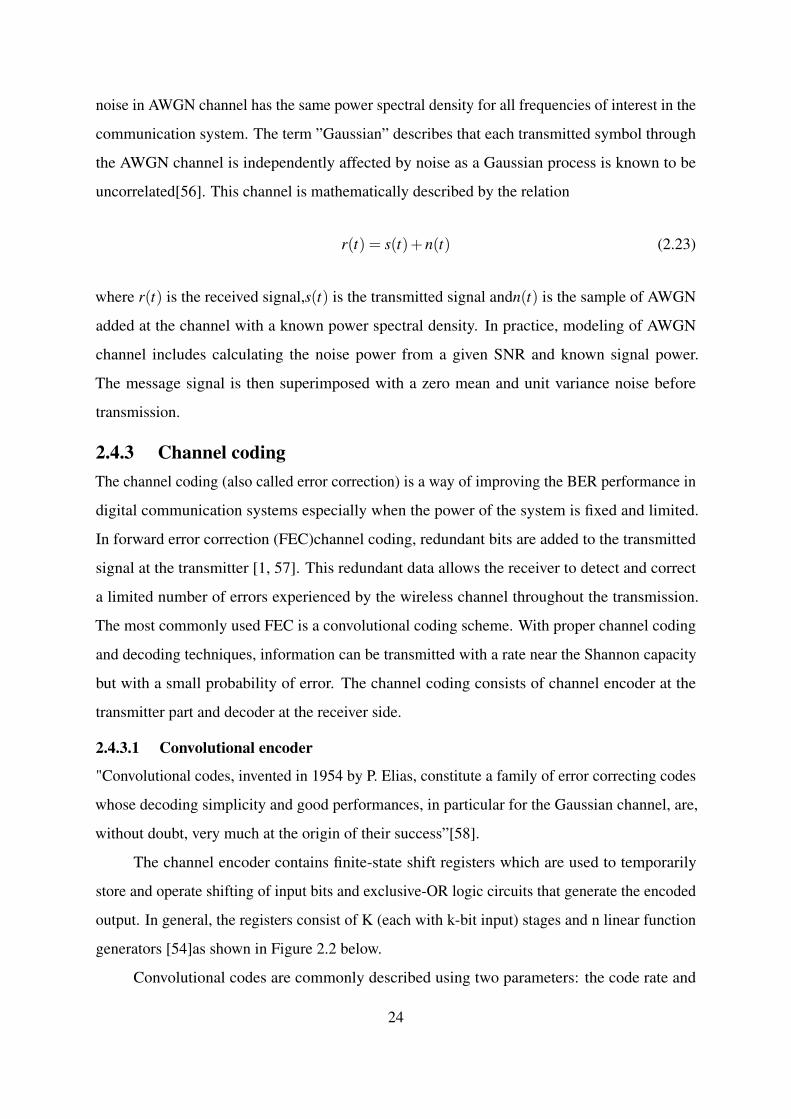
noise in AWGN channel has the same power spectral density for all frequencies of interest in the

communication system. The term ”Gaussian” describes that each transmitted symbol through

the AWGN channel is independently affected by noise as a Gaussian process is known to be

uncorrelated[56]. This channel is mathematically described by the relation

r(t) = s(t)+n(t) (2.23)

where r(t) is the received signal,s(t) is the transmitted signal andn(t) is the sample of AWGN

added at the channel with a known power spectral density. In practice, modeling of AWGN

channel includes calculating the noise power from a given SNR and known signal power.

The message signal is then superimposed with a zero mean and unit variance noise before

transmission.

2.4.3 Channel codingThe channel coding (also called error correction) is a way of improving the BER performance in

digital communication systems especially when the power of the system is fixed and limited.

In forward error correction (FEC)channel coding, redundant bits are added to the transmitted

signal at the transmitter [1, 57]. This redundant data allows the receiver to detect and correct

a limited number of errors experienced by the wireless channel throughout the transmission.

The most commonly used FEC is a convolutional coding scheme. With proper channel coding

and decoding techniques, information can be transmitted with a rate near the Shannon capacity

but with a small probability of error. The channel coding consists of channel encoder at the

transmitter part and decoder at the receiver side.

2.4.3.1 Convolutional encoder

"Convolutional codes, invented in 1954 by P. Elias, constitute a family of error correcting codes

whose decoding simplicity and good performances, in particular for the Gaussian channel, are,

without doubt, very much at the origin of their success”[58].

The channel encoder contains finite-state shift registers which are used to temporarily

store and operate shifting of input bits and exclusive-OR logic circuits that generate the encoded

output. In general, the registers consist of K (each with k-bit input) stages and n linear function

generators [54]as shown in Figure 2.2 below.

Convolutional codes are commonly described using two parameters: the code rate and

24

Figure 2.2: Convolutional Encoder[47]

the constraint length. The code rate,k/n, is expressed as a ratio of the number of bits into the

convolutional encoder (k) to the number of channel symbols output by the convolutional encoder

(n) in a given encoder cycle. Closely related to K is the parameter m, which indicates how many

encoders cycles an input bit is retained and used for encoding after it first appears at the input

to the convolutional encoder. The m parameter can be thought of as the memory length of the

encoder.

The most widely exploited channel codes in real communication systems for the purpose

of error correction are convolutional encoder. Convolutional encoder encodes the bit based on

the current k input bits and few past temporarily stored inputs. A convolutional channel encoder

is specified by three integers n, k, K or (k/n, K) elements. A channel encoder with input k bits

and output n bits is said to have a rate of k/n. The k/n ratio refers to the coding rate (Rc) of the

system and K is the constraint length of the encoder. The parameter K, which is the constraint

length, designates the” length” of the convolutional encoder. That means it signifies the number

of k-bit stages that are available to provide the combinational logic that results the output symbol.

The range of code rate is between 0 and 1.

The data rate can be increased by using a higher coding rate, but it reduces the BER. For

example, an encoder with three bits of output for every single bit input, i.e. for k=1 and n=3, is

expressed as a code rate of 1/3 as shown in Figure 2.3.

2.4.3.2 Viterbi decoding

The Viterbi decoding algorithm is commonly applied in decoding the convolutionally encoded

data at the receiver side. It uses maximum-likelihood decoding technique in order to recover

the transmitted bits by a trellis diagram. The decoded information is recovered with either a

25

Figure 2.3: K=3, k=1 and n=3 convolutional encoder[54]

hard decision or a soft decision. Hard and soft decisions decoding techniques depend on the

quantization type employed at the receiver.

• Hard decision decoding (HDD): -The received channel symbols are quantized to a single

bit of precision. In HDD each coded bit is demodulated as 0 or 1.i.e the demodulator

detects each coded bit(symbol) individually.HDD typically uses minimum decoding.

• Soft decision decoding (SDD): - uses multi-bit quantization (e.g. 3 bits/sample) on the

received sample values. At least a two bits precision quantization is carried out in this

type decoding. It performs better than a hard decision.In general the performance of SDD

is about 2 dB better than HDD.

2.4.4 Modulation typeModulation is a process of embedding the information message on to a carrier signal by

changing its carrier phase, frequency or amplitude or combination of these. The commonly used

modulation techniques are Phase Shift Keying (such as BPSK and QPSK) and M-ary Quadrature

Amplitude Modulation (such as 8QAM and 256QAM) [47]. Multilevel or multiphase modulation

(PAM, PSK, DPSK, or QAM) are bandwidth-efficient modulation schemes which allow us to

achieve an R/W>1.

The choice of modulation scheme mainly relies on the channel characteristics. If the

amplitude of the received signal is varied rapidly, QAM and PAM may be particularly vulnerable,

because a wideband automatic gain control (AGC) must be employed to reimburse for the

channel variations. In such a case, PSK or DPSK is more suitable, since the information is

conveyed by the signal phase and not by the signal amplitude[54]. However, in MQAM the

26

information bits are encoded in both the amplitude and phase of the transmitted signal. Thus,

whereas both MPAM and MPSK have one degree of freedom in which to encode the information

bits (amplitude or phase), MQAM has two degrees of freedom. As a result, MQAM is more

spectrally efficient than MPAM and MPSK, in that it can encode the greatest number of bits per

symbol for given average energy[47].

2.4.5 Bit error rate (BER) performance

In a wireless communication, the transmitted signal may be affected by noise, interference,

distortion and multipath fading resulting in undesirable errors at the receiver end. Bit error rate

is a crucial digital communication parameter which is employed to evaluate the performance of

data transmission. Numerically it can be defined as the total number of bits received in error by

the total number of bits that have been transmitted[59]. That is :

BER =Number o f bits received as errorTotal number o f transmitted bits

(2.24)

The bit error rate can be enhanced by increasing the transmit power, choosing a desired

modulation order and by channel encoding schemes[47] . The BER is the rate of error that

occurs during transmission of information bits. Assuming perfect coherent receiver detection

and square signal constellation with size of M, the probability of bit error for M-ary QAM

modulation scheme under AWGN channel is expressed as [47]:

BER = αQ(√

βSNR) (2.25)

WhereQ(z) is complementary error function,α andβ are constants expressed as

α = 4

√M−1√

M log2 M, β =

3log2 M(M−1)

(2.26)

SNR is taken as the average received signal-to-noise ratio. The Q function refers to the

probability that a Gaussian variable x with zero mean and unit variance is more than z. It

is given by [47]:

Q(z) = P(x > z) =∫

∞

z(

12π

)exp(−x12 )dx,x > 0 (2.27)

27

For rectangular MQAM and nonrectangular MQAM BER is defined by [47]

Pb ≈ 2(√

M−1)√M log2 M

Q(

√SNR

log2 M(M−1)

) (2.28)

Pb ≈4

log2 MQ(

√3SNR log2 M(M−1)) (2.29)

2.4.6 Capacity in AWGN channel

An additive white Gaussian noise channel mathematically defined as:y[i] = x[i]+n[i], wherex[i]

is input signal to the channel, n[i] is an AWGN random process and y[i] is the channel output

at discrete time i. For a fixed transmission technique, the spectral efficiency is the maximum

limit of information bits a wireless channel can support per second per unit bandwidth. For a

channel having bandwidth B, transmit power S, its SNR, the power in x(i) divided by the power

in y(i), is constant and given by SNR=S/NoB. The capacity of this channel is given by Shannon

formula[47]:

C = B log2(1+SNR) (2.30)

Shannon’s encoding illustrated that a data rate just about the capacity with small probability of

error can be attained by utilizing encoding.

2.5 Soft computing Techniques for Adaptive Modulation and

Coding SchemesIt is known that the wireless channel is complex and involve an indeterministic variation of the

metrological and atmospheric environment. Due to this uncertain propagation path condition,

it is difficult to adapt using the traditional hard computing techniques. The soft computing

methods, do not require mathematical models, unlike the conventional techniques. Because of

its ability to model systems with uncertainty and incompleteness, soft computing has a better

advantage over conventional adaptive and non-adaptive technique in modeling time-varying

wireless channel. Among several soft computing methods, fuzzy logic, neural network and

neuro-fuzzy systems are most commonly used. Detail review of Neuro-Fuzzy based system, and

related works of these techniques are presented in this section.

28

2.5.1 Fuzzy Logic System

Fuzzy set theory, which was initially invented by Lofti Zahed of the University of California

at Berkeley in 1965, is a powerful tool to deal with the imprecision characteristics in decision-

making problems involving uncertainty and vagueness of real-world applications[60]. This

invention was not well recognized until Dr. E. H. Mamdani[61] who is a professor at London

University, applied the fuzzy logic in a practical application to control an automatic steam engine

in, which is almost a decade after the fuzzy theory was invented.

The fuzzy logic idea is similar to the human’s feeling and inference process, unlike

classical control strategy. The classical control method is a point-to-point control, whereas fuzzy

logic control is a range-to-point or range-to-range control. The output of a fuzzy controller

is stemmed from fuzzifications of both inputs and outputs using the associated membership

functions. A crisp input will be converted to the different members of the associated membership

functions based on its value. From this point of view, the output of a fuzzy logic controller is

based on its memberships, which can be considered as a range of inputs.

The fuzzy logic inference system (FIS) performs arithmetic computation utilizing mem-

bership functions for modeling of fuzzy set linguistic variables. The fuzzy logic is useful for

imprecise, uncertain information and complex-ill based systems. It also incorporates human

experience based on if-then fuzzy rules in decision-making. It implements nonlinear systems

using linguistic variables in a straightforward when adequate knowledge about the system is

available.

2.5.1.1 Fuzzy inference system structure

Fuzzy inference systems are also known with other several names: It might be named as

fuzzy-rule-based systems (FRBS), fuzzy models, fuzzy associative memories (FAM), or fuzzy

controllers when used as controllers. The fundamental FIS architecture is shown in Figure 2.4

below[12]. Basically, it contains five components that are used to implement a fuzzy algorithm

and resolve all of the associated ambiguity. These are:

i)Fuzzification: - The objective of the fuzzification is, to pick membership function,

to convert the input from a crisp (real- value) into a set of fuzzy variables. The input is constantly

a crisp numerical value restricted to the universe of discourse of the input variable and output

is a fuzzy degree of membership in the qualifying linguistic set (always the interval 0 and 1).

29

It uses membership functions such as trapezoidal, bell or gaussian shapes for the conversion

process.

ii) Rule-Based Reasoning: - Fuzzy rule-based systems (FRBS) use linguistic

variables to justify via a sequence of logical rules that contain IF-THEN rules which create a

link between antecedent(s) and consequent(s), respectively. An antecedent is a fuzzy clause

with a certain degree of membership (between 0 and 1). Several antecedents might be connected

with AND or OR logical operators in FRBS, where all parts are considered simultaneously and

resolved into a single number. Consequents can also be embraced by numerous components,

which are then combined into a single output of a fuzzy set [62].

Manipulating a fuzzy rule-based system involves the derivation of the desired “If-Then”

fuzzy rules, dividing of universes, and addressing of the membership functions. Fuzzy rules can

be easily and directly formulated by experts in the form of linguistic rules.

iii) Fuzzy set database: - that defines the fuzzy set membership functions used in

fuzzy rules;

iv) Inference engine: - It is reasoning mechanism which performs the inference

procedure based on the rules to draw output or conclusion;

v) Defuzzification: - It is an interface which translates back the fuzzy sets to crisp

output using the center of gravity, mean of maximum or bisector area.

Figure 2.4: Structure of fuzzy logic system

2.5.1.2 Types of Fuzzy inference system

The most commonly used types of fuzzy system are three, namely[63]:

i) Mamdani fuzzy system: - the outputs of this model are fuzzy sets.

ii) Singleton fuzzy system: - the complexity of defuzzification of a linguistic variable may be

simplified by using singleton membership function to the output parameter.

iii) Takagi-Sugeno (TKS) fuzzy system: - the output of this TKS model is a linear function of

30

the input variables plus a constant term.

Their difference emanates from the specification of their consequent part (monotonically

non-decreasing or bell-shaped membership functions, or crisp function) and thus the defuzzi-

fication schemes (weighted average, the centroid of area, etc.) are distinct as well [12]. For

example, the most fundamental difference between Mamdani-type FIS and Sugeno-type FIS

is the way the crisp output is generated from the fuzzy inputs. While Mamdani-type FIS uses

the technique of defuzzification of a fuzzy output, Sugeno-type FIS uses a weighted average to

compute the crisp output. The expressive power and interpretability of Mamdani output are lost

in the Sugeno FIS since the consequents of the rules are not fuzzy [64]. But Sugeno has better

processing time since the weighted average replaces the time-consuming defuzzification process.

Due to the interpretable and intuitive nature of the rule base, Mamdani-type FIS is widely used

in particular for decision support application.

Other differences are that Mamdani FIS has output membership functions whereas Sugeno

FIS has no output membership functions. Mamdani FIS is less flexible in system design in

comparison to Sugeno FIS as the latter can be integrated with ANFIS tool to optimize the

outputs[64].

A comparison of Mamdani and S fuzzy inference type for air conditioning system is

done in [64]. Among these two types of Fuzzy inference systems, Mamdani method is popular

for capturing expert knowledge. It allows us to describe the expertise in a more intuitive,

more human-like manner. However, Mamdani-type FIS entails a substantial computational

burden. In contrast, the Sugeno method is more efficient computationally and works well

with optimization and adaptive techniques, which makes it very attractive in control problems,

particularly for dynamic non-linear systems. These adaptive techniques can be used to customize

the membership functions so that the fuzzy system best models the data.

2.5.1.3 Membership function (MF)

A membership function (MF) is a curve that defines how each point in the input space is mapped

to a membership value (or degree of membership) between 0 and 1. The membership function

can be also expressed as a graphical representation of the contribution of each input. The input

space is sometimes referred to as the universe of discourse. The rules use the input membership

values as weighting factors to determine their influence on the fuzzy output sets of the final

output conclusion. Once the functions are inferred, scaled, and combined, they are defuzzified

31

into a crisp output which drives the system[61].

For any set X, a membership function on X is any function from X to the real unit interval

[0, 1]. The membership function which represents a fuzzy set is usually denoted byµA. For

an element x of X, the value µA(x) is called the membership degree of x in the fuzzy set. The

membership degreeµA(x) quantifies the grade of membership of the element x to the fuzzy set.

The value 0 means that x is not a member of the fuzzy set; the value 1means that x is fully

a member of the fuzzy set. The values between 0 and 1 characterize fuzzy members, which

belong to the fuzzy set only partially. A fuzzy set is completely characterized by its membership

function (MF). Since most fuzzy sets in use have a universe of discourse X consisting of the real

line R, it would be impractical to list all the pair defining a membership function[61].

The simplest membership functions are formed using straight lines. Due to their simple

formulas and computational efficiency, both triangular MFs and trapezoidal MFs have been used

extensively, especially in real-time implementations. However, since the MFs are composed of

straight-line segments, they are not smooth at the corner points specified by the parameters. [4,

5].

The most common types of MF are:

i) Triangular MFs iv) Trapezoidal MFs

ii) Gaussian MFs v) Generalized Membership Function

iii) π-Shaped Membership Function vi) S-Shaped Membership Function

Since the development of a fuzzy logic concept, it has been used for modeling and making

decisions in various wireless communication systems. A wide range of solutions has been

developed concerning the problem of choosing the proper transmission parameters such as

coding rate and modulation scheme for OFDM wireless communication systems based on the

quality of the channel using fuzzy logic approach[65].

An adaptive coding and modulation scheme is proposed[66] using Fuzzy Rule Base

System, where product codes are utilized with Quadrature Amplitude Modulation (QAM). In

this research work, product codes and fuzzy rule base system (FRBS) has been utilized to

enhance attainable throughput in an OFDM system with a fixed target BER and fixed transmit

power for each subcarrier.

32

2.6 Neural Network Based AlgorithmsAn artificial neural network (ANN) is an intelligent system developed for the purpose of

information processing, which mimics the biological neural systems. The ANN is usually used

to process information, which is non-linear, complex and incomplete. It imitates the human brain

with neurons which are interconnected by weights. This kind of neural network, has enormous

skill for learning, optimization abilities and adapt themselves to respond to the continuously

varying environment by adjusting the weights between the layers[63].

Radial basis function neural network (RBFNN), Multi-layer perceptron (MLP) network

and neuro-fuzzy network are the most common architectures of neural networks. RBFNN is

a multilayer feedforward network that consists of three interconnected layers: an input layer,

hidden layer as well as output layer. In RBFNN, radial basis functions are used as activation

functions for each hidden layer of the neural network. The output of the RBFNN is the weighted

linear superposition of the radial basis functions.

RBFNN based adaptive modulation in OFDM systems has proposed in[67] to learn the

features of M-QAM before recovering the original signal under a noisy environment. Adaptive

resource allocation for OFDM systems using fuzzy and neural networks were proposed by[68].

The transmission parameters such as coding rate, power and modulation scheme are adapted

based on the time-varying channel conditions in order to maximize the data rate and reduce

BER.

2.6.1 Neuro-Fuzzy ApproachNeuro-fuzzy system is an artificial intelligence system that combines both fuzzy logic and neural

networks. It takes advantage of fuzzy logic systems (e.g. if-then rules and ease of incorporating

expert human knowledge available in linguistic forms) and neural networks (e.g. learning

capabilities, optimization abilities). Fuzzy logic require adequate prior human knowledge to be

initialized whereas neural network doesn’t require any prior knowledge to be initialized. It only

needs the fuzzy inference rules and parameter membership functions to be adjusted. As a result,

Neuro-Fuzzy is efficient compared to fuzzy logic and neural networks[69].

In a fuzzy based system, the fuzzy rules and membership functions are obtained by trial

and error; this makes the design of fuzzy systems a time-consuming task. The hybrid system

uses the backpropagation learning technique of neural networks to train and automatically update

33

membership functions. It improves the predictive capability of a system working in uncertain,

imprecise and noisy environments.

2.6.1.1 Adaptive Network based Fuzzy Inference System

A special neuro-fuzzy method termed Adaptive Network-based Fuzzy Inference System (ANFIS)

[12] is used as the model in our proposed algorithm. The ANFIS comprises the fuzzy logic

component as well as the neural networks. The fuzzy logic system considers the imprecision

and uncertainty of a system while neural networks takes the adaptability and learning capability

of the system.

2.6.1.2 Neuro-fuzzy (ANFIS) structure

The ANFIS structure illustrated in Figure 2.5 is based on type 3 fuzzy inference system. Takagi

and Sugeno’s (TKS) rule-based fuzzy if-then rules are used in type-3 FIS. For simplicity,

considering x and y as inputs and z as an output, the TKS rule is given by:

I f x is A and y is B then z = f (x,y) (2.31)

where A and B are fuzzy sets and f (x,y) is a crisp function. The function f (x,y) is a polynomial

of the input antecedent variables x and y. In this system, the output for each rule is obtained by

Figure 2.5: Type-3 ANFIS structure

adding a constant value to the linear combination of the input variables. The final result is then

obtained by computing the weighted average of each rule’s output.

34

Usually f(x, y) is assumed to be a first-degree polynomial then a linear Sugeno fuzzy

model is formed. For this case, with two rules it can be expressed as:

Rule1 = i f x is A1 and y is B1 then f1 = p1x+q1y+ r1 (2.32)

Rule2 = i f x is A2 and y is B2 then f2 = p2x+q2y+ r2 (2.33)

where x and y are input parameters, A1, A2, B1,andB2 are membership functions, f1 and f2 are

output linear functions, and p1, p2,q1,q2,r1,andr2 are the consequent parameter set determined

during training of the neuro-fuzzy system.

The ANFIS structure consists of five layers corresponding to various functions. Each layer

of the Type-3 ANFIS structure is presented as follows[12]:

Layer 1:- Every node in the first layer is an adaptive node with a function given as:

O1i = µ(Ai)(x) (2.34)

whereO1i is the output of the ith node in the first layer, x is input to the node i, Ai is the linguistic

variable associated with the bell-shaped node function and µAi is the grade membership function

of Ai and is given by:

O1i = µ(Ai)(x) =

1

1+(x−C j

a j)2b j

(2.35)

where ai , bi , ci is the premise parameters set that define membership functions.

Layer 2:- Each node in this layer is a fixed circle node labeled by π and determines the

firing strength of a rule by multiplying the incoming signals (membership functions). The firing

strength of each fuzzy rule for this layer is given by:

O2i = wi = µAi(x)µbi(x) (2.36)

Layer 3: - This layer is a fixed node used to compute the ratio of the ith rule’s firing

35

strength to the total of the firing strengths, which is normalized value and is given by:

O3i = wi =

wi

w1 +w2(2.37)

Layer 4: - Each node in this hidden layer is an adaptive node with a function given by:

O4i = wi f1 = wi(p1x+q1y+ r1), i = 1,2, ... (2.38)

where wi is the output of the layer 3 and pi , qi , ri is the consequent parameter set.

Layer 5: - This is the output layer with a circle node labeled by∑ and determines the

overall output by summing all the incoming signals, i.e.

O5i = ∑

iwi fi (2.39)

The output of the neuro-fuzzy system is expressed as:

O5i =

∑i µAi(x) fi

∑i µAi(x)(2.40)

2.6.1.3 Hybrid learning algorithm

Finding the best values of the equivalent fuzzy inference system parameters by applying a

learning algorithm is the key objective of the ANFIS. The parameter optimization is done in

such a way during the training session that the error between the target and the actual output

is minimized. A hybrid algorithm is used for optimization, which is the combination of least

square estimate and gradient descent method. The parameters to be optimized in ANFIS are the

premise parameters. These parameters define the shape of the membership functions. Thus, to

train the ANFIS, a hybrid learning technique is utilized [60].

During the forward pass, each node output goes forward until the last layer and the design

parameters are determined by the least square method. In the backward pass, the error signals

propagate to the backward to update the premise parameters/membership functions by gradient

descent technique. Thus, the least squares method and gradient descent technique are used to

optimize design parameters and update the membership functions respectively. The output in

36

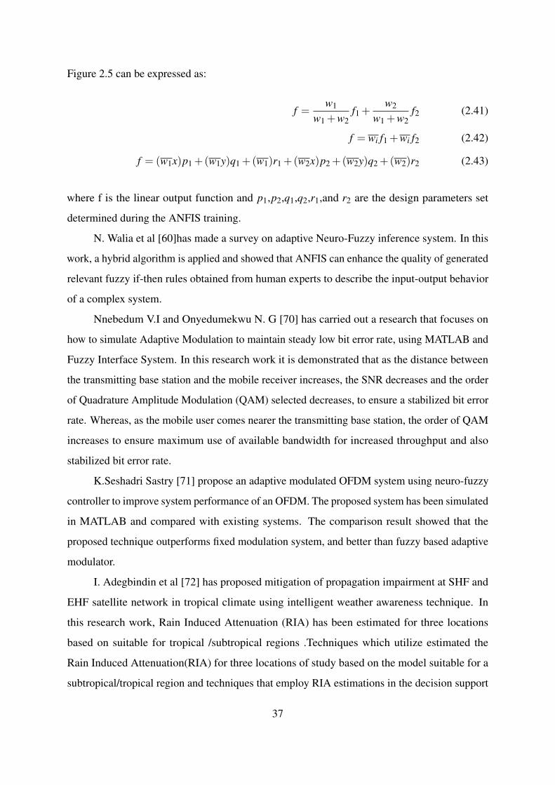
Figure 2.5 can be expressed as:

f =w1

w1 +w2f1 +

w2

w1 +w2f2 (2.41)

f = wi f1 +wi f2 (2.42)

f = (w1x)p1 +(w1y)q1 +(w1)r1 +(w2x)p2 +(w2y)q2 +(w2)r2 (2.43)

where f is the linear output function and p1,p2,q1,q2,r1,and r2 are the design parameters set

determined during the ANFIS training.

N. Walia et al [60]has made a survey on adaptive Neuro-Fuzzy inference system. In this

work, a hybrid algorithm is applied and showed that ANFIS can enhance the quality of generated

relevant fuzzy if-then rules obtained from human experts to describe the input-output behavior

of a complex system.

Nnebedum V.I and Onyedumekwu N. G [70] has carried out a research that focuses on

how to simulate Adaptive Modulation to maintain steady low bit error rate, using MATLAB and

Fuzzy Interface System. In this research work it is demonstrated that as the distance between

the transmitting base station and the mobile receiver increases, the SNR decreases and the order

of Quadrature Amplitude Modulation (QAM) selected decreases, to ensure a stabilized bit error

rate. Whereas, as the mobile user comes nearer the transmitting base station, the order of QAM

increases to ensure maximum use of available bandwidth for increased throughput and also

stabilized bit error rate.

K.Seshadri Sastry [71] propose an adaptive modulated OFDM system using neuro-fuzzy

controller to improve system performance of an OFDM. The proposed system has been simulated

in MATLAB and compared with existing systems. The comparison result showed that the

proposed technique outperforms fixed modulation system, and better than fuzzy based adaptive

modulator.

I. Adegbindin et al [72] has proposed mitigation of propagation impairment at SHF and

EHF satellite network in tropical climate using intelligent weather awareness technique. In

this research work, Rain Induced Attenuation (RIA) has been estimated for three locations

based on suitable for tropical /subtropical regions .Techniques which utilize estimated the

Rain Induced Attenuation(RIA) for three locations of study based on the model suitable for a

subtropical/tropical region and techniques that employ RIA estimations in the decision support

37

techniques bring noticeable improvements in the SNR on satellite communication channels work

on these regions. They were able to improve SNR by better tuning of parameters like transmit

power, modulation, propagation angle, frequency and transmission rate.

Atta Rahman et al [68] propose a real time adaptive resource allocation scheme for OFDM

system using GRBF-Neural Networks and Fuzzy Rule Base System. They designed a real time

system which take CSI and QoS as input, and give optimal Modulation Code Pairs (MCPs) and

power vectors for different subcarriers. Using a Fuzzy Rule Base System (FRBS), MCP by

giving CSI and QoS has been obtained. Employing Differential Evolution (DE) enable to get

the power vector. After training a Gaussian Radial Basis Function Neural Network (GRBF-NN)

is trained in offline mode using sufficient number of such examples, given QoS and CSI as input

GRBF-NN gives Optimum Power Vector (OPV) and FRBS gives optimum MCP immediately.

Comparison of various other schemes of same parameter with the proposed technique by the

simulations showed that the proposed scheme is supreme.

2.7 Research GapsAfter a wide-range review of the existing literature, the following gaps have been identified in

the area of adaptive coding and modulation for single frequency carrier wireless systems.

1. There is a limited research done on adaptive coding and modulation as applied to single

frequency carrier wireless system.

2. There is also a limited research done on mitigating propagation impairment in tropical

regions based on a rain data collected from the study site.There is no such work conducted

in equatorial and tropical African region including Ethiopia.

3. Mitigating rain induced attenuation using Neuro-Fuzzy based adaptive coding and modu-

lation has not been studied adequately.

38

CHAPTER 3

METHODOLOGY

3.1 IntroductionThis chapter discusses the rain attenuation and Neuro-Fuzzy based adaptive coding and modu-

lation (ACM) employed in this research work. A rainfall attenuation based on local rain data

is determined and used as input to mitigate the rain fade. An adaptive coding and modulation

scheme-based controller using Neuro-Fuzzy system to achieve desired BER performance and

channel data rate are investigated.

In order to mitigate fading over a time-varying channel, Neuro-Fuzzy controller is first

utilized to select the desired modulation type and coding rate to maximize data rate at the

receiver end while achieving the target BER. The transmitter then adapts its coding rate and

constellation size depending on the channel parameters to improve the performance of wireless

systems. Hence, section 3.2 present data processing; while section 3.3 covers implementation of

adaptive coding and modulation; finally, the design of Neuro-Fuzzy based adaptive coding and

modulation is described in section 3.4.

3.2 Rain Measurements and Data ProcessingThe cumulative distribution of rainfall rate (Rp) presents the rain intensity versus percentage of

the time (over one year) (p) the indicated rain rate is exceeded. ITU-R[33] requires calculation

R0.01 mm/h to predict the attenuation due to rain. R0.01 occurs at 0.01% of the time exceedance,

which can be read from the ITU-R map [33] or obtained from long-term local measurements.

The parameter relies on the integration time of the rainfall measuring devices used. According

to most researchers finding, the preferred integration time is one minute. If one-minute rainfall

data is not available which is a prevalent situation in most part of our country, converting from

higher integration times to one-minute integration time is therefore required.

39

According to the recommendation of ITU-R rain attenuation prediction procedures [5], the

most effective way of determining cumulative rainfall distribution is through direct measurement

made at the site of interest. Thus, in this research work, one years (october,2017- September

2018) of one- minute rainfall rate recorded with a device installed at Jimma University, Ethiopia

including rainy and non-rainy (zero value) days is utilized. Only the rain intensities with values

different from zero were sorted out and processed, and then the appropriate mathematical

formulation was used to calculate the desired parameters.

The procedure used to compute rain rate exceedance is listed as follows:

Step 1: - A rain data collected each minute having zero and non zero values are obtained.

Step 2: - Only a data having non zero values are taken and sorted out in ascending manner

Step 3: - Frequency of distribution is determined for a range of values with beam width of 1

Step 4: - Cumulative frequency distribution is determined using the result in step 3

Step 5: - Each cumulative distribution is multiplied by the rain rate time( which is one minute

in our case and this result will be divided for)the number of minutes in a year.

Step 6: - Finally using a plot of log axis of the result obtained in previous step versus the range

of values from step 2,rain rate exceeded for 0.01% is determined.

3.3 Determination of Rain AttenuationIn this thesis, the ITU-R rain attenuation model is used to determine the rain attenuation. ITU-R

P.530-17 [5] under section 2.4.1describes the method for the calculation of rain attenuation

over the terrestrial LOS radio systems using long-term rain statistics. The model is presented in

chapter two section 2.2.3 A of this thesis.

3.3.1 The ITU-R Rain Attenuation Model

The prediction procedure outlined in ITU-R attenuation model is considered to be valid in all

parts of the world at least for frequencies up to 100 GHz and path lengths up to 60 km. Thus,

based on the above steps the rain attenuation is calculated for frequencies 11,15,28,38,45,60,

and 72 GHz with a path length of 13.4 km.

Formulas to calculate specific attenuation is given by[40]

ϒR = KRα (3.1)

40

Where ϒR is specific attenuation, R is rain rate for 0.01% exceedance and K and α are coefficients

of vertical polarization.

The constant regression coefficient values for vertical polarization of indicated frequency

is presented in table below. The values are obtained from Recommendation ITU-R P.833-3[40].

Usually, 99.99%service availability in the worst month is the design objective of radio networks,

which implies the network outage should not exceed 432 minutes in a year .

Table 3.1: Coefficients for Kv and αv for indicated frequency of operationFrequency(GHz) Kv αv11 0.01731 1.161715 0.05008 1.044028 0.1964 0.927738 0.3844 0.855245 0.5375 0.812360 0.8515 0.748672 1.0561 0.7171

Terrestrial LOS radio link performance analysis is depending on the calculations of the

link budget. The link budget computation involves the calculation of received signal level, fade

margin and noise figure. Therefore, the expected received signal powerPr is computed using the

following formula.

Pr = Pt +Gtx +Grx−FSL−L (dB) (3.2)

where Pt is the transmitter power in output at the antenna input. This is the amount of microwave

carrier output power, usually expressed in dBm; L is losses due to the presence of atmospheric

gases, vegetation, buildings, clouds and fogs;Gtx = Transmit antenna gain, Grx= Receive antenna

gain, FSL = Free space path loss.

The performance of a radio link is determined by the percentage of the time the signal

will be below the threshold of the radio receiver relative to the total time period. Therefore, the

fade margin, which is the difference between the receiver nominal signal level and the receiver

threshold level, has to be calculated as follows:

FadeMarigin = RSL−RXT H(dB) (3.3)

41

where RSL is the received signal level and RT XH is the receiver threshold.

The performance of a communication system is estimated based on the achievable signal-

to-noise (SNR) at the receiver. The term SNR (in dB) refers to the estimation of signal strength

as a function of signal degradation and background noise. This power can be expressed as

SN

=CN

=(PtGtxGrx)

(KT BLsys)(

λ0

4πd)2 (3.4)

where Lsys is system loss at the receiver and transmitter;λ0= free-space wavelength (m); Gtx and

Grx are transmitting and receiving antenna gain respectively; K is the Boltzmann’s constant =

1.38x10−23 J/ K; B = bandwidth (Hz);and d is the link distance (m). T is the system effective

noise temperature (K) which is defined as:

T = TA +TR (3.5)

where: TA is antenna noise temperature (ambient noise) and TR is the receiver noise temperature

(internal noise), both are in the unit of Kelvin. It must be noted that TR is often expressed as the

receiver’s noise figure in dB. Note that the relationship between the carrier frequency (GHz) and

wavelength in meter is expressed as

λ0(m) =0.3

f (GHz)(3.6)

To express the above equation in decibel the equivalent expression is presented as:

SN

=CN

= Pt +Gtx +Grx−FSL(dB)−L(dB)−10log10 B(dBm.Hz)+174(dBm) (3.7)

SN

= Pr−10log10 B(Hz)+174 (dBm) (3.8)

WherePr is determined from the link profile given parameters.

In practical communications systems it is usually desired to have the received power

level greater than the threshold level required for the minimum acceptable quality of service

(usually expressed as the minimum carrier-to-noise ratio (CNR), or minimum SNR). This design

allowance for received power is referred to as the link margin, and can be expressed as the

difference between the design value of received power and the minimum threshold value of

42

receive power[69]:

Linkmargin(dB) = LM = Pr−Pr(min) (3.9)

where is all quantities are in dB.

Link margin should be a positive number; typical values may range from 3 to 20 dB.

Having a reasonable link margin provides a level of robustness to the system to account for

variables such as signal fading due to weather, movement of a mobile user, multipath propagation

problems, and other unpredictable factors that can degrade system performance and quality of

service. Link margin that is used to account for fading effects is sometimes referred to as fade

margin.The fade margin

Pr = RXT H +FadeMarigin (3.10)

In this case FadeMarigin = Link Margin, and RXT H = Pr(min)

Satellite links operating at frequencies above 10 GHz, for example, often require fade

margins of 20 dB or more to account for attenuation during heavy rain[73].The link budget tells

us that link margin improvement for a given communication system can be done by increasing

the received power (by increasing transmit power or antenna gains), or by reducing the minimum

threshold power (by improving the design of the receiver, changing the modulation method,

or by other means). Increasing link margin therefore usually involves an increase in cost and

complexity, so excessive increases in link margin are usually avoided.Thus, the SNR when there

is rain in a path between transmitter finally computed and used as input for adaptive coding and

modulation system.

3.3.2 SNR Calculation

The signal-to-noise ratio of the particular radio link whose radio link profile has been defined

in Table 3.2 is computed as follows.The computation is based on the values given in the link

profile and the result from rain attenuation determination using ITU-R model.

i) Clear Air SNR calculation:-The received signal is determined using equation 3.2.

Substituting the values from the link profile table,Table 3.2, we get a -68.9 dB received signal

level at the receiver end.Since the threshold received signal level is given and equal to -76.2dB,

43

the link margin can be calculated using equation (3.3).Hence, the link margin for this particular

microwave link is equals to 31.8 dBm or 8.1dB.

The SNR of this link at a clear sky environment can be determined using equation (3.8) as

:

SN

= Pr−B(dB.Hz)+174dBm (3.11)

wherePr =31.8dBm and B=21.7MHz .Thus, SNR is equal to 32.53dB.

ii) Rainy time SNR calculation:- Here the received signal is additionally degraded by the

total rain attenuation amount.Thus The,Pr will be -38.1dBm -57.625dBm which is -95.75dBm.

The Fade Marigin is similarly computed using equation(3.3) except at this link condition the

received signal is equals to -95.75dBm.Finally,the SNR for different fading depth( rain rate) is

computed.

Table 3.2: Link parameters for terrestrial line of sight networksParameters Link Jimma Link MujaAntenna height 10 10Antenna gain(dBi) 42 42Tx line unit loss( dB

100 ) 4.53 4.53Tx line loss 0.91 0.91Frequency(GHz) 11 11Circuit branching loss(dB) 6.8 6.8True azmuth 203.92 23.91Vertical angle 1.48 -1.59Link distance (km) 13.4Free space loss (dB) 139.6Rx threshold level (dBm) -76.2Effective frequency spacing (MHz) 21.7Atmospheric absorption loss (dB) 0.35Tx power (dBm) 30

3.4 Implementation of Adaptive Coding and ModulationAccording to the proposed block diagram shown below in Figure 3.1, the randomly generated

data source is encoded using a feed-forward convolutional encoder with different coding rates

and then the convolutionally encoded data is modulated by M-QAM. The encoded and modulated

symbols are transmitted.Finally, white Gaussian noise is added to the transmitted signal.

44

Figure 3.1: Neuro-Fuzzy based ACM block diagram

At the receiver side, after conversion of the analog signal back to a digital format, the

received data is demodulated using an adaptive MQAM demodulator. Following this, the

convolutionally encoded bits are decoded using Viterbi decoder so as to remove the redundant

bits added for the purpose of error correction.

Practically, the designed system is incapable of regenerating the transmitted message

signal as it is because of the noise superimposed on the wireless medium. It is obvious to have

some bits received in error. By changing the modulation order and coding rate BER is computed

for each SNR based on the system parameters shown in Table 3.2. The comparison of the

performance of BER for adaptive coding and modulation techniques is studied. Comparison of

Adaptive modulation with fixed coding and adaptive coding and modulation is also analyzed.

Table 3.3: System parameters and valuesSchemes Parameter values

Modulation order 4QAM,8QAM,16QAM,32QAM,64QAM,128QAM,256QAM,512QAM and 1024QAM

SNR 0 to 35 dBTarget BER 10−6 to 10−2 bits/sec/HzCoding-rate 1/4, 1/3, 1/2, 2/3, and 3/4spectral efficiency 0.5 to 7.5bits/sec/HzConstraint length 3Channel model AWGN

3.4.1 Neuro-Fuzzy Based Adaptive Coding and Modulation DesignNeuro-fuzzy system is a combination of neural network and fuzzy inference system (FIS),

having the combined benefits of both a fuzzy inference system (FIS) and neural network by

utilizing neural learning methods in adjusting the membership function parameters and the

45

structure of the FIS.

Usually, it has the advantage of allowing an easy transformation of the final system into

a set of if-then rules, and the fuzzy system can be seen as a neural network structure with

knowledge distributed throughout connection strengths. Using this hybrid soft computing

method, an initial fuzzy logic model with its input parameters is first obtained from the input-

output data of the designed adaptive coding and modulation system. A neural network is then

applied to update the initialized fuzzy rules and membership functions to create the final neuro-

fuzzy method. In this neuro-fuzzy approach, back propagation learning and the least squares

method is used to update membership functions and adjust design parameters respectively.The

general neuro-fuzzy approach system flowchart is shown in Figure 3.2 below.

Figure 3.2: Neuro-Fuzzy based system model flow chart

In the following section, each step which are incorporated into the proposed Neuro-Fuzzy

system model will be discussed briefly. Hence, section 3.3.1 presents the generation of I/O data

pairs; section 3.3.2 explain spectral efficiency or data rate optimization; section 3.3.3 shows

Neuro-Fuzzy architecture for ACM; finally, this chapter is completed by describing how the

designed ANFIS system is trained.

3.4.1.1 Generation of Input / Output data pairs

The proposed neuro-fuzzy system must be trained by a manually generated data from the graph

of simulated adaptive coding and modulation for single frequency carrier system.

Figure 3.3 shows how the desired coding rate and modulation order graph coordinate that

fulfill different target bit error rate values such as 10−6, 10−5, 10−4, 10−3,and 10−2demands.

46

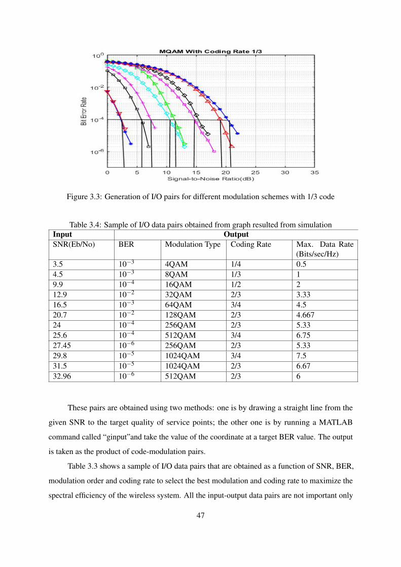
Figure 3.3: Generation of I/O pairs for different modulation schemes with 1/3 code

Table 3.4: Sample of I/O data pairs obtained from graph resulted from simulationInput OutputSNR(Eb/No) BER Modulation Type Coding Rate Max. Data Rate

(Bits/sec/Hz)3.5 10−3 4QAM 1/4 0.54.5 10−3 8QAM 1/3 19.9 10−4 16QAM 1/2 212.9 10−2 32QAM 2/3 3.3316.5 10−3 64QAM 3/4 4.520.7 10−2 128QAM 2/3 4.66724 10−4 256QAM 2/3 5.3325.6 10−4 512QAM 3/4 6.7527.45 10−6 256QAM 2/3 5.3329.8 10−5 1024QAM 3/4 7.531.5 10−5 1024QAM 2/3 6.6732.96 10−6 512QAM 2/3 6

These pairs are obtained using two methods: one is by drawing a straight line from the

given SNR to the target quality of service points; the other one is by running a MATLAB

command called “ginput”and take the value of the coordinate at a target BER value. The output

is taken as the product of code-modulation pairs.

Table 3.3 shows a sample of I/O data pairs that are obtained as a function of SNR, BER,

modulation order and coding rate to select the best modulation and coding rate to maximize the

spectral efficiency of the wireless system. All the input-output data pairs are not important only

47

those that maximize the throughput are taken based on the spectral efficiency optimization.

3.4.1.2 Spectral Efficiency Optimization

Assuming fixed transmit power, optimization of spectral efficiency (η) for adaptive coding and

modulation is given by:

maxη = RC log2(M) such that BER(ϒ )≤ BERT (3.12)

whereϒ is average SNR,RC is code rate,BERis average BER and M is modulation order. The

target of any communication designer is to have a communication link that operates at or below

the specified target BER.

In order to achieve the maximum throughput in the adaptive coding and modulation

scheme, the following consideration should take into account:

1. For the same BER and SNR pair, better throughput is selected.

2. For the same data rate, less modulation and coding rate is chosen that demand less SNR.

3. The lookup table scheme may not have a complete number of data pairs, then those missed

parts are completed by the expert knowledge.

3.4.2 ANFIS Architecture for Adaptive Coding and ModulationIn this thesis, a type of neuro-fuzzy method termed Adaptive Network-based Fuzzy Inference

System (ANFIS) is used for modeling. MATLAB Neuro-Fuzzy designer app has been used

to carry out and test the ANFIS system as a development tool. The tool consists of a fuzzy

logic designer, membership function editor, rule editor, neuro-fuzzy designer, rule and surface

viewers.

The fuzzy logic designer is a GUI tool that illustrates general information of a fuzzy

inference system. The membership function editor displays and edits all of the membership

functions associated with all of the input and output variables. The rule editor allows a designer

to build fuzzy rules automatically. The rule viewer gives a better description and interpretation

of all the FIS rules.

The neuro-fuzzy designer has several features. It is used to load FIS training, save the

trained FIS, open a new Sugeno-type system, generate the FIS, view the ANFIS structure or

any other GUIs to interpret the trained FIS model and test and validate the ANFIS model using

another data. It can also allow loading the test data for validation purpose, load the pre-defined

48

FIS designed by the Fuzzy Logic designer, plot the loaded train data, plot the train data against

the test data for comparison. The output surface viewer is a three-dimensional plot which

represents a mapping of input variables to the output variable.

3.4.2.1 ANFIS System for Training Process

Enhancement of data rate using ANFIS has been developed and examined as depicted in figure

3.2. The architecture of the ANFIS used to achieve the spectral efficiency has been developed

and investigated as shown in Figure 3.4. It consists of five layers corresponding to various

functions. The proposed model is trained with SNR, BER, coding rate and modulation order

as inputs and data rate as an output which is generated from simulations of the OFDM system

using parameters depicted in Table 311.

Both the fuzzy logic system principles and learning capabilities of neural networks are

being employed to construct ANFIS. At the initial stage, a basic fuzzy logic system controller is

built to utilize the linguistic fuzzy rules. Then, the IO data pairs are used to train the ANFIS

controller.

The steps involved in the ANFIS training process are:

Step1: - Loading the I/O training data;

Step2: - Generate an initial fuzzy inference system model;

Step3: - View the FIS model structure;

Step4: -Select the FIS model optimization method (hybrid method);

Step5: - Choose the training epochs and training error tolerances;

Step6: -Train ANFIS and view adjusted membership functions and output surface.

Finally, after the FIS training process are completed validation of the trained system must

be carried out. The trained FIS is validated using a testing or checking data that differs from

the one you used to train the FIS. In this research work validation is done using the data that is

generated using the MATLAB data extraction method. These test data is a BER value for each

integer value of SNR in the range 0to 35 dB and the associated modulation code pair and data

rate.

The range of fuzzy variables for the BER input values given by 10−6,10−5, 10−4, 10−3

and 10−2 should be spaced equally and quantifiable. To get this a logarithmic operation is

49

performed as given in the following equation:

BER = log10 10−p, p = 2,3,4,5,6 (3.13)

BER =−P

In this thesis, 225 first order Sugeno-type fuzzy inference rules have been constructed as follows

Figure 3.4: ANFIS structure with four inputs and one output

for the proposed neuro-fuzzy based ACM.This means, the multiplication of the number of

membership function of the four input parameters i.e 3*3*5*5=225 rules. The general rule:

i f x1 is Ai1 AND x2 is Ai2 AND x3 is Ai3 AND x4 isAi4 then (3.14)

f1 = pix1 +qiX2 + tix3 + six4 + r1i

The specific rules:

IF x1 is A11 AND x2 is A12 AND x3 is A13AND x4 is A14 T HEN (3.15)

f 1 = p1x1 +q1x2 + t1x3 + s1x4 + r1

IF x1 is A21 AND x2 is A22 AND x3 is A23 AND x4 is A24 T HEN (3.16)

f 1 = p2x1 +q2x2 + t2x3 + s2x4 + r1

50

where:

1. pi, qi, ti, si and ri are design parameters,

2. fi are the outputs within the fuzzy area specified by the fuzzy logic rules,

3. Ai j are the fuzzy sets/membership functions for each input variables, and

4. xi is the input parameters to the neuro-fuzzy system and i = 1,2,3, . . .

Layer 1 -Input node: - Each node in this layer is an input node, that corresponds to one

input parameter. These nodes pass the input signals to the layer 2. The proposed fuzzy sets have

three membership function for the input variables SNR and BER designated as low, medium

and high and five membership function for the input variable modulation order (MOD) and code

rate represented as very low, low, medium, high, and very high. The output of the neuron i in the

input node is obtained as:

O1i = f 1

i (net1i ) = net1

i (3.17)

where net1i is the ith input to the node of layer one.

Layer 2- Input membership layer: Each node in this layer acts a linguistic label of

one of the input variables in input node, i.e., specifies the membership functions for each input

parameters. The generalized bell-shaped membership function is used to represent each fuzzy

set variables. The output of neuron j in the layer 2 is given by:

O2j = f 2

j (net22) =

1

1+(x−C j

a j)2b j

(3.18)

where a j, b j and c j are parameters set that define shapes of jth membership function. The

parameter b j is usually positive and the parameter c j locates the center of the curve.

Layer 3-Rule layer: - All the nodes in this layer calculates the firing strength of a rule

via multiplication. Each node takes four inputs, to form 225 nodes in layer 3 and creates a fuzzy

rule for all input variables. The output of the neuron k is obtained as follows:

O3k = f 3

k (net3k ) = net3

k (3.19)

net3k = ∏

jw3

jky3j (3.20)

51

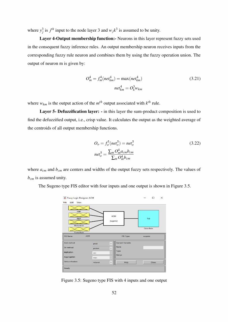
where y3j is jth input to the node layer 3 and w jk3 is assumed to be unity.

Layer 4-Output membership function:- Neurons in this layer represent fuzzy sets used

in the consequent fuzzy inference rules. An output membership neuron receives inputs from the

corresponding fuzzy rule neuron and combines them by using the fuzzy operation union. The

output of neuron m is given by:

O4m = f 4

m(net4km) = max(net4

km) (3.21)

net4km = O3

kwkm

where wkm is the output action of the mth output associated with kth rule.

Layer 5- Defuzzification layer: - in this layer the sum-product composition is used to

find the defuzzified output, i.e., crisp value. It calculates the output as the weighted average of

the centroids of all output membership functions.

Oo = f 5o (net5

o) = net5o (3.22)

net5o =

∑m O4macmbcm

∑m O4mbcm

where acm and bcm are centers and widths of the output fuzzy sets respectively. The values of

bcm is assumed unity.

The Sugeno type FIS editor with four inputs and one output is shown in Figure 3.5.

Figure 3.5: Sugeno type FIS with 4 inputs and one output

52

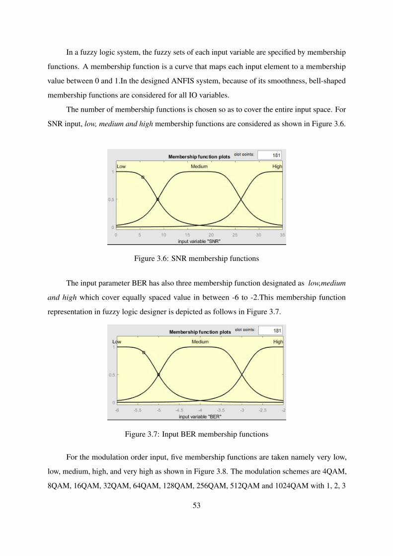
In a fuzzy logic system, the fuzzy sets of each input variable are specified by membership

functions. A membership function is a curve that maps each input element to a membership

value between 0 and 1.In the designed ANFIS system, because of its smoothness, bell-shaped

membership functions are considered for all IO variables.

The number of membership functions is chosen so as to cover the entire input space. For

SNR input, low, medium and high membership functions are considered as shown in Figure 3.6.

Figure 3.6: SNR membership functions

The input parameter BER has also three membership function designated as low,medium

and high which cover equally spaced value in between -6 to -2.This membership function

representation in fuzzy logic designer is depicted as follows in Figure 3.7.

Figure 3.7: Input BER membership functions

For the modulation order input, five membership functions are taken namely very low,

low, medium, high, and very high as shown in Figure 3.8. The modulation schemes are 4QAM,

8QAM, 16QAM, 32QAM, 64QAM, 128QAM, 256QAM, 512QAM and 1024QAM with 1, 2, 3

53

to 9 number of bits per each modulation scheme respectively.

Figure 3.8: Membership functions of input modulation

Figure 3.9 shows the membership functions of the input variable code rate with a range of

0.25 to 0.75. It contains five membership function like input variable modulation type designated

as very-low, medium, high and very-High membership functions. The output of the neuro-fuzzy

model has only one membership function i.e. data rate.

Figure 3.9: Membership functions of code rate

54

CHAPTER 4

RESULT AND DISCUSSION

This research work has been carried out using MATLAB 2018a simulation software. In this

simulation work,

• For a BER vs SNR performance simulation analysis of different modulation schemes and

coding rates, 10 million random bits are exploited.

• Perfect knowledge of the channel state information (CSI) at the receiver is assumed.

• At any point of distance, the power of the signal is assumed to be more than that of the

noise signal, i.e. the SNR is assumed greater than 0dB.

• The designed system under investigation is a single frequency carrier communication

system.

4.1 Rain Attenuation ResultsIn this section, results of the collected rain data analysis are presented. R0.01, specific attenuation,

total attenuation atR0.01 are analyzed for different frequency of operation above 10 GHz and for

a microwave link distance of 10km to 50 km.

Table 4.1: Specific rain attenuation and Total rain attenuation values at R0.01 and path distance13.4 km

Frequency(GHz) Specific Attenuation(ϒR) (dB) Total Rain Attenuation(A0.01)(dB)11 4.201 27.6515 6.97 46.1428 15.768 95.7138 21.91 129.1945 25.01 145.4960 29.32 165.5072 31.33 172.40

55

Figure 4.1: Rain rate versus percentage of time exceeded(R0.01)

Figure 4.1 depicts rain rate versus percentage of time exceeded. Based on computation

carried out using ITU-R rain induced attenuation model, the R0.01 is 113mm/hr.

Figure 4.2 illustrates the relationship between specific attenuation (ϒR) and frequency

of operation at aR0.01equals to113mm/hr. It is seen from the graph that as the frequency of

operation increase the specific attenuation also increases simultaneously. This implies that as we

increase the frequency of operation the impact of rain attenuation increases.

Figure 4.2: Frequency of operation versus specific attenuation(ϒR)

Figure 4.3 below describes the impact of over all rain induced attenuation at a frequency

of operation above 10 GHz. The trend that are presented in the graph demonstrates that rain

56

Figure 4.3: Rain Attenuation at a R0.01 versus frequency of operation above 10 GHz

attenuation increases sharply as the frequency of operation above 10 GHz tends to increase.

For instance, 27.55 dB ,45.14, 95.71 dB, 129.19 dB and 145.49 B rain induced attenuation is

experienced at a frequency of operation 11GHz, 15GHz, 28GHz,38GHz and 45GHz respectively.

In figure 4.4, the relationship between total attenuation and radio link distance between

transmitter and receiver is presented.The total rain attenuation sharply rises as te distance

between the transmitter and receiver increases.It is observed that, 27.55 dB,39.47dB, and 76.2dB

attenuation is encountered at a link distance of 10km,20km, and 30km respectively.

Figure 4.4: Link distance Vs Rain Attenuation at rain rate R0.01 and frequency of operation11GHz

57

4.1.1 Signal Level Analysis

From the computation procedure outlined in section 3.32, it is known that the clear sky(non-

fading channel condition) situation the received signal level at the receiver end using a transmit-

ting power of 30dBm is -38.1 dBmfor the link between Jimma and Muja. From the link profile

Table 4.2: Rain attenuation related resultsRain Rate(mm/hr) Attenuation(A0.01) Received signal(Pr) Fade Marigin S/N

1 0.576323852 -68.76632385 37.43367615 31.863676152 0.860605856 -69.05060586 37.14939414 31.579394143 1.145049792 -69.33504979 36.86495021 31.294950214 1.423380619 -69.61338062 36.58661938 31.016619385 1.696576566 -69.88657657 36.31342343 30.74342343

10 3.014356383 -71.20435638 34.99564362 29.4256436215 4.287171504 -72.4771715 33.7228285 28.152828520 5.535420522 -73.72542052 32.47457948 26.9045794825 6.767708859 -74.95770886 31.24229114 25.6722911430 7.988611848 -76.17861185 30.02138815 24.4513881535 9.200903025 -77.39090302 28.80909698 23.2390969840 10.40641245 -78.59641245 27.60358755 22.0335875545 11.60642176 -79.79642176 26.40357824 20.8335782450 12.80186904 -80.99186904 25.20813096 19.6381309655 13.99346486 -82.18346486 24.01653514 18.4465351460 15.18176223 -83.37176223 22.82823777 17.2582377765 16.36720128 -84.55720128 21.64279872 16.0727987270 17.55013878 -85.74013878 20.45986122 14.8898612275 18.7308685 -86.9208685 19.2791315 13.709131580 19.9096356 -88.0996356 18.1003644 12.530364485 21.08664703 -89.27664703 16.92335297 11.3533529790 22.26207928 -90.45207928 15.74792072 10.1779207295 23.43608423 -91.62608423 14.57391577 9.003915771

100 24.60879358 -92.79879358 13.40120642 7.83120642105 25.78032239 -93.97032239 12.22967761 6.659677614110 26.95077178 -95.14077178 11.05922822 5.489228216115 28.1202312 -96.3102312 9.889768803 4.319768803120 29.28878011 -97.47878011 8.721219891 3.151219891125 30.4564895 -98.6464895 7.553510495 1.983510495130 31.62342306 -99.81342306 6.38657694 0.81657694

given in Table 3.2 , it is observed that the receiver threshold signal level value is -76.2 dBm..

Therefore, by applying (3.3), the fade margin is equal to -38.1 dBm. This implies that, if the

fade depth is between 0 and -38.1 dBm, there is faded reception due to poor signal level. If the

58

fade depth is less than -38.1 dBm, it will results in network outage.

From Table 4.2 we can see that as the rain rate increases the total rain A0.01 attenuation is

increased and the received signal level and signal-to-noise ratio is decreasing.For instance, for

rain rate 5mm/hr,25mm/hr, 50mm/hr, 100mm/hr and130mm/hr the receiver detects a SNR value

of 30.74dB, 25.67dB,19.64dB, 7.83dB and 0.8165dB respectively.When the rain rate is above

130mm/hr,the resulting SNR at the receiving end reduced below 0dB.This implies that, total

network outage will happen when the rain rate is above 130mm/hr.

4.2 Simulation Result of ACM Performance

4.2.1 BER Performance ResultsIn this section, performance plots of BER vs SNR for different modulation schemes are studied

with various code rates under AWGN transmission medium. Each plot in these graphs represents

the BER performance of a specific modulation- code pair.

As has been seen from the graphs in figure 4.5 BER decline dramatically as the SNR tends

to increase. The lower modulation order and coding rates provide better performance with less

SNR. On the contrary, when the received SNR is high, a higher order modulation and higher

coding rate schemes gives a good performance. However, the plots of BER performance for

Figure 4.5: BER Vs SNR for different M-ary QAM with 1/4 code rate

modulation schemes 2QAM and 4QAM are overlapped. As it is clearly indicated, in ACM

technique design, a modulation scheme having a better spectral efficiency over the same SNR

59

range is selected. Thus, 2QAM is not used in the Neuro-Fuzzy based ACM fade mitigation

implementation.

Figure 4.6 demonstrate SNR vs BER graphs for different M-ary QAM with 1/3 coding

rate. In order to achieve a target QoS, higher SNR is required with 1/3 coding rate compared to

FEC of 1/4 coding rate. For instance, for 1024QAM modulation scheme to achieve a target QoS

10−6 it requires less than 20dB when its FEC is 1/4 and more than 20 dB when the FEC is 1/3.


As it can be seen from the result, for a target BER 10−5 and below, for the same values of

SNR utilizing 64QAM and 256QAM outperform 32QAM and 128QAM respectively in terms

of spectral efficiency.


60

The BER performance for various modulation schemes with 1/2 coding rate under AWGN

channel is shown in Figure 4.7. The BER curves indicate that by increasing the code rate

increases the required SNR to operate for a system.

The BER performance comparison for various M-ary QAM using rate 2/3 and 3/4 convo-

lutional codes is shown in Figure 4.8 and Figure 4.9 respectively. In general, each modulation

scheme with code rate 2/3 and 3/4, as the SNR increases the higher modulation order performs

better than the lower one for the same target BER.



The selection of the modulation order and coding rate depends on the quality of the

61

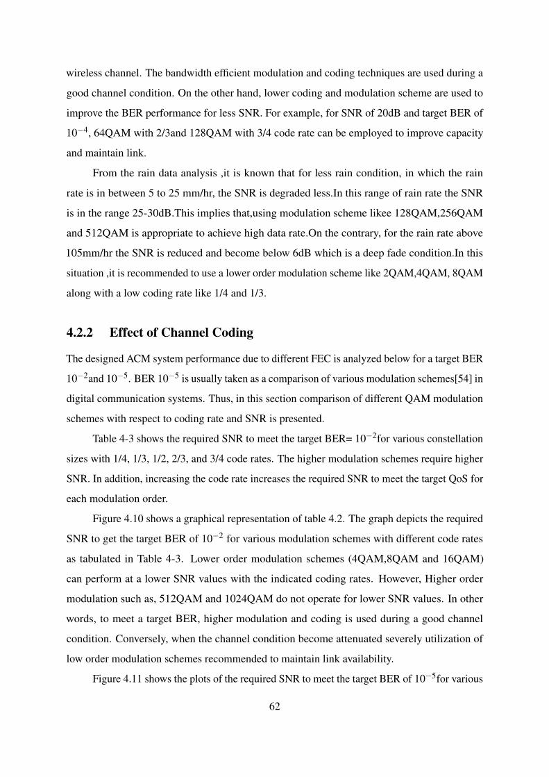
wireless channel. The bandwidth efficient modulation and coding techniques are used during a

good channel condition. On the other hand, lower coding and modulation scheme are used to

improve the BER performance for less SNR. For example, for SNR of 20dB and target BER of

10−4, 64QAM with 2/3and 128QAM with 3/4 code rate can be employed to improve capacity

and maintain link.

From the rain data analysis ,it is known that for less rain condition, in which the rain

rate is in between 5 to 25 mm/hr, the SNR is degraded less.In this range of rain rate the SNR

is in the range 25-30dB.This implies that,using modulation scheme likee 128QAM,256QAM

and 512QAM is appropriate to achieve high data rate.On the contrary, for the rain rate above

105mm/hr the SNR is reduced and become below 6dB which is a deep fade condition.In this

situation ,it is recommended to use a lower order modulation scheme like 2QAM,4QAM, 8QAM

along with a low coding rate like 1/4 and 1/3.

4.2.2 Effect of Channel Coding

The designed ACM system performance due to different FEC is analyzed below for a target BER

10−2and 10−5. BER 10−5 is usually taken as a comparison of various modulation schemes[54] in

digital communication systems. Thus, in this section comparison of different QAM modulation

schemes with respect to coding rate and SNR is presented.

Table 4-3 shows the required SNR to meet the target BER= 10−2for various constellation

sizes with 1/4, 1/3, 1/2, 2/3, and 3/4 code rates. The higher modulation schemes require higher

SNR. In addition, increasing the code rate increases the required SNR to meet the target QoS for

each modulation order.

Figure 4.10 shows a graphical representation of table 4.2. The graph depicts the required

SNR to get the target BER of 10−2 for various modulation schemes with different code rates

as tabulated in Table 4-3. Lower order modulation schemes (4QAM,8QAM and 16QAM)

can perform at a lower SNR values with the indicated coding rates. However, Higher order

modulation such as, 512QAM and 1024QAM do not operate for lower SNR values. In other

words, to meet a target BER, higher modulation and coding is used during a good channel

condition. Conversely, when the channel condition become attenuated severely utilization of

low order modulation schemes recommended to maintain link availability.

Figure 4.11 shows the plots of the required SNR to meet the target BER of 10−5for various

62

Table 4.3: Required SNR for a set of code rates for target BER=0.01Modulationscheme

1/4 1/3 1/2 2/3 3/4

2QAM 2.68 0 1.9 3.82 3.844QAM 2.68 0 1.9 3.83 3.858QAM 1.5 2.85 5.62 8.1 8.216QAM 3 4.25 6.8 9.4 8.1832QAM 4.95 6.6 10.2 12.9 13.164QAM 6.6 8.45 12 13.8 15.3128QAM 8.22 10.4 14.4 17.4 18.15256QAM 9.4 11.75 16.2 18.8 20.3512QAM 10.8 14.55 18.4 22 231024QAM 11.7 14.87 20.7 23.7 25.43

Figure 4.10: Code rate Vs SNR for different modulation schemes for target bit error rate of 10−2

modulation schemes with various code rates as tabulated in Table 4-4. Since BER =10−5 is

very much lower than BER=10−2 it is expected that the SNR required to achieve BER =10−5 is

higher than that of BER=10−5.This is seen from Figure 4.11.

Figure 4.12 and Figure 4.13 shows the bit error rate comparison of 16QAM and 256QAM

with different coding rates respectively. For the same modulation order, the BER performance

varies with coding rate. By reducing the code rate, less SNR is required to meet the desired

target BER.

For a low QoS less SNR is required compared to high QoS for the same code-modulation

pair. For example, for 16QAM with 1/2 code rate, 6.8dB,8.6dB,9.9dB,10.9dB and 11.9dB

63

Table 4.4: Required SNR for a set of code rates for target BER=0.00001Modulationscheme

1/4 1/3 1/2 2/3 3/4

2QAM 0 3.29 6 8.3 6.374QAM 0 3.3 6 8.3 6.378QAM 6.1 6.56 10.2 13.2 10.816QAM 7.25 8.4 10.9 15 10.832QAM 10.1 12.2 16.17 20.2 16.264QAM 11.93 12.39 16.9 18.8 18.47128QAM 14.45 16.49 21.1 25.36 21.4256QAM 13 16.5 22.2 26.2 24.17512QAM 17.76 20.3 24.5 31.5 26.61024QAM 17.2 21.75 26.6 31.5 29.98

Figure 4.11: Code rate Vs SNR for different modulation schemes for target bit error rate of 10−5

SNR is required to meet the bit error rate of 10−2, 10−3, 10−4, 10−5 and 10−6, as seen from

Figure 4.12.Whereas, from figure 4.13 we can seen that 16.2dB,18.9dB,20.65dB, and 22.2dB is

required to achieve a QoS 10−2, 10−3, 10−4, and 10−5 respectively.

As it can be seen in the figure 4.12 and 4.13, for a target bit error 10−3 and less the

performance of FEC 3/4 is better than FEC 2/3 in terms of achieving high spectral efficiency for

the same value of SNR. For instance, to achieve a target BER 10−5 a SNR less than 10.8 dB and

25dB is required for 16QAM and 256QAM with FEC 3/4respectively; whereas 15 dB and 26.6

dB required for 16QAM and 256QAM with FEC 2/3.

64

Figure 4.12: BER Vs SNR for 16QAM for different coding rate

Figure 4.13: BER Vs SNR for 256QAM for different coding rate

To achieve a low BER ,it is necessary to have a good reception at the receiving end which

results in high SNR.This can be satisfied when the channel condition is non-fading or clear

sky.For the link between Jimma and Muja the calculated SNR is 32.5dB.In this channel quality,

a high quality of service and a high data rate can be achived by employing a larger constellation

size modulation scheme i.e 256QAM,512QAM and 102QAM with a high coding rate like 2/3

and 3/4.Even if there is a degradation of received signal when there is a rain in between this link,

it can achieve a high data rate in a rain rate below 20mm/hr.

65

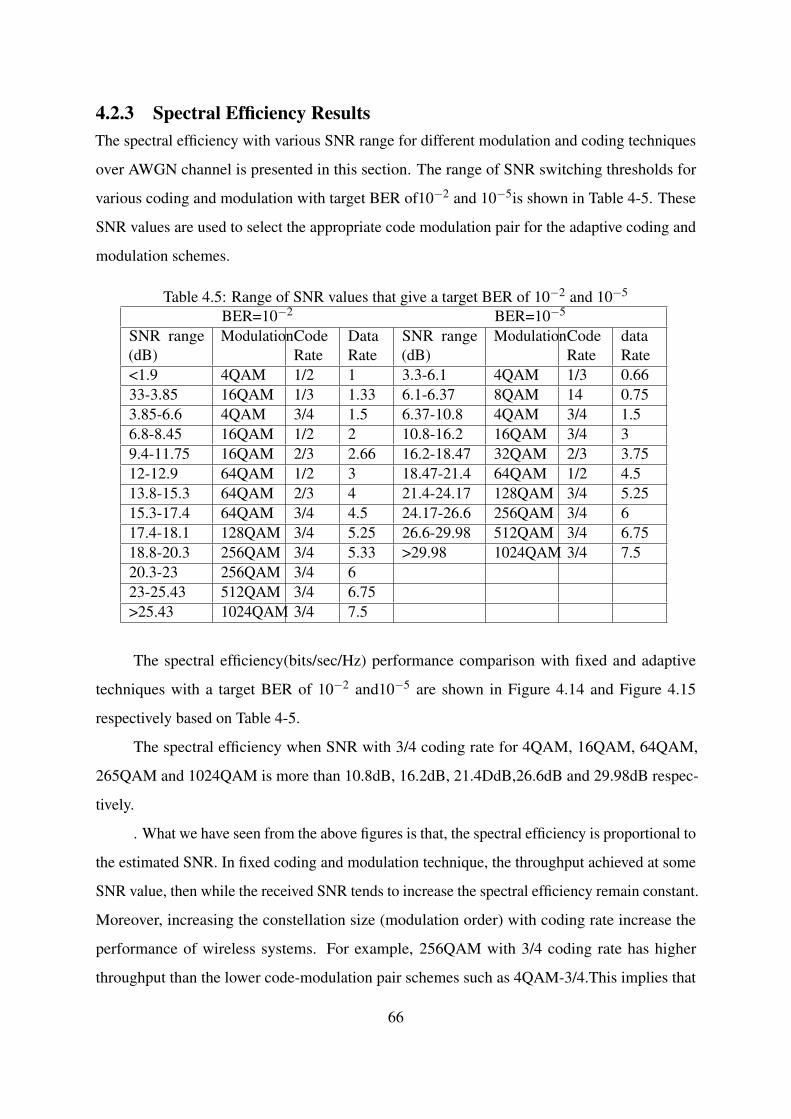
4.2.3 Spectral Efficiency ResultsThe spectral efficiency with various SNR range for different modulation and coding techniques

over AWGN channel is presented in this section. The range of SNR switching thresholds for

various coding and modulation with target BER of10−2 and 10−5is shown in Table 4-5. These

SNR values are used to select the appropriate code modulation pair for the adaptive coding and

modulation schemes.

Table 4.5: Range of SNR values that give a target BER of 10−2 and 10−5

BER=10−2 BER=10−5

SNR range(dB)

ModulationCodeRate

DataRate

SNR range(dB)

ModulationCodeRate

dataRate

<1.9 4QAM 1/2 1 3.3-6.1 4QAM 1/3 0.6633-3.85 16QAM 1/3 1.33 6.1-6.37 8QAM 14 0.753.85-6.6 4QAM 3/4 1.5 6.37-10.8 4QAM 3/4 1.56.8-8.45 16QAM 1/2 2 10.8-16.2 16QAM 3/4 39.4-11.75 16QAM 2/3 2.66 16.2-18.47 32QAM 2/3 3.7512-12.9 64QAM 1/2 3 18.47-21.4 64QAM 1/2 4.513.8-15.3 64QAM 2/3 4 21.4-24.17 128QAM 3/4 5.2515.3-17.4 64QAM 3/4 4.5 24.17-26.6 256QAM 3/4 617.4-18.1 128QAM 3/4 5.25 26.6-29.98 512QAM 3/4 6.7518.8-20.3 256QAM 3/4 5.33 >29.98 1024QAM 3/4 7.520.3-23 256QAM 3/4 623-25.43 512QAM 3/4 6.75>25.43 1024QAM 3/4 7.5

The spectral efficiency(bits/sec/Hz) performance comparison with fixed and adaptive

techniques with a target BER of 10−2 and10−5 are shown in Figure 4.14 and Figure 4.15

respectively based on Table 4-5.

The spectral efficiency when SNR with 3/4 coding rate for 4QAM, 16QAM, 64QAM,

265QAM and 1024QAM is more than 10.8dB, 16.2dB, 21.4DdB,26.6dB and 29.98dB respec-

tively.

. What we have seen from the above figures is that, the spectral efficiency is proportional to

the estimated SNR. In fixed coding and modulation technique, the throughput achieved at some

SNR value, then while the received SNR tends to increase the spectral efficiency remain constant.

Moreover, increasing the constellation size (modulation order) with coding rate increase the

performance of wireless systems. For example, 256QAM with 3/4 coding rate has higher

throughput than the lower code-modulation pair schemes such as 4QAM-3/4.This implies that

66

Figure 4.14: Spectral efficiency Vs SNR for BER of 10−2 for fixed and adaptive coding andmodulation schemes

Figure 4.15: Spectral efficiency Vs SNR for BER of 10−5 for fixed and adaptive coding andmodulation schemes

when the channel condition is good,the receiver receives higher SNR,it is better to use larger

constellation size of modulation scheme with higher coding rate.In contrast,while the channel

quality is bad,the receiver receive low SNR level, it is better to use more robust modulation

scheme having small constellation size with low coding rate.

In other word, 512QAM and 1024QAM with coding rate2/3 and 3/4 is used when the

67

rain rate is less( i.e 0-25 mm/hr) to achieve a high spectral efficiency and high QoS.By using a

medium constellation size modulation order,64QAM, 128QAM, and 256QAM, with coding rate

1/2 and 2/3 ,the link availability is sustained and achieve a moderate spectral efficiency in the

channel condition when the rain rate is in between 30-80mm/hr.However, while the rain rate is

increased above 80mm/hr the adaptive coding and modulation system is forced to use a lower

order modulation scheme (i.e 32QAM,16QAM,8QAM) so as to kept the wireless link alive by

reducing the data rate .Finally, when the channel condition become more worse , more priority

is given to sustaining the link availability than achieving high spectral efficiency.Thus for a rain

rate above 110mm/hr a more robust lower constellation size modulation type with a coding rate

1/4 is used.

4.2.4 Parameter Selection to Maximize Spectral EfficiencyIn this thesis, ACM of a single frequency carrier system is simulated under an AWGN channel.

For each given SNR a BER is computed. The given SNR are investigated for each modulation

order and coding rate. Hence, the spectral efficiency of an adaptive coding and modulation

scheme for the designed single frequency carrier systems is dependent on the BER, SNR, coding

rate and modulation order.

Table 4.6: Neuro-fuzzy parameters and their corresponding valuesInput Variables ACM parame-

tersValues

SNR 0-35dBModulationScheme

4QAM,8QAM,16QAM,32QAM,64QAM,128QAM,256QAM’512QAM,1024QAM

Coding Rate 1/4,1/3,1/2,2/3,and 3/4Output Variables Spectral Effi-

ciency0.5-7.5bits/sec/Gz

The parameters that are used as input and output in ANFIS training along with their

respective values are tabulated in table Table 4-6.

η = f (BER,SNR,m,RC) (4.1)

wherem = log2(M), M is the modulation/constellation size and RC is the FEC convolutional

coding rate.

68

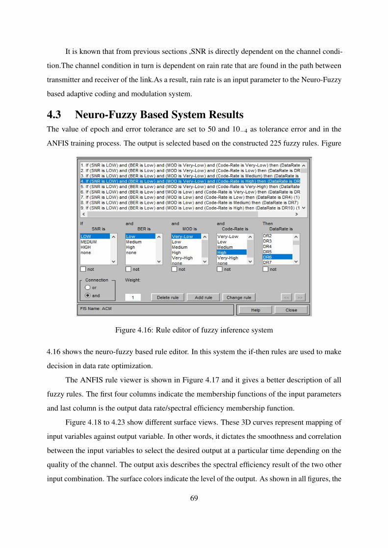
It is known that from previous sections ,SNR is directly dependent on the channel condi-

tion.The channel condition in turn is dependent on rain rate that are found in the path between

transmitter and receiver of the link.As a result, rain rate is an input parameter to the Neuro-Fuzzy

based adaptive coding and modulation system.

4.3 Neuro-Fuzzy Based System ResultsThe value of epoch and error tolerance are set to 50 and 10−4 as tolerance error and in the

ANFIS training process. The output is selected based on the constructed 225 fuzzy rules. Figure

Figure 4.16: Rule editor of fuzzy inference system

4.16 shows the neuro-fuzzy based rule editor. In this system the if-then rules are used to make

decision in data rate optimization.

The ANFIS rule viewer is shown in Figure 4.17 and it gives a better description of all

fuzzy rules. The first four columns indicate the membership functions of the input parameters

and last column is the output data rate/spectral efficiency membership function.

Figure 4.18 to 4.23 show different surface views. These 3D curves represent mapping of

input variables against output variable. In other words, it dictates the smoothness and correlation

between the input variables to select the desired output at a particular time depending on the

quality of the channel. The output axis describes the spectral efficiency result of the two other

input combination. The surface colors indicate the level of the output. As shown in all figures, the

69

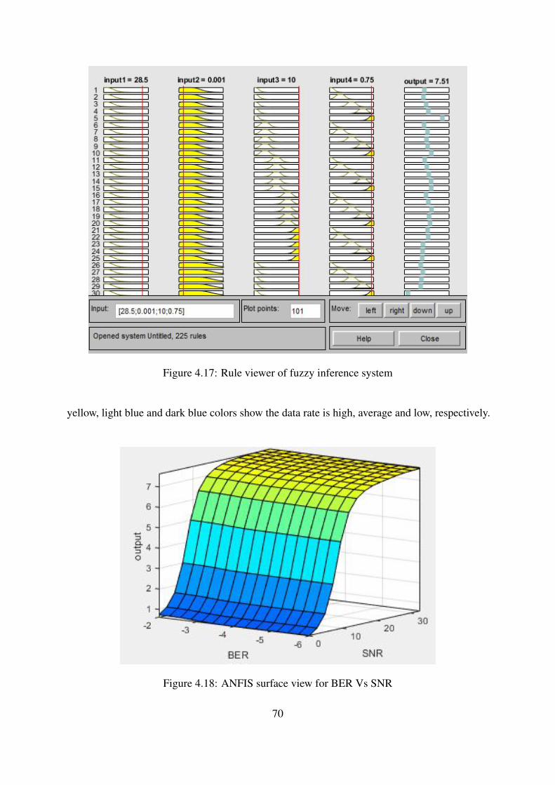
Figure 4.17: Rule viewer of fuzzy inference system

yellow, light blue and dark blue colors show the data rate is high, average and low, respectively.

Figure 4.18: ANFIS surface view for BER Vs SNR

70

The surface view of combined effect for both SNR, and BER is shown in Figure 4.18.This

surface view is displayed by the ANFIS surface viwer when the modulation order and the coding

rate are fixed as 10 and 0.75 respectively.As this two fixed parameters change the view changes

simultaneously. It indicates that by increasing the SNR the data rate is also increased. In addition

to this, for a poor QoS, the spectral efficiency is higher compared to a low target BER. For a

BER of 10-3 and SNR of 28.5dB, a data rate of 7.5 bits/sec/Hz can be achieved. It is seen from

figure 4.17, which is taken from the ANFIS rule viewer, it gives a data rate of 7.51 which is

almost equal to the theoretical value.

Figure 4.19: ANFIS surface view for BER Vs Code-Rate

Figure 4.19 is a surface view of BER versus coding rate while SNR =16.5 dB and

modulation order value of 10. It is seen that as the coding rate tends to increase, the data rate

also increased in proportional way. Data rate can also be improved by raising the modulation

order and coding rate as shown in Figure 4.20.

The two controlled input variables SNR and coding rate are fixed to a value of 16.5 dB

and 0.75 respectively while evaluating BER versus Modulation relationship. The stepsize like

graph in figure 22 implies that as the coding rate increases the achievable data rate also increases

simultaneously.The lower coding rate,coding rate 1/2 and 1/3, allows to achieve a lower data

rate as it can be seen from blue color.Where as a higher data rate can be achieved using high

coding rate( i.e. 2/3 and 3/4)as it is seen from yellow color.

71

Figure 4.20: ANFIS surface view for MOD Vs Code-Rate

Figure 4.21: ANFIS surface view for BER Vs MOD

Figure 4.22: ANFIS surface view for SNR Vs Code-Rate

72

In the SNR and Modulation ANFIS input relationship, the blue color tells that for high

SNR value( clear sky good channel condition) lower order modulation scheme is not selected.In

this type of channel condition , higher order modulation scheme like 256QAM, 512QAM, and

1024QAM are employed to attain higher data rate as it is indicated by yellow color region.On

the contrary ,when the channel quality is lower(rain time) a lower constellation size modulation

scheme( 4QAM,8QAM,16QAM) are used to sustain link availability by penalizing data rate.

Figure 4.23: ANFIS surface view for SNR Vs Modulation

4.3.1 Performance Comparison of the ANFIS to Various Schemes

The simulation results show that the proposed scheme perfoms better compared to the other

techniques in terms of spectral efficency or data rate for a target BER of 10-2 and fixed trasnmit

power. Thus, system performance is maximized by varying code rate and modulation scheme

such that the BER and total transmitted power remain under certain thresholds.Figure 4.22

showed that the graph grows smoothly in spectral efficiency as the SNR increases compared two

the other two.This implies that the the adaptation capability of Neuro-Fuzzy based ACM system

in response to varying channel condition is suprem.

Table 4.7: Data rate comparison of the proposed scheme to different existing models at atargetBER=10−2

Scheme SNR5dB 10dB 15dB 20dB 25dB 35dB

Neuro-Fuzzy based ACM 1.6 5.84 7.2 7.5 7.5 7.5Fuzzy based ACM 1.1 2 3.9 5.8 6.7 7.5

Switching thershold based ACM 1.5 2.66 5.25 6.9 7.5

73

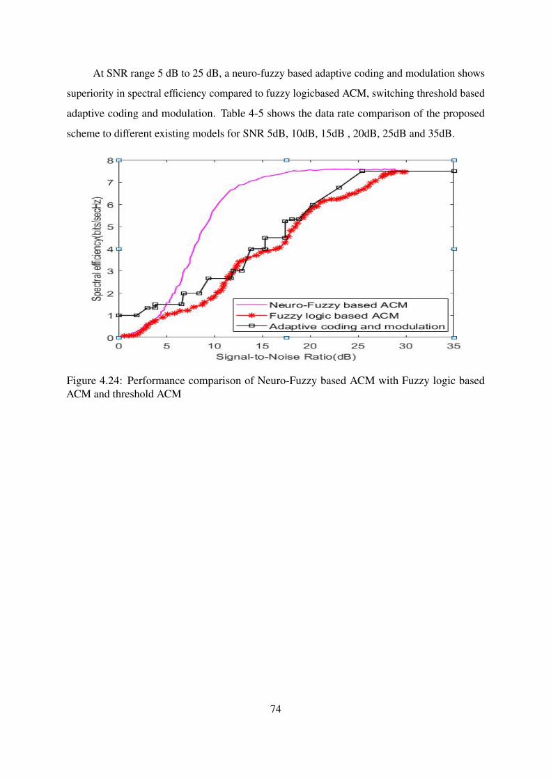
At SNR range 5 dB to 25 dB, a neuro-fuzzy based adaptive coding and modulation shows

superiority in spectral efficiency compared to fuzzy logicbased ACM, switching threshold based

adaptive coding and modulation. Table 4-5 shows the data rate comparison of the proposed

scheme to different existing models for SNR 5dB, 10dB, 15dB , 20dB, 25dB and 35dB.

Figure 4.24: Performance comparison of Neuro-Fuzzy based ACM with Fuzzy logic basedACM and threshold ACM

74

CHAPTER 5

CONCLUSION AND RECOMMENDATION

5.1 Conclusion

In this research, rain attenuation is computed using ITU-R rain attenuation model based on

locally measured rain data. Then, mitigation of this rain attenuation using Neuro-Fuzzy based

ACM system is performed. The performance of Neuro-Fussy based ACM systems in terms of

spectral efficiency and BER using various coding rates and modulation schemes under AWGN

channel was analyzed and compared to fixed and adaptive techniques. Based on the extensive

study and analysis carried out in this research work, the following conclusions are drawn:

• The SNR at the receiving end of the link between Jimma and Muja is 32.5 dB in the clear

sky(non-rain time)condition.On the other hand, for rain rate above 130mm/hr ,there will

be a total link outage.

• the rain rate and SNR at the receiving end is inversely related.Thus,enhancing the data

rate or sustaining the link availability of a wireless system using the received SNR level

means mitigating rain induced attenuation.

• The BER performance is improved by using FEC coding rate. However, selecting lower

code rate can reduce spectral efficiency.

• During good quality of channel (non- rain time), higher coding and modulation orders

such as 256 QAM,512 QAM, 1024 QAM with coding rate 23 and 3

4 , can be used to improve

data rate. Since the frequency spectrum is limited, ACM is applied to efficiently utilize

the available bandwidth.

• During bad channel conditionrainy time, the more robust modulation schemes like 4QAM,

8QAM and 16QAM (lower modulation order QAM) is better in sustaining link availability.

For instance,in rainy condition it is better to use a lower order modulation with a lower

75

coding rate. At a rain rate above 105mm/hr, the signal to noise ratio level is reduced to

around 6dB. This implies that using high order modulation scheme ,which demands high

SNR, such as 128QAM,256QAM,512QAM AND 1024QAM along with high code rate

like 2/3 and 3/4 result in link reliability reduction.

• ACM has shown better system performance in terms of spectral efficiency and achieving

a target BER compared to non-adaptive techniques.

• Comparison of fuzzy based ACM and ANFIS based ACM illustrates that the adaptability

performance of ANFIS-based adaptive coding and modulation system is more efficient.

It is shown that using soft computing techniques as a decision-making mechanism gives

a better result in adaptation of the channel condition compared to the traditional ACM

system.

• Base on simulation result analysis, Neuro-Fuzzy based adaptive coded modulation system

showed a smooth and high adaptation capability than the fuzzy based ACM and the

switching threshold ACM.

5.2 Recommendations and Future WorkThe designed scheme suits a single frequency carrier system in which the communication link

supports a one user down-link or up- link system. Since the study is based on a rain data

collected from Jimma University, Ethiopia, the result can be used as an input in microwave and

millimetric band radio link design in this area. Investigating multicarrier channel transmission

like OFDM using Neuro-Fuzzy based ACM is my future plan.In this future plan, studying of

more link sites are included to cover wide area.

76

REFERENCES

[1] R. L. Freeman, Radio System Design for Telecommunications, Third Edition ed. Hoboken,

New Jersey: John Wiley & Sons, Inc., 2006.

[2] F. D. Diba, "Radio Wave Propagation Modeling under Precipitation and Clear-air at

Microwave and Millimetric Bands over Wireless Links in the Horn of Africa," PhD,

Electronic Engineering, College of Agriculture, Engineering and Science, University of

KwaZulu-Natal, 2017.

[3] R. K. Crane, Propagation handbook for wireless communication system design. CRC press,

2003.

[4] R. M. Islam, Y. A. Abdulrahman, and T. A. Rahman, "An improved ITU-R rain attenuation

prediction model over terrestrial microwave links in tropical region," EURASIP Journal on

Wireless Communications and Networking, vol. 2012, no. 1, p. 189, 2012.

[5] ITU-R, "Propagation data and prediction methods required for the design of terrestrial line-

of –sight systems," in Reccomendations. ITU-R P.530-17, 2017.

[6] M. Maki, Keenanm,T.D.,Sasaki,Y.K.,Nakamura, "Characterstics of rain drop sizedistribu-

tion in tropical continental squall lines observed in Darwin,Australia.," Journal of Applied

Metrology, vol. 40, pp. 1393-1412, 2001.

[7] I. T. Union. Available: http://www.itu.Int’l

[8] A. D. Panagopoulos, P.-D. M. Arapoglou, and P. G. Cottis, "Satellite communications

at Ku, Ka, and V bands: Propagation impairments and mitigation techniques," IEEE

Communications Surveys & Tutorials, vol. 6, no. 3, 2004.

[9] P. Majithiya, A. Sisodia, V. Muralidhar, and V. Garg, "Novel down link rain fade mitigation

technique for Ka-band multibeam systems," International Journal of Satellite Communica-

tions and Networking, vol. 25, no. 1, pp. 45-51, 2007.

[10] A. J. Goldsmith and S.-G. Chua, "Adaptive coded modulation for fading channels," IEEE

Transactions on communications, vol. 46, no. 5, pp. 595-602, 1998.

77

[11] M. Rajesh, B. Shrisha, N. Rao, and H. Kumaraswamy, "An analysis of BER comparison

of various digital modulation schemes used for adaptive modulation," in 2016 IEEE

International Conference on Recent Trends in Electronics, Information & Communication

Technology (RTEICT), 2016, pp. 241-245: IEEE.

[12] J.-S. Jang, "ANFIS: adaptive-network-based fuzzy inference system," IEEE transactions

on systems, man, and cybernetics, vol. 23, no. 3, pp. 665-685, 1993.

[13] ITU-R, "Propagation Data and Prediction Methods Required for the Design of Earth-Space

Telecommunication Systems," Rec. ITU-R P.618-13, 2017.

[14] L. D. S. Mello, M. Pontes, R. De Souza, and N. P. Garcia, "Prediction of rain attenuation

in terrestrial links using full rainfall rate distribution," Electronics Letters, vol. 43, no. 25,

pp. 1442-1443, 2007.

[15] I. Abubakar, H. Y. Lam, and J. Din, "Implimentationof Adaptive Coding and Modulation

for satellite sommunication links in heavy rain regions:ad operator’s perspective " 2006.

[16] J. Friedman and R. Sofer, "Adaptive coding and modulation based on link performance

prediction," ed: Google Patents, 2010.

[17] J. Petranovich, "Mitigating the effect of weather on ka-band high-capacity satellites,"

ViaSat Inc., Carlsbad, CA, 2012.

[18] S. S. Das, S. Mondal, J. Saha, and K. Bandyopadhyay, "Comparison of rain fade mitigation

techniques using Crc and embedded pilot methods in ka-band satellite links," in Vehicular

Technology Conference (VTC Spring), 2011 IEEE 73rd, 2011, pp. 1-5: IEEE.

[19] Q. I. Atta-ur-Rahman and A. N. Malik, "A fuzzy rule base assisted adaptive coding

and modulation scheme for OFDM systems," J. Basic Appl. Sci. Res, vol. 2, no. 5, pp.

4843-4853, 2012.

[20] K. Nagar and K. Sharma, "Adaptive OFDM Implementation Using Fuzzy Inference

System," International Journal of Advanced Research in Computer Science and Software

Engineering (IJARCSSE), vol. 3, no. 7, pp. 309-314, 2013.

[21] K. Singh, "Fuzzy logic based modified adaptive modulation implementation for perfor-

mance enhancement in ofdm systems," International Journal of Intelligent Systems and

Applications, vol. 8, no. 5, p. 49, 2016.

[22] H. Sizun, Radio Wave Propagation for Telecommunication Applications. Paris Springer-

Verlag, 2003.

78

[23] R. K. Crane, Electromagnetic wave propagation through rain. Wiley New York, 1996.

[24] F. Moupfouma, "Electromagnetic waves attenuation due to rain: A prediction model

for terrestrial or LOS SHF and EHF radio communication links," Journal of Infrared,

Millimeter, and Terahertz Waves, vol. 30, no. 6, pp. 622-632, 2009.

[25] H. E. Green. (2004) Propagation Impairment on Ka-Band SATCOM Links in Tropical and

Equatorial Regions, IEEE Antennas and Propagation Magazine.

[26] J. S.Seybold, Introduction to RF propagation. Hoboken, New Jersey: John Wiley & Sons,

Inc., 2005.

[27] M. Singh and J. E. Allnutt, "Rain attenuation predictions at Ku-band in South East Asia

countries," Progress In Electromagnetics Research, vol. 76, pp. 65-74, 2007.

[28] J. S. Ojo, M. O. Ajewole, and S. K. Sarkar, "Rain rate and rain attenuation prediction for

satellite communication in Ku and Ka bands over Nigeria," Progress in Electromagnetics

Research, vol. 5, pp. 207-223, 2008.

[29] J. Ojo and P. Owolawi, "Development of one-minute rain-rate and rain-attenuation contour

maps for satellite propagation system planning in a subtropical country: South Africa,"

Advances in Space Research, vol. 54, no. 8, pp. 1487-1501, 2014.

[30] S. M. Sharif, "Microwave Signal Attenuation Due to Rainfall In Sudan," in The six African

workshop on Wireless Use of Information, 2007, vol. 6, pp. 1-6.

[31] F. D. Diba and T. J. Afullo, "Estimation of rain attenuation over microwave and millimeter

bands for terrestrial radio links in Ethiopia," in AFRICON, 2015, 2015, pp. 1-5: IEEE.

[32] G. Ajayi and E. Ofoche, "Some tropical rainfall rate characteristics at Ile-Ife for microwave

and millimeter wave applications," Journal of Climate and Applied Meteorology, vol. 23,

no. 4, pp. 562-567, 1984.

[33] ITU-R, "Characteristics of precipitation for propagation modelling," Rec. ITU-R P.837-7,

2017.

[34] ] B. Segal, "The influence of raingage integration time, on measured rainfall-intensity

distribution functions," Journal of atmospheric and Oceanic Technology, vol. 3, no. 4, pp.

662-671, 1986.

[35] M. Fashuyi, P. Owolawi, and T. Afullo, "Rainfall rate modelling for LoS radio systems

in South Africa," Trans. of South African Inst. of Elect. Engineers (SAIEE), vol. 97, pp.

74-81, 2006.

79

[36] F. Diba, T. Afullo, and A. Alonge, "Rainfall Rate and Attenuation Performance Analysis at

Microwave and Millimeter Bands for the Design of Terrestrial Line-of-Sight Radio Links

in Ethiopia," SAIEE Africa Research Journal, vol. 107, no. 3, pp. 177-186, 2016.

[37] R. Crane, "Prediction of attenuation by rain," IEEE Transactions on communications, vol.

28, no. 9, pp. 1717-1733, 1980.

[38] F. Moupfouma, "Improvement of a rain attenuation prediction method for terrestrial

microwave links," IEEE Transactions on Antennas and Propagation, vol. 32, no. 12, pp.

1368-1372, 1984.

[39] J. García-López and J. Peiro, "Simple rain-attenuation-prediction technique for terrestrial

radio links," Electronics Letters, vol. 19, no. 21, pp. 879-880, 1983.

[40] M. Odedina and T. Afullo, "Rain attenuation prediction along terrestrial paths in South

africa using existing attenuation models," in AFRICON 2007, 2007, pp. 1-7: IEEE.

[41] ITU-R, "Specific attenuation model for rain for use in prediction methods," Rec. ITU-R

P.838-3, 2005.

[42] ITU-R, "Conversion of annual statistics to worst-month statistics," Recommendation

ITU-R P.841-5, 2016.

[43] T. Patra and S. Sil, "Frequency diversity improvement factor for rain fade mitigation tech-

nique for 50–90 GHz in tropical region," in Industrial Automation and Electromechanical

Engineering Conference (IEMECON), 2017 8th Annual, 2017, pp. 86-90: IEEE.

[44] Briefing on Adaptive Coding and Modulation (ACM) [Online]. Available:

www.telesat.com/sites/default/files/telesat/files/whitepapers/ACM.pdf

[45] L. Castanet, A. Bolea-Alamañac, and M. Bousquet, "Interference and fade mitigation tech-

niques for Ka and Q/V band satellite communication systems," in Proc. 2nd International

Workshop of COST Action, 2003, vol. 280.

[46] A. J. Goldsmith and P. P. Varaiya, "Capacity of fading channels with channel side informa-

tion," IEEE transactions on information theory, vol. 43, no. 6, pp. 1986-1992, 1997.

[47] A. Goldsmith, Wireless communications. Cambridge university press, 2005.

[48] S. Vishwanath and A. Goldsmith, "Adaptive turbo-coded modulation for flat-fading chan-

nels," IEEE Transactions on Communications, vol. 51, no. 6, pp. 964-972, 2003.

[49] S. Cioni, R. De Gaudenzi, and R. Rinaldo, "Adaptive coding and modulation for the reverse

link of broadband satellite networks," in Global Telecommunications Conference, 2004.

80

GLOBECOM’04. IEEE, 2004, vol. 2, pp. 1101-1105: IEEE.

[50] S. H. Salih and M. M. Suliman, "Implementation of adaptive modulation and coding

technique using Matlab," International Journal of Scientific & Engineering Research, vol.

2, no. 5, pp. 137-139, 2011.

[51] E. Alberty et al., "Adaptive coding and modulation for the DVB-S2 standard interactive

applications: capacity assessment and key system issues," IEEE Wireless Commun., vol.

14, no. 4, pp. 61-69, 2007.

[52] G. Albertazzi et al., "Adaptive Coding and Modulation Techniques for Advanced Satellite

Mobile Systems," in EMPS/ASMS 2004 Conf, 2004.

[53] A. J. Goldsmith and C. S-G, "Variable-Rate Variable-Power MQAM for Fading Channels,"

IEEE Transaction on communications, vol. 45, no. 10, 1997.

[54] J. G. Proakis, Digital Communications, Third Edition ed. New York,NY: McGraw-Hill

Inc., 1995.

[55] N. T. Awon, M. Islam, M. Rahman, and A. Islam, "Effect of AWGN & Fading (Raleigh

& Rician) channels on BER performance of a WiMAX communication System," arXiv

preprint arXiv:1211.4294, 2012.

[56] B. Sklar and F. J. Harris, Digital communications: fundamentals and applications. Prentice-

hall Englewood Cliffs, NJ, 1988.

[57] W. C. Huffman and V. Pless, Fundamentals of error-correcting codes. Cambridge university

press, 2010.

[58] A. Glavieux, Channel coding in communication networks: from theory to turbocodes. John

Wiley & Sons, 2013.

[59] G. Sadeque, "Bit Error Rate (BER) Comparison of AWGN Channels for Different Type’s

Digital Modulation Using MATLAB Simulink," American Scientific Research Journal for

Engineering, Technology, and Sciences (ASRJETS), vol. 13, no. 1, pp. 61-71, 2015.

[60] N. Walia, H. Singh, and A. Sharma, "ANFIS: Adaptive neuro-fuzzy inference system-a

survey," International Journal of Computer Applications, vol. 123, no. 13, 2015.

[61] O. A. M. Ali, A. Y. Ali, and B. S. Sumait, "Comparison between the effects of different

types of membership functions on fuzzy logic controller performance," International

Journal, vol. 76, pp. 76-83, 2015.

[62] P. Angeletti and M. Lisi2, "A Systemic Approach to the Compensation of Rain Attenuation

81

in Ka-Band Communication Satellites," International Journal of Microwave Science and

Technology, vol. 2012, p. 7, 2012.

[63] B. Kosko, Neural networks and fuzzy systems: a dynamical systems approach to machine

intelligence (no. QA76. 76. E95 K86). 1992.

[64] A. Kaur and A. Kaur, "Comparison of mamdani-type and sugeno-type fuzzy inference sys-

tems for air conditioning system," International journal of soft computing and engineering,

vol. 2, no. 2, pp. 323-325, 2012.

[65] S. G. Temalow, "Neuro-Fuzzy Based Adaptive Coding and Modulation for Performance

Improvement in OFDM Wireless Systems," JKUAT, 2018.

[66] I. M. Qureshi and M. Z. Muzaffar, "Adaptive coding and modulation for OFDM systems

using product codes and fuzzy rule base system," International Journal of Computer

Applications, vol. 35, no. 4, 2011.

[67] P. Kaur, K. Singh, and H. Kaur, "Adaptive Modulation of OFDM by using Radial Basis

Function Neural Network," International Journal of Advanced Research in Computer and

Communication Engineering, vol. 3, no. 6, pp. 6886-6888, 2014.

[68] A. Rahman, I. Qureshi, A. Malik, and M. Naseem, "A Real Time Adaptive Resource

Allocation Scheme for OFDM Systems Using GRBF-Neural Networks and Fuzzy Rule

Base System," International Arab Journal of Information Technology (IAJIT), vol. 11, no.

6, 2014.

[69] K. S. Sastry and D. M. P. Babu, "Fuzzy logic based adaptive modulation using non data

aided SNR estimation for OFDM system," International Journal of Engineering Science

and Technology, vol. 2, no. 6, pp. 2384-2392, 2010.

[70] V. Nnebedum, "The Implementation of Adaptive Modulation Using Matlab and Fuzzy

Logic Interface System," Imperial Journal of Interdisciplinary Research, vol. 2, no. 12,

2016.

[71] K. S. Sastry and M. P. Babu, "Adaptive Modulation for OFDM system using Fuzzy logic

interface," in 2010 IEEE International Conference on Software Engineering and Service

Sciences, 2010, pp. 368-371: IEEE.

[72] I. Adegbindin, P. Owolawi, and M. Odhiambo, "Intelligent Weather Awareness Technique

for Mitigating Propagation Impairment at SHF and EHF Satellite Network System in a

Tropical Climate," SAIEE Africa Research Journal, vol. 107, no. 3, pp. 136-145, 2016.

82

[73] D. M. Pozar, Microwave engineering. John Wiley & Sons, 2009.

83

APPENDICES

MATLAB Programme Codes

Matlab code for adaptive coding and modulation for OFDM systems with 1/4, 1/3 and 1/2

coding rate

%%%%%%%%%%%%%%%%%%%%%%%%%%%%%%%%%%%%%%%%%%%%%%%%%%%%%

% This code is prepared by Eyob Mersha

% Department of Electronics and Communication Engineering

% School of Electrical Engineering and Computing

% Adama Science and Technology University

% June,2017

% Simulation code of adaptive coding and modulation for with coding rate 1/2 and modula-

tion order 4QAM, 8QAM, 16QAM, 32QAM, 64QAM, 128QAM, 256QAM, 512QAM, and

1024QAM.

%%%%%%%%%%%%%%%%%%%%%%%%%%%%%%%%%%%%%%%%%%%%%%%%%%%%

clc;

clear all;

close all;

for M =[2 4 8 16 32 64 128 256 512 1024] % Size of signal constellation;

k = log2(M); % Number of bits per symbol

numSamplesPerSymbol = k;

codeRate =1/2;

niter=1;

% Setting number of bits to process for each QAM scheme

switch(M)

case 2

numBits =1e7;

i

case 4

numBits =1e7;

case 8

numBits =0.999999e7;

case 16

numBits =1e7;

case 32

numBits =1e7;

case 64


case 128

numBits =0.999992e7 ;

case 256

numBits =1e7;

case 512


case 1024

numBits =1e67;

end % end of number of bit selection that are exact multiple of the modulation order code pair

%%%%%%%%%%%AWGN Channel%%%%%%%%%%%%%%%%%%%

EbNo = [0:35];

SNR =EbNo + 10*log10(k*codeRate)-10*log10(numSamplesPerSymbol);

% or SNR =EbNo + 10*log10(codeRate) noiseVar =10.(−SNR/10);

BER=zeros(1,length(SNR));

for snr=1:length(SNR)

totalber=0; % bit error rate initialization

for runs=1:niter

rng default % Use default random number generator

dataIn = randi([0 1], numBits, 1); % Generate vector of binary data

constlen=3; % length of constraint

codegen=[6 5 7]; % polynomial of the encoder

ii

tPoly = poly2trellis(constlen,codegen);

% polytrellis structure

dataEnc = convenc(dataIn, tPoly);

%%%%%%%%%%Modulate Data% %%%%%%%%%%%%%%%%%%%%%

%Apply QAM modulation

txSignal = qammod(dataEnc,M,’InputType’,’bit’,’UnitAveragePower’,true);

%% Pass the filtered signal through an AWGN channel

rxSignal = awgn(txSignal, snr, ’measured’);

% Receive and Demodulate the Signal

rxDataSoft = qamdemod(rxSignal,M,’OutputType’,’approxllr’,’UnitAveragePower’,true,’NoiseVariance’,noiseVar);

%%%%%%%Viterbi Decoding %%%%%%%%%

traceBack = 16; %Traceback length for decoding

dataout = vitdec(rxDataSoft,tPoly,traceBack,’cont’,’unquant’);

%%%%%%%%%%%%%BER Calculation%%%%%%%%%%%%%%%%%%%%

decDelay =traceBack; % Decoder delay, in bits

[numErrors, ber] = biterr(dataIn(1:end-decDelay),dataout(decDelay+1:end));

totalber=totalber+ber;

end % number of niter loop

% compute average BER

BER(snr) = totalber/(niter);

end % snr loop

% %%%%%% Plot graphs%%%%%%%%%

if M==2

semilogy(EbNo(1:end),BER(1:end),’-b*’,’lineWidth’,1.2, ’MarkerSize’,7);

elseif M==4

semilogy(EbNo(1:end),BER(1:end),’-rv’,’lineWidth’,1.2, ’MarkerSize’,7);

elseif M==8

semilogy(EbNo(1:end),BER(1:end),’-ks’,’lineWidth’,1.2, ’MarkerSize’,7);

elseif M==16

semilogy(EbNo(1:end),BER(1:end),’-m+’,’lineWidth’,1.2, ’MarkerSize’,7);

elseif M==32

iii

semilogy(EbNo(1:end),BER(1:end),’-cd’,’lineWidth’,1.2, ’MarkerSize’,7);

elseif M==64

semilogy(EbNo(1:end),BER(1:end),’-g>’,’lineWidth’,1.2, ’MarkerSize’,7);

elseif M==128

semilogy(EbNo(1:end),BER(1:end),’-ms’,’lineWidth’,1.2, ’MarkerSize’,7);

elseif M==256

semilogy(EbNo(1:end),BER(1:end),’-kd’,’lineWidth’,1.2, ’MarkerSize’,7);

elseif M ==512

semilogy(EbNo(1:end),BER(1:end),’-r<’,’lineWidth’,1.2, ’MarkerSize’,7);

else

semilogy(EbNo(1:end),BER(1:end),’-b*’,’lineWidth’,1.2, ’MarkerSize’,7);

end

axis([0 35 10−7 1 ])

legend(’2QAM’,’4QAM’,’8QAM’,’16QAM’,’32QAM’, . . .,

’64QAM’,’128QAM’,’256QAM’,’512QAM’,’1024QAM’);

grid on

hold on

xlabel(’Signal-to-Noise Ratio(dB)’)

ylabel(’Bit Error Rate’)

title(’MQAM With Coding Rate 1/2’)

MATLAB code for ploting particular modulation scheme with a particular coding rate.In

this case the code for 1024QAM along with coding rate 1/4 is presented.

clc;

clear all;

close all;

M =1024; % Size of signal constellation



codeRate = 1/4;

iv

niter=5; % number of times BER calculation is iterated

%%%%%%%%%%%%%%%%%%%%%%%%%%%%%%%%

EbNo1024 = [0:35];

SNR =EbNo1024 + 10*log10(k*codeRate)-10*log10(numSamplesPerSymbol);

noiseVar= 10.(−SNR/10);

BER1024=zeros(1,length(SNR));


totalber=0; % number of bits received in error initialization

for runs=1:niter

numBits =1e7; % Number of bits to process



constlen=3; % constraint length of the convolutional encoder

codegen=[6 5 7 4]; % polynomial generator

tPoly = poly2trellis(constlen,codegen);

%%%%%Encode the input data using the previously created trellis %%%%%%%%%%


%%%%%%%% Modulate Data%%%%%%%%%%%%% %

%%%%%% Apply QAM modulation.


%%%%%% AWGN CHANNEL %%%%%%%

%%%%%% Pass the modulated signal through an AWGN channel.


%%%%%% Receive and Demodulate Signal

rxDataSoft = qamdemod(rxSignal,M,’OutputType’,’approxllr’,’UnitAveragePower’,true,’NoiseVariance’,noiseVar);

%%%%%%%%% Viterbi Decoding %%%%%%%%%%%5%

traceBack = 16; %Traceback length for decoding


%%%%%%%%%%%%%%%%BER Calculation %%%%%%%%%%%%%%%%%%%

decDelay =traceBack; %Decoder delay, in bits

[numErrors,ber] = biterr(dataIn(1:end-decDelay),dataout(decDelay+1:end));

v

totalber = totalber+ber;


%%%%%%compute average BER

BER1024(snr)=totalber/(niter);

end % snr loop

%%%%%%%%%% Plot graphs %%%%%%%%%%%% semilogy(EbNo1024(1:end),BER1024(1:end),’-

b*’,’lineWidth’,1.2, ’MarkerSize’,7);

axis([0 35 10−7 1 ])

legend(’1024QAM’);

grid on



title(’SNR vs BER’)

format long

[EbNo1024,BER1024,BUT TON]=ginput(12) % code used to extract the value of BER for

each target BER value of 10−2,10−3,10−4,10−5and10−6

Matlab code for BER comparison for 256QAM with different coding rates and 1/2 coding

rate

% %%%%%%%%%%%%%%%%%%%%%%%%%%%%%%%

M = 256; % Size of signal constellation



niter=3;

colorvec1= [’b-’,’r-’,’k-’,’r-’,’g-’, ’k-’,’r-’,’b-’];

% Input the convolutional coding rate

coderate=input(’input the coding rate(1/4, 1/3, 1/2, 2/3,3/4)’);

if (coderate =1/4 && coderate = 1/3 &&

coderate =1/2 && coderate =2/3 &&

@coderate =3/4)

error(’Enter the correct coding rate’)

vi

end

%%%%%%%%%%%%%%AWGN Channel %%%%%%%%%%%%%%%%%%%%%

EbNo = [0:35]; % specify the range of signal-to-noise ratio in dB

SNR =EbNo + 10*log10(k*codeRate)-10*log10(numSamplesPerSymbol);

noiseVar = 10.(−SNR/10);

BER=zeros(1,length(SNR));


totalber =0;

for runs=1:niter

numBits =1e7; % Number of bits to process



% %%%%% Convolutionally encoding data%%%%%%%%%

if coderate ==1/4

constlen=3; % constraint length

codegen=[6 5 7 4]; % polynomial of the encoder

elseif coderate ==1/3

constlen=3;

codegen=[6 5 7];

elseif coderate == 1/2

constlen=3;

codegen=[6 7];


constlen=[3 3];

codegen=[7 6 7 ; 7 4 5 ];


constlen=[3 3 3];

codegen=[7 6 4 5;3 5 7 6;5 4 7 3];

else

constlen=3;

codegen=7;

vii

end

% % polynomial to trellis structure

tPoly = poly2trellis(constlen, codegen);

%%% Encode the input data using the previously created trellis%%%


% %% Modulate Data%%%%%%%

%%%%%Apply QAM modulation


%%%%%Pass the filtered signal through an AWGN channel % %%%%


% %%% Receive and Demodulate Signal%%%%%

rxDataSoft = qamdemod(rxSignal,M,’OutputType’,’approxllr’,’UnitAveragePower’,true,...

’NoiseVariance’,noiseVar);

%%%%%%% Viterbi Decoding

traceBack = 16; % Traceback length for decoding


%%%%%% BER Calculation%%%%%%%%%%%%%%%

%%% setting the tracback length

if coderate < 2/3

decDelay=traceBack;


decDelay = 2*traceBack; % Decoder delay, in bits

else

decDelay = 3*traceBack;

end

[numErrors, ber] = biterr(dataIn(1:end-decDelay),dataout(decDelay+1:end));

totalber = totalber+ber;


%%%%%%% compute average BER%%%%%%%% BER(snr)=totalber/(niter);

end % snr loop

%%%%%%%%%%%%% Plot graphs%%%%%%%%%%%%%%%%%%%%5

viii

semilogy(EbNo(1:end),BER(1:end),’-*’,’lineWidth’,1.2, ’MarkerSize’,7); axis([0 40 10−6 1])

legend(’1/4 code rate’,’1/3 code rate’, ’1/2 code rate’,’code rate 2/3’,’code rate 3/4’,’Uncoded

msg’);

grid on

hold on



title(’16QAM with different coding rate’)

MATLAb code for BER performance data extraction

clear all;

close all;

clc;

h=openfig(’S4QAM-13.fig’); % importing the BER performance plot for a particular Modula-

tion code pair

h=findobj(gca,’Type’,’line’);

x=get(h, ’Xdata’);

y=get(h, ’Ydata’);

A=[];

A(:,1)=x;

A(:,2)=y;

dlmwrite(’data.txt’,A,’,’);

ix

Adaptive Code Modulation for Rainfall Fade Mitigation in ...

Documents

Transcript of Adaptive Code Modulation for Rainfall Fade Mitigation in ...