Adaptive Asymmetric Slot Allocation for Heterogeneous ... · Adaptive Asymmetric Slot Allocation...

Adaptive Asymmetric Slot Allocation for Heterogeneous Traffic in WCDMA/TDD Systems

JinSoo Park

Dissertation submitted to the Faculty of the

Virginia Polytechnic Institute and State University

in partial fulfillment of the requirements for the degree of

Doctor of Philosophy in

Electrical Engineering

Committee:

Dr. Luiz DaSilva, Committee Chair

Dr. Annamalai Jr. Annamalai, Committee Chair

Dr. Milli, Lamine

Dr. Liang, Yao

Dr. Chen, Ing Ray

July 28, 2004 Alexandria, Virginia

Keywords : 3G/4G wireless system, MAC protocol, WCDMA, TDD, slot allocation, quality of service, Pareto distribution, Estimation of parameters

Copyright 2004, JinSoo Park

Abstract

Adaptive Asymmetric Slot Allocation for Heterogeneous Traffic in WCDMA/TDD Systems

JinSoo Park

Even if 3rd and 4th generation wireless systems aim to achieve multimedia services at high

speed, it is rather difficult to have full- fledged multimedia services due to insufficient

capacity of the systems. There are many technical challenges placed on us in order to

realize the real multimedia services. One of those challenges is how efficiently to allocate

resources to traffic as the wireless systems evolve. The review of the literature shows that

strategic manipulation of traffic can lead to an efficient use of resources in both wire- line

and wireless networks. This aspect brings our attention to the role of link layer protocols,

which is to orchestrate the transmission of packets in an efficient way using given

resources. Therefore, the Media Access Control (MAC) layer plays a very important role

in this context.

In this research, we investigate technical challenges involving resource control and

management in the design of MAC protocols based on the characteristics of traffic, and

provide some strategies to solve those challenges. The first and foremost matter in

wireless MAC protocol research is to choose the type of multiple access schemes. Each

scheme has advantages and disadvantages. We choose Wireless Code Division Multiple

Access/Time Division Duplexing (WCDMA/TDD) systems since they are known to be

efficient for bursty traffic. Most existing MAC protocols developed for WCDMA/TDD

systems are interested in the performance of a unidirectional link, in particular in the

uplink, assuming that the number of slots for each link is fixed a priori. That ignores the

dynamic aspect of TDD systems. We believe that adaptive dynamic slot allocation can

bring further benefits in terms of efficient resource management. Meanwhile, this

adaptive slot allocation issue has been dealt with from a completely different angle.

Related research works are focused on the adaptive slot allocation to minimize inter-cell

iii

interference under multi-cell environments. We believe that these two issues need to be

handled together in order to enhance the performance of MAC protocols, and thus

embark upon a study on the adaptive dynamic slot allocation for the MAC protocol.

This research starts from the examination of key factors that affect the adaptive allocation

strategy. Through the review of the literature, we conclude that traffic characterization

can be an essential component for this research to achieve efficient resource control and

management. So we identify appropriate traffic characteristics and metrics. The volume

and burstiness of traffic are chosen as the characteristics for our adaptive dynamic slot

allocation.

Based on this examination, we propose four major adaptive dynamic slot allocation

strategies: (i) a strategy based on the estimation of burstiness of traffic, (ii) a strategy

based on the estimation of volume and burstiness of traffic, (iii) a strategy based on the

parameter estimation of a distribution of traffic, and (iv) a strategy based on the

exploitation of physical layer information. The first method estimates the burstiness in

both links and assigns the number of slots for each link according to a ratio of these two

estimates. The second method estimates the burstiness and volume of traffic in both links

and assigns the number of slots for each link according to a ratio of weighted volumes in

each link, where the weights are driven by the estimated burstiness in each link. For the

estimation of burstiness, we propose a new burstiness measure that is based on a ratio

between peak and median volume of traffic. This burstiness measure requires the

determination of an observation window, with which the median and the peak are

measured. We propose a dynamic method for the selection of the observation window,

making use of statistical characteristics of traffic: Autocorrelation Function (ACF) and

Partial ACF (PACF). For the third method, we develop several estimators to estimate the

parameters of a traffic distribution and suggest two new slot allocation methods based on

the estimated parameters. The last method exploits physical layer information as another

way of allocating slot to enhance the performance of the system.

iv

The performance of our proposed strategies is evaluated in various scenarios. Major

simulations are categorized as: simulation on data traffic, simulation on combined voice

and data traffic, simulation on real trace data.

The performance of each strategy is evaluated in terms of throughput and packet drop

ratio . In addition, we consider the frequency of slot changes to assess the performance in

terms of control overhead.

We expect that this research work will add to the state of the knowledge in the field of

link- layer protocol research for WCDMA/TDD systems.

v

Acknowledgements

First of all, I would like to say that this dissertation is dedicated to my parents, especially

to my father who passed away 5 years ago.

First I would like to thank my two advisors, Dr.DaSilva and Dr.Annamalai for their

valuable knowledge, guidance, patience, and dedication during the entire course of this

research. Without their help, I could not have completed this dissertation today. I also

would like to thank Dr.Mili for his advice and valuable guidance on some related

technical points of this research, and Dr.Chen and Dr.Liang for their valuable inputs to

this research as committee members.

My appreciation also goes to KT people who supported me during my study period.

Without their helps, I would have not come to this far today.

There are some more people I should not forget. First, I would like to thank Latricia for

her hospitality and help during my stay in Alexandria, and Monica and her family for

their hospitality and care for my baby. Also I want to thank Vivek, Muhamad, and

Waltemar for their helps during the last year of my stay at Alexandria.

Finally, I really would like to thank my wife, HyoJin, who cheered me up and stayed with

me when I was in despair. Most of all, I will never forget the moment when our baby was

born. It was the happiest moment in my life ever. I owe her a lot. I also thank my baby

boy, Bryan SungJoon Park, for joining our family, choosing me as his father, and making

me stand up when I was down. Watching him play is the happiest moment of each and

every day of my life.

vi

Table of Contents

Chapter 1 Introduction............................................................................................... 1

1.1 Motivation of this research ................................................................................. 1

1.2 Methodology....................................................................................................... 1

1.3 Major contributions of this research ................................................................... 2

1.4 Organization of this document ............................................................................ 6

Chapter 2 Background and related work ................................................................. 8 2.1 Medium access and resources ............................................................................. 8

2.2 Slot allocation and inter-cell interference ......................................................... 11

2.3 Traffic characterization and measures .............................................................. 15

2.4 Traffic generation.............................................................................................. 16

2.5 Summary ........................................................................................................... 18

Chapter 3 Slot allocation for MAC protocol .......................................................... 20

3.1 Frame and slots in WCDMA/TDD system....................................................... 20

3.2 Fixed versus adaptive........................................................................................ 21

3.3 Adaptive schemes ............................................................................................. 24

3.3.1 Estimation of burstiness: Peak/Median vs. Peak/Mean ........................... 24

3.3.2 Dynamic window size determination based on ACF and PACF.............. 27

3.3.3 Slot allocation based on the estimation of burstiness (B strategy) ............ 34

3.3.4 Adaptive asymmetric slot allocation based on the use of burstiness and

volume information (BV strategy) ............................................................. 35

3.4 Summary ........................................................................................................... 37

Chapter 4 Performance evaluation based on the estimation of burstiness.......... 39

4.1 Methodology for performance evaluation......................................................... 40

4.1.1 On the use of synthetic and real world traffic ........................................... 40

4.1.2 Performance metrics ................................................................................. 41

4.1.3 Physical channel implementation.............................................................. 41

4.1.4 Simulation flow......................................................................................... 43

4.2 Generation of traffic .......................................................................................... 45

4.2.1 Synthetic data and voice traffic generation............................................... 45

4.2.2 Use of trace data........................................................................................ 48

vii

4.3 Simulation on synthetic data traffic .................................................................. 49

4.4 Simulation on combined voice and data traffic ................................................ 59

4.5 Simulation on real world trace data .................................................................. 64

4.6 Summary ........................................................................................................... 70

Chapter 5 Slot allocation based on parameter estimation.................................... 72

5.1 Background ....................................................................................................... 72

5.2 Generalized maximum likelihood estimator for Pareto distribution................. 73

5.3 Generalized moment estimator for Pareto distribution..................................... 77

5.4 Numerical experiment of the estimators ........................................................... 82

5.5 Slot allocation using the estimators .................................................................. 86

5.6 Summary ........................................................................................................... 97

Chapter 6 Cross-layer aware slot allocation......................................................... 100

6.1 Background ..................................................................................................... 100

6.2 Cross-layer aware slot allocation.................................................................... 101

6.3 Numerical experiment and discussion............................................................ 102

6.4 Summary ......................................................................................................... 104

Chapter 7 Conclusions and related areas of research ......................................... 105

Appendix A: ACF and PACF plots of different traffic types................................... 109 Appendix B: Derivation of estimators ......................................................................... 118 Glossary.......................................................................................................................... 121

Bibliography .................................................................................................................. 123

viii

List of Figures

Figure 2.1. Interference in a WCDMA/TDD system........................................................ 13

Figure 3.1 Structure of a WCDMA /TDD frame ............................................................... 21 Figure 3.2 Comparison of mean/median and peak/mean.................................................. 26

Figure 3.3 Sensitivity analysis of two metrics depending on the observation window size and shape parameterα .............................................................................................. 27

Figure 3.4 Sample PACF plot........................................................................................... 30

Figure 3.5 Burstiness comparison using the fixed and dynamic observation window sizes when the fixed window size is set to 5. The bar is drawn in dark blue and light blue for the peak and burstiness (peak/median) measures from the dynamic window system, and drawn in yellow and brown for the peak and burstiness (peak/median) from the fixed window system.................................................................................. 31



Figure 4.1. Simulation flow chart ..................................................................................... 44 Figure 4.2. Average number of generated packets from on-off traffic source depending on

increasing mean on time when the mean off time is fixed at 500msec; α = 1.6; transmission rate is 75000 bits/s; packet size is 1000 bytes. A total of 4000 frames are generated. The number of samples for each offon TT / ratio is 100. ..................... 47

Figure 4.3. Snapshot of trace data..................................................................................... 49 Figure 4.4 Uplink throughput (top) and packet drop ratio response (bottom) .................. 52

Figure 4.5 Downlink throughput (top) and packet drop ratio response (bottom)............. 53

Figure 4.6 Aggregate link throughput and packet drop ratio response............................. 54

Figure 4.7 Uplink response for 8.1=α when ud VV >> .................................................. 56

Figure 4.8 Downlink response for 8.1=α when ud VV >> ............................................. 57

Figure 4.9 Entire link response for 8.1=α when ud VV >> ............................................ 58

Figure 4.10. Uplink throughput (top) and packet drop ratio (bottom).............................. 61

Figure 4.11. Downlink throughput (top) and packet drop ratio (bottom) ......................... 62 Figure 4.12. Entire link throughput (top) and packet drop ratio (bottom) ........................ 63 Figure 4.13. Frequency of slot change ............................................................................. 64

Figure 4.14 Aggregate traffic in the uplink and downlink................................................ 66 Figure 4.15 Uplink throughput and packet drop response from using real trace data ...... 67

Figure 4.16 Downlink throughput and packet drop response from using real trace data . 68 Figure 4.17 Entire link throughput and packet drop response from using real trace data 69

ix

Figure 4.18 Frequency of slot change ............................................................................... 70

Figure 5.1 Probability density function )(yfY of Pareto distribution for different value of p on a log-linear scale when 5.1=α and 1=k ....................................................... 74

Figure 5.2 Logarithm of root mean-squared error (averaged over 200 independent estimates) of different Pareto shape estimators plotted as a function of sample size N when 5.1=α and 1=k . ............................................................................................. 84

Figure 5.3 Variance of various estimators based on 200 experiments for N=100 i.i.d. random variables plotted as a function of α in log-scale ........................................ 85

Figure 5.4 Logarithm of RMS of various estimators based on 200 experiments for N=100 i.i.d. random variables plotted as a function of α .................................................... 86

Figure 5.5 Uplink throughput and packet drop response of four different strategies. Burstiness-based methods yield higher throughput and fewer packet drops than the method BV................................................................................................................. 89

Figure 5.6 Downlink throughput and packet drop response of three different strategies. Burstiness-based methods yield higher throughput and fewer packet drops than the method BV................................................................................................................. 90

Figure 5.7 Aggregate link throughput and packet drop response of three different strategies. Both burstiness-based methods yield higher throughput and fewer packet drops than the method BV. ........................................................................................ 90

Figure 5.8 Comparison of slot change for three different strategies. The method SB and CS generate lower amount of signaling .................................................................... 91

Figure 5.9 Uplink throughput and packet drop response of three different strategies. Burstiness-based methods yield higher throughputs and fewer packet drops than the method BV................................................................................................................. 92

Figure 5.10 Downlink throughput and packet drop response of three different strategies. Burstiness-based methods yield higher throughputs and fewer packet drops than the method BV................................................................................................................. 93

Figure 5.11 Aggregate link throughput and packet drop response of three different strategies. Burstiness-based methods yield higher throughputs and fewer packet drops than the method BV. ........................................................................................ 93

Figure 5.12 Comparison of slot change for three different strategies. The methods SB and CS generate lower amount of signaling .................................................................... 94

Figure 5.13 Uplink throughput and packet drop response from using real trace data ...... 95 Figure 5.14 Downlink throughput and packet drop response from using real trace data . 96

Figure 5.15 Entire link throughput and packet drop response from using real trace data 96 Figure 5.16 Frequency o f slot change ............................................................................... 97 Figure 6.1 Throughput response of cross-layer aware and unaware slot allocation. 1500

measurements of packet drop ratios are averaged for each traffic arrival rate. ...... 103 Figure 6.2 Packet drop response of cross- layer aware and unaware slot allocation during

transmission, assuming that queue size is infinite. 1500 measurements of packet drop ratios are averaged for each traffic arrival rate. .............................................. 104

x

List of Tables

Table 4.1 Confidence intervals for each offon TT / ratio..................................................... 47

Table 4.2 Simulation parameters for each link and values ............................................... 50 Table 4.3 Simulation parameters ...................................................................................... 55

Table 4.4 Simulation parameters and values for voice and data traffic simulation.......... 59

Table 4.5 Simulation parameters ...................................................................................... 65 Table 6.1 Simulation parameters .................................................................................... 102

1

Chapter 1 Introduction

1.1 Motivation of this research This research addresses efficient resource allocation issues for Wireless Code Division

Multiple Access/Time Division Duplexing (WCDMA/TDD) Media Access Control

(MAC) protocols. Recently, WCDMA/TDD systems, less popular compared to

Frequency Division Duplexing (FDD) systems for a long period of time, began drawing

much attention for their attractiveness to multimedia traffic compared to FDD systems.

With regards to the transmission of multimedia traffic in the WCDMA/TDD system, one

of the technical challenges is how to efficiently allocate given resources (i.e., slots) for

each direction of link, uplink or downlink, in the MAC layer. Most existing research on

this issue has been directed to the unidirectional performance aspect of the system, and

there have been a variety of different types of schedulers developed so far to achieve this

goal. There are also several bi-directional approaches on this issue, but the related

literature is scarce and the objectives of those approaches have been focused on

overcoming interference-related problems under multi-cell environments.

As mentioned so far, researches for the allocation of resources in the MAC layer have not

been conducted comprehensively in the light of its importance. Thus, we embark upon a

comprehensive study of the bi-directional allocation of resources in the MAC layer to

achieve heterogeneous multimedia services in WCDMA/TDD systems.

1.2 Methodology

The resource allocation issue can be studied in many ways. In this research, we take a

broad view of this issue in three different ways.

2

Firstly, we can approach this issue from the networking research point of view, making

use of the characteristics of traffic. For example, we can use the representative

characteristics of traffic such as average rate and burstiness, which have been used in the

networking area for a long period of time. The average rate is a representative value of

traffic observed within a certain period of time. The burstiness signifies a degree of peak

value with respect to an average value measured in a certain period of time. These two

types of information can be used to allocate resources in the MAC layer under the

premise that appropriate measures for these two characteristics are available.

Secondly, we may estimate the parameters of a distribution of traffic and use those

parameters for the resource allocation. The reliable and robust estimation of the

parameters of a traffic distribution can lead to an efficie nt use of resources in various

ways.

Thirdly, we can take a bottom-up approach to the resource allocation issue from the

physical layer perspective, which employs physical layer information such as packet error

rate (PER).

In this research, all of these approaches are attempted as a comprehensive study of

resource allocation for WCDMA/TDD systems.

1.3 Major contributions of this research

As major achievements of this research, we first set up a comprehensive research

framework for the slot allocation compared to conventional approaches. The

conventional approaches are either biased for unidirectional performance of links or

focused on the mitigation of interference among neighboring cells. In this research, we

look at the resource allocation approaches both from the network layer and from the

physical layer point of view. To implement each of those methodologies outlined in

Subsection 1.2 for the resource allocation, we present various proposals as follows.

3

For the first methodology, this research introduces appropriate methods to measure the

characteristics of traffic and suggests two strategies based on the measurements: a

strategy based on the estimation of burstiness (method B) and a strategy based on the

estimation of bursitness and volume (method BV). For the measure of the burstiness, this

research presents an enhanced burstiness measure (peak/median). The performance of

this enhanced measure is compared with that of the conventional measure of peak/mean

through a simple demonstration. Also a dynamic observation windowing algorithm is

presented, through which these measures are evaluated. The method B allocates the

number of slots for each link based on the estimated burstiness for each link. The method

BV determines the number of slots based on the weighted traffic volume (called “virtual

weight”) for each link, where the weights are driven by the estimated burstiness for each

link. These strategies are evaluated using different types of traffic: data traffic, combined

data and voice traffic, and rea l trace data.

To implement the second methodology, we present four estimators for a distribution of

traffic: generalized maximum likelihood estimator (GMLE), first generalized moment

estimator (FGME), second generalized moment estimator (SGME), and third generalized

moment estimator (TGME). Modern traffic has been modeled by heavy-tailed

distributions such as a Pareto distribution. These estimators estimate the shape and

location parameters of Pareto distributions, in particular, the shape parameter. All of

these estimators are derived from a simple functional transformation of random

variable pXY /1= . The advantages of the generalization are discussed and demonstrated

through this research. The GMLE for the shape parameter GMLEα is derived to be

equivalent to the original Pareto distribution; that of the location parameter GMLEk is

determined by the minimum of the samples of a distribution. The FGME ( FGMEα

and FGMEk ) is derived from the thv fractional moment and GMLEk . The SGME ( SGMEα

and SGMEk ) is derived from the thv moment of the first order statistics and FGMEk is derived

from the thv fractional moment. The TGME ( TGMEα and TGMEk ) is derived from the

4

relationship of peak/median and from the thv moment of the thN order statistics,

including GMLEk . These estimators are evaluated in terms of root mean-squared error

(RMSE) and variance of the estimators against the different number of sample sizes and

the different values ofα . Our estimators are generalized for any α and for any moments,

integer or fractional. One of the estimators, showing the best performance, is chosen for

the purpose of resource allocation. One thing to note here is that we can indirectly predict

that the performance of slot allocation based on GMLE, FGME, and SGME can be better

than the one based on TGME because it turns out that the performance of GMLE, FGME,

and SGME are better than that of TGME. We propose two resource allocation methods

based on the estimators: constraint-based allocation (method CS) and second burstiness-

based allocation (method SB). The method CS computes a constraint value of a

cumulative distribution function (CDF), where the CDF satisfies a certain quality of

service (QoS) requirement. The method SB calculates burstiness based on the estimated

shape and the peak rate of a distribution. Similarly, these strategies are also evaluated in

the same way as the previous simulations.

The idea of the third methodology is to give more resources to a link under better channel

conditions so that the aggregate performance of the system improves from the entire link

point of view. This approach is dubbed as a channel-aware resource allocation method

(the method CHA). A simple demonstration is provided to test the algorithm in

comparison to an algorithm based on just traffic volume.

In summary, the goal of this research is to enhance resource management in

WCDMA/TDD systems through the adoption of adaptive slot allocation in support of

heterogeneous services.

Thus, in a way to achieve that goal, we make the following major contributions from this

research as:

§ Proposal of new adaptive slot allocation strategies for WCDMA/TDD MAC protocols

• Investigation of traffic characteristics

5

• Suggestion of adaptive scheme based on the estimation of both burstiness and

volume (BV method)

• Suggestion of adaptive scheme based on the estimation of burstiness only (B

method)

• Suggestion of adaptive scheme based on the second burstiness estimation of a

distribution of traffic (SB method)

• Suggestion of adaptive scheme based on the constraint of outage probability (CS

method)

• Suggestion of adaptive scheme based on the exploitation of physical layer

information (CHA method)

§ Suggestion of a new burstiness measure fo r BV and B methods, along with dynamic

window sizing method

• A new burstiness measure: peak/median

• Comparison of performance with peak/mean

• Dynamic observation window sizing method based on autocorrelation function

(ACF) and partial ACF (PACF)

§ Suggestion of parameter estimators for Pareto distributions for SB and CS methods

• Generalized maximum likelihood estimators (GMLE)

• Three generalized moment estimators ( first, second, third GMEs)

We perform the following tasks to achieve the goal of this research:

§ Performance evaluation for BV and B methods

• Simulation on synthetic data traffic

• Simulation on combined voice and data traffic

• Simulation on real trace data

• Implementation of a physical fading channel model (Rayleigh model)

• Investigation on signaling requirement for adaptive allocation methods

§ Performance evaluation for CS and SB methods


6

• Simulation on combined voice and data traffic

• Investigation on signaling requirement for adaptive allocation methods

§ Performance evaluation for CHA method


• Comparison with a conventional volume-based method

§ Framework for dynamic MAC

• Demonstration of potential performance enhancement based on dynamic slot

allocation

1.4 Organization of this document This dissertation is organized as follows. In Chapter 2, we review the literature that

addresses MAC protocols, slot allocation assignment techniques on CDMA as well as

Global System for Mobile Communications /Time Division Multiple Access

(GSM/TDMA) systems, traffic characterization and its measure, and traffic generation. In

Chapter 3, we discuss generic frame structure of a WCDMA/TDD system, compare fixed

and adaptive slot allocation in detail, and present our first two adaptive slot allocation

strategies (the methods BV and B). This chapter also includes discussion on the new

burstiness measure and the dynamic observation window size method for the new

burstiness measure. Chapter 4 presents experimental results for BV and B strategies. It

begins with discussion on the methodology of our experiment, and then discusses

simulation results. Three different approaches (volume-based, burstiness-based, and

burstiness-volume-based methods) are compared in terms of our chosen performance

metrics. The results are illustrated, along with confidence intervals and comments.

Chapter 5 introduces our four estimators for Pareto distributions and presents two new

slot allocation methods (the methods SB and CS) based on the estimators. The

performance of these strategies is evaluated in comparison to the methods BV and B. In

Chapter 6, we discuss our last slot allocation strategy (the method CHA) exploiting

physical layer information, along with performance evaluation against a conventional

7

volume-based method. Finally, Chapter 7 summarizes this dissertation with discussion on

the related areas of this research.

8

Chapter 2 Background and related work

In Chapter 2, we review the literature that serves as background for this research. The

review of the literature proceeds according to a conceptual flow mapped to achieving the

goal of this research - adaptive resource allocation for WCDMA/TDD Medium Access

Control (MAC) protocols. We first describe key resource management considerations for

WCDMA/TDD MAC protocols, namely the allocation of slots. Then we discuss factors

for the resource allocation decision, including investigation of existing methods that

address this issue. Traffic characteristics are important primary factors for this decision,

and therefore we review some major techniques used for the characterization of traffic

and choose appropriate techniques for this research. Finally, we need to understand how

to synthesize traffic for the simulation that is part of this research, so we review well-

known synthesizing techniques.

Following the outlined conceptual flow, this chapter is organized as follows. Section 2.1

addresses the definition of resources available for MAC protocols depending on multiple

access schemes, in particular WCDMA/TDD systems. Section 2.2 discusses existing

adaptive methods for the allocation of these resources, along with the interference issues

related to these adaptive methods. This section also includes discussions of some

adaptive methods designed for Global Systems for Mobile communicatio n (GSM) and

Time Division Multiple Access (TDMA) systems. Section 2.3 discusses primary traffic

characteristics, particularly focusing on traffic volume and burstiness. In Section 2.4, we

describe methods used to generate synthetic voice and data traffic for our experiments.

Finally, we summarize the main points discussed in this chapter in Section 2.5.

2.1 Medium access and resources

9

In the context of cellular wireless networks, MAC is a procedure that is invoked to

arrange packet transmission among all users through a shared medium in the uplink and

the downlink [ABRAMSON94].

MAC protocols are classified according to their resource sharing methods, as well as their

multiple access schemes, which include FDMA, TDMA, and CDMA [AKYILIDIZ99].

The resource sharing methods include dedicated assignment, random access, and

demand-based assignment. Dedicated assignment is appropriate for constant rate traffic,

but it is wasteful for bursty traffic. Random access channel methods are based on

contention for the channel by all users, whenever they have packets to transmit. They are

suitable for bursty data traffic, but may be inappropriate for delay-sensitive traffic.

Demand-based assignment methods assign resources according to requests or

reservations made by users. They are useful for variable rate traffic, including hybrid

multimedia traffic. They incur, however, additional signaling overhead and delay caused

by the reservation process.

Multiple access schemes are usually classified into the following three categories:

frequency division multiple access (FDMA), time division multiple access (TDMA), and

code division multiple access (CDMA). In FDMA, resources are associated with portions

of the spectrum, where users use their own allocated frequency bands to send or receive

data. TDMA schemes assign time slots to each user, during which the user can

communicate with the base station. CDMA schemes, based on spread-spectrum

technology, use a group of codes that are shared by users, and all users in a cell share the

who le spectrum of a carrier at the same time. FDMA schemes were used for first

generation analog wireless mobile systems. For second generation wireless mobile

systems and beyond, TDMA and CDMA schemes are preferred. There also exist some

hybrid systems that adopt both TDMA and CDMA. TDMA and CDMA systems are

further divided into Time Division Duplexing (TDD) and Frequency Division Duplexing

(FDD). FDD systems use two carrier frequencies to distinguish between uplink and

downlink transmissions; TDD systems use only one carrier frequency, so downlink and

10

uplink transmissions occupy different time slots. TDD systems are gaining in popularity

to support broadband heterogeneous traffic due to the following reasons [RAZE01].

§ FDD is best suited for applications that generate symmetric and fairly constant-

rate traffic. Meanwhile, TDD is best suited for bursty, asymmetric traffic such as

Internet traffic, since it is possible to dynamically move capacity from uplink to

downlink, or vice-versa, depending on current traffic demand.

§ In TDD, both the transmitter and receiver are operating on the same frequency but

at different times. Therefore TDD systems reuse filters, mixers, frequency sources

and synthesizers, thereby eliminating the complexity and costs associated with

isolating the transmit antenna and the receive antenna. An FDD system uses a

duplexer and/or two antennas that require spatial separation and typically results

in more costly hardware.

§ ?TDD utilizes the spectrum more efficiently than FDD, since a TDD system can be

implemented on an unpaired band, while an FDD system always requires a pair of

bands. Further, FDD may not be used in some environments where the service

provider does not have enough bandwidth to provide the required guardband

between transmit and receive channels.

Wideband CDMA (WCDMA), the technology that some 3G wireless systems are based

on, adopts both TDD and FDD as its duplexing schemes. We next discuss techniques to

manage the available resources in WCDMA/TDD systems.

In WCDMA/TDD systems, primary resources can be characterized by the number of

slots available for transmission and the number of available orthogonal codes. These

resources are associated with the limited capacity of CDMA systems, which can be

expressed in terms of a given processing gain, required 0/ NEb , background noise and

signal power [JOHANSSON98].

11

Most CDMA MAC related research to date has concentrated on the performance of MAC

protocols when subjected to unidirectional traffic [AKYLIDIZ99-

1][HUANG02][WANG03][KUMARAN03], in particular in the uplink. These works

strive to improve the performance of MAC protocols in the uplink by designing their own

unique scheduler, assuming that the number of available slots for the uplink and

downlink is fixed. In our research, we suggest that there is another way of improving the

MAC performance by utilizing these resources adaptively in response to bi-directional

traffic. Potential research on dynamic TDD was also hinted at in [AKYILDIZ02], where

a WCDMA/TDD MAC protocol was implemented for Wireless Local Area Networks

(WLANs). In the next section, we investigate some existing literature that addresses

dynamic slot allocation and discuss ways to efficiently utilize available resources to

improve the performance of MAC protocols.

2.2 Slot allocation and inter-cell interference

As discussed in Section 2.1, slots are one of the available resources for WCDMA/TDD

MAC, and these slots must be shared between the uplink and the downlink. But all of the

previous MAC protocols surveyed assume a pre-determined number of slots in the uplink

and downlink. We strongly believe that dynamic resource allocation in TDD can bring

further benefits in terms of the efficient use of given resources. However, research on this

aspect has drawn little attention until recently, partly because FDD systems have

dominated until now. Some exceptions are found in [JEONG00][ NAZZARRI02].

A method to dynamically determine the number of slots for each link was proposed in

[JEONG00], where the appropriate slot asymmetry ratio (the ratio of the number of

downlink slots to the number of uplink slots) is determined in a way to maximize the so-

called frequency utilization function for multiple cells, primarily designed for the

minimization of inter-cell interference. This method is based on the temporal asymmetry

of traffic volume between the uplink and the downlink. However, it has some

12

shortcomings: first, it can give rise to significant signaling load due to the high frequency

of slot configuration changes; secondly, it ignores other characteristics of traffic such as

burstiness; and thirdly, it may waste resources from the individual cell point of view due

to global optimization. Further discussion of this method is presented in Chapter 3.

Another adaptive dynamic slot allocation strategy is suggested by [NAZZARRI02] to

resolve misaligned slot interference in a multi-cell environment. This method finds the

slot asymmetry ratio for each cell in a way to maximize a required signal- to-interference

(SIR) ratio for the uplink and downlink. Users are assigned to a pre-determined service

zone in each cell and are served in the order of predetermined service priority to

minimize interference due to misaligned slots. The priority of service is determined from

numerical evaluations of interference levels in each zone. This method is also primarily

designed to minimize interference for multi-cell environments, lacking in consideration

of traffic characteristics, just as [JEONG00].

It is worth investigating some resource management techniques for GSM and TDMA

systems. In fact, GSM and TDMA systems adopt FDD only, so there is no need to

consider slot allocation for the uplink and downlink as in WCDMA/TDD systems.

Instead, there is published work on slot assignment for individual users. We review some

of the recent work in this area, including [AGHA00][CHANG94][OONO97] and

[HORNG03]. In [AGHA00], dynamic slot allocation for multicast services in GPRS

systems is presented, and an algorithm for slot management is proposed to minimize

packet loss during handover. Slot allocation for integrated voice and data traffic is

proposed by [CHANG94]. This is implemented for TDMA systems, and slot allocation is

determined by a heuristic performance criterion called “equilibrium point analysis

(EPA).” Optimal slot allocation is found at a value that maximizes the EPA, which is

composed of voice blocking probability, mean packet delay for data and a weight

parameter. Another dynamic slot allocation technique is proposed by [OONO97], where

the number of slots assigned for data traffic is dynamically controlled depending on total

traffic load. When the traffic load is high, the number of slots assigned for data users

decrease and vice versa. A dynamic slot allocation scheme is proposed by [HORNG03]

13

to control packet delay at TDMA base stations. This algorithm uses feedback about the

status of queues from the base station to each mobile in a cell to control packet delay. The

feedback is used to determine the required data rate for the mobile in the uplink only. All

of these methods adopt dynamic slot allocation, even though their focus of interest is

different. For WCDMA/TDD systems, we look at this dynamic allocation from a cross-

link perspective.

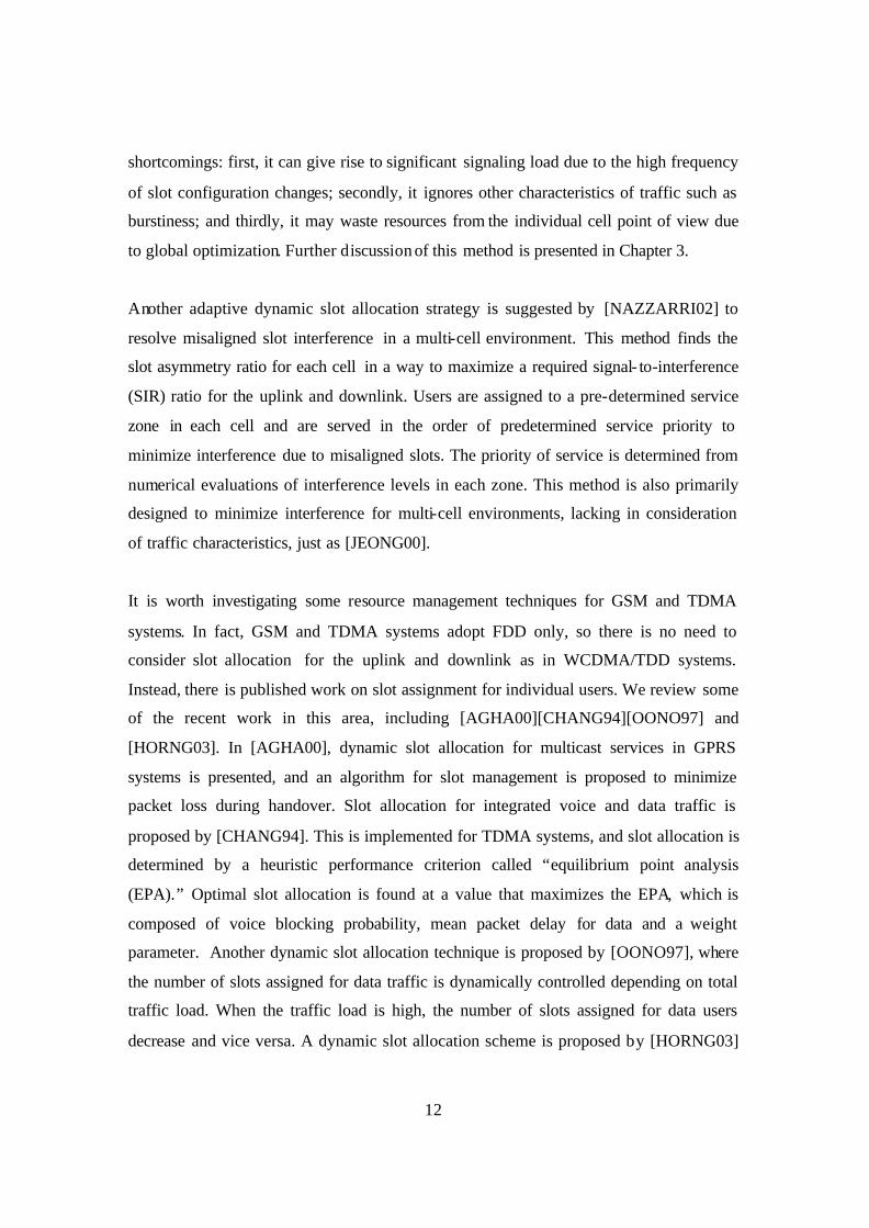
When adaptive slot allocation is employed in WCDMA/TDD systems , interference issues

may arise between adjacent cells. There are two dominant types of interference in a

WCDMA/TDD system: base-station-to-base-station (BS-to-BS) and mobile-to-mobile

(MS-to-MS) interference. This issue can be illustrated as in Figure 2.1.

42:6

13:5

34:4

73:5

64:4

52:6

23:5

1

2

3

4

5

6

7

M1

M2

M3M4

(a) (b)

Figure 2.1. Interference in a WCDMA/TDD system

Figure 2.1(a) shows seven cells with different traffic slot asymmetry ratios. The MS-to-

MS interference (solid line) can occur when mobile M1 interferes with the reception at

mobile M2. The BS-to-BS interference (dotted line) happens when transmission from BS

4 interferes with reception at BS 3. The BS-to-BS interference can be solved through

sophisticated frequency planning [HOLMA01] to provide sufficient signal attenuation

between base stations. When it comes to MS-to-MS interference, however, the problem is

14

more complex due to mobility. This is of particular concern when mobiles are located at

the boundary between cells. In this example, at mobile M2, the transmitted signal from

M1 is stronger than transmitted signal from BS 4, blocking the reception of signal from

BS 4 at M2. Figure 2.1(b) illustrates a situation when slot 3 and slot 4 in cell 4 are being

interfered with uplink traffic in cell 3. There are many mature ways developed so far to

overcome this MS-to-MS interference such as [WIE01][NAZZARRI02]. Both of these

are based on the division of a cell into several zones and make use of received signal

strength. In [WIE01], a base station divides a cell into two zones by measuring the pilot

signal from mobile stations, and then misaligned slots are assigned only to those mobiles

in a zone close to the base station. In [NAZZARRI02], zones are determined from

received signal strength and sectored antenna information of a base station, and then

resources (slots) are allocated to users according to the level of mutual interference

evaluated for each predetermined service zone.

As we have examined so far, slot allocation techniques for WCDMS/TDD systems are

scarce and developed for multi-cell environments, primarily focused on inter-cell

interference. However, their focus on the interference may waste significant resources

from the point of view of each single cell. Because the issue of inter-cell interference may

be addressed through frequency and code planning, in our research we focus on the

efficient use of resources in a single cell through dynamic slot allocation.

Adaptive slot allocation schemes can be devised in various ways. Our proposed scheme

assigns slots to the downlink and uplink based on past characteristics of traffic demand,

namely traffic volume and burstiness. In [ABRAMSON94], the author points out the

importance of taking into consideration traffic characteristics for multiple access protocol

research. Thus, in the next section, we review some well-known techniques for traffic

characterization.

15

2.3 Traffic characterization and measures

Traffic characterization is an important aspect of networking research, primarily for

provisioning network resources.

A variety of traffic characterization techniques was classified by Rueda et al.

[RUEDA96] according to the nature of traffic descriptors: statistical models, traffic flow

models, Markov chain models, autoregressive moving average (ARMA) models, self-

similar models, neural network models, spectral characterization, transform-expand-

sample (TES) models, and wavelet models. We are interested in statistical models

because they are simple and computationally less intensive for swift slot allocation

decisions. Those models include the statistical characterization of average rate, peak rate,

sustained rate, burst length, and burstiness [GIROUX99]. We summarize each of these

here.

The peak rate represents the peak emission rate of a source. The inverse of the peak rate

indicates the theoretical minimum inter-arrival time of packets. It can be limited by the

physical speed (or link rate) of the source. The mean rate is the average volume of data

generated by the source over a certain time interval, usually expressed in bits per second

or packets per second. It can also be measured in a large time scale, such as hours, or

days. The sustained cell rate is an upper bound on the average transmission rate measured

over relatively longer time scales than those for which peak rate is measured. The

maximum burst length represents the maximum number of consecutive data packets (or

bytes) that can be generated by a source at peak rate while still complying with the

negotiated sustained rate. The burstiness has been defined in many ways, which are

further discussed in Chapter 3. One of the common definitions is as the ratio of the peak

rate to the average rate.

Among these traffic characteristics, the average rate has been used for slot allocation in

[JEONG00]. Many works in the literature have emphasized the impact of the burstiness

for resource allocation and management in networking research [ABRAMSON94]

16

[JIANG00] [JIANG01]. In this research, we take into consideration these two

characteristics of traffic (average traffic volume and burstiness) for the slot allocation

decision.

The next step is how to measure these two characteristic s of traffic. A discussion of how

to estimate current traffic volume and burstiness is presented in Chapter 3. As a reference,

a comprehensive survey on the measurement of traffic was performed by

[WILLIAMSON01], which includes types of measurement tools and measurement

methods.

Some of our experiments for performance assessment of the proposed slot allocation

method required the synthetic generation of traffic. Those experiments are discussed in

detail in Chapter 4. In the next section, we review major techniques used to synthesize

traffic, addressing both voice and data traffic.

2.4 Traffic generation

In this section, we examine some methods for the generation of synthetic voice and data

traffic, especially focusing on those that are used for this research. Also, we provide

additional discussion on the self-similar nature of data traffic.

Various models have been developed for the synthetic generation of voice traffic. Several

fluid- flow approximation models, also known as Uniform Arrival Service (UAS) models,

were studied by [ANICK82][TUCKER88]. These models are characterized as

approximated models of a speech multiplexer, a multiplexer of packet arrivals from

individual sources, where each packet arrival process is assumed to be uniform. These

models are known to be appropriate for a small number of superimposed sources. Two

different approximation models were studied by Nagarajan et al. [NAGARAHAN91]; the

first approach is to model superimposed voice sources as a renewal process; and the

17

second approach is to model these sources as a correlated non renewal process, known as

a Markov Modulated Poisson Process (MMPP). Another possibility is to use two-state or

three-state Markov process models: the two states are talk and silent states; the three

states are talking, principal silent gap, and minisilent gap states [GOODMAN91]. This

three state model is an enhanced version of the two state model, where the three state

model can distinguish short silent intervals during continuous speech. This three state

model is based on the behavior of more sensitive speech activity detectors used in an

experimental wide-band packet communication system, while the two state model is

based on the behavior of the speech detector designed for the speech interpolation system

devised to improve the efficiency of undersea transmission. One of the most widely

adopted models is based on the work developed by Erlang [KLEINROCK75], which

considers two user parameters. Those parameters are call arrival rate and average call

holding time. In this model, the statistical distribution of the call arrivals follows a

Poisson distribution, with interarrival times following an exponential distribution. The

length of the call holding time is also exponentially distributed, during which packets are

transmitted back to back. In our modeling of voice traffic, we choose the last model for

our experiment with fixed packet size.

Several different approaches have been suggested for the generation of synthetic data

traffic. Most of these approaches are based on empirical distribution or mathematical

models [RYU96][ABRAHAMSSON00][LEDESMA00][KOS03]. The empirical models

are based on heuristics derived from statistics of user behavior. The mathematical models,

for the most part, are based on the use of the following theoretical models: on-off sources,

Gaussian Noise processes, Fractional ARIMA (FARIMA) processes, Chaotic Maps,

Fractal Point Processes (FPP) [RYU96], etc. We adopt an on-off source model with

heavy-tail-distributed sojourn times using the Pareto distribution. Synthetic data traffic

can be generated by aggregating several on-off traffic sources [PAXSON95], which

results in self-similarity behavior in the generated traffic. During the on time period,

traffic is generated depending on the target data transmission rate and packet size. During

the off time period, no traffic is generated. Details on the use of on-off traffic model are

further discussed and illustrated in Chapter 4.

18

Along with the data traffic generation, it is worth to understand the concept of self-

similarity and methods to assess self-similarity. Self-similarity is a concept that is related

to fractals and chaos theory, where processes exhibit the same patterns regardless of the

degree of resolution. Recently, it has become a very important concept in the analysis of

data traffic analysis [STALLINGS98], prompted by the observation of Ethernet traffic by

[LELAND94]. The discovery that data traffic exhibits self- similarity has led to

questioning of the use of Poisson processes to model data [PAXSON95]. One of the

interesting properties of a self-similar process is referred to as “long-range dependence,”

resulting in clustering and burstiness at all time scales. The terms self-similarity and the

long-range dependence are often used interchangeably depending on the context

[PARK00]. Due to the persistency property, most of self-similarity or long-range

dependency measures are based on the observations requiring a long characterization

time. The variance-time plot is often used for the ana lysis of traffic in a long time scale

[JIANG00][JIANG01]. The slope in a variance-time plot allows us to characterize the

Hurst parameter, which is a measure of self-similarity. However, the variance-time plot

may not be appropriate for the measure of temporal burstiness in a short time scale

because it basically requires lengthy observation data for valid evaluation. The ACF is

used less frequently than the variance-time plot [BERAN94]. The Least-Square

estimation is employed frequently for the estimation of the Hurst parameter in both of the

methods.

2.5 Summary

This chapter presented the review of literature that serves as background for this research.

First, in Section 2.1, we presented a definition of the MAC protocols in wireless mobile

networks and discussed the classification of the MAC protocols depending on the

resource sharing methods and multiple access schemes.

19

In Section 2.2, we emphasized the importance of the limited resources in the MAC layer

and investigated two existing adaptive slot allocation methods developed for

WCDMA/TDD systems and several methods for GSM and TDMA systems.

In Section 2.3, we discussed traffic characterization and associated measures.

Finally, in Section 2.4, we reviewed methods used to generate synthetic voice and data

traffic adopted in this research. In relation to the data traffic, we discussed the self-similar

nature of the data traffic and methods to characterize self-similarity.

20

Chapter 3 Slot allocation for MAC protocol

In Chapter 3, we describe two adaptive slot allocation methods proposed in this research:

one using both traffic burstiness and volume information (BV strategy) and the other one

using burstiness information (B strategy) only. We also outline an adaptive slot allocation

method based on traffic volume (V strategy), for comparison with the proposed methods.

We begin by reviewing the frame structure for WCDMA systems. Then, we discuss fixed

and adaptive slot allocation and summarize a traffic volume-based adaptive allocation

scheme for multi-cell environments proposed by [JEONG00]. Next, we describe the

proposed methods in detail. This includes methods for estimating the burstiness and

traffic volume, and the dynamic decision of observation window size for the estimations.

This chapter begins by discussing the frame structure of WCDMA/TDD systems in

Section 3.1. Then we discuss advantages and disadvantages of fixed and adaptive slot

allocation in Section 3.2, which includes a review of the adaptive slot allocation strategy

described in [JEONG00]. In Section 3.3, we describe our proposed slot allocation

strategies, based on the estimation of burstiness and volume of traffic. In particular,

burstiness metrics and a dynamic window sizing method for the estimation of the

burstiness are emphasized with illustrations. Finally, we present a summary of this

chapter.

3.1 Frame and slots in WCDMA/TDD system

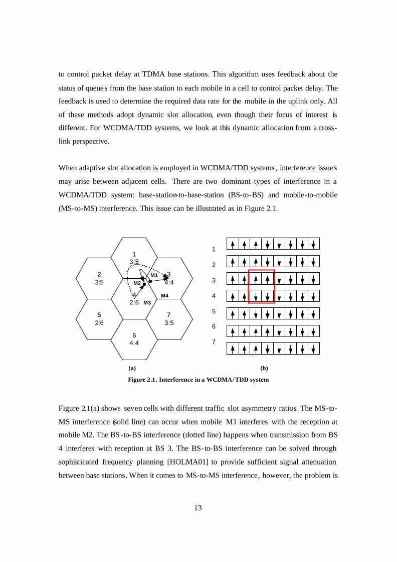
The general structure of WCDMA/TDD MAC frame can be drawn as consisting of slots

for the uplink and the downlink as shown in Figure 3.1.

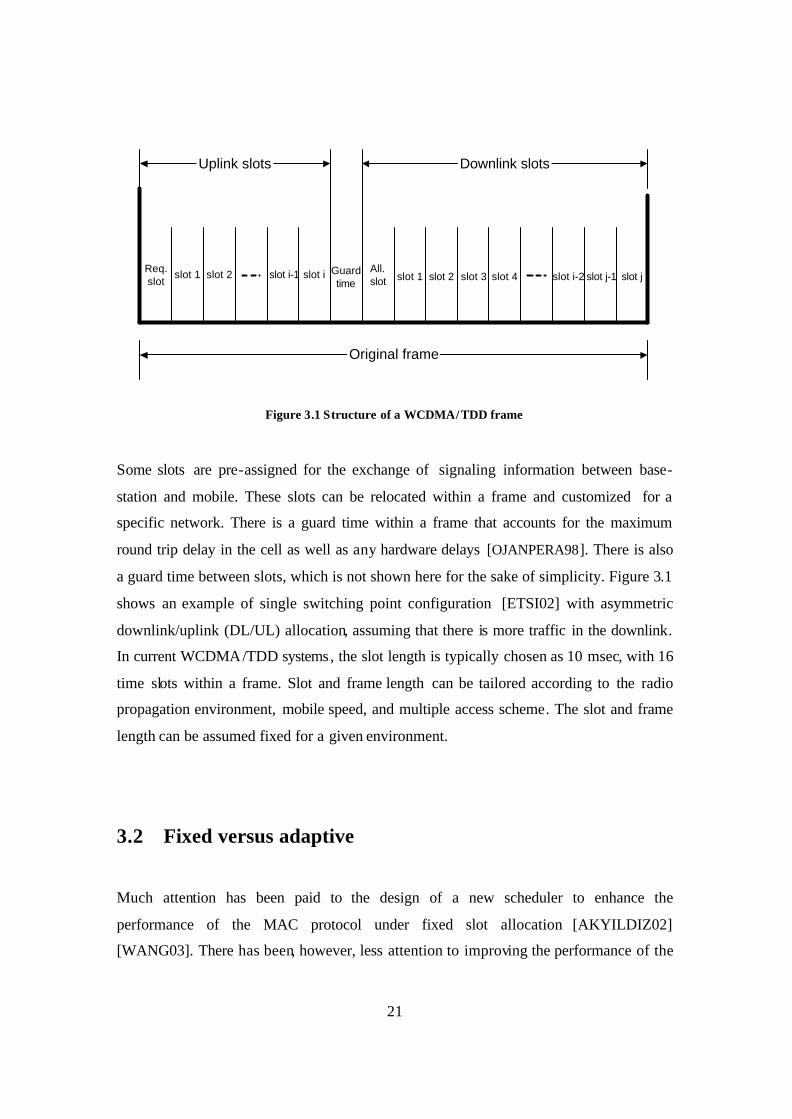
21

Original frame

Guardtime

Req.slot

All.slot

slot 1 slot 2 slot i-1 slot 1 slot 2 slot j

Uplink slots Downlink slots

slot 3 slot 4 slot i-2 slot j-1slot i

Figure 3.1 Structure of a WCDMA/TDD frame

Some slots are pre-assigned for the exchange of signaling information between base-

station and mobile. These slots can be relocated within a frame and customized for a

specific network. There is a guard time within a frame that accounts for the maximum

round trip delay in the cell as well as any hardware delays [OJANPERA98]. There is also

a guard time between slots, which is not shown here for the sake of simplicity. Figure 3.1

shows an example of single switching point configuration [ETSI02] with asymmetric

downlink/uplink (DL/UL) allocation, assuming that there is more traffic in the downlink.

In current WCDMA/TDD systems, the slot length is typically chosen as 10 msec, with 16

time slots within a frame. Slot and frame length can be tailored according to the radio

propagation environment, mobile speed, and multiple access scheme. The slot and frame

length can be assumed fixed for a given environment.

3.2 Fixed versus adaptive

Much attention has been paid to the design of a new scheduler to enhance the

performance of the MAC protocol under fixed slot allocation [AKYILDIZ02]

[WANG03]. There has been, however, less attention to improving the performance of the

22

system through adaptive slot allocation. This section discusses advantages and

disadvantages of fixed and adaptive slot allocation schemes.

Fixed slot allocation schemes maintain the slot assignment ratio between uplink and

downlink constant. Adaptive schemes, on the other hand, dynamically react to traffic and

transmission conditions by changing the number of slots allocated to each of the two

links on the fly. Fixed allocation is attractive for its simplicity and resistance to intercell

interference. It is also advantageous in the sense that it does not require signaling to

inform mobiles of updated slot assignments. However, fixed slot allocation tends to be

wasteful of resources due to its inflexibility to unpredictable traffic conditions.

Meanwhile, some techniques have been developed [OJANPERA98] to avoid intercell

interference when adaptive schemes are employed. In our research, we argue that

adaptive slot allocation can yield higher efficiency in managing resources in a mobile

wireless network. This is particularly important in third generation networks and beyond,

where demand for bursty, asymmetric data traffic is expected to be significant.

Adaptive slot allocation schemes aim to find an optimum slot asymmetry ratio r (number

of downlink slots/number of uplink slots) at any given time. The ultimate objective is to

increase efficiency in managing the available resources, thereby decreasing average

queuing delay and packet losses and increasing throughput. As discussed in the

introduction, the relevant research work on adaptive slot allocation is scarce. An

exception is [JEONG00], where the slot asymmetry ratio is determined by evaluating

what they refer to as the frequency utilization function under a multi-cell environment.

We briefly look at the algorithm proposed in [JEONG00] as an example of adaptive slot

allocation scheme. It is based on the calculation of slot asymmetry ratio ( r ) for all

neighboring cells that maximizes the following overall utility function:

)(rTΩ ∑=

≡M

ii r

M 1

)(1

η and

>++

≤+

+

=

ii

ii

i

i

vrifrv

vrifrv

rv

r,

11

,)1(

)1(

)(η . (3.1)

23

where M is the number of cells of interest, iv is the traffic asymmetry ratio (volume of

downlink traffic/volume of uplink traffic) for each cell, and r is the slot asymmetry ratio.

In [JEONG00], the values of r are constrained to be greater than or equal to one so that

the downlink has more slots than the uplink.

This algorithm disregarded some important points. First, it may waste resources (slots)

from an individual cell point of view because it seeks a globally optimized slot

asymmetry ratio for multi-cell environments (i.e., the algorithm results in the same slot

asymmetry ratio being applied to all cells). Secondly, the algorithm did not consider

traffic burstiness in the slot allocation decision. As mentioned in Chapter 2, a recent study

of wireless trace data confirmed that the volume of downlink traffic is typically higher

than the volume of uplink traffic; however, uplink traffic may be more bursty than

downlink traffic [TANG00]. The author, therefore, claimed that extremely skewed

assignment of capacity is undesirable. Through our literature review, including

[TANG00][JIANG01], we conclude that burstiness needs to be considered in the slot

allocation decision and also that extreme asymmetric slot allocation may be undesirable.

This will be reflected in our strategy for dynamic slot allocation.

There are several ways to implement an adaptive scheme other than [JEONG00]; for

example, we may use traffic characteristics such as volume or burstiness (or both) as

basic input for the asymmetry ratio decision. As described earlier, the downlink traffic is

heavier than the uplink traffic in current wireless mobile wireless networks, and this trend

is expected to continue in future mobile wireless networks; in addition, modern

multimedia traffic is bursty [WALKO02]. So, intuitively, it is desirable to take both

factors into account for the adaptive allocation of slots. Another consideration here is

whether we can make the slot allocation decision based on instantaneous traffic

information collected on the fly or historical information regarding demand for resources.

From the resource management point of view, the use of historical information is

beneficial; namely, if we know what happened so far, it is easier to predict what is going

to come afterwards. Furthermore, the burstiness cannot be estimated based on

24

instantaneous information only; it requires at least a certain amount of past information

for its estimation. In the next section, considering all these factors, we propose two

adaptive slot allocation strategies based on traffic characteristics.

3.3 Adaptive schemes

In this section, we describe two proposed slot allocation strategies based on traffic

characteristics. These traffic characteristics include burstiness and volume that are

evaluated over a certain observation period. We begin by explaining how we estimate

traffic burstiness and volume.

3.3.1 Estimation of burstiness: Peak/Median vs. Peak/Mean Most data traffic is bursty. As mentioned in Chapter 2, there are several ways to define

burstiness, mostly customized for a certain purpose; for example, the ratio of peak rate to

mean rate [SPOHN97], a measure of index dispersion of interval (IDI) or time between

packets, index of dispersion of count (IDC) or number of arrivals in an interval, spectral

characteristics [STALLINGS98], statistical characterization of buffer under- loaded or

overloaded periods [LI02], the entropy rate of the stochastic process for ATM traffic

[PRABHAKAR95], etc. Each method has advantages and disadvantages because it is

customized for a particular purpose. We are interested in a simple measure for the

estimation of burstiness such as the ratio of peak rate to mean rate, because speed in the

computation of such a metric can lead to a swift decision regarding the number of slots to

be assigned to the uplink and downlink . The peak/mean measure is simple but has a few

problems related to the use of the mean. Thus we propose a new burstiness measure, as

explained next.

The peak to mean ratio measures the ratio of the peak to the majority of the data

distribution; the mean is typically used to characterize this "majority." There are two

25

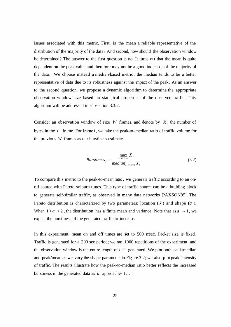
issues associated with this metric. First, is the mean a reliable representative of the

distribution of the majority of the data? And second, how should the observation window

be determined? The answer to the first question is no. It turns out that the mean is quite

dependent on the peak value and therefore may not be a good indicator of the majority of

the data. We choose instead a median-based metric : the median tends to be a better

representative of data due to its robustness against the impact of the peak. As an answer

to the second question, we propose a dynamic algorithm to determine the appropriate

observation window size based on statistical properties of the observed traffic. This

algorithm will be addressed in subsection 3.3.2.

Consider an observation window of size W frames, and denote by tX the number of

bytes in the t th frame. For frame i , we take the peak-to-median ratio of traffic volume for

the previous W frames as our burstiness estimate :

titWi

titWii Xmedian

XBurstiness

<≤−

<≤−=max

(3.2)

To compare this metric to the peak-to-mean ratio , we generate traffic according to an on-

off source with Pareto sojourn times. This type of traffic source can be a building block

to generate self-similar traffic, as observed in many data networks [PAXSON95]. The

Pareto distribution is characterized by two parameters: location ( k ) and shape (α ).

When 21 << α , the distribution has a finite mean and variance. Note that as 1→α , we

expect the burstiness of the generated traffic to increase.

In this experiment, mean on and off times are set to 500 msec. Packet size is fixed.

Traffic is generated for a 200 sec period; we ran 1000 repetitions of the experiment, and

the observation window is the entire length of data generated. We plot both peak/median

and peak/mean as we vary the shape parameter in Figure 3.2; we also plot peak intensity

of traffic. The results illustrate how the peak-to-median ratio better reflects the increased

burstiness in the generated data as α approaches 1.1.

26

Figure 3.2 Comparison of mean/median and peak/mean

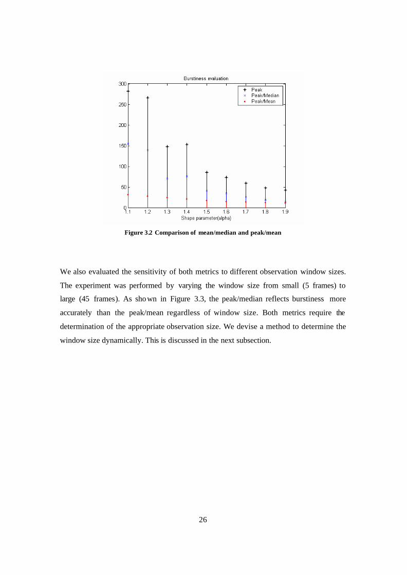
We also evaluated the sensitivity of both metrics to different observation window sizes.

The experiment was performed by varying the window size from small (5 frames) to

large (45 frames). As shown in Figure 3.3, the peak/median reflects burstiness more

accurately than the peak/mean regardless of window size. Both metrics require the

determination of the appropriate observation size. We devise a method to determine the

window size dynamically. This is discussed in the next subsection.

27

Figure 3.3 Sensitivity analysis of two metrics depending on the observation window size and shape parameter α

3.3.2 Dynamic window size determination based on ACF and PACF In this section, we explain the dynamic sizing of the observation window for the

estimation of traffic burstiness and volume. We use the autocorrelation function (ACF)

and partial autocorrelation function (PACF) of the observed data to calculate the

appropriate observation window size. The ACF and PACF are widely used in prediction

techniques such as AR (Auto-Regression), MA (Moving Average), ARMA (Auto

Regression Moving Average), and ARIMA (Auto Regression Integrated Moving

Average). Among these, the ARMA model is known to closely approximate data

exhibiting long-range dependence, such as expected from packet data traffic

[BROCKWELL91].

An ARMA ( qp, ) model is defined as the stationary solution to the equation

[BROCKWELL91]:

qtqtttptpttt XXXX −−−−−− ++++=−−−− εψεψεψεφφφ LL 22112211 (3.3)

28

where tX is a time-series, p and q are integers and tε is stationary white Gaussian

noise.

In the ARMA model, the orders p and q play an important role in the prediction

accuracy of the ARMA model; the order p is the highest order of the AR polynomial and

the order q determines the highest order of the MA polynomial. Several methods for the

determination of p and q have been proposed: one of the most popular methods is found

in [BROCKWELL91], where the order p is determined from the point where the partial

autocorrelation decreases to zero, and the order q is determined where the

autocorrelation function decreases to zero. Meanwhile, the ARMA process model can be

approximated by the AR model [BROCKWELL91]. Based on these facts, we choose the

order p as the observation window size (in frames), which can be determined from the

PACF. Through a number of observations of the ACF and PACF on real wireless trace

data, we determined that we could achieve a moderate window size with the order

p alone. Intuitively, the larger the window size, the more accurate the estimation of

burstiness. However, a large window size can slow the processing of the data and require

significant memory.

We now describe how the ACF and PACF can be calculated.

The ACF ( kρ ) at lag k is calculated as:

0

),(γγ

ρ kkttk XXcorr == − (3.4)

where tX denotes a time-series and kγ is the auto-covariance of tX at lag k . The PACF

( kkφ ) at lag k is a measurement of the correlation between two elements ktX + and tX of

a time series adjusted for the intervening observations 11 ,..., −++ ktt XX . In other words,

),,|,( 11 −+++= kttkttkk XXXXcorr Lφ . (3.5)

29

Mathematically, it can be calculated as [BROCKWELL91]:

1

1

1

11

1321

2311

1221

1321

2311

1221

ρρρρ

ρρρρ

ρρρρρρρρρ

ρρρρρρρρ

φ

LMMMMMM

L

LL

MMMMMM

LL

−−−

−−

−−

−−−

−

−

=

kkk

kk

kk

kkkk

k

k

kk

(3.6)

We dynamically determine the appropriate observation window by finding the smallest

lag k for which there is a zero crossing in the PACF. An alternative method would be to

determine the smallest lag k that satisfies:

1, ≥< kkk εφ . (3.7)

ε can be set to any small value as a threshold. We chose the former method because it

has a more definite criterion for the decision compared to the latter method.

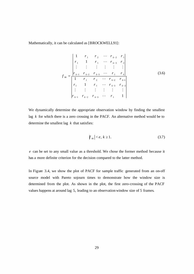
In Figure 3.4, we show the plot of PACF for sample traffic generated from an on-off

source model with Pareto sojourn times to demonstrate how the window size is

determined from the plot. As shown in the plot, the first zero-crossing of the PACF

values happens at around lag 5, leading to an observation window size of 5 frames.

30

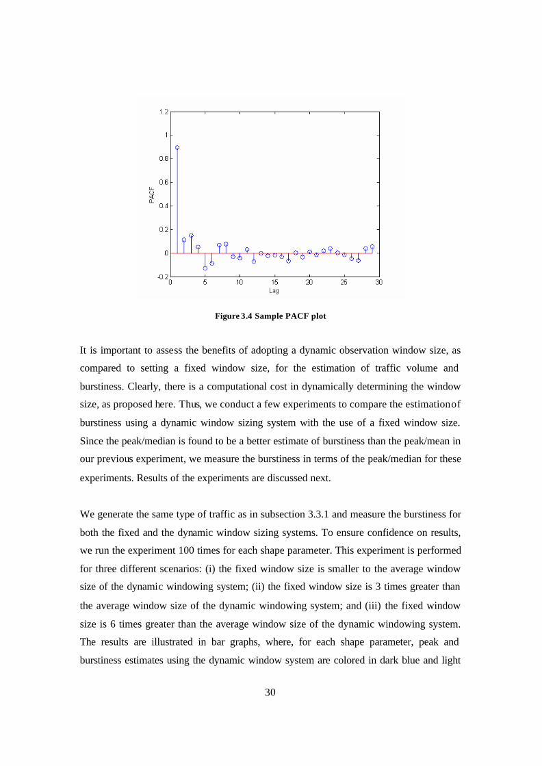
Figure 3.4 Sample PACF plot

It is important to assess the benefits of adopting a dynamic observation window size, as

compared to setting a fixed window size, for the estimation of traffic volume and

burstiness. Clearly, there is a computational cost in dynamically determining the window

size, as proposed here. Thus, we conduct a few experiments to compare the estimation of

burstiness using a dynamic window sizing system with the use of a fixed window size.

Since the peak/median is found to be a better estimate of burstiness than the peak/mean in

our previous experiment, we measure the burstiness in terms of the peak/median for these

experiments. Results of the experiments are discussed next.

We generate the same type of traffic as in subsection 3.3.1 and measure the burstiness for

both the fixed and the dynamic window sizing systems. To ensure confidence on results,

we run the experiment 100 times for each shape parameter. This experiment is performed

for three different scenarios: (i) the fixed window size is smaller to the average window

size of the dynamic windowing system; (ii) the fixed window size is 3 times greater than

the average window size of the dynamic windowing system; and (iii) the fixed window

size is 6 times greater than the average window size of the dynamic windowing system.

The results are illustrated in bar graphs, where, for each shape parameter, peak and

burstiness estimates using the dynamic window system are colored in dark blue and light

31

blue (first two bars); peak and burstiness estimates using the fixed window system are

colored in yellow and brown (next two bars).

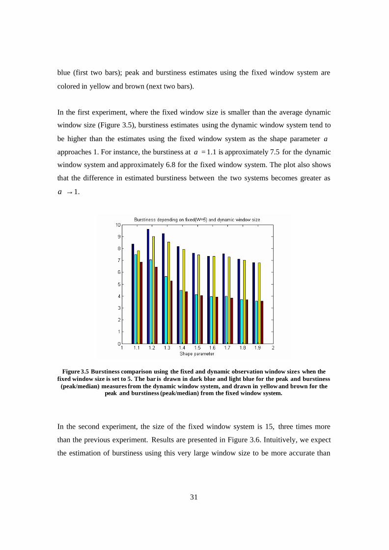
In the first experiment, where the fixed window size is smaller than the average dynamic

window size (Figure 3.5), burstiness estimates using the dynamic window system tend to

be higher than the estimates using the fixed window system as the shape parameter α

approaches 1. For instance, the burstiness at 1.1=α is approximately 7.5 for the dynamic

window system and approximately 6.8 for the fixed window system. The plot also shows

that the difference in estimated burstiness between the two systems becomes greater as

→α 1.

Figure 3.5 Burstiness comparison using the fixed and dynamic observation window sizes when the fixed window size is set to 5. The bar is drawn in dark blue and light blue for the peak and burstiness

(peak/median) measures from the dynamic window system, and drawn in yellow and brown for the peak and burstiness (peak/median) from the fixed window system.

In the second experiment, the size of the fixed window system is 15, three times more

than the previous experiment. Results are presented in Figure 3.6. Intuitively, we expect

the estimation of burstiness using this very large window size to be more accurate than

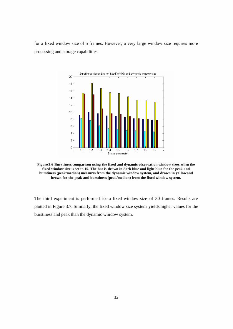
32

for a fixed window size of 5 frames. However, a very large window size requires more

processing and storage capabilities.

Figure 3.6 Burstiness comparison using the fixed and dynamic observation window sizes when the fixed window size is set to 15. The bar is drawn in dark blue and light blue for the peak and

burstiness (peak/median) measures from the dynamic window system, and drawn in yellow and brown for the peak and burstiness (peak/median) from the fixed window system.

The third experiment is performed for a fixed window size of 30 frames. Results are

plotted in Figure 3.7. Similarly, the fixed window size system yields higher values for the

burstiness and peak than the dynamic window system.

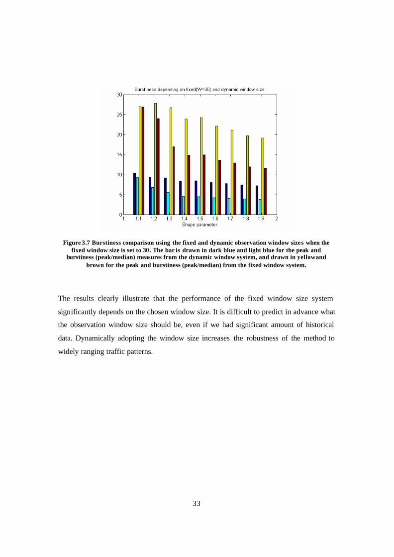
33

Figure 3.7 Burstiness comparison using the fixed and dynamic observation window sizes when the fixed window size is set to 30. The bar is drawn in dark blue and light blue for the peak and

burstiness (peak/median) measures from the dynamic window system, and drawn in yellow and brown for the peak and burstiness (peak/median) from the fixed window system.

The results clearly illustrate that the performance of the fixed window size system

significantly depends on the chosen window size. It is difficult to predict in advance what

the observation window size should be, even if we had significant amount of historical

data. Dynamically adopting the window size increases the robustness of the method to

widely ranging traffic patterns.

34

3.3.3 Slot allocation based on the estimation of burstiness (B strategy) In this subsection, we propose our first adaptive slot allocation method, based on the

estimation of traffic burstiness. Burstiness is estimated based on the peak/median as

described in Section 3.3.1. We estimate the burstiness for uplink and downlink , assuming

that traffic in each link is independent. In the real world, there is correlation between the

uplink and downlink traffic. Consideration of this correlation may be incorporated into a

refinement of the slot allocation algorithm in the future.

Our method begins by estimating the burstiness for each link as we advance for each

frame. Then we make use of the burstiness ratio for the decision of the number of slots to

be allocated to each link. Mathematically, the burstiness ratio can be calculated as

follows.

First, we denote the estimated traffic burstiness in the downlink and the uplink as diB and

uiB respectively, estimated at frame i .

From (3.2), diB and u

iB can be calculated as:

ujijWi

uj

ijWiui Xmedian

XB

u <≤−

<≤−=max

and djijWi

dj

ijWidi vmedian

XB

d <≤−

<≤−=max

(3.8)

where ujX and d

jX are the uplink and the downlink traffic volume, in bytes, at the j th

frame, and uW and dW are the observation window sizes for the uplink and the downlink,

respectively.

Then, the burstiness ratio iB at frame i can be expressed as :

35

ui

di

i BB

B = . (3.9)

We simply allocate the number of slots for each link roughly in proportion to this ratio.

Then, we have the following relationship :

iu

d BNN

≅ , dut NNN += (3.10)

where sum of the slots in each link (uN for the uplink and

dN for the downlink) is equal

to the total number of slots( tN ) in the entire frame.

Consequently, the number of uplink and downlink slots can be derived as:

+

=i

tu B

NN

1, ( )1,max utd NNN −= (3.11)

where the ceiling function and max operator are used to ensure that uN and dN are

integers and that each link is allocated at least one slot.

In the following subsection, we propose our second adaptive strategy.

3.3.4 Adaptive asymmetric slot allocation based on the use of burstiness and volume information (BV strategy)

Our second slot allocation method is proposed in this subsection. The second method is

based on the intuition that traffic in both links differs in terms of volume and burstiness.

Thus, we use two traffic characteristics, burstiness and volume, to calculate the number

of slots allocated to each link . Then, a kind of grafting issue arises on how to relate these

36

two variables. To solve this problem, we adopt a notion of “virtual weight” for traffic

volume in each link, which can be driven by the estimated burstiness in each link. The

virtual weight is described below.

First, we estimate the burstiness for each link ( diB for the downlink and u

iB for the

uplink) at frame i as in (3.8) and save those results for future use. In other words, the

estimated burstiness for each link is saved as the frames advance. Then the virtual weight

driven by the burstiness is calculated by a simple mapping formula:

min,

1,,

1,,1,,

min,max,

)min(minmax

uujiWij

uiu

jiWij

ujiWij

uuui wBB

BBww

wu

uu

+−−−

=−−∈

−−∈−−∈

L

LL

(3.12)

min,

1,,

1,,1,,

min,max,

)min(minmax

ddjiWij

did

jiWij

djiWij

dddi wBB

BBwww

d

dd

+−−−=

−−∈

−−∈−−∈

L

LL

where uiw and d

iw denote the virtual weights for the uplink and the downlink; uiB and

diB are the estimated burstiness at a new frame i for the uplink and the downlink; u

jB and

djB are the recorded burstiness at the j th frame within an observation window uW and

dW ; and max,dw and min,dw are the maximum and the minimum virtual weights,

respectively.

In (3.12), in the case when ujiWij

Bd 1,,

max−−∈ L

= ujiWij

Bd 1,,

min−−∈ L

, we simply set 1=uiw .

Similarly, if djiWij

Bd 1,,

max−−∈ L

= djiWij

Bd 1,,

min−−∈ L

, we set 1=diw .

The maximum and the minimum virtual weights for each link are chosen heuristically.

Burstiness relates to resource control and management issues. Intuitively, highly bursty

traffic requires more resources than less bursty traffic. We chose the maximum and the

minimum virtual weights for each link so that:

37

1,1.0 ≤≤ ui

di ww . (3.13)

In other words, 1max,max, == ud ww and 1.0min,min, == ud ww .

Once the virtual weights are calculated, then the traffic volume in each link can be

weighted by diw and u

iw to assign the number of slots to each link. The resulting slot

asymmetry ratio ir (the ratio between the number of downlink slots and the number of

uplink slots) at frame ican be expressed as:

ui

ui

di

di

i wXwX

r××

= (3.14)

where u

iX and diX are the estimated traffic volume for the uplink and the downlink

respectively. The traffic volumes are also estimated by the median within an

observation window.

As before, the number of slots for each link are calculated as:

+

=i

tu r

NN

1, ( )1,max utd NNN −= (3.16)

Again, the ceiling function and max operator are used to ensure that each link can have at

least one slot and that uN and dN are integers.

3.4 Summary

In this chapter, we propose two adaptive slot allocation schemes, one based on estimated

traffic burstiness and another one based on estimated traffic burstiness and volume.

38

In Section 3.1, we first discussed the generic frame structure of a WCDMA/TDD system.

Then, in Section 3.2, we compared fixed and adaptive slot allocation methods in terms of

advantages and disadvantages, along wit h a brief review of existing adaptive slot

allocation methods.

In Section 3.3, we described our proposed slot allocation methods based on the

estimation of burstiness and volume. The burstiness and volume information are

estimated based on an observation window that is determined dynamically. In order to

measure the burstiness, we devised a new simple burstiness metric based on the

estimation of median and peak within the observation window. The observation window

size is dynamically determined from statistical characteristics of past traffic, in particular

ACF and PACF. The window size is determined at the smallest lag k where a zero-

crossing of the PACF occurs. We formally describe our slot allocation algorithms in sub-

sections 3.3.3 and 3.3.4.

In the next chapter, we present an assessment of the performance of the proposed

resource management strategy.

39

Chapter 4 Performance evaluation based on the estimation of burstiness

This chapter provides experimental results to evaluate the performance of the proposed

adaptive slot allocation methods under various scenarios. We begin by presenting the

methodology for the performance evaluation. This includes a discussion of the types of

traffic used for our experiments, performance metrics, physical channel model

implemented for this research, and simulation flow. Next, we discuss generation of

synthetic voice and data traffic and control of volume and burstiness of the generated

synthetic traffic. We also describe the handling of real world trace data to be used for the

experiment. Experimental results are presented for the following three major scenarios :

first, simulation using synthetic data traffic; secondly, simulation combining voice and

data traffic; and finally, simulation using trace data. All these experiments use a FIFO

scheduler. Each of these scenarios is composed of several sub-scenarios to test the

proposed algorithms in various realistic situations. Simulation results are evaluated in

terms of throughput and packet drop ratio.

The organization of Chapter 4 is as follows. First, we discuss our simulation

methodology in Section 4.1, which includes discussion of performa nce metrics, traffic

types, the physical fading channel model, and simulation flow. In Section 4.2, we discuss

generation and control of synthetic traffic. Discussion of the processing of trace data is

also provided in this section. Section 4.3 provides simulation results when the load

consists of synthetic data traffic. Section 4.4 presents simulation results when the load

consists of synthetic voice and data traffic. Section 4.5 discusses simulation results using

trace data. Finally, we summarize this chapter in Section 4.6.

40

4.1 Methodology for performance evaluation

This section discusses the methodology for the performance evaluation of adaptive slot

allocation, which includes types of traffic used for simulation, performance metrics, and

the physical fading channel model.

4.1.1 On the use of synthetic and real world traffic To evaluate the performance of the proposed algorithms, we generate synthetic traffic

based on a theoretic model. As described in Chapter 2, synthetic data and voice traffic is

generated : the data traffic is generated using an on-off traffic source model with Pareto

distributed sojourn times; the voice traffic is modeled by Poisson arrivals with

exponentially distributed inter-arrival times. These two types of traffic can be

characterized by several key parameters, such as on-off times, packet size, target

transmission rate, packet inter-arrival time, and the shape parameter for the Pareto

distributions. More details on the generation of synthetic data and voice traffic are given

in Subsection 4.2.1.

In addition to the simulation using the synthetic data and voice traffic, we also analyze

the performance of our proposed methods using real world traffic. For this purpose, we

obtained WLAN trace data that was collected by a research group at Stanford University

[TANG00]. This trace data was collected over a 12-week period in a local-area wireless

network with the goal of analyzing overall user behavior, overall network traffic and load

characteristics. The archive consists of a single large file (approximately 2.7 Gbytes),

which we split into a group of files, each having 5 Mbytes of data. As a result, we have

more than 500 files of trace data. These files are analyzed again to measure throughput

for each particular type of traffic; C code is written for this purpose. More details on the

processing of real trace data are available in Subsection 4.2.2, including the format of

trace data.

41

4.1.2 Performance metrics We choose throughput and packet drop ratio as our main performance metrics, as defined

below.

The throughput is calculated as the number of successfully transmitted packets per frame,

where the frame length is 160 msec.

The packet drop ratio DR is defined as

sd

d

PPP

DR+

= (4.1)

where dP and sP denote the number of dropped packets and the number of serviced

packets, respectively.

We also include one more performance metric, signaling load between a base station and

a mobile station related to slot allocation. This metric is relevant because the frequent

exchange of signals between a base station and mobiles may significantly drain the

battery of the mobiles, as well as occupy valuable bandwidth.

4.1.3 Physical channel implementation

The bit error rate performance of binary Phase Shifting Keying (PSK) and binary

Frequency Shifting Keying (FSK) is derived in [PROAKIS95], when these signals are

transmitted over a frequency-nonselective slowly fading channel such as a Rayleigh

fading channel, the chosen physical channel model for this research. We briefly

summarize the derivation of the probability of bit error.

In a Rayleigh flat-fading channel model, we can represent the fading phenomenon using a

random variable R because the fading stays constant during a signaling interval. Since

only amplitude distortion is considered, the instantaneous SNR per bit bγ can be a

random variable represented by the following equation [PROAKIS95]:

42

o

bb N

ER2=γ . (4.2)

Because R is Rayleigh distributed, the probability density function of bγ follows a chi-

squared distribution, which can be expressed as:

bb

bef

bb

γγγ γ

γ /1)( −= , 0≥bγ (4.3)

where bγ is the average SNR per bit given by:

][ 2RENE

o

bb =γ (4.4)

It is well-known that, for a given value of bγ , the probability of error ( eP ) for binary PSK

is calculated as:

)2()( bbe QP γγ = (4.5)

(4.5) can now be calculated as:

+−=

b

beP

γγ

11

21 . (4.6)

In the case of high SNR, i.e., 1>>bγ , (4.6) can be approximated as:

beP

γ41

≈ (4.7)

43

We use (4.6) to calculate packet error rate in our simulations.

Accordingly, with the assumption that bit errors are independent, the packet error

probability PER for an N -bit packet can be calculated as:

NePPER )1(1 −−= (4.8)

In this research, we are primarily interested in adaptive resource allocation at the data

link layer according to an estimate of traffic demand. Impairments at the physical layer

are, therefore, a secondary consideration. Packet drop ratio mostly reflects packets

dropped due to scarcity of slots allocated to the uplink or downlink. In our experiments,

we set 0NEb so as to maintain the packet error rate ( PER) below 10%.

4.1.4 Simulation flow

In this subsection, we describe simulation flow for the simulation of this research. This

simulation flow includes that for additional slot allocation methods CS and SB, which

will be explained in Chapter 5.

First, we generate traffic, voice or data, for a certain period of time or input trace data for

simulation. For the methods B and BV, we determine the observation window size using

certain number of frames N (i.e., a transient period of simulation) from the beginning

point of simulation. We choose 200 for N for all simulation scenarios, associated with the

methods B and BV. The observation window size is maintained during the entire

simulation period. For the simulation with the methods CS and SB, we choose 100 for the

sample size N. In Chapter 5, we demonstrate that the sample size 100 can be used without

much difficulty, which means that we can estimate a distribution of traffic adequately

using 100 samples of data.

44

Next, for the methods B and BV, we estimate burstiness and volume of traffic based on

the observation window size. Then, we calculate the number of slots using the estimated

burstiness and volume of traffic.

For the methods CS and SB, using the estimated shape and location parameters, we

estimate burstiness for the method SB or outage probability for the method CS.

Remaining tasks are the same as the methods B and BV.

Generate voice and data traffic / input trace data

Determine observation window size for N frames

Allocate slots for each link based on each method

Transmit packets based on the allocated number of slots through each link

Evaluatethroughput and packet drop ratio for each link

Estimate burstiness and volume of traffic for the observation window size for each link

For 100 frames, estimate parameters for a Pareto distribution

Estimate burstiness based on the estimated parameters for each link /Calculate outage probability based on the estimated parameters for each link

Methods B or BV Methods CS or SB

Figure 4.1. Simulation flow chart

In our simulations, we have no buffers in our system to obtain more accurate simulation

results; buffers in the system can significantly affect simulation results because they can

smooth burstiness of traffic. In a network transaction involving real-time traffic, buffers

in a system can significantly affect the real-time traffic. Hence, we have no buffers in our

system to obtain more accurate simulation results.

45

4.2 Generation of traffic

In this section, we discuss the generation of synthetic voice and data traffic, including

ways to control traffic volume and burstiness of the synthetic traffic. We also describe

how the WLAN trace data was processed for use in this research.

4.2.1 Synthetic data and voice traffic generation

Synthetic data traffic is generated by using an on-off source model with Pareto

distributed sojourn times. During the on time period, packets are ge nerated at the target

transmission rate. The probability density function of the Pareto distribution is defined as

≥

=

+

otherwise

kxforxk

kxf,0

,)(

1αα (4.9)

where k is a location parameter that specifies the minimum value that the random

variable X can take; α controls the shape of the distribution )(⋅f . The mean and

variance of the random variable X depend on both α and k . Note that if 2≤α , then the

random variable has infinite variance, and if 1≤α , it has infinite mean and variance. In

our models, we set 21 << α . Values of α closer to 1 result in a heavier-tailed

distribution.

Our on-off source model needs five input parameters: mean on time ( onT ), mean off time

( offT ), target transmission rate during on time period, packet size, and shape parameter

( α ). During each on and off time period, the shape parameter is the same

( ααα == offon ). The location parameters for each on and off time period are calculated

46

using onT and offT based on (4.11) and (4.12), which are derived from the expected value

( )( XE ) of a Pareto distribution (4.10):

1)(

−⋅

=αα k

XE (4.10)

αα )1( −⋅

= onon

Tk (4.11)

α

α )1( −⋅= off

off

Tk . (4.12)

where onk and offk are the location parameters of the random variables describing on and

off times, respectively.

We can control burstiness and traffic volume using the on-off traffic source model

described above. Volume of generated traffic may be increased by increasing the target

transmission rate, increasing the mean on time or decreasing the mean off time. An

example is illustrated in Figure 4.2. In Figure 4.2, we plot the generated number of

packets per frame as we increase the mean on time while the mean off time is fixed at

500 msec. As expected, the number of generated packets increases in proportion to the

increasing mean on time.

47

Figure 4.2. Average number of generated packets from on-off traffic source depending on increasing mean on time when the mean off time is fixed at 500msec; α = 1 .6; transmission rate is

75000 bits/s; packet size is 1000 bytes . A total of 4000 frames are generated. The number of samples for each offon TT / ratio is 100.

For the generation of this plot, we use 1.6 for the shape parameter, 75000 bits/sec for the

transmission rate, and 1000 bytes for the packet size. Packets are generated for 4000

frames. The average number of packets is calculated for 100 runs for each offon TT / ratio.

Table 4.1 shows the minimum and maximum values of the 95% confidence interval.

Table 4.1 Confidence intervals for each offon TT / ratio

0.2 0.3 0.4 0.5 0.6 0.7 Min 1.41855054 1.81410471 2.28205653 2.82373567 3.37074452 3.75700712 Max 1.43291164 1.84978667 2.35903855 2.85836637 3.40705615 3.79821023

0.8 0.9 1 1.1 1.2 1.3 1.4

4.16702742 4.63622904 5.09042706 5.60949351 6.07870752 6.4799207 6.96354424 4.25038196 4.71095753 5.32252512 5.68842473 6.20082854 6.69741085 7.11084374

1.5 1.6 1.7 1.8 1.9 2

7.28422646 7.92679188 8.45937693 8.83845977 9.06325601 9.71202177 8.16405373 8.09046434 8.61308596 8.99083214 10.2231745 9.88039535

As described in Chapter 2, voice traffic is modeled as a process with Poisson call arrivals.

For each call arrival, the duration of the call holding time is also exponentially distributed.

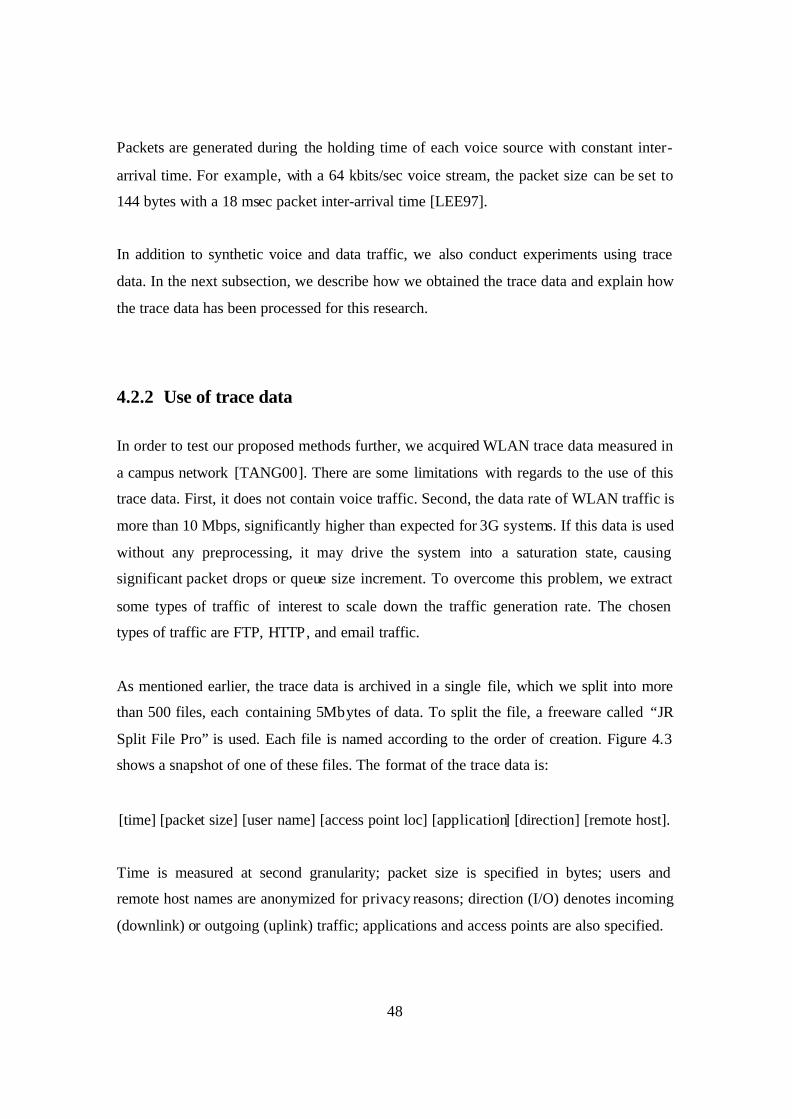
48

Packets are generated during the holding time of each voice source with constant inter-

arrival time. For example, with a 64 kbits/sec voice stream, the packet size can be set to

144 bytes with a 18 msec packet inter-arrival time [LEE97].

In addition to synthetic voice and data traffic, we also conduct experiments using trace

data. In the next subsection, we describe how we obtained the trace data and explain how

the trace data has been processed for this research.

4.2.2 Use of trace data

In order to test our proposed methods further, we acquired WLAN trace data measured in

a campus network [TANG00]. There are some limitations with regards to the use of this

trace data. First, it does not contain voice traffic. Second, the data rate of WLAN traffic is

more than 10 Mbps, significantly higher than expected for 3G systems. If this data is used

without any preprocessing, it may drive the system into a saturation state, causing

significant packet drops or queue size increment. To overcome this problem, we extract

some types of traffic of interest to scale down the traffic generation rate. The chosen

types of traffic are FTP, HTTP, and email traffic.

As mentioned earlier, the trace data is archived in a single file, which we split into more

than 500 files, each containing 5Mbytes of data. To split the file, a freeware called “JR

Split File Pro” is used. Each file is named according to the order of creation. Figure 4.3

shows a snapshot of one of these files. The format of the trace data is:

[time] [packet size] [user name] [access point loc] [application] [direction] [remote host].

Time is measured at second granularity; packet size is specified in bytes; users and

remote host names are anonymized for privacy reasons; direction (I/O) denotes incoming

(downlink) or outgoing (uplink) traffic; applications and access points are also specified.

49

Figure 4.3. Snapshot of trace data

Samples of each type of traffic in each link are included in appendix A, along with ACF

and PACF plots for each type of traffic: email, Web, and FTP traffic. Through these plots,

we can observe that each traffic type exhibits unique patterns of burstiness. These plots

also show the strong correlation between uplink and the downlink traffic, which may be

used as a feature for further development of slot allocation methods.

Using the synthetic traffic and the real trace data, we evaluate our proposed algorithms

for various scenarios. The experiment begins with simulations using synthetic data traffic,

as described in the next section.

4.3 Simulation on synthetic data traffic

In this section, we perform simulations on synthetic data traffic generated from on-off

sources. The primary objective of this simulation is to evaluate the proposed schemes

under different traffic asymmetry conditions. The secondary objective is to verify that our

simulator produces reasonable results in response to an input by simplifying input

50

parameters (e.g., just changing volumes for each link). If both links are configured with

different shape parameters, it may be difficult to check this, so the shape parameter is

fixed in this first simulation scenario. We fix 8.1=α and perform simulations for two

scenarios: (i) ud VV > ; (ii) ud VV >> . In each scenario, dV and uV represent the traffic

volume of the downlink and the uplink, respectively.

We adopt a FIFO scheduler in the experiments described in this section.

§ Scenario (i) First, we perform a simulation when =α 1.8 and the downlink has relatively more traffic

than the uplink ( dV > uV ). To vary traffic load in each link ( dV and uV ) and to make

dV > uV , the downlink (uplink) traffic is generated by the superposition of seven (five)

on/off sources with Pareto-distributed on and off times. The target transmission rate for

the traffic sources in each link is varied to change the traffic volume. Other parameters

such as average on-off times, shape, and packet size are fixed for each link. These

simulation parameters and values are summarized in Table 4.2. Simulation results are

analyzed in terms of throughput and packet drop ratio response.

Table 4.2 Simulation parameters for each link and values

Uplink parameters Mean on/off times(in sec) 1/1 Shape 1.8 Transmission rate(bits/sec) Variable Packet size (bytes) 1500 Number of traffic sources 5 Downlink parameters Mean on/off times(in sec) 1/1 Shape 1.8 Transmission rate(bits/sec) Variable Packet size (bytes) 1500 Number of traffic sources 7 Common parameters Length of frame (in msec) 160 Number of slots per frame 16

51

Number of maximum packets per slot 8 Simulation duration (in number of frames) 2000 Number of simulation runs for each arrival rate 5 times Observation window size (in number of frames) Variable Scheduler FIFO

Uplink simulation results are given at the top of Figure 4.4 for the throughput response

and at the bottom of Figure 4.4 for the packet drop ratio response. 95% confidence

intervals are calculated for each arrival rate and also shown in the plot. The two proposed

methods (B: Burstiness and BV: Burstiness-Volume) yield higher throughput than the

volume-based method (denoted as V) and result in fewer packet drops. This comes from

the pro-downlink nature of the method V, which results in under-allocation of resources

for the uplink. The method V is designed under the assumption that the downlink

dominantly carries more traffic than the uplink [JEONG00].

Downlink simulation results are provided in Figure 4.5. It shows that the method V

outperforms the proposed B and BV strategies due to the reason explained above. All

three methods have fewer packet drops in the downlink than in the uplink. In these

simulations, the method B results in slightly higher throughput and lower packet drop

ratio than the method BV.

Aggregate throughput and packet drop ratio are plotted in Figure 4.6. Simulation results

show that the method B yields around 10% higher aggregate throughput than the method

V at the highest arrival rate. Similarly, the method BV yields 5% higher throughput as

compared to slot allocation based on traffic volume only. Consequently, the volume-

based scheme results in higher packet losses as compared to the proposed schemes.

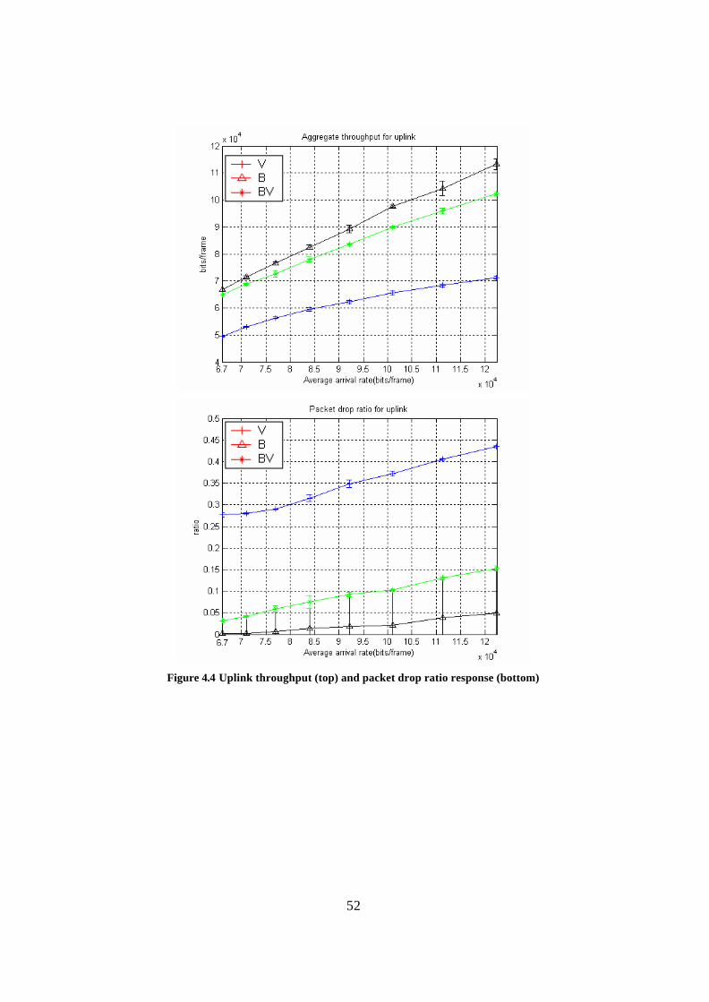
52

Figure 4.4 Uplink throughput (top) and packet drop ratio response (bottom)

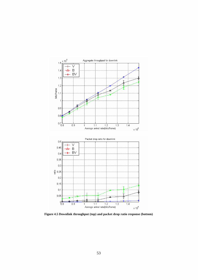
53

Figure 4.5 Downlink throughput (top) and packet drop ratio response (bottom)

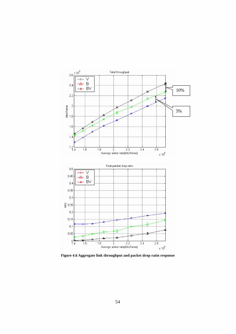
54

Figure 4.6 Aggregate link throughput and packet drop ratio response

10%

5%

55

§ Scenario (ii)

A similar simulation is performed to evaluate the performance of the proposed strategies

when the downlink traffic volume is almost twice that of the uplink. Parameters for this

simulation are given in Table 4.3. Again, the arrival rate of traffic for each link is

controlled by the transmission rate. Other simulation parameters are the same as Table

4.2.

Table 4.3 Simulation parameters

Uplink Number of traffic sources 5 Mean on/off times(in sec) 1/1 Transmission rate(bits/sec) Variable Packet size (bytes) 15000 Shape 1.8 Downlink Number of traffic sources 9 Mean on/off times(in sec) 1/1 Transmission rate(bits/sec) Variable Packet size (bytes) 15000 Shape 1.8

As shown in the uplink response in Figure 4.7, the performance of the method B and the

method BV is better in the uplink than the method V, with fewer packet drops and higher

throughput as compared to the V method.

In the downlink response (Figure 4.8), the throughput of the method V is significantly

superior to that obtained with methods B and BV. That difference in performance is more

pronounced than in scenario (i) (Figure 4.5). This results from the increased number of

on/off traffic sources in the downlink, from 7 to 9, while the number of sources in the

uplink is fixed at 5.

In the aggregate throughput and packet drop response (Figure 4.9), the proposed schemes

show better results until traffic load reaches the maximum capacity of the system, which

is around 2 Mbps. When the traffic load reaches around the maximum system capacity,

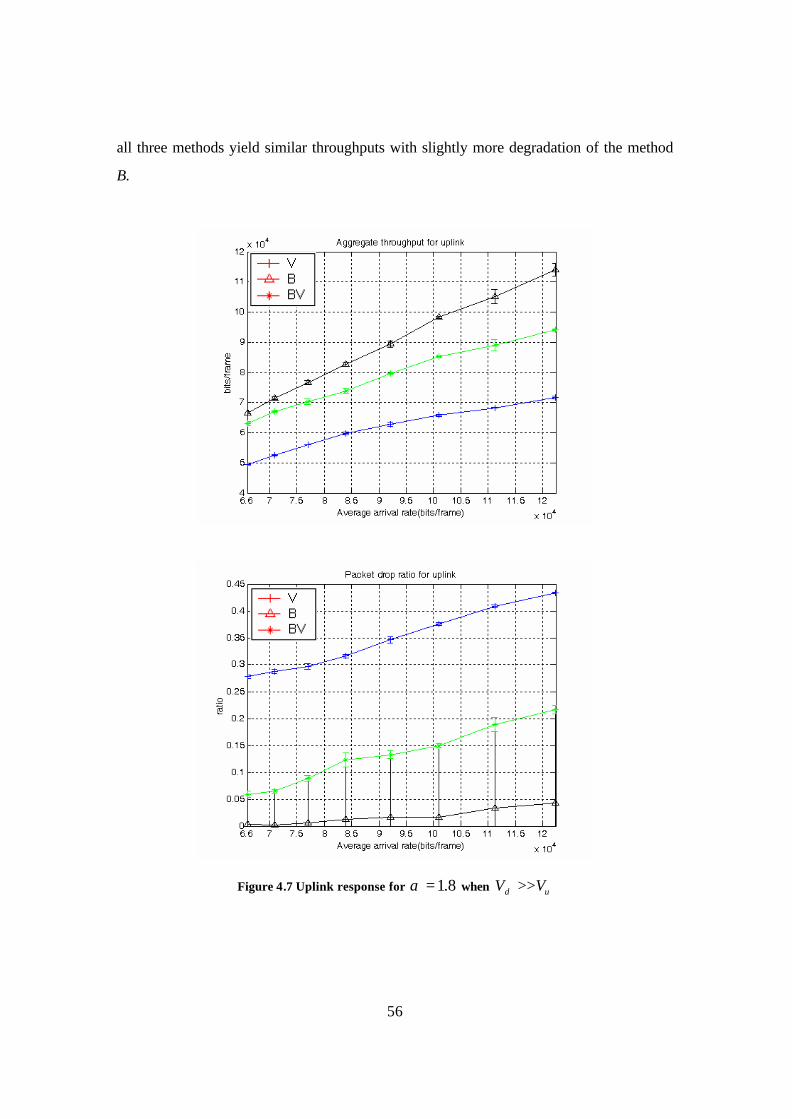
56

all three methods yield similar throughputs with slightly more degradation of the method

B.

Figure 4.7 Uplink response for 8.1=α when ud VV >>

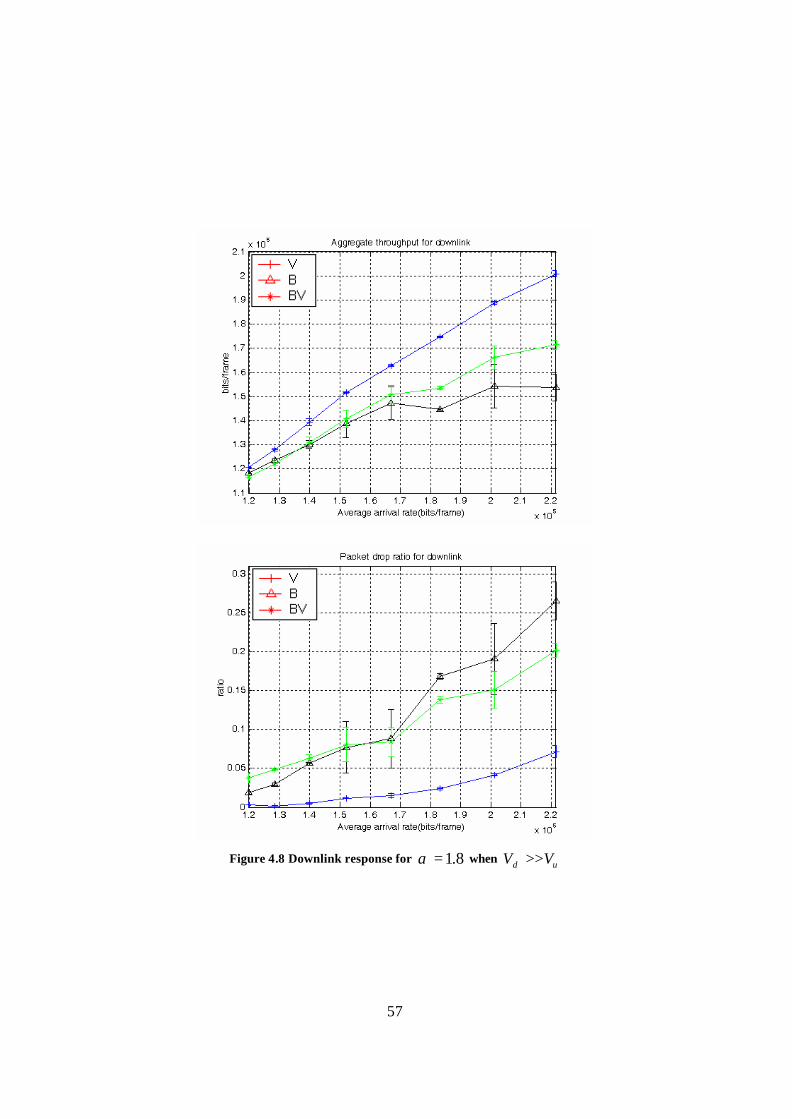
57

Figure 4.8 Downlink response for 8.1=α when ud VV >>

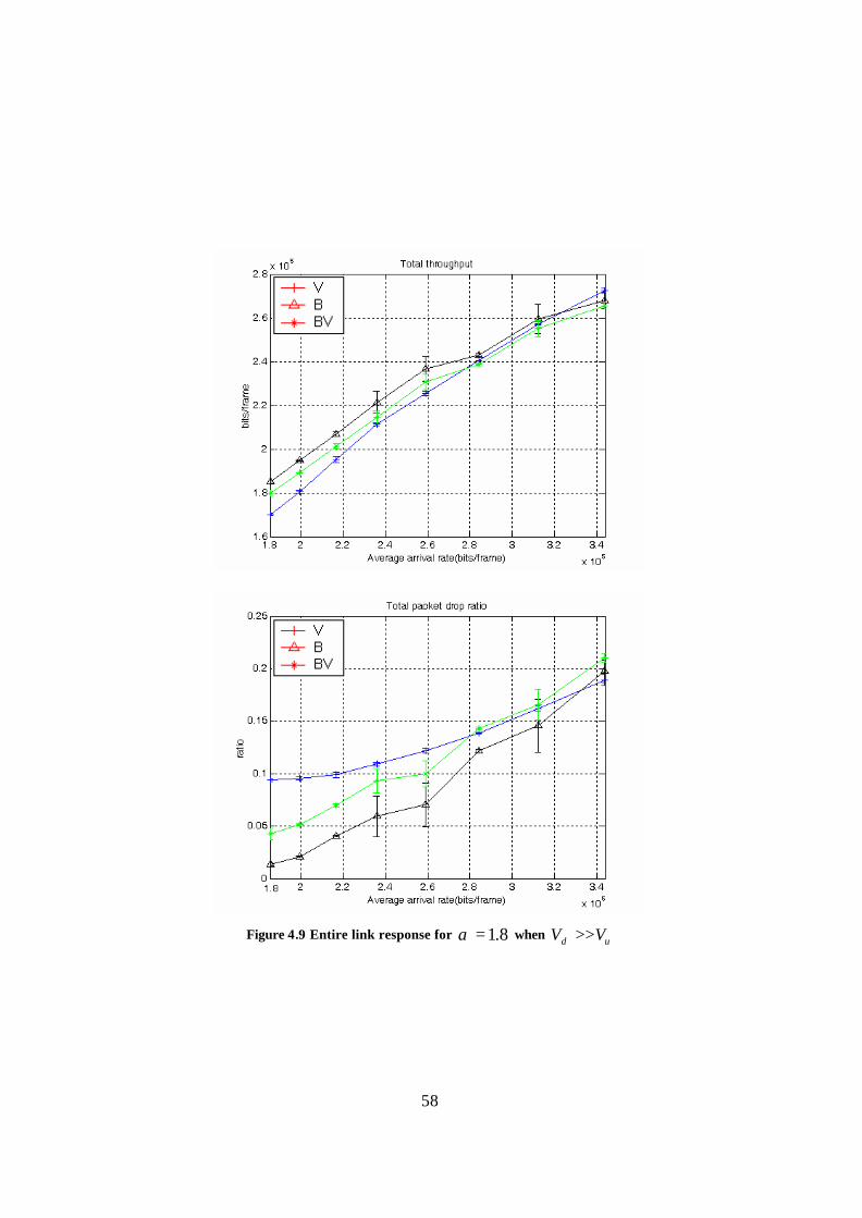
58

Figure 4.9 Entire link response for 8.1=α when ud VV >>

59

4.4 Simulation on combined voice and data traffic

In Section 4.3, we have demonstrated the performance of the proposed strategies in

comparison to a volume-based scheme for data traffic under various scenarios. In practice,

voice traffic can coexist with data traffic and sometimes represents the majority of traffic

in the uplink in wireless mobile networks.

We simulate the effect of combined voice and data traffic for the following scenarios: (i)

uplink traffic is less bursty than downlink traffic, and ud VV > ; (ii) burstiness in both

links is equal, and ud VV > ; and (iii) uplink traffic is less bursty than downlink traffic, and

ud VV >> . All three simulations yield similar results on throughput and packet drop ratio,

so we discuss the first scenario only. Again, the bustiness is controlled by the shape

parameter in our experiment, a traffic is controlled primarily by changing the number of

voice traffic sources and the number of data traffic sources. The voice traffic is generated

by the superposition of sources with Poisson call arrivals, each having an exponentially

distributed holding time. The data traffic is generated in the same way as described in the

previous section.

Again, the performance of each method is evaluated in terms of throughput and packet

drop ratio. In addition to these metrics, we evaluate the signaling load generated by each

method for conveying slot allocation information between the base station and the

mobiles. Simulation parameters are listed in Table 4.4.

Table 4.4 Simulation parameters and values for voice and data traffic simulation

Uplink Number of data traffic sources 3 Number of voice traffic sources 1-8 Packet inter-arrival time of voice traffic(msec) 18 Packet size of voice traffic (bytes) 144 Mean on/off times of data traffic (sec) 1/1 Transmission rate of data traffic(bits/sec) 3000 Packet size of data traffic(bytes) 15000

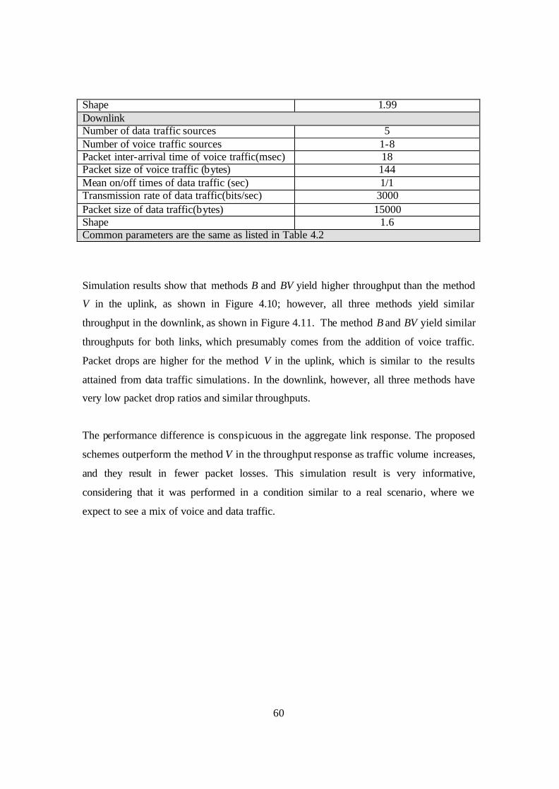
60

Shape 1.99 Downlink Number of data traffic sources 5 Number of voice traffic sources 1-8 Packet inter-arrival time of voice traffic(msec) 18 Packet size of voice traffic (bytes) 144 Mean on/off times of data traffic (sec) 1/1 Transmission rate of data traffic(bits/sec) 3000 Packet size of data traffic(bytes) 15000 Shape 1.6 Common parameters are the same as listed in Table 4.2

Simulation results show that methods B and BV yield higher throughput than the method

V in the uplink, as shown in Figure 4.10; however, all three methods yield similar

throughput in the downlink, as shown in Figure 4.11. The method B and BV yield similar

throughputs for both links, which presumably comes from the addition of voice traffic.

Packet drops are higher for the method V in the uplink, which is similar to the results

attained from data traffic simulations. In the downlink, however, all three methods have

very low packet drop ratios and similar throughputs.

The performance difference is conspicuous in the aggregate link response. The proposed

schemes outperform the method V in the throughput response as traffic volume increases,

and they result in fewer packet losses. This simulation result is very informative,

considering that it was performed in a condition similar to a real scenario, where we

expect to see a mix of voice and data traffic.

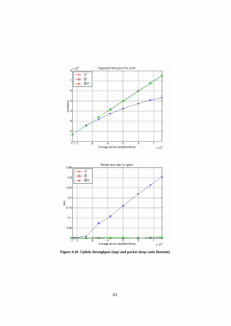
61

Figure 4.10. Uplink throughput (top) and packet drop ratio (bottom)

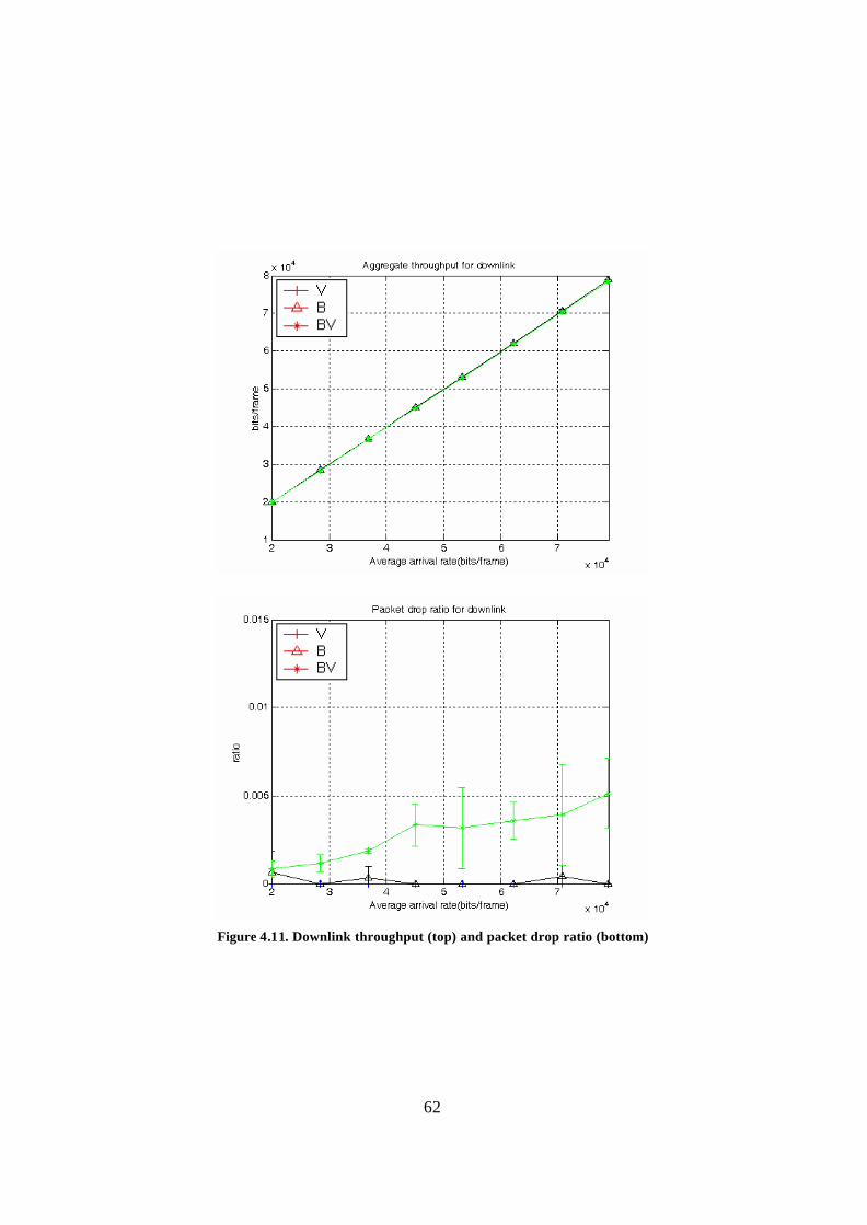
62

Figure 4.11. Downlink throughput (top) and packet drop ratio (bottom)

63

Figure 4.12. Entire link throughput (top) and packet drop ratio (bottom)

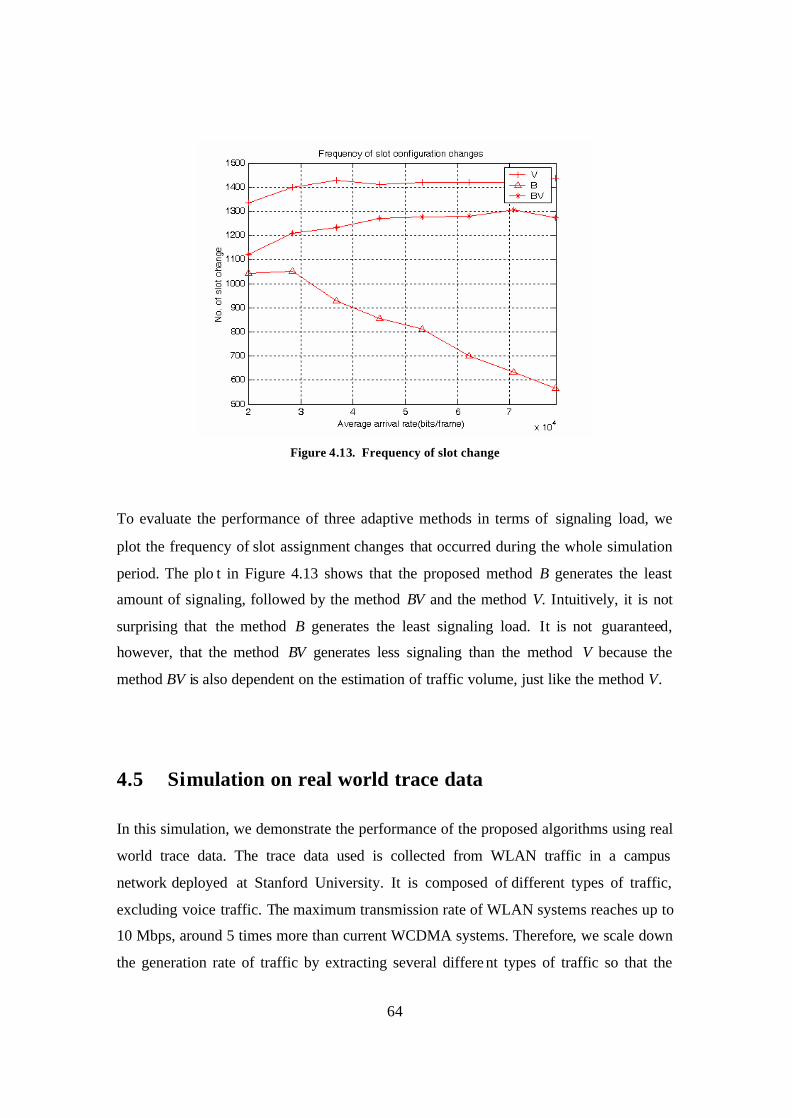
64

Figure 4.13. Frequency of slot change

To evaluate the performance of three adaptive methods in terms of signaling load, we

plot the frequency of slot assignment changes that occurred during the whole simulation

period. The plo t in Figure 4.13 shows that the proposed method B generates the least

amount of signaling, followed by the method BV and the method V. Intuitively, it is not

surprising that the method B generates the least signaling load. It is not guaranteed,

however, that the method BV generates less signaling than the method V because the

method BV is also dependent on the estimation of traffic volume, just like the method V.

4.5 Simulation on real world trace data

In this simulation, we demonstrate the performance of the proposed algorithms using real

world trace data. The trace data used is collected from WLAN traffic in a campus

network deployed at Stanford University. It is composed of different types of traffic,

excluding voice traffic. The maximum transmission rate of WLAN systems reaches up to

10 Mbps, around 5 times more than current WCDMA systems. Therefore, we scale down

the generation rate of traffic by extracting several differe nt types of traffic so that the

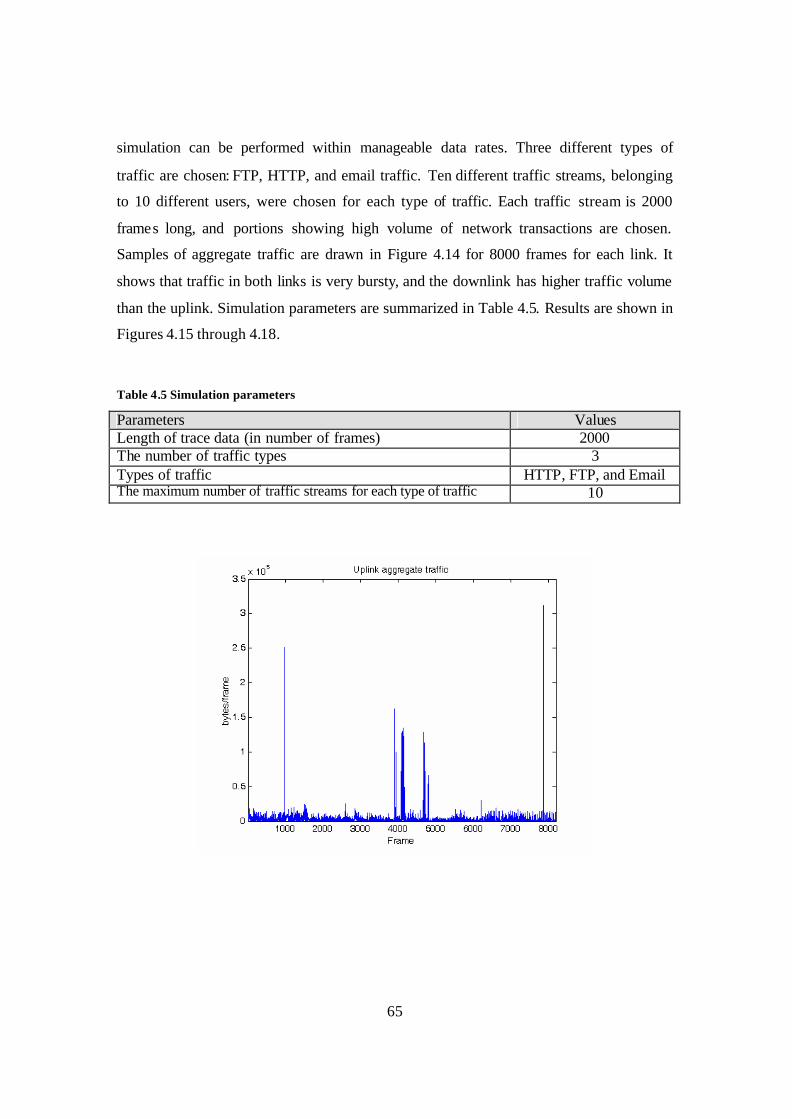
65

simulation can be performed within manageable data rates. Three different types of

traffic are chosen: FTP, HTTP, and email traffic. Ten different traffic streams, belonging

to 10 different users, were chosen for each type of traffic. Each traffic stream is 2000

frames long, and portions showing high volume of network transactions are chosen.

Samples of aggregate traffic are drawn in Figure 4.14 for 8000 frames for each link. It

shows that traffic in both links is very bursty, and the downlink has higher traffic volume

than the uplink. Simulation parameters are summarized in Table 4.5. Results are shown in

Figures 4.15 through 4.18.


Parameters Values Length of trace data (in number of frames) 2000 The number of traffic types 3 Types of traffic HTTP, FTP, and Email The maximum number of traffic streams for each type of traffic 10

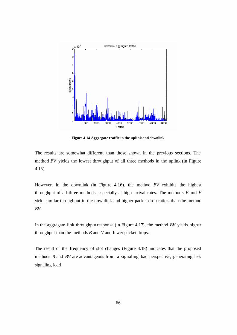
66

Figure 4.14 Aggregate traffic in the uplink and downlink

The results are somewhat different than those shown in the previous sections. The

method BV yields the lowest throughput of all three methods in the uplink (in Figure

4.15).

However, in the downlink (in Figure 4.16), the method BV exhibits the highest

throughput of all three methods, especially at high arrival rates. The methods B and V

yield similar throughput in the downlink and higher packet drop ratio s than the method

BV.

In the aggregate link throughput response (in Figure 4.17), the method BV yields higher

throughput than the methods B and V and fewer packet drops.

The result of the frequency of slot changes (Figure 4.18) indicates that the proposed

methods B and BV are advantageous from a signaling load perspective, generating less

signaling load.

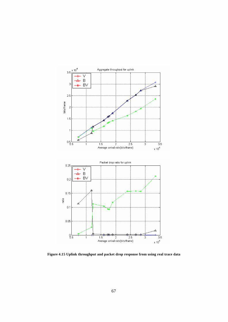
67

Figure 4.15 Uplink throughput and packet drop response from using real trace data

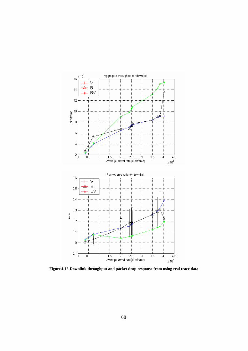
68

Figure 4.16 Downlink throughput and packet drop response from using real trace data

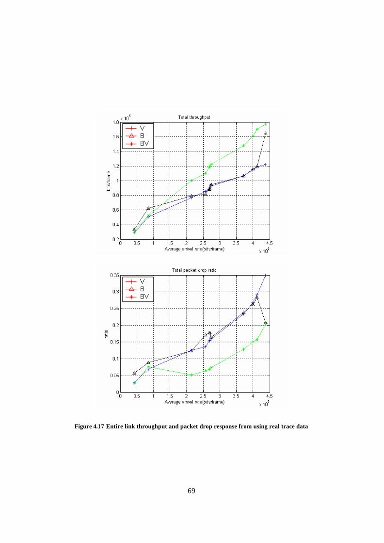
69

Figure 4.17 Entire link throughput and packet drop response from using real trace data

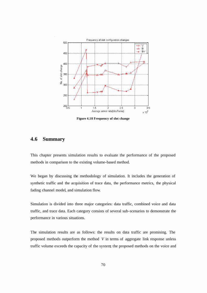
70

Figure 4.18 Frequency of slot change

4.6 Summary

This chapter presents simulation results to evaluate the performance of the proposed

methods in comparison to the existing volume-based method.

We began by discussing the methodology of simulation. It includes the generation of

synthetic traffic and the acquisition of trace data, the performance metrics, the physical

fading channel model, and simulation flow.

Simulation is divided into three major categories: data traffic, combined voice and data

traffic, and trace data. Each category consists of several sub-scenarios to demonstrate the

performance in various situations.

The simulation results are as follows: the results on data traffic are promising. The

proposed methods outperform the method V in terms of aggregate link response unless

traffic volume exceeds the capacity of the system; the proposed methods on the voice and

71

the data traffic are also promising compared to the volume-based method from the

aggregate link perspective. And the method B generates the least signaling load, followed

by the methods BV and V in succession; in the trace data simulation, the method BV

yields higher throughput than the methods B and V and generates the least signaling load.

But the method B yield similar throughput with the method V because of higher

burstiness of uplink traffic.

72

Chapter 5 Slot allocation based on parameter

estimation

In this chapter, we introduce two new strategies for slot allocation based on the parameter

estimation of distribution of traffic. Modern traffic has been modeled with a long-tail

distributed probability model such as Pareto distribution. Accurate and reliable estimation

of the distribution can enable various types of resource allocation tasks such as slot

allocation. In this research, we develop several robust estimators for the Pareto

distribution and compare the performance of those estimators to existing estimators. The

performance of each estimator is evaluated by various performance measures such as root

mean-squared error (RMSE) and variance of the estimator, etc. We also incorporate one

of the estimators into a slot allocation process and present new slot allocation methods

based on that. The performance of the new slot allocation methods is compared to our

previous methods in terms of throughput and packet drop ratio.

This chapter begins by discussing the background of parameter estimation in relation to

slot allocation in Section 5.1. In Section 5.2, we introduce our generalized maximum

likelihood estimator of Pareto distribution. In Section 5.3, we propose three generalized

moment estimators for Pareto distribution. The evaluation of the estimators is given in

Section 5.4 with discussions. In Section 5.5, we incorporate the estimators into a slot

allocation process and demonstrate the performance of new slot allocation methods.

Finally, we present the summary of this chapter in Section 5.6.

5.1 Background

In Chapter 3, we allocated the number of slots for the uplink and the downlink by

estimating burstiness for each link evaluated based on dynamic observation window.

73

Here, we introduce several estimators for a distribution of traffic to allocate slots for each

link by using the estimated parameters in both links. As described earlier, modern traffic

has been modeled by a heavy-tailed distribution model such as Pareto distribution, which

is characterized by shape and location parameters. The shape parameter determines the

shape of decay of the distribution; that is, when the shape parameter becomes smaller, the

distribution decays very slowly and vice versa. Often times, the heavy-tailed distribution

model is compared to a short-tail distribution model such as exponential distribution

where the decay of the distribution becomes fast. The location parameter represents the

minimum value of the distribution by the definition of Pareto distribution. The estimation

of these two parameters enables various types of resource allocation tasks such as slot

allocation. For example, we can we can compute a constraint value T of an outage

probability ( )oP of a traffic distribution (assuming oP is given) and allocate slots based on

the constraint values of each link. This is described in detail in Section 5.5.

In this research, we introduce two new estimators that estimate, primarily, the shape

parameter of Pareto distribution to be used for the calculation of slots for each link. We

first introduce a generalized maximum likelihood estimator (MLE) for Pareto distribution.

Next, we propose three generalized moment estimators (GME) for the Pareto distribution.

The generalized moment estimation techniques have been proposed in

[GAEDDERT04][CHENG02], primarily developed for fading parameter estimation.

Here, we develop new generalized moment estimators for Pareto distribution. The

performance of these estimators is compared to each other and to other well-known

estimators.

5.2 Generalized maximum likelihood estimator for Pareto

distribution

Generalized maximum likelihood estimator (GMLE) seeks to estimate the shape and

location parameters of Pareto distribution from given N independent and identically

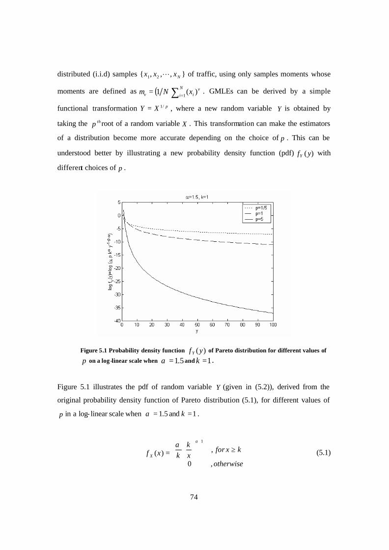
74

distributed (i.i.d) samples Nxxx ,,, 21 L of traffic, using only samples moments whose

moments are defined as ( )∑ ==

N

iv

iv xN1

)(1µ . GMLEs can be derived by a simple

functional transformation pXY /1= , where a new random variable Y is obtained by

taking the thp root of a random variable X . This transformation can make the estimators

of a distribution become more accurate depending on the choice of p . This can be

understood better by illustrating a new probability density function (pdf) )(yfY with

different choices of p .

Figure 5.1 Probability density function )(yf Y of Pareto distribution for different values of

p on a log-linear scale when 5.1=α and 1=k .

Figure 5.1 illustrates the pdf of random variable Y (given in (5.2)), derived from the

original probability density function of Pareto distribution (5.1), for different values of

p in a log- linear scale when 5.1=α and 1=k .

≥

=

+

otherwise

kxforxk

kxf X

,0

,)(

1αα (5.1)

75

where 0>α and 0>k .

The new pdf )(yfY can be derived as:

0,0,,)( /11

>>>=+

kkyypkyf p

pY ααα

α

(5.2)

Derivation of (5.2) is given in the appendix. Figure 5.1 shows that depending on p , the

pdf decays faster or more slowly; when p is larger, the distribution decays fast and vice

versa, indicating that higher p significantly mitigates the impact of outliers compared to

lower p. Later in our experiment, we demonstrate that higher p reduces the susceptibility

of estimators caused by outliers through the evaluation of our estimators, so it can

increase the accuracy of the estimators. In particular in Figure 5.1, a plot for 1=p

corresponds to original Pareto distribution.

Generalized maximum likelihood estimator (GMLE) of the Pareto distribution can be

derived using the new pdf )(yfY . From (5.2), the likelihood function L of the Pareto

distribution can be expressed as:

( ) ∏=

+

=

N

ip

i

N

N ypkyyyL

11,2,11);,(

ααααL (5.3)

where Nyyy ,,2,1 L are the samples of a random variable Y by the transformation

pXY /1= .

Since maximizing )ln( L is equivalent to maximizing L itself, we can take the natural

logarithm of both sides of (5.3):

i

N

i

ypkpNL ∑=

+−++=1

ln)1(lnlnlnln ααα . (5.4)

Then, taking the derivative of Lln with respect to α , and setting it equal to zero, we have:

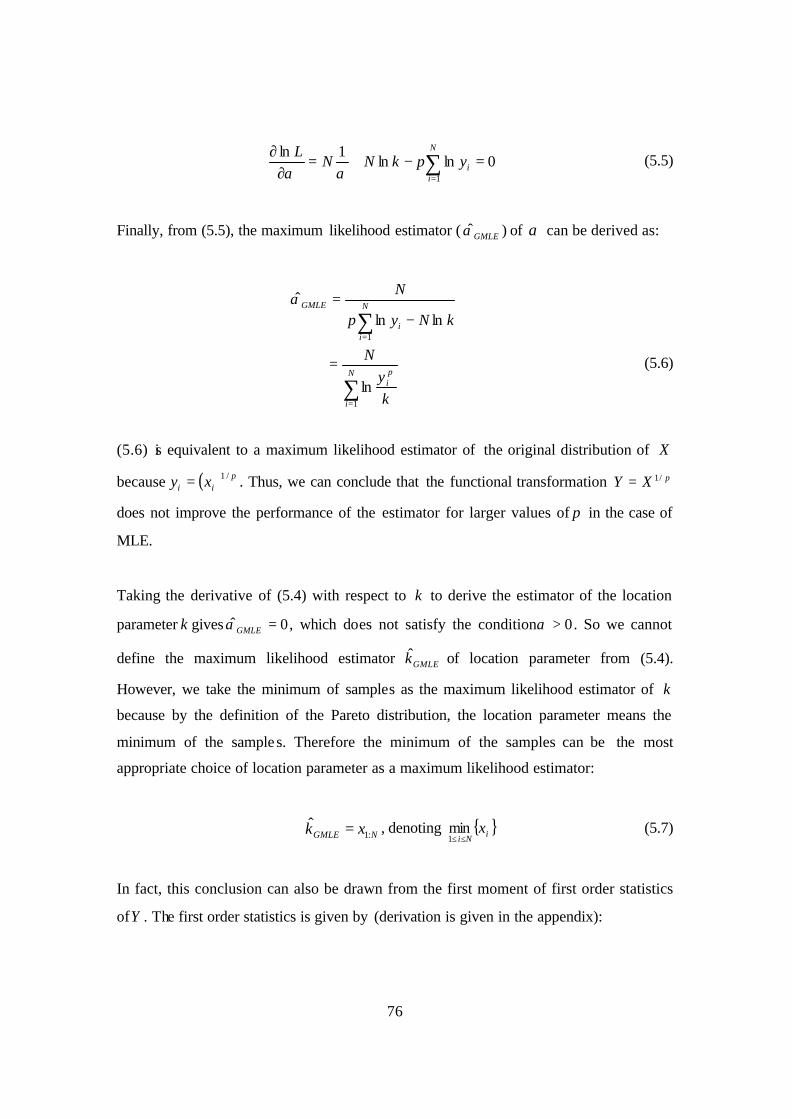
76

0lnln1ln

1

=−+=∂

∂ ∑=

N

iiypkNN

Lαα

(5.5)

Finally, from (5.5), the maximum likelihood estimator ( GMLEα ) of α can be derived as:

∑

∑

=

=

=

−=

N

i

pi

N

ii

GMLE

ky

N

kNyp

N

1

1

ln

lnlnα

(5.6)

(5.6) is equivalent to a maximum likelihood estimator of the original distribution of X

because ( ) pii xy /1= . Thus, we can conclude that the functional transformation pXY /1=

does not improve the performance of the estimator for larger values of p in the case of

MLE.

Taking the derivative of (5.4) with respect to k to derive the estimator of the location

parameter k gives 0ˆ =GMLEα , which does not satisfy the condition 0>α . So we cannot

define the maximum likelihood estimator GMLEk of location parameter from (5.4).

However, we take the minimum of samples as the maximum likelihood estimator of k

because by the definition of the Pareto distribution, the location parameter means the

minimum of the samples. Therefore the minimum of the samples can be the most

appropriate choice of location parameter as a maximum likelihood estimator:

NGMLE xk :1ˆ = , denoting iNi

x≤≤1

min (5.7)

In fact, this conclusion can also be drawn from the first moment of first order statistics

ofY . The first order statistics is given by (derivation is given in the appendix):

77

[ ]

∞

>−=

otherwise

vpN

pNv

k

YE

pv

vN

,

,/

:1

αα

α

(5.8)

Then, the first moment, derivable when 1=v in (5.8), has the following relation:

[ ] 1,1

/1:1:1

/11:1 >==

−= pNxy

pN

kYE p

NN

p

N αα

α (5.9)

where Ny :1 denotes iNiy

≤≤1min .

In particular when ∞→N in (5.9), Nxk :1= . Therefore it makes sense to choose the

minimum of samples as the maximum likelihood estimator of the location parameter. The

performance of the estimator GMLEα is evaluated by various criteria in our numerical

experiments.

5.3 Generalized moment estimator for Pareto distribution

A moment estimator of the shape parameter from samples of Pareto random variable was

suggested by [QUANDT66]. He equated the sample minimum and the sample mean to

their corresponding expectations and solved for the shape parameter ( α ) and the location

parameter ( k ). This procedure, however, only applies when first moments exist

(i.e., 1>α ). Recently, a comparative study of various types of estimation techniques for

Pareto distributions was conducted by [RAHMAN03], including the moment estimator

and the maximum likelihood estimator. He ranked the performance of each estimator by

various criteria, including root mean-squared error (RMSE).

In this subsection, we develop three different types of generalized moment estimator

(GME) for the Pareto distribution.

78

The GME can be derived in a similar way to that of the GMLE. Given N i.i.d. samples

Nxxx ,,, 21 L of traffic data, moment-based estimators seek to estimate parameters of

Pareto distribution using only the sample moments of random traffic volume X , again

defined as ( )∑ ==

N

iv

iv xN1

)(1µ . In [CHENG02], Cheng and Beaulieu showed that better

moment-based estimators can be found by adopting the use of non- integer (fractional)

moments. The thv moment of a Pareto distribution can be derived as:

[ ]

∞

>−⋅

==otherwise

vv

kXE

v

vv

,

, ααα

µ (5.10)

Meanwhile, the thv fractional moment of the Pareto distribution can be derived by

evaluating ][ vYE using (5.2):

∞

>−==

otherwise

vppv

kYE

pv

pvv

,

,/][

/

/α

αα

µ (5.11)

In (5.11), especially when 1=v (for the lowest order moment),

1,1

/1

/1 >−

= pp

k p

p αα

αµ (5.12)

From (5.12), we can easily derive a generalized moment estimator ( FGMEα ) of shape

parameter as:

pp

p

FGME kp

/1/1

/11

ˆ−

⋅

=µ

µα . (5.13)

79

We call this a first generalized moment estimator (FGME) of the Pareto distribution

hereon. For k , we use Nxk :1= in (5.13) based on the reason given in Subsection 5.2.

p/1µ can be calculated from the sample moments.

Another GME can be derived from the thv moment of first order statistics ofY , which is

again given by:

vpN

pNv

kYE

pvvN >

−= α

α

α,][

/

:1 (5.14)

Detailed derivation of (5.14) is given in the appendix.

From (5.14), we have the following relation (same as (5.9)):

1,1

][ :1

/11:1 >=

−= pNy

pN

kYE N

p

N αα

α (5.15)

Meanwhile, k can be derived from (5.12) as:

p

p

pk

−= 1/1 α

α

µ (5.16)

By substituting (5.16) into (5.15), we can derive a new estimator of α as follows:

[ ]Np

NpSGME ypN

yN

:1/1

:1/1ˆ−

−=

µ

µα (5.17)

where again pN

ppNN xxxyyyy /1/1

2/1

121:1 ,,,min,,,min LL == .

We call this a second generalized moment estimator (SGME) of Pareto distribution.

80

As a special case, when 1=p , (5.17) can be equal to the integer moment estimator

( QMEα ) proposed in [QUANDT66] where the first moment is used as follows:

( )N

NQME xN

xN

:11

:11ˆ−−

=µµ

α (5.18)

where N denotes the total number of samples and 1µ is the first moment of a distribution.

Our developed FGME, SGME, and GMLE can be used for various applications. For

example, it can be used as means for slot allocations. For this purpose, one of these

estimators, showing the best performance, will be chosen to be used for the slot allocation.

As an analytical way to prove that the slot allocation can be further improved by

incorporating these estimators than what we have demonstrated so far, we develop

another estimator (named Third GME (TGME)) that can be derived from peak/median

relationship. By comparing the performance of TGME with the best (i.e., GMLE) of our

estimators, we can indirectly predict that the slot allocation based on GMLE may achieve

better performance than the one based on TGME. In other words, if the performance of

the best of GMLE, FGME, or SGME is better than the one of TGME, we can confirm

that the slot allocation based on the best of GMLE, FGME, or SGME can achieve better

performance than the one based on TGME.

We begin by deriving the thv moment of the thN order statistics of Y as follows (derivation

is available in the appendix):

+= 1;1;,][ 12

/: NN

pv

FkYE pvvNN α

(5.19)

81

where )1;;,(12 cbaF is the confluent hypergeometric function1 of the second kind (in [GRADSHTEYN93]).

In );;,(12 dcbaF , if )Re()Re( bac +> , then we can obtain the following relation:

( ) ( ) ( )( ) ( )2 1 , ; ;1c c a b

F a b cc a c b

Γ Γ − −=

Γ − Γ − (5.20)

Using (5.20), (5.19) can be written as:

( )

( )

/ /

/2 1

1 1 ! 1, ;1 ;1

1 1 1

p p

p

k N k Np p

k F N Np

N Np p

ν ν

ν

ν να αν

α ν να α

Γ + Γ − Γ − + = = Γ + − Γ Γ + −

NNy := (5.21)

where iNiNN yy

≤≤=

1: max and N is the number of samples.

When v=1 in (5.21), we have:

NN

p

y

pN

pNk

:

/1

11

11!=

−+Γ

−Γ

α

α (5.22)

Now, we can establish a peak/median relationship as follows:

1

11

11!/1

1

:

−

−+Γ

−Γ

=

αα

ααµ k

pN

pNk

yp

NN (5.23)

where )(⋅Γ is a gamma function.

1 ( )

( )1

2 10, ;1 ;

1

u x udx F ux

µ µ

νν µ µ β

µβ

−

= + −+∫ with ( )arg 1 ,Re[ ] 0uβ π µ+ < > in

([GRADSHTEYN93], Eq.(3.194.1))

82

In (5.23), we know the values of Nxk :1= (from MLE), 1µ , p (any positive number), N (the

number of samples), iNiNN yy≤≤

=1: max (the maximum of samples). The only unknown is the

shape parameterα . Unfortunately, we cannot derive a closed form solution ofα to find

an estimator TGMEα because of the gamma function. Instead, we simply find TGMEα where

(5.23) is satisfied by increasing α in a fine resolution between 1.1 and 10; the resolution

of the increment of α is chosen as e-2. We call this third generalized moment estimator

(TGME).

Meanwhile, our generalized estimators including TGME have lots of advantages

compared to the integer estimator derived by [QUANDT66]. First, our estimators are

generalized for any moment (integer or fractional). Second, our estimators are

generalized for any α . The method in [QUANDT66], however, is restricted by 1>α ,

which means that this estimator cannot be used for 1≤α because the first moment does

not exist for this range ofα . Next, the performances of our estimators given in (5.13),

(5.17), and (5.23) are compared to the integer estimator in our experiments depending on

different values of p .

5.4 Numerical experiment of the estimators

Our proposed estimators are evaluated by several performance criteria in comparison to

other estimators that include MLE and QGME. First, we evaluate the logarithm of root

mean-squared error (RMSE) of the estimators depending on the sample size N , where

RMSE is defined as:

∑=

−=m

kkm

RMSE1

2)ˆ(1

)( ααα (5.24)

where m is the number of independent estimates of the estimator, kα is an estimated

shape parameter, and α is original shape parameter.

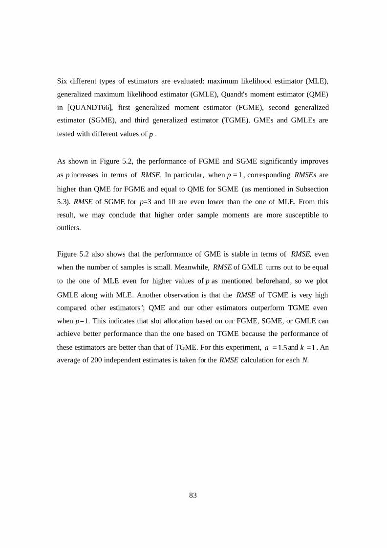
83

Six different types of estimators are evaluated: maximum likelihood estimator (MLE),

generalized maximum likelihood estimator (GMLE), Quandt’s moment estimator (QME)

in [QUANDT66], first generalized moment estimator (FGME), second generalized

estimator (SGME), and third generalized estimator (TGME). GMEs and GMLEs are

tested with different values of p .

As shown in Figure 5.2, the performance of FGME and SGME significantly improves

as p increases in terms of RMSE. In particular, when 1=p , corresponding RMSEs are

higher than QME for FGME and equal to QME for SGME (as mentioned in Subsection

5.3). RMSE of SGME for p=3 and 10 are even lower than the one of MLE. From this

result, we may conclude that higher order sample moments are more susceptible to

outliers.

Figure 5.2 also shows that the performance of GME is stable in terms of RMSE, even

when the number of samples is small. Meanwhile, RMSE of GMLE turns out to be equal

to the one of MLE even for higher values of p as mentioned beforehand, so we plot

GMLE along with MLE. Another observation is that the RMSE of TGME is very high

compared other estimators’; QME and our other estimators outperform TGME even

when p=1. This indicates that slot allocation based on our FGME, SGME, or GMLE can

achieve better performance than the one based on TGME because the performance of

these estimators are better than that of TGME. For this experiment, 5.1=α and 1=k . An

average of 200 independent estimates is taken for the RMSE calculation for each N.

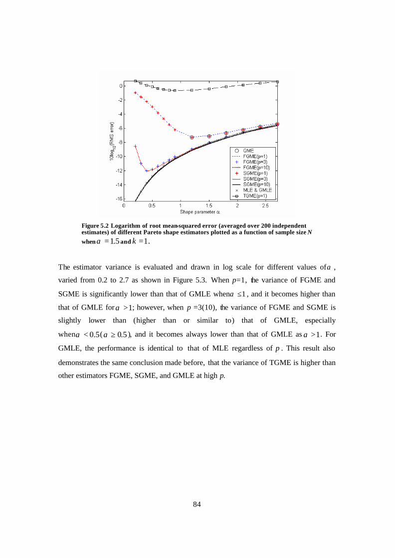
84

Figure 5.2 Logarithm of root mean-squared error (averaged over 200 independent estimates) of different Pareto shape estimators plotted as a function of sample size N when 5.1=α and 1=k .

The estimator variance is evaluated and drawn in log scale for different values ofα ,

varied from 0.2 to 2.7 as shown in Figure 5.3. When p=1, the variance of FGME and

SGME is significantly lower than that of GMLE when 1≤α , and it becomes higher than

that of GMLE for 1>α ; however, when p =3(10), the variance of FGME and SGME is

slightly lower than (higher than or similar to) that of GMLE, especially

when 5.0<α ( 5.0≥α ), and it becomes always lower than that of GMLE as 1>α . For

GMLE, the performance is identical to that of MLE regardless of p . This result also

demonstrates the same conclusion made before, that the variance of TGME is higher than

other estimators FGME, SGME, and GMLE at high p.

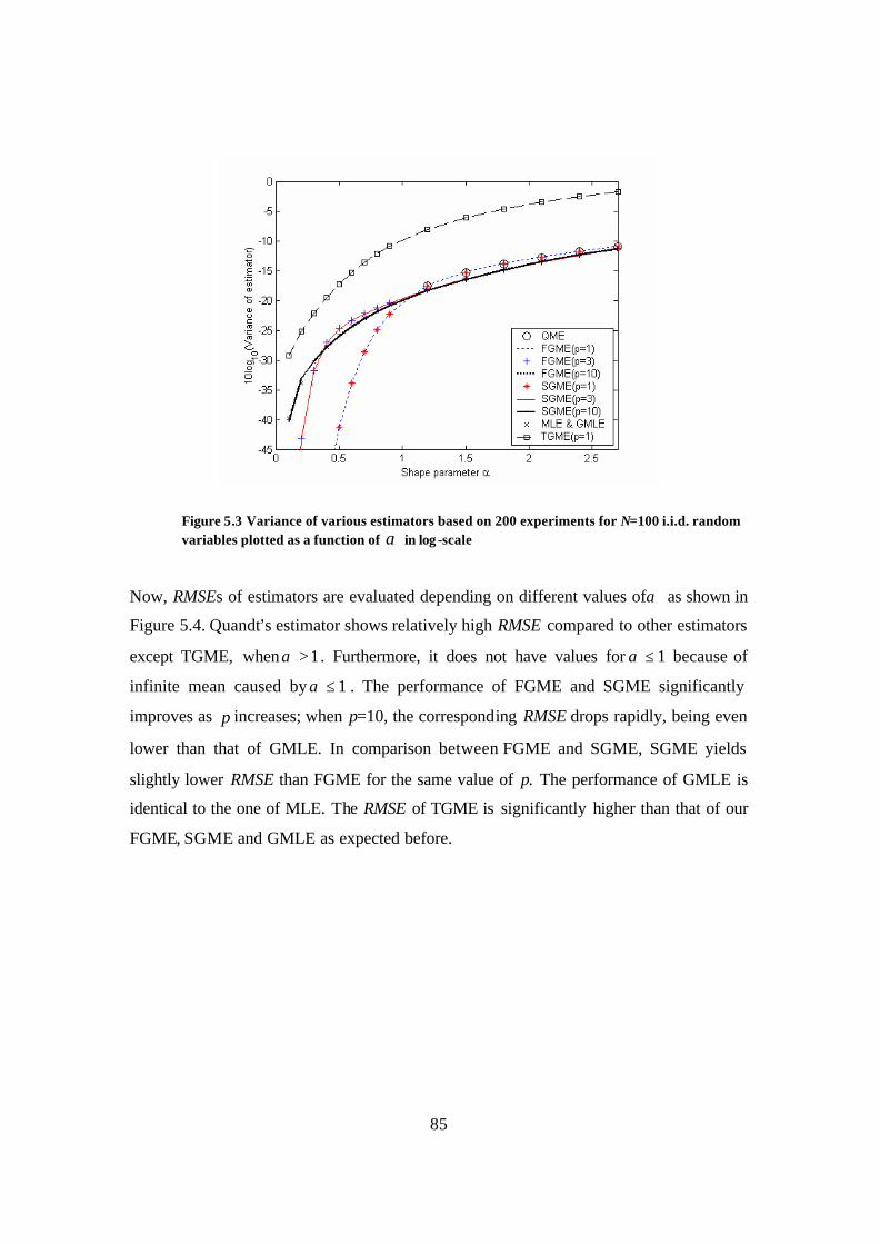
85

Figure 5.3 Variance of various estimators based on 200 experiments for N=100 i.i.d. random variables plotted as a function of α in log -scale

Now, RMSEs of estimators are evaluated depending on different values ofα as shown in

Figure 5.4. Quandt’s estimator shows relatively high RMSE compared to other estimators

except TGME, when 1>α . Furthermore, it does not have values for 1≤α because of

infinite mean caused by 1≤α . The performance of FGME and SGME significantly

improves as p increases; when p=10, the corresponding RMSE drops rapidly, being even

lower than that of GMLE. In comparison between FGME and SGME, SGME yields

slightly lower RMSE than FGME for the same value of p. The performance of GMLE is

identical to the one of MLE. The RMSE of TGME is significantly higher than that of our

FGME, SGME and GMLE as expected before.

86

Figure 5.4 Logarithm of RMS of various estimators based on 200 experiments for N=100 i.i.d. random variables plotted as a function of α

5.5 Slot allocation using the estimators

Now, we discuss a way to incorporate the proposed estimators into slot allocation. The

estimated shape and location parameters can be incorporated into the slot allocation

process in many ways. For example, we can compute a constraint value T of an outage

probability of a random variable X (traffic volume) and allocate slots based on the

constraint values of each link. X can represent the number of packets (bits or bytes) per

frame. An outage probability can be defined as:

( ) PTXPPo =<= (Traffic volume < T). (5.25)

Based on this notion, the outage probability of each link can be derived using (5.2) as:

pd

dd

o Tk

TXPP α

α

−=<= 1)( (5.26)

87

pu

uu

o TkTXPP

α

α

−=<= 1)( (5.27)

where doP and u

oP are the outage probabilities of the downlink and the uplink respectively,

dT and uT are the constraints we seek for the downlink and the uplink respectively,

k and α are the estimated parameters, and p can be any positive number.

If we set the outage probabilities for each link to a value such as 1%, then dT and uT can

be calculated easily because k ,α , and p are known. Then, we can take a ratio between

dT and uT as:

u

d

TT

(5.28)

Using this ratio, slots for each link can be allocated by using the formulas defined in

(3.9)-(3.11). For the sake of convenience, we call this a constraint-based slot allocation

(CS).

As another example, we can employ the first moment of X and calculate burstiness using

this and the peak value of samples. The peak value can be obtained by a point that

satisfies pX y

kyF α

α

−= 1)( =0.99, meaning 99% of data is considered to calculate the peak.

From this, using known α , k , and p , we can calculate the peak of distribution maxy that

satisfies the equation:

pk

yαα /1

max 01.0

= (5.29)

The mean can be calculated by (5.10). Therefore a new burstiness can be defined as:

[ ]1max

1

max

XE

yyB ==

µ (5.30)

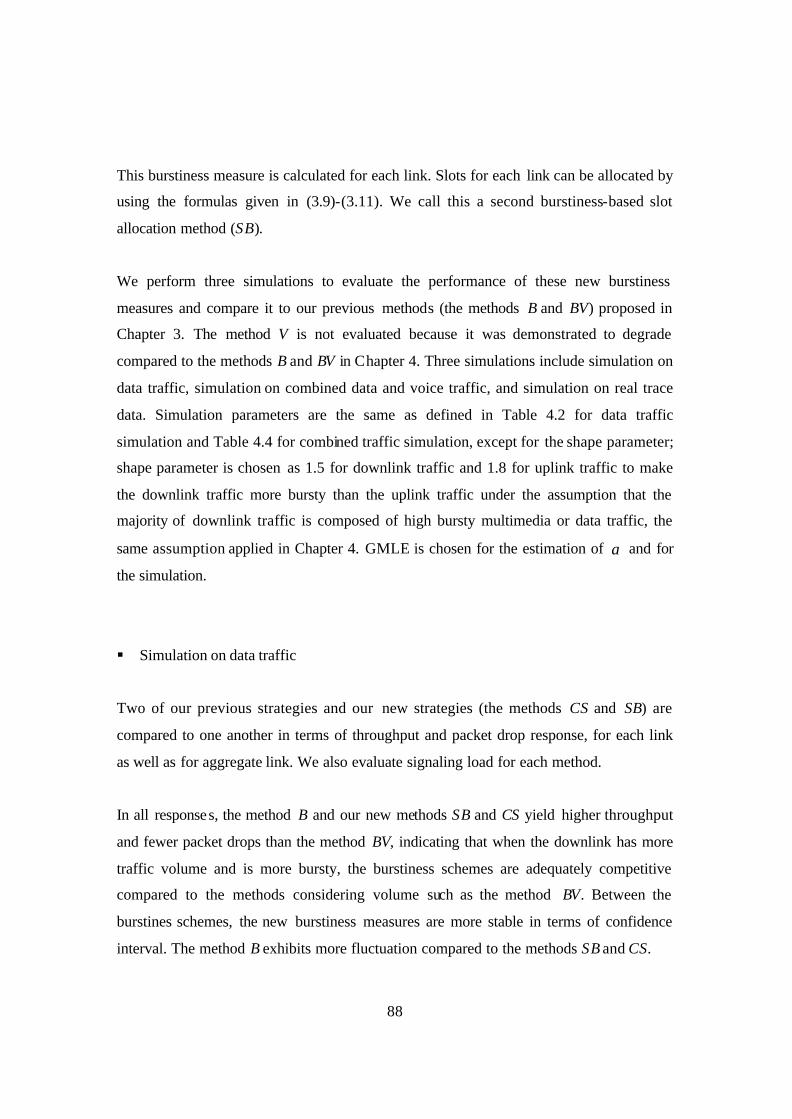
88

This burstiness measure is calculated for each link. Slots for each link can be allocated by

using the formulas given in (3.9)-(3.11). We call this a second burstiness-based slot

allocation method (SB).

We perform three simulations to evaluate the performance of these new burstiness

measures and compare it to our previous methods (the methods B and BV) proposed in

Chapter 3. The method V is not evaluated because it was demonstrated to degrade

compared to the methods B and BV in Chapter 4. Three simulations include simulation on

data traffic, simulation on combined data and voice traffic, and simulation on real trace

data. Simulation parameters are the same as defined in Table 4.2 for data traffic

simulation and Table 4.4 for combined traffic simulation, except for the shape parameter;

shape parameter is chosen as 1.5 for downlink traffic and 1.8 for uplink traffic to make

the downlink traffic more bursty than the uplink traffic under the assumption that the

majority of downlink traffic is composed of high bursty multimedia or data traffic, the

same assumption applied in Chapter 4. GMLE is chosen for the estimation of α and for

the simulation.

§ Simulation on data traffic

Two of our previous strategies and our new strategies (the methods CS and SB) are

compared to one another in terms of throughput and packet drop response, for each link

as well as for aggregate link. We also evaluate signaling load for each method.

In all responses, the method B and our new methods SB and CS yield higher throughput

and fewer packet drops than the method BV, indicating that when the downlink has more

traffic volume and is more bursty, the burstiness schemes are adequately competitive

compared to the methods considering volume such as the method BV. Between the

burstines schemes, the new burstiness measures are more stable in terms of confidence

interval. The method B exhibits more fluctuation compared to the methods SB and CS.

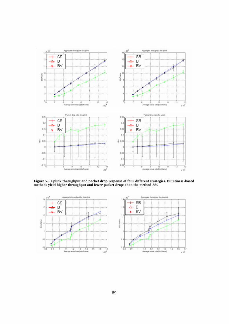
89

Figure 5.5 Uplink throughput and packet drop response of four different strategies. Burstiness -based methods yield higher throughput and fewer packet drops than the method BV.

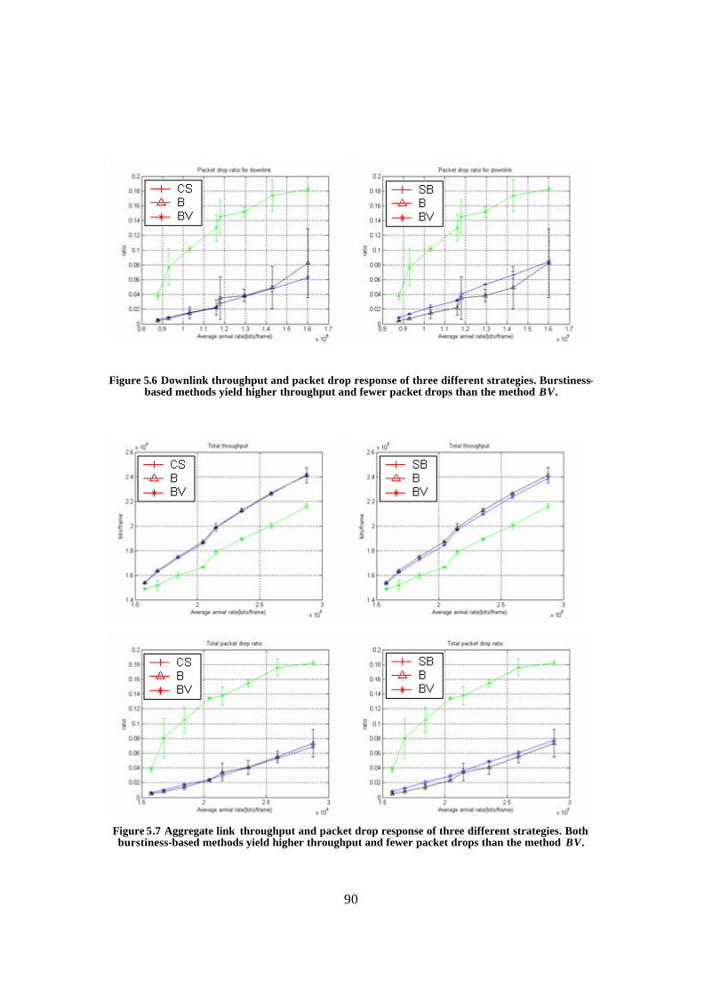
90

Figure 5.6 Downlink throughput and packet drop response of three different strategies. Burstiness-based methods yield higher throughput and fewer packet drops than the method BV.

Figure 5.7 Aggregate link throughput and packet drop response of three different strategies. Both burstiness-based methods yield higher throughput and fewer packet drops than the method BV.

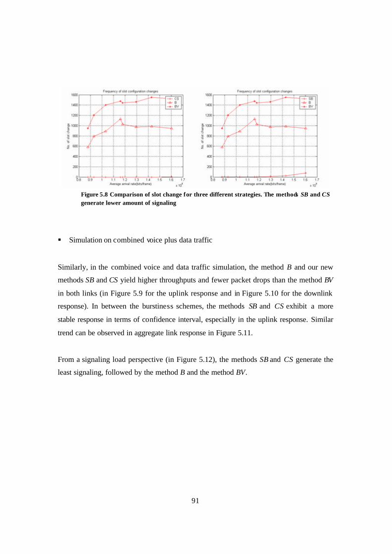
91

Figure 5.8 Comparison of slot change for three different strategies. The methods SB and CS generate lower amount of signaling

§ Simulation on combined voice plus data traffic

Similarly, in the combined voice and data traffic simulation, the method B and our new

methods SB and CS yield higher throughputs and fewer packet drops than the method BV

in both links (in Figure 5.9 for the uplink response and in Figure 5.10 for the downlink

response). In between the burstiness schemes, the methods SB and CS exhibit a more

stable response in terms of confidence interval, especially in the uplink response. Similar

trend can be observed in aggregate link response in Figure 5.11.

From a signaling load perspective (in Figure 5.12), the methods SB and CS generate the

least signaling, followed by the method B and the method BV.

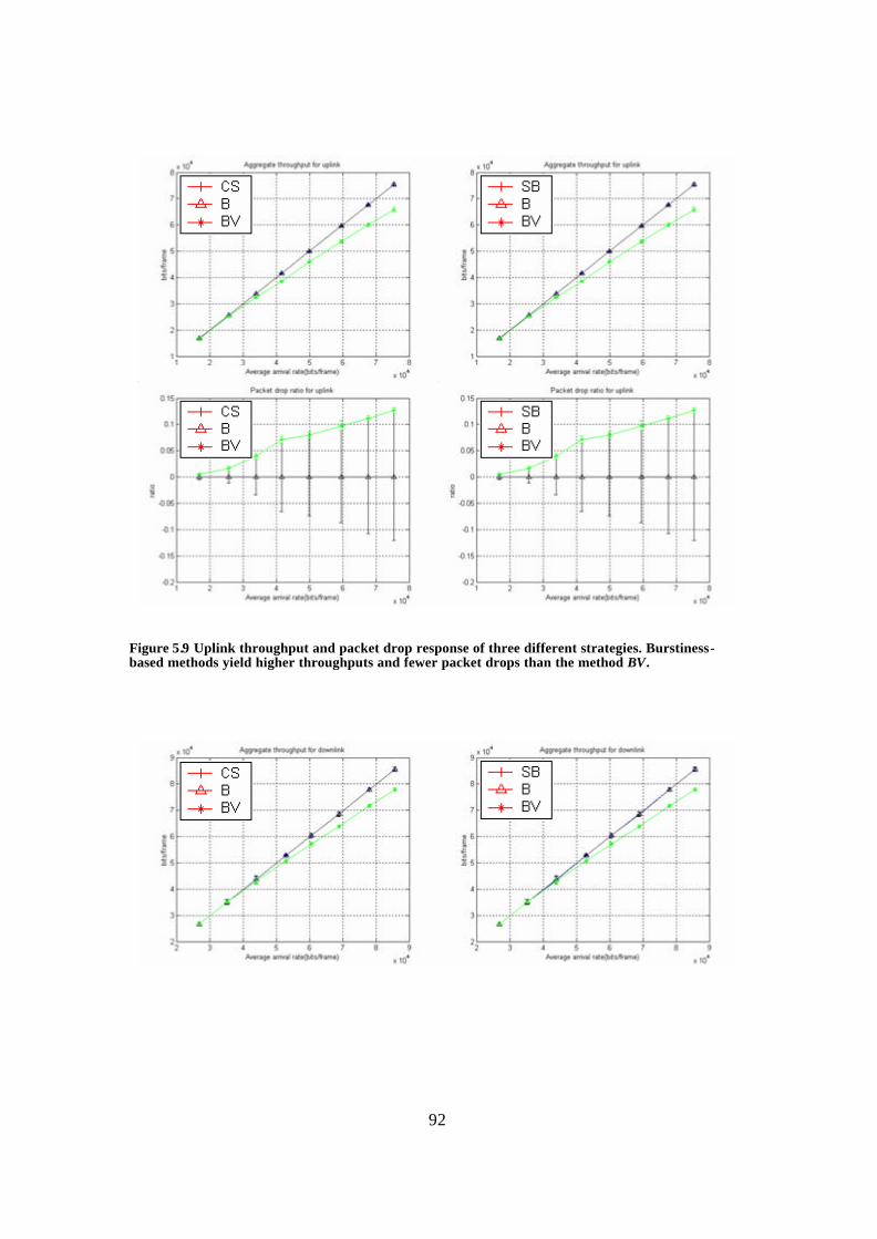
92

Figure 5.9 Uplink throughput and packet drop response of three different strategies. Burstiness-based methods yield higher throughputs and fewer packet drops than the method BV.

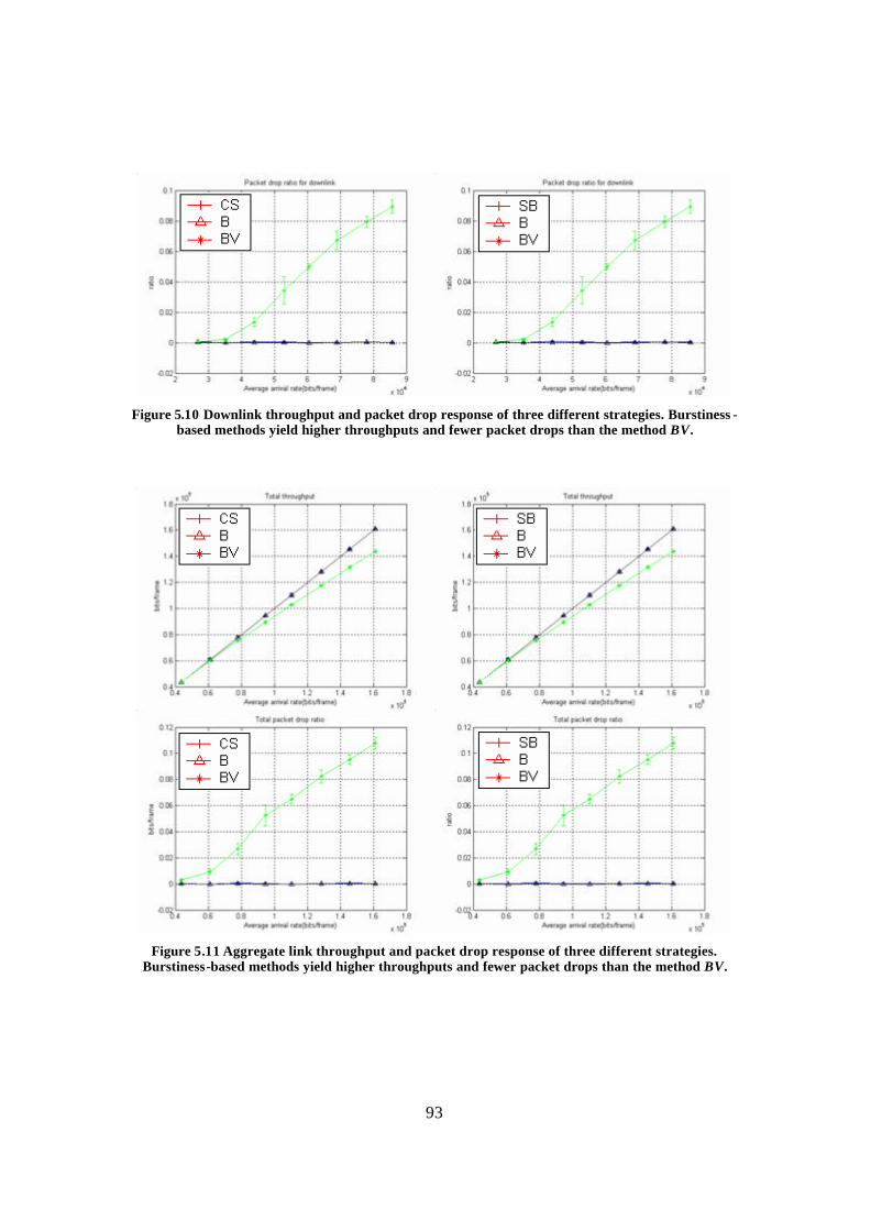
93

Figure 5.10 Downlink throughput and packet drop response of three different strategies. Burstiness -

based methods yield higher throughputs and fewer packet drops than the method BV.

Figure 5.11 Aggregate link throughput and packet drop response of three different strategies.

Burstiness-based methods yield higher throughputs and fewer packet drops than the method BV.

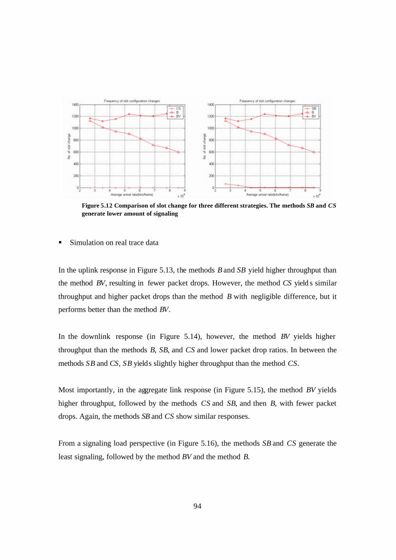
94

Figure 5.12 Comparison of slot change for three different strategies. The methods SB and CS generate lower amount of signaling

§ Simulation on real trace data

In the uplink response in Figure 5.13, the methods B and SB yield higher throughput than

the method BV, resulting in fewer packet drops. However, the method CS yield s similar

throughput and higher packet drops than the method B with negligible difference, but it

performs better than the method BV.

In the downlink response (in Figure 5.14), however, the method BV yields higher

throughput than the methods B, SB, and CS and lower packet drop ratios. In between the

methods SB and CS, SB yields slightly higher throughput than the method CS.

Most importantly, in the aggregate link response (in Figure 5.15), the method BV yields

higher throughput, followed by the methods CS and SB, and then B, with fewer packet

drops. Again, the methods SB and CS show similar responses.

From a signaling load perspective (in Figure 5.16), the methods SB and CS generate the

least signaling, followed by the method BV and the method B.

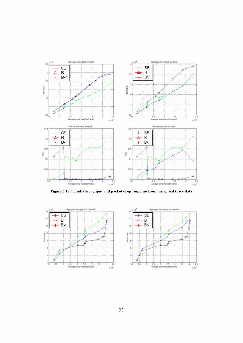
95

Figure 5.13 Uplink throughput and packet drop response from using real trace data

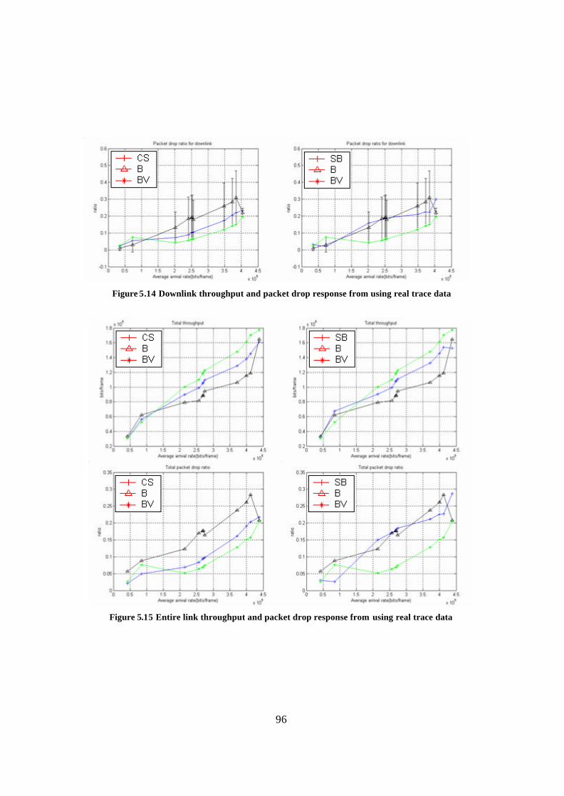
96

Figure 5.14 Downlink throughput and packet drop response from using real trace data

Figure 5.15 Entire link throughput and packet drop response from using real trace data

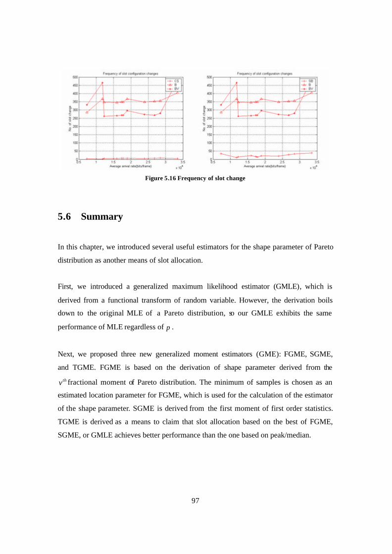
97

Figure 5.16 Frequency of slot change

5.6 Summary

In this chapter, we introduced several useful estimators for the shape parameter of Pareto

distribution as another means of slot allocation.

First, we introduced a generalized maximum likelihood estimator (GMLE), which is

derived from a functional transform of random variable. However, the derivation boils

down to the original MLE of a Pareto distribution, so our GMLE exhibits the same

performance of MLE regardless of p .

Next, we proposed three new generalized moment estimators (GME): FGME, SGME,

and TGME. FGME is based on the derivation of shape parameter derived from the

thv fractional moment of Pareto distribution. The minimum of samples is chosen as an

estimated location parameter for FGME, which is used for the calculation of the estimator

of the shape parameter. SGME is derived from the first moment of first order statistics.

TGME is derived as a means to claim that slot allocation based on the best of FGME,

SGME, or GMLE achieves better performance than the one based on peak/median.

98

Our GMEs have the following major advantages compared to the integer moment

estimator. First, our estimators are generalized for any integer or fractional moment.

Second, our estimators are not restricted by the choice of shape parameter α .

The performance of our proposed estimators is evaluated in terms of RMSE and variance

of estimators. Our FGME and SGME estimators outperform the existing Quandt’s

estimator for higher p ; that is, they have lower RMSE and variance compared to

Quandt’s method when 1>p . As p becomes higher, the performance of our GMEs

approaches that of MLE. GMLE, however, does not show any improvement for

higher p as explained before. Also, our estimators exhibit robust performance even for a

small number of samples. TGME is outperformed by our FGME, SGME, and GMLE in

terms of RMSE and variance of estimators. Hence, we have reinforced our previous claim

that slot allocation based on the best of FGME, SGME, or GMLE achieves better

performance than the one based on peak/median. Also, TGME was not obtained in a

closed form solution, another weakness of this estimator.

One of our estimators (GMLE) is chosen for the slot allocation procedure and for our

simulations. Slots can be allocated by the ratio of constraints for each link, where the

constraint is found by evaluating outage probability requirement for each link, or by a

ratio of new burstiness measure.

Three simulations are performed: simulation on data traffic, simulation on combined

voice plus data traffic, and simulation on real trace data. In the first two simulations, the

downlink is controlled to have more traffic volume and to be more bursty. However, in

the trace data, the burstiness in the uplink is higher than that in the downlink, which is

unfavorable to the burstiness-based methods. In the first two simulations, three burstiness

methods yield higher throughputs and fewer packet drops compared to the method BV. In

comparison between the burstiness strategies, the methods SB and CS exhibit more stable

response in terms of confidence intervals and generate less signaling, significant

advantages compared to the method B. In the trace data simulation, the methods BV, CS,

and SB yield higher throughputs and fewer packet drops than the method B. The methods

99

CS and SB yield comparable throughput and packet drops to the method BV based on

evaluation of burstiness alone . This saves appreciable computational load because it does

not evaluate traffic volume. In comparison between the burstiness-based methods, the

methods SB and CS yield higher throughput and fewer packet drops than the method B,

showing more stable results even with the higher burstiness in the uplink traffic.

Furthermore, the methods CS and SB generate the least signaling load compared with the

other two methods, saving considerable power for mobiles. In general, the SB and CS

show similar responses.

100

Chapter 6 Cross-layer aware slot allocation

In this chapter, we attempt to incorporate physical layer information in order to increase

throughput and decrease packet drops from the aggrega te link perspective.

This chapter first investigates available information in the physical layer in Section 6.1

for our cross- layer aware slot allocation. In Section 6.2, we introduce our method of

cross- layer aware slot allocation, including a formula for the slot allocation for each link.

Simple evaluation of the proposed method is given in Section 6.3. Finally, we summarize

this chapter in Section 6.4.

6.1 Background

In the previous approaches for the slot allocation introduced so far, including our

proposed strategies, there has been little effort to exploit physical layer information to

enhance the performance of the system. We now incorporate physical layer statistics into

our slot allocation process. Physical layer statistics can play an important role in slot

allocation because they can be indicative of current channel condition. It is useless to

transmit a large number of packets when the current channel condition is bad, resulting in

huge packet losses. There is a lot of information available to us for the slot allocation: bit

error rate (BER), packet error rate (PER), received signal strength (RSSI), etc. Here, we

strive to incorporate PER into our slot allocation and compare the performance of this

strategy with an existing method. Performance is evaluated in throughput and packet drop

ratio.

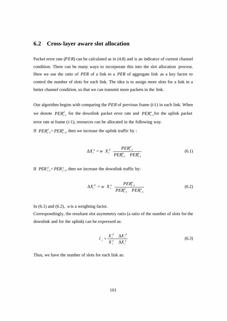
101

6.2 Cross-layer aware slot allocation

Packet error rate (PER) can be calculated as in (4.8) and is an indicator of current channel

condition. There can be many ways to incorporate this into the slot allocation process.

Here we use the ratio of PER of a link to a PER of aggregate link as a key factor to

control the number of slots for each link. The idea is to assign more slots for a link in a

better channel condition, so that we can transmit more packets in the link.

Our algorithm begins with comparing the PER of previous frame (i-1) in each link. When

we denote diPER 1− for the downlink packet error rate and u

iPER 1− for the uplink packet

error rate at frame (i-1), resources can be allocated in the following way.

If diPER 1− > u

iPER 1− , then we increase the uplink traffic by :

ui

di

did

iui PERPER

PERXwX

11

1

−−

−

+⋅⋅=∆ (6.1)

If diPER 1− < u

iPER 1− , then we increase the downlink traffic by:

ui

di

uiu

idi PERPER

PERXwX

11

1

−−

−

+⋅⋅=∆ (6.2)

In (6.1) and (6.2), w is a weighting factor.

Correspondingly, the resultant slot asymmetry ratio (a ratio of the number of slots for the

downlink and for the uplink) can be expressed as:

ui

ui

di

di

i XXXX

∆+∆+

=λ (6.3)

Thus, we have the number of slots for each link as:

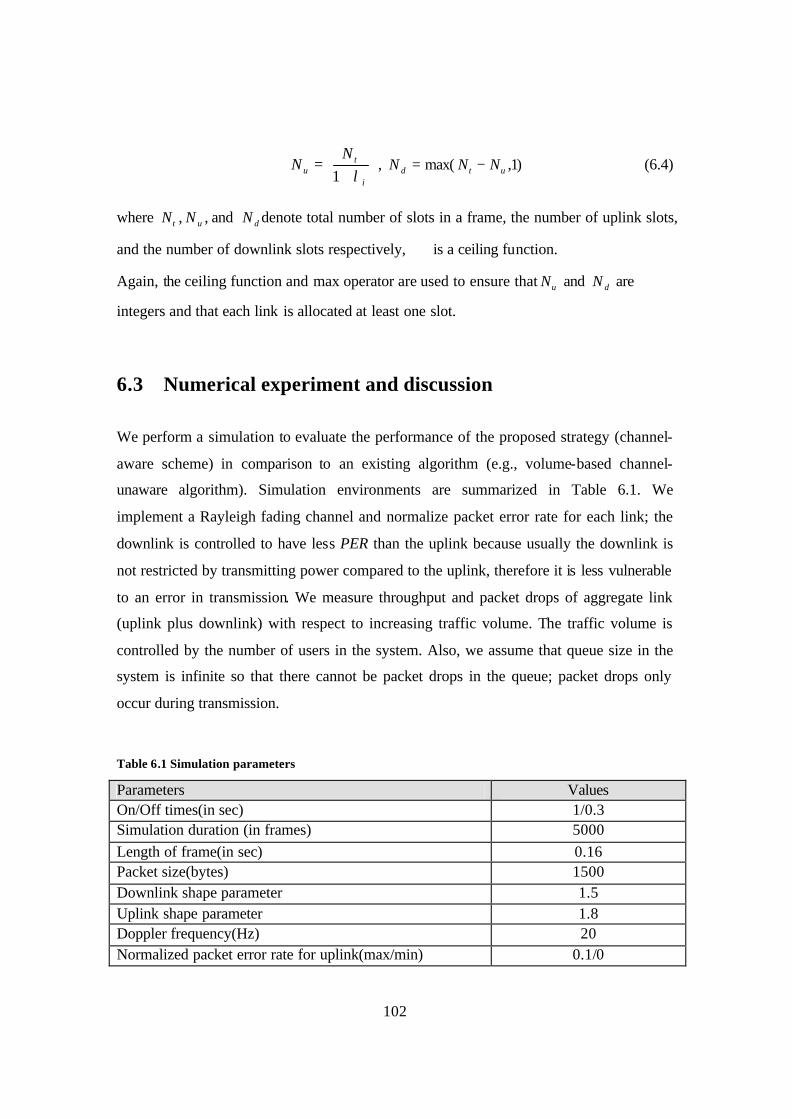
102

+

=i

tu

NN

λ1, )1,max( utd NNN −= (6.4)

where tN , uN , and dN denote total number of slots in a frame, the number of uplink slots,

and the number of downlink slots respectively, ⋅ is a ceiling function.

Again, the ceiling function and max operator are used to ensure that uN and dN are

integers and that each link is allocated at least one slot.

6.3 Numerical experiment and discussion

We perform a simulation to evaluate the performance of the proposed strategy (channel-

aware scheme) in comparison to an existing algorithm (e.g., volume-based channel-

unaware algorithm). Simulation environments are summarized in Table 6.1. We

implement a Rayleigh fading channel and normalize packet error rate for each link; the

downlink is controlled to have less PER than the uplink because usually the downlink is

not restricted by transmitting power compared to the uplink, therefore it is less vulnerable

to an error in transmission. We measure throughput and packet drops of aggregate link

(uplink plus downlink) with respect to increasing traffic volume. The traffic volume is

controlled by the number of users in the system. Also, we assume that queue size in the

system is infinite so that there cannot be packet drops in the queue; packet drops only

occur during transmission.


Parameters Values On/Off times(in sec) 1/0.3 Simulation duration (in frames) 5000 Length of frame(in sec) 0.16 Packet size(bytes) 1500 Downlink shape parameter 1.5 Uplink shape parameter 1.8 Doppler frequency(Hz) 20 Normalized packet error rate for uplink(max/min) 0.1/0

103

Normalized packet error rate for downlink(max/min) 0.05/0 Number of slots in a frame 14 Maximum number of packets per slot 8 Weighting factor ( w ) 0.5 Number of iteration for measurements 1500 Aggregate throughput is measured in packets per frame as shown in Figure 6.1. Our

cross- layer aware scheme is drawn with circles, and the existing channel unaware scheme

is drawn with asterisks. The results show that our proposed scheme yields higher

throughput than the existing scheme regardless of packet arrivals.

Figure 6.1 Throughput response of cross-layer aware and unaware slot allocation. 1500 measurements of packet drop ratios are averaged for each traffic arrival rate.

Packet drops are assumed to occur only in channel, not in queue. The results show that

our proposed scheme yields less packet drop compared to the existing scheme.

104

Figure 6.2 Packet drop response of cross-layer aware and unaware slot allocation during transmission, assuming that queue size is infinite. 1500 measurements of packet drop ratios are averaged for each traffic arrival rate.

6.4 Summary

In this chapter, we introduced a new slot allocation method based on a statistic (PER)

reflected from the physical layer transmission. The idea is to allocate more resources for

a link in a better channel condition, so that we can increase throughput and decrease

packet drops from the aggregate link perspective.

The simulation result complies well with our expectation; our proposed scheme yield

higher throughput and less packet drop compared to an existing scheme.

We believe that this simple demonstration is very informative and can be a framework for

the use of other types of information for the slot allocation.

105

Chapter 7 Conclusions and related areas of research

7.1 Summary and conclusions

The main contribution of this research is the adoption of adaptive slot allocation in the

link layer to enhance the performance of MAC protocols. In the existing MAC protocol

research for WCDMA/TDD systems, the fixed allocation of slots is assumed in advance.

Meanwhile, the slot allocation issue in the WCDMA/TDD system has been addressed for

a completely different angle. Some authors adopted adaptive slot allocation techniques in

order to maximize system utilization under interference-constrained multi-cell

environments. We believe that these two directions of research need to be incorporated in

order to enhance the performance of MAC protocols.

In this research, we suggest four major adaptive dynamic slot allocation strategies: (i)

strategy based on the estimation of burstiness and volume of traffic (method BV), (ii)

strategy based on estimation of burstiness information only (method B), (iii) strategy

based on the estimated parameters of a distribution of traffic (methods SB and CS), and

(iv) strategy based on the use of physical layer information (method CHA).

For the strategies (i) and (ii), the estimations of burstiness and volume of traffic are

performed based on a new burstiness measure and a dynamic observation window

method, proposed in this research. The new burstiness measure is peak/median, making

use of the advantage of median against peak variation. The performance of this new

burstiness measure was demonstrated in comparison to peak/mean, a typical burstiness

measure. The dynamic observation window algorithm is devised based on statistical

analysis of traffic-ACF and PACF.

106

Proposed adaptive methods (i) and (ii) are evaluated in terms of throughput and packet

drop ratio. The proposed methods yield higher throughputs and fewer packet drops in

most cases compared to the conventional volume-based method from the aggregate link

perspective. The method B is sufficiently competitive especially when the downlink has

more traffic and is more bursty than the uplink. But when the uplink is more bursty, it

yields the least throughput and more packet drops as shown in the real trace data

simulation. The method BV showed stable performance compared to the method B even

when the burstiness of uplink traffic is high.

For the strategy (iii), we developed several robust estimators for the parameters (shape

and location) of the Pareto distribution: generalized maximum likelihood estimator

(GMLE), first generalized moment estimator (FGME), second generalized mo ment

estimator (SGME), and third generalized moment estimator (TGME). These proposed

estimators (except TGME) outperform an existing integer moment estimator at high p in

terms of RMSE and variance of the estimators, where p is the order for the functional

transformation of random variable . Also, their performance is stable and robust even for a

small number of samples. These estimators are generalized for any shape parameter and

for any moments, integer and fractional. We incorporated these estimators into a slot

allocation process. Two new slot allocation methods are introduced, both based on the

estimated parameters: (a) slot allocation based on the constraint of CDF (method CS), and

(b) slot allocation based on a new burstiness measure (method SB). The performance of

these slot allocation methods is evaluated in comparison to the strategies (i) and (ii).

In general, the methods based on the estimation of parameters of a distribution were

demonstrated to be advantageous compared to strategies (i) and (ii). They are also

efficient in terms of power consumption because of less signaling load.

As a final strategy, we presented a cross- layer aware slot allocation method where

physical layer information is employed to enhance the performance of the system. The

packet error rate of the previous frame in each link is used as a key factor of slot

allocation. The idea is to send more packets through a link under better channel

107

conditions. The evaluation of this method is presented in comparison to a volume method.

It yields higher throughput and fewer packet drops compared to the volume-based

method, just as we expected.

7.2 Related areas of research

The following may be the reasonable future directions for this research.

§ Resource control and management based on the prediction techniques for MAC

protocols

Predictions techniques are in widespread use in the engineering and economics areas; for

example, AR, MA, ARMA, ARIMA, FARIMA, Kalman, etc. One of these techniques

can be used for the purpose of slot allocation to further enhance the performance of the

system. Among these techniques, FARIMA models are particularly attractive for our

resource allocation purpose because they have been used to model long range-dependent

time series data in economics. Recently, this model has been used for the prediction of

Internet traffic, admission control, and buffer management in the networking area. The

model enables both one-step and h-step predictions of time series data, where the

accuracy of single-step prediction is higher than that of the h-step prediction. This model

also involves the estimation of parameters of a distribution, where the estimation can be

conducted using various methods. One of our estimation techniques can also be used for

this purpose; for example, GMLE may yield the robust estimation of the Gaussian noise

that arises in the FARIMA model.

If we can predict the number of packets in the next frame, it may be easier to manage

queues in the system and to control the required resources in response to the prediction.

This approach has not been attempted so far, so it is worthwhile to examine this

technique and its potential applications for our resource allocation purposes.

108

§ Development of slot allocation algorithms using cross-link correlation

information

So far, we assumed that traffic in each link is uncorrelated; that is, the majority of the

uplink traffic is composed of voice traffic, and that of the downlink traffic is composed of

data traffic. This may be an acceptable assumption for experimental purposes. However,

this is not true in a real world scenario , where network transactions in the uplink and the

downlink are correlated. Some parts of the techniques introduced in this research can be

applied to assess the correlation of the network transaction such as ACF and PACF. If we

can quantify the degree of the correlation and use it for resource allocation, the resource

allocation may be more realistic from the implementation point of view.

§ Global resource optimization under multi-cell environments

This research focuses on the efficient use of resources from the single cell point of view,

assuming that the efficient use of resources is more important than the control of the

interference problem, a concern of the existing resource allocation methods. As an

extension of this research, it is worth investigating a global solution under multi-cell

environments. In addition to a solution for a single cell, a global solution needs to

consider the interference issue among neighboring cells. To find a global solution, we

may consider using mathematical programming techniques that are primarily used to

compute an optimized solution under a refined set of constraints and an objective

function. Those techniques include Linear Programming (LP), Non-Linear Programming

(NLP), etc.

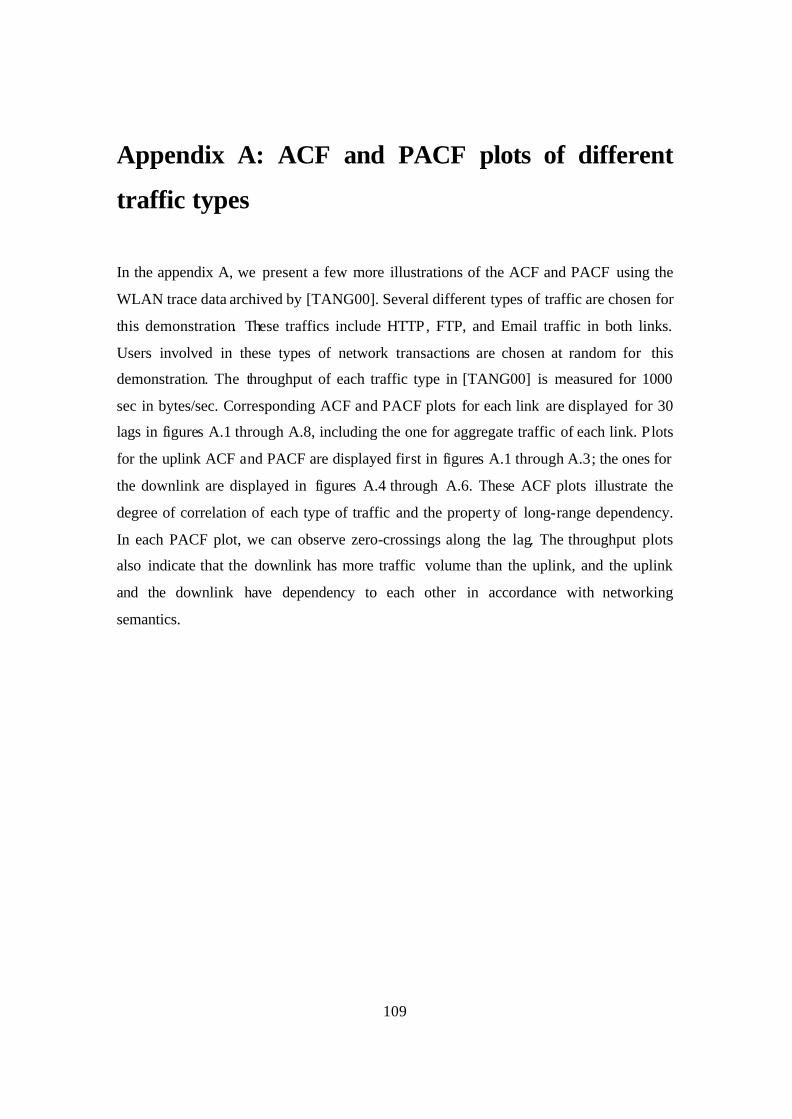
109

Appendix A: ACF and PACF plots of different

traffic types In the appendix A, we present a few more illustrations of the ACF and PACF using the

WLAN trace data archived by [TANG00]. Several different types of traffic are chosen for

this demonstration. These traffics include HTTP, FTP, and Email traffic in both links.

Users involved in these types of network transactions are chosen at random for this

demonstration. The throughput of each traffic type in [TANG00] is measured for 1000

sec in bytes/sec. Corresponding ACF and PACF plots for each link are displayed for 30

lags in figures A.1 through A.8, including the one for aggregate traffic of each link. Plots

for the uplink ACF and PACF are displayed first in figures A.1 through A.3; the ones for

the downlink are displayed in figures A.4 through A.6. These ACF plots illustrate the

degree of correlation of each type of traffic and the property of long-range dependency.

In each PACF plot, we can observe zero-crossings along the lag. The throughput plots

also indicate that the downlink has more traffic volume than the uplink, and the uplink

and the downlink have dependency to each other in accordance with networking

semantics.

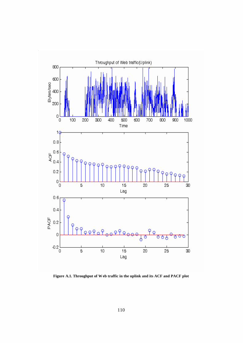
110

Figure A.1. Throughput of W eb traffic in the uplink and its ACF and PACF plot

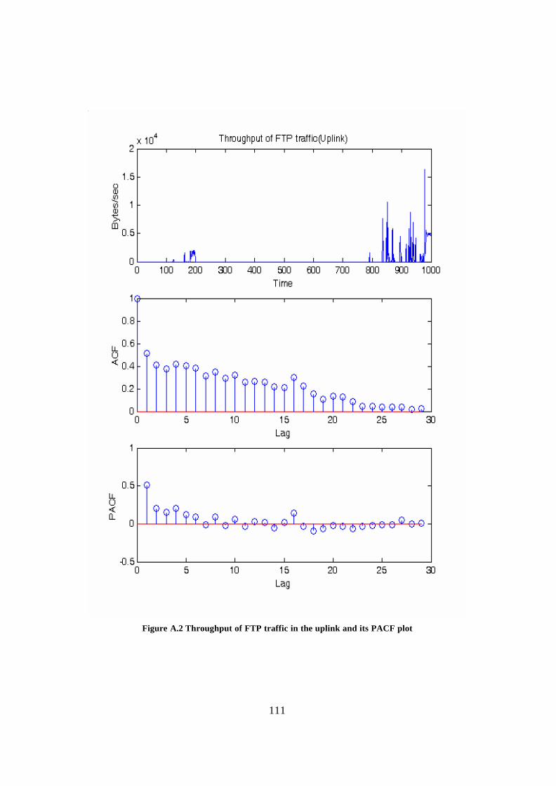
111

Figure A.2 Throughput of FTP traffic in the uplink and its PACF plot

112

Figure A.3 Throughput of Email traffic in the uplink and its ACF and PACF plot

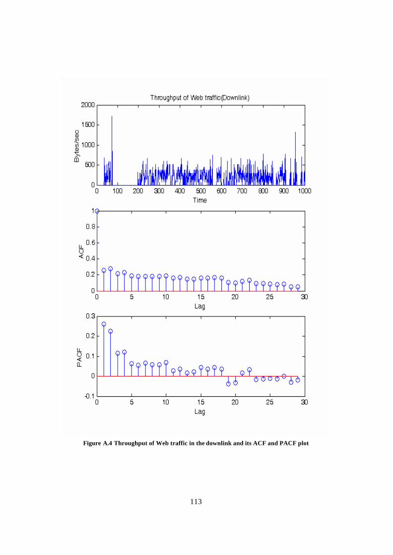
113

Figure A.4 Throughput of Web traffic in the downlink and its ACF and PACF plot

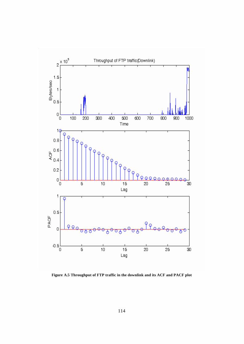
114

Figure A.5 Throughput of FTP traffic in the downlink and its ACF and PACF plot

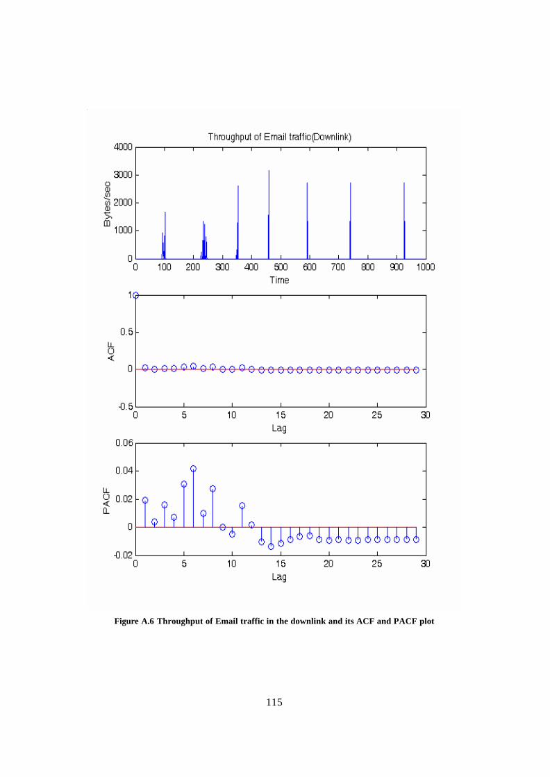
115

Figure A.6 Throughput of Email traffic in the downlink and its ACF and PACF plot

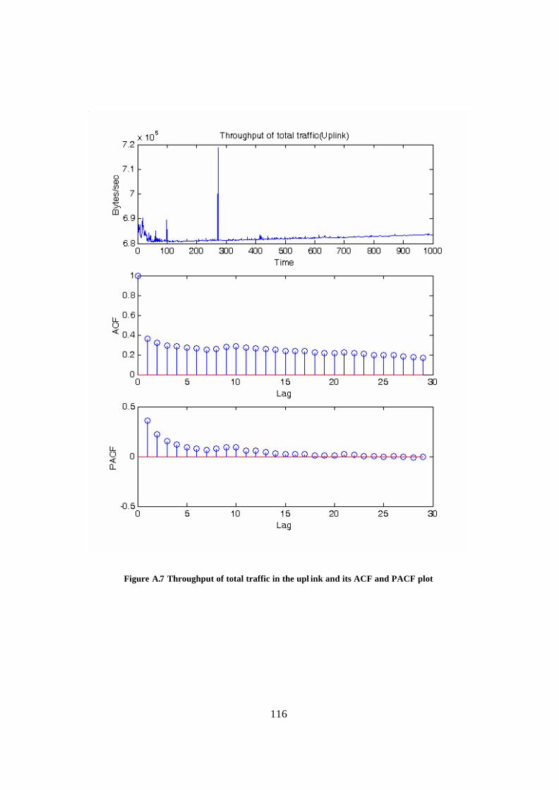
116

Figure A.7 Throughput of total traffic in the upl ink and its ACF and PACF plot

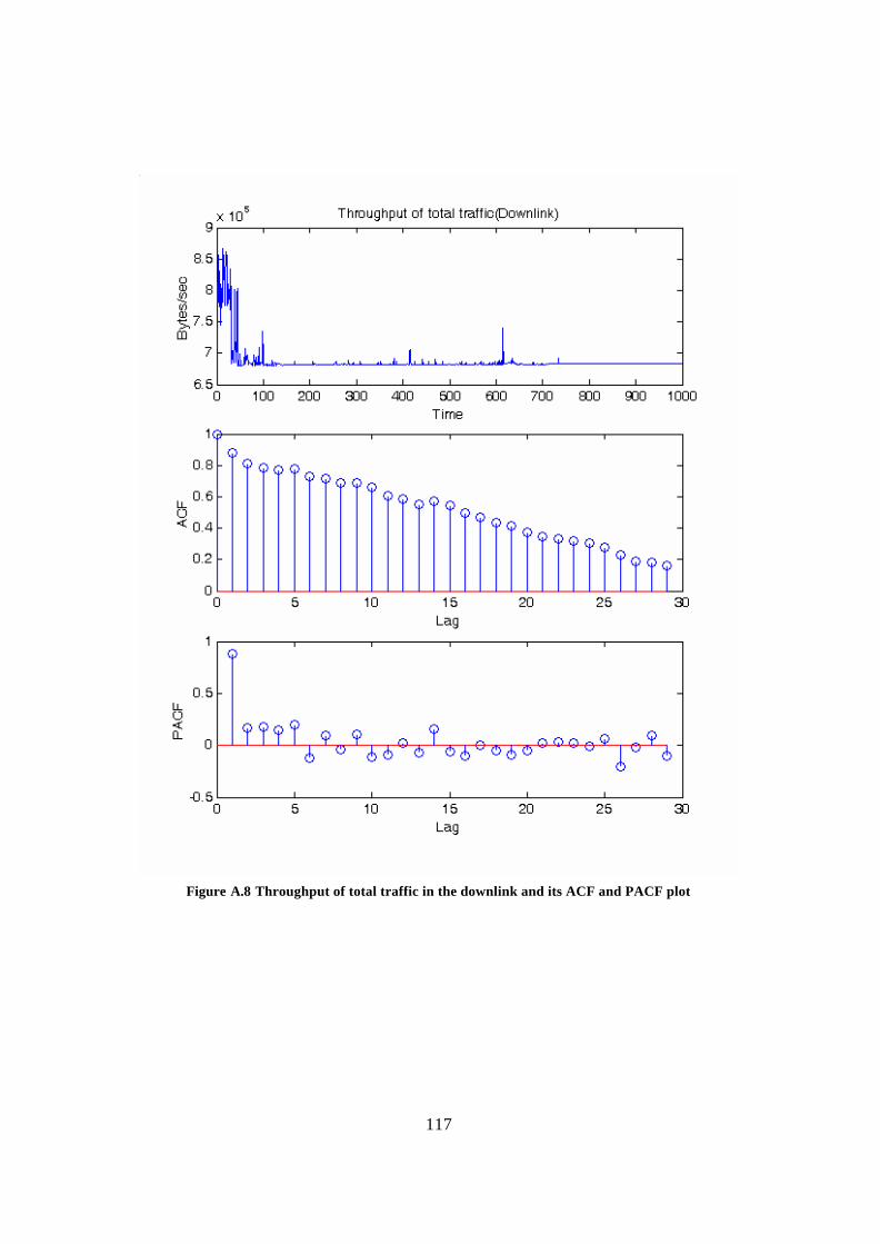
117

Figure A.8 Throughput of total traffic in the downlink and its ACF and PACF plot

118

Appendix B: Derivation of estimators

§ Derivation of (5.2):

0,,

)(

)()(

/11

1

>>=

=

=

+

−

αα

α

αp

p

ppX

pXY

kyypk

pyyf

dydxyfyf

where 0,,)(1

>>=+

ααα

α

kxx

kxf X


∞

>−=

−

=

=

∞−

∞

∫

otherwise

nppv

k

pvy

pk

dyyfyYE

pv

k

pv

k

Yvv

p

p

,

,/

)(][

/

/1

/1

αα

α

αα

αα


Using ∫ −==+

y

kppY

p yk

dxxpk

yF/1

1)(1 α

α

α

αα,

119

[ ]

[ ]

vpN

pNv

k

vpNpNk

ypNv

pNk

dyypNk

dyy

pkyk

Ny

dyyfyFNy

dyyfyYE

pv

pv

kpNvN

k

pNvN

kp

N

pv

k

YN

Yv

kN

vvN

p

p

p

p

p

>−

=

−=

−=

=

⋅

⋅⋅=

−⋅⋅=

⋅=

∞−

∞−−

∞

+

−

∞−

∞

∫

∫

∫

∫

αα

α

αα

αα

α

α

αα

αα

α

α

α

α

,

1

)()(1

)(][

/

/

1

11

1

111

1

11

111

11

11:11:1

/1

/1

/1

/1

/1

If ,1=v then

[ ]

∞

>−=

otherwise

pN

pN

k

YE

p

N

,

1,1

/1

1:1

αα

α

§ Derivation of (5.19): By changing variable as:

=

=−

+ dtdyy

pk

tyk

NpN

pN

1

1

α

α

α

α

α

(5.19) can be derived as:

120

[ ]

+=

⋅

−=

⋅

−=

⋅

−⋅⋅=

⋅⋅=

⋅=

−

−

∞

+

−

∞−

∞

∫

∫

∫

∫

∫

1;1;,

11

1

1

)()(

)(][

12/

1

/1

0

/

11

0

/

1

1

1

::

/1

/1

/1

NNpv

Fk

dttt

Nk

dttt

kN

dyy

pk

y

kNy

dyyfyFNy

dyyfyYE

pv

N

pv

pv

Npv

N

kp

N

N

pN

vN

N

k

NYN

NYvN

N

k

NNNvN

vNN

p

p

p

α

α

α

αα

α

α

α

α

121

Glossary ACF: Auto Correlation Function

AMPS: Advanced Mobile Phone System

AR: Auto Regressive

ARMA: Auto Regressive Moving Average

ATM : Asynchronous Transfer Mode

BER : Bit Error Rate

BS: Base Station

CS: Constraint-based slot allocation

DL: Downlink

EDGE: Enhanced Data rate for Global Evolution

FARIMA: Fractional Auto Regression Integrated Moving Average

FDD: Frequency Division Duplexing

FDMA: Frequency Division Multiple Access

FGME: First Generalized Moment Estimator

FIFO : First In First Out

FPP: Fractal Point Processes

FSK: Frequency Shifting Keying

FTP: File Transfer Protocol

GMLE: Generalized maximum likelihood estimator

GPRS: General Packet Radio Service

GSM : Global System for Mobile Communications

M A: Moving Average

MAC: Medium Access Control

MLE: Maximum likelihood estimator

MMPP: Markov Modulated Poisson Process

MS: Mobile Station

NAMPS: Narrowband AMPS

NRT: Non Real Time

PACF: Partial ACF

122

PER : Packet Error Rate

PDC: Personal Digital Cellular

PSD : Power Spectral Density

PSK: Phase Shifting Keying

QME: Quandt’s moment estimator

QoS : Quality of Service

RMSE: root mean-squared error

RT: Real Time

SIR: Signal to Interference Ratio

SB: Second Burstiness

SGME: Second Generalized Moment Estimator

SNR: Signal to Noise Ratio

TACS : Total Access Cellular System

TDD: Time Division Duplexing

TGME: Third Generalized Moment Estimator

UAS : Uniform Arrival Service

UL: Uplink

UMTS: Universal Mobile Telecommunications System

VBR: Variable Bit Rate

WCDMA: Wideband Code Division Multiple Access

WLAN: Wireless LAN

123

Bibliography

[ABRAHAMSSON00] H. Abrahamsson and B. Ahlgren, “Using Empirical Distributions

to Characterize Web Client Traffic and to Generate Synthetic Traffic,” in Proceedings of

IEEE GLOBECOM, vol.1, 2000, pp. 428-433.

[ABRAMSON94] N. Abramson, “Multiple Access in Wireless Digital Networks,” in

Proceedings of IEEE, vol.82, Sept. 1994, pp. 1360–1370.

[AGHA00] K. Agha and K Boussetta, “Dynamic Slot Allocation for multicasting in

GPRS systems,” in Proceedings of VTC 2000, vo l.3, 2000, pp. 2355-2359.

[AKYLIDIZ99-1] I. F. Akylidiz, D.A. Levine, and I. Joe, “A Slotted CDMA Protocol

with BER Scheduling for Wireless Multimedia Networks,” IEEE/ACM Transactions on

Networking, vol.7, no.2, pp. 146-59, Apr. 1999.

[AKYILDIZ02] I.F. Akyildiz and X. Wang, “A New Medium Access Control Protocol

for TDD Mode Wideband CDMA Wireless Local Area Networks,” in European Wireless

2002, February 2002.

[BERAN94] J. Beran, Statistics for Long Memory Process, Chapman and Hall, 1994.

[BROCKWELL91] P. J. Brockwell, R, A, Davis, and S, E, Fienberg, Time Series: Theory

and Methods, Springer-Verlag, 1991.

[CHANG94] C-J. Chang and C-H Wu, “Slot Allocation for an Integrated Voice/Data

TDMA Mobile Radio System with a Finite Population of Buffered Users,” in

Proceedings of VTC 1994, vol.43, 1994, pp.21-26.

124

[CHENG02] J. Cheng and N. C. Beaulieu, “Generalized Moment Estimators for the

Nakagami Fading Parameter,” IEEE Communications Letters, vol.6, no.4, pp. 144-146,

2002.

[ETSI02] ETSI, “Physical Channels and Mapping of Transport Channels onto Physical

Channels (TDD)”, 3GPP Technical Specification 25.221 V.5.1.0, 2002-06.

[GAEDDERT04] J. Gaeddert and A. Annamalai, “Further Results on Nakagami-m

Parameter Estimation,” accepted by IEEE Communications Letter, 2004.

[GIROUX99] N. Giroux and S. Ganti, “Quality of Service in ATM Networks,” in The

Traffic Contract, Prentice-Hall, 1999, pp. 10-32.

[GRADSHTEYN93] I. S. Gradshteyn and I. M. Ryzhik, Table of Iintegrals, Series, and

Products, Academic Press, 5th, 1994.

[HOLMA01] Harri Holma and Antti Toskala, WCDMA for UMTS, John Wiley & Sons

Ltd., 2001.

[HORNG03] M-F Horng and Y-H, Kuo, “Dynamic Slot Allocation to Control Delays in

TDMA Wireless Base Station, ” in IEEE international symposium on computers and

communication(ISCC’03), 2003, pp. 1126-1131.

[HUANG02] V. Huang and W. Zhuang, “QoS-Oriented Access Control for 4G Mobile

Multimedia CDMA Communications,” IEEE Communications Magazine, vol.40, no.3,

pp. 118-125, March 2002.

[JIANG00] M. Z. Jiang, “Analysis of Wireless Data Network,” M.S. thesis, Simon Fraser

University, Surrey, Canada, April 2000.

125

[JIANG01] M. Jiang, M. Nikolic, S. Hardy, and L. Trajkovic, “Impact of Self-similarity

on Wireless Data Network Performance,” in IEEE International Conference on

Communications, vol.2, June 2001, pp. 477-481.

[JEONG00] D. G. Jeong and W. S. Jeon, “Time Slot Allocation in CDMA/TDD Systems

for Mobile Multimedia Services,” IEEE Communications Letters, vol.4, no.2, pp. 59-61,

Feb. 2000.

[JOHANSSON98] B. Johansson, “Packet Data Capac ity in a Wideband CDMA System,”

in Proceedings of VTC’98, 1998, vol.3, pp.1878-1883.

[KLEINROCK75] L. Kleinrock, Queueing systems Volume 1: Theory, John Wiley &

Sons, New York, 1975.

[KOS03] A. Kos, M. Pustisek, J. Bester, “Generation of Synthetic Traffic Based on Real

Traffic Samples,” in Proceedings of 7th Int’l Conf. on Telecommunications, 2003, pp.301-

305.

[KUMARAN03] Krishnan Kumaran and Lijun Qian, “Uplink Scheduling in CDMA

Packet-Data Systems,” in Proceedings of IEEE Infocom 2003, vol.1, 2003, pp. 292-300.

[LEE97] Lee, B. O., Frost, V. S., Jonkman, R. "NetSpec 3.0 Source Models for telnet, ftp,

voice, video and WWW traffic", Technical Report ITTC-TR10980 -19, University of

Kansas, January, 1997.

[LELAND94] W. E. Leland, M.S. Taqqu, W. Willinger, and D.V. Wilson, “On the Self-

similar Nature of Ethernet Traffic (extended version),” IEEE/ACM Trans. On Networking,

vol.2, no.1, pp.1-15, 1994.

[LI02] Qiong Li and D. L. Mills, "Control Architecture for Tuning Intensity anc

Burstiness of Traffic," in Proceedings of GlobeCom '02, vol. 3, 2002, pp. 17-23.

126

[OJANPERA98] T. Ojanpera and R. Prasad, Wideband CDMA for Third Generation

Mobile Communications, Artech House Publishers, 1998.

[OONO97] T. Oono, H Takanashi, and T. Tanaka, “Dynamic Slot Allocation Technology

for Mobile Multi-Media TDMA Systems Using a Distributed Control Scheme,” in

Proceedings of IEEE 6th International Conference on Universal Personal

Communications Record, Oct. 12, 1997, pp. 74-78.

[PARK00] K. Park and W. Willinger, “Self-similar Network Traffic: an Overview,” in

Self-similar Network Traffic and Performance Evaluation, Wiley Inter-Science, 2000,

pp.17-27.

[PAXSON95] V. Paxson and S. Floyd, “Wide Area Traffic: The Failure of the Poisson

Model,” IEEE/ACM Trans. on Networking, vol.3, no.3, pp. 236-244, June 1995.

[PRABHAKAR95] B. Prabhakar and N. Bambos, "The Entropy and delay of traffic

processes in ATM networks," in Proceedings of the Conference on Information Science

and Systems, 1995, pp.448-453.

[PROAKIS95] J. G. Proakis, “Digital Communicatio ns,” in Digital Communication

Through Fading Multipath Channels, McGraw-Hill, 1995, pp. 772-777.

[QUANDT66] Quandt, R. E., “Old and new Methods of Estimation and the Pareto

Distribution,” Metrika, vol.10, pp. 55-82, 1966.

[RAHMAN03] M. Rahman and L. M. Pearson, “A Note on Estimating Parameters in

Two-Parameter Pareto Distributions,” International Journal of Mathematical Education

in Science and Technology, vol.34, no.2, pp. 298-306.

127

[RUEDA96] A. Rueda and W. Kinsner, “A Survey of Traffic Characterization

Techniques in Telecommunication Networks,” in Proceedings of IEEE Canadian

Conference on Electrical and Computer Engineering(ICCECE ’96), vol.2, 1996, pp. 830-

833.

[SPOHN97] D.L. Spohn, Data Network Design, McGraw-Hill, New York, N.Y., 1997. [STALLINGS98] W. Stallings98, "High Speed Networks: TCP/IP and ATM Design

Principles," Prentice-Hall, 1998.

[TANG00] D. Tang and M. Baker, “Analysis of a Local-Area Wireless Network,” in

Proceedings of 6th annual International Conference on Mobile Computing and

Networking, vol.8, 2000, pp. 107-120.

[WANG03] X. Wang, “An FDD Wideband CDMA MAC Protocol for Wireless

Multimedia Networks,” in Proceedings of IEEE Infocom2003, vol.1, 2003, pp. 734-744.

[WIE01] S-H Wie and D-H Cho, “Time Slot Allocation Scheme based on a Region

Division in CDMA/TDD Systems,” in Proceedings of VTC’01, vol.4, 2001, pp. 2445-

2449.

[WILLIAMSON01] C. Williamson, “Internet Traffic Measurement,” IEEE Internet

Computing, vol.5, no.6, 2001, pp.70-74.

[ZHAO03] D. Zhao, X. Shen, and J. W. Mark, “Radio Resource Management for

Cellular CDMA Systems Supporting Heterogeneous Services,” IEEE Trans. on Mobile

Computing, vol.2, no.2, pp. 147-159, 2003.

Adaptive Asymmetric Slot Allocation for Heterogeneous ... · Adaptive Asymmetric Slot Allocation...

Documents

Transcript of Adaptive Asymmetric Slot Allocation for Heterogeneous ... · Adaptive Asymmetric Slot Allocation...