OIiC FILE COPY

UMIACS-TR-90-40 March 1990oCS-TR-243700 Recursive Star-Tree Parallel Data-Structure

Omer Berknan and Uzi VishkintInstitute for Advanced Computer Studies and

tDepartment of Electrical EngineeringUniversity of Maryland

College Park, MD 20742and

Tel Aviv University A ELI

COMPUTER SCIENCETECHNICAL REPORT SERIES

DTICI ELECTE

OCT17 10

UNIVERSITY OF MARYLANDCOLLEGE PARK, MARYLAND

20742

tistlbslon UaiD~tgjIS h3ON S TMApoved for pubaoi3i

9 0 t6~o~ i9 1

UMIACS-TR-90-40 March 1990CS-TR-2437

Recursive Star-Tree Parallel Data-Structure

Omer Berkman and Uzi VishkintInstitute for Advanced Computer Studies and

"Department of Electrical EngineeringUniversity of Maryland

College Park, MD 20742and DTIC

Tel Aviv University J 0 ELECT E

OCT 171

ABSTRACT

This paper introduces a novel parallel data-structure, called recursiveSTAR-tree (denoted '* tree'). For its definition, we use a generalization ofthe * functional 1. Using recursion in the spirit of the inverse-Ackermannfunction, we derive recursive *-trees.

The recursive *-tree data-structure leads to a new design paradigm forparallel algorithms. This paradigm allows for:* Extremely fast parallel computations. Specifically, O(a(n)) time (wherec(xn) is the inverse of Ackermann function) using an optimal number of pro-cessors on the (weakest) CRCW PRAM.e These computations need only constant time, using an optimal number ofprocessors if the following non-standard assumption about the model ofparallel computation is added to the CRCW PRAM: an extremely smallnumber of processors can write simultaneously each into different bits of thesame word.

Applications include:

(1) A new algorithm for finding lowest common ancestors in trees which isconsiderably simpler than the known algorithms for the problem.

(2) Restricted domain merging.(3) Parentheses matching.(4) A new parallel reducibility. i" -DSiTtBUTION STAT Mt A

A.).--oyed for publle fslecansj-.. ' .)t~o-j Onlim jt,4

t The research of this author was supported by NSF grants CCR-8615337 and CCR-8906949 and ONR grantN00014-85-K-0046.' Given a real function f, denote f (1)(n) = f (n) and f " (n) = f (f" (-(n)) for i > 1. The * functional maps finto another function *f . *f (n) = minimwn (i I f (I)(n) < 1). If this minimum does not exist then *f (n) = **.

Introduction

The model of parallel computation that is used in this paper is the concurrent-read

concurrent-write (CRCW) parallel random access machine (PRAM). We assume that several pro-

cessors may attempt to write at the same memory location only if they are seeking to write the

same value (the so called, Common CRCW PRAM). We use the weakest Common CRCW

PRAM model, in which only concurrent writes of the value one are allowed. Given two parallel

algorithms for the same problem one is more efficient than the other if: (1) primarily, its time-

processor product is smaller, and (2) secondarily (but important), its parallel time is smaller.

Optimal parallel algorithms are those with a linear time-processor product. A fully-parallel algo-

rithm is a parallel algorithm that runs in constant time using an optimal number of processors. An

almost fully-parallel algorithm is a parallel algorithm that runs in at(n ) (the inverse of Ackermann

function) time using an optimal number of processors.

The notion of fully-parallel algorithm represents an ultimate theoretical goal for designers of

parallel algorithms. Research on lower bounds for parallel computation (see references later) indi-

cates that for nearly any interesting problem this goal is unachievable. These same results also

preclude almost fully-parallel algorithms for the same problems. Therefore, any result that

approaches this goal is somewhat surprising. 7 .

The class of doubly logarithmic optimal parallel algorithms and the challenge of designing

such algorithms is discussed in [BBGSV-89]. The class of almost fully-parallel algorithms

represents an even more strict demand.

There is a remarkably small number of problems for which there exist optimal parallel algo-

rithms that run in o (loglogn) time. These problems include: (a) OR and AND of n bits. (b) Find-

ing the minimum among n elements, where the input consists of integers in the domain [1,... ,n'c

for a constant c. See Fich, Ragde and Wigderson [FRW-84]. (c) log(k) n-coloring of a cycle

where log(k) is the k 'th iterate of the log function and k is constant [CV-86a]. (d) Some proba-

bilistic computational geometry problems, [S-88]. (e) Matching a pattern string in a text string,

following a processing stage in which a table based on the pattern is built [Vi-89].

Not only that the number of such upper bounds is small, there is evidence that for almost any

interesting problem an o (loglogn) time optimal upper bound is impossible. We mention time,r

lower bounds for a few very simple problems. Clearly, these lower bounds apply to more involved

problems. For brevity, only lower bounds for optimal speed up algorithms are stated. (a) Parity of 0

n bits. The time lower bound is (logn/loglogn). This follows from the lower bound of [H-86], '

for circuits together with the general simulation result of [StV-84], or from Beame and Hastad AV=

[BHa-87]. (b) Finding the minimum among n elements. Lower bound: fl(loglogn) on comparison

model, [Va-75]. Same lower bound for (c) Merging two sorted arrays of numbers, [BHo-85]. -Al C.dS

STATEMENT "A" Per Dr. Andre Van TillborgONR/Code 1133 tTELECON 10/15/90 VG

L~

-2-

The main contribution of this paper is a parallel data-structure, called recursive *-tree. Thisdata-structure provides also a new paradigm for parallel algorithms. There are two known exam-pies where tree based data-structures provide a "skeleton" for parallel algorithms:

(I) Balanced binary trees. The depth of a balanced binary tree with n leaves is logn.(2) "Doubly logarithmic" balanced trees. The depth of such a tree with n leaves is loglogn. Eachnode of a doubly logarithmic tree, whose rooted subtree has x leaves, has x" children.Balanced binary trees are used in the prefix-sums algorithm of [LF-80] (that is perhaps the mostheavily used routine in parallel computation) and in many other logarithmic time algorithms.[BBGSV-89] show how to apply doubly logarithmic trees for guiding the flow of the computationin several doubly logarithmic algorithms (including some previously known algorithms). Simi-larly, the recursive *-tree data-structure provides a new pattern for almost fully-parallel algorithms.

In order to be able to list results obtained by application of *-trees we define the followingfamily of extremely slow growing functions. Our definition is direct. A subsequent commentexplains how this definition leads to an alternative definition of the inverse-Ackermann function.For a more standard definition see [Ta-75]. We remark that such direct definition is implicit inseveral "inverse Ackermann related" serial algorithms (e.g., [HS-861).

The Inverse-Ackermann function

Consider a real function f. Let f (i) denote the i-th iterate of f. (Formally, we denotef (1)(n) = f (n) and f (')(n)= f (f (-1 )(n)) for i _> 1.) Next, we define the * (pronounced "star")functional that maps the function f into another function *f.*f (n) = minimum {i I f ("(n) < 1 ). (Notational comment. Note that the function log* will bedenoted * log using our notation. This change is for notational convenience.)

We define inductively a series lk of slow growing functions:

(i) 10(n) = n-2, and (ii) Ik = *Ik t .

The first four in this series are familiar functions: 10(n) = n-2, 11(n) [n/2J, 12(n) = [lognj and

13(n ) = L* lognj.

The "inverse-Ackermann" function is a(n) = minimum (i I 1i (n) < i ). See the following

comment.

Comment. Ackermann's function is defined as follows:A (0,0) = 0; A (i,0) = 1, fori > 0; A (0,j) =j+2, forj > 0; andA (ij) =A (i-1,A (ij-1), for ij > 0.

It is interesting to note that Ik is actually the inverse of the k 'th recursion level of A, the Acker-mann function. Namely: lk(n) = minimum ji I A (k,i) , n ) or ,t(A (k,n)) = n. The definition ofc(n) is equivalent to the more often used definition (but perhaps less intuitive): minimum{i I A(iji)> n}

-3-

Applications of recursive *trees

1. The lowest-common-ancestor (LCA) problem. Suppose a rooted tree T is given for prepro-

cessing. The preprocessing should enable a single processor to process quickly queries of the fol-

lowing form. Given two vertices u and v, find their lowest common ancestor in T.

Results. (i) Preprocessing in I. (n) time using an optimal number of processors. Queries will be

processed in 0 (m) time that is 0 (1) time for constant m. A more specific result is: (ii) almost

fully-parallel preprocessing and 0 (ot(n)) for processing a query. These results assume that the

Euler tour of the tree and the level of each vertex in the tree are given. Without this assumption

the time for preprocessing is 0 (logn), using an optimal number of processors, and each query can

be processed in constant time. For a serial implementation the preprocessing time is linear and a

query can be processed in constant time.

Significance: Our algorithm for the LCA problem is new and is based on a completely different

approach than the serial algorithm of Harel and Tarjan [HT-84] and the simplified and paralleliz-

able algorithm of Schieber and Vishkin [ScV-881. Its serial version is considerably simpler than

these two algorithms. Specifically, consider the Euler tour of the tree and replace each vertex in

the tour by its level. This gives a sequence of integers. Unlike previous approaches the new LCA

algorithm is based only on analysis of this sequence of integers. This provides another interesting

example where the quest for parallel algorithms enriches also the field of serial algorithms. Algo-

rithms for quite a few problems use an LCA algorithm as a subroutine. We mention some: (1)

Strong orientation [Vi-85]; (2) Computing open ear-decomposition and st-numbering of a bicon-

nected graph [MSV-86]; also [FRT-891 and [RR-89] use as a subroutine an algorithm for st-

numbering and thus also the LCA algorithm. (3) Approximate string matching on strings [LV-881

and on trees [SZ-891, and retrieving information on strings from their suffix trees [AILSV-88].

2. The all nearest zero bit problem. Let A =(a ,a 2,... ,an) be an array of bits. Find for

each bit ai the nearest zero bit both to its left and right.

Result: An almost fully-parallel algorithm.

Literature. A similar problem was considered by [CFL-83] where the motivation was circuits.

3. The parentheses matching problem. Suppose we are given a legal sequence of

parentheses. Find for each parenthesis its mate.

Result. Assuming the level of nesting of each parenthesis is given, we have an almost fully-

parallel algorithm. Without this assumption T=O (logn/loglogn), using an optimal number of pro-

cessors.

Literature. Parentheses matching in parallel was considered by [AMW-88], [BSV-88], [BV-851

and [DS-83].

-4-

Remark. The algorithm for the parentheses matching is delayed into a later paper ([BeV-90a]), inorder to keep this paper within reasonable length.

4. Restricted domain merging. Let A = (a i,...,an) and B = (b 1,...,b ), be two non-decreasinglists, whose elements are integers drawn from the domain [1 ,...,n . The problem is to merge them

into a sorted list.

Result: An almost fully-parallel algorithm.

Literature. Merging in parallel was considered by [Van-891, [BHo-85], [Kr-83], [SV-81] and [Va-

751.

Remark. The merging algorithm is presented in another paper ([BeV-90]). The length of thispaper was again a concern. Also, we recently found a way to implement it on a less powerfulmodel (CREW PRAM) with the same bounds, and somewhat relax the restricted-domain limitation

using unrelated techniques.

5. Almost fully-parallel reducibility. Let A and B be two problems. Suppose that any inputof size n for problem A can be mapped into an input of size 0 (n) for problem B. Such mappingfrom A to B is an almost fully-parallel reducibility if it can be realized by an almost fully-parallel

algorithm.

Given a convex polygon, the all nearest neighbors (ANN) problem is to find for each vertex of thepolygon its nearest (Euclidean) neighbor. Using almost fully-parallel reducibilities we prove thefollowing lower bound for the ANN problem: Any CRCW PRAM algorithm for the ANN problemthat uses 0 (n logcn ) (for any constant c ) processors needs Q(loglog n ) time.

We note that this lower bound was proved in [ScV-88a] using a considerably more involved

technique.

Fully-parallel results

For our fully-parallel results we introduce the CRCW-bit PRAM model of computation. In addi-tion to the above definition of the CRCW PRAM we assume that a few processors can writesimultaneously each into different bits of the same word. Specifically, in our algorithms thisnumber of processors is very small and never exceeds O (Id (n )), where d is a constant. Therefore,the assumption looks to us quite reasonable from the architectural point of view. We believe thatthe cost for implementing a step of a PRAM on a feasible machine is likely to absorb implementa-tion of this assumption at no extra cost. Though, we do not suggest to consider the CRCW-bitPRAM as a theoretical substitute for the CRCW PRAM.Specific fully-parallel results

1. The lowest common ancestor problem. The preprocessing algorithm is fully-parallel, assumingthat the Euler tour of the tree and the level of each vertex in the tree are given. A query can be

Sp cii fu l - ar le

resultsllnlml

i IIH

mm

-5-

processed in constant time.

2. The all nearest zero bit problem. The algorithm is fully-parallel.

3. The parentheses matching problem. Assuming the level of nesting of each parenthesis is given,

the algorithm is LIlly-parallel.

4. Restricted domain merging. The algorithm is fully-parallel. Results 3 and 4 can be derived

from [BeV-90a] and [BeV-901 respectively similar to the fully-parallel algorithms here.

We elaborate on where our fully-parallel algorithms use the CRCW-bit new assumption. The

algorithms work by mapping the input of size n into n bits. Then, given any constant d, we

derive a value x = 0 (Id (n)). The algorithms proceed by forming n Ix groups of x bits each. Infor-

mally, our problem is then to pack all x bits of the same group into a single word and solve the

original problem with respect to an input of size x in constant time. This packing is exactly

where our almost fully-parallel CRCW PRAM algorithms fail to become fully-parallel and the

CRCW-bit assumption is used. We believe that it is of theoretical interest to figure out ways for

avoiding such packing and thereby get fully-parallel algorithms on a CRCW PRAM without the

CRCW-bit assumption and suggest it as open problem.

A repeating motif in the present paper is putting restrictions on domain of problems. Perhaps

our more interesting applications concern problems whose input domain is not explicitly res-

tricted. However, as part of the design of our algorithms for these respective problems, we

identified a few subproblems, whose input domains come restricted.

The rest of this paper is organized as follows. Section 2 describes the recursive *-tree data-

structure and section 3 recalls a few basic problems and algorithms. In section 4 the algorithms

for LCA and all nearest zero bit are presented. The almost fully parallel reducibility is presented

in Section 5 and the last section discusses how to compute efficiently functions that are used in

this manuscript.

2. The recursive *-tree data-structure

Let n be a positive integer. We define inductively a series of ct(n)-I trees. For each

2 < m < a(n) a balanced tree with n leaves, denoted BT(m) (for Balanced Tree), is defined. For

a given m, BT(m) is a recursive tree in the sense that each of its nodes holds a tree of the form

BT(m-1).

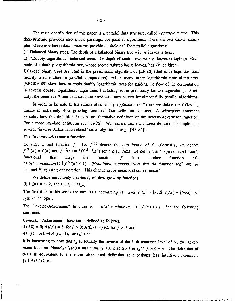
The base of the inductive definition (see Figure 2.1). We start with the definition of the *-tree

BT(2). BT(2) is simply a complete binary tree with n leaves.

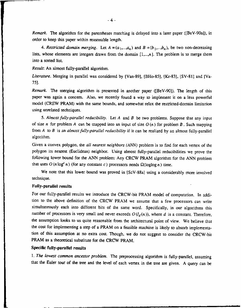
The inductive step (see Figure 2.2). For m, 3 5 m 5 t(n), we define BT (m) as follows. BT (m)

has n leaves. The number of levels in BT(m) is *ImI(n)+l (= n(n)+l). The root is at level 1

-6-

and the leaves are at level *IJ1 l(n)+l. Consider a node v at level 1 5 1 5 *I11 l(n) of the tree.Node v has IM-1)(n)/Ig2 1 (n) children (we define Im(0) 1 (n) to be n). The total number of leaves

in the subtree rooted at node v is l,.'-jl) (n ). We refer to the part of the BT(m) tree described so

far as the top recursion level of BT(m) (denoted for brevity TRL-BT(m) ). In addition, node v

contains recursively a BT(m-1) trc- The number of leaves in this tree is exactly the number of

children of node v in BT(m).

In a nutshell, there is one key idea that enabled our algorithms to be as fast as they are.

When the m 'th tree BT(m) is employed to guide the computation, we invest 0 (1) time on the

top recursion level for BT(m)! Since BT(m) has m levels of recursion, this leads to a total of

0 (m ) time.

Similar computational structures appeared in a few contexts. See, [AS-87] and [Y-82] for

generalized range-minima computations, [HS-861 for Davenport-Schinzel sequences and [CFL-83]

for circuits.

3. Basics

We will need the following problems and algorithms.

The Euler tour technique

Consider a tree T = (V,E), rooted at some vertex r. The Euler tour technique enables to

compute several problems on trees in logarithmic time and optimal speed-up (see also [TV-85]and [Vi-85]). The technique is summerized below.

Step 1: For each edge (v -u) in T we add its anti-parallel edge (u -4v). Let H denote the new

graph.

Since the in-degree and out-degree of each vertex in H are the same, H has an Euler path

that start and ends in the root r of T. Step 2 computes this path into a vector of pointers D,where for each edge e of H, D (e) will have the successor edge of e in the Euler path.

Step 2: For each vertex v of H, we do the following:

(Let the outgoing edges of v be (v-4u0 ) , ' ' •, (V---Ud )

D(ui--'v):=(v"4U(i+l),,od d), for i = 0, .. ,d-1. Now D has an Euler circuit. The "correction"D (Ud-l--->r):=end-of -list (where the out-degree of r is d) gives an Euler path which starts and

ends in r.

Step 3: In this step, we apply list ranking to the Euler path. This will result in ranking the edges

so that the tour can be stored in an array. Similarly, we can find for each vertex in the tree its

distance from the root. This distance is called the level of vertex v. Such applications of list

ranking appear in [TV-85]. This list ranking can be performed in logarithmic time using anoptimal number of processors, by [AM-88], [CV-861 or [CV-89].

-7-

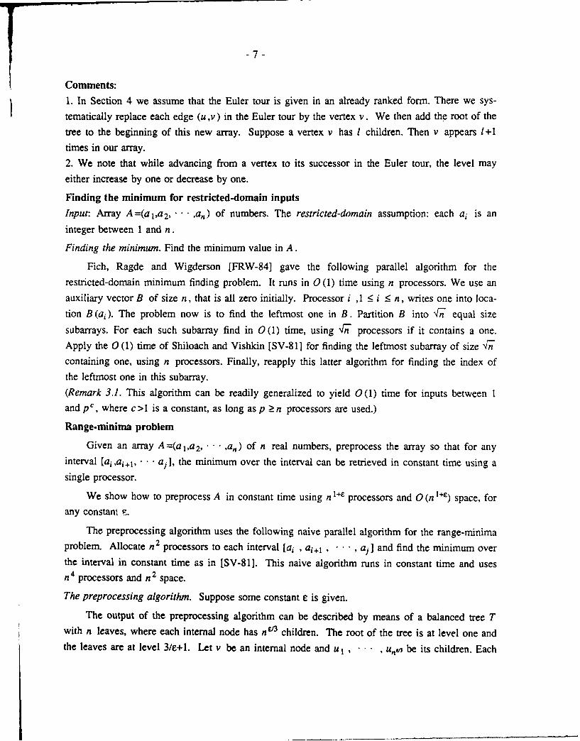
Comments:1. In Section 4 we assume that the Euler tour is given in an already ranked form. There we sys-

tematically replace each edge (u,v) in the Euler tour by the vertex v. We then add the root of the

tree to the beginning of this new array. Suppose a vertex v has 1 children. Then v appears 1+1

times in our array.2. We note that while advancing from a vertex to its successor in the Euler tour, the level may

either increase by one or decrease by one.

Finding the minimum for restricted-domain inputs

Input: Array A =(a 1,a2, ... ,a) of numbers. The restricted-domain assumption: each ai is an

integer between 1 and n.

Finding the minimum. Find the minimum value in A.

Fich, Ragde and Wigderson [FRW-84] gave the following parallel algorithm for therestricted-domain minimum finding problem. It runs in 0 (1) time using n processors. We use an

auxiliary vector B of size n, that is all zero initially. Processor i ,1 _ i < n, writes one into loca-tion B (ai ). The problem now is to find the leftmost one in B. Partition B into I1n equal size

subarrays. For each such subarray find in 0 (1) time, using NIn processors if it contains a one.Apply the 0 (1) time of Shiloach and Vishkin [SV-81] for finding the leftmost subarray of size "'ncontaining one, using n processors. Finally, reapply this latter algorithm for finding the index of

the leftmost one in this subarray.(Remark 3.1. This algorithm can be readily generalized to yield 0(1) time for inputs between Iand pC, where c >1 is a constant, as long as p - n processors are used.)

Range-minima problem

Given an array A =(a1,a 2, ... ,a) of n real numbers, preprocess the array so that for anyinterval [ai ,a i , • aj ], the minimum over the interval can be retrieved in constant time using a

single processor.

We show how to preprocess A in constant time using n l+E processors and 0 (n l+E) space, for

any constant s.

The preprocessing algorithm uses the following naive parallel algorithm for the range-minimaproblem. Allocate n 2 processors to each interval [ai , ai+l , • • • , aj] and find the minimum over

the interval in constant time as in [SV-81]. This naive algorithm runs in constant time and uses

n 4 processors and n 2 space.

The preprocessing algorithm. Suppose some constant e is given.

The output of the preprocessing algorithm can be described by means of a balanced tree Twith n leaves, where each internal node has n V3 children. The root of the tree is at level one and

the leaves are at level 3/e+l. Let v be an internal node and u1 , , u,n be its children. Each

-8 -

internal node v will have the following data.

1. M (v) - the minimum over its leaves (i.e. the leaves of its subtree).

2. For each 1 < i < j < nV3 the minimum over the range {M(ui) , M(ui+), , M(uj)).

This will require 0 (n 2/E) space per internal node and a total of 0 (n 1+W3) space.

The preprocessing algorithm advances through the levels of the tree in 3/e steps, starting

from level 3/e. At each level, each node computes its data using the naive range-minima algo-

rithm.

Each internal node uses n 41F processors and 0 (n 2/) space and the whole algorithm uses n I+E

processors, 0 (n 1+V3) space and 0 (3/e) time.

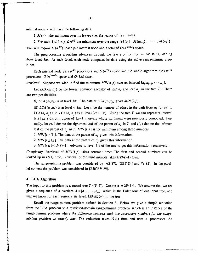
Retrieval. Suppose we wish to find the minimum, MIN(i ,j) over an interval [ai,ai+, aj].

Let LCA (ai ,aj) be the lowest common ancestor of leaf ai and leaf aj in the tree T. There

are two possibilities.

(i) LCA (ai ,aj) is at level 3/s. The data at LCA (ai ,aj) gives MIN (ij).

(ii) LCA (ai ,aj) is at level < 3/e. Let x be the number of edges in the path from ai (or aj) to

LCA (ai ,aj) (i.e. LCA (ai ,aj ) is at level 3/e+l-x). Using the tree T we can represent interval

[iJ] as a disjoint union of 2x-1 intervals whose minimum were previously computed. For-

mally, let r (i) denote the rightmost leaf of the parent of ai in T and (j) denote the leftmost

leaf of the parent of aj in T. MIN [i j] is the minimum among three numbers.

1. MIN [i ,:. (i)]. The data at the parent of ai gives this information.

2. MIN [l (),J ]. The data at the parent of a gives this information.

3. MIN [r(i )+l,l (j)-l]. Advance to level 3/e of the tree to get this information recursively.

Complexity. Retrieval of MIN(i,j) takes constant time: The first and second numbers can belooked up in 0 (1) time. Retrieval of the third number takes 0 (3/e-1) time.

The range-minima problem was considered by [AS-87], [GBT-84] and [Y-82]. In the paral-

lel context the problem was considered in [BBGSV-891.

4. LCA Algorithm

The input to this problem is a rooted tree T=(V,E). Denote n = 21V I-1. We assume that we aregiven a sequence of n vertices A = [a 1, . . . ,a, , which is the Euler tour of our input tree, and

that we know for each vertex v its level, LEVEL (v), in the tree.

Recall the range-minima problem defined in Section 3. Below we give a simple reductionfrom the LCA problem to a restricted-domain range-minima problem, which is an instance of therange-minima problem where the difference between each two successive numbers for the range-

minima problem is exactly one. The reduction takes 0(1) time and uses n processors. An

-9-

algorithm for the restricted-domain range-minima problem is given later, implying an algorithm

for the LCA problem.

4.1. Reducing the LCA problem into a restricted-domain range-minima problem

Let v be a vertex in T. Denote by I (v) the index of the leftmost appearance of v in A and by

r (v) the index of its rightmost appearance. For each vertex v in T, it is easy to find I (v) and r (v)

in 0 (1) time and n processors using the following (trivial) observation:

I (v) is where at(,)=v and LEVEL (a,(V)-,)=LEVEL (v)-I.

r(v) is where ar(v)--v and LEVEL(ar(v)+I)=LEVEL(v)-.

The claims and corollaries below provide guidelines for the reduction.

Claim 1: Vertex u is an ancestor of vertex v iff 1 (u) < I (v) < r (u).

Corollary 1: Given two vertices u and v, a single processor can find in constant time

whether u is an ancestor of v.

Corollary 2: Vertices u and v are unrelated (namely, neither u is an ancestor of v nor v is

an ancestor of u ) iff either r (u) < I (v) or r (v) < 1 (u).

Claim 2. Let u and v be two unrelated vertices. (By Corollary 2, we may assume without

loss of generality that r(u) < l(v).) Then, the LCA of u and v is the vertex whose level is

minimal over the interval [r (u) , l(v)] in A.

The reduction. Let LEVEL (A) = [LEVEL (a 1), LEVEL (a 2),...,LEVEL (an)]. Claim 2 shows that

after performing the range-minima preprocessing algorithm with respect to LEVEL (A), a query ofthe form LCA (u,v) becomes a range minimum query. Observe that the difference between the

level of each pair of successive vertices in the Euler tour (and thus each pair of successive entries

in LEVEL (A)) is exactly one and therefore the reduction is into the restricted-domain range-

minima problem as required.

Remark. [GBT-84] observed that the problem of preprocessing an array so that each range-

minimum query can be answered in constant time (this is the range-minima problem defined in the

previous section) is equivalent to the LCA problem. They gave a linear time algorithm for the

former problem using an algorithm for the latter. This does not look very helpful: we know to

solve the range-minima problem based on the LCA problem, and conversely, we know to solve

the LCA problem based on the range-minima problem. Nevertheless, using the restricted domain

properties of our range-minima problem we show that this cyclic relationship between the two

problems can be broken and thereby, lead to a new algorithm.

- 10-

4.2. The restricted-domain range-minima algorithm

We define below a restricted-domain range-minima problem which is slightly more general than

the problem for LEVEL(A). The more general definition enables recursion in the algorithm

below. The rest of this section shows how to solve this problem.

The restricted-domain range-minima problem

Input: Integer k and array A =(a ,a2, ' • ,an ) of integers, such that lai -ai +1 <- k. In words, the

difference between each ai , 1 5 i < n, and its successor ai+1 is at most k. The parameter k need

not be a constant.

The range-minima problem. Preprocess the array A =(a ,a 2, ,an ) so that any query MIN [iJ,

1 < i < j < n, requesting the minimal element over the interval [ai , , aj], can be processed

quickly using a single processor.

Comment 1: We make the simplifying assumption that V is always an integer.

Comment 2. In case the minimum in the interval is not unique, find the minimal element in

[a,, . . , aj I whose index is smallest ("the leftmost minimal element"). Throughout this section,

whenever we refer to a minimum over an interval, we will always mean the leftmost minimal ele-

ment. Finding the leftmost minimal element (and not just the minimum value) will serve us later.

We start by constructing inductively a series of c0(n )-1 parallel preprocessing algorithms for

our range-minima problem:

Lemma 4.2.1. The algorithm for 2 !5 m < cx(n) runs in cm time, for some constant c, using

nI (n ) + vTn processors. The preprocessing aigorithm results in a table. Using this table, any

range-minimum query can be processed in cm time. In addition, the preprocessing algorithm finds

explicitly all prefix-minima and suffix-minima, and therefore there is no need to do any processing

for prefix-minima or suffix-minima queries.

Our optimal algorithms, whose efficiencies are given in Theorem 4.3.1, are derived from this

series of algorithms.

We describe the series of preprocessing algorithms. We give first the base of the inductive

construction and later the inductive step.

The base of the inductive construction (the algorithm for m =2)

In order to provide intuition for the description of the preprocessing algorithm for m =2 we present

first its output and how the output can be used for processing a range-minimum query.

Output of the preprocessing algorithm for m =2."

- 11 -

(1) For each consecutive subarray ajlog3n+l a(j+l)log3n, 0 j - n/log3n-1, we keep a

table. The table enables constant time retrieval of any range-minimum query within the subar-

ray.

(2) Array B = b I , /Ig3n consisting of the minimum in each subarray.

(3) A complete binary tree BT (2), whose leaves are b1 , • • • , bn/log3n. Each internal node v of

the tree holds an array Pv with an entry for each leaf of v. Consider prefixes that span

between I (v), the leftmost leaf of v, and a leaf of v. Array Pv has the minima over all these

prefixes. Node v also holds a similar array S,. For each suffix, that spans between a leaf v

and r (v), the rightmost leaf of v, array S, has its minimum.

(4) Two arrays of size n each, one contains all prefix-minima and the other all suffix-minima

with respect to A.

Lemma 4.2.2. Let m be 2. Then Im (n) = logn. The preprocessing algorithm will run in 2c time

for some constant c using n logn +'W'n processors. The retrieval time of a query MIN [ij ] is 2c.

How to retrieve a query MIN [i ,j] in constant time?

There are two possibilities.

(i) ai and aj belong to the same subarray (of size log 3n). MIN(ij) is computed in 0(1) time

using the table that belongs to the subarray.

(ii) ai and aj belong to different subarrays. We elaborate below on possibility (ii).

Let right(i) denote the rightmost element in the subarray of ai and left (j) denote the leftmost

element in the subarray of aj. MIN [ij ] is the minimum among three numbers.

1. MIN [i ,right (i)], the minimum over the suffix of ai in its subarray.

2. MIN[left(j),j], the minimum over the prefix of aj in its subarray.

3. MIN [right (i)+l,left (j)-l].

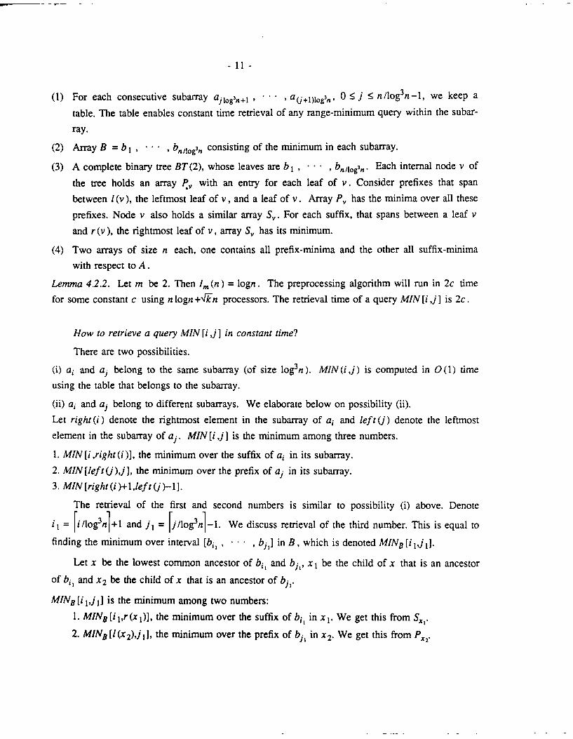
The retrieval of the first and second numbers is similar to possibility (i) above. Denote

il = Ii/log3n]+l and j, = [j/log3n]-l. We discuss retrieval of the third number. This is equal to

finding the minimum over interval [biI , • • • , bj] in B, which is denoted MINB [i ,J 1].

Let x be the lowest common ancestor of bi, and bj1, x I be the child of x that is an ancestor

of bi, and x 2 be the child of x that is an ancestor of bj1 .

MINB [i ,j I] is the minimum among two numbers:

1. MINB [i I,r(x 1)], the minimum over the suffix of bi in x 1. We get this from Sx,.

2. MINB [1 (x 2),j 11, the minimum over the prefix of bj in x 2. We get this from PX2.

- 12-

It remains to show how to find x, x1 and x 2 in constant time. It was observed in [HT-84] that the

lowest common ancestor of two leaves in a complete binary tree can be found in constant time

using one processor. (The idea is to number the leaves from 0 to n-1. Given two leaves i1 and J ,

it suffices to find the most significant bit in which the binary representation of il and j, are

different, in order to get their lowest common ancestor.) Thus x (and thereby also x 1 and x 2) can

be found in constant time. Constant time retrieval of MIN(ij) query follows.

The preprocessing algorithm for m =2

Step 1. Partition A into subarrays of log3n elements each. Allocate log4n processors to each

subarray and apply the preprocessing algorithm for range-minima given in Section 3 (for e = 1/3).

This uses log 4n processors and 0(log3nlog" 3n) space per subarray and n logn processors and

o (n logn) space overall.

Step 2. Take the minimum in each subarray to build q'ray B of size n /log3n. The

difference between two successive elements in B is at most k lo, a .

Step 3: Build BT(2), a complete binary tree, whose leaves are the elements of B. For each

internal node v of BT(2) we keep an array. The array consists of the values of all leaves in the

subtree rooted at v. So, the space needed is n/log3n per level and n/log2n for all levels of the

tree. We allocate to each leaf at each level Vk" log2n processors and the total number of processors

used is thus k'n.

Step 4: For each internal node, find the minimal element over its array. If the minimal ele-

ment is not unique, the leftmost one is found. We apply the constant time algorithm mentioned in

Remark 3. 1. Consider an internal node of size r. After subtracting the first element of the array

from each of its elements, we get an array whose elements range between -krlog 3n and kr log3n.

The size of the range, which is 2krlog3n+l, does not exceed the square of number of processors,

which is r klog2n, and the algorithm of Remark 3.1 can be applied.

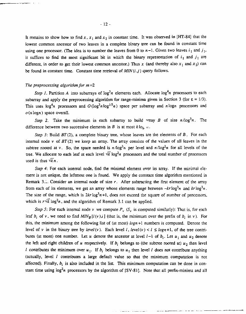
Step 5: For each internal node v we compute P, (S, is computed similarly): That is, for each

leaf bi of v, we need to find MINB [1 (v),i ] (that is, the minimum over the prefix of bi in v). For

this, the minimum among the following list of (at most) logn+l numbers is computed. Denote the

level of v in the binary tree by level(v). Each level 1, level(v) < 1 < logn+l, of the tree contri-

butes (at most) one number. Let u denote the ancestor at level I-I of bi . Let u 1 and u 2 denote

the left and right children of u respectively. If bi belongs to (the subtree rooted at) u 2 then level

I contributes the minimum over u 1. If bi belongs to u1 then level I does not contribute anything

(actually, level I contributes a large default value so that the minimum computation is not

affected). Finally, bi is also included in the list. This minimum computation can be done in con-

stant time using log 2n processors by the algorithm of [SV-81]. Note that all prefix-minima and all

- 13 -

suffix-minima of B are computed (in the root) in this step.

Step 6. For each ai we find its prefix minimum and its suffix minimum with respect to A

using one processor in constant time. Let bj be the minimum representing the subarray of size

log3n containing ai . The minimum over the prefix of ai with respect to A is the minimum

between the prefix of bj 1 with respect to B and the minimum over the prefix of aj with respect

to its subarray.

This completes the description of the inductive base: Items (1), (2), (3) and (4) of the output were

computed (respectively) in steps 1, 2, 5 and 6 above.

Complexity of the inductive base. 0 (1) time using n logn+"kn processors.

Lemma 4.2.2 follows.

The inductive step

The algorithm is presented in a similar way to the inductive base.

Output of the m'th preprocessing algorithm

(1) For each consecutive subarray ajt3(n)+la, , a+2(, ), 0 <j < n/I 3(n)-l, we keep a

table. The table enables constant time retrieval of any range-minimum query within the subar-

ray. (Comment. The notation I,3(n) means ([in(n))3 where Ira(n) is defined earlier.)

(2) Array B = b1 , - • - , b,,pt2(, ) consisting of the minimum in each subarray.

(3) TRL-BT(m), the top recursion level of (the recursive *-tree) BT(m), whose leaves are

b I , • • , b,,1.3(,, ). Each internal node v of TRL-BT(m) holds an array P, and array S,

with an entry for each leaf of v. These arrays hold (as in the binary tree for m =2) prefix-

minima and suffix-minima with respect to the leaves of v.

(4) Let ul , ... , uY be the children of v, an internal node of TRL-BT(m). Denote by

MIN (ui ) be the minimum over the leaves of node ui , 1 5 i < y. Each such node v has recur-

sively the output of the m-l'th preprocessing algorithm with respect to the input

MIN(u 1 ) , - , MIN(uY).

(5) Two arrays of size n each, one contains all prefix-minima and the other all suffix-minima

with respect to A.

How to retrieve a query MIN [i ] in cm time?

We distinguish two possibilities.

(i) ai and aj belong to the same subarray (of size 13m(n)). MIN(ij) is computed in O(1) time

using the table that belongs to the subarray.

14-

(ii) ai and aj belong to different subarrays. We elaborate on possibility (ii).

Again, let right (i) denote the rightmost element in the subarray of ai and left (j) denote the left-

most element in the subarray of aj. MIN [i ,j] is the minimum among three numbers.

1. MIN [i,right (i)].

2. MIN [left (j),j].

3. MIN [right (i)+,lef t (j)-11.

The retrieval of the first and second numbers is similar to possibility (i) above. Denote

il= 1iI(n)]+1 and jl= [j/13(n)1-1. Retrieval of the third number is equal to finding the

minimum over interval [bi , ... , bjl ] in B which is denoted MINB [i ,Jj ].

Let x be the lowest common ancestor of biI and bj in TRL -BT (m), x 3i1) be the child of x

that is an ancestor of bi, and x (jo) be the child of x that is an ancestor of bj. MINB[il,jlI is

(recursively) the minimum among three numbers.

1. MINB [i 1,r (x p(iI))], the minimum over the suffix of bi, in x p(i"). We get this from Sxq.

2. MINE [I (x p(j,)),j l], the minimum over the prefix of bj, in X(j 1). We get this from Pxw

3. MINB [r(x0(i1))+l,l(x (j1))-l]. This will be recursively derived from the data at node x.

The first two numbers are precomputed in TRL-BT (m). The recursive definition of the third

number implies that MNsil,j1] is actually the minimum among 4(m-l)-2 precomputed

numbers. Therefore, in order to show that retrieval of MIN [ij] takes time proportional to m, as

claimed, it remains to explain how to find the nodes x, xp(il) and xp(jl) in constant time using one

processor. This is done below.

We first note that for each leaf of TRL-BT(m), finding the child of the root which is its

ancestor needs constant time using one processor. Given two leaves of TRL-BT(m) consider

their ancestors among the children of the root. If these ancestors are different, we are done. Sup-

pose these ancestors are the same.

Each child of the root has l,'_(n/13(n)) l m-(n) leaves. Observe that for TRL-BT(m)

the same subtree structure is replicated at each child of the root. For each pair of two leaves u

and v of the generic subtree structure, we will compute three items into a table: (1) their lowest

common ancestor w; (2) the child f of w which is an ancestor of u; (3) the child g of w which

is an ancestor of v. The size of the table is only 0 (12_. (n)).

It remains to show how the table is computed. Consider an internal node w of the tree and

suppose that its rooted subtree has r leaves. At node w each pair of leaves u, v is allocated to a

processor. The processor determines in constant time if w is the LCA of u and v. This is done

by finding whether the child of w which is an ancestor of u, denoted f, and the child of w which

-15-

is an ancestor of v are different. If yes, then w, f and g are as required for the table. The

number of processors needed for computing the table is O(12_1 (n)).

The preprocessing algorithm for m

Inductively, we assume that we have an algorithm that preprocesses the array

A =(a1 ,a 2, -. ,a,) for the range-minima problem in c (m-1) time using n/ -(n) + 'Fkn proces-

sors, where c is a constant; and that following this preprocessing any MIN[i j] query can beanswered in c (m-i) time. We construct an algorithm that solves the range-minima problem in

c l+c (m-i) time for some constant c1, using n1r,. (n) + 4 "k'n processors. We have already shown

that a query can be answered in c2m time for some constant c2 . Selecting initially c > c1 and

c > c2 implies that the algorithm runs in cm time using nlrn (n) + 4rkn processors and that a

query can be answered in cm time.

Step 1. Partition A into subarrays of 13(n ) elements each. Allocate 1,,,(n) processors to eachsubarray and apply the preprocessing algorithm for range-minima given in Section 3 (for P = 1/3).

This uses 14(n) processors and O(123(n)lm113(n)) space per subarray and nlm (n) processors and

o (n'm (n)) space overall.

Step 2. Take the minimum in each subarray to build array B of size n/13(n). The

difference between two successive elements in B is at most k/d3(n).

Step 3: Build TRL-BT(m), the upper level of a BT(m) tree whose leaves are the elements ofB. Each internal node of TRL-BT(m), whose rooted tree has r leaves, has r/"rn-I (r) children.For each such internal node v of TRL-BT(m) we keep an array. The array consists of the values

of the r leaves of the subtree rooted at v. TRL-BT(m) will have *ImI(n13!(n))+1 < (n)+1levels. So, the space needed is n /1m(n) per level and O(n/,(n)) for all levels of TRL-BT(m).

We allocate to each leaf at each level 1+'k'J,,2(n) processors and the total number of processors

used is thus n/I2(n) + VkLn (which is less than n,, (n) + 1k'n

Step 4.1: For each internal node of TRL-BT(m), find the minimum over its array. Thedifference between the minimum value and the maximum value in an array never exceeds the

square of its number of processors and we apply the constant time algorithm mentioned in Remark

3.1 as in Step 4 of the inductive base algorithm.

Step 4.2: We focus on internal node v having r leaves in TRL-BT(m). Each of its r/Im-.(r)

children contributes its minimum and we preprocess these minima using the assumed algorithm form-l. The difference between adjacent elements is at most klm-l(r) 3(n). Thus, this computation

takes c (m -I) time using r+ k-- r processors. (To see this, simplify

r Im-l(r)+Vklm-(r)1 3(n) r the processor count term for this problem, into

r+ imTn)r/41m_l(r) which is less than r+V'kJ[T 7 r processors.) This amounts to

-16-

n /13 (n )+4 U n(n ) n /!,3(n) per level or a total of n/1,2(n )+-Flkn/4 7(n) processors which is less

than n/ln,(n )+lkn.

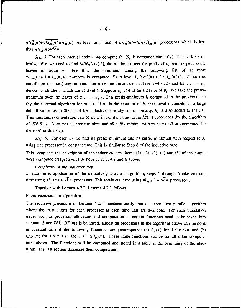
Step 5: For each internal node v we compute P, (S, is computed similarly). That is, for each

leaf bi of v we need to find MINB [1 (v),i ], the minimum over the prefix of bi with respect to the

leaves of node v. For this, the minimum among the following list of at most*lm-I(n)+l = lm(n)+l numbers is computed: Each level 1, level (v) < I < lm(nf)+l, of the tree

contributes (at most) one number. Let u denote the ancestor at level 1-1 of bi and let u 1, " " " uy

denote its children, which are at level 1. Suppose uj, j>l is an ancestor of bi . We take the prefix-

minimum over the leaves of u1 , ,uj-,. This prefix-minimum is computed in the previous step

(by the assumed algorithm for m-l). If u 1 is the ancestor of bi then level I contributes a large

default value (as in Step 5 of the inductive base algorithm). Finally, bi is also added to the list.

This minimum computation can be done in constant time using 1,2(n) processors (by the algorithm

of [SV-81]). Note that all prefix-minima and all suffix-minima with respect to B are computed (in

the root) in this step.

Step 6. For each ai we find its prefix minimum and its suffix minimum with respect to A

using one processor in constant time. This is similar to Step 6 of the inductive base.

This completes the description of the inductive step: Items (1), (2), (3), (4) and (5) of the output

were computed (respectively) in steps 1, 2, 5, 4.2 and 6 above.

Complexity of the inductive step

In addition to application of the inductively assumed algorithm, steps 1 through 6 take constant

time using n/m (n) + 'n processors. This totals cm time using nlm (n) + 'TkIn processors.

Together with Lemma 4.2.2, Lemma 4.2.1 follows.

From recursion to algorithm

The recursive procedure in Lemma 4.2.1 translates easily into a constructive parallel algorithm

where the instructions for each processor at each time unit are available. For such translationissues such as processor allocation and computation of certain functions need to be taken into

account. Since TRL-BT(m) is balanced, allocating processors in the algorithm above can be done

in constant time if the following functions are precomputed: (a) Im (x) for I < x < n and (b)

I4i2, (x) for 1 < x 5 n and 1 < i < Im (x). These same functions suffice for all other computa-

tions above. The functions will be computed and stored in a table at the beginning of the algo-rithm. The last section discusses their computation.

17 -

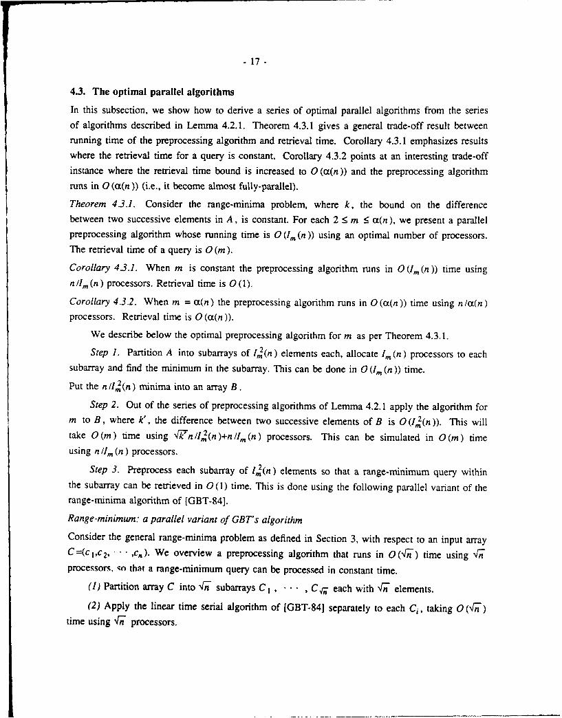
4.3. The optimal parallel algorithms

In this subsection, we show how to derive a series of optimal parallel algorithms from the seriesof algorithms described in Lemma 4.2.1. Theorem 4.3.1 gives a general trade-off result betweenrunning time of the preprocessing algorithm and retrieval time. Corollary 4.3.1 emphasizes resultswhere the retrieval time for a query is constant. Corollary 4.3.2 points at an interesting trade-offinstance where the retrieval time bound is increased to 0 (((n)) and the preprocessing algorithmruns in 0 (ct(n)) (i.e., it become almost fully-parallel).

Theorem 4.3.1. Consider the range-minima problem, where k, the bound on the differencebetween two successive elements in A, is constant. For each 2 < m < a(n), we present a parallelpreprocessing algorithm whose running time is O (I (n)) using an optimal number of processors.The retrieval time of a query is 0 (m).

Corollary 43.1. When m is constant the preprocessing algorithm runs in O(lm(n)) time using

n/Im (n) processors. Retrieval time is 0 (1).

Corollary 4.3.2. When m = a(n) the preprocessing algorithm runs in 0 (a(n)) time using n /a(n)processors. Retrieval time is 0 (a(n )).

We describe below the optimal preprocessing algorithm for m as per Theorem 4.3.1.

Step 1. Partition A into subarrays of I2(n) elements each, allocate In (n) processors to eachsubarray and find the minimum in the subarray. This can be done in 0 (1. (n)) time.

Put the n /12(n) minima into an array B.

Step 2. Out of the series of preprocessing algorithms of Lemma 4.2.1 apply the algorithm form to B, where k', the difference between two successive elements of B is O (I2(n)). This willtake 0 (m) time using "'Wn/J2(n )+nlm(n) processors. This can be simulated in 0(m) time

using n/In (n) processors.

Step 3. Preprocess each subarray of 12(n) elements so that a range-minimum query withinthe subarray can be retrieved in 0(1) time. This is done using the following parallel variant of therange-minima algorithm of [GBT-84].

Range-minimum: a parallel variant of GBT's algorithm

Consider the general range-minima problem as defined in Section 3, with respect to an input arrayC=(c 1,c2, '.,c*). We overview a preprocessing algorithm that runs in 0(-n ) time using "n1processors, .o that a range-minimum query can be processed in constant time.

(1) Partition array C into 4n_ subarrays CI , - • • , Cr - each with -in elements.

(2) Apply the linear time serial algorithm of [GBT-84] separately to each Ci, taking 0 ('-n)

time using V1W processors.

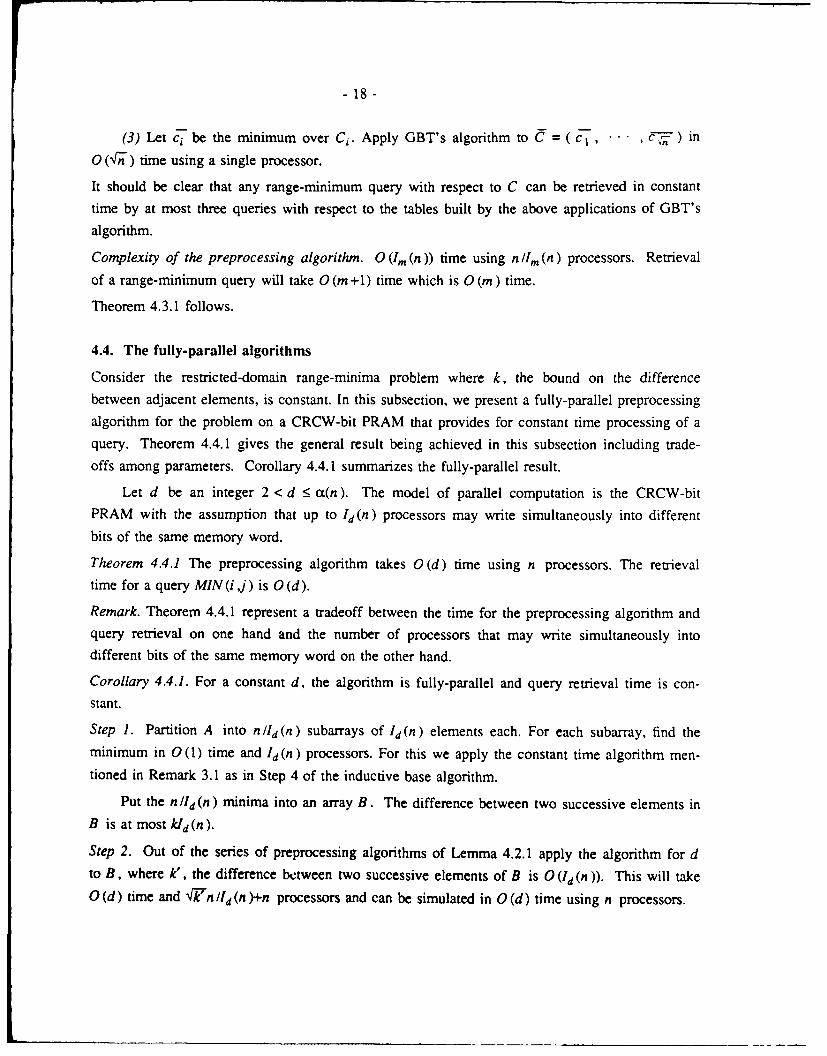
- 18 -

(3) Let ci be the minimum over Ci . Apply GBT's algorithm to C=(c 1 , ) in

0 ('n) time using a single processor.

It should be clear that any range-minimum query with respect to C can be retrieved in constanttime by at most three queries with respect to the tables built by the above applications of GBT's

algorithm.

Complexity of the preprocessing algorithm. 0 (Im (n)) time using n "irn(n) processors. Retrieval

of a range-minimum query will take 0 (m+1) time which is 0 (m) time.

Theorem 4.3.1 follows.

4.4. The fully-parallel algorithms

Consider the restricted-domain range-minima problem where k, the bound on the differencebetween adjacent elements, is constant. In this subsection, we present a fully-parallel preprocessingalgorithm for the problem on a CRCW-bit PRAM that provides for constant time processing of aquery. Theorem 4.4.1 gives the general result being achieved in this subsection including trade-offs among parameters. Corollary 4.4.1 summarizes the fully-parallel result.

Let d be an integer 2 < d -o(n). The model of parallel computation is the CRCW-bitPRAM with the assumption that up to 'd(n) processors may write simultaneously into different

bits of the same memory word.

Theorem 4.4.1 The preprocessing algorithm takes 0(d) time using n processors. The retrievaltime for a query MIN (i,j) is 0 (d).

Remark. Theorem 4.4.1 represent a tradeoff between the time for the preprocessing algorithm andquery retrieval on one hand and the number of processors that may write simultaneously intodifferent bits of the same memory word on the other hand.

Corollary 4.4.1. For a constant d, the algorithm is fully-parallel and query retrieval time is con-

stant.

Step 1. Partition A into n /d (n) subarrays of Id (n) elements each. For each subarray, find theminimum in 0 (1) time and Id (n ) processors. For this we apply the constant time algorithm men-

tioned in Remark 3.1 as in Step 4 of the inductive base algorithm.

Put the nild (n) minima into an array B. The difference between two successive elements inB is at most k/d (n).

Step 2. Out of the series of preprocessing algorithms of Lemma 4.2.1 apply the algorithm for dto B, where k', the difference between two successive elements of B is 0 (Id (n)). This will take0 (d) time and 'n /Id (n )+n processors and can be simulated in 0 (d) time using n processors.

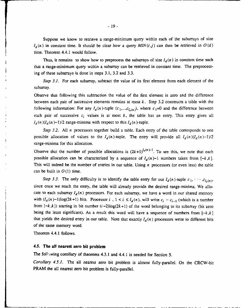
- 19-

Suppose we know to retrieve a range-minimum query within each of the subarrays of size

ld (n) in constant time. It should be clear how a query MIN (i j) can then be retrieved in 0 (d)

time. Theorem 4.4.1 would follow.

Thus, it remains to show how to preprocess the subarrays of size Id(n) in constant time such

that a range-minimum query within a subarray can be retrieved in constant time. The preprocess-

ing of these subarrays is done in steps 3.1, 3.2 and 3.3.

Step 3.1. For each subarray, subtract the value of its first element from each element of the

subarray.

Observe that following this subtraction the value of the first element is zero and the difference

between each pair of successive elements remains at most k. Step 3.2 constructs a table with thefollowing information: For any I (n)-tuple (c 1,...,cjd(,n)), where c 1=0 and the difference between

each pair of successive ci values is at most k, the table has an entry. This entry gives all

1 (n )(1d (n )- 1)/2 range-minima with respect to this Id (n )-tuple.

Step 3.2. All n processors together build a table. Each entry of the table corresponds to onepossible allocation of values to the ld(n)-tuple. The entry will provide all ld(n)(ld(n)-l)/2

range-minima for this allocation.

Observe that the number of possible allocations is (2k+l)d(n) - . To see this, we note that eachpossible allocation can be characterized by a sequence of 1d(n)-I numbers taken from [-k,k].This will indeed be the number of entries in our table. Using n processors (or even less) the table

can be built in 0 (1) time.

Step 3.3. The only difficulty is to identify the table entry for our l(n)-tuple c 1, ,ct~n),since once we reach the entry, the table will already provide the desired range-minima. We allo-cate to each subarray 1d (n) processors. For each subarray, we have a word in our shared memorywith (I(n)-l)log(2k+l) bits. Processor i , 1 < i < ld(n ), will write ci - ci_ 1 (which is a number

from [-k,k]) starting in bit number (i-2)log(2k+l) of the word belonging to its subarray (bit zerobeing the least significant). As a result this word will have a sequence of numbers from [-k,k]that yields the desired entry in our table. Note that exactly !1 (n) processors write to different bits

of the same memory word.

Theorem 4.4.1 follows.

4.5. The all nearest zero bit problem

The foll,)wing corollary of theorems 4.3.1 and 4.4.1 is needed for Section 5.

Corollary 4-5.1. The all nearest zero bit problem is almost fully-parallel. On the CRCW-bitPRAM the all nearest zero bit problem is fully-parallel.

- 20 -

Proof. Recall that the algorithm for the restricted-domain range-minima problem computes all

suffix-minima. Recall also that in case that the minimum over an interval is not unique, the left-

most minimum is found. Thus if we apply the restricted-domain range-minima algorithm (with

difference between successive elements at most one) with respect to A then the minimum over the

suffix of entry i+1 gives the nearest zero to the right of entry i. Thus, the all nearest zero bit is

actually an instance of the restricted-domain range-minima problem (with difference between suc-

cessive elements at most one). It follows that the almost fully-parallel and the fully-parallel algo-

rithms for the latter apply for the all nearest zero bit problem as well.

5. Almost fully-parallel reducibility

We demonstrate how to use the * -tree data structure for reducing a problem A into another prob-lem B by an almost fully parallel algorithm. We apply this reduction for deriving a parallel lower

bound for problem A from a known parallel lower bound for problem B.

Given a convex polygon with n vertices, the all nearest neighbors (ANN) problem is to find

for each vertex of the polygon its nearest (Euclidean) neighbor.

Theorem 5.1. Any CRCW PRAM algorithm for the ANN problem that uses 0 (n logcn) (for any

constant c) processors needs K2(loglog n) time.

Proof. We give below an almost fully-parallel reduction from the problem of merging two sortedlists of length n each to the ANN problem with 0 (n) vertices. This reduction together with the

following lemma imply the Theorem.

Lemma. Merging two sorted lists of length n each using 0 (n logcn ) (for any constant c ) proces-

sors on a CRCW PRAM needs Q(loglog n) time.

A remark in [ScV-88a] implies that Borodin and Hopcroft's ([BHo-85]) lower bound for mergingin a parallel comparisons model can be extended to yield the Lemma.

Proof of Theorem 5.1 (continued).

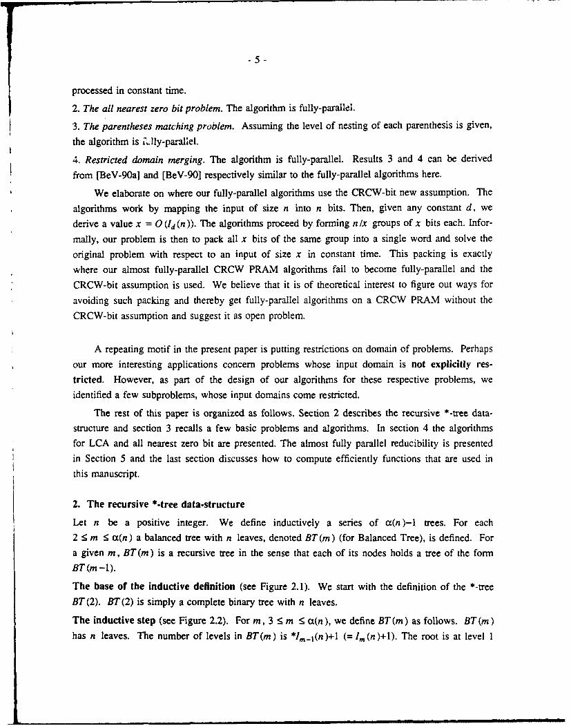
The reduction (see Figure 5.1):

Let A =(a ,a 2, • • • ,an) and B=(b l,b 2, • • • ,bn) be two increasing lists of numbers that we wish to

merge. Assume, without loss of generality, that the numbers are integers and that a1 = b 1,

an = b, . (The lower bound for merging assumes that the numbers are integers.) Consider the fol-

lowing auxiliary problem: For each 1 < i 5 n, find the minimum index j such that bj > ai . The

position of ai in the merged list is i+j-1 and therefore an algorithm for the auxiliary problem

(together with a similar algorithm for finding the positions of the bi numbers in the merged list)

suffices for the merging problem.

We give an almost fully-parallel reduction from the auxiliary problem to the ANN problem

with respect to the following convex polygon.

-21 -

Leta 1+a 2 a 2+a3 an-+an ,a The

(c'c 2 ""c 2 -) =(a, ' 2 2 2a1 '

numbers c1 , c2 , , c2n_ 1 form an increasing list. The convex polygon is(C 10) ,(C 2,0) ,' ' '.,(c 2 n, 1,0) , (b , 1/4) , (b n -, 1/4) , ... , (b 1,l/4).

In [ScV-88a] a similar construction is given and the lower bound proof then follows by (nontrivial) Ramsey theoretic arguments.

Let D [1,.. ,2n-11 be a binary vector. Each vertex (c1 ,O) finds its nearest neighbor withrespect to the convex polygon (using a 'supposedly existing' algorithm for the ANN problem) andassigns the following into vector D.

If the nearest vertex is of the form (bk,1/ 4 )then D (1) := 0else D (1) := 1

Next we apply to vector D the almost fully-parallel algorithm for the nearest zero bit problem ofSubsection 4.5. Finally, we show how to solve our auxiliary problem with respect to every ele-ment aj. We break into two cases concerning the nearest neighbor of (ai ,O) ( = (C 1 -,0)).

Case (i). The nearest neighbor of (ai ,O) is a vertex (b., 114). Then, the minimum index jsuch that bj > ai is either a or a+l. A single processor can determine the correct value ofj in 0 (1) time.

Case (ii). Otherwise. Then, D (2i -1)=. The nearest zero computation gives the smallestindex k >2i-1 for which D(k)=0. Let the nearest neighbor of (ck,O) be (b ,1/4) . Then

j = x is the minimum index for which bj > aj.

6. Computing various functions

We need to compute certain functions during our algorithms. For each 2 < m < ea(n) we needI,(21 (n) for all I < i < In,, (n). Fortunately, the function parameters that we are actually concernedwith are small, relative to n. For instance, in order to compute 13 (n) = log*n, it is enough tocompute log* (loglog n ) since log* n = log* (loglog n )+2.

We show only how to compute In (n) for each 2 5 m X(n ). Computation of l(2t (n) for2 < m < 0a(n ) and all 1 < i _< 1m (n) is similar. Our computation works by induction on m.The inductive hypothesis: Let x = loglog n. We know to compute the following values in 0 (m - 1)time using o(n/a(n)) processors: (1) Im,1(n); and (2) 'n-,(Y) for all I 5 y S loglogn.

We show the inductive claim (the claim itself should be clear), assuming the inductivehypothesis. The inductive base is given later. First, we describe (informally) the computation of

[m(x) in 0() (additional) time using o(n/at(n)) processors. Consider all permutations of thenumbers 1, .. . ,x. The number of these permutations is (much) less than n. The idea is to

- 22 -

identify a permutation that provides the sequence (X , I- (x) , .() (x)I • • (, Ik(,) 1 W = 1 , - - • 1. So if I._j(Pi) =pj+j for all 0 i < k-1 we conclude I.(x) = k. We

can check this condition in 0(1) time using x processors per permutation, using the ability of theCREW PRAM to find the AND of x bits in 0 (1) time. The total number of processors is

o (n (n)). We make two remarks: (1) Computing I .(y) for all 1 5 y < loglog n, the rest of theinductive claim, in 0 (1) time using o (n /c(n)) processors is similar. (2) there are easy ways forfinding all permutations in 0(1) time using the number of available processors.

We finish by showing the inductive base. We compute logn in 0(1) time and o(nl/c(n)processors as follows. If n is given in a binary prepresentation then the index of the leftmost oneis logn. Following [FRW-84]), this can be computed in 0 (1) using as many processors as thenumber of bits of a number. By iterating this we get log(2)n. Finally, we find logy for all

1 < y _< loglog n. The number of processors used for this computation is o (n ct(n)).

Acknowledgments

We are grateful to Pilar de la Torre and to Baruch Schieber for fruitful discussions and help-

ful comments.

References[AILSV-88] A. Apostolico, C. Iliopoulos, G.M. Landau, B. Schieber and U. Vishkin, "Parallel

construction of a suffix tree with applications", Algorithmica 3 (1988), 347-365.[AM-88] R.J. Anderson and G.L. Miller, "Deterministic parallel list ranking", Proc. 3rd

AWOC (1988), 81-90.[AMW-881 R.J. Anderson, E.W. Mayr and M. K. Warmuth, "Parallel approximation algorithm.

for bin packing", Information and Computation, 82 (1989), 262-277.[AS-87] N. Alon and B. Schieber, "Optimal preprocessing for answering on-line product

queries", TR 71/87, The Moise and Frida Eskenasy Institute of Computer Science,Tel Aviv University (1987).

[BBGSV-89] 0. Berkman, D. Breslauer, Z. Galil, B. Schieber and U. Vishkin, "Highly Paralleliz-able Problems", Proc. 21th ACM Symp. on Theory of Computing (1989), 309-319.

[BHa-871 P. Beame and J. Hastad, "Optimal Bound for Decision Problems on the CRCWPRAM", Proc. 19th ACM Symp. on Theory of Computing (1987), 83-93.

[BHo-85] A. Borodin and J.E. Hopcroft, "Routing, merging, and srting on parallel models ofcomparison", J. of Comp. and System Sci., 30 (1985), 130-145.

[BSV-881 0. Berkman, B. Schieber and U. Vishkin, "Some doubly logarithmic parallel algo-rithms based on finding all nearest smaller values", UMIACS-TR-88-79, Universityof Maryland institute for advanced computer studies (1988).

[BV-851 I. Bar-On and U. Vishkin, "Optimal parallel generation of a computation tree form",ACM Trans. on Prog. Lang. and Systems, 7 (1985), 348-357.

V- 23 -

[BeV-901 0. Berkman and U. Vishkin, "On parallel integer merging", UMIACS-TR-90-15,University of Maryland Inst. for Advanced Comp. Studies (1990).

[BeV-90a] 0. Berkman and U. Vishkin, "Almost fully-parallel parentheses matching", inpreparation.

[CFL-83] A.K. Chandra, S. Fortune and R. Lipton, "Unbounded fan-in circuits and associativefunctions", Proc. 15th ACM Symp. on Theory of Computing (1983), 52-60.

[CV-86] R. Cole and U. Vishkin, "Approximate and exact parallel scheduling with applica-tions to list, tree and graph problems", Proc. 27th Annual Symp. on Foundations ofComputer Science (1986), 478-491.

[CV-86a] R. Cole and U. Vishkin, "Deterministic coin tossing with applications to optimalparallel list ranking", Information and Control, 70 (1986), 32-53.

[CV-89] R. Cole and U. Vishkin, "Faster optimal prefix sums and list ranking", Informationand Computation 81,3 (1989), 334-352.

[DS-831 E. Dekel, and S. Sahni, "Parallel generation of postfix and tree forms", ACM Trans.on Prog. Languages and Systems, 5 (1983), 300-317.

[FRT-89] D. Fussell, V. Ramachandran and R. Thurimella, "Finding triconnected componentsby local replacements", Proc. 16th ICALP (1989).

[FRW-84] F.E. Fich, R.L. Ragde and A. Wigderson, "Relations between concurrent-writemodels of parallel computation" (preliminary version), Proc. 3rd ACM Symp. onPrinciples of Distributed Computing (1984), 179-189. Also, SIAM J. Comput. 17,3(1988), 606-627.

[GBT-84] H.N. Gabow, J.L. Bentley and R.E. Tarjan, "Scaling and related techniques forgeometry problems", Proc. 16th ACM Symp. on Theory of Computing (1984), 135-143.

[H-86] J. Hastad, "Almost optimal lower bounds for small depth circuits", Proc. 18th ACMSymp. on Theory of Computing (1986), 6-20.

[HS-861 S. Hart and M. Sharir, "Non linearity of Davenport-Schinzel sequences and general-ized path compression schemes", Combinatorica, 6,2 (1986), 151-177.

[HT-84] D. Harel and R.E. Tarjan, "Fast algorithms for finding nearest common ancestors",SIAM J. Comput., 13 (1984), 338-355.

(Kr-83] C.P. Kruskal, "Searching, merging, and sorting in parallel computation", IEEETrans. on Computers, C-32 (1983), 942-946.

[LF-80] R.E. Ladner and M.J. Fischer, "Parallel Prefix Computation", J. Assoc. Comput.Mach., 27 (1980), 831-838.

[LV-881 G.M. Landau and U. Vishkin, "Fast parallel and serial approximate string match-ing", J. of Algorithms, 11 (1989), 157-169.

[MSV-861 Y. Maon, B. Schieber, and U. Vishkin, "Parallel ear decomposition search (EDS)and st-numbering in graphs", Theoretical Computer Science, 47 (1986), 277-298.

[RR-89) V. Ramachandran and J. H. Reif, "An optimal parallel algorithm for graph planar-ity", Proc. 30th Symposium on the Foundations of Computer Science (1989), 282-

- 24 -

287.

[S-881 Q. F. Stout, "Constant-time geometry on PRAMs", ICPP 1988, 104-107.

[SV-81] Y. Shiloach and U. Vishkin, "Finding the maximum, merging and sorting in aparallel computation model", J. of Algorithms, 2 (1981), 88-102.

[SCV-881 B. Schieber, and U. Vishkin, "On finding lowest common ancestors: simplificationand parallelization", SIAM J. Comput., 17,6 (1988), 1253-1262.

[ScV-88a] B. Schieber and U. Vishkin, "Finding all nearest neighbors for convex polygons inparallel: a new lower bound technique and a matching algorithm", UMIACS-TR-88-82, University of Maryland Inst. for Advanced Comp. Studies (1988). To appearin Discrete Applied Math.

[StV-841 L.J. Stockmeyer, and U. Vishkin, "Simulation of parallel random access machinesby circuits", SIAM J. Comput., 13 (1984), 409-422.

ISZ-891 D. Shasha and K. Zhang, "New Algorithms for the Editing Distance betweenTrees", SPAA 1989, 117-126. To appear in Journal of Algorithms as "Fast Algo-rithms for the Unit Cost Editing Distance Between Trees".

[Ta-751 R.E. Tarjan, "Efficiency of a good but not linear set union algorithm", J. Assoc.Comput. Mach., 22 (1975), 215-225.

[TV-851 R.E. Tarjan and U. Vishkin, "An efficient parallel biconnectivity algorithms", SIAMJ. Comput., 14,4 (1985), 862-874.

[Va-751 L.G. Valiant, "Parallelism in comparison models", SIAM J. of Computing, 4 (1975),348-355.

[Van-891 A. Van Gelder, "PRAM processor allocation: A hidden bottleneck in sublogarithmicalgorithms" IEEE Trans. on Computers, 38,2 (1989), 289-292.

[Vi-851 U. Vishkin, "On efficient parallel strong orientation", Information ProcessingLetters, 20 (1985), 235-240.

[Vi-891 U. Vishkin, "Deterministic sampling for fast pattern matching", to be presented at22 ACM Symp. on Theory of Computing (1990). Also UMIACS-TR-2285, Univer-sity of Maryland Inst. for Advanced Comp. Studies (1989).

[Y-821 A.C. Yao, "Space-time tradeoff for answering range queries", Proc. 14 ACM Symp.on Theory of Computing (1982), 128-136.

Number or Number or Levelchildren leaves or the BT(2)per node per node tree

_ , IC'.% 3

FiGURE 2-

00

- -,,)

o -+' I • • t I -_ _

n leaves

BT(m) - m'th recursive *-tree

(0a)-< "-) " ( 1 "I •

.,,, , ,,,,, ,, -- Pi2_f__ 2 -2T ?C../,ii+.. r (rL) 3 H e

+ii

0 1=4 !r - + - _ _ _

ni leaves

Node V recursivelyV holds a BT(m-1)

troe with y leaves

(bl, -) (b 2 ', ) (b, 4-) (nb,, ) (bn,-)

C , 0 ) C2 , 0 )(C 3 ,0 C2i. 2 , 0 ) C2i.1 ' 0 ) ( k , 0 ) C2n. 1 ,

al + a2

(where cl= a1 ,c 2 - 2 c2i1 = a i ,

Figure 5.1