AD-A228 119 Characterization of Elastic Properties of ... · aerispace applications is evident by...
80
JHU-CNDE-IW.7 AD-A228 119 Characterization of Elastic Properties of Interfaces in Composite Materials T.M. Hsieh, K.A. Hirshman, EA. Lindgren, M. Rosen c........ N6A~ . September 1990 Approvd ,,oozc, Final Report Dunumo U.--dited, , Contract N00014-87-K-0341 for Steven G. Fishman, Program Manager Department of the Navy Office of Naval Research Arlington, VA 22217 9 0
Transcript of AD-A228 119 Characterization of Elastic Properties of ... · aerispace applications is evident by...

JHU-CNDE-IW.7
AD-A228 119
Characterization of Elastic Properties ofInterfaces in Composite Materials
T.M. Hsieh, K.A. Hirshman, EA. Lindgren, M. Rosen
c........ N6A~
. September 1990
Approvd ,,oozc, Final ReportDunumo U.--dited, ,
Contract N00014-87-K-0341
for
Steven G. Fishman, Program ManagerDepartment of the NavyOffice of Naval Research
Arlington, VA 22217
9 0

I
Table of Contents
Table of Contents ................................................................................................... iI. Executive Sum m ary ........................................................................................... 1II. Introduction ....................................................................................................... 3
III. Background ...................................................................................................... . 4IV. Experim ental Considerations ......................................................................... 10
IV.1 Physical Characteristics of Interface W aves .................................. 10
V. Stoneley W ave Propagation for NDE ............................................................. 11
V.1 Introduction ................................................................................... .. 11V.2 Experim ental Proceedure .................................................................. 13
V.3 Ultrasonic M easurem ents ..................... ......................................... 15V.4 Results and Discussion ................................................................... 24
V.5 Conclusion .......................................................................................... 48VI. Leaky W ave Propagation for NDE ............................................................... 49
VI.1 Tneoictical Considerations ............................................................. 49
VI.2 Experim ental Proceedure .................................................................. 56
VI.3 Experim ental M easurement Technique .......................................... 60VI.4 Results and Discussion ................................................................... 62
VI.5 Conclusions ........................................................................................ 75VII. References .................................................................................................... 77
, ~ - -,:ACC,., ("
NTV3 ("...
STATENENT "A" per Dr. Steven FishmanONR/Code 1131TELECON 10/15/90 VG By O c
t',A
[ A-I
II

I. Executive Summary
The Strategic Defense Initiative Organization has placed a great deal of
emphasis on the development of new composite materials, specifically metal and ceramic
Imatrix composites. These types of composite materials offer the advantages of being
lighter, stiffer, stronger, and more resistant to creep and corrosion. However, because of
ithe physical and chemical differences of the matrix and reinforcing agents the interface is
plagued by chemical reactions and a high level of residual stress. This impedes the
Jability of the interface to bear and transfer load and results in fracture upon subsequent
loading. Thus, the need for nondestructive characterization of interfaces is critical to the
development of these high technology composite materials.
Feedback from a nondestructive interface characterization technique is also
critical to the further development and refinement of the materials processing
procedures. iThe unique propagation characteristics of leaky interface waves appear tobe ideally sted for this purpose. While bulk moduli measurements usually yield
relatively o average values of modulus for fiber reinforced composites, leaky waves
offer the/potential for microscopic measurement of these physical parameters at localized
regions of interest. It is clear that nondestructive interface characterization is necessary
for tJie accurate modeling of the mechanical behavior of metal matrix composites.
In rface wave propagation measurements may provide the necessary information for
m' deling the micro and macrobehavior of these composites.
"--The goal of the Johns Hopkins University program was to study these
characteristics and develop techniques which utilize interface waves for nondestructive
evaluation of composite interfaces. This final report summarizes the results of two
j projects which examined the use of interface waves for nondestructive evaluation of
interfaces. The first project focused on Stoneley waves and their sensitivity to
interfacial bond quality and microstructural changes. The results demonstrated thatStoneley waves propagate with higher velocities gft5 igh interfaces of good surface
finish than they do throRgh interfaSces.gmprise-'of poorly finished surfaces. Stoneley
interf acwave velocities were also found to be dependent on the quality of the bond andthe icrostructure at the interface.
The second project focused on the use of leaky waves for the nondestructive
characterization of interfaces. " emote generation of leaky waves along a planar silicon
Jcarbide/aluminum interface wai demonstrated by mode conversion of a Iongitudinal wave
incident at an angle equivalentto the leakage angle. Direct measurement of interfacew~wave leakage was also acconiplished. It was shown that remote generation of leaky
U.-

2
waves and direct measurement of interface wave leakage in a silicon carbide/aluminum
interface is a viable method for nondestructive evaluation and characterization of a
planar interce.The results achieved during this program are summarized below:
• Sioneley interface waves were generated and detected between steel-titanium planarinterfaces. It was shown that Stoneley waves are sensitive to changes in
microstruc'ure near the bondline.
• Stoneley waves were shown to be sensitive to the amount of bonding between two
surfaces.
* Development of an approach to launch leaky modes by conversion from a bulk wa,e
incident on a bonded interface at a critical angle was accomplished. It was shown thatremote generation is a valuable method for exciting leaky modes when direct access to
the interface is impossible.
, Experimental verification of several of the theoretically predicted interface modes for aplanar silicon carbide/aluminum interface.
• Remote measurement of the leakage energy of an interface wave was accomplished. Itwas concluded that this direct measurement of leakage is a valuable method forseparating modes and will contribute to nondestructive interface characterization.
ji • It was shown that leaky waves offer several potential benefits for nondestructive
interface wave characterization including detection of disbonds and elastic
characterization.
This program demonstrated the feasibility of guided interface wave techniques fordetermining the elastic properties and adhesion of interfaces. In order to achieve the
goal of a simple and accurate nondestructive method for composite interfacecharacterization, further work must be done to implement the techniques developed here
for use on actual composite materials.
"7i

3
II. Introduction
The advantages offered by metal and ceramic matrix composites for strw, ural
aerispace applications is evident by the widespread use of these new materi.ls.
However the mechanical properties and structural integrity of these composites are
largely determined by the elastic, anelastic and plastic behavior of the interface between
the matrix and reinforcing agent. Feedback from a nondestructive interface
characterization technique is critical to the further development and refinement of the
processing procedures for these materials. No method exists for the determination of
the local elastic properties at composite interfaces. The purpose of the Johns Hopkins
University program is to develop such a technique to characterize interface properties
and to use it to study to micromechanics of composites. This will also provide an
opportunity to understand the relationship between process variables and interface
Iproperties.References to the existence of acoustic wave, that travel along an interface have
sporadically appeared in the literature since they were first predicted by Richard
Stoneley in 1924. Many of these presented theoretical predictions of wave propagation
between two ideal media with only a few papers citing experimental observations.
Interface waves are defined as elastic Aaves which propagate along the boundary
between two solid half-spaces with both longitudinal and shear components of particle
motion. It has been shown that they are sensitive to near bond line conditions including
microstructural variations and degree of contact. Recently, renewed interest in these
types of waves has developed because of their potential applications for characterizing
composite interfaces.
The scientific research goal of The Johns Hopkins University program is to
develop a nondestructive technique to characterize the properties of interfaces. The
specific goals of the research agenda include the following:
0 Study the propagation characteristic of ultrasonic Stoneley and leaky waves and
their sensitivity to interfacial bond quality and microstructural variations.
0 Develop techniques for the generation and detection of leaky waves at a composite
interface.IEvaluate the potential of these waves for nondestructive evaluation of local elastic
properties at interfaces.
I

4
I1. Background
Interface waves are elastic waves which propagate along the plane boundary
between two different elastic solid media. They are, generally, classified in two groupsby energy flow characteristics. The energy of leaky waves is attenuated as it
propagates along the boundary region with both normal and parallel components ofparticle displacements. Energy is radiated away from the interface into the less dense
material, hence the name leaky waves. Stoneley waves are non-leaking waves that
propagate unattenuated along the interface if the materials at the boundary satisfy
certain requirements. The bulk of the research that has appeared in the literature has
concentrated on Stoneley waves and has been analytical in nature. Very few of these
have presented experimental observations of interface waves of either type.
By considering the energy dissipation of seismic disturbances, Richard Stoneley
[1] first predicted the existence of these waves in 1924. He postulated that they are
similar in nature to Rayleigh and Love waves, but propagate between adjacent layers ofsubterranean rock. Essentially, Stoneley extended Lord Rayleigh's earlier work on
surface waves by modeling the interface as the plane boundary between two isotropicelastic half spaces (2,3,4]. Both continuity of stress and particle displacement across
V. the boundary was assumed. The characteristic Stoneley equation shown in Figure 1 has
8 roots for the complex velocity V2 . Therefore, there are 16 possible values of V, 8 ofwhich are independent. To interpret this equation, Stoneley resorted to the case where
the longitudinal and shear waves were approximately equal for an incompressible media,
although the densities were assumed to be different. Under these conditions, a positive
real root was found always to exist for the quantity Vs t / Vs, where Vs t is the Stoneleywave velocity and Vs is the shear wave velocity. The root was always less than unity
indicating that the velocity of the Stoneley wave was less than that of the shear wave. Itwas concluded that these types of waves may only exist if the densities and Lame'sconstants approximately satisfy Weichert's condition which states, Pl/P2 = =l/,2
M4LPl.i2, where k and i are Lame's constants, p is the density, and the subscriptsdenote the two solids.
Sezawa and Kanai [5,6,7] re-derived the Stoneley equation and analytically
determined that in certain situations a longitudinal or normally polarized shear wave
incident at an oblique angle upon a solid-solid interface would have interface, as well as
reflected and refracted wave components. They also investigated the possible range of
existence for these types of waves in terms of the densities and Lame's constants. It

5
was ascertained that for a large ratio of the densities Pl/P2 > 2 or a small ratio Pl/P2 <
0.5, the range of [t1/R2 for Stoneley wave existence is relatively wide. When the ratio of
the densities is near unity, Stoneley waves cannot exist unless Weichert's condition is
satisfied. Further analysis showed that Stoneley waves, like Rayleigh waves, are non-
dispersive. Scholte [8,9] extended the calculations of Sezawa and Kanai and examined
the existence range for Stoneley waves for several pairs of theoretical material pairs.
Velocity, amplitude, and particle motion of these waves was studied through
mathematical analysis by Yamaguchi and Sato [10]. They determined that the lower
limit of Stoneley wave velocity is the Rayleigh wave velocity which is given as
(0.8453...)1/2Vs. The ratio of the amplitude of the vertical component (w) and of the
horizontal component (u) was found to be a minimum when (VST/Vs) 2 = 0.8453...
This corresponds to a situation analogous to a Rayleigh wave. As the ratio of the
displacements increases, the ratio of the densities increases. However, as Pl
approaches P2 the horizontal component begins to shrink. When the two densities are
equal, the horizontal component disappears. By analyzing the expressions that
represent the real components of displacement, it was also shown that the rotation of
the particle orbit was in an elliptical retrograde type motion similar to that of a Rayleigh~wave.
Several papers have appeared in the literature which have shown results of
calculations of Stoneley wave ' elocities. Ginzbarg and Strick [11] graphically presented
ratios of Stoneley wave velocities and shear wae velocities for a wide range of elastic
properties. Owen [12] showed that of 900 isotropic materials, only 30 pairs would
support Stoneley waves.Stoneley waves in anisotropic materials was examined by Lim and Musgrave
[13]. Calculations for an interface composed of two crystalline half-spaces of cubic
symmetry revealed that there are several orientations which would allow the
propagation of an interface wave. It was also shown that the amplitude of these waves
dampen in a sinusoidal fashion with increasing distance from the source instead of in an
exponential manner as seen in isotropic materials. Chadwick and Currie [14] were able
to demonstrate that the secular equation for interface waves can be constructed directly
from the complex vectors that result from the analysis of Rayleigh waves on a free
surface. This equation was then reduced to a single real relation to demonstrate that
Stoneley waves in anisotropic materials are not restricted to certain directions of
propagation, but that the wave speed continuously depends on the parameters of the
transmitting materials.

'I I Icn6> >
.130>
IN -INcnj
'4 r-4
>-4
a. C
Nq N cc"
lccI
j~ > > >1 - -
> 42
N0.
>~ N
Lcr J 4 ) )
1-4-
NCi
C4

7
2.0° 8
1 1.6i.4
1I.2
N 1.0-
zL0.8'0.60.4
0.2i01 I I I I I I0.2 0.4 0.6 0.8 1.0 1.2 1.4 1.6 1.8 2.0
p'/p
Figure 2. Possible range of existence of Stoneley waves for X R, W= .' betweencurves from Sezawa and Kanai [5].

8
The sixteen independent roots of the Stoneley wave equation were studied in-depth by Pilant [15]. By varying the material parameters over a wide range, the
behavior of the sixteen roots was examined. His mathematical analysis showed thatthere are two types of behavior outside the range of existence of Stoneley waves. First,
an attenuated leaky wave will propagate if the denser material has a faster velocity thanthe less dense material. If the difference in velocity is greater than about a factor of
three, the leaky root disappears and the energy is propagated as a Rayleigh-type wave.
The second case involves a less dense material with an acoustic velocity much faster
than the more dense material. Although this case is of little physical significance, it isinteresting that the results of the analysis predict that no energy would propagate.
The studies mentioned above dealt with interface waves in a purely analyticalnature. One of the earliest reported experimental observations of interface waves wasin 1977 by Lee and Corbly [16]. Utilizing a mode conversion technique, they were able
to generate and detect Stoneley and leaky waves on both planar and cylindricalgeometries. Interface waves were generated by mode conversion from Rayleigh wavesbetween Al/Ti, steei/Al, and Ti/steel pairs. In the planar case, each couple wascomposed of a larger base plate and a smaller plate which rested on top. A schematic
diagram of their experimental set-up is shown in Figure 3. A Rayleigh wave which wasgenerated on the surface of the base plate mode converted to an interface wave at theboundary. This interface wave propagated along the boundary region until it re-converted to a Rayleigh wave at the far side of the top plate. Travel times were
measured as a function of stress applied to the couple. Figure 4 shows an ultrasonicecho wave train from a steel/aluminum specimen. The generally good quantitativeagreement found between the predicted interface wave velocity and the measured wavevelocities suggested the possibility of utilizing these wave for nondestructive inspection
of joints coupled by interference-fit fasteners.A direct optical measurement of interface waves was reported by Claus and
Palmer [17,18,19,20] in which the normal component of wave motion was observed
between a nickel/pyrex couple. Utilizing a differential interferometric optical system,they were able to measure the normal component of interface wave propagation andattenuation as a function of surface roughness. A scan of the interface wave is shown inFigure 5. The interface waves were generated by mode conversion from Rayleigh waves
between several pairs of materials which were held together by mechanical compressionand adhesive bonding. Their results also suggested potential applications for
Bnondestructive evaluation of adhesively bonded materials.

9
Surface Wave A] Surface WaveTransducer 01r- Transducer
(to receiver) (to pulser)~~Fe (orT-i),/
' Hydralic
j -Ram
IFigure 3. Schematic representation of the experimental set-up used by Lee and Corbly to
measure Stoneley wave on a planar interface.
:BACK SIDE OF
-J SECOND LAYER
Vr4
SURFACE WAVE--- FAYING END OFINTERFACE WAVE SURFACE PIN REFLECTIONTRANSITION REFLECTiON
Figure 4. Ultrasonic echo wave train from a steel/aluminum specimen from Lee andCorbly [16].

r10
"'" 0.03-
0.023
uJ., 0.02-1
0.01Lzj
4 -000--i 1 rn rn -
Figure 5. Scan of Stoneley wave on the interface between clamped Coming 7070 Pyrexand nickel samples from Claus and Palmer [17].
IV. Experimental Considerations
IV.1 Physical Characteristics of Interface WavesInterface wave is a generalized term used to describe two dissimilar but related
types of waves that travel along the plane boundary between two different solidmaterials. From the analytical results presented by some of the papers mentioned in theprevious section, the important physical characteristics of Stoneley and leaky wavesmay be summarized.
Stoneley waves correspond to real solutions of the wave equation (Figure 1).
This implies that they exist only for a limited range of material pairs includingsteel/titanium and nickel/pyrex. The existence criterion has been simplified to(satisfaction of Weichert's condition for isotropic materials or in more general terms thatthe shear wave velocities of the two materials be nearly equal. The velocity of theStoneley wave is highly dependent on the Poisson's ratio of the denser material, while

11
the Poisson's ratio of the less dense material has little influence. It is bounded at the
lower end by the fastest Rayleigh velocity and at the upper end by the slowest shear
velocity. These waves travel along the interface with the wave energy confined to a
region near the boundary. None of the energy is radiated away from the interface.
Particle displacement is composed of normal and parallel components which are
attenuated with distance into either medium. These displacements have been describedas elliptical retrograde in the denser material similar to that of a Rayleigh wave. A
schematic diagram of this motion is shown in Figure 6.
Leaky interface waves correspond to the complex solution of the wave equation.
This suggests that leaky waves will exist for many more material pairs, since the
existence criterion is not as stringent. It is possible for a leaky wave to exist if the
wave velocity of the denser material is greater than the wave velocity of the less dense
material. The particle motion of these waves is also elliptical retrograde in the denser
medium, but resemble shallow shear wave fields in the less dense medium. Part of the
wave energy is radiated away from the interface into one or both of the bounding
materials at an angle proportional to the imaginary component of the solution to the
wave equation. Figure 7 depicts this motion. For a detailed mathematical analysis of
the sixteen roots see Pilant [11].
V. Stonely Wave Propagation for NDE
V.1 Introduction
This investigation focused on the sensitivity of Stoneley interface waves to
interfacial bond quality, and their ability to evaluate microstructural change. Through
various heat treatments of 4340 steel, several pearlitic and martensitic microstructures
were obtained. The steel samples were each coupled with a Titanium-6 Aluminum-4
Vanadium sample, and Stoneley interface waves were generated along the planar
interface between the two specimens. The Stoneley interface waves were generated
and detected by Rayleigh mode conversion wedges. The corresponding ultrasonic
velocities were calculated using time-of-flight measurements as a function of
microstructure, surface finish, and interfacial bond quality.

Distance into material 1 12
jf Material 1
Interface
Material 2
Distance into material 2
Figure 6. Schematic representation of the elliptical retrograde particle rotation of aStoneley interface wave with both normal and parallel components. The constantellipse size along the x-axis represents the fact that the energy of these waves isconfined to a region near the interface are non-attenuative.
Distance into material I
Material 1
Interface
Material 2
Distance into material 2Figure 7. Schematic representation of the elliptical retrograde particle rotation of a leaky
interface wave with both normal and parallel components. The decreasing size ofthe ellipses represents the fact that part of the energy is radiated away from the
Interface into the less dense material.

13
V.2 Experimental Procedure
Five 4340 steel specimens were cut from a 305 cm x 5.08 cm x 1.27 cm slab. The
lengths of the five specimens were varied between 18 and 23 centimeters foridentification purposes. Five smaller pieces were also cut from the original plate to paireach one with a large specimen.
Heat TreatmentsHeat treatments were performed on the five specimens to obtain five different
microstructures. The Time-Temperature-Transformation (T-T-T) diagram for 4340 steelwas used for heat treatment informational purposes (Figure 8) [21]. Specimen one was
kept in its as-received state for comparison purposes. Specimen two was austenitizedat 843"C for 90 minutes. It was then transferred to a molten salt heater at 648"C for
j approximately 48 hours tu transform the microstructure to coarse pearlite (see
transformation diagram). After isothermal cooling, it was allowed to air-cool to
ambience. Specimen three was austenitized at 843"C for 70 minutes, quenched in oil for
6 minutes and then quenched in water until ambient temperatures were reached. Thetransformation diagram revealed the time period needed to obtain a fully quenched
martensite is well within the period of time required to quench a 1.27 centimeter thick
slab. The fourth specimen was austenitized at 843°C for 70 minutes and then quenchedin oil for 6 minutes. The sample was then transferred to a liquid nitrogen bath for 10
minutes and allowed to reach ambient temperatures. The specimen was then tempered
at 204'C for 100 minutes and then quenched in oil. The fifth specimen was austenitized
at 843"C for 70 minutes and was air-cooled to room temperature or normalized.
MetallographySections approximately 1.27 cm x 0.635 cm x 0.635 cm were cut from all five
smaller steel slabs. These five pieces were mounted into clear Lucite to provide across-section for metallography. The five specimens were mechanically sanded on 60
grit to 600 grit paper and then polished on three wheels: six micron diamond, threemicron diamond, and one-half micron aluminum oxide. A nital etch, 2 ml. of HN03 and 98
ml. of ethanol, was applied to the steel specimens to prepare for microstructural
observation. The titanium alloy was also prepared for metallographic observation. Ablock, 5.08 cm x 5.08 cm x 1.918 cm, was ground to have two large, flat, parallel faces.For metallographic purposes, one side was subjected to the same polishing process asthe 4340 steel specimens. A Kroll's reagent, 1-3 ml. of HF, 2-6 ml. of HNO3 and H20
14
0 0 v - coN~-S3O~ -N N pe) v
10.10
illl
40
IC 0
000L 00004
0 00 00CD N

15
Ito 1000 ml., was applied to the surface and allowed to react for fifteen seconds to
prepare for microstructural observation. Metallographic examination was performed on a
Unitron inverted stage metallograph. The 4340 steel specimens were examined at
magnifications of 160x, 320x, 500x, and 1000x to reveal the various microstructures
completely. The titanium specimen was observed at 100x, 320x, 500x, and 1000x to
examine the preferred orientation of the grains.
Hardness
Rockwell "B" hardness measurements were performed on specimens one and
two. The hardness tester was calibrated using standard calibration test blocks to a
value of plus or minus one Rockwell "B" hardness point. The measurements were
performed on pieces cut from the smaller steel slabs. By traversing the specimens in
three perpendicular directions, an average hardness value could be obtained. Rockwell
"C" tests were performed on steel specimens three, four, five, and the titanium alloy.
The hardness tester was again calibrated and measurements were performed across
each specimen in three perpendicular directions.
Density Measurements
Density measurements were performed on the five steel samples and the
titanium alloy by a method developed by Davis and Schoonover [22-23]. A high
precision, servo-controlled balance was used for the hydrostatic weighing of solid
objects. A mathematical deriv:tion in Davis' paper permitted the precise calculation of
the various volumes. The densities were then obtained by dividing the mass of each
specimen by their corresponding calculated volumes.
V.3 Ultrasonic Measurements
Ultrasonic Velocity Test Specimens
The two large faces of each 4340 steel specimen were ground flat and parallel.
one side of each specimen was then polished to a finish of 0.2 microns. The opposite
side of the titanium alloy block, 5.08 cm x 5.08 cm x 1.91 cm, was polished to 0.2
microns. Each 0.2 micron finished 4340 steel specimen was then coupled with the 0.2
micron finished titanium block to provide several different interfaces to evaluate the
f sensitivity of Stoneley waves to microstructural changes as a function of interfacial
bonding quality.
ii
14..

16
A second titanium block of similar dimensions was ground flat and parallel. This
specimen was polished to a finish of 12 microns, and coupled with a 12 micron polished
4340 steel specimen in its as-received state. This pair was utilized to investigate the
effects of surface finish on Stoneley wave velocity as a function of interfacial bonding
quality.
Bulk Ultrasonic velocity measurements
There are several types of acoustic waves that propagate in a solid medium.
Shear and longitudinal waves were two types of body waves used in this investigation.
As a result of the two waves different propagation schemes, their measured velocities
disclosed substantial information about the microstructure in various directions. The
particle displacement of a longitudinal body wave is parallel to the direction of
propagation, while that of a shear wave is perpendicular to the direction of propagation.
By rotating a shear transducer 900, the sampling direction of the particle displacement of
a shear wave reveals the degree of anisotropy within a particular material. These
measured velocities were then coupled with density values, and the elastic constants
were calculated in the two different direction schemes. The four elastic parameters
calculated in this investigation were Young's modulus (E), Shear modulus (G), Bulk
modulus (B), and Poisson's ratio (v) (Figure 9).
The technique employed to make time-of-flight measurements on shear and
longitudinal waves was the pulse-echo overlap method. A Matec pulser-receiver was
used as the wave generator and a Hewlett-Packard Amplitude-Scan Delta Time
oscilloscope was used to measure the travel time between successive pairs of echoes.
A light oil was used to couple a 5 MHz Panametrics longitudinal transducer with the
steel and titanium ultrasonic samples for velocity measurements. A viscous silicone
grease was used to couple a 5 MHz Panametrics shear transducer with the samples for
shear velocity measurements. The maximum peak overlap convention was used
throughout the bulk ultrasonic investigation because of iis consistent time-of-flight
readings.
Stoneley Wave Velocity Measurements
Theory suggested that Rayleigh waves generated in the denser medium would be
mode converted to Stoneley waves at the point of intersection with an interface, if
certain conditions were satisfied. The Stoneley wave would then propagate along the

17
Young's Modulus (E) p [ S]
Shear Modulus (G) = p V2ISI
I Bulk Modulus (B) E v
2 2
Poisson's Ratio (v) E I. L = SVL- VS]
Figure 9. Equations used in calculations of elastic constant values. VLis the
longitudinal velocity, is the shear velocity and p is the density.
I.

18
interfacial boundary region until it encountered a free surface, whereupon it would
reconvert into a Rayleigh wave.
In this investigation, several techniques were employed to generate and detect
Stoneley waves. The first was a surface wave generation method. It involved the
utilization of two broadband conical Industrial Quality, Inc.(IQI) transducers which
launched surface waves over a very wide frequency range, D.C. to 2 MHz. Many
problems were encountered with this technique. The two IQI transducers were used for
both sending and receiving the surface waves. However, because of their broadbandJnature, they are usually only used for the receiving of acoustic signals. Another problem
arose when trying to maintain point contact between the conical transducer and the
sample. Several attempts included the use of c-clamps and a specially designed plastic
mount. Both methods proved to be inefficient. Stoneley waves were also generated anddetected by setting two longitudinal transducers at the corners, of the base plate. The
Mangles between the transducers and the base plate were varied to obtain the best waveforms. Clamps were used to hold the transducers at different angles. This method alsoproved to be inefficient because it was extremely difficult to find the angles that produced
the highest resolution wave forms. Surface acoustic wave wedges were then employed
to generate and detect Stoneley waves. Waveforms with high amplitude and relatively
little noise were obtained. However, the exact travel distances were not easily
measurable. Thus, the ultrasonic velocity values were inconsistent.
The technique utilized in this investigation for the generation and detection ofStoneley waves involved Rayleigh mode conversion wedges (Figure 10) [24]. Accurate
wave path distances between successive echoes and waveforms of high resolution wereeasily obtainable by this method. The set-up included two-machined aluminum wedges
in a sliding mount. Contact was made with the base plate through the knife-edge
surfaces of the wedges. The critical angle between the wedge and the base plate
measured to be approximately 60'. This critical angle provided the maximum mode-conversion efficiency for a longitudinal wave into a Rayleigh wave and the reverse
conversion. Longitudinal piezoelectric transducers were mounted inside of each wedge
for the sending and receiving of the acoustic waves. During ultrasonic testing, the
titanium alloy block, dimensions 5.08 cm x 5.08 cm x 1.91 cm, was placed in the path of
the generated Rayleigh wave. A hollow steel block was designed to allow the
application of a compressive load perpendicular to the interface (Figure 11). The effect of
interfacial bond quality on Stoneley wave velocity was then evaluated as a function of
the applied stress. The tensile tester was capable of exerting 25 metric tons.
I

19
I
SlidinR Mount
/V/.
Transmitting 1// Receiving
Transducer i Transducer
"" ' /Longitudinal
'Aluminum wedges Waves
Specimen
Figure 10. Schematic of wedges used to generate and detect Rayieigh surface
I
ii

20
Load
IH ~Tensile Machine
Transmitting R~ ~ eceivingTransducer 5, '". ,,Transducer
-' '; ~46~y4 Lonitudinal
Material 1- Wves
M a t e r a l 2S t o n e l e y I n t e r f a c e
Figure 11. Schematic diagram of Stoneley wave set-up. Tensile test machine and modifiedsteel block were used to investigate the effects of interfacial bond quality.

21
The standard ultrasonic set-up previously described was used to measure the
time-of-flight of the Stoneley wave. The steps involved in the generation and detection
of Stoneley waves are as follows. First, a longitudinal wave was piezoelectrically
generated and propagated through one wedge. The longitudinal wave was then mode-
converted to a Rayleigh wave at the point of contact with the base plate. This acoustic
surface wave traveled along the base plate until it intersected the interfacial region,whereupon it mode-converted into a Stoneley wave. After the wave traveled across the
boundary region, it reconverted into a Rayleigh wave at the intersection with the free
surface and continued to the second wedge. At the point of contact with the wedge, the
surface wave became a longitudinal wave and was subsequently detected by the second
piezoelectric transducer. This technique is referred to as the pitch-catch method (Figure
12). The maximum peak overlap technique was used to make consistent time-of-flight
measurements. Stoneley wave velocity readings were performed on all five 0.2 micron
interfaces, and the corresponding Stoneley wave velocities were calculated using the
equation in Figure 13. This procedure was also performed on the 12 micron finished
interface to determine the effects of surface finish on Stoneley wave velocity. In both
cases, these velocities were plotted as a function of the interfacial bond quality, as
§determined by the magnitude of the compressive load.
Ifi
I

22
j Pulse Modulator/Receiver
j zt lime Oscilloscope Sn u
Sync. Out R.F. Plug-in
Chi Ch2 of Trigger input FF.~/ouInto Receiver
IAttenuator
Tensile Machine
Long. ie Machie Long. sendingreceving.. transducertransducer
Ti Aluminum Rayleighwedges
Fe
Figure 12. Experimental set-up used to measure the ultrasonic velocity ofinterface waves propagating on a steel/titanium interface.
I

23
DistanceR ]DistanceTotal
Velocitysr= VelocitYTota l - Ve'ClotyR Distancerotal DistanceST
I
V
Velocity R = Stoneley velocity
Velocity R = Rayleigh velocity
iVelocity Total = Total measured velocity, (Distance between wedges divided bycalculated travel time)
Distance R = Distance travelled by Rayleigh wave on free surface
IDistance sr = Distance travelled by Stoneley wave (length of interface region)
Distance Total = Total distance between wedges
A travel time for the longitudinal waves in the wedges must be subtracted from the timef reading on the digital display unit.
F!I
Figure 13. Equation utilized for the determination of Stoneley wave velocities.
!I

24
V.4 Results and Discussion
The theory for Stoneley wave existence and the experimental background have
been presented. The results of the sensitivity of Stoneley waves to microstructural
variations will be examined. In addition, the effects of interfacial bonding quality and
surface finish on Stoneley wave velocity will be determined and discussed.
Metallographic examination of the 4340 steel specimens revealed ail five to have
f different microstructures (Figures 14-18). The photomicrograph in Figure 14 indicated
the as-received specimen resembled a coarse pearlite within a ferritic matrix. The
lamellar structure, pearlite, consists of alternating bands of alpha iron and iron carbide.
The dark areas are iron carbide, and the ferritic matrix appears as the light colored
regions. Similarly, specimen t" o, the austenitized and isothermally cooled sample, also
contains partially spheroidized lamellar regions (pearlite) within a ferritic matrix (Figure
15). Comparison of the two microstructures revealed the pearlitic area of specimen one
to be more defined. One possible cause for the larger extent of localized spheroidization
within the pearlitic regions of specimen two, the coarser pearlite, may be the longer
isothermal cooling periods it underwent. The photomicrograph of specimen three (Figure
16) indicated a fairly coarse martensitic structure, resulting from a rapid oil quench.
Specimen four, the quenched and tempered steel, underwent nearly the same heat
treatments as specimen three. In addition, a tempering process followed the quench.
The photomicrograph (Figure 17) disclosed a microstructure that contained remnants of
needle-like platelets of martensite that have been decomposed as a result of the
tempering process. The photomicrograph of specimen five (figure 18) revealed a
microstructure consisting of a conglomeration of coarse martensitic regions and small
areas of bainite. Metallography ot the titanium alloy was also performed to determine
the grain texture. Its photomicrograph (Figure 19) showed the grains to be elongated in
the rolling direction. The highly anisotropic microstructure suggested that ultrasonic
behavior might vary in different directions. Consequently, in preliminary experiments,
Stoneley waves were generated in directions parallel and perpendicular to the rolling
direction.
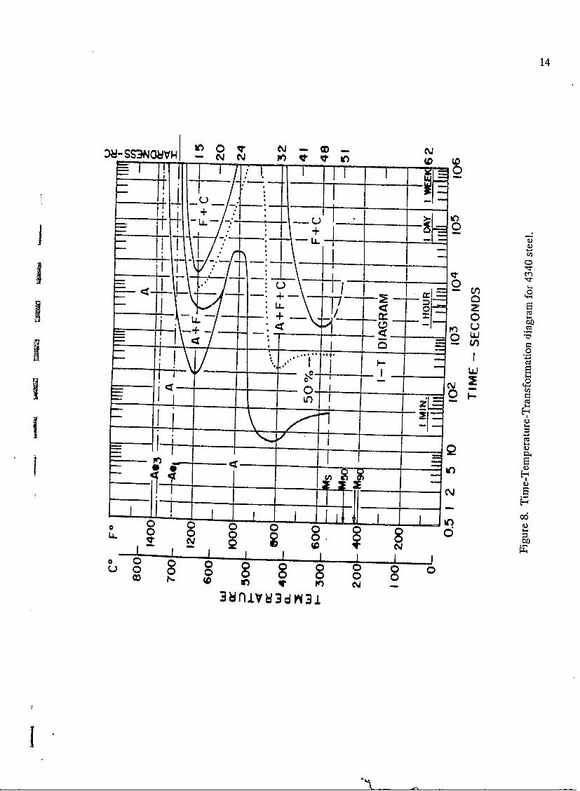
Specimen one and two both have hardnesses indicative of a microstructurecontaining a mixture of pearlite and ferrite (Table I). Their two hardnesses are 96.2 RB
and 92.3 RB respectively. One possible cause for the discrepancy in hardness values
may be accounted for by the extent of spheroidization that has taken place within
specimen two. Previous literature indicated that, for the same grade of steel,

25
spheroidization of the pearlitic regions causes a small decrease in hardness [25]. The
hardenability profile of 4340 steel is pictured in Figure 20 [26]. It suggests a martensite
quenched to approximately 98% will have a corresponding Rockwell C hardness of 56 to
58. Accordingly, specimen three, an almost fully quenched martensite, has an averagehardness of 58.7 RC. Specimen four has a lower average hardness value, 54.1 RC This
reduction in hardness verifies the tempering process specimen four underwent. Thus,the ductility of the steel was increased at the expense of the hardness. The lowerhardness value 50.7 RC for specimen five suggested the presence of small areas of
bainite within a mostly martensitic matrix.
As expected, the density values for the pearlitic specimens are larger than those
of the martensitic (Table I). Specimens one and two have density values of 7.839
grams/centimeter3 and 7.840 grams/centimeter 3 respectively. Specimen three, thequenched martensite, has a density value of 7.807 grams/centimeter 3 , which is quitesimilar to specimen four's value of 7.805 3 grams/centimeter 3. The density value of
specimen five,3 7.817 grams/centimeter 3 , is greater than the two other martensitic
specimens but less than the two pearlitic. Close examination of the titanium alloyrevealed its hardness and density values to be similar to those listed in previousliterature [27]. The alloy had an average hardness of 33.1 RC and a density of 4.430
grams/centimeter 3 .The ultrasonic velocity measurements, in Table II, exhibited that longitudinal,
shear, and Rayleigh waves travel with higher velocities within the pearlitic
microstructures of 4340 steel than in those corresponding to martensites. In accordancewith these results, previous literature suggested for the same grade of steel, thatsamples with higher hardness values generally correspond to lower ultrasonic velocities
[28]. The consistency of the measured shear velocities in two perpendicular directions
signified that the steel microstructures are not highly anisotropic. Furthermeasurements on the titanium alloy disclosed a consistent longitudinal velocity, 6287.42
meters/second. The shear velocities measured parallel and orthogonal to the rollingdirection vary to a large degree, and thus, the titanium alloy is highly anisotropic. The
shear velocity measured in one direction is 3158.90 meters/second. The shear velocity,
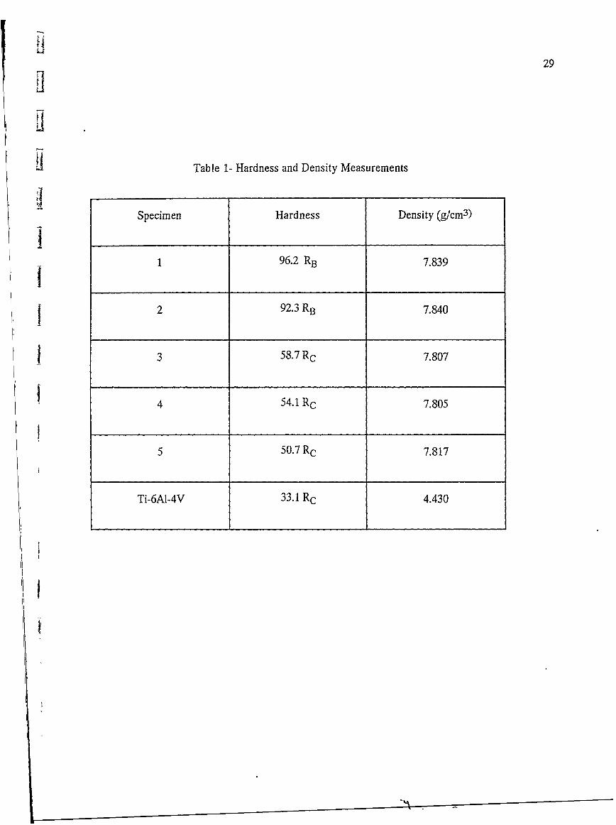
measured by rotating the transducer 900, was found to equal 3276.22 meters/second.The calculated elastic constants exhibited the same trends as the ultrasonic
velocity values. The pearlitic microstructure yielded higher elastic constant values than
the martensitic specimens (Table III-VII). Moreover, and as expected, the Poisson's
ratio values of the martensitic specimens are larger than those of the two pearliticspecimens. The elastic constants of the titanium alloy in Table VIII vary significantly
'-3

26
Figure 14. Specimen 1, the as-received sample. At 1000x. 2% Nital etch.
.1
Figure 15. Specimen 2 after austenitizing at 843 C and isothermally cooling at 648 C
for 48 hours. At 1000x. 2% Nital etch.

27
fm
Figure 16. Specimen 3 after austenitizing at 843 C and quenching in oil.. At 1000x. 2%I Nital etch.
I
H
dFigure 17. Specimen 4 after austenitizing at 843 C, quenching in oil and tempering at204 C for 100 minutes. At 1000x. 2% Nital etch.

28
vII
Figure 18. Specimen 5 after austenitizing at 843 C and air-cooling. At 1000x. 2% NitalI etch.
-4 4
- -
- . t a ~ t ~ ~ c S r t 'X y ..2
I 'F
Af%
-' APr-
Fiur 1. itnim- Aumnu-4Vaadum Lngaxs f hegrin cinid wththrolin diecion A 50x Krolsr~ ' Reagen etch.%
29
Table 1- Hardness and Density Measurements
Specimen Hardness Density (g/cm3 )
1 96.2 RB 7.839
j 2 9 2 .3 RB 7.840
1 3 58.7 RC 7.807
4 54.1 RC 7.805
5 50.7 RC 7.817
Ti-6AI-4V 33.1 RC 4.430
I

30
Table II- Ultrasonic Velocity Measurements
Longitudinal Shear Velocity Shear Velocity RayleighSpecimen Velocity 1 2* Velocity
(m/sec) (m/sec) (m/sec) (m/sec)
1 5934 3235 3237 3000
2 5952 3250 3252 3005
3 5850 3156 3156 2909
4 5868 3170 3172 2931
5 5869 3175 3173 2935
Ti-6AI-4V 6287 3276 3159
*Measured by rotating transducer 90.
i.t
31
Table III- Specimen 1 - Elastic Constants
Calculated using Calculated using Averageshear velocity 1 shear velocity 2
Young's Modulus 211,385 211,638 211,511
(E)
Shear Modulus (G) 82,020 82,147 82,083
Bulk Modulus (B) 166,666 166,492 166,579
Poisson's Ratio (v) 0.289 0.288 0.288
*1
1!l!HEl

32
Table IV- Specimen 2 - Elastic Constants
Calculated using Calculated using Averageshear velocity 1 shear velocity 2 MPa
MPa MPa
Young's Modulus 213,307 213,418 213,362I (E) ,,
Shear Modulus (G) 82,839 82,895 82,867
Bulk Modulus (B) 167,281 167,209 167,245
Poisson's Ratio (v) 0.287 0.287 0.287
)I

33
Table V- Specimen 3 - Elastic Constants
Calculated using Calculated using Averageshear velocity 1 shear velocity 2 MPa
MPa MPa
Young's Modulus 201,373 201,384 201,378
Shear Modulus (G) 77,768 77,775 77,771
i Bulk Modulus (B) 163,481 163,727 163,604
Poisson's Ratio (v) 0.295 0.295 0.295
I

34
I Table VI- Specimen 4 - Elastic Constants
ICalculated using Calculated using Averageshear velocity 1 shear velocity 2 MPa
MPa MPa
Young's Modulus 202,994 203,158 203,076
(E)
Shear Modulus (G) 78,445 78,527 78,486
i Bulk Modulus (B) 164,126 164,012 164,069
Poisson's Ratio (v) 0.294 0.294 0.294
I
1

35
Table VII- Specimen 5 - Elastic Constants
Calculated using Calculated using AverageIshear velocity 1 shear velocity 2 MPa
MPa MPa
Young's Modulus 203,791 203,557 203,674
, ~(E)...
j Shear Modulus (G) 78,801 78,683 78,742
Bulk Modulus (B) 164,167 164,306 164,236
Poisson's Ratio (v) 0.293 0.293 0.293
LiL

36
Table VIII- Titanium-Aluminum-6-Vanadium-4 - Elastic Constants
Calculated using Calculated using Averageshear velocity 1 shear velocity 2 MPa
MPa MPa
Young's Modulus 124,925 117,688 121,306
- (E)Shear Modulus (G) 47,550 44,205 45,877
Bulk Modulus (B) 111.710 116,174 113,942
Poisson's Ratio (v) 0.314 0.331 0.322

37
with direction measured and are characteristically lower than the 4340 steel values. The
Poisson's ratios are larger than those of the 4340 steel, but the anisotropy within the
specimen causes a large deviation between the parallel and orthogonal directions, 0.331
and 0.314.
The experimentally calculated results of Weichert's condition for the various 4340steel samples and the titanium alloy couple appear in Table IX. The values for the ratios
of the densities and ratios of the shear modulus are calculated to determine the possible
range of existence for Stoneley waves along the interface according to Sezawa andKanai's graphical depiction in Figure 2. The ratios of the densities vary between 0.565and 0.567, while the ratios for the shear modulus ranges from 0.52 to 0.60. Theoretically,
if the point plotted according to the two ratios, for each interfacial couple, is within the
two curves (Figure 2), then Stoneley waves will exist along the interface. Thisapproximation of Weichert's condition is satisfied for the two pearlitic-titanium couples.dBoth ratios for the densities of the two media were calculated and equal 0.565. Theratios for the shear modulus in the two media comprising the interface were found togdiffer in two perpendicular measured directions. This arose as a result of the anisotropypresent within the titanium alloy block. However, both measured shear modulusorientations provided ratios that satisfied the range of existence for Stoneley waves
according to the approximation made by Sezawa and Kanai. The ratios of the densities
for the interfaces comprised of specimen three, four, and five were calculated and equal
0.567 for three and four and 0.566 for specimen five. once again, the ratio of the shearmodulus in two perpendicular directions was calculated for the samples. The ratios ofthe shear modulus measured perpendicular to the rolling direction of the titanium block
exhibited values of 0.611, 0.606, and 0.604 for specimens three, four, and five,
respectively. When taken in conjunction with the calculated density ratios, all three
plotted points seem to be near the upper limit for the possible range of existence forStoneley waves. However, the ratios of the shear modulus measured parallel to the
rolling direction of the titanium block revealed values that are approximately equal to thethree density ratios. These three measured shear modulus ratios are 0.568 for the
interface comprised of specimen three, 0.563 for the interface comprised of specimen four,and 0.561 for that of specimen five. When combined with the density ratios for their
respective material combinations, all three plotted points are well within the possiblerange of existence for Stoneley waves along the interfacial region. It is believed thisapproximation of Weichert's condition held true during experimentation. Duringultrasonic testing, a shear wave transducer was placed on the side of the lighter medium
(in this experimentation, the titanium block) to detect the possible existence of leaky

38
iX
S-L
• ° .- - -
JS
.7' '7
S- o
rein Tianu (dnsty=4.-3g/'
Z~ CO
j Q an 1 V -= t5 i a
u/) V)c 1 n0 1 ,r
dre ion Titgansduer rta e 90= 4.4 g/ ,05cmT sha mouls die 1 = 4
diecio 2E (tandue rotte 90' = 420 E
39
waves along the interface. If leaky waves were present, the shear wave transducer
would receive a signal, thus indicating the presence of shear wave displacement fields
within the lighter material. For all five experimental material combinations, there was
no indication of this phenomenon.
The depiction by Yamaguchi and Sato of the relationship between densities,
shear modulus and interface wave velocities enabled the determination of theoretical
Stoneley velocities [10]. For each material combination in this investigation, the ratio of
the densities and the ratio of the shear modulus were plotted on the horizontal and
vertical axes, respectively. A theoretical value for the ratio of the maximum Stoneley
wave velocity to the shear wave velocity, quantity squared, could then be obtained upon
extrapolation. This ratio was determined to equal approximately 0.995 for all five
interfacial combinations. Subsequently, each theoretical Stoneley velocity was obtained
by multiplying each steel's average shear velocity by 0.997 (Table X). As expected, the
Jtwo interfaces comprised of the pearlitic specimens exhibited higher theoretical Stoneley
wave velocities than the three containing the martensitic samples.
The ability of Stoneley waves to detect variations in microstructure was
evaluated on the five 0.2 micron finished titanium-steel couples. For each experimental
interface, the Stoneley wave velocities were calculated as a function of interfacial bond
quality. Through the utilization of a tensile test machine, a compressive load was
applied perpendicular to each interface. It was hypothesized that as the pressure was
-A increased, the interface would change from a boundary region with finite areas of contact
to one of continuous contact. Thus, with each increment of air gap elimination, the
interface wave would travel with higher velocities. Eventually, when continuous contact
between the two adjoining surfaces was achieved, a maximum would be reached
4 corresponding to the Stoneley wave velocity. Subsequently, a correlation could be made
between the Stoneley wave velocity and the quality of the interfacial region as
determined by the magnitude of the applied pressure. Experimentally, this was
accomplished by plotting the Stoneley wave velocity versus the normalized stress for
each steel-titanium couple. The normalized stresses were taken to equal the applied
stress, force per unit interfacial area, divided by the yield stress of each steel specimen.
The approximate yield stresses were obtained by utilizing several tables that converted
'I Rockwell hardnesses for a specific heat treatment to yield strengths [29]. The yield
stresses are as follows:

40
Table X- Theoretical and Experimentally Measured Stoneley Wave Velocities
Interface comprised of Theoretical Stoneley Experimentally MeasuredTitanium and Specimen # Velocity (m/sec) Stoneley Velocity
(m/see)
1 3226 3210
2 3241 3220
3 3146 3085
4 3161 3155
5 3173 3160
I
I

41
Specimen one = 70 ksi
Specimen two = 55 ksi
Specimen three = 225 ksi
Specimen four = 225 ksi
Specimen five = 150 ksi
Because of the anisotropy present within the titanium alloy block, Stoneley wave
velocities were measured in two directions, one coinciding with the blocks rolling
direction and the other by rotating the block 900. The most consistent results were
obtained when the Stoneley waves traveled through the interface parallel to the rolling
direction of the titanium block.
The characteristic Stoneley wave velocities of the two pearlitic specimens versus
normalized stress profiles are depicted in Figure 21. At zero applied pressure,corresponding to the vertical axis, the Stoneley wave velocity of specimen one nearly
equaled the Rayleigh wave, 2995 meters/second. As the pressure was increased, the
interfacial bond quality was improved, and the Stoneley wave velocity increased
asymptotically to a maximum of 3210 meters/second. Comparison of this experimentally
measured value with Yamaguchi and Sato's approximated theoretical Stoneley velocity
of 3226 meters/second, suggested the interfacial region may be approaching full
continuity at the maximum applied pressure. The Stoneley wave velocity of specimen
'I two also increased asymptotically with improved interfacial bonding, from its measuredRayleigh velocity of 3005 meters/second to approximately 3220 meters/second.
However, a small discrepancy at the lower end of the curve is believed to exist as aresult of the surface finish on the steel. Although specimen two was provided with a 0.2
micron finish, the surface was accidentally allowed to corrode slightly. Consequently,
small surface inconsistencies were present and these effects tended to move the
immediate rise in interface wave velocity with increasing pressure to the right. Initially,
higher applied pressures were necessary to bring the two adjoining media into intimate
contact because of the rough surface finish on specimen two. At the upper end of the
curve, it appears the Stoneley velocity has not reached its maximum value.
Extrapolation of this curve would produce a Stoneley wave velocity of slightly higher
magnitude and closer in value to the approximated theoretical prediction of 3241
meters/second. Experimentally it is believed the measurable Stoneley wave velocityA would increase with the application of higher pressures and the subsequent

42
Interface Velocity vs. Normalized Stress for Pearlitic Specimens
3300-
Specimen 1. As-received
3200 0 - 20
.* [][
S3100 2
3000 J. mP Specimen 2, Austenitized
2900 1 * * * * '
0.00 005 0.10 0.15 0.20 0.25
Normalized Stress
iFigure 21. Stoneley velocity versus normalized stress for pearlitic specimens. Stress
normalized to yield stress, Specimen 1- 70 ksi, Specimen 2- 55 ksi.

43
improvement of the interfacial bond quality. In retrospect, all of measured elastic
acoustic waves propagate in specimen two with higher velocities than in specimen one.
Both curves in Figure 21 seemed to reach their maximum Stoneley velocities at
approximately 0.25 of their normalized stresses. A more complete analysis of the
stresses required to form an interfacial region suitable for the propagation of Stoneley
waves could not be determined because of the accidental surface variation on specimen
two.
The Stoneley wave velocities of the martensitic specimens versus normalized
stress profiles are depicted in Figure 22. All three experimentally measured Stoneley
wave velocities are lower than the two pearlitic values. Individually, the Stoneley wave
velocity for each martensitic-titanium couple increased with improving interfacial bond
quality in a different manner. At zero applied pressure, the Stoneley wave velocity of
specimen three (quenched martensite) was 2910 meter/second, corresponding to a
jRayleigh surface wave traveling on the steel plate. As the pressure was increased, the
interfacial bond quality improved, thus causing the elastic wave to be transmitted
through the boundary region with higher velocities. Eventually, the Stoneley wave
reached an experimental maximum velocity at 3085 meters/second. However, the slope
of the curve appeared to be still rising at approximately 0.06 normalized stress. It was
speculated that the Stoneley velocity did not approach a maximum in this case because
the tensile tester used in this investigation was not capable of exerting the higher
stresses necessary to bring the martensitic steel and titanium alloy into complete
contact. If complete contact of this continuous interfacial region occurred, it is believed a
Stoneley wave would propagate through the interface with higher velocities. Theoretical
predictions indicated the Stoneley wave would propagate at 3146 meters/second. Since
the tempered steel, specimen four (RC = 54.1), is softer than the quenched steel (RC =
58.7), lower applied stresses were needed to form the necessary continuous interface for
the propagation of Stoneley wave-. As with the other steel specimens, the interface
comprised of specimen four and the titanium alloy also had an interface wave
propagating along the boundary region with a velocity equal to its Rayleigh wave at zero
applied pressure, 2930 meters/second. Within this interface couple, the Stoneley wave
reaches higher velocities at lower normalized stresses. After the initial rise in velocity
hthe curve leveled off asymptotically at approximately 3155 meters/second. Theoretically,a velocity of 3161 meters/second was calculated. Comparison of these two values
Bindicated the controlled interface may not have achieved full continuity. However, thesame patterns in velocity measurements were observed as in previous experiments.
Namely, longitudinal, shear, Rayleigh, and Stoneley waves were all measured to travel
I.

44
Interface Velocity vs. Normalized Stress for Martensitic Specimens
3200'Specimen 4, Tempered
El ME
30 Ole rSpecimen 5, Air-cooled3100 *
El Specimen 3, Quenched
>U
29000.00 0.02 0.04 0.06 0.08
Normalized Stress
3
Figure 22. Stoneley velocity versus normalized stress for martensitic specimens. Stress
normalized to yield stress, Specimen 3- 225 ksi, Specimen 4- 225 ksi, Specimen5- 150 ksi.

45
with higher velocities in specimen four than in specimen three. The interface comprised
of specimen five, the air-cooled sample, and the titanium alloy had a Stoneley velocity
versus normalized stress profile similar to specimen four. In agreement, the shear,longitudinal, and Rayleigh waves all propagated with nearly equal velocities in each ofthese material combinations. The dissimilarities between the initial rise in velocity with
applied stress in specimens four and five is unclear. It is believed that higher applied
stresses might allow for a clearer distinction between the two specimens. Incomparison with specimen three, lower applied stresses were needed to form the
necessary continuous interface. This was attributed to the lower hardness of specimenfive (Rc = 50.7). At the upper end of the curve the Stoneley wave velocity
experimentally reached a value of 3160 meters/second. The theoretically determined
Stoneley velocity of 3173 meters/second is also slightly higher in value than thetheoretically calculated value for the tempered martensite-titanium couple. Once again,
jthe lower experimental velocity suggested the interface may not be fully continuous as a
result of the hardness of martensitic steel. Thus, it was hypothesized for the martensiticsteel couples that an acoustic wave was not capable of being transmitted along the
boundary region with a velocity indicative of a Stoneley wave. Higher applied pressures
may possibly cause the interfacial region to improve and subsequently increase the
maximum velocities attained by the interface wave. All three Stoneley waves travelingthrough the martensitic couples were observed to reach their experimental maximums
between 0.05 and 0.08 their normalized stresses. These reduced values in normalized
stress, in comparison to the pearlitic couples, arose because of the martensitic
specimens higher yield strengths.In further investigations, Stoneley waves were generated between a 12 micron
finished as-received 4340 steel sample and titanium alloy of the same finish. The
Stoneley wave velocity versus the normalized stress profile is depicted in Figure 23.Once again, at zero applied pressure to the interface, an acoustic wave was measured to
propagate between the 12 micron finished couple with a velocity nearly equal to aRayleigh wave on the steel sample. However, as the pressure was increased there was
not an immediate rise in interface wave velocity. This behavior suggested that higherapplied pressures are needed to bring the two comparatively rougher surfaces into
intimate contact. Accordingly, it was speculated that poor surface finish may cause anacoustic wave to travel along the interface with velocities only slightly higher than a
Rayleigh wave. Increases in interface wave velocity were not observed untilapproximately 0.15 of the normalized stress. In comparison, the 0.2 micron finished
couple demonstrated an immediate rise in Stoneley wave velocity with applied
I

46
EFFECT OF SURFACE FINISH ON INTERFACE WAVE VELOCITY
3300
Optical Finish, -0.2 microns
3200 * *
> 3100iW
> 1300 El (
3000 E r
Machined Finish, -12 microns
2900 1 i0.00 005 0.10 0.15 0.20
Normalized Stress
Figure 23. Effect of surface finish on Stoneley wave velocity.

47
pressure. The two profiles suggest interfaces comprised of optically finished surfaces
require less force to attain a continuous boundary region necessary for the propagation ofStoneley waves than do interfaces comprised of comparatively rougher adjoining
surfaces.
In this investigation, the sensitivity of Stoneley waves to interfacial bond qualitywas examined as a function of applied stress, surface finish and variations in
microstructure. For all six experimental couples, the interface wave was observed to
propagate with a velocity indicative of a Rayleigh wave at zero applied pressure. In thefive 0.2 micron finished couples, the successive elimination of air gaps and thesubsequent improvement of the interfacial bond quality caused the interface wave
velocity to increase asymptotically to a maximum value nearly equal to the theoretical
Stoneley velocity. The effects of surface finish revealed an acoustic wave traveled along
the boundary region , ith velocities only slightly higher than a Rayleigh wave for poorly
finished (12 micron) surfaces at low and intermediate pressures. Upon comparison withthe 0.2 micron finished surfaces, higher applied stresses were required to cause a smallJincrease in the interface wave velocity for the rougher surfaces. Thus, the effects of
surface finish suggest that an interface comprised of finely polished surfaces required
lower stress to form the necessary continuous boundary region for the propagation of
Stoneley waves than do rougher surfaces.
In summation, it is believed that Stoneley waves may be used to evaluate thecoherency and integrity of an interfacial region. Moreover, the various calculated
Stoneley velocities indicated that interface wave velocity measurements are sensitive to
microstructural variation and surface finish. Namely, Stoneley waves traveled through
the two pearlitic steel-titanium interfaces with higher velocities than in the three
martensitic steel-titanium couples. The effects of surface finish indicated that surfaceswith better finishes require less force to attain the necessary continuous boundary
[region for the propagation of Stoneley waves.
u

48
V.5 Conclusions
Stoneley interface waves were generated and detected between steel-titanium
planar interfaces.
Stoneley interface waves were found to be sensitive to changes in microstructure.
Interface waves propagated through the pearlitic 4340 steel-titanium interfaces
Iwith greater experimental Stoneley interface wave velocities than through the
martensitic 4340 steel-titanium interfaces. Interface waves propagated with higher
velocities through steel-titanium interfaces of good surface finish than they did
through steel-titanium interfaces comprised of poorly finished surfaces. Interface
-] wave velocities were found to be dependent on the quality of the interfacial bond.
It was hypothesized that as the pressure applied to the interface was increased,
the interface would change from a boundary region with finite areas of contact to
Ione of continuous contact. Thus, with each increment of air gap elimination, the
interface wave would travel with higher velocities. Upon achievement of
Icontinuous contact between the two adjoining surfaces, a maximum velocity would
be reached corresponding to that of a Stoneley wave. The interface waves were
observed to propagate through the steel-titanium interfacial regions with a
velocity corresponding to a Rayleigh wave at zero applied pressure. As the
pressure applied to the interface was increased, the interface wave velocities
increased asymptotically to a maximum that was slightly less than theoretical
predictions. Through the utilization of Yamaguchi and Sato's method for predicting
Stoneley interface wave velocities, interface waves were theoretically calculated
to propagate through the two pearlitic steel-titanium interfaces with higher
velocities than through the three martensitic steel-titanium interfaces.
The five steel-titanium interfacial couples were tested to evaluate the possibleexistence of leaky waves along the boundary region. For all five material
combinations, there was no observable detection of this phenomena.
El

49
VI. Leaky wave Prpoagation for NDE
VI.1 Introduction
The previous experiments demonstrate the feasibility of generating both Stoneley
and leaky waves at a planar solid-solid interface through mode conversion. In addition,
theoretical analysis allowed particle motion, energy flow, and velocity predictions for
comparison to experimental results. It was shown that interface waves were sensitive
to microstructural variation as well as quality of surface contact. These microstructural
effects which caused small changes in elastic properties are manifested as changes in
ultimate interface wave velocity and were measured simply and accurately.
The problems of expanding this research to include more relevant engineering
material pairs are numerous. It is obvious from the theoretical analysis that the limited
region of existence of Stoneley waves makes it impractical for nondestructive
characterization of many composite materials. Leaky waves which exist for a much
larger range of material pairs, including silicon carbide/aluminum, seem to offer much
more potential as a nondestructive evaluation tool. However, the lack of previous work
and the limited theoretical analysis of these waves forced a fundamental approach to the
problem. The approach taken in this study consisted of several experimental projects
designed with specific, but related goals. The first is an experiment to further our
understanding of basic leaky wave propagation characteristics. While some theoretical
analysis exists, experimental observation and understanding is limited. The goal was
not only to generate and detect leaky waves, but to measure the leakage and determine
its potential for interface characterization. The second part of this project was to develop
a technique to remotely generate and detect leaky waves in order to address the
problem of interface access when mode conversion at free surface is not feasible. Once
these problems are overcome, techniques for nondestructive evaluation of interface
elastic properties may be developed utilizing leaky interface waves.
VI.2 Theoretical Considerations
In order to understand the experimental approach taken to examine the potential
usefulness of leaky waves for nondestructive evaluation of interfaces, Stoneley's
equation for phase velocity along an interface must be scrutinized. The original equation
given in 1924 is,

50
(P 1 2)2- 1P I 2 1) (132+P 2B1f
+2Kc2{p 1A2B2-p 2A1Bj-p 1+P41+K(A 1B-}1) (A2B2-1) = 0 eq(1)
where,A 1 = ( 1-/i A2 = (ic2/ V) 2
B 1 = (1 C2/V 21) 1 2 B -" 1c 2V 2)1/
K = 2(p 1Vs -p V 2 eq(2)
VL and VS are the longitudinal and shear wave velocities, p is the density, and the
subscripts 1 and 2 refer to the two media. Medium 2 is defined as the more dense
medium.To further investigate this equation the concept of a Riemann surface must be
introduced. A Riemann surface is a geometrical device which allows the complexities ofa multiple-valued function to be more easily handled [30]. It is defined as aj generalization of the z plane to a surface of more than one sheet such that the multiplevalued function has only one value corresponding to each point on that surface. The
surface is composed of sheets which correspond to a branch of the function, so that oneach sheet the function is single-valued. The advantage of the Riemann surface is thatthe various values of multiple-valued functions are obtained in a continuous fashion.
From equation 1, it can be seen that there are 16 possible combinations of signsof the functions A1, A2, B1, and B2. Since changing all of the signs would leave the
equation unaltered, there are only 8 which are independent. Each of these eightindependent Riemann sheets was investigated by Pilant [11] for the presence of real orcomplex roots out to a radius where Ic21 / VS22 =64. Following his notation, a signconvention is chosen so that the real part of B2 is always positive. The sign conventionfor the eight Riemann sheets then, is given as Re{Al}, Re{B 1}, Re{A2}. Using thisnotation, (+ - +) means that Re{A 1}>0, Re{B1}<0, Re{A 2}>0 and Re{B 2} is always
>0. For a continuous cyclic variation in material parameters it was determined thatthere were 16 roots which could be followed about the various Riemann surfaces,
Before considering the case of an aluminum/silicon carbide interface, the generalbehavior of the sixteen roots as presented by Pilant was reviewed. Each of the roots
was followed as the ratios of the shear velocities and the densities were varied in a half-

51
square as shown in Figure 24. Poisson's ratio is defined as 0.25 for both materials with
material 2 designated as the denser of the two. Beginning with (Vs2/Vs1) 2 and P1/P2 =
1, the density ratio was decreased to 0.5. The velocity ratio was then increased to 2.0
and finally the density ratio was increased back to 1.0. The graphical representation ofthe results are shown in Figure 25. Three points on this figure are of specific interest.
At the first point, (VS2IVS1) 2 = 0.5 and PI/P2 = f/2 both real and complex roots
become very large or go through the point at infinity and return with opposite sign. The
second point, (Vs 2 /Vs 1)2 =0.5 and P1/P2 = .05 shows that many of the root values are
zero on different Riemann sheets. The third combination is the pair (Vs2/Vsl) 2 = 1 and
P1/P2 = .05. At this point many of the roots have a value of 4 including a double root on
the (+ - -) sheet. In this range of parameters, the only real root was the Stoneley root
on the (++ +) sheet. It is also clear that although the roots jump from sheet to sheet as
the parameters are varied, the number of roots remains constant. Notice that in Figure
25 vertical tangents appear on the solid lines representing two real roots converging on
the real axis which become a complex conjugate pair. Conversely, two complex
conjugate roots meeting on the real axis create two real roots.
The boundary condition matrix equation for the planar interface case was
examined in detail by Lee and Corbly [16] and Simmons and Krasicka [31]. Simmons
and Krasicka extended the work of Lee and Corbly on cylindrical interfaces. To examine
a planar interface, the radius of curvature was set to infintiy. If the z axis of a rectangular
Cartesian system is defined to lie in the plane interface between two materials and the x
axis is defined to extend into the less dense material, the displacement fields um are
given by,
SU m=VTm+Vx(0A'p' 0)
where eq(3)
1 =ctexP(-kAx+ikz-iwt)
yP 1=Pexp(-0c 1x+ikz-iwt)
4 ~ 2=yex kA2x+ikz-iwt)
S27yex kA 2x+ikz-icot)
eq(4)
where1/2
Am=(l-c2/a2m

52
5.0-
3.0 HALF-SQUARE
f 2.0 (2.0,0.5) 4 3 (2.0,1.0)
V2 1.5s2
V 2 1.0- (1.0,0.5) - I(.0,1.0)
0.7-
0.5 (0.5,0.5)6 (0.5,1.0)
0.4-
0.3 I I I I , I
0.1 0.2 0.3 0.5 0.7 1.0P,/P,
Figure 24. The path of variation of the parameters chosen by Pilant to evaluate the 16roots of the equation governing elastic wave propagation on a solid-solidinterface. Poisson's ratio is kept at 0.25, r is the density, and Vs is the shearwave velocity. Medium 2 is defined as the denser material.

5312.0
10.0 4- .00 HIDOEN STONELEY.99+_
8.0 .7DEALINTERFACEoff 9 DTIscole)0.90 0.95 1.00
6.0Re S
41.0
+ INTERFAC
+NSEE DETAIL 4~ -- 0--0.0 -REAL ROOT --..L. SHEET CHANGE
-------------------------COMPLEX ROOT PAIR
S2 V 0.5 0.6 0.7 0.8 0,9 1.001.101.25 1.40 1.70 2.0 V 2.1.0 0.9 0.8 0.7 0.6 0.5 p, /p2 - 0.5 0.6 0.7 0.8 0.9 1.0
1.2.0
10.0 I 4+-- _++ .05 -DETAIL
/1 .03-8.0 -. 02-
I C2 16.0 3.00Re C
, 1 .998 1.000 1.002 1.00452 I
4.0/2SEE DETAIL - - - - - --- - - - ++--
- - - - - - - - - - - -- - .- - - - - ----- 0-
0. :---~--:--.--REAL ROOT -iSHEET CHANGE----- COMPLEX ROOT PAIR
0.5. V 2 /VT-0.5 0607080910 I1.5.4 1702.00 - V5 VsV2.0
1.0 Q9 0.8 0.7 0.6 0.5 p, / P2 0.5 0.6 0.? 0.8 0.9 1.0
Figure 25. Graphical representation of the behavior of the 16 roots of the Stoneleyequation as a result of varying the parameters over the half-square shown in Figure 24.

54
2 1/2B -- 1-c /b )
c=O/k eq(5)
The subscript m represents the two materials where 1 denotes the less dense and 2
denotes the denser material. The longitudinal and shear wave velocities are am and bm
respectively. When the boundary conditions of continuity of normal tractions and
displacements at the interface is imposed the characteristic matrix takes the form shown
below in Equation 6.
In order to study the Al/SiC system, experimentally determined values were
substituted into the determinant and the following analytical results were obtained
utilizing computer models at the National Institute for Standards and Technology. A
double index notation was used, referring to s, t modes where s, t = 2p + q. Both p and q
may be 0 if the negative principal square root value is chosen or 1 if the positive
principal square root value for the longitudinal (p) and shear (q) components. Therefore,
s and t range from 0 to 3. The first index refers to the matrix material, aluminum in this
case and the second index to the reinforcing material, silicon carbide.
2p bTA1 2p 2b p 1bi(2 )b') p 2 /(2~c,I ' 9
p(c22b 2) -p c2 -2b 2 -2plb2B1 2 o1 -1 B1 .B2 k
A1 A2 1 1
eq (6)
All 16 branches of the matrix equation can produce solutions, however, not all
solutions may physically exist. Leaky waves were calculated by NIST from Equation 3
by locating the approximate real and pure imaginary roots and then using Newton'smethod for computing the real and complex roots. Solution to the boundary matrixproduces two types of modes. Decomposable modes which are a superposition of a
longitudinal and shear plane waves and non-decomposable modes. The decomposable
modes represent certain reflection/refraction situations in which one or more outputwave is missing. Table XI shows the 10 interface modes for the SiC/Al system as
calculated at NIST. There are six non-decomposable modes and four decomposable
modes that appear.

55
Table XI
Nondecomposible Leaky Waves in Al/Sic
Type Velocity: Asymtotic LeakageReal part, imaginary part Angle in Al
0,3 5562,1113 21.01,3 8643, 2458 49.02,3 4730, 231 49.21,1 4619, 3416 48.33,1 10481, 2454 -73.83,0 5562, 1113 -57.9
Decomposible Leaky Waves in Al/SiC
Type Velocity Longitudinal Wave Angle Shear Wave Anglein Al in SiC in Al in SiC
0,3 10030 50.9 15.8 72.0 58.82,3 10077 -51.3 16.8 72.0 59.03,2 11531 -56.7 33.2 -74.4 -63.22,1 16377 -67.3 -53.0 79.0 71.5
I$II

56
In order to better visualize these analytically determined leaky waves, Figures
26 and 27 show the energy flow and particle displacement for a non-decomposable and a
decomposable type wave. The ellipses represent the shape of the particle orbit at a
number of points with the arrowheads indicating the sense of the particle motion. The
arrow from the center of the ellipse shows the energy flow or Poynting vector averaged
over one period. Although the ellipse sizes and arrow lengths are arbitrarily scaled for
graphing purposes, the sizes within each figure are consistent. Figure 26 which plots
the energy flow for the non-decomposable 1,3 mode shows most of the acoustic energy
propagating through the silicon carbide and leaking into the aluminum. Figure 27 plots
the decomposable 0,3 wave. A superimposed longitudinal and shear wave at angles 16
and 590 respectively is represented by the flipping of the ellipses. The resultant wave is
also composed of a longitudinal and shear wave, but the longitudinal component is
extremely small so the shear component dominates the leakage into the aluminum.
The experimental approach was designed to measure several aspects of the
leaky waves. These include leakage angle, wave speed, and a qualitative measure of
amplitude. These results from the experimentally measured leaky waves on a silicon
carbide/aluminum interface were compared to the general analytical results of Pilant and
the theoretical analysis of the sihcon carbide/aluminum interface.
VI.3 Experimental Procedures
Specimen Preparation
The requirements of a specimen to study the propagation of leaky waves musthave two unique characteristics. First, it must be large enough to allow relatively low
frequency ultrasonic waves to propagate while consisting of relevant composite
materials. Second, it must have a geometry to allow the angles of leakage to be
determined. A silicon carbide/aluminum specimen was chosen because of its
widespread use in metal matrix composites and since several leaky modes are believed
to exist in these materials. An aluminum hemisphere 4 inches in diameter was
machined to enable determination of the leakage angle, since as with all high modulus
fiber reinforcement in relatively low modulus matrix composites the leakage is into the
metal matrix. Two aluminum shims approximately the same diameter as the transducer
face were also machined from the same block of 2024 aluminum to focus the wave and to
allow the flat transducer faces to conform to the curvature of the hemisphere. They were
attached to the transducers by a solid wax couplant obtained from Acoustic Emission
Technology Corporation.

57
E
/
/
E
0/
0 2 4 6 8 10 12 14
Parallel Direction (mm)
Figure 15. Representation of the displacement field of a non-decomposable leaky wavepropagating on a silicon carbide/aluminum interface. The ellipses trace the orbitof a particle and the arrowheads show particle motion. The arrows show theenergy flow averaged over one period.

1 58
I5
A3
0 INTERFACE
-
5),0 2 4 6 8 10
Tangential Direction (mm)
Figure 27. Representation of the displacement field of a decomposable leaky wavepropagating on a silicon carbide/aluminum interface. The ellipses trace theorbit of a particle and the arrowheads show particle motion. The arrows showthe energy flow averaged over one period.

59
c C)0
CD 0j
O0
CDC
C' C
- -1-
coj
00
00
CD-
- 00
J) C\
00 00 -

60
The sintered SiC plate 4" x 4" x 3/4" was obtained from the Standard Oil
Engineered Materials Company. Table XII lists the measured physical properties of the
silicon carbide and aluminum. The elastic constants were determined by conventional
pulse-echo ultrasonic techniques.
VI.4 Experimental Measurement Technique
Leaky waves were generated on the SiC/Al interface through a mode conversion
from incident longitudinal waves. Pairs of 1, 5, and 7.5 MHz commercial longitudinal
transducers 0.5 inches in diameter were mounted on the aluminum shims with a solid
wax couplant. These in turn were coupled to the aluminum hemisphere by silicone
grease. Additionally, a pinducer was mounted at the far end of the specimen normal to
the SiC/AI interface. The specimen was fixed to a rotation stage which allowed precise
determination of the incident and reflected angles. A schematic of the experimental
apparatus is shown in Figure 28.
Ultrasonic waves were generated using a conventional pitch-catch technique
which utilized a MATEC Pulser Receiver (Model 6600) and a Hewlett Packard A-scan
Oscilloscope (Model 1743A). The A time mode of the oscilloscope provided two
intensified delayed sweeps which could be positioned at any point relative to the main
oscilloscope sweep. These were positioned over the main-bang and either the reflected
wave or the leakage from an interface wave. To determine velocity, these two signals
were expanded to full screen and overlapped utilizing the 100 MHz crystal timing
reference to directly measure the time difference between the two signals. The
oscilloscope permitted travel time measurements to within one nanosecond.
Longitudinal waves were generated by the transducers in the aluminum shims.
This focused wave was introduced into the hemisphere and allowed to reflected off the
interface. Detection was accomplished by the second longitudinal transducer mounted
on the opposite side of the hemisphere. Silicone grease was used as the couplant
between the aluminum shims and the aluminum hemisphere. Simultaneous monitoring of
energy propagating along the interface was accomplished by the pinducer. The 1.5 mm
diameter pinducers obtained from Valpey-Fisher utilizes a 1 mm thick PZT 5A element.
These transducers are nominally 4 MHz and extremely broadbanded. Measurements
were conducted with no bonding between the surfaces and with the surfaces joined by
epoxy. Travel times were measured at 5 degree increments from zero to 85 degrees
with the transducers placed symmetrically about the normal axis of the hemisphere. The
receive transducer was also scanned along the side of the hemisphere from its position

61
A Time Oscilloscope
_Pulse ModulatorReceiverTM IMT @ Sync.Out
Ch Ig 2 ext. trigger R.F. Plug-n
F input R.F.echo mesr t
• • Into Receiver
tr 000000
Step Attenuator 20 dB
Sending transducer / Receiving transducer
;~ AI
Figure 28. Schematic of the experimental apparatus used to measure the' t travel times of the leaky waves at a planar silicon
carbide/aluminum interface.

62
to the interface at the predicted angles of leaky wave generation to measure the leaked
energy. When an signal was detected by the pinducer, increments of the sending
transducer were decreased by 1 degree.
Finally, direct measurement of the leakage energy was made keeping the sending
transducer fixed at its position when a signal was detected at the interface by the
pinducer. The receive transducer was then moved to allow the pinducer to scan the side
of the hemisphere in several degree increments.
VI.5 Results and Discussion
The measured travel times for both the receive transducer and the pinducer in the
case of casual contact are shown in Figure 29 for the 5 MHz transducers. Degrees are
measured counter-clockwise from the right interface edge arbitrarily designated 0
degrees to the normal at 90 degrees for the received signal. The incident wave degree
designation is a mirror reflection of this with the normal also at 90*. The travel times
were used to calculate wave velocity by subtracting the travel times through the two
shims which was determined by a pulse-echo technique to be 5.053 microseconds.
Figure 29 shows that the longitudinal wave incident on the interface was reflected and
detected by the receive transducer. The reflected wave traveled with at the longitudinal
velocity of approximately 6284 m/sec. No attempt was made to quantitatively measure
the reflected bulk wave amplitudes or to evaluate the reflected bulk waves themselves.
A review of acoustic pressure values at free boundaries and at solid-liquid boundaries
is presented in several manuscripts including Ultrasonic Testing of Materials by
Krautkramer [32].
The fact that no energy was measured by the pinducer placed on the interface at
any of the incident angles indicated that all of the energy was being reflected or
frefracted. There was no generation of interface waves at angles between 5* and 85*
suggesting that no bonding was apparent to the incident acoustic wave. This case,
where the aluminum hemisphere was placed in casual contact with the SiC plate, is
representative of a complete lack of bonding as determined acoustically. Results from
the 1 and 7.5 MHz waves are identical to the 5 MHz results shown above. At zero
applied pressure the ultrasonic wave travels with the velocity of a surface wave. The
important condition of existence for a Rayleigh surface wave is a free surface. The fact
that an ultrasonic wave propagates with the Rayleigh velocity indicates that it travels
on the titanium surface and sees a free surface instead of the steel. This reflects that
the acoustic wave senses a complete lack of bonding between the two surfaces. This is
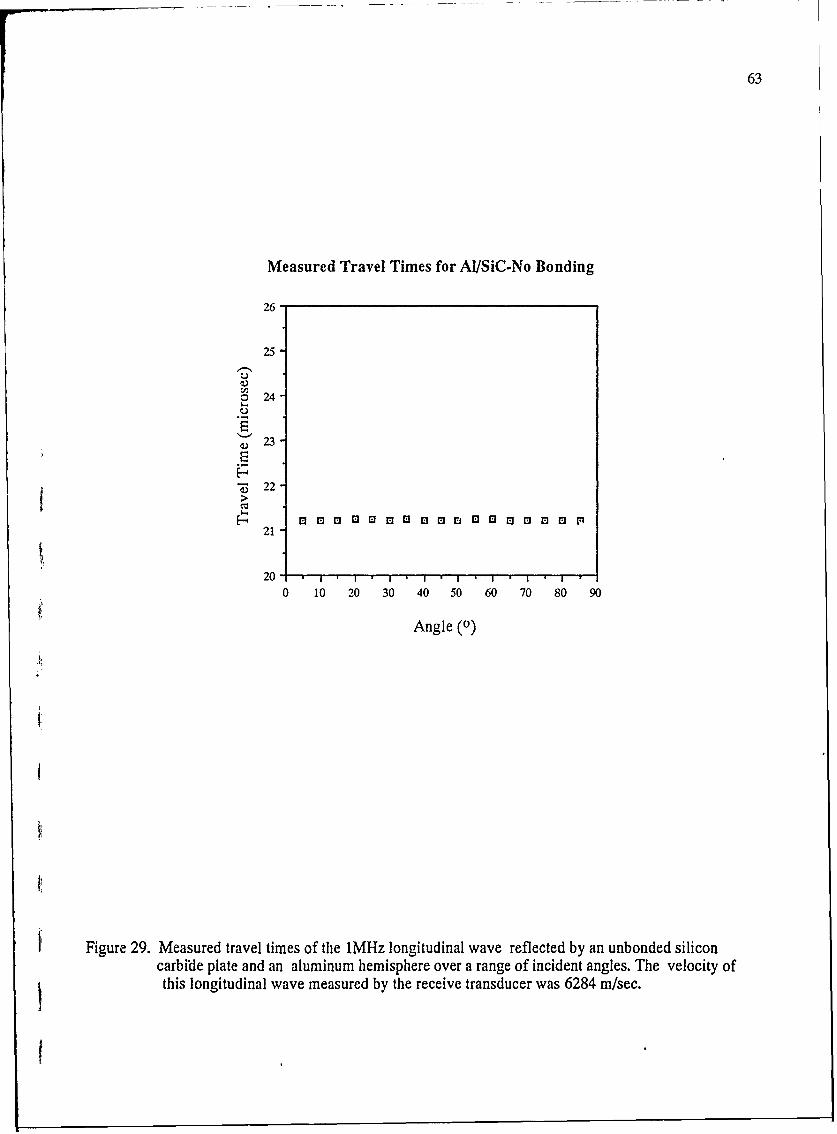
63
Measured Travel Times for Al/SiC-No Bonding
26
25
o24
E
S22
200 10 20 30 40 50 60 70 80 90
Angle (0)
Figure 29. Measured travel times of the 1MHz longitudinal wave reflected by an unbonded siliconcarbide plate and an aluminum hemisphere over a range of incident angles. The velocity ofthis longitudinal wave measured by the receive transducer was 6284 m/sec.
f

64
also the case with the silicon carbide/aluminum interface. With the aluminum
hemisphere resting on the silicon carbide, the acoustic wave sensed no bonding between
the surfaces. No interface wave was detected by the pinducer and no refracted wavewas detected in the silicon carbide. This was also confirmed by propagating a Rayleighwave on the silicon carbide using the Rayleigh wedges shown in Figure 10. The velocity
of the Rayleigh wave was determined to be 6831 m/sec. When the aluminum was
bonded to the silicon carbide by a thin layer of glue, two distinct leaky modes were
evident at 1 MHz. Figure 30 is a plot of the measured travel times for the receivetransducer as a function of its transducer position. Superimposed on this plot are the
measured travel times of the pinducer as a function of the transmitting transducer
position. The pinducer output reflects the appearance of two leaky modes which occur at
approximately 23* and at 55*. The transmitting angle was changed to one degree
increments as soon as pinducer input was detected. Although no effort was made toquantitatively measure the amplitude of the detected signal at the second transducer,
the appearance of the reflected longitudinal wave even at leaky wave angles indicatesthat only a fraction of the energy is mode converted into a leaky wave. Several factors
including beam spread and difficulties determining exact reflection angle made amplitudemeasurements impractical.
Figure 31 is a schematic representation of both the no bond case and the bondedcase. When the two surfaces are in casual contact, the reflected wave is detected by the
receive transducer. There is no signal at the interface. However, when the two surfaces
are bonded with epoxy, the reflected wave is detected by the receive transducer and the
interface wave detected by the pinducer at approximately 23' and 55*.The measured travel times of the two waves at approximately 23* and 55*
represent a combination of velocities which follow a law of mixtures type argument. It iscomposed of a longitudinal wave which passes through the aluminum shim and then
propagates through the aluminum hemisphere a distance equal to the radius of the
hemisphere. At the interface, part of this wave is mode converted to a leaky wave whichtravels the length of the radius at the interface and is detected by the pinducer. Bysubtracting the initial longitudinal wave from the travel time, leaky wave velocity
information was determined. This is shown in Figure 32. The leaky wave generated by
mode conversion from approximately 53* to 57* traveled at a velocity of 10064 ± 82
m/sec. The second leaky wave generated from approximately 210 to 25' traveled at avelocity of 5224 ± 119 m/sec.
The velocity of the wave generated by mode conversion at 55*- 2* implies that it
is largely affected by the silicon carbide whose longitudinal velocity is 11965 m/sec. As
.1

65
Measured Travel Times for Al/SiC-Bonded with Epoxy
22
55 13 555 55G 5 [5ra 5I 55 a
21
20, A
19
18-
> 17
16
1t5
0 10 20 30 40 50 60 70 80 90
Degrees (0)
Figure 30. Measured travel times of a 1MHz ultrasonic wave reflected by asilicon carbide plate bonded to an aluminum hemisphere over a rangeof incident angles. Pinducer output is represented by the triangles andthe longitudinal receive transducer output is represented by thesquares.

66
Unbonded
Transmitting ReceivingLongitudinal 0 LongitudinalTransducer 90Transducer
Bonded
Transmitting ReceivingLongitudinal 0LongitudinalTransducer 9Q0 Transducer
wave At 230 and 550,
Figure 33. Schematic representation of the wave propagation and transducer output signals forboth the bonded and unbonded cases.

67
Velocity of Leaky Waves in Bonded Al/SiC at 1 MHz
11000
10000
> 7000
N~ ~ H iiIIn x ai I8 9a R a ! NI RI Ml a
0M
5000
0 Ic 20 30 40 50 60 70 80
Angle (0)
Figure 32. Velocities of the 1 MHz leaky waves generated at a planarsilicon carbide/aluminum interface at two incident angles.

68
Relative Amplitude of Leakage Measured Parallel to Interface
3,
rZu
2I0JS
20 30 40o5 60
Angle (0)
Figure 33. Relative amplitudes of the two leaky waves measured by the pinducermounted at the interface.
i

69
this wave propagates along the interface, an examination of the displacement field
normal to the interface would show that the majority of the energy is propagated through
the denser silicon carbide as predicted by analytical studies. Energy is leaked away
from the interface through the lighter media, aluminum in this case, at a fairly steep angle(~55*) indicating a relatively attenuative leaky wave. The second wave has a much
shallower leakage angle approximately 230.± 20 and is less attenuative than the faster
wave. This is corroborated by Figure 33 which plots the relative amplitudes of the
leaky waves as measured by the pinducer. Since more energy is radiated away from the
55* leaky wave, its relative displacement amplitude measured by the pinducer parallel to
the interface is much less than that of the 230 wave. Therefore the steeper leaky wave
appears as the more attenuative wave. This leaky wave travels at a much slower
velocity of approximately 5224 m/sec. This wave appears to be largely affected by the
aluminum, since its leaky wave velocity is closer to that of the longitudinal wave velocity
of the aluminum. The leakage is also into the aluminum, but at a much steeper angle.
The appearance of these interface waves also demonstrates the effectiveness of
remotely generating leaky waves by mode conversion through the bulk of one of the
materials. The critical angles of generation are consistent with the angles of leakage forthe these waves so that any modes that exist can be generated by varying the incidentangle of the transducer.
These two waves correlate well to the analytically predicted leaky modes in a
planar silicon carbide/aluminum interface. The first leaky wave experimentally measured
corresponds to the non-decomposable (0,3) leaky mode predicted to leak at an angle of
21.0" and travel with a velocity of 5562 m/sec. The experimentally determined wave had
a leakage angle of 23* ± 20 and traveled at a velocity of at 5224 ± 119 m/sec. The (1,3),
(2,3), and the (1,1) analytical modes leak at angles of 49.0', 49.2, and 48.3*
respectively. Although the experimental measurement of the leaky waves was not able
to distinguish three individual modes, the fastest mode was observed. The (1,3) mode
has a leakage angle of 49.0* and a predicted velocity of 8643 m/sec. This corresponds to
the appearance of the second experimentally observed leaky wave at 55*_ 2* which
travelled with a velocity of 10064 ± 82 m/sec. The three analytical modes are grouped
within one degree of each other and therefore could not be distinguished experimentally
by leakage angle. Only the fastest of these three modes the (1,3) was detected by the
pinducer. Several possible explanations exist to adequately account for this fact. One is
that the waves were not generated at all. The incident transducer was increased by
increments of one degree, the workable limit of the translators. Although the beam
spread of the incident longitudinal wave should have covered all possible angles, it is

70
conceivable that the bulk of the energy was never directed exactly at the angles needed
for mode conversion into the (2,3) or (1,1) analytical leaky modes. However, assuming
that the leaky waves were generated, another possibility is that they completely
attenuated before reaching the pinducer at the edge of the interface (see Figure 28). If
the majority of the energy was leaked away from the interface, the arrival of the leakage
at the second transducer would have been masked by the reflecting longitudinal wave
whose arrival time is within several nanoseconds of both of these two leaky waves.
Additionally, the amplitude of the longitudinal wave would have been much larger than
either leaky wave. Consequently, the arrival of the leaky wave at the pinducer would
have been undetectably small.
No attempt was made to measure any of the decomposible leaky modes. This
was due to the potential difficulty generating these modes and the questionable ability of
measuring the generation and leakage angles with any accuracy.
Figures 29 and 30 show the two extreme cases of zero bonding and complete
bonding which are measured in terms of the presence of a leaky wave and its velocity.
Utilizing these typcs of measurements, the quality of an interfacial bond may be
examined by nondestructive acoustic means. The measurement of an specific interface
wave velocity for known propagation distances will allow the bond along that interface to
be qualitatively determined. By decomposing the measured interface wave velocity into
its leaky wave and/or Rayleigh wave components through a law of mixtures type
argument, the contribution of the Rayleigh wave can be determined and directly related
to the amount of disbonding. In the same manner, the percentage contribution of the
leaky wave can be directly related to the percentage by bonding.
Figure 34 shows the velocities of the leaky waves measured at 5 MHz. One
leaky wave appeared between 54* and 60*. The interface wave velocity was measured
to be 10020 t 282 m/sec. This wave is analogous to the one observed at 55* -t 2* at 1
MHz and also to the (1,3) analytical mode. The velocity indicates that the bulk of the
energy is propagated through the silicon carbide and that the leakage is into the
aluminum. The steeper leakage angle is again representative of a more attenuative
interface wave.
Another leaky wave occurred between 24* and 35*. Its velocity was measure to
be 5365 ± 394 m/sec. This waves is similar to the one measured at 23* ± 2* at 1 MHz
and the (0,3) analytical mode. Its slower velocity indicates that the bulk of its energy is
propagated through the aluminum and that the leakage is also into the aluminum
hemisphere, but at a much shallower angle. This wave is less attenuative than the
leaky wave that appeared at the steeper angle.

71
Velocity of Leaky Waves in Bonded AI/SiC at 5 MHz
10800
9800 A
A
.4 7800-
.7800
5800
AAA A
4800AAiA1 1 10 11) 20 30 40 50 60 70 80 90
Angle ()
Figure 34. Velocities of the 5 MHz leaky waves generated at a planar silicon carbide/aluminuminterface at two incident angles.

72
No consistent measurements were produced utilizing the 7.5 MHz transducers.
Inconsistent travel times and low amplitude measurements were characteristic of the
difficulties encountered at this frequency.It is clear that at these relatively low ultrasonic frequencies that the leaky waves
are non-dispersive. The velocities of shallower wave at 1 MHz and 5MHz are 5562 t
119 m/sec. and 5365 t 349 m/sec. respectively, within 4 percent of each other while thevelocities of the steeper wave are within less than 1 percent of each other. The mean
leakage angles of the steeper wave 57* and 55* are within two degrees of each other,
however the shallower leakage angles show a slight discrepancy. At 1 MHz the leakage
angle is 23* ± 2* and at 5 MHz the leakage angle becomes 29.50 ± 3.5*. Although this
variance is too large to be explained by the shift in energy flow (analogous to the Goos-
Hanchen shift in optics), its probable cause is the fact that the diameter of the sending
and receiving longitudinal transducer faces covers an arc of several degrees when placed
on the hemisphere. Care was taken to place both transducers in symmetric positions,
however, any slight variation in one of the transducers would cause an error in both
angular measurements.
Direct measurement of the leakage at both generation angles was also
accomplished. Figure 35 shows the measured relative amplitudes of the leakage of the
first interface wave to appear at 1 MHz. At a specific incident angle of generation of
leaky waves determined by a pinducer signal at the interface, the pinducer was scanned
along the reflected face of the aluminum hemisphere. Figure 35 shows the relative
amplitudes of the leakage for an interface generated at an incident angle of 23'. A line
drawn from the center of the hemisphere which corresponds to the point of generation of
the leaky wave through the maximum leakage point shows the angle of leakage to be
consistent with the incident angle. Note that by earlier definition the center of the
hemisphere corresponds to the 90* designation at the surface of the hemisphere. ThisJ line represents the angle of maximum acoustic energy flow of the leakage away from the
interface.
Figure 36 shows the direct leakage measurements of an interface wave
generated from an incident angle of 55*. Its relative leakage amplitude maximum is
larger than that of the leakage from the 23* wave. This substantiates the contention that
the steeper leaky wave is the more attenuative of the two interface waves. The line
drawn from the point of generation of the wave on the interface through the maximum
leakage points again shows that the angle of maximum energy flow away from the
interface is consistent with the incident angle of generation.
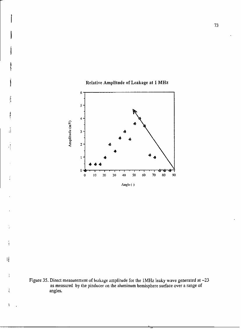
73
I
I
Relative Amplitude of Leakage at 1 MHz
6
5-
4>
V~ 34
4
1 4444
0 10 20 30 40 50 60 70 80 90
Angle
Figure 35. Direct measurement of leakage amplitude for the 1MHz leaky wave generated at -23as measured by the pinducer on the aluminum hemisphere surface over a range ofangles.

---.74
Relative Amplitude of Leakage at 1 MHz
E E
0 10 20 30 40 50 60 70 80 90
Angle (0)
Figure 36. Direct measurement of leakage amplitude for the IMHz leaky wavegenerated at -550 as measured by the pinducer on the aluminumhemisphere surface over a range of angles.
75
Remote generation and detection of leakage and leaky waves demonstrated by
these experiments offers even greater possibilities for nondestructive acoustic
evaluation of the interfacial structure. While direct measurement of leaky waves offers
several benefits as describe previously, results from figures 33, 34, 35, and 36 allow
considerable insight into the structure and properties of the planar silicon
carbide/aluminum interface. Each leaky wave propagates through both materials and
contains certain information about the elastic properties of the interface depending on the
mode. Remote generation by reflection from a surface generated bulk wave allows the
potential for all modes to be produced. Additionally, detection of the leakage at the
surface of either material is crucial for nondestructive interface characterization. By
measuring the leakage or absence of leakage of a certain leaky mode, the presence and
location of disbonding can be determined. Leakage measurements also offer insight into
the elastic character of both of the materials comprising the interface as well as the
interface itself if that structure is different (i.e. heat affected zone, etc.).
VI.6 Conclusions
1. Two leaky modes were remotely generated by mode conversion from a bulk wave
incident on a bonded silicon carbide/aluminum interface at a critical angle. One wave
was generated at -23' and travelled with a velocity of -5224 m/sec, while the second
leaky wave was generated at -55* and travelled with a velocity of 10064 m/sec. It was
concluded that remote generation is a valuable method for exciting leaky modes when
direct access to the interface is impossible.
2. Theoretical analysis by NIST computer modeling predicts four decomposable modes
and six non-decomposable modes for a planar silicon carbide/aluminum interface. Two
of these have been experimentally verified.
3. No interface waves were generated on the unbonded silicon carbide plate and theI aluminum hemisphere.
4. Relative amplitude measurements of the leakage energy show that maximum leakage
energy of the steeper wave was greater than that of the shallower wave. Direct
measurement of the leaky wave amplitude at the interface confirmed this fact. It was
concluded that the steeper wave was more attenuative than the shallower leaky wave.

76
5. Measurements utilizing 5 MHz longitudinal transducers produced two leaky waves
with leakage angles of approximately 29.5* and 57* with velocities of approximately
5365 m/sec. and 10020 m/sec. respectively. These measurements did not reveal any
significant advantages or disadvantages of using a s"ghtly higher frequency for
generation of interface waves. The slight shift in leakage angle was probably due to
the fact that the incident transducer face covered an arc of about 5* on the aluminum
hemisphere and resulted in slightly shifted angular measurements.
6. Remote measurement at the surface of the aluminum hemisphere of the leakage
energy was accomplished. These measurements confirmed that the leakage angle was
the same as the incident generation angle. It was concluded that this direct
measurement of leakage is a valuable method for separating modes and will contribute
to nondestructive interface characterization.I7. It was shown that leaky waves offer several potential benefits for nondestructive
interface wave characterization including detection of disbonds and elastic
characterization.
rI

77
VII. References
1. Stoneley, R., Proc. Roy Soc., 106, p.416 (1924).
2. Rayeligh, Lord, Proc. Lond. math. Soc., 17, 4 (1885).
3. Love, A.E.H., A Treatise on the Mathematical Theory of Elasticity. New York,Dover, (1944).
4. Viktorov, I.A., Rayleigh and Lamb Waves. New York, Plenum, (1967).
5. Sezawa, K., Kanai, K., Bull. Earthquake Res. Inst., 17, p.1 (1939).
6. Sezawa, K., Kanai, K., Bull. Earthquake Res. Inst., 16, p.683 (1938).
7. Sezawa, K., Kanai, K., Bull. Earthquake Res. Inst., 16, p.504 (1938).
8. Scholte, J.G., R. Astron. Soc. London Monthly Notices Geophys. Suppl., 5, p.120(1947).
9. Scholte,J.G., Proc. Ned. Akad. V. Wetensch. Amst., 45, pp. 20, 159 (1942).
10. Yamaguchi, R., Sato, Y., Bull. Res. Earthquake Inst., 33, p.549 (1955).
11. Ginzbarg, A.S., Strick, E., Bull. Seismol. Soc. Am., 48, p.51 (1958).
12. Owen, T.E., Prog. Appi. Mater. Res., 6, p.69 (1964).
13. Lim, T.C., Musgrave, M.J.P., Nature, 225, p. 372 (1970).
14. Chadwick, P., Currie, P.K., Quart. J.Mech. Appl. Math., 27, p.497 (1974).
15. Pilant, W.L., Bull. Seismol. Soc. Am., 62, p.285 (1975).
16. Lee, D.A., Corbly, D.M., IEEE Trans Sonics Ultrason., SU-24, p. 206 (1977).
17. Claus, R.O., Palmer, C.H., IEEE Trans Sonics Ultrason., SU-27, p.97 (1980).
18. Claus, R.O., Palmer, C.H., Appl. Phys. Lett., 3L p.577 (1977).
19. Claus, R.O., Proc. SPIE, 192 (1979).
20. Claus, R.O., Kline, R.A., J. Appl. Phys., 50, July, p.8066 (1979).
21. United States Steel, Isothermal Transformation Diagrams, United States SteelPubl., p.109, 1964.

1 78
22. Schoonover, R.M., Davis, R.S., Procedings of the 8th Conference of the IMEKO,Poland, 1980.
23. Davis, R.S., Metrologia, 18, p. 193, 1982.
24. Elkind, B.J., "Ultrasonic Characterization of microstructurally modified Surfaces ofSteel Subjected to Electron Beam Irradiation", Master's Thesis, 1984.
25. Dieter, G.E., Mechanical Metallurgy, New York: McGrawHill Inc., 1975.
26. United States Steel, Isothermal Transformation Diagrams, United States SteelPubl., p.105, 1964.
27. American Society for Metals, Metals Handbook Vol. 3, ASM Publ., p. 388,1980.
28. Elkind, B.J., "Ultrasonic Characterization of Microstructurally Modified Surfacesof Steel Subjected to Electron Beam Irradiation", Master's Thesis, 1984.
29. Bethlehem Steel Company, Modern Steels And Their Properties, p. 124, 1961.
30. Estermann, T., Complex Numbers and Functions London, Athlone Press (1962).
31. Krasicka, E., Simmons, J., Propagation and Dispersion of Radial-Axial LeakyModes in Infinitely Clad Rods., to be published.
32. Krautkramer, J.,Krautkramer, H., Ultrasonic Testing of Materials. Berlin,Heidelberg, and New York, Springer, 1977.
,1
I
I