V

•Js

UNCLASSIFIED

AD 243 881 h Reproduced

' %NX ^ Ute

^ ARMED SERVICES TECHNICAL INFORMATION AGENCY J ARLINGTON HALL STATION

ARLINGTON 12, VIRGINIA

UNCLASSIFIED

. - ....

NOTICE: When government or other drawings, sped- flcations or other data are used for any purpose other than In connection with a definitely related government procurement operation, the U. S Government thereby incurs no responsibility, nor any obligation whatsoever; and the fact that the Govern- ment my have fomulated, furnished, or In any way supplied the said drawings, specifications,^; other data is not to be regarded by Implication or other- wise as in any manner licensing the holder or anv other person or corporation, or conveying any riehts or peimlsslon to manufacture, use or siS SJ

thereto inVenti0n that ""V iD ^y way be related

Oof

DEPARTMENT OF INDUSTRIAL AND ENGINEERING ADMINISTRATION

SIBLEY SCHOOL OF MECHANICAL ENGINEERING

0CT12 1960

CORNELL UNIVERSITY

ITHACA, WEW YORK

SAMPLING PLANS BASED ON THE WEIBÜLL DISTRIBUTION*

Technical Report No. 1

Department of the Navy Office of Naval Research

Contract Numbers Nonr-U01(U3)

Henry P. Goode and John H. K. Kao Department of Industrial and Engineering Administration

Sibley School of Mechanical Engineering Cornell University, Ithaca, New York

*This research was supported (in part) by the Office of Naval Research. Reproduction in whole or in part is permitted for any purpose of the United States Government.

SUMMARY

This paper presents a proposed set of acceptance-sampling plans for

life testing and reliability when the underlying life distribution is of

the Weibull form. Inspection of the sample is by attributes with the

life test truncated at a preassigned time, t. A set of conversion tables

is also provided from which attrüaute sampling-inspection plans of any

desired form may be designed for the Weibull model or from which the

operating characteristics of any given plan may be determined. A pro-

cedure using these tables for applying the MIL-STD-lOfJB plans to reliabili-

ty and life-testing applications is included.

INTRODUCTION

The paper is a generalization of papers by Sobel and Tischendorf1

2 ~nd by Epstein that appeared respectively in the Proceedings of the

Fifth and Sixth National Symposium on Reliability and Quality Control in

Electronics. Related work has also been done by Gupta and Groll3 who

have extended the Sobel and Tischendorf procedures from the exponential

form to the gamma form. The garana variable is the sum of exponential

variables and hence the exponential model is a special case of the gamma.

In the two papers first cited the authors assume that the underlying life

density is exponential (Eq. 1) whereas in this paper the Weibull form is

assumed (Eq. 2). The exponential distribution is a special case of the

Weibull and so will be covered in the plans and conversion tables.

f(x) = (l/n) exp [-x/n], u > 0, x > 0 (, j

Ux) = (ß/r, )(x/t| )ß'1 exp [-(x/n)ß ], T, > 0, ß>0, x > 0 (2)

Both f(x) are equal to zero, otherwise. In these and the equations that

follow, X is a random variable which represents item life for which x

is its value, jx represents mean item life for the population, and ß

is the symbol for the shape parameter for the Weibull distribution. For

simplification in discussion and computation, the characteristic life,

T) has been used. For the Weibull distribution

n = n/r(i/ß +i)

For further discussion of the Weibull distribution as a statistical model

for lifelength of components or systems, reference may be made to a paper

by Kao in the Proceedings of the Sixth National Symposium on Reliability

and Quality Control in Electronics.

From Eq. (3), it will be noted that for a given r\ the Weibull mean

life depends on the shape parameter, ß. The effect of differences in the

parameter on the shape of the distribution, as well as the general nature

of the Weibull model, may be observed by study of Figure 1. In this

figure the Weibull probability density function has been plotted for

various value of ß. A plot for ß « 1, the exponential case, has been in-

cluded for reference. This initial set of Weibull sampling plans is for

product for which the value of this parameter is known or can be assumed

to approximate some given value. Conversion tables and sampling plans

are provided for nine values for ß ranging from 1/3 to 5»

A relatively small number but a broad range of values for ß was

selected for this initial study. The principal objectives were to develop

practical methods and techniques and to explore the effect of differences

in value for this parameter (which is the key one for the Weibull distri-

bution). As the use of this distribution as a statistical model increases,

additional conversion tables and sampling inspection plans may be con-

structed for intervening values for ß, particularly in the widely encoun-

tered region ranging from 1/2 to 2.

For the procedures and plans developed in this study, lot or product

quality is evaluated in terms of mean item life, p,. Subsequent work has

been planned in which related conversion tables and sampling inspection

procedures will be developed for application when lot quality must be

evaluated in terms of the instantaneous failure rate, Z(t), at some

specified life or future time, t.

FORM OF ACCEPTANCE CRITERIA

For the plans considered in this paper, the following acceptance-

sampling procedure for life testing has been assumed:

1. Select a random sample of n items from the lot.

2. Put the sample items to life test for some preassigned period

of t time units.

3. Denote by y the number of failures observed prior to time t.

li. Accept the lot if y S c, the acceptance number; if y > c,

reject the lot.

Curtailed inspection for accepting lots prior to t is possible for the

rejection of the lot since it is possible to observe (c + 1) failures

before time ts

Note that this acceptance procedure is the same as that specified for

the MIL-STD-105B5 sampling plans with the exception of the introduction

of a testing truncation time, t. It is also possible (as for the 105-B

plans) to employ double or multiple sampling instead of single sampling

as described above and by so doing reduce the average number of items

at p« - AQL that must be put on life test. However, the "economy" achieved

is at the expense of longer elapsed testing time.

The probability of acceptance for a lot, P(A), under plans of the

above form depends on the probability, p», of item life being less than

(or equal to) the test truncation time, t. For cases for which ß is

known and with time, t, preassigned, p< is thus a function of mean item

life, |j., only. The operating characteristics of any specified plan thus

depend only on t and n. In order to provide tables for general use in

the design or evaluation of plans for any application rather than working

in terras of specific values for t and p, the dimensionless ratio t/n will

be used. In application of the plans or tables to a specific application,

conversion between the ratio and specific t and n values is extremely

easy.

* »et of con^ion UM« has W eaxmted t0 pr0Tlde ,„. ^ Wei_

W! di.trl.uUon th. ejection «-« tha di-^^o«. „^ t/lx

-a p- (T.ba.s x and „. ¥ith .^ table8 ^^^^^^ piaM of

deaired t«. can be dasind ar a^luatad „sing attrlbuta aa»pl^ theoriaa and practice.

For oaaaa for .hioh tha lot aiaa, K, u larga in ralation to tha

aa.pla aiza. n, tha number of faiiurea prior to t approxi^taa tha bi-

nonial diafihotion rtth para.atera n and p.. whera p. ia daii^d aa tha

araa ondar tha lifa-laneth diatrihution up to t. Tha probability or

aooaptanoa Pft, dapanda on tha au-a.u» nu„bar ol rallu^a prior to ti«

t. This probability is given by

H") - P (y Jc) . I (J, p,y (i-p.^-V yen (<•)

Iha bino^al diatribntion haa baan aaan^d ior the aa„pli„6 p^ glven ^

thi. paper except for caaea for „hich the aa.nple siae ia relatively large.

For theee, the Poiaacn di5tributio„ te been used as an appro^tion to

the bincial. Tha probability „f acceptance for the Poisson is given by

P(A) • P (y S c) . t ("P')1' e-np' y-o y! (5)

An i^ortant potential use for the conversion tables provided in

this paper I. in the adaptation of the MIL.SID-105B plans to reliability

and life-testing applicationa. m describing the operating characteris-

tics of these 105B plans, the „uality of subnitted lots ia „eaaured in

tar» of p.. the par cent defective. With the conversion factors this

f.m of description »ay be converted directly to neasurenent in te^ of

the t/p ratio. With this conversion tha 105B plans ^y be cataloged for

appropriate choice in reliabiiity applications. (Plans have been »de

for the preparation of tables listing for various values of ß this ratio

at the AQL and the LTPD for each plan in the 105B manual.) Alternatively,

if some 105B plan has been selected, its operating characteristic curve

may be determined in terms of the t/n ratio, or if the testing time, t,

has been specified, in terms of the lot mean, *. An example employing

such a conversion is shown later in this paper. It should also be noted

that with the matching plans provided in the 105B collection, the options

of double-sampling and multiple-sampling are also available. The sample

sizes and acceptance numbers listed may be used and the established pro-

cedures for employing this form of sampling in attribute inspection may be

followed.

COMPUTATION OF CONVERSION TABLES

The probability, p., of an item failing before the end of test time

t is given by the cumulative distribution function (c.d.f.). For the

Weibull model the equation for this function is

cd.f. o F(x) - 1 - exp l-xß/a].

The equation for the mean, n, of the Weibull distribution is

n » a,/ß r(i/ß + i) .

Computations may be simplified by the following substitutions:

b - 1/ß

(6)

(7)

(8)

^ (9)

Equation (6) then becomes -

F(x) - 1 - exp[.(x/n)l/b] ^ (10)

and Equation (7) becomes

n = TJ r (b+i) (II)

The probability, p«, of an item failing before the end of test time,

t, is thus given by

F(t) - ! . exp [-(t/T,)1^] = p. .

This may be rewritten as

1/(1 - p.») - exp [(t/rj)1^] ,

which in turn may be converted to

-In (1 -p«) - (t/T,)l/t

where In denotes the Naperian logarithm.

Raising both sides of the above equation to the b power gives

Hn(l-p')]b = t/r, .

This equation may be solved for TJ to give

1 = t/[-ln(l-p')]b .

But from Equation (11),

Ti = M/r(b+l) .

Substitution of this value for TJ in Equation (16) gives:

n/r(b+l) =t/ Hn(l-p')]b ,

or t/fx - Mn(l-p')]b / r(b+() .

(12)

(13)

(HO

(15)

(16)

(17)

(18)

(19)

This equation establishes the relationship between the dimensionless ratio

t/ji and p«, the probability of item life being equal to or less than t.

7

It my be noted that for the attribute form of sampling inspection

considered here, onOy this dimensionless ratio between test time, t, and

item mean life, *, need be of concern. The Weibull scale parameter^

(or its equivalent characteristic life, „ ) has been eliminated. In the

mathematics of these plans and procedures it has been assumed that the

Weibull location parameter, 7,has a value of 0. If in application,

however, 7 has some non-zero value, all that is necessary is to subtract

the value for 7 from the value for t to get to, and from the true lot

mean jx, to get ^ These converted values, to and ^ are then used for

all computations. Any solutions in terms of to or % can be readily con-

verted back to real or absolute values by simply adding the value for7.

This procedure for handling the location parameter will be illustrated

later in Example 3. Only the parameterß (or b, which is l/ß) must be

known.

To put this relationship equation (Eq. 19) m a form for which nu-

merical values for relationships may be more easily computed, the fol-

lowing change may be made:

(20) - exp{ b In [-ln(l-p')]} /r(b+l) .

Values for the expression

In [-In (1-pi) J (2|)

were obtained from a table of the inverse of the cumulative probability

function of extremes prepared by the National Bureau of Standards.6

This table tabulates the function

- In (- In « ) . (22)

8

By substituting (1 - p') for 9 the negative value of Expression 21 is

obtained. Values for e raised to this power were read from the National

Bureau of Standards tables of the exponential function.7 Values for the

gamma function, r(b ♦ 1), were obtained from a table prepared by Dwight,8

A table of values for the per cent truncation, (t/ji) x 100%, for

various values of p« has been prepared. It is presented as Table 1.

Values for p» range from .010^ to 80* with the tabulated values selected

in accordance with a standard preferred number series. For convenience

in both tabulation and use, both the ratio t/|i and p» are expressed as

percentages rather than decimal ratios.

For determining without interpolation the value for p' when some

rounded value for the (t/p.) x 100 ratio is given, the relatively simple

task of preparing a table of p' has been carried out. Referring to pre-

vious equations it was noted that

t/y. - Mn(l-p')]b/r(b+l) . Eq.(20)

Raising each side of this equation to the ß power gives

(t/»)K -ln(l-p')/[ r(b+l)]p . (25)

From this, an expression giving the value for p» is found. It is

p' - 1 - exp{ -(Vn)P [ r(b+l) 3ß} . (24)

The table of values for p» for various values for (W) x 100 is

presented as Table 2. Values for (W) x 100 range from .010 to 100.

Again, the values used for tabulation form a preferred number series.

With this alternate table available together with the basic original one

(Table 1), a conversion may readily be made either way—from (t/V) x 100

to p» or from p« to (t/v, x 100, Also, it will be noted that the two

9

Supplement each other in that ß values giving a compressed range of

figures in one table give an expanded range in the other. This allows

for somewhat more precise interpolation in conversion. The two together

supply basic data for the design or evaluation of any life-testing and

reliability sampling inspection plan based on the Weibull (or exponen-

tial) distribution and of an attribute form. For general information, the

relationship between the (t/ji) x 100 percentage and p» as given by these

two tables has been plotted in Figure 2 for each of the various ß values.

ESTIMATION OF THL SHAPE PARAI'JETER

In many applications the shape parameter, ß, may be known for the

product in question. From past analysis of life testing results, it may

be established that some value of known magnitude may be expected regularly

and so may be used in sampling inspection procedures. For example, for

a certain class of electron tubes of receiving type, Kao9 has found from

study of approximately 2,000 tubes of a variety of types and applications

that a value of 1.7 may be appropriate. For ball bearings, Lieblein and

Zelen found a mean value of 1.51 with <&% of approximately 5,000 bear-

ings tested having ß in the interval 1.17 to 1.7U.

For products for which the value for ß is not known, this parameter

must be estimated using failure data from past inspection and research.

Such data may be available in either grouped or ungrouped form.

Ungrouped Data

In this case the failure data will consist of the exact life length

of each of the r items that fail out of the n that are tested. These

life values may be listed in order and designated by the notation

0 < < < < x| " x

2 • • •B xr _ 2. a \ • The method of maximum likelihood

10

may then be applied and an estimate for ß, (ß), obtained by solving the

following equation:

r 'N ß

(l/D { Z ** + (n-r) x* J - l^-^^J r . (25) r/ß + Z In x.

Grouped Data

For this case the failure data will consist of the numbers failing,

f, during each of a series of k conveniently chosen inspection time in-

tervals, z. This ordered paired data may be noted as z , f j z f . 1 1 2* 2

"" Zk - 1' fk - 1' V fk where zi < z2 ••••<zk and where fi + f2 +

.... fk - r. The maximum likelihood estimate for the shape parameter

(and for the scale parameter, a, as well) are obtained by maximizing the

expression

-i-(jf. fr>*fml ^'nce-^.e— ,. (26)

For grouped data the method of minimized chi-squares may be used. Esti-

mates for the two parameters are obtained by minimizing the expression

k 2 2/< k "Z,-| -Zj

'" " >. " ' ^ * jf, '^ ' « " -^ • (37)

Graphical Method

The above methods for estimation, it will be noted, are quite in-

volved. For accuracy and economy in computation a high-speed electronic

computer must be used. However, a simple graphical method for estimation

of the Weibull parameters has been devised. Estimates are obtained by

Plotting failure data on Weibull probability paper. The method depends

11

on the fact that the Weibull edf vfv\ < ^ ^ e weiouij. c.d.f., F(x), gXven by Eq. (6) becomes a

straight-line equation upon a double logarithmic transformation.

Thus

In In T'- F(x) " "I« ö + ß In (x) . (28)

This Weibull paper has In In versus In coordinates so the c.d.f. „ill

Plot as a straight line. Convenient scales are provided for direct

Plotting of raw data and for obtaining the desired parameter estimates.

Further discussion of the above estimation methods may be found in

papers by Kao> * Also, in a recent study by Weiss a method has been

detemined that may be used to estimate this parameter by transformed

sample spacings,12

USE OF THE CONVERSION TABLES

One form of application that should be of considerable use is that

of evaluating the quality protection afforded by a proposed or existing

acceptance-sampling plan. A possibility of immediate interest is the

use of a plan from the MIL-STD-105B Tables.

Example (1)

Suppose, for example, that a 105B plan with an Acceptable (^ality

Level (AQL) of 2.5% and Sample Size Letter J has been proposed for

use. Reference to the 105B Tables shows that for single sampling a

sample size of 75 items and an acceptance number of k is specified.

Suppose life testing time is to be 80 hours with simply a count made

of the test items failing by the end of that period. From inspection

experience with the product to which the plan is to be applied, it

seems most appropriate to assume a Weibull distribution with a value

for ß of 1 2/3. The lot size will be relatively large compared to

12

the sample size of 75 so binomial probabilities for sample items can

be assumed. Actually, Table III of MIL-STD-10SB specifies that the lot

size should be from 1300 to 3200, 501 to 800, and 181 to 300 for

Inspection Levels I, II, and III respectively.

The first step is to determine the probability of acceptance,

P(A), for various values of p«. These probabilities can readily be

obtained from any one of the readily available tables of the cumulative

binomial terms or tables of the incomplete beta distribution. They may

also be read from the operating characteristic curves published as a

part of the MIL-STD-105B Tables. A few of these values for this plan

are shown in the first and second columns of the tabulation below.

Next, the first of the conversion tables. Table 1, is used to obtain

values for the ratio (t/V) x 100 for each of the p» values. These

table values are listed in the third column. Finally, using the value

for t of 80 hours each of the (t/n) x 100 ratios are converted to

values for ji. For example, the ratio for a p« of $% is I8.8I1, Thus

(80/|j,) x 100 « l6o6h or n - k2$ hours. These computations have been

made with results as shown in the last column. One may now note that

if a lot is submitted to this plan whose mean life is 215 hours, the

probability of its acceptance is only .01 or one in a hundred; on the

other hand, if the mean life for a lot is 7U5 hours the probability

of acceptance is .98. These probability and mean life figures based

upon t - 80 hours can be plotted, if desired, to give the operating

characteristic curve. (Of course similar 00 curves for other known

values of t may be plotted.) This curve is the one ghown for ß - 1 2/3

in Figure 3»

13

P' (in %)

2 3 1*

6 1/2 8

10 12 15

(A) (t/n) x 100 ^

.98 10.77 7U5

.92 13.78 580

.82 I6.ii2 1*90

.68 i8. eu U25 M 22.15 360 .27 25.20 315 .12 29.01 275 .ou 32,58 2U5 .01 37.63 215

To indicate the importance of considering the shape of the life

density for a product, operating characteristic curves for this plan

have been computed and plotted in Figure 3 for other selected values for

ß. Included is a curve for the case in which ß equals 1. This repre-

sents the exponential distribution widely used as a model in reliability

and life-testing sampling inspection. From these curves it may be noted

that if the underlying distribution is actually of the Weibull form and

the exponential is assumed, the actual operating characteristics of the

plan may differ very much from those contemplated. A discussion of the

sensitivity of statistical procedures in current use to departures from

the assumed exponentiality will be found in a paper by Zelen and Danne-

miller.

It may be noted in connection with this example that the MIL-STD-105B

plans include matching double and multiple sampling plans. These offer

alternative possibilities for reliability and life testing applications.

If incoming lots are either quite good or quite bad (as is commonly the

case), substantial reductions in the number of items that must be tested

may be made. If items are expensive and if testing is destructive (as

it most likely will be in life testing), a reduction in average sample

size may be of importance. If the test period, t, is relatively long,

however, the elapsed time required for testing a second sample (or

11»

subsequent ones in mltiple sampling) when such samples are required to

reach a decision may raise difficulties.

Example (2)

For a second example consider the case of a manufacturer who

knows that his current production of a certain component has a mean

life of approximately 52,000 cycles. Furthermore, he has learned from

his past experience with life testing of these components that he can

assume a ß value of 1/2. A life test period of 1000 cycles seems

justifiable and facilities are available for testing a sample of 1^0

items from each lot. This manufacturer would like to know what accept-

ance criteria to apply so that virtually all lots will be passed as

long as the expected mean life of 52,000 cycles is maintained. He

would also like to know what consumer protection will be afforded. A

final question is whether for this application changing to a proposed

test period of 300 cycles and a sample size of 500 items would yield

comparable or better quality assurance.

The first step toward answers to these questions is to compute

the (t/jx) x 100 ratio at the mean life considered acceptable. This

ratio is (1000/52,000) x 100 or 1.93. Entering Table 2 with this

value gives (with rough interpolation) a value for p> of 18$ for a

P value of 1/2. Assuming a probability of acceptance of .95 is de-

sired for lots at the acceptable quality level of 52,000 cycles for

the lot mean, entering a table of the cumulative binomial distribution

indicates an acceptance number, c, of 35 items gives this probability

for a sample size of 150 items. This, then is the desired acceptance

criteria.

15

A simple measure of consumer's protection is to find the lot

mean value at which lots will lilce^ be rejected. Suppose a probability

of rejection of .90 (of acceptance of .10) seems to be a meaningful

figure. Reference again to a binomial table indicates that for n - 1*)

and c - 35, the probability of rejection is .90 at a p. of approxi-

mately 28.U*. Entering Table 2 with this value gives a (t/V) x 100

ratio of approximately 5-7. Substituting a value of 1000 cycles for

t in this ratio and solving for „ gives a lot mean of 17,500 cycles.

This figure for consumer-s protection can be interpreted as follows-

since this quality (^ . 17,500) corresponds to a P(A) - .10, under

this sampling plan (n - ISO, 0 - 35) on the average 90^ of the lots

passed to the consumer will have a mean life of no less than 17,500

cycles. This may or may not represent adequate consumer protection.

If it does not, a plan with a larger sample size must be designed

and used.

An answer to the third question may be found by making similar

computations for an n of 500 items and a value for t of 300 cycles.

In this case (t/n) x 100 equals (300/52,000) x 100 or .58. From Table 2

it is found that p. is approximately lOJg at this truncation ratio.

Scanning a binomial table indicates an acceptance number of 62 will

give a probability of acceptance of .95 or more when the sample size

is 500 items. With this sample size and acceptance number, the proba-

bility of rejection is .90 at a p« value of approximately 1U%, With

this value for p., a (t/V) x 100 value of approximately 1.15 is found

from Table 1. Substituting 300 cycles for t in this ratio gives a

lot mean value of 26,100 cycles as compared to 17,500 cycles for the

first plan. Thus this combination of sample size and length of test

16

period gives better discrimination between good and bad lots and the

consumer is therefore better protected.

Example {3)

In this example, reference will be made to a case for which the

component life can best be characterized by a mixture of two Wei-

bul distributions. Kao1^ gives an example of this for the life of

electron tubes. Prom the electron tube life experience, the wearout

failures, i.e., drift of electrical properties beyond some set limits,

invariably occur near the latter part of life. Hence the failures of

electron tubes are classified both as of the wearout type and as of the

non-wearout or catastrophic type, each type being represented by a sub-

population of the whole. In electronic terms, these failure types are

referred to as electrical rejects and inoperative rejects respectively.

The catastrophic (or inoperative rejects) sub-population is assumed

to start at time zero, i.a, the location parameter 7( - o, when the

components are exposed to risks. The wearout (or electrical rejects)

sub-population is assumed not to start until some delayed period has

elapsed, i.e., ^ > o, since the limits set on the component drift

depend on many factors such as environmental stress, maintenance po-

licy, legal regulations, etc. Since, in general, failures due to wear-

out and non-wearout reasons are identifiable, it is possible to treat

the two sub-populations separately.

Suppose that for some application of electron tubes, the manu-

facturer's past experience indicates that the Weibull shape parameter

associated with the catastrophic sub-population, ß( B 1/2 and that

associated with the wearout sub-population ß,, - 3 1/3 are reasonable

values, and furthermore that electrical drift or wearout failure has

17

never been experienced prior to 1000 hours of life ( y, - 0, ^ - looo).

Suppose further that the manufacturer knows that approximately 2 1/2%

of the total tube failures are of the inoperative type and that the

mean life of his current production is,

^ - (.025) (25,000) ♦ (.975) (11,000) - 11,325 hrs

where ^ - 25,000 is the mean life of the catastrophic sub-population

and ^ - 11,000 is that of the wearout sub-population. (See the ap-

pendix of the paper by Kao1^ for the derivation of this formula.)

A life test period of 500 hours for inoperatives and of 5000 hours

for electrical drifts are recommended and acceptance numbers ^ - 2

and c2 . 2 for each failure type are considered satisfactory, ^hat

are the necessary sample sizes so that the producer's risk is no more

than 5^? Also, what would be the consumer's protection under this

sampling plan?

To answer these questions, the two sub-populations are treated se-

parately and are denoted by subscripts 1 and 2 as done before for the

inoperatives and electrical drifts respectively. For inoperatives,

(V^) x 100 - (500 x 100) /25,0O0 « 2.0. Entering Table 2 with

this value gives a value for p{ of 18.13*5 for a ß value of 1/2. From

a binomial table with P(A) a .95 and p{ - I8.l35g, a value for ^ = 5

is obtained. The same binomial table for n. - 5, „ - 2 and

P(A) * .10 gives pi - 75^. Entering Table 2 with this value gives

(t^) x 100 . 96.5 and ^ . (500 x 100) /96.5 - 5l8i2U hourSi a

value which will be commented on later. For electrical drifts, y2

must be subtracted from tj, and ^ giving new values for t2 and ^

equal to U,000 and 10,000 respectively. Hence, (t^) x 100 = '

(U,000 x 100) /10,000 - i,0.0 . Enters Table 2 with this value

18

gives for p. a figure of 3.2S^ for ft ß ^ Qf ^ ^ ^^ ^

binoMal table with P(A) ^ .95 and p. . 3.25*5, it is found that

n2 - 25, The same binomial table for n2 - 25, 0,, - 2, P(A) s .w

givea p. . 20$, Entering Table 1 with this value gives (t^) x 100 •

71.0k, Thus Ma - (MOO x 100) /71.0U - 5,631 hours, which upon re-

addlng r2 gives 6,631 hours. Combining this value of corrected ^

with ^ obtained for inoperatives gives the consumer's protection2

expressed in terms of a mean value equal to,

^ - (.025) (518,21;) ♦ (e975) (6,63!) . g^g ^^

This means under the sampling plan of running a life test for inopera-

tives of n =• 5 and c - 2 for 500 hours and another life test for

electrical drifts of n - 25 and c - 2 for 5000 hours, 90% of the

lots passed to consumers will have a mean life of at least 6,^8 hours.

To illustrate the danger of extrapolation in a mixed distribution

case, assume that the second test of 5000 hours duration was not run

at all, then the producer could only base his conclusion upon the

500-hour test and claim as consumers« protection, with 90% confi-

dence, a mean life of at least .518.2^0^3, a result which is

altogether too modest.

REIATIONSHIP BETWEEN ACCEPTABLE AND UMfcCCEPTABLE LOT QUALIIY

Sampling plans are most conveniently cataloged, selected, or de-

signed in terms of a producer's risk and a consumer's risk. Some lot

quality figure will be specified as satisfactory and for lots of this

quality or better the probability of acceptance should be high, conven-

tionally .95 or more (the producer's risk of rejection small, .05 or less).

For these plans for life testing, this specification will be a lot mean

19

life, ^95,at which P(A) ä .95. Likewise, an unsatisfactory quality level

will be specified for which the probability of acceptance will be low,

conventionalUr .10. This specification will be a lot mean life, n ,

at which P(A) s .10. (For other values of producer's and consumer's

risks reference may be made to a paper by Kao.1^)

In plan selection or design, one objective is to find a combination

of sample size and acceptance number which simultaneously yields the

desired values for both the consumer risk and the producer risk. If

working from tables of plans, the values for lot quality at the two risk

figures may be listed. In the design of a plan, one may cut and try

until a suitable plan is found in a manner suggested in Example 2. Also,

factors are available which, in conjunction with the conversion tables

supplied here, enable a direct determination to be made.16

A simple alternative solution for the form of plan discussed here is

to make use of one of its properties, namely that for a given acceptance

number, c, (and for a given value forß ) the ratio between the lot means

at the two risk values is approximately constant for all values of sample

size, n. These ratios (or multipliers) have been determined for values

for c ranging from 0 to 15 for each of the various values forß . They are

presented in Table 3. The table values are in the fom of multipliers

for finding n^, given n 10, or using the reciprocal of the multiplier,

for finding n ^ given n^. That is, n^ (for which P(A) - .95) is

equal (approximately) to »^ (for which P(A) = .10) times the appro-

priate table multiplier. These multipliers may be used both to assist

in evaluating the operating characteristics of some given plan and to

assist in the design of a plan to meet some acceptance-inspection re-

quirement.

20

Example (U)

For a certain purchased component the lot mean life should be

at least 1^,000 hoursj this value is accordingly chosen for * ,A.

Also, the producer has been informed that lots whose mean life is

10,000 hours or more are reasonably sure of acceptance through the

sampling procedure. Accordingly, this value is to be used for n ..

A value for ß of 1 can be assumed. A testing period, t, of 200 hours

has been specified. Values for sample size, n, and acceptance number,

c, must be found to meet these requirements.

The ratio between the two lot means, n#^^ , ig 10,000A,000 or

2=5 . Examination of the table of mean life multipliers. Table 3,

under the column f or ß - 1 indicates that an acceptance number, c,

of 10 items will give this ratio. The (t/lO x 100 ratio at n

is (200A,000) x 100 or 5. Entering Table 2, the table of pt] with

this truncation ratio value of 5, gives a pi of U.8835. Reference

to a table of the cumulative binomial distribution or use of the

Poisson approximation for c - 10 and p> . .OJ488 at P(A) = .10 shows

that a sample size, n, of 315 items meets the requirements. A check

for this solution can be made, if desired. For n = 315, c = 10, and

P(A) = .95 the Poisson approximation indicates a p« of 1.96$. Entering

Table 1, the table for per cent truncation, with this value for p',

a value for (t/V) x 100 of approximately 2.0 is found. Solving for

^95 yields (200A0 x 100 - 2.0 or ^ . io,000 which is the desired

value.

TABLES OF SAMPLING PLANS

A set of tables of sampling inspection plans has been prepared, one

table for each of the niije values for ß for which the relationship

21

between p. and (tM , 100 ^ ^ eBtablishedi ^^ ^ ^^^

as Tables i^a through hi.

Baeh UM. liste valuee for the .cceptance nuaber, =, and for the

■—. ee.pm ,1M. „, ,„ . TOrlety of ol)Jective ^ ^^^ iii8

paane are deslened 30 that if 100 tinee the ratio between the teet tine,

t, and the no« iifs value t„ tho ^ ^ or ^ ^ ^ ^ ^ ^ ^

greater than the .elected oolnnn «„,. in the Ubu> the probabiuty of

ecoeptanoe, P(A), wiU he .10 or lese, stated otherwiee, the plane

aeenre with W confidence or „or, the acceptance of lots for which the

<t/p) , 100 ratio is e^oal to or less than tho selected colu™ or objoc

tive valne. The ratios in the coin™ ladings ffor which the pOans have

been dasind) ™y thns b. considered in the sane way as Ic tolerance

Per cent dofective (IIH)) .aloes ,re in describing operating characteris-

tics of the widely used attribute and variables acceptance plans.

It has been ass™ed that in acceptance inspection for reliability

the consuls ris. will be of pri»^ ooncern. Por this reason, these

Plans have been catalc6ed by P(A) . .l0 ratios uhich mmn ^^

protection. However, in addition for each plan the (t/p) x 100 ratio

is given for which the probability of acceptance is .,5 or «re. Each

such P(A) . .» rati0 value is shown in parentheses vmder the corresponding

sa^le siss n^cber. These ratio values nay be consider si^lar to

acceptable quality level U,L) Values ^ lndicatin6 the ^^ ^

If tho nean Ufa for the it«M in the lot is such that the t/p ratio is

equal to or less than the tabulated value th.™ i. u^aMjo vauue, there is assurance with con-

fidence of 95« or »or. that the lot „ill be accepted.

The two ratio values, one in the coin™ heading and the other in

parentheses below the sample si,e number, hroadiy describe the operating

22

characteristics of each plan and so form a basis for making an appro-

priate choice for any acceptance inspection application. These values

may also be used to determine approximately the operating characteristics

of any acceptance plan that has been specified or that is in use and

for which n and c match closely one of the table plans. It is easy to

convert these ratios to hours, cycles or some other measure of lifelength

to fit the product and test specifications involved. This will be illus-

trated by two examples which follow later.

In the preparation of these plans, binomial tables prepared by

17 Grubbs were employed for values for c up to 9 and for n up to 150.

For higher values of c and for values for n up to 60 or so, the Pearson

tables of the incomplete beta-function were used.10 Higher values of n

were dotenained by the Poisson approximation, using a table of npi«

values prepared by Cameron.1 The Poisson match was checked and was

found close, even for the smaller sample sizes and large values for p».

The slight differences that may exist in some cases is on the conserva-

tive side; the value for n is slightly larger than that theoretically

required. As this is primarily an exploratory study, plans showing

extremely large sample sizes have been included to indicate the order

of magnitude involved and not with the expectation that samples of this

size would ordinarily be used.

Example (5)

An acceptance inspection plan is required which will assure

with 90% confidence a mean life for items of 1^,000 hours or more for

each lot accepted. Also, it will be desirable to assure the pro-

ducer that if the mean life for items in a lot is 25,000 hours or

more, there will be a high probability (.95) of its acceptance.

23

A test period of hOO hours for the inspection of sample items has

been specified. Through past experience it has been determined that

the distribution of item life is of the Weibull form with ß equal

to approximately 1/2.

For these sampling plan specifications 100 times the ratio of test

time, t, to mean life, ^ is (U00A,000) x 100 or 10 for which a

probability of acceptance of .10 or less is desired. At the ,9$

probability value the ratio is (400/25,000) x 100 or 1.6. A plan

approximating this may be found in Table i* which gives plans for

distributions for which ß - 1/2. The column for which (t/tf x 100 - 10

is entered and scanned for the ratio value 1.6 among the values listed

in parentheses. This value is found well down in the column. The

corresponding sampling inspection plan specifies a sample size, n, of

U3 and an acceptance number, c, of 11.

Example (6)

A sampling inspection plan specifies that a random sample of

3000 items be drawn from the lot and tested for a period of 1,80

hours. If no more than 7 items fail before the end of the test

period, the lot is to be accepted; if more than 7 items do not live

through the test period, the lot is to be rejected. Life measure-

ments for past inspection and research for the product to which the

plan is to be applied indicate the distribution is of the Weibull form

with ß equal to approximately 1 2/3. The prospective user of this plan

would like to know what quality protection will be given. Inspection

of Table hd which lists plans for ß - 1 2/3 discloses a plan match-

ing reasonably well the one specified, the plan for which o, the

acceptance number, is ? and n, the sample size, is 3,019. For this

2h

table plan the (t/jx) x 100 ratio at P(A) - .10 is U. Substitution of

the specified test period length of 2|80 hours for t gives (U80/n) x

100 - it. Solving for ii gives 12,000 hours as the mean value for item

life for the lot for which the probability of acceptance is .10 or

less. A similar substitution for t using the ratio at which P(A) -

.95 gives ikBO/n) x loo • 2,1, Solving for H again gives 23,000

hours as a lot mean value for which the probability of acceptance is

.95 or better. The values for the lot mean at these two probability

values broadly, but very practically, describe the operating charac-

teristics of the specified plan.

In the use of these tables of plans, several points of practice

should be noted. First, in using the p» values associated with values

for (t/ii) xlOO for the Weibull distribution to find values for c and n,

the binomial probability distribution has been used. Hence the size of the

lot should be relatively large compared to the size of the sample for

the stated probability values to precisely apply. Second, if a plan is not

available for which a (t/|i) x 100 ratio in the column headings matches

closely the desired ratio, to be conservative, a plan should be chosen

from the column with the next smaller ratio heading. This will assure

with confidence greater than 90^ the specified mean life for acceptance.

If the acceptable quality level (the ratio or mean life for which P<A)=.95)

must also be guaranteed and a matching ratio value is not found in the

selected column of plans, a plan with the next greater value should be

selected. Lots equal to or better than the specified "acceptable quality"

will have an assurance of greater than 95% of being accepted. With

proper care, some rough interpolation may be employed between listed

sample sizes (either down or across the table or both) to find a new

25

plan having more nearly the desired characteristics. Finally, if a

plan is found for which the desired and given ratios closely match but

for practical reasons it seems desirable to round off the sample size to

the nearest number ending in zero or five, such rounding off should be

done to the next larger size. This will assure retention of the proba-

bility values of .10 or less for the ratios given in the column headings.

Acknowledgment;

The authors wish to acknowledge the very careful assistance of

John D. Stelling in the preparation, of figures and the making of compu-

tations .

26

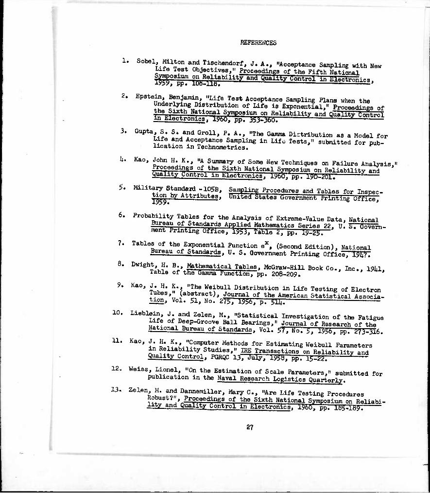
REFERENCES

1. Sobel*i^1*°n^nd Tischendorf, J. A., "Acceptance Sampling with New

Life Test Objectives," Proceedings of the Fifth National Symposium ^sliabilit.y and duality (Jontroi in ElicSFSnics.

2. Epstein, Benjamin, "Life Test Acceptance Sampling Plans when the Underlying Distribution of Life is Exponential," Proceedings of

a^^rSlFl?^!^^^and ^^^^ 3. Gupta, S. S. and Groll, P. A., "The Gamma Dictribution as a Model for

Life and Acceptance Sampling in Life Tests," submitted for pub- lication in Technometrics. ^

U. Kao, John H. K., "A Summary of Some New Techniques on Failure Analysis." .Proceedings of the Sixth National Symposium on Reliability and quality uontrol in klectronics. lybö. pp. 1^6-^1-

5. Military Standard-105B, Sampling Procedures and Tables for Inan^- tion by Attributes. United States Government Printing Office,

6. Probability Tables for the Analysis of Extreme-Value Data, National Bureau of Standards Applied Mathematics Series 22, U. Ü. Govern- ment Minting Office, 19$S, Table ü, pp. I9-2Z.

7. Tables of the E^onential Function ex, (Second Edition), National Bureau of Standards. U. S. Government Printing Office, l^?.

8. Dwight H B. Mathematical Tables. McGraw-Hill Book Co., Inc., 19U, Table of tne Gamma Function, pp. 208-209, * •"* *

9* Ka0' T,;^: u'f ^J6 V****3?- Distribution in Life Testing of Electron Tubes, (abstract). Journal of the American Statistical Associa- tion, vol. 51, No. 275; i9S6, p. SET* S—^

10. Lieblein, J. and Zelen, M., "Statistical Investigation of the Fatigue Life of Deep-Groove Ball Bearings," Journal of Research of the National Bureau of Standards. Vol. 5V, Mo. T, 1^6, pp. 273-316.

11. Kao, J. H-K-, "Computer Methods for Estimating Weibull Parameters in Reliability Studies," IRE Transactions on Reliability and Quality Control. PQRQC 13; Juiy, Mö, pp. l^Ü. r

12. Weiss, Lionel, "On the Estimation of Scale Parameters," submitted for publication in the Naval Research Logistics Quarterly.

13. Zelen M. and Dannemiller, Mary C, "Are Life Testing Procedures Robust?", Proceedings of the Sixth National Symposium on Reliabi- iity and Quality Control in Electronics, 1^60. pp. lü^-ltift.

27

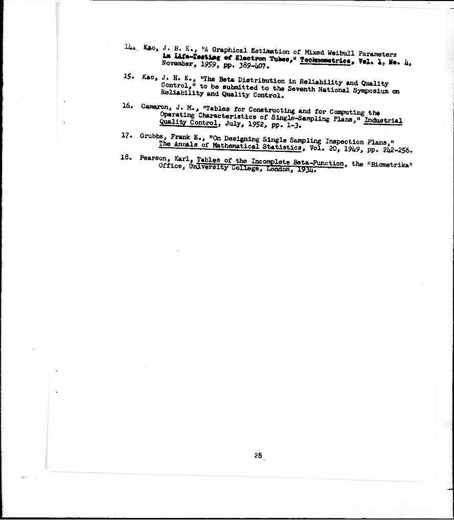
Uu K*oa J ^ "A Gr*Pjical E3ti»ation of Mixed Weibull Parameters *M M(*-«Mta«c ©f Electron Tubes.H TeolmeMtrle« Vmi i «I i November, 1959, pp. 309-^07. ZSSSSSSS*™** »•!• ij U: k>

15. Kao, J H K. "The Beta Distribution in Reliability and Quality

Äiitr^ &%ixs:seventh NatioLi sÄS - 16. CaraM^^M., "Tables for Constructing and for Computing the

17. Grub^'pf«JE., "to Designing Single Sampling Inspection Plans « The Annals of Mathematical St»t^.^ Si. 2^m^ ^^2-256.

18. ^^^,1^11^^^ the 1IBiOTnetriItall

28

O o

00|x(r1/^

«a

0)

10

o

iO >

o

s

0) >

II

u

o L. 10

-C o en c

10 I. 0)

to»

0)

en

II

c

(V)d - aoue+deDov +o A+iiiqeqoJd

TABLE 1

Table of Values for Per cent Truncation, (t/V) x 100

39.09 1*2.69 i*5.71 U9.57 52.88

32*. 93 36.57 38.68 U.59 hk'01

1*6.09 1*9.59 52.50 56.18 59.29

1*3.1*0 1*5.02 1*7.09 1*9.90 52.21

51*.17 57.1*5 60.13 63.1*6 66.26

35.37 51.08 69.31

10U.98 160.91*

60.29 7l*.79 89.32

115.23 11*8.91

36.63 1*0.31* 1*5.1*8 53.30 60.53

67.39 80.61; 93.95

115.61 11*3.14

1*5.82 1*9.50 51*.1*9 61.85 68.1i7

7U.62 86.15 97.33

111*. 92 136.31*

56.73 60.11 6U.60 71.01; 76.67

81.79 91.09 99.82

113.06 128.53

62.85 65.96 70.05 75.83 80.80

85.26 93.27

100.67 111.68 124.27

69.1*1* 72.18 75.73 80.68 8U.89

88.62 95.22

101.21 109.98 119.79

TABLE 2

Table of Probability Values at Truncation Point, p. (*)

kvWx 100 V3 1/2

.010

.012

.015

.020

.025

.030

.oho

.050

.065

.080

0,09 8.57 9.20

10.08 10.82

ll.ii5 12.53 13.2*3 li*.56 15.52

16.61 17.56 10.78 20.k6 21.86

23.06 25.06 26.71 28.76 30.^7

l.iiO 1.51» 1.72 1.98 2.21

2.^2 2.79 3.11 3.5U 3.92

ii.37 ii.78 5.33 6.13 6.83

7.1*5 8.56 9.52

10.78 11.88

32.hO 3ii.03 36.12 38.9U ia.22

U3.Jii 1*6.28 hB.dO 50.90 51*. 30

56.98 59.19 61.92 65.1*5 68.17

70.37 73.79 76.36 79.28 81.1*9 83.75

13.19 11*.35 15.90 18.13 20.01*

21.73 21*.61* 27.11 30.27 32.97

36.06 38.73 1*2.17 1*6.87 50.69

53.91 59.12 63.21 68.02 71.77 75.69

.010

.012

.015

.020

.025

.030

.01*0 .050 .065 .080

.10

.12

.15

.20

.25

.30

.1*0

.50

.65

.80

1.00 1.19 1.1*9 1.98 2.1*7

2.96 3.92 1*.88 6.29 7.69

Shape Parameter - ß

1 2/3 2 2 1/2 3 1/3

.001

.002

.003

.001*

.005

.009

.012

.019

.027

.038

.052

.076 .12 .18

.21*

.39

.56

.89 1.22

9.52 11.31 13.93 18.13 22.12

25.92 32.97 39.35 1*7.80 55.07 63.21

1.77 2.39 3.1*5 5.51 7.89

10.56 16.1*7 22.98 33.26 U3.51* 56.35

.001

.002

.003

.005

.008

.on

.018

.031

.01*9

.071

.13

.20

.33

.50

.78 1.12 1.75 3.09 1*.79

.001

.002 .001* .007

.012 .021* .ou .080 .13

.23 .37 .61*

1.32 2.29

6.82 11.81 17.83 28.21* 39.51 51*.la

3.59 7.23

11.28 22.32 3U.59 52.36

.001

.002 .003 .008 .015

.033

.060

.13

.33

.69

1.26 3.25 6.72

15.37 28.35 50. la

.001

.003

.007 .011* .031* .11 .26

.55 1.71 1*.13

11.35 21*. 15 1*9.08

.001

.002

.005

.021

.061*

.16

.67 2.02 7.29

19.25 1*7.93

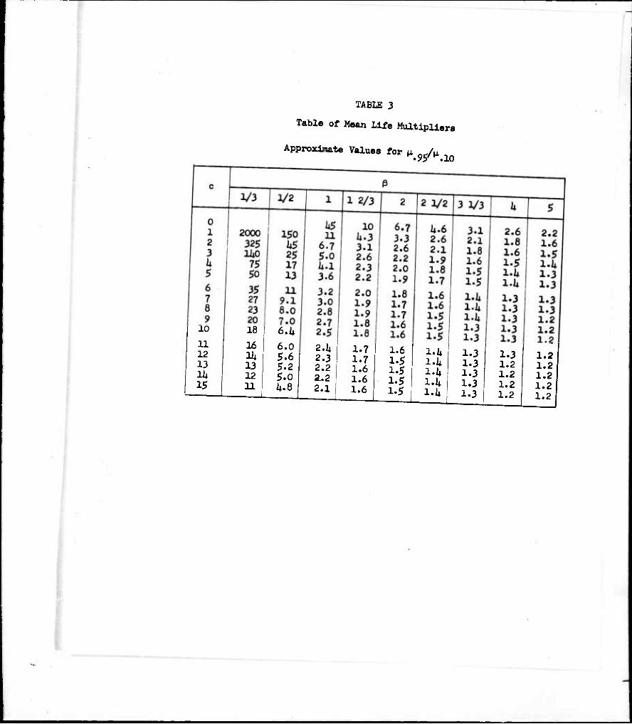
TABLE 3

Table of Mean Life Multipliers

Approximate Values for u Ju. •95' .10

11 16 12 11» 13 13 lit 12 15 11

6.1i

6.0 5.6 5.2 5.0 Iu8

3.2 3.0 2.8 2.7 2.5

2.1« 2.3 2.2 2.2 2.1

1.7 1.6 1.7 1.5 1.6 1.5 1.6 1.5 1.6 1.5

l.i* 1.4 i-U 1.1» 1.1»

1.3 1.3 1.3 1.3 1.3

1.3 1.2 1.2 1.2 1.2

1.2 1.2 1.2 1.2 1.2

TABLE ija

Table of Sampling Plans for ß - 2/3

(t/ti) x 100 Ratio for which P(A) - .10 (or Less)

(VW x 100 ratios in parentheses are for P(A) - .95 (or more)

TABLE lib

Table of Sampling Plans for ß - 1/2

1 .

c (t/ji) x 100 Ratio for which P(A) - .10 (or less)

-

100 50 25 10 5 2.5 1 0.5 0.25 ' 0.1 o.o5| 0.0251 o.oi 0 2

(.03) 3

(.02) 1*

(.01) 6 8 11 17 23 33 52 73 103 165

1 it (.52)

5 (.32)

7 (.16)

10 (.07)

13 (.01*)

18 (.02)

28 (.01)

1*0 56 88 121* 177 278

2 5 (2.2)

7 (.91*)

9 (.51*)

13 (.21*)

18 (.12)

25 (.05)

39 (.02)

55 (.01)

77 (.01)

120 172 21*1 381

3 7 (3.3)

9 (1.7)

12 (.85)

17 (.1*0)

23 (.21)

32 (.10)

1*9 (.01*)

69 (.02)

96 (.01)

153 215 303 1*78

U 9 (U.l)

11 (2.5)

11* (1.1*)

20 (.60)

28 (.30)

38 (.15)

59 (.06)

82 (.03)

115 (.02)

183 (.01)

258 362 571

5 10 (6.1»)

13 (3.3)

16 (1.9)

2i* (.75)

32 (.1*0)

1*5 ' 68 (.19)1(.08)

96 (.01*)

131* (.02)

213 (.01)

299 1*20 663

6 12 (7.2)

11* (1*.7)

19 (2.2)

27 (.91*)

37 (.1*6)

51 (.21*)

78 (.10)

109 (.05)

155 (.02)

21^2 (.01)

339 1*77 753

7 13 (9.7)

16 (5.3)

21 (2.6)

30 (1.1)

1*1 (.55)

57 (.28)

87 (.11)

122 (.06)

173 (.03)

270 (.01)

379 (.01)

533 81*1

b (12)

18 (6.0)

23 (3.2)

31* (1.2)

1*6 (.61)

63 (.33)

96 (.13)

131* (.07)

191 (.03)

298 (.01)

las (.01)

589 929

9 16 (12)

20 (6.1*)

26 (3.3)

37 (1.1*)

50 (.73)

69 (.36)

105 (.11*)

11*7 (.08)

208 (.01*)

326 (.01)

1*57 (.01)

61*3 1,015

1

1 1

10 17 (15)

22 1 (6.8)

28 (3.7)

1*0 (1.5)

51* (.78)

77 (.38)

118 (.15)

162 (.08)

226 (.01*)

353 (.02)

1*96 (.01)

698 1,101

11 19 (16)

23 (8.0)

30 (U.l)

1*3 (1.6)

58 (.83)

83 (.1*0)

126 (.16)

175 (.08)

21*1* (.01*)

380 (.02)

531* (.01)

752 1,186

12 20 (17)

25 (8.8)

32 (1*.6)

1*7 (1.7)

66 (.87)

89 (.1*2)

135 (.17)

187 (.09)

261 (.01*)

1*07 (.02)

572 (.01)

805 1,271

13 22 (18)

27 (9.0)

31* (5.0)

50 (1.9)

70 (.90)

95 (.1*1*)

11*1* (.19)

200 (.09)

278 (.05)

1*31* (.02)

610 (.01)

858 1,355

. 12» 23

(19) : 29

(9.2) 37

(5.0) 53

(2.0) 75

(.92) 101

(.1*7) 153 (.20)

212 (.10)

295 (.05)

1*61 (.02)

61*8 (.01)

911 (.01)

1,1*38

15 25 (19)

31 (9.1*)

39 (5.0)

56 (2.2)

79 (.98)

107 (.1*9)

162 (.21)

22U (.11)

312 (.05)

1*88 (.02)

685 (.01)

961* (.01)

1,521

(Vn) . K 100 ratios in pa. renthe ses ar« 9 for P(A) f .95 ( or raor e)

6

7

8

9

10

11

12

13

11»

15

TABLE kc

Table of Sampling Plans for ß - 1

(W) x 100 Ratio for which P(A) - .10 (or less)

100

3 (1.7)

5 (8.0)

7 ilk)

9 (19)

11 (22)

13 (25)

50

Hi (30)

16 (33)

18 (35)

20 34 (36) (16)

5 (1.0)

9 (U.2)

12 (7.1*)

15 do)

19 (12)

22 (13)

25

25 (15)

28 (16)

31 (17)

10 (.51)

17 (2.1)

23 (3.7)

29 (5.0)

3U (6.2)

UO (7.0)

10

22 (38)

37 (19)

23 hO (UO) (20)

25 0*2)

27 (U2)

29 (hh)

31 (U*)

1*6 (7.5)

51 (8.2)

57 (9.0)

62 (9.3)

70 (9.5)

21* (.20)

1*0 (.90)

55 (1.5)

69 (2.0)

82 (2.1*)

96 (2.8)

i*3 (20)

1*5 (21)

1*8 (22)

51 (22)

76 (9.8)

81 (10)

86 (10)

91 (11)

97 (11)

109 (3.0)

122 (3.3)

135 (3.5)

11*7 (3.7)

162 (3.9)

1*6 (.11)

79 (.1*5)

108 (.76)

135 (1.0)

I6ii (1.2)

191 (1.1*)

2.5

175 (1*.0)

187 (1*.2)

200 (U.3)

212 (U.l*)

22U (1*.6)

216 (1.5)

2i|2 (1.7)

267 (1.8)

292 (1.9)

316 (2.0)

92 .06)

158 .22)

216 .38)

271 .50)

321* .61)

376 .69)

0.5

31*1 (2.1)

365 (2.2)

389 (2.2)

1*13 (2.3)

1*37 (2.1*)

1*27 (.77)

1*77 (.83)

527 (.89)

576 (.91*)

62li (1.0)

231 (.02)

389 (.09)

533 (.15)

669 (.20)

800 (.21*)

928 (.28)

1*61 (.01)

778 (.05)

1,065 (.08)

1,337 (.10)

1,600 (.12)

1,855 (.11*)

0.25

672 (1.1)

720 (1.1)

768 (1.1)

815 (1.1)

863 (1.2)

1,051* (.31)

1,178 (.31*)

1,300 (.36)

1,1*21 (.38)

1,51*1 (.1*0)

1,660 (.1*2)

1,780 (.1*3)

1,896 (.1*5)

2,013 (.1*6)

2,130 (.1*7)

2,107 (.16)

2,355 (.17)

2,600 (.18)

2,81i2 (.19)

3,082 (.20)

922

1,556 (.02)

2,129 (.01*)

2,673 (.05)

3,200 (.06)

3,710 (.07)

0.1

1*,213 (.08)

1*,709 (.08)

5,200 (.09)

5,683 (.10)

6,163 (.10)

2,303

3,890 (.01)

5,322 (.02)

6,681 (.02)

8,000 (.02)

9,275 (.03)

0.05

3,320 (.21)

3,557 (.22)

3,792 (.22)

1*,026 (.23)

1*,260 (.21*)

6,6U0 (.10)

7,113 (.11)

7,58U (.11)

8,052 (.12)

8,517 (.12)

105-2 (.03)

118-2 (.03)

130-2 (.01*)

11*2-2 (.01*)

15U-2 (.01*)

1*,606

7,780

106-2 (.01)

13U-2 (.01)

160-2 (.01)

186-2 (.01

0.025 0.01

166-2 (.01*) 178-2 (.01*)

190-2 (.05)

201-2 (.05)

213-2 (.05)

211-2 (.02)

235-2 (.02)

260-2 (.02)

28ii-2 (.02)

308-2 (.02)

9,212

156-2

213-2

267-2

320-2

371-2 (.01)

332-2 (.02)

336-2 (.02)

379-2 (.02)

1*03-2 (.02)

1*26-2 (.02)

1*21-2 (.01)

1*71-2 (.01)

520-2 (.01)

568-2 (.01)

616-2 (.01)

230-2

389-2

532-2

668-2

800-2

928-2

66k-2 (.01)

711-2 (.01)

758-2 (.01)

805-2 (.01)

852-2 (.01)

105-3

118-3

130-3

11*2-3

15U-3

166-3

178-3

190-3

201-3

213-3

(t/u) x 100 ratios in parentheses are for P(A) - ,95 (or more)

The figure following the dash in sample size numbers shows the number of zeros to addj for example, 15U-3 - 151*,000.

10

n

12

13

11*

15

TABUS kd

Table of Sampling Plans for ß - 1 2/3

(t/V) x 100 Ratio for which P(A) - ,10 (or less)

100

3 (9.8)

50

9 (5.0)

16 (22) (12)

25 15

8 (31)

10 (38)

12 (U2)

Hi (ii6)

17 (U7)

19 (50)

21 (52)

23 (5ii)

2li (57)

22 (16)

28 (19)

33 (21)

39 (23)

26 (59)

26 (60)

30 (61)

33 (61)

35 (62)

lili (25)

ii9 (26)

5U (27)

59 (28)

68 (28)

28 (2.5)

li8 (5.9)

66 (8.1)

83 (9.6)

100 (11) 116

(12)

66 (1.5)

112 (3.5)

155 (li.8)

19li (5.7)

232 (6.10

26;?

10

129 (1.0)

220 (2.3)

301 (3.2)

378 (3.8)

US2 (U.3)

525 (U.6)

8

132 (12)

HiS (13)

165 (13)

181 (Hi)

196 (Hi)

73 (29)

78 (29)

83 (29)

88 (30)

93 (30)

211 (15)

226 (15)

21*1 (15)

256 (15)

270 (16)

306 (7.U)

3ii2. (7.7)

377 (8.1)

lil2 (8.3)

lili7 (8.6)

U82 (8.9)

516 (9.0)

550 (9.1)

58U (9.3)

618 (9.U)

596 (li.9)

666 (5.2)

735 (5.ii)

803 (5.6)

871 (5.7)

189 (.80)

319 (1.9)

ii37 (2.6)

5U8 (3.1)

656 (3.1i)

761 (3.7)

938 (5.9)

1,005 (6.0)

1,072 (6.1)

1,138 (6.3)

1,203 (6.1i)

861* (3.9)

965 (li.2)

1,066 (li.3)

1,165 (U.5)

1,263 (li.6)

U12 (.50)

695 (1.2)

951 (1.6)

l,19li (1.9)

l,li28 (2.1)

1,657 (2.3)

1,881 (2.5)

2,102 (2.6)

2,321 (2.7)

2,537 (2.8)

2,752 (2.9)

591 (.liO)

998 (.96)

1,365 (1.3)

l,7Hi (1.5)

2,050 (1.7)

2,379 (1.9)

2.5-

1,361 (li.7)

l,li58 (li.8)

1,55U (U.9)

1,650 (5.0)

l,7li6 (5.1)

2,961* (2.9)

3,176 (3.0)

3,386 (3.1)

3,595 (3.1)

3,803 (3.2)

2,701 (2.0)

3,019 (2.1)

3,333 (2.2)

3,61*3 (2.2)

3,951 (2.3)

1,280 (.25)

2,162 (.60)

2,957 (.81)

3,712 (.96)

li,lili2 (1.1)

5,153 (1.2)

1.5

li,256 (2.3)

li,560 (2.1*)

U,862 (2.5)

5,162 (2.5)

5,li60 (2.6)

5,852 (1.3)

6,51iO (1.3)

7,220 (l.li)

7,893 (l.li)

3,031 (.15)

5,119 (.35)

7,003 (.1*9)

8,791 (.58)

105-2 (.65)

122-2 (.69)

6,061 (.10)

102-2 (.23)

11*0-2 (.32)

176-2 (.38)

210-2 (.1*2)

2liU-2 (.li5)

0.5

277-2 (.Ii8)

310-2 (.51)

8,560 203-2 (1.5) (.86)

9,222 (1.5)

9,879 (1.5)

105-2 (1.6)

112-2 (1.6)

118-2 (.16)

139-2 (.75)

155-2 (.78)

171-2 (.80)

187-2 37li-2 (.81i) (.55)

li05-2 (.57)

l8i*-2 (.05)

311-2 (.11)

li26-2 (.16)

53li-2 (.19)

61|0-2 (.21)

7li2-2 (.23)

0.25

8U3-2 (.25)

9U2-2 (.26)

576-2 (.03)

973-2 (.06)

133-3 (.08)

167-3 (.09)

200-3 (.10)

232-3 (.11)

218-2 (.89)

23li-2 (.90)

21*9-2 (.92)

265-2 (.9W 280-2 (.95)

3li2-2 10h'3 (.53) (.27)

llli-3 (.28)

123-3 (.29)

li37-2 133-3 (.58)|(.30)

1*68-2 (.59)

li99-2 (.61)

530-2 (.62)

560-2 (.63)

11*2-3 (.30)

152-3 (.31)

161-3 (.31)

170-3 (.32)

263-3 (.12)

29li-3 (.13)

325-3 (.13)

355-3 (.Hi)

385-3 (.Hi)

lil5-3 (.15)

1*1*5-3 (.15)

li75-3| (.15)

505-3 (.16)

535-3 (.16)

(t/p.) x 100 ratios in parentheses are for P(A) - .95 (or more)

The figure following the dash in sample size numbers shows the number of zeros to add; for example, 218-2 - 21,800.

TABI£ its

Table of Sampling Plans for ß - 2

(VtQ x 100 Ratio for ^^ p(A) . #10 (or leg8)

loo 50 25 15

1(29)

be)

12 101 8

51

131 (2.2)

223 (k.S)

305 (5.8)

382 1 597 (6.7) (5.W

1*571 711! (7. W 1(5.9)

206 (1.8)

(3.6)

U76i (1».7)

530 (7.9)

829 (6.3)

296 (1.5)

ii99 (3.0)

683 (3.9)

857 (4.5)

1,025 (5.0)

1,190 (5.3)

1,152 (.76)

1,9U5 (1.5)

10

120

9ia (6.6)

1,051 (6.9)

1,161 (7.2)

1,272; (7.i*) 1,376 (7.5)

(33) (17)

9h9 (9.6)

1,017 (9.8)

l,08ii (.(10)

1,151 do)

1,217 |l,902 (10) (8.2)

1,482 (7.7)

1,588 (7.8)

1,693 (8.0)

1,798 (8.1)

1,351 (5.6)

1,510 (5.8)

1,667 (6.0)

1,822 (6.1)

1,976 (6.3)

1,06U (3.1)|

1,336 (3.6)

1,599j (4.0)

1,8551 (4.2)1

2,128 (6.1») 2,280 (6.5)

2,431 (6.6)

2,581 (6.7)

2,730 (6.8)

2,106 (4.5)

2,351* (4.6)

2,600 (4.8)

2,8U (4.9), 3,081 (5.0)

3,341 (2.3)

3,977 (2.5)

4,638 (2.7) 5,211i (2.8)

3,320 (5.1)

3,556 (5.2)

3,792 (5.3)

li,026 (5.4)

U,258 (5.5)

5,886 (2.9)

6,li98 (3.0)

7,103 (3.1)

7,701^ (3.2)

1,772 (.62)

2,993 (1.2)

|M94 (1.6)

5,140 (1.8)

6,150 (2.0)

7,135 (2.2)

8,299 (3.3)

8,891 (3.3)

9,1479 i3.k) 101-2 (3.1;)

106-2 (3.5)

9,055 (2.k)

9,997 (2.4)

109-2 (2.5)

1119-2 (2.6)

k»700 (.38)

7,939 (.76)

109-2 (.98)

136-2 (1.1)

163-2 (1.2)

189-21 (1.3)

1.5

128-2 (.23) 216-2 (.1*6)

296-2 (.60)

288-2 (.16)

486-2 (.30)

665-2 (.40)

371-21835-2 (•70)j(.47)

1*1*4-21999-2 (.76) (.51)

515-2 116-3 (.81), (.51,)

33l*-3 (.210

128-2 (2.6)

137-2 (2.7)

!l46-2 (2.7)

155-2 (2.8)

161^-2 (2.8)

215-2 (1.4) 2I1O-2 (1.5) 265-2 (1.5) 290-2 (1.5) 311»-2 (1.6)

585-21132-3 (.85) (.57) 651*-2 (.88)

722-2 (.91)

147-3 (.60)

162-3 (.62)

339-2 (1.6)

'363-2 (1.6)

387-2 (1.7) 1*11-2 (1.7)

435-2 (1.7)

789-2 178-3 (.91*) (.63)

856-2 193-3 (*96) (.65) 922-2 (9.8)

i988-2 (1.0)

20763 (.66)

222-3 U67)

('

105-3)237-3 (1.0) (.68);

112-3'252-3 (1.0)

118-3 (1.0)

(.69)

266-3 (.70)

IO6-I1 (.36)

(t/iO x 100 ratios in parentheses are for P(A) - .95 (or more)

t^aSrSr^iÄ nS-^utST' ^ "^ ShOW8 the ™*~ <* —3

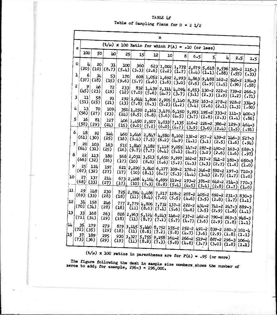
TABLE kf Table of Sampling Plans for ß 2 1/2

n

100

(t/tx) x 100 Ratio for which P(A) - .10 (or leas)

25 IS

31 (8.7)

h6 72 (23) (19)

109 (23)

81 127 (29)

292 (13)

61 18 (61)

11

121 31 (70)

131 33 (71)

lldi (25)

103 163 (31) (25)

180 (26)

122i 197 (32)| (27)

2U* (27)

515 (16)

lt0Ut (7.8)

1,250 (8.5) 1,1*50 (9.0)

lii8 (33) 158

(31;) 168

(3U)

230 (28)

725 (18)

1,61^6 (9.1i)

1,81^0 (9.7)

2,220 (10)|

2,1408 (10)

623 (2.6)

1,052 (li.6)

1,1*39 (5.6)

1,806 (6.3) 2,161 (6.8)

2,507 (7.2)

1,002 (2.2)

1,692 (3.8)

2,311* a.7) 2,905 (5.2)

3,1*76 (5.6)

li,033 (6.0)

8

1,772 (1.7)

2,879 (1.1*)

2,993 1^,863 (3.0) (2.5)

li,09l*l6,653 (3.7) (3.1)

5,11*0 8,352 U.2) (3.1*)

6,150|9,993

2,81*7 (7.5) 3,182 (7.7)

1*,580 (6.2)

5,118 (6.10 5,65oi (6.6)

(1*.5)

7,135 (li.7)

8,102 (1*.9)

9,055 (5.1)

9,997 (5.2)

(3.7)

116-2 (3.9)

5,618 (1.1) 9,1*88 (1.9)

130-2 (2.3) 163-2 (2.6)

195-2 (2.8) 226-2 (3.0)

2.5 1.5

279 (29) 295

(29)

879 (18) 930

(19)

2,591* (11)

2,779 (11)

2,963 (11)

3,11*5 (11)

3,327 (11)

1*,1*86 (8.10

6,699. (6.8)

119-2 (5.1*)

132-2 (l*.l) 11*7-2 a.2) 162-2 (1*.3) 178-2 (l*.l*)l

257-2 (3.1)

287-2 (3.2)

317-2 (3.3) 31*6-2 (3.1*)

9,596 (.88)

162-2 (1.5) 222-2 (1.9)

278-2 (2.1)

333-2 (2.3)

386-2 (2.1*)

320-2 (.55) 51*0-2 (.96)

739-2 (1.2)

928-2 (1.3) 111-3 (1.10 129-3 (1.5)

1*39-2 1^6-3 (2.5) (1.6)

115-3 (.33) 19l*-3 (.58)

266-3 (.71)

33l*-3 (.80)

1*00-3 (.86)

l*61*-3 (.91)

7,217 128-2 207-2 (7.0)|{5.5) a.6)

1*90-2 (2.6)

51*1-2 (2.7) 592-2 (2.7)

163-3 (1.6)

180-3 (1.6)

527-3 (.91*)

589-3 (.97)

650-3 (1.0)

197-3 710-3 (1.7) (1.0)

61*2-2 21^-3 (2.8)|(1.7)

l*,806i 7,732 137-2| 222-2 (8.6)j (7.1)

5,121a 8,21*3 (8.7) (7.1)

5,1*1*0 (8.8)

5,755 (8.8)

(5.6)|(k.6)

11*6-2 237-2 (5.7) (1*.7)

8,752 155-2 (7.2) 9,258 (7.3)

(5.8) I6I1-2 (5.8)

1*05-2 (3.5) l*3l*-2 (3.5)

692-2 (2.8)

71*1-2 (2.9)

231-3 (1.7)

2li7-3 (1.8)

770-3 (1.0)

1*62-2 790-2 (3.6) (2.9)

252-2 (1*.7) 266-2 (1*.8)

1*91-2 (3.6) 519-2 (3.7)

839-2 (2.9) 887-2 (3.0)

263-3 (1.8)

280-3 (1.8) 296-3 (1.8)

889-3 (1.1) 91*8-3 (1.1)

101-k (1.1) 106-U (1.1)

(tAO x 100 ratios in parentheses are for P(A) - .95 (or more)

JS; Ä^IÄ ^ 2Ä!iZe «-^•h~ ^ number of

TABLE kg

Table of Sampling Plans for ß ■ 3 1/3

100

k (30)

7 ih6)

9 (56)

12 (60)

Hi (65)

16 (68)

65

Hi (21)

2k (32)

33 (37)

li2 (liO)

51 (ii2)

59 (M)

(t/ji) x 100 Ratio for which P(A) - .10 (or less)

50

10

ii

12

13

lii

15

19 (69)

21 (71)

23 (73)

26 (7U)

28 (75)

30 (76)

32 (77)

35 (77)

37 (78)

39 (79)

67 (ii6)

75 (1*7)

83 (1*7)

90 (U8)

101 (li8)

3k (16)

57 (21»)

78 (28)

98 (31)

117 (33)

136 (310

108 ik9) 116

(li9)

12k (50)

131 (50)

139 (51)

157 (35)

176 (36)

19li (36)

212 (37)

230 (38)

2li7 (38)

265 (39)

283 (39)

300 (39)

317 (UO)

2iO

70 (13)

30

183 (9.6)

119 309 (19) (lii)

I6ii I k23 (23) i (17)

25

206 (25)

21*6 (26)

286 (27)

531 (19)

635 (20)

737 (21)

325 (28)

363 (29)

liOO (29)

ii38 (30)

ii75 (30)

511 (31)

51i8 (31)

836 (21)

935 (22)

1,032 (22)

1,128 (22)

1,228 (23)

33li (8.0)

56U (12)

772 (Hi)

969 (15)

1,159 (16)

l,32i5 (17)

20

1,318 (23)

1,102 (23)

58U 1,505 (31) (210

1,527 (17)

1,698 (18)

1,66k (18)

2,059 (19)

2,233 (19)

698 (6.10

1,179 (9.8)

1,613 (11)

2,025 (12)

2,1*23 (13)

2,811 (Hi)

15

620 (32)

656 (32)

1,598 (210

1,690 (210

2,^06 (19)

2,578 (20)

2,7li8 (20)

2,918 (20)

3,086 (20)

3,192 (Hi)

3,567 (Hi)

3,938 (15)

U,305 (15)

li,669 (15)

1,772 Oi.8)

2,993 (7.10

li,09li (8.7)

5,Hi0 (9.1*)

6,150 (10)

7,135 (10)

12

8,102 (11)

9,055 (11)

9,997 (11)

109-2 (11)

119-2 (12)

3,839 (3.8)

6,li8U (5.8)

8,870 (6.8)

111-2 (7.5)

133-2 (7.9)

155-2 (8.2)

10

5,030 (15)

5,389 (15)

5,7li5 (16)

6,100 (16)

6,U53 (16)

128-2 277-2 (12) (9.3)

176-2 (8.1*)

196-2 (8.7)

217-2 (8.8)

237-2 (9.0)

257-2 (9.2)

6,979 (3.2)

118-2 (li.8)

161-2 (5.7)

202-2 (6.2)

2k2-2 (6.6)

281-2 (6.8)

8 6.5

319-2 (7.0)

357-2 (7.2)

39li-2 (7.1*)

li30-2 (7.5)

1*67-2 (7.6)

H*9-2 (2.5)

251-2 (3.9)

3li3-2 (1*.5) li31-2 (ii.9)

516-2 (5.2)

598-2 (5.10

679-2 (5.6)

759-2 11*7-3 (5.8) (I*.?)

288-2 (2.1) li86-2 (3.2)

665-2 (3.7)

835-2 (1*.0)

999-2 (ii.3)

116-3 (li.li)

132-3 (ii.6)

698-2 (1.6)

118-3 (2.1*)

161-3 (2.8)

202-3 (3.1)

2U2-3 (3.3)

281-3 (3.1»)

137-2 (12)

Hi6-2 (12)

155-2 (12)

161^-2 (12)

296-2 (9.1*)

316-2 (9.1*)

335-2 (9.5)

355-2 (9.6)

162-3 (li.8)

838-2 (5.9)

917-2 (6.0)

99li-2 193-3 (6.0) (li.?)

503-2 107-3 (7.7)|(6.1)

539-2 (7.8)

57li-2 (7.9)

610-2 (8.0)

6U5-2 (8.0)

115-3 (6.2)

122-3 (6.2)

130-3 (6.3)

137-3 (6.10

319-3 (3.5)

357-3 (3.6)

39li-3 (3.7)

178-3 U30-3 (li.9) (3.7)

1*67-3 (3.8)

207-3 (5.0)

222-3 (5.0)

237-3 (5.1)

252-3 (5.2)

266-3 (5.2)

503-3 (3.8)

539-3 (3.9)

57li-3 (3.9)

610-3 (3.9)

6U5-3 (li.O)

(t/V) x 100 ratios in parentheses are for P(A) - .95 (or more)

The figure following the dash in sample size numbers shows the number of zeros to add; for example, 319-3 - 319,000.

TABLE iih

Table of Säugling Plans for ß - U

n

100

(37)

7 (53)

9 (62)

12 (66)

15 (68)

17 (71)

(t/n.) x 100 Ratio for which P(A) - .10 (or less)

80 65

9 (30)

15 (kh)

21 (50)

26 (5U)

50 1(0

10

19 (710

22 (75)

2k (76)

27 (77)

29 178)

55 (19)

93 (27)

128 (31)

57 I 162 (1*10 j (33)

20 (25)

33 (36)

1*6 (1*0)

31 69 (56) | (1*6)

37 (58)

11

12

13

11*

15

31 (79)

33 (80)

36 (81)

38 (82)

1*0 (82)

1*2 (59)

1*7 (60)

52 (61)

57 (62)

61* (62)

80 (1*8)

69 (63)

71* (63)

79 (61*)

81* (61*)

89 (61*)

91 (1*9)

102 (50)

112 (50)

123 (51)

136 (51)

191* (35)

225 (36)

131* (15) 226

(22)

312 (25)

391 (27) 1*68

(28)

51*3 (29)

30

11*7 (52)

157 (52)

167 (53) 178

(53)

188 (53)

255 (37)

286 (38)

315 (39)

31*1* (39)

373 (1*0)

1*02 (1*0)

616 (30)

689 (30)

760 (31)

831 (31) 901

(32)

1*19 (12)

708 (16)

968 (19)

1,215 (20)

1,1*52* (21)

1,687 (22)

25

971 (32)

l*3l|l,oliO (1*0) (32)

1*60 (U)

1*88 (ia)

516 (ia)

1,915 (22)

2,11*0 (23)

2,363 (23)

2,583 (23)

2,802 (21*)

886 (9.1*)

1,1*97 (H*)

2,01^7 (16)

2,570 (17)

3,075 (18)

3,568 (18)

20 15

1*,051 9,575 (19) (15)

2,091* (7.6)

3,537 (11)

1*,839 (12)

6,071* (13)

7,268 (H*)

8,1*32 (15)

6,771* (5.8)

lll*-2 (8.0)

157-2 (9.2)

197-2 (10)

235-2 (10)

273-2 (11)

12

l61*-2 (1*.7)

10 n 329-2 (l*.o)

278-2 556-2 (6.5) (5.6)

1,109 (33)

1,177 (33)

1,21*6 (33)

3,018 (21*)

3,233 (21*)

3,1*1*7 (21*)

3,660 (25)

3,872 (25)

1*,528 (19)

1*,998 (19)

5,1*61* (20)

5,926 (20)

6,381* (20)

6,81*0 (20)

7,292 (20)

7,71*2 (21)

8,190 (21)

107-2 (15)

118-2 (15)

129-2 (16)

11*0-2 (16)

151-2 (16)

162-2 (16)

172-2 (16)

183-2 (17)

19l*-2 (17)

310-2 (11)

31*6-2 (U)

382-2 (12)

ia8-2 (12)

1*53-2 (12)

380-2 (7.1*)

1*77-2 (7.9)

571-2 (8.3) 663-2 (8.6)

760-2 (6.2)

951*-2 (6.6)

8| 6.5

768-2 (3.2)

130-3 (1*.5)

177-3 (5.1)

223-3 (5.5)

lll*-3 266-3 615-3 (7.0) (5.8)!(U.7)

177-3 (2.6)

299-3 (3.7)

1*09-3 (1*.2)

5ll*-3 (U.5)

752-2 (8.8)

8la-2 (9.0)

928-2 (9.1)

101-3 (9.2)

110-3 (9.1*)

133-3 (7.2)

150-3 (7.1*)

309-3 (6.0),

713-3 (1*.9)

351-3 (6.1)

168-3 392-3 (7.6) (6.2)

186-3 (7.7)

203-3 (7.8)

1*88-2 (12)

523-2 (12)

558-2 (12)

592-2 (12)

626-2 (12)

119-3 (9.1*)

127-3 (9.5)

135-3 (9.6)

ll*l*-3 (9.7)

152-3 (9.8)

1*33-3 (6.3)

220-3 5ll*-3 (7.8) (6.1*)

237-3 (7.9)

251*-3 (8.0)

271-3 (8.1)

810-3 (5.0)

905-3 (5.1) 100-1* (5.2)

l*7i*-3|l09-l* (6.3)j(5.3) j

119-1* j (5.3)

553-3 128-1* (6.1*) (5.1*)

593-3 (6.5)

632-3 (6.5)

288-3 671-3 (8.2) (6.6)

30l*-3 (8.2)

710-3 (6.6)

137-1* (5.)*) 11*6-1* (5.5)

155-1* (5.5) 161*-1* (5.6)

(t/V) x 100 ratios in parentheses are for P(A) - .95 (or more)

The figure following the dash in sample size mnnbers shows the number of zeros to add; for example, 30l*-3 - 30l*,000.

TABLE ki. Table of Sampling Plans for ß

n

c (t/V) x 100 Ratio for which P(A) ■ ,10 (or less)

100 80 65 50 1*5 1*0 35 30 25 20 15 12 10

0

1

2

3

k

5

U (U6)

7 (53)

10 (68)

12 (73)

15 (76)

17 (78)

11 (37)

19 (1*9)

26 (55)

33 (58)

ho (60)

U6 (62)

31 (30)

53 (UO)

72 (U5)

90 (U7) 108

(1*9)

125 (51)

113 (23)

193 (31)

261* (3U)

331 (36)

396 (38)

1*60 (39)

192 (21)

325 (28)

1*1*1. (31)

557 (33)

667 (31*)

773 (35)

31*1* (19)

581 (25)

795 (27)

998 (29)

1,191* (30)

1,385 (31)

678 (16)

1,11*5 (22)

1,566 (21*)

1,965 (25)

2,352 (26)

2,728 (27)

1,1*1*0 (Hi)

2,1*32 (19)

3,327 (21)

1*,176 (22)

1*,997 (23)

5,797 (23)

3,599 (12)

6,079 (15)

8,316 (17)

10l*-2 (18)

125-2 (19)

11*5-2 (19)

110-2 (9.1*)

185-2 (12)

253-2 (Ik)

318-2 (HO

381-2 (15)

1*1*2-2 (15)

1*61-2 (7.0)

778-2 (9.2)

106-3 (10)

13lt-3 (11)

160-3 (11)

186-3 (12)

135-3 (5.6)

229-3 (7.5)

313-3 (8.3)

393-3 (8.8)

1*70-3 (9.1)

51*6-3 (9.1*)

329-3 (U.8)

556-3 (6.3)

760-3 (7.0)

95U-3 (7.1*)

lll*-l* (7.6)

132-1* (7.8)

6

7

8

9

10

20 (79)

22 (80)

25 (81)

27 (62)

30 (83)

53 (63)

59 (6U)

66 (65)

72 (66)

81 (66)

U43 (52)

1.62 (52)

179 (53)

195 (SU) 212

(51*)

522 (1*0)

583 (1*0)

61*1* (1*1)

701* (ia)

763 (ia)

878 (36)

981 (36)

1,083 (37)

1,181* (37)

1,281* (37)

1,572 (32)

1,757 (32)

1,91*0 (33)

2,121 (33)

2,300 (33)

3,098 (28)

3,1*63 (28)

3,823 (29)

1*,179 (29)

1*,532 (29)

6,583 (21*)

7,357 (21*)

8,122 (25)

8,879 (25)

9,630 (25)

165-2 (20)

18U-2 (20)

203-2 (20)

222-2 (20)

2lil-2 (21)

502-2 (16)

561-2 (16)

619-2 (16)

676-2 (16)

73l*-2 (17)

211-3 (12)

235-3 (12)

260-3 (12)

281*-3 (12)

308-3 (12)

620-3 (9.6)

692-3 (9.7)

761*-3 (9.8)

836-3 (10)

906-3 (10)

150-1* (8.0)

168-1* (8.1)

187-1* (8.2)

203-1* (8.3) 220-1* (8.1*)

11

12

13

Hi

15

32 (81*)

3U (8W

37 (85)

39 (85)

ui (86)

87 (66)

93 (67)

99 (67)

105 (68)

111 (68)

228 (55)

2hh (55) 261

(55)

277 (56)

293 (56)

822 (1*2) 881

(1*2)

939 (1*2)

997 (1*3)

1,055 (1*3)

1,381* (38)

1,1*82 (38)

1,580 (38)

1,678 (39)

1,775 (39)

2,1*78 (31*)

2,655 (31*)

2,830 (31*)

3,005 (31*)

3,178 (35)

1*,882 (29)

5,230 (30)

5,576 (30)

5,920 (30)

6,263 (30)

10l*-2 (25)

111-2 (25)

116-2 (26)

126-2 (26)

133-2 (26)

259-2 (21)

278-2 (21)

296-2 (21)

311*-2 (21)

333-2 (21)

790-2 (17)

81*7-2 (17)

903-2 (17)

958-2 (17)

101-3 (17)

332-3 (13)

356-3 (13)

379-3 (13)

1*03-3 (13)

1*26-3 (13)

976-3 (10)

105-1* (10)

112-1* (10)

118-1* (10)

125-1* (10)

237-1* (8.5)

251*-1* (8.6)

271-1* (8.6)

288-1* (8.6)

30l*-l* (8.7)

(t/ii) x 100 ratios in parentheses are for P(A) - .95 (or more)

The figure following the dash in sample size numbers shows the number of zeros to add; for example, 203-2 > 20,300.

DISTRIBUTION LIST

Head, Logistics and Mathematical Statistics Branch

Office of Naval Research Washington 25, D. C.

Commanding Officer Office of Naval Research Branch Office Navy #100 Fleet Post Office New York, New York

ASTIA Document Service Center Arlington Hall Station Arlington 12, Virginia

Office of Technical Services Department of Commerce Washington 25, D. 0.

3 copies

2 copies

5 copies

1 copy-

Technical Information Officer Naval Research Laboratory Washington 25, D. C. 6 copies

DISTRIBUTION LIST

Professor T. W. Anderson Department of Mathematical Statistics Columbia university New York 27, New York 1

Professor Z. W. Birnbaum Laboratory of Statistical Research Department of Mathematics University of Washington Seattle $, Washington 1

Professor A, H. Bowker Applied Mathematics & Statistics Lab. Stanford University Stanford, California 1

Professor Ralph A. Bradley Department of Statistics Florida State University Tallahassee, Florida 1

Dr. John W. Cell Department of Mathematics North Carolina State College Raleigh, North Carolina l

Professor Herman Chernoff Applied Mathematics & Statistics Lab. Stanford University Stanford, California 1

Professor W. G. Cochran Department of Statistics Harvard University Cambridge, Massachusetts 1

Dr. C. Clark Cockerham Institute of Statistics North Carolina State College Raleigh, North Carolina 1

Professor Cyrus Derman Department of Industrial Engineering Columbia University New York 27, New York 1

Professor Benjamin Epstein Applied Mathematics & Statistics Lab. Stanford University Stanford, California 1

Professor W. T. Federer Department of Plant Breeding Biometrics Units Cornell University Ithaca, New York i

Dr. R. J. Freund Department of Statistics &

Statistical Lab. Virginia Polytechnic Institute Blacksburg, Virginia i

Professor H. P. Goode Dept. of Industrial and

Engineering Administration Cornell University Ithaca, Mew York i

Professor W. Hirsch Institute of Mathematical Sciences New York University New York 3, New York i

Professor Harold Hotelling Associate Director Institute of Statistics University of North Carolina Chapel Hill, North Carolina 1

Professor Oscar Kempthorne Statistics Laboratory Iowa State College Ames, Iowa i

Professor Gerald J. Lieberman Applied Mathematica and

Statistics Lab. Stanford University Stanford California i

Dr. Arthur E. Mace Battelle Memorial Institute 505 King Avenue Columbus 1, Ohio

Professor J. Neyraan department of Statistics university of California Berkeley h, California

Dr. F, Oberhettinger Department of Hathematics Oregon State College Corvallis, Oregon

Professor Herbert Robbins Mathematical Statistics Dept, Fayerweather Hall Columbia university New York 27, New York

Professor Murray Rosenblatt Department of Mathematics Brown university Providence 12, Rhode Island

Professor H. Rubin Department of Statistics Michigan State university East Lansing, Michigan

Professor I. R. Savage School of Business Administration University of Minnesota Minneapolis, Minnesota

Professor L. J. Savage Statistical Research Laboratory Chicago University Chicago 37, Illinois

Professor W. L, Smith Statistics Department University of North Carolina Chapel Hill, North Carolina

Professor Prank Spitser Department of Mathematics university of Minnesota Minneapolis, Minnesota

Dr. H. Teicher Statistical Laboratory Engineering Administration Bldg. Purdue university Lafayette, Indiana

Professor M.B. Wilk Statistics Center Rutgers-The State University New Brunswick, New Jersey

Professor S.S. Wilks Department of Mathematics Princeton university Princeton, New Je.sey

Professor J. Wolfowitz Department of Mathematics Lincoln Hall Cornell University Ithaca, New York