Activity Based Travel Demand Model Systemwith Daily Activity Schedules

by

John L. Bowman

Submitted to the Department of Civil and Environmental Engineeringin Partial Fulfillment of the Requirements for the Degree of

Master of Science in Transportation

at the

Massachusetts Institute of Technology

June 1995

© Massachusetts Institute of Technology 1995All rights reserved

Signature of Author________________________________________________________Department of Civil and Environmental Engineering

May 12, 1995

Certified by______________________________________________________________Moshe Ben-Akiva

Professor of Civil and Environmental EngineeringThesis Supervisor

Accepted by_____________________________________________________________Joseph M. Sussman

Chairman, Departmental Committee on Graduate Studies

2

3

Activity Based Travel Demand Model Systemwith Daily Activity Schedules

byJohn L. Bowman

Submitted to the Department of Civil and Environmental Engineeringon May 12, 1995 in partial fulfillment of the

requirements for the Degree of Master of Science in Transportation

Abstract

We present an integrated activity based discrete choice model system of an individual'sdaily activity and travel schedule, intended for use in forecasting urban passenger traveldemand. The system is demonstrated using a 1991 travel survey and transportationsystem level of service data for the Boston metropolitan area.

The model system is implemented as a set of choice models, integrated as a sequentiallyestimated nested logit model system. Three types of models comprise the system: (1)daily activity pattern, (2) primary tour and (3) secondary tour. The daily activity patterndecision includes the decision of whether to travel, the choice of the day’s primaryactivity, the complexity of the primary tour and the number and purpose of additionaltours. The primary and secondary tour models include the choice of time, destination andmode of travel. The tour models are conditioned by the choice of a daily activity pattern,and the choice of a daily activity pattern is influenced by the expected maximum utilityderived from the available tour alternatives. The expected maximum utility derived fromthe tour alternatives varies for different daily activity patterns, as does the change inexpected maximum utility when environmental and socioeconomic changes occur. Thus,for example, increases in fuel prices would reduce the utility of high mileage daily activitypatterns more than that of low mileage patterns. This would cause a predicted shifttoward the lower mileage patterns, such as those which chain activities in fewer tours orsubstitute in-home activities for those which require travel.

The daily activity schedule model system can be used for forecasting travel demand bygenerating origin destination trip tables by time of day, using the method of sampleenumeration, also known as microsimulation. The expected benefit of the daily activityschedule model system is improved travel demand forecasts, in comparison to trip andtour based models in use today, for policy alternatives such as 1) roadway expansion 2)employer provided carpooling incentives, and 3) increased fuel prices. It should also yieldimproved emissions estimates under all policy scenarios.

Thesis Supervisor: Dr. Moshe Ben-Akiva

Title: Professor of Civil and Environmental Engineering

4

5

Biographical Note

John L. Bowman is currently a doctoral candidate in the Center for Transportation Studiesat the Massachusetts Institute of Technology, studying the interaction of activity andtravel decisions with mobility and lifestyle decisions of urban residents, and developingintegrated forecasting models of these decisions. He is especially interested in the role ofnonmotorized transportation in the urban setting.

Mr. Bowman received a BS in mathematics, summa cum laude, in 1977 from MariettaCollege, Marietta, Ohio, and is a member of Phi Beta Kappa. Prior to his study oftransportation he worked for 14 years in systems development, product development andmanagement for an insurance and financial services firm.

Publication of portions of the work in this thesis is pending in the journal Transportation.

Acknowledgments

I wish to thank several people for their role in the development of this thesis. I deeplyappreciate the guidance I have received from my advisor and mentor, Moshe Ben-Akiva.Dinesh Gopinath laid some of the foundation for my work, served as a sounding board formy ideas, and wrote early drafts of some of the reviews in Chapter 2. Ian Harrington,Karl Quackenbush, Jim Gallagher and others at the Central Transportation Planning Staffsupplied me with data and the perspective of a metropolitan planning organization.Guang-Ien Cheng, Rajesh Anandan and Scott Miller assisted with the preparation of thedata for model estimation. Finally, I thank my wife Joanne, daughter Sarah, and sonPhillip, who at great personal cost gave their blessing to my decision to return to school,and have been a source of support and encouragement.

The research for this thesis was partially funded by grants from the U. S. Department ofTransportation University Transportation Centers Program.

6

7

Contents

Abstract..............................................................................................................................................3Biographical Note...............................................................................................................................5Acknowledgments ..............................................................................................................................5Contents.............................................................................................................................................7Figures ...............................................................................................................................................9Tables ................................................................................................................................................9

1 The Urban Travel Forecasting Problem .....................................................11

1.1 Introduction...............................................................................................................................111.2 The Need for Urban Travel Forecasting Models .........................................................................131.3 The Framework of Urban Travel Decisions ................................................................................151.4 Activity Based Travel Theory ....................................................................................................171.5 Weaknesses of Most Urban Travel Forecasting Models ..............................................................18

2 Research and Development in Urban Travel Forecasting........................20

2.1 Introduction...............................................................................................................................202.2 Incorporating the Decision Framework in a Discrete Choice Model System................................212.3 Tour Based Models....................................................................................................................232.4 Daily Activity Budgets, Schedules and Travel Patterns...............................................................302.5 Event Microsimulation and Dynamic Models .............................................................................322.6 Evaluation .................................................................................................................................34

3 A Model System with Daily Activity Schedules.........................................37

3.1 Design Objectives......................................................................................................................373.2 System Architecture...................................................................................................................39

4 Model System Estimation ...........................................................................47

4.1 Introduction...............................................................................................................................474.2 The Boston Household Diary Survey and Transportation System Performance Data ...................474.3 The Structure of the Demonstration System................................................................................484.4 Specification and Estimation of the Model System .....................................................................52

Secondary Tour Destination and Mode Choice Model ................................................................53Primary Tour Destination and Mode Choice Model ....................................................................59Tour Time of Day Choice Models ..............................................................................................65Daily Activity Pattern Choice Model..........................................................................................68Summary of the Daily Activity Schedule Model System.............................................................77

5 Conclusion ...................................................................................................80

5.1 Model Specification Issues.........................................................................................................805.2 Forecasting with the Daily Activity Schedule Model System ......................................................825.3 Expected Forecasting Results.....................................................................................................845.4 Research and Development Needs..............................................................................................865.5 Summary ...................................................................................................................................88

Bibliography..............................................................................................................................90

8

9

Figures

Figure 1.1 Urban travel decision framework..........................................................................................16Figure 2.1 MTC travel choice hierarchy ................................................................................................22Figure 2.2 A non-home based tour within a home-based tour.................................................................26Figure 2.3 Stockholm model tour types .................................................................................................27Figure 3.1 The Daily Activity Schedule ................................................................................................40Figure 3.2 The Daily Activity Schedule in the context of a comprehensive forecasting model system.....42Figure 3.3 Hypothetical travel diary example ........................................................................................44Figure 4.1 Daily Activity Schedule hierarchy as designed .....................................................................49Figure 4.2 Daily Activity Schedule hierarchy as implemented ...............................................................51Figure 4.3 Seven subdivisions of the model system ...............................................................................52Figure 4.4 Nested logit model of the daily activity pattern ....................................................................69Figure 5.1 Forecasting travel demand via sample enumeration...............................................................82Figure 5.2 Generating origin-destination trip tables ...............................................................................83

Tables

Table 2.1 Types of tours ....................................................................................................................24Table 2.2 Mean activity times and round trip distances for home-based tours .....................................25Table 4.1 Modes chosen for tours in the estimation data set................................................................55Table 4.2 Secondary tour destination and mode choice model ............................................................57Table 4.3 Primary tour destination and mode choice model: work tours..............................................61Table 4.4 Primary tour destination and mode choice model: nonwork tours ........................................62Table 4.5 Coefficient comparisons of destination and mode choice models.........................................64Table 4.6 Secondary tour time of day model ......................................................................................66Table 4.7 Primary tour time of day model ..........................................................................................67Table 4.8 Daily Activity Pattern primary activities reported in the estimation data set.........................69Table 4.9 Primary Tour Types in the estimation data set ....................................................................70Table 4.10 No. and purpose of secondary tours among daily activity patterns in the estimation data set 71Table 4.11 The daily activity pattern alternatives and their relative frequency in the estimation data set72Table 4.12 Daily activity pattern model: workers .................................................................................74Table 4.13 Daily activity pattern model: non-workers ..........................................................................76Table 4.14 Dimensions of the Daily Activity Schedule decision (continued on next page) ....................78

10

11

1

The Urban Travel Forecasting Problem

1.1 Introduction

In recent years urban policymakers, faced with the growing and complex problems of air

pollution and congestion, brought on at least in part by the increase in highway travel,

have begun to ask for more sophisticated decisionmaking tools, including models to

forecast travel demand and its effects under various circumstances. The basic methods of

disaggregate choice modeling, and their application to travel demand, have been well

documented and demonstrated (Ben-Akiva and Lerman, 1985), making them available for

this purpose. Furthermore, the choice processes on which the disaggregate models must

be based have become better understood through research on the nature of individual

activity and travel decisionmaking, known as activity based travel analysis. However,

most activity based travel analysis has not yet resulted in the design and implementation

of significantly improved travel demand forecasting models. The best activity based

designs which have been developed fully enough to be implemented as operational

systems are tour based models, which model the interrelated decisions a person makes

regarding the travel from home to one or more activity locations and back home again.

These models begin to address complexities, such as trip chaining, but ignore the

interactive effect of decisions people make about multiple potential tours away from

home. What had not been done until now, and what this thesis does, is to demonstrate a

forecasting model system, designed to be implemented as a forecasting tool, which

explicitly models an individual’s choice of a daily activity schedule, including its

component tours and their interrelationships.

12

This model system is an integrated, disaggregate, discrete choice, activity based model

system. Equations in the model incorporate the effect of transportation system and other

environmental attributes, as well as decision-maker characteristics. Coefficients of the

model system can be estimated from data commonly available to metropolitan planners;

those of the demonstration system were estimated using diary survey and transportation

system performance data from the Boston metropolitan area.

Three types of models comprise the system: (1) daily activity pattern, (2) primary tour and

(3) secondary tour. The daily activity pattern decision includes the decision of whether to

travel, the choice of the day’s primary activity, the complexity of the primary tour, and the

number and purpose of additional or secondary tours. The primary and secondary tour

models include the choice of time, destination and mode of travel.

The tour models are conditioned by the choice of a daily activity pattern. Conversely, the

choice of a daily activity pattern is influenced by the expected maximum utility derived

from the available tour alternatives. The expected maximum utility derived from the tour

alternatives varies for different daily activity patterns, as does the change in expected

maximum utility when environmental and socioeconomic changes occur. Thus, for

example, increases in fuel prices would reduce the utility of high mileage daily activity

patterns more than that of low mileage patterns, causing a predicted shift toward low

mileage patterns. The model incorporates the inter-tour trade-offs a person would make in

responding to the new prices. They might choose to reduce the number of tours in the

pattern. On the other hand, they might choose to reduce the length of their primary tour.

The model’s forecast depends on the values of the estimated coefficients and (among

other variables) the new fuel costs.

The remainder of Chapter 1 places the development of the activity based model system in

the context of the evolving needs of planners, and the theory of activity and travel

decisionmaking. Chapter 2 examines research and development efforts of the last 20

years which have aimed directly at incorporating new theory and methods in models

which can be used for forecasting travel demand. Against this backdrop, Chapter 3

presents the conceptual design of the daily activity schedule. Chapter 4 reports the

development of the demonstration system itself, including the details of the estimated

13

models. The conclusions drawn from the research are reported in Chapter 5, along with

an agenda for further research and development.

1.2 The Need for Urban Travel Forecasting Models

Urban travel forecasting models were first put to extensive use during the 1950's and

1960's to support major road infrastructure investment decisions. Since then, in many

parts of the developed world, new construction subsided as the number of urban highways

approached practical space and financial limits. Policymakers began turning their

attention to the problems of air pollution, congestion and suburban sprawl, brought on at

least in part by the increase in highway travel. They introduced a new array of policy

alternatives to deal with these problems, such as the promotion of transit, non-motorized

travel, intermodal connections, clean-fuel vehicles, travel demand management and land

use management. The desire to inform these policy decisions has replaced infrastructure

investment as the primary motivation for the use of travel forecasting models.

The early travel demand models were simplistic models with few parameters, and were

estimated with aggregate data. As the policy decisions began to change, planners began to

recognize the need for more sophisticated models. This led to the development of the

disaggregate modeling approach. Disaggregate models are estimated on individual or

household data, and can explicitly account for the choice processes the individual or

household uses in making travel decisions. By the late 1970's the basic ideas of

disaggregate modeling that were developed in a research environment had been translated

into operational model systems. Methodological improvements were made during the

1980's and experience was gained from practical applications of these models. A textbook

documenting these methodologies was published in 1985 (Ben-Akiva and Lerman, 1985).

At the same time that the disaggregate modeling approaches were under development,

researchers also turned their attention to understanding better the nature of the individual

and household decisions concerning activities and travel. Through this research, which

became known as activity based travel analysis, it became more widely understood that

the demand for most travel is derived from the demand for activities, that humans face

14

temporal-spatial constraints, that households and lifecycle conditions affect individual

decisions, and that travel decisions interact dynamically under changing conditions

(Hagerstrand, 1970; Chapin, 1974; Jones, et al, 1983; Goodwin et al, 1990).

Notable examples of early disaggregate travel demand model systems that capture some

important aspects of traveler decision behavior are: (1) in the United States, the

Metropolitan Transportation Commission (MTC) model system developed for the San

Francisco Bay area (see Ruiter and Ben-Akiva, 1978); and (2) in Europe, the National

Model System for Traffic and Transport of the Netherlands (Hague Consulting Group,

1992). Model systems currently under development in Stockholm, Sweden, (Algers, Daly

and Widlert, 1991) and Italy (Cascetta, Nuzzolo and Velardi, 1993) provide more

advanced representations of traveler decisions, taking into account more of the

understandings of activity based travel analysis.

However, most activity based travel analysis has not yet resulted in the design and

implementation of significantly improved travel demand forecasting models.

Furthermore, simple aggregate models continue to be used extensively for forecasting

urban travel. This is especially true in the United States, where there was very little

funding for the improvement of demand models throughout the 1980's. Most travel

demand model systems used in the US are limited in their usefulness because they fail to

incorporate an adequate representation of decision behavior, and are not sensitive to

important policy alternatives.

On the other hand, in the United States the attention on travel forecasting has surged with

the passage of the Clean Air Act Amendments of 1990 (CAAA) and the Intermodal

Surface Transportation Efficiency Act of 1991(ISTEA). The CAAA introduced strict air

quality requirements and requires metropolitan areas to defend their air quality attainment

programs with model-based travel forecasts. ISTEA introduced new planning

requirements with a multimodal emphasis aimed especially at the problem of congestion.

States and Metropolitan Planning Organizations (MPOs) have been forced to take both the

CAAA and the ISTEA seriously because failure to comply can cause the loss of federal

transportation dollars, and increases the risk of lawsuits. The need for improved

disaggregate, activity based travel demand model systems is acute.

15

1.3 The Framework of Urban Travel Decisions

Figure 1.1 shows the overall framework of the decisions relevant to urban travel demand,

depicting the important decision categories and their interactions (Ben-Akiva and Lerman,

1985; Ben-Akiva, Bowman and Gopinath, 1995). It focuses on the household and

individual decisions that lead to a demand for travel, including mobility and lifestyle,

activity and travel scheduling, and rescheduling. The framework also includes the urban

development process which affects individual decisions, and the interaction of all

decisions with the performance of the transportation system. The aim of disaggregate

travel demand model systems is to explicitly and accurately represent the important

decisions and interactions of this framework.

Each of the three categories of individual and household choices, (1) mobility and

lifestyle, (2) activity and travel scheduling, and (3) rescheduling, falls into a distinct

timeframe of decisionmaking. Mobility and lifestyle decisions, such as residential

location, employment and automobile ownership, occur at irregular and infrequent

intervals, in a timeframe of years. Activity and travel scheduling is a planning function

which occurs at more frequent and regular intervals such as days and weeks. It involves

the selection of a particular set of activities, the assignment of the activities to particular

members of the household, the sequencing of the activities, and the selection of activity

locations, times and methods of required travel. Rescheduling occurs on the shortest

timeframe, within the day, as activities are carried out, in response to information which

prompts changes to the planned activity and travel schedule.

Urban development decisions include the decisions of governments, real estate developers

and firms. Government bodies may provide public transportation services, and tax and

regulate the behavior of individuals and firms. Real estate developers provide the

16

Mobility and LifestyleDecisions

Urban Development

Activity and TravelScheduling

Activity and TravelRescheduling

Transportation SystemPerformance

Figure 1.1Urban travel decision framework

locational opportunities for firm and individual location decisions. Firms determine the

locations of job opportunities.

Urban development directly influences the decisions of individuals and households, and

together the urban development and individual decisions affect the performance of the

transportation system. This is manifested in several ways, including travel volumes,

speeds, congestion and environmental impact. These manifestations of transportation

system performance simultaneously affect the urban development and individual

decisions.

17

1.4 Activity Based Travel Theory

Activity based travel theory provides additional guidance for modeling the individual and

household decisions of the urban travel decision framework. Hagerstrand (1970) laid the

foundation of activity based travel theory when he articulated the temporal-spatial

constraints with which all humans must live, and described the role of travel as enabling

humans to engage in desired activities. Since then the concepts included in what is now

called activity based travel theory have expanded somewhat, and a substantial amount of

empirical analysis has been done to test specific hypotheses related to the concepts. The

important elements of activity based travel theory can be summarized as four basic ideas.

First, the demand for travel is derived from the demand for the activities which require

travel (Jones, 1977). In fact, travel by itself causes disutility and is only undertaken when

the net utility of the activity and travel exceeds the utility available from activities

involving no travel. This calls for a modeling approach in which the activities pursued

form the basis of the travel demand model.

Second, human behavior is constrained in time and space (Hagerstrand, 1970; Jones,

1977). Humans function in different locations at different points in time by experiencing

the time and cost of movement between the locations. Furthermore, they are generally

constrained to return daily to a home base for rest and personal maintenance activities.

Third, the household significantly affects individual activity and travel decisions (Chapin,

1974; Jones et al, 1983). Humans generally operate in a household context, frequently

living and sharing resources with other members of the household. Many decisions are

made by or for the household as a unit, and many individual decisions are constrained or

influenced by the other members of the household. The type of household, and the life

stage of its members affect the individual and household choices.

Finally, activity and travel decisions occur dynamically (Goodwin, et al, 1990). Decisions

at one time are influenced by past and anticipated future events. Behavior is often shaped

by habits or inertia, with responses to change exhibiting lags and asymmetry.

18

1.5 Weaknesses of Most Urban Travel Forecasting Models

Although the quality and sophistication of travel demand models in use today varies

widely, all of them fall short of their potential in light of the modeling tools available.

They fail to implement the concepts embodied in the travel decision framework and

activity based travel theory. In particular, most are weak in the following categories:

1. Aggregation. Two standard models are the models of trip generation and trip

distribution. These correspond to the individual decisions to travel and where to

travel. Although the production of trips is often modeled as an individual or

household decision using disaggregate data, the destination choice is nearly always

modeled as an aggregate phenomenon of geographic areas, via linear regression

trip attraction models and gravity trip distribution models (JHK & Associates,

1992).

2. Long term decisions. The long term individual decisions of mobility and lifestyle

are to a great extent missing, as are the urban development decisions. To the

extent that they are modeled, they are generally aggregate models, such as the

employment and population models which are gaining wider use today

(Cambridge Systematics and Hague Consulting Group, 1991).

3. Integration. Frequently the models of trip generation, distribution, mode choice

and traffic assignment are developed and applied separately, with inconsistent

assumptions and results. This represents the failure to incorporate the simultaneity

and interdependence of decisions reflected in the decision framework (JHK &

Associates, 1992).

4. Activity based travel demand. Although the models in use usually distinguish

major categories of trip purposes, they fail to represent the possibility of

accomplishing activities without travel. This weakness is becoming more and

more important as the advance of information technology introduces more non-

travel alternatives such as telecommuting.

5. Time and space constraints. Nearly all models in use today represent decisions

related to single, one-way trips. They ignore the interdependency of travel

19

decisions across multiple trips in the face of temporal and spatial constraints. For

example, they ignore the fact that travelers are frequently constrained to use the

same mode for the trip away from home and the return trip, and that the decision to

chain together several stops on a tour away from home has distinctly different

effects on the transportation system than the decision to take several different

home-based trips. Another facet of this problem is the lack of a representation of

time of day in travel decisions. Most models are based on aggregate 24-hour trip

data, and predict travel for a single time period, usually a morning or evening peak

period, not considering the factors which cause people to vary their travel behavior

temporally during the day.

6. Explanatory variables. Most models incorporate the important influence of travel

time and cost on travel behavior. However, the importance of household and life

cycle characteristics, as well as the decisions of employers and government

policymakers, are frequently ignored.

The next chapter will take a brief look at some of the most important research and

development efforts of the last 20 years which have attempted to incorporate the decision

framework or activity based travel theory into forecasting models of urban travel demand.

20

2

Research and Development in Urban

Travel Forecasting

2.1 Introduction

The basic ideas of activity based travel theory are distilled from an extensive amount of

theoretical and descriptive empirical research on the relation of human activity and travel

behavior. This body of research provides insights into the nature and complexity of

activity and travel decisions, and can be used to inform the decisions of model structure

and explanatory variables in forecasting model systems. For more extensive summaries of

the results, and access to reading lists, the interested reader can examine one or more of

the published reviews of this literature. Damm (1983), compiles a list of empirical

research, categorizes the hypotheses tested, lists the explanatory variables associated with

each class of hypothesis, and presents the statistical results of parameter estimates. Golob

and Golob (1983), examine the literature by categorizing 361 works by primary and

secondary focus, with the five focus categories being activities, attitudes, segmentations,

experiments, and choices. Kitamura (1988) updates the review, categorizing works by the

topics of activity participation and scheduling, constraints, interaction in travel decisions,

household structure and roles, dynamic aspects, policy applications, activity models and

methodological developments.

Since the primary objective of this thesis is the incorporation of activity based theory in

travel forecasting systems, this chapter provides a review of prototypes and operational

model systems intended for use in travel forecasting. The operational systems are

21

representative of the best current practice worldwide, while the prototypes demonstrate

various aspects of the current frontier in model development. Each model system in the

review incorporates the decision framework, or one or more of the basic ideas of activity

based travel theory presented in Chapter 1.

2.2 Incorporating the Decision Framework in a Discrete Choice ModelSystem

The MTC Model System was developed for the San Francisco Bay Area (Ruiter and Ben-

Akiva, 1978; Ben-Akiva, Sherman and Kullman, 1978). It is the most notable early

example in the United States of an integrated system of disaggregate discrete choice

models. It has been used, with ongoing enhancements, for the last 15 years. Here we

emphasize the model structure and the manner in which trip purpose linkages are

incorporated in the system.

Model System Structure

The overall model system structure is based on the travel choice framework described in

Chapter 1. The decisions modeled at each level of the decision framework are shown in

Figure 2.1, with the models of interest for this review being the mobility and travel

decision models. A key distinction is made between choices related to the work-trip and

the choices of non-work travel patterns, wherein work-place and mode are treated as

longer term mobility decisions and the corresponding non-work decisions are treated as

shorter term travel decisions. This is reflected in the sequential structure of the model

systems, in which models of home-based non-work trips (HBO) and non-home-based trips

(NHB) are estimated and exercised conditional on the outcome of work trip models. The

travel choices incorporated as disaggregate models in the model system include

frequency, destination and mode.

22

Urban Development Decisions

Location of jobsLocation of housing types

Mobility Decisions

Number of workersWorkplaceResidential locationHousing typeAuto ownershipMode to work

Travel Decisions

FrequencyDestinationModeRouteTime of day

Figure 2.1MTC travel choice hierarchy

Source: Ruiter and Ben-Akiva (1978)

Trip Purpose and Linkages

The trips in an individual's or a household's daily travel pattern are clearly interdependent.

Modeling a travel pattern consisting of tours which are a sequence of two or more trips

starting and ending at a fixed location is complex. Therefore, the classification of trips

into Home-Based Work (HBW), Home-Based Other (HBO), and Non-Home Based

(NHB) is used as the basis of the model system. Using this representation, each trip type is

modeled separately, with tours indirectly predicted only as a result of combining the

separate trips.

23

HBO and NHB trips encompass a broad range of travel purposes. A single NHB trip

purpose is modeled explicitly and plays an important role in determining the directionality

of HBW and HBO trips as well as predicting NHB frequency and distribution. The unique

features of the linkages between home based and non-home based trips are:

Conditionality or sequence -- the output of one model influences the travel prediction.

For example, the primary worker mode choice decision directly affects the car

availability measure for secondary worker and the car availability in the HBO models,

and the non-home ends of home based trips serve as potential origins and destinations

for non-home based trips.

Accessibility or expected maximum utility -- linkages between different travel purpose

models. For example, accessibility to transit for HBO trips can influence the work

mode choice decision.

These features are important strengths of this model system, which make it the first

operational model system to address the activity based features of time and space

constraints and household interactions. Weaknesses of the model system include the

separation of the modeling of decisions which jointly comprise the choice of activity

schedule, thereby ignoring some natural time-space constraints, and the exclusion of

duration and time of day modeling in the disaggregate model structure.

2.3 Tour Based Models

The tour approach is potentially a powerful tool for explaining travel behavior, as a

number of shorter trips may be explained as links in one longer tour. The development of

tour based models has taken place in the Netherlands, resulting in practical tour based

model systems operational in, among other places, the Zuidvleugel region of the

Netherlands (Daly, van Zwam and van der Valk, 1983) and the Dutch National Model

(Gunn, van der Hoorn and Daly, 1987).

The groupings of trips into tours is based on the fact that all travel can be viewed in terms

of round-trip journeys based at the home. Each of these tours visits a number of stops or

24

destinations. Within these destinations it is natural to assume some ranking of importance.

The first step in setting up such a ranking is to identify one of the destinations as the most

important, the "primary" destination. From this point, the other destinations ("secondary",

"tertiary," etc.) are visited conditionally on the primary destination. The behavioral

hypothesis is that travelers make choices about less important activities in a tour

conditional on decisions about more important activities in the tour. Thus the primary

destination approach is a constructive approach for modeling complicated tours. It

implicitly captures the fact that multiple-stop journeys usually have a primary activity and

destination that is the major motivation for the journey, and other secondary destinations

that are of lesser importance as determinants of the frequency, mode, time of day, and

even route of the journey.

Table 2.1Types of tours

Tour Base Tour Destination(s)Number oftours

Percent of total

home workplace only 1760 15.1home workplace and intermediate destination(s) 315 2.7home one non-work destination 7790 66.7home multiple non-work destinations 1605 13.7work one non-home destination 173 1.5work multiple non-home destinations 31 0.3Total 11,674 100.0Source: Weisbrod and Daly (1979)

Defining Primary Destinations

Weisbrod and Daly (1979), and Antonisse, Daly and Gunn (1986), examine the difference

between the tour approach and the common trip approach to travel demand modeling

using empirical data from a travel survey in the Netherlands. The primary destination

approach is based on the assumption that it is possible to identify one activity and

destination that is the most important motivator for the tour generation and destination,

and represents the principal constraint on the starting and ending times of the tour. In the

Dutch survey, as shown in Table 2.1, most tours (83%) involved a single destination. For

the 17% of the tours for which there were multiple destinations, however, the primary

destination approach requires that a primary destination be identified. Three alternative

definitions of the primary destination were considered: (1) the destination that is the

farthest from the (home or work) base, (2) the destination whose purpose is highest on a

25

ranking list of importance, (3) the destination at which the longest amount of time was

spent. The approach selected for the Dutch model system is based on a combination of the

last two definitions.

Recognizing a priori the dominance of working as an activity, the primary destination is

the destination highest on the following ranking:

1. usual (fixed) workplace;

2. other work-related destination; and

3. the non-work destination with the longest activity time.

Implications of the activity time criterion for ranking destinations are shown in Table 2.2,

which presents the average activity time and distance from home for each type of primary

destination chosen. The average activity time spent and the average distance from home

were far higher at work-related destinations than at any other type of destination,

suggesting that the primary destination definition based on workplace precedence would

seldom yield a primary destination different from that identified by either activity time or

distance criteria. On intuitive grounds, it appears that the activity time criterion yields a

ranking of destinations that is more reasonable than that of distance from the home.

Table 2.2Mean activity times and round trip distances for home-based tours

Primary Destination Type Average Activity Time(hrs:min)

Average Round-TripDistance (km)

% of Total

Hours

Usual Work Place 6:32 12.9 18.1Other Work Destination 4:23 35.8 3.1Shopping 0:40 3.4 17.9Education 3:34 3.9 24.4Social Visiting 2:15 8.6 11.0Recreation 1:26 4.7 9.3Personal Business 0:50 5.7 3.3Serve Passenger 0:16 3.5 4.7Other 1:13 6.9 8.2All Home-Based Tours 2:50 7.2 100.0

Source: Weisbrod and Daly (1979)

Modeling Tour Type, Household Interactions and Time of Day

The ideas developed for the Netherlands have been taken and developed further in other

locations. The Stockholm Model System (Algers, Daly and Widlert, 1991) has

26

implemented the primary destination tour approach, incorporating the modeling of tour

type and dealing extensively with household interactions. A system under development

for Italy (Cascetta, Nuzzolo, and Velardi, 1993) also models tour type, and is

incorporating the time of day decision. Although the way in which these features are

included in the models differs between the two model systems, and also across travel

purposes within each model system, the additional decisions are generally incorporated as

additional tiers in a nested logit model structure.

Home

Destination #3Destination #2Destination #1

Figure 2.2A non-home based tour within a home-based tour

Tour Type. While all travel can be defined in terms of home-based tours, it is also

possible to identify non-home-based tours within home-based tours. Figure 2.2, for

example, can be interpreted in two ways. First, it can be viewed as one home-based tour to

destinations #1, #2 and #3. The same journey could be alternatively viewed as one home-

based tour to destinations #l and #2, within which there is a separate tour based at

destination #2 to destination #3. Such non-home based tours can be modeled separately to

the extent that they are based on locations which are reasonably fixed for the household or

individual, and are regularly used as origin for travel. Home locations clearly meet these

requirements, but workplace and education locations could also be included in this

category. The group that clearly fails the criteria are shopping, and recreation destinations,

the locations of which are generally far less fixed and less constantly used.

27

The Stockholm model system includes a tour type choice set similar to that shown in

Figure 2.3 for some of its models.

P

H H

No secondarydestination

Secondarydestination

before primarydestination

P

S

P

H

S

S

PP

H H

Secondarydestination after

primarydestination

Work-basedtour, non-home

destination

Work-basedtour, homedestination

1

1

1 11

22

2 2 23

3

3

344

H = home, P = primary destination, S = secondary destination1, 2, 3, 4 refer to order of trips

Figure 2.3Stockholm model tour types

Household Interactions. Two approaches can be used to represent household

interactions in travel decisions. The first is to explicitly model decisions as joint decisions

of multiple household members, while the second is to use household characteristics to

help explain individual decisions. The trip based MTC system, reviewed earlier, models

household decisions. The tour based Stockholm model system also makes extensive use

of the joint household decision. In this model, individuals jointly choose car ownership,

workplaces, tour frequency, allocation of trips among family members and travel mode.

The model therefore explicitly represents, for example, the possibility of two workers in

the same household coordinating work locations and schedules so they can share a car for

the work trip.

Time of Day. The tour based model system under development in Italy (Cascetta,

Nuzzolo and Velardi, 1993) explicitly includes the modeling of time of day for activities

in the tour. The time of day is modeled for the primary activity of the tour, conditional on

the activity purpose. The timing of the secondary activity is modeled conditional on the

28

purpose and timing of the primary activity, and the tour type. The time of the return home

is conditioned by the same factors, as well as by the time of the secondary activity. Mode

choice for the tour is modeled conditional on all other tour decisions, including the timing

decisions. This incorporation of time of day decisions is an important enhancement to a

tour based model system. Trips which are linked sequentially in a tour clearly do not

create simultaneous demand on the transportation network. The trip timing models aid in

the assignment of trips to the network at times which are consistent with traveler behavior.

This should improve the model's forecasting accuracy and policy sensitivity substantially

over approaches which assign trips to time of day based only on fixed proportions. This

argument can be extended to the sequential nature of multiple tours in the same day, and

points out a weakness of tour based model systems: they only partially address the

sequential time constraint of human activity. The full benefit of incorporating activity

based features such as secondary activities and time sequencing within tours is lost

because the same features are ignored in the links between same-day tours, where their

application is just as important.

Strengths and Weaknesses of the Tour Approach

The disaggregate choice models for tour based destination, mode, and time of day model

systems are very similar to those of trip-based systems. They are able to achieve an

improved behavioral representation, making more accurate predictions of future behavior,

without requiring extensive development of new techniques. The improvements can be

summarized as follows.

Frequency. The definition of tours with primary destinations facilitates the modeling of

trip generation. Modeling secondary destination for a given purpose conditional on

primary destination and purpose is much more satisfactory than modeling non-home-

based trips.

Time of Day. Time of day modeling with the tour based approach offers a great

advantage over the trip approach in that it can model simultaneously the trip from home

and the return trip. Linking activities in a tour via the tour type also explicitly handles the

time constraints across activities.

29

Destination. A tour model improves the representation of the primary destination choice

because it gives consideration to both outward and return trips. Further, and more

importantly, secondary destination choices can be modeled conditional on primary

destination, considering the incremental travel costs associated with travel to a secondary

location.

Travel Mode. In the Dutch study 96.5 percent of the tours used the same mode in both

directions, and the modes used to secondary destinations were the same as those used to

the primary destinations in more than 82 percent of the cases. By modeling all tour-

related travel jointly, and including only one mode choice per tour, the model systems

reviewed are able to impose a reasonably realistic restriction on mode choice which is not

possible in trip models. However, the tour approach allows for a more sophisticated

treatment of the mode decision. It would be possible to associate particular modes with

each leg of a multiple stop tour, allowing for a larger, but still restricted set of mode

combinations within the tour.

In addition to the strengths described above, the tour modeling approach has one

important weakness. There is no connection of multiple tours for the same person in the

same day. Tour frequency is modeled, but it is modeled separately for each activity

purpose and, if multiple tours are modeled, the decisions of each tour are modeled

separately, without taking into consideration the decisions of the other tours. Although

this allows multiple tours of various purposes to be modeled for the same person, which is

important in light of the frequency of complex travel patterns, it allows forecasts which

violate the constraints of a single time-space path for a given individual. Thus it fails to

capture trade-offs people consider in light of these constraints, such as the decision to

combine several activities in a single tour versus conducting separate tours to accomplish

the same purposes. Time of day modeling is limited in its effectiveness, because the

temporal relation among multiple tours in the same day is not captured. The weakness

also limits the forecasting capabilities of the mode and destination choice models.

30

2.4 Daily Activity Budgets, Schedules and Travel Patterns

Ben-Akiva et al. (1980) develop two interrelated models to capture a behaviorally

consistent representation of individuals' daily activity/travel patterns. The first group of

models focus on what is termed as "activity duration" or "time budgeting", representing

the allocation of time in a day by two adult household members to the activity categories

of shopping, social and recreational activities, and other non-work purposes. The second

group of activity models represent "activity scheduling", reflecting the daily pattern of

activities of adult workers over five periods defined with respect to home and work. Each

group of models treats the participation and duration decisions jointly, using a joint

discrete/continuous choice model. Both groups of models incorporate an accessibility

variable from a conditional mode and destination choice model. This measure of the

availability and ease of transportation to the modeled activity is specific to the worker’s

home and work locations, as well as the activity purpose.

The strengths of this modeling approach are its ability to allocate activity participation and

duration among household members, and its incorporation of activity duration and an

accessibility measure. A weakness of the model system is its limited scope; it models

only non-work activities of workers on a work day. Another weakness is the model fails

to associate activity purposes in the time budget with particular activity periods in the

activity schedule. Therefore it is unable to condition travel decisions of mode and

destination on both activity purpose and activity schedule. For the same reason, the

accessibility measures supplied by the mode and destination models cannot be made

specific to both activity purpose and schedule.

Adler and Ben-Akiva (1979) develop a model of daily non-work travel patterns. In this

model, the choice of travel pattern is modeled as a single complex decision, in which

many component decisions together define a day's travel. The model is implemented as a

multinomial logit model. Each alternative in the model is defined as a specific

combination of 1) number of tours, 2) number of destinations, 3) location for each

destination, and 4) the travel mode for each tour. Here a tour is defined as a set of trips

which together form a round trip, beginning and ending at home. The universal choice set

31

is taken as the full set of patterns observed in the sample data. Because of the large

number of alternatives, alternative sampling is used in model estimation.

The strength of this modeling approach is its treatment of the daily travel pattern as a

single complex decision encompassing the entire days itinerary. This fully incorporates

time and space constraints among the trips in a full day's trip chain. The major

weaknesses of the approach are the very large choice set and the exclusion of activity

duration and timing from the travel pattern decision.

Recker, McNally and Root (1986a and 1986b) develop a model, called STARCHILD, of

an individual’s choice of a daily activity pattern. The model involves four stages,

including the generation of individual activity programs from an externally supplied

household activity program, the enumeration of feasible daily activity patterns, the

reduction of the number of feasible patterns to a small choice set, and the selection of a

daily activity pattern via a random utility choice model. The household activity program

consists of a list of planned activities, with attributes such as location, duration,

importance, participants and time constraints. Individual activity program generation

involves assigning activities, in descending order of importance, to particular individuals,

taking into consideration and updating scheduling constraints in the process. Activity

patterns consist of the activity program, with additional attributes including the sequence

of activities, mode used for each tour and optional intermediate home stops. These are

enumerated, taking into consideration time and space constraints such as activity

sequence, duration and travel times. The reduction of the feasible activity patterns to a

choice set is accomplished by a statistical classification method, in which a particular set

of similarity measures is used to evaluate the similarity of each feasible activity pattern to

a set of representative patterns, and the representative set is selected which optimizes the

similarity of patterns to their representative. The elimination of activity patterns which

are inferior to some other pattern in all dimensions of a particular vector of objectives

(such as travel time) is proposed as an alternative or supplemental method of choice set

reduction. The choice of daily activity pattern is modeled as a multinomial logit model.

Initial testing of the STARCHILD Model System focused on the sequential application of

each of the four stages to a small sample data set, and served to illustrate model operation.

32

The greatest strength of STARCHILD is that the attribute set of its daily activity pattern is

complete enough to provide demand information to traffic assignment algorithms,

including activity sequence, location and duration, as well as travel mode and timing.

Additionally, it incorporates time-space, household and transportation system constraints

in the enumeration of feasible daily activity patterns, and incorporates activity pattern

attributes such as available free time, risk of missing important activities and availability

of family time in the activity pattern choice model. The biggest weakness of

STARCHILD is that its design assumes an externally supplied detailed household activity

program, making no provision for the modeling of activity location or duration. Another

weakness is that the proposed choice set generation methods use ad hoc measures of

similarity and inferiority, and ignore important influence of awareness, habit and long

term decisions on the choice set.

2.5 Event Microsimulation and Dynamic Models

Hirsh, Prashker and Ben-Akiva (1986) present a dynamic model of an individual’s weekly

pattern of shopping activity, based on the theory that individuals plan their activity

participation on a weekly basis, and update these plans daily throughout the week. The

model can be implemented as a nested logit system under the simplifying assumption that

the utility of a day’s activity alternatives, when considered in advance, is a scalar multiple

of the utility when considered on the day of the activity. In the nested hierarchy, each

successive day is modeled conditional on the preceeding days’ activity choices and

incorporates the expected utility of subsequent days’ activities. Within each day the

alternatives modeled include (1) not shopping, (2) shopping in the morning, and (3)

shopping in the afternoon.

The strength of this modeling approach is its explicit identification of a model form and

choice parameters which capture (1) systematic differences in activity behavior by day of

the week, and (2) the interdependence of decisions across days. One weakness of the

approach is it requires each survey respondent to report activity information from multiple

days. Another weakness is the limited scope of the model system, which examines only

33

shopping activities, and ignores the important decisions of destination, trip chaining and

travel mode.

Goulias and Kitamura (1992) develop a demand forecasting system, based on the

simulation of demographic changes in the population, incorporating dynamic choice

models for mobility decisions. The dynamic choice models include the household choices

of car ownership, and weekly levels of motorized-trip generation, modal split, car trip

distance and transit trip distance. They incorporate temporal effects by including variables

from five different time periods.

The simulator, which they call a microanalytic simulator, mimics through yearly updates

the development and evolution of households and their characteristics, such as household

type, members' ages, education levels, employment and children. For each yearly update,

the dynamic choice models described above are used to simulate the mobility choices,

using socioeconomic and simulated demographic data as inputs.

The estimation of the demographic and mobility models requires the use of panel data.

Goulias and Kitamura use five annual waves of the Dutch National Mobility Panel data,

spanning the period April 1984 through April 1988.

The primary strength of this approach is its consideration of the impacts of time (such as

lagged effects, and serial correlation effects) on an individual's mobility decisions. This

occurs in the dynamic choice models, as well as in the time-based simulator. The

weaknesses of this modeling approach include the computational complexity of the

method, the sophisticated model estimation required, and the need for large panel surveys.

Furthermore, the mobility choices modeled in the dynamic choice models are trip-based

instead of activity based and, thus, ignore the interdependence among activities and

factors such as time of day.

Axhausen et al. (1991) propose a dynamic, activity-oriented and information sensitive

microscopic simulation model. A sample of simulated households is used to model the

evolution of travel behavior in daily, medium-term and longer-term time frames.

Decision-making is handled at distinct points in time, called "events", allowing for

34

temporal effects such as diffusion, delay, memory, search and full or partial information.

Probabilistic choice models are employed at many of these decision points.

Long term lifestyle decisions and life cycle development, such as births, marriage,

residential location and employment, are simulated on an infrequent cycle, such as

annually. Constrained by these long term events, household scheduling and daily

scheduling occur more frequently, with the daily schedule being laid out for a one or two

week period. Individuals carry out and revise their activity schedules via within-trip

rerouting and within-day rescheduling decisions in response to transportation system

performance and activity performance.

This model architecture is the most complicated representation of urban activity and travel

behavior which has yet been attempted, and it extensively incorporates all the defining

characteristics of activity based model systems. A notable feature is the inclusion within

an integrated model system of decisions which range in time frame from several years to a

few minutes.

The complexity of the model architecture is also the source of its weakness. This,

combined with the use of separately estimated model elements using separate and

inconsistent data sources, and the large data and computational requirements, may

undermine its forecasting accuracy, render it inflexible under changing needs, or even

prevent its implementation. Unlike the other models reviewed above, this model system

has not been implemented as a prototype.

2.6 Evaluation

This chapter concludes with a summary evaluation of the strengths and weaknesses of the

reviewed model systems.

MTC Trip-based Model System

This model system is based on the decision framework described in Chapter 1, and is

estimated as an integrated disaggregate choice model system using statistically sound

35

econometric modeling methods, and data which is available from cross-sectional daily

activity and travel diary surveys. The linkages across models introduce a partial

representation of time and space constraints and household interactions. However, the

system still ignores some natural time and space constraints by modeling trip decisions

separately, and excluding the modeling of duration and time of day.

Tour Based Models

The tour based models are also based on the decision framework and provide an

integrated model system. The modeling of tour decisions provides an incremental

improvement over the trip based model systems, incorporating an explicit representation

of temporal-spatial constraints among activity stops within a tour. In addition to these

strengths, a remaining weakness of the tour based approach is the lack of a connection

among multiple tours for the same person in the same day. It thereby fails to capture

trade-offs people consider in light of intertour temporal-spatial constraints, and its ability

to model the time of day decision is weakened.

Daily Travel Models

The strength of the daily travel models is their consideration of activity budgets or

schedules across an entire day, enabling them to capture some of the interactions that

occur in decisionmaking across tours. However, their weakness, as implemented, was the

incomplete representation of the daily decision, either separating the modeling of different

activity purposes, or leaving out key dimensions of the daily decision, such as activity

duration, sequence, timing, destination or mode choice. Thus the architectures aren’t

complete enough to use for a comprehensive forecast of urban travel demand and network

performance.

Event Simulators and Dynamic Models

These models incorporate time and space constraints, intrahousehold interactions and time

dynamics. However, they require panel data which are not widely available, are

36

extremely complex and expensive, and present a difficult migration path from the models

widely in use today. Furthermore, the event simulators suffer from the more fundamental

problem of potential internal inconsistencies arising from their reliance on separately

estimated model parameters and inconsistent assumptions about the decision environment,

and they lack statistically sound methods of overcoming the resulting inconsistencies.

37

3

A Model System with Daily Activity

Schedules

This chapter presents the architecture of an urban travel forecasting model system based

on a daily activity schedule. It first lays out a set of design objectives in light of the urban

travel forecasting problem described in Chapter 1 and the review in Chapter 2 of other

recent attempts. This is followed by the presentation of the architecture itself, and then by

an example illustrating how the architecture represents one individual’s hypothetical daily

activity and travel itinerary.

3.1 Design Objectives

Three basic objectives guide the design of the new model system architecture. First, it

must be based on the ideas of activity based travel demand laid out in Chapter 1; in

particular, it must include a representation of activity and travel decisions which captures

the interactions among an individual's decisions throughout a 24 hour day. Second, it

must be an integrated model system, based on the decision framework of Chapter 1, with

components which are consistent with each other and subject to statistical validation.

Third, it must be a practical architecture, in the sense that it can lead directly to a system

which can be implemented and used in a metropolitan area for regional travel forecasting

and policy analysis.

38

Activity Based Representation of a Daily Travel Decision

We start with the premise that an improved representation of human activity and travel

decisionmaking is an essential ingredient in developing model systems which can deal

effectively with issues such as air quality and congestion, with sensitivity to emerging

policy alternatives such as demand management and intermodal resource allocation.

Accordingly, we need a representation of activity and travel decisions which captures the

interactions among an individual’s decisions throughout a 24 hour day. This includes two

important new components: a representation of tours and their interrelationships in a

pattern of the day’s activity, as well as the explicit representation of the activity and travel

times of day.

The objective includes a daily decision timeframe for several reasons. First, by extending

the temporal scope of decisionmaking beyond a trip or a tour, a daily representation can

capture very important interactions which affect the choices of time of day, location and

mode. This can make the models respond more accurately to policy alternatives.

Second, in extending the temporal scope of the activity and travel decisions, there are

good reasons to choose the daily timeframe. It is a universal human experience to operate

on a daily cycle with a daily return to a home place for an extended period of rest.

Associated with this daily cycle of rest and activity, activities are often planned on a daily

basis. Also, many activities, most notably the work activity, occur in a daily routine.

Some activity based analysis has pointed to the importance of activity and travel planning

on a longer time horizon, such a week or month (for example, Hirsh, Prashker and Ben-

Akiva, 1986). Activities which occur less frequently than daily, but on a periodic basis,

may be planned less frequently, in light of factors which can’t be captured by a daily

representation. However, this does not negate the value of a daily representation, which

may capture more important trade-offs, from a policy perspective, than those which occur

on a weekly or monthly basis. Furthermore, the implementation of a daily representation

does not preclude the implementation of separate models for different days of the week or

subsequent enhancement of the architecture to include decisions on a longer timeframe.

39

Integrated, Consistent and Validatable Model System

Practical model systems must separate decisions which in reality are not always separated.

However, the most important relations among decisions, as reflected in the decision

framework, must be preserved. Further, the objective is to integrate all the decisions

which occur within the activity and travel scheduling model system, preserving the most

important links among these decisions. The nested logit model enables the modeling of

discrete choices, integrated in a conditional hierarchy, using statistically testable

econometric model estimation. Although it imposes restrictions on the representation of

the choice process, it holds potential for meeting the objectives of integration, consistency

and validatability in the context of a complex decision process.

Practical Design

Much activity based analysis has occurred over the last 20 years, but little has made its

way to travel demand forecasting. The aim at the outset is a result which can be

implemented in practice for forecasting, in light of the prevailing modeling environment

in metropolitan planning organizations, including the aspects of budget, technology, data

and investment in existing forecasting systems. This calls for using and extending the best

aspects of existing demand models, which are disaggregate discrete choice models, most

often implemented for the mode choice, but also in use for other mobility and travel

decisions. More importantly, it requires designing the new architecture to work with other

existing components of forecasting model systems, including land use, mobility and

network performance models.

3.2 System Architecture

The Daily Activity Schedule

The distinguishing feature of the proposed model system architecture is the daily activity

schedule. The individual's daily demand for activity and travel can be viewed as one

multidimensional choice. The daily activity schedule is a representation of this choice,

40

encompassing, through a categorical decomposition, all the possible combinations of

activity and travel an individual might choose through the course of a day. Figure 3.1

depicts the particular categorical decomposition of the daily activity schedule which we

have used. The schedule is decomposed into a set of tours which are organized and tied

together by an overarching daily activity pattern.

Daily Activity Pattern

--Primary activity--Primary tour type--Secondary tours

--number--purpose

Secondary Tours

--times of day--destinations--modes

Primary Tour

--times of day--destinations--modes

Figure 3.1The Daily Activity Schedule

An individual’s multidimensional choice of a day’s activities and travel consists of tours interrelatedin a daily activity pattern.

41

The daily activity pattern further decomposes the daily choice into (1) the choice of a

primary activity, with one alternative being to remain at home for all the day's activities;

(2) the type of tour for the day’s primary activity, including the number, purpose and

sequence of activity stops; and (3) the number and purpose of secondary tours. For each

tour in the daily activity pattern the tour schedule includes the choices of destinations for

activities in the tour, as well as the mode and timing of the associated travel.

The daily activity schedule is a natural extension of the tour based modeling approach

which considers simultaneously the timing, destinations and travel modes of all trips in a

tour. By also including a daily activity pattern, the daily activity schedule extends the

linkage to include all the tours which occur in a single day, thereby explicitly representing

the ability of individuals to make inter-tour trade-offs. For example, with the daily

activity schedule, the model can capture the choice between combining activities into a

single tour and spreading them among multiple tours, incorporating the factors which

influence this type of decision.

We hypothesize that when an individual is planning a daily activity schedule, the

decisions are conditioned by the relative priority of the day's activities. Decisions related

to lower priority activities are conditioned by the decisions related to higher priority

activities. Likewise, decisions of lower priority tours are conditioned by the decisions of

higher priority tours. Thus, for example, the destination chosen for a secondary stop on a

tour depends on the destination chosen for the primary stop. Furthermore, the factors

considered for a lower priority activity, including travel time and cost, are the incremental

costs over the cost of a schedule which excludes the lower priority activity. Thus, the cost

of stopping to make a purchase on the way home from work at a location adjoining the

workplace is less than the cost of going home and returning later to make the purchase.

This conditionality is represented in Figure 3.1 by the relative position of boxes and the

downward pointing arrows which connect them. Lower level decisions with incoming

arrows are conditioned by higher level decisions from which the arrows come. This

conditionality is modeled through the use of conditional choice models.

The utility of a particular alternative in a higher priority decision is also directly

influenced by the utility of the lower level alternatives comprising it. This influence of

42

lower level decision alternatives on upper level decisions is represented in Figure 3.1 by

the upward flowing arrows. It is modeled through the use of an inclusive value variable in

the higher level decision model, consisting of a composite measure of the utilities of the

lower level alternatives as modeled in the lower level model. The measure is derived as

the expected maximum utility of the lower level alternatives (Ben-Akiva and Lerman,

1985).

Urban development models

Network traffic assignmentmodels

Daily activity schedule models

Mobility and lifestyle models

Figure 3.2The Daily Activity Schedule in the context of a comprehensive forecasting model system

Although the focus of the research is limited to the daily activity and travel decisions, the

design objectives require them to be modeled so they can tie into other elements of the

framework. The models must be conditioned by urban development and mobility models,

and can supply them with expected maximum utility. The timeframe of rescheduling

decisions is shorter than that required for much regional travel forecasting, and is left out

of the model. The network performance can be represented using existing traffic

assignment methods, as long as the daily travel model can supply it with origin-

destination trip matrices by time of day, and an equilibration procedure is used to assure

consistency of network levels of service between the models. Thus, the decision

43

framework of Chapter 1 can be recast as in Figure 3.2 to represent a practical model

system architecture for metropolitan travel forecasting and policy analysis.

Example

Figure 3.3 illustrates the model architecture using a hypothetical observation of one

individual’s travel diary. The itinerary shows that this person departed for work at 7:30

A.M., traveling by transit from home in traffic zone A to work in traffic zone B. At noon

they walked out for lunch and personal business, returning to work for the afternoon. At

4:40 P. M. they returned home from work, again by transit. That evening at 7:00 PM they

drove to the mall in traffic zone C for shopping, and drove home later that evening.

Figure 3.3 also depicts how the proposed model architecture categorically decomposes

this choice of a daily activity schedule, representing it as a set of related subdecisions,

including the daily activity pattern decisions, as well as the tour scheduling decisions. In

the daily activity pattern, the primary activity is work; the primary tour type is the

sequence “home-work-other-work-home”, reflecting the purpose and sequence of the

activity stops in the tour; and one secondary tour is undertaken, with a purpose of “other”

(“other” represents any purpose other than work or school). In the tour schedule, the work

destination is zone B, the mode of the primary activity is transit, with travel to and from

the activity occurring during the AM and PM peak periods; the destination, mode and

timing of the secondary activity of the primary tour are zone B, walk, and midday; and

finally, the destination, mode and timing of the secondary tour are zone C, auto, and

evening.

The example illustrates two important features of the model system architecture. First, the

model includes timing decisions as the choice of departure times to and from the activity,

providing a simple and useful categorization of travel timing. This also implicitly

incorporates a simple representation of activity duration in the model.

44

Itinerary

7:30 AM Travel by transit from home in zone A to work in zone B.noon Walk for lunch and personal business, returning to work4:40 PM Return home by transit.7:00 PM Drive to mall in zone C for shopping, returning home

Daily Activity Schedule

Daily Activity Pattern

Primary activity workPrimary tour type home-work-other-work-homeNumber and purpose of secondary tours 1 tour, purpose ‘other’

Primary Tour

Primary destination zone Bmode transittiming AM peak

PM peakSecondary destination zone B

mode walktiming midday

midday

Secondary Tour

Primary destination zone Cmode autotiming evening

evening

Figure 3.3Hypothetical travel diary example

A 24 hour itinerary and the corresponding Daily Activity Schedule

Second, the temporal-spatial constraints which people face in scheduling their activities

are captured in the model by the restriction of choice sets. In this example, the auto mode

was excluded from the choice set for the lunch trip because the traveler chose to leave the

auto at home for the higher priority work trip. Likewise, the secondary activity could not

occur in the early morning or late evening, because the traveler chose to pursue this

activity as a side trip during the daytime work activity. For the secondary tour, the auto

mode was again available to the traveler, but the timing alternatives were limited to the

PM peak and evening time periods.

45

The example necessarily defined categories for the subchoices of the daily activity

schedule, as must any particular implementation of the model system architecture. The

architecture itself, on the other hand, accommodates a variety of categorizations. The

particular definition of categories chosen for implementation can significantly affect the

complexity of the model system, as well as its ability to provide usable, policy-sensitive

forecasts. The definitions reflected in the example are about the simplest which would

provide meaningful forecasts of travel demand by time of day. This issue is addressed

further as a model specification issue in Chapter 4.

Summary

The design which has just been presented addresses the objectives laid out at the

beginning of the chapter. The daily activity schedule, which decomposes the daily

activity and travel decision into a set of tours which are related in a daily activity pattern,

achieves the first objective of capturing the interaction among an individual’s decision in a

24 hour day. The design can be implemented as a fully integrated set of conditional

disaggregate discrete choice models, and can be linked with the other choice models and

network performance models in the decision framework via conditionality and

equilibration procedures; in these ways the architecture achieves the second objective of

integration, consistency and statistical validation. The same features also contribute

toward the satisfaction of the third objective, a practical model architecture which can be

implemented in light of the prevailing modeling environment in metropolitan planning

organizations, including the aspects of budget, technology, data and installed capital and

human investment in existing forecasting systems. In terms of the traditional “four step”

model system of trip generation, distribution, mode split and traffic assignment, this

model architecture essentially extends the mode split step backwards to encompass trip

generation and distribution, and provides a traditional interface to the traffic assignment

model. As the following chapters indicate, however, the achievement of the first two

objectives requires incremental advances in many dimensions of the prevailing modeling

environment, including budget, technology, data and human skills.

46

47

4

Model System Estimation

4.1 Introduction

Chapter 4 demonstrates the daily activity schedule model system, which was described

conceptually in Chapter 3, using a travel diary survey and transportation system

performance data from the Boston metropolitan area. Section 4.2 describes the Boston

data set supplied by the Central Transportation Planning Staff (CTPS) of the Boston

Metropolitan Planning Organization. Section 4.3 explains the overall design of the nested

logit demonstration system, including its subdivision into a hierarchy of 5 tiers. Section

4.4 provides a detailed model specification and estimation results for the models in each

tier of the system. Section 4.5 concludes the chapter with a summary of the model system

specification and a recap of the daily activity schedule choice set.

4.2 The Boston Household Diary Survey and Transportation SystemPerformance Data

The primary data for the demonstration model system consists of a household travel diary

survey collected in 1991 and transportation system performance data for the same time

period, both from the Boston metropolitan area. In the diary survey, a stratified sample of

households reported their basic household socioeconomic data and, for each household

member, a 24 hour weekday diary of activities and corresponding travel. All activities

48

requiring travel were reported, along with their purpose, location, timing, the cost and

means of travel to each activity, including all mode changes.

The transportation system performance data supplied by CTPS is based on a 787 zone

partitioning of the Boston metropolitan area. The data includes geographic, population

and employment attributes for each zone. For each pair of zones it includes travel

distances, times and costs by auto and by transit, including either auto or walk access to

transit, depending on the proximity of the zone to transit service. Performance data for the

auto mode were provided for three time periods, including AM peak, PM peak and off-

peak periods, but only AM peak period data were available for transit. Travel times were

generated partially by hand, and partially by skimming performance data from the traffic

assignment models.

Certain households were removed from the data set for the purposes of the demonstration

system. These included households which made trips outside the 787 zone area, and those

for which the reported data were inconsistent. Individuals with birth year after 1974 were

also excluded from the analysis. This left a data set consisting of 6,477 individuals.

Subsequently, during model estimation, additional observations were removed

representing individuals for whom important data were missing, or who used modes

which were excluded from the analysis.

4.3 The Structure of the Demonstration System

The design of the demonstration system involves a somewhat simpler structure than the

conceptual design of the previous chapter. The structure was simplified by removing

secondary destinations from the tour schedules. The aim was to preserve the essential

features needed to demonstrate the architecture, while at the same time keeping within the

resources available for the research. An operational implementation of the model system

would benefit by explicitly modeling at least one secondary stop on the primary tour.

The pre-estimation design specified some aspects of the decision hierarchy, grouping the

elemental decisions into five tiers: 1) daily activity pattern, 2) primary tour time of day, 3)

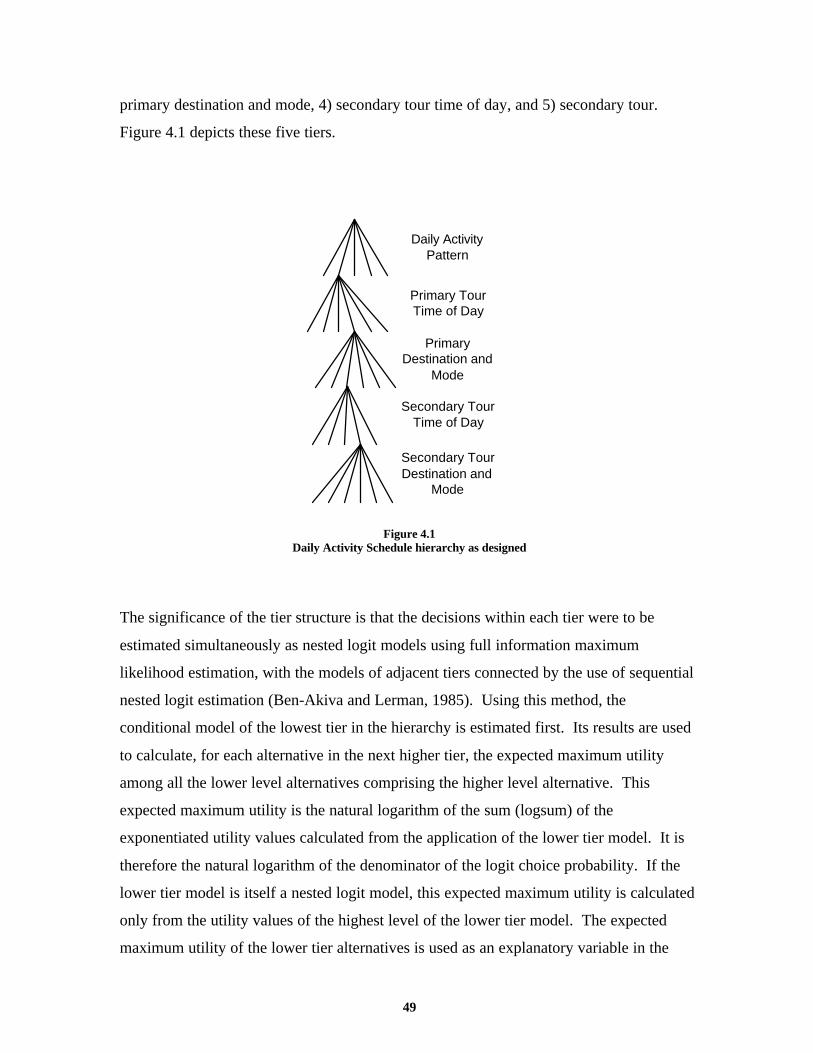
49

primary destination and mode, 4) secondary tour time of day, and 5) secondary tour.

Figure 4.1 depicts these five tiers.

Daily ActivityPattern

Primary TourTime of Day

PrimaryDestination and

Mode

Secondary TourTime of Day

Secondary TourDestination and

Mode

Figure 4.1Daily Activity Schedule hierarchy as designed

The significance of the tier structure is that the decisions within each tier were to be

estimated simultaneously as nested logit models using full information maximum

likelihood estimation, with the models of adjacent tiers connected by the use of sequential

nested logit estimation (Ben-Akiva and Lerman, 1985). Using this method, the

conditional model of the lowest tier in the hierarchy is estimated first. Its results are used

to calculate, for each alternative in the next higher tier, the expected maximum utility

among all the lower level alternatives comprising the higher level alternative. This

expected maximum utility is the natural logarithm of the sum (logsum) of the

exponentiated utility values calculated from the application of the lower tier model. It is

therefore the natural logarithm of the denominator of the logit choice probability. If the

lower tier model is itself a nested logit model, this expected maximum utility is calculated

only from the utility values of the highest level of the lower tier model. The expected

maximum utility of the lower tier alternatives is used as an explanatory variable in the

50

estimation of the parameters of the higher tier model. Estimation thus proceeds from the

lowest tier of decisions to the highest tier, with the calculation of the expected maximum

utility occurring after estimation of each of the first four tiers, prior to the estimation of

the next higher tier. In summary, the decision hierarchy has five major tiers, with each

tier being a simultaneously estimated nested logit model, and the five tiers connected via

sequential nested logit estimation using the expected maximum utility variable.

Ideally the design would provide for the simultaneous estimation of all the parameters in

the entire nested model system. However, the identification of tiers for the use of

sequential estimation was necessary in this case because of the complexity of the model

system and the capacity limits of the available software for simultaneous nested logit

estimation.

The demonstration system was implemented as designed with one exception. The models

of time of day were included in the conditional hierarchy but were not connected to the

other models via the logsum expected maximum utility variables. The models of time of

day did not include logsum variables, and the calculation of logsum variables for higher

level models bypassed the time of day. The downward flowing arrows in Figure 4.2 show

the time of day models included in the conditionality structure. The upward flowing

arrows show how they are bypassed in the expected maximum utility connection. This

change arose from estimation and testing of the system, which is discussed in Section 4.4.

In addition to this change in the design, the daily activity pattern model and the primary

tour destination and mode choice model were each subdivided into two models. Each of

the two daily activity pattern models represents the choice of a daily activity pattern, but

one applies to employed persons (workers) and the other applies to persons who are not

employed (nonworkers). This essentially results in two separate model systems of daily

activity schedule, each applied to a separate case. Likewise, the two models of primary

tour destination and mode choice apply to two separate cases: work tours and tours of

other purposes. These two models therefore apply to separate major branches of the

hierarchy. The purpose of the subdivisions was to overcome model size limits imposed by

51

Daily Activity Pattern

Secondary Tour(s)Time of Day

Primary TourDestination and Mode

Primary TourTime of Day

Secondary Tour(s)Destination and Mode

Figure 4.2Daily Activity Schedule hierarchy as implemented

Lower tier models are conditioned by decisions in higher tiers. Upward flowing arrows indicateexpected maximum utility from lower tier is used in higher tier model. Time of day models areincluded in the conditional hierarchy but bypassed in the expected maximum utility connections.

the estimation software, and they do not constitute a material change in the model system.

The subdivisions of the model system, shown in Figure 4.3, are reflected in the

presentation of estimation results in Section 4.4 .

The model system includes only one model of secondary tour choices, even though some

of the alternatives in the daily activity schedule have two or more secondary tours. The

choice of a daily activity pattern determines the number of secondary tours in the daily

activity schedule. The model system conditions the choice of secondary tour time,

destination and mode upon the choice of a daily activity pattern. For daily activity

patterns with 2 or more secondary tours, the choice probabilities for the time, destination

52

Daily ActivityPattern

Non-worker

Non-workPrimary TourDestination and

Mode

Secondary TourDestination and

Mode

Work

Worker

Primary TourTime

Secondary TourTime

Figure 4.3Seven subdivisions of the model system

and mode of each of the secondary tours are calculated independently of the

corresponding choice probabilities for the other secondary tour(s). The probabilities for

all secondary tours are calculated using the same secondary tour models. An alternative

approach would substantially increase the complexity of the model, by requiring the

representation of one or more tiers of tertiary tour decisions. It would also increase the

sample size requirement, since only 11% of the daily activity patterns involve 2 or more

secondary tours. Finally, it would require the accurate evaluation of the relative priority

of the various secondary tours in the estimation data set. For these reasons, a model

structure with a single representation of secondary tour choices was selected.

4.4 Specification and Estimation of the Model System

The model system structure described in Section 4.3 provides the structure for the

presentation of the model specification and estimation results. This section takes the tiers

of the model system, starting at the bottom with the secondary tour destination and mode

choice, and presents the specifation and the estimation results. The chapter then ends with

53

a summary of the daily activity schedule choice set, an important element of the system

design. The daily activity schedule choice set consists of the cartesian product of the

choice sets for each tier of the model system described separately below.

Secondary Tour Destination and Mode Choice Model

Specification. The secondary tour destination and mode choice model was estimated as a

multinomial (MNL) choice model with alternative sampling. A choice set of up to 48

alternatives was constructed for each secondary tour in the data set, using stratified

importance sampling (Ben-Akiva and Lerman, 1985, page 266), as follows.

Intrazonal tours were first removed from the data set and not considered in the analysis.

This was done to simplify the modeling effort for the demonstration system. An

operational implementation should include intrazonal tours, especially if non-motorized

modes are included in the model. However, this requires the provision of accurate

transportation system level of service data, which is difficult for very short tours.

For each tour in the data set a sample of 8 destination zones was drawn from the 786

remaining possible zones. Four of the 8 were drawn randomly from the 20 zones nearest

the tour's home zone, and 4 were drawn randomly from the remaining zones. The

destination actually chosen for the tour replaced one of the randomly drawn alternatives in

the choice set.

Each of the 8 sampled destinations was combined with up to 6 available mode

alternatives, bringing the maximum tour choice set sample to 48 alternatives. Alternative

sampling required the addition, during parameter estimation, of a correction factor in each

of the 48 utility functions. A description of the 6 modes and the decision rule used to

determine their availability for each tour is provided below.

In addition to alternative sampling, several important model specification decisions were

required which related directly to the preparation of data for the destination and mode

choice models. These include the definition of tour and activity priorities within a daily

activity pattern, and the definition of mode choice alternatives. Based on the research of

54

Weisbrod and Daly (1979), all the activities within a tour were assigned to a category,

with work being the highest priority category, followed in order by work related, school,

and all other purposes. Ties were broken within a category by assigning higher priority to

activities of longer duration. Within an individual’s daily activity pattern the tours were

assigned relative priorities by giving highest priority to the tour containing the highest

priority activity, and so on until all tours were assigned a priority. The definition of tour

priorities provided the necessary information to separate the data set into two subsets, one

of primary tours and one of secondary tours.

The destination and mode choice model in the demonstration system involves the choice

of a mode for the tour instead of the usual choice of mode for a trip. This introduced a

problem because the Boston survey respondents did not report their travel mode on a tour

basis. Instead, they reported every mode used, in sequence, sometimes reporting several

modes for a single trip, with different sets of modes used for different trips in the same

tour. Thus, the modeling of a tour mode choice required a decision rule for translating a

huge set of potentially complex sequences of reported modes into a relatively small choice

set of mode alternatives. Six important mode alternatives were selected based on

experience, preliminary data analysis and an awareness of important intermodal policy

issues. These alternatives include auto drive alone, shared ride, transit with auto, transit

with walk, walk, and bicycle. An intuitive decision rule was established for translating

reported mode combinations into these six alternatives. The rule involved dividing the

tour into two half tours, one leading to the primary activity location, and the other leading

back home. A mode was assigned to each half tour, giving priority to transit with auto,

transit with walk, drive alone, shared ride, bicycle, walk and all other modes, in that order.

The two half tour modes were then considered, and one was selected as the tour mode,

giving priority to drive alone, bicycle, walk, transit with auto, transit with walk, shared

ride and other modes. The rule assigned one of the 6 modes to over 98% of the sample.

The remaining observations, including tours which were made entirely by schoolbus, taxi

or paratransit, and those which the rule could not interpret, were removed from the

estimation data set. In an operational implementation, these tours could be individually

analyzed to assign a tour mode. The decision rule was tested by applying it to several

hypothetical and many actual reported tours, and comparing the result to intuitive

55

assignments. It also yielded models with reasonable coefficients and a relatively high

degree of fit, as reported below, in contrast to a simpler decision rule which was tried first.

Table 4.1 shows the shares of the 6 mode alternatives in the estimation data set for

primary and secondary tours.

Table 4.1Modes chosen for tours in the estimation data set

Primary Tours Secondary Tours

Drive alone (da) 56% 41%

Shared ride (sr) 15 30

Walk (wa) 13 26

Transit with walk access (tw) 10 2

Transit and auto (ta) 4 <<1

Bicycle (bi) 1 1

Total 100% 100%

Deterministic decision rules were used to judge which of the 6 mode alternatives were

available to each person in the estimation data set. Drive alone was considered available

if at least 1 vehicle was available in the household and the individual was a licensed

driver. Shared ride was always considered available. The availability of the transit

alternatives was determined by evaluating transit system connectivity for each zone pair.

Bicycle and walk were always considered available.

Estimation of the destination and mode choice model required the definition of

transportation system performance variables and preparation of transportation system

performance data for all of the mode alternatives by the four time of day categories used

in the time of day choice models. Transportation performance data was supplied by

CTPS, from which the estimation data set was prepared.

All performance data were defined on the basis of a direct round trip from home to the

primary activity location and back home again. The hypothesis is that persons consider

the direct round trip travel in making the decisions about the highest priority activity in a

tour. Additional travel required by side trips to secondary destinations is considered in

making the choices about the secondary activities. Under this hypothesis, the secondary

activity models, which were excluded from the demonstration system, would have used

56

incremental round trip distances, costs and times (incremental over the times described

here for the primary activity) in the estimation of transportation system performance

parameters.

Distance was chosen as the best measure of transportation system performance for walk

and bicycle modes, since the data set provided no good level-of-service attributes for

them, such as travel times, bikeway availability or sidewalk connectivity. Distance was

defined as the interzonal roadway distance, and taken directly from the CTPS data. Costs

were defined as out-of-pocket costs per person, including tolls, fares, and parking. In-

vehicle times were defined as time spent traveling in the auto and/or transit vehicle. Out-

of-vehicle times included walk and wait time for transit journeys, and destination walk

time for auto journeys. For transit journeys, walk and wait times for the PM period were

assumed to equal the AM peak times in the reverse direction, off-peak wait times were

assumed to equal twice the peak time wait times, and off-peak in-vehicle times were

assumed to equal peak period times in the non-peak direction. In-vehicle and out-of-

vehicle times for shared ride were derived from drive alone times, using a regression

model supplied by CTPS.

Estimation Results. Table 4.2 shows the estimation results of the secondary tour

destination and mode choice model. (The numbering of variables in this table has been

coordinated with that of subsequent tables of similar models for primary tours, so some

variable numbers are skipped in the numbering sequence.) Coefficients 1 through 5 are

the alternative specific constants for five of the six mode alternatives, with drive alone

serving as the base case. The transportation system level of service variables of

cost/income, in-vehicle time and out-of-vehicle time all bear the expected signs for the

motorized modes. A comparison of the magnitude of these coefficients reveals a value of

in-vehicle time of $114 per hour for auto use and $77 for transit use, using the estimated

57

Table 4.2Secondary tour destination and mode choice model

Variablenumber Variable name

Coefficientestimate

Asymptoticstandarderror

tstatistic

1 shared ride constant 1.164 .211 5.5

2 transit w/auto constant -4.063 .732 -5.6

3 transit w/walk constant -1.084 .509 -2.1

4 walk constant -.3371 .330 -1.0

5 bicycle constant -4.672 .964 -4.8

10 cost/income ($/$10,000), motorized modes -.2757 .0654 -4.2

11 in-vehicle time (min), auto -.09761 .00201 -48.6

12 in-vehicle time (min), transit -.06533 .00938 -7.0

13 out-of-vehicle time (min), auto -.1153 .0148 -7.8

14 out-of-vehicle time (min), transit -.02607 .00960 -2.7

15 distance squared (mi2), walk -.4163 .0311 -13.4

16 distance (mi), bicycle -.8454 .191 -4.4

17 autos per driver, shared ride -.4419 .210 -2.1

18 autos per driver, transit w/auto -2.118 .845 -2.5

19 autos per driver, transit w/walk -2.839 .491 -5.8

20 autos per driver, walk -1.517 .295 -5.1

21 autos per driver, bicycle .4832 .894 .5

22 household income ($10,000), transit w/walk -.1318 .0688 -1.9

23 household income ($10,000), walk -.05412 .0330 -1.6

24 household income ($10,000), bicycle -.2299 .139 -1.7

25 Dummy: mode matches primary tour mode, drive alone .3295 .108 3.1

26 Dummy: mode matches primary tour mode, shared ride .5064 .137 3.7

27 Dummy: mode matches primary tour mode, bicycle 5.477 .732 7.5

28 Dummy: work tour, destination matches primary tourdestination

1.113 .274 4.1

32 natural logarithm of employment (100,000), CBD zones .8218 .100 8.2

33 natural logarithm of employment (100,000), non-CBDzones

.6550 .0294 22.3

Summary statistics

Number of observations = 2068

L(0) = -11163

L(C) = -10001 ρ 2 = .104 (restricted model: variables 1 through 5 only)

L ( $ )β = -4773 ρ 2 = .570

sample mean household income of $54,000. Two factors might partially explain the

larger than expected magnitude of these figures. First, the estimates of costs for the auto

mode may be higher than the actual perceived costs. Second, we expect the disutility of

travel time to be greater for secondary tours, whereas the disutility of travel cost might not

58

increase correspondingly. The value of out-of-vehicle time relative to in-vehicle time is

1.2 for auto use and .4 for transit use. We expected these ratios to be equal or greater than

2. One possible explanation for the low values is an upward bias in the in-vehicle-time

coefficient associated with the fact that people are less familiar with destinations further

from home. This problem would have probably been reduced by including destination

specific constants in the model. The data set provided no good level-of-service attributes

for bicycle and walk modes, such as travel times, bikeway availability or sidewalk

connectivity; the best available measure was roadway distance, which yielded coefficients

with the expected signs.

The socioeconomic variable of autos per driver yielded the expected signs in all but one

case, with increasing auto availability decreasing the attractiveness (relative to drive

alone) of transit with walk, transit with auto, walk, and shared ride in that order, while the

coefficient for the bicycle mode was not statistically significantly different from zero.

The socioeconomic variable of income also yielded the expected signs, with somewhat

lower statistical significance; increasing income decreases the attractiveness (relative to

drive alone, shared ride and transit with auto) of bicycle, transit with walk, and walk.

Since the secondary tour destination and mode choice model is conditioned by the choice

of destination and mode for the primary tour, the actual choices of mode and destination

in the primary tour were used to explain choices in the secondary tour. Coefficients 25

through 27 indicate a tendency for people who choose drive alone, shared ride or bicycle

in their primary tour to choose the same mode again for their secondary tours, with the

effect being dramatically strong for the bicycle mode, as evidenced by the large

coefficient estimate of nearly 5.5. Coefficient 28 indicates a similar effect in destination

choice for work tours, with persons tending to choose the same destination zone for

secondary work tours as they chose for their primary (work) tour. The last two variables,

logarithm of employment for CBD destinations and non-CBD destinations, respectively,

are required because the zonal destination alternatives represent aggregations of elemental

destination alternatives (Ben-Akiva and Lerman, 1985, pages 253-261). They reflect an

assumption that employment is a reasonable measure of the relative size of the aggregate

alternatives. Their coefficients are in the acceptable range between zero and 1, and are

59

statistically significantly different from 1, indicating that the parameter estimates of the

model are dependent on the zonal aggregation scheme.

Primary Tour Destination and Mode Choice Model

Specification. The primary tour destination and mode choice model was estimated as an

MNL model with alternative sampling, in the same way as the secondary tour destination

and mode choice model described above, with two differences. First, the model was

estimated separately for work tours and non-work tours, because of the expected

difference in choice behavior in the two cases. Second, and more importantly, the model

includes the expected maximum utility variable computed from the secondary tour model,

the link which turns the primary and secondary tour destination and mode choice models

together into a sequentially estimated nested logit model system.

The calculation of the expected maximum utility variable for this model required a special

application of the theory of the nested logit model to capture the expected maximum

utility from a multiple number of secondary tours. Under the assumption that the utility

among multiple secondary tours in a daily activity pattern is additive, the expected

maximum utility of all secondary tours is equal to the sum of the expected maximum

utility of each of the tours. This is simply an application of the additivity of mathematical

expectation. Since the expected maximum utility of a single tour is equal to the logarithm

of the sum of the exponentiated systematic utilities of all available tour alternatives

(logsum), the expected maximum utility among multiple tours is simply the sum of the

logsums across all secondary tours in the pattern. This can be shown notationally as

follows:

E U E U

E U

V

n lnl

L

l

L

ln

ilni Cl

L

n

n

ln

n

(max ) ( max )

( max )

ln exp( )

= ∑

= ∑

= ∑∑

=

=

∈=

1

1

1

60

where

() denotes mathematical expectation

is the maximum utility derived from secondary tours

in daily activity pattern

is the maximum utility derived from secondary tour

in daily activity pattern

is the number of secondary tours in daily activity pattern

is the natural logarithm operator

exp is the exponentiation operator

is the systematic portion of the utility of alternative

for secondary tour in daily activity pattern

is the choice set for secondary tour in daily activity pattern

E

U

n

U l

n

L n

V i

l n

C l n

n

ln

n

iln

ln

max

max

ln

The calculation of the logsum variable thus involves using the secondary destination and

mode choice model parameters to calculate the denominator of the logit model for each

secondary tour in the daily activity pattern, taking the logarithm of each denominator

separately, and summing the results. However, this is computationally intensive since it

involves summing the utility of as many as 4716 (786 destinations times 6 modes)

alternatives for each secondary tour in each daily activity pattern. Therefore, we

calculated a consistent estimate of the variable using the same sample of 8 destinations

used to estimate the secondary destination and mode choice parameters. Although this

was necessary in light of the computational power and time available to the research, it

should not be done in the implementation of an operational system. The reason is that

using a sample based estimate compromises the results by unnecessarily introducing

measurement error in an explanatory variable of the primary destination and mode choice

model.

Estimation Results. Table 4.3 and Table 4.4 show the estimation results of the primary

tour destination and mode choice model for work and non-work tours, respectively. The

transportation system level of service variables of cost, cost/income, in-vehicle time and

out-of-vehicle time all bear the expected signs for the motorized modes. A comparison of

61

Table 4.3Primary tour destination and mode choice model: work tours

Variablenumber Variable name

Coefficientestimate

Asymptoticstandarderror

tstatistic

1 shared ride constant -.1129 .324 -.3

2 transit w/auto constant -1.064 .428 -2.5

3 transit w/walk constant 1.086 .365 3.0

4 walk constant .7419 .352 2.1

5 bicycle constant -1.463 .538 -2.7

6 cost ($), motorized modes -.05051 .0241 -2.1

7 cost ($) for persons with employer drive-alone incentives,drive alone

.1919 .0286 6.7

8 cost ($) for persons with employer transit incentives,transit w/auto

.4822 .0820 5.9

9 cost ($) for persons with employer transit incentives,transit w/walk

.3821 .0797 4.8

10 cost/inc ($/$10,000), motorized modes -.2316 .0638 -3.6

11 in-vehicle time (min), auto -.04160 .00162 -25.7

12 in-vehicle time (min), transit -.01922 .00278 -6.9

13 out-of-vehicle time (min), auto -.06555 .0152 -4.3

14 out-of-vehicle time (min), transit -.02831 .00459 -6.2

15 distance squared (mi2), walk -.1895 .0220 -8.6

16 distance (mi), bicycle -.4430 .0855 -5.2

17 autos per driver, shared ride -1.943 .352 -5.5

18 autos per driver, transit w/auto -1.291 .406 -3.2

19 autos per driver, transit w/walk -3.731 .323 -11.5

20 autos per driver, walk -3.162 .378 -8.4

21 autos per driver, bicycle -3.019 .625 -4.8

29 dummy: age under 20, bicycle 2.461 1.10 2.2

30 dummy: simple tour, transit w/walk .3557 .165 2.2

32 size variable: employment (100,000), CBD zones .8061 .0737 10.9

33 size variable: employment (100,000), non-CBD zones .9990 .0328 30.5

34 logsum: expected maximum utility from secondary tours .5556 .229 2.4

Summary statistics

Number of observations = 1901

L(0) = -7740

L(C) = -6355 ρ 2 = .178 (restricted model: variables 1 through 5 only)

L ( $ )β = -3733 ρ 2 = .514

the magnitude of these coefficients for work tours reveals a value of in-vehicle time of

$33 per hour for auto use and $16 per hour for transit use, again assuming the mean

household

62

Table 4.4Primary tour destination and mode choice model: nonwork tours

Variablenumber Variable name

Coefficientestimate

Asymptoticstandarderror

tstatistic

1 shared ride constant .8928 .241 3.7

2 transit w/auto constant -1.862 .516 -3.6

3 transit w/walk constant .8493 .363 2.3

4 walk constant 1.261 .324 3.9

5 bicycle constant -1.661 .537 -3.1

7 cost ($) for persons with employer drive-alone incentives,drive alone

.2637 .0384 6.9

10 cost/inc ($/$10,000), motorized modes -.4397 .0561 -7.8

11 in-vehicle time (min), auto -.05963 .00150 -39.6

12 in-vehicle time (min), transit -.02774 .00341 -8.1

13 out-of-vehicle time (min), auto -.08635 .0142 -6.1

14 out-of-vehicle time (min), transit -.02786 .00498 -5.6

15 distance squared (mi2), walk -.4161 .0341 -12.2

16 distance (mi), bicycle -.5369 .106 -5.1

17 autos per driver, shared ride -1.030 .245 -4.2

18 autos per driver, transit w/auto -.9127 .509 -1.8

19 autos per driver, transit w/walk -4.013 .345 -11.6

20 autos per driver, walk -2.709 .334 -8.1

21 autos per driver, bicycle -3.566 .645 -5.5

29 dummy: age under 20, bicycle 1.220 .780 1.6

31 dummy: simple tour, transit w/auto -1.060 .360 -2.9

32 size variable: employment (100,000), CBD zones .9052 .0837 10.8

33 size variable: employment (100,000), non-CBD zones .8700 .0306 28.4

34 logsum: expected maximum utility from secondary tours .5146 .260 2.0

Summary statistics

Number of observations = 1929

L(0) = -9126

L(C) = -8196 ρ 2 = .101 (restricted model: variables 1 through 5 only)

L ( $ )β = -4641 ρ 2 = .489

income of $54,000, and a value of out-of-vehicle time relative to in-vehicle time of 1.6 for

auto use and 1.5 for transit use. For non-work tours the values of in-vehicle time are $44

per hour for auto use and $20 per hour for transit use, and a value of out-of-vehicle time

relative to in-vehicle time of 1.4 for auto use and 1.0 for transit use. Coefficient 7 in both

work and non-work models indicates that the presence of any or all of the employer

incentives of mileage allowance, subsidized parking or company car tends to offset the

disutility of the cost of driving alone. Coefficients 8 and 9 yield similar, but even stronger

63

effects on the disutility of transit costs in the presence of employer subsidized transit

passes, but this effect occurs only for work tours. Although coefficients 7 through 9 are

important coefficients, it would have been better to associate them with the same cost

variable (cost per income) as the primary cost coefficient (10). As specified, the net effect

of cost of the drive alone mode could be positive for high income individuals. For walk

and bicycle modes, roadway distance yielded coefficients with the expected signs in both

models. The socioeconomic variable of autos per driver yielded the expected signs in all

cases, with strong negative effects on the attractiveness of non-auto alternatives.

Coefficient 29 reveals the significant positive influence of youth on the attractiveness of

bicycling to work, with a similar but less sizable positive influence for non-work tours.

(A similar, but statistically insignificant, effect was encountered for ages in the 20’s and

30’s, and was left out of the model). Coefficient 30 reveals that, in work tours, the

attractiveness of transit with walk is increased when the work tour is simple, involving

only the trips to and from work. Coefficient 31 reveals a negative effect of simple tours

on the attractiveness of transit with auto for non-work tours. Finally, the secondary tours

expected maximum utility coefficient, which is in the acceptable range for nested logit

models, reveals a strong influence of secondary tour utility on the choice of alternatives at

this level of the model system. Daily activity patterns with more secondary tour travel,

due either to more or longer tours, generally have smaller values (less positive or more

negative) of the logsum variable. Thus, the positive sign of this coefficient means that

primary tour alternatives which are linked in a daily activity pattern with a substantial

amount of secondary tour travel will have lower utility than those with little or no

secondary tour travel, all other things being equal.

Table 4.5 provides a side by side comparison of the coefficient estimates from the

secondary tour model and both primary tour models, revealing the following significant

differences. The presence of a cost coefficient (6) in the primary work tour model,

accompanied by smaller absolute value of the cost/income coefficient (10), indicates that

low income does not increase cost sensitivity as much for primary work tours as it does

for non-work and secondary tours. The effect of employer incentives for mode choice

64

Table 4.5Coefficient comparisons of destination and mode choice models

Coefficient estimate

Variablenumber Variable name

Secondarytours

primaryworktours

primarynonworktours

1 shared ride constant 1.164 -.1129 .89282 transit w/auto constant -4.063 -1.064 -1.8623 transit w/walk constant -1.084 1.086 .84934 walk constant -.3371 .7419 1.2615 bicycle constant -4.672 -1.463 -1.6616 cost ($), motorized modes -.050517 cost ($) for persons with employer drive-alone incentives,

drive alone.1919 .2637

8 cost ($) for persons with employer transit incentives,transit w/auto

.4822

9 cost ($) for persons with employer transit incentives,transit w/walk

.3821

10 cost/inc ($/$10,000), motorized modes -.2757 -.2316 -.439711 in-vehicle time (min), auto -.09761 -.04160 -.0596312 in-vehicle time (min), transit -.06533 -.01922 -.0277413 out-of-vehicle time (min), auto -.1153 -.06555 -.0863514 out-of-vehicle time (min), transit -.02607 -.02831 -.0278615 distance squared (mi2), walk -.4163 -.1895 -.416116 distance (mi), bicycle -.8454 -.4430 -.536917 autos per driver, shared ride -.4419 -1.943 -1.03018 autos per driver, transit w/auto -2.118 -1.291 -.912719 autos per driver, transit w/walk -2.839 -3.731 -4.01320 autos per driver, walk -1.517 -3.162 -2.70921 autos per driver, bicycle .4832 -3.019 -3.56622 household income ($10,000), transit w/walk -.131823 household income ($10,000), walk -.0541224 household income ($10,000), bicycle -.229925 dummy: mode matches primary tour mode, drive alone .329526 dummy: mode matches primary tour mode, shared ride .506427 dummy: mode matches primary tour mode, bicycle 5.47728 dummy: work tour, destination matches primary tour

destination1.113

29 dummy: age under 20, bicycle 2.461 1.22030 dummy: simple tour, transit w/walk .355731 dummy: simple tour, transit w/auto -1.06032 size variable: employment (100,000), CBD zones .8218 .8061 .905233 size variable: employment (100,000), non-CBD zones .6550 .9990 .870034 logsum: expected maximum utility from secondary tours .5556 .5146

(coefficients 7-9) is limited primarily to mode choice for the primary work tour. The

value of time is generally higher for secondary tours than for primary tours. Auto

availability (coefficients 17-21) affects mode choice differently for secondary tours than

for primary tours, with a stronger negative impact on transit with auto in secondary tours

(18), and a stronger negative impact on transit with walk, walk and especially bicycle in

primary tours (19-21). Income (22-24) has a more noticeable impact on mode choice for

65

secondary tours than for primary tours, with higher income reducing the use of non-

motorized modes.

Tour Time of Day Choice Models

Specification. Two similar MNL models of the choice of tour time of day were

estimated, one each for secondary and primary tours. Each of the 16 alternatives was

comprised of 1 of 4 time periods for departure from home to the primary destination and 1

of 4 time periods for departure from the primary destination returning home. These 4 time

periods include AM peak, midday, PM peak, and Other. All time periods were considered

available to all persons for primary tours. For secondary tours, times which overlapped

with the chosen primary tour time were removed from the choice set.

The models were estimated with the expected maximum utility variable from the

corresponding destination and mode choice model. However, these parameter estimates

did not fit in the theoretically acceptable range of 0 to 1 and also had very high standard

errors, so we re-estimated the models without them. A likely reason for the difficulties

encountered include the inadequacy of the transportation system performance data by time

of day, and the coarse granularity of the time of day choice categories. In the face of

project time constraints, further work on the time of day models was dropped for both the

secondary tours and the primary tour. The nested logit model system therefore excludes

the time of day models from the logsum linkages, although the destination and mode

choice models are still conditioned by their respective time of day choices. The model

system can be implemented as an operational model system with separately estimated

time of day models, and the full incorporation of the choice of time of day into the nested

model structure remains an open research topic.

Estimation Results. Table 4.6 and Table 4.7 show the estimation results of the time of

time of day choice models for secondary tours and primary tours, respectively. In the

secondary tour model, coefficients 1 through 8 are alternative specific constants, with a

base case of travel to and from the primary destination occurring after the PM peak.

66

Table 4.6Secondary tour time of day model

Variablenumber Variable name

Coefficientestimate

Asymptoticstandarderror

tstatistic

1 before AM peak to AM peak constant (base case is afterPM peak to after PM peak)

-1.702 .604 -2.8

2 AM peak to AM peak constant -.2498 .568 -.4

3 AM peak to midday constant -.4120 .566 -.7

4 midday to midday constant -1.384 .143 -9.7

5 midday to PM peak constant -.5157 .566 -.9

6 PM peak to PM peak constant .9019 .560 1.6

7 PM peak to after PM peak constant 1.823 .553 3.3

8 constant for other alternatives other than after PM peak toafter PM peak

-4.572 .335 -13.7

9 Dummy: alternatives with travel during at least 1 peakperiod

-2.355 .545 -4.3

10 Dummy: primary activity of daily activity pattern (DAP)is work, alternatives with travel during at least 1 peakperiod

.6265 .115 5.5

11 Dummy: primary activity of DAP is work, alternative isafter PM peak to after PM peak

.4454 .154 2.9

12 Dummy: primary tour type is HPH, alternatives in whichactivity ends during AM peak

.5990 .151 4.0

13 Dummy: primary tour type is HPH, alternative is PM peakto PM peak

.3701 .120 3.1

14 Dummy: primary tour type is HPH, alternatives other thanthose ending in AM peak, or starting and ending during orafter PM peak

.8453 .0987 8.6

15 Dummy: primary activity of DAP is other than work orschool, alternative is before PM peak to before or duringPM peak,

2.140 .129 16.6

16 Dummy: primary activity of DAP is other than work orschool, alternative is PM peak to PM peak

1.286 .152 8.4

17 Dummy: DAP has 2 or more secondary tours, alternativesin which activity ends before or during PM peak

.7851 .0880 8.9

18 Dummy: DAP has 2 or more secondary tours, alternativeswith a long tour (ie, fully spanning a time period)

-2.033 1.03 -2.0

Summary statistics

Number of observations = 2873

L(0) = -7966

L(C) = -5404 ρ 2 = .321 (restricted model: variables 1 through 8 only)

L ( $ )β = -4943 ρ 2 = .377

Coefficients 9 and 10 indicate a preference of avoiding travel during the peak periods,

which is partially offset if the primary activity of the day is work. Coefficient 11 indicates

a tendency for persons whose primary activity of the day is work to make their secondary

tours in the evening after the peak period. Coefficients 12 through 17 indicate the

67

Table 4.7Primary tour time of day model

Variablenumber Variable name

Coefficientestimate

Asymptoticstandarderror

tstatistic

1 before AM peak to AM peak constant (base case is middayto midday)

-5.889 .710 -8.3

2 before AM peak to midday -3.196 .153 -20.9

3 before AM peak to PM peak -5.549 .734 -7.6

4 AM peak to AM peak constant -6.024 .740 -8.1

5 AM peak to midday constant -3.347 .730 -4.6

6 AM peak to PM peak -5.448 .740 -7.4

7 AM peak to after PM peak -5.428 .733 -7.4

8 midday to PM peak constant -4.433 .731 -6.1

9 midday to after PM peak constant -3.201 .165 -19.4

10 PM peak to PM peak constant -5.298 .743 -7.1

11 PM peak to after PM peak constant -3.953 .733 -5.4

12 after PM peak to after PM peak constant -1.061 .128 -8.3

13 Dummy: alternatives with travel during at least 1 peakperiod

2.920 .727 4.0

14 Dummy: work purpose, alternatives with travel during atleast 1 peak period

2.426 .133 18.3

15 Dummy: work purpose, alternative is AM peak to PMpeak

2.580 .129 20.0

16 Dummy: work purpose, alternative is before AM peak tobefore PM peak, or after AM peak to after PM peakpurpose

4.324 .190 22.8

17 Dummy: work purpose, alternative is after PM peak toafter PM peak

.5969 .301 2.0

18 Dummy: complex primary tour, alternative is before AMpeak to midday or midday to after PM peak

-.5542 .125 -4.4

19 Dummy: complex primary tour, alternative is in theevening (ie, from during or after PM peak to before orduring AM peak)

-1.212 .129 -9.4

20 Dummy: alternative is AM peak to midday or PM peak .3071 .0790 3.9

21 Dummy: no secondary tours, alternative involves travelduring or after PM peak

-1.116 .144 -7.8

22 Dummy: no secondary tours, alternative is daytime withpeak period travel

-.2268 .0854 -2.7

23 Dummy: no secondary tours, alternatives which fully spanmidday

.5985 .0882 6.8

Summary statistics

Number of observations = 4546

L(0) = -12604

L(C) = -9214 ρ 2 = .268 (restricted model: variables 1 through 12 only)

L ( $ )β = -7921 ρ 2 = .370

preference of several types of people to conduct secondary tour(s) before the evening.

Coefficients 12 through 14 indicate this preference among people whose primary tour

involves a single activity, coefficients 15 and 16 are for people whose primary activity of

68

the day is other than school or work, and 17 is for people who conduct 2 or more

secondary tours. Coefficient 18 indicates a tendency for secondary tours of short duration

if there are 2 or more in the daily activity pattern.

In the primary tour time of day model, shown in Table 4.7, coefficients 1 through 12 are

the alternative specific constants, with a base case of travel to and from the primary

destination during the midday time period. Coefficients 13 through 15 indicate a general

tendency to travel during peak periods, with work purpose greatly increasing this

tendency. Coefficient 16 captures a strong tendency to shift the work tour schedule so

travel occurs before or after the AM and PM peak periods, and coefficient 17 captures a

slight tendency for the work tour to occur during the night. Coefficients 18 through 20

reveal preferences when the primary tour involves more than one activity stop: there is a

tendency to avoid tours which span a peak period or occur in the evening, and a slight

tendency to start the tour during the AM peak. Coefficients 21 through 23 indicate timing

preferences when there are no secondary tours in the pattern, with a tendency to avoid

evening tours and those which require peak period travel, and to choose a schedule which

fully spans the midday period.

Daily Activity Pattern Choice Model

Specification. The model of the choice of daily activity pattern is a nested logit model,

estimated simultaneously by full information maximum likelihood estimation. As in the

case of the primary tour destination and mode choice, it includes the expected maximum

utility variable from the lower level alternatives, completing the links which make the

entire daily activity schedule a sequentially estimated nested logit model system. The

daily activity pattern model represents the choice between traveling and remaining at

home, with the choice of a particular pattern of travel conditioned by the decision to

travel, as depicted in Figure 4.4.

Each daily activity pattern involving travel is comprised of a primary activity, a primary

tour type and the number and purpose of secondary tours. As mentioned already, this

rather simple categorization of the components of the daily activity pattern was chosen for

69

implementation in the demonstration system, and could be expanded for an operational

implementation. Each of the components is described below.

Home Travel

54 patterns involving travel30 work12 school12 other

Figure 4.4Nested logit model of the daily activity pattern

The upper level is a binary choice between staying at home all day and a pattern involving travel.The lowel level, conditioned by the upper level decision, is a choice among 54 alternatives involvingtravel.

The modeled primary activities include home, work, school and other. Table 4.8 shows

the relative frequency in the Boston data set of the daily activity pattern primary activity

purpose. The ‘other’ category combines many of the less frequently chosen alternatives,

and could be expanded. The collection in the diary survey of information about activities

Table 4.8Daily Activity Pattern primary activities reported in the estimation data set

Percentage

Primary activity of Daily Activity Pattern‘other’subcategories

modeledcategories

At home 16.5%Work 41.2School 5.7Other 36.6

banking and personal business 11.1%pick up or drop off passenger 9.4shopping 6.5eat out 3.0recreation 2.6work related 2.1social 1.8other .2

Total 36.6% 100%

conducted at home would enable a more detailed categorization of the at-home alternative,

and could lead to a restructuring of the model’s hierarchy, such as making home an

alternative in the destination choice model.

70

The definition of tour type includes the number, purpose and sequence of activity stops on

the tour. Using the purpose classification described above, we counted the number of

occurrences of every possible tour type in the estimation data set, and partitioned the set

into categories of similar patterns. Choosing a categorization scheme requires a

compromise. On the one hand, many detailed categories are desirable to enable the

explicit modeling of travel to particular destinations by time of day for as many activities

in the tour as possible. On the other hand, a small number of categories is desirable to

preserve computational feasibility. The demonstration model system partitions the

observed work tour types into 5 categories. The three predominant categories are (1) the

simple tour from home to work and back again (hwh), (2) the tour with at least 1

additional stop for another activity (hwh+), and (3) the tour which involves a work based

subtour for another activity as well as any number (including zero) of additional stops for

other activities (hw+wh). Two additional work tour categories involve a mid-tour return

home, one with no additional activity stops (hwhwh) and another involving any number of

additional stops (hwhwh+). School and other tours received a simpler categorization

involving only the analogs of the first two work tour types. This scheme worked for the

demonstration, but information about the sequence and purpose of secondary activities

would be desirable for an operational system. Table 4.9 shows the tour types and their

relative frequencies in the Boston data set.

Table 4.9Primary Tour Types in the estimation data set

Primary Activity Tour Type Percentage

Work hwh 19.6%hwh+ 24.9hw+wh 17.3hwhwh 1.1hwhwh+ 1.4

School hsh 3.2hsh+ 3.0

Other hoh 12.3hoh+ 12.8

Total 100%

The classification of the daily activity pattern decision by number and purpose of

secondary tours distinguishes 2 purposes and 3 frequencies. The first purpose category

includes purposes which usually involve tight schedule constraints, including work, work

related, school, and banking/personal business (constrained), and the second category

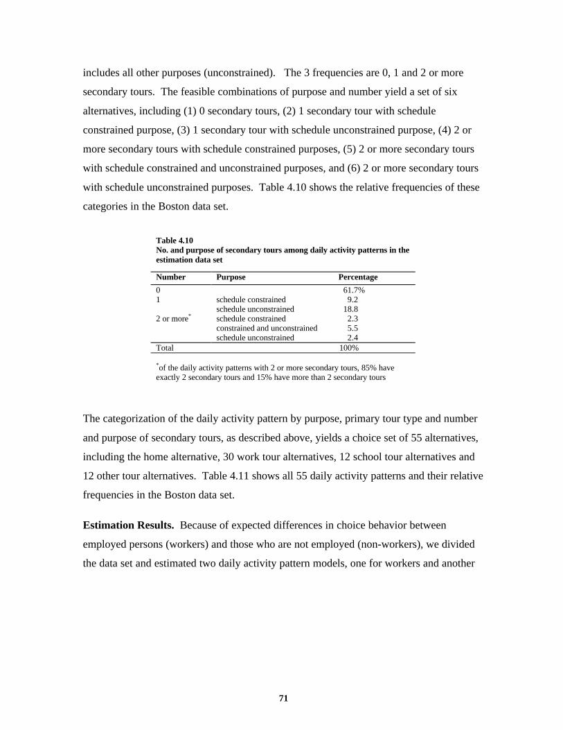
71

includes all other purposes (unconstrained). The 3 frequencies are 0, 1 and 2 or more

secondary tours. The feasible combinations of purpose and number yield a set of six

alternatives, including (1) 0 secondary tours, (2) 1 secondary tour with schedule

constrained purpose, (3) 1 secondary tour with schedule unconstrained purpose, (4) 2 or

more secondary tours with schedule constrained purposes, (5) 2 or more secondary tours

with schedule constrained and unconstrained purposes, and (6) 2 or more secondary tours

with schedule unconstrained purposes. Table 4.10 shows the relative frequencies of these

categories in the Boston data set.

Table 4.10No. and purpose of secondary tours among daily activity patterns in theestimation data set

Number Purpose Percentage

0 61.7%1 schedule constrained 9.2

schedule unconstrained 18.82 or more* schedule constrained 2.3

constrained and unconstrained 5.5schedule unconstrained 2.4

Total 100%

*of the daily activity patterns with 2 or more secondary tours, 85% haveexactly 2 secondary tours and 15% have more than 2 secondary tours

The categorization of the daily activity pattern by purpose, primary tour type and number

and purpose of secondary tours, as described above, yields a choice set of 55 alternatives,

including the home alternative, 30 work tour alternatives, 12 school tour alternatives and

12 other tour alternatives. Table 4.11 shows all 55 daily activity patterns and their relative

frequencies in the Boston data set.

Estimation Results. Because of expected differences in choice behavior between

employed persons (workers) and those who are not employed (non-workers), we divided

the data set and estimated two daily activity pattern models, one for workers and another

72

Table 4.11The daily activity pattern alternatives and their relative frequency in the estimation data set

Primary Activity Primary Tour Type Number and Purpose of Secondary Tours Percentage

at home 16.26%work hwh 0 10.51

1 constrained 2.861 unconstrained 4.332+ constrained 0.372+ constrained and unconstrained 0.992+ unconstrained 0.52

hwh+ 0 13.191 constrained 1.711 unconstrained 4.122+ constrained 0.412+ constrained and unconstrained 1.012+ unconstrained 0.39

hw+wh 0 9.071 constrained 0.971 unconstrained 3.792+ constrained 0.162+ constrained and unconstrained 0.312+ unconstrained 0.19

hwhwh 0 0.471 constrained 0.081 unconstrained 0.272+ constrained 0.002+ constrained and unconstrained 0.062+ unconstrained 0.06

hwhwh+ 0 0.701 constrained 0.101 unconstrained 0.292+ constrained 0.042+ constrained and unconstrained 0.002+ unconstrained 0.02

school hsh 0 1.201 constrained 0.191 unconstrained 0.782+ constrained 0.102+ constrained and unconstrained 0.252+ unconstrained 0.21

hsh+ 0 1.551 constrained 0.351 unconstrained 0.762+ constrained 0.102+ constrained and unconstrained 0.142+ unconstrained 0.14

other hoh 0 3.671 constrained 1.481 unconstrained 2.312+ constrained 0.802+ constrained and unconstrained 1.482+ unconstrained 0.52

hoh+ 0 5.111 constrained 1.481 unconstrained 2.102+ constrained 0.332+ constrained and unconstrained 1.302+ unconstrained 0.39

Total 100%

73

for non-workers. The non-worker model includes only the 25 non-work daily activity

pattern alternatives.

Table 4.12 and Table 4.13 show the estimation results of the daily activity pattern choice

models for workers and non-workers, respectively. In the worker model the first 33

coefficients are alternative specific constants, with some of the 54 alternatives combined

because early versions of the model revealed insignificant differences between the

estimated coefficients. Coefficients 34 through 44 are for various socioeconomic

characteristics associated with particular subsets of the population and particular subsets

of the daily activity pattern alternatives. Coefficients 34 through 36 are associated with

the simplest non-home daily activity pattern, involving only a single commute to the

primary activity location, revealing a tendency of 1 adult households and students to have

complex patterns, while men with more children tend to have simple patterns.

Coefficients 37 and 38 deal with patterns involving secondary tours, with school aged

children causing more secondary tours, and females with young children making less

secondary tours. Coefficients 39 and 40 show the tendency toward more trip making

among higher income, part-time employees. Coefficients 41 through 44 show

socioeconomic variations in the choice of primary activity, with full-time workers tending

to choose work, parents with young children choosing not to work, homemakers choosing

travel for other purposes and individuals with school-aged children choosing not to stay

home.

Coefficients 45 through 47 are the logsum coefficients which capture the effect of

expected utility from the tour models on the choice of daily activity pattern. The values,

between 0 and 1, fall within the theoretically acceptable range for the nested logit

structure, and the small size indicates a rather small influence of travel utility on the

choice of daily activity pattern. Nevertheless, the effect of these variables is one of the

key features of the daily activity schedule model system. Suppose, for example, that this

model were being used to predict the effect of an increase in fuel prices. A fuel price

increase would manifest itself in the secondary and primary tour models as negative

utility. Negative utility in these lower level models would reduce the size of variables 45

74

Table 4.12Daily activity pattern model: workers

Variablenumber Variable name

Coefficientestimate

Asymptoticstandarderror

tstatistic

Alternative specific constants for HWH patterns (HWH with 0 secondary tours is base case)

1 1 secondary tour with constrained purpose -1.362 .107 -12.8

2 1 secondary tour with unconstrained purpose -.9497 .0952 -10.0

3 2+ secondary tours with the same (c or u) purpose -2.945 .172 -17.1

4 2+ secondary tours with mixed purpose categories -2.405 .176 -13.6

Alternative specific constants for HWH + patterns

5 0 secondary tours .2224 .0760 2.9

6 1 secondary tour with constrained purpose -1.626 .132 -12.3

7 1 secondary tour with unconstrained purpose -.8107 .107 -7.6

8 2+ secondary tours with the same (c or u) purpose -2.874 .192 -15.0

9 2+ secondary tours with mixed purpose categories -2.091 .182 -11.5

Alternative specific constants for HW+WH patterns

10 0 secondary tours -.08887 .0792 -1.1

11 1 secondary tour with constrained purpose -2.167 .162 -13.4

12 1 secondary tour with unconstrained purpose -.8356 .108 -7.7

13 2+ secondary tours with the same (c or u) purpose -3.662 .261 -14.0

14 2+ secondary tours with mixed purpose categories -3.264 .283 -11.5

Alternative specific constants for HWHWH and HWHWH+ patterns

15 HWHWH -3.965 .168 -23.6

16 HWHWH+ -3.349 .157 -21.3

Alternative specific constants for HSH patterns

17 0 secondary tours .4971 .267 1.9

18 1 secondary tour with constrained purpose -2.233 .588 -3.8

19 1 secondary tour with unconstrained purpose -.3875 .255 -1.5

20 2+ secondary tours -1.932 .309 -6.2

Alternative specific constants for HSH+ patterns

21 0 secondary tours .1021 .206 .5

22 1 secondary tour with constrained purpose -1.191 .355 -3.4

23 1 secondary tour with unconstrained purpose -.6154 .279 -2.2

24 2+ secondary tours -2.207 .351 -6.3

Alternative specific constants for HOH patterns

25 0 secondary tours -1.042 .161 -6.5

26 1 secondary tour with constrained purpose -1.853 .211 -8.8

27 1 secondary tour with unconstrained purpose -1.853 .211 -8.8

28 2+ secondary tours -2.532 .197 -12.8

Alternative specific constants for HOH+ patterns

29 0 secondary tours -.7726 .148 -5.2

30 1 secondary tour with constrained purpose -1.896 .221 -8.6

31 1 secondary tour with unconstrained purpose -1.378 .185 -7.4

32 2+ secondary tours -2.529 .209 -12.1

75

Table 4.12 (continued from previous page)Daily activity pattern model: workers

Variablenumber Variable name

Coefficientestimate

Asymptoticstandarderror

tstatistic

Other variables

33 home pattern constant -1.736 .302 -5.7

34 dummy: 1-adult households, simple patterns (HWH, HSHor HOH with no secondary tours)

-.7299 .165 -4.4

35 dummy: students with simple patterns -.5822 .189 -3.1

36 ratio of children to adults, males with simple patterns .1981 .0867 2.3

37 Number of children age 5-15 in household, patterns with1+ secondary tours

.2567 .0394 6.5

38 dummy: females with children under 5 and no secondarytours

.2642 .177 1.5

39 income ($10,000), part-time workers with 2+ secondaryunconstrained tours

.1238 .0205 6.0

40 income ($10,000), part-time workers with extra stops onprimary tour

.07644 .0150 5.1

41 dummy: full-time workers with work patterns 1.673 .112 14.9

42 dummy: children under 5 in household, work patterns -.3674 .135 -2.7

43 dummy: homemaker with ‘other’ primary tour purpose .4766 .205 2.3

44 dummy: children age 5-15 in household, home patterns -.6696 .135 -5.0

45 logsum: expected maximum utility from primary tourdestination and mode alternatives, patterns with simpleprimary tours

.04868 .0175 2.8

46 logsum: expected maximum utility from primary tourdestination and mode alternatives, patterns with complexprimary tours

.09213 .0176 5.2

47 logsum: expected maximum utility from daily activitypatterns involving travel

.09965 .103 1.0

Summary statistics

Number of observations = 3758

L(0) = -14263

L(C) = -10837 ρ 2 = .238 (restricted model: multinomial logit with variables 1 through 33 only)

L ( $ )β = -10585 ρ 2 = .255

47, with the complex daily activity patterns being affected more than the simple activity

patterns, and the stay at home alternative being totally unaffected. Thus, this model

system would predict a simplification in travel patterns in response to an increase in fuel

prices. This simplification might take various forms, depending on the values of the

estimated parameters and the magnitude of the change in fuel prices. For example, it

might predict a shift toward simpler primary tours and a reduction in the number of

76

Table 4.13Daily activity pattern model: non-workers

Variablenumber Variable name

Coefficientestimate

Asymptoticstandarderror

tstatistic

Alternative specific constants for HOH patterns (HOH with 0 secondary tours is base case)

1 1 secondary tour with constrained purpose -1.087 .179 -6.1

2 1 secondary tour with unconstrained purpose -.5373 .158 -3.4

3 2+ secondary tours -1.589 .238 -6.7

Alternative specific constants for HOH+ patterns

4 0 secondary tours .09310 .172 .5

5 1 secondary tour with constrained purpose -1.169 .242 -4.8

6 1 secondary tour with unconstrained purpose -.9782 .236 -4.1

7 2+ secondary tours -2.146 .315 -6.8

Alternative specific constants for HSH patterns

8 0 secondary tours 1.689 .227 7.4

9 1 secondary tour with constrained purpose -.08377 .406 -.2

10 1 secondary tour with unconstrained purpose 1.271 .268 4.7

11 2+ secondary tours -.4455 .350 -1.3

Alternative specific constants for HSH+ patterns

12 0 secondary tours 1.832 .256 7.2

13 1 secondary tour with constrained purpose .1809 .392 .5

14 1 secondary tour with unconstrained purpose 1.115 .313 3.6

15 2+ secondary tours -.7189 .412 -1.7

Other variables

16 home pattern constant -.5606 .157 -3.6

17 Number of children age 5-15 in household, patterns with1+ secondary tours

.2885 .0755 3.8

18 dummy: children under 5 in household, patterns with 1+secondary tours

.3087 .173 1.8

19 ratio of children to adults, males with simple patterns .6308 .248 2.5

20 income ($10,000), patterns with 2+ secondaryunconstrained tours

.1154 .0200 5.8

21 income ($10,000), patterns with extra stops on primarytour

.03409 .0211 1.6

22 children 5-15 in household, home patterns -.5896 .148 -4.0

23 logsum: expected maximum utility from primary tourdestination and mode alternatives, patterns with simpleprimary tours

.03764 .0390 1.0

24 logsum: expected maximum utility from primary tourdestination and mode alternatives, patterns with complexprimary tours

.05467 .0415 1.3

25 logsum: expected maximum utility from daily activitypatterns involving travel

.1249 .0794 1.6

Summary statistics

Number of observations = 1474

L(0) = -4006

L(C) = -3354 ρ 2 = .159 (restricted model: multinomial logit with variables 1 through 16 only)

L ( $ )β = -3274 ρ 2 = .176

77

secondary tours. It might, however, predict a reduction in the number of secondary tours

with a partially offsetting increase in the complexity of primary tours. A closer look at

this effect in the model system explains the relative size of coefficients 45 and 46. The

larger value of coefficient 46 indicates that , given a particular logsum variable value,

patterns with complex primary tours are affected more than those with simple primary

tours. This is because the formulation of the tour models used in the demonstration

system does not explicitly capture the differences in utility between simple and complex

primary tours because secondary stops are not modeled explicitly. The greater effect of a

fuel price increase, for example, on patterns with complex primary tours is captured by the

larger size of coefficient 46, rather than by a larger value of the logsum variable. This

stands in contrast to the effect of a fuel price increase on the number of tours, where the

calculation of the logsum variable captures a greater effect among patterns with more

tours.

The non-worker model, shown in Table 4.13, provides results which are similar to the

worker model, but with a smaller number of alternative specific constants, a somewhat

different set of socioeconomic variables, and some differences in the magnitude of

coefficients. The logsum coefficients are somewhat smaller in magnitude than those of

the worker model, which means the predicted response to changes in factors affecting

travel utility would be smaller for non-workers than for workers. The estimates also have

a higher standard error, which can be partially explained by the substantially smaller

estimation sample size.

Summary of the Daily Activity Schedule Model System

The model of the choice of a daily activity pattern completes the daily activity schedule

model system. The system represents an individual’s choice of one daily activity schedule

from a very large set of alternatives. Dimensions of the decision include the primary

activity, primary tour type, number and purpose of secondary tours; time, destination and

mode of the primary tour; and time, destination and mode of the secondary tours.

78

Table 4.14Dimensions of the Daily Activity Schedule decision (continued on next page)

Decision ChoiceAlternative

Description

Daily Activity Pattern

Primary activity home at home all daywork the daily activity pattern includes at least 1 work activityschool the daily activity pattern includes no work activities and at least 1

school activityother the daily activity pattern includes no work or school activities

Primary tour type HWH simple tour from home to work and backHWH+ work tour with at least 1 additional stop for another activityHW+WH work tour with a work-based subtour, and any number of

additional stopsHWHWH work tour with an intermediate stop at homeHWHWH+ work tour with an intermediate stop at home, plus 1 or more

additional stopsHSH simple tour from home to school and backHSH+ school tour with at least 1 additional stop for another activityHOH simple tour with purpose other than work or schoolHOH+ tour with purpose other than work or school, with atat least 1

additional stop for another activity

Number and purpose ofsecondary tours

0 no secondary tours

1,C one secondary tour, with a purpose (ie the primary activity of thetour) which is time constrained (work, work related, school,banking/personal business)

1,U one secondary tour with a purpose which is not time constrained(social, recreational, eat out, shopping)

2+,C two or more secondary tours, all time constrained2+,CU two or more secondary tours, 1 or more time constrained and 1 or

more not time constrained2+,U two or more secondary tours, none time constrained

Table 4.14 lists and describes all dimensions of the decision as it was modeled in the

demonstration system. As indicated in the sections above, an operational implementation

would be improved by adjusting this categorization somewhat, especially by (1) including

a more detailed categorization of primary tour types which identifies the sequence of all

activities modeled in the primary tour, and (2) explicitly modeling the secondary activity

on primary tours.

The models in the system are ordered in a conditional hierarchy, with primary tour models

conditioned by the choice of a daily activity pattern, and the secondary tour models

conditioned by the primary tour choices. Except for the time of day models, the entire

79

Table 4.14 (continued from previous page)Dimensions of the Daily Activity Schedule decision

Decision ChoiceAlternative

Description

Tour Schedule (defined the same for primary and secondary tours)

Departure time from hometo activity

A.M. peak 6:30 AM to 9:29 AM

midday 9:30 AM to 3:59 PMP.M. peak 4:00 PM to 6:59 PMother 7:00 PM to 6:29 AM

Departure time fromactivity to home

A.M. peak 6:30 AM to 9:29 AM

midday 9:30 AM to 3:59 PMP.M. peak 4:00 PM to 6:59 PMother 7:00 PM to 6:29 am

Destination zone of the tour's primary activity location

Mode the principal mode used on the tourAuto, drive alone Drive alone is the principal mode used on the journey to or the

journey from the tour's primary activity location.Auto, shared ride Shared ride is the principal mode used for both the journey to and

the journey from the tour's primary activity location.Transit, with auto Transit is the principal mode of the tour, and the journey to or the

journey from the tour's primary activity location includes bothtransit and auto.

Transit, with walk Transit is the principal mode of the tour, and neither the journey tonor the journey from the tour's primary activity location includesdrive alone or auto access to transit.

Walk Walk is the exclusive mode used on the journey to or the journeyfrom the tour's primary activity location, and the other journeydoes not include bicycle or drive alone.

Bicycle Bicycle is the principal mode on the journey to or the journeyfrom the tour's primary activity location, and the other journey isnot principally by drive alone.

system of models is linked as a nested logit model system, with the lower level

conditional models supplying logsum variables of expected maximum utility, a measure

of accessibility, to the higher level models.

80

5

Conclusion

Chapter 5 summarizes important issues related to the specification and estimation of the

daily activity schedule model, explains how to use the model for forecasting, describes

how the model should yield improved forecasts, identifies research and development

needed both to operationalize and extend the model, and closes the thesis with a summary

of the research results in light of the original research objectives.

5.1 Model Specification Issues

Model System Design Limited by Data Quality and Availability

The Boston data provided the basics of what is needed to demonstrate the model system,

but results could have been improved with better data. The most important weakness

associated directly with the demonstration of the model system architecture is the quality

of the level of service data. Despite major efforts by the Boston MPO to develop high

quality data, especially pertaining to the extensive transit network, what they could supply

fell short in a few ways. First, at a minimum, the model design requires level of service

data for three different time periods, including AM peak, PM peak and off-peak periods.

We constructed level of service data for these time periods, using reasonable but arbitrary

transformations of the available data. Second, all travel times and distances were based

on zonal centroids, which limits the accuracy by the granularity of the zonal system.

Some level of service attributes, such as transit access times, could be improved through

the use of disaggregate estimates derived from GIS-based address locations. Other

81

attributes, especially those for non-motorized modes, would also require finer granularity

of the zonal system.

Although the model system architecture presented in this thesis can accommodate the

modeling of at-home activities in more detail, the demonstration system does not because

the Boston survey data provides no details of activities performed at home. Including at-

home activities in the model system would provide a clear improvement because it would

capture the trade-offs involved in the substitution of non-travel activity approaches for

travel-based activities. For example, such a model system could capture trade-offs

between travel commuting and telecommuting.

The daily activity schedule model can capture the interrelationship of tours, and secondary

activities on tours, but its effectiveness in doing this is limited by the availability of

relevant variables which explain the interrelationships. Of particular importance in this

context is the modeling of walking as a secondary mode on tours, and the modeling of

walking and bicycling for short secondary tours. Adequate level of service attributes for

non-motorized modes, such as sidewalk connectivity and terrain, are not available in

MPOs’ data sets, even though they could be collected for these modes as they are for auto

and transit. Adequate measures of the urban design characteristics which influence the

selection of non-motorized secondary modes are likewise not available. Thus, the

successful implementation of a daily activity schedule model system calls for the

definition and collection of new transportation and land use data which provides a more

detailed characterization of the transportation environment.

Definition and Generation of Variables Unique to Daily Activity Schedule

As reported in Chapter 4, the daily activity schedule requires definitions of decision

variables not encountered in trip based models, which are not directly reported in activity

diaries. These include the definitions of activity priorities, tour types and tour modes.

Transportation level of service data must also be associated with activities using the

principle of “incremental tour costs”. Finally, the possibility of multiple secondary tours

82

in a model system with a single secondary tour model requires the development of a

special variation of the logsum variable which captures utility from multiple tours.

5.2 Forecasting with the Daily Activity Schedule Model System

The daily activity schedule model system can be used for forecasting travel demand using

the method of sample enumeration, described in Ben-Akiva and Lerman (1985) and

depicted in Figure 5.1. In the first step, a sample of individuals representing the

population is generated, either by survey or simulation. The daily activity schedule model

is applied to each observation in the sample, resulting in a set of origin-destination trip

tables by time of day, covering the study area. These tables are used by traffic assignment

models to estimate equilibrium conditions on the network. The transportation system

levels of service are then calculated and compared to the level of service assumptions used

in the demand model. If they differ, the assumptions of the demand model are adjusted.

The demand model and traffic assignment model are run reiteratively until the level of

service assumptions of the demand model match the results of the traffic assignment

model.

Generate a representative sample

Assign traffic to network

Calculate level of service

Generate origin-destination trip tableswith the daily activity schedule model

Figure 5.1Forecasting travel demand via sample enumeration

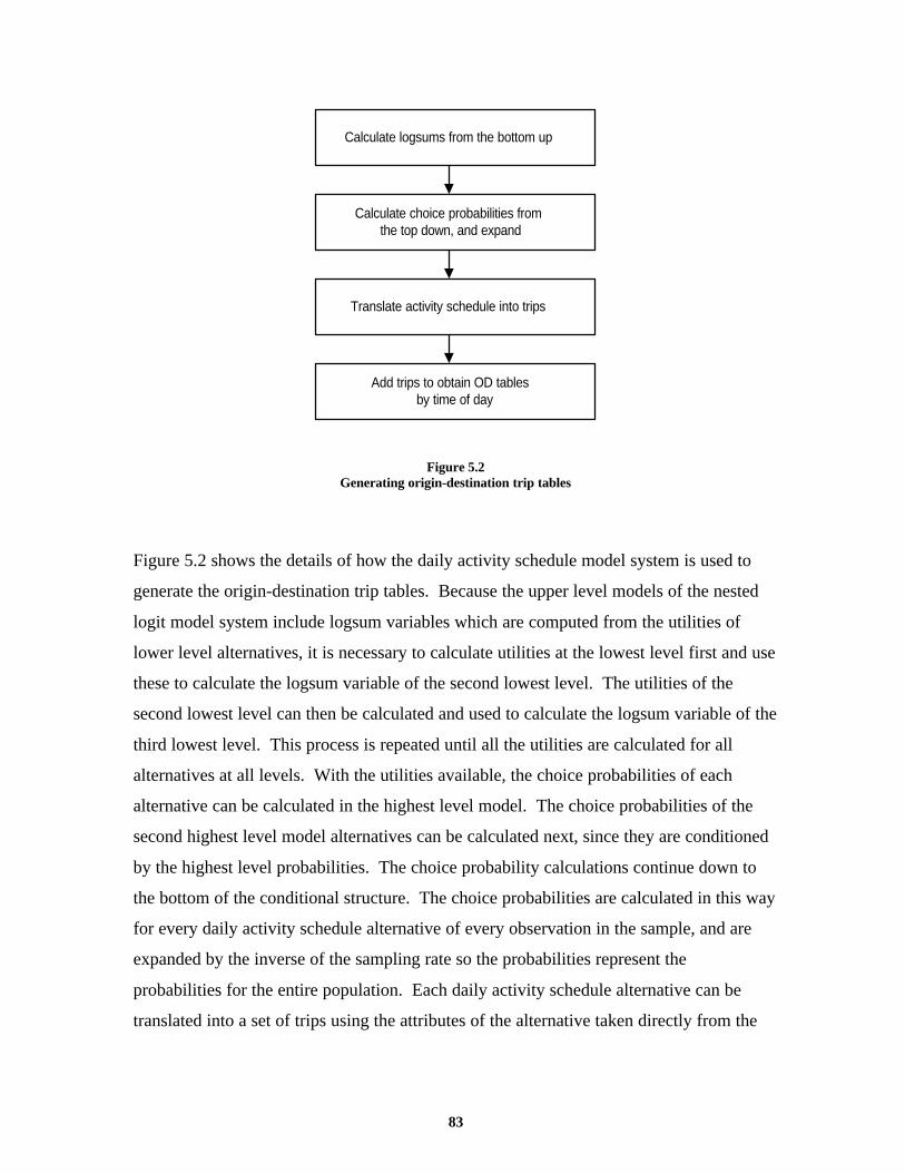
83

Calculate logsums from the bottom up

Translate activity schedule into trips

Add trips to obtain OD tables by time of day

Calculate choice probabilities fromthe top down, and expand

Figure 5.2Generating origin-destination trip tables

Figure 5.2 shows the details of how the daily activity schedule model system is used to

generate the origin-destination trip tables. Because the upper level models of the nested

logit model system include logsum variables which are computed from the utilities of

lower level alternatives, it is necessary to calculate utilities at the lowest level first and use

these to calculate the logsum variable of the second lowest level. The utilities of the

second lowest level can then be calculated and used to calculate the logsum variable of the

third lowest level. This process is repeated until all the utilities are calculated for all

alternatives at all levels. With the utilities available, the choice probabilities of each

alternative can be calculated in the highest level model. The choice probabilities of the

second highest level model alternatives can be calculated next, since they are conditioned

by the highest level probabilities. The choice probability calculations continue down to

the bottom of the conditional structure. The choice probabilities are calculated in this way

for every daily activity schedule alternative of every observation in the sample, and are

expanded by the inverse of the sampling rate so the probabilities represent the

probabilities for the entire population. Each daily activity schedule alternative can be

translated into a set of trips using the attributes of the alternative taken directly from the

84

model. The relevant attributes include the timing, destination and mode from the tour

models, and the tour type from the daily activity pattern. Each trip has the same choice

probability as its daily activity schedule. The trip probabilities are treated as predicted trip

fractions, and are added together to form the set of forecast trip tables.

5.3 Expected Forecasting Results

The expected benefit of the demand model with daily activity schedules is improved travel

demand forecasts, in comparison to the trip and tour based models in use today. This

section describes briefly how the model is expected to provide improved forecasts under

three relevant policy alternatives, including 1) roadway expansion 2) employer provided

carpooling incentives, and 3) increased fuel prices. It also describes how the model

should yield improved emissions estimates under all policy scenarios.

Roadway Expansion

When road capacity is expanded to alleviate congestion we observe an increase in travel

induced by the improved travel conditions. This induced demand includes people who

previously avoided the congested locations and times, and also people who previously

stayed at home or carried out a simpler travel pattern because of the congestion. Trip and

tour based models, if they explicitly represent destination and time choices, might capture

the destination and timing effects. However, unlike the model of daily activity schedule,

they will be unable to capture the shift from non-traveling patterns to patterns with travel,

and the shift from simple to more complex travel patterns.

Employer Provided Carpooling Incentives

In this scenario, employers encourage carpooling by reducing parking subsidies, providing

preferred parking for carpools, and offering subsidies for carpoolers. Under such a policy,

we would expect the mode share of shared ride to increase relative to drive alone for work

85

trips. We would also expect an increase in the number of nonwork tours as commuters

shift secondary activities away from the work tour. These nonwork tours might occur

during peak periods, at least partially offsetting the desired benefits of the carpool

incentive. Trip and tour based models will predict the mode shift, but will be unable to

accurately predict the associated shift in demand to other trips. In contrast, the model of

daily activity schedules will capture both effects because it explicitly models the effect of

travel costs and incentive programs on the choice of a daily activity pattern.

Increased Fuel Prices

During previous energy crises we observed that people did not simply reduce their

tripmaking, but made significant changes in their travel patterns, such as combining

activities into complex tours, as they tried to achieve their activity objectives with less

travel. As in the previous examples, the model with daily activity schedules can capture

these complex adjustments in daily travel patterns which the trip and tour models fail to

capture.

Emissions Estimates

Vehicle emissions are much higher when a cold engine starts than after it has reached

regular operating temperatures. Emissions models rely on travel forecasts, but current

travel forecasting models are unable to distinguish high emission cold engine travel from

low emission warm engine travel. Crude aggregate measures are used to allocate the

travel to these two engine operating modes. The model of daily activity schedules,

although it does not explicitly track a particular vehicle’s movements through a day, offers

the potential of improved estimates of operating modes by using auto availability

information in combination with explicitly modeled daily activity patterns of all members

in a household.

86

5.4 Research and Development Needs

Although the claims of improved forecasts from the daily activity schedule model are

based on the fact that the model system incorporates well founded theories of human

activity and travel behavior, they have not yet been empirically substantiated.

Furthermore, the potential exists for significantly improving the model system which was

demonstrated, and extending it to address additional problems which limit the

effectiveness of today’s travel demand models. This section lays out an agenda for

subsequent research and development, including some specific design ideas which

emerged during the course of the current research.

Theoretical Validation

The daily activity schedule model is a discrete choice model based on the theory of utility

maximization. An important theoretical question is whether people use utility maximizing

behavior in this choice situation. In particular, it is impossible for an individual to

rationally consider all of the 300 billion daily activity schedule alternatives which are

explicitly represented in the model. Perhaps it can be argued that people behave as utility

maximizers even though they don’t go through the detailed rational process. Or, as

theorized by Ben-Akiva and Gershenfeld (1993), it may be possible to specify utility

functions which reflect the combination of two processes: (1) the generation of a small

choice set and (2) the selection of one alternative from the small choice set. But perhaps

other theories of human decisionmaking processes in complex decision situations could

lead to an improved model of the daily activity schedule.

Empirical validation

A more practical next step in the research and development is empirical testing of the

model. The model could be used to prepare forecasts, for relevant policy scenarios like

those discussed above, using the Boston survey sample. These forecasts could be

compared to corresponding forecasts prepared using the best existing models available for

87

the Boston metropolitan area. It might also be possible to prepare backcasts to real

situations from previous years for which actual travel and population data is available and

in this way have a true basis for evaluating the accuracy of the model of activity

schedules.

Operational Model System

After the initial empirical tests, an ideal step would be to develop and implement a

complete forecasting model system for a metropolitan area, as a pilot case. Within this

context, the model system could be enhanced in some or all of the following ways:

1. Incorporate improved data sources, including better level of service data by time of

day, level of service attributes for non-motorized modes, and stated preferences.

2. Improve the model specification, giving consideration to alternative decision

variable definitions, more powerful and useful explanatory variables, and a refined

model structure.

3. Implement the full model system design, including decisions of secondary

activities on tours.

4. Incorporate at-home activities and information technology options such as

telecommuting and teleshopping

5. Develop dynamic choice models, using panel data or retrospective survey

questions.

Extended Model System

There is a widely recognized need to improve the connection of travel models with

models of longer term lifestyle and mobility decisions, as well as urban development

decisions. Of particular concern is the insensitivity of residential location models to the

performance of the transportation system. The daily activity schedule model has great

potential for improving residential location models, and other lifestyle and mobility

models, in this respect because of its ability to supply them with a sophisticated measure

88

of accessibility. For each residential location alternative in a model of residential location

choice, a form of the expected maximum utility variable can be generated from the utility

of all available daily activity schedules. With such a variable in the residential location

model, a transportation system change which made a location more accessible would yield

an increase in the attractiveness of the residential location because of the increased utility

of daily activity schedules available at that residential location. This is perhaps the most

exciting and promising new avenue of research opened up by the development of the

model of daily activity schedules.

5.5 Summary

This thesis has presented the results of research which led to the development of a travel

demand model system with daily activity schedules. Chapter 1 motivated the research by

emphasizing the need for improved travel demand models. It also established a context

for the work by describing the travel decision framework, activity based travel theory and

the weaknesses of current modeling practices. Chapter 2 reviewed significant model

system development efforts of the last 20 years. These served as a springboard for the

objectives and design of the model of daily activity schedules presented in Chapter 3.

Chapter 4 presented the model system itself, estimated as a demonstration system for the

Boston metropolitan area. Finally, this chapter has discussed how the model system could

be used to make improved travel forecasts, and prescribed further research and

development work to test, operationalize and extend the usefulness of the model system.

The most important conclusion of the research presented in this thesis is that it is possible

to successfully estimate a model system of an individual’s daily activity schedule which

meets the objectives laid out in Chapter 3. The three objectives include (1) capture the

interactions among an individual’s decisions throughout a 24 hour day, including explicit

representations of tours and their interrelationships in a daily activity pattern, as well as

activity and travel times of day; (2) represent the daily activity schedule decisions in an

89

integrated, statistically testable econometric choice model system; and (3) estimate a

model system which can be implemented in practice for forecasting. The daily activity

schedule model system, which was estimated as an integrated nested logit model, using an

available diary survey and transportation level of service data, and which can be used to

generate origin to destination trip tables by time of day, achieves all three objectives.

Bibliography

Adler, T. and M. Ben-Akiva, "A Theoretical and Empirical Model of Trip ChainingBehavior", Transportation Research B, 13B, 1979.

Algers, S., A. Daly and S. Widlert, "Modelling Travel Behaviour to Support PolicyMaking in Stockholm", unpublished report, Stockholm, Sweden, 1991.

Antonisse, R. W., A Daly and H. Gunn, "The Primary Destination Tour Approach toModeling Trip Chains", in Transportation Planning Methods: PTRC Proceedings ofSeminar M, P282, July, 1986.

Axhausen, K., A. Ayerbe, M. Bannelier, E. van Berkum, M. Billotte, P. Goodwin, M.Herry, H. Katteler, P. van der Mede, H. Meurs, J. Polak, R. Schwarzmann, D. Selva, A.Yune and D. Zumkeller, "EUROTOPP - Towards a Dynamic and Activity-basedModeling Framework", Advanced Telematics in Road Transport: Proceeding of DRIVEConference, 1991.

Ben-Akiva, M., J. L. Bowman and D. Gopinath, “Travel Demand Model System for theInformation Era”, publication pending in Transportation, 1995.

Ben-Akiva, M. and S. Gershenfeld, “Analysis of Pricing and Packaging Strategies forEnhanced Calling Services”, unpublished paper, Massachusetts Institute of Technology,Cambridge, Massachusetts, 1993.

Ben-Akiva, M. and S. Lerman, Discrete Choice Analysis: Theory and Application toTravel Demand, Cambridge, Massachusetts, MIT Press, 1985.

Ben-Akiva, M., S. R. Lerman, D. Damm, J. Jacobson, S. Pitschke, G. Weisbrod, and R.Wolfe, "Understanding, Prediction and Evaluation of Transportation Related ConsumerBehavior", unpublished report, Center for Transportation Studies, MIT, Cambridge,Massachusetts, 1980.

Ben-Akiva, M., L. Sherman, B. Kullman, "Disaggregate Model of Non-Home BasedTravel", Transportation Research Record, 673, 1978.

Cambridge Systematics, Inc. and Hague Consulting Group, “Making the Land UseTransportation Air Quality Connection, Volume 4: Modeling Practices”, prepared for1000 Friends of Oregon, Portland, Oregon, 1991.

Cascetta, E., A. Nuzzolo and V. Velardi, "A System of Mathematical Models for theEvaluation of Integrated Traffic Planning and Control Policies", unpublished report,University of Naples, Italy, November, 1993.

91

Chapin, F. S., Human Activity Patterns in the City: Things People Do in Time andSpace, New York, Wiley, 1974.

Daly. A. J., H. H. P. van Zwam and J. van der Valk, “Application of DisaggregateModels for a Regional Transport Study in the Netherlands”, Proceedings of the WorldConference on Transport Research, Hamburg, 1983.

Damm, D., "Theory and Empirical Results: A Comparison of Recent Activity-basedResearch, in S. Carpenter and P. Jones, eds., Recent Advances in Travel DemandAnalysis, Aldershot, England, Gower, 1983.

Goodwin, P., R Kitamura and H Meurs, “Some Principles of Dynamic Analysis of TravelBehavior”, in Developments in Dynamic and Activity-Based Approaches to TravelAnalysis, Aldershot, England, Gower, 1990.

Golob, J. M. and T. F. Golob, “Classification of Approaches to Travel-BehaviorAnalysis”, TRB Special Report 201, Transportation Research Board, 1983.

Goulias, K. and R. Kitamura, "Travel Demand Forecasting with DynamicMicrosimulation", Research Report UCD-ITS-RR-92-4, Institute of TransportationStudies, University of California, Davis, Davis, California, March 1992.

Gunn, H. F., A. I. J. M. van der Hoorn and A. J. Daly, “Long-Range, Country-WideTravel Demand Forecasts from Models of Individual Choice”, Proceedings of the FifthInternational Conference on Travel Behaviour, Aiix-en-Provence, 1987.

Hagerstrand, T., "What About People in Regional Science?", Papers of the RegionalScience Association, Vol. 24, 1970.

Hague Consulting Group, “The National Model System for Traffic and Transport:Outline”, report prepared for the Ministry of Transport and Public Works, Rotterdam,The Netherlands, 1992.

Hirsh, M., J. N. Prashker, and M. Ben-Akiva, “Dynamic Model of Weekly ActivityPattern”, Transportation Science, Vol. 20, No. 1, 1986.

JHK & Associates, “State of California Department of Transportation Travel ForecastingGuidelines”, Emeryville, California, 1992.

Jones, P. M., “New Approaches to Understanding Travel Behaviour: The HumanActivity Approach”, Working Paper 28, Transport Studies Unit, University of Oxford,Oxford, England, 1977.

Jones, P. M., M. C. Dix, M. I. Clarke, and I. G. Heggie, Understanding Travel Behaviour,Aldershot, England, Gower, 1983.

92

Kitamura, R., “An Evaluation of Activity-Based Travel Analysis”, Transportation, 15,1988.

Recker, W., M. McNally and G. S. Root, "A Model of Complex Travel Behavior:Part I--Theoretical Development", Transportation Research A, Vol. 20A, No. 4, 1986.

Recker, W., M. McNally and G. S. Root, "A Model of Complex Travel Behavior:Part II--An Operational Model", Transportation Research A, Vol. 20A, No. 4, 1986.

Ruiter, E. R., and M. Ben-Akiva, "Disaggregate Travel Demand Models for the SanFrancisco Area: System Structure, Component Models, and Application Procedures",Transportation Research Record, 673, 1978.

Weisbrod, G., and A. Daly, “The Primary Destination Tour Approach to Travel DemandModelling: Empirical Analysis and Modelling Implications”, unpublished report, HagueConsulting Group, The Hague, Netherlands, 1979.