Active Shape Models - 'Smart Snakes'T.F.Cootes and C.J.Taylor

Department of Medical BiophysicsUniversity of Manchester

Oxford RoadManchester M13 9PT

email: bim@wiau.mb.man.ac.uk

Abstract

We describe 'Active Shape Models' which iteratively adapt to refine esti-mates of the pose, scale and shape of models of image objects. Themethod uses flexible models derived from sets of training examples.These models, known as Point Distribution Models, represent objects assets of labelled points. An initial estimate of the location of the modelpoints in an image is improved by attempting to move each point to abetter position nearby. Adjustments to the pose variables and shape para-meters are calculated. Limits are placed on the shape parameters ensur-ing that the example can only deform into shapes conforming to globalconstraints imposed by the training set. An iterative procedure deformsthe model example to find the best fit to the image object. Results of ap-plying the method are described. The technique is shown to be a powerfulmethod for refining estimates of object shape and location.

1 Introduction

Flexible models can represent classes of objects whose shape can vary, and can beused to recognise examples of the class in an image. Various authors have describediterative techniques for fitting flexible models to image objects. Kass, Witkin andTerzopoulos [1] described Active Contour Models', flexible snakes which can stretchand deform to fit image features to which they are attracted. The iterative energyminimisation technique used is a powerful one, but only simple, local shape con-straints are applied. Yuille et al [2] describe hand built models consisting of variousgeometric parts designed to represent image features; they also describe methodsfor adjusting their models to best fit an image. Unfortunately both the models andthe optimisation techniques have to be individually tailored for each application.Staib and Duncan [3] use a Fourier shape model, representing a closed boundary asa sum of trigonometric functions of various frequencies. They too use a form of itera-tive energy minimisation technique to fit a model to an image. However, using trig-onometric functions does not always provide an appropriate basis for capturingshape variability, and is limited to closed boundaries. Lowe [4] describes a techniquefor fitting projections of three-dimensional parameterised models to two dimen-sional images by iteratively minimising the distance between lines in the projectedmodel and those in the image.

We have developed a method of building flexible models by representing theobjects as sets of labelled points and examining the statistics of their co-ordinatesover a number of training shapes - Point Distribution Models (PDMs) [5]. In this

BMVC 1992 doi:10.5244/C.6.28

267

paper we describe an iterative optimisation scheme for PDMs allowing initial esti-mates of the pose, scale and shape of an object in an image to be refined. The linearnature of the model leads to simple mathematics allowing rapid execution. Becausethe models can accurately represent the modes of shape variation of a class of objectsthey are compact and prevent 'implausible' shapes from occurring. Since PDMs canrepresent a wide variety of objects the same modelling and refinement frameworkcan be applied in many different applications.

Given an estimate of the position, orientation, scale and shape parameters ofan example in an image, adjustments to the parameters can be calculated which givea better fit to the image. Suggested movements are calculated at each model point,giving the displacement required to get to a better location. These movements aretransformed to suggested adjustments of the parameters, giving a better overall fitof the model instance to the data. By applying limits to the ranges of the parametersit can be ensured that the shape of the instance remains similar to the original train-ing examples. Enforcing these limits applies global shape constraints, allowing onlycertain deformations to occur. Because the models attempt to deform to better fitthe data, but only in ways which are consistent with the shapes found in the trainingset we call them Active Shape Models' or 'Smart Snakes'.

2 The Point Distribution Model

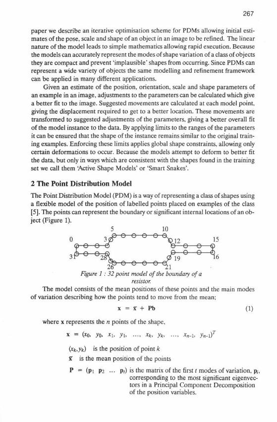
The Point Distribution Model (PDM) is a way of representing a class of shapes usinga flexible model of the position of labelled points placed on examples of the class[5]. The points can represent the boundary or significant internal locations of an ob-ject (Figure 1).

5 10„ a / 7 ~ O O O O « 1C

0 3 CD ID 12 15

- ~ ~ -e—e- '-e—&-Q> 1Q

O O26Figure 1: 32 point model of the boundary of a

resistor.The model consists of the mean positions of these points and the main modes

of variation describing how the points tend to move from the mean;

x = x + Pb (1)

where x represents the n points of the shape,

x = (xo, yo, xi, yh ..., xk, yk, ..., xn.h yn_i)r

(xk,yk) is the position of point k

x is the mean position of the points

P = (Pi P2 ••• Pr) is the matrix of the first t modes of variation, p,,corresponding to the most significant eigenvec-tors in a Principal Component Decompositionof the position variables.

268

b = (bi 62 ... bt)T is a vector of weights for each mode.

The columns of P are orthogonal so pTp = 1 and

b = Pr(x - x) (2)

The mean and linearly independent modes of variation are estimated from a setof training examples. The above equations allow us to generate new examples fromthe class of shapes by varying the parameters (6,-) within suitable limits. The limitsare derived by examining the distributions of the parameter values required to gener-ate the training set (typically three standard deviations from the mean). Each para-meter varies the global properties of the shape reconstructed.

We can define the shape of a model object, in an object centred co-ordinateframe, by choosing values for b. We can then create an instance, X, of the model inthe image frame by defining the position, orientation and scale;

X = M(s,0)[x] + X, (3)

where Xc = (Xc, Yc, Xc, Yc, ..., Xc, YC)T

M(s, 9)[ ] is a rotation by0 and a scaling by s.

(Xc Yc) is the position of the centre of the model in the image frame.

3 Using the PDM as a Local Optimiser - Active Shape Models

Suppose we have a PDM of an object, and we have an estimate of the position, orien-tation, scale and shape parameters of an example of the object in an image. We wouldlike to improve our estimate, updating the pose and shape parameters to make themodel instance fit more accurately to the image evidence. The approach we use isas follows: at each point in the model we calculate a suggested movement requiredto displace the point to a better position; we calculate the changes to the overall posi-tion, orientation and scale of the model which best satisfy the displacements; any re-sidual differences are used to deform the shape of the model object by calculatingthe required adjustments to the shape parameters. The global shape constraints areenforced by ensuring that the shape parameters remain within appropriate limits.

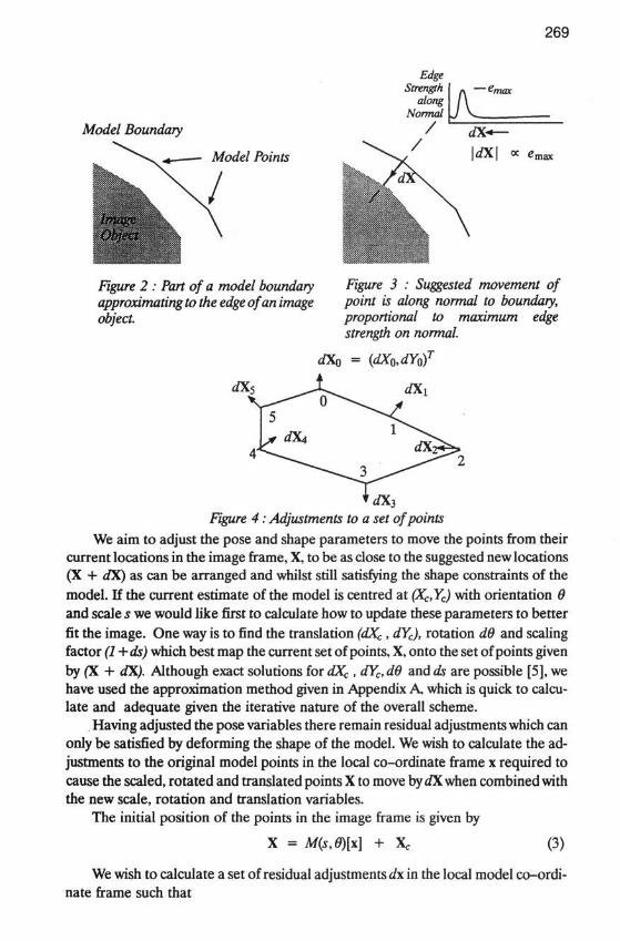
3.1 Calculating The Suggested Movement of Each Model PointGiven an initial estimate of the positions of a set of model boundary points whichwe are attempting to fit to the outline of an image object (Figure 2) we need to esti-mate an adjustment to apply to move each boundary point toward the edge of theimage object. There are various approaches that could be taken. In the examples wedescribe later we use an adjustment along a normal to the model boundary towardsthe strongest image edge, with a magnitude proportional to the strength of the edge(Figure 3).

A set of adjustments can be calculated, one for each point of the shape (Figure4). We denote such a set as a vector dX, where

dX = (dX0, dY0, ..., dXn.h dYn.xf

269

EdgeStrength

alongNormal

Model Boundary

Model Points

ImageObjett

Figure 2 : Part of a model boundaryapproximating to the edge of an imageobject.

Figure 3 : Suggested movement ofpoint is along normal to boundary,proportional to maximum edgestrength on normal.

= (dX0,dY0)T

Figure 4: Adjustments to a set of points

We aim to adjust the pose and shape parameters to move the points from theircurrent locations in the image frame, X, to be as close to the suggested new locations(X + dX) as can be arranged and whilst still satisfying the shape constraints of themodel. If the current estimate of the model is centred at (Xc,Yc) with orientation 0and scale s we would like first to calculate how to update these parameters to betterfit the image. One way is to find the translation (dXc, dYc), rotation d6 and scalingfactor (1 +ds) which best map the current set of points, X, onto the set of points givenby pi. + dX). Although exact solutions for dXc , dYc, dO and ds are possible [5], wehave used the approximation method given in Appendix A, which is quick to calcu-late and adequate given the iterative nature of the overall scheme.

Having adjusted the pose variables there remain residual adjustments which canonly be satisfied by deforming the shape of the model. We wish to calculate the ad-justments to the original model points in the local co-ordinate frame x required tocause the scaled, rotated and translated points X to move by dX when combined withthe new scale, rotation and translation variables.

The initial position of the points in the image frame is given by

X = M(s,0)[x] + (3)

We wish to calculate a set of residual adjustments dx in the local model co-ordi-nate frame such that

270

M(s(l +ds),6 + dO)[x + dx] + (Xc + dXc) = (X + dX) (4)

Thus

M(s(l +ds),9 + dO)[x + dx] = (M(s,0)[x] + dX) - (X,

and since M'\s,9)[ ] = M(s'\-9)[ ]

we obtain

dx = M((s(l + ds))-\ -(9 + dO))[M(s, 0)[x] + dX - dXc] - x (5)

Equation 5 gives a way of calculating the suggested movements to the points xin the local model co-ordinate frame. These movements are not in general consistentwith our shape model. In order to apply the shape constraints we transform dx intomodel parameter space giving db, the changes in model parameters required to ad-just the model points as closely to dx as is allowed by the model. Equation 1 gives

x = x + Pb (1)

We wish to find db such that

x + dx = x + P(b + db) (6)

Since there are only t (<2n) modes of variation available and dx can move thepoints in 2n different degrees of freedom, in general we can only achieve an approxi-mation to the deformation required, since we only allow deformation in the mostsignificant modes observed in the training set. This truncating of the modes of vari-ation is equivalent to setting limits of zero on the parameters controlling othermodes of variation. Applying such limits and truncation enforces the global shapeconstraints.

Subtracting (1) from (6) gives

dx

db = VTdx (7)

It can be shown that Equation 7 is equivalent to using a least squares approxima-tion to calculate the shape parameter adjustments, db.

3.2 Updating the Pose and Shape Parameters

The equations above allow us to calculate changes to the pose variables, dXc, dYc, d9and ds, and adjustments to the shape parameters db required to improve the matchbetween an object model and image evidence. We have applied these to update theparameters in an iterative scheme as follows;

Xc -* Xc + w, dXc (8)

YC^YC + w, dYc (9)

9 -> 9 + we de (10)

s -* s(l + ws ds) (11)

271

b -* b + W6 db (12)

Where w,, ws and we are scalar weights, and W& is a diagonal matrix ofweights for each mode. This can either be the identity, or each weight can be propor-tional to the standard deviation of the corresponding shape parameter over the train-ing set. The latter allows more rapid movement in modes in which there tends to belarger shape variation.

In order to ensure that the new shape is plausible it is necessary to apply limitsto the 6-parameters. If the variance about the origin of the Ith parameter over thetraining set is A, then a shape can be considered acceptable if the Mahalanobis dis-tance Dm is less than a suitable constant, Dma* (for instance 3.0);

(13)

(The vector b lies within a hyper-ellipsoid about the origin.) If updating b using(12) leads to an implausible shape, ie (13) is violated, it can be re-scaled to lie onthe closest point of the hyper-ellipsoid using

A,--*/.^P- (/ = M (14)

Once the parameters have been updated, and limits applied where necessary,a new example can be calculated, and new suggested movements derived for eachpoint. The procedure is repeated until no significant change results.

4 Examples Using Active Shape Models

The techniques described above have been used successfully in a number of applica-tions, both industrial and medical [8]. Here we show results obtained using the resis-tor and hand models described in the companion paper [5].

In both cases initial estimates of the position, orientation and scale are made,and the shape parameters are all initialised at zero (£, = 0 (i = l..f)). Suggestedmovements for each model point are calculated by finding the strongest edge (in thecorrect direction) along the normal to the boundary at the point (See 3.1 and Figure3). Adjustments to the parameters are calculated and applied, and the process re-peated.

4.1 Finding Resistors with an ASM

We have constructed a Point Distribution Model of a resistor representing its bound-ary using 32 points (Figure 1). Figure 5 shows an image of part of a printed circuitboard with the resistor boundary model superimposed as it iterates towards theboundary of a component in the image. We interpolate an additional 32 points, onebetween each pair of model points around the boundary, and calculate adjustmentsto each point by finding the strongest edge along profiles 20 pixels long centred ateach point. We use a shape model with 5 degrees of freedom. Each iteration takesabout 0.025 seconds on a Sun Sparc Workstation.

272

(a) Original (b) Initial (c) After 30 (d) After 60 (e) After 90 (f) After 120Image Position iterations iterations iterations iterations

Figure 5: Section of Printed Circuit Board with resistor model superimposed,showing its initial position and its location after 30, 60, 90 and 120 iterations.

The ends of the wires are not found correctly since they are not well defined -there is little edge evidence to latch on to. We intend to produce a better model byincluding the square solder pads. The method is effective in maintaining the globalshape constraints of the model and works well given a sufficiently good starting ap-proximation; we discuss methods of obtaining such initial hypotheses elsewhere[6,7,8].

The relatively simple method of calculating the movement of each point, lookingfor a strong nearby edge, can cause problems when a model is initialised some dis-tance from a component. Highlights and the banding patterns on the resistors canattract the boundary of the model, pulling it away from the true edge. A more soph-isticated technique which modelled the banding and possible highlights would be re-quired to overcome this.

4.2 Finding Hands with an ASM

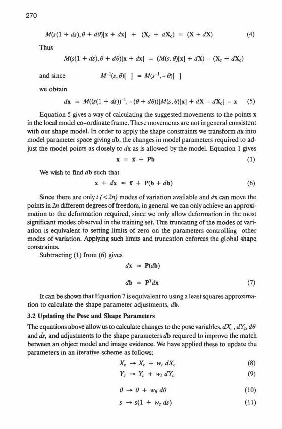
We have constructed a Point Distribution Model of a hand representing the bound-ary using 72 points. Figure 6 shows an image of the author's hand and an exampleof the model iterating towards it. We calculate adjustments to each point by findingthe strongest edge on a profile 35 pixels long centred on the point. The shape modelhas 8 degrees of freedom, and each iteration takes about 0.03 seconds on a Sun SparcWorkstation. The result demonstrates that the method can deal will limited occlu-sion.

As in the previous example the method works reliably, given a reasonable start-ing approximation. The example shows that the method is tolerant to quite seriouserrors in the starting approximation, though this depends on the amount of clutterin the image.

5 Discussion and Conclusions

The iterative approach described above, using image evidence to deform a Point Dis-tribution Model, is effective at locating objects, given an initial estimate of theirposition, scale and orientation. How good an estimate is required will depend on howcluttered the image is and how well the model describes the object in the image.

273

(a) Initial Position (b) 100 iterations (c) 200 iterations (d) 350 iterations

Figure 6: Image of authors hand with hand model superimposed, showing its in-itial position and its location after 100,200 and 350 iterations.

How suggested adjustments are found for each point is important. Calculatingthe suggested movement by looking for strong nearby edges is simple and has provedeffective in many cases. However, when searching for more complex objects, wherethe model points do not necessarily lie on strong edges, more sophisticated algo-rithms are required. Potential maps can be derived, describing how likely each pointin an image is to be a particular model point. During a search each model point at-tempts to move to more likely locations, climbing hills in the potential map. Alterna-tively a model of the expected grey levels around each model point can be generatedfrom the training examples, and each point moved toward areas which best matchits local grey level model. Preliminary experiments using both these techniques haveproved promising [9]. The model points do not have to lie only on the boundary ofobjects, they can represent internal features, and even sub-components of a complexassembly. In the latter case the model describes both the variations in the shapes ofthe sub-components and the geometric relationships between components. The re-finement technique can be applied as easily in this situation as to a model of a singleboundary.

By allowing the model to deform, but only in ways seen in the class of examplesused as a training set, we have a powerful technique for refinement. The constraintson the shape of the model are applied by the limits on the shape parameters. The2n-t unrepresented modes of variation effectively have limits of zero on their para-meters. Rather than fixed limits being used to enforce shape constraints, restoringforces in the parameter space could be applied, pulling the parameters back towardszero against the external 'forces' from the image;

b + - kb\Vbh (0 <kb < 1) (15)

This would give more weight to solutions closer to the mean shape, and requirestrong evidence for shapes which are considerably deformed. However, this wouldbe likely to lead to compromise solutions between image data and model.

The work we present here can be thought of as a two dimensional applicationof Lowe's refinement technique [4]. Because of the linear nature of the Point Dis-tribution Model, the mathematics is considerably simpler and can lead to rapid ex-ecution.

274

We have conducted experiments which suggest that the local optimisationmethod described can be fruitfully used in conjunction with a Genetic Algorithm(GA) search [8]. The GA can be run as a cue generator to produce a number of objecthypotheses, which can be refined using the Active Shape Model. Alternatively theASM can be combined with the GA search, applying one iteration at each generationof the Genetic Algorithm. Both techniques appear very promising.

The method of calculating the parameter changes is straightforward, and newexamples of a model can be generated rapidly using linear algebra. As well as theexamples of resistors and hand models shown above, the technique has been success-fully used in a variety of applications and has great potential for image search in manyimage analysis domains.

AcknowledgementsThis work is funded by SERC under the IEATP Initiative (Project Number 3/2114).The authors would like to thank the other members of the Wolfson Image AnalysisUnit for their help and advice, particularly D.H.Cooper, J.Graham, D.Bailes andAHill.

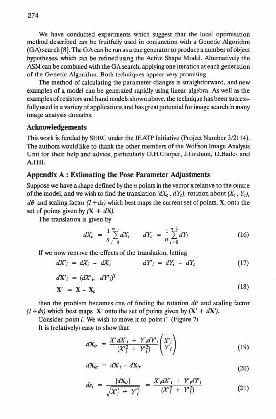
Appendix A : Estimating the Pose Parameter AdjustmentsSuppose we have a shape defined by the n points in the vector x relative to the centreof the model, and we wish to find the translation (dXc, dYc), rotation about (X:, Yc),dO and scaling factor (1 +ds) which best maps the current set of points, X, onto theset of points given by (X + dX).

The translation is given by

dXe = -j^dXi dYc = -j^dYi (16)n /=o n /=o

If we now remove the effects of the translation, lettingdX'i = dXi - dXc dYi = dYt - dYc (17)

dX'i = (dX't, dYif

X' = X - Xc (1 8 )

then the problem becomes one of finding the rotation d6 and scaling factor(1 +ds) which best maps X' onto the set of points given by (X' + dX').

Consider point i. We wish to move it to point i' (Figure 7)It is (relatively) easy to show that

(X'j + Y}) \ri) (19)

_ \dXjr\ _ X'fOCj +

JxJTVj

275

Origin ofModel

Origin ofModel

Figure 7: Estimating the angle and scale changes require tomap one point to a new position.

Then

6 References

dO

ds

V

sss —

n

sas —

n

/A. j T / ,•

y\ dOii = 0

( = 0

(22)

(23)

(24)

[1] M. Kass, A. Witkin and D. Terzopoulos, Snakes: Active Contour Models. FirstInternational Conference on Computer Vision, pub. IEEE Computer SocietyPress, 1987; pp 259-268.

[2] A.L. Yuille, D.S. Cohen and P. Hallinan, Feature extraction from faces usingdeformable templates. Proc. Comp. Vision Part. Rec. 1989; ppl04-109.

[3] L.H. Staib and J.S Duncan, Parametrically Deformable Contour Models.IEEE Computer Society conference on Computer Vision and Pattern Recogni-tion, San Diego, 1989.

[4] D.G. Lowe, Fitting Parameterized Three Dimensional Models to Images.IEEE PAMI 1991; 5, pp441-450.

[5] T.F. Cootes, CJ . Taylor, D.H. Cooper and J. Graham, Training Models ofShape from Sets of Examples. This Volume.

[6] A. Hill and C.J. Taylor, Model-Based Interpretation using Genetic Algo-rithms. Proc. British Machine Vision Conference, Glasgow, 1991, pub.Springer Verlag, pp266-274.

[7] A. Hill, C.J. Taylor and T.F. Cootes, Object Recognition by Flexible Tem-plate Matching using Genetic Algorithms. Proc. European Conference onComputer Vision, Genoa, Italy, 1992.

[8] A. Hill, T.F. Cootes and C.J. Taylor, A Generic System for Image Interpreta-tion Using Flexible Templates. This Volume.

[9] A. Lanitis, Modelling Faces. Internal Progress Report, Wolfson Image Analy-sis Unit, Manchenster University, 1992.