Active Postmarketing Drug Surveillance for Multiple …web.stanford.edu/~bayati/papers/drug.pdf ·...

Submitted to Operations Researchmanuscript

Active Postmarketing Drug Surveillance for MultipleAdverse Events

Joel GohStanford Graduate School of Business, CA 94305, [email protected]

Margret V. BjarnadottirRobert H. Smith School of Business, MD 20742, [email protected]

Mohsen BayatiStanford Graduate School of Business, CA 94305, [email protected]

Stefanos A. ZeniosStanford Graduate School of Business, CA 94305, [email protected]

Active postmarketing drug surveillance is important for consumer safety. However, existing methods have

limitations that prevent their direct use for active drug surveillance. One important consideration that has

been absent thus far is the modeling of multiple adverse events and their interactions. In this paper, we

propose a method to monitor the effect of a single drug on multiple adverse events, which explicitly captures

interdependence between events. Our method uses a sequential hypothesis testing paradigm, and employs

an intuitive test-statistic. Stopping boundaries for the test-statistic are designed by asymptotic analysis and

by reducing the design problem to a convex optimization problem. We apply our method to a dynamic

version of Cox’s proportional hazards model, and show both analytically and numerically how our method

can be used as a test for the hazard ratio of the drug. Our numerical studies further verify that our method

delivers Type I/II errors that are below pre-specified levels and is robust to distributional assumptions and

parameter values.

Key words : Health Care, Stochastic Models, Drug Surveillance, Adverse Drug Events

1. Introduction

In most countries, before a drug is approved for commercial distribution, the drug has to undergo

a series of clinical trials, designed to assess both its efficacy and potential side effects. However,

clinical trials may fail to detect all the adverse side effects associated with the drug. Researchers

have pointed to the small size and low statistical power of clinical trial populations (Wisniewski

et al. 2009) and pressures for quick drug approval (Deyo 2004) as possible reasons for such failures.

Postmarketing drug surveillance is the process of monitoring drugs that are already commercially

distributed, in order to flag drugs that have potential adverse side effects. It is typically based on

observational data and cannot definitively establish or refute causal relationships between drugs

1

Goh, Bayati, and Zenios: Postmarketing Drug Surveillance2 Article submitted to Operations Research; manuscript no.

and adverse events. Nevertheless, if a causal relationship exists, effective drug surveillance would

provide preliminary evidence for this relationship and an early warning signal for regulators to take

mitigating actions (e.g., limit the drug’s distribution, issue warnings to consumers, order further

studies), thereby acting as a final safeguard to protect the consumer population from lapses in the

initial process of drug approval.

Drug surveillance systems may be classified as either passive or active. A passive surveillance

system relies on physicians and patients to voluntarily report suspected drug-associated adverse

events to the relevant health authorities. In contrast, an active surveillance system employs auto-

mated monitoring of public health databases to proactively infer associations between drugs and

adverse events. In the U.S., the present system of drug surveillance is passive. The medical commu-

nity, however, has long argued against passive surveillance, citing its high susceptibility to biases

such as underreporting of adverse events, and has repeatedly called upon the U.S. Food and Drug

Administration (FDA) to develop an active surveillance system (e.g., Brewer and Colditz 1999,

Furberg et al. 2006, Brown et al. 2007, McClellan 2007). In response, the FDA, also recognizing

the importance of active surveillance, launched the Sentinel Initiative in May 2008, which aims to

“develop and implement a proactive system . . . to track reports of adverse events linked to the use

of its regulated products” (FDA 2012).

Existing methods that have been proposed for active drug surveillance still possess significant

limitations. The report by the FDA (Nelson et al. 2009) presents a comprehensive account of

existing methods and discusses their limitations. The report concludes that a common limitation

of existing methods is the limited handling of confounding factors. Other limitations in individual

methods include failure to account for the temporal sequence of adverse events and drug usage, lack

of control over statistical parameters of interest (such as false detection rates), and high sensitivity

to distributional parameters.

1.1. Contributions

Our central contribution in this paper is to propose a method for active drug surveillance, termed

Queueing Network Multi-Event Drug Surveillance (QNMEDS), that overcomes some of the lim-

itations listed above. In particular, QNMEDS allows simultaneous surveillance of the effect of a

drug on multiple adverse events, and explicitly accounts the temporal dependencies between these

adverse events, which is an important confounding factor that has been neglected in other meth-

ods. Specifically, QNMEDS allows an adverse event that has occurred in the past to affect the rate

at which other adverse events occur in the future. Because drug surveillance uses public health

data, it does not have have a well-controlled study population (unlike, e.g., clinical trials), and

therefore, multiple adverse events are expected to exist in the study population. Moreover, the

Goh, Bayati, and Zenios: Postmarketing Drug SurveillanceArticle submitted to Operations Research; manuscript no. 3

epidemiological literature suggests that the magnitude of these interdependencies can be signifi-

cant. For example, diabetics are known to have around two times the risk of cardiac events than

non-diabetics (e.g., Abbott et al. 1987, Manson et al. 1991). One way that this interdependency

complicates the problem of drug surveillance is when a drug that may be “safe” for patients who

are free of adverse events could be “unsafe” for patients who had previously experienced some

adverse event. For example, researchers have found that antiplatelet therapy, which is prescribed to

prevent adverse cardiovascular events, actually increased the risk of major adverse cardiovascular

events if the patient had Type II diabetes (Angiolillo et al. 2007). These considerations suggest

that surveillance methods that fail to account for the interactions between multiple adverse events

may make erroneous conclusions. This point is further supported by our simulation study in §7.3.

In addition, QNMEDS also possesses the following desirable features: 1) it is designed for sequen-

tially arriving data, 2) it incorporates temporal dynamics such as the sequencing of drug treatment

and adverse events, 3) it allows the user to control statistical parameters such as the false detection

probability (Type I error), and 4) it is robust to distributional assumptions, unlike other tests

that require strong assumptions about likelihood functions, such as the Sequential Probability

Ratio Test (SPRT). With regard to the last point in particular, our numerical study on simulated

data for two adverse events finds that an SPRT-based heuristic performs very poorly under mild

perturbations of its parametric assumptions, even though it has excellent performance when its

assumptions are met. Specifically, in simulated data where the drug increased the risk of an adverse

event between 40% to 60%, if the SPRT-based heuristic assumed a slightly mis-specified distribu-

tion of random event times, it could only detect this elevated risk in 0-2% of all the simulation

runs. In contrast, on the same data, QNMEDS detected this association in 100% of the runs.

Through our analysis of QNMEDS, we make two further technical contributions:

1. As part of our analysis, we had to estimate the probability of hitting a certain set for a multi-

dimensional Brownian Motion (B.M.) process with correlated components. We develop a novel

method to bound this hitting probability from above by constructing a new multidimensional

B.M. process with independent components, and calculating the hitting probability for the

new B.M. process, which turns out to be more tractable.

2. We introduce a cross-hazards model that captures the dynamic interactions between multiple

adverse events. Our cross-hazards model can be viewed as a dynamic version of the classi-

cal Cox proportionate hazards model. We show how QNMEDS can be used for active drug

surveillance in the context of this cross-hazards model.

1.2. Outline

We presently sketch an outline of how QNMEDS operates (details are given by Algorithm 3 in

§5.4). QNMEDS receives sequentially arriving patient data on the times of adverse events and


Vector-valuedtest-statistic, L,

(§3)

Vector-valuedtest-statistic, L,

(§3)

Model event occurrences by a

M/G/∞/Mqueueing network

(§4.1)

Model event occurrences by a

M/G/∞/Mqueueing network

(§4.1)

Asymptotic moments of test-statistc

(§4.2)

Asymptotic moments of test-statistc

(§4.2)

Approximate test-statistic as a multidimensionalBrownian Motion

(§4.3)

Approximate test-statistic as a multidimensionalBrownian Motion

(§4.3)

Limiting test-statistic, Y

(§4.3)

Limiting test-statistic, Y

(§4.3)

Limiting hypothesis test for the drift of Y

(§5.1)

Limiting hypothesis test for the drift of Y

(§5.1)

Stopping boundaries

for limiting test(§5.3)

Stopping boundaries

for limiting test(§5.3)

Formulate problem of designing

stopping boundaries as a math program

(§5.2)

Formulate problem of designing

stopping boundaries as a math program

(§5.2)

Transform Standard Scale Brownian Scale

Scaling(§5.4)

Scaling(§5.4)

Stopping boundaries for L,

(§5.4)

Stopping boundaries for L,

(§5.4)Detection algorithm

Detection algorithm

Legend:

Process

Outcome

Final Outcome

FormalizeHypothesis Test

(§3)

FormalizeHypothesis Test

(§3)

Figure 1 Illustrated overview of analytical steps in QNMEDS.

drug treatment, and uses these data to construct a certain vector-valued test-statistic, which is

defined in §3. The components of this test-statistic capture the effect of the drug on each adverse

event. If the test-statistic reaches a certain region of its state-space, called the stopping region,

QNMEDS terminates and flags the drug as unsafe. The primary analysis of this paper focuses on

how this stopping region is constructed in order to control the false detection rate and minimize

the expected detection time.

Our analysis begins after a brief review of related methods in §2. Figure 1 illustrates the steps

of our analysis, which occurs in three broad steps spanning §3 through §5. First, in §3, we describe

the quantities that are to be statistically investigated, formalize a hypothesis test for these quan-

tities, and define the test-statistic to be monitored. Second, in §4, we formulate a model of event

occurrences in patients as a M/G/∞/M queueing network model with an arborescent (tree-like)

structure. The queueing network models the dynamic nature of the surveillance system: patients

arrive (i.e., join the surveillance system) and depart (i.e., leave the system due to death, migration,

etc.) with time. Furthermore, this formulation allows us to apply results from queueing theory to

characterize the first two asymptotic moments of our test-statistic (§4.2). Using this characteriza-

tion, in §4.3, we proceed to apply standard convergence properties to show that our test-statistic

weakly converges to a multidimensional Brownian Motion (B.M.) process as the arrival rate of


Is Feature Present ? SPRT-based

Groupsequential

Data-mining

QNMEDS

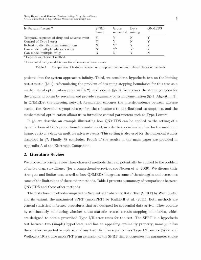
Temporal sequence of drug and adverse event Y Y N YControl of Type I error Y Y N YRobust to distributional assumptions N Ya Y YCan model multiple adverse events N Yb Yb YCan model multiple drugs N N Y Na Depends on choice of method.

b Does not directly model interactions between adverse events.

Table 1 Comparison of features between our proposed method and related classes of methods.

patients into the system approaches infinity. Third, we consider a hypothesis test on the limiting

test-statistic (§5.1), reformulating the problem of designing stopping boundaries for this test as a

mathematical optimization problem (§5.2), and solve it (§5.3). We recover the stopping region for

the original problem by rescaling and provide a summary of its implementation (§5.4, Algorithm 3).

In QNMEDS, the queueing network formulation captures the interdependence between adverse

events, the Brownian asymptotics confers the robustness to distributional assumptions, and the

mathematical optimization allows us to introduce control parameters such as Type I errors.

In §6, we describe an example illustrating how QNMEDS can be applied to the setting of a

dynamic form of Cox’s proportional hazards model, in order to approximately test for the maximum

hazard ratio of a drug on multiple adverse events. This setting is also used for the numerical studies

described in §7. Finally, §8 concludes. Proofs of the results in the main paper are provided in

Appendix A of the Electronic Companion.

2. Literature Review

We proceed to briefly review three classes of methods that can potentially be applied to the problem

of active drug surveillance (for a comprehensive review, see Nelson et al. 2009). We discuss their

strengths and limitations, as well as how QNMEDS integrates some of the strengths and overcomes

some of the limitations of these other methods. Table 1 presents a summary of comparisons between

QNMEDS and these other methods.

The first class of methods comprise the Sequential Probability Ratio Test (SPRT) by Wald (1945)

and its variant, the maximized SPRT (maxSPRT) by Kulldorff et al. (2011). Both methods are

general statistical inference procedures that are designed for sequential data arrival. They operate

by continuously monitoring whether a test-statistic crosses certain stopping boundaries, which

are designed to obtain prescribed Type I/II error rates for the test. The SPRT is a hypothesis

test between two (simple) hypotheses, and has an appealing optimality property; namely, it has

the smallest expected sample size of any test that has equal or less Type I/II errors (Wald and

Wolfowitz 1948). The maxSPRT is an extension of the SPRT that endogenizes the parameter choice


in the alternative hypothesis, and has been applied in several studies on vaccine safety surveillance

(e.g., Lieu et al. 2007, Yih et al. 2009, Klein et al. 2010, Kulldorff et al. 2011). Despite its strengths,

the SPRT (and, by extension, the maxSPRT), suffers from two limitations. First, it is known to be

very sensitive to distributional assumptions (e.g., Hauck and Keats 1997, Pandit and Gudaganavar

2010). This is because it is based on likelihood ratios and consequently requires the modeler to

assume that the random occurrence times of adverse events follow certain distributions. A mis-

specification of the distribution can adversely affect its performance. Second, it is designed to test

a single outcome, which in this application, is a single type of adverse event. It does not model

multiple types of adverse events and their correlations, which are likely to be present in the large

public health databases used for active surveillance.

The second class of methods comprise group sequential testing methods, which are reviewed

in much detail by Jennison and Turnbull (1999). These methods are similar to the SPRT-based

methods in that they are designed for sequential data arrival. However, they unlike the SPRT-

based methods, which review the test-statistic continuously, group sequential methods review the

test statistics at discrete time points. A common goal of these methods is to distribute the Type I

error of the test across the review points, and different methods provide varying ways of achieving

this (see, e.g., Pocock 1977, O’Brien and Fleming 1979, Lan and DeMets 1983). These methods

are very flexible and can be designed to handle confounding variables. However, as in the case of

SPRT-based methods, we are unaware of a group sequential test for multiple outcomes that have

temporal dependencies as considered in this paper.

The third class of methods comprise data mining methods, such as the proportional reporting

ratio (PRR) by Evans et al. (2001), the Bayesian confidence propagation neural network (BCPNN)

by Bate et al. (1998), and the multi-item gamma Poisson shrinker (MGPS) by DuMouchel (1999).

These methods are based on detecting drug-adverse event combinations that are disproportionately

large compared to expected outcomes frequencies from within the database and were designed

to be deployed on large datasets containing multiple drugs and multiple adverse events. While

such methods do not explicitly incorporate the effect of confounding factors such as comorbidities,

they are particularly amenable to subgroup analysis or stratification, which can reduce the prob-

lem of confounding factors. They typically do require some distributional assumptions, but these

assumptions play a less critical role than in SPRT-based methods. However, these methods have

the limitation that they were designed for hypothesis generation rather than hypothesis testing,

and do not provide control over common parameters of statistical interest, such as Type I errors.

A second limitation is that they were designed to find cross-sectional associations of drug-adverse

event combinations, and do not incorporate considerations of temporal sequence (e.g., whether the

adverse event occurred before or after the drug was taken).


QNMEDS incorporates the main strengths and overcomes the key limitations of each class of

methods. Similar to the SPRT and group sequential methods, but unlike the data-mining methods,

QNMEDS is based on the paradigm of sequential hypothesis testing, allows control over Type I

errors, and furthermore is implicitly designed for sequentially-arriving data. Moreover, QNMEDS

is designed to be robust to distributional assumptions. Finally, a unique strength of QNMEDS

is that it handles not just multiple outcomes (unlike the SPRT methods), but also the temporal

interdependence between these outcomes (unlike the group sequential and data-mining methods).

3. Problem Definition: Hypothesis Test Formulation

In this section, we formulate a hypothesis testing problem that determines whether a single drug

increases the maximum incidence rate of a collection of adverse events beyond an exogenous thresh-

old. We make the following assumptions in our formulation:

(A1) Patients arrive exogenously into the surveillance system (henceforth referred to as the system)

according to a homogeneous Poisson process with a known rate.

(A2) Once in the system, patients experience the following events: treatment with the drug, adverse

events, and departure from the system (i.e., death) at random times. Only the first occurrence

time of each event is recorded for each patient. For brevity, we henceforth refer to these first

occurrence times as simply the event times.

(A3) For each patient, the distribution of event times can depend on events that have previously

occurred for the same patient.

(A4) Each patient’s event times are distributed identically and independently.

Assumption (A1) is a standard assumption for arrival processes. Assumption (A2) does not limit our

model because we can simply account for the second, third, etc. occurrence of the same (physcial)

adverse event as separate events within our model (see §4.1 for a discussion of how this can be

done). Assumption (A3) enables us to model the effect of the drug on adverse events, as well

as the interdependence between adverse events. The first part of Assumption (A4), that patients

are statistically identical, is reasonable if we stratify patients into relatively homogeneous socio-

demographic groups with similar risk profiles, which is most feasible if the system contains many

patients. The second part, that patients are statistically independent, is also reasonable since

the drug-related adverse events monitored in a surveillance system are typically non-infectious

conditions that do not interact between patients.

Deferring the full stochastic description of the system and these random times until §4, we

proceed to define some notation and formalize our problem. Let m ∈ N represent the number

of adverse events we are monitoring. Further, label the event of initiating drug treatment with

index 1, and label the incidence of each adverse event with indices j ∈M := 2, . . . ,m+ 1. For


completeness, label the event of patient arrival into the system as event 0 and departure from the

system as event m+ 2.

Let λ represent the rate of (Poisson) patient arrival into the system. Also, let SAj (t) represent

the set of patients that experienced adverse event j ∈M after treatment by time t, and SBj (t)

represent the set of patients who experienced adverse event j ∈M before treatment by time t. In

other words, for a given patient, if we let tj represent the (random) occurrence time of adverse

event j, and t1 represent the (random) occurrence time of event 1 (drug treatment), then at

time t, the patient belongs in set SAj (t) if t1 ≤ tj ≤ t, and the patient belongs in set SB

j (t) if

tj ≤mint1, t. Note that the definition of SBj (t) includes patients who have experienced adverse

event j by time t, but have not received drug treatment by that time. For each i ∈ A,B, we

refer to the monotonically increasing process∣∣Sij∣∣ := ∣∣Sij(t)∣∣ , t≥ 0

as a patient count process, and

define ηij as its (asymptotic) rate, normalized by the arrival rate λ. Formally,

ηij := limt→∞

1

λtE(∣∣Sij(t)∣∣) i∈ A,B , j ∈M (1)

The normalization by λ is not essential, but is done primarily for expositional and analytical

convenience.

The parameters ηij, i∈ A,B , j ∈M are unknown and will be the subject of our statistical test.

Our hypothesis test isH0 : ηAj − kjηBj ≤ 0 for all j ∈M

H1 : ηAj − kjηBj ≥ εj for any j ∈M.(2)

where kj, εj > 0 are model parameters. Intuitively, (2) tests whether the incidence rate of any

adverse event after taking the drug, ηAj , is higher than some fixed multiple (kj) of the corresponding

baseline rate ηBj before taking the drug. For example, if kj = 1 for all j, then (2) investigates

whether, for any adverse event, the patients who took the drug have a higher incidence rate of that

adverse event, compared to patients who did not take the drug. The parameters εj > 0 represents

tolerance levels for the test. In §6, we discuss a specific application that illustrates how these model

parameters kj, εj can be chosen in a principled way.

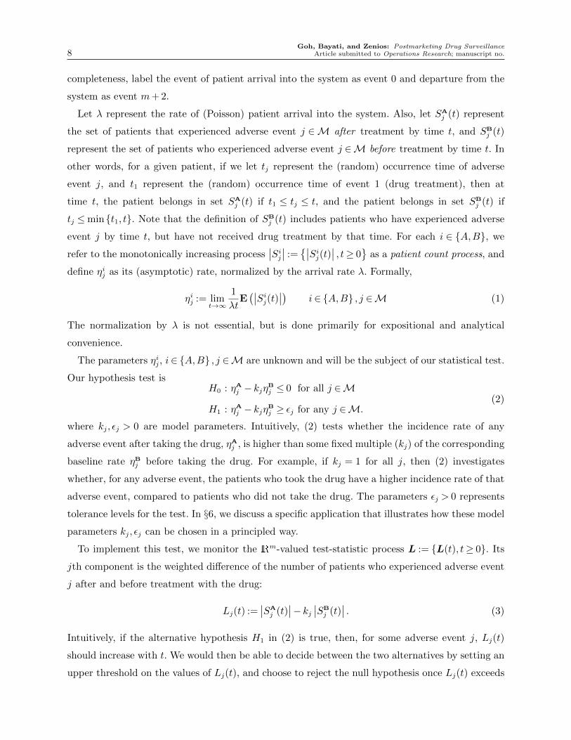
To implement this test, we monitor the Rm-valued test-statistic process L := L(t), t≥ 0. Its

jth component is the weighted difference of the number of patients who experienced adverse event

j after and before treatment with the drug:

Lj(t) :=∣∣SAj (t)

∣∣− kj ∣∣SBj (t)

∣∣ . (3)

Intuitively, if the alternative hypothesis H1 in (2) is true, then, for some adverse event j, Lj(t)

should increase with t. We would then be able to decide between the two alternatives by setting an

upper threshold on the values of Lj(t), and choose to reject the null hypothesis once Lj(t) exceeds


this threshold. Note that our choice of a unit weight on∣∣SAj (t)

∣∣ is without loss of generality, since

it simply represents a choice of scale for the space of L.

Our test-statistic was motived by several considerations. First, it is intuitive and simple to

compute from data. We later show (Proposition 2) that under our model of event occurrences,

the patient count processes∣∣SAj

∣∣ and∣∣SBj

∣∣ are independent for each j. Our proposed test-statistic

process may be viewed as an analog of the test-statistic for the classical independent two-sample

t-test, and is intuitively appealing. Second, it is not distribution-dependent, and the same test

statistic applies, regardless of our distributional assumptions on various stochastic parameters.

This is in contrast to the SPRT, which uses the likelihood ratio test statistic, and its performance is

potentially very sensitive to the choice of the assumed distribution. This is verified in our numerical

study in §7. Third, it is motivated by the structure of the optimal likelihood ratio test-statistics for

a collection of simpler tests (discussed in §6.4) where event times are assumed to be exponentially

distributed.

4. Modeling Event Occurrences by a M/G/∞/M Queueing Network

In this section, we describe our stochastic model of how events occur to patients. Specifically, we

define an arborescent (tree-like) M/G/∞/M queueing network, which we formally construct in

§4.1, and use it to model event occurrence in patients. This queueing network formulation equips

us with useful analytical tools to study stochastic properties of the patient count processes, and

therefore, our proposed test-statistic.

Our development in this section, illustrated in Figure 2, proceeds in three steps. First, in §4.1, we

provide a formal description of this queueing network, and show how it is used to represent event

occurrences in patients. Second, in §4.2, we characterize the patient count processes∣∣SAj

∣∣ and∣∣SBj

∣∣as sums of flow processes of the network, and use this characterization to derive expressions for

their first two moments. Third, in §4.3, we describe an asymptotic regime and the test-statistic’s

limiting distribution in this regime. Our focus throughout this section is to describe the system

and derive the relationships between quantities. Hence, for now at least, it is useful to think of

all the parameters of the queueing model as fully known. We return to the problem of testing for

unknown model parameters in §5.

4.1. Description of the Queueing Network

To better convey the underlying intuition, we first describe the structure of the queueing network

for m= 2 adverse events (illustrated in Figure 3). Each node represents an ordered collection of

events that can occur to patients. For example, in Figure 3, if a patient is at node 21, at some time

t0, it means that he has already experienced event 2 and event 1, in that order, by time t0. Suppose


Stochastic System: arborescent

queueing network

a subset of the system

function of system's

random variablesTest-statistic

asymptotic regime

Limiting Test

Statistic

Figure 2 Illustration of steps of our development: 1) describe stochastics of queueing network, 2) express patient

count processes in terms of flow processes of network, 3) describe asymptotic properties and distribution

of the test statistic.

that at time t1 > t0, he experiences event 3. In the network, this is represented by him transitioning

to node 213 at time t1. Suppose at time t2 > t1, he departs the system. This is represented by him

transitioning out of the system at time t2.

0

1

2

3

12

21

31

13

23

32

123

213

312

132

231

321

0 1 2 3

Figure 3 Illustration of queueing network for m= 2 adverse events, depicting the partition of the set of nodes, V

into the sets Vk. Upward arrows represent departures from the system. Not all departures are illustrated.

For general m, the nodes of the graph are constructed as follows. Define V0 := 0 and for k ∈

1, . . . ,m+ 1, define Vk as the set of all k-tuples with distinct elements from 1, . . . ,m+ 1. Then,

the set of nodes of the graph are V :=⊎m+1

k=0 Vk, where⊎

represents a disjoint union. For a node

v ∈ Vk, we refer to k as the length of node v and write len (v) = k. Moreover, for v := (v1, . . . , vk), we

also use the concise representation v= v1v2 . . . vk, and we let v(j) := vj denote its jth component.


Next, we describe the edges of the graph. Two nodes u, v ∈ V, are joined by an edge iff len (v) =

len (u) + 1 and v(k) = u(k) for all 1 ≤ k ≤ len (u). Moreover, this edge points toward v. By con-

struction, it is clear that for any node v ∈ V \0, there exists a unique directed path from 0 to v.

Consequently, the graph is arborescent with node 0 as its root, and it makes sense to talk about

the parent-child relationship between nodes. Specifically, for nodes u, v connected by an edge that

is directed to v, we term v the child node and u the parent node.

Quantity of Interest Queueing Network Analog

Incidence of an event Arrival at a nodeTime until the next event Waiting time at a node

Probability that some event happens next Routing probability to a child node

Table 2 Quantities of interest and their queueing network analogs.

Table 2 summarizes various quantities of interest and their analogs in the queueing network

formulation. Since each node of the network represents an ordered collection of events that occurs

to patients, the temporal interdependence between events is modeled by appropriate assignment

of waiting time distributions at each node. For example, for the network illustrated in Figure 3, to

capture the idea that event 3 increases the occurrence rate of event 2, the waiting time distributions

for the network could be constructed such that the waiting time at node 0, conditional on being

routed to node 2, is stochastically larger than the waiting time at node 3, conditional on being

routed to node 32. In §6, we present an example of how waiting times for the network can be

explicitly constructed in order to model a very natural type of interdependence between events.

As we noted previously, our model can be used to capture multiple occurrences of the same

(physical) adverse event. For example, for the network illustrated in Figure 3, we can let event 2

represent the first occurrence of a certain adverse event, and event 3 represent the second occurrence

of the the adverse event. We can assign routing probabilities to the network so that event 3 does not

occur before event 2, (i.e., the edges from node 0 to node 3 and from node 1 to node 13 have zero

probability). Moreover, any dependence between the first and second occurrences of the adverse

event can be modeled through the waiting time distributions at each node.

At each node of the network we assume a general integrable waiting time distribution and

independent stationary Markovian routing. For any node v := (v1, . . . , vk)∈ V, we denote by pv the

routing probability into node v from its parent, with p0 := 1 for completeness. Also, we define πv as

the total routing probability from node 0 to node v, which is the product of the individual routing

probabilities along the unique directed path from 0 to v.

A useful stochastic process for our subsequent discussion is the process that counts the number

of patients that have ever visited each node. This is defined below.


Definition 1. For any node v ∈ V, denote the cumulative arrival process into v as Av :=

Av(t), t≥ 0. Further, denote the expected number of cumulative arrivals as Λv(t) := E (Av(t)).

It can be shown that each Av process is a nonhomogeneous Poisson process. This follows from the

arborescent structure of the network, Poisson thinning, and Theorem 1 by Eick et al. (1993), which

states that the departure processes of an Mt/G/∞ queue with nonhomogeneous Poisson input is

also nonhomogeneous Poisson. A useful long run asymptotic property of the expected number of

cumulative arrivals, Λv(t), is established in the following lemma.

Lemma 1. The following asymptotic relationship holds for each node v ∈ V.

limt→∞

1

tΛv(t) = λπv. (4)

4.2. Distribution and Asymptotic Moments of Patient Count Processes

We proceed to characterize the distribution of the patient count processes∣∣Sij∣∣, for each i ∈

A,B , j ∈M, and derive expressions for its first two asymptotic moments (means, covariance

matrix) in terms of the routing probabilities of the queueing network. These derivations are inter-

mediate steps in order to characterize an approximate distribution for the test-statistic process L

in §4.3. Recall from (1), the asymptotic mean is represented by the symbol ηij, and analogously,

we define the asymptotic covariance matrix Σ∈R2m×2m between the patient count processes, with

components

Σ(i, j, i′, j′) := limt→∞

1

λtCov

(∣∣Sij(t)∣∣ , ∣∣∣Si′j′(t)∣∣∣) i, i′ ∈ A,B , j, j′ ∈M. (5)

Our derivation relies on observing that∣∣Sij∣∣ can be decomposed into the sum of mutually inde-

pendent patient arrival processes into a set of nodes, V ij (defined below) which furthermore implies

(by Poisson superposition) that∣∣Sij∣∣ is a nonhomogeneous Poisson process. This is established in

Proposition 1, which follows.

Proposition 1. Fixing i ∈ A,B and j ∈ M, construct the set V ij ⊆ V as V i

j :=⊎m+1

k=1 Vij (k),

whereVAj (k) := v ∈ Vk : v(k) = j and ∃k′ <k,v(k′) = 1 ,V Bj (k) := v ∈ Vk : v(k) = j and v(k′) 6= 1 ∀k′ <k .

Then,∣∣Sij(t)∣∣ has representation

∣∣Sij(t)∣∣ =∑

v∈V ijAv(t), where the arrival processes in the set

Avv∈V ij

are mutually independent.

In Proposition 1, the set VAj (k) is interpreted as the collection of all nodes of length k, for which

the adverse event j occurs after drug treatment. Similarly, the set V Bj (k) is interpreted as the

collection of all nodes of length k, for which the adverse event j occurs before drug treatment

(including the case that treatment has not occurred).


Applying Proposition 1, we can establish independence between the patient count processes∣∣SAj

∣∣and

∣∣SBj

∣∣, as well as derive expressions for their first two asymptotic moments. These are stated in

the following two propositions.

Proposition 2. For each adverse event j ∈M, the processes∣∣SAj

∣∣ and∣∣SBj

∣∣ are independent.

Proposition 3. For any i∈ A,B and j ∈M, we have

ηij =∑v∈V i

j

πv i∈ A,B , j ∈M. (6)

Also, for i, i′ ∈ A,B and j, j′ ∈M, there exists a set T (i, j, i′, j′), with T (i, j, i, j) = V ij , such that

Σ(i, j, i′, j′) =∑

v∈T (i,j,i′,j′)

πv i, i′ ∈ A,B , j, j′ ∈M. (7)

In Appendix 8, we demonstrate the explicit computation of the sets T (i, j, i′, j′) for m= 2 adverse

events. Algorithm 1 details how the sets T (i, j, i′, j′) are constructed for general m. It uses the

commmonroot subroutine provided in Algorithm 2.

Algorithm 1 Procedure to compute T := T (i, j, i′, j′).

Require: (i, j), (i′, j′)∈ A,B×M.

1: Compute the sets V ij , V i′

j′ from their definitions in Proposition 1.

2: T ← ∅.

3: for all Nodes v ∈ V ji and v′ ∈ V j′

i′ do

4: T ←T ∪ commonroot(v, v′)

5: end for

Algorithm 2 The commonroot subroutine used in Algorithm 1

Require: Two nodes v and v′. Assumes: len (v)≤ len (v′).

1: for k= 1 to len (v) do

2: if v(k) 6= v′(k) then

3: return ∅

4: end if

5: end for

6: return v′


4.3. Asymptotic Distribution of the Test Statistic Process

We have already characterized the first two moments of the patient count processes and the test-

statistic process. However, exact analysis with the test statistic process remains difficult, because

we were not able to explicitly characterize its distribution. Therefore, we pursue an approximate

analysis in a Large System Regime, defined below, where the arrival rate of patients into the system

goes to infinity.

The underlying intuition of this approximation is that our actual system may be viewed as a

time-scaled version of a hypothetical system with a unit arrival rate. Suppose that we can evaluate

the asymptotic distribution of the test-statistic for the hypothetical system, in the limit as time

and space are both appropriately scaled. Then we can use this asymptotic distribution as an

approximate distribution for the test-statistic in the actual system, after a suitable re-scaling. In

the remainder of this section, we proceed to show that in this asymptotic regime, the test-statistic

process for the normalized system weakly converges to a multidimensional B.M.. In §5, we will use

this limiting test-statistic process to derive stopping boundaries, and also show how to map them

into stopping boundaries for the original test-statistic.

Let us first establish some notation. We use a “hat”, i.e. the symbol · , to represent normalized

processes under a unit arrival rate. Formally, we have Lj(t) :=Lj(t/λ),∣∣∣Sij(t)∣∣∣ := ∣∣Sij(t/λ)

∣∣ for each

adverse event j ∈M and Λv(t) := Λv(t/λ) for each node v ∈ V of the queueing network. Note that

all the results thus far also extend to the “hatted” symbols as well.

Consider a sequence of systems indexed by λ, such that the λth system has arrival rate λ. We

associate with the λth system a scaled test-statistic process L(λ)

and asymptotic rate parameters

ηA,λj and ηB,λj (these play the role of ηAj , ηBj in our original system), and where L

(λ)is a time and

space-scaled version of L, which is explicitly given by

L(λ)

:=L

(λ)(t) : t≥ 0

with L

(λ)(t) := λ−1/2L(λt),

and we assume that ηA,λj , ηB,λj vary with λ in the following Large System Regime:

λ→∞, and (8a)

limλ→∞

√λ(ηA,λj − kjηB,λj

)= cj, (8b)

for some cj ∈R, for all j ∈M.

The first part (8a) is an assumption about the true parameter value of λ, and is most appropriate

when the true value of λ is large relative to the service rates of the queueing network. This is

likely to be true in practice, since a “service” in our context represents an experience of an adverse

event, which should occur much more infrequently than arrivals of patients into the system. The


second part (8b) is an assumption about how the parameters ηA,λj , ηB,λj vary with λ. Since all we

require is that cj exists, and do not make any restrictions on its sign or magnitude, (8b) will hold

without any further data requirement. Instead, (8b) will play a role in the design of our limiting

test, a discussion that we defer until §5. For now, we apply these constructs to establish that L is

distributed asymptotically as a multidimensional B.M..

Proposition 4. Let c := (cj)j∈M be defined through assumption (8b), and further define Q :=

V ΣV T , where:

1. The covariance matrix Σ is defined as in (5),

2. The m× 2m matrix V comprises two diagonal blocks, V := [I,−K], and

3. K is a diagonal matrix with diagonal entries Kjj := kj for each j ∈M.

Let Y := Y (t), t≥ 0 represent a (c, Q) multidimensional B.M.. Then, L(λ)

converges weakly to

Y as λ→∞.

The multi-dimensional B.M., Y , defined in Proposition 4, will be termed the limiting test-

statistic process. From the same proposition, we observe that Y admits the decomposition Y (t) =

ct+Q1/2W (t), where W := W (t), t≥ 0 is a standard m-dimensional B.M., and Q1/2 is a decom-

position of Q such that Q1/2(Q1/2)T =Q.

5. Optimal Boundary Design for the Limit Problem

We now propose a sequential hypothesis test (called the limiting test) for the parameters of the

limiting test-statistic process Y , and show that this limiting test approximates the hypothesis

test (2). After defining the limiting test in §5.1, we show in §5.2 how the problem of designing

stopping boundaries for this limiting test can be posed as a mathematical optimization problem,

and proceed to solve this problem in §5.3. The section concludes with §5.4, which summarizes the

results of our analysis and concisely describes how our drug surveillance method is implemented.

5.1. Limiting Hypothesis Test on the Drift of Y

We propose the limiting testH0 : cj ≤ 0 for all j ∈M,H1 : cj ≥ cj for any j ∈M,

(9)

where the constants cj in the alternate hypothesis are defined as

cj :=√λεj. (10)

This test is an appropriate approximation of (2) as a result of the following lemma, which implies

that in the limit as λ→∞, a correct choice between the null and the alternative on the limiting

test (9) leads to a correct choice between the null and the alternative in the hypothesis test (2).


x1

x2

y1, y2

r1,r2

x1

x2

y1, y2

r1,r2

Figure 4 Sample path of Brownian motion for m= 2 and moving continuation region C(t), which starts at point

(y1, y2) and drifts at rate (r1, r2) per unit time.

Lemma 2. For each j ∈M, let cj satisfy (8b). Then,

1. If cj < 0 for all j ∈M, then ηA,λj − kjηB,λj < 0 for all large enough λ, for all j ∈M.

2. If for some j∗ ∈M, cj∗ > cj∗, then ηA,λj − kjηB,λj > εj for all large enough λ.

5.2. Boundary Design as an Optimization Problem

For some r,y ∈Rm+ , we consider a moving continuation region C(t) := x∈Rm :x≤ rt+y (the

vector inequality denotes a component-wise inequality), where we stop sampling and reject H0 once

Y (t) /∈ C(t). This continuation region is illustrated in Figure 4 for m= 2 dimensions.

Our goal is to choose parameters r and y that are “optimal” in a sense that will be formally

defined. We will do this in 3 steps: First, we apply a change of axes to transform the moving

continuation region to a fixed continuation region. Second, we relate the decision parameters r,y to

testing parameters such as the Type I/II errors and expected detection time. Third, we formulate

a mathematical optimization problem to choose r and y.

Step 1: Change of axes. We use a fixed continuation region C := x∈Rm :x≤ y instead of the

moving continuation region C(t), and simultaneously subtract rt from our limiting test-statistic

process Y . Our problem is therefore to choose optimal boundary parameters r and y that define

the fixed continuation region C, and test-statistic, Z(t) := Y (t)− rt = (c− r)t+Q1/2W (t). We

stop sampling and reject H0 once Z(t) /∈ C. This step is not strictly necessary, but will simplify our

subsequent analysis.

Step 2: Relate decisions to testing parameters. We seek a stopping rule that has a controlled

false detection probability and a minimized true detection time. Specializing this definition to our


current context, we will design the test to have a Type I error below an exogenous parameter

α ∈ (0,1), a Type II error of zero, and a minimized expected detection time under the alternative

hypothesis, H1, of (9). Lemma 3, which follows, relates the choice of boundary parameters r,y to

the Type I/II errors and expected time of rejection under H1 for the test.

Lemma 3. For the sequential test (9), suppose that rj < cj for all j. Further, let S be any diagonal

matrix such that S Q, and let its corresponding diagonal entries be represented by σ2j := Sjj.

Then, the Type II error is zero, the worst-case expected time of rejection under H1 is given by

maxj∈Myj

cj−rj, and the Type I error is bounded above by 1−

∏j∈M

(1− exp

(− 2rjyj

σ2j

)).

One way to choose S is to solve the following semidefinite programming (SDP) problem:

minS

∑j∈M

Sjj

s.t. S QS is diagonal.

(11)

Since we can interpret the positive semidefinite matrix Q as representing an ellipsoid, intuitively,

problem (11) finds an ellipsoid (represented by S) that is aligned to the principal coordinate axes

and that covers the ellipsoid represented by Q. The objective minimizes the sum of eigenvalues

of S, and intuitively finds a “small” covering ellipsoid. Other objectives can be used as well (e.g.,

other matrix norms, product of eigenvalues).

Step 3: Formulate Mathematical Optimization Problem. Lemma 3 implies that to compute

the optimal boundary parameters for the test (9), we need to solve the following optimization

problem.

minr,y

maxj∈M

yjcj − rj

s.t.∏j∈M

(1− exp

(−2rjyj

σ2j

))≥ 1−α,

y≥ 00≤ rj < cj j ∈M.

(12)

In problem (12), we note that the objective is exactly the worst-case expected detection time under

H1 and the first constraint is a statement that the Type I error should not exceed α. Also, in the

LHS of the same constraint, the σj parameters are completely determined by problem data, and

obtained by the solution of the SDP (11).

5.3. Solution

We now proceed to solve (12).

Proposition 5. The optimal solution to (12) is

(r∗j , y∗j ) =

(cj2,cj2s∗)

j ∈M.


where s∗ solves the transcendental equation∏j∈M

(1− exp

(−c2js∗

2σ2j

))= 1−α, (13)

and is also the optimal value of (12), which represents the expected detection time under H1.

Proposition 5 allows us to analyze certain comparative statics, summarized in the following

proposition.

Proposition 6. The expected detection time, s∗, increases as σj increases for any j. The expected

detection time also increases as m= |M|, the number of effects being monitored, increases.

The optimal value of r∗ from Proposition 5 is quite intuitive. Recall that r represents the

additional negative drift imparted to the B.M. test statistic. Since we are distinguishing between

the case of zero drift and a maximum drift of cj for the jth component, it makes sense that

we would impart the B.M. with an additional negative drift that is between the two extremes.

The conclusions of Proposition 6, however, might seem rather unintuitive at first glance. As the

system experiences more volatility (higher σj) or if there are more adverse events monitored (higher

m), one might expect the test-statistic process to fluctuate more wildly, and consequently exit

the continuation region sooner. This intuition would be true if the continuation region remained

unchanged. However, the continuation region does change as σj and m changes. In particular, it

changes to maintain the Type I error at α. As the proposition shows, the latter effect is in fact

dominant, and the expected time to detection increases as either σj or m increases.

5.4. Implementation

In practice, the sequential test can be implemented by a simple algorithm, which updates the test

statistic at prespecified discrete time points,t(n)

, with t(0) := 0 and t(n) ≤ t(n+1). This algorithm

is described in Algorithm 3.

6. Application: Test for Hazards Ratio

In this section, we apply our surveillance method to a concrete example of practical interest. In

epidemiological studies, the hazard ratio is a common measure of the incremental risk associated

with a particular drug or treatment. We will demonstrate how QNMEDS can be used to approx-

imately test if the hazard ratio of a drug on any of a collection of adverse events is higher than

a pre-specified clinical threshold. We do this in four steps: First, in §6.1, we introduce a specific

statistical model (termed the cross-hazards model) of event occurrences in patients. Second, in

§6.2, we show that the cross-hazards model is a special case of our general queueing network for-

mulation. Third, in §6.3, we formally state the test for the hazard ratios and describe how, by an


Algorithm 3 Sequential Detection Algorithm for Multiple Adverse Events

Require: Sequentially-arriving occurrence times of adverse events and times of drug treatment.

1: For each j ∈M, set cj by (10), as

cj←√λεj.

2: Compute the covariance matrix Q from Proposition 4 and by Algorithm 1.

3: Obtain a diagonal matrix S such that S Q by solving the SDP (11). Set σ2j ← Sjj.

4: rj← cj/2, yj← cjs∗/2 where s∗ solves the transcendental equation

∏j∈M

(1− exp

(−c2js∗

2σ2j

))= 1−α.

5: Initialize n← 0,

6: repeat

7: n← n+ 1.

8: Compute the test statistic L := (Lj)j∈M as

Lj =∣∣SAj (t(n))

∣∣− kj ∣∣SBj (t(n))

∣∣ ∀j ∈M.

9: until Lj > rjt(n)√λ+ yj

√λ for some j ∈M

10: Stop the test and reject H0.

appropriate choice of parameters kj and εj, the hypothesis test (2) can be used as an approximate

test for the hazard ratio. Fourth, in §6.4, we provide additional motivation for the structure of the

test-statistic process.

6.1. Description of Cross-hazards Model of Event Occurrences

We proceed to describe our cross-hazards model, which captures the interdependence between

occurrence times of events. Our model assumes that past events have a multiplicative effect on the

hazard rate of future events, through a cross-hazard matrix Φ ∈R(m+1)×(m+2)+ . The cross-hazards

matrix has components φ`(j) := φ(`, j), which represents the fractional increase in hazard rate of

event j after event ` has occurred, or more concisely, the hazard ratio (HR) of event j due to event

`.

Consider a generic patient in the system at some time t0 ≥ 0 just after the occurrence of some

event in 0, . . . ,m+ 1. For this patient, let A ⊆ 0, . . . ,m+ 1 represent the set of events that

has already occurred, and Y ⊆ 1, . . . ,m+ 2 the set of events that has yet to occur. For any non-

negative r.v. T with a well-defined density, its hazard rate function is also well-defined, and we


denote it by hT . We model the time to the next event, τ , as the r.v. τ := minj∈Y Tj, where Tjj∈Yare mutually independent r.v.s, and each Tj is distributed such that hTj (t), is given by

hTj (t) = hTbasej

(t)∏`∈A

φ`(j) ∀t≥ 0 (14)

where Tbasej is a non-negative r.v. that represents the random occurrence time of each event, in

the absence of previously-occurring events.

Our model makes some technical assumptions about the collection of r.v.s,Tbasej

m+2

j=1, which

requires the following definition.

Definition 2. For a set J of non-negative r.v.s Tjj∈J , we say that they satisfy a proportional

hazards condition if there exists positive constants αjj∈J , not all zero, and a function g : [0,∞)→R+ such that

hTj (t) = αjg(t) t≥ 0, j ∈J . (15)

We assume that the r.v.s,Tbasej

m+2

j=1, (A) are independent and (B) satisfy a proportional hazards

condition with constantsαbasej

m+2

j=1. Note that (B) is not overly restrictive and encompasses

standard distributions such as the exponential, Weibull, and Pareto distributions. Finally, we also

assume that the Tj r.v.s constructed via (14) are all integrable. This is a regularity condition for

event times, and holds without further qualification for a variety of distributions of Tbasej (e.g.,

Weibull).

Our cross-hazard model (14) of interdependence between adverse effects was chosen for several

reasons. First, from a practical standpoint, the hazard ratio is a well-established reporting metric

in the medical literature, especially for empirical studies that analyze risk factors for diseases (e.g.

Frasure-Smith et al. 1993, Haffner et al. 1998, Luchsinger et al. 2001). Consequently, such data

can be estimated with reasonable accuracy from existing medical studies. For two events ` and

j for which no association has been conclusively established, a hazard ratio of unity can be used

to model their independence. Second, from a theoretical perspective, our cross-hazards model is

a form of Cox’s proportional hazards model (Cox 1972). In our model, the φ`(j) parameters for

past events ` are exactly the multiplicative factors in Cox’s model for the hazard rate of event

j. Consequently, our model may be viewed as a dynamic form of Cox’s model, with sequentially-

updated multiplicative factors as events occur to patients (we refer readers to Appendix D for a

more detailed description of Cox’s model and how our model compares with it). It is precisely the

dynamic updating of multiplicative factors in our model that makes the standard Cox regression

unsuitable for our model. We verify this point in our numerical study. Finally, as will be shown

in the next subsection, our cross-hazards model is a special case of the arborescent M/G/∞/Mqueueing network model discussed earlier, will allow us to employ the analytic tools that we have

developed to perform hypothesis testing.


6.2. Cross-Hazards Model as a Queueing Network

The cross-hazards model of event occurrences is a special case of the M/G/∞/M network that we

described in §4. The following proposition establishes the main analytical step for this result.

Proposition 7. Let t0 ≥ 0 be the occurrence time of any event in 0, . . . ,m+ 1, and Y ⊆

1, . . . ,m+ 2 be the set of events that have yet to occur by t0. Then, the collection Tjj∈Y , defined

through (14), satisfies a proportional hazards condition for some constants αjj∈Y , defined by

αj := αbasej

∏`/∈Y φ`(j) for each j ∈ Y. Moreover, the time until the next event, τ := minj∈Y Tj,

satisfies

P (τ = Tj, τ > t) = qjP (τ > t) , (16)

where qj := αj/∑

`∈Y α`.

Suppose that an event occurs to a given patient at time t0 ≥ 0. In the equivalent network

formulation, this is represented by the patient arriving at some node at time t0. Proposition 7 shows

that the probability that an event j ∈Y is the next to occur is constant in time and independent of

the distribution of τ , the time until the next event. This exactly fits the probabilistic description

of a node in our M/G/∞/M queueing network, where τ represents the service time at the node

and qjj∈Y the routing probabilities after service.

In particular, Proposition 7 shows that for a node v= (v1, . . . , vk)∈ V, we can explicitly represent

the node routing probabilities into that node, pv (defined in §4.1), in terms of the cross-hazard

matrix Φ and proportionality constants αbasej for the base event times Tbase

j (defined through

Definition 2), as

pv :=αbasevk

∏`=v1,...,vk−1

φ`(vk)∑j 6=v1,...,vk−1

(αbasej

∏`=v1,...,vk−1

φ`(j)) . (17)

6.3. Using (2) to Test for Hazard Ratio

Since φ1(j) represents the increase in hazard of event j ∈M due to treatment with the drug (i.e.,

event 1), the hypothesis test for hazard ratios can be stated as

H0 : maxj∈M

φ1(j)≤ 1,

H1 : maxj∈M

φ1(j)≥Θ,(18)

where Θ > 1 represents a clinically meaningful threshold parameter. The null hypothesis states

that the maximum hazard ratio of the drug is less than unity, while the alternate hypothesis states

the maximum hazard ratio of the drug is greater than the threshold Θ. Using (17), we can relate

the hazard ratios φ1(j) of present interest to the rates ηAj and ηBj from (2), and furthermore choose

parameters kj, εj such that the test (2) approximates (18).


Proposition 8, which follows, collects two rather intuitive properties capturing the relationship

between φ1(j) and ηij. For i ∈ A,B, since ηij represents the asymptotic rate at which subjects

are being accumulated into the set Sij(t), it is not surprising that ηBj , the rate of adverse event j

occurring in patients who have not been previously treated with the drug, is unaffected by φ1(j′)

for any j′ ∈M. Similarly, it is not surprising that ηAj , the rate of adverse event j occurring in

patients that have been treated with the drug, is increasing in φ1(j).

Proposition 8. For any i ∈ A,B and j ∈M, write ηij(φ1(2), . . . , φ1(m+ 1)) as the value of ηij

as a function of the hazard ratios (φ1(2), . . . , φ1(m+ 1)). Then,

1. ηBj (φ1(2), . . . , φ1(m+ 1)) is constant with respect to φ1(j′) for any j′ ∈M, and

2. ηAj (φ1(2), . . . , φ1(m+ 1)) is increasing in φ1(j).

Remark 1. A quick perusal of the proof reveals that in non-degenerate cases, ηAj (φ1(2), . . . , φ1(m+

1)) in fact strictly increases in φ1(j).

We write ηAj (θ) := ηAj (1, . . . , θ, . . . ,1), with θ in the jth coordinate on the RHS, and note that

Proposition 8 implies that ηAj (θ) increases in θ. Using this notation, we choose

kj =ηAj (1)

ηBjand εj = ηAj (Θ)− ηAj (1), (19)

We note that for any fixed value of θ, ηAj (θ) is a well-defined constant by equations (6) and (17).

Hence, the parameters kj and εj as defined through (19), are also well-defined constants.

Under these choices of kj and εj, the test (2) approximates test (18) in the following sense. We

want the null hypothesis of (18) to be rejected as long as the hazard ratio of the drug for any

adverse adverse event exceeds Θ, even if the drug has no effect on the other adverse events (i.e., has

a unit hazard ratio for the other events). From Proposition 8 and the definitions of kj, εj, we see

that the test (2) will indeed reject the null hypothesis in this circumstance. Specifically, if it is true

that for some j ∈M, φ1(j)≥Θ, and φ1(j′) = 1 for all j′ 6= j, then it follows that ηAj − kjηBj ≥ εj.

6.4. Motivation for Test-Statistic

Using the cross-hazards model of event occurrences, we obtain a further motivation for the form

of our test-statistic L. Specifically, our test-statistic has a similar structure to the optimal test-

statistics for a collection of |M| simpler tests, which we refer to as marginal tests. In marginal test

j ∈M, we test for the increase in hazard rate of event j due to treatment with the drug, assuming

that the base event timesTbasej

m+2

j=1are exponentially distributed, but with unknown rate, and

that there are no cross-hazard effects between adverse events. We note that these specialized

assumptions are only made to develop these marginal tests (i.e., within this section) in order to

motivate the structure of the test-statistic, but are not used for the rest of our analysis.


In the rest of this section, we will formally define these marginal tests and derive their optimal

test-statistics in four steps. First, we define the marginal tests. Second, we derive the maximum

likelihood estimator (MLE) for the unknown base event rates. Third, we use the MLE to derive

the optimal test statistic for the marginal tests. Finally, we use the structural insight from the

marginal test statistics to motivate the structure of our proposed test-statistic.

Step 1: Description of Marginal Test

Fix some j ∈M and let ζj > 1 be some fixed parameter. Consider the case that the base event

time Tbasej is exponentially-distributed with apriori unknown rate parameter µbase

j := 1

E(Tbasej )

and

assume that there are no cross-hazard effects between adverse events. To investigate the effect of

the drug on the hazard rate of j, we have the simple hypothesis test

H0 : φ1(j) = 1,H1 : φ1(j) = ζj.

(20)

The optimal sequential test (Wald 1945, Wald and Wolfowitz 1948) for such problems is Wald’s

SPRT. In the SPRT, the relevant test-statistic is the sequentially-updated likelihood ratio between

the two alternatives, or equivalently, the log-likelihood ratio (LLR). When the LLR exceeds some

fixed interval, computed from the exogenous Type I/II errors for the test, the test terminates and

we conclude in favor of either the null or the alternative, depending on whether the LLR exits the

interval through its upper or lower boundary.

Step 2: MLE for µbasej

Suppose patients are indexed in increasing order of their arrival into the system. For any event

j ∈ 0, . . . ,m+ 2, let tkj represent the time of event j for patient k. Also, recall from Definition 1

that A0(t) counts represent the total number of patients that have ever visited node 0 by time t,

which is equivalent to the number of patients that have ever entered the system by time t.

Proposition 9. The MLE, µbasej , for µbase

j , is given by

µbasej =

∣∣SBj (t)

∣∣∑A0(t)

k=1 (tk1 ∧ tkj ∧ tkm+2 ∧ t− tk0), (21)

Step 3: LLR for Marginal Tests

Proposition 10. The LLR, Lj(t), for the simple hypothesis test (20) is given by

Lj(t) =∣∣SAj (t)

∣∣ log ζj −∣∣SBj (t)

∣∣ (ζj − 1)

∑A0(t)

k=1 (tk1 ∧ tkj ∧ tkm+2 ∧ t− tk1)∑A0(t)

k=1 (tk1 ∧ tkj ∧ tkm+2 ∧ t− tk0)(22)


Step 4: Motivation of Test Statistic

The Wald-statistic for the marginal tests appear complicated at first glance. Nevertheless, from

(22), we observe that the statistic is in fact quite intuitive. At each time t, it is a (weighted)

difference of the counts of two different groups of patients: those who have experienced the side

effect after taking the drug and those who have experienced the side effect before taking the drug.

This further motivates the structural form of our proposed test-statistic in (3).

7. Numerical Study

We describe three simulation studies which investigate the performance of QNMEDS in the context

of the cross-hazards model described in §6. These studies demonstrate four important features of

QNMEDS:

1. QNMEDS has controlled false detection rates (Type I errors below an exogenously-specified

level of 10%) and 100% true detection rates (zero Type II errors),

2. The approximations made in applying QNMEDS to the cross-hazards model of §6 do not

detract from its performance,

3. QNMEDS is robust to assumptions about distributional shapes, and

4. QNMEDS is robust to values of its input parameters.

In particular, Study 1 demonstrates features 1 through 3, whereas Studies 2 and 3 demonstrates

features 1, 2 and 4.

We conduct our numerical study using the cross-hazards model of §6 with m= 2 adverse effects.

Let adverse event 2 represent the incidence of diabetes, and adverse event 3 represent the incidence

of a cardiac event. The medical literature consistently shows that diabetics have about 2 times

the risk of cardiac events than non-diabetics (e.g., Kannel and McGee 1979, Abbott et al. 1987,

Barrett-Connor and Khaw 1988, Manson et al. 1991). We assume that the hazard ratio of mortality

(departure from the system) due to cardiac events is about 5, while all other hazard ratios are

unity. This leads to a cross-hazards matrix, Φ, given by

Φ =

1 ψ2 ψ3 11 1 2 11 1 1 5

, (23)

where ψ2,ψ3 represent the aprioi unknown hazard ratios of adverse events 2 and 3 respectively

due to treatment with the drug. We will test whether either quantity exceeds the hazard ratio

threshold of Θ = 1.4. Specifically, for these numerical studies, we test

H0 : maxψ2,ψ3 ≤ 1,H1 : maxψ2,ψ3 ≥ 1.4,

which is exactly the test (18) using the present parameters (i.e., m= 2 and Θ = 1.4).


In §7.1, we describe our data generation procedure, and in §7.2 through §7.4, we will proceed to

describe the three studies in detail. All simulations and numerical analyses were done in MATLAB,

and we used CVX (Grant and Boyd 2011) running the SDPT3 optimizer (Toh et al. 1999, Tutuncu

et al. 2003) to solve the SDP (11).

7.1. Data Generation

We proceed to detail the general setup of our data generation procedure. Our data are divided into

individual datasets. Each dataset comprises 50 independent and statistically identical simulation

runs and each simulation run comprises 200,000 simulated patients, arriving at a rate of λ= 100.

We used a fixed total patient size since we could not simulate indefinitely.

The random base event timesTbasej

4

j=1were modeled as Weibull random variables with rates

(reciprocal of their means) of (µbase1 , µbase

2 , µbase3 , µbase

4 ) = (4,0.5,0.2,0.1) that were held fixed across

all datasets. The rates on the event times are much smaller in magnitude than the patient arrival

rate (λ), to model the fact that diabetes, cardiac events, and mortality are relatively rare events.

The relative magnitudes of the rates were chosen so that the more serious adverse events would

occur at a slower rate.

Across datasets, we varied the shape parameter of the Weibull distribution, κ, as well as the

hazard ratio of the drug on each adverse event, ψ2 and ψ3. The parameter values used in each

dataset are reported together in their respective results tables.

7.2. Study 1: Sensitivity Analysis on Distributional Assumptions

The first study investigated the robustness of QNMEDS against distributional assumptions. For this

study, we simulated 18 separate datasets, varying the shape parameter of the Weibull distribution,

κ, as well as the hazard ratio of the drug on adverse event 2, ψ2.

We used QNMEDS as described in Algorithm 3, controlling for a Type I error of α= 0.10. As a

benchmark, we used the following SPRT-based method. For each adverse event j ∈ 2,3, we com-

puted the likelihood ratio (LLR) for the marginal hypothesis test in (20), assuming exponentially-

distributed base event times. The method terminates and rejects H0 when the LLR for either

adverse events 2 or 3 exceeds the boundary log(2/α), which approximately controls the Type I

error below α (Siegmund 1985, Chapter II). The additional factor of 2 represents a Bonferroni cor-

rection (see, e.g., Shaffer 1995). Exponential base event times were assumed (even if the data were

not exponentially-generated) in order to investigate the sensitivity of distributional assumptions

for the SPRT-based method. In these cases, the assumed exponential distributions were fitted by

equating means.


Data Parameters QNMEDS SPRT-based method

κ H? ψ2 ψ3 Rate (95% CI) Time (95% CI) Rate (95% CI) Time (95% CI)

0.5 H0 0.8 1.0 0.0 (0.0, 0.0) 100.0 (100.0, 100.0) 100.0 (100.0, 100.0) 0.1 (0.1, 0.1)0.9 1.0 2.0 (0.0, 5.9) 98.1 (94.4, 100.0) 100.0 (100.0, 100.0) 0.1 (0.1, 0.1)1.0 1.0 8.0 (0.4, 15.6) 92.7 (85.8, 99.6) 100.0 (100.0, 100.0) 0.1 (0.1, 0.1)

H1 1.4 1.0 100.0 (100.0, 100.0) 12.2 (10.9, 13.6) 100.0 (100.0, 100.0) 0.1 (0.1, 0.1)1.5 1.0 100.0 (100.0, 100.0) 8.9 (7.9, 9.8) 100.0 (100.0, 100.0) 0.1 (0.1, 0.1)1.6 1.0 100.0 (100.0, 100.0) 7.1 (6.4, 7.7) 100.0 (100.0, 100.0) 0.1 (0.1, 0.1)

1.0 H0 0.8 1.0 4.0 (0.0, 9.5) 96.4 (91.5, 100.0) 2.0 (0.0, 5.9) 98.0 (94.1, 100.0)0.9 1.0 0.0 (0.0, 0.0) 100.0 (100.0, 100.0) 2.0 (0.0, 5.9) 98.0 (94.1, 100.0)1.0 1.0 8.0 (0.4, 15.6) 92.8 (86.0, 99.6) 4.0 (0.0, 9.5) 96.0 (90.5, 100.0)

H1 1.4 1.0 100.0 (100.0, 100.0) 13.0 (11.7, 14.4) 100.0 (100.0, 100.0) 0.1 (0.1, 0.1)1.5 1.0 100.0 (100.0, 100.0) 8.9 (8.0, 9.7) 100.0 (100.0, 100.0) 0.1 (0.1, 0.1)1.6 1.0 100.0 (100.0, 100.0) 7.7 (7.0, 8.4) 100.0 (100.0, 100.0) 0.1 (0.1, 0.1)

1.5 H0 0.8 1.0 0.0 (0.0, 0.0) 100.0 (100.0, 100.0) 0.0 (0.0, 0.0) 100.0 (100.0, 100.0)0.9 1.0 6.0 (0.0, 12.6) 95.0 (89.4, 100.0) 0.0 (0.0, 0.0) 100.0 (100.0, 100.0)1.0 1.0 2.0 (0.0, 5.9) 98.7 (96.0, 100.0) 0.0 (0.0, 0.0) 100.0 (100.0, 100.0)

H1 1.4 1.0 100.0 (100.0, 100.0) 14.9 (13.3, 16.5) 0.0 (0.0, 0.0) 100.0 (100.0, 100.0)1.5 1.0 100.0 (100.0, 100.0) 10.2 (9.2, 11.1) 0.0 (0.0, 0.0) 100.0 (100.0, 100.0)1.6 1.0 100.0 (100.0, 100.0) 8.7 (7.9, 9.4) 2.0 (0.0, 5.9) 98.0 (94.1, 100.0)

Table 3 Detection rates (%) and times (%) for QNMEDS and SPRT-based method for Weibull-distributed base

event times. Detection rates in green font and regular typeface are rates that are within the test specifications,

whereas those in red font and bold typeface are rates that are out of the test specifications. The shape parameter of

the Weibull distribution, κ, and the hazard ratio of the drug on adverse event 2, ψ2, are varied across datasets. The

hazard ratio of the drug on adverse event 3, ψ3, was fixed at unity.

Results of both methods are reported in Table 3. Each row of the table represents a dataset and

the first four columns represent the parameters used to generate the data. In particular, column

2 with heading H?, denotes which hypothesis (H0 or H1) is true for the given dataset. For each

dataset, we report two performance metrics: the rate and time of detection (rejection of H0). Both

quantities are reported as percentages: The detection rate is reported as a percentage of the total

number of simulation runs and the detection time is reported as a percentage of the length of the

total observation window. Specifically, for datasets where H0 is true (i.e., maxψ2,ψ3 ≤ 1), the

detection rate represents the Type I error, while for datasets where H1 is true (i.e., maxψ2,ψ3 ≥

1.4), the detection rate represents the power. We report 95% confidence intervals for all computed

metrics.

From Table 3, we observe that for the datasets where the shape parameter κ = 1.0 (rows 7–

12), both methods perform as expected (and as designed) in terms of Type I/II errors, with

false detections rates below 10% and true detection rates that are 100%. For QNMEDS, the true

detection time, corresponding to datasets with ψ2 ≥ 1.4, ranges from about 7% to 15% of the

total observation window. As expected, the performance of QNMEDS is robust as κ varies from

0.5 to 1.5, performing similarly across these datasets. The benchmark SPRT-based method has


an extremely good detection time when its distributional assumptions are fulfillled (κ= 1.0, rows

10–12). However, it is highly sensitive to distributional assumptions, and performed very poorly on

non-exponential datasets. On datasets with κ= 0.5 (rows 4–6), it registered a 100% false detection

rate, while the converse held for datasets with κ = 1.5, it essentially failed to render any true

detections (rows 16–18).

These results show that despite the strong theoretical merits of SPRT-based methods, they

exhibit extreme sensitivity to distributional assumptions, which may be difficult to empirically jus-

tify. This limits the direct applicability of SPRT-based methods to the problem of drug surveillance.

In contrast, QNMEDS, which is designed for robustness, strikes a balance between robustness and

efficiency, and performs well across varied datasets.

We also conducted a non-sequential retrospective regression analysis on these datasets. Specifi-

cally, for each simulation run of each dataset, we ran two separate right-censored Cox regressions

on the full data for each simulation run. For the first regression, the dependent variable was the

length of time from a patient’s entry into the system until occurrence of adverse event 2. In the case

that the patient departed from the system before adverse event 2 occurred, then, the observation

is flagged as right-censored and the dependent variable was the length of time that the patient

spent in the system. Two binary predictor variables were used in the regression: (1) Whether drug

treatment preceded adverse event 2, and (2) whether adverse event 3 preceded adverse event 2.

The second regression was identical except that the roles of adverse events 2 and 3 were reversed.

This analysis was defined to have made a detection if the regression coefficient for the first predic-

tor in either regression (i.e., the log hazard ratio of the drug on the target adverse event for that

regression) was significantly positive.

We found that across all datasets, even those where maxψ2,ψ3 was as high as 1.6, this retro-

spective analysis yielded zero detections (results not tabulated). These results are not surprising:

Cox regression is not designed for dynamically updating event times, which is a feature that is

present in our stochastic model of event occurrences. We note that this regression analysis was

fails even though (unlike the sequential methods) it had the unfair advantage of using all the data

over the entire simulation time horizon. Therefore, this analysis would fail even if it was modified

to operate as a group sequential test. These negative results underscore the importance of using a

detection method that is tailored to the stochastics of the system.

7.3. Study 2: Mis-specification of Cross-Hazards

SPRT-based methods (e.g., Wald and Wolfowitz 1948, Kulldorff et al. 2011) are designed detecting

single adverse events, and have very good theoretical properties. One way to extend them to

handle multiple adverse events is to ignore any possible correlations between the adverse events and


perform multiple single-hypothesis tests on each adverse event. This is equivalent to (incorrectly)

assuming that adverse events are independent. In the present numerical study, we investigate the

performance degradation incurred by QNMEDS and the SPRT-based method when both methods

make this fallacious assumption.

Specifically, our present study corresponds to assuming a cross-hazards matrix of

Φ =

1 ψ2 ψ3 11 1 1 11 1 1 1

for both methods instead of the true Φ that generates the random events (from (23)). We empha-

size that, if the actual cross-hazards matrix were indeed given by Φ, the SPRT-based method

corresponds exactly to the classic SPRT with a Bonferroni correction for multiple hypotheses. We

repeat the data generation procedure in the previous subsection, with the following modifications.

The distributional family is fixed to be exponential (i.e., κ = 1.0), and we vary both the hazard

ratio of the drug on adverse events 2 and 3 (ψ2,ψ3) across datasets.

Results are presented in Table 4. The SPRT-based method performs very poorly, exhibiting

a 100% false detection rate throughout (rows 1–3, 7–9, 13–15). QNMEDS also saw an elevated

false detection rate, especially in datasets at the “boundary” of the testing parameters, where

maxψ2,ψ3= 1.0.

These results speak to the importance of accounting for the correlations between adverse events:

A surveillance method that speciously ignores correlations between adverse events can perform

very poorly. The results also motivate the necessity of incorporating such correlations in designing

QNMEDS. The results also suggest that the SPRT-based method is not only sensitive to distribu-

tional assumptions (as shown in §7.2), but also to its input parameters.

To further investigate the sensitivity of the SPRT-based method, we re-ran it on the same

datasets using a small (20%) perturbation of the elements of Φ (i.e., Φ(2,3) = 1.6,Φ(3,4) = 4.0).

Even with this small perturbation, the SPRT-based method still registered a 100% (false) detec-

tion rate (results not tabulated) for all datasets with maxψ2,ψ3 = 1.0. These results further

underscore the sensitivity of the SPRT-based method, and further limits its practical applicability.

7.4. Study 3: Sensitivity Analysis on Parameter Values

In the third study, we investigate the robustness of QNMEDS to perturbations in its input param-

eter values. We repeat the data generation procedure in the previous subsection, and additionally

vary the arrival rate λ across datasets. Data parameters and results are reported in Table 5.

The results show consistently that QNMEDS is robust to perturbations in its input parameters,

and has good performance over a range of parameter values. As before, QNMEDS features Type

I errors below 10% as designed, and has a 100% true detection rate, with true detection occurring

within 7% to 15% of the entire observation window.


Data Parameters QNMEDS SPRT-based method

H? ψ2 ψ3 Rate (95% CI) Time (95% CI) Rate (95% CI) Time (95% CI)

H0 0.8 1.0 4.0 (0.0, 9.5) 96.3 (91.3, 100.0) 100.0 (100.0, 100.0) 0.2 (0.2, 0.2)0.9 1.0 0.0 (0.0, 0.0) 100.0 (100.0, 100.0) 100.0 (100.0, 100.0) 0.2 (0.2, 0.2)1.0 1.0 10.0 (1.6, 18.4) 91.1 (83.7, 98.6) 100.0 (100.0, 100.0) 0.2 (0.2, 0.2)

H1 1.4 1.0 100.0 (100.0, 100.0) 12.1 (10.7, 13.5) 100.0 (100.0, 100.0) 0.1 (0.1, 0.1)1.5 1.0 100.0 (100.0, 100.0) 7.7 (6.9, 8.5) 100.0 (100.0, 100.0) 0.1 (0.1, 0.1)1.6 1.0 100.0 (100.0, 100.0) 6.7 (6.1, 7.3) 100.0 (100.0, 100.0) 0.1 (0.1, 0.1)

H0 0.8 1.0 0.0 (0.0, 0.0) 100.0 (100.0, 100.0) 100.0 (100.0, 100.0) 0.6 (0.5, 0.6)0.9 1.0 2.0 (0.0, 5.9) 98.1 (94.3, 100.0) 100.0 (100.0, 100.0) 0.2 (0.2, 0.3)1.0 1.0 10.0 (1.6, 18.4) 91.1 (83.7, 98.6) 100.0 (100.0, 100.0) 0.2 (0.2, 0.2)

H1 1.4 1.0 100.0 (100.0, 100.0) 13.4 (10.4, 16.3) 100.0 (100.0, 100.0) 0.1 (0.1, 0.1)1.5 1.0 100.0 (100.0, 100.0) 10.0 (8.3, 11.7) 100.0 (100.0, 100.0) 0.1 (0.1, 0.1)1.6 1.0 100.0 (100.0, 100.0) 9.0 (7.5, 10.4) 100.0 (100.0, 100.0) 0.1 (0.1, 0.1)

H0 0.8 0.8 0.0 (0.0, 0.0) 100.0 (100.0, 100.0) 100.0 (100.0, 100.0) 0.9 (0.7, 1.1)0.9 0.9 0.0 (0.0, 0.0) 100.0 (100.0, 100.0) 100.0 (100.0, 100.0) 0.3 (0.2, 0.3)1.0 1.0 10.0 (1.6, 18.4) 91.1 (83.7, 98.6) 100.0 (100.0, 100.0) 0.2 (0.2, 0.2)

H0 1.4 1.4 100.0 (100.0, 100.0) 9.9 (8.2, 11.7) 100.0 (100.0, 100.0) 0.1 (0.1, 0.1)1.5 1.5 100.0 (100.0, 100.0) 7.2 (6.1, 8.3) 100.0 (100.0, 100.0) 0.1 (0.1, 0.1)1.6 1.6 100.0 (100.0, 100.0) 6.7 (5.8, 7.6) 100.0 (100.0, 100.0) 0.1 (0.1, 0.1)

Table 4 Detection rates (%) and times (%) for QNMEDS and SPRT-based method, assuming that adverse

events are independent, with exponential base event times and varying input parameter values. Detection rates in

green font and regular typeface are rates that are within the test specifications, whereas those in red font and bold

typeface are rates that are out of the test specifications.

8. Conclusion

In this paper we have presented a method, QNMEDS, for surveillance of a drug’s effect on multiple

adverse events. QNMEDS uses an intuitive vector-valued test-statistic: its components are weighted

differences between the number of patients who have experienced the adverse event after and

before taking. By analyzing the properties of this test-statistic in a limiting regime, we design

stopping boundaries for the test-statistic that has a minimizes its expected detection time, subject

to constraints its Type I error. Finally, we introduced our cross-hazards model, an adaptation

of the Cox proportional hazards model to a dynamic setting, and showed both analytically and

numerically how QNMEDS can be used as a test of the drug’s hazard ratio on each adverse event.

We verified QNMEDS’s functionality and performance on simulated data. The simulations high-

lighted several desirable features of QNMEDS for practical applications. Namely, QNMEDS is

robust to both distributional assumptions and to its parameter values. In comparison, an SPRT-

based heuristic is very sensitive to distributional and parameter assumptions. Practically, it is

unlikely that the modeler can get the distribution shapes or input parameters exactly right, or

(as is required by SPRT-based methods) that the likelihood function has an analytically tractable

form. These considerations suggest that QNMEDS is better suited for practical drug surveillance

than SPRT-based methods.


Data Parameters QNMEDS Data Parameters QNMEDS

λ H? ψ2 ψ3 Rate (95% CI) Time(95% CI) λ H? ψ2 ψ3 Rate (95% CI) Time(95% CI)

100 H0 0.8 1.0 4.0 (0.0, 9.5) 96.4 (91.5, 100.0) 200 H0 0.8 1.0 0.0 (0.0, 0.0) 100.0(100.0, 100.0)0.9 1.0 0.0 (0.0, 0.0) 100.0(100.0, 100.0) 0.9 1.0 2.0 (0.0, 5.9) 98.7 (96.1, 100.0)1.0 1.0 8.0 (0.4, 15.6) 92.8 (86.0, 99.6) 1.0 1.0 2.0 (0.0, 5.9) 98.2 (94.7, 100.0)

H1 1.4 1.0 100.0(100.0, 100.0) 13.0 (11.7, 14.4) H1 1.4 1.0 100.0(100.0, 100.0) 14.5 (13.0, 15.9)1.5 1.0 100.0(100.0, 100.0) 8.9 (8.0, 9.7) 1.5 1.0 100.0(100.0, 100.0) 11.2 (10.2, 12.2)1.6 1.0 100.0(100.0, 100.0) 7.7 (7.0, 8.4) 1.6 1.0 100.0(100.0, 100.0) 8.2 (7.5, 9.0)

100 H0 1.0 0.8 0.0 (0.0, 0.0) 100.0(100.0, 100.0) 200 H0 1.0 0.8 0.0 (0.0, 0.0) 100.0(100.0, 100.0)1.0 0.9 0.0 (0.0, 0.0) 100.0(100.0, 100.0) 1.0 0.9 2.0 (0.0, 5.9) 98.3 (94.9, 100.0)1.0 1.0 8.0 (0.4, 15.6) 92.8 (86.0, 99.6) 1.0 1.0 2.0 (0.0, 5.9) 98.2 (94.7, 100.0)

H1 1.0 1.4 100.0(100.0, 100.0) 15.3 (12.0, 18.6) H1 1.0 1.4 100.0(100.0, 100.0) 19.2 (15.6, 22.8)1.0 1.5 100.0(100.0, 100.0) 11.6 (9.7, 13.4) 1.0 1.5 100.0(100.0, 100.0) 12.9 (11.0, 14.9)1.0 1.6 100.0(100.0, 100.0) 9.9 (8.3, 11.4) 1.0 1.6 100.0(100.0, 100.0) 7.9 (7.0, 8.8)

100 H0 0.8 0.8 0.0 (0.0, 0.0) 100.0(100.0, 100.0) 200 H0 0.8 0.8 0.0 (0.0, 0.0) 100.0(100.0, 100.0)0.9 0.9 0.0 (0.0, 0.0) 100.0(100.0, 100.0) 0.9 0.9 0.0 (0.0, 0.0) 100.0(100.0, 100.0)1.0 1.0 8.0 (0.4, 15.6) 92.8 (86.0, 99.6) 1.0 1.0 2.0 (0.0, 5.9) 98.2 (94.7, 100.0)

H1 1.4 1.4 100.0(100.0, 100.0) 10.8 (9.0, 12.6) H1 1.4 1.4 100.0(100.0, 100.0) 11.4 (9.8, 13.0)1.5 1.5 100.0(100.0, 100.0) 7.9 (6.8, 9.0) 1.5 1.5 100.0(100.0, 100.0) 8.7 (7.6, 9.8)1.6 1.6 100.0(100.0, 100.0) 7.4 (6.5, 8.3) 1.6 1.6 100.0(100.0, 100.0) 7.2 (6.4, 8.1)

Table 5 Detection rates (%) and detection times (%) using QNMEDS on datasets with

exponentially-distributed base times and varying input parameter values. Detection rates in green font and regular

typeface are rates that are within the test specifications, whereas those in red font and bold typeface are rates that

are out of the test specifications.

A limitation of QNMEDS is that it is designed to monitor a single drug, and does not explicitly

capture any interactive effects of multiple drugs that can either accentuate or attenuate adverse

events. Incorporating such interactions into our model is a subject of future research. QNMEDS

was also designed to have a Type II error of zero, and this was motivated because postmarket-

ing surveillance represents the last line of protection for consumers and because the health and

economic consequences of having a false negative (i.e., an “unsafe” drug that escapes detection)

are potentially enormous. However, it may be practically infeasible to continue monitoring a drug

indefinitely, especially if there is overwhelming evidence that it is safe. An interesting question for

future research is how QNMEDS can be extended to incorporate non-zero Type II errors. Finally,

we are presently also working on empirically validating QNMEDS on a large U.S. health insurance

claims database.

References

Abbott, R., R. Donahue, S. MacMahon, D. Reed, K. Yano. 1987. Diabetes and the risk of stroke. J Amer

Med Assoc 257(7) 949.

Angiolillo, D. J., E. Bernardo, M. Sabate, P. Jimenez-Quevedo, M. A. Costa, J. Palazuelos, R. Hernandez-

Antolin, R. Moreno, J. Escaned, F. Alfonso, et al. 2007. Impact of platelet reactivity on cardiovascular


outcomes in patients with type 2 diabetes mellitus and coronary artery disease. Journal of the American

College of Cardiology 50(16) 1541–1547.

Barrett-Connor, E., K.-T. Khaw. 1988. Diabetes mellitus: an independent risk factor for stroke? Am J

Epidemiol 128(1) 116.

Bate, A., M. Lindquist, I. Edwards, S. Olsson, R. Orre, A. Lansner, R. De Freitas. 1998. A bayesian neural

network method for adverse drug reaction signal generation. European Journal of Clinical Pharmacology

54(4) 315–321.

Billingsley, P. 2008. Probability and measure. John Wiley and Sons.

Brewer, T., G. Colditz. 1999. Postmarketing surveillance and adverse drug reactions. J Amer Med Assoc

281(9) 824–829.

Brown, J., M. Kulldorff, K. Chan, R. Davis, D. Graham, P. Pettus, S. Andrade, M. Raebel, L. Herrinton,

D. Roblin, et al. 2007. Early detection of adverse drug events within population-based health networks:

application of sequential testing methods. Pharmacoepidem Dr S 16(12) 1275–1284.

Cox, D. R. 1972. Regression models and life-tables. Journal of the Royal Statistical Society. Series B

(Methodological) 187–220.

Deyo, R. 2004. Gaps, tensions, and conflicts in the fda approval process: implications for clinical practice. J

Am Board Fam Med 17(2) 142.

DuMouchel, W. 1999. Bayesian data mining in large frequency tables, with an application to the FDA

spontaneous reporting system. The American Statistician 177–190.

Efron, B. 1977. The efficiency of Cox’s likelihood function for censored data. Journal of the American

Statistical Association 72(359) 557–565.

Eick, S., W. Massey, W. Whitt. 1993. The physics of the Mt/G/∞ queue. Oper Res 41 731–742.

Evans, S., P. Waller, S. Davis. 2001. Use of proportional reporting ratios (PRRs) for signal generation from

spontaneous adverse drug reaction reports. Pharmacoepidemiology and drug safety 10(6) 483–486.

FDA. 2012. FDA’s Sentinel Initiative. URL http://www.fda.gov/Safety/FDAsSentinelInitiative/.

Last Accessed Apr 10, 2012.

Frasure-Smith, N., F. Lesperance, M. Talajic. 1993. Depression following myocardial infarction. J Amer Med

Assoc 270(15) 1819.

Furberg, C., A. Levin, P. Gross, R. Shapiro, B. Strom. 2006. The FDA and drug safety: A proposal for

sweeping changes. Arch Intern Med 166 1938–1942.

Grant, M., S. Boyd. 2011. CVX: Matlab software for disciplined convex programming, version 1.21. URL

http://cvxr.com/cvx.

Haffner, S., S. Lehto, T. Ronnemaa, K. Pyorala, M. Laakso. 1998. Mortality from coronary heart disease in

subjects with type 2 diabetes and in nondiabetic subjects with and without prior myocardial infarction.

N Engl J Med 339 229–234.

http://www.fda.gov/Safety/FDAsSentinelInitiative/

http://cvxr.com/cvx


Harrison, J. 1985. Brownian motion and stochastic flow systems. John Wiley and Sons.

Hauck, D. J., J. B. Keats. 1997. Robustness of the exponential sequential probability ratio test (sprt)

when weibull distributed failures are transformed using a “known” shape parameter. Microelectronics

Reliability 37(12) 1835 – 1840. doi:http://dx.doi.org/10.1016/S0026-2714(96)00287-9. URL http:

//www.sciencedirect.com/science/article/pii/S0026271496002879.

Jennison, C., B. W. Turnbull. 1999. Group Sequential Methods with Applications to Clinical Trials. Chapman

and Hall/CRC.

Kannel, W., D. McGee. 1979. Diabetes and cardiovascular disease. J Amer Med Assoc 241(19) 2035.

Klein, N., B. Fireman, W. Yih, E. Lewis, M. Kulldorff, P. Ray, R. Baxter, S. Hambidge, J. Nordin, A. Nale-

way, et al. 2010. Measles-mumps-rubella-varicella combination vaccine and the risk of febrile seizures.

Pediatrics 126(1) e1–e8.

Kulldorff, M., R. Davis, M. Kolczak, E. Lewis, T. Lieu, R. Platt. 2011. A maximized sequential probability

ratio test for drug and vaccine safety surveillance. Sequential Analysis 30(1) 58–78.

Lan, K. G., D. L. DeMets. 1983. Discrete sequential boundaries for clinical trials. Biometrika 70(3) 659–663.

Lieu, T., M. Kulldorff, R. Davis, E. Lewis, E. Weintraub, K. Yih, R. Yin, J. Brown, R. Platt, et al. 2007.

Real-time vaccine safety surveillance for the early detection of adverse events. Med Care 45(10) S89–

S95.

Luchsinger, J., M. Tang, Y. Stern, S. Shea, R. Mayeux. 2001. Diabetes mellitus and risk of alzheimer’s

disease and dementia with stroke in a multiethnic cohort. Am J Epidemiol 154(7) 635.

Manson, J., G. Colditz, M. Stampfer, W. Willett, A. Krolewski, B. Rosner, R. Arky, F. Speizer, C. Hennekens.

1991. A prospective study of maturity-onset diabetes mellitus and risk of coronary heart disease and

stroke in women. Arch Intern Med 151(6) 1141.

McClellan, M. 2007. Drug safety reform at the fdapendulum swing or systematic improvement? New England

Journal of Medicine 356(17) 1700–1702.

Nelson, J., A. Cook, O. Yu. 2009. Evaluation of signal detection methods for use in prospective post licensure

medical product safety surveillance. FDA Sentinel Initiative Safety Signal Identification Contract 1–40.

O’Brien, P. C., T. R. Fleming. 1979. A multiple testing procedure for clinical trials. Biometrics 549–556.

Pandit, P. V., N. V. Gudaganavar. 2010. On robustness of a sequential test for scale parameter of gamma

and exponential distributions. Applied Mathematics 1(4) 274–278.

Pang, G., R. Talreja, W. Whitt. 2007. Martingale proofs of many-server heavy-traffic limits for markovian

queues. Probability Surveys 4 193–267.

Pocock, S. J. 1977. Group sequential methods in the design and analysis of clinical trials. Biometrika 64(2)

191–199.

Shaffer, J. 1995. Multiple hypothesis testing. Annu Rev Psychol 46(1) 561–584.

http://www.sciencedirect.com/science/article/pii/S0026271496002879

http://www.sciencedirect.com/science/article/pii/S0026271496002879


Siegmund, D. 1985. Sequential analysis: tests and confidence intervals. Springer.

Toh, K., M. Todd, R. Tutuncu. 1999. SDPT3 – a MATLAB software package for semidefinite programming,

version 1.3. Optim Method Softw 11(1) 545–581.

Tutuncu, R., K. Toh, M. Todd. 2003. Solving semidefinite-quadratic-linear programs using SDPT3. Math

Program 95(2) 189–217.

Wald, A. 1945. Sequential tests of statistical hypotheses. Ann Math Stat 16(2) pp. 117–186.

Wald, A., J. Wolfowitz. 1948. Optimum character of the sequential probability ratio test. Ann Math Stat

19(3) pp. 326–339.

Whitt, W. 1980. Some useful functions for functional limit theorems. Math Oper Res 67–85.

Wisniewski, S., A. Rush, A. Nierenberg, B. Gaynes, D. Warden, J. Luther, P. McGrath, P. Lavori, M. Thase,

M. Fava, et al. 2009. Can phase III trial results of antidepressant medications be generalized to clinical

practice? A STAR* D report. Am J Psychiat 166(5) 599.

Yih, W., J. Nordin, M. Kulldorff, E. Lewis, T. Lieu, P. Shi, E. Weintraub. 2009. An assessment of the safety

of adolescent and adult tetanus-diphtheria-acellular pertussis (tdap) vaccine, using active surveillance

for adverse events in the vaccine safety datalink. Vaccine 27(32) 4257–4262.

e-companion to Goh, Bayati, and Zenios: Postmarketing Drug Surveillance ec1

This page is intentionally blank. Proper e-companion title

page, with INFORMS branding and exact metadata of the

main paper, will be produced by the INFORMS office when

the issue is being assembled.

ec2 e-companion to Goh, Bayati, and Zenios: Postmarketing Drug Surveillance

Appendix A: Proofs of Results

Proof of Lemma 1

Proof. Let the service distribution at any node v ∈ V be represented as Fv and let H(t) = 1t≥0

represent the Heaviside (unit step) function. Let ? represent the convolution operator, which has

well-known algebraic properties such as associativity and distributivity (see, e.g. Billingsley 2008,

§20).

Fix a node v ∈ V, with representation v= (v1, . . . , vk) = v1v2 . . . vk. The arrival process into node

v1 is a thinned departure process (with probability pv1) out of node 0, and hence is nonhomoge-

neous Poisson with rate λpv1 [H ?Fv1(t)]. Similarly, the arrival process into node v1v2 is a thinned

departure process (with probability pv1v2) out of node v1, and is nonhomogeneous Poisson with

rate λpv1pv1v2 [H ?Fv1 ? Fv1v2(t)]. Repeating this, the instantaneous arrival rate at node v may be

represented as

λv(t) = λpv1pv1v2 . . . pv1v2...vk [H ?Fv1 ?Fv1v2 ? . . . ? Fv1v2...vk(t)] = λπv[H ?Gv(t)],

where Gv(t) is a convolution of a finite number of service time distributions (i.e. it is the distribution

of the sum of a finite number of service time distributions) at each node.

Note that limt→∞[H ? Gv(t)] =∫∞

0dGv(t) = 1, where the final equality is because Gv(·) is a

distribution function. Observe that λv(t) is uniformly bounded. The required result then follows

from consistency of Cesaro averages.

Proof of Proposition 1

Proof. Let V ij be as defined in the proposition statement. V i

j is constructed as a disjoint union

because Vk partitions V. Moreover, the representation∣∣Sij(t)∣∣=∑v∈V i

jAv(t) follows immediately

from the definitions of Sij(t) and V ij . We will proceed to prove the independence assertion by

recursively showing that the subtrees rooted at any two distinct nodes in⊎m′+1

k=1 V ij (k) are disjoint

for any m′ ∈ 0, . . . ,m. Independence of the arrival processes then follows from Lemma EC.1.1.

Consider the case that m′ = 0. For i = A, we have VAj = VA

j (1) = ∅, while for i = B, we have

V Bj = V B

j (1) = j, and both are trivially disjoint. Next, fix some m′ ∈ 0, . . . ,m− 1, and suppose

that the subtrees rooted at any node in⊎m′+1

k=1 V ij (k) are disjoint. Further suppose for a contradiction

that for some v ∈ V ij (m′ + 2), we also had v ∈ tree

(⊎m′+1

k=1 V ij (k)

). The first inclusion implies

that v(m′ + 2) = j. The second inclusion implies that v(k) = j for some k ∈ 0, . . . ,m′+ 1, a

contradiction. Thus, it is necessary that V ij (m′ + 2) is not contained in any subtree with root in⊎m′+1

k=2 V ji (k).



Proof. Fix j ∈ M. By Proposition 1, there exists sets VAj , V

Bj ⊆ V such that

∣∣Sij(t)∣∣ =∑n∈V i

jAv(t) for each i ∈ A,B. We claim that ∆(VA

j , VBj ) = ∅. Suppose for a contradiction that

∃n ∈∆(VAj , V

Bj ) = tree

(VAj

)∩ tree

(V Bj

). Let k1, kj be defined such that n(k1) = 1 and n(kj) = j.

Since n∈ tree(VAj

), we must have k1 <kj, while since n∈ tree

(V Bj

), we have k1 >kj, a contradic-

tion. Hence, ∆(VAj , V

Bj ) = ∅. The proposition follows by Corollary EC.1.1.


Proof. The first part of Proposition 3 follows immediately from Proposition 1, the linearity of

expectations, and Lemma 1. For the second part, fix i, i′ ∈ A,B, and j, j′ ∈M. By Proposition 1

and Corollary EC.1.2, ∃ a set of nodes T (i, j, i′, j′)⊆V such that

Σ(i, j, i′, j′) = limt→∞

1

λtCov

(∣∣Sij(t)∣∣ , ∣∣∣Si′j′(t)∣∣∣) [By definition (7)]

= limt→∞

1

λt

∑v∈T (i,j,i′,j′)

Λv(t) [Proposition 1 and Corollary EC.1.2]

=∑

v∈T (i,j,i′,j′)

πv [Lemma 1].

Finally, the result that T (i, j, i, j) = V ij follows directly from Corollary EC.1.2.


Proof. From Proposition 1, and the linearity of expectations, we have E(∣∣∣Sij(t)∣∣∣) =∑

v∈V ij

Λv(t). Consider the vector-valued (martingale) process with components∣∣∣Sij(λt)∣∣∣−∑v∈V ij

Λv(λt)√λ

∀(i, j)∈ A,B×M.

This is a martingale because Sij is a nonhomogeneous Poisson process and∑

v∈V ij

Λv is the compen-

sator for the process. By applying the FCLT for multidimensional martingales (Pang et al. 2007,

Theorem 8.1(ii)) to this process, we can show that this converges weakly to a (0,Σ) Brownian

Motion, as λ→∞.

By adding and subtracting terms, and recalling that ηij =∑

v∈V ijπv from (6), we have

L(λ)j (t) =

∣∣∣SAj (λt)

∣∣∣√λ− kj

∣∣∣SBj (λt)

∣∣∣√λ

=

∣∣∣SAj (λt)

∣∣∣−∑v∈VAj

Λv(λt)√λ

− kj

∣∣∣SBj (λt)

∣∣∣−∑v∈VBj

Λv(λt)√λ

+

∑v∈VA

j

[Λv(λt)−πvλt

]√λ

+ kj

∑v∈VB

j

[Λv(λt)−πvλt

]√λ

+ t√λ

[ηA,λj − kjηB,λj

].


Hence, the desired convergence follows from the continuous mapping theorem (see Whitt 1980)

and by assumption (8b) if we can prove that

limλ→∞

Λv(λt)−πvλt√λ

= 0 ∀v ∈ V. (EC.1)

As in Lemma 1, let H represent the Heaviside function, ? the convolution operator. Also, let Gv

be the distribution function defined in Lemma 1, and Gv = 1−Gv its complement. Then,

limλ→∞

∣∣∣Λv(λt)−πvλt∣∣∣ ≤ lim

λ→∞

∫ λt

0

∣∣∣λv(s)−πv∣∣∣ds=

∫ λt

0

|πv[H ?Gv(s)]−πv|ds [See proof of Lemma 1]

≤∫ ∞

0

|πv[H ?Gv(s)]−πv|ds [Integrand is positive]

= πv

∫ ∞0

H ? (1−Gv)(s)ds

= πv

∫ ∞0

∫ s

0

dGv(τ)dτds

= πv

∫ ∞0

Gv(s)ds

< ∞,

where the final inequality is due to the assumption of integrable event times. Hence, (EC.1) holds

and the proof is complete.

Proof of Lemma 2

Proof. Suppose that c= (cj)j∈M < 0. Then (8b) implies that given any 0< δ <−minj cj, for

all sufficiently large λ, we have∣∣∣√ληA,λj −√λkjη

B,λj − cj

∣∣∣< δ =⇒ ηA,λj ≤ kjηB,λj +cj + δ√

λ< kjη

B,λj ∀j,

where the last inequality is by the condition on δ.

Similarly, if cj∗ > cj∗ , then for any 0< δ < cj∗ − cj∗ and sufficiently large λ,∣∣∣√ληA,λj −√λkjη

B,λj − cj

∣∣∣< δ =⇒ ηA,λj∗ ≥ kj∗ηB,λj∗ +

cj∗ − δ√λ

The result follows from noting that

kj∗ηB,λj∗ +

cj∗ − δ√λ

= kj∗ηB,λj∗ +

cj∗√λ

+cj∗ − cj∗ − δ√

λ

> kj∗ηB,λj∗ +

cj∗√λ

[By δ < cj∗ − cj∗ ]

= kj∗ηB,λj∗ + εj [Definition of cj∗ ].


Proof of Lemma 3

Proof. First, assume H0 is true. Fix some drift vector c≤ 0 of Y

Let Q = UD2UT represent the decomposition of Q into a unitary matrix U and a diagonal

matrix D. Also let D be a diagonal matrix such that D2

= S. Noting that by definition, Z(t) =

(c− r) t+UDW (t), we define the B.M. process Z analogously, as Z(t) := (c− r) t+DW (t). Also

define the stopping times τ := inf t≥ 0 :Z(t)∈ ∂C, and θ := inft≥ 0 : Z(t)∈ ∂C

.

The probability of (incorrectly) rejecting H0 is exactly P (τ <∞). We will show that this quantity

can be bounded above by P (θ <∞), which in turn can be computed as

P (θ <∞) =

1−∏j∈M

(1− exp

(−2(rj − cj)yj

σ2j

))if cj ≤ rj,

1 otherwise,

by applying a well-known result (e.g., Harrison 1985, Chapter 3) for hitting probabilities of a one-

dimensional B.M., and by the independence of the components of W (t). The statement of the

lemma would then follow by observing that the expression for P (θ <∞) is monotonically increasing

in each cj, which would give us

supc≤0

P (τ <∞)(∗)≤ sup

c≤0P (θ <∞) = 1−

∏j∈M

(1− exp

(−2rjyj

σ2j

)),

as long as we can prove the inequality (∗) in the display above.

It remains to show that the inequality P (τ <∞)≤P (θ <∞) holds. Since S Q, there exists

some matrix A := [a1, . . . ,am] ∈Rm×m such that S −Q=AAT , i.e., D2

=UD2UT +AAT . Let

W :=W (t), t≥ 0

be a multidimensional B.M., independent of W , and let FWt , t≥ 0 be the

filtration generated by W (t), and FW∞ := σ(⋃

t≥0Ft). Then, by conditioning on the path of the

original B.M., we have the following inequality:

P (θ <∞) = P(∃t≥ 0 : (c− r) t+ DW (t)∈ Cc

)[By definition of θ]

= P(∃t≥ 0 : (c− r) t+UDW (t) +AW (t)∈ Cc

)[By D

2=UD2UT +AAT ]

= P(∃t≥ 0 :Z(t) +AW (t)∈ Cc

)[By definition of Z]

= E(P(∃t≥ 0 :Z(t) +AW (t)∈ Cc|FW∞

))[Tower Property]

≥ E(P(∃t≥ 0 :Z(t) +AW (t)∈ Cc, τ <∞|FW∞

))= E

(1τ<∞P

(∃t≥ 0 :Z(t) +AW (t)∈ Cc|FW∞

))Next, define the event H :=

∃t :Z(t) +

∑j∈MajWj(t)∈ Cc

. Substituting the definition of H

into both sides of the inequality above, we observe that the key inequality (∗) would follow if we

can show that

1τ<∞P(H|FW∞

) a.s.= 1τ<∞.


Fix a path Z(t), t≥ 0 ∈ τ <∞∈FW∞ . This fixes the stopping time τ <∞, and the hitting

point Z(τ) ∈ ∂C. Let the unit vector h ∈ Rm represent a supporting hyperplane of Cc at Z(τ).

Since Cc is the finite union of halfspaces, we may choose the components of h to be signed such

that an arbitrary x∈ Cc if and only if 〈h,x−Z(τ)〉 ≤ 0, where 〈·, ·〉 represents the inner product.

Path continuity of Z implies that for any ε > 0, there exists some δ > 0 such that ‖Z(t)−Z(τ)‖ ≤

ε for all |t− τ | ≤ δ. Hence, for t∈ [τ − δ, τ + δ],⟨h,Z(t) +

∑j∈M

ajWj(t)−Z(τ)

⟩=∑j∈M

Wj(t) 〈h,aj〉+ 〈h,Z(t)−Z(τ)〉

≤∑j∈M

Wj(t) 〈h,aj〉+ ‖Z(t)−Z(τ)‖

≤ Ω∑j∈M

Wj(t) + ε,

(EC.2)

where Ω := maxj∈M |〈h,aj〉|. For notational brevity, define W := 1m

∑j∈M Wj(t) and note that W

is a standard (single-dimensional) B.M.. Moreover, we observe that H ⊇ Fε, where Fε is defined by

Fε :=W ≤− ε

mΩfor some t∈ [τ − δ, τ + δ]

.

This is because if the event Fε occurs, then the RHS of (EC.2) is negative, which would imply that

Z(t) +∑

j∈MajWj(t)∈ Cc.

Next, consider the following event

Gε :=

inf

0≤t≤τ−δW (t)≤− ε

mΩ

.

A B.M. has level sets that contain no isolated point and is unbounded (Billingsley 2008, Theorem

37.4), and thus, as long as the B.M. W hits level − εmΩ

before time τ − δ, it will a.s. hit this same

level again within the time interval [τ − δ, τ + δ]. Thus, P (Gε \Fε|FW∞ ) = 0 for all ε. As ε ↓ 0,

P (Gε|FW∞ ) ↑ 1 and thus P (Fε|FW∞ ) ↑ 1, which implies that P (H|FW∞ ) = 1 on τ <∞. Thus, we

have 1τ<∞P (H|FW∞ )a.s.= 1τ<∞ as required.

Now assume H1 is true, which means that there exists some j ∈M such that cj ≥ cj. Since

r< c, Z(t) is a multi-dimensional B.M., with a drift vector possessing at least one strictly positive

component. Thus, w.p.1., the test statistic will exit C eventually, i.e. the Type II error is zero.

Define the hitting time of boundary j, as a function of the drift cj as Tj(cj) :=

inf t≥ 0 :Zj(t) = yj. If j is such that cj > rj, by optional sampling and monotone convergence, we

can easily see that Tj(cj) is integrable with E (Tj(cj)) =yj

cj−rj. Conversely, if j is such that cj ≤ rj,

then there exists some non-trivial probability that Tj(cj) = +∞ and therefore E (Tj(cj)) = +∞. The

overall stopping time for the test is the earliest of these hitting times, i.e. T (c) := minj∈M Tj(cj).


Since the alternate hypothesis is a composite hypothesis, the objective of the optimization is

to minimize the worst-case expected time among all c that satisfies H1. Defining the set R :=

c∈Rm : maxj∈M(cj − cj)≥ 0, the optimization objective is exactly the quantity,

supc∈R

E

(minj∈MTj(cj)

).

Define ∂R := c∈Rm : maxj∈M(cj − cj) = 0. It is immediate from the geometry of R that

supc∈R

E

(minj∈MTj(cj)

)= supc∈∂R

E

(minj∈MTj(cj)

),

because each Tj is monotonically decreasing in its argument.

Hence, the result would follow if we can show that

supc∈∂R

E

(minj∈MTj(cj)

)= max

j∈ME (Tj(cj)) . (EC.3)

For any j∗ ∈ arg maxj E (Tj(cj)), consider the feasible point c∈R, constructed as follows: c(n)j∗ =

cj∗ and c(n)j = rj for all j 6= j∗. Hence, minj Tj(cj)= Tj∗(cj∗). Taking expectations on both sides

yields E (minj Tj(cj)) = E (Tj∗(cj∗)) = maxj∈ME (Tj(cj)). Since c is an arbitrary feasible point

in R, we have shown that

supc∈R

E

(minj∈MTj(cj)

)≥max

j∈ME (Tj(cj)) .

To show the converse, observe that for any c ∈ ∂R, there exists some ` ∈M, such that c` =

c`, which implies that T`(c`) = T`(c`). Thus, for each c ∈ R, we may write minj∈M Tj(cj) =

T`(c`) ∧ minj 6=` Tj(cj), for some ` ∈ M. Now, define for each ` ∈ M, the sets U` :=

c∈Rm : cj ≤ cj,∀j 6= `, and note that each U` ⊇ ∂R. Then, we have

supc∈∂R

E

(minj∈MTj(cj)

)≤ max

`∈Msupc∈U`

E

(T`(c`)∧min

j 6=`Tj(cj)

)[Since U` ⊇ ∂R for each `]

≤ max`∈M

supc∈U`

E (T`(c`)) [Monotonicity of expectation]

= max`∈M

E (T`(c`)) [E (T`(c`)) is constant in c]

thus establishing (EC.3).


Proof. Our proof proceeds by first simplifying problem (12). First, we claim that there is no

loss of generality in restricting to the linear subspace where rj = cj/2 for all j. To see this, apply a


change-of-variable, rj =cj2

(1 + δj), and wj = yj(1 + δj). In terms of variables (δj,wj) problem (12)

becomes

minδ,w

maxj∈M

2wj(1− δ2

j )cj

s.t.∏j∈M

(1− exp

(−cjwj

σ2j

))≥ 1−α,

w≥ 0−1≤ δj < 1 ∀j ∈M.

From the above, it is clear that any non-zero value of δj can only increase the objective.

Hence, under the restriction of rj = cj/2, problem (12) becomes

miny

maxj∈M

[2yjcj

]s.t.

∑j∈M

log

(1− exp

(−cjyjσ2j

))≥ log(1−α),

y≥ 0.

We linearize the problem above by introducing an auxiliary variable s, and apply the change-of-

variables xj = yj/σ2j to transform it into a more amenable form for optimization,

mins,x

s

s.t.2σ2

j

cjxj ≤ s ∀j ∈M∑

j∈M

log (1− exp (−cjxj))≥ log(1−α),

x≥ 0.

(EC.4)

The KKT conditions are necessary for optimality of (EC.4) due to Slater-type constraint qual-

ifications and for sufficiently large x, s. Moreover, (EC.4) is a convex program, and hence, the

KKT conditions are also sufficient for optimality. We will proceed to derive the KKT optimality

conditions. We associate dual variables νj, j ∈M with the first set of constraints and ξ with the

second constraint. The KKT conditions read

s :∑j∈M

νj = 1

xj : −νj2σ2

j

cj+ ξ

cje−cjxj

1− e−cjxj= 0 ∀j

(EC.5)

together with the complementary slackness conditions. Suppose for a contradiction that ξ = 0.

Then we must have that vj = 0 for all j ∈M, which violates the first condition. Hence, we must

have ξ > 0, and by complementary slackness, the second constraint of (EC.4) must bind, i.e., we

have∑

j∈M log (1− exp (−cjxj)) = log(1−α).

Furthermore, this implies that vj > 0 for all j ∈M, otherwise, the second set of constraints of


(EC.5) will be violated. By complementary slackness of the first set of constraints of (EC.4), we

require2σ2

jxj

cj= s =⇒ xj =

cj2σ2

j

s ∀j ∈M,

where s solves the equation ∑j∈M

log

(1− exp

(−c2js

2σ2j

))= log(1−α).

By the transformation yj = σ2jxj we recover the solution to (12).


Proof. Consider the function f(σ) := log

(1− exp

(− c2js

2σ2

))for any fixed c > 0 and s > 0.

Direct computation shows that f ′(σ)≤ 0. Hence, the function∑

j∈M log

(1− exp

(− c2js

2σ2j

)), which

increases with s, decreases with each σj. Recall that s∗ denotes a solution of (13). Hence, for each

j, ceteris paribus, as σj ↑, we also have s∗ ↑.Consider a fixed number of adverse events |M|, and fixed σj, j ∈M. Let s∗ solve (13) for these

parameters. For a new pair (c,σ)> 0, consider(1− exp

(−c2s∗

2σ2

)) ∏j∈M

(1− exp

(−c2js∗

2σ2j

))=

(1− exp

(−c2s∗

2σ2

))(1−α)< (1−α).

Hence, for s to solve (13) with |M|+ 1 adverse events, it must necessarily be larger than s∗.


Proof. Equations (15) and (14) forTbasej

m+2

j=1directly imply that Tjj∈Y satisfies the pro-

portional hazards condition with constants αj as defined in the proposition statement.

Fix t≥ 0 and j ∈ Y. For each ` ∈ Y, define F `(t) := P (T` > t), and let f` be the density of T`.

We observe that by independence, P (τ > t) =∏`∈Y F `(t), and

P (τ = Tj, τ > t) = P

(Tj > t∩

⋂` 6=j

T` >Tj

)=

∫ ∞t

∏6=j

P (T` > s)fj(s)ds [Independence]

=

∫ ∞t

∏6=j

F `(s)fj(s)ds [Definition of F `]

= αj

∫ ∞t

∏`∈Y

F `(s)g(s)ds [By (15) for Tjj∈Y ]

Sum across j on both sides. The LHS simplifies since τ must take the value of some Tj, and the

RHS simplifies directly. This yields

P (τ > t) =

(∫ ∞t

∏`∈Y

F `(s)g(s)ds

)(∑j∈Y

αj

).


The result follows by direct substitution.


Proof. Recall from (6), that ηBj =∑

v∈VBjπv. To show part 1, it suffices to note that from the

definition of V Bj from Proposition 1, for any node v ∈ V B

j , there does not exist a k such that

v(k) = 1. Consequently, for any node v ∈ V Bj , the routing probability πv is constant with respect

to φ1(j′) for any j′ ∈M.

To prove part 2, fix some j ∈M. Define for any node v ∈ V,

P (v) := VAj ∩u∈ V : len (u)≥ len (v) , u(k) = v(k),1≤ k≤ len (v) .

In words, P (v) is the subset of nodes in VAj that have v as a prefix. Also define

κ(v) :=

1

πv

∑u∈P (v)

πu if πv > 0,

0 otherwise.

In words, κ(v) is the sum of routing probabilities over the set P (v), and normalized by πv. Alter-

natively, κ(v) represents the sum of routing probabilities from node v to its child nodes that have

j after 1. We note that by construction, P (0) := VAj and κ(0) := ηAj . Finally, define Z as the set of

nodes that do not contain either 1 or j.

For the rest of the proof, to keep notation manageable, we use the following two shorthands.

First, for any node v ∈ V, we write the condition ∀j′ /∈ v as a shorthand to mean that j′ is the

subset of elements of 1, . . . ,m+ 1 such that v has no component equal to j′. Second, for any

node v ∈ V, we write the shorthand ∂jpv to mean the partial derivative ∂pv/∂φ1(j).

The following three preliminaries hold by straightforward manipulations and their proofs will

only be sketched.

κ(v1j′) = κ(vj′1) ∀v ∈Z,∀j′ /∈ v1j, (EC.6)

∂jpv1j′ ≤ 0 ∀v ∈Z,∀j′ /∈ v1j, (EC.7)

∂jpv = 0 if 6 ∃k < len (v) such that v(k) = 1. (EC.8)

Firstly, (EC.6) follows from fact that pvj = pσ(v)j for any permutation σ(·), which in turn follows

immediately from the definition of pv in (17) and the fact that products commute. Secondly, both

(EC.7) and (EC.8) follows immediately from the definition of pv in (17).

Finally, to prove the proposition statement, we claim that

∂jκ(v)≥ 0 and ∂jκ(v1)≥ 0 (EC.9)


for all nodes v ∈ V that do not contain 1 or j. Indeed, this implies the proposition statement

because ηAj = κ(0). We shall prove our claim by backward induction on the length of v.

First, consider any node v ∈ V, with length m−1, that does not contain 1 or j. The node v1 only

has a single child, namely v1j, and hence, κ(v1) = pv1j. Further, by (17), the routing probability

to that child node is

pv1j =φ1(j)

[∏j′ 6=j φj′(j)αj

]φ1(j)

[∏j′ 6=j φj′(j)αj

]+[∏

j′ 6=j φj′(m+ 2)αm+2

] .Note that pv1j 6= 1 in general because there is some probability of departing the system. Never-

theless, we still have ∂jpv1j ≥ 0 from the expression above, since the terms in square brackets are

constants with respect to φ1(j). Similarly, the node v only has two children, v1 and vj. However,

since the node vj /∈ VAj , hence vj /∈ P (n). Therefore κ(v) = κ(v1), and hence ∂jκ(v) = ∂jκ(v1)≥ 0.

To prove the result for nodes v of general length, suppose that (EC.9) holds for all nodes that

do not contain 1 or j and have length strictly greater than some `. Let v be a node of length `,

that does not contain 1 or j. We note that the following recursions hold.

κ(v) = pv1κ(v1) +∑j′ /∈vj

pvj′κ(vj′), (EC.10)

and

κ(v1) = pv1j +∑j′ /∈v1j

pv1j′κ(v1j′). (EC.11)

Then, by the chain rule, we get

∂jκ(v1) = ∂jpv1j +∑j′ /∈v1j

κ(v1j′)∂jpv1j′ +∑j′ /∈v1j

pv1j′∂jκ(vij′) [Chain rule]

= ∂jpvij +∑j′ /∈vij

κ(vij′)∂jpvij′ +∑j′ /∈vij

pvij′∂jκ(vj′1) [By (EC.6)]

≥ ∂jpvij +∑j′ /∈vij

κ(vij′)∂jpvij′ [By inductive hypothesis]

=∑j′ /∈vij

(κ(vij′)− 1)∂jpvij′ [By pvij = 1−∑

j′ /∈vij pvij′ ]

≥ 0 [By (EC.7) and κ(·)∈ [0,1]].

Noting that by (EC.8) that pv1 and pvj′ are constant with respect to φ1(j), we have

∂jκ(v) = pv1∂jκ(v1) +∑j′ /∈vj

pvj′∂jκ(vj′)≥ 0,

by the inductive hypothesis and since we just showed that ∂jκ(v1)≥ 0.



Proof. Throughout this proof, let C represent some generic constant free of µj. Fix a patient

k ∈N. Clearly, k≤A0(t) to contribute anything to the log-likelihood function (LLF) of µj.

First, consider k ∈ SBj (t). The (additive) contribution of this patient to the LLF is logµj−µj(tkj −

tk0) +C. Second, consider k /∈ SBj (t). The contribution of this patient to the LLF is −µj(tk1 ∧ tkm+2∧

t− tk0) +C, since if either treatment or departure occurs, there is no further contribution to the

LLF of µj.

Thus, the LLF for µj is

LLFj(t) :=∣∣SBj (t)

∣∣ logµj −µjA0(t)∑k=1

(tk1 ∧ tkj ∧ tkm+2 ∧ t− tk0) +C,

and the expression for the MLE is obtained via straightforward differentiation.


Proof. Fix a patient k ∈N and suppose µj is known. Clearly patient k only contributes to the

LLR if tk1 < t. First, if k ∈ SAj (t), the additive contribution to the LLR is log ζj−µj(ζj−1)(tkj − tk1).

For k /∈ SAj (t) and tk1 < t, the additive contribution to the LLR is −µj(ζj − 1)(tkm+2 ∧ t− tk1).

To summarize, the overall LLR is

LLRj(t) =∣∣SAj (t)

∣∣ log ζj −µj(ζj − 1)

A0(t)∑k=1

(tk1 ∧ tkj ∧ tkm+2 ∧ t− tk1).

Finally, (22) is obtained by substituting the MLE (21) for µj.

Appendix B: Technical Lemmas

In this Appendix, we establish several technical results that are used as components of proofs in

the main paper. These results show how the position of nodes within the arborescent queueing

network affect the correlation of their arrival processes. We begin with several definitions.

Definitions

For nodes u, v ∈ V, such that u is the (unique) parent of v, we define parent (·) , child (·) as u :=

parent (v) and v ∈ child (u). Also, for any node v ∈ V, define tree (v) the set of nodes that are

descendants of v, i.e.

tree (v) := u∈ V : len (u)≥ len (v) , u(k) = v(k),1≤ k≤ len (v) .

Similarly, for any finite collection of nodes A⊆ V, define tree (A) :=⋃v∈A tree (v). Moreover, for

T = tree (v) for some v ∈ V, we define root (T ) := v.


Also, we define the tree intersection for two nodes u, v ∈ V as

∆(u, v) := tree (u)∩ tree (v) .

We apply the same notation to sets, i.e. for U,V ⊆V, ∆(U,V ) := tree (U)∩tree (V ). For ∆(u, v) 6= ∅,

define r(u, v) := root (∆(u, v)). Finally, note that if u∈ tree (v), then r(u, v) = u, and vice-versa.

Three Technical Results

Lemma EC.1. Given two nodes u, v⊆V, let T := ∆(u, v) and define processes X := X(t), t≥ 0,

Y := Y (t), t≥ 0, with X(t) :=Au(t), Y (t) :=Av(t). Then,

1. If T = ∅, then X and Y are independent.

2. If T 6= ∅, then Cov (X(t), Y (t)) = Λr(u,v)(t) for all t≥ 0.

Proof. First, consider the case that u and v have the same lengths. The arrivals to u and v

are then thinned processes from some common (and generically nonhomogeneous) Poisson process.

Thus, Au and Av are independent, unless u= v, in which case Au =Av and Cov (Au(t),Av(t)) =

Var (Au(t)) = Λu(t) for all t≥ 0.

Next, suppose u and v have different lengths. WLOG, let len (u) < len (v). By going up the

tree, we can find the ancestor v′ such that v ∈ tree (v′), and v′ is in the same generation as u, i.e.

len (v′) = len (u). First, suppose T = ∅. Then, it is necessary that v′ 6= u. Otherwise, v ∈ tree (u).

Thus, from above, the processes Av′ and Au are independent by Poisson thinning. Since Av is

derived from Av′ by a sequence of repeated queueing and thinning, it is also independent of Au.

Second, suppose that T 6= ∅. Then, it is necessary that v ∈ tree (u), and thus T = tree (v). Letting

K := len (v)− len (u), define uK := v, and recursively uk−1 := parent (uk) for each k ∈ 1, . . . ,K.

Then we have u0 = u, and uk are ancestors of v for each k.

Fix some t≥ 0. We claim that for each k ∈ 0, . . . ,K, we may write

Auk(t) =Buk(t) +Auk+1(t). (EC.12)

where Buk(t) and Auk+1(t) are independent. Indeed, letting Quk := Quk(t), t≥ 0 represent the

queue length process at node uk, and Duk := Duk(t), t≥ 0 the departure process from that node,

we have

Auk(t) =Quk(t) +Duk(t) +Auk+1(t) +∑

w∈child(uk)w 6=uk+1

Aw(t).

By a Poisson thinning argument, Auk+1(t) is independent of Aw(t) for all w ∈ child (uk)\uk+1

and

also independent of Duk(t). Moreover, by Eick et al. (1993, Theorem 1), Auk+1(t) is independent of


Quk(t). Hence, if we define Buk(t) :=Auk(t)−Auk+1(t), then Buk(t) and Auk+1(t) are independent.

By recursively expanding (EC.12), we get

Au(t) =K−1∑k=0

Buk(t) +Av(t),

with Av(t) independent of∑K−1

k=0 Buk(t). Thus, Cov (Au(t),Av(t)) = Var (Av(t)) = Λv(t) = Λr(u,v)(t).

This Lemma is extended by the following corollary.

Corollary EC.1. Given two sets of nodes U,V ⊆V, let T := ∆(U,V ) and define processes X :=

X(t), t≥ 0, Y := Y (t), t≥ 0, with X(t) :=∑

u∈U Au(t), Y (t) :=∑

v∈V Av(t). Then,

1. If T = ∅, then X and Y are independent.

2. If T 6= ∅, then Cov (X(t), Y (t)) =∑

(u,v)∈T Λr(u,v)(t) for all t≥ 0, where

T := (u, v)∈U ×V : ∆(u, v) 6= ∅ .

Proof. Note that U,V are finite sets, and admit the representation U =⊎u∈U u and V =⊎

v∈V v. By definition,

T = tree (U)∩ tree (V )

=

(⊎u∈U

tree (u)

)∩

(⊎v∈V

tree (v)

)=⊎u∈U

⊎v∈V

(tree (u)∩ tree (v))

=⊎

(u,v)∈T

∆(u, v)

Hence, if T = ∅, we have tree (u) ∩ tree (v) = ∅ for all u ∈ U , v ∈ V . By Lemma EC.1, the vec-

tor processes (Au)u∈U and (Av)v∈V are independent. Since Borel functions applied separately to

independent vectors preserves their independence, and X and Y are sums over the components of

(Au)u∈U and (Av)v∈V respectively, X and Y are also independent.

Conversely, if T 6= ∅, then T 6= ∅ either. Thus, for any t≥ 0,

Cov (X(t), Y (t)) =∑u∈U

∑v∈V

Cov (Au(t),Av(t)) [Bilinearity of Cov (·)]

=∑

(u,v)∈T

Cov (Au(t),Av(t)) [Lemma EC.1.1]

=∑

(u,v)∈T

Λr(u,v)(t). [Lemma EC.1.2]


Appendix C: Illustration with m = 2 Adverse Events

In this Appendix, we consider a small example with m = 2 adverse events, labelled with indices

2,3. Index 0 represents arrival to the system, index 1 represents treatment with the drug, and

index 4 represents departure from the system. The M/G/∞/M queueing network for this small

example is illustrated in Figure 3 of the main text. Through this example, we demonstrate how

to compute the means and covariances of the the patient count processes∣∣Sij(t)∣∣ in Proposition 3.

This small and concrete example serves to illustrate the key ideas invoked in the derivations for

the case of general m.

Decomposition of Patient Counts into Cumulative Arrivals

We begin by exhibiting the result of Proposition 1, by expressing the patient count processes∣∣Sij(t)∣∣

as sums of cumulative arrival processes Av (defined in Definition 1).

First, |SB2 (t)|, the number of patients who experienced adverse event 2 before treatment, can be

obtained as the sum

|SB2 (t)|=A2(t) +A32(t), (EC.13)

Note that each of the arrival processes are all independent, because of Poisson thinning. Similarly,

|SA2 (t)|, the number of patients who experienced side effect 2 after treatment, can be obtained as

the sum

|SA2 (t)|=A12(t) +A132(t) +A312(t). (EC.14)

Analogous expressions can be derived for adverse event 3.∣∣S3B(t)

∣∣=A3(t) +A23(t), (EC.15)

and ∣∣S3A(t)

∣∣=A13(t) +A123(t) +A213(t). (EC.16)

Covariance Calculations

First, consider the covariance between |SB2 (t)| and |SA

2 (t)| (Eqs. (EC.13) and (EC.14)). The arcs

used are depicted in Figure EC.1. From the figure, it is clear that |SA2 (t)| is independent of |SB

2 (t)|,illustrating the result of Lemma 2. A completely analogous argument shows that the same holds

for adverse event 3: |SB3 (t)| and |SA

3 (t)| are independent.

Second, consider the covariance between |SB2 (t)| and |SB

3 (t)| (Eqs. (EC.13) and (EC.15)). The

relevant processes are depicted in Figure EC.2. While there are no overlapping arcs used, there

is still dependence. For example, the processes A2(t) and A23(t) are generally not independent.

Indeed

A2(t) =A23(t) +A21(t) +A24(t) +Q2(t).


0

1

2

3

12

21

31

13

23

32

123

213

312

132

231

321

Figure EC.1 Blue: Arcs used in constructing∣∣SB

2 (t)∣∣. Red: Arcs used in constructing

∣∣SA2 (t)

∣∣. Departures not

illustrated.

0

1

2

3

12

21

31

13

23

32

123

213

312

132

231

321

Figure EC.2 Red: Arcs used in constructing∣∣SB

2 (t)∣∣. Blue: Arcs used in constructing

∣∣SB3 (t)


illustrated

Note that A24(t) represents the “arrival” to node 24, which is the external departure process from

Node 2. Node 2 behaves like a Mt/G/∞ queue. Eick et al. (1993, Theorem 1) show that for such

queues, the queue length process is independent of the departure process from the queue. Thus,

A23 and Q2 are independent. Moreover, A21, A23, and A24 are mutually independent by Poisson

thinning. Hence, Cov(A2(t),A23(t)) = Var(A23(t)). A similar relationship holds for A3 and A32.

Thus, the covariance can be computed as

Cov(|SB2 (t)| , |SB

3 (t)|)= Cov(A2(t) +A23(t),A3(t) +A32(t)) [(EC.13) and (EC.15))]= Cov(A23(t),A23(t)) + Cov(A32(t),A32(t)) [Independence]= Var(A23(t)) + Var(A32(t))= Λ23(t) + Λ32(t).

Third, consider the covariance between |SA2 (t)| and |SA

3 (t)| (Eqs. (EC.14) and (EC.16)). The

relevant processes are depicted in Figure EC.3. Again, the processes A12(t) and A123(t) are generally

not independent. Indeed, we express


0

1

2

3

12

21

31

13

23

32

123

213

312

132

231

321

Figure EC.3 Red: Arcs used in constructing∣∣SA


∣∣SA3 (t)


illustrated

A12(t) =A123(t) +A124(t) +Q12(t),

and note that A123 and Q12 are independent by Eick et al. (1993, Theorem 1), while A123 and

A124 are independent by Poisson thinning. Hence, Cov(A12(t),A123(t)) = Var(A123(t)). A similar

relationship holds for A13 and A132. Thus, the covariance can be computed as

Cov(|SA2 (t)| , |SA

3 (t)|)= Cov(A12(t) +A132(t) +A312(t),A13(t) +A123(t) +A213(t)) [(EC.14) and (EC.16))]= Var(A123(t)) + Var(A132(t)) [Independence]= Λ123(t) + Λ132(t).

Fourth, consider the correlation between SB2 (t) and SA

3 (t) (Eqs. (EC.13) and (EC.16)). The

relevant processes are depicted in Figure EC.4. From the Figure, it is clear that by the same

0

1

2

3

12

21

31

13

23

32

123

213

312

132

231

321

Figure EC.4 Red: Arcs used in constructing∣∣SB


∣∣SA3 (t)

∣∣.

argument, the only correlation that can arise comes from the processes A2 and A213, and this gives

us the covarianceCov(|SB

2 (t)| , |SA3 (t)|) = Var(A213(t))

= Λ213(t).


Finally, consider the covariance between |SA2 (t)| and |SB

3 (t)| (Eqs. (EC.14) and (EC.15)). The

relevant processes are depicted in Figure EC.5. Their covariance is

Cov(|SA2 (t)| , |SB

3 (t)|) = Var(A312(t))= Λ312(t).

0

1

2

3

12

21

31

13

23

32

123

213

312

132

231

321

Figure EC.5 Red: Arcs used in constructing∣∣SA


∣∣SB3 (t)

∣∣.

Appendix D: Hazard Rates and the Cox Proportional Hazards Model

For a nonnegative random variable T that has a density fT and cumulative distribution function

FT , the hazard rate function of T is a non-negative valued function hT :R+→R+ that is defined

as

hT (s) :=fT (s)

1−F (s).

The Cox proportional hazards model is a model of the relationship between a nonnegative random

variable, T (which usually has the interpretation as the random time to an event) and a vector

of predictor variables, which we will denote as x := (x1, . . . , xN). The model assumes that these

predictors have a multiplicative effect on the hazard rate of T , hT . More precisely, it assumes that

there is a baseline hazard rate function, hTbase , such that hT is given by

hT (s) = hTbase(s)eβ′x, (EC.17)

where the vector of coefficients β := (β1, . . . , βN), is estimated from data. The usual method of

estimating these coefficients is through maximizing a quantity known as the partial likelihood. This

model has several other attractive properties: It can handle right-censored data, and the estimation

procedure for β does not require specification of the baseline hazard rate function hTbase . We refer

interested readers to Cox (1972) or Efron (1977) for details.


It is useful to compare the classical version of the proportional hazards model in (EC.17) from

our dynamic version of the proportional hazards model (14). In the classical version, predictor

variables can be real-valued or binary-valued, and are assumed to be known at time 0. In our

model (14), the “predictor variables” are binary-valued and dynamically updated as the stochastic

system evolves.

Active Postmarketing Drug Surveillance for Multiple …web.stanford.edu/~bayati/papers/drug.pdf ·...

Documents

Transcript of Active Postmarketing Drug Surveillance for Multiple …web.stanford.edu/~bayati/papers/drug.pdf ·...