Seminar 2010/2011

Active noise controlMentor: dr. Daniel Svensek

Author: Matej Tekavcic

24.11.2010

Abstract

Active noise control is a method of reducing unwanted sound in the environment byusing destructive interference between sound fields generated by primary sources of theoriginal noise and secondary sources which can be controlled and are usually moving coilloudspeakers controlled by an electrical signal. It works best at low frequencies of sound,where the distance between these sources is small compared to acoustical wavelength. Thereare two basic control strategies called feedforward and feedback control, the basic differencebeing that feedback control only measures resulting error field in the so called zone of quietaround monitor microphone and feedforward control uses an reference signal of the noisebefore it reaches this zone. Some examples of system where active noise has proven to beeffective are used in reducing noise in ducts, engine exhausts, mains transformers, protectiveheadsets, car and aircraft interiors.

1

Contents

1 Introduction 2

2 Acoustical principles 32.1 Description of sound waves . . . . . . . . . . . . . . . . . . . . . . . . . . . . . . 32.2 Basic principles . . . . . . . . . . . . . . . . . . . . . . . . . . . . . . . . . . . . . 42.3 Sound field of two monopole sources . . . . . . . . . . . . . . . . . . . . . . . . . 5

3 Control System Design 83.1 Feedback control . . . . . . . . . . . . . . . . . . . . . . . . . . . . . . . . . . . . 83.2 Feedforward control . . . . . . . . . . . . . . . . . . . . . . . . . . . . . . . . . . 103.3 Practical example . . . . . . . . . . . . . . . . . . . . . . . . . . . . . . . . . . . . 12

4 Conclusions 14

1 Introduction

Noise control is the field of acoustical engineering that deals with reducing unwanted soundin the environment. Three basic principles are: reducing the energy of noise near a listener,creating a sound barrier between the source of noise and a listener and reducing the powerof a noise at its source. The energy density of sound waves decreases as they spread out sothe trivial solution is to increase the distance from source, but that is not always an option.Conventional passive methods include sound insulation, silencers, vibration mounts, dampingand absorptive treatments and mufflers. They work best at middle and high frequencies but arenot very effective at low frequencies because size and mass of passive treatment usually dependon acoustical wavelength. In air under normal conditions a sound wave with frequency 100 Hzwill have a wavelength of about 3.4 m. This leads to some very impractical solutions. Manyimportant noise problems are dominated by contributions from low frequencies and thereforemethods of active noise control were developed. They work on the principle of destructiveinterference between sound fields generated by primary sources of the original noise and othersecondary sources which can be controlled. Secondary source is usually a moving coil loudspeakercontrolled by an electrical signal.

The basic ideas of active noise control were first described by Paul Lueg in a patent in UnitedStates in 1936 [1]. He described the principle of measuring the sound field of plane waves travelingin a duct with a microphone and then feeding an appropriate signal to secondary loudspeaker sothat the superposition of both waves results in destructive interference. This strategy is using anupstream microphone can be characterized as feedfoward control. Another paper was publishedin 1953 by Harry Olson and Everet May [1] with description of a system they called electronicsound absorber. Their ideas of application in an airplane or automobile were quite visionaryfor that time. They also measured the extent of zone of quiet around single microphone. Bycontrast with Lueg’s earlier work, they concentrated on using no prior knowledge of the soundfield so their system was characterized as feedback control. In some cases it is not necessary todetect the primary waveform with a microphone to generate reference signal as it was shown in1956 by William Conover [1] who was working on reduction of acoustic noise from large mainstransformers. Noise from these transformers is principally at the even harmonics of the linefrequency, so any signal with the same frequency components as the original transformer noisewill be an adequate reference.

2

However methods of active noise control at that time were not practical because the techno-logical limitations of analogue electronic control systems. So the practical step forward was withfirst applications of digital signal processing techniques and devices in this field in the 1970s.

2 Acoustical principles

2.1 Description of sound waves

Sound waves are any disturbance that is propagated in elastic medium. In fluids, that is liquidsand gases, sound waves can only be longitudinal which is associated with compression anddecompression of fluid in the direction in which wave travels. In solids however we also gettransverse waves, due to shear deformation of elastic medium perpendicular to the direction oftravel. In this seminar we only deal with sound waves in air which is a compressible fluid.

A variation in pressure above and below atmospheric pressure is called sound pressure mea-sured in Pascals [Pa]. A person with normal hearing can detect sound pressure as audible inthe frequency range from 15 Hz to 16 kHz and can detect pressures as low as about 20 µPa atfrequencies between 3000 and 6000 Hz where the ear is most sensitive [2].

The sound wave equation for pressure field p(r, t) is written as

∂2p

∂t2− c2∇2p = 0 , (1)

where c is the speed of sound which can be written with thermodynamic definition of compress-ibility χS as

c =

√(∂p

∂ρ

)S

=

√ρ0χS

, (2)

where ρ0 is density of air. At 20◦C the speed of sound is 331.5 m/s [2].A monochromatic plane sound wave can be represented by the equation for sound pressure

p(r, t) = Re[p0 exp(i(kr− ωt))] , (3)

where p0 is the maximum amplitude, ν is the frequency so that ω = 2πν and k is the wave vectordefined as k = (ω/c)n, where n is the unit vector in direction of propagation. The time fromt = 0 to t = 1/ν = T is known as the period. Propagation of acoustic wave is a linear process andthe principle of superposition applies. Therefore monochromatic waves are important becausea sound wave may be viewed as a combination of harmonically related and unrelated singlemonochromatic waves with various frequencies and wave vectors.

We define root-mean-square or effective value of amplitude as

prms =

√1

T

∫ T

0p2dt . (4)

For non-periodic waves such as noise T is not the period of the wave and we must calculate thelimit of integral in (eq:prms) as T →∞.

Because the range of pressure amplitudes and intensities can span over many orders ofmagnitude we use logarithmic measures called levels with units dB. The most used is soundpressure level defined as

SPL = 20 log(prms/pref) dB , (5)

where the reference pressure is pref = 20 µ Pa.

3

A sound spectrum is a plot of p2rms versus frequency. If the number of combinations are small(finite) we have a line spectrum spectrum otherwise we have continuous spectrum of sound. Forexample a random noise has a continuous spectrum.

If sound wave travels through boundary between two mediums with different propagationspeeds it undergoes refraction and reflection. In first medium we get a combination of reflectedand incident wave, in the second medium we get only refracted wave. The relation betweenthese waves depends on boundary condition at the surface of separation, where the pressureand normal velocities of fluid of these waves must be equal.

2.2 Basic principles

The basic idea of active noise control is illustrated in figure 1 where have two acoustic sources

Figure 1: Disturbance source and control source [2]

placed a distance L from one another. One is called disturbance source and is the source ofunwanted noise. The other, called control source, is the loudspeaker with which we want tocreate sound that will be out of phase with the sound from disturbance source in order to cancelit as much as possible due to destructive interference between two waves. We can observe thebasic limitation of active noise control. Cancellation of the sound radiation in all directions isonly possible if the distance between control and disturbance is small compared to acousticwavelength, because the phases of the two sound fields surrounding the two sources are nearlythe same at every location in space [2] which is shown in figure 2.

Figure 2: The wavefronts from primary and secondary source. On the left the source separationis small and on the right the source separation is large compared with acoustic wavelenght. [1]

When a monitor microphone which measures primary source at some point and a secondarysource loudspeaker are positioned close together they will be well coupled and only a modestdrive voltage is required to achieve cancellation at these point so that sound pressure at other

4

points further away will not be significantly affected. We get a zone of quiet around the monitormicrophone where we have reductions in the primary sound level greater than 10 dB. Dimensionsof the zone are approximately one tenth of a wavelength. This is useful at low frequencies. Afrequency of 100 Hz with λ = 3.4 m in air, translates to a zone of quiet with dimensions of 0.34m. However, the full three-dimensional shape of the zone of quiet is much more complicatedand is discussed in literature [1].

2.3 Sound field of two monopole sources

Let’s consider primary and secondary monopole sound wave sources at distance L = 2h withsame frequency ω. The configuration is shown in figure 3. We set the amplitude of secondarysource to be the same but out of phase with the primary source. Both sources are small andspherical - they radiate sound in all directions.

Figure 3: Configuration of primary and secondary monopole sound source

Because the superposition principle, we can write sound field at point T as

p(T ) =A

r1exp(i(ωt− kr1))−

A

r2exp(i(ωt− kr2)) . (6)

We assume that T is in the farfield and therefore r � L and r1, r2 and r are approximatelyparallel

r1 ≈ r − h cosϑ , r2 ≈ r + h cosϑ . (7)

We use these expressions in the exponents or phase factors in equation (6). The terms ±h cosϑare small compared to r, however they can be significant because of their effect on the phases oftwo signals. For example at given point they determine that if two signals arrive at that pointin phase and thus sum together or if they arrive out of phase and cancel each other out. Inamplitude factor of equation (6) we can simplify 1/r1 ≈ 1/r2 ≈ 1/r, because the extra distancehas little effect on the amplitude. Using these approximations we can write equation (6) as

p =A

rexp(i(ωt− kr)) (exp(ikh cosϑ)− exp(−ikh cosϑ)) (8)

=A

rexp(i(ωt− kr)) (2i sin(kh cosϑ)) , (9)

where we can see that the first expression before the brackets with sine represents the pressureof a single monopole p1 without any additional monopole sources.

5

For calculating the intensity of power that is radiated by these two sources we use thefollowing equation [3], that holds for outgoing spherical waves in free field

I =p2rms

ρ0c, (10)

where ρ0 is the density of a medium and c the speed of sound in that medium, which is air inour case. The quantity Z = ρ0c is also known as specific acoustic impedance of a spherical wavein free field. If we define the intensity of a single monopole source as I1 = p2rms1/ρ0c = A2/2r2ρ0cwe can write the ratio of intensities of two sources versus one source as

I

I1= 4 sin2(kh cosϑ) . (11)

It is common in acoustics that we define the logarithmic ratio in dB as

Ratio = 10 log(I/I1) [dB]. (12)

In figure 4 we can see the change of this ratio from equation (12)as a function of angle θ andthe product of acoustical wave number and separation of the two sources k0L. If k0L = 0.1we get reduction of 20 dB or more for all angles. However for higher values of k0L = 1 we getreasonable cancellation only at certain angles or even for large value of k0L = 10 we get almostno cancellation at all.

Figure 4: Change in the ratio of controlled to uncontrolled sound pressure level as a function offrequency and angle [2]

To calculate the total radiated power at the distance r from the two sources, we integratethe intensity over a sphere centered at origin

P =

∫IdS , (13)

using surface element dS = 2πr2 sinϑdϑ. Defining total radiated power of single source asP1 = 4πr2I1 we can write

P = 2P1

(1− sin(kL)

kL

). (14)

6

Note that L = 2h. Again we can define the logarithmic ratio in dB as 10 log(P/P1). This resultis shown in figure 5 as dashed curve where we can see that for r < 0.3λ the total power of twosources is less than that of primary source alone. However, for r > λ the total power of bothsources will be approximately double that of primary source alone.

Figure 5: Change in the total radiated output power as a function of the separation betweensources for unoptimized secondary source Ptd and optimized secondary source Pto.

We can minimize the total power output Ptd by adjusting the secondary source strength inrespect to kL. Let us denote with Ap the strength of primary source and As the strength. Forsmall values of kL we can use the same configuration as we already mentioned before, that istwo sources of equal strength but opposite phase, that is As = −Ap = −A. This is also knownas dipole configuration. For large values of kL we want the strength of secondary source to beAs = 0. Obviously then the total radiated power at least won’t be greater than the power of asingle source. The optimal solution that is discussed in literature [1] but it’s exact derivation isbeyond the scope of this seminar so we will only write the result for optimum secondary sourcestrength as

Asopt = −Apsin(kL)

kL. (15)

Using this optimal source strength gives an expression for minimum total power output whichcan be achieved [1]

Pto = P1

(1−

(sin(kL)

kL

)2). (16)

As it is clear from the solid curve in figure 5 this is never larger than the radiated power fromjust a single monopole source P1.

Thus with observing this simple model of two monopole sources in free space, we have a wayof reducing total radiated power of primary source for small values of kL. Small values of kLmean either low frequencies as k = ω/c or small separation L between primary and secondarysource. Usually loudspeakers can be modeled as simple spherical sources and therefore can beused as this controlled secondary source.

7

3 Control System Design

The basic elements of active noise control systems are sensors for example microphones, con-trollers like digital filters and control sources that are usually loudspeakers in acoustic applica-tions.

The active element of a control source might be used to move a speaker cone, modulateairflow or even deform a it’s structure. A sufficient control authority, that is sufficient spaceand power must be available in order to have an adequate performance of such a system. Forsimple example the diameter of a speaker cone must not be small compared to the wavelengthof sound it produces. The propagation of an acoustic wave is a very nearly linear process unlessit’s amplitude is corresponding to extremely loud noise [1]. Most nonlinearity is usually due toproblems with loudspeaker design. For example, when producing a low-frequency the cone of thespeaker might undergo considerable excursions which can generate higher frequency harmonics.These harmonics will not be canceled and may become audible.

In signal processing theory we describe system response with transfer function H(s), thatare defined as the ratio of Laplace transformation of input X(s) and output Y (s) signal

H(s) =X(s)

Y (s)=

L(x(t))

L(y(t)). (17)

Active noise controllers are basically filters. It’s inputs are signals from sensor microphones andit’s outputs are the drive signals to the control surfaces. When required magnitude and phaseresponses of the filters are relatively simple function of frequency we can use analog controllers.However in most cases, especially when characteristic of these filters are required to change overtime and are made adaptive, digital controllers offer many advantages over analog controllersin terms of flexibility, accuracy and cost.

Let’s look at two basic control architectures.

3.1 Feedback control

A very basic configuration of a feedback control approach is illustrated in figure 6 on the leftwhere we have just a sensor microphone connected to a amplifier that drives the control speaker.On the right we have the block diagram of signal path in such setup. There we can see thatwe basically have a simple feedback loop where we drive the signal measured with microphonedenoted as residual e through control filer W and plant P back to the disturbance signal of theoriginal noise d. Both signals are summed together at the point where we have our microphone.With the transfer function of the filter W we describe what happens with the signal as it travelsthrough electrical path of the system. With transfer function of the plant P we describe thephysical path of the signal, that is response of the loudspeaker that generates the control soundsignal and any effects on sound wave as it travels from the speaker to the microphone. We canwrite the transfer function of such system as ratuo between disturbance and measured error [2]

E(s)

D(s)=

1

1 + P (s)W (s). (18)

For periodic signals we can use operator s = iω.In the ideal case where the frequency response of the plant P and electronics W would be

relatively flat and free from phase shift we could use a simple inverting amplifier W (iω) = Awith A→∞ and therefore causing the overall transfer function (18) to become very small. In thereal case this cannot be done, because the electro-acoustical response of a moving coil speakerinduces considerable phase shift near its mechanical resonance frequency [1]. Some delay is also

8

Figure 6: Left: Basic active noise control system using feedback control. Right: Block diagramof the signal path. [2]

inevitably introduced due to acoustic propagation time between loudspeaker and microphone.When the phase shift approaches π the negative feedback becomes positive and the system canbecome unstable, which means that the amplitude of the output signal grows beyond all means,thus amplifying the noise.

We can look at filter system as a regulator part H(iω) with added compensating filtersG(iω) ≈ P (iω)−1 that are designed to approximate the plant inverse and compensate for it’samplitude and phase shifts. We can write W (iω) = G(iω)H(iω). Entering this into equation(18) we can see that the transfer functions simplifies to 1/H(iω)� 1 when |H(iω)| � 1. When|H(iω)| � 1 equation (18) is equal to 1 which means no gain or reduction of input signal. Thismeans that we can design a regulation filter with gain that is large for frequency range wherecontrol is desired. For frequencies that are not controlled, regulator gain remains small and wedo not amplify any noise outside regulation band.

Stability is described with Nyquist criterion, which in this particular case states that thephase of H(iω) should not exceed π until its magnitude is less than 1. For more detailed andformal Nyquist stability requirements we must draw a Nyquist plot. That is a curve in thecomplex plane with the real part of loop gain on the x axis and imaginary part on the y axisthat is traced out as the frequency changes. The radius from origin to the point on the curverepresents the magnitude of the loop gain at particular frequency. The angle from x axis to theradius represents phase angle or phase shift. The analysis of system stability and the optimaldesign of such filters is somewhat beyond the scope of this seminar [1].

The most successful application of active noise control using feedback system are active noisecancellation headsets mainly used by aircraft pilots. A schematic example is illustrated in figure7, where we can see the shell of one side of the headset in which we have a small speaker and amicrophone placed very close together. Here we have a special case because the speaker not onlygenerates the control signal to reduce noise coming through the shell from outside, but it alsogenerates whatever signal, for example from communications tower, pilots need to hear. Bothsignals are picked up by microphone and we must design filter W so it attenuates the unwantednoise but keeps the desired signal relatively unchanged. Because microphone and speaker areplaced so close together, the upper frequency limit of 1 kHz is mostly because the electronicsstability requirement. In very loud environments the performance of such headset is also limitedbecause the small speaker can only generate limited sound level within the shell.

9

Figure 7: Typical noise cancellation headset [2]

3.2 Feedforward control

An example of basic feedforward control system would be a system for controlling sound ina duct that is shown in figure 8 on the left. We have a reference microphone with which we

Figure 8: Left: Schematic diagram of using feedforward active noise control of sound in ducts.Right: Block diagram of the signal path. [2]

measure unwanted noise somewhere in a duct. The signal is driven trough appropriate electronicsto create a signal that drives a loudspeaker some distance downstream from the microphone. Ifeverything is done right the sound wave from the speaker cancels out with unwanted noise.

If we look at the signal path diagram in the figure 8 on the right we again have a electroniccontrol filter W and physical plant P , through which the reference signal r from microphone isdriven to the point where it adds up with uncontrolled disturbance signal d. In this particularcase we also have a transfer function B that describes how the noise reference signal travels asphysical sound waves trough the air in duct from the point where it was measured with thereference microphone to the point when it reaches the control speaker. No information aboutresidual error signal e is driven back to the system and therefore we have no feedback loop. Thetransfer function of such system is thus

E(iω)

D(iω)= 1− P (iω)W (iω)

B(iω). (19)

10

The main difference with feedback control is that now we have a separate reference signal xthat is used with electrical controller W to drive the secondary source [1]. Reference signal mustbe well correlated with the primary source. It provides advance information of primary noisebefore it reaches the monitor microphone. In special cases of so called harmonic control theelectrical reference can be obtained directly from the mechanical operation of primary source.We could for example use the signal from engine’s tachometer as a reference in active exhaustmuffler. In these cases we control only certain frequency ranges as contrast to broadband noisecontrol.

Sometimes it is useful to use both approaches. That means that in addition of using areference microphone we also use a microphone to measure the residual signal and we drive itback in a feedback loop. A schematic example of such feedforward control in a car is illustrated infigure 9. Somewhat similar principle can be used in the control of aircraft interior as illustratedin figure 10. In addition to control speakers, other actuators such as piezoelectric patches onfuselage panels and inertial shakers on the ribs and strings have also been tried, effectivelyturning the fuselage into a loudspeaker [2].

Figure 9: Schematic of an active automobile interior noise suppression system. [2]

Figure 10: Schematic of an active aircraft interior noise control system. [2]

11

3.3 Practical example

Let’s look at a particular example [2] of a diesel-electric locomotive that generates significantnoise when operated at full power. This can have a significant adverse impact on the quality oflife of people living near major railroad lines. We can see in figure 11 that the primary sourceof locomotive noise come from engine exhaust and the cooling fans.

Figure 11: Noise sources on an SD40-2 diesel electric locomotive measured at 30.48 m at fullthrottle and at full load. [2]

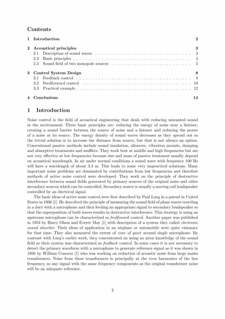
Active noise control concentrated on reducing noise from the exhaust and the basic conceptis illustrated in figure 12 where we can see a plan top view of locomotive hood with number ofloudspeakers surrounding the exhaust and a number of microphones located near the edges thatact as residual sensors. Due to tonal characteristic of this noise a feedforward architecture wasselected. It used a tachometer on the locomotive diesel engine as the reference. This exampleused active system was set with performance goal of reducing the noise by 10 dBA. Here we usea A-weighted sound pressure level defined as

LA = 10 log(pA(t)/pref )2 dBA , (20)

where pA is the instantaneous sound pressure measured using the standard A-frequency weight-ing [2].

An active system provides 10dB reduction of noise below 250 Hz and a passive silencerprovides 5 dB of broadband noise reduction from 250 to 500 Hz and 15 dB reduction from 500to 5500 Hz. The system is illustrated in figure 13.

The performance of such system can be observed in figure 14 which shows the reduction oftonal noise at microphone on the roof due to the use of active system. Locomotive was operatingat half the full throttle. We can see significant reduction of all the important tones (peaks inspectrum) with some amplification of low-amplitude tones. The reduction of the overall soundlevel below 250 Hz is in excess of 12 dB.

12

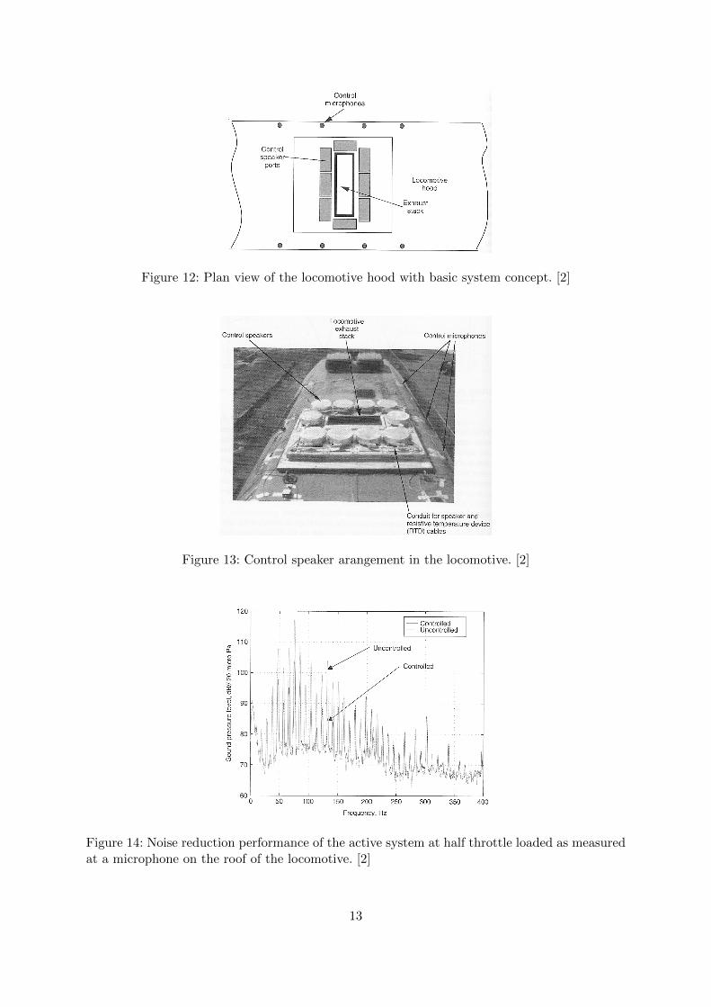
Figure 12: Plan view of the locomotive hood with basic system concept. [2]

Figure 13: Control speaker arangement in the locomotive. [2]

Figure 14: Noise reduction performance of the active system at half throttle loaded as measuredat a microphone on the roof of the locomotive. [2]

13

4 Conclusions

Active noise control can be effective way of reducing unwanted noise in the environment if weconsider it’s limitations. It works best for sound fields that are spatially simple for example lowfrequency sound waves traveling trough a duct which is an one dimensional problem. Activecontrol system are more locally oriented as often reducing noise in some local region causesincrease in the noise elsewhere. It does not reduce noise globally unless sound fields are verysimple and the primary mechanism is impedance coupling. Controlling spatially complex fieldsuch as surroundings of a house is somewhat hopelessly complex as much more so called actua-tors, microphones and loudspeakers are required. Active noise control also works well in enclosedspaces such as various vehicle cabins.

As we saw it is most effective at reducing noise in systems where the acoustic wavelengthis large compared to dimensions of the system. At higher frequencies passive methods are usu-ally much better. Therefore active noise control systems are usually not used alone since acombination of passive and active systems can cover a larger range of frequencies.

Another important factor in active noise control is whether or not the disturbance can bemeasured before it reaches the area where noise reduction is desired. This so called feedforwardcontrol is sometimes not possible and the control signal can only be calculated from error sensormeasurement. This feedback control can be very unstable under some circumstances and isusually even less effective at higher frequencies as feedforward control.

Noise that contains wide range of frequencies, so called broad band noise, is clearly muchharder to control than narrow band noise. For example, in aircraft cabin it is difficult to controlthe broadband noise of wind flowing over an aircraft fuselage, but it is much easier to controlthe tonal noise caused by propellers which move with somewhat constant rotational speed.

Special case of active noise control is adaptive noise control where controller usually employsa mathematical model of the plant dynamics and if possible one of the sensors and actuators.Sometimes the plant changes too much over time because changes in temperature and otheroperation conditions and the performance suffers. Good controller is one that monitors the plantcontinuously and updates its internal model of dynamics.

Active noise control is closely related to the field of active vibration control where we controlthe unwanted vibrations of solid mechanical systems. Sometimes it is possible to reduce thenoise of a system by reducing it’s vibration which may cause unwanted noises. For examplewhen dealing with unwanted noise in rooms and buildings, the source of outside noise for aobserver in a room are actually the walls of the room. If we reduce vibrations of these wallsthat are caused by outside noise sources we can reduce the transfer of noise from outside into aroom. Here we can control vibrations with actuators placed over the whole surface of the walls.

14

References

[1] S. J. Elliott and P. A. Nelson,Active noise control, IEEE Signal Processing Mag. 10, 12,(1993)

[2] I. L. Ver and L. L. Beranek, Noise and Vibration Control Engineering (John Wiley&Sons,New Jersey, 2006)

[3] D. T. Blackstock, Fundamentals of physical acoustics (John Wiley&Sons, New Jersey, 2000)

[4] S. M. Kuo and D. R. Morgan, Active Noise Control: a tutorial review, Proceedings of theIEEE 87, 6, (1999)

[5] (2010, November) TULARC. Online. http://stason.org/TULARC/physics/noise-control-faq/

15