Active Convolution: Learning the Shape of Convolution for Image Classification

Yunho Jeon

EE, KAIST

jyh2986@kaist.ac.kr

Junmo Kim

EE, KAIST

junmo.kim@kaist.ac.kr

Abstract

In recent years, deep learning has achieved great suc-

cess in many computer vision applications. Convolutional

neural networks (CNNs) have lately emerged as a major

approach to image classification. Most research on CNNs

thus far has focused on developing architectures such as

the Inception and residual networks. The convolution layer

is the core of the CNN, but few studies have addressed the

convolution unit itself. In this paper, we introduce a convo-

lution unit called the active convolution unit (ACU). A new

convolution has no fixed shape, because of which we can

define any form of convolution. Its shape can be learned

through backpropagation during training. Our proposed

unit has a few advantages. First, the ACU is a general-

ization of convolution; it can define not only all conven-

tional convolutions, but also convolutions with fractional

pixel coordinates. We can freely change the shape of the

convolution, which provides greater freedom to form CNN

structures. Second, the shape of the convolution is learned

while training and there is no need to tune it by hand.

Third, the ACU can learn better than a conventional unit,

where we obtained the improvement simply by changing the

conventional convolution to an ACU. We tested our pro-

posed method on plain and residual networks, and the re-

sults showed significant improvement using our method on

various datasets and architectures in comparison with the

baseline. Code is available at https://github.com/

jyh2986/Active-Convolution.

1. Introduction

Following the success of deep learning in the ImageNet

Large Scale Visual Recognition Challenge (ILSVRC) [20],

the best performance in classification competitions has al-

most invariably been achieved on convolutional neural net-

work (CNN) architectures. AlexNet [16] is composed of

three types of receptive field convolutions (3 × 3, 5 × 5,

11 × 11). VGG [21] is based on the idea that a stack of

two convolutional layers with a receptive field 3×3 is more

effective than a 5 × 5 convolution. GoogleNet [24, 25, 26]

introduced an Inception layer for the composition of various

receptive fields. The residual network [10, 11, 29], which

adds shortcut connections to implement identity mapping,

allows more layers to be stacked without running into the

gradient vanishing problem. Recent research on CNNs has

mostly focused on composing layers rather than the convo-

lution itself.

Other basic units, such as activation and pooling units,

have been studied with many variations. Sigmoid [7] and

tanh were the basic activations for the very first neural net-

work. The rectified linear unit (ReLU) [19] was suggested

to overcome the gradient vanishing problem, and achieved

good results without pre-training. Since then, many vari-

ants of ReLUs has been suggested, such as the leaky ReLU

(LReLU) [18], randomized LReLU [27], parametric ReLU

[9], and exponential linear unit [3]. Other types of activa-

tion units have been suggested to learn subnetworks, such

as Maxout [5] and local winner-take-all [23].

Pooling is another basic operation in a CNN to reduce the

resolution and enable translation invariance. Max and aver-

age pooling are the most popular methods. Spatial pyramid

pooling [8] was introduced to deal with inputs of varying

resolution. The ROI pooling method was used to speed up

detection [4]. Recently, fractional pooling [6] has been ap-

plied to image classification. Lee et al. [17] proposed a gen-

eral pooling method that combines pooling and convolution

units. On the other hand, Springenberg et al. [22] showed

that using only convolution units is sufficient without any

pooling.

However, only a few studies have considered convolu-

tion units themselves. Dilated convolution [1, 28] has been

suggested for dense prediction of segmentation. It reduces

post-processing to enhance the resolution of the segmented

result. Permutohedral lattice convolution [14] is used to

expand the convolved dimension from the spatial domain

to the color domain. It enables pairwise potentials to be

learned for conditional random fields.

In this paper, we propose a new convolution unit. Unlike

conventional convolution and its variants, this unit does not

have a fixed shape of the receptive field, and can be used

to take more diverse forms of receptive fields for convolu-

14201

Figure 1. Concept of the ACU. Black dots represent each synapse.

The ACUs output is the summation of values in all positions pkmultiplied by weight. The position is parameterized by pk.

tions. Moreover, its shape can be learned during the train-

ing procedure. Since the shape of the unit is deformable and

learnable, we call it the active convolution unit (ACU).

The main contribution of this paper is this convolution

unit to provide greater flexibility and representation power

to a CNN for a meaningful improvement in the image clas-

sification benchmark. We explain the new convolution unit

in Section 2. In Sections 3 and 4, we report experiments of

our unit on plain and residual networks. Finally, we show

the results on a general dataset in Section 5, and conclude

the paper in Section 6.

2. Active Convolution Unit

In this section, we describe the basic concept of the

ACU. The ACU is a new type of convolution unit with posi-

tion parameters. Conventionally, the shape of a convolution

unit is fixed when the network is initialized, and is not flex-

ible. Fig. 1 shows the concept of the ACU. The ACU can

define more diverse forms of the receptive fields for con-

volutions with learnable positions parameters. Inspired by

the nervous system, we call one acceptor of the ACU the

synapse. Position parameters can be differentiated, and the

shape can be learned through backpropagation.

2.1. Capacity of ACU

The ACU can be considered a generalization of the con-

volution unit. Any conventional convolution can be repre-

sented with the ACU by setting the positions of the synapses

properly and fixing all positions. Dilated convolution can

be also represented by multiplying the dilation factor with

the position parameters. Compared to a conventional con-

volution, the ACU can generate fractional dilated convo-

lutions and be used to directly calculate the results of the

interpolated convolution. It can also be used to define Ksynapses without any restriction (e.g., cross-shaped con-

volution with five synapses, or a circular convolution with

many synapses).

(a) Basic convolution (b) Active convolution

Figure 2. Comparison of a conventional convolution unit with the

ACU. (a) Conventional convolution unit with four input neurons

and two output neurons. (b) Unlike the convolution unit, the

synapses of the ACU can be connected at inter-neuron positions

and are movable.

At the network level, the ACU converts a discrete input

space to a continuous one (Fig. 2). Since the ACU uses bi-

linear interpolation between adjacent neurons, synapses can

connect inter-neuron spaces. This lends greater representa-

tional power to the convolution units. The position param-

eters control the synapses that connect neuron spaces, and

the synapses can move around the neuron space to reduce

error.

2.2. Formulation

A convolution unit has a number of learnable filters, and

each filter is convolved with its receptive field. A filter of the

convolution unit has weight W and bias b. For simplicity,

we provide a formulation for the case with one output chan-

nel, but we can simply expand this formulation for cases

with multiple output channels. A conventional convolution

can be formulated as shown in Eqs. (1) and (2):

Y = W ∗X + b (1)

ym,n =∑

c

∑

i,j

wc,i,j · xc,m+i,n+j + b (2)

where c is the index of the input channel and b the bias. mand n are the spatial positions, and wc,i,j and xc,m,n are the

weight of the convolution filter and the value in the given

channel and position, respectively.

Compared with the basic convolution, the ACU has a

learnable position parameter θp, which is the set of posi-

tions of the synapses (Eq. (3)):

θp = {pk|0 ≤ k < K} (3)

where k is the index of the synapse and pk = (αk, βk) ∈R

2. The parameters αk and βk define the horizontal and

vertical displacements, respectively, of the synapse from the

origin. With parameter θp, the ACU can be defined as given

in Eqs. (4),(5):

Y = W ∗Xθp + b (4)

4202

Figure 3. Coordinate system of interpolation. m,n represent the

base position of the convolution αk, andβk is the displacement of

the kth synapse.

ym,n =∑

c

∑

k

wc,k · xpkc,m,n + b

=∑

c

∑

k

wc,k · xc,m+αk,n+βk+ b

(5)

For instance, the conventional 3 × 3 convolution can be

represented by the ACU with θp = {(−1,−1), (0,−1),(1,−1), (−1, 0), (0, 0), (1, 0), (−1, 1), (0, 1), (1, 1)}.

In this paper, θp is shared across all output units ym,n. If

the number of synapses, input channels, and output chan-

nels are K, C, and D, respectively, the dimensions of

weight W should be D×C×K. The additional parameters

for the ACU are 2×K; this number is very small compared

to the number of weight parameters.

2.3. Forward Pass

Because the position parameter pk is a real number,

xc,m+αk,n+βkcan refer to a nonlattice point. To obtain the

value of a fractional position, we use bilinear interpolation:

xpkc,m,n =xc,m+αk,n+βk

={Q11c,k · (1−∆αk) · (1−∆βk)

+Q21c,k ·∆αk · (1−∆βk)

+Q12c,k · (1−∆αk) ·∆βk

+Q22c,k ·∆αk ·∆βk}

(6)

where∆αk = αk − ⌊αk⌋

∆βk = βk − ⌊βk⌋(7)

m1k = m+ ⌊αk⌋,m

2k = m1

k + 1,

n1k = n+ ⌊βk⌋, n

2k = n1

k + 1(8)

Q11c,k = xc,m1

k,n1

k, Q12

c,k = xc,m1

k,n2

k,

Q21c,k = xc,m2

k,n1

k, Q22

c,k = xc,m2

k,n2

k.

(9)

We can obtain the value of the fractional position by us-

ing the four nearest integer points Qabc,k. The interpolated

value xpkc,m,n is continuous with respect to any pk, even at

the lattice point.

2.4. Backward Pass

The ACU has three types of parameters: weight, bias,

and position. They can all be differentiated and learned

thorough backpropagation. The partial derivative of weight

w is the same as that for a conventional convolution, except

that the interpolated value of xpkc,m,n (Eq. (10)) is used. The

gradient of the bias is the same as that of the conventional

convolution (Eq. (11)):

∂ym,n

∂wc,k

= xpkc,m,n , (10)

∂ym,n

∂b= 1. (11)

Because we use bilinear interpolation, the positions are

simply differentiated as defined in Eqs. (12),(13):

∂ym,n

∂αk

=∑

c

wc,k·{(1−∆βk) · (Q21c,k −Q11

c,k)

+ ∆βk · (Q22c,k −Q12

c,k)},

(12)

∂ym,n

∂βk

=∑

c

wc,k·{(1−∆αk) · (Q12c,k −Q11

c,k)

+ (∆αk · (Q22c,k −Q21

c,k)}.

(13)

The derivatives of the positions are valid in subpixel re-

gions, i.e., between lattice points. They may not be dif-

ferentiable at lattice points because we use the four near-

est neighbors for interpolation. Empirically, however, we

found that this was not a problem if we set an appropriate

learning rate for the position parameters. This is explained

in Section 2.5.

The differential with respect to the input of the ACU is

given simply as

∂ym,n

∂xpkc,m,n

= wc,k. (14)

2.5. Normalized Gradient

The backpropagated value of the position of the synapse

controls its movement. If the value is too small, the synapse

stays in almost the same position and the ACU has no effect.

By contrast, a large value diversifies the synapses. Hence,

controlling the magnitude of movement is important. The

partial derivatives with respect to position are dependent

on the weight, and the backpropagated error can fluctuate

across layers. Hence, determining the learning rate of the

position is difficult.

One way to reduce the fluctuation of the gradient across

layers is to use only the direction of the derivatives, and not

4203

the magnitude. When we use the normalized gradient of

position, we can easily control the magnitude of movement.

We observed in experiments that the use of a normalized

gradient made it easier to train and achieve a good result.

The normalized gradient of the position is defined as

∂L

∂αk

=∂L

∂αk

/Z,

∂L

∂βk

=∂L

∂βk

/Z

(15)

where L is loss function, and Z is the normalization factor:

Z =

√

(∂L

∂αk

)2 + (∂L

∂βk

)2 (16)

An initial learning rate of 0.001 is typically appropriate,

which means that a synapse moves 0.001 pixel in an iter-

ation. In other words, a synapse can move a maximum of

one pixel in 1,000 iterations.

2.6. Warming up

As noted above, the direction of movement is influenced

by weight. Since the weight is initialized with a random dis-

tribution, the movement of the synapse wanders randomly

in early iterations. This can cause the position to stick to a

local minimum; hence, we first warm up the network with-

out learning the position parameters. In early iterations, the

network only learns weights with fixed shape. It then learns

positions and weights concurrently. This helps the synapses

learn a more stable shape; in experiments, we obtained an

improvement of 0.1%–0.2% over benchmark data.

2.7. Miscellaneous

The index of synapse k starts at 0, which represents the

base position. In experiments, we fixed p0 to the origin,

where p0 = (α0, β0) = (0, 0), xp0

c,m,n = xc,m,n, and the

learning rate for p0 was set to 0. Since p0 was fixed, we did

not need to assign a parameter to it, but we set the index to

0 for convenience.

The ACU was implemented on Caffe [13]. Owing to the

calculation of bilinear interpolations, the ACU was approx-

imately 1.6 times slower than the conventional convolution

for the forward pass with a normal graphics processing unit

(GPU) implementation. If we implement the ACU using a

dedicated multi-processing API, like the CUDA Deep Neu-

ral Network library (cuDNN) [2], it can be run faster than

the current implementation.

3. ACU with a Plain Network

To evaluate the performance of the proposed ACU, we

created a simple network consisting of convolution units

Layer Name Type Size

conv0 1×1 conv 16

conv1/1 3×3 conv 48

conv1/2 3×3 conv 48

conv2/1 3×3 conv,stride 2 96

conv2/2 3×3 conv 96

conv3/1 3×3 conv,stride 2 192

conv3/2 3×3 conv 192

fc1 1×1 conv 1000

- global average-pooling

- softmax 10

Table 1. Baseline structure of the plain network.

without a pooling layer [22] (Table 1). Batch normaliza-

tion [12] and ReLU were applied after all convolutions.

We used the CIFAR dataset for the experiment [15].

CIFAR-10/100 is widely used for image classification, and

consists of 60k 32 × 32 color images: 50k for training and

10k for testing in 10 and 100 classes, respectively. The

weight parameters were initialized by using the method pro-

posed by He et al. [9] for all experiments. The positions of

the synapses were initialized with the shape of a conven-

tional 3× 3 convolution.

3.1. Experimental results

We simply changed all 3× 3 convolution units to ACUs

from the baseline. The 3 × 3 convolution unit can be sub-

stituted by an ACU with nine synapses (one is fixed: p0).

The position parameters were shared across all kernels in

the same layer; thus, 8 × 2 more parameters were required

per ACU layer. We replaced six convolution layers with the

ACU; hence, only 96 parameters were added compared to

the baseline. To test the performance only of the ACU, all

other parameters were kept constant.

The network was trained with 64k iterations by using

stochastic gradient descent with the Nesterov momentum.

The initial learning rate was 0.1, and was divided by 10 after

32k and 48k iterations. The batch size was 64, and the mo-

mentum was 0.9. We used L2 regularization, and the weight

decay was 0.0001. We warmed up the network for 10k iter-

ations without learning positions. We used the normalized

gradient for the synapses, and the learning rate was set to

0.01 times the base learning rate. When the base learning

rate decreased, so did the learning rate of the synapse, which

meant that their movement was limited over iterations.

We preprocessed input data with commonly used meth-

ods [5]: global contrast normalization and ZCA whitening.

For data augmentation, we performed random cropping on

images padded by four pixels on each side as well as hori-

4204

Network CIFAR-10(%) CIFAR-100(%)

baseline 8.01 27.85

ACU 7.33 27.11

Improvement +0.68 +0.74

Table 2. Error rate on test set with the plain network. Using the

ACU on the plain network improved accuracy over the baseline.

Figure 4. Training curve for CIFAR-10 with the plain network.

Solid lines represent training loss and the dotted line the test error.

zontal flipping, as in previous studies [5].

Table 2 presents the experimental results. The baseline

network obtained error rates of 8.01% with CIFAR-10 and

27.85% with CIFAR-100. Once we changed the convolu-

tion units to ACUs, the error rate dropped to 7.33% with

CIFAR-10, a 0.68% improvement over the baseline. We ob-

tained a similar result with CIFAR-100: the ACU reduced

the error rate by 0.74%. Fig. 4 shows the training curve for

CIFAR-10. Both the training loss and the test error were

less than those of the baseline.

3.2. Learned Position

Fig. 5 shows the results of position learning. The exact

positions were different in each trial due to the weight ini-

tialization but had similar characteristics. In the lower layer,

the ACU settled down to a conventional 3× 3 convolution.

By contrast, the upper layers tended to grow. The last ACU

was similar to the two dilated convolutions. Since we nor-

malized the magnitude of movement, all synapses moved by

the same magnitude in an iteration. Thus, this phenomenon

was not due to gradient flow. We think that the lower lay-

ers focused on capturing local features and the higher layers

became wider to integrate the spatial features from the pre-

ceding layers.

Fig. 6 shows the movement of αk in the first and the last

layers. We see the first layer tended to maintain the initial

shape of the receptive field. Unlike in the first layer, the

positions of synapses monotonically grew in the last layer.

Although the lower layer was similar to a conventional

convolution, we found that the ACU was still effective for

it. Since the synapses move continuously during training,

Figure 5. Learned position on CIFAR-10. High layers tended to

grow, and the first layer was almost identical to the conventional

convolution.

Figure 6. Movement of position. Each figure shows changes in

the horizontal position (αk) with iterations. Each figure shows the

first and the last ACU layers. Each color represents one synapse

(9 synapses in total).

the same inputs and weights do not yield the same outputs.

The output of the ACU is spatially deformed in every iter-

ation, which lends an augmentation effect without explicit

data augmentation.

4. ACU with the Residual Network

Recent work has shown that a residual structure [10, 11,

24, 29] can improve performance using very deep layers.

We experimented on our convolution unit with a residual

network and investigated how the ACU can collaborate with

residual architecture. All our experiments were based on

pre-activation [11] residual, and the experimental parame-

ters were the same as those described in the previous sec-

tion, except for network structure.

4205

Network CIFAR-10(%) CIFAR-100(%)

Basic residual 8.01 30.06

ACU 7.54 29.38

Improvement +0.47 +0.68

Bottleneck residual 7.64 27.93

ACU 7.12 27.47

Improvement +0.52 +0.46

Table 3. Error rate on test set with a residual network. Using the

ACU with the residual network improved accuracy over the base-

line.

conv3

+

conv3

conv3

conv1

+

conv1

(a) Basic (b) Bottleneck

Figure 7. Comparison of residual structures: (a) basic residual and

(b) bottleneck structure. We changed all conv3 layers to ACUs.

4.1. Basic Residual Network

The basic residual network consists of residual blocks

with two 3 × 3 convolutions in series. To check the avail-

ability of the ACU, we formed a 32-layer residual network

with five residual blocks. We used projection shortcuts to

increase the number of dimensions, where the other short-

cuts were identity.

Table 3 presents the experimental results. The basic

residual network achieved an 8.01% error rate with CIFAR-

10. We replaced all convolution units with ACUs in the

residual blocks. This yielded a 7.54% error, an improve-

ment of 0.47% over the baseline. With CIFAR-100, we ob-

tained a 0.68% improvement, which was better than that

with CIFAR-10.

4.2. Bottleneck Residual Network

A bottleneck residual unit consists of three successive

convolution layers: 1 × 1, 3 × 3, and 1 × 1 [10, 11]. The

first layer reduces the number of dimensions and the last

1 × 1 convolution restores the original dimensions. Fig. 7

shows the difference between the basic and the bottleneck

residual blocks. This architecture has a similar complexity

to that of the basic residual block, but can increase network

depth.

Figure 8. Training curve for CIFAR-10 with the residual network.

Solid lines represent training loss and the dotted line the test error.

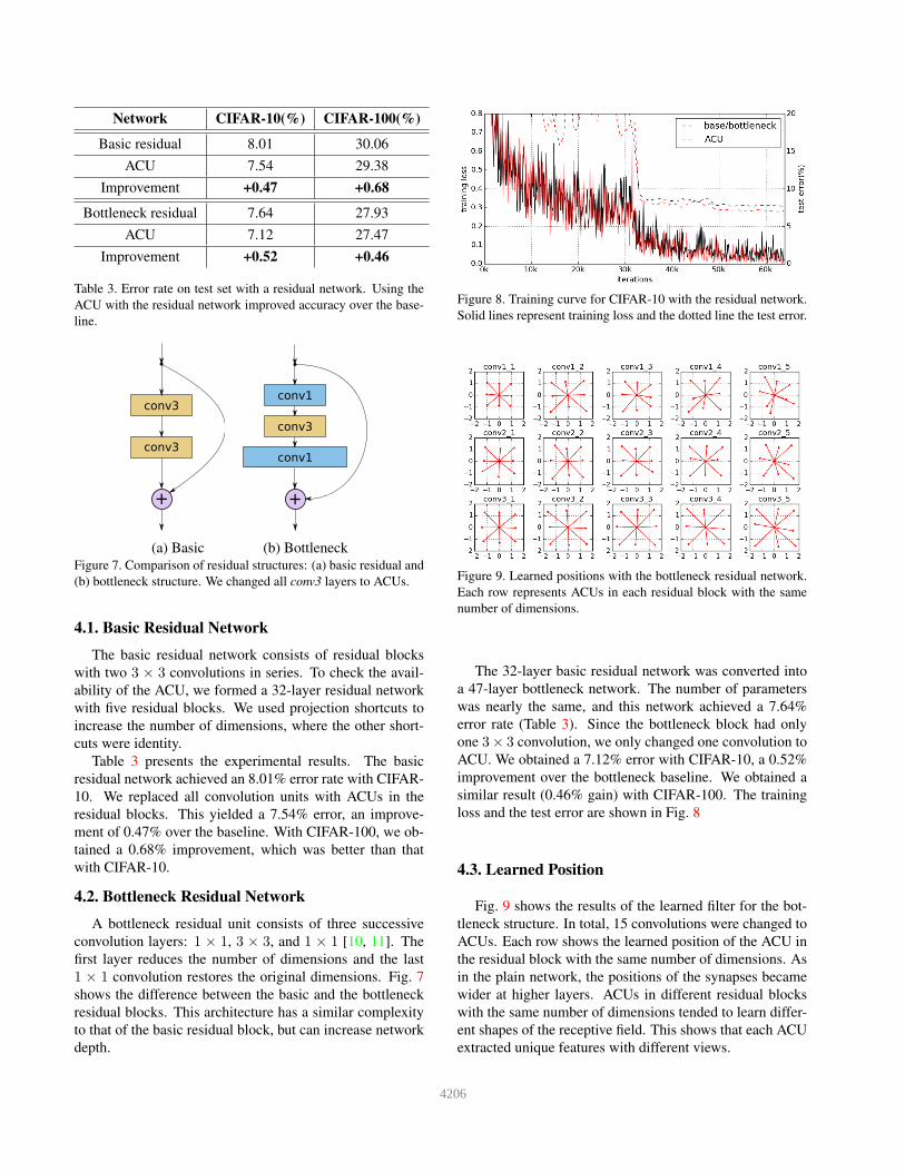
Figure 9. Learned positions with the bottleneck residual network.

Each row represents ACUs in each residual block with the same

number of dimensions.

The 32-layer basic residual network was converted into

a 47-layer bottleneck network. The number of parameters

was nearly the same, and this network achieved a 7.64%

error rate (Table 3). Since the bottleneck block had only

one 3× 3 convolution, we only changed one convolution to

ACU. We obtained a 7.12% error with CIFAR-10, a 0.52%

improvement over the bottleneck baseline. We obtained a

similar result (0.46% gain) with CIFAR-100. The training

loss and the test error are shown in Fig. 8

4.3. Learned Position

Fig. 9 shows the results of the learned filter for the bot-

tleneck structure. In total, 15 convolutions were changed to

ACUs. Each row shows the learned position of the ACU in

the residual block with the same number of dimensions. As

in the plain network, the positions of the synapses became

wider at higher layers. ACUs in different residual blocks

with the same number of dimensions tended to learn differ-

ent shapes of the receptive field. This shows that each ACU

extracted unique features with different views.

4206

5. Experiment on Place365

In the previous experiment, we had used the CIFAR-

10/100 datasets to check the validity of our approach. How-

ever these sets had consisted of small image patches of lim-

ited data size. To verify our approach in more realistic

situations, we tested the ACU with the Place365-Standard

benchmark set [30, 31].

Place365 is the latest subset of the Place2 database,

which contains more than 10 million images. Place365-

Standard is a benchmark set with more than 1.8 million

training images in 365 scene categories.

To represent plain and residual networks, we trained

AlexNet [16] and a 26-layer residual network with a bottle-

neck structure. We resized images to 256× 256 pixels, and

randomly cropped and flipped them horizontally for aug-

mentation. The networks were trained for 400k iterations

by using stochastic gradient descent. We divided the learn-

ing rate by 10 after 200k and 300k iterations, and used four

GPUs with 32 batch sizes each.

When we trained the network with the ACU, we warmed

it up network with 50k iterations with fixed positions. We

tested the networks with a validation set containing 100 im-

ages per class. Top-1 and top-5 accuracies are obtained by

the standard 10-crop testing [16].

5.1. AlexNet

Following the conventions of AlexNet, we used a weight

decay of 0.0005, and the momentum was 0.9. The initial

learning rate was 0.01. We could have changed the 11 ×11 and 5 × 5 convolutions to ACUs, but decided to only

change the 3×3 convolutions because we had not completed

analyzed the effects of large convolutions. Since the second

and third layers of the 3×3 convolution split the channels by

two in AlexNet (Fig. 11), we assigned two set of positions to

each convolution, and five sets of position parameters were

used in total.

Simply by changing the 3 × 3 convolution layers to

ACUs, we obtained an improvement of 0.79% for AlexNet

(Table 4). Fig. 10 shows the training curve of AlexNet and

its ACU network. Their accuracies were almost identical

during the warming up iterations; but after warming up (50k

iterations), test error began to decrease. This shows the ef-

fect of the ACU.

Fig. 12(a) shows the position learned after training. The

first ACU layer (conv3) was not the first layer of the net-

work (conv1), and the shape of this layer was not similar to

that of conventional convolutions, unlike in previous exper-

iments. The learned shape of the synapses is interesting in

that it is similar to combinations of two receptive fields of a

convolution. With small numbers of weight parameters, the

ACU tried to learn multiple receptive field features.

Figure 10. Training curve of AlexNet on Place365. Blue dotted

line represents the warming up iteration. After the warm up, test

error began to decrease in the ACU network.

5.2. Residual Network

To test with the residual network, we constructed a 26-

layer residual network, which was an 18-layer basic net-

work [10] converted into a bottleneck structure. Due to re-

strictions on hardware, we were not able to use deeper archi-

tecture. In the residual network, weight decay was 0.0001

and the initial learning rate was 0.1. To prevent overfitting,

we stopped training at 350k iterations.

With the residual network, we replaced all 3 convolu-

tions in the residual block, as in the previous experiment.

In total, eight convolutions were replaced with ACUs, and

thus, 128 parameters were added. With this small number

of parameters, we obtained a 0.49% gain in top-5 accuracy.

On the both of the plain and the residual networks, we

obtained a meaningful improvement using the ACU. This

results show that the ACU can be applied not only to simple

image classification as in CIFAR-10/100, but also to more

general problems.

The final shape of the ACU is shown in Fig. 12(b). As in

our previous experiments, the higher layer tended to enlarge

its receptive field. However, its coverage was greater than in

the previous CIFAR-10/100 experiment. We think that since

the image size of Place365 was larger than that of images in

the CIFAR dataset, the last layer preferred a larger receptive

field.

6. Conclusion

In this study, we introduced the ACU that contains posi-

tion parameters to provide more freedom to a conventional

convolution and allow its position to be learned through

backpropagation. Through various experiments, we showed

the effectiveness of our approach. Simply by changing the

convolution layers to our unit, we were able to boost the

performance of equivalent networks.

Since the shape of the ACU can be freely defined, we

believe that it can expand network architectures in a more

diverse manner. In this study, we shared only one set of po-

4207

Top-1(%) Top-5(%)

Network base ACU Improvement base ACU Improvement

AlexNet 51.68 52.28 0.6 81.29 82.08 0.79

ResNet26 55.33 55.71 0.38 85.24 85.73 0.49

Table 4. Classification accuracy on the validation set. We used the average score over standard 10 crops of images.

11x11

5x5

3x3

3x3

3x3

3x3

3x3

conv1 conv2 conv3 conv4/1

conv4/2

conv5/1

conv5/2

...

Figure 11. Structure of AlexNet. We changed all 3 × 3 convolu-

tions to ACU.

(a) AlexNet

(b) Residual network

Figure 12. Learned positions on Place365 dataset: (a) Result of

AlexNet. (b) Result of residual network.

sition parameters; it is possible to define other sets of posi-

tions in a layer. Using multiple set of positions, the models

representational power could be expanded. In future work,

we plan to investigate variations in ACU in greater detail.

Acknowledgement

This work was partly supported by the ICT R&D pro-

gram of MSIP/IITP, 2016-0-00563, Research on Adaptive

Machine Learning Technology Development for Intelligent

Autonomous Digital Companion.

References

[1] L.-C. Chen, G. Papandreou, I. Kokkinos, K. Murphy, and

A. Yuille. Semantic image segmentation with deep convolu-

tional nets and fully connected crfs. In International Confer-

ence on Learning Representations, 2015.

[2] S. Chetlur, C. Woolley, P. Vandermersch, J. Cohen, J. Tran,

B. Catanzaro, and E. Shelhamer. cudnn: Efficient primitives

for deep learning. arXiv preprint arXiv:1410.0759, 2014.

[3] D.-A. Clevert, T. Unterthiner, and S. Hochreiter. Fast and

accurate deep network learning by exponential linear units

(elus). In Proceedings ICLR 2016, 2016.

[4] R. Girshick. Fast r-cnn. In Proceedings of the IEEE Inter-

national Conference on Computer Vision, pages 1440–1448,

2015.

[5] I. J. Goodfellow, D. Warde-Farley, M. Mirza, A. C.

Courville, and Y. Bengio. Maxout networks. ICML (3),

28:1319–1327, 2013.

[6] B. Graham. Fractional max-pooling. arXiv preprint

arXiv:1412.6071, 2014.

[7] J. Han and C. Moraga. The influence of the sigmoid function

parameters on the speed of backpropagation learning. In In-

ternational Workshop on Artificial Neural Networks, pages

195–201. Springer, 1995.

[8] K. He, X. Zhang, S. Ren, and J. Sun. Spatial pyramid pooling

in deep convolutional networks for visual recognition. In

European Conference on Computer Vision, pages 346–361.

Springer, 2014.

[9] K. He, X. Zhang, S. Ren, and J. Sun. Delving deep into

rectifiers: Surpassing human-level performance on imagenet

classification. In Proceedings of the IEEE International Con-

ference on Computer Vision, pages 1026–1034, 2015.

[10] K. He, X. Zhang, S. Ren, and J. Sun. Deep residual learn-

ing for image recognition. In Computer Vision and Pattern

Recognition (CVPR), 2016 IEEE Conference on, 2016.

[11] K. He, X. Zhang, S. Ren, and J. Sun. Identity mappings in

deep residual networks. In Computer Vision–ECCV 2016,

2016.

[12] S. Ioffe and C. Szegedy. Batch normalization: Accelerating

deep network training by reducing internal covariate shift. In

Proceedings of The 32nd International Conference on Ma-

chine Learning, pages 448–456, 2015.

[13] Y. Jia, E. Shelhamer, J. Donahue, S. Karayev, J. Long, R. Gir-

shick, S. Guadarrama, and T. Darrell. Caffe: Convolu-

tional architecture for fast feature embedding. In Proceed-

ings of the 22nd ACM international conference on Multime-

dia, pages 675–678. ACM, 2014.

[14] M. Kiefel, V. Jampani, and P. V. Gehler. Permutohedral lat-

tice cnns. arXiv preprint arXiv:1412.6618, 2014.

[15] A. Krizhevsky and G. Hinton. Learning multiple layers of

features from tiny images. 2009.

4208

[16] A. Krizhevsky, I. Sulskever, and G. E. Hinton. ImageNet

Classification with Deep Convolutional Neural Networks.

NIPS, pages 1–9, 2012.

[17] C.-Y. Lee, P. W. Gallagher, and Z. Tu. Generalizing pooling

functions in convolutional neural networks: Mixed, gated,

and tree. In International Conference on Artificial Intelli-

gence and Statistics, 2016.

[18] A. L. Maas, A. Y. Hannun, and A. Y. Ng. Rectifier nonlin-

earities improve neural network acoustic models. In Proc.

ICML, volume 30, 2013.

[19] V. Nair and G. E. Hinton. Rectified linear units improve

restricted boltzmann machines. In Proceedings of the 27th

International Conference on Machine Learning (ICML-10),

pages 807–814, 2010.

[20] O. Russakovsky, J. Deng, H. Su, J. Krause, S. Satheesh,

S. Ma, Z. Huang, A. Karpathy, A. Khosla, M. Bernstein,

A. C. Berg, and L. Fei-Fei. ImageNet Large Scale Visual

Recognition Challenge. International Journal of Computer

Vision (IJCV), 115(3):211–252, 2015.

[21] K. Simonyan and A. Zisserman. Very Deep Convolu-

tional Networks for Large-Scale Image Recognition. arXiv

preprint arXiv:1409.1556, pages 1–14, 2015.

[22] J. T. Springenberg, A. Dosovitskiy, T. Brox, and M. Ried-

miller. Striving for Simplicity: the All Convolutional Net.

ICLR, pages 1–14, 2015.

[23] R. K. Srivastava, J. Masci, S. Kazerounian, F. Gomez, and

J. Schmidhuber. Compete to compute. In Advances in neural

information processing systems, pages 2310–2318, 2013.

[24] C. Szegedy, S. Ioffe, and V. Vanhoucke. Inception-v4,

inception-resnet and the impact of residual connections on

learning. arXiv preprint arXiv:1602.07261, 2016.

[25] C. Szegedy, W. Liu, Y. Jia, P. Sermanet, S. Reed,

D. Anguelov, D. Erhan, V. Vanhoucke, and A. Rabinovich.

Going deeper with convolutions. In Computer Vision and

Pattern Recognition (CVPR), 2015.

[26] C. Szegedy, V. Vanhoucke, S. Ioffe, J. Shlens, and Z. Wojna.

Rethinking the inception architecture for computer vision.

arXiv preprint arXiv:1512.00567, 2015.

[27] B. Xu, N. Wang, T. Chen, and M. Li. Empirical evaluation of

rectified activations in convolutional network. arXiv preprint

arXiv:1505.00853, 2015.

[28] F. Yu and V. Koltun. Multi-scale context aggregation by di-

lated convolutions. In ICLR, 2016.

[29] S. Zagoruyko and N. Komodakis. Wide residual networks.

arXiv preprint arXiv:1605.07146, 2016.

[30] B. Zhou, A. Khosla, A. Lapedriza, A. Torralba, and A. Oliva.

Places: An image database for deep scene understanding.

arXiv preprint arXiv:1610.02055, 2016.

[31] B. Zhou, A. Lapedriza, J. Xiao, A. Torralba, and A. Oliva.

Learning deep features for scene recognition using places

database. In Advances in neural information processing sys-

tems, pages 487–495, 2014.

4209