Active control of jet mixing

C.C.L. Yuan, M. Krstic and T.R. Bewley

Abstract: A control law to improve jet flow mixing is presented. The control law employs a pair ofactuators at the jet nozzle exit that act on the shear layers near the corners by blowing andsubtracting fluid in an anti-symmetric fashion and a sensor downstream or at the nozzle exit with atime delay that measures the pressure difference across the nozzle diameter. A 2-D jet flow isnumerically simulated along with massless/mass particles and a passive scalar. The mixingenhancement produced by these controllers is demonstrated visually by snapshots of the vorticity,streaklines, particle distribution and scalar field. Probability function for the particles and the scalarfield are constructed, which serve as an index of mixing quality and the effectiveness of thecontrollers. This closed-loop control law successfully alters the jet flow and improves the mixing ofparticles with mass and passive scalar.

1 Introduction

Jet flow has been thoroughly studied through theory [1],experiment [2–5] and numerical simulations [6]. Threeregions were observed to develop in experiments: (i) thenear field; (ii) the transition field; and (iii) the far field.In the near field, two shear layers develop separately witha near-constant centreline streamflow direction velocity.Shear layers appear in the transient field as the jet flow startsto enter the fully developed region. Self-similar profiles areobserved in the far field where the mean velocity profilesexperience a linear growth of the jet width and a lineardecay of the square-of-centreline velocity. The mean streamdirection velocity profiles are observed to have a similarbell-shape in all three regions with a smaller centrelinevelocity and a wider width further downstream. A largenumber of unstable modes have been observed in the thinshear layers close to the nozzle whereas only the first helicalmode has been observed in the fully developed jet at somedistance from the end of the potential core [7]. Welldeveloped parabolic velocity profiles at the nozzle exit leadto the initial dominance of the sinuous mode, i.e. the firsthelical mode of instability [8]. The simulation results of a jetflow without a controller performed in this study closelycoincide with the above observations.

The enhancement of jet flow mixing is frequentlydesirable in many engineering applications. For instancea well mixed air=fuel mixture can improve the overallcombustor performance by increasing the combustionefficiency, reducing combustion instability and undesiredemissions. Stealth plays a crucial role in the survivability ofa warplane. A ground attack plane normally flies at lowaltitude and thus places it in danger of being tracked by aninfrared-homing anti-air missile, e.g. the lightweight stingermissile. The main source of infrared signature is at the jet

nozzle exit, and this can be significantly reduced by anefficient mixing mechanism to quickly disperse the hotgases. A lighter and cheaper material can reduce themanufacturing cost of the lift flap of a C-17, provided thatjet exhaust mixing is used to reduce thermal stresses [9].

Many different techniques have been studied to amplifyor to excite the unstable modes of a jet flow to increase themixing quality. Several configurations of static tabs at thejet nozzle exit have been experimentally and numericallyexamined [2]. Non-circular jets have also receivedconsiderable attention and have been thoroughly studied.The results of the experimental and numerical studies onnon-circular, rectangular, square and elliptic, nozzle jets canbe found in a survey by Gutmark and Grinstein [10]. Inaddition to these passive methods, different configurationsof secondary jets have also been studied. Fuel has beeninjected at a constant frequency through circumferentialholes parallel to the main air jet at the exit plane to obtainsoot reduction and more energy release in [11]. High-amplitude low-mass flux-pulsed slot jets blowing normal tothe shear layers of the main jet near the nozzle exit planehave been examined experimentally in [12] and numericallyin [9]. These transverse jets with constant pulsatingfrequencies effectively excite the unstable modes and thussignificantly alter the development of jet flows. Lardeauet al. [13] have simulated two auxiliary jets, one with andone without constant pulsating frequencies being injectedinto the main jet with an impinging angle of 45�; andsuccessfully reduced the jet potential core and spread of thejet expansion. MEMS-based micro-flap actuators distribu-ted along a round nozzle have also been employedsuccessfully for the (open-loop) control of a jet flow bySuzuki et al. [14].

The control methods studied in these previous works areeither passive or open-loop in nature. A closed-loop controllaw will be developed in this study to continuously monitorthe jet flow parameter and update the actuator on-line so thatthe mixing quality can be improved. To the best of theauthors’ knowledge, this is the first attempt to control jetflow mixing using a closed-loop control law.

2 Numerical setup and technique

The equations governing the jet flow in the present caseare non-dimensionalised incompressible Navier–Stokes

q IEE, 2004

IEE Proceedings online no. 20041053

doi: 10.1049/ip-cta:20041053

The authors are with the Department of Mechanical and AerospaceEngineering, University of California at San Diego, La Jolla, CA92093-0411, USA

Paper first received 17th September 2003 and in revised form 23rd July2004

IEE Proc.-Control Theory Appl., Vol. 151, No. 6, November 2004 763

equations and the continuity equation (in primitivevariables):

@ui

@tþ@uiuj

@xj

¼ � @p

@xi

þ 1

ReD

@2ui

@x2j

ð1Þ

H � u ¼ 0 ð2Þ

where ui is the velocity, u ¼ ðu1; u2Þ is the velocity vector,p is pressure field, xi is the spatial coordinate, and thesubscripts i and j represents the spatial direction, ‘1’ is forthe streamflow direction and ‘2’ is for the normal direction.The Reynolds number ReD is based on the jet nozzlediameter D and the centreline velocity at nozzle inlet U0:The governing equations, (1) and (2), are used to simulatea spatially evolving jet flow in the computational domainconsisting of a jet nozzle with dimensions of 2 � 1 and anopen field with dimensions of 50 � 40: All the units arenormalised by the nozzle diameter D. The computationaldomain is shown in Fig. 1. The numerical method used inthis research was developed for a backward facing stepsimulation [15] and a boundary control problem of channelflow [16], and is modified for the current geometry.Therefore, it will be stated here with only a minimalexplanation, however, a detailed derivation of this numeri-cal scheme can be found in [15].

The origin of the coordinate system is at the centre of thenozzle exit plane. In the nozzle, the grids are equispaced inthe streamflow direction, and stretched in the normaldirection with a hyperbolic tangent function. In the openfield, a 1-D stretching formula [17] is adapted for thestreamflow distribution; in the normal direction, the gridlines in the jet core are equal to the ones in the nozzle, andare distributed using the same 1-D stretching formulaotherwise. This stretching formula gives a smooth transitionfrom the finer grids used near the walls and around the shearlayers to the coarser grids used in the far field. The total gridnumbers are 201 � 175 in the open field and 11 � 15 in thenozzle. Sampled grid lines are also illustrated in Fig. 1.A finite-difference scheme is used for the spatial derivatives.Whereas the interior nodes use a second-order accuratecentral-difference scheme, the boundary nodes use asecond-order inward-biased scheme to keep the overallaccuracy second-order in space. The primitive variablesnamely the pressure at the cell centre and the velocities atthe grid lines are stored in a staggered grid. The momentumequations are evaluated at the corresponding velocity nodes,and the continuity equation is enforced at the pressure node.

The illustration of a staggered grid can also be found inFig. 1. Note that the half-grid lines are exactly locatedat the midpoint between primary grid lines, thus thecentral-difference approximations of the spatial derivativesacross the half-grid lines are exactly second-order accurate.However, the primary grid lines are not located exactlyhalfway between half-grid lines because of a non-uniformgrid distribution, and the differentiations across theseprimary grid lines are thus not fully second-order accurate.Therefore, the overall accuracy in space is only quasi-second-order accurate even when the second-orderpreservation formula for velocity interpolation to adjacentgrids is used.

A fine resolution near the solid walls and around the shearlayers is necessary to resolve the large velocity gradient.The minimum grid spacing is 0.19 in the streamflowdirection and 0.04 in the normal direction, and the ratio ofthe maximum to the minimum grid spacing is 4.71 and23.29 in the streamflow direction and normal direction,respectively. The grid distribution in the normal directionseverely limits the time step, and therefore it is preferred tocompute the derivatives in the normal direction implicitlywhereas the derivatives in the streamflow direction aretreated explicitly. This leads to a hybrid time integrationscheme using a low storage third-order Runge–Kuttascheme for the explicitly treated terms and a second-orderCrank–Nicholson scheme for the implicitly treated terms,respectively (see [15, 16, 18] for further information).The overall accuracy in time is thus second-order.

The discretised Navier–Stokes equations take the form:

uki � uk�1

i

Dt¼ bk½BðukÞ � Bðuk�1Þ � 2bk

dpk

dxi

þ gkAðuk�1Þ þ zkAðuk�2Þ ð3Þ

AðuiÞ ¼ nd2ui

dx21

� du1ui

dx1

ð4Þ

BðuiÞ ¼ nd2ui

dx22

� du2ui

dx2

ð5Þ

where b; g and z are the coefficients of the third-orderRunge–Kutta scheme, AðuiÞ and BðuiÞ are the explicit andimplicit operator respectively, and n ¼ 1=ReD is thenormalised kinematic viscosity. The superscript and sub-script k represents the Runge–Kutta substep, where k ¼ 0 isat time step n and k ¼ 3 is at time step n þ 1:

Fig. 1 Computational domain, sampled grid lines, staggered grid illustration, and locations of sensors and actuators

IEE Proc.-Control Theory Appl., Vol. 151, No. 6, November 2004764

A no-slip condition is applied along all the solid walls.The inflow condition at the inlet of the jet nozzle is aconstant parabola for the stream direction velocity with aunit centreline velocity U0 ¼ 1; and it is a still field for thetransverse velocity u2 ¼ 0: This inflow boundary conditiongives us a constant mass flux throughout the computationprocess. In order to pass the vortical structure through thecomputation domain smoothly, a convection boundarycondition is used along the open boundaries in the openfield:

@ui

@tþ Ucon

@ui

@n¼ 0 ð6Þ

where Ucon is a convection velocity and is chosen to be halfof U0 in the streamflow direction and a quarter of U0 in thenormal direction, and n is the direction normal to theboundary. This convection boundary condition is computedat full time step by a forward-in-time inward-in-spacescheme and is interpolated for each Runge–Kutta substep.To further decrease the non-physical effect of the fictitiousboundary of the computation domain, a buffer zone oflength ten is inserted in each open boundary. A dampingterm based on the computed boundary condition is added tothe right-hand side of the discretised Navier–Stokesequation, (3). These extra damping terms in the overlap ofthe buffer zones along the streamflow and normal directionsare calculated by a weighted ratio of the distance from twoboundaries.

Equation (3) is advanced in time by a fractional stepmethod; a non-divergence free-velocity field is solved firstand then this is projected onto a solenoidal field by apressure update. In order to treat the implicit and explicitterms in a single framework, we have implemented a hybridRunge–Kutta=Crank–Nicolson technique. The completeRunge–Kutta substep is now written out (in order of actualcomputation sequence) as follows:

�I � BðuuÞguu ¼ Dtfuk�1 � bk½Bðuk�1Þ þ 2Hpk

þ gkAðuk�1Þ þ zkAðuk�2Þg ð7Þ

H2f ¼ 1

2bkDtH � uu ð8Þ

uk ¼ uu � 2bkDtHf ð9Þ

pk ¼ pk�1 þ f ð10Þ

where uu is the intermediate velocity field which is notsolenoidal, I is the identity matrix and f is the pressureupdate. Equation (7) is the result of an implicitCrank–Nicolson scheme, and is solved through a tridiago-nal system solver. To solve the pressure update, a Poissonsolver implementing LU-decomposition is used to solve thePoisson equation, (8); the singularity of this matrixgenerated by the Poisson equation is removed byprescribing the reference value of zero at the last cellðNx1

;Nx2Þ in the open field. The divergence is computed after

each full time step to ensure a solenoidal field.In order to monitor the flow evolution, massless particles

are introduced to simulate the passive tracer. The positionsof these massless particles are governed by the equationdx=dt ¼ u; where x is the position vector of the particle, andu is the velocity vector of the flow fluid at the same point.Streaklines are constructed from the connection betweenthese particles released from the same insertion point.Particles with mass are also injected into the jet to examine

the effectiveness of the control action in a gas-particle jetflow. The particle-particle interaction is neglected due to alarge particle spacing. The Basset–Boussinesq–Oseenequation, the governing equation of particle evolution, canbe justifiably simplified for gas-particle flow with a verysmall density ratio between the carrier phase and thediscrete phase ðrf=rp 10�3Þ and with the assumption ofone-way coupling that only the carrier phase has influenceon the particle but not vice versa [19]. Thus, the particles aregoverned by these non-dimensionalised motion equations:

dv

dt¼ f

Stðu � vÞ ð11Þ

dx

dt¼ v ð12Þ

where v is the particle velocity, f ¼ 1 þ 0:15Re0:687p is a

correction factor which is a function of the particle relativeReynolds number Rep ¼ ðdpju � vjÞ=n; dp is the particlediameter, n is the kinematic viscosity of the flow, and St isthe particle Stokes number which is the ratio of theparticle’s momentum response time to the flow fieldcharacteristic time. By definition, a larger Stokes numberrepresents a larger or heavier particle, and a smaller orlighter particle has a smaller Stokes number. Three differentStokes numbers, 0.1, one, and ten, are simulated to examinethe response of light, medium and heavy particles to thecontrol action. The particles are fed into the flow at the jetexit plane with normal coordinates y ¼ 0 and �0:5 everytime step, and (11) and (12) are advanced in time by thethird-order Runge–Kutta scheme.

In addition to the streaklines and particles with mass, anevolution equation of a passive scalar S is also simulated:

@S

@tþ@ujS

@xj

¼ 1

ReD

1

Sc

@2S

@x2j

ð13Þ

where Sc is the Schmidt number defined as the ratio of thefluid kinematic viscosity to the scalar’s molecular diffusiv-ity and it is set to unity in this study. That this scalar is‘passive’ means that the scalar’s evolution is influenced bythe flow, but that the scalar itself does not have anyinfluence on the flow. The evolution of such a passive scalarprovides a useful indicator for mixing in many practicalapplications, such as combustion studies assuming fastkinetics [6]. Since the scalar field has no influence on thevelocity field, the explicit Runge–Kutta scheme is also usedto advance (13) in time, as in the particle evolutionequations. The scalar field is calculated on the pressurenode, and the first-order upwind scheme is used for thespatial derivatives of the convection terms in (13). Thescalar field has a highest possible value of one in the nozzlethroughout the whole simulation, and a lowest possiblevalue of zero at the open boundaries initially. Theconvection boundary condition is used. The details ofhow to advance particle and scalar fields in time arecontained in [18].

3 Control strategy

Parekh et al. [12] demonstrated tremendous increases inmixing by exciting the flapping mode which is the dominantmode in a low Reynolds number jet flow. This isaccomplished by exciting the jet shear layer adjacent tothe jet nozzle exit with pulsed fluidic actuators.

In [20] and [21], an active feedback control was appliedto excite the instability mechanisms in a 2-D channel flowand a 3-D pipe flow. Mixing was considerably enhanced

IEE Proc.-Control Theory Appl., Vol. 151, No. 6, November 2004 765

with an extremely small control effort by applying acarefully designed closed-loop boundary control law.Decentralised wall-normal suction and blowing was usedfor actuation with the pressure difference between oppositepoints on the wall for sensing. The advantage of thisfeedback control law is its simplicity: a static output-feedback law and a zero net mass flux.

A similar feedback control law is now adapted for jet flowmixing. The controller consists in a pair of actuators actingin the streamflow direction at the jet lips in an anti-symmetric fashion U1ðtÞ ¼ �U2ðtÞ; and a sensor measuringthe pressure difference across the nozzle diameterDp ðx1; t � tÞ ð¼ py¼�0:5 � py¼þ0:5Þ: The control laws aredepicted in Fig. 1 and written out for a configuration of asensor downstream and a sensor at the nozzle exit with timedelays, respectively:

U1ðtÞ ¼ KDpðx1; tÞ ð14Þ

U1ðtÞ ¼ KDpð0; t � tÞ ð15Þwhere K is the feedback gain, and t is the time delay. Thecontrol law is computed at each time step and kept constantthrough a full time step. The saturation of the actuatormagnitude is set to the maximum centreline velocity at thenozzle inlet U0; and the actuator change rate is saturated at0:2U0 between time steps. The net mass flux introduced bythese controllers is kept at zero by injecting and subtractingthe same amount of mass.

The control laws (14) and (15) both use delayed pressuremeasurements, the latter with a temporal delay and theformer with spatial delay. The effect of both is similar andthe amount of delay applied affects the damping of thedominant (flapping) mode of vortex shedding as well as thefrequencies of additional unstable modes that becomeexcited. An optimal level of delay exists, as will beillustrated in subsequent Sections. Whereas the spatialdelay (14) is intuitively clear (sufficiently far downstreamvortex shedding is sufficiently developed so that measure-ments of the flow perturbation can be used to amplify it bycontrol) the temporal delay (15) is physically less clear but itis physically implementable because a non-intrusivepressure sensor can be placed at the nozzle. In summary,the implementable temporal delay emulates the effect of theintuitive spatial delay.

More than from any other source, the motivation for thefeedback strategies (14) and (15) comes from the work ofAamo et al. [21] on the control of mixing in pipe flows.In [21] it was shown using an energy-based argument that asimilar strategy achieves an optimal enhancement of flowquantities related to mixing. The effect on mixing wasconfirmed by simulations. While the control strategy in [21]has inspired (14) and (15), the analogy is not complete.In [21] the 3-D pipe flow is controll using actuators andsensors distributed on the (2-D) wall of the pipe. In the jetflow problem here, which is 2-D, point actuation andsensing are employed (i.e. 0-D). Due to the ‘underactuated’nature of the problem we consider that the use of a delay(or some more complex compensator dynamics) is essential.We demonstrate that a delay is sufficiently capable ofsignificantly affecting the flow, although more complex,fully theoretically justified control strategies, might be evenmore effective.

4 Simulation results

4.1 Uncontrolled jet

Simulation results for the jet flow without a controller at aReynolds number ReD ¼ 100 are used to validate the code

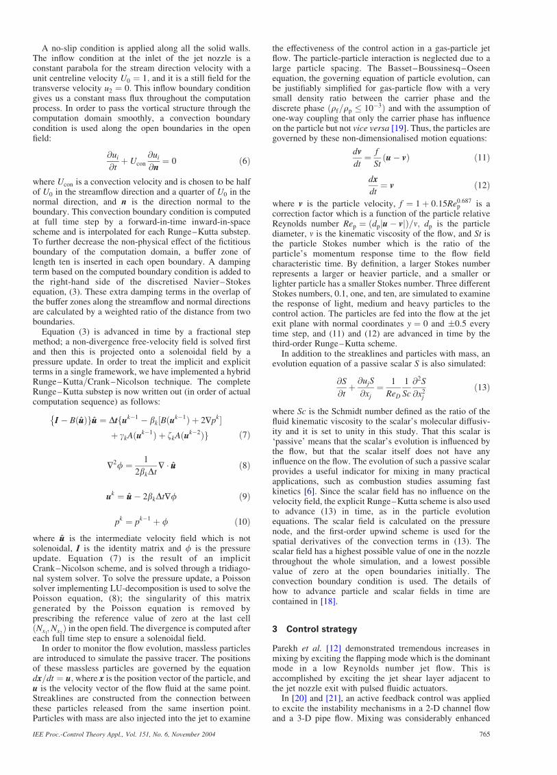
relative to theory and previous works, and serve as the basecase. The jet’s half-width growth rate, centreline velocitydecay rate and normalised velocity profiles of the statisticaldata at t ¼ 1000 after the simulation is initiated, areexamined. The jet’s half-width is found to grow linearlyand the squared ratio of the centreline velocity to the exitcentreline velocity also has a linear growth along thestreamflow direction of the jet beyond the potential core.The half-width growth rate and centreline velocity decayrate can be described by linear functions:

d1=2ðx1Þ ¼ Cdðx1 þ xdÞ ð16Þ

U0

ucðx1Þ

� �2

¼ Cuðx1 þ xuÞ ð17Þ

where d1=2; the half-width, is the distance between thecentreline and the point where the mean streamflowvelocity is half that of the centreline velocity uc; Cd andCu are the growth and decay rates, and xd and xu are thevirtual origins. The virtual origin is a point source locatedupstream of the nozzle exit where a theoretical jet isinitiated. The theoretical jet initiated from this virtual originwill have the same momentum as the actual momentum of areal jet discharged at the nozzle exit, and will produce a self-similar velocity profile beyond the potential core.

The half-width growth and centreline velocity decay ofthe current results are plotted in Figs. 2a and 2b,respectively, along with plots of the least-square fit linearfunction. The linear relation of the growth and decay ratewith the stream coordinate is obvious. The slopes and virtualorigins of (16)–(17) obtained from this work and previousexperimental and numerical works are also listed in Table 1for comparison. The current results show a slower growthrate and virtual origin that is further upstream for the half-width, whereas the decay rate and virtual origin fall in thenominal range for centreline velocity. One should keep inmind that the initial condition at the jet nozzle exit has longlasting effects on the jet flow development downstream. Thevelocity profile at the jet nozzle in our study is a welldeveloped channel flow which gives almost no near fieldand the jet flow directly enters the transient field. Therefore,a virtual origin that is further upstream and a slower growthrate is expected.

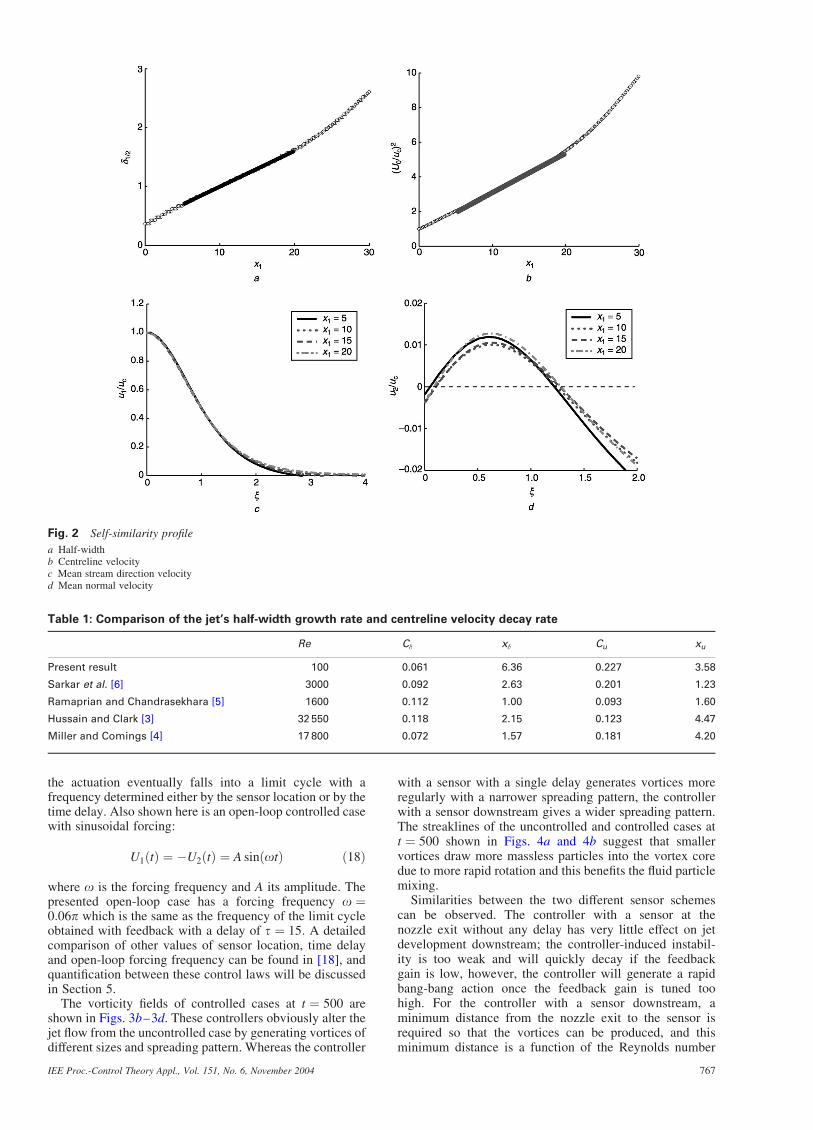
The normalised stream direction velocity and transversevelocity are plotted against a normalised coordinate �between x1 ¼ 5 to x1 ¼ 20 in Figs. 2c and 2d, respectively.The normalised coordinate � is a cross-stream similarityvariable defined as the normal coordinate x2 as a function ofthe half-width d1=2ðx1Þ: In the fully developed region, theprofiles of the normalised velocity in the streamflow direc-tion u1=uc at different streamflow locations, plotted against�; collapse onto a single curve. The profiles of velocity in thenormal direction u2=uc also become self-similar with littleinconsistency due to the effect of the 2-D simulation. Despitethe small deviations in the half-width growth, the currentresults agree with the theoretical and experimental results.The vorticity plot and streaklines of an uncontrolled jet att ¼ 500; shown in Fig. 3a and Fig. 4a, confirm that thedominant unstable mode is the flapping mode.

4.2 Controlled jet

Two closed-loop controlled cases with the same feedbackgain but different sensor configurations, one with a sensordownstream at x1 ¼ 5 and the other with a sensor at the jetexit with a delay of t ¼ 15; are presented to demonstrate theeffectiveness of the control laws (14) and (15) by comparingthem with the uncontrolled case. Due to the feedback-loop,

IEE Proc.-Control Theory Appl., Vol. 151, No. 6, November 2004766

the actuation eventually falls into a limit cycle with afrequency determined either by the sensor location or by thetime delay. Also shown here is an open-loop controlled casewith sinusoidal forcing:

U1ðtÞ ¼ �U2ðtÞ ¼ A sinðotÞ ð18Þ

where o is the forcing frequency and A its amplitude. Thepresented open-loop case has a forcing frequency o ¼0:06p which is the same as the frequency of the limit cycleobtained with feedback with a delay of t ¼ 15: A detailedcomparison of other values of sensor location, time delayand open-loop forcing frequency can be found in [18], andquantification between these control laws will be discussedin Section 5.

The vorticity fields of controlled cases at t ¼ 500 areshown in Figs. 3b–3d. These controllers obviously alter thejet flow from the uncontrolled case by generating vortices ofdifferent sizes and spreading pattern. Whereas the controller

with a sensor with a single delay generates vortices moreregularly with a narrower spreading pattern, the controllerwith a sensor downstream gives a wider spreading pattern.The streaklines of the uncontrolled and controlled cases att ¼ 500 shown in Figs. 4a and 4b suggest that smallervortices draw more massless particles into the vortex coredue to more rapid rotation and this benefits the fluid particlemixing.

Similarities between the two different sensor schemescan be observed. The controller with a sensor at thenozzle exit without any delay has very little effect on jetdevelopment downstream; the controller-induced instabil-ity is too weak and will quickly decay if the feedbackgain is low, however, the controller will generate a rapidbang-bang action once the feedback gain is tuned toohigh. For the controller with a sensor downstream, aminimum distance from the nozzle exit to the sensor isrequired so that the vortices can be produced, and thisminimum distance is a function of the Reynolds number

Fig. 2 Self-similarity profile

a Half-widthb Centreline velocityc Mean stream direction velocityd Mean normal velocity

Table 1: Comparison of the jet’s half-width growth rate and centreline velocity decay rate

Re C� x� Cu xu

Present result 100 0.061 6.36 0.227 3.58

Sarkar et al. [6] 3000 0.092 2.63 0.201 1.23

Ramaprian and Chandrasekhara [5] 1600 0.112 1.00 0.093 1.60

Hussain and Clark [3] 32 550 0.118 2.15 0.123 4.47

Miller and Comings [4] 17 800 0.072 1.57 0.181 4.20

IEE Proc.-Control Theory Appl., Vol. 151, No. 6, November 2004 767

of the flow. A minimum feedback gain is also essentialto sustain the instability introduced by the actuator and tobreak it up into vortices. For the control law with asensor at the jet exit with a delay, in order to be able togenerate vortices and to maintain this generation,the delay and feedback gain must meet minimumdemand values, too. Even although these similaritiesare observed, no direct relation between the sensorlocation and the time delay length for these two sensorconfigurations is available. For the downstreamsensor configuration the generated vortices go throughdifferent spatial developments and various convectionvelocities before reaching the sensor. This feedback-loop

involves the uncertainty in the spatial development. Onthe other hand, the sensor at the exit is less influenced bythe downstream spatial development of the flow.

By carefully tuning the feedback gain and delay, a controllaw with a delayed sensor can produce a very similar flowfield to the one generated by the controller with adownstream sensor. The underlining mechanism for thisexchange between the two types of sensors is that thetimescale provided by the delay can replace the lengthscaleprovided by the sensor location. Measuring the pressuredifference at the jet nozzle exit is more practical than takinga measurement downstream, and we shall concentrate on thecontrollers with delayed sensors.

Fig. 3 Vorticity fields at t ¼ 500

a Uncontrolled jetb x1 ¼ 5c t ¼ 15d Open-loop forcing

Fig. 4 Streaklines at t ¼ 500

a Uncontrolled jetb x1 ¼ 5c t ¼ 15d Open-loop forcing

IEE Proc.-Control Theory Appl., Vol. 151, No. 6, November 2004768

4.3 Particles with mass

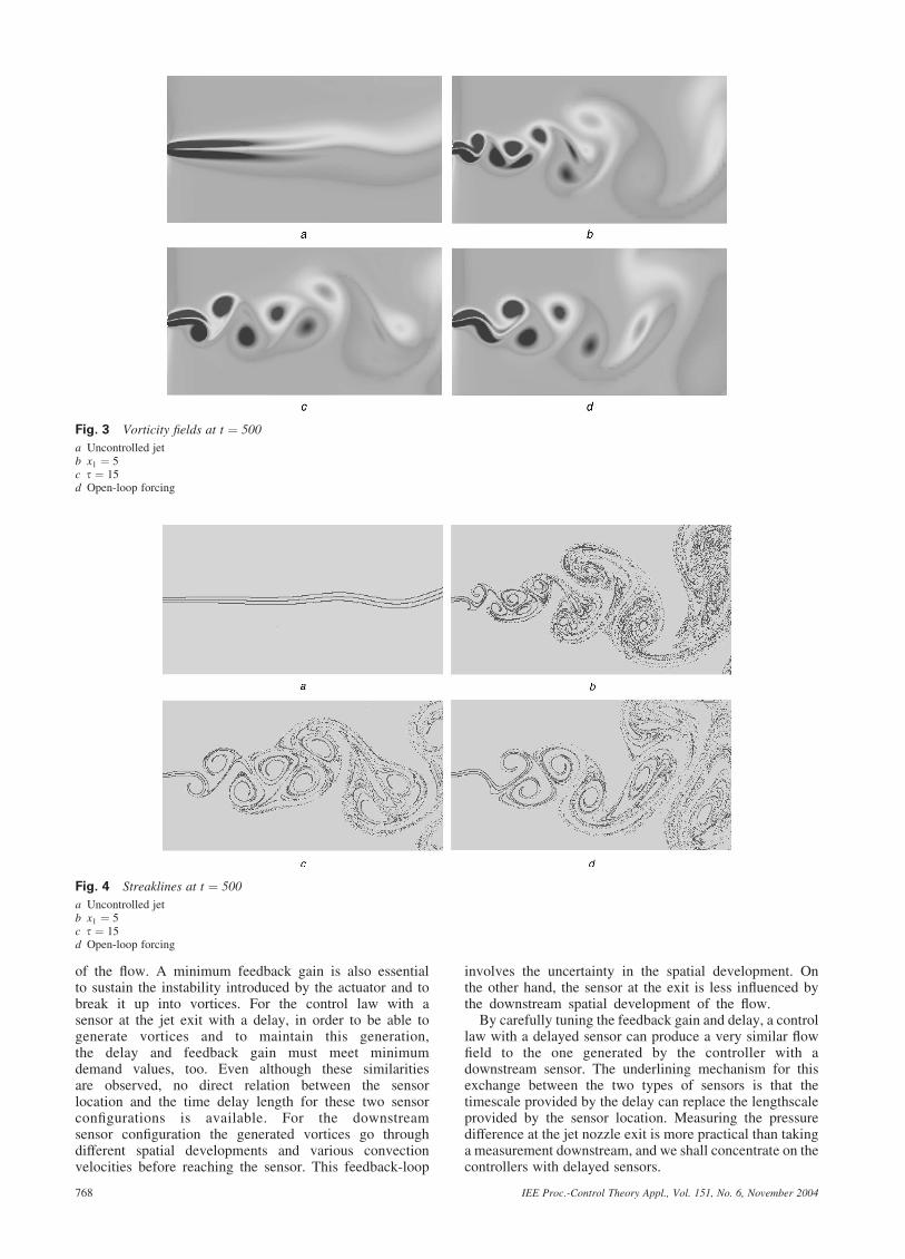
The distribution of particles with mass is an essential tool tostudy the gas-particle jet flow. The closed-loop controlledcase using the sensor at the exit with a delay t ¼ 15 is usedto show the results of particle mixing. The distribution ofparticles with different Stokes numbers at t ¼ 500 is shownin Fig. 5 along with the streaklines. Whereas the lightparticles are attracted into the vortical structure andtransported by the vortices, the heavy particles are not sotransported. This result is consistent with the observations of[19] and [22].

The light particles with St ¼ 0:1 closely follow the fluidmotion acting like a tracer. The distribution of particles

almost duplicates the streaklines except that fewer particlesare attracted into the eddy cores. Since the particle mass isconsidered in the evolution, the additional drag force slowsdown the particle motion and the particle does not followthe fluid motion instantaneously.

Particles with a unity Stokes number tend to centrifugeout of the vortex cores and concentrate on the peripheriesof the vortical structures. The response time of themedium particles with St ¼ 1 is too slow to followthe large velocity gradient temporally and spatially insidethe vortices. Thus, they are radiated out from the high-vorticity region eddy core and accumulate betweenvortices. This is also called a demixing phenomenon byCrowe et al. [19].

Fig. 5 Particle distribution of controlled jet (sensor with delay t ¼ 15)

a Streaklinesb St ¼ 0:1c St ¼ 1d St ¼ 10

Fig. 6 Scalar field at t ¼ 500

a Uncontrolled jetb x1 ¼ 5c t ¼ 15d Open-loop forcing

IEE Proc.-Control Theory Appl., Vol. 151, No. 6, November 2004 769

For a large Stokes number, the inertia of heavyparticles is too great to let the carrier fluid significantlyinfluence the particle motion. The particles travel a longdistance before the vortices start to have any influence onthem. A small fraction of the medium particles in the farfield are centrifuged by the radial force of the strongvortices, but most of the particles are directly convecteddownstream but are not dispersed by the vortices. Once aheavy particle is pushed by the surrounding fluid, it willnot respond fast enough to any subsequent opposingvelocity vectors due to its long momentum responsetime. This slow reaction of the heavy particles to thefluid motion leaves the traces of vortex passage shown inFig. 5d in which particles are pushed outwards from theeddies and slowly convected downstream by subsequentfluid motion.

The closed-loop controller has shown a promising resulton the mixing enhancement of particles with mass, yet theperformance degrades as the particles become heavier.

4.4 Passive scalar

The scalar field for an uncontrolled and a controlled jetobtained using different control laws is shown in Fig. 6. Thecontrolled jet evidently has a better mixed scalar field thanthe uncontrolled jet. The scalar dispersion is found to bemostly carried out by the rotation, convection and spreadingof generated vortices. A smaller vortex with a strongvorticity seems to constrain the diffusion of the passivescalar. On the other hand, wider vortex spreading helps toconvect and transport the scalar field. Once the vortex ringsare convected downstream and expanded, the diffusioneffect becomes more apparent as the intensity of thevorticity subsides.

The diffusivity of the studied scalar is comparable to thatof the carrier fluid if the Schmidt number is set to unity.Thus, the evolution of the scalar is mainly dominated by theconvection terms. This can be observed by comparing thescalar field plots with the vorticity plots such that the con-centration of the scalar is consistent with the vorticalstructure.

5 Discussion

Without the length separation provided by the sensordownstream or time separation by the sensor at the nozzleexit with a delay, the controller produces insufficientinfluence on the jet. Another important factor is the

amplitude of the actuator. The interval between an actuatorswitching directions is determined by the sensor, but thefeedback gain decides whether the perturbation induced bythe actuation will grow strong enough to break up into avortex or will just subside. The time histories of a controlsignal for the single delay case t ¼ 15 with two differentfeedback gains, K ¼ 15 and 10, upto t ¼ 500; are plotted inFig. 7a. With a feedback gain higher than the minimumrequirement ’13; the actuation grows exponentially until itreaches saturation and it then enters a limit cycle; with afeedback gain lower than the minimum requirement, thecontrol decays and provides insufficient perturbation to theflow. The control change rate is plotted in Fig. 7b, and it islimited to a maximum value of 0:2U0:

A measure of mixing is necessary to quantify theeffectiveness of the presented control law. Severaldiagnostic tools for finite-time mixing are available. Thenotions of finite-time stable and unstable manifolds, wereintroduced and applied in [23–25] where as [26] and [28]examined the mixing property using statistical properties.(Please see these references for more details.) In this study, aprobability function similar to the one used in [20, 21] isconstructed for both the particle distribution and scalar field.

The physical domain is divided into N boxes, and theprobability P of a box holding the number of particles np orscalar value ns in a certain range at time t is calculated by:

PpðtÞ ¼1

Np

XNp

i¼1

evalð25 nipðtÞ 75Þ ð19Þ

PsðtÞ ¼1

A

XNs

i¼1

evalð0:25 nisðtÞ 0:5Þ � ai A ¼

XNs

i¼1

ai

ð20Þ

where the subscripts p and s denote particle and scalar,respectively, the superscript i indicates the ith box, eval is afunction that returns value of one if ni

p or nis falls between

the lower and the upper limit, A is the total area in thephysical domain, and ai is the area of the local cell. The boxsize for the particle probability is uniform and has a unityarea; the box size for a scalar field is not uniform and isconsistent with the computation cell. If the number ofparticles (or the scalar value) in a cell is above the upperlimit, the mixture is too dense; below the lower limit it is toothin, and in-between it is considered well mixed. One should

Fig. 7 Control signal and control change rate of controlled jet (t ¼ 15)

a Control signalb Control change rate

IEE Proc.-Control Theory Appl., Vol. 151, No. 6, November 2004770

note that this probability function is a function of time andwould be altered if the lower or upper bounds are changed.The choice of these limits which defines the mixing qualityis application dependent but this topic will not be furtherdiscussed.

In [18], closed-loop controllers based on (14) and (15)with various values for x1 and t were compared. For the casewith the downstream sensor, (14), the values x1 ¼ 0; 2.5, 5,7.5 and 10 were tested, and x1 ¼ 5 was found to give thebest performance based on the metric defined in (19) formassless particles. Similarly, for the case of a sensor at thenozzle exit with a delay (15), the values t ¼ 0; 5, 10, 15, 20and 25 were examined, and t ¼ 15 was found to give thebest result. A comparison between these two specific closed-loop controllers and open-loop forcing with same frequencyof the limit cycle of t ¼ 15 is made through (19) and (20).The probability functions of the scalar field and particleswith a mass for both uncontrolled and controlled casesare plotted in Fig. 8. Since the evolution of light particlesðSt ¼ 0:1Þ is very similar to the massless particles, acomparison of probability functions for their streaklines willnot be presented.

The controlled cases show a significant improvement inscalar mixing over the non-controlled case by doubling(downstream sensor and open-loop forcing) and tripling(sensor at nozzle exit with a delay) the probability functionvalue in the quasi-steady-state conditions. The bumpsobserved in the probability function curves are caused by

the vortex structures leaving the domain, and this confirmsthat the convection and expansion of a vortex is a significantcontributor to the scalar mixing. The delayed sensor caseshows the best performance among these three controlledcases. The holding interval of the actuation for the delayedsensor case (see Fig. 7) helps to produce stronger vorticesand to let the vortex penetrate into the downstream. Thisstrong intensity and penetration helps to keep the scalar inthe nominal range. The sensor downstream case or open-loop forcing, on the other hand, generates a wider spreadingpattern or weaker vortices such that the diffusion effectbecomes dominant but dilutes the scalar beyond the lowerlimit.

The controlled jet flows also show a better mixing qualityfor particles with mass, but the effectiveness of thecontroller decreases as the Stokes number of the particleincreases. For light particles St ¼ 0:1; the closed-loopcontrollers produce a higher probability function valuethan the open-loop forcing, and the value is three times asgreat as the one of the uncontrolled case in the quasi-steady-state conditions. For medium particles St ¼ 1; the closed-loop controlled cases still show a better performance thanthe open-loop forcing case and the value of the probabilityfunction is around double that of the uncontrolled case at theend. For heavy particles St ¼ 10; all controlled cases showno improvement on mixing from the base case. This is incontrast to the particle distribution shown in Fig. 5d inwhich the particles are very different from the uncontrolled

Fig. 8 Probability function of scalar field and particles with different Stokes numbers

a Scalar fieldb St ¼ 0:1c St ¼ 1d St ¼ 10

IEE Proc.-Control Theory Appl., Vol. 151, No. 6, November 2004 771

case. One should note that a lower limit will increase thevalue of the probability function. Apparently, a controllerthat acts solely on the carrier phase has a very limited effecton the path of heavy particles. A separate controller that actsdirectly on the particles is necessary to enhance the mixingfor heavier particles.

6 Conclusions

The formation of vortices and their interactions govern theentrainment and mixing in jet flows. The perturbationinitiated at the nozzle exit is an essential phenomenon and isresponsible for vortex break up downstream, and this is inturn is the key to mixing enhancement. The closed-loopcontrollers developed here successfully produce a vortexgeneration pattern that enhances the overall mixing.Whereas the configuration of a downstream sensor providesan idea for a control law, the length scale obtained from thesensor location can be used as the delay in the more feasibleconfiguration of a sensor at the nozzle exit.

Whereas all the controlled cases presented here showpromising results on mixing as evidenced by the snapshotstaken at the vorticity field and streaklines, the closed-loopcontroller with a sensor at the nozzle exit with a delay givesthe best mixing result measured in terms of a probabilityfunction in the scalar field and particles with a mass. Theperformance of a controller should not be decided by asingle criterion and one should take into account manyaspects, e.g. vorticity field, streaklines, distribution ofparticles or scalar, and=or probability functions of particlesor scalar. The performance criterion is application depen-dent, and fine tuning of the control parameters, delay lengthand feedback gain, is necessary to have an effective vortexgeneration pattern that leads to a desired mixing quality.Extremum seeking [28] is one option available for such non-model-based optimisation=tuning.

In Section 5 we compared the performance of ourfeedback strategy with both the uncontrolled flows and withthose resulting from open-loop forcing at the frequency ofvortex shedding. Since, in steady-state conditions, thefeedback controller results in a periodic actuation signal,one can argue that its effect is not significantly differentfrom the effect of periodic open-loop forcing. This argumentcould be supported with the results of the mixingexperiments where the open-loop forcing is not significantlyless successful than the feedback strategies. However, oneshould not forget that the open-loop strategy requires anexact knowledge of the frequency of limit cycling achievedby the feedback controller, whereas the feedback controllerenters such oscillation ‘on its own’. Whereas a well tunedopen-loop controller forces certain modes of the flow, thefeedback controller destabilises them, it becomes a part ofthe dynamics of those modes.

7 Acknowledgments

This work was supported by the Taiwan (Republic of China)Navy, the Office of Naval Research, the Air Force Office ofScientific Research, and the National Science Foundation.

8 References

1 Schlichting, H., and Gersten, K.: ‘Boundary layer theory’ (Springer-Verlag, 2000)

2 Grinstein, F.F., Gutmark, E.J., Parr, T.P., Hanson-Parr, D.M., andObeysekare, U.: ‘Streamwise and spanwise vortex interaction in anaxisymmetric jet. A computation and experimental study’, Phys. Fluids,1996, 8, (6), pp. 1515–1524

3 Hussain, A.K.M.F., and Clark, A.R.: ‘Upstream influence on the nearfield of a plane turbulent jet’, Phys. Fluids, 1977, 20, (9), pp. 1416–1426

4 Miller, D.R., and Comings, E.W.: ‘Static pressure distribution in thefree turbulence jet’, J. Fluid Mech., 1957, 3, pp. 1–16

5 Ramaprian, B.R., and Chandrasekhara, M.S.: ‘LDA measurements inplane turbulent jets’, Trans. ASME, I. J. Fluids Eng., 1985, 107,pp. 264–271

6 Stanley, S.A., Sarkar, S., and Mellado, J.P.: ‘A study of the flow-fieldevolution and mixing in a planar turbulent jet using direct numericalsimulation’, J. Fluid Mech., 2002, 450, pp. 377–407

7 Paschereit, C.O., Wygnanski, I., and Fiedler, H.E.: ‘Experimentalinvestigation of subhar monic resonance in an axisymmetric jet’,J. Fluid Mech., 1995, 283, pp. 365–407

8 Thomas, F.O., and Prakash, K.M.K.: ‘An experimental investigation ofthe natural transition of an untuned planar jet’, Phys. Fluids A, 1991, 3,pp. 90–105

9 Freund, J.B., and Moin, P.: ‘Mixing enhancement in jet exhaust usingfluidic actuators: direct numerical simulations’. Proc. of FEDSM98,ASME, New York, 1998

10 Gutmark, E.J., and Grinstein, F.F.: ‘Flow control with noncircular jets’,Annu. Rev. Fluid Mech., 1999, 31, pp. 239–272

11 Gutmark, E.J., Parr, T.P., Wilson, K.J., and Schadow, K.C.: ‘Activecontrol in combustion systems with vortices’. Proc. 4th IEEE Conf. onControl Applications, 1995, pp. 679–684

12 Parekh, D.E., Kibens, V., Glezer, A., Wiltse, J.M., and Smith, D.M.:‘Innovative jet flow control: mixing enhancement experiments’.Paper 96-0308 presented at the AIAA Conf., 1996

13 Lardeau, S., Lamballais, E., and Bonnet, J.-P.: ‘Direct numericalsimulation of a jet controlled by fluid injection’, J. Turbul., 2002, 3,p. 002

14 Suzuki, H., Kasagi, N., and Suzuki, Y.: ‘Active control of anaxisymmetric jet with distributed electromagnetic flap actuators’,Exp. Fluids, Fluid Dyn., 2004, 36, pp. 498–509

15 Akselvoll, K., and Moin, P.: ‘Large eddy simulation of turbulenceconfined coannular jets and turbulent flow over a backward facing step’,Report TF-63, Thermosciences Division, Dept. of Mech. Eng., StanfordUniversity, Stanford, CA, 1995

16 Bewley, T.R., Moin, P., and Teman, R.: ‘DNS-based predictive controlof turbulence: an optimal benchmark for feedback algorithms’, J. FluidMech., 2001, 447, pp. 179–225

17 Colonius, T., Lele, S.K., and Moin, P.: ‘Boundary conditions for directcomputation of aerodynamic sound generation’, AIAA J., 1993, 31, (9),pp. 1574–1582

18 Yuan, C.-C.: ‘Control of jet flow mixing and stabilization’.PhD dissertation, University of California at San Diego, San Diego,CA, 2002

19 Crowe, C.T., Sommerfeld, M., and Tsuji, Y.: ‘Multiphase flows withdroplets and particles’ (CRC Press, 1998)

20 Aamo, O.M., and Krstic, M.: ‘Flow control by feedback’ (Springer,2002)

21 Aamo, O.M., Balogh, A., and Krstic, M.: ‘Optimal mixing by feedbackin pipe flow’. Presented at the IFAC World Congress, Barcelona, 2002

22 Loth, E.: ‘Numerical approaches for motion of dispersed particles,droplets and bubbles’, Prog. Energy Combust. Sci., 2000, 26,pp. 161–223

23 Haller, G., and Poje, A.C.: ‘Finite time transport in aperiodic flows’,Physica D, 1998, 119, pp. 352–380

24 Haller, G.: ‘Finding finite-time invariant manifolds in two-dimensionalvelocity fields’, Chaos, 2000, 10, (1), pp. 99–108

25 Haller, G., and Yuan, G.: ‘Lagrangian coherent structures and mixing intwo-dimensional turbulence’, Physica D, 2000, 147, pp. 352–370

26 D’Alessandro, D., Mezic, I., and Dahleh, M.: ‘Statistical properties ofcontrolled fluid flows with applications to control of mixing’, Syst.Control Lett., 2002, 45, pp. 249–256

27 Mezic, I., and Narayanan, S.: ‘Overview of some theoretical &experimental results on modeling and control of shear flows’. Proc. 39thIEEE Conf. on Decision and Control, Sydney, Australia, 11–15December 2000

28 Krstic, M., and Wang, H.-H.: ‘Stability of extremum seeking feedbackfor general dynamical systems’, Automatica, 2000, 36, pp. 595–601

IEE Proc.-Control Theory Appl., Vol. 151, No. 6, November 2004772