El 84 UDC 621.313.33:519.62/.64:519.853

ACTAPOLYTECHNICASCANDINAVICA

ELECTRICAL ENGINEERING SERIES No. 84

Structural Optimisation of an Induction Motor using a

Genetic Algorithm and a Finite Element Method

SAKARI PALKO

Helsinki University of TechnologyLaboratory of ElectromechanicsFIN-02150 Espoo, Finland

Dissertation for the degree of Doctor of Technology to be presented with due permission for publicexamination and debate in Auditorium S1 at Helsinki University of Technology, Espoo, Finland, onthe 27 August, at 12 o'clock noon.

HELSINKI 1996

2

Palko, S., Structural Optimisation of an Induction Motor using a Genetic Algorithm and a

Finite Element Method, Acta Polytechnica Scandinavica, Electrical Engineering Series, No. 84,

Helsinki, 1996, 99 p. ISBN 951-666-490-3. ISSN 0001-6845. UDC 621.313.33:519.62/.64:

519.853.

Keywords: numerical simulation, finite element method, non-linear optimisation, genetic algorithm,

structural optimisation, induction motor, slot shape, torque, electromagnetic losses

ABSTRACT

Several dozen variables affect the characteristics of an electric motor. The magnetic circuit of anelectric motor is highly non-linear and analytically it is not possible to calculate the torque or lossesin motors with sufficient accuracy for optimisation of the near air gap region. Only with the finiteelement method (FEM) is it possible to obtain sufficient accuracy. To be able to accurately evaluatethe losses caused by higher harmonics the time-stepping method is needed to simulate the rotationof the rotor. The purpose of this work is to design and to test a method for structural optimisationand to use this method for the design of a new slot shape for induction motors, especially in theoptimisation of the near air gap region. This method enables the design of more efficient andsmaller motors, or vice versa, design of motors with a higher shaft power from the same amount ofmaterials. This optimisation method is based on a genetic algorithm, and it is applied to theoptimisation of the slot dimensions and the whole slot geometry with different voltage sources andoptimisation constraints. In the genetic algorithm, optimisation is based on a population. Thealgorithm changes an entire population of designs instead of one single design in optimisation. TheFEM is not accurate, i.e. all the changes in the mesh do not necessarily correspond realimprovements in the characteristics of a motor. To improve the reliability of the optimisationresults with FEM, the average design of the population is studied. The results obtained clearlyindicate the usefulness and the effectiveness of both the optimisation method selected and the FEMin a design for induction motors.

3

PREFACE

This research work has been accomplished in the Laboratory of Electromechanics, Helsinki

University of Technology. This work is applied to the optimisation of the cage induction motor

using a finite element analysis with a simulation of the rotor rotation.

To my supervisor, Professor Tapani Jokinen, I would like to express my gratitude for this

challenging opportunity to continue my post-graduate studies in the field of electromechanics.

Furthermore I am deeply grateful to Associate Professor Marek Rudnicki, Doctor Juhani Tellinen

and Mr. Jarmo Perho, LicTech, for discussions, advice and guidance during this work. Last, but not

least is Harvey Benson. Thank you for the revision of the language.

I sincerely appreciate the financial support for this work from the Emil Aaltonen Foundation,

and the Electric Engineers Foundation's ABB-Strömberg Fund.

I thank you, my darling wife Teija and my “next generation”, for the inspiration and

encouragement during this work.

Espoo, January 1996

Sakari Palko

4

CONTENTS

PREFACE ......................................................................................................................... 3

LIST OF SYMBOLS......................................................................................................... 6

1 INTRODUCTION .................................................................................................. 9

1.1 Background of this work ................................................................................. 9

1.2 Optimisation .................................................................................................. 10

1.3 A short review of finite element optimisation ............................................... 12

1.4 Conclusions and the scope of this study ........................................................ 15

1.5 The aim of this work ...................................................................................... 16

1.6 Previous work associated with this study ...................................................... 16

2 MESH GENERATION, DERIVATION AND OBJECTIVE FUNCTIONS ...... 18

2.1 Defining the shape ......................................................................................... 18

2.2 Interior nodes of the mesh ............................................................................. 20

2.3 Problems of the derivatives ........................................................................... 22

2.3.1 Truncation ....................................................................................... 22

2.3.2 Free nodes ....................................................................................... 24

2.3.3 Master nodes ................................................................................... 26

2.4 The need for the time-stepping method ......................................................... 28

2.4.1 Maximisation of the torque ............................................................. 28

2.4.2 Minimisation of losses .................................................................... 31

2.5 Mesh generation and statistical analysis ........................................................ 32

2.5.1 A word about accuracy problems.................................................... 32

2.5.2 Mesh generation .............................................................................. 33

2.5.3 Statistical analysis of the population............................................... 35

2.6 Objective functions and constraints ............................................................... 37

2.6.1 Characteristics of the motor ............................................................ 37

2.6.2 Objective functions ......................................................................... 40

2.6.3 Constraints ...................................................................................... 41

2.7 Conclusions.................................................................................................... 41

3 GENETIC ALGORITHM .................................................................................... 44

3.1 Background of the method............................................................................. 44

3.2 Population size ............................................................................................... 45

3.3 The effect of genetic operators ...................................................................... 46

3.4 The effect of the mutation probability ........................................................... 48

3.5 Improvements ................................................................................................ 49

3.5.1 Checking ......................................................................................... 49

3.5.2 Restarting ........................................................................................ 49

3.5.3 Parallel computing .......................................................................... 50

5

3.5.4 Elitist selection ................................................................................ 52

3.6 Discussion ...................................................................................................... 53

4 NUMERICAL OPTIMISATION CASES............................................................ 54

4.1 Background of the tests ................................................................................. 54

4.2 Computation environment ............................................................................. 54

4.3 Near air gap region ........................................................................................ 55

4.3.1 The initial motor for the near air gap .............................................. 55

4.3.2 Electromagnetic losses .................................................................... 56

4.3.3 Locked rotor torque......................................................................... 57

4.3.4 Conclusions ..................................................................................... 59

4.4 The whole slot geometry ............................................................................... 59

4.4.1 Asymmetric slots............................................................................. 60

4.4.2 Symmetric slots ............................................................................... 63

4.4.3 Conclusions ..................................................................................... 65

4.5 Minimisation of losses in a 15 kW motor...................................................... 65

4.5.1 The original motor .......................................................................... 66

4.5.2 Minimisation of EM losses with a sinusoidal supply voltage......... 67

4.5.3 Free shape optimisation with a sinusoidal supply........................... 71

4.5.4 Free shape optimisation with an inverter supply ............................ 74

4.5.5 Conclusions ..................................................................................... 76

4.6 Optimisation of a 90 kW motor ..................................................................... 77

4.6.1 Background ..................................................................................... 77

4.6.2 Constraints ...................................................................................... 78

4.6.3 Original motor ................................................................................. 80

4.6.4 Rotor slot dimension ....................................................................... 81

4.6.5 Free shape optimisation .................................................................. 85

4.6.6 Conclusions ..................................................................................... 90

4.7 Critical review ............................................................................................... 91

5 SUMMARY.......................................................................................................... 93

REFERENCES ................................................................................................................ 96

6

LIST OF SYMBOLS

AC cross sectional area of the conductors in a stator slot

AS cross sectional area of the conductive region in a stator slot

a, b, c length of the vertices in a triangle

ai experimental coefficient for the i th inequality constraints

Br , Bϕ radial and tangential components of the flux density

bj experimental coefficient for the j th equality constraints

bi , di , hi variables defining the shape of the slot

e fraction of the program computed in parallel

F x( ) objective function

f supply frequency

f i x( ) objective function or constraint function

f i,0 initial value or minimum value of the constraint function

f i, r initial value or variation range of the constraint function

f i x( ) scaled objective function or constraint function

gi x( ) i th inequality constraint function

gi x( ) i th scaled inequality constraint function

hj x( ) j th equality constraint function

hj x( ) j th scaled equality constraint function

I number of the inequality constraints

Ip peak current

IN terminal current or current at rated power

J number of the equality constraints

l sum length of the stator core and the overhang winding

N number of elements with a common corner node

NC number of the conductors in a stator slot

n number of the variables

nC number of the coefficients in the second order polynomial surface

m number of processors

p number of pole pairs

P binary number corresponding to a chromosome string

P1, P2 binary numbers corresponding to the parental chromosome strings

PEM electromagnetic losses in an induction motor

Pin input power

Pm mechanical power

PN rated power

Pr resistive rotor losses

PS shaft power

7

q number of slots per pole and phase

qc common quality factor

qiquality factor of the element i

Rr' rotor resistance

Rk resistance of the stator phase

Rn n -dimensional real valued vector space

r , ϕ co-ordinates of a circular co-ordinate system

rs , rr outer and inner radii of the air gap

S integration surface

Sag cross-sectional area of the air gap

Sm , Sm' scaleability of a problem

s slip

sp half of the perimeter of a triangle

TB breakdown torque

TC torque at a constant shaft power curve

Te electromagnetic torque

TLR locked rotor torque

TN rated torque

TPU pull-up torque

t computation time

Um utilisation degree of m processors

u, x real variables

w coil pitch

Xb end-winding reactance associated with a stator phase

Xk short circuit reactance

x n -dimensional design parameter vector

α coefficient indicating the speed of the matrix library

∆F change in the function value

∆Pin error in input power

∆PS error in shaft power

∆T ripple of torque in simulation

∆x length of the perturbation

∆η error in efficiency

δ air gap

η efficiency of the motor

µ0 permeability of vacuum

τ pole pitch

Ω feasible domain for variables

8

Abbreviations

CPU central processing unit

EM electromagnetic

FEM finite element method

FOFD first order forward difference

IEC International Electrotechnical Commission

p.f. power factor

r.m.s. root mean square

Matrices and vectors are denoted in boldface.

9

1 INTRODUCTION

1.1 Background of this work

The aim in motor design is to make highly efficient, low noise, low cost, and modular motors with

a high power factor. In Finland over 65% of the electricity is consumed by electric motors.

Therefore even a small reduction in losses significantly reduces the total energy consumption and

the total costs of the motor, because the life time of a motor can be over 20 years. High torque of

the motor is useful in applications like servo motors, lifts, cranes, and rolling mills.

A desired torque determines the volume of an electric motor. This relationship has been to a

great extend empirical. Using optimisation it is possible to obtain the same torque from a smaller

volume. Therefore this work makes possible the design of more efficient and smaller motors or vice

versa, motors that have a higher shaft power from the same amount of materials.

Several dozen variables affect the characteristics of an electric motor. The magnetic circuit of

an electric motor is highly non-linear, and analytically it is not possible to calculate the torque or

losses accurately, especially in the air gap region. Only with the finite element method (FEM) is it

possible obtain sufficient accuracy for optimisation. To be able to evaluate the losses caused by

higher harmonics, one must simulate the rotation of the rotor with the time-stepping method.

The shape of the design changes in structural optimisation with FEM, i.e. the shape of the finite

element mesh is changed to obtain improved characteristics of the model. The simulation of these

characteristics in a computer is, in many cases, faster and cheaper than building a real motor and

one can avoid design failures using optimisation. The number of nodes in the finite element mesh is

easily several thousands in electric motor simulations with FEM simulations, and the number of

free variables has to be limited in the optimisation. This is often made by using master nodes.

These master nodes describe the position of the other nodes, e.g. in the boundary layer.

In spite of the apparent fitness of FEM to structural optimisation, it has its own drawbacks. The

optimisation of electric motors using FEM and proper modelling of losses is often regarded as quite

an impossible task due to the lengthy duration of the simulation. Even in powerful workstations one

simulation with the time-stepping method and second order elements lasts nearly two hours.

A numerical simulation causes a problem of accuracy in the optimisation. An increased

numerical precision does not directly improve the accuracy contrary to analytical functions. The

shape of the elements and the order of the shape functions in the mesh affect the accuracy of field

calculations, as well as the non-linearity of the materials. The long simulation duration does not

allow us to use adaptive mesh refinement techniques in the optimisation using the time-stepping

method.

The refinement of the mesh improves the accuracy of field calculations, but it may also destroy

the accuracy of the first order forward differences, used as estimates for the derivatives, as the

position of the interior nodes is changed. Furthermore, the simulation of rotation in the time-

stepping method causes additional round-off errors and truncation errors during the computation.

10

Even if the field calculations are accurate, usually the evaluation of torque and electromagnetic

losses is not accurate. In the structural optimisation, one may find several local extrema (minimum

or maximum point) to a problem, especially, if the individual nodes in the mesh are allowed to

move. The usage of the master nodes reduces the number of local extrema, but it is still possible to

find several extrema. All the changes in the mesh do not necessarily correspond real change in the

characteristics of the motors, they also reflect the accuracy of the FEM. Therefore the

characteristics of the local extrema should be studied using statistical means to be able to obtain

reliable results.

This numerical accuracy also affects the choice of suitable optimisation algorithms. In the case

of a noisy objective function, many optimisation methods, e.g. the Newton method, fail to

determine the right derivatives. Furthermore, to be able to make the optimisation within a feasible

time, the optimisation algorithm has to have the ability to make decisions, use the experience from

previous results and be able to avoid trapping to a local minimum.

In this work the selected optimisation method is based on a genetic algorithm. The basic idea in

genetic optimisation is to imitate the evolution in nature. The design is described with genes, and

instead of one single design an entire population of designs is studied. This enables to use statistical

means for studying the results and improving the reliability of the results.

During optimisation the genetic algorithm employs genetic operators in order to mutate or

crossover the parental genes as they are transferred to the next generation. Also totally new

members are inserted into the population. The algorithm tries to find the best combination of genes

for a population member to be able to “live” most successfully in the environment defined by the

objective function and the constraints.

The numerical test cases are closely related to current needs in the motor industry, and they

concentrate on the minimisation of electromagnetic (EM) losses, maximisation of torque, and

minimisation of error due to constraint violations. Using these as objective functions, the

dimensions of the slots, including the coil arrangements, the shape of the air gap, and the whole slot

geometry are optimised.

1.2 Optimisation

The optimisation methods can be divided into two main groups (Haataja, 1994):

1) Deterministic methods

2) Stochastic methods

Deterministic optimisation methods are a category of optimisation algorithms converging to a

local extremum. Calculation of the derivatives or approximations for the derivatives is typical for

these methods, e.g. the Newton iteration. In the other main group, stochastic methods, like random

search algorithm and simulated annealing (Press et al., 1989), the optimisation uses random

numbers and some search strategy to find the global extremum. In recent years the dramatic

increase in computation power of personal computers has made it possible to use these stochastic

11

algorithms effectively in many applications, such as in telecommunications (Neittaanmäki et al.,

1994) and in circuit design.

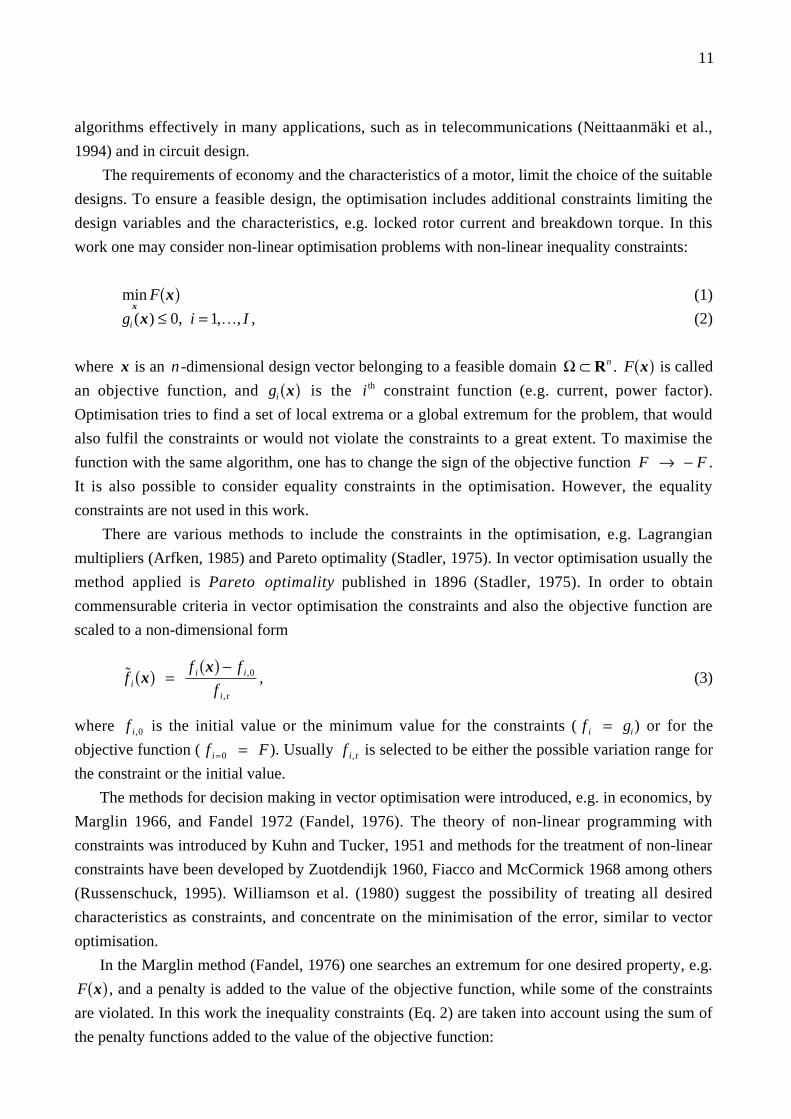
The requirements of economy and the characteristics of a motor, limit the choice of the suitable

designs. To ensure a feasible design, the optimisation includes additional constraints limiting the

design variables and the characteristics, e.g. locked rotor current and breakdown torque. In this

work one may consider non-linear optimisation problems with non-linear inequality constraints:

minx

F x( ) (1)

gi (x) ≤ 0, i = 1,…, I , (2)

where x is an n -dimensional design vector belonging to a feasible domain Ω ⊂ Rn . F x( ) is called

an objective function, and gi x( ) is the i th constraint function (e.g. current, power factor).

Optimisation tries to find a set of local extrema or a global extremum for the problem, that would

also fulfil the constraints or would not violate the constraints to a great extent. To maximise the

function with the same algorithm, one has to change the sign of the objective function F → − F .

It is also possible to consider equality constraints in the optimisation. However, the equality

constraints are not used in this work.

There are various methods to include the constraints in the optimisation, e.g. Lagrangian

multipliers (Arfken, 1985) and Pareto optimality (Stadler, 1975). In vector optimisation usually the

method applied is Pareto optimality published in 1896 (Stadler, 1975). In order to obtain

commensurable criteria in vector optimisation the constraints and also the objective function are

scaled to a non-dimensional form

f i x( ) = f i x( ) − f i,0

f i, r

, (3)

where f i,0 is the initial value or the minimum value for the constraints ( f i = gi) or for the

objective function ( f i=0 = F). Usually f i, r is selected to be either the possible variation range for

the constraint or the initial value.

The methods for decision making in vector optimisation were introduced, e.g. in economics, by

Marglin 1966, and Fandel 1972 (Fandel, 1976). The theory of non-linear programming with

constraints was introduced by Kuhn and Tucker, 1951 and methods for the treatment of non-linear

constraints have been developed by Zuotdendijk 1960, Fiacco and McCormick 1968 among others

(Russenschuck, 1995). Williamson et al. (1980) suggest the possibility of treating all desired

characteristics as constraints, and concentrate on the minimisation of the error, similar to vector

optimisation.

In the Marglin method (Fandel, 1976) one searches an extremum for one desired property, e.g.

F x( ) , and a penalty is added to the value of the objective function, while some of the constraints

are violated. In this work the inequality constraints (Eq. 2) are taken into account using the sum of

the penalty functions added to the value of the objective function:

12

F x( ) → F x( ) + ai max 0, gi x( )[ ] 2

i=1

I

∑ , (4)

where ai is an experimental parameter, x is the design vector, and g denotes the scaled function.

The function “max” is defined as

max 0,u( ) = 0, if u ≤ 0

u, else

. (5)

The equality constraints hj x( ) = 0, j = 1,…, J can be added to the optimisation similar to the

inequality constraints (Fandel, 1976):

+ bj hj x( )[ ]2

j =1

J

∑ , (6)

where bj is an experimental coefficient, and h denotes the scaled function. The other possibility is

to eliminate some variables using equality constraints. Usually, this is possible only in the case of

the linear constraints.

The advantage of the Marglin method (Fandel, 1976) is that the revolutionary improvements in

the characteristics of the design are taken into account in a natural manner, i.e. if the desired

characteristic increases drastically and causes constraint violations, it may still be the best new

design. There may exist even better designs close to this new design in the parameter space (close

in a sense that only small variations in parameters are needed to move to those better extrema).

It is not always necessary to implement constraints. In some cases it can be useful to test how

the optimisation algorithm changes variables in the unconstrained optimisation, especially, if one is

interested in knowing, how much gain can be obtained by violating some of the constraints. The

design variables must afterwards be changed manually to fulfil desired constraints. This is

recommended only with a small number of variables.

1.3 A short review of finite element optimisation

The idea of structural optimisation was introduced in the early 1960's in the field of mechanical

engineering. In 1960 L. A. Schmit suggested combining the FEM and optimisation methods, in

structural analysis (Braibant et al., 1990). In the late 1960's and the early 1970's other engineering

fields, such as aeronautical engineering (e.g. Dwyer et al., 1971), had adopted FEM in structural

optimisation. In 1967 Halbach optimised the pole shapes for magnets and the coil arrangements

using FEM (Russenschuck, 1995).

The development of the finite element analysis and optimisation has been closely linked to the

performance of the computers and the requirements of memory. In the early stages the structural

optimisation was possible only in mainframe computers, and the optimisation problems mainly

concerned partial problems. Also, the accuracy of the calculations has always been a special

concern with the finite element method. Watz et al. (1970) studied the accuracy of FEM in

13

structural problems. Afterwards, various mesh refinement techniques and automatic mesh

generation procedures have been introduced by e.g. Girdinio et al. (1978), Viviani (1978),

Lindholm (1983), Cendes et al. (1985), and Luomi et al. (1988).

In 1971 the finite element method was used in the stationary field analysis for DC motors and

synchronous motors by Chari and Silvester (Arkkio, 1987). The development of both the field

analysis and the computation power gradually enabled more detailed modelling of electrical motors

using two and three-dimensional FEM and time-stepping, including a method for the analysis of the

cage induction motor in a general operating state in a two-dimensional case by Arkkio (1987).

Zienkiewicz et al. (1973) used the position of the mesh nodes as a design variable. In 1986

Ding reported that this method has four drawbacks (Lund, 1994):

1) The number of variables is very large

2) Compatibility and continuity problems between boundary nodes

3) Problems to maintain adequate mesh

4) Structural shape sensitivities might not be accurate

According to these experiences Braibant (1986) made a distinction between the design model

and the analysis model. The design model is defined as a variable description of the domain shapes

including the material design variables, and the analysis model is the finite element model used for

the numerical analysis.

The problem of handling several free nodes was partially due to the optimisation algorithm.

Palko (1994) applied a similar approach to Zienkiewicz (1973) using a genetic algorithm in the

optimisation of a slot shape for induction motors with the time-stepping method. Using statistical

means with a population size from 300 to 1240 Palko (1994) studied the characteristics of an entire

population of designs instead of one single design, and suggested averaging to give rational slot

shapes. One problem with this method is the need of a large population and the time duration. The

method usually applied is to describe the boundaries using a group of master nodes, then fit a spline

to these master nodes, and define the position of the other nodes from this spline, e.g. Schoofs

(1987), and Lund (1994).

In many mechanical engineering problems, like in free-vibration analysis and in static-stress

analysis, only linear models are necessary, even in the analysis of load-carrying capabilities

(Lund, 1994). In electrical motors it is necessary to include in our field analysis the non-linearity

(the effect of saturation in iron). This leads to iterative solution methods and it also may lead to

accuracy problems from the optimisation point of view. To simplify the field analysis, the

hysteresis characteristics of iron are usually neglected, and the reluctivity of iron is modelled with a

single-value monotonic curve (e.g. Arkkio, 1987).

The other difficulty encountered was the accuracy problems in the numerical differentiation,

i.e. the problem of calculating the correct semi-analytical design sensitivities (Zienkiewicz et al.,

1973), when the first order forward finite differences are used as an approximation for derivatives.

These forward differences are extremely sensitive to the size of the perturbation in a design variable

due to truncation and round-off errors.

14

Using special design variables, it may also be possible to obtain analytical derivatives for

matrices in a linear case (Braibant, 1986). Also other methods have been introduced to obtain more

reliable approximation for the design sensitivities, e.g. Lund (1994) in the case of linear materials

and a motionless body. In the case of non-linear materials, an iterative solution of the field may

cause additional accuracy problems to design sensitivities.

Russenschuck (1995) concludes that one has to overcome several problems to be able to make

reliable finite element optimisation: constraints in computers, problems with discontinuities and

non-differentabilities arising from a finite element mesh, accuracy of finite element solutions, and

software implementation problems. The basic problem remains the same: FEM is not accurate.

Keskinen (1992) lists several factors affecting the accuracy of field analysis, such as: discrete finite

elements (shape and number of elements, order of shape functions), formulation to solve the fields,

material modelling, unknown temperature distribution, internal accuracy of the computer, and

simplifications in modelling.

Since the late 1980's a huge improvement in the performance of PCs finally enabled practically

anybody to apply structural optimisation using FEM. Schoofs (1987) applied structural

optimisation and FEM in a design of church bells, and Plank (1993) to obtain the maximum driving

comfort in an automobile. Also different optimisation algorithms have been tested with FEM, e.g.

various deterministic methods and stochastic methods (Russenschuck, 1990), (Neittaanmäki et al.,

1994)

The first tests in electromagnetic field calculation and optimisation considered partial

problems, e.g. Preis et al. (1990) in the optimisation of the pole shape for a magnet, or a simple

geometry, like a transformer or a solenoid (Mohammed, 1990; Takahashi, 1990) and actuators

(Cheng et al., 1994). Pyrhönen et al. (1994) studied the effect of shaped tooth edges in a solid rotor

asynchronous motor.

More rigorous attempts to optimise the whole electric motor have been made. Park et al. (1990)

applied a method of steepest descent as a search direction and a quadratic approximation for the

optimal step size in the reduction of the cogging torque by smoothing the energy variations in a

permanent magnet motor. Russenschuck (1990) optimised a permanent magnet synchronous motor

with different optimisation algorithms at a steady state operation, and Palko (1994) the air gap

region and the whole slot shape for induction motors with a time-stepping method.

The time-stepping method, in spite of the powerful workstations, causes an extremely heavy

computational load. Therefore simplified methods have been introduced, e.g. single slot model

(Suontausta, 1989), and statistical experiment design, e.g. Nikolova-Yatcheva (1989) and

Brandisky et al. (1994) in structural optimisation. Suontausta (1989) reported the computation time

needed for single slot model to be only 1% compared with the modelling of the whole motor.

Williamson et al. (1995) applied the single slot model in the optimisation of the rotor slot shapes

for induction motors.

The problems in statistical experiment design (Box et al. 1960, 1987) arise with the large

number of design variables. Even with a second order polynomial surface the number of

15

coefficients nC = (n + 1) ⋅ (n + 2) / 2, where n is the number of the variables to be optimised, is

fairly large. To improve accuracy of the quadratic fitting, Brandisky et al. (1994) fitted 3 nC tests

using a least square method. In this manner, with 40 variables, the number of experiments needed

would be over 2500 before any optimisation could be made! Also the experiment design has to be

repeated at a new extremum, because the real function surface is not necessarily a polynomial.

Compared with a single slot model, the time-stepping method makes it possible to optimise

both the shape of the stator and the rotor slots simultaneously. The time-stepping method also

enables more accurate modelling of higher harmonics and optimisation of inverted fed motors. The

long simulation duration is the penalty for using the time-stepping method, but the gain is more

accurate modelling of an electric motor, especially in the near air gap region.

Parallel computation has also been applied to structural optimisation problems, e.g. Palko

(1994). The current trend in structural optimisation seems to be in genetic and evolutionary

algorithms, not only because they are suited for parallel computing, but also because of their ability

to scan the parameter space effectively and to avoid local trapping, e.g. caused by the mesh

generation problems. Another asset with FEM is the possibility to avoid the evaluation of estimates

for the derivatives.

1.4 Conclusions and the scope of this study

Structural optimisation by the finite element method has been applied to different fields of

engineering and science. Optimisation with constraints enables the designer to avoid, in advance,

possible design failures or to achieve a feasible design.

There are many different deterministic and stochastic optimisation algorithms suitable for

structural problems, but researchers tend to use genetic and evolutionary algorithms. This is

partially due to their suitability for parallel computing and operation without derivatives, and also

their inherent ability to work in a noisy environment (de Jong, 1993). If the nodes of the mesh are

allowed to move freely, it is possible to find several local extrema to the problem (Preis et al.,

1990). Usually the applied method to describe the shape of our design is the use of a group of

master nodes, and splines to determine the position of the other nodes. With linear materials this

improves the accuracy of design sensitivities (Braibant, 1986).

The finite element analysis is not an accurate objective function. Most of these accuracy

problems are linked to discontinuities and non-differentabilities arising from a finite element mesh

and accuracy of the finite element solutions, but also the modelling of the rotation causes accuracy

problems in the evaluation of the derivatives. In the case of linear materials, various methods have

been introduced to improve the accuracy of the first order forward differences used to approximate

the derivatives of the element matrices (Lund, 1994).

Furthermore the method for evaluating the torque or losses in induction motors is not accurate.

By comparing the results of the previous studies in this field, it is possible to determine the

correctness of the results and robustness of the optimisation algorithm and applied statistical

16

analysis to determine relevant design changes. In the case of non-linear materials, the fields are

solved iteratively, and the approach, even with master nodes, might give accuracy problems in the

estimation of the derivatives. The situation becomes further complicated, when the rotation of a

rotor is included. This causes additional truncation errors and round-off errors. These accuracy

problems in the estimates of the derivatives with FEM suggest that we use methods that tolerate

noisy objective functions, such as genetic algorithms.

Several problems are associated with FEM, but only with a finite element method one can

obtain sufficient accuracy in the analysis of the torque and losses. Furthermore, the simulation of

the rotor rotation is needed to be able to reliably take into account the higher harmonics in the air

gap region and also in the design of inverter fed motors.

1.5 The aim of this work

The main purpose of this work is to design a suitable optimisation method for structural

optimisation with FEM, even when the time consuming rotation of the rotor has to be modelled,

and to use this method for a design of induction motors.

The work consists of two main tasks. The first task is to construct an optimisation method and

to test it with a finite element objective function. This part involves the mesh generation, studies

with mesh refinement techniques, numerical derivation, and analysis methods for a reliable shape

optimisation.

The next task is to use this method in the optimisation. The main purpose is to use structural

optimisation and FEM in a design of new slot shapes for induction motors. The results are

compared with earlier studies.

The selected objective functions are the EM losses, the torque, and the error due to a violation

of the constraints. This study is mainly limited to a single choice of material, unskewed motors and

three supply wave forms (sinusoidal, and two inverter supplies). Also the finite element method

itself contains several simplifications affecting the optimisation results, such as: the two-dimension

approach, iron is modelled as a non-conducting material, hysteresis is neglected, and eddy current

losses are neglected in the stator coils. The optimisation is tested with a 15 kW and a 90 kW

induction motor modelled with FEM.

1.6 Previous work associated with this study

In this work a part of the routines has been constructed from the previously developed two-

dimensional field analysis packages in the Laboratory of Electromechanics. The applied mesh

refinement routines are based on the interactive and adaptive mesh generator by Rouhiainen (1986).

The characteristics of an induction motor are evaluated in the optimisation using the programs

for the field analyses with the time-stepping method in a general operating state of an induction

motor. These analysis methods contain many simplifications, and they are discussed in detail

17

elsewhere (Arkkio, 1987). The modelling is based on a two-dimension field analysis. The end-

region fields are modelled using constant end-winding impedance in the circuit equations. The rotor

bars are assumed to have a constant conductivity (constant temperature). The laminated iron core is

modelled with a magnetically non-linear, non-conducting medium, and hysteresis properties are

neglected, modelling the non-linearity of iron with a single value monotonic curve.

The field analysis library consists of four different programs that are used in this work: (for

details, Arkkio, 1991b)

1) MESH Program generates a finite element mesh for the cross sectional geometry of an

induction motor from the data containing the dimensions, slot numbers and the

slot geometry codes.

2) CIMAC Program calculates operating characteristics assuming a sinusoidal time variation.

In this time-harmonic analysis with a pseudo stationary rotor the magnetic field

varies with the slip frequency in the rotor. The higher harmonic components are

not modelled properly. Therefore optimisation with CIMAC is not reliable

especially in the near air gap region.

3) ACDC Program is used to calculate the proper initial state for time-stepping analysis

from the time harmonic analysis.

4) CIMTD Program calculates operating characteristics of an induction motor by solving

field equations with the Crank-Nicholson time-stepping method. The non-linear

system of equations at each time step is solved by the Newton-Raphson method.

The method based on Maxwell's stress tensor is applied in these programs in the calculation of

torque. The electromagnetic torque is obtained as an integral over the cross-sectional area of the air

gap Sag (Arkkio, 1987)

Te = 1

µ0 rs − rr( ) rBr BϕSag

∫ dS , (7)

where Br is the radial component of the flux density,

Bϕ the tangential component of the flux density,

r , ϕ co-ordinates of a circular co-ordinate system,

rs , rr outer and inner radii of the air gap,

S integration surface, and

µ0 permeability of vacuum.

Arkkio (1987) states that Eq. 7 gives more reliable results than the use of the integration paths

due to a large variation of the torque as a function of the selected radii.

18

2 MESH GENERATION, DERIVATION AND OBJECTIVE FUNCTIONS

The refinement of the mesh and the simulation of the rotor rotation significantly affect the

computationally inexpensive first-order forward differences. Three methods for describing the

shape will be presented and the problems associated with them. Statistical means are used to

improve the reliability of the optimisation results. The problems with the forward differences

finally suggest the use of derivative-free methods in optimisation, when the simulation of a rotor

rotation is modelled. The need of a time-stepping method is indicated using two examples, and the

method of evaluating the motor characteristics used in the numerical test cases is presented.

2.1 Defining the shape

One of the first intentions of the finite element optimisation in the early 1970's was to optimise the

whole shape by moving all the independent nodes in the mesh. In these early tests the problem of

accuracy, linked to the finite element mesh, was discovered. During optimisation one can find

several local extrema close to each other, while the differences in the properties of these designs

may vary from infinitesimal changes to totally enhanced characteristics. The optimisation

algorithms were also not capable of determining the relevant design changes. Many structures were

hardly realisable due to manufacturing techniques. This led to a need for smoothing in optimisation.

The shape of the boundaries or surfaces is usually defined by master nodes in structural

optimisation problems when performing smoothing. The position of other boundary nodes is

defined by fitting a spline to the master nodes or using some analytical formulas (Fig. 1). In the

optimisation, the positions of these master nodes define the generalised design variables allowing

the parameterisation of the model.

Master node

Other boundary node

Interior nodes

Fig. 1. The surface or the boundary of the material is defined by master nodes. The arrows indicatethe selected direction of movement for nodes in this example, as the master node moves.

19

One of the basic problems in the time-stepping method, is the long duration of the simulation.

The contradicting interests are the accuracy of the simulation, and the time duration. The

optimisation algorithm has to be capable of performing somewhat rational decisions in a case,

where nearly all boundary nodes are master nodes. A higher number of nodes in the boundary

would have a devastating effect on the effectiveness of optimisation.

Another approach is a topology optimisation (Bendsøe et al., 1988). In topology optimisation

there is a fixed mesh, and the material properties of the independent elements are altered, e.g.

density.

The author tested optimisation of topology using a locked rotor torque as an objective function

with the time-stepping method and four material choices: non-linear iron, aluminium, copper, and

air. This resulted in extremely difficult and hardly realisable structures (Fig. 2). The number of

elements required in the test was almost threefold to be able to describe the shape of the design to

some degree of precision. Optimisation increased the locked rotor torque from 195 Nm to 364 Nm.

Fig. 2. Topology optimisation easily leads to hardly realisable structures. The material of elementsis a varied in the maximisation of locked rotor torque. The flux between the curves is 1.59 mW/m.The rotor contains elements in which the materials are air, aluminium, or iron. In the stator side,the elements can be air, copper coils (marked with dashed or solid lines), or iron.

Topology optimisation has two main problems. It easily leads to designs in which there are

parts that have no structural significance, as stated by Olhoff et al. (1992), i.e. these parts neither

20

increase desired characteristics nor decrease them. The optimisation algorithms are not capable of

determining the relevant changes in the mesh. This must be made by the user. The second problem

is the huge number of elements needed for modelling a detailed shape. Topology optimisation is

not used in this work.

2.2 Interior nodes of the mesh

There have been various opinions about the importance of moving the internal nodes of the mesh.

Braibant (1986) and Botkin 1988 (Lund, 1994) moved the inner nodes of the mesh concluding that

it is also necessary to move interior nodes, because the object of optimisation is the finite element

mesh and not a real structure.

Pedersen (1988) argued that the perturbation of the inner nodes may lead to maximisation of

errors in the FEM simulations. The perturbation of inner nodes leads to differences in the stiffness

matrix. These differences do not reflect changes in properties; they are inaccuracies in the

sensitivity analysis. After making several comparisons, Kibsgaard (1991) stated that the best results

are obtained by moving only the boundary nodes in linear problems, and he suggested using only

these perturbated elements in the analysis of design sensitivities. In the case of non-linear materials

and a moving rotor, the problem becomes even more complicated due to round-off and truncation

errors.

The perturbation of one single interior node is observed to result in step-like discontinuities in

the evaluated properties, and therefore more nodes have to be moved, if any reliable refinement of

the mesh is to be performed. In this work the refining of the shape of the elements is based on the

common quality factor by Lindholm (1983) (Fig. 3).

a)

b)

Fig. 3. The effect of maximisation of common quality factor to mesh. The air gap region of theunrefined (a) and refined mesh (b) are shown. The refinement is made once.

21

The common quality factor is defined as a ratio between the radius of the largest circle inside

the element and of the smallest circle outside the element. This number is scaled to one for an

equilateral triangle. If the length of vertices are a , b , and c , the quality factor for the element i is

qi = 8 sp − a( ) sp − b( ) sp − c( )

abc, (8)

where sp = a + b + c( ) 2. The common quality factor for N elements, which have a common

corner node, is defined using independent quality factors qi as

qc = N

1qii=1

N∑. (9)

The common quality factor (Eq. 9) emphasises the worst shaped elements. In refinement this

quality factor is maximised by optimising the position of the nodes, and the shape of worst

elements is corrected.

Usually the refinement of the element shapes is included in the adaptive mesh refinement

(Cendes et al., 1985). The adaptive refinement technique used in this work uses a local error

estimate based on the solution of a field with second-order shape functions. See Rouhiainen (1986),

Luomi et al. (1988) for details. Combined with the time-stepping method, adaptive refinements

(Fig. 4) become extremely time consuming. With second order elements and only one adaptive

refinement at each time step, the duration of the simulation is nearly five times longer than without

refinement.

Fig. 4. Adaptively refined mesh at one time instant. The rotor mesh is moved to a positioncorresponding to the angle of the rotor.

22

According to simulation tests, the modification of the inner nodes does not significantly change

the simulation results. Table 1 indicates that the position of the inner nodes had practically no effect

on the simulation results, but even one adaptive refinement changes the results by nearly 1%. Note

that in adaptive refinement with the time-stepping method, the air gap boundary is allowed to be

refined, but the creation of additional inner corner nodes to the air gap is eliminated. This naturally

affects the accuracy of the results.

Table 1. The effect of using common quality factor and adaptive refinement to the torque and theinput power in a 15 kW induction motor modelled with the time-stepping method at a fixed 3.45%slip using a sinusoidal supply. A total of 900 steps is simulated and the number of steps per periodis 300. The results are average values from the last full period. All the decimals shown in torqueand power are not significant compared to the accuracy of the FEM. The number of the decimals islarge to give the reader an impression of the magnitude of the differences in the simulations.

Refinement Air gap torque / Nm Input power / kW

None 92.259 15.277

Maximised quality one time 92.255 15.274

factor ten times 92.232 15.273

Adaptive refinement one time 91.358 15.127

It is not possible to consider adaptive refinement of the mesh in the optimisation, because of

the lengthy simulation duration. With second-order elements and with only one adaptive refinement

at every time step, the duration of the simulation is nearly five times longer than without

refinement, lasting approximately 16 hours.

The decimals shown in Table 1 give a fairly good impression to the reader of the controversial

problems associated with finite element simulatios. From the viewpoint of the derivatives, or the

estimates of the derivatives, the FEM should be able to reliably notice even the smallest changes in

the element mesh, but due to the resolution of the FEM these differences are not necessarily

significant.

Only in the case of highly deformed elements was the maximisation of the common quality

factor observed to be useful.

2.3 Problems of the derivatives

2.3.1 Truncation

In numerical analysis, the usual estimate for derivatives of function F is the first order forward

difference (FOFD) approximation

23

∂F

∂x ≈

∆F

∆x =

F x + ∆x( ) − F x( )∆x

, (10)

where ∆x is the perturbation length. This forward difference approximation is computationally in-

expensive, but generally strongly dependent on the perturbation length ∆x . Lund (1994) reported

accurate forward differences to be achievable even at relative perturbations ∆x x of the order from

10-2 to 10-10 in the analysis of vibration frequencies in thin plate structures.

In optimisation, a change in design parameters perturbates the position of a node or nodes.

When the perturbation length approaches zero, truncation errors due to different storage and

internal precision, e.g. when the mesh is saved to a file, may significantly change the value of ∆x ,

and therefore of the forward differences also.

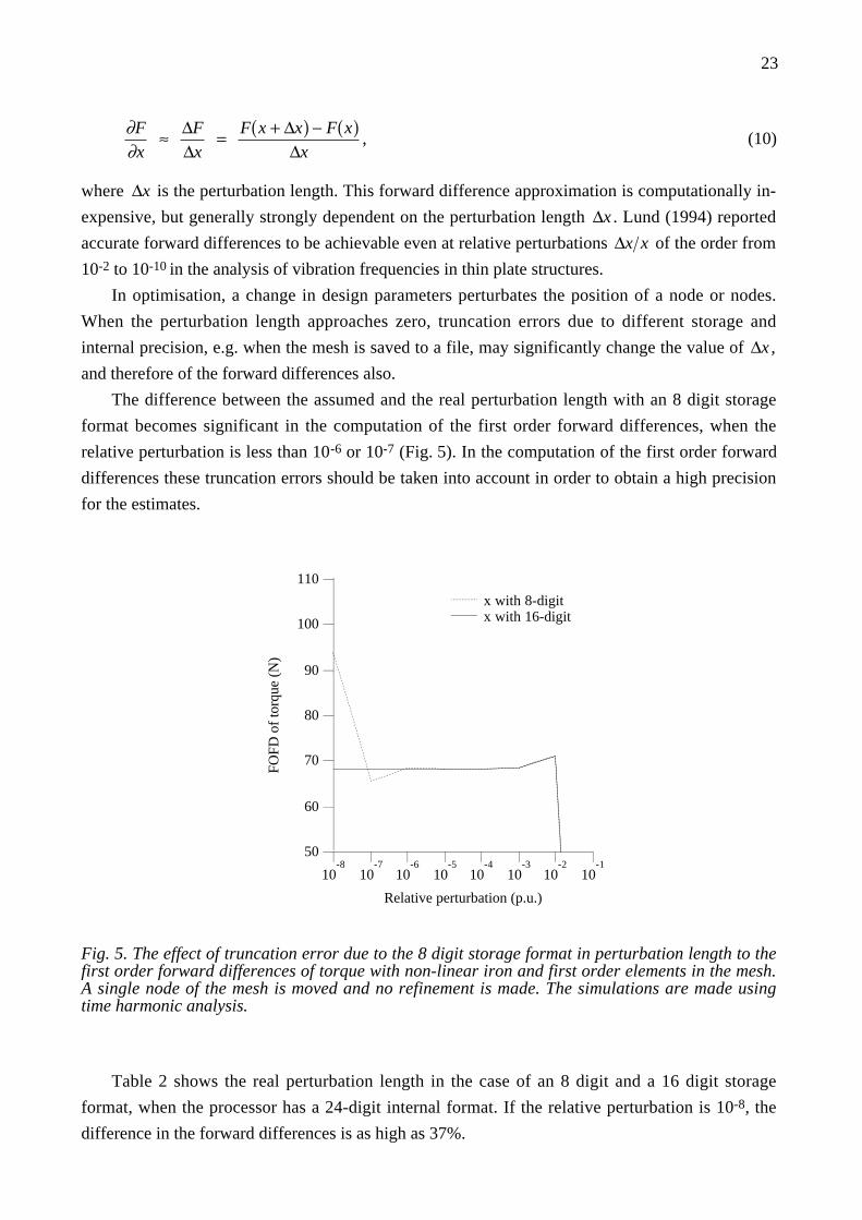
The difference between the assumed and the real perturbation length with an 8 digit storage

format becomes significant in the computation of the first order forward differences, when the

relative perturbation is less than 10-6 or 10-7 (Fig. 5). In the computation of the first order forward

differences these truncation errors should be taken into account in order to obtain a high precision

for the estimates.

110

100

90

80

70

60

50

FOFD

of

torq

ue (

N)

10-8

10-7

10-6

10-5

10-4

10-3

10-2

10-1

Relative perturbation (p.u.)

x with 8-digit x with 16-digit

Fig. 5. The effect of truncation error due to the 8 digit storage format in perturbation length to thefirst order forward differences of torque with non-linear iron and first order elements in the mesh.A single node of the mesh is moved and no refinement is made. The simulations are made usingtime harmonic analysis.

Table 2 shows the real perturbation length in the case of an 8 digit and a 16 digit storage

format, when the processor has a 24-digit internal format. If the relative perturbation is 10-8, the

difference in the forward differences is as high as 37%.

24

Table 2. The effect of relative perturbation and numerical precision to perturbation length ∆x dueto truncation errors. The correct decimals are printed in boldface. The processor has a 24-digitinternal format, and only 16 decimals are printed.

relative perturbation ∆x x ∆x with 16 digits ∆x with 8 digits

10-1 .7284220411223341e-02 .7284221000000007e-0210-2 .7284220411223341e-03 .7284220000000063e-0310-3 .7284220411223064e-04 .7284200000000352e-0410-4 .7284220411227227e-05 .7284000000010171e-0510-5 .7284220411157838e-06 .7290000000048646e-0610-6 .7284220411574172e-07 .7300000000320939e-0710-7 .7284220407410835e-08 .7000000010193297e-0810-8 .7284220493044199e-09 .9999999994736442e-0910-9 .7284220434044199e-10 under-flow

2.3.2 Free nodes

The refinement of the mesh, i.e. moving the nodes in the mesh, generates differences in the element

matrices, and this has a radical impact on forward differences. By taking into account the

mentioned truncation errors in computations the forward differences converged properly, even with

non-linear materials and first order elements. In these tests one single boundary node is allowed to

move, and the simulation is made using a time harmonic analysis (Fig. 6).

101

102

103

104

105

106

FOFD

of

Tor

que

(Nm

/m)

10-8

10-7

10-6

10-5

10-4

10-3

10-2

10-1

Relative perturbation (p.u.)

Unrefined mesh Optimised q-factor Adaptive refinement Linear iron (unref.) Linear iron (adapt.)

a)

108

107

106

105

104

103

102

101

FOFD

of

Los

ses

(W/m

)

10-8

10-7

10-6

10-5

10-4

10-3

10-2

10-1

Relative perturbation (p.u.)

Unrefined mesh Optimised q-factor Adaptive refinement Linear iron (unref.) Linear iron (adapt.)

b)

Fig. 6. The effect of the perturbation length on the first order forward differences of torque (a) andelectromagnetic losses (b) using time harmonic analysis with different refinement schemes andsecond order elements. The perturbed node connects the stator coil to the iron nearest the air gap.

25

The evaluation of the forward differences is tested using an unrefined mesh with linear and

non-linear iron, an optimised common quality factor, and adaptive refinement with linear and non-

linear iron. The unrefined mesh proved to be the most reliable source for the forward differences

even with non-linear iron, i.e. the forward differences remained the same until the under-flow error

was encountered. While using non-linear iron and maximisation of the common quality factor, the

accuracy of the forward differences is lost usually with a relative perturbation smaller than 10-5.

With the time-stepping method and non-linear materials, the sign changes are also typical, when the

perturbation length decreases.

Adaptive refinement is also a disappointment from the point of view of the forward differences.

Usually forward differences lose accuracy, when the relative perturbation is smaller than 10-6. Only

after several and very elaborate adaptive refinements did these estimates for the derivatives

converge properly, but usually the confidential interval for relative perturbation did not improve.

With the time-stepping method the simulation of rotation combined with non-linear materials

causes additional truncation and round-off errors, and the forward differences do not converge

properly (Fig. 7). A similar test with time harmonic analysis is made with the time-stepping

method, where the position of one boundary node is changed to calculate forward differences for

the torque and losses.

101

102

103

104

105

106

FOFD

of

Tor

que

(Nm

/m)

10-8

10-7

10-6

10-5

10-4

10-3

10-2

10-1

Relative perturbation (p.u.)

Unrefined mesh Optimised q-factor Adaptive refinement Linear iron (unref.) Linear iron (adapt.)

a)

108

107

106

105

104

103

102

101

FOFD

of

Los

ses

(W/m

)

10-8

10-7

10-6

10-5

10-4

10-3

10-2

10-1

Relative perturbation (p.u.)

Unrefined mesh Optimised q-factor Adaptive refinement Linear iron (unref.) Linear iron (adapt.)

b)

Fig. 7. The effect of the perturbation length on the first order forward differences of the torque (a)and electromagnetic losses (b) using the time-stepping method with different refinement methodsand second order shape functions. The perturbed node connects the stator coil to the iron nearestthe air gap.

The tests show that only with linear iron it is possible to obtain somewhat reliable estimates for

derivatives with the time-stepping method. The confidential interval usually ranged from 10-5

26

to 10–2, and in some cases the usage of adaptive refinements is observed to destroy the convergence

properties of the forward differences even with linear materials. Improvement of the accuracy in

simulations by using adaptive refinements may only lead to exhausting loops of refinements and

resolving of the field. Furthermore the duration of the time-stepping method impairs more serious

usage of adaptive refinement.

One could try to use the forward differences from the time harmonic analysis as an estimate for

the time-stepping method. The problem is that these forward differences are not correct and the

difference may be even several orders of magnitude and of the opposite sign, especially in the case

of near air gap changes. The usage of linear iron with the time-stepping method to evaluate forward

differences did not prove to be a good solution to the problem similar to time harmonic analysis.

The SPARSPAK library did not significantly affect the forward differences at the tested

numerical precision range. This was tested by changing the order in which the elements are

assembled in the matrix equations. In the SPARSPAK library, subroutines generate a permutation

matrix that is applied in the solution of linear equations (see Chu et al., 1984, for details), and even

a random assembly of elements to the matrix did not change the analysis results in the test cases.

Usually, the unrefined mesh proved to be the best source for the forward differences. The

refinement of mesh generates differences in the field matrix. This destroys the convergence

properties, even without time-stepping. The tests with free nodes lead to a conclusion that, if the

independent nodes of the mesh are allowed to be moved, there are tremendous difficulties with

forward differences, especially, when the simulation of the rotation is modelled and there are non-

linear materials. The order of magnitude and the sign of the forward differences vary, when the

perturbation length decreases. Therefore additional smoothing is needed in optimisation with the

time-stepping method.

The numeric value of the first order forward differences with different variables varies from

insignificant values to huge numbers. Reader should remember that these forward differences do

not necessarily reflect real change in properties, but also the accuracy of the FEM. Author made the

previous tests with other boundary nodes in the mesh and also with other cross-sectional geometry.

The problems of the forward differences remained the same in all cases.

2.3.3 Master nodes

The usage of master nodes for smoothing was tested with the mesh generator program MESH. This

program uses analytical formulas to evaluate the position of nodes in the mesh, when the

dimensions of the slot are varied. Not only the boundary nodes, but also other interior nodes are

also moved. In this program one defines the dimensions of the slot similarly as one would define

the dimensions of the punch. The evaluation of forward differences is tested with time harmonic

analysis and the time-stepping method for torque (Fig. 8) and EM losses (Fig. 9).

27

-20

-10

0

10

20

FOFD

of

torq

ue (

N)

10-5 10-4 10-3 10-2 10-1

x /x (p.u.)

a)

400

200

0

-200FOFD

of

torq

ue (

N)

10-5 10-4 10-3 10-2 10-1

x /x (p.u.)

b)

4

2

0

FOFD

of

torq

ue (

kN)

10-5 10-4 10-3 10-2 10-1

x /x (p.u.)

c)

-8

-4

0

4

FOFD

of

torq

ue (

kN)

10-5 10-4 10-3 10-2 10-1

x /x (p.u.)

d)

20

15

10

5

0FOFD

of

torq

ue (

kN)

10-5 10-4 10-3 10-2 10-1

x /x (p.u.)

e)

-12

-8

-4

0

FOFD

of

torq

ue (

kN)

10-5 10-4 10-3 10-2 10-1

x /x (p.u.)

f)

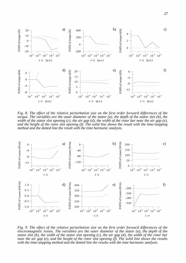
Fig. 8. The effect of the relative perturbation size on the first order forward differences of thetorque. The variables are the outer diameter of the stator (a), the depth of the stator slot (b), thewidth of the stator slot opening (c), the air gap (d), the width of the rotor bar near the air gap (e),and the height of the rotor slot opening (f). The solid line shows the result with the time-steppingmethod and the dotted line the result with the time harmonic analysis.

-12

-8

-4

0

FOFD

of

Los

ses

(W/m

)

10-5 10-4 10-3 10-2 10-1

x /x

a)

-120

-80

-40

0

FOFD

of

Los

ses

(W/m

)

10-5 10-4 10-3 10-2 10-1

x /x

b)

200

150

100

50

0

FOFD

of

Los

ses

(W/m

)

10-5 10-4 10-3 10-2 10-1

x /x

c)

-1.0

-0.5

0.0

0.5

1.0

FOFD

of

Los

ses

(kW

/m)

10-5 10-4 10-3 10-2 10-1

x /x

d)

400

350

300

250

200FOFD

of

Los

ses

(W/m

)

10-5 10-4 10-3 10-2 10-1

x /x

e)

-320

-280

-240

-200

FOFD

of

Los

ses

(W/m

)

10-5 10-4 10-3 10-2 10-1

x /x

f)

Fig. 9. The effect of the relative perturbation size on the first order forward differences of theelectromagnetic losses. The variables are the outer diameter of the stator (a), the depth of thestator slot (b), the width of the stator slot opening (c), the air gap (d), the width of the rotor barnear the air gap (e), and the height of the rotor slot opening (f). The solid line shows the resultswith the time-stepping method and the dotted line the results with the time harmonic analysis.

28

One of the basic problems with the time-stepping method is the loss of accuracy at very large

relative perturbations, such as 10-4 or even 10-3. The sign of the forward differences may also

change. The time harmonic analysis is stable to the relative perturbation of 10-6, with the exception

of the near air gap variables, where the forward differences did not converge at all.

The calculation of the forward differences for the torque and electromagnetic losses is tested by

changing the slot dimension. The test is made with first-order elements, sinusoidal supply and 900

time steps. The average values are evaluated from the last full period. For many variables, the

forward differences of the torque and losses converge smoothly. The forward differences of the

time harmonic analysis and the time-stepping method proved to behave similarly as the

perturbation length decreases, but the actual value is usually different. One could use the forward

differences from the time harmonic analysis as an estimate. A problem is the air gap region, where

the forward differences from the time harmonic analysis do not converge or the difference is

several orders of magnitude or opposite sign compared to the time stepping method. Even 106

differences are observed.

Despite this approach with master nodes, the confidential interval for the forward differences

with the time-stepping method varies tremendously making the computation of the forward

differences unreliable. The confidential interval is observed to be very narrow occasionally, e.g.

from 10-4 to 10-5 (Fig. 8a). One might be able to make the forward differences more reliable by

keeping the position of the interior nodes fixed as in the case of the free node.

2.4 The need for the time-stepping method

Despite the fact of the long simulation duration, the time-stepping method is needed for a reliable

optimisation. The usual choice has been to keep variables fixed, if our model can not determine or

estimate the correct effect, e.g. in the air gap region, (Poloujadoff et al., 1994). The values of these

parameters are defined using the experience of the designer.

2.4.1 Maximisation of the torque

In the first example the author benefited from the stability of the forward differences in the time

harmonic analysis. The optimisation is made using the Broyden-Fletcher-Goldfarb-Shanno

algorithm (Press et al., 1989) and second order elements in the simulations. The objective function

is the torque at a fixed 3% slip. The optimisation maximises the torque at a fixed slip from A to B

(Fig. 10). When the motor operates at a constant load, the actual operation point C is at a smaller

slip. The resistive rotor losses are proportional to the slip and therefore the optimisation should lead

to a minimisation of the rotor losses.

29

Tor

que

Load line

Rotational Speed

A

B

C

Fig. 10. The effect of maximising torque at a fixed 3% slip (from A to B). At a constant load themotor operates at point C.

Optimisation includes additional constraints. The locked rotor current is limited below 260 A,

and the breakdown torque must be at least 1.6 times the rated torque. The temperature rise (see

Kopylov, 1980, for details) in the stator coils must be less than 80°C. The motors have four poles

and 36 stator slots and 32 rotor slots. The evaluation of the objective function lasts 12 minutes with

3300 second-order elements. The initial cross-section of the motor is shown in Fig. 11.

a) b)

Fig. 11. The initial (a) and the optimised (b) stator and the rotor geometry of the four pole motor.

30

In the initial shape, the air gap surface consists of saw tooth shaped peaks and both the rotor

and the stator slots have a narrower part in the middle of the slots. In the inverted fed motors this

could be used to change the path of the high harmonic flux further away from the air gap. The

shape of the stator and the rotor slots are allowed to change freely during the optimisation. The

optimisation results are shown in Table 3.

Table 3. The optimisation results at a fixed 3% slip The results at a constant torque are alsosimulated with the time-stepping method using a sinusoidal supply. The total electromagnetic lossesalso include the calculated core losses at 50 Hz in the case of the time harmonic analysis.

Time harmonic analysis Torque / Nm Resistive rotor

losses / kW

Resistive stator

losses / kW

Total EM

losses / kW

At 3% Initial 83 0.4 1.0 1.6

slip Optimised 129 0.6 1.2 2.0

Time-stepping method Slip / % Rotor losses /

kW

Stator losses /

kW

Total EM

losses/ kW

At 100 Nm Initial 4.0 0.7 1.8 2.5

torque Optimised 2.4 0.7 1.3 2.0

The results in Table 3 indicate remarkable improvement from the original design. The equal

torque values are calculated using the time-stepping method and 300 steps per period to verify the

results. The decrease in total losses is as high as 500 W. The resistive rotor losses decreased in the

time-stepping simulation only from 714 W to 706 W, while the air gap flux density increased from

0.786 T to 0.927 T. The improved characteristics are mainly due to a higher flux density in the air

gap. The maximisation of the torque enforces the air gap flux leading to a higher mechanical power.

This results in better efficiency and lower stator losses at the nominal point.

The time harmonic analysis does not calculate the losses caused by the higher time harmonics.

This also affects the optimisation results: the stator coils and the rotor bars move closer to the air

gap. The shape of the slots is more reliable further away from the gap, where the losses caused by a

higher harmonic field are smaller. The narrower part vanishes from the stator slots, and the shape of

the stator slot is generally straight.

One could use time harmonic analysis in optimisation, but that would limit the choice of

variables excluding the air gap region. One could ask then, what is the gain of using this time

consuming FEM, because the results could have been obtained by using more conventional design

methods, e.g. Vogt (1983).

31

2.4.2 Minimisation of losses

The second example involves minimisation of the EM losses using a genetic algorithm and a time

harmonic analysis. The population size is 200 in the optimisation. The shape of the slots may

change freely, but the air gap surface is smooth. The test motor has four poles, 36 stator slots, and

32 rotor slots (Fig. 12). Optimisation is made by searching for a constant shaft power slip. The

constraints are: locked rotor torque (> 3.4 times the rated torque), locked rotor current (< 254 A),

and the breakdown torque (> 1.6 times the rated torque).

a) b)

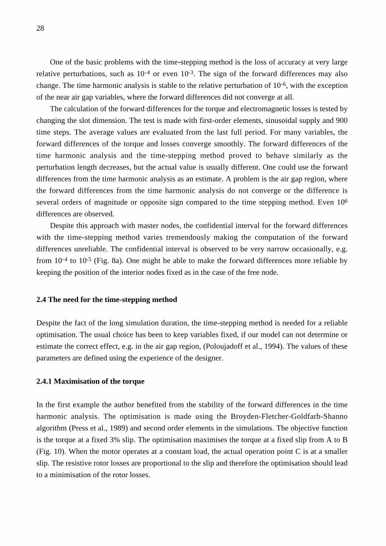
Fig. 12. The initial (a) and the optimised (b) stator and the rotor geometry for the four pole motor.

In the optimised motor, the area of the rotor bars expand near the gap in order to reduce EM

losses. The stator coils and the rotor bars move towards the air gap, because the higher time

harmonic losses are not modelled. The opening of the stator slots expands to decrease the leakage

reactance and this increases the breakdown torque. The locked rotor current limits the decrease of

the leakage reactance. The results are obvious, if one considers only the fundamental harmonic

field.

Table 4 shows the EM losses at the rated power in the initial and the optimised motor. The

reduction of losses with the time-stepping method is only 2.5%, while the time harmonic analysis

shows over a 10% decrease in losses. The difference in losses with the time-stepping method is

only 50 W. The difference in losses is very small, and therefore the author evaluated the EM losses

using second-order elements. With second-order elements the difference is 20 W.

32

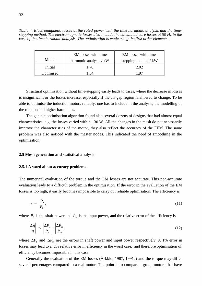
Table 4. Electromagnetic losses at the rated power with the time harmonic analysis and the time-stepping method. The electromagnetic losses also include the calculated core losses at 50 Hz in thecase of the time harmonic analysis. The optimisation is made using the first order elements.

ModelEM losses with time

harmonic analysis / kW

EM losses with time-

stepping method / kW

Initial 1.70 2.02

Optimised 1.54 1.97

Structural optimisation without time-stepping easily leads to cases, where the decrease in losses

is insignificant or the losses increase, especially if the air gap region is allowed to change. To be

able to optimise the induction motors reliably, one has to include in the analysis, the modelling of

the rotation and higher harmonics.

The genetic optimisation algorithm found also several dozens of designs that had almost equal

characteristics, e.g. the losses varied within ±30 W. All the changes in the mesh do not necessarily

improve the characteristics of the motor, they also reflect the accuracy of the FEM. The same

problem was also noticed with the master nodes. This indicated the need of smoothing in the

optimisation.

2.5 Mesh generation and statistical analysis

2.5.1 A word about accuracy problems

The numerical evaluation of the torque and the EM losses are not accurate. This non-accurate

evaluation leads to a difficult problem in the optimisation. If the error in the evaluation of the EM

losses is too high, it easily becomes impossible to carry out reliable optimisation. The efficiency is

η = PS

Pin

, (11)

where PS is the shaft power and Pin is the input power, and the relative error of the efficiency is

∆ηη

≤ ∆PS

PS

+ ∆Pin

Pin

, (12)

where ∆PS and ∆Pin are the errors in shaft power and input power respectively. A 1% error in

losses may lead to a 2% relative error in efficiency in the worst case, and therefore optimisation of

efficiency becomes impossible in this case.

Generally the evaluation of the EM losses (Arkkio, 1987, 1991a) and the torque may differ

several percentages compared to a real motor. The point is to compare a group motors that have

33

been evaluated by the same method, e.g. one average design to an other. The modelling itself might

be erroneous compared to a real motor. The optimisation algorithm modifies these designs in

accordance with the phenomena that has been taken into account in modelling. Using statistical

analysis it is possible notice relevant design changes in the population. In the case of optimising the

torque, the improvements are usually several dozens of percentages, and the problem is avoided.

These problems emphasise a need for a robust optimisation algorithm. The algorithm has to be

capable of determining the relevant design changes, even for non-accurate objective functions.

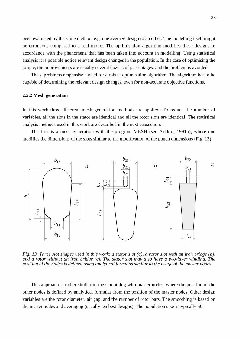
2.5.2 Mesh generation

In this work three different mesh generation methods are applied. To reduce the number of

variables, all the slots in the stator are identical and all the rotor slots are identical. The statistical

analysis methods used in this work are described in the next subsection.

The first is a mesh generation with the program MESH (see Arkkio, 1991b), where one

modifies the dimensions of the slots similar to the modification of the punch dimensions (Fig. 13).

b13

b12

b11

h 1

h 13

h 11

a)

h 21

h 22

b21

h 23

b23

b22 b)

b22

b21

b23

h 23

h 21

c)

Fig. 13. Three slot shapes used in this work: a stator slot (a), a rotor slot with an iron bridge (b),and a rotor without an iron bridge (c). The stator slot may also have a two-layer winding. Theposition of the nodes is defined using analytical formulas similar to the usage of the master nodes.

This approach is rather similar to the smoothing with master nodes, where the position of the

other nodes is defined by analytical formulas from the position of the master nodes. Other design

variables are the rotor diameter, air gap, and the number of rotor bars. The smoothing is based on

the master nodes and averaging (usually ten best designs). The population size is typically 50.

34

In the case of a free shape of the air gap (Fig. 14), the independent nodes of the mesh are

allowed to move, and the interior nodes of the mesh are in fixed positions. Because the surface of

the gap is allowed to change, a layer of additional air elements is generated to the surface of the

teeth. This is due to the method of evaluating the air gap torque. The problems of the derivation

recommended allow only the position of the boundary nodes to move. Therefore the position of the

interior nodes is not modified. The shape of the slot is defined using a list of the co-ordinates

corresponding to the positions of the boundary nodes. The statistical analysis of significance is used

to find out the relevant design changes. The optimised design is the average of 100 to 300 best

designs depending on the population size. Population size is typically several hundreds.

a) b)

Fig. 14. The boundary nodes in a freely shaped mesh using a list of nodes, when the shape of thenear air gap (a), and the whole slot shape (b) is allowed to move. At the surface of the gap is alayer of air elements. The boundary nodes can move either to a radial or to a tangential direction.

Later the shape of the slots is limited to a smooth air gap surface and symmetrical slots

(Fig. 15) in accordance with experiences from the optimisation tests. The number of variables in

this third applied method is typically from 30 to 40, and the population size is typically 100.

Averaging contains usually 20 population members. The shape of the slot is allowed to be

modified. In the tests, the averaging caused less than 0.05 mm variations in the parameter values.

The smaller number of variables allowed a reduction in the number of population members and

the simulation of more generations in the same amount of time. It also improved the effectiveness

of the optimisation. The smoothing is mainly based on averaging in the population. Also the small

number of variables reduces the variations of the element mesh performing smoothing in the mesh.

The analysis of the significance is omitted, because analysis may contain only a small amount

of the population members. In optimisation one can find many good motors close each other by

modifying slightly the parameter values. All these changes in the variables are not necessarily

significant considering the accuracy of the FEM. Therefore averaging is applied to improve the

reliability of the results.

35

h1

h2

h3

h4

h5

h6

h7

d1

d2

d3

d4

d5

d6

d7

a)

h1

d1

d2d3

d4d5

h2h3

d6

d7

d8

d9

d10

d11

h4 h5h6h7

h8

h9

h10

h11

b)d1

d2

d4d3

d5

d6

d7

d8

d9

d10

h1h2h3h4

h5

h6

h7

h8

h9

c)

Fig. 15. The three slot shapes in this work: a stator slot (a), a rotor slot with an iron bridge (b), anda rotor without an iron bridge (c). The stator slot may have a two-layer winding. The shape of theslots is defined in these cases using 33 to 36 variables.

2.5.3 Statistical analysis of the population

The finite element method is not accurate, and therefore statistical means, e.g. averaging and

statistical tests of significance are needed to improve the reliability of the results. The genetic

optimisation algorithm is based on a population. The averaging is made by taking a sample from

this population. The sample may contain all the successive designs in the population or from ten to

twenty designs, depending on the population size.

In the case of an asymmetric mesh (free nodes) the nodes are allowed to move in one or two

directions, and the smoothing is based on averaging and statistical tests of significance, see Palko

(1994) for details. This is based on the idea that optimisation is like any other treatment or a change

of the control parameters. Using statistical means one can analyse if this treatment has caused

significant changes.

Fig. 16 shows the normalised probability distribution of the initial and the optimised population

for the function values and the optimisation parameters. This distribution plot is formed by using

100 intervals. These population members are sorted to these bins according to the numerical value

of the variables in the optimisation. The initial population is made by generating small changes to

the initial design. In this population (see Fig. 16), most of the designs peaked close to the initial

design, but some side peaks exist too. These peaks contain new designs, some better and some

worse. In the optimised population there are two clear peaks.

The statistical significance of the changes in the variables is tested in this work by an F-test and

Student's t-test (Press et al., 1989) comparing the initial distribution and the optimised distribution.

36

With the Student's t-test, one can test if the initial and optimised distribution have the same mean

value and with the F-test the variance can be tested. The parameter values and objective function

values are analysed in the successive designs. The number of variables ranges from 38 to 138, and

the population size is between 300 and 1240 in order to make reliable statistical analyses. An

example of the effect of averaging on the shape of the air gap surface is shown in Fig. 17

1.0

0.8

0.6

0.4

0.2

0.0

Nor

mal

ised

Pro

babi

lity

Dis

trib

utio

n

350340330320310300

Torque (Nm)

Population: 350Variables: 38

Optimised Initial

Fig. 16. The normalised probability distribution of the initial and the optimised population in a testwith a four pole induction motor. The objective function is the locked-rotor torque. The distributionis formed using 100 intervals between the maximum and the minimum value in the populations. Theanalysis contains 253 and 183 successive designs in the population. In the initial population thedesigns are sharply peaked around the initial value, and new designs appear in the tail areas.

a)

b)

Fig. 17. The near air gap region in one single extremum (a), and in the averaged design (b). Theresults are from the minimisation of EM losses in a 15 kW induction motor. The notch in the statorteeth in the rightmost figure is caused by the properties of averaging as a non-robust estimate.

37

The surface of the gap is smooth in both cases in Fig. 17, with the exception of the slot

openings. The results are from the minimisation of the EM losses in a 15 kW induction motor. The

averaging has removed the small variations from the surface of the gap.

The eminent problem of these non-robust estimates, e.g. average value, is that they are easily

disturbed by the outlying data points (Press et al. 1989). In Fig. 17b there is a notch in the stator

teeth. A more careful inspection of the population showed that this notch in the stator teeth was

caused by several totally different designs in the tail are of the distribution.

The usage of large population proved to be very elaborate, and therefore the population size

had to be able to make optimisation in a rational time. Later the population size was fixed to 50 or

100 and the number of the variables was limited below 50 (in even air gap meshes).

This has an interesting effect on the applied genetic optimisation algorithm: not only did

optimisation become faster, but also the algorithm scanned the parameter space further away from a

local extremum. A small number of variables decreases the variations of the objective function

producing smoothing in the mesh. Therefore the number of the local extrema is reduced, and the

algorithm is more likely to generate larger changes in the design. This was also noticed from the

population, i.e. the population became very sharply peaked. Also the probability of changing the

correct variables becomes larger with a small number of variables.

The statistical analysis of the significance is not reliable, because analysis can contain only a

small amount of population members, and therefore it is omitted. The averaging is used to improve

the reliability of the results. The smaller number of variables allowed a reduction in the number of

population members and the simulation of more generations in the same amount of time improving

the effectiveness of the optimisation. The averaging is made from the best ten to twenty designs in

the population. The averaging caused usually less than 0.05 mm variations in the parameter values,

indicating the reliability of the optimisation algorithm.

In optimisation one can find many good motors close to each other by slightly modifying the

parameter values. The averaging is applied to improve the reliability of the results.

2.6 Objective functions and constraints

2.6.1 Characteristics of the motor

By using the time-stepping method it is possible to evaluate the whole torque versus a speed curve

for each motor design. This would be extremely time consuming with the time-stepping method

and useless from the point of view of optimisation. Therefore the simulations are limited to a few

rotational speeds (Fig. 18). Therefore the motors are supposed to be used only within the studied

slip range, especially, when the number of slots is varied in optimisation. The motors may have

totally undesired characteristics outside this slip range.

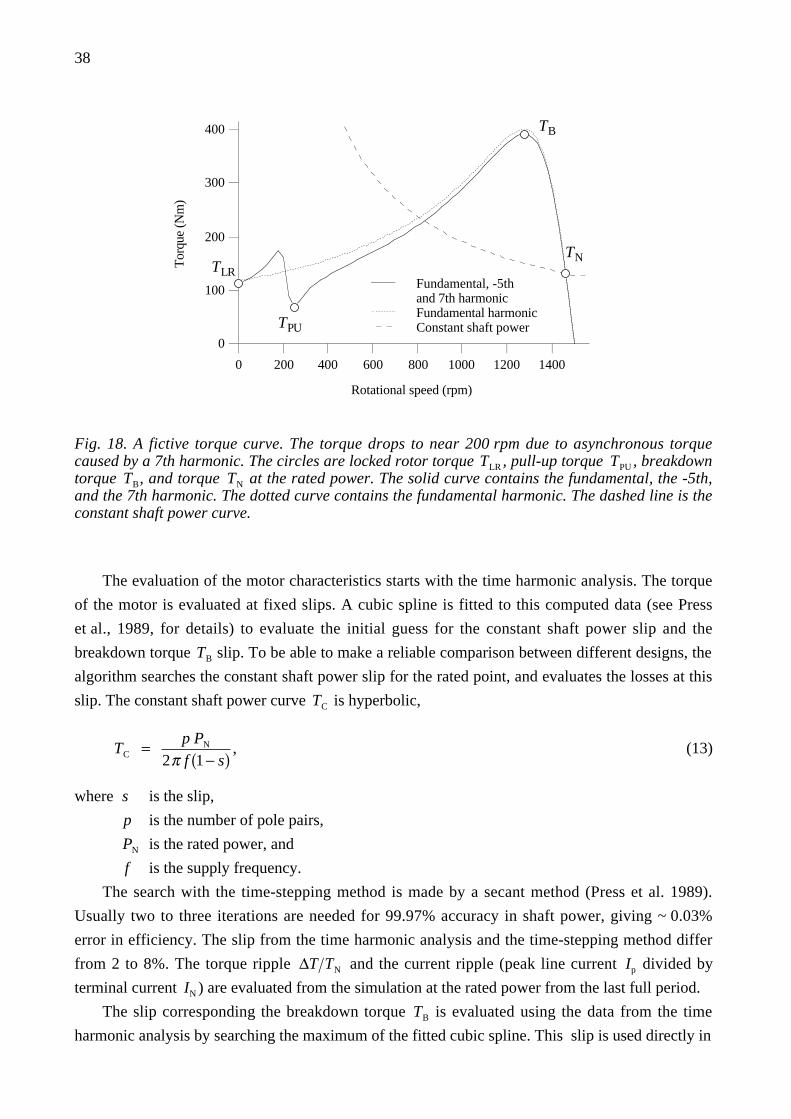
38

400

300

200

100

0

Tor

que

(Nm

)

1400120010008006004002000

Rotational speed (rpm)

TPU

TLR

TN

Fundamental, -5th and 7th harmonicFundamental harmonicConstant shaft power

TB

Fig. 18. A fictive torque curve. The torque drops to near 200 rpm due to asynchronous torquecaused by a 7th harmonic. The circles are locked rotor torque TLR , pull-up torque TPU , breakdowntorque TB, and torque TN at the rated power. The solid curve contains the fundamental, the -5th,and the 7th harmonic. The dotted curve contains the fundamental harmonic. The dashed line is theconstant shaft power curve.

The evaluation of the motor characteristics starts with the time harmonic analysis. The torque

of the motor is evaluated at fixed slips. A cubic spline is fitted to this computed data (see Press

et al., 1989, for details) to evaluate the initial guess for the constant shaft power slip and the

breakdown torque TB slip. To be able to make a reliable comparison between different designs, the

algorithm searches the constant shaft power slip for the rated point, and evaluates the losses at this

slip. The constant shaft power curve TC is hyperbolic,

TC = p PN

2π f 1 − s( ), (13)

where s is the slip,

p is the number of pole pairs,

PN is the rated power, and

f is the supply frequency.

The search with the time-stepping method is made by a secant method (Press et al. 1989).

Usually two to three iterations are needed for 99.97% accuracy in shaft power, giving ~ 0.03%

error in efficiency. The slip from the time harmonic analysis and the time-stepping method differ

from 2 to 8%. The torque ripple ∆T TN and the current ripple (peak line current Ip divided by

terminal current IN ) are evaluated from the simulation at the rated power from the last full period.

The slip corresponding the breakdown torque TB is evaluated using the data from the time

harmonic analysis by searching the maximum of the fitted cubic spline. This slip is used directly in

39

the evaluation of the breakdown torque without any iterations.

The minimum of the asynchronous torque of the harmonics was used as an initial guess for the

pull-up torque TPU , but usually three to five time-stepping simulations are needed for a reliable

estimation of the pull-up torque. The evaluation of the pull-up torque was too time consuming for

optimisation. The computation time of the objective function was almost two times longer.

Therefore the evaluation of the pull-up torque is omitted in this work, even though it is defined in

the standards, e.g. in IEC 34-1 (1994), in the minimum performance specifications.

The effects of the synchronous torque are not taken into consideration in the optimisation. This

is partially because the undesirable effects can be avoided by using a proper combination of the

stator and the rotor slots and using skewed rotor slots.

The locked rotor characteristics are evaluated using only the time harmonic analysis, unless the

locked rotor torque TLR is to be optimised. The number of time steps per period is one tenth of the

steps at the rated point and the average and r.m.s. values are evaluated from the last ten periods.

The rational polynomials are tested to interpolate the shape of the torque curve. High order

polynomials are needed for accurate interpolation of the torque curve. This usually leads to a

residual point near the breakdown torque making the search for a maximum very difficult.

One possible method to speed up the optimisation would be to use a previous field as an initial

guess for the next simulation. However, this causes serious oscillatory behaviour in the simulations

linked to the trapezoidal method applied in the time-stepping program (Fig. 19). Oscillations could

be reduced by using the Euler method in the first steps, as Väänänen (1995) suggested in his work

combining the field calculations with circuit simulation techniques.

Fig. 19. The problem of the oscillation in torque, when the next simulation is initiated from theresults of the previous simulation. Oscillations are caused by the trapezoidal method in simulation.

The slow evaluation of the objective function forces the optimisation algorithm to frequently

make radical changes to a design, and therefore the previous field is not necessarily better than the

40

initial guess from the time harmonic analysis. Therefore the usage of the previous field is omitted.

2.6.2 Objective functions

In this work the objective functions are:

1) Minimise total electromagnetic losses

2) Maximise the torque at a constant slip / variable slip

3) Minimise the error due to constraint violations

In this work optimisation concentrates on these objective functions, although some cost

considerations are discussed in Chapter 4. The optimisation of the torque concentrates on the

maximisation of the locked rotor torque TLR , and the breakdown torque TB is used as a constraint.

Torque is evaluated using Maxwell's stress tensor as an integral over the air gap (Eq. 7)

(Arkkio, 1987). The EM losses include resistive losses in the stator coils and in the rotor cage

including the end-rings, and the core losses in the stator and rotor yoke, teeth, and tooth tips.

During optimisation, the algorithm can be allowed to change the number of the conductors in a

stator slot and the area of the stator slots. This affects the stator phase resistance and the end-

winding reactance. The filling factor of the stator slots is assumed to be constant, and the resistance

of the stator phase Rk is proportional to

Rk ∝ NCl

AC

, (14)

where NC is the number of the conductors in series in a stator slot, l is the sum length of the stator

core and the overhang winding, and AC is the cross sectional area of the conductors in a stator slot.

The area AC is proportional to the area of the conductive region in a stator slot AS ,

AS ∝ NC AC , (15)

when the filling factor is constant. The resistance of the stator phase is then

Rk ∝ NC

2 lAS

. (16)

End-winding reactance associated with the stator phase winding is modelled in optimisation

using the formula by Vogt (1983). The end-winding reactance Xb is

Xb ∝ pq2 NC2 sin2 w

τπ2

, (17)

where p is the number of pole pairs, q is the number of slots per pole and phase, NC is the number

of the conductors in a stator slot, w is the coil pitch, and τ is the pole pitch. The average length of

the overhang and the number of the stator slots have to be constants. In well-designed real motors

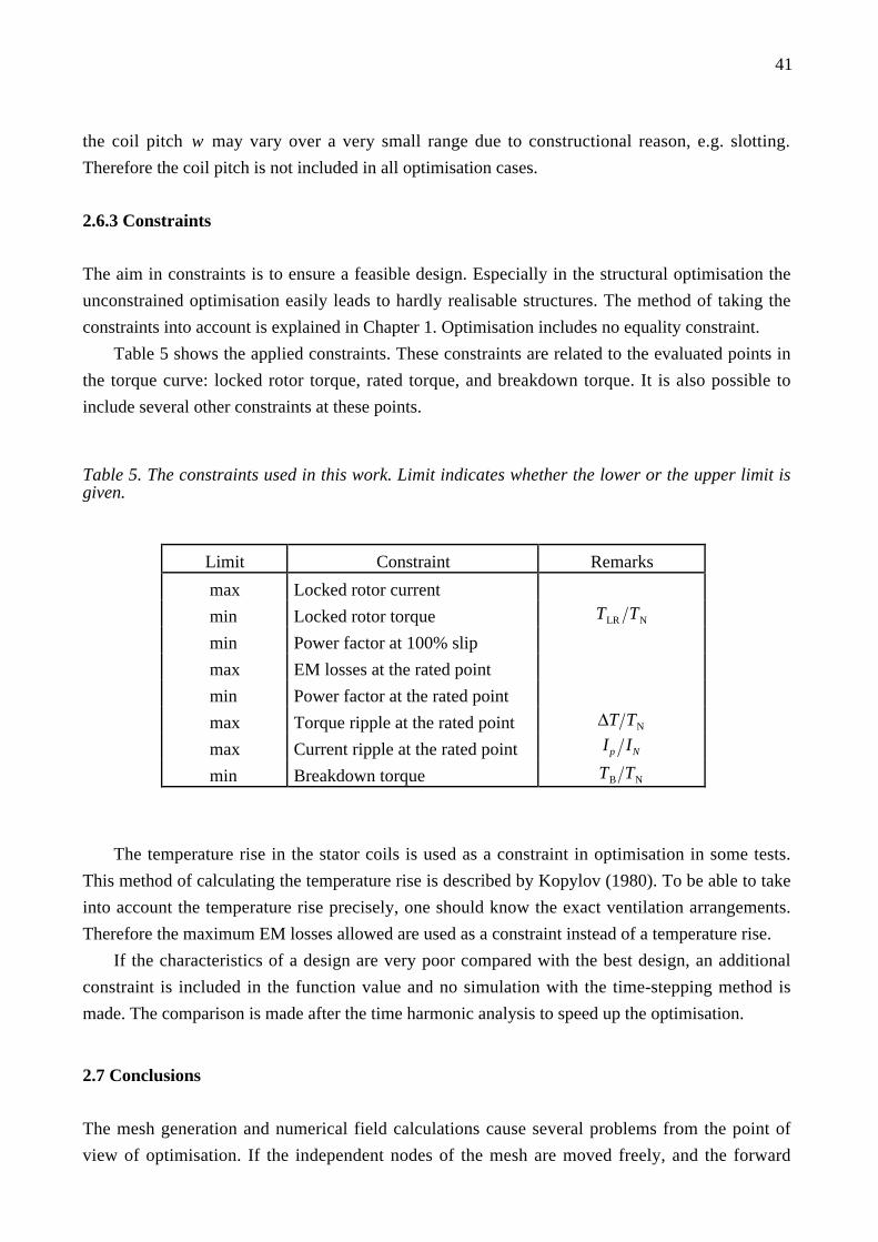
41

the coil pitch w may vary over a very small range due to constructional reason, e.g. slotting.

Therefore the coil pitch is not included in all optimisation cases.

2.6.3 Constraints

The aim in constraints is to ensure a feasible design. Especially in the structural optimisation the

unconstrained optimisation easily leads to hardly realisable structures. The method of taking the

constraints into account is explained in Chapter 1. Optimisation includes no equality constraint.

Table 5 shows the applied constraints. These constraints are related to the evaluated points in

the torque curve: locked rotor torque, rated torque, and breakdown torque. It is also possible to

include several other constraints at these points.

Table 5. The constraints used in this work. Limit indicates whether the lower or the upper limit isgiven.

Limit Constraint Remarks

max Locked rotor current

min Locked rotor torque TLR TN

min Power factor at 100% slip

max EM losses at the rated point

min Power factor at the rated point

max Torque ripple at the rated point ∆T TN

max Current ripple at the rated point Ip IN

min Breakdown torque TB TN

The temperature rise in the stator coils is used as a constraint in optimisation in some tests.

This method of calculating the temperature rise is described by Kopylov (1980). To be able to take

into account the temperature rise precisely, one should know the exact ventilation arrangements.

Therefore the maximum EM losses allowed are used as a constraint instead of a temperature rise.

If the characteristics of a design are very poor compared with the best design, an additional

constraint is included in the function value and no simulation with the time-stepping method is

made. The comparison is made after the time harmonic analysis to speed up the optimisation.

2.7 Conclusions

The mesh generation and numerical field calculations cause several problems from the point of

view of optimisation. If the independent nodes of the mesh are moved freely, and the forward

42

differences converge properly, the algorithm may still have difficult problems. In optimisation, it is

possible to find several local extrema to a problem, i.e. several similar designs close to each other,

and therefore one must use some method of smoothing in the optimisation. The simplest method of

smoothing applied to this work is the requirement of the symmetrical slots and a small number of

variables, but also master nodes and statistical means are used, e.g. averaging.

In structural optimisation the derivatives are usually evaluated using computationally

inexpensive first order forward difference approximation. The forward differences are highly

dependent on the perturbation length. In the case of a motionless body it is possible to obtain

reliable estimates for the derivatives, i.e. the forward differences that converge as the perturbation

length decreases with the time harmonic analysis.

Refinement of the mesh, e.g. maximisation of the common quality factor or adaptive

refinements, causes differences in the field matrix, destroying the convergence properties of the

forward differences, and not only with non-linear materials. Only after several adaptive refinements

is it possible to obtain properly converging forward differences. Therefore the interior nodes of the

mesh are in optimisation at fixed positions. With linear materials it is possible to obtain converging

forward differences, but the first order forward differences differ by several orders of magnitude or

they are of the opposite sign compared to the non-linear case. Therefore forward differences with

linear material can not be used as a reliable estimate.

The time-stepping method causes additional truncation and round-off errors when combined

with non-linear materials in simulation. Therefore the convergence of the forward differences is

poor. The adaptive refinement techniques are not possible due to lengthy simulation duration. The

usage of master nodes improves the reliability of the forward differences, but not always the

confidential interval. The problem of the forward differences suggests the use of derivative-free

methods as an optimisation algorithm, e.g. genetic algorithms, especially with the time-stepping

method. Smoothing with master nodes improves the convergence of the forward differences, but

the confidential interval of the perturbation length is usually only from 10-2 to 10-4.

The objective functions selected in this work are the locked rotor torque, the EM losses, and

the minimisation of the error due to constraint violations. In the computation of the objective

function, the main attention is given to the evaluation of the characteristics of the motor at certain

positions of the torque curve, i.e. locked rotor torque, breakdown torque, and characteristics at the

rated point. This is to enable optimisation in a rational time.

The finite element method is not accurate. The difference between the real and the computed

motors may be several percentages. All the changes in the finite element mesh i.e. the changes in

the optimisation variables, are not necessarily significant. They may reflect only the accuracy

problems of the analysis. One can also find several local extrema to a problem only by making

small changes in the parameter values. Therefore statistical means are needed for reliable analysis

of the results.

The statistical analysis is based on statistical test of the significance and averaging with large

populations. Later the author reduced the population size and the number of the variables to speed

43

up optimisation. In the case of a small population size the statistical tests are not suitable, and the

smoothing is made by taking the average value among the best ten to twenty motors. Averaging is

applied to improve the reliability of the results.

In spite of the undesired aspect, the time-stepping method is needed for a reliable optimisation

of induction motors. With this method it is possible to optimise both the rotor and the stator

simultaneously, and especially at the near air gap region. The time-stepping method also enables

reliable modelling of the inverter fed motors, and to taking into account the effects caused by

higher harmonics. Only with the time-stepping method is it possible to obtain sufficient accuracy

for optimisation.

44

3 GENETIC ALGORITHM

The unreliability of the forward differences suggests the use of derivative-free optimisation

algorithms. In this work optimisation is made using a genetic algorithm. The idea is to speed up

evolution in the computer instead of building real motors. This chapter presents the parameter

settings for the algorithm, when the objective function is extremely slow to evaluate. Also four

efficient improvements are presented in the standard algorithm, e.g. parallel computing.

3.1 Background of the method

A genetic algorithm is based on nature's own evolutionary principles which are simulated in a

computer. In this algorithm the variables are described as a string of bits 0, 1, chromosomes,

suggested by Holland (1975). For each variable to be optimised, a feasible interval is defined. The

upper boundary of the interval is described with a string of ones "111...1", while the lower

boundary consists of zeros "000...0". In this work the range is usually ±100% of the initial value

and the number of the bits in the strings is 16. The chromosomes consist of individual parts, genes.

The approach to simulate a genetic system in a computer using genetic operators was proposed

and examined by Fraser (1957). Holland (1975) studied the mathematical basis for these

techniques. Davis (1991) suggested the following to be a standard genetic algorithm:

1) Initialise a population of solutions.

2) Evaluate each solution in the population.

3) Create new solutions by mating current solutions:

apply mutations and recombination as the parent solutions mate.

4) Delete members of the population to make room for the new solutions.

5) Evaluate the new solutions and insert them into the population.

6) If the available time has expired, halt and return to the best solution;

if not, go to step 3.

In optimisation, the algorithm alters the chromosomes, the genome of the population members,

using genetic operators. It crossovers the genes and generates mutations to the genes to obtain

better designs. The aim is to find the right genes for a population member to be able to “live” most

successively in the environment described by the objective function and the constraints. It is also

possible to study the results and the characteristics of an entire population using statistical means.

The population gives the genetic algorithm a possibility to utilise more information in the selection

of the new designs, and it is not limited to a one and only interpolation scheme, e.g. a quadratic

interpolation scheme suggested by Palosaari et al. (1986) in random search methods.

The roulette wheel parent selection (Davis, 1991; Michalewicz, 1992) is a commonly applied

method to select the parents. This method evaluates a fitness for each population member, and the

chance of becoming a parent is proportional to this fitness. After assigning these weights for each

member, a group of members is chosen to reproduce and a group of other members is chosen to die.

45

Genetic operators are applied and a new generation is produced to replace the members that died.

The examination of the convergence properties of the genetic algorithms is difficult. The

stochastic optimisations with random methods offers an asymptotic guarantee for finding the global

minimum, when the sample size increases (Dixon et al., 1978). Using Markov chain analysis

Rudolph (1994) showed that the genetic algorithm defined by Holland (1975) is not convergent,

regardless of the initialisation, genetic operators, and the objective function. According to Rudolph

(1994) the search can be easily made to converge globally by adding an elitist selection. According

to this rule one must always maintain the best solution in the population for all later generations.

Bäck et al. (1993) showed that it is possible to obtain geometrical convergence rates with

certain objective functions by modifying selection rules in mating. Schwefel (1981) found that the

convergence rate can be improved by generating multiple offspring from the same parents, similar

to nature. Schwefel (1981) and Bäck et al. (1991) also studied self-adaptiveness of the operators to

improve the convergence rates. One of the suggested methods is to use information about the

gradient in the mutation operators, i.e. adaptive step size.

In the simulation of the evolution in computers, there are two main categories of algorithm:

evolution strategy and genetic algorithms. According to Fogel (1994) the philosophical difference

is that genetic algorithms emphasise the genetic operators observed in nature and use these

operators on the chromosomes, while evolution strategy emphasises mutational transformations that

maintain behavioural linkage between the parent and its offspring.

The genetic optimisation usually involves non-linear stochastic operations. To make the

mathematical analysis traceable, one has to make simplifications in the procedures, and the actual

algorithm is no longer studied. Therefore the author selected an empirical approach and statistical

means to study the performance of the genetic algorithm. Naturally this limits the generality of the

results in other optimisation problems.

3.2 Population size

The population size is one of the most important parameters for a genetic algorithm. Too large a

population slows down the optimisation, while a small population does not utilise the genetic

operators effectively. The population size affects the convergence properties of a stochastic

algorithm as shown by Dixon et al. (1978). Haataja (1994) states that the population size and the

coding of the variables to the chromosomes significantly affect the effectiveness of the genetic

algorithms. When the population size increases, it is also possible to analyse the population using

statistical means, as suggested by Bäck et al. (1993) and Palko (1994).

The population size in this work ranges from 50 to 1240, while most of the calculations have

been made with a population size of 50 to 100 members. Large population sizes are applied in the

optimisation of the air gap region or the whole geometry for induction motors to enable statistical

analysis of the results. Generally the author applied a population size of 5 to 10 times the number of

the variables. The population size is also discussed in Chapter 2 in statistical analysis. One of the

46

main objectives set for the optimisation method in this work is that the performance of this method

is good even with a small number of function evaluations. The duration of the optimisation tests

was selected according to the current computer resources corresponding to a typical optimisation

case. This limits the number of population members to 50 and the number of generations to 10.

3.3 The effect of genetic operators

In genetic algorithms the evolution of the population is simulated using genetic operators. The

typical value for crossover probability in literature ranges from 0.6 to 0.95 and for a bit mutation

from 0.001 to 0.01 (Schraudolph et al., 1992). The genetic operators are selected in this work in

accordance to work by Michalewicz (1992). The following seven mutation operators are applied in

this work:

1) Uniform mutation

2) Boundary mutation

3) Non-uniform mutation

4) Non-uniform boundary mutation

5) Whole arithmetic crossover

6) Simple arithmetic crossover

7) Adoption

These operators can be divided into three categories: mutation operators (1 to 4), crossover

operators (5, and 6) and adoption (7).

In the uniform mutation a new value is selected randomly from the feasible interval or intervals

for variables. In the boundary mutation the algorithm selects one of the limiting boundaries of the

feasible interval(s). The non-uniform mutation operator is similar to the uniform mutation, except

that the algorithm mutates genes either with the lower or the higher part of the interval. In the non-

uniform boundary mutation a parent is mutated either with the lower or upper limit of the interval.

In the non-uniform mutation the lower or upper values are selected using a 50-50 probability.

The algorithm uses two different crossover operators. In the whole arithmetic crossover, genes

are summed together, i.e. a new child gets part ( u ) from parent number one and part (1 − u) from

parent number two. The binary value of chromosome P is evaluated as

P = P1 ⋅u + P2 ⋅ (1 − u). (18)

In biology these summing genes are called multiple alleles. The other operator, simple arithmetic

crossover, is similar to the previous crossover operator. Instead of summing, the parts of the genes

from the parents are joined to each other as a whole (see Table 6). The probability of the gene

crossover is fixed at 0.75 in this work.

The adoption operator inserts a totally new member into the population. The genes of this new

member are selected randomly without using any information about the other population members.

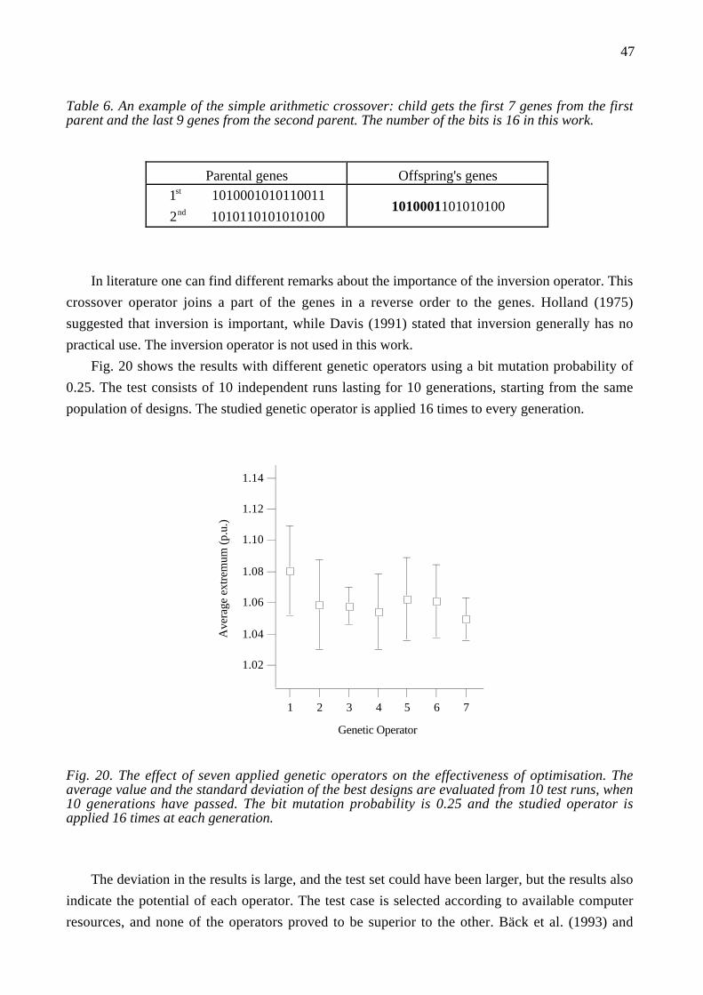
47

Table 6. An example of the simple arithmetic crossover: child gets the first 7 genes from the firstparent and the last 9 genes from the second parent. The number of the bits is 16 in this work.

Parental genes Offspring's genes1st 1010001010110011

2nd 10101101010101001010001101010100

In literature one can find different remarks about the importance of the inversion operator. This

crossover operator joins a part of the genes in a reverse order to the genes. Holland (1975)

suggested that inversion is important, while Davis (1991) stated that inversion generally has no

practical use. The inversion operator is not used in this work.

Fig. 20 shows the results with different genetic operators using a bit mutation probability of

0.25. The test consists of 10 independent runs lasting for 10 generations, starting from the same

population of designs. The studied genetic operator is applied 16 times to every generation.

1.14

1.12

1.10

1.08

1.06

1.04

1.02

Ave

rage

ext

rem

um (

p.u.

)

7654321

Genetic Operator

Fig. 20. The effect of seven applied genetic operators on the effectiveness of optimisation. Theaverage value and the standard deviation of the best designs are evaluated from 10 test runs, when10 generations have passed. The bit mutation probability is 0.25 and the studied operator isapplied 16 times at each generation.

The deviation in the results is large, and the test set could have been larger, but the results also

indicate the potential of each operator. The test case is selected according to available computer

resources, and none of the operators proved to be superior to the other. Bäck et al. (1993) and

48

Fogel (1994) state that there is no inherent benefit of using one single operator to generate new

trials for the population. They also suggest adaptiveness for the operators. The author applied each

operator 4 times in later optimisation tests.

3.4 The effect of the mutation probability

The genetic algorithm performs bit mutations similar to reproduction in nature. When the parental

genes are copied to the next generation, some copying errors may occur. In nature some of these

errors increase the reproductiveness of the population members, while others can be lethal.

In literature some authors suggest a very low mutation probability 0.008 (Davis, 1991) to

ensure asymptotic convergence of the method in a feasible domain. According to Fogel (1994) the

growing field of interest is in the importance of mutation, while earlier this operator was considered

redundant.

In the finite element optimisation the low mutation probability is in serious contradiction with

the time duration of the optimisation, though in some test cases a small mutation probability of 0.01

resulted in extremely good effectiveness in the optimisation. Usually the author applied very low

mutation probability, if the results from the simulation with a higher mutation probability were not

satisfactory. Due to the long duration of the FEM simulations, the algorithm has to be able to scan a

large parameter space efficiently. This led to high mutation probability in tests (Fig. 21).

1.10

1.08

1.06

1.04

1.02

1.00

Ave

rage

ext

rem

um (

p.u.

)

1.00.80.60.40.20.0

Probability of Bit Mutation

Fig. 21. The effect of bit mutation probability on the effectiveness of the optimisation. The resultsare from the optimisation of the breakdown torque in the inverter fed motor modelled with the time-stepping method. The results are the average and the standard deviation of the best designs in 10test runs, where 10 generations have passed. Each operator is applied 4 times in every generation.

49

A mutation probability higher than 50% decreases the effectiveness of the method. This

suggests avoidance of fully random optimisation methods. With a small mutation probability the

deviation of the results increases strongly: the best and the worst results were obtained using a very

low mutation probability. With the time-stepping method the author suggests the use of a mutation

probability less than 50%. At a very low mutation probability of 0.001 or less, the ability of the

optimisation algorithm to find better designs has been observed to be poor.

3.5 Improvements

It is seldom feasible to apply an optimisation method directly. Usually one has to make more or less

radical changes to the method. Various genetic algorithms are available, but combined with an

extremely slow objective function, such as FEM, special attention is required.

3.5.1 Checking

In optimisation problems with FEM, one has to operate with a limited number of genes and a small

population, i.e. a small number of design variables, and discrete values in the intervals. Therefore

the population members are not necessarily unique and the children from two different parents may

have the same genome. This was also noticed in the simulations.

This leads to the first improvement: checking of the previous generation. The algorithm does

not recalculate the genome that has already been evaluated. This also involves the checking of the

older good designs. This tracing of the best designs improved optimisation speed approximately

5%. The removal of all described recalculations reduced optimisation time from 5 to 20%. The

efficiency improves in later generations as searching is concentrated on a smaller region.

3.5.2 Restarting

The author also experienced that restarting of a genetic algorithm improves the effectiveness of the

optimisation. In nature this would mean for example a natural catastrophe, disease, increased

radiation in the environment, or war. The increase in optimisation effectiveness was found to be

several hundred percentages. The restarting of a globally converging optimisation algorithm is also

widely used in different optimisation cases (Haataja, 1994).

The method of restarting is tested using 38 design variables in this work (Fig. 22). The

optimisation is restarted after 1.3 and 23.5 hours. The content of the population is saved before each

restarting time to be able to continue optimisation later with a restart. This experiment shows

approximately a six fold convergence rate for a restarted optimisation. The bit mutation probability

is, in this test, 0.25 and each operator is applied four times while the population size is 350. The

behaviour is rather similar to trapping of a local minimum with deterministic methods. The author

also experienced a similar behaviour in different optimisation cases.

50

0.924

0.922

0.920

0.918

0.916

0.914

0.912

Eff

icie

ncy

403020100

Time (h)

Restarts after 1.3and 23.5 hours

Fig. 22. The time evolution of the best design in the optimisation of the efficiency using 38 designvariables. The dashed line shows the optimisation without restarts.

In optimisation, a relatively small number of function values are evaluated resulting in a large

variance. Combined with a high mutation probability and the stochastic nature of this method, the

result can be similar to local trapping.

3.5.3 Parallel computing

In the case of a genetic algorithm and FEM calculations, there are two main approaches when using

parallel computing. The first is to calculate the finite element matrix calculations using a

multiprocessor environment and the other possibility is to evaluate objective function values in

different CPUs. However, programmers are usually disappointed with the moderate gain of parallel

computing. The feasibility of parallel computing is often characterised by Amdahl's law (Quinn,

1987) describing the scaleability Sm of the problem.

mS = 1

1 − e + em

m→∞ →

11 − e

, (19)

where e is the fraction of the program computed parallel ( e ∈ 0,1[ ) ), and

m is the number of processors.

Eq. 19 is derived from the total time consumption of the calculations. The computation time is

the sum of the serial and the parallel parts

t = 1 − e( ) + e

m. (20)

51

When the number of processors approaches infinity, the limiting factors are the serial parts of the

program code, i.e. 1 − e( ) .

The time-stepping analysis program “CIMTD” available at the laboratory of Electromechanics

uses the SPARSPAK library of Waterloo University (Chu et al., 1984). Nearly 75% of the serial

computation time is used by the SPARSPAK library in the CIMTD program. This would lead to a

scaleability of four, if only the matrix operations would be computed in parallel.

Actually, the limit of scaleability, when the number of processors increase, is not even

proportional to the method of solving the matrix equations. If α indicates the time needed for

matrix calculations with a new method compared to the SPARSPAK, the computation time is

t = 1 − e( ) + αe

m, (21)

where α > 0 . This would lead to scaleability

Sm' =

11 − e( ) + αe

m

m→∞ →

11 − e

. (22)

The conclusion is that without totally restructuring the serial parts of the program “CIMTD”, it is

useless to apply parallel computing. The computation of matrix calculation in parallel also results in

a vast communication between the processors. This further reduces the gain of parallel computing.

One can also study the utilisation degree Um of m processors:

Um = mSm

. (23)

The utilisation degree is plotted in Fig. 23 with different parallel computing fractions in the

program. Even if 90% of the program could be calculated in parallel, the scaleability Sm would be

only ten. With 50 processors the utilisation degree is 17%, corresponding to a total of 8.5

processors on full load. Therefore parallel computing is used for calculating the objective functions

in the separate CPUs.

Genetic algorithms are suitable for parallel computing. Not only the evaluation of the objective

function, but the genetic operators can be computed in parallel. The genetic operators are not

evaluated using parallel computing in this work, because over 99.95% of the CPU time is needed

for the function evaluations even with a small population of 50 members. In this optimisation test

the CPU time for the serial part is only 102 seconds, while the function evaluations take nearly

216,000 seconds.

Genetic algorithms need very little communication between the individual processors. They

just send the initial data and the result between the master and the worker procedure. The time

needed for the genetic operators is insignificant for the time of function evaluations , when the

time-stepping simulation is used. Therefore the genetic algorithm has an extremely high

scaleability.

52

100

80

60

40

20

0

Util

isat

ion

degr

ee [

%]

250200150100500

Number of processors

Fraction of the parallel computing in program:

90% 99% 99.9% 99.99% 100%

Fig. 23. The utilisation degree of the processors with different parallel fractions. If over 99% of theprogram can be computed in parallel, the usage of the highly parallel environment is justified.

The author has tested optimisation from 1 up to 100 CPUs (some of the processors were

virtual) in IBM SP1 and SP2 workstations. Later the number of CPUs was limited to four due to a

lack of resources. Parallel computing does not necessarily increase the effectiveness of the

optimisation. The author experienced cases, where the serial optimisation was faster in finding a

better optimum with the same parameter values and the initial design. This is closely linked to the

stochastic nature of this optimisation method, but it also indicates the usefulness and robustness of

selected optimisation methods in a non-parallel computation environment.

The parallel implementation in this work is based on the master-worker approach, i.e. the

master selects the new design to be evaluated and passes the design variable data to workers.

Workers evaluate the values of the objective function and send the results back to the master, who

has been waiting and collecting results. The workers use only local memory and local hard disks in

order to minimise the computation time. One possibility to speed up the finite element calculations

would be to use larger memory. In this manner it would be possible to avoid the usage of low speed

I/O devices, such as hard disks.

3.5.4 Elitist selection

The rule of elitist selection defined by Rudolph (1994) was implemented after a couple of test

cases, where the optimisation algorithm lost the best design found. This was implemented by the

removal of the worst population member. The best design was usually lost, if the convergence rate

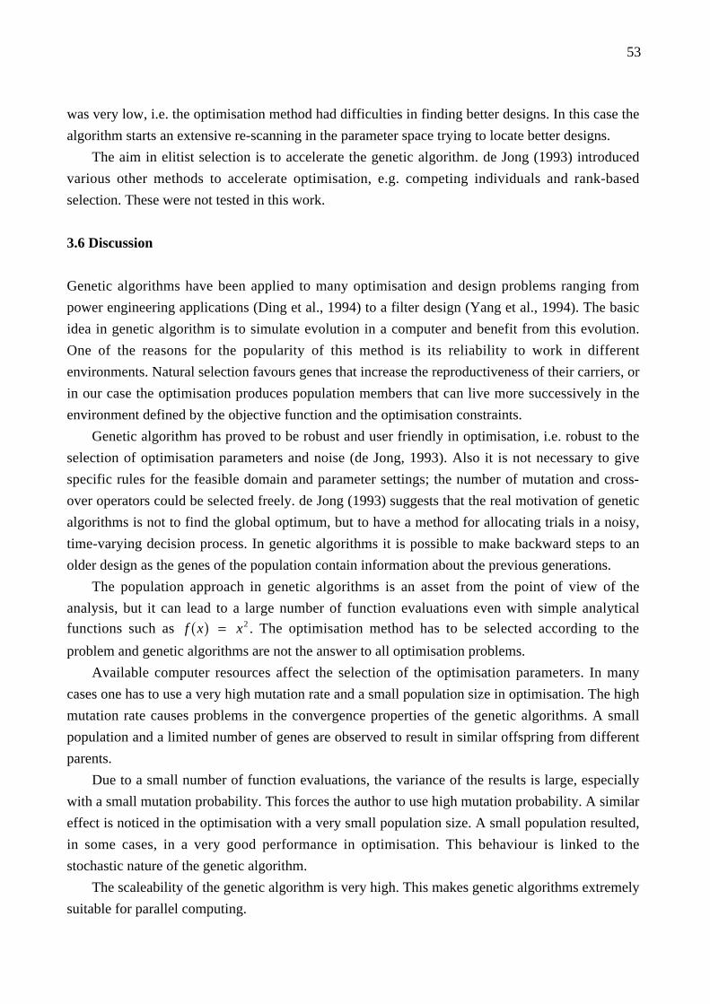
53

was very low, i.e. the optimisation method had difficulties in finding better designs. In this case the

algorithm starts an extensive re-scanning in the parameter space trying to locate better designs.

The aim in elitist selection is to accelerate the genetic algorithm. de Jong (1993) introduced

various other methods to accelerate optimisation, e.g. competing individuals and rank-based

selection. These were not tested in this work.

3.6 Discussion

Genetic algorithms have been applied to many optimisation and design problems ranging from

power engineering applications (Ding et al., 1994) to a filter design (Yang et al., 1994). The basic

idea in genetic algorithm is to simulate evolution in a computer and benefit from this evolution.

One of the reasons for the popularity of this method is its reliability to work in different

environments. Natural selection favours genes that increase the reproductiveness of their carriers, or

in our case the optimisation produces population members that can live more successively in the

environment defined by the objective function and the optimisation constraints.

Genetic algorithm has proved to be robust and user friendly in optimisation, i.e. robust to the

selection of optimisation parameters and noise (de Jong, 1993). Also it is not necessary to give

specific rules for the feasible domain and parameter settings; the number of mutation and cross-

over operators could be selected freely. de Jong (1993) suggests that the real motivation of genetic

algorithms is not to find the global optimum, but to have a method for allocating trials in a noisy,

time-varying decision process. In genetic algorithms it is possible to make backward steps to an

older design as the genes of the population contain information about the previous generations.

The population approach in genetic algorithms is an asset from the point of view of the

analysis, but it can lead to a large number of function evaluations even with simple analytical

functions such as f x( ) = x2 . The optimisation method has to be selected according to the

problem and genetic algorithms are not the answer to all optimisation problems.

Available computer resources affect the selection of the optimisation parameters. In many

cases one has to use a very high mutation rate and a small population size in optimisation. The high

mutation rate causes problems in the convergence properties of the genetic algorithms. A small

population and a limited number of genes are observed to result in similar offspring from different

parents.

Due to a small number of function evaluations, the variance of the results is large, especially

with a small mutation probability. This forces the author to use high mutation probability. A similar

effect is noticed in the optimisation with a very small population size. A small population resulted,

in some cases, in a very good performance in optimisation. This behaviour is linked to the

stochastic nature of the genetic algorithm.

The scaleability of the genetic algorithm is very high. This makes genetic algorithms extremely

suitable for parallel computing.

54

4 NUMERICAL OPTIMISATION CASES

This chapter contains numerical optimisation cases with a genetic algorithm using the described

method of evaluating the characteristics of the motor and taking constraints into account.

Optimisation is made by minimising the EM losses, maximising the locked rotor torque, or

minimising the error due to constraint violations. In the first tests the near air gap region and the

whole slot geometry is optimised allowing motors to have an uneven air gap. Later optimisation is

limited to a smooth air gap. The tests are made with a 15 kW and a 90 kW motor. Optimisation is

allowed to alter the shape of the slots and the coil arrangements using different objective functions

and supply wave forms. The reliability of the results is improved by calculating an average design

in the population. The results are discussed and compared with other studies. The feasible range

selected for variables is usually ±100% of the initial value.

4.1 Background of the tests

In literature one finds various suggested slot shapes for induction motors, e.g. Vogt (1983), Perho

et al. (1995). Laithwaite (1973) presented various induction motor constructions with an uneven air

gap. Pyrhönen et al. (1994) have studied the effect of shaped teeth edges in a solid rotor high speed

induction motor. The interesting question is, could the desired characteristics of the motor be

enhanced by shaping the air gap, e.g. using an uneven air gap?

The high frequency flux in inverter fed motors does not penetrate very far into the rotor cage

and it causes additional resistive losses at the surface of the rotor (Arkkio, 1991a). If the stator coils

are made from small conductors, the higher harmonics do not cause large eddy current losses in the

stator winding. Therefore it would be possible to modify the stator slot shape in order to alter the

path of the flux in the air gap region. The optimisation is made with the first-order elements and the

time-stepping method in all cases. The usage of the first-order elements affects the results of the

optimisation. It is also possible that the optimisation algorithm has not noticed the best possible

design. The statistical analysis is also applied to improve the reliability of the results.

One aim in this work is to design new slot shapes for induction motors using a genetic

algorithm and the finite element method. The other aim is to demonstrate the reliability of the

optimisation method. All the motors are unskewed and the stator coils are assumed to be made from

small conductors. The iron material is the same for all motors.

4.2 Computation environment

The element mesh and numerical calculations are made with a two-dimensional FCSMEK B Finite

Element Program package (Arkkio, 1991) available in the Laboratory of Electromechanics. The

computations are made in IBM RISC SYSTEM 6000 workstations equipped with a minimum of

55

64 MB memory, and the SPARSPAK library (Chu et al., 1984). With the first order elements the

time needed for the evaluation of the characteristics is 25 minutes. The parallel optimisations are

made in an IBM AIX SP1/2 computer using 4 CPUs and a fast switching net for message passing.

4.3 Near air gap region

The task is to find a suitable shape for the air gap surface of an induction motor. This is tested for

the minimisation of the EM losses and the maximisation of the locked rotor torque. The tests are

made using a sinusoidal voltage supply and an asymmetrical slot shape. The supply frequency is

50 Hz and the voltage is 380 V. The rotors rotate counter-clockwise in the simulations.

In optimisation, the boundary nodes of the mesh are allowed to move. Smoothing is based on

averaging, and statistical tests at a 5% risk level. The population sizes are 350 or 700, and the

number of variables is respectively 38 or 66 (nodes move in one or two directions). The locked

rotor current is limited below 260 A. The breakdown torque must be higher than 1.6 times the rated

torque. The EM losses at the rated point and the locked rotor torque are not used as constraints.

4.3.1 The initial motor for the near air gap

The initial geometry and the mesh for the 15 kW motor are in Fig. 24, and the characteristics are

shown in Table 7. This four pole motor has 36 stator and 32 rotor slots, and two pole pairs. The

simulations are made using 300 steps per period and a total of 900 steps. The results are the r.m.s.

and average values from the last full period.

a) b)

Fig. 24. The initial motor (a) and the mesh used in optimisation (b). The mesh has 1650 elements.

56

Table 7. The characteristics of the initial 15 kW motor at rated power and 100% slip. Supplyfrequency is 50 Hz and the supply voltage is 380 V. The breakdown torque is 403 Nm at 33% slip.

Slip / % Current / A p.f. η T / Nm PEM / kW

3.10 31.1 0.793 0.893 98.4 1.79

100 253. 0.616 - 309 103.

Due to the method of evaluating the torque, there is a smaller layer of air elements on the

surface of the rotor and stator in the mesh. The results of this mesh are very close to the results of

the simulation without this small layer, e.g. the difference in EM losses is only 40 W. The author

assumed that this small layer does not cause significant changes to the reliability of the results.

4.3.2 Electromagnetic losses

The locked rotor torque decreases with the minimisation of the EM losses, and the stator slot

openings become fairly small, but the rotor slot openings remain nearly the same in both cases. In

many designs the rotor teeth are slanted counter-clockwise, but in the averaged design there are

slightly narrower rotor slot openings compared with the original motor. Fig. 25 shows the air gap of

the optimised motors. The characteristics of the optimised motors are shown in Table 8.

Optimisation reduced the EM losses by an average of 180 W, improving the efficiency by 1.1%.

The number of the significantly changed variables are 30 out of 38 and 59 out of 66.

a) b)

Fig. 25. Average optimised gap shapes for a motor with 38 variables (a) and with 66 variables (b).Rotors rotate counter-clockwise in simulations.

57

Table 8. The characteristics of the optimised 15 kW motor at the rated power and 100 % slip. Theminimisation of EM losses is made with 38 variables and 66 variables using a sinusoidal supply(380 V). The breakdown torque is 389 Nm at 32% slip (38 variables), and 398 Nm at 33% slip (66variables). The number of the significantly changed variables are 30 out of 38 and 59 out of 66.The results are the average of 97 and 153 motors.

Variables Slip / % Current / A p.f. η T / Nm PEM / kW

3.08 30.5 0.803 0.904 98.5 1.5938 100 249 0.604 - 305 100.

3.09 31.2 0.803 0.902 98.5 1.6366 100 252 0.610 - 302 102.

The smaller slot openings reduce the variation in the flux density in the gap similar to the

results of Pyrhönen et al. (1994). Smaller variation in the flux density reduces the pulsation losses

in the teeth, which improves the efficiency of the motor. Generally the surface of the rotor and the

stator is very smooth, also in the non-averaged designs (see Fig. 17). A smooth air gap also

minimises the flux density variations.

To study the reliability of the results, the notches are moved from the stator teeth in the case of

38 variables. This increases the EM losses 10 W, and when the rotor slot opening are changed to

the initial one, losses increased by an additional 20 W. Notches are significant even at a very low

0.1% risk level, but from the viewpoint of the analysis model, these changes of 10 to 20 W are not

significant. The notches in the averaged motor are due to non-robust estimation, as discussed in

Chapter 2, and the enhanced motor characteristics are due to the reshaped stator slot openings.

When the motors operated to clockwise direction, the EM losses are 5 W and 10 W larger in

simulation, while other characteristics are practically the same. Considering the accuracy of FEM,

these results also suggest that the enhanced motor characteristics are due to the reshaped stator slot

openings.

The reduction of EM losses is fairly small in this case. This is due to the locked rotor current

used as a constraint. The modification of the slot openings change the leakage reactance. A smaller

leakage reactance would increase the breakdown torque, but it would also increase the locked rotor

current. In many design the losses were smaller, but the locked rotor current exceeded the allowed

maximum value.

4.3.3 Locked rotor torque

In the maximisation of the locked rotor torque the simulations are made with the same mesh, but

the number of steps per period is at 100% slip, 30 steps per period, and the results are the r.m.s. and

average values from the last ten periods. The characteristics of the optimised motors are in Table 9,

and the optimisation results are shown in Fig. 26.

58

Table 9. The characteristics of the optimised 15 kW motor at the rated power and 100% slip. Themaximisation of the locked rotor torque is made with 38 variables and 66 variables using asinusoidal supply (380 V). The breakdown torque is 407 Nm at 33% slip (38 variables), and409 Nm at 34% slip (66 variables). The number of the significantly changed variables are 25 out of38 and 56 out of 66. The results are the average of 94 and 213 best designs.

Variables Slip / % Current / A p.f. η T / Nm PEM / kW

3.12 34.5 0.725 0.890 98.6 1.8638 100 260 0.612 - 338 108.

3.13 32.8 0.759 0.889 98.6 1.8766 100 260 0.616 - 351 109.

a) b)

Fig. 26. Averaged optimised gap shapes for a motor with 38 variables (a) and with 66 variables (b)while maximising the locked rotor torque.

The maximisation of the locked rotor torque by shaping the near air gap region resulted in only

a 10% increase in the torque. Optimisation of the locked rotor torque enlarges the slot openings.

The air gap is practically at the allowed minimum, i.e. 0.05 mm smaller than in the initial motor,

with the exception of the notches in the rotor teeth. The position of the notches is asymmetric and

statistically significant at a 5% risk level. The number of the significantly changed variables are 25

out of 38 and 56 out of 66.

The achieved increase in torque is rather moderate, even though the increase is nearly 10%;

only 30 Nm and 40 Nm with 38 and 66 variables respectively. Considering the first-order shape

functions used, the optimisation results are also evaluated with the second-order shape functions.

The difference in the locked rotor torque decreased to 10 Nm and 20 Nm. This moderate gain in the

torque suggested the optimisation of the whole slot shape in later tests.

59

If the optimised motors are compared with the initial motor, there are very small changes.

Therefore the increased torque in both cases is assumed to be due to a higher flux density in the air

gap. This conclusion is also supported by the fact that most of the significantly changed parameters

are on the air gap surface. The shaping of the teeth has caused only a minor improvement, e.g. the

removal of the notches from the rotor surface reduces the locked rotor torque by only 5 Nm.

4.3.4 Conclusions

The results from these previous optimisation cases with sinusoidal voltages indicate the following.

The air gap of an induction motor should be smooth, at least for motors of this power range. A

larger gap diminishes the flux density and causes a smaller torque. Near the slot openings a detailed

structure improves the motor characteristics mainly by minimising the variations of the flux

density. A smaller variation of the flux density also causes less pulsation losses in the teeth. The

EM losses are reduced nearly 200 W by shaping the slot openings of the stator teeth. The increase

in locked rotor torque is very small.

In many evaluated motor designs there are small variations in the parameter values. With

averaging it is possible to find out the relevant changes in the design. Reliable estimation of the

shape proved to be very elaborate even with statistical means due to the large population size. A

typical simulation duration of previous tests is two months, when one processor is used. This

suggested the study of other means of smoothing in optimisation, to reduce the population size, and

to test parallel computing.

4.4 The whole slot geometry

The results from the maximisation of the locked rotor torque were not good in the near air gap

region. Therefore the next task is to optimise not only the gap region, but also the shape of the rotor

slots and stator slots. The maximisation of the torque involves two tests: asymmetric slot shape and

symmetric slot shape. The author tested minimisation of the EM losses, but the result was only

minor improvements, partially due to available resources. The number of the significantly changed

variables was very small, e.g. only 6 out of 138 changed significantly in one month using one

processor.

The optimisation is made using 76 and 138 variables. The population sizes are 680 and 1240.

The initial geometry for a 15 kW motor is in Fig. 27 (see also Fig. 14b). This four pole motor also

has 36 stator slots and 32 rotor slots. The characteristics of the initial motor are in Table 10. The

values in Table 10 differ from the values of Table 7 due to a different air gap and different slot

openings.

The locked rotor current is limited below 260 A and the breakdown torque must be 1.6 times

higher than the rated torque. In the case of symmetric slots, the electromagnetic losses at the rated

point are used as an additional constraint in optimisation, but the locked rotor torque is not used as

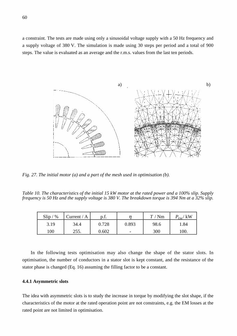
60

a constraint. The tests are made using only a sinusoidal voltage supply with a 50 Hz frequency and

a supply voltage of 380 V. The simulation is made using 30 steps per period and a total of 900

steps. The value is evaluated as an average and the r.m.s. values from the last ten periods.

a) b)

Fig. 27. The initial motor (a) and a part of the mesh used in optimisation (b).

Table 10. The characteristics of the initial 15 kW motor at the rated power and a 100% slip. Supplyfrequency is 50 Hz and the supply voltage is 380 V. The breakdown torque is 394 Nm at a 32% slip.

Slip / % Current / A p.f. η T / Nm PEM / kW

3.19 34.4 0.728 0.893 98.6 1.84

100 255. 0.602 - 300 100.

In the following tests optimisation may also change the shape of the stator slots. In

optimisation, the number of conductors in a stator slot is kept constant, and the resistance of the

stator phase is changed (Eq. 16) assuming the filling factor to be a constant.

4.4.1 Asymmetric slots

The idea with asymmetric slots is to study the increase in torque by modifying the slot shape, if the

characteristics of the motor at the rated operation point are not constraints, e.g. the EM losses at the

rated point are not limited in optimisation.

61

The optimisation results are in Table 11. The area of the stator slots increases by 26% and by

12%, while the area of the rotor bars decreases by 37% and by 22% in the motors shown in Fig. 28a

and Fig. 28b respectively. Optimisation of the locked rotor torque enlarges the area of the stator

slots and creates double or triple cage rotor bars. The width of the rotor bar increases by 50% near

the air gap. The air gap surface is smooth.

Table 11. The characteristics of the optimised 15 kW motor at the rated power and a 100% slip.The maximisation of the locked rotor torque is made with 76 variables and 138 variables using asinusoidal supply (380 V). The losses at the rated point are not used as a constraint in optimisation.The breakdown torque is 491 Nm at a 100% slip (76 variables), and 434 Nm at a 45% slip (138variables). The number of significantly changed variables are 68 out of 38 and 112 out of 138. Theresults are the average of 153 and 273 best designs.

Variables Slip / % Current / A p.f. η T / Nm PEM / kW

5.67 59.7 0.436 0.783 101. 4.1776 100 256 0.682 - 491 118

4.06 39.1 0.640 0.850 99.5 2.65138 100 255 0.649 - 412 113.

a) b)

Fig. 28. Averaged optimised slot shapes for a motor with 76 variables a) and 138 variables b)while maximising the locked rotor torque.

The reliability of the results is also tested with second order shape functions. The change in the

torque and the current at a 100% slip is nearly the same in all cases: torque decreases by 30 Nm and

62

line current by 10 A. With the second order shape functions and two adaptive refinements locked

rotor torque increases by 5 Nm, but the locked rotor current remains practically the same. This

indicates the reliability of the results.

Optimisation of the torque greatly changes the shape of the slots both in the stator and the

rotor, e.g. the rotor bars expand near the air gap. The resistance of the stator phase is inversely

proportional to the area of the stator slots, and the current increases. This increases the flux density

giving a larger torque. In the initial motor the flux density in the gap is 0.50 T, while it is 0.60 T in

the optimised motor. By dividing the rotor bars into separate cages, the optimisation algorithm

succeeds in keeping the stator current below the allowed maximum, e.g. if the initial rotor slot is

restored, the line currents of the motors are 278 A (78 variables) and 277 A (138 variables). The

double cage of the motor in Fig. 28b increases the locked rotor torque by 35 Nm.

The breakdown torque of the motor in Fig. 28a is at 100% slip and rotor resistance is therefore

equal to the leakage reactance of the motor. The reduced rotor bar area, due to the double or triple-

cage, increases the rotor resistance, and therefore the breakdown torque moves to a larger slip. The

motor operates at a very large slip at the rated power giving a poor efficiency, but it is possible to

increase the torque by dozens of percentages. The smooth air gap surface minimises the variations

of the flux density and reduces the pulsation losses in the teeth. The optimisation lasted from one to

two months in these tests, when one processor was used.

The triple cage of the motor is studied closer (Fig. 29). By joining the lowest two cages

together, the locked rotor torque is reduced to 461 Nm while the line current remains the same,

i.e. 254 A. With the initial rotor, the locked rotor torque is 390 Nm. The locked rotor torque is

396 Nm and the line current is 221 A with the initial stator slots and optimised rotor slot.

390 Nm 415 Nm 461 Nm 491 Nm

Fig. 29. The shape of the rotor bars and the locked rotor torque with optimised stator slot shapes.

If the motors operate clockwise direction the characteristics of the motors change. In the

motor, optimised with 76 variables, the locked rotor torque increases to 505 Nm, but the locked

rotor current is 265 A exceeding the allowed maximum. In the other motor (138 variables) the

locked rotor torque is 402 Nm and the current is 258 A.

63

4.4.2 Symmetric slots

It proved necessary to limit the losses at the rated power in the optimisation of the whole slot

geometry. Therefore, in the case of a symmetric slot shape, the allowed maximum losses are

1.85 kW. The symmetrical shape of the slot is defined using 41 variables. The optimisation in made

using a population size of 350. The maximisation of the locked rotor torque starts from the initial

slot shapes. Fig. 30 shows the evolution of the slot shapes.

a) b)

c) d)

Fig. 30. Evolution of the non-averaged slot shape in maximisation of the locked rotor torque. Thelocked rotor torque is, in the initial motor 300 Nm (a), and in the optimised motors 327 Nm (b),343 Nm (c) and 360 Nm (d). The allowed maximum losses are 1.85 kW at the rated power of 15 kW.

One of the first changes is a double rotor cage, which increases torque by 30 Nm. In addition,

the area of the conducting material in the stator slot increases. Later, the lower rotor cage becomes

64

smaller and the width of the rotor slot openings increases by 10% giving 10 Nm more torque. The

slot leakage reactance is inversely proportional to the width of the rotor slot opening and therefore

the leakage reactance decreases causing a larger breakdown torque. The slot opening of the rotor

expands below the gap surface. In this manner the flux density variations are smaller in the air gap.

The lower cage has almost vanished in the last stage (Fig. 30d), and it is only a very narrow

peak. There is practically no current in this part and this part has no significant effect on the

characteristics of the motor. The algorithm can not remove this part, because some of the nodes are

allowed to move only in one direction. The characteristics of the optimised motor are given in

Table 12.

Table 12. The characteristics of the optimised 15 kW motor at the rated power and a 100% slip.The maximisation of the locked rotor torque is made using symmetrical slots and 76 variables. Thelosses at the rated point are also used as a constraint. The breakdown torque is 420 Nm at a 35%slip. The results are from the best design in the population (non-averaged).

Variables Slip / % Current / A p.f. η T / Nm PEM / kW

4.01 32.1 0.78 0.89 99.7 1.841 100 248 0.66 - 360. 113.

The locked rotor torque is 348 Nm with the initial stator slot shape, while the optimised stator

slot shape gives only 4 Nm more torque with the initial rotor slot shape. Compared with an

asymmetric case, the area of stator slots has increased very little, i.e. only by 4%.

The air gap surface of the teeth is very smooth, but near the slot openings there is a detailed

structure. The shaping of teeth edges is reported by Preis et al. (1990) and Pyrhönen et al. (1994).

Preis et al. (1990) optimised the surface shape of a magnetic pole, while Pyrhönen studied the

shaped teeth edges in a solid rotor asynchronous motor. The result of all these studies is the same,

the minimisation of the flux density variations.

The results shown in this subsection are not averaged. The author found that usually there were

very few differences between the best extremum and averaged design with a small number of

variables. This also suggested that the population size could be smaller.

The symmetrical slot and a smaller number of variables had an interesting effect on the applied

optimisation algorithm; the optimisation not only became faster, but the algorithm started to scan

the parameter space more often and from a wider part of the parameter space. This is explained to

be partially due to the fact that the symmetrical slot decreases variations of the objective function.

A smaller number of master nodes creates additional smoothing and this reduces the number of

local extrema. Therefore the algorithm generates larger changes in the design. Averaging can be

applied to improve the reliability of the results.

65

4.4.3 Conclusions

The results with sinusoidal voltages indicate that the air gap surface of an induction motor should

be smooth. There could be a detailed shape near the slot openings. All this minimises the flux

density variations and reduces the pulsation losses in teeth. The leakage reactance decreases, if the

rotor slot openings expand below the gap surface, and not from the air gap surface. This enables

optimisation to minimise the flux density variations in the air gap and to increase the torque.

The usage of double or triple-rotor cages is beneficial from the standpoint of torque, also if the

motor characteristics at the rated power are not allowed to change. In an induction motor the double

cage rotors are used to obtain a large torque at a large slip.

The results indicated that a reduction in the number of variables has two main advantages:

optimisation becomes faster and the algorithm recognises the significant changes more reliably.

The probability of changing the correct variables becomes larger, if the number of variables is

smaller. A symmetrical slot and a smaller number of variables also perform smoothing. The gain in

the optimisation speed is remarkable; with approximately 40 variables the duration of the

optimisation decreased from 1-2 months to a couple of weeks. With parallel computing it is

possible to diminish the duration of the optimisation to a few days.

In previous cases the number of conductors was fixed, partially due to computational resources.

The dimensions of the near-gap variables were studied separately, because they can be used to

adjust the motor characteristics. In later tests the coils will also be considered in the optimisation.

4.5 Minimisation of losses in a 15 kW motor

The previous tests with an asymmetric and symmetric slot shape, as well as the test with time

harmonic analysis in Chapter 2 suggested keeping the air gap smooth. All later tests are limited to a

smooth air gap. The number of variables selected is small and the slots are symmetric to increase

the reliability of the optimisation recognising relevant changes in the designs without statistical

means. The table values and the best design shown are based on averaging in the population by

taking ten or twenty best design from the population of 50 or 100 members, respectively. Statistical

analysis of the significance is omitted due to a small population size. The finite element mesh is

created using a parametrised mesh generator program. The number of conductors in series in the

stator slot is also optimised. The number of the conductors in series in the stator slots is 21 in the

initial motor.

The test cases with a 15 kW induction motor concentrate on the minimisation of the EM losses.

It starts from the optimisation of the dimensions for the stator and the rotor. Later the slot shape of

the stator and the rotor are allowed to change freely and the constraints are changed. Most of the

simulations are with a 50 Hz sinusoidal supply and a supply voltage of 380 V, but also an inverter

supply is tested (Fig. 31). The switching frequency of the inverter is 800 Hz with 7 pulses in a half

period.

66

-1000

-500

0

500

1000

Vol

tage

(V

)

6050403020100

Time (ms)

Fig. 31. Inverter supply used in optimisation (the switching frequency is 800 Hz, 7 pulses in a halfperiod). During the first period a sinusoidal voltage is transformed to a desired inverter wave form.

The optimisation constraints and the limiting values are in Table 13. The breakdown torque

could have been larger. It is small to allow larger variation in the shape of the torque versus speed

curve. The breakdown torque remains, in all successive motors, larger than 3.6 times the rated

torque.

Table 13. Optimisation constraints for the minimisation of the EM losses in a 15 kW motor.

Constraint Value Remarks

line current / A 254. at a 100% slip

locked rotor torque 3.46 TLR TN

power factor 0.625 at a 100% slip

power factor 0.845 at rated power

EM losses / kW 2.02 at rated power

breakdown torque 1.600 TB TN

4.5.1 The original motor

The original four pole motor has 36 stator slots and 32 rotor slots. During the minimisation of the

EM losses the outer radius of the stator and the length of the motor are kept constant, i.e. the

volume of the motor is constant. The number of the conductors in series in the stator slots is 21.

The original motor is in Fig. 32 and the characteristics are in Table 14.

67

Fig. 32. The original 15 kW motor used in the optimisation.

Table 14. The characteristics of the original 15 kW motor at the rated power and a 100 % slip.Supply frequency is 50 Hz and the fundamental harmonic of the wave form is 380 V. Thebreakdown torque is 416 Nm at a 45% slip.

Supply Slip / % Current / A p.f. η T / Nm PEM / kW

sinusoidal 3.71 29.9 0.826 0.881 99 2.02

inverter 3.74 31.4 0.734 0.866 99 2.33

sinusoidal 100 244. 0.640 - 348 102.

4.5.2 Minimisation of EM losses with a sinusoidal supply voltage

The optimisation starts from the original motor using 15 design variables (Table 15) including the

number of rotor slots and the number of stator conductors. All the constraints in Table 13 are used

in the minimisation of the EM losses in this 15 kW induction motor.

The rotor slot opening expands by 5% to decrease leakage reactance and breakdown torque

increases. The width of the rotor bars decreases 3% from the top of the rotor bar and 25% from the

bottom of the rotor bar. This increases slot leakage reactance and increases the resistance of rotor

bars. Therefore the breakdown torque and the current decrease. The resistive rotor losses increase

by 3% giving a higher mechanical power (see Eq. 24). The initial and optimised dimensions are in

Table 15. The number of conductors is 21.

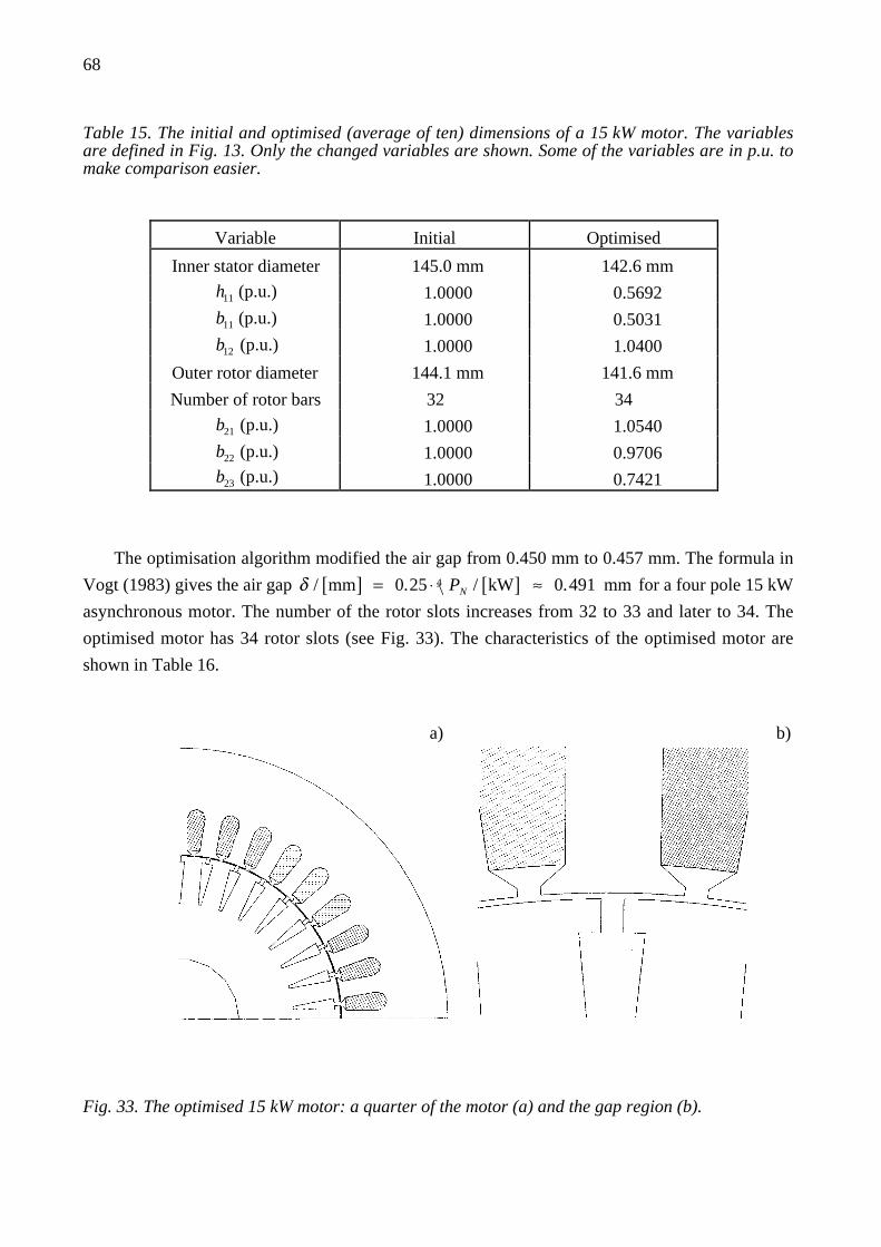
68

Table 15. The initial and optimised (average of ten) dimensions of a 15 kW motor. The variablesare defined in Fig. 13. Only the changed variables are shown. Some of the variables are in p.u. tomake comparison easier.

Variable Initial Optimised

Inner stator diameter 145.0 mm 142.6 mm

h11 (p.u.) 1.0000 0.5692

b11 (p.u.) 1.0000 0.5031

b12 (p.u.) 1.0000 1.0400

Outer rotor diameter 144.1 mm 141.6 mm

Number of rotor bars 32 34

b21 (p.u.) 1.0000 1.0540

b22 (p.u.) 1.0000 0.9706b23 (p.u.) 1.0000 0.7421

The optimisation algorithm modified the air gap from 0.450 mm to 0.457 mm. The formula in

Vogt (1983) gives the air gap δ / mm[ ] = 0.25 ⋅ PN / kW[ ]4 ≈ 0.491 mm for a four pole 15 kW

asynchronous motor. The number of the rotor slots increases from 32 to 33 and later to 34. The

optimised motor has 34 rotor slots (see Fig. 33). The characteristics of the optimised motor are

shown in Table 16.

a) b)

Fig. 33. The optimised 15 kW motor: a quarter of the motor (a) and the gap region (b).

69

Table 16. The characteristics of the optimised 15 kW motor at the rated power and a 100 % slip,when all the constraint are applied. Supply frequency is 50 Hz and the fundamental harmonic of thewave form is 380 V. The breakdown torque is 419 Nm at a 47% slip using a sinusoidal supply. Theresults are the average of ten.

Supply Slip / % Current / A p.f. η T / Nm PEM / kW

sinusoidal 3.34 28.6 0.857 0.896 98.9 1.74

inverter 3.37 30.1 0.767 0.866 98.8 1.98

sinusoidal 100 254. 0.638 - 344 106.

The EM losses were reduced, with the tested wave forms, from 10 to 15 % depending on the

order of the shape functions. The stator slot openings are narrower than in the initial design. This

minimises the flux density variations and the pulsation losses in the teeth, improving the efficiency

of the motor. None of the selected constraints is violated in the optimised design.

Optimisation has a tendency to favour an odd number of rotor slots, e.g. 31 and 33, but an odd

number of rotor slots generate large forces between the stator and the rotor (Arkkio, 1995). An odd

number of rotor slots causes an unbalanced magnetic pull rotating with a high frequency (Fig. 34)

in the air gap. Using optimisation it was possible to reduce this force from 490 N to 320 N with 33

rotor slots, mainly by increasing the air gap. This force is too large compared with the rotor mass of

19.3 kg. The number of rotor slots was limited to even numbers after this test.

-800

-400

0

400

800

y-co

mpo

nent

[N

]

-800 -400 0 400 800

x-component [N]

Fig. 34. The unbalanced magnetic pull in an induction motor with 33 rotor slots rotating at a highfrequency. The value of this force is one hundredth with an even number of rotor slots insimulations.

The duration of this optimisation was 18 days using one processor. The reliability of the results

is tested by using the second-order shape functions. With the second-order shape functions the

losses decreased from 1.85 kW to 1.62 kW using a sinusoidal supply.

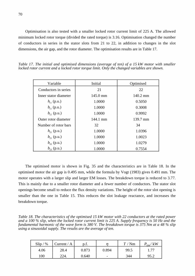
70

Optimisation is also tested with a smaller locked rotor current limit of 225 A. The allowed

minimum locked rotor torque (divided the rated torque) is 3.16. Optimisation changed the number

of conductors in series in the stator slots from 21 to 22, in addition to changes in the slot

dimensions, the air gap, and the rotor diameter. The optimisation results are in Table 17.

Table 17. The initial and optimised dimensions (average of ten) of a 15 kW motor with smallerlocked rotor current and a locked rotor torque limit. Only the changed variables are shown.

Variable Initial Optimised

Conductors in series 21 22

Inner stator diameter 145.0 mm 140.2 mm

h11 (p.u.) 1.0000 0.5050

b11 (p.u.) 1.0000 0.3008

b12 (p.u.) 1.0000 0.9992

Outer rotor diameter 144.1 mm 139.7 mm

Number of rotor bars 32 34

h21 (p.u.) 1.0000 1.0396

b21 (p.u.) 1.0000 1.0023

b22 (p.u.) 1.0000 1.0279b23 (p.u.) 1.0000 0.7554

The optimised motor is shown in Fig. 35 and the characteristics are in Table 18. In the

optimised motor the air gap is 0.495 mm, while the formula by Vogt (1983) gives 0.491 mm. The

motor operates with a larger slip and larger EM losses. The breakdown torque is reduced to 3.77.

This is mainly due to a smaller rotor diameter and a fewer number of conductors. The stator slot

openings become small to reduce the flux density variations. The height of the rotor slot opening is

smaller than the one in Table 15. This reduces the slot leakage reactance, and increases the

breakdown torque.

Table 18. The characteristics of the optimised 15 kW motor with 22 conductors at the rated powerand a 100 % slip, when the locked rotor current limit is 225 A. Supply frequency is 50 Hz and thefundamental harmonic of the wave form is 380 V. The breakdown torque is 375 Nm at a 48 % slipusing a sinusoidal supply. The results are the average of ten.

Slip / % Current / A p.f. η T / Nm PEM / kW

4.06 28.4 0.873 0.894 99.5 1.77

100 224. 0.640 - 344 95.2

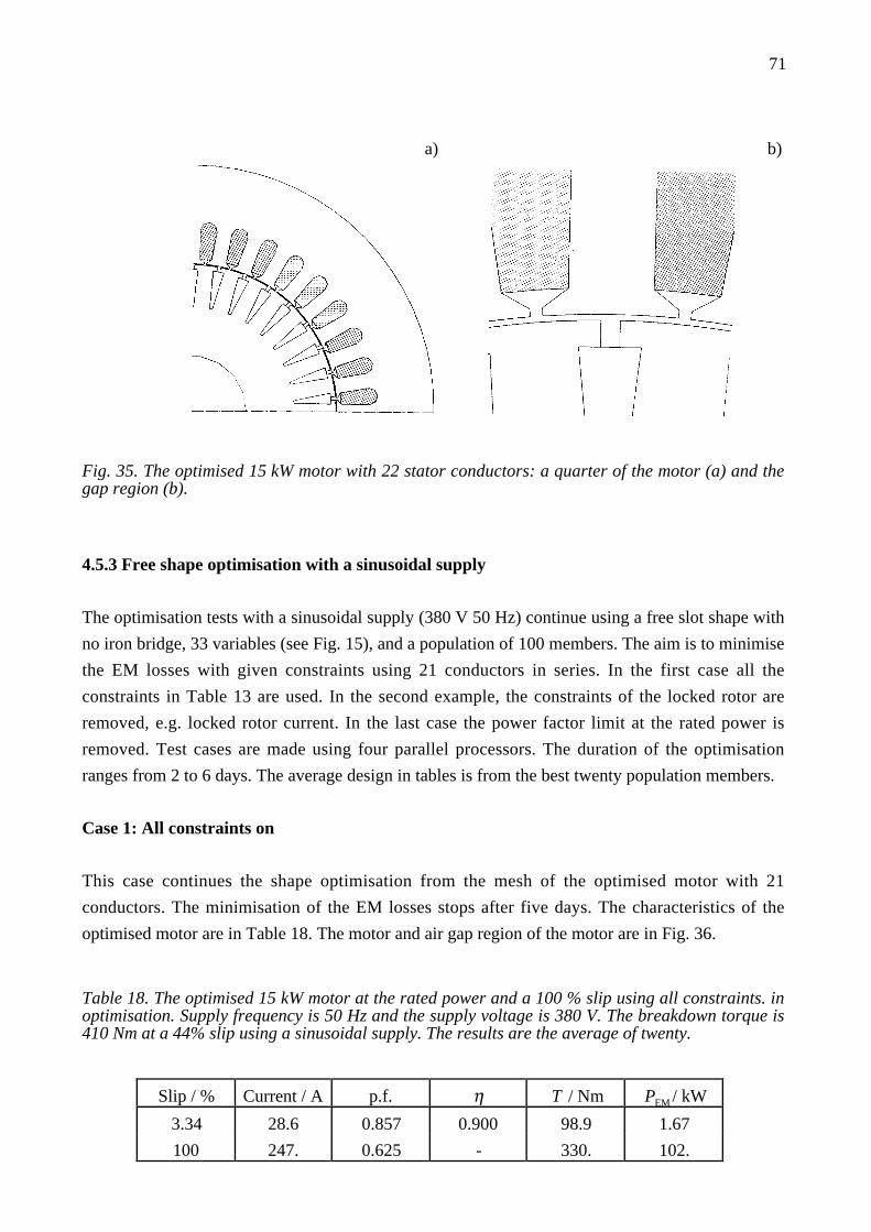
71

a) b)

Fig. 35. The optimised 15 kW motor with 22 stator conductors: a quarter of the motor (a) and thegap region (b).

4.5.3 Free shape optimisation with a sinusoidal supply

The optimisation tests with a sinusoidal supply (380 V 50 Hz) continue using a free slot shape with

no iron bridge, 33 variables (see Fig. 15), and a population of 100 members. The aim is to minimise

the EM losses with given constraints using 21 conductors in series. In the first case all the

constraints in Table 13 are used. In the second example, the constraints of the locked rotor are

removed, e.g. locked rotor current. In the last case the power factor limit at the rated power is

removed. Test cases are made using four parallel processors. The duration of the optimisation

ranges from 2 to 6 days. The average design in tables is from the best twenty population members.

Case 1: All constraints on

This case continues the shape optimisation from the mesh of the optimised motor with 21

conductors. The minimisation of the EM losses stops after five days. The characteristics of the

optimised motor are in Table 18. The motor and air gap region of the motor are in Fig. 36.

Table 18. The optimised 15 kW motor at the rated power and a 100 % slip using all constraints. inoptimisation. Supply frequency is 50 Hz and the supply voltage is 380 V. The breakdown torque is410 Nm at a 44% slip using a sinusoidal supply. The results are the average of twenty.

Slip / % Current / A p.f. η T / Nm PEM / kW

3.34 28.6 0.857 0.900 98.9 1.67

100 247. 0.625 - 330. 102.

72

a) b)

Fig. 36. The optimised 15 kW motor: a quarter of the motor (a) and the gap region (b).

The optimisation reduces the EM losses from 1.74 kW to 1.67 kW with the first order elements

while the change in losses is 60 W with second order shape functions. The largest changes are in

the near air gap region, and otherwise the shape of the slots remains the same as in the initial motor.

The rotor slot openings expand below the surface of the air gap, and not from the surface. In

this manner the flux density variations in the air gap do not increase, but larger rotor slot openings

reduce the leakage reactance and generate more torque. This also increases the line current at the

start. The stator slot openings become narrower to reduce the flux density variations. If the slot

openings in the stator and the rotor are forced to be straight, the locked rotor torque is smaller than

the allowed minimum and the losses increase by 10 W.

The author tested averaging in the population by taking a sample of 25 members. The averaged

and best extremum were almost the same, i.e. the variation in parameters was less than 0.005 mm.

This indicated that the results of optimisation are trustworthy without averaging. The averaging can

be used to improve the reliability of the results.

Case 2: No locked rotor constraints

In this case the constraints involving a 100% slip are cancelled and the minimisation of the EM

losses continue from the best design in Case 1. The optimisation lasted, in this case, two days and

four hours using parallel computing. The characteristics of the optimised motor are shown in Table

19, and the optimised motor is shown in Fig. 37.

Shape optimisation reduces the losses by an additional 83 W from the initial design (75 W with

second-order elements). In the optimised motor the rotor slot opening expands closer to the gap

compared with the initial motor. A test with first order elements shows an insignificant 0.1 mW

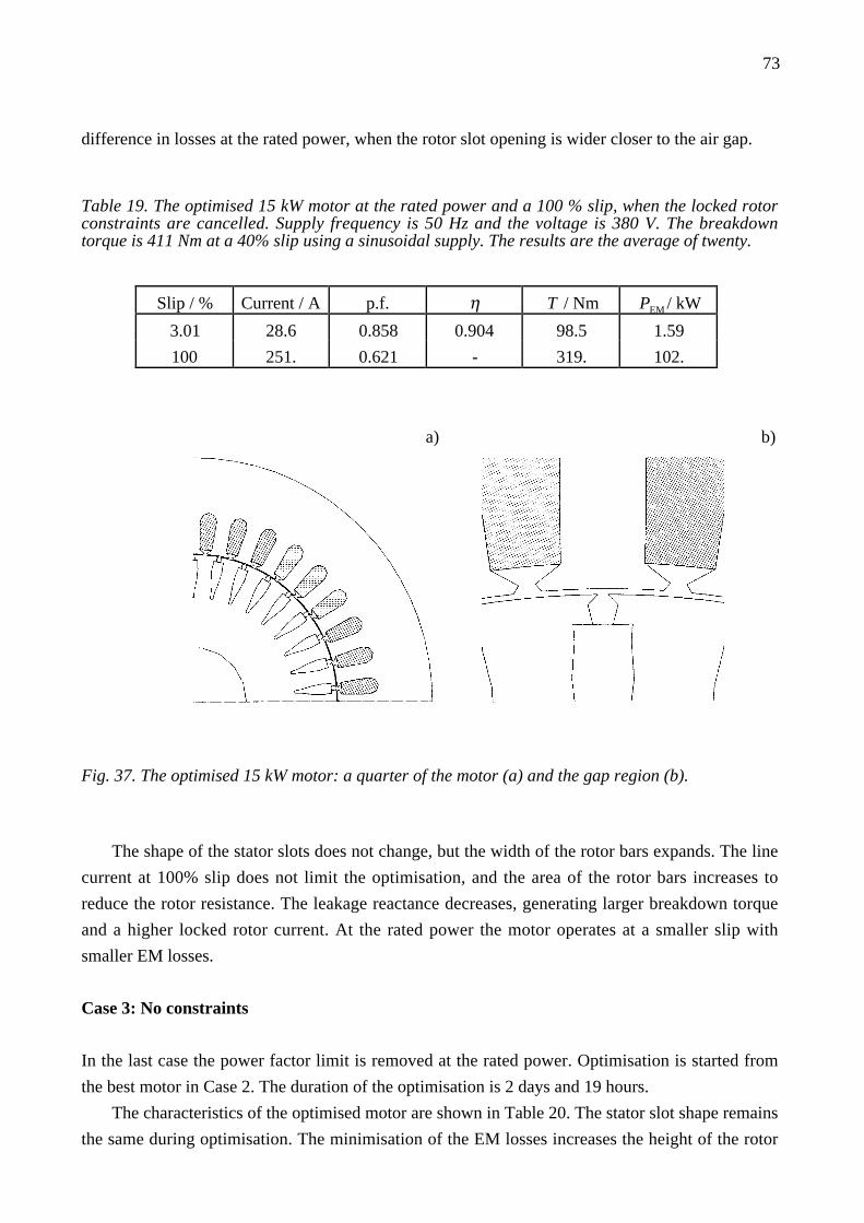
73

difference in losses at the rated power, when the rotor slot opening is wider closer to the air gap.

Table 19. The optimised 15 kW motor at the rated power and a 100 % slip, when the locked rotorconstraints are cancelled. Supply frequency is 50 Hz and the voltage is 380 V. The breakdowntorque is 411 Nm at a 40% slip using a sinusoidal supply. The results are the average of twenty.

Slip / % Current / A p.f. η T / Nm PEM / kW

3.01 28.6 0.858 0.904 98.5 1.59

100 251. 0.621 - 319. 102.

a) b)

Fig. 37. The optimised 15 kW motor: a quarter of the motor (a) and the gap region (b).

The shape of the stator slots does not change, but the width of the rotor bars expands. The line

current at 100% slip does not limit the optimisation, and the area of the rotor bars increases to

reduce the rotor resistance. The leakage reactance decreases, generating larger breakdown torque

and a higher locked rotor current. At the rated power the motor operates at a smaller slip with

smaller EM losses.

Case 3: No constraints

In the last case the power factor limit is removed at the rated power. Optimisation is started from

the best motor in Case 2. The duration of the optimisation is 2 days and 19 hours.

The characteristics of the optimised motor are shown in Table 20. The stator slot shape remains

the same during optimisation. The minimisation of the EM losses increases the height of the rotor

74

bars (see Fig. 38). This increases the slot leakage reactance and decreases the breakdown torque.

The power factor decreases, because the motor operates at a smaller slip at the rated power. The

increased rotor area reduces the resistive rotor losses giving lower EM losses, similar to Case 2. If

the shape of the rotor slot opening is changed back to a straight one, by using the average width of

the opening, the EM losses increase by 20 W (10 W with second-order shape functions).

Table 20. The characteristics of the optimised 15 kW motor at the rated power and a 100 % slipusing a sinusoidal supply, when all the constraints are cancelled. Supply frequency is 50 Hz andthe supply voltage is 380 V. The breakdown torque is 403 Nm at a 40% slip. At 18 kW shaft powerthe EM losses are 2.01 kW, and the power factor is 0.860. The results are the average of twenty.

Slip / % Current / A p.f. η T / Nm PEM / kW

2.46 28.5 0.840 0.909 97.9 1.50

100 262. 0.580 - 283. 100.

a) b)

Fig. 38. The optimised 15 kW motor: a quarter of the motor (a) and the air gap region (b).

4.5.4 Free shape optimisation with an inverter supply

All the previous tests have been made with a sinusoidal source. In the following test an inverter

wave form is used (see Fig. 31) and the aim is to minimise EM losses. Optimisation starts from the

best motor in the previous subsection in Case 2 (Fig. 37 and Table 21). The constraints at a 100%

slip are cancelled. The optimisation variables define the slot shape and the number of the

conductors.

75

Table 21. The characteristics of the initial and optimised 15 kW motor (the average of 20) at therated power, when the locked rotor constraints are cancelled. Supply frequency is 50 Hz and thefundamental harmonic of the inverter is 380 V. The breakdown torque is 419 Nm at a 40% slip forthe initial motor and 385 Nm at a 47% slip for the optimised motor with a sinusoidal supply.

Motor Slip / % Current / A p.f. η T / Nm PEM / kW

Initial 3.06 30.2 0.766 0.892 98.4 1.80

Optimised 2.99 29.7 0.767 0.899 98.4 1.69

The losses in the original motor (Table 14) are 2.33 kW at the rated power. Optimisation starts

from a motor, where the losses are 1.80 kW. The reduced losses are mainly related to the

fundamental harmonic of the inverter. The optimised motor (Fig. 39) creates over 27% smaller

losses than the original motor with an inverter supply. The duration of optimisation is 4 days and 17

hours. The air gap is constant and the power factor at the rated power is > 0.765 in optimisation.

a) b)

Fig. 39. The optimised 15 kW motor: a quarter of the motor (a) and the air gap region (b).

In the optimised motor the number of conductors is initial, i.e. 21. The rotor bars are moved

further away from the air gap. This reduces the losses caused by higher harmonics in the rotor bars.

Arkkio (1991a) studied the effect of the air gap in an inverted fed 37 kW motor reporting a larger

air gap to give lower EM losses. In this case the air gap is fixed and the high frequency flux at the

rotor surface could not be reduced. Therefore the rotor bars are moved further away from the gap.

The rotor slot opening near the gap does not consist of sharp edges. Wider edges keep the

higher harmonic flux closer to the surface of the rotor, and reduce the losses in the rotor bars. The

76

rotor slot openings expand slightly near the rotor bars, but the rotor slot opening is narrower and

this reduces the torque. The shape of the stator openings becomes almost straight. The height of the

rotor bars is 1.5% higher than in the initial motor, but the stator slot is 9% higher. This reduces the

resistance of the stator phase and increases the stator current and flux density in the air gap.

Narrower edges near the air gap cause 35 W higher losses than wide edges in the simulation.

During optimisation the shape of the slots varies greatly. The algorithm found one interesting

motor with a narrower part in the stator slots (Fig. 40). The EM losses in this motor are 1.73 kW at

the rated power and the breakdown torque is 358 Nm. The torque of the motor drops, and therefore

the rotor slot openings and the width of the rotor bars expand near the air gap to generate more

torque. The height of the stator slots and the rotor bars increases by 14% and 9% respectively.

Narrowing of the stator slots changes the path of a high frequency flux caused by the inverter and

reduces the losses at the air gap region. Later optimisation rejected this.

Fig. 40. A motor design found during optimisation. The narrowing in a stator slot changes the pathof the higher harmonic flux. The plot is made by subtracting the flux from a simulation with asinusoidal supply from one with an inverter. The difference between the flux lines is 0.12 mW/m.

4.5.5 Conclusions

The EM losses are reduced approximately 25% in a motor with a sinusoidal and inverter supply.

Most of the changes are in the near air gap region, e.g. rotor and stator slot openings, but also the

height of the stator and rotor slots increases with an inverter supply, i.e. the air gap may not be

considered as a separate part of the motor. The air gap is fixed in tests with an inverter supply, and

therefore the stator coils and the rotor bars move further away from the gap. This reduces the losses

in the rotor bars caused by higher harmonics in the air gap region. The width of the rotor bars does

77

not expand significantly near the air gap.

The tests with a 15 kW motor show that a smooth air gap is not a limitation in motor design.

The characteristics of the motor can be adjusted by modifying the air gap and slot openings. The

results suggest the allowance of all dimensions to vary in optimisation for maximum gain.

The optimisation found one interesting motor with a narrowing in the stator slot, when the

supply was changed from a sinusoidal supply to an inverter. Fifteen population members of 100

had this narrowing the stator slots. These designs were later rejected, because a better design was

found by changing the near air gap region. It suggests always having straight stator slots. From the

manufacturing point of view, e.g. the winding and the filling factor, the narrowing of the stator slots

would not be suitable. A better solution is to change the air gap region.

With parallel computing and a small population size of 50 or 100 the optimisation times are

reduced from weeks to days.

4.6 Optimisation of a 90 kW motor

4.6.1 Background

The purpose is to modify a previously existing motor to fulfil desired characteristics. The motor has

6 poles, 54 stator slots, and 66 rotor slots (Fig. 41). The motor is used in a crane with a weight

measuring system to avoid overloading of the motor. Earlier this motor was used at a 55 kW rated

power, but now the aim is to have a 90 kW motor in a continuously running duty with a 50 Hz

fundamental harmonic in the inverter.

a) b)

Fig. 41. The original 55 kW motor with a two-layer stator winding (a) and the air gap region (b).

78

The optimisation is made by minimising the error due to constraint violations. The motor is to

be designed for an inverter supply (Fig. 42), with a switching frequency of 2500 Hz and 11 pulses

in a half period. No other supply wave forms is with this motor. The fundamental harmonic can be

either 50 Hz or 100 Hz. The breakdown torque is evaluated using the fundamental frequency, in

order to obtain the numerical value, in the following tables describing the characteristics of the

motors. In real motors the maximum torque would be less due to the current limit of the inverter

supply.

-1000

-500

0

500

1000

Vol

tage

(V

)

302520151050

Time (ms)

Fig. 42. The line voltage used in the optimisation with the time-stepping method (100 Hzfundamental component). The switching frequency is 2500 Hz with 11 pulses in a half period.

The design changes needed are assumed to be made with minimal cost. The order of increasing

costs due to the manufacturing system is:

1) Stator coil arrangements (conductors per slot and coil pitch)

2) Air gap

3) The number of the rotor slots

4) Shape of the rotor slot

5) Shape of the stator slot

6) Inner stator radius

The optimisation and the simulations are made using a population of 50 members, first-order

elements, 300 time steps per period, and a total of 900 steps. The analysis is made from the last full

period. The temperature of the stator coils and the rotor bars is assumed to be 80°C and 100 °C

respectively in simulations. Optimisation is divided into two parts: 1) optimisation of coil

arrangements and dimensions of the slots, and 2) the free slot shape.

4.6.2 Constraints

For the optimisation the following constraints are set:

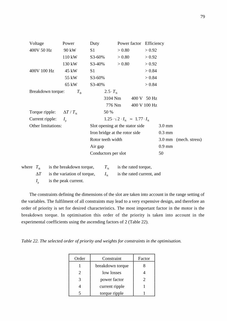
79

Voltage Power Duty Power factor Efficiency

400V 50 Hz 90 kW S1 > 0.80 > 0.92

110 kW S3-60% > 0.80 > 0.92

130 kW S3-40% > 0.80 > 0.92

400V 100 Hz 45 kW S1 > 0.84

55 kW S3-60% > 0.84

65 kW S3-40% > 0.84

Breakdown torque: TB 2.5 ⋅ TN

3104 Nm 400 V 50 Hz

776 Nm 400 V 100 Hz

Torque ripple: ∆T / TN 50 %

Current ripple: Ip 1.25 ⋅ 2 ⋅ IN ≈ 1.77 ⋅ IN

Other limitations: Slot opening at the stator side 3.0 mm

Iron bridge at the rotor side 0.3 mm

Rotor teeth width 3.0 mm (mech. stress)

Air gap 0.9 mm

Conductors per slot 50

where TB is the breakdown torque, TN is the rated torque,

∆T is the variation of torque, IN is the rated current, and

Ip is the peak current.

The constraints defining the dimensions of the slot are taken into account in the range setting of

the variables. The fulfilment of all constraints may lead to a very expensive design, and therefore an

order of priority is set for desired characteristics. The most important factor in the motor is the

breakdown torque. In optimisation this order of the priority is taken into account in the

experimental coefficients using the ascending factors of 2 (Table 22).

Table 22. The selected order of priority and weights for constraints in the optimisation.

Order Constraint Factor

1 breakdown torque 8

2 low losses 4

3 power factor 2

4 current ripple 1

5 torque ripple 1

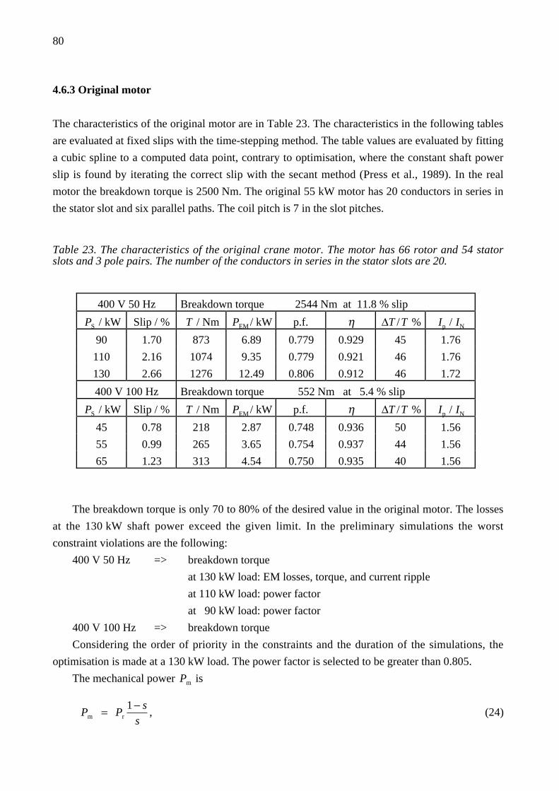
80

4.6.3 Original motor

The characteristics of the original motor are in Table 23. The characteristics in the following tables

are evaluated at fixed slips with the time-stepping method. The table values are evaluated by fitting

a cubic spline to a computed data point, contrary to optimisation, where the constant shaft power

slip is found by iterating the correct slip with the secant method (Press et al., 1989). In the real

motor the breakdown torque is 2500 Nm. The original 55 kW motor has 20 conductors in series in

the stator slot and six parallel paths. The coil pitch is 7 in the slot pitches.

Table 23. The characteristics of the original crane motor. The motor has 66 rotor and 54 statorslots and 3 pole pairs. The number of the conductors in series in the stator slots are 20.

400 V 50 Hz Breakdown torque 2544 Nm at 11.8 % slip

PS / kW Slip / % T / Nm PEM / kW p.f. η ∆T /T % Ip / IN

90 1.70 873 6.89 0.779 0.929 45 1.76

110 2.16 1074 9.35 0.779 0.921 46 1.76

130 2.66 1276 12.49 0.806 0.912 46 1.72

400 V 100 Hz Breakdown torque 552 Nm at 5.4 % slip

PS / kW Slip / % T / Nm PEM / kW p.f. η ∆T /T % Ip / IN

45 0.78 218 2.87 0.748 0.936 50 1.56

55 0.99 265 3.65 0.754 0.937 44 1.56

65 1.23 313 4.54 0.750 0.935 40 1.56

The breakdown torque is only 70 to 80% of the desired value in the original motor. The losses

at the 130 kW shaft power exceed the given limit. In the preliminary simulations the worst

constraint violations are the following:

400 V 50 Hz => breakdown torque

at 130 kW load: EM losses, torque, and current ripple

at 110 kW load: power factor

at 90 kW load: power factor

400 V 100 Hz => breakdown torque

Considering the order of priority in the constraints and the duration of the simulations, the

optimisation is made at a 130 kW load. The power factor is selected to be greater than 0.805.

The mechanical power Pm is

Pm = Pr

1 − s

s, (24)

81

where Pr is resistive rotor losses, and s is the slip. If the losses are not allowed to increase, the slip

has to decrease in order to obtain a higher mechanical power. In this case the breakdown torque slip

also decreases. The breakdown torque slip is

sb = Rr'

Xk

, (25)

where Rr' is rotor resistance and Xk is the short circuit reactance.

In order to have a smaller slip at the rated point, one possibility would be to increase the

reactance, but this would also decease the breakdown torque. The other possibility would be to

decrease the rotor resistance by replacing the rotor bars with a material of a higher conductivity,

e.g. with copper, because the motor is fed by an inverter and the locked rotor torque is no problem.

In the simulation with a sinusoidal supply, the copper rotor bars decrease the EM losses nearly 9%

at 90, 110, and 130 kW power. The breakdown torque is not proportional to the resistive rotor

losses, and the breakdown torque remains the same, as observed in the simulations (Table 24). The

usage of copper bars would not increase the torque but would increase the material costs. Therefore

copper bars are not used.

Table 24. The effect of changing the rotor bar material on the breakdown torque and the EMlosses. The simulation is with a sinusoidal supply. With copper rotor bars, the losses decrease 9%,but the breakdown torque remains practically the same.

Rotor bar Breakdown The EM losses in kW at the shaft power ofmaterial torque / Nm 90 kW 110 kW 130 kWAluminium 2545 6.20 8.63 11.69Copper 2529 5.93 7.85 10.39

4.6.4 Rotor slot dimension

In the optimisation of the rotor slot dimension the main purpose is to find the design modifications

needed at minimal cost. The stator slot dimensions are not considered, due to large additional

expenses. The optimisation is divided into three cases.

Case 1: Coil arrangements and air gap

The optimisation is initiated by allowing the coil arrangements to change, i.e. the number of the

conductors in series in the stator slots and the coil pitch, and later the air gap is added. The filling

factor of the stator slots is assumed to be a constant in the simulations. The number of conductors in

a slot affects the value of the stator phase resistance (Eq. 16) and the end-winding reactance

82

(Eq. 17). The motor has a two-layer winding, and the number of conductors per slot is limited to

even numbers. The characteristics of the optimised motor are in Table 25.

Table 25. The characteristics of the optimised motor, when the coil arrangements and the air gapare optimised. The motor has 18 conductors per slot and original rotor slot dimensions. If thefilling factor is reduced by 10% which corresponds to the smaller number of stator conductors, thebreakdown torque decreases from 3244 Nm to 3148 Nm. The results are the average of ten motors.

400 V 50 Hz Breakdown torque 3234 Nm at 12.8 % slip

PS / kW Slip / % T / Nm PEM / kW p.f. η ∆T /T % Ip / IN

90 1.29 873 6.54 0.74 0.932 49 1.88

110 1.63 1074 8.39 0.77 0.929 47 1.83

130 1.99 1276 10.71 0.79 0.924 48 1.80

400 V 100 Hz Breakdown torque 706 Nm at 5.1 % slip

PS / kW Slip / % T / Nm PEM / kW p.f. η ∆T /T % Ip / IN

45 0.60 220 2.91 0.74 0.939 54 1.60

55 0.76 268 3.51 0.75 0.940 50 1.58

65 0.93 314 4.26 0.76 0.938 45 1.57

400 V 50 Hz Breakdown torque 3148 Nm at 11.8 % (filling factor changed)

PS / kW Slip / % T / Nm PEM / kW p.f. η ∆T /T % Ip / IN

90 1.30 870 6.85 0.74 0.939 48 1.88

110 1.64 1066 8.82 0.77 0.925 46 1.83

130 2.01 1267 11.31 0.79 0.920 48 1.80

The optimisation decreases the number of conductors from 20 to 18, but the coil pitch remains

the same (7). This leads to increased flux and this results in a larger stator current. The

characteristics of the motor change: the locked current increases by 29%, while the breakdown

torque increases by 28%. If the filling factor of the stator slots is diminished by 10%, which

corresponds to the decreased number of conductors, the breakdown torque decreases to 3148 Nm.

With this change from 20 to 18 conductors in series, the motor fulfils the desired characteristics

fairly well. Some constraint violations exist, especially in the power factor and the current ripple. A

larger air gap weakens the characteristics of the motor, e.g. efficiency, breakdown torque, and the

power factor. The optimal air gap is expected to be less than the allowed minimum of 0.9 mm.

Case 2: Coil arrangements, air gap, and the number of rotor bars

In this case the number of rotor bars is allowed to increase in addition to the air gap, the number of

conductors in series in the stator slots, and the coil pitch. The number of rotor bars affects the

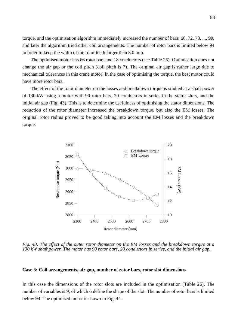
83

torque, and the optimisation algorithm immediately increased the number of bars: 66, 72, 78, ..., 90,

and later the algorithm tried other coil arrangements. The number of rotor bars is limited below 94

in order to keep the width of the rotor teeth larger than 3.0 mm.

The optimised motor has 66 rotor bars and 18 conductors (see Table 25). Optimisation does not

change the air gap or the coil pitch (coil pitch is 7). The original air gap is rather large due to

mechanical tolerances in this crane motor. In the case of optimising the torque, the best motor could

have more rotor bars.

The effect of the rotor diameter on the losses and breakdown torque is studied at a shaft power

of 130 kW using a motor with 90 rotor bars, 20 conductors in series in the stator slots, and the

initial air gap (Fig. 43). This is to determine the usefulness of optimising the stator dimensions. The

reduction of the rotor diameter increased the breakdown torque, but also the EM losses. The

original rotor radius proved to be good taking into account the EM losses and the breakdown

torque.

3100

3050

3000

2950

2900

2850

2800

Bre

akdo

wn

torq

ue (N

m)

280027002600250024002300

Rotor diameter (mm)

20

18

16

14

12

10

EM

Losses (kW

)

Breakdown torque EM Losses

Fig. 43. The effect of the outer rotor diameter on the EM losses and the breakdown torque at a130 kW shaft power. The motor has 90 rotor bars, 20 conductors in series, and the initial air gap.

Case 3: Coil arrangements, air gap, number of rotor bars, rotor slot dimensions

In this case the dimensions of the rotor slots are included in the optimisation (Table 26). The

number of variables is 9, of which 6 define the shape of the slot. The number of rotor bars is limited

below 94. The optimised motor is shown in Fig. 44.

84

Table 26. The original and optimised value of the variables. See also Fig. 13 for the definition ofthe variables. Some of the results are given in p.u. to make comparison easier.

Variable Initial Optimised

conductors in stator slot 20 18

coil pitch (in slot pitches) 7 7

air gap (mm) 0.9 0.9

h21 (p.u.) 1.000 0.955

h22 (p.u.) 1.000 1.014

h23 (p.u.) 1.000 0.909

b21 (p.u.) 1.000 0.877

b22 (p.u.) 1.000 0.514

b23 (p.u.) 1.000 1.000

a) b)

Fig. 44. The optimised 90 kW motor: a quarter of the motor (a) and the air gap region (a).

Optimisation reduces the height of the rotor bars by 9%. The iron bridge in the rotor is moved

further away from the gap. The thickness of the iron-bridge is at the allowed minimum value of

0.3 mm. The characteristics of the optimised motor are given in Table 27. The locked rotor torque

increases by 33% and locked rotor current increases by 29%.

85

Table 27 The characteristics of the optimised motor, when also the rotor slot dimensions areoptimised. The motor has 18 conductors per slot and optimised slot dimensions. The results are theaverage of ten.

400 V 50 Hz Breakdown torque 3247 Nm at 13.0 % slip

PS / kW Slip / % T / Nm PEM / kW p.f. η ∆T /T % Ip / IN

90 1.37 873 6.65 0.74 0.931 47 1.82

110 1.72 1070 8.54 0.77 0.928 45 1.80

130 2.10 1268 10.91 0.79 0.923 44 1.76

400 V 100 Hz Breakdown torque 717 Nm at 5.1 % slip

PS / kW Slip / % T / Nm PEM / kW p.f. η ∆T /T % Ip / IN

45 0.63 218 2.93 0.74 0.939 49 1.60

55 0.80 266 3.54 0.75 0.940 46 1.57

65 0.97 314 4.29 0.76 0.938 44 1.56

The optimised motor has higher EM losses compared with the initial rotor, but the torque ripple

and the current ripple are smaller due to smaller variations in the flux density. The smaller rotor slot

openings reduce the flux density variations and the pulsation losses. This increases the leakage

reactance and decreases the torque. The smaller cross-sectional area of the rotor bars increases

resistive rotor losses, but increases the torque due to a smaller leakage reactance. The motor

operates at a larger slip and the power factor increases from 0.791 to 0.793 at 130 kW power.

4.6.5 Free shape optimisation

The shape optimisation is divided into three cases. In the first case a rotor slot shape is optimised

with 20 conductors in the stator slots. The second case has 18 conductors per slot and in the last

case the stator slot shape is allowed to vary using 18 conductors in the stator slots. The optimisation

is made at a shaft power of 130 kW. The aim is to find a motor that fulfils the constraints. The

symmetrical rotor and stator slot shapes are defined using 36 variables (14 for the stator slot and 22

for the rotor slot, see Fig. 15). The coil pitch is fixed at seven for all later test cases.

Case 1: 20 Conductors per slot and free rotor slot shape

The shape is allowed to transform rather freely during optimisation, but the thickness of the iron

bridge is more than 0.3 mm and the width of the rotor teeth is larger than 3.0 mm. The stator side is

kept constant during optimisation and the number of rotor bars is fixed at 66. The optimisation is

started from the original motor. The number of variables defining the shape of the rotor slots is 22.

The characteristics of the optimised motor are in Table 28, and the motor is shown in Fig. 45.

86

Table 28. The characteristics of the optimised motor, when the motor has 20 conductors per slotand a freely optimised shape for the rotor slot dimensions. The results are the average of twenty.

400 V 50 Hz Breakdown torque 3137 Nm at 11.8 % slip

PS / kW Slip / % T / Nm PEM / kW p.f. η ∆T /T % Ip / IN

90 1.30 866 6.40 0.78 0.934 60 1.86

110 1.62 1063 8.52 0.80 0.928 55 1.82

130 1.97 1266 11.30 0.81 0.920 51 1.79

400 V 100 Hz Breakdown torque 707 Nm at 5.1 % slip

PS / kW Slip / % T / Nm PEM / kW p.f. η ∆T /T % Ip / IN

45 0.60 218 2.78 0.76 0.940 55 1.59

55 0.76 266 3.46 0.77 0.941 50 1.56

65 0.94 314 4.36 0.77 0.936 46 1.56

a) b)

Fig. 45. The optimised 90 kW motor with 20 conductors in the stator slots: a quarter of the motor(a) and the air gap region (b).

In the optimised motor, the rotor bars are 39% wider than in the original motor, and the height

of the rotor bars is reduced by 10%. To reach the breakdown torque limit, the area of the rotor bars

enlarges to decrease the leakage reactance and to generate more torque. To reduce increased losses,

the optimisation decreases the width of the rotor slot openings. Smaller slot openings reduce the

flux density variations, and pulsation losses in the teeth, but they also increase the leakage

reactance. The width of the iron-bridge is nearly constant, but it is shifted closer to the air gap. This

distance from the gap is only 2/3 of the original one, which causes a high saturation in the bridge

region and reduces the leakage reactance. This generates a larger torque. The opening in the rotor

87

slots is wider below the surface of the air gap to avoid flux density variations in the gap. In the

optimised motor, the EM losses are nearly 700 W smaller than in the original motor.

Case 2: 18 conductors per slot and free rotor slot shape

The number of conductors in the stator slots is 18 and the optimisation starts from the motor in

Case 1. A smaller number of the conductors increases the breakdown torque to 4000 Nm, but

constraints of the EM losses (13.8 kW), the power factor (0.72), the torque ripple (67%), and the

current ripple (1.9) are badly violated. Therefore optimisation searches for a motor fulfilling these

constraints, and allows the pull out torque to decrease during optimisation.

The stator slot shape is fixed in this case, and the minimum iron-bridge thickness is 0.3 mm in

the rotor. The shape of the rotor slots is defined using 22 variables (Fig. 15). The characteristics of

the optimised motor are in Table 29.

Table 29. The characteristics of the optimised motor, when the motor has 18 conductors per slotand a freely optimised shape for rotor slot dimensions. The results are the average of twenty.

400 V 50 Hz Breakdown torque 3506 Nm at 14.1 % slip

PS / kW Slip / % T / Nm PEM / kW p.f. η ∆T /T % Ip / IN

90 1.56 877 6.62 0.74 0.931 52 1.64

110 1.95 1072 8.56 0.77 0.927 48 1.83

130 2.37 1270 11.06 0.79 0.921 50 1.84

400 V 100 Hz Breakdown torque 749 Nm at 6.3 % slip

PS / kW Slip / % T / Nm PEM / kW p.f. η ∆T /T % Ip / IN

45 0.72 218 2.91 0.73 0.939 58 1.60

55 0.91 266 3.54 0.75 0.940 50 1.57

65 1.11 313 4.31 0.76 0.937 46 1.57

The optimised motor is shown in Fig. 46. In the optimised motor, the rotor bar height is only

73% of the original one, which causes a smaller leakage reactance and more torque. The width of

the rotor bars reverted nearly to the original, but near the iron-bridge the width of the rotor bars

increased by 22 %. This wider part is less than 9% of the rotor bar height. This enlarged rotor bar

top reduces resistive losses and decreases the leakage reactance, further increasing torque. The iron-

bridge and the rotor bars move further away from the gap to reduce losses, but the air gap is 90 %

of the original. The width of the slot openings in the rotor is the same as in Case 1, i.e. 30%

narrower than in the original motor, which reduces the pulsation losses.

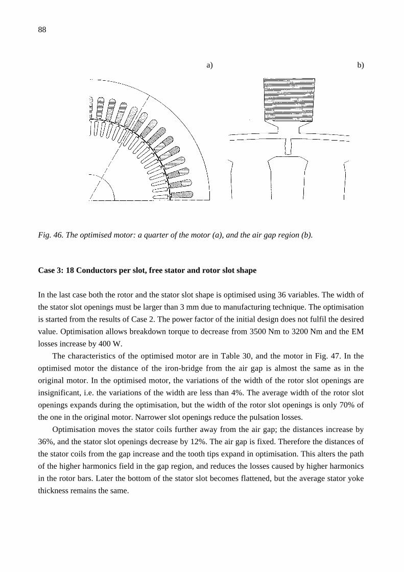
88

a) b)

Fig. 46. The optimised motor: a quarter of the motor (a), and the air gap region (b).

Case 3: 18 Conductors per slot, free stator and rotor slot shape

In the last case both the rotor and the stator slot shape is optimised using 36 variables. The width of

the stator slot openings must be larger than 3 mm due to manufacturing technique. The optimisation

is started from the results of Case 2. The power factor of the initial design does not fulfil the desired

value. Optimisation allows breakdown torque to decrease from 3500 Nm to 3200 Nm and the EM

losses increase by 400 W.

The characteristics of the optimised motor are in Table 30, and the motor in Fig. 47. In the

optimised motor the distance of the iron-bridge from the air gap is almost the same as in the

original motor. In the optimised motor, the variations of the width of the rotor slot openings are

insignificant, i.e. the variations of the width are less than 4%. The average width of the rotor slot

openings expands during the optimisation, but the width of the rotor slot openings is only 70% of

the one in the original motor. Narrower slot openings reduce the pulsation losses.

Optimisation moves the stator coils further away from the air gap; the distances increase by

36%, and the stator slot openings decrease by 12%. The air gap is fixed. Therefore the distances of

the stator coils from the gap increase and the tooth tips expand in optimisation. This alters the path

of the higher harmonics field in the gap region, and reduces the losses caused by higher harmonics

in the rotor bars. Later the bottom of the stator slot becomes flattened, but the average stator yoke

thickness remains the same.

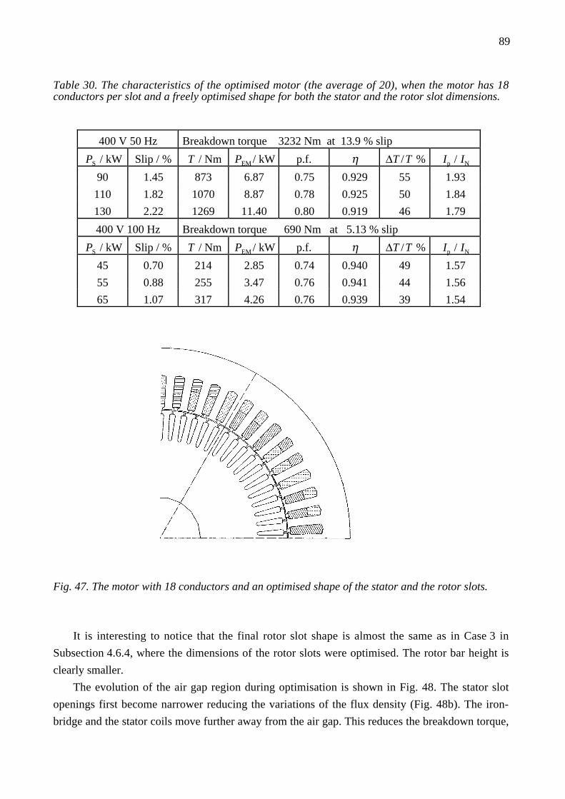
89

Table 30. The characteristics of the optimised motor (the average of 20), when the motor has 18conductors per slot and a freely optimised shape for both the stator and the rotor slot dimensions.

400 V 50 Hz Breakdown torque 3232 Nm at 13.9 % slip

PS / kW Slip / % T / Nm PEM / kW p.f. η ∆T /T % Ip / IN

90 1.45 873 6.87 0.75 0.929 55 1.93

110 1.82 1070 8.87 0.78 0.925 50 1.84

130 2.22 1269 11.40 0.80 0.919 46 1.79

400 V 100 Hz Breakdown torque 690 Nm at 5.13 % slip

PS / kW Slip / % T / Nm PEM / kW p.f. η ∆T /T % Ip / IN

45 0.70 214 2.85 0.74 0.940 49 1.57

55 0.88 255 3.47 0.76 0.941 44 1.56

65 1.07 317 4.26 0.76 0.939 39 1.54

Fig. 47. The motor with 18 conductors and an optimised shape of the stator and the rotor slots.

It is interesting to notice that the final rotor slot shape is almost the same as in Case 3 in

Subsection 4.6.4, where the dimensions of the rotor slots were optimised. The rotor bar height is

clearly smaller.

The evolution of the air gap region during optimisation is shown in Fig. 48. The stator slot

openings first become narrower reducing the variations of the flux density (Fig. 48b). The iron-

bridge and the stator coils move further away from the air gap. This reduces the breakdown torque,

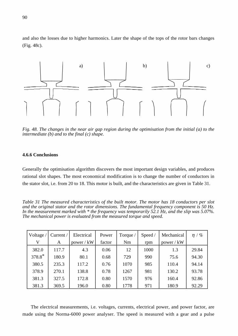
90

and also the losses due to higher harmonics. Later the shape of the tops of the rotor bars changes

(Fig. 48c).

a)

b)

c)

Fig. 48. The changes in the near air gap region during the optimisation from the initial (a) to theintermediate (b) and to the final (c) shape.

4.6.6 Conclusions

Generally the optimisation algorithm discovers the most important design variables, and produces

rational slot shapes. The most economical modification is to change the number of conductors in

the stator slot, i.e. from 20 to 18. This motor is built, and the characteristics are given in Table 31.

Table 31 The measured characteristics of the built motor. The motor has 18 conductors per slotand the original stator and the rotor dimensions. The fundamental frequency component is 50 Hz.In the measurement marked with * the frequency was temporarily 52.1 Hz, and the slip was 5.07%.The mechanical power is evaluated from the measured torque and speed.

Voltage /

V

Current /

A

Electrical

power / kW

Power

factor

Torque /

Nm

Speed /

rpm

Mechanical

power / kW

η / %

382.0 117.7 4.3 0.06 12 1000 1.3 29.84

378.8* 180.9 80.1 0.68 729 990 75.6 94.30

380.5 235.3 117.2 0.76 1070 985 110.4 94.14

378.9 270.1 138.8 0.78 1267 981 130.2 93.78

381.3 327.5 172.8 0.80 1570 976 160.4 92.86

381.3 369.5 196.0 0.80 1778 971 180.9 92.29

The electrical measurements, i.e. voltages, currents, electrical power, and power factor, are

made using the Norma-6000 power analyser. The speed is measured with a gear and a pulse

91

detector. The error in the torque is less than 3%, when the torque is higher than 500 Nm, but larger

below 500 Nm. Therefore it is not possible to draw exact conclusions from the measured results

and the computed results. These differences between the measured and the simulated motors may

also arise from the first-order elements used in the simulations, and from the differences in the

values of the stator phase resistance and the end-winding reactance in the real motor.

The number of conductors enables adjustment of the air gap flux and the stator currents.

Another result is that the height of the rotor bars can be reduced from 10 to 15%. The optimisation

of the slot dimensions improves the desired motor characteristics. The optimal air gap is assumed to

be less than 0.9 mm, but due to mechanical tolerances it is not feasible to change the air gap.

In the case of the free slot shape and 20 conductors in series in the stator slots, the width of the

rotor bars increases strongly to meet the breakdown torque constraint. The air gap region is

different form the initial one: the iron-bridge is shifted closer to the air gap, and the rotor slot

opening is narrower. Narrower rotor slot openings increase the leakage reactance and therefore they

decrease the torque, but they also reduce the pulsation losses. To minimise, simultaneously, the

leakage reactance and the variations of the flux density, the slot openings expand below the air gap.

This causes a reduction in the pulsation losses in the teeth.

With 18 conductors the optimisation with a free slot shape does not generate radical changes to

the design, as the number of stator conductors is properly adjusted for the motor. Only the height of

the rotor bars is smaller and the near air gap region is different from the original motor; the iron

bridge moves closer to the gap and the slot openings are narrower in the rotor. The rotor bar

expands near the air gap, but when the stator slots are allowed to change, the final geometry is very

close to the previously optimised rotor slot dimension, with the exception of the rotor bar height.

4.7 Critical review

There are differences between the optimisation results and the requirements of a real motor

construction. Some of the optimised motor design would be very expensive to manufacture. The

sharp corners in the slot shapes are not realisable in all parts of the slot, when the motors are

manufactured by punching. The sharp edges in the stator slots should also be avoided in the real

motors, because they decrease the filling factor of the slots due to isolation.

The iron is treated, in optimisation, as a non-conducting material corresponding to the

situation, where the isolation between the laminated iron and rotor bars is perfect. In real motors

this isolation is hardly perfect, especially in sharp corners. Most of the results are, however,

rational, e.g. the smooth air gap surface, the modified slot openings, and the results with the

inverter fed motors. One major limitation in this method is that the characteristics of the motors are

evaluated only at the fixed slips. Therefore these motors should be used only within the studied slip

range.

The optimisation of the free air gap geometry indicates that the air gap surface of an induction

motor should be smooth both at the rotor and stator side, to minimise flux density variations in the

92

air gap. Near the slot openings a detailed structure may be used to enhance desired characteristics

of the motor. Both the results from the maximisation of the locked rotor torque and the

minimisation of the total electromagnetic losses indicate this.

Furthermore, the optimisation results with an inverter supply, also indicated that another

possibility to have a larger air gap (Arkkio, 1991a) is to modify the slot openings and the distance

between the rotor bars and the air gap. Moreover it proved to be necessary to allow both the near-

gap region and other slot dimensions to change simultaneously with both a sinusoidal and inverter

supply. The air gap region can not be considered as a separate part of the motor in an optimisation

when trying to obtain maximum performance from the motor.

The results indicate only a small change in the width of the rotor bars near the gap with a

proper number of conductors in series in the stator slots. It is typical is that the rotor bar tops

expand less than 20%.

Compared with changing one parameter at a time, the optimisation with a genetic algorithm

can be faster, especially with the time-stepping method, because the genetic optimisation algorithm

is robust enough to determine relevant design changes. This multivariant search has a disadvantage

compared with the univariant search described by Poloujadoff et al. (1994): the conflicting interests

may remain invisible to the user, even when the algorithm recognises them. Naturally one may

benefit from the multivariant approach and apply the method to a larger selection of motors, and

then formulate general rules to identify the common characteristics.

93

5 SUMMARY

This work deals with an optimisation based design of an induction motor. The motors are modelled

by the two-dimensional finite element method with a simulation of the rotating rotor. This

modelling has several simplifications, e.g. the rotor bars are unskewed, the hysteresis characteristics

of the iron are neglected, and the iron is treated as a non-conducting material. In rotor, the skin

effect is taken into account, but neglected in the conductors in the stator. Also the eddy current

losses are not modelled in the conductors in the stator slots.

A numerical simulation with the finite element method as an objective function causes serious

accuracy problems in the evaluation of the estimates for the derivatives and therefore problems to

derivative based optimisation algorithms. The refinement of the mesh destroys the convergence

properties of the first order forward differences used as an estimate for derivatives. It also causes

changes in the field matrix, which reflect inaccuracy in design sensitivities rather than changes in

the real properties of the motor. The simulation of the rotation combined with non-linear materials

causes additional truncation and round-off errors during the simulation, and the forward differences

are unreliable even in the case of a parametrised mesh generator.

With the time-stepping method it is possible to calculate the whole torque curve. The

evaluation of the motor characteristics is focused on a few points in the torque curve, e.g. rated

power, breakdown torque, and locked rotor torque, to limit both the computation time and the

optimisation duration to a rational level. The most time consuming part is to search for the correct

slip to evaluate the characteristics at the rated power. This is especially important while minimising

the losses in the induction motors. The evaluation of the pull-up torque was cancelled in the tests,

because the time needed to evaluate the objective function is two times longer in that case.

The long simulation duration with the time-stepping and the problems with the design

sensitivities suggested the use of a robust optimisation algorithm that recognises the most important

design changes as well as the ability to work in a noisy environment. The optimisation algorithm is

based on the computer simulation of the evolution. This genetic algorithm is based on a population

instead of one single design. It is possible to use statistical methods in the analysis of the

optimisation results. The design parameters are described using a chromosome string, and the range

for the optimisation variables is usually ±100% of the initial value.

The algorithm generates changes the genome of the population and searches for the best design

to live in the environment defined by the objective function and the constraints. The method proved

to be robust to numerical problems and the setting of the optimisation parameters. Furthermore it is

easy to mix both integer and real-valued variables in the optimisation, e.g. the number of

conductors, the coil pitch in the slot pitches, and the slot dimensions. The algorithm recognises the

integer variables and modifies the step size. By using constraints in the optimisation it possible to

avoid design failures.

Genetic algorithms need very little communication between the individual processors. Only the

initial data and the final result must be passed from the master procedure to the worker procedure.

94

The scaleability of the algorithm and the utilisation degree of the processors is very high with finite

element objective functions. The genetic algorithm is extremely suitable for parallel computing

giving a significant reduction in the optimisation duration. Even 99.95% scaleability was observed

in simulations with four processors.

The time-stepping method based objective function is extremely slow to evaluate. This affects

the parameter setting of the genetic algorithm and suggests the use of a very large mutation

probability. This work gives new information about the parameter settings in cases, where the

computational resource seriously affects the simulation duration.

The optimisation with the genetic algorithm can be faster than changing one parameter at a

time, especially with the time-stepping method, because the genetic optimisation algorithm is

robust enough to determine the relevant design changes. Naturally one may benefit from this

robustness and apply the method to a large selection of motors, and then formulate general rules to

identify the common characteristics.

The finite element analysis is numerically inaccurate, and one must apply some smoothing

strategy, for example statistical analysis or master nodes, in optimisation or in analysis. If the

independent nodes are allowed to move, the smoothing may be based on a population. Using

statistical analysis one can find the significant changes in the design variables. Even with master

nodes it is possible to find several design that have almost the same parameter values and the

characteristics. All the changes in the mesh, i.e. changes in the optimisation variables, are dot

significant, they may also reflect the accuracy problems of the FEM. Using statistical analysis, e.g.

averaging and variance, we can improve the reliability of the optimisation results.

Despite all the problems linked to the FEM, it is needed to be able to make reliable shape

optimisation, especially near the air gap region. Analytically it is not possible to calculate the

torque or losses with sufficient accuracy. Only with the finite element method is this possible.

An effective method for combining the finite element method with structural optimisation of

induction motors is presented, when the time consuming rotation of the rotor has to be modelled

and the materials are highly non-linear. The applied methodology enables the optimisation of

induction motors, using the time stepping method, within a reasonable time, only a few days with

parallel computing and four processors.

The optimisation tests concentrate on the minimisation of losses, the maximisation of the

torque and the minimisation of the errors due to constraint violations. These are closely related to

the current needs of the industry. The optimisations are made using first-order elements. The

simulations with the second-order elements also support the results. The optimisation reduced EM

losses in a 15 kW motor by nearly 25% and in the 90 kW motor the breakdown torque increased

over 60%. Furthermore the results with the real motor were successful.

The optimisation of the free air gap geometry indicates that the air gap surface of an induction

motor should be smooth both at the rotor and the stator side to minimise the variations of the flux

density in the air gap. Near the slot openings a detailed structure can be applied to enhance desired

95

characteristics. Both the results from the maximisation of the locked rotor torque and the

minimisation of the total electromagnetic losses indicate this.

It is beneficial to expand the rotor slot openings below the air gap to reduce leakage reactance

and to generate more torque. The result is only a small change in the width of the rotor bars near the

gap with a properly adjusted number of conductors in the stator slot. This emphasises a need to

optimise all relevant design variables at the same time to obtain the best performance from the

motor.

A new slot geometry for induction motors fed by an inverter was discovered. In this motor

there is a narrower part in a stator slot, reducing the higher harmonic flux in the air gap region. The

problem is that this also reduces the fundamental flux component and therefore the torque

decreases. A better design is found by changing the air gap region of the motor. The result

suggested making the stator teeth straight with a sinusoidal and inverter supply.

Optimisation results with an inverter supply also indicated that an alternative to having a larger

air gap to reduce losses due to higher harmonics is to modify the slot openings and the distance of

the rotor bars from the air gap. It proved to be necessary to allow both the near-gap region and other

slot dimensions to change simultaneously with a sinusoidal and inverter supply. The air gap region

can not be considered as a separate part of the motor in the optimisation.

The optimisation method developed, easily recognises traditional design solutions, e.g. double

cage rotor, when the locked rotor torque is maximised. The results clearly show the effectiveness

and rational operation of the method in the structural optimisation of induction motors.

96

REFERENCES

Arfken, G. 1985. Mathematical Methods for Physicists, Academic Press Inc. 985 p.

Arkkio, A. 1987. Magnetic Field Analysis of Induction Motors based on the Numerical Solution ofthe Coupled Field and Circuit Equations. Acta Polytechnica Scandinavica. El. Eng. No. 59. 97 p.

Arkkio, A. 1991a. Analysis of a 37 kW Cage Induction Motor. Helsinki Univ. of Technology, Lab.of Electromechanics, Report 30. 64 p.

Arkkio, A. 1991b. FCSMEK, PART B, Users Guide, Programmes for analysing cage inductionmotors, Release 2, Helsinki Univ. of Tech., Laboratory of Electromechanics, Finland. 135 p.

Arkkio, A. 1995. Unbalanced magnetic pull in a four pole induction motor with an odd number ofrotor slots. Proceedings of CICEM'95. 31 Aug. - 2 Sept. 1995, Hangzhou, China. pp. 343-348.

Bendsøe, M. P., Kikuchi, N. 1988. Generating optimal topologies in structural design usinghomogenisation method. Comp. Methods in Applied Mech. Engineering. No. 171. pp. 197-224.

Braibant, V. 1986. Shape Optimal Design Using B-splines. Journal of Structural Mechanics,Vol. 14. pp. 209-228.

Braibant, V., Morelle, P. 1990. Shape optimisation and free mesh generation. StructuralOptimisation, Vol. 2, Is. 4. pp. 223-231.

Brandisky, K., Belmans, R., Pahner, U. 1994. Optimal design of a segmental PM DC motor usingstatistical experiment design method in combination with numerical field calculations. ICEM'94Proceedings. Paris, France. Vol. 3. pp. 210-215.

Box, G. E. P., Behnken, D. W. 1960, Some New Three Level Design for Study of QuantitativeVariables. Technometrics, Vol. 2, No. 4. pp. 455-475.

Box, G. E. P., Draper, N. R. 1987. Empirical Model-Building and Response Surfaces. John Wiley& Sons.

Bäck, T., Rudolph, G., Schwefel, H.-P. 1993. Evolutionary Programming and Evolution Strategies:Similarities and Differences. Proc. of Second Ann. Conf. on Evolutionary Programming. EditorsD. B. Fogel and W. Atmar. La Jolla, CA: Evolutionary Programming Society. pp. 11-22.

Cendes, Z. J., Shenton D. N. 1985. Adaptive Mesh Refinement in the Finite Element Computationof Magnetic Fields. IEEE Trans. on Magn., Vol. MAG-21, No. 5, Sept. 1985. pp. 1181-1186.

Cheng, Y. B., Sykulski, J. K. 1994. CAD and optimisation of electromagnetic actuators. ICEM'94Proceedings. Paris, France. Vol. 3. pp. 187-192.

Chu, E., George, A., Liu, J., Ng, E. 1984. SPARSPAK: Waterloo sparse matrix package, User'sguide for SPARSPAK-A. Univ. of Waterloo, Ontario, Canada, Research Report CS-84-36. 63 p.

Davis, L. 1991. Handbook of Genetic Algorithms. New York: Van Nostrand Reinhold.

Ding, H., El-Keib, A. A., Smith R. E. 1994. Optimal clustering of power networks using geneticalgorithms. Electric Power Systems Research, Vol. 30. No 3. pp. 209-214.

Dixon, L. C. W., Szegö, G. P. 1978. The Global Optimisation Problem, in Towards GlobalOptimisation 2, Dixon, Szegö (Editors), North Holland Publishing, Amsterdam.

Dwyer, W. J., Emerton, R. K., Ojalvo, I. U. 1971. An automated procedure for the optimization ofpractical aerospace structures. Edition 1. Wright-Patterson air force base (OH).

97

Fandel, H. 1976. Optimale Entscheidung bei mehrfacher Zielsetzung, Lecture Notes in Economicsand Mathematics. Springer Verlag. 221 p.

Fraser, A. S. 1957. Simulation of Genetic Systems by Automated Digital Computers. I. Introduction.Australian J. of Biol. Sci., Vol. 13. pp. 150-162.

Fogel, D. B. 1994. Evolutionary Computation, Toward a New Philosophy of Machine Intelligence.IEEE Press, New York.

Girdinio, P., Molfino, P., Molinari, G., Puglisi, L., Viviani, A. 1978. Finite Difference and FiniteElement Grid Optimisation by Grid Iteration Method. IEEE Trans. on Magn. MAG-19, No. 6.pp. 2543-2546.

Haataja, J. 1994. Solving Optimisation Problems. CSC - Center for Scientific Computing Ltd,Yliopistopaino. ISBN 952-9821-02-6. Ed 1. 232 p. (In Finnish)

Holland, J. H. 1975. Adaptation in Natural and Artificial Systems. Ann Arbor: University ofMichigan Press.

IEC 34-1. 1994. Rotating Electrical machines - Part 1: Rating and performance. 129 p.

de Jong, K. A. 1993, Genetic Algorithms are NOT function optimizers. Foundation of GeneticAlgorithms 2. Amsterdam: North-Holland. pp. 3-13.

Keskinen, E. 1992. Application of Vector Potentials in the Finite Element Solution of Three-Dimensional Eddy Current Problems. Acta Polytechnica Scandinavica, El. Eng. No. 71. 99 p.

Kibsgaard, S. 1991. Analysis and Optimization of FE-discretized Structures. PhD thesis, SpecialReport No. 6, Institute of Mech. Engineering, Aalborg Univ., Denmark.

Kopylov, I. P., Gorjainov, F. A., Klokov, B. K. 1980. Designing of electrical motors. Moscow,Energy. 496 p. (In Russian)

Laithwaite, E. R. 1973. Induction Machines for Special Purposes. London, George Newnes Ltd.

Lindholm, D. 1983. Automatic Triangular Mesh Generation on Surfaces of Polyhedra. IEEETransactions on Magn., Vol. MAG-19, No. 6. pp. 2539-2542.

Lund, E. 1994. Finite Element Based Design Sensitivity Analysis and Optimisation. Institute ofMechanical Engineering, Aalborg University, Special Report No. 23. 240 p.

Luomi, J., Rouhiainen, H. 1988. Adaptive mesh refinement for magnetic field problems involvingsaturable ferromagnetic parts. IEEE Trans. on Magn., Vol.-24, No 1, Jan. 1988. pp. 311-314.

Michalewicz, Z. 1992. Genetic Algorithms + Data Structures = Evolution Programmes. SpringerVerlag. 251 p.

Mohammed, A. 1990. Optimal Design of Magnetic Circuits by Finite Elements and DynamicSearch Procedure. COMPEL – The International Journal for Computation and Mathematics inElectrical and Electronic Engineering, Vol. 9, Supplement A. pp. 106-110.

Neittaanmäki, P., Rudnicki, M., Savini, A. 1994. Inverse Problems and Optimal Design inElectricity and Magnetism. Oxford University Press.

Nikolova-Yatcheva, I. I. 1989. Synthesis of fields in electrical devices. Doctoral Thesis, Sofia,Bulgaria. 34 p. (In Bulgarian)

Olhoff, N., Lund, E., Rasmussen, J. 1992. Concurrent Engineering Design Optimisation In a CADEnvironment. Special Report No. 16, Inst. of Mech. Engineering. Aalborg Univ. Denmark. 64 p.

98

Palko, S. 1994. Structural optimisation of Cage Induction Motors Using Finite Element Analysis.Licentiate Thesis, Helsinki Univ. of Technology, Lab. of Electromechanics, Report 45, 61 p.

Palosaari, S., Parviainen, S., Hiironen, J., Reunanen, J., Neittaanmäki, P. 1986. A random SearchAlgorithm for Constrained Global Optimisation. Acta Polytechnica Scandinavica, Chem. Tech. andMetallurgy Series, No. 172, Helsinki. 45 p.

Park, I., Lee, B., Hahn, S. 1990. Pole Shape Optimisation for Reduction of Cogging Torque bySensitivity Analysis. COMPEL – The International Journal for Computation and Mathematics inElectrical and Electronic Engineering, Vol. 9, Supplement A. pp. 111-114.

Pedersen, P. 1988. Design for Minimum Stress Concentration - Some Practical Aspects. StructuralOptimization, pp. 182-187, Kluver, Dordrecht, The Netherlands. pp. 225-232.

Perho, J., Niemenmaa, A., Jokinen, T., Arkkio, A. 1995. Harmonic effects in AC machines.Helsinki Univ. of Technology, Laboratory of Electromechanics, TKK OFFSET, ISBN 951-22-2850-5. 178 p. (In Finnish)

Plank, E. 1993. Optimisierung des Schwindungskomfort mit Hilfe der Finite-Element-Methode amBeispiel eines frontgetriebenen PKW's. Technische Universität München, Doctoral Thesis. 135 p.

Poloujadoff, M., Christaki, E., Bergmann, C. 1994. Univariant Search: An opportunity to identifyand solve conflicting problems in optimisation. IEEE Trans. on Energy Conversion, Vol. 9, No. 4,Dec. 1994. pp. 659-664.

Preis, K., Ziegler, A. 1990. Optimal Design of Electromagnetic Devices with Evolution Strategies.COMPEL – The International Journal for Computation and Mathematics in Electrical andElectronic Engineering, Vol. 9, Supplement A. pp. 119-122.

Press, W. H., Flannery, B. P., Teukolsky, S.A., Vetterling, W. T. 1989. NUMERICAL RECIPES,The Art of Scientific Computing (FORTRAN VERSION). Cambridge University Press. 702 p.

Pyrhönen, J., Kurronen, P. 1994. Increasing efficiency of high-speed solid rotor inductionmachines. Proceedings of ICEM'94. Paris, France. Vol. 1. pp. 47-52.

Quinn, M. J. 1987. Designing Efficient Algorithms for Parallel Computers, McGraw-Hill.

Rouhiainen, H. 1986. Interactive and adaptive mesh generator for the numerical calculation of thesaturable magnetic fields. Master's Thesis, Helsinki Univ. of Tech, Finland. 101 p. (In Finnish)

Rudolph, G. 1994. Convergence Analysis of Canonical Genetic Algorithms. IEEE Trans. on NeuralNetworks. Vol. 5:1. pp. 96-101.

Russenschuck, S. 1990. Mathematical Optimisation Techniques for the design of permanentmagnet synchronous machines based on numerical field calculation. IEEE Trans. on Magn., Vol.MAG-26. 6 p.

Russenschuck, S. 1995. Mathematical Optimization Techniques in Computational Electromag-netics. International Compumag Society Newsletter. Vol. 2, No. 1. pp. 3-7.

Schoofs, A. J. G. 1987. Experimental Design and Structural Optimisation. Technical University ofEindhoven, Dissertation. 151 p.

Schraudolph, N. N., Belew, R. K. 1992. Dynamic Parameter Encoding for Genetic Algorithms.Machine Learning, Vol. 9. pp. 9-21.

Schwefel, H.-P. 1981. Numerical Optimisation of Computer Models. Chichester, UK: John Wiley.

99

Stadler, W. 1975. Preference optimality and application of Pareto-optimality, in Marzollo,Leitmann: Multi-criterion Decision Making. CISM Courses and Lectures. Springer Verlag.

Suontausta, A. 1989. The Effect of End Winding Inductance to Slot Impedance of a Cage InductionMotor. Helsinki Univ. of Tech., Laboratory of Electromechanics. Report No. 23. 23 p. (In Finnish)

Takahashi, N. 1990. Optimal Design Method of Magnetic Circuit. COMPEL – The InternationalJournal for Computation and Mathematics in Electrical and Electronic Engineering, Vol. 9,Supplement A. pp. 101-106.

Viviani, A. 1978. Grid and Mesh Optimisation in Finite difference and Finite Element Methods inMagnetic Problems. IEEE Trans. on Magn. MAG-14, No. 5. pp. 461-463.

Vogt, K. 1983. Electriche Maschinen, Berechnung rotierender electrische Machinen. VEB VerlagTechnik, Berlin, 500 p.

Väänänen, J. 1995. Combination of two-dimensional finite-element analysis of electrical machineswith circuit simulation techniques. Acta Polytechnica Scandinavica, Electrical Engineering SeriesNo. 80, Helsinki 1995. 104 pp.

Watz, J. E., Fulton, R. E., Cyrus, N. J., Epping, R. T. 1970. Accuracy of Finite Approximations toStructural Problems. NASA Technical Note D-5728.

Williamson, S., Smith, J. R. 1980. The application of minimisation algorithms in electricalengineering. IEE Proc., Vol. 127, Pt A, No. 8. pp. 528-530.

Williamson, S., McClay, C. I. 1995. Optimisation of the geometry of closed rotor slots for cageinduction motors. IAS'95 Annual Conference, Orlando, Vol. 1. pp. 507-514.

Yang, H. Q., Richards, G. C. 1994. Optimum distribution system harmonic filter design using agenetic algorithm and simulated annealing. Electric Power Systems Research, Vol. 30. No 3. pp.263-268.

Zienkiewicz, O. C., Campbell, J. S. 1973. Shape Optimisation and Sequential Programming.Optimum Structural Design, Theory and Applications, Wiley & Sons, London.