ACRP REPORT 76

AIRPORTCOOPERATIVE RESEARCH PROGRAM

Sponsored by the Federal Aviation AdministrationAddressing Uncertainty about

Future Airport Activity Levels in Airport Decision Making

ACRP OVERSIGHT COMMITTEE*

CHAIR

James WildingMetropolitan Washington Airports Authority

(retired)

VICE CHAIR

Jeff HamielMinneapolis–St. Paul

Metropolitan Airports Commission

MEMBERS

James CritesDallas–Fort Worth International AirportRichard de NeufvilleMassachusetts Institute of TechnologyKevin C. DollioleUnison Consulting John K. DuvalAustin Commercial, LPKitty FreidheimFreidheim ConsultingSteve GrossmanJacksonville Aviation AuthorityKelly JohnsonNorthwest Arkansas Regional Airport AuthorityCatherine M. LangFederal Aviation AdministrationGina Marie LindseyLos Angeles World AirportsCarolyn MotzAirport Design Consultants, Inc.Richard TuckerHuntsville International Airport

EX OFFICIO MEMBERS

Paula P. HochstetlerAirport Consultants CouncilSabrina JohnsonU.S. Environmental Protection AgencyRichard MarchiAirports Council International—North AmericaLaura McKee Airlines for AmericaHenry OgrodzinskiNational Association of State Aviation OfficialsMelissa SabatineAmerican Association of Airport ExecutivesRobert E. Skinner, Jr.Transportation Research Board

SECRETARY

Christopher W. JenksTransportation Research Board

TRANSPORTATION RESEARCH BOARD 2012 EXECUTIVE COMMITTEE*

OFFICERS

Chair: Sandra Rosenbloom, Professor of Planning, University of Arizona, Tucson ViCe Chair: Deborah H. Butler, Executive Vice President, Planning, and CIO, Norfolk Southern

Corporation, Norfolk, VAexeCutiVe DireCtor: Robert E. Skinner, Jr., Transportation Research Board

MEMBERS

Victoria A. Arroyo, Executive Director, Georgetown Climate Center, and Visiting Professor, Georgetown University Law Center, Washington, DC

J. Barry Barker, Executive Director, Transit Authority of River City, Louisville, KYWilliam A.V. Clark, Professor of Geography and Professor of Statistics, Department of Geography,

University of California, Los AngelesEugene A. Conti, Jr., Secretary of Transportation, North Carolina DOT, RaleighJames M. Crites, Executive Vice President of Operations, Dallas-Fort Worth International Airport, TXPaula J. C. Hammond, Secretary, Washington State DOT, OlympiaMichael W. Hancock, Secretary, Kentucky Transportation Cabinet, FrankfortChris T. Hendrickson, Duquesne Light Professor of Engineering, Carnegie Mellon University,

Pittsburgh, PAAdib K. Kanafani, Professor of the Graduate School, University of California, BerkeleyGary P. LaGrange, President and CEO, Port of New Orleans, LAMichael P. Lewis, Director, Rhode Island DOT, ProvidenceSusan Martinovich, Director, Nevada DOT, Carson CityJoan McDonald, Commissioner, New York State DOT, AlbanyMichael R. Morris, Director of Transportation, North Central Texas Council of Governments, ArlingtonTracy L. Rosser, Vice President, Regional General Manager, Wal-Mart Stores, Inc., Mandeville, LAHenry G. (Gerry) Schwartz, Jr., Chairman (retired), Jacobs/Sverdrup Civil, Inc., St. Louis, MOBeverly A. Scott, General Manager and CEO, Metropolitan Atlanta Rapid Transit Authority, Atlanta, GADavid Seltzer, Principal, Mercator Advisors LLC, Philadelphia, PAKumares C. Sinha, Olson Distinguished Professor of Civil Engineering, Purdue University,

West Lafayette, IN Thomas K. Sorel, Commissioner, Minnesota DOT, St. PaulDaniel Sperling, Professor of Civil Engineering and Environmental Science and Policy; Director, Institute

of Transportation Studies; and Acting Director, Energy Efficiency Center, University of California, DavisKirk T. Steudle, Director, Michigan DOT, LansingDouglas W. Stotlar, President and CEO, Con-Way, Inc., Ann Arbor, MIC. Michael Walton, Ernest H. Cockrell Centennial Chair in Engineering, University of Texas, Austin

EX OFFICIO MEMBERS

Rebecca M. Brewster, President and COO, American Transportation Research Institute, Smyrna, GAAnne S. Ferro, Administrator, Federal Motor Carrier Safety Administration, U.S.DOT LeRoy Gishi, Chief, Division of Transportation, Bureau of Indian Affairs, U.S. Department of the

Interior, Washington, DCJohn T. Gray II, Senior Vice President, Policy and Economics, Association of American Railroads,

Washington, DCJohn C. Horsley, Executive Director, American Association of State Highway and Transportation

Officials, Washington, DCMichael P. Huerta, Acting Administrator, Federal Aviation Administration, U.S.DOTDavid T. Matsuda, Administrator, Maritime Administration, U.S.DOTMichael P. Melaniphy, President and CEO, American Public Transportation Association, Washington, DCVictor M. Mendez, Administrator, Federal Highway Administration, U.S.DOTTara O’Toole, Under Secretary for Science and Technology, U.S. Department of Homeland Security,

Washington, DCRobert J. Papp (Adm., U.S. Coast Guard), Commandant, U.S. Coast Guard, U.S. Department

of Homeland Security, Washington, DCCynthia L. Quarterman, Administrator, Pipeline and Hazardous Materials Safety Administration,

U.S.DOTPeter M. Rogoff, Administrator, Federal Transit Administration, U.S.DOTDavid L. Strickland, Administrator, National Highway Traffic Safety Administration, U.S.DOTJoseph C. Szabo, Administrator, Federal Railroad Administration, U.S.DOTPolly Trottenberg, Assistant Secretary for Transportation Policy, U.S.DOTRobert L. Van Antwerp (Lt. Gen., U.S. Army), Chief of Engineers and Commanding General,

U.S. Army Corps of Engineers, Washington, DCBarry R. Wallerstein, Executive Officer, South Coast Air Quality Management District,

Diamond Bar, CAGregory D. Winfree, Acting Administrator, Research and Innovative Technology Administration,

U.S.DOT

*Membership as of July 2012.*Membership as of March 2012.

A I R P O R T C O O P E R A T I V E R E S E A R C H P R O G R A M

ACRP REPORT 76

TRANSPORTAT ION RESEARCH BOARDWASHINGTON, D.C.

2012www.TRB.org

Research sponsored by the Federal Aviation Administration

Subscriber Categories

Aviation  •  Economics   •  Planning and Forecasting

Addressing Uncertainty about Future Airport Activity Levels

in Airport Decision Making

Ian Kincaid Michael Tretheway

InterVISTAS ConsultIng llCBethesda, MD

Stéphane GrosDavid Lewis

HDr InC.Silver Spring, MD

AIRPORT COOPERATIVE RESEARCH PROGRAM

Airports are vital national resources. They serve a key role in trans­portation of people and goods and in regional, national, and inter­national commerce. They are where the nation’s aviation system connects with other modes of transportation and where federal respon­sibility for managing and regulating air traffic operations intersects with the role of state and local governments that own and operate most airports. Research is necessary to solve common operating problems, to adapt appropriate new technologies from other industries, and to introduce innovations into the airport industry. The Airport Coopera­tive Research Program (ACRP) serves as one of the principal means by which the airport industry can develop innovative near­term solutions to meet demands placed on it.

The need for ACRP was identified in TRB Special Report 272: Airport Research Needs: Cooperative Solutions in 2003, based on a study spon­sored by the Federal Aviation Administration (FAA). The ACRP carries out applied research on problems that are shared by airport operating agencies and are not being adequately addressed by existing federal research programs. It is modeled after the successful National Coopera­tive Highway Research Program and Transit Cooperative Research Pro­gram. The ACRP undertakes research and other technical activities in a variety of airport subject areas, including design, construction, mainte­nance, operations, safety, security, policy, planning, human resources, and administration. The ACRP provides a forum where airport opera­tors can cooperatively address common operational problems.

The ACRP was authorized in December 2003 as part of the Vision 100­Century of Aviation Reauthorization Act. The primary participants in the ACRP are (1) an independent governing board, the ACRP Oversight Committee (AOC), appointed by the Secretary of the U.S. Department of Transportation with representation from airport operating agencies, other stakeholders, and relevant industry organizations such as the Airports Council International­North America (ACI­NA), the American Associa­tion of Airport Executives (AAAE), the National Association of State Aviation Officials (NASAO), Airlines for America (A4A), and the Airport Consultants Council (ACC) as vital links to the airport community; (2) the TRB as program manager and secretariat for the governing board; and (3) the FAA as program sponsor. In October 2005, the FAA executed a contract with the National Academies formally initiating the program.

The ACRP benefits from the cooperation and participation of airport professionals, air carriers, shippers, state and local government officials, equipment and service suppliers, other airport users, and research orga­nizations. Each of these participants has different interests and respon­sibilities, and each is an integral part of this cooperative research effort.

Research problem statements for the ACRP are solicited periodically but may be submitted to the TRB by anyone at any time. It is the responsibility of the AOC to formulate the research program by iden­tifying the highest priority projects and defining funding levels and expected products.

Once selected, each ACRP project is assigned to an expert panel, appointed by the TRB. Panels include experienced practitioners and research specialists; heavy emphasis is placed on including airport pro­fessionals, the intended users of the research products. The panels pre­pare project statements (requests for proposals), select contractors, and provide technical guidance and counsel throughout the life of the project. The process for developing research problem statements and selecting research agencies has been used by TRB in managing cooper­ative research programs since 1962. As in other TRB activities, ACRP project panels serve voluntarily without compensation.

Primary emphasis is placed on disseminating ACRP results to the intended end­users of the research: airport operating agencies, service providers, and suppliers. The ACRP produces a series of research reports for use by airport operators, local agencies, the FAA, and other interested parties, and industry associations may arrange for work­shops, training aids, field visits, and other activities to ensure that results are implemented by airport­industry practitioners.

ACRP REPORT 76

Project 03­22 ISSN 1935­9802 ISBN 978­0­309­25857­9 Library of Congress Control Number 2012948248

© 2012 National Academy of Sciences. All rights reserved.

COPYRIGHT INFORMATION

Authors herein are responsible for the authenticity of their materials and for obtaining written permissions from publishers or persons who own the copyright to any previously published or copyrighted material used herein.

Cooperative Research Programs (CRP) grants permission to reproduce material in this publication for classroom and not­for­profit purposes. Permission is given with the understanding that none of the material will be used to imply TRB or FAA endorsement of a particular product, method, or practice. It is expected that those reproducing the material in this document for educational and not­for­profit uses will give appropriate acknowledgment of the source of any reprinted or reproduced material. For other uses of the material, request permission from CRP.

NOTICE

The project that is the subject of this report was a part of the Airport Cooperative Research Program, conducted by the Transportation Research Board with the approval of the Governing Board of the National Research Council.

The members of the technical panel selected to monitor this project and to review this report were chosen for their special competencies and with regard for appropriate balance. The report was reviewed by the technical panel and accepted for publication according to procedures established and overseen by the Transportation Research Board and approved by the Governing Board of the National Research Council.

The opinions and conclusions expressed or implied in this report are those of the researchers who performed the research and are not necessarily those of the Transportation Research Board, the National Research Council, or the program sponsors.

The Transportation Research Board of the National Academies, the National Research Council, and the sponsors of the Airport Cooperative Research Program do not endorse products or manufacturers. Trade or manufacturers’ names appear herein solely because they are considered essential to the object of the report.

Published reports of the

AIRPORT COOPERATIVE RESEARCH PROGRAM

are available from:

Transportation Research BoardBusiness Office500 Fifth Street, NWWashington, DC 20001

and can be ordered through the Internet at

http://www.national­academies.org/trb/bookstore

Printed in the United States of America

The National Academy of Sciences is a private, nonprofit, self-perpetuating society of distinguished scholars engaged in scientific

and engineering research, dedicated to the furtherance of science and technology and to their use for the general welfare. On the

authority of the charter granted to it by the Congress in 1863, the Academy has a mandate that requires it to advise the federal

government on scientific and technical matters. Dr. Ralph J. Cicerone is president of the National Academy of Sciences.

The National Academy of Engineering was established in 1964, under the charter of the National Academy of Sciences, as a parallel

organization of outstanding engineers. It is autonomous in its administration and in the selection of its members, sharing with the

National Academy of Sciences the responsibility for advising the federal government. The National Academy of Engineering also

sponsors engineering programs aimed at meeting national needs, encourages education and research, and recognizes the superior

achievements of engineers. Dr. Charles M. Vest is president of the National Academy of Engineering.

The Institute of Medicine was established in 1970 by the National Academy of Sciences to secure the services of eminent members

of appropriate professions in the examination of policy matters pertaining to the health of the public. The Institute acts under the

responsibility given to the National Academy of Sciences by its congressional charter to be an adviser to the federal government

and, on its own initiative, to identify issues of medical care, research, and education. Dr. Harvey V. Fineberg is president of the

Institute of Medicine.

The National Research Council was organized by the National Academy of Sciences in 1916 to associate the broad community of

science and technology with the Academy’s purposes of furthering knowledge and advising the federal government. Functioning in

accordance with general policies determined by the Academy, the Council has become the principal operating agency of both the

National Academy of Sciences and the National Academy of Engineering in providing services to the government, the public, and

the scientific and engineering communities. The Council is administered jointly by both Academies and the Institute of Medicine.

Dr. Ralph J. Cicerone and Dr. Charles M. Vest are chair and vice chair, respectively, of the National Research Council.

The Transportation Research Board is one of six major divisions of the National Research Council. The mission of the Transporta-

tion Research Board is to provide leadership in transportation innovation and progress through research and information exchange,

conducted within a setting that is objective, interdisciplinary, and multimodal. The Board’s varied activities annually engage about

7,000 engineers, scientists, and other transportation researchers and practitioners from the public and private sectors and academia,

all of whom contribute their expertise in the public interest. The program is supported by state transportation departments, federal

agencies including the component administrations of the U.S. Department of Transportation, and other organizations and individu-

als interested in the development of transportation. www.TRB.org

www.national-academies.org

C O O P E R A T I V E R E S E A R C H P R O G R A M S

AUTHOR ACKNOWLEDGMENTS

The research reported herein was performed under ACRP Project 03­22 by InterVISTAS Consulting LLC (hereinafter referred to as “InterVISTAS”) in collaboration with subcontractor HDR Decision Eco­nomics (hereinafter referred to as “HDR”).

Dr. Michael Tretheway of InterVISTAS was Principal Investigator, and Ian Kincaid of InterVISTAS was Project Manager and primary author of the guidebook. Dr. David Lewis and Dr. Stéphane Gros were lead investigators for HDR. Dr. Richard Mudge of Delcan acted as Senior Advisor. Other project researchers involved were Nicole Geitebruegge, Steven Martin, Robert Andriulaitis, and Solomon Wong of InterVISTAS and Dr. Vijay Perincherry, Dr. Alejandro Solis, Kate Ko, and May Raad of HDR. Debbie Homonai of InterVISTAS served as Administrative Officer for the project. Amy Kvistad of Amy Kvistad Design provided graphical support, and Jane Norling of KMT Communications provided assistance with organizing, presenting, and editing the report.

The authors are very grateful for the guidance and help provided by the project panel for ACRP Project 03­22. The project team would also like to sincerely thank the airports, academics, and other practitioners that contributed to the guidebook through interviews and review of the draft materials.

CRP STAFF FOR ACRP REPORT 76

Christopher W. Jenks, Director, Cooperative Research ProgramsCrawford F. Jencks, Deputy Director, Cooperative Research ProgramsMichael R. Salamone, ACRP ManagerLawrence D. Goldstein, Senior Program OfficerAnthony Avery, Senior Program AssistantEileen P. Delaney, Director of PublicationsDoug English, Editor

ACRP PROJECT 03-22 PANELField of Policy and Planning

Frederick R. Busch, Denver International Airport, Denver, CO (Chair)Richard de Neufville, Massachusetts Institute of Technology, Cambridge, MA Naren Doshi, MMM Group, Thornhill, ON James H. Lambert, University of Virginia, Charlottesville, VA JoJo Quayson, Port Authority of New York & New Jersey, New York, NY Dipasis Bhadra, FAA Liaison Paul Devoti, FAA Liaison Kimberly Fisher, TRB Liaison

F O R E W O R D

By Lawrence D. GoldsteinStaff OfficerTransportation Research Board

ACRP Report 76 provides a guidebook on how to develop air traffic forecasts in the face of a broad range of uncertainties. It is targeted at airport operators, planners, designers, and other stakeholders involved in planning, managing, and financing of airports, and it provides a systems analysis methodology that augments standard master planning and strategic planning approaches. This methodology includes a set of tools for improving the understanding and application of risk and uncertainty in air traffic forecasts as well as for increasing overall effectiveness of airport planning and decision making.

In developing the guidebook, the research team studied existing methods used in tradi­tional master planning as well as methods that directly address risk and uncertainty, and based on that fundamental research, they created a straightforward and transparent systems analysis methodology for expanding and improving traditional planning practices, appli­cable through a wide range of airport sizes. The methods presented were tested through a series of case study applications that also helped to identify additional opportunities for future research and long­term enhancements.

Forecasting activity levels is an essential step in airport planning and financing, yet critical parameters essential for preparation of air traffic forecasts (e.g., economic growth, fuel costs, and airline yields) have recently become more volatile. For example, extreme fuel price rises experienced in 2008 led air carriers to cut air service. Price increases were followed by a sharp economic downturn, which, in turn, put additional pressure on airline yields, traffic levels, and air carrier viability. Subsequent variations in fuel prices, both up and down, have continued to result in uncertainty. In addition, continuing concerns around shock events (e.g., terrorism or health pandemics) have magnified the degree of uncertainty involved in producing reliable air traffic forecasts. The effects of changing economic conditions on air cargo demand, airline mergers and bankruptcies, and airline decisions concerning routes and hubbing activities have also affected the reliability of air traffic forecasts.

The traditional approach to handling uncertainty has been to supplement base­case fore­casts with high­ and low­case forecasts to account for a range of potential outcomes. This approach, however, provides only a cursory understanding of the risk profile and provides no detail on how unforeseen events and developments actually affect forecasts and result­ing decisions. A critical lesson demonstrated by this research is that forecasting must con­sider what can happen in addition to what seems most likely to happen. Thus, the research concludes that a forecasting process that is less prescriptive and more informative can be effective in addressing future risk and uncertainty while responding accordingly. Forecasts should provide more information on the type, range, and potential impacts of different future outcomes because all airports face significant risks that can have different outcomes

based on commercial decisions made by carriers. Another finding is that many of the plan­ning options that can mitigate air traffic risk are already in use today but have never been developed into a systematic approach. Furthermore, these options can have benefits beyond just risk mitigation. For example, configuring terminal space to handle different traffic flows (such as domestic and international) can reduce the overall terminal space requirements.

The guidebook concludes with recommendations for further expansion of the systems analysis framework, principally in relation to possible occurrence of rare, high­impact events and political risk. While the systems analysis methodology presented in this guide­book reflects current approaches to deal with these two broad factors, additional research offers the potential for continuing to advance the state of the art.

C O N T E N T S

1  Summary

8 Chapter 1  Introduction 8 1.1 Purpose of This Guidebook 8 1.2 How to Use This Guidebook 9 1.3 How the Research Was Conducted 9 1.4 Related Materials

P A R T I Primer on Risk and Uncertainty in Future Airport Activity

13 Chapter 2  Uncertainty in Airport Activity 13 2.1 Defining Risk and Uncertainty 14 2.2 Sources and Types of Uncertainty Facing Airports 15 2.3 Forecast Accuracy and Traditional Airport Planning

17 Chapter 3  Implications of Unforeseen Events and Conditions 17 3.1 Lambert­St. Louis International Airport 18 3.2 Baltimore/Washington International Thurgood Marshall Airport 19 3.3 Louis Armstrong New Orleans International Airport 20 3.4 Bellingham International Airport 22 3.5 Zurich Airport and Brussels Airport 23 3.6 Washington Dulles International Airport

25 Chapter 4   Approaches for Incorporating Uncertainty  into Demand Forecasting

25 4.1 Standard Procedures to Account for Uncertainty in Aviation Demand Forecasting

27 4.2 More Advanced Procedures for Incorporating Uncertainty into Forecasting 31 4.3 Is It Possible to Predict and Forecast the Impact of Rare

or High­Impact Events?

33 Chapter 5   Addressing Risk and Uncertainty  in Airport Decision Making

33 5.1 Flexible Approaches to Airport Planning 35 5.2 Real­World Applications of Flexible Airport Planning 37 5.3 Diversification and Hedging Strategies 39 5.4 Assessment of the Reviewed Approaches

P A R T I I A Framework and Methodology for Addressing Uncertainty about Future Airport Activity Levels in Airport Decision Making

43 Chapter 6  Introduction 43 6.1 Overview of the Framework 43 6.2 Tailoring the Framework

46 Chapter 7  Step 1: Identify and Quantify Risk and Uncertainty 46 7.1 Categories of Airport Activity Risk and Uncertainty 46 7.2 Approach and Tools for Identifying and Quantifying Risk

and Uncertainty 51 7.3 Advanced Approaches to Quantifying Probabilities and Impacts 53 7.4 Developing a Risk Register

56 Chapter 8  Step 2: Assess Cumulative Impacts 56 8.1 Developing a Model 57 8.2 Analyzing the Cumulative Impact of Risks 61 8.3 Examining Extreme Outcomes

64 Chapter 9  Step 3: Identify Risk Response Strategies 64 9.1 Overview of Risk Response Strategies 64 9.2 Specific Risk Response Strategies in Airport Planning 64 9.3 Developing Ideas for Risk Response Strategies

69 Chapter 10  Step 4: Evaluate Risk Response Strategies 69 10.1 Overview of the Assessment Approach 70 10.2 Largely Qualitative Approaches to Evaluation 71 10.3 Principally Quantitative Approaches to Evaluation

74 Chapter 11  Step 5: Risk Tracking and Evaluation 74 11.1 Tools to Assist Tracking and Evaluation 76 11.2 Updating the Risk Register

P A R T I I I Applying the Methodology Using Real Life Case Studies

79 Chapter 12  Bellingham International Airport 79 12.1 Background 79 12.2 Application of the Methodology

90 Chapter 13   Baltimore/Washington International  Thurgood Marshall Airport

90 13.1 Background 91 13.2 Application of the Methodology

P A R T I V Conclusions and Recommendations for Further Research

109 Chapter 14   Conclusions and Recommendations  for Further Research

109 14.1 Conclusions 109 14.2 Recommendations for Further Research

111 Appendix A  References

114 Appendix B  Glossary

118 Appendix C  Acronyms, Abbreviations, and Airport Codes

120 Appendix D   Further Information on Approaches  for Incorporating Uncertainty  into Demand Forecasting

128 Appendix E   Flexible Approaches to Airport Planning  and Real Options

136 Appendix F   Modeling Techniques to Assess  Cumulative Risk Impacts

S U M M A R Y

The management and planning of airports depends heavily on projections of the future requirements of a wide range of airport users and stakeholders (airlines, passengers, other commercial customers, government and regulators, lenders, and so forth) over a long-term horizon. Airport facilities have long life spans of 20 years or more. Investment decisions such as terminal expansion can lock in the airport to a particular service level and operating cost for long periods of time.

Forecasts of future airport activity are thus an essential tool for airport planning and financing decisions. These forecasts provide guidance on future passenger, cargo, and air-craft activity that the airport may face that, when compared to existing capacity, helps define future facility, commercial, and financing requirements. An accurate forecast used to drive investment policy creates significant value for the airport and its users. Conversely, an inac-curate forecast can result in poor timing of investment and lock in higher operating and financing costs.

Why Was This Guidebook Written?

In recent years, the ability of traditional forecast techniques to produce reliable estimates has come into question. There are numerous examples of unforeseen events and develop-ments that led to weaker traffic than anticipated. Terrorist attacks, economic recession, natural disasters, technological changes, new airline business models, air carrier failures or mergers, and other events have caused dramatic and unexpected shifts in air traffic levels at some airports. While some airports have experienced negative changes in airport activity, others have experienced unexpected strong growth, placing pressure on airport resources. More gradual societal changes, such as the increasing concern about the environmental impact of aviation, can also affect the accuracy of longer-term forecasts.

Nevertheless, many airports still rely on traditional forecasts to guide their planning and decision making. One of the challenges of the traditional forecast approach is that it typically treats uncertainties in the future as minor perturbations to the general trend line (normally expressed through low and high scenarios). In reality, few airports find their actual traffic matches these trend forecasts, either in the long-term level of traffic or in the timing at which traffic reaches the critical levels requiring new capacity. Both the level and timing of future traffic is uncertain, and investment decisions based on steady trends can lock in airport costs and service levels in unwanted ways.

The purpose of this guidebook is to provide a straightforward and transparent systems analysis methodology to assist airport management in making decisions in the face of an uncertain traffic outlook. The guidebook offers tools for improving the understanding of risk and uncertainty in air traffic forecasting and provides approaches for enhancing the

1

2

robustness of airport planning and decision making. It is designed to augment standard master planning and strategic planning approaches with methodologies that directly address risk and uncertainty and allow the incorporation of relevant risk mitigation measures.

The guidebook is structured to be accessible to a wide range of users. In addition to this summary, which provides an overview of the issues and methodology:

• The main report provides an expanded discussion of the issues and detailed guidance on the use of the methodology, including illustrations of its application using two case studies; and

• Technical appendices provide more technical readers with in-depth information on the background research, methodologies, and statistical techniques.

Uncertainties Inherent to Airports

Some of the uncertainty faced by airports originates from being part of the larger aviation industry, which itself faces risk and uncertainty, and some arises from the specific character-istics and circumstances at individual airports. Both types of uncertainty can affect the overall volume of traffic (total passengers, operations, air cargo) and the type or mix of passengers (domestic versus international, low-cost carrier versus legacy, aircraft mix, and so forth). Common sources of uncertainty are:

• Global, regional, or local economic conditions. This can range from national recession to the health of a local manufacturing plant.

• Airline strategy. Decisions to expand or contract services or changes to hubbing strategies.• Airline structure. Mergers, restructuring, or failure.• Low-cost carrier growth. The entry and expansion of a low-cost carrier can result in

rapid traffic growth.• Technological change. Developments in aircraft technology, air traffic control, and

passenger facilitation.• Increased competition from other regional airports. For example, low-cost carrier

growth at secondary airports has placed additional competitive pressures on primary airports or competition for air cargo operations.

• Regulatory and government policy. Government decisions regarding security require-ments, noise restrictions, emission standards, carbon taxes and caps, and so forth.

• Social or cultural factors. Changes in the attitude of society and business towards the use and value of air travel.

• Shock events. The September 11, 2001 (9/11) terrorist attacks, the SARS outbreak in 2003, Hurricane Katrina in 2005, and so forth.

These types of uncertainty have had implications for airports that depended on conven-tional forecasts to guide their development. This guidebook describes a number of exam-ples where unforeseen events and changing conditions, not accounted for in the original forecasts, have had significant positive or negative impacts on the airport, in many cases changing the economics of the airport due to locked-in capacity decisions. Some of these examples are:

• Lambert-St. Louis International Airport: loss of a major carrier. The airport experienced large reductions in passenger traffic due to the collapse of its largest carrier, TWA, leading to excess airport capacity and unused facilities.

3

• Baltimore/Washington International Thurgood Marshall Airport: significant change in traffic mix. The airport experienced a significant shift in traffic mix due to the downsizing by US Airways and the growth of Southwest Airlines, causing underutilization of the inter-national terminal and congestion in the domestic facilities.

• Louis Armstrong New Orleans International Airport: large natural disaster. The New Orleans region was devastated by Hurricane Katrina in the summer of 2005, which resulted in an immediate and substantial loss in passenger traffic that has not yet been recovered.

• Bellingham International Airport: unexpected upside traffic growth. Bellingham Inter-national Airport has experienced much higher than forecasted traffic growth largely as a result of the entry of low-cost carrier Allegiant Air.

• Zurich Airport and Brussels Airport: collapse and restructuring of the main hub airline. Both airports experienced a similar event involving the collapse of a home carrier that was replaced, but only partially, by a smaller restructured airline. Both airports saw traffic decline dramatically, which was then followed by varying degrees of recovery.

• Washington Dulles International Airport: widely fluctuating traffic volumes. Over the last decade, the airport experienced extreme fluctuations in traffic volumes, due largely to market entries and exits of diverse air carriers as well as economic downturns and the 9/11 terrorist attacks. This has made forecasting challenging and resulted in large changes in the airport outlook.

How to Better Address Uncertainty in Air Traffic Forecasting

The traditional approach to addressing uncertainty in air traffic forecasting is to supple-ment the base-case forecasts with high and low forecasts. These do convey that there is uncertainty in the forecast and provide a rough, although typically narrow, range of likely outcomes. Other standard approaches include the use of what-if analysis, which generally looks at the impact of a single event, and sensitivity analysis, which examines the impact of varying key assumptions or model parameters.

However, these approaches provide airport planners and investors with only a cursory understanding of the risk profile facing the airport and offer little information on the vari-ous factors that may influence traffic development. Furthermore, due in part to the limited insight they provide, the findings from these approaches are rarely incorporated into the planning process in any meaningful way.

The research for this guidebook has identified additional methodologies that can be used in air traffic forecasting to provide richer information on the implications of risk and uncertainty—information that can feed directly into the planning process. The selection of forecasting techniques will depend on the needs and resources of the airport, but may include:

• Delphi or formal elicitation methods. These are a broad set of techniques incorporating input from subject matter experts and stakeholders; they allow risk factors to be identified and their impacts explored.

• Scenario analysis. A large number of separate scenarios can be developed and played out to assess the impact of different sets of events occurring together. These scenarios can be built on the findings from the Delphi/elicitation methods.

• Monte Carlo. A statistical simulation technique that makes use of randomization and probability statistics to generate an often wide range of possible traffic outcomes and provide estimates of the probabilities of such outcomes. Monte Carlo analysis has become much more accessible to general users thanks to the availability of specialized statistical software packages.

4

These forecasting approaches are not necessarily intended to produce more accurate fore-casts; they are designed to provide a greater understanding and awareness of future uncer-tainty. This understanding can then be used in the planning process as well as for providing input to strategic analysis and financial analysis.

Incorporating Flexibility into Airport Planning

The enhanced forecasting techniques provide the greatest value when combined with a planning process that seeks to achieve maximum flexibility in the face of an uncertain future. A number of conceptual and practical approaches have been developed in airport master and strategic planning that allow greater flexibility and diversification. Many of these approaches come under the umbrella of real options. Like financial options, a real option is the right, but not the obligation, to take a certain course of action. Real options apply this approach in the real, physical world rather than the financial world (although real options still have financial implications). The concept started to develop in the 1970s and 1980s as a means to improve the valuation of capital-investment programs and offer greater managerial flexibility to organizations. Real options and real options analysis are used in many industries, particularly those undertaking large capital investments (e.g., oil extraction and pharmaceutical).

The use of the real options concept and its related analytical techniques is not prevalent as a concept in airport planning and design. However, some of the design choices made by airports do encapsulate the ideas behind real options. Examples of real options or flexible airport planning are:

• Land banking: Reserving or purchasing land for future development to allow for the option of expanding the airport as traffic grows.

• Reservation of terminal space: Similar to land banking, this involves setting aside space within the terminal for future use (e.g., for security processes). The space can be designed in such a way that it remains productive in the short term (e.g., using it for retail that can be removed easily).

• Trigger points/thresholds: The next stage of development goes ahead only when prede-termined traffic levels are reached.

• Modular or incremental development: Building in stages as traffic develops. This avoids the airport committing to a large capacity expansion when it is uncertain when and how the traffic will develop. At the same time, the airport can respond to strong growth by adding additional modules.

• Common-use facilities/equipment: For example, common-use terminal equipment (CUTE), common-use self service (CUSS), common gates, lounges, and terminal space.

• Linear terminal design and centralized processing facilities: These allow the greatest flexibility for airport expansion since they are more easily expandable in different direc-tions and allow flexibility in the face of changing traffic mix.

• Swing gates or spaces: Can be converted from domestic to international traffic (or between types of international traffic) on a day-to-day basis.

• Non-load-bearing (or glass) walls: As with swing gates, terminal space can easily be con-verted from one use to another.

• Use of cheap, temporary buildings: Allows the airport to service one type of traffic (e.g., low-cost carriers) while keeping options open to serve other types (e.g., full service or transfer). An example is Amsterdam Schiphol’s low-cost carrier pier.

• Self-propelled people movers (e.g., buses) rather than fixed transit systems: The service is easier to expand, contract, and redirect.

5

• Air service development: A diversification/hedging strategy to increase the range of carri-ers and routes operated at the airport to reduce exposure to a particular carrier or market.

• Development of non-aeronautical revenues and ancillary activities: Revenue diversifi-cation as a risk mitigation strategy. By relying less on aircraft operations and passenger enplanements, airports can reduce their systemic revenue uncertainty associated with the air travel industry.

The greater flexibility that real options provide can have significant value to a decision maker. However, real options sometimes (but not always) impose a cost. The trade-off between the real option’s value and its cost will determine whether to go ahead with the option. Various analytical approaches have been developed to evaluate and value real options, some of which have been incorporated into this guidebook.

A General Framework and Methodology for Addressing Uncertainty in Future Airport Activity

At the core of this guidebook is a systems analysis framework and series of related meth-odologies for addressing uncertainty in airport decision making. The framework and related methodologies have been developed from research on forecasting techniques and flexible planning. The systems analysis framework and related methodologies are designed to assist airport decision makers with:

• Identifying and characterizing risks (threats or opportunities), including their plausibility and magnitude;

• Assessing the impact of these threats and opportunities (i.e., determining what could happen, to which air facility, and when it might occur); and

• Developing response strategies to avoid or lessen the impact of threats or foster the real-ization of opportunities.

The methodology in this guidebook is designed to be general enough to accommodate a variety of airports and projects and to be scalable in order to match the methodology with the resources and needs of the airport. It has the ability to allow planners to consider a broad range of events and risks and to help them anticipate possible changes that may follow. It is not designed to replace the master planning process or any other planning or decision-making processes. Instead, the approach augments existing approaches with methodologies that allow airport planners to better analyze risk and uncertainty and incorporate relevant mitigation measures into the planning process.

As illustrated in Figure S-1, the systems analysis framework is composed of five key steps. Each step can be executed at differing levels of quantitative detail depending on airport and project size, scope, and complexity. The five steps are:

1. Identify and quantify risk and uncertainty. Using a combination of data-based and judgment-based methodologies, the first step identifies and attempts to quantify risks and uncertainties facing the airport. The ultimate output from this step is a risk register that summarizes what is known about each risk and can feed this information into the other steps of the process. The guidebook identifies risk factors that have affected airports in the past and provides techniques to identify additional risks specific to the airport and to quantify their implications.

2. Assess cumulative impacts. This step involves analysis and modeling to assess the combined impact of the identified risks and the implications for traffic development.

6

It involves the development of a structural model incorporating uncertainty whose pri-mary purpose is to evaluate the combined effect of multiple risks on airport activity and help define and assess alternative courses of action (response strategies).

3. Identify risk response strategies. Based on the output from Steps 1 and 2, this step iden-tifies risk response strategies that will help avoid or mitigate negative risks and exploit or enhance positive risks. It is often the case that the same strategies can address a broad range of risks. One key finding from this research is that many risk strategies are appli-cable regardless of the risk profile or even the circumstances of the airport.

4. Evaluate risk response strategies. This step undertakes a qualitative and quantitative evaluation of the risk response strategies identified in Step 3 to demonstrate their effec-tiveness and value for money. This may result in revisions to the risk response strategies. The risk response strategies from Step 3 are designed to reduce the likelihood or impact of potential threats and to capitalize on possible opportunities. Inevitably, the choice of a strategy to respond to a particular risk is difficult—in particular, because its effec-tiveness cannot be fully understood until the risk actually occurs. An evaluation of the economic and/or financial value of risk response strategies can be conducted to assist in the selection. The evaluation serves a number of purposes: to identify the highest value

Figure S-1. Systems analysis methodology overview.

7

risk response strategy, to demonstrate robustness over a wide range of outcomes, and to determine value for money.

5. Risk tracking and evaluation. This final step is slightly different from the others because it represents an ongoing process of review and revision. Step 5 involves tracking risks and traffic over time and flagging potential issues, taking action prescribed in the risk response strategies if potential risks do materialize, and making revisions to the risk register and risk response strategies. The ultimate aim of Step 5’s risk tracking and evaluation is to foster a high level of risk awareness and responsiveness within the organization.

The system analysis methodology provided in this guidebook has a number of goals:

• Increase awareness of the degree of risk and uncertainty facing an airport through par-ticipative approaches with the airport management team and other relevant stakeholders. This will encourage a greater consideration of risk and uncertainty within the decision-making process at the airport.

• Increase robustness by encouraging planning and design concepts that allow greater flex-ibility to deal with unexpected and unplanned events and circumstances.

• Increase readiness by having a reasonable road map to follow should certain events arise. It would not be viable to make investments in anticipation of events that at the time appear fairly unlikely (such as a new carrier arriving). In some cases, airports will have to wait for events to develop. Nevertheless, the methodology provides airports with a considered plan to follow rather than having to scrap an old plan and rapidly come up with a new one (which can potentially lead to poor decision making).

A key lesson is that forecasting must take into consideration what can happen in addition to what seems most likely to happen. Forecasts should provide more information on the type, range, and impacts of different future outcomes. The forecasting methods described in this guidebook offer forecasts that are less prescriptive and more informative.

It should also be noted that the methodology is based on identified risks. However, there are also unidentified risks that are impossible to anticipate (sometimes referred to as unknown unknowns or black swans). Nevertheless, by applying the methodology in this guidebook, airport planning will be more robust with regard to unanticipated as well as anticipated risks.

Furthermore, it should be noted that although much of the material in this guidebook is focused on master planning processes, its methodology can also be applied to strategic, business, and financial planning.

The guidebook concludes with recommendations for further development of the systems analysis framework, principally in relation to rare, high-impact events and political risk. While the systems analysis methodology presented here reflects the state of the art in dealing with these two factors, additional research offers the potential for advancing the state of the art.

8

1.1 Purpose of This Guidebook

Air traffic forecasts are an essential tool in airport plan-ning and financing decisions. However, in recent years the ability of traditional forecast techniques to produce reli-able estimates has come into question. There are numerous examples of situations where unforeseen events and devel-opments have had a significant effect on the realization of airport development plans. Many parameters essential for preparation of air traffic forecasts (such as economic growth, fuel costs, and airline yields) have recently become more volatile. For example, the extreme fuel price increases experienced in 2008 led some air carriers to cut air service. This fuel price increase was followed by a severe recession in 2008/09, which in turn put additional pressure on air-line yields, traffic levels, and air carrier viability. In addi-tion, concerns about shock events (e.g., terrorism, health pandemics, natural disasters) have magnified the degree of uncertainty involved in producing reliable air traffic forecasts.

The traditional approach to incorporating uncertainty into air traffic forecasting has been to supplement the base-case forecasts with high and low forecasts. This method pro-vides a rough range of likely outcomes and is intended to convey that there is uncertainty in the forecast. However, this approach offers only a cursory understanding of the airport’s risk profile and provides no detail on the likelihood and mag-nitude of the various risk factors in terms of their impact on future traffic development.

The purpose of this guidebook is to provide a methodol-ogy to assist airport management when making decisions in the face of an uncertain traffic outlook. The guide-book offers tools for improving the understanding of risk and uncertainty in the forecasting process and provides approaches for enhancing the robustness of airport plan-ning and decision making.

1.2 How to Use This Guidebook

The guidebook is structured to be accessible to a wide range of users. The summary at the start of this document provides an overview of the issues and methodology, while the main body of the report provides an expanded discussion of the issues and detailed guidance on the use of the method-ology, including illustrations of its application using two case studies. Appendices at the end provide significantly more in-depth information on some of the materials reviewed to develop the methodology, as well as the analytical techniques outlined in the guidebook.

The guidebook is organized into three main parts, plus a concluding section:

Part I, following this chapter, provides a primer on risk and uncertainty in future airport activity, including:

• The nature of the risks and uncertainties facing airports;• Examples of airports that have been significantly affected

by unexpected events, both positive and negative;• An overview of existing methodologies for incorporating

uncertainty into the demand forecasting process; and• Existing approaches for addressing uncertainty in the air-

port decision-making process.

Key Takeaways text boxes at the beginning of sections in Part I summarize the key points of that section. Readers who do not require extensive background information can review these points to advance more quickly through the guidebook.

Part II outlines the systems analysis methodology, which can assist airport planners in:

• Identifying and characterizing risks (threats or opportuni-ties), including their plausibility and magnitude;

• Assessing the impact of these threats and opportunities (i.e., determining what can happen, to what airport or sector, and when these events are most likely to occur); and

C h a p t e r 1

Introduction

9

• Developing response and mitigation strategies to avoid or lessen the impact of threats or to foster the realization of opportunities.

The methodology is general enough to be used by a wide range of airports, regardless of size, traffic mix, and market conditions. It has been designed to allow users to consider a broad range of events and risks and help them anticipate possible changes that may follow.

Part III illustrates the methodology by applying it to two case studies: a small regional airport and a large hub airport, each facing different market conditions and eco-nomic circumstances.

Part IV provides general conclusions derived from this research and suggests potential areas for further research.

It is not necessary for the reader to review the entire guide-book to understand the methodology put forward. Some users may prefer to skip the primer in Part I and start with the methodology in Part II, referring back to Part I for back-ground material as needed.

1.3 How the Research Was Conducted

The project began with an extensive review of materials and intelligence on a number of areas related to this project. The research covered the following:

• Current procedures for incorporating uncertainty into avia-tion demand forecasting. This investigation was based pri-marily on a review of industry publications and scholarly journal articles, but also leveraged the collective knowl-edge and experience of the project team in the treatment of uncertainty.

• Current industry best practices for recognizing and accom-modating unforeseen events and developments in plans that rely on airport activity level forecasts. The research involved both a literature review and interviews with leading researchers and practitioners in the airport planning field.

• Previous instances where unforeseen events or changing conditions, not accounted for in the original forecasts, had a significant impact on airports, either positive or negative. Research was conducted on selected airports using a com-bination of literature reviews and interviews.

The key findings from this research are presented in the main portion of this guidebook, with additional supporting data provided in the appendices.

Drawing on all the research conducted, a systems analysis methodology was devised that aided in the identification, quan-tification, and management of risk and uncertainty. The frame-work and details of the methodology were tested and refined through application to two case studies of previous instances of unexpected events and conditions affecting airports. The two airports selected were Bellingham International Airport and Baltimore/Washington International Thurgood Marshall Airport. Both had been substantially affected by unexpected events, and each had different characteristics in terms of size, market conditions, and economic circumstances.

The application of the systems analysis methodology to the case studies was conducted by the ACRP 03-22 project team, and draft versions of the results were provided to the management of the two airports. The feedback received from the airport management was incorporated into the final case studies as presented in this guidebook.

1.4 Related Materials

Although this guidebook focuses on uncertainty in future airport activity, it touches on many other aspects of airport management and planning, including the forecasting of air-port activity, the master planning and strategic planning of airports, the use of air service development, revenue diver-sification, and jet fuel price volatility. While this guidebook functions as a stand-alone document, the following ACRP publications are available on the Transportation Research Board website at www.trb.org for readers interested in these related topics:

• ACRP Synthesis 2: Airport Aviation Activity Forecasting,• ACRP Report 20: Strategic Planning in the Airport Industry,• ACRP Report 25: Airport Passenger Terminal Planning

and Design,• ACRP Report 18: Passenger Air Service Development

Techniques,• ACRP Synthesis 19: Airport Revenue Diversification, and• ACRP Report 48: Impact of Jet Fuel Price Uncertainty on

Airport Planning and Development.

Primer on Risk and Uncertainty in Future Airport Activity

P a r t I

13

As noted in Section 1.1, airport activity is subject to a significant degree of uncertainty. Some of this uncertainty derives from the fact that airports are part of the larger avia-tion industry, and some is due to the specific characteristics and circumstances of individual airports. The sections that follow provide an overview of the uncertainty and risk factors facing airports and their implications for the performance of air traffic forecasts.

2.1 Defining Risk and Uncertainty

Risk has an unknown outcome, but we know what the under-lying outcome distribution looks like. Uncertainty also implies an unknown outcome, but we don’t know what the underly-ing distribution looks like. So games of chance like roulette or blackjack are risky, while the outcome of a war is uncertain. Knight said that objective probability is the basis for risk, while subjective probability underlies uncertainty. (Mauboussin, 2006, p. 36)

This distinction between risk and uncertainty has been criticized on the basis that, in most real-world cases, it is very difficult to obtain accurate and complete a priori probability information (Taleb, 2007). Even in cases where extensive data exists (e.g., the stock market), probabilistic analysis based on historical data has proven to be a poor predictor of future events (such as stock market crashes). Taleb put forward the idea of black swan events, a concept that goes beyond Knightian uncertainty, referring to high-impact events that are impossible to predict or anticipate because there is no historical precedent for them (Taleb, 2007). A similar concept, the unknown unknown, was popularized following its use by former Secretary of Defense Donald Rumsfeld (in a press briefing on February 12, 2002).

In this guidebook, the terms risk and uncertainty are used interchangeably. There are some variables of inter-est that reflect the characteristics of Knight’s definition of risk (such as fuel prices, for which there are extensive data and forward markets) and others that are closer to Knightian uncertainty (such as terrorist events or techno-logical advancement). There may also be unknowns that are black swans in that it is not known what these events are or when they may occur.

The discussion and methodology in this guidebook are designed to enhance the robustness of airport decision mak-ing in the face of all these forms of risk and uncertainty (both positive and negative) regardless of the information available on them. Data can be incorporated into the analysis when

C h a p t e r 2

Uncertainty in Airport Activity

Key Takeaways

Separate and distinct definitions of risk and uncertainty have been put forward, but there is not total agreement on these. In this guide-book the terms risk and uncertainty are used interchangeably to refer to the broad range of unpredictable factors, both positive and negative, that influence future airport activity.

In common with much of the literature in this area, this guidebook uses the terms risk and uncertainty. Before dis-cussing their nature in the airport context, these two terms are discussed in the following, in particular as to whether they refer to different concepts.

In the field of economics, Knight first formally distin-guished between risk and uncertainty. He defined risk as a situation where some quantification is possible (i.e., probabil-ities can be assigned to events), while uncertainty (sometimes referred to as Knightian uncertainty) is immeasurable and not possible to calculate (Knight, 1921). Mauboussin expands on this definition as follows:

14

available, but fundamentally this guidebook does not differ in its treatment of risk and uncertainty.

2.2 Sources and Types of Uncertainty Facing Airports

• Airline restructuring or failure. A number of airports have experienced extreme changes in traffic volumes and traffic mix as a result of the restructuring or failure of an incum-bent airline (see examples in Chapter 3).

• LCC growth. The entry or expansion of a low-cost carrier can result in rapid traffic growth and put competitive pres-sures on other carriers at the airport (sometimes resulting in other carriers cutting back service).

• Competition from other airports. For example, LCC growth at secondary airports has placed additional com-petitive pressures on primary airports. Airport competition is arguably more pronounced for air cargo than passenger traffic—shippers have considerable flexibility to change cargo routings (modes of transport as well as airports) and will do so for relatively small cost or efficiency improvements.

• Technology change. Developments in aircraft technology, air traffic control, and passenger facilitation can have impli-cations for traffic levels and airport capacity. For example, a new aircraft design that lowers unit costs can open up new route opportunities. Changes in aircraft technology can also affect air cargo. For example, the use of more narrow-body aircraft on longer haul routes could reduce the amount of belly space available for cargo.

• Regulatory and government policy. Government deci-sions regarding security requirements, noise restrictions, emission standards, carbon taxes and caps, and so forth can all have implications for air traffic volumes (whether for passengers, cargo, or aircraft operations), as can changes to air service bilaterals and open skies agreements. Taxa-tion levels on the aviation sector can also affect airport traffic.

• Social or cultural factors. Changes in the attitude of soci-ety and business toward the use and value of air travel can affect traffic volumes and mix—for example, a greater willingness of businesses to use Internet technologies to conduct meetings rather than flying staff to meetings. Public concerns regarding greenhouse gas emissions from air transport may lead to some consumers curtailing their air travel.

• Shock events. Shock events such as the September 11, 2001 (9/11) terrorist attacks, the SARS outbreak in 2003 (which affected air traffic at Hong Kong and Toronto in particular), and severe weather events can have short- and long-term implications for air traffic development.

• Statistical or model error. Often, forecasts of future airport activity are derived from analytical models of air traffic activity. For example, a model may be based on a statistical relationship between air traffic and gross domestic product (GDP) growth. Model mis-specification or errors in the data analysis can result in an erroneous

Key Takeaways

Both the overall volume of traffic and the mix of traffic at an airport are subject to risk and uncertainty. The causes of this uncertainty can range from the fairly global (e.g., the state of the national economy) to the local (e.g., the performance of a local air carrier).

Uncertainty about future airport activity levels can mani-fest itself in two fundamental ways:

1. The overall volume of traffic: total passengers, total air-craft operations, air cargo volumes, and so forth, and their volatility over time.

2. The mix or type of traffic at the airport: domestic versus international, origin/destination (O/D) versus connecting, low-cost carrier (LCC) versus full service/legacy carrier, turboprop versus regional jet versus large jets, and so forth.

In either case, there can be profound implications for the development of airport facilities and operations. For exam-ple, declines in total passenger traffic can lead to facilities that are underutilized, with high operating and capital costs, and supported by too small a traffic base; or the sudden growth of international traffic could require the airport to enhance its facilities for processing international traffic (e.g., immigra-tion control, customs inspections, security processes).

Uncertainty in the volume and mix of airport activity stems from various sources. Some are fairly global, while others are specific to the airport in question. Sources of uncertainty include:

• Global, regional or local economic conditions. His-torically, air traffic has more or less tracked economic conditions—increasing during periods of economic growth (generally faster than the economy) and declin-ing during recessions.

• Airline strategy. Airlines’ decisions to start, expand, con-tract, or shut down service have major implications for the airport, particularly when the airline makes up a large share of airport operations (e.g., hub carriers).

15

forecast. More fundamentally, the historical relation-ships captured in the model may not continue into the future due to structural changes in the market. For exam-ple, GDP may not drive traffic growth in quite the same way as it has in the past. Some of these factors have only short-term implications for airport traffic. Traffic levels often recover and revert to trend following a recession. Traffic volumes in the United States reverted back to trend approximately 4 years after the 9/11 attacks. Other factors may have longer-lasting implications for an air-port or may trigger longer-lasting impacts. The loss of a major carrier can result in depressed traffic volumes for an extended period, and while U.S. traffic as a whole did recover from the 9/11 attacks, some airports saw long-term changes in traffic as a result of airline decisions made after the attacks.

2.3 Forecast Accuracy and Traditional Airport Planning

Air traffic forecasting is a crucial building block of the air-port decision-making and planning process. The configura-tion and the size of an airport are often determined on the basis of detailed estimates of long-term airport activity. The standard airport master plan approach can be characterized as follows:

1. Determination of the forecast, and2. Selection of a single plan that best suits this forecast.

This standard practice is embedded, for example, in the guidelines for master planning issued by both the Federal Aviation Administration (FAA, 2005) and the International Civil Aviation Organization (ICAO, 1987). This approach is fairly workable in a largely stable business environment

Key Takeaways

Airport decision making and planning relies heavily on forecasts of future airport activity. Research has found that airport traffic is subject to greater volatility now than has been the case in the past. The accuracy of air traffic forecasts has been mixed at best, due in great part to unanticipated events and circumstances not accounted for in the forecasts.

where changes in traffic patterns are slow and predictable. Certainly, this model of airport planning characterized the development of airports in the pre-deregulation era. However, since airline deregulation (in 1978 in the United States and in the 1990s in Europe), the aviation industry has arguably become more volatile and unpredictable.

Empirical research confirms that airline deregulation has indeed increased the traffic volatility experienced by U.S. air-ports. For example, de Neufville and Barber (1991) found that deregulation had resulted in a more than threefold increase in volatility (measured in terms of actual traffic vol-umes versus the long-term trend).

Such variability creates significant challenges when trying to predict future levels of airport activity. Maldonado com-pared forecasts and actual volumes of total annual aircraft operations at 22 airports in the six states of the FAA New England region. The forecasts were obtained from individ-ual airport master plans and the data on actual traffic vol-umes from FAA records. Ratios of forecast to actual volumes were calculated at all airports for three planning horizons: short-term (5 years), medium-term (10 years), and long-term (15 years). Overall, forecasting errors were found to be large, with ratios ranging from 0.64 (forecast traffic was two thirds of actual traffic achieved) to 3.10 (forecasts were over three times actual traffic) and tended to get larger for longer forecasting horizons. In addition, no relationship was found between forecast errors and the size of the airport (Maldonado, 1990).

The challenges in air traffic forecasting are illustrated in Figure 1, which shows passenger enplanements at Hartsfield-Jackson Atlanta International Airport, the world’s busiest airport (in terms of total passengers and aircraft operations) between 2000 and 2011. Also shown are the FAA’s Terminal Area Forecasts (TAFs) of traffic at the airport for various years between 2001 and 2009. As can be seen, the forecasts were sub-ject to considerable revision since the airport traffic was af- fected by the 9/11 terrorist attacks, recession in 2001 and 2008/ 09, and Delta Air Line’s entry into bankruptcy protection in 2005 and subsequent restructuring. Many of the forecasts produced failed to track actual volumes over the period reviewed.

Due to the observed unreliability of airport traffic fore-casts, de Neufville and Odoni argue that “the forecast is always wrong” (de Neufville and Odoni, 2003, p. 70) since there will always be unanticipated events and circumstances that will cause traffic to deviate from the expected trend. Thus, future traffic development, more likely than not, will be very different from the forecast. Therefore, a master plan based on a single traffic forecast and a single future is much more likely to be wrong than right.

16

35

37

39

41

43

45

47

49

51

53

55

2000 2002 2004 2006 2008 2010 2012 2014

Pas

sen

ger

En

pla

nem

ents

(M

illio

ns)

Actual TrafficTAF 2001TAF 2003TAF 2005TAF 2007TAF 2009

Source: Hartsfield-Jackson Atlanta International Airport operational statistics and FAA TAFs.

Figure 1. Actual and forecasted total passenger enplanements at Hartsfield-Jackson Atlanta International Airport.

17

The following sections provide examples where unfore-seen events and changing conditions, not accounted for in the original forecasts, had a significant impact on an airport, either positive or negative. These examples were selected to illustrate the difficulties airports face as a result of air traffic uncertainty and in no way are meant to suggest any deficien-cies in the decision making of the airport authorities.

3.1 Lambert-St. Louis International Airport

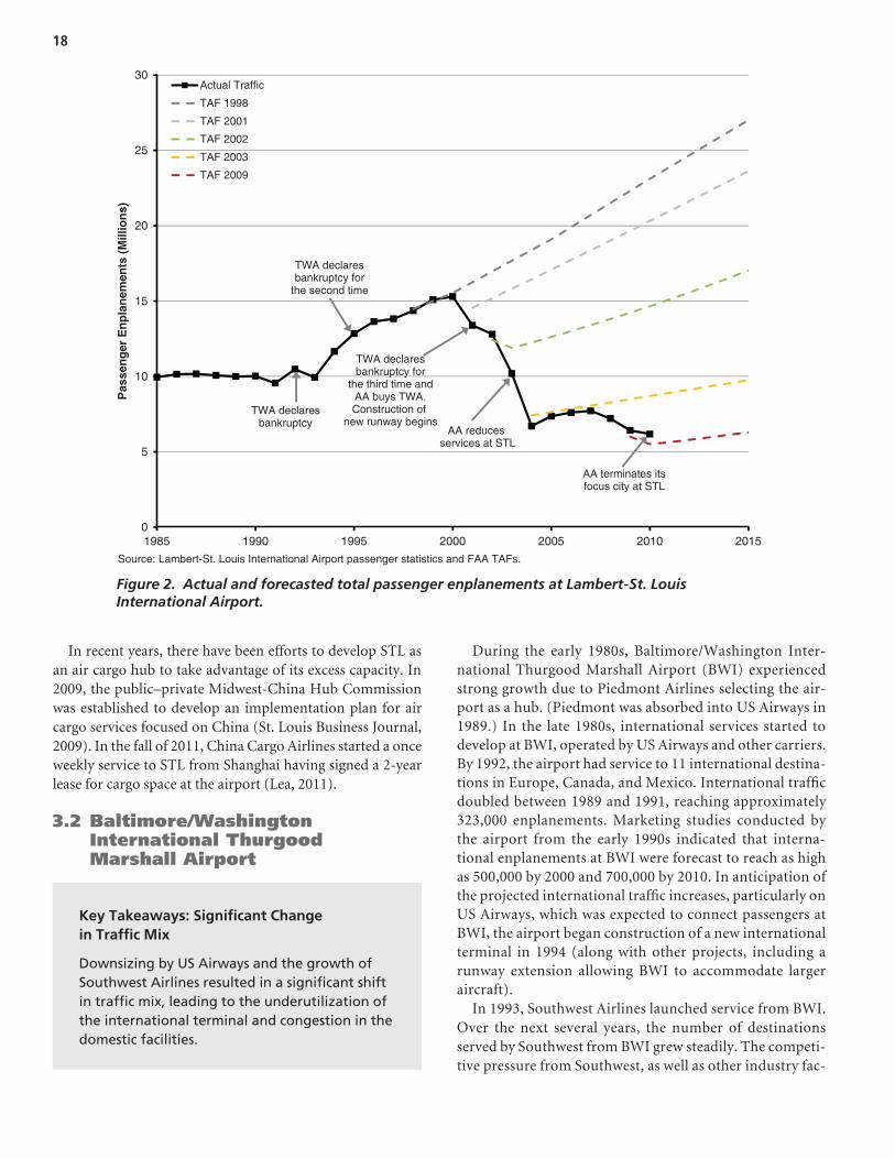
predicted that traffic would reach 20 million enplaned pas-sengers by 2006 and 25 million enplaned passengers by 2012.

In early 2001, TWA again experienced financial difficulties, which resulted in its assets being acquired by American Air-lines’ (AA) parent company (AMR Corporation), and the air-line declared bankruptcy for a third time. AA initially indicated that it planned to keep STL as a hub, in light of the conges-tion at Chicago O’Hare. However, with the severe downturn in traffic that followed the terrorist attacks of 9/11, AA began reducing its STL operations, focusing more on its main hub operations at Chicago O’Hare and Dallas/Fort Worth (DFW). In 2003, AA converted many routes to regional services, result-ing in a significant loss of total capacity.

As a result of TWA’s collapse, passenger volumes at STL declined by 56% between 2000 and 2004, to 6.7 million enplanements. Traffic failed to recover significantly from this level and declined further between 2008 and 2010 as result of economic conditions and further cutbacks by AA. The cut-backs by AA have been somewhat offset by Southwest Airlines, which increased operations at the airport in 2010 and is now the largest carrier at STL in terms of departures.

Due to delays in the planning process, construction of the proposed third runway did not start until 2001. While some consideration was given to delaying the construction, given the uncertainty regarding the operations of TWA/AA, it was decided to continue development. This decision was supported by the FAA on the basis of enhancing national system capacity. During the period of construction, FAA continually revised its forecasts for STL enplanements downward. By the time the FAA completed its forecasts for 2003, it was projecting STL’s pas-senger traffic in 2015 would be less than levels achieved in 1993.

As a result of this traffic decline, Concourse D, previously used by TWA, has been largely empty, and large parts were closed off in the fall of 2008. In addition, Concourse B has limited traffic and Concourse C is not currently used for commercial traffic. The newly built runway, completed in 2006 at a cost of $1.1 billion, is heavily underutilized.

C h a p t e r 3

Implications of Unforeseen Events and Conditions

Key Takeaways: Loss of a Major Carrier

The airport experienced large reductions in passenger traffic due to the collapse of its largest carrier, resulting in excess airport capacity and unused facilities.

In 1982, Trans World Airlines (TWA) named Lambert-St. Louis International Airport (STL) as its principal domes-tic hub, which resulted in passenger traffic at the airport almost doubling between 1981 and 1986, from 5.3 million to 10.0 million enplaned passengers (see Figure 2). During the 1990s, TWA drove strong traffic growth again, with total enplanements at the airport reaching 15.3 million passengers in 2000, despite the carrier entering bankruptcy protection twice (in 1992 and 1995). Connecting traffic accounted for a large proportion of passenger volume during this period. In response to this growth, a 1994 airport master plan update for STL proposed the construction of a third runway. The new runway was expected to allow STL to reduce delay times (which the airport had become prone to), improve capabili-ties in adverse weather, enhance capacity, and continue to accommodate TWA’s hubbing operations. This recommen-dation was supported by FAA TAFs around that time, which

18

In recent years, there have been efforts to develop STL as an air cargo hub to take advantage of its excess capacity. In 2009, the public–private Midwest-China Hub Commission was established to develop an implementation plan for air cargo services focused on China (St. Louis Business Journal, 2009). In the fall of 2011, China Cargo Airlines started a once weekly service to STL from Shanghai having signed a 2-year lease for cargo space at the airport (Lea, 2011).

3.2 Baltimore/Washington International Thurgood Marshall Airport

During the early 1980s, Baltimore/Washington Inter-national Thurgood Marshall Airport (BWI) experienced strong growth due to Piedmont Airlines selecting the air-port as a hub. (Piedmont was absorbed into US Airways in 1989.) In the late 1980s, international services started to develop at BWI, operated by US Airways and other carriers. By 1992, the airport had service to 11 international destina-tions in Europe, Canada, and Mexico. International traffic doubled between 1989 and 1991, reaching approximately 323,000 enplanements. Marketing studies conducted by the airport from the early 1990s indicated that interna-tional enplanements at BWI were forecast to reach as high as 500,000 by 2000 and 700,000 by 2010. In anticipation of the projected international traffic increases, particularly on US Airways, which was expected to connect passengers at BWI, the airport began construction of a new international terminal in 1994 (along with other projects, including a runway extension allowing BWI to accommodate larger aircraft).

In 1993, Southwest Airlines launched service from BWI. Over the next several years, the number of destinations served by Southwest from BWI grew steadily. The competi-tive pressure from Southwest, as well as other industry fac-

0

5

10

15

20

25

30

1985 1990 1995 2000 2005 2010 2015

Pas

sen

ger

En

pla

nem

ents

(M

illio

ns)

Actual Traffic

TAF 1998

TAF 2001

TAF 2002

TAF 2003

TAF 2009

TWA declaresbankruptcy

TWA declaresbankruptcy for

the second time

TWA declaresbankruptcy for

the third time andAA buys TWA.Construction of

new runway beginsAA reduces

services at STL

AA terminates itsfocus city at STL

Source: Lambert-St. Louis International Airport passenger statistics and FAA TAFs.

Figure 2. Actual and forecasted total passenger enplanements at Lambert-St. Louis International Airport.

Key Takeaways: Significant Change in Traffic Mix

Downsizing by US Airways and the growth of Southwest Airlines resulted in a significant shift in traffic mix, leading to the underutilization of the international terminal and congestion in the domestic facilities.

19

tors (including the 9/11 attacks) contributed to US Airways scaling down its BWI operations and moving operations to Philadelphia.

US Airways’ moving its hub to Philadelphia resulted in BWI losing about a third of its international traffic. With limited options for connecting traffic, and with opera-tions dominated by LCCs, BWI struggled to attract addi-tional international service. As a result, total international passenger enplanements dropped by half between 1991 and 2009, falling from the 1991 high of 323,000 to less than 163,000 in 2009 (see Figure 3). International traffic increased slightly again in 2010, reaching almost 190,000 enplaned passengers.

The decline in international traffic left BWI with an underutilized international terminal. However, the rapid growth of Southwest led to increased demand for domes-tic facilities. Despite having an underutilized international facility, BWI had to undertake additional capital spending on its domestic facilities because the international terminal was not suitable to meet the needs of Southwest.

Although international traffic failed to reach forecast lev-els, total traffic was broadly in line with the long-term fore-casts, as illustrated in Figure 4. However, the mix of traffic

was quite different from the forecasts. This example also sug-gests that forecasting O/D traffic is perhaps inherently less risky than forecasting connecting traffic. Total O/D traffic at BWI developed in a manner reasonably close to the fore-cast, but the connecting traffic transferred to another airport (Philadelphia).

3.3 Louis Armstrong New Orleans International Airport

0

50

100

150

200

250

300

350

1972

1974

1976

1978

1980

1982

1984

1986

1988

1990

1992

1994

1996

1998

2000

2002

2004

2006

2008

2010

Pas

sen

ger

En

pla

nem

ents

(T

ho

usa

nd

s)

Piedmont announces hub

Sept. 11, 2001, and recession March - Nov 2001

RecessionDec 2007 -June 2009

End of USAirways alliance with British Airways

US Airways moves international operations to Philadelphia

New flights by KLM, Icelandair,US Airways

Source: U.S. DOT data and Ralph M. Parsons Company (1987). Data from 1985 to 1988 could not be obtained. Note: This figure excludes military passengers carried by the U.S. Air Mobility Command.

Figure 3. International passenger enplanements at Baltimore/Washington International Thurgood Marshall Airport.

Key Takeaways: Large Natural Disaster

Devastation by Hurricane Katrina in 2005 resulted in an immediate and substantial loss in passenger traffic, which has not yet been recovered.

In August 2005, Hurricane Katrina hit New Orleans. The storm resulted in one of the largest natural disasters in U.S. history, causing widespread flooding, billions of dollars of

20

0

2

4

6

8

10

12

1972

1974

1976

1978

1980

1982

1984

1986

1988

1990

1992

1994

1996

1998

2000

2002

2004

2006

2008

2010

Pas

sen

ger

En

pla

nem

ents

(M

illio

ns)

Actual Traffic

1987 Master Plan Forecast (Baseline)

Piedmont announces hub

First Gulf Warand recession

Southwest Airlines launches services

9/11 andrecession

Recession

US Airways "de-hubs"

Source: Analysis of data from FAA and the 1987 Master Plan.

Figure 4. Actual and forecasted total passenger enplanements at BWI.

property damage, and more than 1,300 deaths. Hurricane Rita followed less than a month later, adding to the devas-tation. During the immediate time period of the storm and recovery, Louis Armstrong New Orleans International Air-port (MSY) was closed to commercial air traffic. However, MSY itself escaped sizable damage during the hurricanes and reopened after only 2 weeks.

Nevertheless, the hurricane had a catastrophic impact on the airport and resulted in a 39% decline in traffic in 2006 relative to 2004 (pre-Katrina) levels, as shown in Figure 5. While nearly all the major carriers have returned to MSY, passenger traffic levels in 2009 were still 21% below 2004 levels, due to the loss of tourism and conventions, declines in the local population, economic decline, and reduced air carrier capacity. Moreover, traffic levels are well below the FAA’s TAFs produced before Hurricane Katrina, and more recent forecasts have been revised downward, suggesting a long recovery period. According to the 2010 TAF, the FAA does not expect MSY to return to 2004 passenger lev-els until 2021.

Hurricane Katrina is an example of a sudden and unex-pected event. Mitigating the traffic impacts of such an event is

challenging. The airport has instigated an incentive program to encourage new service to the airport.

3.4 Bellingham International Airport

Key Takeaways: Unexpected Upside Traffic Growth

Entry of low-cost carrier Allegiant Air resulted in much higher than forecast traffic growth.

Bellingham International Airport (BLI) is located in Whatcom County, Washington, 3 miles northwest of Bellingham, a city with a metro population of approximately 200,000. The airport is approximately 21 miles south of the Canadian border and 90 miles north of Seattle.

Prior to the 9/11 terrorist attacks, BLI had service to Seat-tle operated by Horizon Air and United Express/SkyWest

21

(accounting for 79% of seat capacity in 2000), plus service to the San Juan Islands off the coast of Washington (URS et al., 2004). In October 2001 the United Express/SkyWest services were terminated, in part due to service rationaliza-tion following the 9/11 attacks. Traffic declined to a low of 64,365 in 2003 due to further service cutbacks.

In August 2004, low-cost carrier Allegiant Air entered the market at BLI and started service to Las Vegas. Over the next few years, the airline increased the range and frequencies of service out of BLI. By January 2008, Allegiant Air opened up its sixth base at BLI. As of December 2011, the airline oper-ated direct service to Las Vegas, Los Angeles, Palm Springs, San Diego, Oakland, and Phoenix. As a result of Allegiant’s entry, traffic at BLI increased by 374% between 2004 and 2010, an average growth rate of nearly 30% per annum.

The airport also experienced the short-lived entry of two other carriers:

• Western, an LCC headquartered in Bellingham, entered the BLI market (serving three destinations) on January 18, 2007, but ceased operations due to financial difficulties on February 7, 2007.

• Skybus, an ultra low-cost carrier based in Ohio, operated flights to Ohio between May and October 2007 before can-celling the service.

As can be seen in Figure 6, since the entry of Allegiant, traffic levels have greatly exceeded forecasts produced by the FAA and in the airport’s 2004 master plan.

BLI’s expansion plans were affected by the rapid and un-expected increase in traffic. For example, the expansion of the terminal building, originally scheduled to be completed in 2018, has been accelerated to be completed by 2013. In addition, a $29 million runway resurfacing project was completed in September 2010 that will enable larger aircraft to operate at BLI (Puget Sound Business Journal, 2010). This will allow Allegiant Air to operate its larger B757 aircraft at BLI, as well as existing MD-80 services, potentially contributing to fur-ther traffic growth.

This BLI example shows that upside risk can lead to a need for rapid airport expansion in order to keep airlines and passengers satisfied to ensure that airlines can continue to expand their services and to avoid congestion that may lead to a loss of passengers or the exit of a carrier.

0

1

2

3

4

5

6

7

8

1980 1982 1984 1986 1988 1990 1992 1994 1996 1998 2000 2002 2004 2006 2008 2010 2012 2014

Pas

sen

ger

En

pla

nem

ents

(Mill

ion

s)

Actual Traffic

TAF 2001

TAF 2004

TAF 2005

TAF 2009

Hurricane Katrina

Source: FAA TAFs.

Figure 5. Actual and forecasted total passenger enplanements at Louis Armstrong New Orleans International Airport.

22

0

50

100

150

200

250

300

350

400

450

1985 1990 1995 2000 2005 2010 2015 2020

Pas

sen

ger

En

pla

nem

ents

(T

ho

usa

nd

s)

Actual Traffic

TAF 2000

TAF 2003

Master Plan Forecast

United Express/ SkyWest exits in 2001

Allegiant enters in August 2004 and rapidly develops service

Allegiant opens base at BLI in January 2008

Source: Bellingham International Airport Master Plan Update (URS et al., 2004), FAA TAFs, and BLI airport statistics.

Figure 6. Actual and forecasted total passenger enplanements at Bellingham International Airport.

3.5 Zurich Airport and Brussels Airport As a result of restructuring, Swiss International Air Lines cut its seat capacity at ZRH by 43% between 2000 and 2004. The airline was subsequently taken over by Lufthansa (in 2007) but continues to operate as a separate brand.

The capacity cuts by its home carrier contributed to a 25% decline in total traffic at ZRH between 2000 and 2004. (Swissair accounted for 66% of traffic before its failure.) In the years following, traffic gradually recovered (by 5.4% per annum) to reach close to its pre-collapse levels by 2008 before declining in 2009 due in large part to the global recession.

A similar story occurred at Brussels Airport (BRU), which was the primary hub of Sabena, the former national carrier of Belgium. In fact, the two events are connected since it was the failure of Swissair to make a scheduled payment of U.S.$200 million to Sabena in 2001 that triggered Sabena’s collapse. In November 2001, Sabena ceased operations, and many of its assets were transferred to a short-haul sub-sidiary, Delta Air Transport. In early 2002, the airline was renamed SN Brussels Airlines. The new airline cut seat capacity by 68% between 2001 and 2002. In 2007, the airline merged with Virgin Express (an LCC based at BRU) and was renamed Brussels Airlines.

The airport experienced a 33% decline in traffic between 2000 and 2002 (Sabena accounted for 55% of traffic before

Key Takeaways: Collapse and Restructuring of the Main Hub Airline

Both airports experienced the collapse of a home carrier that was partially replaced by a smaller, restructured airline. Traffic declined sharply at both airports, which was then followed by varying degrees of recovery.

Zurich Airport (ZRH) served as the hub for Swissair, former national carrier of Switzerland. Due to its central position in Europe, Swissair (and thus ZRH) profited from generating transfer passengers. However, with the deregula-tion and liberalization of the air industry in the European Union (which Switzerland participated in despite not being a member of the EU) and the economic downturn during 2000 and 2001, Swissair experienced severe financial difficulties, leading to the airline filing for bankruptcy in October 2001. Many of Swissair’s assets were taken over by a subsidiary of Swissair, changing the name to Swiss International Air Lines.

23

its failure), after which traffic grew by 4.3% per annum so that by 2008 passenger traffic levels were 21% below its pre-collapse levels.

Both airports saw traffic decline dramatically, which was then followed by modest recovery. Both have yet to recover fully to pre-collapse levels. Even though some recov-ery has occurred, both airports are way off the traffic trend that was apparent prior to the airline failure. In both cases, the traffic recovery was largely a result of the home carrier rather than other carriers replacing the lost capacity.

Despite the loss of traffic following Swissair’s collapse, ZRH decided to continue expansion plans started in 2000. In September 2003, ZRH completed its new Dock E. As a consequence, ZRH had considerable excess capacity. The lack of traffic led to a closure of the existing Dock B in the same year. As an example of adapting facility use, Dock B was converted into an event venue (EventDock) for a period of time, although it has since undergone reconstruction and was reopened in December 2011.

BRU had started construction of a new pier (Pier A), which was completed in May 2002, before the collapse of Sabena. Fol-lowing Sabena’s collapse, the decision was made to close the satellite terminal that had originally served as the terminal for

Figure 7 shows total passenger enplanement at Washing-ton Dulles International Airport (IAD) since 1990. Strong growth occurred in 1998 to 2000 as a result of a build-up of

Key Takeaways: Widely Fluctuating Traffic Volumes

Over the last decade, the airport has experi-enced widely fluctuating traffic volumes, due largely to market entries and exits of diverse air carriers as well as economic downturns and the 9/11 terrorist attacks. This has made forecasting challenging and resulted in large changes in the airport outlook.

0

5

10

15

20

25

1990 1992 1994 1996 1998 2000 2002 2004 2006 2008 2010 2012 2014

Pas

sen

ger

En

pla

nem

ents

(M

illio

ns)

Actual Traffic

TAF 2000

TAF 2001

TAF 2003

TAF 2004

TAF 2005

TAF 2009

Source: FAA TAFs and Washington Dulles International Airport air traffic statistics.

Figure 7. Actual and forecasted total passenger enplanements at Washington Dulles International Airport.

the intercontinental operations of the airline. After some recon-struction, that terminal is now used as office space (BRU, 2009).

3.6 Washington Dulles International Airport

24

traffic levels, followed by Virgin America a year later. Passen-ger levels declined in 2008 and 2009, with JetBlue, Southwest, and Mesa all making significant cuts (of more than 10%) in capacity, due in large part to economic conditions.

The FAA TAFs for IAD since 2000 are also shown in Fig-ure 7. These forecasts have required considerable revisions in response to changing market conditions. These revisions demonstrate how fluctuations in carrier activity and traffic volumes can create considerable uncertainty regarding the long-term outlook for traffic. In the case of IAD, most of this volatility has been the result of domestic operations, which have caused domestic passenger volumes to change by as much as -20% to +41% year-on-year. By comparison, inter-national traffic has exhibited more steady growth, averaging a 4.2% increase per annum between 2000 and 2010.

competition between United Airlines and US Airways. After 2000, US Airways decided to remove considerable capacity from IAD, which combined with a similar capacity response from United Airlines, the economic recession in the United States, and the 9/11 terrorist attacks, resulted in traffic levels declining.

In June 2004, Independence Air started service as an LCC based at IAD. This resulted in enplaned passenger volumes increasing significantly in 2004 and 2005. However, Indepen-dence Air ceased operations in January 2006, resulting in pas-senger volumes declining again in that year. In addition, other LCCs entered the market at IAD. JetBlue Airways commenced air service in November 2001, followed by Mesa Airlines, a regional LCC, in 2004. In 2007, Southwest Airlines began operations at the airport, further contributing to increased

25

In the aviation sector, procedures used to account for risks and uncertainties have traditionally been ancillaries to the methods used for developing demand or air traffic forecasts. This is because in the early stages of the aviation planning process, decisions are made regarding the intended use of forecasts, and a method (or set of methods) is subsequently selected for producing demand projections based on perceived accuracy, ease of use and interpretation, and adaptability or flexibility in applications.

As described in ACRP Synthesis 2: Airport Aviation Activ-ity Forecasting, the techniques that are often employed in forecasting can be grouped within four categories (Spitz and Golaszewski, 2007):

• Time-series methods: trend extrapolation using statisti-cal techniques that rely on lagged and contemporaneous traffic data to infer future values.

• Econometric modeling with explanatory variables: sta-tistical techniques that examine the relationship between traffic and possible explanatory variables, such as the econ-omy (e.g., gross domestic product or personal incomes), population, fuel prices, and so forth.

• Market share analysis: a technique used to forecast local activity as a share of some larger, aggregated forecast. For example, a forecast of airport traffic may be based on its assumed share of national traffic, as forecasted by a third party.

• Simulations: a technique involving the use of com-plex models that evaluate different snapshots of a travel network.

The sections that follow examine approaches for address-ing uncertainty in aviation demand forecasting. Where information from the aviation industry is limited, relevant methodologies from other industries in the transportation sector (e.g., toll road demand forecasting) and other sectors or disciplines (e.g., demographic forecasting) have also been

reviewed. Readers requiring more detailed information are encouraged to review Appendix D.

4.1 Standard Procedures to Account for Uncertainty in Aviation Demand Forecasting

C h a p t e r 4

Approaches for Incorporating Uncertainty into Demand Forecasting

Key Takeaways

Three fairly common procedures are used in air traffic forecasting to account for uncertainty:

• High and low forecasts• What-if analysis• Sensitivity analysis

However, these approaches provide only a cursory understanding of risk and uncertainty and are rarely incorporated into the planning process in any meaningful way.

Three standard procedures commonly used to account for uncertainty in demand forecasts are described in the follow-ing sections. All three have been used in conjunction with the four forecasting techniques described previously.

4.1.1 High and Low Forecasts

In developing demand projections under this approach, many (or all) of the forecasting assumptions are modified in one direction to produce an optimistic forecast, then in the opposite direction to produce a pessimistic forecast. For example, the high forecast may assume that GDP growth will be one percentage point higher per annum than the rate used in the baseline or most likely forecast.

26

This procedure is fairly common in air traffic forecasting since it can be easily incorporated into standard forecast -ing techniques, including market share analysis and econo-metric modeling. It is also one of the easiest procedures to implement once a forecasting model has been developed. In addition, interpreting the outcomes of the analysis is generally straightforward and does not require any spe-cific knowledge of probability theory—the concepts of “high” and “low,” or “optimistic” and “pessimistic,” are intuitive and generally understood. The low/high forecasts can be based on analysis of trends, judgment, or projec-tions of key input values developed outside of the forecast model.

However, there are a number of limitations to the high/low forecast approach:

• The range between the low and high forecasts is often rela-tively small (e.g., +/- 25% relative to the baseline forecast). However, as illustrated in Chapter 3, traffic deviations can be much larger than this.

• The forecasts provide no information on the likelihood of such outcomes, which limits their use and applicability. Indeed, the very idea that multiple assumptions will veer from baseline expectations in the same direction is itself arbitrary.

• Although frequently provided in forecast exercises, the high and low forecasts have little input into subsequent planning efforts. The baseline forecasts are used for most of the planning, with little consideration given to the high and low forecasts.

4.1.2 What-If Analysis

In this procedure, also known as “impact analysis,” the impact of a single event (such as an economic downturn, a rapid increase in fuel prices, or a health pandemic) is estimated and reported relative to the baseline forecast. Uncertainties are typically assumed to be event-specific and are defined as either threats or opportunities.

The procedure involves the following steps:

1. Establish a baseline forecast using any of the four techniques mentioned at the beginning of this chapter and assuming that none of the identified events will materialize.

2. Determine the magnitude of the events (e.g., the sever-ity and duration of an anticipated downturn in economic activity or the percentage increase in fuel prices).

3. Estimate the effect of each event, taken individually, on the baseline forecast. This can be done with the estimated parameters of the forecasting model itself, by using infor-mation or similar events in the past, or through judgment (or a combination of the three).

4. Report the outcomes of the analysis. Impacts are typi-cally reported one at a time, with no reference to potential dependencies or correlations with other events.

One of the main strengths of this approach is that it can be used with a variety of forecasting tools and techniques, including econometric methods and complex simulation models.

On the other hand, the use of what-if analysis requires reference to a baseline, most likely forecast, the probability of which is typically unknown. Furthermore, as with the high/low forecast, the probability of alternative outcomes under different what-ifs often remains unknown, mak-ing the interpretation of the outcomes somewhat difficult. Furthermore, assumptions do not veer from expectations one at a time in the real world, making what-ifs difficult to translate into implications for airport planning.

4.1.3 Sensitivity Analysis

In a sensitivity analysis, forecasting assumptions are var-ied one at a time, and the resulting changes in the projected outcomes (e.g., passenger demand forecast) are reported accordingly.

A sensitivity analysis may serve multiple purposes, including:

• Helping to identify the variables and model parameters whose variations have the greatest impact on the forecast: the critical variables.

• Evaluating the impact of changes in the critical variables (i.e., of reasonable departures from their preferred, base-line values).

• Assessing the robustness of the forecast. In particular, whether the general conclusions reached using the base-line assumptions are significantly altered through changes to the key assumptions.

Occasionally, the sensitivity analysis will involve chang-ing multiple assumptions simultaneously. This is sometimes referred to as scenario analysis.

The limitations of sensitivity analysis have been docu-mented in a number of publications. For example, sensitivity analysis forecasting assumptions are often varied by arbi-trary amounts instead of by reference to reasoned analysis of potential error (Lewis, 1995). In addition, varying one assumption at a time does not provide an accurate view of the real world, where all factors affecting forecasts are likely to vary simultaneously. On the other hand, this procedure can be useful for assessing the significance of individual fore-casting assumptions in the production of the overall demand

27

Advanced procedures have been developed to incorporate uncertainties into forecasting. These address some of the con-cerns highlighted in the previous sections, particularly with respect to quantifying the probability of alternative outcomes and forecasts. However, to date, it appears that these proce-dures are not widely used in the aviation industry. They vary in scope and complexity but can be grouped into two broad cat-egories: data-driven (objective probability) or judgment-based (subjective probability) procedures. Section 4.2.1 describes the methodologies for data-driven statistical analysis available to produce objective measures of probability. Section 4.2.2 dis-cusses the use of judgment and opinion to produce subjective measures of probability.

These two categories are defined solely to assist in grouping methods for the purpose of the following discussion. In prac-tice, procedures based on historical data are often combined with judgment-based input, as is described in Section 4.2.3.

4.2.1 Data-Driven Procedures

Three classes of methods have been identified where the incorporation of uncertainty relies exclusively on the analysis

forecasts, and it has been used fairly extensively in aviation demand forecasting.

4.2 More Advanced Procedures for Incorporating Uncertainty into Forecasting

of historical data: (1) time-series methods, (2) extrapolation of empirical errors, and (3) distribution fitting and simula-tions. These methods are summarized in the following.

4.2.1.1 Prediction Intervals from Time-Series Methods

Time-series methods use statistically estimated models to estimate future values of a variable of interest (e.g., air pas-senger enplanements) based on the historical values of that variable. They include extrapolative methods, which are based solely on identifying data patterns in the variable of interest (e.g., autoregressive moving averages) and explanatory vari-able methods (e.g., regression analysis), which introduce causal variables to explain and forecast the variable of interest.

Most time-series methods recognize the uncertainty asso-ciated with model specification through the inclusion of an error term and stochastic parameter values (as reflected in standard error, t-statistic, and R-squared statistics, etc.). Time-series methods allow estimation of a prediction inter-val, similar to a confidence interval, within which future estimates (or forecasts) will fall at a certain probability. For example, the prediction interval could be described as fol-lows: based on the error terms of the model, there is a 95% probability that forecast passenger traffic in 2030 will be in the range of 10 to 12 million. A common feature of predic-tion intervals is that they increase in length as the forecast horizon increases (i.e., uncertainty increases as we forecast further into the future).

However, this distribution only reflects uncertainty in the model specification (the functional form of the model) and its parameter values (i.e., statistical uncertainty). It does not reflect uncertainty due to changes in the economic environment, air carrier decisions, rare shock events, and so forth. Although prediction intervals can be derived from most statistical software packages, it is rare for this infor-mation to be provided for forecasts derived through statis-tical methods.

4.2.1.2 Extrapolation of Empirical Errors

This general approach consists of developing ranges of pos-sible forecast values based on observed errors from historical forecasts (i.e., the difference between actual values and prior forecasts of those values). As a simple example, if analysis found that previous forecasts had differed from actual values by +/- 20%, it could be assumed that the prediction interval related to current forecasts of future values is +/-20%.

Research for this guidebook found very few applications of this extrapolation approach being used in aviation demand forecasting. However, this approach has been used in fore-casts of population growth. The National Research Council conducted an analysis of the distribution of past errors in

Key Takeaways

Although to date not widely used in aviation activity forecasts, there are analytical proce-dures that have the potential to enhance the understanding of risk and uncertainty, catego-rized as follows:

• Data-driven procedures involving the statistical analysis of historical data (objective probability), and

• Judgment-based procedures incorporating the judgment and opinion of experts and stake-holders (subjective probability).

These types of procedures can be used in com-bination to develop a deeper understanding of the risk and uncertainty facing an airport. They can be enhanced by the use of computational methodologies such as Monte Carlo simulation.

28

population forecasts by the United Nations over two decades to define predictive intervals for more current UN popula-tion projections (Bongaarts and Bulatao, 2000).

A similar concept is called reference class forecasting, which aims to address optimism bias and general uncertainty in demand and cost forecasting for public works. Reference class forecasting involves evaluating (or even developing) a forecast for a particular project by referencing it against actual outcomes from a group of similar projects. This process is composed of the following steps (Flyvbjerg et al., 2005):

1. Identify a group of similar past projects, called the refer-ence class.

2. Using data from projects within the reference class, estab-lish a probability distribution for the variable of interest (e.g., traffic levels).

3. Compare the specific project with the reference class dis-tribution in order to establish the most likely outcome for the new project.

The approach is designed to provide an outside view of the project, without the need to identify and forecast the impact of specific events (Flyvbjerg et al., 2005).

This approach has been used in the UK, Netherlands, Denmark, and elsewhere for forecasts of highway traffic and project costs. No formal applications of reference class fore-casting for aviation demand have been identified. However, informal use of this approach likely occurs, for example, by comparing a forecast against traffic development at other similar airports.

4.2.1.3. Distribution Fitting and Simulation

Under this group of methods, a probability distribution is defined for the variable of interest on the basis of past growth rates or activity levels. Simulation techniques are used to combine multiple realizations of this distribution over time and develop probable growth paths.

The process is composed of three steps (summarized in Figure 8):

1. Historic, annual growth rates or activity levels for the vari-able of interest for a specific airport (e.g., total passen-ger volumes) are used to identify a distribution through goodness-of-fit evaluation tests;

2. Monte Carlo simulations (see Monte Carlo text box) are run to produce the entire distribution of possible growth rates or levels over the forecasting horizon, using the dis-tribution function identified in step 1; and

3. Simulated growth rates or levels and associated probabili-ties are converted into annual forecasts.

Bhadra and Schaufele (2007) applied this approach to fore-casting traffic at the top 50 commercial airports in the United States. As noted by the authors, the approach has a number of limitations:

• It is assumed that the distributions of annual growth rates or levels for the variable of interest are independent. (This can be formally tested to rule out the possibility of correlation.)

Probability Distribution for One Period of Traffic Growth

Monte Carlo Simulations

of Distribution Combined

with Forecast

Point Forecast with Fitted Distribution

Actual Data Forecast

HistoricalTraffic Data

Distribution Fitting

Source: Based on Bhadra and Schaufele, 2007.

Figure 8. Distribution fitting and simulation.

29

• The same fitted distribution of the relevant variable is used throughout the entire forecasting period (i.e., time-invariant property of the distribution) resulting in the range of prob-able outcomes widening over time.

• Since each variable is being simulated separately at each airport, the method ignores network dependencies (i.e., competition or interactions between airports).

• The sources and the nature of uncertainty remain unknown, making the interpretation of possible outcomes and the practical use of the forecasts difficult.

4.2.2 Judgment-Based Procedures

Under this group of procedures, the probability of an event is viewed as the degree of belief sustained by an informed person (or group of stakeholders) that it will occur, rather than any property of the physical world. Sub-jective probabilities can be blended with objective data

(e.g., historical variations in enplanements) and/or market data (e.g., crude oil futures prices) to arrive at a distribu-tion for future outcomes.

In aviation demand forecasting, as in other fields, forecast-ers often use experts’ opinions and judgments to assess traffic outlook and uncertainties. This is particularly true when point forecasts and/or prediction intervals are difficult to obtain through objective methods or when the variable of interest may be affected by rare events.

There are a number of techniques for eliciting expert opin-ions and judgments on forecast outlooks and probabilities. One of the most well established techniques is Delphi forecast-ing. The Delphi technique is an elicitation technique defined by four key features: anonymity, iteration, controlled feed-back, and the statistical aggregation of group responses (Rowe and Wright, 1999).

Delphi forecasting typically begins with the planner select-ing a group of experts and preparing a questionnaire, which

Introduction to Monte Carlo Simulation

Monte Carlo simulation (or the Monte Carlo method) is a computerized simulation technique that makes use of randomization and probability statistics to investigate problems involving uncertainty. Typically, it involves a computer model of a system or project (e.g., air traffic at an airport). The inputs to the model, instead of being fixed numbers or variables, are specified as probability distributions. For example, in the model described in Figure 8, rather than traffic growth being set at X% per annum, it may be defined as having normal (bell-curve) distribution with a mean of X% and a standard deviation of 1.0%. Using computer software, the model is run multiple times, each time randomly sampling from the input distributions, resulting in different outcomes each time. Often, the model will be run thousands or tens of thousands of times (known as iterations), and the results are collected from each run.

With enough iterations of the model, the output can demonstrate the range of possible outcomes and provide statistical estimates of the probabilities of various outcomes. Depending on the complexity of the model and input distributions assumed, the range of outcomes can be large and not always linear. Expected or most likely values can also be generated.

Monte Carlo can be seen as a powerful what-if or scenario-generating exercise where every possible what-if or scenario is generated (within the confines of the model specification), including interactions between the various input factors. Another way of looking at it is that each iteration of the model represents one possible future for the system being modeled. By running the model thousands of times, the user can view whole sets of possible futures, assess which are most likely to occur, and identify areas of greatest downside or upside.

Monte Carlo is used extensively in a wide range of fields. One of its first applications was in designing the shield-ing for nuclear reactors at the Los Alamos National Laboratory in the 1940s. (The name Monte Carlo was coined as a code name by scientists at the laboratory in reference to the Monte Carlo casino resort.) Monte Carlo simu-lation has since been used in finance, project planning, engineering studies, traffic modeling, cancer radiation therapy, and telecommunications network design, among many other applications.

Monte Carlo simulations are also discussed in Part II of the guidebook.

30

in the context of airport planning may include a series of projections. The questionnaire is distributed to each respondent separately. The answers provided by the experts are summarized and tabulated, and the results are returned to the experts for a second round. In this second round, the experts are asked to assess the group responses and justify their choices. During subsequent rounds, group averages and comments are provided, and experts are asked to re-evaluate their choices. The rounds continue until an agreed level of consensus is reached. The literature suggests that by the third round a sufficient consensus is usually obtained.

One of the most important factors in Delphi forecasting is the selection of experts:

The persons invited to participate must be knowledgeable about the issue, and represent a variety of backgrounds. The number must not be too small to make the assessment too nar-rowly based, nor too large to be difficult to coordinate. It is widely considered that 10 to 15 experts can provide a good base for the forecast. (Rodrigue et al., 2009, p.14)

The Delphi technique is listed as a qualitative forecasting method in the 2006 ICAO Manual on Air Traffic Forecasting (ICAO, 2006). Other elicitation techniques are:

• Statistical groups: where individuals give their forecasts without interacting with each other;

• Unstructured interacting groups: where individuals can interact freely with each other; and

• Nominal group technique: using a Delphi structure, but allowing face-to-face discussions between rounds.

Defined broadly, the elicitation process helps experts con-struct a set of carefully reasoned and considered judgments. Specifically, elicitation is conducted with a range of available or circumstance-specific protocols (such as Delphi) to obtain people’s subjective but accurately specified quantitative expres-sions of future probability.

A number of shortcomings of the elicitation approach have been highlighted in the academic literature:

• Existing research has found that experts may often be too confident and attach too high a probability to their predic-tions (Keilman et al., 2002).

• Experts may encounter problems in determining the exact probability bounds associated with a given prediction inter-val [e.g., the difference between a 90% and a 99% probabil-ity (Keilman et al., 2002)].

• There is evidence to suggest that objective methods are gen-erally more accurate than subjective methods as changes

in the environment increase and the forecasting horizon is lengthened (Armstrong and Grohman, 1972).

An alternative to the use of formal elicitation techniques, which combines judgment—often informally—with data and statistical modeling, has been presented in the academic literature as “the Poor Man’s Bayesian Analysis” (Armstrong and Grohman, 1972). This alternative method can be as simple as changing the parameters in an econometric model to reflect effects not captured in previous analysis (e.g., low-ering the GDP elasticity to capture the idea that economic growth provides less stimulus to traffic growth as the econ-omy becomes wealthier). Rather than changing the model parameters, the same effect can be achieved by adjusting the forecast values directly.

The use of elicitation techniques in aviation planning is not well documented but is fairly common, although on a more informal basis:

Frequently, a group of professionals knowledgeable about aviation and the factors affecting aviation trends are assembled to examine forecasts from several different sources, and compos-ite forecasts are prepared in accordance with the information in these sources and the collective judgment of the group. (Horonjeff et al., 2010, p.153)

4.2.3 Combining Data-Driven and Judgment-Based Analysis

The objective information from data analysis can be com-bined with subjective information obtained through elicita-tion techniques to form an even richer assessment of risk and uncertainty. Lewis proposes a risk analysis elicitation frame-work to best achieve this aim. The framework uses data analysis to initially estimate the probabilities’ values and distributions, which are then modified and expanded upon using elicitation techniques to obtain risk and probability beliefs from experts and stakeholders. A final set of probability distributions can then be developed, which are a combination of objective and subjective probability information. These are combined using Monte Carlo simulation techniques to produce forecasts of future activity together with estimates of the probability of achieving alternative outcomes (Lewis, 1995).

This sort of framework has been used to provide decision support in a number of areas, including traffic and revenue forecasting for toll roads, the quantification of airport invest-ment risk, the estimation of construction cost, and the sched-uling of large infrastructure projects. The Risk Uncertainty Analysis text box provides an example of a similar form of risk analysis used in air traffic forecasting at Portland Inter-national Airport (PDX).

31

Risk and Uncertainty Analysis Example: Portland International Airport

The 2008 Airport Master Plan Update for PDX provides forecasts of unconstrained passengers, cargo, general aviation, and military aircraft operations for the years 2012, 2017, 2027, and 2035.

The forecast incorporates probabilistic elements and is based on a review of the FAA’s TAFs, historical demand data, and inputs from airport planning stakeholders and representatives from the City of Portland. The sources of uncertainty considered in the passenger demand model include coefficient estimation errors and uncertainty in demand determinants such as per capita income, oil prices, non-fuel costs, carbon taxes/climate change policies, and load factors. Probability distributions for each determinant were tested and fitted inde-pendently to available historic data. Additionally, sensitivity tests were conducted for the 2035 results based on probable changes in technology (e.g., 5% substitution of video conferencing for business travel), changes in the propensity to travel by age and income group (e.g., 65 and older persons will take an additional trip), oil shocks (e.g., 20% increase in oil prices), and other potential changes. The cargo model was developed using oil prices and uncertainty around those prices.

The figure that follows, extracted from the master plan update, illustrates some of the outcomes of the risk and uncertainty analysis. The lines indicate the traffic forecasts at different levels of probability. For example, the top 90% line indicates that there is a 90% probability the traffic will be at or below the line.

Source: Jacobs Consultancy, 2008.

High-impact events for which there is a sparse or nonexis-tent historical record pose two challenges for airport demand forecasting. One is anticipating them: will a volcano erupt and shut down the air traffic system, as occurred in Europe in 2010? The other is anticipating their impact on demand: how long will volcanic ash keep the system down and what effects will that have on demand? Some rare events have a high but short-lived impact on demand, while others have longer-term implications.

The literature on anticipating rare, high-impact events cuts across a range of professional disciplines, including sta-tistics, forecasting, and decision sciences, and addresses a range of events (e.g., weather and environmental, economic, crime, terrorism, and political), and it deals with a variety of

4.3 Is It Possible to Predict and Forecast the Impact of Rare or High-Impact Events?

Key Takeaways

Lack of historical data and innate human biases make the prediction and forecasting of rare events difficult—and often unsuccessful. How-ever, there are techniques airports can employ that will better prepare them to manage rare, high-impact events should they occur.

32

stakeholders (e.g., human safety and welfare, infrastructure enterprises, business firms, and governments).

Goodwin and Wright (2010) conclude that existing fore-casting methods, including statistical approaches and expert judgment (i.e., Delphi forecasting), are not effective in antici-pating and estimating the impact of rare events on enterprise outcomes. Bonabeau further explains that our inability to predict low-frequency, high-impact events is due to two fun-damental cognitive biases that affect human decision mak-ing: availability and linearity. Availability heuristics guide us toward choices that are easily available from a cognitive per-spective (i.e., if it is easy to remember, it must make sense). Linearity heuristics make us seek simple cause-and-effect rela-tionships in everything (Bonabeau, 2008).

Bonabeau makes the case that anticipating rare events requires augmented paranoia—that is, the rejection of both cognitive biases: availability and linearity. His corrective strat-egies include tapping the collective intelligence of people in a group (i.e., the wisdom of crowds) and tapping the creative power of evolution (i.e., considering a more-or-less randomly generated population of solutions and selecting, altering, and/or breeding the fittest until a satisfactory solution emerges) (Bonabeau, 2008).

Rather than attempting to forecast rare events, methodolo-gies have been put forward that attempt to develop a capability to manage such events. These include scenario planning. Sce-nario planning abandons the assumption that rare events can be predicted or given a meaningful probability of occurrence. Instead, scenario planning assumes that the best that can be done is to identify critical outcome uncertainties and plan for the range of futures that could plausibly unfold:

Essentially, scenarios highlight the causal reasoning under-lying judgments about the future and give explicit attention to sources of uncertainty without trying to turn an uncertainty into a probability. (Granger and Henrion, 1990, p. 363)

A similar concept is protective strategy, the systematic means of protecting an organization from the occurrence of events with negative impacts while allowing it to benefit from the occurrence of events with positive impacts. Open and wide-ranging discussion forums (sometimes called “devil’s advo-cacy” or “dialectical inquiry”) can be combined with Delphi approaches and scenario planning to enhance the anticipation of, and robustness to, rare events (Goodwin and Wright, 2010).

While the previous discussion and broad conclusions pertain to forecasting rare events for organizations in gen-eral, the aviation literature suggests a convergence of ideas. Horonjeff et al. report the increased use of techniques that rely less on mathematical modeling and more on an analysis of different scenarios, human judgment, and protective strat-egy: “Although judgment has always played a role in demand forecasting, it is becoming more important as a subjective test of the reality associated with forecasting outcomes.” (Horonjeff et al., 2010, p.168).

Furthermore, Horonjeff et al. state that in the wake of the 2008/09 financial crisis and recession, airport planning pro-cesses are becoming more phase-oriented and continuous in recognition of uncertainty about rare events and their impacts on demand forecasts. The authors point to an increasing use of ongoing sensitivity, trade-off, and scenario analysis in the planning and design of airport facilities and operational procedures.

33

The sections that follow describe some of the approaches that have developed in academia and industry to better address risk and uncertainty in airport decision making, including theoretical methodologies, practical applications, and diversification strategies.

5.1 Flexible Approaches to Airport Planning

with greater ease or lower costs than if no flexible options were considered (McConnell, 2007).

Different authors have proposed slightly different steps and procedures or variations:

• Dynamic strategic planning (de Neufville and Odoni, 2003);• Flexible strategic planning (Burghouwt, 2007);• Adaptive airport strategic planning (Kwakkel et al., 2010).

As the names suggest, these three approaches are fundamen-tally very similar, although they differ in detail. They are largely conceptual, although based on real-world experience, and have not been fleshed out into detailed planning procedures. While there are examples of airport planning that have contained some elements of these approaches, they have so far not been applied in practice. The three approaches are described in more detail in Appendix E. The contrast between these approaches and more traditional airport master planning is characterized in Table 1.

One of the ways these approaches differ from traditional master planning is that rather than have most of the planning developed around a single forecast, the plan considers a range of forecasts. The approach allows for plans that can be rela-tively easily adjusted over time as events unfold and conditions change.

While not all aspects of uncertainty can be eliminated or mitigated, it is possible to reduce or mitigate some uncertain-ties through demand management techniques (i.e., uncer-tainties that are caused by market fluctuations) (de Neufville, 2004). Airports can impede certain traffic types and facilitate others through pricing or direct controls (e.g., encourag-ing general aviation traffic to move to other airports, freeing capacity for commercial operations). One example of this is Kansas City International Airport, where the passenger ter-minal was impractical to serve transfer traffic. As a result, the planning team encouraged the locally based airline to estab-lish a hub at another airport (de Neufville and Odoni, 2003).

C h a p t e r 5

Addressing Risk and Uncertainty in Airport Decision Making

Key Takeaways

A number of alternative approaches to airport planning have been proposed by practitioners and academics that seek to incorporate much greater flexibility into the planning process. To date, these approaches are largely theoretical and have not been applied in practice.

A concept that offers considerable promise in making airport planning more flexible is real options. Drawing from the use of options in finan-cial markets, real options is the right, but not the obligation, to take a certain course of action.

5.1.1 Conceptual Frameworks

Given the traffic uncertainties facing airports and the difficulty in addressing them in traditional airport master plans, a number of alternative, adaptable approaches to airport planning have been proposed in the literature. A key element of these proposed approaches is building far greater flexibility into the planning process. While many definitions of flexibility exist, what all of them have in com-mon is that flexibility allows a system to undergo change

34

• Staged investment. Staging investment as a series of out-lays, which allows abandonment of the project if conditions change. Each stage is an option on the value of subsequent stages.

• Option to alter scale. The ability to accelerate or expand if conditions are favorable or contract if conditions are less favorable. At the extreme, it is the ability to halt produc-tion and restart later.

• Option to abandon. If market conditions decline severely, options can be abandoned—and equipment and land sold off.

• Option to switch. Develop a facility in such a way that it can change the output mix produced (alternatively, change the input mix).

• Growth options. An early investment (e.g., in land, in R&D) that opens up future growth opportunities.

• Multiple interacting options. Projects often involve a collection of put and call options in combination. Their combined value may differ from the sum of sepa-rate values.

The greater flexibility that real options provide can have significant value to the decision maker. However, real options often (but not always) impose a cost. The trade-off between the real option’s value and its cost will determine whether to go ahead with the option. Various sophisticated analytical approaches have been developed to evaluate and value real options (and are discussed in Appendix E). Some of these have been incorporated into the systems analysis methodol-ogy described in Part II.

5.1.2 Real Options

One concept that appears frequently in the literature on flexible or adaptive airport planning is real options. The con-cept of real options is based on and developed from financial options. In a financial context, options allow investors the right to acquire or to sell an asset (e.g., stock) at a specified price during a specified time frame. In short, an option is the right, but not the obligation, to take a certain course of action. There are two types of options: a call option (the right to buy, generally to take advantage of a good situation) or a put option (the right to sell, to get out of a bad situation). A remarkable feature of options is that their value increases with risk, which is the opposite of most other forms of assets (de Neufville and Odoni, 2003). As such, options are particu-larly useful in risky situations.

Real options apply to the real, physical world rather than the financial world (although real options still have financial implications). The concept started to develop in the 1970s and 1980s as a means to improve the valuation of capital-investment programs and offer greater managerial flexibil-ity to organizations. Real options and real options analysis are used in many industries, particularly those undertaking large capital investments (e.g., oil extraction and pharma-ceuticals). A number of common real options are available to organizations (Trigeorgis, 1996):

• Option to defer. A form of call option, where, for exam-ple, an organization may hold the lease on some land but defer building a plant on the land until market conditions are right.

Traditional Master Planning Flexible Strategic Planning

Passive, reactive, adaptive Re-adaptive, proactive

Once-and-for-all anticipation/adjustment to change Continuous anticipation/adjustment to change

Supply driven Demand driven

Forecasts as predictions of the future Backcasting: Scenarios as guidelines of what may happen in the future

Single-future robustness of plan and projects Multi-future robustness of plan and projects

Long-term and short-term commitments Short-term commitments, long-term strategic thinking

Preferred analytical tools: forecasting and net present value analysis

Preferred analytical tools: scenario planning, decision analysis and real options, contingent road maps, scanning, experimenting

Preferred alternative is optimal solution for a specific future

Preferred alternative is best alternative across a range of possible future scenarios.

Risk implicitly ignored or risk aversion Think risk culture. Risk as an opportunity

Top-down/inside-out Top-down/bottom-up, inside-out/outside-in

Reprinted by permission of the publishers from Airline Network Development in Europe and its Implications for Airport Planning by Guillaume Burghouwt (Farnham: Ashgate, 2007), p. 208. Copyright 2007.

Table 1. Characteristics of flexible planning.

35

As previously noted, the flexible planning approaches put forward in the literature remain largely conceptual and have not been applied in any airport planning projects. Likewise, real options methodologies, while used in other industries, have not been applied to any real-world airport planning projects.

Nevertheless, there are a lot of examples of airports devel-oping ways to build flexibility into the airport planning pro-cess that reflect the ideas behind real options. In general, these represent common-sense approaches based on experience in the field of airport planning rather than any formal method-ology. The sections that follow provide a summary of some of these examples, which represent industry best practice.

5.2.1 A Second Airport for Sydney, Australia

During the 1970s and early 1980s, the Australian govern-ment grappled with the issue of a second airport to serve Sydney, Australia’s largest city. (The main airport in Sydney is difficult to expand due to its proximity to the city center.) Two separate studies had produced contradictory conclu-sions: one recommending the building of a new airport, and the other concluding it was not necessary.

In 1985, the government embarked on a third planning pro-cess that used a decision analysis methodology. This approach recognized that the future was uncertain and therefore the plan needed to consider a wide range of scenarios rather than a single forecast. In addition, it recognized that a second airport

5.2 Real-World Applications of Flexible Airport Planning

was a long-term project, and not all decisions had to be made right away. Thus, the question was changed from “should a second airport be built?” to “should land be reserved for a pos-sible future airport?” This question was considered under dif-ferent traffic growth scenarios, with the analysis finding that acquiring a site generally provided the best outcome over the scenarios, and as a result, the government of Australia did acquire a site for the second airport, which is yet to be built.

5.2.2 Toronto Pearson International Airport

A critical focus of Greater Toronto Airport Authority (GTAA) is risk management, which is reflected in its approach to flexible airport planning (based on discussions with the air-port CEO). Recently, GTAA has adopted an exercise involving the management team spending one day a year considering the absolute worst-case and best-case scenarios that the airport could face (a form of scenario planning as described in Section 4.3). In both cases, the management team has to consider what actions can be taken, both now and in the future, to accom-modate such an outcome if it were to occur. GTAA has found that usually, the best-case scenario (high growth) produces the greatest challenges to the management team. The worst case can be handled by postponing or canceling development and shutting down or changing the use of a facility. However, main-taining flexibility to take advantage of the best case has proven to be more difficult. This process was integral to the authority’s response to the 2008–2009 economic downturn and in recent decisions on the development of terminal facilities.

In addition, the airport has introduced other forms of flex-ible planning into its design:

• In Canada, airports deal with three types of traffic: domestic, U.S. (referred to as transborder), and other international. Each traffic type has its own processing requirements. For example, at major Canadian airports, passengers to the United States are precleared by U.S. Customs and Border Protection officials, eliminating the need to go through these processes when they arrive in the United States. At Toronto, as well as other Canadian airports such as Vancou-ver and Edmonton, the terminals have systems of movable walls and internal passageways so that the gates (known as swing gates) can be switched between transborder and inter-national traffic or even domestic traffic, as required.

• As well as providing the flexibility to adjust terminal space to match traffic levels on both a daily and long-term basis, the use of swing gates also reduces the overall terminal space needed to handle passenger traffic since peaks in different types of traffic flows often occur at different times of the day (e.g., the peak in international traffic does not always occur at the same time as the domestic traffic peak). Swing gates are explained in more detail in the Swing Gates text box.

Key Takeaways

A number of real-world examples of flexible airport planning exist that reflect some of the conceptual ideas described in Section 5.1.2. The strategies employed include:

• Reserving land or terminal space for future development;

• Scenario planning workshops to consider the management of best-case and worst-case scenarios;

• Terminal space designed so that the same area can serve different traffic types (e.g., domestic and international) while still meeting customs, immigration, and security requirements; and

• Use of trigger points: additional development is triggered by traffic reaching predetermined levels.

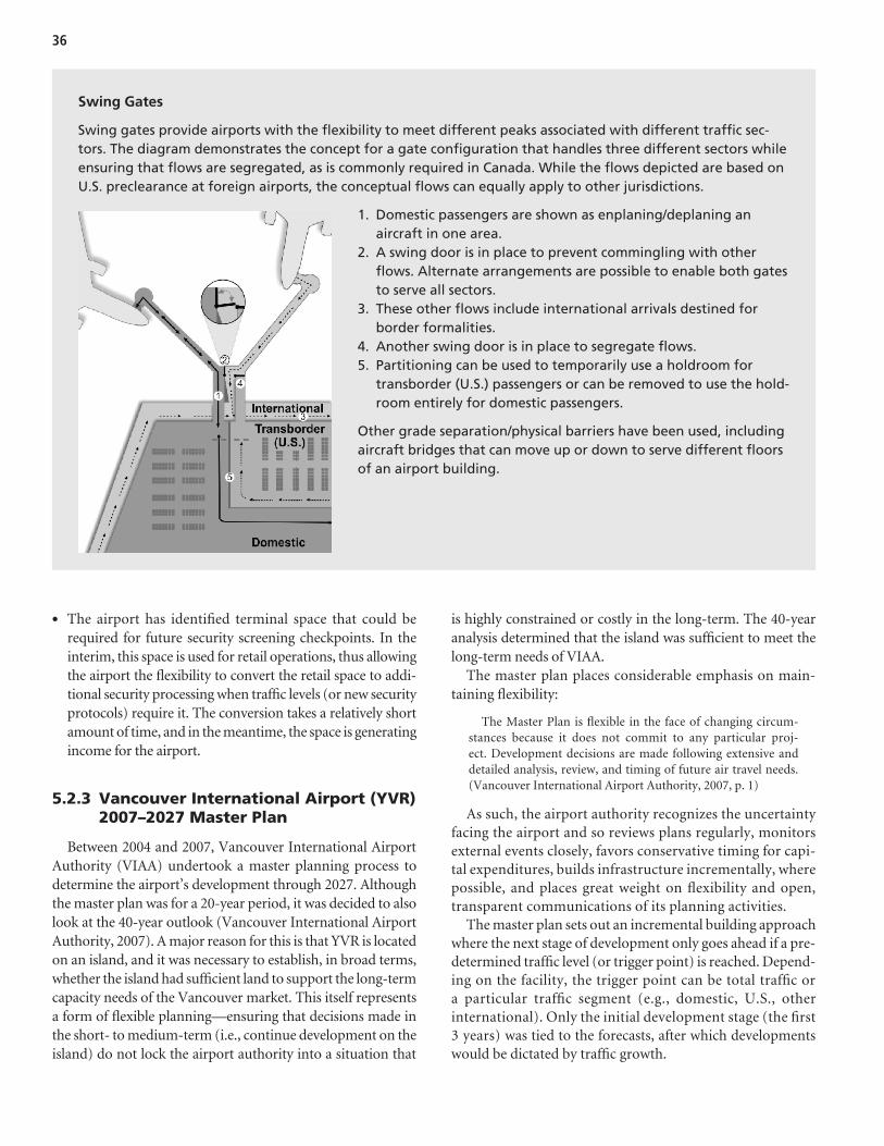
36

• The airport has identified terminal space that could be required for future security screening checkpoints. In the interim, this space is used for retail operations, thus allowing the airport the flexibility to convert the retail space to addi-tional security processing when traffic levels (or new security protocols) require it. The conversion takes a relatively short amount of time, and in the meantime, the space is generating income for the airport.

5.2.3 Vancouver International Airport (YVR) 2007–2027 Master Plan

Between 2004 and 2007, Vancouver International Airport Authority (VIAA) undertook a master planning process to determine the airport’s development through 2027. Although the master plan was for a 20-year period, it was decided to also look at the 40-year outlook (Vancouver International Airport Authority, 2007). A major reason for this is that YVR is located on an island, and it was necessary to establish, in broad terms, whether the island had sufficient land to support the long-term capacity needs of the Vancouver market. This itself represents a form of flexible planning—ensuring that decisions made in the short- to medium-term (i.e., continue development on the island) do not lock the airport authority into a situation that

is highly constrained or costly in the long-term. The 40-year analysis determined that the island was sufficient to meet the long-term needs of VIAA.

The master plan places considerable emphasis on main-taining flexibility:

The Master Plan is flexible in the face of changing circum-stances because it does not commit to any particular proj-ect. Development decisions are made following extensive and detailed analysis, review, and timing of future air travel needs. (Vancouver International Airport Authority, 2007, p. 1)

As such, the airport authority recognizes the uncertainty facing the airport and so reviews plans regularly, monitors external events closely, favors conservative timing for capi-tal expenditures, builds infrastructure incrementally, where possible, and places great weight on flexibility and open, transparent communications of its planning activities.

The master plan sets out an incremental building approach where the next stage of development only goes ahead if a pre-determined traffic level (or trigger point) is reached. Depend-ing on the facility, the trigger point can be total traffic or a particular traffic segment (e.g., domestic, U.S., other international). Only the initial development stage (the first 3 years) was tied to the forecasts, after which developments would be dictated by traffic growth.

Swing Gates

Swing gates provide airports with the flexibility to meet different peaks associated with different traffic sec-tors. The diagram demonstrates the concept for a gate configuration that handles three different sectors while ensuring that flows are segregated, as is commonly required in Canada. While the flows depicted are based on U.S. preclearance at foreign airports, the conceptual flows can equally apply to other jurisdictions.

1. Domestic passengers are shown as enplaning/deplaning an aircraft in one area.

2. A swing door is in place to prevent commingling with other flows. Alternate arrangements are possible to enable both gates to serve all sectors.

3. These other flows include international arrivals destined for border formalities.

4. Another swing door is in place to segregate flows.5. Partitioning can be used to temporarily use a holdroom for

transborder (U.S.) passengers or can be removed to use the hold-room entirely for domestic passengers.

Other grade separation/physical barriers have been used, including aircraft bridges that can move up or down to serve different floors of an airport building.

37

In order to ensure that the master plan could remain rele-vant over a wide range of future scenarios, and to obtain buy-in and feedback from stakeholders, the master plan involved extensive consultation processes with stakeholders, industry experts, and the community (discussions with Michael Matthews, director of the master plan).

5.2.4 Dallas/Fort Worth International Airport

DFW handled 56.9 million passengers in 2010. It is a hub for American Airlines and package delivery company United Parcel Service (UPS). The airport’s most current master plan—the 1997 Airport Development Plan (ADP) update—places considerable weight on an incremental and flexible planning process:

It [the ADP update] utilizes a holistic approach to airport development; providing flexibility to respond to ever changing market demands.

Key elements of this approach include ongoing research, regu-lar performance reviews, and close integration of planning, opera-tions, management, and new technology at DFW Airport. (Dallas/Fort Worth International Airport, 1997, p. 47)

The ADP update sets out a phased capital plan meant to ensure the “goal of incremental or phased development that is timely and logical” (Dallas/Fort Worth International Airport, 1997). In addition, the capital improvement plan incorporates the following three ideas: continuous planning, proactive man-agement, and focus on market-based action. All investments require input from stakeholders and must consider soon-to-be-needed capacity.

5.2.5 Mombasa Airport

Mombasa Airport (also known as Moi International Air-port) is the second largest airport in Kenya. De Neufville and Odoni (2003) describe the incorporation of flexibility into the airport master plan.

The original master plan for the redevelopment of the passenger terminals anticipated two buildings—one for domestic traffic and another for international traffic. Each building was to be large enough to meet anticipated traffic in either sector. However, the dynamic strategic plan rec-ognized that a major risk was that the proportion of inter-national traffic could shift radically (passengers may come directly from Europe), in which case one of the buildings would be crowded and the other one underutilized. Thus, the strategy was changed to build a single passenger termi-nal with a domestic area on one side, an international area on the other, and a mixed use area in the middle to serve either type of traffic.

This strategy reduced the overall size of the facility required to handle total traffic at the airport and allowed flexibility in handling different traffic mixes in the future.

5.2.6 Pease International Tradeport

Karlsson (2002) describes the application of real options planning at Pease International Tradeport near Portsmouth, New Hampshire. Pease International Tradeport is a public-use joint civil–military airport. As of 2010, it has no sched-uled passenger services, but in 2002 (at the time Karlsson’s paper was published), it had scheduled passenger volumes of up to 40,000 passengers per annum.

Traffic volume exhibited considerable volatility due to the entry and exit of carriers. Therefore, in the 2001 master plan, it was decided that any terminal development would be triggered by traffic reaching certain thresholds. (Specifi-cally, Phase I of the development was to be triggered by traf-fic reaching 80% of current capacity.) As the type of service was also uncertain, analysis was carried out to ensure that the terminal expansion could handle a wide range of plausible aircraft sizes. In addition, other aspects of flexible planning employed at Pease were:

• A domestic/international swing gate,• Temporary use of an unutilized aircraft parking apron as

an overflow car park, and• Non-load-bearing walls, allowing easy expansion or con-

version of the terminal (Karlsson, 2002).

5.3 Diversification and Hedging Strategies

Key Takeaways

Airports can also manage risk and uncertainty by diversifying their traffic and revenue base and employing hedging strategies against certain risks. Potential strategies include:

• Air service development programs to increase the range of carriers serving the airport and the scope of destinations served;

• Multi-use developments such as hotels, gen-eral aviation, logistics and cargo, retail, offices, industrial parks, and leisure facilities;

• Ancillary land use, such as government facili-ties, advertising, renewable energy, intermo-dal facilities, and military/civil joint use;

• Airport city or aerotropolis developments.

Any such diversification strategy must be backed up by a strong business case and be compliant with FAA regulations (e.g., FAA Grant Assurance 21: Compatible Land Use).

38

Addressing uncertainty and risk in the airport environment can go beyond the physical planning of the facilities to other aspects of airport strategy. Diversification involves broadening the airport’s traffic and revenue sources to avoid being heavily exposed to one particular type of risk and to reduce overall volatility. Hedging is taking a position to offset and balance against a particular or general risk. Airlines often use hedging strategies to reduce exposure to fuel price increases.

One means of diversification for airports is to increase the number of carriers and destinations served. Many of the events described in Chapter 3 were the result, in large part, of the airport being heavily dependent on a single carrier. To mitigate this, airports can undertake an air service develop-ment program designed to attract other carriers to operate at the airport. Of course, any such strategy has to be balanced in such a way as to avoid undermining incumbent carriers at the airport. Further guidance on air service development strategies can be found in ACRP Report 18: Passenger Air Service Development Techniques (Martin, 2009). Increasing the number of destinations served can also have diversifica-tion benefits since it reduces exposure to risk factors at each particular destination (e.g., economic downturn, high sea-sonality, one-off disruptive events). Air service development can also provide hedging options—for example, developing legacy and low-cost carrier traffic to protect against separate developments with the two types of traffic.

Revenue diversification involves an airport modifying and diversifying its products to reduce its dependence on aero-nautical revenues alone. Figure 9 shows typical aeronauti-cal and non-aeronautical revenue sources for airports. To minimize and mitigate risk, airports can focus more on the non-aeronautical revenue sources that are less dependent on traffic volumes.

ACRP Synthesis 19: Airport Revenue Diversification discusses multi-use developments at airports that provide alternative revenue streams (Kramer, 2010). Examples include:

• General aviation (GA) developments,• Air cargo and logistics centers,

• Hotels,• Convention centers,• Offices,• Intermodal centers,• Retail malls,• Industrial parks,• Golf courses, and• Sports arenas.

Similarly, ACRP Synthesis 19 also describes ancillary land use that airports can explore to diversify revenues (Kramer, 2010):

• Advertising and sponsorship. An airport can gener-ate non-aeronautical revenues through advertising—for example, advertising in terminals, naming rights on air-port terminals, advertising on unpaved airfields, or ban-ners on sky bridges.

• Government facilities. Government agencies are fre-quent airport tenants. These agencies also increase non-aeronautical revenues for an airport by leasing space directly from the airport.

• Renewable energy. Renewable energy is another potential non-aeronautical revenue stream that has many advantages for an airport. Not only does it lower the airport’s environ-mental impact (with positive public relations implications), it is also an alternative source of power to operate the airport with the possibility to sell excess power back to the utility company (or to other users).

• Intermodal facilities. Connecting rail, road, marine, and air in an intermodal facility at the airport is another poten-tial non-aeronautical revenue source. Examples include Kansas City Intermodal Business Center and Port Alberta in Edmonton.

• Military/civil joint use agreements. Joint use facilities (e.g., shared air traffic control, safety and rescue, and utili-ties) can have a positive impact on the infrastructure of an airport and lead to large cost savings. Examples include Colorado Springs Airport and Peterson Air Force Base (Kramer, 2010).

Source: Based on Kramer (2010)

Figure 9. Revenue sources for airports.

39

It should be noted that some of these opportunities for diversification may be constrained by the FAA Grant Assur-ances (e.g., FAA Grant Assurance 21: Compatible Land Use) and similar local revenue bond ordinances.

Arguably, the most comprehensive approach to revenue diversification is the airport city or aerotropolis concept developed by some larger airports, largely in Europe and Asia. Airport cities involve the development of multiple, and often complimentary, commercial and industrial activities on air-port land that may benefit from the transportation linkages that the airport offers. This can include logistics centers, free trade zones, manufacturing, offices, retail, hotels, and rec-reational facilities (e.g., golf courses, sports centers). These activities have a less direct linkage with traffic levels and can serve a wide range of customer/client types. The concept is illustrated in Figure 10.

While the revenue diversification strategies described have the potential to better manage and offset uncertainty in aviation activity, simply developing new non-aeronautical activities does not guarantee an overall reduction in risk. In fact, such a strategy can expose the airport to new risks and uncertainty since non-aviation activities have their own risk profiles. The airport needs to determine that there is a strong business case for any diversification strategy and that the risks are well understood.

5.4 Assessment of the Reviewed Approaches

Source: Dr. John Kasarda at Aerotropolis Schematic (2009).

Figure 10. Schematic of airport city and aerotropolis.

Key Takeaways

Flexible airport planning, real options, diversi-fication strategies, and similar approaches can offer considerable benefits to airport decision making in the face of uncertainty. However, there are issues around the application and effectiveness of these approaches. They may require decision makers to consider politically or institutionally unpopular outcomes (e.g., the loss of a major carrier) and will require the incorpo-ration of new processes and ways of thinking. It should also be recognized that there are limits to the success of these approaches—they can reduce risk, but not eliminate it.

The previous sections describe theoretical and practi-cal approaches to addressing traffic uncertainty in airport decision making. As noted, the generalized flexible plan- ning approaches described in Section 5.1.1 are untested. The

40

practical examples of flexible planning have been found to include fairly pragmatic ideas such as land banking, swing gates, and common-use facilities. Although there is little formal analysis of the benefits of these approaches, it can be argued that the success of these approaches is reflected in their increased use in airport planning. Swing gates, common-use terminal equipment (CUTE) and common-use self service (CUSS), trigger points, and movable walls have become more commonplace in airports around the world. It also appears that many of these approaches are applicable to a wide range of airports, from large hubs to small regional airports, since they have minimal resource requirements and some may even reduce costs (e.g., shared space and equipment can reduce overall facility size requirements). Nevertheless, there may be other aspects of flexible planning that may require more detailed or complex analysis.

Consideration also needs to be given to some of the poten-tial issues around a more flexible approach to airport planning and decision making:

• Flexible planning and risk evaluation appear to be particu-larly successful where they have taken a wider prominence in the airport organization (e.g., Toronto). Nevertheless, in some cases, it can be politically or institutionally uncom-fortable to dwell on worst-case scenarios, so they are not addressed in any significant way in planning (for example, the exit of an airline that is the airport’s largest customer).

• Building in flexibility will require additional analysis to cor-rectly assess the costs and benefits of certain options. This may involve the need to adopt new analytical approaches

and could impose more costs and time requirements on the planning process.

• Burghouwt (2007) comments that the choice for flexibility can sometime be a “wicked problem,” which is one that exists where there are competing interests between stake-holders (or within the same organization). For example, land banking may create tensions with the surround-ing community because the land is unavailable for other uses. Equally, it creates an uncertainty for the community since it is not known whether an airport or expansion will appear on the land.

• It should be recognized that these approaches, while offer-ing improvements on traditional airport planning, still have their limitations. They have the potential to reduce risk but not to eliminate it entirely. For example, trigger points allow an airport to more closely match development to exact traffic levels, but it is still possible for developments to be mistimed. For example, an airport could have com-pleted an expansion in 2007 based on the positive traffic and business environment of the time, only to see traffic drop dramatically in the 2008 recession, which could then be compounded by cutbacks by carriers or even carrier failures.

• On the other hand, it is also important that there not be an overreaction to changing market conditions and that airports have the tools to evaluate the permanence of any changes (i.e., are changing traffic trends a short-term fluc-tuation or part of a long-term trend change?). An airport scaling back its development plans in response to a drop in traffic (e.g., due to recession or terrorism event) may find that it has inadequate capacity when traffic growth returns.

A Framework and Methodology for Addressing Uncertainty about Future Airport Activity Levels in Airport Decision Making

P a r t I I

43

Part II provides guidance on the application of a systems analysis framework and a series of related methodologies for addressing uncertainty in airport decision making. The framework and related methodologies have been devel-oped from the material summarized in Part I and refined through application to a number of case studies (described in Part III). The systems analysis framework and the related methodologies are designed to assist airport decision mak-ers with:

• Identifying and characterizing risks (threats or opportuni-ties), including their plausibility and magnitude;

• Assessing the impact of these threats and opportunities (i.e., determining what can happen, to whom, and when); and

• Developing response strategies to avoid or lessen the impact of threats or to foster the realization of opportunities.

The systems analysis framework is designed to be general enough to accommodate a variety of airports and projects and to be scalable in order to match the methodology with the resources and needs of each airport. The framework allows planners to consider a broad range of events and risks and helps them anticipate possible changes that may follow. It is not intended to replace the master planning process or any other planning or decision-making model. Instead, the framework augments the master plan with methodologies that allow airport planners to analyze risk and uncertainty and incorporate relevant mitigation measures into the plan-ning process.

6.1 Overview of the Framework

As illustrated in Figure 11, the systems analysis framework is composed of five key steps:

1. Identify and quantify risk and uncertainty. Using a combination of data-based and judgment-based method-

ologies, identify and attempt to quantify risks and uncer-tainties facing the airport. The ultimate output from this step is a risk register (detailed in Section 7.4), which sum-marizes the risks and can feed information into other steps of the process.

2. Assess cumulative impacts. This step involves analysis and modeling to assess the impact of the identified risks occur-ring in various combinations and the implications for air-port traffic development.

3. Identify risk response strategies. Based on the output from Steps 1 and 2, identify risk response strategies that will help avoid or mitigate negative risks and exploit or enhance positive risks.

4. Evaluate risk response strategies. Undertake qualita-tive and quantitative evaluation of the risk response strategies identified in Step 3 to demonstrate value for money and effectiveness. This may result in revisions to the risk response strategies.

5. Risk tracking and evaluation. This final step is slightly different from the others because it represents an ongoing process of review and revision. It involves tracking risks and traffic over time and flagging potential issues, taking action prescribed in the risk response strategies if poten-tial risks do materialize, and making revisions to the risk register and risk response strategies.

Each of these steps is described in detail in Chapters 7 to 11.

6.2 Tailoring the Framework

The guidebook provides different tracks that the method-ology can follow, with each track having different data, analy-sis, and resource requirements and generating output with differing levels of detail and depth. The four tracks suggested are summarized in Table 2.

The selection of the track is at the discretion of the user, although it may be useful to base the selection on the size of

C h a p t e r 6

Introduction

Figure 11. Systems analysis methodology overview.

Table 2. Methodology tracks.

Step

Track A Track B Track C Track D

Mostly Qualitative Some Quantification Quantitative, with LimitedStakeholder Involvement

Quantitative, with Peer Review and Structured Elicitation

1. Identify and quantify risk and uncertainty

Development of the risk register based largely on the guidebook combined with qualitative analysis, visual aids, and informal elicitation within the airport.

Development of the risk register based largely on the guidebook combined with qualitative analysis, visual aids, and formal elicitation (e.g., Delphi) within the airport.

Development of the risk register based on quantitative analysis, where possible, combined with formal elicitation (e.g., Delphi) within the airport and with key stakeholders.

Development of the risk register based on quantitative analysis, where possible, combined with formal elicitation (e.g., Delphi and structured workshops) with airport management/planners, subject matter experts, and a wide range of stakeholder groups.

2. Assess cumulative impacts

Based on basic scenario analysis and qualitative approaches.

Based on basic scenario analysis and other simple modeling approaches.

Use of more advanced modeling procedures such as Monte Carlo simulation.

Use of more advanced modeling procedures such as structure and logic diagrams and Monte Carlo simulation.

3. Identify risk response strategies

Based largely on the information provided in the guidebook with informal elicitation within the airport.

Based on the guidebook and research on examples and best practice at other airports with informal elicitation within the airport.

Based on research of examples and best practice at other airports and informal elicitation within the airport and with key stakeholders.

Based on research of examples and best practice at other airports and formal elicitation within the airport and with stakeholders.

4. Evaluate risk response strategies

Largely qualitative and basic quantitative assessment.

Largely qualitative and basic quantitative assessment.

Quantitative analysis such as expected net present value.

Quantitative analysis such as expected net present value.

5. Risk tracking and evaluation

Tracking of traffic against forecasts and trigger points and annual review of risk register.

Tracking of traffic against forecasts and trigger points and annual review of risk register.

The risk register is updated continuously (possibly using a database system) whenever new pieces of information come in. Full periodic reviews of the risk register.

Major risks may be assigned to specific airport staff (risk managers) for tracking and updates. The risk register is updated continuously (possibly using a database system) whenever new pieces of information come in. Full periodic reviews of the risk register.

45

airport and size of planning project being contemplated, as illustrated in Figure 12.

Figure 12 is for guidance only—issues around the budget and time available for such analysis will also be important. It may be that a large airport only has time for a quali-tative (Track A) approach; this can still provide insight for the decision maker. Equally, a small airport may find value in pursuing a more quantitative approach (Track C or D).

Similarly, it is not necessary to stick to one track through-out the process. For example, an airport could undertake Track D (highly quantitative) for Steps 1 to 4 but select a more modest approach to the risk tracking and evaluation (Step 5) if it is unable to commit significant ongoing resources to this component.

Figure 12. Selection of the system analysis methodology track (A to D).

46

7.1 Categories of Airport Activity Risk and Uncertainty

Airport risks and uncertainty include both threats and oppor-tunities and can be grouped within the following categories:

• Macroeconomic: Events in the general economy that can have implications for air traf-fic, such as a national reces-sion, demographic changes (e.g., aging population), or more localized events such as the loss of a major employer.

• Market: Events affecting the supply of, and/or demand for, aviation services in the airport catchment area. For example, entry of a new car-rier, loss of an incumbent carrier, airline mergers, and emergence of a new airport in the region.

• Regulatory/policy: Changes in regulations and rules governing the activities of airlines and/or airports. This can also include new environmental regulations on noise or emissions or the introduction of cap-and-trade policies.

• Technology: Innovations that may influence the supply of and demand for airport services, such as new aircraft mod-els that reduce the cost of air travel and open up opportu-nities for new routes.

• Social/cultural: Changes in the attitude of society and business toward the use and value of air travel (e.g., use of Internet technologies to conduct meetings rather than face-to-face meetings requiring air travel).

• Shock events: Unpredictable, infrequent events with poten-tially significant impacts (wars, terrorist attacks, geopolitical instability, etc.).

• Statistical or model: Forecasts of airport activity are based on analytical models. Such models can be mis-specified (i.e., they do not correctly represent the underlying relationships) or are subject to estimation error. Also, the historical rela-tionships captured in the model may not continue into the future due to structural changes in the market.

These categories are related to risk and uncertainty associ-ated with air traffic activity. However, airports face other risks outside of this: obtaining funding (e.g., cuts to state or city budgets), opposition from local communities, and changes to local land use regulations. These risks are not covered in this guidebook, although it is feasible that these risks can also be addressed by the systems analysis methodology.

Airport activity uncertainty may further be characterized in terms of the geographic scale and/or reach of their expected impacts, including:

• Airport-specific impacts: A single airport would be affected by the event;

• Local or regional impacts: A group of airports located in relatively close proximity would be affected (e.g., all five London airports);

• State or national impacts: All airports within a state or country would be affected; or

• Global impacts.

Table 3 provides common examples of these categories of risk and uncertainty. The list is not exhaustive but may pro-vide a starting point for Step 1.

7.2 Approach and Tools for Identifying and Quantifying Risk and Uncertainty

In order to identify and quantify the risks and uncertainty facing an airport, the following questions need to be answered for each possible risk factor:

C h a p t e r 7

Step 1: Identify and Quantify Risk and Uncertainty

47

Table 3. Categories of airport activity risks and uncertainties, with examples.

Increased security requirements for air cargo could result in some cargo shipments being transported by other modes.

New/revisions of airport taxes and passenger duties

National Ecological departure tax in Germany in 2011.

Nighttime restrictions or bans Local Restrictions on night operations can harm an airport’s ability to attract and sustain air services. This is particularly the case for air cargo since shippers require 24-hour operations.

Aviation cap and trade or new carbon taxes

Global/national Entry of aviation into the EU Emission Trading Scheme (ETS) in 2012.

Category Risk/Uncertainty Scale of Impact Comments and Examples

Macro- economic

Economic shifts/general business cycle

Global/national Global recession in 2008/09; U.S. recession in 2001.

Fuel price volatility Global Fuel price peak in 2008; Gulf War 1991.

International monetary crisis altering trade and exchange rates

Global Asia 1997.

Closure of a major local business State/local

Market

Exit/collapse of a major carrier Local TWA at St Louis in 2001; DHL shutting down domestic shipping operations at Wilmington International Airport in 2008.

Entry of a new carrier stimulating traffic

Local Southwest Airlines at multiple airports; Allegiant Air at Bellingham.

Airlines merger Global/national Continental Airlines merging with United Airlines to form the world's largest carrier.

Increased competition from surrounding airports for air passengers

Regional/local Oakland vs. San Francisco airport. Often associated with an LCC starting operations at a nearby airport.

Competition from airports for air cargo

Regional/local Shippers have considerable flexibility to change cargo routings and will do so for relatively small cost or efficiency improvements.

Increased GA or military activity Local May affect commercial operations.

Connecting traffic operations at an airport can be transferred to other airports or simply downsized by the carrier.

Local Examples of airport losing significant connecting traffic: Baltimore, Pittsburgh, St. Louis.

Changes in aircraft size Local Carrier decides to switch from mainline to regional services (e.g., American Airlines at St. Louis in 2003).

Modal competition Regional/local Development of high-speed rail on certain corridors; competition from truck, rail, and marine for certain types of cargo movements.

Changes in seating capacity, aircraft utilization, and load factor

Global

Regulatory/Policy

Liberalization of certain air markets

Global/national EU–U.S. Open Skies Agreement.

Privatization of airlines National British Airways privatized in 1987.

New security requirements Local Various new requirements since 9/11.

(continued on next page)

48

• What is the particular risk/uncertainty?• What is the probability or likelihood of that risk/uncertainty

occurring?• What will be the impact of the risk/uncertainty factor if it

were to occur, both in the short- and long-term?

This information will be obtained from brainstorming and elicitation techniques, as well as analysis of historical data and other quantitative methods. A number of iterations of the process may be required in order to obtain all of the relevant information. The steps are as follows:

1. The team leading the risk project develops an initial list of risks and uncertainties. The initial list can be developed using information within this guidebook, as well as from analysis of historical events and the current business and economic environment.

2. Formal and informal elicitation exercises are undertaken with airport management and other stakeholders, using the initial list of risks and uncertainties to develop more infor-mation, including basic estimates of probability and impact.

3. The probability and impact information is refined using quantitative analysis and other evidence (e.g., review of

similar events or information from literature reviews) to produce a draft risk register (explained in more detail in Section 7.4).

4. Additional elicitation exercises to review, confirm, or revise the risk register.

5. Finalization of the risk register.

7.2.1 Analysis of Historical Data

In some cases, historical data can be used to determine the likelihood and probable impact of recurring events. In this context, recurring events refer to those events that have occurred at least once in the past and may occur again. They may be recurring within the aviation industry but not neces-sarily at a specific airport.

This approach, however, has some limitations. First—and this is a critique applicable to most forecasting techniques used in airport planning—the past is not necessarily a good indicator of what will happen in the future. Second, isolating the impact of a specific event on a measure of airport activity may not be straightforward due to data limitations (data may be limited in quantity, quality, or both) or inadequate statis-tical skills. Third, historical data is only marginally relevant to

Technology

New aircraft design reducing operating costs

Global The Boeing 747 significantly reduced the cost of long-haul air travel.

Reductions in belly space Global The amount of belly space on some aircraft designs is limited, reducing the scope for the carriage of cargo.

Social/Cultural

Using of internet technology Global Firms and individuals may be willing to replace face-to-face meetings with Internet-based approaches (e.g., WebEx video conferencing).

Changing attitudes to climate change

Global Concerns regarding greenhouse gas emissions from air transport may lead to curtailing of air travel. For example, some companies now publish their carbon footprint; public pressure to reduce their footprint may result in less air travel by employees.

ShockEvents

War Regional/national First Gulf War.

Pandemic Global/regional Swine flu; SARS.

Terrorist attack, hijackings, and geopolitical instability

Global/national 9/11, London liquid explosives 2006, Northwest flight Amsterdam–Detroit 2009.

Natural disaster Regional/local Hurricane Katrina 2005; Indian Ocean tsunami 2004; Icelandic volcanic ash 2010.

Statistical/Model

Mis-specification or errors Local The model does not correctly represent the underlying relationships.

Structural changes Local Future changes in the underlying relationships (e.g., the relationship between economic growth and traffic growth).

Category Risk/Uncertainty Scale of Impact Comments and Examples

Table 3. (Continued).

49

assess the likelihood of rare events or to quantify threats and opportunities whose frequency and/or impacts vary with no apparent pattern over time.

Planners choosing to evaluate the probable impact of future events based on historical data can:

• Use evidence and priors published in the literature.• Use an existing airport activity forecasting model, cali-

brated specifically for the airport being reviewed, and con-duct sensitivity analysis and/or scenario testing.

• Perform statistical analysis of airport activity data, whereby the impact of a past event—or a series of past events—is estimated while accounting for the influence of other fac-tors (i.e., holding everything else constant).

An example of this approach is the quantification of the impact that terrorist attacks would have on air traffic in the United States using historical data from the 9/11 attack. The result of that historical event was an immediate reduction in passenger travel in the U.S. domestic and international mar-kets. Total passenger enplanements in the United States during the month of September 2001 decreased by 45.3% compared to the previous month. Additionally, historical data indicates that it took the industry 33 months (until June 2004) to return to the same level of activity as before the attacks (Bureau of Transportation Statistics, 2011). These numbers may be used as a basis for quantifying the probable impacts of similar events (i.e., major terrorist attack) although they would have to be adjusted—using judgment—to reflect changes in the market since the 9/11 attack.

Since historical responses to specific events occurred under specific conditions that may not apply today, quantifying risk impacts using historical evidence may lead to misleading con-clusions. As an alternative, a range of probable impacts may be

estimated for each event drawing on relevant historical data. In this approach, data on recorded occurrences similar to the one under examination can be analyzed throughout history, focus-ing on the type of impacts that each event had on relevant out-puts, their frequency of occurrence, and any other data that can help differentiate this event from others. Based on this analysis (which can be as statistically sophisticated as the data allows), a range of possible impacts may be created for each event.

7.2.2 Elicitation Techniques

Eliciting information from airport management and other stakeholders will be a key element of the risk and uncertainty identification and quantification process. Depending on the track selected (or the resources available), this information may simply be obtained from within the airport organization (e.g., Track A or B). However, the elicitation can be extended to include external subject matter experts (from academia or consulting), colleagues from other airports, airlines and other customers, government officials, and representatives of other stakeholders (e.g., air navigation, community, and business groups), as may be the case with Track C and D. Drawing from a wider group can lead to the identification of a greater number of risks but will also create challenges in terms of managing the process and achieving a degree of consensus. One solution is to conduct specialty workshops focusing on specific risk catego-ries. For example, a separate session on technology risks may be facilitated to identify risks in that category.

These discussions can be held in the context of formal workshops and involve a variety of elicitation and group aggregation techniques. Table 4 provides an overview of the methods available to airport planners to elicit probability and/or measures of impact and to summarize (or aggregate) elicited opinions.

Technique Description Pros Cons

Delphi Refinement of experts’ opinions by providing feedback through a series of surveys, without open interactions.

Consensus may be reached relatively quickly.

No direct interactions between experts.

Statistical groups

One-time survey of experts’ opinions, without interactions.

Experts cannot influence each other.

Consensus may not be reached.

Nominal groups

Refinement of experts’ opinions by a series of survey-based sessions, with interactions.

Consensus may be reached relatively quickly.

Discussions may be time-consuming; some experts may be influenced by others.

Unstructured interacting groups

One-time survey of experts’ opinions, with interactions, possibly in a workshop setting.

Consensus may be reached through discussions.

Discussions may be time-consuming; some experts may be influenced by others.

Table 4. Overview of elicitation and group aggregation techniques.

50

Subjective assessments of preferences, probabilities, or impacts are typically best obtained via choices (e.g., “choose A or B?”) rather than open-ended opinions (e.g., “I like A”). To assist the participants in determining risk probabilities and impacts, visual aids should be used such as the qualitative risk assessment matrix (heat diagram) shown in Figure 13. The participant selects the cell that represents the likelihood/impact combination for a particular risk/uncertainty factor. (This can

be done individually or as a group exercise.) Risks marked in the red (or sometimes yellow) areas are defined as “hot” [i.e., they have the potential for significant harm (or benefit)].

Another approach (which can be combined with the heat diagram) is to ask the participants to provide a probability for an event. In doing so, there should be clarity about what that probability represents. Is it the probability that the event will occur at some point in the next 20 years, or is it the prob-ability that the event will occur in any given year? The differ-ence between the two is quite large—the first is equivalent to rolling a die once while the latter is equivalent to rolling a die 20 times. Furthermore, in some cases the probability may vary over time. For example, the probability of new aircraft technology being developed may be very low over the next 5 years, but higher further into the future (10+ years).

Thought also needs to be given to what is being affected. Some risks will affect total passenger volumes, while others will affect only specific sectors (e.g., international, connect-ing). In addition, some risks may affect only air cargo, peak hour operations, general aviation, or aircraft movements but not passengers (e.g., fleet changes).

Having obtained input on a range of risk factors, the infor-mation gathered can be represented in a simplified form, as illustrated in Figure 14. The summary plot diagram can effec-

Like

lihoo

d

VeryHigh

High

Moderate

Low ´

VeryLow

VeryLow Low Moderate High Very

High

Impact on Activity

Figure 13. Illustrative example of qualitative risk assessment matrix (heat diagram).

Economic recession

Fuel price spikes

New FAA taxes

Terroristattack

Loss/failure of Carrier X

Entry of new carrier(e.g., LCC)

Pandemic

Open Skies Liberalization

High Speed Rail Competition

Major tourism event

Increased security requirements

New aircraft technology

Economic boom

5%

10%

15%

20%

25%

30%

35%

-5 -4 -3 -2 -1 0 1 2 3 4 5

Prob

abilt

y

Impact Opportunity >< Threat

Macroeconomic

Market

Regulatory/Policy

Technology

Social/Cultural

Key:

Shock Event

Use of Internet for meetings

Figure 14. Illustrative example of a summary plot of identified risks and uncertainties.

51

tively provide feedback to the participants and help identify critical uncertainties (those with high probabilities and/or high impacts).

7.3 Advanced Approaches to Quantifying Probabilities and Impacts

Section 7.2 discussed the probability and impacts of risks and uncertainties as fairly straightforward point values or ranges. This may be sufficient for Track A or B analysis or where time and resources are limited. However, enhance-ments can be made to the analysis, which are discussed in the following.

7.3.1 Direct and Indirect Impacts

An important consideration in the quantification of impacts is the distinction between direct and indirect impacts. In a direct impact, the occurrence of an event directly affects the activity of the airport being analyzed. Examples of events that create direct impacts are the destruction of airport infrastruc-ture by a hurricane or the de-hubbing/downsizing of an air-line at a specific airport, which directly affects the number of passengers that use that particular facility. On the other hand, an indirect impact is when the occurrence of an event indi-rectly affects the activity at the airport (usually through a well-established transmission mechanism). Examples of indirect impacts include a global economic recession or an increase in jet fuel prices. A recession will reduce employment, consumer confidence, and disposable income, ultimately weakening the demand for air travel. Likewise, increases in jet fuel costs can feed through into higher ticket prices, which dampen demand (or result in air service cutbacks by carriers). It may be neces-sary to undertake additional analysis to understand the impact of certain variables on traffic levels. For example, ACRP Report 48: Impact of Jet Fuel Price Uncertainty on Airport Plan-ning and Development contains parameters on the sensitivity of traffic levels to changes in fuel prices, which can be used to estimate the impact of fuel price increases or decreases (Spitz and Berardino, 2011).

7.3.2 Probability Distributions

Rather than expressing the impact of an event (if it occurs) as a single figure such as the percentage or absolute change in traffic, the impact can be characterized by a probability distribution. This distribution represents a range of possible values, along with an estimate of how likely these different outcomes may be. This can be done to address uncertainty about the outcome or to reflect the range of outcomes that have occurred in the past.

Determination of the distributions can involve elicitation methods, analysis of historical data, or a combination of the two. A large number of distributions are available to char-acterize potential outcomes. However, for elicitation and review purposes, it is common to consider only a small set of representative distributions, as illustrated in Figure 15. Selection of an appropriate distribution, however, should always be guided by the characteristics of the event being considered.

It is recommended that probability distributions be defined with a limited number of data points (e.g., most likely value, 10th percentile, 90th percentile) rather than technical parameters such as the mean or variance. In the context of nominal or interacting groups, the extremes of a probability distribution (e.g., the minimum and maximum impact values) should be elicited first to avoid anchoring on a single, most likely value.

In some cases it may be possible to estimate distributions from historical data. For example, data could be collected on quarterly or annual GDP growth rates and a distribution fit-ted that approximates the distribution of data. Distribution fitting can be done with many statistical packages or with spe-cific risk analysis software. (The latter software is described in Section 8.2.2.)

An example of distribution fitting is shown in Figure 16. The histogram bars are the observed historical distribution of GDP growth rates, and the black line is the statistical distri-bution fitted to the histogram.

7.3.3 Duration of the Event

Different events will have different durations. Some may be short lived, such as a pandemic or hurricane that may be expected to cause traffic to decline for, possibly, 6 months before it recovers to pre-event levels. Other events may be more long lived, such as the 9/11 attacks from which traffic took several years to recover. And there may be some events that result in a structural change in traffic from which there is no full recovery (e.g., the loss of a major carrier).

Event duration can also be specified as a probability distri-bution, in the same way as the event impact.

7.3.4 Correlations and Dependencies

All risks and uncertainties are not necessary independent of each other. The occurrence of one event may increase or decrease the probability of another event occurring. For example, high fuel prices can increase the likelihood of an economic recession, or the entry of an aggressive LCC can increase the likelihood of an incumbent carrier exiting. Fur-thermore, there can also be dependencies over time, such

52

Density Function Description

Uniform: a distribution where all values within a range of potential outcomes have the same probability. For example, a uniform distribution should be used to characterize the impacts of a threat that may lead to a 10% reduction in airport activity, a 20% reduction, or any value in between, with the same probability. The uniform distribution is fully specified with a minimum value and a maximum value.

Discrete: a distribution where each potential outcome is represented by a single value and a corresponding probability. A discrete distribution is defined by a list of possible discrete values and corresponding probabilities, where the sum of all probabilities is equal to 1.

Normal: a distribution that is often used as a first approximation to describe random variables that tend to cluster symmetrically around a single mean. The normal (or Gaussian) distribution uses the mean (location of the peak) and the variance (the measure of the width of the distribution) as input parameters and can be used to represent risks made up of the sum of a large number of random variables.

Generalized triangular: a distribution that uses the median, lower percentile (such as 10%), and upper percentile (such as 90%) as input parameters. Based on these parameters, a triangular distribution is fitted to the data, and the absolute minimum and maximum are calculated as a function of the distribution. This distribution is often used for event risks, where there is equal probability of an input parameter being lower or higher than the median.

PERT (program evaluation and review technique ): a special form of the beta distribution. The beta distribution allows for a skew to the data, either upward or downward, and therefore can be used to represent risks where, for example, the upper extreme is further from the median than the lower extreme. The PERT distribution uses the median, minimum (or lower percentile, such as 10%), and maximum (or upper percentile, such as 90%) as input parameters.

Derived from material by Palisade Corporation, @RISK for MS Excel.

Figure 15. Examples of probability distributions used in the quantification of uncertainty.

53

that the probability of an event depends on whether it has occurred before. More formally, this can be expressed as:

• Dependencies across risks: The occurrence of Event k may increase or decrease the probability of Event j occurring.

• Dependencies over time: The occurrence of Event k in Year t may increase or reduce the probability of Event k occurring in Year t + s, where s is the interval considered in the assessment of probabilities.

Such dependencies can be captured by specifying corre-lation coefficients between variations. However, in practice this can be difficult to communicate in the elicitation process and can greatly increase the complexity of the analysis.

7.4 Developing a Risk Register

It is recommended that the information from the identifica-tion and quantification of risks and uncertainties be captured in a risk register. This register forms the basis for much of the work in the subsequent steps and the ongoing tracking of risks.

The risk register may include several fields, grouped within two broad categories, as follows:

Risk Identification

• Risk ID code;• Risk name and brief description;• Risk status: active, dormant, or retired;• Risk category; and• Date the risk was first identified.

Risk Evaluation

• Probability of occurrence;• Description of the impact;• Metric or metrics being affected (e.g., number of aircraft

operations, passengers);• Magnitude of impact, defined as a single value or a prob-

ability distribution;• Duration of impacts; and• Recovery—expected extent of recovery.

Which fields are included is at the discretion of the user, and additional fields can be added to provide supplemen-tary information. An example of a risk register is provided in Table 5.

0

10

20

30

40

50

60

70

-1.5% -0.5% 0.5% 1.5% 2.5% 3.5% 4.5% 5.5% 6.5% 7.0%

Fre

qu

ency

GDP Growth Rate (Mid-Point)

Histogram of GDP Growth Data

Fitted Distribution

Figure 16. Example of distribution fitting (using illustrative data).

Risk Identification Risk Evaluation

RiskID

RiskCategory Status Threat or

Opportunity Probability/ Likelihood Description of Impact Impact On

Magnitude of Impacts (on Traffic)

Low Medium High ExpectedDuration

ExpectedRecovery

E1 Macro-economic

Rapid increase in fuel prices

10% Rising fuel prices result in increased operating costs, which may either be passed onto consumers in higher fares, (lowering demand) or result in carriers cutting back services (or a combination of the two).

Aircraft ops, passengers

Generallyshort-term

Full

E2 Macro-economic

Economicslowdown/recession

10% Economic recession leads to declining passenger volumes and service reductions by airlines.

Aircraft ops, passengers

Short to medium-term

Full

R1 Regulatory/policy

New security measures for cargo

20% Increased security measures for cargo reduces bellyhold cargo activity.

Cargovolumes

Long-term Partial

M1 Market Loss or failure of major carrier

30% The exit of Airline X due to economic conditions or other factors.

Aircraft ops, passengers

Long-term Limited

S1 Shockevent

Swine flu pandemic

5% Swine flu outbreak centered in the local area resulting in passengers avoiding the airport.

Aircraft ops, passengers

Short-term Full

… … … … … … … … … … …

… … … … … … … … … … …

Table 5. Example risk register. (All estimates are for illustrative purposes only.)

55

It may also be beneficial to add fields to incorporate infor-mation on the risk response strategies in Step 3 and the risk tracking and evaluation in Step 5. To facilitate this, the risk register can be developed as a spreadsheet or database system, which would offer ease of updating and tracking. An example of such a database is provided in Figure 17. This software

Source: HDR Inc., Risk Management System for the SR 520 Bridge Replacement and HOV Program, on behalf of Washington State Department of Transportation (2011).

Figure 17. Screen shot from an example of a risk management and tracking database.

encompasses all aspects of the risk management process, including heat diagrams and the risk register, into an easy-to-use database that can be controlled by the management team. Clearly, this requires a greater investment of time and resources but may be suitable for Track C or D applications of the methodology.

56

Step 2 involves integrating the risks identified in Step 1 into a structural model of uncertainty. The purpose of this model is to evaluate the com-bined effect of multiple risks on airport activity and help define and assess alternative courses of action (response strategies).

The first undertaking con-sists of developing an analysis of the risks identified in the previous step, paying atten-tion to the way the relation-ships between events, variables, and outcomes will be modeled, as well as to the transmission mechanisms between them. The goal is to create a model that captures—with as much preci-sion as possible—the impacts uncertain events will have on relevant indicators of airport activity.

Once a model for quantifying the impacts of uncertainty is in place, the next activity consists of quantifying cumulative impacts of uncertain events on airport activity. To do this, it is necessary to define the different risk scenarios that will be analyzed as well as the characteristics of each one. Tools such as scenario analysis and Monte Carlo simulation are com-monly used at this stage.

Finally, an effective assessment of cumulative risk impacts requires that the outcome of this process be expressed in terms that allow airport planners an easy identification of risk response strategies.

8.1 Developing a Model

The term “model” is interpreted fairly broadly in this guidebook—it can range from a simple trend model based on assumed growth rates to a complex multivariate model of

the airport. It is anticipated that most airports will fall into one of two camps:

1. Airport planners have access to a calibrated activity forecast-ing model (e.g., multivariate regression model of demand, simulation model), which can be used for uncertainty analy-sis and scenario testing.

2. Airport planners do not have a forecasting model, instead relying on outside forecasts (e.g., the FAA TAFs).

In the first case, the existing model can be used as the basis for the assessment of cumulative impacts. For example, the model may contain parameters related to economic activity, which can be used to assess the impact of macroeconomic risk factors. The model has the benefit that it already con-tains information on the transmission mechanisms by which chance events and other sources of uncertainty affect relevant variables and outcomes. Nevertheless, modifications may be necessary to allow for risk factors not addressed in the model. For example, the model may not contain any parameters specifically related to shock events (pandemics, terrorism attacks, etc.).

In the case where there is no access to a forecasting model but the airport does have an outside forecast, the cumula-tive impacts can still be assessed by considering the likely deviation from the forecast. For example, the loss of a car-rier may cause traffic to drop below the forecast level, and then some or all of the lost traffic may gradually be recov-ered (as other carriers enter the market). This is illustrated in Figure 18.

Whether the airport has access to a forecasting model or not, there are various tools and techniques available to enhance existing models or develop new models to better assess the cumulative impact of uncertainty. These techniques can be used to map out how the uncertainty events may occur, their implications for activity levels, and the interactions between events. These techniques are:

C h a p t e r 8

Step 2: Assess Cumulative Impacts

57

• Structure and logic diagrams,• Decision trees,• Influence diagrams,• Program flowcharts,• Stock and flow diagrams (system dynamics), and• Reference class forecasting.

All six of these techniques are described in Appendix F. However, the two most relevant and accessible techniques—structure and logic diagrams and reference class forecasting—are described in the following. (Decision trees are also discussed in Step 4 as a tool to evaluate risk response strategies.)

8.1.1 Structure and Logic Diagrams

A structure and logic (S&L) diagram is a graphical rep-resentation of a model where each box is a variable (input, intermediate output, output), and links between boxes are operations (add, multiply, divide, etc.). S&L diagrams reflect cause-and-effect relationships among economic, finan-cial, demographic, policy, and political factors. Figure 19 is an example of an S&L diagram for estimating aircraft movements.

8.1.2 Reference Class Forecasting

Section 4.2.1 introduced the concept of reference class forecasting. The basic idea is that a forecast is evaluated or

even developed by referencing against actual outcomes from similar airports. It is recommended that this approach be incorporated into the forecasting and uncertainty analysis process where practical. This can be done in a fairly unstruc-tured way by comparing forecasts and cumulative event impacts against similar airports or events in the past. For example, in the latter case, the impact of a carrier exiting can be compared against previous examples. Undoubtedly, there will be differences in the circumstances of the airports and various factors that may result in different outcomes to pre-vious events, but this approach can still provide useful guid-ance regarding future traffic development.

8.2 Analyzing the Cumulative Impact of Risks

Two general approaches are recommended for this analysis:

• Scenario analysis, and• Monte Carlo simulations.

The scenario analysis presented here is a less techni-cally demanding approach that is suitable for Tracks A and B, while Monte Carlo is more technically demanding but provides a richer output and may be suitable for Tracks C and D. Again, the approach selected is at the discretion of the user.

Time

En

pla

ned

Pas

sen

ger

s

Original Forecast

Traffic impact of carrier exitand partial recovery

Figure 18. Analyzing the impact of air carrier exit on forecast traffic.

58

Source: Hickling Corporation (1990, p. 51).

Figure 19. Structure and logic diagram for estimating aircraft movements.

59

8.2.1 Scenario Analysis

Scenario analysis is a process of analyzing the impact of possible future events by considering alternative outcomes. In this case, the scenarios examine the impact of the occur-rence of a series of uncertain events that have a defined impact on relevant variables and result in a specific outcome. A num-ber of separate scenarios may be developed and played out to assess the impact of different sets of events occurring together. Since scenario analysis consists of skipping forward to the outcome of a series of events, it is important to keep in mind that the outcomes are, strictly speaking, expected outcomes with an implicit probability of occurrence.

Selection of the events to be considered in the scenarios can be based on the heat diagrams and summary plots described in Step 1. The events considered in combination will be those flagged in Step 1 as having high probabilities and/or high impacts and acting in the same direction (i.e., to either increase or lower traffic). For example, based on the risk register infor-mation, a scenario may be developed that considers a combi-nation of the occurrence of the following upside events:

• Entry of a highly stimulative LCC;• New aircraft technology, which lowers operating costs,

leads to trans-Atlantic service; and• A new manufacturing plant opens locally, generating a

specified number of passenger trips per year and a certain tonnage of air cargo.

Each event can be further specified based on reasonable assumptions and analysis. For example, the traffic impact of the LCC can be estimated assuming a given frequency, air-craft size, and load factor, and then further refined to allow for the new service diverting traffic from existing services (e.g., only two-thirds of the traffic carried by the LCC is incremental). Overlapping impacts of the event can also be addressed. For example, some of the traffic generated by the new manufacturing plant will be carried on the LCC entrant, and so the overall gain has to be netted out. Further, the sce-nario can be specified in terms of developments over time (e.g., the entrance of the LCC is assumed to occur in the first 5 years of the forecast period, while the new aircraft technol-ogy is assumed to not occur for another 10 years).

The traffic outcomes (whether in terms of passengers, cargo, operations, or even peak hour passengers) can be generated using the airport’s existing forecasting model or considering deviations from an existing forecast, as described in Section 8.1. Multiple scenarios can be devel-oped to address upside and downside risks and impacts to specific traffic segments.

Clearly, this approach has a lot in common with the high/low forecasts described in Chapter 2, which are commonly

applied to air traffic forecasts. However, there are some cru-cial differences or enhancements:

• The scenarios are developed from a comprehensive risk register and thus provide a more considered means of eval-uating a wide range of significant risk factors.

• The scenarios (or at least some of them) are designed to produce extreme results in order to demonstrate the wide scope of potential outcomes and to test the robustness of the airport system and its plans.

• The scenarios are a critical input into the planning process rather than an often-ignored adjunct to the forecasts.

The scenario approach provides an accessible means of evaluating the overall risk profile facing an airport, although it has some shortcomings. Most notably, it provides little information on probabilities (the information generated relates largely to outcomes) and has limited ability to address interactions between events and developments over time.

An example of the scenario approach is described in the Bellingham International Airport case study in Part III.

8.2.2 Monte Carlo Simulation

Monte Carlo simulation was described in Section 4.2.2. In essence, Monte Carlo simulation involves running the fore-cast model multiple times (generally thousands of times), each time with the inputs (and in many cases, the parame-ters) being randomly generated based on the probability dis-tribution assumed for each input (or parameter). Under this approach, each forecast produced is associated with a prob-ability of occurrence based on the individual probabilities of occurrence associated with the variables within the model. The probabilities associated with each outcome allow more quantitative analysis to be undertaken, providing airport planners with a richer set of information.

As in the case of scenario analysis, a successful probabilis-tic risk assessment requires a robust structural model and a detailed characterization of risks. The difference, however, lies in the fact that under this approach, every possible com-bination of risks can be modeled and quantified, putting a higher burden on the assumptions made about the interac-tions between variables and their estimated magnitudes.

Figure 20 illustrates a simple example of the use of the Monte Carlo simulation approach to analyze the impact of risk and uncertainty on future traffic operations at an airport. The total number of aircraft operations at an airport—identified by F—is modeled as a function of airport taxes, average load factor, and average aircraft capacity. However, it is also assumed that these three variables, along with the price elasticity of demand for air travelers (i.e., the elasticity of demand for that specific airport by passengers with respect to airport taxes),

60

have uncertain behavior with well-defined probability den-sity functions. Through the use of Monte Carlo simulations, several point estimates for the total number of aircraft oper-ations are calculated based on individual draws from each probability distribution function associated with each. At the end of the simulation, all point estimates for aircraft opera-tions obtained through this process can be used to construct a probability distribution function for this output.

As Figure 20 illustrates, Monte Carlo simulation can handle both direct and indirect impacts (discussed in Sec-tion 7.3.1), both of which can be modeled with considerable complexity. An example of a direct impact is a major carrier exiting an airport. A number of characteristics of this particu-lar event can be modeled and randomized:

• Probability of exit: Specified as a probability of exit in any given year (e.g., 5% probability). With the probability expressed in this way, not only is the occurrence of the event randomized (i.e., whether it occurs), but also the timing of the event. In some iterations the event will occur in the first year of the forecast, in other iterations it will occur at the end of the forecast period, and so forth.

• Impact of event: This can be specified as a percentage or absolute decline in traffic immediately after exit of the car-

rier. The size of the decline can be specified as a probabil-ity distribution [e.g., triangular distribution with a median value of 25% (loss of traffic), a 10% percentile of 20%, and a 90% percentile of 35% (see Section 7.3.2 for information on probability distributions)]. The values are based on the carrier’s share of traffic, with a range used to reflect uncer-tainty about the carrier’s future size. A more advanced approach would be to include a risk factor reflecting the carrier’s growth at the airport and link the carrier exit vari-able to the growth variable.

• Extent of recovery: The proportion of lost traffic that returns due to capacity in-fill by other carriers. This can be a fixed number or probability distribution (e.g., a uniform distribution with range of 50% to 100% recovery of traf-fic). This range could reflect the level of recovery found in previous examples of carrier exit.

• Time to recover: The time taken to reach the full extent of recovery. Again this variable can be specified as a prob-ability distribution (e.g., a uniform distribution ranging between 2 and 4 years).

Indirect impacts involve variables not directly related to traffic. In Figure 20, the impact of airport taxes is modeled as an indirect impact: the tax increase (which is randomized)

Figure 20. An illustration of the use of Monte Carlo simulation techniques to account for multiple sources of uncertainty.

61

output distribution). After all, the model output itself indi-cates a very low probability of such an outcome. However, many of the unexpected events that have occurred at airports described in Chapter 3 would likely have been assessed as low probability before the event occurred. In fact, the case study of Baltimore/Washington International Thurgood Marshall Airport in Part III placed a probability of only 0.5% on the event that did occur (loss of international traffic).

Obviously, basing the airport planning entirely on such extreme outcomes is not desirable. However, there may be

would result in increased ticket prices and, through a fare elasticity (which can also be randomized), result in a decline in traffic.

Monte Carlo simulation can also be used to address con-cerns about statistical or model error. For example, the impact of a changing relationship between traffic growth and GDP growth can be explored by randomizing the GDP parameter within the model.

The Monte Carlo method can be very powerful—large numbers of uncertainties can be considered simultaneously, each of which can have different, randomized characteristics. Interactions or correlations between the variables can also be modelled, as well as different timings of events. Given the complexity and the need for repeated random sampling of inputs or variables, Monte Carlo is performed by a computer. There are a number of software products that can be used to conduct Monte Carlo simulation, as discussed in the Monte Carlo Software text box.

The output from the Monte Carlo simulations can be pre-sented in a number of ways. Figure 21 shows forecast traffic for a given year. The histogram provides information on the probability density—or probability of occurrence—of each bin (i.e., a small interval for the number of passengers). The S-curve shows the cumulative probability (probability of not exceeding, along the right axis) associated with each bin. For example, the chart indicates that, when all risks and sources of uncertainty are being considered simultaneously, there is an 80% probability that the number of enplanements at the airport will be 2.2 million or less in year 10 (or a 20% prob-ability that traffic will exceed 2.2 million in year 10).

So-called tornado diagrams can also be derived from the Monte Carlo output and help identify critical risk factors (i.e., those input variables that contribute most to the dis-persion of forecast traffic), as illustrated in Figure 22. In this example, variation in economic growth is found to cause the traffic forecast to vary from -1.8 million to +3.5 passengers relative to the expected or most likely forecast.

Figure 23 shows a time-series plot of the mostly likely or base forecast along with the prediction interval produced from Monte Carlo. The darkest gray range shows the 25th to 75th percentile range—50% of the forecasts produced in the Monte Carlo were within that range. The outer band shows the 5th to 95th percentile range—90% of all forecasts gener-ated in the Monte Carlo simulation were within that range. (In other words, based on the model developed, there is 90% probability that future traffic will lie within this range.)

8.3 Examining Extreme Outcomes

With the Monte Carlo analysis in particular, there may be a temptation to ignore or pay little attention to the extreme outcomes produced by the analysis (i.e., the far tails of the

Monte Carlo Software

It is possible to conduct Monte Carlo simulation using a standard spreadsheet package such as Microsoft Excel. For example, Excel contains a number of statistical functions that can be used to model probability distributions and can gener-ate pseudo-random numbers. (Most computers cannot generate genuinely random numbers but instead produce approximations known as pseudo-random numbers). Visual Basic macros may be required in order to produce large itera-tions of the model and to collect the output data, depending on the complexity of the model.

There are a number of software products on the market that offer Monte Carlo functionality in combination with Microsoft Excel, which may be particularly useful for airport forecasting. The user can set up a forecasting model in Excel in the usual manner, and then use the add-on fea-tures of these software packages to specify prob-ability distribution, run multiple iterations, and collect, analyze, and visualize the output data. Some have additional functionality enabling distribution fitting and model optimization.

In addition, there are a wide variety of stand-alone packages that can run Monte Carlo simu-lations. Some of these combine Monte Carlo with decision analysis techniques (e.g., deci-sion trees). There are also specialist packages designed for engineering, project planning, or scientific research.

An Internet search using search terms such as “Monte Carlo software” and “risk analysis soft-ware” will identify software options currently available on the market.

-3.0 -2.5 -2.0 -1.5 -1.0 -0.5 0 0.5 1.0 1.5 2.0 2.5 3.0 3.5 4.0

Average Aircraft Size

New Security Measures

Population Growth

New Carrier Entry

Fuel Prices

Economic Growth

Expected Traffic Change (Millions of Passengers)

Figure 22. Illustrative tornado diagram for key risks affecting airport traffic.

0%

20%

40%

60%

80%

100%

0%

2%

4%

6%

8%

10%

12%

14%

1,00

0

1,10

0

1,20

0

1,30

0

1,40

0

1,50

0

1,60

0

1,70

0

1,80

0

1,90

0

2,00

0

2,10

0

2,20

0

2,30

0

2,40

0

2,50

0

2,60

0

2,70

0

2,80

0

2,90

0

3,00

0

3,10

0

Cu

mu

lati

ve P

rob

abili

ty

Pro

bab

ility

Passenger Enplanements (Thousands)

Probability Density (Left Hand Scale)

Cumulative Probability (Right Hand Scale)

Figure 21. Illustrative probability density and cumulative probability output from the Monte Carlo simulations.

63

As such, it is recommended that the output from the analy-sis draw attention to low-probability, high-impact outcomes. For example, the time-series plots from the Monte Carlo simu-lation could contain information on low-probability forecasts, as illustrated in Figure 23, which highlights the boundary of forecasts with a 1% probability using a dotted line.

value in examining these extreme outcomes and consider-ing whether the airport plan is robust to such extremes (or can be made robust). While these outcomes are not true black swans (which would lie outside the model), they are indicative of potential gray swans that could be avoided or mitigated.

0

100

200

300

400

500

600

700

Year 0 Year 5 Year 10 Year 15 Year 20

Pas

sen

ger

En

pla

nem

ents

(T

ho

usa

nd

s)

Original Forecast

25th / 75th Percentile Range

10th / 90th Percentile Range

5th / 95th Percentile Range

1% Boundary

Figure 23. Illustrative prediction intervals from the Monte Carlo simulation.

64

Having identified and quan-tified the risks and uncertain-ties in air traffic activity and assessed their cumulative impacts, the next step in the methodology is to identify risk response strategies. The following sections define risk response strategies and set out a number of approaches through which they can be developed.

9.1 Overview of Risk Response Strategies

The risk and uncertainties facing airports present both threats and opportunities. As set out in Table 6, there are four broad categories of response to these threats and opportunities.

This guidebook focuses on response strategies in the areas of planning, management, and business development. Finan-cial approaches to risk mitigation, such as insurance and other financial instruments, are outside the scope of this guide-book, although there is certainly value to these approaches. Other strategies, such as public–private partnerships (PPPs) or privatization, are generally not available to U.S. airports at this time. As such, most of the strategies discussed for Step 3 fall into the avoid/exploit and mitigate/enhance categories.

9.2 Specific Risk Response Strategies in Airport Planning

Based on practices at other airports, research by academ-ics, and the experience of the project team, a number of risk response strategies are put forward in Table 7. Further details on these strategies can be found in Part I and Appendix E. This

list is not exhaustive but is designed to provide a starting point for identifying strategies. Airports may find or devise other strategies that are suited to their situation and their risk register.

Table 7 identifies the broad risk category that each strategy primarily addresses:

• Macroeconomic,• Market,• Regulatory/policy,• Technology,• Social/cultural, and• Shock events.

As can be seen, it is often the case that the strategies address a broad range of risks. One key finding derived from this research is that many risk strategies were applicable regard-less of the risk profile or even the circumstances of the airport (e.g., airport size, number of carriers). For example, applying a modular design mitigates a wide range of risks (e.g., eco-nomic development, air carrier exit, changes in technology). In a few cases, there may be specific strategies to address spe-cific risks, but in general there are a number of key strategies that can be applied to a wide set of circumstances.

9.3 Developing Ideas for Risk Response Strategies

The general approach to developing a set of response strat-egies corresponding to a predefined risk profile is similar to that of risk identification. Given the nature of the risks being analyzed, there is no stand-alone method or tool that can offer the correct set of strategies. Furthermore, given the diversity of airport activity risks, the set of recommended strategies should be flexible and scalable enough to be imple-mented by airports of different sizes and locations.

There are two primary approaches that may aid the risk response identification process:

C h a p t e r 9

Step 3: Identify Risk Response Strategies

65

• Evidence based, and• Judgment based.

The evidence-based approach relies on reviewing the most current aviation practices and risk-based demand forecasts. By reviewing practices at other airports, planners can under-stand how to develop and implement response strategies. This approach can also be used to assess the pros and cons of various strategies and areas for improvement based on past performance. Chapter 5 provides an overview of the current best practices being used to address risk and uncertainty at airports. (Additional details are available in Appendix E.) Decision makers may also find it useful to seek out additional examples of airports with similar characteristics to their own.

The judgment-based approach is based on elicitation from stakeholders and subject matter experts. This can be achieved using Delphi, nominal group, or other elicitation techniques described in Step 1 (see Section 7.2.2). For example, a workshop can be held after the risks and uncertainties have been identi-fied and quantified. The purpose of the workshop is to elicit recommendations and consensus on response strategies that are feasible and likely to align with the airport’s overall stra-

tegic plans. Workshop participants can engage in developing response strategies using the same aggregation techniques as those identified for risk quantification. An additional advantage of this approach is that the risk profile can be further analyzed and refined during the workshop.

A similar approach is scenario planning (described in Sec-tion 4.3), where participants are presented with various fore-cast outcomes from Step 2 (e.g., very high growth, very low growth, exit of the home carrier) and asked to devise response strategies to address these outcomes. This approach provides a realistic and plausible future scenario (or set of scenarios) upon which the response strategies can be based rather than an abstract list of risk factors. A possible shortcoming, how-ever, is that the scenarios being analyzed (and for which a response strategy has been formulated) may be different from actual future conditions. Therefore, the participants should be encouraged to adopt a real options approach (i.e., selecting risk response strategies that provide the maximum amount of flexibility for the airport). The response strate-gies should avoid committing to long-term courses of action since this creates inflexibilities that are costly to correct in case changes need to be made in the near to mid future.

Threats Opportunities

AvoidAction is taken to eliminate the impact of a risk. Some threats can be avoided entirely by changing operations or eliminating practices deemed risky. This will often incur a cost. Eliminating risky practices may disappoint stakeholders or degrade the overall business case.

ExploitMake a proactive decision to take action and show that an opportunity is realized.

Transfer The impact of the risk is transferred to another party, willing and better able to handle the risk (such as an insurance company or investors in a futures market). This typically involves payment of a fee (e.g., outsourcing to a skilled expert) or a premium (e.g., insurance).

ShareAssign ownership of the opportunity to a third party who is best able to capture the benefit for the operation. Examples include forming risk-sharing partnerships, teams, or joint ventures, which can be established with the express purpose of managing opportunities.

MitigateAction is taken to lessen the expected impact of a risk. Mitigation generally requires positive actions and can have a resource cost. These actions should be considered new practices and controlled like any other airport operations. They may affect the airport operating budget but are often preferable to a do-nothing approach (see discussion on evaluation in the next section).

EnhanceTake action to increase the probability and/orimpact of the opportunity for the benefit of the operation. Seek to facilitate or strengthen the cause of the opportunity and proactively target and reinforce the conditions under which it may occur.

Accept No action is taken. After trying to avoid, transfer, or mitigate the threats, the operation will be left with residual risks—threats that cannot be reduced further. In active acceptance, airport management may set up a contingency reserve fund to accountfor the residual expected value of the remainingrisks. A passive form of acceptance simply acknowledges the risk and moves forward with existing practices without reserves, which may seem sensible for risks with small expected values.

AcceptTake no action when a response may be too costly to be effective or when the risk is uncontrollable and no practical action may be taken to specifically address it.

Table 6. General risk response strategies to threats and opportunities.

66

Strategy Risk Types Addressed

Comments

Land banking: reserving or purchasing land for future development

Macroeconomic, market

Mitigates or hedges against the upside risk associated with strong traffic growth. The airport authority (or government) has the flexibility to expand and take advantage of high traffic growth, but it is not committed to do so.

Reservation of terminal space:similar to land banking, this involves setting aside space within the terminal for future use (e.g., for security processes)

Macroeconomic, market,regulatory/policy

Mitigates risks from high traffic growth or changes in traffic mix (e.g., from domestic to international or O/D to transfer). Also mitigates risks from changes in government policy or regulation (or the overall security environment).

The space can be designed in such a way that it remains productive in the short-term (e.g., using it for retail that can be removed quickly).

Trigger points/thresholds: next stage of development goes ahead only if predetermined traffic levels are reached

Macroeconomic, market,regulatory/policy, technology, social/cultural, shock events

Addresses both upside and downside risks and can be applied to specific traffic categories. For example:

- Total passengers, - Domestic or international passengers, - Total aircraft operations, and - Large aircraft operations (triggering a runway

extension).

Since many construction projects have long lead times (due to planning, construction, etc.), the trigger should be specified to allow for this lag. For example, the trigger to expand the terminal facilities may be when passenger volumes reach 90% of existing capacity, allowing time for the additional facilities to be built before the terminal reaches full capacity.

This approach is applicable to not only capital developments. For example, a downside trigger could be determined for certain traffic markets, so if traffic falls below that level, additional air service development work would be undertaken.

The trigger does not necessarily have to be traffic based. For example, information from airport marketing may trigger actions or capital improvements to accommodate new air service.

Modular or incremental development: building in stages as traffic develops

Macroeconomic, market,technology,social/cultural

Avoids airports committing to large capacity expansion when it is uncertain whether and how the traffic will develop. At the same time, they can respond to strong growth by adding additional modules.

Provides the flexibility to delay or accelerate expansion as traffic develops. Also mitigates risks from traffic mix changes—facilities designed to serve one traffic type can also be designed for incremental development.

This option is closely linked to the trigger point concept described previously.

Common-usefacilities/equipment: such as CUTE, CUSS, common gates, lounges, and terminal space

Macroeconomic, market,regulatory/policy, technology

Mitigates risks from changes in the mix of traffic and carriers operating at the airport. Also has the benefit of reducing the overall space requirements of the terminal.

Table 7. Potential risk response strategies.

67

Strategy Risk Types Addressed

Comments

Linear terminal design and centralized processing facilities

Macroeconomic, market,regulatory/policy, technology,social/cultural,shock events

Allows the greatest flexibility for airport expansion since it is the most easily expandable in different directions (especially in combination with modular design). It also allows flexibility in the face of changing traffic mix (e.g., O/D vs. connecting).

Swing gates or spaces: can be converted from domestic tointernational traffic (or between types of international traffic) on a day-to-day basis

Macroeconomic, market,technology, shock events

Mitigates risks from changes in traffic mix. Allows a very fine level of control since it can allow adjustment to changes in traffic during the day as well as long-term developments.

Can also reduce overall space requirements since domestic traffic and international traffic often peak at different times of the day.

Non-load-bearing (or glass) walls: as with swing gates, terminal space can be converted from one use to another

Macroeconomic, market,regulatory/policy, technology,social/cultural,shock events

Avoids the airport being locked in to a narrow traffic development path, allowing greater flexibility to manage changes in traffic mix. Unlike swing gates, this is less short-term in nature (not day-to-day).

Also allows a broader flexibility in the overall function of the terminal (e.g., converting space from domestic to international, from retail to security).

Use of inexpensive,temporary buildings

Macroeconomic, market

Allows the airport to service one type of traffic (e.g., LCCs) while keeping options open to serve other types (e.g., full service or transfer). Example: Amsterdam Schiphol’s LCC pier.

Self-propelled people movers(e.g., buses) rather than fixed transit systems

Macroeconomic, market,technology

Mitigates risks from changes in traffic growth and traffic mix. The service is easier to expand, contract, and redirect.

Tug-and-cart baggage systems

Macroeconomic, market,regulatory/policy, social/cultural, technology

Provides much greater flexibility to make changes to the operation of the baggage system than does a fixed system. Mitigates risks from upside and downside traffic growth, traffic mix changes, and checked-baggage trends (e.g., less baggage due to checked-baggage charges).

Stakeholder consultation Macroeconomic, market,regulatory/policy, social/cultural

Helps ensure that stakeholders understand the airport’s plans and enables the airport to respond to concerns (e.g., an airline concerned that the airport is becoming too crowded). Also allows identification of additional risks (including lack of support from certain stakeholder groups).

Air service development Market A diversification/hedging strategy to increase the range of carriers and routes operating at the airport, reducing exposure to particular carriers or markets.

Development of non-aeronautical revenues and ancillary activities

Macroeconomic, market,technology, social/cultural, shock events

Revenue diversification (discussed in Section 5.3) can also be an effective risk mitigation strategy. Airports can engage directly (or partner with third parties) in non-aeronautical activities to diversify their sources of income. By relying less on aircraft operations and passenger enplanements, airports can reduce the systemic revenue uncertainty associated with the air travel industry. However, diversification can expose the airport to greater risks from other sectors of the economy.

Table 7. (Continued).

68

9.3.1 Augmenting the Risk Register

The risk response strategies can be incorporated in the risk register, thus providing a more complete living docu-ment for the management and tracking of risk and uncer-tainty (which will be beneficial in Step 5). In the case of Track A or B, this could be a matter of adding columns to the risk register, which identifies which risk strategies are expected to address which risk factors. Track C or D may involve a more advanced (and more resource-intensive) approach, such as setting up a database system for track-ing risks and mapping them to risk response strategies, as illustrated in Figure 24.

The approach chosen to generate response strategies may depend on the methodology track selected:

• Track A: evidence-based approach, drawing on the exam-ples in this guidebook;

• Track B: evidence-based approach, using research on additional examples and best practice;

• Track C: evidence-based approach, combined with infor-mal elicitation from airport management; and

• Track D: evidence-based approach, combined with formal elicitation methods involving airport management and other stakeholders.

Field Name Example of Content

Risk ID M1

Status Active, Dormant, Retired

Risk Type Market

Date Identified 01-01-2011

Risk Name Loss of major carrier

Description Carrier X removes the majority of its operations from the airport either through financial failure or change in strategy.

… …

Risk response strategies Linked to the following files: RR1; RR8

Field Name Example of Content

Risk Response ID RR1

Risk Strategy Air service development

Description Air service development program to attract additional carrier to the airport

Current Status Targeting airlines Y and Z

… …

Field Name Example of Content

Risk Response ID RR8

Risk Strategy Modular terminal design

Description Modular design to allow halting, slowdown, or acceleration of terminal development

Current Status Phase 2 triggered in April 2012

… …

Figure 24. Illustrative database design for an augmented risk register (Track C or D).

69

The risk response strategies are designed to reduce the like-lihood or impact of potential threats and capitalize on pos-sible opportunities. Inevita-bly, the choice of a strategy to respond to a particular risk is difficult—in particular, because its effectiveness cannot be fully understood until the risk actu-ally occurs. A probabilistic eval-uation of the economic and/or financial value of risk response strategies can be conducted to assist in the selection. The evaluation serves a number of purposes: identify the highest value risk response strategy, demonstrate robustness over a wide range of outcomes, and determine value for money. The last point is particularly important. In some cases (but not always), the risk response strategy may result in additional costs—it is necessary to determine whether the benefits are likely to outweigh these costs when judging the merits of any particular response strategy.

Consider the following simplified example. A small regional airport is within driving distance of a larger airport and is faced with one of its carriers considering consolidating its operations at the larger airport (i.e., exiting the regional airport). Information from the regional airport shows that the loss of the carrier would reduce its annual net revenue by $70 million. The management team of the regional air-port estimates that there is a 30% probability that the airline will move to the larger airport, and is evaluating different response strategies. One of the options consists of an aggres-sive lobbying campaign and incentive program to attempt to keep the carrier at the smaller airport. This strategy would cost approximately $10 million and is expected to reduce the probability of the airline moving to the larger airport by

20 percentage points (i.e., from 30% to 10%). If the regional airport decides not to take any action, its expected net rev-enue loss is $21 million ($70 million × 30%). However, if the airport decides to implement the campaign, its net revenue is expected to decrease by only $17 million ($70 million × 10% minus $10 million for the cost of the campaign). By implementing the campaign, the regional airport reduces its expected loss of net revenue by $4 million. This is a sim-plified example, where costs and benefits are estimated for only 1 year. To be more accurate, expected revenues and costs would have to be calculated for multiple years and expressed in present discounted value terms. Sensitivity tests could also be conducted to determine the extent to which the results are driven by certain key assumptions (e.g., the probability assumed).

10.1 Overview of the Assessment Approach

In order to perform a detailed evaluation of the risk responses, it is necessary to perform an appraisal of a response strategy under different circumstances, ranging from the traditional evaluation using the best estimate for the effectiveness of the response strategy to situations where the effectiveness is given extreme values (i.e., conducting a stress test). The evaluation process relies on the com-parison between the degree of usefulness of a risk response strategy—in terms of its ability to alter the probability of occurrence of a risk or its impact on airport activity—and its implementation cost. In more advanced analysis, the ben-efits of implementing a risk reduction strategy can be mon-etized and compared to the monetary cost associated with the implementation of the strategy. In some cases, having conducted the initial analysis in Step 4, it may be necessary to loop back to Step 3 to identify additional risk response strategies (or modify selected strategies). This process is summarized in Figure 25.

C h a p t e r 1 0

Step 4: Evaluate Risk Response Strategies

70

The approaches for evaluating the risk response strategies can be broadly categorized as follows:

• Largely qualitative: relying on judgment, expert opinion, and some basic quantitative approaches; and

• Principally quantitative: using output from Step 2 as a means to conduct analytical assessment.

In practice, elements from both categories may be used in the process, although it is likely that Tracks A and B will draw mainly from the first category while Tracks C and D will draw more from the latter category.

10.2 Largely Qualitative Approaches to Evaluation

The largely qualitative approach involves assessing the risk response strategy (or strategies) against a number of traffic scenarios and evaluating them based on judgment, historical examples, and simple quantification. This approach is most appropriate in combination with the scenario analysis in Step 2.

An example is the approach taken to determine the need for a second airport in Sydney, Australia, described in Sec-tion 5.2. The Australian government faced uncertainty as to whether a second airport would be required for the city. The analysis focused on whether land should be reserved that would allow a second airport to be built. This decision was considered under three different traffic growth scenarios, as summarized in Table 8. This evaluation was based on reasoned judgment and did not require complex analysis. It showed that acquiring a site generally provided the best outcome across the scenarios, and as a result, the govern-ment of Australia did acquire a site for the second airport (de Neufville and Odoni, 2003). This approach can be applied to a single response strategy or can be used to consider a number of strategies in combination. (An example of the latter is provided in the Bellingham International Airport case study in Part III.)

An expanded version of this approach uses decision trees. Figure 26 shows the Sydney example as a decision tree. The nodes of the tree represent decision points or event outcomes. The advantage of using decision trees is that they can handle

Alternatives

AlternativesAlternatives

Alternatives

Risk Response Strategy

Net Present Value > 0

Cost of Implementation

($)

Change in Probability of

Occurrence (%)

Legend

Decision

Input

Alternatives

Change in Risk Impact

(enplanement)

Monetization of Impacts

($ per enplanement)

Abandon or Redefine

Prioritize & Implement

“Best” Strategy

No

YesOutput

Figure 25. Flowchart for the assessment of risk response strategies.

71

more dimensions than the tabular approach (e.g., combi-nations of response strategies). However, a complex system could involve large numbers of decision points and events, resulting in a large and potentially unmanageable decision tree. (Computer software is available to make this process more manageable.)

Another example of the use of decision trees is provided in Figure 27. In this example, a subset of the relationship between market conditions and airport decision making is illustrated through a series of expected impacts and potential strategies. In this case, a predefined trigger point for passenger enplane-ment loss due to an airline filing for bankruptcy (greater than 5% traffic loss) establishes the need for a mitigation strategy in flexible airport planning (e.g., explore multifunctional air-port development options). If the situation escalates to the loss of the carrier, the 10% accumulated loss in enplanement triggers another mitigation strategy (e.g., promote airport infrastructure to attract investment and other airlines) that is expected to reduce the net expected loss to 5%.

Decision tree analysis can be used to provide more quanti-tative output by applying values and probabilities to each out-come. For example, in the case of Sydney, probabilities could be assigned to each traffic outcome (e.g., low: 20%, medium: 60%, high: 20%), and some measure of value applied to each

outcome or end node (e.g., cost, revenues, profit). From that, the expected value (E) of each decision can be assessed as the sum of the probability-weighted values:

E Value of Decision k Probability of event i Value of event ii

N

1∑( ) = ×

=

Where k is one of the decisions available (e.g., either acquire a site or do not acquire) and N is the number of outcomes (three in the case of Sydney). Assessed on this basis, the opti-mal decision (or decisions) would be the one that maximizes project value or minimizes project loss. The use of expected value is discussed further in the next section.

10.3 Principally Quantitative Approaches to Evaluation

The Monte Carlo simulations described in Chapter 8 pro-vide a rich source of information to be used in the quantitative evaluation of risk response strategies. Typically, thousands of forecasts are generated by the Monte Carlo simulation, each with a probability attached. This allows for a variety of risk-based analytical procedures, including expected values as described in Section 10.2. To calculate expected value, a mea-sure of value must be selected and calculated that represents

Figure 26. Decision tree for second Sydney airport.

Alternative Low Traffic Growth Medium Traffic Growth High Traffic Growth

Acquirethe site

OK result. Site not needed, but government owns valuable land it can sell.

OK result. Site may or may not be needed. Can wait and see.

Good result. Site is needed and available.

Do not acquire the site

Good result. Site not needed. No money or effort expended.

Questionable result. Site may be needed and, with growth of city, is more difficult to acquire.

Poor result. Site needed and not available.

Source: de Neufville and Odoni, Airport Systems: Planning, Design, and Management, copyright theMcGraw-Hill Companies, Inc., 2003

Table 8. Decision analysis for a second airport serving Sydney.

72

the desired outcome of the risk response strategies. If the airport planner is looking for risk response strategies that minimize capital spending, the value could be capital costs. Another measure used is net present value (NPV).

NPV is a means of producing a single monetary value for an option based on the future cash flow stream (both incom-ing and outgoing, hence net). Future cash flows are converted to a present value using a discount rate, which reflects the time value of money—money today has a greater value than money in the future. This is not due to inflation (NPV gener-ally uses real values) but rather the opportunity cost associ-ated with the project (money invested in the project could have earned returns elsewhere) and its risk profile (money in the future is less certain).

The NPV is calculated using the following formula:

NPVC

r

t

tt

N

=+( )=

∑10

Where r is defined as the discount rate, N is the number of time periods, and Ct is net cash flow in each period. Calcu-lating the NPV of each option allows for a simple ranking of different options. (Favorable options have a higher NPV compared to less favorable options.)

It is possible to calculate an NPV associated with each fore-cast generated by the Monte Carlo simulation, reflecting the revenues and costs (including capital costs) resulting from that traffic outcome. Such information may be generated as part of the planning process, although it may need adjustment to account for the various traffic outcomes. Alternatively, to keep the analysis simpler, NPV can be estimated for blocks of fore-casts rather than each specific outcome (e.g., NPV for 5–10 million enplanements, NPV for 10–15 million enplanements).

The expected net present value (ENPV) can then be cal-culated as the sum of the product of the NPVs and their probabilities (de Neufville, Scholtes, and Wang, 2006;

de Neufville and Scholtes, 2011). As with NPV, ENPV can be used to rank risk response options to aid decision mak-ing. As well as a single ENPV, plots can be made to assess the performance of the risk response strategies over a range of traffic outcomes, as illustrated in Figure 28. In this example (based on fictional data), two options are being examined for an airport terminal: (1) a single-stage design where capac-ity is built in one stage based on a single, baseline forecast; and (2) a flexible design with staged, modular development and options for expansion. The chart shows the NPV of each design against the cumulative probability from the Monte Carlo analysis. (In this case, the cumulative probability is reflective of forecast traffic levels. The bottom of the y axis equates to low traffic levels, while the top reflects high traffic levels). The chart highlights a number of characteristics of the two designs:

• The flexible design reduces the probability and size of negative NPV outcomes [e.g., the bottom (left tail) of the distribution for the flexible design extends as far as -$20 mil-lion compared with -$40 million for the single-stage design].

• At the middle of the distribution (around the 50% prob-ability, where traffic develops in line with the baseline fore-cast), the single-stage design has the higher NPV.

• The flexible design allows the airport to take advantage of upside opportunities. The NPVs are considerably higher for the flexible design at the top (right tail) of the distribution.

• As a result of the reduced downside NPVs and higher upside NPVs associated with the flexible plan, this plan has a higher ENPV than the single-stage plan.

These curves are sometimes referred to as value-at-risk-or-gain (VARG) curves (de Neufville, de Weck, and Lin, 2008),

Figure 27. Illustration of a decision tree related to changes in market conditions.

73

reflecting a similar concept to value at risk (VAR), which is used widely in the financial industry.

Other measures can be used besides NPV, including:

• Internal rate of return (IRR): The discount rate that makes the NPV of all cash flows (both positive and negative) from a particular response strategy equal to zero.

• First year rate of return (FYRR): The rate of return observed during the first year of implementation of a response strat-egy. This measure is used in determining the optimal timing

Figure 28. Illustrative NPV value curves for airport terminal design options.

10%

20%

30%

40%

50%

60%

70%

80%

90%

100%

-40 -30 -20 -10 0 10 20 30 40 50 60 70

Cu

mu

lati

ve P

rob

abili

ty

Net Present Value ($ Millions)

Single Stage Design

Flexible Design

of the implementation of a response strategy. If the FYRR for a specific strategy is smaller than the discount rate, con-sideration must be given to postponing its implementation for another year (or more).

• Cost–benefit analysis (CBA): As with NPV, future benefits and costs are discounted. Unlike NPV, CBA can also con-sider noncash factors (such as noise and emission impacts, local community impacts). However, this approach requires considerable additional data and analysis and is often controversial.

74

The first four steps are part of a single exercise to identify and address the risks and uncertain-ties facing the airport. Step 5, however, is an ongoing process of review, revision, and engage-ment. The goal of the risk track-ing and evaluation in Step 5 is to continually assess the risk environment facing the airport, flag new or changing risks, and take action where necessary. The ultimate aim of the risk tracking and evaluation is to foster a high level of risk awareness and responsiveness within the organi-zation. It is recommended to use the risk register as a basis for tracking and evaluating risks in conjunction with various decision-support tools (described in the following) and trig-ger points to assess alternative courses of action.

11.1 Tools to Assist Tracking and Evaluation

Various tools and techniques are recommended to aid in the tracking and evaluation of risk and uncertainty. Their selection will depend on the resources and time available.

11.1.1 Tracking Trigger Points

The trigger points are established in Step 3. These iden-tify traffic levels (in terms of total passengers, aircraft opera-tions, international passengers, etc.) or other measures (e.g., inquiries from airlines) that would trigger certain actions or developments. Where a trigger point has been met or exceeded, the first task is to evaluate traffic levels to deter-mine whether this is reasonably permanent and likely to be sustained in the future. For example, some trigger points will

have long lead times built into them to allow for the planning and construction necessary to build new or augmented facili-ties. It may be prudent to ascertain whether the outlook for short-term traffic growth necessitates accelerating, slowing, or postponing construction (e.g., due to economic conditions).

Any such evaluation would involve discussion with relevant airport management knowledgeable about the cause of this traffic growth (or decline), such as marketing and operations staff. Clearly, the extent of the review will depend on the action being contemplated—a major capital project, such as a runway extension, will involve consider-ably more analysis than, say, expansion of the air service development program.

Once there is a reasonable consensus that the trigger point has been met, the action or capital development specified can be initiated. As noted previously, downside (or defen-sive) trigger points can also be established that lead to project slowdowns or pauses.

11.1.2 Establish a Risk Management Team

Risk tracking is an active endeavor. It requires monitor-ing the risk profile of the airport through regular updates of the risk register and response strategies. Large airports in particular may choose to establish a risk management team, composed of airport personnel from different departments, whose activities have a direct connection to the identi-fied risk factors (e.g., operations for infrastructure risks, marketing for airline-related risk). Large airports may be interested in this approach not only because they have the resources to establish such a team but also because they have greater system complexity, making it more difficult to identify and track risks. The purpose of such a team is to bring together various parts of the organization—marketing, planning, finance, operations, security, and so forth—with each providing a unique perspective on the risk and uncer-tainties facing the airport.

C h a p t e r 1 1

Step 5: Risk Tracking and Evaluation

75

The risk management team may assign a risk owner to par-ticular risks who is responsible for tracking and recording any developments related to these risks and the related risk response strategies. The selection of a risk owner for a specific risk depends on a number of factors:

• Impact of the specific risk on the risk owner’s activity: risk owners whose activity is threatened by the risk will pay closer attention to it;

• Degree of control for implementing the response strat-egy: risk owners should have a role in any avoid/mitigate/exploit actions related to the risk they own; and

• Internal organizational structure of the airport: risk own-ers should have direct access to upper-management staff to discuss the implementation of response strategies.

Each risk owner will be responsible for the following:

• Tracking their assigned risk(s) and creating awareness within the organization when that risk changes or manifests;

• Helping identify and develop any necessary response strategies;

• Maintaining documentation of the risks and any action taken to address these risks, including the effectiveness of the actions; and

• Considering the timing of any response, how it may affect other responses and/or risks, and overall measures of air-port activity.

11.1.3 Periodic Updates

Periodic (e.g., quarterly) update memos can serve as a com-munication tool to summarize the key risks, mitigation status, and changes to the risk profile. This memo can be developed by the risk management team, if one has been established, or by an assigned member of staff. The memo should incor-porate a brief description of the current performance of the

airport, any changes to the risk or traffic outlook, and a sum-mary of what has changed since the previous analysis was completed. The update can be provided in tabular form, as illustrated in Figure 29.

11.1.4 Annual Review

Approximately once a year, a review should be undertaken to step back and re-evaluate the risk register and the risk response strategies. The review should consider the following issues:

• Have any of the risk factors changed in terms of magni-tude or likelihood?

• Are there any additional risk factors that need to be added or any that can be removed?

• Based on this review, is there a need to revisit the traffic scenarios or re-evaluate possible traffic outcomes?

• Based on the previous bullet points, is there a need to adjust or update any of the airport’s plans?

The format of the review is flexible—it could consist of a desktop exercise by the risk management team or it could incorporate a workshop with members of the airport man-agement. Scenario planning or gaming exercises could also be undertaken to test and revise the risk response strategies. The purpose of this annual review is not to rewrite the air-port’s plans every year, but to allow the airport to respond to evolving situations and events and to maintain the focus on risk robustness within the airport.

11.1.5 Benchmarking

During the process of risk tracking, information can also be sought from other airports nationally and around the world. Events and activities at other airports may provide indicators of risks that could spread to the decision maker’s own airport. In addition, the responses of these airports may provide infor-mation on which actions to take and which to avoid.

Risk Area RiskID Description

Expected Impact Status/Comments

High Medium Low Null(Retired)

Regulation/policy R1 New airport taxes � No government

support for new taxes

Macro-economic E2 Rapid increase in

fuel prices � Awaiting latest long-term EIA forecast

Market M11 New carrier entry �Final negotiations with carrier X for new service

Note: EIA = Energy Information Administration.

Figure 29. Example update memo.

76

11.2 Updating the Risk Register

The risk register provides the foundation for much of the risk tracking and evaluation—it contains informa-tion on the risks facing the airport and can also contain information on the risk response strategies. At the same time, the risk register should be updated as new informa-tion becomes available. It can also be used to track the risk response strategies—their implementation, progress, and degree of success—which can provide information to draw on in the future. As mentioned previously, the risk register will likely have to be developed in a computer data-base, or some other software program, to provide the needed functionality.

11.1.6 Information Collection and Management

All of the risk tracking and evaluation tools listed in the pre-vious sections highlight the importance of data collection and management in order to monitor ongoing performance. Air-port decision makers should seek to understand the causes of fluctuations in standard measures of activity such as passenger traffic volumes, aircraft operations, and air cargo volumes.

Passenger survey data should also be considered as a means of identifying areas of passenger dissatisfaction (or high satisfac-tion) that may influence demand levels and of detecting changes in passenger behavior and characteristics (e.g., aging passenger profile, which may have implications for airport facilities).

P a r t I I I

Applying the Methodology Using Real Life Case Studies

not realistic to expect that a decision maker could foresee the financial crisis and severe recession that occurred in 2008 and 2009. However, it is reasonable to assume that a recession of the type experienced in previous decades would be possible at some time in the future.

The purpose of this exercise is not to suggest deficiencies in the planning or management of these airports but rather to determine whether the devised methodology is applicable to the circumstances at the airports and the extent of the benefit it provides.

Draft versions of the case studies were provided to the air-port management of the two airports, and their feedback was incorporated into the final case studies.

In Part III, the methodology described in Part II is applied to two historical examples to demonstrate how it may be applied in practice. The two examples are Bellingham Inter-national Airport and Baltimore/Washington International Thurgood Marshall Airport. As described in the following sections, the two airports differ in size, market conditions, and traffic mix, and the methodology is adapted to each air-port accordingly.

In each case, the methodology is applied to a period in the past and as such, the ACRP 03-22 project team has the benefit of hindsight. To the extent possible, the project team has tried to work with the information that would have been avail-able to the airport management at the time. For example, it is

79

12.1 Background

The circumstances of BLI were described in Section 3.4. BLI is operated by the Port of Bellingham and is located in Whatcom County, Washington, 3 miles northwest of Bellingham, a city with a population of approximately 200,000. The airport is approximately 21 miles south of the Canadian border and 90 miles north of Seattle, as shown in Figure 30.

From a relatively low base, the airport experienced rapid traffic growth due to the entry and expansion of LCC Alle-giant Air starting in 2004. (Prior to Allegiant’s entry, the main scheduled service at BLI was turboprop service to Seattle operated by Horizon Air.) As a result of Allegiant’s entry, traf-fic at BLI increased dramatically, by an average growth rate of nearly 30% per annum over the next 6 years, or by 373% in total (from 2004 to 2010).

The methodology was applied to the airport’s circumstances as of 2003–2004, about the time the Port of Bellingham released its master plan for the airport (URS et al., 2004; the master plan was developed between 2002 and 2004). The 2004 master plan evaluated in detail the facility requirements and planning footprint for the airport over a 20-year period to 2022. It also provided a broad overview of the require-ments up to 2050. A major component of this evaluation was the air traffic forecast produced as part of the master plan. Figure 31 shows the passenger traffic forecasts for BLI from that master plan and the actual traffic that did occur. Mod-est growth of 1.3% per annum was forecasted for between 2000 and 2022, resulting in passenger traffic forecasted to reach 151,627 enplanements by 2022. (The start year for the air traffic forecasts was 2000.) After 2022, passenger traffic was forecasted to grow by an average of 2.1% per annum up to 2050.

Based in part on the air traffic forecasts, the 2004 master plan identified approximately $34 million (in 2004 dollars) of capital improvements to BLI to be phased in in three parts between 2003 and 2022. The master plan document did raise

the issue that the phasing in and capital improvements could be subject to change due to changing traffic conditions or other factors (URS et al., 2004, Chapter 9: Implementation Plan). As Figure 31 illustrates, traffic volumes at BLI have greatly exceeded the predictions in the master plan document.

12.2 Application of the Methodology

As described in Part II, users are free to select the degree of complexity and resources required to apply the systems analysis methodology. Guidelines are provided on the basis of airport and project size, as shown in Figure 32, but ultimately the track selected is at the discretion of the user in order to best meet their needs and match their resources.

In this case, Track A (largely qualitative) was selected as most applicable to BLI.

The key elements of the methodology can be summarized as follows:

1. Risk identification and quantification, using a risk register and other visual aids;

2. Assessment of cumulative risk impacts, using qualitative and scenario-based approaches;

3. Identification of risk response strategies, based on infor-mation from the previous tasks and informal elicitation;

4. Assessment of the response strategies, largely qualitative and basic quantitative; and

5. Risk tracking and plan evaluation program—ongoing monitoring.

12.2.1 Risk Identification and Quantification

The risk identification and quantification process used a combination of information on common airport risks provided in Part II of the guidebook, nominal group sessions within the ACRP 03-22 project team, and information obtained from the

C h a p t e r 1 2

Bellingham International Airport

80

138

242

280

329

401

114

110

123

152

275

0

50

100

150

200

250

300

350

400

450

1985 1990 1995 2000 2005 2010 2015 2020 2025 2030 2035 2040 2045 2050

Pas

sen

ger

En

pla

nem

ents

(T

ho

usa

nd

s)

Actual Traffic

Master Plan Forecast

2004 Master PlanDevelopment

68

Source: Bellingham International Airport Master Plan Update (URS et al., 2004) and BLI airport statistics.

Figure 31. Forecasted passenger traffic at BLI.

Figure 30. Location of Bellingham, Washington.

81

Therefore, the scenario applied adjustments to the forecasted growth rates to allow for different assumptions regarding economic growth and other factors. An alternative approach would be to use the Airport Forecasting Risk Assessment Pro-gram model produced as part of ACRP Report 48: Impact of Jet Fuel Price Uncertainty on Airport Planning and Develop-ment, available at http://www.trb.org/Main/Blurbs/165241.aspx. The model allows the user to estimate the impact of different GDP and fuel price assumptions to the FAA’s TAFs for individual airports. (The model includes data and param-eters for BLI.) However, the model covers the period of 2010 to 2014 and so could not be used in this instance since an earlier period was being examined (2004 onwards).

The scenarios considered were as follows:

Extreme Upside Scenario

• Strong economic growth, averaging an additional 1% per annum GDP growth. In line with previous research, it was assumed that economic growth would produce a more than proportional increase in traffic. (Typically, air traffic has growth at 2 to 3 times the rate of the economy). Thus, a conservative elasticity of 1.4 was applied so that traffic at BLI grew at a rate 1.4 percentage points above the 2004 forecast.

• Canadian dollar strengthens from its early 2000s level of around U.S.$0.66 to around U.S.$0.80 by 2012. This has the effect of making fares at BLI cheaper for Canadians and fares at YVR more expensive for U.S. residents. A fare elasticity of –1.5 was applied so that each 1% decline in relative fares resulted in 1.5% increase in traffic at BLI. It was further assumed that only 20% of traffic at BLI would be affected by the change in the exchange rate (i.e., 20% of passengers are geographically located so that trade-offs between YVR and BLI are practical).

• A new carrier starts operation at BLI within 5 years. The carrier operates 150-seat aircraft and starts in the first year with twice-weekly service to a U.S. destination (e.g., Las Vegas or another sunspot destination). Service builds up so that within 5 years, the carrier is operating 21 flights a week (3x daily) to various destinations, with further growth in the years following. It is assumed the carrier achieves 75% load factors, and that 60% of its traffic is stimulation (40% is taken from other services at BLI).

Extreme Upside Scenario with New Carrier Exit

The entry of a new carrier raises concerns about its perma-nence and the extent to which an airport should base plans on such a carrier. Therefore, this scenario is the same as the extreme upside scenario; however, the new carrier exits the market after 2 years, with the loss of all the traffic stimulated by that carrier.

2004 master plan and other sources on Bellingham Interna-tional Airport.

The findings are summarized in the risk register in Table 9. It is anticipated that, in practice, populating the risk register would involve interactive discussions with various mem-bers of the airport management team and other stakehold-ers. Reflecting the qualitative nature of Track A, the risks are evaluated in terms of their approximate percentage probability/likelihood and impact, the latter on an arbitrary scale of 1 to 5.

The risk register can be represented graphically using the chart shown in Figure 33. This type of chart can be developed using the X-Y scatter charts provided in Microsoft Excel and other spreadsheet and statistical software packages. From this chart, it is possible to identify the risk factors with the larg-est impacts or likelihood (or both), including negative fac-tors such as the exit of Horizon Air, fuel price spikes, and competition from other airports, and positive factors such as increases in the Canadian dollar, an economic boom, and the entry of a new carrier.

12.2.2 Assessment of Cumulative Impacts

Having identified and quantified the impact of individual risks and uncertainties, the next step is to consider the cumu-lative impact of these uncertainties and the likely implica-tions for traffic at BLI.

To avoid the need for complex and expensive modeling techniques, the approach taken was to develop a small num-ber of scenarios to estimate the impact of key risk factors. The scenarios used the 2004 master plan forecasts as a base and applied adjustments to allow for various risk factors, which ultimately resulted in higher or lower passenger volumes.

The 2004 master plan forecasts were developed using trend and market share models and so did not estimate parameters related to economic growth or possible explanatory variables.

Figure 32. Identification of the analysis track for BLI.

Risk Identification Risk Evaluation Comments

RiskID

RiskCategory

Threat or Opportunity Event

Probability/ Likelihood Description of Impact

Magnitude of Impacts

DirectionScale

(1 = Low, 5 = High)

Duration/ Permanence

E1 Macro-economic

Fuel price spikes/ volatility

20% Rising fuel prices result in increased operating costs, which are either passed on to consumers through higher fares, which will lower demand, or result in carriers cutting back services (or a combination of the two). ACRP Report 48: Impact of Jet Fuel Price Uncertainty on Airport Planning and Development found that each 1% increase in fuel prices led to a 0.062% decline in departing seats (non-hub airports).

Negative 3 Generallyshort-term

Probability of a spike assumed to be once every 5 years. Although duration is short-term, long-term impacts can result. For example, fuel spikes in 2008 led to US Airways pulling out of its night hub at Las Vegas.

E2 Macro-economic

Economicslowdown/recession

10% Economic recession can lead to declining passenger volumes and service reductions by airlines. ACRP Report 48 found that each 1% decline in per capita local income led to a 0.14% decline in departing seats (non-hub).

Negative 3–4 Short- to medium-term

Probability reflects recessions occurring roughly once a decade.

E3 Macro-economic

Economic boom 20% Strong economic growth generally boosts passenger demand and can lead airlines to expand existing services and introduce new ones. ACRP Report 48 found that each 1% increase in per capita local income led to a 0.14% increase in departing seats (non-hub).

Positive 3–4 Short- to medium-term

The U.S. economy has experienced more growth periods than recession periods, so probability is higher than E2.

E4 Macro-economic

Significant increase in the Canadian dollar relative to the U.S. dollar

15% A rising Canadian dollar would make services at BLI cheaper for Canadians and services at YVR more expensive for catchment area residents.

Positive 1–2 Depends on exchange

rates

The 2004 master plan identifies the risk of leakage to YVR and the fact that some Canadians use BLI. Since the master plan, the strengthening of the Canadian dollar, along with other cost advantages and improved service offerings, has resulted in increased passenger volumes from Canada.

E5 Macro-economic

Weakening in the Canadian dollar

10% A weaker Canadian dollar makes YVR a more attractive alternative to BLI.

Negative 1–2 Depends on exchange

The Canada dollar was fairly undervalued at the time of the master plan, so probability of further declines

relative to the U.S. dollar

rates is lower than increases.

Table 9. Bellingham International Airport risk register.

M1 Market Loss or failure of Horizon Air

10% The exit of Horizon Air due to economic conditions or other factors.

Negative 5 Long-term Horizon Air was the largest carrier at BLI in the 2002–2004 period, accounting for over 80% of traffic. Many carriers were suffering financial difficulties after the 9/11 terrorist attacks, although Horizon itself did not enter bankruptcy protection.

M2 Market Diversion increases to YVR or Seattle-Tacoma

20% The 2004 master plan identified the potential for YVR to draw traffic from BLI given its close location to Bellingham and larger range of service offerings. Another possibility is commercial services starting from Everett Paine Field.

Negative 1–2 Long-term

M3 Market Entry of a major new carrier (possibly an LCC)

20% Starts operating out of BLI and develops additional frequencies and destinations over time.

Positive 3–5 Long-term if sustained(see M4)

Unlikely to be Southwest since market is too small. However, there are cases of LCCs that have entered small markets. Some examples are Ryanair in Europe and WestJet in Canada. In the U.S., Allegiant began operations in 2007. Frontier began Frontier Express operations with smaller aircraft. Spirit operates to Plattsburg, NY, a market similar in some ways to BLI.

M4 Market Exit of new carrier after entry (only temporary rising traffic level)

10% Linked to factor M3. Having entered the market for a period of time, the carrier then exits due to financial distress, low demand, or some other reason.

Negative 3–5 Short- and long-term

Example is Hamilton. WestJet entered Hamilton in 2000. Over 2 years, traffic increased from less than 25,000 pax/year to 1 million pax/year. Then WestJet shifted half its capacity from Hamilton to Toronto, and Hamilton traffic dropped significantly (although some services remain). BLI has already experienced other carrier entries and exits (e.g., Alaska Air, US Airways).

M5 Market High GA or military growth

5% Strong growth in GA or military aircraft operations leading to pressure on airfield capacity and land requirements.

Positive and

negative

1 Medium- to long-term

GA and military make up a small portion of aircraft operations, so even high growth will have a limited impact.

M6 Market Changes in average aircraft size

10% Changes in aircraft may result in changes to utilization levels or revenues based on weight-based landing fees (e.g., use of smaller aircraft leading to more operations but lower revenues). Change to larger aircraft could increase facility requirements.

Positive or

negative

2–3 Medium- to long-term

This is linked to other risk factors—fuel prices, change in demand levels (economic conditions), and new carrier entry can all affect aircraft size.

(continued on next page)

M7 Market High growth in international traffic

5% High growth in international traffic (e.g., services to Canada or the Caribbean).

Positive 1 Medium- to long-term

BLI had no significant international traffic at the time the master plan was produced. The forecasts in the master plan anticipate less than 1,500 enplaned passengers by 2050.

R1 Regulatory/policy

Open Skies liberalization

15% The U.S. is (and was) pursuing Open Skies agreements with countries around the world. This could stimulate traffic at BLI through increased feeder traffic to SEA (and possibly other airports) or (less likely) direct international service.

Positive 1 Long-term

R2 Regulatory/policy

New additional security requirements by the TSA

20% Additional security requirements by the TSA due to potential security risk, resulting in increased space requirements for security operations. May also result in longer airport dwell time, which may be unattractive to passengers.

Possibly negative

1–2 Long-term Impact may not be entirely negative: new measures may increase confidence in flying and may affect larger airports more severely, making small airports like BLI more attractive to travelers.

R3 Regulatory/policy

New U.S. taxes on aviation

10% New taxes on the aviation sector (e.g., security taxes), increasing the cost of air travel and reducing demand.

Negative 2 Long-term

R4 Regulatory/policy

IncreasedCanadian airport fees or taxes, and/or increase in U.S. international taxes that are applied at YVR.

10% Increased taxes on Canadian airports, reducing leakage to YVR.

Positive 1–2 Long-term

T1 Technology New aircraft technology

5% in next 10 years;

20% after 10 years

New aircraft technology reducing the cost of air travel and making new routes economically viable.

Generalpositive

1–2 Long-term New aircraft technology tends to arise fairly infrequently— less than once a decade.

S1 Shockevent

Terrorism attack 5% An aviation-related terrorist event leading to a decline in traffic volumes and possible service cuts.

Negative 3–4 Short- to medium-term

9/11 contributed to the loss of the United Express/SkyWest service at BLI.

S2 Shockevent

Natural disaster 5% Natural disaster in or around Bellingham, resulting in a temporary decline in traffic.

Negative 2–3 Short- to medium-term

BLI could face earthquake or tsunami event.

S3 Shockevent

Pandemic 5% Pandemic, similar to SARS. Negative 1–2 Short-term

Note: pax = passengers; SEA = Seattle–Tacoma International Airport; TSA = Transportation Security Administration.

Risk Identification Risk Evaluation Comments

RiskID

RiskCategory

Threat or Opportunity Event

Probability/ Likelihood Description of Impact

Magnitude of Impacts

DirectionScale

(1 = Low, 5 = High)

Duration/ Permanence

Table 9. (Continued).

85

forecasts are critical to evaluating facility requirements under the scenarios.

It should be made clear that the scenario forecasts are not designed to be better (more accurate) forecasts than those used in the 2004 master plan. In actuality, traffic at BLI grew at a faster rate than even the extreme upside forecast, as shown in Figure 34. Nevertheless, the scenario forecasts are a useful thought exercise to illustrate the magnitude of traffic outcomes facing BLI, using realistic scenarios. Their purpose is to encourage decision makers to consider how the airport plans can be made more robust in the face of such an uncer-tain future.

12.2.3 Identification of Risk Response Strategies

Another elicitation exercise with the ACRP 03-22 project team was undertaken to determine strategies that could miti-gate risks or take advantage of the traffic outcomes from the scenario forecasts previously discussed. These strategies are summarized in Table 10.

Extreme Downside Scenario

• A combination of competition from YVR, fuel price spikes, and slow economic growth results in traffic growth half that projected in the 2004 forecasts.

• Horizon exits the BLI market within the next 5 years, with the loss of most of its traffic. A quarter of the traffic carried by Horizon is recaptured by existing or new carriers.

The forecasts produced by these scenarios, alongside the 2004 master plan forecasts, are shown in Figure 34.

The scenarios produce a wide range of traffic forecasts—the extreme upside is 2.3 times the master plan forecast by 2022, while the extreme downside is only 40% of the master plan forecast by 2022. The scenario forecasts can be taken fur-ther to produce forecasts of aircraft operations, aircraft mix, and peak hour passengers and operations. Aircraft operations and mix forecasts based on the scenarios will be useful since they may identify additional requirements related to larger or smaller aircraft. For example, the new carrier in the extreme upside scenario could use larger aircraft that may require runway reinforcement or extension. In addition, peak hour

Note: No relevant social/cultural risks were identified for BLI (based on the outlook in 2003–2004); CAD = Canadian dollar; USD = U.S. dollar.

Pandemic

New aircraft technology

Economic recession

Fuel price spikes

New U.S. aviation taxes

Terrorist attack

Natural disaster

Exit of Horizon

Entry of new carrier(e.g., LCC)

Open Skies liberalization

Increased airport diversion(Vancouver, Seattle)

High GA/Military growth

Exit of LCC(after entry)

Large increase inthe CAD (vs USD)

Large decline in the CAD (vs USD)

Change in average aircraft size (impact mixed)

Additional airport security

High international traffic growth

Economic boom

Increased Canadian air taxes

5%

10%

15%

20%

25%

-5 -4 -3 -2 -1 0 1 2 3 4 5

Prob

abilt

y

Impact Opportunity >< Threat

Carrier exit following earlier entry

Macroeconomic

Market

Regulatory/Policy

Technology

Key:

Shock Event

Figure 33. Likelihood and severity of uncertainty at BLI.

86

• Ensure that any related terminal design documents incor-porate the features listed previously and that maximum flexibility is maintained by, for example, the use of non-load-bearing walls.

• Recommend pursuing an air service development program.

12.2.4 Assessment of the Mitigation Strategies

In order to minimize resource requirements and complex-ity, the assessment approach was largely qualitative, providing a comparison of the augmented plan with the original master plan over a range of potential traffic outcomes. However, if the airport management chose, it would be entirely possible to undertake a more quantitative approach, as described in the case study in Chapter 13.

The assessment is provided in Table 11. Also provided are the estimated capital improvement costs associated with each possible scenario, based around the $34 million costs estimated for the 2003–2022 time period in the 2004 master plan. These estimates are based on judgment rather than any detailed analysis of the plans and are designed to be indicative.

Based on these mitigation strategies, it is proposed that the master plan be augmented in the following way:

• Expand the facility requirement assessment to take into con-sideration the additional facility requirements under the extreme upside scenario, at least at a basic level. As noted previously, the 2004 master plan did include an assessment for 2050 that was based on much higher traffic levels, so the additional resource requirements would be modest.

• The master plan should ensure that, where possible, the requirements of the upside scenario should not be unduly infringed on by other aspects of the master plan—for example, ensuring that possible plans for expansion of GA or cargo do not impede the ability to accommodate high passenger volumes, should they arise.

• Incorporate the use of a modular design to allow the facil-ity to be developed in a cost-effective, incremental manner.

• Establish trigger points for the expansion of airport facilities. Trigger points can also be specified for lower levels of traffic to slow down or postpone certain capital improvements.

• Allow for additional space to be used for future security requirements. This space can be used for other purposes in the meantime but with the ability to be converted when needed.

Figure 34. Scenario forecasts for BLI.

Source: Bellingham International Airport Master Plan Update (URS et al., 2004), BLI airport statistics, and analysis by the project team.

68

242

280

329

401

110

123

152

114151

255

354

162

136150

195

25

2840

61

0

50

100

150

200

250

300

350

400

450

1985

1987

1989

1991

1993

1995

1997

1999

2001

2003

2005

2007

2009

2011

2013

2015

2017

2019

2021

Pas

sen

ger

En

pla

nem

ents

(T

ho

usa

nd

s)

Actual Traffic 1980-2000

Post-Master Plan Traffic (2000-2010)

Master Plan Forecast

Extreme Upside Scenario

Extreme Upside with New Carrier Exit

Extreme Downside Scenario

87

Scenario Mitigation Strategies

Master plan forecast

If traffic develops in line with 2004 master plan forecast, then implement master plan as defined.

Extremeupside

Develop High-Level Requirements PlanDevelop high-level plan that identifies the facility requirements should high traffic growth occur. For example, identify land on the airport that can be used for additional terminal space, car parking, taxiways, runway extensions (or strengthening), and so forth. Within the terminal, identify the space necessary for passenger processing, security requirements, and gate requirements, and identify potential solutions for expanding the terminal as necessary. The plan would identify short- and long-term measures to accommodate demand. The 2004 master plan contains an appendix identifying the facility requirements in 2050 (i.e., very long-term)—this would provide a starting point for development of this aspect of the plan since it identifies facility requirements at much higher traffic levels than previously experienced (URS et al., 2004, Appendix F).

Modular/Simple Facility Design Within the master plan, ensure that the plan for terminal space, taxiways, and other facilities allows for gradual and relatively quick expansion of the airport as demand grows while still allowing a full build-out of the airport capacity. The use of simple, cheap, and incremental designs will also reduce the impact if air service subsequently drops away.

Establish Trigger Points Establish trigger points in the master plan, in terms of annual and peak hour movements, where expansion would occur. For example:

▪ Add an additional boarding bridge when peak traffic reaches or exceeds 95% of 150 enplanements per hour and annual traffic reaches 95% of 150,000 enplanements on a sustained and regular basis.

▪ Expand terminal space by 15,000 sq ft and undertake apron expansion when traffic reaches 90% of 225 peak passengers and 90% of 250,000 annual enplanements.

Note: Both triggers have been expressed as a percentage of overall capacity to allow for the lead time necessary to bring on additional capacity. Terminal and apron space is expected to take longer to develop than an additional bridge—hence the lower percentage applied to the terminal space/apron expansion.

Extremeupside with new carrier exit

A number of the previous strategies would also mitigate risks in this scenario, in particular:

▪ Modular design: lowers the risk of severe overbuild.▪ Trigger points: build to demand. However, recognizing the risk that new

traffic may ultimately result in carrier exit, the trigger point should incorporate some delay in action to allow demand to prove some degree of permanence. Plans for interim, temporary capacity should be established. For example, some airports have used moveable or temporary structures for certain airport functions, freeing up existing terminal space for passenger operations.

▪ Outside of the planning process, the airport can also undertake an air service development program to attract additional carriers, thereby reducing the impact from one carrier failing. The entry of a new carrier to BLI may attract the interest of other carriers and so provide a useful marketing opportunity for the airport. The air service development strategy would need to be carefully balanced to ensure that it does not unnecessarily undermine the positions of carriers already serving BLI.

Guidance on air service development can be found in ACRP Report 18:Passenger Air Service Development Techniques (Martin, 2009).

Table 10. Mitigation strategies for Bellingham International Airport.

(continued on next page)

88

Scenario Mitigation Strategies

The plan would also ensure that whatever cutbacks or postponements are made do not jeopardize the airport’s ability to accommodate additional traffic if and when it arises.

As with the previous scenario, an air service development program can also potentially mitigate the impacts of this scenario.

New TSA securityrequirements

Although not addressed in the scenarios, concern about future security requirements was viewed as sufficiently important to be directly addressed in the planning process. The 2004 master plan itself raises the issue of new security requirements affecting space requirements as well as drop-off points and vehicle parking. Mitigation measures include:

▪ Reservation of terminal space to allow for future expansion of passenger screening or holdroom space requirements. This space could be initially allocated to other purposes (e.g., retail, office space) until it is required for security purposes (or in case it is never required) to improve utilization. When required, the space can be easily converted to security.

▪ Use of non-load-bearing walls so that areas of the terminal can be easily reconfigured.

Extremedownside

Again, the use of modular design and trigger points will reduce the possibility of facility overbuild if traffic levels decline. Further, the planning process could also identify actions that can be taken in case of severe traffic declines—for example, postponing any expansion plans but maintaining aspects of the plans related to maintenance. The 2004 master plan identifies capacity-related and maintenance-related improvements, so it would be a straightforward task to add this to the readiness plan. Essentially, the plan would identify trigger points for traffic declines that initiate slowdown or postponement actions.

Table 10. (Continued).

Approach Traffic Development

Master PlanForecast

Extreme UpsideScenario

Extreme Upside Scenario with Carrier Exit

Extreme DownsideScenario

2004master plan

Airport facility developed in an effective manner to accommodate traffic. Costs/benefits:Generally minimizes capital costs.Estimated project costs:$34 million

Master plan unsuitable for traffic developments and is scrapped. A completely revised plan has to be developed and implemented fairly rapidly. Costs/benefits:Additional costs associated with scrapping the old plan and developing a new plan. Additional costs may be incurred due to the need for a rapid response. Estimated project costs:$50 million

Master plan unsuitable for initial rise in traffic and is revised. Traffic then drops, and the airport plans have to be revised again. Costs/benefits:Additional costs associated with various revisions to the plans and some investment in capacity not needed after carrier exit. Estimated project costs:$42 million

Some overbuild of capacity but the capital program is still slowed down. Costs/benefits:Some cost savings due to program slowdown. Estimated project costs:$30 million

Augmentedplan

Airport facility developed in an effective manner to accommodate traffic. Costs/benefits:Additional costs associated with the more modular design and additional planning work. Estimated project costs:$36 million

Plan provides a road map to accelerate development to meet rising traffic levels. Costs/benefits:The increased traffic can be managed in a more considered manner, reducing unnecessary costs.Estimated project costs:$45 million

The use of modular design and trigger points minimizes overbuild after the exit of the carrier. Costs/benefits:Some additional costs associated with planning work and partial capacity expansion. Estimated project costs:$40 million

The use of modular design and trigger points identifies areas for slowdown and postponement of the capital program.Costs/benefits:Some cost savings. Estimated project costs:$26 million

Table 11. Assessment of the mitigation strategies for BLI.

89

mitigation with potential revenue and cost benefits. (The 2004 master plan does not address air service development—in line with most master plans—and it is not known what air service development was planned or undertaken by BLI at the time.)

12.2.5 Risk Tracking and Evaluation

The final step in the methodology involves risk tracking. It is anticipated that traffic and events will be routinely moni-tored and will feed into a process of referencing against the plan and, where necessary, updating the plan. This involves the following:

1. Trigger points: Traffic levels are regularly tracked against the specified trigger points. Where a trigger point has been met or exceeded, the first task is to evaluate the traffic level to assess whether this traffic level is reasonably permanent and likely to be sustained in the future. This would involve discussion with relevant airport management knowledge-able about the cause of this traffic growth (or decline), such as marketing and operations. Once there is a reason-able consensus that the trigger point has been met, the capital development specified by the augmented master plan can be initiated.

2. Annual review: It is recommended that, approximately once a year, a review be conducted to evaluate the risk factors affecting BLI. This would involve a review of the risk regis-ter by relevant airport management to assess the following:a. Have any of the risk factors changed in terms of mag-

nitude or likelihood?b. Are there any additional risk factors that need to be

added or that can be removed?c. Based on this review, is there a need to revisit the traffic

scenarios or re-evaluate possible traffic outcomes?d. Based on the previous points, is there a need to adjust

or update the augmented master plan?

The purpose of this annual review is not to rewrite the master plan every year, but to allow the airport to respond to evolving situations and events and to maintain the focus on risk robustness within the airport.

If some broad assumptions are made about the probabil-ity of the traffic outcomes (which are in line with the earlier risk register), a basic quantitative element can be added to the assessment by estimating expected values, as follows:

• Master plan forecast: 60% probability,• Extreme upside: 15%,• Extreme upside with carrier exit: 10%, and• Extreme downside: 15%.

The expected value associated with the 2004 master plan is as follows:

(34 million × 60%) + (50 million × 15%) + (42 million × 10%) + (30 million × 15%) = 36.6 million

while the augmented plan’s expected value is:

(36 million × 60%) + (45 million × 15%) + (40 million × 10%) + (26 million × 15%) = 36.3 million

As can be seen, the augmented plan has a marginally lower expected project cost. Clearly, the difference is small and could be tipped in favor of the original master plan by assum-ing slightly different project costs and probabilities. However, this basic analysis does not take account of other factors that may favor the augmented plan:

• Finance costs: The more modular basis of the augmented plan can reduce finance costs because the financial require-ments are made more incremental. Rather than borrow in large lumps, airports can obtain financing in smaller amounts nearer the time they are needed. Furthermore, in the event traffic is lower than expected, a more modular plan helps avoid the building of an underutilized facility whose financing cost must still be met.

• Revenue impacts: The expected value calculations are based on project costs only. The augmented plan may also have revenue benefits since it allows the airport to more fully accommodate rapid traffic growth, reduce overcrowding (which may put off passengers and airlines), and increase opportunities for non-aeronautical revenues.

• The use of an air service development program as recom-mended in the augmented plan may offer additional risk

90

13.1 Background

BWI is owned and operated by the State of Maryland, which purchased the airport from the City of Baltimore in 1972. Located about 30 miles north of Washington, D.C., it competes within the same catchment area as both Washing-ton Dulles International Airport and Ronald Reagan Wash-ington National Airport.

Some background on BWI was provided in Section 3.2. The systems analysis methodology was applied, retrospectively, to the conditions of the airport in the mid-1980s to early 1990s, during which time the Maryland Aviation Administration ini-tiated a master plan update and began development of a new international terminal.

Figure 35 shows total passenger enplanements at BWI between 1972 and 2010. As can be seen, the airport went through two extended periods of rapid growth. Significant growth began in 1983, when Piedmont Airlines selected the airport as a hub and expanded the number of flights it offered. The airline was absorbed into US Airways in 1989, but hubbing activities were maintained.

In September 1993, Southwest Airlines launched services from BWI to Chicago and Cleveland. Over the next several years, the number of destinations served by Southwest from BWI grew steadily. The carrier added three cities in 1994, another four in 1995, and four more in 1996. By 2001, South-west was serving 32 destinations. Along with this expansion, BWI’s total passenger traffic grew significantly.

The competitive pressure from Southwest Airlines, as well as other industry factors, led US Airways to gradually scale down its operations at the airport, effectively closing its hub. Many operations were moved to Philadelphia.

13.1.1 1987 Master Plan Update

The master plan update was initiated in April 1985 as a result of rapid changes in the airline industry since the com-pletion of the previous plan (in 1977). The update evaluated facility requirements over a 20-year horizon (up to 2005).

The air traffic forecasts developed in support of the mas-ter plan update were based on event-driven indicators as opposed to econometric forecasting techniques. The master plan indicated that this was necessary because the airport had been experiencing very high—and unprecedented—rates of growth with the development of the Piedmont hub. Tracking and annual updates, presumably to re-examine those indica-tors, were contemplated in the plan.

Based on the air traffic forecasts, the master plan identified a capital improvement program of approximately $566 million (in 1987 dollars) made up of several projects in the categories of airside and landside development as well as roadways and environmental/noise abatement improvements. A key feature of the capital improvement program was the expansion of existing terminals and the construction of new ones, as shown in Figure 36.

The capital improvement program was structured in three phases as follows:

• Phase I: 1986–1988, with an estimated cost of $55.2 million;• Phase II: 1989–1992, with an estimated cost of $178.7 mil-

lion; and• Phase III: 1993 and beyond, with an estimated cost of

$332.5 million.

13.1.2 Development of the International Terminal

In the early 1990s, BWI experienced rapid growth in inter-national traffic volumes (as documented in Section 3.2). International enplanements doubled between 1989 and 1991 to 323,000, and market research by the airport indicated that international enplanements at BWI could reach as high as 500,000 by 2000 and 700,000 by 2010 (Maryland Depart-ment of Transportation, 1993). This projection was in fact lower than earlier forecasts in the 1987 master plan, which projected 750,000 international enplanements by 2000 and 900,000 by 2005.

C h a p t e r 1 3

Baltimore/Washington International Thurgood Marshall Airport

91

In anticipation of future international traffic growth, it was decided to construct an international terminal, which was completed in 1997 at a cost of $140 million. The airport also extended Runway 10/28 to 10,500 ft (increased from 7,800 ft), enabling the airport to handle long-haul air traffic in most weather conditions. The new terminal, which was built in place of the proposed Pier F in Figure 36, added six inter-national gates (more than originally planned in the master plan update) and more ticket counter space, and expanded the U.S. federal inspection service facilities.

As illustrated in Figure 37, international passenger traffic at BWI failed to develop to the levels anticipated in the 1987 master plan and the 1993 projections. Due in large part to the withdrawal of US Airways, international traffic has since declined to 189,855 enplanements in 2010.

13.1.3 Renovation of Piers A and B

The rapid growth of Southwest, starting in 1993, led to increased demand for domestic facilities that had not been anticipated in the 1987 master plan. As a result of South-west’s operations, more passengers were using BWI to con-nect between flights. However, BWI’s physical layout at the

time was not conducive to passengers connecting between concourses since each concourse was behind its own security checkpoint, resulting in passengers having to be rescreened.

In response to this situation, BWI started a renovation plan in 1999 (completed in 2005 at a cost of $85 million) to pro-vide more gates for Southwest Airlines in piers A and B and to improve the connectivity between them.

13.2 Application of the Methodology

The methodology set out in Part II provides four tracks, which offer different types of output and require different resources. In this case, Track D (quantitative with formal elici-tation) was selected as the most applicable to BWI, as shown in Figure 38.

The key elements of the methodology can be summarized as follows:

1. Risk identification and quantification using a risk register and quantitative analysis, where possible.

2. Assessment of cumulative risk impacts, using quantita-tive approaches such as structure and logic diagrams and Monte Carlo simulation.

Source: U.S. DOT Data and the Ralph M. Parsons Company (1987).

0

2

4

6

8

10

12

1972

1974

1976

1978

1980

1982

1984

1986

1988

1990

1992

1994

1996

1998

2000

2002

2004

2006

2008

2010

Pas

sen

ger

En

pla

nem

ents

(M

illio

ns)

Piedmont announces hub

First Gulf Warand recession

Southwest Airlines launches services

9/11 and recession

Recession

US Airways "de-hubs"1987 Master Plan

Development

Figure 35. Total passenger enplanements at BWI, 1972–2010.

92

3. Identification of risk response strategies based on infor-mation from the previous tasks, and formal and informal elicitation methods.

4. Assessment of the response strategies using quantitative analysis.

5. Risk tracking and plan evaluation program—ongoing monitoring.

13.2.1 Risk Identification and Quantification

The risk identification and quantification process used a combination of information on common airport risks provided in Part II of the guidebook, Delphi sessions within the ACRP 03-22 project team, and information obtained from the 1987 master plan and other planning documents. In real practice, the Delphi process would have been conducted with the airport management team and other stakeholders.

The findings are summarized by the risk register in Table 12. In contrast to the Bellingham case study, the risk register for Baltimore contains more quantitative information. For exam-ple, the impact of risk factors is presented as a low-medium-high range, expressed in terms of the anticipated absolute or

percentage change in traffic levels, rather than the five-point scale used for Bellingham.

13.2.2 Assessment of Cumulative Impacts

While the previous step identified and attempted to quan-tify the impacts of individual risk factors, the purpose of this step is to consider the cumulative impact of these factors and the likely implications on traffic at BWI.

The approach taken used a combination of structure and logic diagrams and Monte Carlo simulation using a simple spreadsheet-based traffic simulation tool, which replicated the forecasting approach used in the 1987 master plan update. The primary purpose of the S&L diagrams was to set out the relationships between the key variables affecting air traffic and thus the underlying structure of the traffic model. An example of the diagrams generated for BWI is shown in Figure 39.

Based on the S&L diagrams, the Monte Carlo simulations were conducted. The risk factors set out in the risk register were input into the model as ranges or distributions drawn from the values contained in the risk register. For example, variability in economic growth (risk IDs E2 and E3) were

Source: Ralph M. Parsons Company (1987) and BWI’s website.

Figure 36. Proposed terminal expansion at BWI in the 1987 master plan update.

93

modeled as deviations from the expected long-term eco-nomic growth trend. So, in some years economic growth will be 1% higher than expected in the 1987 master plan fore-cast, in other years 2% lower, and so on as randomly deter-mined by the model. Modeling deviation from the trend was necessary because the 1987 master plan did not specify the

assumed economic growth rate. If it had, the modeling could have been done on the basis of the specified growth rate, but the results would have been more or less the same.

The distribution assumed for this deviation from trend was based on analysis of historical GDP growth rates and approximated a normal distribution with a 10% to 90% range of -3% to +3%, as illustrated in Figure 40.

The impact of this economic variability on traffic growth required the use of an elasticity parameter. The parameter used was taken from ACRP Report 48: Impact of Jet Fuel Price Uncertainty on Airport Planning and Development, which found that each 1% decline in per capita local income led to a 0.39% decline in domestic departing seats (Spitz and Berardino, 2011). The parameter itself was also randomized based on the standard error reported for this estimate in ACRP Report 48.

The impact of a major carrier failing (M1) was input with a probability of failure of 30% (i.e., 30% of iterations would involve the carrier failure, determined on a random basis). The impact of failure (loss of traffic) was also randomly determined assuming a PERT distribution with a 10%–90% range of -0.5 million to -1.5 million (based on the risk regis-ter), as shown in Figure 41.

Source: U.S. DOT Data (data from 1985 to 1989 could not be obtained), Ralph M. Parsons Company (1987), and Maryland Department of Transportation (1993).

0

100

200

300

400

500

600

700

800

900

1,000

1972

1974

1976

1978

1980

1982

1984

1986

1988

1990

1992

1994

1996

1998

2000

2002

2004

2006

2008

2010

Pas

sen

ger

En

pla

nem

ents

(T

ho

usa

nd

s)

Actual Traffic

1993 Projection

1987 Master Plan Forecast(Baseline)

1987 Master PlanDevelopment

Planning forInternational

Terminal

Figure 37. Actual and forecast international traffic at BWI.

Figure 38. Identification of the uncertainty analysis track for BWI.

Risk Identification Risk Evaluation Comments

RiskID

RiskCategory

Threat or Opportunity Event

Probability/ Likelihood Description of Impact Impact On

Magnitude of Impacts (on Traffic)

Low Medium High Duration/ Permanence

E1 Macro-economic

Fuel price spikes/ volatility

20% Rising fuel prices result in increased operating costs, which are either passed on to consumers through higher fares, which will lower demand, or result in carriers cutting back services (or a combination of the two). ACRP Report 48 found that each 1% increase in fuel prices led to a 0.099% decline in domestic departing seats (other large-medium hubs).

Aircraft ops, passengers(domestic & international)

-7.4% -3.9% -0.8% Generallyshort-term

Probability of a spike assumed to be once every 5 years. Although duration is short-term, long-term impacts can result. For example, fuel spikes in 2008 led to US Airways pulling out of its night hub at Las Vegas.

E2 Macro-economic

Economicslowdown/recession

10% Economic recession can lead to declining passenger volumes and service reductions by airlines. ACRP Report 48 found that each 1% decline in per capita local income led to a 0.39% decline in domestic departing seats (other large-medium hubs).

Aircraft ops, passengers(domestic & international)

-2.2% -1.2% -0.3% Short- to medium-term

Probability reflects recessions occurring roughly once a decade.

E3 Macro-economic

Economic boom 20% Strong economic growth generally boosts passenger demand and can lead airlines to expand existing services and introduce new ones.

Aircraft ops, passengers(domestic & international)

0.4% 1.2% 1.7% Short- to medium-term

The U.S. economy has experienced more growth periods than recession periods, so the probability of growth is higher than E2.

M1 Market Loss or failure of major carrier

30% The exit of Piedmont Airlines due to economic conditions or other factors.

Aircraft ops, passengers(domestic & international)

-2.0million

-1.0million

-0.5million

Long-term

M2 Market Entry of a major new carrier (possibly LCC)

25% Impacts in terms of additional passengers. Lasts as long as market risk M4 does not materialize.

Aircraft ops, passengers(domestic)

+0.5million

+1million

+1.5million

Long-term if sustained

Table 12. Baltimore/Washington International Thurgood Marshall Airport risk register.

M3 Market Exit of new carrier after entry (only temporary increase in traffic level)

5% Linked to factor M2. Having entered the market for a period of time, the carrier then exits, due to financial distress, low demand, or some other reason. Realization of this risk depends on realization of M2.

Aircraft ops, passengers(domestic)

Reversal of M2 Short- and long-term

M4 Market High GA or military growth

5% Strong growth in GA or military aircraft operations leads to pressure on airfield capacity and land requirements. This risk is not quantified in the case study.

Generalaviation,military

operations

N/A N/A N/A Medium- to long-term

GA and military make up a small portion of aircraft operations so even high growth will have a limited impact.

M5 Market Changes in average aircraft size

40% Changes in aircraft may result in changes to utilization levels and facility requirements (e.g., use of smaller aircraft leading to more operations). Impacts are expressed as % change relative to the master plan (baseline) forecast. Secondary impacts on demand, through operating cost effects, were not modeled.

Aircraft ops (domestic & international)

-10.0% 0.0% 10.0% Medium- to long-term

Changes in aircraft linked to other risk factors. Fuel prices, change in demand levels (economic conditions), and new carrier entry can all affect aircraft size.

M6 Market High or low growth in international traffic

5% This risk captures unexpected deviations in international traffic growth relative to the master plan (baseline) forecast. In this case study, it was assumed that the impacts of this risk are captured elsewhere (i.e., M1, M2).

Aircraft ops, passengers

(international)

N/A N/A N/A Medium- to long-term

M7 Market Changes in average load factors (all carriers)

40% Impacts are expressed in percentage point changes relative to the master plan (baseline) projections.

Aircraft ops (domestic & international)

-5.0% 0.0% 5.0% Short- to medium-term

M8 Market Changes in peak hour traffic

20% Impacts are expressed in percentage point changes relative to the master plan (baseline) forecasts.

Trafficpeaking

0.0% 2.0% 4.0% Medium- to long-term

R1 Regulatory/policy

Open Skies liberalization

10% The United States is (and was) pursuing Open Skies

Aircraft ops, passengers

10.0% 20.0% 30.0% Long-term

(continued on next page)

agreements with countries around the world. This could stimulate traffic at BWI through increased feeder traffic or direct international service.

(international)

R2 Regulatory/policy

New additional security requirements by the TSA

20% Additional requirements due to potential security risks, resulting in increased space requirements for security operations. May also result in longer airport dwell time, which may be unattractive to passengers.

Aircraft ops, passengers(domestic & international)

-10.0% -5.0% 0.0% Long-term

R3 Regulatory/policy

New U.S. taxes on aviation

10% New aviation taxes (e.g., security taxes), which increase the cost of air travel and reduce demand.

Aircraft ops, passengers(domestic & international)

-7.5% -5.0% -2.5% Long-term

T1 Technology New aircraft technology

5% in next 10 years;

20% after 10 years

New aircraft technology that reduces the cost of air travel and makes new routes economically viable.

Aircraft ops, passengers(domestic & international)

5.0% 5.0% 5.0% Long-term

S1 Shockevent

Terrorism attack 5% An aviation-related terrorist event leading to a decline in traffic volumes and possible service cuts.

Aircraft ops, passengers(domestic & international)

-20.0% -10.0% -5.0% Short- to medium-term

S2 Shockevent

Natural disaster 5% Natural disaster on or around BWI, resulting in a temporary decline in traffic.

Aircraft ops, passengers(domestic & international)

-10.0% -5.0% -2.5% Short- to medium-term

S3 Shockevent

Pandemic 1% Pandemic, similar to SARS. Aircraft ops, passengers(domestic & international)

-20.0% -10.0% -5.0% Short-term

Risk Identification Risk Evaluation Comments

RiskID

RiskCategory

Threat or Opportunity Event

Probability/ Likelihood Description of Impact Impact On

Magnitude of Impacts (on Traffic)

Low Medium High Duration/ Permanence

Table 12. (Continued).

97

model developed, there is 90% probability that future traffic will be between those two lines.

Figure 43 shows the probability distribution of total traffic in a single year (2005). Similar distributions were generated by the model for each year within the planning horizon.

Figure 44 shows the Monte Carlo output for international passenger traffic. The analysis is based on the forecasts of international passenger enplanements in the 1987 master plan update (rather than the 1993 projections). Even the 5th percentile suggests traffic growth higher than actually occurred. The Monte Carlo simulation did produce forecasts of international traffic that pointed to declining or very low growth. However, the probability estimate for such an out-come was around 0.5%. (The 0.5 percentile is shown in the chart.) The difficulty for the decision maker is that with such a low probability, it is likely that little consideration will be

All of the other risk factors were defined in this same way, and Monte Carlo simulation was undertaken using spreadsheet-based software of the type described in Sec-tion 8.2.2. Clearly, such software was not readily available in the late 1980s. However, the purpose of this case study is not to test whether the methodology would have been workable in the past, only whether it may work on current situations similar to those in the past.

The results of the Monte Carlo simulation are provided in Figure 42. The median (average) forecast from the Monte Carlo simulation is close to the forecast from the 1987 mas-ter plan, largely because most risk variables were specified as deviations from the 1987 forecast. Also shown are the 10th/90th and 5th/95th percentile ranges from the Monte Carlo analysis. For example, the 5th/95th lines indicate that 90% of all forecasts generated in the Monte Carlo simulation were between those two lines. In other words, based on the

DSC Passenger Enplanements in Base Year

Annual Growth in DSC Passenger

Enplanements

Total DSC Passenger

Enplanementsin Year t

PercentConnecting in

Total DSC Passenger Enplanements (%)

DSC ConnectingPassenger

Enplanementsin Year t

DSC OriginatingPassenger

Enplanementsin Year t

A1

A2

A3

Ratio of Charter(domestic & international) to Domestic Scheduled

Originations

A4

Total Charter Passenger

Enplanementsin Year t

Figure 39. Structure and logic diagram for domestic scheduled (DSC) and charter passenger enplanements at BWI.

98

–8% –7% –6% –1%–5% –4% –3% –2% 0% 1% 2% 4%3% 5% 6% 7% 8%

Pro

bab

ility

Deviation from Long Term Economic Growth Rate

10% to 90% Range

Figure 40. Assumed distribution for economic growth, BWI case study.

005,2000,2005,1000,10050

Pro

bab

ility

Loss of Enplaned Passengers (Thousands)

10% to 90% Range

Figure 41. Assumed distribution for loss of traffic from carrier exit, BWI case study.

99

associated probability of occurrence). For simplification, three representative growth paths were selected for each market:

• Low growth: low traffic growth based on the level of traf-fic where there is an 80% probability that level will be exceeded,

• Midrange: traffic growth in line with the median forecast, and

• High growth: high traffic growth based on the level of traffic where there is a 20% probability that level will be exceeded.

The selection of the probability bands is a management choice, and each airport should set its own thresholds. A traffic scenario can then be defined for each combination of market-specific growth paths, as illustrated in Table 13.

Scenario E corresponds to the realization of the master plan forecast, whereas scenarios A, C, G, and I correspond to extreme traffic levels and/or traffic mixes (shaded in Table 13):

• A: low to very low total airport traffic relative to the master plan forecast;

given to such an outcome. Nevertheless, given that such out-comes are within the bounds of the model, there is value in exploring the far tails of the forecast distribution and giving consideration to the implications of such outcomes.

13.2.3 Identification of Risk Response Strategies

The 1987 master plan for BWI did include some flexibility in its implementation. The disaggregation of the plan into three different phases allowed for periodical revisions and updates—at least before the implementation of each new phase. This general level of flexibility was used to increase the number of gates built in the international terminal (from three in the 1987 master plan to six actually completed) and to extend the 10/28 runway from 7,800 ft to 10,500 ft.

Based on the analysis described in the previous section and circumstances at the airport, additional risk response strategies have been identified and were assessed under alternative proba-bilistic growth paths in the domestic and international markets (each path representing a particular traffic forecast with an

Source: U.S. DOT Data, Ralph M. Parsons Company (1987), and analysis by the project team.

0

4

8

12

16

20

1975

1977

1979

1981

1983

1985

1987

1989

1991

1993

1995

1997

1999

2001

2003

2005

Pas

sen

ger

En

pla

nem

ents

(M

illio

ns)

Actual Traffic

1987 Masterplan (Baseline)

Median Forecast from the Monte Carlo

10th/90th Percentile

5th/95th Percentile

Figure 42. Summary of Monte Carlo analysis retroactively applied to total passenger enplanements at BWI.

100

• C: large to very large shift in traffic mix toward international traffic and, depending on the initial mix of traffic, either lower than expected or higher than expected total traffic;

• G: large to very large shift in traffic mix toward domestic traf-fic and, depending on the initial mix of traffic, either lower than expected or higher than expected total traffic; and

• I: high to very high total airport traffic relative to the mas-ter plan forecast.

A situation similar to Scenario G actually occurred when US Airways moved its international operations to Phila-delphia and Southwest Airlines increased its operations at BWI. The analysis focuses on these four extreme scenar-ios since they are likely to cause the greatest challenges, although scenarios B and D or scenarios H and F may also be problematic.

A list of possible mitigation strategies, related primarily to the design and construction of the international termi-nal, is provided in Table 14 for each of the four scenarios. For ease of understanding, mitigation strategies related to the design and construction of other facilities and infra-structure (e.g., runways) are not to be considered as part of this case study.

In summary, the main mitigation strategies identified for BWI are:

• Introduction of flexible spaces in the design of the inter-national terminal, allowing use of international gates for domestic flights;

• Introduction of modularity in the design of the interna-tional terminal to allow relatively quick expansions or reductions of planned capacity;

• Establishing trigger points to determine the appropriate timing for the implementation of flexibility measures (e.g., swing gates) or to start expansion or slow down or postpone certain capital improvements.

13.2.4 Assessment of the Mitigation Strategies

Using data for actual investment costs and assumptions on how spending would have changed across different traf-fic growth scenarios, an ex-post evaluation was conducted of the mitigation strategies developed in the previous step. The analysis was conducted by evaluating two courses of action:

Source: U.S. DOT Data, Ralph M. Parsons Company (1987), and analysis by the project team.

0%

10%

20%

30%

40%

50%

60%

70%

80%

90%

100%

0%

2%

4%

6%

8%

10%

12%

2,38

8

4,05

9

5,72

9

7,40

0

9,07

1

10,7

42

12,4

13

14,0

84

15,7

55

17,4

26

19,0

97

20,7

68

22,4

39

24,1

10

25,7

81

27,4

52

29,1

23

Cu

mu

lati

ve P

rob

abili

ty

Pro

bab

ility

Den

sity

Passenger Enplanements in 2005 (Thousands)

Probability Density

Cumulative Probability

Figure 43. Histogram and cumulative probability distribution for forecast total passenger enplanements in 2005 at BWI.

101

traffic, but allowing for the potential use of the swing gates available in the international terminal.

For simplification, the two planning options are assessed on the basis of total capital expenditures. Total expenditures were evaluated under the traffic scenarios introduced in Table 15 (scenarios A through I).

The total construction cost of the international terminal that was eventually built was reported as $140 million (in 1994 dollars). As explained earlier, the facility and the new gates were designed under a single-use standard and were physically sepa-

1. Traditional (semi-flexible) planning option. The inter-national terminal is designed and scaled according to the baseline forecast of international traffic prevalent at the time, with six single-use gates. Subsequent renovations of piers A and B are scaled on the basis of domestic traffic developments, with 0 to 11 additional domestic gates.

2. Flexible planning option. The international terminal is designed modularly, with either three or six multi-use swing gates (depending on how traffic develops). As in the traditional planning option, subsequent renovations of piers A and B are scaled to observed growth in domestic

International Traffic

Domestic Traffic

Low Growth Midrange High Growth

Low growth A D G

Midrange B E H

High growth C F I

Table 13. Definition of traffic mix scenarios for risk mitigation.

Figure 44. Summary of Monte Carlo analysis retroactively applied to international enplanements at BWI.

Source: U.S. DOT Data (data from 1985 to 1989 could not be obtained), Ralph M. Parsons Company (1987), Maryland Department of Transportation (1993),and analysis by the project team.

0

200

400

600

800

1,000

1,200

1,400

1,600

1,800

2,000

1975

1977

1979

1981

1983

1985

1987

1989

1991

1993

1995

1997

1999

2001

2003

2005

Pas

sen

ger

En

pla

nem

ents

(T

ho

usa

nd

s)

Actual Traffic

1987 Masterplan (Baseline)

Median

10th/90th Percentile

5th/95th Percentile

0.5% Percentile

102

Scenarios Proposed Mitigation Strategies

A Lower end of the distribution for domestic traffic and lower end of the distribution for international traffic

Modularity in design: introduce modularity in the design of the international terminal, to allow scaling down, slowing down, or postponing improvements.

C Lower end of the distribution for domestic traffic and upper end of the distribution for international traffic

Modularity in design and shared use: introduce modularity in the design of the international terminal to allow scaling up or accelerating improvements. Additionally, consider shifting investments in the domestic terminals to increase flexibility in the use of domestic space and gates (such as swing gates that can be used for international flights). High-level requirements plan: develop a high-level plan that identifies facility requirements should high international traffic growth occur. For example, identify the number of gates that would be required to service higher than expected international traffic. The plan should identify short- and long-term measures to accommodate this demand, including possible future expansion of the terminal. Trigger points: establish trigger points in the plan, in terms of annual and peak hour international movements, to initiate facility development, including expansion of the international terminal. Trigger points may also be defined in terms of the size of the anticipated shift in the traffic mix and the probability that it will occur. Thus, additional swing gates or shared-use facilities may be planned for when the probability of a large shift in traffic mix exceeds a given threshold.

G Upper end of the distribution for domestic traffic and lower end of the distribution for international traffic

Shared use: within the design of the international terminal, include flexible facilities such as swing gates that ensure international gates can be switched to domestic gates when demand warrants, allowing for temporary and rapid expansion of the number of domestic gates. High-level requirements plan: develop a high-level plan that identifies the facility requirements should high domestic traffic growth occur. For example, identify the number of gates that would be required to service high-growth traffic, the estimated levels of passenger flows between terminals (for connecting purposes), and the required security checkpoints and their locations. The plan should identify short- and long-term measures to accommodate this demand, including possible expansion of domestic terminals. Trigger points: establish trigger points in the plan, in terms of annual and peak hour domestic movements.

I Upper end of the distribution for domestic traffic and upper end of the distribution for international traffic

Modularity in design: introduce modularity in the design of the international terminal to allow scaling up or accelerating improvements. Additionally, continue to update the plan based on new projections and available information.

Table 14. Mitigation strategies for BWI.

International Traffic

Domestic Traffic

Low Growth Midrange High Growth

Traditional Planning

Low growth 6, 0 6, 5 6, 11

Midrange 6, 0 6, 5 6, 11

High growth 6, 0 6, 5 6, 11

Flexible Planning

Low growth 3, 0 3, 5 3, 8

Midrange 3, 0 3, 5 3, 8

High growth 6, 0 6, 5 6, 8

Note: The first number in each cell is the number of gates in the international terminal; the second is the number ofnew domestic gates built as part of the renovations of piers A and B.

Table 15. Assumed number of gates built under different traffic developments at BWI.

103

• Domestic Traffic – Low growth: no new gates needed; – Midrange: five new gates; – High growth: 11 new gates.

Table 15 summarizes the assumed number of domestic and international gates required under each of the nine traffic growth scenarios (A through I) and two planning approaches (traditional planning and flexible planning).

Combining the previous assumptions on the number of gates with the costing assumptions presented earlier leads to the total cost estimates summarized in Table 16. All estimates are in millions of 1987 dollars.

The two planning approaches (traditional and flexible) were evaluated against a range of traffic outcomes, as sum-marized in Figure 45. The chart shows the capital costs for the traditional and flexible planning approaches over the range of forecast outcomes produced by the Monte Carlo simula-tion. This is a similar approach to the NPV analysis described in Section 10.3, although this focuses only on capital costs and does not apply discounting.

The y axis (vertical axis) shows the cumulative probability that traffic is lower [i.e., the bottom represents low forecast traf-fic (thus the probability is small that traffic is lower), and the top represents high traffic].

As can be seen, the flexible planning approach offers lower capital costs over a wide *+ of traffic outcomes (i.e., the dashed line for the flexible plan is to the left of the solid line for the traditional plan). However, the flexible option incurs higher costs in situations where both domestic and international traffic experience very significant growth, and the more expensive flexible gates built in the international terminal are always swung to international use.

The two planning approaches can also be assessed in terms of expected value. A simplified approach was used where the estimated probabilities of all nine scenarios (A to I) were

rated from the other airport piers. The total cost of reno-vating piers A and B was estimated at $85 million (1999 dollars). This renovation created 11 new gates, all designed for domestic use.

Combining both investments, a total of $165.3 million was spent (converted to 1987 dollars) in capital improvements between 1994 and 2005. (The Consumer Price Index, U.S. City Average, All Urban Consumers was used to convert 1994 and 1999 dollars into 1987 dollars.)

A number of assumptions were made to derive the esti-mates of capital costs considered in our assessment:

• International Terminal – 50% of total capital costs are fixed and do not vary with

the number of gates; the other 50% vary proportion-ately with the number of gates;

– Designing and building swing gates, under the flexible planning option, increases total capital costs by 10%;

– Additional improvements would be required, under the flexible planning option, to link the international termi-nal to other piers and minimize hassle for connecting passengers (of having to go through a security check-point on their way to a connecting gate).

• Subsequent Renovations of Piers A and B – 40% of total capital costs are fixed and do not vary with

the number of gates; the other 60% vary proportion-ately with the number of gates.

It was further assumed that a minimum number of gates, for international and/or domestic use, would be required to accommodate different levels of traffic, as follows:

• International Traffic – Low growth: no new gates needed; – Midrange: three new gates; – High growth: six new gates.

International Traffic

Domestic Traffic

Low Growth Midrange High Growth

Traditional Planning

Low growth $107.3 $146.3 $165.3

Midrange $107.3 $146.3 $165.3

High growth $107.3 $146.3 $165.3

Flexible Planning

Low growth $98.5 $137.5 $147.0

Midrange $98.5 $137.5 $147.0

High growth $128.0 $167.0 $176.5

Note: Figures are in millions of 1987 dollars; all estimates for illustration only.

Table 16. Total capital cost estimates for BWI.

104

multiplied by the estimated capital cost in each scenario. The probability of occurrence of each traffic scenario is shown in Table 17 and is based on output from the Monte Carlo simu-lations. Each probability reflects a large number of assump-tions, including the manner in which the risks identified in the risk register affect domestic and/or international traffic.

Multiplying these probabilities against the capital costs for traditional and flexible planning (from Table 16), produced the following expected values:

• Traditional: $143 million, and• Flexible: $137 million.

Thus, these calculations demonstrate that the flexible approach is expected to result in lower capital costs.

Caveats and Limitations

The assessment presented in this section is limited in some respects:

• The options are compared with each other under a lim-ited number of traffic scenarios, the definition of which is largely arbitrary;

0%

10%

20%

30%

40%

50%

60%

70%

80%

90%

100%

80 90 100 110 120 130 140 150 160 170 180 190

Cu

mu

lati

ve T

raff

ic P

rob

abili

ty (

Pro

bab

ility

Tra

ffic

is L

ow

er)

Capital Expenditures (Millions of 1987 Dollars)

Tradional

Flexible

Figure 45. Cumulative probability distribution of total capital expenditures under alternative planning options.

International Traffic

Domestic Traffic

Low Growth Midrange High Growth

Low growth 10.4% 9.4% 0.2%

Midrange 9.6% 41.9% 8.5%

High growth 0.1% 8.7% 11.2%

Note: for illustration only.

Table 17. Simulated probabilities of occurrence of traffic mix scenarios.

105

13.2.5 Risk Tracking and Evaluation

The final step in the methodology involves risk track-ing. It is anticipated that traffic and events will be routinely monitored and will feed into a process of referencing against the plan and, where necessary, updating the plan. Similar to the Bellingham case study, the tracking and evaluation may involve the following:

• Trigger points: tracking traffic against the specified trig-ger points and, when the trigger has been met, assessing its permanence and determining from planning documents the next step (e.g., facility expansion).

• Periodic updates, memos, or reports: updating manage-ment (e.g., every quarter) on any significant developments related to the risks identified in the risk register and other relevant information (e.g., possible new risk factors).

• Annual review: to assess and re-evaluate the risk fac-tors facing BWI. The review will also determine whether there have been any significant changes and develop pos-sible action plans. This could take the form of an all-day management/planning workshop, similar to that used by Toronto Pearson International Airport (see Section 5.2).

• The analysis ignores differences in the timing of invest-ments, and reports cost estimates in constant dollars—as opposed to present discounted value terms;

• Uncertainty in capital cost estimates is ignored; and• The impacts of alternative design options (e.g., use of

swing gates) on the operating and maintenance costs of the airport (and its airline customers) are not addressed.

In addition, as in the Bellingham case study, the analysis does not take into account a number of other factors that may favor or penalize the flexible option, including:

• Finance costs: The more modular basis of the flexible approach can reduce finance costs. When the financial requirements are more incremental, airports can obtain financing in smaller amounts nearer the time it is needed rather than borrow in large increments.

• Revenue impacts: The expected value calculations are based on project costs only. The flexible option may also have rev-enue implications if, for example, the transit time between the swung gates of the international terminal and the rest of the airport is perceived negatively by domestic passengers.

Conclusions and Recommendations for Further Research

P a r t I V

109

14.1 Conclusions

This report finds that (1) differences between assumed and actual events significantly diminish the accuracy of airport activity forecasts developed with traditional techniques and, (2) the principal forecasting challenge is dealing with the risks and uncertainties that drive a wedge between assumed and actual outcomes. While it can be instructive to explore singly the effect on airport activity forecasts of assumptions made about this or that particular outcome, in the real world literally every important outcome will differ from the one initially assumed. Another approach is to develop forecasts under worst-case and best-case conditions. However, this approach has little practical value because the likelihood of everything deviating from expectations in the same direction is just as remote as everything turning out exactly as assumed.

To be useful as a guide to airport planning and decision making, forecasts must take into consideration the cumula-tive and simultaneous effect of risk and uncertainty in every factor germane to development of airport activity forecasts. A unified systems analysis framework has been developed here that enables airport activity forecasters to identify risk factors, understand the extent to which each risk factor introduces uncertainty into activity forecasts, and ascertain how the risks and uncertainties are likely to interact so as to examine realistically their combined implications for air traffic going forward.

Although a unified systems analysis methodology has been developed, it need not and should not be viewed as a one-size-fits-all approach for all airports and all projects. The guide-book develops the systematic protocols airport planners can employ in order to apply the systems analysis methodology at different levels of quantitative and qualitative detail. This ranges from almost no quantitative analysis at all to highly sophisticated statistical and simulation-based methods. In all cases, however, we find that there is a very important role for management and stakeholder discussion and consensus,

and elicitation methods are presented as part of the systems analysis methodology.

Airport activity forecasts, when developed within the sys-tems analysis methodology presented here, can inform the airport planning process in ways that lead to better invest-ment decisions in relation to facility scale, design, and sched-uling. The understanding of risk and uncertainty brings with it the ability to make airport master plans and com-ponent project plans a great deal more robust in relation to risk, uncertainty, and, in general, difficult-to-anticipate outcomes. Airport design and engineering sciences have produced mechanisms that enable staged development and other means of maximizing value by averting premature or later-than-optimal expansion. By significantly expanding airport management’s understanding of the risk to the timing of capacity requirements, the unified systems analysis devel-oped in this guidebook enables the most effective use of new design and engineering advances.

14.2 Recommendations for Further Research

In applying the methodology presented in this report, air-port forecasting and planning will be more robust to uncer-tainty and risk. The report does, however, identify the need for additional research and methodological development in relation to two factors that continue to threaten the accuracy and productive role of airport activity forecasts, namely:

• Rare, high-impact events, and• Political risk.

Rare, high-impact events are events of significant conse-quence for which there is a sparse historical record from which to develop statistically predictive patterns (see Section 4.3). Such events nonetheless pose material challenges for air-port activity forecasting and planning. One is identifying

C h a p t e r 1 4

Conclusions and Recommendations for Further Research

110

methods can be integrated with the methodology developed in this guidebook to enhance the way airports accommodate the reality of rare, high-impact events in the planning process.

The risks of political factors altering the appropriate design, timing, or financial arrangements for airport development, while less amenable to quantitative treatment than economic, demographic, and other statistically measurable variables, can be no less significant in their implications for airport plans. Runway development, for example, is often a source of significant political risk, and systematic approaches to explicitly dealing with such risk would be productive. In general, infrastructure is susceptible to political factors, and the aviation research in the literature has examined these factors specifically in relation to runway and air traffic control development (for example, see Bodde and Lewis, 1984). Further research is required to more fully and formally integrate political risk into the systems analysis methodology.

and anticipating them: Will a volcano erupt and shut down the airport and airway system? The second is anticipating their impact on demand and formulating an appropriate planning response: some rare events have a high but short-lived impact on demand and thus do not call for a long-term planning response. Other kinds of rare events create the need for a mitigation or risk management plan.

Further research is required in relation to the identification of rare events whose impact can justify a strategic response and shift the pattern or growth of airport activity on a long-term basis. The latter includes sudden technological events—for example, the abrupt arrival of microwave landing system tech-nology in the 1980s with the promise of major runway capacity improvements and the equally abrupt arrival of satellite-based avionics that doomed microwave technology to early obso-lescence. To mitigate such risks, the research should explore airport-related applications of remedies such as protective strategy and dialectical inquiry (see Section 4.3) and how such

111

Andreoni, A. and M. N. Postorino, “A Multivariate ARIMA Model to Forecast Air Transport Demand,” Association for European Transport and Contributors (2006).

Armstrong, S. J. and M. C. Grohman, “A Comparative Study of Meth-ods for Long-Range Market Forecasting.” Management Science, Vol. 19, Issue 2 (1972).

Baden, W., G. Foster, D. Millner, and G. Solomos, “An Approach to Incorporating Demand Uncertainty in NAS-Wide Modeling,” The MITRE Corporation (2007).

Belin S. C. and R. de Neufville, “Airport Passenger Buildings: Efficiency Through Shared Use of Facilities.” ASCE Journal of Transportation Engineering, Vol. 128, No. 3 (2002), pp. 211–217.

Bhadra, D. and R. Schaufele, “Probabilistic Forecasts for Aviation Traf-fic at FAA’s Commercial Terminals: Suggested Methodology and Example.” Transportation Research Record: Journal of the Transpor-tation Research Board, No. 2007, Transportation Research Board of the National Academies, Washington, D.C. (2007), pp. 37–46.

Bodde, D. L. and D. L. Lewis, “Understanding Political Risk in Invest-ment Planning: An Analysis of National Airspace System Plan.” Journal of Policy Analysis and Management, Vol. 3, No. 4 (1984), pp. 554–560.

Bonabeau, E., “Augmented Paranoia.” Part of Anticipating Rare Events: Can Acts of Terror, Use of Weapons of Mass Destruction or Other High Profile Acts Be Anticipated? A Scientific Perspective on Prob-lems, Pitfalls and Prospective Solutions, Office of the Secretary of Defense White Paper, (November 2008).

Bongaarts, J. and R. A. Bulatao (editors), Beyond Six Billion: Forecast-ing the World’s Population, National Academy Press, Washington, D.C. (2000).

Bonnefoy, P. A. and R. J. Hansman, “Emergence of Secondary Airports and Dynamics of Regional Airport Systems in the United States,” Report No. ICAT-2005-02, MIT International Center for Air Trans-portation (2005).

BRU, “Satellite Gets New Life as Office Environment.” Brussels Airport News (2009). http://www.brusselsairport.be/en/news/newsItems/ 343625. (Accessed November 24, 2010).

Bureau of Transportation Statistics, U.S. Air Carrier Traffic Statistics, Revenue Passenger Enplanements (2011). http://www.bts.gov/xml/air_traffic/src/index.xml. (Accessed on April 9, 2011).

Burghouwt, G., Airline Network Development in Europe and its Implica-tions for Airport Planning, Ashgate Publishing Company, Burling-ton, Vermont (2007).

Butts, G. and K. Linton, “The Joint Confidence Paradox: A History of Denial,” Presentation Paper, NASA Cost Symposium (2009).

Chambers, R. D., “Tackling Uncertainty in Airport Design: A Real Options Approach,” Master of Science Thesis, MIT Technology and Policy Program, Cambridge, MA (2007).

Coffman Associates, Inc., Roberts Field Redmond Municipal Airport Master Plan: Final Technical Report, Redmond, Oregon (2005).

Dallas/Fort Worth International Airport, Airport Development Plan Update (1997).

De Neufville, R., “Uncertainty Management for Engineering Systems Planning and Design,” Monograph draft for Engineering Systems Division (2004).

De Neufville, R. and J. Barber, “Deregulation Induced Volatility of Airport Traffic.” Transportation Planning and Technology, 16(2) (1991), pp. 117–128.

De Neufville, R. and M. A. Cardin, “A Direct Interaction Approach to Identify Real Options ‘in’ Large-Scale Infrastructure Systems,” Real Options Conference (2009).

De Neufville, R. and A. Odoni, Airport Systems: Planning, Design, and Management, McGraw-Hill, New York (2003).

De Neufville, R. and S. Scholtes, Flexibility in Engineering Design, MIT Press (2011).

De Neufville R., S. Scholtes, and T. Wang, “Valuing Real Options by Spreadsheet, Parking Garage Case Example.” Journal of Infrastruc-ture Systems, Vol. 12, No. 3 (2006).

De Neufville R. and T. Wang, “Identification of Real Options ‘in’ Projects.” Proceedings, INCOSE International Symposium, Orlan-do (2006).

De Neufville, R., O. de Weck, and J. Lin, “Identifying Real Options to Improve the Design of Engineering Systems,” Working book chap-ter (2008). http://ardent.mit.edu/real_options/Real_opts_papers/nembhard%20final%20draft.pdf.(Accessed December 15, 2010).

Federal Aviation Administration, Terminal Area Forecasts Summary Fiscal Years 1998–2015, Washington, D.C. (1998).

Federal Aviation Administration, Terminal Area Forecasts Summary Fiscal Years 1999–2015, Washington, D.C. (1999).

Federal Aviation Administration, Terminal Area Forecasts Summary Fiscal Years 2000–2015, Washington, D.C. (2000).

Federal Aviation Administration, Terminal Area Forecasts Summary Fiscal Years 2001–2015, Washington, D.C. (2001).

Federal Aviation Administration, Terminal Area Forecasts Summary Fiscal Years 2002–2020, Washington, D.C. (2002).

Federal Aviation Administration, Terminal Area Forecasts Summary Fiscal Years 2003–2020, Washington, D.C. (2003).

Federal Aviation Administration, Terminal Area Forecasts Summary Fiscal Years 2004–2020, Washington, D.C. (2004).

A p p e n d i x A

References

112

Kwakkel, J., W. E. Walker, and V. Marchau, “Assessing the Efficacy of Adaptive Airport Strategic Planning: Results from Computational Experiments,” submitted to Transport Policy (2010).

Kwakkel, J. H., W. E. Walker, and R. A. A. Wijnen, “The Treatment of Uncertainty in Airport Strategic Planning: The Case of Schiphol Air-port’s Long-Term Vision,” Paper presented at the 12th Air Trans-port Research Society World Conference, Athens, Greece (2008).

Lambert-St. Louis International Airport Official Website, Historical Passenger Statistics. http://www.lambert-stlouis.com/flystl/media-newsroom/stats/. (Accessed February 27, 2012).

Landrum & Brown, ACRP Report 25: Airport Passenger Terminal Plan-ning and Design: Volume 1: Guidebook, Transportation Research Board of the National Academies, Washington, D.C. (2010).

Lea, J., “Lambert Celebrates Launch of China Cargo.” Air Transport News (September, 2011). http://www.airtransportnews.aero/article.pl?id=32309. (Accessed February 22, 2012).

Lewis, D. L., “The Future of Forecasting: Risk Analysis as a Philosophy of Transportation Planning.” TR News, Issue 177 (March–April, 1995), pp. 3–9.

Maldonado, J., “Strategic Planning: An Approach to Improving Airport Planning under Uncertainty,” Master’s thesis, Massachusetts Insti-tute of Technology, Cambridge, MA (1990).

Martin, S. C., ACRP Report 18: Passenger Air Service Development Tech-niques, Transportation Research Board of the National Academies, Washington, D.C. (2009).

Maryland Department of Transportation, “A Report to the Maryland General Assembly Senate Budget and Taxation Committee and House Appropriations Committee Regarding New Internation-al Terminal at Baltimore/Washington International Airport” (1993).

Mauboussin, M. J., More Than You Know: Finding Financial Wisdom in Unconventional Places, Columbia University Press, New York (2006).

McConnell, J., “A Life-Cycle Flexibility Framework for Designing, Evaluating and Managing Complex Real Options,” PhD Disserta-tion, MIT Engineering Systems Division, Cambridge, MA (2007).

McCullough, B. D., “Consistent Forecast Intervals when the Forecast-period Exogenous Variables are Stochastic.” Journal of Forecasting, Vol. 15, Issue 4 (1996), pp. 293–304.

Puget Sound Business Journal, “Bellingham Airport Closes to Resur-face Runway.” Puget Sound Business Journal (August 2010). http://www.bizjournals.com/seattle/stories/2010/08/30/daily10.html. (Accessed November 19, 2010).

Ralph M. Parsons Company, Volume I: Overview of Baltimore/Washington International Airport Master Plan Update, Maryland Department of Transportation, Maryland (1987).

Ricondo and Associates, Inc., Booz Allen Hamilton, Inc., George Mason University, and National Service Research, ACRP Report 20: Strategic Planning in the Airport Industry, Transportation Research Board of the National Academies, Washington, D.C. (2009).

Rodrigue J. P., C. Comtois, and B. Slack, The Geography of Transport Systems, New York: Routledge (2009).

Rowe, G. and G. Wright, “The Delphi Technique as a Forecasting Tool: Issues and Analysis.” International Journal of Forecasting, Vol. 15 (1999), pp. 353–375.

Spitz, W. and F. Berardino, ACRP Report 48: Impact of Jet Fuel Price Uncer-tainty on Airport Planning and Development, Transportation Research Board of the National Academies, Washington, D.C. (2011).

Spitz, W. and R. Golaszewski, ACRP Synthesis 2: Airport Aviation Activ-ity Forecasting, Transportation Research Board of the National Academies, Washington, D.C. (2007).

Federal Aviation Administration, Terminal Area Forecasts Summary Fiscal Years 2005–2025, Washington, D.C. (2005).

Federal Aviation Administration, Terminal Area Forecasts Summary Fiscal Years 2006–2025, Washington, D.C. (2006).

Federal Aviation Administration, Terminal Area Forecasts Summary Fiscal Years 2007–2025, Washington, D.C. (2007).

Federal Aviation Administration, Terminal Area Forecasts Summary Fiscal Years 2008–2025, Washington, D.C. (2008).

Federal Aviation Administration, Terminal Area Forecasts Summary Fiscal Years 2009–2030, Washington, D.C. (2009).

Federal Aviation Administration, Terminal Area Forecasts Summary Fiscal Years 2010–2030, Washington, D.C. (2010).

Federal Aviation Administration, Terminal Area Forecasts Summary Fiscal Years 2011–2040, Washington, D.C. (2011).

Federal Aviation Administration, FAA Aerospace Forecast Fiscal Years 2012–2032, Washington, D.C. (2012).

Feldstein, M. S., “The Error of Forecast in Econometric Models when the Forecast-Period Exogenous Variables are Stochastic.” Econo-metrica, Vol. 39, No. 1 (1971), pp. 55–60.

Flyvbjerg, B., M. K. S. Holm, and S. L. Buhl, “How (In)accurate Are Demand Forecasts in Public Works Projects?: The Case of Trans-portation.” Journal of the American Planning Association, Vol. 71, No. 2 (2005), pp. 131–146, Taylor & Francis, Ltd.

Goodwin P. and G. Wright, “The Limits of Forecasting Methods in Anticipating Rare Events.” Technological Forecasting & Social Change, Vol. 77, No. 3 (2010), pp. 355–368.

Granger M. and M. Henrion, Uncertainty: A Guide to Dealing with Uncertainty in Quantitative Risk and Policy Analysis, Cambridge University Press (1990).

Hartsfield-Jackson Atlanta International Airport Official Website, Operational Statistics. http://www.atlanta-airport.com/Airport/ATL/operation_statistics.aspx. (Accessed February 27, 2012).

HDR Inc., Risk Management System for the SR 520 Bridge Replace-ment and HOV Program for the Washington State Department of Transportation (2011).

Hickling Corporation, Economic Analysis of Airfield Capacity Enhance-ment Strategies for Vancouver International Airport (1990).

Horonjeff R., F. McKelvey, W. Sproule, and S. Young, Planning and Design of Airports, Fifth Edition, McGraw-Hill, New York (2010).

International Civil Aviation Organization (ICAO), Airport Planning Manual, Part 1, Master Planning, Montreal, Canada (1987).

International Civil Aviation Organization (ICAO), Manual on Air Traf-fic Forecasting, 3rd Edition (2006).

Jacobs Consultancy, Memphis International Airport Master Plan Update: Final Technical Report, Memphis, Tennessee (2010).

Jacobs Consultancy, Master Plan Update, Portland International Air-port: Technical Memorandum No. 2—Aviation Demand Forecasts, Port of Portland (2008).

Karlsson, J., “Dynamic strategic planning in practice: Pease Interna-tional Tradeport.” Conference Proceedings: Aviation Management and Research Conference, Montréal, Québec: Concordia Univer-sity’s International Aviation MBA Program and International Center for Aviation Management Education and Research (2002).

Kasarda J. D., “Airport Cities.” Urban Land (April 2009), pp. 56–60.Keilman, N., D. Q. Pham, and A. Hetland, “Why Population Fore-

casts Should Be Probabilistic—Illustrated by the Case of Norway.” Demographic Research, Vol. 6, Article 15 (2002).

Knight, F. H., Risk, Uncertainty and Profit, Harper Torchbooks, New York (1921).

Kramer L. S., ACRP Synthesis 19: Airport Revenue Diversification, Trans-portation Research Board of the National Academies, Washington, D.C. (2010).

113

Vilain, P. and T. Muhammad, “Risk Analysis for Demand Forecasts,” Halcrow Consulting Inc., Technical Memorandum (2009).

Walker, W. E., “Policy Analysis: A Systematic Approach to Supporting Policymaking in the Public Sector.” Journal of Multicriteria Deci-sion Analysis, Vol. 9 (2000), pp. 11–27.

Walker, W. E., S. A. Rahman, and J. Cave, “Adaptive Policies, Policy Analysis, and Policy-Making.” European Journal of Operational Research, Vol. 128 (2001), pp. 282–289.

Washington Dulles International Airport Official Website, Air Traffic Statistics, http://www.mwaa.com/dulles/653.htm. (Accessed November 29, 2010).

Yokum, T. J. and J. S. Armstrong, “Beyond Accuracy: Comparison of Criteria Used to Select Forecasting Methods.” International Journal of Forecasting, Vol. 11, Issue 4 (1995), pp. 591–597.

St. Louis Business Journal, 2009, “Commission Looks to Bring Chinese Air Freight to St. Louis.” St. Louis Business Journal (January 2009). http://www.bizjournals.com/stlouis/stories/2009/01/19/daily56.html. (Accessed February 22, 2012).

Taleb, N. N., The Black Swan: The Impact of the Highly Improbable, Random House Publishing Group, New York (2007).

Trigeorgis, L., Real Options: Managerial Flexibility and Strategy in Resource Allocation, MIT Press, Cambridge, MA (1996).

UK Department for Transport, UK Air Passenger Demand and CO2 Forecasts, London (2009).

URS, Leibowitz & Horton AMC, and JUB Engineers, Inc., Bellingham International Airport Master Plan Update, Port of Bellingham (2004).

Vancouver International Airport Authority, YVR: Your Airport 2027, 20-Year Master Plan, Vancouver (2007).

114

Aeronautical Revenue: Revenues that an airport derives from activities associated with flight operations (e.g., aero-nautical fees, ground handling).

Airport City/Aerotropolis: Airport cities involve the devel-opment of multiple, and often complimentary, commercial and industrial activities on airport land that may benefit from the transportation linkages that the airport offers, including logistics centers, free trade zones, manufacturing, offices, retail, hotels, and recreational facilities.

Airport Master Plan: Documented concept for the long-term development of an airport, providing the strategy for future airport development capable of meeting forecasted future aviation demand.

Air Service Development (ASD): ASD describes a variety of activities focusing on retaining the existing air service or improving air access and capacity. It also involves all activi-ties directly related to enhancing commercial passenger ser-vice at an airport.

Air Traffic Control: Service provided by ground-based con-trollers who direct aircraft on the ground and in the air.

Availability Heuristics: Availability heuristics guide indi-viduals toward choices that are easily available from a cog-nitive perspective: if it is easy to remember, it must make sense.

Benchmarking: Benchmarking is a management tool that compares performance and processes of a sector, an industry, or a firm to other similar sectors, industries, or firms.

Beta Distribution: The beta distribution allows for a skew to the data, either upward or downward, and therefore can be used to represent risks where, for example, the upper extreme is further from the median than the lower extreme.

Bilateral Agreement: Air service agreement normally between two nation states.

Black Swans: High-impact events that are impossible to pre-dict or anticipate.

Brainstorming: A technique used to find a solution for a specific problem by spontaneously allowing solutions to come to mind, either individually or in a group setting.

Call Options: An investment term meaning that investors have the right (but not the obligation) to buy a stock, gener-ally to take advantage of a good situation.

Capital Cost: Capital costs define costs that occur when pur-chasing land, as well as building, construction, and equipment costs.

Common-Use Self Service (CUSS): CUSS kiosks can be installed around the airport as well as off-site (e.g., transit stations, parking lots). CUSS kiosks cut down space require-ments and allow for greater flexibility.

Common-Use Terminal Equipment (CUTE): CUTE allows the airport to reassign gates and check-in counters without having to address individual airlines’ computer systems.

Correlation: Correlation is a statistical measure analyzing the relationship of two variables. Usually, possible correla-tions range from +1 to -1, where a zero correlation indicates that there is no relationship, a correlation of +1 indicates a perfect positive correlation, and a correlation of -1 indicates a perfect negative correlation.

Cost–Benefit Analysis: Cost–benefit analysis is used to ana-lyze large infrastructure projects (e.g. airport developments). Cost–benefit analysis determines a ranking of different options by calculating the ratio of benefits and costs.

Decision Tree: Decision trees illustrate cumulative impacts of events and decisions. They contain chance nodes, decision nodes, and end nodes to represent a set of competing alterna-tives and help assess their implications. Decision trees model the relationships between states of nature, the decisions for-

A p p e n d i x B

Glossary

115

absolute minimum and maximum are calculated as a func-tion of the distribution.

Gross Domestic Product (GDP): A measure of the total national income and output of an economy.

Heat Diagram: Also referred to as “qualitative risk assess-ment matrix.” Visual aid that assists in determining risk probabilities and impacts.

Hedging: Hedging is taking a position to offset and balance against a particular or general risk. Airlines often use hedging strategies to reduce exposure to fuel price increases.

Histogram: A histogram is a graphical representation con-sisting of rectangles whose area is proportional to the fre-quency of a variable.

Hub airport/Hubbing: A hub airport is one that an airline (or many airlines) use as a transfer point to get passengers to their intended destination. It is part of a hub-and-spoke model, where travelers moving between airports not served by direct flights change planes en route to their destinations.

Indirect Impact: An indirect impact is observed when the occurrence of an event indirectly affects the activity at the air-port (e.g., global economic recession, increase in jet fuel prices).

Intermodal Facilities: An intermodal facility is defined as a place where interface occurs between transportation systems.

Land Banking: Land banking involves reserving or pur-chasing land for future development to allow the option to expand the airport as traffic grows.

Linearity Heuristics: Linearity heuristics make individuals seek simple cause-and-effect relationships in everything.

Low-Cost Carrier (LCC): Also known as a no-frills or bud-get carrier, these are airlines that typically offer low fares for an air service with lower levels of service than traditional network or legacy carriers. Although there is considerable variation in the business models, LCCs typically operate a single aircraft type (to reduce training and maintenance costs), do not offer first- or business-class travel, do not provide in-flight services such as meals and entertain-ment (or offer them at additional charge), and emphasize point-to-point travel offering limited connecting options. Examples include Southwest Airlines, JetBlue Airways, and Allegiant Air in the United States and EasyJet and Ryanair in Europe.

Market Share Analysis: A technique used to forecast local activity as a share of some larger, aggregated forecast.

Mean: A mean is the mathematical average of a set of numbers.

Monte Carlo Simulation: Monte Carlo simulation (or the Monte Carlo method) is a computerized simulation technique

mulated depending upon each of the states, and the expected outcomes of the series of actions taken.

Delphi Forecasting: Delphi forecasting is a qualitative fore-casting method based on an elicitation technique incorporat-ing the opinions of a group of experts. It is defined by four key features: anonymity, iteration, controlled feedback, and the statistical aggregation of group responses.

Direct Impact: The occurrence of an event directly affecting the activity of the airport (e.g., destruction of airport infra-structure by a hurricane or the downsizing of an airline).

Discrete Distribution: A distribution where each potential outcome is represented by a single value and a corresponding probability, where the sum of all probabilities is equal to 1.

Downside Risk: When actual volumes are below forecasted volumes.

Econometric Modeling: Statistical techniques that exam-ine the relationship between traffic and possible explanatory variables.

Elicitation Process: A process that helps experts construct a set of carefully reasoned and considered judgments.

Empirical Error: Observed errors from historical forecasts (i.e., the difference between actual values and prior forecasts of those values).

Enplanements: The total number of passengers boarding aircraft at a given airport (or within a geographic area or country) over a specified period of time.

Expected Value: The expected value of a random variable is the weighted average of all possible outcomes.

Explanatory Variable: An explanatory variable (also inde-pendent variable) is used in a relationship to explain or to predict changes in the values of another variable (the depen-dent variable).

Extrapolative Methods: Statistic methods that seek to iden-tify data patterns in the variable of interest.

Financial Options: In a financial context, options allow inves-tors the right to acquire or to sell an asset (e.g., stock) at a speci-fied price during a specified time frame.

General Aviation (GA): GA is civil aviation operations such as business aviation, private aircraft, specialized air chart, flight training, and air ambulance.

Generalized Triangular Distribution: The generalized tri-angular distribution is often used for event risks and uses the median, lower percentile (such as 10%) and upper percentile (such as 90%) as input parameters. Based on these param-eters, a triangular distribution is fitted to the data, and the

116

Regression Analysis: Explanatory variable method that introduces causal variables to explain and forecast the vari-able of interest.

Reference Class Forecasting: Reference class forecasting involves evaluating (or even developing) a forecast for a par-ticular project by referencing it against actual outcomes from a group of similar projects.

Revenue Diversification: Revenue diversification involves an airport modifying and diversifying its products to reduce its dependence on aeronautical revenues and thus potentially reduce overall volatility.

R-Squared Statistic: The R-squared statistic is a measure between 0 and 1 of how well a regression line approximates real data. The closer the R-squared value of a model is to 1, the greater is the ability of that model to predict a trend.

Scenario Analysis: Scenario analysis is a process of analyzing the impact of future events by considering alternative possible outcomes.

Sensitivity Analysis: In a sensitivity analysis, the forecasting assumptions are varied one at a time and the resulting changes in projected outcomes (e.g., passenger demand forecast) are reported accordingly.

Shock Event: A shock event is an unpredictable, infrequent event with potentially significant impacts (such as wars, terrorist attacks, or geopolitical instability).

Simulation: A technique involving the use of complex mod-els that evaluate different snapshots of a travel network.

Stakeholder: An individual or business that has an interest in an airport. Key stakeholders may include airport manage-ment, airlines, resident companies, tourism industry, and neighboring communities.

Standard Error: The standard error measures the accuracy with which a sample represents the whole.

Statistical Groups: Statistical groups are used to perform one-time surveys of experts’ opinions, without any interac-tions among the experts.

Structure and Logic (S&L) Diagram: S&L diagrams are graphical representations of models reflecting cause-and-effect relationships among economic, financial, demographic, policy, and political factors.

Swing gate: A swing gate is a gate that can be converted from domestic to international traffic (or between types of inter-national traffic) on a daily basis.

System Analysis: The goal of a system analysis is to deter-mine the most efficient method for a specific procedure.

that makes use of randomization and probability statistics to investigate problems involving uncertainty.

Net Present Value (NPV): NPV is a means of producing a single monetary value for an option based on the future cash flow stream (both incoming and outgoing—hence “net”).

Nominal Group: Refinement of experts’ opinions by a series of survey-based sessions; experts are allowed to interact.

Non-Aeronautical Revenue: Revenues that an airport derives from activities not associated with flight operations (e.g., car rental, parking fees, concessions).

Normal Distribution: A normal (also Gaussian) distribution describes random variables that tend to cluster symmetrically around a single mean.

O/D Traffic: Origin/destination traffic. In aviation, this refers to the traffic between two cities or countries where the origin is the starting point of the air journey and the destination is the final destination of the air traveler. As such, it does not include connecting traffic at the origin or destination. For example, O/D traffic between the United States and the UK would cap-ture the total traffic that started in the United States and ended in the UK (and vice versa in the other direction). It would not include passengers starting in the United States and connecting in the UK en route to other destinations (e.g., Germany).

Open Skies: An Open Skies air service agreement creates a very liberal market between the two signatory nations. It allows any number of airlines from either nation unlimited rights to fly between any city-pair involving the two countries, without sig-nificant restrictions on capacity, frequency, or price.

Percentile: A percentile is the value of a variable below which a certain percent of observations fall (e.g., the 10th percentile determines the value below which 10% of the observations fall).

PERT Distribution: A PERT distribution is a special form of the beta distribution. The PERT distribution uses the medi-an, minimum (or lower percentile, such as 10%), and maxi-mum (or upper percentile, such as 90%) as input parameters.

Probability Distribution: A probability distribution repre-sents a range of possible values along with an estimate of how likely these different outcomes may be.

Put Option: An investment term meaning that investors have the right (but not the obligation) to sell a stock, generally to get out of a bad situation.

Real Options: The concept of real options is based on and developed from financial options. A real option is the right, but not the obligation, to take a certain course of action.

Qualitative Risk Assessment Matrix: See “Heat Diagram.”

117

Unknown Unknowns: Unknown unknowns are conditions or events that no one knows the existence of before the con-ditions or events actually materialize or are discovered. The term was popularized following its use by former Secretary of Defense Donald Rumsfeld (in a press briefing on February 12, 2002). See also Black Swans.

Upside Risk: When actual volumes exceed forecasted volumes.

Variance: Variance is a measure of how far a set of numbers is spread out.

What-If Analysis: Also known as impact analysis. An estimate of the impact of a single event (such as an economic downturn, a rapid increase in fuel prices, or a health pandemic) on the variable of interest (e.g., air passenger traffic).

Time-Series Method: Trend extrapolation using statistical techniques that rely on lagged and contemporaneous traffic data to infer future values.

Tornado Diagram: Tornado diagrams are designed to help identify critical factors by ranking risk variables (threats and opportunities) by their expected impact.

t-Statistic: The t-statistic is the regression coefficient (of an explanatory variable) in ratio to its standard error. If the t-statistic is greater than 2, it can be concluded that the vari-able in question has a significant impact on the dependent variable (i.e., the variable is significant).

Uniform Distribution: A uniform distribution describes random variables where all values within a range of potential outcomes have the same probability.

118

A p p e n d i x C

AA American AirlinesAASP Adaptive Airport Strategic PlanningACRP Airport Cooperative Research ProgramADP Airport development planAMR AMR Corporation, parent company of American AirlinesARIMA Autoregressive integrated moving averageARMA Autoregressive moving averageASD Air Service DevelopmentATADS Air Traffic Activity Database SystemATL Hartsfield-Jackson Atlanta International AirportB747 Boeing 747 aircraftB757 Boeing 757 aircraftBLI Bellingham International AirportBRU Brussels AirportBWI Baltimore/Washington International Thurgood Marshall AirportCEO Chief Executive OfficerCBA Cost–Benefit AnalysisCUSS Common-Use Self ServiceCUTE Common-Use Terminal EquipmentDFW Dallas/Fort Worth International AirportDfT United Kingdom Department for TransportDSC Domestic scheduledDSM Design structure matrix EM Exploratory modeling ENPV Expected Net Present ValueETS Emission Trading SchemeEU European UnionFAA Federal Aviation AdministrationFBO Fixed base operator FYRR First Year Rate of ReturnGA General AviationGDP Gross Domestic ProductGTAA Greater Toronto Airport AuthorityIAD Washington Dulles International AirportIATA International Air Transport AssociationICAO International Civil Aviation OrganizationID Identification

Acronyms, Abbreviations, and Airport Codes

119

IFR Instrument Flight RulesIRR Internal Rate of ReturnLCC Low-Cost CarrierMD-80 McDonnell Douglas MD-80 aircraftMBA Moi International Airport (Mombasa)MSY Louis Armstrong New Orleans International AirportNAS National Airspace SystemNPV Net Present ValueO/D Origin/DestinationOEP Operational Evolution PlanPERT Program evaluation and review techniquePDX Portland International AirportPPPs Public–Private PartnershipsQSI Quality Service IndexR&D Research and DevelopmentSARS Severe Acute Respiratory SyndromeSEA Seattle–Tacoma International AirportS&L Structure and LogicSTATFOR Statistics and Forecast ServiceSTL Lambert-St. Louis International AirportTAF Terminal Area ForecastTRB Transportation Research BoardTRACON Terminal Radar Approach ControlTSA Transportation Security AdministrationTWA Trans World AirlinesUK United KingdomUN United NationsU.S. DOT United States Department of TransportationVAR Value at RiskVARG Value at Risk or GainYVR Vancouver International AirportZRH Zurich Airport

120

Chapter 4 summarizes the state of the practice in incorporat-ing uncertainty into aviation demand forecasting. This appen-dix provides more detailed information from the research that was conducted in this area. The research involved primarily a review of industry publications and scholarly journal articles but also leveraged the collective knowledge and experience of the project team regarding the treatment of uncertainty. In particular, it covers recent applications of risk analysis tech-niques for decision support in the aviation industry.

The contents of Appendix D include:

• Examples of the use of approaches for incorporating uncer-tainty, which are fairly standard in aviation activity fore-casting: high/low forecasts, what-if analysis, and sensitivity analysis.

• Discussion of more advanced, data-driven procedures for incorporating uncertainty into forecasting.

• An evaluation of both the standard and advanced method-ologies for addressing uncertainty in forecasting.

Examples of the Use of Standard Approaches for Incorporating Uncertainty

High/Low Forecasts

Roberts Field, City of Redmond, Oregon: Aviation fore-casts for commercial service, air cargo, military service and general aviation are presented in the airport master plan (Coffman Associates, Inc., 2005). In particular, time-series regression analysis (with population, income, and employ-ment as explanatory variables), together with a market share analysis, were used to examine trends in passenger enplane-ments and growth.

To account for demand uncertainty, constant and increasing market share scenarios were used for projec-

tions between 2008 and 2023. The constant market share scenario assumed that Roberts Field’s share of total U.S. domestic enplanements would remain at its 2003 level of 0.031%. This translates to an additional 118,500 enplane-ments by 2023 (from a base of 181,100 enplanements). A second market share scenario assumed that the airport’s share would increase steadily from 0.031% in 2008 to 0.035% in 2023. This assumption produced an increase of 151,200 enplanements by 2023.

Memphis International Airport, Memphis, Tennessee: As part of the airport master plan (Jacobs Consultancy, 2010), high- and low-growth forecasts were developed in addition to a baseline. A combination of time-series regression analy-sis, travel propensity analysis, airline schedule analysis, and professional judgment were used to develop the baseline. The factors driving higher passenger demand included faster than projected growth in population, employment, and per capita income at the local, state, and national levels, and an increase of about 10% in airline services at the airport. These additional assumptions produced an annual growth rate of 2.2% per annum in annual enplanements from 2007 to 2027, 0.3 percentage points higher than the baseline average annual growth rate. Under the low-growth scenario, slower economic growth is assumed and capacity constraints are imposed (reductions of 10% to 15% relative to existing ser-vices). These assumptions produced an annual enplanement growth rate of 1.1%, 0.7 percentage points lower than the baseline average.

For air cargo, various carrier-specific assumptions regard-ing frequency of services were used. Averaging the estimates throughout the forecast horizon, the baseline produced an average annual growth rate of 2.2% in terms of freight ton-nage. The high-growth scenario assumed a higher level of international services provided by FedEx and one additional all-cargo airline to begin operations in 2010 (and another in

A p p e n d i x d

Further Information on Approaches for Incorporating Uncertainty into Demand Forecasting

121

was used to forecast passenger demand between 2005 and 2020. Demand projections developed using this model could account for uncertainty in service growth resulting from additional air carrier operations. In particular, the model was calibrated for weighting seating features (e.g., jets with 56 seats versus 100+ seats) that can affect specific services (e.g., meal offerings, seating comfort) and for con-nections provided by aircraft serving both hub and non-hub markets, as well as by regional jets. The what-if options considered in the plan included operations of reconfigured aircraft and penetrations of new hub and non-hub mar-kets. For example, the scenario that produced the high-range forecast included a total of 26 new flights servicing two new hub markets and five new non-hub markets; the scenario that produced the low-range forecast included only 13 new services. Other options considered in the network scenarios include changes in market shares due to different timing of entry into new markets, or congestion conditions at a competing airport (such as DFW).

Sensitivity Analysis

Department for Transport (DfT), United Kingdom: The UK DfT produces demand forecasts for air travel at UK airports to inform and monitor long-term strategic air traf-fic policy and wider government policy on climate change. In the past, these forecasts have also been used as inputs into the appraisal of proposed airport developments. At the time of writing, the most recent forecasts available were pro-vided in a January 2009 report entitled “UK Air Passenger Demand and CO2 Forecasts.” These forecasts were devel-oped in two stages. First, unconstrained air travel demand was forecasted using a time-series econometric model with explanatory variables such as national income, exchange rates, or oil prices (the National Air Passenger Demand Model). Second, constrained demand forecasts were pro-duced with an airport choice model that took into account the effect of airport capacity constraints (the National Air Passenger Allocation Model). Forecasts were presented for a central case and under a set of sensitivity test assump-tions. The latter included alternative economic activity trend growth (for GDP, consumer spending, and trade), changes in oil prices, revisions in the structure and rates of government taxes, and changes in the fuel efficiency of new aircraft. The outcomes of the sensitivity analysis were sum-marized in a table providing 2030 demand forecast under the central case and all sensitivity tests, as well as the vari-ance from the central case in both value and percentage. The largest relative change is obtained under the “high-high” oil price test (increase from U.S.$38 to U.S.$136 per barrel by 2030), resulting in a 10% reduction in constrained terminal passenger demand.

2012). This scenario produced a 3% average annual growth rate in tonnage transported. In the low-growth scenario, FedEx was assumed to allocate some air cargo to surface modes (although no estimates are mentioned in the report). It was further assumed that other carriers experience slower service growth (relative to the baseline) and that there is no new all-cargo carrier until 2027. These translated to a 1.7% average annual rate in air cargo tonnage.

What-If Analysis

European Organization for the Safety of Air Navigation, EUROCONTROL: The EUROCONTROL Statistics and Forecast Service (STATFOR) prepared short-term (2 years), medium-term (7 years), and long-term (through 2030) fore-casts of instrument flight rules (IFR) aircraft movements (EUROCONTROL, 2008 and EUROCONTROL, 2010). The long-term forecast was developed by growing baseline traffic using a model of economic and industry development, taking into account factors related to passenger demand, economic growth, prices, air network structure, and fleet composition. The model was calibrated to provide traffic forecast by O/D pair under four scenarios:

1. Global growth,2. Business as usual,3. Regulation and growth, and4. Fragmenting world.

These scenarios were defined by a variety of characteris-tics, including economic conditions, environmental regula-tions, fuel prices, and demographics. An impact analysis was provided as “another way of looking at the importance of the forecast factors.” The what-if options considered in the analysis included much higher oil prices, use of current air-craft fleet, full auctioning of allocations under the Emission Trading Scheme by 2020, no Emission Trading Scheme (zero CO2 costs for aviation), extension of the high-speed rail net-work to all links within 400 km air distance, flat ticket prices, and no aging population. The effects of these options were expressed in terms of passenger demand, and were estimated under all four forecasting scenarios.

Dallas Love Field (DAL), City of Dallas, Texas: In the 2000 Airport Impact Analysis/Master Plan, a quality of service index (QSI) model was used to simulate and evalu-ate the effects of service changes on DAL market shares, traffic, and passenger flows by terminal. QSI points were assigned to each service offering (defined in terms of jet equipment type and type of service provided), and market shares were computed based on the share of QSI points in each city-pair market. (This is equivalent to dividing up traffic according to service choices available.) The model

122

pendent variables or occurrence of rare events) are typically not addressed.

Prediction intervals can be derived with most statistical software packages; yet, based on our research, they are rarely reported along with point forecasts derived through time-series methods.

An important limitation of this general approach to incor-porate uncertainty is that time-series methods are best suited for short-run forecasting. When applied to longer-term hori-zons, both the point forecast and prediction intervals may become unrealistic. Another limitation, as mentioned pre-viously, is that the uncertainty in the independent variables themselves is typically ignored by postulating that the future values of those variables are known.

Advanced Data-Driven Procedures for Incorporating Uncertainty into Forecasting

Section 4.2 identifies three classes of methods where the incorporation of uncertainty relies exclusively on the analysis of historical data: (1) time-series methods, (2) distribution fitting and simulations, and (3) extrapolation of empirical errors. All three methods—sometimes described as “frequentist”—have been used to some degree for demand forecasting in aviation and other transportation industries.

In all three methods, past observed variations in aviation activity are used to specify a probability distribution for future activity. In other words, inferences and forecasts rely on some form of probability distribution for the underlying activity—even though that distribution is not always presented in its entirety.

Prediction Intervals from Time-Series Methods

Time-series methods are based on the assumption that historical values of the variable of interest have been gen-erated by means of a statistical model, which also holds for the future (Keilman, 2002). These methods include extrapolative methods, which are based solely on iden-tifying data patterns in the variable of interest—such as autoregressive moving average (ARMA) and autoregres-sive integrated moving average (ARIMA) modeling—and explanatory variable methods (or time-series regression analysis), where causal variables are introduced to explain and forecast the variable of interest.

The UK DfT’s National Air Passenger Demand Model is an example of a time-series regression model (UK Department for Transport, 2009). Similarly, the FAA mentions the use of regression analysis techniques in the production of its TAFs (FAA, 2010). The Terminal Area Forecast text box describes the FAA’s TAFs in more detail. An application of ARIMA modeling to forecast air transport demand can also be found in Andreoni and Postorino (2006).

Most time-series methods recognize the uncertainty asso-ciated with model specification through the inclusion of an error term and stochastic parameter values. By imposing dis-tributional restrictions on the error structure, they allow esti-mation of a prediction interval—an interval in which future individual observations will fall within a certain probability.

In other words, the application of time-series methods allows the production of a statistical high and low range and a distribu-tion of demand forecasts around a point forecast or expected value. However, this distribution only reflects uncertainty in the model specification and parameter values—statistical uncertainty. Other forms of uncertainty (e.g., stochastic inde-

FAA’s Terminal Area Forecasts

The FAA produces and maintains a database of airport-specific annual historic aviation activ-ity, as well as airport-specific demand forecasts known as Terminal Area Forecasts. Included in the TAF database are enplanements, itiner-ant operations (for air carriers, commuters and air taxis, general aviation, and military aircraft), local operations (for civil and military aircraft), and terminal radar approach control (TRACON) operations (for aircraft operations under radar control). As of September 2008, the data included 3,368 FAA towered airports, federal contract towered airports, terminal radar approach control facilities, and non-FAA airports.

In developing the passenger demand forecast, the FAA analyzes the historical relationships between airport activity and local and national economic indicators (such as income and employment) and/or aviation industry-specific factors (such as growth of originating and connecting traffic and airfares) using statisti-cal trend analysis. Regression models are then applied to produce the forecast, based on the growth rates and projections of relevant model drivers. As for the hub forecast, additional fac-tors such as seating capacity and load factors of commercial aircraft are included. The forecast for military operations is much less involved. The FAA assumes that activity levels remain constant unless the Department of Defense announces changes in Air Force activity. Similarly, unless

123

tory variables (X) and numerically integrating out their joint densities. To provide a numerical approximation of Feldstein’s formulation, McCullough introduces a semi-parametric boot-strap method, where the bootstrapped forecast error is formed by resampling from a uniform distribution. An additional advantage of McCullough’s approach is that it allows for non-symmetric intervals (McCullough, 1996). The approach is summarized in Figure D-1.

Based on our research, there are no applications of this approach in aviation demand forecasting. However, an application to traffic and revenue forecasting for toll roads can be found in Vilain and Muhammad (2009). In this working paper, the authors use statistical approxima-tions to develop prediction intervals for traffic and revenue, based on an econometric model. After identifying the prob-ability distributions that the explanatory variables (includ-ing income, fuel prices, inflation, and population growth) may follow, the authors use Monte Carlo methods to sim-ulate and combine these distributions with the model’s variance–covariance matrix. Additionally, forecast errors are simulated to reflect growing uncertainty with respect to time. The resulting forecasts thus incorporate the sampling error, errors in the explanatory variables, and the random error—the three types of errors outlined in Feldstein’s and McCullough’s papers.

Distribution Fitting and Simulation

Under this group of methods, a probability distribution is defined on the basis of past growth rates or activity levels, and simulation techniques are used to combine multiple realiza-tions of this distribution over time in order to estimate prob-able growth paths.

Bhadra and Schaufele (2007) introduced an application of this method to forecast traffic at the top 50 commercial air-ports in the United States. The process outlined in the paper comprises three steps:

1. Historic annual growth rates of total operations are used to identify a distribution for each airport through goodness-of-fit evaluation tests;

2. Monte Carlo simulations are run to produce the entire dis-tribution of possible growth rates over the forecasting hori-zon, using the distribution function identified in step 1; and

3. The simulated growth rates and associated probabilities are converted into an annual traffic forecast for each airport.

Simulation results for Hartsfield-Jackson Atlanta Inter-national Airport are presented in the paper as an illustra-tion. A Gumbel distribution was identified as the best fit to the annual growth rates of total operations at that airport (Bhadra and Schaufele, 2007).

Approaches to accounting for uncertainty in the future value of explanatory variables when developing prediction intervals have been explored in seminal papers such as Feldstein (1971) and McCullough (1996). Motivated to overcome the limita-tions of forecasts generated by treating exogenous future val-ues as known constants, Feldstein formulated an analytical solution to derive the forecast error variance (used to produce prediction intervals) with probabilistic explanatory variables. Building on Feldstein’s work, McCullough provided statisti-cal approximations of the variance of the forecast error since Feldstein’s approach was computationally cumbersome, even under the simplest distributional assumptions.

Both papers examined forecasting errors when the explan-atory variables themselves are unknown or characterized by some degree of uncertainty. Feldstein shows that the stan-dard error of the forecast is a function of the forecasted values of the explanatory variables (X̂), the regression coefficients (b̂), the covariance matrix of (X̂b̂), and the variance of the regression residuals (Feldstein, 1971).

Prediction intervals are derived assuming a maximum width (based on Tchebychev inequality), rather than relying on parametric assumptions for the residuals and explana-

otherwise specified by local or regional FAA officials, activity levels for all FAA and federal contract towered airports and non-FAA facilities are assumed to be constant.

Forecast uncertainties are not incorporated into the TAFs, unlike the national-level FAA Aero-space Forecasts. The Aerospace Forecasts (FAA, 2012) account for uncertainty in income (gross domestic and disposable), consumption, price level (consumer price index), and unemployment in domestic and international aviation activ-ity (aggregate, not airport specific). Baseline estimates of passenger enplanement, available seats, revenue miles, miles flown, number of departures, and nominal passenger yield (per mile per passenger fare) are reported, along with high (optimistic) and low (pessimistic) forecast ranges.

Similar to the TAFs, the Aerospace Forecasts are produced using econometric analysis. In addi-tion, the forecasts and assumptions are discussed among and presented to aviation associates and industry experts and staff. The resulting com-ments and suggestions are then incorporated into the analysis.

124

As noted by the authors, although it was assumed that the distributions of annual growth rates are independent, this assumption should be formally tested in future applications, and correlation factors should be introduced where needed. The authors also question the time-invariant property of the distribution of annual growth rates resulting—mechanically—in a widening of the range of probable traffic levels over time. They argue that the proportionality of the uncertainty may instead remain fairly constant. Finally, as traffic growth

at each airport is being simulated separately, the method ignores network dependencies (i.e., competition and inter-actions across airports). But the most important limitation of this type of approach is that the sources and the nature of uncertainty remain unknown, making the interpretation of possible outcomes and the use of the forecasts difficult.

The MITRE Corporation has been producing simulation-based performance assessments of the National Airspace System (NAS) for the FAA’s Operational Evolution Plan (OEP). The

Figure D-1. Formulation of forecast interval (Feldstein, 1971 and McCullough, 1996).

125

2015 assessments described in Baden et al. were based on arrival delays, forecast on the basis of NAS-wide demand and capacity (Baden et al., 2007). Sources for data include individual airport traffic schedules from the Official Airline Guide, non-scheduled traffic from the Air Traffic Activity Database System (ATADS) during known good weather days, and baseline demand fore-cast from the FAA’s TAFs. The 2015 NAS-wide demand simu-lations were developed for good and bad (as a portion of the good) weather scenarios (although not explicitly stated, these are essentially high and low scenarios), together with or without an OEP in place. Each of the four weather/capacity scenarios was simulated based on the 2006 TAF airport-specific baseline forecast, as well as 22 additional forecasts that were generated through variations on individual airport’s growth.

The 2006–2015 TAFs for each of the 35 OEP airports were used to establish baseline trends for each airport along the fore-cast horizon. To generate demand growth variations, twenty-two 10-year trend lines were computed based on samples starting from 1976. The differences between the historical data and the trend within their respective periods were extrap-olated to generate 22 different sets of deviations from the TAF baseline trend (which can be interpreted as residuals from a regression line). This error-sampling (or more appropriately, deviation sampling) method incorporated uncertainty under the assumption that historic peaks and troughs in demand are cyclical. The resulting 2015 demand levels were then used to calculate the demand growth for each airport from 2006, which were ultimately input in the simulation model.

The model produced a range of 11-min to 18-min annual average delay per flight in 2015 under the OEP, and a wider range of 17 min to 36 min otherwise. The model results sug-gested that OEP not only enhances the NAS performance, it also increases the likelihood that the system will be operating at a predefined efficiency level (in terms of arrival delay minutes).

Our research leads us to conclude that, other than the few cases presented herein, distribution fitting and simulation are generally not used in aviation demand forecasting. On the other hand, some applications can be found in demography, and the approach is gaining in popularity in the analysis of project cost and cost escalation uncertainty.

Extrapolation of Empirical Errors

This general approach consists of developing ranges of possible forecast values based on observed errors from his-torical forecasts. Based on our research, its applications in aviation demand forecasting remain limited. Examples of applications in other sectors are presented in the following.

Keilman et al. explore methods to develop probabilistic forecasts of population growth. They explain that a variety of methods, formal or informal, may be used to predict errors for current forecasts on the basis of past errors. They also

argue that this general approach is often used, informally, in combination with others to derive population forecasts. Two important problems are identified. First, time series of historical errors are usually short, limiting the applicability of the approach to long-term forecasting. Second, extrapolation is often difficult because errors may have diminished over successive forecast rounds as a result of better forecasting methods (Keilman et al., 2002).

An example of application in demography is that con-ducted by the National Research Council, which analyzed the distribution of past errors in population forecasts by the United Nations over two decades and, by way of stochastic simulations, produced predictive intervals for the current UN projections:

The approach assumes that the accuracy of current forecasts will be closely related to that of past forecasts. We estimate that a 95-percent prediction interval for world population in 2030 would extend from 7.5 to 8.9 billion, and a similar interval for world population in 2050 would extend from 7.9 to 10.9 billion. The intervals are asymmetric around the UN medium projection of 8.9 billion in 2050. This indicates that, based on the record of previous projections, a greater risk exists of a large under-statement of future world growth than of a large overstatement. (Bongaarts and Bulatao 2000, p.10)

Flyvbjerg et al. recommend the use of reference class forecasting to address optimism bias and general uncertainty in demand forecasting for public works (Flyvbjerg et al., 2005). Reference class forecasting for a specific project involves the following steps:

1. Identify a group of past, similar projects—the reference class.

2. Using data from projects within the reference class, estab-lish a probability distribution for the variable of interest (e.g., demand).

3. Compare the specific project with the reference class dis-tribution in order to establish the most likely outcome for the specific project.

There are, to our knowledge, no formal applications of reference class forecasting for aviation demand. Applica-tions in the transportation sector include guidance on dealing with optimism bias in project cost estimates for the UK DfT.

Another example of error extrapolation methods is Butts and Linton’s Joint Confidence Level approach to correcting optimism bias in project cost and schedule estimates for the National Aeronautics and Space Administration (Butts and Linton, 2009). The approach consists of developing probabil-ity distributions for project costs and schedule based on his-torical project performance. Essentially, a “fat tail” is added to the right side of the distribution to allow for cost or schedule

126

increases due to unknown-unknown events. That adjustment is reduced—along with the probability of cost growth—as the project progresses and more risks are being recognized. Important to this approach is that corrections to the initial cost estimates are applied probabilistically and adjusted over time. As in reference class forecasting, there is no need to identify and forecast the impact of specific events. Or in the words of Flyvbjerg et al.:

The outside view is established on the basis of information from a class of similar projects. The outside view does not try to forecast the specific uncertain events that will affect the particu-lar project, but instead places the project in a statistical distribu-tion of outcomes from this class of reference projects. (Flyvbjerg et al., 2005, p.140)

As noted earlier, we have found no formal applications of reference class forecasting or similar approaches in avia-tion demand forecasting. But informal uses of extrapolation methods are likely since errors from past predictions may be used to adjust current forecasts.

Evaluation of the Approaches for Incorporating Uncertainty into Demand Forecasting

The approaches presented in this document are sum-marized in Table D-1. The table includes a brief descrip-tion of the procedure, identifies the specific questions being addressed, and assesses the extent to which the procedure is being used for aviation demand forecasting.

Based on Yokum and Armstrong, Table D-2 evaluates each procedure against a set of criteria, defined as follows (Yokum and Armstrong, 1995):

1. Ease of use for airport applications;2. Ease of interpretation—whether the outcomes of the pro-

cedure can be easily understood and interpreted;3. Flexibility—whether the procedure can be applied to a

wide range of conditions and airports;4. Ability to identify the nature and sources of uncertainty;5. Ability to consider multiple risks and sources of uncer-

tainty in combination;

Procedures Brief Description Specific Questions Being Addressed

Current Usage In

Aviation Transportation

Stan

dard

Pro

cedu

res

High/low forecasts All assumptions are modified in the same direction to produce an optimistic and a pessimistic forecast.

How low (high) could demand fall (rise) if all circumstances turn for the worst (best)?

Widelyused

Widelyused

What-if analysis The impact of a single event is estimated relative to a baseline, most likely forecast.

How will demand be affected by a specific, foreseeable event?

Frequentlyused

Frequentlyused

Sensitivity analysis Forecasting assumptions are modified one at a time, in various degrees.

How robust are the forecasts? What are the critical variables or risk factors?

Sometimesused

Frequentlyused

Mor

e Ad

vanc

ed P

roce

dure

s

Use

d in

For

ecas

ting

Prediction intervals fromtime-series methods

An interval reflecting uncertainty in model specification and coefficient values is derived using a formula.

How accurate are the demand forecasts given the specific data and model at hand?

Sometimesused

Sometimesused

Distribution fitting and simulation

A distribution is fitted to historical growth rates and used to produce probabilistic growth paths through simulation.

How likely may alternative demand trajectories be given past, observed variations in annual growth rates?

Generallynot used

Generallynot used

Extrapolation of errors Past, observed forecasting errors are analyzed and are used to adjust current forecasts.

How may future demand deviate from forecasted values, given errors observed in similar settings?

Generallynot used

Gaining in popularity

Judgmental methods (e.g., Delphi)

Experts are engaged in a formal setting to review and adjust point forecasts and prediction intervals or to help determine the probable value of forecasting assumptions.

What is the experts’ view on future aviation demand and associated uncertainties?

Sometimesused

Generallynot used

Poor man’s Bayesian analysis Forecasting models and forecasts are adjusted by practitioners based on judgment or prior examples from the literature.

How may demand forecasts be adjusted to account for all available evidence when statistical modeling alone performs poorly?

Generallynot used

Sometimesused

Risk analysis elicitation or similar

Probability distributions are specified for all independent variables and model parameters and combined through simulation techniques. May involve consensus building through stakeholder engagement.

What is the likelihood of alternative demand forecasts given perceived uncertainties in the forecasting assumptions?

Sometimesused

Sometimesused

Rar

e Ev

ents Scenario planning Critical future uncertainties are identified, and plans

are defined accordingly, with no attempt to assign probabilities.

What is the best approach to dealing with rare/high-impact events?

Sometimesused

Generallynot used

Table D-1. Overview of the approaches for incorporating uncertainty into demand forecasting.

127

6. Ability to assign a probability to different outcomes;7. Ability to account for, and properly represent, conditional

probabilities and correlations between sources of uncer-tainty and risk;

8. Whether the procedure combines objective probability with judgment-based probability or only relies on one or the other; and

9. Whether the procedure can be easily updated in light of new pieces of information or planning decisions.

The ratings shown in the table were developed, somewhat subjectively, by the project team. The first three criteria are rated on a scale of 1 to 4 (stars), with 4 representing the easiest or most flexible procedure and 1 the least.

Ease of Use for Airport

Applications

Ease of Interpretation Flexibility

Identify Sources of Uncertainty

Consider Multiple Risks at

Once

AssignProbability to Different Outcomes

Account for Correlations

BetweenRisks

Combine Objective

Probability with

Judgment

Update with New Pieces of Information or

Decisions

Impact or what-if analysis

���� ���� Yes No No No Yes No

High/low scenarios ��� Occasionally Yes Occasionally Occasionally Yes No

Sensitivity analysis ���� Yes No No No No No

Prediction intervals from time-series methods

� No Yes Yes Yes No No

Distribution fitting and simulation

�� No Yes Yes Yes No Requiresre-estimation

Extrapolation of errors

� No Yes Yes Yes Yes No

Judgmentalmethods(e.g., Delphi)

��� Yes Yes,generally

Notprecisely

Notprecisely

No Yes

(Poor man’s) Bayesian analysis

� Yes Yes Yes Yes Yes Yes

Quantitative risk analysis and risk analysis elicitation

��� Yes Yes Yes Yes Yes Yes

Scenario planning ����

����

��

��

��

���

��

��

����

���

����

���

���

��

�

��

���

��

��

� Yes Yes No Yes, indirectly Yes Yes

Note: Four stars represent the easiest or most flexible procedure; 1 star represents the least ease or flexibility.

Table D-2. Ratings of the approaches for incorporating uncertainty into demand forecasting.

128

This appendix summarizes research identifying, describing, and evaluating methodologies for recognizing and accom-modating unforeseen events and developments in plans that rely on airport activity level forecasts. The research involved a combination of a literature review and sourcing information from airport planners, managers, and other industry experts.

Literature Review

A review of previous research was undertaken in order to better understand methods and procedures for recognizing uncertainty and accommodating it into the airport planning process, and to gain insight into how uncertainties and risks can be incorporated into the airport planning process. In total, nearly 50 studies were reviewed. Most documents were retrieved from peer-reviewed academic or industry journals and other publications. Other materials were the product of government-related commissions or public–private policy institutes, theses or working papers, or airport and transpor-tation planning textbook chapters.

Industry Review

In addition to the literature review, information was obtained from the following members of the wider airport community (information correct at the time of research):

• Lloyd McCoomb, CEO, Greater Toronto Airport Authority.• Dr. Richard de Neufville, Professor of Engineering Systems

and Civil and Environmental Engineering, MIT.• Dr. Romano Pagliari, Course Director, MSc in Airport

Planning and Management, Cranfield University.• Michael Matthews, Project Director of the Vancouver

International Airport 2007-27 Master plan.• Paul Wessels, Director, Master Planning and Studies and

Gerard van der Veer, Director Architectural Planning and Engineering, NACO, Netherlands Airport Consultants B.V.

• Dr. Guillaume Burghouwt, SEO Economic Research. Dr. Burghouwt has written on flexible planning concepts and conducted a detailed case study of the planning pro-cess at Amsterdam Schiphol Airport.

• Jan Kwakkel, PhD student, Delft University of Technol-ogy. At the time the research for ACRP Project 03-22 was conducted, Mr. Kwakkel was undertaking PhD research into adaptive airport strategic planning.

• U.S. Transportation Security Administration (TSA). Pro-vided insight into the impact of security requirements on flexible airport planning.

The findings from both elements of the research have been blended into a single discussion on industry best practice for recognizing unforeseen events and accommodating them into airport planning.

Flexible Frameworks for Airport Planning

Given the shortcomings of the traditional airport master plans and the traffic uncertainties facing airports, a num-ber of academics and researchers have proposed alterna-tive, more adaptable approaches to airport planning. A key element of these proposed approaches is to try to build far greater flexibility into the planning process. McConnell notes that while many definitions of flexibility exist, all of them share the common premise that flexibility allows a system to undergo change with greater ease or lower costs than if no flexible options were considered (McConnell, 2007).

Different authors have proposed slightly different steps and procedures or variations, which can be identified as follows:

• Dynamic strategic planning (e.g., de Neufville and Odoni, 2003),

• Flexible strategic planning (Burghouwt, 2007), and

A p p e n d i x e

Flexible Approaches to Airport Planning and Real Options

129

• Reduce the uncertainty in the system;• Increase system robustness; and• Incorporate flexibility into the system (de Neufville, 2004).

De Neufville notes that while not all aspects of uncer-tainty can be eliminated or mitigated, it is possible to reduce or mitigate some uncertainties through demand manage-ment techniques (i.e., uncertainties that are caused by mar-ket fluctuations) (de Neufville, 2004). The author suggests adjusting the price or the quality of a service provided by a system at different times and thereby making it possible to increase or decrease demand. As such, airport planners can influence the nature of the airport traffic (e.g., they can impede certain traffic types or facilitate others) (de Neufville and Odoni, 2003).

De Neufville and Odoni use the following examples to clarify their point (de Neufville and Odoni, 2003):

• Kansas City International Airport, where the passenger terminal was impractical to serve transfer traffic. Thus, the planning team encouraged the locally based airline to establish a hub at another airport.

• London Luton Airport, where airport planners consciously targeted price-sensitive passengers and built airport facili-ties accordingly to keep costs low.

• Singapore Changi Airport, which developed its airport facilities for premium services and became a major hub for business travelers.

Flexible Strategic Planning

This approach to planning, outlined by Burghouwt, draws heavily on the dynamic strategic planning approach of de Neufville and Odoni. However, it places additional empha-sis on proactive planning in the face of a broader range of uncertainties than just those inherent in traffic development (e.g., competitive positioning relative to other airports, influ-ence on regulatory changes) (Burghouwt, 2007). Burghouwt contrasts the differences between traditional master planning and flexible strategic planning as shown in Table E-1.

Adaptive Airport Strategic Planning

Adaptive airport strategic planning (AASP) (Kwakkel et al., 2008; Kwakkel et al., 2010) draws on ideas from the con-cept of adaptive policymaking as well as the two airport plan-ning approach described previously. Adaptive policymaking (Walker, 2000; Walker et al., 2001) is a generic approach for all kinds of organizations and uncertainties. Adaptive poli-cymaking attempts to create a base for future actions that is adaptable over time as future conditions and developments become manifest.

• Adaptive airport strategic planning (Kwakkel, Walker, and Marchau, 2010).

As the names suggest, these three approaches are fundamen-tally very similar, although they differ in detail, as discussed in the following. It should be noted that these approaches are largely conceptual, although based on real-world experience, and have not been fleshed out into detailed planning pro-cedures. In addition, the project team is not aware of these approaches being applied in practice, although there are exam-ples of airport planning that have, coincidently, used some ele-ments of these approaches.

Each approach is discussed in further detail in the following.

Dynamic Strategic Planning

De Neufville and Odoni outline a dynamic strategic plan-ning concept in their airport systems book. They emphasize that dynamic strategic planning is compatible with the basic elements of traditional airport planning (i.e., master planning and strategic planning), and they consider dynamic strategic planning as “a marriage of the best elements of both master and strategic planning” (de Neufville and Odoni, 2003, p. 81).

One of the ways dynamic strategic planning differs from traditional master planning is that rather than have most of the planning developed around a single forecast, the plan con-siders a range of forecasts. The approach allows for plans that can be relatively easily adjusted over time as events unfold and conditions change. De Neufville and Odoni compare a good airport planner with a chess player who thinks many moves ahead, chooses an immediate move that positions him/her to respond well to whatever happens next, rethinks the issue after seeing what happens in the next phase, and finally adjusts his/her moves correspondingly.

De Neufville and Odoni outline the following elements for development of the dynamic strategic plan:

• Inventory of existing conditions;• Development of a forecast range of future traffic, includ-

ing possible scenarios for major components (e.g., inter-national, domestic, transfer);

• Determination of facility requirements suitable for several possible levels and types of traffic;

• Development of several alternatives for comparative analysis purposes; and

• Selection of the most acceptable initial development—the one that enables flexible responses to possible future condi-tions (de Neufville and Odoni, 2003).

Discussing the management of uncertainty in engineering systems generally, de Neufville identifies three basic strategies to cope with uncertainties:

130

5. The implementation step involves the continual man-agement and adjustment of the plan based on the sign-posts and triggers set out in step 4. Four types of remedial actions are identified:a. Defensive: to protect the plan and preserve its benefits;b. Corrective: adjust the plan to meet unfolding events

and conditions;c. Capitalizing: to take advantage of opportunities that

arise and that will improve the performance of the basic plan; and

d. Reassessment: when the analysis and assumptions crit-ical to the plan’s success have clearly lost validity.

Kwakkel et al. also explore the use of exploratory modeling (EM) as a means to improve flexibility in the airport planning process (Kwakkel et al., 2010). EM is an operational research technique developed by the RAND Corporation. It involves the use of computer models to conduct experiments on the system of interest. In EM, the results of a model run are not viewed as a prediction or forecast of the future but rather as one possible outcome from the system under a given set of circumstances. By adjusting the inputs and behavior of the model, the analysis can build up a picture of the range of out-comes from the system. It can be seen as a form of scenario analysis involving greater technical analysis (“scenario analy-sis on steroids”). The authors developed a model of Amster-dam Airport Schiphol that incorporates a wide range of risk factors, including demand growth, technology, weather, and population. The model was used to assess the performance of the traditional master plan versus a flexible, adaptive plan. The model output provided not just financial and traffic per-formance but also noise impacts and emissions.

AASP is designed to be a synthesis of the approaches above. As Kwakkel et al. state:

The central idea of AASP is to have a plan that is flexible and over time can adapt to the changing conditions under which an airport must operate. AASP offers a framework and stepwise approach for making such adaptive or flexible plans. (Kwakkel et al., 2010, p. 1)

The framework for adaptive airport strategic planning is illustrated in Figure E-1.

The framework is made up of five steps:

1. Analyze existing conditions and specific goals for future development.

2. Specify the basic plan for achieving these goals, given exist-ing conditions.

3. Build in plan robustness through specification of:a. Mitigating actions to reduce certain adverse impacts of

the plan;b. Hedging actions to reduce the risk or impact of uncer-

tain adverse effects;c. Seizing actions to seize certain opportunities when they

arise; andd. Shaping actions to reduce the chance that an uncertain

external condition or event will make the plan fail, or increase the chance of an external condition or event making the plan succeed.

4. Contingency planning: specify signposts to be tracked in order to determine whether the plan is achieving its con-ditions for success. Critical values (i.e., triggers) are also specified that indicate when remedial action should be taken to keep the plan on track.

Traditional Master Planning Flexible Strategic Planning

Passive, reactive, adaptive Re-adaptive, pro-active

Once-and-for-all anticipation/adjustment to change Continuous anticipation/adjustment to change

Supply driven Demand driven

Forecasts as predictions of the future Backcasting: Scenarios as guidelines of whatmay happen in the future

Single-future robustness of plan and projects Multi-future robustness of plan and projects

Long-term and short-term commitments Short-term commitments, long-term strategic thinking

Preferred analytical tools: forecasting and net present value analysis

Preferred analytical tools: scenario planning,decision analysis and real options, contingent road maps, scanning, experimenting

Preferred alternative is optimal solution for a specific future

Preferred alternative is best alternative across a range of possible future scenarios

Risk implicitly ignored or risk aversion Think risk culture; risk as an opportunity

Top-down/inside-out Top-down/bottom-up, inside-out/outside-in

Reprinted by permission of the publishers from Airline Network Development in Europe and its Implications for Airport Planning by Guillaume Burghouwt (Farnham: Ashgate, 2007), p. 208. Copyright 2007.

Table E-1. Characteristics of flexible planning.

131

As such, options are particularly useful in risky situations (de Neufville and Odoni, 2003).

The real options concept applies this approach in the real, physical world rather than the financial world (although real options still have financial implications). The concept started to develop in the 1970s and 1980s as a means to improve the valuation of capital-investment programs and offer greater managerial flexibility to organizations. Trigeorgis (1996) identifies a number of common real options available to organizations:

• Option to defer: A form of call option where, for example, an organization may hold the lease on some land but defer building a plant on the land until market conditions are right.

• Staged investment: Staging investment as a series of out-lays, which allows abandonment of the project if conditions

Real Options

One concept that appears frequently in the literature on flexible or adaptive airport planning is real options. The concept of real options is based on, and developed from, financial options. In a financial context, options allow investors the right to acquire or to sell an asset (e.g., stock) at a specified price during a specified time frame. In short, an option is the right but not the obligation to take a certain course of action. There are two types of options: put options (the right to sell, generally to take advantage of good situation) and call options (the right to buy, to get out of a bad situation). As noted by de Neufville and Odoni, a remarkable feature of options is that their value increases with risk, which is the opposite of most other forms of assets. (Riskier assets generally have a lower value.)

Source: Kwakkel et al., 2010, p. 5.

Figure E-1. The steps of adaptive airport strategic planning.

132

Real options can also be applied to the mix of traffic as well as its volume. ACRP Report 25 describes the use of swing gates and space—a system of movable walls and internal pas-sageways allowing gates to be switched between domestic and international traffic, on a day-to-day basis [or to switch between different types of international traffic (e.g., U.S. ver-sus other international in Canada, or Schengen versus non-Schengen in Europe)]. The use of swing gates is becoming more common. Belin lists 29 airports worldwide using these gates, and the number is probably considerably larger over 10 years later (Belin and de Neufville, 2002).

The overall layout of the airport also has real options implications. Where possible, a linear terminal layout is preferable to other layouts since it is the most easily expand-able in different directions (de Neufville and Odoni, 2003). Similarly, a modular design approach that includes repeat-able modules provides benefits regarding flexibility since it allows for an incremental airport development process that can be matched to traffic development (Landrum & Brown, 2010). Airport planners have to assume that airport facilities will acquire different uses over their lifetimes.

Based on the literature review and the project team’s expe-rience, Table E-2 provides a summary of airport planning and design options that can be characterized as real options approaches.

Real Options “on” Versus “in” a System

De Neufville and Wang (2006) and de Neufville and Car-din (2009) distinguish between real options on versus real options in an infrastructure system. Whereas real options on a system focus on managerial flexibility such as abandon-ment and growth, real options in a system require technical and engineering knowledge (de Neufville and Wang, 2006; de Neufville and Cardin, 2009). As such, real options on a system are basically financial options taken on technical items where the technology itself is treated as a black box. Real options in a system are created by changing the physical design of the technical system.

Chambers defines four primary maneuvers that can be done with real options on a system (Chambers, 2007):

• Buy the system,• Sell the system,• Expand the size of the system, or• Contract the size of the system.

These can be seen as broadly equivalent to the defer, scale, and abandon options set out by Trigeorgis (1996). Each maneuver keeps the ability open to delay important invest-ment decision on the system until the required information is

change. Each stage is an option on the value of subsequent stages.

• Option to alter scale: The ability to accelerate or expand if conditions are favorable, or contract if conditions are less favorable. At the extreme is the ability to halt production and restart later.

• Option to abandon: If market conditions decline severely, options can be abandoned and equipment and land sold off.

• Option to switch: Develop a facility in such a way that it can change the output mix produced (alternatively, change the input mix).

• Growth options: An early investment (e.g., in land, in R&D) that opens up future growth opportunities.

• Multiple interacting options: Projects often involve a col-lection of put and call options in combination. Their com-bined value may differ from the sum of the separate values.

Realization of Real Options at Airports

The use of real options and associated analytical techniques is not prevalent as a concept in airport planning and design. However, some of the design choices made for airports do encapsulate the ideas behind real options.

For example, de Neufville and Odoni list a number of examples (de Neufville and Odoni, 2003, p. 816):

• Reserving land for future development (land banking);• Preserving right-of-ways for public transport to airports;• Facilities designed for shared use between airlines; and• Glass or other non-load-bearing walls dividing domestic and

international areas allowing the option to expand either area.

Common examples of real options are shared-use facili-ties and equipment designed to serve many users, which allows the option of allocating space to different functions (e.g., domestic and international traffic, as needed) (Belin and de Neufville, 2002; Landrum & Brown, 2010). This also has direct financial implications since shared-use facilities increase the utilization of facilities and equipment and reduce the overall space required. Belin and de Neufville estimate that shared facilities could reduce capital expenditures by as much as 30%.

Similarly, CUTE allows the airport to reassign gates and check-in counters without having to address individual air-lines’ computer systems (Landrum & Brown, 2010). It also eliminates the need for each airline to individually own equipment and reduces the overall space requirements of the terminal. CUSS kiosks can be installed around the airport as well as off-site (e.g., transit stations, parking lots), thus reducing space requirements and allowing greater flexibility in airport design.

133

available. By contrast, in real options are more equivalent to the staged investment and option to switch defined by Trigeor-gis (1996). The broad categories of on and in real options are summarized in Figure E-2.

Real options in the system tend to involve greater tech-nical complexity and can be more difficult to identify. Fur-

thermore, decisions to implement a real option in a system will most likely have an impact on other design decisions and therefore create interdependencies (Chambers, 2007). To illustrate, de Neufville and Cardin describe an office building development in Chicago designed to enable phased vertical expansion (i.e., the real option to build more stories on to the building once office space demand warrants it) (de Neufville and Cardin, 2009). The building plan involved careful design of the elevator shafts, columns, and footings in order to allow future expansion. Chambers offers the example of the 25 de Abril Bridge, which spans the Tagus River outside of Lisbon, Portugal. The bridge was originally constructed as a four-lane roadway that could be retrofitted in order to support both a highway and a railroad. As a result, bridge designers made engineering decisions internal to the bridge design that allowed for future retrofits.

In an airport setting, the practice of land banking can be considered a real option on a system. Land banking helps to ensure that an airport can be built or expanded in the future or the land can be sold again or used for non-aviation prod-ucts. Thus, the decision is not irreversible, and the option to defer important investment decisions until the information required becomes available helps to protect against uncer-tainty and risk (Chambers, 2007).

On the other hand, real options in a system cannot be applied to a system without consideration of the system’s design. Therefore, real options in a system require an appro-priate level of engineering knowledge (Chambers, 2007).

Category Possible Real Option Implementations

Common-Use Facilities/Equipment

CUTE

CUSS

Common gates, terminals, lounges

Swing spaces, swing gates

IncrementalDevelopment Options

Modular design approach

Land banking

Room to expand in all directions

Linear terminal design – more easily expandable and can be combined with centralized check-in, security, and retail areas

Self-propelled people movers (e.g., buses) rather than fixed transit systems – easier to expand, contract, and redirect

Multiple ground transportation systems and rights-of-way

Tug-and-cart baggage systems

Multi-Functionality

Swing spaces, swing gates

Gates accommodating different aircraft types

Lounges accommodating different passenger types

Transverse transition zones

Source: InterVISTAS based on diverse authors.

Table E-2. Examples of real option approaches.

Source: InterVISTAS representation based on diverse authors.

Figure E-2. On and in real options.

134

The NPV is calculated using the following formula:

NPV=F

r

n

nt

n

10 +( )=∑

Where r is defined as the discount rate, n is the number of periods, and Fn determines the revenue in each period. Calculating the NPV of each option allows for a simple ranking of different options. (Favorable options have higher NPV compared to less favorable options.)

• Cost–Benefit Analysis CBA is typically used to analyze large infrastructure proj-

ects such as airport developments. CBA determines a rank-ing of different options by calculating its ratio of benefits and costs:

Cost BenefitBenefits

Costs= ∑

∑

As with NPV, future benefits and costs are discounted. Unlike NPV, CBA can also consider noncash factors (e.g., impacts on local communities, environment), although this is often controversial since it requires establishing monetary values for these factors. Chambers argues that CBA allows for a fairer ranking of projects than NPV, espe-cially projects of different sizes (Chambers, 2007).

• Value at Risk VAR is a widely used risk measure in the financial industry

that measures the potential loss in value on a risk asset over a defined period for a given confidence interval. Thus, if the VAR on an asset is $100 million at one week with a 95% confidence level, there is only a 5% chance that the value of the asset will drop more than $100 million over any given week. The same approach can also be applied to gains (value at gain).

In the airport context, VAR could be used to apply a confidence level to an expected gain or loss associated with a project or an element of the project. A well designed, flex-ible option would decrease the project’s maximum loss (or increase its maximum gain) (Chambers, 2007).

Application of the Analysis

De Neufville, Scholtes, and Wang propose a simple spread-sheet analysis to estimate the value of real options in engi-neering systems (de Neufville, Scholtes, and Wang, 2006). The spreadsheet approach is based on the tools discussed previously. Their proposed spreadsheet approach for analyz-ing real options consists of three steps:

1. The spreadsheet is set up to represent the most likely pro-jections of future costs and revenues of the specific project.

Swing spaces could be considered as real options in a system since they offer multi-functionality. Swing spaces can be con-nected in different ways (e.g., escalators or passages) and thus allow easy adjustment to traffic shifts. However, they can have knock-on implications for other aspects of the airport design.

Valuing Real Options

The greater flexibility that real options offer can have sig-nificant value for a decision maker. However, real options often (but not always) impose a cost. The trade-off between the real option’s value and cost will determine whether to go ahead with the option. Consider the example of a build-ing designed for staged vertical development. Designing the building in this way will likely impose greater engineering and construction costs than if the building was built in an non-expandable form. If the second stage of the building is never initiated, the remaining building will be more expen-sive than a standard building built to the same height. Simi-larly, if the second stage is built, then the final building will be more expensive than if it had been built to that height originally.

However, before construction, the developer does not know with certainty what the future level of demand for office space will be. The benefits of the real option of staged devel-opment are the ability to avoid having an under-occupied building if demand is low (which may not cover the financing and operating costs) plus the ability to achieve greater returns if demand is high. The monetary value of that real option will depend on how well it performs over a range of outcomes in the local office market and the likelihood of those outcomes.

As a result, various sophisticated analytical approaches have been developed to evaluate and value real options (for example, see Trigeorgis, 1996). There is now also a small body of literature on the application of these and other techniques to real options (and flexibility in general) in the airport plan-ning context. These analytical approaches are:

• Net Present Value (Also Known as Discounted Cash Flow) NPV calculation is one of the most common methods

to evaluate the financial value of diverse investments (Chambers, 2007). NPV is a means of producing a single monetary value for an option based on the future cash flow stream (both incoming and outgoing, hence net). Future cash flows are converted to a present value using a discount rate, which reflects the time value of money—money today has a greater value than money in the future. This is not due to inflation (NPV generally uses real val-ues) but rather the opportunity cost associated with the project (money invested in the project could have made returns elsewhere) and its risk profile (money in the future is less certain).

135

Thereby, the design that maximizes the NPV serves as a base case against which other flexible solutions are compared.

2. Possible scenarios are simulated to examine the implica-tions of uncertainty and risks and thereby determining an ENPV and the VAR. In other words, the probabilities of worst-case scenarios occurring.

3. The effects of various ways to provide flexibility (by changing the costs and revenues) are analyzed to reflect the design alternatives. The difference between the result-ing best ENPV and the NPV of the base case is the value of flexibility. Computer-based spreadsheets (such as Micro-soft Excel) can provide the needed tools for this procedure (de Neufville, Scholtes, and Wang, 2006).

De Neufville and Cardin identify a need for analytical tools specifically to evaluate real options in a system. In their paper, the authors discuss some of the research issues involved in developing this field and suggest some tools (de Neufville and Cardin, 2009). These include:

• Direct Interaction This approach involves direct interactions (e.g., discus-

sions, brainstorming) with designers and planners to iden-tify and examine real options in a technical system. This technique provides a high-level approach to consider real

options. However, the direct interaction approach is not very well structured (de Neufville and Cardin, 2009).

• Design Structure Matrix (DSM) Design structure matrices (or variations of) are used to

identify real options in a system and are considered an indirect approach to identifying real options. A DSM is a complex matrix where the rows and columns contain design components of the system, and entries describe the relationship between the components and thereby analyze all real options in the system. DSM methods are difficult to use since a lot of effort and resources are required to develop and examine them (Neufville and Cardin, 2009).

• Screening and Simulation Models These methods help identify the real options that are most

likely to add the most value and flexibility to a project. Possible methods include screening models and simula-tion models (de Neufville and Wang, 2006; de Neufville et al., 2008) to identify desirable real options for engineering systems. Screening models are computerized models that depict a conceptually simplified presentation of the system (only reflecting its most critical issues) and provide an ana-lytical base for determining which options are potentially most valuable. The simulation model is a more detailed means to validate critical considerations (e.g., robustness and reliability of the design options).

136

Section 8.1 (part of Step 2 of the methodology) identified six modeling techniques to assess the cumulative impact of uncertainty:

1. Structure and logic diagrams,2. Decision trees,3. Influence diagrams,4. Program flowcharts,5. Stock and flow diagrams (system dynamics), and6. Reference class forecasting.

For the sake of brevity, only two of the most relevant and accessible techniques—structure and logic diagrams and ref-erence class forecasting—were described in Section 8.1. For the benefit of more technical readers, this appendix provides an overview of all six techniques.

Structure and Logic Diagrams

An S&L diagram is a graphical representation of a model where each box is a variable (input, intermediate output, out-put) and links between boxes are operations (add, multiply, divide, and so forth). S&L diagrams reflect cause-and-effect relationships among economic, financial, demographic, policy, and political factors. Figure F-1 is an example of a structure and logic diagram for estimating aircraft movements.

Decision Trees

To the extent that airport planning decisions may depend on the realization of uncertain events and, in turn, affect demand forecasts and/or airport performance, decision trees may be developed to illustrate the cumulative impact of these events and decisions.

Decision trees combine chance nodes, decision nodes, and end nodes to represent a set of competing alternatives and help assess their implications. They are essential in under-

standing the impacts of flexible planning strategies and help-ing design or select these strategies. An example of a decision tree is shown in Figure F-2. The figure illustrates a flexible airport strategy under uncertain introduction of aviation cap-and-trade policy.

The decision tree represents the sequential development of airport actions in response to the event of imposing a cap-and-trade mechanism during a given period of time. However, the outcome or end nodes (represented in the dia-gram with a triangle) have not yet been quantified. In a real-life situation, the end nodes would provide information on the change in airport activity resulting from the occurrence of an event and from the action taken by airport manage-ment in response to that event. For example, the first end node (reading the figure from left to right) could be associ-ated with an X percent increase in airport revenue, the sec-ond end node could be associated with a Y percent increase in airport revenue, and the third could represent a Z percent reduction in revenue.

Influence Diagrams

An influence diagram is a simplified, graphical representa-tion of a decision situation. It is made of a series of nodes and arcs (i.e., arrows between nodes). Three types of arcs (functional, conditional, and informational) and four types of nodes are generally considered. The symbols typically used to represent different nodes and arcs are shown in Table F-1.

Figure F-3 and Figure F-4 provide examples of influence diagrams in the context of airport activity forecasting and planning.

Influence diagrams may be used as a basis for develop-ing computer tools that describe and simulate a system or as a description of mental models planners or managers use to assess the impact of their actions. They are often used as an alternative to decision trees, in particular when there are many variables to consider.

A p p e n d i x F

Modeling Techniques to Assess Cumulative Risk Impacts

137

Source: Hickling Corporation, 1990, p. 51.

Figure F-1. Structure and logic diagram for estimating aircraft movements.

138

Figure F-2. Illustrative example of a decision tree—cap-and-trade policy.

Symbol Purpose

Decision node, corresponding to each decision to be made

Uncertainty node, corresponding to each chance event or uncertainty to be modeled

Deterministic node, corresponding to a special type of uncertainty whose outcomes are known once the outcomes of some other uncertainties are also known

Value node (intermediate and/or outcome variable)

Conditional arcs (influence between elements)

Informational arcs (information communicated between elements and/or precedence)

Functional arcs

Table F-1. Symbols typically used to represent nodes and arcs in an influence diagram.

Program Flowcharts

Flowcharts may be used in the assessment of airport capital programs and/or major capital projects, where the sequence and/or timing of activities are important and where the cumu-lative impact of schedule risks needs to be evaluated. Flow-charts are sequential and are best understood as a simplified, graphical representation of a program or project schedule. Figure F-5 provides an example of a program flowchart.

Program flowcharts are mainly used in airport planning exercises to determine the time a specific improvement may

take to implement. As such, they can be used with certain milestones of airport activity—such as number of passen-gers using the airport—to determine time windows when decisions or actions about enhancements have to be made in order to ensure a smooth transition to a new level of airport activity. Since airports’ master plans are somewhat flexible with respect to the timing of their investments, a good use of flowcharts in this context may consist of combining them with preferred risk (or opportunity) response strategies to trigger revisions of the plan and adjust it based on changes in airport activity.

139

Jet Fuel Price

AirportRevenues

Crude OilPrice

Price ofairplane ticket

Demand for airtravel

Gasoline Price

Fleetcomposition

Flightitineraries anddestinations

Airport’s market share

Utilization ofairport capacity

AirportOperating

Costs

Figure F-3. Influence diagram for understanding the impacts of sustained increases in fuel prices.

Cap onEmissions

AirportRevenues

Demand for airtravel

Fleetcomposition

Flightitineraries anddestinations

Airport’s market share

Utilization ofairport capacity

AirportOperating

Costs

Number ofcertificatespurchased/

sold

Price ofairplane ticket

Price ofcertificates

Figure F-4. Influence diagram for understanding the impacts of introducing aviation cap and trade.

140

Figure F-5. Illustrative example of a program flowchart.

Stock and Flow Diagrams (System Dynamics)

Stock and flow diagrams are used in system dynamics to assess the impact of shocks to a system modeled as a series of stocks and flows. The idea behind these diagrams is simple: stocks are entities that accumulate or deplete over time, and flows are the rates at which the stocks accumulate or deplete in a defined unit of time. As such, stock and flow diagrams explicitly include the concept of dynamic analysis in the rela-tionship between variables.

An example of a stock and flow diagram in the context of airport planning can be found in Figure F-6, where the analysis is performed for a single airport along two clearly identified outcomes—airport attractiveness to airlines and passengers. In this example, four feedback or causal loops are identified, each with different sets of stock and flow relations. The four loops feature the same type of reinforcement for both output variables and are identified as demand stimula-tion (positive reinforcement), airport growth (positive rein-

forcement), airport congestion (negative reinforcement), and airport capacity adjustment (negative reinforcement). The system works through a series of measurable air travel activity indicators—stocks—including demand for air trans-portation, enplanements, commercial operations, general aviation operations, and the summation of these last two, total operations.

Reference Class Forecasting

Flyvbjerg recommends the use of reference class forecasting to address optimism bias and general uncertainty in demand forecasting for public works (Flyvbjerg, 2005). Reference class forecasting for a specific project involves the following steps:

• Identify a group of similar past projects, called the refer-ence class.

• Using data from projects within the reference class, estab-lish a probability distribution for the variable of interest (e.g., traffic levels).

141

Source: Bonnefoy and Hansman, 2005.

Figure F-6. System dynamics analysis of a single airport.

• Compare the specific project with the reference class dis-tribution in order to establish the most likely outcome for the new project.

Applications in the transportation sector include guidance on dealing with optimism bias in project cost estimates for the UK DfT.

Another example is Butts and Linton’s Joint Confidence Level approach to correcting optimism bias in project cost and schedule estimates for the National Aeronautics and Space Administration. The approach consists of developing probability distributions for project costs and schedule, based on historical project performance (Butts and Linton, 2009). Essentially, a “fat tail” is added to the right side of the distri-bution to accommodate for cost or schedule increases due to unknown-unknown events. That adjustment is reduced—along with the probability of cost growth—as the project

progresses and more risks are being recognized. Importantly in this approach, corrections to the initial cost estimates are applied probabilistically and adjusted over time. As in refer-ence class forecasting, there is no need to identify and forecast the impact of specific events. Or in the words of Flyvbjerg:

The outside view is established on the basis of information from a class of similar projects. The outside view does not try to forecast the specific uncertain events that will affect the particular project, but instead places the project in a statistical distribution of outcomes from this class of reference projects (Flyvbjerg, 2005, p. 140).

There are, to our knowledge, no formal applications of reference class forecasting for aviation demand. However, informal use of this approach likely occurs—for example, comparing a forecast against traffic development at other similar airports.

Abbreviations and acronyms used without definitions in TRB publications:

AAAE American Association of Airport ExecutivesAASHO American Association of State Highway OfficialsAASHTO American Association of State Highway and Transportation OfficialsACI–NA Airports Council International–North AmericaACRP Airport Cooperative Research ProgramADA Americans with Disabilities ActAPTA American Public Transportation AssociationASCE American Society of Civil EngineersASME American Society of Mechanical EngineersASTM American Society for Testing and MaterialsATA American Trucking AssociationsCTAA Community Transportation Association of AmericaCTBSSP Commercial Truck and Bus Safety Synthesis ProgramDHS Department of Homeland SecurityDOE Department of EnergyEPA Environmental Protection AgencyFAA Federal Aviation AdministrationFHWA Federal Highway AdministrationFMCSA Federal Motor Carrier Safety AdministrationFRA Federal Railroad AdministrationFTA Federal Transit AdministrationHMCRP Hazardous Materials Cooperative Research ProgramIEEE Institute of Electrical and Electronics EngineersISTEA Intermodal Surface Transportation Efficiency Act of 1991ITE Institute of Transportation EngineersNASA National Aeronautics and Space AdministrationNASAO National Association of State Aviation OfficialsNCFRP National Cooperative Freight Research ProgramNCHRP National Cooperative Highway Research ProgramNHTSA National Highway Traffic Safety AdministrationNTSB National Transportation Safety BoardPHMSA Pipeline and Hazardous Materials Safety AdministrationRITA Research and Innovative Technology AdministrationSAE Society of Automotive EngineersSAFETEA-LU Safe, Accountable, Flexible, Efficient Transportation Equity Act: A Legacy for Users (2005)TCRP Transit Cooperative Research ProgramTEA-21 Transportation Equity Act for the 21st Century (1998)TRB Transportation Research BoardTSA Transportation Security AdministrationU.S.DOT United States Department of Transportation