Acoustic Force Density Acting on Inhomogeneous Fluids in Acoustic Fields

Jonas T. Karlsen,1,* Per Augustsson,2 and Henrik Bruus1,†1Department of Physics, Technical University of Denmark, DTU Physics Building 309, DK-2800 Kongens Lyngby, Denmark

2Department of Biomedical Engineering, Lund University, Ole Römers väg 3, 22363 Lund, Sweden(Received 22 April 2016; revised manuscript received 24 June 2016; published 9 September 2016)

We present a theory for the acoustic force density acting on inhomogeneous fluids in acoustic fields ontime scales that are slow compared to the acoustic oscillation period. The acoustic force density dependson gradients in the density and compressibility of the fluid. For microfluidic systems, the theory predictsa relocation of the inhomogeneities into stable field-dependent configurations, which are qualitativelydifferent from the horizontally layered configurations due to gravity. Experimental validation is obtainedby confocal imaging of aqueous solutions in a glass-silicon microchip.

DOI: 10.1103/PhysRevLett.117.114504

The physics of acoustic forces on fluids and suspensionshas a long and rich history including early work onfundamental phenomena such as acoustic streaming[1–4], the acoustic radiation force acting on a particle[5,6] or an interface of two immiscible fluids [7], andacoustic levitation [8,9]. Driven by applications related toparticle and droplet handling, the field continues to beactive with recent advanced studies of acoustic levitators[10–12], acoustic tweezers and tractor beams [13–15],thermoviscous effects [16–18], and, in general, rapidadvances within the field of microscale acoustofluidics[19]. In the latter, acoustic radiation forces are used toconfine, separate, sort, or probe particles such as micro-vesicles [20,21], cells [22–26], bacteria [27,28], and bio-molecules [29]. Biomedical applications include the earlydetection of circulating tumor cells in blood [30,31] and thediagnosis of bloodstream infections [32].The theoretical treatment of acoustic forces involves

nonlinear models including multiple length and time scales[33]. Steady acoustic streaming [34] describes a steadyswirling fluid motion, spawned by fast-time-scale acousticdissipation either in boundary layers [2] or in the bulk [3].Similarly, the acoustic radiation force acting on a particle[18] or an interface of two immiscible fluids [35,36] isdue to interactions between the incident and the scatteredacoustic waves. This force derives from a divergence inthe time-averaged momentum-flux-density tensor, which isnonzero only at the position of the particle or the interface.Recently, in microchannel acoustofluidics experiments,

it was discovered that acoustic forces can relocate inho-mogeneous aqueous salt solutions and stabilize the result-ing density profiles against hydrostatic pressure gradients[37]. Building on this discovery, isoacoustic focusing wassubsequently introduced as an equilibrium cell-handlingmethod that overcomes the central issue of cell-sizedependency in acoustophoresis [38]. The method can beconsidered a microfluidic analog to density gradientcentrifugation, achieving spatial separation of different cell

types based on differences in their acoustomechanicalproperties. Not surprisingly, the subtle nonlinear acousticphenomenon of relocation and stabilization of inhomo-geneous fluids was discovered in the realm of micro-fluidics, where typical hydrostatic pressure differences(∼1 Pa) are comparable to, or less than, the acoustic energydensities (1–100 Pa) obtained in typical microchannelresonators [38–40].The main goal of this Letter is to provide a theoretical

explanation of this phenomenon. To this end, we extendacoustic radiation force theory beyond the requirementof immiscible phases, and we present a general theoryfor the time-averaged acoustic force density acting on afluid with a continuous spatial variation in density andcompressibility. The starting point of our treatment is toidentify and exploit the separation in time scales betweenthe fast time scale of acoustic oscillations and the slow timescale of the oscillation-time-averaged fluid motion. Weshow that gradients in density and compressibility result ina divergence in the time-averaged momentum-flux-densitytensor, which, in contrast to the case of immiscible phases,is generally nonzero everywhere in space. Our theoryexplains the observed relocation and stabilization of inho-mogeneous fluids. Furthermore, we present an experimen-tal validation of our theory obtained by confocal imaging inan acoustofluidic glass-silicon microchip.Characteristic time scales.—Consider the sketch in

Fig. 1 of a long, straight microchannel of cross-sectionalwidth W ¼ 375 μm and height H ¼ 150 μm filled with

a fluid of inhomogeneous density ρ0ðrÞ ¼ ½1þ ρ̂ðrÞ�ρð0Þ0 ,adiabatic compressibility κ0ðrÞ, and dynamic viscosityη0ðrÞ. Here, ρ̂ðrÞ is the relative deviation away from the

reference density ρð0Þ0 . Assuming an acoustic standing half-wave resonance at angular frequency ω, the wave numberis k ¼ ω=c ¼ π=W, where c ¼ 1=

ffiffiffiffiffiffiffiffiffiρ0κ0

pis the speed of

sound. In terms of the parameters of the microchannel andof water at ambient conditions, the fast acoustic oscillationtime scale t is

PRL 117, 114504 (2016) P HY S I CA L R EV I EW LE T T ER Sweek ending

9 SEPTEMBER 2016

0031-9007=16=117(11)=114504(6) 114504-1 © 2016 American Physical Society

t ∼1

ω¼ 1

kc¼ 1

πW

ffiffiffiffiffiffiffiffiffiρ0κ0

p∼ 0.1 μs: ð1Þ

In contrast, the time scales associated with flowsdriven by hydrostatic pressure gradients are much slower.Given the length scale H, the gravitational accelerationg, and the kinematic viscosity ν0 ¼ η0=ρ0, we estimatethe time scale of inertia tinertia ∼

ffiffiffiffiffiffiffiffiffiffiffiffiffiffiffiH=ðgρ̂Þp

, of viscousrelaxation trelax ∼H2=ν0, and of steady shear motiontshear ∼ ν0=ðHgρ̂Þ, with the latter being obtained by bal-ancing the shear stress η0=tshear with the hydrostaticpressure difference Hρ0gρ̂. Remarkably, in our systemwith ρ̂ ≈ 0.1, all time scales are of the order of 10 ms,henceforth denoted as the slow time scale τ,

τ ∼ tinertia ∼ trelax ∼ tshear ∼ 10 ms: ð2Þ

Furthermore, for acoustic energy densities Eac of the orderρ0gH, the time scale of flows driven by time-averagedacoustic forces is also τ. Hence, we have identified aseparation of time scales into a fast acoustic time scale t anda slow time scale τ ∼ 105t. This separation is sufficientto ensure τ ≫ t in general, even for large variations inparameter values.Fast-time-scale dynamics.—The dynamics at the fast

time scale t describes acoustics for which viscosity may beneglected [41–43]. On this time scale ρ0, κ0, and η0 can beassumed to be stationary, and the acoustic fields are treatedas time-harmonic perturbations at the angular frequency ω[43]. The perturbation expansion for the density ρ thustakes the form

ρ ¼ ρ0ðr; τÞ þ ρ1ðr; τÞe−iωt; ð3Þ

and likewise for the pressure p and the velocity v. Interms of the material derivative ðd=dtÞ ¼ ∂t þ ðv · ∇Þ, thedensity-pressure relation for a fluid particle is

dρdt

¼ 1

c2dpdt

; where1

c2¼

�∂ρ∂p

�S¼ ρ0κ0: ð4Þ

Here, c is the adiabatic local speed of sound, whichdepends on the position through the inhomogeneity in κ0and ρ0. Combining Eqs. (3) and (4) leads to the first-orderrelation

∂tρ1 þ ðv1 · ∇Þρ0 ¼ ρ0κ0½∂tp1 þ ðv1 · ∇Þp0�; ð5Þwhere we have discarded terms involving v0, as they arenegligible for jv0j ≪ c. From the governing equations formass and momentum [41–43] follows j∇p0j ≪ c2j∇ρ0j,and the term involving ∇p0 in Eq. (5) is also negligible.This results in the first-order equations

κ0∂tp1 ¼ −∇ · v1; ð6aÞρ0∂tv1 ¼ −∇p1; ð6bÞ

and the wave equation for the acoustic pressure p1 in aninhomogeneous fluid [42,44],

1

c2∂2t p1 ¼ ρ0∇ ·

�1

ρ0∇p1

�: ð7Þ

Note that the curl of Eq. (6b) yields ∇ × ðρ0v1Þ ¼ 0, whichimplies that acoustics in inhomogeneous fluids should beformulated in terms of the mass current potential ϕρ insteadof the usual velocity potential,

ρ0v1 ¼ ∇ϕρ and p1 ¼ −∂tϕρ: ð8ÞCombining Eqs. (6a) and (8) reveals that the mass currentpotential ϕρ fulfills the same wave equation as p1.The acoustic force density.—The first-order acoustic

fields lead to no net fluid displacement since the timeaverage hg1i ¼ ð1=TÞ R T

0 g1dt over one oscillation period Tof any time-harmonic first-order field g1 is zero. Thedescription of time-averaged effects thus requires thesolution of the time-averaged second-order equations,and the introduction of the time-averaged acousticmomentum-flux-density tensor hΠi [41],

hΠi ¼ hp2iIþ hρ0v1v1i: ð9ÞHere, I is the unit tensor, and the second-order meanEulerian excess pressure hp2i is given by the differencebetween the time-averaged acoustic potential and kineticenergy densities [45–47],

hp2i ¼ hEpoti − hEkini ¼1

2κ0hjp1j2i −

1

2ρ0hjv1j2i: ð10Þ

In the well-known case of a particle suspended in ahomogeneous fluid in an acoustic field, the deviation indensity and compressibility introduced by the particle leadsto a scattered acoustic wave, which induces a divergence∇ · hΠi in hΠi. The radiation force exerted on the particle

FIG. 1. Sketch of a long, straight acoustofluidic microchannelof length L ¼ 40 mm along x, width W ¼ 375 μm and heightH ¼ 150 μm with an imposed half-wave acoustic pressureresonance (sinusoidal curves) inside a glass-silicon chip. A saltconcentration (black, low; white, high) leads to an inhomo-geneous-fluid density ρ0ðrÞ, compressibility κ0ðrÞ, and dynamicviscosity η0ðrÞ. The gravitational acceleration is g ¼ −gez.

PRL 117, 114504 (2016) P HY S I CA L R EV I EW LE T T ER Sweek ending

9 SEPTEMBER 2016

114504-2

may then be obtained by integrating the force density−∇ · hΠi over a volume enclosing the particle, therebypicking out the divergence at the particle position [18,48].In the case of an inhomogeneous fluid, the gradient in the

continuous material parameters ρ0ðrÞ and κ0ðrÞ will like-wise lead to a nonzero divergence in hΠi. This is the originof the acoustic force density f ac acting on the inhomo-geneous fluid at the slow time scale. Consequently, weintroduce f ac as

f ac ¼ −∇ · hΠi ¼ −∇hp2i − ∇ · hρ0v1v1i: ð11Þ

Here, hp2i is given by the local expression (10), whichremains true in an inhomogeneous fluid, while the diver-gence term is rewritten using Eq. (6a) for ∇ · v1 and Eq. (8)defining the mass current potential ϕρ,

∇ · hρ0v1v1i ¼ hv1 · ∇ðρ0v1Þi þ hρ0v1ð∇ · v1Þi; ð12aÞ

¼��

1

ρ0∇ϕρ

�· ∇ð∇ϕρÞ

�þ hð∇ϕρÞðκ0∂2

tϕρÞi; ð12bÞ

¼ 1

2ρ0∇hj∇ϕρj2i − κ0hð∇∂tϕρÞð∂tϕρÞi; ð12cÞ

¼ 1

2ρ0∇hj∇ϕρj2i −

1

2κ0∇hj∂tϕρj2i; ð12dÞ

¼ 1

2ρ0∇hjρ0v1j2i −

1

2κ0∇hjp1j2i: ð12eÞ

In Eq. (12c) we have used hf1ð∂tg1Þi ¼ −hð∂tf1Þg1i, validfor time-harmonic fields f1 and g1.Combining Eqs. (9)–(12) and evaluating the time aver-

ages [49], we arrive at our final expression for the acousticforce density f ac acting on an inhomogeneous fluid,

f ac ¼ −1

4jp1j2∇κ0 −

1

4jv1j2∇ρ0: ð13Þ

This main result, obtained in part by using the mass currentpotential ϕρ, demonstrates that gradients in compressibilityand density lead to a time-averaged acoustic force densityacting on an inhomogeneous fluid.Our theory is consistent with the classical expression for

the radiation pressure on an immiscible fluid interfacegiven by the difference in the mean Lagrangian pressurehpL

2 i ¼ hEpoti þ hEkini (not the Eulerian pressure hp2i)across the interface [45]. Considering a straight interface aty ¼ 0 between two immiscible fluids a and b, we maywrite the fluid property q (either ρ0 or κ0) using theHeaviside step function HðyÞ as qðyÞ ¼ qa þ ΔqHðyÞ,where Δq ¼ qb − qa. Integrating f ac across the interfacethen yields the force per area Fac=A on the interface,

Fac

A¼ −

1

4½jp1j2Δκ0 þ jv1j2Δρ0�n ¼ −ΔhpL

2 in; ð14Þ

where n is the normal vector pointing from fluid a to b, andthe continuous acoustic fields p1 and v1 are evaluated at theinterface. Inserting into Eq. (14) the explicit expressions forp1 and v1 in the case of a normally incident wave beingpartially transmitted from fluid a to fluid b, we recoverthe radiation pressure given by Lee and Wang [45] intheir Eq. (109).Analytical approximation for jρ̂j ≪ 1.—We can obtain

analytical results that provide physical insight into theexperimentally relevant limit of fluids with a constant speedof sound c and a weakly varying density [37,38]. Writing

the latter as ρ0ðr; τÞ ¼ ρð0Þ0 ½1þ ρ̂ðr; τÞ�, where jρ̂ðr; τÞj ≪ 1

and the superscript (0) indicates zeroth-order in ρ̂, weobtain ∇κ0 ¼ 1

c2 ∇ð1=ρ0Þ ¼ −ðκ0=ρ0Þ∇ρ0. To first order inρ̂, f ac in Eq. (13) thus becomes

f ð1Þac ¼�1

4κð0Þ0 jpð0Þ

1 j2 − 1

4ρð0Þ0 jvð0Þ1 j2

�∇ρ̂: ð15Þ

Compared to Eq. (13), this expression constitutes a majorsimplification since it is linear in ∇ρ̂ and it employs the

ρ̂-independent homogeneous-fluid fields pð0Þ1 and vð0Þ1 .

Based on Eq. (15), we demonstrate analytically thatour theory is capable of explaining recent experimentalresults [37,38]. For the system in Fig. 1, with a horizontalacoustic half-wave pressure resonance of amplitude pa, thehomogeneous-fluid field solution takes the form,

pð0Þ1 ¼ pa sinðkyÞ with k ¼ π

W; ð16aÞ

vð0Þ1 ¼ pa

iρð0Þ0 ccosðkyÞey: ð16bÞ

In this case Eq. (15) reduces to

f ð1Þac ¼ − cosð2kyÞEð0Þac ∇ρ̂; ð17Þ

where Eð0Þac ¼ 1

4κð0Þ0 p2

a is the homogeneous-fluid time-averaged acoustic energy density. Consider a fluid that isinitially stratified in horizontal density layers ρ̂ðr; 0Þ ¼ ρ̂ðzÞ(not the vertical layers seen in Fig. 1), with the dense fluidoccupying the floor of the channel (∂zρ̂ < 0). Equation (17)then predicts that the fluid layers will be pushed down-wards near the channel sides, but upwards in the center.This explains the initial phase in the slow-time-scalerelocation of the denser fluid to the center of the channelobserved experimentally [37].Slow-time-scale dynamics.—Our experiments confirm

the observation [38] that acoustic streaming is suppressedin the bulk of an inhomogeneous fluid. On the slow timescale τ, the dynamics is therefore governed by the acoustic

PRL 117, 114504 (2016) P HY S I CA L R EV I EW LE T T ER Sweek ending

9 SEPTEMBER 2016

114504-3

force density f ac, the gravitational force density ρ0g, andthe induced viscous stress, such that the Navier–Stokesequation and the continuity equation take the form

∂τðρ0vÞ ¼ ∇ · ½σ − ρ0vv� þ f ac þ ρ0g; ð18aÞ∂τρ0 ¼ −∇ · ðρ0vÞ; ð18bÞ

where σ is the stress tensor, given by

σ ¼ −pIþ η0½∇vþ ð∇vÞT � þ�ηb0 −

2

3η0

�ð∇ · vÞI:

Here, the superscript T indicates tensor transposition and ηb0is the bulk viscosity, for which we use the value of water[17]. The inhomogeneity in the fluid parameters is assumedto be caused by a spatially varying concentration fieldsðr; τÞ of a solute molecule with diffusivityD, satisfying theadvection-diffusion equation

∂τs ¼ −∇ · ½−D∇sþ vs�: ð18cÞIn our experimental setup, aqueous solutions of iodix-

anol are used to create inhomogeneities in density, whilemaintaining an approximately constant speed of sound. Therelevant solution properties have been measured as func-tions of the iodixanol volume-fraction concentration s inour previous work [38]. For the density ρ0 and viscosity η0,the resulting fits, valid for s ≤ 0.6 and s ≤ 0.4, respectively,

are ρ0¼ρð0Þ0 ½1þa1s� and η0 ¼ ηð0Þ0 ½1þ b1sþ b2s2 þ b3s3�,with ρð0Þ0 ¼ 1005 kg=m3, ηð0Þ0 ¼ 0.954 mPa s, and a1 ¼0.522, b1 ¼ 2.05, b2 ¼ 2.54, b3 ¼ 22.8. The diffusivitywas measured in situ to be D ¼ 0.9 × 10−10 m2=s.Comparison to experiments.—Our experimental setup is

described in detail in Ref. [38]. The microchannel in theglass-silicon microchip has the dimensions given in Fig. 1.The horizontal half-wave resonance is excited by driving anattached piezoelectric transducer with an ac voltage Uswept repeatedly in frequency from 1.9 to 2.1 MHz incycles of 1 ms to ensure stable operation. The resultingaverage acoustic energy density is measured by observingthe acoustic focusing of 5 μm beads [50]. The channel inletconditions are illustrated in Fig. 1: a fluorescently marked36% iodixanol solution (white) is laminated by 10%iodixanol solutions on either side (black) [51]. The corre-sponding density variation is 13%, with the maximum atthe channel center. At the outlet, after a retention time ofτret ¼ 17 s, the fluorescence profile is imaged using con-focal microscopy in the channel cross section. The char-acteristic time for diffusion across one third of the channelwidth is τdiff ¼ ð1=2DÞðW=3Þ2 ¼ 87 s, so diffusion isimportant but not dominant in the experiment.We simulate numerically the time evolution in the system

using the finite-element solver COMSOL Multiphysics [52],by implementing Eqs. (17) and (18) with the measureddependencies of density ρ0ðsÞ and viscosity η0ðsÞ on

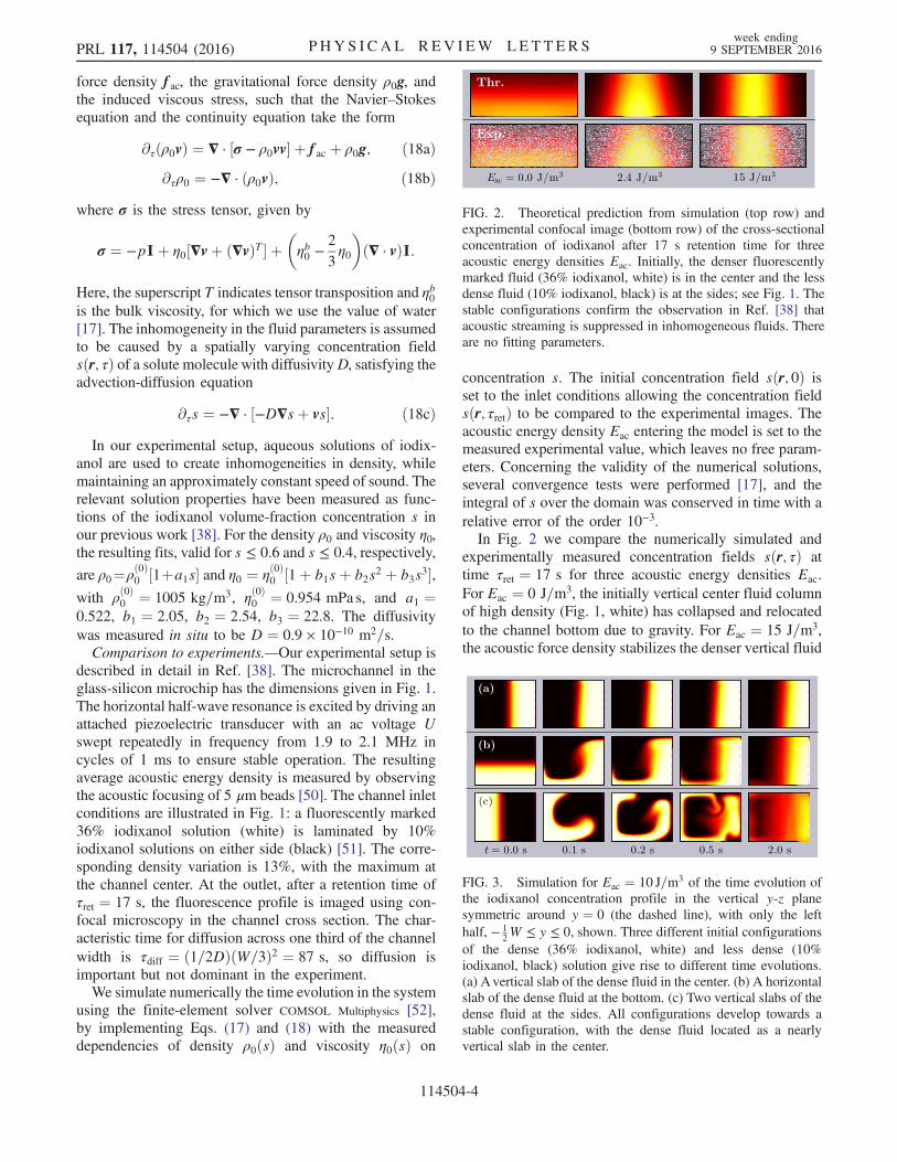
concentration s. The initial concentration field sðr; 0Þ isset to the inlet conditions allowing the concentration fieldsðr; τretÞ to be compared to the experimental images. Theacoustic energy density Eac entering the model is set to themeasured experimental value, which leaves no free param-eters. Concerning the validity of the numerical solutions,several convergence tests were performed [17], and theintegral of s over the domain was conserved in time with arelative error of the order 10−3.In Fig. 2 we compare the numerically simulated and

experimentally measured concentration fields sðr; τÞ attime τret ¼ 17 s for three acoustic energy densities Eac.For Eac ¼ 0 J=m3, the initially vertical center fluid columnof high density (Fig. 1, white) has collapsed and relocatedto the channel bottom due to gravity. For Eac ¼ 15 J=m3,the acoustic force density stabilizes the denser vertical fluid

FIG. 2. Theoretical prediction from simulation (top row) andexperimental confocal image (bottom row) of the cross-sectionalconcentration of iodixanol after 17 s retention time for threeacoustic energy densities Eac. Initially, the denser fluorescentlymarked fluid (36% iodixanol, white) is in the center and the lessdense fluid (10% iodixanol, black) is at the sides; see Fig. 1. Thestable configurations confirm the observation in Ref. [38] thatacoustic streaming is suppressed in inhomogeneous fluids. Thereare no fitting parameters.

FIG. 3. Simulation for Eac ¼ 10 J=m3 of the time evolution ofthe iodixanol concentration profile in the vertical y-z planesymmetric around y ¼ 0 (the dashed line), with only the lefthalf, − 1

2W ≤ y ≤ 0, shown. Three different initial configurations

of the dense (36% iodixanol, white) and less dense (10%iodixanol, black) solution give rise to different time evolutions.(a) Avertical slab of the dense fluid in the center. (b) A horizontalslab of the dense fluid at the bottom. (c) Two vertical slabs of thedense fluid at the sides. All configurations develop towards astable configuration, with the dense fluid located as a nearlyvertical slab in the center.

PRL 117, 114504 (2016) P HY S I CA L R EV I EW LE T T ER Sweek ending

9 SEPTEMBER 2016

114504-4

column against gravity, such that it broadens only bydiffusion. For the intermediate value Eac ¼ 2.4 J=m3,where the gravitational and acoustic forces are comparable,the stable configuration has a triangular shape. Note that thegood agreement between the simulated and measuredconcentration profiles has been obtained without fittingparameters.In Fig. 3 we show time-resolved simulations obtained

with Eac ¼ 10 J=m3 for (a) the stable initial configurationwith the denser fluid at the center, (b) the unstable initialconfiguration with the denser fluid at the bottom, and(c) the unstable initial configuration with the denser fluid atthe sides. While the stable initial configuration (a) evolvesonly by diffusion, the unstable initial configurations (b) and(c) evolve by complex advection patterns into essentiallythe same stable configuration, with the denser fluid at thecenter. This fluid relocation is in full qualitative agreementwith recent experiments [37]. Movies are provided in theSupplemental Material [53].Discussion.—Our theory for the acoustic force density

acting on an inhomogeneous fluid explains recent exper-imental observations [37,38] and agrees with our exper-imental validation without free parameters. The additionalobservation that steady acoustic streaming, driven bydissipation in the acoustic boundary layers, is suppressedin the bulk of an inhomogeneous fluid [38] has not beentreated in this Letter. However, Figs. 2 and 3 demonstratethat the acoustic force density stabilizes a particularinhomogeneous configuration, which suggests that thereis a competition between the inhomogeneity-inducedacoustic force density (13) and the boundary-drivenshear-force density associated with acoustic streaming.The experimental observation of stable inhomogeneousconfigurations further suggests that the latter is negligible.By adding acoustic boundary layers to our model, we arecurrently investigating this hypothesis. The extension ofacoustic radiation force theory to include inhomogeneousfluids through the introduction of the acoustic force density(13) represents an increased understanding of acousto-fluidics, in general, and further has the potential to open upnew ways for microscale handling of fluids and particlesusing acoustic fields.

We thank Mads Givskov Senstius, Technical Universityof Denmark, for assistance with the experiments. P. A. hadfinancial support from the Swedish Research Council(Grant No. 2012-6708), the Royal PhysiographicSociety, and the Birgit and Hellmuth Hertz Foundation.

*jonkar@fysik.dtu.dk†bruus@fysik.dtu.dk

[1] L. Rayleigh, Philos. Trans. R. Soc. London 175, 1 (1884).[2] H. Schlichting, Phys. Z. 33, 327 (1932).[3] C. Eckart, Phys. Rev. 73, 68 (1948).[4] W. L. Nyborg, J. Acoust. Soc. Am. 30, 329 (1958).

[5] L. V. King, Proc. R. Soc. A 147, 212 (1934).[6] K. Yosioka and Y. Kawasima, Acustica 5, 167 (1955).[7] G. Hertz and H. Mende, Z. Phys. 114, 354 (1939).[8] K. Bücks and H. Müller, Z. Phys. 84, 75 (1933).[9] A. Hanson, E. Domich, and H. Adams, Rev. Sci. Instrum.

35, 1031 (1964).[10] D. Foresti, M. Nabavi, M. Klingauf, A. Ferrari, and D.

Poulikakos, Proc. Natl. Acad. Sci. U.S.A. 110, 12549(2013).

[11] D. Foresti and D. Poulikakos, Phys. Rev. Lett. 112, 024301(2014).

[12] A. Marzo, S. A. Seah, B. W. Drinkwater, D. R. Sahoo,B. Long, and S. Subramanian, Nat. Commun. 6, 8661(2015).

[13] C. R. P. Courtney, C. E. M. Demore, H. Wu, A. Grinenko,P. D. Wilcox, S. Cochran, and B.W. Drinkwater, Appl.Phys. Lett. 104, 154103 (2014).

[14] D. Baresch, J.-L. Thomas, and R. Marchiano, Phys. Rev.Lett. 116, 024301 (2016).

[15] C. E. M. Démoré, P. M. Dahl, Z. Yang, P. Glynne-Jones, A.Melzer, S. Cochran, M. P. MacDonald, and G. C. Spalding,Phys. Rev. Lett. 112, 174302 (2014).

[16] A. Y. Rednikov and S. S. Sadhal, J. Fluid Mech. 667, 426(2011).

[17] P. B. Muller and H. Bruus, Phys. Rev. E 90, 043016 (2014).[18] J. T. Karlsen and H. Bruus, Phys. Rev. E 92, 043010 (2015).[19] H. Bruus, J. Dual, J. Hawkes, M. Hill, T. Laurell, J. Nilsson,

S. Radel, S. Sadhal, and M. Wiklund, Lab Chip 11, 3579(2011).

[20] M. Evander, O. Gidlof, B. Olde, D. Erlinge, and T. Laurell,Lab Chip 15, 2588 (2015).

[21] K. Lee, H. Shao, R. Weissleder, and H. Lee, ACS Nano 9,2321 (2015).

[22] F. Petersson, L. Åberg, A. M. Sward-Nilsson, and T.Laurell, Anal. Chem. 79, 5117 (2007).

[23] M. Wiklund, Lab Chip 12, 2018 (2012).[24] D. J. Collins, B. Morahan, J. Garcia-Bustos, C. Doerig, M.

Plebanski, and A. Neild, Nat. Commun. 6, 8686 (2015).[25] D. Ahmed, A. Ozcelik, N. Bojanala, N. Nama, A.

Upadhyay, Y. Chen, W. Hanna-Rose, and T. J. Huang,Nat. Commun. 7, 11085 (2016).

[26] F. Guo, Z. Mao, Y. Chen, Z. Xie, J. P. Lata, P. Li, L. Ren, J.Liu, J. Yang, M. Dao, S. Suresh, and T. J. Huang, Proc. Natl.Acad. Sci. U.S.A. 113, 1522 (2016).

[27] B. Hammarström, T. Laurell, and J. Nilsson, Lab Chip 12,4296 (2012).

[28] D. Carugo, T. Octon, W. Messaoudi, A. L. Fisher, M.Carboni, N. R. Harris, M. Hill, and P. Glynne-Jones, LabChip 14, 3830 (2014).

[29] G. Sitters, D. Kamsma, G. Thalhammer, M. Ritsch-Marte,E. J. G. Peterman, and G. J. L. Wuite, Nat. Methods 12, 47(2015).

[30] P. Augustsson, C. Magnusson, M. Nordin, H. Lilja, andT. Laurell, Anal. Chem. 84, 7954 (2012).

[31] P. Li, Z. Mao, Z. Peng, L. Zhou, Y. Chen, P.-H. Huang, C. I.Truica, J. J. Drabick, W. S. El-Deiry, M. Dao, S. Suresh, andT. J. Huang, Proc. Natl. Acad. Sci. U.S.A. 112, 4970 (2015).

[32] B. Hammarström, B. Nilson, T. Laurell, J. Nilsson, and S.Ekström, Anal. Chem. 86, 10560 (2014).

PRL 117, 114504 (2016) P HY S I CA L R EV I EW LE T T ER Sweek ending

9 SEPTEMBER 2016

114504-5

[33] Nonlinear Acoustics, edited by M. F. Hamilton and D. T.Blackstock (Acoustical Society of America, Melville, NY,2008).

[34] N. Riley, Annu. Rev. Fluid Mech. 33, 43 (2001).[35] M. J. Marr-Lyon, D. B. Thiessen, and P. L. Marston, Phys.

Rev. Lett. 86, 2293 (2001).[36] N. Bertin, H. Chraïbi, R. Wunenburger, J.-P. Delville, and

E. Brasselet, Phys. Rev. Lett. 109, 244304 (2012).[37] S. Deshmukh, Z. Brzozka, T. Laurell, and P. Augustsson,

Lab Chip 14, 3394 (2014).[38] P. Augustsson, J. T. Karlsen, H.-W. Su, H. Bruus, and J.

Voldman, Nat. Commun. 7, 11556 (2016).[39] R. Barnkob, P. Augustsson, T. Laurell, and H. Bruus, Lab

Chip 10, 563 (2010).[40] P. Augustsson, R. Barnkob, S. T. Wereley, H. Bruus, and T.

Laurell, Lab Chip 11, 4152 (2011).[41] L. D. Landau and E. M. Lifshitz, Fluid Mechanics, 2nd ed.,

Vol. 6 (Pergamon Press, Oxford, 1993).[42] P. M. Morse and K. U. Ingard, Theoretical Acoustics

(Princeton University Press, Princeton, NJ, 1986).[43] H. Bruus, Lab Chip 12, 20 (2012).[44] P. G. Bergmann, J. Acoust. Soc. Am. 17, 329 (1946).[45] C. P. Lee and T. G. Wang, J. Acoust. Soc. Am. 94, 1099

(1993).

[46] B. L. Smith and G.W. Swift, J. Acoust. Soc. Am. 110, 717(2001).

[47] L. Zhang and P. L. Marston, J. Acoust. Soc. Am. 129, 1679(2011).

[48] Z. Fan, D. Mei, K. Yang, and Z. Chen, J. Acoust. Soc. Am.124, 2727 (2008).

[49] The time average of the product of two time-harmoniccomplex-valued fields f1 and g1 is hf1g1i¼1

2Re½f�1g1�, where

the asterisk denotes complex conjugation.[50] The average acoustic energy density Eac is estimated as a

function of the piezoelectric-transducer voltage U byobserving the focusing of 5 μm polystyrene particles in ahomogeneous 10% iodixanol solution and comparing totheoretical models; see Refs. [39,40]. In our system, thisyields Eac ¼ kU2, with k ¼ 1.2 Jm−3 V−2 [38].

[51] We use a fluorescent dextran tracer with the molecularweight of 3000 Da and a diffusivity close to that ofiodixanol, which allows indirect visualization of the iodix-anol concentration profile; see Ref. [38].

[52] COMSOL Multiphysics 5.2, http://www.comsol.com (2015).[53] See Supplemental Material at http://link.aps.org/

supplemental/10.1103/PhysRevLett.117.114504 for moviesof the time evolution of the concentration fields.

PRL 117, 114504 (2016) P HY S I CA L R EV I EW LE T T ER Sweek ending

9 SEPTEMBER 2016

114504-6