ACKNOWLEDGEMENTS

I would like to offer my gratitude to my family who gave me thesupport and encouragement I needed while working on this project.Thanks also to fellow students past and present who gave adviseand feedback on areas of difficulty. Lastly and most importantly Iwould like to thank my supervisor, Michael Manzke who was notonly instrumental in my project progress, but who also showed un-derstanding and compassion when they were needed the most. Spe-cial thanks to all of the above.

1

Contents

1 First Chapter 7

1.1 Introduction . . . . . . . . . . . . . . . . . . . . . . . 7

1.1.1 The Kalman Filter Equations . . . . . . . . . 8

1.2 Two Different Sets Of Equations . . . . . . . . . . . . 8

1.2.1 Time Update Equations . . . . . . . . . . . . 8

1.2.2 Measurement Update Equations . . . . . . . . 9

1.3 Specific Kalman Filter Equations And Their Role . . 9

1.3.1 Additional Variable In The Equations . . . . . 10

2 Second Chapter 11

2.1 Background Mathematics . . . . . . . . . . . . . . . 11

2.1.1 Vectors and Matrices . . . . . . . . . . . . . . 11

2.1.2 Vector addition and subtraction . . . . . . . . 12

2.1.3 Matrix addition and subtraction . . . . . . . . 13

2

2.1.4 Matrix Multiplication . . . . . . . . . . . . . . 14

2.1.5 Matrix-Vector Multiplication . . . . . . . . . . 15

2.1.6 Matrix Transpose . . . . . . . . . . . . . . . . 17

2.1.7 Matrix Inversion . . . . . . . . . . . . . . . . 17

3 Third Chapter 23

3.1 Algorithms for Adding, Subtracting and Multiplication 23

3.2 Addition and Subtraction of Std logic vectors . . . . 24

3.3 Six Bit Adder . . . . . . . . . . . . . . . . . . . . . . 24

3.4 Alternative Adder/Subtractor . . . . . . . . . . . . . 27

3.4.1 Addition/Subtraction for Fixed Point Numbers 28

3.4.2 Fixed Point Adder/Subtractor . . . . . . . . . 29

3.5 Algorithms for Multiplication . . . . . . . . . . . . . 29

3.5.1 Shift And Add Algorithm . . . . . . . . . . . 30

3.5.2 Booths Multiplication Algorithm . . . . . . . 31

3.5.3 Implementation of Sequential Shift and AddMultiplier . . . . . . . . . . . . . . . . . . . . 32

3.5.4 Design for Booths Algorithm in VHDL . . . . 33

3.6 Problems in Simulation - Type unsigned . . . . . . . 34

3.7 Problems in Simulation - Types in VHDL . . . . . . 35

3.7.1 Libraries in VHDL . . . . . . . . . . . . . . . 36

3

3.7.2 Packages in VHDL . . . . . . . . . . . . . . . 37

3.8 Sequential Multiplier - The final Curtain . . . . . . . 39

3.9 Signed Combinational Multiplier - Alternative Ap-proach . . . . . . . . . . . . . . . . . . . . . . . . . . 40

4 Fourth Chapter 41

4.1 Dealing with two dimensional arrays - matrices inVHDL . . . . . . . . . . . . . . . . . . . . . . . . . . 41

4.2 Overview of Arrays . . . . . . . . . . . . . . . . . . . 41

4.2.1 Addition of Arrays - Attempt One . . . . . . 43

4.2.2 Addition of Arrays - Attempt Two . . . . . . 44

4.2.3 Addition of Arrays - Final Attempt . . . . . . 45

4.3 Matrix Multiplication using Block Ram . . . . . . . . 46

5 Fifth Chapter 49

5.1 Simplistic Transpose Design . . . . . . . . . . . . . . 49

5.2 Inverting a Matrix - Design for an Adjoint Matrix . . 50

5.2.1 Fraction Divisor in VHDL . . . . . . . . . . . 51

5.3 Inverting a matrix . . . . . . . . . . . . . . . . . . . 53

6 chapter six 54

6.1 Review of the project and personal thoughts . . . . . 54

4

6.2 Doing it all over again .... . . . . . . . . . . . . . . . 56

6.3 Future Work . . . . . . . . . . . . . . . . . . . . . . . 57

5

ABSTRACT

The overall aim of this project was to design, implement and evalu-ate the performance of a kalman filter using FPGAs. The projectsmain concern is the design of a synthesisable VHDL model for thealgorithm which defines this filter. From the project viewpoint itwas not essential for me to become an expert in minimum meansquare error filtering and state space methods. What was required,however, was for me to be familiar with the algorithm, that definesthe kalman filter. The set of equations, their relevance to one an-other and indeed the overall functionality of the algorithm requiredcomplete comprehension. If successful the resulting program wouldthen be implemented with field programmable gate arrays, enablingthe end result to be appreciated visually.

6

Chapter 1

First Chapter

1.1 Introduction

The overall aim of this project was to design, implement and evalu-ate the performance of a kalman filter using FPGAs. The projectsmain concern is the design of a synthesisable VHDL model for the al-gorithm which defines this filter. From the project viewpoint it wasnot essential for me to become an expert in minimum mean squareerror filtering and state space methods. What was required, how-ever, was for me to be familiar with the algorithm, that defines thekalman filter. The set of equations, their relevance to one anotherand indeed the overall functionality of the algorithm required com-plete comprehension. If successful the resulting program would thenbe implemented with field programmable gate arrays, enabling theend result to be appreciated visually. This chapter firstly presentsthese equations, describes their meaning in terms of the next and theprevious equation and outlines what would be needed for success-ful implementation in a hardware descriptive language. A completebreakdown of all follows.

7

1.1.1 The Kalman Filter Equations

The kalman filter equations are a set of mathematical equations thatprovide an efficient computational means to estimate the state of aprocess, in a way that minimizes the mean of the squared error. Thefilter is a very powerful device as it supports the estimation of past,present and future states. It even extends its functionality so it cancarry out this procedure when the precise nature of the modelledsystem is unknown. The system may or may not be subjected toa series of random disturbances, when this occurs it is required toestimate the state variables from noisy observations. The kalmanfilter equations uses two different types of equations in a predictionof the state variable, these being both the time update equationsand the measurement update equations.

1.2 Two Different Sets Of Equations

The filter estimates its process by using a form of feedback control,as implied in the previous section. The filter will estimate the pro-cess state at some time and then obtains its feedback in the formof noisy measurements. These equations fall into the category ofeither Time update equations or measurement update equations.

1.2.1 Time Update Equations

The time update equations are used to predict the current state andcovariance matrix, used in time t+1 to predict the previous state.These equations can be generally seen as predictor equations as theyare responsible for projecting forward in time. K is representative ofthe time step, so the time update equations are basically indicativeof K+1.

8

1.2.2 Measurement Update Equations

The measurement equations are responsible for feedback and forcorrecting the errors that have been made in the time update equa-tions. In a sense they are back propagating to get new values forthe prior state to improve the ”guess” for the next state. Theseequations can be seen as corrector equations and the final estima-tion algorithm resemble that of a predictor-corrector algorithm. Soby definition measurement equations adjust the projected estimateby an actual measurement at that time.

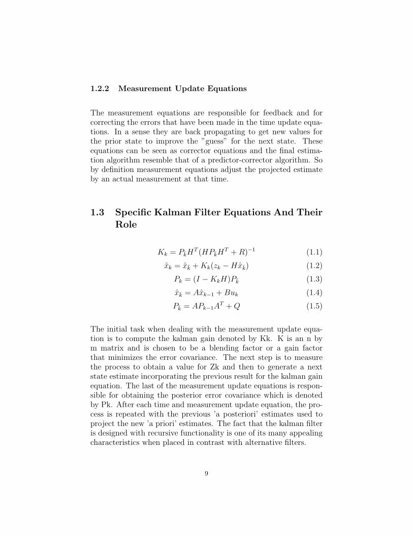
1.3 Specific Kalman Filter Equations And TheirRole

Kk = Pk̄HT (HPk̄H

T + R)−1 (1.1)

x̂k = x̂k̄ + Kk(zk −Hx̂k̄) (1.2)

Pk = (I −KkH)Pk̄ (1.3)

x̂k̄ = Ax̂k−1 + Buk (1.4)

Pk̄ = APk−1AT + Q (1.5)

The initial task when dealing with the measurement update equa-tion is to compute the kalman gain denoted by Kk. K is an n bym matrix and is chosen to be a blending factor or a gain factorthat minimizes the error covariance. The next step is to measurethe process to obtain a value for Zk and then to generate a nextstate estimate incorporating the previous result for the kalman gainequation. The last of the measurement update equations is respon-sible for obtaining the posterior error covariance which is denotedby Pk. After each time and measurement update equation, the pro-cess is repeated with the previous ’a posteriori’ estimates used toproject the new ’a priori’ estimates. The fact that the kalman filteris designed with recursive functionality is one of its many appealingcharacteristics when placed in contrast with alternative filters.

9

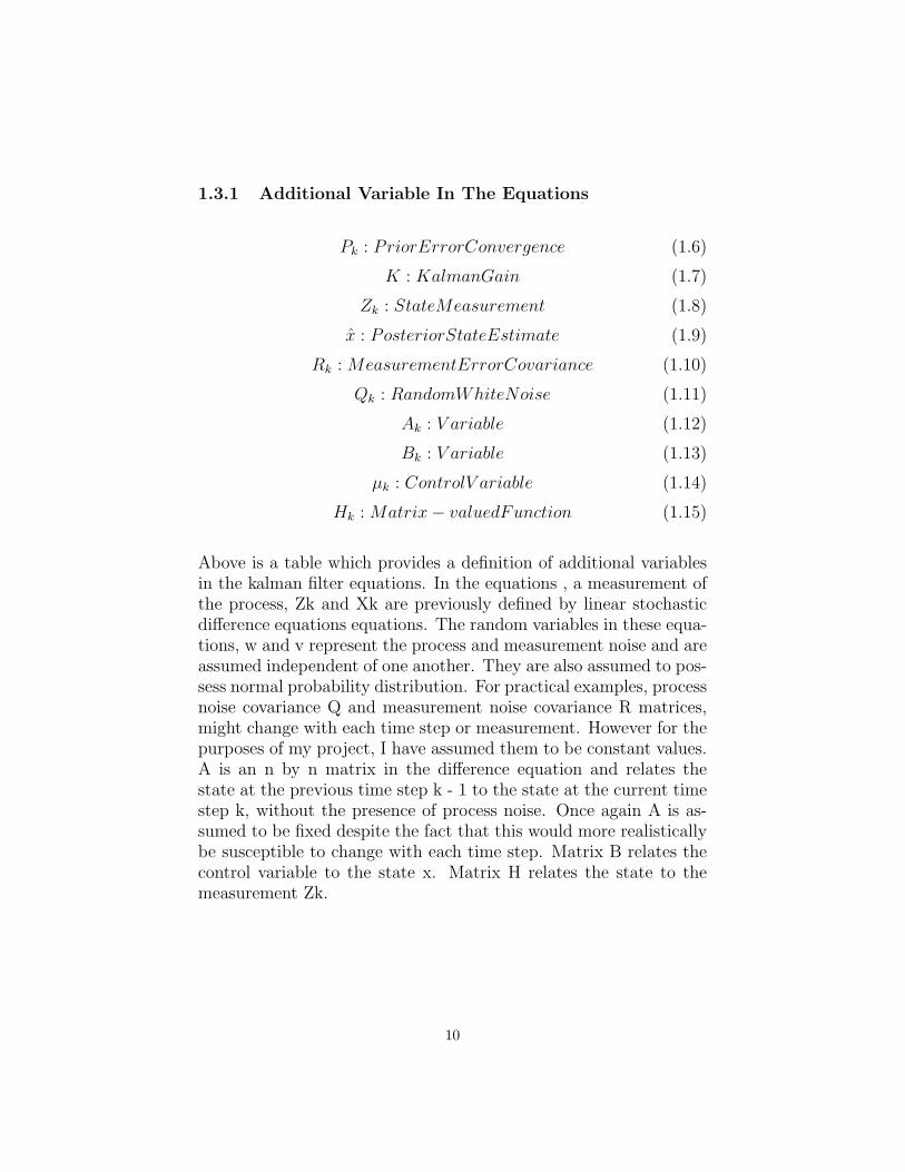
1.3.1 Additional Variable In The Equations

Pk : PriorErrorConvergence (1.6)

K : KalmanGain (1.7)

Zk : StateMeasurement (1.8)

x̂ : PosteriorStateEstimate (1.9)

Rk : MeasurementErrorCovariance (1.10)

Qk : RandomWhiteNoise (1.11)

Ak : V ariable (1.12)

Bk : V ariable (1.13)

µk : ControlV ariable (1.14)

Hk : Matrix− valuedFunction (1.15)

Above is a table which provides a definition of additional variablesin the kalman filter equations. In the equations , a measurement ofthe process, Zk and Xk are previously defined by linear stochasticdifference equations equations. The random variables in these equa-tions, w and v represent the process and measurement noise and areassumed independent of one another. They are also assumed to pos-sess normal probability distribution. For practical examples, processnoise covariance Q and measurement noise covariance R matrices,might change with each time step or measurement. However for thepurposes of my project, I have assumed them to be constant values.A is an n by n matrix in the difference equation and relates thestate at the previous time step k - 1 to the state at the current timestep k, without the presence of process noise. Once again A is as-sumed to be fixed despite the fact that this would more realisticallybe susceptible to change with each time step. Matrix B relates thecontrol variable to the state x. Matrix H relates the state to themeasurement Zk.

10

Chapter 2

Second Chapter

2.1 Background Mathematics

A complete examination of matrices, their functionality and effectsfor my particular design was the next step required. This chapterconsists of an overview of vector and matrix fundamentals acquiredpreviously in the course and reviewed and revised courtesy of linearalgebra books and websites. A little time was allocated to usingmatrices in matlab which was in itself beneficial and worthwhile.

2.1.1 Vectors and Matrices

As is probably evident at this stage all equations are comprisedof matrices, vectors or single values. Some arithmetic function isperformed on these components to result in the output value whichis passed to the next equation. Below I have taken each equationindependently and examined the operations that are required toprovide the output function.

Kk = P−k HT (HP−k HT + R)−1

(2.1)

11

In this equation P, H and R are all matrices. For the purpose of myproject I assumed that all matrices were n by n despite the fact thatthe kalman gain itself can be defined in terms of an n by m matrix.With the aid of more time, experience and expertise this could havebeen accounted for. H is transposed and multiplied by matrix P,the result is stored. The transpose of H is multiplied by P and theresult is multiplied by H, this is then added to R. This new resultis inverted and multiplied by the previously stored result which de-termines the kalman gain. The Kalman gain is then taken in by thenext equation where similar operations are performed. Variableswhich posess the hat are vector values with all the other variablesrepresenting matrices. The time update equations are basically sim-ilar with the primary difference being that the time step has nowbeen updated and we are looking at new time t and new time k.

A Breakdown of the Algorithm

After the algorithm was successfully broken down, it was evidentthat understanding every single part of this algorithm came a poorsecond to actually being able to implement it in VHDL. Althoughthe algorithm primarily had all the appearance of being intriguinglycomplex and indeed the theory behind it perplexing at times it soonbecame obvious that its implementation required no more than afull comprehension of mathematical operations on n sized matricesand vectors which had previously been studied in the course.

It was then apparent that a full overview of matrices and vectors wasrequired in order to become proficient in this area and to successfullycode these operations in VHDL.

2.1.2 Vector addition and subtraction

Adding two vectors is an extremely simple process, one basicallyadds the elements in the same position in the vector.

12

X1

X2

X3

X4

+

Y1

Y2

Y3

Y4

=

X1 + Y1

X2 + Y2

X3 + Y3

X4 + Y4

(2.2)

It is important to note that vector addition is only feasible whenvectors of a similar size are being dealt with. Vector addition is alsoreflexive which means x + y = y + x. Vector subtraction is simplyvector addition of the negative.

2.1.3 Matrix addition and subtraction

2 4 61 8 34 2 7

+

3 9 12 3 47 5 1

=

5 13 73 11 711 7 8

(2.3)

The procedure for adding and subtracting matrices is very simple.First it must be made sure that the dimensions of the matrices arethe same. For this reason I stuck to fixed size n by n matrices anddiscarded using m by n matrices. In the eventuality that I wouldhave to add an m by n matrix to an n by n matrix this would havecaused problems so I rejected this straight off. Dimensions referto the size of the matrix. You can add or subtract matrices thathave the same dimensions, i.e three by three matrices or five byfive matrices but one can not add or subtract those which containdifferent dimensions such as a three by two matrix multiplied bya ten by six. The resulting matrix will have dimensions the samesize as the input matrices. When adding matrices each element ofmatrix one is simply added to the corresponding element of matrix2 in the same cell.

4 2 39 6 712 2 1

−

2 3 64 1 57 8 9

=

2 −1 −35 4 25 −6 −8

(2.4)

13

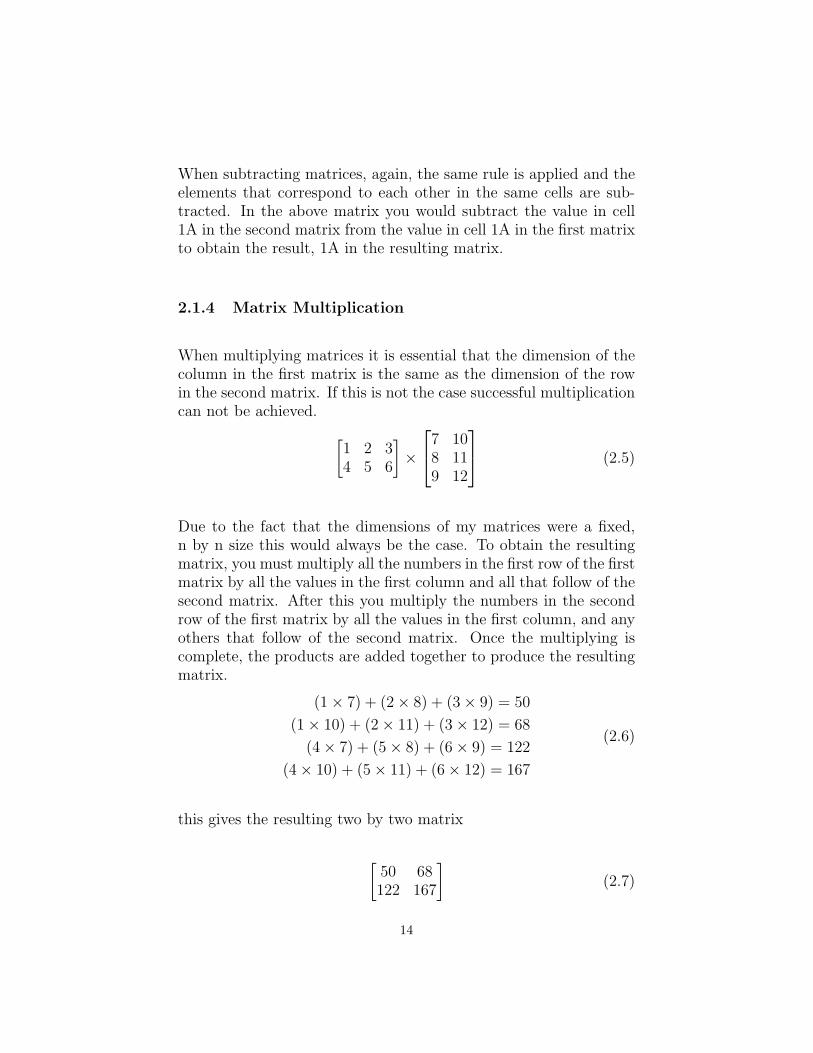
When subtracting matrices, again, the same rule is applied and theelements that correspond to each other in the same cells are sub-tracted. In the above matrix you would subtract the value in cell1A in the second matrix from the value in cell 1A in the first matrixto obtain the result, 1A in the resulting matrix.

2.1.4 Matrix Multiplication

When multiplying matrices it is essential that the dimension of thecolumn in the first matrix is the same as the dimension of the rowin the second matrix. If this is not the case successful multiplicationcan not be achieved. [

1 2 34 5 6

]×

7 108 119 12

(2.5)

Due to the fact that the dimensions of my matrices were a fixed,n by n size this would always be the case. To obtain the resultingmatrix, you must multiply all the numbers in the first row of the firstmatrix by all the values in the first column and all that follow of thesecond matrix. After this you multiply the numbers in the secondrow of the first matrix by all the values in the first column, and anyothers that follow of the second matrix. Once the multiplying iscomplete, the products are added together to produce the resultingmatrix.

(1× 7) + (2× 8) + (3× 9) = 50

(1× 10) + (2× 11) + (3× 12) = 68

(4× 7) + (5× 8) + (6× 9) = 122

(4× 10) + (5× 11) + (6× 12) = 167

(2.6)

this gives the resulting two by two matrix

[50 68122 167

](2.7)

14

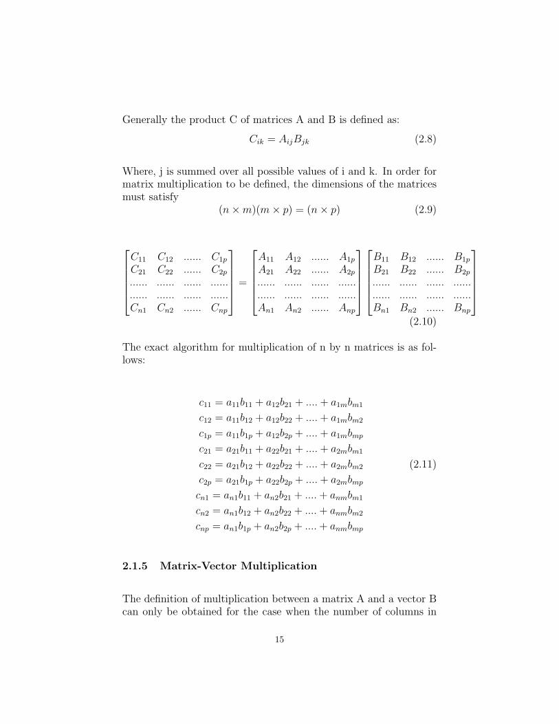
Generally the product C of matrices A and B is defined as:

Cik = AijBjk (2.8)

Where, j is summed over all possible values of i and k. In order formatrix multiplication to be defined, the dimensions of the matricesmust satisfy

(n×m)(m× p) = (n× p) (2.9)

C11 C12 ...... C1p

C21 C22 ...... C2p

...... ...... ...... ......

...... ...... ...... ......Cn1 Cn2 ...... Cnp

=

A11 A12 ...... A1p

A21 A22 ...... A2p

...... ...... ...... ......

...... ...... ...... ......An1 An2 ...... Anp

B11 B12 ...... B1p

B21 B22 ...... B2p

...... ...... ...... ......

...... ...... ...... ......Bn1 Bn2 ...... Bnp

(2.10)

The exact algorithm for multiplication of n by n matrices is as fol-lows:

c11 = a11b11 + a12b21 + .... + a1mbm1

c12 = a11b12 + a12b22 + .... + a1mbm2

c1p = a11b1p + a12b2p + .... + a1mbmp

c21 = a21b11 + a22b21 + .... + a2mbm1

c22 = a21b12 + a22b22 + .... + a2mbm2

c2p = a21b1p + a22b2p + .... + a2mbmp

cn1 = an1b11 + an2b21 + .... + anmbm1

cn2 = an1b12 + an2b22 + .... + anmbm2

cnp = an1b1p + an2b2p + .... + anmbmp

(2.11)

2.1.5 Matrix-Vector Multiplication

The definition of multiplication between a matrix A and a vector Bcan only be obtained for the case when the number of columns in

15

A equals the number of rows in B. The general formula for matrix-vector multiplication is:

a11 a12 ...... a1n

a21 a22 ...... a2n

...... ...... ...... ......

...... ...... ...... ......am1 am2 ...... amn

x1

x2

...

...xn

(2.12)

=

a11x1 + a12x2 + ...... + a1nxn

a21x1 + a22x2 + ...... + a2nxn

am1x1 + am2x2 + ...... + amnxn

(2.13)

The process of matrix-vector multiplication is one which takes thedot-product of B with each of the rows of A (hence the reason whythe number of columns in A has to be equal to the number of com-ponents in vector B). The first element of the matrix-vector productis the dot-product of B with the first row of A.

For example, if A is the matrix[1 −1 20 −3 1

](2.14)

And B is the vector, (2, 1, 0) then

[1 −1 20 −3 1

]×

210

=

[1−3

](2.15)

When multiplying a vector by a scalar value, each element of thevector must be multiplied by this value. Similarly when multiply-ing a matrix by a scalar the same procedure is adhered to and theresulting matrix is the product of each element of the matrix andthe scalar.

16

2.1.6 Matrix Transpose

To transpose a matrix all that is necessary is for the columns to beconverted to rows and vice versa. The result is the object obtainedby replacing all objects of Aij with Aji. The matrix transpose, mostcommonly denoted AT, is the matrix obtained by exchanging A’srows and columns and satisfies the identity:

(AT )−1 = (A−1)T (2.16)

1 2 34 5 67 8 9

=>

1 4 72 5 83 6 9

(2.17)

When dealing with an n by m matrix the transposed result matrixwill be an m by n matrix, a matrix is symmetric if AT = A andis antisymmetric if AT = -A. For the purpose of my project this isuseless trivia. The transpose of a matrix is the matrix product ofthe transposed matrix in reverted order,

(AB)T = AT BT (2.18)

2.1.7 Matrix Inversion

There were a couple of different matrix inversion methods that Iexamined before making a decision as to which one would be mostfeasible to implement in VHDL and which one would be most suit-able in terms of the algorithm.

Matrix Inversion using Gaussian Elimination

For moderate and large matrices the best approach for inversion isthe use of Gaussian elimination more commonly known as Gauss

17

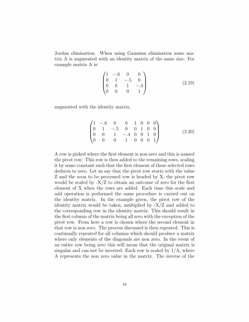
Jordan elimination. When using Gaussian elimination some ma-trix A is augmented with an identity matrix of the same size. Forexample matrix A is:

1 −.6 0 00 1 −.5 00 0 1 −.40 0 0 1

(2.19)

augmented with the identity matrix,

1 −.6 0 0 1 0 0 00 1 −.5 0 0 1 0 00 0 1 −.4 0 0 1 00 0 0 1 0 0 0 1

(2.20)

A row is picked where the first element is non zero and this is namedthe pivot row. This row is then added to the remaining rows, scalingit by some constant such that the first element of these selected rowsdeduces to zero. Let us say that the pivot row starts with the valueZ and the soon to be processed row is headed by X, the pivot rowwould be scaled by -X/Z to obtain an outcome of zero for the firstelement of X when the rows are added. Each time this scale andadd operation is performed the same procedure is carried out onthe identity matrix. In the example given, the pivot row of theidentity matrix would be taken, multiplied by -X/Z and added tothe corresponding row in the identity matrix. This should result inthe first column of the matrix being all zero with the exception of thepivot row. From here a row is chosen where the second element inthat row is non zero. The process discussed is then repeated. This iscontinually repeated for all columns which should produce a matrixwhere only elements of the diagonals are non zero. In the event ofan entire row being zero this will mean that the original matrix issingular and can not be inverted. Each row is scaled by 1/A, whereA represents the non zero value in the matrix. The inverse of the

18

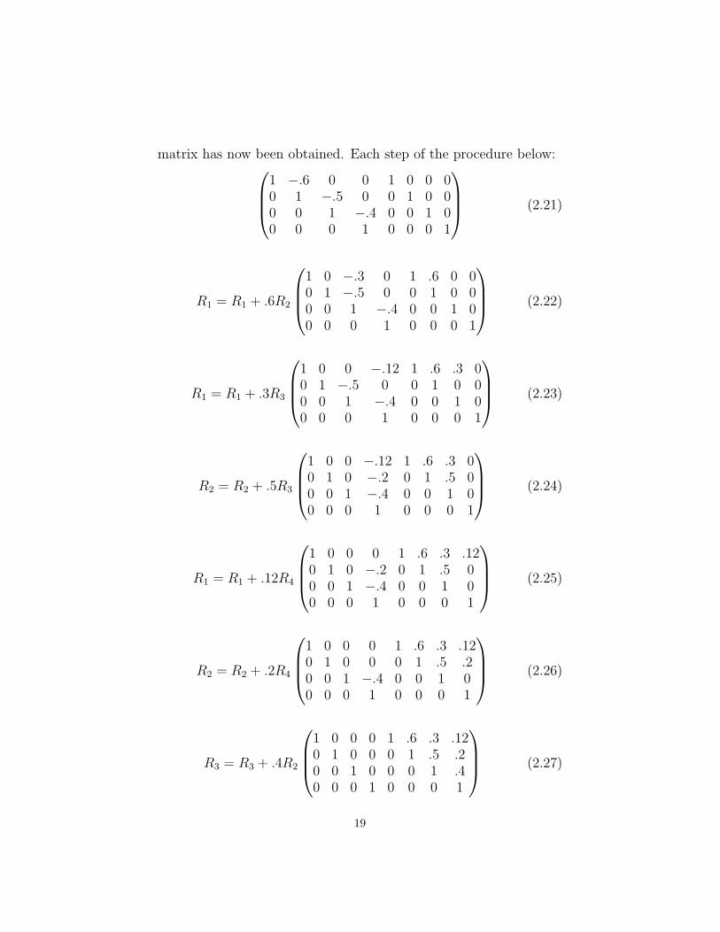
matrix has now been obtained. Each step of the procedure below:1 −.6 0 0 1 0 0 00 1 −.5 0 0 1 0 00 0 1 −.4 0 0 1 00 0 0 1 0 0 0 1

(2.21)

R1 = R1 + .6R2

1 0 −.3 0 1 .6 0 00 1 −.5 0 0 1 0 00 0 1 −.4 0 0 1 00 0 0 1 0 0 0 1

(2.22)

R1 = R1 + .3R3

1 0 0 −.12 1 .6 .3 00 1 −.5 0 0 1 0 00 0 1 −.4 0 0 1 00 0 0 1 0 0 0 1

(2.23)

R2 = R2 + .5R3

1 0 0 −.12 1 .6 .3 00 1 0 −.2 0 1 .5 00 0 1 −.4 0 0 1 00 0 0 1 0 0 0 1

(2.24)

R1 = R1 + .12R4

1 0 0 0 1 .6 .3 .120 1 0 −.2 0 1 .5 00 0 1 −.4 0 0 1 00 0 0 1 0 0 0 1

(2.25)

R2 = R2 + .2R4

1 0 0 0 1 .6 .3 .120 1 0 0 0 1 .5 .20 0 1 −.4 0 0 1 00 0 0 1 0 0 0 1

(2.26)

R3 = R3 + .4R2

1 0 0 0 1 .6 .3 .120 1 0 0 0 1 .5 .20 0 1 0 0 0 1 .40 0 0 1 0 0 0 1

(2.27)

19

hence the inverse

1 .6 .3 .120 1 .5 .20 0 1 .40 0 0 1

(2.28)

Matrix Inversion using the Adjoint Matrix Formula

For smaller matrices, those of dimensions two, three and four, aless complex approach to the problem is using the adjoint matrixformula. When dealing with any non singular matrix, let us call itA, the inverse of A can be successfully computed by dividing theadjoint of A by the overall determinant of A. The procedure forcalculating the adjoint of A is quite simple and poses minimum dif-ficulty for the mathematician. The first step is to find the matrixof minors for A. This is done by effectively eliminating the ith andjth row and column of the matrix and computing the determinantsof the resulting two by two matrix at each step. Each of these cor-responding results will produce the adjoint A. To find the cofactorsof A a sign change is applied to selected elements of the matrix, thisis discussed in more detail below. To find the adjoint, the matrix ofcofactors is then transposed. After finding the adjoint each value inthis new matrix is divided by the determinant of the original matrix.The resulting matrix is the inverted matrix.

Matrix Determinants

To find the determinant of a two by two matrix, each element isaligned to a matrix with elements A, B, C and D respectively. Thealgorithm for the determinant is AD - BC, so the resulting determi-nant will be a single value.

In attempting to find the determinant of a three by three matrix,the procedure is simply extended. The overall determinant can be

20

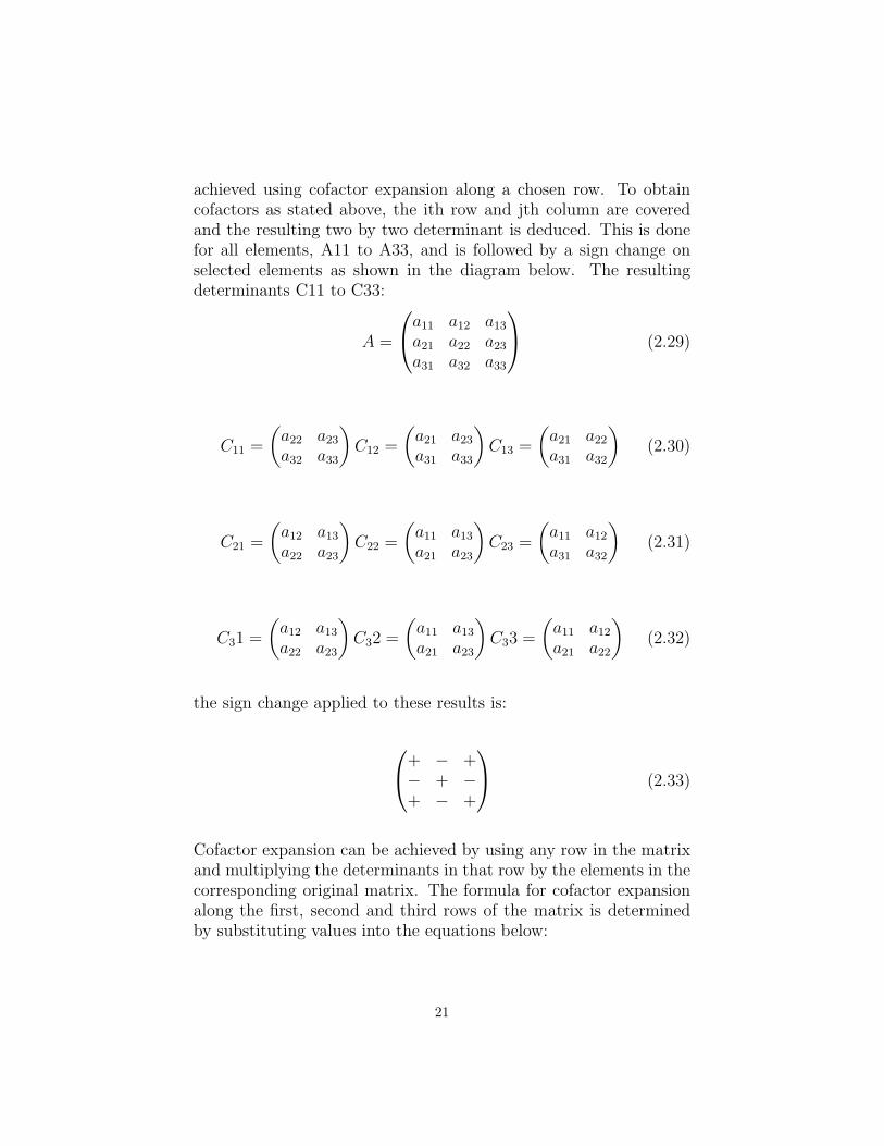
achieved using cofactor expansion along a chosen row. To obtaincofactors as stated above, the ith row and jth column are coveredand the resulting two by two determinant is deduced. This is donefor all elements, A11 to A33, and is followed by a sign change onselected elements as shown in the diagram below. The resultingdeterminants C11 to C33:

A =

a11 a12 a13

a21 a22 a23

a31 a32 a33

(2.29)

C11 =

(a22 a23

a32 a33

)C12 =

(a21 a23

a31 a33

)C13 =

(a21 a22

a31 a32

)(2.30)

C21 =

(a12 a13

a22 a23

)C22 =

(a11 a13

a21 a23

)C23 =

(a11 a12

a31 a32

)(2.31)

C31 =

(a12 a13

a22 a23

)C32 =

(a11 a13

a21 a23

)C33 =

(a11 a12

a21 a22

)(2.32)

the sign change applied to these results is:

+ − +− + −+ − +

(2.33)

Cofactor expansion can be achieved by using any row in the matrixand multiplying the determinants in that row by the elements in thecorresponding original matrix. The formula for cofactor expansionalong the first, second and third rows of the matrix is determinedby substituting values into the equations below:

21

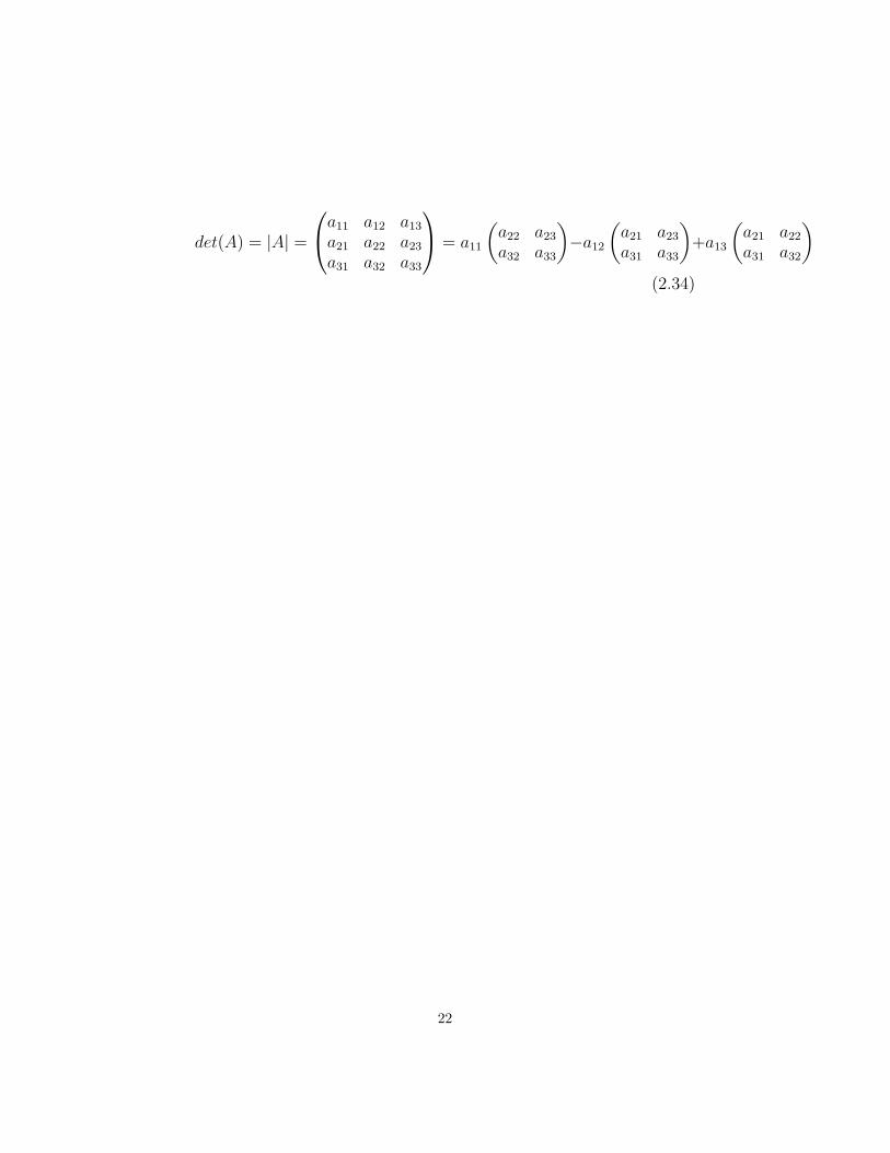
det(A) = |A| =

a11 a12 a13

a21 a22 a23

a31 a32 a33

= a11

(a22 a23

a32 a33

)−a12

(a21 a23

a31 a33

)+a13

(a21 a22

a31 a32

)(2.34)

22

Chapter 3

Third Chapter

3.1 Algorithms for Adding, Subtracting and Mul-tiplication

After the preliminary step of refreshing the matrix mathematicscourse most of which had been covered previously in first year maths,it was now inevitable that these formulae be converted to VHDLcode. After some thought I came to the realization that writingcode for adding, subtracting and multiplying logic vectors was whatwas required. These entities would then be used when attemptingto carry out matrix addition and multiplication. With some delib-eration I finally came up with an algorithm that I felt would befeasible for implementation in my project but this was only after Ihad toyed with various ways to do each. One by one, for some rea-son or another I felt I had to discard these procedures in pursuit ofcode that would cater for all eventualities. Below is a run throughof some of the algorithms I experimented with for both addition andsubtraction and then for multiplication of logic vectors. I have alsoaccounted for the reasons why I then found it necessary to pursuealternatives. Unfortunately for a lot of the time it was only afterthe code had been written that I found it to be inappropriate forcertain cases or in some small way flawed.

23

3.2 Addition and Subtraction of Std logic vec-tors

Due to the fact that the project specification stated that the equa-tions would be evaluated using FPGAs , I felt that an algorithm foraddition that would be compatible with FPGAs was necessary. Thiswould mean it would be easier to use the board when the time camein the closing stages of the application. For this reason I optedfor a design that would use a series of full-adders to add vectors.These full-adders would be constructed from two half-adders as isthe usual implementation style. I rehashed a section of the codefrom ’HDL Chip Design’ which I have referenced in my project andbibliography.

entity HALF_ADDER is

port(A, B: in std_logic; Sum, C_out: out

std_logic);

end entity;

architecture Logic of HALF_ADDER is

begin

Sum <= A xor B;

C_out <= A and B;

end architecture Logic;

3.3 Six Bit Adder

The sixbit addsub2bit as the name suggests either adds or subtractsa 2-bit value to or from a 6-bit value. This logical structure isbasically modelled by a series of full adders. A full-adder in turncomprises two half adders and an OR gate.

24

begin

HA1: HALF_ADDER port map (A => A, B => B, Sum => AplusB, C_out =>

CoutHA1);

HA2: HALF_ADDER port map(A => AplusB, B => Cin, Sum => Sum, C_out

=> C_outHA2);

C_out <= CoutHA1 or CoutHA2;

A single bit half adder is modelled using a single XOR logical oper-ator and a single AND logical operator. For the adder/subtractorcircuit , the entity, is designed by instantiating six of these full adderswith a ripple carry chain from one full adder to the next. Input B,the addend uses two XOR functions in order to create the ones com-plement; they are XORed with the two least significant bits of inputA, the augend. The twos complement which is required for subtrac-tion, is designed by connecting input SubAddBar to the carry in ofthe first, least Significant bit.

Extra logic is modelled to force the output to binary 111111 inthe event of overflow caused by addition. Similarly if underflowoccurs from subtraction the output will result in binary 000000. Anoverflow will result in the case where the carry out from the mostsignificant bit full adder, i.e carryOut[5], is at logic 1. An overflowwill be created when subtracting and carryOut[5] is at 0. This designonly requires minimum changes in order to remodel it with differentbit widths. VHDL constants specify the bus width of inputs A andB which will later be referenced in the entities body. The designof the model is such that it uses generate statements to instantiatethe single bit adders in a way that only the constants widthA andwidthB require changes. This will then change the input and outputbit widths.

Problems with the Six Bit Adder

This adder seemed very practical for my application as it allowedfor the input sizes to be changed without difficulty. As can be seenfrom a segment of the code and indeed is implied in the name, this

25

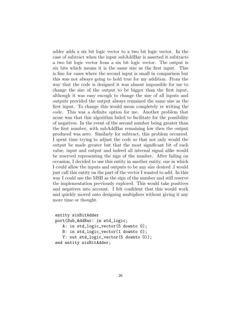
adder adds a six bit logic vector to a two bit logic vector. In thecase of subtract when the input subAddBar is asserted it subtractsa two bit logic vector from a six bit logic vector. The output issix bits which means it is the same size as the first input. Thisis fine for cases where the second input is small in comparison butthis was not always going to hold true for my addition. From theway that the code is designed it was almost impossible for me tochange the size of the output to be bigger than the first input,although it was easy enough to change the size of all inputs andoutputs provided the output always remained the same size as thefirst input. To change this would mean completely re writing thecode. This was a definite option for me. Another problem thatarose was that this algorithm failed to facilitate for the possibilityof negatives. In the event of the second number being greater thanthe first number, with subAddBar remaining low then the outputproduced was zero. Similarly for subtract, this problem occurred.I spent time trying to adjust the code so that not only would theoutput be made greater but that the most significant bit of eachvalue, input and output and indeed all internal signal alike wouldbe reserved representing the sign of the number. After failing onoccasion, I decided to use this entity in another entity, one in whichI could allow the inputs and outputs to be any size desired .I wouldjust call this entity on the part of the vector I wanted to add. In thisway I could use the MSB as the sign of the number and still reservethe implementation previously explored. This would take positivesand negatives into account. I felt confident that this would workand quickly moved onto designing multipliers without giving it anymore time or thought.

entity sixBitAdder

port(Sub_AddBar: in std_logic;

A: in std_logic_vector(5 downto 0);

B: in std_logic_vector(1 downto 0);

Y: out std_logic_vector(5 downto 0));

end entity sixBitAdder;

26

It was only later when designing the matrix multiplier that I onceagain encountered setbacks. This was mainly as a result of thesubAddBar input which needed to be set for each addition or sub-traction that took place on an individual logic vector. For matrixaddition it was not too problematic as it could just be left at zerothe entire time. However with matrix multiplication it had to befirstly set to one for subtracting determinants and then it had tobe reset to zero for adding the partial results. This meant that Iwould need two input subAddBar signals. This seemed extremelymessy and I felt that it would be best to do away with this com-pletely and to just have two different entities that would either addor subtract and that would be called separately as needed. Whenrealising that the problem of overflow and the size of the output hadnot been completely overcome as was previously believed, I decidedafter some consternation to rewrite this entity doing away with the’series of full-adder approach’ yet drawing on the knowledge previ-ously acquired with respect to integer values as opposed to naturalnumbers.

In the end this adder was actually used in the very last part ofthe inverse of a matrix implementation, which will be discussedlater. However in reference to matrix multiplication and matrixaddition/subtraction it was never used.

3.4 Alternative Adder/Subtractor

This adder was a lot less complex in that it used the arithmeticlibrary defined in VHDL to add and subtract logic vectors. TheMSB of the inputs and outputs were reserved to represent the signof the number, thus indicating whether it was positive or negative.The entity entailed a process that took in the inputs and contained aseries of if statements that tested the MSB of the inputs to ascertaintheir sign and to test which of the values was the greater. Dependingon the outcome it would then add or subtract these inputs and setthe sign of the output accordingly, this again being its MSB. Theoutput was greater than the inputs which meant that on occasionwhen the sign of the output was negative larger numbers were being

27

dealt with in the test bench. The code was changed slightly to dealwith subtraction which at most meant readjusting the if statementsin the process again for each different case. This algorithm althoughpretty basic worked for all possible cases.

3.4.1 Addition/Subtraction for Fixed Point Numbers

Obviously my program would have to deal with something morethan whole numbers, positive and negative. After exploring thefloating point number system for some time and due to the factthat time itself was pushing on I opted to represent all numbers asfixed point as opposed to floating point. This understandably mademy job somewhat easier. A fixed point number is basically just avalue with a fractional and integer part. As opposed to floatingpoint numbers, fixed point numbers allow you to fix the position ofthe decimal point and then carry out logical operations. Generally,fixed point representation has ”int” bits to the left of the decimalpoint and has ”fract” bits for the fractional part to the right ofthe decimal point. When ”fract” = ’0’ the number is treated asan integer. After researching the fixed point number system withregard hardware arithmetic functions it became apparent that thelogic vectors would be indicative of completely different values whenconverted to decimal and would be interpreted accordingly. In ret-rospect this should have been apparent straight away given thatnegatives in VHDL are also different values when converted to thedecimal system. Alas it took time before finally getting to grips withthis notion, which in the end proved to be quite simplistic. Workingoff the premise that a four bit std logic vector, from left to right,would have two bits that entailed the integer part, then the decimalpoint, and the remaining two bits would be representative of thefractional part of the number. For example with a vector such as01.01, in decimal form this would be interpreted as 1.25. The MSBwould still be maintained to hold the sign of the number.

28

Fraction Adder/Subtractor

First off was the coding of a fraction adder which added two fractionsas normal numbers. The numbers are merely interpreted as fractionsand the second most significant bit of the output becomes a one inthe event of overflow. This will be representative of a one before thedecimal point, i.e an integer. The most significant bit of all numbersis used for the sign and the output is obviously one bit bigger thanthe inputs to allow for the possibility of an integer. The same holdstrue for subtraction.

3.4.2 Fixed Point Adder/Subtractor

Much the same idea was used when coding the fixed point adder.The integer and fraction parts of the logic vector were separated.The two fractions were added and if overflow occurred a one wasadded to the integer parts which were in turn added. If no overflowtook place then it was not necessary to update the output of theinteger parts. When dealing with subtraction the procedure waschanged for the possibility that the integer part of the first numberwas smaller than the integer part of the second input whilst thefractional part of the first number was greater. This would meanthat the first input was greater and that numbers needed to be sub-tracted as normal and then the decimal point placed in the correctposition.

3.5 Algorithms for Multiplication

The first two algorithms which I attempted to use were sequentialmultipliers also compliments of ’HDL Chip Design’. First was theshift and add algorithm and second was booths multiplier. Boothsalgorithm was specifically designed to speed up sequential multi-plication operations. Sequential multipliers and dividers are oftenimplemented because of the substantial savings in chip area. Combi-

29

national logic multipliers are faster, but are significantly larger thantheir sequential counterparts for input bit widths in excess of three.The area of the combinational circuit increases with significance asthe input and output bits grow. Contrasting this, sequential circuitsare much smaller but will take a set number of clock cycles in whichto carry out an operation.

3.5.1 Shift And Add Algorithm

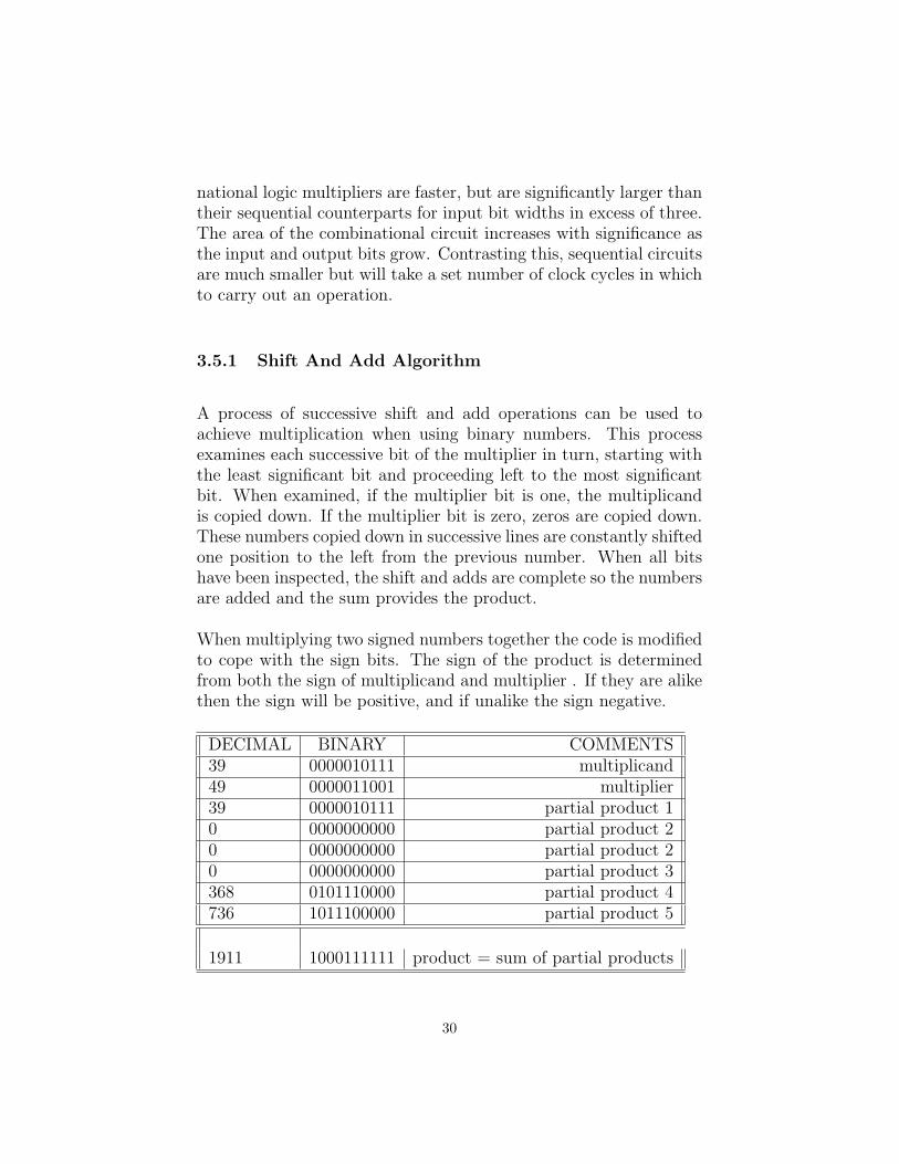
A process of successive shift and add operations can be used toachieve multiplication when using binary numbers. This processexamines each successive bit of the multiplier in turn, starting withthe least significant bit and proceeding left to the most significantbit. When examined, if the multiplier bit is one, the multiplicandis copied down. If the multiplier bit is zero, zeros are copied down.These numbers copied down in successive lines are constantly shiftedone position to the left from the previous number. When all bitshave been inspected, the shift and adds are complete so the numbersare added and the sum provides the product.

When multiplying two signed numbers together the code is modifiedto cope with the sign bits. The sign of the product is determinedfrom both the sign of multiplicand and multiplier . If they are alikethen the sign will be positive, and if unalike the sign negative.

DECIMAL BINARY COMMENTS39 0000010111 multiplicand49 0000011001 multiplier39 0000010111 partial product 10 0000000000 partial product 20 0000000000 partial product 20 0000000000 partial product 3368 0101110000 partial product 4736 1011100000 partial product 5

1911 1000111111 product = sum of partial products

30

3.5.2 Booths Multiplication Algorithm

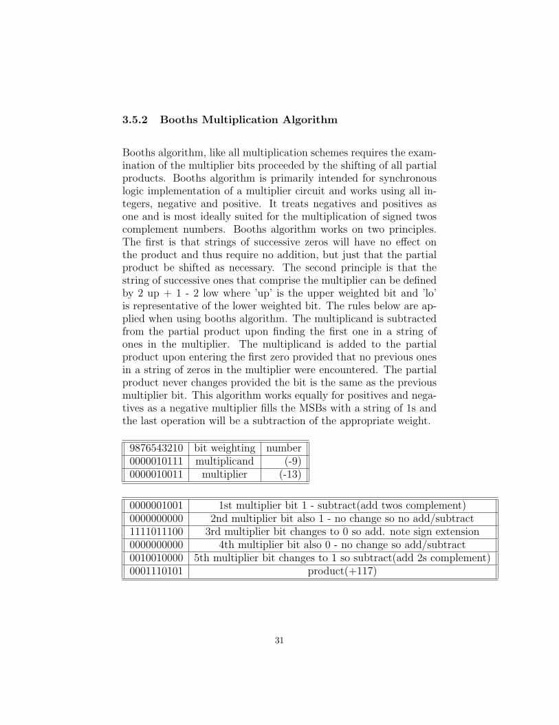
Booths algorithm, like all multiplication schemes requires the exam-ination of the multiplier bits proceeded by the shifting of all partialproducts. Booths algorithm is primarily intended for synchronouslogic implementation of a multiplier circuit and works using all in-tegers, negative and positive. It treats negatives and positives asone and is most ideally suited for the multiplication of signed twoscomplement numbers. Booths algorithm works on two principles.The first is that strings of successive zeros will have no effect onthe product and thus require no addition, but just that the partialproduct be shifted as necessary. The second principle is that thestring of successive ones that comprise the multiplier can be definedby 2 up + 1 - 2 low where ’up’ is the upper weighted bit and ’lo’is representative of the lower weighted bit. The rules below are ap-plied when using booths algorithm. The multiplicand is subtractedfrom the partial product upon finding the first one in a string ofones in the multiplier. The multiplicand is added to the partialproduct upon entering the first zero provided that no previous onesin a string of zeros in the multiplier were encountered. The partialproduct never changes provided the bit is the same as the previousmultiplier bit. This algorithm works equally for positives and nega-tives as a negative multiplier fills the MSBs with a string of 1s andthe last operation will be a subtraction of the appropriate weight.

9876543210 bit weighting number0000010111 multiplicand (-9)0000010011 multiplier (-13)

0000001001 1st multiplier bit 1 - subtract(add twos complement)0000000000 2nd multiplier bit also 1 - no change so no add/subtract1111011100 3rd multiplier bit changes to 0 so add. note sign extension0000000000 4th multiplier bit also 0 - no change so add/subtract0010010000 5th multiplier bit changes to 1 so subtract(add 2s complement)0001110101 product(+117)

31

3.5.3 Implementation of Sequential Shift and Add Multi-plier

This multiplier was modelled on the algorithm previously examined.It also entails a sign bit. The products sign is the result of exclusiveORing the sign of the two inputs. The operation starts when loadbecomes a logic one and the registers are loaded with values. regAbecomes zero, regB is loaded with the multiplicand minus its MSB,similarly regQ holds the multiplier without its sign bit. Ps, holdsthe sign when exclusive oring takes place between multiplicand andmultiplier sign bits. SequenceCounter is the number of bits in themultiplier without the sign bit. Multiplicand and multiplier arenow in registers B and Q respectively and operation is ready. Asis indicative of this algorithm, a series of consecutive test, add andshift right operations occur. The signal AddShiftB is controlling addor shift operations. When this signal is one the sum of regA andregB become the partial product that is then stored in another reg,EA, a combination of flip-flop E and register A. The carry out fromthe adder in flip-flop E needs to be stored so that it can be usedwhen it is time to generate the next partial product summation.EAQ is shifted right, the least significant bit of register A is shiftedinto the most significant bit of register Q. The bit from E is shiftedinto the MSB of register A, while logic 0 is then shifted into E.This shift causes one bit of the partial product in register A tobe shifted into register Q, forcing the multiplier bits one positionright. The rightmost flipflop in register Q, now Qn, will hold thebit of the multiplier which is next in line for examination. Onceinspected, if Qn is a logic 1 an addition will result before the nextshift occurs. However if Qn is a logic 0 no addition is necessary. Asingle multiplication will take from the width of the multiplier minus1 multiplied by the width of the multiplicand minus 1 multiplied bytwo, clock cycles to finish. This is dependent on the logic zerosand ones in the multiplier. When a multiplication has taken placethe one bit output, Done is set to 1. In this multiplier the inputand output bit widths can be specified according to the users needs.This particular model is also instantiated such that the width of theoutput is not necessarily the same as the combined width of the sumof the two input magnitude widths.

32

3.5.4 Design for Booths Algorithm in VHDL

I also toyed with the possibility of using a sequential multiplier thatimplemented booths algorithm. This hardware structure containeddistinct similarities with the structure implemented in the previ-ously examined shift and add algorithm. The three fundamentaldifferences, however, were firstly the need for an extra flipflop tobe placed at the LSB of the multiplying register. This is mainly tofacilitate double bit inspection of the multiplier. Secondly, this al-gorithm required the ability to subtract and lastly the flipflop thatheld the carry out from the adder in the standard shift and addapproach is not needed as an add here can never cause any over-flow. Once again when load is set the registers are loaded as before.After the two numbers to be multiplied are loaded into the appro-priate registers the operation starts by examining two test bits ofthe multiplier in a simple case statement. In the event of these twobits being ’10’, the first 1 in a string of 1s has been found in themultiplicand. This then requires a subtraction of the multiplicandfrom the partial product. After this subtraction has taken place oneor more shift operations take place until the multiplier bits storedin a register are equal to binary ’01’, t meaning that the positionof the first ’0’ in the multiplier has been found. When this first ’0’is found in the multiplier the multiplicand is added to the partialproduct, one or more arithmetic shift rights can occur until eitherthe next ’1’ is located or the total number of shifts is equivalent tothe length of the multiplier. After loading data again, if the twotest multiplier bits are equal to ’00’, no addition or subtraction isrequired and the shifting begins, searching for the first ’1’ in themultiplier. No overflow will ever take place due to the fact that ad-dition and subtraction operations alternate and the numbers beingeither added of subtracted have different signs. This condition willnever yield overflow. Following addition or subtraction the arith-metic shift right occurs on the partial product, the multiplier andthe flipflop. The arithmetic shift ensures that the most significantbit of the register of the partial products, before the shift, is copiedinto the most significant bit of the register, after the shift. This ad-dition/subtraction process is repeated for the number of bits in themultiplier. The VHDL implementation uses a process which takes invariables to compute intermediate values of addition or subtraction

33

prior to the shifting process. A procedure is then used to performthe shifting process as it is identical for each of the case statementsthat examine the test bits.

3.6 Problems in Simulation - Type unsigned

The code for both these implementations synthesised perfectly. How-ever when I tried to generate results for a testbench waveform I raninto difficulties. The code would not generate results although Iwas able to get a testbench module. Each time I tried to generateresults or perform simulation for the testbench I got an error whichread, ”no feasible entries for subprogram write”. After trying tofind the reason for this apparent error I stumbled on a conclusion.All my inputs and outputs were of type unsigned. I soon came tothe conclusion that VHDL can not simulate testbenches when theoutputs are of type unsigned. I tried out other entities with all out-puts of type unsigned and the same error occurred. However when Ichanged these to type std logic vector, testbenches were simulatedcorrectly and results generated as expected. I tried to verify on nu-merous occasions that what I had established was in fact correct. Iasked several other students doing VHDL and Verilog projects whodidn’t know if this was in fact true for all cases. I then asked paststudents who had previously completed a project in a hardware de-scriptive language. They both said that they thought that it waspossible to generate a testbench using this type. There was little orno information in VHDL books that helped and information on web-sites was again minimal. So for a time I was undecided on this issueuntil I came across a question on a website from a student tryingto simulate testbenches using all unsigned inputs and outputs andagain encountering similar difficulties. The response to her querywas in fact that it was not possible to simulated testbenches usingthis type but was possible for the remainder of types. To this pointI still am uncertain as to whether or not this can be done.

library.IEEE; use IEEE.STD_Logic_1164.all; IEEE.Numeric_STD.all;

entity MULT_SEQUENT is

34

generic(WidthMultiplicand, WidthMultiplier, MaxCount: Natural);

port(Clock, Reset, Load: in unsigned(WidthMultiplicand - 1 downto

0); Multiplier: in unsigned(WidthMultiplier - 1 downto 0); Done:

out std_logic; Product: out unsigned(WidthMultiplicand +

WidthMultiplier - 2 downto 0))

end entity MULT_SEQ;

3.7 Problems in Simulation - Types in VHDL

I disregarded the possibility of using unsigned outputs. Dealingfirstly with the sequential shift and add algorithm, I changed theoutputs to std logic vector, whilst leaving the inputs as unsigned.As I expected I got a type conversion error as I was foolishly try-ing to convert an unsigned input to an output of std logic vector.I then began researching type conversion in VHDL. I had previ-ously thought that these two types convert automatically as theyare closely linked types. Converting from one of these types to theother requires a type conversion in the form of casting or a typeconversion function. VHDL does have automatic type conversions.It is possible to convert from std logic vector to std ulogic vector.Type casting can be used when two types have a common base, likeunsigned and std logic vector.

FROM TO FUNCTIONStd Logic Vector unsigned unsigned(Std Logic Vector)Unsigned integer to integer(unsigned)Integer unsigned to unsigned(integer, no of bits)Unsigned Std Logic Vector Std Logic Vector

I tried endlessly to convert one type to another in VHDL usingpredefined functions that should have made my job pretty simplebut that didn’t. I would be unable to say for definite if this wasdown to me or problems with these functions in general that posedsuch difficulties. I also attempted writing my own type conversion

35

functions but I encountered similar setbacks. I was getting errorsin synthesis saying that these conversions were in compatible withthe packages, namely numeric std. However other functions in theprogram depended on this package and when I changed it, I got awhole new set of errors, although it seemed to fix this particular one.I finally admitted defeat and what I had learnt on type conversionand casting now seemed fruitless. A whole new approach to theproblem was necessary.

3.7.1 Libraries in VHDL

Back to square one, I made the decision to totally exclude all inputs,outputs, signals and variables of type unsigned from my instantia-tion in the hope that issues connected with them would now be re-solved. I hoped that I could simply replace them with std logic vectorsand began wondering why I hadn’t just done that in the first placeand saved myself needless intricacies. Back on track and with allvariables converted, I once more synthesised my instantiation. Thepackage that I included was the previously defined package for thisentity, ’numeric std’. Once synthesised, this generated more er-rors for me in the form of ’shift-right can not have operands in thisform’. I was swamped with similar error messages for the resizeoperator, which was primarily used to adjust the size of registers tohold growing bits in variables and signals. After running a differentexample from a different source(not my own work), using the samepackage and inputs/outputs of type std logic vector, when using theshift right operator I got exactly the same error message in synthe-sis. However, if changed to an slr or sll operator with the operandsrearranged to suit I found that the entity synthesised. It also simul-tated a testbench and generated the appropriate results accordingly.Having finally made a breakthrough I tried this approach on my pre-vious code, exactly as was in the simpler entity only to find it didn’thave a similar effect and once again left me with the same errors.On examining my new-found situation, I found that for pre-definedoperations, the package numeric std is used to define types of signedand unsigned and all arithmetic, comparison and logical operationsfor these types. Similarly for the package std logic arith it defines

36

arithmetic and comparison operations for types signed and unsigned.

3.7.2 Packages in VHDL

Whilst experimenting with packages, I changed the package fromnumeric to arithmetic whilst keeping all types as before. This time,after synthesis, error messages were different. They took the formof ”Undefined symbol ’resize’” and ”Undefined symbol ’shift-right’”.This would in fact verify the deduction that these functions are notavailable to std logic vectors when using std logic arith. Howeverthis may not be the case for std logic vectors and the package nu-meric std as the error indicates that these operations are compatiblewith this particular package but that they should simply take a dif-ferent form. In the event of both of these packages being excluded,it becomes apparent that these operations are dependant on nu-meric std as once again an ’undefined symbol’ message is returned.

Reviewing these Packages

From the synthworks website, I ascertained most of the basics neededwhen dealing with packages and types in VHDL. As stated in theprevious subsection, numeric std is used for types signed and un-signed and all logic, arithmetic and comparison operators carriedout on them. Std logic arith defines types signed and unsigned andarithmetic and comparison operators can be defined within the scopeof these types . Std logic unsigned defines arithmetic and compari-son operators for std logic vectors. From the aforementioned sourceand a couple of other sources, it is widely recommended that oneuses numeric std for all new designs. This package also maintainscompatibility with the package std logic unsigned. It is also ad-vised that for numeric operations, you can use std logic arith withstd logic unsigned, but that the packages std logic arith and nu-meric std should never be used together. When examining this Ifound that if these two packages are used together, the one namedfirst is the one used and the other package is ignored. Other thanthis it has no effect on the entity. The higher one simply takes

37

precedence and the later will be unaffecting. When using arith-metic operations availing of the package unsigned in conjunctionwith the arithmetic package worked best. It was useful to later findout that this was due to the unsigned packages influence as opposedto any other which primarily didn’t register. When replacing oreliminating the arithmetic package errors were endured, which pre-sumably meant that there was a reliance on this package but thatthe unsigned package was priority. These packages were later usedtogether in pursuit of alternatives.

Influencing Nature of these Packages

Believing that a wealth of knowledge would have been obtained fromthe experiences with these packages, difficulties were attempted tobe rectified once and for all. Needless to say this was easier saidthan done. Failure at every point when trying to adjust the shiftand resize statements to work effectively for my design was met.To this point I do not know if the shift operator can be used withstd logic vectors when using the numeric package. I only know thatit is impossible with the arithmetic one. If it is not possible for logicvectors and only possible for type unsigned it is in fact useless if onecan not generate testbench waveform outputs. However on eitherof these counts I would be open to correction and indeed any feed-back or expertise that could shed light on my apparent inabilities.Regrettably not an awful lot of information was available to me.Any information that was on offer was sometimes ambiguous andoften contradictory. Confusing would be an understatement. Any-thing else ascertained on this subject was through plain old trialand error. With more experience in the first place setbacks couldhave been avoided or once encountered eliminated. Examinationof the need to use unsigneds in the first place brings its own con-clusions and in hindsight this was perhaps completely unnecessaryand logic vectors would have been a safer alternative. Lessons werelearnt as frustration mounted and from here on in the easier optionwould inevitably be pursued as more confidence and ability with theconstructs of the language was paramount to any progress.

38

3.8 Sequential Multiplier - The final Curtain

Rewriting the shift right operator to simply shift the vector one placeto the right and concatenating it with a zero in its lsb and similarlycoding a function for resize that placed all contents of a register intoa register of a greater defined size made my entity synthesisable.

E_regA_regQ := shift_right(E & RegA & regQ), 1);

This is replaced by a small set of instructions. RegG was previouslydeclared a signal one bit size larger.

E_regA_regQ := E & RegA & RegQ;

RegG <= E_regA_regQ & ’0’;

Test bench waveform results were all undefined for certain inputsand for a time I believed it to be the readjusted code. However oncloser examination I realized that it was because of the structureof the if statements and that because of the inputs I had given arelevant output could never be met because the program had nowhere to go. I further verified this by inserting fixed inputs into thetestbench that I knew would result in output as it would comply withthe first if statement and would not require any further testing in theprogram. The results were as expected. Due to the complexity andstructure of the entity I was unable to change it. However this wasthe first time I had found a flaw in the code. Due to my frustrationand ongoing struggles with this particular piece of code, I firmlydecided to leave it where it was, in a book. I felt now that if I hadbetter employed my time in writing entities of my own as opposedto using ones from source it would have been more rewarding. Codelike this, on both counts, turned out to be worthless in terms ofmy project. I resigned myself for future exploits to design and codefrom scratch given these prior dilemmas and experiences.

39

3.9 Signed Combinational Multiplier - Alterna-tive Approach

This combinational multiplier is also modelled on the shift and addalgorithm and is the one I used in my implementation. Once moreit contains an exclusive OR of the input sign bits when generatingthe output sign. The models structure is based on parallel adders.Partial products are computed according to the algorithm, zero ifthe associated bit in the multiplier is zero or a shifted version in theevent of a one. The partial products are obtained using conditionalsignal assignments and don’t infer logic but merely specify how theshifted multiplier input is connected with the adders. It is much lesscomplex than the sequential multiplier but was easily implementedand adjusted to deal with fixed point numbers and integers alike.The input bit width can be changed at will, however all internalsignals then have to be modified accordingly. This can be achievedwithout too much effort or indeed thought. As stated fixed pointnumbers were taken into account by a modification of the designthat once again separates out the integer and fractional parts of thenumber, dealing with them separately and outputting an integerand fraction when the set bit is asserted. When the set bit is a zerointeger multiplication simply takes place incurring a single integeroutput.

40

Chapter 4

Fourth Chapter

4.1 Dealing with two dimensional arrays - ma-trices in VHDL

This chapter entails examining two dimensional arrays in VHDLand finding the most feasible approach to matrix implementation.

4.2 Overview of Arrays

Like in most software object oriented languages, an array in vhdlis an indexed collection of objects all of the same type. Arraysmay be one dimensional or indeed multidimensional. In VHDL,an array type may be constrained, in which the bounds for theindex are determined when the type is first defined. Naturally anunconstrained array would imply that the type is defined and theindex bounds are established subsequently. This is exactly whathappens.

type myWord is array(15 downto 0)of std_logic;

41

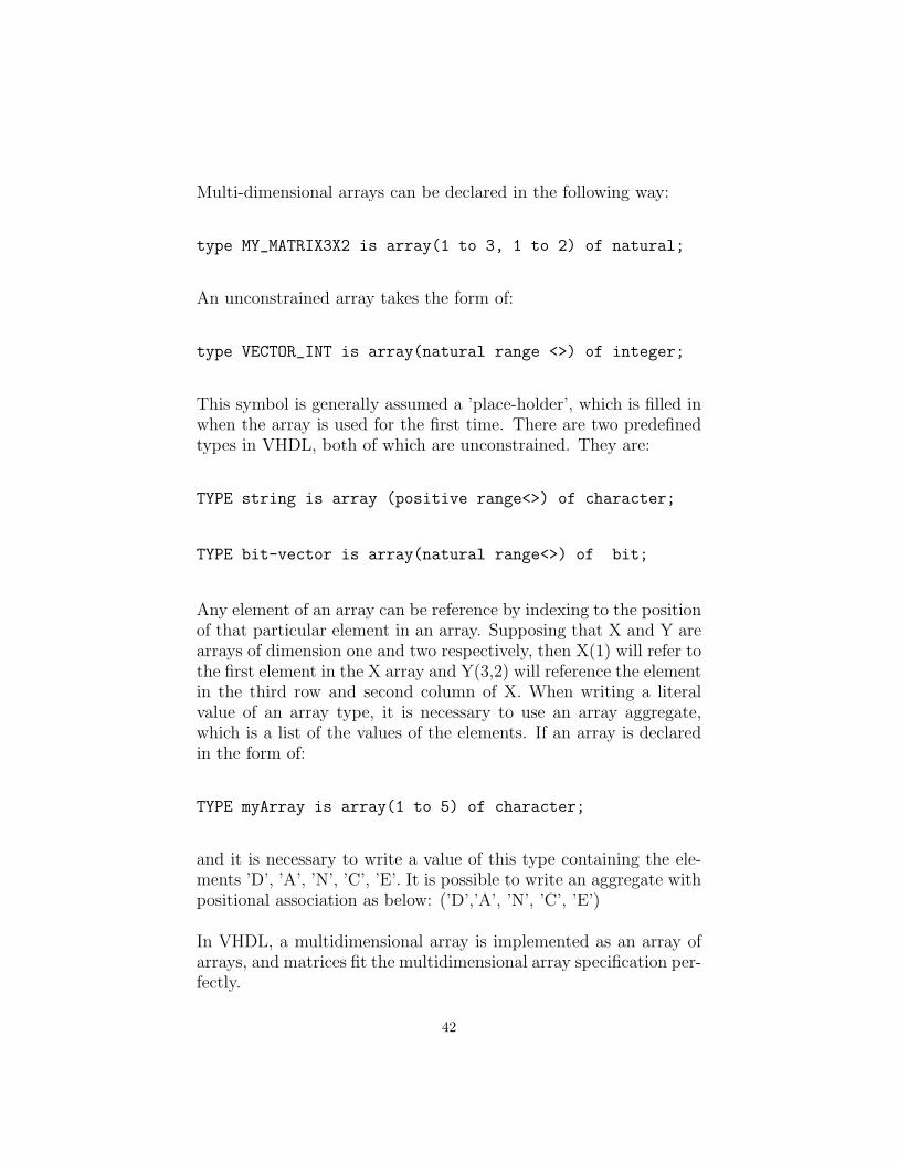
Multi-dimensional arrays can be declared in the following way:

type MY_MATRIX3X2 is array(1 to 3, 1 to 2) of natural;

An unconstrained array takes the form of:

type VECTOR_INT is array(natural range <>) of integer;

This symbol is generally assumed a ’place-holder’, which is filled inwhen the array is used for the first time. There are two predefinedtypes in VHDL, both of which are unconstrained. They are:

TYPE string is array (positive range<>) of character;

TYPE bit-vector is array(natural range<>) of bit;

Any element of an array can be reference by indexing to the positionof that particular element in an array. Supposing that X and Y arearrays of dimension one and two respectively, then X(1) will refer tothe first element in the X array and Y(3,2) will reference the elementin the third row and second column of X. When writing a literalvalue of an array type, it is necessary to use an array aggregate,which is a list of the values of the elements. If an array is declaredin the form of:

TYPE myArray is array(1 to 5) of character;

and it is necessary to write a value of this type containing the ele-ments ’D’, ’A’, ’N’, ’C’, ’E’. It is possible to write an aggregate withpositional association as below: (’D’,’A’, ’N’, ’C’, ’E’)

In VHDL, a multidimensional array is implemented as an array ofarrays, and matrices fit the multidimensional array specification per-fectly.

42

4.2.1 Addition of Arrays - Attempt One

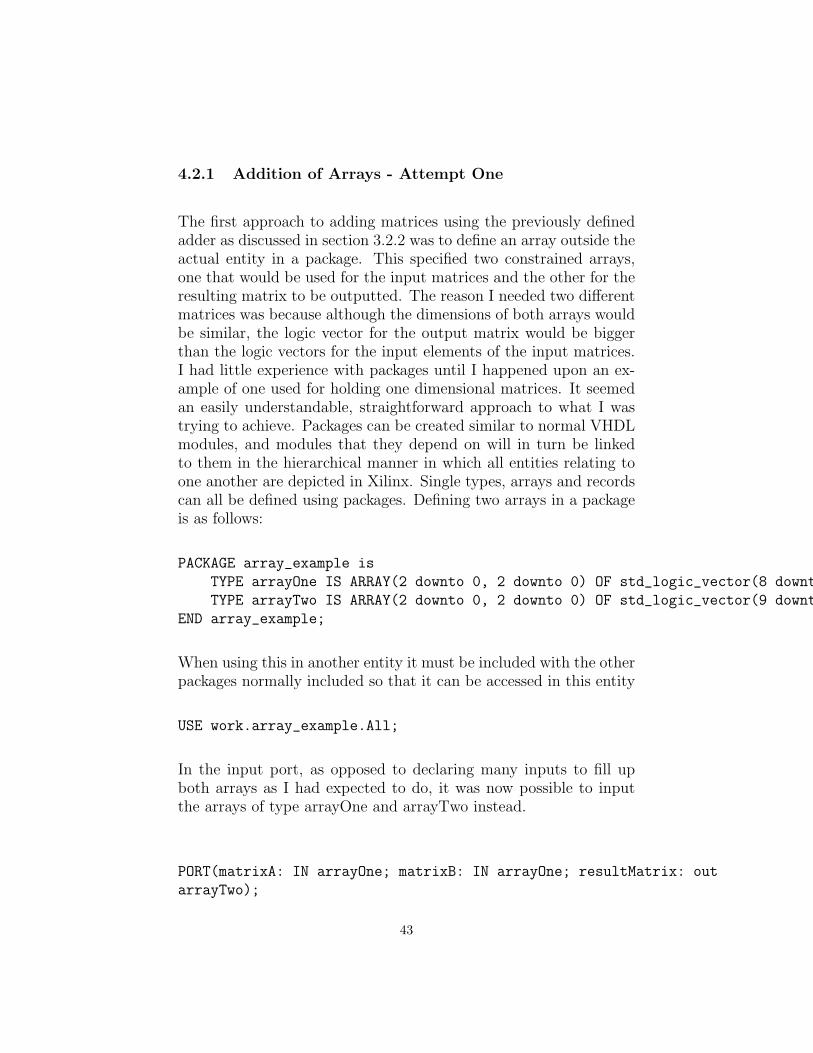
The first approach to adding matrices using the previously definedadder as discussed in section 3.2.2 was to define an array outside theactual entity in a package. This specified two constrained arrays,one that would be used for the input matrices and the other for theresulting matrix to be outputted. The reason I needed two differentmatrices was because although the dimensions of both arrays wouldbe similar, the logic vector for the output matrix would be biggerthan the logic vectors for the input elements of the input matrices.I had little experience with packages until I happened upon an ex-ample of one used for holding one dimensional matrices. It seemedan easily understandable, straightforward approach to what I wastrying to achieve. Packages can be created similar to normal VHDLmodules, and modules that they depend on will in turn be linkedto them in the hierarchical manner in which all entities relating toone another are depicted in Xilinx. Single types, arrays and recordscan all be defined using packages. Defining two arrays in a packageis as follows:

PACKAGE array_example is

TYPE arrayOne IS ARRAY(2 downto 0, 2 downto 0) OF std_logic_vector(8 downto 0);

TYPE arrayTwo IS ARRAY(2 downto 0, 2 downto 0) OF std_logic_vector(9 downto 0);

END array_example;

When using this in another entity it must be included with the otherpackages normally included so that it can be accessed in this entity

USE work.array_example.All;

In the input port, as opposed to declaring many inputs to fill upboth arrays as I had expected to do, it was now possible to inputthe arrays of type arrayOne and arrayTwo instead.

PORT(matrixA: IN arrayOne; matrixB: IN arrayOne; resultMatrix: out

arrayTwo);

43

In the body of the entity was a process containing the two inputmatrices which would be subsequently indexed through using a forloop and the corresponding elements would be added together usingportmaps. The output of the adder would then carry the results toeach position in the resulting matrix.

MA1: adder port map(adder1 => matrixA(i), adder2 => matrixB(i),

adderOut => resultMatrix(i));

After a little work the code synthesised and the testbench waveformwas generated. However when I tried to input numbers into thetestbench that contained more than one bit, a warning was returnedwhich read, ”string error” ”bit width is more than 1”

On entering a 1 or a 0 into the testbench no warning was returned,however anything bigger caused the above warning to be outputted.This was of course little use to me as the problem could not belocated as all of the logic vectors were nine and ten bits wide re-spectively. Once again, having hit a brick wall, it was back to thedrawing board. Rectifying this error by checking it out on the inter-net was impossible and finding a means of resolution was difficult.However in a bid to prove that this was not to do with my code,an example from a VHDL textbook , which my code was closelymodelled on was synthesised. This code used a package to declaretwo one dimensional arrays of type bit and with 32 and 8 bit arrayelements respectively. A function was performed on these arrayswhich is irrelevant to the problem description. When the bits werechanged to anything more than a single bit, the error once more oc-curred in the testbench. A couple of other examples gave a similarerror and I was unable to sort it out. Disillusioned, I disregardedthe possibility of using packages to define arrays and set about tofind an alternative way to do this.

4.2.2 Addition of Arrays - Attempt Two

After this it was decided that I would declare all inputs and outputsof the array in the input port. This meant I would now be using

44

arrays of fixed size and I decided on firstly using three by threematrices until I was in a better position to be changing the sizewhen required. This was very easy to do. After all inputs weredeclared, two array types were defined in the architecture of theentity. Then three matrices of these types were declared as signals.

TYPE arrayOne IS ARRAY(2 downto 0, 2 downto 0) OF

std_logic_vector(8 downto 0);

TYPE arrayTwo IS ARRAY(2 downto 0, 2

downto 0) OF std_logic_vector(9 downto 0);

Signal matrixA: arrayOne; Signal matrixB: arrayOne; Signal

ResultMatrix: arrayTwo;

Each of the inputs were placed into each element of the arrays, theseelements were then added together and results were placed in theresulting array, which were in turn outputted. Although a verysimple approach, this was one that worked.

4.2.3 Addition of Arrays - Final Attempt

After a meeting with my supervisor, I was strongly advised to imple-ment these arrays in VHDL using blockram. Previously unknownto me, once again research was inevitable. The Spartan 2E FPGAshave blocks of bits, 4096 bits per block, called block ram that can beconfigured as single port or dual port ram. Block ram can be used asdata ram for a processor or if broken into smaller pieces can be usedas register files. To my understanding, in dual port ram the inputsare written to memory using the address lines and the outputs aresubsequently read. Depending on the size of the board being usedthe input bit widths have to be adjusted accordingly. Deciding notto make this factor a priority, I firstly set the data inputs to 20 bits.This meant that data for both the first element of matrix A and thefirst element of matrix B would come in on the first data line. Thedata outputs were set to 10 bits. This was done as below:

45

Generic(data_width1 : natural := 20;

Addr_width1: natural := 18;

Data_width2: natural : = 10;

Addr_width2 : natural := 10);

The same amount of address lines as data input lines were required.An array was created to store the data elements. This took the formof:

Type mem_type is array(2 downto 0, 2 downto 0) of

std_logic_vector(data_width -1 downto 0);

On realising that the inputs and outputs were not the same size,difficulties were envisioned. Attempting dual ported ram would notbe feasible unless two different arrays were created of different bitsizes or if inputs were made one bit bigger. In reality neither ofthese options would work due to the fact that the same memoryarray would be needed when writing and reading values. Due to thisI opted for the easier option of using single port block ram wherethe inputs would be written to memory and outputted from here.This was done using a process, on the rising edge of the clock withthe write signal asserted, all data inputs were written to memory.From here, exactly the same procedure as was described above toadd the matrices using portmapping was carried out. The code wassynthesised and testbench outputs verified that the implementationworked as expected. Some time was allocated to trying to get thedesign to work for dual port ram. However with time pushing onand so much other work needing to be done, I resigned myself towhat I had and made a mental note to return to this in the eventof me having any spare time towards the end. I hoped rather thanbelieved this would be the case.

4.3 Matrix Multiplication using Block Ram

The next logical step in the project was to similarly use block ram inan implementation of matrix multiplication. Block ram was used in

46

exactly the same way as above to allocate memory for storage of eachof the data inputs. The algorithm for matrix multiplication requiredthe use of the multiplier entity to multiply the data inputs and thenthe adder entity to add these products. Internal signals were usedto hold the results of the partial products after multiplication wasachieved. These signals had to be continually changed to facilitatethe growing bit widths, as data inputs were multiplied added toanother product of multiplication and this in turn added to anotherproduct. This also meant that the bit widths of the adder had tobe changed.

As the signals grew in size to store products it was essential that thesign was handled. If a zero was concatenated with a number, in orderto make it bigger, and it was positive this would be fine. Howeverin the event of it being negative and the msb being representative ofits sign, this would seriously damage the process. For this a processwas created with a series of if statements which tested whether themsb was a 1 or a zero. In the case of a one, this one was shifted tothe most significant bit and a zero was put into this position, therest of the logic vector remaining as it was. This meant that it wouldbe still the same number and represent that number whether it wasplus or minus. When generating expected outputs in the test benchit made it a little difficult to calculate whether the design workedas required as the growing bit widths meant that for any negativenumbers, the output number was extremely high. However afterchecking all these results, clearly the design worked as expected.

Problems with Block Ram

One of the only difficulties encountered when using block ram wasthe size of the data inputs. When declared at the beginning of theentity as:

Generic(data_width1: natural:= 20);

This being used to effectively hold two data inputs it appeared tobe fine to do this. However in synthesis the process ran forever and

47

never came to the point where it returned the output message ’syn-thesis completed’. On one occasion, when left, the process had notfinished after forty five minutes so the process was then terminatedas it looked as though it would never synthesise. If the data widthwas subsequently changed to ten and then synthesised, obviouslywith the size of everything else changed too, then the process wasvery slow but it did eventually synthesise. Beyond this point if thebit width was changed the process became slower and slower to thepoint where it was uncertain whether or not it would ever finish.Obviously changing the data width to ten was of little use to meas it was too small to hold two inputs. Afterwards, not knowingthe cause of this and not really knowing what to do, I just allowedall data inputs to be independent of one another and were declaredseparately in the entity. This was indeed contradictory to one datainput holding two matrix values but on feeling that it couldn’t behelped this was the next best thing.

48

Chapter 5

Fifth Chapter

5.1 Simplistic Transpose Design

The most non complex of all entities, the module basically took nineinputs and outputted them in order which is intrinsic to the trans-pose algorithm. Placing the elements into different array positionsand then outputting these results was all that was needed in thisimplementation. The size of the matrix could be changed at willas is understandable from the simplistic nature of matrix transposealgorithm. Sizes were adjusted in accordance with what would beneeded for successful implementation of this entity in the designfor a matrix inverter. The time taken to complete this design wasminimal in comparison with previous entities. Synthesis was per-formed and simulation results proved that this specification workedas expected.

49

5.2 Inverting a Matrix - Design for an AdjointMatrix

As the size of the previous matrices were all three by three in dimen-sion, the adjoint matrix presented itself as a very real possibility forsuccessful matrix inversion. Having been advised by my supervisorto implement an inverter using Gaussian elimination, I researchedthis once again in great detail and examined the C++ code on ma-trix inversion that was presented to me. Naturally, Gaussian elimi-nation would have been the most effective and indeed elegant optionto pursue as it deals with matrices of any dimension. The adjointmatrix formula is limited to a specific size and is inefficient for ma-trix inversion when the dimensions grow in excess of four by four.However due to the apparent complexities that would be involvedin carrying out Gauss Jordan elimination in VHDL I opted for thelater and time permitting would perhaps review my choice. Onceagain I was dubious. Feeling that I was ill equipped for concatena-tion of an identity matrix with the original matrix in the very firststep evidently posed some concerns. This coupled with a series ofcomplex tests and adds of individual rows, whilst trying to derivean identity matrix on the LHS, further confirmed my reservations.A more confident VHDL programmer may have had the means andability to successfully deal with this. Regrettably I was not at thisstage of expertise.

As is indicative of the adjoint matrix formula, cofactor expansionneeded successful coding. First off was the task of computing thematrix of minors. This involved computing cofactors(determinantsof the matrix for ith row and jth column as in chapter 1). Availingof the multiplier entity along with a subtractor (already designed)this was achieved quite easily. To compute the matrix of minors, asign change is then applied to the second, fourth, sixth and eightelements of the newly formed matrix of cofactors. This sign changewas computed by making all elements one bit larger whilst dealingwith the msb as the sign of the number as in matrix multiplica-tion. Subsequently, the second, fourth, sixth and eight elementswere exclusive ored with a one, changing their signs. This had thesame effect as multiplying them by minus one. This being achieved

50

the values were transposed and this completed the first stage , thematrix of minors.

Next logical step was to compute the determinant of the whole ma-trix. Cofactor expansion along the third row seemed appropriate.This step again was straightforward in that matrix multiplicationand subtraction, coupled with addition of these results, was all thatwas necessary. Not very complex as all were previously coded enti-ties. This concluded this step.

The final step was were any difficulty would lie. All the values in thematrix of minors needed to be divided by the overall determinantachieved through cofactor expansion. This inevitably required afractional divisor, as the values in the matrix are always going to bemuch smaller than the determinant value.

5.2.1 Fraction Divisor in VHDL

The combinational divider was modelled closely on a 10 bit divide by5 bit combinational logic divider from ’HDL chip design. Howeverthis divider had to be changed to a fraction divider for the purposesof my design implementation. With this divisor instead of usingconsecutive sequences of shift, compare and subtract operations, itis more appropriate to use consecutive sequences of shift and adda twos complement number. Adding a twos complement number isequivalent to subtraction, however its convenience lies in that factthat a single adder can perform both the compare and subtractoperations. The carry out from this will provide an indication as towhich of the inputs is the larger of the two.

The first compare is of the upper bits of the dividend this size alwaysbeing the same as the size of the divisor. This is followed by a chainof add, compare and shift operations. The VHDL code used for thisimplementation is a series of signal assignments and if statements.As the number of bits in the dividend grows with the dividend re-maining the same there will be a significant growth in the numberof if statements.

51

SIGNAL NAME BINARY VALUE OPERATIONA (dividend) 0111000010 (450)B (divisor) 10001 (17)2’s comp B 01111Overflow 0Compare1[5:0] 101011 A[8:4] + 2’s comp BQuotient[4] 1PartRem1[4:0] 01011 Compare1[4:0]PartRem1 Abit[4:0] 10110 Bring down dividend bit 3Compare2[5:0] 100101 Compare1 Abit + 2’s comp BQuotient[3] 1PartRem2[4:0] 00101 compare2[4:0]PartRem2 Abit[4:0] 01010 Bring down dividend 2Compare3[5:0] 011001 Compare2 Abit + 2’s comp BQuotient[2] 0PartRem3[4:0] 01010 Compare2 AbitPartRem3 Abit[4:0] 10101 Bring down dividend bit 1Compare4[5:0] 100100 Compare3 Abit + 2’s comp BQuotient[1] 1PartRem4[4:0] 00100 PartRem3 Abit - BPartRem4 Abit[4:0] 01000 Bring down dividend bit 0Compare5[5:0] 010111 Compare4 Abit + 2’s comp BQuotient[0] 0Quotient[4:0] 11010(26)Remainder[4:0] 01000(8)

Changing the structure of this entity a little, a 20 bit divide by 10bit divider took on the same form as the previous divider. Whencompleted a 9 bit divide by 10 bit was attempted using the be-haviour modelled in the 20 bit divide by 10 bit. The 9 bit input wasmultiplied by 100 and concatenated with zeros so it would fit thetwenty bit wide stipulation. To multiply the number by 100 it wasmultiplied by 10 twice. This was achieved by shifting it to the leftthree times storing the result. The original was shift left once andsubsequently added to the stored result. The procedure with thisnew result was repeated, effectively multiplying the original numberby 100.

52

Because it was a fraction divisor there was a need for an extra bitwhich held the sign of the number. The input signs were testedin a process containing a series of if statements The output signswere then deduced accordingly. The output number was also con-catenated with a 0 to represent the bit left of the decimal point.Testbench outputs verified its functionality.

5.3 Inverting a matrix

With this new divisor successfully implemented, matrix inversionseemed like just a step away. First the design was tested to seeif the matrix of minors was working. This along with cofactor ex-pansion for finding the matrix determinant was working. Howeverwhen trying to divide by the determinant it became apparent thatbit widths didn’t match because the sign part of the fraction divisorhad been overlooked. Having spent an awful lot of time on the divi-sor and encountering some difficulties, I felt that it would be moreappropriate to change the bit width of the rest of the entity. Withjust a day to the demonstration, this seemed like an impossible task.After changing the entity and allowing the divisor to remain as was,I was in undated with a series of synthesis errors and was unable tofigure out what they were. Disappointed and disillusioned, I decideto just demonstrate what I had done with the hope of perhaps get-ting it working after the demo. Needless to say once again this didnot materialise, at large due to difficulties with an adequate divisorand ongoing commitments to other course material.Previously find-ing it difficult to locate appropriate material on this topic, did nothelp my cause.

53

Chapter 6

chapter six

6.1 Review of the project and personal thoughts

The initial task which was probably of most importance was back-ground research. A lot of this proved to be informative and at timesinteresting. Without this key factor project progress would havebeen impossible and reference material, though at times sparse, en-abled a form of resolution and even verification. It was paramountto achieving any kind of finished product and to say that it proveda helping hand is an understatement. Without resources readilyavailable any support a student has would be severely diminished.My only reservation is that at stages I personally felt that I did nothave as much material as I could have. From the early stages of theproject, it was thought-provoking to see how the kalman filter actu-ally worked. Without deep examination, one could not understandits capabilities and what I believe of it now is far removed from anyinitial reaction towards it.

Its implementation in VHDL although at times difficult and evenstraining was all in all a worthwhile experience. My familiarity withthe language grew in leaps and bounds as the project progressedand in the later stages I felt I had really obtained a firm grasp ofthe key concepts of VHDL. For a relatively inexperienced program-

54

mer, it was refreshing to know that most things in VHDL can bedone using simple statements, namely processes, if statements andloops. This strongly influenced my learning curve as the spectrumof what was needed to be known could often be kept to a minimum.I would now have a strong belief in what was attempted to be in-stilled in me from first year. This being, that the only way to learnanything in any programming language is to actually take the timeto sit down and do it for yourself, without interruption. The hard-ware labs provided an environment to do just that, an environmentthat is not always available when dealing with other languages. Itprovided solitude, isolation and above all somewhere to think and towork. I wished I had taken this advise earlier on, and my relation-ship with and of course attitude towards the course would have beendifferent. Ideally this habit should come naturally to a student butunfortunately for me it was a case of needs must. It was only towardthe end of the project that I really appreciated how dedication andhard work were of utmost importance and anything else would comesecond. Arguably interest should remain high on ones agenda butwhere this is lacking dedication towards some form of interest couldin circumstances compensate. Despite at times being set back ordisappointed, sometimes this could have been mistaken for negativ-ity, there were areas of the project that proved enjoyable. There isan immense sense of achievement as stages are completed, goals ob-tained and the finishing line in sight as opposed to a tiny spec far,far away. This of course also empowers the student and providesconfidence for the next stage. As confidence builds the next stage ismore do able. As things become easier, productivity grows and timeis more well spent. It is only when resolution seems impossible thatones ability to apply themselves wane and that time is consumedneedlessly. Also paths taken that need not be taken are also unde-niably another factor that uses time and resource. However this isprobably all part and parcel of the learning curve. Indecisivenessand reliability on trial and error understandably did not help mycase but I suppose that this could be eliminated with practice.

55

6.2 Doing it all over again ....

At my demonstration, I was asked that all important question ”whatwould I do differently if I was starting the project now?” I felt Ihadn’t answered the question as well as I could have. Obviouslya lot of things could have been done differently but at times toomany approaches seemed to be more of a problem than anything.Justifiably I would spend less time on research as full knowledge ofthe kalman filter although interesting was a little more than use-less. Also given that I did not have time to put my project on theboard, thorough research of FPGAs seemed a little wasted. Timelike this could have been better spent on actual coding and at thevery least getting a working inverter. Too much time was spentchecking alternative code that had no reference to my project, justto see if a particular thing worked in VHDL. A lot of frustrationcame from the fact that at times things seem much harder to do inthis hardware language than they would in an alternative softwareone. Also my limited knowledge on libraries, types and packagesleft me naturally disadvantaged. As time was an issue I would haveset out a timetable for steps to be achieved. I would not have al-lowed myself to be as flexible as I was though. In hindsight loomingdeadlines for other coursework at times did not give me much scope.If I started tomorrow with the benefit of what I now know I wouldbe more focused and have a definite plan in mind of the path theproject would take. I would also not allow myself to become dis-heartened when things didn’t work out as planned and with moretime I would be able to step back, take a deep breath and regainmy focus. In saying this continually crashing computers wouldn’thelp my cause. Needless to say timing was a major issue and every-thing considered there just seemed there wasn’t enough of it. Withthe benefit of hindsight things could have been managed better anddemonstration more successful.

56

6.3 Future Work

Scope for improvement - obviously, quite definitely. My work is onlya tip of the iceberg in comparison to what could be done with thisproject. With adjustments across the board, namely with a vari-able size for matrices and bit widths, the kalman filter algorithmcould be successfully carried out in VHDL. Also some work wouldbe needed for an efficient inverter and fractional divisor. This allbeing achieved it would be time to implement the all important,aforementioned equations. There would only be a very small transi-tion between having a working inverter and having a working kalmanfilter implementation. I strongly propose that another student takeon this project and see what they can achieve. Undoubtedly the fin-ished product would be well worth the hard work and I personallywould take a great interest in its implementation in the later stages.

57

BIBLIOGRAPHY

(1.) Pellerin Taylor - VHDL Made Easy, 1997 Prentice Hall

(2.) Lipsett/Schaefer/Ussery - VHDL: Hardware Description andDesign, Eleventh printing 1993

(3.) Weng Fook Lee - VHDL Coding and Synthesis with Synopsys,2000 Academic Press

(4.) Morris M Mano - Logic and Computer Design Fundamentals,3rd Edition

(5.) Wiley - VHDL Programming with Advanced Topics, WileyProfessional computing

(6.) Douglas E Ott, Thomas j Wilderotter - Introductory VHDLfrom Simulation to Synthesis, Klumei Academic Publishers

(7.) Smith, Douglas J - HDL chip design: A Practical Guide forDesigning, Synthesising and Simulating ASICS and FPGAs usingVHDL or Verilog, Madison, Al Doone Publications(1996).

(8.) Yu-chin hsu, Kevin F Tsai, Jessie T Liu, Eric S Lin - VHDLModelling for Digital Design Synthesis, Klumer Academic Publish-ers

(9.) Ercegovac, Lang, Moreno - Introduction to Digital Systems

(10.)Kevin Skahill - VHDL for Programmable Logic, Addison Wes-ley

(11.) Charles E. Roth, Jr.- Digital System Design Using VHDL,PWS Publishing Company

(12.) Sudhakar Yalamanchili - VHDL Starter’s Guide

(13.) Brian Hahn - Essential Matlab for Scientists and Engineers

58

(14.) Darren Redfern - The Matlab Handbook

(15.) Anton - Elementary Linear Algebra, John Wiley and Sons Inc

(16.) Hoffman/Kunze - Linear Algebra, Second Edition

(17.) Lang - Linear Algebra, 3rd edition

(18.) F.R. Gantmacher - The Theory of Matrices, Amer Mathemat-ical Society

(19.) http://www.xilinx.com/bvdocs/appnotes/xapp204.pdf

(20.)http://www.eda.ei.tum.de/forschung/vhdl/

(21.) http://www.eda.org/comp.lang.vhdl/FAQ1.html

(22.)http://ieeexplore.ieee.org/

(23.)http://www.acc-eda.com/

(24.)http://toolbox.xilinx.com/

(25.)http://www.ashenden.com.au/

59