ACKNOWLEDGEMENTS - core.ac.uk · for their continuous support, namely, Omar Alburaiki, M. Fuady,...

ACKNOWLEDGEMENTS

All praise is to Almighty Allah and his beloved messenger Muhammad(SAWS).

I am grateful to King Fahd University of Petroleum and Minerals for providing

a great environment for education and research.

I extend my deepest gratitude to my thesis advisor Dr. Magdi S. Mahmoud

for his continuous support, patience and encouragement. He stood by me in all

times and was the greatest support I had during my tenure in the university

and most importantly during my thesis. I would also like to thank my thesis

committee Dr. Abdul-Wahid Al-Saif and Dr. Moustafa ElShafei for their time

and valuable comments.

I would also like to thank the deanship for scientific research (DSR) at KFUPM

for financial support through research group project RG-1105-1.

A very special thanks goes out to Hadhramout Establishment for Human Devel-

opment for the scholarship which enabled me to undertake an M.Sc. program

at King Fahd University of Petroleum and Minerals in Saudi Arabia. I am

truly thankful to all of the Hadhramout Establishment members and supporters

specially Eng. Abdullah Ahmed Bugshan and Dr. Saleh Arm.

I would like to acknowledge my parents for their everlasting love, trust and

faith in me for providing me the finest things I ever needed. I could never

have pursued my higher education without their encouragement and support.

To beloved my wife, my dauther Renad, my sisters, and my brothers, Walid,

Abdullrab , Zuhair, Omar. Also I am thankful to all my family who have always

loved and supported me in all forms of life, their love gives me immense strength

to keep moving ahead.

Last but not the least, I would like to thank all my friends and colleagues back at

home and at KFUPM whose presence and discussions were the biggest support

during times of loneliness and despair. Things would not have been better if not

for their continuous support, namely, Omar Alburaiki, M. Fuady, Mirza H. and

M. Masood.

ii

Contents

ACKNOWLEDGEMENTS i

TABLE OF CONTENTS iii

LIST OF FIGURES vii

ABSTRACT (ENGLISH) x

ABSTRACT (ARABIC ) x

1 INTRODUCTION 1

1.1 Overview . . . . . . . . . . . . . . . . . . . . . . . . . . . . . . . 1

1.2 Fundamental Issues of NCSs . . . . . . . . . . . . . . . . . . . . 5

1.2.1 Band-Limited . . . . . . . . . . . . . . . . . . . . . . . . 5

1.2.2 Time Delay . . . . . . . . . . . . . . . . . . . . . . . . . 5

iii

1.2.3 Packet Dropouts . . . . . . . . . . . . . . . . . . . . . . 6

1.3 Why Networked Control Systems (NCSs)? . . . . . . . . . . . . 6

1.4 Thesis Objectives . . . . . . . . . . . . . . . . . . . . . . . . . . 8

1.5 Problem Statement . . . . . . . . . . . . . . . . . . . . . . . . . 8

1.5.1 Plant Model . . . . . . . . . . . . . . . . . . . . . . . . . 8

1.5.2 Hold Input Scheme Model . . . . . . . . . . . . . . . . . 11

1.5.3 Zero Input Scheme Model . . . . . . . . . . . . . . . . . 12

1.6 Thesis Organization . . . . . . . . . . . . . . . . . . . . . . . . . 13

2 LITERATURE SURVEY 15

2.1 Literature Review . . . . . . . . . . . . . . . . . . . . . . . . . . 15

2.2 Stability Criteria of NCSs . . . . . . . . . . . . . . . . . . . . . 25

3 LINEAR QUADRATIC GAUSSIAN (LQG) DESIGN 29

3.1 Introduction . . . . . . . . . . . . . . . . . . . . . . . . . . . . . 29

3.2 Problem Formulation . . . . . . . . . . . . . . . . . . . . . . . . 30

3.3 LQG Optimal Control Over TCP Protocol . . . . . . . . . . . . 33

3.3.1 Estimator Design . . . . . . . . . . . . . . . . . . . . . . 33

3.3.2 Controller Design . . . . . . . . . . . . . . . . . . . . . . 40

iv

3.3.3 Finite and Infinite Horizon LQG control . . . . . . . . . 42

3.4 LQG Optimal Control Over UDP Protocol . . . . . . . . . . . . 49

3.4.1 Estimator Design . . . . . . . . . . . . . . . . . . . . . . 50

3.4.2 Controller Design . . . . . . . . . . . . . . . . . . . . . . 56

3.5 Numerical Example . . . . . . . . . . . . . . . . . . . . . . . . . 58

3.6 Conclusion . . . . . . . . . . . . . . . . . . . . . . . . . . . . . . 70

4 OBSERVER BASED NETWORKED CONTROL SYSTEMS

WITH NONSTATIONARY PACKET DROPOUT 74

4.1 Introduction . . . . . . . . . . . . . . . . . . . . . . . . . . . . . 75

4.2 Hold Input Strategy . . . . . . . . . . . . . . . . . . . . . . . . 77

4.2.1 Main Results . . . . . . . . . . . . . . . . . . . . . . . . 84

4.2.2 Numerical Examples . . . . . . . . . . . . . . . . . . . . 96

4.3 Zero Input Strategy . . . . . . . . . . . . . . . . . . . . . . . . . 103

4.3.1 Main Results . . . . . . . . . . . . . . . . . . . . . . . . 110

4.3.2 Numerical Examples . . . . . . . . . . . . . . . . . . . . 121

4.4 Conclusion . . . . . . . . . . . . . . . . . . . . . . . . . . . . . . 125

5 CONCLUSIONS AND FUTURE WORK 127

v

6 Appendix 131

6.1 Appendix A . . . . . . . . . . . . . . . . . . . . . . . . . . . . . 131

6.1.1 The Principle Unbiased Prediction: Chapter 3 . . . . . . 131

6.2 Appendix B . . . . . . . . . . . . . . . . . . . . . . . . . . . . . 133

6.2.1 Proof Theorem 3.2.1: Chapter 3 . . . . . . . . . . . . . . 133

6.2.2 Proof theorem 3.3.2: Chapter 3 . . . . . . . . . . . . . . 136

REFERENCES 150

vi

List of Figures

1.1 A basic traditional control systems structure . . . . . . . . . . . 2

1.2 Lossy networked control systems structure [52] . . . . . . . . . . 10

3.1 An NCS structure with TCP-like protocol . . . . . . . . . . . . 33

3.2 An NCS structure with UDP-like protocol . . . . . . . . . . . . 49

3.3 Comparison of the trajectories of the estimated states ˆx1 for UDP

and TCP. . . . . . . . . . . . . . . . . . . . . . . . . . . . . . . 62


and TCP. . . . . . . . . . . . . . . . . . . . . . . . . . . . . . . 63


and TCP. . . . . . . . . . . . . . . . . . . . . . . . . . . . . . . 64


and TCP. . . . . . . . . . . . . . . . . . . . . . . . . . . . . . . 65

3.7 Comparison of the trajectories of the sixth estimated states ˆx5

for UDP and TCP. . . . . . . . . . . . . . . . . . . . . . . . . . 66

vii


and TCP. . . . . . . . . . . . . . . . . . . . . . . . . . . . . . . 67


and TCP . . . . . . . . . . . . . . . . . . . . . . . . . . . . . . 70


and TCP . . . . . . . . . . . . . . . . . . . . . . . . . . . . . . 71


and TCP . . . . . . . . . . . . . . . . . . . . . . . . . . . . . . 72

4.1 Trajectories of system states for nonstationary packet loss using

hold input scheme . . . . . . . . . . . . . . . . . . . . . . . . . . 98

4.2 Trajectories of the estimated states for nonstationary packet loss

using hold input scheme . . . . . . . . . . . . . . . . . . . . . . 98

4.3 Bernoulli sequences αk . . . . . . . . . . . . . . . . . . . . . . . 99

4.4 Bernoulli sequences βk . . . . . . . . . . . . . . . . . . . . . . . 99

4.5 Bernoulli sequences αk and βk . . . . . . . . . . . . . . . . . . . 100

4.6 States trajectories under nonstationary random dropout using

hold input scheme . . . . . . . . . . . . . . . . . . . . . . . . . . 101

4.7 Estimated states trajectories under nonstationary random dropout


4.8 Trajectories of system states for nonstationary packet dropout


viii

4.9 Trajectories of the estimated states for nonstationary packet dropout



using zero input scheme . . . . . . . . . . . . . . . . . . . . . . 122

4.11 Trajectories of system states for nonstationary packet loss using

zero input scheme . . . . . . . . . . . . . . . . . . . . . . . . . . 123



4.13 Trajectories of system states for nonstationary packet dropout


4.14 Trajectories of the estimated states for nonstationary packet dropout


ix

THESIS ABSTRACT

Name: Nezar Mohammed A. Al-Yazidi.

Title: Control and Estimation Over Unreliable Communication Networks .

Degree: MASTER OF SCIENCE.

Major Field: Systems Engineering.

Date of Degree: November, 2012.

The topic of this thesis is control and estimation over unreliable com-

munication networks such as wireless network. It is assumed that the plant and

control unit are connected though unreliable channels. We considered the prob-

lems of estimation and control under two different protocols. In the TCP-like

protocol, where the control unit provides acknowledgments successfully delivered

of the packets, while the acknowledgments are absent in case of UDP-like proto-

col. This thesis investigates techniques for designing linear quadratic Gaussian

LQG controller and estimation schemes subject to packet dropout using state and

output feedback. Firstly, LQG optimal controller is designed using optimal the-

ory based on Linear quadratic regulator and a discrete Kalman filter with packet

dropout according to Bernoulli process. Necessary and sufficient conditions to

guaranty stability are stated. Then estimation schemes are elaborated for a class

of networked control system with nonstationary data lost. Two observer based

stabilizing controller of networked control systems (NCSs) are designed in case

of zero input and hold input strategies. Sufficient conditions for stability are de-

x

rived in terms of using linear matrix inequality (LMIs). Theoretical analysis and

simulation results are presented using MATLAB software for several numerical

examples.

xi

Chapter 1

INTRODUCTION

1.1 Overview

Communications and control theories are extremely attractive topics with a

slight intersection. However, these two problems had been addressed indepen-

dently up to 1990s due to the fact that the assumption of signal transmission

through the communication channel was implemented with infinite precision

in the value for state estimation and control. Hence, the system is operating

well usually when the design and the analytic have been made easier over large

bandwidth systems. In its traditional, control design considers with assumption

1

2

that system observations, which are observed by a sensor are feedback, without

failure through infinite bandwidth transmission channels to estimation/control

unit where an estimator estimates the state of the operation process. This es-

timate is directed to a controller to optimize a quadratic cost function. Then

a control packet is transmitted to an actuator in the process side to make ac-

tions, see Fig 1.1. In particular, control and observation packets are sent via

a communication path with a limited capacity according to system constraints

and limitations. This becomes a problem for large systems that have a massive

number of packets need to be transmitted immediately. For instance, the com-

munication bandwidth of large-scale control systems for platoons of underwater

vehicles design is severely limited, see [2].

Figure 1.1: A basic traditional control systems structure

In addition, these issues rising and become difficult in the state estimation/control

theory with numerous sensors and actuators sending and receiving signals though

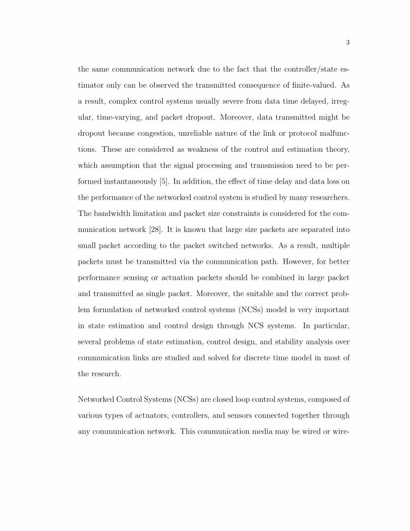
3

the same communication network due to the fact that the controller/state es-

timator only can be observed the transmitted consequence of finite-valued. As

a result, complex control systems usually severe from data time delayed, irreg-

ular, time-varying, and packet dropout. Moreover, data transmitted might be

dropout because congestion, unreliable nature of the link or protocol malfunc-

tions. These are considered as weakness of the control and estimation theory,

which assumption that the signal processing and transmission need to be per-

formed instantaneously [5]. In addition, the effect of time delay and data loss on

the performance of the networked control system is studied by many researchers.

The bandwidth limitation and packet size constraints is considered for the com-

munication network [28]. It is known that large size packets are separated into

small packet according to the packet switched networks. As a result, multiple

packets must be transmitted via the communication path. However, for better

performance sensing or actuation packets should be combined in large packet

and transmitted as single packet. Moreover, the suitable and the correct prob-

lem formulation of networked control systems (NCSs) model is very important

in state estimation and control design through NCS systems. In particular,

several problems of state estimation, control design, and stability analysis over

communication links are studied and solved for discrete time model in most of

the research.

Networked Control Systems (NCSs) are closed loop control systems, composed of

various types of actuators, controllers, and sensors connected together through

any communication network. This communication media may be wired or wire-

4

less. In general, controllers and actuator are event driven while sensors are time

driven. Although, event driven nodes reduce the time delay, but generate a

difficulty in the analysis result in time varying systems.

Many approaches have been used to derive the optimal control law for discrete

time systems with quadratic objective function when the NCSs have Lossy links.

For particular information structures, most of the previous works developed the

optimal control law based on dynamic programming approach for different pro-

tocols Transmission Control Protocol TCP and User Datagram Protocol UDP

such as in [1, 2, 10, 12, 15, 16]. In addition, some estimation algorithms for a

class of networked control systems for unreliable communication channels have

been investigated for UDP-like protocol with random data lost,[37, 41, 39, 38].

Examination of the key issues involved in controller and estimator design, when

measurements and control packets are randomly lost due to unreliability of com-

munication links. It is known that there are two actions for the actuator when

the control packets lost. In the first case, the ”last available control” is ap-

plied, called hold-input strategy [17, 42, 45, 46], while in the second case, ”zero

control” is applied, called zero-input strategy [1, 17, 41, 44].

In this thesis, sensors, actuators, and controller are assumed to be time driven

rather than even driven [21]. Moreover, this thesis presents some approaches,

in one chapter, to design linear quadratic Gaussian LQG problems for both

TCP-like and UDP-like protocols, where LQGs are used to optimize the infinite

horizon cost function based on standard LQR optimal techniques. In addition,

our approach differs drastically, in which the data transmission is assumed to

5

be nonstationary packet dropout. Researchers also studied the problem of non-

stationary delay, see [71, 72].

1.2 Fundamental Issues of NCSs

1.2.1 Band-Limited

It is well known that there is specified bandwidth of any communication channel

as result of that packet size, bit rate and amount of transmission are limited.

These constraints affect the stability and the overall performance when large

size packet or huge amount of information need to be transmitted per unit of

time. In addition, the quantization effects on NCS stability and performance

are ignored.[36]

1.2.2 Time Delay

Transmission data through communication channels suffers from networking de-

lay, processing delay, and waiting delay. These factors has salient impacts on

the system performance and can be gone to instability.

6

1.2.3 Packet Dropouts

This issue is our work mainly concerned. Usually packet suffer from trans-

mission delay during transmission and sometimes Long transmission delay is

considered as packet dropout. Packet loss has worse impacts on the stability

and the performance of the control system. Data transmitted may be lost as

result of congestion on the path, unreliable nature of the link or protocol mal-

functions. In TCP-like protocol, acknowledgment of packet reception is used,

the transmitter knows if the sending packet is received or not. Even though

retransmission mechanisms is used in TCP case, but sometimes it is not enough

to deliver the lost packet due to time limitations. However, in UDP-like proto-

col the acknowledgment of packet reception is absent. So the receiver and the

transmitter do not know if the sending packet is received or not, [34].

1.3 Why Networked Control Systems (NCSs)?

Networked control systems is a rising area in modern control engineering and

applications, that give flexibility and the opportunity for companies to reduce

the overall operation cost, where the companies can site their most expert con-

trol and maintenance engineers in one control facility like in London, and their

control systems located abroad such as in India, China, or Korea. Although,

NCSs are still an academic research, however, the interaction between com-

munication and control is an interesting subject. NCSs are already used in

7

some manufactures such as aircraft, automobile, and health care systems, see

[3][5]. In mathematical electrical engineering, a new chapter is concerned about

the communication and control systems. In fact, numeric of control strategies

emerging from classical control theory are considered for NCS systems like PID

control, adaptive control, optimal control, robust and intelligent control as well,

that might make the control over network challenge as given in [4]. This the-

sis presents that at each time k the plant send measurement (sensing) packets

over a lossy communication links and the control unit send a control (actua-

tion) packet to the plant over a lossy network but with different probability

of link failure. Packets dropping network have studied when the transmission

media has probability to fail because of the congestion, unreliable of the link

or protocol malfunctions with negligible quantization effects. In addition, the

control/estimation could be performed instantaneously. It is known that packet

dropout normally degrades the performance of the NCS and result to instability.

The unreliable nature of the link from the sensor to the estimation /control unit

and from the later to the actuator are modeled by two independent identically

distributed (i.i.d) Bernoulli processes. The stability of the control system for the

NCS is approved in finite and infinite horizon cases of both transmission control

protocol TCP and user datagram protocol UDP, as given in [1][6][15] [8], and

the state-feedback gains are mode-dependent, where many control techniques

are used to calculate the state-feedback gains.

8

1.4 Thesis Objectives

The main objectives of the thesis are to

• To design Linear Quadratic Gaussian (LQG) controller using optimal the-

ory. In addition, the analysis of a discrete Kalman filter will be considered

in details.

• To design an observer based stabilizing controller with nonstationary packet

drops out on both directions. Furthermore, two compensation strategies

will be used to compensate the control packets dropouts. In addition, a

modified feedback controller will be used in our case.

1.5 Problem Statement

1.5.1 Plant Model

In this thesis, we consider a discrete linear time-invariant (LTI) system. The

plant consists of one or more output elements (sensors) and one or more input

elements (actuators). The state-space model of the system subject to packet

dropout is described by

xk+1 = Axk + αkBuk + wk; k = 0, 1, 2.. (1.1)

9

yk = βkCkxk + vk (1.2)

where xk ∈ ℜn is the state vector, yk ∈ ℜp is the measured output by the

sensors, uk ∈ ℜm; is the control input that applied by the actuator. wk ∈ ℜq

is the input disturbance while vk ∈ ℜp is the measurement disturbance, which

are independent zero mean second-order random vectors and also independent

of αk and βk. The unreliable of the links from sensor to the controller/estimator

unit and from the later to the actuator are modeled by two i.i.d. Bernoulli

processes βk and αk respectively. The model matrices are, the dynamic matrix

A ∈ ℜn×n, the control input matrix B ∈ ℜn×m, and the output observation

matrix C ∈ ℜp×n.

Pr(αk) =

αk; if αk = 1;

1− αk = αk; if αk = 0.

P r(βk) =

βk; if βk = 1;

1− βk = βk; if βk = 0.

The observer form is given as

xk+1 = Axk + αkBuk +Kk(yk − yk) (1.3)

where Kk is the Kalman filter gain while xk and yk define the estimated state

10

Figure 1.2: Lossy networked control systems structure [52]

and measurement respectability. The estimated measurement is given as

yk = βkCkxk

We consider the quadratic cost function in finite horizon as where N > 0 is

a finite horizon, and the weighted matrices Q =QT ≥0 , where Q ∈ ℜn×n,

R =RT >0 , where R ∈ ℜm×m, and F =F T ≥0.

11

1.5.2 Hold Input Scheme Model

To compensate the loss of the control packets using last applied control, the

plant model can be presented by

xk+1 = Axk + αkBuk + (1− αk)Bξk + wk (1.4)

ξk+1 = αkξk + (1− αk)uk (1.5)

The state variable ξk keeps track the last available control applied by the actu-

ator. The applied control input by the actuator in hold scheme according to αk

is

uk =

uk; if αk = 1;

uk−1; if αk = 0.

The state equation is

xk+1 =

Axk +Buk + wk; if αk = 1;

Axk +Buk−1 + wk; if αk = 0.

and the observer based is considered as following for hold input method

xk+1 =

Axk +Buk +Kk(yk − yk); if αk = 1;

Axk +Buk−1 +Kk(yk − yk); if αk = 0.

12

1.5.3 Zero Input Scheme Model

To compensate the loss of the control packets by zero input, the plant model

can be presented by

xk+1 = Axk + αkBuk + wk (1.6)

the plant will receive a control input from the actuator according to the random

values of αk according to

uk =

uk; if αk = 1;

0; if αk = 0.

Then, the state equation is written as

xk+1 =


Axk + wk; if αk = 0.

The observer based in terms of the zero input scheme can be written as

xk+1 =

Axk +Buk +Kk(yk − yk); if αk = 1;

Axk +Kk(yk − yk); if αk = 0.

As can be seen from the above equation, the compensation schemes are applied

when the control signal get lost. However, the compensation schemes are not

13

used to compensate the lost of the measurement signals

1.6 Thesis Organization

This thesis contains several chapters, the first of which is the introduction. Chap-

ter 2 showing the previous work on NCSs plants subject to estimation and con-

trol theory that were developed. Chapter 3 contains linear quadratic Gaussian

controller design over lossy communication channels when observation noise is

available for both transmission control protocol TCP and user datagram proto-

col UDP. Chapter 4 is focused on a class of an observer based networked control

system with nonstationary packet Loss in terms of zero and hold input strate-

gies. In chapters conclusions will be drawn and directions for future research

will be presented.

Notations: The Euclidean norm |.| is used for vectors in the n-dimensional

space ℜn and we denote by ||.|| the corresponding induced matrix norm in ℜn.

The notation W t, W−1, λm(W ) and λM(W ) denote the transpose, the inverse,

the minimum eigenvalue and the maximum eigenvalue of any square matrix W ,

respectively. We use W < 0 (≤ 0) to denote a symmetric negative definite

(negative semidefinite) matrix W and Ij to denote the nj × nj identity matrix.

Matrices, if their dimensions are not explicitly stated, are assumed to be com-

patible for algebraic operations. In symmetric block matrices or complex matrix

expressions, we use the symbol • to represent a term that is induced by symme-

14

try. Sometimes, the arguments of a function will be omitted when no confusion

can arise.

Chapter 2

LITERATURE SURVEY

2.1 Literature Review

With the rapid advance in the control engineering and its applications, net-

worked control systems (NCS) acquired a significant attention currently because

of the advantages that NCS provide. The purpose of this section is to provide

background and motivation that make control and estimation problems over

communication networks subject to packet lost an interesting area.

In 2004s, Gupta Vijay [18], investigated an optimal linear quadratic Gaussian (

LQG) control problem when the sensor to the controller is unreliable link where

15

16

the measurements packets drops randomly according to a Markov chain. Packet

dropout was modeled by a switch. It was shown that, the separation principle

exists between the optimal estimate and the optimal control law. The stability

and performance analysis of the algorithm were compared to other methods

presented in the literature.

In [20], a mutual analysis of control and coding for stability and performance

of remotely an LTI plant over communication links was studied. Further, the

authors considered stability of the differential entropy and mean-square stabil-

ity of the state estimation error with the requisite communication rate. It was

shown, the optimal control law which optimizes a quadratic performance objec-

tive function is linear function of the estimated states. The separation principle

is hold as a result of that. Its solution was dependent on the individual de-

sign of the estimator and the LQR controller. Researchers also reported that

the communication rate requirements was impacted by the estimation problem

when the measured state was quantized.

In [21], different policies for a stochastic control with a fixed end-time were

investigated. It was focused on distinction between feedback and closed-loop

policies in stochastic control. When the control has a dual effect the feedback

policy can only be actively adaptively. In addition, the separation principle

holds has been expanded if the certainty equivalence property formerly known.

A controller and an estimator can be designed separately.

Great attention has been paid to a solution of the infinite horizon control. Gen-

17

erally, a discrete time linear system and a performance index were studied with

independent stochastic parameters. Compared with properties of the determin-

istic systems, authors introduced that mean square m.s. stabilizability property

was a stronger condition while m.s. observability property was a weaker condi-

tion. It is presented that, if the system is m.s stabilizability the infinite time

problem will has a solution. Furthermore, the solution will be unique even when

it is m.s. observability as well. On the other hand, m.s. observability does not

guarantee the existence of the solution, see [24].

In [19], the authors proposed an LQG optimal control problem for scalar models

under network limitations, where the quadratic objective function was extended

to involve a quadratic penalty for communication where the optimization prob-

lem has to be quasi-convex in the output matrix C. However, with assumption

that, the system was unstable, the problem was convex. The problem was fig-

ured out in a computationally efficient way using semidefinite programming.

In [12], they discussed the problem of a discrete LQG under transfer control pro-

tocol (TCP) where measurements and control packets can get lost over sensor to

estimation/control unit and from the later to the actuator respectively. Packets

dropout are on both direction because of unreliable features of the communi-

cation links. It is will known that in TCP-like protocol case, the transmitter

receive an acknowledgment whether the sending packet received or not. How-

ever, authors investigated the problem when the acknowledgment was always

available for the control packet reception. Besides, LQG optimal control was

established to be a linear function of the state. It was shown, the existence of

18

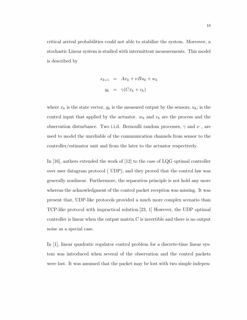
critical arrival probabilities could not able to stabilize the system. Moreover, a

stochastic Linear system is studied with intermittent measurements. This model

is described by

xk+1 = Axk + νBuk + wk

yk = γ(Cxk + vk)

where xk is the state vector, yk is the measured output by the sensors, uk; is the

control input that applied by the actuator. wk and vk are the process and the

observation disturbance. Two i.i.d. Bernoulli random processes, γ and ν , are

used to model the unreliable of the communication channels from sensor to the

controller/estimator unit and from the later to the actuator respectively.

In [16], authers extended the work of [12] to the case of LQG optimal controller

over user datagram protocol ( UDP), and they proved that the control law was

generally nonlinear. Furthermore, the separation principle is not hold any more

whereas the acknowledgment of the control packet reception was missing. It was

present that, UDP-like protocols provided a much more complex scenario than

TCP-like protocol with impractical solution.[23, 1] However, the UDP optimal

controller is linear when the output matrix C is invertible and there is no output

noise as a special case.

In [1], linear quadratic regulator control problem for a discrete-time linear sys-

tem was introduced when several of the observation and the control packets

were lost. It was assumed that the packet may be lost with two simple indepen-

19

dent Bernoulli random processes, and there was no observation noise. Moreover

the structure of the controller counted on the features of the communication

networks. Researchers focused on design of LQR optimal controller using dy-

namic programming approach with quadratic cost function in finite and infinite

horizon. The control law is linear with state when the acknowledgment was

always available. Sufficient and necessary conditions of mean square stability

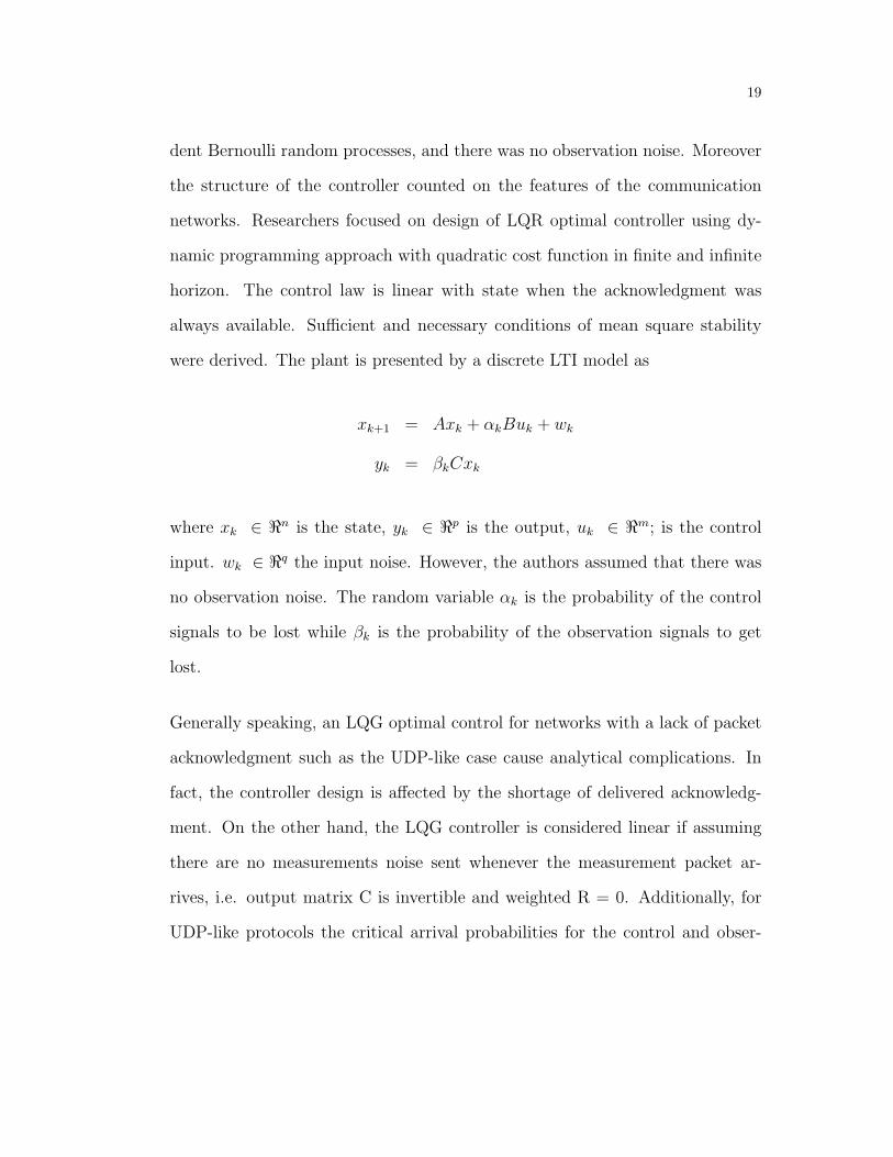
were derived. The plant is presented by a discrete LTI model as

xk+1 = Axk + αkBuk + wk

yk = βkCxk

where xk ∈ ℜn is the state, yk ∈ ℜp is the output, uk ∈ ℜm; is the control

input. wk ∈ ℜq the input noise. However, the authors assumed that there was

no observation noise. The random variable αk is the probability of the control

signals to be lost while βk is the probability of the observation signals to get

lost.

Generally speaking, an LQG optimal control for networks with a lack of packet

acknowledgment such as the UDP-like case cause analytical complications. In

fact, the controller design is affected by the shortage of delivered acknowledg-

ment. On the other hand, the LQG controller is considered linear if assuming

there are no measurements noise sent whenever the measurement packet ar-

rives, i.e. output matrix C is invertible and weighted R = 0. Additionally, for

UDP-like protocols the critical arrival probabilities for the control and obser-

20

vation channels were coupled. Otherwise, the critical arrival probabilities for

the control and observation channels are independent for TCP-like protocols.

In particular, the UDP protocols were considered as the exclusive solution for

extremely lossy channels that guarantee successful delivery of acknowledgment,

see [23].

Besides the models established above, single input single output SISO, LTI sys-

tem was investigated with one-degree-of-freedom control architectures via lossy

communications links. Also, signals might be lost across erasure links with i.i.d.

Bernoulli random process. It was shown that the result of [73] was extended

by considering additional i.i.d. noise channel instead of the the analog erasure

channel, where the controller was designed consequently. A necessary and suffi-

cient conditions were derived to ensure m.s. stability. In fact, output feedback

controller was designed over UDP like protocols, see [11]

In [14], optimal estimation problem over lossy communication channels were

studied. The control packets, the observation packets in addition to the acknowl-

edgment packets were subject to loss. Packet drop properties were considered

as unknown i.i.d. Bernoulli random variables. Furthermore, the focus of that

research was to design suboptimal control in terms of linear matrix inequalities

(LMIs) with the present of uncertain networks constraints.

In [15], an LQG optimal via TCP-like unreliable communication networks was

considered. Also, all the transmission packets which were damaged sited as i.i.d.

Bernoulli processes, see e.g. [43]. Moreover the work in [41] was extended to

21

multi -input -multi -output (MIMO) communication channels. It was shown

that the separation principle was hold, and the optimal control law was linear

function of the estimated state. Sufficient and necessary conditions for systems

stability for infinite horizon LQG control were given in form of LMIs.

In [17], zero input and hold input schemes were investigated, which are compen-

sation schemes that normally used to compensate the fate of the control input

packets. Bernoulli random processes were used to model the fate of the trans-

mission packets. In zero input scheme, in which zero control is applied by the

actuator when the control input is lost. Nevertheless, the last available control

input is applied in case of hold input scheme. For control applications, the linear

quadratic performance for both compensation schemes using a static feedback

were analyzed. As a conclusion of that, although zero input strategy was used

widely to simplify mathematical problems, but no one of these compensation

scheme was considered as the best strategy for most of the systems.

In [10], authors proposed an LQG discrete problem in two events using dynamic

programming approach. Firstly, the acknowledgment are available constantly,

where the optimal control law considered using hold input strategy was linear.

In the second the event, the acknowledgment can be lost, in which zero input

strategy was considered for simplifying the optimal control problem due to the

fact that the optimal control law was nonlinear and the separation principle was

not hold. As result, a suboptimal LTI approach was investigated. In addition,

22

the plant was assumed in the following form

xk+1 = Axk +Buak + wk

yk = γk(Cxk + vk)

uak is the actual control input applied by the actuator under zero and hold

strategies.

An estimation LTI stochastic problem over erase communication channels for

both TCP and UDP protocols was studied. For TCP-like protocol, the impact

of packet retransmissions and acknowledgment mechanisms on the system sta-

bility and performance were discussed. A comparison between UDP and TCP

protocols was shown in two cases. In the first case, while a single sensor device

communicated via a single path, TCP protocol provided better exhibit than

UDP. In the second case, multi sensors communicated across communication

channels, UDP protocol provided better exhibit than TCP protocol, see [39]

In [37] and [38], estimation strategies over unreliable networked without packet

acknowledgment (e.g. UDP) were studied. It was shown that the standard

observer strategy could not be used in case for user datagram protocol due to the

lack of acknowledgment packets. The main of that works was focused on design

of simple estimator involved of mode and state observer where the measurement

packets were assumed to be regularly delivered to the control/estimation unit.

Furthermore, a discrete time has been modeled using Jump Linear System to

pick up the lost control packets. Moreover in [38], the system was supported by

23

an additional control input to ensure recovering the lost control packets . After

that, in [52] the works of [37]and [38] were extended in case the measurement

packets randomly dropped out through a lossy network. Hence, the discrete

linear system is described by

xk+1 = Axk + βkBuk + wk

yk = γk(Cxk + vk)

Moreover, they assumed that there were two estimators, one to estimate the state

and the other to estimate the fate of the control packets. The state estimator is

considered as

xk+1 = Axk + βkBuk + γkLk(yk+1 − yk+1)

where yk is the estimated output. Furthermore, the fate estimator is given by

βk = argmin ∥yk+1 − yk+1∥2

this fate observer is used to determine the value of βk

In [55], the authors have considered a model predictive control MPC technique

over lossy communication network. Interestingly, MPC method has the feature

to be a good explanation for the networked control systems constraints, in which

future control packets are sending at the last control input. In fact, the com-

pensation strategy here was totally different in its compensate to the fate of the

24

control packet by the future control input packet. Moreover a switching strategy

was used to swap various control laws.

In [40] the focus of the research was on the important of packet acknowledgment

and its impact on the communication between the controller/estimator unit and

the plant. To present these affects, a discrete LQG control was investigated

across a lossy channels with two strategies of packet acknowledgment. Firstly,

packet delivered is acknowledged under TCP-like protocol. Hence, the control

system is linear and the separation principle between the controller and the

estimator is hold. In the second case, packet received does not acknowledged

under UDP-like protocol. It is shown that the separation principle between the

controller and the estimator does not hold. The performance and stability are

affected due to the control system nonlinearity.

Recently, In [30] a problem of kalman filter state estimation over wireless sen-

sor networks (WSNs) with the effect of unmatched sensors connected via NCS.

These sensors usually generate measurements disturbances,that transported with

measurements packets to a fusion center. This research was focused on using

partial broadcasting policy to optimize the estimation error covariance. More-

over due to the issues of data lost, battery power, and bandwidth limitation,

partial broadcasting policy could not be an optimal method. As result of that,

a good-sensor-late-broadcasting was investigated using finite horizon LTI dis-

crete system in case of perfect packet transmission without lost. There are

several researches about the optimal estimation and kalman filter estimation,

see ([13],[47],[48], [49], [50], [51], [53], and [54])

25

2.2 Stability Criteria of NCSs

Generally speaking, stability analysis of the networked control systems under

networking constraints is a fundamental problem. This section addresses the

stability of feedback loops that are closed over a network with time delay and

package dropout constraints. In fact, there were various technique developed to

establish the stability condition for NCS’s with different assumptions. As given

in [25], time delay normally exists in most communication network. In particu-

lar, transmission delay takes place on both paths from sensors to controllers as

well as from controllers to actuators. It is well know that time delay can debase

the performance of control systems and may take the system to unstable side. In

addition, long delay of a packet was considered as packet dropout after a spec-

ified time. On the other hand, packet dropout might be occurred on an NCS

fitfully when there are link failures or congestion result in buffering problem. In

order to avoid these problems, the vast majority of transmission protocols were

supplied by retransmission mechanisms, in which the lost packet was retrans-

mitted until it successfully delivered such as in TCP -like. However, there are

limited time for retransmission process, otherwise the packet was considered as

dropped.

In [27], the conditions mean square m.s. stable were studied of lossy undisturbed

NCS. In the main of this work, authors concentrated on data lost because net-

working errors such as network congestion. It was shown that the uncertainty

threshold principle was employed to clarify the stability under certain condi-

26

tions. In particular, they discussed the impacts of applying the retransmission

strategy and do not applying on the system stability when some packets got

lost.

In [28], a stabilization strategy for a class of unreliable networked control systems

was investigated. The unreliable features of the communication channels were

considered as erase channels. It is well known that control gains affected by

the trade off between packets dropout and instability parameters. Particularly,

researchers extended the work in [22] for addressing upper dimensional dynamic

system under satisfied conditions.

More specifically, an exponential stability with a dynamic output feedback con-

trol was discussed under the influence of time varying delays and data lost .

Data lost may occur on both direction sensor to controller and the latter to the

plant. The asynchronous dynamic system theory , Lyapunov principle, and LMI

methods were accomplished for the control system stability analysis. Further-

more, the conditions of negative semi-definite matrix with exponential stable

and control design were studied, see [31].

In [32], try-once-discard (TOD) control protocol was considered for MIMO net-

worked control systems, in which several autonomously sensors and actuator

were connected to the network. Primarily, mathematical analysis was done for

global exponential stability for TOD protocol and the traditional protocols (e.g.

statically scheduled protocol) as well. First of all, authors established a con-

troller design for TOD protocol to study the impacts of networks constraints on

27

the performance of system. After that, the system performances for both TOD

control protocol and statically scheduled protocol were compared.

In [33], stability analysis of NCS via output feedback control was studied when

data packet lost and packet time delay could be occurred through the networked

control system links. Based on Lyapunov function method, the sufficient con-

ditions of stability of NCSs were investigated by using asynchronous dynamical

system (ADS) approach. The idea of this could be found in Nilsson’s Ph.D.

dissertation [26].

In [42], the problem of stability analysis and controller design were studied based

on a new model of the NCSs with single and multiple packets transmission. As

considered in the previous works, transmission data may be get lost when the

packet sending from sensor-to-controller as well as from the later-to-actuator.

However, the feature of data dropout characterized by two different independent

Markov chains. Sufficient and necessary conditions for stochastic stability were

obtained via LMIs.

In [6], the author investigated a discrete LQG optimal problem across analog

erase communication links to study the effects of the acknowledgments (e.g.

TCP) using smart actuator and global actuator which do not have direct access

to the plant. They concluded that, although the acknowledgment with smart

actuator can provided several processing alone, it could not upgraded the stabil-

ity performance region better than that for the global actuator, see also [5]and

[7].

28

[29] considered a NCS architecture where the plant normally was nonlinear,

in which a packetized predictive controller uses over lossy network affected by

signal loss. It was shown that the input to state stability was guaranteed by

determining the value of the turning parameters of the control system design,

in which packet lost became limited. Furthermore, the effect of the disturbance

on the constrained nonlinear system has been investigated.

In the next chapter we will consider problems of discrete linear quadratic Gaus-

sian when the transmission data packets prone to failure because of the unreliable

communication channels using hold and zero input strategies.

Chapter 3

LINEAR QUADRATIC

GAUSSIAN (LQG) DESIGN

3.1 Introduction

In this chapter, we introduce an optimal control problem of discrete LTI system

with a quadratic cost objective function. As noted in the literature review,

linear quadratic (LQ) methods are one of the most useful linear optimal control

approaches. It is well known that in LQ methods, a quadratic objective function

is optimized to get a suitable state feedback gain Gk through minimizing the

29

30

estimation error covariance. In fact, the linear quadratic regulator (LQR) is used

when all the true state available for the control. This problem increases for high

order systems and when the control systems contain noise due to the fact that

we can not find the exact states. Hence, the linear quadratic Gaussian (LQG)

solves that problem by estimating states using a kalman filter, so there is need to

evaluate all the states. Consequently, the classical LQG is LQR linked together

with a kalman filter to eliminate input Gaussian white noise and to estimate

state, see [56][57]. Broadly speaking, we are concerned in the design of linear

quadratic Gaussian over unreliable communication networks. The unreliable

features of the channels are modeled by a Bernoulli stochastic process. The

stability of the control system for the NCS is proved in finite and infinite horizon

cases of both transmission control protocol TCP and user datagram protocol

UDP, also see [10, 12, 1, 2]. In particular, we extend the work of [1] and [10]

further to the case where measurement noise is present. Our analytical approach

is based on the linear-quadratic optimal approach [57, 47, 48]. Furthermore,

we discuss the optimal control problem design in terms of both compensation

schemes hold-input and zero-input.

3.2 Problem Formulation

In this chapter, we are specifically interested in the design of linear quadratic

Gaussian (LQG) controller using optimal theory. In addition, the analysis of

a discrete Kalman filter will be considered in details. It is known that there

31

are two actions for the actuator when the control packets lost in terms of LQG

optimal control approach. In the first case, the ”previous available control”

is applied, while the second case, ”zero control” is applied. In this work, we

assume the previous available control input will be applied by the actuator to

compensate the fate of control packets. The plant process given by a discrete-

time state-space model, is described in our work by

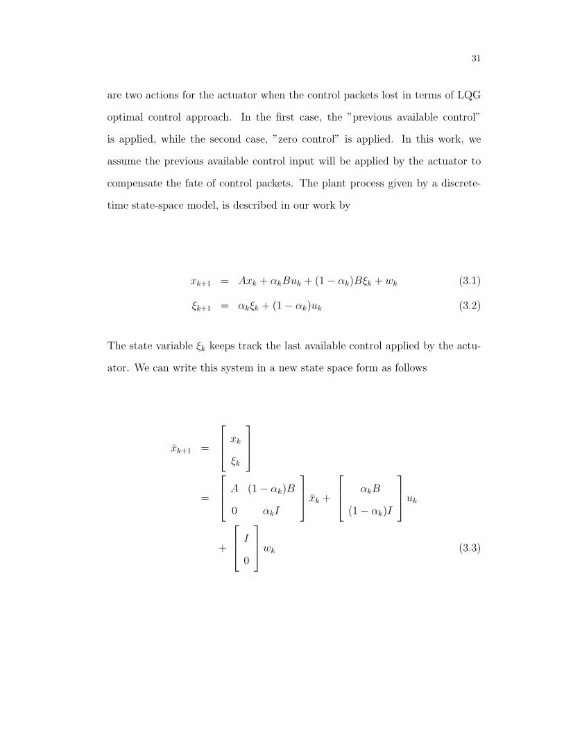
xk+1 = Axk + αkBuk + (1− αk)Bξk + wk (3.1)

ξk+1 = αkξk + (1− αk)uk (3.2)

The state variable ξk keeps track the last available control applied by the actu-

ator. We can write this system in a new state space form as follows

xk+1 =

xk

ξk

=

A (1− αk)B

0 αkI

xk +

αkB

(1− αk)I

uk

+

I

0

wk (3.3)

32

In compact form, this is described by the discrete-time model

xk+1 = Akxk + Bkuk + Iwk

yk = βkCkxk + vk (3.4)

where

A =

A (1− αk)B

0 αkI

, B =

(1− αk)B

αkI

, I =

I

0

where xk ∈ ℜn is the state vector, yk ∈ ℜp is the measured output, uk ∈ ℜm

is the control input, wk ∈ ℜq, vk ∈ ℜp are respectively, the input and mea-

surement disturbances, which are independent zero mean second-order random

vectors and also independent of αk and βk. The stochastic processes αk and βk

are Bernoulli processes represent the lossy nature of the controller- actuator and

sensor- controller links respectively. Associated with system (3.4), the quadratic

performance function:

J = E[xTNFxN +

N−1∑K=0

xTkQxk + uT

kRuk]

where N > 0 is a finite horizon, and the weighted matrices Q =QT ≥0 , where

Q ∈ ℜn×n, R =RT >0 , where R ∈ ℜm×m, and F =F T ≥0.

33

3.3 LQG Optimal Control Over TCP Protocol

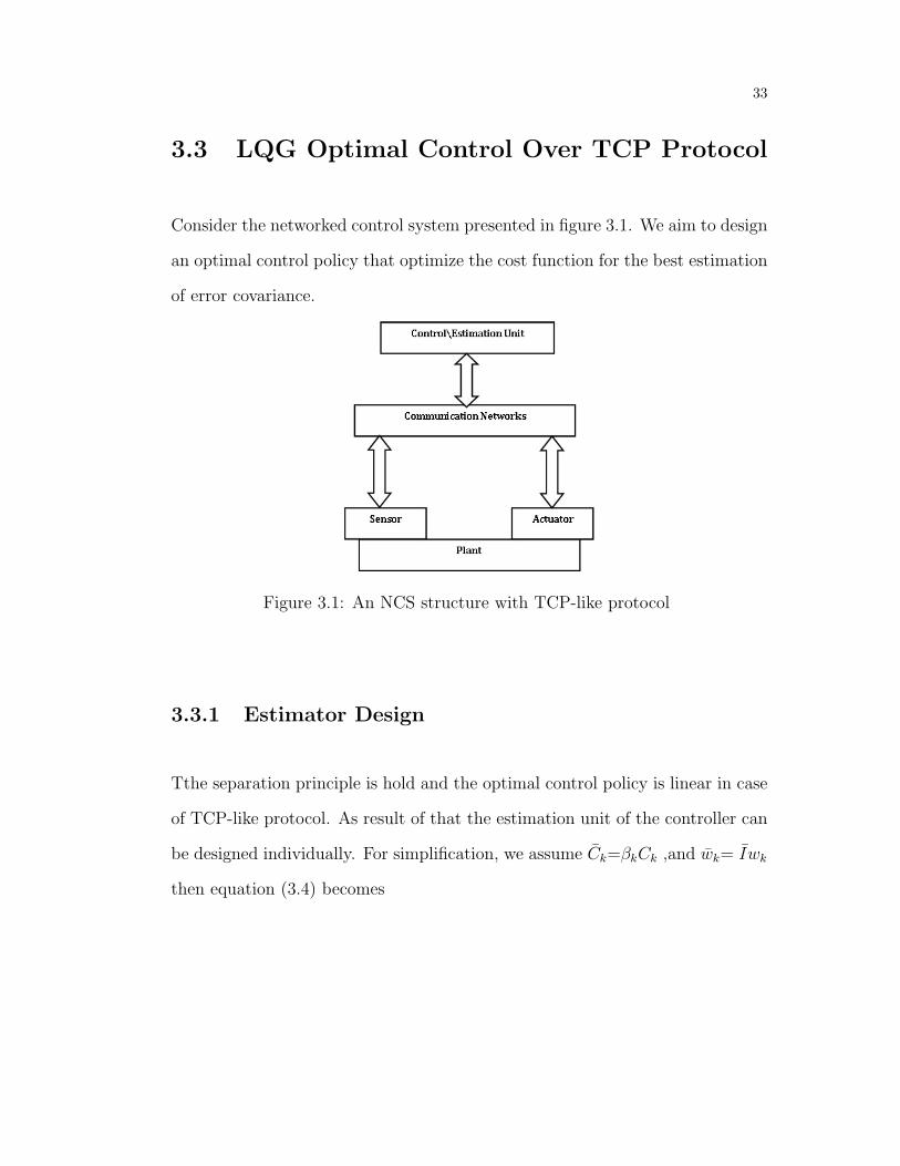
Consider the networked control system presented in figure 3.1. We aim to design

an optimal control policy that optimize the cost function for the best estimation

of error covariance.

Figure 3.1: An NCS structure with TCP-like protocol

3.3.1 Estimator Design

Tthe separation principle is hold and the optimal control policy is linear in case

of TCP-like protocol. As result of that the estimation unit of the controller can

be designed individually. For simplification, we assume Ck=βkCk ,and wk= Iwk

then equation (3.4) becomes

34

xk+1 = Akxk + Bkuk + wk (3.5)

yk = Ckxk + vk (3.6)

First, define some variables as

ˆxk = E[xk] (3.7)

where the estimation error is

ek = xk − ˆxk (3.8)

The estimation error covariance matrix is given as The noises wk, and vk are

uncorrelated i.i.d. processes with zero mean, and the covariance matrices corre-

sponding to the orthogonality principle is deduced as

E[wTk wk] = Sw, E[vTk vk] = Sv

E[wTk vk] = 0, E[xkv

Tk ] = 0

E[wTk x0] = 0 (3.9)

35

The a priori estimate of the process model is given as

E[xk+1] = AkE[xk] + BkE[uk] (3.10)

ˆxk+1|k = Ak ˆxk|k + Bkuk (3.11)

from estimation error equation, we have

ek+1|k = xk+1 − ˆxk+1

= Akxk + Bkuk + wk − (Ak ˆxk + Bkuk)

= Akek + wk (3.12)

The a priori estimation error covariance can be calculated as

Σk+1|k = E[ek+1eTk+1] = E[[xk+1 − ˆxk+1][xk+1 − ˆxk+1]

T ]

= E[[Akek + wk][Akek + wk]T ]

= AkΣkATk + Sw (3.13)

where the control input uk is considered as deterministic function. It is shown,

there are no dual effect between the estimator and the controller over the TCP

networks according to the separation principle, see [1, 12, 41].

Lemma 3.3.1 [41]: By using the algebraic operations , we have:

36

1.

E[(xk − ˆxk)ˆxTk ] = E[ek ˆx

Tk ]

= 0

2. For ∀ T > 0, the following fact is true

E[xTk T xk] = E[ˆxT

k T ˆxk] + tr(TΣk)

proof 3.3.1 1.

E[(xk − ˆxk)ˆxTk ] = E[xk ˆx

Tk − ˆxk ˆx

Tk ]

= E[xk]ˆxTk − ˆxk ˆx

Tk

= ˆxk ˆxTk − ˆxk ˆx

Tk ; (from(3.7))

= 0

2.

E[xTk T xk] = E[(ek + ˆxk)

TT (ek + ˆxk)]

= ˆxTk T ˆxk + 2tr(T E[ek ˆx

Tk ])

+tr(T E[ekeTk ])

= ˆxTk T ˆxk + tr(TΣk)

37

The observer form of the Kalman filter is given as

ˆxk+1 = Ak ˆxk + Bkuk +Kk+1[yk+1 − Ck+1 ˆxk+1] (3.14)

where

yk+1 = Ck+1xk+1 + vk+1

Rearranging the observer form we get

ˆxk+1 = Fk+1 ˆxk+1 + Bk+1uk+1 +Kk+1yk+1 (3.15)

where Fk+1 = Ak+1 − Kk+1Ck+1. The main idea here, we use kalman filter to

filter the observations through the part (yk+1− Ck+1 ˆxk+1) so -called observation

innovation so as estimate the state ˆxk to minimize the effects of the process and

observation distributions wk and vk respectively. The correction step of TCP is

given as

ˆxk+1|k+1 = ˆxk+1|k +Kk+1(yk+1 − Ck+1 ˆxk+1) (3.16)

ek+1|k+1 = xk+1|k+1 − ˆxk+1|k+1 (3.17)

38

For the prediction updating, we supposed that, the updating prediction is a

weighed linear function of the discrete system given in (3.12), and an observation.

ˆxk+1|k+1 = K ′k+1

ˆxk+1|k +Kk+1yk+1

= K ′k+1

ˆxk+1|k +Kk+1Ck+1xk+1|k

+Kk+1vk+1|k (3.18)

K ′k+1 is gain matrix with different size from the Kalman gain matrix Kk+1.

when the prediction is unbiased:

E[ˆxk+1|k+1] = E[xk+1|k]

E[ˆxk+1|k+1] = K ′k+1E[ˆxk+1|k] +Kk+1Ck+1E[xk+1|k] (3.19)

According to 3.20, and by assumption E[ˆxk+1|k+1] = E[xk+1|k], we have

I = K ′k+1 +Kk+1Ck+1

K ′k+1 = I −Kk+1Ck+1 (3.20)

then the updating of the prediction can be arranged as

ˆxk+1|k+1 = (I −Kk+1Ck+1)ˆxk+1|k +Kk+1yk+1

= (I −Kk+1Ck+1)ˆxk+1|k +Kk+1Ck+1

ˆxk+1|k −Kk+1vk+1 (3.21)

39

The principle unbiased prediction is represented in Appendix A. The a posteriori

estimation error covariance is described by

Σk+1|k+1 = E[ek+1|k+1eTk+1|k+1]

= E[[xk+1 − ˆxk+1|k+1][xk+1 − ˆxk+1|k+1]T ]

= (I −Kk+1Ck+1)E[ek+1|keTk+1|k](I −Kk+1Ck+1)

T

+Kk+1E[vk+1|kvTk+1|k]K

′k+1

+2(I −Kk+1Ck+1)E[ek+1|kvTk+1|k]K

′k+1

= (I −Kk+1Ck+1)Σk+1|k(I −Kk+1Ck+1)T

+Kk+1SvK′k+1 (3.22)

We can get the Kalman gain by differentiating the trace of the estimation error

covariance matrix with respect to K.

L = minKK+1tracE[Σk+1|k+1]

= minKK+1tracE[(I −Kk+1Ck+1)Σk+1|k(I −Kk+1Ck+1)

T

+Kk+1SvK′k+1] (3.23)

and setting the differentiation of L equal to zero, we obtain

∂L∂KK+1

= −2(I −Kk+1Ck+1)Σk+1|kCTk+1

+2Kk+1Sv = 0

40

Then, the Kalman gain matrix is

KK+1 = Σk+1|kCTk+1[Ck+1Σk+1|kC

Tk+1 + Sv]

−1 (3.24)

To minimize the error covariance, we firstly rearrange the error covariance equa-

tion (3.23) as

Σk+1|k+1 = (I −Kk+1Ck+1)Σk+1|k(I −Kk+1Ck+1)T

+Kk+1SvK′k+1

= Σk+1|k −Kk+1Ck+1Σk+1|k − Σk+1|kCTk+1K

′k+1

+Kk+1Ck+1Σk+1|kCTk+1K

′k+1 +Kk+1SvK

′k+1 (3.25)

Substitute the Kalman gain matrix into the posteriori estimation error covari-

ance (3.26), we deduce

Σk+1|k+1 = Σk+1|k+1 −Kk+1Ck+1Σk+1|k+1 (3.26)

3.3.2 Controller Design

In this section, we investigate the optimal LQR control law by means of the

quadratic performance index

J = E[xTNFxN +

N−1∑K=0

xTkQxk + uT

kRuk] (3.27)

41

Applying Lemma 3.2.1 on the performance index function, we obtain

J = E[ˆxTNF ˆxN +

N−1∑K=0

ˆxTkQˆxk + uT

kRuk]

+N−1∑K=0

[tr(FΣk) + tr(QΣk)]

= minu

E[ˆxTNF ˆxN +

N−1∑K=0

ˆxTkQˆxk + uT

kRuk] (3.28)

Because of the trace terms are independent of the control input, so they will be

canceled when the quadratic function is minimizing, and we have assuming

ˆxN = ˆxk+1

J = minu

E[ˆxTk+1F ˆxk+1 +

N−1∑K=0

ˆxTkQˆxk + uT

kRuk] (3.29)

We have

u∗k = Gk ˆxk

J = minu

E[(Ak ˆxk + Bkuk)TF (Ak ˆxk + Bkuk)

+ˆxTkQˆxk + uT

kRuk]

= minu

E[(ˆxTk A

TkFAk ˆxk + uT

k BTk FBkuk

+2ˆxTk A

TkFBkuk + ˆxT

kQˆxk + uTkRuk]

42

By differentiating with respect the control input gain and make it equal to zero,

we can get the state feedback Gk as

0 = BTk FBku

∗k + BT

k FAk ˆxk +Ru∗k

u∗k = −(R + BT

k FBk)−1BT

k FAkxk

Then the state feedback gain is

Gk = −(R + BTk FBk)

−1BTk FAk (3.30)

3.3.3 Finite and Infinite Horizon LQG control

The following theorems summarize the results for the finite and the infinite LQG

optimal control problem over TCP protocol:

Theorem 3.3.1 Consider the system in (3.4) and (3.28), and assuming that

(A, S12w) to be controllable,( A, C) to be observable, and A to be unstable ma-

trix. Then there exists a critical observation arrival probability βc such that

the expectation of estimator error covariance is bounded if and only if the ob-

servation arrival probability is greater than the critical arrival probability, i.e.

E[Σk|k] ≤ M ∀k , βc < β. where M is a positive definite matrix possibly

43

dependent on P0, see [58]

The proof is available in Appendix B. For infinite horizon, where k 7→ ∞ as

N 7→ ∞, we assume the matrices Ak, Bk,Ck are time-invariant , and we deduce

Ak = A∞ = A, Bk = B∞ = B, Ck = C∞ = C

xk = x∞ = x, uk = u∞ = u, vk = v∞ = v

wk = w∞ = w, Fk = F∞ = F, Kk = K

Gk = G∞ = G, QN = Qk = Q∞ = Q, Pk = P∞ = P

Σk = Σ∞ = Σ

In fact, there are difficulty to calculate the minimal of the objective function

analytically without a limit and the exception of the estimation error covariance

matrices E[Σk]. It is shown that the estimator gain does not converge to a

steady state value, however it is tightly time-varying result since it is a function

of a stochastic parameter βk. It is well known that, the optimal LQG regulator

stabilize the system usually in case packets lost. The system become unstable

if the packets lost become below some certain threshold.

xk+1 = xk

= x∞ = x

44

e∞ = x∞ − ˆx∞

e = x− ˆx

= Aˆx+ Bu+ w − (Aˆx+ Bu)

= Ae+ w (3.31)

Σ∞ = E[ek+1eTk+1] = E[[xk+1 − ˆxk+1][xk+1 − ˆxk+1]

T ]

= [Ae+ w][Ae+ w]T

= AΣ∞A+ Sw (3.32)

The observer form of the Kalman filter for the infinite horizon system Σ∞ is

given as

ˆx∞ = A∞ ˆx∞ + B∞u∞ +K∞[y∞ − C∞ ˆx∞] (3.33)

ˆx = Aˆx+ Bu+K[y − C ˆx] (3.34)

Rearranging the observer form we have

ˆx = F ˆx+ Bu+Ky (3.35)

45

Where F = A −KC. The updating prediction at infinite horizon gives as

E[ˆx∞] = E[K ′∞ ˆx∞

+K∞C∞x∞ +K∞v∞]

ˆx∞ = K ′∞ ˆx∞

+K∞C∞x∞ +K∞v∞

where K is the kalman filter gain

Σ∞ = (I −KC)E[eeT ](I −KC)T +KE[vvT ]K ′

+2(I −KC)E[evT ]K ′

= (I −KC)Σ∞(I −KC)T +KSvK′ (3.36)

We can get the Kalman gain by differentiating the trace of the estimation error

covariance matrix and make it equal to zero, we obtain:

L = minK∞

tracE[Σ∞]

= minK∞

tracE[(I −KC)Σ∞(I −KC)T +KSvK′] (3.37)

∂L∂K

= −2(I −KC)Σ∞CT + 2KSv = 0 (3.38)

46

Then, the Kalman gain matrix is

K = Σ∞CT [CΣ∞CT + Sv]−1 (3.39)

The quadratic performance index is

J∞ = minu

E[ˆxTF ˆx+ limk→∞

∞∑K=0

xTQx+ uTRu]

= minu

E[ˆxTK+1F ˆxk+1 lim

k→∞

∞∑K=0

ˆxTQˆx+ uTRu]

+∞∑

K=0

[tr(QΣk)] (3.40)

Assuming

ˆxN = ˆx∞ = ˆx

J∞ = minu

E[ˆxTF ˆx+ limk→∞

∞∑K=0

ˆxTQˆx+ uTRu] (3.41)

The trace terms are independent of the control input, so they will be canceled

when the quadratic function is minimizing, and we have

J = minu

E[ˆxTF ˆx+∞∑

K=0

ˆxTQˆx+ uTRu] (3.42)

47

Therefore,

J∞ = limN→∞

minu

E[(Ak ˆx+ Bku)TF (Ak ˆx+ Bku)

+ˆxTQˆx+ uTRu]

= limN→∞

minu

E[(ˆxTk A

TkFAk ˆxk + uT

k BTk FBkuk

−2ˆxTk A

TkFBkuk + ˆxT

kQˆxk + uTkRuk]

By differentiating with respect the control input gain and make it equal to zero,

we can get the state feedback gain G as

0 = BTk FBku

∗ + BTk FAk ˆx+Ru∗

u∗∞ = −(R + BT

k F∞Bk)−1BT

k F∞Akx∞

u∗ = −(R + BTk FBk)

−1BTk FAkx

Then the state feedback gain is given as

G∞ = −(R + BT∞F∞Bk)

−1BT∞F∞A∞ (3.43)

and

G = −(R + BTFB)−1BTFA (3.44)

48

Theorem 3.3.2 Studying the equations that are defined in (3.4) and (3.28) with

the assumptions FN= Fk= F , QN= Qk= Q, and RN= Rk= R, In addition, let

(A,B) and (A, S12w) be controllable, and (A,C) (A, S

12w) be observable. Besides,

βmax<β and αc<α Then we have the following.

1. The optimal controller gain at infinite horizon be a constant.

limk→∞

G = −(R + BTFB)−1BTFA (3.45)

2. The optimal estimator gain Kk, is stochastic and time-varying result in it

depends on the previous observation packets, that arrival sequence βj when

j = 1→ k

3. The expected minimum cost can be bounded. This theorem is available at

[41].

The proof of this theorem can be found in Appendix B. In this section, equations

the optimal LQG control over TCP-like protocol were derived in which the

estimator and the controller is designed independently due to the fact that the

separation principle is hold here using the standard Kalman filter. In the next

section, we are going to derive the same results for UDP-like protocol.

49

3.4 LQG Optimal Control Over UDP Protocol

In this section, we investigate the LQG problem under UDP-like protocol. Fig-

ure 3.1. introduced a simply structure of NCS over UDP protocol. Hence, our

goal is to design an optimal control policy that optimize the cost function that

claim for the best estimation of error covariance. However, because of acknowl-

edgment missing in UDP-like protocol and due to the quantization impacts into

the networked control systems, there will be a dual effect between the estimator

and the controller. So the separation principle does not hold here. In particular,

the quantization impacts will not be considered. To show the difference between

protocols with and without acknowledgments, we add a stochastic process σ in

UDP-like case, and the expectation of this element E[σ] define as σ.

Figure 3.2: An NCS structure with UDP-like protocol

50

3.4.1 Estimator Design

We assume the discrete system as

xk+1 = Akxk + σBkuk + wk (3.46)

The Kalman filter estimates of the UDP discrete system is given by

E[xk+1] = AkE[xk] + σBkE[uk] + E[wk] (3.47)

ˆxk+1 = Ak ˆxk + σBkuk (3.48)

The estimation error is written as

ek+1 = xk+1 − ˆxk+1

ek+1 = Ak ˆxk + σBkuk + wk − (Ak ˆxk

+σBkuk) (3.49)

ek+1 = Akek + (σ − σ)Bkuk + wk (3.50)

the difference (σ − σ) is available at UDP-like protocol due to the fact that the

estimated value E[αk] = αk and E[βk] = βk result in the acknowledgment is not

available here. Therefore, we assume a random variable σ at UDP-like protocol

51

case. In addition, the standard Kalman filter is not used anymore in case of

measurement loss and the absent of the acknowledgment. Hence, the estimation

error covariance for UDP-like protocol is

Σk+1 = E[ek+1eTk+1] = E[[xk+1 − ˆxk+1][xk+1 − ˆxk+1]

T ]

= [Akek + (σ − σ)Bkuk + wk][Akek + (σ − σ)Bkuk + wk]T

= AkΣkATk + (1− σ)σBkuku

Tk B

Tk + Sw (3.51)

From the previous equation (3.51) and (3.52), It is found that the estimation

error and its covariance depend on the input control uk. As a result, there is

a dual effect between the estimator and the controller over the UDP networks,

and the separation principle is not valid anymore. However, we find that the

correction step of the UDP-like protocol is the same as that for the TCP-like

protocol.

ˆxk+1|k+1 = ˆxk+1|k +Kk+1(yk+1 − Ck+1 ˆxk+1)

ek+1|k+1 = xk+1|k+1 − ˆxk+1|k+1

and

Σk+1|k+1 = Σk+1|k −Kk+1Ck+1Σk+1|k

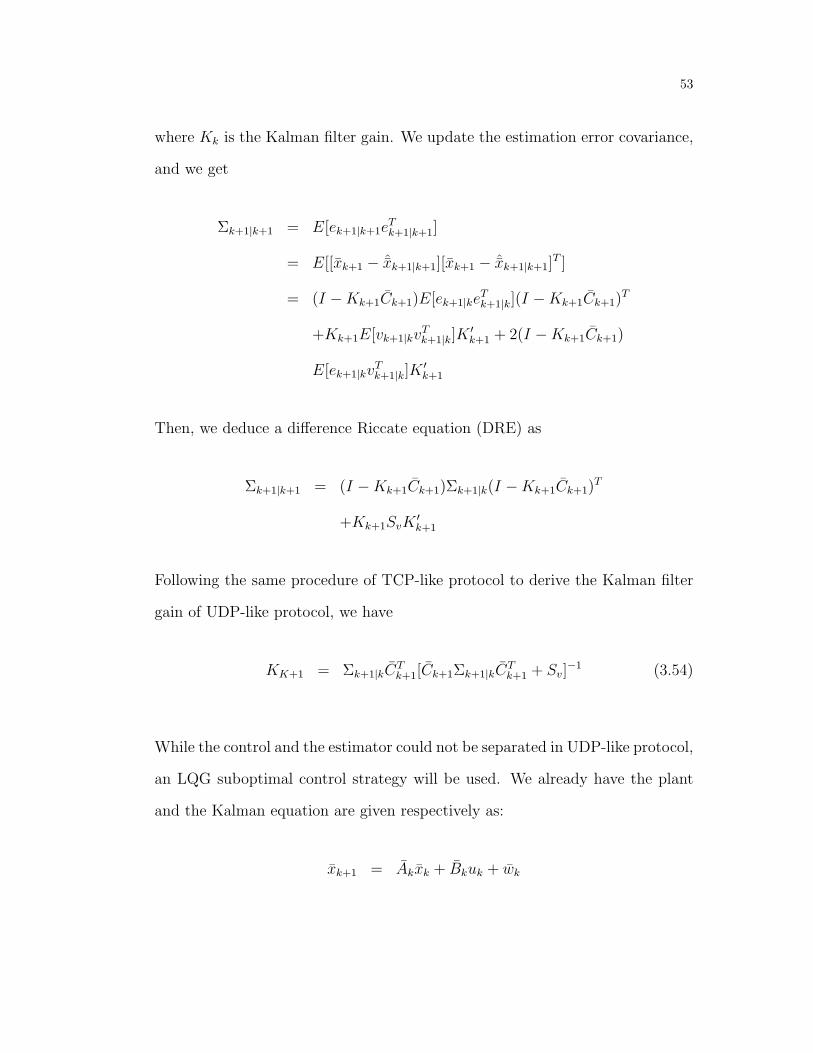
53

where Kk is the Kalman filter gain. We update the estimation error covariance,

and we get

Σk+1|k+1 = E[ek+1|k+1eTk+1|k+1]

= E[[xk+1 − ˆxk+1|k+1][xk+1 − ˆxk+1|k+1]T ]

= (I −Kk+1Ck+1)E[ek+1|keTk+1|k](I −Kk+1Ck+1)

T

+Kk+1E[vk+1|kvTk+1|k]K

′k+1 + 2(I −Kk+1Ck+1)

E[ek+1|kvTk+1|k]K

′k+1

Then, we deduce a difference Riccate equation (DRE) as

Σk+1|k+1 = (I −Kk+1Ck+1)Σk+1|k(I −Kk+1Ck+1)T

+Kk+1SvK′k+1

Following the same procedure of TCP-like protocol to derive the Kalman filter

gain of UDP-like protocol, we have

KK+1 = Σk+1|kCTk+1[Ck+1Σk+1|kC

Tk+1 + Sv]

−1 (3.54)

While the control and the estimator could not be separated in UDP-like protocol,

an LQG suboptimal control strategy will be used. We already have the plant

and the Kalman equation are given respectively as:

xk+1 = Akxk + Bkuk + wk

54

ˆxk+1 = Ak ˆxk + Bkuesk +Kk+1[yk+1 − Ck+1 ˆxk+1]

The error dynamic is written as

ek+1 = xk+1 − ˆxk+1

= (Ak −KkCk)ek + Bkuk − Bkuesk + wk −Kkvk

where we assume that uesk is the estimated input, and uk is the actual input.

The estimation error covariance of the error dynamic is

Σk+1 = E[ek+1|keTk+1|k]

= (Ak −KkCk)Σk(Ak −KkCk)T + Bkuku

Tk B

Tk

+BkueskuTeskB

Tk − 2Bkuku

TeskB

Tk

+Sw +KkSvK′k

Then, the estimation error covariance is minimized with respect to uk and set

the derivative equal to zero to get the control law. In addition, using trace

operator properties on the the estimation error covariance, and eliminate the

parts that is independent from the uk, we deduce

tr[BkueskuTeskB

Tk − 2Bkuku

TeskB

Tk + Bkuku

Tk B

Tk ]

Differentiating trace of the estimation error covariance with respect uk , we

55

obtain

0 = BkBTk uk + 0− BkB

Tk uesk

Then the control law of the predictive estimation is

u∗esk = uk (3.55)

For the case of packet missing on the communication links, there are two cases

to be considered. Zero input strategy where we have

u∗esk =

uk; if αk = 1;

0; if αk = 0.

and hold input strategy where

u∗esk =

uk; if αk = 1;

uk−1; if αk = 0.

56

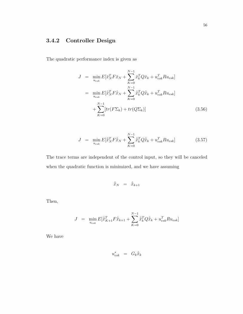
3.4.2 Controller Design

The quadratic performance index is given as

J = minuesk

E[xTNFxN +

N−1∑K=0

xTkQxk + uT

eskRuesk]

= minuesk

E[ˆxTNF ˆxN +

N−1∑K=0

ˆxTkQˆxk + uT

eskRuesk]

+N−1∑K=0

[tr(FΣk) + tr(QΣk)] (3.56)

J = minuesk

E[ˆxTNF ˆxN +

N−1∑K=0

ˆxTkQˆxk + uT

eskRuesk] (3.57)

The trace terms are independent of the control input, so they will be canceled

when the quadratic function is minimized, and we have assuming

ˆxN = ˆxk+1

Then,

J = minuesk

E[ˆxTK+1F ˆxk+1 +

N−1∑K=0

ˆxTkQˆxk + uT

eskRuesk]

We have

u∗esk = Gk ˆxk

57

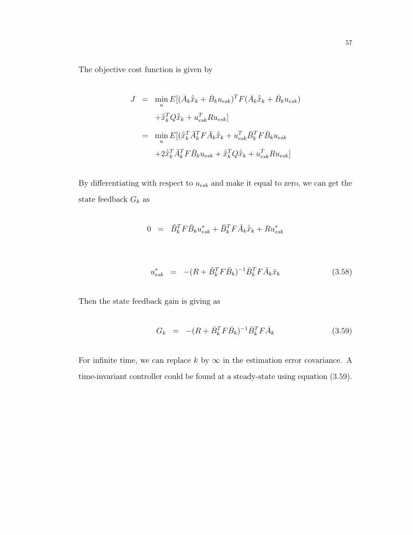
The objective cost function is given by

J = minu

E[(Ak ˆxk + Bkuesk)TF (Ak ˆxk + Bkuesk)

+ˆxTkQˆxk + uT

eskRuesk]

= minu

E[(ˆxTk A

TkFAk ˆxk + uT

eskBTk FBkuesk

+2ˆxTk A

TkFBkuesk + ˆxT

kQˆxk + uTeskRuesk]

By differentiating with respect to uesk and make it equal to zero, we can get the

state feedback Gk as

0 = BTk FBku

∗esk + BT

k FAk ˆxk +Ru∗esk

u∗esk = −(R + BT

k FBk)−1BT

k FAkxk (3.58)

Then the state feedback gain is giving as

Gk = −(R + BTk FBk)

−1BTk FAk (3.59)

For infinite time, we can replace k by ∞ in the estimation error covariance. A

time-invariant controller could be found at a steady-state using equation (3.59).

58

3.5 Numerical Example

In this section, numerical examples and simulations are considered to illustrate

the effectiveness of the proposed approaches and to verify the design method

developed in terms of hold input strategy.

Example 3.5.1

Consider MIMO system represented by the following state space model:

A =

0.3679 0 0 0

0 0.3679 0 0

0.2864 −0.1432 0.6065 0

0 0.0239 0 0.6065

B =

0.6321 0

0 0.6321

0.1858 −0.0929

0 0.0155

C =

0 0 1 0

0 0 0 1

59

We consider the state feedback u = Gˆxk, where the weighted matrices are chosen

as

R =

0.01 0

0 0.01

and

Q =

0.01 0 0 0 0 0

0 0.01 0 0 0 0

0 0 0.01 0 0 0

0 0 0 1.0 0 0

0 0 0 0 1.0 0

0 0 0 0 0 1.0

and the positive definite matrix F is stated as

F =

1 0 0 0 0 0

0 1 0 0 0 0

0 0 1 0 0 0

0 0 0 1 0 0

0 0 0 0 1 0

0 0 0 0 0 1

60

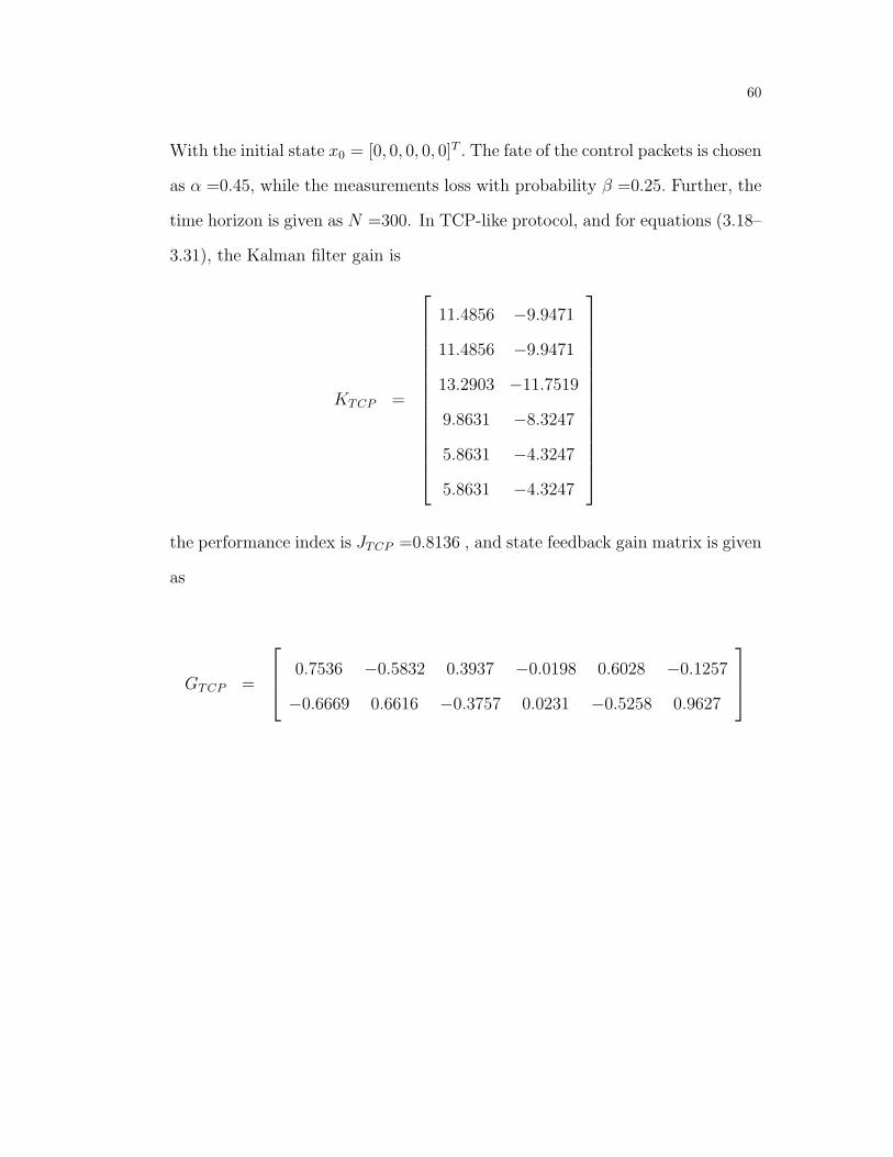
With the initial state x0 = [0, 0, 0, 0, 0]T . The fate of the control packets is chosen

as α =0.45, while the measurements loss with probability β =0.25. Further, the

time horizon is given as N =300. In TCP-like protocol, and for equations (3.18–

3.31), the Kalman filter gain is

KTCP =

11.4856 −9.9471

11.4856 −9.9471

13.2903 −11.7519

9.8631 −8.3247

5.8631 −4.3247

5.8631 −4.3247

the performance index is JTCP =0.8136 , and state feedback gain matrix is given

as

GTCP =

0.7536 −0.5832 0.3937 −0.0198 0.6028 −0.1257

−0.6669 0.6616 −0.3757 0.0231 −0.5258 0.9627

61

In UDP-like protocol case, using equations (3.47–3.60), the Kalman filter gain

is deduced as

KUDP =

6.5734 −4.7953

6.9555 −5.2018

9.2986 −7.5411

6.3577 −4.6528

2.3577 −0.6528

2.3577 −0.6528

As result of our approach, the minimum of the cost function is JUDP = 0.2930,

and state feedback gain matrix is given as

GUDP =

0.7536 −0.5832 0.3937 −0.0198 0.6028 −0.1257

−0.6669 0.6616 −0.3757 0.0231 −0.5258 0.9627

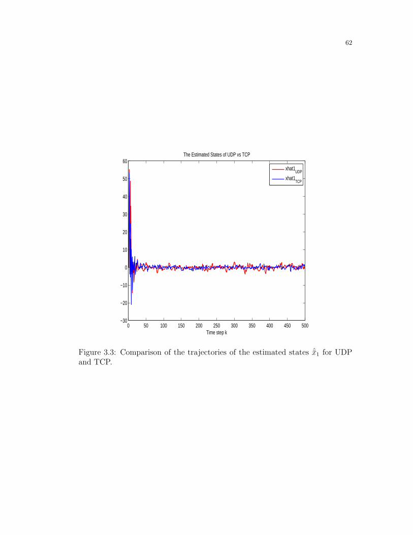
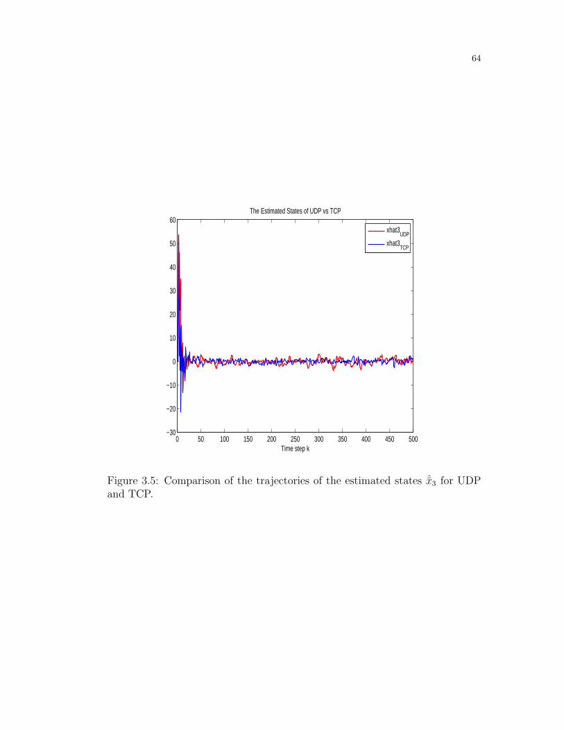
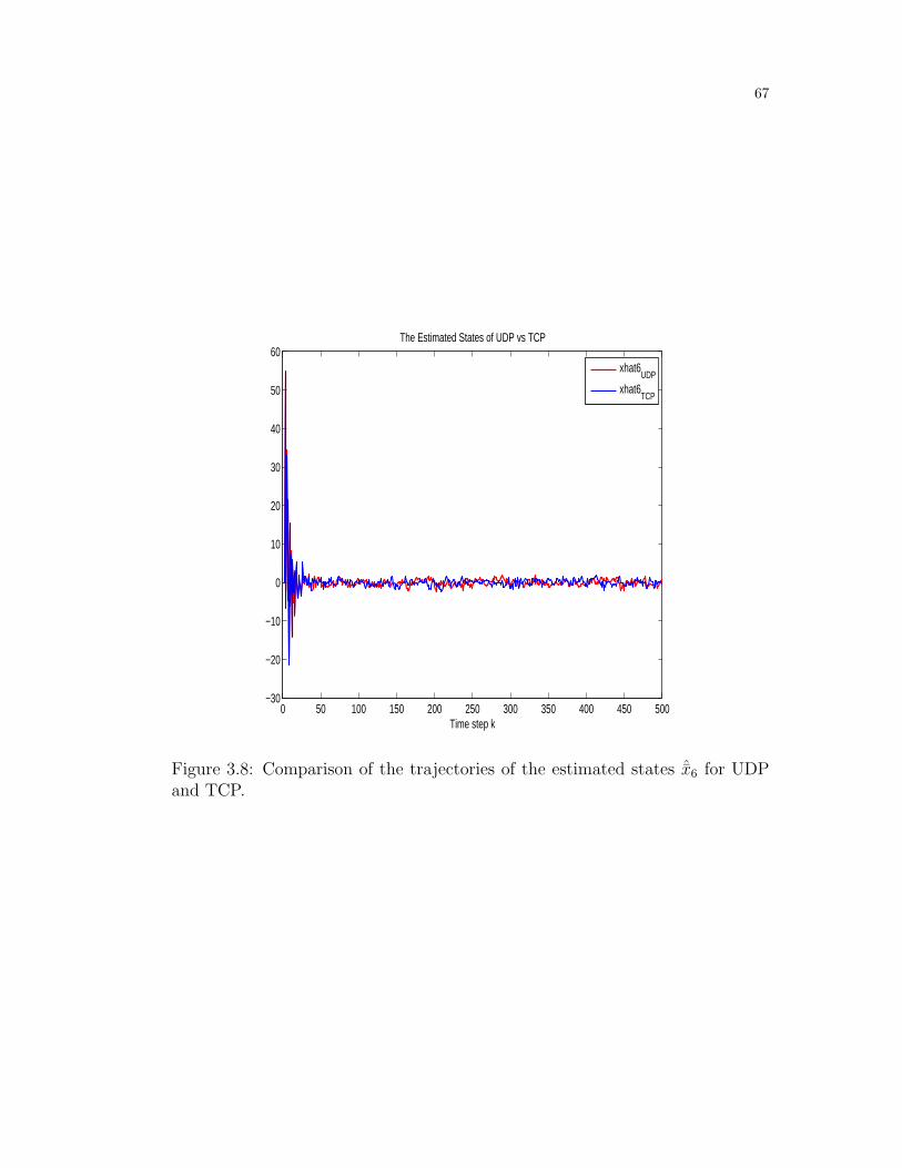
Figures 3.3– 3.8 show the comparison of the estimated states of LQG under

UDP-like protocol and LQG under TCP-like protocol according to our approach

designed in this chapter.

Example 3.5.2

In this example, we investigate single input single output SISO LTI system. To

see the efficiency of our proposed approach in designing different LTI system

62

0 50 100 150 200 250 300 350 400 450 500−30

−20

−10

0

10

20

30

40

50

60

Time step k

The Estimated States of UDP vs TCP

xhat1

UDP

xhat1TCP

Figure 3.3: Comparison of the trajectories of the estimated states ˆx1 for UDPand TCP.

63

0 50 100 150 200 250 300 350 400 450 500−20

−10

0

10

20

30

40

50

60

Time step k


xhat2UDP

xhat2TCP


64

0 50 100 150 200 250 300 350 400 450 500−30

−20

−10

0

10

20

30

40

50

60

Time step k


xhat3

UDP

xhat3TCP


65

0 50 100 150 200 250 300 350 400 450 500−20

−10

0

10

20

30

40

50

60

Time step k


xhat4

UDP

xhat4TCP


66

0 50 100 150 200 250 300 350 400 450 500−30

−20

−10

0

10

20

30

40

50

60

Time step k


xhat5

UDP

xhat5TCP

Figure 3.7: Comparison of the trajectories of the sixth estimated states ˆx5 forUDP and TCP.

67

0 50 100 150 200 250 300 350 400 450 500−30

−20

−10

0

10

20

30

40

50

60

Time step k


xhat6

UDP

xhat6TCP


68

structures. The SISO control system is described by

A =

0.66 0.209

−0.123 −0.5

B =

−1

1

C =

[2 1

]

The LQ state feedback control is u =Gˆxk, where the weighted matrices are given

as R =1.00e−03 and

Q =

0.01 0 0

0 0.01 0

0 0 0.01

and the positive definite matrix F is selected as

F =

1 0 0

0 1 0

0 0 1

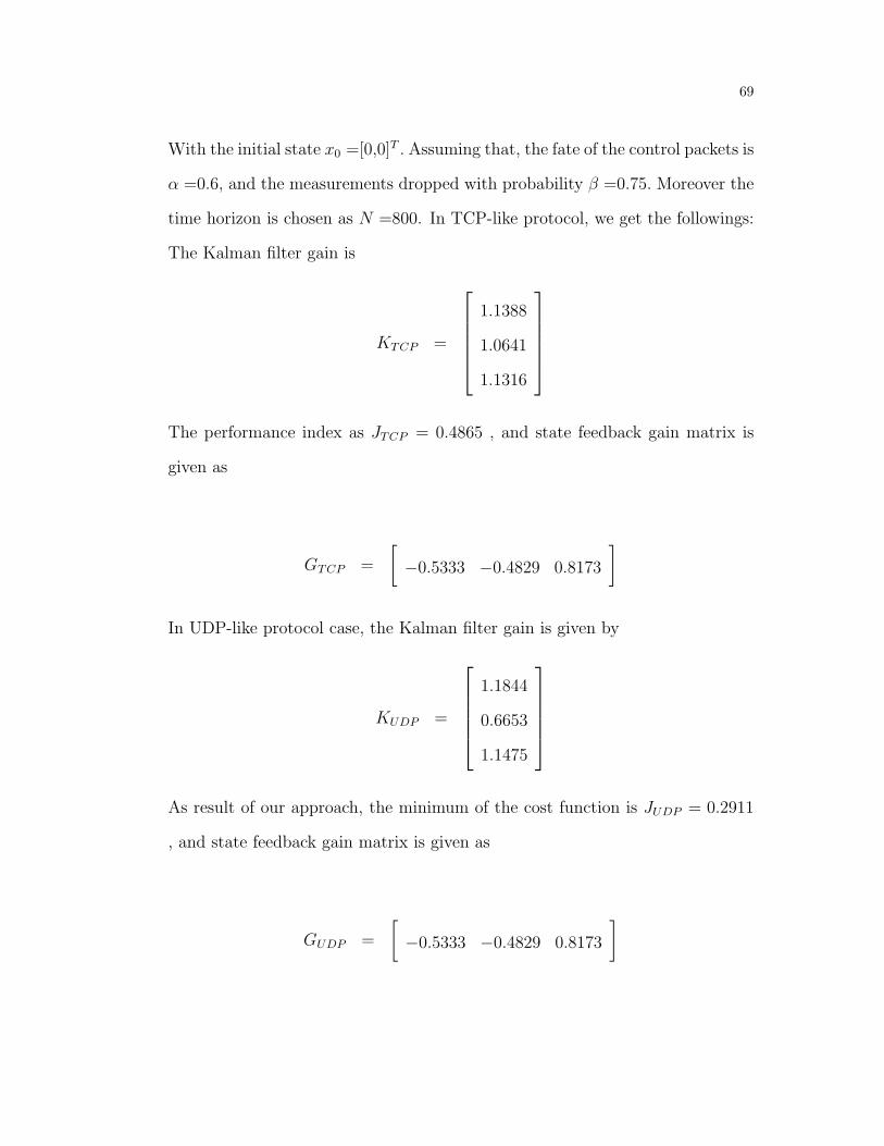
69

With the initial state x0 =[0,0]T . Assuming that, the fate of the control packets is

α =0.6, and the measurements dropped with probability β =0.75. Moreover the

time horizon is chosen as N =800. In TCP-like protocol, we get the followings:

The Kalman filter gain is

KTCP =

1.1388

1.0641

1.1316

The performance index as JTCP = 0.4865 , and state feedback gain matrix is

given as

GTCP =

[−0.5333 −0.4829 0.8173

]

In UDP-like protocol case, the Kalman filter gain is given by

KUDP =

1.1844

0.6653

1.1475

As result of our approach, the minimum of the cost function is JUDP = 0.2911

, and state feedback gain matrix is given as

GUDP =

[−0.5333 −0.4829 0.8173

]

70

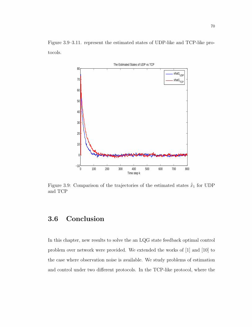
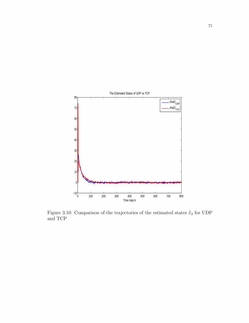
Figure 3.9–3.11. represent the estimated states of UDP-like and TCP-like pro-

tocols.

0 100 200 300 400 500 600 700 800−10

0

10

20

30

40

50

60

70

80

Time step k


xhat1

UDP

xhat1TCP

Figure 3.9: Comparison of the trajectories of the estimated states ˆx1 for UDPand TCP

3.6 Conclusion

In this chapter, new results to solve the an LQG state feedback optimal control

problem over network were provided. We extended the works of [1] and [10] to

the case where observation noise is available. We study problems of estimation

and control under two different protocols. In the TCP-like protocol, where the

71

0 100 200 300 400 500 600 700 800−10

0

10

20

30

40

50

60

70

80

Time step k


xhat2

UDP

xhat2TCP


72

0 100 200 300 400 500 600 700 800−10

0

10

20

30

40

50

60

70

80

90

Time step k


xhat3

UDP

xhatTCP


73

estimation/ control unit provides acknowledgments when successfully the packet

are delivered. On the other-hand, there is no acknowledgments are permitted

in the UDP-like case. We addressed the nonlinearity for UDP protocol using

suboptimal approach.

It is worth while to note that from our examples, the suboptimal controller design

for UDP like protocol using zero input strategy gives better performance than

the standard linear quadratic Gaussian approach in case of TCP-like protocol

using hold input strategy. Moreover the steady state response of the suboptimal

approach for UDP protocol convergence faster than standard LQG approach for

TCP-like protocol as Fig. (3.3–3.11).

75

Chapter 4

OBSERVER BASED

NETWORKED CONTROL

SYSTEMS WITH

NONSTATIONARY PACKET

DROPOUT

4.1 Introduction

Due to the rapid evolution of communication and industrial technologies, many

industrial control applications have been devoted more attention to networked

76

control systems. It becomes increasingly apparent that stabilization problem

of networked control systems has been addressed in the presence of networks

constraints such as time delay and data lost as given in [25] and [59]. More-

over necessary and sufficient conditions have been studied for NCSs stability by

applying state and output feedback [60]-[62].

It is well known that data can be sent across communication networks in packet

form, this makes it possible in NCSs to cover packets time delay and packet

lost by sending a sequence control predirection in one packet for routing control

according the last network condition. However, transmission packet may be

completely lost due to unreliable nature of the communication channels. As

result, the packets transmitted from a sensor to a controller/estimator (S/C) and

from the controller to an actuator (C/A) are randomly loss. In practice, these

communication properties can affect the estimation and control performance.

The effect of packet dropout is proposed by many authors, see [52] and [37].

This chapter investigates an estimation schemes in networked control systems

(NCS). A class of observer based stabilizing controller of networked control sys-

tems (NCSs) is considered with nonstationary packet dropped out. Furthermore,

the fate of control and observation signals are modeled by two mutually inde-

pendent random variables. In particular, there are two compensation strategies

that are used to compensate the control packet fates. Hold input strategy, at

which the last control packet is used for compensation if the control packet get

lost, while in zero input strategy zero control is applied when the control (actu-

ation) packet failed to reach the actuator. It is shown that the observer based

77

controller is designed to stabilize Networked systems in means of exponential

stability, where a sufficient condition for stability is driven in terms of using

linear matrix inequality (LMIs).

In this chapter, we present an extension the work of [63] by designing an ob-

server based stabilizing control scheme for state and control estimation with

nonstationary packet lost, where data loss occurs due to unreliable nature of the

link, transmission errors and/or congestion or long time delays. We assume that

time delay and quantization error are avoided. It is shown that the observer is

figured out to stabilize NCS in the sense of exponential stability using linear

matrix inequality (LMI). We formulate the design problem on hold-input and

zero-input strategies [17].

4.2 Hold Input Strategy

In this section, we consider a networked control system with a packet drop

over both directions. In addition, probabilities of the control input packet and

the observation packets to get lost are modeled by two mutually independent

random variables. The hold input strategy, where the last control packet is used

for compensation if the control input packet is lost, will be applied. The plants

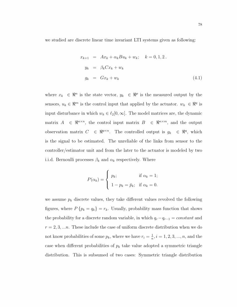
78

we studied are discrete linear time invariant LTI systems given as following:

xk+1 = Axk + αkBuk + wk; k = 0, 1, 2..

yk = βkCxk + wk

gk = Gxk + wk (4.1)


sensors, uk ∈ ℜm is the control input that applied by the actuator. wk ∈ ℜq is

input disturbance in which wk ∈ ℓ2[0,∞]. The model matrices are, the dynamic

matrix A ∈ ℜn×n, the control input matrix B ∈ ℜn×m, and the output

observation matrix C ∈ ℜp×n. The controlled output is gk ∈ ℜq, which

is the signal to be estimated. The unreliable of the links from sensor to the

controller/estimator unit and from the later to the actuator is modeled by two

i.i.d. Bernoulli processes βk and αk respectively. Where

P (αk) =

pk; if αk = 1;

1− pk = pk; if αk = 0.

we assume pk discrete values, they take different values revolved the following

figures, where P pk = qk = rk. Usually, probability mass function that shows

the probability for a discrete random variable, in which qr−qr−1 = constant and

r = 2, 3, ...n. These include the case of uniform discrete distribution when we do

not know probabilities of some pk, where we have ri =1n, i = 1, 2, 3, ..., n, and the

case when different probabilities of pk take value adopted a symmetric triangle

distribution. This is subsumed of two cases: Symmetric triangle distribution

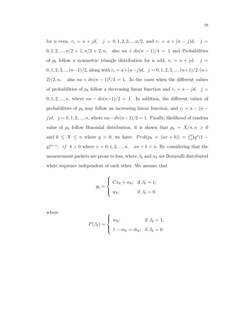
79

for n even, ri = a + jd, j = 0, 1, 2, 3, .., n/2, and ri = a + (n − j)d, j =

0, 1, 2, ..., n/2 + 1, n/2 + 2, n, also na + dn(n − 1)/4 = 1 and Probabilities

of pk follow a symmetric triangle distribution for n odd, ri = a + jd, j =

0, 1, 2, 3, .., (n−1)/2, along with ri = a+(n−j)d, j = 0, 1, 2, 3, ..., (n+1)/2, (n+

2)/2, n, also na + dn(n − 1)2/4 = 1. In the cases when the different values

of probabilities of pk follow a decreasing linear function and ri = a − jd, j =

0, 1, 2, ..., n, where na − dn(n−1)/2 = 1. In addition, the different values of

probabilities of pk may follow an increasing linear function, and ri = a − (n −

j)d, j = 0, 1, 2, ..., n, where na−dn(n−1)/2 = 1. Finally, likelihood of random

value of pk follow Binomial distribution, it is shown that pk = X/n, n > 0

and 0 ≤ X ≤ n where q > 0, we have: Prob(pk = (ax + b)) =(nx

)qx(1 −

q)n−x; if b > 0 where x = 0, 1, 2, ..., n, an + b < n. By considering that the

measurement packets are prone to loss, where βk and αk are Bernoulli distributed

white sequence independent of each other. We assume that

yk =

Cxk + wk; if βk = 1;

wk; if βk = 0.

where

P (βk) =

mk; if βk = 1;

1−mk = mk; if βk = 0.

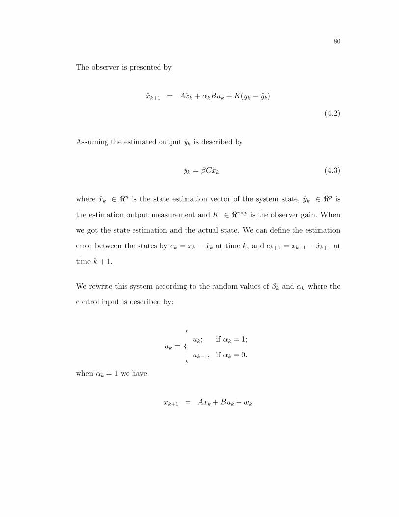
80

The observer is presented by

xk+1 = Axk + αkBuk +K(yk − yk)

(4.2)

Assuming the estimated output yk is described by

yk = βCxk (4.3)

where xk ∈ ℜn is the state estimation vector of the system state, yk ∈ ℜp is

the estimation output measurement and K ∈ ℜn×p is the observer gain. When

we got the state estimation and the actual state. We can define the estimation

error between the states by ek = xk − xk at time k, and ek+1 = xk+1 − xk+1 at

time k + 1.

We rewrite this system according to the random values of βk and αk where the

control input is described by:

uk =

uk; if αk = 1;

uk−1; if αk = 0.

when αk = 1 we have

xk+1 = Axk +Buk + wk

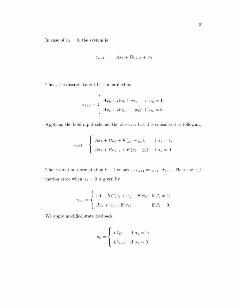
81

In case of αk = 0, the system is

xk+1 = Axk +Buk−1 + wk

Then, the discrete time LTI is identified as

xk+1 =


Axk +Buk−1 + wk; if αk = 0.

Applying the hold input scheme, the observer based is considered as following

xk+1 =

Axk +Buk +K(yk − yk); if αk = 1;

Axk +Buk−1 +K(yk − yk); if αk = 0.

The estimation error at time k + 1 comes as ek+1 =xk+1−xk+1. Then the esti-

mation error when αk = 0 is given by

ek+1 =

(A−KC)ek + wk −Kwk; if βk = 1;

Aek + wk −Kwk; if βk = 0.

We apply modified state feedback

uk =

Lxk; if αk = 1;

Lxk−1; if αk = 0.

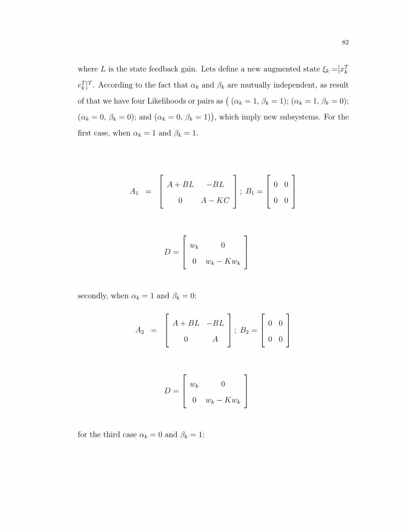
82

where L is the state feedback gain. Lets define a new augmented state ξk =[xTk

eTk ]T . According to the fact that αk and βk are mutually independent, as result

of that we have four Likelihoods or pairs as((αk = 1, βk = 1); (αk = 1, βk = 0);

(αk = 0, βk = 0); and (αk = 0, βk = 1)), which imply new subsystems. For the

first case, when αk = 1 and βk = 1.

A1 =

A+BL −BL

0 A−KC

; B1 =

0 0

0 0

D =

wk 0

0 wk −Kwk

secondly, when αk = 1 and βk = 0:

A2 =

A+BL −BL

0 A

; B2 =

0 0

0 0

D =

wk 0

0 wk −Kwk

for the third case αk = 0 and βk = 1:

83

A3 =

A 0

0 A−KC

; B3 =

BL −BL

0 0

D =

wk 0

0 wk −Kwk

for the last pair αk = 0 and βk = 0

A4 =

A 0

0 A

; B4 =

BL −BL

0 0

D =

wk 0

0 wk −Kwk

The new discrete model is considering as

ξk+1 =

xk

ek

= Ajξk + Bjξk−1 +D (4.4)

84

where Aj = Ai; i = 1, 2, 3, 4, and Bj = Bi; i = 1, 2, 3, 4

gk =

[G 0

] xk

ek

+ wk

= Gξk + wk (4.5)

The goal of this work is to design an observer based stabilizing controller, in

which the equation (4.2) with a compensation input scheme for control packets,

such that the closed loop system is exponential stable. Basing on the switched

time delay systems [74], we present

σ1 = Prob αk = 1, βk = 1 , E[σ1] = σ1

σ2 = Prob αk = 0, βk = 1 , E[σ2] = σ2

σ3 = Prob αk = 1, βk = 0 , E[σ3] = σ3

σ4 = Prob αk = 0, βk = 0 , E[σ4] = σ4

4.2.1 Main Results

In this section, we analyze the stability property for nonstationary packet dropout

process, and closed loop problems are considered, where a necessary and a suf-

ficient stability conditions for the closed loop system is derived using adopted

packet dropout independent Lyapunov functions, see [75].

V (ξk) =2∑

i=1

Vi(ξk) (4.6)

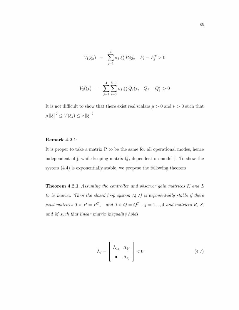
85

V1(ξk) =4∑

j=1

σj ξTk Pjξk, Pj = P T

j > 0

V2(ξk) =4∑

j=1

k−1∑i=0

σj ξTk Qjξk, Qj = QT

j > 0

It is not difficult to show that there exist real scalars µ > 0 and ν > 0 such that

µ ∥ξ∥2 ≤ V (ξk) ≤ ν ∥ξ∥2

Remark 4.2.1:

It is proper to take a matrix P to be the same for all operational modes, hence

independent of j, while keeping matrix Qj dependent on model j. To show the

system (4.4) is exponentially stable, we propose the following theorem

Theorem 4.2.1 Assuming the controller and observer gain matrices K and L

to be known. Then the closed loop system (4.4) is exponentially stable if there

exist matrices 0 < P = P T , and 0 < Q = QT , j = 1, .., 4 and matrices R, S,

and M such that linear matrix inequality holds

Λj =

Λ1j Λ2j

• Λ3j

< 0; (4.7)

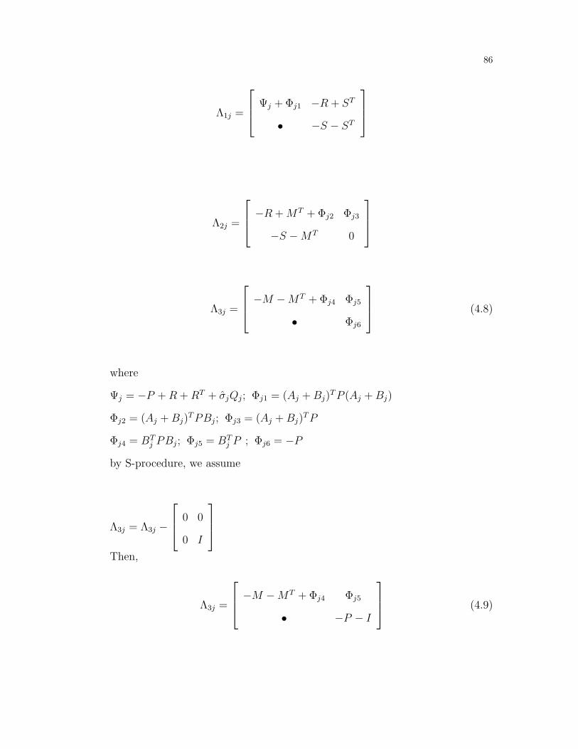
86

Λ1j =

Ψj + Φj1 −R + ST

• −S − ST

Λ2j =

−R +MT + Φj2 Φj3

−S −MT 0

Λ3j =

−M −MT + Φj4 Φj5

• Φj6

(4.8)

where

Ψj = −P +R +RT + σjQj; Φj1 = (Aj +Bj)TP (Aj +Bj)

Φj2 = (Aj +Bj)TPBj; Φj3 = (Aj +Bj)

TP

Φj4 = BTj PBj; Φj5 = BT

j P ; Φj6 = −P

by S-procedure, we assume

Λ3j = Λ3j −

0 0

0 I

Then,

Λ3j =

−M −MT + Φj4 Φj5

• −P − I

(4.9)

87

proof 4.2.1 Defining yk = xk+1 − xk, one has

ξk−1 = ξk − yk−1 (4.10)

where

λk = yk−1; D = ωk

then we have

ξk − ξk−1 − λk = 0 (4.11)

After that, the systems can be transmitted into:

ξk+1 = (Aj +Bj)ξk −Bjλk + ωk (4.12)

For some matrices R, S, and M, we deduce

2[ξTk R + ξTk−1S + λTkM ][ξk − ξk−1 − λk] = 0 (4.13)

88

Then,

∆V1(ξk) = V1(ξk+1)− V1(ξk)

=4∑

j=1

σj

[ξTk [Φj1 +Ψj]ξk − 2ξTk Rξk−1

+2ξTk−1Sξk − 2ξTk Φj2λk − 2ξTk Rλk

−2ξTk Φj3ωk − 2ξTk−1Sξk−1 + λTkΦj4λk

+2λTkΦj5ωk − 2ξTk−1Sλk + 2λT

kMξk

−2λTkMξk−1 − 2λT

kMλk + ωTk Φj6ωk

](4.14)

The difference of V2 is described by

∆V2(ξk) =4∑

j=1

σj

[ k∑i=1

ξTk Qjξk −k−1∑i=0

ξTk Qjξk]

≤ ξTk Qjξk − ξTk−1Qjξk−1

+k−1∑i=0

ξTi Qjξi (4.15)

∆V2(ξk) =4∑

j=1

σj

[ k∑i=1

ξTk Qjξk −k−1∑i=0

ξTk Qjξk]

≤ ξTk Qjξk − ξTk−1Qjξk−1

+k−1−∑i=0

ξTi Qjξi (4.16)

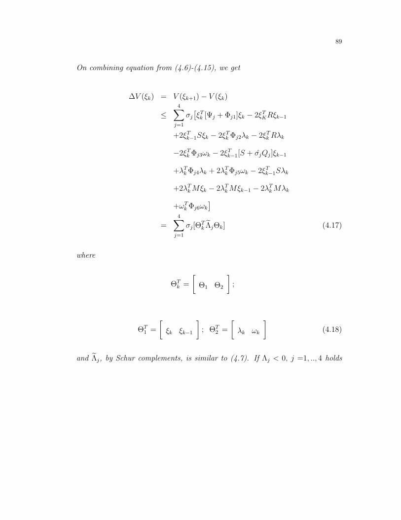
89

On combining equation from (4.6)-(4.15), we get

∆V (ξk) = V (ξk+1)− V (ξk)

≤4∑

j=1

σj

[ξTk [Ψj + Φj1]ξk − 2ξTKRξk−1

+2ξTk−1Sξk − 2ξTk Φj2λk − 2ξTk Rλk

−2ξTk Φj3ωk − 2ξTk−1[S + σjQj]ξk−1

+λTkΦj4λk + 2λT

kΦj5ωk − 2ξTk−1Sλk

+2λTkMξk − 2λT

kMξk−1 − 2λTkMλk

+ωTk Φj6ωk

]=

4∑j=1

σj[ΘTk ΛjΘk] (4.17)

where

ΘTk =

[Θ1 Θ2

];

ΘT1 =

[ξk ξk−1

]; ΘT

2 =

[λk ωk

](4.18)

and Λj, by Schur complements, is similar to (4.7). If Λj < 0, j =1, .., 4 holds

90

then

∆V (ξk) = V (ξk+1)− V (ξk)

=4∑

j=1

σj[ξTk Λjξk]

≤4∑

j=1

σj[−Λmin(Λj)ξTk ξk]

−4∑

j=1

σj[ηjξTk ξk] (4.19)

where 0 < ηj < min[λmin(Λj),max λmax(P ), λmax(Oj)][63]. It clear that an

inequality (4.18) indicates V (ξk+1) − V (ξk) < −ϕV (ξk), where ϕ is bounded

variable define as 0 < ϕ < 1. In manner of [64], we get

∥ξk∥2 ≤ νκ∥ξ0∥2 (1− ϕ)k + λ

µϕconsider the objective function

Jk =k∑

κ=0

(gTk gk − γ2wTk wk) (4.20)

For wk ∈ ℓ[0; ∞) = 0, with zero initial condition, we deuce

Jk =k∑

κ=0

(gTk gk − γ2wTk wk +∆V (x)|1 −∆V (ξk)|1)

≤k∑

κ=0

(gTk gk − γ2wTk wk +∆V (x)|1)

where ∆V (x)|1 describes the difference of the Lyapunov functions along the anal-

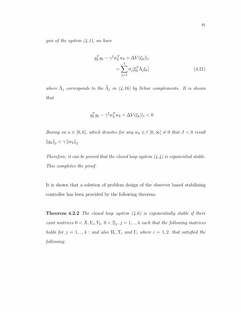
91

ysis of the system (4.1), we have

gTk gk − γ2wTk wk +∆V (ξk)|1

=4∑

j=1

σj[ξTk Λjξk] (4.21)

where Λj corresponds to the Λj in (4.16) by Schur complements. It is shown

that

gTk gk − γ2wTk wk +∆V (ξk)|1 < 0

Basing on κ ∈ [0, k], which denotes for any wk ∈ ℓ [0,∞] = 0 that J < 0 result

∥gk∥2 < γ ∥wk∥2

Therefore, it can be proved that the closed loop system (4.4) is exponential stable.

This completes the proof.

It is shown that a solution of problem design of the observer based stabilizing

controller has been provided by the following theorem:

Theorem 4.2.2 The closed loop system (4.6) is exponentially stable if there

exist matrices 0 < X, Y1, Y2, 0 < Ξj, j = 1, .., 4 such that the following matrices

holds for j = 1, .., 4 : and also Πi,Υi and Γi where i = 1, 2. that satisfied the

following:

92

Λ1j Λ2j Ωj Ωj 0 XGT

• Λ3j 0 0 0 0

• • −X X ΓT 0 0

• • • −X 0 0

• • • • −γ2I ΦT

• • • • • −I

< 0; (4.22)

X =

X 0

X X

(4.23)

Ψj =−X +Π1+ΠT1 + Ξj

Λ1j =

Ψj −Π1 +Υ1

• −Υ1 −ΥT1

Λ2j =

−Π1 + ΓT1 0

−Υ1 − ΓT1 0

Λ3j =

−Γ1 − ΓT1 0

• 0

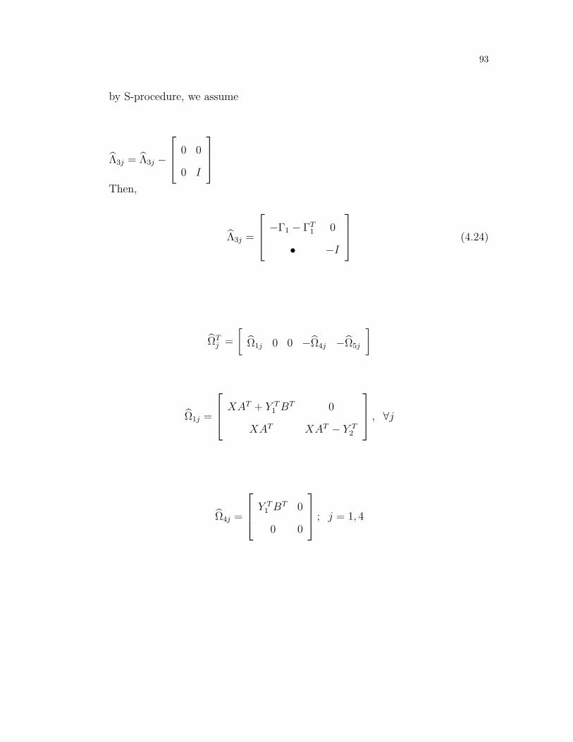
93


Λ3j = Λ3j −

0 0

0 I

Then,

Λ3j =

−Γ1 − ΓT1 0

• −I

(4.24)

ΩTj =

[Ω1j 0 0 −Ω4j −Ω5j

]

Ω1j =

XAT + Y T1 BT 0

XAT XAT − Y T2

, ∀j

Ω4j =

Y T1 BT 0

0 0

; j = 1, 4

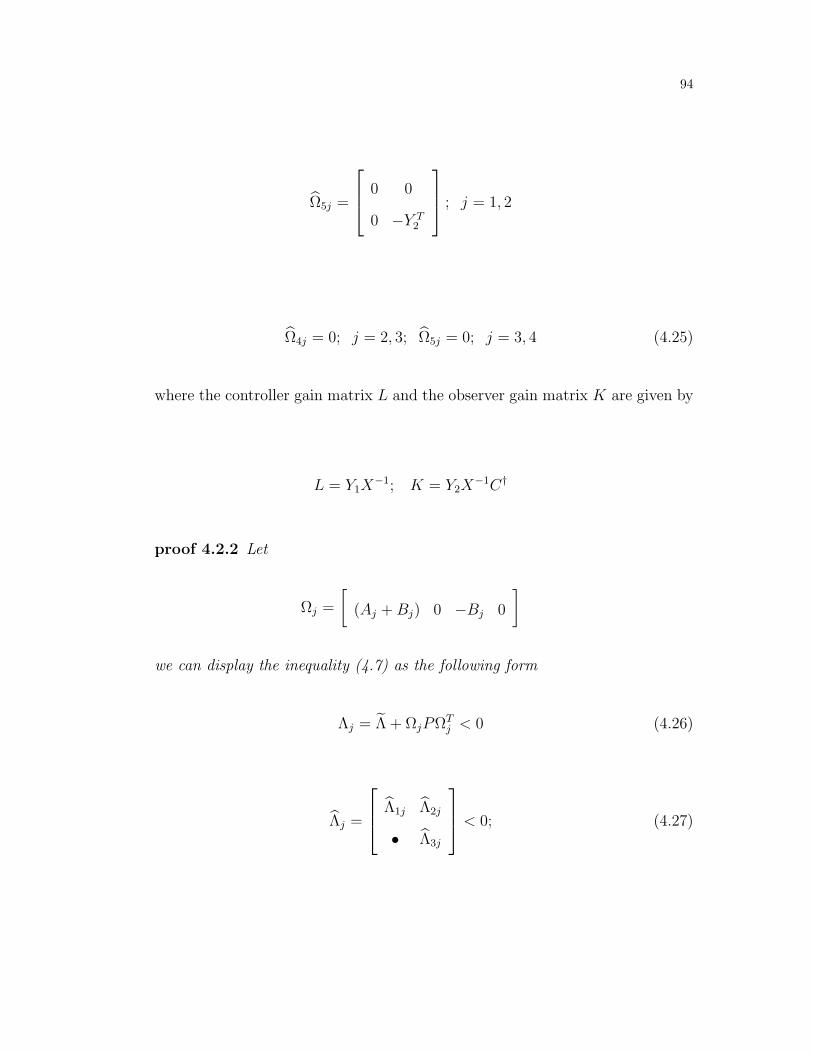
94

Ω5j =

0 0

0 −Y T2

; j = 1, 2

Ω4j = 0; j = 2, 3; Ω5j = 0; j = 3, 4 (4.25)

where the controller gain matrix L and the observer gain matrix K are given by

L = Y1X−1; K = Y2X

−1C†

proof 4.2.2 Let

Ωj =

[(Aj +Bj) 0 −Bj 0

]

we can display the inequality (4.7) as the following form

Λj = Λ + ΩjPΩTj < 0 (4.26)

Λj =

Λ1j Λ2j

• Λ3j

< 0; (4.27)

95

Λ1j =

Ψj −R + ST

• −S − ST

Λ2j =

−R+MT 0

−S −MT 0

Λ3j =

−M+MT 0

• −I

Put X = P−1, using Schur complements, the matrix Λj in (4.24) can be repre-

sented as


• Λ3j 0 0 0 0

• • −X −ΓTP 0 0

• • • −P 0 0

• • • • −γ2I ΦT

• • • • • −I

< 0; (4.28)

Employing the congruence transformation

Tj = diag[ X , X , X, X, I , X, I, I]

96

this apply for matrix inequality in (4.26) and manipulating using (4.22), so we

deduce

Ξj = XQjX, Πj = XRjX, Γj = XMjX ωj = XSjX

Remark 4.2.2:

Setting X as represent at (4.22) has benefit that the solution of bilinear matrix

inequalities is converted that linear matrix inequalities. It is shown that the

LMI (4.21) subject to dropout models that characterized by E[βk], E[αk] and

E[σi] , which are quite useful in illustrating different operating conditions of the

communications network.

4.2.2 Numerical Examples

In this section, numerical examples and simulations are considered to illustrate

the effectiveness of the proposed approaches in terms of previous input strategy.

We assumed βk = 0.1 and αk = 0.1. Our purpose is to design an observer-based

stabilizing controller in the form of (4.2).

Example 4.2.1:

We study the uninterruptible power system UPS, in which we try to control the

pulsewidth-modulated inverter to guarantee the output ac voltage is kept at the

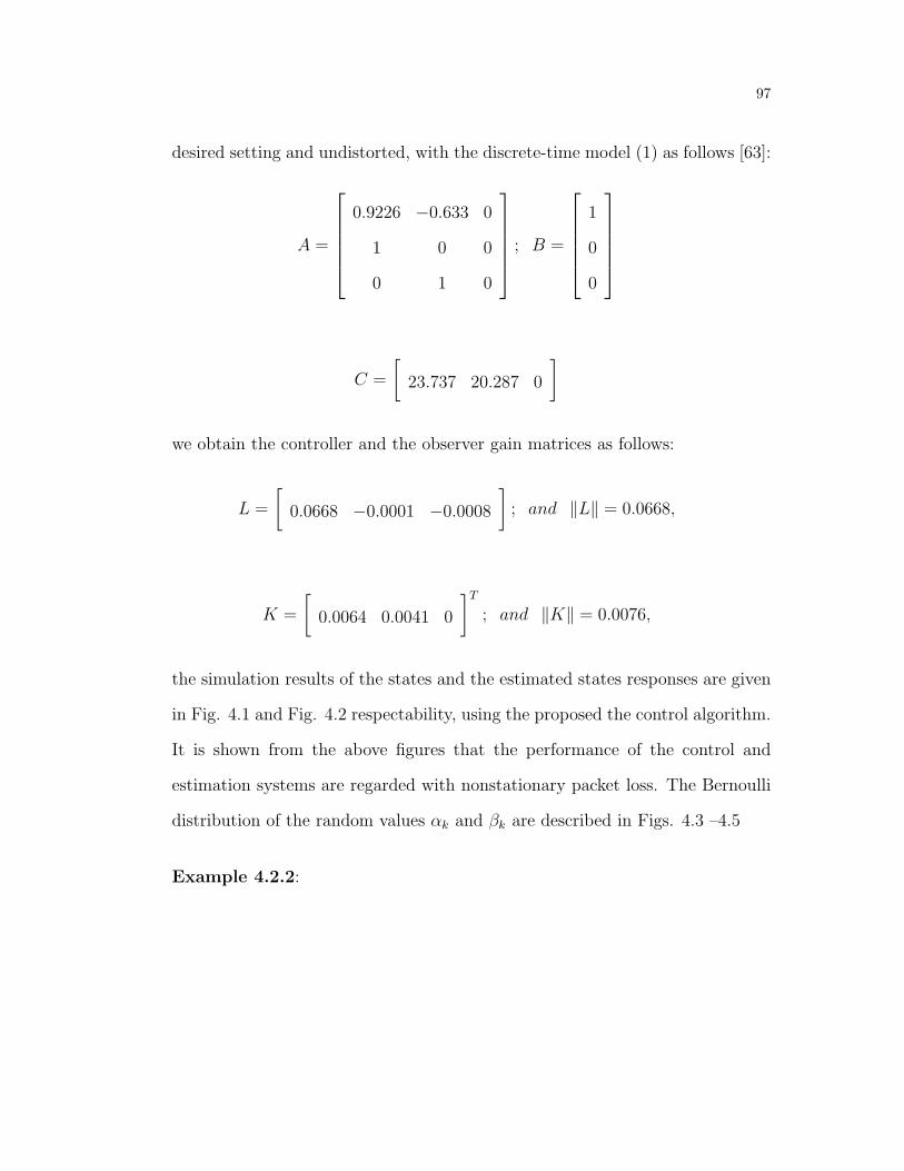
97

desired setting and undistorted, with the discrete-time model (1) as follows [63]:

A =

0.9226 −0.633 0

1 0 0

0 1 0

; B =

1

0

0

C =

[23.737 20.287 0

]

we obtain the controller and the observer gain matrices as follows:

L =

[0.0668 −0.0001 −0.0008

]; and ∥L∥ = 0.0668,

K =

[0.0064 0.0041 0

]T; and ∥K∥ = 0.0076,

the simulation results of the states and the estimated states responses are given

in Fig. 4.1 and Fig. 4.2 respectability, using the proposed the control algorithm.

It is shown from the above figures that the performance of the control and

estimation systems are regarded with nonstationary packet loss. The Bernoulli

distribution of the random values αk and βk are described in Figs. 4.3 –4.5

Example 4.2.2:

98

Figure 4.1: Trajectories of system states for nonstationary packet loss using holdinput scheme

Figure 4.2: Trajectories of the estimated states for nonstationary packet lossusing hold input scheme

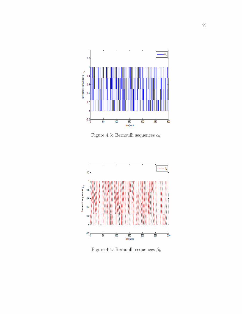
99

Figure 4.3: Bernoulli sequences αk

Figure 4.4: Bernoulli sequences βk

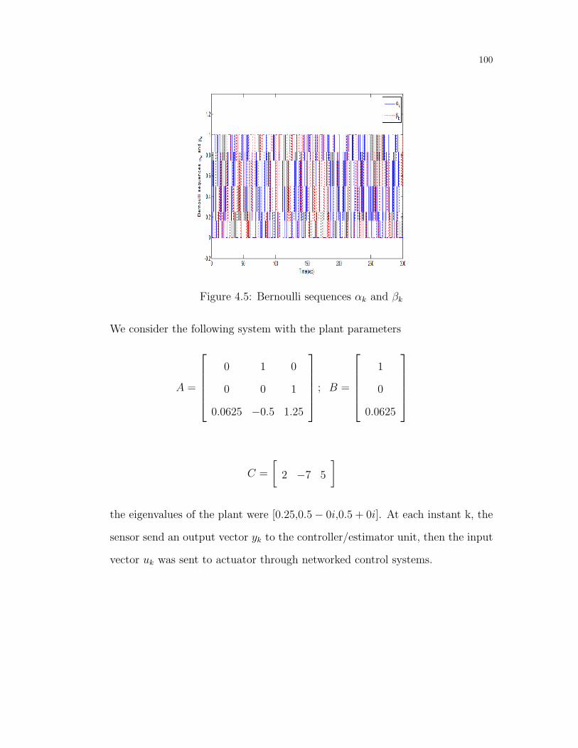
100

Figure 4.5: Bernoulli sequences αk and βk

We consider the following system with the plant parameters

A =

0 1 0

0 0 1

0.0625 −0.5 1.25

; B =

1

0

0.0625

C =

[2 −7 5

]

the eigenvalues of the plant were [0.25,0.5− 0i,0.5 + 0i]. At each instant k, the

sensor send an output vector yk to the controller/estimator unit, then the input

vector uk was sent to actuator through networked control systems.

101

we obtain the state feedback controller and observer gain matrices as follows:

L =

[−0.0001 0.0683 0.0055

]; and ∥L∥ = 0.0686,

K =

[0.0227 −0.0053 −0.0015

]T; and ∥K∥ = 0.0233,


Figure 4.6: States trajectories under nonstationary random dropout using holdinput scheme

in Fig. 4.6 and Fig. 4.7 respectability, using the proposed the control algorithm.

It is shown from the above figures that the performance of the control and

estimation systems are regarded with nonstationary packet loss.

Example 4.2.3:

In this example, we investigate a second order linear system. The state space

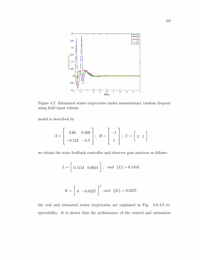
102

Figure 4.7: Estimated states trajectories under nonstationary random dropoutusing hold input scheme

model is described by

A =

0.66 0.209

−0.123 −0.5

; B =

−1

1

; C =

[2 1

]

we obtain the state feedback controller and observer gain matrices as follows:

L =

[0.1154 0.0824

]; and ∥L∥ = 0.1418,

K =

[0 −0.0237

]T; and ∥K∥ = 0.0237,

the real and estimated states trajectories are explained in Fig. 4.8-4.9 re-

spectability. It is shown that the performance of the control and estimation

103

systems are suffered when the measurements and control packet are sending

over NCSs with nonstationary packet dropout.

Figure 4.8: Trajectories of system states for nonstationary packet dropout usinghold input scheme

4.3 Zero Input Strategy

This section investigate an NCS with nonstationary packet loss in both direction

from the sensor to the estimation/control unit and between the latter and the

actuator, in which the lost of the control packets are compensated by zero input

104

Figure 4.9: Trajectories of the estimated states for nonstationary packet dropoutusing hold input scheme

control packets. The discrete plant of NCS is described by

xk+1 = Axk + αkBuk + wk; k = 0, 1, 2..

yk = βkCxk + wk

gk = Gxk + wk (4.29)


sensors, uk ∈ ℜm is the control input that applied by the actuator. wk ∈ ℜq

is input disturbance in which wk ∈ ℓ2[0,∞]. The model matrices are, the dy-

namic matrix A ∈ ℜn×n, the control input matrix B ∈ ℜn×m, and the output

observation matrix C ∈ ℜp×n. The controlled output is gk ∈ ℜq, which is

the signal to be estimated. The unreliable of the links from sensor to the con-

troller/estimator unit and from the later to the actuator is modeled by two i.i.d.

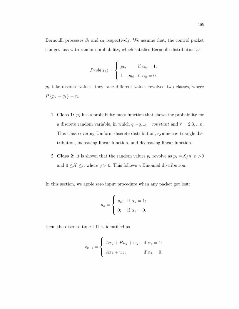
105

Bernoulli processes βk and αk respectively. We assume that, the control packet

can get loss with random probability, which satisfies Bernoulli distribution as

Prob(αk) =

pk; if αk = 1;

1− pk; if αk = 0.

pk take discrete values, they take different values revolved two classes, where

P pk = qk = rk.

1. Class 1: pk has a probability mass function that shows the probability for

a discrete random variable, in which qr−qr−1= constant and r = 2,3, ...n.

This class covering Uniform discrete distribution, symmetric triangle dis-

tribution, increasing linear function, and decreasing linear function.

2. Class 2: it is shown that the random values pk revolve as pk =X/n, n >0

and 0 ≤X ≤n where q > 0. This follows a Binomial distribution.

In this section, we apple zero input procedure when any packet got lost:

uk =

uk; if αk = 1;

0; if αk = 0.

then, the discrete time LTI is identified as

xk+1 =


Axk + wk; if αk = 0.

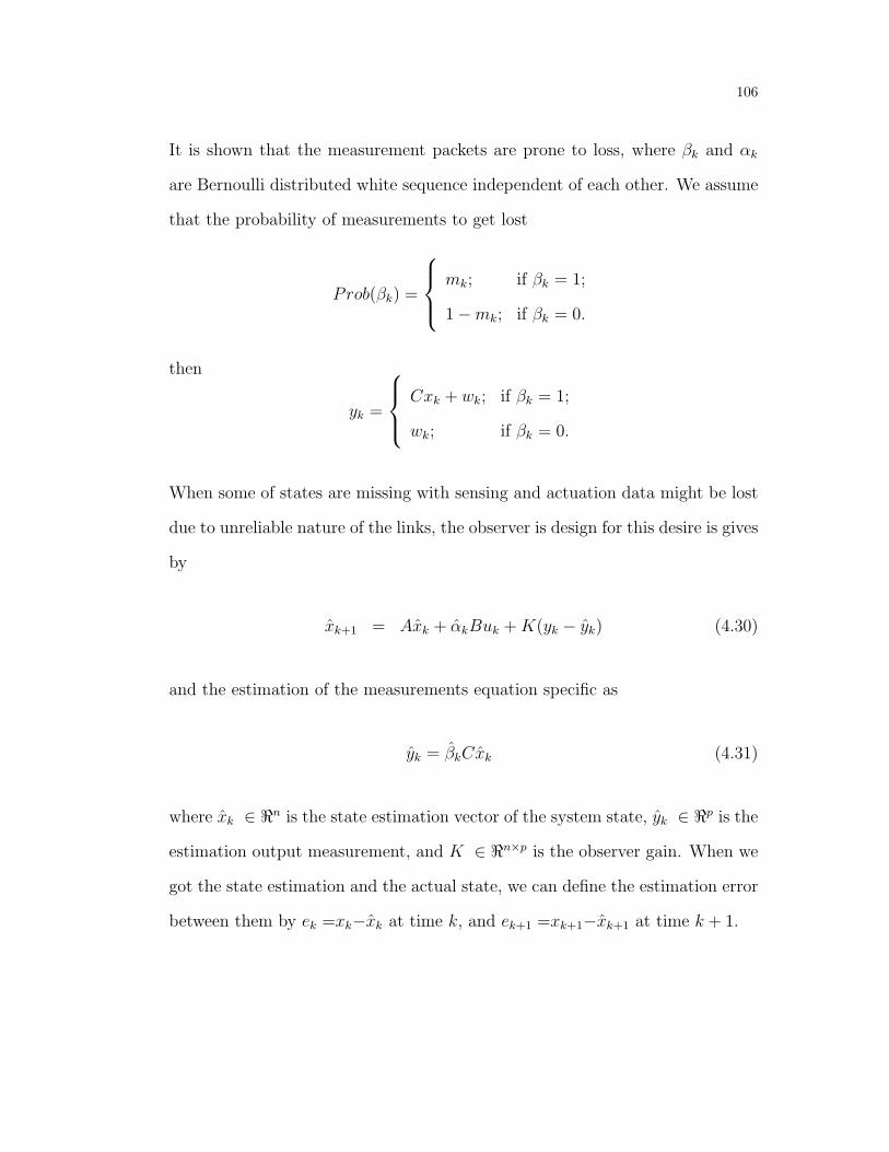
106

It is shown that the measurement packets are prone to loss, where βk and αk

are Bernoulli distributed white sequence independent of each other. We assume

that the probability of measurements to get lost

Prob(βk) =

mk; if βk = 1;

1−mk; if βk = 0.

then

yk =

Cxk + wk; if βk = 1;

wk; if βk = 0.

When some of states are missing with sensing and actuation data might be lost

due to unreliable nature of the links, the observer is design for this desire is gives

by

xk+1 = Axk + αkBuk +K(yk − yk) (4.30)

and the estimation of the measurements equation specific as

yk = βkCxk (4.31)

where xk ∈ ℜn is the state estimation vector of the system state, yk ∈ ℜp is the

estimation output measurement, and K ∈ ℜn×p is the observer gain. When we

got the state estimation and the actual state, we can define the estimation error

between them by ek =xk−xk at time k, and ek+1 =xk+1−xk+1 at time k + 1.

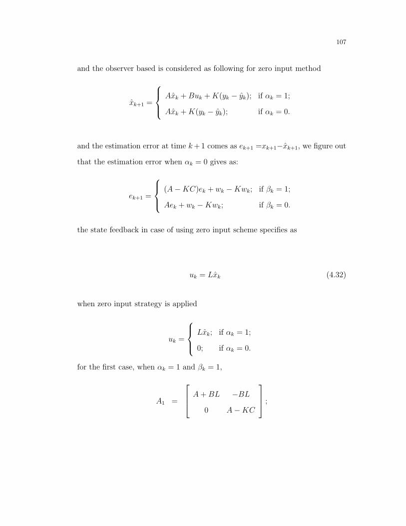
107

and the observer based is considered as following for zero input method

xk+1 =

Axk +Buk +K(yk − yk); if αk = 1;

Axk +K(yk − yk); if αk = 0.

and the estimation error at time k+1 comes as ek+1 =xk+1−xk+1, we figure out

that the estimation error when αk = 0 gives as:

ek+1 =

(A−KC)ek + wk −Kwk; if βk = 1;

Aek + wk −Kwk; if βk = 0.

the state feedback in case of using zero input scheme specifies as

uk = Lxk (4.32)

when zero input strategy is applied

uk =

Lxk; if αk = 1;

0; if αk = 0.

for the first case, when αk = 1 and βk = 1,

A1 =

A+BL −BL

0 A−KC

;

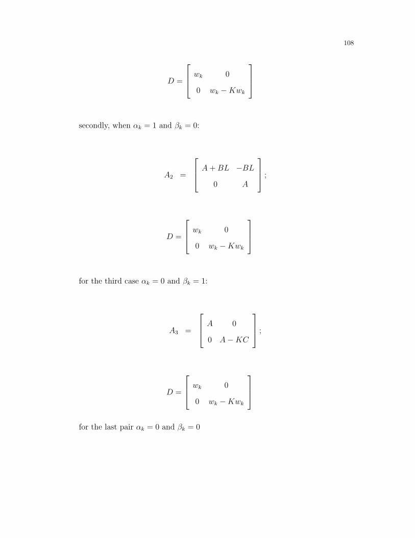
108

D =

wk 0

0 wk −Kwk

secondly, when αk = 1 and βk = 0:

A2 =

A+BL −BL

0 A

;

D =

wk 0

0 wk −Kwk

for the third case αk = 0 and βk = 1:

A3 =

A 0

0 A−KC

;

D =

wk 0

0 wk −Kwk

for the last pair αk = 0 and βk = 0

109

A4 =

A 0

0 A

;

D =

wk 0

0 wk −Kwk

the new discrete model is considering as:

ξk+1 =

xk

ek

= Ajξk +D (4.33)

where Aj = Ai; i = 1, 2, 3, 4.

gk =

[G 0

] xk

ek

+ wk

= Gξk + wk (4.34)

The aim of this paper is design an observer based stabilizing controller corre-

sponding to equations (4.28) and (4.30) such that the closed loop system (4.31)

is exponential stable in sense of mean square see [74], we present

σ1 = Prob αk = 1, βk = 1 , E[σ1] = σ1

σ2 = Prob αk = 0, βk = 1 , E[σ2] = σ2

110

σ3 = Prob αk = 1, βk = 0 , E[σ3] = σ3

σ4 = Prob αk = 0, βk = 0 , E[σ4] = σ4

4.3.1 Main Results

In this section, we analyze the stability property for nonstationary packet dropout

process, and closed loop problems are considered, where a necessary and a suf-

ficient stability conditions for the closed loop system is derived using adopted

packet dropout independent Lyapunov functions, see [75].

V(ξk) =4∑

j=1

σj ξTk Pjξk, Pj = P T

j > 0 (4.35)

I t is not difficult to show that there exist real scalars µ > 0 and ν > 0 such that

µ ∥ξ∥2≤ V (ξk)≤ ν ∥ξ∥2, see lemma 3.1 in [63].

Theorem 4.3.1 Assuming, we know the observer and the controller gains, the

closed loop system (4.31) is exponential stable if there exist matrix 0 < P= P T ,

and matrices R, S, and M such that the following matrix inequality holds.

111

Λj =

Λ1j Λ2j

• Λ3j

< 0; (4.36)

Λ1j =

Ψj + Φj1 −R + ST

• −S − ST

Λ2j =

−R +MT + Φj2 Φj3

−S −MT 0

;

Λ3j =

−M +MT + Φj4 Φj5

• Φj6

(4.37)

where Ψj = −P +R +RT ; Φj1 = ATj PAj

Φj2 = ATj P ; Φj3 = P ; Φj4 = Φj5 = Φj6 = 0


Λ3j = Λ3j −

0 0

0 I

112

Then,

Λ3j =

−M +MT 0

• −I

(4.38)

proof 4.3.1 Defining λk = yk−1; D = ωk then we find that

ξk − ξk−1 − λk = 0 (4.39)

For the matrices R, S, and M

2[ξTk R + ξTk−1S + λTkM ][ξk − ξk−1 − λk] = 0 (4.40)

we have that

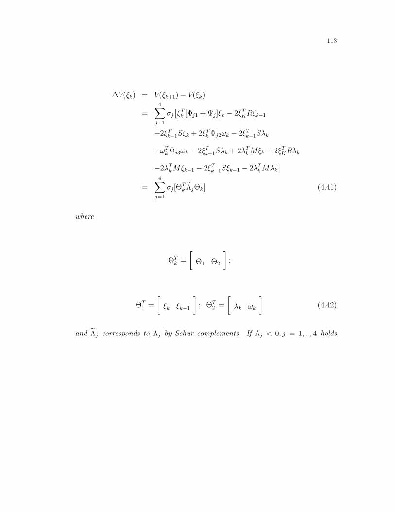
113

∆V(ξk) = V(ξk+1)− V(ξk)

=4∑

j=1

σj

[ξTk [Φj1 +Ψj]ξk − 2ξTKRξk−1

+2ξTk−1Sξk + 2ξTk Φj2ωk − 2ξTk−1Sλk

+ωTk Φj3ωk − 2ξTk−1Sλk + 2λT

kMξk − 2ξTKRλk

−2λTkMξk−1 − 2ξTk−1Sξk−1 − 2λT

kMλk

]=

4∑j=1

σj[ΘTk ΛjΘk] (4.41)

where

ΘTk =

[Θ1 Θ2

];

ΘT1 =

[ξk ξk−1

]; ΘT

2 =

[λk ωk

](4.42)

and Λj corresponds to Λj by Schur complements. If Λj < 0, j = 1, .., 4 holds

114

then

∆V (ξk) = V (ξk+1)− V (ξk)

=4∑

j=1

σj[ξTk Λjξk]

≤4∑

j=1

σj[−Λmin(Λj)ξTk ξk]

−4∑

j=1

σj[ηjξTk ξk] (4.43)

where

0 < ηj<min[λmin(Λj),max λmax(P ), λmax(Oj)]

Inequality (4.40) implies that V (ξk+1)− V (ξk) < −ϕV (ξk,

where 0 < ϕ < 1. In manner of [64], we get

∥ξk∥2 ≤ νκ∥ξ0∥2 (1− ϕ)k + λ

µϕ

consider the objective function

Jk =k∑

κ=0

(gTk gk − γ2wTk wk) (4.44)

For wk ∈ ℓ[0; ∞)= 0, with zero initial condition, we deuce

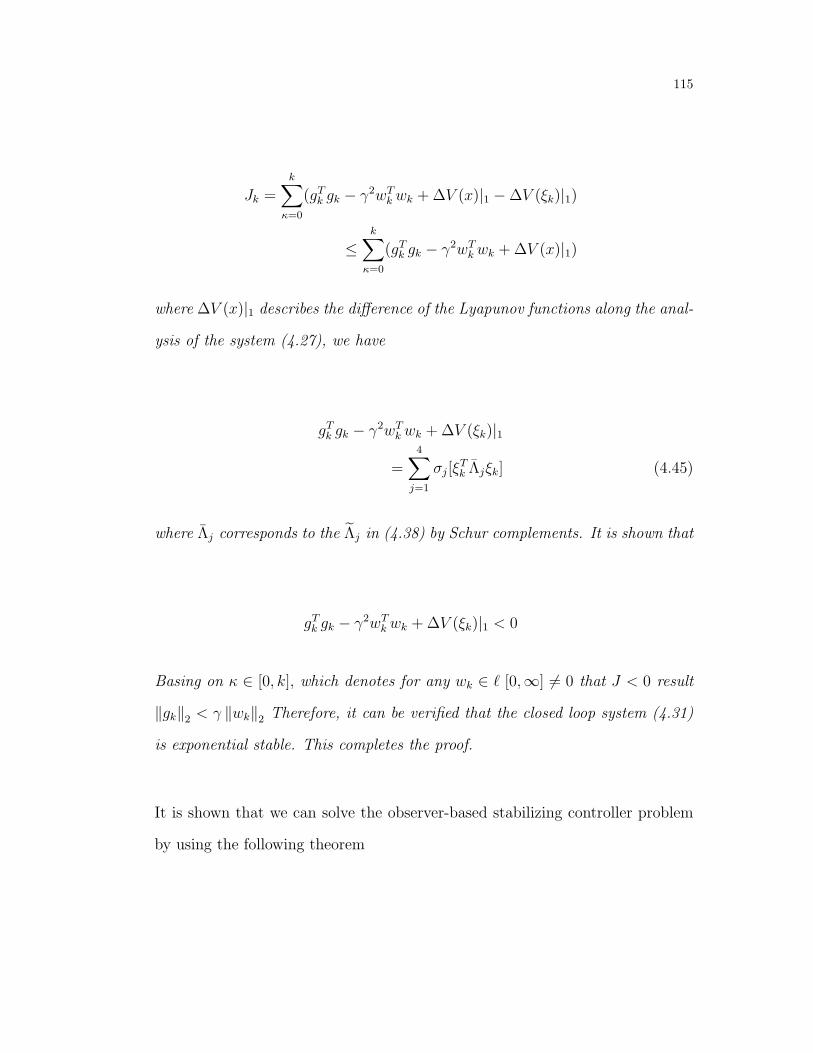
115

Jk =k∑

κ=0

(gTk gk − γ2wTk wk +∆V (x)|1 −∆V (ξk)|1)

≤k∑

κ=0

(gTk gk − γ2wTk wk +∆V (x)|1)

where ∆V (x)|1 describes the difference of the Lyapunov functions along the anal-

ysis of the system (4.27), we have

gTk gk − γ2wTk wk +∆V (ξk)|1

=4∑

j=1

σj[ξTk Λjξk] (4.45)

where Λj corresponds to the Λj in (4.38) by Schur complements. It is shown that

gTk gk − γ2wTk wk +∆V (ξk)|1 < 0

Basing on κ ∈ [0, k], which denotes for any wk ∈ ℓ [0,∞] = 0 that J < 0 result

∥gk∥2 < γ ∥wk∥2 Therefore, it can be verified that the closed loop system (4.31)

is exponential stable. This completes the proof.

It is shown that we can solve the observer-based stabilizing controller problem

by using the following theorem

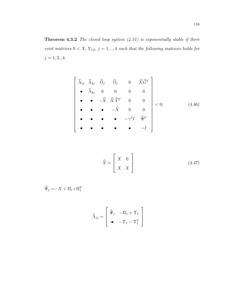
116

Theorem 4.3.2 The closed loop system (4.31) is exponentially stable if there

exist matrices 0 < X, Y1,2, j = 1, .., 4 such that the following matrices holds for

j = 1, 2., 4.


• Λ3j 0 0 0 0

• • −X X ΓT 0 0

• • • −X 0 0

• • • • −γ2I ΦT

• • • • • −I

< 0; (4.46)

X =

X 0

X X

(4.47)

Ψj =−X +Π1+ΠT1

Λ1j =

Ψj −Π1 +Υ1

• −Υ1 −ΥT1

117

Λ2j =

−Π1 + ΓT1 0

−Υ1 − ΓT1 0

Λ3j =

−Γ1 − ΓT1 0

• 0

Using S-procedure, we obtain

Λ3j = Λ3j −

0 0

0 I

Then,

Λ3j =

−M +MT 0

• −I

(4.48)

ΩTj =

[Ω1j 0 0 −Ω4j −Ω5j

]

Ω1j =

XAT + Y T1 BT 0

XAT XAT − Y T2

, ∀j

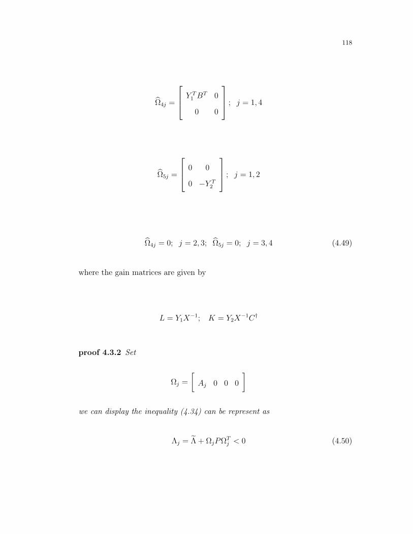
118

Ω4j =

Y T1 BT 0

0 0

; j = 1, 4

Ω5j =

0 0

0 −Y T2

; j = 1, 2

Ω4j = 0; j = 2, 3; Ω5j = 0; j = 3, 4 (4.49)

where the gain matrices are given by

L = Y1X−1; K = Y2X

−1C†

proof 4.3.2 Set

Ωj =

[Aj 0 0 0

]

we can display the inequality (4.34) can be represent as

Λj = Λ + ΩjPΩTj < 0 (4.50)

119

Λj =

Λ1j Λ2j

• Λ3j

< 0; (4.51)

Λ1j =

Ψj −R + ST

• −S − ST

Λ2j =

−R+MT 0

−S −MT 0

Λ3j =

−M+MT 0

• −I

Setting X =P−1, invoking Schur complements, we write matrix Λj in (4.42)

equivalently as

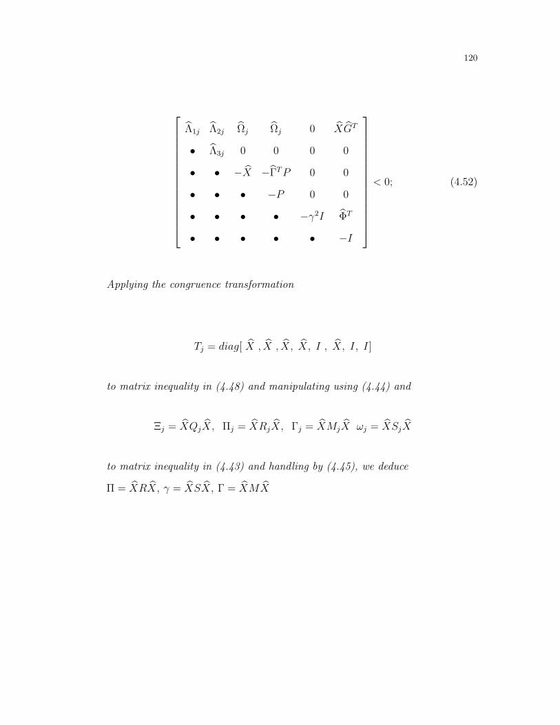
120


• Λ3j 0 0 0 0

• • −X −ΓTP 0 0

• • • −P 0 0

• • • • −γ2I ΦT

• • • • • −I

< 0; (4.52)

Applying the congruence transformation

Tj = diag[ X , X , X, X, I , X, I, I]

to matrix inequality in (4.48) and manipulating using (4.44) and

Ξj = XQjX, Πj = XRjX, Γj = XMjX ωj = XSjX

to matrix inequality in (4.43) and handling by (4.45), we deduce

Π = XRX, γ = XSX, Γ = XMX

121

4.3.2 Numerical Examples

In this section, a numerical example and some simulations are given to confirm

the effectiveness of the proposed approaches in terms of zero input strategy[17].

We assumed βk = 0.1 and αk = 0.1. Our purpose is to design an observer-based

controller in the form of equation (4.31).

Example 4.3.1:

We consider the uninterruptible power system UPS, in which we try to control

the pulsewidth-modulated inverter to guarantee the output ac voltage is kept at

the desired setting and undistorted, the discrete-time model was presented into

[63]:

A =

0.9226 −0.633 0

1 0 0

0 1 0

; B =

1

0

0

, CT =

23.737

20.287

0

we obtain the controller and observer gain as

L =

[0.0000 −0.0000 0.2329

]; and ∥L∥ = 0.2329,

K =

[−0.0009 −0.0020 −0.0000

]T; and ∥K∥ = 0.0022,

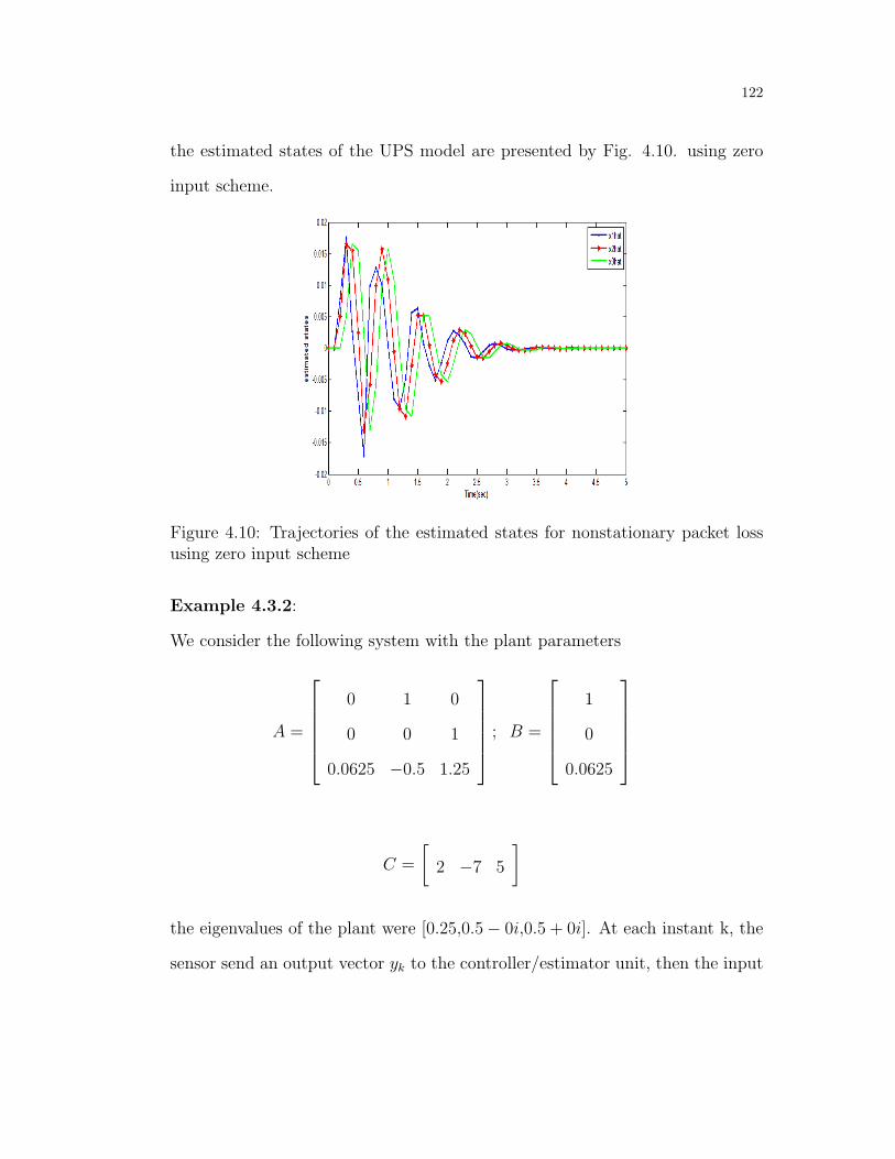
122

the estimated states of the UPS model are presented by Fig. 4.10. using zero

input scheme.

Figure 4.10: Trajectories of the estimated states for nonstationary packet lossusing zero input scheme

Example 4.3.2:

We consider the following system with the plant parameters

A =

0 1 0

0 0 1

0.0625 −0.5 1.25

; B =

1

0

0.0625

C =

[2 −7 5

]

the eigenvalues of the plant were [0.25,0.5− 0i,0.5 + 0i]. At each instant k, the

sensor send an output vector yk to the controller/estimator unit, then the input

123

vector uk was sent to actuator through networked control systems.

we obtain the controller and observer gain matrices as follows:

L =

[0.0231 0.0389 −0.0001

]; and ∥L∥ = 0.0453,

K =

[0.0016 −0.0001 0.0274

]T; and ∥K∥ = 0.0275,


in Fig. 4.11 and Fig. 4.12 respectability, using the proposed the control algo-

rithm. It is shown from the above figures that the performance of the control

and estimation systems are regarded with nonstationary packet loss.

Figure 4.11: Trajectories of system states for nonstationary packet loss usingzero input scheme

Example 4.3.3:

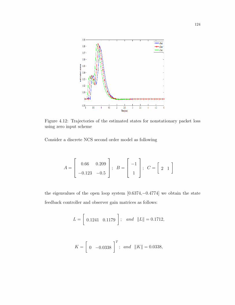
124

Figure 4.12: Trajectories of the estimated states for nonstationary packet lossusing zero input scheme

Consider a discrete NCS second order model as following

A =

0.66 0.209

−0.123 −0.5

; B =

−1

1

; C =

[2 1

]

the eigenvalues of the open loop system [0.6374,−0.4774] we obtain the state

feedback controller and observer gain matrices as follows:

L =

[0.1241 0.1179

]; and ∥L∥ = 0.1712,

K =

[0 −0.0338

]T; and ∥K∥ = 0.0338,

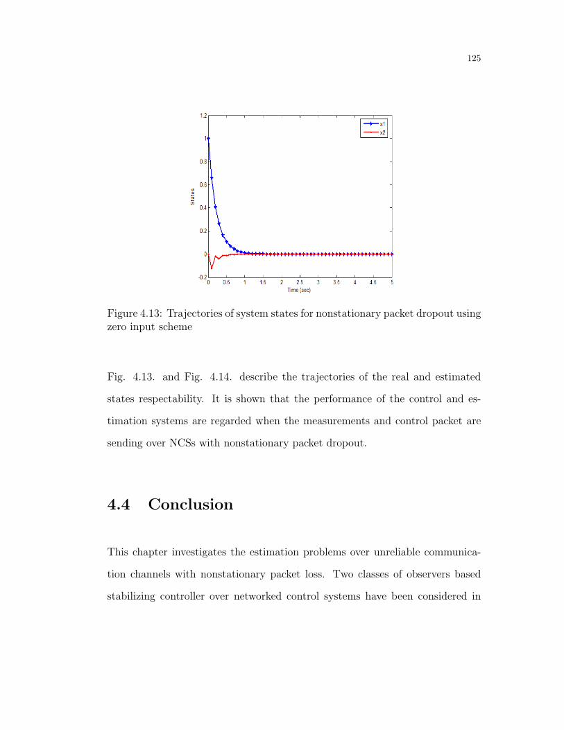
125

Figure 4.13: Trajectories of system states for nonstationary packet dropout usingzero input scheme

Fig. 4.13. and Fig. 4.14. describe the trajectories of the real and estimated

states respectability. It is shown that the performance of the control and es-

timation systems are regarded when the measurements and control packet are

sending over NCSs with nonstationary packet dropout.

4.4 Conclusion

This chapter investigates the estimation problems over unreliable communica-

tion channels with nonstationary packet loss. Two classes of observers based

stabilizing controller over networked control systems have been considered in

126

Figure 4.14: Trajectories of the estimated states for nonstationary packetdropout using zero input scheme

terms of different compensation strategies. Firstly, observer based controller

problem is addressed based on hold input strategy, where the last available con-

trol input applied by the actuator is used when control packet lost. The other

strategy, we employ zero input strategy to design observer based controller where

zero control input is applied by the actuator when the control packet dropped

out. It is shown that the former scheme gives better performance than the later

when compared on the basis of the proposed examples where the response of the

second strategy so-called zero input has more vibration, where the hold input

response converge faster with higher gains. Furthermore, a necessary and suf-

ficient conditions for observer stabilizability are addressed using linear matrix

inequalities LMIs. As a result, the proposed schemes have been successfully

evaluated on the given numerical examples.

Chapter 5

CONCLUSIONS AND

FUTURE WORK

In this thesis, we have been interesting in control and estimation over

unreliable communication networks. Problems of packet dropped in the control

loops under two different protocols are discussed. TCP-like protocol, where the

control node received acknowledgments for successfully delivered of the control

input packets, while the acknowledgments are absent in case of UDP-like pro-

tocol. In both cases, observations, control, and acknowledgments packets are

assumed to be subject to failure with different random probabilities. The sys-

tem performance and stability may be effected by data lost. We consider the

famous two compensation strategies, hold input and zero input, in which they

used to compensate the lost of control packets.

127

128

In general, Chapter 1 was dedicated to an motivation, an introduction, objectives

and thesis contribution of this thesis. A discrete linear time invariant LTI system

was considered, where data transmitted via lossy communication links with

input and measurement disturbances.

More specifically, in Chapter 2, literature review has been introduced for some

classes of networked control system, in which lots of problems of estimation and

control over NCSs subject to difference communication networks constraints

were presented.

In Chapter 3, we studied the problems of discrete linear quadratic Gaussian

LQG when data packets transmitted over lossy networks. It is shown that at

the absent of the acknowledgments such as (UDP protocol case) the separation

principle not hold more. Moreover, new suboptimal approach was developed

for UDP-like protocol, while the separation principle in hold in TCP-like pro-

tocol where the estimator and controller can design separately. In addition, we

assumed that the packets dropped out across networked control systems accord-

ing to different independent Bernoulli processes. Moreover, the solution of the

infinite horizon LQG control was derived.

In Chapter 4, two estimation schemes were derived for class of networked control

systems with nonstationary data packets dropped out over both communication

channels, from a sensor to a control/estimation unit and from the latter to an

actuator. Furthermore, the fate of control and observation signals are modeled

by two mutually independent random variables. In particular, two observer

129

based stabilizing controller of networked control systems (NCSs) are designed

to stabilize networked systems in means of exponential stable for both zero input

and hold input strategies. Essentially, in both problems, we derived sufficient

conditions for stability by using linear matrix inequality (LMIs).

In different chapters, numerical examples and simulations were used to illus-

trate the effectiveness of the proposed approaches subjects to packet lost. The

simulation results clearly indicated that

• New results to the an LQG state feedback optimal control problem were

provided for both TCP-like and UDP-like protocols. It is worth while

to note that from our examples that, the suboptimal controller design

for UDP like protocol gives better performance that the standard linear

quadratic Gaussian approach in case of TCP-like protocol using hold input

strategy using a quadratic cost function.

• Problems of estimation over loss networked control systems were addressed

with stationary packet dropout for both compensation strategies. Two

classes of observer based controller for NCS with output feedback control

gains were designed using linear matrix inequalities (LMIs). A sufficient

condition for stabilization by has been derived using a packet drop depen-

dent Lyapunov function approach.

130

Suggestions for future work would be

• Designing LQG controllers over networked control systems with nonsta-

tionary packet drop out and quantization effects.

• Designing LQG controllers when data packet lost according to Markovian

random process with nonlinearity and disturbance.

• Designing an estimation scheme for Markovian random process packet drop

out with modified feedback.

• Designing an observer based stabilizing controller by applying the hold-

zero strategies when the measurements packets get lost as well.

Chapter 6

Appendix

6.1 Appendix A

6.1.1 The Principle Unbiased Prediction: Chapter 3

In this part, we aim to present that, when the prediction is unbiased, the un-

biased minimum variance estimator that given in equation 3.20 is developed

expression of K ′k+1 to get equation 3.21 as

ˆxk+1|k+1 = K ′k+1

ˆxk+1|k +Kk+1yk+1

131

133

the above expression implies

0 = [Kk+1Ck+1 − I +K ′k+1]xk+1|k

Then, according to 3.20, we have

I = K ′k+1 +Kk+1Ck

K ′k+1 = I −Kk+1Ck

6.2 Appendix B

6.2.1 Proof Theorem 3.2.1: Chapter 3

This lemma will be used to prove the following theorem see [58]

Lemma 6.2.1 Assuming, we have

ϕ(K,X) = (1− β)(AkXATk + Sw) + β(FXF t + V ) (6.1)

where F = Ak + KCk, V = KSvKT . Let X ∈ S = S ∈ Rn×n|S ≥ 0, Sv > 0,

Sw ≥ 0, and (Ak, S12w) is controllable. Then, following facts are true.

134

1. With Kx = −AkXCTk (CkXCT

k + Sv)−1, gβ(X) = ϕ(KX , X).

2. gβ(X) = minKϕ(K,X) ≤ ϕ(K,X),∀K.

3. If β1 ≤ β2, thengβ1(X) ≥ gβ2(X)

proof 6.2.1 In this part, we proof the previous facts:

1. Define F = Ak +KxCk, and observe that

FxXCk +KxSv = (Ak +KxCk)XCTk +KxSv

= AkXCTk +Kx(CkXCT

k + Sv) = 0

Then, we deduce

gβ(X) = (1− β)(AkXATk + Sw) + β(AkXAT

k

+Sw − AkXCTk (CkXCT

k + Sv)−1CkXCT

k )

= (1− β)(AkXATk + Sw) + β(AkXAT

k + Sw +KxCkXATk

= (1− β)(AkXATk + Sw) + β(FxXAk + Sw)

= (1− β)(AkXATk + Sw) + β(FxXAk + Sw) + (FxXCk +KXSv)K

TX

= ϕ(KX , X).

135

2. Assume φ(K,X) = (Ak +KCk)X(Ak +KCk)T +KSvK

T +Sw. Note that

minK

ϕ(K,X) = minK

FXF T + V

= minK

φ(K,X)

Since X,Sv ≥ 0, ϕ(K,X) is quadratic and convex in the variable K, there-

fore, the minimizer might be found by solving the differentiation given by

(∂φ(K,X))/∂K = 0, which holds 2(Ak +KCk)XCk + 2KSv = 0 ⇒ K =

−AkXCTk (CkXCT

k +Sv)−1. As result of the fact that the minimizer present

according to KX , the proof of fact 2 runs after fact 1.

3. Note that AkXCTk (CkXCT

k + Sv)−1 ≥ 0.

gβ1(X) = AkXATk + Sw − β1AkXCT

k (CkXCTk + Sv)

−1CkXAk

≥ AkXATk + Sw − β2AkXCT

k (CkXCTk + Sv)

−1CkXAk

= gβ2(X).

This completes the proof of the lemma.

proof 6.2.2 This theorem is shown, there are two conditions available. First

of all, if βc = 1, we get a standard Riccati difference equation. As result, it is

converge to a fixed point, under the theorem’s assumption. Consequently, the

estimator error covariance matrix is bounded for all initial conditions Σ0 ≥ 0.

If βc = 1, the prediction becomes open loop prediction, and if the matrix A

is unstable, then the estimator error covariance matrix Σk diverges for some

136

initial condition Σ0 ≥ 0 . After that we prove the existence of a single point of

transition between both cases. Set 0 < β1 < 1 such that Eβ1 [Σk] is bounded for

any initial condition . More what, for any β2 ≥ β1, it is shown that Eβ2 [Σk] is

also bounded for any initial condition Σ0 ≥ 0 as well. Actually, we have

Eβ1 [Σk+1] = AkΣkATk + Sw − βk+1AkΣkC

Tk (CkΣkC

Tk + Sv)

−1

CkΣkAk]

= AkΣkATk + Sw − β1AkΣkC

Tk (CkΣkC

Tk + Sv)

−1

CkΣkAk]

= E[gβ1(Σk)]

≥ E[gβ2(Σk)]

= Eβ2 [(Σk+1)]

We use part 3 of lemma 6.2.1 to rewrite the last inequality. By choosing βc =

inf β∗ : β > β∗ ⇒ Eβ[(Σk)], ∀Σ0 ≥ 0 is bounded any initial condition The

proof is complete.

6.2.2 Proof theorem 3.3.2: Chapter 3

proof 6.2.3 1. According to the fact that if α > αc, then limk→∞ Fk = F∞ :

∀F0 ≥ 0. As result, equation 3.47 follows from equation 3.46.

137

2. Due to the fact that the optimal state estimator gain Kk was derived ac-

cording the random variable of arrival sequences β and α, as given (3.5),

(3.14), (3.15), (3.23), and (3.25).

3. For βmax < β and αc < α, we have limk→+∞ Σk = Σ+∞, and limk→−∞Σk =

Σ−∞, the estimation error covariance Σk was defined in (3.14). In addi-

tion, limk→∞ Fk = F∞ : ∀F0 ≥ 0. Final result, from equation (3.28) -

(3.42), we conclude that the expected minimum cost function can be bounded.

Bibliography

[1] O. C. Imer, S. Yksel and T. Basar, ”Optimal Control of LTI Systems over

Unreliable Communication Links”, Automatica, vol. 42, no. 9. pp. 1429–

1439. September 2006.

[2] O. C. Imer, S. Yksel and T. Basar,”Optimal Control of Dynamical Sys-

tems over Unreliable Communication Links,”In Proceedings of NOLCOS

Stuttgart, Germany. 2004.

[3] D. J. Stilwell and B. E. Bishop, ”Platoons of Underwater Vehicles,” IEEE

Control Systems, vol. 20, no. 6, pp. 45–52, Dec. 2000.

[4] Shuang -Hua Yang,”Internet Based Control Systems Design and Applica-

tions,” London: Springer-Verlag London Limited, Febraruy 2011. ISBN–10:

1849963584.

[5] V. Gupta, N.C. Martins, and J. S. Baras,”Optimal Output Feedback Con-

trol Using Two Remote Sensors Over Erasure Channels,”IEEE Transac-

tions on Automatic Control, vol. 54, no. 7, pp. 1463–1476 July 2009.

138

139

[6] V. Gupta, N.C. Martins, and J. S. Baras ,”On Stability in the Presence of

Analog Erasure Channel Between the Controller and the Actuator,”IEEE

Transactions on Automatic Control, vol. 55, no.1, pp. 175–179 January

2010.

[7] V. Gupta, S. Adalakha, B. Sinopoli, and A. Goldsmith, ”Towards Reced-

ing Horizon Networked Control,”In Proceedings of Allerton conference on

communication, control and computing, pp. 169-176. 2006.

[8] Fei-Yue Wang and Derong Liu,”Networked Control Systems Theory and

Applications,” London: Springer - Verlag London Limited, 4th June 2008.

ISBN–10: 1848002149.

[9] A. Matveev and A. Savkin, ”Estimation and Control over Communication

Networks,”. Boston, MA: Birkhuser, Springer, 2009.

[10] M. Moayedi, K. Foo, and C. Soh,”Networked LQG Control over Unreliable

Channels,” In Proceedings of the 49th IEEE Conference on Decision and

Control, CDC 2010, December 15–17, 2010, Atlanta, Georgia, USA. pages

5851–5856, IEEE, 2010.

[11] Silva, Goodwin, Quevedo, ” On the Design of Control Systems over Unreli-

able Channels,”In Proceedings of European Control Conference, Budapest,

Hungary, pp. 377–382., 2009.

[12] B. Sinopoli, L. Schenato, M. Franceschetti, K. Poolla, M. Jordan, and

S. Sastry, ”Optimal Control with Unreliable Communication: The TCP

140

Case,”In Proceedings of American Control Conference, Portland, OR , vol.

5, pp. 3354–3359. Jun. 2005.

[13] B. Sinopoli, L. Schenato, M. Franceschetti, K. Poolla, M. Jordan, and S.

Sastry, ”Estimation and Control over Lossy Networks,”The Forty–Third

Annual Allerton Conference on Communication, Control, and Computing,

Monticello, IL, September 2005.

[14] Kogel, M.J., Blind, R., Allgower, F., ”Optimal Control over Unreliable Net-

works with Uncertain Loss Rates,” American Control Conference (ACC),

On page(s): 3672–3677, July 2–30 2010.

[15] Garone, Sinopoli, Goldsmith and Casavola,”LQG Control for MIMO Sys-

tems over Multiple Erasure Channels with Perfect Acknowledgment,” IEEE

Transactions on Automatic Control, vol. 57, issue 2, pp. 450– 456 Feberury

2012.

[16] L. Schenato, M. Franceschetti, K. Poolla, and S. Sastry ”LQG Control with

Missing Observation and Control Packets,”In Proceedings of the 16th IFAC

World Congress. Prague, Czech Republic, vol.16, July 2005.

[17] Luca Schenato,”To Zero or to Hold Control Inputs With Lossy Links,”IEEE

Transaction on Automation and Control, vol. 54, issue 5, pp.1093–1099,

May 2009.

[18] V. Gupta, D. Spanos, B. Hassibi, and R. M. Murray, ”Optimal LQG Con-

trol Across Packet Dropping Links,” In Proceedings of System and Control

Letters, vol 56, no. 6, pp. 439–446, June 2007.

141

[19] C.K. Ko, X. Gao, S. Prajna, and L. J. Schulman, ”On Scalar LQG Control

with Communication Cost,” In Proceedings of the 44th IEEE Conference on

Decision and Control and European Control Conference (CDC-ECC ’05),

Seville, Spain, pp. 2805–2810, Dec. 2005.

[20] S. Yuksel , O. C. Imer and T. Basar,”Constrained State Estimation And

Control over Communication Networks,” In Proceedings of the 38th Annual

Conference on Information Science and Systems (CISS), Princeton, NJ,

March 2004.

[21] Bar Shalom, Y., and Tse, E. ”Dual Effect, Certainty Equivalence, and Sep-

aration in Stochastic Control,” IEEE Transaction on Automatic Control,

vol. 19, issue 5 , pp. 494–500. Oct. 1974

[22] C . N. Hadjicostis and R . Touri, Feedback Control Utilizing Packet Drop-

ping Network Links,” In Proceeding of 41st IEEE Conference on Decision

and Control, vol. 2 , pp. 1205-1210, Las Vegas, NV, Dec. 2002.

[23] Sinopoli, B., Schenato, L., Franceschetti, M., Poolla, K. and Sastry, S.

”Optimal Linear LQG Control over Lossy Networks without Packet Ac-

knowledgement,” In Proceeding of 45th IEEE Conference on Decision and

Control, pp. 392–397. Dec. 2006.

[24] W. Koning, ”Infinite Horizon Optimal Control for Linear Discrete Time

Systems with Stochastic Parameters,” Automatica, vol. 18, no. 4, pp. 443–

453, 1982.

142

[25] W. Zhang, M. S. Branicky, and S. M. Phillips, ”Stability of Networked

Control Systems,” IEEE Control Systems Magazine, vol. 21, no. 1, pp. 84–

99, 2001.

[26] J. Nilsson, ”Real Time Control System with Delay,”Ph.D. Dissertation,

Lund Institute of Technology, Sweden, 1998.

[27] B. Azimi-Sadjadi, ”Stability of Networked Control Systems in The Presence

of Packet Losses,” In Proceedings of 42nd IEEE Conference Decision and

Control, vol.1, pp. 676–681. 9–12th Dec. 2003.

[28] H. Mo and C. N. Hadjicostis, ”Feedback Control over Packet Dropping

Network Links”, In Proceedings of IEEE Mediterranean Conference Control

Automation, pp.1–6 , 27–29 June 2007.

[29] D. E. Quevedo and D. Nesic, ”Input-to-State Stability of Packetized Predic-

tive Control over Unreliable Networks Affected by Packet-Dropouts,”IEEE

Transactions on Automatic Control, vol. 56, no. 2, pp. 370–375, Feb. 2011.

[30] Q.S. Jia, L. Shi, Y. Mo, and B. Sinopoli,”On Optimal Partial Broadcast-

ing of Wireless Sensor Networks for Kalman Filter,”IEEE Transactions on

Automatic Control, vol. 57, no. 3. pp. 715–721 , March 2012.

[31] Dang ,Zhang, ”Stability and Controller Design of Networked Control Sys-

tem with Time-Varying Delays and Data Packet Dropout,”Control and De-

cision conference Chinese, pp. 1376–1379. July 2008

143

[32] G. Walsh, H. Ye, and L. Bushnell,”Stability Analysis of Networked Control

Systems,”Control Systems Technology, IEEE Transactions on, vol. 10, no.

3, pp. 438–446, May 2002.

[33] Y. Ge, Q. Chen, M. Jiang, and Z. an Liu, ”Stability Analysis of Networked

Control Systems with Data Dropout and Transmission Delays,”World

Congress on Intelligent Control and Automation, pp. 7986–7991, June 25–

27, 2008.

[34] Sachi Mittal, Anwar S. Siddiqui,”Networked Control System: Survey and

Directions,” Journal of Engineering Research and Studies , vol. 1. no. 2.

Dec. 2010.

[35] Khalil and J. Grizzle, ”Nonlinear systems”Prentice Hall New Jersey, 3th

edt. 2002. ISBN 0-13-067389-7.

[36] J. Hespanha, P. Naghshtabrizi, and Y. Xu,”A Survey of Recent Results in

Networked Control Systems,”Proceedings of the IEEE, vol. 95, no. 1, pp.

138–162, Jan. 2007.

[37] M. Epstein, L. Shi, and R. M. Murray, ”An Estimation Algorithm for

A Class of Networked Control Systems Using UDP-Like Communication

Schemes,” In 45th IEEE Conference on Decision and Control, pp.5597–

5603, Dec. 2006.

[38] Michael Epstein, Ling Shi and Richard M. Murray,”Estimation Schemes

for A Class of Networked Control Systems Using UDP-Like Communica-

144

tion,”In 45th IEEE Conference on Decision and Control, pp.3945–3951 ,

Dec. 2007.

[39] Vijay Gupta,”On Estimation across Analog Erasure Links with and without

Acknowledgements,”American Control Conference Marriott Waterfront,

Baltimore, MD, USA. vol. 55, no.12, pp. 2896–2901, Dec. 2010.

[40] E. Garone, B. Sinopoli, A. Casavola, ” On the Effect of Packet Acknowledg-

ment on the Stability and Performance of Networked Control Systems,” In

Modeling, Estimation and Control of Networked Complex Systems, Under-

standing Complex Systems, Volume . ISBN 978-3-642-03198-4., Springer

Verlag collection, pp. 191. 2009.

[41] L. Schenato, B. Sinopoli, M. Franceschetti, K. Poola, and S. S. Sastry ,”

Foundations of Control and Estimation over Lossy Networks,”Proceedings

of the IEEE, vol. 95, no. 1, pp. 163–187, Jan. 2007.

[42] Jing Wu and Tongwen Chen,”Design of Networked Control Systems With

Packet Dropouts,”IEEE Transactions on Automatic Control, vol. 52, no. 7,

pp. 1314–1319, July 2007.

[43] E. Garone, B. Sinopoli, and A. Casavola, ”LQG Control over Multi-

Channel TCP-like Erasure Networks with Probabilistic Packet Acknowl-

edgements,”In Proceedings of 47th IEEE Confernce Decision Control, Can-

cun, Mexico, pp. 2686–2691. Dec. 2008.

[44] Hideaki Ishii,” H∞ Control with Limited Communication and Message

Losses,” Systems and Control Letters 57. pp. 322–331. 2008.

145

[45] D. Hristu-Varsakelis,”Short-Period Communication and the Role of Zero-

Order Holding in Networked Control Systems,”IEEE Transactions. Au-

tomation. Control, vol. 53, no. 5, June 2008.

[46] Wen-An Zhang and Li Yu, ”Output Feedback Stabilization of Networked

Control Systems With Packet Dropouts,” IEEE Transactions. Automation.

Control, vol. 52, no. 9, September 2007.

[47] G. Welch, and G. Bishop,”An Introduction to The Kalman Fil-

ter,”Departmenet of Computer Science, updated Monday, July 24, 2006.

visit http : //www.cs.unc.edu/ welch/media/pdf/kalmanintro.pdf

[48] Juan Andrade-Getto,” The Kalman Filter,”UPC-CSIC Barcelona, Spain,

May, 2005. visit http://digital.csic.es/bitstream/10261/30069/1/doc1.pdf

[49] M. Kogel, and R. Findeisen,”Robust Suboptimal Control over Lossy Net-

works using Extended Input Schemes,”IEEE Internatinal Symposium on

Computer- Aided Control Design CACSD, pp. 210–215, September 28–30,

2011.

[50] M. Kogel, R. Blind, F. Allgower, and R. Findeisen,”Optimal and Optimal

-Linear Control over Lossy, Distributed Networks,”18th International Fed-

eration of Automatic Control IFAC World Congress, Milano (Italy), pp.

13239–13244, September 2, 2011.

[51] L. Shi, M. Epstein, and R. Murray,”Kalman Filtering over A Packet-

Dropping Network: A Probabilistic Perspective,”IEEE Transactions on

Automatic Control, vol. 55,no.3, pp. 594–604, March, 2010

146

[52] Rainer Blind, Frank Allgower,”Estimating the Fates of the Control Packets

for Networked Control Systems with Loss of Control and Measurement

Packets,”IEEE Conference on Decision and Control , Shanghai, P.R. China,

pp. 2687–2692, December 16–18, 2009.

[53] V. Gupta, R. Murray, L. Shi, B. Sinopli,” Networked Sens-

ing, Estimation and Control Systems,”DRAFT v1.1a, 20 December,

2009. http : //www.cds.caltech.edu/ murray/books/AM05/pdf/ncs −

author20Dec09.pdf .

[54] Y. Mo and B. Sinopoli,”Kalman Filtering With Intermittent Observations:

Tail Distribution and Critical Value,”IEEE Transactions on Automatic

Control, vol. 57, no. 3, pp. 677–689, March, 2012.

[55] Eva Miklovicova, Marian Mrosko,”Model Predictive Control over Unreli-

able Communication Links,”In Mathematical Methods and Techniques in

Engineering and Environmental Science, 4th WSEAS International Con-

ference on Visualization, Imaging and Simulation. Catania, Sicily, pp.144–

149, 2011.

[56] Jeffrey B. Burl, ”Linear Optimal Control”, Prentice Hall, Edit 1, November

19, 1998. ISBN-10: 0201808684.

[57] Desineni S. Naidu,” Optimal Control Systems,”CRC Press LLC, 2003.

ISBN 13: 9780849308925.

147

[58] B. Sinopoli, L. Schenato, M. Franceschetti, K. Poolla, M. Jordan, and S.

Sastry,B,” Kalman Filtering with Intermittent Observations,” Automatic

Control, IEEE Transactions on, vol. 49, no. 9, pp. 1453–1464, Sep. 2004.

[59] M . S. Brani cky, S. M. Phillips, W. Zhang, ”Stability of Networked Control

Systems: Explicit Analysis of Delay”,Proceedings of the American Control

Conference, Chicago, vol. 4. pp. 2352–2357, 2000.

[60] L. A. Montestruque, P. J. Antsaklis, ”Model Based Networked Control

Systems: Stability,”ISIS Technical Report, University of Notre Dame, pp.

1–58, January 2002.

[61] L. A. Montestruque, P. J. Antsaklis, ”State and Output Feedback Control

in Model Based Networked Control Systems,”Proceedings of the 41st IEEE

Conference on Decision and Control, vol. 2, pp. 1620–1625, Dec. 2002.

[62] S. Mu, T. Chu, L. Wang, G. Xie, ”State Feedback Control of Networked Sys-

tems Via Periodical Switching,”IEEE Confernce Computer - Aided Control

System Design, pp. 356–361, Sept. 2004.

[63] X . Luan , P. Shi, and F . Liu ,”Stabilization of Networked Control Systems

with Random Delays,” Industrial Electronics, IEEE Transactions on, vol.

58, no. 9, pp. 4323–4330, Sept. 2011.

[64] F. W. Yang, Z. D. Wang, Y. S. Hung, and M. Gani,”H∞ Control for Net-

worked Systems with Random Communication Delay,”IEEE Transaction

Automatic Control, vol. 51, no. 3, pp. 511–518, March 2006.

148

[65] D. Wu, J. Wu, S. Chen,”Separation Principle for Networked Control Sys-

tems with Multiple-Packet Transmission,”IET Control Theory and Appli-

cation, vol. 5, no. 3, pp. 507–513, 2010.

[66] Z. Jin, V. Gupta, and R. Murray,” State Estimation over Packet Dropping

Networks using Multiple Description Coding,”Automatica, vol. 42, no. 9,

pp. 1441–1452, 2006.

[67] J. Yu,L. Wang, M. Yu, Y. Jia, J. Chen,”Packet Loss Dependent Con-

troller Design for Networked Control Systems via Switched System Ap-

proach,”Proceedings of the 47th IEEE Conference on Decision and Control,

pp. 3354–3359, Dec. 2008.

[68] J. Yu,L. Wang, M. Yu, Y. Jia, J. Chen,” Stabilizability of Networked Con-

trol Systems via Packet -Loss Dependent Output Feedback,”American Con-

trol Conference, pp. 3620–3625, June 2008.

[69] V. Gupta, N. C. Martins and J. S. Baras,”Stabilization Using Multiple Sen-

sors over Analog Erasure Channels,”Modeling and Optimization in Mobile,

Ad Hoc and Wireless Networks and Workshops, 2007. WiOpt 2007. 5th

International Symposium on, pp. 1–7, April 2007.

[70] Luca Schenato ,”Optimal Estimation in Networked Control Systems Sub-

ject to Random Delay and Packet Drop,”IEEE Transactions on Automatic

Control, vol. 53, no. 5, pp. 1311–1317, June 2008.

[71] Y. T. Chan, J. M. F. Riley, and J. B. Plant,”Modeling of Time Delay and

Its Application to Estimation of Nonstationary Delay,”IEEE Transaction

149

on Acoustics, Speech, and Signal Processing, vol. 29, no. 3, pp. 577–581,

June 1981.

[72] Y.T. Chan, P.C. Ching,”Non -Stationary Time Delay Estimation With A

Multipath,”Proceedings of Acoustics, Speech, and Signal Processing, 1989.

ICASSP-89., 1989 International Conference on, vol. 4, pp. 2736–2739, May

1989.

[73] Q. Ling and M. Lemmon, ”Power spectral analysis of networked control

systems with data dropouts,”IEEE Transactions on Automatic Control,

vol. 49, no. 6, pp. 955–960, June 2004.

[74] Mahmoud, M. S., ”Switched Time-Delay Systems,”Springer -Verlag, New

York, 2010.

[75] Mahmoud, M. S. Xia, Y.” Robust Stability and Stabilization of a Class of

Nonlinear Switched Discrete-Time,”Systems with Time-Varying Delays. J.

Optim. Theory Appl., 143, pp. 329–355. 2009.

150

Vitae

• Nezar Mohammed A. AL-Yazidi.

• Al-Hami, Yemen on 09th September 1980.

• Received Bachelor of Science (BSc) degree in Electronic and Communica-

tion Engineering from Hadramout University

• Joined King Fahd University of Petroleum and Minerals in February 2009

as Full Time student in Systems Engineering(Automation and Control).

• Contact details:+966535752183

• Present Address: Department of Systems Engineering, King Fahd Uni-

versity of Petroleum and Minerals, P.O. Box 6254, Dhahran 31261, Saudi

Arabia.

• E-mail Address: [email protected]

ACKNOWLEDGEMENTS - core.ac.uk · for their continuous support, namely, Omar Alburaiki, M. Fuady,...

Documents

Transcript of ACKNOWLEDGEMENTS - core.ac.uk · for their continuous support, namely, Omar Alburaiki, M. Fuady,...