
Accurate Predictions of Postmortem Interval Using Linear ... · 32 by analyzing the expression of...
30
Accurate Predictions of Postmortem Interval Using 1 Linear Regression Analyses of Gene Meter Expression 2 Data 3 4 Authors: M. Colby Hunter 1 , Alex E. Pozhitkov 2 , and Peter A. Noble 1,2,3 5 Author Affiliations: 6 1. Ph.D. Microbiology Program, Department of Biological Sciences, Alabama State 7 University, Montgomery, Alabama, USA 36104 8 2. Department of Oral Health Sciences, University of Washington, Box 357444, Seattle, 9 WA USA 98195. 10 3. Department of Periodontics, School of Dentistry, Box 355061, University of 11 Washington, Seattle, Washington, USA 98195 12 *Correspondence to: 13 Peter A Noble 14 Email: [email protected] 15 Phone: 206-409-6664. 16 17 Other authors’ emails: 18 MCH: [email protected] 19 AEP: [email protected] 20 Short title: 21 PMI Prediction Using Gene Meter Analysis of Expression Data 22 Keywords 23 Postmortem transcriptome; postmortem gene expression; Gene meters; calibrated DNA 24 microarrays, thanatotranscriptome; postmortem interval, forensic science. 25 (which was not peer-reviewed) is the author/funder. All rights reserved. No reuse allowed without permission. The copyright holder for this preprint . http://dx.doi.org/10.1101/058370 doi: bioRxiv preprint first posted online Jun. 12, 2016;
Transcript of Accurate Predictions of Postmortem Interval Using Linear ... · 32 by analyzing the expression of...

Accurate Predictions of Postmortem Interval Using 1
Linear Regression Analyses of Gene Meter Expression 2
Data 3
4
Authors: M. Colby Hunter1, Alex E. Pozhitkov2, and Peter A. Noble1,2,3 5
Author Affiliations: 6
1. Ph.D. Microbiology Program, Department of Biological Sciences, Alabama State 7
University, Montgomery, Alabama, USA 36104 8
2. Department of Oral Health Sciences, University of Washington, Box 357444, Seattle, 9
WA USA 98195. 10
3. Department of Periodontics, School of Dentistry, Box 355061, University of 11
Washington, Seattle, Washington, USA 98195 12
*Correspondence to: 13
Peter A Noble 14
Email: [email protected] 15
Phone: 206-409-6664. 16
17
Other authors’ emails: 18
MCH: [email protected] 19
AEP: [email protected] 20
Short title: 21
PMI Prediction Using Gene Meter Analysis of Expression Data 22
Keywords 23
Postmortem transcriptome; postmortem gene expression; Gene meters; calibrated DNA 24
microarrays, thanatotranscriptome; postmortem interval, forensic science. 25
(which was not peer-reviewed) is the author/funder. All rights reserved. No reuse allowed without permission. The copyright holder for this preprint. http://dx.doi.org/10.1101/058370doi: bioRxiv preprint first posted online Jun. 12, 2016;

Abstract 26 27
In criminal and civil investigations, postmortem interval is used as evidence to help sort 28
out circumstances at the time of human death. Many biological, chemical, and physical 29
indicators can be used to determine the postmortem interval – but most are not accurate. 30
Here, we sought to validate an experimental design to accurately predict the time of death 31
by analyzing the expression of hundreds of upregulated genes in two model organisms, 32
the zebrafish and mouse. In a previous study, the death of healthy adults was conducted 33
under strictly controlled conditions to minimize the effects of confounding factors such as 34
lifestyle and temperature. A total of 74,179 microarray probes were calibrated using the 35
Gene Meter approach and the transcriptional profiles of 1,063 significantly upregulated 36
genes were assembled into a time series spanning from life to 48 or 96 h postmortem. In 37
this study, the experimental design involved splitting the gene profiles into training and 38
testing datasets, randomly selecting groups of profiles, determining the modeling 39
parameters of the genes to postmortem time using over- and/or perfectly- defined linear 40
regression analyses, and calculating the fit (R2) and slope of predicted versus actual 41
postmortem times. This design was repeated several thousand to million times to find the 42
top predictive groups of gene transcription profiles. A group of eleven zebrafish genes 43
yielded R2 of 1 and a slope of 0.99, while a group of seven mouse liver genes yielded a 44
R2 of 0.98 and a slope of 0.97, and seven mouse brain genes yielded a R2 of 0.93 and a 45
slope of 0.85. In all cases, groups of gene transcripts yielded better postmortem time 46
predictions than individual gene transcripts. The significance of this study is two-fold: 47
selected groups of upregulated genes provide accurate prediction of postmortem time, 48
and the successfully validated experimental design can now be used to accurately predict 49
postmortem time in cadavers. 50
51
(which was not peer-reviewed) is the author/funder. All rights reserved. No reuse allowed without permission. The copyright holder for this preprint. http://dx.doi.org/10.1101/058370doi: bioRxiv preprint first posted online Jun. 12, 2016;

52
Introduction 53
The postmortem interval (PMI) is the elapsed time between death of an organism and the 54
initiation of an official investigation to determine the cause of death. Its determination is 55
important to civil investigations such as those involving life insurance fraud because 56
investigators need to determine if the person was alive or not when the policy was in 57
effect [1]. The PMI is also important to criminal investigations, especially suspicious 58
death cases where there are no witnesses, because it can help determine the time 59
relationship between a potential suspect and the victim and eliminate people from a 60
suspect list, which speeds up investigations. Accurate prediction of PMI is considered 61
one of the most important and complex tasks performed by forensic investigators [2]. 62
Several studies have suggested that RNA could be used to estimate PMI [3,4,5,6,7]. 63
While most studies focused on the degradation of mRNA gene markers, some examined 64
gene expression. The RNA degradation studies include: a model to predict PMI based on 65
the degradation of Beta actin (Actb), Glyceraldehyde-3-phosphate dehydrogenase 66
(Gapdh), Cyclophilin A (Ppia) and Signal recognition particle 72 (Srp72) genes in 67
mouse muscle tissue samples [3], a model to predict PMI based on degradation of an 68
amplified Actb gene and temperature in rat brain samples [4], and a study that predicted 69
PMI based on the degradation of Gapdh, Actb and 18S rRNA genes in the spleens of rats 70
[5]. The gene expression studies include: a study that found increased expression of 71
myosin light chain 3 (Myl3), matrix metalloprotease 9 (Mmp9) and vascular endothelial 72
growth factor A (Vegfa) genes in human body fluids after 12 h postmortem [6], a study 73
that found increased expression of Fas Ligand (Fasl) and ‘phosphatase and tensin 74
homologue deleted on chromosome 10’ (Pten) genes with postmortem time in rats [7], 75
and a study that found individual gene transcripts did not increase using PCR-based gene 76
expression arrays of frozen human brain cadaver samples [8]. Common to these studies 77
is the requirement: (i) to amplify cDNA by polymerase chain reaction (PCR) and (ii) to 78
normalize the data with a control in order to facilitate sample comparisons. These 79
requirements introduce methodological biases that could significantly affect 80
interpretation of the data. An approach that minimizes or eliminates these biases is 81
highly desirable because it might lead to better PMI predictions. 82
(which was not peer-reviewed) is the author/funder. All rights reserved. No reuse allowed without permission. The copyright holder for this preprint. http://dx.doi.org/10.1101/058370doi: bioRxiv preprint first posted online Jun. 12, 2016;

Since conventional DNA microarray approaches yield noisy data [9], in 2011 we 83
developed the “Gene Meter” approach that precisely determines specific gene 84
abundances in biological samples and minimizes noise in the microarray signal [10,11]. 85
The reason this approach is precise is because the behavior of every microarray probe is 86
determined by calibration – which is analogous to calibrating a pH meter with buffers. 87
Without calibration, the precision and accuracy of a meter is not known, nor can one 88
know how well the experimental data fits to the calibration (i.e., R2). The advantages of 89
the Gene Meter approach over conventional DNA microarray approaches is that the 90
calibration takes into consideration the non-linearity of the microarray signal and 91
calibrated probes do not require normalization to compare biological samples. Moreover, 92
PCR amplification is not required. We recognize that next-generation-sequencing (NGS) 93
approaches could have been used to monitor gene expression in this study. However, the 94
same problems of normalization and reproducibility are pertinent to NGS technology 95
[12]. Hence, the Gene Meter approach is currently the most advantageous high 96
throughput methodology to study postmortem gene expression and might have utility for 97
determining the PMI. 98
The Gene Meter approach has been used to examine thousands of postmortem gene 99
transcription profiles from 44 zebrafish (Danio rerio) and 20 house mice (Mus musculus) 100
[13]. Many genes were found to be significantly upregulated (relative to live controls). 101
Given that each sampling time was replicated two or three times, we conjectured that the 102
datasets could be used to assess the feasibility for predicting PMIs from gene expression 103
data. Although many approaches are available to determine PMI (see Discussion), an 104
approach that accurately determines the time of death is highly desired and it is the goal 105
of our study to determine if specific gene transcripts or groups of gene transcripts could 106
accurately predict postmortem time. Zebrafish and mice are ideal for testing 107
experimental designs because the precise time of human deaths is often not known, and 108
other variables such as lifestyle, temperature, and health condition are also often not 109
known or sufficiently controlled in human studies. Given that these variables could have 110
confounding effects on the interpretation of gene expression data in human studies, 111
testing experimental designs under controlled conditions using model organisms is ideal. 112
In our study, the timing of death and health of the zebrafish and mice are known, which 113
(which was not peer-reviewed) is the author/funder. All rights reserved. No reuse allowed without permission. The copyright holder for this preprint. http://dx.doi.org/10.1101/058370doi: bioRxiv preprint first posted online Jun. 12, 2016;

enables the testing of different experimental designs to provide “proof of principle”. It is 114
our intent to use the best design to determine PMI of cadavers for future studies. 115
The objectives of our study are twofold: (1) to identify specific upregulated genes or 116
groups of upregulated genes that accurately predict the PMI in the zebrafish and mouse, 117
and (2) to design and evaluate a robust experimental approach that could later be 118
implemented to predict PMI from cadavers. 119
Materials and Methods 120
Although the details of zebrafish and mouse processing, the extraction of RNA, and 121
microarray calibrations are presented in a previous study [13], we have provided relevant 122
experimental protocols to aid readers in the interpretation of the results of this study. 123
Zebrafish processing. The 44 zebrafish were maintained under standard conditions in 124
flow-through aquaria with a water temperature of 28oC. Prior to sacrifice, the zebrafish 125
were placed into 1 L of water of the same temperature as the aquaria. At zero time, four 126
fish were extracted and snap frozen in liquid nitrogen. These live controls were then 127
placed at -80oC. To synchronize the time of death, the remaining 40 fish were put into a 128
small container with a bottom made of mesh and placed into an 8 L container of ice water 129
for 5 mins. The small container with the mesh bottom was placed into the flow-through 130
aquarium with a water temperature of 28oC for the duration of each individual’s 131
designated postmortem time. The postmortem sampling times used for the zebrafish 132
were: 0, 15 min, 30 min, 1, 4, 8, 12, 24, 48 and 96 h. At each sampling time, 4 133
individuals were taken out of the small container in the flow-through aquarium, snap 134
frozen in liquid nitrogen and then stored at -80oC. One zebrafish sample was not 135
available for use (it was accidentally flushed down the sink) however this was taken into 136
account for calculation of extraction volumes. 137
Mouse processing. Twenty C57BL/6JRj male mice of the same age (5 months) and 138
similar weight were used. Prior to sacrifice, the mice had ad libitum access to food and 139
water and were maintained at room temperature. At zero time, the mice were sacrificed 140
by cervical dislocation and each mouse was placed in a unique plastic bag with pores to 141
permit the transfer of gases. The mice were kept at room temperature for the designated 142
postmortem sampling times. The sampling times used were: “zero” time, 30 min, 1, 6, 143
(which was not peer-reviewed) is the author/funder. All rights reserved. No reuse allowed without permission. The copyright holder for this preprint. http://dx.doi.org/10.1101/058370doi: bioRxiv preprint first posted online Jun. 12, 2016;

12, 24 and 48 h. At each sampling time, a brain and two liver samples were obtained 144
from each of three mice, except for the 48 h sampling where only two mice were 145
sampled. The samples were immediately snap frozen in liquid nitrogen and placed at -146
80oC. 147
RNA Processing and Labeling. Gene expression samples for each PMI were done in 148
duplicate for zebrafish and in triplicate for mice (except for the 48 h PMI sample that was 149
duplicated). The zebrafish samples were homogenized with a TissueLyzer (Qiagen) with 150
20 ml of Trizol. The mouse brain and liver samples (~100 mg) were homogenized in 1 151
ml of Trizol. One ml of the homogenate was placed into a centrifuge tube containing 200 152
µl of chloroform. The tube was vortexed and placed at 25oC for three min. Following 153
centrifugation for 15 min at 12000 RPM, the supernatant was placed into a new 154
centrifuge tube containing an equal volume of 70% ethanol. Purification of the RNA was 155
accomplished using the PureLink RNA Mini Kit (Life Technologies, USA). The purified 156
RNA was labeled using the One-Color Microarray-based Gene Expression Analysis 157
(Quick Amp Labeling). The labeled RNA was hybridized to the DNA microarrays using 158
the Tecan HS Pro Hybridization kit (Agilent Technologies). The zebrafish RNA was 159
hybridized to the Zebrafish (v2) Gene Expression Microarray (Design ID 019161) and 160
the mouse RNA was hybridized to the SurePrint G3 Mouse GE 8x60K Microarray 161
Design ID 028005 (Agilent Technologies) following the manufacturer’s recommended 162
protocols. The microarrays were loaded with 1.65 µg of labeled cRNA for each 163
postmortem time and sample. 164
Calibration of the DNA microarray. Oligonucleotide probes were calibrated by 165
hybridizing pooled serial dilutions of all samples for the zebrafish and the mouse. The 166
dilution series for the Zebrafish array was created using the following concentrations of 167
labeled cRNA: 0.41, 0.83, 1.66, 1.66, 1.66, 3.29, 6.60, and 8.26 µg. The dilution series 168
for the Mouse arrays was created using the following concentrations of labeled cRNA: 169
0.17, 0.33, 0.66, 1.32, 2.64, 5.28, 7.92, and 10.40 µg. The behavior of each probe was 170
determined from these pooled dilutions as described in the previous studies [10,11]. The 171
equations of the calibrated probes were assembled into a dataset so that they could be 172
used to back-calculate gene abundances of unknown samples (Supporting Information 173
Files S1 and S2 in Ref. 13). 174
(which was not peer-reviewed) is the author/funder. All rights reserved. No reuse allowed without permission. The copyright holder for this preprint. http://dx.doi.org/10.1101/058370doi: bioRxiv preprint first posted online Jun. 12, 2016;

Statistical analyses. Gene transcription profiles were constructed from the gene 175
abundance data determined from the 74,179 calibrated profiles. Expression levels were 176
log-transformed for analysis to stabilize the variance. A one-sided Dunnett’s T-statistic 177
was applied to test for upregulation at one or more postmortem times compared to live 178
control (fish) or time 0 (mouse). A bootstrap procedure with 109 simulations was used to 179
determine the critical value for the Dunnett statistics in order to accommodate departures 180
from parametric assumptions and to account for multiplicity of testing. The profiles for 181
each gene were centered by subtracting the mean values at each postmortem time point to 182
create “null” profiles. Bootstrap samples of the null profiles were generated to determine 183
the 95th percentile of the maximum (over all genes) of the Dunnett statistics. Significant 184
postmortem upregulated genes were selected as those having Dunnett T values larger 185
than the 95th percentile. Only significantly upregulated genes were retained for further 186
analyses. The significantly upregulated transcriptional profiles are found in the 187
Supporting Information - Compressed/ZIP File Archive. The archive contains 3 files: 188
zebrafish_calib_probe_abundance.txt, mice_liver_probe_log10_abundance.txt, and 189
mice_brain_probe_log10_abundance.txt. Each file has the following four columns: 190
Agilent Probe Identification Tag, sample time, sample number and log10 concentration. 191
The software for calculating the numerical solution of the over- and perfectly-defined 192
linear regressions was coded in C++ and has been used in previous studies [14,15]. The 193
C++ code allowed us to train and test thousands to millions of regression models. A 194
description of the analytical approach can be found in the original publication [15]. 195
Briefly, the abundances of each gene transcript in a gene set was numerically solved in 196
terms of predicting the postmortem times with modeling parameters (i.e. coefficients). A 197
version of the C++ source code is available at http://peteranoble/software under the 198
heading: “Determine the coefficients of an equation using matrix algebra”. The web page 199
includes a Readme and example files to help users implement the code. To aid readers in 200
understanding the linear matrix algebra used in the study, we have provided a primer in 201
the Supplemental Information section. The postmortem time was predicted from the sum 202
of the product of the gene abundances multiplied by the coefficients for each gene 203
transcript. Comparing the predicted to actual PMIs with the testing dataset was used to 204
assess the quality of the prediction (the fit (i.e., R2) and slope. 205
(which was not peer-reviewed) is the author/funder. All rights reserved. No reuse allowed without permission. The copyright holder for this preprint. http://dx.doi.org/10.1101/058370doi: bioRxiv preprint first posted online Jun. 12, 2016;

Gene annotation. The genes were annotated by performing BLASTN searches using the 206
NCBI databases. Genes that had a bit score of greater than or equal to 100 were 207
annotated. 208
Experimental design. Three different datasets were used in this study: the whole 209
zebrafish transcriptome, the mouse brain transcriptome, and the mouse liver 210
transcriptome. The datasets were split into training and testing data. The training data 211
was used to build the regression equations and the testing data was used to validate the 212
equations. Three different experimental designs were tested. 213
1. Simple linear regressions using individual genes. We examined if simple linear 214
regressions (PMIpredict=m* transcript abundance + b) of individual gene transcripts 215
could be used to predict PMIs. The values of m and b were determined using the 216
training dataset. The performance of the regression was assessed using the R2 of 217
the predicted versus actual PMIs with both training and testing datasets. 218
2. Over-defined linear regressions using top performing genes from Experimental 219
Design 1. An over-defined linear regression is used when the data consisted of 220
more rows (postmortem times) than columns (gene transcripts). The top three 221
individual gene transcripts in Experimental Design 1 were combined and trained 222
to predict PMIs using an over-defined linear regression model. The performance 223
of the model was assessed using the R2 of the predicted versus actual PMIs of 224
both training and testing datasets. 225
3. Perfectly defined linear regressions using randomly selected gene transcript sets. 226
A perfectly-defined linear regression is used for data consisting of equal number 227
of rows (postmortem times) and columns (gene transcripts). A random number 228
generator was used to select sets of genes from the datasets in order to find the top 229
PMI predictors. The analysis yields a set of coefficients (i.e., m’s), one 230
coefficient for each gene transcript in a set. The coefficients were used to predict 231
the PMIs of a gene set. The R2 and slope of the predicted versus actual PMIs 232
were determined using the training and testing data. The procedure of selecting 233
the gene transcript sets from the training set, determining the coefficients, and 234
(which was not peer-reviewed) is the author/funder. All rights reserved. No reuse allowed without permission. The copyright holder for this preprint. http://dx.doi.org/10.1101/058370doi: bioRxiv preprint first posted online Jun. 12, 2016;

testing the coefficients was repeated at least 50,000 or more times and the gene 235
transcript sets generating the best fit (R2) and slopes were identified (Fig 1). 236
237
238
Fig 1. Cartoon of experimental design for three different datasets. Bold box was repeated 239 10,000+ times. The top 3 probe datasets were determined by the R2 between predicted 240 versus actual PMI and the slope closest to one using the test dataset. If X=’zebrafish’ then 241 n=548, t=11, p=11; if X=’mouse brain’ then n=478, t=7, p=7; if X=’mouse liver’ then n=36, 242 t=7, p=7. 243
244
Results 245
The 36,811 probes of the zebrafish and 37,368 probes of the mouse were calibrated. Of 246
these, the transcriptional profiles of 548 zebrafish genes and 515 mouse genes were found 247
to be significantly upregulated. Of the 515 upregulated genes, 36 were from the liver and 248
478 genes were from the brain. It is important to note that each datum point in a 249
zebrafish transcriptional profile represents the mRNA obtained from two zebrafish and 250
each datum point in a mouse profile represents the mRNA obtained from one mouse. In 251
other words, each datum point represents a true biological replicate. Duplicate samples 252
were collected for each postmortem time for the zebrafish profiles, and triplicate samples 253
were collected for the mouse (with exception of the 48 h postmortem sample which was 254
duplicated) at each postmortem time. 255
Predicting PMI with 1 or 3 gene transcripts. 256
The ability of individual gene transcripts to accurately predict PMIs was assessed using 257
the simple linear regression: 258
PMIpredict=m log2 G + b, 259
with m as the slope (i.e., the coefficient), G is the individual gene transcript abundance, 260
and b is the intercept. 261
(which was not peer-reviewed) is the author/funder. All rights reserved. No reuse allowed without permission. The copyright holder for this preprint. http://dx.doi.org/10.1101/058370doi: bioRxiv preprint first posted online Jun. 12, 2016;

For the zebrafish, one of the duplicates (at each postmortem time) was used to determine 262
the linear regression equation (i.e., m and b) and the other one was used to test the 263
regression equation. For the mouse, one of the triplicates at each postmortem time was 264
used to determine the linear equation and the remaining data (2 data points) were used to 265
test the regression equation. The three gene transcripts of the zebrafish, mouse brain, and 266
mouse liver with the highest fits (R2) between predicted and actual PMIs are shown in 267
Table 1. 268
Table 1. Top three fits (R2) of predicted and actual PMIs by organism/organ based on the 269 training and testing datasets of individual probes (probe names were designated by Agilent) 270 targeting specific transcripts. Corresponding gene names and functions are shown. Whole, 271 RNA was extracted from whole organisms; Brain, RNA extracted from mouse brains; 272 Liver, RNA extracted from mouse livers. 273 Organism/
Organ Oligonucleotide
Probe Name R2 Number of data points Gene Name and Function Zebrafish
Whole A_15_P121158 0.94 11 duplicates Non-coding A_15_P295031 0.84 11 duplicates Non-coding A_15_P407295 0.82 11 duplicates Non-coding
Mouse
Brain A_66_P130916 0.67 6 triplicates and 1 duplicate Histocompatibility 2, O region beta locus
A_55_P2127959 0.61 6 triplicates and 1 duplicate Zinc finger protein 36, C3H type-like 3 A_55_P2216536 0.60 6 triplicates and 1 duplicate E3 ubiquitin-protein ligase
Liver A_55_P2006861 0.94 6 triplicates and 1 duplicate Triple functional domain protein A_30_P01018537 0.91 6 triplicates and 1 duplicate Prokineticin-2 isoform 1 precursor
A_51_P318381 0.90 6 triplicates and 1 duplicate Placenta growth factor isoform 1 precursor
274
For the zebrafish, the gene transcript targeted by probe A_15_P121158 yielded a fit 275
(combined training and testing data) of R2=0.94, while the other gene transcripts yielded 276
moderate fits (R2<0.90). The top predictors of PMIs for the mouse brain samples yielded 277
weak R2-values (0.61 to 0.67), and the top predictors for the mouse liver samples yielded 278
reasonable R2-values (0.90 to 0.94) (Table 1) suggesting that the liver was more suitable 279
for predicting PMI than the brain. 280
In addition to assessing the PMI prediction of individual gene transcripts, we investigated 281
if a combination of the top gene transcripts would improve upon PMI predictions. Using 282
an over-defined linear regression: 283
PMIpredict= ∑3i=1 mi log2 Gi 284
(which was not peer-reviewed) is the author/funder. All rights reserved. No reuse allowed without permission. The copyright holder for this preprint. http://dx.doi.org/10.1101/058370doi: bioRxiv preprint first posted online Jun. 12, 2016;

and one of the duplicate/triplicate samples from each postmortem time as the training 285
data, we determined the coefficient for each gene transcript and tested the regression 286
equation using the remaining test data. For the zebrafish, the derived coefficients for 287
genes targeted by probes A_15_P295031, A_15_P121158, and A_15_P407295 were 288
-162.97, 22.44, and 35.10, respectively. Using the gene transcript abundances for these 289
probes at 48 h postmortem (-0.33 a.u., -0.89 a.u., and -0.25 a.u., respectively) and the 290
equation above, the predicted PMI is ~25.3 h. For the mouse brain gene transcripts 291
targeted by probes A_66_P130916, A_55_P2127959, and A_55_P2216536, the derived 292
coefficients were 3.70, -3.57, and 45.25, respectively. Using the gene transcript 293
abundances for these probes at 48 h postmortem (1.21 a.u., 0.36 a.u., and 0.80 a.u., 294
respectively) and the equation above, the predicted PMI is ~39.2 h. For the mouse liver 295
gene transcripts, the derived coefficients targeted by probes A_51_P318381, 296
A_30_P01018537, and A_55_P2006861 were -3.75, 36.21, and -13.93, respectively. 297
Using the gene transcript abundances for these probes at 48 h postmortem (1.04 a.u., 1.65 298
a.u., and 0.48 a.u., respectively) and the equation above, the predicted PMI is ~49.3 h. 299
The fits (R2) of the predicted versus actual PMIs for the zebrafish, the mouse brain and 300
mouse liver were 0.74, 0.64, and 0.86, respectively. 301
302
While some of the individual gene transcript abundances yielded reasonable PMI 303
predictions using simple linear equations (Table 1), combining the individual gene 304
transcript abundances and using an over-defined linear regression did not significantly 305
improve upon PMI predictions based on individual genes. 306
307
These experiments showed that neither simple linear regression equations derived from 308
the individual gene transcripts, nor over-defined linear regressions derived from the top 309
three individual gene transcripts satisfactorily predicted PMIs. 310
Predicting PMI with many genes 311
312
To predict PMIs using perfectly defined linear regressions, the number of gene transcripts 313
used for the regression has to equal the number of postmortem sampling times. The 314
zebrafish was sampled 11 times and the mouse was sampled 7 times, therefore 11 and 7 315
(which was not peer-reviewed) is the author/funder. All rights reserved. No reuse allowed without permission. The copyright holder for this preprint. http://dx.doi.org/10.1101/058370doi: bioRxiv preprint first posted online Jun. 12, 2016;

genes could be used for the regressions, respectively. The regression equation for the 316
zebrafish was: 317
318
PMIpredict= ∑11i=1 mi log2 Gi 319
320
The regression equation for the mouse was: 321
322
PMIpredict= ∑7i=1 mi log2 Gi 323
324
The procedure to find gene transcript sets that provide the best PMI predictions included: 325
assigning randomly-selected genes to gene transcript sets, determining the coefficients of 326
the gene transcripts in the set using a defined least squared linear regression, and 327
validating the regression model with gene transcript sets in the test data. We rationalized 328
that if this process was repeated thousands to millions of times, groups of gene transcripts 329
could be identified that accurately predict PMIs with high R2=>0.95 and slopes of 0.95 to 330
1.05. 331
332
The number of upregulated genes in the zebrafish, mouse brain, and mouse liver 333
transcriptome datasets is relevant to determining the optimal gene transcript set for PMI 334
predictions because of the magnitude of possible combinations to be explored. For 335
example, there are 2.85 x 10²² combinations of 11 gene transcripts for the zebrafish 336
dataset (n=548), 1.08 x 10¹⁵ combinations of 7 gene transcripts for the mouse brain 337
dataset (n=478) and 8.35 x 10⁶ possible combinations of 7 gene transcripts for the mouse 338
liver dataset (n=36). Therefore, for some transcriptome datasets (i.e., zebrafish and 339
mouse brain), the determination of the best gene transcript set to accurately predict PMI 340
was constrained by the number of possible combinations explored in reasonable 341
computer time. 342
Validation of PMI prediction 343
After training 50,000 random selections, about 95% (n=47,582) of the selected gene 344
transcript sets yielded R2 and slopes of 1 with the training datasets. The remaining 345
(which was not peer-reviewed) is the author/funder. All rights reserved. No reuse allowed without permission. The copyright holder for this preprint. http://dx.doi.org/10.1101/058370doi: bioRxiv preprint first posted online Jun. 12, 2016;

selections (n=2,418) did not yield R2 and/or slopes of 1 because the equations could not 346
be resolved, or else the fits and/or slopes were <1. The R2 and slopes of the predicted 347
versus actual PMIs using the testing data were used to identify the top gene sets. 348
The top three gene transcript sets with the highest R2 and slopes closest to one are shown 349
in Fig 2. The gene transcript set used in Panel A had smaller confidence intervals than 350
those found in Panels B and C. At the 99% confidence level, the predicted PMIs for the 351
gene set in Panel A ranged from 7 to 11 h for the actual PMI of 9 h, from 8 to 16 h for the 352
actual PMI of 12 h, from 21 to 27 h for the actual PMI of 24 h, from 46 to 50 h for the 353
actual PMI of 48 h, from 96 h for the actual PMI of 96 h. These results suggest that PMIs 354
could be accurately predicted using zebrafish gene sets and the derived coefficients. 355
356
357
Fig 2. Predicted versus actual PMIs determined for the zebrafish by three equations 358 representing different gene transcript sets. R2 and slopes are based on both training and 359 testing datasets. Gray line represents 99% confidence limits of the linear regression. Open 360 circles, training data; closed circles, testing data. See Table 1 for information on the genes 361 and annotations. 362 363
The gene transcription profiles of the 11 genes used in Fig 2, Panel A are shown in Fig 3. 364
Note that the gene transcript abundances of the duplicate samples used for training and 365
testing are similar at all sampling times. These results show the high precision of the 366
Gene Meter approach since each datum point represents different zebrafish. Note that 367
each gene has a different postmortem transcriptional profile. 368
(which was not peer-reviewed) is the author/funder. All rights reserved. No reuse allowed without permission. The copyright holder for this preprint. http://dx.doi.org/10.1101/058370doi: bioRxiv preprint first posted online Jun. 12, 2016;
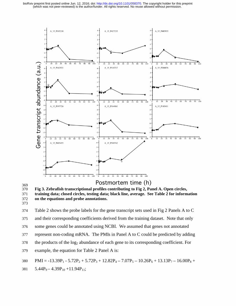
369 Fig 3. Zebrafish transcriptional profiles contributing to Fig 2, Panel A. Open circles, 370 training data; closed circles, testing data; black line, average. See Table 2 for information 371 on the equations and probe annotations. 372 373
Table 2 shows the probe labels for the gene transcript sets used in Fig 2 Panels A to C 374
and their corresponding coefficients derived from the training dataset. Note that only 375
some genes could be annotated using NCBI. We assumed that genes not annotated 376
represent non-coding mRNA. The PMIs in Panel A to C could be predicted by adding 377
the products of the log2 abundance of each gene to its corresponding coefficient. For 378
example, the equation for Table 2 Panel A is: 379
PMI = -13.39P1 - 5.72P2 + 5.72P3 + 12.82P4 – 7.07P5 – 10.26P6 + 13.13P7 – 16.00P8 + 380
5.44P9 – 4.39P10 +11.94P11; 381
(which was not peer-reviewed) is the author/funder. All rights reserved. No reuse allowed without permission. The copyright holder for this preprint. http://dx.doi.org/10.1101/058370doi: bioRxiv preprint first posted online Jun. 12, 2016;

where Pi are the gene abundances represented by the probes A_15_P105218 (0.39 a.u.), 382
A_15_P427235 (-0.54 a.u.), A_15_P485935 (-0.39 a.u.), A_15_P163931 (1.27 a.u.), 383
A_15_P110717 (-0.53 a.u.), A_15_P204076 (0.16 a.u.), A_15_P197726 (0.82 a.u.), 384
A_15_P164061 (0.58 a.u.), A_15_P105411 (-0.40 a.u.), A_15_P405455 (-1.13 a.u.), 385
A_15_P569742 (0.46 a.u.). In this example, the predicted PMI is ~24 h. Based on 386
Figure 2 panel A, the 99% confidence interval is between 20.9 and 27.1 h. 387
388
Table 2. Zebrafish genes used to predict PMI by Panel. The gene annotations of the probes were 389
determined using NCBI with a 100 bit minimum. 390
Panel Probe Label Coefficient Gene Gene Name
A A_15_P105218 -13.39 Gpr98 G-protein coupled receptor 98 precursor
A_15_P427235 -5.72 Noncoding A_15_P485935 5.72 Noncoding A_15_P163931 12.82 Moxd1 DBH-like monooxygenase protein 1 homolog precursor A_15_P110717 -7.07 Svep1 Sushi von Willebrand factor type A, EGF and pentraxin A_15_P204076 -10.26 Pde4b 5'-cyclic-AMP and -GMP phosphodiesterase 11 A_15_P197726 13.13 Plek2 Pleckstrin-2 A_15_P164061 -16.00 Rassf6 Ras association domain-containing protein 6 A_15_P105411 5.44 Grm7 Metabotropic glutamate receptor 7-like A_15_P405455 -4.39 Noncoding A_15_P569742 11.94 Trim25 E3 ubiquitin/ISG15 ligase TRIM25-like B A_15_P104895 19.66 Noncoding A_15_P522677 -26.62 Noncoding A_15_P105411 13.32 Grm7 Metabotropic glutamate receptor 7-like A_15_P119193 15.64 Noncoding A_15_P401770 5.89 Lrrc59 Leucine-rich repeat-containing protein 1 A_15_P104490 -27.55 Wif1 Wnt inhibitory factor 1 precursor A_15_P177366 -3.88 Bmpr2 Bone morphogenetic protein receptor, type II a A_15_P586597 -7.64 Noncoding A_15_P168556 6.77 Sema6d Semaphorin-6D isoform X1 A_15_P105618 17.47 Gpr143 G-protein coupled receptor 143 A_15_P171831 6.86 Il20 Interleukin-20 isoform X1 C A_15_P569842 3.20 Myo3a Myosin-IIIa A_15_P176341 2.03 Prrt4 Proline-rich transmembrane protein 4 A_15_P107601 8.59 Atf3 Cyclic AMP-dependent transcription factor ATF-3 A_15_P168526 -5.03 Pglyrp1 Peptidoglycan recognition protein 1 A_15_P328806 -5.37 Kdm5b Lysine-specific demethylase 5B A_15_P309786 2.33 FimC Integumentary mucin C.1-like A_15_P120901 0.31 Gnai1 Guanine nucleotide-binding protein G(i) subunit alpha-1
(which was not peer-reviewed) is the author/funder. All rights reserved. No reuse allowed without permission. The copyright holder for this preprint. http://dx.doi.org/10.1101/058370doi: bioRxiv preprint first posted online Jun. 12, 2016;

A_15_P165836 6.98 C3ar1 C3a anaphylatoxin chemotactic receptor-like A_15_P576307 1.91 Noncoding A_15_P110820 -34.27 Gucy1a3 Guanylate cyclase soluble subunit alpha-3 A_15_P105618 32.01 Gpr143 G-protein coupled receptor 143
391
Mouse 392 After training 50,000 random selections (each selection consisted of 7 genes), about 96% 393
(n=47,847) of the selected gene sets yielded R2 and slopes of 1. The remaining selections 394
were not used for validation because the equations (n=2,153 selections) could not be 395
resolved, or they had fits and/or slopes that were <1 (n=25 selections). The R2 and slopes 396
of predicted versus actual PMIs determined using the testing dataset identified the top 397
performing gene sets. 398
The top selected gene transcript sets for the mouse liver and brain are shown in Fig 4. As 399
indicated by the R2, slopes, and size of the 99% confidence intervals, gene transcript sets 400
from the liver were better at predicting PMIs than those from the brain. The mouse genes 401
used in the gene transcript sets, their coefficients, and annotations are shown in Table 3 402
and the transcriptional gene profiles for the mouse liver samples are shown in Fig 5. 403
Note that the high similarity in the gene transcript abundance between the data used for 404
training and testing of the selected genes. In most cases (but not all), the duplicate 405
samples (represented by dots) are located on top of one another. 406
407
Fig 4. Predicted versus actual PMI determined for the mouse for three different equations 408 as represented by the panels. R2 and slopes are based on both training and testing datasets. 409 Gray line represents 99% confidence limits of the linear regression. Open circles, training 410 data; closed circles, testing data. See Table 3 for information on the equations and probes. 411 412
The poor predictability of the brain gene transcript sets (i.e., R2<0.95) could be attributed 413
to the low number of repeated selections of gene transcript sets and the variability in gene 414
(which was not peer-reviewed) is the author/funder. All rights reserved. No reuse allowed without permission. The copyright holder for this preprint. http://dx.doi.org/10.1101/058370doi: bioRxiv preprint first posted online Jun. 12, 2016;

abundances between the training and testing datasets. We repeated the analysis of the 415
brain samples an additional 1,000,000 times, which resulted in some improvement. The 416
best fit and slope for 50,000 gene transcript set selections was R2=0.83 and m=0.77 (not 417
shown). The best fit and slope for 1,000,000 selections was R2=0.93 and m=0.85 (Fig 4, 418
Panel B) with the second best being R2=0.92 and m=0.86 (Fig 4, Panel C). Hence, the 419
number of combination of gene transcript sets examined is important for selecting the 420
best ones. It is important to emphasize that the computation time for running 1,000,000 421
selections was approximately 1 week using a Mac OS X 10.8.6. 422
The PMIs in Panel A to C could be predicted by adding the products of the log2 423
abundance of each gene to its corresponding coefficient. The predicted PMIs for mouse is 424
calculated same way as for zebrafish (shown above). 425
426
(which was not peer-reviewed) is the author/funder. All rights reserved. No reuse allowed without permission. The copyright holder for this preprint. http://dx.doi.org/10.1101/058370doi: bioRxiv preprint first posted online Jun. 12, 2016;

Table 3. Mouse probes used to target gene transcripts and their coefficients used to predict 427 PMIs by Panel. The annotations of probes were determined by using NCBI database with 428 100 bit minimum. 429
Panel Organ Probe Coefficient Gene Gene Name
A Liver A_55_P2007991 12.7 Tuba3b Tubulin, alpha 3B A_51_P227077 -21.43 Mdh1b Malate dehydrogenase 1B, NAD (soluble) A_55_P2112609 14.97 Non-coding A_30_P01028777 -1.6 Non-coding A_51_P318381 9.91 Pgf Placental growth factor A_55_P2197847 18.41 Non-coding
A_30_P01026843 7.59 Ifitm2 Interferon induced transmembrane protein 2
B Brain A_52_P627085 14.2729 Mrps18c 28S ribosomal protein S18c, mitochondrial A_30_P01025266 -59.3569 Klf14 Krueppel-like factor 14 A_55_P1955891 -5.57821 Ppm1e Protein phosphatase 1E
A_55_P2109107 1.92003 Gfra2 GDNF family receptor alpha-2 isoform 3 precursor
A_30_P01031213 -61.0776 Acsl1 Long-chain-fatty-acid--CoA ligase 4 isoform 1
A_52_P418795 -11.3343 Grk4 G protein-coupled receptor kinase 4 A_66_P100268 59.9399 Non-coding C Brain A_30_P01028032 9.30294 Flo11l Flocculation protein FLO11-like A_55_P1972018 -37.7273 Hist1h4a Histone H4 A_55_P2410304 -10.5218 Non-coding A_52_P1082736 15.8909 Sept1 Septin-1 A_66_P117204 9.66267 Gpc3 Glypican-3 isoform
A_30_P01020727 6.36972 Adam2 Disintegrin and metalloprotease domain 4b precursor
A_52_P236705 5.9439 Ripply3 Protein ripply3 430 431
We compared the variability in gene transcript abundances between training and testing 432
data sets for the mouse liver and mouse brain. Transcriptional gene profiles of the gene 433
sets used in Fig 4 Panels A and B are shown in Figs 5 and 6, respectively. While most of 434
the mouse liver gene transcript abundances are similar for the training and testing data 435
sets in Fig 5, many of the mouse brain gene transcript abundances are not similar in Fig 436
6. A two-tailed T-test of the standard deviations of the gene transcript abundances in the 437
training and testing datasets for the liver and brain samples (Fig 5 versus Fig 6) by 438
postmortem time were significantly different (P< 0.006), with higher standard deviations 439
in the brain samples than the liver. This finding indicates that variability in the gene 440
transcript abundances affects PMI predictability. 441
(which was not peer-reviewed) is the author/funder. All rights reserved. No reuse allowed without permission. The copyright holder for this preprint. http://dx.doi.org/10.1101/058370doi: bioRxiv preprint first posted online Jun. 12, 2016;

442
Fig 5. Mouse liver transcriptional profiles contributing to Fig 4, Panel A. Open circles, 443 training data; closed circles, testing data; black line, average. See Table 3 for information 444 on the equations and probe annotations. 445
(which was not peer-reviewed) is the author/funder. All rights reserved. No reuse allowed without permission. The copyright holder for this preprint. http://dx.doi.org/10.1101/058370doi: bioRxiv preprint first posted online Jun. 12, 2016;

Fig 6. 446 Mouse brain transcriptional profiles contributing to Fig 4, Panel B. Open circles, training 447 data; closed circles, testing data; black line, average. See Table 3 for information on the 448 equations and probe annotations. 449 450
To further test this phenomenon, a small amount of random noise was added to the 451
abundances of mouse liver gene transcripts (Fig 5), which originally had very low 452
(which was not peer-reviewed) is the author/funder. All rights reserved. No reuse allowed without permission. The copyright holder for this preprint. http://dx.doi.org/10.1101/058370doi: bioRxiv preprint first posted online Jun. 12, 2016;

standard deviations by postmortem time. When the introduction of noise approached 453
10%, the fit and slopes were drastically altered, indicating that similarity in the gene 454
transcript abundances between the training and test data sets can directly affect the fit and 455
slopes of predicted versus actual PMIs. 456
Randomization challenge 457
Experiments using perfectly-defined linear regressions revealed that 95% of the training 458
data for the zebrafish and mouse yielded fits (R2) and slopes of 1 for predicted versus 459
actual PMIs. To demonstrate that the ‘perfect’ fits and slopes are functions of the linear 460
regressions, we randomized gene transcript abundances at every postmortem time for all 461
genes in the zebrafish dataset. This randomization maintained the variance in the dataset 462
at each postmortem time so that the variance of the first postmortem time in the 463
randomized dataset was the same as the variance of the gene transcript abundances at the 464
first postmortem time in the original dataset and so on for the gene transcript abundances 465
at all postmortem times. 466
As anticipated, training of the randomized zebrafish dataset using perfectly-defined linear 467
regressions (11 genes by 11 postmortem times x 50,000 repeated gene transcript 468
selections) yielded fits (R2) and slopes of 1 for predicted versus actual PMIs for 95% of 469
the regressions. When we tested the 50,000 regressions using a test dataset, not one of the 470
gene transcript sets approached a fit (R2) and slope of 1. In fact, most yielded slopes of 471
zero and R2 <0.80. The significance of this experiment is twofold: (i) it confirms that 472
‘perfect’ fits and slopes using the training datasets are a function of ‘perfectly-defined’ 473
linear regressions, and (ii) it confirms the need to validate the regression equations using 474
testing datasets. 475
Discussion 476
In addition to the different stages of body decomposition (i.e., rigor mortis, livor mortis, 477
algor mortis and putrefaction) [16,17,18], there are many biochemical, biological, 478
chemical, and physical ways to determine PMI. Biochemical indicators and 479
corresponding sample sites include: pH and spectrophotometer readings of blood and 480
serum [19], cardiac troponin-I and cadaveric blood in the heart [19,20], lactate and malate 481
dehydrogenase in the liver [21], melatonin in the brain, sera, and urine [22], DNA 482
(which was not peer-reviewed) is the author/funder. All rights reserved. No reuse allowed without permission. The copyright holder for this preprint. http://dx.doi.org/10.1101/058370doi: bioRxiv preprint first posted online Jun. 12, 2016;

degradation in many tissues and organs [23,24,25,26], endothelial growth factors in the 483
brain, heart, liver, and kidneys [27], insulin and glucagonin in pancreatic beta cells 484
[28,29], cells in the cerebrospinal fluid [30], apoptotic cells in skin bruises [31] and 485
histology of labial muscosa [32]. Biological indicators and sample sites include: ciliary 486
motility in the nose [33], sweat gland morphology in the arm pit [34], muscle contraction 487
[35] and pyrosequencing of the buccal cavity, rectum and GI tract samples [36], 488
entomological [37,38,39] and botanical processes occurring in and around the body 489
[40,41]. Chemical indicators and sample sites include: electrolytes in human vitreous 490
humour [42], biomarkers (e.g. amino acids, neurotransmitters) in body organs and 491
muscles [43], hypoxanthine in the vitreous humour or cerebrospinal fluid [44,45,46] and 492
potassium in the vitreous humour [47,48,49]. Physical indicators and sample sites 493
include: microwave probe to the skin [50], infrared tympanic thermography and 494
temperature of the ear [51,52], and temperature of the eye and body core [53,54,55]. 495
Several formulae have also been developed to estimate PMI that are based on multiple 496
environmental and physicochemical conditions [e.g., 56]. Despite these many 497
approaches, accurate PMI prediction remains an enigma [43]. The motivation for this 498
study was to test experimental designs that could accurately predict PMI using 499
upregulated gene expression data in order to provide “proof of principle”. 500
The abundance of a gene transcript is determined by its rate of synthesis and its rate of 501
degradation [57]. In this study, the synthesis of mRNA had to far exceed its degradation 502
to be a significantly upregulated gene (at some postmortem time) in our study. As 503
demonstrated in the previous study [13] and shown in this study (Figs 3, 5, and 6), the 504
timings of the upregulation differed between genes. Some gene transcripts, such as the 505
one targeted by probe A_15_P105218, were upregulated right after organismal death and 506
reached maximize abundance at 24 h postmortem while, others, such as the one targeted 507
by probe A_15_P569742, increased substantially at 48 h postmortem (Fig 3). It is 508
presumed that differences in the transcript profiles affect the value of the coefficients in 509
the linear equations because it is not possible to generate coefficients if the gene 510
transcript abundances changed in the same way. That is, a numerical solution could not 511
be mathematically resolved. 512
(which was not peer-reviewed) is the author/funder. All rights reserved. No reuse allowed without permission. The copyright holder for this preprint. http://dx.doi.org/10.1101/058370doi: bioRxiv preprint first posted online Jun. 12, 2016;

It should be noted that the upregulation of postmortem genes is optimal for PMI 513
prediction because only about 1% of the total genes of an organism were upregulated in 514
organismal death – which is rare indeed. In contrast, a focus on downregulated genes 515
would not be practical because one does not know if downregulated genes are due to 516
repression, degradation of the total RNA, or exhausted resources such as those needed for 517
the transcript machinery function (e.g., dNTPs and RNA polymerase). 518
Given that gene transcripts from the liver were better at PMI predictions than those from 519
the brain suggests that mRNA transcripts from some organs are better than others. It is 520
conceivable that upregulated postmortem genes could be found in the heart, kidney, 521
spleen or muscle, which needs further exploration. 522
It is important to recognize that this study would probably not be possible using 523
conventional microarray approaches because normalizations could yield up to 20 to 30% 524
differences in the up- or down-regulation depending on the procedure selected [59-62]. 525
The Gene Meter approach does not require the data to be normalized since the microarray 526
probes are calibrated. Moreover, in the processing of samples, the same amount of 527
labeled mRNA was loaded onto the DNA microarray for each sample (1.65 µg), which 528
eliminates the need to divide the microarray output data by a denominator in order to 529
compare samples. 530
We recognize that our experimental design did not consider factors such as temperature, 531
which have been considered in other models [e.g., 4]. To do so would go beyond the 532
stated objectives of providing a “proof of principle” for the optimal experimental design 533
(i.e., perfectly-defined linear regressions based on multiple gene transcripts) using a high 534
throughput approach. Nonetheless, future studies could make our experimental design 535
more universal by integrating temperature and other factors into the regression models. 536
In addition to providing “proof of principle” of a new forensic tool for determining PMI, 537
the approach could be used as a tool for prospective studies aimed at improving organ 538
quality of human transplants. 539
(which was not peer-reviewed) is the author/funder. All rights reserved. No reuse allowed without permission. The copyright holder for this preprint. http://dx.doi.org/10.1101/058370doi: bioRxiv preprint first posted online Jun. 12, 2016;

Conclusion 540
We examined if significantly upregulated genes could be used to predict PMIs in two 541
model organisms using linear regression analyses. While PMIs could be accurately 542
predicted using selected zebrafish and mouse liver gene transcripts, predictions were poor 543
using selected mouse brain gene transcripts, presumably due to high variability of the 544
biological replicates. The experimental design of selecting groups of gene transcripts, 545
extracting the coefficients with linear regression analyses, and testing the regression 546
equations with testing data, yielded highly accurate PMI predictions. This study warrants 547
the implementation of our experimental design towards the development of an accurate 548
PMI prediction tool for cadavers and possibly a new tool for prospective studies aimed at 549
improving organ quality of human transplants. 550
Authors’ contributions 551
PAN and AEP designed the study. MCH and PAN conducted the statistical analyses and 552
wrote the manuscript. All authors read and approved the final manuscript. 553
Acknowledgements 554 555
Financial disclosure 556
The work was supported by funds from the Max-Planck-Society. 557
Supplemental Information 558
Primer on Matrix Algebra 559
Our PMI prediction approach using a perfectly defined system relies on matrix linear 560
algebra. The following is an explanation of matrix linear algebra and how it was used in 561
our study to predict PMI with gene expression profiles. A matrix is defined as a 562
rectangular array of related values. These values, which are called elements, usually are 563
scalars. Scalars are numbers that represent physical quantities. Elements in a horizontal 564
line are called rows and elements in a vertical line are columns and the number of rows 565
and columns describe a matrix. A matrix, S, with y number of rows and z number of 566
columns is denoted as a y x z matrix. This matrix can also be notated with subscripts and 567
appears as Sy,z . Mathematical operations can be performed using matrices, including 568
(which was not peer-reviewed) is the author/funder. All rights reserved. No reuse allowed without permission. The copyright holder for this preprint. http://dx.doi.org/10.1101/058370doi: bioRxiv preprint first posted online Jun. 12, 2016;

multiplication. Matrices can be multiplied by one another if one matrix has as many 569
columns as the other matrix has rows. We used linear equations to obtain a matrix 570
product. The number of gene transcripts used in a selected gene transcript set was limited 571
by the number of postmortem sample times. 572
Example: 573 If we arrange individual genes with their transcript abundances at specific postmortem 574
times in columns then, essentially, we have a matrix A where the columns are the 575
transcriptional profiles for individual genes. Furthermore, we can construct another 576
matrix, B, which defines the data in a different way. In this matrix the values are the 577
actual postmortem sampling times that are ordered in the same way as the abundances of 578
individual gene transcripts. Finally, we can define another matrix, consisting of one 579
column of coefficient values. These are the weighing factors that we will determine 580
using the rules of linear matrix algebra. To deconvolute the transcriptional profiles from 581
the mixtures and solve for the weighing factors, we set up the matrices like so: A x C = 582
B. When this is done we are left with several equations. To solve for x and y we need to 583
follow the rules of linear matrix algebra. First, we must transpose A, which becomes AT, 584
then multiply both sides of the equation A x B = C with AT. Next, we are required to 585
invert the matrix product of AT x A, thus A becomes A-1 and also multiply both sides of 586
our original equation A x C = B. Our modified equation, which looks like this (AT * A)-587
1AT*A*C = (AT*A)-1 * AT * B, is now ready to be solved for x and y in matrix C. 588
Solving for C, we get C = (AT * A)-1 * AT * B. Now the values in the matrix C are x and 589
y. Next, we plug our values for x and y into our matrix equations to obtain predicted 590
(calculated) PMI values. To ascertain whether the predicted PMIs from our group of 591
gene transcripts is accurate, we plotted the actual and predicted PMIs and determined the 592
slope and fit of the regression line. The R2 and the slope of the line was observed to 593
determine how well a group of gene transcripts predicted PMI. The R2 is the measure of 594
how much variability is accounted for by the model. For example, if the R2 is 0.95, then 595
the model accounts for 95% of the variability. The other 5% is due to undetermined 596
phenomena. 597
598
(which was not peer-reviewed) is the author/funder. All rights reserved. No reuse allowed without permission. The copyright holder for this preprint. http://dx.doi.org/10.1101/058370doi: bioRxiv preprint first posted online Jun. 12, 2016;

Literature Cited 599 600
1. Anderson, B. Five notorious, homicidal tales of life insurance fraud Real-life clients 601 from hell. LifeHealthPro. Published October 25, 2013 602 http://www.lifehealthpro.com/2013/10/25/5-notorious-homicidal-tales-of-life-603 insurance-frau 604
2. Ferreira M. T. and Cunha E. Can we infer post mortem interval on the basis of 605 decomposition rate? A case from a Portuguese cemetery, Forensic Science 606 International 2013;298: e1-298.e6. 607
3. Sampaio-Silva F, Magalhães T, Carvalho F, Dinis-Oliveira RJ, Silvestre R. Profiling 608 of RNA degradation for estimation of post mortem interval. PLoS One. 2013; 8: 609 e56507. 610
4. Ma J, Pan H, Zeng Y, Lv Y, Zhang H, Xue A, Jiang J, Ma K, Chen L. Exploration of 611 the R code-based mathematical model for PMI estimation using profiling of RNA 612 degradation in rat brain tissue at different temperatures. Forensic Sci Med Pathol. 613 2015;11: 530-7. 614
5. Lv YH, Ma KJ, Zhang H, He M, Zhang P, Shen YW, Jiang N, Ma D, Chen L. A time 615 course study demonstrating mRNA, microRNA, 18S rRNA, and U6 snRNA changes 616 to estimate PMI in deceased rat's spleen. J Forensic Sci. 2014, 59: 1286-94. 617
6. González-Herrera L, Valenzuela A, Marchal JA, Lorente JA, Villanueva E. Studies 618 on RNA integrity and gene expression in human myocardial tissue, pericardial fluid 619 and blood, and its postmortem stability. Forensic Sci Int. 2013; 232: 218-28. 620
7. Zapico SC, Menéndez ST, Núñez P. Cell death proteins as markers of early 621 postmortem interval. Cell Mol Life Sci. 2014;71: 2957-62. 622
8. Birdsill AC, Walker DG, Lue L, Sue LI, Beach TG. Postmortem interval effect on 623 RNA and gene expression in human brain tissue. Cell Tissue Bank. 2011;12: 311-8. 624
9. Tu Y,Stolovitzky G, Klein U. Quantitative noise analysis for gene expression 625 microarray experiments. Proc Natl Acad Sci USA 2002;99: 14031. 626
10. Pozhitkov AE, Noble PA, Bryk J, Tautz D. A revised design for microarray 627 experiments to account for experimental noise and uncertainty of probe response. 628 PLoS One. 2014;9: e91295. 629
11. Harrison A., Binder, H. Buhot, A., Burden, C.J., Carlon, E., Gibas, C., Gamble, L.J. 630 Halperin, A., Hooyberghs, J., Kreil, D.P., Levicky, R., Noble, P.A., Ott, A., Pettitt, 631 B.M., Tautz, D., Pozhitkov, AE. Physico-chemical foundations underpinning 632 microarray and next-generation sequencing experiments. Nucl Acids Res. 2013; 41: 633 2779-96. 634
12. Amend AS, Seifert KA, Bruns TD. Quantifying microbial communities with 454 635 pyrosequencing: does read abundance count? Mol Ecol 2010;19: 5555. 636
13. Pozhitkov AE, Neme R, Domazet-Loo T, Leroux BG., Soni S, Tautz D and Noble 637 PA. Thanatotranscriptome: genes actively expressed after organismal death. PlosOne 638 2016; (PONE-6-02773). 639
14. Pozhitkov AE, Nies G, Kleinhenz B, Tautz D, Noble PA. Simultaneous quantification 640 of multiple nucleic acid targets in complex rRNA åmixtures using high density 641
(which was not peer-reviewed) is the author/funder. All rights reserved. No reuse allowed without permission. The copyright holder for this preprint. http://dx.doi.org/10.1101/058370doi: bioRxiv preprint first posted online Jun. 12, 2016;

microarrays and nonspecific hybridization as a source of information. J Microbiol 642 Methods. 2008;75: 92-102. doi: 10.1016/j.mimet.2008.05.013. 643
15. Pozhitkov AE, Bailey KD, Noble PA. Development of a statistically robust 644 quantification method for microorganisms in mixtures using oligonucleotide 645 microarrays. J Microbiol Methods. 2007;70: 292-300. 646
16. Council of Europe, Strasbourg, 1999. Recommendation No. R (99) 3 on the 647 Harmonization of Medico-Legal Autopsy Rules and Its Explanatory Memorandum. 648 Strasbourg: Council of Europe; 1999. 649
17. Kolusayın Ö, Koç S. Ölüm, içinde Soysal Z, Çakalır C. Forensic Medicine, Print I, 650 Istanbul University Cerrahpsa School of Medicine’s Publication, Istanbul; 1999; 93-651 152. 652
18. Nashelsky MB, Lawrence CH. Accuracy of cause of death determination without 653 forensic autopsy examination. Am J Forensic Med Pathol. 2003;24: 313-9. 654
19. Donaldson AE, Lamont IL. Biochemistry changes that occur after death: potential 655 markers for determining post-mortem interval. PLoS One. 2013;8: e82011. 656
20. Sabucedo AJ, Furton KG. Estimation of postmortem interval using the protein marker 657 cardiac Troponin I. Forensic Sci Int. 2003;134: 11–16. 658
21. Gos T, Raszeja S. Postmortem activity of lactate and malate dehydrogenase in human 659 liver in relation to time after death. Int J Legal Med. 1993;106: 25–29 660
22. Mikamimi H, Terazawa K, Takatori T, Tokudome S, Tsukamoto T, Haga K. 661 Estimation of time of death by quantification of melatonin in corpses. Int J Legal 662 Med. 1994;107: 42–51. 663
23. Di Nunno N, Costantinides F, Cina SJ, Rizzardi C, Di Nunno C, Melato M. What is 664 the best sample for determining the early postmortem period by on-the-spot flow 665 cytometry analysis? Am J Forensic Med Pathol. 2002, 23:173-80. 666
24. Di Nunno N, Costantinides F, Melato M. Determination of the time of death in a 667 homicide-suicide case using flow cytometry. Am J Forensic Med Pathol. 1999;20: 668 228-31. 669
25. Di Nunno N, Costantinides F, Bernasconi P, Bottin C, Melato M. Is flow cytometric 670 evaluation of DNA degradation a reliable method to investigate the early postmortem 671 period? Am J Forensic Med Pathol. 1998;19:50-3. 672
26. Cina SJ. Flow cytometric evaluation of DNA degradation: a predictor of postmortem 673 interval? Am J Forensic Med Pathol. 1994;15: 300-2. 674
27. Thaik-Oo M, Tanaka E, Tsuchiya T, Kominato Y, Honda K, Yamazaki K, Misawa S. 675 Estimation of postmortem interval from hypoxic inducible levels of vascular 676 endothelial growth factor. J Forensic Sci. 2002;47: 186-9. 677
28. Wehner F, Wehner HD, Schieffer MC, Subke J. Delimination of time of death by 678 immunohistochemical detection of insulin in pancreatic beta-cells. Forensic Sci Int. 679 1999; 105: 161-9. 680
29. Wehner F, Wehner HD, Subke J. Delimitation of the time of death by 681 immunohistochemical detection of glucagon in pancreatic a-cells. Forensic Sci Int. 682 2002;124: 192–199. 683
(which was not peer-reviewed) is the author/funder. All rights reserved. No reuse allowed without permission. The copyright holder for this preprint. http://dx.doi.org/10.1101/058370doi: bioRxiv preprint first posted online Jun. 12, 2016;

30. Wyler D, Marty W, Bär W. Correlation between the post-mortem cell content of 684 cerebrospinal fluid and time of death. Int J Legal Med.1994;106: 194–199. 685
31. Sawaguchi T, Jasani B, Kobayashi M, Knight B. Post-mortem analysis of apoptotic 686 changes associated with human skin bruises. Forensic Sci Int. 2000;108: 187-203. 687
32. Yadav A, Angadi PV, Hallikerimath S. Applicability of histologic post-mortem 688 changes of labial mucosa in estimation of time of death - a preliminary study. Aust J 689 For Sci. 2012;44: 343-352. 690
33. Romanelli MC, Gelardi M, Fiorella ML, Tattoli L, Di Vella G, Solarino B. Nasal 691 ciliary motility: a new tool in estimating the time of death. Int J Legal Med. 2012; 692 126: 427-33. 693
34. Cingolani M, Osculati A, Tombolini A, Tagliabracci A, Ghimenton C, Ferrara SD. 694 Morphology of sweat glands in determining time of death. Int J Legal Med. 695 1994;107: 132–140. 696
35. Warther S, Sehner S, Raupach T, Püschel K, Anders S. Estimation of the time since 697 death: post-mortem contractions of human skeletal muscles following mechanical 698 stimulation (idiomuscular contraction). Int J Legal Med. 2012;126: 399-405. 699
36. Hyde ER, Haarmann DP, Lynne AM, Bucheli SR, Petrosino JF. The living dead: 700 bacterial community structure of a cadaver at the onset and end of the bloat stage of 701 decomposition. PLoS One. 2013;8: e77733. 702
37. Meiklejohn KA, Wallman JF, Dowton M.DNA barcoding identifies all immature life 703 stages of a forensically important flesh fly (Diptera: Sarcophagidae). J Forensic Sci. 704 2013;58: 184-7. 705
38. Warren JA, Anderson GS. Effect of fluctuating temperatures on the development of a 706 forensically important blow fly, Protophormia terraenovae (Diptera: Calliphoridae). 707 Environ Entomol. 2013;42: 167-72. 708
39. Vasconcelos SD, Soares TF, Costa DL. Multiple colonization of a cadaver by insects 709 in an indoor environment: first record of Fannia trimaculata (Diptera: Fanniidae) and 710 Peckia (Peckia) chrysostoma (Sarcophagidae) as colonizers of a human corpse. Int J 711 Legal Med. 2014;128: 229-33. 712
40. Cardoso HF, Santos A, Dias R, Garcia C, Pinto M, Sérgio C, Magalhães T. 713 Establishing a minimum postmortem interval of human remains in an advanced state 714 of skeletonization using the growth rate of bryophytes and plant roots. Int J Legal 715 Med. 2010;124: 451-6. 716
41. Lancia M, Conforti F, Aleffi M, Caccianiga M, Bacci M, Rossi R. The use of 717 Leptodyctium riparium (Hedw.) Warnst in the estimation of minimum postmortem 718 interval. J Forensic Sci. 2013;58 Suppl 1: S239-42. 719
42. Bocaz-Beneventi G, Tagliaro F, Bortolotti F, Manetto G, Havel J. Capillary zone 720 electrophoresis and artificial neural networks for estimation of the post-mortem 721 interval (PMI) using electrolytes measurements in human vitreous humour. Int J 722 Legal Med. 2002;116: 5-11. 723
43. Vass AA. The elusive universal post-mortem interval formula. Forensic Sci Int. 2011; 724 204: 34-40. 725
(which was not peer-reviewed) is the author/funder. All rights reserved. No reuse allowed without permission. The copyright holder for this preprint. http://dx.doi.org/10.1101/058370doi: bioRxiv preprint first posted online Jun. 12, 2016;

44. Madea B, Herrmann N, Henbge C. Precision of estimating the time since death by 726 vitreous potassium--comparison of two different equations. Forensic Sci Int. 1990; 727 46: 277-84. 728
45. Madea B, Käferstein H, Hermann N, Sticht G. Hypoxanthine in vitreous humor and 729 cerebrospinal fluid--a marker of postmortem interval and prolonged (vital) hypoxia? 730 Remarks also on hypoxanthine in SIDS. Forensic Sci Int. 1994;65: 19-31. 731
46. MadeaB. Importance of supravitality in forensic medicine. Forensic Sci Int. 1994; 69: 732 221-41. 733
47. Lange N, Swearer S, Sturner WQ. Human postmortem interval estimation from 734 vitreous potassium: an analysis of original data from six different studies. Forensic 735 Sci Int. 1994;66: 159-74. 736
48. Zhou B, Zhang L, Zhang G, Zhang X, Jiang X. The determination of potassium 737 concentration in vitreous humor by low pressure ion chromatography and its 738 application in the estimation of postmortem interval. J Chromatogr B Analyt Technol 739 Biomed Life Sci. 2007;852: 278-81. 740
49. Lendoiro E, Cordeiro C, Rodríguez-Calvo MS, Vieira DN, Suárez-Peñaranda JM, 741 López-Rivadulla M, Muñoz-Barús JI. Applications of Tandem Mass Spectrometry 742 (LC-MSMS) in estimating the post-mortem interval using the biochemistry of the 743 vitreous humour. Forensic Sci Int. 2012;223: 160-4. 744
50. Al-Alousi LM, Anderson RA, Land DV. A non-invasive method for postmortem 745 temperature measurements using a microwave probe. Forensic Sci Int. 1994;64: 35-746 46. 747
51. Cattaneo C, Di Giancamillo A, Campari O, Orthmann N, Martrille L, Domeneghini 748 C, Jouineau C, Baccino E. Infrared tympanic thermography as a substitute for a probe 749 in the evaluation of ear temperature for post-mortem interval determination: a pilot 750 study. J Forensic Leg Med. 2009;16: 215-7. 751
52. Baccino E, De Saint Martin L, Schuliar Y, Guilloteau P, Le Rhun M, Morin JF, 752 Leglise D, Amice J. Outer ear temperature and time of death. Forensic Sci Int. 753 1996;83: 133-46. 754
53. Kaliszan M. Studies on time of death estimation in the early post mortem period -- 755 application of a method based on eyeball temperature measurement to human bodies. 756 Leg Med (Tokyo). 2013;15: 278-82. 757
54. Nelson EL. Estimation of short-term postmortem interval utilizing core body 758 temperature: a new algorithm. Forensic Sci Int. 2000;109: 31-8. 759
55. Muggenthaler H, Sinicina I, Hubig M, Mall G. Database of post-mortem rectal 760 cooling cases under strictly controlled conditions: a useful tool in death time 761 estimation. Int J Legal Med. 2012;126: 79-87. 762
56. Megyesi MS, Nawrocki SP, Haskell NH. Using accumulated degree-days to estimate 763 the postmortem interval from decomposed human remains. J Forensic Sci. 2005;50: 764 618-26. 765
57. Neymotin, Athanasiadou R, Gresham D. Determination of in vivo RNA kinetics using 766 RATE-seq. RNA. 2014;20: 1645. 767
(which was not peer-reviewed) is the author/funder. All rights reserved. No reuse allowed without permission. The copyright holder for this preprint. http://dx.doi.org/10.1101/058370doi: bioRxiv preprint first posted online Jun. 12, 2016;

58. Bauer M, Gramlich I, Polzin S, Patzelt D. Quantification of mRNA degradation as 768 possible indicator of postmortem interval--a pilot study. Leg Med (Tokyo). 2003;5: 769 220-7. 770
59. Barash Y, Dehan E, Krupsky M, Franklin W, Geraci M, Friedman N, Kaminski N. 771 Comparative analysis of algorithms for signal quantitation from oligonucleotide 772 microarrays. Bioinform. 2004, 20: 839. 773
60. Seo J, Bakay M, Chen YW, Hilmer S, Shneiderman B, Hoffman EP. Interactively 774 optimizing signal-to-noise ratios in expression profiling: project-specific algorithm 775 selection and detection p-value weighting in Affymetrix microarrays. Bioinform. 776 2004, 20: 2534. 777
61. Harr B, Schlötterer C, Comparison of algorithms for the analysis of Affymetrix 778 microarray data as evaluated by co-expression of genes in known operons. Nucl 779 Acids Res. 2006, 34: e8. 780
62. Millenaar FF, Okyere J, May ST, van Zanten M, Voesenek LA, Peeters AJ. How to 781 decide? Different methods of calculating gene expression from short oligonucleotide 782 array data will give different results. BMC Bioinform. 2006, 7: 137. 783
784
785
(which was not peer-reviewed) is the author/funder. All rights reserved. No reuse allowed without permission. The copyright holder for this preprint. http://dx.doi.org/10.1101/058370doi: bioRxiv preprint first posted online Jun. 12, 2016;