Accurate Confidence Limits for Quantiles under Random ...mparzen/published/parzen8.pdf · Accurate...

Accurate Confidence Limits for Quantiles under Random CensoringAuthor(s): Robert L. Strawderman, Michael I. Parzen, Martin T. WellsSource: Biometrics, Vol. 53, No. 4 (Dec., 1997), pp. 1399-1415Published by: International Biometric SocietyStable URL: http://www.jstor.org/stable/2533506Accessed: 12/08/2009 21:17

Your use of the JSTOR archive indicates your acceptance of JSTOR's Terms and Conditions of Use, available athttp://www.jstor.org/page/info/about/policies/terms.jsp. JSTOR's Terms and Conditions of Use provides, in part, that unlessyou have obtained prior permission, you may not download an entire issue of a journal or multiple copies of articles, and youmay use content in the JSTOR archive only for your personal, non-commercial use.

Please contact the publisher regarding any further use of this work. Publisher contact information may be obtained athttp://www.jstor.org/action/showPublisher?publisherCode=ibs.

Each copy of any part of a JSTOR transmission must contain the same copyright notice that appears on the screen or printedpage of such transmission.

JSTOR is a not-for-profit organization founded in 1995 to build trusted digital archives for scholarship. We work with thescholarly community to preserve their work and the materials they rely upon, and to build a common research platform thatpromotes the discovery and use of these resources. For more information about JSTOR, please contact [email protected].

International Biometric Society is collaborating with JSTOR to digitize, preserve and extend access toBiometrics.

http://www.jstor.org

http://www.jstor.org/stable/2533506?origin=JSTOR-pdf

http://www.jstor.org/page/info/about/policies/terms.jsp

http://www.jstor.org/action/showPublisher?publisherCode=ibs

BIOMETRICS 53, 1399-1415 December 1997

Accurate Confidence Limits for Quantiles Under Random Censoring

Robert L. Strawderman,1 Michael I. Parzen,2 and Martin T. Wells3

'Department of Biostatistics, University of Michigan, Ann Arbor, Michigan 48109-2029, U.S.A.

2Department of Statistics, Graduate School of Business, University of Chicago, Chicago, Illinois 60637-1504, U.S.A.

3Department of Social Statistics, Cornell University, Ithaca, New York 14851-0952, U.S.A.

SUMMARY

In survival analysis, estimates of median survival times in homogeneous samples are often based on the Kaplan-Meier estimator of the survivor function. Confidence intervals for quantiles, such as median survival, are typically constructed via large sample theory or the bootstrap. The former has suspect accuracy for small sample sizes under moderate censoring and the latter is computationally intensive. In this paper, improvements on so-called test-based intervals and reflected intervals (cf., Slud, Byar, and Green, 1984, Biometrics 40, 587-600) are sought. Using the Edgeworth expansion for the distribution of the studentized Nelson-Aalen estimator derived in Strawderman and Wells (1997, Journal of the American Statistical Association 92), we propose a method for producing more accurate confidence intervals for quantiles with randomly censored data. The intervals are very simple to compute, and numerical results using simulated data show that our new test-based interval outperforms commonly used methods for computing confidence intervals for small sample sizes and/or heavy censoring, especially with regard to maintaining specified coverage.

1. Introduction

Median survival times are often used in medical studies as a way to characterize the survival experience of a group of patients. In many instances, the applications in which quantiles such as the median and associated confidence intervals are desired have small samples sizes. For example, in a Phase II clinical trial with 30 patients and approximately 50% censoring, the effective sample size is closer to 15 patients. Hence, confidence limits for median survival times may be adversely affected by the tacit use of normal theory approximations. Since Phase II trial results are often used in the design of larger Phase III studies, such inaccuracy may have further unpredictable and undesirable effects.

Direct calculation of confidence intervals for median survival times on the survival time scale poses a particular problem when small sample sizes are involved. The standard asymptotic approach requires the failure time density to be estimated in order to approximate the variance of the estimated median survival time (e.g., Andersen et al., 1993, p. 276). Efron (1981) proposed using the bootstrap; while this often works reasonably well, it is computationally intensive. More importantly, as we shall later show, significant improvement is available without bootstrapping and consequently the computational effort it does require would be misplaced. Various other one-sample nonparametric procedures for generating confidence limits for the median survival time that avoid these problems have appeared in the literature over the past 15 years (e.g., Brookmeyer and Crow- ley, 1982; Emerson, 1982; Jennison and Turnbull, 1985; Reid, 1981; Simon and Lee, 1982; Slud, Byar, and Green, 1984). Most of these methods can either be classified as test-based or reflected;

Key words: Edgeworth expansion; Kaplan-Meier estimator; Median survival; Nelson-Aalen estimator; Second-order accuracy.

1399

1400 Biometrics, December 1997

an excellent discussion of the two interval types can be found can be found in Slud et al. (1984). Slud et al. (1984) showed via simulation that test-based intervals tend to be anticonservative; that is, such intervals typically have less-than-nominal coverage in small samples. They propose an asymptotically equivalent reflected interval, which is shown to be quite conservative. Jennison and Turnbull (1985) show that the coverage error for reflected intervals can also be highly asymmetric in the tails and propose an ad hoc modification to the test-based interval of Brookmeyer and Crowley (1982). In each of the above papers, a first-order approximation based on the standard normal distribution is used in computing the confidence limits. In this paper, we propose a new test-based interval that (i) is simple to compute and (ii) is julstifiable, at least theoretically, as a way to improve small-sample performance.

Studies of the small sample behavior of the Kaplan-Meier and Nelson-Aalen estimators have been conducted (cf., Chen, Hollander, and Langberg, 1982; Klein, 1991; Penia and Rohatgi, 1993). However, these papers have primarily dealt with the behavior of the moments of these estimators under the proportional hazards (i.e., Koziol-Green) censorship model. Relatively little has been in accomplished in the way of producing accurate approximations to the distribution functions of these censored data statistics. Recently, some important progress has been made (cf., Chen and Lo, 1996; Lai and Wang, 1993; Mykland, 1992, 1993, 1995; Strawderman and Wells, 1997). Strawderman and Wells (1997), building on the work of Lai and Wang (1993), demonstrated that the BCa and percentile-t bootstrap methodologies (Efron, 1987; Hall, 1988) could be used to devise second-order correct confidence limits for the cumulative hazard and survivor functions based on the Nelson- Aalen estimator. In that paper, a specific formula for the Edgeworth expansion of the distribution function of the studentized Nelson-Aalen estimator is also derived under the assuimption of random censorship. This expansion is of central importance to this paper, for we use it to motivate more accurate test-based confidence limits for quantiles.

In Section 2, we summarize the relevant results of Strawderman and Wells (1997) and then demonstrate how these results may be used to derive better test-based confidence limits for quantiles in Section 3. In Section 4, we investigate via simulation the extent of improvement provided by these results in the one-sample setting, restricting our attention to median survival times. The simulation study also provides some insight as to how the different intervals behave and, in particular, the nature of the corrections provided by both the new interval and the reflected intervals over the standard test-based interval. We close the paper in Section 5 with a summary of our results and some brief remarks.

2. Methods 2.1 Notation

Let (Xi, Ai), i = I ... n, denote a right-censored sample, where Xi (Ti, Ui), Ai = I(Xi-Ti), i. i. d

Ti, r1_F for an absolutely continuous failure time distribution F(.) 1 - S(t) = 1-exp -A(.)} , i. i.

and Ui rC G for an arbitrary censoring distribution G(.). We further assume that the failure time Ti and censoring time Ui are independent.

Let Ni(t) = I{X- < t, Ai = 1}, Yi(t) = I{Xi > t}, N(t) = i Ni(t), and Y(t) = Z Yi(t). Let w(t) = P{X > t} E[Yi(t)] for i 1... n, and suppose T e (0, oo) satisfies F(T) < 1 and G(T-) < 1; that is, there is positive probability of being at risk at T. We will assume throughout this section that t < r; while important mathematically, it will also ultimately pose no real restriction for the applications to be considered here.

The Nelson-Aalen estimator of the cumulative hazard A(t) may be written

Z ANi(X-) A(t) ~Y(Xi)

i: X2 < t ( )

where ANi (t) = Ni (t) - Ni (t-) equals one if Xi is a failure time and is zero otherwise. In stochastic integral form (cf., Fleming and Harrington, 1991, Section 3.2),

if(t = ;IY(U) >o?} -(

where we use the usual survival analysis convention that 0/0 equals zero. We shall use the latter notation exclusively in this paper; the reader unfamiliar with this material may wish to consult Klein and Moeschberger (1997) for an introductory account.

Accurate Confidence Limits 1401

For t< ?, the (asymptotic) variance of A(t) may be written as

52(t)= j A(U)du (1)

where A(u) = dA(u) /du. For future reference, we shall denote by &2(t) any estimator of u2 (t) that satisfies 82(t) = o-2(t) + Op(n7-3/2 ) and 8(t) = Op (n- 1/2) . Note that this notation embeds the normalization constant n-1. It is straightforward to verify that the usual variance estimator

&A 2 t / { U:9}dN(u) (2)

satisfies these conditions under the above assumptions, but in the sequel we shall have occasion to consider other possibilities.

2.2 An Edgeworth Expansion for the Nelson-Aalen Estimator For a fixed point t e [0, Tj and any z e R, define

K(z; t) = pr { <z} . (3)

Strawderman and Wells (1997, Theorems 1, 2) prove that

K(z; t) = {z - c(t) (z2 _ 1) + K2 + O(n 1), (4)

where

2( ) A )j r(u) z73()= /(t) j A(U) du, (5)

3 K3 (t) = 2 v(t) - 212(t), (6) 2

z2 (t) = n,2(t) (see equation (1)), and Ib(.) is the standard normal cumulative distribution function. Before continuing on, it may be helpful to the unfamiliar reader to note the following heuristic

characterization of Kt(t), j 2,3. We may write (cf., DiCiccio and Efron, 1996)

A(t) - A(t) - A(t) - A(t) ( - &A(t)-2(t) + Op(n- &A (t) u7(t) \ 2a2 (t) )

Letting 1A3(t) approximate the standardized skewness of the normalized term {A(t) -A(t)}/o-(t) (cf., Andersen et al., 1993, p. 194), it can be shown that

E A(t) - A(t) K _/2 (t)

L &A (t) 2n1 /2

and

SKEW A-\(t) -A(t) 3 (t) t3 (t) -32 (t)

where SKEW(X) denotes the skewness of the standardized version of a random variable X and

Ki2 (t) 1-_ E [ ( (t)) ((t) o-2(t) 1

E [ (kt) -~9 o(t)-j

Although the formulas for tj (t), j 2, 3, given in (5) and (6) are necessarily obtained somewhat differently, the above emphasizes the fact that (4) is really just a bias- and skewness-corrected version of the usual normal theory approximation to the distribution of the studentized Nelson-- Aalen estimator.

The Cornish-Fisher expansion corresponding to (4) for the l00acth percentile of the distribution of the studentized Nelson-Aalen estimator is

K ((a) t) =Zc + (z2 - 1 + 0(1 I) (7) 6nm 2n2


where 'b(z,) = c. The right-hand side is equal to z, plus a term that is O(n-1/2); simply using zc, to approximate K-1(ca; t) is standard practice and amounts to assuming that {A(t) -A(t)}/&A(t) is normally distributed with mean zero and variance one. As discussed earlier, incorporating the next term into an approximation for K '(ca; t) helps account for the bias and skewness arising in finite samples, thus yielding a more accurate approximation to the l00acth percentile of the distribution of {A(t) - A(t)}/&A(t).

Carrying this further, suppose we define AEX(a; t) = A(t) - A(t) K-1(1 - a; t); then it is easy to see that pr {AEX((a; t) > A(t)} ac and therefore that AEX((a; t) constitutes an upper l 00cth percent confidence limit for A(t). First-order asymptotic theory dictates that K ( - a; t) be approximated by zl-,; since &A(t) = Op(n-l/2), it can be seen from (7) that the first-order approximation A(t) - &A( zl-a to AEX(a; t) satisfies A(t) - &A(t) zlo - AEX(a; t) = Op(n-1). However, if instead we substitute (7) into AEX((a; t) and express ,3(t) via K2(t) as in (6), we obtain

A ~ ~ ~ +Ev(t) K.2 (t)] 2 _ [ (t) +K2 (t) 1 Op(n3/2).(8 AEX(ac;t) = A(t)- &A(t) zl -o + 4 1/2 - 1/21 Z 4 1/2 + 6m1/2f p(n ) (8)

A better approximation to AEX((a; t) may be constructed based on the right-hand side of (8) by finding appropriate estimates for the unknown terms (i.e., those inside the square brackets). Suppose we can find k(t) such that n1/2 k(t) = K2 (t) + Op (n- 1/2); then, since n 1/2 &A (t) = i (t) + Op (n - 1/2)

and &A (t) = Op (n- 1/2), it follows that AEX (a; t) - Asw (a; t) = Op (n-3/2), where

Asw(a; t) = A(t) - &A(t) {Z1 +) + ) } (9)

While the above may seem somewhat complicated, it is perhaps useful to point out here that the conditions on &A(t) and k(t) simply ensure that one has selected estimators having sufficient accuracy so as to not disturb the overall Op(n-3/2) error term. A simple estimator satisfying the important condition nm1/2k(t) = K2 (t) + Op(n-l/2) is

k(t)= 31 jt) 3 } dN(u) (10)

(Strawderman and Wells, 1997, Theorem 3). This can be easily computed using any standard software package that outputs the number at risk at each death time (e.g., S-PLUS). In the next section, we show how Asw (c; t) may be used to devise better confidence limits for quantiles within a class of time-transformed methods.

Before doing so, however, we should note that the most restrictive assumptions being made in this section are (i) the absolute continuity of the failure time distribution and (ii) the fact that the censoring times represent a random sample from a fixed distribution. Consequently, for example, the results we present above or in the ensuing sections do not hold for discrete failure time distributions. Technically, the results we present do not even hold for grouped continuous data, such as survival times rounded to the nearest day or week in a clinical trial. If the grouping is very fine relative to the time scale considered, then the effect of the grouping will likely be minimal in practice. For not-too-coarsely grouped data, it may be possible to adjust the expansions (4), (7), and (8) using Sheppard-corrected cumulants in a manner similar to Kolassa and McCullagh (1990); however, this will not be investigated further here.

3. Confidence Intervals for Quantiles

3.1 Test-Based Intervals

Brookmeyer and Crowley (1982) propose the test-based interval estimator

S(-2 -< S)ZI-o/2 (11)

for the median survival time tO.5, where S(t) is the usual Kaplan-Meier estimator of the survivor function, (2 (t) = S2 (t) &2 (t), and

-7G(t 2 t II{Y(u) > 0} dN(u) UGc J( Y(){Y(uu- 1 (12)


The interval (11) is referred to as a test-based interval since it represents the set of t for which the null hypothesis Ho: S(t) = 1/2 is not rejected at an asymptotic level of ca. Note that ((t) is Greenwood's estimator for the variance of S(t) (cf., Fleming and Harrington, 1991, p. 104) and also that n&2(t) consistently estimates the variance of both nr/2(log S(t) - log S(t)) and nrJ2(A(t)-A(t)). The simulation study of Klein (1991) showed that (S(t) is to be preferred over S2(t)&2(t) for estimating the variance of S(t) since it is less biased and has comparable mean squared error.

The interval (11) can easily be generalized via the delta method as well as be extended to arbitrary quantiles. Suppose S(t) is a consistent estimator of S(t), nms(t) is a consistent estimator for the asymptotic variance of n/2(S(t) -S(t)), and nr/2(S(t) - S(t)) is asymptotically normally distributed. Then, if g(.) is a continuous differentiable function such that g'{S(t)} 4 0, an obvious generalization of (11) is (cf., Andersen et al., 1993, Section 4.3)

{t g{S(t)} - g{S(tp)} ? V (13)

where tp is the pth quantile of the failure time distribution (i.e., S(tp) = - p). Note that (13) reduces to (11) when S(t) = S(t), (S(t) = (S(t), p = 0.5, and g(x) = x.

Let r(ca; t) = g{S(t)} - g'{S(t)} tS(t) b-1(1 - c). Then an equivalent reformulation of (13) is

{t: g{S(tp)} e [r(a/2; t), r(1 - a/2; t)]};

taking g(x) -log(x), S(t) = exp{-A(t)}, and -2 (t) = exp{-2A(t) }&7G (t), we obtain

I1 = {t: A(tp) e [r(a/2; t), r(1 - c/2; t)]}, (14)

where r(oa;t) A(t) - aG(t)b-(1-o). At p = 1/2, A(tp) = log2 and thus (14) is simply the analog to (11) based on the Nelson-Aalen estimator. This interval was not considered in Slud et al. (1984).

An advantage of using test-based intervals to form confidence sets for quantiles is that the density function of the failure time distribution need not be estimated. However, the quantiles used in calculating any of the test-based intervals above assume that the distribution of the relevant studentized statistic (e.g., {A(t) -A (t)}/&A(t)) is standard normal. For small sample sizes or under heavy censoring, this approximation is usually inadequate; evidence of this in the case of the Nelson-Aalen estimator can be found in Strawderman and Wells (1997). We may use the results of Section 2.2 to improve upon (14); in particular, define

2 = {t : A(tp) E [Asw (c/2; t), Asw (1 - c/2; t)]}, (15)

where Asw(av; t) is defined in (9). Due to the relationships between r(a; t), Asw(cv; t), and AEX((a; t), it is easily seen that this interval is an appropriate generalization of (14). In addition, the interval endpoints Asw(.; t) are theoretically speaking more accurate (in probability) than those used to compute (14) since the former match the corresponding exact endpoints to Op(n-3/2) instead of Op(n-1) on the cumulative hazard scale. Computation of Asw(.; t) (and hence 12) can be done exactly as described in Section 2.2 [see (9)]. Alternatively, one can calculate (9) using any other estimates 3(t) and ki(t) provided &(t)-&A (t) = Op (n-3/2 ) and nr /2k(t) = s2 (t) + Op (n- 1/2)-

3.2 Reflected Intervals Let ip = inf{t : A(t) > - log(1 -p)} denote an estimate of tp based on the Nelson-Aalen estimator. Slud et al. (1984) propose a transformed-reflected confidence interval (TRCI) procedure for to.5 that only utilizes A(tO.5). The appropriate generalization of this interval to arbitrary quantiles is

13 = {t: A(t) e [r(a/2; tp), r(I - c/2; Ep)] }, where r((a; t) = A(t) - &G(t)-1 -(1 - a). Asymptotically, this can be shown to be equivalent to the test-based intervals of the previous section; the relevant argument is similar to that found in Slud et al. (1984) for the median survival time.

The interval 13 has a modest computational advantage over test-based intervals since the interval endpoints need only be computed at a single point. Since the endpoints of 13 are only required at one point, namely tp, it is feasible here to use the nonparametric bootstrap to estimate K(z; tp) and consequently construct a bootstrap analog to 13. An example of this approach may be found in Strawderman and Wells (1997); however, due to the extensive computational burden involved, simulations using the bootstrap-based interval were not conducted.


The simulation study of Slud et al. (1984) demonstrated that confidence intervals for tO5 based on 13 had substantially better coverage properties than (11). A theoretical justification for why this should occur was not provided; however, their results indicate that the length of the interval 13 is typically larger than (11), and this may provide part of the answer. However, as our simulation study will show, it is not the entire answer, for the interval I1 (the analog to (11) on the cumulative hazard scale) is typically the longest and also has coverage inferior to 13. At the end of Section 4, we provide some additional justification as to why the latter occurs and, in the process, describe the nature of the correction implicit in using 13.

We may construct a number of competitors to 13 using the expansion (9), the most obvious being

14 {t: At) E [Asw(av/2; Ep), Asw(1 - ca/2; ip)] } (16)

To first order, 14 behaves identically to 13. However, a number of issues now arise. An immediate concern here is that the expansions of Section 2.2 were derived assuming that t is not stochastic, which most certainly is not the case for the data-dependent stopping time tp. If the results of Strawderman and Wells (1997) extend directly to stopping times, the resulting theory suggests that Asw (; tp) is a more accurate approximation to AEX (a; 4p) than is A(ip) - 8dp) -1 (1 - ce). However, as we discuss below, the value of improving this approximation in the case of a reflected interval is unclear.

A more fundamental issue to consider when using reflected intervals is the following. The interval 13 can be rewritten as

{t: A(t) - ZZ-o/2}, .

This is similar in form to a test-based interval, except that A(tp) and o(tp) have respectively replaced A(tp) and v(t). The test-based interval I1 is formed by finding the set of t for which

{A(t) - pt}/f(t)l < Zl-a/2, where p = A(tp) is fixed. Here, t plays the role of an unknown parameter for a test of Ho: A(t) = p (cf., Brookmeyer and Crowley, 1982, p. 31), and underlying the construction of the associated confidence interval is the assumption that {A(t) - pJI-(t) is asymptotically standard normal under Ho, hence pivotal. Now, using the fact that A(tp) is /n-consistent (cf., Slud et al., 1984, p3), it can be readily seen from the above representation

that the reflected interval 13 is essentially equivalent to a test-based interval constructed from {A(t) - it}/o(tp). By Slutsky's Theorem, the latter is asymptotically normally distributed with variance u2(t)/,72(tp) under Ho, hence not pivotal since the variance is an increasing function of the parameter t that equals 1 only for t = tp. The first-order asymptotic validity of 13 is assured since ultimately we only really require that {A(t) - A(tp)}/,f(tp) N(O, 1) x (1 + op(1)) for t in a neighborhood about tp of size O(n-1/2), which is indeed the case. However, these observations cast some considerable doubt on the appropriateness of reflected intervals in the case of small samples and/or heavy censoring. Furthermore, any improvements in coverage accuracy gained from using 12 over I1 are essentially predicated upon the fact that a pivotal statistic is being inverted to form a confidence interval; hence, one should not necessarily expect to realize such gains from using 14 in place of 13.

3.3 Interval Computation in Practice Each of the intervals in Sections 3.1 and 3.2 is computed on a time-transformed scale and can be expressed in the form {t A(t) C [L(t), U(t)]} or {t S(t) e [L(t), U(t)]} as appropriate. To translate these intervals onto the original time scale, the associated inverse functions for A(t) and S(t) are needed; these are defined (cf., Slud et al., 1984) as A-l(x) = inf{t: A(t) > x} and 5S 1(x) = inf{t: S(t) < x}. The fact that the Kaplan-Meier and Nelson-Aalen estimators are right-continuous step functions must be accounted for when making this translation since failure to compute these confidence limits properly can have important implications for the coverage properties of both test-based and reflected intervals.

We will illustrate the computations involved for the interval II, which is defined in (14) and uses the Nelson-Aalen estimator. Recalling that b(z,) = a, we first note that this interval may be rewritten in the form

{t A(t) E [A(tp) + OG(t)Zo /2, A(tp) + 3G(t) I-o/2]}:

where A(tp) -log(1 -p) is a known constant; for example, if p = 1/2, then A(to.5) = log 2. Here, L(t) = A(tp) + &fG(t)Zo,/2 and U(t) = A(tp) + &fG(t)Z1-a/2.


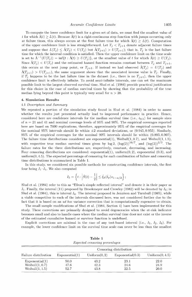
To compute the lower confidence limit for a given set of data, we must find the smallest value of t for which A(t) > L(t). Because A(t) is a right-continuous step function with jumps occurring only at failure times, this always occurs at the first failure time for which A(t) > L(t). Computation of the upper confidence limit is less straightforward. Let Tj < Tj+1 denote adjacent failure times and suppose that L(Tj) < ATj) < U(Tj) but A(Tj+l) > U(Tj+l); that is, Tj is the last failure time for which the interval condition is satisfied. Then the upper confidence limit on the time scale is set to A-l (U(Tj)) = inf{t : A(t) > U(Tj)}, or the smallest value of t for which A(t) > U(Tj). Since A(Tj) < U(T,) and the estimated hazard function remains constant between T3 and Tj+l, this occurs at the next jump point, or Tj+l. If instead we had observed A(T.) = U(T3) and

A(Tj+l) > U(Tj+l), the same argument shows that the associated inverse value is Tj. Finally, if Tj happens to be the last failure time in the dataset (i.e., there is no Tj+?), then the upper confidence limit is effectively infinite. To avoid semi-infinite intervals, one can set the maximum possible limit to the largest observed survival time. Slud et al. (1984) provide practical justification for this choice in the case of median survival times by showing that the probability of the true median lying beyond this point is typically very small for n > 20.

4. Simulation Results 4.1 Description and Summary

We repeated a portion of the simulation study found in Slud et al. (1984) in order to assess whether the r esults just presented actually lead to improved performance in practice. Hence, considered here are confidence intervals for the median survival time (i.e., to.5) for sample sizes of n = 21 and 41 and nominal coverage levels of 95% and 90%. The empirical coverages reported here are based on 7600 replications; therefore, approximately 95% of the empirical coverages for the nominal 95% intervals should lie within ?2 standard deviations, or (0.945,0.955). Similarly, 95% of the empirical coverages for the nominal 90% intervals should lie within (0.893,0.907). The failure time distributions considered are exponential(1), Weibull(1, 0.7), and Weibull(1, 1.5), with respective true median survival times given by log 2, (log(2))10/7, and (log(2))2/3. The failure rates for the three distributions are, respectively, constant, decreasing, and increasing. Four censoring distributions are considered: exponential(1), uniform(0,2), exponential (0.3), and uniform(0, 4.5). The expected percentage of censoring for each combination of failure and censoring time distributions is summarized in Table 1.

In this study, we considered six possible methods for constructing confidence intervals, the first four being 11-14. We also computed

15 {t : S(t) - 2 < ?S(iP)Zl-a/2

Slud et al. (1984) refer to this as "Efron's simple reflected interval" and denote it in their paper as I1. Finally, the interval (11) proposed by Brookmeyer and Crowley (1982) will be denoted by 16; in Slud et al. (1984), this is interval 14. The interval proposed in Jennison and Turnbull (1985), while a viable competitor to each of the intervals discussed here, was not considered further due to the fact that it is based on an ad hoc variance correction that is computationally expensive to obtain.

The small sample modifications of Slud et al. (1984, Section 4) have been implemented for this study. These corrections are primarily designed to avoid degeneracies when the at-risk indicator becomes small and also to handle cases where the median survival time does not exist or the inverse of the estimated cumulative hazard or survivor function is undefined.

Explicit corrections are minimal in the case of any test-based interval (i.e., I1, 12, 16). For example, the lower confidence limit on the survival time scale can never be less than the smallest

Table 1 Expected censoring percentages

Censoring distribution

Failure distribution Exponential(i) Uniform(0, 2) Exponential(0.3) Uniform(0, 4.5)

Exponential(1) 50.0 43.2 23.1 22.0 Weibull(1, 0.7) 47.6 42.3 24.6 24.9 Weibull(1, 1.5) 52.7 43.8 22.5 20.0


observed failure time this is automatic by construction and not forced to occur. The aforementioned convention of setting infinite upper limits to the largest observed survival time has been adopted; computationally, this choice is also effectively automatic. No other small sample corrections were needed for test-based intervals.

For the reflected intervals 13, 14, and 15, similar corrections are used. The minimum allowable lower confidence limit is set to the smallest observed death time; however, unlike test-based intervals, this is not guaranteed to occur. This is because on the cumulative hazard scale, the lower limit of the interval used to construct 13 could be negative, whence the definition of Ak- (x) evaluated at negative x leads to t = 0. Similarly, semi-infinite intervals are not allowed, and so the maximum possible limit has been set to the largest observed survival time. Under heavy censoring, there may be a significant percentage of reflected intervals for which the median survival time cannot be estimated; this is because the probability that the estimated survival curve will not cross 0.5 can be substantial. In such cases, the confidence interval is taken to be (smallest death time, largest observation time). In theory, this is more likely to occur for 13 (which is based on A(t)) than for 15 (which is based on S(t)) since S(t) < exp{ -A(t)} for all t (cf., Fleming and Harrington, 1984); practically speaking, the rates for which this occurs should be about the same and drop quickly as the sample size (censoring percentage) increases (decreases).

Through experimentation, we found that the choice of variance estimator, while unimportant asymptotically, made a substantial difference in practice for the test-based intervals. The variance estimators used by Slud et al. (1984) in all simulations were based on

(t) {Yu)> } dN(u), J0 max{Y(u)(Y(u) - 1), I}

which is a (very) slight modification of the Greenwood-type estimator (12). The denominator modification merely avoids degeneracy in the situation where the maximum observation time is a failure. Among all estimators considered, this variance estimate led to the best results for test-based intervals I1 and 16; in contrast, use of &A(t) resulted in substantially inferior coverage for intervals I1 and 16. The fact that &2 (t) - &A(t) > 0 and that use of the larger variance estimate tends to improves coverage is likely to be at least part of the explanation for this phenomenon. Comparable results were obtained for reflected intervals 13 and 15 using either &2 (t) or &2(t), and results are thus reported for the former. This similarity should not be surprising since the difference between &2 (t) and &2(t) is typically small for t < to 5.

For the intervals 12 and 14, we estimated the variance and correction term exactly as described in Section 2.2; that is, we used &2(t) and k(t) as respectively defined in (2) and (10). These choices consistently led to the most impressive results. Other estimators were also considered; for example, we used &2(t) and also the corresponding modification of (10) and found both intervals to be conservative for smaller sample sizes.

Tables 2-4 summarize the results for n = 21, and Tables 5-7 summarize the results for n = 41. For a given a level, the confidence intervals should have coverage 100(1 - o)%, the percentage of times the lower confidence limit exceeds the true median survival time (miss low) should be (1/2)a, and the percentage of times the upper confidence limit is less than the true median survival time (miss high) should be (1/2)o. We also calculated the average and median interval lengths, the percentage of intervals with the lower confidence limit set equal to the minimum observed failure time, the percentage of intervals with the upper confidence limit set equal to the minimum observed survival time, and the percentage of intervals that were set to (smallest death time, largest observation time). Those results are briefly summarized below as well.

Our simulation results show that the new test-based interval 12 is superior to all others considered in terms of maintaining coverage accuracy, being very close to nominal levels in all cases. In fact, for the 48 empirical coverages we calculated, only 3 were (barely!) outside the 95% Monte Carlo coverage limits given at the beginning of this section. The degree of correction provided by 12 over its unadjusted analog I1 is substantial, both in terms of length and coverage. The intervals 13 and Is are much more conservative, having substantially larger empirical coverage than 12 in almost every case. The intervals 1i, 14, and 16 almost always have less than nominal coverage, often significantly so. None of the intervals considered are particularly impressive with regard to balancing coverage errors appropriately, although 12 consistently does reasonably well for n = 41. All of the test-based intervals (and also 14) have a tendency to under cover on the left and over cover on the right; the opposite appears to be true for the reflected intervals 13 and I15. This is particularly evident under heavy censoring. The interval 12, while not perfect, seems to have most


Table 2 Emrpirical coverage for n = 21, exponenttial(1) failure tirmes

ol Summary I1 12 13 14 15 16

Expected Censoring Percentage: 50% 0.05 Coverage 0.9183 0.9478 0.9661 0.9451 0.9753 0.9158

Miss low 0.0789 0.0447 0.0000 0.0309 0.0016 0.0464 Miss high 0.0028 0.0075 0.0339 0.0239 0.0232 0.0378

0.10 Coverage 0.8821 0.8993 0.9447 0.8722 0.9408 0.8576 Miss low 0.1141 0.0703 0.0012 0.0888 0.0082 0.0775 Miss high 0.0038 0.0304 0.0541 0.0389 0.0511 0.0649

Expected Censoring Percentage: 43.2% 0.05 Coverage 0.9332 0.9580 0.9654 0.9458 0.9716 0.9225









appropriately distributed the total error into the two tails. In contrast, the interval 16 balances coverage quite well in both tails for both sample sizes but is always anticonservative.

Jennison and Turnbull (1985) comment on the often asymmetric distribution of the errors in the two tails for the reflected intervals 13 and 15 and also suggest a modification of the Brookmeyer-Crowley interval 16. This modified version is, through limited reporting of a more extensive simulation study, shown to maintain an excellent balance of coverage error. The proposed modification requires estimating the variance at each time t under the constraint that S(t) = 1/2, which is exactly the null hypothesis used to derive all the test-based confidence intervals considered here. However, calculation of the adjusted variance involves a number of iteratively determined constrained optimizations. We prefer the interval 12 for the simple reasons that (i) it has a solid theoretical basis; (ii) it can be computed using output from standard software packages or, for that matter, on a hand calculator; and (iii) as the above results show, it performs extremely well for all the examples considered, particularly with respect to maintaining overall nominal coverage.

The interval index generally described its rank in terms of overall average length; that is, I1 was typically the longest, 12 was typically next, and so on. Table 8 summarizes the average interval length for intervals 12, 13, and 15. The lengths for 13 (transformed-reflected) and L5 (Efron's simple reflected) are very close to those reported in Table 5 of Slud et al. (1984). Except in the case of very heavy censoring, the length of 12 is comparable to the reflected intervals 13 and 15. For o& = 0.05, a similar pattern was also observed for n = 21, although the discrepancy in length between the three intervals was somewhat more pronounced. The lengths of each of 12, 13, and 15 were very similar for o = 0.10 at both n = 21 and n = 41. Finally, regardless of censoring pattern or level, interval


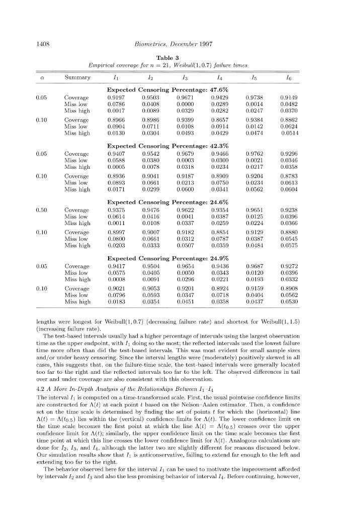
Table 3 Emnpirical coverage for n = 21, Weibull(1, 0.7) failure timnes

ol Summary 1 12 13 14 15 16













lengths were longest for Weibull(1, 0.7) (decreasing failure rate) and shortest for Weibull(1, 1.5) (increasing failure rate).

The test-based intervals usually had a higher percentage of intervals using the largest observation time as the upper endpoint, with I1 doing so the most; the reflected intervals used the lowest failure time more often than did the test-based intervals. This was most evident for small sample sizes and/or under heavy censoring. Since the interval lengths were (moderately) positively skewed in all cases, this suggests that, on the failure-time scale, the test-based intervals were generally located too far to the right and the reflected intervals too far to the left. The observed differences in tail over and under coverage are also consistent with this observation.

4.2 A More In-Depth Analysis of the Relationships Between 'i -14 The interval h1 is computed on a time-transformed scale. First, the usual pointwise confidence limits are constructed for A(t) at each point t based on the Nelson-Aalen estimator. Then, a confidence set on the time scale is determined by finding the set of points t for which the (horizontal) line A(t) A A(t5) lies within the (vertical) confidence limits for A(t). The lower confidence limit on the time scale becomes the first point at which the line A(t) = A(to.5) crosses over the upper confidence limit for A(t); similarly, the upper confidence limit on the time scale becomes the first time point at which this line crosses the lower confidence limit for A(t). Analogous calculations are done for 12, 13, and 14, although the latter two are slightly different for reasons discussed below. Our simulation results show that II is anticonservative, failing to extend far enough to the left and extending too far to the right.

The behavior observed here for the interval I1 can be used to motivate the improvement afforded by intervals 12 and 13 and also the less promising behavior of interval 14. Before continuing, however,

Accutrate Confidence Limits 1409

Table 4 Empirical coverage for n = 21, Weibuli(l, 1.5) failure times

al Suimmary I1 12 13 14 15 16













it is helpful to note that we may rewrite

13 = {t: A(p) C [A(t) + *(p)Zcy/2, At) + *P)Zi-a/2] }.

Also, starting from the definition of 14, we have

14 {t A(ip) C [A(t) + (tp)k(o&/2; pp), A(t) + &(p)k( -( /2; i,)] },

where k(a; t) = zc, + [(1/4)a(t) - (1/3)k(t)]z2 - [(1/4)a(t) + (1/6)k(t)]. These intervals are now written in a form similar to test-based intervals but with some distinct differences. First, the theoretical target A(tp) has been replaced by its sample analog A(tp). Second, unlike the test-based intervals II and 12, the width of the confidence limits (on the cumulative hazard scale) used to compute 13 and 14 does not vary with t; rather, the length is fixed according to the values of &2(ip) and k(tp). Hence, for the o& levels considered, 13 and 14 are essentially computed by constructing a modified 100(1 - 2o)% Gill confidence band (cf., Fleming and Harrington, 1991, Section 6.3) for A(t) when t < Ep, and those limits are then extrapolated forward through time for t > tp. This is not entirely accurate; however, it is a reasonable interpretation and provides justification for why the reflected interval 13 is so conservative. It also helps to explain the rather uneven performance of 14, for viewed as an interval for tp based on a confidence band for the cumulative hazard function, it is clear that the adjustment made to 13 by 14 is ad hoc at best and hence should not be expected to improve upon 13.

Table 9 gives the analog of Table 1 in Slud et al. (1984, Section 5), and provides order statistic numbers for the various confidence intervals in the case of uncensored data. Each of these intervals


Table 5 Empirlical coverage for n = 41, exponenttial(1) failure tirmes

Summary Ij 12 13 14 15 16

Expected Censoring Percentage: 50% 0.05 Coverage 0.9395 0.9497 0.9633 0.9364 0.9671 0.9311












take the form (T( ), T(k)) for j < k, where T(-) is the ith order statistic in a set of n uncensored failure times; the values of j and k are what is given in the table, along with their associated exact binomial coverage probabilities. The nature of the corrections provided by 12, 13, and 14 relative to I1 can be clearly identified from this table. Specifically, note first that 12 is typically shifted to the left of I1, helping to explain why 12 better balances the coverage error in the left and right tails. Also, in general, 12 has equal to or better coverage than I1, although this is not always the case. The interval 13 is typically shifted to the left of 12, which helps to explain why 13 tends to err more in the opposite tail relative to I1 and 12. Interestingly, the interval 14 appears to lie somewhere in between 12 and 13 and, in particular, shows that incorporating the correction term typically affects 13 by moving it back toward 12. This helps to explain the better balance in the coverage error for 14. We also see that 14 is occasionally shorter than 12, perhaps helping to explain its anticonservatism.

We now outline how these corrections are actually made. To understand the nature of the correction provided by 12, the following observation is helpful. Suppose we fix a such that z > 1; then, from (9), it can be easily shown that Asw(&; t) > A(t) - (t)>b (1 - a) whenever

^ _(t) 4 2 _

A check of this condition for cg 0.05 and cg 0.10 for the simulated censored data considered in Tables 2-7 showed that, on average, less than 0.5% of the observation times failed to satisfy this condition. See Strawderman and Wells (1997, Proposition 1) for additional results along these lines.


Table 6 Emrpirical coverage for n = 41, Weibull(1, 0.7) failure timnes

ol Summary I1 12 13 14 15 16













The fact that Asw(o; t) nearly always exceeds A(t) - 6(t)- (1 - &) implies that, on the cumulative hazard scale, the confidence limits are no longer symmetric about A(t) but rather skewed and shifted in the positive (vertical) direction. In turn, this results in a shift of the lower and upper confidence limits for to05 (i.e., on the time scale) to the left. In addition, since the confidence limits on the cumulative hazard scale tend to fan outward as t gets larger, moving the confidence limits on the cumulative hazard scale upward shortens the right tail of the interval while lengthening the left tail. This leftward shift improves the balance of these errors on either side of the true median survival time.

The behavior of 13 relative to I1 can be similarly motivated. We see from the test-based representation of L3 given earlier in this section that the interval width on the cumulative hazard scale is fixed at 23(to.5)zl ,/2. Since 6(t) is an increasing function of t, this implies that on the cumulative hazard scale the interval being used is more conservative than the pointwise limit used for computing I1 when t < to.5; similarly, it is too narrow when t > t0o5. Relative to I1, this implies that, on the failure time scale, 13 extends much farther to the left but not nearly as far to the right. This helps to explain why 13 over covers on the left and under covers on the right, the behavior being consistent with observations made in Section 3.2. In addition, the fact that I1 over covers on the right suggests that use of a conservative endpoint on the left will have a bigger impact on coverage thlan will the use of an anticonservative endpoint on the right.

Finally, comparing 14 to 13, the analogous test-based form of 14 and the nature of the correction for 12 discussed above together imply that on the cumulative hazard scale the limits used in computing 14 are shifted downward relative to those used to compute 13. This adjustment counter-


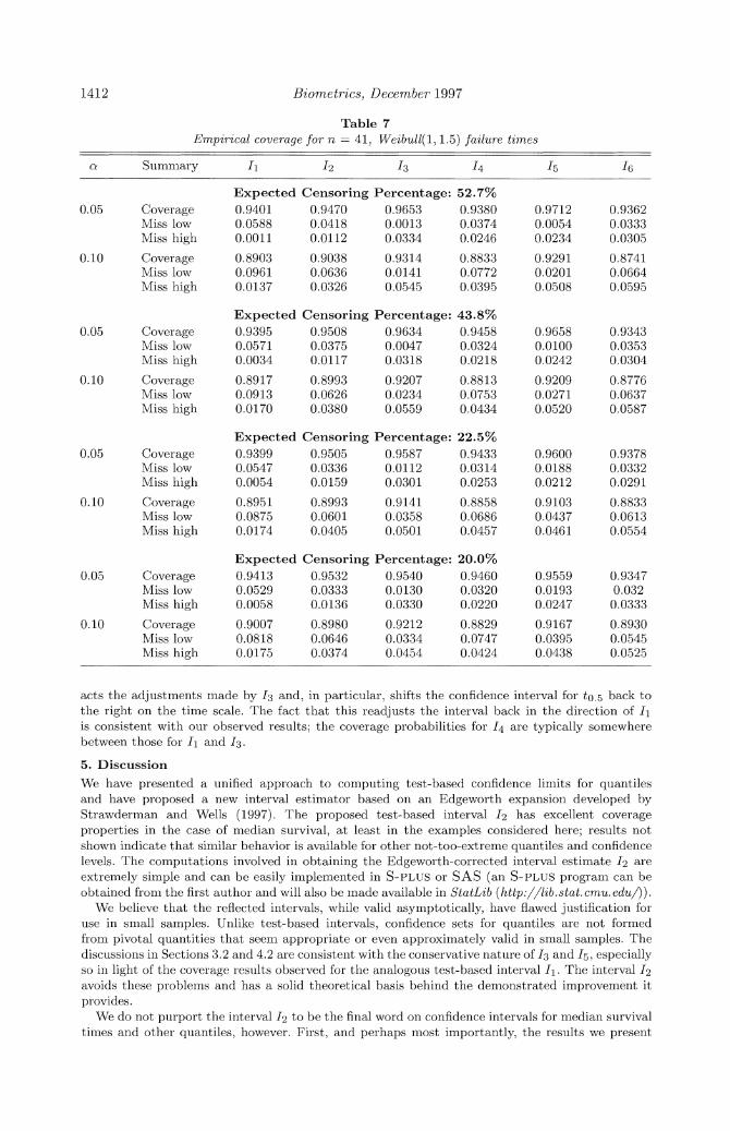
Table 7 Emrpirical coverage for n = 41, Weibull(1, 1.5) failure tines

ag Summary I1 12 13 14 15 16













acts the adjustments made by 13 and, in particular, shifts the confidence interval for to.5 back to the right on the time scale. The fact that this readjusts the interval back in the direction of I1 is consistent with our observed results; the coverage probabilities for 14 are typically somewhere between those for I1 and 13.

5. Discussion We have presented a unified approach to computing test-based confidence limits for quantiles and have proposed a new interval estimator based on an Edgeworth expansion developed by Strawderman and Wells (1997). The proposed test-based interval 12 has excellent coverage properties in the case of median survival, at least in the examples considered here; results not shown indicate that similar behavior is available for other not-too-extreme quantiles and confidence levels. The computations involved in obtaining the Edgeworth-corrected interval estimate 12 aie extremely simple and can be easily implemented in S-PLUS or SAS (an S-PLUS program can be obtained from the first author and will also be made available in StatLib (http:lllib.stat.cmu.edu/)).

We believe that the reflected intervals, while valid asymptotically, have flawed justification for use in small samples. Unlike test-based intervals, confidence sets for quantiles are not formed from pivotal quantities that seem appropriate or even approximately valid in small samples. The discussions in Sections 3.2 and 4.2 are consistent with the conservative nature of 13 and I5, especially so in light of the coverage results observed for the analogous test-based interval 1. The interval T2 avoids these problemus and has a solid theoretical basis behind the demonstrated improvement it provides.

We do not purport the interval '2 to be the final word on confidence intervals for median survival timnes and other quantiles, however. First, and perhaps most importantly, the results we present


Table 8 Empirical average lengths for 12, 13, and 15 confidence level = 0.95, n = 41

Lifetimne Censoring distribution Interval distribution Exponential(1) Uniform(0, 2) Exponential(0.3) Uniform(0, 4.5)

12 Weibull(1,0.7) 1.4112 1.0457 0.9759 0.9568 Exponential(1) 1.1125 0.8712 0.7486 0.7355 Weibull(1, 1.5) 0.8180 0.6529 0.5441 0.5352

13 Weibull(1,0.7) 1.2012 0.9633 0.8807 0.8650 Exponential(1) 0.9767 0.8098 0.7008 0.6951 Weibull(1, 1.5) 0.7501 0.6213 0.5326 0.5260

15 Weibull(1, 0.7) 1.2073 0.9730 0.8986 0.8811 Exponential(i) 0.9710 0.8090 0.7077 0.7004 Weibull(1, 1.5) 0.7422 0.6132 0.5292 0.5246

Table 9 Order statistic numbers and exact binomial coverage

probabilities for all confidence intervals (uncensored data case)

N '1 12 13 14 I5 16

a = 0.05

21 7, 18, 0.960 7, 16, 0.948 6, 15, 0.948 7, 16, 0.948 6, 16, 0.973 7, 15, 0.922 22 8, 18, 0.931 7, 17, 0.965 6, 15, 0.925 7, 16, 0.948 7, 16, 0.948 7, 16, 0.948 41 16, 29, 0.936 15, 28, 0.956 14, 27, 0.956 15, 27, 0.940 15, 27, 0.940 15, 27, 0.940 42 16, 29, 0.946 16, 29, 0.946 14, 27, 0.946 15, 28, 0.956 15, 28, 0.956 15, 28, 0.956

a = 0.10

21 8, 16, 0.892 8, 15, 0.866 7, 15, 0.922 8, 15, 0.866 7, 15, 0.922 7, 15, 0.922 22 8, 17, 0.925 8, 16, 0.907 7, 15, 0.907 8, 15, 0.866 8, 15, 0.866 8, 15, 0.866 41 17, 27, 0.865 16, 27, 0.912 15, 26, 0.912 16, 27, 0.912 16, 26, 0.883 16, 26, 0.883 42 17, 28, 0.896 16, 27, 0.912 15, 26, 0.896 16, 27, 0.912 16, 27, 0.912 16, 27, 0.912

here depend rather heavily on the fact that the failure time distribution is absolutely continuous. The first-order methods are valid under more general conditions; more specifically, the existence of the failure time density in a neighborhood about the true quantile of interest is really all that is needed to ensure their validity. This is not to say that our results cannot be extended, only that the tools used to establish the expansions summarized in Section 2.2 depend on the assumption of absolute continuity. For example, the results of Mykland (1992, 1993, 1995) can be used to produce expansions such as (4) under weaker conditions; the stated convergence properties are, of course, commensurately weaker as well. Second, the lack of balance in coverage error exhibited by '2 for small sample sizes is a source of some (perhaps minor) concern. This behavior may possibly be imnproved through the use of variance-stabilizing transformations, such as those considered in Bie, Borgan, and Liest0l (1987). Of course, rather than considering variance stabilizing transformations, one could instead seek transformations that attempt to strike a balance between correcting for skewness and stabilizing the variance. This is the main idea underlying the BCa interval of Efron (1987); analytical approximations to this transformation are also possible (e.g., Konishi, 1991). A third possibility is to use smoothing. It would be worthwhile to explore these various ideas further, keeping in mind that, in the absence of readily available software, computational simplicity is a real virtue for practitioners. Finally, although the specific test-based interval proposed in Jennison and Turnbull (1985, Section 2) constitutes an ad hoc adjustment to the Brookmeyer-Crowley interval, its reportedly good behavior and connections to computing likelihood ratio-based confidence intervals for survival probabilities (cf., Thomas and Grunkmeier, 1975) strongly suggest that it would be worth studying its likelihood ratio-based cousin in considerably more detail. However, the relevant theory is at this time largely undeveloped; some very important first steps in this particular area can be found in Murphy (1995) and also Hollander, McKeague, and Yang (1997).


ACKNOWLEDGEMENTS

The authors would like to thank the associate editor and two referees for their detailed comments. The support of NIH grants RO1-DK49529 and RO1-CA61120 and NSF grant DMS 9625440 is also gratefully acknowledged.

RESUME

Dans les analyses de survie, les estimateurs de la mediane des temps de survie dans les echantillons homogenes sont souvent bases sur l'estimateur de Kaplan-Meier de la fonction de survie. Des intervalles de confiance pour les quantiles, comme la mediane de survie, sont generalement construits a partir de la theorie des grands echantillons ou du bootstrap. La premiere methode mene a une precision suspecte pour de petites tailles d'echantillons avec une censure moderee, la deuxieme exige des calculs tres lourds. Dans ce papier, des amn6liorations sont recherchees pour les "tests- fondes-sur-les-intrevalles" et pour les intrevalles refletes (cf. Slud, Byar et Green, 1984, Biometrics 40, 587-600). En utilisant le developpement d'Edgeworth pour la distribution de l'estimateur studentise de Nelson-Aalen obtenu par Strawderman et Wells (1997, Journal of the American Statistical Association 92), nous proposons une methode conduisant a des intervalles de confiance plus precis pour les quantiles avec des donnees censures au hasard. Les intrevalles sont tres simples a calculer et des resultats numeriques sur donnees simulees montrent que notre nouvel intrevalle fonde sur le test surpasse les methodes couramment utilisees pour calculer des intervalles de confiance dans le cas de petits echantillons et/ou de censure lourde, specialement pour maintenir une precision de recouvrement specifiee.

REFERENCES

Andersen, P. K., Borgan, O., Gill, R., and Keiding, N. (1993). Statistical Models Based on Counting Processes. New York: Springer-Verlag.

Bie, O., Borgan, 0., and Liest0l, K. (1987). Confidence intervals and confidence bands for the cumulative hazard rate function and their small sample properties. Scandinavian Journal of Statistics 14, 221-233.

Brookmeyer, R. and Crowley, J. (1982). A confidence interval for the median survival time. Biometrics 38, 29-41.

Chen, K. and Lo, S. H. (1996). On bootstrap accuracy with censored data. Annals of Statistics 24, 569-595.

Chen, Y., Hollander, M., and Langberg, M. A. (1982). Small sample results for the Kaplan-Meier estimator. Journal of the American Statistical Association 77, 141-144.

DiCiccio, T. and Efron, B. (1996). Bootstrap confidence intervals (with discussion). Statistical Science 11, 189-228.

Efron, B. (1981). Censored data and the bootstrap. Journal of the American Statistical Association 76, 312-319.

Efron, B. (1987). Better bootstrap confidence intervals. Journal of the American Statistical Association 82, 171-200.

Emerson, J. (1982). Nonparametric confidence intervals for the median in the presence of right censoring. Biometrics 38, 17-27.

Fleming, T. R. and Harrington, D. P. (1984). Nonparametric estimation of the survival distribution in censored data. Commuanications in Statistics Theory and Methods 13, 2469-2486.

Fleming, T. R. and Harrington, D. P. (1991). Counting Processes and Survival Analysis. New York: John Wiley and Sons.

Hall, P. (1988). Theoretical comparison of bootstrap confidence intervals. Annals of Statistics 16, 927-953.

Hollander, M., McKeague, I., and Yang, J. (1997). Likelihood ratio-based confidence bands for survival functions. Joarnal of the American Statistical Association 92, 215-226.

Jennison, C. and Turnbull, B. W. (1985). Repeated confidence intervals for the median survival time. Biometrika 72, 619-625.

Klein, J. P. (1991). Small sample moments of some estimators of the variance of the Kaplan-Meier and Nelson-Aalen estimators. Scandinavian Joarnal of Statistics 18, 333-340.

Klein, J. P. and Moeschberger, M. (1997). Survival analysis: Techniques for censored and truncated data. New York: Springer-Verlag.

Kolassa, J. and McCullagh, P. (1990). Edgeworth series for lattice distributions. Annals of Statistics 18, 981-985.


Konishi, S. (1991). Normalizing transformations and bootstrap confidence intervals. Annals of Statistics 19, 2209-2225.

Lai, T. L. and Wang, J. Q. (1993). Edgeworth expansions for symmetric statistics with applications to bootstrap methods. Statistica Sinica 3, 517-542.

Murphy, S. A. (1995). Likelihood ratio-based confidence intervals in survival analysis. Journal of the American Statistical Association 90, 1399-1405.

Mykland, P. (1992). Asymptotic expansions and bootstrapping distributions for dependent variables: A martingale approach. Annals of Statistics 20, 623-654.

Mykland, P. (1993). Asymptotic expansions for martingales. Annals of Probability 21, 800-818. Mykland, P. (1995). Martingale expansions and second-order inference. Annals of Statistics 23,

707-731. Pefia, E. and Rohatgi, V. (1993). Small sample and efficiency results for the Nelson-Aalen estim'ator.

Journal of Statistical Planning and Inference 37, 193-202. Reid, N. (1981). Estimating the median survival time. Biometrika 68, 601-608. Simon, R. and Lee, Y. J. (1982). Nonparametric confidence limits for survival probabilities and

median survival time. Cancer Treatment Technical Reports 66, 37-42. Slud, E. V., Byar, D. P., and Green, S. B. (1984). A comparison of reflected versus test-based

confidence intervals for the median survival time based on censored data. Biometrics 40, 587-600.

Strawderman, R. L. and Wells, M. T. (1997). Accurate bootstrap confidence limits for the cumulative hazard and survivor functions under random censoring. Journal of the American Statistical Association 92.

Thomas, D. R. and Grunkmeier, G. L. (1975). Confidence interval estimation of survival probabilities for censored data. Journal of the American Statistical Association 70, 865-871.

Received June 1996; revised April 1997; accepted May 1997.

Accurate Confidence Limits for Quantiles under Random ...mparzen/published/parzen8.pdf · Accurate...

Documents

Transcript of Accurate Confidence Limits for Quantiles under Random ...mparzen/published/parzen8.pdf · Accurate...