Accuracy analysis and Calibration of

Total Station based on the

Reflectorless Distance Measurement

Amezene Reda & Bekele Bedada

Master of Science Thesis in Geodesy

TRITA-GIT EX 12-009

School of Architecture and the Built Environment

Royal Institute of Technology (KTH)

Stockholm, Sweden

December 2012

ii

Abstract

Reflectorless EDM technology uses phase measuring or pulsed lasers to measure targets of a

reflective and non-reflective nature. Reflectorless distance measurement provides rapid

measurement by saving time and labour for surveyors. However, the accuracy of these types

of measurements is under question because of the variety of constraints that affect the

measurement.

This paper attempts to show the techniques of total station calibration and to investigate

the possible sources of error in reflectorless distance measurement. As a result, the effects

of different color targets and angle incidence on distance measurement were checked. The

precision of reflectorless distance measurement also investigated. In addition, comparison

was made for manual and automatic target recognition measurement. Further experiment

was performed on how to calibrate the total station instrument and the performance of the

instrument was checked by KTH-TSC software.

The experiments were evaluated by taking the reflector reading as ‘true value’ to check the

accuracy of reflectorless measurement. The effects of colour surfaces on distance

measurement have no significant difference. Besides, the result shows that the error in

distance increased as the angle of incidence in the target increases. The result also indicates

that automatic target recognition mode is the most advisable technique for precise

measurement. Finally, an optimal number of seven target points was found for the

calculation of prism constant.

Keywords: automatic target recognition, calibration, prism constant, reflectorless

measurement

iii

Sammandrag

Reflektorlös EDM-tekniken använder fas mätning eller pulsade lasrar för att mäta mål en

reflekterande och icke-reflekterande karaktär. Reflektorlös avståndsmätning ger snabb

mätning genom att spara tid och arbete för inspektörer. Emellertid är noggrannheten hos

dessa typer av mätningar under fråga på grund av olika begränsningar som påverkar

mätningen.

Denna uppsats försöker visa de metoder för totalstation kalibrering och att undersöka

eventuella felkällor i reflektorlös avståndsmätning. Som ett resultat var effekterna av olika

färger mål och vinkel inverkan på avståndsmätning kontrolleras. Noggrannheten i

reflektorlös avståndsmätning undersökt också. Dessutom gjordes jämförelse för manuell och

automatisk måligenkännande mätning. Ytterligare experiment utfördes på hur man

kalibrerar totalstationen instrumentet och prestanda instrumentet kontrollerades av KTH-

TSC programvara.

Experimenten utvärderades genom att reflektorn läsning som "sanna värdet" för att

kontrollera riktigheten i reflektorlös mätning. Effekterna av färgytor på avståndsmätning har

ingen signifikant skillnad. Dessutom visar resultatet felet i avståndet ökade infallsvinkeln i

målet ökar. Resultatet visar också automatiskt måligenkännande läget är det mest lämpligt

tekniken för exakt mätning. Slutligen ett optimalt antal av sju målpunkter hittades för

beräkning av prismakonstanten.

Nyckelord: automatisk mål erkännande, kalibrering, prismakonstant, reflektorlös mätning

iv

Acknowledgement

We would like to express our gratitude to our advisor, Dr. Milan Horemuz, for his support,

patience, and encouragement throughout our work and studies. It is not often that one finds

an advisor that always finds the time for listening us to solve our problem both on field and

in laboratory works. His technical and editorial advice was essential to the completion of this

thesis. His understanding, encouraging and personal guidance have provided us a good basis

for the present and future knowledge.

We would deeply thankful to Mr. Erick Asenjo for his valuable advice and friendly help

detailed and constructive remarks and for his important support throughout this work. We

also appreciated and have lead to many interesting and good spirited discussions relating to

this thesis.

We would also deeply grateful to our examiner, Professor Lars E Sjöberg for his detailed and

constructive comments.

Last but not the least; we would like to thank our friends Mr Andenet Ashagrie, Mr. Shahjalal

Hossaina, Mr. Amin Alizadeh for their valuable comment on our document. We wish to

extend our warmest thanks to all those who have helped us in our work. Also we would like

to thank our friend from the department of Geodesy Mr. Fentaw Degie for his help in

handling of the instrument in the field.

Amezene and Bekele

October 2012

v

Table of Content

Abstract ...................................................................................................................................... ii

Acknowledgement ..................................................................................................................... iv

List of Figure ........................................................................................................................... viii

List of Table ............................................................................................................................... x

List of Abbreviations ................................................................................................................. xi

Chapter One ................................................................................................................................ 1

1 Introduction ......................................................................................................................... 1

Chapter Two ............................................................................................................................... 3

2 Total Station ........................................................................................................................ 3

Chapter Three ............................................................................................................................. 5

3 Distance Measurement ........................................................................................................ 5

3.1 Introduction ................................................................................................................. 5

3.2 Phase measurement ...................................................................................................... 6

3.3 Time of flight (TOF) or pulse laser distance measurement ......................................... 8

3.4 Reflector vs. Reflectorless ......................................................................................... 10

3.5 Error source in Reflectorless Measurements ............................................................. 10

3.6 Incidence angle measurement .................................................................................... 12

3.7 Error source in distance measurement when measuring not perpendicular to the

target 13

Chapter Four ............................................................................................................................. 14

4 Angle measurement .......................................................................................................... 14

4.1 Principle of angle measurement ................................................................................ 14

vi

4.2 Automatic target recognition ..................................................................................... 14

4.3 Source of errors in angular measurement .................................................................. 16

4.3.1 Horizontal collimation (or line of sight) error .................................................... 16

4.3.2 Vertical Collimation (of vertical index) Error .................................................... 16

4.3.3 Tilting axis error ................................................................................................. 17

4.3.4 Compensator index error .................................................................................... 17

4.3.5 The vertical axis error v ..................................................................................... 18

Chapter Five ............................................................................................................................. 19

5 Checking and Calibrating Total Station ............................................................................ 19

5.1 Overview of Calibration of Total Station .................................................................. 19

5.2 Built in calibration programs ..................................................................................... 22

5.3 KTH-TSC .................................................................................................................. 24

5.4 Offset of the instrument and prism ............................................................................ 26

5.5 Calculating the prism offset for use in a Leica total station for a non-leica prism .... 28

5.6 Calculating the prism offset for use in a Trimble total station for a non-Trimble

prism 29

5.7 EDM Errors ............................................................................................................... 30

Chapter Six ............................................................................................................................... 32

6 Methodology of the Thesis ............................................................................................... 32

6.1 Measurements in Different Surface Objects .............................................................. 32

6.2 Reflectorless reading ................................................................................................. 33

6.3 Different incidence Angle Measurement ................................................................... 34

6.4 Manual Method and Automatic Target Recognition Method ................................... 35

6.5 KTH TSC ................................................................................................................... 36

6.6 Prism or additive constant ......................................................................................... 37

vii

Chapter Seven .......................................................................................................................... 39

7 Results of the Study .......................................................................................................... 39

7.1 Results of the Reflectorless Measurement ................................................................. 39

7.2 Results of angle of incidence measurement .............................................................. 45

7.3 The effect of reflectorless measurements in different colours .................................. 47

7.4 Results of automatic target recognition measurement (ATR) ................................... 51

7.5 KTH-TSC .................................................................................................................. 52

7.6 Prism or additive constant calculation ....................................................................... 52

Chapter Eight ............................................................................................................................ 54

8 Conclusions and Recommendations ................................................................................. 54

8.1 Conclusions ............................................................................................................... 54

8.2 Recommendations ..................................................................................................... 54

9 References ......................................................................................................................... 55

viii

List of Figure

Figure 2-1 Leica and Trimble total station ................................................................................. 4

Figure 3-1 Phase shift ................................................................................................................. 7

Figure 3-2 Measurement wave from an EDM. .......................................................................... 7

Figure 3-3 Measurement process in electro optical EDM. ......................................................... 8

Figure 3-4 Principle of pulse distance meter (Source: Schofield and Breach, 2007) .............. 10

Figure 3-5 Laser beam divergence in long distance. ................................................................ 11

Figure 3-6 Leica Circular Prism ............................................................................................... 12

Figure 3-7 Incidence angle (source Wikipedia) ....................................................................... 13

Figure 4-1 Automatic Fine pointing ......................................................................................... 15

Figure 4-2 Horizontal collimation error ................................................................................... 16

Figure 4-3 Vertical collimation error ....................................................................................... 16

Figure 4-4 Tilting axis error ..................................................................................................... 17

Figure 4-5 Compensator index error ........................................................................................ 18

Figure 5-1 Principal axes of total station. ................................................................................ 20

Figure 5-2 Procedure for additive constant calculation............................................................ 21

Figure 5-3 Spatial Free Station position ................................................................................... 25

Figure 5-4 Structure of prism and offset of EDM instrument. ................................................. 26

Figure 5-5 EDM errors. ............................................................................................................ 30

Figure 6-1 Special holders of the colour targets....................................................................... 32

Figure 6-2 Colour target used for surface reflectivity .............................................................. 32

Figure 6-3 GPR 1 Reflector and target designed for non-reflector observation ...................... 33

ix

Figure 6-4 Field observation on reflectorless experiment ........................................................ 34

Figure 6-5 Field procedure for fixing of target point. .............................................................. 35

Figure 6-6 Distance measurement at different incidence angle ............................................... 35

Figure 6-7 Angle of incidence trial experiments. ..................................................................... 35

Figure 6-8 Field procedure for ATR and manual observation. ................................................ 36

Figure 6-9 Steps of Calculating Additive/Prism Constant ....................................................... 38

Figure 7-1 Difference in reflector and reflectorless distance measurement using total station

TPS 1201+ ................................................................................................................................ 40

Figure 7-2 Difference in reflector and reflectorless distance measurement using total station

Trimble S8 ................................................................................................................................ 41

Figure 7-3 Distance measurement on 12 meter and 61 meter from different angle of incidence

by Leica total station. ............................................................................................................... 46

Figure 7-4 Distance measurement from 13 meter and 63 meter different angle of incidence by

Trimble S8 total station ............................................................................................................ 47

Figure 7-5 The difference between reflectorless colour surface and reflector reading using

Leica 1201+ total station. ......................................................................................................... 49

Figure 7-6 The difference between reflectorless colour surface and reflector reading using

Trimble S8 total station ............................................................................................................ 51

x

List of Table

Table 2-1 The specification of Leica 1201+ total station on distance measurement ................ 4

Table 2-2 The specification of Trimble S8 total station on distance measurement ................... 4

Table 4-1 Angular specification for Trimble and Leica total station. ...................................... 14

Table 7-1 The difference between reflector and reflectorless distance measurement by using

Leica total station ..................................................................................................................... 39

Table 7-2 The difference between reflector and reflectorless distance measurement by using

Trimble total station S8 ............................................................................................................ 40

Table 7-3 Misclosures (ei) in distance measurement by Leica total station. ............................ 42

Table 7-4 Misclosures (ei) in distance measurement by Trimble total station. ........................ 42

Table 7-5 Reliability of reflectorless distance measurement using Trimble total station ........ 43

Table 7-6 Reliability of reflectorless distance measurement using Leica total station ............ 44

Table 7-7 Distance measurement from different angle of incidence by Leica total station .... 45

Table 7-8 Distance measurement from different angle of incidence by Trimble total station . 46

Table 7-9 Reflectorless reading at different colour surface for Leica Total Station ................ 48

Table 7-10 Reflectorless reading at different colour surface for Trimble Total Station .......... 49

Table 7-11 Standard deviation of horizontal and vertical angle measurement by ATR and

manual method using Trimble S8 total station ......................................................................... 51

Table 7-12 Standard deviation of horizontal and vertical angle measurement by ATR and

manual method using Leica total station .................................................................................. 52

Table 7-13 Standard deviation of measuring elements of variance-components-estimation for

spatial free station positioning .................................................................................................. 52

Table 7-14 Result of prism or additive constant using Leica total station ............................... 53

Table 7-16 Result of prism or additive constant using Trimble total station ........................... 53

xi

List of Abbreviations

EDM Electronic distance measurement

TOF Time of flight

ATR Automatic target recognition

Sr Horizontal direction

Sz Zenith distance

Ss Slope distance

KTH Royal Institute of Technology

TSC Total Station Check

RL Reflectorless

ICc Instrument correction

Laser Light Amplification by Stimulated Emission of Radiation

SD Standard deviation

ei Misclosures

p passed

N.p not passed

M.a.v maximum absolute value

n number of observation

1

Chapter One

1 Introduction

Total station has been widely applied in engineering and industrial surveying systems to

measure distances and angles automatically. (Zhiguo Xia et al, 2006). Its function, automatic

tracking survey, is very useful especially in the field of dynamic surveying. On the small scale

and a local coordinate system, the surveying technology by the total station is more superior

to others concerning surveying precision and flexibility.

To obtain accurate and reliable results, it is necessary to check and adjust the instrument

regularly. A check of an EDM instrument is a process to establish whether or not an

instrument is functioning properly and whether any large changes in the instrument

correction (ICs) have been detected. (Staiger, 2007) Checks are normally made daily, or

weekly, are simpler than calibrations, and can be carried out on-site, in the field, or on a

local test field.

Precise digital levels and reflectorless total stations are used nowadays for several

applications in geodetic engineering due to their highly accurate and fast measurements in

an automated measuring process. The effect of inclined angle of reflecting surface, its

colours and types on the accuracy of reflectorless total station measurements was

previously investigated (Beshr and Elnaga, 2011). Their result shows the accuracy of

measured slope distance for the white surface is higher than the accuracy of any other

surface colour; hence this surface has the strongest reflectivity for reflectorless total station

ray as compared with any other surface. The surface of the black target has a very low-

reflectivity, so it absorbs more energy (Beshr and Elnaga, 2011). The results also show that

increasing the inclination angle of reflecting surface leads to increase the errors of slope

distance measured by the reflectorless total station.

This thesis attempts to show the techniques of total station calibration and to investigate

the possible sources of error in reflectorless distance measurement. The effects of different

2

colour targets and angle incidence on distance measurement were checked. The accuracy of

reflectorless distance also investigated. In addition, comparison was made for manual and

automatic target recognition measurement. Further experiment was performed how to

calibrate the total station instrument.

The objectives of this project are:

Measuring at colour targets to check the effect of different colour surfaces in

distances measurement using reflectorless technology.

Investigate the accuracy of reflectorless measurement over short and long

distances.

Measurement at targets of varying angle of incidence to see the difference in the

measurements with respect to a perpendicular target.

Identify optimal number of target points needed for the estimation of prism

constant.

Test the performance of total station by using free station method from a number

of stations and targets; apply variance covariance components estimation to

determine the accuracy of the total station.

Test angular accuracy of total station for automatic target recognition method.

The basic field operation performed by a surveyor involves distance and angular

measurements. Different types of engineering works require various tolerances in the

precision of the measurements made and the accuracy achieved by these measurements.

Therefore, the primary goal was checking or calibrating the total station instrument by using

different measurement techniques.

3

Chapter Two

2 Total Station

Today a total station is a usual measurement instrument in the surveying field and the

application of laser (Light Amplification by Stimulated Emission of Radiation) technology to

surveying engineering. Modern total stations have ability to measure inaccesible or hard to

reach targets more than 1 km without reflector with accuracy of 3 mm. There are many

applications of automatic or robotic Total Stations such as a stakeout of points, deformation

monitoring, cadastral surveys, tunnelling, volume calculations and construction. Structure

deformation can be measured via reflectroless total station insrument.

Verification of EDM equipment is concerned with the determination of instrument errors

which can then be used to monitor the performance of the instrument. A 'reflectorless' EDM

instrument is an electronic tacheometer (‘total station’) that has the ability to measure as an

electronic distance meter (strictly to reflective targets) and as a reflector less distance meter.

The question occurs then, of the accuracy of such technology should be assessed or

investigated. How then, can we rely upon such measurements, especially when high

accuracy results are essential, and even simple checks like using a tape measure between

two distinct points is impossible. Since the signal may reflect upon any surface present in the

line between the instrument and the target, blunders may easily occur. For example, the

signal may be reflected by a leaf present in the line of sight. Users should be aware of these

types of side effects by understanding the physics of the system well.

The main advantage of such reflectorless total station instruments is the ability to measure

inaccessible points and allows us to collect data faster and mark‐up points in the field with

increasing speed and accuracy. There could be any number of reasons that points are

inaccessible, including safety concerns, such as forgoing the need to enter unsupported

ground in underground mine surveying, detail surveys of busy road intersections where

traffic control is undesirable or impossible.

4

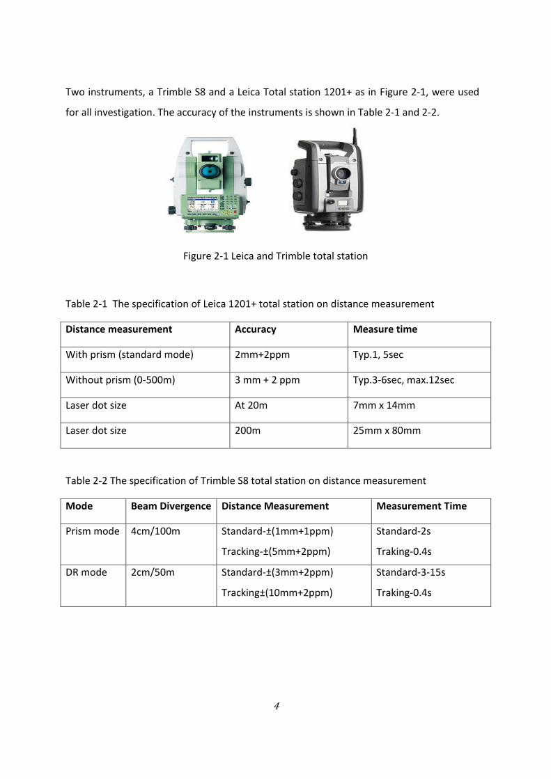
Two instruments, a Trimble S8 and a Leica Total station 1201+ as in Figure 2-1, were used

for all investigation. The accuracy of the instruments is shown in Table 2-1 and 2-2.

Figure 2-1 Leica and Trimble total station

Table 2-1 The specification of Leica 1201+ total station on distance measurement

Distance measurement Accuracy Measure time

With prism (standard mode) 2mm+2ppm Typ.1, 5sec

Without prism (0-500m) 3 mm + 2 ppm Typ.3-6sec, max.12sec

Laser dot size At 20m 7mm x 14mm

Laser dot size 200m 25mm x 80mm

Table 2-2 The specification of Trimble S8 total station on distance measurement

Mode Beam Divergence Distance Measurement Measurement Time

Prism mode 4cm/100m Standard-±(1mm+1ppm)

Tracking-±(5mm+2ppm)

Standard-2s

Traking-0.4s

DR mode 2cm/50m Standard-±(3mm+2ppm)

Tracking±(10mm+2ppm)

Standard-3-15s

Traking-0.4s

5

Chapter Three

3 Distance Measurement

3.1 Introduction

For over two millennia, surveyors have used taping for measurement of distance. Probably

the first use of electronics for distance measurement was the fathometer. That device,

invented in 1919 by Reginald Fessenden, measures the distance from a vessel to the ocean

floor by observing the time for a sound wave to be reflected and returned.

The earliest electronic devices for distance measurement on land were first developed in

Sweden in the early 1950s1. Typical of these was the Geodimetre. That device transmitted a

modulated light beam to reflect off a mirror at the end of the line being measured and then

made phase comparisons between the transmitted and reflected pulses.

Most of the modern EDM devices are electro-optical, and use a laser or infrared light source.

Most EDM devices manufactured today are incorporated into total stations to provide ability

for angular as well as distance measurement in the same instrument. Some of the

developments in EDM technology are “reflectorless” units that measure distance to objects

without using retro-prisms with typical ranges of 1000 meter.

The EDM technology currently available in the market can be classified as being based on

either a time-of-flight (TOF) or a phase shift measurement. (for detail description about

these techniques refer section 3.2 and 3.3) In Leica TPS 1200+ Total Station, the reflected

laser after entering the telescope is directed by appropriate optics to a receiver that analyses

the data according to the types of the target. Leica Geosystems uses a phase shift method

for reflector target. It also uses a unique System Analyser that provides an accuracy of 2 mm

+ 2 ppm to distances of 500 m in reflectorless measurement. The System Analyzer combines

the advantages of the phase and TOF measurements without having to deal with their

disadvantages; this is because it is neither a pure TOF meter nor a pure phase shift meter.

This technology will permit accurate reflectorless measurements (Bayoud, 2006). But

1 www.faculty.evc.edu/z.yu/nsf2/Curriculum%20modules/Module%201.pdf.

6

Trimble S8 Total Stations uses Time-of-flight method for the reflectorless measurement

(Höglund and Large, 2005).

3.2 Phase measurement

Phase shift is typically measured in degrees where a complete cycle is 360 degrees. This is

the difference between the phasing of the emitted and the received signal. When two

waves reach exactly the same phase angle at exactly the same time, they are said to be in

phase, consistent or phase locked. However, when two waves reach the same phase angle at

different times, they are out of phase or phase shifted. EDM compares the phase angle of

the returning signal to that of a replica of the transmitted signal to determine the phase

shift. In the Figure 3-1, the second wave is shifted by the specified amount from the original

wave.

Because the horizontal axis on the Figure 3-2 denotes time, a phase shift represents a shift in

time from the original wave. The signal in a circuit, for example will have some phase shift

between the input and the output. When designing an operational amplifier, for example

engineer prefers to minimize the phase shift as much as possible to avoid unwanted

oscillations.

The phase shift method is considered to be the most accurate one; it allows a very narrow

beam, but its measuring range is limited. The pulse method has much wider range but has

the disadvantage of poor performance on short ranges. This is due to the limitation of the

built-in clock and the width of the spot size. Normally, instruments that use the phase-shift

principle, the measurement has to be done several times to solve the ambiguity. The time

per point is longer than for the TOF-principle. Thus, for long distances and fast

measurements the TOF method has more advantages. For short distances, the phase-shift-

principle is better, but not so fast when related with TOF.

7

Figure 3-1 Phase shift

Figure 3-2 Measurement wave from an EDM.

The measurement wave shown in the dashed line on Figure 3-2 has returned to the EDM

from a reflector. Compared with the transmitted wave shown in the solid line, it is out of

phase by one quarter of a wavelength.

The light beam is modulated, or split into wavelengths of a certain frequency. Measurement

of distance is accomplished as on the Figure 3-3 by setting up the transmitter of the signal at

one end of the line to be measured and a reflector at the other end. The reflected light is

converted to an electrical signal by the EDM to allow phase comparison between the

transmitted and reflected signals. The phase difference is then used determine the length of

the line which would be equivalent to one-half of the sum of the number of wavelengths in

the double path distance plus the partial wavelength represented by the phase difference.

8

The integral number of wave lengths included in the double path is determined by

transmitting pulses on multiple frequencies and comparing the results. The phase difference

is then used determine the length of the line which would be equivalent to one-half of the

sum of the number of wavelengths (λ) in the double path distance(d) plus the partial

wavelength represented by the phase difference. This determination is represented by the

equation

D =½ (nλ + d ) (3.1)

where

D is the distance between the instrument and prism

λ is the wavelength of the modulated beam

n is the integral number of wavelengths in the double path of the light

d is the distance representing the phase difference.

Figure 3-3 Measurement process in electro optical EDM.

3.3 Time of flight (TOF) or pulse laser distance measurement

Time of Flight (TOF) in this type of measurement the radiation is transmitted to a reflector

target which immediately transmits it back along a parallel path, to the receiver Figure 3-4.

The distance is computed from signal speed and of time difference between the reference

stations to the target. The round trip for each light pulse is determined electronically, hence

the time of flight is known. The velocity of light through the medium can be accurately

estimated, along with the travel time, giving the ability to compute the distance between

instrument and target. A short, intensive pulse of radiation is transmitted to a reflector

target, which immediately transmits it back, along a parallel path, to the receiver. The

9

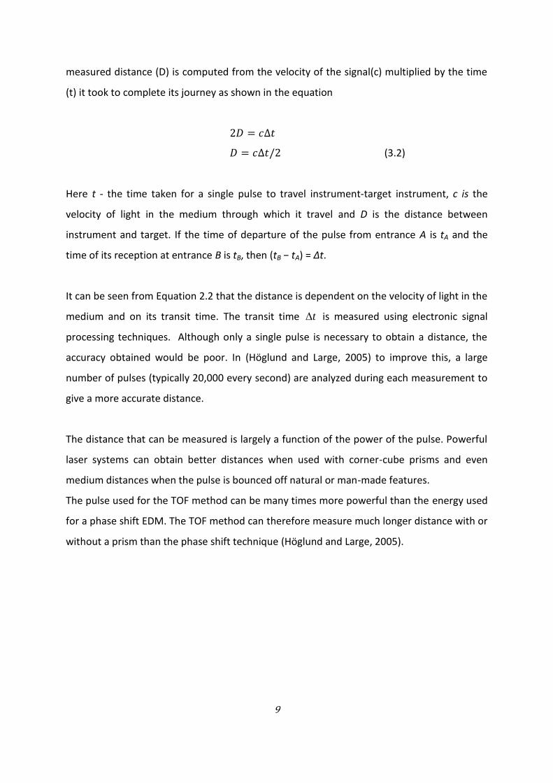
measured distance (D) is computed from the velocity of the signal(c) multiplied by the time

(t) it took to complete its journey as shown in the equation

=

= (3.2)

Here t - the time taken for a single pulse to travel instrument-target instrument, c is the

velocity of light in the medium through which it travel and D is the distance between

instrument and target. If the time of departure of the pulse from entrance A is tA and the

time of its reception at entrance B is tB, then (tB − tA) = ∆t.

It can be seen from Equation 2.2 that the distance is dependent on the velocity of light in the

medium and on its transit time. The transit time t is measured using electronic signal

processing techniques. Although only a single pulse is necessary to obtain a distance, the

accuracy obtained would be poor. In (Höglund and Large, 2005) to improve this, a large

number of pulses (typically 20,000 every second) are analyzed during each measurement to

give a more accurate distance.

The distance that can be measured is largely a function of the power of the pulse. Powerful

laser systems can obtain better distances when used with corner-cube prisms and even

medium distances when the pulse is bounced off natural or man-made features.

The pulse used for the TOF method can be many times more powerful than the energy used

for a phase shift EDM. The TOF method can therefore measure much longer distance with or

without a prism than the phase shift technique (Höglund and Large, 2005).

10

Figure 3-4 Principle of pulse distance meter (Source: Schofield and Breach, 2007)

3.4 Reflector vs. Reflectorless

There are two methods of measuring distance the prism method, which uses a reflective

prism at the target measurement point, and the non-prism or reflectorless method that does

not use a reflective prism.

With the prism method, a laser is beamed at a reflective prism (also called a mirror) placed

at the measurement point, and the distance is measured by the time it takes for light to be

reflected back from the prism, though this method is more accurate (Beshr and Elnaga,

2011). With the reflectorless method, it is possible to survey areas from a distant location.

Even areas of impossible to reach, such as danger disaster areas (e.g. landslides) can safely

and efficiently be surveyed with this method, which has the additional advantage of

requiring less labour and time (there is no need for a second team to handle the prism at the

target point). When surveying roads, for example, traffic restrictions need to be put into

place if reflective prisms are used. This is not the case with the reflectorless method. The

decision to use the prism or reflectorless method is made according to conditions at the

survey site.

3.5 Error source in Reflectorless Measurements

There are two main deviations in the use of reflectorless total station measurements. These

are caused either by reflector uncertainty or beam divergence. Reflector uncertainly is a

situation when the laser beam is reflected off something other than what it was supposed to

read or targeted. This can only be avoided through care, checks on measurements, and

instrument knowledge. One of the main concerns with the accuracy of reflectorless total

11

stations is beam divergence. The beam divergence of an electromagnetic beam is an angular

measure of the increase in beam diameter or radius with distance from the optical opening

or antenna opening from which the electromagnetic beam emerges.

As the size of the laser spot increases with distance from the instrument increase, so the

accuracy of the measurement becomes less reliable. The size of the laser beam depends on

the distance from the EDM system; the greater the distance, the larger the laser spot size

(see Figure 3-5). It is also noted that depending on the characteristics of the reflecting

surface the waveform of the laser beam scattered back by the surface may be a rather

unclear version of the emitted pulse. This distortion can lead to uncertainties in the distance

measured and can either give an erroneous result or no resultant distance at all. Also

suggest that as the beam divergence increases, so too does the time range of the reflected

signal off a certain plane.

Beam divergence causes the footprint of the laser beam to have a certain extent, meaning

that the laser spot hitting the surface is not a defined point but a beam with a physical shape

similar to an elongated ellipse. The size depends on the distance from the EDM system; the

greater the distance, the larger the laser spot size. As shown in Figure 3-5, there are two

parts of the error caused by laser beam divergence, the size of the dot on the reflected

surface and the angle of incidence with the surface.

Figure 3-5 Laser beam divergence in long distance2.

Unfortunately, by moving the instrument to a more distant position to lower the angle of

incidence also has the effect of increasing the size of the laser dot. The idea would be to

2 Source: (http://amrita.vlab.co.in/?sub=1&brch=189&sim=342&cnt=1)

12

setup the instrument at a perpendicular angle for each measurement. This would allow for a

more reliable measurement but this is often either impossible or impracticable. There are a

number of common total stations in Trimble and Leica, each having their own specifications.

When it comes to reflectorless specifications in the field, as long as the limitations are

understood, errors should be avoided. According to Leica (Leica Geosystems), the laser beam

divergence varies greatly between instrument manufacturers, with the laser ‘spot’ varying in

size from 9x28 mm to 100x110 mm at a distance of 50 m from the instrument. Obviously,

with such a variation, different instruments could be used in some applications while others

would become unreliable.

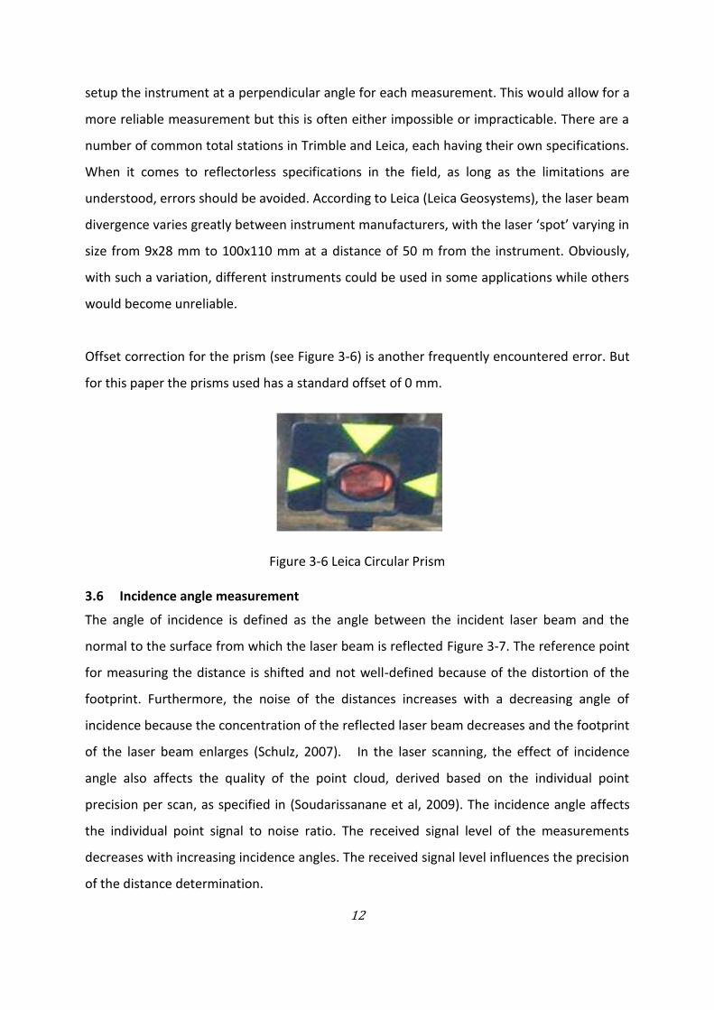
Offset correction for the prism (see Figure 3-6) is another frequently encountered error. But

for this paper the prisms used has a standard offset of 0 mm.

Figure 3-6 Leica Circular Prism

3.6 Incidence angle measurement

The angle of incidence is defined as the angle between the incident laser beam and the

normal to the surface from which the laser beam is reflected Figure 3-7. The reference point

for measuring the distance is shifted and not well-defined because of the distortion of the

footprint. Furthermore, the noise of the distances increases with a decreasing angle of

incidence because the concentration of the reflected laser beam decreases and the footprint

of the laser beam enlarges (Schulz, 2007). In the laser scanning, the effect of incidence

angle also affects the quality of the point cloud, derived based on the individual point

precision per scan, as specified in (Soudarissanane et al, 2009). The incidence angle affects

the individual point signal to noise ratio. The received signal level of the measurements

decreases with increasing incidence angles. The received signal level influences the precision

of the distance determination.

13

Figure 3-7 Incidence angle (source Wikipedia)

3.7 Error source in distance measurement when measuring not perpendicular to the

target

While measurements at right angles to an object are generally well within manufacturers

specifications, measurements to surfaces that are not at right angles to the measurement

beam can introduce errors. The angle of incidence influences the distances to be measured

in two different ways. On one hand, the centre of reference for the distance is shifted

because the footprint of the laser beam varies from a circular form to an elliptical form. On

the other hand, the footprint of the laser spot increases and covers a larger area. The

reference point for measuring the distance is shifted and not well-defined because of the

distortion of the footprint. Thus, the distance has a systematic offset leading to a false range

between object and the instrument. Furthermore, the noise of the distances increases with a

decreasing angle of incidence because the strength of the reflected laser beam decreases

and the footprint of the laser beam enlarges. There is going to be several possible errors

caused in these situations. The first one possible error is the alignment of the measurement

signal with the optical alignment would make the measurement signal reflect off a point that

is not the same as the point that is lined up using the eyepiece. The Second problem that

would increase the error as distance increases is the size of the measuring signal and the

effects of beam divergence.

14

Chapter Four

4 Angle measurement

Horizontal and vertical angles are fundamental measurements in surveying. The vertical

angle is used in obtaining the elevation of points and in the reduction of slant distance to the

horizontal. The horizontal angle is used primarily to obtain direction to a survey control

point, or to topographic detail points, or to points to be set out or the point to be surveyed.

It follows that, although the points observed are at different elevations, it is always the

horizontal angle and not the space angle which is measured. The specification of the Leica

1201+ and Trimble S8 total station for angle measurement are shown in Table 4-1.

Table 4-1 Angular specification for Trimble and Leica total station.

Mode TrimbleS8 Leica 1201+

Accuracy (standard deviation based on DIN

18723)

2₺ (0.6 mgon) 1” (0.3mgon)

4.1 Principle of angle measurement

Horizontal angular measurements are made between survey lines to determine relative

direction of the line. When horizontal distance measurements are applied to the derived

direction, the relative position of a point is established. Horizontal angles are measured on a

plane perpendicular to the vertical axis (plumb line) and always clockwise in relationship to

the initial back sight. The directional method will be used exclusively for surveys associated

with control traverse, ties to photo control points, cadastral surveys (right-of-way, property

corners and property controlling corners) and secondary control traverse.

4.2 Automatic target recognition

Automatic Target Recognition enables automatic angle and distance measurements to a

prism without the user accurately sighting the prism and it enables the instrument to be able

to lock on to and track a moving prism. Automatic Target Recognition can be used in a

number of different ways. In ATR mode, the prism is roughly sighted as in Figure 4-1 and the

instrument turns to the prism when we measure the distance.

15

The infrared beam transmitted from the telescope is reflected back by the prism and

analyzed instantly. As you do not need to fine point or focus, you measure much quicker and

more relaxed and the advantages of this method is in repetition measurement and when

measuring large number of point in short period of time.

Automatic target recognition (ATR) has different names depending on the manufacturer,

some of these include:-

ATR- Automatic Target Recognition (Leica);

Auto Lock / Fine Lock (Trimble);

Auto Pointing (Sokkia).

The name of ATR is different in different companies but the process of calculating and

finding the centre of a target is the same. This involves light been reflected back from any

prism and returned to the total station. The returning light signal is converted to digital data

on sensor much like what is found in a standard video camera. This concentrated light

source is used to calculate the horizontal and vertical displacements of the prism in relation

to the total station.

Figure 4-1 Automatic Fine pointing

16

4.3 Source of errors in angular measurement

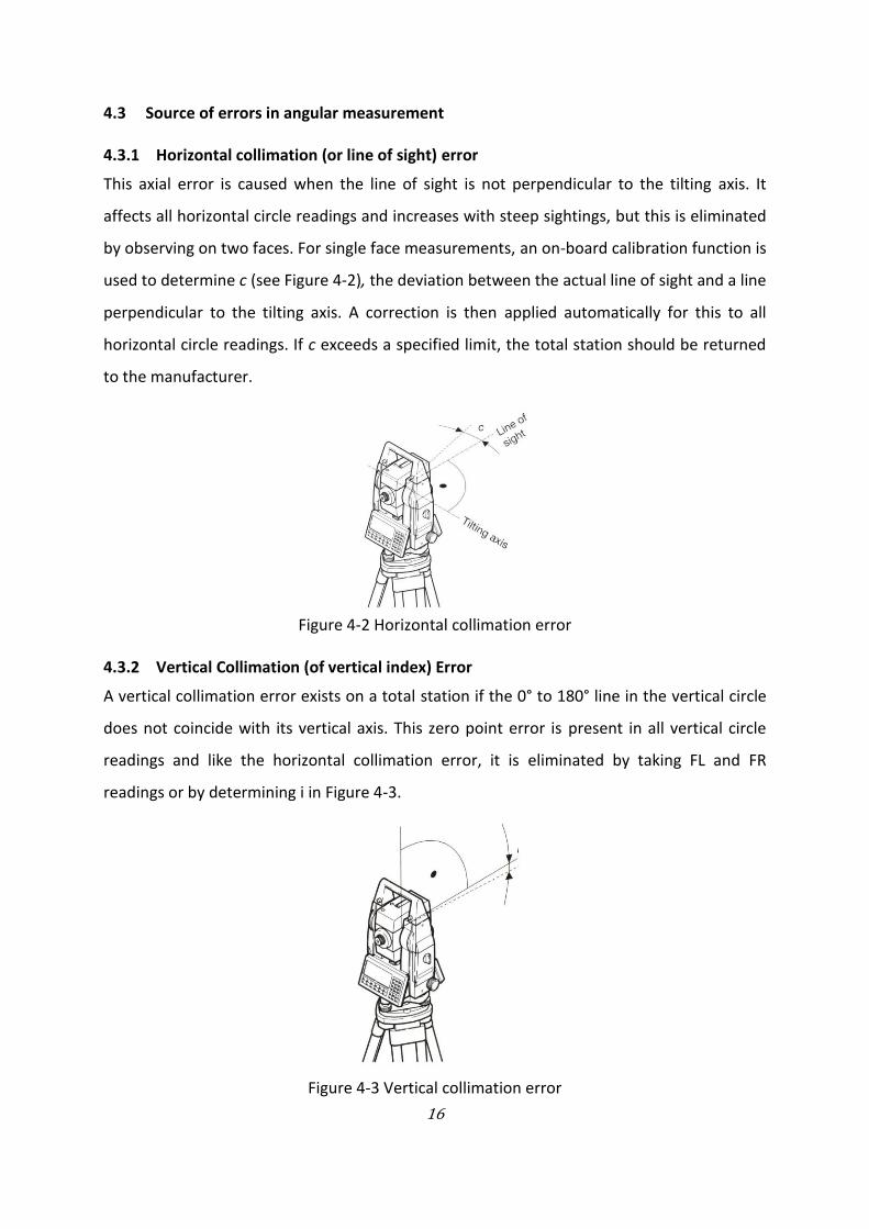
4.3.1 Horizontal collimation (or line of sight) error

This axial error is caused when the line of sight is not perpendicular to the tilting axis. It

affects all horizontal circle readings and increases with steep sightings, but this is eliminated

by observing on two faces. For single face measurements, an on-board calibration function is

used to determine c (see Figure 4-2), the deviation between the actual line of sight and a line

perpendicular to the tilting axis. A correction is then applied automatically for this to all

horizontal circle readings. If c exceeds a specified limit, the total station should be returned

to the manufacturer.

Figure 4-2 Horizontal collimation error

4.3.2 Vertical Collimation (of vertical index) Error

A vertical collimation error exists on a total station if the 0° to 180° line in the vertical circle

does not coincide with its vertical axis. This zero point error is present in all vertical circle

readings and like the horizontal collimation error, it is eliminated by taking FL and FR

readings or by determining i in Figure 4-3.

Figure 4-3 Vertical collimation error

17

4.3.3 Tilting axis error

These axial errors occur when the titling axis of the total station is not perpendicular to its

vertical axis. This has no effect on sightings taken when the telescope is horizontal, but

introduces errors into horizontal circle readings when the telescope is tilted, especially for

steep sightings. As with horizontal collimation error, this error is eliminated by two face

measurements, or the tilting axis error a (see Figure 4-4) is measured in a calibration

procedure and a correction applied for this to all horizontal circle readings – as before if a is

too big, the instrument should be returned to the manufacturer.

Figure 4-4 Tilting axis error

4.3.4 Compensator index error

Errors caused by not leveling a theodolite or total station carefully cannot be eliminated by

taking face left and face right readings. If the total station is fitted with a compensator it will

measure residual tilts of the instrument and will apply corrections to the horizontal and

vertical angles for these. However all compensators will have a longitudinal error l (See

Figure 4-5) and traverse error t known as zero point errors. These are averaged using face

left and face right readings but for single face readings the errors must be determined by the

calibration function of the total station.

18

Figure 4-5 Compensator index error

4.3.5 The vertical axis error v

This is not an instrument error but rather a setting up error because the vertical axis is not

plumb. It can be practically avoided if the vertical axis brought to the plumb position with

determination of the bubble centre.

The effect (v) of a vertical axis error v on a measured direction is a function of the vertical

angle h to the target as well as the angle a representing the separation of the measured

direction from the vertical plane containing the inclined vertical axis. This effect is calculated

by the equation

( ) = ( ) ( ) (4.1)

Unlike the collimation and horizontal axis errors, this effect (v) cannot be eliminated when

measuring in both telescope positions. Since (v) increase with the tangent of the vertical

angle, the vertical axis has to be plumbed extremely carefully when measuring inclined

directions.

Some theodolite and electronic tachometers are additionally equipped with a horizontal axis

micrometre or an electronic level to measure the remaining tilt of the vertical axis. The

measuring results obtained with these additional devices permit correction of the horizontal

directions for vertical axis errors.

19

Chapter Five

5 Checking and Calibrating Total Station

5.1 Overview of Calibration of Total Station

Calibration is a comparison between measurements – one of known magnitude or

correctness made or set with one device and another measurement made in as similar a way

as possible with a second device. The device with the known or assigned correctness is called

the standard. The second device is the unit under test, test instrument, or any of several

other names for the device being calibrated. (Source: Wikipedia)

All distances measured by a particular EDM/reflector combination are subject to a constant

error. It is caused by three factors:

• electrical delays, geometric detours, and eccentricities in the EDM;

• differences between the electronic centre and the mechanical centre of the EDM; and

• differences between the optical and mechanical centres of the reflector.

This error may vary with a change of reflectors, after receiving jolts, with different

instrument mountings and after service. The additive constant (or prism constant) is a

system constant that depends on the instrument and reflector being used. It cannot be

attributed just to a reflector or an instrument alone. It is only valid for the combination of

both. The additive constant or zero/index correction is an algebraic constant to be applied

directly to every measured distance. However, the prism offset is a function of the physical

and geometrical properties of the prism.

To maintain the high level of accuracy offered by modern total stations, there is now much

more emphasis on monitoring instrumental error. With this in mind, some construction sites

require all instruments to be checked on a regular basis using procedures outlined in the

manuals. Some instrumental errors are eliminated by observing on two faces of the total

station and averaging, but because one face measurements are the preferred method on

site, it is important to determine the magnitude of instrumental errors and correct for them.

For total stations, instrumental errors such as collimation error, tilting axis error and

20

compensator index error are measured and corrected using electronic calibration

procedures that are carried out at any time and can be applied to the instrument on site.

These are preferred to the mechanical adjustments that used to be done in labs by

technicians. Since calibration parameters can change because of mechanical shock,

temperature changes and rough handling of what is a high-precision instrument, an

electronic calibration should be carried out on a total station as follows:

Before using the instrument for the first time.

After long storage periods.

After rough or long transportation.

After long periods of work.

Following big changes in temperature.

The instrument errors can be used to monitor the performance of the total station over time

and if significant, should be applied to measurements taken subsequent to the calibration.

As shown on the Figure 5-1, principal axes of a total station should be perpendicular to each

other. Also, the RL total station reference laser beam, the ATR zero point, and the line of

sight should coincide precisely.

V = Vertical Axis, H= Tilting Axis, Z= Line of Sight

Figure 5-1 Principal axes of total station.

There are two methods for calibrating a total station, the field method and the laboratory

method. For the field calibration, total station must be calibrated over a series of distances

representative of the range of the instrument known as baseline. The baseline is a

permanently marked distance, the length of which is known. As explained by Staiger (2007)

the baselines should consist of at least of four marked monuments, all in a straight line over

21

uniformly sloping terrain. These baselines are designed to generate a statistically accurate

determination of the errors of the total station (Staiger, 2007). The verification method

involves the measurement of a set of segments on the total station base to determine the

existence and magnitude of any errors present. The length of the baseline is ranging from

500 and 1400 m (Buckner, 1998), so the field method is suitable for determination of the

scale error. The engineering manual of the US Army (2002) stated that establishing a

calibration baseline and keeping it in good order can be expensive and time consuming when

maintenance is considered.

For the laboratory calibration, a series of distances ranging from five to one hundred metres

could be measured. In general, calibration measurements over short distances assist or help

in the determination of the additive constant while longer distances help determine scale

error (Staiger, 2007).

The additive constant (C) is generally computed using the parts to the whole method. As an

example, a test with four pillar line would give the combinations for additive constant as in

equation 5.1:

2C = - (d12 + d23 + d34 - d14) (5.1)

where d12, d23, d34 and d14 are the distances between the pillar stations as shown in

Figure 5-2 .

Figure 5-2 Procedure for additive constant calculation.

Scale errors are linearly proportional to the measured distance and can arise from both

internal and external sources. Internal sources are ageing, drift and temperature effects.

External sources are variations from the standard value of the refractive index of the air

caused by changes of the ambient atmosphere along the measured distance. These changes

introduce scale errors. Incorrect atmospheric data can be introduced in many ways;

uncalibrated instruments; incorrect atmospheric measurement procedures; and often by

incorrect entry of the atmospheric correction term at the EDM instrument keyboard or

setting knob.

22

5.2 Built in calibration programs

Total stations instrumental errors are measured and corrected using electronic calibration

procedures that are carried out at any time and can be applied to the instrument on site.

These are preferred to the mechanical adjustments that used to be done in labs by

technicians. Before determining the instrument errors, the instrument has to be levelled up

using the electronic level. The tribrach, the tripod and the underground should be very

stable and secure from vibrations or other disturbances. The instrument should be protected

from direct sunlight in order to avoid thermal warming. It is also recommended to avoid

strong heat shimmer and air turbulence. The best conditions are usually early in the morning

or with overcast sky. Before starting to work, the instrument has to be become adjust to the

ambient temperature. Approximately two minutes per degree centigrade of temperature

difference from storage to working environment but at least 15 min should be taken into

account. Even after good adjustment of the ATR, the crosshair might not be positioned

exactly on the centre of the prism after an ATR measurement has been executed. This is

normal effect. To speed up the ATR measurement, the telescope is normally not positioned

exactly on the centre of the prism. The small rest deviations, the ATR offsets are measured

individually for each measurement and corrected electronically. This means that the Hz- and

V- angles are corrected twice: first by the determined ATR errors for Hz and V and then by

the individual small deviations of the current pointing.

Horizontal collimation (or line of sight) error (C) is caused when the line of sight is not

perpendicular to the tilting axis. It affects all horizontal circle readings and increases with

steep sightings, but this is eliminated by observing on two faces. For single face

measurements, an on board calibration function is used to determine (C), the deviation

between the actual line of sight and a line perpendicular to the tilting axis. A correction is

then applied automatically for this to all horizontal circular readings. If (C) exceeds a

specified limit, the total station should be returned to the manufacturer.

Tilting axis errors occur when the tilting axis of the total station is not perpendicular to its

vertical axis. This has no effect on sighting taken when the telescope is horizontal, but

introduces errors into horizontal circle readings when the telescope is tilted, especially for

steep sightings. As with horizontal collimation error, this error is eliminated by two face

measurements, or the tilting axis error (a) is measured in a calibration procedure and a

23

correction applied for this to all horizontal circle readings – as before if (a) is too big, the

instrument should be returned to the manufacturer.

Compensator index errors caused by not levelling a theodolite or total station carefully

cannot be eliminated by taking face left and face right readings. If the total station is fitted

with a compensator it will measure residual tilts of the instrument and will apply corrections

to the horizontal and vertical angles for these.

However all compensators will have a longitudinal error (l) and traverse error (t) known as

zero point errors. These are averaged using face left and face right readings but for single

face readings must be determined by the calibration function of the total station

In Leica total station, the red laser beam used for measuring without reflector is arranged

coaxially with the line of sight of the telescope, and emerges from the objective port. If the

instrument is well adjusted, the red measuring beam coincides with the visual line of sight.

External influences such as shock, stress or large temperature fluctuations can displace the

red measuring beam relative to the line of sight. The direction of the beam should be

inspected before precise measurements of distances are attempted, because an excessive

deviation of the laser beam from the line of sight can result in imprecise distance

measurements.

Adjustment of the laser plummet, the laser plummet is located in the vertical axis of the

instrument. Under normal conditions of use, the laser plummet does not need adjusting. If

an adjustment is necessary due to external influence, the instrument has to be returned to

any Leica Geosystem authorized service workshop.

In Trimble total station, the principles of angle measurement are based on reading an

integrated signal over two opposite areas of the angle sensor and producing a mean angular

value. This eliminates inaccuracies caused by eccentricity and graduation. In addition, the

angle measurement system compensates for the following automatic corrections:

Mislevelment (deviation of the plumb axis),

Horizontal and vertical collimation error

Tilt axis error.

24

Modern total station warns the operator immediately of any Mislevelment in excess of ±6´

(±0.11 gons). Corrections for the horizontal angle, vertical angle, and slope distance are

calculated in the field application software and applied to all measurements.

The deviation of the tilt axis from a plane perpendicular to the vertical axis is known as the

tilt axis error. The vertical circle will no longer be in a vertical plane and angles will be

measured with respect to a false zenith. Averaging face left and faces right readings and/or

software reduces this error to negligible or second order levels.The horizontal collimation

error is the deviation of the sighting axis from its required position at right angles to tilt axis.

The vertical collimation error is the difference between the vertical circle zero and the plumb

axis of the Trimble total station.

Traditionally, collimation errors were eliminated by observing angles in both faces. In the

Trimble total station, a pre-measurements collimation test is performed to determine the

collimation errors. Angular measurements are observed in both faces, the collimation errors

are calculated, and the respective correction values are stored in the Trimble total station.

The collimation correction values are then applied to all subsequent angle measurements.

Angles observed in a single face are corrected for collimation errors, which eliminates the

need to measure in both faces.

A Trimble auto lock/robotic total station can automatically lock and track a prism target.

Pointing errors caused by slight misalignment of the Trimble auto lock/robotic total stations

tracker have a similar effect to the HA and VA collimation errors detailed above. To correct

for the tracker collimation errors, carry out a tracker collimation test. The tracker collimation

test automatically observes angular measurements to a target in face1 and face2, the

tracker auto lock/robotic total station. The tracker collimation correction values are then

applied to all subsequent angle measurements observed. Angle observed in a single face is

corrected for collimation errors, which removes the need to measure in both faces.

5.3 KTH-TSC

Modern total station instrument contain a number of sensors and corresponding system, by

which it is impossible to obtain the original values of measurement (Horemuz and

Kampmann, 2005). Therefore, it is a must to calibrate the instrument at regular intervals. In

this thesis, the KTH Total Station Check (KTH-TSC) is used for verification of total stations

25

(Horemuz and Kampmann, 2005). Verification is a test to confirm that the accuracy attained

by a measuring instrument is within allowable accuracy limits as defined in the specification.

Error in survey measurements mainly comes from instrument and external factors. However,

the instruments internal signal processing of sensors is not published by producers hence

the determination of causal coherences and the elimination-calibration-of instrumental

errors is usually reserved for special laboratories of calibration and for producers of

instruments. For system verification the single components of surveying instrument is not

investigated deliberately rather an accuracy for obtained measured size of the instrument is

striven for -co-ordinates which are staked out or determined station position referred to

measuring scenario. That means functionality verification is undertaken (Horemuz and

Kampmann, 2005).

In this procedure polar measurements (see Figure 5-3) for determination of the three-

dimensional position of a total station in the intersection of visual axis and horizontal axis

are executed to marked points which co-ordinates are made up in a uniform three-

dimensional reference-system. Within the scope of variance-component-estimation with

least squares method not only the calculated position of a station can be derived, but also a

characteristic total accuracy for each group of observations – horizontal direction, zenith

angle, slope distances. With that an indication of the achievable accuracy of measurement

components will be obtained related to chosen measurement scenario (distance between

target points, their spreading over horizon, length of slope distances (Horemuz and

Kampmann, 2005).

1, 2,3,4,5,6,7,8 ………….base of column points

101,102,103,104,105 ……free stations (Teskey and Radovanovic, 2001)

Figure 5-3 Spatial Free Station position

26

5.4 Offset of the instrument and prism

In surveying, prism constant3 refers to the offset of the centre of the prism to the reflective

section and the adjustment required achieving an accurate reading. Each alternative of

prisms has its own independent prism constant that must account for when taking readings.

So that, setting the correct prism constant is a simple operation but sometimes leads to

some confusion and the cause of systematic errors in survey measurements. The

measurements from an EDM using infra-red beams to a corner cube commonly called a

prism uses a beam emitted from the EDM to the prism and then the beam is returned from

the prism to the EDM. The property of the corner cube is such that the beam from the prism

to the EDM is returned along the same exact path parallel to the incoming beam. There is

some error in this return path called angular beam deviation. So, the distance that the user

wants is the distance from the centre of the instrument to the vertical axis of the prism not

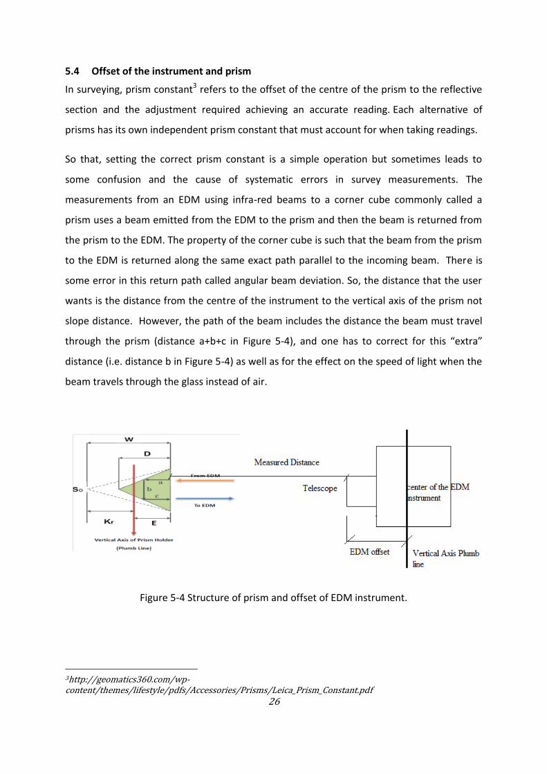
slope distance. However, the path of the beam includes the distance the beam must travel

through the prism (distance a+b+c in Figure 5-4), and one has to correct for this “extra”

distance (i.e. distance b in Figure 5-4) as well as for the effect on the speed of light when the

beam travels through the glass instead of air.

Figure 5-4 Structure of prism and offset of EDM instrument.

3http://geomatics360.com/wp-content/themes/lifestyle/pdfs/Accessories/Prisms/Leica_Prism_Constant.pdf

27

So, the basic issue for a prism constant is that the beam from the EDM travels to the prism,

and then travels through a short distance through the glass at a different speed (a+b+c in

Figure 5-4), and then is returned to the EDM.

If the beam actual travelled a distance equal to distance a+b+c and was compensated for the

effect of the travelling slower in the glass the beam would travel to a theoretical reversal

point (Point So in Figure 5-4) and then reflect back to the EDM. By the design of the prism

and the prism holder the distance from the front surface of the prism to the corner point of

the prism (distance D in Figure 5-4) is known and distance from the front surface of the of

the prism to the vertical axis of the prism housing (distance E in Figure 5-4) is known by

design. The next distance involved is the distance from the front surface of the prism to the

theoretical reversal Point so (distance W in Figure 5-4) which accounts for the distance

a+b+c and the effect of index of refraction of the glass on the beam. So for common prism

with –30 mm offsets or -40 mm offsets, the prism offset is the distance from the theoretical

reversal Point So back to the vertical axis of the prism housing which is distance Kr in Figure

5-4.

The additive constant implies that the combination of both the offset of the prism and the

offset of the instrument, Figure 5-4 shows the distance measured is from the telescope to

the surface of the prism, so that the offsets E and EDM offset must applied on the measured

distance. The prism offset is a correction applied to each distance to allow for the difference

between the mounting point centre and the optical centre of the prism. With Leica

equipment there are a number of different prism constants in use. The system is designed

to have zero constant with the standard LEICA round prism. Having a fix on prism target

introduces a constant of 34.4 mm, the 360 prism has a constant of 23.1 mm, or 30 mm (this

was dependent on the model of the prism used) and the mini prism has a constant of 17.5

mm or zero. When used with no prism reflectorless (i.e. in Red Laser) a 34 mm constant is

applied. But it is possible to shoot to a prism using RL either deliberately (with the

correction applied) or inadvertently with no correction and thus the wrong distance is

observed. This typically happens at the end of a series of non-contact detail when reverting

back to the prism.

28

With other manufactures such as Topcon and Trimble this is less of a problem with their

total stations since they are all set up with a zero constant to a Topcon Trimble round prism.

The additive constant with the Trimble 360 prism is only 2 mm. Direct Reflex (Reflectorless)

observations require no change in prism constant.

There is sometimes a case to use prism and total station from different company for survey

measurement. Therefore, the surveyor should know how to calculate the prism constant for

this kind of scenario. As an example, section 5.5 and 5.6 discuss how to compute prism

constant for Leica and Trimble total stations.

5.5 Calculating the prism offset for use in a Leica total station for a non-leica prism

The difference in Leica prisms and third-party prisms for the prism offset is how the value for

Kr is handled. From the explanation in section 5.4, the prism constant by design for a Leica

Geosystem standard Prism is Kr = -34.4 mm. This is the value that Leica used for many years

and is considered the optimal design to eliminate any deviations of the beam when the

prism face is tilted or not perpendicular to the path of the EDM beam. Leica Geosystem

defines this value, Kr = KLEICA = 0 mm in the Leica total stations. It is only a matter of

understanding that Leica Geosystem has a prism constant to -34.4 mm for their optimal

prism design. Within the Leica instruments this value is set to 0 mm (KLEICA). Leica builds from

defining this as the base point of 0 mm to have Leica Prism offsets for their mini prism, 360°

prisms and reflectorless offsets. A Leica circular prism has a prism offset KLEICA = –34.4 mm.

To account for this the EDM software in a Leica total station is programmed with a +34.4 mm

which makes the prism offset 0 when using a Leica circular prism. If a prism has an offset

other than 34.4 mm a correction must be applied. The correction is the difference between

the – 34.4 mm and the actual offset of the prism being used (Kr).

If someone likes to use different type of prism for other type, it needs to remember the

following equation to use a non-Leica prism with your Leica total station. In the firmware the

term Absolute Constant is used in place of Kr or prism constant.

Kr = Absolute Constant = Manufacturers Prism Constant

So, to compute the value to be entered in a Leica total station for a non-Leica prism.

29

Leica Prism Constant for Non-Leica Prism = KLEICA = Kr + 34.4 mm

KLEICA = Absolute Constant + 34.4 mm

So for a non-Leica prism that has a design prism offset of -30 mm

Leica Prism Constant = (-30 mm) + 34.4 mm

Leica Prism Constant = +4.4 mm. The value of + 4.4 mm is the correct value for created a

user defined prism in a Leica total Station with this design offset.

For a non-Leica prism that has a design prism offset of 0 mm

Leica Prism Constant = (0 mm) + 34.4 mm

Leica Prism Constant = +34.4 mm

The value of 0.0 mm is the correct value for created a user defined prism in a Leica total

station with this design offset.

5.6 Calculating the prism offset for use in a Trimble total station for a non-Trimble prism

All total stations manufactured by Trimble4, in combination with their reflectors are adjusted

with the additive constant 0.000. In case of measurements to reflectors of other

manufacturers, a possibly existing additive constant can be determined by measurement

and entered.

Another possibility consists in calculating an additive constant by means of the known prism

constant of the reflector used and entering it. This prism constant is calculated as function of

the geometric value of the prism, the type of glass and the place of the mechanical reference

point. In case of measurements to reflectors of other manufacturers the user has to enter

the prism constant and check the correctness by measurements to known distances.

The connection between addition constant A and prism constant is shown in the following

calculation formula:

A = PF + 35 mm

where PF is the foreign reflector prism constant

Example:

4 http://www.geosoft.ee/UserFiles/File/Juhendid/Tahhumeetrid/Elta_CU_User.pdf

30

Foreign reflector prism constant PF = -30 mm

Addition constant in connection with this foreign reflector A = + 5 mm

5.7 EDM Errors

The distances measured by EDM reflector combination are subject to three types of error, as

shown in Figure 5-5.

Figure 5-5 EDM errors.

Zero Error (Additive Constant) is caused by three factors as listed by

electrical delays, geometric detours, and eccentricities in the EDM,

differences between the electronic centre and the mechanical centre of the EDM

Differences between the optical and mechanical centres of the reflector.

The additive constant or zero/index correction is added to the measured distances to correct

for these differences. This error may vary with changes of reflector, so only one reflector

should be used for EDM calibration.

Scale errors are linearly proportional to the measured distance and can arise from both

internal and external sources. Internal sources are ageing, drift and temperature effects (e.g.

insufficient warm-up time) of the oscillator (Staiger, 2007).

Internal frequency errors, including those caused by external temperature and

instrument "warm-up" effects,

Un-modelled variations in atmospheric conditions which affect the velocity of

propagation,

Non-homogeneous emission/reception patterns from the emitting and receiving

diodes (Phase in homogeneities).

31

Cyclic Error (Short Periodic Error) is a function of the actual phase difference measurement

by the EDM (Staiger, 2007). Phase measurement error is caused by unwanted feed through

the transmitted signal onto the received signal (Tulloch, 2012). Cyclic error is usually

sinusoidal in nature with a wavelength equal to the unit length of the EDM. The unit length is

the scale on which the EDM measures the distance, and is derived from the fine measuring

frequency (Tulloch, 2012). The stability of the EDM internal electronics can also vary with

age, therefore, the cyclic error can change significantly over time. Cyclic error is inversely

proportional to the strength of the returned signal, so its effects will increase with increasing

distance (i.e., low signal return strength). Calibration procedures exist to determine the EDM

cyclic error that consist of taking bench measurements through one full EDM modulation

wavelength, and then comparing these values to known distances and modeling any cyclic

trends found in the discrepancies.

32

Chapter Six

6 Methodology of the Thesis

6.1 Measurements in Different Surface Objects

This experiment was to check the effect of different colour surfaces in total station

measurement. The experiment used Leica and Trimble total station instrument. Targets

which were used in the experiment were covered by paper of different colour such as white,

green, black, yellow, red and blue. The field data were collected by a total station setting on

the first point and a tripod with special holder of coloured targets were placed on second

point as in Figure 6-1.

Figure 6-1 Special holders of the colour targets

Coloured targets (see Figure 6-2) were set at different places by increasing the distance

approximately 10 m. This is done without changing the total station and horizontal angle in

order to have the same measuring condition for each coloured target. These distances were

compared with the reflector mode which is considered as ‘true distance’. The ‘true distance’

was measured in both face 1 and face 2 position of the instrument. The experiment started

at a close range of approximately 6 m and ended at 156 m. Finally the differences between

the value of the measured distance using a prism (reflector) and colour targets in each

location were checked.

Figure 6-2 Colour target used for surface reflectivity

33

6.2 Reflectorless reading

This experiment was to test the accuracy of reflectorless measurement in total station. The

back side of the prism covered by paper was used as target for the measurement.

For this trial, Leica circular prism GPR 1 (See Figure 6-3), Leica Total station 1201+ and

Trimble S8 were used. Before outdoor measurement, laboratory check was performed to

calculate the offset between the prism and non-prism mode by measuring distance and

calculating the difference. This difference was compensated by applying additive constant to

the non-prism measurement (for which we got 17 mm). In the field the total station was set

permanently on one point and the position of the target was moved by an interval of 20 m.

The total station position was permanently fixed on one point and both reflector and

reflectorless positions were moved by an interval of 20 m. The distance from the beginning

to the end (200 m) were measured with both reflector and reflectorless mode (see Figure 6-

4).

The horizontal distance measured on the prism was considered as ‘true distance’. A number

of measurements for reflector and reflectorless mode were observed and the root mean

square was computed by equation 6.1 as

= ( )

(6.1)

where is the root mean square, is the value of reflector measurements, is the

value of reflectorless measurement and n is the number of observations.

a) b)

Figure 6-3 GPR 1 Reflector and target designed for non-reflector observation

34

Figure 6-4 Field observation on reflectorless experiment

6.3 Different incidence Angle Measurement

This experiment was performed to investigate the influence of incidence angle of the

reflectorless measurement on the accuracy of measured horizontal distance. In this test HDS

target was used (Figure 6-7). This was carried out using both the Trimble S8 and Leica 1201+

instruments. The horizontal distance at near and far targets to the total station were

measured in order to investigate its effect on the accuracy of the measurement by

calculating the root mean square error by equation 6.1.

In the field,

1) the instrument was first set at A ( see Figure 6-5 ) and the target was mounted at

B.

2) align the instrument perpendicular to the target (zero degree) position.

3) four points were marked by rotating the instrument at 10 degree interval (10, 20,

30, 40 degrees) from the perpendicular instrument position.

4) after the point was fixed, the total station was moved to HDS target position (see

Figure 6-6) and the HDS target on the position of total station

5) the first measurement was taken after alignment of the total station was fixed to

the perpendicular direction of the HDS target.

6) the next measurements were taken by rotating the HDS target to the marked

points

All measurements were taken in two modes, namely face left and face right.

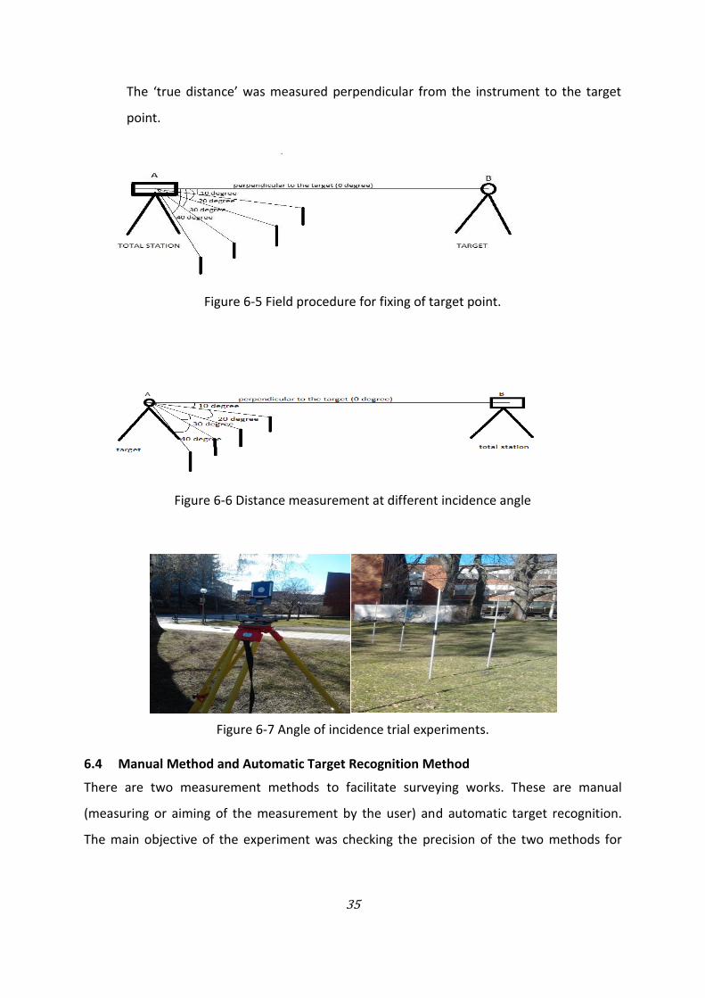
35

The ‘true distance’ was measured perpendicular from the instrument to the target

point.

Figure 6-5 Field procedure for fixing of target point.

Figure 6-6 Distance measurement at different incidence angle

Figure 6-7 Angle of incidence trial experiments.

6.4 Manual Method and Automatic Target Recognition Method

There are two measurement methods to facilitate surveying works. These are manual

(measuring or aiming of the measurement by the user) and automatic target recognition.

The main objective of the experiment was checking the precision of the two methods for

36

angle observation by calculating the standard deviation for each group of observation by

equations 6.2.

. = ( )

(6.2)

where is the standard deviation, is the value of individual angle measurements, is the

mean value of the measurements and n is the number of observations.

On this experiment, both Leica 1201+ and Trimble S8 total stations were used. Field

procedures were carried out, by setting up the instrument on one point, and placing the

prism at the reference target (see Figure 6-8). The instrument aligned to the reference target

to fix the horizontal angle zero. The angular measurement was done by rotating the

instrument to the target. Additional measurements were made by changing the prism at

different distance.

Figure 6-8 Field procedure for ATR and manual observation.

For all (manual and ATR) measurements both face one and face two instrument positions

were used. The standard deviation of angular measurements was calculated from each

distance.

6.5 KTH TSC

The main focus of this experiment was to test the performance of the instrument by

measuring slope distance, horizontal and vertical bearing between the instrument and the

target. Standard deviation of the measurement was calculated to check the quality of the

observations. In this test both Leica 1201 and Trimble S8 total station were used. The

37

measurement scenario contained four total station positions to take measurements and four

to seven spatial target points with prism. All targets were measured in clockwise direction

from each station. The collected data were imported to the KTH-TSC software to determine

the accuracy of the measurement. The calculated standard deviations of horizontal direction

(Sr), zenith distance (Sz), and slop distance (Ss) for both instruments by variance-component

estimation are indicated in the result table.

6.6 Prism or additive constant

The reflector constant is a given property of the particular model. It defines the relation of

the distance measurement to different reflector models. Surveying reflectors in particular -

are important accessories for various applications in surveying. Widely accepted as reliable

accessories, surveyors normally do not consider the influence which surveying reflectors

have on measurements. However, obtaining a certain level of accuracy and reliability

requires the consideration of all possible effects on the measurements.

Centring accuracy and the geometrical alignment to the instruments line of sight are two

examples that may have a crucial effect on the survey results. In addition we have to know

the property of the prism in distance measurement especially when the instrument and the

prism are from different company. Therefore, it is better to determine the prism constant

before field measurement.

This experiment shows how to calculate the prism constant. Leica 1201+ and Trimble S8

total stations and Geotronic, Leica circular prism and Trimble 360 circular prism were used

for this experiment. The field procedures carried out by setting up the instrument on one

point and horizontally placing three tripods on straight line. As an example, instrument was

set up at point 1 and measurement was done from point 1 to A, and C as in Figure 6-9. This

was continued with setting up the instrument at point A and measuring point B. Finally point

C was measured from the instrument at point B. Furthermore, the instrument was set at C to

measure in backward direction. This helps to check the accuracy of the prism constant.

38

Figure 6-9 Steps of Calculating Additive/Prism Constant

The number of target points then increased from 3 to 7 to check the optimal number for

determination of prism constant. Forward and backward measurements were taken for the

seven target points with the same procedure. The prism constant for the measurement as in

Figure 6-10 can be calculated using Equation 6.3

P = (T- X-Y-Z)/2. (6.3)

where P is the prism constant, T is the total distance from the instrument position to point C,

X is the distance between the instrument and point A, Y is the distance between point A and

B and Z is the distance between point B and C.

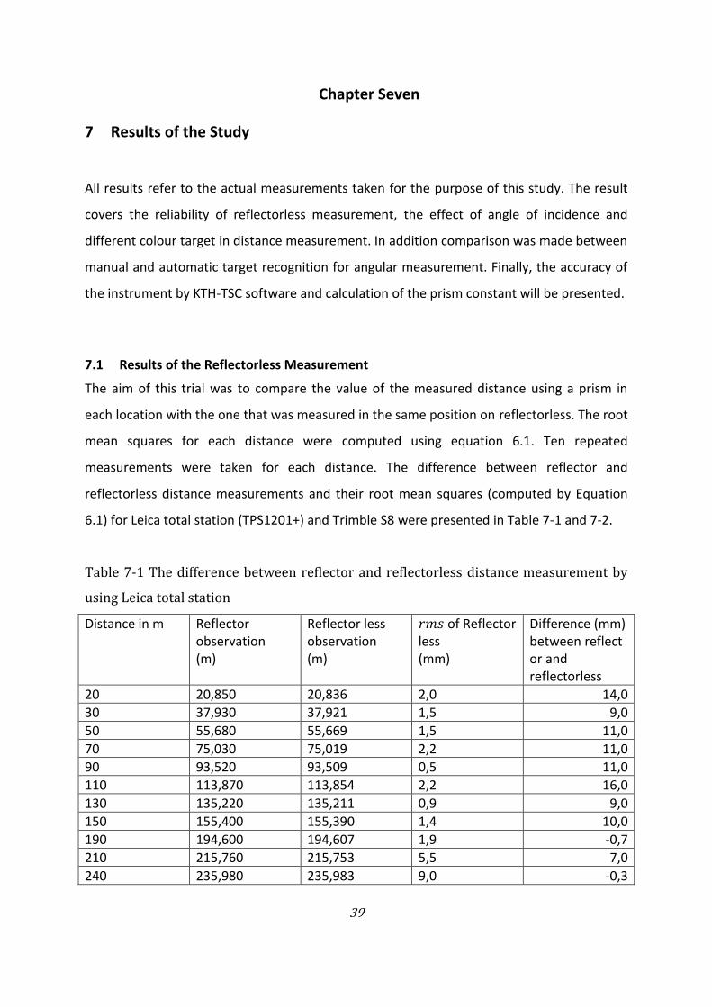
39

Chapter Seven

7 Results of the Study

All results refer to the actual measurements taken for the purpose of this study. The result

covers the reliability of reflectorless measurement, the effect of angle of incidence and

different colour target in distance measurement. In addition comparison was made between

manual and automatic target recognition for angular measurement. Finally, the accuracy of

the instrument by KTH-TSC software and calculation of the prism constant will be presented.

7.1 Results of the Reflectorless Measurement

The aim of this trial was to compare the value of the measured distance using a prism in

each location with the one that was measured in the same position on reflectorless. The root

mean squares for each distance were computed using equation 6.1. Ten repeated

measurements were taken for each distance. The difference between reflector and

reflectorless distance measurements and their root mean squares (computed by Equation

6.1) for Leica total station (TPS1201+) and Trimble S8 were presented in Table 7-1 and 7-2.

Table 7-1 The difference between reflector and reflectorless distance measurement by

using Leica total station

Distance in m Reflector observation (m)

Reflector less observation (m)

of Reflector less (mm)

Difference (mm) between reflect or and reflectorless

20 20,850 20,836 2,0 14,0

30 37,930 37,921 1,5 9,0

50 55,680 55,669 1,5 11,0

70 75,030 75,019 2,2 11,0

90 93,520 93,509 0,5 11,0

110 113,870 113,854 2,2 16,0

130 135,220 135,211 0,9 9,0

150 155,400 155,390 1,4 10,0

190 194,600 194,607 1,9 -0,7

210 215,760 215,753 5,5 7,0

240 235,980 235,983 9,0 -0,3

40

Table 7-2 The difference between reflector and reflectorless distance measurement by

using Trimble total station S8

Distance in m

Mean of Reflector observation in m

Mean of Reflectorless observation in m

of Reflectorless observation in mm Difference in mm

20 22,650 22,640 0,5 10,0

40 44,540 44,530 0,5 10,0

60 69,220 69,213 1,4 7,0

90 90,010 90,001 3,0 9,0

100 114,800 114,790 0,5 10,0

130 134,620 134,628 1,4 -8,0

150 155,830 155,836 0,8 -6,0

170 177,620 177,631 0,8 -11,0

200 201,150 201,152 1,2 -2,0

220 219,520 219,530 0,9 -10,0

Figure 7-1 Difference in reflector and reflectorless distance measurement using total station

TPS 1201+

-2

0

2

4

6

8

10

12

14

16

18

20 30 50 70 90 110 130 150 190 210 240

Dif

fere

nce

in m

m

Distance from the instrument

Reflector vs refelectorles

Reflector vs refelectorles

41

Figure 7-2 Difference in reflector and reflectorless distance measurement using total station

Trimble S8

The graph in Figure 7-1 and 7-2 shows a maximum difference of 1.6 cm between reflector

and reflectorless measurement. Therefore it is possible to use reflectorless mode for

surveying application that demand less than 1.6 cm accuracy.

The reliability of these two methods was tested statistically (see Table 7-5 and 7-6) to

compare one with the other. The differences between reflectorless and reflector

measurement are calculated after checking randomness test. One can construct various

statistics to directly test whether a set of measurement error e1, e2…..en are random or not.

The risk level is chosen to be α=4.55%, for which the critical value of the standard normal

distribution is ½ =2. Five different test steps were performed in the table 11a and 11b.

Step 1.Testing the maximum absolute value of errors in this step if the value of |em|> ½

the test will be passed otherwise it will fail, where em maximum absolute value of error.

Step2 Testing the sum of error let’s take S as the sum of e (error) S=e1+e2+e3---+en and if the

value calculated was |S|< δ.C ½α the test will pass.

Step3 Testing the number of positive versus negative errors if the value of |s+-s- |where s+,

s- denotes the number of positive errors and negative errors respectively is less than the

value got from .C ½α. There residual or misclosure error for this computation is shown in

Table 7-3 and 7-4.

Step 4 testing the signs of the errors in this test let us take S1 as number of adjacent error

pairs which have the same sign and S0 denotes the number of adjacent error pair with

opposite sign. For the chosen risk level if the value of |s+-s- |< . C ½α the test will

pass.

-15

-10

-5

0

5

10

15

20 40 60 90 100 130 150 170 200 220

Dif

fere

nce

in m

m

Distance from the instrument

Reflector vs. reflectorles

Reflector vs. …

42

Step 5 Tests the sum of positive versus negative errors squared in this test let as take s2 as

the difference between the sum of positive error squared and the sum of negative errors

squared. Then if the value of |s2|< δ2.C ½α the test will pass (Fan, 1997).

Table 7-3 Misclosures (ei) in distance measurement by Leica total station.

No Error in

mm

No Error in

mm

No Error in

mm

No Error in

mm

No Error in

mm

1 4,0 11 1,8 21 -2,7 31 2,0 41 6,3

2 -5,0 12 -1,2 22 1,3 32 -1,0 42 -8,7

3 -1,5 13 -2,2 23 2,3 33 2,5 43 10,3

4 2,5 14 0,8 24 -0,7 34 -1,5 44 -7,7

5 1,3 15 2,8 25 1,3 35 0,5

6 -1,7 16 -1,2 26 -0,7 36 -1,5

7 -0,7 17 0,3 27 0,3 37 3,8

8 1,3 18 0,3 28 -0,7 38 -5,2

9 -1,2 19 0,3 29 -1,0 39 5,8

10 0,8 20 -0,7 30 0,0 40 -4,2

Table 7-4 Misclosures (ei) in distance measurement by Trimble total station.

No Error in

mm

No Error in

mm

No Error in

mm

No Error in

mm

1 -0,5 11 -2,0 21 1,0 31 0,0

2 0,5 12 1,0 22 -2,0 32 0,0

3 0,5 13 1,8 23 1,0 33 -1,6

4 -0,5 14 -3,3 24 0,0 34 1,4

5 -0,3 15 4,8 25 0,0 35 0,4

6 -0,3 16 -3,3 26 1,0 36 -0,1

7 0,8 17 0,3 27 1,0 37 0,8

8 -0,3 18 -0,8 28 -1,0 38 -0,3

9 1,0 19 0,3 29 -1,0 39 0,8

10 0,0 20 0,3 30 0,0 40 -1,3

43

Table 7-5 Reliability of reflectorless distance measurement using Trimble total station

p= passed, N.p =not passed, M.a.v =maximum absolute value=number of observations

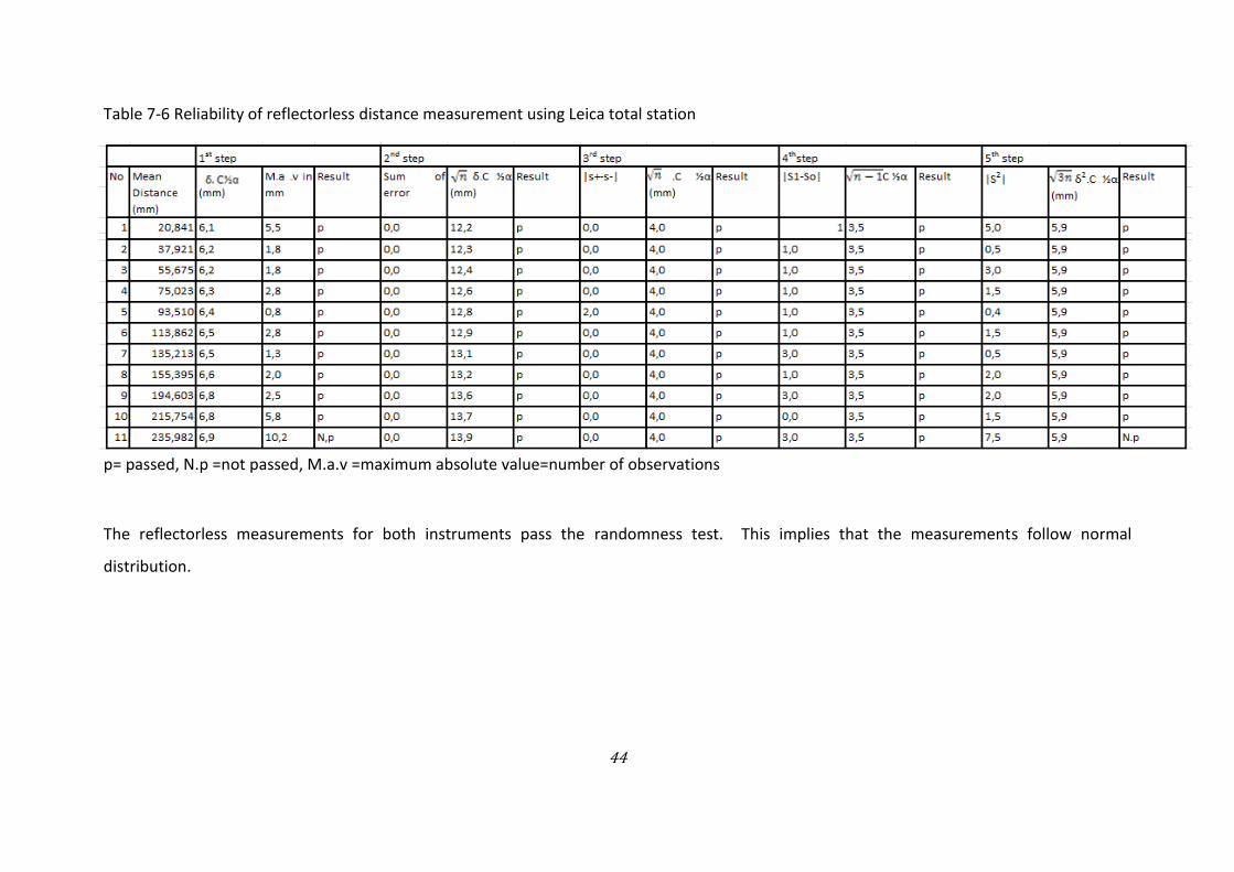
44

Table 7-6 Reliability of reflectorless distance measurement using Leica total station

p= passed, N.p =not passed, M.a.v =maximum absolute value=number of observations

The reflectorless measurements for both instruments pass the randomness test. This implies that the measurements follow normal

distribution.

45

7.2 Results of angle of incidence measurement

The result shows that there is a decrease in error of Leica reflectorless measurement from

short to large distance for zero angle of incidence. However, the reverse happens for the

Trimble total station. The possible explanation for this may be due to the difference in

strength of the laser beams of the instrument. There is also some difference in distance from

zero angle of incidence as the angle of incident increases. In fact this is because when the

surface of HDS target was changed according to the angle of incidence, the signal from the

instrument does not get the target centre. The total station cannot measure when the

incidence angle of the target point is greater than 45 degree hence the observation was

limited to 40 degree.

The graph in Figure 7-3 shows similar difference in short and long distance measured by

Leica total station as the angle of incidence increases. In Trimble total station (see Figure 7-

4), there was an increase in difference between short and long distance as the angle of

incidence increases. The root mean square error for each observation ( ) was calculated

as in equation 6.1. The root mean square error in Table 7-7 and 7-8 shows similar trend with

instrument specification.

Table 7-7 Distance measurement from different angle of incidence by Leica total station

Angle in degree

Prism (m)

Distance 12 m Difference between prism and non prism (mm)

Distance 61 m Difference between prism and non-prism( mm)

Non-prism (m)

rms for non-prism (mm)

Prism (m) Non-prism (m)

rms for non-prism (mm)

0° 12,090 12,080 0.4 4,0 61,090 61,090 0.5 1,0

10° 12,090 12,080 0.4 3,0 61,090 61,090 0.8 -1,0

20° 12,090 12,090 0.4 0, 4 61,090 61,090 1.1 -2,0

30° 12,090 12,090 0.5 -1.4 61,090 61,090 0.5 -3,0

40° 12,090 12,090 0.4 -2,0 61,090 61,090 0.5 -4,0

46

Figure 7-3 Distance measurement on 12 meter and 61 meter from different angle of

incidence by Leica total station.

Table 7-8 Distance measurement from different angle of incidence by Trimble total station

Angle In degree

Distance 13 m Difference between prism and non prism (mm)

Distance 63 m Difference between prism and non prism (mm)

Prism (m) Non-prism (m)

rms for non-prism (mm)

Prism (m) Non-prism (m)

rms for non-prism (mm)

0° 13.700 13,702 0.5 0,0 63.180 63.181 0.8 0,4

10° 13.700 13,704 0.5 -1,0 63.180 63.182 0.5 -0,4

20° 13.700 13,706 0.5 -3,0 63.180 63.182 0.5 -0,1

30° 13.700 13,708 0.5 -5,0 63.180 63.183 0.5 -0,2

40° 13.700 13,710 0.9 -8,0 63.180 63.184 0.5 -0,2

47

Figure 7-4 Distance measurement from 13 meter and 63 meter different angle of incidence

by Trimble S8 total station

7.3 The effect of reflectorless measurements in different colours

Different materials have different reflective properties. The effect of different colour surface

was checked by taking reflectorless measurement at different colour surface such as white,

green, black, blue, red and yellow colours. The result in Table 7-9, 10 and Figure 7-5, 6 shows

the difference in distance between reflectorless reading on different colour surfaces and

prism reading and standard deviation (compute by Equation 6.2) at different distance for

Leica and Trimble Total Stations.

The maximum standard deviation for all measurement is less than 6 mm. The standard error

of the instrument is 3 mm + 2ppm. The risk level is chosen to be α=4.55%, for which the

critical value of the standard normal distribution is ½ =2. This means that all

measurements are statically equal for 95% confidence level. Therefore, there is no significant

difference in measuring reflectorless measurement on different colour surfaces.

-9

-8

-7

-6

-5

-4

-3

-2

-1

0

1

0° 10° 20° 30° 40°

Dif

fere

nce

in m

m

Different angle of incidence

Diffrent angle of incidence measurment from different distance

difference between prism observation and HDS target from 13 m Difference between prism observation and HDS target from 63 m

48

Table 7-9 Reflectorless reading at different colour surface for Leica Total Station

No

Mean Distance(m), Difference (mm), SD* (mm)

Prism Reading

Reflectorless reading

White Green Black Blue Red Yellow

1

Mean (m) 5,972 5,973 5,971 5,973 5,972 5,971 5,971

Difference(mm) -1,0 0,3 -1,0 -0,7 0,2 0,8

SD(mm) 1,6 1,1 2,0 1,8 1,7 1,3

2

Mean (m) 11,825 11,824 11,826 11,823 11,826 11,826 11,826

Difference(mm) 1,0 -1,0 2,0 -1,0 -0,7 -1,0

SD(mm) 0,3 1,2 1,5 1,2 0,5 1,2

3

Mean (m) 22,983 22,982 22,983 22,983 22,984 22,982 22,983

Difference(mm) 0,1 -0,6 -0,4 -1 0,5 -0,2

SD(mm) 1,0 1,1 0,9 0,8 1,0 1,2

4

Mean (m) 34,437 34,436 34,434 34,434 34,437 34,437 34,437

Difference(mm) 0,9 2,0 2,0 -0,5 -0,3 -0,7

SD(mm) 2,0 3,0 1,0 1,2 2,2 1,2

5

Mean (m) 45,408 45,413 45,406 45,406 45,405 45,405 45,406

Difference(mm) -5,0 1,0 1,0 2,0 2,0 1,0

SD(mm) 2,0 4,0 1,2 3,0 3,0 1,0

6

Mean (m) 56,858 56,857 56,856 56,855 56,859 56,855 56,855

Difference(mm) 0,5 1,0 2,0 -1,0 3,0 2,0

SD(mm) 1,0 1,2 1,2 1,2 3,0 3,0

7

Mean (m) 68,334 68,332 68,333 68,335 68,335 68,333 68,332

Difference(mm) 1,0 0,2 -1,0 -1,0 0,8 1,0

SD(mm) 1,0 2,0 2,0 1,0 2,0 1,0

8

Mean (m) 80,009 80,007 80,008 80,004 80,007 80,007 80,008

Difference(mm) 1,0 0,5 4,0 1,0 1,0 1,0

SD(mm) 1,0 1,0 3,0 4,0 3,0 4,0

9

Mean (m) 92,151 92,149 92,151 92,148 92,152 92,150 92,154

Difference(mm) 1,0 -0,8 2,0 -1,0 0,5 -3,0

SD(mm) 1,0 1,0 5,0 1,0 1,0 1,0

10

Mean (m) 105,15 105,149 105,147 105,149 105,151 105,147 105,151

Difference(mm) 1,0 2,0 0,1 -1,0 2,0 -1,0

SD(mm) 1,0 4,0 1,0 2,0 5,0 1,5

11

Mean (m) 117,8465 117,845 117,848 117,848 117,851 117,846 117,847

Difference(mm) 1,0 -2,0 -2,0 -4,0 0,0 -0,6

SD(mm) 1,0 5,0 4,0 5,0 1,0 1,0

12

Mean (m) 130,249 130,246 130,247 130,247 130,252 130,247 130,250

Difference(mm) 2,0 1,0 1,0 -3,0 1,0 -1,0

SD(mm) 4,0 1,0 1,0 4,0 1,8 2,2

13

Mean(m) 141,863 141,859 141,859 141,859 141,861 141,863 141,861

Difference(mm) 3,0 3,0 3,0 2,0 -0,6 1,0

SD(mm) 4,0 5,0 5,0 4,0 3,6 5,0

SD* is standard deviation

49

Figure 7-5 The difference between reflectorless colour surface and reflector reading using

Leica 1201+ total station.

Table 7-10 Reflectorless reading at different colour surface for Trimble Total Station

No

Mean Distance(m), Difference (mm), SD* (mm)

Prism reading

Reflectorless reading

White Blue Black Yellow Red Green

1

Mean(m) 7,1 7,100 7,097 7,099 7,099 7,100 7,099

SD(mm)

0,5 0,8 0,8 0,5 0,9 0,5

Difference(mm)

-0,2 3,0 1,0 0,6 -0,5 0,2

2

Mean(m) 20,25 20,252 20,252 20,251 20,252 20,252 20,251

SD(mm)

1,0 1,0 1,0 1,0 1,8 1,7

Difference(mm)

-2,0 -2,0 -1,0 -2,0 -2,0 -1,0

3

Mean(m) 34,622 34,625 34,622 34,623 34,623 34,623 34,623

SD(mm)

1,0 1,0 1,0 1,8 1,0 2,0

Difference(mm)

-3,0 -0,2 -1,0 -1,0 -1,0 -1,0

4

Mean(m) 48,644 48,646 48,644 48,645 48,646 48,645 48,644

SD(mm)

1,0 1,0 1,0 2,0 1,2 1,2

Difference(mm)

-2,0 -0,5 -1,0 -2,0 -1,0 -0,7

5

Mean(m) 62,416 62,421 62,416 62,416 62,418 62,420 62,416

SD(mm)

1,0 1,0 1,0 1,0 4,0 2,0

Difference(mm)

-5,0 -0,7 -0,7 -2,0 -4,0 0,0

6

Mean(m) 76,022 76,023 76,023 76,022 76,023 76,021 76,021

SD(mm)

1,0 1,0 1,0 1,0 5,0 1,0

Difference(mm)

-1,0 -1,0 -0,5 -1,0 0,2 0,5

-0.008

-0.006

-0.004

-0.002

0

0.002

0.004

0.006

5 20 40 60 90 120 150

Dif

fere

nce

Distance

Prism vs colors reading by Leica 1201

Yellow

Red

Blue

Black

green

white

50

7

Mean(m) 90,51 90,514 90,511 90,510 90,510 90,508 90,513

SD(mm)

1,0 1,0 0,5 1,8 1,8 2,0

Difference(mm)

-4,0 -1,0 -0,7 -0,2 1,0 -3,0

8

Mean(m) 104,269 104,272 104,270 104,270 104,268 104,266 104,268

SD(mm)

1,0 2,0 1,7 1,0 4,0 1,0

Difference(mm)

-3,0 -1,0 -1,0 1,0 2,0 0,5

9

Mean(m) 118.624 118.624 118.624 118.624 118.623 118.624 118.623

SD(mm)

1,0 1,7 1,7 1,0 1,5 1,5

Difference(mm)

-0,7 -0,2 -0,5 0,5 -0,7 0,7

10

Mean(m) 132,317 132,316 132,315 132,314 132,315 132,315 132,315

SD(mm)

1,0 2,0 3,0 2,0 1,7 1,8

Difference(mm)

0,7 1,0 2,0 2,0 1,7 1,0

11

Mean(m) 146,579 146,577 146,578 146,577 146,577 146,576 146,578

SD(mm)

2,0 2,6 2,8 2,0 2,8 1,2

Difference(mm)

1,0 0,2 0,2 1,5 2,0 0,5

12

Mean(m) 160,855 160,852 160,856 160,856 160,856 160,853 160,857

SD(mm)

1,0 1,5 1,2 1,5 2,0 2,0

Difference(mm)

2,0 -1,0 -1,7 -1,0 1,0 -2,0

13

Mean(m) 173,305 173,304 173,306 173,304 173,308 173,301 173,307

SD(mm)

1,0 1,5 1,0 2,0 1,0 2,0

Difference(mm)

1,0 -1,0 0,2 -3,0 3,0 -2,0

14

Mean(m) 184,788 184,783 184,783 184,786 184,782 184,782 184,782

SD(mm)

1,0 1,0 3,0 1,7 1,0 1,5

Difference(mm)

4,0 4,0 1,0 5,0 5,0 5,0

15

Mean(m) 201,864 201,863 201,867 201,868 201,868 201,867 201,861

SD(mm)

1,5 2,0 2,0 5,0 2,3 2,7

Difference(mm)

0,7 -3,0 -4,0 -4,0 -3,0 2,0

SD* is standard deviation

51

Figure 7-6 The difference between reflectorless colour surface and reflector reading using

Trimble S8 total station

7.4 Results of automatic target recognition measurement (ATR)

Both manual and automatic recognition methods are important for surveying measurement.

In this experiment, repeated horizontal and vertical angle measurements were taken at

different distances for manual and ATR method. The standard deviation of the measured

horizontal and vertical angle for both methods were computed. The result shows (see Table

7-11 and 7-12) that ATR method was more precise than manual method. Therefore, for

precise survey measurement ATR method is more recommended.

Table 7-11 Standard deviation of horizontal and vertical angle measurement by ATR and

manual method using Trimble S8 total station

Distance ( m)

Manual ATR

Horizontal angle (gon)

SD horizontal (mgon)

Vertical angle (gon)

SD of vertical angle (mgon)

Horizontal angle (gon)

SD horizontal ( mgon)

Vertical angle (gon)

SD of vertical angle (mgon)

11.750 59,990 0,8 106,050

0,9

59,990 0,2 106,040 0,3

24,540 59,990 0,6 104,050 0,5

59,990 0,09 104,050 0,2

37,090 60,000 0,7 103,590

0,6

59,990 0,08 103,590 0,1

49,920 60,000 1,0 103,240

0,3

60,000 0,2 103,230 0,1

-1

-0.8

-0.6

-0.4

-0.2

0

0.2

0.4

0.6

0.8

1

10 20 30 50 60 80 90 110 120 130 140 160 170 190 200

Dif

fren

ce i

n (

mm

)

Distance in (m)

Prism vs color reading by Trimble S8 Total Station

Green

Red

yellow

black

blue

white

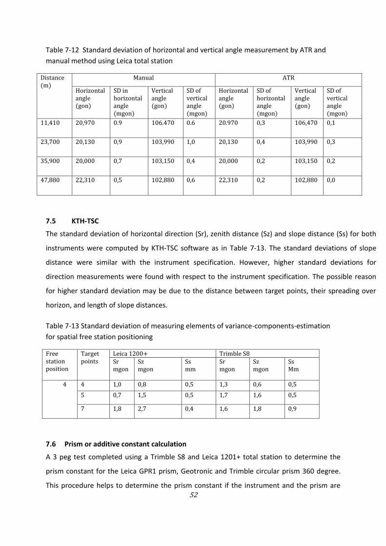
52

Table 7-12 Standard deviation of horizontal and vertical angle measurement by ATR and

manual method using Leica total station

Distance (m)

Manual ATR

Horizontal angle (gon)

SD in horizontal angle (mgon)

Vertical angle (gon)

SD of vertical angle (mgon)

Horizontal angle (gon)

SD of horizontal angle (mgon)

Vertical angle (gon)

SD of vertical angle (mgon)

11,410 20,970 0.9 106.470 0.6 20.970 0,3 106,470 0,1

23,700 20,130 0,9 103,990 1,0 20,130 0,4 103,990 0,3

35,900 20,000 0,7 103,150 0,4 20,000 0,2 103,150 0,2

47,880 22,310 0,5 102,880 0,6 22,310 0,2 102,880 0,0

7.5 KTH-TSC

The standard deviation of horizontal direction (Sr), zenith distance (Sz) and slope distance (Ss) for both

instruments were computed by KTH-TSC software as in Table 7-13. The standard deviations of slope

distance were similar with the instrument specification. However, higher standard deviations for

direction measurements were found with respect to the instrument specification. The possible reason

for higher standard deviation may be due to the distance between target points, their spreading over

horizon, and length of slope distances.

Table 7-13 Standard deviation of measuring elements of variance-components-estimation

for spatial free station positioning

Free station position

Target points

Leica 1200+ Trimble S8 Sr mgon

Sz mgon

Ss mm

Sr mgon

Sz mgon

Ss Mm

4 4 1,0 0,8 0,5 1,3 0,6 0,5

5 0,7 1,5 0,5 1,7 1,6 0,5

7 1,8 2,7 0,4 1,6 1,8 0,9

7.6 Prism or additive constant calculation

A 3 peg test completed using a Trimble S8 and Leica 1201+ total station to determine the

prism constant for the Leica GPR1 prism, Geotronic and Trimble circular prism 360 degree.

This procedure helps to determine the prism constant if the instrument and the prism are

53

from different companies. The result shows that different instruments may give different

prism constant. This is because each total station have different offset from the centre of the

EDM.

The prism constant is computed by four, five and seven target points as in table 7-14 and 7-

15. The computed results at five and seven targets were similar. Therefore the prism

constant computed by seven targets will be the final result.

Table 7-14 Result of prism or additive constant using Leica total station

Number of targets Leica circular prism (mm)

Trimble circular prism 360 ° (mm)

Geotronic (mm)

3 2,0 34.5 35,0

4 1,7 34,6 34,6

5 1,2 34,5 34,2 7 1,0 34,2 34,2

Table 7-15 Result of prism or additive constant using Trimble total station

Number of targets Leica circular prism (mm)

Trimble circular prism 360 ° (mm)

Geotronic (mm)

3 -32,0 1,0 0,0

4 -32,6 1,8 0,0

5 -32,3 2,0 0,0

7 -32.3 1,9 0,0

54

Chapter Eight

8 Conclusions and Recommendations

8.1 Conclusions

This paper attempts to show the techniques of total station calibration and to investigate the

possible sources of error in reflectorless distance measurement. The effects of different

color targets and angle incidence on distance measurement were checked. The accuracy of

reflectorless distance measurement is also investigated. In addition, comparison was made

for manual and automatic target recognition measurement. Further experiment was

performed how to calibrate the total station instrument.

The experiments were evaluated by taking the reflector reading as true value. The effect of

colour surfaces on distance measurement was found statistically equal. In addition, when we

check the effect of angle of incidence on distance measurement, the result shows the error

in distance increased as the incident angle in the target increases. The result also shows that

automatic target recognition mode is the most advisable technique for precise

measurement. In this study, we got seven targets as the optimal number of target points for

determination of the prism constant.

8.2 Recommendations

Based on our study and result, we recommend the following:

Always first test the instrument when accurate reflectorless observations are

required.

If possible, it is good to avoid higher angle of incidence of targets for reflectorless

measurement.

To calibrate your instrument one can use KTH-TSC software by measuring slope

distance, horizontal and vertical angles towards targets.

55

9 References

Bayoud Fadi A. (2006), Leica’s Pinpoint EDM Technology with Modified Signal Processing and

Novel Opt mechanical Features, XXIII FIG Congress, Munich, Germany.

Beshr A. A. A., Elnaga I. M. A. (2011), Investigating the accuracy of digital levels and reflector

less total stations for purposes of geodetic engineering, Alexandria University,

doi:10.1016/j.aej.2011.12.004.

Fan H. (1997) Theory of Error and Least Square Adjustment, Royal Institute of Technology (KTH) Division of Geodesy and Geoinformatics, Stockholm, Sweden.

Höglund R. and Large P. (2005), Direct reflex EDM technology for the surveyor and civil

enginer, Trimble survey, Westminster, Colorado,USA.

Horemuz M. and Kampmann G. G. (2005), About system-verification of electronic total

stations for practical evaluation and verification, Royal Institute of Technology (KTH), Division

of Geodesy and Geoinformatics, Stockholm, Sweden.

Mao J. and Nindl D. (2009), Surveying Reflectors -White Paper: Characteristics and

Influences, Leica Geosystem AG, Heerbrugg, Switzerland.

Schofield W. and Breach M. (2007), Engineering Surveying, Sixth Edition, Elsevier, Oxford, UK

Schulz T. (2007), Calibration of a Terrestrial Laser Scanner for Engineering Geodesy, Doctoral Dissertation, ETH ZURICH. Dipl.-Ing., Technical University of Berlin, DISS.ETH NO.17036

Soudarissanane S., Lindenbergh R., Menenti M. and Teunissen P. (2009), Incidence angle

influence on the quality of teresterial laser scanning point, Delft Institute of Earth

Observation and Space Systems(DEOS), Delft University of Technology, Netherland.

56

Staiger R. (2007), Recommended procedures for routine checks of electro-optical distance

meters. International Federation of Surveyors (FIG), M A R Cooper, City University London.

Teskey W. F. and Radovanovic R. S. (2001), Free station method of leveling. Journal of

Surveying Engineering, Vol. 127, No. 1.

Tulloch J. E. (2012), EDM Calibration Handbook, Department of Sustainability and

Environment. Surveyor-General Victoria, Melbourne Victoria.

Xia Z., Luo Y., Zheng Y. and Pan H. (2006), Error analysis of a reflector in total station angle

measurement. Third International Symposium on Precision Mechanical Measurements, doi:

10.1117/12.716307, Vol. 6280 62802X-1.

Laser beam divergence and spot size,

www.amrita.vlab.co.in/?sub=1&brch=189&sim=342&cnt=1(visited on May 2012)

Leica Prism Constant,

http://geomatics360.com/wp-

content/themes/lifestyle/pdfs/Accessories/Prisms/Leica_Prism_Constant.pdf (visited on

June 2012)

Total Station

www.faculty.evc.edu/z.yu/nsf2/Curriculum%20modules/Module%201.pdf (Visited on

Feb 2012)

Trimble Prism Constant,

http://www.geosoft.ee/UserFiles/File/Juhendid/Tahhumeetrid/Elta_CU_User.pdf (visited on

June 2012)