http://www.cambridge.org/9780521620536

This page intentionally left blank

Cambridge, New York, Melbourne, Madrid, Cape Town, Singapore, São Paulo

Cambridge University PressThe Edinburgh Building, Cambridge , United Kingdom

First published in print format

- ----

- ----

- ----

© Cambridge University Press 2002

2002

Information on this title: www.cambridge.org/9780521620536

This book is in copyright. Subject to statutory exception and to the provision ofrelevant collective licensing agreements, no reproduction of any part may take placewithout the written permission of Cambridge University Press.

- ---

- ---

- ---

Cambridge University Press has no responsibility for the persistence or accuracy ofs for external or third-party internet websites referred to in this book, and does notguarantee that any content on such websites is, or will remain, accurate or appropriate.

Published in the United States of America by Cambridge University Press, New York

www.cambridge.org

hardback

paperbackpaperback

eBook (EBL)eBook (EBL)

hardback

Contents

Preface to the first edition page ixPreface to the second edition xiPreface to the third edition xiii

1 ACCRETION AS A SOURCE OF ENERGY 11.1 Introduction 1

1.2 The Eddington limit 2

1.3 The emitted spectrum 5

1.4 Accretion theory and observation 6

2 GAS DYNAMICS 82.1 Introduction 8

2.2 The equations of gas dynamics 8

2.3 Steady adiabatic flows; isothermal flows 11

2.4 Sound waves 12

2.5 Steady, spherically symmetric accretion 14

3 PLASMA CONCEPTS 233.1 Introduction 23

3.2 Charge neutrality, plasma oscillations and the Debye length 23

3.3 Collisions 26

3.4 Thermal plasmas: relaxation time and mean free path 30

3.5 The stopping of fast particles by a plasma 32

3.6 Transport phenomena: viscosity 34

3.7 The effect of strong magnetic fields 37

3.8 Shock waves in plasmas 41

4 ACCRETION IN BINARY SYSTEMS 484.1 Introduction 48

4.2 Interacting binary systems 48

4.3 Roche lobe overflow 49

4.4 Roche geometry and binary evolution 54

4.5 Disc formation 58

4.6 Viscous torques 63

4.7 The magnitude of viscosity 69

4.8 Beyond the α-prescription 71

4.9 Accretion in close binaries: other possibilities 73

Contents vii

5 ACCRETION DISCS 805.1 Introduction 80

5.2 Radial disc structure 80

5.3 Steady thin discs 84

5.4 The local structure of thin discs 88

5.5 The emitted spectrum 90

5.6 The structure of steady α-discs (the ‘standard model’) 93

5.7 Steady discs: confrontation with observation 98

5.8 Time dependence and stability 110

5.9 Dwarf novae 121

5.10 Irradiated discs 129

5.11 Tides, resonances and superhumps 139

5.12 Discs around young stars 148

5.13 Spiral shocks 150

6 ACCRETION ON TO A COMPACT OBJECT 1526.1 Introduction 152

6.2 Boundary layers 152

6.3 Accretion on to magnetized neutron stars and white dwarfs 158

6.4 Accretion columns: the white dwarf case 174

6.5 Accretion column structure for neutron stars 191

6.6 X-ray bursters 202

6.7 Black holes 207

6.8 Accreting binary systems with compact components 209

7 ACTIVE GALACTIC NUCLEI 2137.1 Observations 213

7.2 The distances of active galaxies 220

7.3 The sizes of active galactic nuclei 223

7.4 The mass of the central source 225

7.5 Models of active galactic nuclei 228

7.6 The gas supply 230

7.7 Black holes 234

7.8 Accretion efficiency 238

8 ACCRETION DISCS IN ACTIVE GALACTIC NUCLEI 2448.1 The nature of the problem 244

8.2 Radio, millimetre and infrared emission 246

8.3 Optical, UV and X-ray emission 247

8.4 The broad and narrow, permitted and forbidden 250

8.5 The narrow line region 252

8.6 The broad line region 255

8.7 The stability of AGN discs 265

9 ACCRETION POWER IN ACTIVE GALACTIC NUCLEI 2679.1 Introduction 267

9.2 Extended radio sources 267

9.3 Compact radio sources 272

9.4 The nuclear continuum 278

9.5 Applications to discs 281

viii Contents

9.6 Magnetic fields 285

9.7 Newtonian electrodynamic discs 287

9.8 The Blandford–Znajek model 289

9.9 Circuit analysis of black hole power 292

10 THICK DISCS 29610.1 Introduction 296

10.2 Equilibrium figures 298

10.3 The limiting luminosity 303

10.4 Newtonian vorticity-free torus 306

10.5 Thick accretion discs 309

10.6 Dynamical stability 314

10.7 Astrophysical implications 316

11 ACCRETION FLOWS 31911.1 Introduction 319

11.2 The equations 320

11.3 Vertically integrated equations – slim discs 323

11.4 A unified description of steady accretion flows 325

11.5 Stability 331

11.6 Optically thin ADAFs – similarity solutions 333

11.7 Astrophysical applications 334

11.8 Caveats and alternatives 337

11.9 Epilogue 342

Appendix Radiation processes 345Problems 350Bibliography 366Index 380

Preface to the first edition

The subject of this book is astrophysical accretion, especially in those circumstanceswhere accretion is believed to make an important contribution to the total light ofan astrophysical system. Our discussion therefore centres mainly on close binarysystems containing compact objects and on active nuclei. The reader is assumed topossess a basic knowledge of physics at first degree level, but only a rudimentaryexperience of astronomy is required. We have tried to concentrate on those features,particularly the basic physics, that are probably more firmly established; but thetreatment is necessarily somewhat heterogeneous. For example, there is by now atolerably coherent line of argument showing that the formation of an accretion discis very likely in many close binaries, and giving a plausible picture of what such adisc is like, at least in some simple cases. In other areas, such as accretion on tothe surface of a compact object, or in active nuclei, we are not so fortunate, and wemust work back and forth between theory and observation. Our aim is that the bookshould provide a systematic introduction to the subject for graduate students. Wehope it may also serve as a reference for interested astronomers in other fields, andthat selected material will be suitable for undergraduate options in astronomy.

In Chapters 2 and 3 we present introductory material on fluid dynamics and plasmaphysics. Many excellent texts exist in these areas, but they tend to be too detailed forour needs; we have tried to extract just those basic ideas necessary for the subsequentdiscussion, and to set them in an astrophysical context. We also need basic concepts ofradiation mechanisms and radiative transfer theory. These we have not attempted toexpound systematically since there are many books written for astrophysics studentswhich are suitable. For convenience we have collected some of the necessary resultsin an appendix. The astrophysics of stellar accretion is dealt with in Chapters 4 to6. Chapters 7 and 8 set the observational scene for two models of active nuclei (orpossibly for two aspects of a single model) considered in Chapters 9 and 10. In themain we have not given references to sources, since this would yield an enormous listout of keeping with the spirit of the book. Detailed references can be found in thereviews cited in the bibliography.

A final note on units and notation. For the most part astrophysicists use unitsbased on the cm, g, s (cgs system) when they are not indulging themselves in archaicastronomical conventions. The system one rarely sees in astrophysics is the otherwisestandard mks (SI) system. For ease of comparison with the astrophysical literature

x Preface to the first edition

we have quoted numerical values in cgs units. A special problem arises in electro-magnetism; here the formulae are different in the two systems. We have adopted thecompromise of giving the formulae in cgs units with a multiplicative conversion factorto mks units in square brackets. These factors always involve the quantities ε0, µ0 orc, and no confusion should arise with the use of square brackets in algebraic formulae.Also, we have followed the normal astrophysical usage of the symbols ‘∼’ and ‘∼=’ inalgebraic formulae; the former standing for ‘is of the order of’ of the latter for ‘isapproximately equal to’.

The idea for this book grew out of discussions with Dr Simon Mitton, whom weshould like to thank for his encouragement and advice. We have benefited from thecomments of our students, on whom some of the early versions of much of this materialwere tested. We also thank our scientific colleagues for much useful advice. We aregrateful to Diane Fabian for her help in seeing our final efforts through the Press.

Preface to the second edition

In the years since the first edition of this book appeared the study of astrophysicalaccretion has developed rapidly. Perhaps the most fundamental change has beenthe shift in attitude over active galaxies and quasars: the view that accretion is theenergy source is now effectively standard, and the emphasis is much more on closecomparison of observation and theory. This change, and the less spectacular but stillprofound one which has occurred in the study of close binary accretion, have beenlargely brought about by the wealth of new data accumulated in the interval. InX-rays, the ability of EXOSAT to observe continuously for as much as 3 to 4 dayswas a dramatic advance. In the optical, new instrumentation has produced far tighterobservational constraints on theory. Despite these challenges, the basic outlines of thetheory are still recognizably the same.

Of course our understanding is very incomplete. As the most glaring example, westill have essentially no idea what drives disc accretion; and there are new problemssuch as the dynamical stability of thick discs, or the nature of fieldline threading inmagnetic binaries. But it is now difficult to deny that some close binaries possess discsapproximately conforming to theoretical ideas; or that some kind of anisotropic accre-tion occurs in active galactic nuclei. Encouragingly, accretion theory is increasinglyintegrated into wider pictures of the relevant systems. The process is well advancedfor close binaries, particularly for the secular evolution of cataclysmic variables, andis in its early stages for active galaxies.

We were therefore very glad to have the chance to revise our book, and extremelygrateful to many colleagues who made suggestions for improvements. Inevitably thevast expansion of the subject has obliged us to be selective, and we have had to omitor curtail discussion of some topics. This is particularly true of fairly specialized areassuch as quasi-periodic oscillations in low-mass X-ray binaries, or the jets in SS 433(incidentally the subjects of two of EXOSAT’s more spectacular discoveries). We havecompletely rewritten Section 4.4, adding a discussion of secular binary evolution. InChapter 5 on accretion discs we have rewritten Section 5.7 on the confrontation withobservations, particularly of low-mass X-ray binaries, and added three new sections.Section 5.9 deals with tides and resonances and the phenomenon of superhumps. Muchof accretion disc theory is relevant to star formation, and Section 5.10 gives a briefintroduction. In Section 5.11 we discuss accretion via spiral shocks. In Chapter 6,

xii Preface to the second edition

Sections 6.3 (accretion on to magnetized neutron stars and white dwarfs) and 6.4(white dwarf column accretion) have been extensively revised.

The material on active galaxies has been subject to substantial rearrangement,reflecting the changing emphasis in the subject. In Chapter 7 we have added a newsection on the gas supply to the central engine. Chapter 8 includes an extendeddiscussion of the broad line region. New material on X-ray emission has been addedin Chapters 8 and 9, which now include a brief discussion of two-temperature discs(or ion tori) and slim discs.

Finally, Chapter 10 now includes a discussion of the instability of thick discs toglobal non-axisymmetric modes. This is treated in a new Section 10.6, and Section10.7 on astrophysical applications has been rewritten.

We have also added a selection of problems, of varying degrees of difficulty, whichwe hope will make the book more useful for teaching purposes.

We would particularly like to thank Mitch Begelman, Jean-Pierre Lasota, TakuyaMatsuda, Robert Connon Smith and Henk Spruit for pointing out errors in the firstedition and suggesting new material.

Preface to the third edition

In the decade since the second edition of this book, accretion has become a stillmore central theme of modern astrophysics. We now know for example that a γ-rayburst briefly emits a gravitationally powered luminosity rivalling the output of therest of the Universe. This and other startling discoveries are a result of observationalprogress, driven as ever by technological advances. But these advances are also havinga powerful effect on theory; modern supercomputers allow one to perform as a matterof routine calculations which were unthinkable a decade ago. This increasing capabilitywill significantly alter the way theory is done, and indeed thought about.

The impact on accretion theory has already been profound. Most obviously, super-computer simulations have been central in verifying that angular momentum trans-port in accretion discs is probably mediated by the magnetorotational instability. Thisopens the prospect of at last understanding how accretion is driven in the discs wesee.

These changes and others make a new edition of this book timely. We are gratefulfor the opportunity of revising and extending the treatments of the earlier editions.As always, we have been obliged to be selective, but have tried to convey the essenceof recent developments. In addition to discussing the new work on disc viscosityreferred to above, we give a more thorough treatment of the thermal–viscous discinstability model now generally thought to be the basic cause of the outbursts ofdwarf novae and soft X-ray transients. The importance of irradiation of an accretiondisc has been recognized in at least three ways, in affecting global stability properties,in drastically modifying outbursts when they occur, and in tending to make the discwarp. Accordingly we have added an extensive treatment of it. Since the secondedition, the presence of black holes in a significant number of low-mass X-ray binarieshas become widely accepted, and we comment on this changed situation.

The advance in our understanding of active galactic nuclei (AGN) has also beensignificant. There is now compelling observational evidence that most galaxies, eventhose outwardly normal, harbour a black hole whose mass correlates with the mass ofthe spheroidal component of the galaxy, and that all galaxies are active at some level.The Hubble Space Telescope has given clear evidence of discs, dusty tori and jets inactive galactic nuclei, and Chandra has detected the jet in Cen A. There is evidencefrom VLBI observations of Keplerian rotation in the central disc of the active galaxyNGC 4258. On the theory side, the main change is one of focus. Most AGN researchers

xiv Preface to the third edition

now seek to use the knowledge gained from the study of galactic sources. In particularthe majority of workers interpret observations in terms of the kinds of accretion discsfamiliar from those objects, unless there are good reasons to do otherwise. Progresshas been relatively slow in optical spectroscopy and the understanding of strong radiosources, but these are still important for a unified picture, so the basic theory remainsrelevant. The increasing wealth of detailed X-ray observations are likely to providethe most important information on the structure of both galactic and extragalacticblack hole accretion.

Despite recent progress, we still do not know the functional form of the viscosityin an accretion disc. This freedom allows the possibility of several alternative typesof accretion flow, often referred to by acronyms such as ADAF, CDAF, etc. We haveadded a new chapter dealing with these. Finally, we have updated and extended therange of problems at the end of the book.

In line with the remarks above, we have tried to make use of supercomputersimulations to illustrate much of what we say. Interested readers can view anima-tions of many of these flows on the websites of the UK Astrophysical Fluids Facility(http://www.ukaff.ac.uk/movies.shtml) and of the LSU Astrophysics Theory Group(http://www.phys.lsu.edu/astro/home.html).

We thank the many colleagues who offered valuable advice and encouragement aswe prepared this edition. We thank CUP for their forebearance during this process.In particular we are grateful to our copy-editor, Margaret Patterson, for her veryprofessional work on the text.

1 Accretion as a source of energy

1.1 Introduction

For the nineteenth century physicists, gravity was the only conceivable source of en-ergy in celestial bodies, but gravity was inadequate to power the Sun for its knownlifetime. In contrast, at the beginning of the twenty-first century it is to gravity thatwe look to power the most luminous objects in the Universe, for which the nuclearsources of the stars are wholly inadequate. The extraction of gravitational potentialenergy from material which accretes on to a gravitating body is now known to bethe principal source of power in several types of close binary systems, and is widelybelieved to provide the power supply in active galactic nuclei and quasars. This in-creasing recognition of the importance of accretion has accompanied the dramaticexpansion of observational techniques in astronomy, in particular the exploitation ofthe full range of the electromagnetic spectrum from the radio to X-rays and γ-rays.At the same time, the existence of compact objects has been placed beyond doubtby the discovery of the pulsars, and black holes have been given a sound theoreticalstatus. Thus, the new role for gravity arises because accretion on to compact objectsis a natural and powerful mechanism for producing high-energy radiation.

Some simple order-of-magnitude estimates will show how this works. For a body ofmass M and radius R∗ the gravitational potential energy released by the accretion ofa mass m on to its surface is

∆Eacc = GMm/R∗ (1.1)

where G is the gravitation constant. If the accreting body is a neutron star withradius R∗ ∼ 10 km, mass M ∼ M, the solar mass, then the yield ∆Eacc is about1020 erg per accreted gram. We would expect this energy to be released eventuallymainly in the form of electromagnetic radiation. For comparison, consider the energythat could be extracted from the mass m by nuclear fusion reactions. The maximumis obtained if, as is usually the case in astrophysics, the material is initially hydrogen,and the major contribution comes from the conversion, (or ‘burning’), of hydrogen tohelium. This yields an energy release

∆Enuc = 0.007mc2 (1.2)

where c is the speed of light, so we obtain about 6×1018 erg g−1 or about one twentiethof the accretion yield in this case.

2 Accretion as a source of energy

It is clear from the form of equation (1.1) that the efficiency of accretion as an energyrelease mechanism is strongly dependent on the compactness of the accreting object:the larger the ratio M/R∗, the greater the efficiency. Thus, in treating accretion on toobjects of stellar mass we shall certainly want to consider neutron stars (R∗ ∼ 10 km)and black holes with radii R∗ ∼ 2GM/c2 ∼ 3(M/M) km (see Section 7.7). Forwhite dwarfs with M ∼ M, R∗ ∼ 109 cm, nuclear burning is more efficient thanaccretion by factors 25–50. However, it would be wrong to conclude that accretion onto white dwarfs is of no great importance for observations, since the argument takes noaccount of the timescale over which the nuclear and accretion processes act. In fact,when nuclear burning does occur on the surface of a white dwarf, it is likely that thereaction tends to ‘run away’ to produce an event of great brightness but short duration,a nova outburst, in which the available nuclear fuel is very rapidly exhausted. Foralmost all of its lifetime no nuclear burning occurs, and the white dwarf (may) derive itsentire luminosity from accretion. Binary systems in which a white dwarf accretes froma close companion star are known as cataclysmic variables and are quite common inthe Galaxy. Their importance derives partly from the fact that they provide probablythe best opportunity to study the accretion process in isolation, since other sources ofluminosity, in particular the companion star, are relatively unimportant.

For accretion on to a ‘normal’, less compact, star, such as the Sun, the accretionyield is smaller than the potential nuclear yield by a factor of several thousand. Evenso, accretion on to such stars may be of observational importance. For example, abinary system containing an accreting main-sequence star has been proposed as amodel for the so-called symbiotic stars.

For a fixed value of the compactness, M/R∗, the luminosity of an accreting systemdepends on the rate M at which matter is accreted. At high luminosities, the accretionrate may itself be controlled by the outward momentum transferred from the radiationto the accreting material by scattering and absorption. Under certain circumstances,this can lead to the existence of a maximum luminosity for a given mass, usuallyreferred to as the Eddington luminosity, which we discuss next.

1.2 The Eddington limit

Consider a steady spherically symmetrical accretion; the limit so derived will be gen-erally applicable as an order-of-magnitude estimate. We assume the accreting ma-terial to be mainly hydrogen and to be fully ionized. Under these circumstances,the radiation exerts a force mainly on the free electrons through Thomson scatter-ing, since the scattering cross-section for protons is a factor (me/mp)2 smaller, whereme/mp

∼= 5 × 10−4 is the ratio of the electron and proton masses. If S is the ra-diant energy flux (erg s−1cm−2) and σT = 6.7 × 10−25 cm2 is the Thomson cross-section, then the outward radial force on each electron equals the rate at which itabsorbs momentum, σTS/c. If there is a substantial population of elements otherthan hydrogen, which have retained some bound electrons, the effective cross-section,

1.2 The Eddington limit 3

resulting from the absorption of photons in spectral lines, can exceed σT consider-ably. The attractive electrostatic Coulomb force between the electrons and protonsmeans that as they move out the electrons drag the protons with them. In effect,the radiation pushes out electron–proton pairs against the total gravitational forceGM(mp + me)/r2 ∼= GMmp/r2 acting on each pair at a radial distance r from thecentre. If the luminosity of the accreting source is L(erg s−1), we have S = L/4πr2

by spherical symmetry, so the net inward force on an electron–proton pair is(GMmp − LσT

4πc

)1r2

.

There is a limiting luminosity for which this expression vanishes, the Eddington limit,

LEdd = 4πGMmpc/σT (1.3)∼= 1.3 × 1038(M/M) erg s−1. (1.4)

At greater luminosities the outward pressure of radiation would exceed the inwardgravitational attraction and accretion would be halted. If all the luminosity of thesource were derived from accretion this would switch off the source; if some, or all, ofit were produced by other means, for example nuclear burning, then the outer layersof material would begin to be blown off and the source would not be steady. For starswith a given mass–luminosity relation this argument yields a maximum stable mass.

Since LEdd will figure prominently later, it is worth recalling the assumptions madein deriving expressions (1.3,1.4). We assumed that the accretion flow was steady andspherically symmetric. A slight extension can be made here without difficulty: if theaccretion occurs only over a fraction f of the surface of a star, but is otherwise de-pendent only on radial distance r, the corresponding limit on the accretion luminosityis fLEdd. For a more complicated geometry, however, we cannot expect (1.3,1.4) toprovide more than a crude estimate. Even more crucial was the restriction to steadyflow. A dramatic illustration of this is provided by supernovae, in which LEdd isexceeded by many orders of magnitude. Our other main assumptions were that theaccreting material was largely hydrogen and that it was fully ionized. The former isalmost always a good approximation, but even a small admixture of heavy elementscan invalidate the latter. Almost complete ionization is likely to be justified howeverin the very common case where the accreting object produces much of its luminosityin the form of X-rays, because the abundant ions can usually be kept fully stripped ofelectrons by a very small fraction of the X-ray luminosity. Despite these caveats, theEddington limit is of great practical importance, in particular because certain types ofsystem show a tendency to behave as ‘standard candles’ in the sense that their typicalluminosities are close to their Eddington limits.

For accretion powered objects the Eddington limit implies a limit on the steadyaccretion rate, M(g s−1). If all the kinetic energy of infalling matter is given up toradiation at the stellar surface, R∗, then from (1.1) the accretion luminosity is

Lacc = GMM/R∗. (1.5)

4 Accretion as a source of energy

It is useful to re-express (1.5) in terms of typical orders of magnitude: writing theaccretion rate as M = 1016M16 g s−1 we have

Lacc = 1.3 × 1033M16(M/M)(109 cm/R∗) erg s−1 (1.6)

= 1.3 × 1036M16(M/M)(10 km/R∗) erg s−1. (1.7)

The reason for rewriting (1.5) in this way is that the quantities (M/M),(109 cm/R∗) and (M/M), (10 km/R∗) are of order unity for white dwarfs and neu-tron stars respectively. Since 1016 g s−1(∼ 1.5 × 10−10M yr−1) is a typical order ofmagnitude for accretion rates in close binary systems involving these types of star, wehave M16 ∼ 1 in (1.6,1.7), and the luminosities 1033 erg s−1, 1036 erg s−1 representvalues commonly found in such systems. Further, by comparison with (1.4) it is im-mediately seen that for steady accretion M16 is limited by the values ∼ 105 and 102

respectively. Thus, accretion rates must be less than about 1021 g s−1 and 1018 g s−1

in the two types of system if the assumptions involved in deriving the Eddington limitare valid.

For the case of accretion on to a black hole it is far from clear that (1.5) holds. Sincethe radius does not refer to a hard surface but only to a region into which matter canfall and from which it cannot escape, much of the accretion energy could disappearinto the hole and simply add to its mass, rather than be radiated. The uncertainty inthis case can be parametrized by the introduction of a dimensionless quantity η, theefficiency, on the right hand side of (1.5):

Lacc = 2ηGMM/R∗ (1.8)

= ηMc2 (1.9)

where we have used R∗ = 2GM/c2 for the black hole radius. Equation (1.9) showsthat η measures how efficiently the rest mass energy, c2 per unit mass, of the accretedmaterial is converted into radiation. Comparing (1.9) with (1.2) we see that η = 0.007for the burning of hydrogen to helium. If the material accreting on to a black holecould be lowered into the hole infinitesimally slowly - scarcely a practical proposition -all of the rest mass energy could, in principle, be extracted and we should have η = 1.As we shall see in Chapter 7 the estimation of realistic values for η is an importantproblem. A reasonable guess would appear to be η ∼ 0.1, comparable to the valueη ∼ 0.15 obtained from (1.8) for a solar mass neutron star. Thus, despite its extracompactness, a stellar mass black hole may be no more efficient in the conversion ofgravitational potential energy to radiation than a neutron star of similar mass.

As a final illustration here of the use of the Eddington limit we consider the nucleiof active galaxies and the closely related quasars. These are probably the least under-stood class of object for which accretion is thought to be the ultimate source of energy.The main reason for this belief comes from the large luminosities involved: these sys-tems may reach 1047 erg s−1, or more, varying by factors of order 2 on timescales ofweeks, or less. With the nuclear burning efficiency of only η = 0.007, the rate at whichmass is processed in the source could exceed 250 M yr−1. This is a rather severe

1.3 The emitted spectrum 5

requirement and it is clearly greatly reduced if accretion with an efficiency η ∼ 0.1 ispostulated instead. The accretion rate required is of order 20 M yr−1, or less, andrates approaching this might plausibly be provided by a number of the mechanismsconsidered in Chapter 7. If these systems are assumed to radiate at less than theEddington limit, then accreting masses exceeding about 109M are required. Whitedwarfs are subject to upper limits on their masses of 1.4 M and neutron stars can-not exceed about 3 M thus, only massive black holes are plausible candidates foraccreting objects in active galactic nuclei.

1.3 The emitted spectrum

We can now make some order-of-magnitude estimates of the spectral range of theemission from compact accreting objects, and, conversely, suggest what type of com-pact object may be responsible for various observed behaviour. We can characterizethe continuum spectrum of the emitted radiation by a temperature Trad defined suchthat the energy of a typical photon, hν, is of order kTrad, Trad = hν/k, where wedo not need to make the choice of ν precise. For an accretion luminosity Lacc froma source of radius R, we define a blackbody temperature Tb as the temperature thesource would have if it were to radiate the given power as a blackbody spectrum:

Tb = (Lacc/4πR2∗σ)1/4. (1.10)

Finally, we define a temperature Tth that the accreted material would reach ifits gravitational potential energy were turned entirely into thermal energy. Foreach proton–electron pair accreted, the potential energy released is GM(mp +me)/R∗ ∼= GMmp/R∗, and the thermal energy is 2 × 3

2kT ; therefore

Tth = GMmp/3kR∗. (1.11)

Note that some authors use the related concept of the virial temperature, Tvir = Tth/2,for a system in mechanical and thermal equilibrium. If the accretion flow is opticallythick, the radiation reaches thermal equilibnum with the accreted material beforeleaking out to the observer and Trad ∼ Tb. On the other hand, if the accretion energyis converted directly into radiation which escapes without further interaction (i.e. theintervening material is optically thin), we have Trad ∼ Tth. This occurs in certaintypes of shock wave that may be produced in some accretion flows and we shall see inChapter 3 that (1.11) provides an estimate of the shock temperature for such flows.In general, the radiation temperature may be expected to lie between the thermal andblackbody temperatures, and, since the system cannot radiate a given flux at less thanthe blackbody temperature, we have

Tb ∼< Trad ∼< Tth.

Of course, these estimates assume that the radiating material can be characterizedby a single temperature. They need not apply, for example, to a non-Maxwellian

6 Accretion as a source of energy

distribution of electrons radiating in a fixed magnetic field, such as we shall meet inChapter 9.

Let us apply the limits (1.10), (1.11) to the case of a solar mass neutron star. Theupper limit (1.11) gives Tth ∼ 5.5×1011 K, or, in terms of energies, kTth ∼50 MeV. Toevaluate the lower limit, Tb, from (1.10), we need an idea of the accretion luminosity,Lacc; but Tb is, in fact, very insensitive to the assumed value of Lacc, since it is pro-portional to the fourth root. Thus we can take Lacc ∼ LEdd ∼1038 erg s−1 for a roughestimate; if, instead, we were to take a typical value ∼1036 erg s−1 (equation (1.10))this would change Tb only by a factor of ∼ 3. We obtain Tb ∼107K or kTb ∼1 keV,and so we expect photon energies in the range

1 keV ∼< hν ∼< 50 MeV

as a result of accretion on to neutron stars. Similar results would hold for stellar massblack holes. Thus we can expect the most luminous accreting neutron star and blackhole binary systems to appear as medium to hard X-ray emitters and possibly as γ-ray sources. There is no difficulty in identifying this class of object with the luminousgalactic X-ray sources discovered by the first satellite X-ray experiments, and addedto by subsequent investigations.

For accreting white dwarfs it is probably more realistic to take Lacc ∼1033 erg s−1

in estimating Tb (cf. (1.6)). With M = M, R∗ = 5 × 108 cm, we obtain

6 eV ∼< hν ∼< 100 keV.

Consequently, accreting white dwarfs should be optical, ultraviolet and possibly X-ray sources. This fits in neatly with our knowledge of cataclysmic variable stars,which have been found to have strong ultraviolet continua by the Copernicus andIUE satellite experiments. In addition, some of them are now known to emit a smallfraction of their luminosity as thermal X-ray sources. We shall see that in many wayscataclysmic variables are particularly useful in providing observational tests of theoriesof accretion.

1.4 Accretion theory and observation

So far we have discussed the amount of energy that might be expected by the accretionprocess, but we have made no attempt to describe in detail the flow of accretingmatter. A hint that the dynamics of this flow may not be straightforward is providedby the existence of the Eddington limit, which shows that, at least for high accretionrates, forces other than gravity can be important. In addition, it will emerge laterthat, certainly in many cases and probably in most, the accreting matter possessesconsiderable angular momentum per unit mass which, in realistic models, it has tolose in order to be accreted at all. Furthermore, we need a detailed description of theaccretion flow if we are to explain the observed spectral distribution of the radiationproduced: crudely speaking, in the language of Section 1.3, we want to know whetherTrad is closer to Tb or Tth.

1.4 Accretion theory and observation 7

The two main tools we shall use in this study are the equations of gas dynamics andthe physics of plasmas. We shall give a brief introduction to gas dynamics in Sections2.1–2.4 of the next chapter, and treat some aspects of plasma physics in Chapter3. In addition, the elements of the theory of radiative transfer are summarized in theAppendix. The reader who is already familiar with these subjects can omit these partsof the text. The rest of the book divides into three somewhat distinct parts. First, inChapters 4 to 6 we consider accretion by stellar mass objects in binary systems. Inthese cases, we often find that observations provide fairly direct evidence for the natureof the systems. For example, there is sometimes direct evidence for the importanceof angular momentum and the existence of accretion discs. This contrasts greatlywith the subsequent discussion of active galactic nuclei in Chapters 7 to 10. Here, theaccretion theory arises at the end of a sequence of plausible, but not unproblematic,inductions. Furthermore, there appears to be no absolutely compelling evidence for, oragainst, the existence of accretion discs in these systems. Thus, whereas we normallyuse the observations of stellar systems to test the theory, for active nuclei we use thetheory, to some extent, to illustrate the observations. This is particularly apparent inthe final part of the book, where, in Chapters 9 and 10, we discuss two quite differentmodels for powering an active nucleus by an accretion disc around a supermassiveblack hole. Finally, in Chapter 11 we review all possible accretion flows, most ofwhich have already been studied in earlier chapters, classifying them according towhich physical effects dominate their properties and behaviour. We also describe insome detail recent advances in our understanding of accretion flows, with particularemphasis on the class of advection dominated accretion flows or ADAFs.

2 Gas dynamics

2.1 Introduction

All accreting matter, like most of the material in the Universe, is in a gaseous form.This means that the constituent particles, usually free electrons and various species ofions, interact directly only by collisions, rather than by more complicated short-rangeforces. In fact, these collisions involve the electrostatic interaction of the particlesand will be considered in more detail in Chapter 3. On average, a gas particle willtravel a certain distance, the mean free path, λ, before changing its state of motion bycolliding with another particle. If the gas is approximately uniform over lengthscalesexceeding a few mean free paths, the effect of all these collisions is to randomize theparticle velocities about some mean velocity, the velocity of the gas, v. Viewed ina reference frame moving with velocity v, the particles have a Maxwell–Boltzmanndistribution of velocities, and can be described by a temperature T . Provided weare interested only in lengthscales L λ we can regard the gas as a continuousfluid, having velocity v, temperature T and density ρ defined at each point. We thenstudy the behaviour of these and other fluid variables as functions of position andtime by imposing the laws of conservation of mass, momentum and energy. This isthe subject of gas dynamics. If we wish to look more closely at the gas, we have toconsider the particle interactions in more detail; this is the domain of plasma physics,or, more strictly, plasma kinetic theory, about which we shall have something to say inChapter 3. Note that the equations of gas dynamics may not always be applicable. Forexample, these equations may themselves predict large changes in gas properties overlengthscales comparable with λ; under these circumstances the fluid approximationis invalid and we must use the deeper but more complicated approach of the plasmakinetic theory.

2.2 The equations of gas dynamics

Here we shall write down the three conservation laws of gas dynamics, which, togetherwith an equation of state and appropriate boundary conditions, describe any gasdynamical flow. We shall not give the derivations, which can be found in many books,for example Landau & Lifshitz, 1959, but merely point out the significance of thevarious terms.

Given a gas with, as before, a velocity field v, density ρ and temperature T , all

2.2 The equations of gas dynamics 9

defined as functions of position r and time t, conservation of mass is ensured by thecontinuity equation:

∂ρ

∂t+ ∇ · (ρv) = 0. (2.1)

Because of the thermal motion of its particles the gas has a pressure P at each point.An equation of state relates this pressure to the density and temperature. Astrophys-ical gases, other than the degenerate gases in white dwarfs and neutron stars and thecores of ‘normal’ stars, have as equation of state the perfect gas law:

P = ρkT/µmH. (2.2)

Here mH ∼ mp is the mass of the hydrogen atom and µ is the mean molecular weight,which is the mean mass per particle of gas measured in units of mH or, equivalently,the inverse of the number of particles in a mass mH of the gas. Hence, µ = 1 for neutralhydrogen, 1

2 for fully ionized hydrogen, and something in between for a mixture ofgases with cosmic abundances, depending on the ionization state.

Gradients in the pressure in the gas imply forces since momentum is thereby trans-ferred. Other, as yet unspecified, forces acting on the gases are represented by theforce density, the force per unit volume, f. Conservation of momentum for each gaselement then gives the Euler equation:

ρ∂v∂t

+ ρv · ∇v = −∇P + f . (2.3)

This has the form (mass density) × (acceleration) = (force density) and is, in fact,simply an expression of Newton’s second law for a continuous fluid. The term ρv · ∇von the left hand side of (2.3) represents the convection of momentum through thefluid by velocity gradients. The presence of this term means that steady motionsare possible in which the time derivatives of the fluid variables vanish, but v is non-zero. An example of an external force is gravity: in this case f = −ρg, where g isthe local acceleration due to gravity. Another example would be the force due to anexternal magnetic field. Further important contributions to f can come from viscosity,which is the transfer of momentum along velocity gradients by random motions ofthe gas, especially turbulence and thermal motions. The inclusion of viscosity usuallyconsiderably complicates the momentum balance equation, so it is fortunate that inmany cases it may be neglected. We anticipate some later results by stating thatviscous effects are chiefly important in flows which show either large shearing motionsor steep velocity gradients.

The third, and most complicated, conservation law is that of energy. An elementof gas has two forms of energy: an amount 1

2ρv2 of kinetic energy per unit volume,and internal or thermal energy ρε per unit volume, where ε, the internal energy perunit mass, depends on the temperature T of the gas. According to the equipartitiontheorem of elementary kinetic theory, each degree of freedom of each gas particle isassigned a mean energy 1

2kT . For a monatomic gas the only degrees of freedom arethe three orthogonal directions of translational motion and

10 Gas dynamics

ε =32

kT/µmH. (2.4)

Molecular gases have additional internal degrees of freedom of vibration or rotation.In reality, cosmic gases are not quite monatomic and the effective number of degreesof freedom is not quite three; but in practice (2.4) is usually a good approximation.

The energy equation for the gas is

∂

∂t

(12

ρv2 + ρε)

+ ∇ ·[(1

2ρv2 + ρε + P

)v]

= f · v −∇ · Frad −∇ · q. (2.5)

The left hand side shows a family resemblance to the continuity equation (2.1), withthe expected difference that the conserved quantity ρ is replaced by (12ρv2 + ρε).The last term in the square brackets represents the so-called pressure work. Twonew quantities appear on the right hand side: first, the radiative flux vectorFrad=

∫dν

∫dΩnIν(n, r) where Iν is the specific intensity of radiation at the point

r in the direction n and the integrals are over frequency ν and solid angle Ω (seethe Appendix). The term −∇ · Frad gives the rate at which radiant energy is beinglost by emission, or gained by absorption, by unit volume of the gas. In general, thespecific intensity Iν is itself governed by a further equation, the conservation of energyequation for the radiation field. Fortunately, we can often approximate the radiativelosses quite simply. For example, let jν (erg s−1 cm−3 sr−1) be the rate of emissionof radiation per unit volume per unit solid angle; jν is the emissivity of the gas andis usually given as a function of ρ, T (and ν), but might also depend on externalmagnetic fields or the radiation field itself (examples are given in the Appendix). Ifthe gas is optically thin, so that radiation escapes freely once produced and the gasitself reabsorbs very little, the volume loss is just −∇ · Frad = −4π

∫jνdν. For a hot

gas radiating thermal bremsstrahlung (or ‘free–free radiation’), this has the approx-imate form constant ×ρ2T 1/2. At the opposite extreme, if the gas is very opticallythick, as in the interior of a star, then Frad approximates the blackbody flux and−∇ · Frad is given by the Rosseland approximation Frad = (16σ/3κRρ)T 3∇T whereκR is a weighted average over frequency of the opacity. This Rosseland approximationis discussed in any book on stellar structure (see the Appendix).

The second new quantity in the energy equation (2.5) is the conductive flux of heat,q. This measures the rate at which random motions, chiefly those of electrons, trans-port thermal energy in the gas and thus act to smooth out temperature differences.Standard kinetic theory (cf. equation (3.42)), shows that for an ionized gas obeyingthe requirement λ T/|∇T |

q ∼= −10−6T 5/2∇T erg s−1 cm−2. (2.6)

(See Section 3.6 for a discussion of transport processes.) Obviously the term −∇ · qraises the order of differentiation of T in the energy equation, so it is again fortunatethat, in many cases, temperature gradients are small enough that this term can beomitted from (2.5).

The system of equations (2.1)–(2.6), supplemented, if necessary, by the radiative

2.3 Steady adiabatic flows; isothermal flows 11

transfer equation and the specification of f, give, in principle, a complete descriptionof the behaviour of a gas under appropriate boundary conditions. Of course, in prac-tice one cannot hope to solve the equations in the fearsome generality in which theyhave been presented here, and all known solutions are either highly specialized orapproximate in some sense. To show how useful information can be extracted fromthese equations, we shall discuss a number of simple solutions. Some of these will beof considerable importance later.

2.3 Steady adiabatic flows; isothermal flows

Let us consider first steady flows, for which time derivatives are put equal to zero,and let us specialize to the case in which there are no losses through radiation and nothermal conduction.

Our three conservation laws of mass, momentum and energy then become

∇ · (ρv) = 0, (2.7)

ρ(v · ∇)v = −∇P + f , (2.8)

∇ ·[(1

2ρv2 + ρε + P

)v]

= f · v. (2.9)

Substituting the first of these equations in the third implies

ρv · ∇(1

2v2 + ε + P/ρ

)= f · v, (2.10)

while (2.8), the Euler equation, shows that f·v = ρv(v·∇)v + v·∇P = ρv·(12v2)+v·∇P ; hence, eliminating f·v from (2.10) we get

ρv · ∇(ε + P/ρ) = v · ∇P,

or, expanding ∇(P/ρ) and rearranging,

v · [∇ε + P∇(1/ρ)] = 0.

By the definition of the gradient operator, this means that, if we travel a small distancealong a streamline of the gas, i.e. if we follow the velocity v, the increments dε andd(1/ρ) in ε and 1/ρ must be related by

dε + P d(1/ρ) = 0.

But from the expression for the internal energy (2.4) and the perfect gas law (2.2) thisrequires that

32

dT + ρT d(1/ρ) = 0,

which is equivalent to

ρ−1T 3/2 = constant

or

12 Gas dynamics

P ρ−5/3 = constant (2.11)

using (2.2).Equation (2.11) describes the so-called adiabatic flows. Although we have demon-

strated only that the combination P ρ−5/3 is constant along a given streamline, inmany cases it is assumed that this constant is the same for each streamline, i.e. it isthe same throughout the gas. This condition is equivalent to setting the entropy ofthe gas constant. The resulting flows are called isentropic. Note that adiabatic andisentropic are often used synonymously in the literature.

In a sense, our derivation of the adiabatic law (2.11) is ‘back-to-front’, since ther-modynamic laws go into the construction of the energy equation (2.5). It is presentedhere to demonstrate the consistency of (2.5) with expectations from thermodynamics.If our gas were not monatomic, so that the numerical coefficient in (2.4) differed from32 , we would obtain a result like (2.11), but with a different exponent for ρ:

P ρ−γ = constant. (2.12)

In this form γ is known as the adiabatic index, or the ratio of specific heats. A furtherimportant special type of flow results from the assumption that the gas temperatureT is constant throughout the region of interest. This is called isothermal flow, andis obviously equivalent to postulating some unspecified physical process to keep T

constant. This, in turn, means that the energy equation (2.5) is replaced in our systemdescribing the gas by the relation T = constant. Formally, this latter requirement canbe written, using the perfect gas law (2.2), as

P ρ−1 = constant,

which has the form of (2.12) with γ = 1.

2.4 Sound waves

An obvious class of solution to our gas equations is that corresponding to hydrostaticequilibrium. In this case, in addition to the restriction to steady flow, and the absenceof losses assumed in Section 2.3 above, we take v = 0. Then the only equationremaining to be satisfied is (2.8), which reduces to

∇P = f ,

together with an explicit expression for f, and the perfect gas law (2.2). Solutionsof this type are, for example, appropriate to stellar, or planetary, atmospheres inradiative equilibrium.

Let us assume that we have such a solution, in which P and ρ are certain functionsof position, P0 and ρ0, and consider small perturbations about it. We set

P = P0 + P ′, ρ = ρ0 + ρ′, v = v′

2.4 Sound waves 13

where all the primed quantities are assumed small, so that we can neglect second andhigher order products of them. In place of the energy equation (2.5), we assume thatthe perturbations are adiabatic, or isothermal: in reality, either of these cases canoccur. Thus

P + P ′ = K(ρ + ρ′)γ , K = constant (2.13)

with γ = 53 (adiabatic) or γ = 1 (isothermal). Linearizing the continuity equation (2.1)

and the Euler equation (2.3), and using the fact that ∇P0 = f , we get

∂ρ′

∂t+ ρ0∇ · v′ = 0, (2.14)

∂v′

∂t+

1ρ0

∇P ′ = 0. (2.15)

From (2.13) P is purely a function of ρ, so ∇P ′ = (dP/dρ)0∇ρ′ to first order, wherethe subscript zero implies that the derivative is to be evaluated for the equilibriumsolution, i.e. (dP/dρ)0 = dP0/dρ0. Thus, (2.15) becomes

∂v′

∂t+

1ρ0

(dP

dρ

)0

∇ρ′ = 0. (2.16)

Eliminating v′ from (2.16) and (2.14) by operating with ∇· and ∂/∂t respectively andthen subtracting, gives

∂2ρ′

∂t2= c2s∇2ρ′, (2.17)

where we have defined

cs =(

dP

dρ

)1/2

0

. (2.18)

Equation (2.17) will be recognized as the wave equation, with the wave speed cs. It iseasy, now, to show that the other variables P ′, v′ obey similar equations; this impliesthat small perturbations about hydrostatic equilibrium propagate through the gas assound waves with speed cs. From (2.13), (2.18) we see that the sound speed cs canhave two values:

adiabatic : cads =(

5P

3ρ

)1/2

=(

5kT

3µmH

)1/2

∝ ρ1/3, (2.19)

isothermal : cisos =(

P

ρ

)1/2

=(

kT

µmH

)1/2

. (2.20)

The sound speeds cads , cisos , are basic quantities which can be defined locally at anypoint of a gas. Note first that both cads and cisos are of the order of the mean thermalspeed of the ions of the gas, cf. equation (2.4). Numerically,

cs ∼= 10(T/104K)1/2 km s−1 (2.21)

14 Gas dynamics

where cs stands for either sound speed.Since cs is the speed at which pressure disturbances travel through the gas, it limits

the rapidity with which the gas can respond to pressure changes. For example, if thepressure in one part of a region of the gas of characteristic size L is suddenly changed,the other parts of the region cannot respond to this change until a time of order L/cs,the sound crossing time, has elapsed. Conversely, if the pressure in one part of theregion is changed on a timescale much longer than L/cs the gas has ample time torespond by sending sound signals throughout the region, so the pressure gradient willremain small. Thus, if we consider supersonic flow, where the gas moves with |v| > cs,then the gas cannot respond on the flow time L/|v| < L/cs, so pressure gradients havelittle effect on the flow. At the other extreme, for subsonic flow with |v| < cs, the gascan adjust in less than the flow time, so to a first approximation the gas behaves as ifin hydrostatic equilibrium.

These properties can be inferred directly from an order-of-magnitude analysis ofthe terms in the Euler equation (2.3). For example, for supersonic flow we have

|ρ (v · ∇)v||∇P | ∼ v2/L

P/ρL∼ v2

c2s> 1

and pressure gradients can be neglected in a first approximation. A very importantproperty of the sound speed is its dependence on the gas density (2.19). This meansthat regions of higher than average density have higher than average sound speeds, afact which gives rise to the possibility of shock waves. In a shock the fluid quantitieschange on lengthscales of the order of the mean free path λ and this is representedas a discontinuity in the fluid. Shock waves are important in physics and astrophysicsand we shall return to them in Section 3.8.

2.5 Steady, spherically symmetric accretion

Let us now attack a real accretion problem and show how all of the apparatus wehave developed in Sections 2.1–2.4 can be put to use. We consider a star of mass M

accreting spherically symmetrically from a large gas cloud. This would be a reasonableapproximation to the real situation of an isolated star accreting from the interstellarmedium, provided that the angular momentum, magnetic field strength and bulk mo-tion of the interstellar gas with respect to the star could be neglected. For other typesof accretion flows, such as those in close binary systems and models of active galacticnuclei, spherical symmetry is rarely a good approximation, as we shall see. Nonethe-less, the spherical accretion problem is of very great significance for the theory, as itintroduces some important concepts which have much wider validity. Furthermore,it is possible to give a fairly exact treatment, allowing us to gain insight into morecomplicated problems. The problem of accretion of gas by a star in relative motionwith respect to the gas was first considered by Hoyle and Lyttleton (1939) and laterby Bondi and Hoyle (1944). The spherically symmetric case in a form similar to what

2.5 Steady, spherically symmetric accretion 15

is presented here arises when the accreting star is at rest with respect to the gas. Thiscase was first studied by Bondi (1952), and is referred to as Bondi accretion.

Let us ask what we might hope to discover by analysing this problem. First, weshould expect to be able to predict the steady accretion rate M (g s−1) on to our star,given the ambient conditions (the density ρ(∞) and the temperature T (∞)) in theparts of the gas cloud far from the star and some boundary conditions at its surface.Second, we might hope to learn how big a region of the gas cloud is influenced bythe presence of the star. These questions can be answered in a natural and physicallyappealing way. In addition, we shall obtain an understanding of the relation betweenthe gas velocity and the local sound speed which can be carried over quite generallyto more complicated accretion flows.

To treat the problem mathematically we take spherical polar coordinates (r, θ, φ)with origin at the centre of the star. The fluid variables are independent of θ and φ

by spherical symmetry, and the gas velocity has only a radial component vr = v. Wetake this to be negative, since we want to consider infall of material; v > 0 wouldcorrespond to a stellar wind. For steady flow, the continuity equation (2.1) reduces to

1r2

ddr

(r2ρv

)= 0 (2.22)

using the standard expression for the divergence of a vector in spherical polar coordi-nates. This integrates to r2ρv = constant. Since ρ(−v) is the inward flux of material,the constant here must be related to the (constant) accretion rate M ; the relation is

4πr2ρ(−v) = M. (2.23)

In the Euler equation the only contribution to the external force, f, is from gravity,and this has only a radial component

fr = −GMρ/r2

so that (2.3) becomes

vdv

dr+

1ρ

dP

dr+

GM

r2= 0. (2.24)

We replace the energy equation (2.5) by the polytropic relation (2.12):

P = Kργ , K = constant. (2.25)

This allows us to treat both approximately adiabatic (γ ∼= 53 ) and isothermal (γ ∼= 1)

accretion simultaneously. After the solution has been found, the adiabatic or isother-mal assumption should be justified by consideration of the particular radiative coolingand heating of the gas. For example, the adiabatic approximation will be valid if thetimescales for significant heating and cooling of the gas are long compared with thetime taken for an element of the gas to fall in. In reality, neither extreme is quitesatisfied, so we expect 1 < γ < 5

3 . In fact, the treatment we shall give is valid for1 < γ < 5

3 : the extreme values require special consideration (see e.g. (2.33), (2.34)).The interested reader may consult the article by Holzer & Axford (1970).

16 Gas dynamics

Finally, we can use the perfect gas law (2.2) to give the temperature

T = µmHP/ρk (2.26)

where P (r), ρ(r) have been found.The problem therefore reduces to that of integrating (2.24) with the help of (2.25)

and (2.23) and then identifying the unique solution corresponding to our accretionproblem. We shall integrate (2.24) shortly, but it is instructive to see how muchinformation can be extracted without explicit integration, since this technique is veryuseful in other cases when analytic integration is not possible, or not straightforward.We write first

dP

dr=

dP

dρ

dρ

dr= c2s

dρ

dr.

Hence, the term (1/ρ)(dP/dr) in the Euler equation (2.24) is (c2s/ρ)(dρ/dr). But,from the continuity equation (2.22),

1ρ

dρ

dr= − 1

vr2ddr

(vr2

).

Therefore, (2.24) becomes

vdv

dr− c2s

vr2dv

dr+

GM

r2= 0

which, after a little rearrangement, gives

12

(1 − c2s

v2

)ddr

(v2

)= −GM

r2

[1 −

(2c2sr

GM

)]. (2.27)

At first sight, we appear to have made things worse by these manipulations, since c2sis, in general, a function of r. However, the physical interpretation of cs as the soundspeed, plus the structure of equation (2.27), in which factors on either side can inprinciple vanish, allow us to sort the possible solutions of (2.27) into distinct classesand to pick out the unique one corresponding to our problem. First, we note thatat large distances from the star the factor [1 − (2c2sr/GM)] on the right hand sidemust be negative, since c2s approaches some finite asymptotic value c2s (∞) related tothe gas temperature far from the star, while r increases without limit. This meansthat for large r the right hand side of (2.27) is positive. On the left hand side, thefactor d(v2)/dr must be negative, since we want the gas far from the star to be atrest, accelerating as it approaches the star with r decreasing. These two requirements(d(v2)/dr < 0, the r.h.s. of (2.27)> 0) are compatible only if at large r the gas flow issubsonic, i.e.

v2 < c2s for large r. (2.28)

This is, of course, a very reasonable result, as the gas will have a non-zero temperatureand hence a non-zero sound speed far from the star. As the gas approaches the star,r decreases and the factor [1− (2c2sr/GM)] must tend to increase. It must eventually

2.5 Steady, spherically symmetric accretion 17

reach zero, unless some way can be found of increasing c2s sufficiently by heating thegas. This is very unlikely, since the factor reaches zero at a radius given by

rs =GM

2c2s (rs)∼= 7.5 × 1013

(T (rs)104 K

)−1(M

M

)cm (2.29)

where we have used (2.21) to introduce the temperature. The order of magnituders ∼= 7.5 × 1013 cm in (2.29) is so much larger than the radius, R∗, of any compactobject (R∗ ∼< 109 cm) that very high temperatures would be required to make rssmaller than R∗. In fact, it is clear from (2.16) and (1.7) that a gas temperature oforder Tth is required: this can be achieved, for example, in a standing shock waveclose to the stellar surface. We shall have much to say about this possibility later on,but it does not enter our analysis here as it requires discontinuous jumps in ρ, T , P ,etc. A similar analysis of the signs in (2.27) for r < rs shows that the flow must besupersonic near the star:

v2 > c2s for small r. (2.30)

The discussion above shows that the problem we are considering is not mathematicallywell posed if we only give the ambient conditions at infinity. To specify the problemcorrectly we need a condition at or near the stellar surface also. Here we have imposed(2.30), which will have the effect of picking out just one solution (Type 1 below).Without (2.30) there would be another possible solution (Type 3).

The existence of a point rs satisfying the implicit equation (2.29) is of great im-portance in characterizing the accretion flow. The direct mathematical consequenceis that at r = rs the left hand side of (2.27) must also vanish: this requires

either v2 = c2s at r = rs, (2.31)

orddr

(v2

)= 0 at r = rs. (2.32)

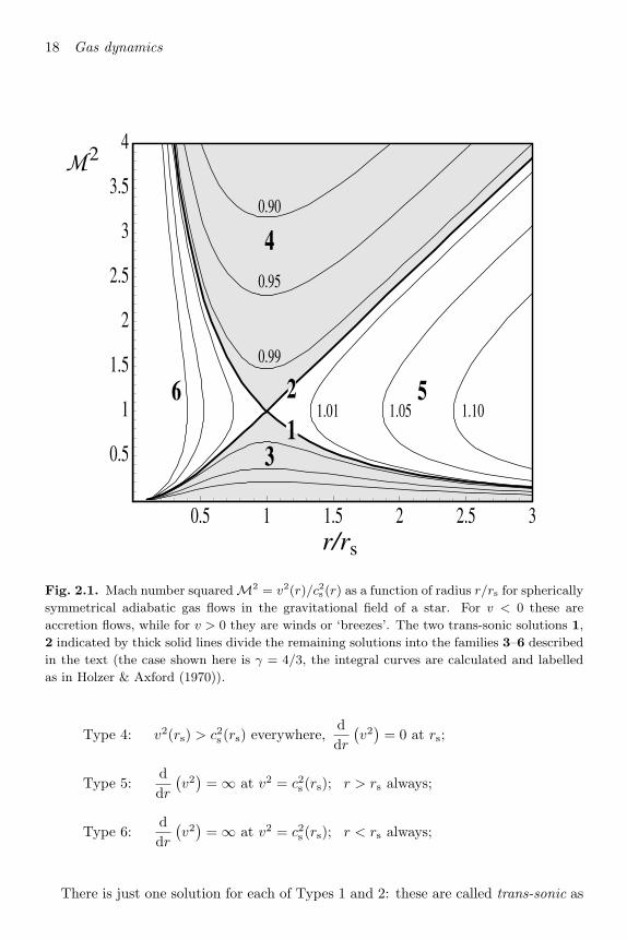
All solutions of (2.27) can now be classified by their behaviour at rs, given by either(2.31) or (2.32), together with their behaviour at large r; for example, (2.28). This isvery easy to see if we plot v2(r)/c2s (r) against r (Fig. 2.1).

From the figure it is clear that there are just six distinct families of solutions:

Type 1: v2(rs) = c2s (rs), v2 → 0 as r → ∞(v2 < c2s , r > rs; v2 > c2s , r < rs);

Type 2: v2(rs) = c2s (rs), v2 → 0 as r → 0(v2 > c2s , r > rs; v2 < c2s , r > rs);

Type 3: v2(rs) < c2s (rs) everywhere,ddr

(v2

)= 0 at rs;

18 Gas dynamics

0.5 1 1.5 2 2.5 3

0.5

1

1.5

2

2.5

3

3.5

4

0.99

0.95

0.90

1.01 1.05 1.10

4

3

56 2

1

M2

r/rs

Fig. 2.1. Mach number squaredM2 = v2(r)/c2s (r) as a function of radius r/rs for spherically

symmetrical adiabatic gas flows in the gravitational field of a star. For v < 0 these are

accretion flows, while for v > 0 they are winds or ‘breezes’. The two trans-sonic solutions 1,

2 indicated by thick solid lines divide the remaining solutions into the families 3–6 described

in the text (the case shown here is γ = 4/3, the integral curves are calculated and labelled

as in Holzer & Axford (1970)).

Type 4: v2(rs) > c2s (rs) everywhere,ddr

(v2

)= 0 at rs;

Type 5:ddr

(v2

)= ∞ at v2 = c2s (rs); r > rs always;

Type 6:ddr

(v2

)= ∞ at v2 = c2s (rs); r < rs always;

There is just one solution for each of Types 1 and 2: these are called trans-sonic as

2.5 Steady, spherically symmetric accretion 19

they make a transition between sub- and supersonic flow at rs; rs itself is known as thesonic point for these solutions. The occurrence of sonic points is a quite general featureof gas dynamical problems. Types 3 and 4 (shaded regions on Fig. 2.1) represent flowwhich is everywhere sub- or supersonic. Types 5 and 6 do not cover all of the range ofr and are double-valued in the sense that there are two possible values of v2 at a givenr. We exclude these last two for these reasons, although they can represent parts of acorrect solution if shocks are present. Types 2 and 4 must be excluded since they aresupersonic at large r, violating (2.28), while Type 3 is subsonic at small r, violating(2.30). A solution of Type 2 with v > 0 describes a stellar wind: note that (2.27)is unchanged for v → −v. Solutions of Type 3 with v > 0 give the so-called stellar‘breeze’ solutions which are everywhere subsonic; if v < 0 this is a slowly sinking‘atmosphere’.

We are left finally with just the Type 1 solution: this has all the properties we wantand is the unique solution to our problem. The sonic point condition (2.31) will leadus to the goal of relating the accretion rate M to the conditions at infinity.

With the question of uniqueness settled, we now integrate (2.24) directly, using thefact that (2.25) makes ρ a function of P :

v2

2+

∫dP

ρ− GM

r= constant.

From (2.25) we have dP = Kγργ−1dρ, and performing the integration, we obtain (forγ = 1)

v2

2+

Kγ

γ − 1ργ−1 − GM

r= constant.

But Kγργ−1 = γP/ρ = c2s , and we obtain the Bernoulli integral:

v2

2+

c2sγ − 1

− GM

r= constant. (2.33)

(The strictly isothermal (γ = 1) case gives a logarithmic integral.) From the knownproperty of our physical solution (Type 1) we have v2 → 0 as r → ∞, so the constantin (2.33) must be c2s (∞)/(γ − 1), where cs(∞) is the sound speed in the gas far awayfrom the star. The sonic point condition now relates cs(∞) to cs(rs), since (2.31),(2.29) imply v2(rs) = c2s (rs), GM/rs = 2c2s (rs), and the Bernoulli integral gives

c2s (rs)[

12

+1

γ − 1− 2

]=

c2s (∞)γ − 1

or

cs(rs) = cs(∞)(

25 − 3γ

)1/2

. (2.34)

We now obtain M from (2.23):

M = 4πr2ρ(−v) = 4πr2s ρ(rs)cs(rs) (2.35)

20 Gas dynamics

since M is independent of r. Using c2s ∝ ργ−1 we find

ρ(rs) = ρ(∞)[

cs(rs)cs(∞)

]2/(γ−1).

Putting this and (2.35) into (2.34) gives, after a little algebra, the relation we arelooking for between M and conditions at infinity:

M = πG2M2 ρ(∞)c3s (∞)

[2

5 − 3γ

](5−3γ)/2(γ−1). (2.36)

Note that the dependence on γ here is rather weak: the factor [2/(5−3γ)](5−3γ)/2(γ−1)

varies from unity in the limit γ = 53 to e3/2 ∼= 4.5 in the limit γ = 1. For a value

γ = 1.4, which would be typical for the adiabatic index of a part of the interstellarmedium, the factor is 2.5.

Equation (2.36) shows that accretion from the interstellar medium is unlikely to bean observable phenomenon; reasonable values would be cs(∞) = 10 km s−1, ρ(∞) =1024 g cm−3, corresponding to a temperature of about 10 K and number density near1 particle cm−3. Then (2.36) gives (with γ = 1.4)

M ∼= 1.4 × 1011(

M

M

)2(ρ(∞)10−24

)(cs(∞)

10 km s−1

)−3g s−1. (2.37)

From (1.46) even accreting this on to a neutron star yields Lacc only of the order2 × 1031 erg s−1; at a typical distance of 1 kpc this gives far too low a flux to bedetected.

To complete the solution of the problem to find the run of all quantities with r wecould now get v(r) in terms of cs(r) from (2.35), using c2s = γP/ρ ∝ ργ−1:

(−v) =M

4πr2ρ(r)=

M

4πr2ρ(∞)

[cs(∞)cs(r)

]2/(γ−1).

Substituting this into the Bernoulli integral (2.33) gives an algebraic relation for cs(r);the solution of this then gives ρ(r) and v(r). In practice, the algebraic equationfor cs(r) has fractional exponents and must be solved numerically. However, themain features of the r-dependence can be inferred by looking at the Bernoulli integral(2.33). At large r the gravitational pull of the star is weak and all quantities havetheir ‘ambient’ values (ρ(∞), cs(∞), v ∼= 0). As one moves to smaller r, the inflowvelocity increases until (−v) reaches cs(∞), the sound speed at infinity. The onlyterm in (2.33) capable of balancing this increase is the gravity term GM/r; since cs(r)does not greatly exceed cs(∞) this must occur at a radius

r ∼= racc =2GM

cs(∞)2∼= 3 × 1014

(M

M

)(104KT (∞)

)cm. (2.38)

At this point ρ(r) and cs(r) begin to increase above their ambient values. At the sonicpoint r = rs (see (2.31)) the inflow becomes supersonic and the gas is effectively infree fall: from (2.33) v2 c2s implies

2.5 Steady, spherically symmetric accretion 21

v2 ∼= 2GM/r = v2ff

with v2ff the free-fall velocity. The continuity equation (2.23) now gives

ρ ∼= ρ(rs)(rs

r

)3/2for r ∼< rs.

Finally, we can, in principle, get the gas temperature, using the perfect gas law andthe polytropic relation

T ∼= T (rs)(rs

r

)[3/2](γ−1)for r ∼< rs.

However, the steady increase in T for decreasing r predicted by this equation is proba-bly unrealistic: radiative losses must begin to cool the gas, so a better energy equationthan (2.25) is needed at this point.

The radius racc defined by (2.38) has a simple interpretation: at a radius r the ratioof internal (thermal) energy to gravitational binding energy of a gas element of massm is

thermal energybinding energy

∼ mc2s (r)2

r

GMm∼ r

raccfor r ∼> racc

since cs(r) ∼ cs(∞) for r > racc. Hence, for r racc the gravitational pull of thestar has little effect on the gas. We call racc the accretion radius: it gives the rangeof influence of the star on the gas cloud which we sought at the outset. Note that interms of r the relation (2.36) giving the steady accretion rate can be rewritten as

M ∼ πr2acccs(∞)ρ(∞). (2.39)

Dimensionally racc must have a form like (2.33); however, since the proper specificationof the accretion flow involves a ‘surface’ condition like (2.30) the numerical factor inthe formula for racc is in general undetermined, and the concept of an ‘accretion radius’is not well defined. A Type 3 solution for the same cs(∞), ρ(∞) would give a smalleraccretion rate M than (2.36). If an M greater than the value (2.36) is externallyimposed (e.g. by mass exchange in a binary system) the flow must become supersonicnear the star and must involve discontinuities (i.e. shocks).

We have treated the problem of steady spherical accretion at some length. Themain conclusions we can draw from this study and apply generally are:

(i) The steady accretion rate M is determined by ambient conditions at infinity(equation (2.36)) and a ‘surface’ condition (e.g. equation (2.30)). For accretionby isolated stars from the interstellar medium, the resulting value of M is toolow to be of much observational importance. Clearly, we must look to closebinaries to find more powerful accreting systems.

(ii) The star’s gravitational pull seriously influences the gas’s behaviour only insidethe accretion radius racc.

(iii) A steady accretion flow with M greater than or equal to the value (2.36) mustpossess a sonic point; i.e. the inflow velocity must become supersonic near thestellar surface.

22 Gas dynamics

The immediate consequence of point (iii) is that, since for a star (although not fora black hole) the accreting material must eventually join the star with a very smallvelocity, some way of stopping the highly supersonic accretion flow must be found.Consideration of how this stopping process can work leads us naturally into the areaof plasma physics, which we touched on briefly at the beginning of this chapter. Inthe next chapter we shall develop in more detail the plasma concepts we shall need.

3 Plasma concepts

3.1 Introduction

Whenever we need to consider the behaviour of a gas on lengthscales comparable tothe mean free path between collisions, we must use the ideas of plasma physics. Inthis chapter we shall briefly introduce some of the concepts that will be important toour study of accretion.

A plasma differs from an atomic or molecular gas in that it consists of a mixture oftwo gases of electrically charged particles: an electron gas and an ion gas, with verydifferent particle masses me and mi.

The electrons and ions interact with each other through their electrostatic Coulombattractions and repulsions. These Coulomb forces decrease only slowly (∝ r−2) withdistance and do not have a characteristic lengthscale. Thus, a plasma particle inter-acts with many others at any one instant, and this makes the description of collisionsmore complicated than in atomic or molecular gases, where the interparticle forces arevery short-range. A further complication arises from the great difference in particlemasses me and mi. Since collisions between particles of very different masses cantransfer only a small fraction of the kinetic energy of order me/mi 1, it is possi-ble for electrons and ions to have significantly different temperatures over appreciabletimescales. These two properties – the long-range nature of the Coulomb force andthe disparity in electron and ion masses – give the physics of plasmas its particularcharacter. A further series of complex phenomena occurs when the plasma is perme-ated by a large-scale magnetic field; this is particularly relevant for the study of gasaccreting on to highly magnetized neutron stars and white dwarfs.

3.2 Charge neutrality, plasma oscillations and the Debye length

Let us begin by examining in more detail the consequences of the long-range characterof the Coulomb force between charged particles.

Note first that the number densities of ions and electrons at any point must beapproximately equal, and therefore a plasma must always be close to charge neutrality:even a small charge imbalance would result in very large electric fields which would actto move the plasma particles so as to restore neutrality very quickly. As an example,suppose that there is a 1% charge imbalance in a sphere of radius r in a plasma of

24 Plasma concepts

number density N ; then electrons near the edge of the sphere experience an electricfield E and an acceleration

v =e|E|me

∼= 4πr3

3me

N

100e2

[4πε0]r2

where (−e) is the charge on an electron. For a sphere of radius r = 1 cm in a typicalastrophysical plasma having N = 1010 cm−3 we find v ∼ 1017 cm s−2, electronswould move very rapidly to neutralize the charge imbalance in a time of order 3 ×10−9 s. Indeed, they would move so rapidly that they would overshoot, and induceoscillations of the plasma. Since all plasmas are subject to small perturbations (e.g. thepassage through them of electromagnetic radiation, or the thermal motion of theplasma particles) which tend to disturb charge neutrality, the natural frequency ofthese oscillations is a fundamental quantity called the plasma frequency.

To calculate the plasma frequency, let us consider an otherwise uniform plasmawith a small excess of electrons in some (small) region. We assume the ions have onaverage a charge Ze ∼= e, and we take the ion and electron number densities as

Ni∼= N0, Ne = N0 + N1(r, t),

with N1 N0, and N1 zero outside our small region. The charge excess N1 gives riseto an electric field E through the Maxwell equation

∇ ·E = − 4π

[4πε0]N1e. (3.1)

This electric field causes motion of the plasma particles. Since mi me, we mayneglect the motions of the ions which are much slower than those of the electrons.The electrons will move as a fluid with a velocity field ve(r,t) (cf. Chapter 2), where|ve| is proportional to N . Since N1 is assumed small, we can neglect the term (ve ·∇)vein the Euler equation (cf. (2.3)) for the electron fluid. Further, the force density is−NeeE and the mass density Neme so that the equation of motion of the electronfluid reduces to that of the individual electrons:

me∂ve∂t

= −eE. (3.2)

Finally, there must be an equation ensuring charge conservation for the electrons:as charge is a scalar quantity carried around, like mass, by each electron, the requiredequation must resemble the continuity equation (2.1):

∂Ne

∂t+ ∇ · (Neve) = 0 (3.3)

or, neglecting products of small quantities,

∂N1

∂t+ N0∇ · ve = 0. (3.4)

We can now eliminate ve from these equations by taking the divergence of (3.2) andthe time derivative of (3.4) and subtracting:

3.2 Charge neutrality, plasma oscillations and the Debye length 25

1N0

∂2N1

∂t2− e

me∇ ·E = 0.

Using (3.1) we get

∂2N1

∂t2+

4π

[4πε0]N0e

2

me

N1 = 0.

Thus, the charge imbalance N1 oscillates with the plasma frequency

ωp =

4π

[4πε0]N0e

2

me

1/2

. (3.5)

Numerically, with N0 measured in cm−3, we have

ωp = 5.7 × 104N1/20 rad s−1

andνp =

ωp2π

= 9.0 × 103N1/20 Hz.

(3.6)

A plasma is opaque to electromagnetic radiation with frequency ν < νp because theplasma oscillations are more rapid than the variations in the applied electromagneticfields, and the plasma electrons move to ‘short out’ the radiation. For the Earth’sionosphere N0

∼= 106 cm−3, so that radio waves of frequency less than about 107 Hzcannot penetrate it and are reflected.

Associated with the typical timescale ν−1p of charge oscillations must be a typical

lengthscale l for the field set up by the charge imbalance N1. This is given to an orderof magnitude by estimating the derivatives as

∂/∂t ∼ ωp, ∇ ∼ 1/l.

From (3.3) we find

l ∼ ve/ωp. (3.7)

Thus, the field E set up by the charge imbalance is limited in range to ∼ l by the shield-ing effect of the flow of electrons. Since even an unperturbed plasma will be subject tocharge fluctuations due to the thermal motion of the electrons, there is a fundamentalshielding distance λDeb, the Debye length, given by setting ve ∼ (kTe/me)1/2 in (3.7)where Te is the electron temperature

λDeb =

[4πε0]kTe4πN0e2

1/2

. (3.8)

Numerically, with N0 measured in cm−3 and Te in K,

λDeb ∼= 7(Te/N0)1/2 cm. (3.9)

The importance of λDeb is that it gives the lengthscale over which there can be appre-ciable departures from charge neutrality; thus it gives an effective range for Coulombcollisions in a plasma. Clearly, for our description of plasmas to be consistent, we

26 Plasma concepts

require that a large number of particles are involved in a plasma oscillation, and alsothat plasma quantities do not vary on lengthscales L smaller than λDeb: thus

Neλ3Deb 1, L λDeb. (3.10)

If these conditions are not satisfied, collective effects will not be important, and wecan treat the gas as a system of independent particles.

3.3 Collisions

Let us now consider Coulomb collisions between plasma particles. Because thesecollisions involve the acceleration of charged particles, electromagnetic radiation mustbe produced at the expense of the kinetic energy of the two particles. However, it ispossible to show (e.g. Jackson (1999, p. 718)) that the energy loss rates Prad, Pcoll ofa particle of speed v, due to radiation and collisions respectively, are in the ratio

PradPcoll

<∼ e2

[4πε0]hc

(v

c

)2∼ 1

137

(v

c

)2 1, (3.11)

where e2/[4πε0]hc is the fine-structure constant and h = h/2π, the reduced Planckconstant. Thus, the radiation energy loss is negligible in a collision and, to a goodapproximation, we can regard collisions as elastic, i.e. energy conserving. Thus, theproblem concerns two particles, charges e1, e2, interacting via the Coulomb forcee1e2/[4πε0]r2 at a separation r.

In such problems, it is easiest to study the trajectories of the colliding particlesin a reference frame moving with the centre of mass. If the initial velocities of thetwo particles in the laboratory frame are v1, v2, and they have masses m1, m2, thecentre-of-mass frame has velocity

vCM =m1v1 + m2v2

m1 + m2. (3.12)

In this frame, the incident particles have equal and opposite momenta ±mv, and theirtotal kinetic energy is 1

2mv2, where

m = m1m2/(m1 + m2),v = v1 − v2.

(3.13)

Since the Coulomb force obeys an inverse square law, the trajectories of the collidingparticles in the centre-of-mass frame are hyperbolae, which can be characterized by animpact parameter b (Fig. 3.1). Furthermore, the particle speeds, and hence energies,in this frame are unaltered by the collisions: the particles are merely deflected. Thedeflection angle θ will be appreciable, say of order 90, when b takes a value b0 such thatthe kinetic and potential energies of the particles are comparable at closest approach:

e1e2[4πε0]b0

∼ 12

mv2 ∼ kT (3.14)

3.3 Collisions 27

CM

b

(a)

θθ

CM

b

(b)

θ

θ

Fig. 3.1. Coulomb collisions of two particles of like (here positive) charge and mass, (a)

close collision, (b) distant collision. The impact parameter b before and after the collision

remains the same because of angular momentum conservation.

for thermal particles. For b b0, θ ∼ e1e2/[4πε0]bmv2 which is very small. In anatomic or molecular gas, b0 would measure the size of the gas particles, and give across-section

σ⊥ = πb20 =π

[4πε0]2e21e

22

(kT )2. (3.15)

For a gas particle density N , the mean free path λ⊥ between such collisions wouldthen be

λ⊥ =1

Nσ⊥∼= [4πε0]2

πN

(kT

e1e2

)2

(3.16)

since, by definition of λ⊥ and σ⊥, the Nλ⊥ particles in a volume of unit cross-sectionand length λ⊥ must present a unit area target to an incoming particle. From (3.16),for e1e2 = e2, we obtain

λ⊥ ∼= 7 × 105 T 2/N cm. (3.17)

However, any charged particle must interact electrostatically with all the plasma par-ticles inside a sphere of radius λDeb at any time. These distant collisions produce onlysmall deflections, since

28 Plasma concepts

λDeb/b0 ∼ [4πε0]kT λDeb/e2 ∼ 4πN0λ3Deb 1

using (3.8) and (3.10). Nonetheless, there are so many particles within a Debye spherethat the cumulative effect of the distant collisions outweighs that of the close encoun-ters with b ∼ b0. We can show this most easily in the case where the colliding particleshave comparable masses: m1 ∼ m2 ∼ m (e.g. electron–electron or ion–ion encoun-ters). Then each particle has initial speed ∼ v, and in a distant collision acquires avelocity increment

∆vb ∼ vθ ∼ e1e2[4πε0]mvb

orthogonal to its original direction of motion. For comparable masses and initial(e.g. thermal) speeds v1, v2, this estimate carries over into the laboratory frame. (Note,however, that in general this will not be so.) The total effect of all the distant collisionsin deflecting a given particle is obtained by suitably summing the increments ∆vb overb: since ∆vb can be either positive or negative, depending on initial conditions, it isnatural to consider its square:

(∆vb)2 ∼ e21e22

[4πε0]2m2v2b2.

In a time dt, the given particle ‘collides’ at impact parameter b with all the2πb db v dt N particles in the cylindrical shell (see Fig. 3.2), where N is the num-ber density of target particles (electrons or ions). Hence, the total rate of change of(∆v)2 is

d(∆v)2

dt∼ Nv

∫(∆vb)22πb db

=2πNe21e

22

[4πε0]2m2vln

(bmaxbmin

)(3.18)

where bmax and bmin are the largest and smallest values of b contributing to the integral.We shall assign values to them below.

To establish the relative importance of distant and close collisions, we need toassociate a mean free path with the change (∆v)2 in (3.18), to compare with λ⊥. Tothis end we define, from (3.18), a deflection time:

td =v2

d(∆v)2/dt=

[4πε0]2m2v3

2πNe21e22 ln Λ

(3.19)

where we have used the standard notation Λ = bmax/bmin. Clearly, td measures thetime that elapses before a plasma particle of velocity v is appreciably deflected fromits initial trajectory. Associated with td is a mean free path or deflection length

λd = vtd =[4πε0]2m2v4

2πNe21e22 ln Λ

. (3.20)

Comparing (3.20) and (3.15) and using mv2 ∼ kT , we find that

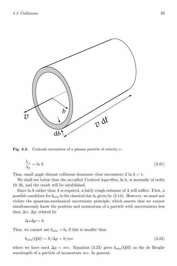
3.3 Collisions 29

b

db

vv dt

Fig. 3.2. Coulomb encounters of a plasma particle of velocity v.

λ⊥λd

∼ ln Λ. (3.21)

Thus, small angle distant collisions dominate close encounters if ln Λ > 1.We shall see below that the so-called Coulomb logarithm, ln Λ, is normally of order

10–20, and the result will be established.Since ln Λ rather than Λ is required, a fairly rough estimate of Λ will suffice. First, a

possible candidate for bmin is the classical size b0 given by (3.14). However, we must notviolate the quantum-mechanical uncertainty principle, which asserts that we cannotsimultaneously know the position and momentum of a particle with uncertainties lessthan ∆x, ∆p, related by

∆x∆p ∼ h.

Thus, we cannot use bmin = b0 if this is smaller than

bmin(QM) ∼ h/∆p ∼ h/mv (3.22)

where we have used ∆p ∼ mv. Equation (3.22) gives bmin(QM) as the de Brogliewavelength of a particle of momentum mv. In general,

30 Plasma concepts

bmin = maxh/mv, 2e1e2/[4πε0]mv2, (3.23)

so bmin is given by the classical value, b0, unless

v ∼>e2

[4πε0]hcc =

c

137. (3.24)

To find bmax we recall that the plasma reacts to charge disturbances in a characteristictime 1/νp (cf. (3.6)). Thus, the plasma can ‘screen off’ the Coulomb field of anyparticle whose characteristic interaction time ∼ b/v is longer than 1/νp. Hence, wecan set

bmax =v

νp.

Of course, if v is the thermal velocity ve of an electron, we find

bmax = λDeb

as expected. In general in this book we shall be interested in ln Λ for thermal particleswith mv2 ∼ kT in (3.23), so that

ln Λ = ln(λDeb/b0);

i.e., using (3.9),

ln Λ ∼= 10 + 3.45 log T − 1.15 log Ne (3.25)

with Ne in cm−3. It is easy to verify that ln Λ is in the range 10–20 for all astrophysicalplasmas. This finally proves our claim that the effect of many weak, distant collisionsin a plasma is more important than the strong, close collisions. As a matter of practicalimportance, it shows that ln Λ is extremely insensitive to errors in our estimates ofbmax, bmin: if ln Λ = 15 an error in bmax/bmin of a factor 100 either way only producesln Λ = 10–20. Thus, (3.25) is likely to be a reasonable estimate, even if (3.24) issatisfied.

3.4 Thermal plasmas: relaxation time and mean free path

Let us apply our basic results (3.19), (3.20) to the case of plasma particles movingwith thermal velocities. We shall avoid the problem of summation over the range ofvelocities of the particles contributing to the deflection by simply putting mv2 ∼ kT .This will produce the correct order of magnitude for λd in (3.26) below. However, ingeneral, a full kinetic theory analysis of the time evolution of the velocity distribution,given by the Fokker–Planck equation, is required. This is particularly important forthe energy exchange time tE for fast (suprathermal) particles to be considered inSection 3.5. (For further details see, for example, Chapter 10 of Boyd & Sanderson(1969).)

Using mv2 ∼ kT in (3.20), we see that, for colliding particles of comparable mass,

3.4 Thermal plasmas: relaxation time and mean free path 31

λd ∼= 7 × 105

ln ΛT 2

Ncm. (3.26)

This is independent of the particle mass, so the average distance travelled before anappreciable deflection occurs is the same for electrons and ions, and λd given by (3.26)is the mean free path for both types of particles. Note that the deflection time td(e–e)for electrons with electrons is (mp/me)1/2 ∼ 43 times shorter than that for ions withions, but this is compensated for by the higher electron velocity. For unequal masses,it can be shown by a similar analysis that formulae of the form (3.19), (3.20) hold withm of the order of the smaller mass and v of the order of the greater thermal speed.Thus, for electron–ion encounters, m ∼ me, v ∼ (kT/me)1/2,

td(e−i) ∼ [4πε0]2m1/2e (kT )3/2

2πNe21e22 ln Λ

∼ td(e−e). (3.27)

Thus, electron–ion encounters occur at a similar rate to electron–electron encounters.One sometimes defines an (electron) collision frequency as

νc ∼ 1/td(e−i) ∼= 2 ln ΛZ2NeT−3/2 s−1 (3.28)

(Ne in cm−3), where Ze is the average ion charge, and an ion–ion collision frequencyas

νc(i−i) ∼ 1/td(i−i) ∼= 5 × 10−2 ln ΛZ4NeT−3/2 s−1. (3.29)

So far, we have considered only the deflections of plasma particles: the timescales tdgive an approximate measure of the time for an initially anisotropic velocity distri-bution to relax to isotropy. Ultimately, any initial distribution of particle velocitiesmust tend to an equilibrium Maxwell–Boltzmann distribution; the timescale for thisrelaxation to occur is the energy exchange timescale:

tE =E2

d(∆E)2/dt(3.30)

where E is the energy of a test particle and ∆E the change due to collisions (cf. (3.19)).Note that there is no a priori reason to expect tE to be similar to td; after all,

in the centre-of-mass frame there is a deflection θ, but no energy exchange betweenthe particles, since, as we remarked in Section 3.3, their speeds remain unaltered. Insome important special cases (e.g. particles of comparable masses and similar initialvelocities) tE and td are very similar, and, indeed, the distinction between them is notalways adequately drawn in the astrophysical literature. In general, however, tE canexceed td considerably.

An important example of this difference occurs for electron–ion collisions in a plasmain thermal equilibrium: since me mi

∼= mp and the centre-of-mass frame differs fromthe laboratory frame only by a velocity vCM ∼= (me/mi)1/2vi vi (cf. (3.12)). Fromthe fact that no energy is exchanged in the centre-of-mass frame, we find the maximumenergy transfer in the laboratory frame in a head-on collision is of order

∆E = 2miv2CM

∼= 2mev2i ,

32 Plasma concepts

i.e.

∆E12miv2i

∼ me

mi 1. (3.31)

Thus, collisions between electrons and ions are very inefficient in transferring en-ergy. Hence, although, as remarked after (3.27), electron–ion encounters and electron–electron encounters occur at similar rates in a plasma, a difference in average energybetween electrons and ions will take ∼ mi/me ∼ mp/me ∼ 1836 times longer to evenout by collisions than a similar difference among the electrons themselves.

For like-particle encounters with comparable velocities, we expect tE ∼ td, so(3.28, 3.29) now imply that the relaxation times to establish, from an originallynon-equilibrium situation, (i) an electron thermal distribution, (ii) an ion thermaldistribution, (iii) equipartition between electrons and ions, are in the ratio

tE(e−e) : tE(i−i) : tE(e−i) = 1 : (mp/me)1/2 : (mp/me). (3.32)

Thus, the electrons reach equilibrium first, followed by the ions, followed finally byequipartition. This behaviour is particularly important in the study of shock wavesin plasmas (see Sections 3.8 and 6.4).

3.5 The stopping of fast particles by a plasma

In our study of accretion, we shall need to consider how high-velocity infalling matteris incorporated into the material of the accreting star. This process again involvescollisions, but with the difference now that the velocities of the infalling particlesgreatly exceed those of the ‘background’ particles of the stellar envelope.

Let a test particle (i.e. a particle whose influence on the ambient medium can beneglected) having mass m1, velocity U , and charge e1 be incident on a plasma ofnumber density N , temperature T , particle mass m2, and charge e2. This will allowus to consider the stopping by the electron and ion plasmas separately. We supposeour test particle to be fast (suprathermal) in the sense that

12

m1U2 3

2kT =

12

m2v2th;

i.e. U greatly exceeds the typical thermal speed of the background particles. A fullkinetic theory treatment (e.g. Boyd & Sanderson (1969) Chapter 10) yields a furthertimescale, characterizing the stopping of the test particle, in addition to td and tEThis is the slowing-down timescale:

ts = − U

dU/dt. (3.33)

For suprathermal particles, but assuming non-relativistic velocities U < c, one finds

ts ∼ [4πε0]2m21U

3

8πNe21e22 ln Λ

m2

m1 + m2,

3.5 The stopping of fast particles by a plasma 33

td ∼ [4πε0]2m21U

3

8πNe21e22 ln Λ

,

tE ∼ [4πε0]2m21U

3

8πNe21e22 ln Λ

m2U2

2kT. (3.34)

Here ln Λ is the Coulomb logarithm, with bmax = U/νp. Of course, since we are againconsidering collisions, there is a family resemblance between these expressions and ourearlier one (3.19) for td for thermal particles. Two interesting conclusions follow fromthe expressions (3.34):

(i) The factor m2/(m1 + m2) in ts means that suprathermal ions are best sloweddown by electrons; this occurs in a time

ts ∼ (me/mp)td.

(ii) Suprathermal electrons are slowed down at similar rates by both electrons andions; the timescale ts is the same as the deflection time td.

It is often of interest to calculate the average distance λs ∼ Uts travelled by aparticle before slowing down; this is sometimes referred to as the stopping length. Fora proton incident on the plasma, we have

λs = Uts ∼[4πε0]2m2

pU4

8πNe4 ln Λme

mp(3.35)

since the stopping is mainly by electrons. Writing 12mpU2 = Ep, the kinetic energy

of the proton,

λs =[4πε0]2me

2πNe4 ln ΛmpE2p. (3.36)

Using the fact that Nmp∼= ρ, the background plasma mass density, we see that the

column density ρλs of plasma required to slow down an incident proton depends onlyon the square of the proton energy (neglecting the slow dependence of ln Λ on plasmaproperties). In fact, the stopping power of a plasma is often expressed in terms of thecolumn density per (keV)2 of incident particle energy: numerically,

ρλs = 4.6 × 10−10g cm−2(keV)−2 for ln Λ = 15. (3.37)

The energy of a supersonic accretion flow is almost all carried by ions. Therefore,as an example of the use of λs let us consider the problem of a proton freely fallingon to a star. It is of interest to know whether or not the proton will penetrate thephotosphere of the star before being slowed down; if this is the case, most of theaccretion energy supplied by a stream of such protons will be released as blackbodyradiation at a temperature ∼ Tb (equation (1.10)). It is easy to answer this questionin the case in which the opacity of the surface layers of the star is due to electronscattering, as, for example, for neutron stars. The condition for penetration is that λsshould exceed the mean free path λph of photons through the surface material. Foran electron scattering opacity

34 Plasma concepts

λph ∼= 1/NσT

where

σT = [4πε0]−28π

3e4

m2ec4

(3.38)

is the Thomson cross-section. Using (3.35), (3.38), we find

λsλph

=mp

me

13 ln Λ

(U

c

)4

.

Hence, for ln Λ = 15, the condition for penetration is

U 2.6(me/mp)1/4c ∼ 0.4c. (3.39)

If for U we take the free-fall speed, (2GM/R∗)1/2, it is clear that (3.39) implies thatpenetration by ions is possible only for objects which are compact in the sense that

R∗ ∼< 6RSchw (3.40)

where RSchw is the gravitational or Schwarzschild radius of the object.

RSchw =2GM

c2∼= 3 km

(M

M

).

While the inequality (3.40) obviously holds for black holes (R∗ = RSchw), the conceptof penetration in this case is not meaningful. Penetration is, in principle, possible forneutron stars (R∗ ∼= RSchw), but not for less compact objects.

3.6 Transport phenomena: viscosity

The fact that the particles of a plasma are constantly in thermal motion, carrying withthem their momenta, energies, etc., means that they tend to share out these quanti-ties and try to even out any gradients in the plasma. Thus, the microscopic structureof a plasma, on scales of a mean free path, affects its macroscopic (gas dynamical)properties through transport processes, as these effects are known. Examples of trans-port processes, which we briefly encountered in Chapter 2, are viscosity and thermalconductivity; in these cases the quantities being transferred are various componentsof momentum and (thermal) energy respectively. As we shall see, transport processesbecome important when there are large gradients (e.g. of velocity or temperature) ina plasma, a situation which often occurs in accretion problems.

Let us examine how viscosity works in a simple case. We consider a plasma flowingwith (bulk) velocity v(x) in the x-direction (Fig. 3.3). We draw a surface S orthogonalto the gas velocity at a certain point, and consider the transfer of x-momentum acrossS by thermal motions. This will give us the effect of bulk viscosity,1 which can be

1 The bulk viscosity vanishes to lowest order for monoatomic ideal gases (see e.g. Physical Kineticsby E.M. Lifshitz & L.P. Pitaevskii (Pergamon Press 1981), §8, pp. 24–26. Non-zero bulk viscosityrequires some dissipation.

3.6 Transport phenomena: viscosity 35

vv+λd

∂v∂xv λd

∂v∂x

S

x

λd λd

Fig. 3.3. Bulk viscous transport of momentum.

important in shock fronts (see Section 3.8). The transfer of the other (y, z) componentsof momentum gives the shear viscosity which is generally more important in influencingthe gas motion (see Section 4.6). By symmetry, the transfer of x-momentum will bezero unless there is a velocity gradient at S: we write ∂v/∂x = v/L, so that L isthe scale length of velocity variation at S. The particles which can carry momentumacross S, by virtue of their thermal motions, are just the plasma particles originatingfrom within one deflection length, λd (equation (3.20)), of S: since no appreciabledeflection occurs over a length shorter than λd these particles carry essentially alltheir momentum across S. Of course, we should add up the momentum transfers dueto all particles on each side of S, taking account of their differing values of λd. Weshall obtain a correct result, in an order-of-magnitude sense, if we assume that most ofthe momentum transfer is performed by particles with thermal energy E ∼ kT : thenthe appropriate value for λd is the thermal mean free path (3.26) for all particles.A second simplification follows from realizing that the systematic momentum (themomentum associated with the bulk motion v) of a plasma flow resides almost totallyin the ions because of their greater mass. Finally, we assume that only the velocity v,not ρ, λd or the sound speed cs, changes over the lengthscale λd: hence, the net rateat which systematic momentum is transferred across unit area of S is approximately

−ρcs

(v + λd

∂v

∂x

)+ ρcs

(v − λd

∂v

∂x

)∼= −2ρcsλd

∂v

∂x. (3.41)

Here we have used the facts that the ions of a plasma have thermal velocities ofthe order of the sound speed cs (equations (2.19, 2.20)) and that the change in bulkvelocity over a distance λd is ∼ λd∂v/∂x.

Now let us consider a volume element, dV , in the plasma flow, bounded by surfacesS, S′, at x, x + dx (Fig. 3.4), each of area dA; so dV = dxdA. The momentum transferrate (3.41) means that there is a force acting in the x-direction on the volume elementdV due to viscosity. This force is given by the difference between the expression (3.41)

36 Plasma concepts

v

S SdV

x x+dx

dAdA

Fig. 3.4. Bulk viscous force density: net force per unit volume.

evaluated at x and at x + dx:

dFvisc = 2ρcsλddA

(∂v

∂x+

∂2v

∂x2dx

)

−2ρcsλddA∂v

∂x

∼= 2ρcsλd∂2v

∂x2dV.

Hence, there is a (bulk) viscous force density

fvisc,bulk ∼= −2ρcsλd∂2v

∂x2(3.42)

acting at each point of the plasma. Note that the force vanishes (correctly) if there isno velocity gradient.

To see when this viscous force is important, we recall the Euler equation (2.3):clearly, we must compare fvisc with the pressure gradient ∂P/∂x. If the pressurechanges over scale length L, the ratio is

viscous forcepressure force

∼ ρcsλdv

L2

L

P.

But, from the equation of state (2.2), we have P ∼= ρc2s , so the ratio becomes

viscous forcepressure force

∼ v

cs

λdL

. (3.43)

Equation (3.43) shows that viscosity will be important for supersonic flow (v > cs)with large gradients (L ∼ λd) – precisely the conditions which are encountered inshock waves. If gradients are small (L λd) viscosity can generally be neglected,unless the flow is highly supersonic (v cs). This is fortunate, since the viscous forcein (3.42) involves second derivatives of v and its inclusion considerably complicatesthe problem of solving the equations of gas dynamics.

In the discussion above we have considered viscous effects only in a one-dimensional

3.7 The effect of strong magnetic fields 37

gas flow, so-called bulk viscous effects. Clearly, if the velocity field varies in directionsorthogonal to the flow (shearing motions) similar (shear) viscous effects will comeinto play. Further, if there are more violent random motions in the gas involving thebodily displacement of blobs of material (turbulent motion), these can also give rise to(turbulent) viscous effects. We shall be much concerned with turbulent shear viscosityin our discussion of accretion discs (Chapters 5, 6); it is worth bearing in mind thatall these viscous effects involve the same basic transport process we have discussedabove.

Another similar transport process, referred to at the beginning of this section, isthermal conduction. The main difference here is that, because the quantity beingtransferred is internal (thermal) energy, of which the electrons have the same amountas the ions, the transport process is dominated by the electrons, since they are quickerby a factor (mi/me)1/2 ∼ 43. With this modification, a calculation very similar tothe one performed above for bulk viscosity shows that a temperature gradient ∂T/∂x

gives rise to an electron thermal conduction flux:

q ∼ −NekT

meveλdk

∂T

∂x(3.44)

where ve = (kT/me)1/2. The formula for the coefficient of thermal conductivity usedin (2.6) follows directly from (3.44) and (3.26).

3.7 The effect of strong magnetic fields

Frequently, in accretion problems, we deal with plasmas immersed in strong magneticfields. For neutron stars, surface fields of 1012 G (=108 T) are often met with. Manyaccreting white dwarfs possess magnetic fields of the order of 106–107 G (102–103

T). Because plasmas are, by definition, electrically conducting gases, there is a host ofeffects produced by the field. For example, the transfer of radiation, particularly takinginto account its polarization properties, becomes immensely more complicated. In thisbook we shall touch only rather superficially upon two particular types of magneticeffect: the influence of magnetic fields on gas flows and on transport processes.

In outline, the presence of currents in a moving plasma modifies the magnetic field,while the electromagnetic field acts on the charges to produce currents. Therefore,in general, the influence of a magnetic field on the gas flow is quite complicated.However, we shall find that, if the plasma has sufficiently high electrical conductivity,a condition usually realized in practice, then the plasma and the magnetic field movetogether in a sense that will be explained precisely below. We shall then determine theconditions under which the gas follows the motion of the magnetic field or, conversely,the magnetic field is dragged around by the gas.

The magnetic field, B, is governed by Maxwell’s equations:

∇ ·B = 0,

∇∧B =[

1c

]1c

∂E∂t

+[cµ0

4π

] 4π

cj.

(3.45)

38 Plasma concepts

The first tells us that we can represent B by unending lines of force; in the second,the displacement current term (∝ ∂E/∂t) can usually be neglected in astrophysics, sowe shall drop it here. The current density j is now related to the electromagnetic fieldby a form of Ohm’s law appropriate to moving media; in the so-called hydromagneticapproximation (see Boyd & Sanderson (1969) Chapter 3), this is

j = σ(E+ [c]v ∧B/c) (3.46)

where σ is the electrical conductivity. Essentially, this states that the force due tothe fluid velocity in the magnetic field moves charges in addition to the electromotiveforce. Taking the curl of (3.45) and using (3.46), with σ assumed constant, we obtain

∇∧ (∇∧B) =[cµ0

4π

] 4π

cσ(∇∧E+ [c]∇∧ (v ∧B)/c).

On the right hand side Faraday’s law,

∇∧E = −[c]1c

∂B∂t

,

can be used to eliminate the electric field E. The left hand side is

∇∧ (∇∧B) = −∇2B−∇(∇ ·B) = −∇2B;

so we obtain

∂B∂t

= ∇∧ (v ∧B) +[

4π

c2µ0

]c2

4πσ∇2B. (3.47)

Thus, the time rate of change of the magnetic field is governed by diffusion of thefield (∝ σ−1∇2B) and convection (∇∧(v∧B)) of the field by the fluid. We can neglectdiffusion if for changes in B on a lengthscale L[

4π

c2µ0

]c2

4πσ

|B|L2

( |v||B|L

)−1=

[4π

c2µ0

]c2

4π

1σ|v|L =

1Rm

1,

i.e. for sufficiently large σ. Rm is known as the magnetic Reynolds number.To see how the field and fluid move together for Rm 1, consider the magnetic

flux, Φ, through a surface S(t), bounded by a closed curve C(t), moving with the fluid(Fig. 3.5).We have

dΦdt

= limdt→0

[∫S(t+dt)

B(t + dt) · dS−∫S(t)

B(t) · dS

]1dt

.

But, since the flux through a closed surface is zero, we have, at time t + dt,∫S(t+dt)

B(t + dt) · dS+∫SB(t + dt) · dS −

∫S(t)

B(t + dt) · dS = 0,

where S is the surface generated by the motion of C(t). Therefore:

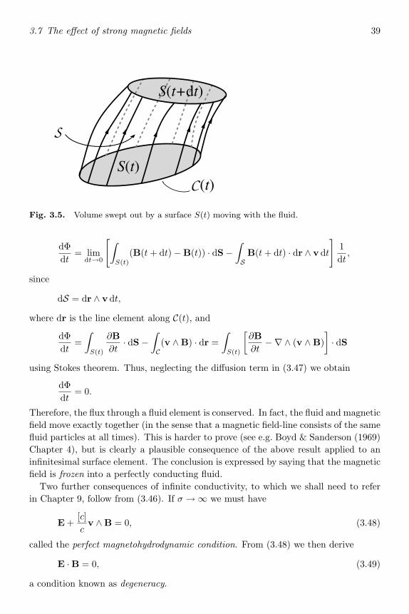
3.7 The effect of strong magnetic fields 39

S(t)

S(t+dt)

S

C(t)

Fig. 3.5. Volume swept out by a surface S(t) moving with the fluid.

dΦdt

= limdt→0

[∫S(t)

(B(t + dt) −B(t)) · dS−∫SB(t + dt) · dr ∧ v dt

]1dt

,

since

dS = dr ∧ v dt,

where dr is the line element along C(t), and

dΦdt

=∫S(t)

∂B∂t

· dS−∫C(v ∧B) · dr =

∫S(t)

[∂B∂t

−∇ ∧ (v ∧B)]· dS

using Stokes’ theorem. Thus, neglecting the diffusion term in (3.47) we obtain

dΦdt

= 0.

Therefore, the flux through a fluid element is conserved. In fact, the fluid and magneticfield move exactly together (in the sense that a magnetic field-line consists of the samefluid particles at all times). This is harder to prove (see e.g. Boyd & Sanderson (1969)Chapter 4), but is clearly a plausible consequence of the above result applied to aninfinitesimal surface element. The conclusion is expressed by saying that the magneticfield is frozen into a perfectly conducting fluid.

Two further consequences of infinite conductivity, to which we shall need to referin Chapter 9, follow from (3.46). If σ → ∞ we must have

E+[c]cv ∧B = 0, (3.48)

called the perfect magnetohydrodynamic condition. From (3.48) we then derive

E ·B = 0, (3.49)

a condition known as degeneracy.

40 Plasma concepts

To complete the discussion, consider the magnetic forces on the plasma. Eachcharge is subject to the Lorentz force (e/c)v ∧ B[c], so the magnetic force density is

fmag =[c]cj ∧B.

Using (3.45), without the displacement current term, to eliminate j yields

fmag =[

4π

µ0

]1

4π(∇∧B) ∧B

and this is equivalent to

fmag =[

4π

µ0

]−∇

(B2

8π

)+

14π

(B · ∇)B

. (3.50)

Comparison with the Euler equation (2.3) shows that the first term on the right of(3.50) behaves as a hydrostatic pressure of magnitude

Pmag =[

4π

µ0

]B2

8π. (3.51)

The final term in (3.50) is less important, but, by considering special cases, for exampleB = (0, 0, B(z)), one can show it behaves as a tension of magnitude [4π/µ0](B2/4π)along the fieldlines.

An order-of-magnitude analysis of the Euler equation (2.3) now shows that the rel-ative importance of the inertia (or ram pressure), gas pressure and magnetic pressureterms is given by

ρv2 : ρc2s :B2

8π

[4π

µ0

]. (3.52)

It follows that the fluid velocity will be determined by the magnetic field if the magneticpressure dominates. If the ram pressure is the largest, then the magnetic field isdragged around by the fluid, which moves essentially as if the magnetic forces wereabsent. In the intermediate case, ρc2s B2/8π[4π/µ0] ρv2, the magnetic fieldmoves the fluid, but is itself confined by gas pressure. The equality of kinetic andmagnetic energy densities defines a velocity

vA =(

B2

4πρ

[4π

µ0

])1/2

,

the Alfven velocity, at which magnetic disturbances propagate in the plasma. From(3.52), magnetic forces dominate if vA max(v, cs). We shall meet examples of theinfluence of strong magnetic fields on accretion flows in Chapter 6.

The importance of magnetic fields in modifying transport processes arises from theeffect these fields have on the motions of individual charged particles. It is shown inmany books on dynamics and electrodynamics that a non-relativistic charged particle,of mass m and charge q, will spiral about a uniform magnetic field B with angularfrequency

3.8 Shock waves in plasmas 41

Ω =qB

mc[c] rad s−1, (3.53)

variously known as the Larmor frequency, gyro-frequency, or cyclotron frequency. Theradius of the spiral is given by the particle velocity component v⊥ orthogonal to B;this is the Larmor radius:

rL = v⊥/Ω.

If v⊥ is given by an average thermal velocity (kT/m)2 we have

rL =(mkT )1/2

qB

c

[c],

which for electrons and ions of mass Amp and charge Ze give

rLe ∼= 2.2 × 10−2T 1/2/B cm,

rLi ∼= AT 1/2/ZB cm

(3.54)

respectively (B in gauss = 10−4 tesla). Clearly, rL limits the distance which a particlecan travel through the plasma in a given direction orthogonal to B. Thus, transportprocesses across the field-lines will tend to be suppressed if rL < λd for the relevantspecies of particle, while transport rates along the field-lines are unaffected. Forexample, if conditions in the plasma are such that rLe < λd (equation (3.26)), electronthermal conduction across field-lines will be greatly reduced.

3.8 Shock waves in plasmas

Very often in astrophysics we have to deal with situations where the bulk velocity of agas flow makes a transition between supersonic and subsonic values. A good exampleof this is provided by our study of steady adiabatic, spherical, accretion (Section 2.5).The gas velocity will, in general, be close to the free-fall velocity vff and thereforehighly supersonic near to the surface of the accreting star (as noted in number 3 ofthe conclusions at the end of Section 2.5). Clearly, in order to accrete to the star, thegas must somehow make a transition to a subsonic ‘settling’ flow, in which the gasvelocity becomes very small near the stellar surface.

From the point of view of the gas, i.e. seen in a reference frame moving with thegas velocity v, the surface of the star is pushing into the gas at a supersonic speed∼= vff . To simplify the geometry, let us approximate this to a piston being pushedinto a tube of gas (Fig. 3.6). We assume that the changes induced by the pistonare so rapid that the gas behaves adiabatically. As the piston starts from rest witha small displacement, a signal travels into the gas at the sound speed and the gas isslightly compressed. As the piston continues to accelerate into the gas, a further signaltravels into the already compressed gas and acts to compress it further; this signaltravels at the sound speed of the already compressed gas. Because the sound speedcads ∝ ρ1/3 (equation (2.19)) this new sound speed is slightly higher than the original.Hence, arbitrarily dividing the gas in front of the piston into zones labelled 1, 2, 3,...,

42 Plasma concepts

motion of piston

1 2 3

Fig. 3.6. Compression of gas in a long cylinder or shock tube.

we see that the densities ρ(1), ρ(2), ρ(3),... in these zones obey ρ(1) > ρ(2) > ρ(3) >...,so that the sound speeds obey cads (1) > cads (2) > cads (3).... Thus, ‘news’ of the pistontravels into the gas at cads , and gas sufficiently far to the right remains at its originaldensity until this ‘news’ has had time to arrive. Hence, the denser zones to the leftcontinually try to catch up the lower-density zones to the right; the compression ofthe left hand zones continually increases, and the density profile in front of the pistontherefore steepens (Fig. 3.7).

But the steepening of the density profile cannot continue indefinitely: once thedensity scale length, L ∼= ρ/|∇ρ|, becomes of the order of the mean free path, λd, thensince the gas velocity is of the order of the sound speed, cs, in the higher-density region(and thus supersonic for the undisturbed gas), our estimate (3.43) shows that bulkviscous forces, so far neglected, will become important. The effect of the viscous forceson the gas is to dissipate energy: i.e. ordered kinetic energy gets converted by viscousprocesses into chaotic thermal motions. The precise description of this conversion is,in general, a very difficult problem in kinetic theory, particularly for shock waves inplasmas, where the inefficient energy exchange between ions and electrons complicatesmatters still further. In many cases; however, a detailed picture of the structure ofthe shock is not required; since the shock thickness (∼ λd) is much smaller than thelengthscales of gradients in the gas on each side of it, we can approximate the shock asa discontinuity in the gas flow. The connection between the gas density, velocity andpressure (or temperature) across this idealized discontinuity can be found by applyingconservation laws.

To see how this works, it is convenient to choose a reference frame in which theshock is at rest. Since the shock thickness is so small, we can regard it as locallyplane; further, since the gas flows through the shock so quickly, changes in the gasconditions cannot affect the details of the transition across the shock, so we can regardthe flow into and out of the shock as steady. Hence, we have the situation depicted inFig. 3.8 in which gas flows into the shock with density, velocity and pressure ρ1, v1, P1,and emerges with ρ2, v2, P2. (If the shock is oblique to the flow, v1, v2 are just thecomponents of the upstream and downstream flow velocities which are orthogonal tothe shock front; the tangential components are continuous. The jump conditions canbe modified accordingly.) Let us now apply the conservation laws of mass, momentum

3.8 Shock waves in plasmas 43

x

ρ

x

ρ

x

ρ λd~

SHOCKED,COMPRESSED

GAS

shock wave

UNDISTURBEDGAS

(a) (b) (c)

Fig. 3.7. The formation of a shock wave in a gas. (a) The denser gas in zone 1 tends to

overtake the dilute gas in zone 2 since its adiabatic sound speed is greater; (b) as a result, the

density gradient, and hence the overtaking tendency, increase, leading (c) to a shock wave of

thickness of the order of the mean free path of the gas particles.

and energy across the shock front; this is equivalent to integrating the appropriateforms of the gas dynamics equations, (2.1), (2.3), (2.5), across the discontinuity. If x

measures distance from the shock front, we integrate with respect to x from −dx to+dx, where dx ∼ λd/2, and take the limit dx → 0.

First, we have from the continuity equation (2.1):

ddx

(ρv) = 0,

which integrates to

ρ1v1 = ρ2v2 = J. (3.55)

Clearly, the quantity J = ρv which is conserved here is the mass flux. From the Eulerequation (2.3) we get

ρvdv

dx+

dP

dx= fx

ord

dx(P + ρv2) = fx

where fx is the force density in the x direction. Integrating across the shock frontx = 0, we get

(P1 + ρ1v21) − (P2 + ρ2v

22) = lim

dx→0

∫ dx

−dxfx dx = 0,

since fx is finite. Thus,

44 Plasma concepts

Shock

∼λd

ρ1 , v1 , P1 ρ2 , v2 , P2

Fig. 3.8. The calculation of the shock jump (Rankine–Hugoniot) conditions.

P1 + ρ1v21 = P2 + ρ2v

22 = I. (3.56)

Here, the conserved quantity I = P + ρv2 is the momentum flux.Finally, the energy equation (2.5) implies

ddx

[v

(12

ρv2 + ρε + P

)]= fxv

if we assume that radiative losses and thermal conduction, etc., across the shock frontare negligible. This is the adiabatic assumption, and the resulting jump conditions areknown as the adiabatic shock conditions. The assumption has, of course, to be testedin any individual case. Using ρv = constant and ε = 3

2P/ρ, the energy equation canbe written as

ρvd

dx

[12

v2 +52

P

ρ

]= fxv

for a monoatomic gas. Integrating over the shock front implies (using 3.55)

12

v21 +52

P1ρ1

=12

v22 +52

P2ρ2

= E, (3.57)

since∫

fxv dx over the shock vanishes. The quantity E = 12v2+ 5

2P/ρ is then the spe-cific total energy, where account is taken of the work done by pressure in compressingthe gas across the shock. The three conservation equations (3.55), (3.56), (3.57), re-lating the upstream and downstream values of ρ, v, P are known as Rankine–Hugoniotconditions; they give three equations to determine the jumps in ρ, v, P . In general,deriving these relations involves a little algebra.

First, let us divide I by Jv: (3.55), (3.56) give

I

Jv=

P

ρv2+ 1.

3.8 Shock waves in plasmas 45

Defining the Mach number M by

M2 =v2

(cads )2=

35

ρv2

P, (3.58)

we get

I

Jv=

35M2

+ 1. (3.59)

Also, using (3.55), (3.56) in (3.57),

E =v2

2+

52

(Iv

J− v2

)or

v2 − 54

I

Jv +

E

2= 0.

This is a quadratic equation for v, and therefore has two roots. Since the quadraticwas derived by manipulation of the conservation laws, these roots can only be v1, v2.Hence, v1 + v2 is given by the sum of the roots of the quadratic:

v1 + v2 =54

I

J,

i.e.

1 +v2v1

=54

I

Jv1=

54

[3

5M21

+ 1]

(3.60)

using (3.59). Here M1 = v1/cads (1) is the upstream Mach number.Very often we encounter situations where this quantity is large, i.e. where the flow

is highly supersonic. The limit M1 1 is the case of a strong shock: for such shockswe get, from (3.60),

v2v1

=14

, (3.61)

i.e. the velocity drops to one-quarter of its upstream value across the shock. From(3.55) we get

ρ2ρ1

= 4, (3.62)

which shows that the gas is compressed by a factor 4 in a strong shock. The values14 and 4 in (3.61) and (3.62) come from taking the adiabatic index γ = 5

3 ; they caneasily be found for a general value of γ.

From (3.56) we have

I = ρ1v21

(1 +

35M2

1

)∼= ρ1v

21

for a strong shock. Thus, ahead of a strong shock the thermal pressure P1 is negligible,compared to the ram pressure ρ1v

21 . From (3.56) we thus get the pressure behind the

shock as

46 Plasma concepts

P2 = ρ1v21 − ρ2v

22 = ρ1v1(v1 − v2),

using (3.55), so that

P2 =34

ρ1v21 , (3.63)

from (3.61). Thus, behind the shock the thermal pressure is 34 of the ram pressure.

Clearly, what has happened is that the dissipation processes (e.g. viscosity) operatingin the shock front have converted most of the kinetic energy of the ordered, supersonicflow into heat – i.e. random motion of the post-shock gas particles. This post-shockgas is indeed subsonic, for its sound speed is

cs(2) =(

5P23ρ2

)1/2

=(

5ρ1v21

16ρ1

)1/2

=√

54

v1 > v2 =v14

, (3.64)

using (3.63), (3.62) and (3.61).Note that we have assumed implicitly throughout that (ρ1,v1,P1) and (ρ2,v2,P2)

refer to the pre- and post-shock gas respectively, not the reverse, so that the gas flowgoes from supersonic to subsonic. This is justified by the result that ordered motion(pre-shock) gets randomized in the shock (equation (3.63)): it can easily be shownthat the entropy of the gas in the state (ρ2,v2,P2) is greater than that of the state(ρ1,v1,P1) confirming that the ‘arrow of time’ indeed points in the direction we haveassumed.

The temperature T2 of the post-shock gas is given by the perfect gas law (2.2):

T2 =µmHP2

kρ2=

316

µmH

kv21 . (3.65)

If, as in the example which motivated our discussion of shocks, v1 is the free-fallvelocity, equal to (2GM/R∗)1/2, on to an accreting star of mass M and radius R∗(3.65) gives

T2 =38

GMµmH

kR∗. (3.66)

Comparing (3.66) with (1.11), we see that the temperature estimate Tth is quiteclose to the shock temperature, T2, since mH ∼ mp, µ ∼ 1 and 3

8 ∼ 13 . (The value 3

8

in (3.66) arises from taking γ = 53 ; it can easily be generalized to other values of γ.)

Thus, in a strong shock the ordered kinetic energy of the supersonic pre-shock gas isconverted to random thermal motions; the post-shock ion thermal velocity (∼= cs(2))is of the order of the pre-shock bulk velocity (of. (3.64)). The shock temperatureT2 will only observably characterize the emergent radiation if the post-shock gas isoptically thin; otherwise, a blackbody temperature (cf. (1.10)) will be detected. Shockheating of optically thin gas therefore offers a way of generating high temperaturesand, consequently, high-energy emission.

Although we have restricted our discussion to strong shocks, M1 1, there is nodifficulty, in principle, in the extension of these results to weak shocks (finite M1).

3.8 Shock waves in plasmas 47

Relations similar to (3.61), (3.62) and (3.63) are obtained with coefficients dependenton the strength (M2

1) of the shock.We note finally that in the one-dimensional discussion given above, the steepening

of sound waves into shocks was inevitable, as the sound speed increased with density,and the density continually increased ahead of the pressure disturbance. In morecomplicated situations this need not happen, as dissipation and geometrical expansioncan reverse both tendencies. This almost always holds (fortunately!) for sound wavesproduced in everyday situations.

4 Accretion in binary systems

4.1 Introduction

The importance of accretion as a power source was first widely recognized in the studyof binary systems, especially X-ray binaries. This is still the area where the greatestprogress in the understanding of accretion has been made. The reason for this issimply that, by their very nature, binaries reveal more about themselves, notablytheir masses and dimensions, than do other astronomical objects. This is particularlytrue in the case of eclipsing binaries, where we get direct information about spatialrelations within the source. The importance of accretion is further manifested by therealization that probably a majority of all stars are members of binary systems which,at some stage of their evolution, undergo mass transfer.

The detailed study of interacting binary systems has revealed the importance ofangular momentum in accretion. In many cases, the transferred material cannot landon the accreting star until it has rid itself of most of its angular momentum. Thisleads to the formation of accretion discs, which turn out to be efficient machines forextracting gravitational potential energy and converting it into radiation. This prop-erty has made accretion discs attractive candidates for the role of the central enginein quasars and active galactic nuclei; the question of whether or not this assignmentis correct will be a theme of later chapters. In the context of binaries, however, theirexistence and importance is well attested through observation; we shall discuss theevidence for this in Chapter 5.

4.2 Interacting binary systems

There are two main reasons many binaries transfer matter at some stage of theirevolutionary lifetimes:

(i) In the course of its evolution, one of the stars in a binary system may increasein radius, or the binary separation shrink, to the point where the gravitationalpull of the companion can remove the outer layers of its envelope (Roche lobeoverflow).

(ii) One of the stars may, at some evolutionary phase, eject much of its mass in theform of a stellar wind; some of this material will be captured gravitationallyby the companion (stellar wind accretion).

4.3 Roche lobe overflow 49

The situation described in (i) can come about other than by the swelling up of one ofthe stars in the course of its evolution; for example, the binary separation may decreasebecause orbital angular momentum is being lost from the system as a consequenceof stellar wind mass loss, or gravitational radiation. For the purpose of studyingthe accretion process, the distinctions between these alternatives are unimportant,although crucial to the study of binary evolution (see Sections 4.4 and 6.8). In ourdiscussion of binary accretion we shall have much to say about (i) and comparativelylittle about (ii), because the former is considerably better understood.

4.3 Roche lobe overflow

The situation described in (i) above, in which one star orbits another so closely thatits outer layers are disrupted by the companion, has close parallels in other branchesof astronomy. The problem was first studied by the nineteenth century French math-ematician Edouard Roche in connection with the destruction or survival of planetarysatellites, and is usually associated with his name. The essence of the Roche approachis to consider the orbit of a test particle in the gravitational potential due to twomassive bodies orbiting each other under the influence of their mutual gravitationalattractions. These bodies (in our case the two stars of the binary system) are assumedto be so massive that the test particle does not perturb their orbits (because of thisthe problem is sometimes known as the restricted three-body problem). Thus, the twostars execute Kepler orbit s about each other in a plane: the Roche problem assumesthese orbits to be circular. This is usually a good approximation for binary systems,since tidal effects tend to circularize originally eccentric orbits on timescales shortcompared to the time over which mass transfer occurs, although there are importantexamples where this is not so. A further restriction on the Roche problem, in additionto circular orbits, is the assumption that the two stars are ‘centrally condensed’ inthe sense that they can be regarded as point masses for dynamical purposes. Again,this is normally an excellent approximation. Thus, we have the configuration shownin Fig. 4.1.

It is convenient to write the masses of the two stars as M1 = m1M and M2 =m2M since m1 and m2 then lie in the range 0.1-100 for all types of star. The binaryseparation, a, is then given in terms of the fundamental observational quantity, thebinary period, P , through Kepler’s law:

4π2a3 = GMP 2, (4.1)

where M = M1 + M2 = mM. For binary periods of the order of years, days, orhours, a can be conveniently expressed in the alternative forms:

a =

1.5 × 1013 m1/31 (1 + q)1/3 P

2/3yr cm,

2.9 × 1011 m1/31 (1 + q)1/3 P

2/3day cm,

3.5 × 1010 m1/31 (1 + q)1/3 P

2/3hr cm,

(4.2)

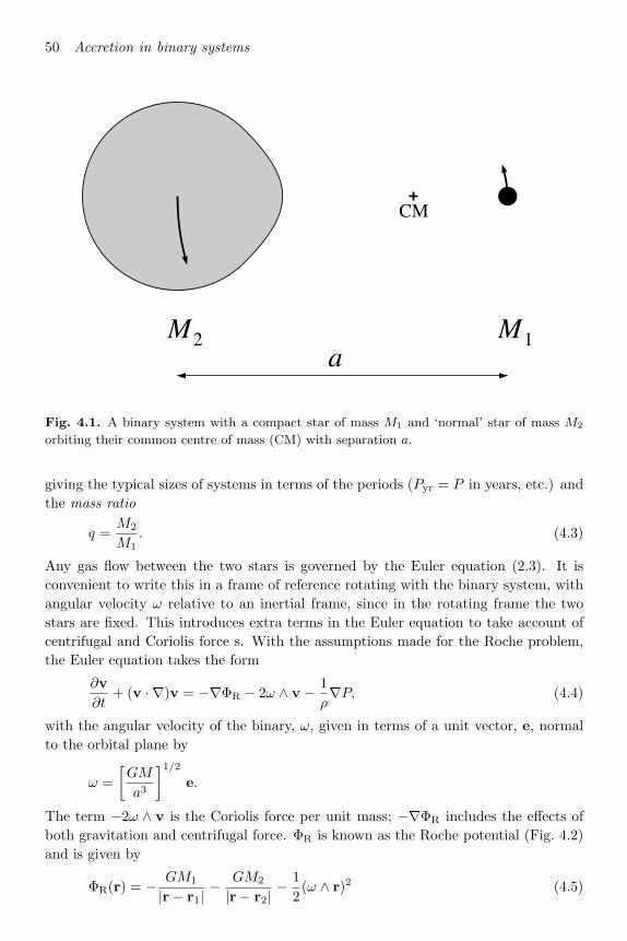
50 Accretion in binary systems

CM

M2 M1a

Fig. 4.1. A binary system with a compact star of mass M1 and ‘normal’ star of mass M2

orbiting their common centre of mass (CM) with separation a.

giving the typical sizes of systems in terms of the periods (Pyr = P in years, etc.) andthe mass ratio

q =M2

M1. (4.3)

Any gas flow between the two stars is governed by the Euler equation (2.3). It isconvenient to write this in a frame of reference rotating with the binary system, withangular velocity ω relative to an inertial frame, since in the rotating frame the twostars are fixed. This introduces extra terms in the Euler equation to take account ofcentrifugal and Coriolis force s. With the assumptions made for the Roche problem,the Euler equation takes the form

∂v∂t

+ (v · ∇)v = −∇ΦR − 2ω ∧ v − 1ρ∇P, (4.4)

with the angular velocity of the binary, ω, given in terms of a unit vector, e, normalto the orbital plane by

ω =[

GM

a3

]1/2e.

The term −2ω ∧ v is the Coriolis force per unit mass; −∇ΦR includes the effects ofboth gravitation and centrifugal force. ΦR is known as the Roche potential (Fig. 4.2)and is given by

ΦR(r) = − GM1

|r− r1| −GM2

|r− r2| −12

(ω ∧ r)2 (4.5)

4.3 Roche lobe overflow 51

2

-1

0

1

2

-2

-1

0

1

2

-4

-3

-2

-1

0

1

2

Fig. 4.2. A surface representing the Roche potential for a binary system with mass ratio

q = M2/M1 = 0.25 (the same as in Fig. 4.3). The larger pit is around the more massive

star. The downward curvature near the edges is due to the ‘centrifugal’ term; a test particle

attempting to corotate with the binary at these distances experiences a net outward force.

where r1, r2 are the position vectors of the centres of the two stars. We gain con-siderable insight into accretion problems by plotting the equipotential surfaces of ΦR

and, in particular, their sections in the orbital plane (Fig. 4.3). When doing this, wemust be careful to remember that some of the forces, in particular the Coriolis forces, acting on the accreting gas are not represented by ΦR.

The shape of the equipotentials is governed entirely by the mass ratio q, while theoverall scale is given by the binary separation a. Figure 4.3 is drawn for the caseq = 0.25, but its qualitative features apply for any mass ratio. Matter orbiting atlarge distances (r a) from the system sees it as a point mass concentrated at thecentre of mass (CM). Thus, the equipotentials at large distances are just those ofa point mass viewed in a rotating frame. Similarly, there are circular equipotentialsections around the centres of each of the two stars (r1, r2); the motion of matter hereis dominated by the gravitational pull of the nearer star. Hence, the potential ΦR

has two deep valleys centred on r1, r2. The most interesting and important feature ofFig. 4.3 is the figure-of-eight area (the heavy line), which shows how these two valleysare connected. In three dimensions, this ‘critical surface’ has a dumbbell shape; thepart surrounding each star is known as its Roche lobe. The lobes join at the innerLagrange point L1, which is a saddle point of ΦR; to continue the analogy, L1 is like ahigh mountain pass between two valleys. This means that material inside one of the

52 Accretion in binary systems

1

1

2

3

3

4

4 4

56

2

3567

7

M2

CM

M1

L4

L5

L2 L3L1

Fig. 4.3. Sections in the orbital plane of the Roche equipotentials ΦR = constant, for a

binary system with mass ratio q = M2/M1 = 0.25. Shown are the centre of mass (CM) and

Lagrange points L1–L5. The equipotentials are labelled 1–7 in order of increasing ΦR. Thus

the saddle point L1 (the inner Lagrange point) forms a ‘pass’ between the two ‘Roche lobes’,

the two parts of the figure-of-eight equipotential 3. The Roche lobes are roughly surfaces of

revolution about the line of centres M1–M2. L4 and L5 (the ‘Trojan asteroid’ points) are

local maxima of ΦR but Coriolis forces stabilize synchronous orbits of test bodies at these

points.

lobes in the vicinity of L1 finds it much easier to pass through L1 into the other lobethan to escape the critical surface altogether.

Now let us examine the consequences of this picture for mass transfer in binaries.We suppose initially that both stars are considerably smaller than their Roche lobesand that the rotation of each star on its axis is synchronous with the orbital motion,with axes orthogonal to the binary plane. Synchronism is usually a good assumption,

4.3 Roche lobe overflow 53

CMM2 M1

L1

Fig. 4.4. A binary system with the secondary star filling the Roche lobe and transferring

mass through L1 into the lobe of the compact primary.

as tidal forces tend to bring it about on a timescale similar to that for circularizationof the binary orbit. In this case, the surface of each star will conform to one of theapproximately circular equipotential sections in Fig. 4.3 (or the qualitatively identicalversion of this figure for the appropriate q). This follows from the Euler equation (4.4)since v = 0 and P is constant on the surface. There is then no tendency for material tobe pulled off either of the stars by the gravitational attraction of the other; the binaryis said to be detached, and mass transfer could proceed only via the wind mechanism((ii) of Section 4.2). Suppose now that for some reason (e.g. stellar evolution), oneof the stars swells up so that its surface, which must lie on an equipotential of ΦR,eventually fills its Roche lobe. We shall usually label the stars so that this is star 2.Thus, we have the situation shown in Fig. 4.4.

Henceforth, we shall often refer to star 2 which fills the Roche lobe as the sec-ondary and star 1 as the primary. Note that this does not necessarily agree with thedesignation of primary and secondary on the basis of, say, the optical luminosity.

We note that, particularly for a mass ratio q 1, the surface of the secondaryis very distorted from the spherical. This distortion can sometimes be detected asellipsoidal variation in the light curves of close binaries, sometimes even when theyare detached. More important, however, is the fact that part of the envelope of thesecondary lies very close to the inner Lagrange point L1. Any perturbation of thismaterial will push it over the L1 point into the Roche lobe of the primary, whereit must, eventually, be captured by the star. Such perturbations are always present,provided, for example, by pressure forces (see (4.4)). A system like this is said to besemi-detached, and will efficiently transfer mass from star 2 to star 1 for as long asthe secondary remains in contact with its Roche lobe. This type of mass transfer iscalled Roche lobe overflow. Since mass is removed from the star quite readily whenthe lobe is filled (see below) the star cannot be significantly larger than its Roche lobe.Thus if the lobe-filling condition is maintained, through either further evolutionary

54 Accretion in binary systems

expansion of the star or shrinkage of the binary via angular momentum loss, the starwill have to adjust its structure so that its radius moves in step with the lobe. Afurther interesting situation (although not one of much relevance for this book) comesabout if both stars for some reason fill their Roche lobes simultaneously. Systems ofthis type (e.g. the W UMa stars) are called contact binaries.

4.4 Roche geometry and binary evolution

To treat Roche lobe overflow in a quantitative manner, we need some idea of thegeometry of the critical surface; in particular, its dependence on the mass ratio q andbinary separation a. The main quantities we shall need are measures of the sizes of theRoche lobes and of the distances of the L1 point from either star. Since the lobes arenot spherical we need some average radius to characterize them; a suitable measure isthe radius of a sphere having the same volume as the lobe. The complicated form (4.5)of ΦR means that we must resort to numerical calculation to find this; but a goodfit to these results for all values of q is given by the approximate analytic formula(Eggleton (1983))

R2

a=

0.49q2/3

0.6q2/3 + ln(1 + q1/3). (4.6)

Obviously the lobe radius R1 of the primary is given by replacing q by q−1. For0.1 ∼< q ∼< 0.8 it is often convenient to use a simple form due to Paczynski:

R2

a=

234/3

(q

1 + q

)1/3

= 0.462(

M2

M1 + M2

)1/3

. (4.7)

Another approximation which is often useful is that for mass ratios 0.03 < q < 1, theratio of primary and secondary Roche lobes obeys

R1

R2=

(M1

M2

)0.45

(4.8)

to an accuracy of better than 5%.The distance b1 of the L1 point from the centre of the primary (mass M1) is given

to good accuracy by a fitted formula of Plavec and Kratochvil:

b1a

= 0.500 − 0.227 log q. (4.9)

An interesting consequence of the form (4.7) for R2/a for q ∼< 0.8 is that the meandensity ρ of a lobe-filling star is determined solely by the binary period P :

ρ =3M2

4πR32

∼= 35π8GP 2

∼= 110P−2hr g cm−3 (4.10)

where we have used (4.1) to eliminate a. Equation (4.10) shows that, for binaryperiods of a few hours, stars with mean densities typical of the lower main sequence

4.4 Roche geometry and binary evolution 55

(ρ ∼ 1–100 g cm−3) can fill their Roche lobes. If one assumes a structure for thelobe-filling star, and thus a relation R2(M2), (4.10) fixes its properties uniquely for agiven period. For example, if we assume that the lobe-filling star is close to the lowermain sequence we know that its radius and mass are approximately equal in solarunits, i.e.

m2∼= R2/R

(e.g. Kippenhahn & Weigert (1990)). Thus

ρ =3M2

4πR32

=3M4πR3

1m22

=1.4m22

g cm−3

where we have used the solar mean density ρ = 1.4 g cm−3. This relation and (4.10)now give a period–mass relation

m2∼= 0.11Phr (4.11)

and a period–radius relation

R2∼= 0.11Ph R = 7.9 × 109Phr cm. (4.12)

Note that these very simple relations come about because of our assumption thatthe secondary was close to the lower main sequence: however, since the star is in abinary and losing mass to the companion it is not obvious that its structure will bethe same as an isolated star of the same mass. Thus we cannot in general assume amain-sequence (or any other) structure without checking carefully the conditions forthis to hold (see below).

The vigilant reader will have realized that the process of mass transfer in a binarywill change its mass ratio q. Equally true, if not quite so obvious, is that the periodP and separation a will be altered by the same process, because of the redistributionof angular momentum within the system. Since the Roche geometry is determined bya and q, it is important to ask whether the effect of these changes is to shrink or swellthe Roche lobe of the mass-losing star. In the former case, the lobe-overflow processwill be self-sustaining at least for some time, and indeed may run away; in the lattercase the mass transfer will switch off unless some effect, such as the nuclear evolutionof the mass-losing star, can increase its radius at a sufficient rate. The determiningquantity for these questions is the orbital angular momentum J . Writing ω for thebinary’s angular velocity (= 2π/P ), this is

J = (M1a21 + M2a

22)ω,

where

a1 =(

M2

M

)a, a2 =

(M1

M

)a

are the distances of the two stars from the centre of mass, and M = M1 + M2.Substituting for a1, a2 above and using (4.1) gives

56 Accretion in binary systems

J = M1M2

(Ga

M

)1/2

. (4.13)

Usually it is a good approximation to assume that all the mass lost by the secondarystar is accreted by the primary, so that M1 + M2 = 0, M2 < 0 (the treatment can beextended to cover cases where this does not hold). Then logarithmically differentiating(4.13) with respect to time gives

a

a=

2J

J+

2(−M2)M2

(1 − M2

M1

). (4.14)

Conservative mass transfer is characterized by constant binary mass and angular mo-mentum; setting J = 0 in (4.14) and remembering that M2 < 0, we see that the binaryexpands (a > 0) if conservative transfer takes place from the less massive to the moremassive star: more matter is placed near the centre of mass, so the remaining mass M2

must move in a wider orbit to conserve angular momentum. Conversely, transfer fromthe more massive to the less massive star shrinks the binary separation. The Rochelobe size is affected by the change in mass ratio as well as separation. Logarithmicdifferentiation of (4.7) gives

R2

R2=

a

a+

M2

3M2,

so combining with (4.14) yields

R2

R2=

2J

J+

2(−M2)M2

(56− M2

M1

). (4.15)

Clearly there are two cases, depending on whether q is larger or smaller than 56 . For

q > 56 conservative mass transfer shrinks the Roche lobe down on the mass-losing

star, and any angular momentum loss (J < 0) will accentuate this. Unless the starcan contract rapidly enough to keep its radius smaller than R2, the overflow processwill become very violent, proceeding on a dynamical or thermal timescale dependingon whether the star’s envelope is convective or radiative. The possibility that thestar could shrink makes the critical value of q for this type of unstable mass transferdepend on its mass–radius relation, so it may differ slightly from 5

6 . The rapid overflowwill stop once enough mass has been transferred to make q smaller than this criticalvalue. All interacting binaries must undergo unstable mass transfer when the moremassive star expands as it evolves off the main sequence, and other episodes can occur.For example, a binary with q ∼> 5

6 may reach contact because of orbital shrinkagethrough angular momentum loss before the lobe-filling star has evolved off the mainsequence. Systems like this, with white dwarf primaries, are a likely model for manyof the supersoft X-ray binaries, which may thus offer a rare observable example ofthermal-timescale mass transfer. However, such unstable mass transfer is probably ingeneral unobservable; it is certainly too violent and short-lived to be typical of themass-exchanging binaries we do observe, which must therefore correspond to the caseq ∼< 5

6 . Equation (4.15) shows that conservative mass transfer will expand the Roche

4.4 Roche geometry and binary evolution 57

lobe in this case. Mass transfer therefore only continues if either (i) the star expands,or (ii) the binary loses angular momentum. In both cases the Roche lobe and thestellar radius will move in step. In case (i) the expansion of the Roche lobe slowsdown if it gets even a little ahead of the stellar radius, reducing mass transfer, whilein case (ii) the shrinking of the star slows if it in turn is too rapid for the shrinkageof the Roche lobe, again reducing mass transfer. Case (i) occurs for example whenthe secondary star evolves off the main sequence and becomes a giant or a subgiant.Then its radius will expand on a nuclear timescale tnuc determined by hydrogen shellburning. By the argument above the Roche lobe will also expand on the timescaletnuc. Thus R2/R2 ∼ t−1nuc, and (4.15) fixes the transfer rate in terms of tnuc:

−M2 =M2

(5/3 − 2q)tnuc. (4.16)

Combining this with (4.14) and (4.1) shows that a and P increase on similar timescales:

a

a=

2P

3P=

(1 − q)(5/3 − 2q)tnuc

.

Case (i) describes mass transfer driven by evolutionary expansion of the secondarystar. Since this must be a giant or a subgiant, this case is confined to relativelylong-period systems where the Roche lobe is large enough to accomodate such a star.In short-period binaries (cataclysmic variables are an example) the lobe is too smalland this mechanism cannot be operating. Mass transfer must be driven by angularmomentum loss (case ii) in such systems. A variety of effects can give J < 0: in short-period systems gravitational radiation is quite efficient, and any mechanism whichspins down the secondary star will ultimately remove angular momentum from thebinary, as tides force the secondary to corotate. Angular momentum loss in a windmagnetically linked to the secondary is a currently favoured possibility. The nature ofthe transfer process in case (ii) depends on the secondary’s reaction to the mass loss,and hence on the behaviour of its radius as M2 is reduced. If mass loss is sufficientlygentle the star will stay close to thermal equilibrium, so that a secondary on the mainsequence before mass transfer started will remain close to it, keeping R2 approximatelyproportional to M2. Setting R2/R2 = M2/M2 in (4.15) gives

−M2

M2=

−J/J

4/3 − M2/M1. (4.17)

Mass transfer therefore proceeds on the timescale for angular momentum loss, and(4.14) and (4.1) now show that a and P decrease on similar timescales:

a

a=

2P

3P=

2J/3J

4/3 − q. (4.18)

It is important to realise that the transfer rates (4.16) and (4.17) are the averagerates driven by evolutionary expansion or angular momentum loss respectively. Theinstantaneous mass transfer rate is given by (see Problem 7 of Chapter 4)

58 Accretion in binary systems

−M2(inst) = M0 exp[

R∗ − R2

H∗

](4.19)

where R∗ is the photospheric radius of the star, H∗ is the photospheric scaleheightand M0 is a constant, typically ∼ 10−8M yr−1 for a lower main-sequence star. SinceH∗/R∗ 1 (it is ∼ 10−4 for a lower main-sequence star), the instantaneous transferrate is very sensitive to the relative size of the star and Roche lobe. This has severalimportant consequences. First, the mass transfer rate can adjust to any required long-term average with only tiny changes to the difference R∗−R2. For many purposes wecan simply regard R∗ and R2 as identical. Thus in many binaries with lower main-sequence secondaries the observed average mass transfer rates 10−9–10−10M yr−1

mean that the Lagrange point L1 lies several scaleheights above the photosphere.However this is still very small compared with the stellar radius R∗. Second, therecan be wide deviations from the long-term average mass transfer rate for epochs ∼(H∗/R∗)tevol, which is small compared to the binary evolution time tevol (= tnuc,−J/J

for nuclear expansion or angular momentum loss respectively). Finally, it is clear thatto change −M2(inst) significantly we must change the difference R∗ − R2 by severaltimes H∗, which is usually difficult to do on short timescales. For example, it isoften suggested that irradiation of the secondary by the accreting primary componentcan have an effect on the mass transfer rate. However irradiating the star below itsphotosphere only causes it to expand on a thermal (Kelvin–Helmholtz) timescale tKH,so the required expansion ∼ few ×H∗ takes (H∗/R∗)tKH ∼> 104 yr for a lower main-sequence secondary. This expansion is driven by the star’s internal radiation flux,which is partially blocked by the irradiation. The expansion stops once the star hasexpanded enough (usually only a few per cent in radius) that the unblocked surfaceis large enough to radiate this blocked flux. Irradiation above the photosphere isunlikely to cause any significant effect on the mean mass transfer rate (see Section4.9 below). Thus in general we can at most expect observed mass transfer rates tofluctuate around the mean values (4.16) and (4.17) on timescales which are too longto be directly observable; observed (rapid) changes in accretion luminosity probablydo not result from changes in the mass transfer rate but from other effects. In linewith this, (4.16) and (4.17) do account successfully for the average observed accretionrates ∼ 1015–1018 g s−1 (∼ 10−11–10−8M yr−1) in various types of binary systems.

4.5 Disc formation

The considerations of the last two sections have shown how mass transfer in closebinary systems can occur via Roche lobe overflow. A consequence of this process is thatthe transferring material has rather high specific angular momentum in many cases,so that it cannot accrete directly on to the mass-capturing star. This is illustrated inFig. 4.5. Note that matter must pass from the Roche lobe of the secondary to that ofthe primary through the L1 point; as far as the primary is concerned, it is as thoughmaterial were being squirted at it from a nozzle which rotates around it in the binary

4.5 Disc formation 59

CM

b1

a

~R2

~R1M2

M1

L1

Fig. 4.5. Roche geometry: R1 and R2 are defined as the radii of spheres having a volume

equal to the volume of the corresponding Roche lobe.

plane. Unless the binary period is quite long, this nozzle rotates so rapidly that thegas stream appears to the primary to move almost orthogonally to the line of centresas it emerges through L1. For let v‖, v⊥ be the components of the stream velocityin a non-rotating frame along and at right-angles to the instantaneous line of centres.We have

v⊥ ∼ b1ω

while

v‖ ∼< cs,

where cs is the sound speed in the envelope of the secondary, since the gas is presum-ably pushed through L1 by pressure forces. From (4.9) we have b1 ∼> 0.5a, unless q isvery large; using ω = 2π/P and (4.2) for a we obtain

v⊥ ∼ 100m1/31 (1 + q)1/3 P

−1/3day km s−1.

By contrast, (2.21) shows that v‖ ∼ cs cannot be much more than about 10 km s−1

for normal stellar envelope temperatures (< 105 K).The discussion above also shows that the gas stream issuing through L1 is super-

sonic. This will hold a fortiori as the stream is accelerated by the primary’s gravita-tional attraction within its Roche lobe. This fact enormously simplifies the calculationof the stream trajectory, for the work of Chapter 2 shows that pressure forces can beneglected: the stream will follow a ballistic trajectory determined by the Roche po-tential, as though it consisted simply of a set of test particles. Further, since v‖ ∼ csis much smaller than the velocities acquired during free fall towards the primary, theinitial conditions near L1 have little effect on the trajectory, which is therefore essen-tially unique; on energetic grounds one can show that the width of the stream issuingthrough L1 is ∼ 0.1P cs, much smaller than the radius of the secondary for example.

60 Accretion in binary systems

To a good approximation we can take the stream trajectory as the orbit of a testparticle released from rest at L1, and thus with a given angular momentum, falling inthe gravitational field of the primary alone. (Note that in Fig. 4.3 the equipotentialcurves are approximately circular within the lobes.) This would give an elliptical orbitlying in the binary plane: the presence of the secondary causes this to precess slowly.(The secondary changes the effective potential from the exact 1/r dependence whichis required for closed periodic orbits.) A continuous stream trying to follow this orbitwill therefore intersect itself, resulting in dissipation of energy via shocks. On theother hand, the gas has little opportunity to rid itself of the angular momentum ithad on leaving L1, so it will tend to the orbit of lowest energy for a given angularmomentum, i.e. a circular orbit. We thus expect the gas initially to orbit the primaryin the binary plane at a radius Rcirc such that the Kepler orbit at Rcirc has the samespecific angular momentum as the transferring gas had on passing through L1. Thusthe gas will have circular velocity

vφ(Rcirc) =(

GM1

Rcirc

)1/2

where

Rcirc vφ(Rcirc) = b21 ω.

Using ω = 2π/P , where P is the binary period, these can be combined to give

Rcirc/a = (4π2/GM1P2)a3(b1/a)4

which, by (4.1), becomes

Rcirc/a = (1 + q)(b1/a)4.

Finally, we use (4.9) to write

Rcirc/a = (1 + q)[0.500 − 0.227 log q]4. (4.20)

The radius Rcirc is often called the circularization radius. The particular form of(4.20) depends on the assumption that the accretion occurs via Roche lobe overflow(see Section 4.9 for Rcirc under a different assumption).

It is easy to show that Rcirc is always smaller than the lobe radius RL of the primary.Typically it is a factor 2–3 smaller, except for very small q: for example, for q = 1,Rcirc = 0.125a, RL = 0.38a. Hence, left to itself, the captured material would orbitthe primary well inside the Roche lobe. This will be prevented, however, if the primaryalready occupies this space, i.e. if its radius R∗ > Rcirc. Using (4.2) to rewrite (4.20)as

Rcirc∼= 4(1 + q)4/3[0.500 − 0.227 log q]4P 2/3

day R (4.21)

we find that Rcirc can be of the order R or less for typical parameters. For example,

Rcirc∼= 1.2P

2/3day R for q = 0.3

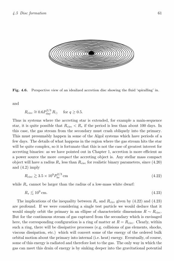
4.5 Disc formation 61

Fig. 4.6. Perspective view of an idealized accretion disc showing the fluid ‘spiralling’ in.

and

Rcirc∼= 0.6P

2/3day R for q ≥ 0.5.

Thus in systems where the accreting star is extended, for example a main-sequencestar, it is quite possible that Rcirc < R∗ if the period is less than about 100 days. Inthis case, the gas stream from the secondary must crash obliquely into the primary.This must presumably happen in some of the Algol systems which have periods of afew days. The details of what happens in the region where the gas stream hits the starwill be quite complex, so it is fortunate that this is not the case of greatest interest foraccreting binaries: as we have pointed out in Chapter 1, accretion is more efficient asa power source the more compact the accreting object is. Any stellar mass compactobject will have a radius R∗ less than Rcirc for realistic binary parameters, since (4.20)and (4.2) imply

Rcirc ∼> 3.5 × 109P 2/3hr cm (4.22)

while R∗ cannot be larger than the radius of a low-mass white dwarf:

R∗ ∼< 109 cm. (4.23)

The implications of the inequality between R∗ and Rcirc given by (4.22) and (4.23)are profound. If we were considering a single test particle we would deduce that itwould simply orbit the primary in an ellipse of characteristic dimensions R ∼ Rcirc.But for the continuous stream of gas captured from the secondary which is envisagedhere, the corresponding configuration is a ring of matter at R = Rcirc. Clearly, withinsuch a ring, there will be dissipative processes (e.g. collisions of gas elements, shocks,viscous dissipation, etc.) which will convert some of the energy of the ordered bulkorbital motion about the primary into internal (i.e. heat) energy. Eventually, of course,some of this energy is radiated and therefore lost to the gas. The only way in which thegas can meet this drain of energy is by sinking deeper into the gravitational potential

62 Accretion in binary systems

of the primary, that is, by orbiting it more closely; this in turn requires it to loseangular momentum. The timescale on which the orbiting gas can redistribute itsangular momentum is normally much longer than both the timescale over which itloses energy by radiative cooling, trad, and the dynamical (or orbital) timescale, tdyn.Therefore, the gas will lose as much energy as it can for a given angular momentum,which itself decreases more slowly. Since a circular orbit has the least energy for agiven angular momentum, we might expect most of the gas to spiral slowly inwardstowards the primary through a series of approximately circular orbits in the binaryorbital plane, a configuration known as an accretion disc (Fig. 4.6). This spiralling-in process entails a loss of angular momentum: in the absence of external torques,this can only occur by transfer of angular momentum outwards through the disc byinternal torques. Thus the outer parts of the disc will gain angular momentum andwill spiral outwards. The original ring of matter at R = Rcirc will spread to bothsmaller and larger radii by this process.

In most cases, the total mass of gas in the disc is so small, and its mean density somuch lower than that of the primary, that we may neglect the self-gravity of the disc.The circular orbits are then Keplerian, with angular velocity

ΩK(R) = (GM1/R3)1/2. (4.24)

The binding energy of a gas element of mass ∆M in the Kepler orbit which justgrazes the surface of the primary is 1

2GM1∆M/R∗. Since the gas elements start atlarge distances from the star with negligible binding energy, the total disc luminosityin a steady state must be

Ldisc =GM1M

2R∗=

12

Lacc (4.25)

where M is the accretion rate and Lacc the accretion luminosity (1.5). The other halfof Lacc has still to be released very close to the star (see Section 6.2).

Thus half of the available energy is radiated while the matter in the disc spiralsslowly inwards. On the other hand, since the specific angular momentum R2Ω(R) ∝R1/2 and R∗ Rcirc, the material must somehow get rid of almost all its originalangular momentum. Clearly, the processes which cause the conversion of orderedkinetic energy into heat must also exert torques on the spiralling material. The effectof these is to transport angular momentum outward through the disc (Section 4.6).Near the outer edge of the disc some other process must finally remove this angularmomentum. It is likely that angular momentum is fed back into the binary orbitthrough tides exerted on the outer disc by the secondary (see Section 5.9).

An important consequence of this angular momentum transport is that the outeredge of the disc will in general be at some radius Rout exceeding Rcirc given by (4.20);Rcirc is often referred to as the minimum disc radius. Clearly the outer disc radiuscannot exceed the primary Roche lobe radius (we will see in Section 5.11 below thatthe maximum size is slightly smaller than this). Typically the maximum and minimumdisc radii differ by a factor 2–3.

4.6 Viscous torques 63

4.6 Viscous torques

From our discussion of the last section we see that an accretion disc can be an efficient‘machine’ for slowly lowering material in the gravitational potential of an accretingobject and extracting the energy as radiation. A vital part of this machinery isthe process which converts the orbital kinetic energy into heat. The main unsolvedproblem of disc structure is the precise nature of this: it is surprising (and fortunate)that despite this lack of knowledge considerable progress has been achieved in someareas. Recent progress is beginning to illuminate the nature of viscosity in accretiondiscs and place some constraints on its magnitude and functional form.

The Keplerian rotation law (4.24) implies differential rotation; i.e. material at neigh-bouring radii moves with different angular velocity Ω. This will also be true in casesother than Keplerian: whenever the rotation law departs from Ω = const or solidbody rotation, fluid elements on neighbouring streamlines will slide past each other.Because of the ever present chaotic thermal motions of fluid molecules or turbulentmotions of fluid elements, viscous stresses are generated just as in the case of bulkviscosity discussed in Section 3.6. The only difference is that we consider transportof momentum, etc. orthogonal to the gas motion, rather than along it. This type oftransport process is known as shear viscosity, as the effect must vanish (by symmetry)if t is no sliding (shearing) of adjacent gas streams past one another. Shearing isabsent in two particularly simple states of fluid motion: uniform translational motionwith v = const and solid body (uniform) rotation. In both cases the relative distancesbetween any pairs of fluid elements remain constant in time, or put another way, thefluid moves without internal distortions (without strain). Stresses appear when thereis strain in a fluid and it is natural to assume that to lowest order the local stressesare proportional to the local rate of strain. We can write this relationship in such away that the coefficients of proportionality between stress and strain are the bulk andshear viscosity mentioned above (see Sections 2.3 and 3.3 of Batchelor (1970)). Thesestatements about the stresses are quite general: they can be made without referenceto the nature of the viscosity and are thus independent of any particular microscopicmodel of the processes transporting momentum.

However, non-local mechanisms of angular momentum transport may exist, forwhich the simple linear proportionality between local stress and strain breaks down.For example, magnetic loops may couple fluid elements across macroscopic distancesand generate stresses which have no obvious relationship to the local rate of strain.Except where explicitly stated, we shall restrict the following discussion to small scaleprocesses for which the local approximation is valid.

Given a typical scale λ and speed v for the chaotic motions, the force density andtorques exerted by shear viscosity can be calculated by a method similar to thatused to obtain the bulk viscous force (3.42). The approach taken there and belowis a simplified version of the elementary theory of transport phenomena discussed indetail in Chapter 6 of Chapman & Cowling, (1952). In our calculation of the bulkviscosity, we took λ to be of the order of the mean free path λd and v to be of the

64 Accretion in binary systems

z0

z0−λ

z0+λ

v~

u(z0−λ/2)

v~u(z0+λ/2)

Fig. 4.7. Exchange of fluid blobs in a plane shearing flow.

order of the sound speed cs. Here we shall leave λ and v free in order to treat theviscous effect of other chaotic motions, especially turbulent ones. Before we considerthe case of an accretion disc, let us begin by discussing the simpler theory of shearviscosity in a uniform gas whose streaming motion is entirely in the x-direction withvelocity u(z). Such a motion in which the fluid planes slide parallel to one another isknown as a simple shearing motion. Consider the x-momentum transport across anarbitrary plane z = z0 due to the exchange of fluid elements (or molecules) betweenthe levels z0±λ/2, where λ is either the scale of the turbulence (or the mean free pathof the molecules) (see Fig. 4.7). We assume that during their ‘free’ motion betweeninteractions (collisions) no forces act on the turbulent elements (molecules), and theymove in straight lines with characteristic speed v. Thus linear momentum (and angularmomentum) are exactly conserved, and the upward moving elements carry with themthe x-momentum from a level ∼ z0 − λ/2 whereas downward moving elements carrythe x-momentum from a level ∼ z0 + λ/2. Since by assumption there is no net massmotion across z0, the average upward and downward mass fluxes must be the same.Therefore the net upward x-momentum flux density is ∼ ρv[u(z0−λ/2)−u(z0+λ/2)].The only non-vanishing component of the stress in this case is the x-component ofthe force per unit surface of the z0-plane, exerted by the gas below on the gas above.This is given by

σxz = −η∂u

∂z= −fρvλu′(z0),

where η is the dynamical viscosity, and f ∼ 1 is a dimensionless factor whose exactvalue depends on the details of the turbulence spectrum (or molecular velocity dis-tribution). Adopting the standard definition for the kinematic viscosity ν = η/ρ, we

4.6 Viscous torques 65

v~

vφ(R−λ/2)

v~ vφ(R+λ/2)

R−λ

R

R+λ

A

B

Fig. 4.8. Exchange of fluid blobs in differentially rotating flow.

see that the kinematic viscosity due to either hydrodynamic turbulence or moleculartransport in a simple shearing motion is

ν ∼ λv,

with the appropriate interpretations of λ and v. In the case of molecular transport,λ and v are the mean free path and thermal speed of the molecules respectively. Inthe case of turbulent motions, λ is the spatial scale or characteristic wavelength of theturbulence, and v is the typical velocity of the eddies.

Can we use the above arguments to obtain an estimate for the viscosity in the caseof a differentially rotating fluid and for an accretion disc in particular? After all, wemay reason that as long as λ R, the processes responsible for the stresses are local,and a small neighbourhood of an arbitrary point will look very similar to a simpleshearing motion. It turns out that this case is more complex than it appears at firstsight, although as we shall see, the final answer can be obtained by a simple argument.With the application to accretion discs in mind, we consider the situation shown inFig. 4.8, where the gas flow lies between the planes z = 0 and z = H of cylindricalpolar coordinates (R, φ, z). We assume azimuthal symmetry, with gas flowing in theφ direction with angular velocity Ω(R) about the origin.

Let us consider two neighbouring rings of width λ on both sides of a surface R =const. Because of the chaotic motions, gas elements such as A and B are constantlyexchanged across this surface, with speeds ∼ v. A typical element travels a distance∼ λ before interacting on the other side of the surface R = const. As these elementsof fluid are exchanged, they carry slightly different amounts of angular momentum:elements such as A will on average carry an angular momentum corresponding tothe location R − λ/2, while elements such as B will be representative of a radial

66 Accretion in binary systems

location R + λ/2. Here the main pitfall appears: which should we conserve, theirangular momentum or their linear momentum, as they cross the distance λ? Theanswer to this question lies in whether the assumption of ‘force-free’ motion betweeninteractions is valid here. If we think of the elements as not interacting with thestreaming fluid, and subject only to external forces such as gravity, the appropriateassumption is that angular momentum is conserved. If on the other hand we aredealing with fluid eddies advected by the streaming fluid, we must include the effects ofthe surrounding fluid, i.e. pressure gradients. Since in a steady state the effects of bulkrotation and pressure gradients must cancel external forces, conservation of streamwisemomentum is perhaps a better approximation in this case. In reality the situation maybe somewhere in between these two extremes. Note that this problem does not appearin a simple shearing flow because conservation of one quantity implies conservationof the other. The best known example of the first case is probably provided by therings of Saturn, which consist of particles of different sizes which are essentially non-interacting unless they collide bodily. The viscosity in this case has been studied indetail and we shall comment on the implications of these results below. The secondcase is perhaps illustrated by accretion discs, but with the added complication thatmagnetic fields may play a significant role in the generation of viscosity (see Section4.8) and even couple widely separated regions in the disc. Fortunately, it turns outthat in either case, when the estimates are carried out consistently, the result has thesame sign.

We consider further the case of angular momentum transport in planetary rings, anddiscuss other aspects of this problem that have led to some confusion in the literature.Planetary rings are cold systems rotating with Keplerian velocity, and can be thoughtof as perhaps the best realization of the ‘blob’ or particle model of viscosity. In this casethe naive approach of exchanging blobs whose angular momentum is strictly conservedleads to a negative viscosity and an inward transport of angular momentum. This hasbeen used to argue that hydrodynamic turbulence transports angular momentum thewrong way. Actually what is wrong is the use of the naive calculation in this case.Although the details of a correct calculation (see Fridman & Gorkavyi (1999)) arebeyond the scope of our treatment we shall give the main arguments and refer thereader to the discussion in Greenberg (1988). Collisions between particles are relativelyinfrequent and thus a particle can travel azimuthal distances ∼ R between collisionseven if the radial excursions are small (λ R). The best way of calculating theangular momentum transport in this case is to consider the motion of the ring particlesin the comoving frame. During their ‘free’ motion between collisions the particles moveunder the effects of tidal and Coriolis forces, executing an epicyclic motion which forsmall amplitudes is an ellipse elongated in the azimuthal direction (see e.g. Binney &Tremaine (1987)). The naive argument is based on the assumption that the velocitydistribution of the particles is spherically symmetrical. This is not the case in epicyclicmotion: in fact the local velocity distribution is elliptical but elongated in the radialdirection. Collisions between particles tend to circularize the velocity distributionby preferentially creating particles with larger than average deviations in vφ. Those

4.6 Viscous torques 67

moving more slowly than the average epicyclic swarm will move inward in response tothe imbalance between gravity and rotation, whereas those with excess vφ will moveout. Thus angular momentum has been transported outward as a result of collisions,contrary to the result of the naive blob argument. The effect of collisions in thiscase is to introduce a positive correlation between azimuthal velocity fluctuations andradial velocity fluctuations, which in the language of turbulent fluids means that theReynolds stress 〈ρvRvφ〉 transports angular momentum outwards.

Since a calculation based on particle epicycles may or may not hold for hydrody-namic or hydromagnetic turbulence, we shall limit ourselves to giving below a simpleargument that assumes blobs or elements carry their streamwise or φ-momentum, andwhich does produce the correct sign and proportionality to the rate of shearing in adifferentially rotating medium.

Because the chaotic motion takes place in an equilibrium flow, the exchange offluid elements cannot result in the net transfer of any matter between the two rings.Therefore, mass crosses the surface R = const at equal rates in both directions, of theorder Hρv per unit arc length, where ρ(R) is the mass density. Since the two massfluxes nonetheless carry different angular momenta, there is a transport of angularmomentum due to the chaotic process, i.e. a viscous torque exerted on the outerstream by the inner stream and an equal and opposite torque exerted by the outerstream on the inner.

Adopting the approximation that the streamwise momentum is conserved duringthe motion of the elements, and following the same method as in the case of a simpleshearing motion described above, we can express the φ-momentum flux per unit arclength through R = const in the outward direction as

ρvH(R + λ/2)vφ(R − λ/2).

An analogous expression, changing the sign of λ, gives the average inward angularmomentum flux per unit arc length. The torque exerted on the outer ring by theinner ring is given by the net outward angular momentum flux. Since the mass fluxdue to chaotic motions is the same in both directions, one obtains to first order in λ

the torque per unit arc length as

−ρvHλR2Ω′,

where Ω′ = dΩ/dr, and we have assumed that the angular velocity changes slowlyover the lengthscale of chaotic motions. The non-vanishing component of the stressin this case is the force in the φ-direction per unit area, and is given by

σrφ = −ηRΩ′ ∼ −ρvλRΩ′,

yielding again a positive kinematic viscosity

ν ∼ λv (4.26)

of the same form as in the case of simple shearing motion and the case of bulk viscosity.For the case of circular rings of gas (as in an accretion disc), we get the total torque

68 Accretion in binary systems

R

R+dRRΩ

G(R+dR)

G(R)

Fig. 4.9. Differential viscous torque.

simply by multiplying by the length 2πR of the circular boundary. Setting ρH = Σ,the surface density, we can write the torque exerted by the outer ring on the inner(= − the torque of the inner on the outer) as

G(R) = 2πRνΣR2Ω′. (4.27)

Let us check that the form (4.27) for G(R) agrees with our expectations. First, thetorque vanishes for the case of rigid rotation Ω′ = 0. This is reasonable since there isno shearing of gas elements in this case. Second, the sign of (4.27) means that for arotation law in which Ω(R) decreases outwards (e.g. Ω = the Keplerian value given by(4.24)) G(R) is negative; hence, in this case, the inner rings lose angular momentumto the outer ones and the gas slowly spirals in, as envisaged above.

Now let us consider the net torque on a ring of gas between R and R + dR. As thishas both an inner and an outer edge, it is subject to competing torques (Fig. 4.9); thenet torque (trying to speed it up) is

G(R + dR) − G(R) =∂G

∂RdR.

Because this torque is acting in the sense of angular velocity Ω(R), there is a rate ofworking

Ω∂G

∂RdR =

[∂

∂R(GΩ) − GΩ′

]dR (4.28)

by the torque. But the term

∂

∂R(GΩ)dR

is just the rate of ‘convection’ of rotational energy through the gas by the torques; ifwe were to integrate (4.28) over the whole disc, this term would give a contribution[GΩ]outer edgeinner edge determined solely by conditions at the edges of the disc. The term−GΩ′dR, on the other hand, represents a local rate of loss of mechanical energy tothe gas. This lost energy must go into internal (heat) energy. The viscous torquestherefore cause viscous dissipation within the gas at a rate GΩ′dR per ring width dR.Ultimately, this energy will be radiated over the upper and lower faces of the disc; we

4.7 The magnitude of viscosity 69

are therefore interested in the rate per unit plane surface area D(R). Rememberingthat each ring has two plane faces and thus a plane area 4πR dR, we find that

D(R) =GΩ′

4πR=

12

νΣ(RΩ′)2 (4.29)

using (4.27). Note that D(R) ≥ 0, vanishing only for the case of rigid rotation. Aparticular case we shall often consider is where the angular velocity has the Keplerform

Ω = ΩK =(

GM

R3

)1/2

at radius R. Using (4.29) this gives

D(R) =98

νΣGM

R3. (4.30)

4.7 The magnitude of viscosity

So far, our treatment of viscosity has been rather formal in that we have not given anyphysical prescription for the lengthscale λ and speed v. It might be wondered whywe did not simply set λ ∼ λd and v ∼ cs as in the case of the plasma bulk viscositydiscussed in Section 3.6. The reason is connected with the magnitude of the viscousforce terms. In Section 4.6 we calculated only viscous torques in the accretion disc;had we calculated a force density, as in Section 3.6, we would have found that shearviscosity gives a force density in the φ direction which is dimensionally identical tothe bulk viscous force density (3.42):

fvisc,shear ∼ ρλv∂2vφ∂R2

∼ ρλvvφR2

.

Let us compare this with the inertia terms ρ(∂v/∂t + (v · ∇)v) in the Euler equation(2.3). The Reynolds number

Re =inertiaviscous

∼ v2φ/R

λvvφ/R2=

Rvφλv

(4.31)

measures the importance of viscosity: if Re 1 viscous forces dominate the flow; ifRe 1 the viscosity associated with the given λ and v is dynamically unimportant.This is certainly the case for the standard ‘molecular’ viscosity given by λ ∼ λd, v ∼ csbecause using (3.26), (2.21) and (4.24) we find that

Remol ∼ 0.2Nm1/21 R

1/210 T

−5/24 . (4.32)

Here R10 is the distance from the centre of the accreting star in units of 1010 cm, T4is the gas temperature in units of 104 K and N (cm−3) is the gas density. In typicalregions of an accretion disc (see Chapter 5), we shall have m

1/21 ∼ R

1/210 ∼ T

−5/24 ∼ 1,

while N usually comfortably exceeds 1015 cm−3, so that

70 Accretion in binary systems

Remol > 1014. (4.33)

Even in regions where extreme conditions hold, it is hard to reduce Remol very muchbelow this estimate. Hence, molecular viscosity is far too weak to bring about theviscous dissipation and angular momentum transport we require.

Curiously, a clue to the right kind of viscosity is provided by the very large estimate(4.33); it is known from laboratory experiments that, if the (molecular) Reynoldsnumber of a fluid flow is gradually increased, there is a critical Reynolds number atwhich turbulence sets in: i.e. the fluid velocity v suddenly begins to exhibit large andchaotic variations on an arbitrarily short time and lengthscale. For most laboratoryfluids, the critical Reynolds number is of the order 10–103. Because of the size ofthe estimate (4.33), we may conjecture that the gas flow in accretion discs is alsoturbulent, although there is, as yet, no proof that this is so. If this is the case,the flow will be characterized by the size λturb and turnover velocity vturb of thelargest turbulent eddies (see e.g. Landau & Lifshitz (1959) and Frisch (1995)). Sincethe turbulent motion is completely chaotic about the mean gas velocity, our simpleviscosity calculations apply: there is a turbulent viscosity νturb ∼ λturbvturb. Althoughthis result has a neat appearance, it is here that our troubles with viscosity reallybegin. Turbulence is one of the major uncharted areas of classical physics and we donot understand the onset of turbulence, still less the physical mechanisms involvedand how they determine the lengthscale, λturb, and turnover velocity vturb. The mostwe can do with present knowledge is to place plausible limits on λturb and vturb.

First, the typical size of the largest turbulent eddies cannot exceed the disc thicknessH, so λturb ∼< H. Second, it is unlikely that the turnover velocity vturb is supersonic,for, in this case, the turbulent motions would probably be thermalized by shocks (seeSection 3.8). Thus, we can write

ν = αcsH (4.34)

and expect α ∼< 1. This is the famous α-prescription of Shakura and Sunyaev (1973).It is important to realize that (4.34) is merely a parametrization: all our ignoranceabout the viscosity mechanism has been isolated in α rather than in ν and apart fromthe expectation α ∼< 1 we have gained nothing. There is certainly no cogent reason,for example, for believing α to be constant throughout a disc structure; even α ∼< 1might be violated in small regions of the disc where some physical input continuallyfeeds the supersonic turbulence. Nonetheless, the α-prescription has proved a usefulparametrization of our ignorance and has encouraged a semi-empirical approach tothe viscosity problem, which seeks to estimate the magnitude of α by a comparisonof theory and observation. There is, for example, some reason to believe that α ∼ 0.1in accretion discs in cataclysmic variables, at least some of the time (see Section 5.8).Moreover, the α-prescription can be formulated in an identical fashion for viscositiesdue to the winding-up of chaotic magnetic fields in the disc; here, too, one expectsα ∼< 1 on dimensional grounds (see Section 4.8 below).

4.8 Beyond the α-prescription 71

4.8 Beyond the α-prescription

In recent years we have seen some progress in understanding the physical mechanismswhich may generate a viscosity of the type described in Section 4.7 and predict itsmagnitude and radial dependence, thus obviating the need for ad hoc assumptionsabout α. We have alluded to hydrodynamic turbulence in the previous sections with-out identifying the source of the energy sustaining the turbulence or the physicalmechanism which converts this energy into random motions. Implicit in the discus-sion of Section 4.7 is the idea that the turbulence somehow taps the kinetic energy inshear or the thermal energy of the fluid to convert it into small scale random motionsover scales ranging from the largest (∼ H) down to a small scale where the energyis finally given up as heat. While this may be true in a variety of situations, consis-tency demands that the proposed mechanism can tap the energy, for example throughsuitable instabilities, and that it can transport angular momentum outward and massinward as required by observations and energy considerations. Further, in so doing,instead of exhausting its energy source, it must feed back to the large scale motionsso that it can sustain itself over macroscopic timescales.

The obvious candidates for the processes described above are pure hydrodynamicinstabilities, such as experimentally observed in shear layers or in the Taylor–Couetteflow between cylinders, and thermally driven convection. We consider these in turnsince there has recently been a great deal of discussion of the relevance of these twoviscosity mechanisms for accretion discs.

Early estimates of the angular momentum transport by convection showed that themagnitude of α obtained by following the standard mixing length theory was signif-icantly smaller than required by observations, so the idea never gained widespreadacceptance. While the discs in cataclysmic variables are largely stable against convec-tion, there may be situations such as the cool and extended discs around protostarsand young stars (see Section 5.12) where viscosity resulting from convection is rele-vant. The question is also of some theoretical importance in other situations; it isjust possible that the standard mixing length approach misses some key element ofthe accretion disc situation which – if taken into account – could yield a workableviscosity mechanism. In recent years renewed efforts combining analytic and numer-ical techniques have addressed this question. Unfortunately the magnitude and thesign of the viscosity predicted depend on the model adopted. Calculations based ona local normal mode analysis seem to predict a negative viscosity, meaning that an-gular momentum is transported inward (Ryu & Goodman (1992)). This would implythat convection cannot be the mechanism operating in accretion discs since a negativeviscosity cannot drive accretion and would result in the break up of the disc first intorings and then probably to further fragmentation. Other approaches based on theBoltzmann equation, in which the behaviour of convective eddies is closer to parti-cles or blobs, seem to yield a positive viscosity as required in the nonlinear regime(Kumar, Narayan & Loeb (1995)). Treating convection as discrete blobs makes thisprocess more akin to the situation in planetary rings (see Section 4.6) and perhaps

72 Accretion in binary systems

it is therefore not surprising that angular momentum is transported outward in thisapproach. This is an important but still unresolved theoretical question which iscurrently attracting great interest.

Accretion discs are linearly stable to pure hydrodynamic perturbations: they sat-isfy the classical Rayleigh criterion for axisymmetric perturbation by a safe marginand they are also stable to non-axisymmetric disturbances. There remains the pos-sibility that finite disturbances may develop and sustain turbulence in the nonlinearregime, but this remains to be shown. So far all efforts in this direction have failed.Quite general arguments suggest that pure local hydrodynamic turbulence cannot bea self-sustaining mechanism for the generation of viscosity in Keplerian accretion disks(Balbus, Hawley and Stone (1996)). The essence of the argument is that the (Rayleighstable) angular momentum gradient (or epicyclic term) becomes a sink in the energyequation for azimuthal velocity fluctuations when the Reynolds stress transports angu-lar momentum outwards. Thus, even if the shear in the mean flow generates turbulencewith the desired correlations between radial and azimuthal velocity fluctuations andtransports angular momentum outward, the Reynolds stress will inevitably decay un-less some other effect feeds energy back into the fluctuations. Note that in a simpleshear layer the epicyclic term is replaced by the velocity gradient across streamlinesand growth is possible. These conclusions are supported also by numerical simulations.

A mechanism that currently looks very promising in that it seems to satisfy allthe consistency requirements mentioned above and predicts a viscosity of the rightmagnitude and sign is magnetohydrodynamic (MHD) turbulence. This idea of MHDturbulence is not new, but has received fresh impetus in the context of accretiondiscs through the recent rediscovery by Balbus and Hawley (1991) of a weak fieldinstability originally discussed by Velikhov (1959) and Chandrasekhar (1960, 1961).These investigations showed that a weak vertical field is unstable if the angular velocityof the fluid decreases outward. In an accretion disc, a small radial kink in an otherwisevertical field is subjected to two opposing forces: the magnetic tension attempts tostraighten out the kink whereas the imbalance between gravity and rotation tends toincrease the kink. For simplicity assume that the distorted fieldline rotates at theangular speed of the unperturbed line. Then the outward bulging portion of the fieldline will rotate faster than is required for balance and will be pulled further out, whilethe inward bulging portion will rotate too slowly and will be pulled further in bygravity. If the field is too strong or the wavelength of the perturbation is too short,the restoring effect of magnetic tension suppresses the instability. In accretion discsthe longest unstable wavelength must be λ ∼ H and hence there is a critical verticalmagnetic field intensity beyond which growth is suppressed.

In contrast to the pure hydrodynamic case, the presence of the smallest verticalmagnetic field renders the situation linearly unstable and generates radial field out ofpurely vertical field. The radial field thus produced is eventually stretched azimuthallyby the differential rotation, generating a growing azimuthal field. Since the fluid and itsmagnetic field remain in pressure balance, it follows that where the magnetic pressureis higher than the local average the fluid pressure is lower. Generally this means

4.9 Accretion in close binaries: other possibilities 73

that the mass density inside flux tubes is lower than the ambient density, so the fluxtubes are buoyant and will rise (this effect is known as the Parker instability). Thenet result of this is that vertical field is generated, closing the cycle and feeding backinto the instability. A cycle of the type just described which yields α ∼ 0.01–0.1 hasbeen shown to work at least under some simplifying assumptions. However, it is notthe only way in which MHD turbulence can develop and enhance angular momentumtransport. Other numerical realizations of the process have already been developedand more are in progress. These show that all field geometries are unstable (includingthose with zero vertical component) and develop MHD turbulence as they evolve.

Again contrary to the pure hydrodynamic case, when MHD fluctuations are allowed,a new source term which couples directly to the angular velocity gradient appears inthe energy equation for azimuthal velocity fluctuations. This term offsets the effectof the epicyclic term and allows a positive feedback which allows the turbulence togrow. This is also confirmed by numerical simulations. Eventually one expects onsmall scales to limit the growth and a stable value of the local turbulent viscosity tobe reached.

While the above considerations do not prove conclusively that pure hydrodynamicturbulence cannot be the source of viscosity in all accretion disks, it is more likelythat MHD turbulence is involved whenever the degree of ionization is sufficient tocouple fluid and field. It is conceivable, however, that in some situations other effects,for example spiral waves or tides, feed the turbulence enough to offset the effect ofthe epicyclic term so that sustained growth and hence hydrodynamic viscosity arepossible.

4.9 Accretion in close binaries: other possibilities

In this chapter we have concentrated almost entirely on accretion via Roche lobe over-flow, since this is the best understood of the various possibilities and clearly demon-strates the necessity of disc formation in many cases. We should not lose sight of thefact that in many close binaries accretion proceeds via different mechanisms. Indeed,we mentioned in Section 4.2 the possibility of accretion from a stellar wind. This isparticularly relevant for systems containing an early-type (O or B) star and a neutronstar (or a black hole) in a close orbit. Often the neutron star spins asynchronouslyand gives rise to regular X-ray pulses. Such systems can be very luminous and manyof the first galactic X-ray sources to be discovered (e.g. Cen X-3, SMC X-1, Vela X-1)probably fall into this category. Cyg X-1 is a non-pulsed source where the compact ob-ject is thought to be a black hole accreting from a stellar wind. The general situationis depicted in Fig. 4.10.

The stellar wind of the early-type companion is both intense, with mass loss rates10−6-10−5 M yr−1, and highly supersonic, with velocity

vw(r) ∼ vesc(RE) =(

2GME

RE

)1/2

(4.35)

74 Accretion in binary systems

Luminousearly-type

star

orbitingcompactobject

bowshock

stellar wind

Fig. 4.10. Compact star accreting from the stellar wind of an early-type companion.

at a distance r from the centre of the early-type star. Here, ME and RE are themass and radius of this star and vesc is the escape velocity at its surface. For typicalparameters vw is a few thousand km s−1 which greatly exceeds the sound speed cs ∼10 km s−1 (equation (2.21)). If the orbital velocity of the compact star (which wehenceforth assume to be a neutron star) about its companion is vn, the wind sweepspast the neutron star at an angle β ∼= tan−1(vn/vw) to the line of centres (Fig. 4.11)with speed

vrel ∼= (v2n + v2w)1/2. (4.36)

Since the gas flow relative to the neutron star is highly supersonic, we can neglectthe gas pressure and think of the flow as a collection of test particles. Then thosewind particles which pass so close to the neutron star that their kinetic energy is lessthan the gravitational potential energy will be captured and ultimately accreted by it.Thus capture will occur within a cylindrical region with axis along the relative winddirection (vrel) and radius

racc ∼ 2GMn/v2rel. (4.37)

Note the strong resemblance between this equation and (2.38) for capture from theinterstellar medium: the basic argument is the same. Again, we call racc the accretionradius: but note from the discussion of Section 2.5 that it is a rather ill-definedquantity. Because the wind flow is highly supersonic there will be a strong bow shockat about racc from the neutron star (see Fig. 4.11). Of more concern to us here isroughly how much wind material gets captured, and whether or not this has enoughangular momentum to form an accretion disc.

For simplicity, let us consider these questions for the case vw vn, so that β = 0

4.9 Accretion in close binaries: other possibilities 75

bow shock

to early-type star

racc

vn

vrel

vwβ

Fig. 4.11. Bow shock and accretion radius in stellar wind accretion.

and vrel = vw. This is usually quite a good approximation, as one can see from (4.2),which implies vn = 200(ME/M)1/3(1 + q)1/3P−1/3

day km s−1 with q = Mn/ME. Thenthe fraction of the stellar wind captured by the neutron star is given by comparingthe mass flux into the accretion cylinder of radius racc with the total mass loss rate−Mw of the star: using (4.37),

M

−Mw

∼= πr2accvw(a)4πa2vw(a)

=G2M2

n

a2v4w(a)(4.38)

where a is the binary separation. From (4.35) we find

M

−Mw

∼= 14

(Mn

ME

)2(RE

a

)2

. (4.39)

For parameters typical of the X-ray binaries, (4.39) implies accretion rates of order10−4-10−3 of the mass-loss rate −Mw. Thus accretion from a stellar wind is a veryinefficient process by comparison with Roche lobe overflow, where almost all the ma-terial lost by one star is accreted by the other. It is only because the mass-loss ratesare themselves so large (10−6-10−5M yr−1) that sources powered in this way areobservable; from (1.7) we have

Lacc ∼ 1037(

M

−10−4Mw

)(−Mw

10−5M yr−1

)erg s−1

76 Accretion in binary systems

for a neutron star accreting from a stellar wind. Although the luminosity of the early-type companion may well exceed this, the fact that Lacc is emitted mainly as X-raysmakes it readily detectable.

Now let us ask if this accreted material has sufficient angular momentum for discformation to occur. If we were to neglect completely the neutron star’s orbital motionabout the companion, the accreted angular momentum would be zero by symmetry.However, since the whole accretion cylinder rotates about the companion with theorbital angular velocity ω( = vn/a) the specific angular momentum l of the capturedmaterial is very approximately that of a flat circular disc of radius racc rotating rigidlyabout a diameter:

l ∼ 14

r2acc ω. (4.40)

This is smaller by a factor ∼ (racc/a)2 than the corresponding value for Roche lobeaccretion; thus, we expect that the chances of disc formation are smaller in this case.To make this more precise we again define a circularization radius Rcirc given byl = (GMnRcirc)1/2. From (4.40) and (4.37), we get

Rcirc∼= G3M3

nω2

v8w. (4.41)

Setting v2w = λ(r)v2esc(RE) with λ(r) ∼ 1 (cf. (4.35)), we find from (4.35) and Kepler’slaw (4.1)

Rcirc

a=

M3n(Mn + ME)16λ4(a)M4

E

(RE

a

)4

(4.42)

which can be compared with (4.20) for the Roche lobe case.The first point to note about Rcirc given by (4.41) and (4.42) is that it is very

uncertain: theory and observations of stellar winds are not yet in such good accordthat one can be confident about any wind law λ(r), not to mention the problem ofdefining racc mentioned above. Since vw appears to the eighth power (λ4(a)) in theformulae for Rcirc, our lack of knowledge of λ can have a serious effect on estimates ofRcirc. As a numerical example, let us take RE = 0.5a and ME = 10Mn. Then

Rcirc =13

λ4(a)

(ME

M

)1/3

P2/3day km

where we have used Kepler’s law (4.2) for a. If, say, ME = 10 M and P = 10 days,this comfortably exceeds the radius (∼ 10 km) of a neutron star for λ(a) = 1. Buta change in λ(a) by a factor of less than two completely alters this result. Thus, itis no easy matter to decide if disc formation occurs in stellar wind accretion: if theneutron star has a strong magnetic field, as is often the case, the problem is furthercomplicated, since Rcirc must exceed the radius at which the magnetic field begins tocontrol the flow if a disc is to form (see Section 6.3). We recall, however, that providedthe necessary condition on Rcirc is satisfied, the resulting disc can be much larger thanRcirc because of angular momentum transport by viscous torques, as noted at the end

4.9 Accretion in close binaries: other possibilities 77

of Section 4.5. This possibility also means that the accretion process can, in principle,extract angular momentum and so spin down the neutron star, even though accretionis taking place. (See Section 6.3 for a further discussion.)

Some further possible modes of mass transfer in close binary systems are worth amention. First, if the ‘normal’ star in a close binary rotates asynchronously, its surfaceneed not lie on a Roche equipotential; indeed, it can lose matter to its companionwhen smaller than its Roche lobe. Asynchronism of this kind is expected to be arather short-lived phenomenon, as tidal effects tend to enforce corotation. A similarlyshort-lived situation occurs when the orbits of the stars are eccentric. (Indeed, thecircularization and synchronization timescales are comparable.) This can come about,for example, as the result of the supernova which precedes the formation of a neutronstar: if this involves a sufficiently large fraction of the total mass (∼< 0.5) the systemmay become almost unbound, with a very eccentric orbit (see Section 6.8). If theperiastron separation of the neutron star and the companion is sufficiently small,matter can be pulled off the envelope of the companion, giving a burst of accretioneach time the neutron star reaches periastron, even though for most of the orbit thestars are too far apart for accretion to occur. Eccentric orbits for the neutron stars insome X-ray binaries are observed, as shown by Doppler analysis of the X-ray pulses(see Section 6.3).

It is occasionally suggested that in some close binaries the mass transfer processcould possibly be self-sustaining, in that the luminosity resulting from accretion couldirradiate the companion star and stimulate further mass transfer. However there aresevere obstacles to be overcome. First, as we have also seen in Section 4.4, heatinga star below the photosphere causes (at best) only slow expansion. In particular theexpansion stops once the star has reached a size allowing it to radiate away the intrinsicstellar flux blocked by the irradiation. This may cause the mass transfer from a lobe-filling star to undergo long-term cycles around a mean value. However this meanvalue must itself be the result of other processes such as angular momentum loss,so subphotospheric heating cannot by itself drive mass transfer, but only modulateit (King et al. (1996)). Similarly, heating a Roche lobe overflow in optically thinregions again only modulates a predetermined transfer rate. This kind of irradiationusually causes an ionization front which perturbs the pressure stratification of theatmosphere. This in turn leads to oscillations of the instantaneous mass transfer rateon the dynamical timescale of the atmosphere, which is H∗/cS ∼ 5 × 10−2P with P

the orbital period (see King (1989)).Accordingly, the only possibilities left open for driving mass transfer by irradiating

the companion star involve effects of the strong wind losses that may result. Clearlyrather special conditions are needed for this kind of ‘bootstrap’ evolution, in which ir-radiation stimulates wind loss, which drives mass transfer, which in turn gives enoughirradiation to keep the whole process going. Each of these steps has inherent inef-ficiencies which reduce the potential viability of the whole scheme. The secondarysubtends a small solid angle at a compact primary, so that much of the accretionluminosity does not irradiate it. That fraction which does hit the secondary may have

78 Accretion in binary systems

the wrong spectral characteristics for driving a strong wind. Finally the companionstar must again fill the Roche lobe: direct capture of the stimulated wind by the pri-mary, as considered earlier in this Section, adds yet another considerable inefficiency.In the lobe-filling case, wind losses (even intrinsic ones) carrying off the specific angu-lar momentum of the secondary do stably shrink the Roche lobe at the same rate asthe stellar radius provided that the latter does not contract too rapidly on mass loss(from equation (4.7) this requires d(ln R2)/d(ln M2) ∼< 1/3). The shrinkage drives aRoche lobe overflow rate of about one-half of the wind mass loss from the compan-ion. The bootstrap can then work provided that the accretion and spectral efficienciesself-consistently produce at least this much mass loss via irradiation. We examine thevarious cases in turn.

Accretion on to a white dwarf at typical CV rates has too low an accretion efficiencyfor irradiation to drive a strong wind. Hence for CVs this process cannot be thesole driver of mass transfer: wind losses enhance the mass transfer rate driven byangular momentum losses only very slightly. At first sight low-mass X-ray binariesappear promising candidates for the bootstrap process, as their accretion efficiencies(∼ 1020 erg g−1) are very high. However, their radiation spectra are very unsuitedfor driving strong winds from the companion, most of the emitted radiation being atphoton energies far greater (keV) than the typical values (few eV) for strong transitionsin abundant ions. Hence the powerful irradiation of the secondary is surprisinglyineffective in driving a wind from the companion, and it is unclear that a bootstrapcan be made to work in any LMXB. If it does, a stability analysis shows that theresulting mass transfer rate will settle in a regime where the wind losses grow moreslowly than linearly in response to small perturbations of the transfer rate.

The one reasonably promising group of candidates for bootstrap evolution are theso-called supersoft X-ray binaries . Here a white dwarf accretes at rates sufficientlyhigh (∼ 10−7M yr−1) that the accreted matter undergoes steady nuclear burn-ing on its surface. This raises the radiative yield from the accreting matter from∼ 1017 erg g−1 for pure gravitational release to ∼ 4×1018 erg g−1 for nuclear burningof the same matter. Although this is smaller than in LMXBs, supersoft sources have amajor advantage in that their spectra are much better suited to driving strong windsfrom the companion. These spectra are close to blackbody, and so as usual for a whitedwarf we expect Teff ∼ 105 K and thus photon energies in the most efficient range fordriving a wind (∼ 1–10 eV). Thus it is possible that at least some of the supersoftX-ray binary systems are driven in this way (see van Teeseling & King (1998), andKing & van Teeseling (1998)). However, in general bootstrap evolution of this kind isexceptional.

Similar discouraging remarks apply to most proposals of ‘consequential angular mo-mentum loss’, i.e. where angular momentum is lost as a consequence of mass transferalready occurring for some other reason. In particular, angular momentum loss frommagnetized winds from an accretion disc can never be significant compared with thatactually driving the mass transfer, simply because the total angular momentum storedin the disc is far smaller than that in the binary (King & Kolb (1995)). To see this, we

4.9 Accretion in close binaries: other possibilities 79

note that the matter joining the disc has average specific angular momentum b21ω

about the primary , where b1 is the distance of L1 from the primary and ω the binaryangular velocity. On average the disc cannot lose angular momentum at a greaterrate than it receives it (angular momentum about the primary is conserved providedthat mass is added or lost in circular symmetry). Thus |Jdisc| < |m2|Mb21ω. We cancompare this with the orbital angular momentum J of the binary, using (4.4), to getthe result

|Jdisc|J

<

(b1a

)2M

M1

|M2|M2

. (4.43)

Now using (4.9) it is easy to show that the product of the first two factors on ther.h.s. is always less than 0.5. Hence the effect of a disc wind, even under the mostoptimistic assumptions, is to amplify mass transfer by a factor less than 1.5.

5 Accretion discs

5.1 Introduction

In the previous chapter we have seen that in many binary systems undergoing masstransfer the accreting material will have sufficient angular momentum to form anaccretion disc. In this chapter we shall study these discs in detail. In many cases thedisc flow is confined so closely to the orbital plane that to a first approximation onecan regard the disc as a two-dimensional gas flow. This thin disc approximation, whichwill be made quantitative in the course of our discussion, has proved very successful,and allows quite an elaborate theory to be developed. Much of the present interest inaccretion discs stems from the encouraging results of comparison between this theoryand observations of close binary systems.

5.2 Radial disc structure

Let us consider the dynamics of a thin disc. We assume that in cylindrical polarcoordinates (R, φ, z) the matter lies very close to the plane z = 0. We assume thatthe matter moves with angular velocity Ω in circles about the accreting star whichhas mass M (for simplicity we drop the label ‘1’) and radius R∗. Often the angularvelocity will have the Keplerian value

Ω = ΩK(R) =(

GM

R3

)1/2

(5.1)

so that the circular velocity is then

vφ = RΩK(R). (5.2)

In addition to vφ, the gas is assumed to possess a small radial ‘drift’ velocity vR, whichis negative near the central star, so that matter is being accreted. In general, vR willbe a function of both radius R and time t, because we shall want to be able to treattime-varying situations. The disc is then characterized by its surface density Σ(R, t),which is the mass per unit surface area of the disc, given by integrating the gas densityρ in the z-direction (see Section 4.6).

We now exploit these assumptions to write conservation equations for the mass andangular momentum transport in the disc due to the radial drift motions. An annulusof the disc material lying between R and R + ∆R has total mass 2πR∆RΣ and total

5.2 Radial disc structure 81

angular momentum 2πR∆RΣR2Ω. The rate of change of both of these quantities isgiven by the net flow from the neighbouring annuli. For the mass of the annulus,

∂

∂t(2πR∆RΣ) = vR(R, t)2πRΣ(R, t) − vR(R + ∆R, t)

×2π(R + ∆R)Σ(R + ∆R, t)

∼= −2π∆R∂

∂R(RΣvR).

Thus, in the limit ∆R → 0 we get the mass conservation equation

R∂Σ∂t

+∂

∂R(RΣvR) = 0. (5.3)

The conservation equation for angular momentum is similar, except that we mustinclude the transport due to the net effects of the viscous torques G(R, t) (equation(4.27)). Thus,

∂

∂t(2πR∆RΣR2Ω) = vR(R, t)2πRΣ(R, t)R2Ω(R)

−vR(R + ∆R, t)2π(R + ∆R)Σ(R + ∆R, t)

×(R + ∆R)2Ω(R + ∆R) +∂G

∂R∆R

∼= −2π∆R∂

∂R(RΣvRR2Ω) +

∂G

∂R∆R.

Again proceeding to the limit ∆R → 0, we get

R∂

∂t(ΣR2Ω) +

∂

∂R(RΣvRR2Ω) =

12π

∂G

∂R. (5.4)

Equations (5.3) and (5.4), together with the relation from Section 4.6

G(R, t) = 2πRνΣR2Ω′ (5.5)

defining the torque, and a relation for ν in terms of the other variables, determine thedisc structure in the radial direction. Using (5.3), (5.4) can be simplified to give

RΣvR(R2Ω)′ =1

2π

∂G

∂R, (5.6)

where we have assumed ∂Ω/∂t = 0. This will hold for orbits in a fixed gravitationalpotential. Combining equations (5.3) and (5.6) to eliminate vR yields

R∂Σ∂t

= − ∂

∂R(RΣvR) = − ∂

∂R

[1

2π(R2Ω)′∂G

∂R

]. (5.7)

Only at the next step do we use the assumption of Keplerian, rather than merelycircular, orbits. Substituting for G from (4.27) and using (5.1), we get finally

∂Σ∂t

=3R

∂

∂R

R1/2 ∂

∂R[νΣR1/2]

. (5.8)

82 Accretion discs

This is the basic equation governing the time evolution of surface density in a Kepleriandisc. In general, it is a nonlinear diffusion equation for Σ, because ν may be a functionof local variables in the disc, i.e. Σ, R and t. Given a solution of (5.8), vR followsusing (5.5) and (5.6):

vR = − 3ΣR1/2

∂

∂R[νΣR1/2]. (5.9)

Clearly, to make further progress we need some prescription for ν. As we stressed inthe last chapter, there is no particularly cogent choice here. We gain some insightinto the evolution of discs by choosing forms for ν which render (5.8) tractable; butwe should remember that this is in general just a mathematical exercise designed toshow how the disc ‘machinery’ works, rather than a physically based prediction of thetheory. First, we note that (5.8) is linear in Σ if ν is independent of Σ. Moreover, ifν varies as a power of R, (5.8) can be solved by separation of variables.

As an example, suppose ν = constant. Then (5.8) can be rewritten as

∂

∂t(R1/2Σ) =

3ν

R

(R1/2 ∂

∂R

)2

(R1/2Σ).

Thus, setting s = 2R1/2, the equation becomes

∂

∂t(R1/2Σ) =

12ν

s2∂2

∂s2(R1/2Σ).

Hence we can write R1/2Σ = T (t)S(s), finding

T ′

T=

12ν

s2S′′

S= constant = −λ2.

The separated functions T and S are therefore exponentials and Bessel functionsrespectively. It is interesting to find the Green function, which is, by definition, thesolution for Σ(R, t) taking as the initial matter distribution a ring of mass m atR = R0:

Σ(R, t = 0) =m

2πR0δ(R − R0)

where δ(R − R0) is the Dirac delta function. Standard methods give

Σ(x, τ) =m

πR20

τ−1x−1/4exp− (1 + x2)

τ

I1/4(2x/τ) (5.10)

where I1/4(z) is a modified Bessel function and we have used the dimensionless radiusand time variables x = R/R0, τ = 12νtR−2

0 . Figure 5.1 shows Σ(x, τ) as a functionof x for various values of τ . We can see from the figure that viscosity has the effect ofspreading the original ring in radius on a typical timescale

tvisc ∼ R2/ν (5.11)

at each radius R, obtained by setting (1 + x2)τ−1 ∼ x2τ−1 ∼ 1 in the argument of theexponential in (5.10). Note that τ ∼ t/tvisc(R0). From (5.9),

5.2 Radial disc structure 83

x = R/R0

0.5 1.0 1.5 2.0

πΣR

02 /m

1

2

3

4

5

6τ= 0.002

τ= 0.008

τ= 0.032

τ= 0.128τ= 0.512

Fig. 5.1. A ring of matter of mass m placed in a Kepler orbit at R = R0 spreads out under

the action of viscous torques. The surface density Σ, given by equation (5.10), is shown as a

function of x = R/R0 and the dimensionless time variable τ = 12νtR−20 , with ν the constant

kinematic viscosity.

vR ∼ ν/R; (5.12)

therefore (5.11) may be re-expressed as

tvisc ∼ R/vR; (5.13)

tvisc is known as the viscous or radial drift timescale, since in the form (5.13) it givesan estimate of the timescale for a disc annulus to move a radial distance R.

From the diffusion equation (5.8) we see that if in some region of the disc Σ hasspatial gradients characterized by a lengthscale l = R in general, tvisc will be given by∼ l2/ν. In particular, density enhancements involving sharp spatial gradients (smalll) diffuse more quickly than smoother density distributions.

From (5.9) and (5.10), with ν = constant, we get

vR = −3ν∂

∂Rln(R1/2Σ)

= − 3ν

R0

∂

∂xln(x1/2Σ)

84 Accretion discs

= − 3ν

R0

∂

∂x

14

ln x − (1 + x2)τ

+ ln I1/4

(2x

τ

).

The asymptotic behaviour

I1/4(z) ∝ z−1/2ez, z 1

∝ z1/4, z 1

now shows that

vR ∼ 3ν

R0

1

4x+

2x

τ− 2

τ

> 0 for 2x τ

and

vR ∼ −3ν

R0

1

2x− 2x

τ

< 0 for 2x τ

Hence the outer parts of the matter distribution (2x τ) move outwards, taking awaythe angular momentum of the inner parts, which move inwards towards the accretingstar. Moreover, the radius at which vR changes sign moves outwards itself, for if wechoose some point at which x is initially much greater than τ , after a sufficient timethis same point will have x much less than τ . Thus parts of the matter distributionwhich are at radii R > R0 just after the initial release of the ring (t ∼ 0) at first moveto larger radii, but later begin themselves to lose angular momentum to parts of thedisc at still larger radii and thus drift inwards. At very long times (τ 1) after theinitial release, almost all of the original mass m has accreted on to the central star(R ∼ 0); all of the original angular momentum has been carried to very large radii bya very small fraction of the mass.

5.3 Steady thin discs

We have seen in the previous section that changes in radial structure in a thin discoccur on timescales ∼ tvisc ∼ R2/ν. In many systems external conditions (e.g. masstransfer rate) change on timescales rather longer than tvisc. In this case, a stable discwill settle to a steady-state structure, which we can examine by setting ∂/∂t = 0 inthe conservation equations (5.3) and (5.4).

From (5.3) we get, with ∂/∂t = 0,

RΣvR = constant.

Clearly, as an integral of the mass conservation equation, this represents the constantinflow of mass through each point of the disc. Since vR < 0 we write

M = 2πRΣ(−vR) (5.14)

where M (g s−1) is the accretion rate.From the angular momentum equation (5.4) we get, with ∂/∂t = 0,

5.3 Steady thin discs 85

RΣvRR2Ω =G

2π+

C

2π

with C a constant. Using (5.5) for G we get

−νΣΩ′ = Σ(−vR)Ω + C/(2πR3). (5.15)

The constant C is related to the rate at which angular momentum flows into thecompact star, or equivalently, the couple exerted by the star on the inner edge of thedisc. For example, let us suppose that our disc extends all the way down to the surfaceR = R∗ of the central star. In a realistic situation, the star must rotate more slowlythan break-up speed at its equator, i.e. with angular velocity

Ω∗ < ΩK(R∗). (5.16)

In this case the angular velocity of the disc material remains Keplerian and thusincreases inwards, until it begins to decrease to the value Ω∗ in a ‘boundary layer’of radial extent b. Hence, there exists a radius R = R∗ + b at which Ω′ = 0. Weshall show (Section 6.2) that in practice b R∗, and thus that Ω is very close to itsKeplerian value at the point where Ω′ = 0, i.e.

Ω(R∗ + b) =(

GM

R3∗

)1/2

[1 + O(b/R∗)]. (5.17)

If b is instead comparable to R∗, the thin disc approximations all break down atR = R∗ + b: this is no longer a boundary layer, but some kind of thick disc. AtR = R∗ + b, (5.15) becomes

C = 2πR3∗ΣvRΩ(R∗ + b)|R∗+b

which, using (5.17) and (5.14), implies

C = −M(GMR∗)1/2 (5.18)

to terms of order b/R∗. Substituting this into (5.15) and setting Ω = ΩK (equation(5.1)), we find

νΣ =M

3π

[1 −

(R∗R

)1/2]

. (5.19)

Although this is the usual result, there are cases where it is not valid, i.e. where C

does not have the value (5.18). For example, if the central star has a sufficiently strongmagnetic field that it can control the flow of disc material out to radii R such that

vφ = RΩ∗ > vφ(Kepler) = RΩK(R)

then (5.19) is invalid; in this case, the disc would be pulled around by the star, andindeed would extract rotational energy and angular momentum from it.

The expression (5.19) for a steady-state disc with a slowly rotating central star (orthe equivalent one for a disc with a central torque) has an important and elegant

86 Accretion discs

result. If we set Ω = ΩK in the expression (4.29) for the viscous dissipation per unitdisc face area D(R) and use (5.19), we obtain

D(R) =3GMM

8πR3

[1 −

(R∗R

)1/2]

. (5.20)

Hence the energy flux through the faces of a steady thin disc is independent ofviscosity. This is an important result: D(R) is a quantity of prime observationalsignificance, and (5.20) shows that its dependence on M , R, etc. is known, eventhough we are at present fairly ignorant as to the physical nature of the viscosityν. The result relies on the implicit assumption that ν can adjust itself to give therequired M . The independence of D(R) from ν has come about because we were ableto use conservation laws to eliminate ν; clearly the other disc properties (e.g. Σ, vR,etc.) do depend on ν.

Let us use (5.20) to find the luminosity produced by the disc between radii R1 andR2. This is

L(R1, R2) = 2∫ R2

R1

D(R)2πR dR,

the factor 2 coming from the two sides of the disc. From (5.20) we get

L(R1, R2) =3GMM

2

∫ R2

R1

[1 −

(R∗R

)1/2]

dR

R2

which can be evaluated by putting y = R∗/R, with the result

L(R1, R2) =3GMM

2

1

R1

[1 − 2

3

(R∗R1

)1/2]− 1

R2

[1 − 2

3

(R∗R2

)1/2]

.(5.21)

Letting R1 = R∗ and R2 → ∞, we obtain the luminosity of the whole disc:

Ldisc =GMM

2R∗=

12

Lacc (5.22)

which is our old result (4.25). As we explained in Section 4.5, the fact that matter atR∗ still retains as kinetic energy half of the potential energy it has lost in spirallingin, means that half of Lacc is still available to be radiated from the boundary layeritself, which is therefore just as important as the disc for the total emission. We shalldiscuss the boundary layer in the next chapter.

Before investigating further the structure of steady discs we should consider thedissipation rate (5.20) a little more closely. The total rate at which energy is dissipatedin a ring between R and R + dR is

2 × 2πR dRD(R) =3GMM

2R2

[1 −

(R∗R

)1/2]

dR.

Of this total, GMM dR/2R2 comes from the rate of release of gravitational bindingenergy between R + dR and R. The remainder

5.3 Steady thin discs 87

GMM

R2

[1 − 3

2

(R∗R

)1/2]

dR (5.23)

is convected into the ring from smaller R. Thus, for radii R > 9R∗/4 the rate ofenergy release exceeds that coming from the release of binding energy; for R R∗this viscous transport of energy liberated lower down in the potential well is twice asimportant as the local binding energy loss. The viscous transport only redistributesthe energy release within the disc; it cannot change the total rate. To compensatefor the higher rate in the outer parts of the disc the energy released in the regionR∗ ≤ R < 9R∗/4 is less than the binding energy loss, because the expression (5.23) isnegative.

We are now in a position to check some of the assumptions we have made in con-structing our steady-state disc. In particular, we may see if the azimuthal velocity vφconforms to the Keplerian value (5.2), and whether the assumption that the disc isthin is self-consistent.

We consider first the structure of the disc in the z-(vertical) direction. As there isessentially no flow in this direction, hydrostatic equilibrium must hold:

1ρ

∂P

∂z=

∂

∂z

[GM

(R2 + z2)1/2

].

(This is the z-component of the Euler equation (2.3) with all the velocity terms ne-glected.) For a thin disc, z R and this becomes

1ρ

∂P

∂z= −GMz

R3. (5.24)

If the typical scaleheight of the disc in the z-direction is H, we may set ∂P/∂z ∼P/H and z ∼ H; the ‘thin’ assumption amounts then to requiring H R. WithP ∼ ρc2s , where cs is the sound speed, we find

H ∼= cs

(R

GM

)1/2

R (5.25)

so that we demand

cs (

GM

R

)1/2

, (5.26)

i.e. for a thin disc we require that the local Kepler velocity should be highly supersonic.This is clearly a condition on the temperature of the disc and thus, ultimately, on thecooling mechanism, which must be checked at each point of the disc and in many casesis satisfied. It need not hold throughout a disc, however, so that we must considercases where the thin disc approximation breaks down. In Section 5.6 we shall showthat this occurs in the central regions of some discs. In Section 11.3 (slim discs) andChapter 10, we discuss disc structures for which the ‘thin disc’ requirement is relaxedeither partially or completely.

We can now show that if the thin disc condition (5.26) holds, the circular matter

88 Accretion discs

velocity vφ will be very close to the Keplerian value. The radial component of theEuler equation (2.3) is

vR∂vR∂R

− v2φR

+1ρ

∂P

∂R+

GM

R2= 0. (5.27)

Because of (5.26) we may neglect the pressure term (l/ρ)∂P/∂R ∼ c2s/R by comparisonwith the gravity term. To evaluate the vR ∂vR/∂R term we use (5.14) and (5.19) toobtain

vR = − 3ν

2R

[1 −

(R∗R

)1/2]−1

. (5.28)

Note that this is indeed of order ν/R as anticipated on dimensional grounds (5.12). Forany reasonable viscosity, vR is highly subsonic, since, adopting the α-parametrization(4.34), we have

vR ∼ ν

R∼ αcs

H

R cs. (5.29)

Hence the vR ∂vR/∂R term in (5.27) is even smaller than the pressure gradient term.Defining the Mach number M (cf. (3.58)),

M = vφ/cs, (5.30)

(5.27) implies

vφ =(

GM

R

)1/2

[1 + O(M−2)] (5.31)

while (5.25) and (5.29) can be rewritten as

H ∼ M−1R,

vR ∼ αM−1cs.

(5.32)

Thus in a thin disc the circular velocity vφ is Keplerian and highly supersonic; theradial drift velocity and vertical scaleheight are self-consistently small.

5.4 The local structure of thin discs

If the thin disc approximation holds, the task of computing the detailed disc structureis enormously simplified. Both the pressure and temperature gradients are essentiallyvertical, so that the vertical and radial structures are largely decoupled. Thus wecan treat the vertical disc structure at a given radius as if it were a one-dimensionalversion of stellar structure. As there (see e.g. Kippenhahn & Weigert (1990)) we havethe equations of hydrostatic equilibrium and energy transport to solve, with the radialdisc structure only entering the calculation in the fixing of the local energy generationrate D(R).

For an isothermal z-structure, the hydrostatic equation (5.24) would give

5.4 The local structure of thin discs 89

ρ(R, z) = ρc(R) exp(−z2/2H2) (5.33)

with H given by (5.25); here ρc(R) is the density on the central disc plane z = 0.Thus in general we can define a central disc density approximately by

ρ = Σ/H,

H = Rcs/vφ.

(5.34)

The sound speed cs is given by

c2s = P/ρ (5.35)

where in general the pressure P is the sum of gas and radiation pressures:

P =ρkTcµmp

+4σ

3cT 4c . (5.36)

Here σ is the Stefan–Boltzmann constant, and we have assumed that the temperatureT (R, z) is close to the central temperature Tc(R) = T (R, 0).

The temperature Tc must itself be given by an energy equation relating the energyflux in the vertical direction to the rate of generation of energy by viscous dissipation.As in stars, the vertical energy transport mechanism may be either radiative or con-vective, depending on whether or not the temperature gradient required for radiativetransport is smaller or greater than the gradient given by the adiabatic assumption(2.12). We shall touch on this question later (Section 5.8), and for the time beingassume that the transport is radiative: this is indeed true in many important cases.Because of the thin disc approximation, the disc medium is essentially ‘plane-parallel’at each radius, so that the temperature gradient is effectively in the z-direction, as wepointed out above. Under these circumstances, the flux of radiant energy through asurface z = constant is given by

F (z) =−16σT 3

3κRρ

∂T

∂z(5.37)

where κR is the Rosseland mean opacity. It is implicitly assumed in writing (5.37)that the disc is optically thick in the sense that

τ = ρHκR(ρ, Tc) = ΣκR (5.38)

is 1, so that the radiation field is locally very close to the blackbody value: once τ

given by (5.38) becomes ∼< 1 the expression (5.37) breaks down as the radiation canescape directly. The energy balance equation is

∂F

∂z= Q+

where Q+ is the volume rate of energy production by viscous dissipation. Integrating,we have

F (H) − F (0) =∫ H

0

Q+(z) dz = D(R) (5.39)

90 Accretion discs

since the total dissipation rate through one-half of the vertical structure must give thedissipation rate per unit face area D(R) (equation (5.20)). From (5.37) we have

F (z) ∼ (4σ/3τ)T 4(z)

using (5.38), so that provided the central temperature exceeds the surface temperatureenough to make T 4

c T 4(H), (5.39) becomes approximately

4σ

3τT 4c = D(R) (5.40)

which is our required energy equation.To complete the set of equations we need a relation κR = κR(ρ, Tc) for the opacity,

equation (5.19) relating ν and Σ to M , and some relation (such as the α-prescription(4.34)) for the viscosity ν. We collect these together:

1. ρ = Σ/H;2. H = csR

3/2/(GM)1/2;3. c2s = P/ρ;

4. P =ρkTcµmp

+4σ

3cT 4c ;

5.4σT 4

c

3τ=

3GMM

8πR3

[1 −

(R∗R

)1/2]

;

6. τ = ΣκR(ρ, Tc) = τ(Σ, ρ, Tc);

7. νΣ =M

3π

[1 −

(R∗R

)1/2]

;

8. ν = ν(ρ, Tc, Σ, α, . . .).

(5.41)

These eight equations can now be solved for the eight unknowns ρ, Σ, H, cs, P , Tc, τ

and ν as functions of M , M , R and any parameter (e.g. α) appearing in the viscosityprescription 8. Once the equations (5.41) are solved, the radial drift velocity vR canbe read off from (5.28).

5.5 The emitted spectrum

Before proceeding to solve the disc structure equations (5.41) for a particular case(Section 5.6), let us note an extremely important consequence of the assumption thatthe disc is optically thick in the z-direction. If this holds, each element of the discface radiates roughly as a blackbody with a temperature T (R) given by equating thedissipation rate D(R) per unit face area to the blackbody flux:

σT 4(R) = D(R). (5.42)

Using (5.20), we get

T (R) =

3GMM

8πR3σ

[1 −

(R∗R

)1/2]1/4

. (5.43)

5.5 The emitted spectrum 91

For R R∗,

T = T∗(R/R∗)−3/4

where

T∗ =

(3GMM

8πR3∗σ

)1/4

= 4.1 × 104 M1/416 m

1/41 R

−3/49 K

= 1.3 × 107 M1/417 m

1/41 R

−3/46 K.

(5.44)

In (5.44) we have used M16 = M/1016 g s−1, m1 = M/M, R9 = R∗/109 cm, etc.to express T∗ numerically for discs around white dwarfs (m1 ∼ R9 ∼ M16 ∼ 1) andneutron stars (m1 ∼ R6 ∼ M16 ∼ 1). Note that T∗ is of the order of the blackbodytemperature defined in Chapter 1. As discussed there, the order of magnitude of thistemperature shows that we should expect accretion discs around white dwarfs andneutron stars or black holes to be ultraviolet and X-ray sources respectively, sinceT (R) attains a maximum value 0.488T∗ at R = (49/36)R∗.

The temperature T (R) plays an analogous role to the effective temperature of astar: very crudely, we can approximate the spectrum emitted by each element of areaof the disc as

Iν = Bν [T (R)] =2hν3

c2(ehν/kT (R) − 1)(erg s−1 cm−2 Hz−1 sr−1).

The approximation involved here neglects the effect of the atmosphere of the disc (i.e.that part of the disc material at optical depths τ ∼< 1 from infinity) in redistributingthe radiation over frequency ν. Hence, this prescription may not represent the detailedspectrum of the disc very well in particular frequency domains, especially those wherethe atmospheric opacity is a rapidly varying function of frequency. For an observer ata distance D whose line of sight makes an angle i to the normal to the disc plane (i.efor binary inclination i) the flux at frequency ν from the disc is

Fν =2π cos i

D2

∫ Rout

R∗Iν R dR

where Rout is the outer radius of the disc, since a ring between radii R and R + dR

subtends solid angle 2πR dR cos i/D2. With the blackbody assumption, we get

Fν =4πh cos i ν3

c2D2

∫ Rout

R∗

R dR

ehν/kT (R) − 1. (5.45)

An important feature of this result is that Fν is independent of the disc viscosity. Thisis a consequence of both the steady and blackbody assumptions. Since both of theseare likely to be at least roughly valid for some systems, we should expect the spectrumspecified by (5.45) to give at least a crude representation of the observed spectrumfor some systems, in the same way that stellar spectra are to a crude approximationblackbody: any serious discrepancy cannot be due to our ignorance of viscosity.

92 Accretion discs

-2

0

2

4

6

-2 -1 0 1 2 3 4

log(hν /kTout)

log

Fν

(arb

itrar

y un

its)

Rout= 105Rin

104

103

102

Fig. 5.2. The continuum spectrum Fν of a steady optically thick accretion disc radiating

locally as a blackbody, for discs with different ratios Rout/Rin. For non-magnetic white dwarfs

and neutron stars Rin = R∗, while for magnetic objects Rin = rM (Section 6.3), and for black

holes Rin = rmin (Section 7.7). The frequency is normalized to kTout/h where Tout = T (Rout).

These spectra illustrate the relative extent of the ‘ν1/3’ continuum for discs with differing

temperature ranges. In particular, discs around white dwarfs with Rout ∼ 102Rin do not

possess an obvious power law character.

The spectrum given by (5.45) is shown in Fig. 5.2. The shape of this spectrumis easy to deduce from (5.45). First, for frequencies ν kT (Rout)/h the Planckfunction Bν takes the Rayleigh–Jeans form 2kT ν2/c2; hence (5.45) gives Fν ∝ ν2.For ν kT∗/h each Planck function Bν assumes the Wien form 2hν3 c−2 e−hν/kT :the integral in (5.45) is dominated by the hottest parts of the disc (T ∼ T∗) andthe integrated spectrum is exponential. For intermediate frequencies ν such thatkT (Rout)/h ν kT∗/h we let x = hν/kT (R) ∼= (hν/kT∗)(R/R∗)3/4. Then (5.45)becomes approximately

Fν ∝ ν1/3∫ ∞

0

x5/3

ex − 1dx ∝ ν1/3 (5.46)

since the upper limit in the integral is hν/kT (Rout) 1 and the lower limit ishν/kT∗ 1. Thus the integrated spectrum Fν (Fig. 5.2) is a stretched-out black-body; the ‘flat’ part Fν ∝ ν1/3 is sometimes considered a characteristic disc spectrum.However, unless Tout = T (Rout) is appreciably smaller than T∗ this part of the curvemay be quite short and the spectrum is not very different from a blackbody. In Section5.7 we shall see that the disc continuum is likely to differ considerably in detail fromthis simple picture.

5.6 The structure of steady α-discs (the ‘standard model’) 93

5.6 The structure of steady α-discs (the ‘standard model’)

We shall now solve the steady disc equations (5.41) for a simple case. This will allowus to check if the blackbody and thin disc approximations are valid for this particularcase, and will illustrate the general procedure for solving these equations. The discstructure we consider was first investigated by Shakura and Sunyaev and is associatedwith their names. To specify a disc model using the system (5.41) we need give onlya viscosity prescription and a relation for the opacity – equations 8 and 6 of (5.41).We take the α-prescription(4.34):

ν = αcsH, (5.47)

and assume that ρ and Tc are such that the Rosseland mean opacity is well approxi-mated by Kramers’ law:

κR = 5 × 1024 ρT−7/2c cm2 g−1. (5.48)

In addition, we shall drop the radiation pressure term (4σ/3c)T 4c from the equation

of state, equation 4 in (5.41): we can use the solution to check where this assumptionis valid.

With our choice for ν and κR the system (5.41) is algebraic and can be solvedstraightforwardly. To show how this is done without the complication of inessentialdetails we omit numerical factors, put f4 = 1 − (R∗/R)1/2 and write D for the righthand side of 5. Thus from 5 (using 6, (5.48) and 2) we get

T 8c ∝ Σ2 DM1/2R−3/2

where we have used 3 and 4 to put cs ∝ T1/2c . Combining this with 7 and 8 now gives

Σ ∝ α−4/5M7/10M1/4R−3/4f14/5

which is one of our required solutions: the others now follow easily and we canuse (5.28) to give vR. To get an idea of the typical sizes of the disc quanti-ties, we express the solutions in terms of R10 = R/(1010 cm), m1 = M/M andM16 = M/(1016 g s−1). (We take µ = 0.615, appropriate to a fully ionized ‘cosmic’mixture of gases.) The Shakura–Sunyaev disc solution is

Σ = 5.2α−4/5M7/1016 m

1/41 R

−3/410 f14/5 g cm−2,

H = 1.7 × 108α−1/10M3/2016 m

−3/81 R

9/810 f3/5 cm,

ρ = 3.1 × 10−8α−7/10M11/2016 m

5/81 R

−15/810 f11/5 g cm−3,

Tc = 1.4 × 104α−1/5M3/1016 m

1/41 R

−3/410 f6/5 K,

τ = 190α−4/5M1/516 f4/5,

ν = 1.8 × 1014α4/5M3/1016 m

−1/41 R

3/410 f6/5 cm2 s−1,

vR = 2.7 × 104α4/5M3/1016 m

−1/41 R

−1/410 f−14/5 cm s−1,

with f =

[1 −

(R∗R

)1/2]1/4

.

(5.49)

94 Accretion discs

(Note that in much of the accretion disc literature, including earlier editions of thisbook, a considerably smaller numerical constant was erroneously used in equation(5.48). Fortunately for most purposes this has little effect, as most quantities dependon very low powers ∼ 0.1 of this quantity. The one exception is τ , which increasesby a factor ∼ 6. This changes none of the conclusions of earlier editions, except toincrease the region of validity of the solution given by equations (5.49) – cf. equation(5.55) below).

Before checking the validity of the assumptions made in deriving this solution, anumber of remarks are in order. First, we note that the unknown α-parameter doesnot enter any of the expressions for the disc quantities with a high power. Thismeans that the very reasonable-looking orders of magnitudes of these quantities arenot particularly sensitive to the actual value of α, which is encouraging. On the otherhand, it also means that we cannot expect to discover the typical size of α by directcomparison of steady-state disc theory with observations. Second, we see from (5.49)that

H/R = 1.7 × 10−2α−1/10M3/2016 m

−3/81 R

1/810 f3/5 (5.50)

so the disc is indeed thin as long as (5.49) holds. In agreement with this, the radialdrift velocity vR ∼ 0.3 km s−1 is highly subsonic (cs ∼ 10 km s−1) while the Keplervelocity vφ ∼ 1000 km s−1 is very supersonic. From the expression for τ we see thatthe disc is certainly optically thick for any reasonable accretion rate, provided that thesolution (5.49) is valid. Moreover, the central and surface temperatures Tc and T (R)are in the ratio ∼ τ1/4 ∼ 3.7, so the disc is roughly uniform in the vertical direction.Thus, unless the solution breaks down (in particular, the Kramers’ law (5.48) maybecome invalid), the disc can extend out to quite large radii, of the order of the Rochelobe of the accreting star. Even for a very large disc, extending out to R ∼ 1011 cm(cf. (4.2)), the solution (5.49) implies that the mass in the disc at any one time is

Mdisc = 2π

∫ Rout

R∗ΣR dR ∼< (10−10M)α−4/5M7/10

16 . (5.51)

Hence, unless α is very small ( ∼ 10−10) the disc mass is negligible compared to thatof the accreting star. Similarly, the neglect of self-gravity of the disc is fully justified:at the disc surface the z-component of gravitational force due to the central star isGMH/R3 at radius R, which compares to the self-gravity contribution ∼ GρH3/H2 ∼GρH, treating the disc as an infinite uniform plane. Thus the condition for the neglectof self-gravitation (and therefore for stability against breaking up into self-gravitatingclumps) is

ρ M/R3 (5.52)

which we see from (5.49) is amply satisfied for all disc radii unless again α is verysmall (∼ 10−10).

In spite of this list of desirable properties, it should not be forgotten that the α-discsolutions are based on the entirely ad hoc viscosity prescription (4.34). As (4.34) is

5.6 The structure of steady α-discs (the ‘standard model’) 95

merely a parametrization, α can in general be a function of M , M , R, and z. Thez-dependence can be ignored if we interpret the α appearing in our solutions (5.49)as a ‘vertically averaged’ α because the disc equations (5.41) essentially treat thevertical structure as uniform (in particular, T (R, z) ∼= Tc(R) throughout.) Since thestructure equations (5.41) are algebraic, the dependence of α on M , M and R neednot be constrained in obtaining the solution (5.49). This means that (5.49) is scarcelya solution at all in a strict mathematical sense: we do not know how α depends onM , M or R, so the dependence of all the other disc quantities is unknown. Thistype of situation is of common occurrence in astrophysics; often, we parametrize someunknown element of a theory in order to see how sensitive our conclusions are toour ignorance. Thus the real importance of the solution (5.49) is that for α ∼< 1 weget believable orders of magnitude for the disc quantities, and this is reinforced bythe comparatively weak dependence on α noted above. What we cannot necessarilyexpect the solution (5.49) to do is to predict correctly the way the disc quantitieschange when M , M or R are varied.

As an example, consider the ratio of disc height to radius (5.50). For R R∗ wehave

H/R ∝ α−1/10 R1/8.

Hence H/R will be an increasing function of R provided α increases with R moreslowly than ∼ R5/4; the disc will then be concave (Fig. 5.3). In this case ‘hard’radiation from the central regions R ∼ R∗ of the disc can heat the disc surfaces andcause potentially observable effects (cf. Section 5.10 below). However, we have no apriori guarantee that the ‘real’ α does not increase rapidly with R, so that the discmight be convex in some regions. What we can be reasonably confident about is thatH/R is always numerically small whenever (5.50) holds.

In this spirit, we can now check where we expect the assumptions (Kramers’ opacityand the neglect of radiation pressure) involved in deriving (5.49) to break down. From(5.49) we get

κR(Kramers) = τ/Σ = 36M−1/216 m

1/41 R

3/410 f−2, (5.53)

independent of α, which we must compare with other opacity sources to see whereKramers’ opacity is dominant. For an ionized gas at T ∼> 104K the major competitiveopacity is electron scattering:

κR(electron scattering) ∼= σT/mp∼= 0.4 cm2 g−1 (5.54)

so that Kramers’ opacity dominates for

R ∼> 2.5 × 107M2/316 m

1/31 f8/3 cm. (5.55)

Except for very high accretion rates this is smaller than the radius of a white dwarf,so for the accretion discs in cataclysmic variables we expect Kramers’ opacity todominate in most of the disc. Near the outer edge of the disc (R10 ∼ 1) Tc may dropsignificantly below the temperature (∼> 104 K) for which Kramers’ opacity is valid, as

96 Accretion discs

disc discstar

compact

Fig. 5.3. Section, φ = constant, (not to scale) through a thin accretion disc with α =

constant, showing that the disc faces are concave in this case.

a result of hydrogen recombining at such temperatures. A more careful considerationof the opacity structure is required in such outer regions. From (5.49) the ratio ofradiation to gas pressure is

PrPg

= 2.8 × 10−3α1/10M7/1016 R

−3/810 f7/5 (5.56)

which is small throughout the region where (5.55) holds. Hence the solution (5.49) isvalid in this region.

Within the radius R given by (5.55) the dominant opacity is electron scattering,although we still have Pr Pg. Since the opacity mechanism no longer involves themicroscopic inverse of the processes emitting the radiation (free–free and bound–freeemission) the emergent radiation need not be precisely blackbody, even for quite largeoptical depths τ through the disc. As shown by Shakura and Sunyaev, the integrateddisc spectrum in this case is somewhat flatter than in the Kramers region (Section5.5).

From (5.56) we see that there is a tendency for the importance of radiation pressureto increase relative to that of gas pressure at smaller radii: Shakura and Sunyaevshow that this tendency continues, and indeed intensifies, in the region where electronscattering dominates the opacity. Eventually, for radii

R ∼< 24α2/21M16/2116 m

−3/211 f4/21 km, (5.57)

radiation pressure exceeds gas pressure. Evidently such regions can exist only in discsaround neutron stars and black holes, and then only for accretion rates M16 ∼> 1. Asthe α-dependences in (5.55), (5.56) and (5.57) are so weak we can have some confidencein the general picture of the disc structure summarized in Fig. 5.4.

We can derive a simple and very important result for the scaleheight H of anydisc region dominated by radiation pressure from the disc structure equations (5.41).Combining equations 3, 4 and 5 of (5.41) and neglecting gas pressure, we get

c2s =3GMMτ

8πR3ρc

[1 −

(R∗R

)1/2]

.

5.6 The structure of steady α-discs (the ‘standard model’) 97

5 6 7 8 9 10 11 12

15

16

17

18

19

.

(ele

ctro

n sc

atte

ring)

= (K

ram

ers)

c =

10

4 K

.

RADIATION PRESSURE,

ELECTRON SCATTERING

OPACITY

GAS PRESSURE,

KRAMERS' OPACITY

GAS PRESSURE,

OTHER OPACITY

SOURCES

GAS

PRESSURE,

ELECTRON

SCATTERING

OPACITY

log R (cm)

log

M.(g

s−1

)

M.

Edd

P r =

Pg

T

Fig. 5.4. Physical regimes in steady α-discs around compact objects.

Since the opacity in such a region must be due to electron scattering, we have from 6and 1

τ = ΣκR(e.s.) ∼= ρHσT/mp.

Thus,

c2s =3GMMσTH

8πR3mpc

[1 −

(R∗R

)1/2]

so that using 2 to eliminate cs gives

H ∼= 3σTM

8πmpc

[1 −

(R∗R

)1/2]

. (5.58)

Hence, the scaleheight of radiation-pressure supported disc regions is essentially in-dependent of R: this really results from the fact that the radiation pressure force∼ T 4

c ∼ MMR−3 is balancing the z-component of gravity ∝ MHR−3.We can put (5.58) into a more instructive form by recalling from Chapter 1 that

radiation pressure limits the accretion luminosity of any object to the Eddington value

98 Accretion discs

LEdd =4πGMmpc

σT. (5.59)

By (1.8), this means that there is a critical accretion rate Mcrit which will supply thisluminosity:

Mcrit =LEddR∗2ηGM

= 1.5 × 1018(

R∗3 km

)( η

0.1

)−1g s−1 (5.60)

where η is the efficiency: we recall that η ∼ 0.1 for neutron stars and black holes.Using (1.3) we can write

Mcrit = 2πR∗mpc/ησT

so that (5.58) becomes

H ∼= 3R∗4η

M

Mcrit

[1 −

(R∗R

)1/2]

. (5.61)

This equation shows that at accretion rates M approaching Mcrit the thin disc approx-imation must break down near the central object. For η = 0.1 and M = Mcrit we findthat H/R = 1 for R = 2R∗. Hence, for near-critical accretion rates, radiation pressureacts to make the innermost parts of the disc quasi-spherical. We note that this resultis independent of viscosity, since only equations 1–6 of the set (5.41) were used in itsderivation. This is a specific example of the breakdown of the thin disc approximation.It is easy to see from equations 2, 3 and 4 of (5.41) that the approximation will alsofail if Tc becomes very large – for example, when the cooling mechanism is inefficient,so that the temperature in the disc greatly exceeds the blackbody temperature T (R).

5.7 Steady discs: confrontation with observation

We must now see to what extent the picture of disc accretion presented above is sup-ported by observation. The accretion flow in the immediate vicinity of the compactstar (e.g. boundary layers, accretion columns), is likely to be different in characterand will therefore be considered separately (Chapter 6). Hence, the disc regions wediscuss here have characteristic temperatures T ∼< 106 K (equations (5.43) and (5.44))and therefore radiate predominantly in the ultraviolet, optical and infrared. To studythese regions observationally, we require binary systems in which the light is domi-nated by the disc contribution in one or more of these parts of the spectrum. X-raybinaries containing giant or supergiant companions, despite being amongst the firstobjects for which accretion was shown to be a plausible power supply, largely fail thistest. The accretion luminosity in these systems, typically up to 1038–1039 erg s−1, isradiated almost entirely as hard X-rays, where it gives information about the accretionprocess very close to the compact object, but very little about any possible disc flow.The companion O or B giant or supergiant stars produce comparable luminosities(up to ∼ 1039 erg s−1), but radiate them all in the ultraviolet and optical regions,

5.7 Steady discs: confrontation with observation 99

completely swamping any disc contribution in most cases. Clearly, we have a muchbetter chance of observing discs in systems where the companion (mass-donating) staris small and faint. There are two main classes with this property: the low-mass X-raybinaries (including the ‘galactic bulge sources’) and the cataclysmic variables (a port-manteau designation including the dwarf novae, novalike variables, old novae, AM Herand intermediate polar systems). In both classes the companion star has a low mass(∼ 0.1M to ∼ 1M) and is faint compared with the accretion luminosity. The twoclasses of system differ in that the compact star is a neutron star or black hole in thelow-mass X-ray binaries and a white dwarf in cataclysmic variables. Nonetheless, inthe optical region of the spectrum the two types of system should have similar lumi-nosities (cf. (5.43)) if our picture of disc accretion applies to both. Observationally,this is not the case: for a given accretion rate (as measured by the bolometric outputof the system) the low-mass X-ray binaries are ∼ 100 times brighter optically thanthe cataclysmics. The extra luminosity must presumably be due to re-absorption ofsome of the X-ray emission, and suggests that these systems will not straightforwardlyconform to the picture presented above. We discuss this further in Section 5.10. Weare left then with only the cataclysmic variables as good candidates for testing simpleideas about disc accretion. It is fortunate that these systems do indeed give manifoldopportunities for such confrontations with observation; it is the successful outcome ofthese comparisons which is the basis for much of the present interest in accretion disctheory. In the main, therefore, the observations we shall discuss in this section areof cataclysmics: evidence from other types of system is helpful in showing how thestandard picture may need modification in some cases.

Let us begin with the evidence for perhaps the most basic requirement for accretiondiscs, namely circular motion of material around the accreting star. Convenientlyfor this purpose, cataclysmic variables show strong emission lines of hydrogen andhelium, which because of the phasing of their periodic red- and blueshifts can befirmly identified as coming from the vicinity of the accreting component of the binarysystem. In many cataclysmics, particularly those where there is reason to believethat the orbital inclination is high, for example from the occurrence of eclipses, theemission lines are found to be double peaked with extensive wings. This is exactlywhat is expected for line emission from a rotating disc of optically thin gas: thevelocity-splitting of the line peaks gives the projected circular velocity v sin i of theouter edge of the disc (and thus increases with inclination i), while the broad wingsare easily explicable if the gas motion is Keplerian, and therefore quite rapid nearthe centre of the gaseous disc. In eclipsing systems where the eclipse is sufficientlylong that good spectra can be obtained during it, the evidence for circular motion isstill stronger. The double-peaked emission lines lose their blueward peaks near thebeginning of the eclipse (ingress) and gradually regain them, losing the redward wingnear the end of the eclipse (egress). This shows that the line-emitting gas aroundthe white dwarf orbits in the same sense as the secondary star (see Fig. 5.5). Theonly reasonable explanation for these observations is that the gas is in roughly circularmotion about the white dwarf. Interpreting this motion as Keplerian, in systems where

100 Accretion discs

Fλ

λ(i)

Fλ

λ(ii)

Fλ

λ(iii)

Fλ

λ(iv)

Fig. 5.5. Eclipse of a double-peaked emission line in a cataclysmic variable. The advancing

side of the disc is eclipsed first, (ii), leading to the disappearance of the blueward component

of the line. As the eclipse proceeds this side of the disc re-emerges and the receeding side is

eclipsed, (iii), leading to the re-appearance of the blueward component and the loss of the

redward component. Outside eclipse ((i) and (iv)) the line appears double-peaked because of

the nearly circular motion in the disc around the white dwarf. Shifts of the line due to the

rotation of the white dwarf about the centre of mass are not shown. The contributions from

the companion and the stream are not shown.

5.7 Steady discs: confrontation with observation 101

we can estimate the inclination and masses of the two stars, leads to the conclusionthat the emitting gas extends from quite close to the white dwarf out to near its Rochelobe. This good qualitative and quantitative agreement means that we can be fairlyconfident that disc flow of some kind occurs in these systems.

What is the evidence for optically thick disc accretion? There are two ways of tryingto find such evidence: we may hope to account for the observed continuum spectrumof an object in terms of a theoretical disc spectrum, or, in eclipsing systems, tryto discover the surface brightness distributions across a disc at various wavelengthsand compare them with those predicted by theory. In both cases it is sensible tochoose binaries where the disc light dominates all other system components at therelevant wavelengths. In the optical this means choosing cataclysmics with shortorbital periods: for P ∼ 100 min the period–mass relation (4.11) gives such a lowmass (∼< 0.2M) that the secondary makes almost no contribution at wavelengthsshorter than the infrared. However, there is still a possible extraneous componentfrom the ‘bright spot’ where the gas stream from the secondary strikes the edge of thedisc (Fig. 5.6). Because this spot presents a varying aspect through the binary cycle,it produces a light variation of its own. In some cataclysmics this variation dominatesall the others at optical wavelengths (Fig. 5.6(b)). In systems with high mass transferrates however, such as novalike variables and dwarf novae in outburst (see Section5.11) the disc is relatively much brighter, and we do not need to consider the brightspot.

In attempting to compare predicted disc spectra with observation, we can use theproperty that in the ultraviolet, only the disc is an important emitter. Since cata-clysmics are relatively nearby systems (∼ 100 pc), interstellar reddening is usuallynegligible, and good-quality UV spectra of several systems have been obtained by thelUE satellite and the Hubble Space Telescope often simultaneously with optical spec-tra. This is vitally important for the spectral-fitting approach, for one needs as wide awavelength coverage as possible to constrain the fit to theory. The main problem withthis approach comes in modelling the disc spectrum theoretically. The blackbody-discspectrum (5.45) (Fig. 5.2) is inadequate for anything but the very crudest comparison.This is hardly surprising, as the disc is very unlikely to radiate locally as a blackbody:a star certainly does not, for example.

The simplest refinement of this picture is given by assuming that the local radiationspectra are given by a standard stellar atmosphere. Such atmospheres are uniquelycharacterized by the effective temperature Teff and surface gravity g (= GM/R2) of thestar; in building up a disc spectrum one can use tabulated atmospheres correspondingto Teff = T (R) and g = GMH/R3 for each disc annulus, and integrate over R.This more elaborate procedure does not give dramatically better results; in particularthe predicted atmospheric absorptions (e.g. the Balmer jump) are generally ratherdeeper than those observed. This is not unexpected, as stellar atmosphere models areconstructed under the assumption that the outward flux of radiation is all generateddeep in the star, at effectively infinite optical depth; there are no energy sources withinthe atmosphere and the total radiative flux integrated over frequency remains constant,

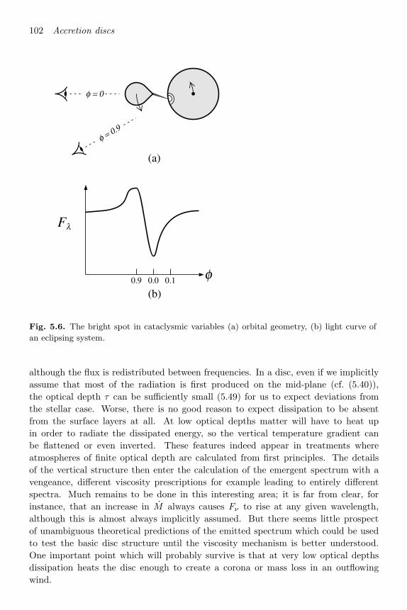
102 Accretion discs

φ = 0.9

φ = 0

(a)

Fλ

φ0.9 0.0 0.1

(b)

Fig. 5.6. The bright spot in cataclysmic variables; (a) orbital geometry, (b) light curve of

an eclipsing system.

although the flux is redistributed between frequencies. In a disc, even if we implicitlyassume that most of the radiation is first produced on the mid-plane (cf. (5.40)),the optical depth τ can be sufficiently small (5.49) for us to expect deviations fromthe stellar case. Worse, there is no good reason to expect dissipation to be absentfrom the surface layers at all. At low optical depths matter will have to heat upin order to radiate the dissipated energy, so the vertical temperature gradient canbe flattened or even inverted. These features indeed appear in treatments whereatmospheres of finite optical depth are calculated from first principles. The detailsof the vertical structure then enter the calculation of the emergent spectrum with avengeance, different viscosity prescriptions for example leading to entirely differentspectra. Much remains to be done in this interesting area; it is far from clear, forinstance, that an increase in M always causes Fν to rise at any given wavelength,although this is almost always implicitly assumed. But there seems little prospectof unambiguous theoretical predictions of the emitted spectrum which could be usedto test the basic disc structure until the viscosity mechanism is better understood.One important point which will probably survive is that at very low optical depthsdissipation heats the disc enough to create a corona or mass loss in an outflowingwind.

5.7 Steady discs: confrontation with observation 103

20 40 60 80 100

5

10

15

20

25

30

R/R*

R B

(T(R

))(a

rbitr

ary

units

)ν

2000 Ao

5500 Ao

22000 Ao

Fig. 5.7. Surface brightness RBν(T (R)) versus R/R∗ for a steady, optically thick disc withT∗ = 7×104 K. At short wavelengths (here 2000 A) the light is strongly concentrated towardsthe central disc regions, while for long wavelengths (here 22000 A) the brightness distribution

is almost uniform outside the central regions.

The second method of checking for the presence of discs, by using eclipses to probethe surface brightness distribution, has proved more successful. The basis of themethod is illustrated in Figs. 5.7 and 5.8. At short wavelengths, the disc light isconcentrated towards its centre, while at longer wavelengths the distribution is moreeven. Hence if we observe a cataclysmic variable with a sufficiently high orbital incli-nation that the companion star eclipses the central regions of the disc, there shouldbe a deep and sharp eclipse at short wavelengths, and a shallower, broader one at longwavelengths.

This method has been used successfully at optical wavelengths, and the advent ofthe Hubble Space Telescope has allowed its extension to the ultraviolet. Typicallyone obtains a large number of light curves, say at U, B and V. These are averagedso as to smooth out short-term fluctuations. A maximum-entropy method gives themost axisymmetric image of the disc in each waveband which is consistent with thedata. The radial flux distributions can then be used to find the dependence T (R) ofeffective temperature on radius, provided we assume something about the way the discradiates locally. This of course is precisely the area of greatest difficulty in modellingthe integrated disc spectrum; fortunately, the predicted run of T (R) is not greatlyaffected by what is assumed at this point. Some results of this procedure are shown inFig. 5.9. As can be seen, they do point to a dependence of the form T (R) ∝ R−3/4 inthis particular case. This is reassuring, as one can see from Section 5.5 that it is very

104 Accretion discs

Disc

White dwarf

Secondary star

Occultedregion

φLine of sight

(a)

1.0

0.5

FλFλ(max)

0.9 0.0 0.1

orbital phase (φ/360˚)

1.0

0.5

FλFλ(max)

0.9 0.0 0.1

orbital phase (φ/360˚)short wavelengths long wavelengths

(b) (c)

Fig. 5.8. (a) Eclipse geometry for a binary system with an accretion disc. Because of the

very different surface brightness distributions at short and long wavelengths (cf. Fig. 5.7) the

light curves predicted are very different: deep and narrow at short wavelengths (b), shallow

and broad at long wavelengths (c).

difficult to avoid such a dependence in a steady-state disc. Further, the estimatedaccretion rate (∼ 10−9 M yr−1) is very reasonable for a dwarf nova in outburst.Not all systems give such good agreement with simple theory, but this can usually beaccounted for by deviations from a steady state.

Another observational technique giving considerable information about the accre-tion flow is called ‘Doppler tomography’. Here one observes the velocity structurerevealed by one particular spectral line. Of course this only gives the radial velocity;but the binary rotation allows one to see the same flow from a range of angles. Plottingthe results in velocity space allows one to distinguish between various types of flowvery easily. For example, a gas stream in a fixed direction has a sinusoidal dependenceof radial velocity on binary phase, whereas an axisymmetric ring obviously shows nosuch variation.

For systems other than cataclysmic variables the evidence for discs is rather lessclearcut, basically for the reasons outlined at the beginning of this section. The lowmass X-ray binaries have similar periods to those of cataclysmics, but differ from them

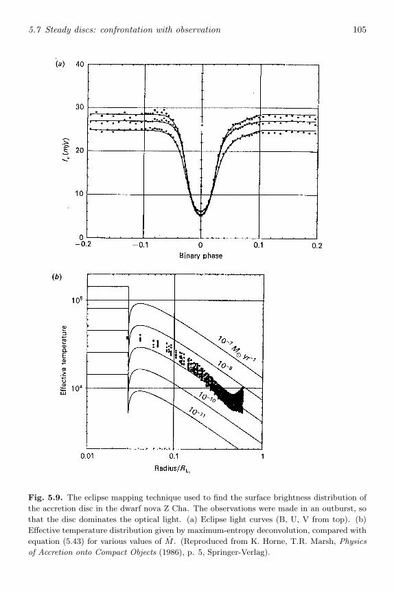
5.7 Steady discs: confrontation with observation 105

Fig. 5.9. The eclipse mapping technique used to find the surface brightness distribution of

the accretion disc in the dwarf nova Z Cha. The observations were made in an outburst, so

that the disc dominates the optical light. (a) Eclipse light curves (B, U, V from top). (b)

Effective temperature distribution given by maximum-entropy deconvolution, compared with

equation (5.43) for various values of M . (Reproduced from K. Horne, T.R. Marsh, Physics

of Accretion onto Compact Objects (1986), p. 5, Springer-Verlag).

106 Accretion discs

Fig. 5.10. The light curves of low-mass X-ray binaries. (a) Axial cross-section showing the

structure of the accretion disc and the corona (Reproduced from J. Frank, A.R. King &

J.P. Lasota (1987), A&A 178, 137.) (b) At high inclination only X-rays scattered from an

extended corona around the accreting neutron star (or black hole) are seen, and eclipses by

the companion star are partial (Reproduced from A.N. Parmar, N.E. White, P. Giommi &

M. Gottwald (1986), Ap. J. 308, 199.)

in having a neutron star or black hole as the accreting component, rather than a whitedwarf. In some systems the companion star is probably significantly nuclear-evolved,despite its currently low mass. As remarked above, the discs in these systems must besignificantly heated by a source other than the local viscous dissipation, probably thecentral X-ray emission. We shall consider this process in detail in Section 5.10. Naivelyone might have expected low-mass X-ray binaries to show straightforward evidence ofdiscs. However the brightest of these systems show a marked lack of binary signatures,particularly eclipses, a fact hindering early identification of the class as binaries at all.

5.7 Steady discs: confrontation with observation 107

Fig. 5.10. The light curves of low-mass X-ray binaries (continued). (c) At lower inclinations

the central point X-ray source is seen, and the X-rays may be modulated by dips (M.G.

Watson, R. Willingale, A.R. King, J.E. Grindlay & J. Halpern (1985) unpublished) and

occasionally total eclipses by the companion.

This is evidently the result of a selection effect: the systems are much brighter inX-rays when viewed at low orbital inclination than when seen at inclinations givingeclipses by the companion star. As fainter systems were discovered, some of them werefound to show periodic features in their X-ray light curves; generally these systemsalso have a lower ratio of X-ray to optical flux. A simple interpretation is that theX-rays from the accreting neutron star are scattered by a tenuous corona above thecentral regions of the accretion disc (Fig. 5.10(a)). This corona probably results fromthe effects of viscous dissipation in the optically thin outer layers of the disc (seeabove); in low-mass X-ray binaries the extra heating caused by X-ray irradiation ofthe disc surface intensifies the effect. The scattering corona acts as a weak, extendedX-ray source in its own right. If we assume that at high inclinations the disc isable to obscure completely the X-ray source near the neutron star surface, we areleft only with this extended source. Eclipses by the companion will be partial andgradual (Fig. 5.10(b)), just like optical eclipses of one star by another, rather than theabrupt total eclipses which would occur if the X-rays came only from the immediatevicinity of the neutron star. At slightly lower inclinations the pointlike X-ray sourceis visible, and we can have a near-total eclipse (the corona providing the residual flux)or ‘dipping’ activity (Fig. 5.10(c)) confined to a restricted phase interval. In systems

108 Accretion discs

where the orbital phasing can be established, usually from optical data, the dips arefound to occur preferentially somewhat before superior conjunction of the X-ray source(i.e. the phase when the companion star is most in front of it). This is reminiscentof the phase of maximum light of the bright spot in cataclysmics (see Fig. 5.6). Thedependence of the dips on X-ray energy shows that they are generally caused byincreased photoelectric absorption. However, the matter causing the absorption musteither be substantially underabundant in heavy elements compared with the solar case,or have most of these elements highly ionized so that they do not absorb. Because allsystems which show an eclipse by the companion also have dips whereas the converseis not true, the structure producing the dips must subtend a greater angle at the X-raysource than the secondary star.

Two main lines of explanation for these orbital modulations have been considered,and quite recently a third has opened up. The first type of model assumed that theouter edge of the disc is able to occult the X-ray source in the central regions ofthe disc. At high inclinations, where only the weak extended X-ray source is seen, acontinuous modulation results if the disc edge causes obscuration all the way aroundthe binary orbit. At slightly lower inclinations the pointlike X-ray source near theneutron star is visible, and dipping activity is assumed to result from the obscurationof this by the most vertically extended part of the disc edge.

It is clear that this model implies a substantial deviation from the standard picture.The repeating nature of the continuous modulation demands a disc rim with a stablevertical structure, which must extend to considerable heights from the disc plane.Even for small mass ratios q ∼ 0.1 the secondary subtends angles sin−1 R2/a ∼> 10

at the X-ray source, implying that the rim structure has a vertical extent H ′ obeyingH ′/Rout ∼> 0.2. This is much larger than the standard thin disc scale height (5.50). Ifwe try to maintain as much as possible of the standard disc picture, the disc rim thuseither involves material much hotter than the thin disc estimates for Tc(Rout) (5.49),or is not in vertical hydrostatic balance at all. In the first case a thin disc descriptionis evidently not appropriate; it is then unclear why changing the central object from awhite dwarf to a neutron star should have such a radical effect on the structure of verydistant regions of the disc. In particular, the estimates in Section 5.10 for the effectsof heating by the central X-ray source do not give high enough surface temperaturesto account for the required central temperatures. If we relax the requirement ofhydrostatic balance for the obscuring matter, we can consider matter following aballistic orbit about the neutron star, or escaping it entirely in the form of a wind.The first type of structure might be caused by the impact of the gas stream from thesecondary on the disc, or spiral shocks within the disc (see Section 5.12 below), whilewinds can be driven off the disc by dissipation in surface layers, as we have remarkedabove. There are difficulties in both cases. Any ballistic orbit will lie in a plane, andintersect the binary plane at two points which are essentially symmetrically disposedabout the neutron star. Thus an orbit leaving the disc rim will intersect it again on theopposite side, with the highest point roughly halfway between. Clearly only rathersmoothly varying azimuthal structure is possible above the disc plane, rather than

5.7 Steady discs: confrontation with observation 109

the fairly jagged profiles that would be required to give the X-ray variation: ‘bulges’with an azimuthal extent much less than about 180 are impossible. (The sameproblem applies also to hydrostatically supported vertical structure, as shown by theequality of the vertical and azimuthal dynamical timescales tφ, tz defined in equations(5.63) and (5.64) below. It is worth noting that this argument does not depend ondetails such as cooling times: tz is the minimum time for the matter to return to theorbital plane.) Further, an orbit producing the periodic X-ray dips in lower inclinationsystems would have to leave the disc plane at a point corresponding to binary phase∼ 0.55 in order to reach its greatest height above the disc at phase ∼ 0.8, wherethe dips are observed. None of the candidate mechanisms for producing the extendedvertical structure readily drive such orbits. Obscuration in a wind from the disc surfaceis possible, although quantitative modelling suggests that the scattering optical depththrough such a wind is likely to be too low to give the observed modulations. Themajor problem in this case is to explain the marked azimuthal structure required forsuch a wind to give the observed periodic modulation. Note that in the case of awind the disc’s own (optical) photosphere could not share this azimuthal dependence,although periodic optical variations are observed in some systems. Finally, all modelsplacing the obscuring matter near the disc edge require large underabundances (factors∼ 10−3) of heavy elements to explain the energy dependence of the X-ray dips: atsuch distances the effects of photoionization by the central X-ray source are far tooweak.

As can be seen, most of the difficulties outlined above would disappear if the ob-scuring matter were located closer in to the neutron star than the disc edge. Onethen needs a way of supplying knowledge of the orbital phase to this material; thesimplest possibilities are that part of the gas stream from the secondary star eitherpenetrates the disc or skims over its upper and lower faces. The latter is particularlyplausible: the estimate w ∼ 0.1P cs (Section 4.5) for the stream radius gives w ∼ 109

cm for P = 5 h, while H as given by (5.49) is at most a few ×108 cm for reasonableparameters. Collisions of the stream either with itself or the disc material then in-evitably occur near the neutron star; the resulting strong shocks (involving velocitiescomparable with the local Kepler value) will automatically put matter at substantialheights above the disc plane, since the shocked gas will have cs ∼< vφ. By (5.32) this gassubtends large angles at the neutron star; this is clearly a promising arrangement forproducing X-ray modulations at the orbital period, provided the gas has the requiredabsorption properties. In this type of model the ionization parameter Ξ = Pion/Pgas,where Pion is the pressure of the ionizing radiation and Pgas is the gas pressure, al-ways turns out to lie in the range 0.1–10 which implies a two-phase instability (seeFig. 8.3). Most of this gas condenses into cool ( ∼ 104 K) clouds scattered through alow-density hot (∼ 107 K) medium. This happens independently of the accretion ratebecause both Pion and Pgas are proportional to M so that it cancels in the expressionfor Ξ. We thus have material cool enough to produce substantial photoelectric absorp-tion subtending a large angle at the X-ray source. This is evidently qualitatively justwhat is needed to produce the various types of X-ray light curves; in particular the

110 Accretion discs

fine structure in X-ray dips can result from the passage of individual cool clouds acrossthe line of sight to the X-ray source. Similar structure does not result in cataclysmics,as the ionization parameter is always lower by a factor Rwd/Rns ∼ 103, leaving thematter in the cool state.

This generic type of model offers physical explanations for the main features of theX-ray behaviour without requiring us to abandon the thin disc picture for low-massX-ray binaries (LMXB). To explain the light curves in detail we must specify thekinematics of the shocked gas stream more closely. The possibility so far exploredin most detail is that the gas stream skims over the disc surfaces and forms a ringat the circularization radius Rcirc. The newly arriving gas then collides with thisring, shocking and rising out of the disc plane at the impact point. The two-phaseinstability forms cool clouds which give rise to the dips (Fig. 5.11). The behaviourwith orbital phase predicted by this model agrees with most, but not all, of theobservations (note that in the thick-rim picture there is no physical constraint at allon the various phases). Another possibility is that no ring forms at Rcirc at all since thestream pinches off vertically near to the distance of closest approach to the neutronstar, colliding with itself and the disc material. This too would give a two-phaseinstability, although details of the resulting behaviour have still to be worked out.

Quite recently, another possible explanation for the orbital modulations in LMXBshas emerged. We shall see (Section 5.10) that in luminous systems the effect of self-irradiation may cause the disc to be warped, so that its central plane at any point needno longer coincide with the orbital plane (Fig. 5.17). The details of the warping arecomplex, but it is clear that it can produce some effects quite similar to those found inthe thick-rim picture, without requiring the unphysically large scaleheights demandedthere. In particular it offers a simple explanation for the presence of cool material inapparently stable positions well away from this plane. Such parts of the disc wouldevidently follow orbits inclined at significant angles H ′/R ∼ 0.2 to this plane, with amuch smaller vertical extent H H ′ about this inclined orbital plane. Moreover, theextended vertical structure need not simply appear at the outer edge of the disc, butover a range of radii, perhaps alleviating some of the problems detailed above withthe energy dependence of the X-ray dips. More work is needed to test this idea (seeSection 5.10).

5.8 Time dependence and stability

In the last five sections, we have dealt in some detail with the theory and observationsof steady thin accretion discs. There are several reasons for extending this study totime-dependent discs. One is that we must check that the steady-state models arestable against small perturbations: if not, we have probably made some assumptionin the course of constructing these discs which is not compatible with the furtherassumption of steadiness. Another reason is that the observable properties of thesteady-state, optically thick discs we have considered above are largely independent of

5.8 Time dependence and stability 111

Fig. 5.11. Three different views of a model LMXB in the penetrating gas-stream picture.

The situation in the orbital plane with line of sight positions at 0.1 phase intervals is depicted

at the top. The mass transfer stream hits the edge of the accretion disc at S1, and the ring

of radius Rcirc at S2. A two-phase medium of cold clouds and hot intercloud gas forms after

impact at S2 due to ionization/thermal instabilities and splashes off the disc plane. The

thick dots represent the cold clouds. The central diagram shows a cut through the binary

axis normal to the orbital plane (OP). The disc and ring at Rcirc appear in cross-section.

The extent of the stream and corona are schematically indicated. The bottom diagram is

a perspective view of the model showing the splitting of the stream at S1, the ring and the

bulge with the cold clouds. (Reproduced from Frank, King & Lasota (1987), A&A 178,

137.)

112 Accretion discs

viscosity; this is a fortunate occurrence for the purpose of showing that such discs doindeed exist, but it means that observations of steady discs are unlikely to give muchinformation about the viscosity. The time dependence of disc flow is, on the otherhand, controlled by the size of the viscosity (cf. Section 5.2). Hence observations oftime-dependent disc behaviour offer one of the few sources of quantitative informationabout disc viscosity. In view of our present ignorance of the basic physical processesinvolved, such a semi-empirical approach to the problem seems the most reasonable.The main arena for the study of time dependence is the problem of the outbursts ofdwarf novae, which also represent an area of prime interest in their own right.

We begin by identifying the typical timescales on which the disc structure may vary.We have already encountered the viscous timescale

tvisc ∼ R2

ν∼ R

vR(5.62)

which gives the timescale on which matter diffuses through the disc under the effect ofthe viscous torques. Note that (5.11) assumes that the typical lengthscale for surfacedensity gradients in the disc is ∼ R (see Section 5.2 above). The shortest characteristictimescale of the disc is the dynamical timescale

tφ ∼ R

vφ∼ Ω−1

K . (5.63)

Clearly, inhomogeneities, such as flares on the disc surface, would cause quasi-periodicvariations in the disc light at some wavelengths with this timescale. Deviations fromhydrostatic equilibrium in the z-direction are smoothed out on a timescale

tz = H/cs. (5.64)

But from (5.32) we see that

tz ∼ R/Mcs = R/vφ ∼ tφ

so that the dynamical timescale also measures the speed with which hydrostatic equi-librium in the vertical direction is established. In addition to tφ, tz and tvisc, we candefine the thermal timescale:

tth =heat content per unit disc area

dissipation rate per unit disc area,

which gives the timescale for re-adjustment to thermal equilibrium, if, say, thedissipation rate is altered. Since the heat content per unit volume of a gas is∼ ρkT/µmp ∼ ρc2s , this gives

tth ∼ Σc2s/D(R). (5.65)

The relation (4.29) between D(R) and νΣ means that tth can be re-expressed in termsof the viscous timescale: for a Keplerian disc, we have (Ω = ΩK)

tth ∼ R3c2sGMν

∼ c2sv2φ

R2

ν∼ M−2 tvisc (5.66)

5.8 Time dependence and stability 113

using (5.30). Using the α-parametrization (4.34) we can also write

tvisc ∼ R2

ν∼ 1

α

R

H

R

vφ· vφ

cs

which, for a thin disc, gives, on using (5.30), (5.32) and (5.63),

tvisc ∼ α−1M2 tφ. (5.67)

Collecting results we have

tφ ∼ tz ∼ αtth ∼ α(H/R)2tvisc. (5.68)

If we assume α ∼< 1 there is thus a well-defined hierarchy of timescales tφ ∼ tz ∼< tth tvisc. Numerically, we have, for the α-disc solutions (5.49),

tφ ∼ tz ∼ αtth ∼ 100m−1/21 R

3/210 s,

tvisc ∼ 3 × 105α−4/5M−3/1016 m

1/41 R

5/410 s.

(5.69)

Thus the dynamical and thermal timescales are of the order of minutes, and the viscoustimescale of the order of days to weeks for typical parameters.

Suppose now that a small perturbation is made to a putative equilibrium solutionand that this perturbation continues to grow rather than being damped. Then thesupposed steady solution is said to be unstable and cannot occur in reality. Thesharp difference we have found in the various timescales means we can distinguishdifferent types of instability. If for example the energy balance is disturbed in thedisc, any instability will grow on a timescale tth, which is much less than tvisc. Sincetvisc is the timescale for significant changes in the surface density Σ to occur, we canassume that Σ is fixed during the growth time tth. We refer to this as a thermalinstability. For α < 1 we also have tth > tφ ∼ tz, so the vertical structure of the disccan respond rapidly, on a timescale tz, to changes due to the thermal instability, andkeep the vertical structure close to hydrostatic equilibrium. Hence we can impose theconditions

Σ ∼ constant,H ∼ cs(Tc)(R3/GM)1/2

(5.70)

(from (5.25)) in examining the growth of any thermal instabilities.Such instabilities arise when the local (volume) cooling rate Q−(erg s−1 cm−3)

within the disc can no longer cope with the (volume) heating rate Q+ ∼ D/H dueto viscous dissipation. In equilibrium we must have Q+ = Q−. But if, when thecentral temperature Tc is increased by a small perturbation ∆Tc, Q+ increases fasterthan Q−, Tc will rise further because the cooling rate is inadequate. In other words,a steady state is impossible in a parameter regime where the instability would grow,despite the fact that formally an ‘equilibrium’ solution can be found.

To make these ideas clearer, let us consider an explicit example. Suppose the localcooling rate is just the optically thin emissivity 4πj (ρ, Tc) (erg s−1 cm−3); i.e. weassume that the disc density is so low that the vertical optical depth τ 1. Generally,

114 Accretion discs

such a gas cools by two-body emission processes so the emissivity depends on thesquare of the density, and has the form 4πj ∝ ρ2Λ(Tc). Λ(Tc) is a function called thecooling curve, which depends principally on how the ionization balance of the gas ismaintained – for example by photoionization, or by collisions. It is the behaviour ofΛ as a function of Tc which largely determines whether the instability grows or not.By (5.70) we can write that during the perturbation

Q− = 4πj ∝ ρ2Λ ∼ (Σ/H)2Λ ∼ c−2s Λ ∼ T−1c Λ,

where we have assumed negligible radiation pressure in the last step. Similarly, wehave

Q+ ∼ D/H ∼ ν/H ∼ αcs ∼ αT 1/2c ,

where we have used the α-parametrization (4.34). Comparing these two expressions,we see that the thermal instability will grow if Q− increases less rapidly with Tc thandoes Q+, i.e. if Λ/α grows more slowly with Tc than T

3/2c . The customary way of

writing the instability criterion is

d ln(Λ/α)d ln Tc

<32

, (5.71)

or, for the general case, in the alternative forms,

dQ−

dTc<

dQ+

dTcd ln Q−

d ln Tc<

d ln Q+

d ln Tc

⇒ unstable. (5.72)

From the form of Λ(Tc), which decreases for Tc ∼> 104 K, and with α ∼ constant, weexpect optically thin regions of the disc to be thermally unstable for Tc > 104 K. SinceΛ(Tc) for other cases has a similar character, this result is of general validity. Notehowever that it is sensitive to the functional form of α: for α ∼ T−2

c , say, our conclusionwould be reversed. As we have stressed in connection with the Shakura–Sunyaevsolution (5.49), we have no knowledge of the form, as opposed to the magnitude, of α.Because we expect α ∼< 1, it is rather unlikely that α could conspire to behave as, say,α ∼ T−2

c for a wide range of Tc, so the result above probably holds for most values ofTc ∼> 104 K; but we cannot rule out a priori the possibility that isolated stable regimes(for restricted ranges of Tc) exist.

In contrast to the optically thin case, for optically thick discs the effective volumecooling rate (taking account of the local re-absorption of radiant energy) is

Q− =dF

dz∼ σT 4

c

κRρH2

by (5.39) and (5.37). For Kramers’ opacity (5.53) this can be rewritten as

Q− ∼ T15/2c

ρ2H2=

T15/2c

Σ2∼ T 15/2

c

5.8 Time dependence and stability 115

omitting constraints and using (5.70). As before, we have Q+ ∼ αT1/2c if gas pressure

dominates, so, unless α decreases more rapidly than T−7c , optically thick parts of

the disc will be thermally stable. Similar conclusions follow when other opacitiesdominate.

Let us now consider changes in the disc structure which take place on the viscoustimescale. This includes viscous instabilities and the evolution of discs in response tochanges in external conditions, such as the mass transfer rate (cf. Section 5.2). Astvisc tth ∼> tz we assume that the disc adjusts so rapidly that it always maintainsboth thermal and hydrostatic equilibrium. Hence, some of equations (5.41) describingsteady discs apply also to time-dependent discs: equations 1, 2, 3, 4, 6 and 8 surviveunaltered. Equations 5 and 7 explicitly used the assumption of steadiness and mustbe changed. The energy transport equation 5 is replaced by the combination of (5.40)and (4.30):

4σ

3τT 4c =

98

νΣGM

R3.

Here we have assumed that tvisc is much longer than the timescale for radiation todiffuse out of the disc; this is amply satisfied by the resulting disc solutions. Equation7 is an integral of the mass and angular momentum equations (5.3) and (5.4). In thetime-dependent case we can replace it by the evolution equation (5.8). Defining themass transfer rate M(R, t) at each radius by equation (5.14), in which Σ and vR arenow allowed to be functions of t, we can rewrite the mass conservation equation (5.3)as

2πR∂Σ∂t

=∂M

∂R. (5.73)

For reference we collect these equations together:

1. ρ = Σ/H;2. H = csR

3/2/(GM)1/2;3. c2s = P/ρ;

4. P =ρkTcµmp

+4σ

3cT 4c ;

5.4σ

3τT 4c = 9

8νΣGMR3 ,

6. τ = ΣκR(ρ, Tc) = τ(Σ, ρ, Tc);

7.∂Σ∂t

= 3R∂∂R

R1/2 ∂

∂R (νΣR1/2)

,

8. ν = ν(ρ, Tc, Σ, α, . . .).

(5.74)

Thus, again we have eight equations for the eight unknowns ρ, Σ, H, cs, P , Tc, τ andν as functions now of R, t and any parameters (e.g. α) in the viscosity prescription8. Because 7 is a diffusion equation we must also provide appropriate boundaryconditions. Once the set (5.74) is solved, M may be found from (5.3) and boundaryconditions, and vR read off from (5.14). As before, we can simplify these equationsand reduce the time-dependent disc problem to one involving fewer variables.

116 Accretion discs

Since the time dependence enters only through equation 7, it is sensible to try toexpress the other quantities in terms of Σ as far as possible, as they depend on t onlythrough Σ and not explicitly. In particular, equations 1–4 can be combined to give

GMΣH

R3=

kTcΣµmpH

+4σ

3cT 4c . (5.75)

From 5 and 6 we have

T 4c =

2732σ

Σ2κRνGM

R3. (5.76)

Since κR and ν are both functions of Σ/H, Tc and R, we can in principle eliminate κR,ν and Tc, say, to get H as a function of R and Σ, with similar results for all the otherquantities. As an example, if κR is given by the Kramers’ form (5.53), ν specified bythe α-prescription (4.34) and gas pressure is assumed to dominate radiation pressure(5.76) assumes the form

T 4c ∝ αΣ3HT−7/2

c (GM/R3)1/2. (5.77)

Using this equation, Tc can be eliminated from (5.75) to give H as a function of R

and Σ. Similarly, we get from the α-prescription

ν = αcsH = α(kTc/µmp)1/2H = ν(R, Σ)

and so on. This rather tedious, if straightforward, algebraic manoeuvring illustratesan important result: the set (5.74) fixes ν as a function of R and Σ, so that equation7 is a nonlinear diffusion equation for Σ(R, t). An exception to this result would ariseif ν were not a function of local conditions within the disc, but somehow determinedfrom outside, so that it involved an explicit t-dependence.

Clearly, to solve the nonlinear equation 7 and subsequently find all the other discvariables is in general a formidable task which must be tackled numerically. We shallconsider shortly the results of some such calculations. However, we can draw someimportant conclusions from the result above and the form of equation 7 alone. Supposethat the surface density in a steady disc is perturbed axisymmetrically at each R, sothat

Σ = Σ0 + ∆Σ

where Σ0(R) is the steady-state distribution. Writing µ = νΣ there will be acorresponding perturbation ∆µ. Since ν = ν(R, Σ) by our result above, we haveµ = µ(R, Σ), so that ∆µ = (∂µ/∂Σ)∆Σ. Because of equation 7 of (5.74), ∆Σ and ∆µ

are related further by

∂

∂t(∆Σ) =

3R

∂

∂R

[R1/2 ∂

∂R(R1/2∆µ)

].

Eliminating ∆Σ we obtain the equation governing the growth of the perturbation

∂

∂t(∆µ) =

∂µ

∂Σ3R

∂

∂R

[R1/2 ∂

∂R(R1/2∆µ)

].

5.8 Time dependence and stability 117

Not surprisingly, ∆µ obeys a diffusion equation, but the interesting thing is that thediffusion coefficient is proportional to ∂µ/∂Σ and in principle can be either positive ornegative, since we have no information about ν and hence about µ. If ∂µ/∂Σ is positivewe get the type of diffusive behaviour discussed in Section 5.2 and the perturbationdecays on a viscous timescale. However, if ∂µ/∂Σ is negative, more material will befed into those regions of the disc that are denser than their surroundings and materialwill be removed from those regions that are less dense, so that the disc will tendto break up into rings. This breakup of the disc on a timescale tvisc constitutes theviscous instability; more precisely stated: steady disc flow is only possible provided∂µ/∂Σ > 0.

From (5.19) and (5.43) we note that µ = νΣ ∝ M ∝ T 4(R), where M , T (R) arethe local equilibrium values of the mass transfer rate and surface temperature, so thatthis requirement can be rewritten as ∂M/∂Σ > 0 or ∂T (R)/∂Σ > 0. Indeed, the firstof these forms makes the stability requirement transparent: if, instead, a region of thedisc had ∂M/∂Σ < 0, the local mass transfer rate would increase in response to adecrease in surface density, and vice versa.

To check the viscous stability of accretion discs we therefore have simply to computethe relation between T 4 and Σ at a given disc radius R. We shall do this here firstfor regions of the disc where gas pressure dominates radiation pressure. The energyequation (5 of 5.74) is equivalent to T 4 ∝ T 4

c /τ . In general we can write the opacityas κR ∝ ρTnc , so that τ ∼ κRρH ∝ Σ2Tnc H−1. Then since H ∝ cs ∝ T

1/2c we get

a relation T 4 ∝ T9/2−nc Σ−2 between the effective and mid-plane temperatures. Since

from the α-prescription, we have ν = αcsH ∝ Tc we also find T 4 ∝ M ∝ νΣ ∝ TcΣ.Eliminating Tc between these two relations gives

T ∝ Σ13−2n

4(7−2n) . (5.78)

This relation shows that ∂T/∂Σ < 0, i.e. the disc is unstable, in regions where thetemperature index n obeys 7/2 < n < 13/2. (Note that in the Kramers’ case n = −3.5we find T ∝ Σ5/14, which is just what we get by eliminating M between eqs. 5.43 and5.49.)

In fact, values of n in the unstable range 7/2 < n < 13/2 will always occur inhydrogen ionization zones, i.e. wherever T is close to the local hydrogen ionizationtemperature TH ∼ 6500 K. For T < TH, hydrogen is predominantly neutral, and κRincreases rapidly with increasing temperature, i.e. n > 13/2. But we know that forT > TH, hydrogen will be essentially fully ionized, and n takes the Kramers’ value−3.5; the opacity drops with temperature as the free electrons become more mobile,reducing both the bound–free and free–free cross-sections. By continuity, n clearlypasses through the unstable range 7/2 < n < 13/2 as T increases above TH. Thuswe must expect the instability to appear wherever a disc has regions with T ∼ TH.This is such a common situation that we would certainly expect the instability tomanifest itself as a widespread feature in disc-accreting systems. This conclusion isreinforced by considering discs with convective vertical structure, as can be expectedif T is close to, but below TH: there also we expect an inverse relation between T and

118 Accretion discs

Σ. In general the relation between T and Σ is S-shaped in such regions (see Fig. 5.12),with an unstable central branch near T = TH lying between two stable branches atlower and higher temperatures.

Viscous instability also appears in another case, namely when the disc is dominatedby radiation pressure, with a pure scattering opacity κR = constant. These conditionshold in the central regions of discs around neutron stars and black holes. Repeating thesteps above, we find that the vertical energy transport equation (5 of 5.74) now givesT 4 ∝ T 4

c Σ−1, while the sound speed is given by c2s ∝ P ρ−1 ∝ T 4cHΣ−1 ∝ T 4

c csΣ−1.Thus cs ∝ H ∝ T 4

c Σ−1 and hence T 4 ∝ νΣ ∝ csHΣ ∼ T 8c Σ−1. Then eliminating Tc

as before we get

T ∝ Σ−1/4.

Thus again we have ∂T/∂Σ < 0, and a viscous instability, this time known as theLightman–Eardley instability. While the T –Σ curve will have a stable branch withpositive slope at lower T , there is formally no such branch for large T . In otherwords the T (Σ) curve is no longer S-shaped, but simply has a maximum in Σ, i.e.resembles a right hand bracket, ). In practice the thin disc approximation breaksdown at large T because the accretion rate approaches the Eddington limit (cf 5.61).An S-shaped T (Σ) curve is recovered if we regard the loss of matter accreting rapidlyinwards (advection) as a cooling term in the energy balance equation Q+ = Q−. Weshall discuss this instability briefly at the end of the next section.

We must now ask what really happens when ∂T/∂Σ < 0 in some region of a disc.The description ‘viscously unstable’ means that equilibrium is not possible under theassumptions we made, namely that the disc structure evolves only on the viscoustimescale, while maintaining dynamical and thermal equilibrium. One of these as-sumptions must break down, allowing the disc to evolve on a shorter timescale whichthen permits it to reach a new, stable, viscous equilibrium. In fact it is easy to seethat the thermal balance condition (5 of 5.74) must fail precisely where ∂T/∂Σ < 0.For this equation simply asserts that the cooling term Q− ∝ T 4 exactly balances theheating term Q+ ∝ µ = νΣ. The general form of this equation (allowing for thetemperature to change in time because of a possible imbalance between heating andcooling) can be written as

∂T

∂t∝ Q+ − Q−. (5.79)

If ∂T/∂Σ < 0 it is clear that a small perturbation tends to exaggerate the mismatchbetween Q+ and Q−, and so causes a thermal instability.

This means that to understand what happens when ∂T/∂Σ < 0 we must allowfor time variations of both T and Σ. If we consider an annulus of the disc (smallrange around fixed R) with a fixed mass supply rate M0, we then have two first-orderordinary differential equations governing the time development of T and Σ, i.e. (5.79)and the diffusion equation (7 of 5.74). The right-hand side of the latter is a complicatedfunction, but the only two things we need to know about it is that the time t does not

5.8 Time dependence and stability 119

appear explicitly, and that it vanishes when T takes the value T0 = T (R, M0) specifiedby (5.43), as this gives ν and Σ precisely the right values to ensure that the local massflow rate is exactly M0 in the annulus. As the time t does not appear explicitly, thesetwo equations are autonomous and T, Σ span a phase plane. We can therefore discoverthe qualitative behaviour of T and Σ without solving the system, or indeed withouteven requiring explicit forms for the right-hand sides of the two equations. The factthat variations of T on the thermal timescale tth are much more rapid than those of Σon the viscous timescale tvisc makes the analysis particularly simple. Using t′ = t/tthas a dimensionless time variable, the system (5.79, 7 of 5.74) takes the form

T = h(T, Σ), (5.80)

Σ = εk(T, Σ), (5.81)

where the overdots now denote derivatives with respect to t′, and we have writtenε = tth/tvisc. Here h, k represent the transformed right-hand sides of (5.79) and thediffusion equation 7 of (5.74) respectively. In this form h and k are both O(1), as T, Σevolve on timescales tth, tvisc. Clearly an equilibrium solution of the system (5.80,5.81) corresponds to T = Σ = 0, and thus to an intersection of the curves h = 0, k = 0plotted on the T, Σ plane of Fig. 5.12. This is called a fixed point of the system. SinceT ∝ Q+ − Q−, the h = 0 curve in general has the characteristic S-shape discussedearlier, whereas k = 0 is simply the horizontal straight line T = T0. The two curvesh = 0, k = 0 divide the T, Σ plane into four regions around the fixed point; in eachone the system evolves in the directions shown by the arrows. As tth tvisc we haveε 1, which means that the motion in T is always much more rapid than that in Σ.The system will thus always move in T until it reaches the thermal equilibrium curveh = 0 before there is significant motion in Σ. Once the system has reached the curveh = 0 (on a thermal timescale) it will evolve along it in Σ in the direction specified bythe arrows (on a viscous timescale), searching for the fixed point at the intersectionwith the curve k = 0, i.e. for the effective temperature T = T0 making the mass flowrate equal to M0.

We can now see that two qualitatively different behaviours are possible for theevolution of the disc annulus. For the directions of the arrows on Fig. 5.12 show thatthe motion in T can only take the system point to parts of the h = 0 curve whichhave positive slope, i.e. ∂T/∂Σ > 0. Moreover, if the system point happens to beon parts of this curve with the opposite slope, a small perturbation will cause it toleave to larger or smaller T . Branches of the S-curve with positive slope are said to beattracting, while those with negative slope are repelling. If M0 is such that the fixedpoint, i.e. the intersection T = T0 with the curve k = 0, lies on an attracting branch,the system will eventually find this point and remain stably there. This situation isdepicted in Fig. 5.12(a). The annulus will remain in this state until M0 is varied, sincethe equilibrium state is stable, as shown by the directions of the arrows. If, on theother hand, M0 is such that the intersection is on a repelling branch (∂T/∂Σ < 0)of the S-curve h = 0 (see Fig. 5.12(b)) the annulus can never settle into a steady

120 Accretion discs

k=0 k=0

h=0h=0

Σ0 Σ

T0

T T

T0

Σ0 Σ(a) (b)

A

C

D

E

B

Fig. 5.12. Phase plane in the vicinity of a fixed point, indicated by a solid dot at the

intersection of the two critical curves h = 0 and k = 0: (a) stable fixed point; (b) unstable

fixed point and stable limit cycle.

configuration. If it starts, say, on the lower stable part of the curve AC, the low valueof T (and hence M) will cause it to evolve through states of increasing Σ in an attemptto raise M to M0. This continues until Σ reaches the value Σmax at point C: the onlyattracting branch for this value of Σ is the high-temperature state represented bypoint D, so any perturbation will cause the annulus to make a transition on a thermaltimescale to this state. During the first part of the rise in T the annulus has Σ > 0,changing to Σ < 0 as the system crosses the Σ = 0 curve T = T0. Thus in principlethe curve CD bends slightly to larger then smaller Σ before reaching D: however thefact that ε 1 means that CD is effectively a vertical straight line. When the systemreaches D the local value of M is larger than the externally fixed value M0, so theannulus evolves towards lower T , Σ until it reaches Σmin (point E). Again T and M

must adjust on a thermal timescale, this time to the lower branch (point B) so thatthe whole cycle BCDE repeats. The annulus therefore displays limit-cycle behaviour,alternating long-lived (low viscosity) states of low M and short-lived (high viscosity)states of high M , with rapid (thermal timescale) transitions between them.

It is important to realise that the discussion above was purely local: we did notallow for changes in the mass supply rate M0 into the annulus, such as might indeedbe triggered by limit-cycle behaviour at larger or smaller radii, or cooling or heatingwaves moving radially across the disc. Changes of both kinds could obviously affect thelocal limit cycle we have found. Clearly the global problem is much more complicated,and we cannot expect to find simple analytic arguments of the type given above. Onlya numerical treatment will reveal under what circumstances large regions of the discbecome unstable. However the local discussion does suggest that we might expectaccretion discs to show some kind of time-dependent behaviour whenever the simple

5.9 Dwarf novae 121

condition T (R) ∼ TH holds for some range of radii R. It is therefore important tocheck for observable consequences.

5.9 Dwarf novae

As we saw in Section 5.7 there is considerable observational evidence that accretiondiscs conforming roughly to the picture we outlined in Section 5.3 to 5.6 actuallyexist in cataclysmic variables and indeed provide most of their light in many cases.A subclass of these systems, the dwarf novae, undergo outbursts from time to timein which they brighten by several magnitudes. These are much smaller in amplitudethan the outbursts of classical novae (hence the name), and recur at intervals of weeksto months. A typical outburst light curve is shown in Fig. 5.13.

It is by now generally agreed that dwarf nova outbursts are powered by a suddenincrease in the accretion rate. The alternative mechanism of runaway thermonuclearburning of the accreted material on the white dwarf, which is believed to power novae,cannot provide recurrence times of less than about 104 yr. J.I. Smak (1971) pointedout that there are two possible models:

(i) The mass transfer rate from the companion star is variable because the envelopeof this star is dynamically unstable; thus, outburst corresponds to a suddenburst of mass transfer from this star.

(ii) The viscosity in the disc varies: between outbursts (in ‘quiescence’) the viscosityis low, so that the viscous timescale is long and matter accumulates in the disc;in outburst the viscosity suddenly rises, the viscous timescale becomes shortand some of the matter previously stored in the disc is rapidly deposited on tothe white dwarf.

We examine the variable mass transfer model first. Models of the companion starinstability suggest an increase in the mass transfer rate by factors ∼ 102 on timescalesof order 105 s, followed by a slower decay back to the quiescent state. To see what sortof changes in the disc structure result, we must introduce this burst of mass transferinto the time-dependent disc equations (5.74) as a source term in the diffusion equation7. This can be done numerically and model light curves resembling Fig. 5.13 produced,provided α is suitably adjusted. In this model, the basic reason for the form of thelight curve (rapid rise, flat top, slow decay) is the dependence (cf. 5.11) of the viscoustimescale on the surface density gradient. Since, for the assumed parameters, thetimescale of the mass transfer burst is always shorter than tvisc, it is the latter whichdetermines the timescale of changes in Σ and ultimately in luminosity. Thus, at thebeginning of the outburst, the disc tries to reach a steady state corresponding tothe new, high accretion rate Mhigh. This evolution proceeds on the viscous timescaletvisc(rise)∼ l2/ν, l R, corresponding to the steep density gradients in the disc causedby the sudden influx of mass. One thus expects a rapid rise in luminosity, startingat long (visible) wavelengths and moving to the ultraviolet as the extra mass diffuses

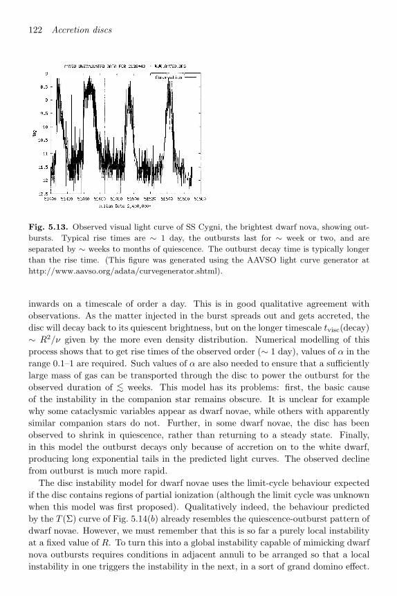
122 Accretion discs

Fig. 5.13. Observed visual light curve of SS Cygni, the brightest dwarf nova, showing out-

bursts. Typical rise times are ∼ 1 day, the outbursts last for ∼ week or two, and are

separated by ∼ weeks to months of quiescence. The outburst decay time is typically longer

than the rise time. (This figure was generated using the AAVSO light curve generator at

http://www.aavso.org/adata/curvegenerator.shtml).

inwards on a timescale of order a day. This is in good qualitative agreement withobservations. As the matter injected in the burst spreads out and gets accreted, thedisc will decay back to its quiescent brightness, but on the longer timescale tvisc(decay)∼ R2/ν given by the more even density distribution. Numerical modelling of thisprocess shows that to get rise times of the observed order (∼ 1 day), values of α in therange 0.1–1 are required. Such values of α are also needed to ensure that a sufficientlylarge mass of gas can be transported through the disc to power the outburst for theobserved duration of ∼< weeks. This model has its problems: first, the basic causeof the instability in the companion star remains obscure. It is unclear for examplewhy some cataclysmic variables appear as dwarf novae, while others with apparentlysimilar companion stars do not. Further, in some dwarf novae, the disc has beenobserved to shrink in quiescence, rather than returning to a steady state. Finally,in this model the outburst decays only because of accretion on to the white dwarf,producing long exponential tails in the predicted light curves. The observed declinefrom outburst is much more rapid.

The disc instability model for dwarf novae uses the limit-cycle behaviour expectedif the disc contains regions of partial ionization (although the limit cycle was unknownwhen this model was first proposed). Qualitatively indeed, the behaviour predictedby the T (Σ) curve of Fig. 5.14(b) already resembles the quiescence-outburst pattern ofdwarf novae. However, we must remember that this is so far a purely local instabilityat a fixed value of R. To turn this into a global instability capable of mimicking dwarfnova outbursts requires conditions in adjacent annuli to be arranged so that a localinstability in one triggers the instability in the next, in a sort of grand domino effect.

5.9 Dwarf novae 123

Σ0 Σ

T0

T T

T0

T2

T1

Σ2 Σ0 Σ1 Σ(a) (b)

A

C

D

E

B

Fig. 5.14. Effective temperature–surface density diagrams with (a) a unique, stable steady

solution (T0,Σ0), and (b) a case where limit-cycle behaviour occurs as the steady solution

(T0,Σ0) lies on a region of the curve with ∂T/∂Σ < 0.

Whether this happens depends on the relation of the surface density distributionΣ(R, t) in the disc to the critical values Σmax(R), Σmin(R) specified by the S-curve(cf. Fig. 5.14(b)). These values can be found from the vertical structure equations ateach radius; since the effective temperature is close to the ionization temperature THat the two bends in the S-curve we must have from (5.42) and (4.30) that

D(R) =98

νΣGM

R3 σT 4

H (5.82)

in both cases. Using the full vertical structure given by the set (5.74), together withthe alpha-prescription (5.47) and Kramers’ opacity (5.48), we find

Σmax = 11.4R1.0510 M−0.35

1 α−0.86c g cm−2, (5.83)

Σmin = 8.25R1.0510 M−0.35

1 α−0.8h g cm−2, (5.84)

where R10 = (R/1010 cm), and αc, αh are characteristic values for the cold andhot states respectively. Thus both Σmax and Σmin increase roughly linearly withdisc radius R. In quiescence Σ(R, t) lies between these two values at each R and sotends to increase outwards, apart from some minor local variations. An outburst istriggered once Σ rises above Σmax at some radius. (Remember that in the quiescentstate Σ is increasing in time everywhere, as shown by the arrows in Fig. 5.14(b).)The disc annulus at that point makes the transition to the hot state, and the steepradial surface density and temperature gradients cause mass (cf. Fig. 5.1) and heat todiffuse rapidly into the adjacent annuli, stimulating them to make the same transition.This leads to the propagation of heating fronts both inwards and outwards from theinitial instability. The heating front is similar to a combustion wave, and the following

124 Accretion discs

simple argument adapted from combustion theory shows that inward-moving frontswill propagate at a velocity vh ∼ αcs. As the front moves inwards at speed vh, itswidth d is set by requiring that heat diffuses a distance d during the thermal time onwhich the cool matter heats up. This by definition means that the front has advanceda distance d in this time. We therefore have

tth =d2

νth(5.85)

and

d = vhtth, (5.86)

where νth is the heat diffusion coefficient in the disc. Eliminating d, we find

v2h =νthtth

.

We can expect νth to be of order ν = αcsH, since the same physical process probablygoverns both transport coefficients. Finally, if we take tth as given by the expression(5.65), we can use the ordering (5.68) to give

tth ∼ H2

ν(5.87)

so that

vh ∼ αcs, (5.88)

as anticipated. Note that from (5.86) and (5.87) we now find that the front width d

should be of order the disc scaleheight H. In practice, numerical simulations of time-dependent discs give rather wider fronts than this estimate. One effect contributing tothis is that equation (5.65) is not the correct thermal timescale for the full attainmentof the hot state behind the front. In particular, this form neglects the work that hasto be done expanding the cool gas to the new scaleheight against gravity (similarly,in a cooling wave the gas has to rid itself of the extra heat liberated as it tries tocollapse to a lower scaleheight ). Nevertheless, (5.88) is a reasonable estimate for theinward propagation of a heating wave. An outward-moving front in practice movesrather more slowly. This is because the front moves into matter at higher density,from which it cannot readily remove angular momentum.

In the hot region left by the passage of a front matter flows inwards because ofthe enhanced viscosity, and so builds up a quasi-steady surface density profile whichnow decreases outwards as Σ(R, t) = Σhot ∼ s(t)Rk, with k ∼ −0.75 (cf 5.49). Thehot disc behaves as though it were steady, with a surface density corresponding to anaccretion rate higher than the mass supply to the disc. Thus we expect Σ = Σhot < 0(i.e. s < 0), which indeed is true (Fig. 5.14(b)), so this surface density profile musteventually cross the Σmin(R) curve at some large radius, and the outer parts of thedisc will make the reverse transition to the cool state (cf. Fig. 5.14(b)). Mass flowsoutwards at this interface as the viscosity in the hot inner region is much higher than

5.9 Dwarf novae 125

that in the cool region. A cooling front now propagates inwards, eventually returningthe entire disc to the cool quiescent state. This front moves with a somewhat slowervelocity vc ∼ 0.1vh than the heating front.

Clearly this sort of behaviour is again qualitatively in agreement with what happensin a dwarf nova outburst. The rise to maximum corresponds to the time tr taken bythe heating front to travel across the disc, and the decline time td to the inward motionof the cooling front. The time at maximum depends on the point when the heatingfront first encounters a surface density Σmin(R). If this occurs while the heatingfront is still moving outwards this front is immediately replaced by an inward-movingcooling wave, giving a short outburst. If by contrast the whole disc can be heated,i.e. Σhot(Rd) > Σmin(Rd) in the hot state, the disc stays hot until the quasi-steadyΣhot(R) ∼ R−0.75 profile decreases sufficiently that Σ(Rd) is reduced to Σmin(Rd),giving a long, flat-topped outburst.

In fact, outbursts of the observed duration and brightness can only be obtained byusing the freedom to manipulate the effective value of the α parameter; in particular,if α has a single constant value no large outburst results, because the resulting S-curveis rather narrow, i.e. Σmax/Σmin ∼< 2 (cf. 5.83, 5.84). Consequently the heating frontdoes not propagate very far through the disc before the cooling wave begins to sweepinwards, shutting off the outburst before it develops fully. The usual remedy is toadopt a larger value α ∼ αh ∼ 0.1 on the upper (hot, high M) branch of the S-curvethan on the lower (cooler, low M) branch, where α = αc ∼ 0.02 (this can be arrangedin a continuous fashion by taking α as α = α0(H/R)n, with n ∼> 1).

It is important to note that even with this ‘standard’ enhancement of the localinstability, only a small fraction (∼ 10%) of the disc mass is actually accreted in anoutburst (cf. Fig. 5.15). Most of the disc mass initially moves inwards at the beginningof the outburst (i.e. Σ ∼ R−0.75) and outwards again near the end (Σ ∼ R).

The nature of the predicted outbursts depends on the external accretion rate Me

from the secondary star into the disc. For low Me the interval between outburstsis long and viscosity has time to affect the matter distribution significantly near thecentre of the disc, bringing it close to Σmax so that outbursts tend to start there.For higher Me the outbursts recur more rapidly and matter has little time to spreadinwards from the outer edge of the disc, so that the outbursts begin there instead.These two types of outbursts are known as inside–out (or Type B) and outside–in(Type A) outbursts respectively. Outside–in bursts have a rapid rise and a slowerdecay, while inside–out bursts have a similar decay but a slower rise, and so are moresymmetrical. We can understand this using the behaviour of the thermal transitionfronts described above. The rise time for an outside–in burst is

tr(out−in) ∼ Rdαhcs

, (5.89)

as the heating front moves inwards with velocity ∼ αhcs. Since outward motion of aheating front is slower (see above), the rise time of an inside–out burst is longer. Inboth cases the decay of the outburst occurs on a timescale

126 Accretion discs

M

50 100 150 200t(y)

log[

M(g

/s)]

.

Fig. 5.15. A theoretical light curve over many cycles of quiescence and outburst calculated

numerically using a disc instability model for parameters relevant to black hole X-ray tran-

sients. The top frame shows the logarithm of the accretion rate and the bottom frame shows

the concurrent variation of the disc mass in a linear scale. Only the largest outbursts drain a

significant fraction of the disc mass. This figure was adapted from Figs. 8 and 9 of Cannizzo

(1998) with permission from the author.

td ∼ 10tr. (5.90)

For parameters typical of CVs (Rd ∼ 1010 cm, cs ∼ 2.5× 106 cm s−1) we find tr(out–in) ∼ 10 hr, td ∼ 2–3 d, in rough agreement with observation. The longer rise timeof inside–out bursts produces a more symmetrical light curve. As the cooling waveterminating the outburst always starts at the outer edge of the heated region of thedisc, inside–out bursts differ depending on whether the heating wave manages to reachthe outer disc or not. In the former case the outburst is naturally longer than thelatter. It is possible to make these wide and narrow outbursts alternate, the quiescent

5.9 Dwarf novae 127

state following either type of outburst being such as to trigger the opposite type, orto produce sequences of narrow outbursts followed by a wide one.

Comparisons of the disc instability picture with observation are quite successful insome areas, but there are also definite problems. The AM Her systems do not havediscs and do not have outbursts either. This suggests that the seat of the outburstsis indeed in the disc and not a property of the secondary star, as in the mass transferinstability model. In outbursts of dwarf novae the bright spot is seen to maintain aconstant luminosity, contrary to the idea that mass is being added to the disc at agreater rate. The rise time tr of outbursts in a given system can vary, as is expectedif the outbursts can start at different radii. However, the decay time td is observed tobe fairly constant; this agrees with the conclusion above that the cooling wave alwaysmoves in from larger radii. In an outside–in burst, the mass accreting to the whitedwarf must give up its angular momentum to the outer parts of the disc, causing thedisc radius to expand. The disc should gradually contract in quiescence, as matter oflow specific angular momentum flows over from the secondary star and is added tothe disc. Observations tend to support both predictions.

The disc instability picture also predicts that the recurrence times trec of the twotypes of outburst described above should differ systematically. For an outside–in burst(expected for large Me) the outburst recurs when enough mass is accumulated at theouter edge of the disc. The accumulation time and hence trec obviously varies asM−1e . By contrast an inside–out burst is triggered by viscous rearrangement within

the disc, so that trec is given by the viscous timescale near the inner edge of the disc,which is independent of Me. Attempts to verify this prediction are complicated bythe difficulty of estimating Me accurately. However, it is clear that at least somesystems do not conform to it, notably those with recurrence times ∼> 1000 d (e.g.WZ Sge, with trec ∼ 33 yr). Straightforward application of the theory would indeeddemand extremely small values αc ∼< 10−4 for these systems. Another difficulty forthe disc instability picture is that the alternating wide and narrow outbursts of SSCygni are best modelled by inside–out bursts (see above), whereas trec for this systemis observed to correlate with M−1

e , as expected for outside–in bursts. The spectralevolution of the two types of outburst differs, the rise being almost simultaneous at allwavelengths for inside–out bursts, while outside–in bursts rise first at long wavelengthsand later at short. However, the predicted lag in the ultraviolet rise in the latter case isconsiderably shorter than the observed delay (∼ 1 d). The most likely explanation forthis ‘UV delay’ is that the quiescent disc does not extend all the way down to the whitedwarf surface, but has a central hole. The timescale (5.89) governs the rise of opticaland longer-wavelength emission, which is dominated by the larger surface area ofthe outer disc. However, ultraviolet emission requires the high effective temperaturesfound only very close to the white dwarf, and there is a delay while the central holeis filled in on a viscous timescale. The delay is naturally rather less in an inside–out burst, as the heating front is moving out only slowly to the regions dominatingthe longer-wavelength emission while the central hole is being filled in. A centralhole agrees with observations suggesting that in many systems there is no boundary

128 Accretion discs

layer in quiescence. Two main reasons for a central hole have been suggested. Aweak (∼ 104−5 G) magnetic field on the white dwarf might tend to deplete the innerdisc in quiescence, or these regions might be unstable to some kind of siphon flow,removing the matter into some kind of corona. However, there is a rather more naturalexplanation (see below) involving irradiation by the central white dwarf. As a finaldifficulty for the disc instability picture, the ultraviolet emission observed in quiescenceexceeds that predicted by about two orders of magnitude. We shall see below thatthis is probably related to the UV delay.

This mixed catalogue of partial successes and failures concerns the detailed natureof the outbursts. We have not yet considered the most basic question of all, namelywhether dwarf nova outbursts are always associated with hydrogen ionization zonesin the disc. As stated at the end of Section 5.8 this simply requires a temperatureT (R) = TH to appear within the disc. If this is correct, systems for which T (R) neverhas such a value should be steady. Since the steady-state temperature distributionT (R) decreases outwards over most of the disc (5.43), steady systems must satisfyeither Tmax = 0.488T∗ < TH or T (Rout) > TH. From (5.44, 5.43) these inequalitiesrequire either M ∼< Mmin 1014 g s−1 or M ∼> MDN 6 × 1016R3

10 g s−1, where R10

is Rout in units of 1010 cm. The first inequality requires systems considerably fainterthan observed cataclysmic variables. Even if such systems exist (to evolve them fromobserved cataclysmic variables with M2 ∼ 0.1M would take a time ∼ M2/M ∼>1011 yr, i.e. greater than the age of the Galaxy) there is an obvious selection effectagainst finding them. By contrast the second inequality specifies accretion rates typicalof those implied by eclipse mapping of persistent cataclysmics (novalike variables),i.e. those showing no outbursts. The disc instability picture therefore satisfies thefundamental requirement of correctly predicting the occurrence of outbursts if andonly if the disc contains ionization zones. Using Roche geometry to estimate Rout interms of binary parameters gives

MDN 3 × 10−9P 23 M yr−1, (5.91)

where P3 is the binary period in units of 3 hr. Dwarf nova outbursts occur only forMe < MDN. Indeed one can refine this last point further and use the disc insta-bility picture to show how different regimes of Me divide cataclysmics into varioussubtypes. For example, observation shows that mass transfer rates Me close to thecritical value MDN characterize the so-called Z Cam systems. These are dwarf novaewhich from time to time have standstills, i.e. become persistent for a time. One caneasily imagine such behaviour resulting from small fluctuations of Me about MDN.Larger fluctuations could produce the low states characteristic of the VY Scl groupof otherwise persistent systems. Both kinds of variations in Me could result fromstarspots partially covering the region near the L1 point from which matter leavesthe secondary star. The fact that dwarf novae have such low states only rarely ifat all is easily explicable using the result that only a small fraction of the disc massis consumed in an outburst, so that the system will hardly notice a decrease in Me

(King & Cannizzo (1998)). We can conclude that the disc instability idea provides

5.10 Irradiated discs 129

the basis for a comprehensive description of these systems, given one (large) proviso,namely that the real viscosity mechanism has the property needed for turning localthermal-viscous instabilities into global ones. As we have seen this can be summarizedas the requirement αh ∼ 10αc ∼ 0.1.

It is natural to wonder if this picture can be extended to other disc-accreting sys-tems. We shall see in the next section that the answer is affirmative, given one furthervital ingredient, which also has subtle consequences even for dwarf novae.

Before turning to these systems we briefly consider the Lightman–Eardley insta-bility discussed at the end of Section 5.8. As mentioned there we also have an S-shapedT (Σ) curve, with advection dominating the upper stable branch. The thin disc ap-proximation fails in this state, so its physics is unclear. However it seems reasonableto imagine that we can get limit-cycle behaviour here also, this time with a muchshorter timescale than for dwarf nova outbursts. This mechanism may be responsiblefor the rapid but structured variability observed in some very luminous X-ray sources,notably GRS 1915+105. This is a galactic object showing superluminal jets, whichprobably involves super-Eddington accretion on to a black hole.

5.10 Irradiated discs

We saw in Section 5.7 that the discs in low-mass X-ray binaries are probably heatedby irradiation by the central accretion source. If the accretor is a luminous star inits own right this can have a similar effect. In this section we consider the resultingchanges in disc structure.

If the central source can be regarded as a point, its total radiative flux at disc radiusR is simply Lpt/4πR2, where Lpt is its total luminosity. The flux crossing the discsurface at this point is

F =Lpt

4πR2(1 − β) cos ψ (5.92)

where β is the albedo (i.e. the effective fraction of incident radiation scattered fromthe surface without absorption), and ψ is the angle between the local inward-directeddisc normal and the direction of the incident radiation. The geometry of the discsurface (see Fig. 5.16) shows that

ψ =π

2− θ + φ,

where

tan θ =dH

dR,

and

tan φ =H

R,

with H the local scaleheight. Since dH/dR, H/R are both 1 for a thin disc we have

130 Accretion discs

disc

sourcecentral

disc mid-planeθ

ψ

φ n

k

Fig. 5.16. Irradiated disc geometry. The unit vector k indicates the direction of propagation

of the radiation incident on the disc and n is the local inward-directed normal vector.

cos ψ = sin(θ − φ) = cos θ cos φ[tan θ − tan φ] dH

dR− H

R.

Finally, defining an effective temperature Tpt resulting from irradiation by the pointsource we find from (5.92) that

T 4pt =

Lpt

4πR2σ

(H

R

)[d ln H

d ln R− 1

](1 − β), (5.93)

or (TptTe

)4

=H

R

(R∗R

)2[d ln H

d ln R− 1

](1 − β), (5.94)

where Te is the effective temperature of the central source, defined by Lpt = 4πR2∗σT 4

e ,with R∗ the characteristic source dimension. Now, from (5.49), H varies as R9/8 inan unirradiated disc. In a disc deriving all its luminosity from irradiation by a pointsource, as here, one can show that H ∝ R9/7 instead. Thus the factor in squarebrackets in (5.94) lies between 1/8 and 2/7, and we write it as g in the following. Theratio H/R is roughly constant in a disc, so Tpt falls off as R−1/2. Thus for a largeenough disc Tpt dominates the disc’s own effective temperature, which goes as R−3/4.Thus from (5.43) we have(

TptTeff

)4

=23

RLpt

GMM

H

Rg(1 − β) . (5.95)

If the central luminosity Lpt results from accretion, as in low-mass X-ray binaries, wehave Lpt = GMM/R∗ where R∗ 10 km for a neutron star, and a similar value fora black hole. Then(

TptTeff

)4

=23

R

R∗H

Rg(1 − β). (5.96)

Even though the combination (H/R)g(1 − β) can be ∼< 10−3, (5.96) shows that the

5.10 Irradiated discs 131

central source will dominate for a disc with a large enough ratio R/R∗. This is whatwe expect in low-mass X-ray binaries, where R∗ ∼ 106 cm and the outer disc radiusis ∼> 1010 cm, so R/R∗ ∼> 104.

This large radius difference means that there is a significant range of surface temper-atures in the disc. In the part dominated by irradiation we have T (R) = Tpt ∝ R−1/2.We can therefore repeat the argument of Section (5.5) for discs emitting locally asblackbodies in order to get some idea of the continuum emission from an irradiateddisc of this type. As before we find that the disc spectrum has Rayleigh–Jeans andWien forms for frequencies ν kT (Rout)/h and ν kT∗/h respectively. For a discwith a large range of radii, as required if irradiation is significant, there is an apprecia-ble difference between these two frequencies. Thus, repeating the derivation of (5.46)by setting x = hν/kT (R) ∝ νR1/2, we find a regime with

Fν ∝ ν−1∫ ∞

0

x3

ex − 1dx ∝ ν−1. (5.97)

Optical and UV spectra of low-mass X-ray binaries do have regimes roughly corre-sponding to (5.97). This contrasts with the usual case for CV discs where the ‘flat’Fν ∝ ν1/3 part of the spectrum is in practice not discernable because the range of discradii is too restricted.

Thus far we have regarded the central source as a point. If the accretor is a blackhole however, and perhaps in some other cases, this source may simply be the innerregion of the disc. In this case we get similar results to (5.94), (5.95), and (5.96),except for an extra factor ∼ H/R on the r.h.s. resulting from the smaller solid angleof the source, i.e.(

Tinner discTeff

)4

∼ 23

R

R∗

[H

R

]2g(1 − β). (5.98)

The irradiation effect is therefore weakened in such systems, but can still be important(see Section 6.8).

The form (5.94) (or the analogous expression 5.98 for an inner-disc source) is ap-propriate for disc regions where H is large compared with the characteristic dimensionR∗. However since

H

R∗=

H

R

R

R∗∼ 10−2

R

R∗(5.99)

is < 1 for R ∼< 100R∗, (5.94) is valid only for discs larger than ∼ 100 stellar radii. Thecentral sources in low-mass X-ray binary discs obey this, as we have seen. However ina CV disc R∗ ∼ 109 cm, R ∼ a few times 1010 cm, so the white dwarf is never a pointsource. (This requires binary periods ∼> 2 d.) The calculation of the correspondingeffective temperature is more complicated for an extended source (see Problem 3,Chapter 5). Neglecting limb-darkening of the source one gets a surface temperaturegiven by

T 4ex =

Lex

4π2R2∗σ

[arcsin ρ − ρ(1 − ρ2)1/2

](1 − β), (5.100)

132 Accretion discs

or (TexTe

)4

=1π

[arcsin ρ − ρ(1 − ρ2)1/2

](1 − β) (5.101)

in an optically thick disc, where ρ = R∗/R. An optically thin disc would probably behotter. It is easy to show that (Tex/Te)4 → (1 − β)/2 for R → R∗, while(

TexTe

)4

23π

(R∗R

)3

(1 − β) (5.102)

for R R∗. Thus Tex ∝ R−3/4, the same radial dependence as the effective tem-perature distribution Teff in a steady disc with accretion rate M (cf. 5.44). Directcomparison shows that(

TexTeff

)4

=4

9π

L∗Lacc

(1 − β), (5.103)

where L∗ = 4πR2∗σT 4

∗ , Lacc = GMM/R∗ are the central source and total accretionluminosities. Thus a source with L∗ ∼> 7.5Lacc(1 − β)−1 would dominate the temper-ature distribution of the disc at all radii; this may be relevant for some protostellardiscs. In (quasi-)steady CV discs, such as those in novalikes or in dwarf nova out-bursts, we have L∗ ∼< Lacc/2, so irradiation raises the local effective temperature by

∼< 2%. Further, if a disc has both a point and an extended central source (such as theaccretion disc corona in a low-mass X-ray binary) we get from (5.94), (5.102) that(

TexTpt

)4

=2

3π

R∗H

Lex

gLpt∼ R∗

H

Lex

Lpt∼ R∗

R

R

H

Lex

Lpt∼ 100

R∗R

Lex

Lpt(5.104)

where R∗ now refers to the extended source. In low-mass X-ray binaries one hasLex/Lpt ∼< 10−2, R∗ ∼ 1010 cm, so the point source is more important than theextended one for R > R∗, i.e. outside the corona. The situation for R < R∗ requiresmore work, but the point source is probably still the more important one.

The most important aspect of irradiation is that it may raise the surface temperatureabove TH in some region of a disc. As one might expect, this straightens out the S-shaped T (Σ) curve and removes the local thermal–viscous instability resulting fromhydrogen ionization. This can affect the outburst behaviour in various ways. First,as we have seen, in a low-mass X-ray binary the temperature of the outer parts isdetermined by irradiation from the central accretion source. If the external masssupply rate Me from the companion star to the disc is such that the temperatureTpt given by (5.94) exceeds TH even at the largest disc radius Rout, the instability issuppressed throughout the disc. One would expect the source to be persistent ratherthan showing outbursts, even though the ‘dwarf nova’ criterion Teff(Rout) < TH mayhold. Comparison with observations shows that this expectation is fulfilled quiteprecisely: only systems with Tpt(Rout) < TH show outbursts: these are called ‘softX-ray transients’. This fact provides extremely strong circumstantial evidence that

5.10 Irradiated discs 133

indeed the hydrogen ionization instability is the fundamental cause of outbursts in disc-accreting systems. The tighter conditions Tpt(Rout) < TH, or Tinner disc(Rout) < TH,appropriate to neutron star or black hole systems respectively, also mean that in softX-ray transients the required mass transfer rate Me from the companion star may beconsiderably lower (sometimes by a factor ∼> 50) than the rate given by the dwarf novacondition Teff(Rout) < TH. Again using Roche geometry to estimate Rout one findsmaximum rates

MNSSXT 5 × 10−11M2/31 P

4/33 M yr−1, (5.105)

MBHSXT ∼ 5 × 10−10M2/31 P

4/33 M yr−1, (5.106)

where again P3 is the binary period in units of 3 hr. Hence soft X-ray transients musthave extremely low mass transfer rates, a fact having profound implications for theirevolution. For neutron star transients (M1 1.4) the condition (5.105) requires masstransfer rates so low that the companion stars must already be significantly nuclearevolved before mass transfer starts, so that they depart considerably from the lowermain-sequence mass–radius relation R2/R M2/M. The condition Me < MBHSXT

is much easier to satisfy, and appropriate, if the primary is a black hole rather thana neutron star; not only is the normalization of (5.106) larger than that of (5.105),but the greater mass makes the binary and hence the disc larger. Further, the greaterinertia of the binary makes Me lower (cf. equations (4.17), (4.13)). This agreeswith the observation that a large fraction of soft X-ray transients contain black holeprimaries (see Section 6.7). The converse is also true: systems where mass determi-nations suggest that the compact object is a black hole appear always to be transientif the companion is a low-mass star. Since their predicted mass transfer rates exceedMNSSXT, but not MBHSXT, this is direct evidence that the compact objects here havethe fundamental black hole property of possessing event horizons.

A second probable effect of irradiation concerns the outbursts themselves. Whiledwarf nova outbursts typically last a few days and recur within weeks, both timescalesare much longer for soft X-ray transients. Outbursts usually last for several monthsand can have recurrence times as long as 50 yr or more (determined by dating thecorresponding optical outburst from archival plates). One way of modelling this withinthe framework of the disc instability model is simply to reduce the values of α by factors

∼> 10. But there is no physical justification for this step, which cannot be regarded asplausible. However it is probably unnecessary. A dwarf nova outburst ends when thesurface density in the outer disc drops below the critical value Σmin, forcing the matterto return to the cool state and launching an inward-travelling cooling front. Duringan outburst of a soft X-ray transient the irradiation temperature Tpt(Rout) is likely toexceed TH. The outer disc therefore cannot return to the cool state until the centralaccretion rate has declined enough to make Tpt(Rout) < TH, i.e. until it is less thanMNSSXT or MBHSXT. The only reason for the central accretion rate to decay is theloss of disc mass as it is accreted, so one gets a long exponential decline of the X-rayson a hot-state viscous timescale tvisc down to this point. Following the treatment of

134 Accretion discs

King & Ritter (1998), we can assume that the outbursting disc is approximately in asteady state with surface density

Σ(R) Mc

3πν, (5.107)

where Mc is the central accretion rate. Integrating this gives the total initial mass ofthe hot zone as

Mh = 2π

∫ Rh

0

ΣR dR McR2h

3ν(5.108)

since the inner disc radius is much smaller than the outer radius Rh reached by theheating front. In (5.108) we interpret ν as some suitable average of the kinematicviscosity in the disc, in practice its value near Rh. Note that (5.108) is effectively adimensional relation, and simply asserts the obvious fact that the mass of a steadydisc is given by the product of the accretion rate and the viscous time at its outeredge: it does not for example assume that ν is constant through the disc.

The only way in which the mass of the hot zone can change is through centralaccretion, so we have Mc = −Mh, so that

−Mh =3ν

R2h

Mh (5.109)

or

Mh = M0e−3νt/R2

h , (5.110)

Here M0 is the initial mass of the hot zone.Eventually Mc drops to the point that irradiation cannot keep the outer edge of the

disc in the hot state. Even then the outburst will continue as the central irradiationwill keep the inner disc regions ionized: one can show that the X-rays decay linearlyrather than exponentially in this regime, still on the hot-state viscous timescale. Sinceeven MNSSXT or MBHSXT is far smaller (factors ∼> 102) than the peak outburst X-rayluminosity, the decay lasts many e-folding times, in agreement with the observed decaytimes ∼ 200–250 d. Since the mass of the disc drops in line with the central accretionrate during the decay, almost all of the original disc mass must have accreted to thecentral star by this point.

The optical and UV light from the disc has a large component dominated by rera-diation of the central X-rays, so we expect it to vary in phase with this emission(assuming that we can see the irradiated parts of the disc, see Fig. 5.17). Note how-ever that the decay at longer wavelengths will have a smaller amplitude than that ofthe X-rays, which are essentially bolometric and reflect the full decrease in centralaccretion rate (T 4 ∼ Mc). By contrast, the locally reprocessed emission changes itscontinuum spectrum. For example, the flux at the peak of a Planck curve varies as T 3,and that on the Rayleigh–Jeans tail as T , so the optical and UV vary as M δ

c , whereδ < 1. In the regime where Mc drops exponentially, i.e. Mc ∝ e−t/tvisc , the opticaland UV thus vary as ∼ e−tδ/tvisc , and thus have e-folding times longer by factors 1/δ

5.10 Irradiated discs 135

than the X-ray timescale. Physically this corresponds to the disc spectrum moving tolonger wavelengths as the decay proceeds, the extra energy thus slowing its decline ata given wavelength.

The total mass accreted during an SXT outburst can be estimated from the inte-grated luminosity, and is typically a few times 1024 g. In quiescence the disc mustaccumulate this mass at a rate ∼< MNSSXT, MBHSXT. Using (5.105), (5.106) this givesrecurrence times

trec ∼> 10−102M24M−2/31 P

−4/33 yr (5.111)

for neutron star and black hole systems respectively, where M24 is the disc mass inunits of 1024 g. For the neutron star system Aql X-1 (M24 ∼< 1, M1 ∼ 1.4, P3 = 6.33)and the black hole system A0620-00 (M24 ∼ 4, M1 ∼ 7.P3 ∼ 2.6) we find minimumrecurrence times ∼< 0.7 yr and 30 yr respectively, compatible with the observed ∼ 1 yrand ∼ 50 yr respectively. Of course this argument does not by itself necessarily predictsuch long recurrence times, as we used an observational estimate for the mass accretedduring the outburst in deriving (5.111), and in particular have given no reason whythe disc should avoid an outburst before reaching this mass. As for WZ Sge (seeSection 5.9 above), one may be forced to consider extremely low values of αc in orderto explain this, particularly for the black hole systems, which must have trec ∼> 30 yrin all cases.

So far we have considered irradiation effects in soft X-ray transients. In CVs, acentral source occupying a significant fraction of the white dwarf makes (5.101) theappropriate formula to use rather than (5.94). The source luminosity may comedirectly from accretion on to the white dwarf (see Chapter 6); also this star itself isusually hot, probably as a longer-term result of accretion. The ‘bare’ white dwarfs inCVs are observed to have surface temperatures T∗ ∼ (1–3) ×104. The correspondingTex exceeds TH out to disc radii Rtr (1–5) R∗. This has little significance in systemswith steady discs (novalike variables), but is very important in dwarf novae. At theend of an outburst, the disc instability picture requires a cooling wave to move inwardsand return the entire disc to the cool state. However, the cooling wave will not be ableto propagate inside Rtr as the white dwarf heating will keep the disc hot there. Theaccretion rate drops to the low cool-state rate outside Rtr, but continues at the hot-state rate within this radius. Very soon the surface density of this region is severelydepleted and the disc is effectively truncated at Rtr. Thus quite generally we do notexpect the quiescent disc to extend all the way down to R∗ (this would require arather cool white dwarf with T∗ ∼< 7700 K). We shall consider some implications ofthis in Chapter 6, but we recall here that this kind of central hole is precisely whatis needed to explain the ultraviolet delay observed in the rise of some dwarf novae:the gap has to be closed by hot-state viscous diffusion before high-state accretion onto the white dwarf can start, initiating the ultraviolet rise. The quiescent ultravioletemission presumably comes from the flow within Rtr, which is likely to be opticallythin, and very variable.

This section has so far considered the energetic effects of disc irradiation. However,

136 Accretion discs

we have already referred (in Section 5.7) to a possible dynamical effect, namely thatthe disc may be warped by self-irradiation. This arises because the irradiating lumi-nosity will be reradiated or scattered from an optically thick disc surface, the resultingradiation pressure exerting a reaction force. Any deviation from complete symmetryabout the orbital plane therefore implies a torque on the disc material and may thuscause the local disc orbits to precess. In effect these orbits gain angular momentum atthe expense of the radiation field emitted from the central accretor, which is distortedfrom isotropy by the reradiation from the disc surfaces.

The radiation force on one side of an optically thick disc can be simply estimated,using the fact that for the usual atomic absorption processes, as well as Thomson scat-tering, incident photons are on average reradiated with front–back symmetry abouttheir original incident directions. Thus all of the incident photon momentum is ab-sorbed by the disc. If we assume that the reradiation (either by re-emission of absorbedflux, or by scattering) is isotropic over the outward hemisphere at the disc surface,the back-reaction on an element of area dA on the disc surface produces a force

dF =23

L

4πR2cdA, (5.112)

inwards along the disc normal, where L is the central irradiating luminosity (assumedisotropic). If the disc remains perfectly symmetrical about its local midplane, theradiation forces (5.112) on its two surfaces are in balance. While the disc may besomewhat squeezed by this effect, there is no net torque. However, one can clearlyimagine a situation in which a small perturbation causes one side of the disc to receivemore radiation than the other. There will then be a net torque on a disc annulus,which will precess, since the torque does not act about its axis of rotation. The resultof this precession can be to increase the initial asymmetry and thus the torque. Inthis way a local perturbation can cause the disc to begin warping at some radius. Wecan get a simple idea of the radius by comparing the radiation torque dGrad ∼ R dF

driving the warp with the viscous torque dGvisc resisting it. From (5.112) we find

12πR

∂Grad

∂R∼ L

6πRc. (5.113)

To find the viscous torque trying to restore the disc to a flat shape we define the unitnormal l to the disc face. Clearly there will be no torque at the interface between twodisc annuli if their normals are parallel, so this torque must be proportional to dl/dr.Using the arguments employed to compute viscous torques in Chapter 4 we see thatthe net restoring viscous torque on a disc annulus of radial extent dR is given by

12πR

∂Gvisc

∂R∼ ΣR2Ω

(∂

∂R

)(ν2

∂l∂R

)∼ ν2ΣΩ, (5.114)

where ν2 is the relevant (vertical) kinematic viscosity coefficient. We might now naivelyconclude that warping will occur if the radiative driving torque is stronger than theviscous restoring torque, i.e. if dGrad > dGvisc, which would lead to the requirementL ∼> 6πν2Σvφc. However, we should remember that the net radiative torque is zero

5.10 Irradiated discs 137

unless the warp is significant, i.e. that we are looking for the condition for a perturba-tion to grow. A full perturbation analysis by Pringle (1996) shows that the conditionfor warping is

L ∼> 12π2ν2Σvφc, (5.115)

the extra factor 2π here expressing the requirement that the radial wavelength of theperturbation should not exceed the disc radius R.

This inequality shows that warping can be expected in sufficiently luminous discs.We can re-express (5.115) in a more transparent form by defining the ratio of thevertical viscosity coefficient ν2 to the usual radial one ν as ψ = ν2/ν. Then we canuse (5.19) to write (5.115) as

L ∼> 12π2ψνΣvφc = 4πψMvφc (5.116)

for a steady disc. We note that

vφ =(

GM

R

)1/2

=(

RSchw

2R

)1/2

c, (5.117)

where RSchw = 2GM/c2 is the Schwarzschild radius of the central star, so combiningwith (5.116) gives the requirement

L ∼> 4πψMc2(

RSchw

2R

)1/2

. (5.118)

If we finally assume that the central luminosity L derives entirely from accretion atthe steady rate M on to a compact object of radius R∗, we can write

L Mc2RSchw

R∗, (5.119)

and use (5.118) to give

R

R∗ ∼> 8π2ψ2 R∗RSchw

. (5.120)

Equation (5.120) now tells us whether warping is likely in various contexts. First,it is clearly very unlikely to occur in white dwarf binaries such as CVs, since withM = 1M, R∗ = 5 × 108 cm and ψ ∼ 1 we find the requirement R ∼> 7 × 1013 cm,corresponding to binary periods of several years. For neutron stars and black holes, onthe other hand, warping is probable if the disc is steady, since with M = 1M, R∗ =106 cm, ψ ∼ 1 we find R ∼> 3 × 108 cm, while for a black hole with R∗ = RSchw wefind that warping will occur for R ∼> 8π2RSchw ∼ 2.4 × 107(M/1M) cm. It thusseems very likely that discs in LMXBs are unstable to warping, at least for persistentsystems. Warping therefore offers a very promising explanation for the observed facts(cf. Section 5.7) that persistent LMXB discs are both irradiated and apparently havelarge vertical extent.

Of course, the discussion above only tells us about the possible onset of warping. Tosee what shape the disc ultimately adopts one must resort to numerical calculations.

138 Accretion discs

Fig. 5.17. Warped discs at different times as calculated in Pringle, J.E. MNRAS, 292, 136

(1997). For illustrative purposes the disc is illuminated externally and the radii have been

plotted on a logarithmic scale such that innermost radius r = 1 is at the origin (logr = 0)

and the outermost radius coresponds to logr = 4. The time is shown in units of a suitably

chosen viscous timescale. Reproduced by permission.

These have so far only been performed in a highly simplified manner, but do providesuggestive results. For example, one might imagine that warps would be self-limiting,in that a significant warp would geometrically block the very radiation driving thewarp. Numerical calculations (see e.g. Fig. 5.17) show that this does not occur: thereason is that warping always starts at large disc radii (cf. 5.120), where the meandisc plane is perturbed away from the original one. Matter flowing inwards from theseradii has angular momentum aligned with the perturbed disc plane, and so transfersa ‘memory’ of it to the inner disc. One can show that a warped disc always hasa line of nodes following a leading spiral, with the result that the disc can becomemarkedly distorted from its original plane shape without shadowing large areas of thedisc and arresting the growth of the warp (cf. Fig. 5.17). Of course these calculationsare highly simplified, and one might in reality expect the warps to be self-limited(perhaps by tidal torques, cf. Section 5.11 below) before attaining such distortedshapes. However, it is clear that radiation-induced warping is a promising mechanism

5.11 Tides, resonances and superhumps 139

for making persistent LMXB discs deviate from the standard picture as we have seenin Section 5.7. An attractive feature of this explanation is that, although the discsdeviate globally from the standard picture, the thin disc approximation neverthelesscontinues to apply locally, in the sense that the warping is always over lengthscalesmuch larger than the local scaleheight H.

We have so far considered warping only in the context of steady discs. It is clear thatirradiation, and thus warping, must be negligible in quiescent soft X-ray transients:their discs are presumably plane. Once an outburst starts, we have seen above thatirradiation is apparently very important in prolonging the outburst and ensuring along viscous decay. One can show that the growth time for a warp is comparableto, but shorter than, the local viscous timescale. It therefore seems likely that thediscs in soft X-ray transients adopt warped shapes during outburst, similar to thoseof persistent LMXBs (observationally the two types of disc appear very similar). Thismay account for their apparent ability to intercept a rather large flux of radiation fromthe central source. Evidently this is a complex area, which has barely been touchedby current research.

5.11 Tides, resonances and superhumps

We have seen that accretion discs act as efficient machines for transporting massinwards and angular momentum outwards. What happens to the matter at the pointwhere it encounters the central object is the subject of the next chapter; here wedeal with the disposal of the angular momentum and the structure of the disc’s outeredge. There must be a significant torque acting as a sink of angular momentum atthis edge; in a steady state the secondary supplies the disc with angular momentumat a rate M(GMRcirc)1/2 (cf. Section 4.5), whereas the central star accretes angularmomentum only at a rate M(GMR∗)1/2, which is in general substantially less. A goodcandidate for this torque presents itself quite straightforwardly: as the disc spreads toradii close to the Roche lobe of the primary, we can see from Fig. 4.3 that the orbitsof test particles will be distorted more and more from circular by the influence ofthe secondary. Clearly the angular momentum is no longer a constant of the motionfor these orbits as it is (approximately) for the near-Keplerian disc orbits furtherin; there can be exchange of angular momentum with the secondary star. This isnot enough to provide the required torque however: after all, for periodic orbits theangular momentum must return to the same values it had on the previous orbit, sothat there can be no net torque on a set of test particles populating all phases of theseorbits.

The crucial element giving the torque is the viscosity, which makes all orbits slightlyaperiodic, and in particular breaks the symmetry about the line of centres whichotherwise causes the net torque to vanish. Another way of thinking of this is to regardthe viscosity as slightly distorting the symmetry of the disc about the line of centres,so leading to a net gravitational torque on it. This is very similar to the torques in

140 Accretion discs

Fig. 5.18. The tidal torques on an accretion disc in a binary system with mass ratio 0.5.

The upper panel shows the torques as a contour plot, the primary being the small circle

and the secondary lying off to the left along the approximate horizontal symmetry axis. The

lower panel gives a surface plot showing the varying signs of the torque around the disc edge.

The secondary is again to the left. (Figure by Dr R. Whitehurst.)

the Earth–Moon system caused by the tidal bulges on the two bodies, and is usuallycalled the tidal torque. Thus the angular momentum balance can be expressed as

M(GMRcirc)1/2 = M(GMR∗)1/2 + Gtides (5.121)

where Gtides is the tidal torque. This must hold over timescales short comparedwith that for orbital angular momentum loss, i.e. J/J . Of course, by removing

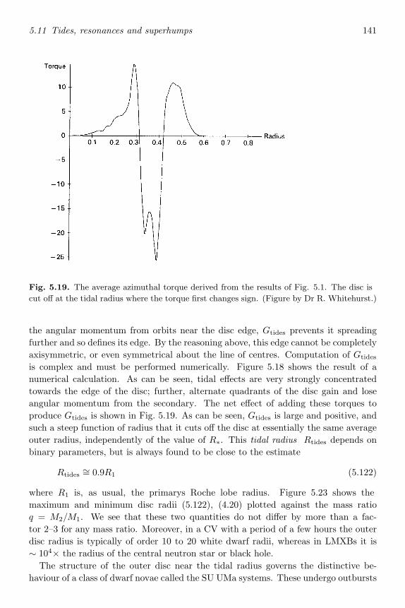
5.11 Tides, resonances and superhumps 141

Fig. 5.19. The average azimuthal torque derived from the results of Fig. 5.18. The disc is

cut off at the tidal radius where the torque first changes sign. (Figure by Dr R. Whitehurst.)

the angular momentum from orbits near the disc edge, Gtides prevents it spreadingfurther and so defines its edge. By the reasoning above, this edge cannot be completelyaxisymmetric, or even symmetrical about the line of centres. Computation of Gtides

is complex and must be performed numerically. Figure 5.18 shows the result of anumerical calculation. As can be seen, tidal effects are very strongly concentratedtowards the edge of the disc; further, alternate quadrants of the disc gain and loseangular momentum from the secondary. The net effect of adding these torques toproduce Gtides is shown in Fig. 5.19. As can be seen, Gtides is large and positive, andsuch a steep function of radius that it cuts off the disc at essentially the same averageouter radius, independently of the value of R∗. This tidal radius Rtides depends onbinary parameters, but is always found to be close to the estimate

Rtides∼= 0.9R1 (5.122)

where R1 is, as usual, the primary’s Roche lobe radius. Figure 5.23 shows themaximum and minimum disc radii (5.122), (4.20) plotted against the mass ratioq = M2/M1. We see that these two quantities do not differ by more than a fac-tor 2–3 for any mass ratio. Moreover, in a CV with a period of a few hours the outerdisc radius is typically of order 10 to 20 white dwarf radii, whereas in LMXBs it is∼ 104× the radius of the central neutron star or black hole.

The structure of the outer disc near the tidal radius governs the distinctive be-haviour of a class of dwarf novae called the SU UMa systems. These undergo outbursts

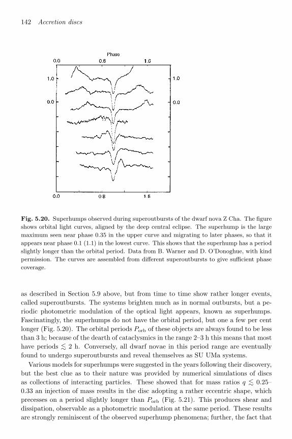
142 Accretion discs

Fig. 5.20. Superhumps observed during superoutbursts of the dwarf nova Z Cha. The figure

shows orbital light curves, aligned by the deep central eclipse. The superhump is the large

maximum seen near phase 0.35 in the upper curve and migrating to later phases, so that it

appears near phase 0.1 (1.1) in the lowest curve. This shows that the superhump has a period

slightly longer than the orbital period. Data from B. Warner and D. O’Donoghue, with kind

permission. The curves are assembled from different superoutbursts to give sufficient phase

coverage.

as described in Section 5.9 above, but from time to time show rather longer events,called superoutbursts. The systems brighten much as in normal outbursts, but a pe-riodic photometric modulation of the optical light appears, known as superhumps.Fascinatingly, the superhumps do not have the orbital period, but one a few per centlonger (Fig. 5.20). The orbital periods Porb of these objects are always found to be lessthan 3 h; because of the dearth of cataclysmics in the range 2–3 h this means that mosthave periods ∼< 2 h. Conversely, all dwarf novae in this period range are eventuallyfound to undergo superoutbursts and reveal themselves as SU UMa systems.

Various models for superhumps were suggested in the years following their discovery,but the best clue as to their nature was provided by numerical simulations of discsas collections of interacting particles. These showed that for mass ratios q ∼< 0.25–0.33 an injection of mass results in the disc adopting a rather eccentric shape, whichprecesses on a period slightly longer than Porb (Fig. 5.21). This produces shear anddissipation, observable as a photometric modulation at the same period. These resultsare strongly reminiscent of the observed superhump phenomena; further, the fact that

5.11 Tides, resonances and superhumps 143

-0.4

0.0

0.4

t = 0 t = 1.6

-0.4 0.0 0.4x

-0.4

0.0

0.4

y

t = 3.2

-0.4 0.0 0.4

t = 4.8

Fig. 5.21. Numerical simulations using Smooth Particle Hydrodynamics (SPH) of the struc-

ture and precession of an accretion disc in a cataclysmic variable for parameters suitable for

an SU UMa system. The mass ratio is q = 0.1, the centre of mass is at (0,0), and only the

Roche lobe of the white dwarf is shown. The typical number of particles in these simulations

is ∼ 50 000. The number of dynamical times (Porb = 2π) since the start of the simulation

is shown on the bottom left corner of each frame. The disc is eccentric and precesses on a

period slightly longer than the orbit. (Simulation by Dr J. Murray, performed on the UK

Astrophysical Fluids Facility (UKAFF) supercomputer at the University of Leicester.)

this behaviour occurs only for q ∼< 0.25–0.33 would then explain why SU UMa systemsall have Porb ∼< 2–3 h. For if the white dwarf masses are typically ∼ 0.6M (whichis plausible on other grounds), the secondaries are restricted to masses ∼< 0.2M.By (4.11) this requires Porb ∼< 2 h. It remains to explain the behaviour seen in thesimulations.

From the numerical simulations it is found that the particles in the precessing discrim follow orbits with approximate periods very close to Porb/3; this strongly suggeststhat the superhumps are in some way caused by resonances between the binary orbitand the orbits followed by gas elements in the disc. Resonance occurs in a disc when thefrequency of radial motion of a particle in the disc is commensurate with the angularfrequency of the secondary star as seen by the particle. This condition ensures that

144 Accretion discs

O B A

C

apsidalprecession

Fig. 5.22. A precessing particle orbit about a mass at O. Starting from A, the particle

completes a full revolution about O after a time 2π/Ω (point B), where Ω is its mean angular

frequency. However, it reaches the same radial distance from O only at point C, at the later

time 2π/(Ω − ω), where ω is the apsidal precession frequency (here shown prograde). The

frequency of radial motion (the epicyclic frequency) is thus (Ω−ω). Resonance with another

orbiting body (e.g. the secondary star, if O is the primary in a binary system) occurs when

this radial frequency is commensurate with the angular frequency Ω−Ωorb of the secondaryas seen by the particle (Ωorb = secondary’s angular frequency); this ensures that the same

relative configuration of primary, secondary and test particle recurs periodically.

the particle will always receive a ‘kick’ from the secondary at exactly the same phaseof its radial motion, so allowing the cumulative effect of repeated kicks to build up andaffect the motion significantly. We recall from the discussion of the tidal torque givenabove that the particle orbits will generally be somewhat aperiodic. This means thatthe orbits do not in general close, so that the particle is not at the same radial distanceonce it has completed an azimuthal motion through 2π about the white dwarf. Theorbits can be closely represented as ellipses whose axes precess at an apsidal precessionfrequency ω (Fig. 5.22) which depends on the particular orbit. If the mean frequency ofangular motion in a given orbit is Ω (measured in a non-rotating frame) the azimuthalperiod is 2π/Ω, but the time for the particle to return to the same radial distanceis somewhat longer, i.e. 2π/(Ω − ω). (Periodic orbits of course have ω = 0 so thatradial and azimuthal periods are the same.) Thus the frequency of radial motion, theepicyclic frequency, is Ω − ω. The particle sees the secondary star move with angularfrequency Ω − Ωorb where P = 2π/Ωorb is the orbital period of the binary. Thusresonance requires

k(Ω − ω) = j(Ω − Ωorb) (5.123)

where j and k are positive integers. Cases with k > 1 arise if the symmetry of the

5.11 Tides, resonances and superhumps 145

binary orbit with respect to the particle orbit breaks down, so that successive kicksby the secondary in opposing directions do not completely cancel. An example of thiswould be a binary eccentricity e′, which causes the secondary’s distance from the whitedwarf to vary by ∼ ±e′a, where a is the binary separation. In the case of a disc thissymmetry-breaking is provided by the viscosity, which causes variations of order λ inparticle orbits, where λ ∼ H is the viscous scalelength (see Sections 3.6 and 4.6). Theapsidal precession frequency ω is in general much smaller than Ω and Ωorb so we seefrom (5.123) that resonances occur very near commensurabilities of the form j:(j − k)between particle and binary frequencies. The effect of aperiodic motion (ω = 0) isto shift the resonances slightly away from precise commensurabilities (similar effectscan occur if we consider vertical motions of the disc particles). There is a largebody of literature on resonances in the context of planetary satellites: perturbationexpansions of the gravitational potential show that the disturbing effect of a (j, k)resonance builds up at a growth rate ∝ ek, where e is the eccentricity of the particleorbit. Since e < 1, the strongest resonances arise near the j:(j − 1) commensurability,followed by j:(j − 2) and so on. Near a given commensurability, those orbits withthe largest values of e compatible with stability will resonate most strongly: these aregenerally aperiodic orbits with non-vanishing precession frequencies ω. Resonancesthus act as filters picking out these extreme orbits provided the viscosity perturbs thedisc orbits enough to populate them.

To get an idea of which resonances are possible in a disc we estimate the typical radiiRjk of resonant orbits near the j:k commensurability. Even quite extreme aperiodicorbits do not differ greatly in size from Keplerian circles, so a good measure is providedby

Rjk = (GM/Ω2jk)

1/3 (5.124)

where Ωjk is the value of Ω given by the resonance condition (5.123). Using Kepler’slaw (4.1) with P = 2π/Ω gives

Rjka

=(

j − k

j

)2/3

(1 + q)−1/3. (5.125)

The possible resonances for a given mass ratio q are given by comparing this estimatewith the tidal radius Rtides given by (5.122). Using (4.6), with q replaced by q−1,the result is shown in Fig. 5.23. Since we must have Rjk < Rtides it is immediatelyapparent that the strongest (k = 1) resonances can only occur for very small massratios: j = 2, k = 1 requires q ∼< 0.025, with still smaller ratios required for largerj. These cannot occur in SU UMa systems, although some low-mass X-ray binarieshave such extreme ratios. For a possible explanation of the superhumps in SU UMasystems we must turn to the next strongest (k = 2) resonances. The smallest radiusis for j = 3, and is inside Rtides for q ∼< 0.33. Larger values of j require mass ratiosat least as extreme as for the j = 2, k = 1 resonance. Thus the strongest resonancepossible in the discs in SU UMa systems is that at j = 3, k = 2, and requires q ∼< 0.33.From (5.123) we see that this will appear for particle orbits in the disc with periods

146 Accretion discs

0.1 0.2 0.3 0.4 0.5 0.6 0.7 0.8 0.9

0.1

0.2

0.3

0.4

0.5

0.6

Mass ratio q

Rm

in/a

,Rm

ax/a

R21 /a

R32 /a

RT /a

Rcirc /a

Fig. 5.23. The minimum (or circularization Rcirc) radius (4.20) and the maximum (or tidal

RT) radius (5.122) for an accretion disc are shown as functions of the mass ratio q =M2/M1

(solid curves). The resonant radii R21 (long dashed line), and R32 (short dashed line) are

also shown for comparison. Resonant orbits can only exist for sufficiently small mass ratios

q; the j = 3, k = 2 resonance (particle period 1/3 of orbital) responsible for superhumps

occurs only for q ∼< 0.3.

close to P/3. This is precisely what is found in the simulations, and so is powerfulcircumstantial evidence that this resonance underlies the superhump phenomenon. Afull explanation of superhumps now requires an understanding of what happens nearresonance in a fluid disc. It is possible to show that indeed small perturbations makinga fluid disc slightly eccentric will tend to reinforce themselves tidally and grow; thedominant forcing term is the j = 3 tide, provided that the j = 3, k = 1 resonanceis inside the disc. The growth timescale is ∼ q−2Porb if this condition is satisfiedbut much longer if it fails. This treatment not only gives strong confirmation of thesimulations, but also shows that two different effects contribute to the disc precessionwhich gives rise to the most characteristic observational feature of superhumps. First,the apsidal precession rate increases strongly with disc radius (where the perturbationsby the companion are stronger), so the size of the disc is important in determining

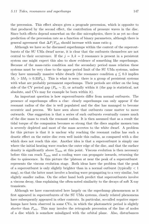
5.11 Tides, resonances and superhumps 147

the precession. This effect always gives a prograde precession, which is opposite tothat produced by the second effect, the contribution of pressure waves in the disc.Since both effects depend somewhat on the disc microphysics, there is as yet no clearprediction of the precession rate as a function of binary parameters, although there isgeneral agreement that ∆P/Porb should increase with mass ratio q.

Although we have so far discussed superhumps within the context of the superout-bursts of the SU UMa dwarf novae, it is clear that the outbursts themselves are notcentral to their occurrence. If the j = 3, k = 2 resonance is present in a persistentsystem one might expect this also to show evidence of something like superhumps.Because of the mass-ratio condition and the secondary period–mass relation thesesystems must be very close to the upper period limit of the SU UMa systems, unlessthey have unusually massive white dwarfs (the resonance condition q ∼< 0.3 impliesM1 > 3M2 0.33Phr). This is what is seen: there is a group of persistent systemswith what are probably permanent superhumps. Their periods are either on the longside of the CV period gap (Phr ∼ 3), or actually within it (the gap is statistical, notabsolute, and CVs may for example be born within it).

An important question is how superoutbursts differ from normal outbursts. Thepresence of superhumps offers a clue: clearly superhumps can only appear if theresonant radius of the disc is well populated and the disc has managed to becomeeccentric and precess. We have seen above that outbursts cause matter to moveoutwards. One suggestion is that a series of such outbursts eventually causes muchof the disc mass to reach the resonant radius. It is then assumed that as a result thetidal torque of the companion becomes so strong that the disc’s angular momentumis severely depleted and most of the mass accretes to the white dwarf. A problemfor this picture is that it is unclear why reaching the resonant radius has such adrastic effect on the entire disc even well inside this radius, as compared with a discwhich does not reach this size. Another idea is that a superoutburst is simply onewhere the initial heating wave reaches the outer edge of the disc, and that the surfacedensity is significantly above Σmin at this point. Viscous evolution is then necessarybefore this can reach Σmin and a cooling wave can propagate inwards, returning thedisc to quiescence. In this picture the ‘plateau’ at near the peak of a superoutburstrepresents the viscous evolution stage. Both ideas have the problem that the peakof a superoutburst is only slightly brighter than in a normal outburst (typically < 1mag), so that the latter must involve a heating wave propagating to a very similar, butslightly smaller radius. On the other hand both predict that superoutbursts involvea viscous decay, thus explaining the often-noted similarity to the decays of soft X-raytransients.

Although we have concentrated here largely on the superhump phenomenon as itfirst appeared in superoutbursts of the SU UMa systems, closely related phenomenahave subsequently appeared in other contexts. In particular, so-called negative super-humps have been observed in some CVs, in which the photometric period is slightlyshorter than Porb. This may involve the retrograde precession of the line of nodesof a disc which is somehow misaligned with the orbital plane. Also, disturbances

148 Accretion discs

extremely similar to superhumps have been observed in the optical light curves oflow-mass X-ray binaries. One might at first sight wonder how this is possible, sincein CVs the superhump arises from a modulation of the intrinsic dissipation in theaccretion disc, and we have asserted in Section 5.7 and 5.10 that in LMXBs this isnegligible by comparison with irradiation heating by the central X-ray source. The keyhere is the realization that other disc properties vary on the superhump period as wellas the intrinsic dissipation. In particular, the disc area (and probably its scaleheighttoo) vary on this period. Thus the solid angle subtended by the disc at the X-raysource varies on this period, making the intercepted irradiation and reprocessed discluminosity vary similarly in their turn (Haswell et al. (2001)).

5.12 Discs around young stars

We have thus far considered accretion discs entirely within the context of mass-transferring binary systems. In Chapters 7–9 we shall see that many of these ideascan be extended to the accretion process in active galactic nuclei. A further importantarea where accretion discs play a central role is in the formation of stars.

The process of star formation by the collapse of a protostellar cloud is a compli-cated phenomenon in which gravity, thermal pressure, rotation, magnetic fields, andmicrophysics all play important parts. It is quite possible that star formation is a‘bimodal’ process with different emphasis on the above ingredients depending on thestellar mass (e.g. Shu, Adams & Lizano (1987)). The formation of stars with massesin excess of a few solar masses is likely to be a violent and efficient process in the sensethat a significant fraction of the collapsing gas mass ends up in the newborn star in adynamical timescale. Since rotation is present, it may well be that a disc of some sortforms while the protostar is dealing with its excess of angular momentum. Becausemassive stars in giant molecular clouds are formed rapidly, they are shrouded fromview in their early life. By the time they become visible the disc is no longer evident,either because a proper disc never formed or because it was destroyed by dynamicalprocesses and/or winds. Fortunately the formation of stars with masses ∼< 2 M ismore accessible to observation and consequently better understood theoretically. Weknow that discs exist around young low-mass stars, and we can explain a number ofimportant observational properties of these systems using a simple model consistingof an accretion disc around a star of mass ∼ 1 M. The rest of this section is thereforeconfined to the study of low-mass young stars typified by those found in the Taurusstar-forming region.

The evidence for discs around young stellar objects has become really compellingover the last few years (e.g. Beckwith et al. (1990)). The direct evidence comes frominterferometric observations of 13CO lines at mm wavelengths. These observationsare capable of spatially resolving the disc in a couple of cases – HL Tau and DGTau – where the disc is seen to extend to ∼> 103 AU. Furthermore, the observationsdemonstrate that the gas is in Keplerian rotation about a ∼ 1 M star. These are

5.12 Discs around young stars 149

in fact the only cases for which we have direct evidence of a circumstellar (accretion)disc in Keplerian rotation. The evidence for accretion is indirect since the radial driftis unobservable. The indirect evidence in favour of discs is more extensive, beingbased on a large number of objects. The observed spatial distribution of polarizationand the association of young stars with bipolar outflows and jets clearly indicatesthe presence of a preferred axis, presumably the axis of rotation of the disc. Thebroad spectral energy distribution and the correlation between the Doppler width ofabsorption features with wavelength can be understood by invoking an accretion discwhose emission results from viscous dissipation and in some cases reprocessing of theradiation from the central star. In the early phases of low-mass star formation, anopaque dusty cloud collapses, forming in its shrouded interior an incipient star plusdisc system. This infall lasts for about ∼ 105 years and reveals, after some massloss, a newly formed T Tauri star (see Hartmann, Kenyon & Hartigan (1993)). Weknow relatively more about the formation of low-mass young stars because they arerevealed to us in a relatively earlier stage of formation. In the same sense used abovefor describing massive star formation, the formation of low-mass stars is a gentle andinefficient process. Recent observational estimates suggest that after the young starhas become visible, it accretes at least 5% to 10% of its mass from the circumstellardisc. The disc around the T Tauri star generally accretes on to the central star at arate of ∼ 10−7Myr−1 with typical variability by a factor of ∼ 10 over months andyears and with occasional outbursts where M ∼ 10−4Myr−1. These ‘Fuor’ eruptions– after the prototype FU Orionis – have a rise time typically ∼ 1 yr, but in somecases the rise is gradual over a decade. The decay times are of the order of decades orcenturies, and in the case of FU Ori itself, probably more than a millennium. Sincethe number of Fuor outbursts observed in the solar neighbourhood is approximatelyten times larger than the estimated local star formation rate, one concludes that theaverage young star undergoes around ten Fuor eruptions in its lifetime. More modestoutbursts of the type observed in EX Ori may occur frequently towards the end of thelife of a classical T Tauri. The classical T Tauri phase ends when accretion stops andthe system probably evolves into a weak-emission T Tauri star.

Currently the most promising model for the Fuor phenomenon is an accretion discinstability analogous to the limit cycle thought to occur in cataclysmic variables (cf.Section 5.9). Detailed hydrodynamic simulations of the limit cycle including the ap-propriate microphysics – in particular the formation and sublimation of grains – re-main to be done. The outburst timescales are indicative of a viscosity parameterα ∼ 10−3–10−2. The strengths of the disc model for Fuors could be summarized bysaying that it is successful in providing a qualitative and quantitative account of thefollowing observations: (a) the broad spectral distribution of the observed radiation,(b) the correlation of rotational broadening with wavelength, (c) the double-peakedabsorption line profiles, and (d) the outburst energetics and timescales. Not every-thing is without problems: the temperature distribution during decline appears flatterthan predicted by steady-state models; also the disc appears to be rotating faster atmaximum light contrary to simple expectations. It is however quite likely that more

150 Accretion discs

realistic time-dependent models will resolve these difficulties. We refer the readerinterested in further details to a recent monograph (Hartmann (2000)) since a quan-titative treatment of these problems is beyond the scope of this book.

5.13 Spiral shocks

When non-axisymmetric waves are excited in an accretion disc – for example by thetidal forces due to a companion star – the differential rotation rapidly shears the dis-turbances into spiral waves. The resultant spiral waves are in general trailing sincethe angular velocity increases inwards in most situations. Although it has been knownfor more than twenty years that such waves are capable of transporting angular mo-mentum by gravitational coupling, it is only recently that the possibility of drivingaccretion by such waves has attracted considerable interest. This is due to two fac-tors: the increasing power of modern vectorized and parallel computers, allowing anexpansion in the scope and spatial resolution of large scale numerical simulations ofaccretion flows in binary systems; and the recent emergence of a better physical un-derstanding of the transport of angular momentum by such waves even in the absenceof gravitational coupling.

It can be shown that trailing spiral waves carry negative angular momentum in thesense that a disc in which trailing spirals are present has a lower angular momentumthan the unperturbed disc. As long as the waves remain linear, they do not interactwith the fluid and the angular momentum of the fluid and the waves is conservedseparately. However, these spiral waves steepen into shocks as they propagate inwardand, as they dissipate, they communicate to the fluid within the angular velocity ofthe outer parts of the disc. The resultant transport of angular momentum outwardsdrives accretion without the requirement of any viscosity except of course within theshocks. The transport of angular momentum by more general non-axisymmetric dis-turbances, with and without the inclusion of gravity, finds applications in very diverseastrophysical problems such as star formation, discs around young stars, cosmogony,planetary rings, discs in accreting binaries, and active galactic nuclei (see also Sec-tion 7.6). A summary of the physics involved in these and other angular momentumtransport processes and other useful references can be found in Morfill et al. (1993).

In the case of accretion discs in close binaries, the numerical simulations of masstransfer in a Roche potential have shown that it is possible to set up a steady two-armed shock pattern which leads to steady accretion. These shocks arise and aremaintained as a result of the dominant m = 2 tidal perturbations at the edge ofthe disc. But as they propagate inwards, they reach a balance between amplificationand dissipation, and yield an angular momentum transport rate which is independentof the strength of the wave excited at the edge. The efficiency of the process, whenexpressed in terms of an effective viscosity parameter α, can be compared to the valuesinferred from observations – in particular from the outburst timescales (Section 5.11).Unfortunately, the values obtained so far are of the order of α ∼ 10−4–10−2, too small

5.13 Spiral shocks 151

for cataclysmic variables and probably also for low-mass X-ray binaries. Althoughobservations of IP Pegasi in outburst revealed the presence of spiral features (Steeghs,Harlaftis & Horne (1997)), their physical interpretation remains uncertain (Godon,Livio & Lubow (1998)). It is possible, however, that future observations and 3-Dhydrodynamic simulations with more detailed physics, including cooling, may yielda more consistent picture and produce higher values of α. In any case, the processmay be relevant to young stars with companions or giant planets since low values ofeffective α are sufficient to drive the evolution of accretion discs around young stars.

6 Accretion on to a compact object

6.1 Introduction

So far, we have seen in some detail how an accretion disc provides an efficient machinefor the extraction of up to half the available accretion energy, but it must be confessedthat our understanding of how the remaining substantial fraction of the accretionluminosity is released near the central object is rather less advanced. We have alreadymentioned the existence of an inner boundary layer in the case where the disc extendsdown to the surface of the accreting star. For neutron stars, runaway nuclear burningmay occur at the surface and give rise to the X-ray bursters. In many systems theaccreting star possesses a magnetic field strong enough to disrupt the inner regions ofthe disc and channel the accretion flow on to the magnetic polecaps. In this event, theaccretion flow more nearly resembles free-fall on to the stellar surface. A black hole,on the other hand, cannot possess an intrinsic magnetic field, so column accretion ofthis kind cannot occur. In this chapter we shall examine these modes of accretion insome detail.

6.2 Boundary layers

In discussing the inner boundary condition for steady thin accretion discs (Section5.3) we postulated that the angular velocity Ω(R) in the disc remains very close to theKeplerian value ΩK(R) = (GM/R3)1/2 until the accreting matter enters a boundarylayer of radial extent b just outside the surface R = R∗ of the accreting star. Withinthis boundary layer Ω must decrease from a value Ω(R∗ + b) ∼= ΩK(R∗ + b) to thesurface angular velocity Ω∗ < ΩK(R∗). Thus we envisage Ω(R) as a function havingthe form shown in Fig. 6.1.

We can see how much luminosity can be radiated from the boundary using thefollowing argument. At first sight one might think that this is simply given by thespecific energy difference between a Kepler orbit at R∗ and a particle with angularvelocity Ω∗ at this radius, i.e.

E =12

MR2∗(Ω2

K − Ω2∗), (6.1)

and indeed an incorrect expression of this form was current in the literature for manyyears. However, this neglects the ‘edge’ term −GΩ acting on the star at its surface

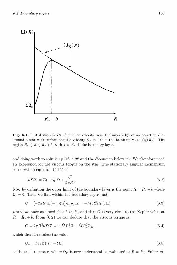
6.2 Boundary layers 153

Ω(R)

ΩK(R)

Ω*

R*+ b R

Fig. 6.1. Distribution Ω(R) of angular velocity near the inner edge of an accretion disc

around a star with surface angular velocity Ω∗ less than the break-up value ΩK(R∗). Theregion R∗ ∼< R ∼< R∗ + b, with b R∗, is the boundary layer.

and doing work to spin it up (cf. 4.28 and the discussion below it). We therefore needan expression for the viscous torque on the star. The stationary angular momentumconservation equation (5.15) is

−νΣΩ′ = Σ(−vR)Ω +C

2πR3. (6.2)

Now by definition the outer limit of the boundary layer is the point R = R∗ + b whereΩ′ = 0. Then we find within the boundary layer that

C = [−2πR3Σ(−vR)Ω]R=R∗+b −MR2∗ΩK(R∗) (6.3)

where we have assumed that b R∗ and that Ω is very close to the Kepler value atR = R∗ + b. From (6.2) we can deduce that the viscous torque is

G = 2πR3νΣΩ′ = −MR2Ω + MR2∗ΩK, (6.4)

which therefore takes the value

G∗ = MR2∗(ΩK − Ω∗) (6.5)

at the stellar surface, where ΩK is now understood as evaluated at R = R∗. Subtract-

154 Accretion on to a compact object

ing G∗Ω∗ from E given by (6.1) we finally get the luminosity available to be radiatedby the boundary layer as

LBL =12

MR2∗[Ω2

K − Ω2∗ + 2Ω2

∗ − 2Ω∗ΩK] =GMM

2R∗

[1 − Ω∗

ΩK

]2. (6.6)

This is always smaller than the incorrect form

E =GMM

2R∗

[1 −

(Ω∗ΩK

)2],

although again LBL reduces to GMM/2R∗ as expected for Ω∗ ΩK.Our derivation of the inner boundary condition (5.18) on the disc, as well as the

discussion of LBL above, assumed b R∗. Let us now justify this assumption. Weconsider in the thin disc approximation the radial component of the Euler equation(2.3), as given by (5.27):

vR∂vR∂R

− v2φR

+1ρ

∂P

∂R+

GM

R2= 0. (6.7)

In a thin Keplerian disc this equation is dominated by the centrifugal (v2φ/R) andgravity (GM/R2) terms as we showed in Section 5.3. However, the boundary layer isby definition that region of the disc in which v2φ < v2K = GM/R. Thus the gravityterm in (5.27) must be balanced either by vR ∂vR/∂R ∼ v2R/b or the pressure gradientρ−1∂P/∂R ∼ c2s/b where as usual we have taken P = ρc2s and set ∂/∂R ∼ b−1 inthe boundary layer. But we can infer that c2s > v2R, since otherwise the inflow to thestellar surface would be supersonic and the ‘news’ of the presence of the stellar surfaceat R = R∗ could not be communicated outwards to the disc. Hence in the boundarylayer (5.27) is approximately

c2sb

∼ GM

R2∗. (6.8)

The boundary-layer size b is now given by noting that just outside R∗ + b the stan-dard disc relation (5.25) implies a scaleheight (assuming radiation pressure can beneglected)

H ∼ cs

(R∗

GM

)1/2

R∗. (6.9)

Assuming that H and cs just inside R∗ + b are similar to their values just outside,(6.9) and (6.8) can be combined to give

b ∼ R2∗

GMc2s ∼

H2

R∗. (6.10)

This justifies our assumption b R∗, for

b ∼ H2/R∗ H R∗.

6.2 Boundary layers 155

A schematic picture of the boundary layer geometry is given in Fig. 6.2. From thefigure it is clear that radiation emitted by the boundary layer emerges through a regionof radial extent ∼ H on the two faces of the disc. If the accretion rate, and thereforethe density, in this region is high enough it will be optically thick and radiate roughlyas a blackbody of area ∼ 2πR∗H × 2. We already know that the luminosity emittedby this area must be 1

2Lacc = GMM/2R∗. Thus there is a characteristic boundarylayer blackbody temperature TBL given by

4πR∗HσT 4BL ∼ GMM

2R∗where σ is the Stefan–Boltzmann constant. Comparison with the expression (5.44)for the characteristic disc blackbody temperature T∗ shows that

TBL ∼(

R∗H

)1/4

T∗. (6.11)

Using (6.9) to eliminate H and remembering that c2s ∼ kT∗/µmH in this region, weget

TBL ∼ T∗(TS/T∗)1/8 (6.12)

where

TS =38

GMµmH

kR∗(6.13)

is the shock temperature (cf. (3.66)) we would have got for radial accretion on thestar. TBL exceeds T∗, but not by a large factor because of the very weak dependenceof TBL on TS/T∗ (equation (6.12)). For accretion on to a white dwarf, where thediscussion given above has the greatest chance of being valid, we have

TBL ∼ 1 × 105M7/3216 m

11/321 R

−25/329 K (6.14)

and TBL ∼ 3T∗. Since the maximum temperature T (R) in the disc is only 0.488T∗(Section 5.5), TBL is significantly higher (∼ 6×) than this maximum temperature.Equation (6.14) predicts that some cataclysmic variables ought to be soft X-ray sourcesas the tail of the blackbody at ∼ 0.1 keV may be observable. This is indeed foundto be the case, although most of the blackbody emission (∼< 0.1 keV) is hidden byinterstellar absorption so that estimates of the total luminosity are very uncertain.

Because of the blackbody assumption made above we are able to avoid any dis-cussion of the internal structure of the boundary layer. However, this is achieved atthe expense of the assumption that the viscosity in the boundary layer can adjustitself suitably to make the structure self-consistent: for example vR < cs must besatisfied. Our ignorance of viscosity is crucial here, not least since the rate of shearing(∝ dΩ/dR) in the boundary layer is very high. This problem becomes still more acuteif the boundary layer is optically thin. Optically thin boundary layers are of especialinterest for cataclysmic variables, since some of these are observed to be hard (∼ 10keV) as well as soft X-ray sources. We know (Section 5.7) that accretion discs roughly

156 Accretion on to a compact object

Star Disc

Boundary Layer

H

H

b

Fig. 6.2. Schematic view (in a plane φ = constant) of an optically thick boundary layer (not

to scale).

corresponding to the ‘standard model’ of Section 5.6 exist in these systems; in manysystems there is no evidence, such as periodic pulsing of the X-rays, that the whitedwarf has a magnetic field strong enough to disrupt the disc (see Section 6.3). Thusthe disc presumably extends down to the white dwarf surface, with the boundary layeras the only plausible site for the X-ray production. As we have seen, the blackbodytemperature TBL for an optically thick boundary layer is too low to give hard X-rayemission, so optically thin boundary layers, with all their attendant complicationsand uncertainties, must be considered. Indeed, an optically thin boundary layer isexactly what we would expect from the discussion of quiescent dwarf novae in Section5.10; inside the ‘truncation’ radius Rtr the quiescent accretion rate ∼ 10−12M yr−1

is driven by the hot-state viscosity, implying a rather low surface density and thusoptical depth.

To date two types of X-ray production mechanism have been proposed. One usesthe fact that the Kepler velocity (GM/R∗)1/2 near the white dwarf surface is highlysupersonic, and will, if the circulating gas can be strongly shocked, produce hard X-raytemperatures: from (3.66) we get

T =316

µmH

k

GM

R∗∼= 1.9 × 108m1 R−1

9 K.

The main difficulty here is in producing the strong shocks in the highly shearing

6.2 Boundary layers 157

boundary layer, rather than a series of weak shocks oblique to the flow. A two-stageprocess has been suggested, in which shocked blobs of gas expand into the path ofcirculating supersonic material, causing further strong shocks. The great complexityof the gas flow in the boundary layer has so far prevented a self-consistent treatmentof this idea.

An alternative treatment shows that the optically thin boundary-layer gas is likely tobe thermally unstable to turbulent viscous heating (cf. Section 5.8), rapidly achievinghard X-ray temperatures (∼ 108 K). At the same time, this gas is likely to expandout of the boundary layer and form a hard X-ray corona around most of the whitedwarf. At high accretion rates M the instability will be largely suppressed, and theboundary-layer luminosity mostly emitted as soft X-rays. The X-ray emission fromthe dwarf nova SS Cygni shows behaviour which supports this picture. At quiescence(low M) there is relatively bright, but very variable, hard X-ray emission. Duringoptical outbursts (high M) the hard X-rays are severely reduced, and the soft X-raysbrighten. The hard X-ray spectra show no evidence for increased absorption, so thatsuppression is not the result of covering the hard X-ray region with cool material, asis appealed to in earlier models.

The accretion torque (6.5) evidently spins up the central star: if this has radius ofgyration k, its angular momentum equation is

ddt

(k2MR2∗Ω∗) = G∗ M(GMR∗)1/2 (6.15)

where the second form assumes Ω∗ ΩK = (GM/R3∗)1/2. One can show that pos-

sible angular momentum losses (e.g. in nova outbursts from a white dwarf) do notsignificantly alter this equation. Assuming a mass-radius relation R∗ = R∗(M) onecan integrate (6.15) to find Ω∗ as a function of the accreted mass; in all cases the staris significantly spun up (Ω∗ ∼ ΩK) once it has accreted a mass ∆M ∼ k2M . For whitedwarfs and neutron stars we have k2 ∼ 0.1 and thus ∆M ∼ 0.1M, whereas manyof these stars are in binaries which will transfer several times this amount over theirlifetimes. Hence only a relatively small fraction of systems should emit the maximumboundary-layer luminosity ∼ 0.5Lacc. In the majority of systems Ω∗ should be closeto ΩK and the luminosity significantly below this level (cf. eq. 6.6).

Once Ω ∼ ΩK, it might appear at first sight that continued accretion might makethe star break up. Indeed, in some compact stars (e.g. white dwarfs with M ∼> 1M),adding mass actually decreases the moment of inertia I, and thus requires that angularmomentum should be removed from the accreting star. In fact in the limit as Ω∗approaches ΩK the disc and boundary-layer structure adjust so that these potentialproblems do not arise. The expression (6.5) was derived under the assumption thatthe angular velocity distribution Ω(R) had a maximum at some radius R = R∗ + b.For Ω∗ ΩK(R∗) this is quite natural, but for Ω∗ ∼ ΩK(R∗) there is no reason forsuch a maximum: we can have dΩ/dR < 0 throughout, so that the viscous torquealways acts outwards (note that in a steady disc, angular momentum is transferredoutwards at every radius even though mass is moving inwards everywhere). Hence

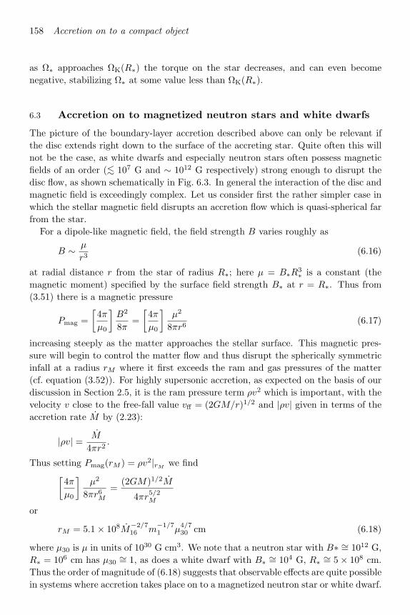
158 Accretion on to a compact object

as Ω∗ approaches ΩK(R∗) the torque on the star decreases, and can even becomenegative, stabilizing Ω∗ at some value less than ΩK(R∗).

6.3 Accretion on to magnetized neutron stars and white dwarfs

The picture of the boundary-layer accretion described above can only be relevant ifthe disc extends right down to the surface of the accreting star. Quite often this willnot be the case, as white dwarfs and especially neutron stars often possess magneticfields of an order (∼< 107 G and ∼ 1012 G respectively) strong enough to disrupt thedisc flow, as shown schematically in Fig. 6.3. In general the interaction of the disc andmagnetic field is exceedingly complex. Let us consider first the rather simpler case inwhich the stellar magnetic field disrupts an accretion flow which is quasi-spherical farfrom the star.

For a dipole-like magnetic field, the field strength B varies roughly as

B ∼ µ

r3(6.16)

at radial distance r from the star of radius R∗; here µ = B∗R3∗ is a constant (the

magnetic moment) specified by the surface field strength B∗ at r = R∗. Thus from(3.51) there is a magnetic pressure

Pmag =[

4π

µ0

]B2

8π=

[4π

µ0

]µ2

8πr6(6.17)

increasing steeply as the matter approaches the stellar surface. This magnetic pres-sure will begin to control the matter flow and thus disrupt the spherically symmetricinfall at a radius rM where it first exceeds the ram and gas pressures of the matter(cf. equation (3.52)). For highly supersonic accretion, as expected on the basis of ourdiscussion in Section 2.5, it is the ram pressure term ρv2 which is important, with thevelocity v close to the free-fall value vff = (2GM/r)1/2 and |ρv| given in terms of theaccretion rate M by (2.23):

|ρv| =M

4πr2.

Thus setting Pmag(rM ) = ρv2|rM we find[4π

µ0

]µ2

8πr6M=

(2GM)1/2M

4πr5/2M

or

rM = 5.1 × 108M−2/716 m

−1/71 µ

4/730 cm (6.18)

where µ30 is µ in units of 1030 G cm3. We note that a neutron star with B∗ ∼= 1012 G,R∗ = 106 cm has µ30 ∼= 1, as does a white dwarf with B∗ ∼= 104 G, R∗ ∼= 5 × 108 cm.Thus the order of magnitude of (6.18) suggests that observable effects are quite possiblein systems where accretion takes place on to a magnetized neutron star or white dwarf.

6.3 Accretion on to magnetized neutron stars and white dwarfs 159

accretion disc

magnetosphericbounda

rylay

erFig. 6.3. Accretion disc around a magnetized neutron star or white dwarf. The magnetic

dipole lines shown represent schematically the boundary of the magnetosphere.

It is often convenient to replace M in (6.18) in terms of the accretion luminosity (1.5),which is more directly related to the observational quantities, especially for X-raysources. Thus

rM =

5.5 × 108m1/7

1 R−2/79 L

−2/733 µ

4/730 cm

2.9 × 108m1/71 R

−2/76 L

−2/737 µ

4/730 cm

(6.19)

with parametrizations appropriate for white dwarfs and neutron star accretors respec-tively (L33 = Lacc/1033 erg s−1, etc.). Of course the estimates (6.18) and (6.19) ofrM are rather crude. However, since Pmag is such a steep function of radius (∼ r−6)we may hope they are acceptable at least in an order-of-magnitude sense. The mainuncertainty arises from the plethora of instabilities which a plasma supported by amagnetic field is prey to. These may, for example, allow matter to slip through thefieldlines before being channelled on to the stellar surface. The quantity rM is knownas the Alfven radius. Within the Alfven radius we expect that the matter will flowalong fieldlines (Section 3.7).

Let us return to the consideration of disc accretion. Here the condition for magneticdisruption at cylindrical radius R = RM must be that the torque exerted by themagnetic field on the disc at RM should be of the order of the viscous torque G(RM ).In a steady state (equation (5.14) et seq.) this is equal to the transport rate of specificangular momentum MR2

MΩ(RM ). The main difficulty in this calculation is in tryingto find an expression for the magnetic torque at RM , for this involves the azimuthalcomponent of B (Bφ), which in turn depends on how much the fieldlines are distortedfrom a dipole-like configuration by the interaction with the disc and the effects ofthe instabilities referred to above. Several estimates of the resulting RM have been

160 Accretion on to a compact object

made, of varying degrees of elaboration. Because of the steep (∼ R−6) dependence ofmagnetic stresses on radius, they all give similar answers, of order the spherical Alfvenradius rM (equations (6.18) and (6.19)):

RM ∼ 0.5rM . (6.20)

The factor 0.5 here is typical, but some estimates give radii RM up to four times larger,i.e. RM ∼ 2rM . Of course, the precise results must depend on the inclination of thedipole axis to the disc plane. In general, the accreting star and hence the magneticfield pattern rotate with an angular velocity Ω∗ about an axis perpendicular to thedisc, usually in the same sense as the disc angular velocity. Since inside R = RMthe matter must flow along fieldlines, if steady accretion is to occur we must haveΩ∗ < ΩK(RM ) where ΩK(RM ) = (GM/R3

M )1/2 is the Kepler angular velocity atRM . Otherwise particles attached to fieldlines at R = RM would spiral outwards tolarger R, repelled by the ‘centrifugal barrier’ at RM . A convenient way of stating thisrequirement is that the ‘fastness parameter’

ω∗ = Ω∗/ΩK(RM ) (6.21)

should be < 1.Combining (6.20) and (6.19), we see that for typical parameters (m1 ∼ R6 ∼ L37 ∼

µ30 ∼ 1) a magnetized neutron star will have rM ∼ RM ∼ 108 cm, well outside thestellar radius R∗ ∼ 106 cm. Since L37 cannot exceed the Eddington limit value ∼ 10(equation (1.4)), and m1, R6 are always near unity, the radii rM and RM can onlybe less than R∗ ∼= 106 cm for rather low values of the magnetic field, B∗ ∼< 109 G.Thus we expect accretion on to neutron stars to be controlled by the magnetic fieldnear the surface in many cases. Furthermore, RM for a neutron star is always lessthan the circularization radius Rcirc (e.g. equation (4.22)) for Roche lobe accretion inany plausible binary geometry. Since Rcirc is a lower limit to the size of any accretiondisc, we see that disc formation is not affected in this case. For wind accretion (cf.(4.42) et seq.), however, the question is much more difficult, and the whole subject ofstellar wind accretion by magnetized neutron stars is one of considerable uncertainty.In all cases it is important to remember that the ideas of disruption of a disc at a fixedradius, with infall along fieldlines within that radius, are considerable idealizations (cf.time-dependent numerical simulations by Miller & Stone (1998). It may be that forsome purposes this picture is too simplistic.

Magnetically controlled accretion gives rise to a simple and immediately recogniz-able observational signature because the accretion flow is channelled on to only a smallfraction of the stellar surface. To see how this works consider the situation depicted inFig. 6.4, in which a disc is disrupted by a dipole-like field. We assume that at point A

matter leaves the disc and follows the magnetic fieldlines down to the polecaps of theaccreting star. In polar coordinates (r, θ) with origin at the star’s centre, the fieldlineshave the approximate equations of dipole geometry r = C sin2 θ, where C is a constantlabelling all those fieldlines emanating from a particular latitude on the star. At A

6.3 Accretion on to magnetized neutron stars and white dwarfs 161

α

β

A DiscDisc

Accretion flow

RM

Mag

netic

axi

s

Fig. 6.4. Accretion from a disc to the polecaps of a magnetized neutron star or white dwarf.

we have r = RM and θ = α so C = RM sin−2 α. This fieldline thus crosses the stellarsurface r = R∗ at colatitude β given by

sin2 β = R∗/C = (R∗/RM ) sin2 α.

If we neglect the possible effects of plasma instabilities, accretion cannot take placeoutside a polecap of half-angle β (see Fig. 6.4), since for larger colatitudes the relevantfieldline crosses the disc plane inside r = RM , which little matter can otherwisepenetrate. The area of an accreting polecap is thus a fraction

fdisc ∼ πR2∗ sin2 β

4πR2∗∼= R∗ sin2 α

4RM

of the total stellar surface; accretion may take place on the opposite polecap also.Thus in general only a fraction

fdisc ∼ R∗/2RM (6.22)

of the stellar surface accretes. From (6.19) and (6.20) we find fdisc ∼ (10−1-10−4)depending on L and µ. Like many of the estimates in this section, fdisc is subject toconsiderable uncertainty because of the complicated role of plasma instabilities. Inparticular there is evidence (from hard X-ray light curves) that fdisc as given by (6.22)may be an underestimate for the intermediate polars. Nonetheless it is clear that fdisc

162 Accretion on to a compact object

is certainly smaller than unity in all cases; we get a very similar estimate fsph ∼ 0.5fdiscfor the case of quasi-spherical accretion simply by making the replacement RM → rM .Because most of the accretion luminosity must be released close to the stellar surfaceand, as we have seen, only over a fraction of it, any rotation of the accreting star willproduce a periodic modulation in the observed flux from such a system. The effect willbe enhanced if the radiation from the accreting polecap is beamed (see Section 6.4).Spin periods Pspin of this kind are observed in many X-ray binaries and intermediatepolar systems, generally in X-rays, but sometimes optically, in the range

1 s ∼< Pspin ∼< 103 s.

Because these periods are so short, it is relatively easy to obtain a sufficient database to detect significant changes in Pspin. These changes are of two main types. Thefirst kind of change in Pspin was noticed in the X-ray binary Cen X-3 very soon afterits discovery by the Uhuru satellite in 1971. The 4.8 s spin period is itself periodicallymodulated, by about one part in 1000, every 2.087 days. This modulation is easy tounderstand if we imagine the X-ray pulsations to act as a clock carried about by theneutron star. In its motion around the companion star, the clock frequency is peri-odically Doppler shifted just like the spectral lines of a spectroscopic binary. Henceone can construct a radial velocity curve from this ‘pulse-timing analysis’ and use itto determine the orbital period (2.087 days for Cen X-3) and a mass function in thestandard way. In several X-ray binary systems, one can also measure radial velocityshifts in the spectral lines of the companion: these systems are then directly analo-gous to double-lined spectroscopic binaries and allow masses and inclinations to bedetermined. Whenever this can be done, the mass of the neutron star is always closelyconsistent with a value ∼ 1.4 M, satisfyingly close to that expected on evolutionarygrounds. Furthermore, the non-compact star is usually found to be quite close tofilling its Roche lobe. Because pulse-timing analysis is relatively ‘clean’ and free frommost of the effects which can produce spurious eccentricities in radial velocity curvesdetermined conventionally, results obtained in this way give reliable evidence that theneutron star orbits in some X-ray binaries are quite eccentric (e ∼> 0.3).

The second type of systematic change in spin periods is more complicated. In manyX-ray binary systems, Pspin is observed to be decreasing steadily on a timescale oforder 104 yr, sometimes with occasional short-lived increases in Pspin. Presumably,the steady decrease in Pspin (spinup) is caused by the torques induced by the accretionprocess, while the occasional increases (spindowns) are caused either by fluctuations inthe accretion torque or possibly by changes in the internal structure of the neutron star.With the observed spin periods (∼> 1 s) and likely values of RM and rM (∼ 108 cm),the fastness parameter ω∗ (6.21) is 1 (cf. equations (6.19), (6.20) and (6.21)).For any such ‘slow rotators’ which accrete from a disc, the straightforward accretionof angular momentum at RM at the rate ∼ MR2

MΩK(RM ) discussed above is thedominant torque. For faster rotators (ω∗ ∼ 1), other effects such as the interactionof the stellar magnetic field with parts of the disc at R > RM , or the loss of angular

6.3 Accretion on to magnetized neutron stars and white dwarfs 163

momentum through the blowing-off of a ‘wind’ of particles along magnetic fieldlinesfrom the stellar surface can be important.

Thus in the case of a slow rotator accreting from a disc, if I is the moment of inertiaof the star we have

IΩ∗ = MR2MΩK(RM ) = M(GMRM )1/2, (6.23)

where we have assumed that Ω∗ is in the same sense as the disc rotation (otherwisespindown occurs). Now using (6.19) and (6.20) and replacing M by RLacc/GM asbefore, we get

ν 2.7 × 10−12 m−3/71 R

6/76 L

6/737 µ

2/730 I−1

45 Hz s−1, (6.24)

where I45 is the moment of inertia (∼ MR2∗) of the accreting star in units of 1045

g cm2, and we have written ν = 1/Pspin for the spin frequency. A neutron star hasI45 ∼ 1, while a white dwarf has I45 ∼ 105. Because of its much larger moment ofinertia, a white dwarf is much harder to spin up, and (other things being equal) hasa much smaller value of ν. From (6.24), we see that ν depends mainly on L6/7.

Data from the BATSE satellite have allowed one to test the simple ideas leading to(6.24) in unprecedented detail. Figure 6.5 shows the spinup data from GRO J1744-28.This is a soft X-ray transient, which uniquely contains a pulsing X-ray source whichalso shows X-ray bursts (see Section 6.6). The source is thought to be close to theGalactic centre, so the pulsed flux F 10−9 erg cm−2 s−1 implies a luminosity oforder L = 4πD2F 1037 erg s−1 for a distance D 10 kpc. As can be seen, thespinup rate ν is of exactly the order expected from (6.24) if the accreting object is aneutron star. The dependence of ν on F is close to the log ν ∝ (6/7) log F predicted by(6.24) but not identical: the best-fit logarithmic slope is slightly steeper (0.957±0.027,rather than 0.857). This difference may arise from a slight increase of pulse fractionwith luminosity.

Other BATSE results do not fit the simple ideas outlined here so neatly. Data froman outburst of the hard X-ray transient A0535+262 show the expected spinup, buthere one can also make an estimate of the inner disc radius RM . This turns out tobe closer to the spherical Alfven value rM than one-half of it as expected from (6.20).BATSE data for Cen X-3 are shown in Fig. 6.6. These show that spinup and spindownalternate, with ν 7×10−12,−3×10−12 Hz s−1 in the two states. The source spendsrather longer spinning down than up, but the net result is a slow spinup.

Eventually, of course, any accreting star that is spun up for a sufficiently long timewill enter the fast rotation regime ω∗ ∼ 1. Here, as mentioned above, other torquesbalance and Pspin attains an equilibrium value in which ω∗ ∼ 1, remaining there untilexternal conditions (e.g. the accretion rate) change. This could, for example, be thecase for the white dwarfs in the intermediate polars we have just discussed. Anotherway of expressing the requirement ω∗ < 1 is to ask that the corotation radius

RΩ =

(GMP 2

spin

4π2

)1/3

= 1.5 × 108P 2/3spinm

1/31 cm, (6.25)

164 Accretion on to a compact object

Fig. 6.5. The spinup rate of GRO J1744-28 during the December 1995 – March 1996 outburst

versus the 20–50 keV r.m.s. pulsed flux. The square symbols are from the the outburst rise,

and the diamond symbols are from the outburst decline. The dotted curve is the power-law

with the expected index of 6/7, while the dashed curve is the best fit power-law of index

0.957 (reproduced with permission from Bildsten et al. (1997)).

Fig. 6.6. High resolution BATSE measurements of the intrinsic spin frequencies for Cen X-3

(reproduced with permission from Bildsten et al. (1997)).

where a particle attached to a fieldline would rotate at the Keplerian rate, should notbe less than RM . Thus at the equilibrium spin period Peq we have RΩ ∼ RM , so thatfrom (6.19) and (6.20)

Peq ∼ 3m−2/71 R

−3/79 L

−3/733 µ

6/730 s

∼ 3m−2/71 R

−3/76 L

−3/737 µ

6/730 s.

(6.26)

Since µ30 ∼< 1 for neutron stars, it is clear that only a few of the X-ray binary accretorscan be near their equilibrium periods: in some of these cases their interpretation aseither fast or slow rotators seems possible.

In principle, one would like to understand the ‘spin history’ of all types of mag-

6.3 Accretion on to magnetized neutron stars and white dwarfs 165

netized accreting stars and relate this to the observed spin period distribution andspinup (spindown) rates. This is an ambitious undertaking, involving an understand-ing of all the various types of torque which can operate, as well as the evolution ofthe binary systems containing the objects, and observational selection effects on thePspin, Pspin distributions. It is scarcely surprising therefore that no general consensushas been arrived at.

An indication that the simple ideas considered here do nevertheless produce rea-sonable results is provided by the discovery of the first low-mass X-ray binary to showcoherent X-ray pulsing. The soft X-ray transient SAX J1808.4-3658 is found (Wij-nands & van der Klis (1998)) to have a 2.49 ms spin period; a pulse-timing analysisshows that the binary has an orbital period of 2.01 hr (Chakrabarty & Morgan (1998)).The remarkable feature is that the X-ray pulsing continues even though the X-ray in-tensity drops by large factors. Thus the magnetic field strength must be such that evenat low luminosity the magnetospheric radius is within corotation, i.e. RΩ > RM (low),while at the peak luminosity the magnetosphere is not crushed down to the neutronstar surface, i.e. RM (peak) > R∗. Assuming that the X-ray intensity is proportionalto the accretion rate, its observed decrease by at least an order of magnitude shows(from equations 6.19, 6.20) that RM (peak) ∼< 0.5RM (low), and thus that

R∗ ∼< 0.5RΩ 13m1/31 km,

where we have assumed only that the proportionality in (6.20) does not change, ratherthan adopting the particular value 0.5. We can combine this result with the mass-radius relation for a neutron star, which has the typical form

R∗ 10m−1/31 km,

with the constant depending on the precise equation of state (EOS) used, to show thatthe neutron star radius R∗ must be less than about 15 km for any reasonable EOS,while the mass m1 cannot differ greatly from the expected value ∼ 1.4 (Burderi &King (1998)). The similarity of these results to independent determinations of neutronstar parameters gives some confidence in the simple scaling RM ∼ M−2/7, which is themain ingredient of the estimate. Note that this scaling removes the model-dependentuncertainty introduced by the proportionality in (6.20), and indeed any uncertaintyderived from a distance estimate. In fact if we adopt the usual value of 0.5 in (6.20)and a distance estimate of 4 kpc, implying a peak luminosity of about 1037 erg s−1,(6.26) implies µ 2×1027 G cm3, or a surface field of about 2×109 G. This is of coursefar lower than the fields inferred in pulsing sources in high-mass X-ray binaries, or inyoung pulsars, and may suggest that the fields decay, perhaps as a result of accretion.

Surface magnetic fields of the order inferred for SAX J1808.4-3658 are too weak tocause coherent pulsing in bright persistent low-mass X-ray binaries (they are noticeablein SAX J1808.4-3658 only because it is transient and has a relatively low accretionrate). However, such weak fields may be the cause of the quasi-periodic oscillations(QPOs) detected in the power spectra of low-mass X-ray binaries. These are low-amplitude (∼ 1–10%) X-ray modulations, with typical frequencies of 5 up to 1000 Hz,

166 Accretion on to a compact object

which can vary dramatically with X-ray intensity and spectral hardness. As the namesuggests, the peaks in the power spectra are rather broad, and these are clearly distinctfrom the strictly periodic modulations seen in the pulsing X-ray sources discussedabove. The idea which has received the most attention is that QPOs represent theinteraction of a rather weak (∼< 1010 G) field on the central neutron star with transientpatterns of blobs in the inner accretion disc orbiting at some preferred radius. TheQPO frequency is assumed to result from the beat between the neutron star spin andthe Kepler frequency of the blobs. Sometimes a higher-frequency QPO is seen, thoughtto be the preferred Kepler frequency itself. Coherent modulation at the spin periodof the type seen in the pulsing sources is apparently undetectable, and considerabletheoretical effort has gone into providing plausible reasons for this. The beat frequencymodel does provide at least qualitative explanations for some of the observed changesin the power spectra, and the idea of weak magnetic fields for the neutron stars inlow-mass X-ray binaries is attractive for evolutionary reasons. However in cases wheretwo QPOs are seen, their difference frequency is not always observed to be constant,as would be expected if this were indeed the spin of the neutron star. The origin ofthe QPOs must still be regarded as unknown. Indeed, there are other suggestions inthe literature, such as the action of the Lense–Thirring effect on the inner edge of theaccretion disc.

The case where the accreting magnetic star is a white dwarf (a magnetic cataclysmicvariable) is particularly interesting, as the larger stellar radius means that µ can bemuch bigger than for neutron stars. In a fairly extreme case, a 0.5 M white dwarfwith R∗ = 109 cm and a field B∗ = 3 × 107 G has µ = 3 × 1034 G cm3. Systemswith these properties can be identified through the optical polarization produced bythermal cyclotron emission in the ∼ 107 G magnetic field (see below) and are calledAM Herculis systems, or polars. They are strong soft X-ray sources (∼< 0.1 keV), andthis is generally how they are discovered. For such systems (6.18) gives rM ∼> 1011 cm,whereas from (4.2), with q < 1 we find a typical orbital separation a ∼= 3.5× 1010P 2/3

hr

cm. The longest orbital period in any of the known AM Her systems is ∼ 8 hr (all butone system actually ∼< 4 hr), so rM > a for this class. It is hard to see how an accretiondisc could form in this case, and indeed none of the usual disc indicators are present. Itappears instead that the accretion stream couples directly to the white dwarf magneticfield at some point, the flow being along fieldlines down to the surface thereafter (weconsider the resulting accretion process in detail in the next section). Further, thewhite dwarf is observed to spin synchronously with the binary orbit, so that it is phase-locked to the secondary star (Fig. 6.7). Since it constantly accretes angular momentumfrom the secondary, this implies the existence of a counter-balancing torque enforcingsynchronism. The most likely candidate mechanism for this is the interaction of thewhite dwarf’s dipole field with that of the secondary, which for quite plausible surfacefields ∼ 100 G has a similar moment. The present limits on the relative rotation ratesof the white dwarf and the orbit do not rule out the possibility that the white dwarfdipoles slowly librate around the equilibrium position with periods ∼ 30 yr.

6.3 Accretion on to magnetized neutron stars and white dwarfs 167

magneticwhite dwarf

companionstar

accretion stream

Fig. 6.7. Schematic view of an AM Herculis system. The rotation of the strongly magnetic

(∼> 107 G) white dwarf is locked to that of the binary (P ∼< 4 h). No accretion disc forms,

matter impinging directly on the magnetosphere, threading and following fieldlines down to

the white dwarf surface.

For somewhat weaker magnetic fields or longer orbital periods the result rM > a willdisappear. One would thus expect the white dwarfs to have spin periods Pspin shorterthan Porb. Systems of this type are found through their hard X-ray emission (few keV),which shows the spin period, and are called intermediate polars. The optical emissionshows both this period and also the orbital sideband period (1/Pspin − 1/Porb)−1,indicating that some of the X-ray emission heats an object which is fixed in the binaryframe. The accretion process in such non-synchronous systems might be expectedto be intrinsically more messy than in the AM Her systems, where the field is sodominant that it imposes order. Indeed, it is at present unclear whether most of theaccretion flow takes place via a disc, rather than crashing directly into the rotatingmagnetosphere of the white dwarf. The simplest condition for a disc to form is thatthe initial gas stream’s minimum distance of approach ∼ 0.5Rcirc to the white dwarfshould exceed the size of the obstacle presented by the magnetosphere (cf. Section4.5). The latter is not easy to work out, as it depends on whether instabilities allowmatter to cross fieldlines or not, but estimates suggest a value ∼ 0.37rM . Using(4.20) and (6.18) one then finds that the simplest disc formation condition fails ifµ ∼> 1033 G cm3, which includes most intermediate polars. Independent evidencewhich may support this tentative conclusion comes from the fact that several of thesesystems seem to arrange their spin periods to be about 10% of Porb (actually slightlyless). This is clearly very different from the equilibrium disc relation (6.26), whichimplies Pspin ∼ M−3/7, as both evolutionary theory and deductions from observationssuggest that M increases roughly as Porb. It is highly suggestive that the observedrelation Pspin ∼ 0.1Porb follows naturally if the white dwarf accretes exactly the orbitalspecific angular momentum (GMRcirc)1/2 from the companion. For in equilibriumthis will be equal to the Keplerian specific angular momentum (GMRΩ)1/2 at thecorotation radius, giving the equilibrium relation as simply RΩ = Rcirc. From (6.25)and (4.20), (4.1) this gives

168 Accretion on to a compact object

Pspin ∼ (1 + q)2[0.5 − 0.225 log q]6Porb, (6.27)

which gives values close to the observed relation Pspin ∼ 0.1Porb. It is clear that therequirement of accreting exactly the orbital specific angular momentum is met if thereis no disc; if a well-developed Keplerian disc is present the accreted specific angularmomentum is less than (GMRcirc)1/2, leading to a shorter spin period when this isequated to (GMRΩ)1/2. This seems to hold only for two systems, DQ Herculis (Pspin =142 s), and the evolved system GK Per (Pspin = 351 s) where a disc must be presentbecause of the unusually long orbital period (Porb = 2 days) (Here the accreting matterhas easily enough angular momentum to orbit outside the magnetosphere and form adisc).

Some progress in understanding the spin evolution of magnetic CVs has resultedfrom the realization that the accretion flow is likely to be highly inhomogeneous (seeSection 6.4), and may behave like a collection of diamagnetic blobs rather than asmooth flow. Such blobs are likely to interact with the white dwarf magnetic field viaa surface drag proportional to the relative velocity across fieldlines. The drag forcemeans that orbital energy and angular momentum will be exchanged between the gasblobs and the white dwarf. One finds that blobs with specific orbital energy E greaterthan a critical value

EE −12

ΩJ, (6.28)

(where J is their specific angular momentum and Ω as before the stellar spin rate)will be expelled centrifugally by the white dwarf, usually to be swept up by thegravitational attraction of the secondary star. Blobs with E < EE on the otherhand are accreted. Thus if Ω is small, EE is not very negative, and is larger than thetypical orbital energy E(L1) of a blob accreting through L1. Most gas blobs thereforeaccrete, spinning up the white dwarf. Eventually Ω gets large enough that EE is equalto E(L1). Further spinup is impossible, as most blobs would be ejected, spinningthe white dwarf down. The equality EE = E(L1) therefore defines an equilibriumspin state. It is easy to see that this state is characterized by equality between thespecific angular momenta ∼ (GMRΩ)1/2 and ∼ (GMRcirc)1/2, and thus gives thePspin ∼ 0.1Porb relation described above. Numerical calculations of the equilibriumspin rate use large numbers of blobs and take into account the full Roche geometry.These predict slightly shorter spin periods, in excellent agreement with those observed.

This approach can report two further successes. At short orbital periods and mod-erate magnetic fields one expects the spin equilibrium to be given by the equalityRΩ ∼ b1 rather than RΩ ∼ Rcirc as above. Here matter is alternately accreted andpushed back to the secondary star as the white dwarf spins with respect to the binary.From (6.25) and (4.9) we find

Pspin ∼ (1 + q)1/2[0.5 − 0.227 log q]3/2Porb. (6.29)

This gives much larger Pspin/Porb ratios than (6.27), i.e. Pspin/Porb ∼ 0.66–0.5 for0.1 < q < 1. Numerical calculations of the equilibrium period ratio for this type of

6.3 Accretion on to magnetized neutron stars and white dwarfs 169

accretion geometry give similar values. These are close to those observed for two of thethree intermediate polars below the CV period gap (EX Hydrae: Pspin/Porb = 0.68;RX 1238-38: Pspin/Porb = 0.42). (The third short-period intermediate polar RX0757+63 has Pspin/Porb = 0.099, presumably corresponding to the ‘standard’ spinequilibrium given by equation 6.27, with a still weaker magnetic field.)

Most remarkably, AE Aquarii, the magnetic CV with the shortest spin period(Pspin = 33 s) and one of the longest orbital periods (Porb = 9.88 hr) is found not tocontain a disc at all, even though the rapid spin rate must indicate a weak magneticfield. The white dwarf spin is observed to be lengthening at such a rate that theloss of spin energy far exceeds the radiative output of the system. Doppler tomog-raphy reveals that AE Aquarii is actually centrifugally ejecting most of the mattertransferred to it from the secondary. This is easy to understand in terms of the dragpicture, where the high rotational motion of the fieldlines compensates for the weakmagnetic field and produces a large torque which expels the blobs (see Fig. 6.8). Thelack of an accretion disc is utterly contrary to the usual picture in which the accretionstream is homogeneous, for the weak field and wide binary orbit should have madedisc formation very easy. The very short spindown timescale (∼ 107 yr) tells us thatwe are observing a rapid transition in which the white dwarf spin tries to adjust to achange from a high to a low mass transfer rate. In the earlier state, the high accretionrate led to the formation of a disc and the spinup of the white dwarf to a short periodPspin < 33 s. The drop in the mass transfer rate has evidently occurred so rapidlythat spin equilibrium has been lost. A probable reason for this sudden decrease in thetransfer rate is that the secondary was rather more massive than the white dwarf inthe past, and the system was a supersoft X-ray binary (cf. the discussion in Section4.4). Once the mass ratio reverses sufficiently the mass transfer rate decreases to typ-ical CV values. In line with this, the UV spectrum of AE Aqr reveals signs of CNOprocessing, showing that the companion must have been significantly more massive inthe past. The fact that we are able to observe AE Aqr in such a short-lived evolu-tionary stage suggests that a large number of systems must pass through this stage.Indeed it appears that a significant fraction of current CVs must have descended fromsupersoft binaries in this way.

The orbital evolution of magnetic cataclysmic variables is a further fascinating area:we have seen that the AM Herculis systems are distinguishable by the fact that rMformally exceeds the binary separation a. Yet it is clear that this inequality dependson the orbital period; not only does a increase as P

2/3orb , but the average accretion

rate M is likely to be higher at longer periods (see Section 4.4), which from (6.18)tends to decrease rM also. Thus it is easy to show that for field strengths typical ofAM Her systems, we do not expect rM > a for Porb ∼> 4 h, and indeed only one AMHer system (out of about 60 with known periods) has a period significantly longerthan this. But since Porb decreases in the course of a short-period binary’s evolution(Section 4.4), at least some of the observed AM Her systems must have descendedfrom some other type of magnetic cataclysmics, presumably non-synchronous. (Upto about two-thirds could simply have begun mass transfer at periods below the CV

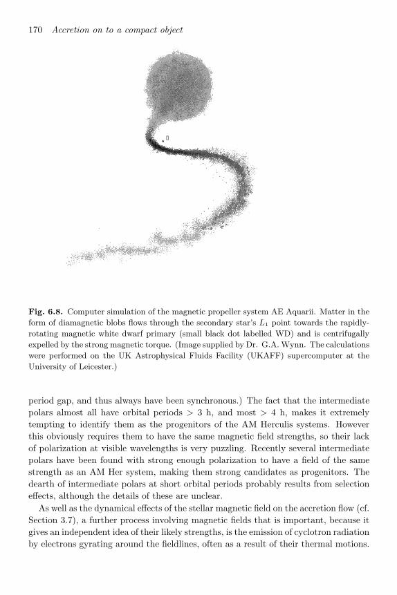
170 Accretion on to a compact object

Fig. 6.8. Computer simulation of the magnetic propeller system AE Aquarii. Matter in the

form of diamagnetic blobs flows through the secondary star’s L1 point towards the rapidly-

rotating magnetic white dwarf primary (small black dot labelled WD) and is centrifugally

expelled by the strong magnetic torque. (Image supplied by Dr. G.A. Wynn. The calculations

were performed on the UK Astrophysical Fluids Facility (UKAFF) supercomputer at the

University of Leicester.)

period gap, and thus always have been synchronous.) The fact that the intermediatepolars almost all have orbital periods > 3 h, and most > 4 h, makes it extremelytempting to identify them as the progenitors of the AM Herculis systems. Howeverthis obviously requires them to have the same magnetic field strengths, so their lackof polarization at visible wavelengths is very puzzling. Recently several intermediatepolars have been found with strong enough polarization to have a field of the samestrength as an AM Her system, making them strong candidates as progenitors. Thedearth of intermediate polars at short orbital periods probably results from selectioneffects, although the details of these are unclear.

As well as the dynamical effects of the stellar magnetic field on the accretion flow (cf.Section 3.7), a further process involving magnetic fields that is important, because itgives an independent idea of their likely strengths, is the emission of cyclotron radiationby electrons gyrating around the fieldlines, often as a result of their thermal motions.

6.3 Accretion on to magnetized neutron stars and white dwarfs 171

For a non-relativistic electron, the Larmor frequency (3.53) implies that most of theradiation is emitted as a spectral line centred at the fundamental cyclotron frequency

νcyc =eB

2πmec[c] = 2.8 × 1013B7 Hz

= 2.8 × 1018B12 Hz

(6.30)

where B7 = B/107 G, etc. If the electron’s speed of gyration is v, the strengths of emis-sion in the harmonics 2νcyc, 3νcyc, . . . are reduced by factors ∼ (v2/c2), (v2/c2)2, . . .

below that of the fundamental. A fact that is very important for observational pur-poses is that radiation emitted at angles close to the fieldlines is circularly polarized,while emission orthogonal to the fieldlines is linearly polarized in the plane of theelectron’s orbit. The defining observational property of the AM Her stars (giving riseto the alternative designation ‘polar’) is the presence of quite strong polarization ofthe optical light, up to 30% in some cases, which varies smoothly and periodically asthe accreting white dwarf rotates. The relative phasing of linear and circular polariza-tion curves is broadly consistent with that expected for thermal cyclotron radiationproduced in a small region (cf. (6.22)), near the magnetic polecap of the white dwarf,provided that the angles of the magnetic axis to the rotation axis, and of the latter tothe line of sight, are chosen appropriately for any individual system.

This simple picture assumes that the emitting gas is optically thin to its own cy-clotron radiation. This is very likely to be invalid for thermal cyclotron emission atthe fundamental, although not at higher harmonics. One can also show this by us-ing the standard Larmor formula for the emission, estimating the line width of thefundamental from thermal Doppler broadening, and using Kirchhoff’s law to derivean absorption coefficient κν . Because the emission is proportional to the magneticenergy density (B2/8π)[4π/µ0], so is κν . If the polarized optical light from the AMHer stars was emitted at the fundamental, field strengths ∼ 108 G (equation (6.30))would be required. The resulting values of κν show that even for very small electroncolumn densities the fundamental has a large optical depth. Because the emission athigher harmonics is less, so is the absorption and hence the optical depth. Never-theless, for plausible accretion column parameters (see Section 6.4) one expects thefirst few harmonics to be self-absorbed up to some ‘last’ harmonic m∗. The actualvalue of m∗ is rather geometry dependent and can differ for different viewing angles(see below), although it is generally in the range 1 ∼< m∗ ∼< 10. Since the emittingelectron gas is thermal, the emergent intensity in the frequency range νcyc to m∗νcycis roughly blackbody. For the AM Her stars hνcyc(∼ 1 eV) is much less than likelyvalues of kT (∼ 10 keV) in the emitting region, so the Planck function can be approxi-mated by the Rayleigh–Jeans form, and the expected emission is shown schematicallyin Fig. 6.9. Hence the cyclotron line gets broadened to a ∼ ν2 continuum between νcycand m∗νcyc. Above m∗νcyc the intensity drops sharply as the optical depth becomesvery small. Thus the total emission of cyclotron radiation is roughly

Lcyc = πA

∫ m∗νcyc

νcyc

2kT ν2

c2dν

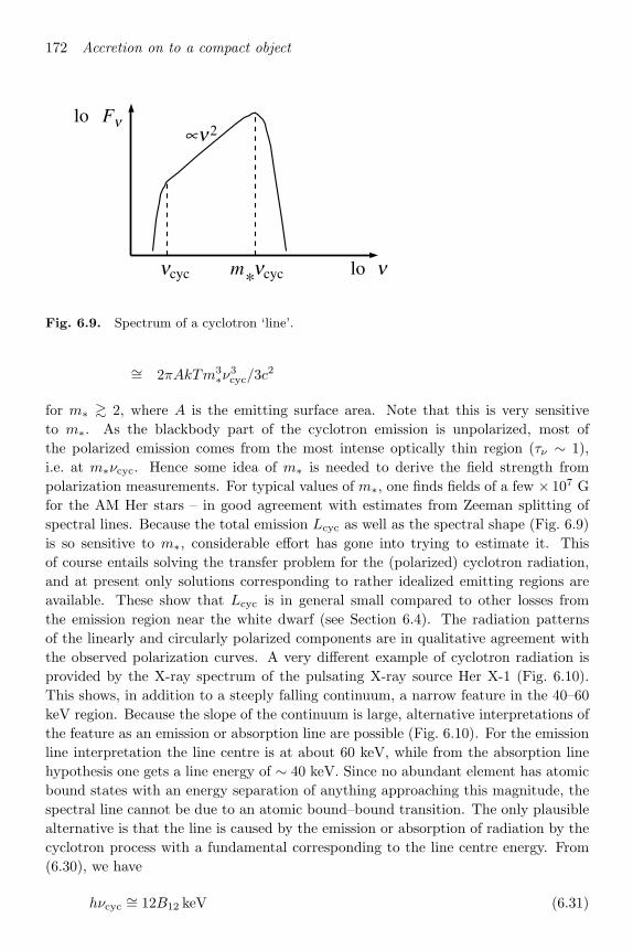
172 Accretion on to a compact object

log Fν

νcyc m*νcyc logν

∝ν2

Fig. 6.9. Spectrum of a cyclotron ‘line’.

∼= 2πAkT m3∗ν3cyc/3c2

for m∗ ∼> 2, where A is the emitting surface area. Note that this is very sensitiveto m∗. As the blackbody part of the cyclotron emission is unpolarized, most ofthe polarized emission comes from the most intense optically thin region (τν ∼ 1),i.e. at m∗νcyc. Hence some idea of m∗ is needed to derive the field strength frompolarization measurements. For typical values of m∗, one finds fields of a few × 107 Gfor the AM Her stars – in good agreement with estimates from Zeeman splitting ofspectral lines. Because the total emission Lcyc as well as the spectral shape (Fig. 6.9)is so sensitive to m∗, considerable effort has gone into trying to estimate it. Thisof course entails solving the transfer problem for the (polarized) cyclotron radiation,and at present only solutions corresponding to rather idealized emitting regions areavailable. These show that Lcyc is in general small compared to other losses fromthe emission region near the white dwarf (see Section 6.4). The radiation patternsof the linearly and circularly polarized components are in qualitative agreement withthe observed polarization curves. A very different example of cyclotron radiation isprovided by the X-ray spectrum of the pulsating X-ray source Her X-1 (Fig. 6.10).This shows, in addition to a steeply falling continuum, a narrow feature in the 40–60keV region. Because the slope of the continuum is large, alternative interpretations ofthe feature as an emission or absorption line are possible (Fig. 6.10). For the emissionline interpretation the line centre is at about 60 keV, while from the absorption linehypothesis one gets a line energy of ∼ 40 keV. Since no abundant element has atomicbound states with an energy separation of anything approaching this magnitude, thespectral line cannot be due to an atomic bound–bound transition. The only plausiblealternative is that the line is caused by the emission or absorption of radiation by thecyclotron process with a fundamental corresponding to the line centre energy. From(6.30), we have

hνcyc ∼= 12B12 keV (6.31)

6.3 Accretion on to magnetized neutron stars and white dwarfs 173

Fig. 6.10. Hard X-ray spectrum of Her X-1 obtained during the pulse phase of the 1.24 s

pulsation. The left-hand figure shows a raw count-rate spectrum. The right-hand figure

shows a spectrum deconvolved from the instrumental response, assuming cyclotron lines in

emission at 58 and 110 keV. (Reproduced from Kirk & Trumper in Accretion-Driven Stellar

X-ray Sources, eds. W.H.G. Lewin & E.P.J. van den Heuvel (1983), Cambridge University

Press.)

so that the magnetic field must be in the range (3-5) × 1012 G, which, satisfyingly,is just of the order expected for a neutron star. There are now at least a dozenconvincing detections of cyclotron resonant scattering features from accreting neutronstars (Makishima et al. (1999)).

The basic difference between the cyclotron process here and that in the AM Her starsis that for Her X-1 the line energy, ∼ 50 keV, is a significant fraction of the electronrest-mass energy, mec

2 ∼ 500 keV. This means that the interaction of the electrons andthe radiation must be treated quantum-mechanically. When the Schrodinger equationdescribing the behaviour of an electron in a strong magnetic field is solved the electronenergy is no longer allowed to take a continuum of values, as in classical mechanics,but is quantized in the so-called Landau levels. The line energy (6.31) reappearsas the energy gap between the two lowest (n = 1, n = 2) Landau levels, while thehigher Landau levels are the energies (n = 3, 4, . . .). Cross-sections for emission and

174 Accretion on to a compact object

absorption of photons of various frequencies and polarizations can be worked out inan analogous fashion to the calculation of atomic bound–bound transition rates. Oncethis is done, one has a similar radiative transfer problem as in the case of the AMHer stars described above. Similarly, here, the overall aim is to predict the radiationpatterns of the emergent flux as a function of photon energy. Since the measurementof polarization in the hard X-ray region is technically difficult, most effort has goneinto trying to predict the X-ray pulse profiles in and near the cyclotron resonance inorder to compare with observation. This problem is even harder than for the AM Herstars and, similarly, has only been solved for idealized emitting regions. For example,not surprisingly, there is no clear decision yet possible as to whether the absorptionor emission line interpretation of the cyclotron hypothesis is more likely.

6.4 Accretion columns: the white dwarf case

We have seen above that many white dwarfs and probably most neutron stars possessmagnetic fields strong enough to disrupt the accretion flow and to channel it directlyon to a small fraction ((6.22) et seq.) of the stellar surface near the magnetic poles.The resulting configuration is often known as an accretion column. Because the accre-tion flow is roughly radial, column accretion is fairly similar to spherically symmetricalaccretion, although there are important differences, particularly concerning the escapeof radiation from the column. Note also that the accretion column could be a ‘hol-low’ rather than a ‘filled’ cylinder, depending on how the matter attaches itself to thefieldlines. Since it is essentially one-dimensional in character, column accretion is in-trinsically simpler to study than the boundary-layer accretion processes we consideredin Section 6.2.

Let us consider first the accretion column problem for white dwarfs since, althoughcomplicated enough, it is somewhat simpler than the neutron star case, which will beconsidered later. The results will be relevant to the AM Her and intermediate polarsystems (see Section 6.3).

In order to set about constructing models of the accretion column, we need to knowif the magnetic fields (∼< a few × 107 G) in these systems produce any other effectsbesides the channelling of the accretion flow on to the small fraction f (see e.g. (6.22))of the stellar surface. This we do by estimating various quantities characterizing theconditions there. For accreting magnetized white dwarfs, temperatures T of order 108

K and densities Ne of order 1016 cm−3 are not untypical (see below). Therefore the gaspressure NekT ∼ 108 dyne cm−2 the magnetic pressure [4π/µ0]B2/8π ∼ 4×1012B2

7

dyne cm−2, with B = 107B7 G. We find from (3.54) Larmor radii

rLe ∼ 2 × 10−5B−17 cm,

rLi ∼ 10−3B−17 cm,

(6.32)

for electrons and ions respectively. Equations (3.9) and (3.26) (with ln Λ = 19, equa-tion (3.25)) give

6.4 Accretion columns: the white dwarf case 175

λDeb ∼ 7 × 10−4 cmand

λd ∼ 3.6 × 104 cm

(6.33)

for the Debye length and electron mean free path. The estimates (6.32), and (6.33)imply

rLe λdand

rLi ∼> λDeb.

(6.34)

The first of these relations implies that electron transport processes, such as thermalconduction, will be strongly suppressed in directions orthogonal to the fieldlines: weneed only consider such processes taking place along the fieldlines, so that the columnis one-dimensional in this sense also. The second equation of (6.34) means that most ofthe simple plasma kinetic theory we described in Chapter 3 is valid, since it implies thatthe trajectory of an ion during a ‘collision’ is approximately a straight line. However,we shall see later that important effects can arise when this is no longer true. Wehave seen already in Section 6.3 that thermal cyclotron radiation is not usually animportant energy loss from the accretion column (although it is very important in a‘diagnostic’ sense). Thus for typical conditions the effects of the magnetic field onthe gross structure of a white dwarf accretion column are confined to channelling theaccretion on to the polecap and causing electron transport processes to take place onlyalong fieldlines.

From our discussion of spherical accretion (Section 2.5) we expect the accretingmatter to be highly supersonic and essentially in free-fall above the polecaps. Since,in order to accrete, the infalling material must be decelerated to subsonic velocities,we expect some sort of strong shock to occur in the accretion stream. In the shock thekinetic energy of infall 1

2v2ff = GM/R per unit mass must be randomized and turnedinto thermal energy. Because of their much greater mass (mp me) the ions bringwith them almost all of this kinetic energy supply. Hence it is of vital importanceto ask where the ions will be stopped by the outer layers of the accreting whitedwarf. If this stopping happens at large optical depths (i.e. below the ‘photosphere’)as occurred for an unmagnetized neutron star in our simple example of Section 3.5, theresulting emission will be largely blackbody; if not, the strong shock must occur ‘outin the open’, with the possibility of much higher radiation temperatures (cf. Chapter1). Even in this case, a substantial fraction of the accretion luminosity will be eitherradiated or transported towards the white dwarf, absorbed and re-emitted, presumablyin roughly blackbody form. This re-emitted luminosity will, for typical accretion ratesM ∼> 1016 g s−1, be of order 1033 erg s−1 (cf. (1.6)), and thus greatly exceed anyintrinsic luminosity (typically 1031 erg s−1) that the white dwarf may have asa result of left-over thermal energy in its degenerate core. Hence the ‘photosphere’referred to above must be a small fraction (∼ f) of the white dwarf surface at thebase of the column, with a temperature of the order

176 Accretion on to a compact object

Tb =(

Lacc

4πR2fσ

)1/4

= 1 × 105M1/416 f

−1/4−2 m

1/41 R

−3/49 K (6.35)

(withf−2 = 102f).The accretion flow will be brought to a halt in a region of the white dwarf envelope

where the gas pressure (cf. (2.2))

Pb =ρbkTbµmH

(6.36)

is of the same order as the ram pressure

Pram = ρv2 (6.37)

of the infalling matter. Here ρb is the density at temperatures Tb in the envelope, whileρ is the density in the steam just above the region where stopping occurs, i.e. wherethe gas velocity v = (2GM/R)1/2. Since the inflow is roughly radial, the continuityequation (cf. (2.23)) implies

4πR2f(−ρv) = M (6.38)

so that from (6.37)

Pram = 4 × 107M16f−1−2m

1/21 R

−5/29 dyne cm−2, (6.39)

−v = vff = 5.2 × 108m1/21 R

−1/29 cm s−1. (6.40)

Now from (6.36) we can find the density ρb in the region where stopping occurs:

ρb =µmH

kTbPram = 3 × 10−6M3/4

16 f−3/4−2 m

1/41 R

−7/49 g cm−3. (6.41)

Our procedure now is to use the estimates (6.35) and (6.41) of Tb to estimate theopacity of the stellar material in the ‘stopping’ region. This in turn will tell us themean free path λph of an ‘average’ photon, i.e. with frequency ν ∼ kTb/h. If λph isshort compared to the lengthscale λs over which ions can be stopped by the stellarmaterial, a self-consistent solution will exist in which most of the accretion luminosityis radiated as blackbody radiation at ∼ Tb. If λph λs, on the other hand, theaccreting matter must be shocked and decelerated above the ‘photosphere’.

For Tb, ρb of the orders indicated by (6.35) and (6.41), standard opacity tablesshow that the Rosseland mean is dominated by Kramers’ opacity:

κR ∼= 5 × 1024ρb T−7/2b cm2 g−1. (6.42)

Combining (6.42), (6.35) and (6.41) we find

λph =1

κRρb∼= 7 × 103M1/8

16 f−1/8−2 m

3/81 R

−7/89 cm. (6.43)

From (3.36), on the other hand, we find

λs ∼= 3M−3/416 f

3/4−2 m

7/41 R

−1/49 cm (6.44)

6.4 Accretion columns: the white dwarf case 177

for the lengthscale over which the infalling ions are stopped. (This is the correctlengthscale for energy exchange also, as the estimate (6.35) implies an electron thermalspeed of order 108 cm s−1, comparable to the infall velocity (6.40) of the ions: these aretherefore not suprathermal.) The estimates (6.43) and (6.44) imply that the protonsare stopped above the photosphere unless the accretion rate per unit area is ratherlow, i.e. unless

M16f−1−2 ∼< 1.4 × 10−4m11/7

1 R6/79 . (6.45)

From (1.6) this implies an accretion luminosity

Lacc ∼< 2 × 1029f−2m18/71 R

−1/79 erg s−1

which is much lower than the bolometric luminosities of observed cataclysmic variables.We must conclude therefore that the infalling matter goes through a strong shockbefore reaching the photosphere in all cases of interest to observation.

At the shock the accretion stream is not, of course, brought completely to a halt:from (3.56) we see that if the shock is adiabatic the gas just below it has a velocity

−v2 =vff4

= 1.3 × 108m1/21 R

−1/29 cm s−1. (6.46)

However, because the shocked gas is now hot, with characteristic (shock) temperature

Ts = 3.7 × 108m1R−19 K (6.47)

(using (3.66), with Ts = T2), the velocity v2 is subsonic, and the gas can be deceleratedby pressure forces and settle on to the white dwarf. It is the structure of this hot, set-tling region (Fig. 6.11) which now concerns us, for this determines the characteristicsof the radiation we see.

Ideally, we might try to discover the structure of this region by ‘switching on’ anaccretion stream and following the development of the shock and associated coolingmechanisms by using the gas dynamics equations (Chapter 2), until a steady statecorresponding to the accretion rate M is reached. This is a formidable undertaking,for several reasons. First, the sheer complexity of even the one-dimensional equationsin the time-dependent case, especially when allowance is made for all the possiblecooling mechanisms, makes such a calculation difficult. Second, it is hard to set upboundary conditions at the ‘base’ of the column which are general enough not toselect one particular type of steady solution. Finally, it is by no means clear thatthe time-dependent flow will reach an authentic steady state; in reality the flow maybe continuously disturbed by instabilities. Hence the approach generally adopted hasbeen to look for steady accretion column solutions of various types and subsequently,in some cases, to study their stability.

In a steady state, the accretion energy released below the shock must be removedfrom the post-shock column at the same rate (Lacc) at which it is deposited. Thisremoval must be effected by a combination of cooling mechanisms such as radiationand particle transport processes and it determines the height of the shock above the

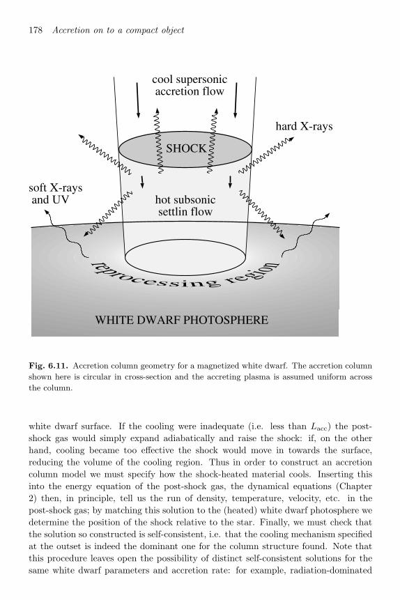
178 Accretion on to a compact object

SHOCK

hot subsonicsettling flow

cool supersonicaccretion flow

hard X-rays

soft X-raysand UV

WHITE DWARF PHOTOSPHEREreprocessing region

Fig. 6.11. Accretion column geometry for a magnetized white dwarf. The accretion column

shown here is circular in cross-section and the accreting plasma is assumed uniform across

the column.

white dwarf surface. If the cooling were inadequate (i.e. less than Lacc) the post-shock gas would simply expand adiabatically and raise the shock: if, on the otherhand, cooling became too effective the shock would move in towards the surface,reducing the volume of the cooling region. Thus in order to construct an accretioncolumn model we must specify how the shock-heated material cools. Inserting thisinto the energy equation of the post-shock gas, the dynamical equations (Chapter2) then, in principle, tell us the run of density, temperature, velocity, etc. in thepost-shock gas; by matching this solution to the (heated) white dwarf photosphere wedetermine the position of the shock relative to the star. Finally, we must check thatthe solution so constructed is self-consistent, i.e. that the cooling mechanism specifiedat the outset is indeed the dominant one for the column structure found. Note thatthis procedure leaves open the possibility of distinct self-consistent solutions for thesame white dwarf parameters and accretion rate: for example, radiation-dominated

6.4 Accretion columns: the white dwarf case 179

solutions in which particle transport processes are negligible, and vice versa. This isthe price we must pay for seeking steady solutions rather than investigating the fulltime-dependent problem. Some insight into which, if any, steady solution is actuallyrealized in a real system may be gained from the analysis of the stability of the steadysolutions against small perturbations. But we should note that the system might alsochoose one of the solutions for ‘historical’ reasons, in the sense that the precise mannerin which the accretion process starts up might favour one or another type of steadysolution.

Let us estimate the physical conditions in the post-shock gas in order to decidewhat cooling processes are potentially important. From the estimate (6.46) of the gasvelocity, and the continuity equation (6.38) we find a post-shock density

ρ2 = 6.2 × 10−10M16f−1−2m

−1/21 R

−3/29 g cm−2 (6.48)

corresponding to an electron density

N2 = 5.9 × 1014M16f−1−2m

−1/21 R

−3/29 cm−3 (6.49)

assuming a fully ionized gas with cosmic abundances. At the temperatures ∼> 108 K(see (6.47)) characteristic of the post-shock gas, the only realistic opacity source iselectron scattering. The shock height D will be found to be ∼< R in all realistic cases(see below) so curvature of the white dwarf surface can be neglected. The cylindricalradius of the column is therefore approximately

d = 2f1/2R = 2 × 108f1/2−2 R9 cm. (6.50)

Thus the ‘horizontal’ optical depth is

τes(d) ∼ NeσTd = 8 × 10−2M16f−1−2m

−1/21 R

−1/29 (6.51)

so that radiative cooling will be optically thin unless the accretion rate per unit area isvery high. On the other hand, the radial optical depth through the column encounteredby photons emitted from the post-shock gas can be large for a high value of M/f :thus all this radiation will leave through the sides of the column after at most a fewscatterings. This is a basic difference from spherical accretion geometries, where allthe radiation must make its escape through the full radial extent of the accretion flow(Fig. 6.12).

Because Ts(equation (6.47)) is so high, radiative cooling of the post-shock gas willbe dominated by free–free (bremsstrahlung) emission. The volume emissivity is

4πjbr ∼= 2 × 10−27N2e T 1/2

e erg s−1 cm−3 (6.52)

for a gas of cosmic abundances with electron temperature Te and electron density Ne.By our considerations of the last paragraph, this cooling is optically thin, so that anelement of shocked gas will be cooled by this process in a characteristic time

trad ∼ 3NekTe4πjbr

∼= 2 × 1011T 1/2e

Nes. (6.53)

180 Accretion on to a compact object

Replacing Ne by N2 (equation (6.49)) and Te by Ts (equation (6.47)) we find

trad ∼ 7M−116 f−2m1R9 s. (6.54)

During this time, the gas element will be settling on to the white dwarf from theshock. Since it starts with velocity −v2 = vff/4 (equation (6.46)) and decelerates, itwould travel a distance

Drad ∼ −v2 trad ∼= 9 × 108M−116 f−2m

3/21 R

1/29 cm (6.55)

before cooling to a temperature of the order of the photospheric value Tb (equation(6.35)) if its cooling were due to radiation alone. Thus (6.55) gives an estimate ofthe shock height D when radiation alone cools the post-shock gas. In general, theremay be other, possibly more efficient, cooling processes operating which would reducethe cooling time and hence reduce D: therefore (6.55) is an upper limit to the shockheight.

For most AM Her and intermediate polar systems, observations suggest M16f−1−2 ∼>

1, so that (6.55) implies D ∼< R, as asserted above.The estimates of the last paragraph show that the post-shock region of the accretion

column is hot, optically thin and lies close to the white dwarf surface. This lastproperty means that, however the accretion luminosity is removed from the column,a substantial fraction of it must be re-emitted from the white dwarf surface withcharacteristic blackbody temperature Tb (equation (6.11)). This suggests a possiblecandidate for a further cooling mechanism: the radiation field characterized by Tb willconsist largely of ‘soft’ photons with energies ( ∼ kTb) much smaller than those of thehot infalling electrons and ions. The scattering of these soft photons by the energeticelectrons involves a transfer of energy from electrons to photons which need not benegligible. The photons will be ‘upscattered’ to higher energies, while the electron gaswill be cooled. The analogous process does not cool the ions directly because of theirvery small scattering cross-section. It is important to distinguish the occurrence ofthis process from the existence of the scattering optical depth in the column: the latterdepends on the probability with which each photon encounters an electron, whereashere we are concerned with the likelihood of each electron encountering a photon.

The theory of Compton scattering shows that a non-relativistic electron of energyE loses energy at an average rate

−E ∼= 83

σT UradE

mec

in a radiation field of energy density Urad (see the Appendix). Thus we can define aCompton cooling time

tCompt =E

−E=

3me c

8σT Urad.

This cooling process will be more important than direct free–free emission in thepost-shock gas only if tCompt < trad: using (6.53) we can write

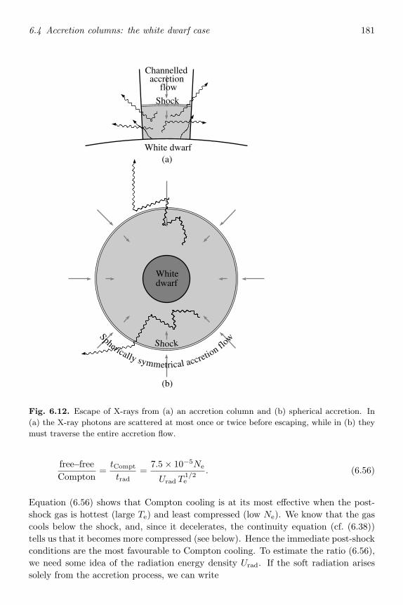
6.4 Accretion columns: the white dwarf case 181

White dwarf

Shock

(a)

Whitedwarf

(b)

Channelledaccretion

flow

Shock

Spherically symmetrical accretion flo

w

Fig. 6.12. Escape of X-rays from (a) an accretion column and (b) spherical accretion. In

(a) the X-ray photons are scattered at most once or twice before escaping, while in (b) they

must traverse the entire accretion flow.

free−freeCompton

=tCompt

trad=

7.5 × 10−5Ne

Urad T1/2e

. (6.56)

Equation (6.56) shows that Compton cooling is at its most effective when the post-shock gas is hottest (large Te) and least compressed (low Ne). We know that the gascools below the shock, and, since it decelerates, the continuity equation (cf. (6.38))tells us that it becomes more compressed (see below). Hence the immediate post-shockconditions are the most favourable to Compton cooling. To estimate the ratio (6.56),we need some idea of the radiation energy density Urad. If the soft radiation arisessolely from the accretion process, we can write

182 Accretion on to a compact object

Urad∼= fsoftLacc

4πR2fc(6.57)

where fsoft is the fraction (≤ 1) of the accretion luminosity which is re-radiated fromthe white dwarf photosphere, since there will be little dilution of this radiation by scat-tering and geometrical effects. Now using (6.47) and (6.49) to estimate the immediatepost-shock conditions, (6.57) and (6.56) give

free−freeCompton

= 6.5f−1softm

−21 R2

9

(TeTs

)−1/2(Ne

N2

). (6.58)

This estimate shows that Compton cooling will only be significant, even near theshock, if the white dwarf is very massive ( ∼ 1.4 M and hence very small in radius,R9 ∼ 0.2). Of course, the fraction fsoft is itself determined by the column structure.If, for example, the accretion column cools only by radiation we would expect ongeometrical grounds fsoft ∼ 0.5. (Actually, as discussed below, fsoft ∼ 0.3 is morelikely because of reflection of hard photons off the white dwarf surface.) Hence for a1M white dwarf (R9 = 0.5) we find

free−freeCompton

∼ 3−5

even at the shock. Compton cooling would be more important if the white dwarf hada high intrinsic luminosity, so that formally fsoft 1 in (6.58). This would be thecase if, for example, the accreted material underwent steady nuclear burning on thewhite dwarf surface. As we shall see shortly, this is rather unlikely.

The final radiative cooling process we must consider is the thermal cyclotron emis-sion discussed in Section 6.3. As mentioned there, estimates of the effectiveness ofthis process are difficult, but generally imply fairly small luminosities Lcyc comparedto Lacc, unless the accretion rate M is rather low, or the magnetic field strength B

is rather high, or both. When cyclotron emission does dominate over free–free wecan show that the electron temperature Te will be somewhat lower than the ion tem-perature Ti. This happens because the cyclotron process cools the electrons fasterthan collisions with the hot post-shock ions can heat them unless there is a significanttemperature difference Ti − Te. The rate at which the ions heat the electrons in aneffort to bring about equipartition is

Γeq ∼= 2 × 10−17N2e T−3/2

e (Ti − Te) erg s−1 cm−3. (6.59)

Under normal circumstances, the energy-loss rate of the electrons can be balancedby Γeq with only a very small temperature difference |Ti − Te| Te. For example,if the electrons lose energy by free–free emission, (6.59) and (6.52) show that theelectron–ion energy balance

Γeq = 4πjbr

implies

Ti − Te ∼ 10−10T 2e .

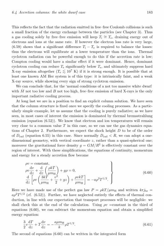
6.4 Accretion columns: the white dwarf case 183

This reflects the fact that the radiation emitted in free–free Coulomb collisions is sucha small fraction of the energy exchange between the particles (see Chapter 3). Thusa gas cooling solely by free–free emission will keep Ti ∼= Te, draining energy out ofelectrons and ions at the same rate. If however the electron loss rate is very large,(6.59) shows that a significant difference Ti − Te is required to balance the losses:thus the electrons will equilibrate at a lower temperature than the ions. Thermalcyclotron radiation can be powerful enough to do this if the accretion rate is low;Compton cooling would have a similar effect if it were dominant. Hence, dominantcyclotron cooling can reduce Te significantly below Ts, and ultimately suppress hardX-ray emission altogether (Te ∼< 107 K) if it is strong enough. It is possible that atleast one known AM Her system is of this type: it is intrinsically faint, and a weakX-ray source, while showing every sign of strong cyclotron emission.

We can conclude that, for the ‘normal’ conditions of a not too massive white dwarfwith M not too low and B not too high, free–free emission of hard X-rays is the onlyimportant radiative cooling process.

At long last we are in a position to find an explicit column solution. We have seenthat the column structure is fixed once we specify the cooling processes. As a partic-ularly simple example, let us assume that the cooling is purely radiative; as we haveseen, in most cases of interest the emission is dominated by thermal bremsstrahlungemission (equation (6.52)). We know that electron and ion temperatures will remainvery close to a common value T in this case, so we can use the gas dynamics equa-tions of Chapter 2. Furthermore, we expect the shock height D to be of the orderof Drad (equation 6.55) in this case. Since normally Drad < R, we can adopt a one-dimensional geometry, with vertical coordinate z, rather than a quasi-spherical one;moreover the gravitational force density g = GM/R2 is effectively constant over theregion of interest. With these simplifications, the equations of continuity, momentumand energy for a steady accretion flow become

ρv = constant,

ρvdv

dz+

ddz

(ρkT

µmH

)+ gρ = 0,

ddz

[ρv

(3kT

µmH+

v2

2+ gz

)+

ρvkT

µmH

]= −aρ2T 1/2.

(6.60)

Here we have made use of the perfect gas law P = ρkT/µmH and written 4πjbr =aρ2T 1/2 (cf. (6.52)). Further, we have neglected entirely the effects of thermal con-duction, in line with our expectation that transport processes will be negligible: weshall check this at the end of the calculation. Using ρv =constant in the third ofequations (6.60), we can subtract the momentum equation and obtain a simplifiedenergy equation:

32

vdT

dz+ T

dv

dz= −aµmH

kρT 1/2. (6.61)

The second of equations (6.60) can be written in the integrated form

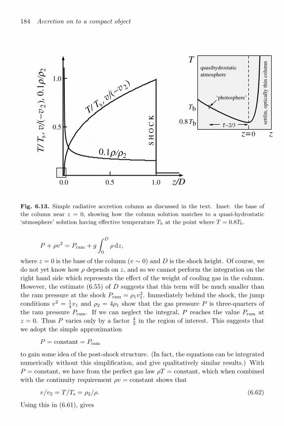
184 Accretion on to a compact object

τ ~2/3

z=0 z

z/D0.5 1.00.0

0.5

1.0

Tb

0.8 Tb

‘photosphere’

settl

ing,

opt

ical

ly th

in c

olum

nTquasi-hydrostaticatmosphere

S H

O C

K

T/ Ts, v/(−

v 2)

0.1ρ/ρ2

T/ T

s, v

/(−v

2),

0.1ρ

/ρ2

Fig. 6.13. Simple radiative accretion column as discussed in the text. Inset: the base of

the column near z = 0, showing how the column solution matches to a quasi-hydrostatic

‘atmosphere’ solution having effective temperature Tb at the point where T = 0.8Tb.

P + ρv2 = Pram + g

∫ D

0

ρ dz,

where z = 0 is the base of the column (v ∼ 0) and D is the shock height. Of course, wedo not yet know how ρ depends on z, and so we cannot perform the integration on theright hand side which represents the effect of the weight of cooling gas in the column.However, the estimate (6.55) of D suggests that this term will be much smaller thanthe ram pressure at the shock Pram = ρ1v

21 . Immediately behind the shock, the jump

conditions v2 = 14v1 and ρ2 = 4ρ1 show that the gas pressure P is three-quarters of

the ram pressure Pram. If we can neglect the integral, P reaches the value Pram atz = 0. Thus P varies only by a factor 4

3 in the region of interest. This suggests thatwe adopt the simple approximation

P = constant = Pram

to gain some idea of the post-shock structure. (In fact, the equations can be integratednumerically without this simplification, and give qualitatively similar results.) WithP = constant, we have from the perfect gas law ρT = constant, which when combinedwith the continuity requirement ρv = constant shows that

v/v2 = T/Ts = ρ2/ρ. (6.62)

Using this in (6.61), gives

6.4 Accretion columns: the white dwarf case 185

52

T 3/2 dT

dz=

µmH a

kT 2s

ρ2(−v2)

so that

T 5/2 =µmH a

k

ρ2 T 2s

(−v2)z + constant.

Near the base of the column (z = 0) we expect v ∼ 0, so T ∼ 0 and the constant inthis equation must be very small. Strictly speaking, several of our assumptions breakdown when T becomes of the order of Tb, since re-heating by the photospheric fluxwill balance the cooling and eventually cause T to reach a minimum value just belowTb, before becoming optically thick and matching on to the white dwarf atmosphere;however, it can be shown that this is not serious for the gross features of the solution.Thus we write

T

Ts=

( z

D

)2/5where

D = kT1/2s (−v2)/(µmHaρ2).

(6.63)

Using (6.55) and the definition of a, it is easy to see that

D ∼ 13

Drad.

The structure we have found is shown graphically in Fig. 6.13.Our next task is to check for self-consistency the assumptions made in deriving

this solution. First, we neglected the weight term g∫D0

ρ dz in the integral of themomentum equation by comparison with the ram pressure term Pram. From oursolution (6.62) and (6.63), we have

g

∫ D

0

ρ dz/Pram =53

(GM/R2)ρ2D/(4ρ2 v2ff) =512

(D/R).

This is clearly justified when, as usual, M/f is sufficiently large that D < R. Second,we neglected the term ρv2 by comparison with P ∼= Pram. We find

ρv2/Pram ∼ ρv22(z/D)2/5/(4ρ2v22) =

14

(z/D)2/5 < 1.

Finally, (2.6) shows that the conductive flux into the white dwarf is

|q| = 4 × 10−7z2/5D−7/5 erg s−1 cm−2.

This vanishes at z = 0, so there is no conduction into the white dwarf; moreover, theneglect of the divergence of this term in the energy equation is justified, since

|dq/dz|/ρv dv/dz ∼ 10−7/(ρ2 v2 D) ∼ 10−12

using (6.55), (6.48) and (6.46). Hence the simple radiative column structure repre-sented by (6.62) and (6.63) is a quite reasonable approximation. Numerical solutions

186 Accretion on to a compact object

of the full set (6.60), some taking account of the corrections due to spherical geome-try, have been obtained: from our work above, it is no surprise that these differ onlyslightly from our simple analytic solution.

Let us see what such radiative column solutions predict for observations of AMHer and intermediate polar systems. We can show, from (6.62) and (6.63), that theshocked gas radiates almost all its luminosity Lacc as hard X-rays with characteristicphoton energies kTs ∼ 60 keV (for m1 = 1, R9 = 0.5). This result arises since thegas is subsonic and thus has in the main only internal energy to draw on to providethe luminosity. Thus the energy removed from a given element of gas is providedessentially by the temperature drop Ts − T at each point of the column. Half of thetotal available luminosity (Lacc) is thus radiated by gas at temperatures T ∼> 0.5Ts,and three-quarters at T ∼> 0.25Ts, etc. Hence almost all of Lacc initially appears ashard X-rays. Since D < R, one-half of these are emitted towards the white dwarfsurface and are intercepted. Of this luminosity 1

2Lacc, a fraction aX(typically ∼ 0.3)is reflected upwards, while the remaining 1

2 (1 − aX)Lacc is absorbed to re-emerge asthe ‘blackbody’ component at ∼ Tb. Hence for radiative solutions

fsoft ∼ 12

(1 − aX) ∼ 0.35

or

LX

Lsoft∼

12 (1 + aX)12 (1 − aX)

∼ 2. (6.64)

The AM Her and intermediate polar stars are indeed found to be hard X-ray and softX-ray–extreme ultraviolet sources in general. However, the LX/Lsoft ratio is alwaysfound to be much smaller than the estimate (6.64). Figure 6.14 shows observations ofAM Her itself. Because of the effects of interstellar absorption the emission between∼ 10 and 100 eV is unobservable; but even a very conservative interpolation betweenthe ultraviolet and soft X-rays implies

LX

Lsoft∼ 0.1. (6.65)

A blackbody interpolation would give LX/Lsoft < 10−2. Thus instead of the hard X-rays being ∼ 2

3 of the total luminosity of the system, as predicted by (6.64), observationimplies that they are no more than 10%.

The very large discrepancy between (6.64) and (6.65) is a serious problem for ra-diative column models: it is easy to convince oneself, for example, that the columngeometry we have discussed does not allow the presence of large volumes of cool gasclose to the accretion column which would ‘degrade’ the hard X-rays. Such a modelwould probably conflict with the evidence of the soft X-ray light-curves, which showthat the soft X-ray source indeed occupies an area of the suggested size (∼ 4πR2f)close to the white dwarf. Thus early attempts to salvage radiative column models cen-tred on the possibility of steady nuclear burning of the accreted matter on the whitedwarf surface. This is at first sight an attractive idea, since (1.1) and (1.2) show that

6.4 Accretion columns: the white dwarf case 187

Blackbody fit,

Fig. 6.14. Schematic UV and X-ray continuum spectrum of AM Herculis, showing the large

(and uncertain) soft X-ray excess.

the nuclear burning luminosity could be ∼ 50 times the accretion luminosity Lacc; thusif the burning region were optically thick this would provide a natural explanation forthe ratio (6.11). The main difficulty with this idea is that steady burning, rather thanan explosive ‘runaway’ event (such as may power classical novae), does not seem to bepossible at the luminosities required by observation. Detailed calculations show thatsteady burning is impossible unless either

Lburn ∼< 2 × 1032f erg s−1

or

Lburn ∼> 4 × 1037f erg s−1.

Observations require 0.1 ∼> f ∼> 10−2–10−3 and Lsoft ∼ 1033–1034 for most AM Hersystems; hence Lsoft falls squarely in the gap between the two possible stable burningregimes.

188 Accretion on to a compact object

Since there was nothing inconsistent or unreasonable in the physical assumptionsbehind the radiative column solutions, it seems sensible to ask if they are unstable.Quite complex stability calculations have been performed. First, these show thatthere is a ‘bouncing’ instability in which the shock height D oscillates between a smallvalue and ∼ Drad with characteristic timescale ∼ trad. The origin of this instabilityis the nature of the bremsstrahlung cooling rate (6.52). If a gas element is slightlycompressed, raising Ne, it tends to cool more rapidly (cf. (6.53)); this in turn reducesits temperature T and indeed its pressure NekT . Thus the element tends to getcompressed still further since it is at a lower pressure than its surroundings, leading toa rise in Ne and still more rapid cooling, and so on. At the same time the gas elementis settling on to the white dwarf on the timescale trad, so this simple analysis is notenough to show that the instability actually grows. But full global investigations oftime-dependent radiative columns do show this. Thus after a time ∼ trad, the shockstructure collapses on to the white dwarf, and the incoming accretion stream has to‘start again’, trying to set up a steady radiative column structure because this is theonly way we are allowing it to cool. This occurs on a timescale ∼ trad, when the wholecycle starts again. Whatever the details involved, it is clear that the assumptionthat the primary cooling process is the emission of bremsstrahlung X-rays means that(6.64) holds in a time-averaged sense, so that there is still a conflict with observation.

One way of escaping the prediction (6.64) would be to ensure that the primaryhard X-ray emission is all absorbed by cool surrounding material; a sufficiently nar-row, dense column would act like a point source, powering the photosphere of theaccretion region from below. As all the photons must escape through large amountsof cool (∼ Tb) material the hard X-ray emission would all be degraded, allowing verylarge observed ratios of soft to hard emission. A quantitative check of this idea givesan interesting result. First, to ensure that ∼> 10 keV X-rays are all absorbed anddegraded requires a column density ∼> 1025 cm−2; below ∼ 10 keV the photons are ab-sorbed photoelectrically by bound-free absorption in the K-shells of heavy elements,while higher energy photons are degraded by repeated Thomson scattering (τes ∼> 7).This result tells us that the accretion flow must penetrate a few scaleheights intothe (heated) white dwarf atmosphere before being stopped. We can see this simplyas follows. The pressure and density in this atmosphere must obey the hydrostaticcondition

dP

dz= −gρ (6.66)

with g = GM/R2 the surface gravity (M and R = white dwarf mass and radius),since the atmosphere has negligible mass or vertical extent. Defining the scaleheightH by dP /dz ∼ P/H and using P ∼ ρc2S , cS ∼ (kTb/µmH)1/2 shows that

H ∼ kTbµmH g

∼ 105T5 cm, (6.67)

for typical parameters, where T5 = Tb/105 ∼ 1–3. If the temperature does not vary

6.4 Accretion columns: the white dwarf case 189

rapidly with z, (6.66) shows that ρ varies as e−z/H . The definition of the photosphereis that the optical depth measured from infinity is of order unity, i.e.∫ ∞

zph

κRρ dz ∼ 1,

i.e.

κR ρH ∼ 1, (6.68)

where κR is the Rosseland mean opacity. For the conditions in the accretion regionthis is close to the electron scattering value (0.34), so (6.68) shows that the electronscattering depth is of order unity over one scaleheight. The requirement τes ∼> 7 forthe effective disappearance of the hard X-rays thus amounts to requiring the accretingmaterial to penetrate ∼ 7 scaleheights below the surrounding photosphere before beingstopped. This is not enough of course: we need also that

d < D ∼< 7H

so that the column is both narrow and short enough to prevent hard X-ray photonsavoiding the absorbing matter. Using (6.50) and (6.67) these conditions yield theconstraints T5 ∼< 5, M ∼< 1015 g s−1. This shows that such ‘buried column’ solutionsare only available for rather small accretion rates. However, there is a simple wayout of this restriction: adding together a number of such buried columns. Providedthese are separated by distances ∼> 7H on the white dwarf surface we can regardthem as independent. They amount to a total accretion flow with a higher M thanallowed above, but still with a very strong excess of soft X-rays. The only conditionleft to check is that the ram pressure in each of the columns is enough to penetrateto the required depth in the atmosphere. From (6.68) the photospheric density isρph ∼ 3×10−5 g cm−3, giving a photospheric pressure Pph ∼ 3×108 dyne cm−2. Thevery small values of f ∼< 10−7 for each of the individual buried columns imply from(6.39) ram pressures considerably exceeding this. Thus photospheric penetration willindeed occur, but be limited to a few scaleheights because of the exponential increaseof atmospheric pressure with depth.

The analysis of the last paragraph shows that it is possible to construct columnsolutions which have soft excesses, as required by observation, although the splittingof the accretion flow into many separate buried columns seems contrived. A morerealistic version of this idea is to suppose that instabilities in the accretion flow abovethe white dwarf surface break it up into well-separated blobs. A favoured site for thisis the region near rM where the flow threads the magnetic field. Blobs which followfieldlines will be compressed sideways as d ∝ (R/rM )3/2, but stretched lengthwaysas l ∝ (rM/R)1/2 because the leading edge accelerates faster than the trailing edgein free fall. Provided that a given blob is not too short to begin with, it is likelyto be much longer than the free–free cooling length D when it reaches the surface.Provided also that the blob’s mass exceeds the mass of atmosphere it has to sweep upbefore stopping a few scaleheights below the photosphere, it is legitimate to treat it

190 Accretion on to a compact object

f zone

f eff

f acc

Fig. 6.15. Highly inhomogeneous accretion on to a magnetic white dwarf. Upper figure:

blobs of varying density and length hit the surface. Sufficiently dense blobs penetrate the

photosphere and radiate almost all their energy as soft X-rays. Lower figure: schematic

picture of the three fractional areas facc, feff and fzone. The fractional area over which blobs

accrete, facc, is always much smaller than that over which the soft X-rays emerge, feff . The

geometrical region over which blobs land is characterized by fzone; in normal accretion states

of AM Herculis systems feff ∼< fzone, while in anomalous states feff fzone.

as a buried column of the type discussed above. A full analysis on these lines showsthat accretion regions giving soft excesses can be constructed without placing extremerequirements on the instabilities producing the blobs. In particular, the instabilities donot need to compress the blobs above the densities already expected in the accretionflow, but merely have to create gaps between them of width > 7H at the white dwarfsurface. Material of lower densities may be present in these gaps and elsewhere, givingthe observed hard X-rays in the usual way. Figure 6.15 shows a schematic view.

At present progress in understanding blob solutions is limited by our lack of knowl-edge of the instabilities which divide the flow. Thus we cannot predict the numberor density spectrum of the blobs in any given case. The blob picture is however veryuseful in understanding some phenomena in a qualitative way. In particular, it isclear that we must now distinguish between three surface fractional areas which wereall previously denoted by f for the case of a single accretion column. If we confineourselves to considering dense blobs penetrating the photosphere these are: facc, the

6.5 Accretion column structure for neutron stars 191

instantaneous fractional area over which blobs accrete, feff , the effective fractionalarea radiating most of the accretion luminosity as soft X-rays, and fzone, the totalzone fractional area over which the blobs are scattered (Fig. 6.15). In all cases thereis a strict hierarchy between these quantities:

facc feff < or fzone < 1.

Clearly feff is the important quantity for the soft X-ray spectrum, and fzone that forthe soft X-ray light curves. The two possible inequalities between feff and fzone giverise to very different types of soft X-ray light curves, especially if the instantaneousphotosphere for each region heated by an individual blob bulges or splashes abovethe surrounding surface, as seems very likely. If the accretion zone is only sparselypopulated by accreting blobs, i.e. feff fzone, we see each individual splash as arather luminous event. The light curve is thus very noisy. Even more strikingly, wesee the sides of all the splashes, and thus most of the emitted soft X-ray flux, as soonas the accretion zone rotates into view at all, giving an effective square-wave lightcurve. All of this is very like what is observed during the ‘anomalous’ X-ray statesof some of the AM Her systems. From time to time (intervals of at least months)some of the AM Her systems are observed to change their soft X-ray light curves quitemarkedly from the usual quasi-sinusoidal shapes, remaining in these states for months.Often these changes involve large phase shifts of the brightest parts of the light curve,suggesting that accretion may switch between the two magnetic poles to some extent.Figure 6.16 gives a comparison between a simulation involving about 15 accretingblobs and observations of an anomalous state of AM Her itself. If the number of blobsis increased so that feff begins to approach fzone, the individual splashes begin toshadow each other and the accretion region behaves like a roughened surface. Thepredicted soft X-ray light curves are quasi-sinusoidal, just as observed during ‘normal’X-ray epochs. It is easy to show that anomalous-type square-wave light curves arepredicted if the number N of instantaneously accreting blobs satisfies

N ∼< fzone/feff , (6.69)

the light curves changing to quasi-sinusoidal if the inequality is reversed.

6.5 Accretion column structure for neutron stars

Our discussion of column structure has so far been concerned with white dwarf ac-cretion; an equally pressing problem is the analogous process for neutron stars. Inthe white dwarf case, the basic physical processes are comparatively better under-stood whereas at the very extreme physical conditions of a neutron star surface, withfree-fall velocities ∼ c/2, magnetic fields B ∼ 1012 G, and sometimes luminosities∼ LEdd, great complications are introduced into the microscopic and macroscopicphysics. Since, as we have seen, our understanding of white dwarf accretion is farfrom complete, it is hardly surprising that it is still less so for neutron stars. Indeed

192 Accretion on to a compact object

Fig. 6.16. Top: soft X-ray light curve of AM Herculis in an anomalous state (J. Heise, A.C.

Brinkman, E. Gronenschild, M. Watson, A.R. King, L. Stella & K. Kieboom (1985) Astron.

Astrophys. 148, L14). Bottom: simulated soft X-ray light curve with random accretion of

blobs dense enough to penetrate the photosphere. (J.M. Hameury & A.R. King (1988) Mon.

Not. R. astr. Soc. 235, 433). On average blobs are accreting on the main polecap at any

given instant. A second diametrically opposed pole accretes 5% of the flow on to the main

pole.

it is probably fair to say that most of the difficulties and uncertainties of the whitedwarf case remain while new ones are added.

Thus, for example, it is unclear in both cases whether the accretion column is a‘hollow’ or ‘filled’ cylinder. Additionally, however, it is far from clear that a shock ofany kind occurs, even when the accretion flow is smoothly homogeneous. The reasonfor this is that the deflection mean free path λd (equation (3.20)) in the accretionflow is always very large compared to any other length in the problem, especially theneutron star radius R ∼ 10 km. To see this, we use the continuity equation (6.38)with −v = vff ∼= c/2 (equation (6.40)) to find the number density

N ∼= 1016M16f−1 cm−3.

From (3.20), with m ∼= mp and v ∼= c/2, we find

λd ∼= 5 × 1011M−116 f cm

with ln Λ = 20. A limit on Mf−1 comes from the consideration that accretion on to afraction of the neutron star surface cannot yield an accretion luminosity Lacc greatly

6.5 Accretion column structure for neutron stars 193

in excess of the Eddington value fLEdd (equation (1.2)) appropriate to that fractionalarea. Using (1.4) and (1.7) we find

M16f−1 ∼< 102

so giving

λd ∼> 5 × 109 cm R∗ ∼= 106 cm

for protons with the energy of free-fall. Thus a collisional ion shock of the type we haveconsidered up to now is impossible in the neutron star case. Unfortunately, this doesnot mean that the possibility of some kind of shock, defined as a region where fluidquantities change almost discontinuously, can be entirely disregarded: the existenceof shocks having a thickness much smaller than the deflection mean free path λd hasbeen known from observation for some time. Such shocks are called collisionless: themost notable example is the bow shock where the solar wind impinges on the Earth’smagnetosphere. Satellite observations show that the shock thickness is ∼< 103 km,while λd for the measured physical conditions is of the order 108 km.

The possibility greatly complicates the discussion of neutron star accretion. Thephysics of collisionless shocks is ill-understood even in the case where there is nomagnetic field, let alone in the ∼ 1012 G fields typical of neutron star polecaps. Themain problem is that some process other than viscosity, which operates over scales∼ λd, must be found to dissipate the ordered energy and randomize it. Our ignoranceof how such shocks work means that we do not know the conditions under which theyform: hence both possibilities (shock or no shock) have to be considered.

A further set of complications is introduced by the fact that for fairly modesteffective accretion rates M16f

−1 ∼< 102 (see above) the radiation pressure due to theaccretion luminosity will become dynamically important: indeed the observed X-rayluminosities of many pulsing neutron star sources is of the order of the Eddingtonvalue ∼ 1038 erg s−1. To all of these problems must be added finally the fact that theaccretion takes place in a highly magnetized (∼ 1012 G) environment, so that everymicroscopic physical process must be calculated accordingly. We have mentionedalready (in Section 6.3) some of the problems which arise in discussing the transfer ofradiation in such a medium; another important effect is on the Coulomb encounters ofcharged particles, making the calculation of the stopping length much more complexthan the simple treatment of Chapter 3.

As one would expect given this formidable list of difficulties, no fully self-consistentcolumn solution has yet been given which incorporates all of these effects. In par-ticular, as we mentioned in Section 6.3, detailed treatments of the radiative transferproblem have been given only for rather simple ad hoc geometries, while models of thecolumn structure always simplify the transfer problem. The ultimate goal, of course,is to combine all these effects in order to predict, for example, the X-ray pulse profileseen by an observer at some angle to the rotation axis as a function of the X-rayenergy. So far, progress has been made in constructing self-consistent column modelsin three cases: we shall describe these briefly.

194 Accretion on to a compact object

If the accretion rate is less than about 1017 g s−1, (1.7) shows that the accretion lu-minosity Lacc will be < 1037 erg s−1 and thus subcritical (i.e. less than the Eddingtonvalue (1.4) ∼ 1038 erg s−1). Hence, for such lower-luminosity objects we may expectthat complications due to radiation pressure may be safely neglected. This subcriticalaccretion regime divides into two cases depending on whether or not a collisionlessshock forms. If no shock forms, the infalling matter bombards the accretion column,compressing it by its ram pressure and heating it by giving up its infall energy viamultiple Coulomb collisions. Since, in the absence of a shock, electrons and ions havethe same (free-fall) velocity ∼ c/2, both of these effects are dominated by the ionsbecause of their much greater masses. Hence the fundamental heating process is theloss of energy by infalling protons. In Section 3.5 we considered this process for an un-magnetized plasma and showed that the stopping power ρλs is inversely proportionalto the square of the energy of the incident proton (3.37). For an infall speed ∼ c/2,we find

y0 = ρλs ∼ 50 g cm−2. (6.70)

Further, in Section 3.5 we showed that such a proton would probably reach significantelectron scattering optical depths τ ∼= y0σT/mp before releasing its energy. The verystrong magnetic fields (∼> 1012 G) inferred for the polecaps of accreting neutron starsmean that the derivation of the stopping ‘length’ y0 given in Section 3.5 is not strictlyvalid; in particular, the inequality rLi ∼> λDeb (equation (6.34)) is now reversed. For‘typical’ parameters Ne = 1023 cm−3, B = 5 × 1012 G, we find from (3.49) and (3.9)

rLi = 1.5 × 10−9 cm < λDeb = 1.7 × 10−7 cm.

This means that the trajectory of the ion during a scattering event will not be astraight line, as implicitly assumed for the unmagnetized case. The result of allowingfor this effect in a detailed treatment using the Fokker–Planck equation is to reducey0 to ∼ 30–40 g cm−2. With y0 known as a function of energy the heating rate ΓCouldue to Coulomb collisions can be taken as roughly uniform within the stopping regiondefined by

y(z) =∫ ∞

z

ρ(z′) dz′ ≤ y0. (6.71)

For a column of cross-sectional area A the total heating rate per unit area must beLacc/A: hence

ΓCoul ∼= Laccρ

Ay0erg s−1 cm−3 for y ≤ y0

ΓCoul = 0 for y > y0.

(6.72)

For a steady column solution, ΓCoul must be balanced by the total cooling rateby radiation from the heated electrons. Two processes are at work here; thermalbremsstrahlung and Compton cooling (cf. the discussion preceding (6.56)) – the lat-ter being important because the electron temperature will be found to increase out-wards. Both processes are affected by the strong magnetic field (in technical language

6.5 Accretion column structure for neutron stars 195

the appropriate cross-sections have resonances at ν = νcyc, equation (6.30)), so thatcyclotron radiation is automatically included. The Compton cooling rate involves aknowledge of the radiation energy density Urad (cf. the equations preceding (6.56))which in turn entails a simultaneous treatment of the radiative transfer problem. Forexample, the simplest approximation is to assume local thermodynamic equilibrium,so that

Urad = (4σ/c)T 4rad.

Under such conditions the radiative transfer equation takes the diffusion form

F = − c

3dUrad

dτ(6.73)

where F is the total flux of radiation and τ the optical depth (see the Appendix). Forthe highly ionized column the only opacity is electron scattering, so

dτ = (σT/mp) dy

while F is given by the total heating rate of material below the point under consider-ation:

F (y) =∫ y

y0

ΓCoul dz =Lacc

Ay0(y − y0) (6.74)

using (6.72). Hence Urad can be found from (6.73) and (6.74):

−cmp

3σT

dUrad

dy=

Lacc

Ay0(y − y0)

so that Urad is quadratic in y, with an appropriate boundary condition at y = 0. Thusthe Compton cooling rate and hence the energy balance equation can be expressed interms of the radiation temperature Trad, the electron temperature Te, y and ρ.

More elaborate treatments of the radiative transfer problem can also be used toobtain Urad, and hence the energy equation. Finally, the column must be in hydrostaticequilibrium under the combined effects of gas pressure (in the outer, non-degeneratelayer), the weight of the column material, and the ram pressure of the infalling matter:thus

P =ρkTeµmH

=(

GM

R2∗+

ρ0v2

y0

)y, 0 < y ≤ y0

=GM

R2∗y + ρ0v

2, y > y0 (6.75)

where v = (2GM/R∗)1/2 is the infall velocity, and ρ0 the density of the infallingmatter. Numerical solution of the energy and pressure balance equations, togetherwith whatever approximate transfer equation is adopted, now yields the density andtemperature structure of the column, together with its radiation field. Figure 6.17shows the results of a calculation of this type, taking magnetic effects approximatelyinto account. For a typical atmosphere, the total stopping ‘length’ ∼ 30–60 g cm−2

196 Accretion on to a compact object

Fig. 6.17. The structure and spectrum of neutron star atmospheres heated by an infalling

stream of matter via Coulomb collisions. Left-hand figure: temperature T and electron

density ne versus column density y =∫ ∞zρ(z′)dz′ for an accretion rate M = 1015 g s−1

and magnetic fields B = 5 × 1012 gauss (solid curves) and B = 1013 gauss (dashed curves).

Right-hand figure: emergent photon number spectrum (Fν/hν) for the same parameters as

the left-hand figure. The cyclotron line is indicated by the arrow; the crossbar measures the

number of photons in the line, not its profile. (Reproduced from P. Meszaros, A.K. Harding,

J.G. Kirk & D.J. Galloway (1983), Astrophys. J. Lett. 266, L33.)

corresponds to a rather thin plane parallel section of the polecap, with vertical extent∆z R∗.

If we assume that a subcritical accretion flow on to a neutron star undergoes acollisionless shock, the resulting column structure bears a qualitative resemblance tothe radiative columns discussed above for white dwarf accretion, especially if M istaken low enough (∼< 1016 g s−1) that the column is optically thin in the transversedirection to Thompson scattering. The biggest difference is that the lack of collisionalcoupling between ions and electrons in the shock means that the ion and electrontemperatures jump independently; hence an equation like (3.66) must be written foreach species, i.e.

Ti =316

µmH

kv2ff

∼= 3.7 × 1011m1R−16 K

and

Te =516

me

kv2ff

∼= 5.5 × 108m1R−16 K

(6.76)

(cf. (6.47)). The factor 516 rather than 3

16 in Te arises because the electrons have onlyone degree of freedom (motion along B) rather than three.

The enormous disparity (∼ mp/me) in Ti and Te means that the ions will heat theelectrons at a rate similar to Γeq, (6.59) (modified by magnetic effects), in an effort to

6.5 Accretion column structure for neutron stars 197

bring about equipartition. This effect is opposed by radiative cooling of the electronsvia bremsstrahlung and cyclotron emission. In fact, the latter dominates the emission,producing at each height in the column a broadened ‘line’ around the local cyclotronfrequency. The shock height D is determined by the time required to equalize ion andelectron temperatures, since the ions have all the energy which must ultimately beradiated by the electrons. Thus

D ∼ (vff/4)teq ∼ λeq. (6.77)

Since from (6.30)

νcyc ∝ B ∼ B∗(r/R∗)−3

where B∗ is the surface field, there is a significant variation of νcyc over the columnheight D if M ∼< 1015f−3 (where f−3 = f/103) and a continuous spectrum which dropssharply at frequencies above the cyclotron frequency νcycB∗ results. For M ∼> 1015f−3g s−1, by contrast, D is sufficiently small that νcyc does not vary greatly over theemission region and the emergent X-ray spectrum is a broadened ‘line’ centred onνcyc(B∗): see Fig. 6.18. Because, especially at low accretion rates, the shocked columnprotrudes a large distance D ∼ R∗ from the stellar surface, radiation is emitted overa much larger solid angle than in the Coulomb-heated case described earlier: this issometimes referred to as a ‘fan’ as opposed to ‘pencil’ beam of radiation.

The two models we have described above both neglect radiation pressure: thusthey cannot be applied to the more luminous X-ray sources such as Sco X-1, HerX-1 or Cen X-3. For such sources one can make instead the approximation thatradiation pressure dominates gas pressure, so that the infalling gas is stopped byphotons acting on the electrons through scattering, while the protons are deceleratedbecause they are closely tied to the electrons by Coulomb forces. In the simplesttreatment of this approximation, all magnetic effects, other than the one-dimensionalchannelling of the accretion on to the polecaps, are neglected, so that in particularthe electron scattering cross-section, and hence the effects of radiation pressure, aretreated as isotropic. Thus, if the radiation field at a point in the accretion columnhas energy density Urad, the corresponding pressure exerted is given by the standardresult Prad = 1

3Urad. In the transverse directions this pressure is easily resisted by themagnetic pressure [4π/µ0]B2/8π; moreover, the same force confines the infall velocityv to be in negative z-direction, where z is as usual the coordinate measured along themagnetic field, assumed normal to the stellar surface. Thus in close analogy with thefirst two of equations (6.60) we can write the steady-state equations of continuity andmomentum for the infalling gas as

ρv = constant,

ρv∂v

∂z+

13

∂Urad

∂z+ gρ = 0.

(6.78)

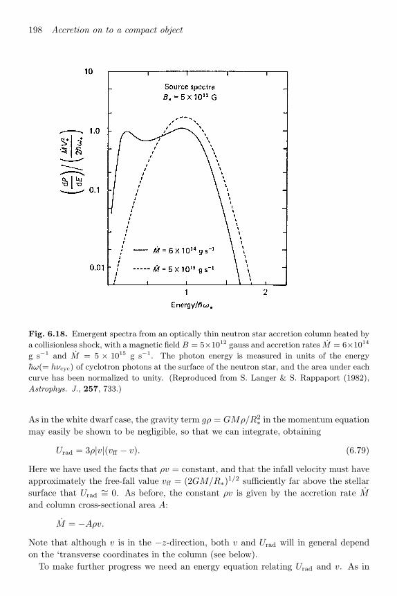
198 Accretion on to a compact object

Fig. 6.18. Emergent spectra from an optically thin neutron star accretion column heated by

a collisionless shock, with a magnetic field B = 5×1012 gauss and accretion rates M = 6×1014g s−1 and M = 5 × 1015 g s−1. The photon energy is measured in units of the energy

hω(= hνcyc) of cyclotron photons at the surface of the neutron star, and the area under each

curve has been normalized to unity. (Reproduced from S. Langer & S. Rappaport (1982),

Astrophys. J., 257, 733.)

As in the white dwarf case, the gravity term gρ = GMρ/R2∗ in the momentum equation

may easily be shown to be negligible, so that we can integrate, obtaining

Urad = 3ρ|v|(vff − v). (6.79)

Here we have used the facts that ρv = constant, and that the infall velocity must haveapproximately the free-fall value vff = (2GM/R∗)1/2 sufficiently far above the stellarsurface that Urad

∼= 0. As before, the constant ρv is given by the accretion rate M

and column cross-sectional area A:

M = −Aρv.

Note that although v is in the −z-direction, both v and Urad will in general dependon the ‘transverse’ coordinates in the column (see below).

To make further progress we need an energy equation relating Urad and v. As in

6.5 Accretion column structure for neutron stars 199

the case of the Coulomb-heated column (equations (6.73) and (6.74)) this must takethe form of an equation relating Urad to the radiative flux, plus an equation specifyinghow the flux is modified by the energy production due to accretion. Since Urad candepend on the transverse coordinates in the column, in particular the cylindrical radialcoordinate R, the radiative transfer equation in the diffusion form analogous to (6.73)would be

F = − c

3mp

σTρ∇Urad.

However, the radiative flux vector F will also be modified by the tendency of the(mildly relativistic) infalling gas to scatter radiation preferentially downwards, imply-ing an extra term on the right hand side:

F = − c

3mp

σTρ∇Urad + vUrad. (6.80)

(By using (6.80) to eliminate ∇Urad from the second equation of (6.78) it will be seenthat the term in F represents the net photon momentum flux before scattering andthe term in Uradv that after scattering.) We must still specify how F is changed bythe energy release due to accretion. The simplest assumption is that the production ofradiation is ‘prompt’, i.e. any diminution of the kinetic energy of the infalling matteris instantaneously converted to radiation. In this case, we have

∇ · F = −ρv · ∇(v2/2) = ρv∂

∂z

(v2

2

). (6.81)

Now let us write Q = v2/v2ff . Then (6.79) can be written in either of two forms:

Urad = 3|ρv|vff(1 − Q1/2) = 3ρv2ff(Q1/2 − Q).

We substitute the first form into the ∇Urad term in (6.80), and the second form intothe vUrad term. Using the fact that ρv = constant we obtain

F =cv2ffmp

2σT∇Q + 3ρvvff(Q1/2 − Q).

Inserting this into (6.81) produces finally

∇2Q =σTρ|v|cmp

∂

∂z(6Q1/2 − 5Q) (6.82)

where, of course,

∇2 ≡ ∂2

∂R2+

1R

∂

∂R+

∂2

∂z2.

Given suitable boundary conditions, (6.82) can be solved numerically to find the infallvelocity v as a function of height and cylindrical radius R. From (6.78) we can findρ, using ρ = −M/Av, and from (6.79) get Urad. Finally, (6.80) gives the radiationfield F. The boundary conditions for (6.82) must involve specifying Q = v2/v2ff at thestellar surface (z = 0), far from the star (z = ∞), and on the cylindrical boundary of

200 Accretion on to a compact object

the column (R = Rc). Clearly, Q → 1 as z → ∞, and Q becomes small as z → 0.We can approximate this last condition by setting Q = 0 at z = 0; although thismakes ρ → ∞ as z → 0, most of the accretion energy has already been released at thispoint. At R = Rc, Q should really be given by some condition on F appropriate tothe optical depth structure of the column. However, if the column is optically thick inthe transverse (R) direction (i.e. (σT/mp)Rcρ > 1), Urad will be much smaller at theboundary R = Rc than in the interior: we may therefore set Urad = 0 (Q = 1) there.This is closely analogous to setting the temperature equal to zero at the surface ofa stellar model; as in stellar structure calculations, we expect this approximation tohave little effect except near the surface R = Rc.

In Fig. 6.19 the contours of constant Q, and hence constant velocity, are shown fora particular case. It will be seen that the velocity decreases rather sharply (from 0.95v

to 0.32v) across the comparatively narrow region between contours a and c; withincontour c the flow is almost at rest. Since ρv = constant, ρ increases by a factor ∼ 3across this region. This is the kind of behaviour found in shock waves (cf. Section 3.8),although here it is the pressure of locally produced radiation rather than viscous forceswhich causes the velocity and density transitions. Thus the term ‘radiative shock’ forthe region between a and c seems quite appropriate. The near-stagnant flow withincontour c means that there is a ‘mound’ of slowly settling high-density material at thebase of the column. From (6.79), the radiation density there is Urad = 3ρ|v|vff . For atypical case, Rc = 105 cm (= 0.1R∗), M = 1017 g s−1 (Lacc = 0.1LEdd) and v = c/2,we find ρ|v| = 3 × 106 g cm−2 s−1 and hence Urad = 1.4 × 1017 erg cm−3. If owing tothe large optical depths (τ(Rc) ∼= (σT/mp)ρRc = 7.5 even at z = ∞) this radiation isthermalized, the equivalent blackbody temperature is

Tb =( c

4σUrad

)1/4= 6.6 × 107 K

in line with our expectations (cf. Chapter 1). At sufficiently high densities, thematter at the base of the column, which must have a temperature ∼ Tb, will exert agas pressure greater than the radiation pressure, and our approximation which takesinto account radiation pressure only will break down. However, this requires a densityρb such that

ρbkTbµmH

∼ Urad

3

i.e.

ρb ∼ 5 g cm−3.

At such densities, |v| ∼ 4 × 10−5vff , so virtually all of the kinetic energy 12ρv2ff =

12 |ρv|vff of infall has been released. Hence the approximation of negligible gas pressureis justified throughout.

The kind of approach we have outlined here can be refined by introducing mag-netic effects into the cross-sections and by a more detailed treatment of the radiativetransfer problem. Qualitatively, the results are quite similar, with, of course, a better

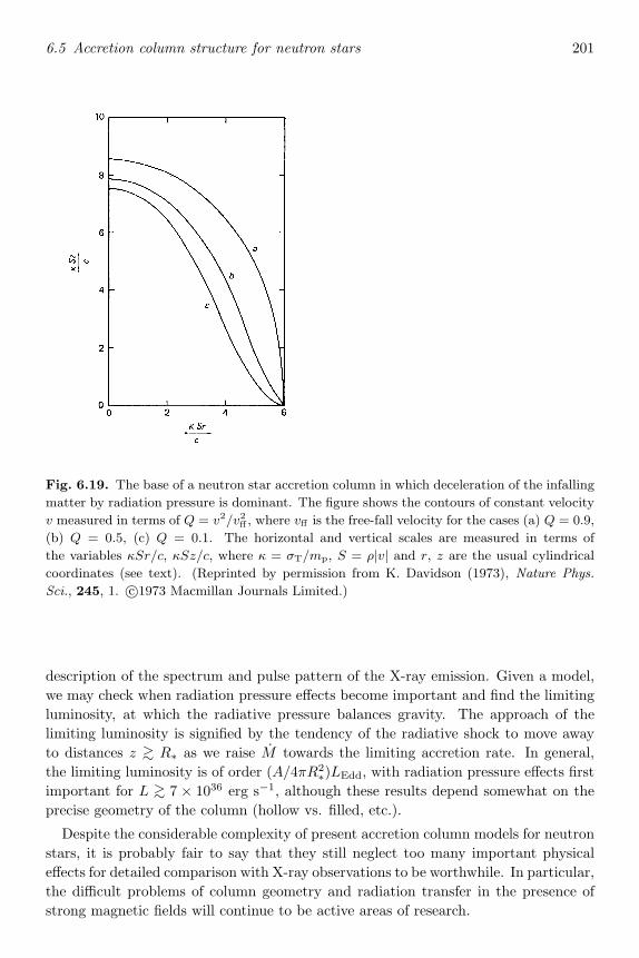
6.5 Accretion column structure for neutron stars 201

Fig. 6.19. The base of a neutron star accretion column in which deceleration of the infalling

matter by radiation pressure is dominant. The figure shows the contours of constant velocity

v measured in terms of Q = v2/v2ff , where vff is the free-fall velocity for the cases (a) Q = 0.9,

(b) Q = 0.5, (c) Q = 0.1. The horizontal and vertical scales are measured in terms of

the variables κSr/c, κSz/c, where κ = σT/mp, S = ρ|v| and r, z are the usual cylindricalcoordinates (see text). (Reprinted by permission from K. Davidson (1973), Nature Phys.

Sci., 245, 1. c©1973 Macmillan Journals Limited.)

description of the spectrum and pulse pattern of the X-ray emission. Given a model,we may check when radiation pressure effects become important and find the limitingluminosity, at which the radiative pressure balances gravity. The approach of thelimiting luminosity is signified by the tendency of the radiative shock to move awayto distances z ∼> R∗ as we raise M towards the limiting accretion rate. In general,the limiting luminosity is of order (A/4πR2

∗)LEdd, with radiation pressure effects firstimportant for L ∼> 7 × 1036 erg s−1, although these results depend somewhat on theprecise geometry of the column (hollow vs. filled, etc.).

Despite the considerable complexity of present accretion column models for neutronstars, it is probably fair to say that they still neglect too many important physicaleffects for detailed comparison with X-ray observations to be worthwhile. In particular,the difficult problems of column geometry and radiation transfer in the presence ofstrong magnetic fields will continue to be active areas of research.

202 Accretion on to a compact object

Fig. 6.20. Profiles of Type I X-ray bursts from five different sources. Note that the gradual

decay (burst ‘tail’) persists longer at low energies than at high, indicating that the burst

spectrum is characterized by steadily decreasing blackbody temperatures. (Reproduced from

W.H.G. Lewin & P.C. Joss in Accretion-Driven Stellar X-ray Sources, eds. W.H.G. Lewin &

E.P.J. van den Heuvel (1983), Cambridge University Press.)

6.6 X-ray bursters

More than 40 X-ray sources, all of which are low-mass X-ray binaries, are now knownto exhibit ‘bursting’ behaviour, in which their X-ray luminosities from time to timebrighten by large factors (∼ 10×), with rise times ∼ 1–10 s (Fig. 6.20). Because theseevents involve X-ray emission, are very luminous and occur on short timescales, thereis immediately a prima facie suspicion that compact objects and possibly accretionare involved. We shall see that there are strong grounds for identifying the site of theburst phenomenon as accreting neutron stars. To do so we need to describe some ofthe observed properties of bursts in more detail.

X-ray bursts divide naturally into two distinct categories, Type I and II. As we shallsee below, Type I bursts are thought to be produced by thermonuclear flashes on thesurface of a neutron star, whereas Type II bursts are likely produced by spasmodicaccretion. Type I bursts recur at intervals of hours to days, or possibly longer. Betweenbursts, the sources are usually detectable through their persistent X-ray emission. Thefundamentally important fact about Type I bursts is that the persistent luminosityoutweighs the luminosity in bursts, averaged over long time intervals, by factors ∼100. Thus, although the luminosity at the peak of a Type I burst is LX(burst) ∼10LX(persistent), the sources only spend about one part in ∼ 103 of their time in aburst state, resulting in

6.6 X-ray bursters 203

LX(Type I bursts, averaged)LX(persistent)

∼ 10−3LX(burst)LX(persistent)

∼ 10−2. (6.83)

Type I bursts have been detected from all but one burst source, while only two sources(MXB1730-335, and recently the ‘bursting pulsar’ GRO 1744-28) are so far known toshow Type II bursts and these only at certain epochs. During these epochs, the TypeII bursts in the MXB1730-335 recur so frequently that they account for almost thetotal luminosity of the source; this behaviour gives the source its other designationas the Rapid Burster, and these frequently recurring bursts are designated Type IIbursts.

The relation (6.83) receives an elegant explanation if we make the hypothesis thatType I bursts result from runaway thermonuclear burning of matter, of which thesteady accretion by the compact object gives rise to the persistent emission. For by(1.1) and (1.2), we have

LX(Type I bursts, averaged)LX(persistent)

∼ ∆Enuc

∆Eacc

∼<0.009c2R∗

GM(6.84)

since ∆Enuc cannot exceed the value 0.009c2 erg g−1 for the complete transformationof pure hydrogen to iron peak elements. Partial or even complete nuclear burning ofhydrogen to helium is thought to occur between thermonuclear bursts. Thus hydrogenburning may contribute up to 0.007c2 erg g−1 to the persistent emission, leaving afurther 0.002c2 erg g−1 to be liberated during the burst as helium is processed to ironpeak elements. Clearly, the only candidate for the compact object is a neutron star:a white dwarf has ∆Eacc < ∆Enuc which would imply LX(Type I bursts, averaged)> LX(persistent), while a black hole has no hard surface on which the thermonuclearreactions can occur. For a neutron star with M ∼ 1 M, R∗ ∼ 10 km, (6.84) and theabove discussion imply

LX(Type I bursts, averaged)LX(persistent)

≈ 0.01 − 0.04 , (6.85)

where the larger value holds for hydrogen burning and the lower value for heliumburning, consistent with the range of observed ratios. By contrast, Type II burstscannot be due to runaway nuclear burning since, by the same argument which leadsto (6.85), they would have to be accompanied by strong persistent X-ray emission (theRapid Burster emits Type I bursts also, so it presumably involves a neutron star).

The reasoning of the last paragraph does not of itself demonstrate that burst sourcesinvolve neutron stars; it merely shows that the ratio of burst to persistent luminositycould be explained naturally if this were so, provided that thermonuclear ‘flashes’ ofthe required duration can indeed be generated on the stellar surface. Observation,however, provides further persuasive arguments in favour of the neutron star hypoth-esis. The X-ray spectra of bursts are found to be roughly blackbody in form. Thusthe received X-ray flux Fν has the form

204 Accretion on to a compact object

Fig. 6.21. Schematic sketch of the surface layers of a non-magnetic accreting neutron star.

(Reproduced from W.H.G. Lewin & P.C. Joss in Accretion-Driven Stellar X-ray Sources, eds.

W.H.G. Lewin & E.P.J. van den Heuvel (1983), Cambridge University Press.)

Fν =A

4πD2πBν(T ) (6.86)

where D is the distance to the source and A its radiating area, assuming isotropicemission. During a burst, the spectrum is observed to ‘soften’ in a way consistentwith a temperature T steadily decreasing from ∼ 3 × 107 K to about half that valuewhile the area A remains roughly constant. To get an estimate of A we need some ideaof the distance D. Now burst sources are not distributed uniformly over the X-ray sky:most of them lie on lines of sight which pass close to the Galactic centre. They arepresumably therefore a stellar population loosely arranged about the Galactic centre,and must lie at distances D of order 10 kpc from us. Setting D = 10 kpc in (6.86)and assuming the radiating area to be a spherical surface of radius R, the spectral fitsimply R ∼ 10 km for all sources. Hence the dimensions of the burst emission regionsare characteristic of neutron star surfaces. One may push this analysis further, forwe might expect the burst process to be self-regulating in that the peak luminosity ofa burst could not greatly exceed the Eddington value (1.4) before radiation pressurewould disrupt whatever conditions are required for the burst to occur. This ideaturns the peak luminosity of a burst into a standard candle. It is found that all tenburst sources for which spectral fits are possible have very similar ratios of radiatingarea A to total peak flux Fmax = AσT 4

max/4πD2. If the average peak luminosities4πD2Fmax = AσT 4

max are assumed to take the value

6.6 X-ray bursters 205

LEdd = 1.8 × 1038 erg s−1

appropriate to a 1.4 M object (assuming its surface is hydrogen rich) the observedvalues of Tmax imply an average source radius 7 km, with only a 20% scatter aboutthis mean.

The arguments given above make it difficult to doubt the neutron star hypothesis,and provide a tight set of constraints that any model of Type I bursts must satisfy.Models in which the bursts result from thermonuclear runaway burning at the surfaceof a neutron star are able to account for the gross observed properties. It is found thatthe outer, hydrogen burning layer (Fig. 6.21) of an accreting neutron star is stableagainst runaway burning, merely adding a small ( ∼ a few per cent) contribution tothe persistent X-ray luminosity, which is, of course, provided mainly by accretion.Further in, a helium burning shell can be unstable in certain ranges of accretionrates and neutron star core temperatures (Fig. 6.21) giving rise to ‘flashes’ of therequisite energy and frequency. The rise and decay times of the bursts also seem tobe explicable in this type of model, despite its severe simplifications, such as sphericalsymmetry and the neglect of magnetic fields. Of course, there are many detailedobservational properties, most notably the sometimes unexpectedly rapid recurrenceof Type I bursts, the origin of which is not yet fully understood. However, one can beoptimistic that refinements of the present highly idealized calculations, including, forexample, the deviations from spherical symmetry brought about by surface magneticfields, will gradually account for these. (Since in only one case (SAX 1808.4-3658,Wijnands & van der Klis (1998)) is the persistent X-ray emission observed to be pulsed,these surface fields are presumably rather weaker (∼< 1011G) than in the pulsing X-raysources.)

The order of magnitude of accretion rates required to explain both the thermonu-clear flashes (Fig. 6.21) and the persistent X-ray emission clearly requires that theneutron stars emitting the bursts must be members of close binary systems. It seemslikely that the companion stars must be rather low-mass, late type main-sequencestars. Most of the optical identifications for X-ray burst sources do not reveal thepresence of normal stellar absorption lines, but in a few cases lines characteristic ofG to K-type main-sequence spectra superimposed on a reddish continuum can be de-tected when the X-ray flux is very weak. When the persistent X-rays are bright theoptical spectra are very blue, sometimes with emission lines. All of this fits quitewell with the idea of a low-mass companion: at typical distances D ∼ 10 kpc, suchcompanions would be very faint. Moreover, when the X-ray flux is high, they will beoutshone by large factors by reprocessed optical emission resulting from the absorp-tion of X-rays by the accretion disc. Simultaneous optical and X-ray bursts from somesources have been observed, supporting this idea. It seems very likely, in fact, thatburst sources are members of the class of galactic bulge sources discussed in Chapter5. Although the faintness of the optical sources makes the usual proofs of binarynature (e.g. radial-velocity variations) difficult, and we have seen in Chapter 5 thatthere may be selection effects against observing X-ray eclipses, the consistency of the

206 Accretion on to a compact object

picture we have sketched above makes the binary hypothesis reasonably secure. Thisis probably also true of the bright X-ray sources located in globular clusters in ourgalaxy, which have very similar properties to the low-mass X-ray binaries, althoughdirect evidence for this will be very difficult to find because most of the clusters arecentrally condensed.

The one large gap in what will be recognized as our otherwise fairly convincingpicture of the burst sources concerns the Type II bursts of the Rapid Burster. As wenoted above, these cannot be due to thermonuclear flashes, and must be attributed tosome form of unsteady accretion. Any model of this process must explain a number ofwell-documented properties of Type II bursts. First, Type II bursts have rise times ∼ 1s and can last from a few seconds up to several minutes. Again the X-ray spectra arereasonably well fitted by blackbody spectra; for Type II bursts, however, the assignedtemperature remains constant at ∼ 1.8×107 K (compared to ∼ 3×107 K at the peakof Type I bursts from the same object), rather than decreasing as in Type I bursts.The scale of the emitting surface decreases as the burst decays, from ∼ 16 km downto ∼< 10 km for an assumed distance of 10 kpc. For moderately energetic Type IIbursts, the total energy involved, assuming this is emitted isotropically, is ∼> 4 × 1038

erg: this total burst energy E is approximately proportional to the waiting time ∆t

to the next burst. Thus a strong burst is followed by a longer than usual wait untilthe next burst.

There have been many attempts to provide accretion instability mechanisms to ac-count for these properties; so far, none has gained wide acceptance. For example, aviscous instability model, like a minutely scaled-down version of the viscous-variationmechanisms for dwarf nova outbursts discussed in Section 5.9, has some attractivefeatures: the timescale tvisc ∼ 1–10 s (5.69) is of the right order to explain the burstprofiles if the instability is assumed to operate very close to the neutron star surface(R10 ∼ 1−2×10−4 in (5.69)) and to be characterized by α ∼ 1. Moreover, from (5.43)and (5.44), the blackbody temperature is of just the observed order. It would remaineffectively constant as the burst of enhanced accretion passed through the inner discregion, while the effective radius would, as observed, decrease. Finally, one might hopeto explain the E − ∆t relation in terms of the time needed to fill up the inner discregion and re-establish the conditions for the viscous transition. Clearly the trigger forsuch behaviour must be the Lightman–Eardley instability discussed in Section 5.8, asradiation pressure is clearly important here. Other types of instability, such as thermaland especially magnetospheric ones, have also been suggested. Clearly, whatever pro-cess does provide the Type II bursts must require rather special conditions to functionat all, for we observe ∼ 40 burst sources, but Type II bursts have been convincinglyidentified from only two: the Rapid Burster and GRO J1744-28. Moreover, the RapidBurster itself emits Type II bursts only when conditions seem to be just right, a stateof affairs which recurs about every 6 months and lasts of the order of a few weeks.The closely related system GRO J1744-28, discovered by the BATSE satellite, is tran-sient, and during its outbursts is the first system seen to produce both coherent X-raypulsing as well as X-ray bursts. Again some kind of Lightman–Eardley instability is

6.7 Black holes 207

suspected as the basic cause of the bursts, the instability this time operating near themagnetospheric boundary.

6.7 Black holes

The opinion of most astronomers about the incidence of black holes in our Galaxy hasundergone a radical change since the last edition of this book (1992). There are nowat least 11 low-mass X-ray binary systems where the compact star is firmly believedto be a black hole, and this number is growing rapidly. The basic line of argument isas follows.

(i) The objects are (at times) bright X-ray sources (1037, 1038 erg s−1), implyingthe presence of a compact object; a neutron star, black hole, or possibly a whitedwarf.

(ii) A white dwarf cannot have a mass exceeding the Chandrasekhar limit (1.4 M); for neutron stars too there is a maximum possible mass which isless certain but probably less than 3 M.

(iii) Spectroscopic evidence implies that the compact components in these systemshave masses exceeding 3 M and therefore must be black holes.

Clearly step (iii) is the crucial one; in all cases the systems are observed to besingle-lined spectroscopic binaries. The Doppler effect on the absorption lines fromthe non-compact companion stars shows that their radial velocities vary on the orbitalperiods, and that the secondary’s orbit is circular. A simple mass limit results for low-mass X-ray binaries. The companion star has a circular orbit about the centre of mass,so the radial velocity amplitude K2 is given by

2π

Pa2 sin i = K2

where a2 is the distance from the centre of the companion to the centre of mass and i isthe inclination of the binary plane to the plane of the sky. Using a2 = M1a/(M1+M2)and Kepler’s law (4.1) shows that the combination

f2 =M3

1 sin3 i

(M1 + M2)2=

K32P

2πG,

the ‘mass function’, is an observable quantity with the dimensions of a mass. Clearlythe value of the mass function f2 is itself an absolute lower limit to the mass of star1, the compact object (M1 = f2 only if M2 = 0 and sin i = 1). For V404 Cygni,which is a soft X-ray transient with a period P = 6.47 d, the observed radial velocityamplitude is K2 = 209 km s−1. The resulting mass function f2 = 6.08 ± 0.06M farexceeds any likely theoretical upper limit on the mass of a neutron star. With realisticestimates for M2 and i moreover the likely primary mass is of order 10–12 M. Thereare ten other systems with measured mass functions exceeding 3M, so there is littledoubt that black holes not only exist but are indeed fairly common in the Galaxy.

208 Accretion on to a compact object

All of these low-mass black hole systems are soft X-ray transients. In Chapter 5 wesuggested that the outbursts of these systems result from disc instabilities which areheavily affected by irradiation by the central X-ray source. As shown there (cf. 5.106and the accompanying discussion) black hole systems are very likely to be transientbecause of their low mass transfer rates, larger discs, and weaker irradiation. Thetransient nature of the black hole sources is therefore powerful support for the disc in-stability picture and simple ideas about disc irradiation. Most importantly, it actuallyconfirms that the compact objects in these systems have the fundamental property ofblack holes, i.e., no stellar surface. For it is only the lack of this surface which weakensthe irradiation effect and allows the discs to be in the unstable regime giving transientoutbursts, i.e. they obey the weaker condition M < MBHSXT (cf. equation 5.106)rather than the neutron star condition M < MNSSXT (cf. equation 5.105). Only thespecial formation conditions for neutron star low-mass X-ray binaries allow the lattercondition to hold in a significant fraction of systems (see Section 6.8 below).

The proper description of the immediate vicinity of a black hole involves the use ofgeneral relativity, Einstein’s theory of gravitation. (Indeed, strictly speaking this isalso true of a neutron star, although the corrections are fairly small.) For the purposesof studying accretion, however, a few general-relativistic results may be extracted and‘standard’ (i.e. non-general-relativistic) physics may be otherwise applied as usual.From general relativity, we find that the boundary (or event horizon) of a black holeof mass M is at a circular radius (the Schwarzschild radius)

RSchw =2GM

c2= 3m1 km (6.87)

unless the hole is rotating at a very high rate, analogous to break-up velocity for anormal star. There is no hard surface at RSchw; the event horizon marks off a regionfrom which no physical effects can propagate into the rest of the Universe, apart fromthe gravitational pull of the mass inside RSchw and the rather academic possibility ofelectrostatic effects due to a net electric charge on the hole. Thus any matter crossinginto r < RSchw can only influence the exterior through its mass: in particular, noradiation can escape from within RSchw. At distances r RSchw the gravitationalfield of the hole is indistinguishable from that of a ‘normal’ star of the same mass M .At distances of a few RSchw, the effects of general relativity become important, forexample modifying the binding energy of circular orbits from the Newtonian value.At 3RSchw the modified ‘potential’ describing circular orbits has a maximum and thecircular orbits do not exist within this radius (see Section 9.2). Small perturbationsimmediately cause matter in this orbit to fall into the hole.

These results are directly applicable to the case of an accretion disc around a blackhole. At distances R RSchw, under the circumstances discussed in Section 5.3, thedisc will be Keplerian. For R ∼ a few RSchw the azimuthal velocity vφ, and hence thebinding energy, deviate from the Keplerian values by terms of order RSchw/R, untilat R = 3RSchw the matter is removed from orbit by instabilities as fast as it arrives.It reaches R = RSchw in the free-fall time ∼ (R3

Schw/GM)1/2 ∼ 10−4 s, and therefore

6.8 Accreting binary systems with compact components 209

radiates very little before disappearing behind the event horizon. Thus the maximumenergy per unit mass which can be extracted by this sort of accretion is the specificbinding energy of the innermost stable circular orbit. For a low angular momentumhole this is 0.057c2 erg g−1; using R = 3RSchw = 6GM/c2 we see that this is ratherless than the GM/2R ∼= 0.083c2 which would result if a Newtonian orbit were possibleat R = 3RSchw, since the ‘potential’ is less than the Newtonian value (see Section7.7, Fig. 7.3). If the hole has been spun up by accretion of angular momentum, theefficiency is increased up to a theoretical maximum of 0.42c2 erg g−1, although valuesapproaching this are only attained within a few parts in 10−3 of the ‘break-up’ angularmomentum Jmax = GM2/c. (It can be shown that accretion of matter with angularmomentum always increases M fast enough to keep J < Jmax.) Note also that theefficiency 0.057c2 erg g−1 for disc accretion on to a non-rotating hole is actually ratherless than the total accretion yield ∼= 0.19c2 erg g−1 from a 1 M neutron star withradius 10 km ∼= 3RSchw. This is because a neutron star has a hard surface, so thatall of the potential energy at R ∼= 3RSchw is released as radiation rather than just thebinding energy of a circular orbit. (The quoted yield includes the general relativisticcorrection to the Newtonian specific potential energy (GM/R) erg g−1.)

These considerations represent most of what distinguishes the discussion of accretionon to stellar-mass black holes from accretion on to unmagnetized neutron stars. Infact, the black hole case is simpler to treat, as one has no boundary layer or torques toworry about, and the boundary condition is that the viscous torque G(R) (equation(4.27)) vanishes at R = 3RSchw (equation (5.19) with R∗ = 3RSchw). As one canshow that spherical infall is likely to produce rather low accretion efficiencies (Section7.8), this largely reduces stellar-mass black hole accretion to a subcase of neutron staraccretion. The one large exception to this close similarity concerns the fact that aneutron star possesses a stellar surface, whereas a black hole by definition does not.Evidence for the latter defining property has been difficult to find, but may now havebegun to emerge, as we have seen above (cf. equations (5.105), (5.106)).

6.8 Accreting binary systems with compact components

In this chapter and the previous one we have discussed a number of different types ofbinary system in which a compact object accretes from a ‘normal’ stellar companion.According to how the mass transfer is effected (Roche lobe overflow, stellar wind, etc.)and properties such as the magnetic field of the compact star, a large variety of possiblemodes of accretion arise. We can classify the systems according to the compact and‘normal’ components (Table 6.1). We can go further than this, and distinguish amongthe systems on the basis of the magnetic field of the compact component. Moreover,in many cases it is possible to decide if the mass transfer is by Roche lobe overflow orstellar wind, and whether an accretion disc or accretion columns (or both) are likelyto form. This is summarized in Table 6.2.

The distribution of systems in these tables is far from uniform. This may be partly

210 Accretion on to a compact object

due to selection effects, but is more likely to be the result of binary evolution clearlyfavouring some combinations over others. The complicating effects of mass transfer(the direction of which may be reversed in some epochs compared to others), massloss, and angular momentum loss are at work here. In particular, it is extremelydifficult to form low-mass X-ray binaries containing neutron stars, and those thatexist are rare and exotic objects. The basic reason for this is that neutron stars areborn in supernova explosions, which expel a large amount of mass. Yet it is easy toshow that the binary must retain at least one-half of its original mass if it is to avoiddisruption by a symmetrical explosion. (Most asymmetric explosions also disrupt, buta small fraction can fortuitously direct the neutron star recoil towards the companionso as to keep the binary bound.) Clearly the binary has greater survival chancesif the companion has a higher mass, thus reducing the fraction of mass lost on thesupernova. Such higher-mass companions are quite likely to have evolved off themain sequence before mass transfer begins, making low-mass neutron star binariesvery different from either black hole or white dwarf binaries. Thus, if the neutronstar progenitor has mass Mprog, and the neutron star and its companion have massesM1, M2, survival of a symmetrical supernova requires

M1 + M2 >12

(Mprog + M2)

or

M2 > Mprog − 2M1. (6.88)

There is strong evidence that all neutron stars begin life with masses close to 1.4M, soto have even a moderately low-mass companion (M2 ∼< 1M) already requires a verylow progenitor mass Mprog ∼< 4M. This can be achieved via unusual evolutionarychannels in which an earlier mass-transfer phase has made the progenitor a heliumstar; but it is clear that neutron star systems with an initial M2 significantly below1M must be very rare. Most companions therefore have M2 ∼> 1M and thus main-sequence lifetimes comparable with the timescale on which orbital angular momentumlosses can shrink the binary and initiate mass transfer. A similar conclusion holds ifwe allow for asymmetrical supernovae. We thus expect that many low-mass neutronstar binaries will have companions which are significantly nuclear-evolved when theX-ray phase begins. This leads to lower mass transfer rates than if the companionwere on the main sequence. Only this property allows a sufficient number of thesesystems to satisfy the very stringent requirement M < MNSSXT (cf. eq. 5.105) andappear as transients, especially at short orbital periods (see King, Kolb & Burderi(1996); King & Kolb (1997); Kalogera, Kolb & King (1998))

By contrast it is clear that black hole binaries can readily form with companions ofany mass. It is not even obvious that all black holes require a supernova at formation,but even if they do, the survival condition (6.88) is very easy to satisfy. In particularit is quite possible for the black hole to bind most of the progenitor mass (M1 >

0.5Mprog), so that (6.88) places no constraint at all on M2. We therefore expect the

6.8 Accreting binary systems with compact components 211

Table 6.1. Compact accreting binary systems

Compact starCompanion star

White dwarf Neutron star Black hole

Early-type, massive None known Massive X-ray binaries Cygnus X-1(e.g X-ray pulsars) LMC X-3

Late-type, low-mass Cataclysmic variables Low-mass X-ray binaries A0620-00(e.g. dwarf novae) (e.g. galactic bulge sources) plus at least

ten others

Intermediate mass, or Supersoft X-ray binaries Progenitors of Cyg X-2 and Microquasarcrossing Hertzsprung gap some radio pulsars

vast majority of black hole binaries to have main-sequence companions and thus masstransfer rates exceeding MNSSXT. The fact that all the low-mass X-ray binaries withmass functions implying M1 ∼> 3M are nevertheless transient shows that irradiationof the disc is much weaker there (cf. equation 5.106). This in turn confirms thatthese massive accretors have the characteristic black hole property of lacking a surface(King, Kolb & Szuszkiewicz (1997)).

An interesting subset of the black hole soft X-ray transients are the microquasars.These systems (see Mirabel & Rodriguez (1999), for a review) are distinguished bythe presence of relativistic jets, and often show superluminal motions for exactly thesame reasons that extragalactic sources do (cf. Chapter 9). It seems likely that themicroquasars are black hole binaries where the companion star has just finished itsmain-sequence life and is expanding across the Hertzsprung gap (King et al. (2001)).As a result their outbursts are highly super-Eddington, which may be connected withthe production of relativistic jets.

7 Active galactic nuclei

7.1 Observations

Accretion on to stellar mass objects occurs in a wide variety of systems and yields awide variety of observational behaviour. While there may be many arguments overdetailed models, the broad basis of these differences is largely understood. Activegalactic nuclei also come in many observed forms. From an observational viewpoint,they can be defined as apparently stellar sources but with non-thermal spectra, and,in cases where they can be determined, significant redshifts. Beyond this, we find awide variety of properties, which we shall classify in more detail below. But in thesecases it is not at all clear how these differences arise, or, indeed, whether one is evendealing with variants of a single basic model. We shall argue that the sources are allmanifestations of accretion on to supermassive black holes (of order 108 M), althougheven this is still not universally accepted. Furthermore, for stellar-mass objects, atleast in some cases, we have a complete picture of the system even if some of thedetails are missing. In no case do we have anything comparable for active galacticnuclei. That is not to say that there are no aspects of active galactic nuclei that arethought to be fairly well understood, but those that are do not include the mechanismof the basic energy source. Thus we have to try to extract from the available datawhat clues we can to the nature of the central engine. This we shall do in the presentchapter and the next, admittedly not with conspicuous ultimate success. On the otherhand, once one gets beyond the inner engine a consensus appears to be emerging on astandard picture, a so-called unified model, in terms of which one can begin to accountfor the variety of active galactic phenomena.

We consider first the observed properties of active galactic nuclei in as far as they arerequired for subsequent discussion, giving first of all (Sections (7.1.1)–(7.1.3)) a surveyof observed properties and secondly (Section (7.1.4)) an outline of the classification ofobserved sources.

7.1.1 Continuum emission

Where the galactic environment of an active nucleus cannot be discerned, or where itwas not discerned in the original identification, the object is referred to as a quasar.About 10% of optically selected quasars show strong radio emission and hence appearin surveys of strong radio sources. In the earlier literature, especially, this distinction

214 Active galactic nuclei

is emphasized by referring to radio quasars as quasi-stellar sources (QSSs) and non-radio ones as quasi-stellar objects (QSOs). (Strictly, the term quasar itself was coinedfor the radio sources only but has come to be used inclusively.) In fact, in neither ofthese cases does the radio emission dominate the energy output (although it may do soin the nuclei of radio galaxies). In some cases the greatest luminosity is emitted in theinfrared, while in others X-rays or γ–rays may be more important. In the case of thequasar 3C 273, the first quasar to be identified, the peak power occurs at low-energyγ–rays. In Fig. 7.1 the spectrum of 3C 273 is plotted as log ν Fν against log ν in thebottom panel. Since the flux in the waveband [ν1, ν2] is

F12 =∫ ν2

ν1

Fν dν =∫ ν2

ν1

νFν d(ln ν),

equal areas under the graph correspond to equal energies. Note that optical quasarswere first found in surveys of excessively blue objects relative to a blackbody spectrum,although in absolute terms quasars are ‘red’ objects. More recent optical surveysdepend on the identification of spectral lines.

7.1.2 Line spectra

The spectra of active galactic nuclei usually show strong emission lines which appearto be of two distinct types. In quasars and some galactic nuclei (Seyfert type 1galaxies, broad line radio galaxies) very broad lines are present with widths in therange 0.05 ∼< δν/ν ∼< 0.1 at the base of the line, the so-called full width at zero intensity(FW0I). In addition, many objects have narrower emission lines with δν/ν ∼ 0.002at half the maximum intensity (FWHM). Type 2 Seyfert galaxies show only narrowlines (but see below) as do narrow emission line galaxies (NELGs) and some rarecases of narrow line quasars, while in the quasar 3C 273 the narrow lines are relativelyweak. Nearby Seyferts are observed to possess also an extended emission line region(EELR) of narrow lines on kpc scales which represents the interstellar medium in thehost galaxy illuminated by a cone of radiation from the active nucleus. A similarphenomenon is observed in some high redshift radio galaxies (although some of theemission is alternatively attributed to star formation.) Since the part of the quasarspectrum that falls in the fixed optical band at which ground observations can be madedepends on the quasar redshift, the prominent emission lines are redshift dependent.In low redshift objects the Balmer lines of hydrogen dominate, while at higher redshiftsultraviolet lines of C, Mg and the Lα hydrogen line are shifted into the optical.

Objects in which emission lines are entirely absent, or only very weak, but whichmanifest the other quasar properties are usually called BL Lacs (or ocassionally, in theolder literature, Lacertids) since the variable ‘star’ BL Lac was the first of this typeto be found. In these cases, where emission line redshifts cannot be determined, theymust be distinguished from galactic objects by, for example, absorption line redshiftsor similarity to other BL Lacs with respect to polarization and variability.

Many quasars (and BL Lacs) show absorption lines in their spectra. In some cases,

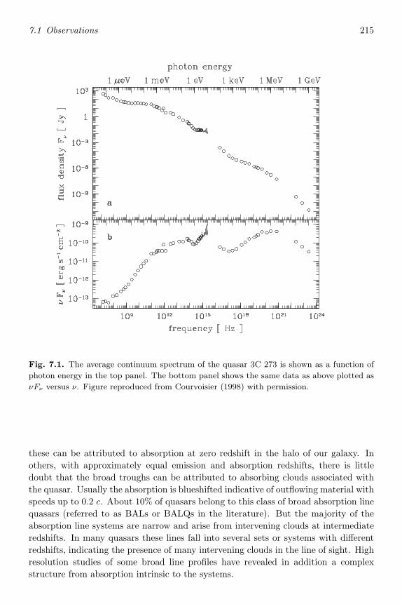
7.1 Observations 215

Fig. 7.1. The average continuum spectrum of the quasar 3C 273 is shown as a function of

photon energy in the top panel. The bottom panel shows the same data as above plotted as

νFν versus ν. Figure reproduced from Courvoisier (1998) with permission.

these can be attributed to absorption at zero redshift in the halo of our galaxy. Inothers, with approximately equal emission and absorption redshifts, there is littledoubt that the broad troughs can be attributed to absorbing clouds associated withthe quasar. Usually the absorption is blueshifted indicative of outflowing material withspeeds up to 0.2 c. About 10% of quasars belong to this class of broad absorption linequasars (referred to as BALs or BALQs in the literature). But the majority of theabsorption line systems are narrow and arise from intervening clouds at intermediateredshifts. In many quasars these lines fall into several sets or systems with differentredshifts, indicating the presence of many intervening clouds in the line of sight. Highresolution studies of some broad line profiles have revealed in addition a complexstructure from absorption intrinsic to the systems.

216 Active galactic nuclei

7.1.3 Polarization and variability

Some quasars and BL Lacs exhibit substantial variability over short timescales (daysto years) in various wavebands. Extreme examples are the quasar OJ 169 which variedin X-rays by a factor 3 over 100 minutes and the BL Lac AO 0235 + 164 which variedin the radio and optical by a similar factor over a month. Sometimes variabilityin different wavebands is correlated, sometimes not. In general, a high percentagepolarization of the optical and radio emission is associated with high variability. Thisis the case in almost all BL Lacs, most of which show high polarization. Quasars whichexhibit these properties are called optically violent variables (OVVs). All OVVs arehighly polarized but rare exceptions to the converse do exist (e.g. PHL 957). Asa class, quasars associated with double radio sources are found to be less variablethan those lacking extended radio structure. Generally speaking, the amplitude ofvariability is larger and the timescale shorter in a given object at shorter wavelengths.The majority of quasars exhibit small amplitude optical varibility of a few tenths of amagnitude over timescales of months to years and a number show similar variabilityon much shorter timescales.

The highly polarized quasars have lower (or zero) polarization in their emissionlines than in the continuum. Quasars with lower polarization (∼< 3%) have the samepolarization in the lines as in the continuum at neighbouring frequencies, and in thesecases the rising polarization to the blue region of the spectrum points to scattering bydust as the polarizing source. In highly polarized quasars, the polarization appearsto be associated with the emission mechanism. Some radio galaxies (the narrow lineradio galaxy 3C 234 appears to have been the first to be discovered) and some Seyfert 2galaxies (NGC 1068 being the first) have weak polarized broad lines. This has provedto be an important clue in determining a unifying model (Section 7.1.5). Recentdetailed mapping of the Hα profile in polarized light in some radio-loud AGN showsa complex structure.

7.1.4 Summary of active galactic nuclei

Seyfert galaxies

With hindsight we know that the first active galactic nuclei were discovered as brightnuclei in short exposure plates of spiral galaxies by Carl Seyfert in 1943 (althoughthe presence of emission lines in the optical spectrum of NGC 1068 had been notedearlier). These nuclei are characterized by a non-stellar continuum and high ionizationemission lines. The class is divided into Type 1 Seyferts and Type 2 Seyferts (or Seyfert1s and 2s) although intermediate types have been defined; the Type 1 Seyferts andintermediate types have emission lines with broad bases which often exhibit variabilityon timescales of tens of days, similar to that of the UV continuum. All types have anarrower emission line component but appear to be distinguished by characteristicallyhigher [OIII]/Hβ intensity ratios in the Type 2 Seyferts. In these also the broad

7.1 Observations 217

component appears to be missing, but spectropolarimetry of some nearby bright Type2 Seyferts has shown a broad base to the permitted lines in polarized light. Type 2Seyferts appear to be stronger radio sources but the X-rays are much weaker. InType 1 Seyferts, on the other hand, X-rays may dominate the energy output, witha characteristic (or ‘canonical’) spectrum Fν ∝ ν−0.7 in the 2–10 keV band; rapidvariability is observed in X-rays with factor 2 changes over timescales of hours. In lowluminosity sources the variability appears chaotic with no characteristic timescales.In about half of the Type 1 Seyfert nuclei where its detection would be possible thereis an excess of soft X-rays above the extrapolated ν−0.7 power law (after allowancefor absorption). Models of the spectral components suggest an intrinsic power lawspectrum with slope −0.9 rather than −0.7 (which is then modified by Comptonscattering to give the observed slope).

Quasars

Low luminosity quasars are indistinguishable from bright Type 1 Seyferts, so thereseems to be a continuum of similar objects separated into two classes by observationallimitations (the failure to resolve low surface brightness spiral galaxies around brightquasars). There is some evidence for the existence of Type 2 quasars (by analogywith Type 2 Seyferts) lacking broad emission lines. A subset of quasars, about 10%,are strong radio sources, (‘radio-loud’ quasars) which, like radio galaxies, may becompact or exhibit the classical double lobe structure. Radio loud quasars appearto occur predominantly, but not exclusively, in elliptical galaxies whereas radio-quietones are in spirals. In a number of radio-loud quasars the radio emitting plasmashows apparent superluminal velocities. Variability, where observed, tends to be ontimescales of years.

BL Lacs (Lacertids)

These show weak lines, if any, but possess something like the characteristic continua ofquasars, although, where the distance can be determined from weak absorption lines inan underlying galaxy, at lower luminosity. There are subclasses of radio-loud BL Lacs(RBL) with the peak of the spectral power in the mm radio or infrared and relativelyradio quieter ones (XBL), discovered through their X-ray emission, for which the peakof the power is in the UV or soft X-ray band. The X-ray spectrum is probably softer(i.e. has a more negative slope) in the 2–10 keV range than that of Seyferts andquasars but the soft excess in the EUV–soft X-ray range below 0.5 keV is not seen.High polarization is a characteristic of the radio and optical emission. Variability isobserved at all wavelengths and timescales down to a few minutes but at low amplitude.BL Lacs are often associated with apparently superluminal jets. Optically violentvariables (OVVs) are somewhat similar to BL Lacs except for their variability and thepresence of stronger emission lines. Highly polarized quasars (HPQs) are also similar,except that they are not necessarily variable. Thus the class of highly polarized quasars

218 Active galactic nuclei

(HPQs) includes OVVs. Quasars in this class (i.e. HPQs with strong emission linesand rapid variability) are called blazars.

Radio galaxies

Strong radio sources in which the underlying galactic type can be distinguished arecalled radio (or ‘radio-loud’) galaxies. Note that the complementary set of ‘radio-quiet’ galaxies are not necessarily radio silent (see Fig. 8.1). Further details of theradio properties are given in Chapter 9. If emission lines are present these may beeither narrow (NLRGs) or include a broad component (BLRGs).

Obviously these classes overlap. The terms active nucleus or active galactic nucleus(AGN) are used to refer to these objects as a whole, although one sometimes distin-guishes between quasars and active galaxies, and occasionally the term quasar itselfis used as all-embracing.

A form of activity usually (but not always) distinguished from that above occurs ingalaxies undergoing bursts of star formation (‘starburst’ galaxies). This is the inter-pretation of a number of galaxies with large infrared luminosity which were revealedby the IRAS (Infrared Astronomical Satellite) sky survey and are therefore sometimesreferred to as IRAS galaxies. (The infrared emission arises from the reprocessing ofstarlight by dust, although the IRAS galaxies might also include cases where the dustreprocesses emission from a quasar nucleus.) Again, there is probably some overlapbetween starburst galaxies and active galactic nuclei. Indeed, the two phenomena maybe related. But we shall exclude from our discussion the theory that starbursts areresponsible for all activity. (The usual reason for excluding this picture is the diffi-culty it has in producing large scale radio jets and short term large amplitude X-rayvariability. We exclude it as beyond the scope of the book.)

7.1.5 Unified models

We have seen that (radio-quiet) quasars are similar to Seyfert 1 galaxies at higherluminosity. Thus one unification scheme suggests itself, based on luminosity. Thisdoes not work even excluding radio-loud objects. (Seyfert 2s are not low luminositySeyferts.) The radio systems suggest, however, that AGN have axial rather thanspherical symmetry. Thus classical double radio sources with lobes separated on theplane of the sky should look like something else when viewed end-on. Early attemptsto use orientation to unify radio-loud and radio-quiet systems or quasars and BLLacs fell foul of the statistics for the relative abundances of the sub-systems and theirputative parent populations. However, more recent unification schemes in which radio-loud quasars are end-on radio galaxies appear more promising. This classification interms of luminosity and angle can be extended to Seyferts as well. The picture almostuniversally accepted as the current working hypothesis is that Seyfert galaxies containa torus of obscuring material (dust) at about 10–100 pc between the smaller innerregion responsible for the broad emission lines and the region further out where the

7.1 Observations 219

14 15 16 17 18 19 20 21

log10

[radius in cm]

jet

thick disc

blackhole

disc

obscuringmedium

BLR

NLR

NLR

radio

X-ra

ys

UV

infrar

ed

Fig. 7.2. The figure shows schematically some of the suggested elements of a ‘unified’ model

of an active galactic nucleus. A powerful jet would be present only in radio-loud sources. The

dotted line indicates how a thick disc might appear if one is present. The obscuring medium

could be a dusty torus or a warped disc.

narrow emission lines are produced. For lines of sight where the torus blocks thedirect view of the inner regions the galaxy appears as a Seyfert 2 or NLRG. Fromcloser to face-on we see into the inner regions and the objects appear Seyfert 1s or, inradio-loud systems, as BLRGs through to radio-loud quasars or, at lower luminosityBL Lacs. Some line emission from the inner region, and continuum from further in, isobserved in scattered (polarized) light. The model works better if the opening angleof the torus is allowed to increase with luminosity so that, among other things, thepaucity of obscured high luminosity quasars can be accounted for.

We now turn to the evidence that active galactic nuclei are at the distances deducedfrom the redshifts of their line spectra according to standard cosmology, hence thatthey are intrinsically luminous objects of small size. We then give several argumentswhich lead to estimates of the mass associated with an active nucleus of order 108 M.From amongst possible models we establish a preference for accretion on to a massiveblack hole as the energy source. In Chapter 8 we present the arguments, not at present

220 Active galactic nuclei

conclusive ones, that the accretion occurs through a disc. The final chapters explorevarious models for the central engine.

7.2 The distances of active galaxies

The cosmological interpretation of the redshifts of active galactic nuclei, which wasa source of intense controversy in the early years of quasar research because of thelarge energies implied, is now almost universally accepted. Doubters by and large donot accept the standard cosmological picture; but this degree of doubt is unprofitable.Here we give several arguments in support of the exclusively cosmological origin ofthe redshifts on the basis of standard cosmology.

In the standard general relativistic cosmological model the redshift z = (λo−λe)/λeof a spectral line emitted at a rest wavelength λe and observed at λo is related to theluminosity distance dL of the source by

dL = cH−10

[z +

12

(1 − q0)z2 + · · ·]

(7.1)

where H0, the Hubble constant, measures the present rate of expansion of the Universeand q0, the deceleration parameter, measures the rate at which the expansion is nowslowing down. The first term in the power series in z is the non-relativistic Dopplershift if we interpret z in terms of a recession velocity, z = v/c, and the subsequentterms represent relativistic corrections, important for z ∼> 1. The precise meaning ofthe distance being measured here is that it gives the diminution in total flux for asource luminosity L radiating isotropically:

∫Fν dν = L/4πd2L. (7.2)

For the quasar 3C 273 this gives L ∼> 6×1046(H0/100 km s−1 Mpc−1) erg s−1, some 102

times larger than that from a giant galaxy and emitted from a volume probably at least106 times smaller. This, and similar energy requirements for other quasars, initiallyled some astronomers to question the cosmological interpretation of the redshift, sincethe power requirements could be considerably reduced if quasars were assumed tobe relatively nearby objects. On the other hand, energies of a similar order werefamiliar to radio astronomers in both radio galaxies and QSSs (quasi-stellar sources orradio quasars), the radio galaxies being at known distances. In addition, apparentlyviolent events were recognized in the centres of otherwise normal galaxies associatedwith luminosities of order 1045 erg s−1 and large total energy content. In retrospect,therefore, the power requirements of quasars are large, but unexceptional, and do notprovide strong grounds for doubting the distances inferred from their redshifts. Infact, we can advance several arguments in support of this interpretation.

7.2 The distances of active galaxies 221

7.2.1 Association with clusters

A number of quasars have been found to be associated with clusters of galaxies atthe same redshift. For these the redshift must therefore be entirely cosmological sincechance associations are too unlikely. Alternatively, the probability of finding a galaxywithin 2 Mpc of a quasar with the same redshift, to within 500 km s−1 to allow forpeculiar motion relative to the Hubble expansion, is far higher than random. Since2 Mpc is the radius of a small group of galaxies, this suggests that quasars are oftenassociated with groups of galaxies. In particular, 3C 273 appears to be a member ofa small group.

Attempts have been made to support a non-cosmological interpretation of redshiftswith the claim that associations of galaxies and quasars at different redshifts are foundwith probabilities far higher than chance coincidence. Quasars might then be objectsejected from relatively nearby galaxies with at least part of the redshift attributableto Doppler motion. Early attempts suffered from a posteriori statistics, associatingimprobabilities with events only after they had been found. More recent investigationsalso appear to be less than convincing. In any case, such an argument cannot overcomethe energy problem for those objects in which the redshift is indisputably cosmological,so, if valid, it would require two populations of rather different types of object withthe same observed properties, and this is generally held to be unlikely.

7.2.2 The continuity argument

The range of luminosities of quasars and Seyfert 1 galaxies overlap with the resultthat, at least with regard to their optical spectra, a high-luminosity Seyfert removedto a greater distance would be indistinguishable from a low-luminosity quasar. Therealso appears to be a continuity of X-ray spectra ranging from quasars at one extremeto Seyfert 2 and narrow emission line galaxies (NELGs). Indeed, several quasars showoptical nebulosity around the central nucleus and in some cases, including 3C 273, thisnebulosity has typical stellar absorption lines, at the same redshift as the emission linesystem, which can be attributed to a surrounding galaxy. The nearer BL Lacs tooexhibit associated absorption features, identified in these cases with giant ellipticalgalaxies.

7.2.3 Absorption lines

In many cases, narrow metal lines are observed with zem − zabs < 0.001 which arepresumably formed in material associated with the active nucleus. At larger zem−zabs,there are sometimes multiple systems of redshifts widely separated compared withthe velocity widths of the lines. Early statistical analyses gave rise to apparentlypreferred redshift differences in these multiple systems and led to the idea of ‘line-locking’. According to this, emission line photons from one cloud could be absorbedin a different atomic transition in another cloud having a suitable relative velocity. The

222 Active galactic nuclei

momentum transfer would tend to accelerate the clouds together, with small velocitydispersion.

However, it is possible to estimate the distances of these absorption clouds from theAGN engine using measurements of the relative strengths of the observed absorptionlines, if we assume the absorption clouds are photoionized. (i.e. the ionization state isdetermined by the incident ionizing photons, not by collisions of ions and electrons).This method of estimating sizes of photoionized systems from line strengths is impor-tant also for the emission line systems and we shall return to the details in Sect. 8.6.The method is based on the fact that the relative abundance of ionized species in aphotoionized medium is controlled by a parameter, called the ionization parameter,of the general form ξ = Lion/4πD2Ne, where Lion is the ionizing flux incident on amedium of electron density Ne at a distance D.

The value of ξ for the absorption line clouds can be obtained from observationsof the relative strengths of the lines from ionization states X(r+1)+ and Xr+ of anatom X (by a curve of growth analysis). Furthermore, an upper limit on the electrondensity in the absorbing clouds is set by the absence of the fine structure C II∗ λ1335.7line when strong C II λ1334.5 is seen. This is because a free electron density Ne ∼> 1cm−3 would be sufficient to populate the fine structure level significantly by collisionalexcitation. Thus

D ∼> (Lion/4πξ)1/2

and estimates of Lion by direct observation of the continuum emission yield distancesin the range 0.5–3 Mpc.

Assuming spherical symmetry, the energy required to produce the observed massoutflow, with a velocity sufficient to produce the measured redshift differences anda column density sufficient to produce the absorption lines at these distances thenturns out to exceed 3 × 1059 erg, considerably greater than the energy estimated,for example, for the compact radio sources. Absorption in intervening material notassociated with the active galactic nuclei, and for which the redshift differences arecosmological, is therefore the accepted origin for the majority of the metal absorptionlines. Since the lines cluster in redshift with an amplitude and scale similar to thatof galaxies, absorption by material in the haloes of intervening galaxies or in proto-galactic clouds is the preferred explanation. In high-redshift quasars, with zem ∼> 2,the Lα λ1216 line is shifted into the optical where it can be seen from the ground. Alarge number of absorption lines longward of the Lyman limit are then seen which areattributed to Lα absorption in clouds at various redshifts along the line of sight, theso-called ‘Lyman α forest’. This interpretation is confirmed by the high incidence ofpairs of lines at the wavelength ratio of 1.2 which are interpreted as Lα, Lβ (λ1025)pairs. These lines are most easily understood as arising in clouds in the intergalacticmedium, since the observed lack of clustering in redshift suggests that in this case theabsorbing material is not associated with galaxies.

We conclude that at least those active galactic nuclei with absorption lines lie behindclouds of absorbing material at cosmological distances.

7.3 The sizes of active galactic nuclei 223

7.2.4 Gravitational lenses

When a light ray passes within a distance R of a spherical body of mass M it is bentthrough an angle

α = 1.75(M/M)(R/R) arcsec.

A galaxy of mass 1011 M and radius 10 kpc will therefore produce a bending of a fewseconds of arc. It is possible that the light from a quasar can be focussed into severaldistinct images by the extended mass distribution in a galaxy, although some of thesemay not be resolvable. The separate images will have identical spectra and redshiftsbut not necessarily the same variability, since there is also a general relativistic timedelay which can differ for the different images by up to a few years. There are nowseveral dozen candidates for such systems and the number is steadily increasing; anumber of them appear to be well established. In several cases the imaging galaxyis seen in a high-redshift cluster. In these cases, at least, a major part of the quasarredshift must be cosmological.

Although not so directly related to the determination of distances, we should never-theless mention an alternative possibility in which the central engine is gravitationallyfocussed by a single star in an external galaxy along the line of sight to a quasar.Indeed, one suggestion was that BL Lac objects are the result of this so-called mi-crolensing of quasars, although this appears to conflict with the different radio struc-tures of the two classes of objects. However, microlensing may be a source of shortterm variability in quasars generally.

Henceforth, we assume that the redshifts of all active galactic nuclei are cosmologicaland we assume the standard interpretation of the cosmological redshift as a distanceindicator according to (7.1) and (7.2).

7.3 The sizes of active galactic nuclei

Upper limits to the sizes of active galactic nuclei can be obtained from direct observa-tions of optical and radio structure; tighter limits can be set indirectly in some casesby observations of the timescales over which large changes in luminosity occur.

7.3.1 Optical structure

Hubble Space Telescope (HST) observations of active galaxies fail to resolve the nu-cleus. For nearby AGN this gives an upper limit to the size of the nucleus of ∼ 1pc.Indirect arguments, similar to those of Section 7.2.3, can be used in general to estimatethe distance of the gas responsible for the broad emission lines from the continuumsource (see Section 8.6). This gives 1–10 pc, so the ionizing continuum comes froma region typically no larger than this. Line variability (Section 8.6) suggests sizes oforder 0.1–1 pc.

224 Active galactic nuclei

7.3.2 Radio structure

In a few cases the radio cores of active galactic nuclei are resolved and in othersVLBI measurements allow upper limits to be placed on the size of the compact cores.Where structure is resolved the lengthscale depends on the wavelength of observationindicating that structure is present on all accessible scales and hence, probably, also onsmaller, currently inaccessible ones. At the relevant redshifts, relativistic correctionscan be neglected and the size–angular size relation is simply l = θcz/H0, where H0,the Hubble constant, is of order 60 km s−1 Mpc−1. The smallest angular structuresresolved are a few milliarcseconds corresponding to a linear scale of order 1 pc at adistance of 100 Mpc or a redshift z ∼ 0.03.

7.3.3 Variability arguments

In general, a system cannot be observed to undergo substantial changes in structureon a lengthscale l in a time shorter than l/c. Any changes must appear smeared outover the difference in time it takes light to reach us from various parts of the system.In general, therefore, observations of variability on a timescale tvar provide an upperlimit on the size of the variable emission region, l ≤ ctvar. Note that the size ofthe region responsible for the variability need not be the same as that of a steadyunderlying source. Note also that the limit refers to the ultimate energy source;reflecting boundaries, for example, could be arranged to have an arbitrary separation.

The shortest reported large amplitude variability appears to be a 60 per cent in-crease in the X-ray flux from the quasar PKS 0558-504 in 3 minutes which correspondsto a lengthscale l < 1013 cm. X-ray flaring on a timescale of hours (l < 1015 cm) ap-pears to be common (e.g. in NGC 4151 and similar Seyfert galaxies). The BL LacH 0323 + 022 shows small amplitude variations across the spectrum from radio toX-rays on a timescale of days (at long wavelengths) down to 30s (in X-rays). Smallamplitude flickering on a timescale of days is common in BL Lacs and some (e.g. OJ287) erupt violently over a few months (l ∼< 3 × 1017 cm). Many quasars change inluminosity by large factors (2–5) over a few years.

If the source motion is relativistic, as is suggested by the apparent superluminalexpansion in a number of objects (Section 9.3), then the observed variability timescaleis shorter than the timescale in the rest frame of the source. There is some evidence(Section 9.3) that this does indeed lead to an underestimate of the size of the mostrapidly variable sources.

We conclude therefore that for rapid variability ctvar is an underestimate of thesource size, while other more direct observations have not resolved the central engine,particularly if we interpret the non-variability of many sources as a result of repro-cessing. A compromise of around 1015(M/108 M) cm is often taken as a reasonableestimate of an upper limit to the size of the central engine. The minimum radius(corresponding to 3 Schwarzschild radii) is ∼ 1014(M/108 M) cm. (See Section 7.7.)

7.4 The mass of the central source 225

7.4 The mass of the central source

If a source of luminosity L has a lifetime ∆t, and if the conversion of matter to energyis accomplished in the source with efficiency η then an amount of mass

M = L∆t/ηc2 (7.3)

must have accumulated somewhere in the system. This provides a method of estimat-ing the masses of the sources in active galactic nuclei if we can estimate ∆t and η. Forη it is usual to assume a fairly generous limit of η ∼ 1

10 (see Section 7.8). Limits on∆t are more convincingly obtained for the radio lobes of double sources than directlyfor the nuclei, but this gives the nuclear mass if we assume the lobes are powered bythe central engine. At the very least we must have ∆t > D/c, where D is the distanceto the lobes. But the lobes are probably not separating at anywhere near the speed oflight. In fact, the natural interpretation of those double sources in which the parentgalaxy lies away from the line joining the lobes, which are found mainly in clusters,is that the parent galaxy is moving through the intracluster medium. The beams arethen bent by the ram pressure of the medium. If the density in the beam is not too fardifferent from that in the medium then, in order that the beam be bent significantly,the velocities must be comparable. For typical giant ellipticals this velocity is of theorder of a few hundred kilometres a second, the same order as the escape velocity,which is the minimum possible speed for the jet material. More detailed investiga-tions have given speeds in the range 500–10000 km s−1 so let us take l03 km s−1 forour estimate. Then for Cyg A, with a lobe separation of 80 kpc, we get ∆t ∼ 4 × 107

yr, and (7.3) gives M ∼ 108 M.For sources which are not double radio sources we need an alternative way of esti-

mating ∆t. It is probable that all galaxies go through an active phase and, since about1% of galaxies are currently active, this would give ∆t = 0.01 × tgal ∼ 108 yr, wheretgal ∼ 1010 yr is a galaxy lifetime. For the more luminous sources, with L ∼> 1047 ergs−1, this would give a central mass of order 1010 M.

In a variant of this argument, instead of taking an estimated lifetime we take theluminosity per unit volume from quasars directly from observation; over the age of theUniverse this gives the energy output per unit volume, and hence the mass density ofreprocessed material. The results are consistent with a quasar phase for every galaxyand an average ‘dead’ mass of 108 M per galaxy, but, of course, alternative solutionsare possible with a larger mass in a fraction of galaxies which undergo a quasar phase.Strictly speaking, in all of these cases where ∆t is not obtained directly it is notnecessary that the quasar phase should be a single event, nor need it relate to a singlemassive object. As far as these arguments are concerned, the nuclear activity couldresult from N independent events lasting ∆t/N yr and involving masses M/N .

Several independent arguments lead to similar results for the mass of the centralsource, as we shall now see.

226 Active galactic nuclei

7.4.1 Alignment of radio sources

Narrow sources, such as Cyg A, have cores aligned to within a few degrees of the outerlobes though the lengthscales involved may differ by factors up to 5 × 106, althoughthere are definite fine scale misalignments of a few degrees. If we assume the coreactivity is recent, rather than a memory of an initial outburst, as seems to be theonly reasonable assumption in view of the recent activity implied in variable compactsources, the implication is that the compact core possesses a memory of direction overthe source lifetime. For some of the largest sources, even the light travel time fromcore to lobe is of order 107 yr and this is the minimum time over which alignmentmust be maintained.

Now a rotating object of mass M can change its axis of rotation by accreting amass ∆M ∼ (lobject/lacc)M , where lobject and lacc are the specific angular momentaof the accreting object and the accreting gas. We have lobject > lacc, unless the objectis rotating at break-up speed, since material with high specific angular momentumcannot fall in. The alignment timescale ∆tl therefore exceeds

∆tl > L/η∆Mc2

and we have

M > L/ηc2∆tl ∼ 108 M.

7.4.2 The Eddington limit

In Section 1.2 we showed that the maximum luminosity generated by spherical accre-tion on to a mass M is (equation (1.4))

LEdd = 1.3 × 1038(M/M) erg s−1.

To power active galactic nuclei by spherical accretion therefore requires masses in therange 106–1010 M or larger, but, as we pointed out in Section 1.2, this limit can beviolated for short times, or for a non-spherical geometry, and, in particular, in viewof the discussion in Section 9.3, if there is relativistic beaming (see also Chapter 10).

7.4.3 Variability

Large variations in light output cannot occur on less than a light-crossing time; thistime is related to the mass by

t ≥ R/c ≥ 2GM/c3 = 0.98 × 10−5(M/M) s. (7.4)

For strictly periodic variations, we get a somewhat stronger condition if we assumethe limiting timescale to be an orbital period, t > tK = 2π(R3/GM)1/2, which givestK ∼> 8.8 × 10−5(M/M) s. Either case gives an upper limit to the black hole mass.Combined with the Eddington limit restriction, L < LEdd, (7.4) gives a timescale–luminosity relation which is, in principle, observable:

7.4 The mass of the central source 227

t ∼> 3 × 10−10(L/L) s.

This could be violated, however, if the Eddington limit is circumvented, by beamingfor example (see Chapter 10).

Two further approaches to obtain a mass for the central source depend on the wayin which such a mass would influence the gas and stars in the galactic environment:

7.4.4 The stellar distribution

The discussion of the distribution of stars moving in their own gravitational field andthat of a central compact mass is rather complicated. There is a net outward flux ofangular momentum and an inward flux of stars governed by a diffusion equation inangular momentum and energy. The steady-state distribution of the number densityof stars turns out to be

n(r) ∝ r−7/4 for r > rmin

where rmin equals either rcoll, the collision radius at which stellar encounters can nolonger be assumed to be elastic, or the radius at which the diffusion approximationbreaks down as low angular momentum stars are irretrievably captured by the blackhole. This leads to an expected cusp in the surface brightness distribution in thegalaxy.

Initial optimism over the observability of the effect has proved unfounded and onlyrather large upper limits have been obtained. For example, the mass of a compactobject in the core of M 87 is less than 2×109 M. Even if higher resolution photome-try is now possible, uncertainties in the mass-to-light ratio for the stellar population,and the fact that dissipative processes and core collapse can also produce steep sur-face brightness distributions reduces the direct detection of luminous cusps to ratherinconclusive evidence for supermassive black holes.

However, direct observation of the velocity dispersion of stars in the nuclei of nearbygalaxies can be used to estimate the mass distribution. For example, for a sphericaldistribution of mass M within a radius r the virial theorem gives v2 ≈ GM/r. Moredetailed mass models show that the mass-to-light ratio in M 31 and M 32 rise sharplywithin a few parsecs of the centre. The results are incompatible with a normal oldstellar population. The simplest interpretation in each case is a compact central objectwith a mass that is somewhat model dependent but is certainly within an order ofmagnitude of 107 M. Initial HST observations of M87 yielded a mass of 2× 109 M.Microwave observations of a water line in NGC 4258 provide evidence for a Keplerdisc around a 3 × 107 M black hole. More recent observations of nuclear velocitydispersions are consistent with the presence of a central black hole in every galaxy.

228 Active galactic nuclei

7.4.5 Activity in normal galaxies

We have noted a certain continuity of properties of systems ranging from high luminos-ity quasars to Seyfert galaxies and NELGs (Section 7.2.3). There is a similar continuityranging between broad line radio galaxies and optically inactive radio sources. In par-ticular some otherwise normal E and S galaxies have been observed to possess weakextended radio structure on scales of a few arcseconds closely aligned with milliarcsec-ond compact radio structure in the galactic nucleus. The luminosities involved are oforder 1039 erg s−1, a factor 106 less than typical radio galaxies. It is therefore possiblethat activity observed in the radio in normal galaxies is indicative of remnant or ‘dead’quasars. Close to the centre of our own Galaxy there is a compact, non-thermal, radiosource, SgrA∗, of size ≤ 3×1014 cm, luminosity 2×1034 erg s−1 which could be a weakactive nucleus. The central 0.1 pc of the Galaxy is complex, containing a number ofinfrared sources, but it is not clear if any of these is associated with SgrA∗ or whichsource, if any, is coincident with the dynamical centre. There is also an intermittentemission of the 511 keV e+–e− annihilation gamma ray line; this line comes from asource about 45′ from the galactic centre which might again be indicative of an activenucleus.

The total mass distribution in to ≈ 0.1 pc is obtained from the dynamics of inter-stellar gas clouds, determined from HI 21 cm and infrared emission lines, assumingthat the gas motions are dominated by gravity (and not, for example, magnetic fields).Additional data comes from the velocities of stars derived from infrared absorptionlines. The stellar mass can be estimated from the 2.2 µm infrared continuum assuminga constant mass to (infrared) light ratio. The two results are compatible if there isan additional mass of about 3 × 106 M within 0.01 pc. Determinations of propermotions of stars in the Galactic centre have recently provided perhaps the clearestevidence for a central black hole with mass 2.5 × 106 M.

7.5 Models of active galactic nuclei

From the foregoing arguments active galactic nuclei must involve the generation ofenergy in a compact region around a massive object, or objects. In this section weconsider various proposed models for the source of energy in this massive core.

7.5.1 Compact star clusters (without black holes)

A supernova is the one established way in which at least a small galaxy can be tem-porarily outshone from a region of stellar size. In this case, the available energy is thedifference between the gravitational binding energy of the neutron star remnant andthe stellar precursor, which is of order GM2/R ∼ 1053 erg for a solar mass neutronstar. The available energy is therefore of order 102–103 times the energy released inthe outburst in the form of radiation, implying efficiencies of order 0.1–1%. Thus, oneproposed model for the energy source of an active nucleus is a dense cluster of massive,

7.5 Models of active galactic nuclei 229

hence rapidly evolving, stars undergoing many supernova outbursts. However, thereare several objections to this model:

(i) Fluctuations: the problem here is that for a population of N independent stars,to which Poisson statistics would be applicable, fluctuations in the supernovarate should decrease with population size, δN/N ∝ N−1/2. Large variabilityby factors ∼> 2 in timescales ∼< 1 yr in the brighter sources must be attributedto cooperative processes in which one supernova can initiate another, so thatstars do not behave independently. But then the less luminous active galacticnuclei should be the more variable, contrary to observation.

(ii) Systematic motion: while in some cases the radio variability of compact coresmight be interpreted as the brightening of fixed components, we shall see (Sec-tion 9.3) that in other cases there is definite evidence for increasing sourceseparation, which, like the absence of apparent source contractions, is incom-patible with a model involving random outbursts. The variant slingshot model,in which random gravitational encounters lead to a large fluctuation in energyand the consequent ejection of a compact object from the nucleus, is difficultto reconcile with the stability of the axis in the case of multiple outbursts.

(iii) Evolutionary argument: evolution of the mass segregation occurs in a star clus-ter, through random gravitational encounters, whereby the small stars escapefrom the cluster carrying with them all the angular momentum, and the moremassive stars fall into the centre, dissipate energy in collisions and evolve to acentral black hole on a timescale of about 107 yr. Thus, the supernova phasecould represent only a short period of quasar history.

A variation on this theme attempts to explain some part of the observed energyoutput as contributed by hot evolved massive stars which have passed through a mass-losing phase. This is clearly important in relating starbursts and active galactic nuclei(through the so-called ‘warmers’ for example) but cannot be the whole story.

7.5.2 Supermassive stars

The well-known upper limit of about M ∼< 60–100M for normal stars to radiatebelow their Eddington limits depends on the standard mass–luminosity relation L ∼∝M3. It is clear that a 108 M star radiating ∼< 1046 erg s−1 would not violate theEddington limit, so could, in principle, exist. For M ∼> 108 M, nuclear reactionscould not provide the heating necessary to maintain pressure support. However, sucha star would not be stable: normal stars are stable to small radial pulsations, sincea small contraction increases the central temperature, hence increases the rate ofenergy generation, and provides the pressure necessary to restore equilibrium throughsubsequent re-expansion; but for supermassive stars Newtonian gravity is insufficientlyaccurate and the effects of general relativity must be taken into account. Accordingto general relativity, the pressure in a star makes an additional contribution to its

230 Active galactic nuclei

gravitational field. Thus, a small contraction of a supermassive star leads to a pressureincrease, the gravitational effect of which causes further contraction. A supermassivestar supported by gas pressure is therefore unstable on a dynamical timescale, whichturns out to be of order 107 yr. Other means of support against gravity have beensuggested: in a magnetoid a turbulent magnetic field provides a magnetic pressure andin the spinar model the star is supported by rapid rotation, except along the axis, andis assumed to radiate by a scaled-up version of the pulsar mechanism (see Chapter9). But neither model can circumvent the general relativistic instability. There is, inprinciple, no reason why supermassive stars should not re-form many times to powerlonger-lived galactic nuclei. But if general relativity – or something like it – is thecorrect theory of gravity, a supermassive star would evolve to a black hole.

7.5.3 Black holes

Massive black holes are stable and can therefore power an active nucleus by accretionas long as there is a supply of gas from which energy can be extracted with sufficientlyhigh efficiency. A black hole model, in which fuel is supplied either by a local starcluster or by the host galaxy globally, has therefore become the current orthodoxy. Thepossible existence of black holes is guaranteed in general relativity, which is supportedin favour of all but rather ad hoc alternative theories by observational tests. Butthese involve relatively weak gravitational fields. Direct evidence would come fromthe detection of stellar mass black holes for which, as discussed in Section 6.7, thereis a growing body of evidence. The problem of the gas supply is taken up in the nextsection, and the efficiency of energy extraction in Section 7.8. In subsequent chapterswe shall discuss active galactic nuclei solely in the context of the black hole model.

7.6 The gas supply

Most models of active galactic nuclei require large amounts of fuel to power the centralengine. Accretion on to a supermassive black hole which, as we saw in Section 7.5, isthe most widely accepted model, needs mass supply rates ≈ 1–100 M yr−1 in orderto power the brightest quasars. Other models of activity which do not involve a blackhole nevertheless require that large amounts of gas be channelled to the nucleus where,for example, it can turn into a cluster of massive stars which undergo supernovae.

The problem of fuelling has two parts: the origin of the gas and the mechanismby which this gas can be delivered to a tiny nuclear region at the rate required.Understanding these problems is likely to contribute to questions such as: Whatmakes a galaxy potentially active? and, What turns the activity on? We discuss twoclasses of models. In the first the black hole is supplied by a ‘local’ or nuclear source– a dense stellar cluster of radius less than 10 pc. In the alternative ‘extranuclear’models the gas comes from scales ≥ 1 kpc, from the main body of the host galaxy, orfrom infall of intergalactic gas, or from galaxy interactions.

7.6 The gas supply 231

In models in which the black hole is fuelled by a dense star cluster, it is assumed thatsome 109 stars have been brought together by stellar dynamical and/or gas dynamicalprocesses to within ∼ 10 pc from the centre of the host galaxy. This assumption infact circumvents the basic problem of fuelling which is how to dispose of the excessangular momentum of the material in a timescale compatible with observations. Oncethe cluster has formed the angular momentum problem has been solved. Even so,supposing such a cluster did form, the rate at which gas is liberated by a variety ofprocesses such as normal stellar evolution, tidal disruptions, ablation, and physicalcollisions between stars, is insufficient, or its retention in the cluster is uncertain, orboth. Let us take a closer look at each of these processes.

The time- and mass-averaged rate at which stars liberate gas during their normalstellar evolution is ∼ 0.01 M yr−1. This is insufficient to power the brightest sources,and furthermore the gas liberated is likely to escape the cluster because of heating bysupernovae. Attempts to use peculiar stellar mass functions and appeal to the effectsof a strong radiation field to enhance mass loss remain inconclusive.

Stars whose orbits lead them too close to the massive black hole at the centre ofthe cluster are torn apart by tidal forces. Two fundamental timescales control theevolution of such a cluster: the dynamical time tdyn and the two-body relaxation timetR. The rate at which gas is liberated by tidal disruptions is limited by the rateat which stellar orbits can diffuse in energy and angular momentum into an inwardopening ‘loss-cone’ of semi-aperture θcrit ∼ (tdyn/tR) around the radial direction invelocity space. The maximum attainable fuelling rate for spherical clusters with near-isotropic velocity distributions is of the order of the cluster mass per relaxation timeor approximately one stellar mass per dynamical time. This rate of disruption provesto be too low unless one pushes the cluster parameters to an extreme regime wherephysical collisions between stars would liberate even more mass than tidal disruptions.Another limitation of this mechanism is that once the black hole mass exceeds some108 M, the tidal forces are no longer capable of tearing the star apart before itplunges irreversibly into the hole with relatively little electromagnetic radiation loss.For recent work on tidal disruptions and their observable consequences see Magorrian& Tremaine (1999) and Ayal, Livio & Piran (2000).

Collisions between stars become disruptive when the typical stellar velocity exceedsa few times the escape velocity from individual stars. If all the debris of stellarcollisions were accreted by the black hole, it would be possible to power quasarswith this process. The rate of gas production by collisions is greater than the tidaldisruption rate by a factor ∼ (vc/v∗)4, where vc is the cluster velocity dispersion andv∗ is the stellar escape velocity. The fate of this gas is however uncertain since it isreleased at high speeds and could escape the cluster.

Finally, ablation of the outer layers of stars which move at speeds exceeding v∗through an interstellar medium has also been suggested. But it turns out that this pro-cess can become dominant only if the density of this hypothetical interstellar mediumexceeds the distributed density of the cluster stars. In other words, when gas is alreadypresent in sufficient quantities then no production mechanism is necessary. Variants

232 Active galactic nuclei

of this idea with stars whose outer layers are bloated through environmental effectshave also been considered but without clear success.

It is worth noting that the dense clusters referred to here cannot form as a result oftwo-body relaxation processes since they would lead to an increasingly small core ofhigh velocity stars which would destroy themselves by collisions. If gas dynamical pro-cesses are involved in first concentrating the gas into a small volume from an initia!lylarger supply, then the angular momentum problem has to be addressed satisfactorily.Since this is the main weakness of local mechanisms, one is driven to take the bullby the horns and examine other processes operating on larger scales which naturallyhave to deal with the angular momentum problem.

Since observations reveal that outside the galactic nucleus large amounts of fuelexist in the form of an interstellar medium, one might ask how long it would take forthis gas to flow in driven by a turbulent (α-) viscosity of the type thought to operatein accretion discs in mass-transferring binaries (cf. Chapter 5). A simple estimateshows that, for reasonable assumptions about the physical state of the gas, and withα ≤ 1, the inflow time exceeds 109 years for gas beyond 10 pc. Thus, a standardaccretion disc cannot steadily supply the required fuel. Furthermore, thin accretiondiscs tend to be gravitationally unstable at large radii where they are likely to be cooland tend to break up into lumps. If these lumps cool and contract, they decouplerapidly leading to even slower accretion. A survey of plausible sources of energy leadsto the conclusion that a hot accretion flow cannot be maintained since it would tendto flow away in a wind. To summarize: in the language of accretion discs, what isrequired to fuel active galactic nuclei is a mechanism with an effective α 1. Afew mechanisms have been suggested which could in principle yield a large effectiveα by coupling fluid at widely different radial scales. We shall briefly talk about twopossibilities: large (galactic) scale magnetic fields and non-axisymmetric gravitationalinstabilities.

If a large scale poloidal magnetic field existed in the galaxies hosting a black hole,the magnetohydrodynamic torques generated by twisting this poloidal field wouldcouple the gas at differing radial scales and effectively transport angular momentumoutwards and matter inwards. This possibility is attractive because the toroidal fieldsgenerated in the process would build up a magnetic pressure tending to collimateany outflow towards the axis of rotation and thus provide a natural explanation forjets. The observational evidence for organized, large scale magnetic fields in our ownGalaxy is very good (e.g. loops near the Galactic centre) and in external galaxies itis suggestive. But it is not clear at this moment whether these magnetic fields are ofthe intensity required for fuelling.

Let us now turn to non-axisymmetric gravitational instabilities such as bars, andother disturbances caused by tidal interactions and mergers with passing galaxies. Theobservational evidence for a correlation between barred spiral galaxies and Seyfert ac-tivity goes back to 1977 and has been extended to include the effects of close compan-ions. The observations suggest that most Seyferts possess some morphological evidenceof transport mechanisms: large scale stellar bars, other signs of non-axisymmetric per-

7.6 The gas supply 233

turbations such as oval discs and rings, and somewhat weaker evidence of excess ofcompanion galaxies. Also galaxies with an abnormally large rate of star formationin their nuclear regions – the starburst galaxies – seem to arise more frequently ingalaxies with distortions and/or companions.

Stimulated by the early evidence of a link between barred morphology and activity,a number of numerical calculations were carried out in the l980s showing that gas,moving in a fixed (non-evolving) bar-like potential, would drift towards the centre in atime ∼ 10 rotation periods. The gas is assumed to be dynamically unimportant at thisstage. One can understand this as follows: the bar exists as a global m = 2 distortion(i.e. with azimuthal angular dependence cos 2φ) of the stellar distribution with somepattern speed Ωp. The gas rotates in the galaxy with the local angular speed fornearly circular orbits Ω(R). Inside the corotation radius where Ω(Rco) = Ωp, the gasrotates faster than the bar. As the gas catches up with the bar it is first acceleratedtowards the bottom of the potential trough and it is then decelerated and compressedas it overtakes the bar. Thus the gas shocks at the leading edge of the bar, losesangular momentum to the bar and flows in as a consequence. A similar inflow wouldbe generated by the bar-like disturbance induced by a close encounter with anothergalaxy.

The gas does not flow all the way to the centre because the effects of the bar becomeweaker as the gas flows in. Typically these processes cease to drive inflow at scales∼ 1 kpc, where ordinary viscous processes are still incapable of bridging the gap tothe black hole. If, however, the mass of gas so accumulated is large enough to bedynamically important, an m = 2 bar-like gravitational instability now in the gaseousdisc may set in, redistributing angular momentum, and driving the gas further inwards.Once the gaseous disc has gone unstable, a significant fraction of the disc mass couldflow in if two competing conditions are met: (a) coupling over different radial scales ismaintained by gravitational or other torques; and (b) the instability efficiently sweepsthe mass at every radial scale down to a smaller scale. These conditions are in principlecontradictory since inflow results in higher mass concentrations, hence higher angularvelocities, and gravitational coupling between non-axisymmetric features that rotateat widely different speeds is poor. The obvious solution is some sort of homologousinflow which might satisfy both constraints. The viability and details of such flowsstill remain to be studied with the help of numerical simulations.

The processes discussed above may also operate in elliptical hosts at radial scales< 1 kpc. Direct infall of the interstellar medium in high luminosity ellipticals whosestars are supported essentially by random motions but with ∼ 1% rotational support, islikely to lead to a gaseous disc at scales ∼< 1 kpc, unless other mechanisms contributeto angular momentum loss during infall. Thus, even in active ellipticals with littlerotational support, a mechanism involving dynamical instabilities may be required totransport material further in to fuel a giant black hole.

In this picture, where dynamical instabilities operate at different radial scales, differ-ences in initial conditions and/or the efficiency of mass transport may lead to differentobservable outcomes. For example, disc galaxies possessing a large scale stellar bar,

234 Active galactic nuclei

but whose swept-up gaseous material fails to go unstable at ∼< 1 kpc scales, may turninto a starburst. Under certain dynamical conditions – e.g. in the presence of reso-nances – a gaseous ring forms which can turn into stars as perhaps is the case in theSeyfert galaxy NGC 1068.

7.7 Black holes

In order to discuss the efficiency of energy extraction we need to consider black holes ina little more detail than has been given so far. A theory of gravity provides equationsfor the motion of particles subject to the gravitational influence of massive bodies. InNewtonian theory, the radial position r(t) of a particle in orbit about a mass M isgiven by the energy equation:

12

(dr

dt

)2

+ V (r) = E (7.5)

where E = constant is the total energy of the particle per unit mass, and

V (r) = h2/2r2 − GM/r (7.6)

is called the effective potential for a particle of constant angular momentum h per unitmass. Particles of zero angular momentum, h = 0, fall radially into the centre, whileparticles of any non-zero angular momentum escape if E ≥ 0 (provided that they donot collide with the mass M). Particles remain bound to the mass M if E < 0; abound particle moves between potential barriers at radii determined by dr/dt = 0,V (r) = E. The particular case of a circular bound orbit is possible if dr/dt = 0 is asolution of (7.5); hence if V (r) = E = constant. Thus circular orbits occur at radii atwhich V (r) has a stationary point, ∂V/∂r = 0.

In general relativity all energy contributes to the gravitating mass of a system, in-cluding the gravitational potential energy, so for strong gravitational fields the New-tonian inverse square law is significantly modified. A gravitational field is strong ifGM/rc2 ∼ 1; this implies GMm/r ∼ mc2 for a body of mass m, i.e. its gravitationalpotential energy is of the order of its rest mass energy, and in such circumstancesspecial relativity must also be taken into account. Thus the energy equation whichreplaces (7.5) must involve proper time s, in place of coordinate (absolute) time t, andthis must be supplemented by a relation between s and t. In particular, for a sphericalbody of mass M in a vacuum (the Schwarzschild solution) it turns out that

1c2

(dr

ds

)2

+ V 2(r) = E2, (7.7)

dt

ds= E(1 − 2GM/rc2)−1, (7.8)

and the effective potential is given by

V 2(r) = (1 − 2GM/rc2)(1 + h2/c2r2), (7.9)

7.7 Black holes 235

c2r/GM

V(r)

2√33.754.004.33

252015105

1.1

1.05

1

0.95

0.9

Newtonian inverse square law

Fig. 7.3. The effective potential V (r) obtained from equation (7.9) for the values of the

dimensionless specific angular momentum ch/GM indicated on the right of the frame.

(Adapted from C.W. Misner, K.S. Thorne & J.A. Wheeler (1973), Gravitation, Freeman.)

The dash-dotted line is the pseudo-Newtonian potential of Paczynski & Wiita (see Problem

1 of chapter 10).

where h = constant is again the (relativistic) angular momentum per unit mass ofthe orbiting body. Figure 7.3 shows the effective potential, V (r), for a number ofvalues of the dimensionless specific angular momentum. For comparison we also showthe Newtonian effective potential defined by equation (7.6), but with an arbitraryconstant added for clarity. We also show, similarly shifted vertically, the effectivepotential corresponding to the so-called pseudo-Newtonian potential Vs(r) = 1/(r −2GM/c2). The pseudo-Newtonian potential can clearly be used to mimic qualitativelythe effects of space-time curvature on an orbiting body in a Newtonian description.As r → 2GM/c2 = RSchw equations (7.9) and (7.7) show V → 0 and dt/ds → ∞and the theory appears to break down. For the Sun we have 2GM/c2 ∼ 3 km,so the orbiting particle encounters the surface of the gravitating mass before it can

236 Active galactic nuclei

approach r = RSchw and the problem is of no significance. However, it is relevantfor a sufficiently compact body. In such a case, essentially by tracing light rays, itcan be shown that r = RSchw represents the surface, or horizon of a black hole, anddemarcates a region of space from the inside of which nothing can escape. This canbe made plausible by an argument discovered independently by Michell and Laplacein the eighteenth century. Namely, we note that the expression for RSchw is equivalentto Vesc = (2GM/RSchw)1/2 = c, so the Newtonian escape velocity from the radio-quiet equals the velocity of light. Thus to escape from a black hole a particle wouldhave to exceed the speed of light, which is impossible. Note also, however, thatthis argument is internally inconsistent, since there is no restriction on the speed ofobjects in Newtonian physics, and is inapplicable since Newtonian theory is certainlyinvalid for strong gravitational fields. The result is properly obtained from a generalrelativistic analysis.

Since we must have (dr/ds)2 ≥ 0 in (7.7), motion is again possible only for V (r) ≤ E

and the particle moves between the turning points. The crucial difference betweenthe Newtonian orbits and the general relativistic ones arises from the facts that (i)V (r) in (7.9) has a maximum as a function of r, as well as a minimum, if h ≥2(3)1/2GM/c2 and (ii) there is no turning point at all if h < 2(3)1/2GM/c2, not just,as in Newtonian theory, if h = 0. The effects of the strong gravitational field thereforeare (i) particles with sufficient energy overcome the centrifugal potential barrier andfall into the gravitating mass whatever their angular momentum, and (ii) particleswith low (not just zero) angular momentum are captured by the hole.

Circular orbits where dr/ds ≡ 0 are possible, as in Newtonian gravity, at radii suchthat ∂V/∂r = 0, but this now includes maxima as well as minima. However, at amaximum a small inward displacement causes the particle to fall in while an outwardperturbation causes it to move out. Therefore the maxima represent unstable circularorbits. Stable circular orbits are possible at r = (GM/2c2)[H2 + (H4 − 12H2)1/2],where H = c2h/GM , if h ≥ 2(3)1/2GM/c2, and the innermost of these stable circularorbits occurs at rmin = 6GM/c2. This is the effective surface for the maximum feasibleextraction of energy from infalling particles; beyond this the infall time must be shortcompared with a radiative lifetime. From an unstable orbit a particle carries its energywith it into the hole. A crude Newtonian analysis, which one might hope would beaccurate to a factor ∼ 2, gives a maximum efficiency of energy generation

εmax = (maximum available gravitational potential energy)/(rest mass energy)

= (maximum binding energy)/(rest mass energy)

=(GMm/2rmin)

mc2=

112

.

A proper relativistic calculation of the binding energy gives a maximum efficiency of6% (see equation (7.10)).

If the black hole itself possesses angular momentum the details of this discussionare somewhat altered quantitatively but not qualitatively. A rotating black hole (theKerr solution) is characterized by a mass M and angular momentum per unit mass H,

7.7 Black holes 237

usually expressed in terms of parameters with the dimensions of lengths: m = GM/c2

and a = H/c. For the Kerr black hole the horizon occurs at r = m + (m2 − a2)1/2.Here the effective potential for motion in the equatorial plane can be defined as theminimum value of the energy per unit mass Emin for which motion is possible at eachradius r, and is given by

V (r) ≡ Emin(r) = [(r2 − 2mr + a2)1/2r2h2 + [r(r2 + a2) + 2a2m]r1/2+ 2ahm][r(r2 + a2) + 2a2m]−1.

We now have a system of curves for various values of h for each value of a/m; for a = 0we regain (7.9), of course. For a = 0 the curves are qualitatively similar with botha maximum and a minimum on each curve, representing unstable and stable circularorbits, provided h is large enough. The innermost stable circular orbit occurs at

rmin = m3 + A2 ∓ [(3 − A1)(3 + A1 + 2A2)]1/2 (7.10)

(Bardeen (1973)) where A1 = 1 + (1 − a2/m2)1/3[(1 + a/m)1/3 + (1 − a/m)1/3], A2 =(3a2/m2 + A2

1)1/2, and where the upper sign refers to particles orbiting in the same

sense as the rotation of the hole, while the lower sign occurs for counter-rotatingparticles. Equation (7.10) reduces to rmin = 6m if a = 0. The last stable orbit inthe equatorial plane can be shown to correspond to a maximum efficiency of energyextraction

εmax = 1 − [rmin − 2m ± (am1/2/r1/2min)][rmin − 3m ± (2am1/2/r

1/2min)]−1/2 (7.11)

or approximately 40% for a particle corotating with a hole having the maximumallowed angular momentum a = m.

So far, our black hole solutions are characterized by at most two parameters and areeither exactly spherically symmetric or exactly axially symmetric. Thus the gravita-tional fields are of a highly symmetrical and restrictive form. In general, the irregularNewtonian gravitational field of a real body requires for its specification a wholerange of parameters corresponding to an analysis into monopole (1/r2), dipole(1/r3),quadrupole(1/r4), . . . components. It is necessary to ask what happens to these irreg-ularities when a real body collapses in on itself with no means of support. Indeed, onemight suspect that the formation of a black hole could be an artefact of the symme-try. However, the singularity theorems show that provided the initial configuration isreasonable, a gravitational singularity of some sort must arise. The cosmic censorshiphypothesis conjectures that the singularity is always hidden behind a horizon, as ablack hole is formed. There is no general proof of this, but there are arguments thatmake it plausible. In particular, for small departures from spherical symmetry, hencein astrophysically reasonable cases, Price’s theorem shows that higher moments of thegravitational field (quadrupole, etc.) are radiated away as gravitational waves leavingonly the monopole (mass) and dipole (angular momentum) terms appropriate to theKerr solution. In other words, the body tends to become more spherically symmetricalas a result of collapse. This is just as required because the Israel–Carter–Robinson

238 Active galactic nuclei

theorem shows that there is a unique (electrically neutral) black hole for a given massand angular momentum, which therefore must be just that given by the Kerr solution.The endpoint of the catastrophic collapse of a massive body in a realistic astrophysicalcontext can therefore be taken to be the formation of a Kerr black hole.

7.8 Accretion efficiency

We have seen that a high efficiency of conversion of gravitational potential energy toradiation energy is an essential requirement of a quasar model if we are to avoid anexcessive accretion rate and the accumulation of an exceedingly massive black holeover a quasar lifetime. In disc accretion material cannot fall into the hole withoutdissipating its binding energy, so the efficiency must be given by the binding energyper unit mass at the last stable orbit, and this exceeds 6% even for a Schwarzschild(non-rotating) black hole. Thus, in a disc the efficiency presents no problem, providedonly that a suitable source of viscosity exists to ensure that material falls in. In thissection we shall show that much the same claim can be made for spherical accretion.Consequently other arguments are required to distinguish between the two possibili-ties. We shall also consider the limits placed on accretion efficiency from observationsof variable sources. The following discussion of the efficiency of spherical accretion istaken from McCray (1979).

Suppose that the black hole accretes optically thin gas and that the infall timescaleis short compared with the radiative timescale due to bremsstrahlung, both some-what unpromising assumptions for maximum efficiency. Within the accretion radius(equation (2.38))

racc = 3 × 1018M8/T8 cm (7.12)

the flow velocity v approaches free fall

v ∼ (2GM/r)1/2;

conservation of mass,

4πr2Nv = constant,

implies

N = N0(racc/r)3/2. (7.13)

From the assumption that the infall is approximately adiabatic we have, using (7.13),

T ∝ Nγ−1 ∼ T0(racc/r) (7.14)

if γ = 53 as appropriate to a fully ionized plasma at a moderate temperature (compare

(2.25) and (2.26)). In fact, the temperature probably becomes high enough that theelectrons, but not the ions, become relativistic, at which stage γ = 13

9 is correct, butwe shall ignore this detail save to note that it changes the results by only a smallfactor.

7.8 Accretion efficiency 239

The emitted luminosity is

L = 4π

∫ racc

RSchw

4πjbr(T )r2 dr

where jbr(T ) is the bremsstrahlung emissivity. The lower limit of integration canbe taken as the Schwarzschild radius of the hole, since, of course, beyond this theaccreting material cannot emit. The upper limit is the accretion radius beyond whichthe gas is relatively uninfluenced by gravity. Since racc RSchw and the integrand isa decreasing function of r, we can let the upper limit tend to infinity. Then

L ∼ 2.5 × 10−27R−1/2Schw r7/2acc N2

0 T1/20 erg s−1

and substituting RSchw = 2GM/c2 for a spherical hole (Section 7.7), and using (7.12),we obtain

L = 4 × 1032M38 T−3

8 N20 erg s−1. (7.15)

By definition, the efficiency is η = L/Mc2 where M is the Bondi accretion rate givenby equation (2.36). Therefore from (2.36), which is valid in the limit γ → 5

3 , whence[2/(5 − 3γ)](5−3γ)/2(γ−1) → 1, we obtain

η = 9 × 10−3(L/LEdd)1/2. (7.16)

For accretion from the interstellar medium by a solar mass black hole, (7.15) gives avery low luminosity (L ∼< 10−16LEdd) and hence a low efficiency. But for luminositiesapproaching LEdd, it appears that the efficiency increases to a reasonable value.

However, it is impossible to achieve L ∼ LEdd in this model without violating theassumptions. Consider first the effects of a non-zero optical depth. We have

τ = σT

∫ ∞

r

Ne dr = σT

∫ ∞

r

N0(racc/r)3/2 dr = 2σTN0r3/2acc r−1/2 (7.17)

for the optical depth from r to infinity due to electron scattering. But this is

τ ∼ σTMc2

4πGMcmp

(GM

c2

)1/2 1r1/2

=1η

L

LEdd

(RSchw

r

)1/2

, (7.18)

where the intermediate step arises from eliminating cs(∞) from (2.29) and (2.36) inthe case γ = 5

3 and substituting for racc in (7.17). Thus L ∼ LEdd at r ∼ RSchw impliesτ ∼ 102 from (7.16). This would have the effect of extracting energy from outwardflowing high-energy photons in Compton scattering off the thermal electrons, therebyreducing the flux above an energy hν = kT (r1), where r1 is the radius at which τ = 1.It also implies that not all the radiation produced can escape. For in order to do sophotons must random walk their way to regions of low optical depth at a speed inexcess of that with which the infalling material would carry in trapped radiation. Thislatter is of the order of the free-fall velocity. After n scatterings of a random walk withmean free path λmfp a photon has travelled a path length nλmfp in a time nλmfp/c andmoved a distance n1/2λmfp equivalent to an optical depth τ = n1/2λmfp/λmfp = n1/2.

240 Active galactic nuclei

Thus the outward random walk velocity is n1/2λmfp/(nλmfp/c) = c/τ . The radius atwhich this equals the infall velocity is called the trapping radius rt and is given by

c/τ(rt) = (2GM/rt)1/2, (7.19)

or using (7.18)

rt =1η

(L

LEdd

)RSchw.

If we try to make L ∼ LEdd we find rt ∼ 102RSchw and most of the high-frequencyradiation is convected into the hole.

The second assumption of the model, that the flow is approximately adiabatic, willbe justified provided the infalling gas cannot radiate its gravitational potential energyon an infall timescale tin. In our case tin ∼ tff ∼ (GM/r3)1/2, and the ratio of thecooling timescale for bremsstrahlung (the time taken by the gas to radiate its internalenergy) to the infall timescale is

tradtin

∼ NkT

4πjbr

(r3

GM

)−1/2∼ 102T 1/2

8 ηLEdd

L

(raccr

)1/2,

where the final estimate follows on using equations (2.36) and (7.14)–(7.15), and thedefinitions of the efficiency and of the Eddington limit. So it is inconsistent to postulatea hot gas (T8 ∼ 1) at r = racc for L ∼ LEdd and assume adiabatic inflow. Highefficiencies cannot be produced in this way.

Since trad/tff ∝ η/L ∝ M−1 we have essentially two distinct cases. For sufficientlylow accretion rates trad > tff and the adiabatic assumption is valid. For high accretionrates trad < tff and the temperature is determined instead by balancing gains andlosses of energy in the gas: in a stationary state the rate of loss of energy by radiation(the ‘rate of cooling’) in an element of volume fixed in space must equal the sum of therate of energy input into the volume (the ‘heating rate’), the rate at which pressuredoes work on the gas, and the net rate of gain by advection of internal energy into andout of the volume element (the ‘enthalpy’ flux, cf. (2.5)). In all cases, there is a generalminimum value for the temperature, whatever the cooling mechanism, given by thetemperature of a blackbody radiating at the same rate. Thus L(r) = 4πr2σT 4

min and

T (r) ∼> 2.3 × 104[L(r)/LEdd]1/4(300RSchw/r)1/2M−1/48 K. (7.20)

It follows that if L ∼ LEdd then T must exceed 104 K at r < 300RSchw. The conditionalso shows that if L ∼ LEdd and if the gas reaches 108 K at r ∼ RSchw then it isradiating at the blackbody limit and so must be optically thick, and this is consistentwith our previous discussion. Of course, the discussion does not imply that theseconditions can be attained: in order for the gas to achieve thermal equilibrium theelectrons and protons must be able to come into equipartition on a timescale shortcompared with the heating timescale, a condition which may well not hold in X-rayemitting active galactic nuclei.

The maximum efficiency of extraction of energy will be obtained if the heating and

7.8 Accretion efficiency 241

cooling rates balance (trad = tff) at the horizon, r = RSchw. This follows because alower cooling rate means that energy that might have been radiated is instead advectedinto the hole. On the other hand, a higher cooling rate at r = RSchw implies a reducedgas temperature and pressure and hence a reduction in the work that can be done onthe gas (

∫P dV ) during infall; as a consequence, the infalling kinetic energy is less

effectively converted into internal energy and radiated. It follows that the inclusion ofother possible cooling mechanisms, in addition to bremsstrahlung, does not necessarilylead to a high efficiency, although it may alter the ambient conditions of temperatureand density far from the hole under which the maximum efficiency is obtained. Forexample, it is probable that the accreted material is threaded by magnetic field sosynchrotron emission will become important if the electrons reach high temperatures(or if the other acceleration mechanisms operate). Detailed calculations show theefficiency is still low even at optimum conditions.

In order to improve the efficiency, in addition to an efficient radiation mechanism,we need a source of heating of the infalling gas which is more effective than adiabaticcompression. Thus we need to invoke dissipative processes to transform the orderedinfall into heat which can be radiated. Realistic models involve heating by dissipationof turbulent velocities in the infalling gas, by reconnection of magnetic fields, or byacceleration in shocks.

Alternatively an improvement in efficiency might be obtained by increasing theinflow timescale. Rather surprisingly there turns out to be a natural way of achievingthis. Solutions exist for spherical accretion in which protons downstream of a standingspherical shock are heated to temperatures at which the e–p collision timescale is longerthan the free-fall timescale. The electrons and protons in this region therefore behaveas individual particles in orbit around the black hole diffusing slowly inwards on ane–p collision timescale.

Consider accreting gas that, in addition to thermal energy, carries with it magneticand turbulent energy. In the interstellar medium these are in approximate equiparti-tion:

Nc2s ∼ Nv2t ∼[

4π

µ0

]B2

8π≡ 1

2v2M N

where vt is the mean turbulent velocity and vM the Alfven velocity (Section 3.7).It is therefore reasonable to assume that the black hole accretes material that is inequipartition outside the accretion radius. This internal energy is then available inprinciple to heat the gas. For turbulent energy this could be achieved by dissipationthrough shear viscosity or hydromagnetic shocks from the collision of turbulent eddies.This turbulence will also act to amplify frozen-in magnetic fields (Section 3.7) to energydensities at which they could locally dominate the flow, and this would lead to currentsin the plasma, and Joule heating. The timescale for dissipation of magnetic energyis the Alfven timescale, l/vM where l is the lengthscale of enhanced field (Section3.7). For equipartition at the accretion radius racc, vt = vM = cs = (2GM/racc)1/2,

242 Active galactic nuclei

so if l ∼ racc we expect the dissipative heating to occur on a free-fall timescale,(r3acc/2GM)1/2 = tff ∼< tin.

We assume that the dissipative heating rate per unit volume, q+(Ne, T ), is of theorder of the rate of loss of gravitational potential energy, hence

q+(Ne, T ) ∼ (GMNmp/r)/tin. (7.21)

At r = racc this follows from equipartition, with tin = tff according to the previousargument, since the energy to be dissipated is ρv2M ∼ ρv2t ∼ ρc2s ∼ GMρ/racc; theassumption consists of extending (7.21) to r ≤ racc. If advected energy can be ne-glected and the system is in a steady state, the temperature of the material, obtainedby balancing energy gains and losses, is given by

q− ≡ N2e Λ(T ) ∼ q+(Ne, T ), (7.22)

since we are assuming dissipative heating dominates adiabatic compression. Whetherthis balance between heating and cooling does in fact hold is governed by the parameter

Q =rate of dissipative heatingrate of radiative cooling

. (7.23)

If Q ∼< 1 cooling is efficient and the gas falls in without a large temperature rise.However, in this case the efficiency with which energy is extracted is not forced to below if dissipation feeds sufficient energy into the gas, which is then radiated. If Q ∼> 1the gas temperature will rise to a value at which cooling does become efficient. Suchpeaks in the cooling function Λ(T ) occur at 104 K, when the line cooling operateseffectively, and above about 108 K when relativistic cooling processes come into play.Thus if Q ∼> 1 at 104 K a rise to efficient cooling at ∼> 108 K is generally assured anda high efficiency of energy extraction virtually guaranteed, provided, of course, thatour initial assumption of a steady state is realized.

For example, suppose for simplicity that the dominant cooling mechanism isbremsstrahlung, so

trad = NekT/4πjbr ∼ NekT/2 × 10−27T 1/2〈N2e 〉 s (7.24)

where the averaging over N2e allows for some clumpiness in the accreting gas. The

accretion rate is

M ∼ 4πr2mpNer/tin ∼ MNet2ff/tin, (7.25)

where we have assumed N ∼ Ne. Therefore, using equations (7.22)–(7.25),

Q ∼ 13

(LEdd

L

)η

(kT

mp c2

)−1/2(RSchw

r

)(tfftin

)2N2e

〈N2e 〉

.

Unless the flow is very lumpy (〈N2e 〉 N2

e ) or the infall timescale is long comparedwith free fall (as in disc accretion), or the overall efficiency η very small, then even forL ∼ LEdd we have Q > 1. Thus the gas is heated by dissipation and, if we can neglectradiation losses during the heating so that kT ∼ GMmp/r, relativistic temperatures

7.8 Accretion efficiency 243

are reached at r ∼ 103RSchw. At this point synchrotron, inverse Compton, or perhapselectron–positron pair production processes radiate the infall energy with an efficiencythat can approach unity.

The efficiency problem in spherical accretion can therefore be overcome if sufficientdissipation occurs. As a final point, we should consider the spectrum of the emergingradiation, since at first sight the observed power law spectra might appear to present adifficulty. In fact, it is only too easy to produce approximate power law spectra eitherdirectly or by reprocessing of the emergent radiation. For example, in the opticallythin bremsstrahlung model with which we started we have

Lν =∫

4πjν dV ∼∝∫

N2e T−1/2e−hν/kT r2 dr ∼∝

∫r−1/2e−hν/kT dr

where we have used (7.13) and (7.14). Defining x = hν/kT ∝ νr and substitutingfor r ∝ x/ν gives Lν ∝ ν−α, α = 1

2 . A similar result is obtained for the sphericalshock model with a slightly different α (∼= 0.6–0.7) arising from the different radialdependence of the temperature. Alternatively, reprocessing by Compton scattering ina hot plasma can produce a power law spectrum (see e.g. Rybicki & Lightman (1979)and Section 9.4).

Finally we turn to an observational constraint on efficiency (Fabian (1979)) that,at least for spherical sources, is largely model-independent. Suppose the luminosityL is radiated by a variable source over a timescale ∆t. If the source has a significantelectron scattering optical depth τes ≥ 1, the observed timescale of variation mustsatisfy

∆t ≥ (1 + τes)R/c.

This follows from the discussion leading to equation (7.19) above where it was shownthat the effective diffusion velocity of radiation in the source is c/τ ; hence the addi-tional time delay due to scattering is R/(c/τes) = τes R/c. If the density of material inthe source is n the mass involved in the outburst is M ≤ 4

3πR3nmp and the luminosityis L = ηMc2/∆t. So, since τes = nσT R, we have

η =3L∆t

4πc2R3mp n≥ 3LσT

4πc4mp ∆t

where we have eliminated n and R and used (1 + τes) > 1. Hence, if L is in erg s−1

and ∆t in seconds, we get

η >L

2 × 1042∆t.

Clearly the argument will yield a limit on the efficiency for a general source of opacity,not only for electron scattering.

Some of the more violent variations observed grossly violate this constraint byimplying η > 1. In these cases relativistic effects have to be invoked to lengthen thetimescale in the frame of the source and to reduce the intrinsic change in luminosity.

8 Accretion discs in active galactic nuclei

8.1 The nature of the problem

The highest resolution images from the Hubble Space Telescope of the central regionsof active galaxies provide direct evidence for some sort of disc-like structures in somenuclei. These structures are usually associated with dust obscuration and their scaleis of the order of 10pc or greater. So they tell us little about the powering of thecentral nucleus by disc accretion. In fact, at first sight, an accretion disc appears tobe an unlikely candidate for the central engine of an active nucleus. Scaling the thindisc equations (5.49) to typical parameters for active nuclei gives

Σ = 5.2 × 106α−4/5M7/1026 M

1/48 R

−3/414 f14/5 g cm−2

H = 1.7 × 1011α−1/10M3/1026 M

−3/88 R

9/814 f3/5 cm

ρ = 3.1 × 10−5α−7/10M11/2026 M

5/88 R

−15/814 f11/5 g cm−3

Tc = 1.4 × 106α−1/5M3/1026 M

1/48 R

−3/414 f6/5 K

τ = 1.9 × 104α−4/5M1/526 f4/5

ν = 1.8 × 1018α4/5M3/1026 M

−1/48 R

3/414 f6/5 cm2 s−1

vR = 2.7 × 104α4/5M3/1026 M

−1/48 R

−1/414 f−14/5 cm s−1

with f = 1 − (6GM/Rc2)1/2, where the inner radius R∗ is taken to be the last stableorbit (Section 7.7) for a Schwarzschild black hole. The effective temperature of thedisc photosphere is, from equation (5.44),

T = 2.2 × 105 M1/426 M

1/48 R

−3/414 K.

The characteristic temperature is therefore 105 K in the inner disc where most of theenergy is released. The spectrum (Fig. 5.2) can be described as a rather broadenedblackbody curve peaking in the soft X-ray region, clearly nothing like the observedpower law extending to hard X-rays. The above formulae are valid for a disc whereKramers’ opacity dominates (Section 5.6). From equation (5.55) Kramers’ opacity ismore important than electron scattering if

R ≥ 5.4 × 1016M2/326 M

1/38 f8/3 cm,

8.1 The nature of the problem 245

so in the inner region we expect electron scattering to dominate. This flattens thespectrum but does not demolish the argument. Gas pressure will be greater thanradiation pressure at radii

R ∼> 5.2 × 1014α8/30M14/1526 M

1/38 f56/15 cm

from equation (5.57). In terms of the critical accretion rate (5.60) this is

R ∼> 0.8 × 1014(

M

Mcrit

)14/15

α8/30η−14/15M19/158 f56/15 cm,

so for efficient subcritical accretion the disc is largely gas pressure dominated. Forsupercritical accretion radiation pressure is important and the thin disc approximationbreaks down (Section 5.6). Other considerations then apply (Chapter 10).

If we take this discussion seriously (and in the next section we shall see why perhapswe should not) then the objective becomes not to explain the observed spectrum interms of an accretion disc but rather to find where the disc emission is hiding.

Let us look in more detail at a representative spectrum of an active nucleus (Fig. 8.1,cf. Fig. 7.1). In Section 7.1 we looked at the typical spectrum from the point of viewof the characteristic flatness of the νFν distribution over many decades of frequency.Now we consider some of the bumps in this spectrum (after due allowance for emissionfrom the host galaxy). One or both of two features can often be found in the UV – abump around 3000 A and a turn-up at shorter wavelengths (as measured in the restframe of the source, of course). A large fraction of X-ray sources show an excess ofsoft X-ray emission around 0.5 keV relative to an extrapolation from the 2–10 keVband of a power law (νFν ∝ ν0.3) modified by absorption. The putative bump whichfills in the spectrum between the upturn in the UV and the steep spectrum in softX-rays is called in the early literature the ‘big blue bump’. This was to distinguish itfrom the 3000 A bump, also called the ‘little blue bump’ with which it was sometimesconfused.

Despite early attempts to ascribe it to blackbody emission from the inner regionsof an accretion disc it is now agreed that the 3000 A feature arises from overlappingFe II lines and Balmer continuum associated with the broad line region (Section 8.6).On the other hand, the UV–soft X-ray peak (the ‘big blue bump’) is widely regardedas the signature of an accretion disc. It can be fitted to a zeroth-order approximationwith a standard thin disc spectrum, particularly if the effects of an electron scatteringatmosphere to the disc are included, and perhaps somewhat better by composite discmodels and the advective discs discussed in Chapter 11. However the argument is byno means conclusive.

We should mention here two arguments that have been raised as objections to thedisc model. The first is the absence of an absorption edge in the spectra of active nucleiat the Lyman limit, which should result from a cool disc atmosphere. The observationis a difficult one since in high redshift objects the UV spectrum is confused by theLyman α ‘forest’ of absorption lines due to intervening material (Section 7.3); and

246 Accretion discs in active galactic nuclei

logν (Hz)

log

F ν

Fig. 8.1. Schematic AGN spectrum.

at low redshifts the Lyman α photons are absorbed in the Galaxy. However, wherethe edge has been looked for it is not observed. Electron scattering in a hot coronawill broaden such features in the observed spectrum, perhaps beyond the limit ofdetectability.

A second objection is the polarization of radiation from a disc surface. When radia-tion is scattered by an electron the cross-section for the two states of linear polarizationdepends on the scattering angle. Depending on inclination, the disc radiation shouldtherefore be partially polarized. In fact, the observed net polarization should be sub-stantial with the electric vector perpendicular to the axis of the disc if the axis is closeto the plane of the sky, i.e. except for close to face-on discs. In radio sources where abig bump is observed one would expect the blue light in the bump to be substantiallypolarized perpendicular to the radio axis. In fact it is weakly polarized parallel tothat axis. Nevertheless, polarization is not observed in cataclysmic variables wherewe know a disc is present. One suggested resolution of the problem is that the discsurface is irregular, so that the scattering angle to the observer spans a wide range,thereby reducing the net polarization to a random residual.

In subsequent sections therefore we shall consider what support the disc picturegains from observational features it can be invoked to explain. Even though thearguments are not (yet) conclusive, accretion discs emerge as increasingly ‘good-buy’models for individual observations; taken as a whole the evidence is widely consideredto be convincing.

8.2 Radio, millimetre and infrared emission

The remarkable alignment of radio structure in classical double radio sources whichmust be maintained over 108 years suggested early in the history of the subject thepresence of net angular momentum in active galactic nuclei, which would provide a

8.3 Optical, UV and X-ray emission 247

constant preferred axis. From this the idea that the angular momentum is in an ac-cretion disc which, moreover, could be responsible for accelerating and collimating therelativistic outflows of jet plasma, developed into the theory of thick discs (Chapter10). Whatever the merits of thick discs, the idea that they are in themselves respon-sible for highly relativistic jets has now been almost universally abandoned (becauseof difficulties in producing speeds close enough to c). We are left with the thoughtthat angular momentum may provide the orientation in radio sources but without anyconclusive evidence that the angular momentum is in a disc rather than the black hole(or the galaxy). Indeed, in BL Lacs where we are presumably exploring the relativisticjet on the smallest scales, there is no evidence for a soft excess in X-rays attributableto a disc. Nevertheless, plausible mechanisms exist for the production and collimationof jets involving the winding of toroidal field which is anchored in a disc.

In those quasars where radio emission is not dominated by a compact core, and evenpossibly where it is, the millimetre emission does not interpolate smoothly betweenthe radio and infrared. This suggests that the radio emission is a separate componentfrom the infrared–optical spectrum, and supports a unified picture in which radioemission in all cases comes from a separate jet component viewed at different angles.

On the other hand the near infrared is related statistically to the 2–10 keV X-rayemission: the X-ray flux can be predicted to within a factor 2 from the near infraredslope in some sample sets of sources. In these cases the connection may be a commonsynchrotron source which may be unrelated to a disc. In general, the very differentvariability timescales, the large amplitude short term fluctuations in X-rays beingentirely absent from the infrared, suggests reprocessing of the primary X-rays at largeradii (in a disc?). Various attempts have been made to tie this in with a unifiedgeometry, in which the reprocessing is done by the obscuring material. (The hotterinner regions of this material, more visible in more face-on systems, should enhancethe near infrared in these sources.)

However, there may be no connection between obscuring structures at 10–100 pcand accretion discs within 0.1 pc. We conclude that, while this region of the spectrumdoes not yet provide direct evidence, one way or the other, on the presence of accretiondiscs, there is an expectation that discs will form part of the overall picture here.

8.3 Optical, UV and X-ray emission

As we remarked in Section 8.1, some authors attempt to identify the big blue bumpwith a modified disc spectrum. Despite the widespread assumption to the contrary, thespectrum almost certainly cannot be represented locally by a blackbody in anythingbut the crudest of approximations, and certainly not for the purpose of fitting observedspectra. Real disc spectra are not available; for illustration therefore Fig. 8.2 showsthe spectrum of a white dwarf having an effective temperature and surface gravitycomparable to the inner part of an accretion disc. The large departures from theblackbody curve at the same temperature as the star arise because at high frequency

248 Accretion discs in active galactic nuclei

Fig. 8.2. Model white dwarf atmospheres computed for solar abundances of H, He, C, N,

O, a temperature of 2.32 × 105 K , and two values of surface gravity log g = 8.11 (dashed

line) and log g = 9.31 (dotted line) by M. Barstow (unpublished). A blackbody curve at the

same effective temperature is shown for comparison (solid line).

the reduced opacity means one is seeing deeper into the atmosphere. More realisticdisc spectra are therefore required to make spectral fits to observations.

Interpreting the blue bump as disc emission suggests that variations in the UV andoptical should be indicative of propagation times of disturbances in the disc betweencharacteristic radii for the respective wavebands. In fact, the times involved are quiteshort. Furthermore, correlated UV and soft X-ray variability has been observed. Theimplication is that the UV and optical could arise from the reprocessing of X-rays ina disc.

Finally here, we should note that entirely different explanations have been putforward. Rapid variability (Section 7.1) implies that the variable X-ray component isemitted from a region of size ≤ 1015 cm at most and within 1013 cm in low luminositysources. From equation (7.18) we see that T ≈ 105 K is a characteristic thermaltemperature within about 30 Schwarzschild radii. Thus any sufficiently dense gas inthis region will radiate at this temperature. A disc provides perhaps the simplest wayto confine this gas, but clouds, either optically thick or optically thin, and confinedperhaps by a magnetic field, have also been proposed.

Above about 2 keV the observed X-ray spectrum can be fitted approximately by apower law with a median energy index of −0.7 (i.e. Fν ∝ ν−0.7) or a photon indexof −1.7 (i.e. counts per second ∝ E−1.7, where E = hν). The soft X-ray spectrum(below ∼1 keV) turns down as a result of absorption in intervening gas. One cantry to model the absorption in various ways: a uniform covering of the source bypartially ionized gas appears most satisfactory for most sources, but partial covering

8.3 Optical, UV and X-ray emission 249

by cold (i.e. not ionized) material also sometimes fits the data. In any case, what isleft after fitting the soft X-ray turnover is a steeper power law with energy index ofabout −0.9 together with a high-energy bump in the 20–100 keV band. The bump iswell-fitted by reflection of a substatial fraction of the X-ray emission from cold gas inwhich high energy X-ray photons are Compton scattered to lower energy and lowerenergy photons are photoelectrically absorbed. Because the cold reflecting materialmust cover a large fraction of the X-ray sky a disc is a natural explanation. Or, to putit another way, this is just what might have been predicted as the signature of a disc,although, again an explanation in terms of reflection from discrete clouds is possible.

Another possible link between X-rays and discs comes from the observation of anX-ray line at about 6.4 keV. This is identified as a fluorescence line of iron. SuchX-ray line photons are produced when an atom, or ion, of a heavy element, is left inan excited state following ejection from an inner K- or L-shell by an incident X-rayphoton of sufficient energy. The ion may return to a lower energy state by emittingan electron from a higher shell (the ‘Auger effect’) or by a radiative transition. Therelative probability of a radiative transition is referred to as the fluorescence yield.For K-shell electrons the fluorescence yield increases with atomic number; the largestproduct of element abundance and yield, by a factor of about 5, occurs for iron. TheL-shell fluorescence yield is comparatively small. The actual yield depends on thestage of ionisation. For neutral iron it is 34%, but it varies between 11% and 75% forhigher states of ionization.

The energy of the Kα line also depends on the number of electrons present. ForFe XXVI which has only one electron, the levels are hydrogenic and the Kα line(the analogue of Lα in hydrogen) is at 6.9 keV. This energy falls to 6.45 keV in FeXVII and then more slowly to 6.4 keV in neutral iron. The photoelectric absorptioncross-section for the removal of the K-shell electrons is approximately independent ofionization stage, but the threshold energy varies between 7.1 keV for neutral iron to9.3 keV for Fe XXVI. Thus the identification of this line at 6.4 keV is evidence forthe presence of relatively cold (T ≤ 106) material irradiated by a sufficient flux ofenergetic X-rays and emitting into our line of sight.

Furthermore, the equivalent width (i.e. the line flux divided by the continuumflux at the line energy) of the observed line is relatively large. This means the coldmaterial must cover a large fraction of the source of hard X-rays without at thesame time obscuring it. Reprocessing of hard X-rays reflected from the surface ofan accretion disc undoubtedly meets these conditions. Furthermore the reprocessingoccurs sufficiently close to the black hole that the general relativistic redshift is animportant contribution to the profile of the lines. Fits to the Kα line have beenobtained for various disc inclinations and black hole masses. Observations of linevariability might allow determination of the black hole spin. Although, as we shall seein the next sections, there is an increasing inclination to associate some componentsof the UV and optical line line emission with a disc in some way, it is probably to thearea of X-ray spectroscopy that we shall look in the future for a definitive conclusion.

250 Accretion discs in active galactic nuclei

8.4 The broad and narrow, permitted and forbidden

We turn now to the information to be obtained from the optical and UV line spectra.We have already mentioned an observationally quite clear distinction between thebroad and narrow emission lines. The principal broad lines, with their wavelengthsin angstroms, are, in the ultraviolet, Mg II λ2798, CIII] λ1909, CIV λ1549, N Vλ1240, and Lα λ1216 and blends of Si IV plus a narrow [O IV] line at λ1400, andO VI + Lβ λ1030, and, in the optical, the Balmer lines of hydrogen, Hα λ6562, Hβ

λ4861 and Hγ λ4340. Helium lines He II λ1640, He II λ4686 and He I λ5876 arecommonly distinguishable (in spectra that sample the appropriate range of redshiftedwavelengths, of course) as are numerous bands of Fe II emission, and Pα λ18751 hasbeen observed in the infrared.

The absence of a square bracket distinguishes a line as permitted, which meansthat the atomic transition giving rise to it has a non-zero probability at the lowest(‘electric dipole’) order of quantum-mechanical perturbation theory, and thereforeoccurs relatively soon after an atom has been excited (typically after less than 10−8

s). The square brackets, as in [O IV] indicate that the transition is forbidden in firstorder perturbation theory, so depends on higher order effects and is therefore slowerto occur. In fact, if there is a high density of free electrons in the emitting plasma,forbidden line emission will tend to be relatively depressed because a bound excitedelectron will more readily lose its excitation energy in a collision with a free electronrather than by making a forbidden radiative transition. We can define a critical freeelectron density N∗

e , above which this effect is important, by balancing the radiativetransition rate from the upper to lower state Aul with the rate of collisions NeRul atwhich an electron in the upper state is collisionally de-excited in a medium of freeelectron density Ne. Thus

N∗e = Aul/Rul. (8.1)

For typical forbidden lines this is in the range 104–107 cm−3. Note that the higher freeelectron density also implies that more bound electrons will be excited by collisions, sothere will be some forbidden line emission at any density. However, at high densitiesit will be depressed relative to the permitted lines to the point where it becomesnegligible in comparison, and hence not detected.

A final technicality is the single square bracket in C III] λ1909 which indicatesthat this is a so-called intercombination line involving a change in electron spin andhaving a transition rate intermediate between those for permitted and forbidden lines.This turns out to be important because the line would be depressed at free electrondensities above about 1010 cm−3. From the ubiquitous presence of a prominent C III]λ1909 line in quasar spectra covering the appropriate redshifted spectral range we cantherefore deduce that the electron density in at least a part of the broad line regionis less than 1010 cm−3.

On the other hand, no broad forbidden lines are seen in the spectra of active nuclei:therefore the electron density in the broad line region must exceed about 107 cm−3.

8.4 The broad and narrow, permitted and forbidden 251

The principal narrow lines are those of [O III] λ5007, [O III] λ4959, [O III] λ4363,[Ne III] λ3869, [O II] λ3727, [Ne V] λ3426, as well as the permitted lines of hydrogen.Since the narrow lines include both permitted and forbidden lines it follows thatthey are formed separately from the broad lines in a region, or regions, with electrondensities below about 104 cm−3.

In fact it is now clear that this division is an oversimplification in two respects.First some AGN show evidence of a broad component to, for example, forbidden [OIII]. There are also examples of an apparently separate non-variable contribution tobroad permitted lines such as CIV λ1549. This is generally agreed to provide evidencefor an intermediate line region or ‘ILR’ between the BLR and NLR. Second, the BLRitself is not a homogeneous entity, but there are clear indications from line profiledifferences of stratification in properties. (For example, a range of density perhapsup to 3 × 1012 cm−3 from the absence of a broad component to CIII] λ 1909 in NGC4151.)

For completeness, although it does not seem to shed much light directly on theaccretion process, we should add two further complications. There is an extendednarrow line emission region (ENLR or EELR) on kpc scales often showing a conicalstructure. The illumination of this region can therefore provide information on theanisotropy of the nuclear ionizing continuum (and the anisotropy requires an expla-nation in terms of nuclear structure). Finally, there are a set of forbidden lines fromhighly ionized species, referred to as ‘coronal lines’, (from their presence in the solarcorona) which may be either broad or narrow and so far lack an explanation.

To produce an emission line region requires an input of energy both to ionize and toexcite the gas. The ionization can be produced either by sufficiently energetic photonsor electrons, or other fast particles, and excited ions can be obtained either by therecombination of electrons and once further ionized species to an excited state, or bycollisional excitation of ions in their ground state. An ion in an excited state can usu-ally be taken to decay, since the relative probability of further excitation or ionizationis in most circumstances negligible. Models in which the ionization is achieved byultraviolet photons are called photoionization models, independently of whether thelines are then formed by radiative transitions following recombination or by collisionalexcitation. (Successful models require both.) These models are characterized by theassumed abundance of the elements, the density of the photoionized gas and the spec-trum of the ionizing radiation from which they yield ratios of emission line intensities.There are now a number of (publicly available) computer codes for the calculation ofemission line strengths from photoionized gas. These differ in the number of physicalprocesses taken into account and in the nature of the assumptions made in order toobtain tractable systems.

Other models have been discussed in which particles provide the energy input via,for example, shocks or relativistic electrons and there are circumstances, for examplein the forbidden line emission associated with ‘knots’ of radio emission in jets, inwhich these alternatives could be relevant. However, we shall confine our attention tophotoionization models for both the narrow and broad line regions.

252 Accretion discs in active galactic nuclei

8.5 The narrow line region

We begin with the physical conditions in the more accessible narrow line regions forwhich the arguments and results are similar to those for planetary nebulae. We assumethe line emitting material is photoionized by ultraviolet radiation from a central source,an assumption consistent with the resemblance between narrow line spectra and thoseof planetary nebulae, for which the photoionization model is established. The linesthemselves are produced mainly by the radiative decay of collisionally excited ions.In these circumstances the relative numbers of ions in two widely spaced excitedlevels depend sensitively on the temperature, and this fact can be used to provide anestimate of the temperature. For a three-level atom in which the levels i = 1, 2, 3have statistical weights gi and populations Ni the emission coefficients for the lines3→2 and 2→1 are related by

j32j21

=N3

N2

hν32A32

hν21A21

where the As are the Einstein coefficients. To illustrate the method we assume localthermodynamic equilibrium (LTE, see the Appendix) in order to eliminate the relativepopulations, N3/N2 = (g3/g2) exp [−(E3 − E2)/kT ], and we obtain

j32j21

=A32

A21

g3g2

ν32ν21

exp[−(E3 − E2)/kT ]. (8.2)

For a medium optically thin to the lines, the ratio of emissivities is also the observedratio of intensities and the remaining quantities other than T in (8.2) are atomic con-stants. Applied to [O III] λ4363 and [O III] λ5007 (+λ4959 which has approximatelythe same lower level and which cannot in practice be separated) this yields tempera-tures in the range (1–2) × 104 K. Of course, detailed applications of the method takeinto account departures from LTE and possible collisional de-excitation of the upperlevels.

The density can be obtained more precisely than the upper limit in Section 8.4from lines corresponding to closely spaced upper levels. These are clearly insensitiveto temperature but depend on the extent of collisional de-excitation. If this is not im-portant then every excited electron gives rise to a line photon: the ratio of emissivitiesis therefore equal to the ratio of collisional excitation rates from the ground state andfor E3 − E2 → 0 this depends only on g3/g2. Thus

j31/j21 = g3/g2.

For example, for [S II] λ6716, λ6731, which arise from transitions from 2D5/2 and2D3/2 states respectively, we have

j(6716)j(6731)

=(2J + 1)J=5/2(2J + 1)J=3/2

= 1.5.

On the other hand, if collisional de-excitation is important the emissivities are givenby an equation similar to (8.2) with E3 − E2 ∼ 0:

8.5 The narrow line region 253

j31j21

=g3A31

g2A21.

For the pair of lines in our example this ratio is 0.35. Thus, if the observed intensityratio, which equals the ratio of emissivities for a medium optically thin to the lines,is near 0.35 both the upper levels must be collisionally de-excited, and the electrondensity must be greater than the critical densities for both levels (equation (8.1)). Inthis case a density greater than 104.5 cm−3 would be implied. If the ratio is found tobe near 1.5 the density must be less than critical for both levels, which here means lessthan 103.5 cm−3. Again, detailed computations can make this more precise. Observedvalues lie in the range 103 cm−3 to 1.6×104 cm−3, but these are averages over thewhole narrow line region. More detailed work, for example in NGC 4151, suggestsa somewhat higher-density high-ionization zone (e.g. [O III]), and a lower-densitylow-ionization region (e.g. [O II], [S II]).

It is now easy to argue that the neglect of collisional ionization is justified. Toget oxygen predominantly as O III rather than O II by collisional ionization wouldrequire T ∼ 106 K, inconsistent with the temperature determined from the line ratios.Our assumption that collisional excitation rather than radiative recombination mustbe responsible for populating the excited levels of the forbidden lines can be shownto follow from the relatively strong [O III] lines compared with, say, the narrow com-ponents of the Balmer lines. Such efficient production of [O III] lines could not beobtained from radiative recombination.

The flux in a given line depends on the product of the electron density with thedensity of the atomic species producing the line and the volume of emitting material;hence, for fixed element abundances and a given ionization state, the flux is propor-tional to the emission measure

∫N2e dV with a factor that depends on the particular

line. Consequently, if Ne is known the volume and mass of emitting material can beobtained from absolute measurements of the line fluxes. Typical masses are found tobe of order 105 M.

The emitting material turns out to occupy a volume much smaller than that avail-able in the narrow line region, V ∼ 106–109 pc3, by a factor, the filling factor, f ∼ 10−3

or less. This is in agreement with indications of cloud-like spatial structure and withthe existence of structure in the line profiles. If we take the widths of the line profilesto indicate radial velocities of order 103 km s−1, the travel time across the narrow lineregion is greater than 105 yr and hence the mass flow rate through the region is lessthan 1 M yr−1.

To try to determine whether this represents a mass outflow or infall we can turnto details of the line profiles. The majority of measured profiles are asymmetric inthe sense that there is more emission to the blue of the peak than to the red. Themore asymmetric examples also have larger Hα:Hβ ratios consistent with absorp-tion by dust, which would ‘redden’ the lines by preferentially absorbing the shorterwavelengths, as a source of the asymmetry. Suppose, for example, that the lines areproduced in outflowing clouds which are embedded in a dusty medium. The greateroptical depth in the medium to redshifted emission from receding clouds on the far

254 Accretion discs in active galactic nuclei

side of the nucleus would give rise to the observed asymmetry. However, it could alsobe produced if dusty infalling clouds in a transparent medium were themselves opaqueto the Lyman continuum, hence ionized only on the side facing the nucleus - becauseredshifted line photons would be absorbed on passing through the nearside cloudsto the observer whereas blueshifted photons from the far side would be unaffected.One should note that a realistic picture might be more complex than either of thesemodels. Although the line profiles are fairly smooth at the resolution available, theydo sometimes appear to consist of distinct components, in particular of a blueshiftednarrow core superimposed on a broader base.

There are also interesting correlations between line asymmetry (and possibly alsoprofile widths) on the one hand and critical density and ionization potential on theother in some systems. On the basis of these correlations a case can be made for dustyinfalling clouds, if the asymmetries are indeed produced by dust extinction and radialcloud motion; this model can produce the asymmetries for lines of both high and lowionization potential with a single gas to dust ratio.

However, where there is direct evidence of gas motions in the NLR this appears tofavour outflow, or, at least, to be against purely radial infall. For example, blueshiftedradio recombination lines are observed in Mrk 668; since this emission results frominduced transitions in which the emitted photon must be travelling away from thesource of ambient photons, the emitting gas must lie between us and the active nucleus.Hence the motion must be outflow.

Nevertheless, we know that the narrow line widths are not correlated with theluminosity of the active nucleus but do correlate with the galactic nuclear light, hencewith the mass. Indeed, the velocity widths are of the same order as the velocitydispersion of stars in the nuclear bulges of early type spiral galaxies. This arguesin favour of an external origin for the NLR gas, hence favours infall, and there issome evidence that gravitationally induced inflow could account for aspects of theline profiles. The true picture might involve also contributions from clouds associatedwith outflowing material in the radio jets where these are present. It appears thatwe cannot avoid the conclusion that we do not know what the gas motion is at theouter boundary of the active nucleus; the Hubble telescope can resolve the narrow lineregion in the nearest Seyferts and may yet provide a verdict.

Surprisingly it is line emission from still further from the nucleus that provides someinsight into the structure of the nuclear region. Spatially resolved spectra of somenearby Seyferts and radio galaxies show an extended narrow line region (‘ENLR’ or‘EELR’, where the second ‘E’ stands for emission) of a few kpc. This can have either aconical or ‘halo-like’ morphology which can be interpreted as gas (possibly in rotationalmotion in the galactic disc) illuminated by ionizing radiation from the active nucleus.The halo morphology could be the result of an ‘end-on’ view of the system.

From the flux in the lines, usually [O III] or Hβ, we can estimate the mass of gasinvolved, and hence the photon flux required to keep it ionized. For some systems withconical structure it turns out that the number of ionizing photons incident on this gasis up to ten times the flux we see directly. We therefore conclude that the radiation

8.6 The broad line region 255

from the central source is anisotropic in these sources. This may be a consequence ofthe emission process or, more probably, a result of reflection or of absorption alongthe direct line of sight.

If the ionizing flux is assumed to be the UV–soft X-ray big bump there is approxi-mate agreement with the statistics of soft X-ray excesses. The fact that about half ofsources in which a bump might be expected on the basis of hard X-rays do not showa detectable feature could be a result of the anisotropy of the radiation field.

It may also tie in with observations of nearby Seyfert 2 galaxies which, in polarizedlight, are seen to have weak broad emission lines. This has been interpreted as lightscattered into the line of sight from a broad line region that is obscured from directview. Presumably the weakness of the hard X-rays in Type 2 Seyferts can be attributedto the same obscuration. The obscuring material must lie between the broad line andnarrow line regions and must be absent along the radio axis; it must therefore havesome sort of toroidal geometry. In this picture, viewing over the top of the torus, theobserver would see a Seyfert 1 nucleus, as would the ENLR gas. These observationshave given rise to the unified models discussed in Section 7.1.

8.6 The broad line region

The most compelling evidence that the broad emission lines, like the narrow ones, arisefrom gas photoionized by the ultraviolet component of the central source comes fromthe absence of any C III λ977 emission in those cases where it would fall within theobserved spectral band. The presence of strong C III] λ1909 in these cases shows thatcarbon is certainly predominantly in its doubly ionized state. The upper level for λ977emission lies at an energy ∆E ∼ 5 eV above that for λ1909, so collisional excitationwould populate the former significantly unless exp (−∆E/kT ) 1, i.e. unless T ∼<7 × 104 K. But to produce C III requires an ionization energy of ∆E′ ∼ 24 eV. Toobtain significant C III by collisional ionization we can estimate roughly that we wouldneed exp (−∆E′/kT ) 1, or T > 3×105 K. This version of the argument is somewhatcrude, because we do not have local thermodynamic equilibrium, but it is in essencecorrect. In fact, photoionization is the only way in which high ionization states can beproduced at low temperatures (less than a few times 104 K), and the evidence for suchtemperatures severely limits the energy that could be deposited in the line-emittingregion by fast particles or shock heating or turbulence.

Further evidence for photoionization comes from a general overall correlation be-tween the strengths of lines relative to the continuum (the equivalent widths) and theoverall level of the continuum flux (extrapolated to the ultraviolet where this is notobserved directly). In individual sources, time variations of the continuum do notalways correlate well with line variability, even allowing for light travel time delays,but this may be taken to indicate a complex dependence of the line-emitting gas onthe continuum power.

The broad line gas lies inside the narrow line region. For example, in NGC 4151

256 Accretion discs in active galactic nuclei

direct observation shows that the broad line region lies within 0.025 pc of the cen-tral source. However, the broad line region cannot be resolved so we have no directinformation on the spatial distribution of gas; this must be determined by indirectarguments.

Note first that we observe strong Lα emission lines but that Lβ, if present at all, ismuch weaker. Now in a medium optically thick to Lβ absorption there is a tendencyfor Lβ photons to be destroyed, whereas Lα photons are not. To see this, observe thatonly absorption from the ground state is important, since the radiative lifetimes ofexcited levels of hydrogen are very short. Then a Lα absorption must be followed bya Lα emission; but the absorption of a Lβ photon, to the second excited state, can befollowed either by a Lβ emission or by Hα followed by Lα with relative probabilities7.5:1. Thus Lβ can come only from regions of low optical depth and conversely alarge Lα:Lβ ratio implies large optical depths in the Lyman lines. From this it doesnot follow that there must be a large optical depth in the Lyman continuum, sinceτ(Lα) ∼ 104τ (Ly limit), a relation which follows directly from the ratio of the cross-sections involved. However, Mg II λ2798 is a prominent quasar line which cannotbe produced efficiently at a temperature of around 104 K by recombination; it musttherefore be produced by collisional excitation of Mg II. But the ionization potentialof Mg II to Mg III is only ∼ 15 eV, very close to the ionization potential of hydrogen.If the medium were optically thin to the Lyman continuum then magnesium wouldbe primarily Mg III. On the other hand, if the medium is optically thick there willbe a transition zone from largely ionized hydrogen to largely neutral hydrogen at thepoint where the supply of Lyman continuum photons is exhausted, and in this regionthe collisional excitation of Mg II will be possible. We conclude that the broad linegas must be optically thick to the ionizing continuum; it cannot consist of a mist ofoptically thin droplets with a total optical depth greater than unity.

Early observations showed, however, that only in a fairly small fraction (∼ 110 ) of

cases was Lyman continuum absorption seen in the spectrum! For example, OQ 172and OH 471 have the same emission line strengths but one has a Lyman continuumjump and the other does not. This led to the idea of a cloud model in which theemission line gas is arranged in clouds that do not completely cover the continuumsource. The Lyman continuum absorption would then appear only if a cloud were inthe line of sight to the central source. This would be consistent with observations ifthe covering factor ε, the fractional area of the quasar sky as viewed from the centrethat is covered by clouds, were of order 1

10 . However, this argument is not, as itstands, conclusive. We know that the ‘Lα forest’ in high-redshift quasars is associatedwith absorption in intervening clouds which are not related to the broad line region.This material will also absorb in the ultraviolet continuum. Analysis of high-redshiftquasars shows that all of their Lyman continuum absorption could be due to suchclouds, i.e. that ε ∼ 0 within the observational errors. At best then, the argumentleads to a rather weak upper limit on ε.

To obtain a better estimate, consider the fate of each Lyman continuum photonin the so-called case B of nebula theory, in which the medium is completely optically

8.6 The broad line region 257

thick to the higher Lyman lines (Lβ, Lγ, etc.). Each Lyman photon ionizes onehydrogen atom and this is followed by a recombination. If recombination directlyto the ground state occurs, another ultraviolet photon capable of ionizing a hydrogenatom is produced and there is no net change. Otherwise a series of radiative transitionsto the ground state ends with the emission of a Lyman line photon. If this is Lα itis resonantly scattered until it escapes. If it is a higher Lyman line then it will bedegraded to, amongst other things, exactly one Lα photon by further absorptionsand re-emissions, according to our case B assumption. Thus, if there is no collisionalexcitation of Lα,

ε =number of Lα photons emitted

number of Ly continuum photons.

The neglect of collisional excitation is unwarranted, but, provided this is not excessive,the argument yields a reasonable estimate of ε. Furthermore, the number of continuumphotons available for absorption must be estimated from the observed continuum. Itis not sufficient to use, for example, the crude approximation F (ν) ∝ ν−1 since thisgives ε > 1! The result is ε ∼ 0.08, somewhat fortuitously close to our first estimateabove. But, in addition to the cloud model already mentioned, this constraint canbe satisfied if the broad lines arise from the photoionized atmosphere of an accretiondisc, or from a disc wind.

The gross physical properties of the broad line region can now be obtained fairlyreadily. This will enable us to introduce what became known as the standard model ofthe broad line region, although it is now recognized to be untenable. We shall explainthe difficulties and why these lead some workers to think that at least part of thebroad line spectrum comes from a disc. We can also reverse the argument: if a disc ispresent then its contribution to the line emission must be considered. If it is not themajor source of line emission one should consider the extent to which its contributioncould remain hidden.

As we mentioned in Section 7.2, the relative strengths of lines from different ioniza-tion species are controlled by an ionization parameter. There are several definitions ofthis parameter current in the literature, all simply related. Here we shall use U , theratio of the number density of photons to the total number density of hydrogen, NH,

U =Q

4πR2c

1NH

, (8.3)

where Q =∫

(Lν/hν) dν and the integration is over the ionizing continuum, Lν ; ν >

νLy. The following equivalent parameters are also used: (i) Ξ = U〈hν〉/kT , whichis, apart from a numerical constant depending on the composition of the gas, theratio of the pressure of ionizing radiation to the gas pressure. (Here 〈hν〉 is the meanenergy of ionizing photons, so L =

∫Lν dν = 〈hν〉Q); (ii) Γ = LνLy/8πR2hcNH; (iii)

U1 = L/NHR2; and (iv) ξ = 2cΓ. In all cases, the total particle density or the electrondensity might be used in place of the total hydrogen density. The relative strengthof emission lines from two ionized species clearly depends on their abundances andcan therefore be used to measure this parameter. The ionizing luminosity is observed

258 Accretion discs in active galactic nuclei

directly (given a distance to the source). Thus, if we can estimate Ne we can obtainthe size of the system R. First we establish the relation between U and the ionizationstate of the plasma.

The balance between the various ionization species in a photoionized cloud is ob-tained by equating the rate at which ionizing photons depopulate an ionization stateof an atomic species and the rate at which recombinations with free electrons repop-ulate it. For these purposes, ions can be considered to be in their ground state sincethe waiting time for a radiative transition to take the ion from an excited state to theground state is generally much less than that for a further ionization. Therefore theabundances N of r and r + 1 times ionized states of an atom X are given by∫ ∞

νion

a(ν)(Fν/hν) N(Xr) dν ∼ αNe N(Xr+1), (8.4)

where α (cm−3 s−1) is the recombination rate of electrons, number density Ne, and theion Xr+1, and a(ν) (cm2) is the cross-section for the absorption of ionizing photonsof frequency ν ≥ νion; Fνdν is the energy flux of radiation between frequencies ν andν + dν, so (Fν/hν)dν is the number flux. Thus, at a distance R from a source ofionizing photons we have, approximately,

n(Xr+1)n(Xr)

∼(

a(νion)αhνion

)Q

4πR2Ne,

where Qion is the rate of emission of photons by the ionizing source above the thresh-old frequency νion required for ionization of Xr. Consequently, apart from atomicconstants, the relative populations of ionization states are controlled by an ionizationparameter U = Qion/(4πR2Nec). For a pure hydrogen plasma that is highly ionized,so Ne

∼= NH+ ∼= NH, we have, to order of magnitude

nH+

nH=

Q

4πR2c

σtot c

α∼ 105 U.

A similar expression for the C IV/C III] ratio yields an estimate of U from theobserved line ratios. Detailed models originally gave log10 U ≈ −2. In fact, laterwork showed that this ratio is double valued as a function of U ; the higher value oflog10 U ≈ −0.5 gives better agreement with the relatively strong lines of O VI and NV. From this we can estimate the size of the broad line region as in Section 7.2 withthe result

rBLR ∼ 1018(

Q56

N9

)1/2

cm ∼ 0.3(

Q56

N9

)1/2

pc, (8.5)

where N9 = Ne/109cm−3 and Q56 = Q/1056 photons s−1. If we take the density tobe of order N9 = 1 and the luminosity Q56 = 1 then log10 U ∼ −0.5 correspondsto a radius of 0.3 pc. In lower luminosity Seyfert galaxies broad line gas almostcertainly exists at higher densities and the size of the BLR is correspondingly smaller.For example, in NGC 4151 the broad component of the CIII] λ1909 line is relatively

8.6 The broad line region 259

weak and narrow suggesting that almost all the BLR gas is at densities greater than1010cm−3.

We can obtain an independent estimate of the size of the BLR in variable sources bylooking at the lag in time between a change in the continuum and the resulting changein the line emission. Some care is required in interpreting this data. The smallest lagwill come from material close to the line of sight where the photon path lengthsthrough a cloud and directly to the observer will be about equal. (The reprocessingtime within the cloud is negligible in this context.) Loci of equal delay are paraboloidsof revolution about the vector joining the observer and the central source. The peakof the response of the lines to changes in the continuum will depend on the radialdependence of the emissivity and the BLR geometry. It will also depend on whethereither can change as the continuum changes. Nevertheless, for a spherical system, orfor a typical line of sight to a non-spherical system, and for sufficiently short termand small amplitude continuum variations, for which the cloud structure is constant,we expect a lag ∆t between the observed line response to changes in the ionizingcontinuum to indicate a BLR size of order c∆t. Values for lower luminosity systemscan be as small as 1016 cm. The use of the high value of U and larger densities bringsdown the radii calculated from the ionization parameter towards those estimated fromthe lag between variability in the continuum and in the lines. The idea of obtainingstructural information about the BLR from the response of the lines to continuumchanges can be developed further and has become known as reverberation mapping.Essentially, by dividing a line into a number of velocity bins and by looking at theresponse in each bin, one can build up a picture of where material with a given velocityalong the line of sight is located in the system. Formally, we define a (two-dimensional)transfer function for a given line Φ(v, t− t′) as the change in flux in the line at velocityv at time t corresponding to a delta-function input in the continuum at time t′. IfL(t) is the continuum light curve and lv(t) that of the line at velocity v from the linecentre, then

lv(t) =∫

Φ(v, t − t′)L(t′)dt′.

In principle, this equation is inverted to obtain the transfer function from observationsof the light curves of the line and continuum, which can then be compared witha model. In practice any straightforward numerical inversion procedure is unstableand various sophisticated techniques have had to be devised to achieve it. A two-dimensional transfer function also requires large amounts of data and so far only alimited number of initial attempts are available. Integrating over the whole or partof the line (i.e. over v) gives a one-dimensional transfer function Φ(t− t′) from whichlags in response can be read off. It is clear that those obtained so far do not matchany simple picture of the motion of clouds in the BLR. In particular they seem to ruleout pure radial inflow or outflow, purely rotational motion – for example, a Kepleriandisc – or solely chaotic motion. It is also now clear that a picture of a homogeneous(‘one-zone’) BLR is untenable: different time lags for the low and high ionization lines

260 Accretion discs in active galactic nuclei

implies radial stratification in the BLR gas. Although reverberation mapping doesnot yet tell us what is happening it is clearly a powerful tool: results so far appear torule out everyone’s favourite picture of the BLR.

The luminosity in the Hβ line, if we assume this arises entirely from recombinationrather than collisional excitation, is

LHβ =(

43

πr3BLRf

)N2e αHβhνHβ . (8.6)

Here αHβ is the ‘Hβ recombination coefficient’ (the rate per unit volume at whichelectron recombination leads to the production of an Hβ photon), and f is the fillingfactor which, as we have seen, gives the fraction of the available volume within rBLRthat is filled with emitting material. We have assumed a fully ionized pure hydrogenmedium, so Ne = Np. Taking LHβ ∼ 109L as found for luminous Seyferts, we obtain

f1/3rBLR = 1.5 × 102N−2/39 pc,

and a mass of line-emitting material of order 30N−19 M, a surprisingly small amount.

Using (8.5) we deduce

f ∼ 3 × 10−8 L−3/246 N

−1/29 .

We shall see that Hβ emission is probably boosted from its recombination value by afactor of about 10, so (8.6) should have this factor on the right hand side. But thismakes little difference to the general conclusion of a relatively small mass of gas fillinga small fraction of the available volume and covering a small fraction of the sourcesky. From the covering factor ε ∼ 1

10 , the mass of broad line gas, MBLR ∼ 30N−19 M,

and the size of the broad line region (equation (8.5)) we can deduce the total numberof clouds involved. If there are Nc spherical clouds each of radius rc then

ε = Ncπr2c/4πr2BLR

and

MBLR =43

πr3cNcmHNe.

So for Ne = 109 cm−3, L = 1046 erg s−1, we deduce Nc ∼ 1016. This is a surprisinglyhigh number, even though it is sensitive to the parameters of the broad line region(Nc ∝ ε3 r6BLR/M2

BLR). Certainly the cloud structure could not be responsible for theirregularities in the line profiles.

In the standard model these conditions are realized by assuming the broad lineregion to consist of a uniform distribution of clouds of density around 109 cm−3, andcolumn density around 1023 cm−2. The ionization parameter is assumed constantacross the region. The clouds are assumed to be confined by a high temperature,low density gas at the same pressure as the clouds, hence at the same value of theionization parameter Ξ. Let us consider if this is a possible solution to the problem ofconfinement.

In the original picture of Krolik, McKee & Tarter (1981) there is a range of ionization

8.6 The broad line region 261

104

105

106

107

108T (K)

-3 -2 -1 0 1 2 3 logΞ

Fig. 8.3. Schematic curve of equilibrium gas temperature as a function of the ionization

parameter Ξ ∝ Pion/Pgas (see discussion following equation (8.3)) for a relatively hard input

spectrum with Compton temperature 108 K.

parameters in which cool clouds at 104 K can be in pressure equilibrium with a hotintercloud medium at 108 K. This can be seen in a plot of the equilibrium temperatureof a photoionized cloud against Ξ shown schematically in Fig. 8.3. In a certain rangea line of constant Ξ intersects the S-shaped curve in three points. The central pointis an unstable equilibrium (because a slight decrease in temperature at this pointleads to a net cooling and an increase in temperature gives a net heating). Theouter points correspond to the two stable phases. However, the existence of multiplesolutions depends on the spectrum of ionizing radiation. The S-shaped curve arisesfor relatively hard spectra; in the presence of a big bump in the UV–X-ray flux thecurve probably does not bend back on itself and a two-phase equilibrium does notexist. In any case, the confining medium must have a column density which wouldhave been detected by X-ray absorption. It appears that this picture can only be savedif the confining medium is somehow heated to mildly relativistic temperatures. Otherproposals for solving the confinement problem include magnetically confined cloudsand line emitting gas gravitationally confined to the bloated atmospheres of externallyirradiated high-mass stars. Alternatively, one can accept that the BLR clouds mustbe short-lived and postulate a way of resupplying them.

A further set of difficulties relates to the dynamics of the clouds. Early work on linebroadening by repeated Compton scattering of line photons by free electrons at 104 K

262 Accretion discs in active galactic nuclei

in the emitting plasma failed to produce sufficient line widths. Turbulence, involvingrandom subsonic motions in the emitting gas, is likewise ruled out as the principalbroadening mechanism. Thus the line widths are generally ascribed to Doppler shiftsfrom large differential velocity components along the line of sight in the photoionizedgas. Note, however, that electron scattering in a hot ambient plasma at 107 K issometimes postulated to account for the broad wings of the lines (i.e. the widthsat zero intensity). If the clouds are in motion with velocities of order 108 cm s−1

then the crossing time of the broad line region is of order 109 s. The problem is nowbasically this: in this time it is impossible to form the clouds (at least as coolingdensity enhancements in the flow) and it is equally difficult to stop them breaking up(by various fluid dynamical instabilities or mass outflow from the flanks). Thus theclouds must be injected already formed throughout the broad line region.

Further problems arise when we consider the structure of a photoionized cloud inmore detail. The presence of hard X-rays in the ionizing spectrum makes this quitedifferent from a standard H II region. This can be seen by returning to the ionizationbalance equation (8.4) for the case of a pure hydrogen plasma. If Lνσν/ν is peakedaround a frequency νp, the ionized hydrogen column is cut off sharply at around adepth τνp

≈ 1. If Lν has a power law form, then, since σν ∝ ν−3, the integral in(8.4) gives nH+/nH ∝ τ−s

0 , for some s > 0. So there is no sharp edge to the ionizedregion. We can therefore distinguish two regions in a photoionized broad line cloud:the normal highly ionized H II region, and an extended H I/H II boundary in which theionized fraction varies between 1

2 and a few per cent. Lines produced predominantlyin the former (e.g. Lα C IV, C III, N V, O VI) are referred to as high ionization linesand those coming from the extended boundary region (e.g. Mg II, Ca II, Fe II, Balmerlines) are called low ionization lines.

The problem is now this: the energy input into the high ionization lines is thatabsorbed in the H II region from the UV part of the spectrum; the energy input intothe H I/H II boundary is the hard X-ray band. Thus, the ratio of luminosity in highto low ionization lines is determined by the spectrum. The observed ratio of aboutunity is an order of magnitude smaller than required by this argument.

One special case which was known from the early days of quasar spectroscopy is theLα/Hβ ratio. This cannot be solved by reddening (the effect of dust absorbing morestrongly in the UV than in the optical) since this would make the required intrinsicHα/Hβ ratio impossibly small, and would imply a highly super-Eddington intrinsiccontinuum. The problem must be solved by enhancing the Balmer emission. This canbe achieved by assuming high densities in the low ionization regions (n ≥ 1011 cm−3)in the following way.

If a Lα photon is produced at a large optical depth its probability of escaping fromthe nebula is small, and its probable absorption will excite a neutral hydrogen atomfrom its ground state to its first excited state. After a short time the excited atomdecays again with the emission of a Lα photon, but because the atom has a randomthermal velocity the emitted photon will be Doppler shifted in frequency relative to theabsorbed photon. Thus, we can picture the Lα photon as executing a random walk in

8.6 The broad line region 263

frequency space, in a region of relatively small spatial extent, until it enters the wingsof the line where the optical depth is sufficiently small that it can leave the nebula ina single leap. As a result, there is a relatively high density of trapped Lα photons insuch a plasma and therefore a high density of atoms in the first excited state. Nowif the electron density is sufficiently high a significant proportion of such atoms canbe excited by collisions to higher states, where they provide an extra contribution toBalmer line emission (in addition to that from radiative recombinations). This can beimportant at the usual nebula temperature of around 104 K when collisional excitationdirectly from the ground state can be neglected.

In a standard H II region, photoionized by the ultraviolet continuum of a hot star,line emission from large optical depths cannot, in fact, occur because the ultravio-let continuum cannot penetrate there. The crucial difference in active nuclei is theexistence of the X-ray continuum. This can ionize the gas at large optical depthsto Lα (and the Lyman continuum) because the continuum absorption cross-sectionfalls off strongly with increasing frequency (σν ∼∝ ν−3). The broad emission lines inactive galactic nuclei therefore probably come from a region quite unlike the standardH II nebula. Detailed computations support the conclusion that the Balmer linescan indeed be enhanced by collisional excitation to yield Lα/Hβ ratios in agreementwith observations and hence that this anomaly is not a fundamental objection to thephotoionization model.

One cannot, however, enhance the other low ionization lines in this way. Theserequire a large column density (1025 cm−2) to absorb the hard X-ray energy. Toenhance Fe II sufficiently relative to Hβ in strong Fe II emitters, mainly radio sources,even this may not be sufficient and an additional heating mechanism may be required.In any case, clouds with density 109 cm−3, column density ∼ 1025 cm−2 would belarger than the broad line region in lower luminosity sources. One can appeal todensity stratification in the clouds but this is, in effect, the same as saying that thebroad line must come from two distinct regions: a low density, high column density,low ionization region, and a higher density, high column density, low ionization region.This brings us to what for our purposes is the main point of this discussion: it is naturalto identify this latter region as the surface of an accretion disc.

In these circumstances one may wonder whether a pure disc model would work.Indeed, in radio sources there is some evidence that line width is correlated withviewing angle (as estimated from the Doppler boosting of the compact core emissionrelative to the extended lobe emission) as would be expected for a flattened emissionregion orthogonal to the radio axis. The ‘Baldwin effect’ has also been cited as possiblesupport for a BLR disc. The effect is the observed correlation between the equivalentwidth of a line with the luminosity of the system, W ∝ Lb, where b ∼ −0.2. It has beenargued that this could arise from orientation effects of a disc, which is brighter closerto face-on, but it is more likely to result from changes in spectrum with luminosity.

However, aside from the problem of line ratios, the line profiles provide furtherconstraints. If a disc is illuminated with a 1/r2 photoionizing flux (at a radius r inthe disc) then, assuming constant emissivity, equal steps in radius contribute equal

264 Accretion discs in active galactic nuclei

fluxes to a line. The line profile will therefore be characterized by the velocities atthe inner and outer radii of the disc emission. Instead of a single peak to the lineone obtains a profile with a central dip and two peaks separated by the smaller ofthese two velocities. However, in at least some of those few cases where such featuresare even present the two peaks do not vary simultaneously in response to variationsin the continuum as would be expected for a disc geometry (since the approachingand receding material in the disc is equidistant both from the central source and fromthe observer). Attempts have been made to interpret some doubled peaked opticaland UV line profiles as originating in relativistic discs (i.e. taking into account thefocussing and redshift effects of gravity as for the X-ray lines), for example Arp 102b.But the independent variablity of the peaks is still problematic.

There is also a general argument, referred to as the [O III]-problem. To understandthis, observe first that the variations in profile between different lines in a given objectare often not large, even though in some cases significant differences certainly exist.As we have explained (above and Section 7.2) the ratio of line intensities from agiven location depends principally on the parameter U at that point. Thus, if theline profiles of different lines match when plotted as functions of the Doppler velocityv/c = (λ − λc)/λc, U must be constant over the regions responsible for the differentvelocities. Hence the ionizing flux F must be proportional to the electron density Ne

in the broad line plasma; if F ∝ r−2 then Ne ∝ r−2, or r ∝ N1/2e . Now compare the

radius of the [O III] emission region from gas of density Ne ∼ 106 cm−3 with that ofthe broad lines from a density Ne ∼ 1010 cm−3. We find

r[O III] ∼ (1010/106)1/2rBLR ∼ 102rBLR.

For a Kepler disc we have v ∝ r−1/2. Hence

v[O III] ∼ 10−1vBLR

which implies that the [O III] lines should be at least an order of magnitude broaderthan observed. This problem also occurs for inflowing clouds in free-fall, since thenv ∝ r−1/2 also.

Both of these problems can be circumvented if the disc illumination falls off fasterthan 1/r2. The smaller contribution to the lines from large radii reduces, or removescompletely, the double peaks. Indeed, one can choose the illumination to give profileswith power law wings (e.g. the Seyfert galaxy 3C 120) or with logarithmic wings, Fν ∝log |ν − ν0|, where ν0 is the line centre, which have been popular descriptions of theobserved line profiles. At first sight this makes the [O III]-problem worse by implyingeven broader wings, but the more rapid decrease in illumination means that the fluxin the wings will be negligible. Nevertheless, the fact that the high ionization lines areoften blueshifted with respect to the low ionization lines, are generally broader, andshow different time lags in response to continuum changes makes a disc origin for allof the lines unlikely. On the other hand, the fact that line profiles do not show largedifferences, in particular that they do not exhibit a two component character, meansthat the velocity fields of the low and high ionization lines must be linked.

8.7 The stability of AGN discs 265

In these circumstances it is difficult to believe that ad hoc modelling of the broadline data is going to tell us very much: every model fits those aspects its inventorconsiders important. Rather we should regard the broad line data as a diagnostic forphysical models of the region producing the emission lines. To show how this workswe present one such model (which just happens to contain a disc). This is one of anumber of ‘disc-winds’ models in which the broad line gas originates from a disc. Inthe model we describe here the broad line material leaves the disc by entrainment ina wind; other models adopt magnetic forces or line radiation pressure to drive thematerial from the disc surface.

Thus, our one assumption, in addition to the presence of a disc and a centralcontinuum source of UV to X-rays, is that there is also a highly supersonic sphericalwind. The disc surface is heated directly and by radiation scattered in the wind.The broad line region then arises as a result of the interaction between the windand the disc surface which results in entrainment of disc material, in the form ofclouds, over a region of the disc. The size of the entrainment region depends on thecontinuum luminosity and the momentum flux in the wind. In this picture material iscontinuously supplied throughout the BLR so there is no requirement that the cloudsshould be confined. (They probably break up after a few sound crossing times asthey are accelerated in the supersonic outflow. Thus the BLR is a geometrically thinstructure close to the surface of the disc.) Further out in the disc (∼ 1018 cm) theexternal illumination produces a corona which is too hot to be bound to the disc.Again material leaves the surface and, exposed to the full ram pressure of the wind,forms into cool clouds (see also Section 9.5). These clouds form the ILR (Section 8.4).

The model makes detailed predictions of line profiles and transfer functions in gen-eral agreement with the range of observations, but which have so far only been testedin detail for the galaxy NGC 4151. Adding an obscuring torus in the disc plane (whichmay of course be an extension of the disc itself) to this picture provides the basis of aunified model. The debris from the BLR clouds provides absorbing material for X-raysand a scattering medium whereby the BLR and central source are viewed indirectlyin obscured systems. Once again, this prediction has been tested in detail only forthe case of NGC 4151. The cloud debris also acts to collimate the UV continuumto produce the ENLR ionization cones. The luminosity dependent and geometricallythin cloud structure alleviates some of the problems associated with the basic unifiedpicture in a natural way. If substantiated by future work it would provide compellingindirect evidence for the existence of an accretion disc.

8.7 The stability of AGN discs

Given that there is a strong case that active galactic nuclei possess accretion discs, it isnatural to ask if these discs will be subject to the thermal–viscous instability discussedextensively for close binary systems (cf. Chapters 5 and 6). As in the binary case,we can get an idea of this by asking if a steady disc contains ionization zones. As we

266 Accretion discs in active galactic nuclei

have seen in Chapter 5, this amounts to asking if the temperature at the edge of thedisc would be above or below a typical ionization temperature TH . Since AGN arestrong X-ray sources, we should again allow for the possible stabilizing effect of thisradiation.

Thus far the analysis resembles that for the soft X-ray transient systems consideredin Chapter 5. However the major difference in the AGN case is that the outer edgeof the disc is not determined by tidal truncation, but probably by the onset of self-gravity. The disc begins to break up into self-gravitating clumps, which interactgravitationally with its outer parts, carrying off angular momentum and preventingfurther spreading. This occurs at radii R where the mean disc density ∼ Σ/H becomescomparable with M/R3, with M the central black-hole mass. This criterion makesmatters more complicated than in the close binary case, where the disc was alwaystruncated in a region dominated by gas pressure and Kramers’ opacity. The precisephysical conditions at the edge of an AGN disc have to be determined self-consistently.

Once this is done, the result is fairly simple (Burderi, King & Szuszkiewicz (1998)):most if not all AGN discs are unstable. Observed AGN therefore represent the out-burst state, although some or all quasars could constitute a steady population havingmarkedly higher fuelling rates than other AGN.

This finding has important implications for the AGN mass supply and for thepresence of supermassive black holes in nearby spirals. Since (cf. Chapters 5, 6)a disc in the high (outburst) state strongly resembles a steady disc, observed AGNshould look like steady discs for the duration of their outbursts (say 104 yr). Howevertheir luminosities in this state do not give a good estimate of the required fuelling rate,since the mass being accreted during the outburst is accumulated over a long quiescentinterval. The fuelling rates required are therefore much lower. In the quiescent statethere is presumably little to mark the host galaxy out from other ‘normal’ galaxies.The likely duty cycles for the outbursts then suggest that a very large fraction (perhapsall) of ‘normal’ galaxies harbour a supermassive black hole in their centres.

9 Accretion power in active galactic nuclei

9.1 Introduction

In these final three chapters we come to the mechanism by which the gravitationalpotential energy of material accreting on to a superrnassive black hole is extractedas radiation. We start with the radio emission on kpc–Mpc scales which, where itoccurs, is probably the best understood feature. To power the extended radio lobesthe central engine in sources with such large-scale radio structure must turn accretionenergy into directed bulk relativistic outflow. It is universally accepted that the powerlaw radio spectrum from the lobes is synchrotron radiation from relativistic electrons.At the other extreme the X-ray emission appears to be produced on scales down totens of Schwarzschild radii, providing the deepest possible probe of conditions nearthe black hole. However, the X-ray power law spectrum seems to admit any numberof explanations. There is a problem here in distinguishing the primary radiation fromany reprocessed components.

Since, therefore, we are not certain of either the geometry of the central source orthe emission mechanism responsible for any part of the spectrum from this region,a discussion of accretion power in active nuclei contrasts sharply with our previousconsideration of binary star systems. We shall present a range of partial theories eachfocussed on a different aspect of the problem. The thick discs expected at super-Eddington accretion rates to be considered in Chapter 10, and the electrodynamicdisc theories discussed here in Sections 9.6–9.8 are primarily concerned with the pro-duction of power in the form of bulk relativistic outflows. In contrast, considerationsof the physical processes, such as the synchrotron–Compton theories and the electron–positron cauldron models (Section 9.4), are directed to producing the observed radi-ation spectrum under various assumptions about possible geometries. Alternatively,various disc theories explore these physical processes in the context of the assumedgeometry, going beyond the optically thick, geometrically thin disc in various ways.It is clear that a more complete picture will emerge as theories and observations areable to go beyond discussions of power law slopes over restricted wavebands.

9.2 Extended radio sources

Extended radio sources generally consist of a pair of lobes, typically 50 kpc across,separated from a central elliptical galaxy by up to a few Mpc, but more typically

268 Accretion power in active galactic nuclei

by a few hundred kpc. They are classified into Fanaroff–Riley (FR) classes. FR Isources are low luminosity, having a power at 14 GHz, P14 < 1025 W Hz−1, with abrightness that fades gradually with increasing distance away from the central object(‘limb darkened’). FR II sources have P14 > 1025 W Hz−1 and are limb-brightenedoften showing bright spots (or ‘hot spots’) a few kpc across. Radio galaxies of theFR II class are also referred to as ‘classical doubles’. The central galaxy itself is alsovery often a radio source. In fact such systems are important here for several reasons:(i) they are similar to the so-called quasi-stellar sources in which the parent galaxyis replaced by a quasar (the FR II class includes double lobe quasars and ‘one-sided’radio quasars); (ii) the total energies involved in giant radio galaxies are not verydifferent from those estimated for quasars; (iii) a radio galaxy can be taken to be atthe distance indicated by the galaxy redshift; (iv) there are, as we shall see, physicallinks between the radio lobes and the central galaxy or quasar which must providethe ultimate source of power for the lobes; (v) furthermore, the continuum emissionfrom the radio lobes, which appears to be well understood, shares many features withthe emission from active nuclei – principally its approximate power law spectrumand polarization – and this can be used as a clue to the nature of the mechanismof energy production in active nuclei. In this section, therefore, we look at extendedradio sources in some detail.

The radio spectrum generally has an approximate power law form, Fν ∝ ν−α withα ∼ 0.6 typically, but with a steepening of the power law, (i.e. α increasing) awayfrom the hot spot and towards the parent galaxy. The emission away from the hotspot is significantly linearly polarized. Possible deviations from this picture includethe absence of a dominant hot spot, and the bending of tails and other distortions ofthe lobes, which can be attributed to environmental influences from either an externalmedium or other nearby galaxies. Now the best studied examples of objects withpower law spectra are supernova remnants and, in particular, the Crab nebula. Thesecan be explained in terms of synchrotron emission from relativistic electrons spirallinground lines of magnetic field, i.e. from electrons having energies much in excess of theirrest-mass energy, so that γ = E/mec

2 1. For we know that cosmic ray electrons,for which there is at least some evidence of an origin in supernovae, have a power lawspectrum, in the sense that the number of electrons per unit volume n(E) dE withenergies between E and E + dE has the form

n(E) dE = n0E−αdE; (9.1)

furthermore the synchrotron emission from such a distribution of electrons is a powerlaw:

Fνdν ∝ ν−(α−1)/2dν. (9.2)

In the case of extragalactic radio sources there is no independent evidence for a powerlaw input spectrum of relativistic electrons. Nevertheless the hypothesis of a syn-chrotron origin for the radiation here too is a reasonable one and is the universallyaccepted theory. Support for this view comes from observations of polarization. For

9.2 Extended radio sources 269

a single electron, synchrotron radiation is linearly polarized with polarization inte-grated over frequencies Π = (Imax − Imin)/(Imax + Imin) of order 75%. For a powerlaw electron distribution, this gives Π = (α + 1)/(α + 7

3 ) ∼ 30%. The observed degreeof linear polarization is much smaller, but this is attributed to inhomogeneities in thesources. As a bonus, the mean magnetic field directions can be mapped by polariza-tion measurements since the magnetic field at each point, projected on to the planeof the sky, is perpendicular to the polarization. Results show a field perpendicular tothe axis joining the lobes to the parent galaxy and rather disordered around the hotspots, and more uniform and parallel to the axis in the diffuse lobes.

The rate of loss of energy of a single electron of energy E mec2 in a magnetic

field B is

−dE/dt =43

σTc(E/mec2)2[4π/µ0]B2/8π

= 1.1 × 10−15γ2B2 erg s−1. (9.3)

The timescale to radiate its energy in synchrotron emission is therefore

tsync = E/(−dE/dt) = 6.7 × 102 B−2 E−1 s. (9.4)

If a synchrotron source has luminosity L the energy content in electrons must be oforder Ue = Ltsync. To estimate this in terms of observable parameters note that apower law spectrum must be cut off at either high or low frequencies, depending onthe slope, to avoid an infinite total luminosity. Let this cut-off be at frequency ν∗.The electrons principally responsible for radiation at frequency ν have energy (see theAppendix)

E ∼ (2πνmec/eB)1/2mec2[c−1/2] (9.5)

and hence at ν∗

E∗ ∼ 5 × 10−10B−1/2ν1/2∗ erg;

therefore

Ue ∼ 1.5 × 1012B−3/2Lν−1/2∗ erg.

The total energy content of the source is obtained by adding the energy of the magneticfield Umag = V [4π/µ0]B2/4π, where V is the volume of the source, and the energy inprotons Up. If the protons are accelerated to the same average velocity as the electronsthen Up = (mp/me) Ue, whereas if the protons and electrons acquire the same averageenergy Up = Ue. Since the acceleration mechanism is unknown we put Up = kUe with1 ∼< k ∼< 2000 (probably). Fortunately, the subsequent discussion will be insensitiveto the value of k.

Thus we have obtained an estimate of the total energy content of a synchrotronsource

U = (1 + k)Ue + Umag

270 Accretion power in active galactic nuclei

as a function of magnetic field and observable quantities. Theminimum energy contentis obtained for a field such that dU/dB = 0, which gives

Umag =34

(1 + k)Ue; (9.6)

i.e. the minimum energy requirement corresponds to approximate equality of magneticand relativistic particle energy or equipartition. For the Crab nebula, (9.6) gives amagnetic field Bmin ∼ 10−4(1 + k)2/7 G, in agreement with estimates from severalindependent methods. For classical double radio sources such as Cygnus A, we obtaina minimum energy requirement of 1059 erg and a field of 5 × 10−5 G. This yields alifetime trad of 107 yr at the observed luminosity of about 5 × 1044 erg s−1.

To see the importance of this result we compare trad with tsync. Electrons radiatingat around the maximum accessible survey frequency of about 1011 Hz in fields of 10−5

G have Lorentz factors γ ∼ 105 (from (9.5)) and lifetimes of 104 yr (from (9.4)). Thusfor these electrons tsync trad; we could increase tsync by reducing the magnetic field(equation (9.4)) but this would increase the energy requirement unreasonably. In fact,tsync is of the order of the light travel time across the hot spots, and much less thanthe light travel time through the lobes or from the central galaxy. It follows that theremust be a mechanism in the hot spots which accelerates the electrons to relativisticenergies. This is consistent with the deficit of higher frequency radio emission from thelobes away from the hot spots as indicated by a steepening of the spectrum away fromthe hot spot observed in Cyg A. It is also consistent with a picture in which ageingelectrons leak out into the lobes from the hot spot, which is continually suppliedwith fresh electrons to be accelerated. We shall not go into the mechanism by whichthis acceleration is achieved. It is assumed that some variant of the several cosmicray acceleration mechanisms will work here too; indeed in some theories radio sourcelobes are supposed to be the origin of a component of cosmic rays.

In principle, the input of fresh electrons could come from the lobe itself or from anambient medium, but the central galaxy appears the most plausible source on bothobservational and theoretical grounds. There are several persuasive arguments. First,the parent galaxy often exhibits radio emission from a compact nuclear region similarto that found in some quasars. Conversely, some 10% of quasars have associateddouble radio lobes similar to the classical doubles. Thus the central galaxy or quasaris a source of activity and hence a potential energy supplier. Second, such a continuoussupply would alleviate problems associated with the large energy requirement of thelobes. But third, and most suggestively, bridges of radio emission are observed in manycases between the active nucleus in the quasar or galaxy and the lobes. Especiallyin those cases where the bridges are long and narrow, they are referred to, somewhatpresumptuously, as jets.

For a long time the one-sided jets observed in the quasar 3C 273 and in the ellipticalgalaxy M 87 were thought to be exceptional. Improvements in resolution through theuse of very long baseline interferometry (VLBI) and in the dynamic range of radiotelescopes (the ability to distinguish low surface brightness features in the neighbour-

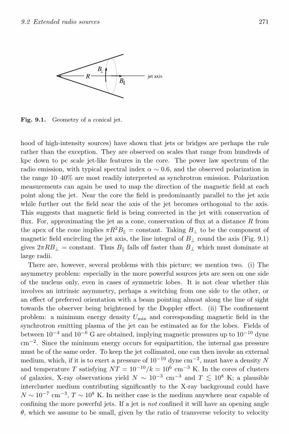
9.2 Extended radio sources 271

jet axisRB

B⊥

Fig. 9.1. Geometry of a conical jet.

hood of high-intensity sources) have shown that jets or bridges are perhaps the rulerather than the exception. They are observed on scales that range from hundreds ofkpc down to pc scale jet-like features in the core. The power law spectrum of theradio emission, with typical spectral index α ∼ 0.6, and the observed polarization inthe range 10–40% are most readily interpreted as synchrotron emission. Polarizationmeasurements can again be used to map the direction of the magnetic field at eachpoint along the jet. Near the core the field is predominantly parallel to the jet axiswhile further out the field near the axis of the jet becomes orthogonal to the axis.This suggests that magnetic field is being convected in the jet with conservation offlux. For, approximating the jet as a cone, conservation of flux at a distance R fromthe apex of the cone implies πR2B‖ = constant. Taking B⊥ to be the component ofmagnetic field encircling the jet axis, the line integral of B⊥ round the axis (Fig. 9.1)gives 2πRB⊥ = constant. Thus B‖ falls off faster than B⊥ which must dominate atlarge radii.

There are, however, several problems with this picture; we mention two. (i) Theasymmetry problem: especially in the more powerful sources jets are seen on one sideof the nucleus only, even in cases of symmetric lobes. It is not clear whether thisinvolves an intrinsic asymmetry, perhaps a switching from one side to the other, oran effect of preferred orientation with a beam pointing almost along the line of sighttowards the observer being brightened by the Doppler effect. (ii) The confinementproblem: a minimum energy density Umin and corresponding magnetic field in thesynchrotron emitting plasma of the jet can be estimated as for the lobes. Fields ofbetween 10−4 and 10−6 G are obtained, implying magnetic pressures up to 10−10 dynecm−2. Since the minimum energy occurs for equipartition, the internal gas pressuremust be of the same order. To keep the jet collimated, one can then invoke an externalmedium, which, if it is to exert a pressure of 10−10 dyne cm−2, must have a density N

and temperature T satisfying NT = 10−10/k = 106 cm−3 K. In the cores of clustersof galaxies, X-ray observations yield N ∼ 10−3 cm−3 and T ∼< 108 K; a plausibleintercluster medium contributing significantly to the X-ray background could haveN ∼ 10−7 cm−3, T ∼ 108 K. In neither case is the medium anywhere near capable ofconfining the more powerful jets. If a jet is not confined it will have an opening angleθ, which we assume to be small, given by the ratio of transverse velocity to velocity

272 Accretion power in active galactic nuclei

along the jet axis: θ = v⊥/v‖. If the transverse velocity arises from internal pressureP , we have P ∼ ρv2⊥ so the ram pressure in the jet is ρv2‖ ∼ P/θ2 ∼ umin/θ2, whichamounts to 4 × 10−2 dyne cm−2 if θ ∼ 1

20 . There appears to be no possibility thatsuch a jet could be stopped by the intergalactic medium to give the observed radiolobes. However, many observed jets are not straight, but show multiple bends andeven, in some cases, appear to curve back on themselves. The forward momentum herecould be destroyed by many small angle collisions with density inhomogeneities in theintergalactic medium. An alternative possibility is that jets are confined magneticallyby fields generated by currents in them.

The conclusion, then, is that at least some active galactic nuclei emit relativisticparticle beams as well as radiation. Further support for this view comes from thevariability arguments to be considered in Section 9.3. Observations have shown radiofeatures in Seyfert galaxies resembling the classical double structure but confinedwithin the galaxy on a much smaller scale. This suggests that the appearance ofextended radio structure may be connected more with the environment of the activegalactic nucleus than with the nature of the central source.

9.3 Compact radio sources

We now turn to the radio emission from the nucleus, with the hope that the largequantity of detailed observational data will provide clues to the overall nature of thecentral engine, despite the relatively small contribution to the total energy outputin most cases. One should not be unaware, however, that the radio emission couldrepresent a minor side-effect, unrelated to the main problem.

With increased detector sensitivity many of the classical double radio sources revealcompact radio cores with angular sizes much less than one arc second, the conventionaldefinition of ‘compact’. In addition, many active nuclei lacking extended radio emis-sion have compact radio cores. The core characteristics do not seem to depend stronglyon the presence or absence of extended emission. However, the core emission of atleast the radio quiet and the lobe dominated radio loud quasars shows a distinct breakin the spectrum in the millimetre region indicating that the radio emission is indeeda separate component.

A simple characterization of the specific intensity at a given observed frequency isthe temperature of a blackbody producing an equal intensity at that frequency. Thisis the brightness temperature TB, of the source at the given frequency, and is given by

Iν =2hν3

c2[exp(hν/kTB) − 1]−1.

Note the distinction between TB and the blackbody temperature Tb (equation (1.10))in that the latter refers to an average over frequency. Clearly, TB is a function offrequency unless the emission is blackbody, in which case TB is the source temperature.For hν kTB on the Rayleigh–Jeans part of the spectrum, the case in which thebrightness temperature is most commonly used, we have

9.3 Compact radio sources 273

kTB = (c2/2ν2)Iν . (9.7)

For compact radio sources, TB is in the range 1010–1012 K. Since blackbodies at suchtemperatures do not emit a significant fraction of their power in the radio, this tellsus that the radio sources cannot be thermal.

The observed spectra fall into two classes. Some cores have power law spectra ratherlike those from the lobes of classical doubles (steep spectrum sources). Others are flat(or, in some cases, inverted) up to several hundred GHz and a turnover to a power lawFν ∝ ν−0.25 can sometimes be observed at millimetre wavelengths (compact sources).It is reasonable to attribute the steep spectrum sources to synchrotron emission, and,indeed, it appears possible that they could be classical doubles with relatively weakcores viewed end-on. The inverted non-thermal spectra in compact sources suggestself-absorbed synchrotron emission, the main points of which we shall briefly recall.

At sufficiently high densities, or, it turns out, at sufficiently low frequencies, theabsorption of radiation by relativistic electrons in the presence of a magnetic field, theprocess inverse to synchrotron emission, can become important. If the same electronsare responsible for producing the radiation in the same magnetic field, we refer tothis as synchrotron self-absorption. Even for theoretically infinite optical depths inthis plasma, the resulting emission will not be blackbody, because the electrons do nothave a thermal distribution and therefore the absorption coefficient µν does not satisfyKirchhoff’s law, i.e. µν = jν/Bν (see the Appendix). The observed flux is obtainedby solving the appropriate radiative transfer equation (see for example Rybicki &Lightman (1979)). For a simplified discussion, imagine each electron to emit andabsorb only at the peak frequency related to its energy by equation (9.5). A properanalysis then shows that we obtain the emitted intensity by replacing the mean energyper particle for a thermal source (∼ kT ) by just the energy given in equation (9.5).Thus in the Rayleigh–Jeans limit, which is appropriate here, we obtain for an opticallythick synchrotron source

Iν =2ν2

c2Eν ∼ 10−30ν5/2B−1/2 erg s−1cm−2 Hz−1sr−1. (9.8)

At a frequency νm the observed intensity equals this limit: below νm (9.8) should hold;above νm the system becomes optically thin and the plasma radiates less efficiently.Thus, if Fν is the observed flux and Ω ∼ θ2 the solid angle of the source, we haveFν = ΩIν ; and (9.8) gives

νm ∼ 1012B1/5F 2/5νm θ−4/5 Hz. (9.9)

An optically thin source cannot be smaller than

θ ∼> 2 × 10−3F 1/2−26B

1/4ν−5/48 arcsec (9.10)

where ν8 = 10−8ν and F−26 = 1026Fν erg s−1 cm−2 Hz−1 is the flux measured in thestandard unit used by radio astronomers, the millijansky (or mJy, 1 Jy = 10−23 ergs−1 cm−2 Hz−1). Equality holds in (9.10) if F−26 is the flux at the turnover frequencyνm.

274 Accretion power in active galactic nuclei

Applying this theory to the observations of the compact sources yields typical valuesfor field strengths and total energies of

B ∼ 10−3 G, Uparticles ∼ 1054 erg, Umag ∼ 1049 erg,

well away from equipartition; but there are large uncertainties since errors in θ getmagnified to large powers. Of course, there is an obvious objection to applying thistheory directly to observed sources, since the spectra are often flat and never as steepas ν5/2. However, inhomogeneous source models with either smooth variations inproperties (field, electron density, etc.) or discrete components can produce agreementwith the observed spectra.

For compact sources in which the self-absorption, and the angular size can be es-timated, the synchrotron lifetime of the relativistic electrons can be obtained. Theobserved brightness temperature, TB ∼ 1012 K at νm, gives the energy and henceLorentz factor of electrons radiating at this frequency;

γ = Em/mec2 ∼ kTB/mec

2 ∼ 100.

The magnetic field B must be such that electrons with this Lorentz factor γ = γmdo indeed radiate at the turnover frequency νm (equation (9.5)). The synchrotronlifetime (9.4) is

tsync ∼ 5 × 1021γ3ν−2m s (9.11)

∼ 200 yr

for νm ∼ 1 GHz, γ = γm ∼ 100. Since this is much less than the source lifetime, whichmust exceed U/L ∼ 103 yr at the very least and is almost certainly a lot longer (inexcess of U/L for the extended lobes), there must be an essentially continuous input ofrelativistic electrons. This is similar to the conclusion we reached for the radio lobesbut the constraints on the nature of the central source, at least for some objects, canbe considerably tightened.

We should ask what happens to the electrons after they lose their energy andcease to be relativistic. Any non-relativistic electrons will lose their remaining energyby cyclotron emission. The timescale is still given by (9.12) but with γ ∼ 1 and νmreplaced by the cyclotron frequency νcyc ∼ νm/γ2m. The resulting loss time is somewhatlonger than the age of the source, and such electrons would eventually be thermalizedby collisions. However, there are limits on the amount of such thermal plasma in theradio source. One approach would be to consider optical depth effects – the smoothingof variability by electron scattering for example. Another is the observation of thevariable polarization of the radio emission during source outbursts on timescales ofmonths to years. This is possible only if Faraday rotation of the plane of polarizationof radiation crossing the source is too small to smear out the polarization changes.Thus we require the rotation ψ = Rmλ2 ∼< 1 radian, where Rm ∼ 106NeBR m−2 for asource of size R pc, electron density Ne cm−3. Relativistic electrons contribute witha factor 1/γ2 since Rm ∝ ω2pωcyc ∝ m−2

e γ−2, and so can be neglected. For B ∼ 10−3

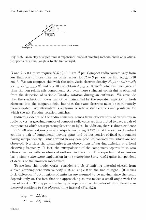
9.3 Compact radio sources 275

to observerfixed point

θ

θ∆l

v ∆te cosθ

v

Fig. 9.2. Geometry of superluminal expansion: blobs of emitting material move at relativis-

tic speeds at a small angle θ to the line of sight.

G and λ ∼ 0.1 m we require NeR ∼< 10−1 cm−3 pc. Compact radio sources vary fromless than one to more than ten pc in radius; for R ∼ 3 pc, say, we find Ne ∼< 1/30cm−3. We can compare this with the relativistic electron density Ne,rel ∼ ue/γmec

2;for ue ∼ Uparticles/R3 and γ ∼ 100 we obtain Ne,rel ∼ 10 cm−3, which is much greaterthan the non-relativistic component. An even more stringent constraint is obtainedfrom the detection of variable Faraday rotation during an outburst. We concludethat the synchrotron power cannot be maintained by the repeated injection of freshelectrons into the magnetic field, but that the same electrons must be continuouslyre-accelerated. An alternative is a plasma of relativistic electrons and positrons forwhich the net Faraday rotation vanishes.

Indirect evidence of the radio structure comes from observations of variations inradio power. A growing number of compact radio cores are interpreted to have a pair ofcomponents which are separating faster than light. In addition, there is direct evidencefrom VLBI observations of several objects, including 3C 273, that the sources do indeedcontain a pair of components moving apart and do not consist of fixed componentsflaring independently – which would in any case produce contractions, which are notobserved. Nor does the result arise from observations of varying emission at a fixedobserving frequency. In fact, the extrapolation of the component separation to zerooften coincides with an observed outburst in the core. This superluminal expansionhas a simple kinematic explanation in the relativistic beam model quite independentof details of the emission mechanism.

To see how this model works, consider a blob of emitting material ejected froma fixed emitting core with velocity v at an angle θ to the line of sight. (It makeslittle difference if both regions of emission are assumed to be moving, since the resultdepends only on the fact that the approaching source makes a small angle with theline of sight.) The apparent velocity of separation is the ratio of the difference inobserved positions to the observed time-interval (Fig. 9.2):

vapp = ∆l/∆to

∆l = ∆tev sin θ,

where

276 Accretion power in active galactic nuclei

to observerθ

Fig. 9.3. Source axes at angles less than θ to the line of sight cut out a conical sector on

the hemisphere of all possible directions.

∆to = ∆te(1 − v/c cos θ),

allowing for the decrease in light travel time as the object approaches. Thus

vapp = v sin θ/(1 − v/c cos θ) (9.12)

is the required expression for the apparent velocity as a function of v and θ. For v

fixed, the maximum apparent velocity vmax occurs for sin θ = 1/γ and is vmax = γv.For θ fixed, the maximum occurs for v = c. So

vmax < vapp(v = c) = sin θ/(l − cos θ) ∼ 2c/θ as θ → 0. (9.13)

It is clear that an arbitrarily high vapp can be achieved for sufficiently small θ andlarge γ, but at the expense of decreasing probability of such alignment. In fact, theprobability P (Θ) that a source axis makes an angle ≤ Θ to the line of sight is theratio of the area of a conical sector of a sphere to the area of a hemisphere (Fig. 9.3);thus

P (θ) = 1/2π

∫ 2π

0

∫ Θ

0

sin θ dθ dφ = (1 − cos Θ), (9.14)

and for γ large, sin Θ ∼ Θ ∼ 1/γ, this is P (Θ) ∼ 1/2γ2. Therefore for γ ∼ 5, asrequired by the observed velocities, the probability of alignment to within an angle≤ 1/γ, at which relativistic effects would be important, is of order 2%. This inter-pretation in terms of specially oriented relativistic outflow is qualitatively consistentwith the interpretation of core dominated radio sources as ‘end-on’ radio doubles ina model in which only orientation effects affect the radio properties of quasars: upto one-half and possibly all of the compact sources, which are themselves a subset ofthe 10% of radio loud quasars exhibit superluminal expansion or milder forms of ‘overrapid’ variability. In this case we should say that the parent population of the beamed(superluminal) sources are the radio loud quasars. An alternative picture which fitsthe statistics better, is the ‘unified model’ of Section 7.1 in which radio galaxies are theparent population and all radio loud quasars the specially oriented, beamed subset. Inthis picture all quasars would host a superluminal source at some level. The idea hassome success in accounting for the distribution of the separation of the radio lobes.

9.3 Compact radio sources 277

A further argument for relativistic bulk motion comes from observations of vari-able sources, since some of the shorter timescales present problems for non-relativisticsource models. In particular, the high energy density implied by the small volume andhigh luminosity leads to what has become known as the inverse Compton catastrophe,which, as implied by the name, was historically considered to be more than a mereproblem. It arises because the synchrotron emitting electrons are also bathed in theradiation they are producing. The energy of a typical radio photon of this radiationfield is clearly much less than the energy of a typical electron so that the net effect ofscattering is a transfer of energy to the radiation which is referred to as the inverseCompton effect. If the radiation field were too intense the electrons would lose all theirenergy by inverse Compton scattering with the catastrophic result that they wouldcease to be synchrotron emitters. If the electron energy were maintained by suitableexternal forces they would further scatter these and subsequent inverse Compton pho-tons with the catastrophe of an infinite energy density as a result. This puts a limiton the brightness temperature of a synchrotron source. The inverse Compton powerof a relativistic electron of energy E in a radiation field of energy density Urad is

−dE/dt ∼ 43

σTc(E/mec2)2Urad. (9.15)

Comparison with (9.3) shows that synchrotron losses will dominate if

UB ∼> Urad. (9.16)

The brightness temperature then satisfies

TB ∼<c3

2ν3k

[4π

µ0

]B2

8π, (9.17)

where we have used (9.7) in (9.16) and estimated Iν by cUrad/4πν. For an equipartitionmagnetic field of somewhat less than 10−3 G, and at the peak of brightness at frequencyν = νm ∼ 109 Hz, we find TB ∼< 1012 K. The limit on TB provided by equation (9.17)cannot be increased by postulating a stronger magnetic field, since measurement ofTB at νm gives a value for B by putting Em = kTB in (9.5). Where TB is obtainedfrom direct measurements of angular size, the inequality (9.17) is found to be satisfiedand the inverse Compton catastrophe is avoided.

Consider, however, those variable sources in which the brightness temperature isinferred. The condition that synchrotron emission is not self–absorbed, Iν = Fν/Ω <

2ν2kTB/c2 (equation (9.8)), can be written

TB ≥ 1012(

∆E

3 × 1044

)1ν39

(3 × 106

tvar

)3

, (9.18)

with equality ν = νm, where the variability on a timescale tvar involves an energy at∆E ∼ νLν tvar, measured in ergs, and we have assumed a source size l < ctvar; ν9 isthe observation frequency in units of 109 Hz. Thus at 1 GHz the limit (9.17) on TB isviolated by variability over less than a month involving an energy in excess of 3×1044

erg or more. Observed violations amount to factors 10–103 in TB. Conversely, in order

278 Accretion power in active galactic nuclei

to avoid the inverse Compton catastrophe, sources have to be larger than the limitl ∼< ctvar by factors of order 10. Other evidence appears to support this conclusion.For example, all sources observed with VLBI are at least partially resolved indicatingsizes for the non-varying source component up to 100ctvar. Furthermore, there is noevidence of the scintillations at radio frequencies caused by inhomogeneities in theinterplanetary medium which should occur for sources of the sizes indicated by thevariability lengthscale.

We can circumvent the light crossing time limit on the source size if either thebrightness temperature or the observed timescale tvar, or both, do not refer to therest frame of the source. Thus, if the radiation is beamed towards us from a sourcemoving at relativistic speed and having Lorentz factor γB 1 close to the line ofsight, then the timescale in the source frame is larger than that observed by a timedilation factor tvar = γBtobs and the emitted intensity is smaller by a factor γ−3

B

(since Iν/ν3 is invariant under Lorentz transformations). Note that γB refers to thebulk motion of material towards the observer, not to be confused with the relativisticparticle velocities in the moving source. Quite modest values of γB would resolve theinverse Compton catastrophe, and would be consistent with the beaming suggestedby the superluminal sources (3 ∼< γmin ∼< 10), and, at least for quasars, would bestatistically consistent with the view that the compact sources are end-on doubles(γB ∼ 5). Note that a preferred source axis is required in all of these cases: relativisticoutflow in a spherical shell would not produce the time dilation effect because lighttravel time delays from different parts of the shell would smear out the outburst overa longer observed timescale. Whether or not the γ3B enhancement of intensity in theapproaching beam, an effect usually referred to as Doppler favouritism, can account forthe observed jet asymmetry (Section 9.2) is unclear at present. Where depolarizationof the lobe emission by Faraday rotation shows that the fainter jet is on the far sideof the source Doppler favouritism is the obvious explanation. But claims of intrinsicasymmetry have been made for other sources.

9.4 The nuclear continuum

The Compton catastrophe appeared historically as a constraint on the source structureimposed by limits to the Comptonized flux. With Lorentz factors of γ2 ∼ 108 envisagedin radio synchrotron models the Comptonized flux will emerge, scattered by a furtherγ2, in X-rays. Given that X-rays are a ubiquitous feature of active nuclei we canturn the discussion round and ask if Comptonization is a viable way of producing theX-ray flux, and, by implication, a significant contribution, at least, to the IR–optical–UV flux. If the same electrons are taken to be responsible for the Comptonizationand synchrotron emission the models are referred to as synchrotron–self-Comptonmodels (SSC). The initial objective is to obtain the canonical (unabsorbed) power lawspectrum in X-rays, Fν ∝ ν−0.9. The relation between the X-ray flux and the far

9.4 The nuclear continuum 279

infrared (or millimetre) emission outlined in Section 8.6 has been cited both for andagainst models of this kind.

An implication of the radio source models is that the synchrotron emission may beassociated with a jet. In many BL Lacs in particular, a reasonably strong case can bemade that the X-rays are either a straightforward extension of the direct synchrotronemission or result from Comptonization. In these cases it is appropriate to model thesources as jets. However, both spherical and disc geometries have also been consideredfor SSC models; the qualitative discussion we give here is essentially independent ofthe assumed geometry.

In the simplest SSC models synchrotron radio photons are Compton scattered byrelativistic electrons of Lorentz factor γ from frequencies νR to γ2νR. The final radi-ation spectrum is therefore wholly a consequence of the input electron spectrum. Ifthe input is a burst of relativistic electrons with a power law energy distribution theoutput will be a power law photon spectrum with a break at a frequency for which theelectron lifetime equals the age of the source; by adjusting the input one can obviouslyobtain more complex outputs to match the observations.

An alternative version is the synchrotron inverse Compton model. In this an extraexternal soft photon input, corresponding to the ‘big bump’, is included since SSCmodels do not produce this as an output. The Compton scattering of the radio istaken to give the infrared emission; further scattering gives soft X-rays, while electronswith the same γ2 (∼ 104) scatter UV photons to hard X-rays. Such models can givequite impressive fits to steady-state spectra. They appear to depend on the unknownacceleration mechanism to give the right electron spectrum, but, against this, onecan argue that the mechanism is invoked in the same way in which it is known to beoperating in the extended radio structures and in synchrotron emitters such as theCrab nebula. Some modification of the simplest models is required to take account ofelectron–positron pair production (see below).

At the opposite extreme one can try to construct theories that yield the observedspectra independently of the input electron spectrum. In fact, Compton scatteringalso provides several ways of doing this. First, if the escape time from a source is muchgreater than the cooling time and the electron distribution reaches a steady state, onefinds that the number of electrons with Lorentz factors between γ and γ +dγ is relatedto the rate of input of fresh electrons at γ, Q(γ), by

n(γ) ∝ γ−1∫

Q dγ

where γ ∝ dE/dt ∝ −γ2 (9.3). Hence Lν ∝ ν−0.5 from equation (9.2). If there is somefurther reprocessing that softens the spectrum (scattering on cool pairs for example –see below) then one may obtain something close to Lν ∝ ν−0.9 in X-rays.

We can also consider the effect of multiple Compton scattering. The general argu-ment here is due to Zeldovich. In a single Compton scattering on average a photonundergoes a relative change in frequency 〈∆ν/ν〉 given by ∆ = 〈∆ν/ν〉 ∼ 〈E〉/mec

2 =〈γ〉, where E is the mean electron energy. After n scatterings we have 〈∆ν〉 ∝ ∆n〈ν〉;

280 Accretion power in active galactic nuclei

if n or ∆E is large, and if ∆ν ν, then we can write this in terms of initial andfinal mean frequencies as νf = ∆nνi. Thus, the probability of an input photon at νiemerging as a Comptonized photon at νf is equal to the probability of n scatterings,i.e. to Pn1 , where P1 is the probability of a single scattering and n = log(νf/νi)/ log ∆.Thus

Lνf = νfPlog(νf/νi)/ log∆1

Lνiνi

= νf

(νfνi

)(logP1/ log∆) Lνiνi

;

so if we input photons in a relatively narrow band about νi we get a power law outputwith energy slope 1 + log P1/ log ∆.

The argument applies provided (i) ∆ν ν; (ii) 〈∆ν/ν〉 ∼ constant, independentof ν, provided that we can ignore the energy dependence of the Klein–Nishina cross-section; (iii) the number of scatterings is large. The first requirement is satisfied ifthe mean electron energy is much greater than the photon energies attained. Thisis also necessary in order that we can ignore down scattering. The second conditionimplies a break in the spectral slope in γ-rays where the fall off in the Klein–Nishinacross-section becomes important. The final condition is controlled by the so-called y-parameter which measures (energy change per scattering) × (number of scatterings).For large optical depth, τ , photons random walk out of the source. To random walkthrough a source of size R with a mean free path λ required (R/λ)2 = τ2 scatterings;so if τ is large, y ∼ (∆E/mec

2)τ2. If τ < 1 the relevant parameter is y ∼ (∆E/mec2)τ :

since only single scatterings are relevant, the mean number of scatterings equals themean fraction of scattered photons which is equal to τ . Note that y may be a functionof frequency through τ if absorption is also important. The argument applies inparticular to a thermal electron distribution for which 〈∆E〉/E = 〈ν〉/ν = 4kT/mec

2

if the electrons are non-relativistic and 〈∆E〉/E = 4kT/mec2 + 16(kT/mec

2)2 in therelativistic case. For multiple scattering of a relativistic distribution we get a powerlaw photon spectrum for y 1 and y 1. This gives rise to many variants ofsynchrotron–Compton models.

In all of these models there are various reasons why electron–positron pairs maybe present. One possibility is that the acceleration of protons in shocks may be moreeffective than that of electrons. Relativistic protons will lose energy by pion production(rather than Compton scattering, since the Compton scattering cross-section is smallerby a factor of (me/mp)2 compared with that for electrons). The pions are unstableand decay to electrons and positrons. In principle inelastic e–p or e–e collisions couldproduce e± pairs. But the other important possibility turns out to be photon–photoninteractions (the inverse of e± annihilations). For this we require a high density of lowenergy photons and high energy γ-rays (hν mec

2). The former may be providedby the ‘big bump’. The latter are observed to be emitted by a number of sources.There is a subclass of blazars for which the power (measured as νFν) peaks in γ-rays.In one case (3C 279) the flux above 100 MeV exceeds that of 3C 273 by an order ofmagnitude and in another (Mrk 421) the γ-ray spectrum has been detected out to TeVenergies. However, not all active nuclei can be strong γ-ray sources since otherwise

9.5 Applications to discs 281

the upper limits on the γ-ray background would be violated. But the idea is that inmost active nuclei the high energy γ-rays would be present but would generally notescape: most would be reprocessed to e± pairs.

The relevant parameter for the importance of photon–photon interactions is the‘compactness parameter’, l. This is the soft photon energy expressed in units of mec

2,intercepted per Thomson cross-section in a photon crossing time:

l =L

mec2· σT

4πR2· R

c=

LσT4πRmec2

.

If γ-rays are present and if l > 10 then e± pairs will be produced in significant numbers.We can rewrite l as

l =12

(mp

me

)(L

LEdd

)(RSchw

R

).

so l > 10 even for L < LEdd near RSchw. The presence of e± pairs modifies thesource opacity. At high enough density e± annihilation becomes important producingγ-rays and a self-sustaining system, the so-called e± cauldron. In most circumstancesthis does not occur: e± pairs modify the radiation spectrum but do not determineit. However, for 30 < l < 300 a self-sustaining system can be obtained in whichCompton scattering on cooled pairs gives rise to a spectrum proportional to ν−0.9

without violating the γ-ray background constraint.

9.5 Applications to discs

There are two ways in which the above considerations impinge on disc models. First,there is the extent to which some of the above processes might operate in a discgeometry to produce a radiation spectrum from the disc that is closer to that observed.Certainly the similarity of the variability timescales of at least the soft X-ray end ofthe big bump and of the hard X-rays suggests an origin in similarly sized regions. Thiswould obviously be satisfied if, given that the big bump comes from the disc, the hardX-rays were to be produced in the disc also. Second, one must consider the influenceof the disc in producing the bulk relativistic outflows associated with jets, spectralconsiderations being relegated to second place after the geometry has been fixed. Theformer question is taken up here and in Chapter 10 and the latter in the remainder ofthis chapter and in Chapter 11.

It is beyond the scope of this book to discuss in detail all the modified disc modelsthat have been proposed to account for various aspects of the observed spectra. Weshall restrict ourselves to showing where the uncertainties lie that make such deviationsfrom the orthodox thin disc possible or necessary.

In Section 5.8 we saw that a viscous instability develops unless dµ/dΣ > 0. For theinner region of a thin accretion disc, where radiation pressure dominates gas pressureand the main source of opacity is electron scattering (Section 5.6) this condition is notsatisfied. In fact, solving (5.68) under these circumstances and with τ = Σκes gives

282 Accretion power in active galactic nuclei

µ ∝ 1/Σ. Thus a steady thin disc solution is not possible. Now, one can suppressthis instability by modifying the ad hoc viscosity prescription. For example, we mightuse the sound speed in the gas, c′s = (Pgas/ρ)1/2, instead of (P/ρ)1/2 (with P givenby equation (5.39)), to construct the viscosity in (4.30). In this case the viscosity isproportional to the gas pressure, rather than the total pressure, and the resulting thindisc turns out to be stable. However, since we are seeking to obtain a spectrum morein agreement with observations than that of the standard thin disc, let us try to usethe instability as an opportunity to depart from the standard model.

To obtain X-rays requires a high temperature; the maximum temperature is Tth(Section 1.3), which, at the surface of a Schwarzschild black hole, R = 2GM/c2, isof the order of the proton rest energy, mpc2/k ∼ 1012 K. Now, if the disc really isresponsible for the emitted radiation we can estimate the ratio of cooling time to infalltime (i.e. to heating time) for the electrons and the protons. If we assume that weare going to be led eventually to a stable disc structure then we must take this to beoptically thin, in order that the radiation pressure does not dominate the gas pressure.Then, using the non-relativistic Compton cooling time from (A.9) and the timescalesfrom Section 5.3, for electrons we have, roughly,

tCompttinfall

∼ α

M2

(˙Mcrit

M

)η

(R

RSchw

)1/2

( me

mp

);

for protons there is a further factor (mp/me)3 ∼ 109. Thus, if the coupling betweenelectrons and protons is weak, we expect a two-temperature disc with the electronscooled by Compton scattering to a lower temperature than the protons.

Suppose the only coupling between electrons and protons is Coulomb collisions,i.e. we ignore possible collective plasma effects. Then the energy exchange timescale,(mp/me)td(e–i), from Section 3.4 can be compared with the infall timescale. It turnsout that the temperature difference between electrons and ions will be maintaineddown to 3RSchw if the density in the disc is less than of order 109 cm−3. Of course, wedo not yet have a consistent disc structure to know whether this condition can hold.We obtain a consistent structure by taking the pressure in the two-temperature discto be

P = nk(Ti + Te).

Thus we replace T by 12 (Ti + Te) in the disc equations, assuming electron scattering

opacity and an optically thin medium with gas pressure dominating radiation pressure.It turns out that this is in principle a consistent picture at intermediate accretionrates (M/Mcrit) < 50(vR/vff)2/η. Note this leaves open the possibility of thick discsat supercritical accretion rates – see Chapter 10. Strictly, if the ion temperaturereaches Tth it is also inconsistent to ignore thick disc effects in the two-temperaturedisc. This model was originally proposed for Cyg X-1 where it gives a good fit to thehigh-state X-ray data. However, in the original form of the theory, the disc structurewas shown to be both thermally and viscously unstable! To obtain a stable structure

9.5 Applications to discs 283

one must take into account that the radiative efficiency of the accretion flow is low, sothat most of the energy is advected with the radial inflow and only a small proportionradiated. This leads to the (two-temperature) advection dominated discs (see Chapter11). These are also called ion tori (since the pressure support is provided mainly bythe ions.)

There are numerous variations that can now be played on these themes. By thread-ing the disc with magnetic field one can include synchrotron emission; if the viscosityparameter is high one can imagine that the implied supersonic turbulence leads toshocks and non-thermal particle injection. Thus, all of the emission mechanisms ofthe previous section become relevant. In particular, one must consider the effects ofelectron–positron pairs. The indications from the present approximate models arethat the disc structure is not much affected by the presence of pairs but that thespectrum may well be.

These considerations may necessitate further modifications of the standard thin discpicture. We can define a new temperature, Tesc at which material becomes gravita-tionally unbound to the black hole by

32

kTesc ∼ 12

mpv2esc =GMmp

R.

Thus, Tesc ∼ Tth, so disc material at its maximum temperature is close to becominggravitationally unbound. In addition, if pairs are present, the Eddington limit isreduced: if the pair density (electrons and positrons) is n± and the density of ionizationelectrons is ne then the mass per electron is reduced from mp to mp(1 + n±/ne) andthe Eddington limit is lowered by the same factor. Thus, we must allow for the lossof mass and angular momentum in a radiatively driven wind from the disc surface inthe inner regions.

In fact, mass loss may also be important in the outer regions of the disc. Thiswill occur if the disc surface intercepts a significant amount of the radiation fluxfrom the inner region, either because it is flaring or by scattering of the radiation offambient material above the disc. This external heating gives rise to a thermally drivenwind wherever the disc surface temperature is raised sufficiently close to Tesc. If thedominant process is Compton scattering the disc surface is raised by a flux Fν to theCompton temperature Tc = 〈hνFν〉/4k〈Fν〉 at which Compton heating and coolingbalance. If the disc is exposed to a typical quasar spectrum then Tc ∼ 107 K, sothis process is important only for radii greater than 1019M8 cm. Magnetically drivenwinds and winds driven by the absorption of line photons may also be important atthese radii.

If the disc extends to even larger radii (10–100 pc) other considerations becomeimportant. The standard model predicts a very low surface temperature so the opacityis dominated by dust grains. Self-gravity in the disc cannot be neglected since itgives rise to the Jeans instability. (If the thermal energy becomes less than the self-gravitational potential energy on some scale then material will tend to form intogravitationally bound clouds (or stars) on that scale.) However, at these radii the disc

284 Accretion power in active galactic nuclei

is no longer powered by accretion: the energy balance in the disc is dominated byexternal heating by radiation from the central source and from starlight.

A further source of significant modifications to all of the above models comes fromrelativistic (strong gravity) effects, since we expect most of the accretion energy to beextracted near the black hole. (Precisely where depends on the disc model but radii5–10×RSchw are typical.) In this region Newtonian gravity is inapplicable and wemust therefore expect a departure from Keplerian rotation. Since vR → c at RSchw wemust have vR > cs at some radius in the disc, and the thin disc approximation breaksdown. We can still have H < R for M < Mcrit so the disc is still thin in some sense;but we cannot neglect the radial motion and the departure of uφ from Keplerian form.Thus in the vertically averaged equation of motion, obtained from the Euler equation(2.3), we must retain the inertial terms and the radial pressure gradients. to get

vRdvRdR

− Ω2R = −1ρ

dP

dR− Ω2

KR.

In addition, the energy equation must allow for the fact that the dissipated energy neednot be radiated locally but can be advected with the flow. Disc structures calculatedwith these modifications have come to be known as ‘slim discs’. The effects, on theemitted spectrum for example, become important as M approaches Mcrit. These discstructures are dealt with in more detail in Chapter 11.

Finally, it is unclear that vertical averaging of the disc structure provides a viablebasis for comparison with observations. We limit ourselve to a few comments andexamples. First, several semi-analytical and numerical results for axisymmetric accre-tion flows in two dimensions point to the possibility of outflow near the mid-plane ofthe disc with inflow away from the mid-plane. The vertically averaged velocity fieldagrees with the thin disc value, but, because not all the disc material is accreting, agiven accretion rate corresponds to a higher surface density than would be anticipatedfrom the thin disc model. However, it is probably fair to say that there is not yetgeneral agreement on the extent to which the flow pattern obtained depends on theparticular assumptions made to simplify the problem. Nevertheless they suggest thatvertical stratification might be important.

Vertical averaging of the thermal structure is even less clearly justified. One canenvisage structures in which the accretion is occuring mainly in the hot surface layersof the disc while the cool interior ‘filling’ serves principally to reprocess the emittedenergy. As an intermediate step one can consider coronal models in which the accret-ing disc material is surrounded by a hot atmosphere (corona) in which reprocessingis occuring. Particular models involving X-ray production by Compton scattering,with or without synchrotron seed photons, have been proposed. The scattering elec-trons may have a non-thermal spectrum, or multiple scattering from thermal electronsmay be involved. These theories should be distinguished by the correlations betweenvariability at different wavelengths they would imply.

9.6 Magnetic fields 285

z

RR0

R2

= R02

+ 2R0 z

current sheet jφ∝ R-1

parabolae

Fig. 9.4. Fieldlines due to a current sheet carrying a pure azimuthal current density jφ ∝R−1.

9.6 Magnetic fields

The inclusion of magnetic fields in models of accretion powered sources has beenmost widely discussed in relation to the generation of collimated bulk outflows or jets.Originally the primary concern was the dynamics of the outflow from the disc. In thesimplest case (electrodynamic models) we consider the motion of individual chargesunder the action of magnetic fields and gravity. At greater density it is necessary totreat the outfiowing material as a fluid (magneto-hydrodynamic models). The basicidea is that collimation occurs via a form of the ‘pinch’ effect: a current flow along thejet generates a toroidal field, Bφ, the magnetic pressure of which, (B2

φ/8π) × [4π/µ0],increases away from the axis and so confines the current flow. Such a jet is thereforeself-collimating.

More recently the structures of magnetized discs have been discussed, particularly toshow that such discs can join smoothly on to the outflow. A steady-state disc modelmust take into account the diffusion of magnetic field to counteract the rotationalwinding up of the fieldlines. A detailed treatment is beyond our scope.

Outside the disc one can imagine the outflowing plasma particle moving alongfieldlines which, projected into a meridional plane, point away from the disc axis(as in Fig. 9.4). The material moves up and out along these fieldlines at constantangular velocity until it reaches the Alfven velocity (Section 3.7). Since this can occurat a radius much greater than the radius at which a given fieldline leaves the disc, asmall mass loss can be accompanied by a large angular momentum loss. In fact, thiscan be the dominant mechanism by which loss of angular momentum drives accretion,dispensing with the need for an anomalous α-viscosity altogether.

286 Accretion power in active galactic nuclei

In the remainder of this chapter we shall look at energy extraction in an electrody-namic disc.

The basic idea of the electrodynamic model is that large-scale magnetic fields tiedto the disc extract rotational energy from the disc which is resupplied by the infall ofmaterial in the disc. The mechanism is taken to be essentially a scaled up version ofpulsar emission. In addition, the rotational energy of the accreting black hole can beextracted by electromagnetic effects and provides a roughly equal contribution to theemitted power for typical parameter values. The model has several clearly desirablefeatures. Thus, in contrast to non-electrodynamic disc models there is no need topostulate ad hoc sources of viscosity: the angular momentum of infalling material isremoved in a natural way by the magnetic field (Section 9.7). The energy is expectedto appear initially as a directed beam of particles, organized by the magnetic field andreadily, in principle, accelerated to relativistic energies. The Faraday rotation problem(Section 9.3) is avoided because these particles radiate in the same field that acceleratesthem, so there is no accumulation of non-relativistic material in the emission region.However, there are also some difficulties, in practice if not in principle. For, sincethere is no definitive pulsar model, details of this scaled-up version are uncertain, and,in particular, the generation of and radiation from the relativistic beam have yet to beworked out. Our aim here is to describe the model and to estimate the luminosity itmight produce. For detailed considerations we refer the reader to the literature citedin the Bibliography.

The motion of an ionized gas with overall charge neutrality is governed by the Eulerequation (2.3) with, in general, a force density

f = −ρg + qE+ [c]/cj ∧B (9.19)

(cf. equation (3.2) and Section 3.7); here q is the charge density. In order to obtainsolutions it is necessary to make various limiting approximations. If the net forcedensity is sufficiently small the velocities induced will be small and the inertial terms(the mass × acceleration terms on the left hand side of the Euler equation) can beneglected. For a sufficiently tenuous plasma with large electric fields the gravitationalterms can be neglected. But in the vicinity of a black hole, the case of interestto us here, the conditions under which this leads to a stationary magnetosphere (aregion in which magnetic fields are important) turn out to be rather artificial. In theopposite extreme of small electromagnetic fields, gravity would dominate and materialwould be accreted; but this would drag in the frozen-in magnetic field and probablyenhance it to the point where electromagnetic forces were no longer small (Section3.7). Thus the relevant limits would appear to be the magnetostatic case, in whichstrong magnetic fields balance gravity, and the force-free case, in which the chargesin the magnetosphere are assumed to be sufficiently mobile to allow them to act assources of field. The force-free condition

qE+ [c]/cj ∧B = 0 (9.20)

then follows if one assumes that large field strengths are set up which dominate the

9.7 Newtonian electrodynamic discs 287

other terms in the force density. Note that this condition is distinct from the perfectmagnetohydrodynamic assumption, for which E + [c]/cv ∧ B = 0 and which is a con-sequence of perfect conductivity irrespective of the forces dominating the dynamics.The two are equivalent only if j = qv, which is rarely satisfied in magnetohydrody-namics, since the currents arise from the net motion of positive and negative carriersin a neutral medium, rather than from a net space charge moving with the fluid. Onthe other hand, the force-free condition requires a non-zero space charge density q

since qE = −j ∧ B = 0. Overall neutrality can be maintained if there are regions ofopposite net charge. Thus charges must be sufficiently mobile that they can flow asneeded if the force-free condition is to be satisfied. The magnetostatic case is probablyimportant in determining the structure of a magnetized accretion disc, and may beimportant above the disc if there is a large amount of plasma there. The force-freecondition is appropriate to pulsar magnetospheres and in the Blandford–Znajek modelbelow.

9.7 Newtonian electrodynamic discs

We turn from these general considerations to an outline of the specific example ofelectrodynamic energy extraction from a disc in a Newtonian gravitational field. Thesimplifying assumption here comes not so much in the choice of a theory of gravity asfrom the fact that one does not have to worry about the boundary conditions for themagnetic and electric fields on a black hole horizon.

Consider first the field of currents flowing in circular paths in the plane z = 0.This is a standard, if somewhat difficult problem in electrodynamics, but we can seewhat must happen as follows. The magnetic field will, of course, be steady, and incylindrical coordinates (R, φ, z) we will have Bφ = 0, but BR and Bz non-zero. If thesurface current in the disc falls off rapidly with increasing R the solution will approachthat of a circular loop of current with an approximately dipole field. Near the axis thefieldlines will open out. If the current falls off more slowly towards the outer edge ofthe disc, so that loops at larger radii dominate as one moves away from the disc nearthe axis, we might expect the fieldlines to bend towards the axis; this would providesome hope of carrying charges away in a directed jet (Fig. 9.4). In fact jφ ∝ R−1

gives parabolic field lines (Blandford (1976)). There is no radiation of energy in thissystem because the axisymmetry implies a stationary field.

Consider now how the picture changes when we replace the current loops by amagnetized disc. The magnetic energy density in the disc must be small compared withthe thermal energy density and much less than the kinetic energy density of rotation,since otherwise the disc would be disrupted. Furthermore, we would expect the densefully ionized disc to have a high electrical conductivity. In these circumstances, themagnetic field will be frozen into the disc, to a good approximation, and the fieldwill be swept round with the disc material. We distinguish between the toroidalcomponent of a vector, here the magnetic field, BT = (0, Bφ, 0) in cylindrical polar

288 Accretion power in active galactic nuclei

coordinates, and its poloidal part BP = (BR, 0, Bz) = B − BT. We can make thesame decomposition of the electric field, E = ET +EP. Since the model is stationarythe components of all observable quantities are independent of time, and since it isaxisymmetric they are independent of the angle φ. In particular, since the magneticflux through a surface spanning a circle on the symmetry axis does not depend ontime, it follows from Faraday’s law that the e.m.f. round the circle is zero. Therefore,in fact, ET = 0, E = EP. Furthermore, since Bφ is independent of φ, we have

∇ ·BT = 0

and therefore, since ∇ ·B = 0, we deduce

∇ ·BP = 0. (9.21)

This result is simple but important. It means we can picture unending lines of magneticfield associated separately with the poloidal and toroidal components. The lines ofpoloidal magnetic field can therefore be thought of as rotating with the disc materialto which they are anchored.

An important result is Ferraro’s law of isorotation, which states that, provided cer-tain conditions are satisfied, the angular velocity of a fieldline is constant along thefieldline. Sufficient conditions for stationary axisymmetric fields are the perfect mag-netohydrodynamic condition (3.48), the force-free condition, (9.20) or, more generally,degeneracy (3.49). In this last case the condition that a charge rotating with the fielddoes not experience a force, hence remains at rest in the rotating frame, is that theelectric field E′ in the rotating frame vanishes; thus

0 = E′ = EP +[c]c

(Ω ∧ r) ∧B

where the angular velocity of the fieldline Ω has the form Ω = (0, 0, ΩF). Therefore,

EP = − [c]c

(Ω ∧ r) ∧BP. (9.22)

Using ∇ ∧ EP = 0, which is a consequence of the time independence of B, and∇ ·BP = 0 (equation (9.21)), we obtain

BP · ∇ΩF = 0.

This expresses the fact that ΩF does not change along poloidal fieldlines. Thereforethe fieldlines cannot wind up and discharge the field and a stationary solution asenvisaged is possible.

Far out along the fieldlines their rotational velocities will exceed the speed of light.We can therefore construct a speed of light surface on which equality holds. Thisconclusion is not in conflict with relativity because fieldlines are purely mathematicalentities, but any charged particles in the region beyond the speed of light surface haveto move outwards and upwards back along lines of the B field if they are to move atless than the speed of light while remaining attached to lines of magnetic field. Inother words, particles are forced to move away from the disc, rather like beads on a

9.8 The Blandford–Znajek model 289

rotating wire. This provides a mechanism for the generation of a flux of relativisticparticles, if only we can produce a supply of particles and a source of energy.

The particles are assumed to be extracted from the disc by a process analogous tothat which operates in pulsar models. Inside the disc the perfect magnetohydrody-namic assumption implies that there is an electric field E = −([c]/c)v ∧B and hencea charge density

q = [1/4πε0]∇.E = −[l/4πε0c]2Ω ·B/c = 0 (9.23)

where Ω = (0, 0, v/R). This charge density gives rise to an electric field outside thedisc which is available to pull charges out of the disc. For a magnetic field of 1012 G(108 T) this gives electric fields which dominate the gravity of the central black holein the region above the disc but do not grossly violate the condition of degeneracy(3.49) (because E ·B ∼ ([c]/c)RΩB2 from (9.23) and hence E ·B [c]B2 if RΩ c).Thus we may idealize the magnetosphere as gravity free and degenerate.

If the particle density in the magnetosphere is sufficiently large the particle inertiawill be important and the region above the disc will not be force-free. In this case, theparticles may be accelerated along fieldlines directly, extracting energy and angularmomentum from the stored gravitational potential energy of the disc (Blandford &Payne (1982)). We shall not discuss this case further. Instead we assume that theparticle density is sufficiently low and there is a force-free region above the disc. Thiscannot extend right out to the speed of light surface because relativistic effects meanthat particles travelling on fieldlines close to the speed of light become more massiveso that inertial terms (mass × acceleration) cannot be neglected in the determinationof their motion. The magnetic fieldlines therefore are attached to non-force-free ma-terial in the disc and to non-force-free material some distance above the disc, whereparticles are accelerated to relativistic velocities. Electromagnetic energy and angularmomentum flow through the intervening force-free region creating a torque on thedisc. This has the same effect as the usual disc viscosity, causing material to flowin and extracting gravitational energy from the disc. The disc does not radiate elec-tromagnetic wave energy, since this is impossible in an axisymmetric configuration,but it transmits a ‘DC’ flux. A rough analogy is the coupling of two flywheels by aviscous medium where the transmitted energy resides in the shear of the medium, notin sound waves.

The detailed implementation of this scheme is far from complete. The force-freeregion can be discussed in some detail, but the acceleration of particles in the non-force-free region, which, as we shall see, actually determines the efficiency of theprocess, is essentially informed guess-work.

9.8 The Blandford–Znajek model

The quasar model consists not of a Newtonian disc, but of a disc around a black hole.We shall see that the black hole can be an important source of energy, but we expect

290 Accretion power in active galactic nuclei

Fig. 9.5. Magnetic surface and current flows in the vicinity of the black hole and disc.

(Adapted from D. Macdonald & K.S. Thorne (1982) M.N.R.A.S. 179, 433.)

its direct effect on the disc to be small except near the horizon. Therefore we canestimate the disc luminosity in the Newtonian model.

We have seen that the magnetic lines of force are approximately frozen into the discmaterial but this freezing-in cannot be exact since there would then be no magnetictorque on the disc and no energy extraction. A small relative velocity is both necessaryand sufficient to extract energy. This slippage of the fieldlines is brought about becausewe have assumed the field to be anchored also in non-force-free material above theplane of the disc, where, as in the disc, the field is controlled by the inertia of thematter. In the intermediate force-free region the field determines the particle motions.

We have seen that the angular velocityΩ is constant on a poloidal fieldline (Ferraro’slaw, Section 9.7). In fact, since Ω is independent of φ by symmetry, it is constantover the surface generated by rotating a poloidal fieldline about the axis of symmetryR = 0. Let us call such surfaces (poloidal) magnetic surfaces (Fig. 9.5). We definethe magnetic flux Φ(r, z) at a point by integrating the normal component of B overany surface bounded by a circle through the given point and centred on the symmetryaxis. As a consequence of flux conservation (∇ · B = 0), Φ is independent of thesurface over which the integration is performed, and is constant on magnetic surfaces.Consider now a magnetic surface in z ≥ 0 bounded by a circle of radius R in the disc.A current I must flow down through the interior of any such surface to generate anon-zero BT in order to give a non-zero energy flux (see equations (9.24) and (9.25)below). It can be shown for both Newtonian and black hole models that the force-freecondition implies that the current flow occurs along magnetic surfaces and that I isconstant on these surfaces (see Fig. 9.5). Ampere’s law applied to a circle centred onthe axis gives the magnitude of BT induced by a given current:

BT =[cµ0

4π

] 2I

cR. (9.24)

9.8 The Blandford–Znajek model 291

Consider now two adjacent magnetic surfaces bounded by circles of radii R andR + dR in the disc, and let I and I + dI be the currents flowing interior to thesesurfaces. In order to avoid a build-up of charge there must be a radial current I

flowing between the two surfaces in the surface of the disc, and also a similar returncurrent in the acceleration region. This is possible because these regions are not force-free so current is not constrained to flow along magnetic surfaces. There is therefore adissipation of energy in the acceleration region, which represents the power transmittedfrom the disc, and a dissipation of energy in the disc. The latter is wasted energy interms of the transmission efficiency, but does not affect the overall efficiency, sinceit is radiated directly by the disc. In the intermediate region it can be shown thatthe force-free condition implies there is no dissipation. (In the black hole case thetransmitted energy suffers the usual general relativistic redshift.)

The electromagnetic power flowing through the force-free region from the disc tothe acceleration region is given by the Poynting vector

S =[

4π

µ0c

]c

4πE ∧B =

[4π

µ0c

]c

4πEP ∧BT (9.25)

since ET = 0. Equation (9.22) gives EP = ([c]/c)(R ∧ Ω) ∧BP; strictly, in the blackhole case Ω should be replaced by the angular velocity of the fieldlines relative to localinertial frames which, for a rotating black hole, are themselves dragged round with anon-zero angular velocity. In either case, we have

S ∼ [4π/µ0]RΩBPBT/4π, (9.26)

and in order to find S we need to know BP and BT, which are, in principle, determinedby conditions in the non-force-free regions. To obtain a numerical estimate whilecircumventing this problem we assume that near the acceleration region particles moveup fieldlines, parallel toBP+BT, with a velocity approaching c, and a circular velocityRΩ parallel to BT. Then a diagram of relative velocities gives

BP/BT ∼ (c2 − R2Ω2)1/2/RΩ ∼ c/RΩ. (9.27)

Therefore the disc luminosity is

LD ∼∫

|S|2πR dR ∼ [4π/µ0]∫

B2c(RΩ/c)22πR dR.

We assume that the major contribution comes from close to the minimum disc radius,which is the innermost stable orbit R ≤ 3RSchw and so we evaluate Ω as the Keplervelocity at this radius. Therefore

LD ∼ 1045(B/104 G)2(M/108 M)2 erg s−1,

which is clearly large enough to be observationally interesting.The major difference in the more realistic general relativistic model is that power can

also be extracted from the rotational energy of the black hole. Magnetic fieldlines areanchored on the hole by the magnetic pressure of fieldlines convected in with material

292 Accretion power in active galactic nuclei

in the disc. (In the absence of magnetic field anchored in the disc the magnetic fieldof the hole would disperse on approximately a light-crossing timescale.) The blackhole behaves as if currents are set up on the horizon; these fictitious currents are justthose required to act as sinks for the current flowing down magnetic surfaces (Fig.9.5) and so ‘complete the circuit’. The horizon is then subject to a torque dependingon the difference between the angular velocity of the fieldlines and that of the hole.The efficiency η′ is defined as the ratio of power extracted to the maximum powerthat could be extracted from material falling into a black hole, i.e. η′ measures thecontribution of the hole to the total power output. It can be shown that η′ = ΩF/ΩH

where ΩH is the angular velocity of the hole at the horizon. The angular velocity of afieldline ΩF will vary from one fieldline to another, and is determined by conditions inthe acceleration region. A plausible value is η′ = 1

2 again obtained if particles movealong fieldlines with v ∼ c at large distances. We shall see that this corresponds tothe maximum power output from the hole. In this case, the luminosity of the hole LH

turns out to be of order LH ∼ (a/m)LD ≤ LD (Section 9.9).These results follow strictly from a formulation of electrodynamics modified to take

account of strong (i.e. non-Newtonian) gravitational effects and, in particular, to im-pose the appropriate boundary conditions on the electromagnetic field at the horizonof the black hole. There is one further qualitative difference from the Newtonian the-ory, in addition to the possibility of energy extraction from the hole, that deservescomment. Away from the equatorial plane of the disc the flow of charge is towardsthe hole near the horizon and away from the hole at large distances. In fact, there arenow two speed of light surfaces, an inner as well as an outer one. If the model is tobe consistent these currents have to be maintained even though, since there can be nocurrent sources, they cannot be supplied by the disc. (If, instead, the black hole werea material body there would be no inner light surface and the body could supply thenecessary charges.) The mechanism postulated is the ‘breakdown’ of the vacuum inthe sense of the creation of electron–positron pairs from high-energy photons scatter-ing in the strong magnetic field, a mechanism that is also supposed to operate in thepulsar environment.

9.9 Circuit analysis of black hole power

The emission of energy from the black hole in the Blandford–Znajek model can bedescribed in terms of an interesting analogy: the black hole behaves as a battery withan internal resistance; the maximum power output from the hole results when thecircuit through which current flows between the hole and the acceleration region is‘impedance matched’.

To see this, note first that the detailed analysis of the boundary conditions on thehorizon leads to a relation between the electric field EH tangential to the horizon andthe surface current density on the horizon. Let JH be the current crossing a unitlength on the horizon; then the total current crossing a circle of radius R is

9.9 Circuit analysis of black hole power 293

I =∫JH · ndl = 2πRJH (9.28)

where n is normal to the curve and where R is a suitably defined radial coordinate inunits such that the horizon is the unit sphere. (See Macdonald & Thorne (1982) fordetails; R is there denoted by ω). Then, it can be shown that

EH = RHJH (9.29)

where RH = [1/4πε0](4π/c) = 377 ohm is the impedance of free space.Consider now two adjacent magnetic surfaces which intersect the horizon at lati-

tudes λ and λ + ∆λ. On the horizon we define a potential difference between thesesurfaces

∆VH = EH∆λ (9.30)

(recall that E is poloidal). If the impedance on the horizon between the magneticsurfaces is ∆ZH, Ohm’s law gives

∆VH = ∆ZHI. (9.31)

Comparing equation (9.31) with equations (9.28)–(9.30) we get

∆ZH = RH∆λ

2πR=

[1

4πε0

]2∆λ

cR. (9.32)

For comparison with our previous results we need to relate ∆λ to the magneticflux difference between the surfaces ∆Φ. This comes from the application of Stokes’theorem to the circuit composed of the two circles of latitude λ and λ + ∆λ (or thedifference of two applications). We obtain

2πR∆λB⊥ = ∆Φ (9.33)

where B⊥, the normal component of magnetic field on the horizon, is the limitingvalue of BP on the horizon. Now we can calculate the potential difference at the baseof the magnetic surfaces on the horizon directly from the electric field induced byrotation of the fieldlines. We have

EH = − [c]c

(v ∧BP)H. (9.34)

The appropriate vH introduces an important subtlety. If the fieldlines were to rotateat the same rate as the hole there would be no torque, hence no power output. Theappropriate velocity in (9.34) is the difference between the rotation rate of the fieldand of the hole R(ΩF − ΩH). This arises naturally in the relativistic analysis; therevH appears as the velocity of the fieldlines in an inertial frame, this being draggedround with velocity ΩH relative to stationary observers at infinity by the gravity ofthe spinning hole. Thus from (9.33) and (9.34)

EH = −([c]/2πc)(ΩF − ΩH)(∇Φ)H,

and from (9.30)

294 Accretion power in active galactic nuclei

∆VH = [c](ΩH − ΩF)∆Φ/2πc. (9.35)

In a precisely similar manner we can calculate VA at the interface of the force-free andacceleration regions. We have

∆VA = I∆ZA (9.36)

corresponding to (9.30)

∆VA = [c]ΩF∆Φ/2πc (9.37)

corresponding to (9.35), provided the acceleration region is sufficiently distant thatthe relativistic dragging of inertial frames can be neglected. We obtain for the ratioof impedances

∆ZA/∆ZH = ΩF/(ΩH − ΩF); (9.38)

and for the current

I = (∆VA + ∆VH)/(∆ZA + ∆ZH) = [4π/cµ0](ΩH − ΩF)R2B⊥/2

using (9.32) for ∆ZH and (9.38) for ∆ZA. The transmitted power is

∆L = ∆ZAI2 = [4π/µ0]ΩF(ΩH − ΩF)R2B⊥∆Φ/4πc. (9.39)

This has a maximum as a function of ΩF at ΩF = ΩH/2 in which case the transmissionefficiency η′ ≡ ΩF/ΩH = 1

2 (Section 9.6). In addition, if ΩF = ΩH/2 we have ∆ZA =∆ZH and the ‘battery’ (the hole) and the ‘load’ (the acceleration region) are impedancematched. It also follows in this case that the power dissipated on the horizon I2∆ZH

equals the power transmitted, which, of course, is consistent with 50% efficiency. From(9.39) we obtain a disc luminosity of order

∆L ∼[

4π

µ0

]c

(ΩR

c

)2B2

16π(2πR∆λ)

which, integrated over the area of the hole, gives an output comparable with thatobtained from the disc in Section 9.8.

The foregoing argument is not, in fact, peculiar to a black hole magnetosphere,except in as much as its resistance is known. We can apply a similar argument to acircuit of current between the disc and the acceleration region. Equations (9.36) and(9.37) remain unchanged while in (9.35) and (9.38) we replace ΩH by ΩD, the angularvelocity at the base of the magnetic surfaces in the disc. As before, the energy outputfrom this region of the disc is

∆L = ∆ZAI2 = I∆VA = ([c]/2πc)ΩI∆Φ.

For comparison with our previous results we use the analogue of (9.33) for ∆Φ interms of BP and (9.28) for I in terms of B⊥, then

∆L =[

4π

µ0

]RΩBPBT

4π2πR dR

9.9 Circuit analysis of black hole power 295

and the flux per unit area is in agreement with our previous calculation, equation(9.26), so we obtain the same disc luminosity.

10 Thick discs

10.1 Introduction

In previous chapters we have discussed extensively the theory and applications of thin(H R) accretion discs. We hope the reader will by now be convinced that thistheory is reasonably well understood, and that it rests on a fairly firm observationalbasis. The case for thick (H ∼ R) accretion discs however is less compelling as thetheory is still under development and the relevant observations are few, difficult andindirect. Furthermore, since the publication of the first papers on equilibrium thickdiscs or tori much work has been done on extending these solutions allowing someform of poloidal flow and studying extensively their dynamical stability. The wealthof these investigations is a testimony to the interest generated by these structures.The results obtained so far virtually rule out the reality of thick discs as non-accretingtoroidal equilibria but leave open the more exciting possibility of the existence ofclosely related accreting flows which could be of astrophysical interest. We begin hereby discussing the toroidal equilibria without accretion and summarize the stabilityresults at the end of this chapter. More recent and more general solutions with radialand other poloidal flows are discussed in Chapter 11.

The current interest in the theory of the structure, evolution and stability of thickaccretion discs is due to the possibility that thick discs may be relevant to the un-derstanding of the central power sources in radio galaxies and quasars (see Chapters7–9). Thick discs may also occur during early stages of star formation, they could beinvolved in the generation of bipolar outflows and jets, and they might form during themerger of two stars as the system attempts to handle its excess angular momentum.The effects of self-gravity in these cases are likely to be relatively more importantthan in AGN models. The observational evidence on powerful radio sources suggeststhat their energy is generated in the central galaxy, beamed to large distances bywell-collimated jets and converted into radiation as the beam interacts with the ex-ternal medium. It is possible that the gas that fuels AGNs (Section 7.6) forms a thickdisc as it accretes on to a massive black hole sitting at the centre of the host galaxy.As we shall see, these thick discs may possess a narrow funnel along the rotation axiswhere large radiative pressure gradients can accelerate matter in collimated jets. Thusthe appeal of thick discs resides in the feasibility of a model which derives its powerfrom accretion and intrinsically generates jets without any extra assumptions (e.g.magnetic fields, a confining cloud, etc).

10.1 Introduction 297

There are other theoretical reasons for pursuing the study of thick discs. As thereader will recall from Chapter 5, in the theory of thin discs the radial pressure gra-dients are neglected and the vertical pressure balance is solved separately. It wasshown that this approximation is adequate as long as the disc is geometrically thin.This condition may be violated in the innermost regions of accretion discs aroundstellar black holes and neutron stars (Section 5.6). The study of thick discs providesa better theoretical understanding of the thin disc as a limiting case and enables usto deal with intermediate situations. Furthermore, the techniques developed can beuseful in the investigation of supercritical accretion. The study of their stability hasfurthered our understanding of the stability of differentially rotating fluids and hashad a stimulating impact on other fields such as planetary discs and the formation ofthe solar system. After the discovery of a strong dynamical instability in differentiallyrotating tori (Section 10.6) thick discs interest in these structures waned at first. Insubsequent years some stabilizing effects were discovered, but the full implications ofthese effects remain still to be understood. In fact, in the mid-nineties interest shiftedto the advection-dominated and similar accretion flows described in Chapter 11, cir-cumventing but leaving open many questions about the tori described here. Despitethe remaining theoretical uncertainties about their structure and stability, thick discsare still with us and may – despite early pessimism – be central to the most energeticphenomena observed in the universe.

A survey of the literature on thick discs will reveal that there is no universally ac-cepted ‘standard’ model for a thick accretion disc. The work published so far demon-strates that it is, in principle, possible to account for the high luminosities inferredfrom observations of AGNs, and to generate the well-collimated and persistent jetsobserved in powerful radio sources. But all the models proposed suffer from seriousinternal inconsistencies and, in most of the cases where radial motion is absent, theyare demonstrably unstable dynamically. We have chosen to present an account of themost frequently used models, which have been the subject of the stability studies, andto discuss some idealized examples to illustrate the assumptions and physics involvedin modelling thick discs.

A brief outline of this chapter is as follows. In Section 10.2 we discuss the equi-librium and structure of fluids in pure rotation in general with particular emphasison differentially rotating compressible tori. The implicit assumption is that realisticthick accretion discs will resemble such configurations if the radial and vertical veloc-ity components are small compared with the velocity of rotation. It is not clear todate whether this assumption is justified, and further investigation is necessary. InSection 10.3 we show how the critical Eddington luminosity can be exceeded by largefactors in toroidal figures in radiative equilibrium. In Section 10.4 we discuss a simpleNewtonian equilibrium thick disc (or torus) designed to illustrate some of the mostimportant properties common to the majority of models. In Section 10.5 we intro-duce viscosity, we allow for radial drift and dissipation, we obtain an expression forglobal energy conservation and we provide examples and criticisms. In Section 10.6we present the main results of over a decade of stability studies. Finally, in Section

298 Thick discs

10.7 we summarize the present status and future prospects and discuss astrophysicalapplications.

10.2 Equilibrium figures

We begin by addressing the question of the shape and internal stratification of a steadythick disc, with no viscosity, in a state of pure rotation. This problem is a special caseof the theory of the shape and structure of rotating masses of fluid. Therefore manyof the results derived here apply to other situations as well and were first obtained inclassical works on the shape of the Earth and the structure of rotating stars. A goodsummary of these and other results can be found in J.-L. Tassoul (1978).

Consider an axially symmetrical mass of fluid in pure rotation about its axis ofsymmetry. We choose a cylindrical system of coordinates (R, φ, z) with the z-axiscoincident with the rotation (symmetry) axis. Then the velocity field has the compo-nents:

vR = 0, vφ = RΩ, vz = 0 (10.1)

where Ω is the angular velocity, in general a function of R and z. The equations ofmotion of an inviscid fluid subject to gravitational forces (including external bodies)reduce in this case to the following:

1ρ

∂P

∂R= −∂Φ

∂R+ Ω2R, (10.2)

1ρ

∂P

∂z= −∂Φ

∂z, (10.3)

where P is the pressure and Φ is the gravitational potential. These equations representthe balance of forces acting on an element of fluid (see Fig. 10.1) and can be writtenin the equivalent vector form:

1ρ∇P = −∇Φ + Ω2R = geff (10.4)

where we have introduced the effective gravity geff as the vectorial sum of gravitationaland centrifugal acceleration. Thus the effective gravity must be orthogonal to surfacesof constant pressure (isobaric surfaces). In particular, if the body under considerationis immersed in an external medium of constant pressure, its (free) surface must beperpendicular to geff at every point.

This property can be exploited to obtain a general relationship between the shapeof the surface (any isobaric surface) and the rotation field on it. Suppose we know theequation of the surface. Because of the assumed symmetry all we need to specify isthe equation of the meridional cross-section:

zs = zs(R), (10.5)

10.2 Equilibrium figures 299

z

R

geffg

P=

cons

t sur

face

-__1ρ ∇P

Ω2R

Fig. 10.1. Balance of forces acting on an element of fluid in the z–R plane. Also shown is

the isobaric surface containing the the fluid element.

where the subscript s indicates quantities on the (isobaric) surface. Thus we musthave

geff,R dRs + geff,z dzs = 0. (10.6)

Using equations (10.2) and (10.3) and the definition of effective gravity, we get

(Ω2R)s =(

∂Φ∂z

)s

∂zs∂Rs

+(

∂Φ∂R

)s

. (10.7)

In general, Φ will depend on the distribution of mass inside the disc. However, if weassume that the mass of the disc is relatively small and that the gravitational forcesare dominated by a central point mass (or any other external sources), then we know Φeverywhere independently of the disc shape and stratification. Under these conditions,equation (10.7) enables us to find the required equilibrium rotation field on the surfacewithout reference to the interior. Conversely, if the coordinates of some point on thesurface are known, equation (10.7) can be integrated to find the cross-section for agiven rotation field.

Let us illustrate some of these points with an example: suppose a cloud of negligiblemass rotates around a point mass M with an angular velocity Ω such that

Ω2 =GMe2

r3=

GMe2

(R2 + z2)3/2. (10.8)

This rotation law is chosen artificially just for mathematical convenience. With Φ =

300 Thick discs

−GM/r appropriate for a point mass, direct integration of equation (10.7) yields forthe meridional cross-section of our ‘disc’,

(1 − e2)R2 + z2 = z2P = constant. (10.9)

As this can be done for any isobaric surface, we conclude that in such a cloud thepressure is constant on oblate spheroids of eccentricity e. No rotation (e = 0) producesspherical surfaces as expected. As e is increased from no rotation to ‘Keplerian’(e = 1), the isobaric surfaces become increasingly flatter. For e ≥ 1 the equilibriumsurfaces are no longer closed. Physically, this is due to the fact that the centrifugalforce near the equator always exceeds gravity.

Consider a case with e < 1. From what we have just said, the pressure must besome function of the constant of integration in (10.9):

P = P (zP ), (10.10)

where zP is the semi-minor axis of the ellipse. We may now learn something aboutthe density stratification from our basic set of equations. From (10.3) we may solvefor the density:

1ρ

= −∂Φ∂z

/∂P

∂z(10.11)

and using (10.10) we write

∂P

∂z=

∂P

∂zP

∂zP∂z

=dP

dzP

z

zP. (10.12)

Thus we obtain finally

1ρ

= − GMzPr3(dP/dzP

). (10.13)

We extract two conclusions from this result. First, physically plausible equilibriarequire dP /dzP < 0 (pressure must decrease outwards to balance gravity). Second,in this example, surfaces of constant density (isopycnic surfaces) do not coincide withisobaric surfaces unless e = 0. This last conclusion follows because ρ is not a functionof zP alone except when r = zP (see 10.9). The case we have discussed illustrates howthe equilibrium equations ((10.2)–(10.3) or (10.4)) determine the geometry of the disc:its shape and stratification. At this point, we are not much further than in the theoryof non-rotating stars when we say that they must be spherically symmetrical. For acomplete model, more physics has to be invoked and appropriate boundary conditionsspecified.

From the example, one also notices that, in general, the density and pressure strat-ifications do not coincide. As we shall see below there is a simple condition on therotation field that governs the relationship between these two families of surfaces. Letus take the curl of the equilibrium equation (10.4), bearing in mind the form of thevelocity field (10.1):

10.2 Equilibrium figures 301

∇(

1ρ

)∧∇P = 2Ω∇Ω ∧ R = 2

∂Ω∂zv. (10.14)

The vectors ∇(1/ρ) and ∇P are orthogonal to isopycnic and isobaric surfaces respec-tively. If ∂Ω/∂z = 0 everywhere, these vectors must be parallel everywhere, whichimplies that surfaces of constant pressure and constant density coincide. Conversely,if they coincide, equation (10.14) implies Ω = Ω(R) for non-vanishing rotation. This isan important result because it simplifies considerably the task of finding the structureof a disc when the angular velocity is constant on cylinders.

Another immediate consequence of the identity of isopycnic and isobaric surfaces isthat the pressure and the density must be functionally related,

P = P (ρ). (10.15)

The systems for which a relationship of this type holds are known as barotropes orbarotropic systems. It must be emphasized that, in general, (10.15) is not the equationof state of the gas: if ∂Ω/∂z = 0 there exists a geometric relationship of the form(10.15) whatever the equation of state. Sometimes these systems are termed pseudo–barotropic to distinguish them from true barotropes, for which P = P (ρ), for physicalreasons independent of the state of rotation.

When ∂Ω/∂z = 0 it is possible to introduce a rotational potential ψrot such that

Ω2(R)R = ∇ψrot (10.16)

where

ψrot =∫ R

Ω2(R′)R′ dR′. (10.17)

Then equation (10.4) states that the effective gravity can be derived from a potentialΦeff = Φ − ψrot,

geff = −∇Φeff (10.18)

and the equation for isobaric/isopycnic surfaces becomes simply

Φeff = constant. (10.19)

Thus in a barotropic configuration the surfaces of constant pressure, density andeffective potential all coincide. Therefore finding the shape and stratification of abarotropic disc is reduced to obtaining the equipotentials of Φeff . The latter task isconsiderably simplified if the gravitational potential is known a priori, as in the casewhere Φ is due to external sources. As all level surfaces satisfy Φeff = constant, wehave

Φeff = Φ(R, z) − ψrot(R) = constant. (10.20)

We may now solve (10.20) for z as a function of R to get an expression for thecross-section of the equipotentials for every value of Φeff . Conversely, we may use(10.20) to obtain the equilibrium rotation field for a given equipotential shape.

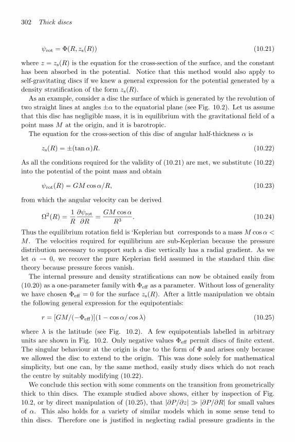
302 Thick discs

ψrot = Φ(R, zs(R)) (10.21)

where z = zs(R) is the equation for the cross-section of the surface, and the constanthas been absorbed in the potential. Notice that this method would also apply toself-gravitating discs if we knew a general expression for the potential generated by adensity stratification of the form zs(R).

As an example, consider a disc the surface of which is generated by the revolution oftwo straight lines at angles ±α to the equatorial plane (see Fig. 10.2). Let us assumethat this disc has negligible mass, it is in equilibrium with the gravitational field of apoint mass M at the origin, and it is barotropic.

The equation for the cross-section of this disc of angular half-thickness α is

zs(R) = ±(tan α)R. (10.22)

As all the conditions required for the validity of (10.21) are met, we substitute (10.22)into the potential of the point mass and obtain

ψrot(R) = GM cos α/R, (10.23)

from which the angular velocity can be derived

Ω2(R) =1R

∂ψrot∂R

=GM cos α

R3. (10.24)

Thus the equilibrium rotation field is ‘Keplerian’ but corresponds to a mass M cos α <

M . The velocities required for equilibrium are sub-Keplerian because the pressuredistribution necessary to support such a disc vertically has a radial gradient. As welet α → 0, we recover the pure Keplerian field assumed in the standard thin disctheory because pressure forces vanish.

The internal pressure and density stratifications can now be obtained easily from(10.20) as a one-parameter family with Φeff as a parameter. Without loss of generalitywe have chosen Φeff = 0 for the surface zs(R). After a little manipulation we obtainthe following general expression for the equipotentials:

r = [GM/(−Φeff)](1 − cos α/ cos λ) (10.25)

where λ is the latitude (see Fig. 10.2). A few equipotentials labelled in arbitraryunits are shown in Fig. 10.2. Only negative values Φeff permit discs of finite extent.The singular behaviour at the origin is due to the form of Φ and arises only becausewe allowed the disc to extend to the origin. This was done solely for mathematicalsimplicity, but one can, by the same method, easily study discs which do not reachthe centre by suitably modifying (10.22).

We conclude this section with some comments on the transition from geometricallythick to thin discs. The example studied above shows, either by inspection of Fig.10.2, or by direct manipulation of (10.25), that |∂P/∂z| |∂P/∂R| for small valuesof α. This also holds for a variety of similar models which in some sense tend tothin discs. Therefore one is justified in neglecting radial pressure gradients in the

10.3 The limiting luminosity 303

z

R

Φ eff= 0

Φeff = 0

z s(R)

zs (R)

α

λr

-1-2-3

4 3 2 1

Fig. 10.2. Meridional section (z–R plane) of the equipotentials for a disc with surface given

by zs = ±(tanα)R. Contours are labelled by energy values in arbitrary units. The boundfluid E < 0 is shown shaded.

standard theory while at the same time keeping vertical pressure gradients to obtainthe thickness (cf. Chapter 5).

Clearly, the standard model is not in a strict sense the limit of any single sequence ofthick discs. More physics and additional assumptions would be necessary to constructsuch a sequence and there is no unique way of doing so.

10.3 The limiting luminosity

In Chapter 1 we discussed the maximum luminosity that could be steadily emittedby a spherically symmetrical, non-rotating body: the Eddington limiting luminosityLEdd (equation (1.3)). In this section we shall show that thick discs can exceed thislimit by large factors. This can happen in a large class of thick discs which contain ahollow axial region commonly known as the ‘funnel’. In such regions the centrifugalforce always exceeds gravity and it is mainly the balance between pressure gradientsand rotation that determines the equilibrium. The maximum radiative output in these

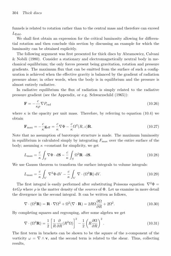
304 Thick discs

funnels is related to rotation rather than to the central mass and therefore can exceedLEdd.

We shall first obtain an expression for the critical luminosity allowing for differen-tial rotation and then conclude this section by discussing an example for which theluminosity can be obtained explicitly.

The following argument was first presented for thick discs by Abramowicz, Calvani& Nobili (1980). Consider a stationary and electromagnetically neutral body in me-chanical equilibrium; the only forces present being gravitation, rotation and pressuregradients. The maximum flux that can be emitted from the surface of such a config-uration is achieved when the effective gravity is balanced by the gradient of radiationpressure alone; in other words, when the body is in equilibrium and the pressure isalmost entirely radiative.

In radiative equilibrium the flux of radiation is simply related to the radiativepressure gradient (see the Appendix, or e.g. Schwarzschild (1965)):

F = − c

κρ∇Prad (10.26)

where κ is the opacity per unit mass. Therefore, by referring to equation (10.4) weobtain

Fmax = − c

κgeff =

c

κ∇Φ − c

κΩ2(R, z)R. (10.27)

Note that no assumption of barotropic structure is made. The maximum luminosityin equilibrium is calculated simply by integrating Fmax over the entire surface of thebody; assuming κ =constant for simplicity, we get

Lmax =c

κ

∫S

∇Φ · dS− c

κ

∫S

Ω2R · dS. (10.28)

We use Gauss’s theorem to transform the surface integrals to volume integrals:

Lmax =c

κ

∫V

∇2Φ dV − c

κ

∫V

∇ · (Ω2R) dV. (10.29)

The first integral is easily performed after substituting Poisson’s equation ∇2Φ =4πGρ where ρ is the matter density of the sources of Φ. Let us examine in more detailthe divergence in the second integral. It can be written as follows,

∇ · (Ω2R) = R · ∇Ω2 + Ω2(∇ ·R) = 2RΩ∂Ω∂R

+ 2Ω2. (10.30)

By completing squares and regrouping, after some algebra we get

∇ · (Ω2R) =12

[1R

∂

∂R(R2Ω)

]2− 1

2

(R

∂Ω∂R

)2

. (10.31)

The first term in brackets can be shown to be the square of the z-component of thevorticity ω = ∇ ∧ v, and the second term is related to the shear. Thus, collectingresults,

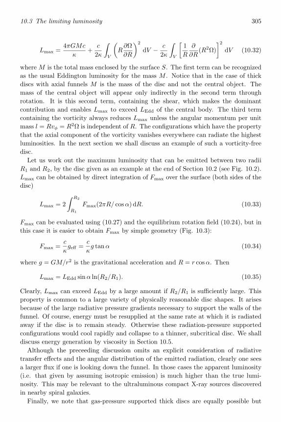
10.3 The limiting luminosity 305

Lmax =4πGMc

κ+

c

2κ

∫V

(R

∂Ω∂R

)2

dV − c

2κ

∫V

[1R

∂

∂R(R2Ω)

]2dV (10.32)

where M is the total mass enclosed by the surface S. The first term can be recognizedas the usual Eddington luminosity for the mass M . Notice that in the case of thickdiscs with axial funnels M is the mass of the disc and not the central object. Themass of the central object will appear only indirectly in the second term throughrotation. It is this second term, containing the shear, which makes the dominantcontribution and enables Lmax to exceed LEdd of the central body. The third termcontaining the vorticity always reduces Lmax unless the angular momentum per unitmass l = Rvφ = R2Ω is independent of R. The configurations which have the propertythat the axial component of the vorticity vanishes everywhere can radiate the highestluminosities. In the next section we shall discuss an example of such a vorticity-freedisc.

Let us work out the maximum luminosity that can be emitted between two radiiR1 and R2, by the disc given as an example at the end of Section 10.2 (see Fig. 10.2).Lmax can be obtained by direct integration of Fmax over the surface (both sides of thedisc)

Lmax = 2∫ R2

R1

Fmax(2πR/ cos α) dR. (10.33)

Fmax can be evaluated using (10.27) and the equilibrium rotation field (10.24), but inthis case it is easier to obtain Fmax by simple geometry (Fig. 10.3):

Fmax =c

κgeff =

c

κg tan α (10.34)

where g = GM/r2 is the gravitational acceleration and R = r cos α. Then

Lmax = LEdd sin α ln(R2/R1). (10.35)

Clearly, Lmax can exceed LEdd by a large amount if R2/R1 is sufficiently large. Thisproperty is common to a large variety of physically reasonable disc shapes. It arisesbecause of the large radiative pressure gradients necessary to support the walls of thefunnel. Of course, energy must be resupplied at the same rate at which it is radiatedaway if the disc is to remain steady. Otherwise these radiation-pressure supportedconfigurations would cool rapidly and collapse to a thinner, subcritical disc. We shalldiscuss energy generation by viscosity in Section 10.5.

Although the preceeding discussion omits an explicit consideration of radiativetransfer effects and the angular distribution of the emitted radiation, clearly one seesa larger flux if one is looking down the funnel. In those cases the apparent luminosity(i.e. that given by assuming isotropic emission) is much higher than the true lumi-nosity. This may be relevant to the ultraluminous compact X-ray sources discoveredin nearby spiral galaxies.

Finally, we note that gas-pressure supported thick discs are equally possible but

306 Thick discs

z

R

R1

R2

α

geffg

Fmax

Fig. 10.3. Relationship between emergent radiative flux and effective surface gravity for

the disc of Fig. 10.2. The luminosity L(R1, R2) emerges through the shaded portions of the

surface.

they are clearly much less luminous. This however need not always be a disadvantage(Section 10.7).

10.4 Newtonian vorticity-free torus

We shall present here a simple model of a thick disc which, although in many respectsunrealistic, illustrates the main features of the subject. It is fair to say at this pointthat a ‘realistic’ model with dissipation driving accretion does not exist at present.Furthermore, the main body of the stability studies so far is confined to barotropictoroidal equilibria in a state of pure rotation with simple power laws of the formΩ(R) ∝ R−q. The vorticity-free tori described here (q = 2) were the first equilibriadiscussed in the literature and the focus of the earliest stability studies (see Section10.6).

Motivated in part by the discussion in the preceding section and by simplicity, weshall consider the equilibrium of a vorticity-free configuration in rotation around a

10.4 Newtonian vorticity-free torus 307

compact object (e.g. a black hole) of mass M , much greater than the disc mass. Byvorticity-free we mean ω = ∇ ∧ v = 0. This implies l = R2Ω = constant through-out and consequently barotropic structure, since ∂Ω/∂z must vanish. We assumeNewtonian dynamics for simplicity. Although this assumption is likely to be violatednear the inner boundary of the disc where l is sufficiently small, some of the mostimportant features remain unaffected.

We can use the methods developed in Section 10.2 to study this system. By virtueof the assumptions made, Ω(R) = lR−2 and there exists an effective potential (seeequations (10.17)–(10.19))

Φeff = −GM

r+

l2

2R2. (10.36)

Φeff turns out to be the energy per unit mass in this case. This is an exclusiveproperty of the l =constant rotation field. The pressure and density stratification issimply obtained by setting Φeff = constant in equation (10.36) and solving for z as afunction of R with parameter Φeff . But before we do so it is convenient to introducesome notation.

Given l, one can always define a Keplerian radius RK such that fluid elementsrotating with the local Keplerian velocity have specific angular momentum l:

l2 = GMRK. (10.37)

We may express all lengths in units of RK, and rewrite (10.36) as follows:

E = 2RKΦeff/GM = (RK/R)2 − 2RK/(R2 + z2)1/2, (10.38)

where E is the specific energy of the fluid in units of the binding energy of a Kepleriancircular orbit of radius RK. For every value of E we have an equipotential (isobaricand isopycnic) surface, the cross-section of which is implicitly given by (10.38). It maybe easily shown from this equation that E reaches its minimum value E = −1 at thecircle R = RK, z = 0. For the fluid to remain bound to the central object we require−1 ≤ E < 0.

From equation (10.38) we may get more explicit forms for the equipotentials. In-troducing the polar angle θ with the usual definition R = r sin θ, we obtain

sin2 θ = R2K/(2rRK + Er2), (10.39)

which is a quadratic equation for r as a function of θ with parameter E. Figure 10.4shows a meridional cross-section through some equipotentials labelled by their E val-ues. The resultant disc is toroidal, with the most tightly bound fluid elements movingaround in an equatorial circle of radius RK. This is also the locus of highest densityand pressure, the actual values of which are still arbitrary. As we move away fromthis limiting equipotential the fluid becomes less tightly bound and the pressure anddensity drop. It can be shown from (10.39) that a given equipotential surface extendsbetween the inner and outer equatorial radii: Rin and Rout respectively. Expressionsfor these may be obtained by solving (10.39) with sin2 θ = 1:

308 Thick discs

-15 -10 -5 5 10 15

-15

-10

-5

5

10

15

z

R

0 0

0 0

-0.1

-0.25

-0.5

1 1

1 1

Fig. 10.4. Meridional cross-section through the equipotentials of the l = constant toroidal

disc discussed in the text. Contours are labelled by the values of dimensionless energy E.

The fluid is bound if E < 0. The dots on the R-axis are at the pressure maximum: R = RK,

z = 0.

Rin = RK[1 + (1 + E)1/2]−1, (10.40)

Rout = RK[1 − (1 + E)1/2]−1. (10.41)

As expected, when E = −1, Rin = Rout = RK, showing that the most tightly boundtoroidal surface degenerates into the equatorial circle of radius RK. When E → 0 onesees that Rin → RK/2 and Rout → ∞. Thus the limiting equipotential for bounddiscs is an open surface. For E > 0 all equipotentials are open (an example is shownin Fig. 10.4 by dotted lines).

An important feature of this disc and other thick disc models is the narrow axialfunnel. Matter in steady rotation supported by pressure can ‘fill’ all equipotentialsup to a small negative value of E. (The precise value of E can be obtained, as inmodels of stellar structure, by providing appropriate boundary conditions and the

10.5 Thick accretion discs 309

mass of the disc.) The resultant configuration is a fat distorted torus with a narrowaxial channel along which large radiation-pressure gradients are set up. This can beseen by direct inspection of Fig. 10.4: near the equator the equipotentials are closelypacked implying large pressure gradients and therefore large fluxes of radiation. Asone moves along the funnel away from the equatorial plane and towards the ‘openings’of the funnel at both ends, the radiative flux emitted by the walls decreases. Thereforethe density of radiation along the funnel is maximal near the equator and falls towardsboth ends. If, as a result of a small viscosity or simply ‘overfilling’, gas drifts into thefunnel, it will either be sucked in by the central object or expelled along the axis byradiation pressure.

We can estimate the aperture of the funnel by differentiating (10.39) with respect tor and finding that the minimum value of θ occurs at r = −RK/E for a given (negative)value of E. Substituting back into (10.39) we obtain

sin2 θmin = −E. (10.42)

If the surface of the disc is the equipotential E then a cone of aperture θmin withvertex at the origin is contained in the funnel and it is tangent to the surface of thedisc (see Fig. 10.5). Thus the collimation provided by the funnel is of the order ofθmin. A narrow funnel requires small |E| and consequently such a funnel is definedby rapidly rotating weakly bound walls. Because the binding energy of material nearthe surface of the funnel is relatively low, it is, in principle, easy for matter entrainedfrom these walls to escape to infinity propelled by radiation pressure. This is thebasic mechanism by which a pair of well-collimated jets in opposite directions couldbe generated by a thick disc.

10.5 Thick accretion discs

So far we have considered the equilibrium of pressure supported rotating fluids in thegravitational field of a central point mass. Such equilibrium models do not allow forradial motions and are not, in principle, ‘accretion’ discs. However, by analogy withthin discs, we can impose certain conditions on the radial motion to guarantee thatthe departures from equilibrium are everywhere small. This should tell us in whichcircumstances equilibrium models may constitute a reasonable approximation to thickaccretion discs.

In the disc model we envisage, the field of motions is dominated by a rapid rotationaround the axis of symmetry specified by the angular momentum distribution l = l(R).Superimposed on this general rotation we allow for a small poloidal velocity vp vφ.This poloidal velocity must have vz ∼ vR in some regions of the disc as a consequenceof the geometry. If viscosity is responsible for a slow radial drift, as in thin discs, wemay assume as a first approximation that the relationship (5.29) derived for α-discsstill holds:

vp ∼ vz ∼ αc2s/vφ ∼ vR ≈ αcs(H/R). (10.43)

310 Thick discs

z

θmin θmin

RK

Fig. 10.5. A perspective view of the axial funnel of semi-aperture θmin generated by a torus

with surface energy E.

Thus the condition of subsonic poloidal motions vp cs ⇒ α 1 imposes a moresevere restriction on α than in the thin case because here H ∼ R. Even if the viscousstresses can be written following the α-prescription (see Section 4.7, equation (4.34)),one expects α to be, in general, a function of both R and z. However, no theoryhas been developed to support a particular choice of viscosity distribution. Modelsin which viscous stresses and poloidal motions are confined either to a thin surfacelayer or to the equatorial plane have been discussed by Paczynski and collaborators(Paczynski (1982)).

Let us assume for the moment that the restriction vp vφ is sufficient to ensurethat the techniques developed in previous sections give us a reasonable approximationto the shape and internal structure of thick discs. There are two main differences fromthe thin disc case that we have to be aware of when we come to build a model.

First, we are free to choose the specific angular momentum distribution (withincertain restrictions based on dynamical equilibrium and stability). As we know frompreceding sections, this determines the shape of the disc and the maximum luminos-ity that can be emitted in radiative equilibrium. By contrast, in the thin disc casethe rotation field is uniquely determined by the balance with gravity. Thus an ex-

10.5 Thick accretion discs 311

tra condition will be necessary to remove this apparent arbitrariness from thick discmodels.

Second, we cannot assume ‘local’ balance of energy, because the heat generated bydissipation can travel in any direction before emerging to the surface. By contrast, in athin disc the geometry is such that vertical gradients dominate and radiative transportis essentially in the z-direction. For thick discs it is easier to impose a global energybalance: in steady state the total luminosity L must equal the total rate of energygeneration by viscosity Lgen.

We shall now discuss this global energy balance in more detail. If the disc at-mosphere can be assumed to be in radiative equilibrium, then the radiative flux is(equation (10.26))

F = − c

κρ∇(1 − β)P, (10.44)

where P is the total pressure and Prad = (1 − β)P following usual notations. Ifβ = 0 the disc is fully supported by radiation pressure and the discussion of Lmax inSection 10.3 applies. If β = constant or more generally if n·∇β = 0 (where n is theunit vector orthogonal to the surfaces P = constant), we can obtain in analogy withequation (10.27) the following expression for the flux of radiation across the surface:

Fn = − c

κ(1 − β)geff =

c

κ(1 − β)(−∇Φ + Ω2R). (10.45)

If the gravitational potential is known a priori (as in the case of negligible self-gravity),all we need to know in order to compute the luminosity is the rotation field on thesurface. Given l(R) we can get the equation of the surface by the methods describedearlier, and we can, in principle, integrate (10.45) over the entire surface to find L:

L = 2∫ Rout

Rin

2πR|Fn|[1 + (dzs/dR)2]1/2 dR, (10.46)

where the factor 2 arises from equatorial symmetry.On the other hand, we must evaluate Lgen. We assume that all the energy is

generated by viscous dissipation. This assumption can always be checked aflerwards:once the density and temperature of the disc are known we can show that nuclearenergy generation is negligible in cases of interest.

By analogy with our discussion of thin discs (see Chapter 5 and Section 4.4 onviscous torques), we introduce the surface density, the accretion rate and the torqueon the material inside a certain radius R:

Σ =∫ zs

−zsρ dz, (10.47)

M =∫ zs

−zs2πRρ(−vR) dz, (10.48)

G = 2πR3 ∂Ω∂R

∫ zs

−zsη dz, (10.49)

312 Thick discs

where zs(R) is the equation of the disc surface and η is the dynamical viscosity.As shown in Section 4.4 (equation 4.28 and following paragraphs), the total rate of

dissipation in a cylindrical shell between radii R and R + dR is given by

dLgen = G(R)(dΩ/dR)dR. (10.50)

This is also valid for thick discs provided that ∂Ω/∂z = 0 or, more generally, ifdissipation and torques due to vertical shear are negligible. The torque can be obtainedfrom the integrated form of angular momentum conservation valid in a steady state(see e.g. equation (5.4) and section 5.3):

G(R) = G0 − M(l − l0); (10.51)

where G0 and l0 are the torque and specific angular momentum at some arbitraryreference radius. (Note that (10.51) reduces to (5.15) with C = −G0 − Ml0.) Thusthe total luminosity generated by viscous dissipation between two arbitrary cylindricalradii R1 and R2 is

Lgen(R1, R2) =∫ R2

R1

(G0 − M(l − l0))(dΩ/dR) dR. (10.52)

To proceed further, we note that after a trivial integration of the constant terms in(10.52) the remainder can be integrated by parts, following the substitution l = R2Ω:∫ R2

R1

R2Ω dΩ =[

12

R2Ω2

]R2

R1

−∫ R2

R1

Ω2R dR. (10.53)

The first term on the right hand side of (10.53) is simply the difference in specifickinetic energies at the two radii, whereas the second term is the corresponding changein ψrot (see equation (10.17)). Collecting results we obtain an expression for theviscous energy generation rate between R1 and R2:

Lgen(R1, R2) =G0(Ω2 − Ω1) + M [l0(Ω2 − Ω1) − 1

2 (v22 − v21) + (ψrot,2 − ψrot,1].(10.54)

When we apply this expression to the whole disc, by taking R1 = Rin and R2 = Rout,since its surface is defined by Φeff =constant (see Section 10.2), we have ψrot,2 −ψrot,1 = Φ2 − Φ1. To eliminate Φ we introduce the energy per unit mass e = 1

2v2 + Φand rewrite (10.54), using v2 = Ωl, as

Lgen ≡ Lgen(Rin, Rout) =Gin(Ωout − Ωin) + M [(eout − ein) − Ωout(lout − lin)]

(10.55)

where the innermost boundary of the disc has been chosen as reference radius. Formost cases, the torque at the inner boundary can be assumed to vanish and alsoloutΩout → 0 as Rout → ∞. Thus for large discs with Rout Rin one has approxi-mately

Lgen = M(−ein). (10.56)

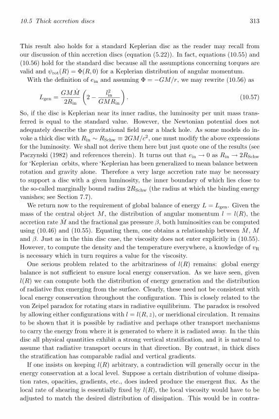
10.5 Thick accretion discs 313

This result also holds for a standard Keplerian disc as the reader may recall fromour discussion of thin accretion discs (equation (5.22)). In fact, equations (10.55) and(10.56) hold for the standard disc because all the assumptions concerning torques arevalid and ψrot(R) = Φ(R, 0) for a Keplerian distribution of angular momentum.

With the definition of ein and assuming Φ = −GM/r, we may rewrite (10.56) as

Lgen =GMM

2Rin

(2 − l2in

GMRin

). (10.57)

So, if the disc is Keplerian near its inner radius, the luminosity per unit mass trans-ferred is equal to the standard value. However, the Newtonian potential does notadequately describe the gravitational field near a black hole. As some models do in-voke a thick disc with Rin ∼ RSchw ≡ 2GM/c2, one must modify the above expressionsfor the luminosity. We shall not derive them here but just quote one of the results (seePaczynski (1982) and references therein). It turns out that ein → 0 as Rin → 2RSchw

for ‘Keplerian’ orbits, where ‘Keplerian’ has been generalized to mean balance betweenrotation and gravity alone. Therefore a very large accretion rate may be necessaryto support a disc with a given luminosity, the inner boundary of which lies close tothe so-called marginally bound radius 2RSchw (the radius at which the binding energyvanishes; see Section 7.7).

We return now to the requirement of global balance of energy L = Lgen. Given themass of the central object M , the distribution of angular momentum l = l(R), theaccretion rate M and the fractional gas pressure β, both luminosities can be computedusing (10.46) and (10.55). Equating them, one obtains a relationship between M , M

and β. Just as in the thin disc case, the viscosity does not enter explicitly in (10.55).However, to compute the density and the temperature everywhere, a knowledge of vRis necessary which in turn requires a value for the viscosity.

One serious problem related to the arbitrariness of l(R) remains: global energybalance is not sufficient to ensure local energy conservation. As we have seen, givenl(R) we can compute both the distribution of energy generation and the distributionof radiative flux emerging from the surface. Clearly, these need not be consistent withlocal energy conservation throughout the configuration. This is closely related to thevon Zeipel paradox for rotating stars in radiative equilibrium. The paradox is resolvedby allowing either configurations with l = l(R, z), or meridional circulation. It remainsto be shown that it is possible by radiative and perhaps other transport mechanismsto carry the energy from where it is generated to where it is radiated away. In the thindisc all physical quantities exhibit a strong vertical stratification, and it is natural toassume that radiative transport occurs in that direction. By contrast, in thick discsthe stratification has comparable radial and vertical gradients.

If one insists on keeping l(R) arbitrary, a contradiction will generally occur in theenergy conservation at a local level. Suppose a certain distribution of volume dissipa-tion rates, opacities, gradients, etc., does indeed produce the emergent flux. As thelocal rate of shearing is essentially fixed by l(R), the local viscosity would have to beadjusted to match the desired distribution of dissipation. This would be in contra-

314 Thick discs

diction, in general, with a viscosity which depends on local density and temperature.Therefore this aspect of the theory of thick discs requires further investigation withthe aim of removing the present arbitrariness of l(R).

10.6 Dynamical stability

The very existence of thick discs was thrown into doubt by the discovery by Papaloizou& Pringle (1984) that the vorticity-free tori described in Section 10.4 are dynamicallyunstable to global non-axisymmetric modes. It would be impossible for such an objectto exist in an equilibrium state in nature since it would be destroyed or drasticallydistorted by the instability during the time over which equilibrium is established. Thisdiscovery stimulated a great number of detailed analytical and numerical studies whichconsidered tori with different rotation laws and entropy distributions. It is impossibleto do justice to all the work done in this field in the space available. The interestedreader should consult review papers by Narayan (1991) and Narayan & Goodman(1989). Here we shall aim to introduce the main concepts, to summarize the currentstatus and to indicate the likely directions of future work.

The term global above in the context of stability studies as opposed to local refersto the fact that the character of the modes and their stability depends on the globalspatial dependence of the eigenmode functions obtained by solving the linearized per-turbation equations subject to appropriate boundary conditions. Unlike local stabilitystudies where only local quantities are involved, a global instability involves a highdegree of coherence over the entire spatial extent of the equilibrium configuration. Atypical non-axisymmetric mode has the form δQ = δQ(R, z)exp(imφ − iωt), whereQ is any of the hydrodynamic quantities (pressure, density, velocities), m ≥ 1 is theazimuthal wave number, and ω is a complex eigenfrequency. The eigenmode equationis a partial differential equation for Q(R, z) on R and z, with ω as the eigenmode,linking spatial dependence and character of the mode. The results of linear studiesare meaningful only when the perturbations remain small. As the mode grows, thelinearized equations no longer describe the evolution correctly and one has to employthe full set of hydrodynamic equations. To follow the evolution of the perturbationsinto the nonlinear regime requires the use of numerical techniques, and some veryinteresting work has already been done, but the details are beyond the scope of thissummary.

Most of the extant stability work is limited to polytropic equilibrium (there-fore barotropic) discs with power law rotation distributions of the form Ω(R) =ΩK(R/RK)−q, with Newtonian gravity entirely dominated by the central object (i.e.non-self-gravitating discs), and in absence of accretion (pure rotational equilibria).Departures from this set of assumptions have also been considered in a few studies.The physical relevant range of rotation power laws stretches from q = 3

2 which yieldsan infinitesimally thin Keplerian accretion disc, to the torus models with q = 2 de-scribed in Section 10.4. The q = 2 models are the thickest tori worth considering since

10.6 Dynamical stability 315

q > 2 violates the well-known local stability criterion for axisymmetric perturbationsdue to Rayleigh. The discs and tori with 3

2 < q ≤ 2 have a pressure maximum at theKeplerian radius RK. The Keplerian disc with q = 3

2 is a degenerate case, and discswith 0 ≤ q < 3

2 have a pressure minimum at RK and require pressure confinement,or have a pressure maximum at the central object and are thus akin to rotating starsand Roche lobe filling equilibria.

Thick discs are divided for descriptive purposes into ‘slender’ and ‘wide’ (or ‘fat’, ifalso H RK) depending on the ratio of the radial width of the disc (Rout − Rin) tothe Keplerian radius RK. The stability studies soon revealed that in slender tori themodes were to a very good approximation independent of z. This simplified the sta-bility analysis considerably, reducing it to a two-dimensional problem with cylindricalsymmetry. Such configurations are termed ‘annuli’ in the literature and their stabilityhas been extensively studied. In fact, most of the nonlinear calculations have beendevoted to annuli, and they have shown that the instability results in fragmentationof the annulus into several blobs or ‘planets’. The term ‘tori’ is henceforth used todescribe true three-dimensional thick discs.

The main results of the stability studies can be summarized as follows. Slenderannuli and tori are very similar in their stability properties. The so-called ‘principalbranch’ modes are the fastest growing modes with Im(ω) ∼ 0.3ΩK whose patternspeed is equal to ΩK thus with ’corotation radius’ Rc = RK. These modes are two-dimensional even in tori, they appear whenever q ≥ √

3, for any polytropic index,and for lower m they grow faster. There exist also higher order modes with slowergrowth rates, which persist for rotation power laws flatter than q =

√3. Numerical

simulations of the nonlinear development show that both slender annuli and slendertori break up into m planets. For wide annuli, the principal branch becomes stableat higher values of q and is stable even for q = 2 if the annulus is sufficiently wide.However, the higher order modes do survive and, although their growth rates aresomewhat lower, they are still dynamical. In wide tori the principal branch is stableand the surviving higher order modes are clearly three-dimensional, particularly nearthe outer radius where the eigenfunctions have many nodes. Numerical integrationsof the initial value problem for the linear stability equations indicate that very widetori become stable even for higher order modes as (Rout−Rin)/RK → ∞. This resultis potentially very interesting since the tori expected in AGNs should be extremelyfat. However, these results must be confirmed by further simulations, since effects ofnumerical dissipation might mimic stability.

Other stabilizing effects studied in the literature include self-gravity and accretionflows. Self-gravity reduces the strength of the principal branch but higher order modessurvive in slender tori. Also new instabilities – probably related to fission – appear inthe self-gravitating case. Concerning the effects of accretion, a very interesting resultwas obtained by studying an annulus in a pseudo-Newtonian potential which simulatesvery well several relativistic effects. It is possible to set up an annulus whose innerradius is smaller than the radius of a critical ‘cusp’ radius such that accretion on tothe central object occurs without any viscosity. This is analogous in some respects to

316 Thick discs

Roche lobe overflow in binaries. It was found that a relatively small rate of accretionwas sufficient to completely stabilize all modes. The physical explanation for thiseffect is still a matter of some debate and it remains to be seen if the effect is alsopresent in tori. In fact, according to some physical interpretations of this effect, itsexpected influence on unstable modes in tori should be weaker. At this point this isstill an open question.

Thus, the most interesting tori astrophysically – at least in the context of AGNtheory – are likely to be fat accretion tori with q ∼= 2. As we have seen, q = 2 is themost violently unstable rotation law for pure rotation equilibrium models. Yet ana-lytical and numerical calculations have shown the stabilizing effects of radial motionand three-dimensional geometry. We are still far from being able to simulate numeri-cally a ‘realistic’ torus model, but future studies of this problem will probably involvelarge scale numerical simulations of the nonlinear evolution of fat tori including theeffects of magnetic fields and poloidal motions. The focus of the numerical simula-tions conducted in recent years has shifted to magnetohydrodynamic simulations ofthe advection-dominated flows described in Chapter 11 rather than tori but the twotypes of flow are closely related. There are severe limitations of resolution and dynam-ical range which make progress difficult, but the rapid development in computationalhardware and our ability to program on massively parallel platforms offer hope ofsignificant progress ahead. The rewards might include a better understanding of thecentral engine in AGNs and the origin of viscosity in discs.

10.7 Astrophysical implications

Originally the attraction of thick disc models in the context of AGN theory stemmedfrom the ability of these discs to generate the energy by accretion and to collimatea substantial fraction of this energy into narrow jets. It was thought initially thatthese jets could be accelerated by the strong radiation pressure gradients along thefunnel. When this idea was examined in detail by modelling numerically the motionof test particles in the funnels of l = const discs, the results were disappointing. Thecalculations show that a light optically thin plasma composed entirely of electronsand positrons could not be accelerated beyond Lorentz factors γ ∼ 3. When a smallfraction of protons was mixed in, then the terminal speeds dropped to v ∼ 0.4c. Thisis too slow for models of superluminal expansion where values of γ from 5 to 10 havebeen invoked (Section 9.3).

Although optically thick jets have not been sufficiently studied, it appears thatradiatively accelerated jets cannot achieve the velocities required by observations ofsuperluminal expansion. It has also been pointed out in the meantime that Comptondrag by disc radiation would limit the achievable plasma terminal Lorentz factors evenif some effective acceleration mechanism existed. Recently, the investigations of jetacceleration have favoured hydromagnetic mechanisms, but a definitive model has notemerged yet. Assuming there is a mechanism generating ultrarelativistic jets near the

10.7 Astrophysical implications 317

central black hole, model calculations have shown that Compton drag in the funnels ofa thick disc would decelerate the jets to values consistent with superluminal expansion.

In our discussion of the equilibrium equations we neglected the pressure of theradiation emitted by one side of the funnel on the opposite side. By analogy withbinaries, this effect has been termed the reflection effect. The treatments of thiseffect in the literature include analytic estimates and iterative numerical procedures.In general it is possible to balance the component of the radiative force normal tothe surface of the funnel but leaving tangential components unbalanced. Thereforeatmospheric layers of the funnel could be accelerated and mixed into the jet material.Once radiative effects get the outer layers of the funnel in motion more material islikely to be entrained by hydrodynamical instabilities. Thus the assumption of anempty funnel – both for calculations of jet acceleration and for the reflection effect –is probably wrong and deserves further study.

The spectrum emitted by a thick disc can be calculated in analogy with thin discsby adding local blackbody contributions, allowing for simple opacity effects whichshift the spectrum to slightly higher effective temperatures. The reflection effect inthe funnels also raises the effective temperature when one looks down the funnel andComptonization of ambient radiation by relativistic jet electrons will likely producesoft X-rays. It has been proposed that the soft X-ray excesses in some optically selectedradio quiet QSOs could be due to this effect. In this picture, when the accretion torusis viewed at high inclination (i.e. nearly perpendicular to the jet axis) an optical/UVbump is observed, whereas at low inclinations an excess in the UV/soft X-ray band isdetected.

Another interesting application of tori models makes use of the angular distributionof ionizing due to the funnel mechanisms already mentioned to explain the alignmentof extended emission line regions with radio and optical structures in Seyfert galaxies.Using the spectrum of ionizing radiation emerging along the funnel it has been shownusing detailed ionization codes that it is possible to get good fits to observed emissionline spectra.

The low efficiency of conversion of mass into energy in most models of accretiontori (Section 10.5) implies that a large amount of ‘dead’ mass must accumulate in thecentral object over the lifetime of an AGN. If quasars occur during early phases ofgalactic evolution then it should be possible to detect massive remnants of an activephase in nearby ‘normal’ galaxies (Section 7.4). Current observational limits on blackhole masses seem to be consistent with efficiencies ∼ 10% but much lower values wouldpose serious problems.

A number of difficulties can be alleviated if we abandon the requirement that thehigh luminosities and the collimation rise jointly from the thick disc without extraingredients. If we consider a thick disc supported by gas pressure, then we no longerhave large unbalanced radiative forces in the funnel and we can deal with the energeticsof the jet and the disc separately. Two-temperature plasma tori supported by ionpressure can exist if the electrons and ions are not coupled effectively by collisions(Rees et al. (1982)). These ion tori emit a relatively small fraction of their luminosity

318 Thick discs

in directions other than the funnel in agreement with observations of double radiosources with relatively weak core luminosities. Work on plasma instabilities suggestshowever that electrons and ions might couple effectively even if collisions are inefficient.Again, the focus of work in these areas shifted in the mid-nineties to the advection-dominated flows discussed in Chapter 11.

The problem with energy balance in radiation pressure dominated tori mentionedin Section 10.5 has not been addressed properly yet. As in radiatively supportedrotating stars, it is likely that a large scale meridional circulation will be driven bythe thermal imbalances. Because of the high rotational velocities involved in tori, itis likely that these circulations are dynamically important and have an effect on thestability properties of thick discs. Another possibility which has remained entirelyunexplored consists of baroclinic equilibria with Ω = Ω(R, z). Neither the equilibriumproperties nor the stability of these configurations has been studied. Nature may haveways of setting up thick discs somewhat different or maybe even radically differentfrom what theorists have been able to come up with so far. The study of thick discsis still in its infancy and perhaps the astrophysically more interesting insights still lieahead.

Despite the theoretical uncertainties involved in the structure and stability of thickdiscs, which make it unclear whether these models are relevant to astrophysical objects,there are clearly a number of areas worth further study. In addition to those we havealready mentioned, possible applications of the theoretical ideas developed in thecourse of these studies include pressure supported discs formed during early stages ofmassive star formation, merging of double degenerate binary stars, bipolar outflows inyoung stellar objects, generation of jets in objects such as SS 433, planet formation,fission of protostellar clouds, and last but not least, the origin of viscosity in accretiondiscs. In this chapter we have confined ourselves to thick discs which have very littleor no poloidal motion and are thus closer to toroidal equilibria rather than accretionflows. In Chapter 11 we remove this restriction and allow for the effects of significantradial motion and meridional circulation.

11 Accretion flows

11.1 Introduction

We have seen in the foregoing chapters that a huge variety of accretion flows are at leasttheoretically possible. The equations describing axially symmetric flows with gravity,pressure and rotation allow a wide array of solutions of astrophysical interest. If oneincludes Ω = 0 (no rotation) as a special case, then even ordinary stars and sphericallysymmetrical Bondi accretion are solutions. More realistically, accretion flows with lowangular momentum may produce supersonic flows which shock at smaller radii if theylack pressure support, or produce settling, cooling solutions if partially supported bypressure. We have already studied in detail spherically symmetrical accretion, thestandard thin disc, and thick discs, and we will study other solutions which haveacquired recognition in the astrophysical literature, such as slim discs and advectiondominated accretion flows (ADAFs). In this chapter we shall attempt to organize allthe different solutions into a coherent picture in order to clarify their relation to eachother.

The fact that black holes possess an event horizon instead of a hard surface makesthe inner boundary condition for black hole accretion flows qualitatively different fromthat for a normal star, and allows the existence of a family of solutions in which asignificant fraction of the dissipated energy is advected through the horizon. Hence,for an external distant observer, ADAFs on to black holes are characterized by a lowradiative efficiency η. (In ADAFs on to objects with a hard surface the advected energymust be ultimately reprocessed and released near the surface – see Section 11.8.3.) Lowradiative efficiencies may occur either because the accretion rate is sufficiently smallthat the inflowing gas has low density and is unable to cool, or because the accretionrate and gas density are so high that the flow is extremely optically thick so thatradiation is trapped and dragged down the hole. The former case occurs at accretionrates much smaller than the Eddington critical rate, almost all the energy resides inthe ions and the coupling to electrons is so weak that very little radiation is emitted.In the latter case, the black hole may accrete at well above the Eddington critical rateand yet produce a sub-Eddington luminosity because the emitted radiation is trapped.

320 Accretion flows

11.2 The equations

We shall start by writing down more general equations governing steady axisymmetricaccretion flows in cylindrical coordinates than those studied in Chapter 10, where onlypure rotations were explicitly allowed. Generalizing the treatment given in Chapter10 we formally split the local fluid velocity in two parts: an azimuthal or toroidalcomponent entirely due to rotation vt = vφ = RΩ, plus a small poloidal componentvp = (vR, vz). In pure rotation (cf. equation (10.1)), the poloidal velocity vanishes.Because of the assumed axial symmetry, ∇ = ∇p has only poloidal components, andthe remaining terms in the momentum equation can be written

(vp · ∇)vp = −1ρ∇P −∇Φ + Ω2R+ (∇ · σ)p = −1

ρ∇P + geff + (∇ · σ)p ,(11.1)

for the poloidal component; and

(vp · ∇)vt +vRvt

R= (∇ · σ)t , (11.2)

for the toroidal component. In the above equations the quantity σ is the stress tensor(see below), so (∇ · σ)p,t stands for the poloidal and toroidal components of theviscous terms whose explicit form will be discussed later. It is immediately clearfrom equation (11.2) that without these viscous terms the poloidal component wouldvanish. This re-emphasizes the connection between accretion and viscosity we havealready encountered in Chapter 5. We see also that if the viscous terms are small, thepoloidal (accretion) velocity is small; if they can be all neglected in equation (11.1),we recover the case of thick discs in pure rotation (cf. (10.4)).

We now write the mass and momentum and conservation equations explicitly incylindrical coordinates. We estimate the relative magnitudes of the various termsunder assumptions appropriate for accretion discs, and finally discuss suitable ap-proximations for the energy conservation equation. For general derivations of theseequations we refer the reader to the textbooks on viscous and compressible fluid dy-namics by Thompson (1972), and O’Neill and Chorlton (1989). The continuity ormass conservation equation reads

1R

∂

∂R(ρRvR) +

∂

∂z(ρvz) = 0 . (11.3)

The three components of the momentum equation are

vR∂vR∂R

+vz∂vR∂z

= (Ω2−Ω2K)R−1

ρ

∂P

∂R+

1ρ

[∂σRR∂R

+σRR − σφφ

R+

∂σRz∂z

].(11.4)

vR∂vz∂R

+ vz∂vz∂z

= −Ω2Kz − 1

ρ

∂P

∂z+

1ρ

[1R

∂(RσRz)∂R

+∂σzz∂z

]. (11.5)

vRR

∂(R2Ω)∂R

+ vz∂(RΩ)

∂z=

1ρ

[1

R2

∂(R2σRφ)∂R

+∂σφ,z∂R

], (11.6)

11.2 The equations 321

where we have written Ω2K = GM/r3, with r being the spherical radius for the gravity

terms. Later on we shall use the same symbol for the Keplerian rotation rate Ω2K =

GM/R3. We adopt for simplicity the so-called Stokes hypothesis, according to whichthe bulk viscosity vanishes; a result that holds exactly for monoatomic gases andis generally valid outside of strong waves (e.g. shock waves). Then, in cylindricalcoordinates and under axial symmetry, the components of the stress tensor can bewritten

σRφ = σφR = µR∂Ω∂R

,

σRz = σzR = µ

(∂vz∂R

+∂vR∂z

),

σφz = σzφ = µ∂(RΩ)

∂z,

(11.7)

σRR = 2µ∂vR∂R

, σzz = 2µ∂vz∂z

, σφφ = 2µvRR

(11.8)

where µ = ρν is the dynamic viscosity. With the above expressions for the viscousstress tensor one can write out explicitly the components of the momentum equation.First, we discuss the order of magnitude of the various terms. In strict cylindricalsymmetry vz = 0 and ∂/∂z = 0. More realistically one can assume vz ∼ (H/R)vRand ∂/∂z ∼ (H/R)∂/∂R (with the possible exceptions of surface and boundary layers).With these approximations we can neglect all terms containing vz and z derivativesin the R-equation, keeping in mind that they may become comparable to vR termswhen the disc is geometrically thick. Thus the radial momentum equation reduces to

vR∂vR∂R

= (Ω2 − Ω2K)R − 1

ρ

∂P

∂R+

2ρ

[∂

∂R

(µ

∂vR∂R

)+ µ

∂

∂R

(vRR

)]. (11.9)

The remaining viscous terms are of the same order as the advective term on the l.h.sabove and may become dominant when there is a viscous boundary layer. Thus theviscous terms in the radial equation should not be neglected a priori when the advec-tion term is kept. Fortunately both the advection term and the viscous accelerationsare a factor (αcs/vK)2 smaller than the pressure gradients and thus thin disc solutionswith quasi-Keplerian rotation such as the standard solution are possible. Even in moregeneral solutions such as the slim discs discussed in Section 11.3, these troublesometerms are small except in the vicinity of sonic points and boundary layers. Under sim-ilar assumptions and caveats as for the R-equation, the lowest order terms remainingin the z-equation are

vR∂vz∂R

= −Ω2Kz − 1

ρ

∂P

∂z+

1ρR

∂

∂R

[µR

(∂vR∂z

+∂vz∂R

)]. (11.10)

Note that unlike vertical velocity gradients, the vertical pressure gradient is not negli-gible because we expect P to decrease from a maximum at the midplane to near zerovalues over the disc thickness. The advective term on the l.h.s. of (11.10) is againof the same order as the remaining viscous term but they are both smaller than the

322 Accretion flows

gravity and pressure gradient term by a factor ∼ (vR/vK)2 and are thus negligible inmost situations where angular momentum is important. Therefore the z-momentumequation reduces under fairly general circumstances to the usual vertical hydrostaticbalance. With similar considerations the angular momentum conservation equation(11.6) reduces to

vRR

∂(R2Ω)∂R

+ vz∂(RΩ)

∂z=

1ρR2

∂

∂R

(µR3 ∂Ω

∂R

)+

1ρ

∂σφ,z∂R

. (11.11)

We note the appearance of two terms representing the vertical advection of angularmomentum and the stresses due to vertical shear. These terms vanish exactly if thefluid rotates on cylinders, as in the case of barotropic discs and the standard thin discsolution, and are negligible in many other cases. With our assumptions above theyare at most ∼ (H/R)2 times the dominant terms.

Assuming that thermal conduction is negligible, and defining qadv as the net energyadvection rate per unit volume, we write down the energy equation in an apparentlysimple form as follows

qadv = ρvRTds

dR= q+ − q− , (11.12)

where s is the specific entropy, q+ and q− are the volume heating and cooling ratesrespectively, and we have already neglected the vertical advection of energy in accor-dance with the approximations adopted for the other equations. The formal simplicityof the r.h.s. hides a number of complications, some of which will be addressed later,but immediately allows a simple classification of the possible solutions depending onwhich of the three terms is negligible compared to the remaining two:

(i) qadv q+ ∼= q−: Cooling-dominated accretion flows including the standardsolution and the Shapiro, Lightman and Eardley solution.

(ii) q− qadv ∼= q+: Advection-dominated accretion flows (ADAFs), includingslim discs and optically thin similarity solutions (see below).

(iii) q+ q− ∼= −qadv: Cooling flows, including low angular momentum settlingsolutions and optically thin Bondi accretion.

In the following we assume that viscous dissipation is the only energy source in theflow, so we equate q+ to the dissipation function (Thompson (1972)) and write

q+ =1

2µσ · σ − (γ − 1)(∇ · v)2 ∼= µσ2rφ = ρνR2

(dΩdR

)2

(11.13)

where, following previous approximations, we have kept just the dominant terms.The volume cooling rate can be written in a variety of ways depending on the phys-

ical situation. For an optically thin tenuous plasma cooling by two-body processes,one may take generally

q− = neniΛ(Te) (11.14)

11.3 Vertically integrated equations – slim discs 323

where ne and ni are the number densities of electrons and ions, Te is the electrontemperature, and Λ(Te) is the cooling function (e.g. for non–relativistic free–free cool-ing Λ ∝ T

1/2e ). For optically thick situations it is in principle impossible to write a

closed local expression for the cooling rate. Formally one could equate q− = ∇ · Fwhere F is the frequency integrated flux of radiation which can only be obtained aftersolving a radiative transfer problem with appropriate boundary conditions. However,one can write approximate expressions a posteriori in some simple cases. For examplein the case of thin discs, assuming that the radiation escapes through the top andbottom surfaces of the disc, one may take q− = σT 4

eff/2H. The effective temperatureis obtainable in terms of the midplane temperature and the optical depth τ (Section5.4), but clearly this procedure is more meaningful when one uses vertically integratedrates rather than local values. Another case where local treatment is possible ariseswhen radiation pressure and electron scattering dominate, since one can take the fluxas given by the local radiation pressure gradient F = −(mc/ρσT)∇P .

One of the earliest discussions of accretion flows taking into account the effects ofadvection was effectively contained in Begelman (1978) where the concept of trappingradius (see Section 7.8) was introduced. In a subsequent paper by Begelman & Meier(1982) the first discussion of two-dimensional similarity solutions (assuming only axialsymmetry) incorporating the effects of optically thick advection was presented. How-ever, the relative complexity of the solutions obtained prevented simple applicationsto observations.

11.3 Vertically integrated equations – slim discs

While the general treatment of accretion flows, even under the assumption of axisym-metry, requires at least a study of the solutions to two-dimensional equations, mostof the progress over the past decade has been based on eliminating the z-componentby some form of vertical integration. We shall first discuss the equations obtained bystraightforward vertical integration along the z-direction and then comment on oneother version in which one integrates along spherical shells. Each averaging procedurehas subtleties which we shall gloss over here because they introduce constants ∼ 1 andultimately do not change the qualitative behaviour of the solutions.

The continuity equation (11.3) can be integrated exactly without any assumptionsabout the magnitude of vz, as long as ρvz vanishes at large distances from the midplaneof the disc (z = 0), which is physically very reasonable. One further natural assump-tion for discs is that of symmetry about the plane z = 0. The resulting equation maythen be immediately integrated radially as well to yield the usual form

M = −2πRvRΣ , (11.15)

where Σ = 2Hρ is the surface density, ρ is the midplane density, and vR is now asuitably defined average radial velocity.

The height-integrated radial momentum, neglecting viscous terms, becomes

324 Accretion flows

vRdvRdR

= (Ω2 − Ω2K)R − 1

Σd

dR(Σc2s ) (11.16)

where cs is here a suitably defined average sound speed. For the vertical hydrostaticbalance we take H = csΩ−1

K . Multiplying through the angular momentum equation(11.11) by ρR2, retaining only the dominant terms, and integrating vertically yields

[ΣR(−vR)

] ddR

(R2Ω) = − ddR

(ΣνR3 dΩ

dR

), (11.17)

where Σν =∫

µdz, with µ being the dynamic viscosity, defines a vertically averagedkinematic viscosity. Since the factor in square brackets on the l.h.s. of the aboveequation is constant because of mass conservation, we may now easily integrate withrespect to the radius once, obtaining

−νR2 dΩdR

= (−vR)(l − lin) (11.18)

where l = R2Ω stands for the specific angular momentum at radius R and lin is thevalue at the inner radius. In obtaining the above result we adopted the standardassumption that the torque is zero at the inner boundary of the disc. We may noweliminate the radial velocity making use of mass conservation, to obtain finally

−2πνΣd ln Ωd ln R

= M

(1 − lin

l

). (11.19)

We write the vertically integrated energy equation in terms of the advection, viscousheating and radiative cooling rates per unit surface formally

Qadv = Q+ − Q− . (11.20)

The viscous disspation rate is

Q+ = νΣ(

RdΩdR

)2

, (11.21)

and the advection rate is given by

Qadv =ΣvRR

Tcds

d ln R=

M

2πR2c2s ξ , (11.22)

where Tc is the local mid-plane temperature and ξ is in general a slowly varyingquantity related to the logarithmic entropy gradient which is ∼ 1 except near theradial boundaries of the flow. In similarity solutions it is a constant weakly dependenton the assumed fraction – also constant – of energy carried by advective transport.

The first self-consistent treatment of accretion discs carrying a near Eddington crit-ical accretion rate was given by Abramowicz et al. (1988) using equations very similarto the ones described above, assuming optically thick cooling with electron scatter-ing and free–free opacities. The geometrical thickness of the solutions so obtained issmall for small accretion rates and approaches H ∼ R as the accretion rate becomescomparable to the Eddington critical rate. Because they represent in this sense a

11.4 A unified description of steady accretion flows 325

regime intermediate between the standard thin disc and thick discs these solutionswere termed ‘slim’ accretion discs (see Section 9.5).

11.4 A unified description of steady accretion flows

In this section we show how a simple treatment of vertically averaged discs yields mostof the disc solutions in the literature and reveals their mutual relationships and theirstability. The treatment presented here is based on a paper by Chen et al. (1995)where the interested reader can find details omitted here and further references. Al-though a black hole is the only accreting object capable of advecting away a significantfraction of the liberated energy, the discussion given below for radiative solutions alsoholds for other accreting objects. To include relativistic effects important for blackholes and neutron stars in an approximate way, we assume a pseudo-Newtonian po-tential Φ = −GM/(r−RS) where r is the spherical radius and RS is the Schwarzschildradius of the central object. The radial momentum conservation equation (11.16) im-plies that a cold non-self-gravitating disc in this potential will be geometrically thinand rotate locally with Keplerian velocity v2K/R = Ω2

KR = −(∂Φ/∂R)z=0. If we re-strict ourselves to geometrically thin (H R) or at most slim discs (H ∼< R), thenthe local rotation Ω(R) is approximately Keplerian. Under these assumptions verticalhydrostatic equilibrium implies that H ∼= cs/Ω. Our starting point will be the remain-ing three basic steady-state conservation equations for mass, angular momentum andenergy, which we write in the following form (see Section 11.3)

M = −2πRΣvr mass conservation (11.23)

M = 3πνΣg/f∗ angular momentum conservation (11.24)

Q+ = Q− + Qadv energy conservation (11.25)

where ν = αcsH = αc2s/ΩK is the local kinematic viscosity, f∗ = 1−9Ω∗/[Ω(R/RS)2],with Ω∗ = ΩK(3RS), is a function (cf. equation (5.19)) which is close to unity every-where except near the inner boundary, and g = − 2

3 (d ln Ω/d ln R). The heating rateper unit surface due to viscous dissipation can be written in terms of the accretionrate as

Q+ =3M

4πΩ2f∗g . (11.26)

The net rate at which advection carries energy inward can also be written as a coolingrate per unit surface as follows

Qadv = −ΣvrR

p

ρξ =

M

2πR2

p

ρξ , (11.27)

where ξ is related to the logarithmic entropy gradient and is close to unity away fromboundaries. The explicit form of ξ does not concern us here, but in general it is afunction of gas parameters such as the ratio of specific heats γ and of the relative

326 Accretion flows

contributions of radiation and magnetic fields to the total pressure. The rate of localradiative cooling per unit surface can have a more or less complex form depending onwhether the disc material is optically thin or thick and on the physical effects included,but in its simplest version, valid for optically thick emission, (as in the standard thindisc solution) it can be written (see Section 5.4)

Q− =4σT 4

c

3τ=

4σT 4c

3κRΣ, (11.28)

where τ is the optical depth to the mid-plane of the disc, κR is the Rosseland meanopacity, and Tc is the central temperature of the disc. In order to discuss all thepossible solutions to the above steady-state solutions and their stability it has becomecustomary to display these solutions on the local (M, Σ)-plane (i.e. at a fixed radius)because the slopes of the solutions immediately reveal their viscous stability properties(Section 5.8) and with only a little extra work one can also deduce graphically theirthermal stability. The discussion can be made approximately independent of the massof the central object by measuring radial distances in units of the Schwarzschild radiusRS and accretion rates in units of the corresponding (critical) Eddington rate MEdd.Figure 11.1 shows the situation at some arbitrarily chosen radius. For our limited goalof giving a qualitative discussion of the possible types of flows and their properties, wehave deliberately left the units on the axes arbitrary since numerical values vary withradius, and the quantitative details are somewhat model dependent. However, theportion of the plane shown spans about six orders of magnitude in both axes so thatthe slopes displayed are meaningful. For typical models at radii ∼< 102RS, the pointat which the thick lines labelled α = αcrit cross one another occurs at accretion rates0.1 ∼< M/MEdd ∼< 10 and surface densities 1 ∼< Σ(g/cm2) ∼< 102. This intersection(Σcrit(R), Mcrit(R)/MEdd plays a critical role in determining which types of solutionare possible at a given radius R.

On this plane the solutions of the three steady state conservation equations arerepresented by curves linking the accretion rate to the local surface density. Becausethe energy equation can be satisfied in different ways depending on the relative im-portance of advection and radiative cooling, and depending on whether the flow isoptically thick or thin, there are in general several solutions at different values of Σfor a given accretion rate. Also for a given surface density, vertical balance can beachieved for different values of the density and temperature depending on whethergas pressure or radiation pressure dominates. Thus there exist in general several so-lutions at fixed Σ with different M/MEdd. Joining the various possible solutions oneobtains the curves shown. As long as the physical regime remains the same one tendsto get straight lines for solutions having in common analogous physical conditions be-cause in these asymptotic regimes most physical quantities approximately obey powerlaws. Therefore one may consider the solution curves as made up of various rectilinear‘branches’ along which physical conditions remain more or less the same (see below).

We derive some examples to illustrate these points, starting with the standardoptically thick solution dominated by gas pressure and radiative cooling. The sound

11.4 A unified description of steady accretion flows 327

speed is in this case c2s = kTc/µmp, the optical thickness can be written τ = κRΣ,and the kinematic viscosity is ν ∼ αc2s/Ω. The energy equation (11.25) shows thatat a given radius c2s ∝ (κRΣM)1/4. Using this last result in the expression for ν andsubstituting into equation (11.23), it is easy to show that

M ∝ α4/3κ1/3R Σ5/3 (11.29)

for the standard solutions shown on Fig. 11.1 for different values of α. The scalingswith other parameters can also be obtained in this way but have been omitted herefor simplicity. The slope of 5/3 derived above holds for electron scattering dominatedsituations since κR = κT is constant. If the physical conditions are such that theKramers approximation is valid, then κR ∝ ρT

−7/2c ∝ ΣT

−7/2c cs/Ω, and solving for M

one obtains

M ∝ α8/7Σ10/7 , (11.30)

which could have been obtained also from the first of the standard solution equations(5.49) derived in Section 5.6.

Another case yielded by this simple analysis is the gas pressure or radiation pressuresupported, advectively cooled solution. We assume that in either case the soundspeed is c2s = P/ρ, where P is the total pressure, and that the viscosity is as beforeν ∼ αc2s/Ω. In principle it matters whether the gas is optically thin or thick, sincethis property together with the viscosity ultimately determines whether advection isimportant or not. But if we assume ab initio that advection dominates we do not needto worry about the optical thickness of the flow and may simply write Q+ = Qadv forthe energy equation. Again since gas pressure dominates we have c2s = kTc/µmp, andthe above energy equation yields c2s = 3v2K/2ξ ∼ constant at a given radius. Thenangular momentum conservation (equation (11.24)) yields

M ∝ αΣ . (11.31)

These solutions are shown in Fig. 11.1 as branches of slope unity. At high accretionrates M/MEdd these solutions are optically thick whereas at low M/MEdd they areoptically thin, since the local column density varies proportionally. Therefore theupper branches of the advection-dominated cases correspond to the slim disc solutionsdiscovered by Abramowicz et al. (1988) for near critical and supercritical accretionrates, whereas the lower branches are the optically thin advection dominated discsdiscussed in Abramowicz et al. (1995) and Narayan and Yi (1995b) for subcriticalaccretion rates. The related similarity flows (Narayan and Yi (1994,1995a)) discussedin Section 11.6 also satisfy M ∝ αΣ and are valid for any accretion rate or opticalthickness.

Another situation which can be treated under some simple assumptions is the op-tically thin, gas pressure dominated, radiatively cooled case. If we assume that theonly cooling mechanism is free–free emission (thermal bremsstrahlung), we may writeQ− = 2HAffρ2T

1/2e = AffΣ2T

1/2e Ω/2cs, where we have assumed a one-temperature

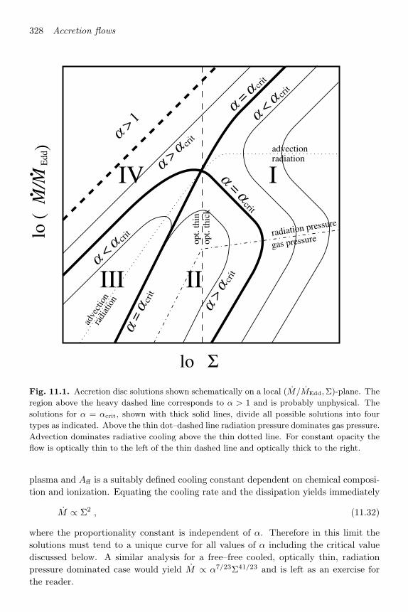
328 Accretion flows

log Σ

log

(M/M

Edd

)

.

.

α > 1

α <α crit

α <α crit

α=

α crit

α =α crit

α=α

crit

α >α crit

α>

α crit

I

III

IV

II

advectionradiation

adve

ctio

nra

diat

ion

radiation pressure

gas pressureopt.

thin

opt.

thic

k

Fig. 11.1. Accretion disc solutions shown schematically on a local (M/MEdd,Σ)-plane. The

region above the heavy dashed line corresponds to α > 1 and is probably unphysical. The

solutions for α = αcrit, shown with thick solid lines, divide all possible solutions into four

types as indicated. Above the thin dot–dashed line radiation pressure dominates gas pressure.

Advection dominates radiative cooling above the thin dotted line. For constant opacity the

flow is optically thin to the left of the thin dashed line and optically thick to the right.

plasma and Aff is a suitably defined cooling constant dependent on chemical composi-tion and ionization. Equating the cooling rate and the dissipation yields immediately

M ∝ Σ2 , (11.32)

where the proportionality constant is independent of α. Therefore in this limit thesolutions must tend to a unique curve for all values of α including the critical valuediscussed below. A similar analysis for a free–free cooled, optically thin, radiationpressure dominated case would yield M ∝ α7/23Σ41/23 and is left as an exercise forthe reader.

11.4 A unified description of steady accretion flows 329

(a)

log Σ

log

(M/M

Edd)

α > 1 α < α crit

Type I

Type III

(b)

log Σlo

g (M

/ME

dd)

α > 1

α >α crit

α>

α crit

Type I

V

Type II

Fig. 11.2. Possible local disc solutions at some arbitrary radius are shown schematically

for (a) α < αcrit and (b) α > αcrit. Thick lines identify branches which are thermally and

viscously stable. The arrows show the thermal-timescale evolution of a disc annulus which is

not on the local equilibrium curve.

Finally let us consider the case found to be unstable by Lightman and Eardley(1974), in which radiation pressure dominates, the disc remains optically thick andcools by radiation. In this case, the energy equation (11.25) yields as in previousoptically thick cases M ∝ T 4

c /(κRΣ). As long as we remain in the non-relativisticregime, the sound speed is given by c2s = 4σT 4

c /(3ρc) ∝ T 4c cs/(ΣΩ), and one obtains

cs ∝ T 4c /Σ. Using the energy equation, we write cs ∝ κRM , and substituting into the

angular momentum conservation equation (11.24), we finally get

M ∝ (ακ2RΣ)−1 . (11.33)

This is consistent with the relation (5.8) found in Section 5.8 (see problem 11.4).These solutions are shown on Fig. 11.1 as the branches of slope −1. Note that theway solutions with different α values nest into one another is correctly predicted bythe expressions (11.29)–(11.33).

Solution curves have bends as one branch merges into another, usually as the re-sult of a single transition in the physics involved, e.g. moving from a gas pressuredominated solution into a radiation pressure dominated solution or from a radiation-dominated into an advection-dominated situation.

Usually for an arbitrarily chosen α there are two non-intersecting solution curveswith one, two or three branches. At every radius there is one particular value of theviscosity parameter αcrit for which the solution curves intersect at a point (Mcrit, Σcrit).These intersecting αcrit curves thus divide the (M, Σ)-plane into four regions labelledI–IV in the diagram. When α < αcrit, the only solutions possible are of Types I andIII; whereas when α > αcrit, the only solutions possible are of Types II and IV. Thisdichotomy is shown graphically and qualitatively on Figs 11.2(a) and 11.2(b).

330 Accretion flows

α HIG

Hα LO

W

log Σ

log

(M/M

Edd)

.

.

α > 1

α <α crit

α <α crit

α=

α crit

α =α crit

α=α

crit

α >α crit

α>

α crit

Fig. 11.3. Accretion disc solutions shown schematically on a local (M/MEdd,Σ)–plane. A

typical dwarf nova or X-ray transient cycle is shown here spanning two equilibrium curves

labelled αHIGH and αLOW.

The optically thick Type I equilibria shown on Fig. 11.1 have a characteristic S-shape which is reminiscent of the S-curves discussed in the context of the disc insta-bility in Chapter 5. The two S-curves should not be confused: the kink responsiblefor the disc instability yielding dwarf novae and soft X-ray transients is due to ioniza-tion of hydrogen and occurs at accretion rates below the ranges shown on Fig. 11.1.The situation is illustrated schematically and qualitatively on Fig. 11.3. Note thatthe width and relative positions of the two types of kinks will in general depend onradial position. The equilibrium curves for α = constant look more like ξ-curves forthose cases where both kinks occur. A typical outburst cycle in ‘local’ phase plane isshown here for simplicity, switching between two values of viscosity corresponding tothe hot/high and cold/low states (see Section 5.9).

Thin radiative discs with α > αcrit, shown as Type II solutions on Fig 11.2(b), canexist only below a maximum accretion rate (or luminosity), a result anticipated byLiang and Wandel (1991) who analyzed in detail the transition from optically thickto thin flows. At higher accretion rates only hot, geometrically slim or thick ADAFsare possible. Note that the H-ionization kink mentioned above may also appear in thelower branches of Type II solutions, as shown on Fig. 11.3.

11.5 Stability 331

11.5 Stability

We discuss the local stability in general terms without any explicit reference to thewavelength of the perturbations and the possible stable/unstable modes. A substantialamount of work on the stability of the many different solutions discussed here alreadyexists in the literature. Our summary attempts to put on a similar qualitative levelresults that can be derived without much effort and is incomplete. For example,unstable short wavelength modes are known to exist in some optically thin ADAFsdespite the fact that the simple treatment given here suggests that they are stable (e.g.Kato et al. (1997)). It turns out, however, that such instabilities are not catastrophicbecause they are dragged in before they grow too much. Therefore the discussionpresented here may still yield results that are qualitatively correct but should not beconsidered a substitute for detailed calculations and numerical simulations.

All branches with positive slopes, i.e. with d log M/d log Σ > 0, are viscously stable.This has effectively been proven already in Section 5.8 but it is worth giving here asimple qualitative argument. Consider a narrow annulus around a given radius andsuppose one arbitrarily increases the local surface density subject to the condition ofthermal equilibrium. Since d log M/d log Σ > 0, the local mass transfer through theannulus will increase with respect to the steady-state value, depleting the mass inthe annulus faster than it can be replenished by neighbouring annuli. Thus the localsurface density will decrease in a viscous timescale restoring the equilibrium. Theargument works in exactly the same way for an initial local decrease of Σ. If on theother hand d log M/d log Σ < 0, the same argument leads to an unstable situation,and the disc would break up into disconnected rings.

From the discussion of Section 5.8 we expect the viscous instability to be associatedwith a thermal instability. This can be discussed by referring to Figs. 11.2(a) and11.2(b). As in Section 5.8, since the conservation equations are satisfied on the solutioncurves, these are by construction the boundaries between regions where either heatingor cooling (radiation + advection) dominates. In regions where heating dominatesthe temperature will tend to increase, while the temperature will decrease wheneverthe total cooling dominates. Finally let us note that if the temperature increases(decreases) locally at constant Σ, then the local viscosity increases (decreases) leadingto a higher (lower) M (cf. equation (11.24)). Thus the local thermal response can bealso represented graphically as upward pointing arrows (higher M) in regions whereheating dominates and pointing down (lower M) where cooling dominates. Note thatthere should also be a viscous response to the perturbation considered above but ingeneral it would take longer for the local surface density to adjust and we may ignorethat when discussing thermal stability (cf. Section 5.8).

It is now easy to see from Figs. 11.1, 11.2(a) and 11.2(b) if a given disc solu-tion is stable. For example the radiation-pressure dominated, optically thick branchpresent in Type I and II solutions at intermediate accretion rates is both viscously andthermally unstable (the Lightman–Eardley instability), while the standard solution isstable on both counts. Also one sees that the advection-dominated branches are both

332 Accretion flows

log Σ

log

(M/M

Edd

)

.

.

α > 1

α <α crit

α <α crit

α=

α crit

α =α crit

α=α

crit

α >α crit

α>

α crit

Fig. 11.4. Accretion disc solutions shown schematically on a local (M/MEdd,Σ)-plane. The

shaded region corresponds to the two-temperature, optically thin, Compton cooled, gas pres-

sure dominated SLE solutions.

thermally and viscously stable for any value of α, but sometimes cannot exist in inter-mediate accretion rates. The branches which can exist in nature must be thermallyand viscously stable and they are indicated on Figs. 11.2(a) and 11.2(b) with thicklines.

The hot two-temperature, gas pressure dominated, optically thin, Compton cooledsolutions of Shapiro, Lightman and Eardley (1976) [SLE] obey M ∝ α−1Σ6. Thusthey are not degenerate in α, unlike the one-temperature free–free cooled solutions.They are not shown on Fig. 11.1 since it assumes a one-temperature plasma. On asimilar diagram allowing for two-temperature effects (see Fig. 11.4), they fall in thedomains of Type II and III solutions (shaded area) depending on α, always below theadvection/radiation boundary (dotted line) since they are assumed radiatively cooled.For values of α > αcrit they bend to the right joining the cool optically thick branches(e.g. Luo and Liang (1994)) and for α < αcrit they bend to the left of the advec-tion/radiation boundary joining the hot optically thin advection dominated branches(Narayan and Yi (1995b)). The same arguments used above for one-temperature flowsshow that they are viscously stable and thermally unstable. Therefore if the accretionrate is such that at a given radius the disc is vulnerable to the Lightman–Eardleyinstability, it will evolve toward hot solutions (to higher M and because of nonlineareffects to lower Σ) until it becomes an optically thin ADAF instead of settling on aSLE solution.

11.6 Optically thin ADAFs – similarity solutions 333

11.6 Optically thin ADAFs – similarity solutions

Even in their vertically averaged form, the equations describing accretion flows in-volve potential complications such as sonic points, which require careful treatment;moreover the energy equation in its most unrestricted form can be quite cumbersome.Most of these complications can be circumvented by seeking power-law solutions ofthese equations and then self-similarity requires that the advected energy is simply aconstant fraction of the generated energy (see equations (11.21) and (11.22))

M

2πR2c2sξ = fνΣR2

(dΩdR

)2

, (11.34)

where f is the advected fraction. The four conservation equations (mass, momentum,angular momentum and energy) together with ν = αc2s/ΩK, completely describe theaccretion flow in terms of the four variables vR, Σ, c2s and Ω. We now seek power-lawsolutions in R for these four variables, assuming further Newtonian gravity and thatquantities such as g, f∗ and ξ (see equations (11.23)–(11.27)) are also constant. Theonly potential danger here is with ξ since g is exactly constant for any power-lawrotation, and f∗ is close to unity far from the inner boundary. By requiring that allterms in a given equation have the same power of R, one obtains a number of indicialequations, some of which are redundant, which lead immediately to

vR ∝ R−1/2 , Σ ∝ R−1/2 , c2s ∝ r−1 and Ω ∝ R−3/2 . (11.35)

Then we may write

−vR = vvK , Σ =M

2πRvvK, cs = cvK and Ω = ΩΩK . (11.36)

The above choice for Σ satisfies mass conservation automatically leaving us with threealgebraic equations to determine the values of the dimensionless constants v, c, andΩ:

−12

v2 = Ω2 − 1 +32

c2 (11.37)

f∗v =32

αgc2 (11.38)

vξ =94

fαΩ2g2 . (11.39)

The constants v, c, and Ω will therefore be mainly functions of the assumed gasproperties through ξ, and of the viscosity parameter α. The influence of f∗ and g isminor and mostly limited to boundaries. We leave the full solution of these equationsas an exercise (see Problems 11.3 and 11.5). Two solutions exist for v of which only thepositive one is physical and represents accretion. We can see that the constant c hasan immediate geometrical interpretation since vertical hydrostatic equilibrium impliesH = cR. Therefore these advective solutions are akin to the sub-Keplerian discs withstraight edges described in Section 10.2; the thicker they are, the more sub-Keplerian

334 Accretion flows

they are. However, the advective solutions differ from those of Section 10.2 in oneimportant respect: they are accretion flows with non-vanishing radial velocities. Infact one readily sees that the radial velocity vanishes if there is no viscosity (α = 0).In that case equation (11.38) shows explicitly that the flow is more sub-Keplerianthe thicker it is geometrically (cf. equation (10.20)). In general c, vR 1, so thesesolutions are quasi-spherical (H R) and the disc temperature is close to the localvirial value. Since ν = αcsH we see that these solutions are characterized by aviscosity which is as large as is physically possible. It is this property which allows thevery efficient extraction of specific angular momentum required for the near-sphericalinfall. Note that in current advection solutions this is simply an assumption: there isno physical model for the viscosity which predicts where this is likely to happen. Thecorresponding radius is therefore taken as a free parameter in applications, althoughit would not be free if we had a predictive theory of disc viscosity.

The similarity solution described above is often regarded as the characteristicadvection-dominated flow. However, it is clear that if the accretion flow is Keplerianat large radii, but obeys the similarity solution within some radius Rtr, the transitionmust itself occur over a region of radial extent a few times Rtr.

11.7 Astrophysical applications

Fairly detailed ADAF model spectra and fits to a variety of situations have beendeveloped by several groups. The relative success of these models in some cases whencompared to fits using the standard thin disc model has provided a renewed impetusto the study of radiation spectra emitted by accretion flows around black holes andneutron stars. It has led to the suggestion that an ADAF with bolometric luminositywell below the naive expectation for a given accretion rate may sometimes constitutethe signature of a black hole. A neutron star accreting at the same rate, even if anADAF were to develop at some radial distance, would eventually release the advectedenergy at or near its surface, where the ADAF is brought to a halt. For the sameaccretion rate, the neutron star accretor should be more luminous than the black holeby a factor ∼ Rtr/R∗, where Rtr is the radius where the advective flow starts, and R∗is the neutron star radius.

11.7.1 The Galactic centre: Sagittarius A∗

Dynamical evidence for a dark mass at the centre of our Galaxy, obtained from stellarradial velocities and proper motions, now indicates fairly conclusively that a massiveblack hole of (2.4 ± 0.4) × 106M (Eckart & Genzel (1997)) lurks there virtuallyunseen. The radio source at the centre of our Galaxy, Sgr A∗, may be the observablemanifestation of a relatively dormant quasar powered by a massive black hole. Every104 yr or so it may flare up when a star is tidally disrupted and the debris consumed.In the present quiescent state it emits a spectrum which in the past has been explained

11.7 Astrophysical applications 335

as the superposition of several more or less ad hoc components. With a suitable choiceof Rtr, Narayan, Yi & Mahadevan (1995) were able to fit the spectrum over nearly tendecades of frequency, albeit sparsely sampled, with the model spectrum of an ADAFwith a black hole mass of 7 × 105M and an accretion rate of M ∼ 10−5αM yr−1.

By construction (choosing Rtr the black hole’s Schwarzschild radius) this modelpredicts a relatively low X-ray luminosity despite carrying a high mass accretion rate,because the electrons in the innermost region do not have time to equilibrate with theions before they are swallowed by the black hole. The physical situation is similar tothe ion tori proposed by Rees et al. (1982) to account for the lack of core emissionin radio sources (see Section 9.5 and discussion below), except that the models areaccretion flows with non-zero radial velocity.

The ADAF spectra referred to above are based on a two-temperature version of asimilarity solution of the type described in Section 11.6 but with a more detailed treat-ment of the energy balance. The two-temperature plasma is immersed in a magneticfield whose contribution to the total pressure is assumed to be a constant fraction ofthe total pressure pm = (1 − β)p. Note that radiation pressure in these optically thinflows with M < Mcrit is negligible. The resultant spectra depend on four parameters:the mass of the hole M , the ratio of accretion rate to viscosity M/α, the fractionalgas pressure β, and the truncation radius Rtr. Sometimes reasonable constraints onβ (e.g. equipartition) are invoked, effectively reducing the degrees of freedom in thesemodels. The energy generated by dissipation is assumed to appear entirely as ionthermal energy (this assumption has been relaxed in later studies). The electrons areheated by two-body collisions with the ions, and cool by optically thin synchrotron,bremsstrahlung and multiple Compton scatterings off all the soft photon componentspresent. The resultant spectra have characteristic peaks or bumps due to all of theseprocesses: a low frequency synchrotron peak in the far infrared or mm waveband, twoCompton peaks due to single (in the IR–optical range) and double scattering (in theEUV–soft X-ray range) of synchrotron photons, and finally a bremsstrahlung peak inhard X-rays. The model predicts less emission at radio frequencies than observed butplausible ways of accounting for the excess have been suggested.

11.7.2 Active galactic nuclei

It has been recognized for quite some time that powerful radio galaxies emit remark-ably little waste heat from their central engines. In fact since both radio galaxiesand quasars seem to be associated with elliptical galaxies, it is quite likely that mostof these have gone through a quasar or radio galaxy phase and have grown massiveblack holes in their centres. Also, most giant ellipticals seem to be embedded in cool-ing flows capable of delivering a substantial fuelling rate for their hypothetical blackholes. Under these assumptions most ellipticals could be expected to emit over 1043

erg s−1 in X-rays or other wavebands and yet only a few exceptional cases exist inwhich LX > 1042 erg s−1 (Fabian & Rees (1995)). Similar arguments led Rees et

336 Accretion flows

al. (1982) to examine ion-supported tori, which they argued could be sustained atsub-Eddington accretion rates. They showed that when the accretion rate is less thana critical value Mcrit ∼ 50α2MEdd, the coupling between ions and electrons is so in-efficient that most of the energy generated by dissipation is dragged down the hole,thus reducing the radiative efficiency. The discussion of inflow times and electron–ioncoupling times in Rees et al. was actually based on approximations of the type thatlead to the vertically integrated equations and therefore it is not surprising that thecritical accretion rate they derived is similar in concept and not too far in magnitudefrom the critical rate derived in two-temperature ADAFs.

The mass of the central object in the LINER NGC 5258 has been determined quiteaccurately from the motions of the H2O maser spots (see Section 7.4.4) which areconsistent with Keplerian rotation around a black hole of M = 3.7 × 107M. Themeasured X-ray LX ∼ 10−5LEdd and optical/UV luminosities Lopt/UV ∼< 3×10−4LEdd

in this object are extremely sub-Eddington. Estimating the required accretion rateby adopting a standard thin disc approximation with ηeff = 0.1, yields values ordersof magnitude lower than in Seyfert galaxies and quasars. Furthermore, at those rates,a standard thin disc without a corona would be unable to produce the observed X-rays. Models for starved AGN with an accretion disc corona have been proposedto account for the X-ray emission but require additional assumptions and introducenew adjustable parameters. Lasota et al. (1996) have shown that it is possible tounderstand the spectrum of NGC 4258 with a combination of standard thin discoutside Rtr ∼> 10–103RS and an ADAF in the innermost region. The required accretionrate is only moderately sub-critical (M/α ∼= 0.16MEdd) and the level and slope of theX-ray spectrum is fitted within observational uncertainties. In order to discriminatebetween competing models, multiwavelength observations of this object ranging fromradio to γ-rays are clearly required.

11.7.3 Soft X-ray transients

Perhaps the most interesting application of ADAFs is the search for an observationalsignature of event horizons in a subset of quiescent soft X-ray transients (SXTs). Theseare X-ray binaries with either neutron star or black hole primaries; systems of bothtypes are known (see Sections 6.7, 6.8, and Table 6.2). A pure standard disc modelprovides a poor fit to the sparsely sampled quiescent spectra of black hole SXTs, whilethey can be fitted by an ADAF inside a transition radius Rtr ∼ 104RS, surrounded bya standard thin disc which nearly fills the Roche lobe (Narayan, Barret & McClintock(1997)).

If indeed ADAFs are common in quiescent black hole SXTs one would expect themalso in quiescent neutron star SXTs: since the binary systems are similar, and theaccretion rate is mainly determined by the orbital parameters and the nature of thecompanion star, one expects the accretion flows to be similar also, at least far fromthe accreting object. However, in this case, the energy advected by the ADAF must

11.8 Caveats and alternatives 337

be released as soft X-ray photons at or near the surface of the neutron star insteadof disappearing through the event horizon. If a fraction f of the accreting massis advected (Section 11.6), the luminosities of quiescent neutron star SXTs shouldbe systematically higher than those observed in black hole SXTs. Assuming thatthe accretion flow consists of an ADAF inside Rtr and a thin disc outside, the ratioof quiescent black hole to neutron star luminosities is approximately LBH/LNS ∼(1 − f) + fRin/Rtr/RS.

In obtaining this estimate we have taken GMBH/Rin∼= GMNS/RNS

∼= c2/6. Spec-tral fits require typically Rtr/Rin ∼ 103–105 and assume f ∼= 1, so we would predictLBH/LNS ∼ (1 − f) 1. Observations of SXTs in quiescence are difficult becauseof the extremely low X-ray fluxes emitted in this state. Only one of these sources(A0620-00) has a quiescent luminosity Lmin high enough to be detected by the X-rayinstruments that preceded the launch of the Chandra X-ray Observatory. Chandraobservations during 1999–2000 (Garcia et al. (2001)) give quiescent X-ray luminosi-ties Lmin which can be combined with mass estimates for the black holes to show thatthe ratio Lmin/LEdd ∝ (1 − f)M/Rin may be about 100 times smaller for black holetransients than for neutron star ones at similar orbital periods. Garcia et al.. assumethat in quiescence the ratio M/Rin is roughly the same for both types of transient ata given orbital period, thus implying that f 0.99 for black hole systems (f = 0 forneutron stars, as they have a hard surface). This could be further evidence that thecompact objects in these binaries, classified as black holes because of their masses, ac-tually possess event horizons, quite independent of the strong propensity for transientbehaviour in black hole systems we noted in Section 5.10.

However caution is in order here, for several reasons. First, the existing theory doesnot have strong predictive power. Both Rtr/Rin and f are a priori unconstrained,and thus allow more freedom in fitting spectra and luminosity ratios respectivelythan one might wish. Second, there is no obvious reason why the quiescent valueof M/Rin should be the same for both types of system at similar orbital periods (itwould for example automatically be a factor ∼ 10 smaller for black hole systems if thequiescent M were similar in the two cases). Finally, one can imagine other systematicevolutionary differences between the two types of SXTs which would predict a realdifference in the observed quiescent luminosities.

11.8 Caveats and alternatives

A survey of the literature reveals just how widespread is the interest in ADAFs andtheir applications. A lot of very detailed studies of their properties and geometry undera variety of assumptions has been carried out. These developments are importantbecause they illustrate the richness of the possible accretion solutions, and manyproblems remain to be worked out in detail. Nevertheless, one must not lose sight ofthe fact that any particular solution to the equations obtained with ad hoc assumptionsabout the physics (e.g. nature or mathematical form of the viscosity, constancy of

338 Accretion flows

α, role of magnetic fields, etc.), or simplifying assumptions about the mathematicalproperties of the solution (e.g. similarity) has at best a limited application. We closethis chapter with some accretion flow solutions which illustrate the effects of alternativeassumptions and also illustrate the link between the recent work on ADAFs and earlierwork.

11.8.1 ADIOS

We have already seen that gas accreting at rates well below the Eddington rate maynot be able to radiate efficiently enough and form a geometrically thick ‘disc’. The netenergy flux which includes the contribution of the viscous torques can be close to zeroat all radii and in all cases the energy of the accreting flow remains positive and thusunbound to the central object. Under these conditions it is energetically possible for(a fraction of) the gas to escape in the form of winds, bipolar flows or even jets whichthen carry away mass, angular momentum and energy. Relaxing the assumption ofconstancy of the mass flux through the disc but retaining the inability of the gas tocool effectively, allows a family of self-similar solutions which both complement andextend ADAFs. Such solutions are known as adiabatic inflow–outflow solutions orADIOS (Blandford & Begelman (1999)). In these solutions the mass accretion rate isassumed to vary as M ∝ rp, with 0 ≤ p ≤ 1; the rotational and radial velocities scaleas ∝ r−1/2 and therefore the density varies as ρ ∝ r−3/2. With p = 0 (no wind) onerecovers the standard ADAF solution.

The ADIOS solutions can also be used to fit the observations of a variety of as-trophysical objects. More detailed work is necessary to develop observational testscapable of distinguishing between these models. In general one would expect that thesame observations which are successfully modelled by an ADAF can be also accom-modated in an ADIOS model with higher mass supply rate. The winds themselvesmay be observable and enable to distinguish between competing models.

Recent numerical simulations of ADAFs in two dimensions (Igumenshev, Chen &Abramowicz (1996), Igumenshev & Abramowicz (1999, 2000)) have shown that indeedoutflows can occur but at rather large viscosities (α ∼> 0.3). At lower viscositiesthe flows are convectively unstable developing large eddies (see below). In anotherapproach, axially symmetric numerical hydrodynamical calculations (Stone, Pringle& Begelman (1999)) have explored the time evolution of a constant specific angularmomentum torus (see Chapter 10) for various forms of the azimuthal shear viscosityν. The resulting complex unsteady flow is dominated by convective eddies but ina time-averaged sense the solution is close to an ADIOS solution with nearly zeronet accretion. The net time-averaged inward mass flow integrated over all angles atconstant r is a strong increasing function of radius (p ∼ 1) but is nearly balanced by thenet time-averaged and angle-integrated outward mass flow at all radii. Note howeverthat none of these calculations appear to produce large scale wind-like outflows likethose envisaged in the original ADIOS picture, at least in the pure hydrodynamical

11.8 Caveats and alternatives 339

case. It is conceivable that MHD effects could change this conclusion but preliminarycalculations do not support this possibility (Stone & Pringle (2001)).

11.8.2 Convection dominated flows: CDAFs

Narayan and Yi (1994) already pointed out in their discussion of ADAFs that theseflows were prone to convection, especially for low values of the viscosity parameterα ∼< 0.1 (Igumenshev, Chen & Abramowicz (1996), Igumenshev & Abramowicz (1999,2000)). The two-dimensional numerical simulations of ADAFs and related flows al-ready mentioned produce unsteady convective complex flows whose time-averaged ra-dial density profiles are much flatter (ρ ∝ r−1/2) than the standard ADAF (ρ ∝ r−3/2).Considerable insight has been gained by studying self-similar accretion solutions in-corporating convection in the mixing-length approximation (Narayan, Igumenshev &Abramowicz (2000)). By further introducing a parametrized form of the angular mo-mentum transport caused by convection it is possible to represent cases in whichconvection transports angular momentum down the gradient of angular velocity, asordinary viscosity does, or down the gradient of specific angular momentum. If therotation is Keplerian with Ω ∝ R−3/2, the former case gives outward angular mo-mentum transport while in the latter case angular momentum is transported inward.When angular momentum is transported outward one recovers the self-similar ADAFsolution. However, if convection transports angular momentum inward it is possibleto obtain for small values of the viscosity parameter α a non-accreting solution inwhich the inward transport of angular momentum is exactly balanced by the outwardtransport due to anomalous α-viscosity. Under some restrictions, this type of solutionexists also if the inward transport of angular momentum by convection is weaker thanthe extreme case discussed above.

In these Convection Dominated Accretion Flows or CDAFs the angular momentumper unit volume ρR2Ω is nearly constant as a result of the balance between the inwardtransport by convection and the outward transport by anomalous viscosity. Thereforethe density profile is ρ ∝ R−1/2, very similar to what is seen in the two-dimensional nu-merical simulations. Recent three-dimensional simulations (Igumenshev, Abramowicz& Narayan (2000)) show that the inward angular momentum transport by convectionis not a consequence of the axisymmetry assumed in two–dimensional calculationsand that the qualitative behaviour described above persists when the restriction toaxisymmetry is removed.

11.8.3 Hot settling flows on to neutron stars

The recent discovery of a new hot settling accretion flow (HSF) to non-magnetic neu-tron stars (Medvedev & Narayan 2000) with unusual properties (see below) shouldstimulate a re-examination of all the possible accretion flows on to compact objects

340 Accretion flows

with hard surfaces. This is obviously a very important topic in view of the still con-troversial issue of the observational signatures of event horizons versus hard surfaces.

We describe briefly here the assumptions and most salient properties of the HSFwithout going into details. One starts by assuming that the dominant cooling isbremsstrahlung, that the coupling between electrons and ions is by Coulomb collisions,and that thermal and angular momentum advection terms can be neglected. Theresulting simplified set of equations is then solved and the assumptions are justifieda posteriori. At the stellar surface the radial velocity must be near zero and theazimuthal velocity of the flow must equal the rotation velocity of the neutron star.At large distances the most important boundary condition is the externally suppliedaccretion rate.

This solution thus obtained is settling in the sense that the radial velocity vr is muchless than the free-fall velocity vff and vr/vff tends to zero as one approaches the stellarsurface. Two regions can be distinguished: an inner (r ∼< 300RSchw) two-temperatureflow with the protons hotter than the electrons and an outer one-temperature region.Simple self-similar solutions can be obtained for these regions with vr = const, andthus ρ ∝ r−2. Detailed numerical calculations, in which the solution is not restrictedto power-laws, yield vr ∼= const through most of the flow except in a surface boundarylayer in which the matter cools rapidly, the density shoots up and vr falls steeply wellbelow its self-similar value.

The angular velocity is a constant fraction s of the local Keplerian value throughoutthe flow so that s = ΩNS/ΩK(RNS), and angular momentum is transported outward byα viscosity. Therefore accretion through the HSF removes angular momentum fromthe star and leads to a secular spindown of the central neutron star (note that weneglected the advected angular momentum). The most unusual property of the HSFis that all the variables pertaining to the gas are independent of M , the only exceptionbeing the (nearly constant) radial velocity which must therefore satisfy vr ∝ M . Sinceall the other gas parameters are independent of M , the total luminosity is independentof M but it is ∝ s4. Physically this is so because the energy radiated comes almostentirely from the rotation of the central neutron star.

11.8.4 Paczynski’s toy model

Paczynski (1998) has constructed a toy model disc around a black hole, in the pseudo-Newtonian approximation, consisting of a thick non-radiating (and thus ‘advective’)disc between Rin and Rout, and a thin radiative disc (in this sense ‘standard’) extendingfrom Rout to very large radii. Therefore the binding energy, dissipation rate and energyflow can all be neglected at the outer boundary of the thin disc. The inner boundaryof the thick disc is chosen at a radius Rin located somewhere between the marginallystable limit 3RSchw and the marginally bound radius 2RSchw. This disc has a cusp atRin and a zero torque boundary condition is applied there. As discussed in Chapter10 the efficiency of such a disc is smaller than that of a thin disc and vanishes as

11.8 Caveats and alternatives 341

Rin approaches the marginally bound radius. Matter can flow through the cusp withnominally zero thermal energy but more realistically with a thermal energy that issmall compared to the local mechanical energy.

The properties of such a composite disc model are similar to ADAF models in somerespects: there is an outer ‘standard’ thin disc, a ‘transition radius’ and an inneradvection dominated thick disc. However, the thick disc is fundamentally differentfrom ADAFs in several ways: by assumption it does not radiate, it is not self-similarand almost no thermal energy is advected into the black hole. As shown below thesame mechanical energy −Mein is advected through the inner boundary as is radiatedaway by the outer thin disc. In the relativistic case, both the advected mechanicalenergy and the radiated energy can be made arbitrarily small since ein → 0 as Rin

approaches the marginally bound radius 2RSchw (see Section 10.5). Since all the energyis radiated away by the outer thin disc, the advective disc does not contribute directlyto the spectrum, but the torques do transport energy outward so that the outer thindisc knows about the inner boundary.

This toy model can be easily discussed using the results obtained in Chapter 10, andSection 10.5 in particular. Let us apply equation (10.55) to the inner fully advectivedisc, recalling that the torque vanishes at the inner boundary Gin = 0,

Lgen ≡ Lgen(Rin, Rout) = M [(eout − ein) − Ωout(lout − lin)] . (11.40)

Since by assumption the thick disc does not radiate, the above expression must vanishyielding

(eout − ein) = Ωout(lout − lin) . (11.41)

The above equation contains only known functions of either Rin or Rout and thusyields a unique relationship between the two of them. Given Rout, equation (11.41)allows us to calculate Rin, and vice versa.

In the thick disc the radial energy flow consists of just two terms: the advectedenergy −Me and the work GΩ done by the torque. Their sum must be independentof radius implying GoutΩout = M(eout − ein). We may now calculate the luminosityemitted by the outer disc using equation (10.55) again between its inner radius Rout

and an arbitrarily large radius. Thus

Lgen(Rout,∞) = −GoutΩout − Meout , (11.42)

which with the previous results simplifies to

Lgen(Rout,∞) = −Mein . (11.43)

This shows that the role of the inner advection dominated disc is that of a ‘buffer’between the radiating thin disc and the accreting object. The advected energy servesto puff up the thick disc and to push the inner boundary closer to the marginallybound radius. The torque applied to the thin disc through Rout increases the specificluminous energy to approximately 3eout as in the standard case (cf. Section 5.3).

342 Accretion flows

This toy model illustrates the similarities and the differences between the thick discapproach adopted in Chapter 10 and the ADAF approach discussed in this chapter.

11.9 Epilogue

In this chapter we have limited ourselves to the discussion of axially symmetrical ac-cretion flows where the axis of symmetry coincides with the axis of rotation. In factmost of this book is devoted to such flows because they are tractable with relativelystandard analytic methods, as well as being very widespread in nature. We sum-marize in Fig. 11.5 the main approximations made in the momentum equation andthe resulting classification of disc models. Further subdivisions and types of modelresult from specific approximations adopted in the energy equation. Evidently morecomplex situations do occur in nature, e.g. a compact source accreting from a windor isolated spinning neutron stars traversing the interstellar medium. These are be-yond our present scope, but sometimes these more complicated situations reduce tothe simpler ones discussed here within a certain radial range, or when one is inter-ested in average properties. Progress in the understanding of complex flows withoutaxial symmetry depends on our rapidly increasing ability to perform large scale three-dimensional numerical simulations of fluid flows with sufficient relevant physics tocapture the essence of these phenomena. Even in the much simpler models discussedin the previous sections there are a number of important unresolved questions. Welist some of these in this section.

We know that a shock forms when a compact object with a hard surface accretesradially and the infalling plasma is accelerated to supersonic velocities. This situationoccurs theoretically if the flow has zero angular momentum; but in practice it hasbeen observed when the accreting object possesses a magnetic field capable of chan-nelling the plasma into nearly radial motion. We also know that Schwarzschild blackholes accrete transonically if the flow has no angular momentum, and that transonicaccretion is possible even if rotation provides significant support, as in optically thickslim discs and at least in some of the optically thin sub-Keplerian solutions. However,flows with little angular momentum may be accelerated radially to supersonic veloc-ities before they reach radii at which rotation becomes important, and in these casesone expects the flow to readjust by going through a shock, and perhaps displayingtime dependent behaviour. Examples of these flows have been investigated numeri-cally (Hawley, Smarr & Wilson (1984)). One of the areas that remains controversial iswhether there are situations in which ADAFs develop shocks instead of going througha radial sonic point. The resolution of this controversy may well be buried in thedetails of the inner boundary conditions and the assumed energy equation. The inter-ested reader may find these questions discussed by the different groups active in thisarea (cf. Chakrabarti (1996); and Narayan (1997)).

We have seen that given a mass transfer rate imposed externally (e.g. by thenature of the companion and orbital parameters in a binary; or by the rate of fuelling

11.9 Epilogue 343

Fig. 11.5. Possible steady accretion (vp ≤ 0) flow solutions classified according to which

terms are dominant. Gravity is always present.

in a galaxy), typically more than one stable α = const solution is possible locally(see Fig. 11.1). How does nature choose? An answer will probably have to awaitglobal time-dependent models computed along lines similar to what has already beendone for standard discs and dwarf nova outbursts, but incorporating all the relevantphysics discussed in this chapter. Current models assume a certain transition radiusRtr, and work is in progress trying to understand how the cold and hot parts of the

344 Accretion flows

disc influence one another. Once this is understood, it may become possible to seewhether the transition radius can remain constant in time or whether transition frontswill propagate through the disc in much the same way as the transition fronts yieldingoutbursts in standard discs.

The nature of the transition is poorly understood: the concept of transition radiusbetween a thin disc and an ADAF is probably an oversimplification. A few calculationsextending ADAFs beyond the similarity solutions, with suitable boundary conditionsand with a sonic radius have already been done. In general it is clear that one hasa transition region rather than a sharp change. It is also possible that an ADAF (ora coronal flow) can coexist with a thin disc sandwiched between the hot flows aboveand below it over a broad radial range, with the coronal flow being fed by evaporationfrom the colder disc. As inflow continues, the coronal flow may be all that is leftafter the cold disc has completely evaporated. Thus the concept of transition ‘radius’or ‘front’ almost certainly will need some revision. An important difficulty with thetransition from thin one-temperature discs to a two-temperature ADAF solution is howone naturally accounts for the divergence of temperatures between electrons and ions.For example, a consistent two-temperature structure arises naturally in shocks butgenerally thermal equilibrium is restored by collisions not far from the discontinuity.How this can be accomplished in a transition front or more gradually over a radialrange still remains to be investigated in detail.

Clearly this is an area of research where advances have been taking place at anaccelerating pace and many of the consequences of these developments remain to bestudied further. The accretion flow around a given object may switch between thedifferent types of flow discussed here as the ‘external’ accretion rate varies or severalof these types may be present simultaneously at different radial distances from thecentral object. Their interdependences and range of applicability are currently beingresearched intensively. A very different epilogue may be needed in future editions!

Appendix Radiation processes

In this appendix we collect together the concepts and results that have been used inthe text. It is not intended as an ab initio introduction to the subject. A thoroughtreatment can be found in Rybicki & Lightman (1979) and Tucker (1975) is a usefulreference.

The (unpolarized) radiation field is defined by the specific intensity Iν(r,n, t) asa function of position r, direction n, time t and frequency ν, which gives the flux ofenergy dE per second per unit solid angle per unit frequency interval in the directionn at r crossing a unit area normal to n at time t. Thus

dE = IνdA cos θdνdΩdt.

The specific flux of radiation is the net rate at which energy crosses unit areaindependent of direction, so is obtained by integrating over solid angle

Fν =∫

Iν cos θdΩ.

The specific luminosity of a source is the flux integrated over an area enclosing thesource

Lν =∫

FνdA.

The flux and luminosity are the corresponding quantities integrated over frequency.The variation of Iν in a medium that is emitting and absorbing radiation is given

by the radiative transfer equation. This simply expresses the conservation of energyfor the radiation field; in the time independent case

n.∇Iν = −µνIν + jν (A.1)

where µν = κνρ/N is the absorption coefficient and jν the emission coefficient (energyemitted per second per steradian per unit volume in direction n). These coefficientsdepend on the processes occurring in the medium, and these processes in turn dependon the radiation field, since this will influence the temperature, state of ionization,etc. This complexity is reduced in several simplified limits.

It is customary to characterize a medium by its source function Sν = jν/µν andthe optical depth τν along a path r = r(s) from the source to the observer, defined by

dτν = µνds (A.2)

346 Appendix Radiation processes

(There is a minus sign in equation (A.2) if the path is in the reverse direction fromobserver to source.) Then (A.1) becomes

dIνdτν

= −Iν + Sν . (A.3)

If the radiation field corresponds to thermal equilibrium at a temperature T, weknow that Iν = Bν(T ), the Planck (blackbody) function. The specific intensity Iν isindependent of position (hence independent of optical depth) so the left side of (A.3)is zero, and

Sν = Bν(T ) ≡ 2hν3

c2[exp(hν/kT ) − 1], (A.4)

whatever the radiation mechanism. If the medium can be characterized by a temper-ature T (i.e. if the emission is thermal) then

Sν ≡ jνµν

= Bν(T ) (A.5)

holds (Kirchoff’s law), independent of whether the radiation field is Planckian, since(A.5) is a relation between atomic properties. In general however, the source functionis determined by the state populations in the medium.

Conversely, Sν will satisfy (A.4) if the states in the medium which contributeto emission and absorption are populated with a Boltzmann distribution (N(E) ∝exp(−E/kT )) at some temperature T, even if other states (the bound electron states,say) are not so populated. Collisions amongst free electrons are so rapid that the freeelectron distribution can usually be taken to be Boltzmann. Thus free–free emission(the radiation from electrons accelerated by ions) and free–free absorption (the inverseprocess) have jν and µν obeying (A.5) even when the bound electrons do not have aBoltzmann distribution.

If the matter states can be described by the Boltzmann formula (and its general-izations to include ionization, etc.), but the radiation field is not in equilibrium withthe matter, then the medium is said to be in local thermodynamic equilibrium (LTE).

A necessary condition for a thermal radiation spectrum (derived by integrating(A.3) with Sν = Bν(T )) is that the optical depth τν → ∞. In this case, we say thatthe medium is optically thick. But in general, in an optically thick medium Iν = Sν(not Bν , unless we have LTE).

At the other extreme, if τν → 0 we can neglect absorption and (A.1) gives

Iν =∫

jνds.

Such a medium is said to be optically thin. The optically thick and thin limits arethose required in the text.

Finally, if Sν = 0 we have a purely absorbing medium for which, from (A.3)

Iν = Iν(0) exp(−τν).

Appendix Radiation processes 347

This is a valid approximation for a scattering medium also if scattering into the lineof sight can be neglected.

In the case of a star, or any other optically thick medium, the state of the mattercan be characterized locally by a temperature T which varies only slowly with position.(i.e. we have approximate thermal equilibrium locally, a special case of LTE). In thisapproximation (A.3) is equivalent to

Fν = − 4π

3κνρ

dBν(T )dr

, (A.6)

(obtained by multiplication of (A.3) by cos θ and integration over solid angle withds = dr/ cos θ). Integrating (A.6) over frequency we obtain

F = − c

3κRρ

ddr

(aT 4), (A.7)

where κR is the Rosseland mean opacity defined by

1κR

=

∫1κν

∂Bν

∂T dν∫∂Bν

∂T dν,

and we have used∫

Bνdν = (ac/4π)T 4 ≡ (σ/π)T 4. This form of the radiative transferequation is required in Chapter 5.

Except in the optically thick case the emergent intensity is specified by knowledgeof jν and κν (or µν). Fortunately, in most astrophysical applications there are onlya relatively small number of emission and absorption mechanisms of importance. Wesummarize some of the processes and coefficients that occur in the text.

(i) Free–free emission (or thermal bremsstrahlung): this is produced by the scat-tering of a thermal distribution of free electrons off ions at sub-relativistic tem-peratures. The emission coefficient is

4πjν ∼= 6.8 × 10−38NiNeT−1/2 exp(−hν/kT ) ergs−1cm−3Hz−1

and

4πj ∼= 1.4 × 10−27Ni NeT1/2 erg s−1cm−3.

This is frequently valid even when the system is not in overall thermal equilib-rium because the electrons relax quickly to a Maxwell–Boltzmann distribution.

(ii) Cyclotron emission: an electron in a circular orbit at sub-relativistic velocity ina magnetic field B gives a spectral line at the Larmor (or cyclotron) frequencyνcyc = eB[c]/mec.

(iii) Synchrotron emission: a relativistic electron of energy E in a magnetic fieldcan be considered, in a zeroth order approximation, to radiate at a frequencyνs ∼= γ2νcyc (where γ = E/mec

2 is the usual Lorentz factor). For an isotropicdistribution of pitch angles an electron of energy E radiates an average power

−dE

dt∼ 4

3σTc

(B2

8π

[4π

µ0

])(E

mec2

)2

∼ 2 × 10−3B2E2 erg s−1,

348 Appendix Radiation processes

where σT = 6.7 × 10−25 cm2 is the Thomson cross-section. The emissioncoefficient for a number density n(E)dE of electrons between energies E andE + dE is given (in cgs units) by

4πjν ∼= 2.5 × 10−2E2B2n(E)dE

dν; E ∼= 4ν1/2B−1/2 erg. (A.8)

For non-relativistic electrons (E/mec2) is replaced by (v/c)(E/mec

2).(iv) Inverse Compton emission: a relativistic electron scatters a lower energy photon

of frequency ν0 and boosts it to a higher frequency ν ∼= γ2ν0. An electron ofenergy E radiates an average power

−dE

dt∼= 4

3σTcUrad

(E

mec2

)2

in an isotropic radiation field of energy density Urad. The emission coefficientis obtained by summing over the electron distribution as in (A.8). For non-relativistic electrons the radiated power is

−dE

dt∼ 8

3σTcUrad

(E

mec2

). (A.9)

(v) Line emission: a density N(X(m+)s ) of excited atoms or ions of species X(m+)

in a state labelled by a set of quantum numbers s, and making spontaneoustransitions to a state with quantum numbers s′ radiates line photons with

4πjν = N(X(m+)s )As→s′hν,

where hν = (Es−Es′) and As→s′ is the Einstein A-coefficient for the transition.Ions may also be stimulated to radiate by the presence of a radiation field at theline frequency, but this is usually taken into account as negative absorption inthe absorption coefficient. Of course, N(X) has to be determined by balancingthe rates of transition into and out of each state.

Absorption processes are the time-reverse of the emission processes. In general, theyare governed by absorption cross-sections σν , with µν = σνN in a medium of absorbersof density N. For a thermal medium µ can be obtained directly from Kirchoff’s law.Pure scattering by electrons is sometimes important and in the non-relativistic limitis governed by the Thomson cross-section

µ = σTNe = Ne × 83

π

(e2

mec2

)2

[4πε0]−2

.

An important non-thermal case in the text is synchrotron self-absorption. If hν E

the absorption coefficient is (see e.g. Rybicki and Lightman (1979))

µνdν = − c2

8πhν2

∑4πjν(E)g(E)

∂

∂E

(N(E)g(E)

)dE

dνdν, (A.10)

Appendix Radiation processes 349

where N(E) is the spectral density of electrons of energy E and g(E) is the statisticalweight of the state of energy E. For free electrons g(E) ∝ E2 and the sum in (A.10)is to be interpreted as an integral. For a power law electron distribution, N(E) =N0E

−α. In the approximation that synchrotron radiation of frequency ν ∝ E2B onlyis emitted by an electron of energy E, the sum contains only one term and

µν ∝ ν−2[E2B2

(dE

dν

)E−α−1

]E=ν1/2B−1/2

or

µν ∝ ν−(α+4)/2B(α+2)/2.

The source function is Sν = jν/µν with jν given by (A.8), hence Sν ∝ ν5/2B−1/2.Hence, in a medium optically thick to synchrotron self-absorption, we have Iν = Sν(= Bν), and Iν ∝ ν5/2B−1/2 as in the text.

Problems

Chapter 1

1 The net result of both the p–p chain and the CNO cycle is the fusion of four atomsof hydrogen into one helium atom. The overall reaction can be written in the form

4H11 → He42 + 2e+ + 2νe + nγ

where n = 2 for the p–p chain and n = 3 for the CNO cycle. The difference in restmass between the left and right sides of the above equation appears as energy carriedaway by the positrons, γ-rays and neutrinos. Look up the rest masses involved andprove the result (1.2) quoted in the text.

2 Using the Newtonian equation (1.1) for the accretion yield, calculate the accretionyields for a neutron star, a white dwarf and a solar type main sequence star. Expressyour results in units of mc2, i.e. obtain η (equation 1.5).

3 What would be the ‘Eddington luminosity’ for the accretion of bricks (i.e. objectswhich are opaque)? Discuss which ratio is essential in the definition (1.2).

4 Following the arguments outlined in Section 1.3, obtain an estimate for the typicaltemperature of the innermost regions of an optically thick accretion disc around astellar mass black hole, accreting at the critical rate, i.e. the rate that yields theEddington luminosity. Assume the disk extends down to the last stable circularorbit of radius 3RSchw = 6GM/c2. Repeat this calculation for a supermassive blackhole of 108Modot. How does Tb depend on the black hole mass?

Chapter 2

1 Consider a black hole accreting spherically symmetrically from a fixed medium (con-stant density and temperature). Show that the accretion rate is proportional to thesquare of the mass of the hole. What is the maximum mass a seed black hole couldgrow to before its luminosity would limit further growth? Assume that the efficiencyη for spherically symmetrical accretion is a free parameter. Calculate its value forfiducial ISM parameters, T = 104 K, n = 1 cm−3. Does this maximum mass havean astrophysical interpretation?

2 Equations (2.19)–(2.21) describe spherically symmetric accretion of gas obeying apolytropic equation of state on to a Newtonian point mass. With the adiabaticsound speed cs defined by (2.15), and γ = 1+ 1/n, where n is the polytropic index,eliminate the density and show that the governing equations may be expressed interms of the local sound speed and the Mach number as follows:

c2n+1s r2M = const

1

2M2c2s + nc2s − GM

r= ncs(∞)2 ,

Problems 351

where M = v/cs is the Mach number. Differentiating both of the above equationsand eliminating dcs/dr, show that one obtains

nr

MdMdr

=M2 + 2n− (2n+ 1)/2rc2s

M2 − 1 .

Therefore, the solution curves (shown on Fig. 2.1) have infinite slope through thehorizontal line M = 1, with the exception of the critical transonic solutions forwhich the numerator vanishes simultaneously at the sonic radius

rs =GM

2c2s (rs).

Show that at the sonic radius all solution curves other than the critical have zeroslope as shown on Fig. 2.1.

Chapter 3

1 If cooling behind a shock front is very effective, the gas temperature may rapidlyreturn to its pre-shock value. If we are not interested in the details of the coolingregion, we can regard it and the shock proper as a single discontinuity, usually calledan isothermal shock, and can treat it in the manner used for adiabatic shocks inSection 3.8. Thus we retain the mass and momentum jump conditions (3.55), (9.6),but replace the energy condition (3.57) by

T1 = T2

where T1,T2 are the gas temperatures each side of the discontinuity, or equivalentlythe equality of isothermal sound speeds:

c1 = c2 = c,

where c1 = (P1/ρ1)1/2 etc. Show that

v2 = c/M1, ρ2 =M21ρ1

and

P2 = ρ1v21 ,

where M1 is the pre-shock Mach number.Strong isothermal shocks result in very large compressions, and in all cases the

post-shock gas pressure is equal to the pre-shock ram pressure.

Chapter 4

1 A degenerate star has a mass–radius relation of the form

R2 = Km−1/32

where K is a constant and m2 is its mass M2 measured in M. Show that if thestar fills the Roche lobe in a close binary with q < 1 we have

P ∝ M−12 .

352 Problems

If K = 2 × 109 cm show that this relation and the main-sequence relation (4.11)intersect at about P = 0.6 h, m2 = 0.07. This shows that there is a minimumorbital period for CVs, since the secondary cannot be smaller than its radius whenfully degenerate. The actual minimum period is somewhat greater because masstransfer makes the secondary deviate from its thermal-equilibrium radius.

2 For the degenerate secondary of problem 1, show that

−M2

M2= − J/J

2/3− q.

3 The evolution of a close binary is driven by angular momentum loss to gravitationalradiation, so that

J

J= −32

5

G3

c5M1M2(M1 +M2)

a4.

Use problems 1, 2 above and the results of Section 4.4 to show that for main-sequenceand degenerate secondaries we have

M 10−10(Phr/2)−2/3M yr

−1

and

M 1.6× 10−12(Phr/2)−14/3M yr−1

respectively.

4 Some non-accreting binary pulsars appear to be evaporating their companion starsat a rate M2 < 0 driven by the stream of high energy particles from the pulsar.If the lost mass has specific angular momentum βj2, where j2 is the companion’sspecific angular momentum and β is a constant, and the orbit remains circular, showthat the binary period evolves as

P ∝ M3(β−1)2 (M1 +M2)

(1−3β)

where M1 (= constant) is the pulsar mass and M2 the companion mass.

5 Consider the Roche potential ΦR (equation (4.5)) in Cartesian coordinates (x, y, z)with z = 0 the orbital plane and the x-axis along the line of centres, x = 0 being thecentre of the secondary star. Let the inner Lagrange point L1 have coordinates (x1,0,). Show that, to order of magnitude, the potential at a nearby point (x1, δy, 0) is

∆ΦR ω2∆y2,

where ω is the binary frequency 2π/P . (Hint: recall that L1 is a saddle point,so that ∇ΦR = 0, and use Kepler’s law to express lengths in terms of ω.) Use anenergy argument to show that matter escapes from a lobe-filling star in a patch ofradius

H = ∆y ∼ cs/ω

around L1, and hence that the instantaneous mass transfer rate is

−M2 ∼ 1

4πρL1c

3sP

2,

where cs and ρL1 are the stellar sound speed and density near L1.

6 For the case of a lower main-sequence star filling the Roche lobe (P = a few hours,surface temperature 3000–4000 K) use the result of problem 5 to show that

−M2 ∼ 10−8(ρL1/ρph)M yr−1

Problems 353

where ρph ∼ 10−6 g cm−3 is the photospheric density. (This result shows that exceptat high transfer rates the L1 point is outside the stellar photosphere: see problems7, 8.)

7 Lobe-filling binaries adjust the instantaneous value of −M2 to that driven by angularmomentum losses (cf. problem 3 above) or nuclear evolution (cf. equation (4.16))by adjusting the binary separation and thus the ratio ρL1/ρph in the equation ofproblem 6 above. Show that near L1, ρ varies as exp( -x

2/H2) along the line ofcentres, where H is defined in problem 5, while away from this line it varies asexp(−x/H∗), where H∗ = c2sR

22/GM2 is the usual stellar scaleheight. Evaluate H,

H∗ for the case Ph = 2, M2 = 0.22, R2 = 0.22R, Teff = 3500 K and show that therequired adjustment is always very small compared with the stellar radius.

8 A binary has Ph = 2, M2 = 0.22 and total mass 1 M. If the mass transfer rate is10−10 M yr−1, find by how much the separation changes in one year. Show thatthe timescale for the separation to change by the scaleheight H∗ is of order 6 × 104

yr. This is a lower limit to the timescale on which the mass transfer rate can changethrough evolutionary effects alone.

9 Write equation (4.19) in the form

F = f(∆R),

where F = −M2 > 0 is the mass transfer rate and ∆R = R∗ − R2. Verify that fhas the two properties

∂f

∂(∆R) f

H=

F

H> 0,

∂f

∂t 0.

These express the fact that the overfill factor ∆R has to vary by the photosphericscaleheight H to cause significant variations in the mass transfer rate −M2.Use the properties of f , and the fact that R2 R∗, to show that

F = FR∗H

(R∗R∗

− R2R2

).

For the case of mass transfer from a star with mass–radius relation R∗ ∝ Mζ2 driven

by angular momentum loss J < 0, show that

F = −2F R∗H

(J

J+D

F

M2

),

where D = 5/6 + ζ/2−M2/M1 (you may assume that all the mass lost by star 2 is

gained by star 1). Assuming that J/J = −1/τ = constant, solve this equation forF in the two cases (i) D > 0, (ii) D < 0. Hence show that if D > 0, F tends to thesteady-state value F0 = M2/Dτ on a timescale t0 ∼ (H/2R∗)τ , while if D < 0, Ftends to grow without limit on the same timescale. (See e.g. A.R. King & U. Kolb(1995), Ap.J. 439, 330.)

10 Show that in Roche lobe overflow, matter tends to escape the binary entirely ratherthan being captured by the primary star once v‖ exceeds a certain value vcrit. Usethe formulae of Section 4.5 to express vcrit in the alternative forms[

2b1(1 + q)

aq2

]1/2v1,

[2b1(1 + q)

a

]1/2v2

354 Problems

where v1, v2 are the orbital velocities of the primary and secondary. vcrit marks theboundary between conventional Roche lobe and wind accretion. Show that vcrit isalways supersonic for the mass-losing star. Find vcrit for a binary with P = 50 days,M1 = 1M and M2 = 8M.

Chapter 5

1 In a certain Keplerian disc, matter is neither accreted nor expelled, and the discsimply extracts angular momentum from the central star at a constant rate. Showthat the disc’s effective temperature varies with radius as

Teff ∝ R−7/8.

2 Matter is injected at a constant rate M0 into Kepler orbits at radius R0 around acentral mass. Within R0 it spirals inwards under the action of viscosity ν, accretingat radius R∗ on to a central object, to which it gives up all its Keplerian angularmomentum. Outside R0 a steady distribution of mass extends to very large radiiand removes the angular momentum of the matter accreting within R0 (cf. problem1). Show that in a steady state

νΣ =M0

3π

[1−

(R∗R

)1/2]

for R < R0 and

νΣ =M0

3π

[(R0R

)1/2−

(R∗R

)1/2]

for R > R0.

3 Consider a spherical star of radius R∗ and uniform temperature T∗ radiating likea blackbody. Assume the star is surrounded by an infinitesimally thin disc of op-tically thick material and calculate the temperature distribution of this ‘passive’disc illuminated by the central star. Hint: Since there is no limb darkening, thecalculation is simpler if one integrates over the projected stellar disc on the planetangent to the star at the sub-photospheric point rather than the surface of the star.Taking r as the radial distance from a generic point on the thin disc to the stellarcentre, show first that the radius of the projected stellar disc is (r−R∗) tanβ, wheresinβ = R∗/r = ρ. Then show that(

T (r)

T∗

)4

=1

π(arcsin ρ− ρ

√1− ρ2).

Compare the T distribution obtained with that of the standard accretion disc.Show by expanding in Taylor series to the required order that at large distancesT (r) ∝ r−3/4. How would you distinguish observationally an accretion disc from anilluminated passive disc around a young star? Finally, compare with the treatmentof mutual illumination between a star and a disc given in the appendix of Adams,Lada & Shu, (1988) Ap. J. 326, 865.

4 Derive some of the equations governing the structure of slim discs around a blackhole (Abramowicz et al., (1988), Ap. J. 332, 646). Assume that the general rela-tivistic effects can be described by the pseudo-Newtonian potential

Ψ = − GM

r −RSchw.

Problems 355

The radial component of the gravitational force can be written conveniently as Ω2KR,where R is the cylindrical radius and ΩK is the regular velocity on circular Keplerianorbits.Starting from the basic equations for fluid motion in cylindrical geometry, assum-

ing equatorial symmetry and neglecting second order terms in small velocities anddisc thickness, write down the equations for mass, r- and z-momentum conservationfor a steady, geometrically thin, axially symmetrical disc where the local rotationvelocity is allowed to depart from the Keplerian value.(a) Show that

P

ρ= B1 Ω

2KH

2

M = B2 4π RHρvR

and

vRdvRdR

+1

ρ

dP

dR+ (Ω2K − Ω2)R = 0 ,

where all variables are defined on the equatorial plane, the Bi are constants whichdepend on vertical structure and the usual notation has been used.(b) Obtain integral expressions for the constants Bi above.(c) Combine the last two equations in (a) to show that a critical sonic point exists.

Compare with spherical accretion in Section 2.5.

5 Consider an optically thin layer above an optically thick Keplerian accretion disc.Assume that there is dissipation caused by an α-viscosity in the layer. Show that inhydrostatic equilibrium the energy balance between viscous heating, Comptoniza-tion, and radiative cooling in the layer can be written

3

2αρ

vKRc2s +

κρF

me c2(E − 4kT1)− ρ2Λ(T1) = 0,

where ρ is the density, vK the Kepler velocity at radius R, cs the local sound speedin the layer, κ the electron scattering opacity coefficient, F the total radiative fluxgenerated locally in the optically thick disc, me the electron mass, Λ the local coolingfunction at the local temperature T1, and E the flux-weighted mean photon energyof photons from the optically thick disc. Find T1(R) for ρ → 0. Use the formulaefor a Shakura–Sunyaev disc with surface temperature T (R), and E ≈ 3.83T (R) toshow that there is no solution for T1 unless the condition

R3/2

f4<κµmHM(GM)1/2

πmec2α

holds, where f4 = 1− (R∗/R)1/2, M and R∗ are the mass and radius of the centralstar, µ the mean molecular mass, and mH the hydrogen atom mass. Show that theleft hand side of this equation has a minimum for R∗ = 16R/9, and hence that thedisc cannot have a hydrostatic atmosphere at all for accretion rates M exceedinga certain value. (This leads to the possibility of mass outflow from discs – see M.Czerny & A.R. King (1989), M.N.R.A.S. 236, 843.)

6 Taking A = 1018A18 cm2 as an estimate for the cross-section of the accretion stream

in an LMXB or a CV (see Chapter 4, problem 5), calculate the mean density of thestream material assuming that part of it reaches the circularization radius Rcirc inan approximately ballistic orbit. Estimate the thermal pressure this material wouldreach if shocked at that radius. Show that if this material is illuminated by radiationfrom a central source with ionizing luminosity Lion = 10

36 L36 erg s−1 the ionization

parameter Ξ = Pion/Pgas is likely to be in the range of two-phase instability (see

356 Problems

Fig. 8.3) for LMXBs. The geometry of LMXBs and CVs is similar but the ionizingluminosities in CVs are a factor ∼ 103 lower. This could be the reason why narrowdips in the X-ray flux are observed in LMXBs but not in CVs. How do theseconsiderations depend on the binary orbital period and on the accretion rate?

Chapter 6

1 Consider a boundary layer of radial thickness b at the inner edge of an accretion discaround a white dwarf of mass M∗ and radius R∗. Assume that viscosity ν heats thegas at a volume rate Γ = νρv2φ/b

2, where ρ is the density and vφ ∼ (GM∗/R∗)1/2.Assuming an α-viscosity (equation (4.34)) with H = b and a volume cooling rateρ2Λ(T ), express the timescales theat, texp, trad for heating, cooling by adiabaticexpansion, and cooling by radiation of a gas element in terms of its temperatureT and the combination ρb. The cooling function can be taken as Λ ∼ T−1 forT ∼< 106 K, Λ ∼ T 1/2 for T > 106 K. By considering the ratios theat/texp, trad/theat,and trad/texp show that gas with ρb sufficiently small tends to heat up to the virialtemperature

Tv ≈ αµmH v2φ/3k ∼ 108K

and forms a hard X-ray emitting corona around the white dwarf.

2 The impact behaviour of blobs of plasma in free-fall along magnetic field-lines onto the polar cap of a magnetic degenerate star can be represented approximatelyas a shock tube problem. Consider the impact of gas of density ρb (blob) movingsupersonically with velocity v towards gas of density ρa (atmosphere) initially atrest. After the two gases have come into contact at t = 0, a moving contact dis-continuity and two shocks propagating in opposite directions relative to the contactdiscontinuity are generated. Find the condition for the backward shock propagatingthrough the blob gas to hover motionless as the shocked blob material pushes fur-ther into the atmosphere: assume that both the atmosphere and the blob materialare cold so that all motions are at infinite Mach number and the shocks are strong.Using mass and momentum conservation and pressure continuity across a contactdiscontinuity, show that the velocity of the backward shock is given by

s1 =1− 1

3

√(ρa/ρb)

1 +√(ρa/ρb)

.

Therefore the net expansion of the shocked blob material is backwards when ρa >9ρb.

3 The white dwarfs in AM Her systems can be taken as having masses ∼ 0.7M andmagnetic moment ∼< 3 × 1034 G cm3. For orbital periods ∼> 3 hours the average

accretion rates are ∼ 4 × 1016(Phr/3)5/3. Show that the white dwarfs in any pro-

genitor systems at periods ∼> 4 h would not rotate synchronously with the orbit.(The dearth of such non-synchronous strong-field systems is not fully understood,but may involve selection effects. See A.R. King & J.P. Lasota (1991), Ap. J. 378,674.)

4 The torque between the two component stars in an AM Her system can be repre-sented as the interaction of two dipoles µ1, µ2. Show that there is an orbital torque

Torb =3

a3[(n · µ2)(n ∧ µ1) + (n · µ1)(n ∧ µ2)]

between the two stars (i.e. tending to change their orbital angular momentum ratherthan their spins), where a is the orbital separation and n the unit vector pointingfrom the white dwarf to the centre of the secondary. The accretion torque is normal

Problems 357

to the orbital plane; show that in equilibrium with the magnetic torque, both dipolesmust lie in the orbital plane. (See A.R. King, J. Frank & R. Whitehurst (1990),M.N.R.A.S. 244, 731.)

5 Diamagnetic gas blobs accreting on to a magnetic star of mass M and spin rate Ωobey the equations of motion

r − rθ2 = −GM

r2− kr ,

d

dt(r2θ) = −kr2(θ − Ω)

in polar coordinates in the orbital plane, where k is a magnetic drag coefficient whichmay be assumed constant. Assuming that k is sufficiently small that the drag canbe regarded as a perturbation to the Keplerian motion, show that the net change oforbital energy of a blob over one loop of a closed orbit can be written as

∆E = −∫orbit

k(v − rΩeθ).vdt = −∫orbit

k(v2 − Ωr2θ)dt,

where v is the velocity vector and eθ the unit vector in the θ-direction. Usingdt = dθ/θ = r2dθ/J , where J is the specific angular momentum of the Kepler orbit,and the energy integral

1

2v2 − GM

r= E,

with E the specific orbital energy, write ∆E in terms of E, J and integrals of r2, r4

over the range 0 to 2π of θ. Now use

r =a(1− e2)

1 + e cos θ,

with a the semimajor axis and e the eccentricity of the orbit, together with theKeplerian relations

a = −GM

2E, 1− e2 = − 2EJ2

G2M2

to obtain finally

∆E = − 2πkGM

(−2E)1/2(1 +

ΩJ

2E

).

Hence show that blobs with initial specific energies E larger than

EE = −ΩJ2

gain energy by interaction with the rotating stellar magnetosphere. Discuss theeventual fate of blobs with (a) E > EE , (b) E < EE . (See A.R. King, (1993),M.N.R.A.S. 261, 144.)

358 Problems

Chapter 7

1 If n(S, z)dSdz is the number of quasars per steradian with flux between S andS +dS and redshift between z and z+dz, show that energy emitted by all quasarsper unit volume in a homogeneous and isotropic universe is given by (A. Soltan(1982), M.N.R.A.S. 200, 115.)

E =4π

c

∫dz(1 + z)

∫dSSn(S, z).

Current estimates give E ∼ 1076 erg Mpc−3. What is the expected average dead(black hole) mass per host galaxy assuming that quasars are powered by accretionon to a massive black hole at the centre of a bright galaxy? Express your answeras a function of the efficiency η and assume a space density of bright galaxies nG ∼2× 10−3h−3 Mpc−3 (h = H0/100 km

−1 s−1 Mpc−1).

2 A spherical cloud of hydrogen of radius rA is in steady free-fall on to a central blackhole, mass M , radius RSchw. Assume that the Mach number of the inflow is unity(which is approximately true for adiabatic flow for r rA) and that matter isresupplied to the cloud at rA to keep this radius fixed. If the medium is opticallythin, show that the bremsstrahlung luminosity is

L = C

∫ rA

RSchw

n2T 1/2r2dr,

where C is a constant and n and T the gas density and temperature. Show thatT = 2GMmH/kr and that n has the form n = nA/(rA/r)

3/2, and hence, whenr RSchw, find an approximate expression for rA as a function of L, nA andphysical constants. Estimate the Compton y-parameter of the medium (assumingmost of the scattering occurs near RSchw) and hence show that if the condition y < 1is satisfied,

L ∼<CGMme

16m1/2H k1/2cσ2T

.

(This is a variation on the efficiency problem discussed in Section 7.8. The nextproblem shows how it can be overcome in spherical accretion if a shock is present.)

3 If gas in free-fall towards a black hole of mass 108m8M accretes at a rate mMcrit

show that the density satisfies n ∼ 1011(r/RSchw)−3/2η−1m−1

8 m. Below a sphericalshock at radius rS electrons are held at a temperature Te ∼ mec

2/k by radiationlosses, but the proton temperature, Tp, reaches the virial temperature; show thatTe Tp.Under these circumstances the electron–proton energy exchange time for rela-

tivistic particles is approximately te−p ∼ (mpc2θe)/neσTmec

3 log Λ) where θe =kTe/mec

2. Show that te−p tff . (So matter diffuses in much more slowly thanfree-fall and can radiate efficiently.)If Te ∝ r−1 above the shock and constant below it show that the emitted

bremsstrahlung spectrum is ν−1/2 below a certain frequency ν0 and falls off ex-ponentially above ν0. (See Meszaros & Ostriker (1983), Ap. J. Lett. 273, L59.)

4 The flux from the surface of a standard thin disc has the form F ∝ r−3D(r) whereD = (1 − (r∗/r)1/2) (cf. equation (5.41)); show that it is a maximum at r =(49/36)r∗. The flux from a disc round a Schwarzschild black hole has a similar

form, F ∝ r−3C−1/2D(r), where D → 0 as r → rms and C → 12; here r is measured

in units of the Schwarzschild radius and rms = 6 is the radius of the last stable orbitin these units. The function C is given by C = 1−3/r but D is complicated and we

Problems 359

cannot differentiate directly to find where F is a maximum. However, the followingallows us to find this radius approximately. Let

L =1

(1− 3/r)1/2 − 2√3

r1/2.

If δ = r − rms = r − 6 show that L ∼ δ2 as δ → 0. Now

D = L− 3

2r1/2I

∫ r

rms

L

I

1

(1− 3/r)dr

r3/2

where i tends to a finite limit as r → 6. It is easy to show that D ∼ δ2 as δ → 0.Now differentiate logF and evaluate the result approximately near r = rms to

show that if the maximum flux occurs near rms then it occurs approximately for

1

2+

1

18√2=2

δ.

Deduce that the maximum occurs at about 10 Schwarzschild radii. (For the Kerrcase the algebra is yet more complicated: for the relevant formulae see I. Novikov& K. Thorne in Black Holes ed. by C. DeWitt & B. DeWitt, Gordon & Breach(1973).)

Chapter 8

1 Starting from equations (5.49) appropriate for accretion on to stellar mass objects,scale up the variables to values appropriate for AGNs (cf. Chapter 8). What wouldbe the temperature distribution of a passive disc of the standard shape with constantα illuminated by a central point source? At what radius would the illumination bythe central source dominate over local viscous dissipation?

2 A gas of two-level atoms is photoionized by a flux of radiation Fν . Ignoring collisionalprocesses show that the ratio of the number densities of ions and atoms in the groundstate satisfies

N+N1

=1

αNe

∫ ∞

ν0

σνFνhν

dν,

where Ne is the free electron density, α the recombination coefficient to the up-per level and σν the photoionization cross-section above a threshold frequency ν0.(Recall that only ionizations from the ground state are significant.)If Fν = F0(ν0/ν)

2 and σν = σ0(ν0/ν)3 find the condition on the ionization

parameter such that N+ N1 and show that, under this condition, the luminosityin the spectral line, at frequency νe, is αN

2e hνe V where V is the volume of the

emitting plasma. Hence formulate a method by which the mass and filling factor ofthe line emitting material may be obtained.

3 Assuming that the broad line clouds are not bound to the central mass and areoptically thick to the Lyman continuum, estimate the minimum mass flow ratethrough the broad line region in terms of the ionizing luminosity L, the gas densityin the clouds N , the ionization parameter Γ, the covering factor f and the black holemass Mbh (and physical constants). If this mass loss rate is assumed to be less thanthe accretion rate and the active nucleus is taken to radiate below the Eddingtonlimit, show that

Mbh ∼>c8mpσ

3TΓ

3f4ε4

α4Nhν0G,

360 Problems

where ε is the accretion efficiency, α the hydrogen recombination coefficient and ν0the Lyman limit frequency. Does this give a useful limit, or could the result be usedto estimate a different parameter?

4 Let the collisional excitation rate coefficient for a model two-level atom be q12 (sothe rate of upward transitions for the atom in its ground state in a medium ofelectron density Ne is q12Ne per second), and let the radiative recombination rateto the ground state be α. Show that the ratio of line emission from radiativerecombination to that from collisional excitation is αN+/q12N1 where N+ and N1are the ionized and ground state populations. Use the results of problem 2 andthe following data to estimate whether the C IV λ1549 line arises from collisionalexcitation or radiative recombination in a broad line cloud of density 1010 cm−3,temperature 104 K. (q12 = 8.36× 10−6ΩT−1/2 eχ/kT (2J ′+1)−1, Ω = 8.88, χ = 8 eV,J ′ = 1/2, α = 8.45 × 10−12 cm3 s−1, σν = 0.68 × 10−18(ν/5.2× 105 cm−1)−2 cm2.)

5 A disc emits isotropically a flux l(r) in a line of rest frequency ν0. If the emittingmaterial moves with circular velocity v(r) in the plane of the disc, the normal towhich makes an angle i to the line of sight, show that an element of angular extentdφ in the disc emits in a frequency interval dν = −(v/c) sin i cosφdφ, where φ ismeasured from the plane of the normal and the line of sight. Hence show that theemission line has a profile

Lν dν =

∫l(r)rdr

(v2/c2) sin2 i− (ν − ν0)2]1/2dν,

where the integral is taken over radii such that (v/c) sin i ≥ |ν − ν0|.By considering the behaviour of the integrand as a function of ν explain why,

provided 1(r) does not fall off too steeply with r, a disc profile will exhibit a doublepeak at a velocity separation v sin i corresponding to the outer edge of the disc.

6 Show that a spherical shell of gas, radius r, thickness dr, moving radially withvelocity v, which emits a line at frequency ν0 in its rest frame with emissivity 4πjν0gives rise to a ’top hat’ line profile,

Lν =4πjν02v/c

4πr2dr, for− v

c≤ ν − ν0 ≤ v

c,

Lν = 0 otherwise.

Hence show that a spherical distribution of nc clouds per unit volume each emit-ting a luminosity Lc in the line gives a profile

Lν =

∫Lcnc(2v/c)

4πr2 dr,

where the integral is over radii such that|ν − ν0| ∼< v(r)/c.

If clouds are thick to the Lyman continuum then recombination lines have Lc ∝AL/r2 where L is the ionizing luminosity of the central source. If ε is the cloudcovering factor (so dε = ncA dr) show that the line profile is

Lν ∝∫dε

v.

According to long held views, broad lines in active nuclei have logarithmic profiles,at least in the wings. Deduce that these are obtained if ε ∝ v.

Problems 361

Chapter 9

1 A synchrotron radio source which has the form of a spherical shell of inner radius rand given volume with a uniform equipartition magnetic field, B, emits a spectralluminosity

Lν =L

2νmax

[νmaxν

]1/2, for νmin < ν < νmax,

and is zero otherwise. Show that the equipartition field is related to the totalluminosity, L, by B ∝ L2/7.Show that the Compton catastrophe will not occur if L < r2Bc/2, and hence

that

L < br14/3,

where b is a constant (independent of B, L and r, but a function of νmax and νmin).

2 The Compton temperature is given by

Tc =4h

∫νLν dν

k∫Lνdν

.

Find the Compton temperature of the radiation from the synchrotron source inproblem 1 as a function of νmax and νmin.Let the synchrotron source surround a central black hole of massM and define the

outer source radius as that at which a fully ionized hydrogen plasma at temperatureTc has a thermal velocity sufficient to escape the (Newtonian) gravity of the hole.Show that R ∼< GMmH/kTc and hence find an upper limit for L. Compare theresult with the Eddington limit.(In this problem the luminosity of the source is limited by the driving of a ther-

mally heated wind in contrast to an Eddington limited source where a wind isgenerated by the deposition of momentum. For a more realistic application of thisprocess to the loss of material from the surface of an accretion disc see M.C. Begel-man, C.F. McKee & G.A. Shields (1983), Ap. J. 271, 89.)

3 A non-relativistic axisymmetric jet has constant velocity v and radius r ∝ zα, αbeing a given constant and z the distance along the jet axis from the origin. Arelativistic electron of energy E at a distance z loses energy at a rate

−dEdt

= kE2B2 + αE

z

dz

dt,

where k = 2σT/3m3e c4µ0 (and the second term on the right represents expansion

losses). If the magnetic field B is parallel to the jet axis, show that it falls off asB ∝ r−2 and that the energy of an electron that starts from z0 with energy E0satisfies

1

Ezα− 1

E0zα0=

kB20z4α0

v(1− 5α) (z1−5α − z1−5α0 ).

Hence find an expression for the maximum frequency νmax of synchrotron emissionas a function of z (which corresponds to E0 → ∞) for z z0. By considering νmaxas z → ∞ deduce that a perturbation in the input electron density will produce aperturbation in the observed spectrum propagating from high to low frequencies forall values of α.

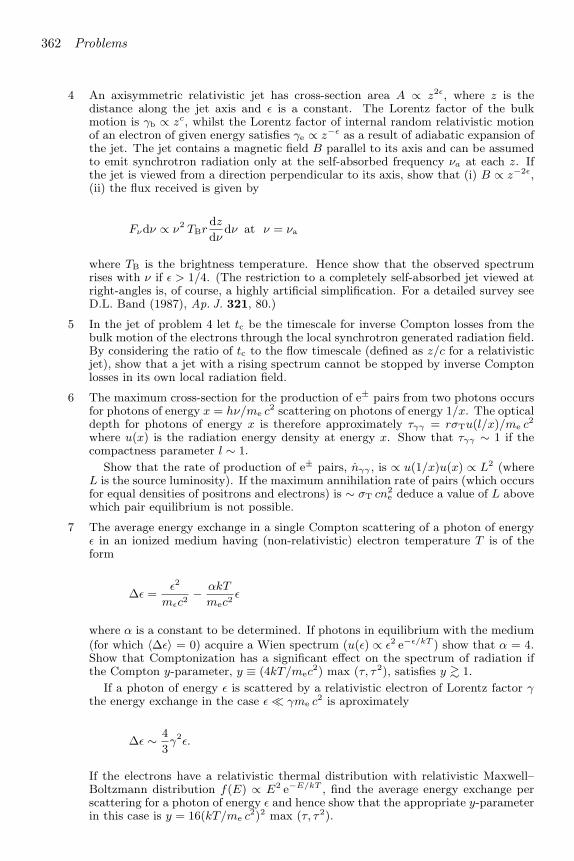
362 Problems

4 An axisymmetric relativistic jet has cross-section area A ∝ z2ε, where z is thedistance along the jet axis and ε is a constant. The Lorentz factor of the bulkmotion is γb ∝ zc, whilst the Lorentz factor of internal random relativistic motionof an electron of given energy satisfies γe ∝ z−ε as a result of adiabatic expansion ofthe jet. The jet contains a magnetic field B parallel to its axis and can be assumedto emit synchrotron radiation only at the self-absorbed frequency νa at each z. Ifthe jet is viewed from a direction perpendicular to its axis, show that (i) B ∝ z−2ε,(ii) the flux received is given by

Fνdν ∝ ν2 TBrdz

dνdν at ν = νa

where TB is the brightness temperature. Hence show that the observed spectrumrises with ν if ε > 1/4. (The restriction to a completely self-absorbed jet viewed atright-angles is, of course, a highly artificial simplification. For a detailed survey seeD.L. Band (1987), Ap. J. 321, 80.)

5 In the jet of problem 4 let tc be the timescale for inverse Compton losses from thebulk motion of the electrons through the local synchrotron generated radiation field.By considering the ratio of tc to the flow timescale (defined as z/c for a relativisticjet), show that a jet with a rising spectrum cannot be stopped by inverse Comptonlosses in its own local radiation field.

6 The maximum cross-section for the production of e± pairs from two photons occursfor photons of energy x = hν/me c

2 scattering on photons of energy 1/x. The opticaldepth for photons of energy x is therefore approximately τγγ = rσTu(l/x)/me c

2

where u(x) is the radiation energy density at energy x. Show that τγγ ∼ 1 if thecompactness parameter l ∼ 1.

Show that the rate of production of e± pairs, nγγ , is ∝ u(1/x)u(x) ∝ L2 (whereL is the source luminosity). If the maximum annihilation rate of pairs (which occursfor equal densities of positrons and electrons) is ∼ σT cn

2e deduce a value of L above

which pair equilibrium is not possible.

7 The average energy exchange in a single Compton scattering of a photon of energyε in an ionized medium having (non-relativistic) electron temperature T is of theform

∆ε =ε2

mεc2− αkT

mec2ε

where α is a constant to be determined. If photons in equilibrium with the medium(for which 〈∆ε〉 = 0) acquire a Wien spectrum (u(ε) ∝ ε2 e−ε/kT ) show that α = 4.Show that Comptonization has a significant effect on the spectrum of radiation ifthe Compton y-parameter, y ≡ (4kT/mec

2) max (τ, τ2), satisfies y ∼> 1.If a photon of energy ε is scattered by a relativistic electron of Lorentz factor γ

the energy exchange in the case ε γme c2 is aproximately

∆ε ∼ 4

3γ2ε.

If the electrons have a relativistic thermal distribution with relativistic Maxwell–Boltzmann distribution f(E) ∝ E2 e−E/kT , find the average energy exchange perscattering for a photon of energy ε and hence show that the appropriate y-parameterin this case is y = 16(kT/me c

2)2 max (τ, τ2).

Problems 363

Chapter 10

1 Most of the physically relevant features of a relativistic torus can be reproducedby adopting the following pseudo-Newtonian potential (B. Paczynski & P. Wiita(1982), A8823.)

Φ = − GM

r −RSchw

where r is the spherical radius.(a) Find an expression for the effective potential Φeff assuming that the angular

velocity of the fluid in the torus follows a simple power law of the form

Ω(R) = ΩK(R/RK)−q,

where R is the cylindrical radius and the allowed range for q is 32< q ≤ 2.

(b) Show that for the potential given above, the ‘Keplerian’ angular momentumfor circular orbits in the equatorial plane is given by

l2K = GMR3/(R−RSchw)2.

Show that for a given angular momentum value (l >√27/2), two circular orbits

are possible with radii R1 and RK. Are they both stable? Show that for q =2 (constant angular momentum) Φeff has extrema at these radii. How do theseproperties generalize for any q in the allowed range?

2 Using the results of problem 1 for Φeff find an expression for the shapes of tori andtheir internal equipotentials for any 3

2< q ≤ 2. Show that they can be written as

follows

z =

[B(1 + φ)(RK −RSchw)

2 −RSchwR1−BK RB

Bφ(RK −RSchw)2 −RSchwR1−BK RB

]2R2Schw −R2

1/2

where φ = −2Φeff/c2 is a constant for a given surface and B = 2− 2q.3 For a torus where electron scattering is the dominant source of opacity and radiation

pressure dominates (β 1), the radiative flux is given approximately by

F = − c

κT(1− β)geff .

Show that the magnitude of the flux can be calculated everywhere from Φeff . Fora pseudo-Newtonian torus with power-law rotation, it is given by (cf. Madau (1988),Ap. J. 327, 116.)

F =c

κT(1− β)

GM

R2Schw×

[1

(r − 1)4 +1

(RK − 1)4(R

RK

)2−4q− 2RK(RK − 1)2(r − 1)2r

(R

RK

)2−2q]1/2where r, R and RK are in units of RSchw. Note that to obtain the effective temper-ature on the surface it will suffice to set F = σT 4eff with r on the surface.

4 Find an approximate expression for the conical opening angle of the funnel of atorus of the type described in problem 2. How does the opening angle depend on qand φ?

364 Problems

5 Consider a situation in which waves propagating in a differentially rotating mediumpossess energies of different signs on different sides of an evanescent (forbidden)region or ‘potential barrier’. Physically this could arise if the energy of the perturbedflow is greater/smaller than in the unperturbed case. A wave of amplitude Aipropagating towards the barrier is transmitted with amplitude τAi where τ dependson the height and width of the barrier as in analogous quantum mechanical problems.(a) Use energy conservation to show that the amplitude of the reflected wave is

given by Ar = (1 +12τ2)Ai for small τ .

(b) Assume that a perfectly reflecting boundary exists at one side of the forbiddenregion, and show that a wave of arbitrary amplitude generated on this side will growexponentially with a growth rate

ω =a

4dτ2,

where d is the distance between the barrier and the reflecting boundary and a is thespeed of propagation of the wave (P. Goldreich & R. Narayan (1985), M.N.R.A.S.213, 7P).

Chapter 11

1 Integrate vertically the general time dependent continuity equation in cylindricalcoordinates. Specify which symmetries are required for the following result to beexact:

∂Σ

∂t+1

R

∂

∂R(RΣvR) .

Obtain the required expression for vR.

2 Assume that a certain accretion disc has an equilibrium power-law rotation of theform Ω(R) ∝ R−q. Show that in steady state the vertically averaged mass andangular momentum conservation equations lead to the following integral

M = 2πqνΣ .

Verify that the above equation yields the well-known result for Keplerian rotation. Isthe above result valid for a rotation law with constant specific angular momentum?

3 Following the procedure outlined in Section 11.4 obtain the expression linking M toα and Σ for an optically thin radiatively cooled branch with q− ∝ ρ2Tn for both gaspressure and radiation pressure dominated cases. Compare with the results quotedin the text for free–free cooling.

4 The various solution branches of one-temperature discs shown on Fig. 11.1 changeslope as they pass from one physical regime to another. Using the approximationsintroduced in Section 11.4 obtain simple power-law expressions for the gas/radiationpressure boundary, and the advection/radiation dominated boundary in the opti-cally thick case.

5 Consider the power-law solution for advection-dominated accretion obtained byNarayan & Yi (1994) (Ap. J. 428, L13; henceforth NY94).(a) From the vertically integrated equations discussed in Section 11.3 obtain

equations (1)–(4) of the above paper. For the energy equation you may assumeTds = dE + PdV = dE − c2sdρ/ρ, where c

2s = p/ρ and E = (3/2)Pg/ρ + aT 4/ρ is

the specific energy. With β = Pg/P = constant, the energy equation becomes

ΣvTds

dR=

(3− 3

2β)2ρHv

dc2sdR

− 2c2sHv dρdR

= Q+ −Q−

Problems 365

which is equivalent to equation (4) of NY94.(b) Assume now that β and the advected fraction f = (Q+−Q−)/Q+ are constant

and show first that power-law solutions are indeed possible. Obtain all the power-indexes (cf. equation (6) of NY94).(c) With the values of the power-indexes known, solve now the resultant algebraic

equations to determine the constants in terms of the Keplerian rotation rate.

Bibliography

Chapter 2

A. Choudhuri (1998), The Physics of Fluids and Plasmas – An Introduction for Astro-physicists, Cambridge University Press. A textbook developing both the macroscopicand microscopic theories of fluids and plasmas aimed primarily at graduate studentsof astrophysics.

F.H. Shu (1992), The Physics of Astrophysics, Vol II: Gas Dynamics, University Sci-ence Books. An advanced graduate-level treatment of compressible fluid dynamicscovering fundamental topics such as accretion discs, fluid instabilities, spiral densitywaves, shock waves, ionization fronts and magnetohydrodynamics.

J. Dyson & D. Williams (2000), Physics of the Interstellar Medium, Manchester Uni-versity Press. An excellent introduction to astrophysical gas dynamics, with applica-tions to supernovae, stellar winds, etc.

L.D. Landau & E.M. Lifshitz (1959), Fluid Mechanics, Pergamon. A classic referencefor all branches of fluid mechanics.

Other references cited in this chapter are:H. Bondi (1952), ‘On spherically symmetrical accretion’, M.N.R.A.S. 112, 195.H. Bondi & F. Hoyle (1944), ‘On the mechanism of accretion by stars’, M.N.R.A.S.104, 273.T.E. Holzer & W.I. Axford (1970), ‘Theory of stellar winds and related flows’, Ann.Rev. Astr. Ap. 8, 31, gives a thorough discussion of spherical winds and accretion.

F. Hoyle & R.A. Lyttleton (1939), ‘The effect of interstellar matter on climatic vari-ation’, Proc. Camb. Phil. Soc. 35, 405.

Chapter 3

A. Choudhuri (1998), op. cit.. See bibliography for Chapter 2.

T.J.M. Boyd & J.J. Sanderson (1969), Plasma Dynamics, Nelson. A comprehensiveintroductory text in plasma physics. Chapter 10 on plasma kinetic theory is particu-larly useful.

R.J. Goldston & P.H. Rutherford (1995), Introduction to Plasma Physics, Institute of

Bibliography 367

Physics Publishing. Chapters 10 and 11 of this modern plasma physics text deal withcollisional relaxation and slowing down of fast particles.

J.D. Jackson (1999), Classical Electrodynamics, (3rd edn, March 1999 reprint) Wiley.

J.I. Katz (1987), High Energy Astrophysics, Addison-Wesley. Discusses much of thephysics of Chapters 2 and 3 in more detail, and some aspects of accretion.

M.S. Longair (1981), High Energy Astrophysics, Cambridge University Press. Gives avery readable account of much of the physics of this chapter.

Chapter 4

R. Kippenhahn & A. Weigert (1990), Stellar Structure and Evolution, Springer-Verlag.An excellent graduate-level textbook discussing the internal structure and evolutionof stars.

S.L. Shapiro & S.A. Teukolsky (1983), Black Holes, White Dwarfs, and Neutron Stars,Wiley Inter-Science. Deals mainly with the internal structure of stellar mass compactobjects, but touches on some areas of accretion.

The standard text on all aspects of cataclysmic variables isB. Warner (1995), Cataclysmic Variable Stars, Cambridge University Press.

For reviews of many aspects of X-ray binaries and related systems seeW.H.G. Lewin, J. van Paradijs & E.P.J. van den Heuvel (1995), X-ray Binaries,Cambridge Astrophysics Series 26, CUP.

Reviews of close binary evolution are given inA.R. King (1988), ‘The evolution of compact binaries’, Q.J.R.A.S. 29, 1,and inH. Ritter (1996), in Evolutionary Processes in Binary Stars, Proc. NATO AdvancedStudy Institute, Cambridge, UK, July 10–21, 1995. Edited by Ralph A.M.J. Wijersand Melvyn B. Davies. Dordrecht: Kluwer Academic Publishers. NATO AdvancedScience Institutes (ASI) Series C, Mathematical and Physical Sciences, Vol. 477, p.223.

For a review of low-mass X-ray binary evolution, including the effects of irradiationand the connection to binary pulsars, seeA.R. King (2001), ‘The evolution of black hole X-ray binaries’, New Astronomy Re-views, in press.

The complex dynamics of accretion from stellar winds is studied byJ.M. Blondin, T.R. Kallman, B.A. Fryxell & R.E. Taam (1990), ‘Hydrodynamic sim-ulation of stellar wind distribution by a compact X-ray source,’ Ap. J. 356, 591.

The famous α-prescription was originally introduced in an insightful discussion of theobservational properties of accreting black holes which anticipated several results nowconsidered standard,

368 Bibliography

N.I. Shakura & R.A. Sunyaev (1973), ‘Black holes in binary systems. ObservationalAppearance’, A&A 24, 337.

Other references cited in this chapter are:S.A. Balbus, J.F. Hawley & J.M. Stone (1996), ‘Nonlinear stability, hydrodynamicalturbulence, and transport in disks’, Ap. J. 467, 76.S.A. Balbus & J.F. Hawley (1991), ‘A powerful local shear instability in weakly mag-netized disks. I – Linear analysis’, Ap. J. 376, 214.G.K. Batchelor (1970), An Introduction to Fluid Dynamics, Cambridge UniversityPress.J. Binney & S. Tremaine (1987, 1994), Galactic Dynamics, Princeton University Press.S. Chandrasekhar (1960), ‘The stability of non–dissipative Couette flow in hydromag-netics’, Proc. Nat. Acad. Sci. USA 46, 253.S. Chandrasekhar (1961), Hydrodynamic and Hydromagnetic Stability, Oxford Uni-versity Press; Dover Publications (1981), ch. IX.S. Chapman & T.G. Cowling The Mathematical Theory of Non-Uniform Gases, Cam-bridge University Press.P.P. Eggleton (1983), ‘Approximations to the radii of Roche lobes’, Ap. J. 268, 368.A.M. Fridman & N.N. Gorkavyi (1999), Physics of Planetary Rings, Springer-Verlag.U. Frisch (1995), Turbulence, Cambridge University Press.R. Greenberg (1998), ‘Particle properties and the large-scale structure of planetaryrings: Rebound characteristics and viscosity’, Icarus 75, 527.A.R. King (1989), ‘Irradiation of the companion star in cataclysmic variables’,M.N.R.A.S. 241, 365.A.R. King, J. Frank, U. Kolb & H. Ritter (1996), ‘Global analysis of mass transfercycles in cataclysmic variables’, Ap. J. 467, 761.A.R. King & U. Kolb (1995), ‘Consequential angular momentum loss and the periodgap of cataclysmic variables’, Ap. J. 439, 330.A.R. King & A. van Teeseling (1998), ‘Wind-driven evolution of accreting binariesand the progenitors of SNe Ia’, A&A 338, 965.P. Kumar, R. Narayan & A. Loeb (1995), ‘On the interaction of convection and rota-tion in stars’, Ap. J. 453, 480.L. Landau & E.M. Lifshitz (1959), Fluid Mechanics, Pergamon Press.D. Ryu & J. Goodman (1992), ‘Convective instability in differentially rotating disks’,Ap. J. 388, 438.A. van Teeseling & A.R. King (1998), ‘Wind-driven evolution of supersoft X-ray bi-naries with low-mass secondaries’, A&A 338, 957.E.P. Velikhov (1959), ‘Stability of an ideally conducting liquid flowing between cylin-ders rotating in a magnetic field’, Sov. Phys. JETP 9, 995 (Russian original: 36, 1398).

Bibliography 369

Chapter 5

General references:R. Kippenhahn & A. Weigert (1990), Stellar Stucture and Evolution, Springer-Verlag.F.H. Shu (1992), Gas Dynamics, University Science Books.B. Warner (1995), Cataclysmic Variable Stars, Cambridge University Press.A standard review of disc theory isJ.E. Pringle (1981), ‘Accretion discs in astrophysics’, Ann. Rev. Astr. Ap. 19, 137.The disc instability model was suggested byJ.I. Smak (1971), Acta Astronomica 21, 15; IAU Colloq. 15, 248, 1971.For a comprehensive review of the disc instability model for dwarf novae and softX-ray transients, seeJ.P. Lasota (2001), ‘The disc instability model of dwarf-novae and low-mass X-raybinary transients’, New Astronomy Reviews, in press (astro-ph/0102072).Radiation-driven disc warping was suggested byJ.E. Pringle (1996), ‘Self-induced warping of accretion discs’, M.N.R.A.S. 281, 357.Eclipse mapping of discs in both lines and continuum is reviewed byK. Horne (1993), ‘Eclipse mapping of accretion disks: The first decade’, in AccretionDisks in Compact Stellar Systems, ed. J.C. Wheeler, Singapore: World Scientific, p.117.The method of Doppler tomography for mapping accretion flows in close binaries isreviewed byT.R. Marsh (2001), ‘Doppler tomography’, in Proceedings of the Astro-tomographyworkshop, Brussels, eds. H. Boffin, D. Steeghs, Springer-Verlag, in press (astro-ph//0011020).At the time of writing there is no comprehensive review of superhumps. The firstdemonstration that superhumps arise from the secondary’s tidal influence in a CVwith an extreme mass ratio was byR. Whitehurst (1988), ‘Numerical simulations of accretion disks. I – Superhumps – Atidal phenomenon of accretion disks’, M.N.R.A.S. 232, 35.The suggestion that the j = 3, k = 2 resonance (3:1 orbital commensurability) is thebasic cause of superhumps first appears inR. Whitehurst & A.R. King (1991), ‘Superhumps, resonances and accretion discs’,M.N.R.A.S. 249, 25,and the treatment byS.A. Lubow (1991), ‘A model for tidally driven eccentric instabilities in fluid disks’, Ap.J. 381, 259, and ‘Simulations of tidally driven eccentric instabilities with applicationto superhumps’, Ap. J. 381, 268,makes this more rigorous.Superhumps in LMXB discs are explained in terms of a disc area modulation byC.A. Haswell, A.R. King, J.R. Murray & P.A. Charles (2001), ‘Superhumps in low-mass X-ray binaries’, M.N.R.A.S. 321, 475.

370 Bibliography

Evidence for discs around young stars is discussed inS.V.W. Beckwith, A.I. Sargent, R.S. Chini & R. Gusten (1990), ‘A survey for circum-stellar disks around young stellar objects.’ Astron. J. 99, 924,and their structure is discussed inL. Hartman, S.J. Kenyon & P. Hartigan (1993), ‘Young stars – Episodic phenomena,activity and variability’, in Protostars and Planets III, eds. E.H. Levy, J. Lunine &M.S. Matthews, University of Arizona Press, p. 497.

A very good and up-to-date review of the observations and theory relevant to accretiondisks around young stars isL. Hartmann (2000), Accretion Processes in Star Formation, Cambridge AstrophysicsSeries, 32, Cambridge University Press.

Star formation is reviewed inF.H. Shu, F.C. Adams & S. Lizano (1987), ‘Star formation in molecular clouds: ob-servation and theory’, Ann. Rev. Astron. Astrophys. 25, 23.

For a general discussion of spiral shocks and other angular momentum transport mech-anisms, seeG. Morfill, H.C. Spruit & E.H. Levy (1993), ‘Physical processes and conditions asso-ciated with the formation of protoplanetary disks’, in Protostars and Planets III, eds.E.H. Levy, J. Lunine & M.S. Matthews, University of Arizona Press, p. 939.

For spiral shocks in cataclysmic variable discs, seeD. Steeghs, E.T. Harlaftis & K. Horne (1997), ‘Spiral structure in the accretion discof the binary IP Pegasi’, M.N.R.A.S. 290, L28.P. Godon, M. Livio & S. Lubow (1998), ‘Spiral shocks in accretion discs’, M.N.R.A.S.295. L11.

The UKAFF websitehttp://www.ukaff.ac.uk/movies.shtmlgives animations of various accretion flows.

Other references cited in this chapter are:J.K. Cannizzo (1998), ‘The accretion disk limit cycle mechanism in the black holeX-ray binaries: toward an understanding of the systematic effects’, Ap. J. 494, 366.A.R. King & H. Ritter (1998), ‘The light curves of soft X-ray transients’, M.N.R.A.S.293, L42.A.R. King & J.K. Cannizzo (1998), ‘Low states in cataclysmic variables’, Ap. J. 499,348.

Chapter 6

A review of boundary-layer theory isO. Regev (1991) ‘Modelling accretion disk boundary layers’, in Structure and EmissionProperties of Accretion Disks, eds. Bertout et al., Editions Frontieres.

Bibliography 371

A comprehensive overview of observational and theoretical aspects of X-ray binariesis given inW.H.G. Lewin, J. van Paradijs & E.P.J. van den Heuvel (1995), X-ray Binaries,Cambridge Astrophysics Series 26, Cambridge University Press.

Both high- and low-mass X-ray binaries are discussed inN.E. White (1990),‘X-ray binaries’, A.& A. Rev. 1 85.

For a review of QPOs seeM. Van der Klis (1989), ‘Quasi-periodic oscillations and noise in low-mass X-ray bi-naries,’ Ann. Rev. Astron. Astrophys. 27, 517.

All aspects of AM Herculis systems (polars) are reviewed inM. Cropper (1990), ‘The polars’, Space Science Reviews, 54, 195,while the possible relation to intermediate polars and evolutionary questions are dis-cussed byA.R. King & J.P. Lasota (1991), ‘Magnetic cataclysmic variables,’ in the review volumeInteracting Close Double Stars, eds. Y. Kondo, G.E. McCluskey, Jr. & J. Sahade,Kluwer.

For X-ray bursters seeW.H.G. Lewin & P.C. Joss (1983), Chapter 2 of Accretion-driven Stellar X-raySources, eds. W.H.G. Lewin & E.P.J. van den Heuvel, Cambridge University Press.and Chapter 4 ofW.H.G. Lewin, J. van Paradijs & E.P.J. van den Heuvel (1995), op. cit.

Binary black hole candidates are discussed byP. Charles (1998), in Theory of Black Hole Accretion Disks, eds. M.A. Abramowicz,G. Bjornsson & J.E. Pringle, Cambridge University Press, p. 1.

Other references cited in this chapter:L. Bildsten et al. (1997), ‘Observations of accreting pulsars’, Ap. J. Supp. 113, 367.D. Chakrabarti & E.H. Morgan (1998), ‘The two-hour orbit of a binary millisecondX-ray pulsar’, Nature 394, 346.V. Kalogera, U. Kolb & A.R. King (1998), ‘Supernova kicks, magnetic braking, andneutron star binaries’, Ap. J. 504, 967.A.R. King & U.C. Kolb (1997), ‘The formation of low-mass transient X-ray binaries’,Ap. J. 481, 918.A.R. King, U.C. Kolb & L. Burderi (1996), ‘Black hole binaries and X-ray transients’,Ap. J. Lett. 464, L127.A.R. King, M.B. Davies, M.J. Ward, G. Fabbiano & M. Elvis (2001), ‘UltraluminousX-ray sources in external galaxies’, Ap. J. Lett. 552, L109.K. Makishima, T. Mihara, F. Nagase & Y. Tanaka (1999), ‘Cyclotron resonance effectsin two binary X-ray pulsars and the evolution of neutron star magnetic fields’, Ap. J.525, 978.K.A. Miller & J.M. Stone (1997), ‘Magnetohydrodynamic simulations of stellarmagnetosphere–accretion disk interaction’, Ap. J. 489, 890.

372 Bibliography

I.F. Mirabel & L.F. Rodriguez (1999), ‘Sources of relativistic jets in the Galaxy’, Ann.Rev. Astr. Ap. 37, 409.R. Wijnands & M. van der Klis (1998), ‘A millisecond pulsar in an X-ray binarysystem’, Nature 394, 344.

Chapter 7

A general introduction to active galaxies at the level of this book isB.M. Peterson (1997), An Introduction to Active Galactic Nuclei, Cambridge Univer-sity Press.

A graduate-level comprehensive treatment of active galactic nuclei is given inJ.H. Krolik (1999), Active Galactic Nuclei, Princeton University Press.

Quasars surveys are reviewed inD.W. Weedman (1986), Quasar Astronomy, Cambridge University Press.

For a discussion of continuum emission which may still serve as a useful starting pointseeD.B. Sanders, E.S. Phinney, G. Neugebauer, B.T. Soifer & K. Mathews (1989), ‘Con-tinuum energy distribution of quasars: shapes and origins’, Ap. J. 347, 29,and, for the dataM. Elvis et al. (1994), ‘Atlas of quasar energy distributions’ , Ap. J. Supp. 95, 1.

The arguments leading to the black hole model are summarized inM.J. Rees (1984), ‘Models for active galactic nuclei ’, Ann. Rev. Astr. Ap. 22, 471.

A review of variability which is also a useful introduction to classes of active galacticnuclei can be found inM.H. Ulrich, L. Maraschi, C.M. Urry (1997), ‘Variability of active galactic nuclei’,Ann. Rev. Astr. Ap. 35, 445,and specifically in the X-ray region inR.F. Mushotzky, C. Done, & K.A Pounds (1993), ‘X-Ray spectra and time variabilityof active galactic nuclei’, Ann. Rev. Astr. Ap. 31, 717.

For gravitational lenses consultJ. Ehlers, P. Schneider & E.E. Falco (1999), Gravitational Lenses, Springer-Verlag.Y. Mellier, B. Fort & G. Soucail (eds.) (1990), Gravitational Lensing, Lecture Notesin Physics, 360, Springer-Verlag.C.S. Kochanek & J.N. Hewitt (eds.) (1996), Astrophysical Applications of Gravita-tional Lensing, IAU Symposium 173, Kluwer.

A review of the older searches for black holes in the centres of galaxies can be foundinJ. Kormendy (1995), ‘Inward bound – The search for supermassive black holes ingalactic nuclei’, Ann. Rev. Astr. Ap. 33, 581.

Recent work derives from

Bibliography 373

K. Gebhardt et al. (2000), ‘A relationship between nuclear black hole mass and galaxyvelocity dispersion’, Ap. J. Lett. 539, L13.L. Ferrarese & D. Merritt (2000), ‘A fundamental relation between supermassive blackholes and their host galaxies’, Ap. J. Lett. 539, L9.

For the problem of the gas supply seeI. Shlosman, M.C. Begelman & J. Frank (1990), ‘The fuelling of active galactic nuclei’,Nature 345, 679.

Two more recent references areS. Ayal, M. Livio & T. Piran (2000), ‘Tidal disruption of a solar-type star by asupermassive black hole’, Ap. J. 545, 772.andJ. Magorrian & S. Tremaine (1999), ‘Rates of tidal disruption of stars by massivecentral black holes’, M.N.R.A.S. 309, 447.

A discussion of many observational and theoretical aspects of the environmental andmorphological characteristics of active galaxies can be found inJ.W. Sulentic, W.C. Keel & C.M. Telesco (eds.) (1990), Paired and Interacting Galax-ies, IAU Coll. 124, Tuscaloosa, Alabama, NASA CP–3098. Washington: U.S. Gov-ernment Printing Office.

J.M. Bardeen (1973), ‘Timelike and null geodesics in the Kerr metric’, in Black Holes,Ecole d’ete de Physique Theorique, Les Houches, 1972, eds. C. DeWitt & B.S. DeWitt,Gordon and Breach, is a useful reference for the effective potential method.

Our discussion of accretion efficiency in spherical accretion followsR. McCray (1979), ‘Spherical accretion onto supermassive black holes’, in ActiveGalactic Nuclei, eds. C. Hazard & S. Mitton, Cambridge University Press;P. Meszaros & J. P. Ostriker (1983), ‘Shocks and spherically accreting black holes: amodel for classical quasars’, Ap. J. Lett. 273, L59.

The efficiency constraint was first raised inA. Fabian (1979), ‘Theories of the nuclei of active galaxies’, Proc. Roy. Soc. A366,449.

Compton scattering is treated in detail inG.B. Rybicki & A.P. Lightman (1979), Radiative Processes in Astrophysics, Wiley.

Other reference cited in this chapter:T.L. Courvoisier (1998), ‘The bright quasar 3C 273’, A& A Review 9, 1.

Chapter 8

The discussion of iron line emission comes fromL.M. George & A.C. Fabian (1991), ‘X-ray reflection from cold matter in active galacticnuclei and X-ray binaries’, M.N.R.A.S. 249, 352.

For a general review see

374 Bibliography

A. Fabian (1997), ‘Testing strong gravity in active galactic nuclei’, Astron. & Geophys.38, 10.

X-ray reprocessing in an irradiated disc is treated byM.W. Sincell & J.H. Krolik (1997), Ap. J. 476, 605.

Cloud motion in the narrow line region is considered byM.M. De Robertis & R.A. Shaw (1990), ‘Line profiles and the kinematics of the narrow-line region in Seyfert galaxies’, Ap. J. 348, 421.

A concise summary of early work on the optical spectroscopy of active nuclei can befound inD.E. Osterbrock (1984), ‘Active galactic nuclei’, Q.J.R.A.S. 25, 1.and a textbook treatment inD.E. Osterbrock (1989), Astrophysics of Gaseous Nebulae and Active Galctic Nuclei,University Science Books.

A recent review of emission lines can be found inJ.W. Sulentic, P. Marziani & D. Dultzin-Hacyan (2000), ‘Phenomenology of broademission lines in active galactic nuclei’ Ann. Rev. Astr. Ap. 38, 521;and an excellent older review inH. Netzer (1991), in Active Galactic Nuclei, Saas-Fee Advanced Course 20, eds. R.D.Blandford, H. Netzer & L. Woltjer, Springer-Verlag.

The ‘classic’ reference,K. Davidson & H. Netzer (1979), ‘The emission lines of quasars and similar objects’,Rev. Mod. Phys. 51, 715,is still a useful starting point.

The ‘standard model’ goes back toJ. Krolik, C.F. McKee & C.B. Tarter (1981), ‘Two phase models of quasars emissionline regions’, Ap. J. 249, 422.

Two widely used publicly available photoionization codes are CLOUDY,(see http://www.pa.uky.edu/∼gary/cloudy/)and XSTAR(links from http://lheawww.gsfc.nasa.gov/users/tim/tim.html).

For radio sources seeA. Ferrari (1998), ‘Modeling extragalactic jets’, Ann. Rev. Astr. Ap. 36, 539.M. Begelman, R.D. Blandford & M.J. Rees (1984), ‘Theory of extragalactic radiosources’, Rev. Mod. Phys. 56, 255.

The OIII problem was described inG.A. Shields (1978), in Proceedings of the Pittsburgh Conference on BL Lacertae Ob-jects, pp. 257–76, ed. A. Wolfe, University of Pittsburgh Press.

Three somewhat different ‘disc-winds’ theories are treated inI. Cassidy & D.J.Raine (1997), ‘NGC 4151 – A unified active galactic nucleus’, A&A 322, 400.J. Chiang & N. Murray (1997), ‘Disk winds and disk emission lines’, Ap. J. 474, 91.

Bibliography 375

M. Bottorff, K.T. Korista, I. Shlosman & R.D. Blandford (1997). ‘Dynamics of broademission line regions in NGC 5548’, Ap. J. 479, 200.

Other reference cited in this chapter:L. Burderi, A.R. King & E. Szuszkiewicz (1998), ‘Does the thermal disk instabilityoperate in active galactic nuclei?’, Ap. J. 509, 85.

Chapter 9

For the origin of the unified model seeP. D. Barthel (1989), ‘Is every quasar beamed?’, Ap. J. 336, 606,and for reviewsR. Antonucci (1993), ‘Unified models for active galactic nuclei and quasars’, Ann. Rev.Astr. Ap. 31, 473,andW.P.J. Gopalkrishna (1995), ‘The case for unification’, Proc. Natl. Acad. Sci. USA92, 11399.For a review of X-ray properties seeR.F. Mushotzky, C. Done & K.A. Pounds (1993), ‘X-ray spectra and time variabilityof active galactic nuclei, Ann. Rev. Astr. Ap. 31, 717.

Comptonization is treated inG.B. Rybicki & A.P. Lightman (1979), Radiative Processes in Astrophysics, Wiley,andR.A. Sunyaev & T. Titarchuk (1980), ‘Comptonisation of X-rays in plasma clouds.Typical radiation spectra’, A& A 86, 121.

The two temperature disc was introduced inS.I. Shapiro, A.P. Lightman & D. Eardley (1976), ‘A two-temperature accretion diskmodel for Cygnus X-1: structure and spectrum’, Ap. J. 204, 187.See also the references for Chapter 11.

The revival of disc–corona models is due toF. Haardt & L. Maraschi (1991), ‘A two-phase model for the X-ray emission fromSeyfert galaxies’, Ap. J. Lett. 380, L51.extended inF. Haardt, L. Maraschi & G. Ghisellini (1997), ‘X-Ray variability and correlations inthe two-phase disk-corona model for Seyfert galaxies’, Ap. J. 476, 620.See alsoM.C. Begelman (1989), in Accretion Discs and Magnetic Fields in Astrophysics, ed.G. Belvedere, Kluwer, p. 255.

Slim discs (see also Chapter 11) were first described inM.A. Abramowicz, B. Czerny, J.-P. Lasota & E. Szuszkiewicz (1988), ‘Slim accretiondiscs’, Ap. J. 332, 646.

376 Bibliography

The elaboration of the cauldron model is based on work of Svensson & Zdziarski, forexampleA.P. Lightman & A.A. Zdziarski (1987), ‘Pair production and Compton scattering incompact sources and comparison to observations of active galactic nuclei’, Ap. J. 319,643.

Magnetized disc winds are treated in R.V. Lovelace, J.C. Wang & M.E. Sulkanen(1987), ‘Self-collimated electromagnetic jets from magnetised accretion disks’, Ap. J.315, 504;A. Konigl (1989), ‘Self-similar models of magnetised accretion discs’, Ap. J. 342, 208.

The Blandford–Znajek model is discussed further inR.D. Blandford & R.L. Znajek (1977), ‘Electromagnetic extraction of energy fromKerr black holes’, M.N.R.A.S. 179, 433;D. Macdonald & K.S. Thorne (1982), ‘Black-hole electrodynamics: an absolute-space/universal-time formalism’, M.N.R.A.S. 198, 345.

More recent developments can be found in, for example,D.L. Meier, S. Koide & Y. Uchida (2001), ‘Magnetohydrodynamic production of rel-ativistic jets’, Science 291, 84.L.X. Li (2000), ‘Screw instability and the Blandford–Znajek mechanism’ Ap. J. Lett.531, L111.M. Livio, G.I. Ogilvie & J.E. Pringle (1999), ‘Extracting energy from black holes: Therelative importance of the Blandford–Znajek mechanism’ Ap. J. 512, 100.R.D. Blandford (2000), ‘Quasar jets and their fields’, Philos. Trans. Roy. Soc. A358, 811.

It may be useful to consultK.S. Thorne, R.H. Price & D. Macdonald (1988), Black Holes: The MembraneParadigm, Yale, for a technical approach to the analysis of black holes based on stan-dard physical ideas.

Other references cited in this chapter are:R.D. Blandford (1976), ‘Accretion disc electrodynamics – a model for double radiosources’, M.N.R.A.S. 176, 465.R.D. Blandford & D.G. Payne (1982), ‘Hydromagnetic flows from accretion discs andthe production of radio jets’, M.N.R.A.S. 199, 883.

Chapter 10

The best review of the material of this chapter isR. Narayan & J. Goodman (1989), ‘Non-axisymmtric shear instabilities in thick ac-cretion disks,’ in Theory of Accretion Disks, eds. Meyer et. al., NATO ASI, Kluwer,pp. 231–47, and this paper is updated byR. Narayan (1991), Structure and Emission Properties of Accretion Discs, IAU Coll.

Bibliography 377

No. 129, eds. C. Bertout, S. Collin-Souffrin, J.-P. Lasota & Tran T. Van, EditionsFrontieres.

Of particular importance isJ.C. Papaloizou & J.E. Pringle (1984), ‘The dynamical stability of differentially ro-tating discs with constant specific angular momentum’, M.N.R.A.S. 208, 721.

Rotating stars are treated inJ.-L. Tassoul (1978), Theory of Rotating Stars, Princeton University Press.A very lucid introduction to the theory and observations of rotation in single andbinary stars is given inJ.-L. Tassoul (2000), Stellar Rotation, Cambridge Astrophysics Series 36, CambridgeUniversity Press.

Other references cited in this chapter are:M.A. Abramowicz, M. Calvani & L. Nobili (1980), ‘Thick accretion disks with super-Eddington luminosities’, Ap. J. 242, 772.B. Paczynski (1982), ‘Thick accretion disks around black holes’, Astron. Gessels. Mit-teilungen 57, 27.M.J. Rees, M.C. Begelman, R.D. Blandford & E.S. Phinney (1982), ‘Ion-supportedtori and the origin of radio jets’, Nature 295, 17.M. Schwarzchild (1965), Structure and Evolution of the Stars, Dover.

Chapter 11

A very nice and detailed treatment of accretion disc flows around black holes whichincludes some of the recent developments and is suitable for both advanced graduatestudents and specialists isS. Kato, J. Fukue & S. Mineshige (1998), Black Hole Accretion Disks, Kyoto UniversityPress.

The material presented in Section 11.4 is based in part onX. Chen, M.A. Abramowicz, J.-P. Lasota, R. Narayan & I. Yi (1995), ‘Unified de-scription of accretion flows around black holes’, Ap. J. Lett. 443, L61.

Other references cited in this chapter are:M.A. Abramowicz, B. Czerny, J.-P. Lasota & E. Suszkiewicz (1988), ‘Slim accretiondisks’, Ap. J. 332, 646.M.A. Abramowicz, X. Chen, S. Kato, J.-P. Lasota & O. Regev (1995), ‘Thermalequilibria of accretion disks’, Ap. J. Lett. 438, L37.M.C. Begelman (1978), ‘Black holes in radiation-dominated gas – an analogue of theBondi accretion problem’, M.N.R.A.S. 184, 53.M.C. Begelman & D.L. Meier (1982), ‘Thick accretion disks – Self-similar, supercriticalmodels’, Ap. J. 253, 873.R.D. Blandford & M.C. Begelman (1999), ‘On the fate of gas accreting at a low rateon to a black hole’, M.N.R.A.S. 303, L1.

378 Bibliography

S.K. Chakrabarti (1996), ‘Accretion processes on a black hole’, Phys. Rep. 266, 238.W. Chen, C.R. Shrader & M. Livio (1997), ‘The properties of X-ray and optical lightcurves of X-ray novae’, Ap. J. 491, 312.A. Eckart & R. Genzel (1997), ‘Stellar proper motions in the central 0.1 pc of theGalaxy’, M.N.R.A.S. 284, 576.A.C. Fabian & M.J. Rees (1995), ‘The accretion luminosity of a massive black hole inan elliptical galaxy’, M.N.R.A.S. 277, L55.M.R. Garcia, J.E. McClintock, R. Narayan, P. Callanan & S.S. Murray (2001), ‘Newevidence for black hole event horizons from Chandra’, Ap. J. Lett. 553, L47.J.F. Hawley, L.L. Smarr & J.R. Wilson (1984), ‘A numerical study of nonsphericalblack hole accretion. II – Finite differencing and code calibration’, Ap. J. Supp. 55,211.I.V. Igumenshev & M.A. Abramowicz (1999), ‘Rotating accretion flows around blackholes: convection and variability’, M.N.R.A.S. 303, 309.I.V. Igumenshev & M.A. Abramowicz (2000), ‘Two-dimensional models of hydrody-namical accretion flows into black holes’, Ap. J. Supp. 130, 463.I.V. Igumenshev, M.A. Abramowicz & R. Narayan (2000), ‘Numerical simulations ofconvective accretion flows in three dimensions’, Ap. J. 537, 271.I.V. Igumenshev, X. Chen & M.A. Abramowicz (1996), ‘Accretion discs around blackholes: two-dimensional, advection-cooled flows’, M.N.R.A.S. 278, 236.J.-P. Lasota, M.A. Abramowicz, X. Chen, J. Krolik, R. Narayan & I. Yi (1996), ‘Isthe accretion flow in NGC 4258 advection dominated?’, Ap. J. 462, 142.E.P. Liang & A. Wandel (1991), ‘Luminosity limit for alpha-viscosity accretion disks’,Ap. J. 376, 746.A.P. Lightman & D.M. Eardley (1974), ‘Black holes in binary systems: instability ofdisk accretion’, Ap. J. 187, 1.C. Luo & E.P. Liang (1994), ‘Stability and oscillations of thermal accretion discsaround black holes’, M.N.R.A.S. 266, 386.M.V. Medvedev & R. Narayan (2000), ‘Self-similar hot accretion flow onto a neutronstar’, Ap. J. 554, 1255.R. Narayan (1997), ‘Advective disks’, in Proc. IAUC No. 163, Accretion Phenomena& Related Outflows, eds. D.T. Wickramasinghe, L. Ferrario & G.V. Bicknell, NewYork: AIP (astro-ph/9611113).R. Narayan, D. Barret & J.E. McClintock (1997), ‘Advection-dominated accretionmodel of the black hole V404 Cygni in quiescence’, Ap. J. 482, 448.R. Narayan, M.R. Garcia & J.E. McClintock (1997), ‘Advection-dominated accretionand black hole event horizons’, Ap. J. Lett. 478, L79.R. Narayan, I.V. Igumenshev & M.A. Abramowicz (2000), ‘Self-similar accretion flowswith convection’, Ap. J. 539, 798.R. Narayan, S. Kato & F. Honma (1997), ‘Global structure and dynamics of advection-dominated accretion flows around black holes’, Ap. J. 476, 49.R. Narayan, J.E. McClintock & I. Yi (1996), ‘A new model for black hole soft X-raytransients in quiescence’, Ap. J. 457, 821.

Bibliography 379

R. Narayan & I. Yi (1994), ‘Advection-dominated accretion: a self-similar solution’,Ap. J. Lett. 428, L13.R. Narayan & I. Yi (1995a), ‘Advection-dominated accretion: self-similarity and bipo-lar outflows’, Ap. J. 444, 231.R. Narayan & I. Yi (1995b), ‘Advection-dominated accretion: underfed black holesand neutron stars’, Ap. J. 452, 710.R. Narayan, I. Yi & R. Mahadevan (1995), ‘Explaining the spectrum of Sagittarius-A*with a model of an accreting black hole’, Nature 374, 623.M.E. O’Neill & F. Chorlton (1989), Viscous and Compressible Fluid Dynamics, Wiley& Sons.B. Paczynski (1998), ‘Advection dominated accretion flows. A toy disk model’, ActaAstronomica 48, 667.M.J. Rees, M.C. Begelman, R.D. Blandford & E.S. Phinney (1982), ‘Ion-supportedtori and the origin of radio jets’, Nature 295, 17.S.L. Shapiro, A.P. Lightman & D.M. Eardley (1976), ‘A two-temperature accretiondisk model for Cygnus X-1 – Structure and spectrum’, Ap. J. 204, 187.J.M. Stone, J.E. Pringle & M.C. Begelman (1999), ‘Hydrodynamical non-radiativeaccretion flows in two dimensions’, M.N.R.A.S. 310, 1002.J.M. Stone & J.E. Pringle (2001), ‘Magnetohydrodynamical non-radiative accretionflows in two dimensions’, M.N.R.A.S. 322, 461.P.A. Thompson (1972), Compressible Fluid Dynamics, McGraw–Hill Book Co.

Appendix

G.B. Rybicki & A.P. Lightman (1979), Radiative Processes in Astrophysics, Wiley.W.H. Tucker (1975), Radiative Processes in Astrophysics, MIT Press.

Index

3C 120, 2643C 234, 2163C 273, 214, 220, 221, 270, 275, 2803C 279, 280

absorption, 214, 256accretionefficiency, 2emitted spectrum, 5energy yield, 1flows, 7luminosity, 3normal stars, 2theory and observation, 6

accretion column, 152, 174, 175, 177–186,188–201, 209, 356

accretion disc, 7, 48, 61, 62, 64–66, 69–72, 74,78, 80–163, 166–169, 205, 206, 208, 209,244, 263

ionization zone, 265outburst, 266thin, 80, 84, 85, 87–89, 93, 98, 108, 113, 118,

129, 132, 139viscosity, 63–73

accretion efficiency, 4accretion luminosity, 62, 77, 97–99, 159, 162,

175–177, 180, 182, 187, 192–194accretion radius, 21, 74, 75, 238accretion rate, 4, 15, 21accretion torque, 157, 158accretion yield, 350active galactic nuclei (AGN), 1, 213, 216, 335disc stability, 265

ADAF, 319, 322, 330–332, 334–342, 344, 364transition radius, 336, 340, 343

adiabatic flows, 12adiabatic index, 45adiabatic inflow–outflow solutions (ADIOS), 338advection, 118, 129, 321–323, 325, 327, 340advection dominated, 283advection/radiation boundary, 332advective cooling, 324Alfven radius, 159, 160, 163Alfven velocity, 40α-viscosity prescription, 70, 71, 88, 90, 93–97,

113–117, 121–123, 125, 150

AM Herculis systems, 166, 167, 169–174, 180,183, 186, 187, 190–192, 213, 356

anomalous states, 190–192angular momentum, 226, 227, 229, 231–233,

236, 246, 285, 289angular momentum equation, 81, 84, 115, 139,

153, 157, 307, 312, 322, 324, 325, 327, 329,364

angular momentum loss, 54, 56, 57, 77, 78, 140,157, 210

consequential, 78AO 0235+164, 216apsidal precession frequency, 144Arp 102b, 264Auger effect, 249

Balbus–Hawley instability, 72Baldwin effect, 263Balmer lines, 214BALs, 215barotropes, 301beaming, 227big bump, 261binary evolution, 49, 54, 58, 210binary pulsars, 352binary radio pulsars, 213binary separation, 48, 49, 54, 56, 75BL Lac, 214BL Lacs, 217, 219, 221, 279black holes, 22, 152, 203, 207–211, 230, 234,

244, 319, 325, 334–336, 340–342, 350, 354,358, 361

blue bump, 245, 247Bondi accretion, 14, 15, 41, 319, 322, 350bootstrap evolution, 77boundary layer, 85, 86, 128, 152–159, 174, 209,

356breezes, 19bremsstrahlung (free–free emission), 179, 183,

188, 194, 197bright spot, 101, 102, 127brightness temperature, 272, 277broad line region, 245, 359broad lines, 250, 255, 257bulk viscosity, 34, 36bursters, 213

Index 381

carbon lines, 250case B, 256cataclysmic variables (CVs), 2, 95, 99–104, 108,

110, 121, 122, 128, 142, 143, 149, 151, 155,166, 169, 177, 211

Chandrasekhar limit, 207circularization radius, 60, 76, 110, 146, 160, 355classical novae, 213close encounters, 26cloud model, 256clusters, 221, 225collisionsCoulomb, 26cross-section, 27cumulative effect of encounters, 28distant and close compared, 28elastic, 26electrons and ions, 32frequency, 31impact parameter, 26radiative losses, 26

column density, 260compactness parameter, 281Compton catastrophe, 277, 278, 361Compton cooling, 180–183, 194, 195Compton scattering, 217, 239, 243, 249, 261,

279, 280, 282, 284, 362Compton temperature, 283conductive flux of heat, 10confinement, 271conservation equations, 44conservation laws, 42conservation laws for steady flow, 11contact binary, 54continuity equation, 9, 320, 325, 333convection-dominated accretion flows (CDAFs),

339Coriolis force, 50–52, 66coronal lines, 251corotation radius, 163, 165, 167cosmic censorship, 237cosmic rays, 268Coulomb collisions, 26, 183, 193, 194, 196, 197,

199, 282Coulomb forces, 197Coulomb logarithm, 29, 33for astrophysical plasmas, 30

covering factor, 256, 260Crab nebula, 268, 270, 279cyclotron emission, 166, 170–175, 182, 183,

195–198, 274cyclotron frequency, 41Cyg A, 225, 226, 270Cyg X-1, 282

de Broglie wavelength, 29Debye length, 25deflection length, 28deflection time, 28electron–electron, 31ion–ion, 31

diffusion equation for time-dependent disc, 82discatmospheres, 91, 101corona, 102, 106, 107, 111, 128, 132instabilities, 109–111, 113–115, 117, 118,

121–123, 125–129, 132, 133, 135, 149spectrum, 90–92, 96, 98, 99, 101–103, 131,

134, 135disc formation, 58, 73, 76disc luminosity, 291, 294disc spectra, 248disc-winds, 265Doppler boosting, 263Doppler effect, 271Doppler favouritism, 278dust, 253dwarf novae, 99, 101, 104, 105, 112, 121, 122,

125, 127–129, 132, 133, 135, 141, 142, 147,156, 157, 206, 211, 213, 330, 342

dynamic range, 270dynamical time, 231dynamical timescaleatmospheric, 77disc, 62, 109, 112, 148stellar, 56

eccentric binaries, 49, 77eclipse mapping of disc, 105, 128Eddington critical rate, 319, 324, 326, 335, 338Eddington limit, 2, 118, 211, 226, 229, 239, 283,

361Eddington luminosity, 2, 319, 336, 350effective potential, 234effective temperature, 244efficiency, 225, 228, 236, 238, 291, 294electron scattering, 274electron thermal conduction flux, 37electron–ion encounters, 31electron–positron pairs, 279–281, 283, 292, 362ellipsoidal variation, 53emission line profile, 360energy equation, 9, 10, 322, 324–327, 329, 333,

342energy exchange timescale, 31epicyclic frequency, 144equipartition, 240equivalent width, 249Euler equation, 9, 11, 13–16, 36, 40, 50, 53, 69,

87, 88, 286event horizon, 133, 319, 336, 337, 339extended emission, 254

Faraday rotation, 274, 278, 286Ferraro’s law, 288filling factor, 253, 260fluorescence, 249forbidden lines, 250force-free, 286, 288, 290FR classes, 268frozen-in fields, 37FW0I, 214

382 Index

FWHM, 214

galactic bulge sources, 99, 211, 213Galactic centre, 228, 334Galaxy, 232γ-rays, 280, 281gas dynamics, 8equations, 8, 320

globular cluster sources, 213gravitational instabilities, 232gravitational lenses, 223Green function for disc, 82–84

H 0323 + 022, 224Hα, 250, 256Hα/Hβ ratio, 253, 262Hβ, 254, 260helium lines, 250Hertzsprung gap, 211, 213high ionization lines, 262horizon, 236hydrogen burning, 4, 350energy yield, 1

hydromagnetic approximation, 38hydrostatic equilibrium, 87, 88, 108, 109, 112,

113, 115

impact parameter, 26minimum and maximum, 29

impedance matched, 292inner Lagrange point, 51, 53intercombination line, 250intermediate line region, 251, 265intermediate polar systems, 99, 213interstellar medium, 271ion temperature, 282ion torus, 283ionization parameter, 109, 110, 222, 257–260,

355, 359ionization zone, 117, 122, 123, 128, 132, 133IRAS galaxies, 218irradiationof accretion disc, 107, 110, 128–136, 139, 148,

354of companion star, 58, 77, 78

isentropic flows, 12isorotation, 288isothermal flows, 11isothermal shock, 351

Jeans instability, 283jets, 211, 247, 270, 271, 361, 362

K shell, 249Kelvin–Helmholtz timescale, 58Kepler orbit, 49, 60, 62Kepler’s law, 49, 76Keplerian disc, 80–83, 85, 87, 88, 94, 99, 109,

112, 139, 145, 148, 149, 354, 355Kerr black hole, 236Kirchhoff’s law, 171, 273

Klein–Nishina cross-section, 280Kramers’ opacity, 176, 266

Lα/Hβ ratio, 262Lagrange point, 52, 58Larmor frequency, 41Larmor radius, 41last stable orbit, 237light-crossing time, 226, 292Lightman–Eardley instability, 329, 331, 332limit cycle, 120, 122, 123, 129, 149line-locking, 221LINER, 336loss cone, 231low ionization lines, 262low-mass X-ray binaries (LMXBs), 110, 111,

137, 139, 141, 148luminosity distance, 220Lyman α, 222, 256Lyman forest, 222, 256Lyman limit, 245

M 31, 227M 32, 227M 87, 227, 270Mach number, 45, 88magnetic effectson transport processes, 41

magnetic fields, 37, 85, 92, 128, 148, 232, 269,271, 277, 285

in neutron stars, 37in white dwarfs, 37

magnetic pressure, 40magnetic tension, 40magnetosphere, 286mass ratio, 50–56, 140–143, 145, 146mass transfer, 48, 49, 53, 55, 57, 77–80, 84, 101,

111, 115, 117, 121, 127, 128, 133, 150conservative, 56thermal-timescale, 56

mass transfer rate, 58, 77, 78massive X-ray binaries, 211Maxwell’s equations, 37Maxwell–Boltzmann distribution, 8mean free path, 8, 27, 30, 35microlensing, 223microquasars, 211, 213momentum equation, 9, 320–323, 325, 342Mrk 421, 280Mrk 668, 254

narrow lines, 251neon lines, 251neutron star, 4, 107, 325, 334, 336, 340, 342NGC 1068, 216, 234NGC 4151, 224, 251, 253, 256, 258, 265NGC 4258, 227nova, 157, 187novalike variables, 99, 101, 213nuclear timescale, 57

OH 471, 256

Index 383

OJ 169, 216OJ 287, 224old novae, 99opacity, 244optical depth, 243, 256OQ 172, 256OVVs, 216oxygen[O III]-problem, 264

oxygen lines, 251–254, 264

Paczynski’s adiabatic disc, 340Parker instability, 73perfect gas law, 9perfect magnetohydrodynamics, 287, 288period minimum, 352period–mass relationdegenerate stars, 351main-sequence stars, 55, 101, 147

permitted line, 250PHL 957, 216photoionization, 222, 251, 255, 258photon–photon interactions, 281PKS 0558-504, 224planetary rings, 66plasmascollisions in, 26definition, 23neutrality, 23, 25plasma frequency, 24plasma oscillations, 24relaxation and equipartition, 32stopping of fast particles, 32

polarization, 216, 246, 268, 271, 274polecap fraction, 152, 160–162, 193, 194, 196,

197in AM Her systems, 171, 175, 192

poloidal stress, 320poloidal velocity, 296, 309, 320Poynting vector, 291primary star, 53, 54, 56, 58–62, 77–79, 133,

139–141, 144pseudo-barotrope, 301pseudo-Newtonian potential, 325, 340, 354, 363pulsing X-ray source, 73, 156, 162–166, 172–174,

193, 201, 203, 205, 206, 211pure rotation, 298, 306, 314, 320

quasars, 213, 221, 358type 2, 217

quasi-stellar objects, 214quasi-stellar sources, 214

radial drift velocity, 80, 83, 88, 90, 94, 149radiationflux, 10intensity, 10

radiation pressure, 3, 89, 93, 95–98, 114,116–118, 136, 154, 193, 197, 200, 201, 204,206

radiative cooling, 324

radio cores, 272, 275radio galaxies, 214, 218, 220radio lobes, 225radio-loud, 219radio sources, 213, 224, 246, 267radio spectrum, 268ram pressure, 40Rankine–Hugoniot conditions, 44redshift, 220, 221, 223relativistic electrons, 270, 279relativistic particles, 289relaxation in plasmas, 31relaxation time, 30, 231resonance, 139, 143–147reverberation mapping, 259Reynolds number, 69, 70rigid (solid-body) rotation, 68, 69Roche geometry, 54, 55, 59Roche lobe, 51–59, 62, 76–78, 94, 101, 139, 141,

143, 336overflow, 48, 49, 53, 54, 58, 60, 75, 77, 78

Roche lobe overflow, 352, 353Roche potential, 50, 51, 59, 352Rosseland approximation, 10Rosseland mean opacity, 176, 189, 326

S-curve, 330scaleheightdisc, 110, 124, 129, 139, 148, 154photospheric, 58

Schwarzschild radius, 34, 325, 326, 335Schwarzschild solution, 234secondary star, 53–62, 77, 78, 99, 101, 108, 109,

125, 127, 128, 139–141, 143–145, 147self-absorption, 273semi-detached binary, 53settling flows, 19, 41, 339Seyfert 1, 214, 216, 221Seyfert 2, 214, 216, 219, 221, 255Seyferts, 272SgrA∗, 228, 334Shapiro, Lightman and Eardley (SLE) solution,

322, 332shear viscosity, 37shockjump conditions, 44

shock formation, 42shock front, 35shock temperature, 46shock tube, 41, 42shock waves, 14, 36, 41entropy change, 46

similarity solutions, 332slim discs, 284, 319, 321–323, 325, 342, 354soft X-ray excessAM Her systems, 187, 189–191

soft X-ray transients (SXTs), 132–135, 139, 147,163, 165, 266, 330, 336

sound speedadiabatic, 13isothermal, 13

384 Index

sound waves, 12spectral index, 243spectral slope, 248, 268, 279, 281spectrum, 217spherical accretion, 238spin periodfor intermediate polars, 167–169for X-ray binaries, 162, 163, 165

stability, 325, 326, 331local, 331thermal, 326, 331viscous, 326, 331

standard model, 257, 260standard solution, 326, 327, 334, 336, 340, 342,

343starbursts, 218, 234steady accretion flows, 325steady adiabatic flows, 11steady, spherically symmetric accretion, 14stellar cluster, 230stellar collisions, 231stellar wind, 15, 18, 19, 48, 76accretion, 48, 53, 73–76

Stokes hypothesis, 321stopping length, 33in neutron stars, 33

stress tensor, 320, 321strong shock, 45, 46SU UMa systems, 141–143, 145, 147subsonic flow, 41supercritical accretion, 245superhumps, 139, 142, 143, 145–148superluminal expansion, 211, 275, 278superluminal velocities, 217, 224supermassive black hole, 266supermassive stars, 229supernovae, 210, 228, 230, 268superoutbursts, 142, 147supersoft X-ray binaries, 56, 78, 169, 211, 213supersonic accretion flow, 33supersonic flow, 36, 41suprathermal electrons, 33suprathermal ions, 33suprathermal particles, 32surface density, 80, 82, 83, 112, 113, 116, 117,

121, 123–125, 134, 135, 147symbiotic stars, 2synchrotron absorption, 273synchrotron emission, 268, 269, 273, 279, 361synchrotron self-absorption, 277synchrotron–self-Compton, 278

temperatureblackbody, 5radiation, 5typical values, 6virial, 5

thermal bremsstrahlung, 10thermal conduction, 37role of electrons, 37

thermal plasmas, 30

thermal timescaledisc, 112, 113, 119, 120, 124stellar, 56

thick disc, 247, 296–298, 303–306, 308–318, 338stability, 296, 297, 306, 314, 315, 318

thin disc, 245, 358Thomson cross-section, 281Thomson scattering, 2tidal disruption, 231tidal forces, 231tidal radius of accretion disc, 141tidal torque on accretion disc, 138, 140, 144, 147tides, 139, 146time-dependent disc equations, 115tori, 218, 265, 338, 363toroidal stress, 320trans-sonic solutions, 18transfer function, 259transport phenomena, 34trapping radius, 240, 323Trojan asteroid points, 52turbulent viscosity, 37two-phase instability, 109–111two-temperature disc, 282two-temperature plasma, 332, 335, 336, 340, 344

unbound flows, 338unified model, 213, 218, 255, 265, 276unstable mass transfer, 56

variability, 216–218, 224, 226, 229, 248, 259, 284vertical disc structure, 87vertically averaged equations, 325, 364vertically integrated equations, 323, 324, 336viscosity, 9, 34, 63–67, 69–73, 82, 83, 86, 88, 90,

91, 93, 98, 102, 112, 120, 121, 124, 125, 129,134, 136, 137, 139, 145, 150

dynamic, 321, 324kinematic, 324, 325

viscosity in shocks, 42viscous and pressure forces compared, 36viscous dissipation, 61–63, 68–71, 73, 86, 89,

107, 149viscous heating rate, 324viscous instability, 281viscous timescale, 112, 113, 115, 118, 119, 121,

127, 133, 134, 138viscous torques, 63, 68, 76, 81, 83, 136von Zeipel paradox, 313

W UMa stars, 54warp of accretion disc, 110, 136–139weak shocks, 46white dwarfs, 4

X-ray burster, 152, 202, 203, 206X-ray dips, 356X-ray production in CVs, 155–157X-rays, 217, 218, 221, 224, 244, 245, 247, 249,

255, 262, 282

y-parameter, 280