Accounting for the Growth of MNC-based Trade using a Structural Model of US MNCsdagger

Susan E Feinberg Robert H Smith School of Business

University of Maryland 3423 Van Munching Hall

College Park MD 20742-1815 (301) 405-2251

feinbergglueumdedu

Michael P Keane Department of Economics

Yale University 37 Hillhouse Avenue Room 29 New Haven CT 06520-8264

(203) 432-3548 michaelkeaneyaleedu

July 2005

The statistical analysis of the confidential firm-level data on US multinational corporations reported in this study was conducted at the International Investment Division Bureau of Economic Analysis US Department of Commerce under arrangements that maintained legal confidentiality requirements The views expressed are those of the authors and do not necessarily reflect those of the Department of Commerce Suggestions and assistance from William Zeile Raymond Mataloni Lorraine Eden and Kevin Stiroh are gratefully acknowledged We have benefited greatly from comments by participants at the NBER Universities Research Conference on Firm Level Responses to Trade Policy especially Keith Head Kala Krishna and Bernie Yeung and by participants at the NBER Conference on Firm Level Data Trade and FDI (2003) and the European Research Workshop on International Trade We have also received helpful comments from seminar participants at Yale ASU Maryland Princeton the US International Trade Commission and Minnesota especially Penny Goldberg TN Srinivasan Russ Hilberry Jason Cummins Richard Rogerson Art Blakemore Phil Haile Sam Kortum and Tom Holmes All remaining errors are of course our own responsibility

Accounting for the Growth of MNC-based Trade using a Structural Model of US MNCs

Abstract

US foreign trade has grown much more rapidly than GDP in recent decades But there is no consensus as to why More than half of US foreign merchandise trade consists of arms-length and intra-firm trade by multinational corporations (MNCs) But prior empirical work on the growth of trade has not focused on the role of MNCs To better understand the growth of trade it is important to understand the reasons for the rapid growth in MNC-based trade

This paper uses confidential BEA data on the activities of US MNCs to shed light on this issue Specifically we estimate a simple structural model of the production and trade decisions of US MNCs with affiliates in Canada the largest trading partner of the US using data from 1983-96 We then use the model as a framework to decompose the growth in intra-firm and arms-length trade flows into components due to tariff reductions changes in technology changes in wages and other factors

We find that tariff reductions can account for a substantial part of the increase in arms-length MNC-based trade between the US and Canada The higher growth in arms-length exports from the US to Canada versus arms-length imports is attributed to an increase in relative wages facing MNC affiliates in Canada as compared to the parents in the US

On the other hand our model attributes most of the growth of intra-firm trade to technical change defined as shifts in the share parameters for intra-firm intermediate inputs in firms production functions with tariff reductions playing only a secondary role Simple descriptive statistics provide face validity for this result since intra-firm trade grew rapidly even in industries where tariffs were negligible to begin with There is essentially no correlation between the growth of intra-firm trade in an industry and the tariff plus transport cost reduction in that industry

Our model is silent on the ultimate source of the technical change that led to increased intra-firm trade But in further analysis we find that growth of intra-firm trade is highly correlated with improvements in the inventory-to-sales (IS) ratio at the industryfirm level It was precisely at the start of our sample period (ie about 1984) when many US MNCs began attempting to adopt advanced logistics management practices especially the just-in-time (JIT) production system So we take improvement in the IS ratio as a measure of success in adopting JIT We argue that intra-firm trade increased because advances in logistics management like JIT have made the fragmentation of production across locations less costly and reduced the inventory carrying cost associated with any given level of trade in intermediates This is consistent with studies in the operations research literature (see Lee et al (1993) Arntzen et al (1995)) which find that inventory carrying costs are a more important component of the cost of intra-firm trade than are tariffs

JEL Codes F230 (Multinational Firms International Business) F150 (Economic Integration)

F100 (International Trade)

1

I Introduction In recent decades trade has grown much more rapidly than GDP Indeed between 1982

and 1994 the growth of US foreign trade (exports plus imports) averaged more than 5 per year in real terms while real GDP grew only 3 per year Although the rapid growth of trade has been widely documented there is no consensus on its source (see Bergoeing and Kehoe (2001) and Yi (2000) for recent discussions of this issue)

In order to understand the sources of the growth in trade it is important to understand the behavior of multinational corporations (MNCs) According to Rugman (1988) over half of world trade involves MNCs Such MNC-based trade includes two components arms-length trade which are shipments between a division of an MNC and unaffiliated buyerssuppliers in other countries and intra-firm trade which are internal shipments between divisions of an MNC Between 1982 and 1994 the total trade of US based MNCs grew an average of 45 per year And the intra-firm component grew more rapidly than the arms-length component1 Indeed between 1982 and 1994 intra-firm trade increased from 355 to 45 of the total merchandise trade of US-based MNCs What explains the rapid growth in MNC-based trade in general and the even faster growth of intra-firm trade between divisions of MNCs in particular In this paper we analyze the sources of the growth in trade activity by US MNCs with affiliates in Canada the largest trading partner of the US We estimate a structural model of the MNCs production and trade decisions using a confidential disaggregated panel data set from the Bureau of Economic Analysis (BEA) on more than 500 US MNCs and their Canadian affiliates from 1983-1996 We then use the model as a framework to decompose changes in intra-firm and arms-length trade flows into components due to changes in tariffs changes in technology changes in wages and other factors (ie changes in prices exchange rates etc)

There were significant bilateral tariff reductions between the US and Canada during our sample period arising both from the GATTWTO and the Canada-US Free Trade Agreement (FTA) in 1989 as is shown in Figure 1 This figure makes clear that tariff reductions were gradual and not concentrated in the immediate aftermath of the FTA As we will see there was also substantial variation across industries in the extent of tariff reductions Thus the US-Canada context provides an excellent opportunity to examine the contribution of trade liberalization to the observed increases in MNC based trade2

1 For US MNCs these trade flows grew an average of 34 and 63 per year respectively We do not include in these statistics trade to and from US affiliates of foreign MNCs All our aggregate statistics on the growth of merchandise trade are derived from figures presented in Zeile (1997) 2 As Trefler (2001) points out most trade liberalizations are accompanied by packages of economic reforms making the pure effect of tariffs difficult to isolate A notable example is NAFTA which included removal of restrictions on

2

Using the same BEA firm level data we examine in this study Feinberg and Keane (2005) find that tariff reductions had no significant effect on MNC based trade on the extensive margin That is tariff reductions did not cause MNCs to commence arms-length or intra-firm trade or to establish new affiliates that engaged in such trade Rather the growth in MNC-based trade over the 1983-1996 period was almost entirely on the intensive margin among the subset of firms already engaged in such activities

Thus in this paper we develop and estimate a structural model of the marginal production decisions of US MNCs and their Canadian affiliates conditioning on the MNCs decision to have an affiliate in Canada and their decisions regarding whether to engage in intra-firm and arms-length trade We estimate the first model of MNC behavior that incorporates all the production and trade decisions of MNCs (in a two country setting) capital labor and materials input in each country output in each country the volume of intra-firm flows and the volume of arms-length imports and exports3

Our main findings are as follows First we find that tariff reductions can explain a substantial fraction of the increase in arms-length MNC-based trade between the US and Canada The model attributes the fact that arms-length exports from the US to Canada increased much more arms-length imports to an increase in relative wages facing MNC affiliates in Canada as compared to the parents in the US

Second our model implies that tariffs can only explain a small portion of the increase in intra-firm MNC-based trade between the US and Canada Our estimates imply that technical change (ie shifts in intermediate input share parameters) accounts for most of the increase4 To explore the source of the technical change we regress the intermediate input share parameters on a wide range of firmindustry characteristics We find that growth in intra-firm trade is highly correlated with improvements in the inventory-to-sales ratio We take this as evidence that advances in logistics management such as the just-in-time production system have reduced the inventory carrying cost associated with any given level of intra-firm trade in intermediates foreign direct investment (FDI) in Mexico To a great extent the US-Canada FTA did not combine tariff reductions with other major policy changes making it according to Trefler an unusually clean trade policy exercise 3 Prior structural modeling of MNCs by Cummins (1998) Ihrig (2000) and Das Roberts and Tybout (2001) has examined investment repatriation or export decisions in isolation and has not considered the production and trade aspects of MNC behavior Cummins (1995) models marginal investment decisions of US parents with affiliates in Canada He allows for capital adjustment costs that are interrelated across the parent and affiliate Ihrig (2000) models MNC decisions about repatriation of profits which we abstract from (ie we assume all profits are repatriated each year) Soboleva (2000) models MNC decisions to locate foreign production facilities across a portfolio of potential host countries and also models production in each location But she does not examine intra-firm trade or bilateral arms-length trade 4 In a sense our effort is analogous to the growth accounting literature (Solow 1957) We obtain technological change as a residual not accounted for by other factors and we do not structurally model its ultimate source

3

The remainder of this paper is organized as follows We discuss some descriptive features of the BEA data and the implications for modeling MNC behavior in section II The model and estimation techniques are discussed in sections III-IV The construction of our dataset is described in section V We describe our estimation results in section VI In section VII we use simulations of our model to quantify the impact of tariffs and other factors on MNC-based trade In Section VIII we study the sources of technical change in our model Section IX concludes II A First Look at the BEA Firm Level Data in Light of Theories of the MNC

Before we settle on a model of MNC behavior to estimate we examine the BEA data at a descriptive level to see which if any of the extant theoretical models of MNCs might be able to fit their observed behavior One contribution of our work is simply to use the confidential firm level BEA data to provide a description of the production and trade arrangements of US MNCs and their foreign affiliates Few such detailed descriptions of the data at the firm level have previously been available presumably because of the restrictions on access to the data5 Markusen and Maskus (1999a b) provide an excellent discussion of the existing theories of the MNC As they note these theories can be divided into those that generate vertical vs horizontal MNCs Classic examples of these two types of models are Helpman (1984) and Markusen (1984) respectively Vertical MNCs fragment the production process across countries to take advantage of factor price differentials eg by locating unskilled-labor intensive parts of the process in low wage countries Horizontal MNCs basically replicate the entire production process in multiple countries thus avoiding tariff and transport costs

The MNC forms we observe in the BEA data do not for the most part fall into the neat verticalhorizontal taxonomy that exists in the theories Models of horizontal MNCs rule out substantial intra-firm flows of intermediates essentially by definition6 But inspection of the BEA firm level data on US MNC parents and their Canadian affiliates suggests that vertical specialization the fragmentation of production processes into parts that are performed in different countries - is indeed pervasive We find that the value of intermediates shipped from US parents to their Canadian affiliates is on average more than one-third of affiliate total sales

5 Hanson Mataloni and Slaughter (2002) also provide a useful description of the BEA data but they mostly focus on data at the industrycountry level while we focus on manufacturing production arrangements at the firm level 6 Obviously simple horizontal models also fail to generate arms-length sales of final goods (either by the parent to the host country or by the affiliate back to the home country) since FDI is used to avoid such trade in these models But Brander (1981) showed how horizontal models can be modified to generate bilateral arms length trade in similar goods by assuming the final goods produced by the parent and affiliate are differentiated Recently Baldwin and Ottaviano (2001) have extended Branders model to also generate intra-industry FDI We note that Rugman (1985) has quantified the importance of bilateral intra-industry trade and FDI at the aggregate industrycountry level

4

And the value of intermediates shipped by affiliates to parents is on average 39 of affiliate total sales Only about 12 of the firms in the BEA data are pure horizontal MNCs in the sense of having negligible intra-firm flows of intermediates

But standard vertical MNC models do not describe the data either The classic models of Helpman (1984 1985) and Helpman and Krugman (1985) do generate intra-firm trade in intermediates but it goes in only one direction For instance in Helpman and Krugman MNCs produce a differentiated product in three stages that require descending levels of capital intensity headquarters services production of intermediates and production of final goods Suppose the factor prices are such that headquarters services and intermediate goods production are located in the home country and final assembly is done by the foreign affiliate This leads to a one-way flow of intermediates from parent to affiliate7 But a striking aspect of the BEA data is the number of cases in which intra-firm flows actually go in both directions - 69 of observations8

In fact if we define vertical MNCs only as those that exhibit a one-way flow in intermediates only 19 of the firms in the BEA data are purely vertical To our knowledge prior empirical work has not documented the great extent of intra-firm flows in intermediates and the fact that less than a third of US MNCs fall into the neat vertical vs horizontal dichotomy9

Furthermore this prevalence of bilateral intra-firm flows of intermediates is not a special feature of US-Canada trade While US MNC affiliates in Canada sample tend to be more vertically specialized than affiliates in other countries we find broadly similar patterns worldwide For example among all foreign manufacturing affiliates nearly 34 have some two-way trade with their US parents10 Nor is the prevalence of bilateral intra-firm trade in US-Canada context limited to a small number of industries While intra-firm flows are large in the

7 Note that in this example all final goods are produced by the affiliate which it sells in both the host and home countries In the BEA data on US MNCs and Canadian affiliates it always the case that both the parent and affiliate have final sales As Helpman (1985) notes vertical models can generate final sales by both parent and affiliate if one adds a distributionmarketing stage that must be tied to the point of sale Alternatively one could simply assume that intermediates can be sold as final goods to third parties (which is what we assume in our model) 8 It is also common for arms length flows to go in both directions - 39 of cases in the US-Canada sample Nearly one third of the MNCs we examine have bilateral intra-firm flows and bilateral arms-length flows simultaneously 9 Helpman and Krugman noted that failure to generate bilateral intra-firm flows of intermediates was a problem for their model But they also noted that in aggregate data intermediates and final goods often share the same industry code so their model would appear to generate two-way intra-industry trade At the firm level however this does not resolve the problem 10 Much recent empirical work on MNCs has focused on whether the vertical or horizontal model is supported by the data Authors who have studied FDI at the industrycountry level generally conclude that horizontal MNCs are the dominant form because most FDI is occurs amongst high-income developed countries and this is hard to rationalize as vertical specialization based on endowment differences (see Markusen and Maskus (1999a b) and Brainard (1993 1997)) But Davis and Weinstein (2001) argue that endowment and factor price differences are substantial even within wealthy OECD countries On the other hand Hanson Mataloni and Slaughter (2002) argue that the BEA data on US affiliates abroad provides strong evidence that vertical fragmentation is important and growing

5

automotive industry there is also significant bilateral intra-firm trade in many other industries such as computers aerospace chemicals and pulp and paper goods

An obvious way to generate bilateral intra-firm trade in intermediates in a vertical model is to fragment the production process into additional stages Dixit and Grossman (1982) and Deardorff (1998) discuss this possibility Absent a strictly descending or ascending ordering of stages by factor intensity this creates the possibility for bilateral flows of intermediates Unfortunately the BEA data does not contain information on stage of processing of intermediates (nor for that matter does it break down other inputs like labor by stage of processing) Thus estimation of an explicit multi-stage production process appears impossible As a consequence there is no off-the-shelf model of MNC behavior that we can estimate structurally that would fit the BEA data at the firm level

Thus a key challenge we face is how to specify a model that generates bilateral intra-firm trade yet that is estimable given available data We chose to do this in the most direct possible way We simply assume a production process in which the final good produced by the parent may be required as an intermediate input in the affiliates production process and simultaneously the final good produced by the affiliate may be required as an intermediate input in the parents production process11 We describe our model in detail in the next section III The Model III1 Overview

This subsection provides a non-mathematical overview of our model At the outset we stress that we model only the marginal production and trade decisions of the MNC conditioning on its decision to place an affiliate in Canada and its decisions regarding whether to import export and have intra-firm flows of intermediates We do not view this as a serious limitation because results in Feinberg and Keane (2005) indicate that essentially all the changes in MNC-based trade over the 1983-1996 period occurred on the intensive and not the extensive margin Loosely speaking the MNCs engaged in exporting importing and trading intra-firm at the start of our sample period were the same ones engaged in these activities at the end Hence a model of MNCs marginal decisions is what is most important for understanding changes in trade flows

11 As an example of this type of process consider the petroleum industry Finished products from a petroleum refinery include fuel oil lubricants and Naphtha In turn these products are also used as intermediates in oil drilling Consider Mobils off shore drilling operation in the Hibernia field off Newfoundland Since Mobil had little refining capacity in Canada the crude was primarily shipped to Mobile refineries in Texas and Louisiana Lubricants and fuel oil were then shipped back to Hibernia as inputs to run the rig Fuel oil requirements are substantial in off shore oil drilling since all power must be generated at the rig

6

There are four types of trade flows that an MNC may potentially choose to utilize in our model arms-length imports and exports and intra-firm trade in intermediates from parent to affiliate and vice versa Thus there are 24 = 16 possible MNC configurations12 While we condition on the MNC configuration we do not wish to assume that a firms configuration is exogenous This could lead to bias in estimates of our structural model if the MNC configuration is influenced by firm specific unobservables To deal with this problem we estimate our structural model fully simultaneously with the reduced form decision rules for the utilization of each flow presented in Feinberg and Keane (2005)

A key data problem that influences the set up of our model is that the BEA data do not allow us to separate quantities of production from prices This problem is certainly not specific to our application In fact it is common to most production function estimation It has been typical in the literature on production function estimation to simply use industry level price indices to deflate nominal sales revenue data in order to construct real output But Griliches and Mairesse (1995) and Klette and Griliches (1996) have pointed out that this procedure is only valid in perfectly competitive industries so that price is exogenous to the firms This condition is obviously violated for MNCs since they have market power This problem has received a great deal of attention recently in the IO literature (see eg Katayama Lu and Tybout (2003) and Levinsohn and Melitz (2002))

The only general solution to the problem of endogenous output prices is to estimate the production function jointly with an assumed demand system But in our case the problem is further exacerbated by the fact that while the BEA data reports nominal values of intra-firm flows imports and exports the prices and quantities for these flows cannot be observed separately Nor can we separate price and quantity for capital and materials inputs or for intermediate inputs shipped intra-firm Furthermore the price of such intermediate inputs is endogenous since it depends on the MNCs other input and trade decisions

The only general solution to the problems created by the inability to observe prices and quantities of outputs or intermediate inputs separately is to assume 1) constant returns to scale (CRTS) Cobb-Douglas production functions for both the parent and affiliate and 2) that both parent and affiliate face isoelastic demand in the market for final goods These two assumptions enable us to identify the price elasticities of demand faced by parents and affiliates using only 12 These decisions should be based on expected present values of profits under each possible MNC configuration Thus estimation of a complete structural model would require nested solution of a discretecontinuous stochastic dynamic programming problem with 16 discrete alternatives each period It is well beyond available computational capacity to implement such a model especially given that we are required to conduct our analysis on site at the BEA In fact the current state of the art in this literature is dynamic modeling of the export decision alone as in Das Roberts and Tybout (2001) or Bernard and Jensen (2001)

7

information on revenues and costs (ie by exploiting Lerner type conditions) Then given the elasticities of demand we can pin down the Cobb-Douglas share parameters using only information on factor shares of revenues (appropriately modified to account for market power)

The solutions proposed by Katayama Lu and Tybout (2003) and Levinsohn and Melitz (2002) allow estimation of more general production functions but these solutions assume that real input quantities are observed In our case generalizations of Cobb-Douglas seem infeasible because we do not observe input price variation that identifies substitution elasticities However we will argue below (in section VII) that relaxing the unit elasticity of substitution assumption inherent in the Cobb-Douglas would be unlikely to alter our main results

The CRTS assumption may seem objectionable since theories of the MNC stress multi-plant economies of scale as a key reason for multinational organization These economies of scale typically arise from intangible firm level fixed inputs that serve as joint inputs for MNC operations in all countries When we take the MNC structure as given and estimate a model of the MNCs marginal decisions we are implicitly assuming that there exists a firm level fixed cost of obtaining the intangible input (which we cannot directly measure since the BEA data contain no information on such intangible inputs)13 and that this fixed cost does not affect marginal production decisions (so we can ignore it in setting up our model) It is important to note however that existence of increasing returns to scale for the MNC as a whole arising from intangible fixed inputs is perfectly compatible with CRTS in the tangible inputs of both the parent and affiliate

Given this background we now lay out the main assumptions of our model as follows 1) The parent and affiliate each produce a different good 2) The good produced by the affiliate may serve a dual purpose it can be sold as a final

good to third parties (in Canada or the US) or it may be used as an intermediate input by the parent We make a symmetric assumption for the good produced by the parent

3) Both the parent and affiliate have market power in final goods markets They each produce a variety of a differentiated product These products are non-rival (ie not substitutes)

4) The parent and affiliate both produce output using a CRTS Cobb-Douglas production function that takes labor capital and materials as inputs In addition intermediates produced by the affiliate may be a required input in the parents production process and intermediates produced by the parent may be a required input in the affiliates production process

13 For instance we could assume that firms have market power by virtue of a fixed investment they have made in establishing brand names or inventing a proprietary production process and that licensing out of foreign operations would potentially dissipate brand equity or risk revelation of proprietary knowledge

8

5) The affiliate and the parent both face iso-elastic demand functions in both the US and Canadian final goods markets

6) The parent and affiliate both face labor force adjustment costs 7) The MNC maximizes the expected present value of profits in US dollars converting

Canadian earnings to US dollars using the nominal exchange rate 8) The expected rate of profit is equalized across firms

9) Parameters of technology and of demand are allowed to be heterogeneous both across firms and within firms over time We will also allow for time trends in these parameters to capture technical change and shifts in demand (We discuss our stochastic specification in section III4)

Assumption 1 enables us to generate bilateral arms-length trade in finished goods which is a pervasive feature of the data The part of assumption 3 that the goods produced by the parent and affiliate are not substitutable (eg US demand facing the parent does not depend on imports from the affiliate) is necessary in order to identify the demand elasticities given only information on revenues and costs as will become apparent below Assumptions 2 is motivated by the fact that the data on intra-firm intermediate flows are not broken down by stage of processing and the fact that the data do not contain information on the composition of output Thus it is not feasible to estimate multi-stage our multi-output production functions The assumption that the affiliate produces a single good that can either be sold as a final good or used as an intermediate by the parent (and the symmetric assumption for the parent) enables our model to generate the pattern (often observed in the data) that affiliates sell intermediates to the parent and simultaneously sell final goods to third parties in both the US and Canada (and vice-versa for parents) Assumption 6 is motivated by the fact that the labor input is the only real quantity we observe directly Thus it makes sense to put adjustment costs on labor rather than capital The main role of adjustment costs is to help explain short-run persistence in firm behavior and we do not think our main results regarding long-run tariff effects are sensitive to this assumption

Assumption 8 is motivated by the fact that the capital stock data is rather imprecise (ie PPE at historical cost) This is of course a very general problem not limited to the BEA data As we discuss below the assumption of an equalized (expected) profit rate across firms which can be rationalized on the basis of capital market equilibrium with mobile capital (and ignoring risk adjustments) - will enable us to dispense with the capital stock data entirely and to construct payments to capital as a residual using the other available cost and revenue data

9

III2 Basic Structure of the Model We present our model graphically in Figure 3 This illustrates the most general case in

which a single MNC exhibits all four of the potential trade flows (arms-length imports and exports and bilateral intra-firm trade) Instances where an MNC has only a subset of these four flows are special cases Qd and Qf denote total output of the parent and affiliate respectively Nd denotes the part of affiliate output shipped to the parent for use as intermediate Similarly Nf denotes intermediates transferred from the parent to the affiliate I (imports) denotes the quantity of goods sold arms-length by the Canadian affiliate to consumers in the US and E (exports) denotes arms-length exports from the US parent to consumers in Canada Thus Sd equiv (Qd -Nf -E) is the quantity of its output the parent sells in the US and Sf equiv (Qf -Nd -I) is the quantity of its output the affiliate sells in Canada

Finally the P denote prices with the superscript j=12 denoting the good (ie that produced by the parent or the affiliate) and the subscript c=df denoting the point of sale Since we do not observe prices and quantities separately in the data we will work with the six MNC firm-level trade and domestic sales flows which are IPd

2 EPf1 fd NP1 df NP2 d

1d SP and f

2f SP

The MNCs domestic and Canadian production functions are Cobb-Douglas given by

(1) MdNdLdKd

dddddd MNLKHQ αααα=

(2) MfNfLfKf

ffffff MNLKHQ αααα=

Note that there are four factor inputs capital (K) labor (L) intermediate goods (N) and materials (M) We assume that the share parameters α sum to one for both the parent and affiliate (CRTS) We allow the constants Hd and Hf to follow time trends in order to capture TFP growth14

14 Interestingly estimation of an aggregate MNC production technology can lead to misleading conclusions regarding returns to scale To see this note that the production function (1) can be expressed directly in terms of capital labor and materials inputs of the parent and affiliate by substituting out for Nd If the decision rules for intermediates are Nd=λNd Qf and Nf=λNf Qd (where obviously optimal λNd and λNf depend on prices) then

NdNfMfLfKfMdLdKd

fffffNdddddd NMLKHMLKHQα

ααααααα λ

=

Substituting for Nf and solving for Qd we can express (1) as

NdNfNdMfLfKfMdLdKdNfNdNdNd 1

1

fffdddNfNdfdd MLKMLKHHQααα

αααααααααα λλminus

=

Note that λNd and λNf are combined with the TFP terms Hd and Hf Thus the aggregate technology for the MNC as a whole exhibits CRTS only if λNd and λNf are fixed as capital labor and material inputs vary However the aggregate technology may exhibit increasing or decreasing RTS if λNd andor λNf vary along with capital labor and materials inputs as input prices output prices andor tariffs vary We would expect tariff reductions to both lead to

10

For the domestically produced good (good 1) the MNC faces the following iso-elastic demand functions in the US and Canada (3) 1g

d1d0

1d SPP minus= 1g1

f01f EPP minus= 0ltg1lt1

Similarly for the good produced in Canada (good 2) the MNC faces the demand functions

(4) 2gf

2f0

2f SPP minus= 2g2

d02

d IPP minus= 0ltg2lt1

Recall that Sd denotes the quantity of the US produced good sold in the US and Sf denotes the quantity of affiliate sales in Canada The g1 and g2 are the (negative) inverses of the price elasticities of demand for the domestic and foreign produced good respectively

Notice that the price elasticity of demand is a property of the good and not the country For instance the price elasticity of demand for the US produced good is -1g1 in both the US and Canadian markets But the demand function intercepts 1

d0P and 1f0P differ15 We also

assume the two goods are not substitutable These assumptions are critical in order to identify the demand elasticities using only information on nominal quantities Given CRTS Cobb-Douglas when we sum the FOCs for all inputs we get two equations in the two unknowns g1 and g2 Complicating the demand functions by letting the demand elasticity for a good differ by country or by letting demand for good 1 depend on price of good 2 would leave us with two equations in more than two unknowns and the demand function parameters would no longer be identified

Next we assume the MNC faces labor force adjustment costs It is often assumed such costs are quadratic eg [ ]2

1 minusminus= tddtddt LLAC δ where 0gtdδ However we found that a generalization of this function led to a substantial improvement in fit and could accommodate many reasonable adjustment cost processes16

(5) ( )( ) ∆minus minus

minus=1

21 td

LLLAC tddtddt

microδ where 000 ge∆gtgt microδd

A similar adjustment cost function is specified for the affiliate which will be allowed to have a different δ parameter (δf) The curvature parameters micro and ∆ are assumed to be common

increases in the size of MNCs (increases in K L M inputs) and to increases in the λ Thus it may appear that MNCs have increasing RTS if an aggregate production function rather than separate parent and affiliate production functions are estimated and if intra-firm flows of intermediates are ignored Another problem arises if one adopts a standard approach of estimating the ln(Qd) equation Then the stochastic terms will subsume changes in the λNd and λNf terms Since these depend on input prices input prices will not be valid instruments for the input quantities 15 With the isoelastic functional form gross revenue from exports is Pd

2E = P0d2E(1-g1) Since 0ltg1lt1 as E goes to

zero revenue goes to zero despite the fact that Pd2 approaches infinity Thus the model can rationalize a decision

not to export although we do not model this decision structurally The same is true with imports 16 For example setting 1=micro and 0=∆ produces [ ] 2

1 minusminus tddtd LLδ Similarly 21=micro and 1=∆ gives

11 )( minusminusminus tdtddtd LLLδ

11

We can write the MNCs period specific profits (suppressing the time subscripts) as

(6) )CTI(EP)CT(NP)ENQ(P ff1ffff

1dfd

1d minusminus++minusminusminus=Π

)CTI(IP)CT(NP)INQ(P dd2

dddd2fdf

2f minusminus++minusminusminus+

)LL(AC)LL(ACKKMMLwLw )1(fff

)1(dddffddffddffdd

minusminus minusminusminusminusminusminusminusminus γγφφ

Here Tf and Cf are the ad valorem Canadian tariff and transportation costs the MNC faces when shipping products from the US to Canada (and similarly for Td and Cd) Transportation costs are measured ad valorem because industry specific transport cost measures are only available in that form Such an assumption is quite common in the trade literature (see eg Head and Reis (2003) Hanson Mataloni and Slughetr (2002))17 The exchange rate enters (6) implicitly because Canadian affiliate costs and revenues are converted into US dollars using the nominal exchange rate Thus the MNC cares about US dollar profits (and hence US dollar output and input prices) wd and wf are the domestic and foreign real wage rates respectively and φd and φf are the domestic and foreign materials prices γ is the price of capital which we assume is equal for the parent and the affiliate (γd = γf)

The MNCs problem is to maximize the expected present value of profits in real US dollars sum Π

infin

=+

1ττ

τβ tE by choice of eight control variables ftftftftdtdtdtdt NKMLNKML The solution to this problem will generate shadow prices on intermediates shipped from the parent to affiliate and vice-versa as we will see when we examine the FOCs in section III3 These shadow prices are distinct from the transfer price that the MNC attaches to goods shipped intra-firm for tariff and tax reporting purposes

In Figure 3 and in our equation for Π we have assumed that the transfer price on Nd the intermediate good shipped from the Canadian affiliate to the parent is equal to 2

fP the price on the same good if sold to final customers in Canada (and vice versa for Nf)18 We do this because IRS code section 482 and the Canadian Income Tax Code section 69 impose an arms-length standard on transfer prices meaning they should be set in the same way as prices charged to unaffiliated buyers

Thus we assume MNCs follow this legal standard and ignore issues of transfer price manipulation The corporate tax structures of the US and Canada do create incentives to manipulate transfer prices to shift profits to Canada since corporate tax rates are lower in

17 Given that a large component of transportation cost is insurance along with the fact that higher value items tend to be shipped using more expensive means the ad valorem specification does not seem completely unreasonable 18 Suppose we had assumed that the price on Nd the intermediate good shipped from the affiliate to the parent was Pd

2 the price on imports from the affiliate to final consumers in the US rather than Pd1 This would make it

impossible to solve our model for firms with Ndgt0 but I=0 because then Pd2 is undefined

12

Canada for manufacturing firms But Eden (1998) reviews the empirical work on transfer price manipulation and shows that the evidence for any such behavior by MNCs in the US-Canada context is quite weak19

Finally recall our assumption 8 that the expected rate of profit is equalized across firms which is driven by the problem that we do not feel there are reliable measures of the payments to capital dd Kγ and ff Kγ for parents and affiliates in the BEA data By assuming a particular profit rate we can back out the payments to capital from data on total revenues and payments to the other factors20 Thus we treat the profit rate which we denote by R as an unknown parameter to be estimated We discuss the intuition for its identification in section IV4 In the next section we discuss some features of MNC behavior in this model

III3 Solution of the Firmrsquos Problem and Derivation of the FOCs We can express the FOCs more compactly if we first define

A=

minusminus+minusminusminus

)()()(

1

11

ENQPCTNPENQP

fdd

fffdfdd =

+minus

dd

fffddd

SPCTNPSP

1

11 )(

B=

minusminus+minusminusminus

)()()(

2

22

INQPCTNPINQP

dff

dddfdff =

+minus

ff

dddfff

SPCTNPSP

2

22 )(

and express the adjustment cost term in the FOC for domestic labor (Ld ) as E(FD) where FD = ∆micromicro 1td1tddt

121tddt L)LL())LL(( minusminus

minusminus minusminuspart

- ∆microβmicro dtdt1dt12

dt1dt L)LL())LL(( minusminus +minus

+ - 1dtdt1dt

2dt1dt L)LL())LL(( +

++ minusminus ∆micro∆β

19 It is possible that MNCs avoid transfer price manipulation because they can use other means such as licensing fees (for intangible inputs) to shift profits According to Eden (1998) such methods may be more common since they are more difficult to detect (than transfer price manipulation on tangible intermediate goods) In light of this we view our arms-length pricing assumption as reasonable 20 The procedure works as follows Denote domestic revenue by RD domestic costs by CD and domestic costs excluding capital costs by CD1 These quantities are given by

)EP)(CT1(NPSPRD 1ffff

1dd

1d minusminus++=

dddd2fdddddd

AC)CT1(NPMKLwCD ++++++= φγ

dd KCD1CD γminusequiv Now let RK denote the fraction of operating profit that is pure profit leaving (1-RK) as the fraction that is the payment to capital This gives Πd = RK sdot [RD-CD1] and thus ]1CDRD[)R1(K Kdd minussdotminus=γ Thus the rate of profit for domestic operations is R = Πd γdKd = RK(1-RK) We treat R as a common parameter across firms and countries that we estimate (we also assume it is equal for the parent and the affiliate) That is for the affiliate we have the analogous equation

]1CFRF[)R1(K Kff minussdotminus=γ

13

The first order conditions for parent factor inputs and parents exports to Canada are then

0)FD(Ew)Ag1(L dd

d1d

1Ld

d LQP

=minusminus

minusα

0)Ag1(K dd

d1d

1Kd

d KQP

=minus

minus γα

0)Ag1(M dd

d1d

1Md

d MQP

=minus

minus φα

0P)CT1(BPg)Ag1(N 2fdd

2f2

d

d1d

1Nd

d NQP

=++minus+

minusα

0P)Ag1()CT1(P)g1(E 1d1ff

1f1 =minusminusminusminusminus

For the affiliate the first order conditions for Lf Kf Mf Nf and I are similar The FOCs for Ld Kd and Md are familiar except for the A term multiplying g1 Note that

A equals one minus the ratio of tariff and transport costs on intermediates to domestic sales With no intra-firm flows A=1 and the g1 terms capture the fact that a firm with market power wants to hold down output in order to raise the sales price But with intra-firm flows Alt1 and the incentive to reduce output is mitigated since a higher price also raises the firms tariff costs

The FOC for Nd the part of affiliate output used as an intermediate input by the parent equates the marginal revenue product from increasing the input of Nd in domestic production to the effective cost of importing Nd This effective cost can be written P)CT(P)Bg1( 2

fdd2f2 ++minus

The first term is lost revenue from failing to sell Nd in Canada The term g2BPf2 arises because

the affiliate has market power The second term is the tariff and transport cost Note that the shadow price is a completely separate quantity from the transfer price 2

fP since obviously it is not optimal for the affiliate to charge the parent the same price it charges third parties

Similarly the FOC for E equates marginal revenue from exports of the domestically produced good to Canada with the marginal revenue from domestic (US) sales If Canadian tariff and transport costs are zero then ( Cf + Tf ) = 0 so A = 1 and the FOC reduces to Pf

1= Pd1

Thus the MNC exports good 1 up to the point where prices in the US and Canada are equalized Tariffs and transport costs create a wedge between the US and Canadian prices for final goods For instance if the affiliate does not use the good produced by the parent (good 1) as an intermediate input then A=1 and the FOC for exports reduces to Pd

1Pf1 = (1-Tf-Cf)lt1 Thus

14

Canadian tariff and transport costs cause good 1 to cost more in Canada21 However if the affiliate uses good 1 as an intermediate then Alt1 The parent then has an incentive to hold down Pd

1 because the tariff and transport cost of shipping intermediates to Canada is increasing in Pd1

This effect is stronger the less elastic is demand (ie the larger is g1) and the higher are tariffs22 III4 Stochastic Specification

Our model contains eight parameters (R β δd δf micro ∆ Hd and Hf) that we assume are common across firms Our model also contains eight technology parameters (αKd αLd αNd αMd αKf αLf αNf αMf) and six demand function parameters (g1 1

d0P 1f0P g2 2

d0P and 2f0P ) that we

allow to be heterogeneous both across firms and within firms over time Given CRTS two of the Cobb-Douglas share parameters (α) are determined by the other

six Thus we have a vector of twelve fundamental parameters that can vary independently We will adopt a random effects specification for these parameters in which each parameter has a mean a firm specific component and firmtime specific stochastic component

A key feature of our specification is that we allow for technical change by letting the means of the Cobb-Douglas share parameters have time trends If the Cobb-Douglas share parameters are stable over time (ie the time trends for these parameters are insignificant or quantitatively small) it implies that changes in tariffs input prices exchange rates and demand conditions along with TFP can explain all the changes in MNC behavior over time - holding technology fixed But if the time trends for the share parameters are significant it will imply that changes in tariffs and the other forcing variables cannot by themselves explain all the changes in MNC behavior during our sample period

In preliminary analysis we found that parents (affiliates) that do not use intermediate inputs from affiliates (parents) have very stable Cobb-Douglas share parameters over time Given the large relative changes in factor input prices from 1984-1996 (see Figure 2) this is striking evidence in favor of a simple Cobb-Douglas specification But we also found that parents and affiliates that use intermediate inputs have important time trends in the share parameters Therefore we allow the time trends and base values of the technology (and also the demand parameters) to differ across firms depending on whether or not they use intermediates 21 Without our assumption that price elasticity of demand for good 1 is equal in both countries the price ratio would also depend on the difference in demand elasticities But with equal elasticities the incentive to raise price by reducing sales is equally strong in both countries so price is equalized except for the tariff and transport cost wedge 22 If the parent tries to lower Pd

1 too much relative to Pf1 it might create an arbitrage opportunity whereby third

parties could buy the good in the US and resell it in Canada We could invoke a segmented markets (or no resale) condition as in Brander (1981) to rule out this possibility Such an assumption is common in trade models with differentiated products Alternatively we could assume transport costs are higher for third parties

15

III4A Production Function Parameters Allowing the Cobb-Douglas share parameters to be stochastic while also imposing that

they are positive and sum to one (CRTS) is challenging To impose these constraints we use a logistic transformation treating the share parameters as analogous to choice probabilities in a multinomial logit (MNL) model For instance for the domestic labor share parameter we have suppressing firm and time subscripts

KdR

MdR

LdR

LdRLd

ααααα

+++=

1)7(

KdKdMdMdLdLd

LdLd

xxxx

εαεαεαεα

+++++++=

expexpexp1exp

where the vector xit includes all firm characteristics that shift the share parameters and Ldα is a vector of parameters The expressions for αKd and αMd are similar Note the expression for αNd is

(8) KdKdMdMdLdLdNd

xxx εαεαεαα

++++++=

expexpexp11

So Ndα plays the role of the base alternative in a multinomial logit model This specification insures that given any values for the xit and any values for the stochastic terms εit the Cobb-Douglas share parameters are guaranteed to be positive and sum to 1

Note that in (7) the quantities LdRα Md

Rα and KdRα are simply latent variables that map into

the share parameters A natural specification for these latent variables is log normality (although we generalize this below) Then for example the stochastic term Ld

Rα would be given by LdLdLd

R x εαα +=ln Ldε ~ )0(N 2Ldσ

and similar equations could be specified for MdRα Kd

Rα This specification insures that 0LdR gtα for

all Ldε which guarantees that the labor share is positive In our empirical application we allow xit to include just an intercept and a time trend t

(t=0 in 1983) But as we noted above we allow different intercepts and time trends for parents (affiliates) that do and do not use intermediate inputs from affiliates (parents)

If the US parent is not structured to use intermediate inputs from the affiliate then αNd=0 and we must constrain the remaining three share parameters αLd αMd and αKd to sum to one This is done just as above except that now we let αKd play the role of the base alternative A similar construct is used for affiliates that do not use intermediates from the parent Because the scale of the coefficients in a MNL model with three alternatives is quite different from that of a MNL model with four alternatives we also introduce a scaling parameter that scales down the error terms in the three alternative case Thus for the αR

Ld equation we have

(9) ln αRLd = α0

Ld + αshiftLd I[Ndgt0] + αTime

Ld sdot tsdot I[Ndgt0] + αTimeLd sdot tsdot I[Nd=0]sdot SCd

+ εLd I[Ndgt0] + SCdsdot I[Nd=0]

16

Similar equations hold for αRMd and αR

Kd except that we simply have αRKd=1 in the Nd=0 case

The same scaling parameter SCd applies in the αRMd equation in the Nd=0 case In the equations

for the affiliate parameters αRLf αR

Mf and αRKf we allow for a different scaling parameter SCf

Originally we estimated the model assuming log normality but this was severely rejected for most of the stochastic terms So instead we turned to a Box-Cox transformation Using a Box-Cox transformation with parameter bc(1) equation (9) becomes

(10) ( ) LdLdbcLd

R xbc

εαα +=minus)1(

1)1(

I[Ndgt0] + SCdsdot I[Nd=0]

Strictly speaking this Box-Cox transformation does not impose positivity on the share parameters But given our estimates of the Box-Cox parameters and the variances of the stochastic terms negative outcomes would be extreme outliers

Expressions similar to (10) hold for the parameters MdRα Kd

Rα and also for the affiliate parameters We denote the Box-Cox parameters in these equations as bc(2) through bc(6)23 Turning to the correlations of the ε we specify that

(11) ( )primeNdMdLd εεε ~ ( )dN Σ0

where Σd is unrestricted Similarly for affiliates Σf is unrestricted But in order to conserve on parameters we do not allow for covariances between the parent and affiliate share parameters24 Finally consider the TFP parameters Hd and Hf in equations (1) and (2) Since we do not observe output prices and quantities separately we cannot identify the scale of the H (either absolutely or for the affiliate relative to the parent) However we can identify technical progress Thus we normalize Hd = Hf = 1 at t=0 (1983) and let each have a time trend

(12) Hjt = (1 + hj )t for j=df

We could not reject a specification with equal time trends so we set hd = hf = h

23 Note that we only have an equation for Kd

Rα in the case of Nd gt 0 because if Nd = 0 we normalize KdRα = 1 and if

Nf = 0 we normalize αRKf = 1 Thus for illustration the equation for Kd

Rα is just

( ) Kdd

Kdtime

Kd0

)3(bcKdR SCtaa

)3(bc1

εα

sdot+sdot+=minus

24 Interpretation of the Σd and Σf terms is rather subtle The logistic transformation already incorporates the negative correlation among the share parameters that is generated by the CRTS assumption If Σd = I we have an IIA setup where if one domestic share parameter increases the other share parameters decrease proportionately The correlations in Σd and Σf allow firms to depart from this IIA situation For example if Σd

12 is very large then we get a pattern where firms with large domestic labor shares also have large domestic materials shares

17

III4B Demand Function Parameters Now we turn to the stochastic specification for the demand function parameters For the

inverse price elasticity of demand or market power parameter g1 we specify ( )

1110

71

)7(1

)13( gshift1time

bc0]middotI[Ndgtgg

bcg

ε+gt+sdot+=minus

A similar equation holds for g2 and the Box Cox parameter in that equation is bc(8)

For the demand function intercepts for good 1 in the domestic market we specify25

101

01

00

)9(10

)9(1)(

)14( dP1 shift0dtimedd

bcd 0]middotI[NdPtPPbc

Pε+gt+sdot+=

minus

Similar equations hold for 20 fP 1

0 fP and 20dP and the Box-Cox parameters in these equations are

denoted by bc(10) bc(11) and bc(12) respectively Preliminary results suggested that cross correlations between the three groups of parameters (technology price elasticities and demand function intercepts) were not important Allowing for such correlations leads to a severe proliferation of parameters Thus we assume 1gε and 2gε are independent of other stochastic terms We let the )(

2d0

1f0

2f0

1d0 PPPP εεεε vector be correlated

within itself with covariance matrix ΣP but it is independent of the other stochastic terms III4C Labor Force Adjustment Cost Parameters

Recall that labor force adjustment costs are given by equation (5) The parameters δd and δf are allowed to vary across firms as follows (15) ]0N[Itwexp dtdddtd01ddt gtsdot+sdot++= δδδδδ ]0N[Itwexp ftffftf01fft gtsdot+sdot++= δδδδδ As with the other structural parameters we allow for the possibility that adjustment costs vary over time and we allow for the possibility that the adjustment costs differ between firms that do and do not have intra-firm flows We also allow the δ to be functions of the wage rate on the premise that search and severance costs for high wagehighly skilled labor are higher) III4D Serial Correlation

We model serial correlation of the errors for each firm using a random effects structure For example for the stochastic part of the parent labor share parameter εLd we have

)()()( itLdiLditLd νmicroε += for t=1hellipTi

and similarly for the other eleven parameters Let microi sim N(0 Σmicro) denote the 12times1 vector of random effects for firm i and let νit sim N(0 Σν) denote the 12times1 vector of firmtime specific error 25 Technically we should impose that g1 and g2 are positive and less than 1 and that the Po terms are positive Equations (12)-(13) do not impose these constraints But given our estimates violations would be extreme outliers

18

components Then Vt equiv Var(εit) = Σmicro + Σν and Ct-j t equiv Cov(εit εit-j) = Σmicro Note that Σmicro and Σν each contain 78 unique elements but these are restricted as described earlier For instance the non-zero elements of Σmicro + Σν consist entirely of elements of Pfd ΣΣΣ and along with 2

1gσ and 22gσ Other cross-correlations are set to zero Defining )( iiT1ii εεε = we have

(16)

=

ii TT1

212

1

i

VC

VCV

)(Var

LL

OMε

So far we have only considered the most general case where a firm has all 4 potential trade flows If a firm has Ndt=0 (or Nft=0) at time t then there is no value for εKd(it) (or εKf(it)) Similarly if Et=0 there is no value for )it(1

f0P and if It=0 there is no value for )it(2d0P

Additionally some firms are not observed for consecutive years In such cases Var(εi) is collapsed in the obvious way (by removing the relevant rows and columns)

IV Estimation IV 1 Overview In this section we discuss our estimation procedure Although our model is quite simple the fact that we allow many parameters to be heterogeneous across firms and time complicates estimation We base estimation on the first order conditions (FOCs) of the MNCs optimization problem Estimation based on FOCs is often implemented using GMM but this is not feasible here because multiple stochastic terms enter the FOCs non-linearly Hence we cannot manipulate the FOCs to obtain a single additive error term from which to construct moments We instead use the SML approach to estimation based on FOCs developed in Keane (2003) IV 2 Derivation of Estimable FOCs Since prices and quantities are not separately observed we cannot take the FOCs from section III3 directly to the data We must first manipulate them to obtain estimable equations that contain only observed quantities and unknown model parameters First if we multiply each first order condition by the associated control variable we obtain

0L)FD(ELw)QP)(Ag1(L ddddd1d1

Ldd =minusminusminus δα

0K)QP)(Ag1(K ddd1

d1Kd

d =γminusminusα

(17) 0M)QP)(Ag1(M dd1

d1Md

d =φminusminusα

0)NP)(CT1(B)NP(g)QP)(Ag1(N d2fddd

2f2d

1d1

Ndd =++minus+minusα

0)EP)(Ag1()CT1)(EP)(g1(E 1d1ff

1f1 =minusminusminusminusminus

19

In the FOC for E the quantity EPd1 is not observable26 However we can exploit the fact that

)EP( 1d = )EP( 1

f1f

1d

P

P

= )EP( 1

f

1g

1f

d1d

1f0

1d0

EP

SP

P

Psdot

minus

to express the FOC for E in terms of observable quantities and the demand function intercepts ( )1

010 fd PP which we treat as unknown parameters as follows

(18) E 0)EP()Ag1()CT1)(EP)(g1( 1f

1g

1f

d1d

1f0

1d0

1ff1f1 EP

SP

P

P=sdot

minusminusminusminusminus

minus

Similarly in the FOCs for the factor inputs the quantity )QP( d1

d is also not observed We

can rewrite this quantity as ( ) )EP(PPNPSPQP 1f

1f

1df

1dd

1dd

1d ++= but again EP1

d is not

observed We therefore repeat the same type of substitution to obtain for domestic labor

(19) 0L)FD(ELw)EP(NPSP)Ag1(L dddd1f

g

1f

d1d

1f0

1d0

f1dd

1d1

Ldd

1

EP

SP

P

P=minusminus

++minus

minus

δα

The FOCs for Kd Md and Nd and for the affiliate are obtained similarly Finally we deal with the unobserved expectation term E(FD)Ld in (21) by invoking a rational expectations assumption

(20) ditdititdititt LFDL)FD(E ηminus=

where ditη is a forecast error assumed orthogonal to all information available at time t

Substituting (20) into (19) we see that the FOC will contain five firm specific stochastic terms (αit

Ld g1it 1d0P 1

f0P and ditη ) that enter non-linearly Hence it is not possible to express the

equation as a moment condition with a single additive error term27

IV3 The SML Based on FOCs Approach and the Stochastic Process for Forecast Errors

The SML approach to estimation based on FOCs developed in Keane (2003) can deal with the fact that multiple stochastic terms enter the FOCs in (18)-(19) in a highly nonlinear way But the SML approach requires that we specify a distribution for the forecast errors ηit

d and ηitf

Without loss of generality we rewrite (20) the equation for forecast errors as follows

(21) )( dtdtdititditit LFDLFDE ησ+=

where dtη is standard normal We tried a generalization where

dtη is normal subject to a Box-Cox 26 Note Pd

1E is the physical quantity of exports times their domestic (not foreign) price an object we cannot construct since we do not observe prices and quantities separately 27 Even if we could linearize (19) finding valid instruments is difficult Usual candidates like input prices would be correlated with firm specific technology parameters if technology changes over time in response to price changes

20

transform But the estimated Box-Cox parameter was extremely close to one implying that the distributions of forecast errors are well described by normality We expect that σdt the standard deviation of the labor adjustment cost forecast error will be increasing in Ldit so we write

(22) dt10ddt Lexp ττσ += ft10fft Lexp τσ τ +=

Regarding serial correlation we assume that the forecast errors are independent over time as

implied by rational expectations But we allow parent and affiliate forecast errors to be correlated within a period as must be the case if their production processes are integrated or if they face common shocks Thus we let ( )primefd ηη sim N(0 Ση) We also let Ση = CCprime where C

is the lower triangular Cholesky decomposition

2212

11

CC0C

Finally let τ = (τd0 τf0 τ1)

The alternative to specifying a distribution on forecast errors is to adopt a full information ML approach This would require us to specify how firms form expectations of future labor inputs which would require us to specify how they forecast future demand and technology shocks tariffs exchange rates etc This means completely specifying the stochastic processes for all these forcing variables This would go well beyond the scope of the present investigation The SML based on FOCs approach is a compromise in which we specify parametric distributions for the demand and taste shocks as in a full ML approach But rather than specify stochastic processes for all the forcing variables (eg tariffs wages etc) we simply substitute realizations of the t+1 labor demand terms for their expectations as in a typical GMM approach Krusell Ohanian Riacuteos-Rull and Violante (2000) confronted a similar problem in estimating a production function with quality of skilled and unskilled labor as two latent stochastic inputs The FOCs of their model also contained an unmeasured expectation of next periods price of capital Thus three stochastic terms entered nonlinearly so the FOCs could not be written in terms of a single additive error They used a simulated pseudo-ML procedure assuming normality for forecast errors Keane (2003) extends this idea by showing how to do SML relax normality (via the Box-Cox transformation) and test the distributional assumptions In terms of what we can do with our model once it is estimated SML based on FOCs represents a compromise between the full solution ML approach and the GMM approach Since we estimate the complete distribution of technology and demand parameters for the MNCs we can do steady state simulations of the responses of the whole population of firms to changes in the tariffs and other features of the environment28 But since we do not model the evolution over

28 Note that even if GMM estimation were feasible for our model it would not be adequate for this purpose The usual argument for GMM over ML is that one avoids making distributional assumptions on the stochastic terms and thereby obtains more robust estimates of model parameters We must estimate the distributions of the firm specific parameters so we can simulate the response of the population of firms to changes in tariffs and other variables

21

time of all the forcing processes we cannot simulate transition paths to a new steady state29

IV4 Identification of Parameters The parameter vector in our model which we denote by θ includes values for the common (or non-stochastic) parameters of the model which are R β δd δf micro ∆ τ and h and also for the parameters of the joint distribution of the 12 firm specific stochastic terms (see section III3) The simulation of the likelihood contribution for a firm involves the following steps First take a draw from the joint distribution of the forecast errors ηd and η f Second use the ten first FOCs for Ld Kd Md Nd Lf Kf Mf Nf E and I (see equations 20-21) and the production functions (1) and (2) as a system of 12 equations to solve for the 12 stochastic terms that rationalize the firms behavior in each time period Third calculate the joint density of the stochastic terms using the multivariate normal distribution with covariance matrix given by (17) Fourth multiply by the Jacobian to obtain the data density Repeat this process at independent draws for ηd and η f and average the data densities obtained in each case to obtain a simulation consistent estimate of the likelihood contribution for the firm (see Keane (2003) for details) Solving the system of 12 nonlinear equations for the 12 stochastic terms in the model is cumbersome Keane (2003) provides details However a basic understanding of the process provides intuition for how the model parameters are identified so we give a brief summary here The market power parameters g1 and g2 are identified by simple markup relationships (ie Lerner conditions) which we can construct using data on sales revenues and costs These relationships are modified slightly to account for labor force adjustment costs and also for the complication that the MNC has an incentive to hold down prices of final goods it ships intra-firm as intermediates (in order to avoid tariff costs) The USCanadian price ratios for goods 1 and 2 denoted PR1 and PR2 are determined by the tariff and transport cost wedge again modified by the incentive to hold down prices of intra-firm intermediates Since the strength of this incentive depends only on g1 and g2 we can solve for PR1 and PR2 once g1 and g2 are obtained Also given g1 and g2 the Cobb-Douglas share parameters are identified by cost shares of modified revenues Finally given g1 and PR1 we can infer the ratio of the US to Canadian demand function intercepts for good 1 (ie P0d

1P0f1) by observing the ratio of US to Canadian sales for good 1

Similarly by comparing affiliate sales in Canada vs imports to the US we can infer the ratio of domestic to foreign demand function intercepts for good 2 (ie P0f

2P0d2)

Thus without separate data on prices and quantities (except wages and employment which we need only to identify the labor force adjustment cost function) we can identify the market power parameters the Cobb-Douglas share parameters and the ratios of the demand

29 It is worth emphasizing that the key difficulty in estimation arises not from dynamics but rather because multiple stochastic terms enter the FOCs This problem would be present in a static model without labor adjustment costs

22

function intercepts for goods 1 and 2 To identify the levels of the demand intercepts we need capital and materials price indices Then we can construct real capital and materials inputs and use the production functions (1)-(2) as additional equations to determine quantities of output30 V Data V1 Construction of the Panel

Our data are from the Benchmark and Annual Surveys of US Direct Investment Abroad administered by the Bureau of Economic Analysis (BEA) These confidential surveys contain the most comprehensive information available on the activities of the population of US-based MNCs and their foreign affiliates

For this study we use the BEA data on US MNCs with one or more Canadian affiliates For the 1983-1996 period this sub-sample contains 24313 affiliate-year observations

We made several alterations to the original BEA data to construct our panel data set First we use only data on manufacturing affiliates since many non-manufacturing industries produce non-tradeables Furthermore in our model we assume that the intermediates shipped intra-firm are goods destined for further processing Such an assumption would obviously be invalid if we included for instance wholesale and retail trade affiliates Limiting the sample to manufacturing affiliates reduced the number of observations from 24313 to 12241

Second we must assign each affiliate to an industry in order to match it with the appropriate tariff and transport cost data The large majority of affiliates are not diversified so the appropriate assignment is clear31 There were however cases that appeared to be spurious changes in industry classification or where affiliates consistently had less than 80 of sales in a single industry We dropped such cases leading to a loss of 1677 affiliate-year observations

Third while the Benchmark Surveys conducted in 1977 1982 1989 and 1994 include all US MNC affiliates smaller affiliates may be exempt from filing the Annual Surveys If an affiliate reports data in a Benchmark Survey but is exempt from the Annual Surveys the BEA carries it forward by estimating data As a result most of the data for smaller affiliates in non-Benchmark years is estimated rather than reported

Ideally we would remove all the estimated data However since we use lead and lag employment data to construct labor force adjustment costs dropping one estimated data point 30 Keane (2003) also gives an intuitive explanation of how the time trends in TFP (h) and in the demand function intercepts (the P0) are separately identified and how the profit rate R is identified Briefly to the extent that growth is more than proportionately slower for firms with more market power it implies that growth is induced by TFP rather than growth in demand Regarding the profit rate the model implies a relation g(1-g) = αK sdot R between market power and capital share If the profit rate is low (high) there is a strong (weak) tendency for firms with more market power to also have larger capital shares so that profits accrue to a larger (smaller) stock of capital 31 On average 91 of Canadian manufacturing affiliate sales were in only one industry The median affiliate sells all output in one industry By contrast only 65 of US parent sales were in one industry

23

could in some instances cost us two additional reported observations on either side of it Thus we decided to drop most of the estimated data but to keep estimated observations if 1) they were bracketed at t-1 and t+1 by valid reported observations and 2) the affiliate also had at some point at least three consecutive valid reported observations This procedure led to the elimination of 4247 affiliate-year (estimated) observations

This left 6358 affiliate-year observations32 Next data on same industry affiliates of the same parent were combined leaving 5583 affiliate-year observations Finally some observations were removed due to missing data or because they were not part of a string of three consecutive observations This left 5175 firm-year observations on 551 parents and 716 affiliates

Our model abstracts from the possibility that an MNC might have multiple Canadian affiliates We care about how tariffs and other factors affect the allocation of MNC activities between the US and Canada not the organizational form of an MNCs Canadian operations Therefore if a parent had multiple affiliates we merged them into one composite affiliate in two steps First if the parent had multiple affiliates in one industry we merge them into a composite affiliate by adding up the inputs and outputs of the individual affiliates Second if the parent had affiliates in multiple industries we take only the largest based on total sales33

Our model does not allow for the possibility that an affiliate would have no domestic sales in Canada (this is a very rare event in the data) We therefore deleted 8 cases of parent-affiliate pairs where the affiliate had zero Canadian sales After this step our sample contained 3385 unique affiliate-year observations on 543 unique parents and affiliates V2 Construction of Variables

The BEA data contain US parents domestic sales affiliates domestic sales (in Canada) the value of intermediates shipped intra-firm (in both directions) and affiliates arms-length sales to the US But they do not contain US parents arms-length sales to Canada To construct this variable we used data from Compustat on total parent sales to Canada and netted out the value of intra-firm shipments34

We also need measures of capital labor and materials inputs The BEA data contain information on employment and the wage bill for both parents and affiliates We use the ratio of these variables as our measures of wage rates which are assumed to be specific to each parent and affiliate35 This is the only instance where we observe separate data on price and quantity 32 There are 41 observations that would have been removed by both the second and third screens 33 This size comparison is done after the merging of same industry affiliates in step one 34 If Compustat data were not available we assume that a parents ratio of arms-length to intra-firm exports is the same for Canada as it is worldwide Then we multiply the parents intra-firm exports to Canada by the worldwide ratio (which is contained in the BEA data) But if the US parent had zero sales to the affiliate this formula could not be used In these cases we multiplied a US parents total (worldwide) arms-length sales by the ratio of Canadian to worldwide arms-length sales for all US parents (obtained from the Benchmark Survey published data) 35 That is each firm requires a particular type of labor (eg a particular skill level) with its own specific wage rate

24

To construct measures of materials input we used information on cost of goods sold (CGS) For affiliates the BEA data contain direct information on CGS We calculate affiliate materials input by subtracting the wage bill imports from US parents and current depreciation from CGS US parents do not report CGS so we needed to obtain this item from Compustat36

As discussed in section III2 we constructed the payments to capital inside our estimation algorithm since payments to capital are not recorded in the BEA data The data do include property plant and equipment (PPE) at historical cost and PPE is often used to construct payments to capital (by assuming a required rate of return and a depreciation rate) However given the well-known limitations of historical PPE data we preferred to implement our new procedure described in section III2 of estimating a profit rate and backing out payments to capital as a residual Interestingly our measures turned out to be highly correlated with PPE

All data on nominal quantities (ie sales trade flows costs of labor and materials inputs) were put in real terms using the US GDP deflator (results were little changed by using the CPI or PPI instead) The BEA instructs firms to report Canadian values in current US dollars so we did not need to make any exchange rate adjustment We implicitly assume that firms use the nominal USCanada exchange rate to do the conversion

Our use of the GDP deflator amounts to an assumption that the MNCs objective is to maximize the present value of profits in GDP-deflated US dollar terms Thus when a firm considers how its current period labor input will affect future labor force adjustment costs it evaluates future costs in GDP-deflated US dollar terms It is crucial to note that this assumption has no implication for the within period producer prices of capital labor and materials This is because we estimate firm specific demand functions implying firm specific output prices The ratio of nominal input prices to these firm specific output prices determines producer prices

As we discussed in Section IV4 all the parameters of our model except the levels of the demand function intercepts are identified without needing measures of real capital and materials inputs But to identify these intercepts in levels we need to measure real inputs To put materials costs in real terms we use for US parents the BLS producer price index (PPI) for intermediate supplies materials and components for manufacturing and for Canadian affiliates the PPI for manufacturing intermediates obtained from Statistics Canada For the cost of capital we use the price index for gross private domestic (non-residential) investment in producer durables from the BLS The cost of capital is assumed to be the same in the US and Canada37

Key variables of interest in our model are tariffs and transport costs We measure US

36 Since cusip numbers are not regularly reported by US parents in the BEA data we generally used the name of the parent firm to match up the BEA and Compustat data For parents with no Compustat data we used the average value of the CGS to Sales ratio for their industry to calculate CGS 37 Note that a large difference in the price of physical capital between the US and Canada would create arbitrage opportunities if capital goods can be shipped across the border

25

and Canadian tariffs on an ad valorem basis for each of our 50 manufacturing industries That is the tariff on imported goods in industry j in year t is measured as the ratio of duties paid to the value of the imports A measure of transportation costs was constructed by dividing the industry-level cost of insurance and freight by the total value of imports in each industry j at time t38 Such ad valorem freight rate measures are commonly used in empirical work (see eg Head and Reis (2003) Hanson Mataloni and Slaughter (2002)) And while our tariff measures are more aggregate than the level at which tariffs are actually imposed they are more disaggregated than measures often used in empirical work (see Grubert and Mutti 1991)

As shown in Figure 1 US and Canadian tariffs fell substantially over the 1983-1996 period Canadian tariffs fell from an average of nearly 6 to 175 and US tariffs fell from 4 to less than 1 There is also considerable cross-industry variation in tariffs US tariffs are highest in tobacco (average 13) and lowest in motor vehicles and pulp and paper (average less than 02) Canadian tariffs are highest in tobacco and apparel (both averaging over 17) and lowest in agricultural chemicals autos and farm machinery (all averaging approximately 1)

Since the affiliates in our data are predominantly single-industry it was straightforward to assign them the appropriate US tariff and transport cost data For diversified US parents we constructed sales-weighted average Canadian tariff and transport cost measures across the (up to) eight industries in which US parents report sales

VI Empirical Results

VIA Descriptive Statistics Table 1 gives descriptive statistics for the firms in our sample To estimate our structural

model we need one-period lags and leads of the labor force data in order to construct current and future labor force adjustment costs Thus although our panel extends from 1983-1996 we use data from 1983 and 1996 only to model labor adjustment costs Table 1 reports summary statistics on the complete data set (which includes 1983 and 1996) and also the analysis data set that only includes the data from 1984-1995 that the model attempts to fit

In the analysis data set parents intra-firm sales to the Canadian affiliates make up 35 of affiliates total sales (which average about 275 million in 1984 US$) Affiliates intra-firm sales to parents are 39 of affiliate total sales These figures imply a high degree of integration of the production processes of parents and affiliates Using the Benchmark survey data from 1989 and 1994 we verified that approximately 93 of the goods shipped intra-firm from US parents to Canadian manufacturing affiliates were intermediates destined for further processing 38 US tariff and transportation cost data were obtained from the Census Bureau Canadian tariff data were obtained from Statistics Canada Canadian tariffs were reported at the three-digit SIC code level which were converted into US SIC codes then BEA ISI codes Transportation cost data for imports into Canada was not available from Statistics Canada so we simply assumed that these costs were the same as for imports into the US

26

Table 1 also reports the fraction of firms that utilize each of the four trade flows In the analysis data set affiliate arms-length sales to the US are positive for 42 of firm-year observations while affiliate intra-firm sales to parents are positive 75 of the time For parents the fraction with arms-length sales to Canada is 86 and the fraction with intra-firm sales to the affiliate is 82 These percentages are quite stable over time despite tariff reductions

Table 2 provides descriptive statistics on the cost shares for labor materials and capital It reports mean and median cost shares for the firms in the analysis sample Statistics are presented for three-year intervals because there is some noise in the means and medians induced by the rather frequent entry and exit of small firms from the data set

Our model with Cobb-Douglas technology implies that cost shares should be stable over time except for minor fluctuations induced by labor force adjustment costs In Table 2 we assume zero profits and measure the capital share as the residual of revenues minus other factor costs This is not exactly consistent with our model in which firms have market power and have positive profits Thus in Table 2 the capital share may appear to change simply because the price elasticity of demand facing firms is changing

Nevertheless Table 2 provides evidence that cost shares were quite stable for those parents and affiliates that did not use intermediates Given the large movements in relative factor prices apparent in Figure 2 this suggests that a Cobb-Douglas specification is reasonable For instance between 1984-86 and 1990-92 the price of labor in Canada rose roughly 20 relative to the prices of materials and capital Yet for affiliates that did not use intermediate inputs from parents (Nf=0) the mean labor share rose only 06 percentage points (about 24) over this period Thus unit elastic demand does not seem like too bad an assumption Input cost shares also seem stable for parents that do not use intermediates shipped from the affiliate (Nd=0)

But cost shares were much less stable for affiliates that use intermediates from parents For such affiliates the mean (median) capital share dropped from 281 (275) in 1984-86 to 212 (212) in 1993-95 At the same time the mean (median) cost share for intermediates shipped from the parent rose substantially from 150 (98) in 1984-86 to 189 (136) in 1993-95 These figures understate the growth in intermediate shares because there was rapid growth in both the first and last three years of the sample Taking a three-year average dampens this out Figure 4 makes the rapid growth in affiliates intermediate input shares more obvious

Figure 4 also shows that the share of intra-firm intermediates in parents costs increased by roughly 230 over the sample period At the same time parents that use intermediates shipped from affiliates (Ndgt0) had downward trending labor shares Prima facie it appears quite implausible that the drop in the mean US tariff rate from about 38 in 1984 to 12 in 1995 could explain this huge increase in intermediates shipped from affiliates This tariff decline decreased the cost of intermediates to parents by only about 25 percent Thus enormous demand

27

elasticities would be needed to rationalize the observed increase in affiliate-to-parent flows of intermediates on this basis A similar story holds for parent-to-affiliate flows of intermediates VIB Parameter Estimates for the Structural Model

Table 3 reports estimates of our structural model of MNCs marginal production and trade decisions The first panel of Table 3 reports estimates of parameters related to the labor share in the parents Cobb-Douglas production technology Recall that these parameters map into the share parameter itself through the transformation given by equations (7) (9) and (10) The estimates in Table 3 are for the parameters in equation (9) The first term is the intercept (α0

Ld) The second term αshift

Ld is a shift parameter that allows the labor share to differ for the subset of firms with positive intra-firm flows (ie it multiplies I[Ndgt0]) The third and fourth terms are time trends which are relevant for parents that do and do not use intermediate inputs from the affiliate respectively Finally the fifth term is the Box-Cox parameter from equation (11) that captures departures of the stochastic term in the labor share equation from log normality (bc(1))

The second and third panels of Table 3 report parameters relevant to the parents material and capital shares respectively Note that the capital share equation has fewer parameters When a parent does not utilize intermediates from the affiliate it has only three inputs so the capital share is just 1-αLd-αMd Thus the capital share equation is only relevant for parents that do use intermediates from the affiliate and so it does not include the shift parameter or the extra time trend that are included in the labor and material share equations The fourth through sixth panels of Table 3 contain exactly the same types of parameters but for the affiliate

A fascinating aspect of the results is that the time trends on the share parameters are small and insignificant for parents and affiliates that do not use intermediates that are shipped intra-firm That is in Table 3 the terms αTime

Ldsdott sdot I[Nd=0] αTimeMdsdott sdot I[Nd=0] αTime

L fsdott sdot I[Nf=0] and αTime

Mfsdott sdot I[Nf=0] are all insignificant and quantitatively small Thus the behavior of these parents and affiliates is well described by a CRTS Cobb-Douglas technology with fixed share parameters consistent with the descriptive statistics on cost shares presented in Table 2

In contrast for the subset of MNC parents that do utilize intermediates from affiliates and affiliates that use intermediates from parents the time trends for the share parameters are all highly significant The direction of all the trends is negative but this result should be interpreted with care Since the trends feed into logistic transformations like (7)-(8) it is only the share of the input with the largest negative time trend that necessarily falls The behavior of shares for inputs with smaller negative trends is ambiguous Clearly however the fact that the time trends are negative for labor capital and materials means the share of the omitted category (intermediates) must be rising Thus conditional on MNCs having had positive intra-firm flows initially the estimates imply that technical change was driving up the share of intermediates

For parents the strongest negative time trend is on the labor share while for affiliates its

28

on the capital share This is consistent with the descriptive statistics in Table 2 which showed that the labor share trended down for parents while the capital share trended down for affiliates

For all the technology parameters the Box-Cox parameters (ie bc(1) through bc(6)) are (slightly) less than zero implying that a transformation function (slightly) more strongly concave than the log is necessary to bring them into line with normality39

The bottom panel on the first page of Table 3 reports estimates of some key parameters of the model that are common across firms The estimated profit rate R is165 and estimated rate of TFP growth h is 45 We could not reject a specification in which h was common across the parent and affiliate Both of these estimates seem reasonable The high rate of TFP growth for US MNCs is consistent with prior work in this area (see Cummins (1998)) and the profit rate estimate seems reasonable given prior estimates (see eg Fraumeni and Jorgenson (1980))

The top four panels on the second page of Table 3 contain estimates of the labor force adjustment cost parameters The estimates for δdw and δfw are both close to one implying that the cost of a given change in the labor force increases one-for-one with the wage rate It is reasonable that search costs are higher (as are severance costs) for high-wage high-skill workers The intercept shift for Nfgt0 is significant and positive in the δf equation suggesting that labor force adjustment costs are greater for affiliates that ship intermediates to parents40 The time trends in the δd and δf equations are both significant and positive suggesting that labor force adjustment costs increased over time

The third panel contains estimates of the generalized labor force adjustment cost function The estimates of micro and ∆ imply that adjustment costs are not well described by the common linear-quadratic in levels specification since they depart substantially from micro=1 and ∆=0 The fact that microlt1 and ∆gt0 implies that the cost of a given absolute change in labor force size is smaller to the extent that the change represents a smaller fraction of the initial labor force

The fourth panel contains estimates of the parameters that determine the variance of labor adjustment forecast errors (τ) Not surprisingly the forecast error variances are an increasing function of labor force size Interestingly the domestic forecast error variance is higher (for a given labor force size) and domestic and foreign forecast errors are positively correlated

The middle two panels on the second page of Table 3 contain estimates of the parameters that determine the (negative) inverse price elasticities of demand for the US and Canadian produced good (g1 and g2) These market power parameters are estimated with an intercept shift

39 The next panel of Table 3 contains estimates of the two scale parameters SCd and SCf which account for the fact that the scale of the parameters and stochastic terms in the logistic equations (7)-(8) that determine shares is not comparable across the three-outcome (Nd = 0 Nf = 0) and four-outcome (Nd gt 0 Nf gt0) specifications As expected both parameters are less than one since the scale should be reduced in the three-outcome case 40 A dummy for Ndgt0 was not significant in the affiliate adjustment cost equation and similarly a dummy for Nfgt0 was not significant in the parent adjustment cost equation

29

and a differential time trend for firms that use intra-firm flows Note that the intercept shift is not significant for either the domestic or foreign market power parameter Also the domestic market power does not vary significantly over time But market power for Canadian produced goods trends downward The Box-Cox parameter for g1 implies that a transform close to the square root is needed to induce normality of the residuals while the transform for g2 is closer to linear

Finally the last four panels of Table 3 contain estimates of the four demand function intercept parameters (ie US and Canadian demand for the US and Canadian produced goods) All four demand function intercepts exhibit significant negative time trends implying reduced demand at any given price level The Box-Cox transform parameters for these four equations are all close to zero implying that the demand shocks are well described by log normality

Recall that each of the 12 technology and demand function parameters is heterogeneous across firms and over time Each parameter has a firmtime specific component consisting of a random effect microi and a transitory error νit This structure implies equal correlations at all leads and lags all the way out to t+11 As we would expect all the firm specific parameters are highly serially correlated The technology and demand function intercept parameters show more persistence (ie correlations in the 072 to 080 range) than do the market power parameters (ie correlations of 046 and 053) The cross-correlations within a time period imply that the demand shocks for the same good across the two countries are extremely highly correlated (roughly 097) while demand shocks for the two different goods within the same country are not so highly correlated (roughly 040)

Keane (2003) develops econometric methods for evaluating distributional assumptions in a model like ours For our model he shows that normality is rejected at the 1 level for only one of the 12 residualsthe affiliate materials shareand at the 5 level for only one additional residualthe parent capital share Recall that a novel feature of our approach which we share with Krusell et al (2000) is the assumption that forecast errors are normal Keane (2003) shows that the simulated posterior distributions (conditional on the data and the model parameters) for the domestic and foreign labor force adjustment cost forecast errors ηd and ηf are essentially indistinguishable from normality Thus our assumptions about the distributions of the stochastic terms appear (for the most part) to be supported

VII Simulations of Tariff Effects on Trade In Table 4 we use simulations of our model to examine the effect of tariff reductions on

MNC-based trade Specifically using a steady-state simulation we compare the baseline levels of intra-firm and arms-length trade in the last year of our sample (1995) given actual tariffs in that year to the levels that would have obtained under two different counterfactual scenarios (1) no tariff reductions (ie keeping tariffs at their 1984 levels) and (2) complete tariff elimination

30

Since we have not implemented a full-solution algorithm41 we cannot simulate the short-run outcomes generated by our dynamic model However we can use a steady-state version of our model (which assumes no labor force adjustment costs) to simulate the long-run response of the population of firms to changes in the policy environment The simulations are done using 543 vectors of technology and demand parameters drawn from the posterior distribution of the firm specific parameters of our model Keane (2003) describes this procedure

The first row of Table 4 shows the mean levels of domestic sales intra-firm and arms-length trade flows and US and Canadian labor that MNCs are predicted to choose (in the long-run steady state) under the actual policy regime that prevailed in 1995 The second row shows levels that would have obtained under the counterfactual that US and Canadian tariffs are held fixed at their 1984 levels and the third row simulates the complete elimination of tariffs In each case the technology and demand parameters are held fixed at their 1995 levels The simulations assume that firms only adjust to tariff changes on the intensive margin since results in Feinberg and Keane (2005) imply that tariffs have no significant effect on the extensive margin

Our simulations imply that arms-length trade is quite sensitive to tariffs If tariffs were returned to their 1984 levels US arms-length exports to Canada would drop 20 while affiliate arms-length sales to the US would drop 30 Since average tariff reductions over this period were about 4 and 3 percentage points for Canada and the US respectively these figure imply demand elasticities for imports and exports in the ballpark of 10 to 5 Head and Reis (2003) obtain an elasticity of substitution between US and Canadian good varieties of about 8 which seems broadly consistent with our results

A key result in Table 4 is the difference in sensitivity of the intra-firm and arms-length trade flows to changes in tariff levels For instance the intra-firm trade flow from US parents to Canadian affiliates is predicted to drop only about 49 if tariffs were raised back to their 1984 level and the intra-firm flow from affiliates to parents is predicted to drop only about 23

Although we highlight the finding that arms-length trade is much more sensitive to tariffs than intra-firm trade we are not suggesting that intra-firm trade is insensitive For example our model predicts that if tariffs were eliminated completely (starting from the 1995 baseline) then US parents would ship 48 more products to Canadian affiliates and affiliates would ship 15 more intermediates back to parents These are quantitatively important effects and they imply that tariffs continue to be a factor restraining intra-firm trade in some industries

Table 4 also reports effects of the tariff experiments on employment and sales When tariffs are raised to 1984 levels Canadian affiliate domestic sales and employment fall by 56

41 To do so would require us to specify the driving processes for demand shocks tariffs wages prices of materials and capital and technical change All this is well beyond the scope of the paper

31

and 85 respectively42 Not surprisingly US parent domestic sales and labor change less under the high-tariff regime with the former dropping by 07 and the latter dropping by 12

As we saw in Figure 2 tariffs were not the only factor that changed substantially during our sample period There were also substantial changes in relative wages and in prices of capital and materials And our estimates imply substantial technical change In Table 5 we decompose changes in key variables of interest into parts due to tariffs vs technology vs wages vs all other factors The first column of Table 5 reports the actual changes in several variables of interest that occurred from 1984-1995 The second column reports the predicted change from 1984 to 1995 in the steady state level of each variable given all changes in the environment The third fourth and fifth columns report the predicted changes due to changes in tariffs technology and wages respectively The last column reports the combined effect of all other factors

Of course the predicted change in steady state levels is not directly comparable to the change in actuals since the latter include transition dynamics However from a face validity standpoint it is comforting that the predicted changes line up reasonably well with the actual changes Our model predicts that all factors combined led to an increase of 99 in US parent intra-firm sales to affiliates and a 79 increase in US parent arms-length sales to Canada The actual changes were 73 and 75 respectively And the model predicts that all factors combined lead to a 123 increase in affiliate intra-firm sales to parents and a 9 increase in affiliates arms-length sales to the US The actual changes were 95 and 4 respectively

Interestingly the model predicts that tariff reductions alone would have increased affiliates arms-length sales to the US by 325 The model implies that technical change was also driving up affiliate arms-length sales Yet overall affiliate arms-length sales to the US only increase 9 in the model simulation and 4 in the data According to the model rising Canadian real wages were a key factor holding down exports to the US As we saw in Figure 2 the real wage (in US dollar terms) paid by Canadian affiliates increased by 20 from 1984-1995 Our model predicts that this reduced affiliates arms-length exports to the US by 20 Table 5 reveals the important role our model assigns to technical change in increasing intra-firm trade Of the 99 increase in parents intra-firm sales to affiliates the model attributes 72 percentage points to technical change And of the 123 increase in affiliates intra-firm sales to parents the model attributes 84 percentage points to technical change The changes attributed to tariff reductions are only about 10 and 5 percentage points respectively While these tariff effects are not trivial they are an order of magnitude smaller than the impact of technology

42 Our finding that tariff reductions increase affiliate employment may appear to contradict Gaston and Trefler (1997) who find (small) negative employment effects But they examine all of Canadian manufacturing while our results are only for affiliates of US MNCs Since tariffs are a tax on internal flows within MNCs it would not be surprising if tariff reductions benefited MNCs relative to national firms

32

Finally a fascinating aspect of both the data and the simulations is the radically changing nature of the parentaffiliate relationship Affiliate sales in Canada have been falling at the same time that shipments to parents have doubled Feinberg and Keane (2001) pointed out that the growth of affiliate shipments of intermediates to parents was clear evidence that Canadian manufacturing is not being hollowed out by free trade as many FTA opponents had feared43 But Canadian manufacturing affiliates are clearly being transformed into production units that are more fully integrated into MNCs overall production process In 1984 sales of intermediates to parents were about 38 of affiliate total sales By 1995 this figure had risen to 63 Our model attributes most of this dramatic change not to tariff reductions but to technology

VIII Analyzing the Sources of Technical Change Why do the Share Parameters Increase

Next we explore the sources of technical change driving up the intra-firm intermediate shares But we first ask whether the key finding - that tariffs explain a substantial increase in arms-length MNC based trade between the US and Canada but little of the growth of intra-firm trade is an artifact of some special feature of our model or if the data clearly speaks to this point Figures 5 and 6 address this issue The left panel of Figure 5 plots the change in US parent arms-length exports between 1989 (the year of the FTA) and 1995 for four groups of firms Firms are grouped into quartiles according to the magnitude of the Canadian tariff reduction for their industry over the period44 Clearly exports to Canada increased more in industries where Canadian tariffs fell most For industries where the Canadian tariff reductions were negligible arms-length exports actually fell In industries with the greatest tariff reductions (4 percentage points at the median) growth in arms-length exports was roughly 35 The right panel of Figure 5 reports a similar graph except for US parent intra-firm sales to Canadian affiliates Here there is no clear relationship between the magnitude of the tariff reduction and the increase in intra-firm flows In fact the largest increase in intra-firm trade

43 Many have argued that tariff jumping FDI led to inefficiently small Canadian manufacturing plants see Eastman and Stykolt (1967) Caves (1984 1990) Baldwin and Gorecki (1986) This led to concern that the FTA would hollow out Canadian industry since US MNCs could most efficiently serve both markets from large US plants Feinberg Keane and Bognanno (1998) and Feinberg and Keane (2001) present firm level evidence that contradicts this view Gaston and Trefler (1997) and Trefler (2001) also examine the impact of US-Canada trade liberalization on Canadian manufacturing using industry level data Their identification strategy exploits the fact that tariff decreases differed substantially across industries Trefler (2001) concludes that the FTA reduced employment of production workers increased earnings of production workers reduced output and raised labor productivity He concludes that the FTA did not affect either the number or scale of Canadian manufacturing plants Head and Ries (1997) also estimate that the FTA had little effect on the scale of Canadian manufacturing plants 44 Note that in Figures 5-6 Canadian tariffs actually increase slightly for firms in the fourth quartile This is because we construct weighted average tariffs for US parent flows to Canada A change in the industry mix of sales may lead to an increase in our tariff measure even if industry level tariffs are decreasing This is an unavoidable consequence of the need to aggregate sales and tariffs across industries

33

(roughly 140) occurred in the 3rd quartile industries where Canadian tariffs reductions were quite small Many of these industries had very low tariffs to begin with

Figure 6 tells a similar story for Canadian affiliate arms-length and intra-firm shipments to the US The former are closely related to tariff changes while the later are not Even in the 3rd and 4th quartile industries where US tariffs changed very little (and were small to begin with) intra-firm shipments to parents grew roughly 100 and 30 respectively

Given these figures it seems obvious that trade liberalization cannot explain much of the growth in intra-firm trade For instance to explain the average 100 increase in intra-firm trade in intermediates we see among the third quartile firms in the right panel of Figure 6 for whom the median tariff decline was only 06 points we would need demand elasticities of at least -100 It would be difficult for any plausible model to generate such large price elasticities of demand for intra-firm intermediates45 so it does not appear that our Cobb-Douglas specification for technology could be critically driving our results Given the lack of correlation between tariffs and intra-firm trade it is not surprising that our model attributes most of the growth of intra-firm trade to technical change (ie trends in the Cobb-Douglas share parameters)46

Nevertheless we proceed to test the Cobb-Douglas specification by regressing the intermediate share parameters on a generic time trend and the factor input prices If factor shares are invariant to factor prices but technical change shifts the share parameters then factor prices should be insignificant and the time trend should capture the technical change We report the results of this regression in Table 6 Not surprisingly the Cobb-Douglas is literally rejected as some of the factor price coefficients are statistically significant Of course we dont think technology is literally Cobb-Douglas so this is to be expected What is surprising is how minor the rejection is The bottom panel of Table 6 interprets the magnitudes of the coefficients by asking how one standard deviation changes in each variable are predicted to shift the share 45 Hanson Mataloni and Slaughter (2002) using a very different methodology from ours exploit cross-industry and cross-country variation in tariffs to estimate a price elasticity of demand for intermediates by US MNC affiliates of about 3 Given this figure tariffs can only explain a small fraction of the increase in intra-firm trade In Yi (2003)s model tariff effects on the costs of intermediates are magnified if goods-in-process must cross the border several times His model generates demand elasticities for intermediates on the order of 10 (see his Table 3) which is still far too small to explain a near doubling of intra-firm trade given tariff declines of a few points or less Indeed our results are actually similar to Yis since his calibrated model still leaves most of the increase in trade in the 80s and 90s unexplained and in his conclusion he speculates that technical change may explain the residual growth of trade 46 In recent models of intra-firm and intra-industry trade by Yi (2003) and Eaton and Kortum (2002) there are many varieties of intermediates and tariff reductions increase the number of varieties that are traded If varieties are close substitutes in production small tariff reductions can have big effects on intra-firm trade (ie their models give demand elasticites on the order of 10 which as we noted above is still too small to explain most of the growth of intra-firm trade) If this variety mechanism is at work we cannot see it because we only observe the total value of intermediates traded intra-firm not the number of varieties However in this case the total value of intra-firm trade should appear very sensitive to tariffs at the industry level This is inconsistent with our finding of essentially no relationship between tariffs and intra-firm trade It is clearly difficult to reconcile a story designed to make intra-firm trade very sensitive to tariffs with data where there is essentially no correlation at the industry level

34

parameter In all cases these shifts are quantitatively quite small For instance in the ND share equation the US tariff plus transport cost is insignificant

The Canadian tariff coefficient is 085 and significant in the most general specification (which includes industry dummies and firm specific random effects) However this coefficient is the wrong sign from the perspective of trying to use misspecification to explain away our result as it implies that Canadian tariff reductions actually reduce the ND share More importantly the magnitude is small As we see in the bottom panel of Table 6 a one standard deviation drop in the tariff is 3275 points The coefficient estimate of 085 implies that this would lower the ND share by only -0278 points47 In contrast the time trend accounts for a 1276 point increase in the ND share over the 84-95 period Recall that the average ND share increased from 14 in 1984 to 30 in 1995 an increase of 16 points Thus the estimates in Table 6 imply that the time trend explains most of that increase while factor price changes operation through misspecification of the Cobb-Douglas only account for small changes in the ND share

Another way to see this is to note that in Table 6 when we add factor prices to the ND regression the coefficient on the generic time trend actually increases (slightly) So changes in factor prices combined with misspecification of the Cobb-Douglas actually cause us to slightly understate the importance of the technical change captured by the time trend The story is basically the same in the NF equation There including factor prices causes the generic trend coefficient to fall very slightly Again the tariff variables are significant but the quantitative magnitude of their coefficients is very small

Thus we feel we have convincingly shown that tariff reductions simply cannot plausibly explain very much of the increase in intra-firm trade between the US and Canada It seems nearly impossible to construct a model where tariffs have a big effect on intra-firm trade yet there is almost no correlation between tariffs and intra-firm trade Our models attribution of the growth in intra-firm trade to technical change is not the result of model misspecification48 47 In a typical industry the Canadian tariff dropped by about 41 points over our sample period Thus the shift in the ND share that arises due to changing Canadian tariffs and misspecification of the Cobb-Douglas is only -35 points 48 Some readers suggested that part of the growth of intra-firm trade may be due to transfer price manipulation US effective corporate tax rates are higher than Canadian rates in manufacturing (46 vs 36 in 1995) creating an incentive to shift profits to Canada To do this the MNC should overprice intermediates shipped from affiliate to parent and vice versa But as Mathewson and Quirin (1979) note tariffs create an incentive to undervalue all intra-firm shipments so tariff reductions might lead to higher transfer prices But this transfer price manipulation story for the increase in intra-firm trade is implausible because as we noted in section III2 MNCs ability to manipulate transfer prices is heavily constrained by US and Canadian tax regulations and in fact there is little evidence that MNCs engage in transfer price manipulation in the US-Canada context More importantly if tariff reductions created transfer price manipulation that led to the appearance of greatly increased intra-firm trade we would see a strong correlation between tariffs and intra-firm trade which we do not

Nevertheless we examined data on real trade quantities to validate our finding of substantial increases in intra-firm trade The US ITC provides Census data on real trade quantities at its website (datawebusitcgov) The data are not broken down into arms-length vs intra-firm However our data indicate that the vast majority of USCanada trade in the computer and office equipment industry (SIC 357) is intra-firm This is also the industry

35

Next we ask if factor prices cant explain the shifts in the intermediate input share parameters then what can If we could find measurable variables that are quantitatively important in the ND and NF share equations and that significantly reduce the generic time trend coefficients it might give us important clues about the underlying causes of increased intra-firm trade Thus we decided to conduct an exploratory regression analysis in which we regress the share parameters on a wide range of industry and firm characteristics

In Table 7 the dependent variable is the ND share The independent variables include tariff and transport costs factor prices and the following industryfirm specific variables the RampD intensity of the industry the Japanese import penetration rate the average ratio of information technology capital to sales (ITS) in the industry (used in Stiroh (2002)) the average inventory-to-sales (IS) ratio in the industry the scale of the MNC (as measured by total third party sales in logs) the growth of the MNC (as measured by the ratio of sales at time t to average sales over the sample period) and several dummy variables to capture the structure of the MNC such as dummies for whether the affiliate sells to third parties in the US whether the parent exports to third parties in Canada whether the parents ships intermediates to the affiliate and finally the size of the MNCs worldwide affiliate network We describe the reasoning behind including this set of variables in detail in our companion paper Keane and Feinberg (2005)

Many of the variables in the regression are entered in two ways First the initial 1983 level of the variable is interacted with trend This allows us to determine whether for instance industries that were more RampD intensive in 1983 had greater trend growth in the ND share Second variables are also entered in current levels This allows us to determine if for instance MNCs that grew more or made greater IT investments also had greater growth in the ND share

A striking result emerges from the regression With a couple minor exceptions that we will note later the only variable that is statistically significant and quantitatively important in predicting growth of shipments of intermediates by affiliates to parents is the industry IS ratio49 Also the generic trend coefficient drops from 116 vs 048 suggesting that the factors we have included explain roughly 60 of the trend growth in intra-firm trade at the aggregate level50

with the second highest volume of intra-firm trade (after autos and auto parts) In SIC 3577 (computer peripheral equipment and parts) the quantity of US exports to Canada increased 446 from 1989 to 1995 while the quantity of imports from Canada increased 169 Since almost all trade in this industry is intra-firm this is clear evidence that the quantity of intra-firm trade did increase substantially The same is true in other sub-categories of SIC 357 49 This result is extremely robust to many changes in specification It is little affected if we use the IS ratio for the firm instead if the industry and across a wide range of alternative specifications that involve adding or deleting other variables from the equation or changing the functional form with which IS is entered Our results are also little changed if we simply use the ND share of total sales as the dependent variable rather than the estimated ND share parameters from the production function These two quantities are very highly correlated 50 For all variables that are interacted with trend we always de-mean the variable before constructing the interaction Thus the generic trend coefficient retains its interpretation as the generic trend for a typical firm This trend captures our ignorance since it measures the trend in the ND share that is not explained by any variables in the model

36

We originally decided to include the IS ratio in the regression as a proxy for advances in logistics management and computer based logistics systems over the past two decades We suspected that these advances might have enabled MNCs to more efficiently organize intra-firm flows of intermediates thus reducing the level of work-in-progress inventories and hence the inventory carrying cost needed to sustain any given level of intra-firm trade51 A reduced IS ratio implies success in adopting these methods The result that the IS ratio is so closely associated with growth in intra-firm trade suggests that this factor may indeed be important

The quantitative magnitude of the IS coefficients is difficult to interpret directly because we enter IS in the equation in a rather flexible way It is entered in level form IS(t) its 1983 level is interacted with trend IS(83)trend and its 1983 level is interacted with its current level We did this because it allows not just the absolute change in IS to matter but also its change relative to its 1983 level The bottom panel of Table 7 clarifies the meaning of the estimates There we calculate the implied change in the ND share under six different scenarios The IS ratio could be average 4 points above average or 4 points below average in 198352 And the change in the IS ratio could be -366 points (the average) or -732 points (twice the average)

The calculations show that for a firm that is completely average (ie average IS ratio in 1983 average decline in the IS ratio from 83 to 96) the predicted increase in the ND share is 1283 points However a firm that had a relatively good IS in 1983 (4 points below average) and had twice the average decline in IS (732 points) is predicted to have a much larger 3325 point increase in the ND share And a firm that had a relatively bad IS ratio in 1983 (4 points above average) and had only the average decline in IS (366 points) and hence no improvement in its relatively bad position is predicted to have almost no change in the ND share Thus the regression model says that improvement in the IS ratio relative to the manufacturing average is a strong predictor of increasing ND share

Although we had hypothesized a relationship between improved logistics and intra-firm trade we were surprised by the finding of such a strong relationship between trade and IS as well as the lack of significance of other factors In order to gain a deeper understanding of these results we undertook case studies of several Canadian affiliates of US MNCs across several industries The results of this work are described in our companion paper Keane and Feinberg (2005) Here we briefly summarize out findings

Many US MNCs suffered serious market share losses in the 70s and early 80s This was largely the result of a challenge from Japanese manufacturers who were producing higher quality 51 For example Materials Requirement Planning (MRP) and Enterprise Resource Planning (ERP) systems collect and integrate transactional data within the firm and feed the data into manufacturing scheduling and other basic business functions such as finance and accounting These systems help firms reduce inventory by synchronizing upstream and downstream activities both across units of the firm and between a firm and its customers and suppliers 52 The mean IS ratio in 1983 was 168

37

products in greater variety yet at lower unit costs Many US MNCs sent study teams to Japan in early 80s to learn how they did it A key discovery was that many Japanese manufacturers had superior logistics management practices to US firms in that they could sustain given levels of output using much lower levels of work-in-progress and final goods inventories This stemmed largely from the development of the just-in-time (JIT) production system by Taichii Ohno at Toyota in the in the 50s and 60s (see Ohno (1988) Shingo (1989)) which spread throughout much of Japanese manufacturing in the 70s Monden (1981) and Schonberger (1982) provided early expositions of the JIT system in English General awareness of the JIT system among US manufacturers developed in the 83-85 period In order to respond to the Japanese manufacturing challenge many US MNCs began to adopt the JIT system during the 80s and 90s However adopting JIT requires a radical reorganization of the firm (ie it is organized around products rather than functional areas) so that successful adoption was gradual53

The gradual adoption of JIT techniques by US manufacturers had dramatic effects In Figure 7 we see that the IS ratio in US manufacturing hovered in a narrow range from 1958-1982 But in 1983 there is a structural break and a clear downward trend begins that has persisted ever since Even more importantly there is great heterogeneity across industries in the extent and timing of IS reduction Figure 8 presents IS ratios for several industries over the 81-96 period For example in the computer industry the drop in IS in the early part of the period is dramatic - from 28 in 1984 to 16 in 1987 but it is then rather flat until another sharp drop occurred in 1996 In contrast in appliances there is little change until the early 90s But there is a sharp drop from 16 in 1990 to 11 in 1992 Interestingly our case studies revealed that this corresponds exactly to the period when the appliance division of GE adopted JIT techniques The industries in Figure 8 were not chosen to be representative but merely serve as illustrations Indeed there are also several industries where IS ratios declined very little

Based on our case studies of individual firms and the evidence in Figures 7-8 we believe the IS ratio serves largely as measure of firms success in adopting the JIT production system

53 The JIT system is not about reducing inventories simply for the sake of reducing carrying costs The central idea of the system is that inventories provide a buffer that allows a production process to keep running despite quality problems (eg faulty parts) and despite process inefficiencies (eg bottlenecks) Thus inventories hide problems By reducing inventories the production process becomes more fragile its problems are revealed and solutions can be found This leads to improved quality and greater productive efficiency in the long run The JIT system also reduces the efficient scale of a plant by about two-thirds since inventory storage quality inspection and rework areas are no longer needed (or at least greatly reduced) A key feature of JIT is its total systemic nature For instance quality problems may stem from the design of the product itself so manufacturing must be considered during the design stage And keeping extremely low inventories requires holding down variance of demand which impacts how one does marketing and distribution It also requires that quick changeovers between producing different varieties of differentiated products be possible which makes it desirable to design the varieties to have many common components Such complementary between different aspects of design manufacture distribution and marketing in modern manufacturing is discussed by Milgrom and Roberts (1990)

38

Thus the results in Table 7 imply that those industries where JIT production techniques have been most successfully adopted are also the industries where US manufacturing parents have most increased their imports of intermediates from Canadian affiliates

We emphasize that this result is not based on correlating two trending variables (ie IS and intra-firm trade) in the aggregate It is important that the timing and success of JIT adoption (and hence inventory reduction) varies considerably across industries and firms because this creates the leverage to identify the relationship between inventories and intra-firm trade at the industryfirm level Furthermore tariffs also exhibit a strong trend over the sample period at the aggregate level (see Figure 1) but they nevertheless fail to correlate with intra-firm trade at the industryfirm level Finally our regression also includes a time trend so the impact of IS on intra-firm trade is identified only from industry specific deviations from the aggregate IS trend

Having found empirical support for the hypothesis that advanced logistics practices like JIT increased intra-firm trade in intermediates we ask whether this finding make sense theoretically We believe it does An important cost of transporting intermediates intra-firm not captured by physical transport costs or tariffs is the inventory carrying cost that arises from the time the goods are in transport and the time they sit in stock before they are used in the next stage of the production process These inventory costs are higher to the extent that larger buffer stocks of intermediates must be held to insure against faulty shipments shutting down the next stage of production Under the JIT system the required buffer stock of work-in-progress inventory needed to support any given level of intra-firm trade is lower Thus the JIT system lowers the inventory carrying cost of intra-firm trade in intermediates At a time (ie 1984) when tariff and physical transport costs were already quite low it seems plausible that inventory carrying costs were a substantial part of the cost of intra-firm trade in many industries Indeed the only two studies of the subject that we are aware of the HP study by Lee Billington and Carter (1993) and the DEC study by Arntzen et al (1995) both found this to be true In fact these studies were used by HP and DEC to reorganize their worldwide manufacturing and distribution systems in ways that reduced the inventory carrying costs of intra-firm trade

Some other aspects of the regression results in Table 7 also seem consistent with the story that improved logistics management and JIT adoption reduced the costs of intra-firm trade

First note that the coefficient on ITS is actually negative (-3376) This finding was quite a surprise to us because our original hypothesis was that IT (ie computers running MRP systems bar codes etc) allowed easier communication between divisions of a firm We expected that this had lowered the cost of coordinating fragmented production processes across locations thus reducing the cost of intra-firm trade But as we later found there is a strong consensus in the industrial engineering literature that mere adoption of IT without the substantial changes in management practice and organizational structure needed to implement a JIT system

39

does little to improve logistics management54 Remember that the regression coefficient on ITS captures the effect of increasing IT investment holding IS fixed Thus a negative sign on ITS makes sense If a firm that adopts IT cannot improve IS it implies its logistics management is poorly organized Such a firm could not successfully organize for increased fragmentation of the production process across locations and increased intra-firm trade Thus we argue it was the JIT system rather than computers per se that reduced the cost of intra-firm trade

Second the interactions of the time trend with firm size in 1983 (as measured by log third party sales of the entire MNC) and with ITS in 1983 are both positive This implies MNCs that were larger and more technologically advanced in 1983 tended to have larger increases in the ND share over our sample period This is consistent with our case studies in Keane and Feinberg (2005) which suggested that larger and more technically advanced MNCs were the first to learn about the JIT system and were the earliest adopters of advance logistics management practices

Finally it is worth emphasizing that tariffs and transport costs are not significant in the regression in Table 7 The significant coefficient on the Canadian tariff plus transport cost that we found in Table 6 is wiped out by inclusion of IS and the other control variables

Next we ran two additional regressions where the dependent variables are (i) the NF share and (ii) a measure of overall intra-firm trade in both directions That is we take ND plus NF and divide by total MNC sales to unaffiliated parties to get the intra-firm trade share of total MNC sales The results of the ND+NF share regression look very similar to those for the ND share in fact they imply an even stronger correlation between improvement in the IS ratio and increases in intra-firm trade so we will not discuss them in detail

However in regression with the NF share as the dependent variable we basically find that nothing is significant except the generic time trend We conjecture that this occurs because the NF share may increase for two diametrically opposed reasons First NF may increase because the affiliate becomes more integrated into the parents overall production process leading to increases in both NF and ND Alternatively NF may increase because the affiliate is being hollowed out and converted into a low valued added screwdriver factory with all the high value added sub-assemblies imported from the parent Suppose these two cases are present in the data with roughly equal frequency Then we would expect to see that NF is uncorrelated with advances in logistics management that enhance the role of affiliates while ND and ND+NF are both positively correlated with such advances 54 It is notable that Toyota originally implemented JIT using the kanban system where physical signals like cards or empty boxes are sent back up the supply chain to signal parts requirements rather than using sophisticated IT technology (see eg Ohno (1988) Shingo (1989)) Schonberger (1982) argued that computerized MRP logistics systems are only highly effective at reducing inventories if they are used to facilitate JIT implementation by computerizing the manual kanban system See Keane and Feinberg (2005) for further references and discussion

40

IX Conclusions In this paper we estimated a structural model of MNC production and trade decisions to

gain insight into the factors causing the substantial observed increase in MNC-based trade between the US and Canada over the past two decades Our model implies that bilateral tariff reductions led to roughly a one-third increase in the volume of arms-length MNC-based trade between the US and Canada over the 1984-1995 period On the other hand tariff reductions can only account for a 5 to 10 increase in intra-firm trade Intra-firm trade nearly doubled over this period and our model implies that technical change accounted for most of the increase

Our structural model is silent about the underlying source of the technical change driving the dramatic increase in intra-firm trade We therefore conducted an exploratory empirical investigation in which we regressed firms cost shares for intra-firm intermediates on a large set of industry and firm characteristics in addition to tariffs transport costs and factor prices We obtain the rather surprising result that success in reducing inventories has a very strong positive relationship with increased intra-firm trade The 1983-85 period is precisely when many US MNCs and Canadian manufacturing affiliates began in earnest to adopt advanced logistics management practices such as the just-in-time (JIT) production system pioneered by Toyota in the 50s and 60s The impact of the adoption of these methods is reflected in the dramatic declines in manufacturing inventories that occurred in many industries during the 80s and 90s Based on this we have argued that improved logistics management in general and JIT in particular is a key reason for increased intra-firm trade

This conclusion is theoretically plausible because improved logistics management enables firms to better organize convergent production processes that involve frequent intra-firm transfers of goods (see Strader Lin and Shaw (1999)) and reduces the inventory carrying cost component of intra-firm trade In the relatively low tariff environment that already existed between the US and Canada in 1984 it is plausible that inventory-carrying costs were often a more important component of trade costs than were tariffs Indeed the industrial engineering studies of the issue by HP (see Lee Billington and Carter (1993)) and DEC (see Arntzen et al (1993)) both concluded that this is the case55

We emphasize that our conclusion that improved logistics management led to increased intra-firm trade is not based simply on correlating two trending variables (ie inventories and intra-firm trade) in the aggregate The timing and success of JIT adoption (and hence inventory reduction) varied considerably across industries and firms creating the leverage to identify the relationship between inventories and intra-firm trade at the industryfirm level

55 It is also possible that increased intra-firm trade occurred in part because MNCs have acquired firms that were previously third party suppliers This is consistent with a story of technical change (ie improved communications technology) reducing governance costs (see Grossman and Helpman (2002)) But this story is implausible because the figures in Table 5 indicate that in terms of both net sales and employment MNCs were shrinking slightly over our sample period

41

Our companion paper Keane and Feinberg (2005) presents case studies that describe how many US MNCs restructured their manufacturing facilities on a worldwide basis in the 80s and 90s Typically they shut down many plants and in those that remained moved toward JIT production systems with more common components across products and global sourcing of those components This led to closer coordination between plants greater intra-firm trade and less local duplication of effort We show how many Canadian affiliates facing potential shut down took the initiative to shift from final goods to high-value added intermediate production while also shifting to JIT in order to become low-cost global suppliers to the MNC In all cases it appears that loss of market share rather than tariff reductions drove the restructuring

The work presented here may have implications that go beyond the US-Canada context The magnitude of the increase in world trade over the past few decades is generally considered an important mystery (see Burgeoning and Kehoe (2001) Yi (2003)) It is hard to explain based on tariffs and transport costs alone because the growth of trade was so massive while declines in tariffs and transport costs were so modest The mystery has become particularly severe since the mid-80s when the growth of world trade accelerated noticeably even though tariffs were already quite low by the early 80s56

The finding that improved IS ratios at the industry level are closely associated with growth of trade provides an important clue about what may be going on The 80s were precisely when many manufacturing firms in the US and Western Europe began in earnest to adopt advanced logistics management systems like the JIT system Since JIT lowers the inventory carrying cost component of trading goods intra-firm it may plausibly account for a decline in the cost of intra-firm trade well beyond that due to declines in tariffs and transport costs Prior empirical work on the growth of trade has focused on tariffs and physical transport costs (see Yi (2003) p91 for a good review) but has not paid attention to inventory carrying costs Our work suggests that these may be crucial especially for explaining the acceleration in trade growth in the 80s

Finally we used our model to perform one more interesting simulation where we reduce the Canadian wage rate by 1 The model predicts that this would increase Canadian affiliate employment by 42 and increase US parent employment by 008 Thus while the MNC substitutes Canadian for US labor the scale effect counteracts this leading to a slight overall positive effect on domestic employment This illustrates how off-shoring part of the production process to lower wage foreign labor can actually increase demand for domestic labor by reducing the parents production costs

56 Yi (2003) is the most successful attempt to explain the growth of trade using tariff reductions in a general equilibrium model but as he notes his model still explains only half of the growth of US exports in the post-1962 period and falls short of capturing the nonlinear export surge beginning in the late 1980s (p 85) In 1989-99 US exports grew 80 but his model generates only a 27 increase (p 88) In his conclusion Yi speculates that one reason for the residual may be technology induced increases in the possibilities for vertical specialization This is basically another way to state our explanation based on technology-induced increases in intermediate input shares

42

References Arntzen Bruce C Gerald G Brown Terry P Harrison and Linda L Trafton 1995 Global

Supply Chain Management at Digital Equipment Corporation Interfaces 251 (Jan) p 69-93 Baldwin JR and P Gorecki 1986 The role of scale in Canada-US productivity differences

Toronto University of Toronto Press Baldwin R E and Ottaviano Gianmarco I P 2001 Multiproduct Multinationals and

Reciprocal FDI Dumping Journal of International Economics 54 pp 429-448 Bernard Andrew and J Bradford Jensen 2001 Why Some Firms Export NBER WP 8349 Bergoeing Raphael and Timothy Kehoe 2001 Trade Theory and Trade Facts Federal Reserve

Bank of Minneapolis Research Department Staff Report 284 Brainard SL 1993 An Empirical Assessment of the Factor Proportions Explanation of

Multinational Sales NBER Working Paper 4583 Brainard SL 1997 An Empirical Assessment of the Proximity-Concentration Trade-off

Between Multinational Sales and Trade American Economic Review 87 520-544 Brander JA 1981 Intra-Industry Trade in Identical Commodities Journal of International

Economics 11(1) 1-14 Caves R E 1984 Multinational enterprise and economic analysis New York Cambridge

University Press Caves RE 1990 Adjustment to International Competition Ottawa Canadian Government

Publishing Centre Cummins Jason G 1998 Taxation and the Sources of Growth Estimates from United States

Multinational Corporations NBER Working Paper 6533 Das S Roberts M and J Tybout 2001 Market Entry Costs Producer Heterogeneity and

Export Dynamics NBER Working Paper 8629 Davis D R and D E Weinstein 2001 An Account of Global Factor Trade American

Economic Review 91(5) 1423-53 Deardorff AV 1998 Fragmentation in Simple Trade Models University of Michigan

Department of Economics working paper 98-11 Dixit A and G Grossman 1982 Trade and Protection with Multistage Production The Review

of Economic Studies 494 583-594

43

Eaton J and S Kortum 2002 Technology Geography and Trade Econometrica 705 (Sept) p 1741-1779

Eden L 1998 Taxing Multinationals Transfer Pricing and Corporate Income Taxation in

North America Toronto University of Toronto Press Eastman H and S Stykolt 1967 The Tariff and Competition in Canada Toronto Macmillan Feinberg S Keane M and M Bognanno 1998 Trade Liberalization and Delocalization New

Evidence from Firm-Level Panel Data Canadian Journal of Economics 31(4) 749-77 Feinberg S and M Keane 2001 US-Canada Trade Liberalization and MNC Production

Location The Review of Economics and Statistics 83(1) 118-132 Feinberg Susan and Michael Keane (2005) Tariff Effects on MNC Decisions to Engage in Intra-Firm and Arms Length Trade Working paper Fraumeni Barbara M and Dale W Jorgenson 1980 Rates of Return by Industrial Sector in

the United States 1948-76 The American Economic Review 70(2) 326-330 Gaston N and D Trefler 1997 The labour market consequences of the Canada-US Free Trade

Agreement Canadian Journal of Economics 30 18-41 Griliches Z and J Mairesse 1995 Production Functions The Search for Identification NBER

Working Paper 5067 Grossman G and E Helpman 2002 Integration versus Outsourcing in Industry Equilibrium

Quarterly Journal of Economics 85-120 Grubert H and J Mutti 1991 Taxes Tariffs and Transfer Pricing in Multinational Corporate

Decision Making The Review of Economics and Statistics 73(2) 285-293 Hanson G H Mataloni R J Jr and M J Slaughter 2002 Vertical Specialization in

Multinational Firms Working Paper Head K and J Ries 1997 Market-Access Effects of Trade Liberalization Evidence from the

Canada-US Free Trade Agreement In Feenstra R C ed The effects of US trade protection and promotion policies Chicago University of Chicago Press

Head K and J Reis 2003 Increasing Returns vs National Product Differentiation as an

Explanation for the Pattern of US-Canada Trade American Economic Review forthcoming Helpman E 1984 A Simple Theory of International Trade with Multinational Corporations

Journal of Political Economy 92(3) 451-71

44

Helpman E 1985 Multinational Corporations and Trade Structure The Review of Economic Studies 52 442-458

Helpman E and PR Krugman 1985 Market Structure and Foreign Trade Increasing

Returns Imperfect Competition and the International Economy Cambridge MA MIT Press Ihrig J 2000 Multinationals response to repatriation restrictions Journal of Economic

Dynamics amp Control (24) 9 p 1345 Katayama H Lu S and J Tybout 2003 Why Plant-Level Productivity Studies are Often

Misleading and an Alternative Approach to Interference NBER Working Paper 9617 Keane M 2003 SML estimation based on first order conditions Working paper Keane M and S Feinberg 2005 Technical Change and the Changing Structure of Canadian

Affiliates of US Multinational Corporations 1984-1995 Working Paper Klette TJ and Z Griliches 1996 The Inconsistency of Common Scale Estimators When

Output Prices Are Unobserved and Endogenous NBER Working Paper 4026 Krusell P Ohanian L E Riacuteos-Rull JV and G L Violante 2000 Capital-Skill

Complementarity and Inequality A Macroeconomic Analysis Econometrica 685 p1029 Lee Hau L Cory Billington and Brent Carter (1993) Hewlett-Packard Gains Control of

Inventory and Service through Design for Localization Interfaces 234 (JulyAug) p 1-11 Levinsohn J and M Melitz 2002 Productivity in a Differentiated Products Market

Equilibrium Working paper University of Michigan Markusen J R 1984 Multinationals Multi-plant Economies and the Gains from Trade

Journal of International Economics 16(3-4) 205-26 Markusen J R and K E Maskus 1999a Discriminating Among Alternative Theories of the

Multinational Enterprise NBER Working paper 7164 Markusen J R and K E Maskus 1999b Multinational Firms Reconciling Theory and

Evidence NBER Working paper 7163 Mathewson GF and GD Quirin 1979 Fiscal Transfer Pricing in Multinational Corporations

Ontario Economic Council Research Series Toronto University of Toronto Press Milgrom P and J Roberts 1990 The Economics of Modern Manufacturing Technology

Strategy and Organization American Economic Review 803 (June) p 511-28 Monden Yasuhiro 1981 What Makes the Toyota Production System Really Tick Industrial

Engineering 13 (January) p 36-46

45

Ohno Taiichi 1988 Toyota Production System Beyond Large-Scale Production Productivity Press New York

Rugman Alan M 1988 The Determinants of Intra-industry Direct Foreign Investment New

York St Martins Press Rugman Alan M 1985 Transfer Pricing in the Canadian Petroleum Industry In Multinationals

and Transfer Pricing A Rugman and L Eden (eds) London Croon Helm p 173-192 Schonberger Richard J 1982 Some Observations on Advantages and Implementation Issues of

Just-in-time Production Systems Journal of Operations Management 31 (Nov) p 1-11 Shingo Shigeo 1989 A Study of the Toyota Production System from an Industrial Engineering

Viewpoint Productivity Press New York Soboleva Nadia 2000 Foreign Direct Investment A Dynamic Model of a Firms Location

Choice Working paper University of Toronto Solow R M 1957 Technical Change and the Aggregate Production Function The Review of

Economics and Statistics 39(3) 312-320 Strader Troy J Lin Fu-Ren and Michael J Shaw 1999 Business-to-business Electronic

Commerce and Convergent Assembly Supply Chain Management Journal of Information Technology 144 (December) p 361-73

Trefler D 2001 The Long and Short of the Canada-US Free Trade Agreement NBER 8293 Yi Kei-Mu 2003 Can Vertical Specialization Explain the Growth of World Trade Journal of

Political Economy 1111 (February) p 52-102 Zeile WJ 1997 US Intrafirm Trade in Goods Survey of Current Business US Dept of

Commerce 77(2) 23-38

Figure 1 Average US and Canadian Tariffs in Manufacturing 1983-1996

Note Average US and Canadian tariffs are calculated for firms in the BEA sample in this study Both tariffs are defined as duties paid in industry j divided by total sales in industry j US data were obtained from the Census Bureau and Canadian data from Statistics Canada

000

100

200

300

400

500

600

700

1983 1984 1985 1986 1987 1988 1989 1990 1991 1992 1993 1994 1995 1996

year

tarif

f rat

e Can Tariff

US Tariff

Figure 2 US and Canadian Real Prices of Capital Materials and Labor

Note Real Prices are nominal wages or price indices divided by the GDP deflator Nominal wages were obtained from the BEA sample used in this research In the middle chart Canadian affiliate wages were converted to Canadian dollars using the nominal exchange rate (Canadian$US$) All prices in the middle chart are deflated using the Canadian GDP deflator Prices on the left and right side charts are deflated using the US GDP deflator The symbols for labor capital and materials indicated in the key apply to all three charts The exchange rate in the third chart is expressed in US$Canadian$

US Prices

07

08

09

1

11

12

13

14

1984 1985 1986 1987 1988 1989 1990 1991 1992 1993 1994 1995

Canadian Prices (Canadian $)

07

08

09

1

11

12

13

14

1984 1985 1986 1987 1988 1989 1990 1991 1992 1993 1994 1995

Labor Capital Materials

Canadian Prices (US $)

07

08

09

1

11

12

13

14

1984 1985 1986 1987 1988 1989 1990 1991 1992 1993 1994 1995

Exchange rate

Figure 3 Structural model of MNC production and trade flows

US Parent Sales of Intermediates to Canadian Affiliates

Canadian Affiliate arms-length sales to the US Canadian Affiliate

sales of intermediates to US Parents

US Parent sales in the US

f

2f SP

fd NP1

EPf

1

Canada USA IPd

2

df NP2

d

1dSP

US Parent arms-length sales to Canada

Canadian affiliate sales in Canada

US Parent

Canadian Affiliate

Canadian Affiliate Inputs Lf Kf Mf

US Parent Inputs Ld Kd Md

Figure 4 Average and Median Intermediate Real Input Shares for US Parents and Canadian Affiliates

Notes Intermediate shares for parents and affiliates are calculated conditional on the shares being greater than zero

Parent Intermediate Input Shares (mean)

00

05

10

15

20

25

30

35

1984 1985 1986 1987 1988 1989 1990 1991 1992 1993 1994 1995

Affiliate Intermediate Input Share (mean)

12

14

16

18

20

22

1984 1985 1986 1987 1988 1989 1990 1991 1992 1993 1994 1995

Parent Intermediate Input Share (median)

00

02

04

06

08

10

12

14

1984 1985 1986 1987 1988 1989 1990 1991 1992 1993 1994 1995

Affiliate Intermediate Input Share (median)

60

80

100

120

140

160

180

1984 1985 1986 1987 1988 1989 1990 1991 1992 1993 1994 1995

Figure 5 Change in US Parent flows to Canada by changes in Canadian tariffs 1989-1995

Figure 6 Change in Canadian Affiliate Flows to the US by changes in US tariffs 1989-1995

Notes Tariff changes are calculated conditional on each flow being greater than zero in both periods Tariff changes are in percentage points and the numbers shown are the medians of each quartile

Arms-Length Sales to Canada

-20

-10

0

10

20

30

40

-407lt25

-23025-50

-15550-75

029gt75

Percentage point change in Canadian tariff

Perc

ent c

hang

e in

flow

Sales of Intermediates to Canadian Affiliates

-20

0

20

40

60

80

100

120

140

160

-388lt25

-20725-50

-09950-75

066gt75

Percentage point change in Canadian tariffs

Perc

ent c

hang

e in

flow

Sales of Intermediates to US Parents

0

20

40

60

80

100

120

-191lt25

-10225-50

-06050-75

-003gt75

Percentage point change in US tariffs

Perc

ent c

hang

e in

flow

Arms-Length Sales to the US

0

20

40

60

80

100

120

140

-191lt25

-09725-50

-04350-75

-003gt75

Percentage point change in US tariffs

Perc

ent c

hang

e in

flow

Sales of Intermediates to US Parents

0

20

40

60

80

100

120

-191lt25

-10225-50

-06050-75

-003gt75

Percentage point change in US tariffs

Perc

ent c

hang

e in

flow

Arms-Length Sales to the US

0

20

40

60

80

100

120

140

-191lt25

-09725-50

-04350-75

-003gt75

Percentage point change in US tariffs

Perc

ent c

hang

e in

flow

Figure 7 InventorySales Ratios in US Manufacturing 1958-1996dagger

10

11

12

13

14

15

16

17

18

1958

1960

1962

1964

1966

1968

1970

1972

1974

1976

1978

1980

1982

1984

1986

1988

1990

1992

1994

1996

P T P T P T P T P T P T

Data for figures 6 and 7 are from the (annual) NBER-CES Manufacturing Industry Database compiled by Bartelsman Becker and Gray (see NBER Technical Working Paper 205 for a discussion of the 1985-1991 data) Inventories to sales were defined as inventories divided by the value of shipments Data were aggregated to three digit SIC codes and matched with corresponding BEA industries P and T denote business cycle peaks and troughs respectively which were constructed using the NBERs business cycle dates

Figure 8 InventorySales Ratios in Selected Industries 1981-1996

8

12

16

20

24

28

32

1981 1982 1983 1984 1985 1986 1987 1988 1989 1990 1991 1992 1993 1994 1995 1996

computersInd_machenginesmetals_nf

P T P T

4

6

8

10

12

14

16

18

1981 1982 1983 1984 1985 1986 1987 1988 1989 1990 1991 1992 1993 1994 1995 1996

autosappliancesind_chemcleaners

P T P T

Table 1 Descriptive Statistics ( $ 000rsquos )

Analysis Data Set n=2335

Complete Data Set n=3855

Mean (St Dev)

Mean (St Dev)

Canadian Affiliate Flows

Sales in Canada fS2fP

156305 (566636)

138493 (531427)

Sales of Intermediates to US Parents d2f NP

108167 (740065)

88164 (667864)

Percent positive observations 752 718

Arms-Length Sales to US IPd2 12393

(41440) 10660 (38389)

Percent positive observations 419 391 US Parent Flows Sales in the US d

1d SP 2894530

(7711666) 2638408 (7137572)

Sales of Intermediates to Canadian Affiliates fd NP1 96772 (673554)

78218 (598080)

Percent positive observations 824 812 Arms-Length Sales to Canada EPf

1 29316 (136145)

25290 (119988)

Percent positive observations 861 849 Canadian Affiliate Inputs Employee Compensation 38803

(123593) 33082

(110112)

Employment 1279 (3724)

1110 (3315)

Materials Cost 93551 (373064)

83345 (353366)

US Parent Inputs Employee Compensation 674557

(1881555) 605531

(1711614)

Employment 20781 (47196)

19111 (43198)

Materials Cost 1240438 (3546697)

1132683 (3293377)

Notes All variables are in thousands (000s) All dollar variables are in 1984 US dollars The analysis data set is smaller than the complete data set because observations from 1983 and 1996 are dropped as these years are only used to construct leads and lags Estimation also requires three consecutive observations to create each data point and some observations are lost due to missing observations

Table 2 Input Shares by Time Period

Notes Parents Ndgt0 are parents that use imports of intermediates from affiliates Similarly Affiliates NFgt0 are affiliates that use imports of intermediates from parents

Input Shares (Mean) Input Shares (Median)Labor Capital Materials Intra-firm Labor Capital Materials Intra-firm

Intermediates IntermediatesParents Ndgt0 1984-1986 287 307 394 12 280 315 385 02 1987-1989 267 319 397 17 256 323 406 03 1990-1992 263 325 392 20 257 326 385 05 1993-1995 252 324 396 28 237 326 395 09

Parents Nd=0 1984-1986 278 331 391 265 333 388 1987-1989 259 316 425 249 320 424 1990-1992 260 319 421 256 325 422 1993-1995 257 328 415 250 331 423

Affiliates Nfgt0 1984-1986 213 281 355 150 208 275 365 98 1987-1989 205 262 381 153 198 263 384 105 1990-1992 220 224 400 155 218 227 385 97 1993-1995 205 212 395 189 197 212 384 136

Affiliates Nf=0 1984-1986 256 314 430 233 308 446 1987-1989 248 314 437 229 317 452 1990-1992 262 287 451 262 300 463 1993-1995 249 282 469 241 292 478

Table 3 Technology Adjustment Cost Market Power and Demand Parameter Estimates Parameter Name Symbol Estimate Std Error

I US Parent Technology Intercept α0Ld -02288 (00925) b

Time trend ([Ndgt0]) αtimeLdmiddot tmiddotI[Ndgt0] -01135 (00089) a

Parent Labor Time trend ([Nd=0]) αtimeLdmiddot tmiddotI[Nd=0] -00149 (00199)

Intercept Shift αshiftLdmiddotI[Ndgt0] 54032 (01096) a

Box Cox parameter bc(1) -00182 (00035) a

Intercept α0Μd 02311 (00834) a

Time trend ([Ndgt0]) αtimeMdmiddot tmiddotI[Ndgt0] -00922 (00083) a

Parent Materials Time trend ([Nd=0]) αtimeMdmiddot tmiddotI[Nd=0] -00044 (00168)

Intercept Shift αshiftMdI[Ndgt0] 48860 (01142) a

Box Cox parameter bc(2) -00398 (00038) a

Intercept α0Kd 45094 (01125) a

Parent Capital Time trend ([Ndgt0]) αtimeKdmiddot tmiddotI[Ndgt0] -00764 (00058) a

Box Cox parameter bc(3) -00635 (00045) a

II Canadian Affiliate Technology Intercept α0Lf -02373 (01172) b

Time trend ([Ndgt0]) αtimeLfmiddot tmiddotI[Nfgt0] -00448 (00058) a

Time trend ([Nd=0]) αtimeLfmiddot tmiddotI[Nf=0] 00167 (00134)

Affiliate Labor Intercept Shift αshiftLfI[Nfgt0] 15053 (00964) a

Box Cox parameter bc(4) -00771 (00091) a

Intercept α0Μf 04295 (01920) b

Time trend ([Ndgt0]) αtimeMfmiddot tmiddotI[Nfgt0] -00301 (00103) a

Affiliate Materials Time trend ([Nd=0]) αtimeMfmiddot tmiddotI[Nf=0] 00259 (00186)

Intercept Shift αshiftMfI[Nfgt0] 13688 (01694) a

Box Cox parameter bc(5) -00277 (00052) a

Intercept α0Kf 12639 (02013) a

Affiliate Capital Time trend ([Ndgt0]) αtimeKfmiddot tmiddotI[Nfgt0] -00808 (00084) a

Box Cox parameter bc(6) -00260 (00062) a

Parent and Affiliate Scaling US Parent Scaling Parameter SCdI[Nd=0] 04065 (00117) a

Parameters for Nd Nf=0 Affiliate Scaling Parameter SCfI[Nf=0] 06334 (00141) a

Profit Rate RK 01652 (00033) a

Common Parameters TFP growth rate h 00453 (00080) a

Discount factor β 09500 -

Notes a = significant at 1 level b=significant at 5 level c=significant at 10 level

Table 3 (Continued)

Parameter Name Parameter Estimate Std Error

US Parent Labor Adjustment Costs Intercept δ0d -51078 (00995) a

Domestic wage δdwdt 10194 (00267) a

Time trend δd timemiddott 00240 (00038) a

Intercept Shift δdmiddotI[Ndtgt0] -00151 (00287)

CA Affiliate Labor Adjustment Costs Intercept δ0f -54817 (00506) a

Foreign wage δfwft 09667 (00073) a

Time trend δf timemiddott 00884 (00049) a

Intercept Shift δfmiddotI[Nftgt0] 01563 (00500) a

Common Adjustment Cost numerator exponent micro 07161 (00015) a

Parameters denominator exponent ∆ 02216 (00047) a

parent intercept τd0 03186 (01409) b

Forecast Errors - Standard Deviation affiliate intercept τf0 -02072 (01247) c

and Correlation labor foce size τ1L 11368 (00143) a

Correlation CORR(τd τf) 02974 (00808) a

Inverse Price elasticity of demand Intercept g10 -13610 (00960) a

for domestically-produced good Time trend g1timet 00001 (00005)

Intercept Shift g1shiftmiddotI[Ndgt0] 00055 (00061)

Box Cox parameter bc(7) 06084 (00674) a

Inverse Price elasticity of demand Intercept g20 -10878 (00435) a

for foreign-produced good Time trend g2timet -00021 (00004) a

Intercept Shift g2shiftmiddotI[Nfgt0] -00002 (00037)

Box Cox parameter bc(8) 08424 (00433) a

Demand function Parameters Intercept P0d10 26898 (00908) a

Domestic demand for domestically- Time trend P0d1

timemiddott -00526 (00085) a

produced good Intercept Shift P0d1shiftmiddotI[Ndgt0] 00647 (00346) c

Box Cox parameter bc(9) -00049 (00157)

Domestic demand for foreign- Intercept P0d20 25330 (01875) a

produced good Time trend P0d2

timemiddott -00740 (00123) a

Intercept Shift P0d2shiftmiddotI[Nfgt0] 03912 (01018) a

Box Cox parameter bc(12) 01013 (00235) a

Foreign demand for domestically- Intercept P0f10 24520 (00816) a

produced good Time trend P0f1

timemiddott -00539 (00083) a

Intercept Shift P0f1shiftmiddotI[Ndgt0] 00583 (00269) b

Box Cox parameter bc(11) -00135 (00136)

Foreign demand for foreign- Intercept P0f20 28451 (02123) a

produced good Time trend P0f2

timemiddott -00888 (00128) a

Intercept Shift P0f2

shiftmiddotI[Nfgt0] 04714 (01129) a

Box Cox parameter bc(10) 01568 (00195) a

Notes a = significant at 1 level b=significant at 5 level c=significant at 10 level

Table 4 Simulated Responses to Tariff Changes

Notes Trade flows are expressed in thousands 1984 dollars The table reports mean values over firms with a positive value for the indicated flow

US Canadian US Parent US Parent Canadian Canadian Parent affiliate intermediates Arms-Length affiliate affiliate US Canadiansales in sales in sales to sales to intermediates Arms-Length parent affiliatethe US Canada to Canadian Canada sales to sales to Labor Labor

affiliates US Parents the USPd

1Sd Pf2Sf Pd

1Nf Pf1E Pf

2Nd Pd2I Ld Lf

1995 Baseline Simulation Steady State Level 3619683 213074 241630 37700 325587 35256 24377 1579

Experiment Fixed tariffs at 1984 level 3588695 198422 229852 30116 317977 24737 23996 1433

difference from Base -09 -69 -49 -201 -23 -298 -16 -92

Experiment Eliminate tariffs 3640632 226825 253316 48014 330548 41955 24602 1667

difference from Base 06 65 48 274 15 190 09 56

difference from Tariffs=1984 14 143 102 594 40 696 25 163

Table 5 Percentage Changes 1984-1995 Data and Model Predictions

Model Decomposition Data Model Tariffs Technology Wages Other

USP Sales

Domestic (Pd1Sd) -196 -90 08 40 -43 -95

Intra-firm (Pd1Nf) 733 991 97 718 144 32

Arms-Length (Pf1E) 753 791 360 90 -13 354

Total -171 -60 11 73 -39 -105 Total Net -202 -98 10 38 -39 -107

CA Sales

Domestic (Pf2Sf) -179 -69 64 -719 183 403

Intra-firm (Pf2Nd) 945 123 52 841 -29 366

Arms-Length (Pd2I) 40 89 325 379 -205 -410

Total 187 383 73 78 112 120 Total Net -05 142 63 -233 99 213

MNC Sales -190 -84 13 24 -30 -91

USP Employment -244 -126 14 124 -16 -248 CA Employment -141 -30 90 155 -70 -205 Notes Data shows percentage change in our analysis data set Model shows percentage change from 1984-95 in the model simulation Under Model Decomposition we compare the change predicted by the model under the baseline simulation with the change the model predicts under the counterfactual that the indicated forcing variable (tariffs technology or wages) stayed fixed at the 1984 level The difference is the percentage change attributable to changes in that particular forcing variable For example the average level of ND increased from $145979000 in 1984 to $325586000 in 1995 in the baseline simulation (see Table 4) a 123 increase If tariffs stayed fixed at the 1984 level we predict that ND would instead be $317977000 in 1995 a 1178 increase The difference of 52 is the percentage increase attributable to tariff reductions

Table 6 Relation between Tariffs Factor Prices and Intermediate Input Share Parameters Variable Nd Share for US Parents Nf Share for Foreign Affiliates

Trend 096

(016) 094 (016)

107 (019)

116 (019)

514 (063)

514 (063)

486 (077)

496 (079)

US Tariff + Trans

-061 (044)

-022 (048)

135 (187)

422 (203)

CA Tariff +Trans

051 (034)

085

(036) -312

(00134) -354 (00144)

USCA-Wage -012 (174)

-021 (175)

1063 (716)

962 (719)

USCA-Materials

-04072 (01631)

-04156

(01629) -15367

(06690) -15517 (06680)

Industry Dummies

YES YES YES YES

GLS-R2 0194 1987 0135 1942 0049 2262 0160 2345 N 1756 1756 1756 1756 1924 1924 1924 1924

Means and Standard Deviations of the Variables and Effects of 1 standard deviation changes

Nd Equation Nf Equation Variable Mean Std Dev Effect Mean Std Dev Effect

Nd or Nf Trend 0189 0394 01276 1698 1668 05456 US Tariff + transport cost 3267 2295 -00050 3325 2216 00935 CA Tariff + transport cost 4557 3275 00278 4736 3456 -01223

USCA Wage Ratio 1120 417 -00009 1116 415 00399 USCA Materials Price 955 029 -00121 954 029 -00450

Table 7 Explaining the Increase in Nd Share Variable Coefficient Std Err T-Statistic Trend 0484 0256 189 Trend interacted with SI (83) -0213 0029 -734 Log Sales(83) 0495 0108 459 RampD S (83) -0001 0056 -002 IT S (83) 0311 0139 224 Japan IMP share (83) -0017 0038 -044 No imports to US 0985 0305 323 No exports to CA 1127 0494 228 NF=0 0545 0590 092 Parent industry different -0628 0363 -173 Industry Characteristics SI (t) -1786 0444 -402 I S (t) middot I S (83) 0096 0027 353 RampD S (t) 0309 0532 058 IT S (t) -3376 1645 -205 Japan IMP share (t) 0642 0350 184 Control variables for MNC structure NF Share (t) 0015 0057 027 worldwide affiliates (t) 0084 0042 198 MNC mean log Sales -6395 1704 -375 MNC sales growth (t83) 0015 0028 055 No imports to US -1652 2131 -078 No exports to CA 6401 3657 175 NF=0 -1905 4384 -043 Parent industry different 2726 2956 092 Tariffs Transport costs and factor prices US Tariff + transport cost -0362 0462 -078 CA Tariff + transport cost 0577 0361 160 USCA wage ratio -0174 1663 -010 USCA material price ratio -0403 0163 -247

Note The regression also includes industry dummies and is estimated with random effects Variables are de-meaned before being interacted with trend or IS(t) (so the main effects are unaffected by inclusion of the interactions)

The Effects of 1 standard deviation changes in each variable on the ND share Coefficient on ∆ ND from 83 to 96 due to Total ∆ ND from 83 to 96 if

)83(bullSI

Trend

I S (t)

Trend

∆ I S = -366

∆ I S = -732

∆ I S = -366

∆ I S = -732

000 0484 -1786 629 654 1307 1283 1936 -400 1336 -2170 1737 794 1588 2531 3325 400 -0368 -1402 -478 513 1026 035 491

Note Define )83()83()83( SISISI minus=bull

• I Introduction
• III2 Basic Structure of the Model
• III3 Solution of the Firmrsquos Problem and Derivation of the FOCs
• III4A Production Function Parameters
• III4C Labor Force Adjustment Cost Parameters
• III4D Serial Correlation
• IV Estimation
• IV 1 Overview
• IV 2 Derivation of Estimable FOCs
• The alternative to specifying a distribution on forecast errors is to adopt a full information ML approach This would require us to specify how firms form expectations of future labor inputs which would require us to specify how they forecast future de
• IV4 Identification of Parameters
• V2 Construction of Variables
• • VI Empirical Results
  • • VIA Descriptive Statistics
    • VIB Parameter Estimates for the Structural Model
    • VII Simulations of Tariff Effects on Trade

1

I Introduction In recent decades trade has grown much more rapidly than GDP Indeed between 1982

and 1994 the growth of US foreign trade (exports plus imports) averaged more than 5 per year in real terms while real GDP grew only 3 per year Although the rapid growth of trade has been widely documented there is no consensus on its source (see Bergoeing and Kehoe (2001) and Yi (2000) for recent discussions of this issue)

In order to understand the sources of the growth in trade it is important to understand the behavior of multinational corporations (MNCs) According to Rugman (1988) over half of world trade involves MNCs Such MNC-based trade includes two components arms-length trade which are shipments between a division of an MNC and unaffiliated buyerssuppliers in other countries and intra-firm trade which are internal shipments between divisions of an MNC Between 1982 and 1994 the total trade of US based MNCs grew an average of 45 per year And the intra-firm component grew more rapidly than the arms-length component1 Indeed between 1982 and 1994 intra-firm trade increased from 355 to 45 of the total merchandise trade of US-based MNCs What explains the rapid growth in MNC-based trade in general and the even faster growth of intra-firm trade between divisions of MNCs in particular In this paper we analyze the sources of the growth in trade activity by US MNCs with affiliates in Canada the largest trading partner of the US We estimate a structural model of the MNCs production and trade decisions using a confidential disaggregated panel data set from the Bureau of Economic Analysis (BEA) on more than 500 US MNCs and their Canadian affiliates from 1983-1996 We then use the model as a framework to decompose changes in intra-firm and arms-length trade flows into components due to changes in tariffs changes in technology changes in wages and other factors (ie changes in prices exchange rates etc)

There were significant bilateral tariff reductions between the US and Canada during our sample period arising both from the GATTWTO and the Canada-US Free Trade Agreement (FTA) in 1989 as is shown in Figure 1 This figure makes clear that tariff reductions were gradual and not concentrated in the immediate aftermath of the FTA As we will see there was also substantial variation across industries in the extent of tariff reductions Thus the US-Canada context provides an excellent opportunity to examine the contribution of trade liberalization to the observed increases in MNC based trade2

1 For US MNCs these trade flows grew an average of 34 and 63 per year respectively We do not include in these statistics trade to and from US affiliates of foreign MNCs All our aggregate statistics on the growth of merchandise trade are derived from figures presented in Zeile (1997) 2 As Trefler (2001) points out most trade liberalizations are accompanied by packages of economic reforms making the pure effect of tariffs difficult to isolate A notable example is NAFTA which included removal of restrictions on

2

Using the same BEA firm level data we examine in this study Feinberg and Keane (2005) find that tariff reductions had no significant effect on MNC based trade on the extensive margin That is tariff reductions did not cause MNCs to commence arms-length or intra-firm trade or to establish new affiliates that engaged in such trade Rather the growth in MNC-based trade over the 1983-1996 period was almost entirely on the intensive margin among the subset of firms already engaged in such activities

Thus in this paper we develop and estimate a structural model of the marginal production decisions of US MNCs and their Canadian affiliates conditioning on the MNCs decision to have an affiliate in Canada and their decisions regarding whether to engage in intra-firm and arms-length trade We estimate the first model of MNC behavior that incorporates all the production and trade decisions of MNCs (in a two country setting) capital labor and materials input in each country output in each country the volume of intra-firm flows and the volume of arms-length imports and exports3

Our main findings are as follows First we find that tariff reductions can explain a substantial fraction of the increase in arms-length MNC-based trade between the US and Canada The model attributes the fact that arms-length exports from the US to Canada increased much more arms-length imports to an increase in relative wages facing MNC affiliates in Canada as compared to the parents in the US

Second our model implies that tariffs can only explain a small portion of the increase in intra-firm MNC-based trade between the US and Canada Our estimates imply that technical change (ie shifts in intermediate input share parameters) accounts for most of the increase4 To explore the source of the technical change we regress the intermediate input share parameters on a wide range of firmindustry characteristics We find that growth in intra-firm trade is highly correlated with improvements in the inventory-to-sales ratio We take this as evidence that advances in logistics management such as the just-in-time production system have reduced the inventory carrying cost associated with any given level of intra-firm trade in intermediates foreign direct investment (FDI) in Mexico To a great extent the US-Canada FTA did not combine tariff reductions with other major policy changes making it according to Trefler an unusually clean trade policy exercise 3 Prior structural modeling of MNCs by Cummins (1998) Ihrig (2000) and Das Roberts and Tybout (2001) has examined investment repatriation or export decisions in isolation and has not considered the production and trade aspects of MNC behavior Cummins (1995) models marginal investment decisions of US parents with affiliates in Canada He allows for capital adjustment costs that are interrelated across the parent and affiliate Ihrig (2000) models MNC decisions about repatriation of profits which we abstract from (ie we assume all profits are repatriated each year) Soboleva (2000) models MNC decisions to locate foreign production facilities across a portfolio of potential host countries and also models production in each location But she does not examine intra-firm trade or bilateral arms-length trade 4 In a sense our effort is analogous to the growth accounting literature (Solow 1957) We obtain technological change as a residual not accounted for by other factors and we do not structurally model its ultimate source

3

The remainder of this paper is organized as follows We discuss some descriptive features of the BEA data and the implications for modeling MNC behavior in section II The model and estimation techniques are discussed in sections III-IV The construction of our dataset is described in section V We describe our estimation results in section VI In section VII we use simulations of our model to quantify the impact of tariffs and other factors on MNC-based trade In Section VIII we study the sources of technical change in our model Section IX concludes II A First Look at the BEA Firm Level Data in Light of Theories of the MNC

Before we settle on a model of MNC behavior to estimate we examine the BEA data at a descriptive level to see which if any of the extant theoretical models of MNCs might be able to fit their observed behavior One contribution of our work is simply to use the confidential firm level BEA data to provide a description of the production and trade arrangements of US MNCs and their foreign affiliates Few such detailed descriptions of the data at the firm level have previously been available presumably because of the restrictions on access to the data5 Markusen and Maskus (1999a b) provide an excellent discussion of the existing theories of the MNC As they note these theories can be divided into those that generate vertical vs horizontal MNCs Classic examples of these two types of models are Helpman (1984) and Markusen (1984) respectively Vertical MNCs fragment the production process across countries to take advantage of factor price differentials eg by locating unskilled-labor intensive parts of the process in low wage countries Horizontal MNCs basically replicate the entire production process in multiple countries thus avoiding tariff and transport costs

The MNC forms we observe in the BEA data do not for the most part fall into the neat verticalhorizontal taxonomy that exists in the theories Models of horizontal MNCs rule out substantial intra-firm flows of intermediates essentially by definition6 But inspection of the BEA firm level data on US MNC parents and their Canadian affiliates suggests that vertical specialization the fragmentation of production processes into parts that are performed in different countries - is indeed pervasive We find that the value of intermediates shipped from US parents to their Canadian affiliates is on average more than one-third of affiliate total sales

5 Hanson Mataloni and Slaughter (2002) also provide a useful description of the BEA data but they mostly focus on data at the industrycountry level while we focus on manufacturing production arrangements at the firm level 6 Obviously simple horizontal models also fail to generate arms-length sales of final goods (either by the parent to the host country or by the affiliate back to the home country) since FDI is used to avoid such trade in these models But Brander (1981) showed how horizontal models can be modified to generate bilateral arms length trade in similar goods by assuming the final goods produced by the parent and affiliate are differentiated Recently Baldwin and Ottaviano (2001) have extended Branders model to also generate intra-industry FDI We note that Rugman (1985) has quantified the importance of bilateral intra-industry trade and FDI at the aggregate industrycountry level

4

And the value of intermediates shipped by affiliates to parents is on average 39 of affiliate total sales Only about 12 of the firms in the BEA data are pure horizontal MNCs in the sense of having negligible intra-firm flows of intermediates

But standard vertical MNC models do not describe the data either The classic models of Helpman (1984 1985) and Helpman and Krugman (1985) do generate intra-firm trade in intermediates but it goes in only one direction For instance in Helpman and Krugman MNCs produce a differentiated product in three stages that require descending levels of capital intensity headquarters services production of intermediates and production of final goods Suppose the factor prices are such that headquarters services and intermediate goods production are located in the home country and final assembly is done by the foreign affiliate This leads to a one-way flow of intermediates from parent to affiliate7 But a striking aspect of the BEA data is the number of cases in which intra-firm flows actually go in both directions - 69 of observations8

In fact if we define vertical MNCs only as those that exhibit a one-way flow in intermediates only 19 of the firms in the BEA data are purely vertical To our knowledge prior empirical work has not documented the great extent of intra-firm flows in intermediates and the fact that less than a third of US MNCs fall into the neat vertical vs horizontal dichotomy9

Furthermore this prevalence of bilateral intra-firm flows of intermediates is not a special feature of US-Canada trade While US MNC affiliates in Canada sample tend to be more vertically specialized than affiliates in other countries we find broadly similar patterns worldwide For example among all foreign manufacturing affiliates nearly 34 have some two-way trade with their US parents10 Nor is the prevalence of bilateral intra-firm trade in US-Canada context limited to a small number of industries While intra-firm flows are large in the

7 Note that in this example all final goods are produced by the affiliate which it sells in both the host and home countries In the BEA data on US MNCs and Canadian affiliates it always the case that both the parent and affiliate have final sales As Helpman (1985) notes vertical models can generate final sales by both parent and affiliate if one adds a distributionmarketing stage that must be tied to the point of sale Alternatively one could simply assume that intermediates can be sold as final goods to third parties (which is what we assume in our model) 8 It is also common for arms length flows to go in both directions - 39 of cases in the US-Canada sample Nearly one third of the MNCs we examine have bilateral intra-firm flows and bilateral arms-length flows simultaneously 9 Helpman and Krugman noted that failure to generate bilateral intra-firm flows of intermediates was a problem for their model But they also noted that in aggregate data intermediates and final goods often share the same industry code so their model would appear to generate two-way intra-industry trade At the firm level however this does not resolve the problem 10 Much recent empirical work on MNCs has focused on whether the vertical or horizontal model is supported by the data Authors who have studied FDI at the industrycountry level generally conclude that horizontal MNCs are the dominant form because most FDI is occurs amongst high-income developed countries and this is hard to rationalize as vertical specialization based on endowment differences (see Markusen and Maskus (1999a b) and Brainard (1993 1997)) But Davis and Weinstein (2001) argue that endowment and factor price differences are substantial even within wealthy OECD countries On the other hand Hanson Mataloni and Slaughter (2002) argue that the BEA data on US affiliates abroad provides strong evidence that vertical fragmentation is important and growing

5

automotive industry there is also significant bilateral intra-firm trade in many other industries such as computers aerospace chemicals and pulp and paper goods

An obvious way to generate bilateral intra-firm trade in intermediates in a vertical model is to fragment the production process into additional stages Dixit and Grossman (1982) and Deardorff (1998) discuss this possibility Absent a strictly descending or ascending ordering of stages by factor intensity this creates the possibility for bilateral flows of intermediates Unfortunately the BEA data does not contain information on stage of processing of intermediates (nor for that matter does it break down other inputs like labor by stage of processing) Thus estimation of an explicit multi-stage production process appears impossible As a consequence there is no off-the-shelf model of MNC behavior that we can estimate structurally that would fit the BEA data at the firm level

Thus a key challenge we face is how to specify a model that generates bilateral intra-firm trade yet that is estimable given available data We chose to do this in the most direct possible way We simply assume a production process in which the final good produced by the parent may be required as an intermediate input in the affiliates production process and simultaneously the final good produced by the affiliate may be required as an intermediate input in the parents production process11 We describe our model in detail in the next section III The Model III1 Overview

This subsection provides a non-mathematical overview of our model At the outset we stress that we model only the marginal production and trade decisions of the MNC conditioning on its decision to place an affiliate in Canada and its decisions regarding whether to import export and have intra-firm flows of intermediates We do not view this as a serious limitation because results in Feinberg and Keane (2005) indicate that essentially all the changes in MNC-based trade over the 1983-1996 period occurred on the intensive and not the extensive margin Loosely speaking the MNCs engaged in exporting importing and trading intra-firm at the start of our sample period were the same ones engaged in these activities at the end Hence a model of MNCs marginal decisions is what is most important for understanding changes in trade flows

11 As an example of this type of process consider the petroleum industry Finished products from a petroleum refinery include fuel oil lubricants and Naphtha In turn these products are also used as intermediates in oil drilling Consider Mobils off shore drilling operation in the Hibernia field off Newfoundland Since Mobil had little refining capacity in Canada the crude was primarily shipped to Mobile refineries in Texas and Louisiana Lubricants and fuel oil were then shipped back to Hibernia as inputs to run the rig Fuel oil requirements are substantial in off shore oil drilling since all power must be generated at the rig

6

There are four types of trade flows that an MNC may potentially choose to utilize in our model arms-length imports and exports and intra-firm trade in intermediates from parent to affiliate and vice versa Thus there are 24 = 16 possible MNC configurations12 While we condition on the MNC configuration we do not wish to assume that a firms configuration is exogenous This could lead to bias in estimates of our structural model if the MNC configuration is influenced by firm specific unobservables To deal with this problem we estimate our structural model fully simultaneously with the reduced form decision rules for the utilization of each flow presented in Feinberg and Keane (2005)

A key data problem that influences the set up of our model is that the BEA data do not allow us to separate quantities of production from prices This problem is certainly not specific to our application In fact it is common to most production function estimation It has been typical in the literature on production function estimation to simply use industry level price indices to deflate nominal sales revenue data in order to construct real output But Griliches and Mairesse (1995) and Klette and Griliches (1996) have pointed out that this procedure is only valid in perfectly competitive industries so that price is exogenous to the firms This condition is obviously violated for MNCs since they have market power This problem has received a great deal of attention recently in the IO literature (see eg Katayama Lu and Tybout (2003) and Levinsohn and Melitz (2002))

The only general solution to the problem of endogenous output prices is to estimate the production function jointly with an assumed demand system But in our case the problem is further exacerbated by the fact that while the BEA data reports nominal values of intra-firm flows imports and exports the prices and quantities for these flows cannot be observed separately Nor can we separate price and quantity for capital and materials inputs or for intermediate inputs shipped intra-firm Furthermore the price of such intermediate inputs is endogenous since it depends on the MNCs other input and trade decisions

The only general solution to the problems created by the inability to observe prices and quantities of outputs or intermediate inputs separately is to assume 1) constant returns to scale (CRTS) Cobb-Douglas production functions for both the parent and affiliate and 2) that both parent and affiliate face isoelastic demand in the market for final goods These two assumptions enable us to identify the price elasticities of demand faced by parents and affiliates using only 12 These decisions should be based on expected present values of profits under each possible MNC configuration Thus estimation of a complete structural model would require nested solution of a discretecontinuous stochastic dynamic programming problem with 16 discrete alternatives each period It is well beyond available computational capacity to implement such a model especially given that we are required to conduct our analysis on site at the BEA In fact the current state of the art in this literature is dynamic modeling of the export decision alone as in Das Roberts and Tybout (2001) or Bernard and Jensen (2001)

7

information on revenues and costs (ie by exploiting Lerner type conditions) Then given the elasticities of demand we can pin down the Cobb-Douglas share parameters using only information on factor shares of revenues (appropriately modified to account for market power)

The solutions proposed by Katayama Lu and Tybout (2003) and Levinsohn and Melitz (2002) allow estimation of more general production functions but these solutions assume that real input quantities are observed In our case generalizations of Cobb-Douglas seem infeasible because we do not observe input price variation that identifies substitution elasticities However we will argue below (in section VII) that relaxing the unit elasticity of substitution assumption inherent in the Cobb-Douglas would be unlikely to alter our main results

The CRTS assumption may seem objectionable since theories of the MNC stress multi-plant economies of scale as a key reason for multinational organization These economies of scale typically arise from intangible firm level fixed inputs that serve as joint inputs for MNC operations in all countries When we take the MNC structure as given and estimate a model of the MNCs marginal decisions we are implicitly assuming that there exists a firm level fixed cost of obtaining the intangible input (which we cannot directly measure since the BEA data contain no information on such intangible inputs)13 and that this fixed cost does not affect marginal production decisions (so we can ignore it in setting up our model) It is important to note however that existence of increasing returns to scale for the MNC as a whole arising from intangible fixed inputs is perfectly compatible with CRTS in the tangible inputs of both the parent and affiliate

Given this background we now lay out the main assumptions of our model as follows 1) The parent and affiliate each produce a different good 2) The good produced by the affiliate may serve a dual purpose it can be sold as a final

good to third parties (in Canada or the US) or it may be used as an intermediate input by the parent We make a symmetric assumption for the good produced by the parent

3) Both the parent and affiliate have market power in final goods markets They each produce a variety of a differentiated product These products are non-rival (ie not substitutes)

4) The parent and affiliate both produce output using a CRTS Cobb-Douglas production function that takes labor capital and materials as inputs In addition intermediates produced by the affiliate may be a required input in the parents production process and intermediates produced by the parent may be a required input in the affiliates production process

13 For instance we could assume that firms have market power by virtue of a fixed investment they have made in establishing brand names or inventing a proprietary production process and that licensing out of foreign operations would potentially dissipate brand equity or risk revelation of proprietary knowledge

8

5) The affiliate and the parent both face iso-elastic demand functions in both the US and Canadian final goods markets

6) The parent and affiliate both face labor force adjustment costs 7) The MNC maximizes the expected present value of profits in US dollars converting

Canadian earnings to US dollars using the nominal exchange rate 8) The expected rate of profit is equalized across firms

9) Parameters of technology and of demand are allowed to be heterogeneous both across firms and within firms over time We will also allow for time trends in these parameters to capture technical change and shifts in demand (We discuss our stochastic specification in section III4)

Assumption 1 enables us to generate bilateral arms-length trade in finished goods which is a pervasive feature of the data The part of assumption 3 that the goods produced by the parent and affiliate are not substitutable (eg US demand facing the parent does not depend on imports from the affiliate) is necessary in order to identify the demand elasticities given only information on revenues and costs as will become apparent below Assumptions 2 is motivated by the fact that the data on intra-firm intermediate flows are not broken down by stage of processing and the fact that the data do not contain information on the composition of output Thus it is not feasible to estimate multi-stage our multi-output production functions The assumption that the affiliate produces a single good that can either be sold as a final good or used as an intermediate by the parent (and the symmetric assumption for the parent) enables our model to generate the pattern (often observed in the data) that affiliates sell intermediates to the parent and simultaneously sell final goods to third parties in both the US and Canada (and vice-versa for parents) Assumption 6 is motivated by the fact that the labor input is the only real quantity we observe directly Thus it makes sense to put adjustment costs on labor rather than capital The main role of adjustment costs is to help explain short-run persistence in firm behavior and we do not think our main results regarding long-run tariff effects are sensitive to this assumption

Assumption 8 is motivated by the fact that the capital stock data is rather imprecise (ie PPE at historical cost) This is of course a very general problem not limited to the BEA data As we discuss below the assumption of an equalized (expected) profit rate across firms which can be rationalized on the basis of capital market equilibrium with mobile capital (and ignoring risk adjustments) - will enable us to dispense with the capital stock data entirely and to construct payments to capital as a residual using the other available cost and revenue data

9

III2 Basic Structure of the Model We present our model graphically in Figure 3 This illustrates the most general case in

which a single MNC exhibits all four of the potential trade flows (arms-length imports and exports and bilateral intra-firm trade) Instances where an MNC has only a subset of these four flows are special cases Qd and Qf denote total output of the parent and affiliate respectively Nd denotes the part of affiliate output shipped to the parent for use as intermediate Similarly Nf denotes intermediates transferred from the parent to the affiliate I (imports) denotes the quantity of goods sold arms-length by the Canadian affiliate to consumers in the US and E (exports) denotes arms-length exports from the US parent to consumers in Canada Thus Sd equiv (Qd -Nf -E) is the quantity of its output the parent sells in the US and Sf equiv (Qf -Nd -I) is the quantity of its output the affiliate sells in Canada

Finally the P denote prices with the superscript j=12 denoting the good (ie that produced by the parent or the affiliate) and the subscript c=df denoting the point of sale Since we do not observe prices and quantities separately in the data we will work with the six MNC firm-level trade and domestic sales flows which are IPd

2 EPf1 fd NP1 df NP2 d

1d SP and f

2f SP

The MNCs domestic and Canadian production functions are Cobb-Douglas given by

(1) MdNdLdKd

dddddd MNLKHQ αααα=

(2) MfNfLfKf

ffffff MNLKHQ αααα=

Note that there are four factor inputs capital (K) labor (L) intermediate goods (N) and materials (M) We assume that the share parameters α sum to one for both the parent and affiliate (CRTS) We allow the constants Hd and Hf to follow time trends in order to capture TFP growth14

14 Interestingly estimation of an aggregate MNC production technology can lead to misleading conclusions regarding returns to scale To see this note that the production function (1) can be expressed directly in terms of capital labor and materials inputs of the parent and affiliate by substituting out for Nd If the decision rules for intermediates are Nd=λNd Qf and Nf=λNf Qd (where obviously optimal λNd and λNf depend on prices) then

NdNfMfLfKfMdLdKd

fffffNdddddd NMLKHMLKHQα

ααααααα λ

=

Substituting for Nf and solving for Qd we can express (1) as

NdNfNdMfLfKfMdLdKdNfNdNdNd 1

1

fffdddNfNdfdd MLKMLKHHQααα

αααααααααα λλminus

=

Note that λNd and λNf are combined with the TFP terms Hd and Hf Thus the aggregate technology for the MNC as a whole exhibits CRTS only if λNd and λNf are fixed as capital labor and material inputs vary However the aggregate technology may exhibit increasing or decreasing RTS if λNd andor λNf vary along with capital labor and materials inputs as input prices output prices andor tariffs vary We would expect tariff reductions to both lead to

10

For the domestically produced good (good 1) the MNC faces the following iso-elastic demand functions in the US and Canada (3) 1g

d1d0

1d SPP minus= 1g1

f01f EPP minus= 0ltg1lt1

Similarly for the good produced in Canada (good 2) the MNC faces the demand functions

(4) 2gf

2f0

2f SPP minus= 2g2

d02

d IPP minus= 0ltg2lt1

Recall that Sd denotes the quantity of the US produced good sold in the US and Sf denotes the quantity of affiliate sales in Canada The g1 and g2 are the (negative) inverses of the price elasticities of demand for the domestic and foreign produced good respectively

Notice that the price elasticity of demand is a property of the good and not the country For instance the price elasticity of demand for the US produced good is -1g1 in both the US and Canadian markets But the demand function intercepts 1

d0P and 1f0P differ15 We also

assume the two goods are not substitutable These assumptions are critical in order to identify the demand elasticities using only information on nominal quantities Given CRTS Cobb-Douglas when we sum the FOCs for all inputs we get two equations in the two unknowns g1 and g2 Complicating the demand functions by letting the demand elasticity for a good differ by country or by letting demand for good 1 depend on price of good 2 would leave us with two equations in more than two unknowns and the demand function parameters would no longer be identified

Next we assume the MNC faces labor force adjustment costs It is often assumed such costs are quadratic eg [ ]2

1 minusminus= tddtddt LLAC δ where 0gtdδ However we found that a generalization of this function led to a substantial improvement in fit and could accommodate many reasonable adjustment cost processes16

(5) ( )( ) ∆minus minus

minus=1

21 td

LLLAC tddtddt

microδ where 000 ge∆gtgt microδd

A similar adjustment cost function is specified for the affiliate which will be allowed to have a different δ parameter (δf) The curvature parameters micro and ∆ are assumed to be common

increases in the size of MNCs (increases in K L M inputs) and to increases in the λ Thus it may appear that MNCs have increasing RTS if an aggregate production function rather than separate parent and affiliate production functions are estimated and if intra-firm flows of intermediates are ignored Another problem arises if one adopts a standard approach of estimating the ln(Qd) equation Then the stochastic terms will subsume changes in the λNd and λNf terms Since these depend on input prices input prices will not be valid instruments for the input quantities 15 With the isoelastic functional form gross revenue from exports is Pd

2E = P0d2E(1-g1) Since 0ltg1lt1 as E goes to

zero revenue goes to zero despite the fact that Pd2 approaches infinity Thus the model can rationalize a decision

not to export although we do not model this decision structurally The same is true with imports 16 For example setting 1=micro and 0=∆ produces [ ] 2

1 minusminus tddtd LLδ Similarly 21=micro and 1=∆ gives

11 )( minusminusminus tdtddtd LLLδ

11

We can write the MNCs period specific profits (suppressing the time subscripts) as

(6) )CTI(EP)CT(NP)ENQ(P ff1ffff

1dfd

1d minusminus++minusminusminus=Π

)CTI(IP)CT(NP)INQ(P dd2

dddd2fdf

2f minusminus++minusminusminus+

)LL(AC)LL(ACKKMMLwLw )1(fff

)1(dddffddffddffdd

minusminus minusminusminusminusminusminusminusminus γγφφ

Here Tf and Cf are the ad valorem Canadian tariff and transportation costs the MNC faces when shipping products from the US to Canada (and similarly for Td and Cd) Transportation costs are measured ad valorem because industry specific transport cost measures are only available in that form Such an assumption is quite common in the trade literature (see eg Head and Reis (2003) Hanson Mataloni and Slughetr (2002))17 The exchange rate enters (6) implicitly because Canadian affiliate costs and revenues are converted into US dollars using the nominal exchange rate Thus the MNC cares about US dollar profits (and hence US dollar output and input prices) wd and wf are the domestic and foreign real wage rates respectively and φd and φf are the domestic and foreign materials prices γ is the price of capital which we assume is equal for the parent and the affiliate (γd = γf)

The MNCs problem is to maximize the expected present value of profits in real US dollars sum Π

infin

=+

1ττ

τβ tE by choice of eight control variables ftftftftdtdtdtdt NKMLNKML The solution to this problem will generate shadow prices on intermediates shipped from the parent to affiliate and vice-versa as we will see when we examine the FOCs in section III3 These shadow prices are distinct from the transfer price that the MNC attaches to goods shipped intra-firm for tariff and tax reporting purposes

In Figure 3 and in our equation for Π we have assumed that the transfer price on Nd the intermediate good shipped from the Canadian affiliate to the parent is equal to 2

fP the price on the same good if sold to final customers in Canada (and vice versa for Nf)18 We do this because IRS code section 482 and the Canadian Income Tax Code section 69 impose an arms-length standard on transfer prices meaning they should be set in the same way as prices charged to unaffiliated buyers

Thus we assume MNCs follow this legal standard and ignore issues of transfer price manipulation The corporate tax structures of the US and Canada do create incentives to manipulate transfer prices to shift profits to Canada since corporate tax rates are lower in

17 Given that a large component of transportation cost is insurance along with the fact that higher value items tend to be shipped using more expensive means the ad valorem specification does not seem completely unreasonable 18 Suppose we had assumed that the price on Nd the intermediate good shipped from the affiliate to the parent was Pd

2 the price on imports from the affiliate to final consumers in the US rather than Pd1 This would make it

impossible to solve our model for firms with Ndgt0 but I=0 because then Pd2 is undefined

12

Canada for manufacturing firms But Eden (1998) reviews the empirical work on transfer price manipulation and shows that the evidence for any such behavior by MNCs in the US-Canada context is quite weak19

Finally recall our assumption 8 that the expected rate of profit is equalized across firms which is driven by the problem that we do not feel there are reliable measures of the payments to capital dd Kγ and ff Kγ for parents and affiliates in the BEA data By assuming a particular profit rate we can back out the payments to capital from data on total revenues and payments to the other factors20 Thus we treat the profit rate which we denote by R as an unknown parameter to be estimated We discuss the intuition for its identification in section IV4 In the next section we discuss some features of MNC behavior in this model

III3 Solution of the Firmrsquos Problem and Derivation of the FOCs We can express the FOCs more compactly if we first define

A=

minusminus+minusminusminus

)()()(

1

11

ENQPCTNPENQP

fdd

fffdfdd =

+minus

dd

fffddd

SPCTNPSP

1

11 )(

B=

minusminus+minusminusminus

)()()(

2

22

INQPCTNPINQP

dff

dddfdff =

+minus

ff

dddfff

SPCTNPSP

2

22 )(

and express the adjustment cost term in the FOC for domestic labor (Ld ) as E(FD) where FD = ∆micromicro 1td1tddt

121tddt L)LL())LL(( minusminus

minusminus minusminuspart

- ∆microβmicro dtdt1dt12

dt1dt L)LL())LL(( minusminus +minus

+ - 1dtdt1dt

2dt1dt L)LL())LL(( +

++ minusminus ∆micro∆β

19 It is possible that MNCs avoid transfer price manipulation because they can use other means such as licensing fees (for intangible inputs) to shift profits According to Eden (1998) such methods may be more common since they are more difficult to detect (than transfer price manipulation on tangible intermediate goods) In light of this we view our arms-length pricing assumption as reasonable 20 The procedure works as follows Denote domestic revenue by RD domestic costs by CD and domestic costs excluding capital costs by CD1 These quantities are given by

)EP)(CT1(NPSPRD 1ffff

1dd

1d minusminus++=

dddd2fdddddd

AC)CT1(NPMKLwCD ++++++= φγ

dd KCD1CD γminusequiv Now let RK denote the fraction of operating profit that is pure profit leaving (1-RK) as the fraction that is the payment to capital This gives Πd = RK sdot [RD-CD1] and thus ]1CDRD[)R1(K Kdd minussdotminus=γ Thus the rate of profit for domestic operations is R = Πd γdKd = RK(1-RK) We treat R as a common parameter across firms and countries that we estimate (we also assume it is equal for the parent and the affiliate) That is for the affiliate we have the analogous equation

]1CFRF[)R1(K Kff minussdotminus=γ

13

The first order conditions for parent factor inputs and parents exports to Canada are then

0)FD(Ew)Ag1(L dd

d1d

1Ld

d LQP

=minusminus

minusα

0)Ag1(K dd

d1d

1Kd

d KQP

=minus

minus γα

0)Ag1(M dd

d1d

1Md

d MQP

=minus

minus φα

0P)CT1(BPg)Ag1(N 2fdd

2f2

d

d1d

1Nd

d NQP

=++minus+

minusα

0P)Ag1()CT1(P)g1(E 1d1ff

1f1 =minusminusminusminusminus

For the affiliate the first order conditions for Lf Kf Mf Nf and I are similar The FOCs for Ld Kd and Md are familiar except for the A term multiplying g1 Note that

A equals one minus the ratio of tariff and transport costs on intermediates to domestic sales With no intra-firm flows A=1 and the g1 terms capture the fact that a firm with market power wants to hold down output in order to raise the sales price But with intra-firm flows Alt1 and the incentive to reduce output is mitigated since a higher price also raises the firms tariff costs

The FOC for Nd the part of affiliate output used as an intermediate input by the parent equates the marginal revenue product from increasing the input of Nd in domestic production to the effective cost of importing Nd This effective cost can be written P)CT(P)Bg1( 2

fdd2f2 ++minus

The first term is lost revenue from failing to sell Nd in Canada The term g2BPf2 arises because

the affiliate has market power The second term is the tariff and transport cost Note that the shadow price is a completely separate quantity from the transfer price 2

fP since obviously it is not optimal for the affiliate to charge the parent the same price it charges third parties

Similarly the FOC for E equates marginal revenue from exports of the domestically produced good to Canada with the marginal revenue from domestic (US) sales If Canadian tariff and transport costs are zero then ( Cf + Tf ) = 0 so A = 1 and the FOC reduces to Pf

1= Pd1

Thus the MNC exports good 1 up to the point where prices in the US and Canada are equalized Tariffs and transport costs create a wedge between the US and Canadian prices for final goods For instance if the affiliate does not use the good produced by the parent (good 1) as an intermediate input then A=1 and the FOC for exports reduces to Pd

1Pf1 = (1-Tf-Cf)lt1 Thus

14

Canadian tariff and transport costs cause good 1 to cost more in Canada21 However if the affiliate uses good 1 as an intermediate then Alt1 The parent then has an incentive to hold down Pd

1 because the tariff and transport cost of shipping intermediates to Canada is increasing in Pd1

This effect is stronger the less elastic is demand (ie the larger is g1) and the higher are tariffs22 III4 Stochastic Specification

Our model contains eight parameters (R β δd δf micro ∆ Hd and Hf) that we assume are common across firms Our model also contains eight technology parameters (αKd αLd αNd αMd αKf αLf αNf αMf) and six demand function parameters (g1 1

d0P 1f0P g2 2

d0P and 2f0P ) that we

allow to be heterogeneous both across firms and within firms over time Given CRTS two of the Cobb-Douglas share parameters (α) are determined by the other

six Thus we have a vector of twelve fundamental parameters that can vary independently We will adopt a random effects specification for these parameters in which each parameter has a mean a firm specific component and firmtime specific stochastic component

A key feature of our specification is that we allow for technical change by letting the means of the Cobb-Douglas share parameters have time trends If the Cobb-Douglas share parameters are stable over time (ie the time trends for these parameters are insignificant or quantitatively small) it implies that changes in tariffs input prices exchange rates and demand conditions along with TFP can explain all the changes in MNC behavior over time - holding technology fixed But if the time trends for the share parameters are significant it will imply that changes in tariffs and the other forcing variables cannot by themselves explain all the changes in MNC behavior during our sample period

In preliminary analysis we found that parents (affiliates) that do not use intermediate inputs from affiliates (parents) have very stable Cobb-Douglas share parameters over time Given the large relative changes in factor input prices from 1984-1996 (see Figure 2) this is striking evidence in favor of a simple Cobb-Douglas specification But we also found that parents and affiliates that use intermediate inputs have important time trends in the share parameters Therefore we allow the time trends and base values of the technology (and also the demand parameters) to differ across firms depending on whether or not they use intermediates 21 Without our assumption that price elasticity of demand for good 1 is equal in both countries the price ratio would also depend on the difference in demand elasticities But with equal elasticities the incentive to raise price by reducing sales is equally strong in both countries so price is equalized except for the tariff and transport cost wedge 22 If the parent tries to lower Pd

1 too much relative to Pf1 it might create an arbitrage opportunity whereby third

parties could buy the good in the US and resell it in Canada We could invoke a segmented markets (or no resale) condition as in Brander (1981) to rule out this possibility Such an assumption is common in trade models with differentiated products Alternatively we could assume transport costs are higher for third parties

15

III4A Production Function Parameters Allowing the Cobb-Douglas share parameters to be stochastic while also imposing that

they are positive and sum to one (CRTS) is challenging To impose these constraints we use a logistic transformation treating the share parameters as analogous to choice probabilities in a multinomial logit (MNL) model For instance for the domestic labor share parameter we have suppressing firm and time subscripts

KdR

MdR

LdR

LdRLd

ααααα

+++=

1)7(

KdKdMdMdLdLd

LdLd

xxxx

εαεαεαεα

+++++++=

expexpexp1exp

where the vector xit includes all firm characteristics that shift the share parameters and Ldα is a vector of parameters The expressions for αKd and αMd are similar Note the expression for αNd is

(8) KdKdMdMdLdLdNd

xxx εαεαεαα

++++++=

expexpexp11

So Ndα plays the role of the base alternative in a multinomial logit model This specification insures that given any values for the xit and any values for the stochastic terms εit the Cobb-Douglas share parameters are guaranteed to be positive and sum to 1

Note that in (7) the quantities LdRα Md

Rα and KdRα are simply latent variables that map into

the share parameters A natural specification for these latent variables is log normality (although we generalize this below) Then for example the stochastic term Ld

Rα would be given by LdLdLd

R x εαα +=ln Ldε ~ )0(N 2Ldσ

and similar equations could be specified for MdRα Kd

Rα This specification insures that 0LdR gtα for

all Ldε which guarantees that the labor share is positive In our empirical application we allow xit to include just an intercept and a time trend t

(t=0 in 1983) But as we noted above we allow different intercepts and time trends for parents (affiliates) that do and do not use intermediate inputs from affiliates (parents)

If the US parent is not structured to use intermediate inputs from the affiliate then αNd=0 and we must constrain the remaining three share parameters αLd αMd and αKd to sum to one This is done just as above except that now we let αKd play the role of the base alternative A similar construct is used for affiliates that do not use intermediates from the parent Because the scale of the coefficients in a MNL model with three alternatives is quite different from that of a MNL model with four alternatives we also introduce a scaling parameter that scales down the error terms in the three alternative case Thus for the αR

Ld equation we have

(9) ln αRLd = α0

Ld + αshiftLd I[Ndgt0] + αTime

Ld sdot tsdot I[Ndgt0] + αTimeLd sdot tsdot I[Nd=0]sdot SCd

+ εLd I[Ndgt0] + SCdsdot I[Nd=0]

16

Similar equations hold for αRMd and αR

Kd except that we simply have αRKd=1 in the Nd=0 case

The same scaling parameter SCd applies in the αRMd equation in the Nd=0 case In the equations

for the affiliate parameters αRLf αR

Mf and αRKf we allow for a different scaling parameter SCf

Originally we estimated the model assuming log normality but this was severely rejected for most of the stochastic terms So instead we turned to a Box-Cox transformation Using a Box-Cox transformation with parameter bc(1) equation (9) becomes

(10) ( ) LdLdbcLd

R xbc

εαα +=minus)1(

1)1(

I[Ndgt0] + SCdsdot I[Nd=0]

Strictly speaking this Box-Cox transformation does not impose positivity on the share parameters But given our estimates of the Box-Cox parameters and the variances of the stochastic terms negative outcomes would be extreme outliers

Expressions similar to (10) hold for the parameters MdRα Kd

Rα and also for the affiliate parameters We denote the Box-Cox parameters in these equations as bc(2) through bc(6)23 Turning to the correlations of the ε we specify that

(11) ( )primeNdMdLd εεε ~ ( )dN Σ0

where Σd is unrestricted Similarly for affiliates Σf is unrestricted But in order to conserve on parameters we do not allow for covariances between the parent and affiliate share parameters24 Finally consider the TFP parameters Hd and Hf in equations (1) and (2) Since we do not observe output prices and quantities separately we cannot identify the scale of the H (either absolutely or for the affiliate relative to the parent) However we can identify technical progress Thus we normalize Hd = Hf = 1 at t=0 (1983) and let each have a time trend

(12) Hjt = (1 + hj )t for j=df

We could not reject a specification with equal time trends so we set hd = hf = h

23 Note that we only have an equation for Kd

Rα in the case of Nd gt 0 because if Nd = 0 we normalize KdRα = 1 and if

Nf = 0 we normalize αRKf = 1 Thus for illustration the equation for Kd

Rα is just

( ) Kdd

Kdtime

Kd0

)3(bcKdR SCtaa

)3(bc1

εα

sdot+sdot+=minus

24 Interpretation of the Σd and Σf terms is rather subtle The logistic transformation already incorporates the negative correlation among the share parameters that is generated by the CRTS assumption If Σd = I we have an IIA setup where if one domestic share parameter increases the other share parameters decrease proportionately The correlations in Σd and Σf allow firms to depart from this IIA situation For example if Σd

12 is very large then we get a pattern where firms with large domestic labor shares also have large domestic materials shares

17

III4B Demand Function Parameters Now we turn to the stochastic specification for the demand function parameters For the

inverse price elasticity of demand or market power parameter g1 we specify ( )

1110

71

)7(1

)13( gshift1time

bc0]middotI[Ndgtgg

bcg

ε+gt+sdot+=minus

A similar equation holds for g2 and the Box Cox parameter in that equation is bc(8)

For the demand function intercepts for good 1 in the domestic market we specify25

101

01

00

)9(10

)9(1)(

)14( dP1 shift0dtimedd

bcd 0]middotI[NdPtPPbc

Pε+gt+sdot+=

minus

Similar equations hold for 20 fP 1

0 fP and 20dP and the Box-Cox parameters in these equations are

denoted by bc(10) bc(11) and bc(12) respectively Preliminary results suggested that cross correlations between the three groups of parameters (technology price elasticities and demand function intercepts) were not important Allowing for such correlations leads to a severe proliferation of parameters Thus we assume 1gε and 2gε are independent of other stochastic terms We let the )(

2d0

1f0

2f0

1d0 PPPP εεεε vector be correlated

within itself with covariance matrix ΣP but it is independent of the other stochastic terms III4C Labor Force Adjustment Cost Parameters

Recall that labor force adjustment costs are given by equation (5) The parameters δd and δf are allowed to vary across firms as follows (15) ]0N[Itwexp dtdddtd01ddt gtsdot+sdot++= δδδδδ ]0N[Itwexp ftffftf01fft gtsdot+sdot++= δδδδδ As with the other structural parameters we allow for the possibility that adjustment costs vary over time and we allow for the possibility that the adjustment costs differ between firms that do and do not have intra-firm flows We also allow the δ to be functions of the wage rate on the premise that search and severance costs for high wagehighly skilled labor are higher) III4D Serial Correlation

We model serial correlation of the errors for each firm using a random effects structure For example for the stochastic part of the parent labor share parameter εLd we have

)()()( itLdiLditLd νmicroε += for t=1hellipTi

and similarly for the other eleven parameters Let microi sim N(0 Σmicro) denote the 12times1 vector of random effects for firm i and let νit sim N(0 Σν) denote the 12times1 vector of firmtime specific error 25 Technically we should impose that g1 and g2 are positive and less than 1 and that the Po terms are positive Equations (12)-(13) do not impose these constraints But given our estimates violations would be extreme outliers

18

components Then Vt equiv Var(εit) = Σmicro + Σν and Ct-j t equiv Cov(εit εit-j) = Σmicro Note that Σmicro and Σν each contain 78 unique elements but these are restricted as described earlier For instance the non-zero elements of Σmicro + Σν consist entirely of elements of Pfd ΣΣΣ and along with 2

1gσ and 22gσ Other cross-correlations are set to zero Defining )( iiT1ii εεε = we have

(16)

=

ii TT1

212

1

i

VC

VCV

)(Var

LL

OMε

So far we have only considered the most general case where a firm has all 4 potential trade flows If a firm has Ndt=0 (or Nft=0) at time t then there is no value for εKd(it) (or εKf(it)) Similarly if Et=0 there is no value for )it(1

f0P and if It=0 there is no value for )it(2d0P

Additionally some firms are not observed for consecutive years In such cases Var(εi) is collapsed in the obvious way (by removing the relevant rows and columns)

IV Estimation IV 1 Overview In this section we discuss our estimation procedure Although our model is quite simple the fact that we allow many parameters to be heterogeneous across firms and time complicates estimation We base estimation on the first order conditions (FOCs) of the MNCs optimization problem Estimation based on FOCs is often implemented using GMM but this is not feasible here because multiple stochastic terms enter the FOCs non-linearly Hence we cannot manipulate the FOCs to obtain a single additive error term from which to construct moments We instead use the SML approach to estimation based on FOCs developed in Keane (2003) IV 2 Derivation of Estimable FOCs Since prices and quantities are not separately observed we cannot take the FOCs from section III3 directly to the data We must first manipulate them to obtain estimable equations that contain only observed quantities and unknown model parameters First if we multiply each first order condition by the associated control variable we obtain

0L)FD(ELw)QP)(Ag1(L ddddd1d1

Ldd =minusminusminus δα

0K)QP)(Ag1(K ddd1

d1Kd

d =γminusminusα

(17) 0M)QP)(Ag1(M dd1

d1Md

d =φminusminusα

0)NP)(CT1(B)NP(g)QP)(Ag1(N d2fddd

2f2d

1d1

Ndd =++minus+minusα

0)EP)(Ag1()CT1)(EP)(g1(E 1d1ff

1f1 =minusminusminusminusminus

19

In the FOC for E the quantity EPd1 is not observable26 However we can exploit the fact that

)EP( 1d = )EP( 1

f1f

1d

P

P

= )EP( 1

f

1g

1f

d1d

1f0

1d0

EP

SP

P

Psdot

minus

to express the FOC for E in terms of observable quantities and the demand function intercepts ( )1

010 fd PP which we treat as unknown parameters as follows

(18) E 0)EP()Ag1()CT1)(EP)(g1( 1f

1g

1f

d1d

1f0

1d0

1ff1f1 EP

SP

P

P=sdot

minusminusminusminusminus

minus

Similarly in the FOCs for the factor inputs the quantity )QP( d1

d is also not observed We

can rewrite this quantity as ( ) )EP(PPNPSPQP 1f

1f

1df

1dd

1dd

1d ++= but again EP1

d is not

observed We therefore repeat the same type of substitution to obtain for domestic labor

(19) 0L)FD(ELw)EP(NPSP)Ag1(L dddd1f

g

1f

d1d

1f0

1d0

f1dd

1d1

Ldd

1

EP

SP

P

P=minusminus

++minus

minus

δα

The FOCs for Kd Md and Nd and for the affiliate are obtained similarly Finally we deal with the unobserved expectation term E(FD)Ld in (21) by invoking a rational expectations assumption

(20) ditdititdititt LFDL)FD(E ηminus=

where ditη is a forecast error assumed orthogonal to all information available at time t

Substituting (20) into (19) we see that the FOC will contain five firm specific stochastic terms (αit

Ld g1it 1d0P 1

f0P and ditη ) that enter non-linearly Hence it is not possible to express the

equation as a moment condition with a single additive error term27

IV3 The SML Based on FOCs Approach and the Stochastic Process for Forecast Errors

The SML approach to estimation based on FOCs developed in Keane (2003) can deal with the fact that multiple stochastic terms enter the FOCs in (18)-(19) in a highly nonlinear way But the SML approach requires that we specify a distribution for the forecast errors ηit

d and ηitf

Without loss of generality we rewrite (20) the equation for forecast errors as follows

(21) )( dtdtdititditit LFDLFDE ησ+=

where dtη is standard normal We tried a generalization where

dtη is normal subject to a Box-Cox 26 Note Pd

1E is the physical quantity of exports times their domestic (not foreign) price an object we cannot construct since we do not observe prices and quantities separately 27 Even if we could linearize (19) finding valid instruments is difficult Usual candidates like input prices would be correlated with firm specific technology parameters if technology changes over time in response to price changes

20

transform But the estimated Box-Cox parameter was extremely close to one implying that the distributions of forecast errors are well described by normality We expect that σdt the standard deviation of the labor adjustment cost forecast error will be increasing in Ldit so we write

(22) dt10ddt Lexp ττσ += ft10fft Lexp τσ τ +=

Regarding serial correlation we assume that the forecast errors are independent over time as

implied by rational expectations But we allow parent and affiliate forecast errors to be correlated within a period as must be the case if their production processes are integrated or if they face common shocks Thus we let ( )primefd ηη sim N(0 Ση) We also let Ση = CCprime where C

is the lower triangular Cholesky decomposition

2212

11

CC0C

Finally let τ = (τd0 τf0 τ1)

The alternative to specifying a distribution on forecast errors is to adopt a full information ML approach This would require us to specify how firms form expectations of future labor inputs which would require us to specify how they forecast future demand and technology shocks tariffs exchange rates etc This means completely specifying the stochastic processes for all these forcing variables This would go well beyond the scope of the present investigation The SML based on FOCs approach is a compromise in which we specify parametric distributions for the demand and taste shocks as in a full ML approach But rather than specify stochastic processes for all the forcing variables (eg tariffs wages etc) we simply substitute realizations of the t+1 labor demand terms for their expectations as in a typical GMM approach Krusell Ohanian Riacuteos-Rull and Violante (2000) confronted a similar problem in estimating a production function with quality of skilled and unskilled labor as two latent stochastic inputs The FOCs of their model also contained an unmeasured expectation of next periods price of capital Thus three stochastic terms entered nonlinearly so the FOCs could not be written in terms of a single additive error They used a simulated pseudo-ML procedure assuming normality for forecast errors Keane (2003) extends this idea by showing how to do SML relax normality (via the Box-Cox transformation) and test the distributional assumptions In terms of what we can do with our model once it is estimated SML based on FOCs represents a compromise between the full solution ML approach and the GMM approach Since we estimate the complete distribution of technology and demand parameters for the MNCs we can do steady state simulations of the responses of the whole population of firms to changes in the tariffs and other features of the environment28 But since we do not model the evolution over

28 Note that even if GMM estimation were feasible for our model it would not be adequate for this purpose The usual argument for GMM over ML is that one avoids making distributional assumptions on the stochastic terms and thereby obtains more robust estimates of model parameters We must estimate the distributions of the firm specific parameters so we can simulate the response of the population of firms to changes in tariffs and other variables

21

time of all the forcing processes we cannot simulate transition paths to a new steady state29

IV4 Identification of Parameters The parameter vector in our model which we denote by θ includes values for the common (or non-stochastic) parameters of the model which are R β δd δf micro ∆ τ and h and also for the parameters of the joint distribution of the 12 firm specific stochastic terms (see section III3) The simulation of the likelihood contribution for a firm involves the following steps First take a draw from the joint distribution of the forecast errors ηd and η f Second use the ten first FOCs for Ld Kd Md Nd Lf Kf Mf Nf E and I (see equations 20-21) and the production functions (1) and (2) as a system of 12 equations to solve for the 12 stochastic terms that rationalize the firms behavior in each time period Third calculate the joint density of the stochastic terms using the multivariate normal distribution with covariance matrix given by (17) Fourth multiply by the Jacobian to obtain the data density Repeat this process at independent draws for ηd and η f and average the data densities obtained in each case to obtain a simulation consistent estimate of the likelihood contribution for the firm (see Keane (2003) for details) Solving the system of 12 nonlinear equations for the 12 stochastic terms in the model is cumbersome Keane (2003) provides details However a basic understanding of the process provides intuition for how the model parameters are identified so we give a brief summary here The market power parameters g1 and g2 are identified by simple markup relationships (ie Lerner conditions) which we can construct using data on sales revenues and costs These relationships are modified slightly to account for labor force adjustment costs and also for the complication that the MNC has an incentive to hold down prices of final goods it ships intra-firm as intermediates (in order to avoid tariff costs) The USCanadian price ratios for goods 1 and 2 denoted PR1 and PR2 are determined by the tariff and transport cost wedge again modified by the incentive to hold down prices of intra-firm intermediates Since the strength of this incentive depends only on g1 and g2 we can solve for PR1 and PR2 once g1 and g2 are obtained Also given g1 and g2 the Cobb-Douglas share parameters are identified by cost shares of modified revenues Finally given g1 and PR1 we can infer the ratio of the US to Canadian demand function intercepts for good 1 (ie P0d

1P0f1) by observing the ratio of US to Canadian sales for good 1

Similarly by comparing affiliate sales in Canada vs imports to the US we can infer the ratio of domestic to foreign demand function intercepts for good 2 (ie P0f

2P0d2)

Thus without separate data on prices and quantities (except wages and employment which we need only to identify the labor force adjustment cost function) we can identify the market power parameters the Cobb-Douglas share parameters and the ratios of the demand

29 It is worth emphasizing that the key difficulty in estimation arises not from dynamics but rather because multiple stochastic terms enter the FOCs This problem would be present in a static model without labor adjustment costs

22

function intercepts for goods 1 and 2 To identify the levels of the demand intercepts we need capital and materials price indices Then we can construct real capital and materials inputs and use the production functions (1)-(2) as additional equations to determine quantities of output30 V Data V1 Construction of the Panel

Our data are from the Benchmark and Annual Surveys of US Direct Investment Abroad administered by the Bureau of Economic Analysis (BEA) These confidential surveys contain the most comprehensive information available on the activities of the population of US-based MNCs and their foreign affiliates

For this study we use the BEA data on US MNCs with one or more Canadian affiliates For the 1983-1996 period this sub-sample contains 24313 affiliate-year observations

We made several alterations to the original BEA data to construct our panel data set First we use only data on manufacturing affiliates since many non-manufacturing industries produce non-tradeables Furthermore in our model we assume that the intermediates shipped intra-firm are goods destined for further processing Such an assumption would obviously be invalid if we included for instance wholesale and retail trade affiliates Limiting the sample to manufacturing affiliates reduced the number of observations from 24313 to 12241

Second we must assign each affiliate to an industry in order to match it with the appropriate tariff and transport cost data The large majority of affiliates are not diversified so the appropriate assignment is clear31 There were however cases that appeared to be spurious changes in industry classification or where affiliates consistently had less than 80 of sales in a single industry We dropped such cases leading to a loss of 1677 affiliate-year observations

Third while the Benchmark Surveys conducted in 1977 1982 1989 and 1994 include all US MNC affiliates smaller affiliates may be exempt from filing the Annual Surveys If an affiliate reports data in a Benchmark Survey but is exempt from the Annual Surveys the BEA carries it forward by estimating data As a result most of the data for smaller affiliates in non-Benchmark years is estimated rather than reported

Ideally we would remove all the estimated data However since we use lead and lag employment data to construct labor force adjustment costs dropping one estimated data point 30 Keane (2003) also gives an intuitive explanation of how the time trends in TFP (h) and in the demand function intercepts (the P0) are separately identified and how the profit rate R is identified Briefly to the extent that growth is more than proportionately slower for firms with more market power it implies that growth is induced by TFP rather than growth in demand Regarding the profit rate the model implies a relation g(1-g) = αK sdot R between market power and capital share If the profit rate is low (high) there is a strong (weak) tendency for firms with more market power to also have larger capital shares so that profits accrue to a larger (smaller) stock of capital 31 On average 91 of Canadian manufacturing affiliate sales were in only one industry The median affiliate sells all output in one industry By contrast only 65 of US parent sales were in one industry

23

could in some instances cost us two additional reported observations on either side of it Thus we decided to drop most of the estimated data but to keep estimated observations if 1) they were bracketed at t-1 and t+1 by valid reported observations and 2) the affiliate also had at some point at least three consecutive valid reported observations This procedure led to the elimination of 4247 affiliate-year (estimated) observations

This left 6358 affiliate-year observations32 Next data on same industry affiliates of the same parent were combined leaving 5583 affiliate-year observations Finally some observations were removed due to missing data or because they were not part of a string of three consecutive observations This left 5175 firm-year observations on 551 parents and 716 affiliates

Our model abstracts from the possibility that an MNC might have multiple Canadian affiliates We care about how tariffs and other factors affect the allocation of MNC activities between the US and Canada not the organizational form of an MNCs Canadian operations Therefore if a parent had multiple affiliates we merged them into one composite affiliate in two steps First if the parent had multiple affiliates in one industry we merge them into a composite affiliate by adding up the inputs and outputs of the individual affiliates Second if the parent had affiliates in multiple industries we take only the largest based on total sales33

Our model does not allow for the possibility that an affiliate would have no domestic sales in Canada (this is a very rare event in the data) We therefore deleted 8 cases of parent-affiliate pairs where the affiliate had zero Canadian sales After this step our sample contained 3385 unique affiliate-year observations on 543 unique parents and affiliates V2 Construction of Variables

The BEA data contain US parents domestic sales affiliates domestic sales (in Canada) the value of intermediates shipped intra-firm (in both directions) and affiliates arms-length sales to the US But they do not contain US parents arms-length sales to Canada To construct this variable we used data from Compustat on total parent sales to Canada and netted out the value of intra-firm shipments34

We also need measures of capital labor and materials inputs The BEA data contain information on employment and the wage bill for both parents and affiliates We use the ratio of these variables as our measures of wage rates which are assumed to be specific to each parent and affiliate35 This is the only instance where we observe separate data on price and quantity 32 There are 41 observations that would have been removed by both the second and third screens 33 This size comparison is done after the merging of same industry affiliates in step one 34 If Compustat data were not available we assume that a parents ratio of arms-length to intra-firm exports is the same for Canada as it is worldwide Then we multiply the parents intra-firm exports to Canada by the worldwide ratio (which is contained in the BEA data) But if the US parent had zero sales to the affiliate this formula could not be used In these cases we multiplied a US parents total (worldwide) arms-length sales by the ratio of Canadian to worldwide arms-length sales for all US parents (obtained from the Benchmark Survey published data) 35 That is each firm requires a particular type of labor (eg a particular skill level) with its own specific wage rate

24

To construct measures of materials input we used information on cost of goods sold (CGS) For affiliates the BEA data contain direct information on CGS We calculate affiliate materials input by subtracting the wage bill imports from US parents and current depreciation from CGS US parents do not report CGS so we needed to obtain this item from Compustat36

As discussed in section III2 we constructed the payments to capital inside our estimation algorithm since payments to capital are not recorded in the BEA data The data do include property plant and equipment (PPE) at historical cost and PPE is often used to construct payments to capital (by assuming a required rate of return and a depreciation rate) However given the well-known limitations of historical PPE data we preferred to implement our new procedure described in section III2 of estimating a profit rate and backing out payments to capital as a residual Interestingly our measures turned out to be highly correlated with PPE

All data on nominal quantities (ie sales trade flows costs of labor and materials inputs) were put in real terms using the US GDP deflator (results were little changed by using the CPI or PPI instead) The BEA instructs firms to report Canadian values in current US dollars so we did not need to make any exchange rate adjustment We implicitly assume that firms use the nominal USCanada exchange rate to do the conversion

Our use of the GDP deflator amounts to an assumption that the MNCs objective is to maximize the present value of profits in GDP-deflated US dollar terms Thus when a firm considers how its current period labor input will affect future labor force adjustment costs it evaluates future costs in GDP-deflated US dollar terms It is crucial to note that this assumption has no implication for the within period producer prices of capital labor and materials This is because we estimate firm specific demand functions implying firm specific output prices The ratio of nominal input prices to these firm specific output prices determines producer prices

As we discussed in Section IV4 all the parameters of our model except the levels of the demand function intercepts are identified without needing measures of real capital and materials inputs But to identify these intercepts in levels we need to measure real inputs To put materials costs in real terms we use for US parents the BLS producer price index (PPI) for intermediate supplies materials and components for manufacturing and for Canadian affiliates the PPI for manufacturing intermediates obtained from Statistics Canada For the cost of capital we use the price index for gross private domestic (non-residential) investment in producer durables from the BLS The cost of capital is assumed to be the same in the US and Canada37

Key variables of interest in our model are tariffs and transport costs We measure US

36 Since cusip numbers are not regularly reported by US parents in the BEA data we generally used the name of the parent firm to match up the BEA and Compustat data For parents with no Compustat data we used the average value of the CGS to Sales ratio for their industry to calculate CGS 37 Note that a large difference in the price of physical capital between the US and Canada would create arbitrage opportunities if capital goods can be shipped across the border

25

and Canadian tariffs on an ad valorem basis for each of our 50 manufacturing industries That is the tariff on imported goods in industry j in year t is measured as the ratio of duties paid to the value of the imports A measure of transportation costs was constructed by dividing the industry-level cost of insurance and freight by the total value of imports in each industry j at time t38 Such ad valorem freight rate measures are commonly used in empirical work (see eg Head and Reis (2003) Hanson Mataloni and Slaughter (2002)) And while our tariff measures are more aggregate than the level at which tariffs are actually imposed they are more disaggregated than measures often used in empirical work (see Grubert and Mutti 1991)

As shown in Figure 1 US and Canadian tariffs fell substantially over the 1983-1996 period Canadian tariffs fell from an average of nearly 6 to 175 and US tariffs fell from 4 to less than 1 There is also considerable cross-industry variation in tariffs US tariffs are highest in tobacco (average 13) and lowest in motor vehicles and pulp and paper (average less than 02) Canadian tariffs are highest in tobacco and apparel (both averaging over 17) and lowest in agricultural chemicals autos and farm machinery (all averaging approximately 1)

Since the affiliates in our data are predominantly single-industry it was straightforward to assign them the appropriate US tariff and transport cost data For diversified US parents we constructed sales-weighted average Canadian tariff and transport cost measures across the (up to) eight industries in which US parents report sales

VI Empirical Results

VIA Descriptive Statistics Table 1 gives descriptive statistics for the firms in our sample To estimate our structural

model we need one-period lags and leads of the labor force data in order to construct current and future labor force adjustment costs Thus although our panel extends from 1983-1996 we use data from 1983 and 1996 only to model labor adjustment costs Table 1 reports summary statistics on the complete data set (which includes 1983 and 1996) and also the analysis data set that only includes the data from 1984-1995 that the model attempts to fit

In the analysis data set parents intra-firm sales to the Canadian affiliates make up 35 of affiliates total sales (which average about 275 million in 1984 US$) Affiliates intra-firm sales to parents are 39 of affiliate total sales These figures imply a high degree of integration of the production processes of parents and affiliates Using the Benchmark survey data from 1989 and 1994 we verified that approximately 93 of the goods shipped intra-firm from US parents to Canadian manufacturing affiliates were intermediates destined for further processing 38 US tariff and transportation cost data were obtained from the Census Bureau Canadian tariff data were obtained from Statistics Canada Canadian tariffs were reported at the three-digit SIC code level which were converted into US SIC codes then BEA ISI codes Transportation cost data for imports into Canada was not available from Statistics Canada so we simply assumed that these costs were the same as for imports into the US

26

Table 1 also reports the fraction of firms that utilize each of the four trade flows In the analysis data set affiliate arms-length sales to the US are positive for 42 of firm-year observations while affiliate intra-firm sales to parents are positive 75 of the time For parents the fraction with arms-length sales to Canada is 86 and the fraction with intra-firm sales to the affiliate is 82 These percentages are quite stable over time despite tariff reductions

Table 2 provides descriptive statistics on the cost shares for labor materials and capital It reports mean and median cost shares for the firms in the analysis sample Statistics are presented for three-year intervals because there is some noise in the means and medians induced by the rather frequent entry and exit of small firms from the data set

Our model with Cobb-Douglas technology implies that cost shares should be stable over time except for minor fluctuations induced by labor force adjustment costs In Table 2 we assume zero profits and measure the capital share as the residual of revenues minus other factor costs This is not exactly consistent with our model in which firms have market power and have positive profits Thus in Table 2 the capital share may appear to change simply because the price elasticity of demand facing firms is changing

Nevertheless Table 2 provides evidence that cost shares were quite stable for those parents and affiliates that did not use intermediates Given the large movements in relative factor prices apparent in Figure 2 this suggests that a Cobb-Douglas specification is reasonable For instance between 1984-86 and 1990-92 the price of labor in Canada rose roughly 20 relative to the prices of materials and capital Yet for affiliates that did not use intermediate inputs from parents (Nf=0) the mean labor share rose only 06 percentage points (about 24) over this period Thus unit elastic demand does not seem like too bad an assumption Input cost shares also seem stable for parents that do not use intermediates shipped from the affiliate (Nd=0)

But cost shares were much less stable for affiliates that use intermediates from parents For such affiliates the mean (median) capital share dropped from 281 (275) in 1984-86 to 212 (212) in 1993-95 At the same time the mean (median) cost share for intermediates shipped from the parent rose substantially from 150 (98) in 1984-86 to 189 (136) in 1993-95 These figures understate the growth in intermediate shares because there was rapid growth in both the first and last three years of the sample Taking a three-year average dampens this out Figure 4 makes the rapid growth in affiliates intermediate input shares more obvious

Figure 4 also shows that the share of intra-firm intermediates in parents costs increased by roughly 230 over the sample period At the same time parents that use intermediates shipped from affiliates (Ndgt0) had downward trending labor shares Prima facie it appears quite implausible that the drop in the mean US tariff rate from about 38 in 1984 to 12 in 1995 could explain this huge increase in intermediates shipped from affiliates This tariff decline decreased the cost of intermediates to parents by only about 25 percent Thus enormous demand

27

elasticities would be needed to rationalize the observed increase in affiliate-to-parent flows of intermediates on this basis A similar story holds for parent-to-affiliate flows of intermediates VIB Parameter Estimates for the Structural Model

Table 3 reports estimates of our structural model of MNCs marginal production and trade decisions The first panel of Table 3 reports estimates of parameters related to the labor share in the parents Cobb-Douglas production technology Recall that these parameters map into the share parameter itself through the transformation given by equations (7) (9) and (10) The estimates in Table 3 are for the parameters in equation (9) The first term is the intercept (α0

Ld) The second term αshift

Ld is a shift parameter that allows the labor share to differ for the subset of firms with positive intra-firm flows (ie it multiplies I[Ndgt0]) The third and fourth terms are time trends which are relevant for parents that do and do not use intermediate inputs from the affiliate respectively Finally the fifth term is the Box-Cox parameter from equation (11) that captures departures of the stochastic term in the labor share equation from log normality (bc(1))

The second and third panels of Table 3 report parameters relevant to the parents material and capital shares respectively Note that the capital share equation has fewer parameters When a parent does not utilize intermediates from the affiliate it has only three inputs so the capital share is just 1-αLd-αMd Thus the capital share equation is only relevant for parents that do use intermediates from the affiliate and so it does not include the shift parameter or the extra time trend that are included in the labor and material share equations The fourth through sixth panels of Table 3 contain exactly the same types of parameters but for the affiliate

A fascinating aspect of the results is that the time trends on the share parameters are small and insignificant for parents and affiliates that do not use intermediates that are shipped intra-firm That is in Table 3 the terms αTime

Ldsdott sdot I[Nd=0] αTimeMdsdott sdot I[Nd=0] αTime

L fsdott sdot I[Nf=0] and αTime

Mfsdott sdot I[Nf=0] are all insignificant and quantitatively small Thus the behavior of these parents and affiliates is well described by a CRTS Cobb-Douglas technology with fixed share parameters consistent with the descriptive statistics on cost shares presented in Table 2

In contrast for the subset of MNC parents that do utilize intermediates from affiliates and affiliates that use intermediates from parents the time trends for the share parameters are all highly significant The direction of all the trends is negative but this result should be interpreted with care Since the trends feed into logistic transformations like (7)-(8) it is only the share of the input with the largest negative time trend that necessarily falls The behavior of shares for inputs with smaller negative trends is ambiguous Clearly however the fact that the time trends are negative for labor capital and materials means the share of the omitted category (intermediates) must be rising Thus conditional on MNCs having had positive intra-firm flows initially the estimates imply that technical change was driving up the share of intermediates

For parents the strongest negative time trend is on the labor share while for affiliates its

28

on the capital share This is consistent with the descriptive statistics in Table 2 which showed that the labor share trended down for parents while the capital share trended down for affiliates

For all the technology parameters the Box-Cox parameters (ie bc(1) through bc(6)) are (slightly) less than zero implying that a transformation function (slightly) more strongly concave than the log is necessary to bring them into line with normality39

The bottom panel on the first page of Table 3 reports estimates of some key parameters of the model that are common across firms The estimated profit rate R is165 and estimated rate of TFP growth h is 45 We could not reject a specification in which h was common across the parent and affiliate Both of these estimates seem reasonable The high rate of TFP growth for US MNCs is consistent with prior work in this area (see Cummins (1998)) and the profit rate estimate seems reasonable given prior estimates (see eg Fraumeni and Jorgenson (1980))

The top four panels on the second page of Table 3 contain estimates of the labor force adjustment cost parameters The estimates for δdw and δfw are both close to one implying that the cost of a given change in the labor force increases one-for-one with the wage rate It is reasonable that search costs are higher (as are severance costs) for high-wage high-skill workers The intercept shift for Nfgt0 is significant and positive in the δf equation suggesting that labor force adjustment costs are greater for affiliates that ship intermediates to parents40 The time trends in the δd and δf equations are both significant and positive suggesting that labor force adjustment costs increased over time

The third panel contains estimates of the generalized labor force adjustment cost function The estimates of micro and ∆ imply that adjustment costs are not well described by the common linear-quadratic in levels specification since they depart substantially from micro=1 and ∆=0 The fact that microlt1 and ∆gt0 implies that the cost of a given absolute change in labor force size is smaller to the extent that the change represents a smaller fraction of the initial labor force

The fourth panel contains estimates of the parameters that determine the variance of labor adjustment forecast errors (τ) Not surprisingly the forecast error variances are an increasing function of labor force size Interestingly the domestic forecast error variance is higher (for a given labor force size) and domestic and foreign forecast errors are positively correlated

The middle two panels on the second page of Table 3 contain estimates of the parameters that determine the (negative) inverse price elasticities of demand for the US and Canadian produced good (g1 and g2) These market power parameters are estimated with an intercept shift

39 The next panel of Table 3 contains estimates of the two scale parameters SCd and SCf which account for the fact that the scale of the parameters and stochastic terms in the logistic equations (7)-(8) that determine shares is not comparable across the three-outcome (Nd = 0 Nf = 0) and four-outcome (Nd gt 0 Nf gt0) specifications As expected both parameters are less than one since the scale should be reduced in the three-outcome case 40 A dummy for Ndgt0 was not significant in the affiliate adjustment cost equation and similarly a dummy for Nfgt0 was not significant in the parent adjustment cost equation

29

and a differential time trend for firms that use intra-firm flows Note that the intercept shift is not significant for either the domestic or foreign market power parameter Also the domestic market power does not vary significantly over time But market power for Canadian produced goods trends downward The Box-Cox parameter for g1 implies that a transform close to the square root is needed to induce normality of the residuals while the transform for g2 is closer to linear

Finally the last four panels of Table 3 contain estimates of the four demand function intercept parameters (ie US and Canadian demand for the US and Canadian produced goods) All four demand function intercepts exhibit significant negative time trends implying reduced demand at any given price level The Box-Cox transform parameters for these four equations are all close to zero implying that the demand shocks are well described by log normality

Recall that each of the 12 technology and demand function parameters is heterogeneous across firms and over time Each parameter has a firmtime specific component consisting of a random effect microi and a transitory error νit This structure implies equal correlations at all leads and lags all the way out to t+11 As we would expect all the firm specific parameters are highly serially correlated The technology and demand function intercept parameters show more persistence (ie correlations in the 072 to 080 range) than do the market power parameters (ie correlations of 046 and 053) The cross-correlations within a time period imply that the demand shocks for the same good across the two countries are extremely highly correlated (roughly 097) while demand shocks for the two different goods within the same country are not so highly correlated (roughly 040)

Keane (2003) develops econometric methods for evaluating distributional assumptions in a model like ours For our model he shows that normality is rejected at the 1 level for only one of the 12 residualsthe affiliate materials shareand at the 5 level for only one additional residualthe parent capital share Recall that a novel feature of our approach which we share with Krusell et al (2000) is the assumption that forecast errors are normal Keane (2003) shows that the simulated posterior distributions (conditional on the data and the model parameters) for the domestic and foreign labor force adjustment cost forecast errors ηd and ηf are essentially indistinguishable from normality Thus our assumptions about the distributions of the stochastic terms appear (for the most part) to be supported

VII Simulations of Tariff Effects on Trade In Table 4 we use simulations of our model to examine the effect of tariff reductions on

MNC-based trade Specifically using a steady-state simulation we compare the baseline levels of intra-firm and arms-length trade in the last year of our sample (1995) given actual tariffs in that year to the levels that would have obtained under two different counterfactual scenarios (1) no tariff reductions (ie keeping tariffs at their 1984 levels) and (2) complete tariff elimination

30

Since we have not implemented a full-solution algorithm41 we cannot simulate the short-run outcomes generated by our dynamic model However we can use a steady-state version of our model (which assumes no labor force adjustment costs) to simulate the long-run response of the population of firms to changes in the policy environment The simulations are done using 543 vectors of technology and demand parameters drawn from the posterior distribution of the firm specific parameters of our model Keane (2003) describes this procedure

The first row of Table 4 shows the mean levels of domestic sales intra-firm and arms-length trade flows and US and Canadian labor that MNCs are predicted to choose (in the long-run steady state) under the actual policy regime that prevailed in 1995 The second row shows levels that would have obtained under the counterfactual that US and Canadian tariffs are held fixed at their 1984 levels and the third row simulates the complete elimination of tariffs In each case the technology and demand parameters are held fixed at their 1995 levels The simulations assume that firms only adjust to tariff changes on the intensive margin since results in Feinberg and Keane (2005) imply that tariffs have no significant effect on the extensive margin

Our simulations imply that arms-length trade is quite sensitive to tariffs If tariffs were returned to their 1984 levels US arms-length exports to Canada would drop 20 while affiliate arms-length sales to the US would drop 30 Since average tariff reductions over this period were about 4 and 3 percentage points for Canada and the US respectively these figure imply demand elasticities for imports and exports in the ballpark of 10 to 5 Head and Reis (2003) obtain an elasticity of substitution between US and Canadian good varieties of about 8 which seems broadly consistent with our results

A key result in Table 4 is the difference in sensitivity of the intra-firm and arms-length trade flows to changes in tariff levels For instance the intra-firm trade flow from US parents to Canadian affiliates is predicted to drop only about 49 if tariffs were raised back to their 1984 level and the intra-firm flow from affiliates to parents is predicted to drop only about 23

Although we highlight the finding that arms-length trade is much more sensitive to tariffs than intra-firm trade we are not suggesting that intra-firm trade is insensitive For example our model predicts that if tariffs were eliminated completely (starting from the 1995 baseline) then US parents would ship 48 more products to Canadian affiliates and affiliates would ship 15 more intermediates back to parents These are quantitatively important effects and they imply that tariffs continue to be a factor restraining intra-firm trade in some industries

Table 4 also reports effects of the tariff experiments on employment and sales When tariffs are raised to 1984 levels Canadian affiliate domestic sales and employment fall by 56

41 To do so would require us to specify the driving processes for demand shocks tariffs wages prices of materials and capital and technical change All this is well beyond the scope of the paper

31

and 85 respectively42 Not surprisingly US parent domestic sales and labor change less under the high-tariff regime with the former dropping by 07 and the latter dropping by 12

As we saw in Figure 2 tariffs were not the only factor that changed substantially during our sample period There were also substantial changes in relative wages and in prices of capital and materials And our estimates imply substantial technical change In Table 5 we decompose changes in key variables of interest into parts due to tariffs vs technology vs wages vs all other factors The first column of Table 5 reports the actual changes in several variables of interest that occurred from 1984-1995 The second column reports the predicted change from 1984 to 1995 in the steady state level of each variable given all changes in the environment The third fourth and fifth columns report the predicted changes due to changes in tariffs technology and wages respectively The last column reports the combined effect of all other factors

Of course the predicted change in steady state levels is not directly comparable to the change in actuals since the latter include transition dynamics However from a face validity standpoint it is comforting that the predicted changes line up reasonably well with the actual changes Our model predicts that all factors combined led to an increase of 99 in US parent intra-firm sales to affiliates and a 79 increase in US parent arms-length sales to Canada The actual changes were 73 and 75 respectively And the model predicts that all factors combined lead to a 123 increase in affiliate intra-firm sales to parents and a 9 increase in affiliates arms-length sales to the US The actual changes were 95 and 4 respectively

Interestingly the model predicts that tariff reductions alone would have increased affiliates arms-length sales to the US by 325 The model implies that technical change was also driving up affiliate arms-length sales Yet overall affiliate arms-length sales to the US only increase 9 in the model simulation and 4 in the data According to the model rising Canadian real wages were a key factor holding down exports to the US As we saw in Figure 2 the real wage (in US dollar terms) paid by Canadian affiliates increased by 20 from 1984-1995 Our model predicts that this reduced affiliates arms-length exports to the US by 20 Table 5 reveals the important role our model assigns to technical change in increasing intra-firm trade Of the 99 increase in parents intra-firm sales to affiliates the model attributes 72 percentage points to technical change And of the 123 increase in affiliates intra-firm sales to parents the model attributes 84 percentage points to technical change The changes attributed to tariff reductions are only about 10 and 5 percentage points respectively While these tariff effects are not trivial they are an order of magnitude smaller than the impact of technology

42 Our finding that tariff reductions increase affiliate employment may appear to contradict Gaston and Trefler (1997) who find (small) negative employment effects But they examine all of Canadian manufacturing while our results are only for affiliates of US MNCs Since tariffs are a tax on internal flows within MNCs it would not be surprising if tariff reductions benefited MNCs relative to national firms

32

Finally a fascinating aspect of both the data and the simulations is the radically changing nature of the parentaffiliate relationship Affiliate sales in Canada have been falling at the same time that shipments to parents have doubled Feinberg and Keane (2001) pointed out that the growth of affiliate shipments of intermediates to parents was clear evidence that Canadian manufacturing is not being hollowed out by free trade as many FTA opponents had feared43 But Canadian manufacturing affiliates are clearly being transformed into production units that are more fully integrated into MNCs overall production process In 1984 sales of intermediates to parents were about 38 of affiliate total sales By 1995 this figure had risen to 63 Our model attributes most of this dramatic change not to tariff reductions but to technology

VIII Analyzing the Sources of Technical Change Why do the Share Parameters Increase

Next we explore the sources of technical change driving up the intra-firm intermediate shares But we first ask whether the key finding - that tariffs explain a substantial increase in arms-length MNC based trade between the US and Canada but little of the growth of intra-firm trade is an artifact of some special feature of our model or if the data clearly speaks to this point Figures 5 and 6 address this issue The left panel of Figure 5 plots the change in US parent arms-length exports between 1989 (the year of the FTA) and 1995 for four groups of firms Firms are grouped into quartiles according to the magnitude of the Canadian tariff reduction for their industry over the period44 Clearly exports to Canada increased more in industries where Canadian tariffs fell most For industries where the Canadian tariff reductions were negligible arms-length exports actually fell In industries with the greatest tariff reductions (4 percentage points at the median) growth in arms-length exports was roughly 35 The right panel of Figure 5 reports a similar graph except for US parent intra-firm sales to Canadian affiliates Here there is no clear relationship between the magnitude of the tariff reduction and the increase in intra-firm flows In fact the largest increase in intra-firm trade

43 Many have argued that tariff jumping FDI led to inefficiently small Canadian manufacturing plants see Eastman and Stykolt (1967) Caves (1984 1990) Baldwin and Gorecki (1986) This led to concern that the FTA would hollow out Canadian industry since US MNCs could most efficiently serve both markets from large US plants Feinberg Keane and Bognanno (1998) and Feinberg and Keane (2001) present firm level evidence that contradicts this view Gaston and Trefler (1997) and Trefler (2001) also examine the impact of US-Canada trade liberalization on Canadian manufacturing using industry level data Their identification strategy exploits the fact that tariff decreases differed substantially across industries Trefler (2001) concludes that the FTA reduced employment of production workers increased earnings of production workers reduced output and raised labor productivity He concludes that the FTA did not affect either the number or scale of Canadian manufacturing plants Head and Ries (1997) also estimate that the FTA had little effect on the scale of Canadian manufacturing plants 44 Note that in Figures 5-6 Canadian tariffs actually increase slightly for firms in the fourth quartile This is because we construct weighted average tariffs for US parent flows to Canada A change in the industry mix of sales may lead to an increase in our tariff measure even if industry level tariffs are decreasing This is an unavoidable consequence of the need to aggregate sales and tariffs across industries

33

(roughly 140) occurred in the 3rd quartile industries where Canadian tariffs reductions were quite small Many of these industries had very low tariffs to begin with

Figure 6 tells a similar story for Canadian affiliate arms-length and intra-firm shipments to the US The former are closely related to tariff changes while the later are not Even in the 3rd and 4th quartile industries where US tariffs changed very little (and were small to begin with) intra-firm shipments to parents grew roughly 100 and 30 respectively

Given these figures it seems obvious that trade liberalization cannot explain much of the growth in intra-firm trade For instance to explain the average 100 increase in intra-firm trade in intermediates we see among the third quartile firms in the right panel of Figure 6 for whom the median tariff decline was only 06 points we would need demand elasticities of at least -100 It would be difficult for any plausible model to generate such large price elasticities of demand for intra-firm intermediates45 so it does not appear that our Cobb-Douglas specification for technology could be critically driving our results Given the lack of correlation between tariffs and intra-firm trade it is not surprising that our model attributes most of the growth of intra-firm trade to technical change (ie trends in the Cobb-Douglas share parameters)46

Nevertheless we proceed to test the Cobb-Douglas specification by regressing the intermediate share parameters on a generic time trend and the factor input prices If factor shares are invariant to factor prices but technical change shifts the share parameters then factor prices should be insignificant and the time trend should capture the technical change We report the results of this regression in Table 6 Not surprisingly the Cobb-Douglas is literally rejected as some of the factor price coefficients are statistically significant Of course we dont think technology is literally Cobb-Douglas so this is to be expected What is surprising is how minor the rejection is The bottom panel of Table 6 interprets the magnitudes of the coefficients by asking how one standard deviation changes in each variable are predicted to shift the share 45 Hanson Mataloni and Slaughter (2002) using a very different methodology from ours exploit cross-industry and cross-country variation in tariffs to estimate a price elasticity of demand for intermediates by US MNC affiliates of about 3 Given this figure tariffs can only explain a small fraction of the increase in intra-firm trade In Yi (2003)s model tariff effects on the costs of intermediates are magnified if goods-in-process must cross the border several times His model generates demand elasticities for intermediates on the order of 10 (see his Table 3) which is still far too small to explain a near doubling of intra-firm trade given tariff declines of a few points or less Indeed our results are actually similar to Yis since his calibrated model still leaves most of the increase in trade in the 80s and 90s unexplained and in his conclusion he speculates that technical change may explain the residual growth of trade 46 In recent models of intra-firm and intra-industry trade by Yi (2003) and Eaton and Kortum (2002) there are many varieties of intermediates and tariff reductions increase the number of varieties that are traded If varieties are close substitutes in production small tariff reductions can have big effects on intra-firm trade (ie their models give demand elasticites on the order of 10 which as we noted above is still too small to explain most of the growth of intra-firm trade) If this variety mechanism is at work we cannot see it because we only observe the total value of intermediates traded intra-firm not the number of varieties However in this case the total value of intra-firm trade should appear very sensitive to tariffs at the industry level This is inconsistent with our finding of essentially no relationship between tariffs and intra-firm trade It is clearly difficult to reconcile a story designed to make intra-firm trade very sensitive to tariffs with data where there is essentially no correlation at the industry level

34

parameter In all cases these shifts are quantitatively quite small For instance in the ND share equation the US tariff plus transport cost is insignificant

The Canadian tariff coefficient is 085 and significant in the most general specification (which includes industry dummies and firm specific random effects) However this coefficient is the wrong sign from the perspective of trying to use misspecification to explain away our result as it implies that Canadian tariff reductions actually reduce the ND share More importantly the magnitude is small As we see in the bottom panel of Table 6 a one standard deviation drop in the tariff is 3275 points The coefficient estimate of 085 implies that this would lower the ND share by only -0278 points47 In contrast the time trend accounts for a 1276 point increase in the ND share over the 84-95 period Recall that the average ND share increased from 14 in 1984 to 30 in 1995 an increase of 16 points Thus the estimates in Table 6 imply that the time trend explains most of that increase while factor price changes operation through misspecification of the Cobb-Douglas only account for small changes in the ND share

Another way to see this is to note that in Table 6 when we add factor prices to the ND regression the coefficient on the generic time trend actually increases (slightly) So changes in factor prices combined with misspecification of the Cobb-Douglas actually cause us to slightly understate the importance of the technical change captured by the time trend The story is basically the same in the NF equation There including factor prices causes the generic trend coefficient to fall very slightly Again the tariff variables are significant but the quantitative magnitude of their coefficients is very small

Thus we feel we have convincingly shown that tariff reductions simply cannot plausibly explain very much of the increase in intra-firm trade between the US and Canada It seems nearly impossible to construct a model where tariffs have a big effect on intra-firm trade yet there is almost no correlation between tariffs and intra-firm trade Our models attribution of the growth in intra-firm trade to technical change is not the result of model misspecification48 47 In a typical industry the Canadian tariff dropped by about 41 points over our sample period Thus the shift in the ND share that arises due to changing Canadian tariffs and misspecification of the Cobb-Douglas is only -35 points 48 Some readers suggested that part of the growth of intra-firm trade may be due to transfer price manipulation US effective corporate tax rates are higher than Canadian rates in manufacturing (46 vs 36 in 1995) creating an incentive to shift profits to Canada To do this the MNC should overprice intermediates shipped from affiliate to parent and vice versa But as Mathewson and Quirin (1979) note tariffs create an incentive to undervalue all intra-firm shipments so tariff reductions might lead to higher transfer prices But this transfer price manipulation story for the increase in intra-firm trade is implausible because as we noted in section III2 MNCs ability to manipulate transfer prices is heavily constrained by US and Canadian tax regulations and in fact there is little evidence that MNCs engage in transfer price manipulation in the US-Canada context More importantly if tariff reductions created transfer price manipulation that led to the appearance of greatly increased intra-firm trade we would see a strong correlation between tariffs and intra-firm trade which we do not

Nevertheless we examined data on real trade quantities to validate our finding of substantial increases in intra-firm trade The US ITC provides Census data on real trade quantities at its website (datawebusitcgov) The data are not broken down into arms-length vs intra-firm However our data indicate that the vast majority of USCanada trade in the computer and office equipment industry (SIC 357) is intra-firm This is also the industry

35

Next we ask if factor prices cant explain the shifts in the intermediate input share parameters then what can If we could find measurable variables that are quantitatively important in the ND and NF share equations and that significantly reduce the generic time trend coefficients it might give us important clues about the underlying causes of increased intra-firm trade Thus we decided to conduct an exploratory regression analysis in which we regress the share parameters on a wide range of industry and firm characteristics

In Table 7 the dependent variable is the ND share The independent variables include tariff and transport costs factor prices and the following industryfirm specific variables the RampD intensity of the industry the Japanese import penetration rate the average ratio of information technology capital to sales (ITS) in the industry (used in Stiroh (2002)) the average inventory-to-sales (IS) ratio in the industry the scale of the MNC (as measured by total third party sales in logs) the growth of the MNC (as measured by the ratio of sales at time t to average sales over the sample period) and several dummy variables to capture the structure of the MNC such as dummies for whether the affiliate sells to third parties in the US whether the parent exports to third parties in Canada whether the parents ships intermediates to the affiliate and finally the size of the MNCs worldwide affiliate network We describe the reasoning behind including this set of variables in detail in our companion paper Keane and Feinberg (2005)

Many of the variables in the regression are entered in two ways First the initial 1983 level of the variable is interacted with trend This allows us to determine whether for instance industries that were more RampD intensive in 1983 had greater trend growth in the ND share Second variables are also entered in current levels This allows us to determine if for instance MNCs that grew more or made greater IT investments also had greater growth in the ND share

A striking result emerges from the regression With a couple minor exceptions that we will note later the only variable that is statistically significant and quantitatively important in predicting growth of shipments of intermediates by affiliates to parents is the industry IS ratio49 Also the generic trend coefficient drops from 116 vs 048 suggesting that the factors we have included explain roughly 60 of the trend growth in intra-firm trade at the aggregate level50

with the second highest volume of intra-firm trade (after autos and auto parts) In SIC 3577 (computer peripheral equipment and parts) the quantity of US exports to Canada increased 446 from 1989 to 1995 while the quantity of imports from Canada increased 169 Since almost all trade in this industry is intra-firm this is clear evidence that the quantity of intra-firm trade did increase substantially The same is true in other sub-categories of SIC 357 49 This result is extremely robust to many changes in specification It is little affected if we use the IS ratio for the firm instead if the industry and across a wide range of alternative specifications that involve adding or deleting other variables from the equation or changing the functional form with which IS is entered Our results are also little changed if we simply use the ND share of total sales as the dependent variable rather than the estimated ND share parameters from the production function These two quantities are very highly correlated 50 For all variables that are interacted with trend we always de-mean the variable before constructing the interaction Thus the generic trend coefficient retains its interpretation as the generic trend for a typical firm This trend captures our ignorance since it measures the trend in the ND share that is not explained by any variables in the model

36

We originally decided to include the IS ratio in the regression as a proxy for advances in logistics management and computer based logistics systems over the past two decades We suspected that these advances might have enabled MNCs to more efficiently organize intra-firm flows of intermediates thus reducing the level of work-in-progress inventories and hence the inventory carrying cost needed to sustain any given level of intra-firm trade51 A reduced IS ratio implies success in adopting these methods The result that the IS ratio is so closely associated with growth in intra-firm trade suggests that this factor may indeed be important

The quantitative magnitude of the IS coefficients is difficult to interpret directly because we enter IS in the equation in a rather flexible way It is entered in level form IS(t) its 1983 level is interacted with trend IS(83)trend and its 1983 level is interacted with its current level We did this because it allows not just the absolute change in IS to matter but also its change relative to its 1983 level The bottom panel of Table 7 clarifies the meaning of the estimates There we calculate the implied change in the ND share under six different scenarios The IS ratio could be average 4 points above average or 4 points below average in 198352 And the change in the IS ratio could be -366 points (the average) or -732 points (twice the average)

The calculations show that for a firm that is completely average (ie average IS ratio in 1983 average decline in the IS ratio from 83 to 96) the predicted increase in the ND share is 1283 points However a firm that had a relatively good IS in 1983 (4 points below average) and had twice the average decline in IS (732 points) is predicted to have a much larger 3325 point increase in the ND share And a firm that had a relatively bad IS ratio in 1983 (4 points above average) and had only the average decline in IS (366 points) and hence no improvement in its relatively bad position is predicted to have almost no change in the ND share Thus the regression model says that improvement in the IS ratio relative to the manufacturing average is a strong predictor of increasing ND share

Although we had hypothesized a relationship between improved logistics and intra-firm trade we were surprised by the finding of such a strong relationship between trade and IS as well as the lack of significance of other factors In order to gain a deeper understanding of these results we undertook case studies of several Canadian affiliates of US MNCs across several industries The results of this work are described in our companion paper Keane and Feinberg (2005) Here we briefly summarize out findings

Many US MNCs suffered serious market share losses in the 70s and early 80s This was largely the result of a challenge from Japanese manufacturers who were producing higher quality 51 For example Materials Requirement Planning (MRP) and Enterprise Resource Planning (ERP) systems collect and integrate transactional data within the firm and feed the data into manufacturing scheduling and other basic business functions such as finance and accounting These systems help firms reduce inventory by synchronizing upstream and downstream activities both across units of the firm and between a firm and its customers and suppliers 52 The mean IS ratio in 1983 was 168

37

products in greater variety yet at lower unit costs Many US MNCs sent study teams to Japan in early 80s to learn how they did it A key discovery was that many Japanese manufacturers had superior logistics management practices to US firms in that they could sustain given levels of output using much lower levels of work-in-progress and final goods inventories This stemmed largely from the development of the just-in-time (JIT) production system by Taichii Ohno at Toyota in the in the 50s and 60s (see Ohno (1988) Shingo (1989)) which spread throughout much of Japanese manufacturing in the 70s Monden (1981) and Schonberger (1982) provided early expositions of the JIT system in English General awareness of the JIT system among US manufacturers developed in the 83-85 period In order to respond to the Japanese manufacturing challenge many US MNCs began to adopt the JIT system during the 80s and 90s However adopting JIT requires a radical reorganization of the firm (ie it is organized around products rather than functional areas) so that successful adoption was gradual53

The gradual adoption of JIT techniques by US manufacturers had dramatic effects In Figure 7 we see that the IS ratio in US manufacturing hovered in a narrow range from 1958-1982 But in 1983 there is a structural break and a clear downward trend begins that has persisted ever since Even more importantly there is great heterogeneity across industries in the extent and timing of IS reduction Figure 8 presents IS ratios for several industries over the 81-96 period For example in the computer industry the drop in IS in the early part of the period is dramatic - from 28 in 1984 to 16 in 1987 but it is then rather flat until another sharp drop occurred in 1996 In contrast in appliances there is little change until the early 90s But there is a sharp drop from 16 in 1990 to 11 in 1992 Interestingly our case studies revealed that this corresponds exactly to the period when the appliance division of GE adopted JIT techniques The industries in Figure 8 were not chosen to be representative but merely serve as illustrations Indeed there are also several industries where IS ratios declined very little

Based on our case studies of individual firms and the evidence in Figures 7-8 we believe the IS ratio serves largely as measure of firms success in adopting the JIT production system

53 The JIT system is not about reducing inventories simply for the sake of reducing carrying costs The central idea of the system is that inventories provide a buffer that allows a production process to keep running despite quality problems (eg faulty parts) and despite process inefficiencies (eg bottlenecks) Thus inventories hide problems By reducing inventories the production process becomes more fragile its problems are revealed and solutions can be found This leads to improved quality and greater productive efficiency in the long run The JIT system also reduces the efficient scale of a plant by about two-thirds since inventory storage quality inspection and rework areas are no longer needed (or at least greatly reduced) A key feature of JIT is its total systemic nature For instance quality problems may stem from the design of the product itself so manufacturing must be considered during the design stage And keeping extremely low inventories requires holding down variance of demand which impacts how one does marketing and distribution It also requires that quick changeovers between producing different varieties of differentiated products be possible which makes it desirable to design the varieties to have many common components Such complementary between different aspects of design manufacture distribution and marketing in modern manufacturing is discussed by Milgrom and Roberts (1990)

38

Thus the results in Table 7 imply that those industries where JIT production techniques have been most successfully adopted are also the industries where US manufacturing parents have most increased their imports of intermediates from Canadian affiliates

We emphasize that this result is not based on correlating two trending variables (ie IS and intra-firm trade) in the aggregate It is important that the timing and success of JIT adoption (and hence inventory reduction) varies considerably across industries and firms because this creates the leverage to identify the relationship between inventories and intra-firm trade at the industryfirm level Furthermore tariffs also exhibit a strong trend over the sample period at the aggregate level (see Figure 1) but they nevertheless fail to correlate with intra-firm trade at the industryfirm level Finally our regression also includes a time trend so the impact of IS on intra-firm trade is identified only from industry specific deviations from the aggregate IS trend

Having found empirical support for the hypothesis that advanced logistics practices like JIT increased intra-firm trade in intermediates we ask whether this finding make sense theoretically We believe it does An important cost of transporting intermediates intra-firm not captured by physical transport costs or tariffs is the inventory carrying cost that arises from the time the goods are in transport and the time they sit in stock before they are used in the next stage of the production process These inventory costs are higher to the extent that larger buffer stocks of intermediates must be held to insure against faulty shipments shutting down the next stage of production Under the JIT system the required buffer stock of work-in-progress inventory needed to support any given level of intra-firm trade is lower Thus the JIT system lowers the inventory carrying cost of intra-firm trade in intermediates At a time (ie 1984) when tariff and physical transport costs were already quite low it seems plausible that inventory carrying costs were a substantial part of the cost of intra-firm trade in many industries Indeed the only two studies of the subject that we are aware of the HP study by Lee Billington and Carter (1993) and the DEC study by Arntzen et al (1995) both found this to be true In fact these studies were used by HP and DEC to reorganize their worldwide manufacturing and distribution systems in ways that reduced the inventory carrying costs of intra-firm trade

Some other aspects of the regression results in Table 7 also seem consistent with the story that improved logistics management and JIT adoption reduced the costs of intra-firm trade

First note that the coefficient on ITS is actually negative (-3376) This finding was quite a surprise to us because our original hypothesis was that IT (ie computers running MRP systems bar codes etc) allowed easier communication between divisions of a firm We expected that this had lowered the cost of coordinating fragmented production processes across locations thus reducing the cost of intra-firm trade But as we later found there is a strong consensus in the industrial engineering literature that mere adoption of IT without the substantial changes in management practice and organizational structure needed to implement a JIT system

39

does little to improve logistics management54 Remember that the regression coefficient on ITS captures the effect of increasing IT investment holding IS fixed Thus a negative sign on ITS makes sense If a firm that adopts IT cannot improve IS it implies its logistics management is poorly organized Such a firm could not successfully organize for increased fragmentation of the production process across locations and increased intra-firm trade Thus we argue it was the JIT system rather than computers per se that reduced the cost of intra-firm trade

Second the interactions of the time trend with firm size in 1983 (as measured by log third party sales of the entire MNC) and with ITS in 1983 are both positive This implies MNCs that were larger and more technologically advanced in 1983 tended to have larger increases in the ND share over our sample period This is consistent with our case studies in Keane and Feinberg (2005) which suggested that larger and more technically advanced MNCs were the first to learn about the JIT system and were the earliest adopters of advance logistics management practices

Finally it is worth emphasizing that tariffs and transport costs are not significant in the regression in Table 7 The significant coefficient on the Canadian tariff plus transport cost that we found in Table 6 is wiped out by inclusion of IS and the other control variables

Next we ran two additional regressions where the dependent variables are (i) the NF share and (ii) a measure of overall intra-firm trade in both directions That is we take ND plus NF and divide by total MNC sales to unaffiliated parties to get the intra-firm trade share of total MNC sales The results of the ND+NF share regression look very similar to those for the ND share in fact they imply an even stronger correlation between improvement in the IS ratio and increases in intra-firm trade so we will not discuss them in detail

However in regression with the NF share as the dependent variable we basically find that nothing is significant except the generic time trend We conjecture that this occurs because the NF share may increase for two diametrically opposed reasons First NF may increase because the affiliate becomes more integrated into the parents overall production process leading to increases in both NF and ND Alternatively NF may increase because the affiliate is being hollowed out and converted into a low valued added screwdriver factory with all the high value added sub-assemblies imported from the parent Suppose these two cases are present in the data with roughly equal frequency Then we would expect to see that NF is uncorrelated with advances in logistics management that enhance the role of affiliates while ND and ND+NF are both positively correlated with such advances 54 It is notable that Toyota originally implemented JIT using the kanban system where physical signals like cards or empty boxes are sent back up the supply chain to signal parts requirements rather than using sophisticated IT technology (see eg Ohno (1988) Shingo (1989)) Schonberger (1982) argued that computerized MRP logistics systems are only highly effective at reducing inventories if they are used to facilitate JIT implementation by computerizing the manual kanban system See Keane and Feinberg (2005) for further references and discussion

40

IX Conclusions In this paper we estimated a structural model of MNC production and trade decisions to

gain insight into the factors causing the substantial observed increase in MNC-based trade between the US and Canada over the past two decades Our model implies that bilateral tariff reductions led to roughly a one-third increase in the volume of arms-length MNC-based trade between the US and Canada over the 1984-1995 period On the other hand tariff reductions can only account for a 5 to 10 increase in intra-firm trade Intra-firm trade nearly doubled over this period and our model implies that technical change accounted for most of the increase

Our structural model is silent about the underlying source of the technical change driving the dramatic increase in intra-firm trade We therefore conducted an exploratory empirical investigation in which we regressed firms cost shares for intra-firm intermediates on a large set of industry and firm characteristics in addition to tariffs transport costs and factor prices We obtain the rather surprising result that success in reducing inventories has a very strong positive relationship with increased intra-firm trade The 1983-85 period is precisely when many US MNCs and Canadian manufacturing affiliates began in earnest to adopt advanced logistics management practices such as the just-in-time (JIT) production system pioneered by Toyota in the 50s and 60s The impact of the adoption of these methods is reflected in the dramatic declines in manufacturing inventories that occurred in many industries during the 80s and 90s Based on this we have argued that improved logistics management in general and JIT in particular is a key reason for increased intra-firm trade

This conclusion is theoretically plausible because improved logistics management enables firms to better organize convergent production processes that involve frequent intra-firm transfers of goods (see Strader Lin and Shaw (1999)) and reduces the inventory carrying cost component of intra-firm trade In the relatively low tariff environment that already existed between the US and Canada in 1984 it is plausible that inventory-carrying costs were often a more important component of trade costs than were tariffs Indeed the industrial engineering studies of the issue by HP (see Lee Billington and Carter (1993)) and DEC (see Arntzen et al (1993)) both concluded that this is the case55

We emphasize that our conclusion that improved logistics management led to increased intra-firm trade is not based simply on correlating two trending variables (ie inventories and intra-firm trade) in the aggregate The timing and success of JIT adoption (and hence inventory reduction) varied considerably across industries and firms creating the leverage to identify the relationship between inventories and intra-firm trade at the industryfirm level

55 It is also possible that increased intra-firm trade occurred in part because MNCs have acquired firms that were previously third party suppliers This is consistent with a story of technical change (ie improved communications technology) reducing governance costs (see Grossman and Helpman (2002)) But this story is implausible because the figures in Table 5 indicate that in terms of both net sales and employment MNCs were shrinking slightly over our sample period

41

Our companion paper Keane and Feinberg (2005) presents case studies that describe how many US MNCs restructured their manufacturing facilities on a worldwide basis in the 80s and 90s Typically they shut down many plants and in those that remained moved toward JIT production systems with more common components across products and global sourcing of those components This led to closer coordination between plants greater intra-firm trade and less local duplication of effort We show how many Canadian affiliates facing potential shut down took the initiative to shift from final goods to high-value added intermediate production while also shifting to JIT in order to become low-cost global suppliers to the MNC In all cases it appears that loss of market share rather than tariff reductions drove the restructuring

The work presented here may have implications that go beyond the US-Canada context The magnitude of the increase in world trade over the past few decades is generally considered an important mystery (see Burgeoning and Kehoe (2001) Yi (2003)) It is hard to explain based on tariffs and transport costs alone because the growth of trade was so massive while declines in tariffs and transport costs were so modest The mystery has become particularly severe since the mid-80s when the growth of world trade accelerated noticeably even though tariffs were already quite low by the early 80s56

The finding that improved IS ratios at the industry level are closely associated with growth of trade provides an important clue about what may be going on The 80s were precisely when many manufacturing firms in the US and Western Europe began in earnest to adopt advanced logistics management systems like the JIT system Since JIT lowers the inventory carrying cost component of trading goods intra-firm it may plausibly account for a decline in the cost of intra-firm trade well beyond that due to declines in tariffs and transport costs Prior empirical work on the growth of trade has focused on tariffs and physical transport costs (see Yi (2003) p91 for a good review) but has not paid attention to inventory carrying costs Our work suggests that these may be crucial especially for explaining the acceleration in trade growth in the 80s

Finally we used our model to perform one more interesting simulation where we reduce the Canadian wage rate by 1 The model predicts that this would increase Canadian affiliate employment by 42 and increase US parent employment by 008 Thus while the MNC substitutes Canadian for US labor the scale effect counteracts this leading to a slight overall positive effect on domestic employment This illustrates how off-shoring part of the production process to lower wage foreign labor can actually increase demand for domestic labor by reducing the parents production costs

56 Yi (2003) is the most successful attempt to explain the growth of trade using tariff reductions in a general equilibrium model but as he notes his model still explains only half of the growth of US exports in the post-1962 period and falls short of capturing the nonlinear export surge beginning in the late 1980s (p 85) In 1989-99 US exports grew 80 but his model generates only a 27 increase (p 88) In his conclusion Yi speculates that one reason for the residual may be technology induced increases in the possibilities for vertical specialization This is basically another way to state our explanation based on technology-induced increases in intermediate input shares

42

References Arntzen Bruce C Gerald G Brown Terry P Harrison and Linda L Trafton 1995 Global

Supply Chain Management at Digital Equipment Corporation Interfaces 251 (Jan) p 69-93 Baldwin JR and P Gorecki 1986 The role of scale in Canada-US productivity differences

Toronto University of Toronto Press Baldwin R E and Ottaviano Gianmarco I P 2001 Multiproduct Multinationals and

Reciprocal FDI Dumping Journal of International Economics 54 pp 429-448 Bernard Andrew and J Bradford Jensen 2001 Why Some Firms Export NBER WP 8349 Bergoeing Raphael and Timothy Kehoe 2001 Trade Theory and Trade Facts Federal Reserve

Bank of Minneapolis Research Department Staff Report 284 Brainard SL 1993 An Empirical Assessment of the Factor Proportions Explanation of

Multinational Sales NBER Working Paper 4583 Brainard SL 1997 An Empirical Assessment of the Proximity-Concentration Trade-off

Between Multinational Sales and Trade American Economic Review 87 520-544 Brander JA 1981 Intra-Industry Trade in Identical Commodities Journal of International

Economics 11(1) 1-14 Caves R E 1984 Multinational enterprise and economic analysis New York Cambridge

University Press Caves RE 1990 Adjustment to International Competition Ottawa Canadian Government

Publishing Centre Cummins Jason G 1998 Taxation and the Sources of Growth Estimates from United States

Multinational Corporations NBER Working Paper 6533 Das S Roberts M and J Tybout 2001 Market Entry Costs Producer Heterogeneity and

Export Dynamics NBER Working Paper 8629 Davis D R and D E Weinstein 2001 An Account of Global Factor Trade American

Economic Review 91(5) 1423-53 Deardorff AV 1998 Fragmentation in Simple Trade Models University of Michigan

Department of Economics working paper 98-11 Dixit A and G Grossman 1982 Trade and Protection with Multistage Production The Review

of Economic Studies 494 583-594

43

Eaton J and S Kortum 2002 Technology Geography and Trade Econometrica 705 (Sept) p 1741-1779

Eden L 1998 Taxing Multinationals Transfer Pricing and Corporate Income Taxation in

North America Toronto University of Toronto Press Eastman H and S Stykolt 1967 The Tariff and Competition in Canada Toronto Macmillan Feinberg S Keane M and M Bognanno 1998 Trade Liberalization and Delocalization New

Evidence from Firm-Level Panel Data Canadian Journal of Economics 31(4) 749-77 Feinberg S and M Keane 2001 US-Canada Trade Liberalization and MNC Production

Location The Review of Economics and Statistics 83(1) 118-132 Feinberg Susan and Michael Keane (2005) Tariff Effects on MNC Decisions to Engage in Intra-Firm and Arms Length Trade Working paper Fraumeni Barbara M and Dale W Jorgenson 1980 Rates of Return by Industrial Sector in

the United States 1948-76 The American Economic Review 70(2) 326-330 Gaston N and D Trefler 1997 The labour market consequences of the Canada-US Free Trade

Agreement Canadian Journal of Economics 30 18-41 Griliches Z and J Mairesse 1995 Production Functions The Search for Identification NBER

Working Paper 5067 Grossman G and E Helpman 2002 Integration versus Outsourcing in Industry Equilibrium

Quarterly Journal of Economics 85-120 Grubert H and J Mutti 1991 Taxes Tariffs and Transfer Pricing in Multinational Corporate

Decision Making The Review of Economics and Statistics 73(2) 285-293 Hanson G H Mataloni R J Jr and M J Slaughter 2002 Vertical Specialization in

Multinational Firms Working Paper Head K and J Ries 1997 Market-Access Effects of Trade Liberalization Evidence from the

Canada-US Free Trade Agreement In Feenstra R C ed The effects of US trade protection and promotion policies Chicago University of Chicago Press

Head K and J Reis 2003 Increasing Returns vs National Product Differentiation as an

Explanation for the Pattern of US-Canada Trade American Economic Review forthcoming Helpman E 1984 A Simple Theory of International Trade with Multinational Corporations

Journal of Political Economy 92(3) 451-71

44

Helpman E 1985 Multinational Corporations and Trade Structure The Review of Economic Studies 52 442-458

Helpman E and PR Krugman 1985 Market Structure and Foreign Trade Increasing

Returns Imperfect Competition and the International Economy Cambridge MA MIT Press Ihrig J 2000 Multinationals response to repatriation restrictions Journal of Economic

Dynamics amp Control (24) 9 p 1345 Katayama H Lu S and J Tybout 2003 Why Plant-Level Productivity Studies are Often

Misleading and an Alternative Approach to Interference NBER Working Paper 9617 Keane M 2003 SML estimation based on first order conditions Working paper Keane M and S Feinberg 2005 Technical Change and the Changing Structure of Canadian

Affiliates of US Multinational Corporations 1984-1995 Working Paper Klette TJ and Z Griliches 1996 The Inconsistency of Common Scale Estimators When

Output Prices Are Unobserved and Endogenous NBER Working Paper 4026 Krusell P Ohanian L E Riacuteos-Rull JV and G L Violante 2000 Capital-Skill

Complementarity and Inequality A Macroeconomic Analysis Econometrica 685 p1029 Lee Hau L Cory Billington and Brent Carter (1993) Hewlett-Packard Gains Control of

Inventory and Service through Design for Localization Interfaces 234 (JulyAug) p 1-11 Levinsohn J and M Melitz 2002 Productivity in a Differentiated Products Market

Equilibrium Working paper University of Michigan Markusen J R 1984 Multinationals Multi-plant Economies and the Gains from Trade

Journal of International Economics 16(3-4) 205-26 Markusen J R and K E Maskus 1999a Discriminating Among Alternative Theories of the

Multinational Enterprise NBER Working paper 7164 Markusen J R and K E Maskus 1999b Multinational Firms Reconciling Theory and

Evidence NBER Working paper 7163 Mathewson GF and GD Quirin 1979 Fiscal Transfer Pricing in Multinational Corporations

Ontario Economic Council Research Series Toronto University of Toronto Press Milgrom P and J Roberts 1990 The Economics of Modern Manufacturing Technology

Strategy and Organization American Economic Review 803 (June) p 511-28 Monden Yasuhiro 1981 What Makes the Toyota Production System Really Tick Industrial

Engineering 13 (January) p 36-46

45

Ohno Taiichi 1988 Toyota Production System Beyond Large-Scale Production Productivity Press New York

Rugman Alan M 1988 The Determinants of Intra-industry Direct Foreign Investment New

York St Martins Press Rugman Alan M 1985 Transfer Pricing in the Canadian Petroleum Industry In Multinationals

and Transfer Pricing A Rugman and L Eden (eds) London Croon Helm p 173-192 Schonberger Richard J 1982 Some Observations on Advantages and Implementation Issues of

Just-in-time Production Systems Journal of Operations Management 31 (Nov) p 1-11 Shingo Shigeo 1989 A Study of the Toyota Production System from an Industrial Engineering

Viewpoint Productivity Press New York Soboleva Nadia 2000 Foreign Direct Investment A Dynamic Model of a Firms Location

Choice Working paper University of Toronto Solow R M 1957 Technical Change and the Aggregate Production Function The Review of

Economics and Statistics 39(3) 312-320 Strader Troy J Lin Fu-Ren and Michael J Shaw 1999 Business-to-business Electronic

Commerce and Convergent Assembly Supply Chain Management Journal of Information Technology 144 (December) p 361-73

Trefler D 2001 The Long and Short of the Canada-US Free Trade Agreement NBER 8293 Yi Kei-Mu 2003 Can Vertical Specialization Explain the Growth of World Trade Journal of

Political Economy 1111 (February) p 52-102 Zeile WJ 1997 US Intrafirm Trade in Goods Survey of Current Business US Dept of

Commerce 77(2) 23-38

Figure 1 Average US and Canadian Tariffs in Manufacturing 1983-1996

Note Average US and Canadian tariffs are calculated for firms in the BEA sample in this study Both tariffs are defined as duties paid in industry j divided by total sales in industry j US data were obtained from the Census Bureau and Canadian data from Statistics Canada

000

100

200

300

400

500

600

700

1983 1984 1985 1986 1987 1988 1989 1990 1991 1992 1993 1994 1995 1996

year

tarif

f rat

e Can Tariff

US Tariff

Figure 2 US and Canadian Real Prices of Capital Materials and Labor

Note Real Prices are nominal wages or price indices divided by the GDP deflator Nominal wages were obtained from the BEA sample used in this research In the middle chart Canadian affiliate wages were converted to Canadian dollars using the nominal exchange rate (Canadian$US$) All prices in the middle chart are deflated using the Canadian GDP deflator Prices on the left and right side charts are deflated using the US GDP deflator The symbols for labor capital and materials indicated in the key apply to all three charts The exchange rate in the third chart is expressed in US$Canadian$

US Prices

07

08

09

1

11

12

13

14

1984 1985 1986 1987 1988 1989 1990 1991 1992 1993 1994 1995

Canadian Prices (Canadian $)

07

08

09

1

11

12

13

14

1984 1985 1986 1987 1988 1989 1990 1991 1992 1993 1994 1995

Labor Capital Materials

Canadian Prices (US $)

07

08

09

1

11

12

13

14

1984 1985 1986 1987 1988 1989 1990 1991 1992 1993 1994 1995

Exchange rate

Figure 3 Structural model of MNC production and trade flows

US Parent Sales of Intermediates to Canadian Affiliates

Canadian Affiliate arms-length sales to the US Canadian Affiliate

sales of intermediates to US Parents

US Parent sales in the US

f

2f SP

fd NP1

EPf

1

Canada USA IPd

2

df NP2

d

1dSP

US Parent arms-length sales to Canada

Canadian affiliate sales in Canada

US Parent

Canadian Affiliate

Canadian Affiliate Inputs Lf Kf Mf

US Parent Inputs Ld Kd Md

Figure 4 Average and Median Intermediate Real Input Shares for US Parents and Canadian Affiliates

Notes Intermediate shares for parents and affiliates are calculated conditional on the shares being greater than zero

Parent Intermediate Input Shares (mean)

00

05

10

15

20

25

30

35

1984 1985 1986 1987 1988 1989 1990 1991 1992 1993 1994 1995

Affiliate Intermediate Input Share (mean)

12

14

16

18

20

22

1984 1985 1986 1987 1988 1989 1990 1991 1992 1993 1994 1995

Parent Intermediate Input Share (median)

00

02

04

06

08

10

12

14

1984 1985 1986 1987 1988 1989 1990 1991 1992 1993 1994 1995

Affiliate Intermediate Input Share (median)

60

80

100

120

140

160

180

1984 1985 1986 1987 1988 1989 1990 1991 1992 1993 1994 1995

Figure 5 Change in US Parent flows to Canada by changes in Canadian tariffs 1989-1995

Figure 6 Change in Canadian Affiliate Flows to the US by changes in US tariffs 1989-1995

Notes Tariff changes are calculated conditional on each flow being greater than zero in both periods Tariff changes are in percentage points and the numbers shown are the medians of each quartile

Arms-Length Sales to Canada

-20

-10

0

10

20

30

40

-407lt25

-23025-50

-15550-75

029gt75

Percentage point change in Canadian tariff

Perc

ent c

hang

e in

flow

Sales of Intermediates to Canadian Affiliates

-20

0

20

40

60

80

100

120

140

160

-388lt25

-20725-50

-09950-75

066gt75

Percentage point change in Canadian tariffs

Perc

ent c

hang

e in

flow

Sales of Intermediates to US Parents

0

20

40

60

80

100

120

-191lt25

-10225-50

-06050-75

-003gt75

Percentage point change in US tariffs

Perc

ent c

hang

e in

flow

Arms-Length Sales to the US

0

20

40

60

80

100

120

140

-191lt25

-09725-50

-04350-75

-003gt75

Percentage point change in US tariffs

Perc

ent c

hang

e in

flow

Sales of Intermediates to US Parents

0

20

40

60

80

100

120

-191lt25

-10225-50

-06050-75

-003gt75

Percentage point change in US tariffs

Perc

ent c

hang

e in

flow

Arms-Length Sales to the US

0

20

40

60

80

100

120

140

-191lt25

-09725-50

-04350-75

-003gt75

Percentage point change in US tariffs

Perc

ent c

hang

e in

flow

Figure 7 InventorySales Ratios in US Manufacturing 1958-1996dagger

10

11

12

13

14

15

16

17

18

1958

1960

1962

1964

1966

1968

1970

1972

1974

1976

1978

1980

1982

1984

1986

1988

1990

1992

1994

1996

P T P T P T P T P T P T

Data for figures 6 and 7 are from the (annual) NBER-CES Manufacturing Industry Database compiled by Bartelsman Becker and Gray (see NBER Technical Working Paper 205 for a discussion of the 1985-1991 data) Inventories to sales were defined as inventories divided by the value of shipments Data were aggregated to three digit SIC codes and matched with corresponding BEA industries P and T denote business cycle peaks and troughs respectively which were constructed using the NBERs business cycle dates

Figure 8 InventorySales Ratios in Selected Industries 1981-1996

8

12

16

20

24

28

32

1981 1982 1983 1984 1985 1986 1987 1988 1989 1990 1991 1992 1993 1994 1995 1996

computersInd_machenginesmetals_nf

P T P T

4

6

8

10

12

14

16

18

1981 1982 1983 1984 1985 1986 1987 1988 1989 1990 1991 1992 1993 1994 1995 1996

autosappliancesind_chemcleaners

P T P T

Table 1 Descriptive Statistics ( $ 000rsquos )

Analysis Data Set n=2335

Complete Data Set n=3855

Mean (St Dev)

Mean (St Dev)

Canadian Affiliate Flows

Sales in Canada fS2fP

156305 (566636)

138493 (531427)

Sales of Intermediates to US Parents d2f NP

108167 (740065)

88164 (667864)

Percent positive observations 752 718

Arms-Length Sales to US IPd2 12393

(41440) 10660 (38389)

Percent positive observations 419 391 US Parent Flows Sales in the US d

1d SP 2894530

(7711666) 2638408 (7137572)

Sales of Intermediates to Canadian Affiliates fd NP1 96772 (673554)

78218 (598080)

Percent positive observations 824 812 Arms-Length Sales to Canada EPf

1 29316 (136145)

25290 (119988)

Percent positive observations 861 849 Canadian Affiliate Inputs Employee Compensation 38803

(123593) 33082

(110112)

Employment 1279 (3724)

1110 (3315)

Materials Cost 93551 (373064)

83345 (353366)

US Parent Inputs Employee Compensation 674557

(1881555) 605531

(1711614)

Employment 20781 (47196)

19111 (43198)

Materials Cost 1240438 (3546697)

1132683 (3293377)

Notes All variables are in thousands (000s) All dollar variables are in 1984 US dollars The analysis data set is smaller than the complete data set because observations from 1983 and 1996 are dropped as these years are only used to construct leads and lags Estimation also requires three consecutive observations to create each data point and some observations are lost due to missing observations

Table 2 Input Shares by Time Period

Notes Parents Ndgt0 are parents that use imports of intermediates from affiliates Similarly Affiliates NFgt0 are affiliates that use imports of intermediates from parents

Input Shares (Mean) Input Shares (Median)Labor Capital Materials Intra-firm Labor Capital Materials Intra-firm

Intermediates IntermediatesParents Ndgt0 1984-1986 287 307 394 12 280 315 385 02 1987-1989 267 319 397 17 256 323 406 03 1990-1992 263 325 392 20 257 326 385 05 1993-1995 252 324 396 28 237 326 395 09

Parents Nd=0 1984-1986 278 331 391 265 333 388 1987-1989 259 316 425 249 320 424 1990-1992 260 319 421 256 325 422 1993-1995 257 328 415 250 331 423

Affiliates Nfgt0 1984-1986 213 281 355 150 208 275 365 98 1987-1989 205 262 381 153 198 263 384 105 1990-1992 220 224 400 155 218 227 385 97 1993-1995 205 212 395 189 197 212 384 136

Affiliates Nf=0 1984-1986 256 314 430 233 308 446 1987-1989 248 314 437 229 317 452 1990-1992 262 287 451 262 300 463 1993-1995 249 282 469 241 292 478

Table 3 Technology Adjustment Cost Market Power and Demand Parameter Estimates Parameter Name Symbol Estimate Std Error

I US Parent Technology Intercept α0Ld -02288 (00925) b

Time trend ([Ndgt0]) αtimeLdmiddot tmiddotI[Ndgt0] -01135 (00089) a

Parent Labor Time trend ([Nd=0]) αtimeLdmiddot tmiddotI[Nd=0] -00149 (00199)

Intercept Shift αshiftLdmiddotI[Ndgt0] 54032 (01096) a

Box Cox parameter bc(1) -00182 (00035) a

Intercept α0Μd 02311 (00834) a

Time trend ([Ndgt0]) αtimeMdmiddot tmiddotI[Ndgt0] -00922 (00083) a

Parent Materials Time trend ([Nd=0]) αtimeMdmiddot tmiddotI[Nd=0] -00044 (00168)

Intercept Shift αshiftMdI[Ndgt0] 48860 (01142) a

Box Cox parameter bc(2) -00398 (00038) a

Intercept α0Kd 45094 (01125) a

Parent Capital Time trend ([Ndgt0]) αtimeKdmiddot tmiddotI[Ndgt0] -00764 (00058) a

Box Cox parameter bc(3) -00635 (00045) a

II Canadian Affiliate Technology Intercept α0Lf -02373 (01172) b

Time trend ([Ndgt0]) αtimeLfmiddot tmiddotI[Nfgt0] -00448 (00058) a

Time trend ([Nd=0]) αtimeLfmiddot tmiddotI[Nf=0] 00167 (00134)

Affiliate Labor Intercept Shift αshiftLfI[Nfgt0] 15053 (00964) a

Box Cox parameter bc(4) -00771 (00091) a

Intercept α0Μf 04295 (01920) b

Time trend ([Ndgt0]) αtimeMfmiddot tmiddotI[Nfgt0] -00301 (00103) a

Affiliate Materials Time trend ([Nd=0]) αtimeMfmiddot tmiddotI[Nf=0] 00259 (00186)

Intercept Shift αshiftMfI[Nfgt0] 13688 (01694) a

Box Cox parameter bc(5) -00277 (00052) a

Intercept α0Kf 12639 (02013) a

Affiliate Capital Time trend ([Ndgt0]) αtimeKfmiddot tmiddotI[Nfgt0] -00808 (00084) a

Box Cox parameter bc(6) -00260 (00062) a

Parent and Affiliate Scaling US Parent Scaling Parameter SCdI[Nd=0] 04065 (00117) a

Parameters for Nd Nf=0 Affiliate Scaling Parameter SCfI[Nf=0] 06334 (00141) a

Profit Rate RK 01652 (00033) a

Common Parameters TFP growth rate h 00453 (00080) a

Discount factor β 09500 -

Notes a = significant at 1 level b=significant at 5 level c=significant at 10 level

Table 3 (Continued)

Parameter Name Parameter Estimate Std Error

US Parent Labor Adjustment Costs Intercept δ0d -51078 (00995) a

Domestic wage δdwdt 10194 (00267) a

Time trend δd timemiddott 00240 (00038) a

Intercept Shift δdmiddotI[Ndtgt0] -00151 (00287)

CA Affiliate Labor Adjustment Costs Intercept δ0f -54817 (00506) a

Foreign wage δfwft 09667 (00073) a

Time trend δf timemiddott 00884 (00049) a

Intercept Shift δfmiddotI[Nftgt0] 01563 (00500) a

Common Adjustment Cost numerator exponent micro 07161 (00015) a

Parameters denominator exponent ∆ 02216 (00047) a

parent intercept τd0 03186 (01409) b

Forecast Errors - Standard Deviation affiliate intercept τf0 -02072 (01247) c

and Correlation labor foce size τ1L 11368 (00143) a

Correlation CORR(τd τf) 02974 (00808) a

Inverse Price elasticity of demand Intercept g10 -13610 (00960) a

for domestically-produced good Time trend g1timet 00001 (00005)

Intercept Shift g1shiftmiddotI[Ndgt0] 00055 (00061)

Box Cox parameter bc(7) 06084 (00674) a

Inverse Price elasticity of demand Intercept g20 -10878 (00435) a

for foreign-produced good Time trend g2timet -00021 (00004) a

Intercept Shift g2shiftmiddotI[Nfgt0] -00002 (00037)

Box Cox parameter bc(8) 08424 (00433) a

Demand function Parameters Intercept P0d10 26898 (00908) a

Domestic demand for domestically- Time trend P0d1

timemiddott -00526 (00085) a

produced good Intercept Shift P0d1shiftmiddotI[Ndgt0] 00647 (00346) c

Box Cox parameter bc(9) -00049 (00157)

Domestic demand for foreign- Intercept P0d20 25330 (01875) a

produced good Time trend P0d2

timemiddott -00740 (00123) a

Intercept Shift P0d2shiftmiddotI[Nfgt0] 03912 (01018) a

Box Cox parameter bc(12) 01013 (00235) a

Foreign demand for domestically- Intercept P0f10 24520 (00816) a

produced good Time trend P0f1

timemiddott -00539 (00083) a

Intercept Shift P0f1shiftmiddotI[Ndgt0] 00583 (00269) b

Box Cox parameter bc(11) -00135 (00136)

Foreign demand for foreign- Intercept P0f20 28451 (02123) a

produced good Time trend P0f2

timemiddott -00888 (00128) a

Intercept Shift P0f2

shiftmiddotI[Nfgt0] 04714 (01129) a

Box Cox parameter bc(10) 01568 (00195) a

Notes a = significant at 1 level b=significant at 5 level c=significant at 10 level

Table 4 Simulated Responses to Tariff Changes

Notes Trade flows are expressed in thousands 1984 dollars The table reports mean values over firms with a positive value for the indicated flow

US Canadian US Parent US Parent Canadian Canadian Parent affiliate intermediates Arms-Length affiliate affiliate US Canadiansales in sales in sales to sales to intermediates Arms-Length parent affiliatethe US Canada to Canadian Canada sales to sales to Labor Labor

affiliates US Parents the USPd

1Sd Pf2Sf Pd

1Nf Pf1E Pf

2Nd Pd2I Ld Lf

1995 Baseline Simulation Steady State Level 3619683 213074 241630 37700 325587 35256 24377 1579

Experiment Fixed tariffs at 1984 level 3588695 198422 229852 30116 317977 24737 23996 1433

difference from Base -09 -69 -49 -201 -23 -298 -16 -92

Experiment Eliminate tariffs 3640632 226825 253316 48014 330548 41955 24602 1667

difference from Base 06 65 48 274 15 190 09 56

difference from Tariffs=1984 14 143 102 594 40 696 25 163

Table 5 Percentage Changes 1984-1995 Data and Model Predictions

Model Decomposition Data Model Tariffs Technology Wages Other

USP Sales

Domestic (Pd1Sd) -196 -90 08 40 -43 -95

Intra-firm (Pd1Nf) 733 991 97 718 144 32

Arms-Length (Pf1E) 753 791 360 90 -13 354

Total -171 -60 11 73 -39 -105 Total Net -202 -98 10 38 -39 -107

CA Sales

Domestic (Pf2Sf) -179 -69 64 -719 183 403

Intra-firm (Pf2Nd) 945 123 52 841 -29 366

Arms-Length (Pd2I) 40 89 325 379 -205 -410

Total 187 383 73 78 112 120 Total Net -05 142 63 -233 99 213

MNC Sales -190 -84 13 24 -30 -91

USP Employment -244 -126 14 124 -16 -248 CA Employment -141 -30 90 155 -70 -205 Notes Data shows percentage change in our analysis data set Model shows percentage change from 1984-95 in the model simulation Under Model Decomposition we compare the change predicted by the model under the baseline simulation with the change the model predicts under the counterfactual that the indicated forcing variable (tariffs technology or wages) stayed fixed at the 1984 level The difference is the percentage change attributable to changes in that particular forcing variable For example the average level of ND increased from $145979000 in 1984 to $325586000 in 1995 in the baseline simulation (see Table 4) a 123 increase If tariffs stayed fixed at the 1984 level we predict that ND would instead be $317977000 in 1995 a 1178 increase The difference of 52 is the percentage increase attributable to tariff reductions

Table 6 Relation between Tariffs Factor Prices and Intermediate Input Share Parameters Variable Nd Share for US Parents Nf Share for Foreign Affiliates

Trend 096

(016) 094 (016)

107 (019)

116 (019)

514 (063)

514 (063)

486 (077)

496 (079)

US Tariff + Trans

-061 (044)

-022 (048)

135 (187)

422 (203)

CA Tariff +Trans

051 (034)

085

(036) -312

(00134) -354 (00144)

USCA-Wage -012 (174)

-021 (175)

1063 (716)

962 (719)

USCA-Materials

-04072 (01631)

-04156

(01629) -15367

(06690) -15517 (06680)

Industry Dummies

YES YES YES YES

GLS-R2 0194 1987 0135 1942 0049 2262 0160 2345 N 1756 1756 1756 1756 1924 1924 1924 1924

Means and Standard Deviations of the Variables and Effects of 1 standard deviation changes

Nd Equation Nf Equation Variable Mean Std Dev Effect Mean Std Dev Effect

Nd or Nf Trend 0189 0394 01276 1698 1668 05456 US Tariff + transport cost 3267 2295 -00050 3325 2216 00935 CA Tariff + transport cost 4557 3275 00278 4736 3456 -01223

USCA Wage Ratio 1120 417 -00009 1116 415 00399 USCA Materials Price 955 029 -00121 954 029 -00450

Table 7 Explaining the Increase in Nd Share Variable Coefficient Std Err T-Statistic Trend 0484 0256 189 Trend interacted with SI (83) -0213 0029 -734 Log Sales(83) 0495 0108 459 RampD S (83) -0001 0056 -002 IT S (83) 0311 0139 224 Japan IMP share (83) -0017 0038 -044 No imports to US 0985 0305 323 No exports to CA 1127 0494 228 NF=0 0545 0590 092 Parent industry different -0628 0363 -173 Industry Characteristics SI (t) -1786 0444 -402 I S (t) middot I S (83) 0096 0027 353 RampD S (t) 0309 0532 058 IT S (t) -3376 1645 -205 Japan IMP share (t) 0642 0350 184 Control variables for MNC structure NF Share (t) 0015 0057 027 worldwide affiliates (t) 0084 0042 198 MNC mean log Sales -6395 1704 -375 MNC sales growth (t83) 0015 0028 055 No imports to US -1652 2131 -078 No exports to CA 6401 3657 175 NF=0 -1905 4384 -043 Parent industry different 2726 2956 092 Tariffs Transport costs and factor prices US Tariff + transport cost -0362 0462 -078 CA Tariff + transport cost 0577 0361 160 USCA wage ratio -0174 1663 -010 USCA material price ratio -0403 0163 -247

Note The regression also includes industry dummies and is estimated with random effects Variables are de-meaned before being interacted with trend or IS(t) (so the main effects are unaffected by inclusion of the interactions)

The Effects of 1 standard deviation changes in each variable on the ND share Coefficient on ∆ ND from 83 to 96 due to Total ∆ ND from 83 to 96 if

)83(bullSI

Trend

I S (t)

Trend

∆ I S = -366

∆ I S = -732

∆ I S = -366

∆ I S = -732

000 0484 -1786 629 654 1307 1283 1936 -400 1336 -2170 1737 794 1588 2531 3325 400 -0368 -1402 -478 513 1026 035 491

Note Define )83()83()83( SISISI minus=bull

• I Introduction
• III2 Basic Structure of the Model
• III3 Solution of the Firmrsquos Problem and Derivation of the FOCs
• III4A Production Function Parameters
• III4C Labor Force Adjustment Cost Parameters
• III4D Serial Correlation
• IV Estimation
• IV 1 Overview
• IV 2 Derivation of Estimable FOCs
• The alternative to specifying a distribution on forecast errors is to adopt a full information ML approach This would require us to specify how firms form expectations of future labor inputs which would require us to specify how they forecast future de
• IV4 Identification of Parameters
• V2 Construction of Variables
• • VI Empirical Results
  • • VIA Descriptive Statistics
    • VIB Parameter Estimates for the Structural Model
    • VII Simulations of Tariff Effects on Trade

2

Using the same BEA firm level data we examine in this study Feinberg and Keane (2005) find that tariff reductions had no significant effect on MNC based trade on the extensive margin That is tariff reductions did not cause MNCs to commence arms-length or intra-firm trade or to establish new affiliates that engaged in such trade Rather the growth in MNC-based trade over the 1983-1996 period was almost entirely on the intensive margin among the subset of firms already engaged in such activities

Thus in this paper we develop and estimate a structural model of the marginal production decisions of US MNCs and their Canadian affiliates conditioning on the MNCs decision to have an affiliate in Canada and their decisions regarding whether to engage in intra-firm and arms-length trade We estimate the first model of MNC behavior that incorporates all the production and trade decisions of MNCs (in a two country setting) capital labor and materials input in each country output in each country the volume of intra-firm flows and the volume of arms-length imports and exports3

Our main findings are as follows First we find that tariff reductions can explain a substantial fraction of the increase in arms-length MNC-based trade between the US and Canada The model attributes the fact that arms-length exports from the US to Canada increased much more arms-length imports to an increase in relative wages facing MNC affiliates in Canada as compared to the parents in the US

Second our model implies that tariffs can only explain a small portion of the increase in intra-firm MNC-based trade between the US and Canada Our estimates imply that technical change (ie shifts in intermediate input share parameters) accounts for most of the increase4 To explore the source of the technical change we regress the intermediate input share parameters on a wide range of firmindustry characteristics We find that growth in intra-firm trade is highly correlated with improvements in the inventory-to-sales ratio We take this as evidence that advances in logistics management such as the just-in-time production system have reduced the inventory carrying cost associated with any given level of intra-firm trade in intermediates foreign direct investment (FDI) in Mexico To a great extent the US-Canada FTA did not combine tariff reductions with other major policy changes making it according to Trefler an unusually clean trade policy exercise 3 Prior structural modeling of MNCs by Cummins (1998) Ihrig (2000) and Das Roberts and Tybout (2001) has examined investment repatriation or export decisions in isolation and has not considered the production and trade aspects of MNC behavior Cummins (1995) models marginal investment decisions of US parents with affiliates in Canada He allows for capital adjustment costs that are interrelated across the parent and affiliate Ihrig (2000) models MNC decisions about repatriation of profits which we abstract from (ie we assume all profits are repatriated each year) Soboleva (2000) models MNC decisions to locate foreign production facilities across a portfolio of potential host countries and also models production in each location But she does not examine intra-firm trade or bilateral arms-length trade 4 In a sense our effort is analogous to the growth accounting literature (Solow 1957) We obtain technological change as a residual not accounted for by other factors and we do not structurally model its ultimate source

3

The remainder of this paper is organized as follows We discuss some descriptive features of the BEA data and the implications for modeling MNC behavior in section II The model and estimation techniques are discussed in sections III-IV The construction of our dataset is described in section V We describe our estimation results in section VI In section VII we use simulations of our model to quantify the impact of tariffs and other factors on MNC-based trade In Section VIII we study the sources of technical change in our model Section IX concludes II A First Look at the BEA Firm Level Data in Light of Theories of the MNC

Before we settle on a model of MNC behavior to estimate we examine the BEA data at a descriptive level to see which if any of the extant theoretical models of MNCs might be able to fit their observed behavior One contribution of our work is simply to use the confidential firm level BEA data to provide a description of the production and trade arrangements of US MNCs and their foreign affiliates Few such detailed descriptions of the data at the firm level have previously been available presumably because of the restrictions on access to the data5 Markusen and Maskus (1999a b) provide an excellent discussion of the existing theories of the MNC As they note these theories can be divided into those that generate vertical vs horizontal MNCs Classic examples of these two types of models are Helpman (1984) and Markusen (1984) respectively Vertical MNCs fragment the production process across countries to take advantage of factor price differentials eg by locating unskilled-labor intensive parts of the process in low wage countries Horizontal MNCs basically replicate the entire production process in multiple countries thus avoiding tariff and transport costs

The MNC forms we observe in the BEA data do not for the most part fall into the neat verticalhorizontal taxonomy that exists in the theories Models of horizontal MNCs rule out substantial intra-firm flows of intermediates essentially by definition6 But inspection of the BEA firm level data on US MNC parents and their Canadian affiliates suggests that vertical specialization the fragmentation of production processes into parts that are performed in different countries - is indeed pervasive We find that the value of intermediates shipped from US parents to their Canadian affiliates is on average more than one-third of affiliate total sales

5 Hanson Mataloni and Slaughter (2002) also provide a useful description of the BEA data but they mostly focus on data at the industrycountry level while we focus on manufacturing production arrangements at the firm level 6 Obviously simple horizontal models also fail to generate arms-length sales of final goods (either by the parent to the host country or by the affiliate back to the home country) since FDI is used to avoid such trade in these models But Brander (1981) showed how horizontal models can be modified to generate bilateral arms length trade in similar goods by assuming the final goods produced by the parent and affiliate are differentiated Recently Baldwin and Ottaviano (2001) have extended Branders model to also generate intra-industry FDI We note that Rugman (1985) has quantified the importance of bilateral intra-industry trade and FDI at the aggregate industrycountry level

4

And the value of intermediates shipped by affiliates to parents is on average 39 of affiliate total sales Only about 12 of the firms in the BEA data are pure horizontal MNCs in the sense of having negligible intra-firm flows of intermediates

But standard vertical MNC models do not describe the data either The classic models of Helpman (1984 1985) and Helpman and Krugman (1985) do generate intra-firm trade in intermediates but it goes in only one direction For instance in Helpman and Krugman MNCs produce a differentiated product in three stages that require descending levels of capital intensity headquarters services production of intermediates and production of final goods Suppose the factor prices are such that headquarters services and intermediate goods production are located in the home country and final assembly is done by the foreign affiliate This leads to a one-way flow of intermediates from parent to affiliate7 But a striking aspect of the BEA data is the number of cases in which intra-firm flows actually go in both directions - 69 of observations8

In fact if we define vertical MNCs only as those that exhibit a one-way flow in intermediates only 19 of the firms in the BEA data are purely vertical To our knowledge prior empirical work has not documented the great extent of intra-firm flows in intermediates and the fact that less than a third of US MNCs fall into the neat vertical vs horizontal dichotomy9

Furthermore this prevalence of bilateral intra-firm flows of intermediates is not a special feature of US-Canada trade While US MNC affiliates in Canada sample tend to be more vertically specialized than affiliates in other countries we find broadly similar patterns worldwide For example among all foreign manufacturing affiliates nearly 34 have some two-way trade with their US parents10 Nor is the prevalence of bilateral intra-firm trade in US-Canada context limited to a small number of industries While intra-firm flows are large in the

7 Note that in this example all final goods are produced by the affiliate which it sells in both the host and home countries In the BEA data on US MNCs and Canadian affiliates it always the case that both the parent and affiliate have final sales As Helpman (1985) notes vertical models can generate final sales by both parent and affiliate if one adds a distributionmarketing stage that must be tied to the point of sale Alternatively one could simply assume that intermediates can be sold as final goods to third parties (which is what we assume in our model) 8 It is also common for arms length flows to go in both directions - 39 of cases in the US-Canada sample Nearly one third of the MNCs we examine have bilateral intra-firm flows and bilateral arms-length flows simultaneously 9 Helpman and Krugman noted that failure to generate bilateral intra-firm flows of intermediates was a problem for their model But they also noted that in aggregate data intermediates and final goods often share the same industry code so their model would appear to generate two-way intra-industry trade At the firm level however this does not resolve the problem 10 Much recent empirical work on MNCs has focused on whether the vertical or horizontal model is supported by the data Authors who have studied FDI at the industrycountry level generally conclude that horizontal MNCs are the dominant form because most FDI is occurs amongst high-income developed countries and this is hard to rationalize as vertical specialization based on endowment differences (see Markusen and Maskus (1999a b) and Brainard (1993 1997)) But Davis and Weinstein (2001) argue that endowment and factor price differences are substantial even within wealthy OECD countries On the other hand Hanson Mataloni and Slaughter (2002) argue that the BEA data on US affiliates abroad provides strong evidence that vertical fragmentation is important and growing

5

automotive industry there is also significant bilateral intra-firm trade in many other industries such as computers aerospace chemicals and pulp and paper goods

An obvious way to generate bilateral intra-firm trade in intermediates in a vertical model is to fragment the production process into additional stages Dixit and Grossman (1982) and Deardorff (1998) discuss this possibility Absent a strictly descending or ascending ordering of stages by factor intensity this creates the possibility for bilateral flows of intermediates Unfortunately the BEA data does not contain information on stage of processing of intermediates (nor for that matter does it break down other inputs like labor by stage of processing) Thus estimation of an explicit multi-stage production process appears impossible As a consequence there is no off-the-shelf model of MNC behavior that we can estimate structurally that would fit the BEA data at the firm level

Thus a key challenge we face is how to specify a model that generates bilateral intra-firm trade yet that is estimable given available data We chose to do this in the most direct possible way We simply assume a production process in which the final good produced by the parent may be required as an intermediate input in the affiliates production process and simultaneously the final good produced by the affiliate may be required as an intermediate input in the parents production process11 We describe our model in detail in the next section III The Model III1 Overview

This subsection provides a non-mathematical overview of our model At the outset we stress that we model only the marginal production and trade decisions of the MNC conditioning on its decision to place an affiliate in Canada and its decisions regarding whether to import export and have intra-firm flows of intermediates We do not view this as a serious limitation because results in Feinberg and Keane (2005) indicate that essentially all the changes in MNC-based trade over the 1983-1996 period occurred on the intensive and not the extensive margin Loosely speaking the MNCs engaged in exporting importing and trading intra-firm at the start of our sample period were the same ones engaged in these activities at the end Hence a model of MNCs marginal decisions is what is most important for understanding changes in trade flows

11 As an example of this type of process consider the petroleum industry Finished products from a petroleum refinery include fuel oil lubricants and Naphtha In turn these products are also used as intermediates in oil drilling Consider Mobils off shore drilling operation in the Hibernia field off Newfoundland Since Mobil had little refining capacity in Canada the crude was primarily shipped to Mobile refineries in Texas and Louisiana Lubricants and fuel oil were then shipped back to Hibernia as inputs to run the rig Fuel oil requirements are substantial in off shore oil drilling since all power must be generated at the rig

6

There are four types of trade flows that an MNC may potentially choose to utilize in our model arms-length imports and exports and intra-firm trade in intermediates from parent to affiliate and vice versa Thus there are 24 = 16 possible MNC configurations12 While we condition on the MNC configuration we do not wish to assume that a firms configuration is exogenous This could lead to bias in estimates of our structural model if the MNC configuration is influenced by firm specific unobservables To deal with this problem we estimate our structural model fully simultaneously with the reduced form decision rules for the utilization of each flow presented in Feinberg and Keane (2005)

A key data problem that influences the set up of our model is that the BEA data do not allow us to separate quantities of production from prices This problem is certainly not specific to our application In fact it is common to most production function estimation It has been typical in the literature on production function estimation to simply use industry level price indices to deflate nominal sales revenue data in order to construct real output But Griliches and Mairesse (1995) and Klette and Griliches (1996) have pointed out that this procedure is only valid in perfectly competitive industries so that price is exogenous to the firms This condition is obviously violated for MNCs since they have market power This problem has received a great deal of attention recently in the IO literature (see eg Katayama Lu and Tybout (2003) and Levinsohn and Melitz (2002))

The only general solution to the problem of endogenous output prices is to estimate the production function jointly with an assumed demand system But in our case the problem is further exacerbated by the fact that while the BEA data reports nominal values of intra-firm flows imports and exports the prices and quantities for these flows cannot be observed separately Nor can we separate price and quantity for capital and materials inputs or for intermediate inputs shipped intra-firm Furthermore the price of such intermediate inputs is endogenous since it depends on the MNCs other input and trade decisions

The only general solution to the problems created by the inability to observe prices and quantities of outputs or intermediate inputs separately is to assume 1) constant returns to scale (CRTS) Cobb-Douglas production functions for both the parent and affiliate and 2) that both parent and affiliate face isoelastic demand in the market for final goods These two assumptions enable us to identify the price elasticities of demand faced by parents and affiliates using only 12 These decisions should be based on expected present values of profits under each possible MNC configuration Thus estimation of a complete structural model would require nested solution of a discretecontinuous stochastic dynamic programming problem with 16 discrete alternatives each period It is well beyond available computational capacity to implement such a model especially given that we are required to conduct our analysis on site at the BEA In fact the current state of the art in this literature is dynamic modeling of the export decision alone as in Das Roberts and Tybout (2001) or Bernard and Jensen (2001)

7

information on revenues and costs (ie by exploiting Lerner type conditions) Then given the elasticities of demand we can pin down the Cobb-Douglas share parameters using only information on factor shares of revenues (appropriately modified to account for market power)

The solutions proposed by Katayama Lu and Tybout (2003) and Levinsohn and Melitz (2002) allow estimation of more general production functions but these solutions assume that real input quantities are observed In our case generalizations of Cobb-Douglas seem infeasible because we do not observe input price variation that identifies substitution elasticities However we will argue below (in section VII) that relaxing the unit elasticity of substitution assumption inherent in the Cobb-Douglas would be unlikely to alter our main results

The CRTS assumption may seem objectionable since theories of the MNC stress multi-plant economies of scale as a key reason for multinational organization These economies of scale typically arise from intangible firm level fixed inputs that serve as joint inputs for MNC operations in all countries When we take the MNC structure as given and estimate a model of the MNCs marginal decisions we are implicitly assuming that there exists a firm level fixed cost of obtaining the intangible input (which we cannot directly measure since the BEA data contain no information on such intangible inputs)13 and that this fixed cost does not affect marginal production decisions (so we can ignore it in setting up our model) It is important to note however that existence of increasing returns to scale for the MNC as a whole arising from intangible fixed inputs is perfectly compatible with CRTS in the tangible inputs of both the parent and affiliate

Given this background we now lay out the main assumptions of our model as follows 1) The parent and affiliate each produce a different good 2) The good produced by the affiliate may serve a dual purpose it can be sold as a final

good to third parties (in Canada or the US) or it may be used as an intermediate input by the parent We make a symmetric assumption for the good produced by the parent

3) Both the parent and affiliate have market power in final goods markets They each produce a variety of a differentiated product These products are non-rival (ie not substitutes)

4) The parent and affiliate both produce output using a CRTS Cobb-Douglas production function that takes labor capital and materials as inputs In addition intermediates produced by the affiliate may be a required input in the parents production process and intermediates produced by the parent may be a required input in the affiliates production process

13 For instance we could assume that firms have market power by virtue of a fixed investment they have made in establishing brand names or inventing a proprietary production process and that licensing out of foreign operations would potentially dissipate brand equity or risk revelation of proprietary knowledge

8

5) The affiliate and the parent both face iso-elastic demand functions in both the US and Canadian final goods markets

6) The parent and affiliate both face labor force adjustment costs 7) The MNC maximizes the expected present value of profits in US dollars converting

Canadian earnings to US dollars using the nominal exchange rate 8) The expected rate of profit is equalized across firms

9) Parameters of technology and of demand are allowed to be heterogeneous both across firms and within firms over time We will also allow for time trends in these parameters to capture technical change and shifts in demand (We discuss our stochastic specification in section III4)

Assumption 1 enables us to generate bilateral arms-length trade in finished goods which is a pervasive feature of the data The part of assumption 3 that the goods produced by the parent and affiliate are not substitutable (eg US demand facing the parent does not depend on imports from the affiliate) is necessary in order to identify the demand elasticities given only information on revenues and costs as will become apparent below Assumptions 2 is motivated by the fact that the data on intra-firm intermediate flows are not broken down by stage of processing and the fact that the data do not contain information on the composition of output Thus it is not feasible to estimate multi-stage our multi-output production functions The assumption that the affiliate produces a single good that can either be sold as a final good or used as an intermediate by the parent (and the symmetric assumption for the parent) enables our model to generate the pattern (often observed in the data) that affiliates sell intermediates to the parent and simultaneously sell final goods to third parties in both the US and Canada (and vice-versa for parents) Assumption 6 is motivated by the fact that the labor input is the only real quantity we observe directly Thus it makes sense to put adjustment costs on labor rather than capital The main role of adjustment costs is to help explain short-run persistence in firm behavior and we do not think our main results regarding long-run tariff effects are sensitive to this assumption

Assumption 8 is motivated by the fact that the capital stock data is rather imprecise (ie PPE at historical cost) This is of course a very general problem not limited to the BEA data As we discuss below the assumption of an equalized (expected) profit rate across firms which can be rationalized on the basis of capital market equilibrium with mobile capital (and ignoring risk adjustments) - will enable us to dispense with the capital stock data entirely and to construct payments to capital as a residual using the other available cost and revenue data

9

III2 Basic Structure of the Model We present our model graphically in Figure 3 This illustrates the most general case in

which a single MNC exhibits all four of the potential trade flows (arms-length imports and exports and bilateral intra-firm trade) Instances where an MNC has only a subset of these four flows are special cases Qd and Qf denote total output of the parent and affiliate respectively Nd denotes the part of affiliate output shipped to the parent for use as intermediate Similarly Nf denotes intermediates transferred from the parent to the affiliate I (imports) denotes the quantity of goods sold arms-length by the Canadian affiliate to consumers in the US and E (exports) denotes arms-length exports from the US parent to consumers in Canada Thus Sd equiv (Qd -Nf -E) is the quantity of its output the parent sells in the US and Sf equiv (Qf -Nd -I) is the quantity of its output the affiliate sells in Canada

Finally the P denote prices with the superscript j=12 denoting the good (ie that produced by the parent or the affiliate) and the subscript c=df denoting the point of sale Since we do not observe prices and quantities separately in the data we will work with the six MNC firm-level trade and domestic sales flows which are IPd

2 EPf1 fd NP1 df NP2 d

1d SP and f

2f SP

The MNCs domestic and Canadian production functions are Cobb-Douglas given by

(1) MdNdLdKd

dddddd MNLKHQ αααα=

(2) MfNfLfKf

ffffff MNLKHQ αααα=

Note that there are four factor inputs capital (K) labor (L) intermediate goods (N) and materials (M) We assume that the share parameters α sum to one for both the parent and affiliate (CRTS) We allow the constants Hd and Hf to follow time trends in order to capture TFP growth14

14 Interestingly estimation of an aggregate MNC production technology can lead to misleading conclusions regarding returns to scale To see this note that the production function (1) can be expressed directly in terms of capital labor and materials inputs of the parent and affiliate by substituting out for Nd If the decision rules for intermediates are Nd=λNd Qf and Nf=λNf Qd (where obviously optimal λNd and λNf depend on prices) then

NdNfMfLfKfMdLdKd

fffffNdddddd NMLKHMLKHQα

ααααααα λ

=

Substituting for Nf and solving for Qd we can express (1) as

NdNfNdMfLfKfMdLdKdNfNdNdNd 1

1

fffdddNfNdfdd MLKMLKHHQααα

αααααααααα λλminus

=

Note that λNd and λNf are combined with the TFP terms Hd and Hf Thus the aggregate technology for the MNC as a whole exhibits CRTS only if λNd and λNf are fixed as capital labor and material inputs vary However the aggregate technology may exhibit increasing or decreasing RTS if λNd andor λNf vary along with capital labor and materials inputs as input prices output prices andor tariffs vary We would expect tariff reductions to both lead to

10

For the domestically produced good (good 1) the MNC faces the following iso-elastic demand functions in the US and Canada (3) 1g

d1d0

1d SPP minus= 1g1

f01f EPP minus= 0ltg1lt1

Similarly for the good produced in Canada (good 2) the MNC faces the demand functions

(4) 2gf

2f0

2f SPP minus= 2g2

d02

d IPP minus= 0ltg2lt1

Recall that Sd denotes the quantity of the US produced good sold in the US and Sf denotes the quantity of affiliate sales in Canada The g1 and g2 are the (negative) inverses of the price elasticities of demand for the domestic and foreign produced good respectively

Notice that the price elasticity of demand is a property of the good and not the country For instance the price elasticity of demand for the US produced good is -1g1 in both the US and Canadian markets But the demand function intercepts 1

d0P and 1f0P differ15 We also

assume the two goods are not substitutable These assumptions are critical in order to identify the demand elasticities using only information on nominal quantities Given CRTS Cobb-Douglas when we sum the FOCs for all inputs we get two equations in the two unknowns g1 and g2 Complicating the demand functions by letting the demand elasticity for a good differ by country or by letting demand for good 1 depend on price of good 2 would leave us with two equations in more than two unknowns and the demand function parameters would no longer be identified

Next we assume the MNC faces labor force adjustment costs It is often assumed such costs are quadratic eg [ ]2

1 minusminus= tddtddt LLAC δ where 0gtdδ However we found that a generalization of this function led to a substantial improvement in fit and could accommodate many reasonable adjustment cost processes16

(5) ( )( ) ∆minus minus

minus=1

21 td

LLLAC tddtddt

microδ where 000 ge∆gtgt microδd

A similar adjustment cost function is specified for the affiliate which will be allowed to have a different δ parameter (δf) The curvature parameters micro and ∆ are assumed to be common

increases in the size of MNCs (increases in K L M inputs) and to increases in the λ Thus it may appear that MNCs have increasing RTS if an aggregate production function rather than separate parent and affiliate production functions are estimated and if intra-firm flows of intermediates are ignored Another problem arises if one adopts a standard approach of estimating the ln(Qd) equation Then the stochastic terms will subsume changes in the λNd and λNf terms Since these depend on input prices input prices will not be valid instruments for the input quantities 15 With the isoelastic functional form gross revenue from exports is Pd

2E = P0d2E(1-g1) Since 0ltg1lt1 as E goes to

zero revenue goes to zero despite the fact that Pd2 approaches infinity Thus the model can rationalize a decision

not to export although we do not model this decision structurally The same is true with imports 16 For example setting 1=micro and 0=∆ produces [ ] 2

1 minusminus tddtd LLδ Similarly 21=micro and 1=∆ gives

11 )( minusminusminus tdtddtd LLLδ

11

We can write the MNCs period specific profits (suppressing the time subscripts) as

(6) )CTI(EP)CT(NP)ENQ(P ff1ffff

1dfd

1d minusminus++minusminusminus=Π

)CTI(IP)CT(NP)INQ(P dd2

dddd2fdf

2f minusminus++minusminusminus+

)LL(AC)LL(ACKKMMLwLw )1(fff

)1(dddffddffddffdd

minusminus minusminusminusminusminusminusminusminus γγφφ

Here Tf and Cf are the ad valorem Canadian tariff and transportation costs the MNC faces when shipping products from the US to Canada (and similarly for Td and Cd) Transportation costs are measured ad valorem because industry specific transport cost measures are only available in that form Such an assumption is quite common in the trade literature (see eg Head and Reis (2003) Hanson Mataloni and Slughetr (2002))17 The exchange rate enters (6) implicitly because Canadian affiliate costs and revenues are converted into US dollars using the nominal exchange rate Thus the MNC cares about US dollar profits (and hence US dollar output and input prices) wd and wf are the domestic and foreign real wage rates respectively and φd and φf are the domestic and foreign materials prices γ is the price of capital which we assume is equal for the parent and the affiliate (γd = γf)

The MNCs problem is to maximize the expected present value of profits in real US dollars sum Π

infin

=+

1ττ

τβ tE by choice of eight control variables ftftftftdtdtdtdt NKMLNKML The solution to this problem will generate shadow prices on intermediates shipped from the parent to affiliate and vice-versa as we will see when we examine the FOCs in section III3 These shadow prices are distinct from the transfer price that the MNC attaches to goods shipped intra-firm for tariff and tax reporting purposes

In Figure 3 and in our equation for Π we have assumed that the transfer price on Nd the intermediate good shipped from the Canadian affiliate to the parent is equal to 2

fP the price on the same good if sold to final customers in Canada (and vice versa for Nf)18 We do this because IRS code section 482 and the Canadian Income Tax Code section 69 impose an arms-length standard on transfer prices meaning they should be set in the same way as prices charged to unaffiliated buyers

Thus we assume MNCs follow this legal standard and ignore issues of transfer price manipulation The corporate tax structures of the US and Canada do create incentives to manipulate transfer prices to shift profits to Canada since corporate tax rates are lower in

17 Given that a large component of transportation cost is insurance along with the fact that higher value items tend to be shipped using more expensive means the ad valorem specification does not seem completely unreasonable 18 Suppose we had assumed that the price on Nd the intermediate good shipped from the affiliate to the parent was Pd

2 the price on imports from the affiliate to final consumers in the US rather than Pd1 This would make it

impossible to solve our model for firms with Ndgt0 but I=0 because then Pd2 is undefined

12

Canada for manufacturing firms But Eden (1998) reviews the empirical work on transfer price manipulation and shows that the evidence for any such behavior by MNCs in the US-Canada context is quite weak19

Finally recall our assumption 8 that the expected rate of profit is equalized across firms which is driven by the problem that we do not feel there are reliable measures of the payments to capital dd Kγ and ff Kγ for parents and affiliates in the BEA data By assuming a particular profit rate we can back out the payments to capital from data on total revenues and payments to the other factors20 Thus we treat the profit rate which we denote by R as an unknown parameter to be estimated We discuss the intuition for its identification in section IV4 In the next section we discuss some features of MNC behavior in this model

III3 Solution of the Firmrsquos Problem and Derivation of the FOCs We can express the FOCs more compactly if we first define

A=

minusminus+minusminusminus

)()()(

1

11

ENQPCTNPENQP

fdd

fffdfdd =

+minus

dd

fffddd

SPCTNPSP

1

11 )(

B=

minusminus+minusminusminus

)()()(

2

22

INQPCTNPINQP

dff

dddfdff =

+minus

ff

dddfff

SPCTNPSP

2

22 )(

and express the adjustment cost term in the FOC for domestic labor (Ld ) as E(FD) where FD = ∆micromicro 1td1tddt

121tddt L)LL())LL(( minusminus

minusminus minusminuspart

- ∆microβmicro dtdt1dt12

dt1dt L)LL())LL(( minusminus +minus

+ - 1dtdt1dt

2dt1dt L)LL())LL(( +

++ minusminus ∆micro∆β

19 It is possible that MNCs avoid transfer price manipulation because they can use other means such as licensing fees (for intangible inputs) to shift profits According to Eden (1998) such methods may be more common since they are more difficult to detect (than transfer price manipulation on tangible intermediate goods) In light of this we view our arms-length pricing assumption as reasonable 20 The procedure works as follows Denote domestic revenue by RD domestic costs by CD and domestic costs excluding capital costs by CD1 These quantities are given by

)EP)(CT1(NPSPRD 1ffff

1dd

1d minusminus++=

dddd2fdddddd

AC)CT1(NPMKLwCD ++++++= φγ

dd KCD1CD γminusequiv Now let RK denote the fraction of operating profit that is pure profit leaving (1-RK) as the fraction that is the payment to capital This gives Πd = RK sdot [RD-CD1] and thus ]1CDRD[)R1(K Kdd minussdotminus=γ Thus the rate of profit for domestic operations is R = Πd γdKd = RK(1-RK) We treat R as a common parameter across firms and countries that we estimate (we also assume it is equal for the parent and the affiliate) That is for the affiliate we have the analogous equation

]1CFRF[)R1(K Kff minussdotminus=γ

13

The first order conditions for parent factor inputs and parents exports to Canada are then

0)FD(Ew)Ag1(L dd

d1d

1Ld

d LQP

=minusminus

minusα

0)Ag1(K dd

d1d

1Kd

d KQP

=minus

minus γα

0)Ag1(M dd

d1d

1Md

d MQP

=minus

minus φα

0P)CT1(BPg)Ag1(N 2fdd

2f2

d

d1d

1Nd

d NQP

=++minus+

minusα

0P)Ag1()CT1(P)g1(E 1d1ff

1f1 =minusminusminusminusminus

For the affiliate the first order conditions for Lf Kf Mf Nf and I are similar The FOCs for Ld Kd and Md are familiar except for the A term multiplying g1 Note that

A equals one minus the ratio of tariff and transport costs on intermediates to domestic sales With no intra-firm flows A=1 and the g1 terms capture the fact that a firm with market power wants to hold down output in order to raise the sales price But with intra-firm flows Alt1 and the incentive to reduce output is mitigated since a higher price also raises the firms tariff costs

The FOC for Nd the part of affiliate output used as an intermediate input by the parent equates the marginal revenue product from increasing the input of Nd in domestic production to the effective cost of importing Nd This effective cost can be written P)CT(P)Bg1( 2

fdd2f2 ++minus

The first term is lost revenue from failing to sell Nd in Canada The term g2BPf2 arises because

the affiliate has market power The second term is the tariff and transport cost Note that the shadow price is a completely separate quantity from the transfer price 2

fP since obviously it is not optimal for the affiliate to charge the parent the same price it charges third parties

Similarly the FOC for E equates marginal revenue from exports of the domestically produced good to Canada with the marginal revenue from domestic (US) sales If Canadian tariff and transport costs are zero then ( Cf + Tf ) = 0 so A = 1 and the FOC reduces to Pf

1= Pd1

Thus the MNC exports good 1 up to the point where prices in the US and Canada are equalized Tariffs and transport costs create a wedge between the US and Canadian prices for final goods For instance if the affiliate does not use the good produced by the parent (good 1) as an intermediate input then A=1 and the FOC for exports reduces to Pd

1Pf1 = (1-Tf-Cf)lt1 Thus

14

Canadian tariff and transport costs cause good 1 to cost more in Canada21 However if the affiliate uses good 1 as an intermediate then Alt1 The parent then has an incentive to hold down Pd

1 because the tariff and transport cost of shipping intermediates to Canada is increasing in Pd1

This effect is stronger the less elastic is demand (ie the larger is g1) and the higher are tariffs22 III4 Stochastic Specification

Our model contains eight parameters (R β δd δf micro ∆ Hd and Hf) that we assume are common across firms Our model also contains eight technology parameters (αKd αLd αNd αMd αKf αLf αNf αMf) and six demand function parameters (g1 1

d0P 1f0P g2 2

d0P and 2f0P ) that we

allow to be heterogeneous both across firms and within firms over time Given CRTS two of the Cobb-Douglas share parameters (α) are determined by the other

six Thus we have a vector of twelve fundamental parameters that can vary independently We will adopt a random effects specification for these parameters in which each parameter has a mean a firm specific component and firmtime specific stochastic component

A key feature of our specification is that we allow for technical change by letting the means of the Cobb-Douglas share parameters have time trends If the Cobb-Douglas share parameters are stable over time (ie the time trends for these parameters are insignificant or quantitatively small) it implies that changes in tariffs input prices exchange rates and demand conditions along with TFP can explain all the changes in MNC behavior over time - holding technology fixed But if the time trends for the share parameters are significant it will imply that changes in tariffs and the other forcing variables cannot by themselves explain all the changes in MNC behavior during our sample period

In preliminary analysis we found that parents (affiliates) that do not use intermediate inputs from affiliates (parents) have very stable Cobb-Douglas share parameters over time Given the large relative changes in factor input prices from 1984-1996 (see Figure 2) this is striking evidence in favor of a simple Cobb-Douglas specification But we also found that parents and affiliates that use intermediate inputs have important time trends in the share parameters Therefore we allow the time trends and base values of the technology (and also the demand parameters) to differ across firms depending on whether or not they use intermediates 21 Without our assumption that price elasticity of demand for good 1 is equal in both countries the price ratio would also depend on the difference in demand elasticities But with equal elasticities the incentive to raise price by reducing sales is equally strong in both countries so price is equalized except for the tariff and transport cost wedge 22 If the parent tries to lower Pd

1 too much relative to Pf1 it might create an arbitrage opportunity whereby third

parties could buy the good in the US and resell it in Canada We could invoke a segmented markets (or no resale) condition as in Brander (1981) to rule out this possibility Such an assumption is common in trade models with differentiated products Alternatively we could assume transport costs are higher for third parties

15

III4A Production Function Parameters Allowing the Cobb-Douglas share parameters to be stochastic while also imposing that

they are positive and sum to one (CRTS) is challenging To impose these constraints we use a logistic transformation treating the share parameters as analogous to choice probabilities in a multinomial logit (MNL) model For instance for the domestic labor share parameter we have suppressing firm and time subscripts

KdR

MdR

LdR

LdRLd

ααααα

+++=

1)7(

KdKdMdMdLdLd

LdLd

xxxx

εαεαεαεα

+++++++=

expexpexp1exp

where the vector xit includes all firm characteristics that shift the share parameters and Ldα is a vector of parameters The expressions for αKd and αMd are similar Note the expression for αNd is

(8) KdKdMdMdLdLdNd

xxx εαεαεαα

++++++=

expexpexp11

So Ndα plays the role of the base alternative in a multinomial logit model This specification insures that given any values for the xit and any values for the stochastic terms εit the Cobb-Douglas share parameters are guaranteed to be positive and sum to 1

Note that in (7) the quantities LdRα Md

Rα and KdRα are simply latent variables that map into

the share parameters A natural specification for these latent variables is log normality (although we generalize this below) Then for example the stochastic term Ld

Rα would be given by LdLdLd

R x εαα +=ln Ldε ~ )0(N 2Ldσ

and similar equations could be specified for MdRα Kd

Rα This specification insures that 0LdR gtα for

all Ldε which guarantees that the labor share is positive In our empirical application we allow xit to include just an intercept and a time trend t

(t=0 in 1983) But as we noted above we allow different intercepts and time trends for parents (affiliates) that do and do not use intermediate inputs from affiliates (parents)

If the US parent is not structured to use intermediate inputs from the affiliate then αNd=0 and we must constrain the remaining three share parameters αLd αMd and αKd to sum to one This is done just as above except that now we let αKd play the role of the base alternative A similar construct is used for affiliates that do not use intermediates from the parent Because the scale of the coefficients in a MNL model with three alternatives is quite different from that of a MNL model with four alternatives we also introduce a scaling parameter that scales down the error terms in the three alternative case Thus for the αR

Ld equation we have

(9) ln αRLd = α0

Ld + αshiftLd I[Ndgt0] + αTime

Ld sdot tsdot I[Ndgt0] + αTimeLd sdot tsdot I[Nd=0]sdot SCd

+ εLd I[Ndgt0] + SCdsdot I[Nd=0]

16

Similar equations hold for αRMd and αR

Kd except that we simply have αRKd=1 in the Nd=0 case

The same scaling parameter SCd applies in the αRMd equation in the Nd=0 case In the equations

for the affiliate parameters αRLf αR

Mf and αRKf we allow for a different scaling parameter SCf

Originally we estimated the model assuming log normality but this was severely rejected for most of the stochastic terms So instead we turned to a Box-Cox transformation Using a Box-Cox transformation with parameter bc(1) equation (9) becomes

(10) ( ) LdLdbcLd

R xbc

εαα +=minus)1(

1)1(

I[Ndgt0] + SCdsdot I[Nd=0]

Strictly speaking this Box-Cox transformation does not impose positivity on the share parameters But given our estimates of the Box-Cox parameters and the variances of the stochastic terms negative outcomes would be extreme outliers

Expressions similar to (10) hold for the parameters MdRα Kd

Rα and also for the affiliate parameters We denote the Box-Cox parameters in these equations as bc(2) through bc(6)23 Turning to the correlations of the ε we specify that

(11) ( )primeNdMdLd εεε ~ ( )dN Σ0

where Σd is unrestricted Similarly for affiliates Σf is unrestricted But in order to conserve on parameters we do not allow for covariances between the parent and affiliate share parameters24 Finally consider the TFP parameters Hd and Hf in equations (1) and (2) Since we do not observe output prices and quantities separately we cannot identify the scale of the H (either absolutely or for the affiliate relative to the parent) However we can identify technical progress Thus we normalize Hd = Hf = 1 at t=0 (1983) and let each have a time trend

(12) Hjt = (1 + hj )t for j=df

We could not reject a specification with equal time trends so we set hd = hf = h

23 Note that we only have an equation for Kd

Rα in the case of Nd gt 0 because if Nd = 0 we normalize KdRα = 1 and if

Nf = 0 we normalize αRKf = 1 Thus for illustration the equation for Kd

Rα is just

( ) Kdd

Kdtime

Kd0

)3(bcKdR SCtaa

)3(bc1

εα

sdot+sdot+=minus

24 Interpretation of the Σd and Σf terms is rather subtle The logistic transformation already incorporates the negative correlation among the share parameters that is generated by the CRTS assumption If Σd = I we have an IIA setup where if one domestic share parameter increases the other share parameters decrease proportionately The correlations in Σd and Σf allow firms to depart from this IIA situation For example if Σd

12 is very large then we get a pattern where firms with large domestic labor shares also have large domestic materials shares

17

III4B Demand Function Parameters Now we turn to the stochastic specification for the demand function parameters For the

inverse price elasticity of demand or market power parameter g1 we specify ( )

1110

71

)7(1

)13( gshift1time

bc0]middotI[Ndgtgg

bcg

ε+gt+sdot+=minus

A similar equation holds for g2 and the Box Cox parameter in that equation is bc(8)

For the demand function intercepts for good 1 in the domestic market we specify25

101

01

00

)9(10

)9(1)(

)14( dP1 shift0dtimedd

bcd 0]middotI[NdPtPPbc

Pε+gt+sdot+=

minus

Similar equations hold for 20 fP 1

0 fP and 20dP and the Box-Cox parameters in these equations are

denoted by bc(10) bc(11) and bc(12) respectively Preliminary results suggested that cross correlations between the three groups of parameters (technology price elasticities and demand function intercepts) were not important Allowing for such correlations leads to a severe proliferation of parameters Thus we assume 1gε and 2gε are independent of other stochastic terms We let the )(

2d0

1f0

2f0

1d0 PPPP εεεε vector be correlated

within itself with covariance matrix ΣP but it is independent of the other stochastic terms III4C Labor Force Adjustment Cost Parameters

Recall that labor force adjustment costs are given by equation (5) The parameters δd and δf are allowed to vary across firms as follows (15) ]0N[Itwexp dtdddtd01ddt gtsdot+sdot++= δδδδδ ]0N[Itwexp ftffftf01fft gtsdot+sdot++= δδδδδ As with the other structural parameters we allow for the possibility that adjustment costs vary over time and we allow for the possibility that the adjustment costs differ between firms that do and do not have intra-firm flows We also allow the δ to be functions of the wage rate on the premise that search and severance costs for high wagehighly skilled labor are higher) III4D Serial Correlation

We model serial correlation of the errors for each firm using a random effects structure For example for the stochastic part of the parent labor share parameter εLd we have

)()()( itLdiLditLd νmicroε += for t=1hellipTi

and similarly for the other eleven parameters Let microi sim N(0 Σmicro) denote the 12times1 vector of random effects for firm i and let νit sim N(0 Σν) denote the 12times1 vector of firmtime specific error 25 Technically we should impose that g1 and g2 are positive and less than 1 and that the Po terms are positive Equations (12)-(13) do not impose these constraints But given our estimates violations would be extreme outliers

18

components Then Vt equiv Var(εit) = Σmicro + Σν and Ct-j t equiv Cov(εit εit-j) = Σmicro Note that Σmicro and Σν each contain 78 unique elements but these are restricted as described earlier For instance the non-zero elements of Σmicro + Σν consist entirely of elements of Pfd ΣΣΣ and along with 2

1gσ and 22gσ Other cross-correlations are set to zero Defining )( iiT1ii εεε = we have

(16)

=

ii TT1

212

1

i

VC

VCV

)(Var

LL

OMε

So far we have only considered the most general case where a firm has all 4 potential trade flows If a firm has Ndt=0 (or Nft=0) at time t then there is no value for εKd(it) (or εKf(it)) Similarly if Et=0 there is no value for )it(1

f0P and if It=0 there is no value for )it(2d0P

Additionally some firms are not observed for consecutive years In such cases Var(εi) is collapsed in the obvious way (by removing the relevant rows and columns)

IV Estimation IV 1 Overview In this section we discuss our estimation procedure Although our model is quite simple the fact that we allow many parameters to be heterogeneous across firms and time complicates estimation We base estimation on the first order conditions (FOCs) of the MNCs optimization problem Estimation based on FOCs is often implemented using GMM but this is not feasible here because multiple stochastic terms enter the FOCs non-linearly Hence we cannot manipulate the FOCs to obtain a single additive error term from which to construct moments We instead use the SML approach to estimation based on FOCs developed in Keane (2003) IV 2 Derivation of Estimable FOCs Since prices and quantities are not separately observed we cannot take the FOCs from section III3 directly to the data We must first manipulate them to obtain estimable equations that contain only observed quantities and unknown model parameters First if we multiply each first order condition by the associated control variable we obtain

0L)FD(ELw)QP)(Ag1(L ddddd1d1

Ldd =minusminusminus δα

0K)QP)(Ag1(K ddd1

d1Kd

d =γminusminusα

(17) 0M)QP)(Ag1(M dd1

d1Md

d =φminusminusα

0)NP)(CT1(B)NP(g)QP)(Ag1(N d2fddd

2f2d

1d1

Ndd =++minus+minusα

0)EP)(Ag1()CT1)(EP)(g1(E 1d1ff

1f1 =minusminusminusminusminus

19

In the FOC for E the quantity EPd1 is not observable26 However we can exploit the fact that

)EP( 1d = )EP( 1

f1f

1d

P

P

= )EP( 1

f

1g

1f

d1d

1f0

1d0

EP

SP

P

Psdot

minus

to express the FOC for E in terms of observable quantities and the demand function intercepts ( )1

010 fd PP which we treat as unknown parameters as follows

(18) E 0)EP()Ag1()CT1)(EP)(g1( 1f

1g

1f

d1d

1f0

1d0

1ff1f1 EP

SP

P

P=sdot

minusminusminusminusminus

minus

Similarly in the FOCs for the factor inputs the quantity )QP( d1

d is also not observed We

can rewrite this quantity as ( ) )EP(PPNPSPQP 1f

1f

1df

1dd

1dd

1d ++= but again EP1

d is not

observed We therefore repeat the same type of substitution to obtain for domestic labor

(19) 0L)FD(ELw)EP(NPSP)Ag1(L dddd1f

g

1f

d1d

1f0

1d0

f1dd

1d1

Ldd

1

EP

SP

P

P=minusminus

++minus

minus

δα

The FOCs for Kd Md and Nd and for the affiliate are obtained similarly Finally we deal with the unobserved expectation term E(FD)Ld in (21) by invoking a rational expectations assumption

(20) ditdititdititt LFDL)FD(E ηminus=

where ditη is a forecast error assumed orthogonal to all information available at time t

Substituting (20) into (19) we see that the FOC will contain five firm specific stochastic terms (αit

Ld g1it 1d0P 1

f0P and ditη ) that enter non-linearly Hence it is not possible to express the

equation as a moment condition with a single additive error term27

IV3 The SML Based on FOCs Approach and the Stochastic Process for Forecast Errors

The SML approach to estimation based on FOCs developed in Keane (2003) can deal with the fact that multiple stochastic terms enter the FOCs in (18)-(19) in a highly nonlinear way But the SML approach requires that we specify a distribution for the forecast errors ηit

d and ηitf

Without loss of generality we rewrite (20) the equation for forecast errors as follows

(21) )( dtdtdititditit LFDLFDE ησ+=

where dtη is standard normal We tried a generalization where

dtη is normal subject to a Box-Cox 26 Note Pd

1E is the physical quantity of exports times their domestic (not foreign) price an object we cannot construct since we do not observe prices and quantities separately 27 Even if we could linearize (19) finding valid instruments is difficult Usual candidates like input prices would be correlated with firm specific technology parameters if technology changes over time in response to price changes

20

transform But the estimated Box-Cox parameter was extremely close to one implying that the distributions of forecast errors are well described by normality We expect that σdt the standard deviation of the labor adjustment cost forecast error will be increasing in Ldit so we write

(22) dt10ddt Lexp ττσ += ft10fft Lexp τσ τ +=

Regarding serial correlation we assume that the forecast errors are independent over time as

implied by rational expectations But we allow parent and affiliate forecast errors to be correlated within a period as must be the case if their production processes are integrated or if they face common shocks Thus we let ( )primefd ηη sim N(0 Ση) We also let Ση = CCprime where C

is the lower triangular Cholesky decomposition

2212

11

CC0C

Finally let τ = (τd0 τf0 τ1)

The alternative to specifying a distribution on forecast errors is to adopt a full information ML approach This would require us to specify how firms form expectations of future labor inputs which would require us to specify how they forecast future demand and technology shocks tariffs exchange rates etc This means completely specifying the stochastic processes for all these forcing variables This would go well beyond the scope of the present investigation The SML based on FOCs approach is a compromise in which we specify parametric distributions for the demand and taste shocks as in a full ML approach But rather than specify stochastic processes for all the forcing variables (eg tariffs wages etc) we simply substitute realizations of the t+1 labor demand terms for their expectations as in a typical GMM approach Krusell Ohanian Riacuteos-Rull and Violante (2000) confronted a similar problem in estimating a production function with quality of skilled and unskilled labor as two latent stochastic inputs The FOCs of their model also contained an unmeasured expectation of next periods price of capital Thus three stochastic terms entered nonlinearly so the FOCs could not be written in terms of a single additive error They used a simulated pseudo-ML procedure assuming normality for forecast errors Keane (2003) extends this idea by showing how to do SML relax normality (via the Box-Cox transformation) and test the distributional assumptions In terms of what we can do with our model once it is estimated SML based on FOCs represents a compromise between the full solution ML approach and the GMM approach Since we estimate the complete distribution of technology and demand parameters for the MNCs we can do steady state simulations of the responses of the whole population of firms to changes in the tariffs and other features of the environment28 But since we do not model the evolution over

28 Note that even if GMM estimation were feasible for our model it would not be adequate for this purpose The usual argument for GMM over ML is that one avoids making distributional assumptions on the stochastic terms and thereby obtains more robust estimates of model parameters We must estimate the distributions of the firm specific parameters so we can simulate the response of the population of firms to changes in tariffs and other variables

21

time of all the forcing processes we cannot simulate transition paths to a new steady state29

IV4 Identification of Parameters The parameter vector in our model which we denote by θ includes values for the common (or non-stochastic) parameters of the model which are R β δd δf micro ∆ τ and h and also for the parameters of the joint distribution of the 12 firm specific stochastic terms (see section III3) The simulation of the likelihood contribution for a firm involves the following steps First take a draw from the joint distribution of the forecast errors ηd and η f Second use the ten first FOCs for Ld Kd Md Nd Lf Kf Mf Nf E and I (see equations 20-21) and the production functions (1) and (2) as a system of 12 equations to solve for the 12 stochastic terms that rationalize the firms behavior in each time period Third calculate the joint density of the stochastic terms using the multivariate normal distribution with covariance matrix given by (17) Fourth multiply by the Jacobian to obtain the data density Repeat this process at independent draws for ηd and η f and average the data densities obtained in each case to obtain a simulation consistent estimate of the likelihood contribution for the firm (see Keane (2003) for details) Solving the system of 12 nonlinear equations for the 12 stochastic terms in the model is cumbersome Keane (2003) provides details However a basic understanding of the process provides intuition for how the model parameters are identified so we give a brief summary here The market power parameters g1 and g2 are identified by simple markup relationships (ie Lerner conditions) which we can construct using data on sales revenues and costs These relationships are modified slightly to account for labor force adjustment costs and also for the complication that the MNC has an incentive to hold down prices of final goods it ships intra-firm as intermediates (in order to avoid tariff costs) The USCanadian price ratios for goods 1 and 2 denoted PR1 and PR2 are determined by the tariff and transport cost wedge again modified by the incentive to hold down prices of intra-firm intermediates Since the strength of this incentive depends only on g1 and g2 we can solve for PR1 and PR2 once g1 and g2 are obtained Also given g1 and g2 the Cobb-Douglas share parameters are identified by cost shares of modified revenues Finally given g1 and PR1 we can infer the ratio of the US to Canadian demand function intercepts for good 1 (ie P0d

1P0f1) by observing the ratio of US to Canadian sales for good 1

Similarly by comparing affiliate sales in Canada vs imports to the US we can infer the ratio of domestic to foreign demand function intercepts for good 2 (ie P0f

2P0d2)

Thus without separate data on prices and quantities (except wages and employment which we need only to identify the labor force adjustment cost function) we can identify the market power parameters the Cobb-Douglas share parameters and the ratios of the demand

29 It is worth emphasizing that the key difficulty in estimation arises not from dynamics but rather because multiple stochastic terms enter the FOCs This problem would be present in a static model without labor adjustment costs

22

function intercepts for goods 1 and 2 To identify the levels of the demand intercepts we need capital and materials price indices Then we can construct real capital and materials inputs and use the production functions (1)-(2) as additional equations to determine quantities of output30 V Data V1 Construction of the Panel

Our data are from the Benchmark and Annual Surveys of US Direct Investment Abroad administered by the Bureau of Economic Analysis (BEA) These confidential surveys contain the most comprehensive information available on the activities of the population of US-based MNCs and their foreign affiliates

For this study we use the BEA data on US MNCs with one or more Canadian affiliates For the 1983-1996 period this sub-sample contains 24313 affiliate-year observations

We made several alterations to the original BEA data to construct our panel data set First we use only data on manufacturing affiliates since many non-manufacturing industries produce non-tradeables Furthermore in our model we assume that the intermediates shipped intra-firm are goods destined for further processing Such an assumption would obviously be invalid if we included for instance wholesale and retail trade affiliates Limiting the sample to manufacturing affiliates reduced the number of observations from 24313 to 12241

Second we must assign each affiliate to an industry in order to match it with the appropriate tariff and transport cost data The large majority of affiliates are not diversified so the appropriate assignment is clear31 There were however cases that appeared to be spurious changes in industry classification or where affiliates consistently had less than 80 of sales in a single industry We dropped such cases leading to a loss of 1677 affiliate-year observations

Third while the Benchmark Surveys conducted in 1977 1982 1989 and 1994 include all US MNC affiliates smaller affiliates may be exempt from filing the Annual Surveys If an affiliate reports data in a Benchmark Survey but is exempt from the Annual Surveys the BEA carries it forward by estimating data As a result most of the data for smaller affiliates in non-Benchmark years is estimated rather than reported

Ideally we would remove all the estimated data However since we use lead and lag employment data to construct labor force adjustment costs dropping one estimated data point 30 Keane (2003) also gives an intuitive explanation of how the time trends in TFP (h) and in the demand function intercepts (the P0) are separately identified and how the profit rate R is identified Briefly to the extent that growth is more than proportionately slower for firms with more market power it implies that growth is induced by TFP rather than growth in demand Regarding the profit rate the model implies a relation g(1-g) = αK sdot R between market power and capital share If the profit rate is low (high) there is a strong (weak) tendency for firms with more market power to also have larger capital shares so that profits accrue to a larger (smaller) stock of capital 31 On average 91 of Canadian manufacturing affiliate sales were in only one industry The median affiliate sells all output in one industry By contrast only 65 of US parent sales were in one industry

23

could in some instances cost us two additional reported observations on either side of it Thus we decided to drop most of the estimated data but to keep estimated observations if 1) they were bracketed at t-1 and t+1 by valid reported observations and 2) the affiliate also had at some point at least three consecutive valid reported observations This procedure led to the elimination of 4247 affiliate-year (estimated) observations

This left 6358 affiliate-year observations32 Next data on same industry affiliates of the same parent were combined leaving 5583 affiliate-year observations Finally some observations were removed due to missing data or because they were not part of a string of three consecutive observations This left 5175 firm-year observations on 551 parents and 716 affiliates

Our model abstracts from the possibility that an MNC might have multiple Canadian affiliates We care about how tariffs and other factors affect the allocation of MNC activities between the US and Canada not the organizational form of an MNCs Canadian operations Therefore if a parent had multiple affiliates we merged them into one composite affiliate in two steps First if the parent had multiple affiliates in one industry we merge them into a composite affiliate by adding up the inputs and outputs of the individual affiliates Second if the parent had affiliates in multiple industries we take only the largest based on total sales33

Our model does not allow for the possibility that an affiliate would have no domestic sales in Canada (this is a very rare event in the data) We therefore deleted 8 cases of parent-affiliate pairs where the affiliate had zero Canadian sales After this step our sample contained 3385 unique affiliate-year observations on 543 unique parents and affiliates V2 Construction of Variables

The BEA data contain US parents domestic sales affiliates domestic sales (in Canada) the value of intermediates shipped intra-firm (in both directions) and affiliates arms-length sales to the US But they do not contain US parents arms-length sales to Canada To construct this variable we used data from Compustat on total parent sales to Canada and netted out the value of intra-firm shipments34

We also need measures of capital labor and materials inputs The BEA data contain information on employment and the wage bill for both parents and affiliates We use the ratio of these variables as our measures of wage rates which are assumed to be specific to each parent and affiliate35 This is the only instance where we observe separate data on price and quantity 32 There are 41 observations that would have been removed by both the second and third screens 33 This size comparison is done after the merging of same industry affiliates in step one 34 If Compustat data were not available we assume that a parents ratio of arms-length to intra-firm exports is the same for Canada as it is worldwide Then we multiply the parents intra-firm exports to Canada by the worldwide ratio (which is contained in the BEA data) But if the US parent had zero sales to the affiliate this formula could not be used In these cases we multiplied a US parents total (worldwide) arms-length sales by the ratio of Canadian to worldwide arms-length sales for all US parents (obtained from the Benchmark Survey published data) 35 That is each firm requires a particular type of labor (eg a particular skill level) with its own specific wage rate

24

To construct measures of materials input we used information on cost of goods sold (CGS) For affiliates the BEA data contain direct information on CGS We calculate affiliate materials input by subtracting the wage bill imports from US parents and current depreciation from CGS US parents do not report CGS so we needed to obtain this item from Compustat36

As discussed in section III2 we constructed the payments to capital inside our estimation algorithm since payments to capital are not recorded in the BEA data The data do include property plant and equipment (PPE) at historical cost and PPE is often used to construct payments to capital (by assuming a required rate of return and a depreciation rate) However given the well-known limitations of historical PPE data we preferred to implement our new procedure described in section III2 of estimating a profit rate and backing out payments to capital as a residual Interestingly our measures turned out to be highly correlated with PPE

All data on nominal quantities (ie sales trade flows costs of labor and materials inputs) were put in real terms using the US GDP deflator (results were little changed by using the CPI or PPI instead) The BEA instructs firms to report Canadian values in current US dollars so we did not need to make any exchange rate adjustment We implicitly assume that firms use the nominal USCanada exchange rate to do the conversion

Our use of the GDP deflator amounts to an assumption that the MNCs objective is to maximize the present value of profits in GDP-deflated US dollar terms Thus when a firm considers how its current period labor input will affect future labor force adjustment costs it evaluates future costs in GDP-deflated US dollar terms It is crucial to note that this assumption has no implication for the within period producer prices of capital labor and materials This is because we estimate firm specific demand functions implying firm specific output prices The ratio of nominal input prices to these firm specific output prices determines producer prices

As we discussed in Section IV4 all the parameters of our model except the levels of the demand function intercepts are identified without needing measures of real capital and materials inputs But to identify these intercepts in levels we need to measure real inputs To put materials costs in real terms we use for US parents the BLS producer price index (PPI) for intermediate supplies materials and components for manufacturing and for Canadian affiliates the PPI for manufacturing intermediates obtained from Statistics Canada For the cost of capital we use the price index for gross private domestic (non-residential) investment in producer durables from the BLS The cost of capital is assumed to be the same in the US and Canada37

Key variables of interest in our model are tariffs and transport costs We measure US

36 Since cusip numbers are not regularly reported by US parents in the BEA data we generally used the name of the parent firm to match up the BEA and Compustat data For parents with no Compustat data we used the average value of the CGS to Sales ratio for their industry to calculate CGS 37 Note that a large difference in the price of physical capital between the US and Canada would create arbitrage opportunities if capital goods can be shipped across the border

25

and Canadian tariffs on an ad valorem basis for each of our 50 manufacturing industries That is the tariff on imported goods in industry j in year t is measured as the ratio of duties paid to the value of the imports A measure of transportation costs was constructed by dividing the industry-level cost of insurance and freight by the total value of imports in each industry j at time t38 Such ad valorem freight rate measures are commonly used in empirical work (see eg Head and Reis (2003) Hanson Mataloni and Slaughter (2002)) And while our tariff measures are more aggregate than the level at which tariffs are actually imposed they are more disaggregated than measures often used in empirical work (see Grubert and Mutti 1991)

As shown in Figure 1 US and Canadian tariffs fell substantially over the 1983-1996 period Canadian tariffs fell from an average of nearly 6 to 175 and US tariffs fell from 4 to less than 1 There is also considerable cross-industry variation in tariffs US tariffs are highest in tobacco (average 13) and lowest in motor vehicles and pulp and paper (average less than 02) Canadian tariffs are highest in tobacco and apparel (both averaging over 17) and lowest in agricultural chemicals autos and farm machinery (all averaging approximately 1)

Since the affiliates in our data are predominantly single-industry it was straightforward to assign them the appropriate US tariff and transport cost data For diversified US parents we constructed sales-weighted average Canadian tariff and transport cost measures across the (up to) eight industries in which US parents report sales

VI Empirical Results

VIA Descriptive Statistics Table 1 gives descriptive statistics for the firms in our sample To estimate our structural

model we need one-period lags and leads of the labor force data in order to construct current and future labor force adjustment costs Thus although our panel extends from 1983-1996 we use data from 1983 and 1996 only to model labor adjustment costs Table 1 reports summary statistics on the complete data set (which includes 1983 and 1996) and also the analysis data set that only includes the data from 1984-1995 that the model attempts to fit

In the analysis data set parents intra-firm sales to the Canadian affiliates make up 35 of affiliates total sales (which average about 275 million in 1984 US$) Affiliates intra-firm sales to parents are 39 of affiliate total sales These figures imply a high degree of integration of the production processes of parents and affiliates Using the Benchmark survey data from 1989 and 1994 we verified that approximately 93 of the goods shipped intra-firm from US parents to Canadian manufacturing affiliates were intermediates destined for further processing 38 US tariff and transportation cost data were obtained from the Census Bureau Canadian tariff data were obtained from Statistics Canada Canadian tariffs were reported at the three-digit SIC code level which were converted into US SIC codes then BEA ISI codes Transportation cost data for imports into Canada was not available from Statistics Canada so we simply assumed that these costs were the same as for imports into the US

26

Table 1 also reports the fraction of firms that utilize each of the four trade flows In the analysis data set affiliate arms-length sales to the US are positive for 42 of firm-year observations while affiliate intra-firm sales to parents are positive 75 of the time For parents the fraction with arms-length sales to Canada is 86 and the fraction with intra-firm sales to the affiliate is 82 These percentages are quite stable over time despite tariff reductions

Table 2 provides descriptive statistics on the cost shares for labor materials and capital It reports mean and median cost shares for the firms in the analysis sample Statistics are presented for three-year intervals because there is some noise in the means and medians induced by the rather frequent entry and exit of small firms from the data set

Our model with Cobb-Douglas technology implies that cost shares should be stable over time except for minor fluctuations induced by labor force adjustment costs In Table 2 we assume zero profits and measure the capital share as the residual of revenues minus other factor costs This is not exactly consistent with our model in which firms have market power and have positive profits Thus in Table 2 the capital share may appear to change simply because the price elasticity of demand facing firms is changing

Nevertheless Table 2 provides evidence that cost shares were quite stable for those parents and affiliates that did not use intermediates Given the large movements in relative factor prices apparent in Figure 2 this suggests that a Cobb-Douglas specification is reasonable For instance between 1984-86 and 1990-92 the price of labor in Canada rose roughly 20 relative to the prices of materials and capital Yet for affiliates that did not use intermediate inputs from parents (Nf=0) the mean labor share rose only 06 percentage points (about 24) over this period Thus unit elastic demand does not seem like too bad an assumption Input cost shares also seem stable for parents that do not use intermediates shipped from the affiliate (Nd=0)

But cost shares were much less stable for affiliates that use intermediates from parents For such affiliates the mean (median) capital share dropped from 281 (275) in 1984-86 to 212 (212) in 1993-95 At the same time the mean (median) cost share for intermediates shipped from the parent rose substantially from 150 (98) in 1984-86 to 189 (136) in 1993-95 These figures understate the growth in intermediate shares because there was rapid growth in both the first and last three years of the sample Taking a three-year average dampens this out Figure 4 makes the rapid growth in affiliates intermediate input shares more obvious

Figure 4 also shows that the share of intra-firm intermediates in parents costs increased by roughly 230 over the sample period At the same time parents that use intermediates shipped from affiliates (Ndgt0) had downward trending labor shares Prima facie it appears quite implausible that the drop in the mean US tariff rate from about 38 in 1984 to 12 in 1995 could explain this huge increase in intermediates shipped from affiliates This tariff decline decreased the cost of intermediates to parents by only about 25 percent Thus enormous demand

27

elasticities would be needed to rationalize the observed increase in affiliate-to-parent flows of intermediates on this basis A similar story holds for parent-to-affiliate flows of intermediates VIB Parameter Estimates for the Structural Model

Table 3 reports estimates of our structural model of MNCs marginal production and trade decisions The first panel of Table 3 reports estimates of parameters related to the labor share in the parents Cobb-Douglas production technology Recall that these parameters map into the share parameter itself through the transformation given by equations (7) (9) and (10) The estimates in Table 3 are for the parameters in equation (9) The first term is the intercept (α0

Ld) The second term αshift

Ld is a shift parameter that allows the labor share to differ for the subset of firms with positive intra-firm flows (ie it multiplies I[Ndgt0]) The third and fourth terms are time trends which are relevant for parents that do and do not use intermediate inputs from the affiliate respectively Finally the fifth term is the Box-Cox parameter from equation (11) that captures departures of the stochastic term in the labor share equation from log normality (bc(1))

The second and third panels of Table 3 report parameters relevant to the parents material and capital shares respectively Note that the capital share equation has fewer parameters When a parent does not utilize intermediates from the affiliate it has only three inputs so the capital share is just 1-αLd-αMd Thus the capital share equation is only relevant for parents that do use intermediates from the affiliate and so it does not include the shift parameter or the extra time trend that are included in the labor and material share equations The fourth through sixth panels of Table 3 contain exactly the same types of parameters but for the affiliate

A fascinating aspect of the results is that the time trends on the share parameters are small and insignificant for parents and affiliates that do not use intermediates that are shipped intra-firm That is in Table 3 the terms αTime

Ldsdott sdot I[Nd=0] αTimeMdsdott sdot I[Nd=0] αTime

L fsdott sdot I[Nf=0] and αTime

Mfsdott sdot I[Nf=0] are all insignificant and quantitatively small Thus the behavior of these parents and affiliates is well described by a CRTS Cobb-Douglas technology with fixed share parameters consistent with the descriptive statistics on cost shares presented in Table 2

In contrast for the subset of MNC parents that do utilize intermediates from affiliates and affiliates that use intermediates from parents the time trends for the share parameters are all highly significant The direction of all the trends is negative but this result should be interpreted with care Since the trends feed into logistic transformations like (7)-(8) it is only the share of the input with the largest negative time trend that necessarily falls The behavior of shares for inputs with smaller negative trends is ambiguous Clearly however the fact that the time trends are negative for labor capital and materials means the share of the omitted category (intermediates) must be rising Thus conditional on MNCs having had positive intra-firm flows initially the estimates imply that technical change was driving up the share of intermediates

For parents the strongest negative time trend is on the labor share while for affiliates its

28

on the capital share This is consistent with the descriptive statistics in Table 2 which showed that the labor share trended down for parents while the capital share trended down for affiliates

For all the technology parameters the Box-Cox parameters (ie bc(1) through bc(6)) are (slightly) less than zero implying that a transformation function (slightly) more strongly concave than the log is necessary to bring them into line with normality39

The bottom panel on the first page of Table 3 reports estimates of some key parameters of the model that are common across firms The estimated profit rate R is165 and estimated rate of TFP growth h is 45 We could not reject a specification in which h was common across the parent and affiliate Both of these estimates seem reasonable The high rate of TFP growth for US MNCs is consistent with prior work in this area (see Cummins (1998)) and the profit rate estimate seems reasonable given prior estimates (see eg Fraumeni and Jorgenson (1980))

The top four panels on the second page of Table 3 contain estimates of the labor force adjustment cost parameters The estimates for δdw and δfw are both close to one implying that the cost of a given change in the labor force increases one-for-one with the wage rate It is reasonable that search costs are higher (as are severance costs) for high-wage high-skill workers The intercept shift for Nfgt0 is significant and positive in the δf equation suggesting that labor force adjustment costs are greater for affiliates that ship intermediates to parents40 The time trends in the δd and δf equations are both significant and positive suggesting that labor force adjustment costs increased over time

The third panel contains estimates of the generalized labor force adjustment cost function The estimates of micro and ∆ imply that adjustment costs are not well described by the common linear-quadratic in levels specification since they depart substantially from micro=1 and ∆=0 The fact that microlt1 and ∆gt0 implies that the cost of a given absolute change in labor force size is smaller to the extent that the change represents a smaller fraction of the initial labor force

The fourth panel contains estimates of the parameters that determine the variance of labor adjustment forecast errors (τ) Not surprisingly the forecast error variances are an increasing function of labor force size Interestingly the domestic forecast error variance is higher (for a given labor force size) and domestic and foreign forecast errors are positively correlated

The middle two panels on the second page of Table 3 contain estimates of the parameters that determine the (negative) inverse price elasticities of demand for the US and Canadian produced good (g1 and g2) These market power parameters are estimated with an intercept shift

39 The next panel of Table 3 contains estimates of the two scale parameters SCd and SCf which account for the fact that the scale of the parameters and stochastic terms in the logistic equations (7)-(8) that determine shares is not comparable across the three-outcome (Nd = 0 Nf = 0) and four-outcome (Nd gt 0 Nf gt0) specifications As expected both parameters are less than one since the scale should be reduced in the three-outcome case 40 A dummy for Ndgt0 was not significant in the affiliate adjustment cost equation and similarly a dummy for Nfgt0 was not significant in the parent adjustment cost equation

29

and a differential time trend for firms that use intra-firm flows Note that the intercept shift is not significant for either the domestic or foreign market power parameter Also the domestic market power does not vary significantly over time But market power for Canadian produced goods trends downward The Box-Cox parameter for g1 implies that a transform close to the square root is needed to induce normality of the residuals while the transform for g2 is closer to linear

Finally the last four panels of Table 3 contain estimates of the four demand function intercept parameters (ie US and Canadian demand for the US and Canadian produced goods) All four demand function intercepts exhibit significant negative time trends implying reduced demand at any given price level The Box-Cox transform parameters for these four equations are all close to zero implying that the demand shocks are well described by log normality

Recall that each of the 12 technology and demand function parameters is heterogeneous across firms and over time Each parameter has a firmtime specific component consisting of a random effect microi and a transitory error νit This structure implies equal correlations at all leads and lags all the way out to t+11 As we would expect all the firm specific parameters are highly serially correlated The technology and demand function intercept parameters show more persistence (ie correlations in the 072 to 080 range) than do the market power parameters (ie correlations of 046 and 053) The cross-correlations within a time period imply that the demand shocks for the same good across the two countries are extremely highly correlated (roughly 097) while demand shocks for the two different goods within the same country are not so highly correlated (roughly 040)

Keane (2003) develops econometric methods for evaluating distributional assumptions in a model like ours For our model he shows that normality is rejected at the 1 level for only one of the 12 residualsthe affiliate materials shareand at the 5 level for only one additional residualthe parent capital share Recall that a novel feature of our approach which we share with Krusell et al (2000) is the assumption that forecast errors are normal Keane (2003) shows that the simulated posterior distributions (conditional on the data and the model parameters) for the domestic and foreign labor force adjustment cost forecast errors ηd and ηf are essentially indistinguishable from normality Thus our assumptions about the distributions of the stochastic terms appear (for the most part) to be supported

VII Simulations of Tariff Effects on Trade In Table 4 we use simulations of our model to examine the effect of tariff reductions on

MNC-based trade Specifically using a steady-state simulation we compare the baseline levels of intra-firm and arms-length trade in the last year of our sample (1995) given actual tariffs in that year to the levels that would have obtained under two different counterfactual scenarios (1) no tariff reductions (ie keeping tariffs at their 1984 levels) and (2) complete tariff elimination

30

Since we have not implemented a full-solution algorithm41 we cannot simulate the short-run outcomes generated by our dynamic model However we can use a steady-state version of our model (which assumes no labor force adjustment costs) to simulate the long-run response of the population of firms to changes in the policy environment The simulations are done using 543 vectors of technology and demand parameters drawn from the posterior distribution of the firm specific parameters of our model Keane (2003) describes this procedure

The first row of Table 4 shows the mean levels of domestic sales intra-firm and arms-length trade flows and US and Canadian labor that MNCs are predicted to choose (in the long-run steady state) under the actual policy regime that prevailed in 1995 The second row shows levels that would have obtained under the counterfactual that US and Canadian tariffs are held fixed at their 1984 levels and the third row simulates the complete elimination of tariffs In each case the technology and demand parameters are held fixed at their 1995 levels The simulations assume that firms only adjust to tariff changes on the intensive margin since results in Feinberg and Keane (2005) imply that tariffs have no significant effect on the extensive margin

Our simulations imply that arms-length trade is quite sensitive to tariffs If tariffs were returned to their 1984 levels US arms-length exports to Canada would drop 20 while affiliate arms-length sales to the US would drop 30 Since average tariff reductions over this period were about 4 and 3 percentage points for Canada and the US respectively these figure imply demand elasticities for imports and exports in the ballpark of 10 to 5 Head and Reis (2003) obtain an elasticity of substitution between US and Canadian good varieties of about 8 which seems broadly consistent with our results

A key result in Table 4 is the difference in sensitivity of the intra-firm and arms-length trade flows to changes in tariff levels For instance the intra-firm trade flow from US parents to Canadian affiliates is predicted to drop only about 49 if tariffs were raised back to their 1984 level and the intra-firm flow from affiliates to parents is predicted to drop only about 23

Although we highlight the finding that arms-length trade is much more sensitive to tariffs than intra-firm trade we are not suggesting that intra-firm trade is insensitive For example our model predicts that if tariffs were eliminated completely (starting from the 1995 baseline) then US parents would ship 48 more products to Canadian affiliates and affiliates would ship 15 more intermediates back to parents These are quantitatively important effects and they imply that tariffs continue to be a factor restraining intra-firm trade in some industries

Table 4 also reports effects of the tariff experiments on employment and sales When tariffs are raised to 1984 levels Canadian affiliate domestic sales and employment fall by 56

41 To do so would require us to specify the driving processes for demand shocks tariffs wages prices of materials and capital and technical change All this is well beyond the scope of the paper

31

and 85 respectively42 Not surprisingly US parent domestic sales and labor change less under the high-tariff regime with the former dropping by 07 and the latter dropping by 12

As we saw in Figure 2 tariffs were not the only factor that changed substantially during our sample period There were also substantial changes in relative wages and in prices of capital and materials And our estimates imply substantial technical change In Table 5 we decompose changes in key variables of interest into parts due to tariffs vs technology vs wages vs all other factors The first column of Table 5 reports the actual changes in several variables of interest that occurred from 1984-1995 The second column reports the predicted change from 1984 to 1995 in the steady state level of each variable given all changes in the environment The third fourth and fifth columns report the predicted changes due to changes in tariffs technology and wages respectively The last column reports the combined effect of all other factors

Of course the predicted change in steady state levels is not directly comparable to the change in actuals since the latter include transition dynamics However from a face validity standpoint it is comforting that the predicted changes line up reasonably well with the actual changes Our model predicts that all factors combined led to an increase of 99 in US parent intra-firm sales to affiliates and a 79 increase in US parent arms-length sales to Canada The actual changes were 73 and 75 respectively And the model predicts that all factors combined lead to a 123 increase in affiliate intra-firm sales to parents and a 9 increase in affiliates arms-length sales to the US The actual changes were 95 and 4 respectively

Interestingly the model predicts that tariff reductions alone would have increased affiliates arms-length sales to the US by 325 The model implies that technical change was also driving up affiliate arms-length sales Yet overall affiliate arms-length sales to the US only increase 9 in the model simulation and 4 in the data According to the model rising Canadian real wages were a key factor holding down exports to the US As we saw in Figure 2 the real wage (in US dollar terms) paid by Canadian affiliates increased by 20 from 1984-1995 Our model predicts that this reduced affiliates arms-length exports to the US by 20 Table 5 reveals the important role our model assigns to technical change in increasing intra-firm trade Of the 99 increase in parents intra-firm sales to affiliates the model attributes 72 percentage points to technical change And of the 123 increase in affiliates intra-firm sales to parents the model attributes 84 percentage points to technical change The changes attributed to tariff reductions are only about 10 and 5 percentage points respectively While these tariff effects are not trivial they are an order of magnitude smaller than the impact of technology

42 Our finding that tariff reductions increase affiliate employment may appear to contradict Gaston and Trefler (1997) who find (small) negative employment effects But they examine all of Canadian manufacturing while our results are only for affiliates of US MNCs Since tariffs are a tax on internal flows within MNCs it would not be surprising if tariff reductions benefited MNCs relative to national firms

32

Finally a fascinating aspect of both the data and the simulations is the radically changing nature of the parentaffiliate relationship Affiliate sales in Canada have been falling at the same time that shipments to parents have doubled Feinberg and Keane (2001) pointed out that the growth of affiliate shipments of intermediates to parents was clear evidence that Canadian manufacturing is not being hollowed out by free trade as many FTA opponents had feared43 But Canadian manufacturing affiliates are clearly being transformed into production units that are more fully integrated into MNCs overall production process In 1984 sales of intermediates to parents were about 38 of affiliate total sales By 1995 this figure had risen to 63 Our model attributes most of this dramatic change not to tariff reductions but to technology

VIII Analyzing the Sources of Technical Change Why do the Share Parameters Increase

Next we explore the sources of technical change driving up the intra-firm intermediate shares But we first ask whether the key finding - that tariffs explain a substantial increase in arms-length MNC based trade between the US and Canada but little of the growth of intra-firm trade is an artifact of some special feature of our model or if the data clearly speaks to this point Figures 5 and 6 address this issue The left panel of Figure 5 plots the change in US parent arms-length exports between 1989 (the year of the FTA) and 1995 for four groups of firms Firms are grouped into quartiles according to the magnitude of the Canadian tariff reduction for their industry over the period44 Clearly exports to Canada increased more in industries where Canadian tariffs fell most For industries where the Canadian tariff reductions were negligible arms-length exports actually fell In industries with the greatest tariff reductions (4 percentage points at the median) growth in arms-length exports was roughly 35 The right panel of Figure 5 reports a similar graph except for US parent intra-firm sales to Canadian affiliates Here there is no clear relationship between the magnitude of the tariff reduction and the increase in intra-firm flows In fact the largest increase in intra-firm trade

43 Many have argued that tariff jumping FDI led to inefficiently small Canadian manufacturing plants see Eastman and Stykolt (1967) Caves (1984 1990) Baldwin and Gorecki (1986) This led to concern that the FTA would hollow out Canadian industry since US MNCs could most efficiently serve both markets from large US plants Feinberg Keane and Bognanno (1998) and Feinberg and Keane (2001) present firm level evidence that contradicts this view Gaston and Trefler (1997) and Trefler (2001) also examine the impact of US-Canada trade liberalization on Canadian manufacturing using industry level data Their identification strategy exploits the fact that tariff decreases differed substantially across industries Trefler (2001) concludes that the FTA reduced employment of production workers increased earnings of production workers reduced output and raised labor productivity He concludes that the FTA did not affect either the number or scale of Canadian manufacturing plants Head and Ries (1997) also estimate that the FTA had little effect on the scale of Canadian manufacturing plants 44 Note that in Figures 5-6 Canadian tariffs actually increase slightly for firms in the fourth quartile This is because we construct weighted average tariffs for US parent flows to Canada A change in the industry mix of sales may lead to an increase in our tariff measure even if industry level tariffs are decreasing This is an unavoidable consequence of the need to aggregate sales and tariffs across industries

33

(roughly 140) occurred in the 3rd quartile industries where Canadian tariffs reductions were quite small Many of these industries had very low tariffs to begin with

Figure 6 tells a similar story for Canadian affiliate arms-length and intra-firm shipments to the US The former are closely related to tariff changes while the later are not Even in the 3rd and 4th quartile industries where US tariffs changed very little (and were small to begin with) intra-firm shipments to parents grew roughly 100 and 30 respectively

Given these figures it seems obvious that trade liberalization cannot explain much of the growth in intra-firm trade For instance to explain the average 100 increase in intra-firm trade in intermediates we see among the third quartile firms in the right panel of Figure 6 for whom the median tariff decline was only 06 points we would need demand elasticities of at least -100 It would be difficult for any plausible model to generate such large price elasticities of demand for intra-firm intermediates45 so it does not appear that our Cobb-Douglas specification for technology could be critically driving our results Given the lack of correlation between tariffs and intra-firm trade it is not surprising that our model attributes most of the growth of intra-firm trade to technical change (ie trends in the Cobb-Douglas share parameters)46

Nevertheless we proceed to test the Cobb-Douglas specification by regressing the intermediate share parameters on a generic time trend and the factor input prices If factor shares are invariant to factor prices but technical change shifts the share parameters then factor prices should be insignificant and the time trend should capture the technical change We report the results of this regression in Table 6 Not surprisingly the Cobb-Douglas is literally rejected as some of the factor price coefficients are statistically significant Of course we dont think technology is literally Cobb-Douglas so this is to be expected What is surprising is how minor the rejection is The bottom panel of Table 6 interprets the magnitudes of the coefficients by asking how one standard deviation changes in each variable are predicted to shift the share 45 Hanson Mataloni and Slaughter (2002) using a very different methodology from ours exploit cross-industry and cross-country variation in tariffs to estimate a price elasticity of demand for intermediates by US MNC affiliates of about 3 Given this figure tariffs can only explain a small fraction of the increase in intra-firm trade In Yi (2003)s model tariff effects on the costs of intermediates are magnified if goods-in-process must cross the border several times His model generates demand elasticities for intermediates on the order of 10 (see his Table 3) which is still far too small to explain a near doubling of intra-firm trade given tariff declines of a few points or less Indeed our results are actually similar to Yis since his calibrated model still leaves most of the increase in trade in the 80s and 90s unexplained and in his conclusion he speculates that technical change may explain the residual growth of trade 46 In recent models of intra-firm and intra-industry trade by Yi (2003) and Eaton and Kortum (2002) there are many varieties of intermediates and tariff reductions increase the number of varieties that are traded If varieties are close substitutes in production small tariff reductions can have big effects on intra-firm trade (ie their models give demand elasticites on the order of 10 which as we noted above is still too small to explain most of the growth of intra-firm trade) If this variety mechanism is at work we cannot see it because we only observe the total value of intermediates traded intra-firm not the number of varieties However in this case the total value of intra-firm trade should appear very sensitive to tariffs at the industry level This is inconsistent with our finding of essentially no relationship between tariffs and intra-firm trade It is clearly difficult to reconcile a story designed to make intra-firm trade very sensitive to tariffs with data where there is essentially no correlation at the industry level

34

parameter In all cases these shifts are quantitatively quite small For instance in the ND share equation the US tariff plus transport cost is insignificant

The Canadian tariff coefficient is 085 and significant in the most general specification (which includes industry dummies and firm specific random effects) However this coefficient is the wrong sign from the perspective of trying to use misspecification to explain away our result as it implies that Canadian tariff reductions actually reduce the ND share More importantly the magnitude is small As we see in the bottom panel of Table 6 a one standard deviation drop in the tariff is 3275 points The coefficient estimate of 085 implies that this would lower the ND share by only -0278 points47 In contrast the time trend accounts for a 1276 point increase in the ND share over the 84-95 period Recall that the average ND share increased from 14 in 1984 to 30 in 1995 an increase of 16 points Thus the estimates in Table 6 imply that the time trend explains most of that increase while factor price changes operation through misspecification of the Cobb-Douglas only account for small changes in the ND share

Another way to see this is to note that in Table 6 when we add factor prices to the ND regression the coefficient on the generic time trend actually increases (slightly) So changes in factor prices combined with misspecification of the Cobb-Douglas actually cause us to slightly understate the importance of the technical change captured by the time trend The story is basically the same in the NF equation There including factor prices causes the generic trend coefficient to fall very slightly Again the tariff variables are significant but the quantitative magnitude of their coefficients is very small

Thus we feel we have convincingly shown that tariff reductions simply cannot plausibly explain very much of the increase in intra-firm trade between the US and Canada It seems nearly impossible to construct a model where tariffs have a big effect on intra-firm trade yet there is almost no correlation between tariffs and intra-firm trade Our models attribution of the growth in intra-firm trade to technical change is not the result of model misspecification48 47 In a typical industry the Canadian tariff dropped by about 41 points over our sample period Thus the shift in the ND share that arises due to changing Canadian tariffs and misspecification of the Cobb-Douglas is only -35 points 48 Some readers suggested that part of the growth of intra-firm trade may be due to transfer price manipulation US effective corporate tax rates are higher than Canadian rates in manufacturing (46 vs 36 in 1995) creating an incentive to shift profits to Canada To do this the MNC should overprice intermediates shipped from affiliate to parent and vice versa But as Mathewson and Quirin (1979) note tariffs create an incentive to undervalue all intra-firm shipments so tariff reductions might lead to higher transfer prices But this transfer price manipulation story for the increase in intra-firm trade is implausible because as we noted in section III2 MNCs ability to manipulate transfer prices is heavily constrained by US and Canadian tax regulations and in fact there is little evidence that MNCs engage in transfer price manipulation in the US-Canada context More importantly if tariff reductions created transfer price manipulation that led to the appearance of greatly increased intra-firm trade we would see a strong correlation between tariffs and intra-firm trade which we do not

Nevertheless we examined data on real trade quantities to validate our finding of substantial increases in intra-firm trade The US ITC provides Census data on real trade quantities at its website (datawebusitcgov) The data are not broken down into arms-length vs intra-firm However our data indicate that the vast majority of USCanada trade in the computer and office equipment industry (SIC 357) is intra-firm This is also the industry

35

Next we ask if factor prices cant explain the shifts in the intermediate input share parameters then what can If we could find measurable variables that are quantitatively important in the ND and NF share equations and that significantly reduce the generic time trend coefficients it might give us important clues about the underlying causes of increased intra-firm trade Thus we decided to conduct an exploratory regression analysis in which we regress the share parameters on a wide range of industry and firm characteristics

In Table 7 the dependent variable is the ND share The independent variables include tariff and transport costs factor prices and the following industryfirm specific variables the RampD intensity of the industry the Japanese import penetration rate the average ratio of information technology capital to sales (ITS) in the industry (used in Stiroh (2002)) the average inventory-to-sales (IS) ratio in the industry the scale of the MNC (as measured by total third party sales in logs) the growth of the MNC (as measured by the ratio of sales at time t to average sales over the sample period) and several dummy variables to capture the structure of the MNC such as dummies for whether the affiliate sells to third parties in the US whether the parent exports to third parties in Canada whether the parents ships intermediates to the affiliate and finally the size of the MNCs worldwide affiliate network We describe the reasoning behind including this set of variables in detail in our companion paper Keane and Feinberg (2005)

Many of the variables in the regression are entered in two ways First the initial 1983 level of the variable is interacted with trend This allows us to determine whether for instance industries that were more RampD intensive in 1983 had greater trend growth in the ND share Second variables are also entered in current levels This allows us to determine if for instance MNCs that grew more or made greater IT investments also had greater growth in the ND share

A striking result emerges from the regression With a couple minor exceptions that we will note later the only variable that is statistically significant and quantitatively important in predicting growth of shipments of intermediates by affiliates to parents is the industry IS ratio49 Also the generic trend coefficient drops from 116 vs 048 suggesting that the factors we have included explain roughly 60 of the trend growth in intra-firm trade at the aggregate level50

with the second highest volume of intra-firm trade (after autos and auto parts) In SIC 3577 (computer peripheral equipment and parts) the quantity of US exports to Canada increased 446 from 1989 to 1995 while the quantity of imports from Canada increased 169 Since almost all trade in this industry is intra-firm this is clear evidence that the quantity of intra-firm trade did increase substantially The same is true in other sub-categories of SIC 357 49 This result is extremely robust to many changes in specification It is little affected if we use the IS ratio for the firm instead if the industry and across a wide range of alternative specifications that involve adding or deleting other variables from the equation or changing the functional form with which IS is entered Our results are also little changed if we simply use the ND share of total sales as the dependent variable rather than the estimated ND share parameters from the production function These two quantities are very highly correlated 50 For all variables that are interacted with trend we always de-mean the variable before constructing the interaction Thus the generic trend coefficient retains its interpretation as the generic trend for a typical firm This trend captures our ignorance since it measures the trend in the ND share that is not explained by any variables in the model

36

We originally decided to include the IS ratio in the regression as a proxy for advances in logistics management and computer based logistics systems over the past two decades We suspected that these advances might have enabled MNCs to more efficiently organize intra-firm flows of intermediates thus reducing the level of work-in-progress inventories and hence the inventory carrying cost needed to sustain any given level of intra-firm trade51 A reduced IS ratio implies success in adopting these methods The result that the IS ratio is so closely associated with growth in intra-firm trade suggests that this factor may indeed be important

The quantitative magnitude of the IS coefficients is difficult to interpret directly because we enter IS in the equation in a rather flexible way It is entered in level form IS(t) its 1983 level is interacted with trend IS(83)trend and its 1983 level is interacted with its current level We did this because it allows not just the absolute change in IS to matter but also its change relative to its 1983 level The bottom panel of Table 7 clarifies the meaning of the estimates There we calculate the implied change in the ND share under six different scenarios The IS ratio could be average 4 points above average or 4 points below average in 198352 And the change in the IS ratio could be -366 points (the average) or -732 points (twice the average)

The calculations show that for a firm that is completely average (ie average IS ratio in 1983 average decline in the IS ratio from 83 to 96) the predicted increase in the ND share is 1283 points However a firm that had a relatively good IS in 1983 (4 points below average) and had twice the average decline in IS (732 points) is predicted to have a much larger 3325 point increase in the ND share And a firm that had a relatively bad IS ratio in 1983 (4 points above average) and had only the average decline in IS (366 points) and hence no improvement in its relatively bad position is predicted to have almost no change in the ND share Thus the regression model says that improvement in the IS ratio relative to the manufacturing average is a strong predictor of increasing ND share

Although we had hypothesized a relationship between improved logistics and intra-firm trade we were surprised by the finding of such a strong relationship between trade and IS as well as the lack of significance of other factors In order to gain a deeper understanding of these results we undertook case studies of several Canadian affiliates of US MNCs across several industries The results of this work are described in our companion paper Keane and Feinberg (2005) Here we briefly summarize out findings

Many US MNCs suffered serious market share losses in the 70s and early 80s This was largely the result of a challenge from Japanese manufacturers who were producing higher quality 51 For example Materials Requirement Planning (MRP) and Enterprise Resource Planning (ERP) systems collect and integrate transactional data within the firm and feed the data into manufacturing scheduling and other basic business functions such as finance and accounting These systems help firms reduce inventory by synchronizing upstream and downstream activities both across units of the firm and between a firm and its customers and suppliers 52 The mean IS ratio in 1983 was 168

37

products in greater variety yet at lower unit costs Many US MNCs sent study teams to Japan in early 80s to learn how they did it A key discovery was that many Japanese manufacturers had superior logistics management practices to US firms in that they could sustain given levels of output using much lower levels of work-in-progress and final goods inventories This stemmed largely from the development of the just-in-time (JIT) production system by Taichii Ohno at Toyota in the in the 50s and 60s (see Ohno (1988) Shingo (1989)) which spread throughout much of Japanese manufacturing in the 70s Monden (1981) and Schonberger (1982) provided early expositions of the JIT system in English General awareness of the JIT system among US manufacturers developed in the 83-85 period In order to respond to the Japanese manufacturing challenge many US MNCs began to adopt the JIT system during the 80s and 90s However adopting JIT requires a radical reorganization of the firm (ie it is organized around products rather than functional areas) so that successful adoption was gradual53

The gradual adoption of JIT techniques by US manufacturers had dramatic effects In Figure 7 we see that the IS ratio in US manufacturing hovered in a narrow range from 1958-1982 But in 1983 there is a structural break and a clear downward trend begins that has persisted ever since Even more importantly there is great heterogeneity across industries in the extent and timing of IS reduction Figure 8 presents IS ratios for several industries over the 81-96 period For example in the computer industry the drop in IS in the early part of the period is dramatic - from 28 in 1984 to 16 in 1987 but it is then rather flat until another sharp drop occurred in 1996 In contrast in appliances there is little change until the early 90s But there is a sharp drop from 16 in 1990 to 11 in 1992 Interestingly our case studies revealed that this corresponds exactly to the period when the appliance division of GE adopted JIT techniques The industries in Figure 8 were not chosen to be representative but merely serve as illustrations Indeed there are also several industries where IS ratios declined very little

Based on our case studies of individual firms and the evidence in Figures 7-8 we believe the IS ratio serves largely as measure of firms success in adopting the JIT production system

53 The JIT system is not about reducing inventories simply for the sake of reducing carrying costs The central idea of the system is that inventories provide a buffer that allows a production process to keep running despite quality problems (eg faulty parts) and despite process inefficiencies (eg bottlenecks) Thus inventories hide problems By reducing inventories the production process becomes more fragile its problems are revealed and solutions can be found This leads to improved quality and greater productive efficiency in the long run The JIT system also reduces the efficient scale of a plant by about two-thirds since inventory storage quality inspection and rework areas are no longer needed (or at least greatly reduced) A key feature of JIT is its total systemic nature For instance quality problems may stem from the design of the product itself so manufacturing must be considered during the design stage And keeping extremely low inventories requires holding down variance of demand which impacts how one does marketing and distribution It also requires that quick changeovers between producing different varieties of differentiated products be possible which makes it desirable to design the varieties to have many common components Such complementary between different aspects of design manufacture distribution and marketing in modern manufacturing is discussed by Milgrom and Roberts (1990)

38

Thus the results in Table 7 imply that those industries where JIT production techniques have been most successfully adopted are also the industries where US manufacturing parents have most increased their imports of intermediates from Canadian affiliates

We emphasize that this result is not based on correlating two trending variables (ie IS and intra-firm trade) in the aggregate It is important that the timing and success of JIT adoption (and hence inventory reduction) varies considerably across industries and firms because this creates the leverage to identify the relationship between inventories and intra-firm trade at the industryfirm level Furthermore tariffs also exhibit a strong trend over the sample period at the aggregate level (see Figure 1) but they nevertheless fail to correlate with intra-firm trade at the industryfirm level Finally our regression also includes a time trend so the impact of IS on intra-firm trade is identified only from industry specific deviations from the aggregate IS trend

Having found empirical support for the hypothesis that advanced logistics practices like JIT increased intra-firm trade in intermediates we ask whether this finding make sense theoretically We believe it does An important cost of transporting intermediates intra-firm not captured by physical transport costs or tariffs is the inventory carrying cost that arises from the time the goods are in transport and the time they sit in stock before they are used in the next stage of the production process These inventory costs are higher to the extent that larger buffer stocks of intermediates must be held to insure against faulty shipments shutting down the next stage of production Under the JIT system the required buffer stock of work-in-progress inventory needed to support any given level of intra-firm trade is lower Thus the JIT system lowers the inventory carrying cost of intra-firm trade in intermediates At a time (ie 1984) when tariff and physical transport costs were already quite low it seems plausible that inventory carrying costs were a substantial part of the cost of intra-firm trade in many industries Indeed the only two studies of the subject that we are aware of the HP study by Lee Billington and Carter (1993) and the DEC study by Arntzen et al (1995) both found this to be true In fact these studies were used by HP and DEC to reorganize their worldwide manufacturing and distribution systems in ways that reduced the inventory carrying costs of intra-firm trade

Some other aspects of the regression results in Table 7 also seem consistent with the story that improved logistics management and JIT adoption reduced the costs of intra-firm trade

First note that the coefficient on ITS is actually negative (-3376) This finding was quite a surprise to us because our original hypothesis was that IT (ie computers running MRP systems bar codes etc) allowed easier communication between divisions of a firm We expected that this had lowered the cost of coordinating fragmented production processes across locations thus reducing the cost of intra-firm trade But as we later found there is a strong consensus in the industrial engineering literature that mere adoption of IT without the substantial changes in management practice and organizational structure needed to implement a JIT system

39

does little to improve logistics management54 Remember that the regression coefficient on ITS captures the effect of increasing IT investment holding IS fixed Thus a negative sign on ITS makes sense If a firm that adopts IT cannot improve IS it implies its logistics management is poorly organized Such a firm could not successfully organize for increased fragmentation of the production process across locations and increased intra-firm trade Thus we argue it was the JIT system rather than computers per se that reduced the cost of intra-firm trade

Second the interactions of the time trend with firm size in 1983 (as measured by log third party sales of the entire MNC) and with ITS in 1983 are both positive This implies MNCs that were larger and more technologically advanced in 1983 tended to have larger increases in the ND share over our sample period This is consistent with our case studies in Keane and Feinberg (2005) which suggested that larger and more technically advanced MNCs were the first to learn about the JIT system and were the earliest adopters of advance logistics management practices

Finally it is worth emphasizing that tariffs and transport costs are not significant in the regression in Table 7 The significant coefficient on the Canadian tariff plus transport cost that we found in Table 6 is wiped out by inclusion of IS and the other control variables

Next we ran two additional regressions where the dependent variables are (i) the NF share and (ii) a measure of overall intra-firm trade in both directions That is we take ND plus NF and divide by total MNC sales to unaffiliated parties to get the intra-firm trade share of total MNC sales The results of the ND+NF share regression look very similar to those for the ND share in fact they imply an even stronger correlation between improvement in the IS ratio and increases in intra-firm trade so we will not discuss them in detail

However in regression with the NF share as the dependent variable we basically find that nothing is significant except the generic time trend We conjecture that this occurs because the NF share may increase for two diametrically opposed reasons First NF may increase because the affiliate becomes more integrated into the parents overall production process leading to increases in both NF and ND Alternatively NF may increase because the affiliate is being hollowed out and converted into a low valued added screwdriver factory with all the high value added sub-assemblies imported from the parent Suppose these two cases are present in the data with roughly equal frequency Then we would expect to see that NF is uncorrelated with advances in logistics management that enhance the role of affiliates while ND and ND+NF are both positively correlated with such advances 54 It is notable that Toyota originally implemented JIT using the kanban system where physical signals like cards or empty boxes are sent back up the supply chain to signal parts requirements rather than using sophisticated IT technology (see eg Ohno (1988) Shingo (1989)) Schonberger (1982) argued that computerized MRP logistics systems are only highly effective at reducing inventories if they are used to facilitate JIT implementation by computerizing the manual kanban system See Keane and Feinberg (2005) for further references and discussion

40

IX Conclusions In this paper we estimated a structural model of MNC production and trade decisions to

gain insight into the factors causing the substantial observed increase in MNC-based trade between the US and Canada over the past two decades Our model implies that bilateral tariff reductions led to roughly a one-third increase in the volume of arms-length MNC-based trade between the US and Canada over the 1984-1995 period On the other hand tariff reductions can only account for a 5 to 10 increase in intra-firm trade Intra-firm trade nearly doubled over this period and our model implies that technical change accounted for most of the increase

Our structural model is silent about the underlying source of the technical change driving the dramatic increase in intra-firm trade We therefore conducted an exploratory empirical investigation in which we regressed firms cost shares for intra-firm intermediates on a large set of industry and firm characteristics in addition to tariffs transport costs and factor prices We obtain the rather surprising result that success in reducing inventories has a very strong positive relationship with increased intra-firm trade The 1983-85 period is precisely when many US MNCs and Canadian manufacturing affiliates began in earnest to adopt advanced logistics management practices such as the just-in-time (JIT) production system pioneered by Toyota in the 50s and 60s The impact of the adoption of these methods is reflected in the dramatic declines in manufacturing inventories that occurred in many industries during the 80s and 90s Based on this we have argued that improved logistics management in general and JIT in particular is a key reason for increased intra-firm trade

This conclusion is theoretically plausible because improved logistics management enables firms to better organize convergent production processes that involve frequent intra-firm transfers of goods (see Strader Lin and Shaw (1999)) and reduces the inventory carrying cost component of intra-firm trade In the relatively low tariff environment that already existed between the US and Canada in 1984 it is plausible that inventory-carrying costs were often a more important component of trade costs than were tariffs Indeed the industrial engineering studies of the issue by HP (see Lee Billington and Carter (1993)) and DEC (see Arntzen et al (1993)) both concluded that this is the case55

We emphasize that our conclusion that improved logistics management led to increased intra-firm trade is not based simply on correlating two trending variables (ie inventories and intra-firm trade) in the aggregate The timing and success of JIT adoption (and hence inventory reduction) varied considerably across industries and firms creating the leverage to identify the relationship between inventories and intra-firm trade at the industryfirm level

55 It is also possible that increased intra-firm trade occurred in part because MNCs have acquired firms that were previously third party suppliers This is consistent with a story of technical change (ie improved communications technology) reducing governance costs (see Grossman and Helpman (2002)) But this story is implausible because the figures in Table 5 indicate that in terms of both net sales and employment MNCs were shrinking slightly over our sample period

41

Our companion paper Keane and Feinberg (2005) presents case studies that describe how many US MNCs restructured their manufacturing facilities on a worldwide basis in the 80s and 90s Typically they shut down many plants and in those that remained moved toward JIT production systems with more common components across products and global sourcing of those components This led to closer coordination between plants greater intra-firm trade and less local duplication of effort We show how many Canadian affiliates facing potential shut down took the initiative to shift from final goods to high-value added intermediate production while also shifting to JIT in order to become low-cost global suppliers to the MNC In all cases it appears that loss of market share rather than tariff reductions drove the restructuring

The work presented here may have implications that go beyond the US-Canada context The magnitude of the increase in world trade over the past few decades is generally considered an important mystery (see Burgeoning and Kehoe (2001) Yi (2003)) It is hard to explain based on tariffs and transport costs alone because the growth of trade was so massive while declines in tariffs and transport costs were so modest The mystery has become particularly severe since the mid-80s when the growth of world trade accelerated noticeably even though tariffs were already quite low by the early 80s56

The finding that improved IS ratios at the industry level are closely associated with growth of trade provides an important clue about what may be going on The 80s were precisely when many manufacturing firms in the US and Western Europe began in earnest to adopt advanced logistics management systems like the JIT system Since JIT lowers the inventory carrying cost component of trading goods intra-firm it may plausibly account for a decline in the cost of intra-firm trade well beyond that due to declines in tariffs and transport costs Prior empirical work on the growth of trade has focused on tariffs and physical transport costs (see Yi (2003) p91 for a good review) but has not paid attention to inventory carrying costs Our work suggests that these may be crucial especially for explaining the acceleration in trade growth in the 80s

Finally we used our model to perform one more interesting simulation where we reduce the Canadian wage rate by 1 The model predicts that this would increase Canadian affiliate employment by 42 and increase US parent employment by 008 Thus while the MNC substitutes Canadian for US labor the scale effect counteracts this leading to a slight overall positive effect on domestic employment This illustrates how off-shoring part of the production process to lower wage foreign labor can actually increase demand for domestic labor by reducing the parents production costs

56 Yi (2003) is the most successful attempt to explain the growth of trade using tariff reductions in a general equilibrium model but as he notes his model still explains only half of the growth of US exports in the post-1962 period and falls short of capturing the nonlinear export surge beginning in the late 1980s (p 85) In 1989-99 US exports grew 80 but his model generates only a 27 increase (p 88) In his conclusion Yi speculates that one reason for the residual may be technology induced increases in the possibilities for vertical specialization This is basically another way to state our explanation based on technology-induced increases in intermediate input shares

42

References Arntzen Bruce C Gerald G Brown Terry P Harrison and Linda L Trafton 1995 Global

Supply Chain Management at Digital Equipment Corporation Interfaces 251 (Jan) p 69-93 Baldwin JR and P Gorecki 1986 The role of scale in Canada-US productivity differences

Toronto University of Toronto Press Baldwin R E and Ottaviano Gianmarco I P 2001 Multiproduct Multinationals and

Reciprocal FDI Dumping Journal of International Economics 54 pp 429-448 Bernard Andrew and J Bradford Jensen 2001 Why Some Firms Export NBER WP 8349 Bergoeing Raphael and Timothy Kehoe 2001 Trade Theory and Trade Facts Federal Reserve

Bank of Minneapolis Research Department Staff Report 284 Brainard SL 1993 An Empirical Assessment of the Factor Proportions Explanation of

Multinational Sales NBER Working Paper 4583 Brainard SL 1997 An Empirical Assessment of the Proximity-Concentration Trade-off

Between Multinational Sales and Trade American Economic Review 87 520-544 Brander JA 1981 Intra-Industry Trade in Identical Commodities Journal of International

Economics 11(1) 1-14 Caves R E 1984 Multinational enterprise and economic analysis New York Cambridge

University Press Caves RE 1990 Adjustment to International Competition Ottawa Canadian Government

Publishing Centre Cummins Jason G 1998 Taxation and the Sources of Growth Estimates from United States

Multinational Corporations NBER Working Paper 6533 Das S Roberts M and J Tybout 2001 Market Entry Costs Producer Heterogeneity and

Export Dynamics NBER Working Paper 8629 Davis D R and D E Weinstein 2001 An Account of Global Factor Trade American

Economic Review 91(5) 1423-53 Deardorff AV 1998 Fragmentation in Simple Trade Models University of Michigan

Department of Economics working paper 98-11 Dixit A and G Grossman 1982 Trade and Protection with Multistage Production The Review

of Economic Studies 494 583-594

43

Eaton J and S Kortum 2002 Technology Geography and Trade Econometrica 705 (Sept) p 1741-1779

Eden L 1998 Taxing Multinationals Transfer Pricing and Corporate Income Taxation in

North America Toronto University of Toronto Press Eastman H and S Stykolt 1967 The Tariff and Competition in Canada Toronto Macmillan Feinberg S Keane M and M Bognanno 1998 Trade Liberalization and Delocalization New

Evidence from Firm-Level Panel Data Canadian Journal of Economics 31(4) 749-77 Feinberg S and M Keane 2001 US-Canada Trade Liberalization and MNC Production

Location The Review of Economics and Statistics 83(1) 118-132 Feinberg Susan and Michael Keane (2005) Tariff Effects on MNC Decisions to Engage in Intra-Firm and Arms Length Trade Working paper Fraumeni Barbara M and Dale W Jorgenson 1980 Rates of Return by Industrial Sector in

the United States 1948-76 The American Economic Review 70(2) 326-330 Gaston N and D Trefler 1997 The labour market consequences of the Canada-US Free Trade

Agreement Canadian Journal of Economics 30 18-41 Griliches Z and J Mairesse 1995 Production Functions The Search for Identification NBER

Working Paper 5067 Grossman G and E Helpman 2002 Integration versus Outsourcing in Industry Equilibrium

Quarterly Journal of Economics 85-120 Grubert H and J Mutti 1991 Taxes Tariffs and Transfer Pricing in Multinational Corporate

Decision Making The Review of Economics and Statistics 73(2) 285-293 Hanson G H Mataloni R J Jr and M J Slaughter 2002 Vertical Specialization in

Multinational Firms Working Paper Head K and J Ries 1997 Market-Access Effects of Trade Liberalization Evidence from the

Canada-US Free Trade Agreement In Feenstra R C ed The effects of US trade protection and promotion policies Chicago University of Chicago Press

Head K and J Reis 2003 Increasing Returns vs National Product Differentiation as an

Explanation for the Pattern of US-Canada Trade American Economic Review forthcoming Helpman E 1984 A Simple Theory of International Trade with Multinational Corporations

Journal of Political Economy 92(3) 451-71

44

Helpman E 1985 Multinational Corporations and Trade Structure The Review of Economic Studies 52 442-458

Helpman E and PR Krugman 1985 Market Structure and Foreign Trade Increasing

Returns Imperfect Competition and the International Economy Cambridge MA MIT Press Ihrig J 2000 Multinationals response to repatriation restrictions Journal of Economic

Dynamics amp Control (24) 9 p 1345 Katayama H Lu S and J Tybout 2003 Why Plant-Level Productivity Studies are Often

Misleading and an Alternative Approach to Interference NBER Working Paper 9617 Keane M 2003 SML estimation based on first order conditions Working paper Keane M and S Feinberg 2005 Technical Change and the Changing Structure of Canadian

Affiliates of US Multinational Corporations 1984-1995 Working Paper Klette TJ and Z Griliches 1996 The Inconsistency of Common Scale Estimators When

Output Prices Are Unobserved and Endogenous NBER Working Paper 4026 Krusell P Ohanian L E Riacuteos-Rull JV and G L Violante 2000 Capital-Skill

Complementarity and Inequality A Macroeconomic Analysis Econometrica 685 p1029 Lee Hau L Cory Billington and Brent Carter (1993) Hewlett-Packard Gains Control of

Inventory and Service through Design for Localization Interfaces 234 (JulyAug) p 1-11 Levinsohn J and M Melitz 2002 Productivity in a Differentiated Products Market

Equilibrium Working paper University of Michigan Markusen J R 1984 Multinationals Multi-plant Economies and the Gains from Trade

Journal of International Economics 16(3-4) 205-26 Markusen J R and K E Maskus 1999a Discriminating Among Alternative Theories of the

Multinational Enterprise NBER Working paper 7164 Markusen J R and K E Maskus 1999b Multinational Firms Reconciling Theory and

Evidence NBER Working paper 7163 Mathewson GF and GD Quirin 1979 Fiscal Transfer Pricing in Multinational Corporations

Ontario Economic Council Research Series Toronto University of Toronto Press Milgrom P and J Roberts 1990 The Economics of Modern Manufacturing Technology

Strategy and Organization American Economic Review 803 (June) p 511-28 Monden Yasuhiro 1981 What Makes the Toyota Production System Really Tick Industrial

Engineering 13 (January) p 36-46

45

Ohno Taiichi 1988 Toyota Production System Beyond Large-Scale Production Productivity Press New York

Rugman Alan M 1988 The Determinants of Intra-industry Direct Foreign Investment New

York St Martins Press Rugman Alan M 1985 Transfer Pricing in the Canadian Petroleum Industry In Multinationals

and Transfer Pricing A Rugman and L Eden (eds) London Croon Helm p 173-192 Schonberger Richard J 1982 Some Observations on Advantages and Implementation Issues of

Just-in-time Production Systems Journal of Operations Management 31 (Nov) p 1-11 Shingo Shigeo 1989 A Study of the Toyota Production System from an Industrial Engineering

Viewpoint Productivity Press New York Soboleva Nadia 2000 Foreign Direct Investment A Dynamic Model of a Firms Location

Choice Working paper University of Toronto Solow R M 1957 Technical Change and the Aggregate Production Function The Review of

Economics and Statistics 39(3) 312-320 Strader Troy J Lin Fu-Ren and Michael J Shaw 1999 Business-to-business Electronic

Commerce and Convergent Assembly Supply Chain Management Journal of Information Technology 144 (December) p 361-73

Trefler D 2001 The Long and Short of the Canada-US Free Trade Agreement NBER 8293 Yi Kei-Mu 2003 Can Vertical Specialization Explain the Growth of World Trade Journal of

Political Economy 1111 (February) p 52-102 Zeile WJ 1997 US Intrafirm Trade in Goods Survey of Current Business US Dept of

Commerce 77(2) 23-38

Figure 1 Average US and Canadian Tariffs in Manufacturing 1983-1996

Note Average US and Canadian tariffs are calculated for firms in the BEA sample in this study Both tariffs are defined as duties paid in industry j divided by total sales in industry j US data were obtained from the Census Bureau and Canadian data from Statistics Canada

000

100

200

300

400

500

600

700

1983 1984 1985 1986 1987 1988 1989 1990 1991 1992 1993 1994 1995 1996

year

tarif

f rat

e Can Tariff

US Tariff

Figure 2 US and Canadian Real Prices of Capital Materials and Labor

Note Real Prices are nominal wages or price indices divided by the GDP deflator Nominal wages were obtained from the BEA sample used in this research In the middle chart Canadian affiliate wages were converted to Canadian dollars using the nominal exchange rate (Canadian$US$) All prices in the middle chart are deflated using the Canadian GDP deflator Prices on the left and right side charts are deflated using the US GDP deflator The symbols for labor capital and materials indicated in the key apply to all three charts The exchange rate in the third chart is expressed in US$Canadian$

US Prices

07

08

09

1

11

12

13

14

1984 1985 1986 1987 1988 1989 1990 1991 1992 1993 1994 1995

Canadian Prices (Canadian $)

07

08

09

1

11

12

13

14

1984 1985 1986 1987 1988 1989 1990 1991 1992 1993 1994 1995

Labor Capital Materials

Canadian Prices (US $)

07

08

09

1

11

12

13

14

1984 1985 1986 1987 1988 1989 1990 1991 1992 1993 1994 1995

Exchange rate

Figure 3 Structural model of MNC production and trade flows

US Parent Sales of Intermediates to Canadian Affiliates

Canadian Affiliate arms-length sales to the US Canadian Affiliate

sales of intermediates to US Parents

US Parent sales in the US

f

2f SP

fd NP1

EPf

1

Canada USA IPd

2

df NP2

d

1dSP

US Parent arms-length sales to Canada

Canadian affiliate sales in Canada

US Parent

Canadian Affiliate

Canadian Affiliate Inputs Lf Kf Mf

US Parent Inputs Ld Kd Md

Figure 4 Average and Median Intermediate Real Input Shares for US Parents and Canadian Affiliates

Notes Intermediate shares for parents and affiliates are calculated conditional on the shares being greater than zero

Parent Intermediate Input Shares (mean)

00

05

10

15

20

25

30

35

1984 1985 1986 1987 1988 1989 1990 1991 1992 1993 1994 1995

Affiliate Intermediate Input Share (mean)

12

14

16

18

20

22

1984 1985 1986 1987 1988 1989 1990 1991 1992 1993 1994 1995

Parent Intermediate Input Share (median)

00

02

04

06

08

10

12

14

1984 1985 1986 1987 1988 1989 1990 1991 1992 1993 1994 1995

Affiliate Intermediate Input Share (median)

60

80

100

120

140

160

180

1984 1985 1986 1987 1988 1989 1990 1991 1992 1993 1994 1995

Figure 5 Change in US Parent flows to Canada by changes in Canadian tariffs 1989-1995

Figure 6 Change in Canadian Affiliate Flows to the US by changes in US tariffs 1989-1995

Notes Tariff changes are calculated conditional on each flow being greater than zero in both periods Tariff changes are in percentage points and the numbers shown are the medians of each quartile

Arms-Length Sales to Canada

-20

-10

0

10

20

30

40

-407lt25

-23025-50

-15550-75

029gt75

Percentage point change in Canadian tariff

Perc

ent c

hang

e in

flow

Sales of Intermediates to Canadian Affiliates

-20

0

20

40

60

80

100

120

140

160

-388lt25

-20725-50

-09950-75

066gt75

Percentage point change in Canadian tariffs

Perc

ent c

hang

e in

flow

Sales of Intermediates to US Parents

0

20

40

60

80

100

120

-191lt25

-10225-50

-06050-75

-003gt75

Percentage point change in US tariffs

Perc

ent c

hang

e in

flow

Arms-Length Sales to the US

0

20

40

60

80

100

120

140

-191lt25

-09725-50

-04350-75

-003gt75

Percentage point change in US tariffs

Perc

ent c

hang

e in

flow

Sales of Intermediates to US Parents

0

20

40

60

80

100

120

-191lt25

-10225-50

-06050-75

-003gt75

Percentage point change in US tariffs

Perc

ent c

hang

e in

flow

Arms-Length Sales to the US

0

20

40

60

80

100

120

140

-191lt25

-09725-50

-04350-75

-003gt75

Percentage point change in US tariffs

Perc

ent c

hang

e in

flow

Figure 7 InventorySales Ratios in US Manufacturing 1958-1996dagger

10

11

12

13

14

15

16

17

18

1958

1960

1962

1964

1966

1968

1970

1972

1974

1976

1978

1980

1982

1984

1986

1988

1990

1992

1994

1996

P T P T P T P T P T P T

Data for figures 6 and 7 are from the (annual) NBER-CES Manufacturing Industry Database compiled by Bartelsman Becker and Gray (see NBER Technical Working Paper 205 for a discussion of the 1985-1991 data) Inventories to sales were defined as inventories divided by the value of shipments Data were aggregated to three digit SIC codes and matched with corresponding BEA industries P and T denote business cycle peaks and troughs respectively which were constructed using the NBERs business cycle dates

Figure 8 InventorySales Ratios in Selected Industries 1981-1996

8

12

16

20

24

28

32

1981 1982 1983 1984 1985 1986 1987 1988 1989 1990 1991 1992 1993 1994 1995 1996

computersInd_machenginesmetals_nf

P T P T

4

6

8

10

12

14

16

18

1981 1982 1983 1984 1985 1986 1987 1988 1989 1990 1991 1992 1993 1994 1995 1996

autosappliancesind_chemcleaners

P T P T

Table 1 Descriptive Statistics ( $ 000rsquos )

Analysis Data Set n=2335

Complete Data Set n=3855

Mean (St Dev)

Mean (St Dev)

Canadian Affiliate Flows

Sales in Canada fS2fP

156305 (566636)

138493 (531427)

Sales of Intermediates to US Parents d2f NP

108167 (740065)

88164 (667864)

Percent positive observations 752 718

Arms-Length Sales to US IPd2 12393

(41440) 10660 (38389)

Percent positive observations 419 391 US Parent Flows Sales in the US d

1d SP 2894530

(7711666) 2638408 (7137572)

Sales of Intermediates to Canadian Affiliates fd NP1 96772 (673554)

78218 (598080)

Percent positive observations 824 812 Arms-Length Sales to Canada EPf

1 29316 (136145)

25290 (119988)

Percent positive observations 861 849 Canadian Affiliate Inputs Employee Compensation 38803

(123593) 33082

(110112)

Employment 1279 (3724)

1110 (3315)

Materials Cost 93551 (373064)

83345 (353366)

US Parent Inputs Employee Compensation 674557

(1881555) 605531

(1711614)

Employment 20781 (47196)

19111 (43198)

Materials Cost 1240438 (3546697)

1132683 (3293377)

Notes All variables are in thousands (000s) All dollar variables are in 1984 US dollars The analysis data set is smaller than the complete data set because observations from 1983 and 1996 are dropped as these years are only used to construct leads and lags Estimation also requires three consecutive observations to create each data point and some observations are lost due to missing observations

Table 2 Input Shares by Time Period

Notes Parents Ndgt0 are parents that use imports of intermediates from affiliates Similarly Affiliates NFgt0 are affiliates that use imports of intermediates from parents

Input Shares (Mean) Input Shares (Median)Labor Capital Materials Intra-firm Labor Capital Materials Intra-firm

Intermediates IntermediatesParents Ndgt0 1984-1986 287 307 394 12 280 315 385 02 1987-1989 267 319 397 17 256 323 406 03 1990-1992 263 325 392 20 257 326 385 05 1993-1995 252 324 396 28 237 326 395 09

Parents Nd=0 1984-1986 278 331 391 265 333 388 1987-1989 259 316 425 249 320 424 1990-1992 260 319 421 256 325 422 1993-1995 257 328 415 250 331 423

Affiliates Nfgt0 1984-1986 213 281 355 150 208 275 365 98 1987-1989 205 262 381 153 198 263 384 105 1990-1992 220 224 400 155 218 227 385 97 1993-1995 205 212 395 189 197 212 384 136

Affiliates Nf=0 1984-1986 256 314 430 233 308 446 1987-1989 248 314 437 229 317 452 1990-1992 262 287 451 262 300 463 1993-1995 249 282 469 241 292 478

Table 3 Technology Adjustment Cost Market Power and Demand Parameter Estimates Parameter Name Symbol Estimate Std Error

I US Parent Technology Intercept α0Ld -02288 (00925) b

Time trend ([Ndgt0]) αtimeLdmiddot tmiddotI[Ndgt0] -01135 (00089) a

Parent Labor Time trend ([Nd=0]) αtimeLdmiddot tmiddotI[Nd=0] -00149 (00199)

Intercept Shift αshiftLdmiddotI[Ndgt0] 54032 (01096) a

Box Cox parameter bc(1) -00182 (00035) a

Intercept α0Μd 02311 (00834) a

Time trend ([Ndgt0]) αtimeMdmiddot tmiddotI[Ndgt0] -00922 (00083) a

Parent Materials Time trend ([Nd=0]) αtimeMdmiddot tmiddotI[Nd=0] -00044 (00168)

Intercept Shift αshiftMdI[Ndgt0] 48860 (01142) a

Box Cox parameter bc(2) -00398 (00038) a

Intercept α0Kd 45094 (01125) a

Parent Capital Time trend ([Ndgt0]) αtimeKdmiddot tmiddotI[Ndgt0] -00764 (00058) a

Box Cox parameter bc(3) -00635 (00045) a

II Canadian Affiliate Technology Intercept α0Lf -02373 (01172) b

Time trend ([Ndgt0]) αtimeLfmiddot tmiddotI[Nfgt0] -00448 (00058) a

Time trend ([Nd=0]) αtimeLfmiddot tmiddotI[Nf=0] 00167 (00134)

Affiliate Labor Intercept Shift αshiftLfI[Nfgt0] 15053 (00964) a

Box Cox parameter bc(4) -00771 (00091) a

Intercept α0Μf 04295 (01920) b

Time trend ([Ndgt0]) αtimeMfmiddot tmiddotI[Nfgt0] -00301 (00103) a

Affiliate Materials Time trend ([Nd=0]) αtimeMfmiddot tmiddotI[Nf=0] 00259 (00186)

Intercept Shift αshiftMfI[Nfgt0] 13688 (01694) a

Box Cox parameter bc(5) -00277 (00052) a

Intercept α0Kf 12639 (02013) a

Affiliate Capital Time trend ([Ndgt0]) αtimeKfmiddot tmiddotI[Nfgt0] -00808 (00084) a

Box Cox parameter bc(6) -00260 (00062) a

Parent and Affiliate Scaling US Parent Scaling Parameter SCdI[Nd=0] 04065 (00117) a

Parameters for Nd Nf=0 Affiliate Scaling Parameter SCfI[Nf=0] 06334 (00141) a

Profit Rate RK 01652 (00033) a

Common Parameters TFP growth rate h 00453 (00080) a

Discount factor β 09500 -

Notes a = significant at 1 level b=significant at 5 level c=significant at 10 level

Table 3 (Continued)

Parameter Name Parameter Estimate Std Error

US Parent Labor Adjustment Costs Intercept δ0d -51078 (00995) a

Domestic wage δdwdt 10194 (00267) a

Time trend δd timemiddott 00240 (00038) a

Intercept Shift δdmiddotI[Ndtgt0] -00151 (00287)

CA Affiliate Labor Adjustment Costs Intercept δ0f -54817 (00506) a

Foreign wage δfwft 09667 (00073) a

Time trend δf timemiddott 00884 (00049) a

Intercept Shift δfmiddotI[Nftgt0] 01563 (00500) a

Common Adjustment Cost numerator exponent micro 07161 (00015) a

Parameters denominator exponent ∆ 02216 (00047) a

parent intercept τd0 03186 (01409) b

Forecast Errors - Standard Deviation affiliate intercept τf0 -02072 (01247) c

and Correlation labor foce size τ1L 11368 (00143) a

Correlation CORR(τd τf) 02974 (00808) a

Inverse Price elasticity of demand Intercept g10 -13610 (00960) a

for domestically-produced good Time trend g1timet 00001 (00005)

Intercept Shift g1shiftmiddotI[Ndgt0] 00055 (00061)

Box Cox parameter bc(7) 06084 (00674) a

Inverse Price elasticity of demand Intercept g20 -10878 (00435) a

for foreign-produced good Time trend g2timet -00021 (00004) a

Intercept Shift g2shiftmiddotI[Nfgt0] -00002 (00037)

Box Cox parameter bc(8) 08424 (00433) a

Demand function Parameters Intercept P0d10 26898 (00908) a

Domestic demand for domestically- Time trend P0d1

timemiddott -00526 (00085) a

produced good Intercept Shift P0d1shiftmiddotI[Ndgt0] 00647 (00346) c

Box Cox parameter bc(9) -00049 (00157)

Domestic demand for foreign- Intercept P0d20 25330 (01875) a

produced good Time trend P0d2

timemiddott -00740 (00123) a

Intercept Shift P0d2shiftmiddotI[Nfgt0] 03912 (01018) a

Box Cox parameter bc(12) 01013 (00235) a

Foreign demand for domestically- Intercept P0f10 24520 (00816) a

produced good Time trend P0f1

timemiddott -00539 (00083) a

Intercept Shift P0f1shiftmiddotI[Ndgt0] 00583 (00269) b

Box Cox parameter bc(11) -00135 (00136)

Foreign demand for foreign- Intercept P0f20 28451 (02123) a

produced good Time trend P0f2

timemiddott -00888 (00128) a

Intercept Shift P0f2

shiftmiddotI[Nfgt0] 04714 (01129) a

Box Cox parameter bc(10) 01568 (00195) a

Notes a = significant at 1 level b=significant at 5 level c=significant at 10 level

Table 4 Simulated Responses to Tariff Changes

Notes Trade flows are expressed in thousands 1984 dollars The table reports mean values over firms with a positive value for the indicated flow

US Canadian US Parent US Parent Canadian Canadian Parent affiliate intermediates Arms-Length affiliate affiliate US Canadiansales in sales in sales to sales to intermediates Arms-Length parent affiliatethe US Canada to Canadian Canada sales to sales to Labor Labor

affiliates US Parents the USPd

1Sd Pf2Sf Pd

1Nf Pf1E Pf

2Nd Pd2I Ld Lf

1995 Baseline Simulation Steady State Level 3619683 213074 241630 37700 325587 35256 24377 1579

Experiment Fixed tariffs at 1984 level 3588695 198422 229852 30116 317977 24737 23996 1433

difference from Base -09 -69 -49 -201 -23 -298 -16 -92

Experiment Eliminate tariffs 3640632 226825 253316 48014 330548 41955 24602 1667

difference from Base 06 65 48 274 15 190 09 56

difference from Tariffs=1984 14 143 102 594 40 696 25 163

Table 5 Percentage Changes 1984-1995 Data and Model Predictions

Model Decomposition Data Model Tariffs Technology Wages Other

USP Sales

Domestic (Pd1Sd) -196 -90 08 40 -43 -95

Intra-firm (Pd1Nf) 733 991 97 718 144 32

Arms-Length (Pf1E) 753 791 360 90 -13 354

Total -171 -60 11 73 -39 -105 Total Net -202 -98 10 38 -39 -107

CA Sales

Domestic (Pf2Sf) -179 -69 64 -719 183 403

Intra-firm (Pf2Nd) 945 123 52 841 -29 366

Arms-Length (Pd2I) 40 89 325 379 -205 -410

Total 187 383 73 78 112 120 Total Net -05 142 63 -233 99 213

MNC Sales -190 -84 13 24 -30 -91

USP Employment -244 -126 14 124 -16 -248 CA Employment -141 -30 90 155 -70 -205 Notes Data shows percentage change in our analysis data set Model shows percentage change from 1984-95 in the model simulation Under Model Decomposition we compare the change predicted by the model under the baseline simulation with the change the model predicts under the counterfactual that the indicated forcing variable (tariffs technology or wages) stayed fixed at the 1984 level The difference is the percentage change attributable to changes in that particular forcing variable For example the average level of ND increased from $145979000 in 1984 to $325586000 in 1995 in the baseline simulation (see Table 4) a 123 increase If tariffs stayed fixed at the 1984 level we predict that ND would instead be $317977000 in 1995 a 1178 increase The difference of 52 is the percentage increase attributable to tariff reductions

Table 6 Relation between Tariffs Factor Prices and Intermediate Input Share Parameters Variable Nd Share for US Parents Nf Share for Foreign Affiliates

Trend 096

(016) 094 (016)

107 (019)

116 (019)

514 (063)

514 (063)

486 (077)

496 (079)

US Tariff + Trans

-061 (044)

-022 (048)

135 (187)

422 (203)

CA Tariff +Trans

051 (034)

085

(036) -312

(00134) -354 (00144)

USCA-Wage -012 (174)

-021 (175)

1063 (716)

962 (719)

USCA-Materials

-04072 (01631)

-04156

(01629) -15367

(06690) -15517 (06680)

Industry Dummies

YES YES YES YES

GLS-R2 0194 1987 0135 1942 0049 2262 0160 2345 N 1756 1756 1756 1756 1924 1924 1924 1924

Means and Standard Deviations of the Variables and Effects of 1 standard deviation changes

Nd Equation Nf Equation Variable Mean Std Dev Effect Mean Std Dev Effect

Nd or Nf Trend 0189 0394 01276 1698 1668 05456 US Tariff + transport cost 3267 2295 -00050 3325 2216 00935 CA Tariff + transport cost 4557 3275 00278 4736 3456 -01223

USCA Wage Ratio 1120 417 -00009 1116 415 00399 USCA Materials Price 955 029 -00121 954 029 -00450

Table 7 Explaining the Increase in Nd Share Variable Coefficient Std Err T-Statistic Trend 0484 0256 189 Trend interacted with SI (83) -0213 0029 -734 Log Sales(83) 0495 0108 459 RampD S (83) -0001 0056 -002 IT S (83) 0311 0139 224 Japan IMP share (83) -0017 0038 -044 No imports to US 0985 0305 323 No exports to CA 1127 0494 228 NF=0 0545 0590 092 Parent industry different -0628 0363 -173 Industry Characteristics SI (t) -1786 0444 -402 I S (t) middot I S (83) 0096 0027 353 RampD S (t) 0309 0532 058 IT S (t) -3376 1645 -205 Japan IMP share (t) 0642 0350 184 Control variables for MNC structure NF Share (t) 0015 0057 027 worldwide affiliates (t) 0084 0042 198 MNC mean log Sales -6395 1704 -375 MNC sales growth (t83) 0015 0028 055 No imports to US -1652 2131 -078 No exports to CA 6401 3657 175 NF=0 -1905 4384 -043 Parent industry different 2726 2956 092 Tariffs Transport costs and factor prices US Tariff + transport cost -0362 0462 -078 CA Tariff + transport cost 0577 0361 160 USCA wage ratio -0174 1663 -010 USCA material price ratio -0403 0163 -247

Note The regression also includes industry dummies and is estimated with random effects Variables are de-meaned before being interacted with trend or IS(t) (so the main effects are unaffected by inclusion of the interactions)

The Effects of 1 standard deviation changes in each variable on the ND share Coefficient on ∆ ND from 83 to 96 due to Total ∆ ND from 83 to 96 if

)83(bullSI

Trend

I S (t)

Trend

∆ I S = -366

∆ I S = -732

∆ I S = -366

∆ I S = -732

000 0484 -1786 629 654 1307 1283 1936 -400 1336 -2170 1737 794 1588 2531 3325 400 -0368 -1402 -478 513 1026 035 491

Note Define )83()83()83( SISISI minus=bull

• I Introduction
• III2 Basic Structure of the Model
• III3 Solution of the Firmrsquos Problem and Derivation of the FOCs
• III4A Production Function Parameters
• III4C Labor Force Adjustment Cost Parameters
• III4D Serial Correlation
• IV Estimation
• IV 1 Overview
• IV 2 Derivation of Estimable FOCs
• The alternative to specifying a distribution on forecast errors is to adopt a full information ML approach This would require us to specify how firms form expectations of future labor inputs which would require us to specify how they forecast future de
• IV4 Identification of Parameters
• V2 Construction of Variables
• • VI Empirical Results
  • • VIA Descriptive Statistics
    • VIB Parameter Estimates for the Structural Model
    • VII Simulations of Tariff Effects on Trade

3

The remainder of this paper is organized as follows We discuss some descriptive features of the BEA data and the implications for modeling MNC behavior in section II The model and estimation techniques are discussed in sections III-IV The construction of our dataset is described in section V We describe our estimation results in section VI In section VII we use simulations of our model to quantify the impact of tariffs and other factors on MNC-based trade In Section VIII we study the sources of technical change in our model Section IX concludes II A First Look at the BEA Firm Level Data in Light of Theories of the MNC

Before we settle on a model of MNC behavior to estimate we examine the BEA data at a descriptive level to see which if any of the extant theoretical models of MNCs might be able to fit their observed behavior One contribution of our work is simply to use the confidential firm level BEA data to provide a description of the production and trade arrangements of US MNCs and their foreign affiliates Few such detailed descriptions of the data at the firm level have previously been available presumably because of the restrictions on access to the data5 Markusen and Maskus (1999a b) provide an excellent discussion of the existing theories of the MNC As they note these theories can be divided into those that generate vertical vs horizontal MNCs Classic examples of these two types of models are Helpman (1984) and Markusen (1984) respectively Vertical MNCs fragment the production process across countries to take advantage of factor price differentials eg by locating unskilled-labor intensive parts of the process in low wage countries Horizontal MNCs basically replicate the entire production process in multiple countries thus avoiding tariff and transport costs

The MNC forms we observe in the BEA data do not for the most part fall into the neat verticalhorizontal taxonomy that exists in the theories Models of horizontal MNCs rule out substantial intra-firm flows of intermediates essentially by definition6 But inspection of the BEA firm level data on US MNC parents and their Canadian affiliates suggests that vertical specialization the fragmentation of production processes into parts that are performed in different countries - is indeed pervasive We find that the value of intermediates shipped from US parents to their Canadian affiliates is on average more than one-third of affiliate total sales

5 Hanson Mataloni and Slaughter (2002) also provide a useful description of the BEA data but they mostly focus on data at the industrycountry level while we focus on manufacturing production arrangements at the firm level 6 Obviously simple horizontal models also fail to generate arms-length sales of final goods (either by the parent to the host country or by the affiliate back to the home country) since FDI is used to avoid such trade in these models But Brander (1981) showed how horizontal models can be modified to generate bilateral arms length trade in similar goods by assuming the final goods produced by the parent and affiliate are differentiated Recently Baldwin and Ottaviano (2001) have extended Branders model to also generate intra-industry FDI We note that Rugman (1985) has quantified the importance of bilateral intra-industry trade and FDI at the aggregate industrycountry level

4

And the value of intermediates shipped by affiliates to parents is on average 39 of affiliate total sales Only about 12 of the firms in the BEA data are pure horizontal MNCs in the sense of having negligible intra-firm flows of intermediates

But standard vertical MNC models do not describe the data either The classic models of Helpman (1984 1985) and Helpman and Krugman (1985) do generate intra-firm trade in intermediates but it goes in only one direction For instance in Helpman and Krugman MNCs produce a differentiated product in three stages that require descending levels of capital intensity headquarters services production of intermediates and production of final goods Suppose the factor prices are such that headquarters services and intermediate goods production are located in the home country and final assembly is done by the foreign affiliate This leads to a one-way flow of intermediates from parent to affiliate7 But a striking aspect of the BEA data is the number of cases in which intra-firm flows actually go in both directions - 69 of observations8

In fact if we define vertical MNCs only as those that exhibit a one-way flow in intermediates only 19 of the firms in the BEA data are purely vertical To our knowledge prior empirical work has not documented the great extent of intra-firm flows in intermediates and the fact that less than a third of US MNCs fall into the neat vertical vs horizontal dichotomy9

Furthermore this prevalence of bilateral intra-firm flows of intermediates is not a special feature of US-Canada trade While US MNC affiliates in Canada sample tend to be more vertically specialized than affiliates in other countries we find broadly similar patterns worldwide For example among all foreign manufacturing affiliates nearly 34 have some two-way trade with their US parents10 Nor is the prevalence of bilateral intra-firm trade in US-Canada context limited to a small number of industries While intra-firm flows are large in the

7 Note that in this example all final goods are produced by the affiliate which it sells in both the host and home countries In the BEA data on US MNCs and Canadian affiliates it always the case that both the parent and affiliate have final sales As Helpman (1985) notes vertical models can generate final sales by both parent and affiliate if one adds a distributionmarketing stage that must be tied to the point of sale Alternatively one could simply assume that intermediates can be sold as final goods to third parties (which is what we assume in our model) 8 It is also common for arms length flows to go in both directions - 39 of cases in the US-Canada sample Nearly one third of the MNCs we examine have bilateral intra-firm flows and bilateral arms-length flows simultaneously 9 Helpman and Krugman noted that failure to generate bilateral intra-firm flows of intermediates was a problem for their model But they also noted that in aggregate data intermediates and final goods often share the same industry code so their model would appear to generate two-way intra-industry trade At the firm level however this does not resolve the problem 10 Much recent empirical work on MNCs has focused on whether the vertical or horizontal model is supported by the data Authors who have studied FDI at the industrycountry level generally conclude that horizontal MNCs are the dominant form because most FDI is occurs amongst high-income developed countries and this is hard to rationalize as vertical specialization based on endowment differences (see Markusen and Maskus (1999a b) and Brainard (1993 1997)) But Davis and Weinstein (2001) argue that endowment and factor price differences are substantial even within wealthy OECD countries On the other hand Hanson Mataloni and Slaughter (2002) argue that the BEA data on US affiliates abroad provides strong evidence that vertical fragmentation is important and growing

5

automotive industry there is also significant bilateral intra-firm trade in many other industries such as computers aerospace chemicals and pulp and paper goods

An obvious way to generate bilateral intra-firm trade in intermediates in a vertical model is to fragment the production process into additional stages Dixit and Grossman (1982) and Deardorff (1998) discuss this possibility Absent a strictly descending or ascending ordering of stages by factor intensity this creates the possibility for bilateral flows of intermediates Unfortunately the BEA data does not contain information on stage of processing of intermediates (nor for that matter does it break down other inputs like labor by stage of processing) Thus estimation of an explicit multi-stage production process appears impossible As a consequence there is no off-the-shelf model of MNC behavior that we can estimate structurally that would fit the BEA data at the firm level

Thus a key challenge we face is how to specify a model that generates bilateral intra-firm trade yet that is estimable given available data We chose to do this in the most direct possible way We simply assume a production process in which the final good produced by the parent may be required as an intermediate input in the affiliates production process and simultaneously the final good produced by the affiliate may be required as an intermediate input in the parents production process11 We describe our model in detail in the next section III The Model III1 Overview

This subsection provides a non-mathematical overview of our model At the outset we stress that we model only the marginal production and trade decisions of the MNC conditioning on its decision to place an affiliate in Canada and its decisions regarding whether to import export and have intra-firm flows of intermediates We do not view this as a serious limitation because results in Feinberg and Keane (2005) indicate that essentially all the changes in MNC-based trade over the 1983-1996 period occurred on the intensive and not the extensive margin Loosely speaking the MNCs engaged in exporting importing and trading intra-firm at the start of our sample period were the same ones engaged in these activities at the end Hence a model of MNCs marginal decisions is what is most important for understanding changes in trade flows

11 As an example of this type of process consider the petroleum industry Finished products from a petroleum refinery include fuel oil lubricants and Naphtha In turn these products are also used as intermediates in oil drilling Consider Mobils off shore drilling operation in the Hibernia field off Newfoundland Since Mobil had little refining capacity in Canada the crude was primarily shipped to Mobile refineries in Texas and Louisiana Lubricants and fuel oil were then shipped back to Hibernia as inputs to run the rig Fuel oil requirements are substantial in off shore oil drilling since all power must be generated at the rig

6

There are four types of trade flows that an MNC may potentially choose to utilize in our model arms-length imports and exports and intra-firm trade in intermediates from parent to affiliate and vice versa Thus there are 24 = 16 possible MNC configurations12 While we condition on the MNC configuration we do not wish to assume that a firms configuration is exogenous This could lead to bias in estimates of our structural model if the MNC configuration is influenced by firm specific unobservables To deal with this problem we estimate our structural model fully simultaneously with the reduced form decision rules for the utilization of each flow presented in Feinberg and Keane (2005)

A key data problem that influences the set up of our model is that the BEA data do not allow us to separate quantities of production from prices This problem is certainly not specific to our application In fact it is common to most production function estimation It has been typical in the literature on production function estimation to simply use industry level price indices to deflate nominal sales revenue data in order to construct real output But Griliches and Mairesse (1995) and Klette and Griliches (1996) have pointed out that this procedure is only valid in perfectly competitive industries so that price is exogenous to the firms This condition is obviously violated for MNCs since they have market power This problem has received a great deal of attention recently in the IO literature (see eg Katayama Lu and Tybout (2003) and Levinsohn and Melitz (2002))

The only general solution to the problem of endogenous output prices is to estimate the production function jointly with an assumed demand system But in our case the problem is further exacerbated by the fact that while the BEA data reports nominal values of intra-firm flows imports and exports the prices and quantities for these flows cannot be observed separately Nor can we separate price and quantity for capital and materials inputs or for intermediate inputs shipped intra-firm Furthermore the price of such intermediate inputs is endogenous since it depends on the MNCs other input and trade decisions

The only general solution to the problems created by the inability to observe prices and quantities of outputs or intermediate inputs separately is to assume 1) constant returns to scale (CRTS) Cobb-Douglas production functions for both the parent and affiliate and 2) that both parent and affiliate face isoelastic demand in the market for final goods These two assumptions enable us to identify the price elasticities of demand faced by parents and affiliates using only 12 These decisions should be based on expected present values of profits under each possible MNC configuration Thus estimation of a complete structural model would require nested solution of a discretecontinuous stochastic dynamic programming problem with 16 discrete alternatives each period It is well beyond available computational capacity to implement such a model especially given that we are required to conduct our analysis on site at the BEA In fact the current state of the art in this literature is dynamic modeling of the export decision alone as in Das Roberts and Tybout (2001) or Bernard and Jensen (2001)

7

information on revenues and costs (ie by exploiting Lerner type conditions) Then given the elasticities of demand we can pin down the Cobb-Douglas share parameters using only information on factor shares of revenues (appropriately modified to account for market power)

The solutions proposed by Katayama Lu and Tybout (2003) and Levinsohn and Melitz (2002) allow estimation of more general production functions but these solutions assume that real input quantities are observed In our case generalizations of Cobb-Douglas seem infeasible because we do not observe input price variation that identifies substitution elasticities However we will argue below (in section VII) that relaxing the unit elasticity of substitution assumption inherent in the Cobb-Douglas would be unlikely to alter our main results

The CRTS assumption may seem objectionable since theories of the MNC stress multi-plant economies of scale as a key reason for multinational organization These economies of scale typically arise from intangible firm level fixed inputs that serve as joint inputs for MNC operations in all countries When we take the MNC structure as given and estimate a model of the MNCs marginal decisions we are implicitly assuming that there exists a firm level fixed cost of obtaining the intangible input (which we cannot directly measure since the BEA data contain no information on such intangible inputs)13 and that this fixed cost does not affect marginal production decisions (so we can ignore it in setting up our model) It is important to note however that existence of increasing returns to scale for the MNC as a whole arising from intangible fixed inputs is perfectly compatible with CRTS in the tangible inputs of both the parent and affiliate

Given this background we now lay out the main assumptions of our model as follows 1) The parent and affiliate each produce a different good 2) The good produced by the affiliate may serve a dual purpose it can be sold as a final

good to third parties (in Canada or the US) or it may be used as an intermediate input by the parent We make a symmetric assumption for the good produced by the parent

3) Both the parent and affiliate have market power in final goods markets They each produce a variety of a differentiated product These products are non-rival (ie not substitutes)

4) The parent and affiliate both produce output using a CRTS Cobb-Douglas production function that takes labor capital and materials as inputs In addition intermediates produced by the affiliate may be a required input in the parents production process and intermediates produced by the parent may be a required input in the affiliates production process

13 For instance we could assume that firms have market power by virtue of a fixed investment they have made in establishing brand names or inventing a proprietary production process and that licensing out of foreign operations would potentially dissipate brand equity or risk revelation of proprietary knowledge

8

5) The affiliate and the parent both face iso-elastic demand functions in both the US and Canadian final goods markets

6) The parent and affiliate both face labor force adjustment costs 7) The MNC maximizes the expected present value of profits in US dollars converting

Canadian earnings to US dollars using the nominal exchange rate 8) The expected rate of profit is equalized across firms

9) Parameters of technology and of demand are allowed to be heterogeneous both across firms and within firms over time We will also allow for time trends in these parameters to capture technical change and shifts in demand (We discuss our stochastic specification in section III4)

Assumption 1 enables us to generate bilateral arms-length trade in finished goods which is a pervasive feature of the data The part of assumption 3 that the goods produced by the parent and affiliate are not substitutable (eg US demand facing the parent does not depend on imports from the affiliate) is necessary in order to identify the demand elasticities given only information on revenues and costs as will become apparent below Assumptions 2 is motivated by the fact that the data on intra-firm intermediate flows are not broken down by stage of processing and the fact that the data do not contain information on the composition of output Thus it is not feasible to estimate multi-stage our multi-output production functions The assumption that the affiliate produces a single good that can either be sold as a final good or used as an intermediate by the parent (and the symmetric assumption for the parent) enables our model to generate the pattern (often observed in the data) that affiliates sell intermediates to the parent and simultaneously sell final goods to third parties in both the US and Canada (and vice-versa for parents) Assumption 6 is motivated by the fact that the labor input is the only real quantity we observe directly Thus it makes sense to put adjustment costs on labor rather than capital The main role of adjustment costs is to help explain short-run persistence in firm behavior and we do not think our main results regarding long-run tariff effects are sensitive to this assumption

Assumption 8 is motivated by the fact that the capital stock data is rather imprecise (ie PPE at historical cost) This is of course a very general problem not limited to the BEA data As we discuss below the assumption of an equalized (expected) profit rate across firms which can be rationalized on the basis of capital market equilibrium with mobile capital (and ignoring risk adjustments) - will enable us to dispense with the capital stock data entirely and to construct payments to capital as a residual using the other available cost and revenue data

9

III2 Basic Structure of the Model We present our model graphically in Figure 3 This illustrates the most general case in

which a single MNC exhibits all four of the potential trade flows (arms-length imports and exports and bilateral intra-firm trade) Instances where an MNC has only a subset of these four flows are special cases Qd and Qf denote total output of the parent and affiliate respectively Nd denotes the part of affiliate output shipped to the parent for use as intermediate Similarly Nf denotes intermediates transferred from the parent to the affiliate I (imports) denotes the quantity of goods sold arms-length by the Canadian affiliate to consumers in the US and E (exports) denotes arms-length exports from the US parent to consumers in Canada Thus Sd equiv (Qd -Nf -E) is the quantity of its output the parent sells in the US and Sf equiv (Qf -Nd -I) is the quantity of its output the affiliate sells in Canada

Finally the P denote prices with the superscript j=12 denoting the good (ie that produced by the parent or the affiliate) and the subscript c=df denoting the point of sale Since we do not observe prices and quantities separately in the data we will work with the six MNC firm-level trade and domestic sales flows which are IPd

2 EPf1 fd NP1 df NP2 d

1d SP and f

2f SP

The MNCs domestic and Canadian production functions are Cobb-Douglas given by

(1) MdNdLdKd

dddddd MNLKHQ αααα=

(2) MfNfLfKf

ffffff MNLKHQ αααα=

Note that there are four factor inputs capital (K) labor (L) intermediate goods (N) and materials (M) We assume that the share parameters α sum to one for both the parent and affiliate (CRTS) We allow the constants Hd and Hf to follow time trends in order to capture TFP growth14

14 Interestingly estimation of an aggregate MNC production technology can lead to misleading conclusions regarding returns to scale To see this note that the production function (1) can be expressed directly in terms of capital labor and materials inputs of the parent and affiliate by substituting out for Nd If the decision rules for intermediates are Nd=λNd Qf and Nf=λNf Qd (where obviously optimal λNd and λNf depend on prices) then

NdNfMfLfKfMdLdKd

fffffNdddddd NMLKHMLKHQα

ααααααα λ

=

Substituting for Nf and solving for Qd we can express (1) as

NdNfNdMfLfKfMdLdKdNfNdNdNd 1

1

fffdddNfNdfdd MLKMLKHHQααα

αααααααααα λλminus

=

Note that λNd and λNf are combined with the TFP terms Hd and Hf Thus the aggregate technology for the MNC as a whole exhibits CRTS only if λNd and λNf are fixed as capital labor and material inputs vary However the aggregate technology may exhibit increasing or decreasing RTS if λNd andor λNf vary along with capital labor and materials inputs as input prices output prices andor tariffs vary We would expect tariff reductions to both lead to

10

For the domestically produced good (good 1) the MNC faces the following iso-elastic demand functions in the US and Canada (3) 1g

d1d0

1d SPP minus= 1g1

f01f EPP minus= 0ltg1lt1

Similarly for the good produced in Canada (good 2) the MNC faces the demand functions

(4) 2gf

2f0

2f SPP minus= 2g2

d02

d IPP minus= 0ltg2lt1

Recall that Sd denotes the quantity of the US produced good sold in the US and Sf denotes the quantity of affiliate sales in Canada The g1 and g2 are the (negative) inverses of the price elasticities of demand for the domestic and foreign produced good respectively

Notice that the price elasticity of demand is a property of the good and not the country For instance the price elasticity of demand for the US produced good is -1g1 in both the US and Canadian markets But the demand function intercepts 1

d0P and 1f0P differ15 We also

assume the two goods are not substitutable These assumptions are critical in order to identify the demand elasticities using only information on nominal quantities Given CRTS Cobb-Douglas when we sum the FOCs for all inputs we get two equations in the two unknowns g1 and g2 Complicating the demand functions by letting the demand elasticity for a good differ by country or by letting demand for good 1 depend on price of good 2 would leave us with two equations in more than two unknowns and the demand function parameters would no longer be identified

Next we assume the MNC faces labor force adjustment costs It is often assumed such costs are quadratic eg [ ]2

1 minusminus= tddtddt LLAC δ where 0gtdδ However we found that a generalization of this function led to a substantial improvement in fit and could accommodate many reasonable adjustment cost processes16

(5) ( )( ) ∆minus minus

minus=1

21 td

LLLAC tddtddt

microδ where 000 ge∆gtgt microδd

A similar adjustment cost function is specified for the affiliate which will be allowed to have a different δ parameter (δf) The curvature parameters micro and ∆ are assumed to be common

increases in the size of MNCs (increases in K L M inputs) and to increases in the λ Thus it may appear that MNCs have increasing RTS if an aggregate production function rather than separate parent and affiliate production functions are estimated and if intra-firm flows of intermediates are ignored Another problem arises if one adopts a standard approach of estimating the ln(Qd) equation Then the stochastic terms will subsume changes in the λNd and λNf terms Since these depend on input prices input prices will not be valid instruments for the input quantities 15 With the isoelastic functional form gross revenue from exports is Pd

2E = P0d2E(1-g1) Since 0ltg1lt1 as E goes to

zero revenue goes to zero despite the fact that Pd2 approaches infinity Thus the model can rationalize a decision

not to export although we do not model this decision structurally The same is true with imports 16 For example setting 1=micro and 0=∆ produces [ ] 2

1 minusminus tddtd LLδ Similarly 21=micro and 1=∆ gives

11 )( minusminusminus tdtddtd LLLδ

11

We can write the MNCs period specific profits (suppressing the time subscripts) as

(6) )CTI(EP)CT(NP)ENQ(P ff1ffff

1dfd

1d minusminus++minusminusminus=Π

)CTI(IP)CT(NP)INQ(P dd2

dddd2fdf

2f minusminus++minusminusminus+

)LL(AC)LL(ACKKMMLwLw )1(fff

)1(dddffddffddffdd

minusminus minusminusminusminusminusminusminusminus γγφφ

Here Tf and Cf are the ad valorem Canadian tariff and transportation costs the MNC faces when shipping products from the US to Canada (and similarly for Td and Cd) Transportation costs are measured ad valorem because industry specific transport cost measures are only available in that form Such an assumption is quite common in the trade literature (see eg Head and Reis (2003) Hanson Mataloni and Slughetr (2002))17 The exchange rate enters (6) implicitly because Canadian affiliate costs and revenues are converted into US dollars using the nominal exchange rate Thus the MNC cares about US dollar profits (and hence US dollar output and input prices) wd and wf are the domestic and foreign real wage rates respectively and φd and φf are the domestic and foreign materials prices γ is the price of capital which we assume is equal for the parent and the affiliate (γd = γf)

The MNCs problem is to maximize the expected present value of profits in real US dollars sum Π

infin

=+

1ττ

τβ tE by choice of eight control variables ftftftftdtdtdtdt NKMLNKML The solution to this problem will generate shadow prices on intermediates shipped from the parent to affiliate and vice-versa as we will see when we examine the FOCs in section III3 These shadow prices are distinct from the transfer price that the MNC attaches to goods shipped intra-firm for tariff and tax reporting purposes

In Figure 3 and in our equation for Π we have assumed that the transfer price on Nd the intermediate good shipped from the Canadian affiliate to the parent is equal to 2

fP the price on the same good if sold to final customers in Canada (and vice versa for Nf)18 We do this because IRS code section 482 and the Canadian Income Tax Code section 69 impose an arms-length standard on transfer prices meaning they should be set in the same way as prices charged to unaffiliated buyers

Thus we assume MNCs follow this legal standard and ignore issues of transfer price manipulation The corporate tax structures of the US and Canada do create incentives to manipulate transfer prices to shift profits to Canada since corporate tax rates are lower in

17 Given that a large component of transportation cost is insurance along with the fact that higher value items tend to be shipped using more expensive means the ad valorem specification does not seem completely unreasonable 18 Suppose we had assumed that the price on Nd the intermediate good shipped from the affiliate to the parent was Pd

2 the price on imports from the affiliate to final consumers in the US rather than Pd1 This would make it

impossible to solve our model for firms with Ndgt0 but I=0 because then Pd2 is undefined

12

Canada for manufacturing firms But Eden (1998) reviews the empirical work on transfer price manipulation and shows that the evidence for any such behavior by MNCs in the US-Canada context is quite weak19

Finally recall our assumption 8 that the expected rate of profit is equalized across firms which is driven by the problem that we do not feel there are reliable measures of the payments to capital dd Kγ and ff Kγ for parents and affiliates in the BEA data By assuming a particular profit rate we can back out the payments to capital from data on total revenues and payments to the other factors20 Thus we treat the profit rate which we denote by R as an unknown parameter to be estimated We discuss the intuition for its identification in section IV4 In the next section we discuss some features of MNC behavior in this model

III3 Solution of the Firmrsquos Problem and Derivation of the FOCs We can express the FOCs more compactly if we first define

A=

minusminus+minusminusminus

)()()(

1

11

ENQPCTNPENQP

fdd

fffdfdd =

+minus

dd

fffddd

SPCTNPSP

1

11 )(

B=

minusminus+minusminusminus

)()()(

2

22

INQPCTNPINQP

dff

dddfdff =

+minus

ff

dddfff

SPCTNPSP

2

22 )(

and express the adjustment cost term in the FOC for domestic labor (Ld ) as E(FD) where FD = ∆micromicro 1td1tddt

121tddt L)LL())LL(( minusminus

minusminus minusminuspart

- ∆microβmicro dtdt1dt12

dt1dt L)LL())LL(( minusminus +minus

+ - 1dtdt1dt

2dt1dt L)LL())LL(( +

++ minusminus ∆micro∆β

19 It is possible that MNCs avoid transfer price manipulation because they can use other means such as licensing fees (for intangible inputs) to shift profits According to Eden (1998) such methods may be more common since they are more difficult to detect (than transfer price manipulation on tangible intermediate goods) In light of this we view our arms-length pricing assumption as reasonable 20 The procedure works as follows Denote domestic revenue by RD domestic costs by CD and domestic costs excluding capital costs by CD1 These quantities are given by

)EP)(CT1(NPSPRD 1ffff

1dd

1d minusminus++=

dddd2fdddddd

AC)CT1(NPMKLwCD ++++++= φγ

dd KCD1CD γminusequiv Now let RK denote the fraction of operating profit that is pure profit leaving (1-RK) as the fraction that is the payment to capital This gives Πd = RK sdot [RD-CD1] and thus ]1CDRD[)R1(K Kdd minussdotminus=γ Thus the rate of profit for domestic operations is R = Πd γdKd = RK(1-RK) We treat R as a common parameter across firms and countries that we estimate (we also assume it is equal for the parent and the affiliate) That is for the affiliate we have the analogous equation

]1CFRF[)R1(K Kff minussdotminus=γ

13

The first order conditions for parent factor inputs and parents exports to Canada are then

0)FD(Ew)Ag1(L dd

d1d

1Ld

d LQP

=minusminus

minusα

0)Ag1(K dd

d1d

1Kd

d KQP

=minus

minus γα

0)Ag1(M dd

d1d

1Md

d MQP

=minus

minus φα

0P)CT1(BPg)Ag1(N 2fdd

2f2

d

d1d

1Nd

d NQP

=++minus+

minusα

0P)Ag1()CT1(P)g1(E 1d1ff

1f1 =minusminusminusminusminus

For the affiliate the first order conditions for Lf Kf Mf Nf and I are similar The FOCs for Ld Kd and Md are familiar except for the A term multiplying g1 Note that

A equals one minus the ratio of tariff and transport costs on intermediates to domestic sales With no intra-firm flows A=1 and the g1 terms capture the fact that a firm with market power wants to hold down output in order to raise the sales price But with intra-firm flows Alt1 and the incentive to reduce output is mitigated since a higher price also raises the firms tariff costs

The FOC for Nd the part of affiliate output used as an intermediate input by the parent equates the marginal revenue product from increasing the input of Nd in domestic production to the effective cost of importing Nd This effective cost can be written P)CT(P)Bg1( 2

fdd2f2 ++minus

The first term is lost revenue from failing to sell Nd in Canada The term g2BPf2 arises because

the affiliate has market power The second term is the tariff and transport cost Note that the shadow price is a completely separate quantity from the transfer price 2

fP since obviously it is not optimal for the affiliate to charge the parent the same price it charges third parties

Similarly the FOC for E equates marginal revenue from exports of the domestically produced good to Canada with the marginal revenue from domestic (US) sales If Canadian tariff and transport costs are zero then ( Cf + Tf ) = 0 so A = 1 and the FOC reduces to Pf

1= Pd1

Thus the MNC exports good 1 up to the point where prices in the US and Canada are equalized Tariffs and transport costs create a wedge between the US and Canadian prices for final goods For instance if the affiliate does not use the good produced by the parent (good 1) as an intermediate input then A=1 and the FOC for exports reduces to Pd

1Pf1 = (1-Tf-Cf)lt1 Thus

14

Canadian tariff and transport costs cause good 1 to cost more in Canada21 However if the affiliate uses good 1 as an intermediate then Alt1 The parent then has an incentive to hold down Pd

1 because the tariff and transport cost of shipping intermediates to Canada is increasing in Pd1

This effect is stronger the less elastic is demand (ie the larger is g1) and the higher are tariffs22 III4 Stochastic Specification

Our model contains eight parameters (R β δd δf micro ∆ Hd and Hf) that we assume are common across firms Our model also contains eight technology parameters (αKd αLd αNd αMd αKf αLf αNf αMf) and six demand function parameters (g1 1

d0P 1f0P g2 2

d0P and 2f0P ) that we

allow to be heterogeneous both across firms and within firms over time Given CRTS two of the Cobb-Douglas share parameters (α) are determined by the other

six Thus we have a vector of twelve fundamental parameters that can vary independently We will adopt a random effects specification for these parameters in which each parameter has a mean a firm specific component and firmtime specific stochastic component

A key feature of our specification is that we allow for technical change by letting the means of the Cobb-Douglas share parameters have time trends If the Cobb-Douglas share parameters are stable over time (ie the time trends for these parameters are insignificant or quantitatively small) it implies that changes in tariffs input prices exchange rates and demand conditions along with TFP can explain all the changes in MNC behavior over time - holding technology fixed But if the time trends for the share parameters are significant it will imply that changes in tariffs and the other forcing variables cannot by themselves explain all the changes in MNC behavior during our sample period

In preliminary analysis we found that parents (affiliates) that do not use intermediate inputs from affiliates (parents) have very stable Cobb-Douglas share parameters over time Given the large relative changes in factor input prices from 1984-1996 (see Figure 2) this is striking evidence in favor of a simple Cobb-Douglas specification But we also found that parents and affiliates that use intermediate inputs have important time trends in the share parameters Therefore we allow the time trends and base values of the technology (and also the demand parameters) to differ across firms depending on whether or not they use intermediates 21 Without our assumption that price elasticity of demand for good 1 is equal in both countries the price ratio would also depend on the difference in demand elasticities But with equal elasticities the incentive to raise price by reducing sales is equally strong in both countries so price is equalized except for the tariff and transport cost wedge 22 If the parent tries to lower Pd

1 too much relative to Pf1 it might create an arbitrage opportunity whereby third

parties could buy the good in the US and resell it in Canada We could invoke a segmented markets (or no resale) condition as in Brander (1981) to rule out this possibility Such an assumption is common in trade models with differentiated products Alternatively we could assume transport costs are higher for third parties

15

III4A Production Function Parameters Allowing the Cobb-Douglas share parameters to be stochastic while also imposing that

they are positive and sum to one (CRTS) is challenging To impose these constraints we use a logistic transformation treating the share parameters as analogous to choice probabilities in a multinomial logit (MNL) model For instance for the domestic labor share parameter we have suppressing firm and time subscripts

KdR

MdR

LdR

LdRLd

ααααα

+++=

1)7(

KdKdMdMdLdLd

LdLd

xxxx

εαεαεαεα

+++++++=

expexpexp1exp

where the vector xit includes all firm characteristics that shift the share parameters and Ldα is a vector of parameters The expressions for αKd and αMd are similar Note the expression for αNd is

(8) KdKdMdMdLdLdNd

xxx εαεαεαα

++++++=

expexpexp11

So Ndα plays the role of the base alternative in a multinomial logit model This specification insures that given any values for the xit and any values for the stochastic terms εit the Cobb-Douglas share parameters are guaranteed to be positive and sum to 1

Note that in (7) the quantities LdRα Md

Rα and KdRα are simply latent variables that map into

the share parameters A natural specification for these latent variables is log normality (although we generalize this below) Then for example the stochastic term Ld

Rα would be given by LdLdLd

R x εαα +=ln Ldε ~ )0(N 2Ldσ

and similar equations could be specified for MdRα Kd

Rα This specification insures that 0LdR gtα for

all Ldε which guarantees that the labor share is positive In our empirical application we allow xit to include just an intercept and a time trend t

(t=0 in 1983) But as we noted above we allow different intercepts and time trends for parents (affiliates) that do and do not use intermediate inputs from affiliates (parents)

If the US parent is not structured to use intermediate inputs from the affiliate then αNd=0 and we must constrain the remaining three share parameters αLd αMd and αKd to sum to one This is done just as above except that now we let αKd play the role of the base alternative A similar construct is used for affiliates that do not use intermediates from the parent Because the scale of the coefficients in a MNL model with three alternatives is quite different from that of a MNL model with four alternatives we also introduce a scaling parameter that scales down the error terms in the three alternative case Thus for the αR

Ld equation we have

(9) ln αRLd = α0

Ld + αshiftLd I[Ndgt0] + αTime

Ld sdot tsdot I[Ndgt0] + αTimeLd sdot tsdot I[Nd=0]sdot SCd

+ εLd I[Ndgt0] + SCdsdot I[Nd=0]

16

Similar equations hold for αRMd and αR

Kd except that we simply have αRKd=1 in the Nd=0 case

The same scaling parameter SCd applies in the αRMd equation in the Nd=0 case In the equations

for the affiliate parameters αRLf αR

Mf and αRKf we allow for a different scaling parameter SCf

Originally we estimated the model assuming log normality but this was severely rejected for most of the stochastic terms So instead we turned to a Box-Cox transformation Using a Box-Cox transformation with parameter bc(1) equation (9) becomes

(10) ( ) LdLdbcLd

R xbc

εαα +=minus)1(

1)1(

I[Ndgt0] + SCdsdot I[Nd=0]

Strictly speaking this Box-Cox transformation does not impose positivity on the share parameters But given our estimates of the Box-Cox parameters and the variances of the stochastic terms negative outcomes would be extreme outliers

Expressions similar to (10) hold for the parameters MdRα Kd

Rα and also for the affiliate parameters We denote the Box-Cox parameters in these equations as bc(2) through bc(6)23 Turning to the correlations of the ε we specify that

(11) ( )primeNdMdLd εεε ~ ( )dN Σ0

where Σd is unrestricted Similarly for affiliates Σf is unrestricted But in order to conserve on parameters we do not allow for covariances between the parent and affiliate share parameters24 Finally consider the TFP parameters Hd and Hf in equations (1) and (2) Since we do not observe output prices and quantities separately we cannot identify the scale of the H (either absolutely or for the affiliate relative to the parent) However we can identify technical progress Thus we normalize Hd = Hf = 1 at t=0 (1983) and let each have a time trend

(12) Hjt = (1 + hj )t for j=df

We could not reject a specification with equal time trends so we set hd = hf = h

23 Note that we only have an equation for Kd

Rα in the case of Nd gt 0 because if Nd = 0 we normalize KdRα = 1 and if

Nf = 0 we normalize αRKf = 1 Thus for illustration the equation for Kd

Rα is just

( ) Kdd

Kdtime

Kd0

)3(bcKdR SCtaa

)3(bc1

εα

sdot+sdot+=minus

24 Interpretation of the Σd and Σf terms is rather subtle The logistic transformation already incorporates the negative correlation among the share parameters that is generated by the CRTS assumption If Σd = I we have an IIA setup where if one domestic share parameter increases the other share parameters decrease proportionately The correlations in Σd and Σf allow firms to depart from this IIA situation For example if Σd

12 is very large then we get a pattern where firms with large domestic labor shares also have large domestic materials shares

17

III4B Demand Function Parameters Now we turn to the stochastic specification for the demand function parameters For the

inverse price elasticity of demand or market power parameter g1 we specify ( )

1110

71

)7(1

)13( gshift1time

bc0]middotI[Ndgtgg

bcg

ε+gt+sdot+=minus

A similar equation holds for g2 and the Box Cox parameter in that equation is bc(8)

For the demand function intercepts for good 1 in the domestic market we specify25

101

01

00

)9(10

)9(1)(

)14( dP1 shift0dtimedd

bcd 0]middotI[NdPtPPbc

Pε+gt+sdot+=

minus

Similar equations hold for 20 fP 1

0 fP and 20dP and the Box-Cox parameters in these equations are

denoted by bc(10) bc(11) and bc(12) respectively Preliminary results suggested that cross correlations between the three groups of parameters (technology price elasticities and demand function intercepts) were not important Allowing for such correlations leads to a severe proliferation of parameters Thus we assume 1gε and 2gε are independent of other stochastic terms We let the )(

2d0

1f0

2f0

1d0 PPPP εεεε vector be correlated

within itself with covariance matrix ΣP but it is independent of the other stochastic terms III4C Labor Force Adjustment Cost Parameters

Recall that labor force adjustment costs are given by equation (5) The parameters δd and δf are allowed to vary across firms as follows (15) ]0N[Itwexp dtdddtd01ddt gtsdot+sdot++= δδδδδ ]0N[Itwexp ftffftf01fft gtsdot+sdot++= δδδδδ As with the other structural parameters we allow for the possibility that adjustment costs vary over time and we allow for the possibility that the adjustment costs differ between firms that do and do not have intra-firm flows We also allow the δ to be functions of the wage rate on the premise that search and severance costs for high wagehighly skilled labor are higher) III4D Serial Correlation

We model serial correlation of the errors for each firm using a random effects structure For example for the stochastic part of the parent labor share parameter εLd we have

)()()( itLdiLditLd νmicroε += for t=1hellipTi

and similarly for the other eleven parameters Let microi sim N(0 Σmicro) denote the 12times1 vector of random effects for firm i and let νit sim N(0 Σν) denote the 12times1 vector of firmtime specific error 25 Technically we should impose that g1 and g2 are positive and less than 1 and that the Po terms are positive Equations (12)-(13) do not impose these constraints But given our estimates violations would be extreme outliers

18

components Then Vt equiv Var(εit) = Σmicro + Σν and Ct-j t equiv Cov(εit εit-j) = Σmicro Note that Σmicro and Σν each contain 78 unique elements but these are restricted as described earlier For instance the non-zero elements of Σmicro + Σν consist entirely of elements of Pfd ΣΣΣ and along with 2

1gσ and 22gσ Other cross-correlations are set to zero Defining )( iiT1ii εεε = we have

(16)

=

ii TT1

212

1

i

VC

VCV

)(Var

LL

OMε

So far we have only considered the most general case where a firm has all 4 potential trade flows If a firm has Ndt=0 (or Nft=0) at time t then there is no value for εKd(it) (or εKf(it)) Similarly if Et=0 there is no value for )it(1

f0P and if It=0 there is no value for )it(2d0P

Additionally some firms are not observed for consecutive years In such cases Var(εi) is collapsed in the obvious way (by removing the relevant rows and columns)

IV Estimation IV 1 Overview In this section we discuss our estimation procedure Although our model is quite simple the fact that we allow many parameters to be heterogeneous across firms and time complicates estimation We base estimation on the first order conditions (FOCs) of the MNCs optimization problem Estimation based on FOCs is often implemented using GMM but this is not feasible here because multiple stochastic terms enter the FOCs non-linearly Hence we cannot manipulate the FOCs to obtain a single additive error term from which to construct moments We instead use the SML approach to estimation based on FOCs developed in Keane (2003) IV 2 Derivation of Estimable FOCs Since prices and quantities are not separately observed we cannot take the FOCs from section III3 directly to the data We must first manipulate them to obtain estimable equations that contain only observed quantities and unknown model parameters First if we multiply each first order condition by the associated control variable we obtain

0L)FD(ELw)QP)(Ag1(L ddddd1d1

Ldd =minusminusminus δα

0K)QP)(Ag1(K ddd1

d1Kd

d =γminusminusα

(17) 0M)QP)(Ag1(M dd1

d1Md

d =φminusminusα

0)NP)(CT1(B)NP(g)QP)(Ag1(N d2fddd

2f2d

1d1

Ndd =++minus+minusα

0)EP)(Ag1()CT1)(EP)(g1(E 1d1ff

1f1 =minusminusminusminusminus

19

In the FOC for E the quantity EPd1 is not observable26 However we can exploit the fact that

)EP( 1d = )EP( 1

f1f

1d

P

P

= )EP( 1

f

1g

1f

d1d

1f0

1d0

EP

SP

P

Psdot

minus

to express the FOC for E in terms of observable quantities and the demand function intercepts ( )1

010 fd PP which we treat as unknown parameters as follows

(18) E 0)EP()Ag1()CT1)(EP)(g1( 1f

1g

1f

d1d

1f0

1d0

1ff1f1 EP

SP

P

P=sdot

minusminusminusminusminus

minus

Similarly in the FOCs for the factor inputs the quantity )QP( d1

d is also not observed We

can rewrite this quantity as ( ) )EP(PPNPSPQP 1f

1f

1df

1dd

1dd

1d ++= but again EP1

d is not

observed We therefore repeat the same type of substitution to obtain for domestic labor

(19) 0L)FD(ELw)EP(NPSP)Ag1(L dddd1f

g

1f

d1d

1f0

1d0

f1dd

1d1

Ldd

1

EP

SP

P

P=minusminus

++minus

minus

δα

The FOCs for Kd Md and Nd and for the affiliate are obtained similarly Finally we deal with the unobserved expectation term E(FD)Ld in (21) by invoking a rational expectations assumption

(20) ditdititdititt LFDL)FD(E ηminus=

where ditη is a forecast error assumed orthogonal to all information available at time t

Substituting (20) into (19) we see that the FOC will contain five firm specific stochastic terms (αit

Ld g1it 1d0P 1

f0P and ditη ) that enter non-linearly Hence it is not possible to express the

equation as a moment condition with a single additive error term27

IV3 The SML Based on FOCs Approach and the Stochastic Process for Forecast Errors

The SML approach to estimation based on FOCs developed in Keane (2003) can deal with the fact that multiple stochastic terms enter the FOCs in (18)-(19) in a highly nonlinear way But the SML approach requires that we specify a distribution for the forecast errors ηit

d and ηitf

Without loss of generality we rewrite (20) the equation for forecast errors as follows

(21) )( dtdtdititditit LFDLFDE ησ+=

where dtη is standard normal We tried a generalization where

dtη is normal subject to a Box-Cox 26 Note Pd

1E is the physical quantity of exports times their domestic (not foreign) price an object we cannot construct since we do not observe prices and quantities separately 27 Even if we could linearize (19) finding valid instruments is difficult Usual candidates like input prices would be correlated with firm specific technology parameters if technology changes over time in response to price changes

20

transform But the estimated Box-Cox parameter was extremely close to one implying that the distributions of forecast errors are well described by normality We expect that σdt the standard deviation of the labor adjustment cost forecast error will be increasing in Ldit so we write

(22) dt10ddt Lexp ττσ += ft10fft Lexp τσ τ +=

Regarding serial correlation we assume that the forecast errors are independent over time as

implied by rational expectations But we allow parent and affiliate forecast errors to be correlated within a period as must be the case if their production processes are integrated or if they face common shocks Thus we let ( )primefd ηη sim N(0 Ση) We also let Ση = CCprime where C

is the lower triangular Cholesky decomposition

2212

11

CC0C

Finally let τ = (τd0 τf0 τ1)

The alternative to specifying a distribution on forecast errors is to adopt a full information ML approach This would require us to specify how firms form expectations of future labor inputs which would require us to specify how they forecast future demand and technology shocks tariffs exchange rates etc This means completely specifying the stochastic processes for all these forcing variables This would go well beyond the scope of the present investigation The SML based on FOCs approach is a compromise in which we specify parametric distributions for the demand and taste shocks as in a full ML approach But rather than specify stochastic processes for all the forcing variables (eg tariffs wages etc) we simply substitute realizations of the t+1 labor demand terms for their expectations as in a typical GMM approach Krusell Ohanian Riacuteos-Rull and Violante (2000) confronted a similar problem in estimating a production function with quality of skilled and unskilled labor as two latent stochastic inputs The FOCs of their model also contained an unmeasured expectation of next periods price of capital Thus three stochastic terms entered nonlinearly so the FOCs could not be written in terms of a single additive error They used a simulated pseudo-ML procedure assuming normality for forecast errors Keane (2003) extends this idea by showing how to do SML relax normality (via the Box-Cox transformation) and test the distributional assumptions In terms of what we can do with our model once it is estimated SML based on FOCs represents a compromise between the full solution ML approach and the GMM approach Since we estimate the complete distribution of technology and demand parameters for the MNCs we can do steady state simulations of the responses of the whole population of firms to changes in the tariffs and other features of the environment28 But since we do not model the evolution over

28 Note that even if GMM estimation were feasible for our model it would not be adequate for this purpose The usual argument for GMM over ML is that one avoids making distributional assumptions on the stochastic terms and thereby obtains more robust estimates of model parameters We must estimate the distributions of the firm specific parameters so we can simulate the response of the population of firms to changes in tariffs and other variables

21

time of all the forcing processes we cannot simulate transition paths to a new steady state29

IV4 Identification of Parameters The parameter vector in our model which we denote by θ includes values for the common (or non-stochastic) parameters of the model which are R β δd δf micro ∆ τ and h and also for the parameters of the joint distribution of the 12 firm specific stochastic terms (see section III3) The simulation of the likelihood contribution for a firm involves the following steps First take a draw from the joint distribution of the forecast errors ηd and η f Second use the ten first FOCs for Ld Kd Md Nd Lf Kf Mf Nf E and I (see equations 20-21) and the production functions (1) and (2) as a system of 12 equations to solve for the 12 stochastic terms that rationalize the firms behavior in each time period Third calculate the joint density of the stochastic terms using the multivariate normal distribution with covariance matrix given by (17) Fourth multiply by the Jacobian to obtain the data density Repeat this process at independent draws for ηd and η f and average the data densities obtained in each case to obtain a simulation consistent estimate of the likelihood contribution for the firm (see Keane (2003) for details) Solving the system of 12 nonlinear equations for the 12 stochastic terms in the model is cumbersome Keane (2003) provides details However a basic understanding of the process provides intuition for how the model parameters are identified so we give a brief summary here The market power parameters g1 and g2 are identified by simple markup relationships (ie Lerner conditions) which we can construct using data on sales revenues and costs These relationships are modified slightly to account for labor force adjustment costs and also for the complication that the MNC has an incentive to hold down prices of final goods it ships intra-firm as intermediates (in order to avoid tariff costs) The USCanadian price ratios for goods 1 and 2 denoted PR1 and PR2 are determined by the tariff and transport cost wedge again modified by the incentive to hold down prices of intra-firm intermediates Since the strength of this incentive depends only on g1 and g2 we can solve for PR1 and PR2 once g1 and g2 are obtained Also given g1 and g2 the Cobb-Douglas share parameters are identified by cost shares of modified revenues Finally given g1 and PR1 we can infer the ratio of the US to Canadian demand function intercepts for good 1 (ie P0d

1P0f1) by observing the ratio of US to Canadian sales for good 1

Similarly by comparing affiliate sales in Canada vs imports to the US we can infer the ratio of domestic to foreign demand function intercepts for good 2 (ie P0f

2P0d2)

Thus without separate data on prices and quantities (except wages and employment which we need only to identify the labor force adjustment cost function) we can identify the market power parameters the Cobb-Douglas share parameters and the ratios of the demand

29 It is worth emphasizing that the key difficulty in estimation arises not from dynamics but rather because multiple stochastic terms enter the FOCs This problem would be present in a static model without labor adjustment costs

22

function intercepts for goods 1 and 2 To identify the levels of the demand intercepts we need capital and materials price indices Then we can construct real capital and materials inputs and use the production functions (1)-(2) as additional equations to determine quantities of output30 V Data V1 Construction of the Panel

Our data are from the Benchmark and Annual Surveys of US Direct Investment Abroad administered by the Bureau of Economic Analysis (BEA) These confidential surveys contain the most comprehensive information available on the activities of the population of US-based MNCs and their foreign affiliates

For this study we use the BEA data on US MNCs with one or more Canadian affiliates For the 1983-1996 period this sub-sample contains 24313 affiliate-year observations

We made several alterations to the original BEA data to construct our panel data set First we use only data on manufacturing affiliates since many non-manufacturing industries produce non-tradeables Furthermore in our model we assume that the intermediates shipped intra-firm are goods destined for further processing Such an assumption would obviously be invalid if we included for instance wholesale and retail trade affiliates Limiting the sample to manufacturing affiliates reduced the number of observations from 24313 to 12241

Second we must assign each affiliate to an industry in order to match it with the appropriate tariff and transport cost data The large majority of affiliates are not diversified so the appropriate assignment is clear31 There were however cases that appeared to be spurious changes in industry classification or where affiliates consistently had less than 80 of sales in a single industry We dropped such cases leading to a loss of 1677 affiliate-year observations

Third while the Benchmark Surveys conducted in 1977 1982 1989 and 1994 include all US MNC affiliates smaller affiliates may be exempt from filing the Annual Surveys If an affiliate reports data in a Benchmark Survey but is exempt from the Annual Surveys the BEA carries it forward by estimating data As a result most of the data for smaller affiliates in non-Benchmark years is estimated rather than reported

Ideally we would remove all the estimated data However since we use lead and lag employment data to construct labor force adjustment costs dropping one estimated data point 30 Keane (2003) also gives an intuitive explanation of how the time trends in TFP (h) and in the demand function intercepts (the P0) are separately identified and how the profit rate R is identified Briefly to the extent that growth is more than proportionately slower for firms with more market power it implies that growth is induced by TFP rather than growth in demand Regarding the profit rate the model implies a relation g(1-g) = αK sdot R between market power and capital share If the profit rate is low (high) there is a strong (weak) tendency for firms with more market power to also have larger capital shares so that profits accrue to a larger (smaller) stock of capital 31 On average 91 of Canadian manufacturing affiliate sales were in only one industry The median affiliate sells all output in one industry By contrast only 65 of US parent sales were in one industry

23

could in some instances cost us two additional reported observations on either side of it Thus we decided to drop most of the estimated data but to keep estimated observations if 1) they were bracketed at t-1 and t+1 by valid reported observations and 2) the affiliate also had at some point at least three consecutive valid reported observations This procedure led to the elimination of 4247 affiliate-year (estimated) observations

This left 6358 affiliate-year observations32 Next data on same industry affiliates of the same parent were combined leaving 5583 affiliate-year observations Finally some observations were removed due to missing data or because they were not part of a string of three consecutive observations This left 5175 firm-year observations on 551 parents and 716 affiliates

Our model abstracts from the possibility that an MNC might have multiple Canadian affiliates We care about how tariffs and other factors affect the allocation of MNC activities between the US and Canada not the organizational form of an MNCs Canadian operations Therefore if a parent had multiple affiliates we merged them into one composite affiliate in two steps First if the parent had multiple affiliates in one industry we merge them into a composite affiliate by adding up the inputs and outputs of the individual affiliates Second if the parent had affiliates in multiple industries we take only the largest based on total sales33

Our model does not allow for the possibility that an affiliate would have no domestic sales in Canada (this is a very rare event in the data) We therefore deleted 8 cases of parent-affiliate pairs where the affiliate had zero Canadian sales After this step our sample contained 3385 unique affiliate-year observations on 543 unique parents and affiliates V2 Construction of Variables

The BEA data contain US parents domestic sales affiliates domestic sales (in Canada) the value of intermediates shipped intra-firm (in both directions) and affiliates arms-length sales to the US But they do not contain US parents arms-length sales to Canada To construct this variable we used data from Compustat on total parent sales to Canada and netted out the value of intra-firm shipments34

We also need measures of capital labor and materials inputs The BEA data contain information on employment and the wage bill for both parents and affiliates We use the ratio of these variables as our measures of wage rates which are assumed to be specific to each parent and affiliate35 This is the only instance where we observe separate data on price and quantity 32 There are 41 observations that would have been removed by both the second and third screens 33 This size comparison is done after the merging of same industry affiliates in step one 34 If Compustat data were not available we assume that a parents ratio of arms-length to intra-firm exports is the same for Canada as it is worldwide Then we multiply the parents intra-firm exports to Canada by the worldwide ratio (which is contained in the BEA data) But if the US parent had zero sales to the affiliate this formula could not be used In these cases we multiplied a US parents total (worldwide) arms-length sales by the ratio of Canadian to worldwide arms-length sales for all US parents (obtained from the Benchmark Survey published data) 35 That is each firm requires a particular type of labor (eg a particular skill level) with its own specific wage rate

24

To construct measures of materials input we used information on cost of goods sold (CGS) For affiliates the BEA data contain direct information on CGS We calculate affiliate materials input by subtracting the wage bill imports from US parents and current depreciation from CGS US parents do not report CGS so we needed to obtain this item from Compustat36

As discussed in section III2 we constructed the payments to capital inside our estimation algorithm since payments to capital are not recorded in the BEA data The data do include property plant and equipment (PPE) at historical cost and PPE is often used to construct payments to capital (by assuming a required rate of return and a depreciation rate) However given the well-known limitations of historical PPE data we preferred to implement our new procedure described in section III2 of estimating a profit rate and backing out payments to capital as a residual Interestingly our measures turned out to be highly correlated with PPE

All data on nominal quantities (ie sales trade flows costs of labor and materials inputs) were put in real terms using the US GDP deflator (results were little changed by using the CPI or PPI instead) The BEA instructs firms to report Canadian values in current US dollars so we did not need to make any exchange rate adjustment We implicitly assume that firms use the nominal USCanada exchange rate to do the conversion

Our use of the GDP deflator amounts to an assumption that the MNCs objective is to maximize the present value of profits in GDP-deflated US dollar terms Thus when a firm considers how its current period labor input will affect future labor force adjustment costs it evaluates future costs in GDP-deflated US dollar terms It is crucial to note that this assumption has no implication for the within period producer prices of capital labor and materials This is because we estimate firm specific demand functions implying firm specific output prices The ratio of nominal input prices to these firm specific output prices determines producer prices

As we discussed in Section IV4 all the parameters of our model except the levels of the demand function intercepts are identified without needing measures of real capital and materials inputs But to identify these intercepts in levels we need to measure real inputs To put materials costs in real terms we use for US parents the BLS producer price index (PPI) for intermediate supplies materials and components for manufacturing and for Canadian affiliates the PPI for manufacturing intermediates obtained from Statistics Canada For the cost of capital we use the price index for gross private domestic (non-residential) investment in producer durables from the BLS The cost of capital is assumed to be the same in the US and Canada37

Key variables of interest in our model are tariffs and transport costs We measure US

36 Since cusip numbers are not regularly reported by US parents in the BEA data we generally used the name of the parent firm to match up the BEA and Compustat data For parents with no Compustat data we used the average value of the CGS to Sales ratio for their industry to calculate CGS 37 Note that a large difference in the price of physical capital between the US and Canada would create arbitrage opportunities if capital goods can be shipped across the border

25

and Canadian tariffs on an ad valorem basis for each of our 50 manufacturing industries That is the tariff on imported goods in industry j in year t is measured as the ratio of duties paid to the value of the imports A measure of transportation costs was constructed by dividing the industry-level cost of insurance and freight by the total value of imports in each industry j at time t38 Such ad valorem freight rate measures are commonly used in empirical work (see eg Head and Reis (2003) Hanson Mataloni and Slaughter (2002)) And while our tariff measures are more aggregate than the level at which tariffs are actually imposed they are more disaggregated than measures often used in empirical work (see Grubert and Mutti 1991)

As shown in Figure 1 US and Canadian tariffs fell substantially over the 1983-1996 period Canadian tariffs fell from an average of nearly 6 to 175 and US tariffs fell from 4 to less than 1 There is also considerable cross-industry variation in tariffs US tariffs are highest in tobacco (average 13) and lowest in motor vehicles and pulp and paper (average less than 02) Canadian tariffs are highest in tobacco and apparel (both averaging over 17) and lowest in agricultural chemicals autos and farm machinery (all averaging approximately 1)

Since the affiliates in our data are predominantly single-industry it was straightforward to assign them the appropriate US tariff and transport cost data For diversified US parents we constructed sales-weighted average Canadian tariff and transport cost measures across the (up to) eight industries in which US parents report sales

VI Empirical Results

VIA Descriptive Statistics Table 1 gives descriptive statistics for the firms in our sample To estimate our structural

model we need one-period lags and leads of the labor force data in order to construct current and future labor force adjustment costs Thus although our panel extends from 1983-1996 we use data from 1983 and 1996 only to model labor adjustment costs Table 1 reports summary statistics on the complete data set (which includes 1983 and 1996) and also the analysis data set that only includes the data from 1984-1995 that the model attempts to fit

In the analysis data set parents intra-firm sales to the Canadian affiliates make up 35 of affiliates total sales (which average about 275 million in 1984 US$) Affiliates intra-firm sales to parents are 39 of affiliate total sales These figures imply a high degree of integration of the production processes of parents and affiliates Using the Benchmark survey data from 1989 and 1994 we verified that approximately 93 of the goods shipped intra-firm from US parents to Canadian manufacturing affiliates were intermediates destined for further processing 38 US tariff and transportation cost data were obtained from the Census Bureau Canadian tariff data were obtained from Statistics Canada Canadian tariffs were reported at the three-digit SIC code level which were converted into US SIC codes then BEA ISI codes Transportation cost data for imports into Canada was not available from Statistics Canada so we simply assumed that these costs were the same as for imports into the US

26

Table 1 also reports the fraction of firms that utilize each of the four trade flows In the analysis data set affiliate arms-length sales to the US are positive for 42 of firm-year observations while affiliate intra-firm sales to parents are positive 75 of the time For parents the fraction with arms-length sales to Canada is 86 and the fraction with intra-firm sales to the affiliate is 82 These percentages are quite stable over time despite tariff reductions

Table 2 provides descriptive statistics on the cost shares for labor materials and capital It reports mean and median cost shares for the firms in the analysis sample Statistics are presented for three-year intervals because there is some noise in the means and medians induced by the rather frequent entry and exit of small firms from the data set

Our model with Cobb-Douglas technology implies that cost shares should be stable over time except for minor fluctuations induced by labor force adjustment costs In Table 2 we assume zero profits and measure the capital share as the residual of revenues minus other factor costs This is not exactly consistent with our model in which firms have market power and have positive profits Thus in Table 2 the capital share may appear to change simply because the price elasticity of demand facing firms is changing

Nevertheless Table 2 provides evidence that cost shares were quite stable for those parents and affiliates that did not use intermediates Given the large movements in relative factor prices apparent in Figure 2 this suggests that a Cobb-Douglas specification is reasonable For instance between 1984-86 and 1990-92 the price of labor in Canada rose roughly 20 relative to the prices of materials and capital Yet for affiliates that did not use intermediate inputs from parents (Nf=0) the mean labor share rose only 06 percentage points (about 24) over this period Thus unit elastic demand does not seem like too bad an assumption Input cost shares also seem stable for parents that do not use intermediates shipped from the affiliate (Nd=0)

But cost shares were much less stable for affiliates that use intermediates from parents For such affiliates the mean (median) capital share dropped from 281 (275) in 1984-86 to 212 (212) in 1993-95 At the same time the mean (median) cost share for intermediates shipped from the parent rose substantially from 150 (98) in 1984-86 to 189 (136) in 1993-95 These figures understate the growth in intermediate shares because there was rapid growth in both the first and last three years of the sample Taking a three-year average dampens this out Figure 4 makes the rapid growth in affiliates intermediate input shares more obvious

Figure 4 also shows that the share of intra-firm intermediates in parents costs increased by roughly 230 over the sample period At the same time parents that use intermediates shipped from affiliates (Ndgt0) had downward trending labor shares Prima facie it appears quite implausible that the drop in the mean US tariff rate from about 38 in 1984 to 12 in 1995 could explain this huge increase in intermediates shipped from affiliates This tariff decline decreased the cost of intermediates to parents by only about 25 percent Thus enormous demand

27

elasticities would be needed to rationalize the observed increase in affiliate-to-parent flows of intermediates on this basis A similar story holds for parent-to-affiliate flows of intermediates VIB Parameter Estimates for the Structural Model

Table 3 reports estimates of our structural model of MNCs marginal production and trade decisions The first panel of Table 3 reports estimates of parameters related to the labor share in the parents Cobb-Douglas production technology Recall that these parameters map into the share parameter itself through the transformation given by equations (7) (9) and (10) The estimates in Table 3 are for the parameters in equation (9) The first term is the intercept (α0

Ld) The second term αshift

Ld is a shift parameter that allows the labor share to differ for the subset of firms with positive intra-firm flows (ie it multiplies I[Ndgt0]) The third and fourth terms are time trends which are relevant for parents that do and do not use intermediate inputs from the affiliate respectively Finally the fifth term is the Box-Cox parameter from equation (11) that captures departures of the stochastic term in the labor share equation from log normality (bc(1))

The second and third panels of Table 3 report parameters relevant to the parents material and capital shares respectively Note that the capital share equation has fewer parameters When a parent does not utilize intermediates from the affiliate it has only three inputs so the capital share is just 1-αLd-αMd Thus the capital share equation is only relevant for parents that do use intermediates from the affiliate and so it does not include the shift parameter or the extra time trend that are included in the labor and material share equations The fourth through sixth panels of Table 3 contain exactly the same types of parameters but for the affiliate

A fascinating aspect of the results is that the time trends on the share parameters are small and insignificant for parents and affiliates that do not use intermediates that are shipped intra-firm That is in Table 3 the terms αTime

Ldsdott sdot I[Nd=0] αTimeMdsdott sdot I[Nd=0] αTime

L fsdott sdot I[Nf=0] and αTime

Mfsdott sdot I[Nf=0] are all insignificant and quantitatively small Thus the behavior of these parents and affiliates is well described by a CRTS Cobb-Douglas technology with fixed share parameters consistent with the descriptive statistics on cost shares presented in Table 2

In contrast for the subset of MNC parents that do utilize intermediates from affiliates and affiliates that use intermediates from parents the time trends for the share parameters are all highly significant The direction of all the trends is negative but this result should be interpreted with care Since the trends feed into logistic transformations like (7)-(8) it is only the share of the input with the largest negative time trend that necessarily falls The behavior of shares for inputs with smaller negative trends is ambiguous Clearly however the fact that the time trends are negative for labor capital and materials means the share of the omitted category (intermediates) must be rising Thus conditional on MNCs having had positive intra-firm flows initially the estimates imply that technical change was driving up the share of intermediates

For parents the strongest negative time trend is on the labor share while for affiliates its

28

on the capital share This is consistent with the descriptive statistics in Table 2 which showed that the labor share trended down for parents while the capital share trended down for affiliates

For all the technology parameters the Box-Cox parameters (ie bc(1) through bc(6)) are (slightly) less than zero implying that a transformation function (slightly) more strongly concave than the log is necessary to bring them into line with normality39

The bottom panel on the first page of Table 3 reports estimates of some key parameters of the model that are common across firms The estimated profit rate R is165 and estimated rate of TFP growth h is 45 We could not reject a specification in which h was common across the parent and affiliate Both of these estimates seem reasonable The high rate of TFP growth for US MNCs is consistent with prior work in this area (see Cummins (1998)) and the profit rate estimate seems reasonable given prior estimates (see eg Fraumeni and Jorgenson (1980))

The top four panels on the second page of Table 3 contain estimates of the labor force adjustment cost parameters The estimates for δdw and δfw are both close to one implying that the cost of a given change in the labor force increases one-for-one with the wage rate It is reasonable that search costs are higher (as are severance costs) for high-wage high-skill workers The intercept shift for Nfgt0 is significant and positive in the δf equation suggesting that labor force adjustment costs are greater for affiliates that ship intermediates to parents40 The time trends in the δd and δf equations are both significant and positive suggesting that labor force adjustment costs increased over time

The third panel contains estimates of the generalized labor force adjustment cost function The estimates of micro and ∆ imply that adjustment costs are not well described by the common linear-quadratic in levels specification since they depart substantially from micro=1 and ∆=0 The fact that microlt1 and ∆gt0 implies that the cost of a given absolute change in labor force size is smaller to the extent that the change represents a smaller fraction of the initial labor force

The fourth panel contains estimates of the parameters that determine the variance of labor adjustment forecast errors (τ) Not surprisingly the forecast error variances are an increasing function of labor force size Interestingly the domestic forecast error variance is higher (for a given labor force size) and domestic and foreign forecast errors are positively correlated

The middle two panels on the second page of Table 3 contain estimates of the parameters that determine the (negative) inverse price elasticities of demand for the US and Canadian produced good (g1 and g2) These market power parameters are estimated with an intercept shift

39 The next panel of Table 3 contains estimates of the two scale parameters SCd and SCf which account for the fact that the scale of the parameters and stochastic terms in the logistic equations (7)-(8) that determine shares is not comparable across the three-outcome (Nd = 0 Nf = 0) and four-outcome (Nd gt 0 Nf gt0) specifications As expected both parameters are less than one since the scale should be reduced in the three-outcome case 40 A dummy for Ndgt0 was not significant in the affiliate adjustment cost equation and similarly a dummy for Nfgt0 was not significant in the parent adjustment cost equation

29

and a differential time trend for firms that use intra-firm flows Note that the intercept shift is not significant for either the domestic or foreign market power parameter Also the domestic market power does not vary significantly over time But market power for Canadian produced goods trends downward The Box-Cox parameter for g1 implies that a transform close to the square root is needed to induce normality of the residuals while the transform for g2 is closer to linear

Finally the last four panels of Table 3 contain estimates of the four demand function intercept parameters (ie US and Canadian demand for the US and Canadian produced goods) All four demand function intercepts exhibit significant negative time trends implying reduced demand at any given price level The Box-Cox transform parameters for these four equations are all close to zero implying that the demand shocks are well described by log normality

Recall that each of the 12 technology and demand function parameters is heterogeneous across firms and over time Each parameter has a firmtime specific component consisting of a random effect microi and a transitory error νit This structure implies equal correlations at all leads and lags all the way out to t+11 As we would expect all the firm specific parameters are highly serially correlated The technology and demand function intercept parameters show more persistence (ie correlations in the 072 to 080 range) than do the market power parameters (ie correlations of 046 and 053) The cross-correlations within a time period imply that the demand shocks for the same good across the two countries are extremely highly correlated (roughly 097) while demand shocks for the two different goods within the same country are not so highly correlated (roughly 040)

Keane (2003) develops econometric methods for evaluating distributional assumptions in a model like ours For our model he shows that normality is rejected at the 1 level for only one of the 12 residualsthe affiliate materials shareand at the 5 level for only one additional residualthe parent capital share Recall that a novel feature of our approach which we share with Krusell et al (2000) is the assumption that forecast errors are normal Keane (2003) shows that the simulated posterior distributions (conditional on the data and the model parameters) for the domestic and foreign labor force adjustment cost forecast errors ηd and ηf are essentially indistinguishable from normality Thus our assumptions about the distributions of the stochastic terms appear (for the most part) to be supported

VII Simulations of Tariff Effects on Trade In Table 4 we use simulations of our model to examine the effect of tariff reductions on

MNC-based trade Specifically using a steady-state simulation we compare the baseline levels of intra-firm and arms-length trade in the last year of our sample (1995) given actual tariffs in that year to the levels that would have obtained under two different counterfactual scenarios (1) no tariff reductions (ie keeping tariffs at their 1984 levels) and (2) complete tariff elimination

30

Since we have not implemented a full-solution algorithm41 we cannot simulate the short-run outcomes generated by our dynamic model However we can use a steady-state version of our model (which assumes no labor force adjustment costs) to simulate the long-run response of the population of firms to changes in the policy environment The simulations are done using 543 vectors of technology and demand parameters drawn from the posterior distribution of the firm specific parameters of our model Keane (2003) describes this procedure

The first row of Table 4 shows the mean levels of domestic sales intra-firm and arms-length trade flows and US and Canadian labor that MNCs are predicted to choose (in the long-run steady state) under the actual policy regime that prevailed in 1995 The second row shows levels that would have obtained under the counterfactual that US and Canadian tariffs are held fixed at their 1984 levels and the third row simulates the complete elimination of tariffs In each case the technology and demand parameters are held fixed at their 1995 levels The simulations assume that firms only adjust to tariff changes on the intensive margin since results in Feinberg and Keane (2005) imply that tariffs have no significant effect on the extensive margin

Our simulations imply that arms-length trade is quite sensitive to tariffs If tariffs were returned to their 1984 levels US arms-length exports to Canada would drop 20 while affiliate arms-length sales to the US would drop 30 Since average tariff reductions over this period were about 4 and 3 percentage points for Canada and the US respectively these figure imply demand elasticities for imports and exports in the ballpark of 10 to 5 Head and Reis (2003) obtain an elasticity of substitution between US and Canadian good varieties of about 8 which seems broadly consistent with our results

A key result in Table 4 is the difference in sensitivity of the intra-firm and arms-length trade flows to changes in tariff levels For instance the intra-firm trade flow from US parents to Canadian affiliates is predicted to drop only about 49 if tariffs were raised back to their 1984 level and the intra-firm flow from affiliates to parents is predicted to drop only about 23

Although we highlight the finding that arms-length trade is much more sensitive to tariffs than intra-firm trade we are not suggesting that intra-firm trade is insensitive For example our model predicts that if tariffs were eliminated completely (starting from the 1995 baseline) then US parents would ship 48 more products to Canadian affiliates and affiliates would ship 15 more intermediates back to parents These are quantitatively important effects and they imply that tariffs continue to be a factor restraining intra-firm trade in some industries

Table 4 also reports effects of the tariff experiments on employment and sales When tariffs are raised to 1984 levels Canadian affiliate domestic sales and employment fall by 56

41 To do so would require us to specify the driving processes for demand shocks tariffs wages prices of materials and capital and technical change All this is well beyond the scope of the paper

31

and 85 respectively42 Not surprisingly US parent domestic sales and labor change less under the high-tariff regime with the former dropping by 07 and the latter dropping by 12

As we saw in Figure 2 tariffs were not the only factor that changed substantially during our sample period There were also substantial changes in relative wages and in prices of capital and materials And our estimates imply substantial technical change In Table 5 we decompose changes in key variables of interest into parts due to tariffs vs technology vs wages vs all other factors The first column of Table 5 reports the actual changes in several variables of interest that occurred from 1984-1995 The second column reports the predicted change from 1984 to 1995 in the steady state level of each variable given all changes in the environment The third fourth and fifth columns report the predicted changes due to changes in tariffs technology and wages respectively The last column reports the combined effect of all other factors

Of course the predicted change in steady state levels is not directly comparable to the change in actuals since the latter include transition dynamics However from a face validity standpoint it is comforting that the predicted changes line up reasonably well with the actual changes Our model predicts that all factors combined led to an increase of 99 in US parent intra-firm sales to affiliates and a 79 increase in US parent arms-length sales to Canada The actual changes were 73 and 75 respectively And the model predicts that all factors combined lead to a 123 increase in affiliate intra-firm sales to parents and a 9 increase in affiliates arms-length sales to the US The actual changes were 95 and 4 respectively

Interestingly the model predicts that tariff reductions alone would have increased affiliates arms-length sales to the US by 325 The model implies that technical change was also driving up affiliate arms-length sales Yet overall affiliate arms-length sales to the US only increase 9 in the model simulation and 4 in the data According to the model rising Canadian real wages were a key factor holding down exports to the US As we saw in Figure 2 the real wage (in US dollar terms) paid by Canadian affiliates increased by 20 from 1984-1995 Our model predicts that this reduced affiliates arms-length exports to the US by 20 Table 5 reveals the important role our model assigns to technical change in increasing intra-firm trade Of the 99 increase in parents intra-firm sales to affiliates the model attributes 72 percentage points to technical change And of the 123 increase in affiliates intra-firm sales to parents the model attributes 84 percentage points to technical change The changes attributed to tariff reductions are only about 10 and 5 percentage points respectively While these tariff effects are not trivial they are an order of magnitude smaller than the impact of technology

42 Our finding that tariff reductions increase affiliate employment may appear to contradict Gaston and Trefler (1997) who find (small) negative employment effects But they examine all of Canadian manufacturing while our results are only for affiliates of US MNCs Since tariffs are a tax on internal flows within MNCs it would not be surprising if tariff reductions benefited MNCs relative to national firms

32

Finally a fascinating aspect of both the data and the simulations is the radically changing nature of the parentaffiliate relationship Affiliate sales in Canada have been falling at the same time that shipments to parents have doubled Feinberg and Keane (2001) pointed out that the growth of affiliate shipments of intermediates to parents was clear evidence that Canadian manufacturing is not being hollowed out by free trade as many FTA opponents had feared43 But Canadian manufacturing affiliates are clearly being transformed into production units that are more fully integrated into MNCs overall production process In 1984 sales of intermediates to parents were about 38 of affiliate total sales By 1995 this figure had risen to 63 Our model attributes most of this dramatic change not to tariff reductions but to technology

VIII Analyzing the Sources of Technical Change Why do the Share Parameters Increase

Next we explore the sources of technical change driving up the intra-firm intermediate shares But we first ask whether the key finding - that tariffs explain a substantial increase in arms-length MNC based trade between the US and Canada but little of the growth of intra-firm trade is an artifact of some special feature of our model or if the data clearly speaks to this point Figures 5 and 6 address this issue The left panel of Figure 5 plots the change in US parent arms-length exports between 1989 (the year of the FTA) and 1995 for four groups of firms Firms are grouped into quartiles according to the magnitude of the Canadian tariff reduction for their industry over the period44 Clearly exports to Canada increased more in industries where Canadian tariffs fell most For industries where the Canadian tariff reductions were negligible arms-length exports actually fell In industries with the greatest tariff reductions (4 percentage points at the median) growth in arms-length exports was roughly 35 The right panel of Figure 5 reports a similar graph except for US parent intra-firm sales to Canadian affiliates Here there is no clear relationship between the magnitude of the tariff reduction and the increase in intra-firm flows In fact the largest increase in intra-firm trade

43 Many have argued that tariff jumping FDI led to inefficiently small Canadian manufacturing plants see Eastman and Stykolt (1967) Caves (1984 1990) Baldwin and Gorecki (1986) This led to concern that the FTA would hollow out Canadian industry since US MNCs could most efficiently serve both markets from large US plants Feinberg Keane and Bognanno (1998) and Feinberg and Keane (2001) present firm level evidence that contradicts this view Gaston and Trefler (1997) and Trefler (2001) also examine the impact of US-Canada trade liberalization on Canadian manufacturing using industry level data Their identification strategy exploits the fact that tariff decreases differed substantially across industries Trefler (2001) concludes that the FTA reduced employment of production workers increased earnings of production workers reduced output and raised labor productivity He concludes that the FTA did not affect either the number or scale of Canadian manufacturing plants Head and Ries (1997) also estimate that the FTA had little effect on the scale of Canadian manufacturing plants 44 Note that in Figures 5-6 Canadian tariffs actually increase slightly for firms in the fourth quartile This is because we construct weighted average tariffs for US parent flows to Canada A change in the industry mix of sales may lead to an increase in our tariff measure even if industry level tariffs are decreasing This is an unavoidable consequence of the need to aggregate sales and tariffs across industries

33

(roughly 140) occurred in the 3rd quartile industries where Canadian tariffs reductions were quite small Many of these industries had very low tariffs to begin with

Figure 6 tells a similar story for Canadian affiliate arms-length and intra-firm shipments to the US The former are closely related to tariff changes while the later are not Even in the 3rd and 4th quartile industries where US tariffs changed very little (and were small to begin with) intra-firm shipments to parents grew roughly 100 and 30 respectively

Given these figures it seems obvious that trade liberalization cannot explain much of the growth in intra-firm trade For instance to explain the average 100 increase in intra-firm trade in intermediates we see among the third quartile firms in the right panel of Figure 6 for whom the median tariff decline was only 06 points we would need demand elasticities of at least -100 It would be difficult for any plausible model to generate such large price elasticities of demand for intra-firm intermediates45 so it does not appear that our Cobb-Douglas specification for technology could be critically driving our results Given the lack of correlation between tariffs and intra-firm trade it is not surprising that our model attributes most of the growth of intra-firm trade to technical change (ie trends in the Cobb-Douglas share parameters)46

Nevertheless we proceed to test the Cobb-Douglas specification by regressing the intermediate share parameters on a generic time trend and the factor input prices If factor shares are invariant to factor prices but technical change shifts the share parameters then factor prices should be insignificant and the time trend should capture the technical change We report the results of this regression in Table 6 Not surprisingly the Cobb-Douglas is literally rejected as some of the factor price coefficients are statistically significant Of course we dont think technology is literally Cobb-Douglas so this is to be expected What is surprising is how minor the rejection is The bottom panel of Table 6 interprets the magnitudes of the coefficients by asking how one standard deviation changes in each variable are predicted to shift the share 45 Hanson Mataloni and Slaughter (2002) using a very different methodology from ours exploit cross-industry and cross-country variation in tariffs to estimate a price elasticity of demand for intermediates by US MNC affiliates of about 3 Given this figure tariffs can only explain a small fraction of the increase in intra-firm trade In Yi (2003)s model tariff effects on the costs of intermediates are magnified if goods-in-process must cross the border several times His model generates demand elasticities for intermediates on the order of 10 (see his Table 3) which is still far too small to explain a near doubling of intra-firm trade given tariff declines of a few points or less Indeed our results are actually similar to Yis since his calibrated model still leaves most of the increase in trade in the 80s and 90s unexplained and in his conclusion he speculates that technical change may explain the residual growth of trade 46 In recent models of intra-firm and intra-industry trade by Yi (2003) and Eaton and Kortum (2002) there are many varieties of intermediates and tariff reductions increase the number of varieties that are traded If varieties are close substitutes in production small tariff reductions can have big effects on intra-firm trade (ie their models give demand elasticites on the order of 10 which as we noted above is still too small to explain most of the growth of intra-firm trade) If this variety mechanism is at work we cannot see it because we only observe the total value of intermediates traded intra-firm not the number of varieties However in this case the total value of intra-firm trade should appear very sensitive to tariffs at the industry level This is inconsistent with our finding of essentially no relationship between tariffs and intra-firm trade It is clearly difficult to reconcile a story designed to make intra-firm trade very sensitive to tariffs with data where there is essentially no correlation at the industry level

34

parameter In all cases these shifts are quantitatively quite small For instance in the ND share equation the US tariff plus transport cost is insignificant

The Canadian tariff coefficient is 085 and significant in the most general specification (which includes industry dummies and firm specific random effects) However this coefficient is the wrong sign from the perspective of trying to use misspecification to explain away our result as it implies that Canadian tariff reductions actually reduce the ND share More importantly the magnitude is small As we see in the bottom panel of Table 6 a one standard deviation drop in the tariff is 3275 points The coefficient estimate of 085 implies that this would lower the ND share by only -0278 points47 In contrast the time trend accounts for a 1276 point increase in the ND share over the 84-95 period Recall that the average ND share increased from 14 in 1984 to 30 in 1995 an increase of 16 points Thus the estimates in Table 6 imply that the time trend explains most of that increase while factor price changes operation through misspecification of the Cobb-Douglas only account for small changes in the ND share

Another way to see this is to note that in Table 6 when we add factor prices to the ND regression the coefficient on the generic time trend actually increases (slightly) So changes in factor prices combined with misspecification of the Cobb-Douglas actually cause us to slightly understate the importance of the technical change captured by the time trend The story is basically the same in the NF equation There including factor prices causes the generic trend coefficient to fall very slightly Again the tariff variables are significant but the quantitative magnitude of their coefficients is very small

Thus we feel we have convincingly shown that tariff reductions simply cannot plausibly explain very much of the increase in intra-firm trade between the US and Canada It seems nearly impossible to construct a model where tariffs have a big effect on intra-firm trade yet there is almost no correlation between tariffs and intra-firm trade Our models attribution of the growth in intra-firm trade to technical change is not the result of model misspecification48 47 In a typical industry the Canadian tariff dropped by about 41 points over our sample period Thus the shift in the ND share that arises due to changing Canadian tariffs and misspecification of the Cobb-Douglas is only -35 points 48 Some readers suggested that part of the growth of intra-firm trade may be due to transfer price manipulation US effective corporate tax rates are higher than Canadian rates in manufacturing (46 vs 36 in 1995) creating an incentive to shift profits to Canada To do this the MNC should overprice intermediates shipped from affiliate to parent and vice versa But as Mathewson and Quirin (1979) note tariffs create an incentive to undervalue all intra-firm shipments so tariff reductions might lead to higher transfer prices But this transfer price manipulation story for the increase in intra-firm trade is implausible because as we noted in section III2 MNCs ability to manipulate transfer prices is heavily constrained by US and Canadian tax regulations and in fact there is little evidence that MNCs engage in transfer price manipulation in the US-Canada context More importantly if tariff reductions created transfer price manipulation that led to the appearance of greatly increased intra-firm trade we would see a strong correlation between tariffs and intra-firm trade which we do not

Nevertheless we examined data on real trade quantities to validate our finding of substantial increases in intra-firm trade The US ITC provides Census data on real trade quantities at its website (datawebusitcgov) The data are not broken down into arms-length vs intra-firm However our data indicate that the vast majority of USCanada trade in the computer and office equipment industry (SIC 357) is intra-firm This is also the industry

35

Next we ask if factor prices cant explain the shifts in the intermediate input share parameters then what can If we could find measurable variables that are quantitatively important in the ND and NF share equations and that significantly reduce the generic time trend coefficients it might give us important clues about the underlying causes of increased intra-firm trade Thus we decided to conduct an exploratory regression analysis in which we regress the share parameters on a wide range of industry and firm characteristics

In Table 7 the dependent variable is the ND share The independent variables include tariff and transport costs factor prices and the following industryfirm specific variables the RampD intensity of the industry the Japanese import penetration rate the average ratio of information technology capital to sales (ITS) in the industry (used in Stiroh (2002)) the average inventory-to-sales (IS) ratio in the industry the scale of the MNC (as measured by total third party sales in logs) the growth of the MNC (as measured by the ratio of sales at time t to average sales over the sample period) and several dummy variables to capture the structure of the MNC such as dummies for whether the affiliate sells to third parties in the US whether the parent exports to third parties in Canada whether the parents ships intermediates to the affiliate and finally the size of the MNCs worldwide affiliate network We describe the reasoning behind including this set of variables in detail in our companion paper Keane and Feinberg (2005)

Many of the variables in the regression are entered in two ways First the initial 1983 level of the variable is interacted with trend This allows us to determine whether for instance industries that were more RampD intensive in 1983 had greater trend growth in the ND share Second variables are also entered in current levels This allows us to determine if for instance MNCs that grew more or made greater IT investments also had greater growth in the ND share

A striking result emerges from the regression With a couple minor exceptions that we will note later the only variable that is statistically significant and quantitatively important in predicting growth of shipments of intermediates by affiliates to parents is the industry IS ratio49 Also the generic trend coefficient drops from 116 vs 048 suggesting that the factors we have included explain roughly 60 of the trend growth in intra-firm trade at the aggregate level50

with the second highest volume of intra-firm trade (after autos and auto parts) In SIC 3577 (computer peripheral equipment and parts) the quantity of US exports to Canada increased 446 from 1989 to 1995 while the quantity of imports from Canada increased 169 Since almost all trade in this industry is intra-firm this is clear evidence that the quantity of intra-firm trade did increase substantially The same is true in other sub-categories of SIC 357 49 This result is extremely robust to many changes in specification It is little affected if we use the IS ratio for the firm instead if the industry and across a wide range of alternative specifications that involve adding or deleting other variables from the equation or changing the functional form with which IS is entered Our results are also little changed if we simply use the ND share of total sales as the dependent variable rather than the estimated ND share parameters from the production function These two quantities are very highly correlated 50 For all variables that are interacted with trend we always de-mean the variable before constructing the interaction Thus the generic trend coefficient retains its interpretation as the generic trend for a typical firm This trend captures our ignorance since it measures the trend in the ND share that is not explained by any variables in the model

36

We originally decided to include the IS ratio in the regression as a proxy for advances in logistics management and computer based logistics systems over the past two decades We suspected that these advances might have enabled MNCs to more efficiently organize intra-firm flows of intermediates thus reducing the level of work-in-progress inventories and hence the inventory carrying cost needed to sustain any given level of intra-firm trade51 A reduced IS ratio implies success in adopting these methods The result that the IS ratio is so closely associated with growth in intra-firm trade suggests that this factor may indeed be important

The quantitative magnitude of the IS coefficients is difficult to interpret directly because we enter IS in the equation in a rather flexible way It is entered in level form IS(t) its 1983 level is interacted with trend IS(83)trend and its 1983 level is interacted with its current level We did this because it allows not just the absolute change in IS to matter but also its change relative to its 1983 level The bottom panel of Table 7 clarifies the meaning of the estimates There we calculate the implied change in the ND share under six different scenarios The IS ratio could be average 4 points above average or 4 points below average in 198352 And the change in the IS ratio could be -366 points (the average) or -732 points (twice the average)

The calculations show that for a firm that is completely average (ie average IS ratio in 1983 average decline in the IS ratio from 83 to 96) the predicted increase in the ND share is 1283 points However a firm that had a relatively good IS in 1983 (4 points below average) and had twice the average decline in IS (732 points) is predicted to have a much larger 3325 point increase in the ND share And a firm that had a relatively bad IS ratio in 1983 (4 points above average) and had only the average decline in IS (366 points) and hence no improvement in its relatively bad position is predicted to have almost no change in the ND share Thus the regression model says that improvement in the IS ratio relative to the manufacturing average is a strong predictor of increasing ND share

Although we had hypothesized a relationship between improved logistics and intra-firm trade we were surprised by the finding of such a strong relationship between trade and IS as well as the lack of significance of other factors In order to gain a deeper understanding of these results we undertook case studies of several Canadian affiliates of US MNCs across several industries The results of this work are described in our companion paper Keane and Feinberg (2005) Here we briefly summarize out findings

Many US MNCs suffered serious market share losses in the 70s and early 80s This was largely the result of a challenge from Japanese manufacturers who were producing higher quality 51 For example Materials Requirement Planning (MRP) and Enterprise Resource Planning (ERP) systems collect and integrate transactional data within the firm and feed the data into manufacturing scheduling and other basic business functions such as finance and accounting These systems help firms reduce inventory by synchronizing upstream and downstream activities both across units of the firm and between a firm and its customers and suppliers 52 The mean IS ratio in 1983 was 168

37

products in greater variety yet at lower unit costs Many US MNCs sent study teams to Japan in early 80s to learn how they did it A key discovery was that many Japanese manufacturers had superior logistics management practices to US firms in that they could sustain given levels of output using much lower levels of work-in-progress and final goods inventories This stemmed largely from the development of the just-in-time (JIT) production system by Taichii Ohno at Toyota in the in the 50s and 60s (see Ohno (1988) Shingo (1989)) which spread throughout much of Japanese manufacturing in the 70s Monden (1981) and Schonberger (1982) provided early expositions of the JIT system in English General awareness of the JIT system among US manufacturers developed in the 83-85 period In order to respond to the Japanese manufacturing challenge many US MNCs began to adopt the JIT system during the 80s and 90s However adopting JIT requires a radical reorganization of the firm (ie it is organized around products rather than functional areas) so that successful adoption was gradual53

The gradual adoption of JIT techniques by US manufacturers had dramatic effects In Figure 7 we see that the IS ratio in US manufacturing hovered in a narrow range from 1958-1982 But in 1983 there is a structural break and a clear downward trend begins that has persisted ever since Even more importantly there is great heterogeneity across industries in the extent and timing of IS reduction Figure 8 presents IS ratios for several industries over the 81-96 period For example in the computer industry the drop in IS in the early part of the period is dramatic - from 28 in 1984 to 16 in 1987 but it is then rather flat until another sharp drop occurred in 1996 In contrast in appliances there is little change until the early 90s But there is a sharp drop from 16 in 1990 to 11 in 1992 Interestingly our case studies revealed that this corresponds exactly to the period when the appliance division of GE adopted JIT techniques The industries in Figure 8 were not chosen to be representative but merely serve as illustrations Indeed there are also several industries where IS ratios declined very little

Based on our case studies of individual firms and the evidence in Figures 7-8 we believe the IS ratio serves largely as measure of firms success in adopting the JIT production system

53 The JIT system is not about reducing inventories simply for the sake of reducing carrying costs The central idea of the system is that inventories provide a buffer that allows a production process to keep running despite quality problems (eg faulty parts) and despite process inefficiencies (eg bottlenecks) Thus inventories hide problems By reducing inventories the production process becomes more fragile its problems are revealed and solutions can be found This leads to improved quality and greater productive efficiency in the long run The JIT system also reduces the efficient scale of a plant by about two-thirds since inventory storage quality inspection and rework areas are no longer needed (or at least greatly reduced) A key feature of JIT is its total systemic nature For instance quality problems may stem from the design of the product itself so manufacturing must be considered during the design stage And keeping extremely low inventories requires holding down variance of demand which impacts how one does marketing and distribution It also requires that quick changeovers between producing different varieties of differentiated products be possible which makes it desirable to design the varieties to have many common components Such complementary between different aspects of design manufacture distribution and marketing in modern manufacturing is discussed by Milgrom and Roberts (1990)

38

Thus the results in Table 7 imply that those industries where JIT production techniques have been most successfully adopted are also the industries where US manufacturing parents have most increased their imports of intermediates from Canadian affiliates

We emphasize that this result is not based on correlating two trending variables (ie IS and intra-firm trade) in the aggregate It is important that the timing and success of JIT adoption (and hence inventory reduction) varies considerably across industries and firms because this creates the leverage to identify the relationship between inventories and intra-firm trade at the industryfirm level Furthermore tariffs also exhibit a strong trend over the sample period at the aggregate level (see Figure 1) but they nevertheless fail to correlate with intra-firm trade at the industryfirm level Finally our regression also includes a time trend so the impact of IS on intra-firm trade is identified only from industry specific deviations from the aggregate IS trend

Having found empirical support for the hypothesis that advanced logistics practices like JIT increased intra-firm trade in intermediates we ask whether this finding make sense theoretically We believe it does An important cost of transporting intermediates intra-firm not captured by physical transport costs or tariffs is the inventory carrying cost that arises from the time the goods are in transport and the time they sit in stock before they are used in the next stage of the production process These inventory costs are higher to the extent that larger buffer stocks of intermediates must be held to insure against faulty shipments shutting down the next stage of production Under the JIT system the required buffer stock of work-in-progress inventory needed to support any given level of intra-firm trade is lower Thus the JIT system lowers the inventory carrying cost of intra-firm trade in intermediates At a time (ie 1984) when tariff and physical transport costs were already quite low it seems plausible that inventory carrying costs were a substantial part of the cost of intra-firm trade in many industries Indeed the only two studies of the subject that we are aware of the HP study by Lee Billington and Carter (1993) and the DEC study by Arntzen et al (1995) both found this to be true In fact these studies were used by HP and DEC to reorganize their worldwide manufacturing and distribution systems in ways that reduced the inventory carrying costs of intra-firm trade

Some other aspects of the regression results in Table 7 also seem consistent with the story that improved logistics management and JIT adoption reduced the costs of intra-firm trade

First note that the coefficient on ITS is actually negative (-3376) This finding was quite a surprise to us because our original hypothesis was that IT (ie computers running MRP systems bar codes etc) allowed easier communication between divisions of a firm We expected that this had lowered the cost of coordinating fragmented production processes across locations thus reducing the cost of intra-firm trade But as we later found there is a strong consensus in the industrial engineering literature that mere adoption of IT without the substantial changes in management practice and organizational structure needed to implement a JIT system

39

does little to improve logistics management54 Remember that the regression coefficient on ITS captures the effect of increasing IT investment holding IS fixed Thus a negative sign on ITS makes sense If a firm that adopts IT cannot improve IS it implies its logistics management is poorly organized Such a firm could not successfully organize for increased fragmentation of the production process across locations and increased intra-firm trade Thus we argue it was the JIT system rather than computers per se that reduced the cost of intra-firm trade

Second the interactions of the time trend with firm size in 1983 (as measured by log third party sales of the entire MNC) and with ITS in 1983 are both positive This implies MNCs that were larger and more technologically advanced in 1983 tended to have larger increases in the ND share over our sample period This is consistent with our case studies in Keane and Feinberg (2005) which suggested that larger and more technically advanced MNCs were the first to learn about the JIT system and were the earliest adopters of advance logistics management practices

Finally it is worth emphasizing that tariffs and transport costs are not significant in the regression in Table 7 The significant coefficient on the Canadian tariff plus transport cost that we found in Table 6 is wiped out by inclusion of IS and the other control variables

Next we ran two additional regressions where the dependent variables are (i) the NF share and (ii) a measure of overall intra-firm trade in both directions That is we take ND plus NF and divide by total MNC sales to unaffiliated parties to get the intra-firm trade share of total MNC sales The results of the ND+NF share regression look very similar to those for the ND share in fact they imply an even stronger correlation between improvement in the IS ratio and increases in intra-firm trade so we will not discuss them in detail

However in regression with the NF share as the dependent variable we basically find that nothing is significant except the generic time trend We conjecture that this occurs because the NF share may increase for two diametrically opposed reasons First NF may increase because the affiliate becomes more integrated into the parents overall production process leading to increases in both NF and ND Alternatively NF may increase because the affiliate is being hollowed out and converted into a low valued added screwdriver factory with all the high value added sub-assemblies imported from the parent Suppose these two cases are present in the data with roughly equal frequency Then we would expect to see that NF is uncorrelated with advances in logistics management that enhance the role of affiliates while ND and ND+NF are both positively correlated with such advances 54 It is notable that Toyota originally implemented JIT using the kanban system where physical signals like cards or empty boxes are sent back up the supply chain to signal parts requirements rather than using sophisticated IT technology (see eg Ohno (1988) Shingo (1989)) Schonberger (1982) argued that computerized MRP logistics systems are only highly effective at reducing inventories if they are used to facilitate JIT implementation by computerizing the manual kanban system See Keane and Feinberg (2005) for further references and discussion

40

IX Conclusions In this paper we estimated a structural model of MNC production and trade decisions to

gain insight into the factors causing the substantial observed increase in MNC-based trade between the US and Canada over the past two decades Our model implies that bilateral tariff reductions led to roughly a one-third increase in the volume of arms-length MNC-based trade between the US and Canada over the 1984-1995 period On the other hand tariff reductions can only account for a 5 to 10 increase in intra-firm trade Intra-firm trade nearly doubled over this period and our model implies that technical change accounted for most of the increase

Our structural model is silent about the underlying source of the technical change driving the dramatic increase in intra-firm trade We therefore conducted an exploratory empirical investigation in which we regressed firms cost shares for intra-firm intermediates on a large set of industry and firm characteristics in addition to tariffs transport costs and factor prices We obtain the rather surprising result that success in reducing inventories has a very strong positive relationship with increased intra-firm trade The 1983-85 period is precisely when many US MNCs and Canadian manufacturing affiliates began in earnest to adopt advanced logistics management practices such as the just-in-time (JIT) production system pioneered by Toyota in the 50s and 60s The impact of the adoption of these methods is reflected in the dramatic declines in manufacturing inventories that occurred in many industries during the 80s and 90s Based on this we have argued that improved logistics management in general and JIT in particular is a key reason for increased intra-firm trade

This conclusion is theoretically plausible because improved logistics management enables firms to better organize convergent production processes that involve frequent intra-firm transfers of goods (see Strader Lin and Shaw (1999)) and reduces the inventory carrying cost component of intra-firm trade In the relatively low tariff environment that already existed between the US and Canada in 1984 it is plausible that inventory-carrying costs were often a more important component of trade costs than were tariffs Indeed the industrial engineering studies of the issue by HP (see Lee Billington and Carter (1993)) and DEC (see Arntzen et al (1993)) both concluded that this is the case55

We emphasize that our conclusion that improved logistics management led to increased intra-firm trade is not based simply on correlating two trending variables (ie inventories and intra-firm trade) in the aggregate The timing and success of JIT adoption (and hence inventory reduction) varied considerably across industries and firms creating the leverage to identify the relationship between inventories and intra-firm trade at the industryfirm level

55 It is also possible that increased intra-firm trade occurred in part because MNCs have acquired firms that were previously third party suppliers This is consistent with a story of technical change (ie improved communications technology) reducing governance costs (see Grossman and Helpman (2002)) But this story is implausible because the figures in Table 5 indicate that in terms of both net sales and employment MNCs were shrinking slightly over our sample period

41

Our companion paper Keane and Feinberg (2005) presents case studies that describe how many US MNCs restructured their manufacturing facilities on a worldwide basis in the 80s and 90s Typically they shut down many plants and in those that remained moved toward JIT production systems with more common components across products and global sourcing of those components This led to closer coordination between plants greater intra-firm trade and less local duplication of effort We show how many Canadian affiliates facing potential shut down took the initiative to shift from final goods to high-value added intermediate production while also shifting to JIT in order to become low-cost global suppliers to the MNC In all cases it appears that loss of market share rather than tariff reductions drove the restructuring

The work presented here may have implications that go beyond the US-Canada context The magnitude of the increase in world trade over the past few decades is generally considered an important mystery (see Burgeoning and Kehoe (2001) Yi (2003)) It is hard to explain based on tariffs and transport costs alone because the growth of trade was so massive while declines in tariffs and transport costs were so modest The mystery has become particularly severe since the mid-80s when the growth of world trade accelerated noticeably even though tariffs were already quite low by the early 80s56

The finding that improved IS ratios at the industry level are closely associated with growth of trade provides an important clue about what may be going on The 80s were precisely when many manufacturing firms in the US and Western Europe began in earnest to adopt advanced logistics management systems like the JIT system Since JIT lowers the inventory carrying cost component of trading goods intra-firm it may plausibly account for a decline in the cost of intra-firm trade well beyond that due to declines in tariffs and transport costs Prior empirical work on the growth of trade has focused on tariffs and physical transport costs (see Yi (2003) p91 for a good review) but has not paid attention to inventory carrying costs Our work suggests that these may be crucial especially for explaining the acceleration in trade growth in the 80s

Finally we used our model to perform one more interesting simulation where we reduce the Canadian wage rate by 1 The model predicts that this would increase Canadian affiliate employment by 42 and increase US parent employment by 008 Thus while the MNC substitutes Canadian for US labor the scale effect counteracts this leading to a slight overall positive effect on domestic employment This illustrates how off-shoring part of the production process to lower wage foreign labor can actually increase demand for domestic labor by reducing the parents production costs

56 Yi (2003) is the most successful attempt to explain the growth of trade using tariff reductions in a general equilibrium model but as he notes his model still explains only half of the growth of US exports in the post-1962 period and falls short of capturing the nonlinear export surge beginning in the late 1980s (p 85) In 1989-99 US exports grew 80 but his model generates only a 27 increase (p 88) In his conclusion Yi speculates that one reason for the residual may be technology induced increases in the possibilities for vertical specialization This is basically another way to state our explanation based on technology-induced increases in intermediate input shares

42

References Arntzen Bruce C Gerald G Brown Terry P Harrison and Linda L Trafton 1995 Global

Supply Chain Management at Digital Equipment Corporation Interfaces 251 (Jan) p 69-93 Baldwin JR and P Gorecki 1986 The role of scale in Canada-US productivity differences

Toronto University of Toronto Press Baldwin R E and Ottaviano Gianmarco I P 2001 Multiproduct Multinationals and

Reciprocal FDI Dumping Journal of International Economics 54 pp 429-448 Bernard Andrew and J Bradford Jensen 2001 Why Some Firms Export NBER WP 8349 Bergoeing Raphael and Timothy Kehoe 2001 Trade Theory and Trade Facts Federal Reserve

Bank of Minneapolis Research Department Staff Report 284 Brainard SL 1993 An Empirical Assessment of the Factor Proportions Explanation of

Multinational Sales NBER Working Paper 4583 Brainard SL 1997 An Empirical Assessment of the Proximity-Concentration Trade-off

Between Multinational Sales and Trade American Economic Review 87 520-544 Brander JA 1981 Intra-Industry Trade in Identical Commodities Journal of International

Economics 11(1) 1-14 Caves R E 1984 Multinational enterprise and economic analysis New York Cambridge

University Press Caves RE 1990 Adjustment to International Competition Ottawa Canadian Government

Publishing Centre Cummins Jason G 1998 Taxation and the Sources of Growth Estimates from United States

Multinational Corporations NBER Working Paper 6533 Das S Roberts M and J Tybout 2001 Market Entry Costs Producer Heterogeneity and

Export Dynamics NBER Working Paper 8629 Davis D R and D E Weinstein 2001 An Account of Global Factor Trade American

Economic Review 91(5) 1423-53 Deardorff AV 1998 Fragmentation in Simple Trade Models University of Michigan

Department of Economics working paper 98-11 Dixit A and G Grossman 1982 Trade and Protection with Multistage Production The Review

of Economic Studies 494 583-594

43

Eaton J and S Kortum 2002 Technology Geography and Trade Econometrica 705 (Sept) p 1741-1779

Eden L 1998 Taxing Multinationals Transfer Pricing and Corporate Income Taxation in

North America Toronto University of Toronto Press Eastman H and S Stykolt 1967 The Tariff and Competition in Canada Toronto Macmillan Feinberg S Keane M and M Bognanno 1998 Trade Liberalization and Delocalization New

Evidence from Firm-Level Panel Data Canadian Journal of Economics 31(4) 749-77 Feinberg S and M Keane 2001 US-Canada Trade Liberalization and MNC Production

Location The Review of Economics and Statistics 83(1) 118-132 Feinberg Susan and Michael Keane (2005) Tariff Effects on MNC Decisions to Engage in Intra-Firm and Arms Length Trade Working paper Fraumeni Barbara M and Dale W Jorgenson 1980 Rates of Return by Industrial Sector in

the United States 1948-76 The American Economic Review 70(2) 326-330 Gaston N and D Trefler 1997 The labour market consequences of the Canada-US Free Trade

Agreement Canadian Journal of Economics 30 18-41 Griliches Z and J Mairesse 1995 Production Functions The Search for Identification NBER

Working Paper 5067 Grossman G and E Helpman 2002 Integration versus Outsourcing in Industry Equilibrium

Quarterly Journal of Economics 85-120 Grubert H and J Mutti 1991 Taxes Tariffs and Transfer Pricing in Multinational Corporate

Decision Making The Review of Economics and Statistics 73(2) 285-293 Hanson G H Mataloni R J Jr and M J Slaughter 2002 Vertical Specialization in

Multinational Firms Working Paper Head K and J Ries 1997 Market-Access Effects of Trade Liberalization Evidence from the

Canada-US Free Trade Agreement In Feenstra R C ed The effects of US trade protection and promotion policies Chicago University of Chicago Press

Head K and J Reis 2003 Increasing Returns vs National Product Differentiation as an

Explanation for the Pattern of US-Canada Trade American Economic Review forthcoming Helpman E 1984 A Simple Theory of International Trade with Multinational Corporations

Journal of Political Economy 92(3) 451-71

44

Helpman E 1985 Multinational Corporations and Trade Structure The Review of Economic Studies 52 442-458

Helpman E and PR Krugman 1985 Market Structure and Foreign Trade Increasing

Returns Imperfect Competition and the International Economy Cambridge MA MIT Press Ihrig J 2000 Multinationals response to repatriation restrictions Journal of Economic

Dynamics amp Control (24) 9 p 1345 Katayama H Lu S and J Tybout 2003 Why Plant-Level Productivity Studies are Often

Misleading and an Alternative Approach to Interference NBER Working Paper 9617 Keane M 2003 SML estimation based on first order conditions Working paper Keane M and S Feinberg 2005 Technical Change and the Changing Structure of Canadian

Affiliates of US Multinational Corporations 1984-1995 Working Paper Klette TJ and Z Griliches 1996 The Inconsistency of Common Scale Estimators When

Output Prices Are Unobserved and Endogenous NBER Working Paper 4026 Krusell P Ohanian L E Riacuteos-Rull JV and G L Violante 2000 Capital-Skill

Complementarity and Inequality A Macroeconomic Analysis Econometrica 685 p1029 Lee Hau L Cory Billington and Brent Carter (1993) Hewlett-Packard Gains Control of

Inventory and Service through Design for Localization Interfaces 234 (JulyAug) p 1-11 Levinsohn J and M Melitz 2002 Productivity in a Differentiated Products Market

Equilibrium Working paper University of Michigan Markusen J R 1984 Multinationals Multi-plant Economies and the Gains from Trade

Journal of International Economics 16(3-4) 205-26 Markusen J R and K E Maskus 1999a Discriminating Among Alternative Theories of the

Multinational Enterprise NBER Working paper 7164 Markusen J R and K E Maskus 1999b Multinational Firms Reconciling Theory and

Evidence NBER Working paper 7163 Mathewson GF and GD Quirin 1979 Fiscal Transfer Pricing in Multinational Corporations

Ontario Economic Council Research Series Toronto University of Toronto Press Milgrom P and J Roberts 1990 The Economics of Modern Manufacturing Technology

Strategy and Organization American Economic Review 803 (June) p 511-28 Monden Yasuhiro 1981 What Makes the Toyota Production System Really Tick Industrial

Engineering 13 (January) p 36-46

45

Ohno Taiichi 1988 Toyota Production System Beyond Large-Scale Production Productivity Press New York

Rugman Alan M 1988 The Determinants of Intra-industry Direct Foreign Investment New

York St Martins Press Rugman Alan M 1985 Transfer Pricing in the Canadian Petroleum Industry In Multinationals

and Transfer Pricing A Rugman and L Eden (eds) London Croon Helm p 173-192 Schonberger Richard J 1982 Some Observations on Advantages and Implementation Issues of

Just-in-time Production Systems Journal of Operations Management 31 (Nov) p 1-11 Shingo Shigeo 1989 A Study of the Toyota Production System from an Industrial Engineering

Viewpoint Productivity Press New York Soboleva Nadia 2000 Foreign Direct Investment A Dynamic Model of a Firms Location

Choice Working paper University of Toronto Solow R M 1957 Technical Change and the Aggregate Production Function The Review of

Economics and Statistics 39(3) 312-320 Strader Troy J Lin Fu-Ren and Michael J Shaw 1999 Business-to-business Electronic

Commerce and Convergent Assembly Supply Chain Management Journal of Information Technology 144 (December) p 361-73

Trefler D 2001 The Long and Short of the Canada-US Free Trade Agreement NBER 8293 Yi Kei-Mu 2003 Can Vertical Specialization Explain the Growth of World Trade Journal of

Political Economy 1111 (February) p 52-102 Zeile WJ 1997 US Intrafirm Trade in Goods Survey of Current Business US Dept of

Commerce 77(2) 23-38

Figure 1 Average US and Canadian Tariffs in Manufacturing 1983-1996

Note Average US and Canadian tariffs are calculated for firms in the BEA sample in this study Both tariffs are defined as duties paid in industry j divided by total sales in industry j US data were obtained from the Census Bureau and Canadian data from Statistics Canada

000

100

200

300

400

500

600

700

1983 1984 1985 1986 1987 1988 1989 1990 1991 1992 1993 1994 1995 1996

year

tarif

f rat

e Can Tariff

US Tariff

Figure 2 US and Canadian Real Prices of Capital Materials and Labor

Note Real Prices are nominal wages or price indices divided by the GDP deflator Nominal wages were obtained from the BEA sample used in this research In the middle chart Canadian affiliate wages were converted to Canadian dollars using the nominal exchange rate (Canadian$US$) All prices in the middle chart are deflated using the Canadian GDP deflator Prices on the left and right side charts are deflated using the US GDP deflator The symbols for labor capital and materials indicated in the key apply to all three charts The exchange rate in the third chart is expressed in US$Canadian$

US Prices

07

08

09

1

11

12

13

14

1984 1985 1986 1987 1988 1989 1990 1991 1992 1993 1994 1995

Canadian Prices (Canadian $)

07

08

09

1

11

12

13

14

1984 1985 1986 1987 1988 1989 1990 1991 1992 1993 1994 1995

Labor Capital Materials

Canadian Prices (US $)

07

08

09

1

11

12

13

14

1984 1985 1986 1987 1988 1989 1990 1991 1992 1993 1994 1995

Exchange rate

Figure 3 Structural model of MNC production and trade flows

US Parent Sales of Intermediates to Canadian Affiliates

Canadian Affiliate arms-length sales to the US Canadian Affiliate

sales of intermediates to US Parents

US Parent sales in the US

f

2f SP

fd NP1

EPf

1

Canada USA IPd

2

df NP2

d

1dSP

US Parent arms-length sales to Canada

Canadian affiliate sales in Canada

US Parent

Canadian Affiliate

Canadian Affiliate Inputs Lf Kf Mf

US Parent Inputs Ld Kd Md

Figure 4 Average and Median Intermediate Real Input Shares for US Parents and Canadian Affiliates

Notes Intermediate shares for parents and affiliates are calculated conditional on the shares being greater than zero

Parent Intermediate Input Shares (mean)

00

05

10

15

20

25

30

35

1984 1985 1986 1987 1988 1989 1990 1991 1992 1993 1994 1995

Affiliate Intermediate Input Share (mean)

12

14

16

18

20

22

1984 1985 1986 1987 1988 1989 1990 1991 1992 1993 1994 1995

Parent Intermediate Input Share (median)

00

02

04

06

08

10

12

14

1984 1985 1986 1987 1988 1989 1990 1991 1992 1993 1994 1995

Affiliate Intermediate Input Share (median)

60

80

100

120

140

160

180

1984 1985 1986 1987 1988 1989 1990 1991 1992 1993 1994 1995

Figure 5 Change in US Parent flows to Canada by changes in Canadian tariffs 1989-1995

Figure 6 Change in Canadian Affiliate Flows to the US by changes in US tariffs 1989-1995

Notes Tariff changes are calculated conditional on each flow being greater than zero in both periods Tariff changes are in percentage points and the numbers shown are the medians of each quartile

Arms-Length Sales to Canada

-20

-10

0

10

20

30

40

-407lt25

-23025-50

-15550-75

029gt75

Percentage point change in Canadian tariff

Perc

ent c

hang

e in

flow

Sales of Intermediates to Canadian Affiliates

-20

0

20

40

60

80

100

120

140

160

-388lt25

-20725-50

-09950-75

066gt75

Percentage point change in Canadian tariffs

Perc

ent c

hang

e in

flow

Sales of Intermediates to US Parents

0

20

40

60

80

100

120

-191lt25

-10225-50

-06050-75

-003gt75

Percentage point change in US tariffs

Perc

ent c

hang

e in

flow

Arms-Length Sales to the US

0

20

40

60

80

100

120

140

-191lt25

-09725-50

-04350-75

-003gt75

Percentage point change in US tariffs

Perc

ent c

hang

e in

flow

Sales of Intermediates to US Parents

0

20

40

60

80

100

120

-191lt25

-10225-50

-06050-75

-003gt75

Percentage point change in US tariffs

Perc

ent c

hang

e in

flow

Arms-Length Sales to the US

0

20

40

60

80

100

120

140

-191lt25

-09725-50

-04350-75

-003gt75

Percentage point change in US tariffs

Perc

ent c

hang

e in

flow

Figure 7 InventorySales Ratios in US Manufacturing 1958-1996dagger

10

11

12

13

14

15

16

17

18

1958

1960

1962

1964

1966

1968

1970

1972

1974

1976

1978

1980

1982

1984

1986

1988

1990

1992

1994

1996

P T P T P T P T P T P T

Data for figures 6 and 7 are from the (annual) NBER-CES Manufacturing Industry Database compiled by Bartelsman Becker and Gray (see NBER Technical Working Paper 205 for a discussion of the 1985-1991 data) Inventories to sales were defined as inventories divided by the value of shipments Data were aggregated to three digit SIC codes and matched with corresponding BEA industries P and T denote business cycle peaks and troughs respectively which were constructed using the NBERs business cycle dates

Figure 8 InventorySales Ratios in Selected Industries 1981-1996

8

12

16

20

24

28

32

1981 1982 1983 1984 1985 1986 1987 1988 1989 1990 1991 1992 1993 1994 1995 1996

computersInd_machenginesmetals_nf

P T P T

4

6

8

10

12

14

16

18

1981 1982 1983 1984 1985 1986 1987 1988 1989 1990 1991 1992 1993 1994 1995 1996

autosappliancesind_chemcleaners

P T P T

Table 1 Descriptive Statistics ( $ 000rsquos )

Analysis Data Set n=2335

Complete Data Set n=3855

Mean (St Dev)

Mean (St Dev)

Canadian Affiliate Flows

Sales in Canada fS2fP

156305 (566636)

138493 (531427)

Sales of Intermediates to US Parents d2f NP

108167 (740065)

88164 (667864)

Percent positive observations 752 718

Arms-Length Sales to US IPd2 12393

(41440) 10660 (38389)

Percent positive observations 419 391 US Parent Flows Sales in the US d

1d SP 2894530

(7711666) 2638408 (7137572)

Sales of Intermediates to Canadian Affiliates fd NP1 96772 (673554)

78218 (598080)

Percent positive observations 824 812 Arms-Length Sales to Canada EPf

1 29316 (136145)

25290 (119988)

Percent positive observations 861 849 Canadian Affiliate Inputs Employee Compensation 38803

(123593) 33082

(110112)

Employment 1279 (3724)

1110 (3315)

Materials Cost 93551 (373064)

83345 (353366)

US Parent Inputs Employee Compensation 674557

(1881555) 605531

(1711614)

Employment 20781 (47196)

19111 (43198)

Materials Cost 1240438 (3546697)

1132683 (3293377)

Notes All variables are in thousands (000s) All dollar variables are in 1984 US dollars The analysis data set is smaller than the complete data set because observations from 1983 and 1996 are dropped as these years are only used to construct leads and lags Estimation also requires three consecutive observations to create each data point and some observations are lost due to missing observations

Table 2 Input Shares by Time Period

Notes Parents Ndgt0 are parents that use imports of intermediates from affiliates Similarly Affiliates NFgt0 are affiliates that use imports of intermediates from parents

Input Shares (Mean) Input Shares (Median)Labor Capital Materials Intra-firm Labor Capital Materials Intra-firm

Intermediates IntermediatesParents Ndgt0 1984-1986 287 307 394 12 280 315 385 02 1987-1989 267 319 397 17 256 323 406 03 1990-1992 263 325 392 20 257 326 385 05 1993-1995 252 324 396 28 237 326 395 09

Parents Nd=0 1984-1986 278 331 391 265 333 388 1987-1989 259 316 425 249 320 424 1990-1992 260 319 421 256 325 422 1993-1995 257 328 415 250 331 423

Affiliates Nfgt0 1984-1986 213 281 355 150 208 275 365 98 1987-1989 205 262 381 153 198 263 384 105 1990-1992 220 224 400 155 218 227 385 97 1993-1995 205 212 395 189 197 212 384 136

Affiliates Nf=0 1984-1986 256 314 430 233 308 446 1987-1989 248 314 437 229 317 452 1990-1992 262 287 451 262 300 463 1993-1995 249 282 469 241 292 478

Table 3 Technology Adjustment Cost Market Power and Demand Parameter Estimates Parameter Name Symbol Estimate Std Error

I US Parent Technology Intercept α0Ld -02288 (00925) b

Time trend ([Ndgt0]) αtimeLdmiddot tmiddotI[Ndgt0] -01135 (00089) a

Parent Labor Time trend ([Nd=0]) αtimeLdmiddot tmiddotI[Nd=0] -00149 (00199)

Intercept Shift αshiftLdmiddotI[Ndgt0] 54032 (01096) a

Box Cox parameter bc(1) -00182 (00035) a

Intercept α0Μd 02311 (00834) a

Time trend ([Ndgt0]) αtimeMdmiddot tmiddotI[Ndgt0] -00922 (00083) a

Parent Materials Time trend ([Nd=0]) αtimeMdmiddot tmiddotI[Nd=0] -00044 (00168)

Intercept Shift αshiftMdI[Ndgt0] 48860 (01142) a

Box Cox parameter bc(2) -00398 (00038) a

Intercept α0Kd 45094 (01125) a

Parent Capital Time trend ([Ndgt0]) αtimeKdmiddot tmiddotI[Ndgt0] -00764 (00058) a

Box Cox parameter bc(3) -00635 (00045) a

II Canadian Affiliate Technology Intercept α0Lf -02373 (01172) b

Time trend ([Ndgt0]) αtimeLfmiddot tmiddotI[Nfgt0] -00448 (00058) a

Time trend ([Nd=0]) αtimeLfmiddot tmiddotI[Nf=0] 00167 (00134)

Affiliate Labor Intercept Shift αshiftLfI[Nfgt0] 15053 (00964) a

Box Cox parameter bc(4) -00771 (00091) a

Intercept α0Μf 04295 (01920) b

Time trend ([Ndgt0]) αtimeMfmiddot tmiddotI[Nfgt0] -00301 (00103) a

Affiliate Materials Time trend ([Nd=0]) αtimeMfmiddot tmiddotI[Nf=0] 00259 (00186)

Intercept Shift αshiftMfI[Nfgt0] 13688 (01694) a

Box Cox parameter bc(5) -00277 (00052) a

Intercept α0Kf 12639 (02013) a

Affiliate Capital Time trend ([Ndgt0]) αtimeKfmiddot tmiddotI[Nfgt0] -00808 (00084) a

Box Cox parameter bc(6) -00260 (00062) a

Parent and Affiliate Scaling US Parent Scaling Parameter SCdI[Nd=0] 04065 (00117) a

Parameters for Nd Nf=0 Affiliate Scaling Parameter SCfI[Nf=0] 06334 (00141) a

Profit Rate RK 01652 (00033) a

Common Parameters TFP growth rate h 00453 (00080) a

Discount factor β 09500 -

Notes a = significant at 1 level b=significant at 5 level c=significant at 10 level

Table 3 (Continued)

Parameter Name Parameter Estimate Std Error

US Parent Labor Adjustment Costs Intercept δ0d -51078 (00995) a

Domestic wage δdwdt 10194 (00267) a

Time trend δd timemiddott 00240 (00038) a

Intercept Shift δdmiddotI[Ndtgt0] -00151 (00287)

CA Affiliate Labor Adjustment Costs Intercept δ0f -54817 (00506) a

Foreign wage δfwft 09667 (00073) a

Time trend δf timemiddott 00884 (00049) a

Intercept Shift δfmiddotI[Nftgt0] 01563 (00500) a

Common Adjustment Cost numerator exponent micro 07161 (00015) a

Parameters denominator exponent ∆ 02216 (00047) a

parent intercept τd0 03186 (01409) b

Forecast Errors - Standard Deviation affiliate intercept τf0 -02072 (01247) c

and Correlation labor foce size τ1L 11368 (00143) a

Correlation CORR(τd τf) 02974 (00808) a

Inverse Price elasticity of demand Intercept g10 -13610 (00960) a

for domestically-produced good Time trend g1timet 00001 (00005)

Intercept Shift g1shiftmiddotI[Ndgt0] 00055 (00061)

Box Cox parameter bc(7) 06084 (00674) a

Inverse Price elasticity of demand Intercept g20 -10878 (00435) a

for foreign-produced good Time trend g2timet -00021 (00004) a

Intercept Shift g2shiftmiddotI[Nfgt0] -00002 (00037)

Box Cox parameter bc(8) 08424 (00433) a

Demand function Parameters Intercept P0d10 26898 (00908) a

Domestic demand for domestically- Time trend P0d1

timemiddott -00526 (00085) a

produced good Intercept Shift P0d1shiftmiddotI[Ndgt0] 00647 (00346) c

Box Cox parameter bc(9) -00049 (00157)

Domestic demand for foreign- Intercept P0d20 25330 (01875) a

produced good Time trend P0d2

timemiddott -00740 (00123) a

Intercept Shift P0d2shiftmiddotI[Nfgt0] 03912 (01018) a

Box Cox parameter bc(12) 01013 (00235) a

Foreign demand for domestically- Intercept P0f10 24520 (00816) a

produced good Time trend P0f1

timemiddott -00539 (00083) a

Intercept Shift P0f1shiftmiddotI[Ndgt0] 00583 (00269) b

Box Cox parameter bc(11) -00135 (00136)

Foreign demand for foreign- Intercept P0f20 28451 (02123) a

produced good Time trend P0f2

timemiddott -00888 (00128) a

Intercept Shift P0f2

shiftmiddotI[Nfgt0] 04714 (01129) a

Box Cox parameter bc(10) 01568 (00195) a

Notes a = significant at 1 level b=significant at 5 level c=significant at 10 level

Table 4 Simulated Responses to Tariff Changes

Notes Trade flows are expressed in thousands 1984 dollars The table reports mean values over firms with a positive value for the indicated flow

US Canadian US Parent US Parent Canadian Canadian Parent affiliate intermediates Arms-Length affiliate affiliate US Canadiansales in sales in sales to sales to intermediates Arms-Length parent affiliatethe US Canada to Canadian Canada sales to sales to Labor Labor

affiliates US Parents the USPd

1Sd Pf2Sf Pd

1Nf Pf1E Pf

2Nd Pd2I Ld Lf

1995 Baseline Simulation Steady State Level 3619683 213074 241630 37700 325587 35256 24377 1579

Experiment Fixed tariffs at 1984 level 3588695 198422 229852 30116 317977 24737 23996 1433

difference from Base -09 -69 -49 -201 -23 -298 -16 -92

Experiment Eliminate tariffs 3640632 226825 253316 48014 330548 41955 24602 1667

difference from Base 06 65 48 274 15 190 09 56

difference from Tariffs=1984 14 143 102 594 40 696 25 163

Table 5 Percentage Changes 1984-1995 Data and Model Predictions

Model Decomposition Data Model Tariffs Technology Wages Other

USP Sales

Domestic (Pd1Sd) -196 -90 08 40 -43 -95

Intra-firm (Pd1Nf) 733 991 97 718 144 32

Arms-Length (Pf1E) 753 791 360 90 -13 354

Total -171 -60 11 73 -39 -105 Total Net -202 -98 10 38 -39 -107

CA Sales

Domestic (Pf2Sf) -179 -69 64 -719 183 403

Intra-firm (Pf2Nd) 945 123 52 841 -29 366

Arms-Length (Pd2I) 40 89 325 379 -205 -410

Total 187 383 73 78 112 120 Total Net -05 142 63 -233 99 213

MNC Sales -190 -84 13 24 -30 -91

USP Employment -244 -126 14 124 -16 -248 CA Employment -141 -30 90 155 -70 -205 Notes Data shows percentage change in our analysis data set Model shows percentage change from 1984-95 in the model simulation Under Model Decomposition we compare the change predicted by the model under the baseline simulation with the change the model predicts under the counterfactual that the indicated forcing variable (tariffs technology or wages) stayed fixed at the 1984 level The difference is the percentage change attributable to changes in that particular forcing variable For example the average level of ND increased from $145979000 in 1984 to $325586000 in 1995 in the baseline simulation (see Table 4) a 123 increase If tariffs stayed fixed at the 1984 level we predict that ND would instead be $317977000 in 1995 a 1178 increase The difference of 52 is the percentage increase attributable to tariff reductions

Table 6 Relation between Tariffs Factor Prices and Intermediate Input Share Parameters Variable Nd Share for US Parents Nf Share for Foreign Affiliates

Trend 096

(016) 094 (016)

107 (019)

116 (019)

514 (063)

514 (063)

486 (077)

496 (079)

US Tariff + Trans

-061 (044)

-022 (048)

135 (187)

422 (203)

CA Tariff +Trans

051 (034)

085

(036) -312

(00134) -354 (00144)

USCA-Wage -012 (174)

-021 (175)

1063 (716)

962 (719)

USCA-Materials

-04072 (01631)

-04156

(01629) -15367

(06690) -15517 (06680)

Industry Dummies

YES YES YES YES

GLS-R2 0194 1987 0135 1942 0049 2262 0160 2345 N 1756 1756 1756 1756 1924 1924 1924 1924

Means and Standard Deviations of the Variables and Effects of 1 standard deviation changes

Nd Equation Nf Equation Variable Mean Std Dev Effect Mean Std Dev Effect

Nd or Nf Trend 0189 0394 01276 1698 1668 05456 US Tariff + transport cost 3267 2295 -00050 3325 2216 00935 CA Tariff + transport cost 4557 3275 00278 4736 3456 -01223

USCA Wage Ratio 1120 417 -00009 1116 415 00399 USCA Materials Price 955 029 -00121 954 029 -00450

Table 7 Explaining the Increase in Nd Share Variable Coefficient Std Err T-Statistic Trend 0484 0256 189 Trend interacted with SI (83) -0213 0029 -734 Log Sales(83) 0495 0108 459 RampD S (83) -0001 0056 -002 IT S (83) 0311 0139 224 Japan IMP share (83) -0017 0038 -044 No imports to US 0985 0305 323 No exports to CA 1127 0494 228 NF=0 0545 0590 092 Parent industry different -0628 0363 -173 Industry Characteristics SI (t) -1786 0444 -402 I S (t) middot I S (83) 0096 0027 353 RampD S (t) 0309 0532 058 IT S (t) -3376 1645 -205 Japan IMP share (t) 0642 0350 184 Control variables for MNC structure NF Share (t) 0015 0057 027 worldwide affiliates (t) 0084 0042 198 MNC mean log Sales -6395 1704 -375 MNC sales growth (t83) 0015 0028 055 No imports to US -1652 2131 -078 No exports to CA 6401 3657 175 NF=0 -1905 4384 -043 Parent industry different 2726 2956 092 Tariffs Transport costs and factor prices US Tariff + transport cost -0362 0462 -078 CA Tariff + transport cost 0577 0361 160 USCA wage ratio -0174 1663 -010 USCA material price ratio -0403 0163 -247

Note The regression also includes industry dummies and is estimated with random effects Variables are de-meaned before being interacted with trend or IS(t) (so the main effects are unaffected by inclusion of the interactions)

The Effects of 1 standard deviation changes in each variable on the ND share Coefficient on ∆ ND from 83 to 96 due to Total ∆ ND from 83 to 96 if

)83(bullSI

Trend

I S (t)

Trend

∆ I S = -366

∆ I S = -732

∆ I S = -366

∆ I S = -732

000 0484 -1786 629 654 1307 1283 1936 -400 1336 -2170 1737 794 1588 2531 3325 400 -0368 -1402 -478 513 1026 035 491

Note Define )83()83()83( SISISI minus=bull

• I Introduction
• III2 Basic Structure of the Model
• III3 Solution of the Firmrsquos Problem and Derivation of the FOCs
• III4A Production Function Parameters
• III4C Labor Force Adjustment Cost Parameters
• III4D Serial Correlation
• IV Estimation
• IV 1 Overview
• IV 2 Derivation of Estimable FOCs
• The alternative to specifying a distribution on forecast errors is to adopt a full information ML approach This would require us to specify how firms form expectations of future labor inputs which would require us to specify how they forecast future de
• IV4 Identification of Parameters
• V2 Construction of Variables
• • VI Empirical Results
  • • VIA Descriptive Statistics
    • VIB Parameter Estimates for the Structural Model
    • VII Simulations of Tariff Effects on Trade

4

And the value of intermediates shipped by affiliates to parents is on average 39 of affiliate total sales Only about 12 of the firms in the BEA data are pure horizontal MNCs in the sense of having negligible intra-firm flows of intermediates

But standard vertical MNC models do not describe the data either The classic models of Helpman (1984 1985) and Helpman and Krugman (1985) do generate intra-firm trade in intermediates but it goes in only one direction For instance in Helpman and Krugman MNCs produce a differentiated product in three stages that require descending levels of capital intensity headquarters services production of intermediates and production of final goods Suppose the factor prices are such that headquarters services and intermediate goods production are located in the home country and final assembly is done by the foreign affiliate This leads to a one-way flow of intermediates from parent to affiliate7 But a striking aspect of the BEA data is the number of cases in which intra-firm flows actually go in both directions - 69 of observations8

In fact if we define vertical MNCs only as those that exhibit a one-way flow in intermediates only 19 of the firms in the BEA data are purely vertical To our knowledge prior empirical work has not documented the great extent of intra-firm flows in intermediates and the fact that less than a third of US MNCs fall into the neat vertical vs horizontal dichotomy9

Furthermore this prevalence of bilateral intra-firm flows of intermediates is not a special feature of US-Canada trade While US MNC affiliates in Canada sample tend to be more vertically specialized than affiliates in other countries we find broadly similar patterns worldwide For example among all foreign manufacturing affiliates nearly 34 have some two-way trade with their US parents10 Nor is the prevalence of bilateral intra-firm trade in US-Canada context limited to a small number of industries While intra-firm flows are large in the

7 Note that in this example all final goods are produced by the affiliate which it sells in both the host and home countries In the BEA data on US MNCs and Canadian affiliates it always the case that both the parent and affiliate have final sales As Helpman (1985) notes vertical models can generate final sales by both parent and affiliate if one adds a distributionmarketing stage that must be tied to the point of sale Alternatively one could simply assume that intermediates can be sold as final goods to third parties (which is what we assume in our model) 8 It is also common for arms length flows to go in both directions - 39 of cases in the US-Canada sample Nearly one third of the MNCs we examine have bilateral intra-firm flows and bilateral arms-length flows simultaneously 9 Helpman and Krugman noted that failure to generate bilateral intra-firm flows of intermediates was a problem for their model But they also noted that in aggregate data intermediates and final goods often share the same industry code so their model would appear to generate two-way intra-industry trade At the firm level however this does not resolve the problem 10 Much recent empirical work on MNCs has focused on whether the vertical or horizontal model is supported by the data Authors who have studied FDI at the industrycountry level generally conclude that horizontal MNCs are the dominant form because most FDI is occurs amongst high-income developed countries and this is hard to rationalize as vertical specialization based on endowment differences (see Markusen and Maskus (1999a b) and Brainard (1993 1997)) But Davis and Weinstein (2001) argue that endowment and factor price differences are substantial even within wealthy OECD countries On the other hand Hanson Mataloni and Slaughter (2002) argue that the BEA data on US affiliates abroad provides strong evidence that vertical fragmentation is important and growing

5

automotive industry there is also significant bilateral intra-firm trade in many other industries such as computers aerospace chemicals and pulp and paper goods

An obvious way to generate bilateral intra-firm trade in intermediates in a vertical model is to fragment the production process into additional stages Dixit and Grossman (1982) and Deardorff (1998) discuss this possibility Absent a strictly descending or ascending ordering of stages by factor intensity this creates the possibility for bilateral flows of intermediates Unfortunately the BEA data does not contain information on stage of processing of intermediates (nor for that matter does it break down other inputs like labor by stage of processing) Thus estimation of an explicit multi-stage production process appears impossible As a consequence there is no off-the-shelf model of MNC behavior that we can estimate structurally that would fit the BEA data at the firm level

Thus a key challenge we face is how to specify a model that generates bilateral intra-firm trade yet that is estimable given available data We chose to do this in the most direct possible way We simply assume a production process in which the final good produced by the parent may be required as an intermediate input in the affiliates production process and simultaneously the final good produced by the affiliate may be required as an intermediate input in the parents production process11 We describe our model in detail in the next section III The Model III1 Overview

This subsection provides a non-mathematical overview of our model At the outset we stress that we model only the marginal production and trade decisions of the MNC conditioning on its decision to place an affiliate in Canada and its decisions regarding whether to import export and have intra-firm flows of intermediates We do not view this as a serious limitation because results in Feinberg and Keane (2005) indicate that essentially all the changes in MNC-based trade over the 1983-1996 period occurred on the intensive and not the extensive margin Loosely speaking the MNCs engaged in exporting importing and trading intra-firm at the start of our sample period were the same ones engaged in these activities at the end Hence a model of MNCs marginal decisions is what is most important for understanding changes in trade flows

11 As an example of this type of process consider the petroleum industry Finished products from a petroleum refinery include fuel oil lubricants and Naphtha In turn these products are also used as intermediates in oil drilling Consider Mobils off shore drilling operation in the Hibernia field off Newfoundland Since Mobil had little refining capacity in Canada the crude was primarily shipped to Mobile refineries in Texas and Louisiana Lubricants and fuel oil were then shipped back to Hibernia as inputs to run the rig Fuel oil requirements are substantial in off shore oil drilling since all power must be generated at the rig

6

There are four types of trade flows that an MNC may potentially choose to utilize in our model arms-length imports and exports and intra-firm trade in intermediates from parent to affiliate and vice versa Thus there are 24 = 16 possible MNC configurations12 While we condition on the MNC configuration we do not wish to assume that a firms configuration is exogenous This could lead to bias in estimates of our structural model if the MNC configuration is influenced by firm specific unobservables To deal with this problem we estimate our structural model fully simultaneously with the reduced form decision rules for the utilization of each flow presented in Feinberg and Keane (2005)

A key data problem that influences the set up of our model is that the BEA data do not allow us to separate quantities of production from prices This problem is certainly not specific to our application In fact it is common to most production function estimation It has been typical in the literature on production function estimation to simply use industry level price indices to deflate nominal sales revenue data in order to construct real output But Griliches and Mairesse (1995) and Klette and Griliches (1996) have pointed out that this procedure is only valid in perfectly competitive industries so that price is exogenous to the firms This condition is obviously violated for MNCs since they have market power This problem has received a great deal of attention recently in the IO literature (see eg Katayama Lu and Tybout (2003) and Levinsohn and Melitz (2002))

The only general solution to the problem of endogenous output prices is to estimate the production function jointly with an assumed demand system But in our case the problem is further exacerbated by the fact that while the BEA data reports nominal values of intra-firm flows imports and exports the prices and quantities for these flows cannot be observed separately Nor can we separate price and quantity for capital and materials inputs or for intermediate inputs shipped intra-firm Furthermore the price of such intermediate inputs is endogenous since it depends on the MNCs other input and trade decisions

The only general solution to the problems created by the inability to observe prices and quantities of outputs or intermediate inputs separately is to assume 1) constant returns to scale (CRTS) Cobb-Douglas production functions for both the parent and affiliate and 2) that both parent and affiliate face isoelastic demand in the market for final goods These two assumptions enable us to identify the price elasticities of demand faced by parents and affiliates using only 12 These decisions should be based on expected present values of profits under each possible MNC configuration Thus estimation of a complete structural model would require nested solution of a discretecontinuous stochastic dynamic programming problem with 16 discrete alternatives each period It is well beyond available computational capacity to implement such a model especially given that we are required to conduct our analysis on site at the BEA In fact the current state of the art in this literature is dynamic modeling of the export decision alone as in Das Roberts and Tybout (2001) or Bernard and Jensen (2001)

7

information on revenues and costs (ie by exploiting Lerner type conditions) Then given the elasticities of demand we can pin down the Cobb-Douglas share parameters using only information on factor shares of revenues (appropriately modified to account for market power)

The solutions proposed by Katayama Lu and Tybout (2003) and Levinsohn and Melitz (2002) allow estimation of more general production functions but these solutions assume that real input quantities are observed In our case generalizations of Cobb-Douglas seem infeasible because we do not observe input price variation that identifies substitution elasticities However we will argue below (in section VII) that relaxing the unit elasticity of substitution assumption inherent in the Cobb-Douglas would be unlikely to alter our main results

The CRTS assumption may seem objectionable since theories of the MNC stress multi-plant economies of scale as a key reason for multinational organization These economies of scale typically arise from intangible firm level fixed inputs that serve as joint inputs for MNC operations in all countries When we take the MNC structure as given and estimate a model of the MNCs marginal decisions we are implicitly assuming that there exists a firm level fixed cost of obtaining the intangible input (which we cannot directly measure since the BEA data contain no information on such intangible inputs)13 and that this fixed cost does not affect marginal production decisions (so we can ignore it in setting up our model) It is important to note however that existence of increasing returns to scale for the MNC as a whole arising from intangible fixed inputs is perfectly compatible with CRTS in the tangible inputs of both the parent and affiliate

Given this background we now lay out the main assumptions of our model as follows 1) The parent and affiliate each produce a different good 2) The good produced by the affiliate may serve a dual purpose it can be sold as a final

good to third parties (in Canada or the US) or it may be used as an intermediate input by the parent We make a symmetric assumption for the good produced by the parent

3) Both the parent and affiliate have market power in final goods markets They each produce a variety of a differentiated product These products are non-rival (ie not substitutes)

4) The parent and affiliate both produce output using a CRTS Cobb-Douglas production function that takes labor capital and materials as inputs In addition intermediates produced by the affiliate may be a required input in the parents production process and intermediates produced by the parent may be a required input in the affiliates production process

13 For instance we could assume that firms have market power by virtue of a fixed investment they have made in establishing brand names or inventing a proprietary production process and that licensing out of foreign operations would potentially dissipate brand equity or risk revelation of proprietary knowledge

8

5) The affiliate and the parent both face iso-elastic demand functions in both the US and Canadian final goods markets

6) The parent and affiliate both face labor force adjustment costs 7) The MNC maximizes the expected present value of profits in US dollars converting

Canadian earnings to US dollars using the nominal exchange rate 8) The expected rate of profit is equalized across firms

9) Parameters of technology and of demand are allowed to be heterogeneous both across firms and within firms over time We will also allow for time trends in these parameters to capture technical change and shifts in demand (We discuss our stochastic specification in section III4)

Assumption 1 enables us to generate bilateral arms-length trade in finished goods which is a pervasive feature of the data The part of assumption 3 that the goods produced by the parent and affiliate are not substitutable (eg US demand facing the parent does not depend on imports from the affiliate) is necessary in order to identify the demand elasticities given only information on revenues and costs as will become apparent below Assumptions 2 is motivated by the fact that the data on intra-firm intermediate flows are not broken down by stage of processing and the fact that the data do not contain information on the composition of output Thus it is not feasible to estimate multi-stage our multi-output production functions The assumption that the affiliate produces a single good that can either be sold as a final good or used as an intermediate by the parent (and the symmetric assumption for the parent) enables our model to generate the pattern (often observed in the data) that affiliates sell intermediates to the parent and simultaneously sell final goods to third parties in both the US and Canada (and vice-versa for parents) Assumption 6 is motivated by the fact that the labor input is the only real quantity we observe directly Thus it makes sense to put adjustment costs on labor rather than capital The main role of adjustment costs is to help explain short-run persistence in firm behavior and we do not think our main results regarding long-run tariff effects are sensitive to this assumption

Assumption 8 is motivated by the fact that the capital stock data is rather imprecise (ie PPE at historical cost) This is of course a very general problem not limited to the BEA data As we discuss below the assumption of an equalized (expected) profit rate across firms which can be rationalized on the basis of capital market equilibrium with mobile capital (and ignoring risk adjustments) - will enable us to dispense with the capital stock data entirely and to construct payments to capital as a residual using the other available cost and revenue data

9

III2 Basic Structure of the Model We present our model graphically in Figure 3 This illustrates the most general case in

which a single MNC exhibits all four of the potential trade flows (arms-length imports and exports and bilateral intra-firm trade) Instances where an MNC has only a subset of these four flows are special cases Qd and Qf denote total output of the parent and affiliate respectively Nd denotes the part of affiliate output shipped to the parent for use as intermediate Similarly Nf denotes intermediates transferred from the parent to the affiliate I (imports) denotes the quantity of goods sold arms-length by the Canadian affiliate to consumers in the US and E (exports) denotes arms-length exports from the US parent to consumers in Canada Thus Sd equiv (Qd -Nf -E) is the quantity of its output the parent sells in the US and Sf equiv (Qf -Nd -I) is the quantity of its output the affiliate sells in Canada

Finally the P denote prices with the superscript j=12 denoting the good (ie that produced by the parent or the affiliate) and the subscript c=df denoting the point of sale Since we do not observe prices and quantities separately in the data we will work with the six MNC firm-level trade and domestic sales flows which are IPd

2 EPf1 fd NP1 df NP2 d

1d SP and f

2f SP

The MNCs domestic and Canadian production functions are Cobb-Douglas given by

(1) MdNdLdKd

dddddd MNLKHQ αααα=

(2) MfNfLfKf

ffffff MNLKHQ αααα=

Note that there are four factor inputs capital (K) labor (L) intermediate goods (N) and materials (M) We assume that the share parameters α sum to one for both the parent and affiliate (CRTS) We allow the constants Hd and Hf to follow time trends in order to capture TFP growth14

14 Interestingly estimation of an aggregate MNC production technology can lead to misleading conclusions regarding returns to scale To see this note that the production function (1) can be expressed directly in terms of capital labor and materials inputs of the parent and affiliate by substituting out for Nd If the decision rules for intermediates are Nd=λNd Qf and Nf=λNf Qd (where obviously optimal λNd and λNf depend on prices) then

NdNfMfLfKfMdLdKd

fffffNdddddd NMLKHMLKHQα

ααααααα λ

=

Substituting for Nf and solving for Qd we can express (1) as

NdNfNdMfLfKfMdLdKdNfNdNdNd 1

1

fffdddNfNdfdd MLKMLKHHQααα

αααααααααα λλminus

=

Note that λNd and λNf are combined with the TFP terms Hd and Hf Thus the aggregate technology for the MNC as a whole exhibits CRTS only if λNd and λNf are fixed as capital labor and material inputs vary However the aggregate technology may exhibit increasing or decreasing RTS if λNd andor λNf vary along with capital labor and materials inputs as input prices output prices andor tariffs vary We would expect tariff reductions to both lead to

10

For the domestically produced good (good 1) the MNC faces the following iso-elastic demand functions in the US and Canada (3) 1g

d1d0

1d SPP minus= 1g1

f01f EPP minus= 0ltg1lt1

Similarly for the good produced in Canada (good 2) the MNC faces the demand functions

(4) 2gf

2f0

2f SPP minus= 2g2

d02

d IPP minus= 0ltg2lt1

Recall that Sd denotes the quantity of the US produced good sold in the US and Sf denotes the quantity of affiliate sales in Canada The g1 and g2 are the (negative) inverses of the price elasticities of demand for the domestic and foreign produced good respectively

Notice that the price elasticity of demand is a property of the good and not the country For instance the price elasticity of demand for the US produced good is -1g1 in both the US and Canadian markets But the demand function intercepts 1

d0P and 1f0P differ15 We also

assume the two goods are not substitutable These assumptions are critical in order to identify the demand elasticities using only information on nominal quantities Given CRTS Cobb-Douglas when we sum the FOCs for all inputs we get two equations in the two unknowns g1 and g2 Complicating the demand functions by letting the demand elasticity for a good differ by country or by letting demand for good 1 depend on price of good 2 would leave us with two equations in more than two unknowns and the demand function parameters would no longer be identified

Next we assume the MNC faces labor force adjustment costs It is often assumed such costs are quadratic eg [ ]2

1 minusminus= tddtddt LLAC δ where 0gtdδ However we found that a generalization of this function led to a substantial improvement in fit and could accommodate many reasonable adjustment cost processes16

(5) ( )( ) ∆minus minus

minus=1

21 td

LLLAC tddtddt

microδ where 000 ge∆gtgt microδd

A similar adjustment cost function is specified for the affiliate which will be allowed to have a different δ parameter (δf) The curvature parameters micro and ∆ are assumed to be common

increases in the size of MNCs (increases in K L M inputs) and to increases in the λ Thus it may appear that MNCs have increasing RTS if an aggregate production function rather than separate parent and affiliate production functions are estimated and if intra-firm flows of intermediates are ignored Another problem arises if one adopts a standard approach of estimating the ln(Qd) equation Then the stochastic terms will subsume changes in the λNd and λNf terms Since these depend on input prices input prices will not be valid instruments for the input quantities 15 With the isoelastic functional form gross revenue from exports is Pd

2E = P0d2E(1-g1) Since 0ltg1lt1 as E goes to

zero revenue goes to zero despite the fact that Pd2 approaches infinity Thus the model can rationalize a decision

not to export although we do not model this decision structurally The same is true with imports 16 For example setting 1=micro and 0=∆ produces [ ] 2

1 minusminus tddtd LLδ Similarly 21=micro and 1=∆ gives

11 )( minusminusminus tdtddtd LLLδ

11

We can write the MNCs period specific profits (suppressing the time subscripts) as

(6) )CTI(EP)CT(NP)ENQ(P ff1ffff

1dfd

1d minusminus++minusminusminus=Π

)CTI(IP)CT(NP)INQ(P dd2

dddd2fdf

2f minusminus++minusminusminus+

)LL(AC)LL(ACKKMMLwLw )1(fff

)1(dddffddffddffdd

minusminus minusminusminusminusminusminusminusminus γγφφ

Here Tf and Cf are the ad valorem Canadian tariff and transportation costs the MNC faces when shipping products from the US to Canada (and similarly for Td and Cd) Transportation costs are measured ad valorem because industry specific transport cost measures are only available in that form Such an assumption is quite common in the trade literature (see eg Head and Reis (2003) Hanson Mataloni and Slughetr (2002))17 The exchange rate enters (6) implicitly because Canadian affiliate costs and revenues are converted into US dollars using the nominal exchange rate Thus the MNC cares about US dollar profits (and hence US dollar output and input prices) wd and wf are the domestic and foreign real wage rates respectively and φd and φf are the domestic and foreign materials prices γ is the price of capital which we assume is equal for the parent and the affiliate (γd = γf)

The MNCs problem is to maximize the expected present value of profits in real US dollars sum Π

infin

=+

1ττ

τβ tE by choice of eight control variables ftftftftdtdtdtdt NKMLNKML The solution to this problem will generate shadow prices on intermediates shipped from the parent to affiliate and vice-versa as we will see when we examine the FOCs in section III3 These shadow prices are distinct from the transfer price that the MNC attaches to goods shipped intra-firm for tariff and tax reporting purposes

In Figure 3 and in our equation for Π we have assumed that the transfer price on Nd the intermediate good shipped from the Canadian affiliate to the parent is equal to 2

fP the price on the same good if sold to final customers in Canada (and vice versa for Nf)18 We do this because IRS code section 482 and the Canadian Income Tax Code section 69 impose an arms-length standard on transfer prices meaning they should be set in the same way as prices charged to unaffiliated buyers

Thus we assume MNCs follow this legal standard and ignore issues of transfer price manipulation The corporate tax structures of the US and Canada do create incentives to manipulate transfer prices to shift profits to Canada since corporate tax rates are lower in

17 Given that a large component of transportation cost is insurance along with the fact that higher value items tend to be shipped using more expensive means the ad valorem specification does not seem completely unreasonable 18 Suppose we had assumed that the price on Nd the intermediate good shipped from the affiliate to the parent was Pd

2 the price on imports from the affiliate to final consumers in the US rather than Pd1 This would make it

impossible to solve our model for firms with Ndgt0 but I=0 because then Pd2 is undefined

12

Canada for manufacturing firms But Eden (1998) reviews the empirical work on transfer price manipulation and shows that the evidence for any such behavior by MNCs in the US-Canada context is quite weak19

Finally recall our assumption 8 that the expected rate of profit is equalized across firms which is driven by the problem that we do not feel there are reliable measures of the payments to capital dd Kγ and ff Kγ for parents and affiliates in the BEA data By assuming a particular profit rate we can back out the payments to capital from data on total revenues and payments to the other factors20 Thus we treat the profit rate which we denote by R as an unknown parameter to be estimated We discuss the intuition for its identification in section IV4 In the next section we discuss some features of MNC behavior in this model

III3 Solution of the Firmrsquos Problem and Derivation of the FOCs We can express the FOCs more compactly if we first define

A=

minusminus+minusminusminus

)()()(

1

11

ENQPCTNPENQP

fdd

fffdfdd =

+minus

dd

fffddd

SPCTNPSP

1

11 )(

B=

minusminus+minusminusminus

)()()(

2

22

INQPCTNPINQP

dff

dddfdff =

+minus

ff

dddfff

SPCTNPSP

2

22 )(

and express the adjustment cost term in the FOC for domestic labor (Ld ) as E(FD) where FD = ∆micromicro 1td1tddt

121tddt L)LL())LL(( minusminus

minusminus minusminuspart

- ∆microβmicro dtdt1dt12

dt1dt L)LL())LL(( minusminus +minus

+ - 1dtdt1dt

2dt1dt L)LL())LL(( +

++ minusminus ∆micro∆β

19 It is possible that MNCs avoid transfer price manipulation because they can use other means such as licensing fees (for intangible inputs) to shift profits According to Eden (1998) such methods may be more common since they are more difficult to detect (than transfer price manipulation on tangible intermediate goods) In light of this we view our arms-length pricing assumption as reasonable 20 The procedure works as follows Denote domestic revenue by RD domestic costs by CD and domestic costs excluding capital costs by CD1 These quantities are given by

)EP)(CT1(NPSPRD 1ffff

1dd

1d minusminus++=

dddd2fdddddd

AC)CT1(NPMKLwCD ++++++= φγ

dd KCD1CD γminusequiv Now let RK denote the fraction of operating profit that is pure profit leaving (1-RK) as the fraction that is the payment to capital This gives Πd = RK sdot [RD-CD1] and thus ]1CDRD[)R1(K Kdd minussdotminus=γ Thus the rate of profit for domestic operations is R = Πd γdKd = RK(1-RK) We treat R as a common parameter across firms and countries that we estimate (we also assume it is equal for the parent and the affiliate) That is for the affiliate we have the analogous equation

]1CFRF[)R1(K Kff minussdotminus=γ

13

The first order conditions for parent factor inputs and parents exports to Canada are then

0)FD(Ew)Ag1(L dd

d1d

1Ld

d LQP

=minusminus

minusα

0)Ag1(K dd

d1d

1Kd

d KQP

=minus

minus γα

0)Ag1(M dd

d1d

1Md

d MQP

=minus

minus φα

0P)CT1(BPg)Ag1(N 2fdd

2f2

d

d1d

1Nd

d NQP

=++minus+

minusα

0P)Ag1()CT1(P)g1(E 1d1ff

1f1 =minusminusminusminusminus

For the affiliate the first order conditions for Lf Kf Mf Nf and I are similar The FOCs for Ld Kd and Md are familiar except for the A term multiplying g1 Note that

A equals one minus the ratio of tariff and transport costs on intermediates to domestic sales With no intra-firm flows A=1 and the g1 terms capture the fact that a firm with market power wants to hold down output in order to raise the sales price But with intra-firm flows Alt1 and the incentive to reduce output is mitigated since a higher price also raises the firms tariff costs

The FOC for Nd the part of affiliate output used as an intermediate input by the parent equates the marginal revenue product from increasing the input of Nd in domestic production to the effective cost of importing Nd This effective cost can be written P)CT(P)Bg1( 2

fdd2f2 ++minus

The first term is lost revenue from failing to sell Nd in Canada The term g2BPf2 arises because

the affiliate has market power The second term is the tariff and transport cost Note that the shadow price is a completely separate quantity from the transfer price 2

fP since obviously it is not optimal for the affiliate to charge the parent the same price it charges third parties

Similarly the FOC for E equates marginal revenue from exports of the domestically produced good to Canada with the marginal revenue from domestic (US) sales If Canadian tariff and transport costs are zero then ( Cf + Tf ) = 0 so A = 1 and the FOC reduces to Pf

1= Pd1

Thus the MNC exports good 1 up to the point where prices in the US and Canada are equalized Tariffs and transport costs create a wedge between the US and Canadian prices for final goods For instance if the affiliate does not use the good produced by the parent (good 1) as an intermediate input then A=1 and the FOC for exports reduces to Pd

1Pf1 = (1-Tf-Cf)lt1 Thus

14

Canadian tariff and transport costs cause good 1 to cost more in Canada21 However if the affiliate uses good 1 as an intermediate then Alt1 The parent then has an incentive to hold down Pd

1 because the tariff and transport cost of shipping intermediates to Canada is increasing in Pd1

This effect is stronger the less elastic is demand (ie the larger is g1) and the higher are tariffs22 III4 Stochastic Specification

Our model contains eight parameters (R β δd δf micro ∆ Hd and Hf) that we assume are common across firms Our model also contains eight technology parameters (αKd αLd αNd αMd αKf αLf αNf αMf) and six demand function parameters (g1 1

d0P 1f0P g2 2

d0P and 2f0P ) that we

allow to be heterogeneous both across firms and within firms over time Given CRTS two of the Cobb-Douglas share parameters (α) are determined by the other

six Thus we have a vector of twelve fundamental parameters that can vary independently We will adopt a random effects specification for these parameters in which each parameter has a mean a firm specific component and firmtime specific stochastic component

A key feature of our specification is that we allow for technical change by letting the means of the Cobb-Douglas share parameters have time trends If the Cobb-Douglas share parameters are stable over time (ie the time trends for these parameters are insignificant or quantitatively small) it implies that changes in tariffs input prices exchange rates and demand conditions along with TFP can explain all the changes in MNC behavior over time - holding technology fixed But if the time trends for the share parameters are significant it will imply that changes in tariffs and the other forcing variables cannot by themselves explain all the changes in MNC behavior during our sample period

In preliminary analysis we found that parents (affiliates) that do not use intermediate inputs from affiliates (parents) have very stable Cobb-Douglas share parameters over time Given the large relative changes in factor input prices from 1984-1996 (see Figure 2) this is striking evidence in favor of a simple Cobb-Douglas specification But we also found that parents and affiliates that use intermediate inputs have important time trends in the share parameters Therefore we allow the time trends and base values of the technology (and also the demand parameters) to differ across firms depending on whether or not they use intermediates 21 Without our assumption that price elasticity of demand for good 1 is equal in both countries the price ratio would also depend on the difference in demand elasticities But with equal elasticities the incentive to raise price by reducing sales is equally strong in both countries so price is equalized except for the tariff and transport cost wedge 22 If the parent tries to lower Pd

1 too much relative to Pf1 it might create an arbitrage opportunity whereby third

parties could buy the good in the US and resell it in Canada We could invoke a segmented markets (or no resale) condition as in Brander (1981) to rule out this possibility Such an assumption is common in trade models with differentiated products Alternatively we could assume transport costs are higher for third parties

15

III4A Production Function Parameters Allowing the Cobb-Douglas share parameters to be stochastic while also imposing that

they are positive and sum to one (CRTS) is challenging To impose these constraints we use a logistic transformation treating the share parameters as analogous to choice probabilities in a multinomial logit (MNL) model For instance for the domestic labor share parameter we have suppressing firm and time subscripts

KdR

MdR

LdR

LdRLd

ααααα

+++=

1)7(

KdKdMdMdLdLd

LdLd

xxxx

εαεαεαεα

+++++++=

expexpexp1exp

where the vector xit includes all firm characteristics that shift the share parameters and Ldα is a vector of parameters The expressions for αKd and αMd are similar Note the expression for αNd is

(8) KdKdMdMdLdLdNd

xxx εαεαεαα

++++++=

expexpexp11

So Ndα plays the role of the base alternative in a multinomial logit model This specification insures that given any values for the xit and any values for the stochastic terms εit the Cobb-Douglas share parameters are guaranteed to be positive and sum to 1

Note that in (7) the quantities LdRα Md

Rα and KdRα are simply latent variables that map into

the share parameters A natural specification for these latent variables is log normality (although we generalize this below) Then for example the stochastic term Ld

Rα would be given by LdLdLd

R x εαα +=ln Ldε ~ )0(N 2Ldσ

and similar equations could be specified for MdRα Kd

Rα This specification insures that 0LdR gtα for

all Ldε which guarantees that the labor share is positive In our empirical application we allow xit to include just an intercept and a time trend t

(t=0 in 1983) But as we noted above we allow different intercepts and time trends for parents (affiliates) that do and do not use intermediate inputs from affiliates (parents)

If the US parent is not structured to use intermediate inputs from the affiliate then αNd=0 and we must constrain the remaining three share parameters αLd αMd and αKd to sum to one This is done just as above except that now we let αKd play the role of the base alternative A similar construct is used for affiliates that do not use intermediates from the parent Because the scale of the coefficients in a MNL model with three alternatives is quite different from that of a MNL model with four alternatives we also introduce a scaling parameter that scales down the error terms in the three alternative case Thus for the αR

Ld equation we have

(9) ln αRLd = α0

Ld + αshiftLd I[Ndgt0] + αTime

Ld sdot tsdot I[Ndgt0] + αTimeLd sdot tsdot I[Nd=0]sdot SCd

+ εLd I[Ndgt0] + SCdsdot I[Nd=0]

16

Similar equations hold for αRMd and αR

Kd except that we simply have αRKd=1 in the Nd=0 case

The same scaling parameter SCd applies in the αRMd equation in the Nd=0 case In the equations

for the affiliate parameters αRLf αR

Mf and αRKf we allow for a different scaling parameter SCf

Originally we estimated the model assuming log normality but this was severely rejected for most of the stochastic terms So instead we turned to a Box-Cox transformation Using a Box-Cox transformation with parameter bc(1) equation (9) becomes

(10) ( ) LdLdbcLd

R xbc

εαα +=minus)1(

1)1(

I[Ndgt0] + SCdsdot I[Nd=0]

Strictly speaking this Box-Cox transformation does not impose positivity on the share parameters But given our estimates of the Box-Cox parameters and the variances of the stochastic terms negative outcomes would be extreme outliers

Expressions similar to (10) hold for the parameters MdRα Kd

Rα and also for the affiliate parameters We denote the Box-Cox parameters in these equations as bc(2) through bc(6)23 Turning to the correlations of the ε we specify that

(11) ( )primeNdMdLd εεε ~ ( )dN Σ0

where Σd is unrestricted Similarly for affiliates Σf is unrestricted But in order to conserve on parameters we do not allow for covariances between the parent and affiliate share parameters24 Finally consider the TFP parameters Hd and Hf in equations (1) and (2) Since we do not observe output prices and quantities separately we cannot identify the scale of the H (either absolutely or for the affiliate relative to the parent) However we can identify technical progress Thus we normalize Hd = Hf = 1 at t=0 (1983) and let each have a time trend

(12) Hjt = (1 + hj )t for j=df

We could not reject a specification with equal time trends so we set hd = hf = h

23 Note that we only have an equation for Kd

Rα in the case of Nd gt 0 because if Nd = 0 we normalize KdRα = 1 and if

Nf = 0 we normalize αRKf = 1 Thus for illustration the equation for Kd

Rα is just

( ) Kdd

Kdtime

Kd0

)3(bcKdR SCtaa

)3(bc1

εα

sdot+sdot+=minus

24 Interpretation of the Σd and Σf terms is rather subtle The logistic transformation already incorporates the negative correlation among the share parameters that is generated by the CRTS assumption If Σd = I we have an IIA setup where if one domestic share parameter increases the other share parameters decrease proportionately The correlations in Σd and Σf allow firms to depart from this IIA situation For example if Σd

12 is very large then we get a pattern where firms with large domestic labor shares also have large domestic materials shares

17

III4B Demand Function Parameters Now we turn to the stochastic specification for the demand function parameters For the

inverse price elasticity of demand or market power parameter g1 we specify ( )

1110

71

)7(1

)13( gshift1time

bc0]middotI[Ndgtgg

bcg

ε+gt+sdot+=minus

A similar equation holds for g2 and the Box Cox parameter in that equation is bc(8)

For the demand function intercepts for good 1 in the domestic market we specify25

101

01

00

)9(10

)9(1)(

)14( dP1 shift0dtimedd

bcd 0]middotI[NdPtPPbc

Pε+gt+sdot+=

minus

Similar equations hold for 20 fP 1

0 fP and 20dP and the Box-Cox parameters in these equations are

denoted by bc(10) bc(11) and bc(12) respectively Preliminary results suggested that cross correlations between the three groups of parameters (technology price elasticities and demand function intercepts) were not important Allowing for such correlations leads to a severe proliferation of parameters Thus we assume 1gε and 2gε are independent of other stochastic terms We let the )(

2d0

1f0

2f0

1d0 PPPP εεεε vector be correlated

within itself with covariance matrix ΣP but it is independent of the other stochastic terms III4C Labor Force Adjustment Cost Parameters

Recall that labor force adjustment costs are given by equation (5) The parameters δd and δf are allowed to vary across firms as follows (15) ]0N[Itwexp dtdddtd01ddt gtsdot+sdot++= δδδδδ ]0N[Itwexp ftffftf01fft gtsdot+sdot++= δδδδδ As with the other structural parameters we allow for the possibility that adjustment costs vary over time and we allow for the possibility that the adjustment costs differ between firms that do and do not have intra-firm flows We also allow the δ to be functions of the wage rate on the premise that search and severance costs for high wagehighly skilled labor are higher) III4D Serial Correlation

We model serial correlation of the errors for each firm using a random effects structure For example for the stochastic part of the parent labor share parameter εLd we have

)()()( itLdiLditLd νmicroε += for t=1hellipTi

and similarly for the other eleven parameters Let microi sim N(0 Σmicro) denote the 12times1 vector of random effects for firm i and let νit sim N(0 Σν) denote the 12times1 vector of firmtime specific error 25 Technically we should impose that g1 and g2 are positive and less than 1 and that the Po terms are positive Equations (12)-(13) do not impose these constraints But given our estimates violations would be extreme outliers

18

components Then Vt equiv Var(εit) = Σmicro + Σν and Ct-j t equiv Cov(εit εit-j) = Σmicro Note that Σmicro and Σν each contain 78 unique elements but these are restricted as described earlier For instance the non-zero elements of Σmicro + Σν consist entirely of elements of Pfd ΣΣΣ and along with 2

1gσ and 22gσ Other cross-correlations are set to zero Defining )( iiT1ii εεε = we have

(16)

=

ii TT1

212

1

i

VC

VCV

)(Var

LL

OMε

So far we have only considered the most general case where a firm has all 4 potential trade flows If a firm has Ndt=0 (or Nft=0) at time t then there is no value for εKd(it) (or εKf(it)) Similarly if Et=0 there is no value for )it(1

f0P and if It=0 there is no value for )it(2d0P

Additionally some firms are not observed for consecutive years In such cases Var(εi) is collapsed in the obvious way (by removing the relevant rows and columns)

IV Estimation IV 1 Overview In this section we discuss our estimation procedure Although our model is quite simple the fact that we allow many parameters to be heterogeneous across firms and time complicates estimation We base estimation on the first order conditions (FOCs) of the MNCs optimization problem Estimation based on FOCs is often implemented using GMM but this is not feasible here because multiple stochastic terms enter the FOCs non-linearly Hence we cannot manipulate the FOCs to obtain a single additive error term from which to construct moments We instead use the SML approach to estimation based on FOCs developed in Keane (2003) IV 2 Derivation of Estimable FOCs Since prices and quantities are not separately observed we cannot take the FOCs from section III3 directly to the data We must first manipulate them to obtain estimable equations that contain only observed quantities and unknown model parameters First if we multiply each first order condition by the associated control variable we obtain

0L)FD(ELw)QP)(Ag1(L ddddd1d1

Ldd =minusminusminus δα

0K)QP)(Ag1(K ddd1

d1Kd

d =γminusminusα

(17) 0M)QP)(Ag1(M dd1

d1Md

d =φminusminusα

0)NP)(CT1(B)NP(g)QP)(Ag1(N d2fddd

2f2d

1d1

Ndd =++minus+minusα

0)EP)(Ag1()CT1)(EP)(g1(E 1d1ff

1f1 =minusminusminusminusminus

19

In the FOC for E the quantity EPd1 is not observable26 However we can exploit the fact that

)EP( 1d = )EP( 1

f1f

1d

P

P

= )EP( 1

f

1g

1f

d1d

1f0

1d0

EP

SP

P

Psdot

minus

to express the FOC for E in terms of observable quantities and the demand function intercepts ( )1

010 fd PP which we treat as unknown parameters as follows

(18) E 0)EP()Ag1()CT1)(EP)(g1( 1f

1g

1f

d1d

1f0

1d0

1ff1f1 EP

SP

P

P=sdot

minusminusminusminusminus

minus

Similarly in the FOCs for the factor inputs the quantity )QP( d1

d is also not observed We

can rewrite this quantity as ( ) )EP(PPNPSPQP 1f

1f

1df

1dd

1dd

1d ++= but again EP1

d is not

observed We therefore repeat the same type of substitution to obtain for domestic labor

(19) 0L)FD(ELw)EP(NPSP)Ag1(L dddd1f

g

1f

d1d

1f0

1d0

f1dd

1d1

Ldd

1

EP

SP

P

P=minusminus

++minus

minus

δα

The FOCs for Kd Md and Nd and for the affiliate are obtained similarly Finally we deal with the unobserved expectation term E(FD)Ld in (21) by invoking a rational expectations assumption

(20) ditdititdititt LFDL)FD(E ηminus=

where ditη is a forecast error assumed orthogonal to all information available at time t

Substituting (20) into (19) we see that the FOC will contain five firm specific stochastic terms (αit

Ld g1it 1d0P 1

f0P and ditη ) that enter non-linearly Hence it is not possible to express the

equation as a moment condition with a single additive error term27

IV3 The SML Based on FOCs Approach and the Stochastic Process for Forecast Errors

The SML approach to estimation based on FOCs developed in Keane (2003) can deal with the fact that multiple stochastic terms enter the FOCs in (18)-(19) in a highly nonlinear way But the SML approach requires that we specify a distribution for the forecast errors ηit

d and ηitf

Without loss of generality we rewrite (20) the equation for forecast errors as follows

(21) )( dtdtdititditit LFDLFDE ησ+=

where dtη is standard normal We tried a generalization where

dtη is normal subject to a Box-Cox 26 Note Pd

1E is the physical quantity of exports times their domestic (not foreign) price an object we cannot construct since we do not observe prices and quantities separately 27 Even if we could linearize (19) finding valid instruments is difficult Usual candidates like input prices would be correlated with firm specific technology parameters if technology changes over time in response to price changes

20

transform But the estimated Box-Cox parameter was extremely close to one implying that the distributions of forecast errors are well described by normality We expect that σdt the standard deviation of the labor adjustment cost forecast error will be increasing in Ldit so we write

(22) dt10ddt Lexp ττσ += ft10fft Lexp τσ τ +=

Regarding serial correlation we assume that the forecast errors are independent over time as

implied by rational expectations But we allow parent and affiliate forecast errors to be correlated within a period as must be the case if their production processes are integrated or if they face common shocks Thus we let ( )primefd ηη sim N(0 Ση) We also let Ση = CCprime where C

is the lower triangular Cholesky decomposition

2212

11

CC0C

Finally let τ = (τd0 τf0 τ1)

The alternative to specifying a distribution on forecast errors is to adopt a full information ML approach This would require us to specify how firms form expectations of future labor inputs which would require us to specify how they forecast future demand and technology shocks tariffs exchange rates etc This means completely specifying the stochastic processes for all these forcing variables This would go well beyond the scope of the present investigation The SML based on FOCs approach is a compromise in which we specify parametric distributions for the demand and taste shocks as in a full ML approach But rather than specify stochastic processes for all the forcing variables (eg tariffs wages etc) we simply substitute realizations of the t+1 labor demand terms for their expectations as in a typical GMM approach Krusell Ohanian Riacuteos-Rull and Violante (2000) confronted a similar problem in estimating a production function with quality of skilled and unskilled labor as two latent stochastic inputs The FOCs of their model also contained an unmeasured expectation of next periods price of capital Thus three stochastic terms entered nonlinearly so the FOCs could not be written in terms of a single additive error They used a simulated pseudo-ML procedure assuming normality for forecast errors Keane (2003) extends this idea by showing how to do SML relax normality (via the Box-Cox transformation) and test the distributional assumptions In terms of what we can do with our model once it is estimated SML based on FOCs represents a compromise between the full solution ML approach and the GMM approach Since we estimate the complete distribution of technology and demand parameters for the MNCs we can do steady state simulations of the responses of the whole population of firms to changes in the tariffs and other features of the environment28 But since we do not model the evolution over

28 Note that even if GMM estimation were feasible for our model it would not be adequate for this purpose The usual argument for GMM over ML is that one avoids making distributional assumptions on the stochastic terms and thereby obtains more robust estimates of model parameters We must estimate the distributions of the firm specific parameters so we can simulate the response of the population of firms to changes in tariffs and other variables

21

time of all the forcing processes we cannot simulate transition paths to a new steady state29

IV4 Identification of Parameters The parameter vector in our model which we denote by θ includes values for the common (or non-stochastic) parameters of the model which are R β δd δf micro ∆ τ and h and also for the parameters of the joint distribution of the 12 firm specific stochastic terms (see section III3) The simulation of the likelihood contribution for a firm involves the following steps First take a draw from the joint distribution of the forecast errors ηd and η f Second use the ten first FOCs for Ld Kd Md Nd Lf Kf Mf Nf E and I (see equations 20-21) and the production functions (1) and (2) as a system of 12 equations to solve for the 12 stochastic terms that rationalize the firms behavior in each time period Third calculate the joint density of the stochastic terms using the multivariate normal distribution with covariance matrix given by (17) Fourth multiply by the Jacobian to obtain the data density Repeat this process at independent draws for ηd and η f and average the data densities obtained in each case to obtain a simulation consistent estimate of the likelihood contribution for the firm (see Keane (2003) for details) Solving the system of 12 nonlinear equations for the 12 stochastic terms in the model is cumbersome Keane (2003) provides details However a basic understanding of the process provides intuition for how the model parameters are identified so we give a brief summary here The market power parameters g1 and g2 are identified by simple markup relationships (ie Lerner conditions) which we can construct using data on sales revenues and costs These relationships are modified slightly to account for labor force adjustment costs and also for the complication that the MNC has an incentive to hold down prices of final goods it ships intra-firm as intermediates (in order to avoid tariff costs) The USCanadian price ratios for goods 1 and 2 denoted PR1 and PR2 are determined by the tariff and transport cost wedge again modified by the incentive to hold down prices of intra-firm intermediates Since the strength of this incentive depends only on g1 and g2 we can solve for PR1 and PR2 once g1 and g2 are obtained Also given g1 and g2 the Cobb-Douglas share parameters are identified by cost shares of modified revenues Finally given g1 and PR1 we can infer the ratio of the US to Canadian demand function intercepts for good 1 (ie P0d

1P0f1) by observing the ratio of US to Canadian sales for good 1

Similarly by comparing affiliate sales in Canada vs imports to the US we can infer the ratio of domestic to foreign demand function intercepts for good 2 (ie P0f

2P0d2)

Thus without separate data on prices and quantities (except wages and employment which we need only to identify the labor force adjustment cost function) we can identify the market power parameters the Cobb-Douglas share parameters and the ratios of the demand

29 It is worth emphasizing that the key difficulty in estimation arises not from dynamics but rather because multiple stochastic terms enter the FOCs This problem would be present in a static model without labor adjustment costs

22

function intercepts for goods 1 and 2 To identify the levels of the demand intercepts we need capital and materials price indices Then we can construct real capital and materials inputs and use the production functions (1)-(2) as additional equations to determine quantities of output30 V Data V1 Construction of the Panel

Our data are from the Benchmark and Annual Surveys of US Direct Investment Abroad administered by the Bureau of Economic Analysis (BEA) These confidential surveys contain the most comprehensive information available on the activities of the population of US-based MNCs and their foreign affiliates

For this study we use the BEA data on US MNCs with one or more Canadian affiliates For the 1983-1996 period this sub-sample contains 24313 affiliate-year observations

We made several alterations to the original BEA data to construct our panel data set First we use only data on manufacturing affiliates since many non-manufacturing industries produce non-tradeables Furthermore in our model we assume that the intermediates shipped intra-firm are goods destined for further processing Such an assumption would obviously be invalid if we included for instance wholesale and retail trade affiliates Limiting the sample to manufacturing affiliates reduced the number of observations from 24313 to 12241

Second we must assign each affiliate to an industry in order to match it with the appropriate tariff and transport cost data The large majority of affiliates are not diversified so the appropriate assignment is clear31 There were however cases that appeared to be spurious changes in industry classification or where affiliates consistently had less than 80 of sales in a single industry We dropped such cases leading to a loss of 1677 affiliate-year observations

Third while the Benchmark Surveys conducted in 1977 1982 1989 and 1994 include all US MNC affiliates smaller affiliates may be exempt from filing the Annual Surveys If an affiliate reports data in a Benchmark Survey but is exempt from the Annual Surveys the BEA carries it forward by estimating data As a result most of the data for smaller affiliates in non-Benchmark years is estimated rather than reported

Ideally we would remove all the estimated data However since we use lead and lag employment data to construct labor force adjustment costs dropping one estimated data point 30 Keane (2003) also gives an intuitive explanation of how the time trends in TFP (h) and in the demand function intercepts (the P0) are separately identified and how the profit rate R is identified Briefly to the extent that growth is more than proportionately slower for firms with more market power it implies that growth is induced by TFP rather than growth in demand Regarding the profit rate the model implies a relation g(1-g) = αK sdot R between market power and capital share If the profit rate is low (high) there is a strong (weak) tendency for firms with more market power to also have larger capital shares so that profits accrue to a larger (smaller) stock of capital 31 On average 91 of Canadian manufacturing affiliate sales were in only one industry The median affiliate sells all output in one industry By contrast only 65 of US parent sales were in one industry

23

could in some instances cost us two additional reported observations on either side of it Thus we decided to drop most of the estimated data but to keep estimated observations if 1) they were bracketed at t-1 and t+1 by valid reported observations and 2) the affiliate also had at some point at least three consecutive valid reported observations This procedure led to the elimination of 4247 affiliate-year (estimated) observations

This left 6358 affiliate-year observations32 Next data on same industry affiliates of the same parent were combined leaving 5583 affiliate-year observations Finally some observations were removed due to missing data or because they were not part of a string of three consecutive observations This left 5175 firm-year observations on 551 parents and 716 affiliates

Our model abstracts from the possibility that an MNC might have multiple Canadian affiliates We care about how tariffs and other factors affect the allocation of MNC activities between the US and Canada not the organizational form of an MNCs Canadian operations Therefore if a parent had multiple affiliates we merged them into one composite affiliate in two steps First if the parent had multiple affiliates in one industry we merge them into a composite affiliate by adding up the inputs and outputs of the individual affiliates Second if the parent had affiliates in multiple industries we take only the largest based on total sales33

Our model does not allow for the possibility that an affiliate would have no domestic sales in Canada (this is a very rare event in the data) We therefore deleted 8 cases of parent-affiliate pairs where the affiliate had zero Canadian sales After this step our sample contained 3385 unique affiliate-year observations on 543 unique parents and affiliates V2 Construction of Variables

The BEA data contain US parents domestic sales affiliates domestic sales (in Canada) the value of intermediates shipped intra-firm (in both directions) and affiliates arms-length sales to the US But they do not contain US parents arms-length sales to Canada To construct this variable we used data from Compustat on total parent sales to Canada and netted out the value of intra-firm shipments34

We also need measures of capital labor and materials inputs The BEA data contain information on employment and the wage bill for both parents and affiliates We use the ratio of these variables as our measures of wage rates which are assumed to be specific to each parent and affiliate35 This is the only instance where we observe separate data on price and quantity 32 There are 41 observations that would have been removed by both the second and third screens 33 This size comparison is done after the merging of same industry affiliates in step one 34 If Compustat data were not available we assume that a parents ratio of arms-length to intra-firm exports is the same for Canada as it is worldwide Then we multiply the parents intra-firm exports to Canada by the worldwide ratio (which is contained in the BEA data) But if the US parent had zero sales to the affiliate this formula could not be used In these cases we multiplied a US parents total (worldwide) arms-length sales by the ratio of Canadian to worldwide arms-length sales for all US parents (obtained from the Benchmark Survey published data) 35 That is each firm requires a particular type of labor (eg a particular skill level) with its own specific wage rate

24

To construct measures of materials input we used information on cost of goods sold (CGS) For affiliates the BEA data contain direct information on CGS We calculate affiliate materials input by subtracting the wage bill imports from US parents and current depreciation from CGS US parents do not report CGS so we needed to obtain this item from Compustat36

As discussed in section III2 we constructed the payments to capital inside our estimation algorithm since payments to capital are not recorded in the BEA data The data do include property plant and equipment (PPE) at historical cost and PPE is often used to construct payments to capital (by assuming a required rate of return and a depreciation rate) However given the well-known limitations of historical PPE data we preferred to implement our new procedure described in section III2 of estimating a profit rate and backing out payments to capital as a residual Interestingly our measures turned out to be highly correlated with PPE

All data on nominal quantities (ie sales trade flows costs of labor and materials inputs) were put in real terms using the US GDP deflator (results were little changed by using the CPI or PPI instead) The BEA instructs firms to report Canadian values in current US dollars so we did not need to make any exchange rate adjustment We implicitly assume that firms use the nominal USCanada exchange rate to do the conversion

Our use of the GDP deflator amounts to an assumption that the MNCs objective is to maximize the present value of profits in GDP-deflated US dollar terms Thus when a firm considers how its current period labor input will affect future labor force adjustment costs it evaluates future costs in GDP-deflated US dollar terms It is crucial to note that this assumption has no implication for the within period producer prices of capital labor and materials This is because we estimate firm specific demand functions implying firm specific output prices The ratio of nominal input prices to these firm specific output prices determines producer prices

As we discussed in Section IV4 all the parameters of our model except the levels of the demand function intercepts are identified without needing measures of real capital and materials inputs But to identify these intercepts in levels we need to measure real inputs To put materials costs in real terms we use for US parents the BLS producer price index (PPI) for intermediate supplies materials and components for manufacturing and for Canadian affiliates the PPI for manufacturing intermediates obtained from Statistics Canada For the cost of capital we use the price index for gross private domestic (non-residential) investment in producer durables from the BLS The cost of capital is assumed to be the same in the US and Canada37

Key variables of interest in our model are tariffs and transport costs We measure US

36 Since cusip numbers are not regularly reported by US parents in the BEA data we generally used the name of the parent firm to match up the BEA and Compustat data For parents with no Compustat data we used the average value of the CGS to Sales ratio for their industry to calculate CGS 37 Note that a large difference in the price of physical capital between the US and Canada would create arbitrage opportunities if capital goods can be shipped across the border

25

and Canadian tariffs on an ad valorem basis for each of our 50 manufacturing industries That is the tariff on imported goods in industry j in year t is measured as the ratio of duties paid to the value of the imports A measure of transportation costs was constructed by dividing the industry-level cost of insurance and freight by the total value of imports in each industry j at time t38 Such ad valorem freight rate measures are commonly used in empirical work (see eg Head and Reis (2003) Hanson Mataloni and Slaughter (2002)) And while our tariff measures are more aggregate than the level at which tariffs are actually imposed they are more disaggregated than measures often used in empirical work (see Grubert and Mutti 1991)

As shown in Figure 1 US and Canadian tariffs fell substantially over the 1983-1996 period Canadian tariffs fell from an average of nearly 6 to 175 and US tariffs fell from 4 to less than 1 There is also considerable cross-industry variation in tariffs US tariffs are highest in tobacco (average 13) and lowest in motor vehicles and pulp and paper (average less than 02) Canadian tariffs are highest in tobacco and apparel (both averaging over 17) and lowest in agricultural chemicals autos and farm machinery (all averaging approximately 1)

Since the affiliates in our data are predominantly single-industry it was straightforward to assign them the appropriate US tariff and transport cost data For diversified US parents we constructed sales-weighted average Canadian tariff and transport cost measures across the (up to) eight industries in which US parents report sales

VI Empirical Results

VIA Descriptive Statistics Table 1 gives descriptive statistics for the firms in our sample To estimate our structural

model we need one-period lags and leads of the labor force data in order to construct current and future labor force adjustment costs Thus although our panel extends from 1983-1996 we use data from 1983 and 1996 only to model labor adjustment costs Table 1 reports summary statistics on the complete data set (which includes 1983 and 1996) and also the analysis data set that only includes the data from 1984-1995 that the model attempts to fit

In the analysis data set parents intra-firm sales to the Canadian affiliates make up 35 of affiliates total sales (which average about 275 million in 1984 US$) Affiliates intra-firm sales to parents are 39 of affiliate total sales These figures imply a high degree of integration of the production processes of parents and affiliates Using the Benchmark survey data from 1989 and 1994 we verified that approximately 93 of the goods shipped intra-firm from US parents to Canadian manufacturing affiliates were intermediates destined for further processing 38 US tariff and transportation cost data were obtained from the Census Bureau Canadian tariff data were obtained from Statistics Canada Canadian tariffs were reported at the three-digit SIC code level which were converted into US SIC codes then BEA ISI codes Transportation cost data for imports into Canada was not available from Statistics Canada so we simply assumed that these costs were the same as for imports into the US

26

Table 1 also reports the fraction of firms that utilize each of the four trade flows In the analysis data set affiliate arms-length sales to the US are positive for 42 of firm-year observations while affiliate intra-firm sales to parents are positive 75 of the time For parents the fraction with arms-length sales to Canada is 86 and the fraction with intra-firm sales to the affiliate is 82 These percentages are quite stable over time despite tariff reductions

Table 2 provides descriptive statistics on the cost shares for labor materials and capital It reports mean and median cost shares for the firms in the analysis sample Statistics are presented for three-year intervals because there is some noise in the means and medians induced by the rather frequent entry and exit of small firms from the data set

Our model with Cobb-Douglas technology implies that cost shares should be stable over time except for minor fluctuations induced by labor force adjustment costs In Table 2 we assume zero profits and measure the capital share as the residual of revenues minus other factor costs This is not exactly consistent with our model in which firms have market power and have positive profits Thus in Table 2 the capital share may appear to change simply because the price elasticity of demand facing firms is changing

Nevertheless Table 2 provides evidence that cost shares were quite stable for those parents and affiliates that did not use intermediates Given the large movements in relative factor prices apparent in Figure 2 this suggests that a Cobb-Douglas specification is reasonable For instance between 1984-86 and 1990-92 the price of labor in Canada rose roughly 20 relative to the prices of materials and capital Yet for affiliates that did not use intermediate inputs from parents (Nf=0) the mean labor share rose only 06 percentage points (about 24) over this period Thus unit elastic demand does not seem like too bad an assumption Input cost shares also seem stable for parents that do not use intermediates shipped from the affiliate (Nd=0)

But cost shares were much less stable for affiliates that use intermediates from parents For such affiliates the mean (median) capital share dropped from 281 (275) in 1984-86 to 212 (212) in 1993-95 At the same time the mean (median) cost share for intermediates shipped from the parent rose substantially from 150 (98) in 1984-86 to 189 (136) in 1993-95 These figures understate the growth in intermediate shares because there was rapid growth in both the first and last three years of the sample Taking a three-year average dampens this out Figure 4 makes the rapid growth in affiliates intermediate input shares more obvious

Figure 4 also shows that the share of intra-firm intermediates in parents costs increased by roughly 230 over the sample period At the same time parents that use intermediates shipped from affiliates (Ndgt0) had downward trending labor shares Prima facie it appears quite implausible that the drop in the mean US tariff rate from about 38 in 1984 to 12 in 1995 could explain this huge increase in intermediates shipped from affiliates This tariff decline decreased the cost of intermediates to parents by only about 25 percent Thus enormous demand

27

elasticities would be needed to rationalize the observed increase in affiliate-to-parent flows of intermediates on this basis A similar story holds for parent-to-affiliate flows of intermediates VIB Parameter Estimates for the Structural Model

Table 3 reports estimates of our structural model of MNCs marginal production and trade decisions The first panel of Table 3 reports estimates of parameters related to the labor share in the parents Cobb-Douglas production technology Recall that these parameters map into the share parameter itself through the transformation given by equations (7) (9) and (10) The estimates in Table 3 are for the parameters in equation (9) The first term is the intercept (α0

Ld) The second term αshift

Ld is a shift parameter that allows the labor share to differ for the subset of firms with positive intra-firm flows (ie it multiplies I[Ndgt0]) The third and fourth terms are time trends which are relevant for parents that do and do not use intermediate inputs from the affiliate respectively Finally the fifth term is the Box-Cox parameter from equation (11) that captures departures of the stochastic term in the labor share equation from log normality (bc(1))

The second and third panels of Table 3 report parameters relevant to the parents material and capital shares respectively Note that the capital share equation has fewer parameters When a parent does not utilize intermediates from the affiliate it has only three inputs so the capital share is just 1-αLd-αMd Thus the capital share equation is only relevant for parents that do use intermediates from the affiliate and so it does not include the shift parameter or the extra time trend that are included in the labor and material share equations The fourth through sixth panels of Table 3 contain exactly the same types of parameters but for the affiliate

A fascinating aspect of the results is that the time trends on the share parameters are small and insignificant for parents and affiliates that do not use intermediates that are shipped intra-firm That is in Table 3 the terms αTime

Ldsdott sdot I[Nd=0] αTimeMdsdott sdot I[Nd=0] αTime

L fsdott sdot I[Nf=0] and αTime

Mfsdott sdot I[Nf=0] are all insignificant and quantitatively small Thus the behavior of these parents and affiliates is well described by a CRTS Cobb-Douglas technology with fixed share parameters consistent with the descriptive statistics on cost shares presented in Table 2

In contrast for the subset of MNC parents that do utilize intermediates from affiliates and affiliates that use intermediates from parents the time trends for the share parameters are all highly significant The direction of all the trends is negative but this result should be interpreted with care Since the trends feed into logistic transformations like (7)-(8) it is only the share of the input with the largest negative time trend that necessarily falls The behavior of shares for inputs with smaller negative trends is ambiguous Clearly however the fact that the time trends are negative for labor capital and materials means the share of the omitted category (intermediates) must be rising Thus conditional on MNCs having had positive intra-firm flows initially the estimates imply that technical change was driving up the share of intermediates

For parents the strongest negative time trend is on the labor share while for affiliates its

28

on the capital share This is consistent with the descriptive statistics in Table 2 which showed that the labor share trended down for parents while the capital share trended down for affiliates

For all the technology parameters the Box-Cox parameters (ie bc(1) through bc(6)) are (slightly) less than zero implying that a transformation function (slightly) more strongly concave than the log is necessary to bring them into line with normality39

The bottom panel on the first page of Table 3 reports estimates of some key parameters of the model that are common across firms The estimated profit rate R is165 and estimated rate of TFP growth h is 45 We could not reject a specification in which h was common across the parent and affiliate Both of these estimates seem reasonable The high rate of TFP growth for US MNCs is consistent with prior work in this area (see Cummins (1998)) and the profit rate estimate seems reasonable given prior estimates (see eg Fraumeni and Jorgenson (1980))

The top four panels on the second page of Table 3 contain estimates of the labor force adjustment cost parameters The estimates for δdw and δfw are both close to one implying that the cost of a given change in the labor force increases one-for-one with the wage rate It is reasonable that search costs are higher (as are severance costs) for high-wage high-skill workers The intercept shift for Nfgt0 is significant and positive in the δf equation suggesting that labor force adjustment costs are greater for affiliates that ship intermediates to parents40 The time trends in the δd and δf equations are both significant and positive suggesting that labor force adjustment costs increased over time

The third panel contains estimates of the generalized labor force adjustment cost function The estimates of micro and ∆ imply that adjustment costs are not well described by the common linear-quadratic in levels specification since they depart substantially from micro=1 and ∆=0 The fact that microlt1 and ∆gt0 implies that the cost of a given absolute change in labor force size is smaller to the extent that the change represents a smaller fraction of the initial labor force

The fourth panel contains estimates of the parameters that determine the variance of labor adjustment forecast errors (τ) Not surprisingly the forecast error variances are an increasing function of labor force size Interestingly the domestic forecast error variance is higher (for a given labor force size) and domestic and foreign forecast errors are positively correlated

The middle two panels on the second page of Table 3 contain estimates of the parameters that determine the (negative) inverse price elasticities of demand for the US and Canadian produced good (g1 and g2) These market power parameters are estimated with an intercept shift

39 The next panel of Table 3 contains estimates of the two scale parameters SCd and SCf which account for the fact that the scale of the parameters and stochastic terms in the logistic equations (7)-(8) that determine shares is not comparable across the three-outcome (Nd = 0 Nf = 0) and four-outcome (Nd gt 0 Nf gt0) specifications As expected both parameters are less than one since the scale should be reduced in the three-outcome case 40 A dummy for Ndgt0 was not significant in the affiliate adjustment cost equation and similarly a dummy for Nfgt0 was not significant in the parent adjustment cost equation

29

and a differential time trend for firms that use intra-firm flows Note that the intercept shift is not significant for either the domestic or foreign market power parameter Also the domestic market power does not vary significantly over time But market power for Canadian produced goods trends downward The Box-Cox parameter for g1 implies that a transform close to the square root is needed to induce normality of the residuals while the transform for g2 is closer to linear

Finally the last four panels of Table 3 contain estimates of the four demand function intercept parameters (ie US and Canadian demand for the US and Canadian produced goods) All four demand function intercepts exhibit significant negative time trends implying reduced demand at any given price level The Box-Cox transform parameters for these four equations are all close to zero implying that the demand shocks are well described by log normality

Recall that each of the 12 technology and demand function parameters is heterogeneous across firms and over time Each parameter has a firmtime specific component consisting of a random effect microi and a transitory error νit This structure implies equal correlations at all leads and lags all the way out to t+11 As we would expect all the firm specific parameters are highly serially correlated The technology and demand function intercept parameters show more persistence (ie correlations in the 072 to 080 range) than do the market power parameters (ie correlations of 046 and 053) The cross-correlations within a time period imply that the demand shocks for the same good across the two countries are extremely highly correlated (roughly 097) while demand shocks for the two different goods within the same country are not so highly correlated (roughly 040)

Keane (2003) develops econometric methods for evaluating distributional assumptions in a model like ours For our model he shows that normality is rejected at the 1 level for only one of the 12 residualsthe affiliate materials shareand at the 5 level for only one additional residualthe parent capital share Recall that a novel feature of our approach which we share with Krusell et al (2000) is the assumption that forecast errors are normal Keane (2003) shows that the simulated posterior distributions (conditional on the data and the model parameters) for the domestic and foreign labor force adjustment cost forecast errors ηd and ηf are essentially indistinguishable from normality Thus our assumptions about the distributions of the stochastic terms appear (for the most part) to be supported

VII Simulations of Tariff Effects on Trade In Table 4 we use simulations of our model to examine the effect of tariff reductions on

MNC-based trade Specifically using a steady-state simulation we compare the baseline levels of intra-firm and arms-length trade in the last year of our sample (1995) given actual tariffs in that year to the levels that would have obtained under two different counterfactual scenarios (1) no tariff reductions (ie keeping tariffs at their 1984 levels) and (2) complete tariff elimination

30

Since we have not implemented a full-solution algorithm41 we cannot simulate the short-run outcomes generated by our dynamic model However we can use a steady-state version of our model (which assumes no labor force adjustment costs) to simulate the long-run response of the population of firms to changes in the policy environment The simulations are done using 543 vectors of technology and demand parameters drawn from the posterior distribution of the firm specific parameters of our model Keane (2003) describes this procedure

The first row of Table 4 shows the mean levels of domestic sales intra-firm and arms-length trade flows and US and Canadian labor that MNCs are predicted to choose (in the long-run steady state) under the actual policy regime that prevailed in 1995 The second row shows levels that would have obtained under the counterfactual that US and Canadian tariffs are held fixed at their 1984 levels and the third row simulates the complete elimination of tariffs In each case the technology and demand parameters are held fixed at their 1995 levels The simulations assume that firms only adjust to tariff changes on the intensive margin since results in Feinberg and Keane (2005) imply that tariffs have no significant effect on the extensive margin

Our simulations imply that arms-length trade is quite sensitive to tariffs If tariffs were returned to their 1984 levels US arms-length exports to Canada would drop 20 while affiliate arms-length sales to the US would drop 30 Since average tariff reductions over this period were about 4 and 3 percentage points for Canada and the US respectively these figure imply demand elasticities for imports and exports in the ballpark of 10 to 5 Head and Reis (2003) obtain an elasticity of substitution between US and Canadian good varieties of about 8 which seems broadly consistent with our results

A key result in Table 4 is the difference in sensitivity of the intra-firm and arms-length trade flows to changes in tariff levels For instance the intra-firm trade flow from US parents to Canadian affiliates is predicted to drop only about 49 if tariffs were raised back to their 1984 level and the intra-firm flow from affiliates to parents is predicted to drop only about 23

Although we highlight the finding that arms-length trade is much more sensitive to tariffs than intra-firm trade we are not suggesting that intra-firm trade is insensitive For example our model predicts that if tariffs were eliminated completely (starting from the 1995 baseline) then US parents would ship 48 more products to Canadian affiliates and affiliates would ship 15 more intermediates back to parents These are quantitatively important effects and they imply that tariffs continue to be a factor restraining intra-firm trade in some industries

Table 4 also reports effects of the tariff experiments on employment and sales When tariffs are raised to 1984 levels Canadian affiliate domestic sales and employment fall by 56

41 To do so would require us to specify the driving processes for demand shocks tariffs wages prices of materials and capital and technical change All this is well beyond the scope of the paper

31

and 85 respectively42 Not surprisingly US parent domestic sales and labor change less under the high-tariff regime with the former dropping by 07 and the latter dropping by 12

As we saw in Figure 2 tariffs were not the only factor that changed substantially during our sample period There were also substantial changes in relative wages and in prices of capital and materials And our estimates imply substantial technical change In Table 5 we decompose changes in key variables of interest into parts due to tariffs vs technology vs wages vs all other factors The first column of Table 5 reports the actual changes in several variables of interest that occurred from 1984-1995 The second column reports the predicted change from 1984 to 1995 in the steady state level of each variable given all changes in the environment The third fourth and fifth columns report the predicted changes due to changes in tariffs technology and wages respectively The last column reports the combined effect of all other factors

Of course the predicted change in steady state levels is not directly comparable to the change in actuals since the latter include transition dynamics However from a face validity standpoint it is comforting that the predicted changes line up reasonably well with the actual changes Our model predicts that all factors combined led to an increase of 99 in US parent intra-firm sales to affiliates and a 79 increase in US parent arms-length sales to Canada The actual changes were 73 and 75 respectively And the model predicts that all factors combined lead to a 123 increase in affiliate intra-firm sales to parents and a 9 increase in affiliates arms-length sales to the US The actual changes were 95 and 4 respectively

Interestingly the model predicts that tariff reductions alone would have increased affiliates arms-length sales to the US by 325 The model implies that technical change was also driving up affiliate arms-length sales Yet overall affiliate arms-length sales to the US only increase 9 in the model simulation and 4 in the data According to the model rising Canadian real wages were a key factor holding down exports to the US As we saw in Figure 2 the real wage (in US dollar terms) paid by Canadian affiliates increased by 20 from 1984-1995 Our model predicts that this reduced affiliates arms-length exports to the US by 20 Table 5 reveals the important role our model assigns to technical change in increasing intra-firm trade Of the 99 increase in parents intra-firm sales to affiliates the model attributes 72 percentage points to technical change And of the 123 increase in affiliates intra-firm sales to parents the model attributes 84 percentage points to technical change The changes attributed to tariff reductions are only about 10 and 5 percentage points respectively While these tariff effects are not trivial they are an order of magnitude smaller than the impact of technology

42 Our finding that tariff reductions increase affiliate employment may appear to contradict Gaston and Trefler (1997) who find (small) negative employment effects But they examine all of Canadian manufacturing while our results are only for affiliates of US MNCs Since tariffs are a tax on internal flows within MNCs it would not be surprising if tariff reductions benefited MNCs relative to national firms

32

Finally a fascinating aspect of both the data and the simulations is the radically changing nature of the parentaffiliate relationship Affiliate sales in Canada have been falling at the same time that shipments to parents have doubled Feinberg and Keane (2001) pointed out that the growth of affiliate shipments of intermediates to parents was clear evidence that Canadian manufacturing is not being hollowed out by free trade as many FTA opponents had feared43 But Canadian manufacturing affiliates are clearly being transformed into production units that are more fully integrated into MNCs overall production process In 1984 sales of intermediates to parents were about 38 of affiliate total sales By 1995 this figure had risen to 63 Our model attributes most of this dramatic change not to tariff reductions but to technology

VIII Analyzing the Sources of Technical Change Why do the Share Parameters Increase

Next we explore the sources of technical change driving up the intra-firm intermediate shares But we first ask whether the key finding - that tariffs explain a substantial increase in arms-length MNC based trade between the US and Canada but little of the growth of intra-firm trade is an artifact of some special feature of our model or if the data clearly speaks to this point Figures 5 and 6 address this issue The left panel of Figure 5 plots the change in US parent arms-length exports between 1989 (the year of the FTA) and 1995 for four groups of firms Firms are grouped into quartiles according to the magnitude of the Canadian tariff reduction for their industry over the period44 Clearly exports to Canada increased more in industries where Canadian tariffs fell most For industries where the Canadian tariff reductions were negligible arms-length exports actually fell In industries with the greatest tariff reductions (4 percentage points at the median) growth in arms-length exports was roughly 35 The right panel of Figure 5 reports a similar graph except for US parent intra-firm sales to Canadian affiliates Here there is no clear relationship between the magnitude of the tariff reduction and the increase in intra-firm flows In fact the largest increase in intra-firm trade

43 Many have argued that tariff jumping FDI led to inefficiently small Canadian manufacturing plants see Eastman and Stykolt (1967) Caves (1984 1990) Baldwin and Gorecki (1986) This led to concern that the FTA would hollow out Canadian industry since US MNCs could most efficiently serve both markets from large US plants Feinberg Keane and Bognanno (1998) and Feinberg and Keane (2001) present firm level evidence that contradicts this view Gaston and Trefler (1997) and Trefler (2001) also examine the impact of US-Canada trade liberalization on Canadian manufacturing using industry level data Their identification strategy exploits the fact that tariff decreases differed substantially across industries Trefler (2001) concludes that the FTA reduced employment of production workers increased earnings of production workers reduced output and raised labor productivity He concludes that the FTA did not affect either the number or scale of Canadian manufacturing plants Head and Ries (1997) also estimate that the FTA had little effect on the scale of Canadian manufacturing plants 44 Note that in Figures 5-6 Canadian tariffs actually increase slightly for firms in the fourth quartile This is because we construct weighted average tariffs for US parent flows to Canada A change in the industry mix of sales may lead to an increase in our tariff measure even if industry level tariffs are decreasing This is an unavoidable consequence of the need to aggregate sales and tariffs across industries

33

(roughly 140) occurred in the 3rd quartile industries where Canadian tariffs reductions were quite small Many of these industries had very low tariffs to begin with

Figure 6 tells a similar story for Canadian affiliate arms-length and intra-firm shipments to the US The former are closely related to tariff changes while the later are not Even in the 3rd and 4th quartile industries where US tariffs changed very little (and were small to begin with) intra-firm shipments to parents grew roughly 100 and 30 respectively

Given these figures it seems obvious that trade liberalization cannot explain much of the growth in intra-firm trade For instance to explain the average 100 increase in intra-firm trade in intermediates we see among the third quartile firms in the right panel of Figure 6 for whom the median tariff decline was only 06 points we would need demand elasticities of at least -100 It would be difficult for any plausible model to generate such large price elasticities of demand for intra-firm intermediates45 so it does not appear that our Cobb-Douglas specification for technology could be critically driving our results Given the lack of correlation between tariffs and intra-firm trade it is not surprising that our model attributes most of the growth of intra-firm trade to technical change (ie trends in the Cobb-Douglas share parameters)46

Nevertheless we proceed to test the Cobb-Douglas specification by regressing the intermediate share parameters on a generic time trend and the factor input prices If factor shares are invariant to factor prices but technical change shifts the share parameters then factor prices should be insignificant and the time trend should capture the technical change We report the results of this regression in Table 6 Not surprisingly the Cobb-Douglas is literally rejected as some of the factor price coefficients are statistically significant Of course we dont think technology is literally Cobb-Douglas so this is to be expected What is surprising is how minor the rejection is The bottom panel of Table 6 interprets the magnitudes of the coefficients by asking how one standard deviation changes in each variable are predicted to shift the share 45 Hanson Mataloni and Slaughter (2002) using a very different methodology from ours exploit cross-industry and cross-country variation in tariffs to estimate a price elasticity of demand for intermediates by US MNC affiliates of about 3 Given this figure tariffs can only explain a small fraction of the increase in intra-firm trade In Yi (2003)s model tariff effects on the costs of intermediates are magnified if goods-in-process must cross the border several times His model generates demand elasticities for intermediates on the order of 10 (see his Table 3) which is still far too small to explain a near doubling of intra-firm trade given tariff declines of a few points or less Indeed our results are actually similar to Yis since his calibrated model still leaves most of the increase in trade in the 80s and 90s unexplained and in his conclusion he speculates that technical change may explain the residual growth of trade 46 In recent models of intra-firm and intra-industry trade by Yi (2003) and Eaton and Kortum (2002) there are many varieties of intermediates and tariff reductions increase the number of varieties that are traded If varieties are close substitutes in production small tariff reductions can have big effects on intra-firm trade (ie their models give demand elasticites on the order of 10 which as we noted above is still too small to explain most of the growth of intra-firm trade) If this variety mechanism is at work we cannot see it because we only observe the total value of intermediates traded intra-firm not the number of varieties However in this case the total value of intra-firm trade should appear very sensitive to tariffs at the industry level This is inconsistent with our finding of essentially no relationship between tariffs and intra-firm trade It is clearly difficult to reconcile a story designed to make intra-firm trade very sensitive to tariffs with data where there is essentially no correlation at the industry level

34

parameter In all cases these shifts are quantitatively quite small For instance in the ND share equation the US tariff plus transport cost is insignificant

The Canadian tariff coefficient is 085 and significant in the most general specification (which includes industry dummies and firm specific random effects) However this coefficient is the wrong sign from the perspective of trying to use misspecification to explain away our result as it implies that Canadian tariff reductions actually reduce the ND share More importantly the magnitude is small As we see in the bottom panel of Table 6 a one standard deviation drop in the tariff is 3275 points The coefficient estimate of 085 implies that this would lower the ND share by only -0278 points47 In contrast the time trend accounts for a 1276 point increase in the ND share over the 84-95 period Recall that the average ND share increased from 14 in 1984 to 30 in 1995 an increase of 16 points Thus the estimates in Table 6 imply that the time trend explains most of that increase while factor price changes operation through misspecification of the Cobb-Douglas only account for small changes in the ND share

Another way to see this is to note that in Table 6 when we add factor prices to the ND regression the coefficient on the generic time trend actually increases (slightly) So changes in factor prices combined with misspecification of the Cobb-Douglas actually cause us to slightly understate the importance of the technical change captured by the time trend The story is basically the same in the NF equation There including factor prices causes the generic trend coefficient to fall very slightly Again the tariff variables are significant but the quantitative magnitude of their coefficients is very small

Thus we feel we have convincingly shown that tariff reductions simply cannot plausibly explain very much of the increase in intra-firm trade between the US and Canada It seems nearly impossible to construct a model where tariffs have a big effect on intra-firm trade yet there is almost no correlation between tariffs and intra-firm trade Our models attribution of the growth in intra-firm trade to technical change is not the result of model misspecification48 47 In a typical industry the Canadian tariff dropped by about 41 points over our sample period Thus the shift in the ND share that arises due to changing Canadian tariffs and misspecification of the Cobb-Douglas is only -35 points 48 Some readers suggested that part of the growth of intra-firm trade may be due to transfer price manipulation US effective corporate tax rates are higher than Canadian rates in manufacturing (46 vs 36 in 1995) creating an incentive to shift profits to Canada To do this the MNC should overprice intermediates shipped from affiliate to parent and vice versa But as Mathewson and Quirin (1979) note tariffs create an incentive to undervalue all intra-firm shipments so tariff reductions might lead to higher transfer prices But this transfer price manipulation story for the increase in intra-firm trade is implausible because as we noted in section III2 MNCs ability to manipulate transfer prices is heavily constrained by US and Canadian tax regulations and in fact there is little evidence that MNCs engage in transfer price manipulation in the US-Canada context More importantly if tariff reductions created transfer price manipulation that led to the appearance of greatly increased intra-firm trade we would see a strong correlation between tariffs and intra-firm trade which we do not

Nevertheless we examined data on real trade quantities to validate our finding of substantial increases in intra-firm trade The US ITC provides Census data on real trade quantities at its website (datawebusitcgov) The data are not broken down into arms-length vs intra-firm However our data indicate that the vast majority of USCanada trade in the computer and office equipment industry (SIC 357) is intra-firm This is also the industry

35

Next we ask if factor prices cant explain the shifts in the intermediate input share parameters then what can If we could find measurable variables that are quantitatively important in the ND and NF share equations and that significantly reduce the generic time trend coefficients it might give us important clues about the underlying causes of increased intra-firm trade Thus we decided to conduct an exploratory regression analysis in which we regress the share parameters on a wide range of industry and firm characteristics

In Table 7 the dependent variable is the ND share The independent variables include tariff and transport costs factor prices and the following industryfirm specific variables the RampD intensity of the industry the Japanese import penetration rate the average ratio of information technology capital to sales (ITS) in the industry (used in Stiroh (2002)) the average inventory-to-sales (IS) ratio in the industry the scale of the MNC (as measured by total third party sales in logs) the growth of the MNC (as measured by the ratio of sales at time t to average sales over the sample period) and several dummy variables to capture the structure of the MNC such as dummies for whether the affiliate sells to third parties in the US whether the parent exports to third parties in Canada whether the parents ships intermediates to the affiliate and finally the size of the MNCs worldwide affiliate network We describe the reasoning behind including this set of variables in detail in our companion paper Keane and Feinberg (2005)

Many of the variables in the regression are entered in two ways First the initial 1983 level of the variable is interacted with trend This allows us to determine whether for instance industries that were more RampD intensive in 1983 had greater trend growth in the ND share Second variables are also entered in current levels This allows us to determine if for instance MNCs that grew more or made greater IT investments also had greater growth in the ND share

A striking result emerges from the regression With a couple minor exceptions that we will note later the only variable that is statistically significant and quantitatively important in predicting growth of shipments of intermediates by affiliates to parents is the industry IS ratio49 Also the generic trend coefficient drops from 116 vs 048 suggesting that the factors we have included explain roughly 60 of the trend growth in intra-firm trade at the aggregate level50

with the second highest volume of intra-firm trade (after autos and auto parts) In SIC 3577 (computer peripheral equipment and parts) the quantity of US exports to Canada increased 446 from 1989 to 1995 while the quantity of imports from Canada increased 169 Since almost all trade in this industry is intra-firm this is clear evidence that the quantity of intra-firm trade did increase substantially The same is true in other sub-categories of SIC 357 49 This result is extremely robust to many changes in specification It is little affected if we use the IS ratio for the firm instead if the industry and across a wide range of alternative specifications that involve adding or deleting other variables from the equation or changing the functional form with which IS is entered Our results are also little changed if we simply use the ND share of total sales as the dependent variable rather than the estimated ND share parameters from the production function These two quantities are very highly correlated 50 For all variables that are interacted with trend we always de-mean the variable before constructing the interaction Thus the generic trend coefficient retains its interpretation as the generic trend for a typical firm This trend captures our ignorance since it measures the trend in the ND share that is not explained by any variables in the model

36

We originally decided to include the IS ratio in the regression as a proxy for advances in logistics management and computer based logistics systems over the past two decades We suspected that these advances might have enabled MNCs to more efficiently organize intra-firm flows of intermediates thus reducing the level of work-in-progress inventories and hence the inventory carrying cost needed to sustain any given level of intra-firm trade51 A reduced IS ratio implies success in adopting these methods The result that the IS ratio is so closely associated with growth in intra-firm trade suggests that this factor may indeed be important

The quantitative magnitude of the IS coefficients is difficult to interpret directly because we enter IS in the equation in a rather flexible way It is entered in level form IS(t) its 1983 level is interacted with trend IS(83)trend and its 1983 level is interacted with its current level We did this because it allows not just the absolute change in IS to matter but also its change relative to its 1983 level The bottom panel of Table 7 clarifies the meaning of the estimates There we calculate the implied change in the ND share under six different scenarios The IS ratio could be average 4 points above average or 4 points below average in 198352 And the change in the IS ratio could be -366 points (the average) or -732 points (twice the average)

The calculations show that for a firm that is completely average (ie average IS ratio in 1983 average decline in the IS ratio from 83 to 96) the predicted increase in the ND share is 1283 points However a firm that had a relatively good IS in 1983 (4 points below average) and had twice the average decline in IS (732 points) is predicted to have a much larger 3325 point increase in the ND share And a firm that had a relatively bad IS ratio in 1983 (4 points above average) and had only the average decline in IS (366 points) and hence no improvement in its relatively bad position is predicted to have almost no change in the ND share Thus the regression model says that improvement in the IS ratio relative to the manufacturing average is a strong predictor of increasing ND share

Although we had hypothesized a relationship between improved logistics and intra-firm trade we were surprised by the finding of such a strong relationship between trade and IS as well as the lack of significance of other factors In order to gain a deeper understanding of these results we undertook case studies of several Canadian affiliates of US MNCs across several industries The results of this work are described in our companion paper Keane and Feinberg (2005) Here we briefly summarize out findings

Many US MNCs suffered serious market share losses in the 70s and early 80s This was largely the result of a challenge from Japanese manufacturers who were producing higher quality 51 For example Materials Requirement Planning (MRP) and Enterprise Resource Planning (ERP) systems collect and integrate transactional data within the firm and feed the data into manufacturing scheduling and other basic business functions such as finance and accounting These systems help firms reduce inventory by synchronizing upstream and downstream activities both across units of the firm and between a firm and its customers and suppliers 52 The mean IS ratio in 1983 was 168

37

products in greater variety yet at lower unit costs Many US MNCs sent study teams to Japan in early 80s to learn how they did it A key discovery was that many Japanese manufacturers had superior logistics management practices to US firms in that they could sustain given levels of output using much lower levels of work-in-progress and final goods inventories This stemmed largely from the development of the just-in-time (JIT) production system by Taichii Ohno at Toyota in the in the 50s and 60s (see Ohno (1988) Shingo (1989)) which spread throughout much of Japanese manufacturing in the 70s Monden (1981) and Schonberger (1982) provided early expositions of the JIT system in English General awareness of the JIT system among US manufacturers developed in the 83-85 period In order to respond to the Japanese manufacturing challenge many US MNCs began to adopt the JIT system during the 80s and 90s However adopting JIT requires a radical reorganization of the firm (ie it is organized around products rather than functional areas) so that successful adoption was gradual53

The gradual adoption of JIT techniques by US manufacturers had dramatic effects In Figure 7 we see that the IS ratio in US manufacturing hovered in a narrow range from 1958-1982 But in 1983 there is a structural break and a clear downward trend begins that has persisted ever since Even more importantly there is great heterogeneity across industries in the extent and timing of IS reduction Figure 8 presents IS ratios for several industries over the 81-96 period For example in the computer industry the drop in IS in the early part of the period is dramatic - from 28 in 1984 to 16 in 1987 but it is then rather flat until another sharp drop occurred in 1996 In contrast in appliances there is little change until the early 90s But there is a sharp drop from 16 in 1990 to 11 in 1992 Interestingly our case studies revealed that this corresponds exactly to the period when the appliance division of GE adopted JIT techniques The industries in Figure 8 were not chosen to be representative but merely serve as illustrations Indeed there are also several industries where IS ratios declined very little

Based on our case studies of individual firms and the evidence in Figures 7-8 we believe the IS ratio serves largely as measure of firms success in adopting the JIT production system

53 The JIT system is not about reducing inventories simply for the sake of reducing carrying costs The central idea of the system is that inventories provide a buffer that allows a production process to keep running despite quality problems (eg faulty parts) and despite process inefficiencies (eg bottlenecks) Thus inventories hide problems By reducing inventories the production process becomes more fragile its problems are revealed and solutions can be found This leads to improved quality and greater productive efficiency in the long run The JIT system also reduces the efficient scale of a plant by about two-thirds since inventory storage quality inspection and rework areas are no longer needed (or at least greatly reduced) A key feature of JIT is its total systemic nature For instance quality problems may stem from the design of the product itself so manufacturing must be considered during the design stage And keeping extremely low inventories requires holding down variance of demand which impacts how one does marketing and distribution It also requires that quick changeovers between producing different varieties of differentiated products be possible which makes it desirable to design the varieties to have many common components Such complementary between different aspects of design manufacture distribution and marketing in modern manufacturing is discussed by Milgrom and Roberts (1990)

38

Thus the results in Table 7 imply that those industries where JIT production techniques have been most successfully adopted are also the industries where US manufacturing parents have most increased their imports of intermediates from Canadian affiliates

We emphasize that this result is not based on correlating two trending variables (ie IS and intra-firm trade) in the aggregate It is important that the timing and success of JIT adoption (and hence inventory reduction) varies considerably across industries and firms because this creates the leverage to identify the relationship between inventories and intra-firm trade at the industryfirm level Furthermore tariffs also exhibit a strong trend over the sample period at the aggregate level (see Figure 1) but they nevertheless fail to correlate with intra-firm trade at the industryfirm level Finally our regression also includes a time trend so the impact of IS on intra-firm trade is identified only from industry specific deviations from the aggregate IS trend

Having found empirical support for the hypothesis that advanced logistics practices like JIT increased intra-firm trade in intermediates we ask whether this finding make sense theoretically We believe it does An important cost of transporting intermediates intra-firm not captured by physical transport costs or tariffs is the inventory carrying cost that arises from the time the goods are in transport and the time they sit in stock before they are used in the next stage of the production process These inventory costs are higher to the extent that larger buffer stocks of intermediates must be held to insure against faulty shipments shutting down the next stage of production Under the JIT system the required buffer stock of work-in-progress inventory needed to support any given level of intra-firm trade is lower Thus the JIT system lowers the inventory carrying cost of intra-firm trade in intermediates At a time (ie 1984) when tariff and physical transport costs were already quite low it seems plausible that inventory carrying costs were a substantial part of the cost of intra-firm trade in many industries Indeed the only two studies of the subject that we are aware of the HP study by Lee Billington and Carter (1993) and the DEC study by Arntzen et al (1995) both found this to be true In fact these studies were used by HP and DEC to reorganize their worldwide manufacturing and distribution systems in ways that reduced the inventory carrying costs of intra-firm trade

Some other aspects of the regression results in Table 7 also seem consistent with the story that improved logistics management and JIT adoption reduced the costs of intra-firm trade

First note that the coefficient on ITS is actually negative (-3376) This finding was quite a surprise to us because our original hypothesis was that IT (ie computers running MRP systems bar codes etc) allowed easier communication between divisions of a firm We expected that this had lowered the cost of coordinating fragmented production processes across locations thus reducing the cost of intra-firm trade But as we later found there is a strong consensus in the industrial engineering literature that mere adoption of IT without the substantial changes in management practice and organizational structure needed to implement a JIT system

39

does little to improve logistics management54 Remember that the regression coefficient on ITS captures the effect of increasing IT investment holding IS fixed Thus a negative sign on ITS makes sense If a firm that adopts IT cannot improve IS it implies its logistics management is poorly organized Such a firm could not successfully organize for increased fragmentation of the production process across locations and increased intra-firm trade Thus we argue it was the JIT system rather than computers per se that reduced the cost of intra-firm trade

Second the interactions of the time trend with firm size in 1983 (as measured by log third party sales of the entire MNC) and with ITS in 1983 are both positive This implies MNCs that were larger and more technologically advanced in 1983 tended to have larger increases in the ND share over our sample period This is consistent with our case studies in Keane and Feinberg (2005) which suggested that larger and more technically advanced MNCs were the first to learn about the JIT system and were the earliest adopters of advance logistics management practices

Finally it is worth emphasizing that tariffs and transport costs are not significant in the regression in Table 7 The significant coefficient on the Canadian tariff plus transport cost that we found in Table 6 is wiped out by inclusion of IS and the other control variables

Next we ran two additional regressions where the dependent variables are (i) the NF share and (ii) a measure of overall intra-firm trade in both directions That is we take ND plus NF and divide by total MNC sales to unaffiliated parties to get the intra-firm trade share of total MNC sales The results of the ND+NF share regression look very similar to those for the ND share in fact they imply an even stronger correlation between improvement in the IS ratio and increases in intra-firm trade so we will not discuss them in detail

However in regression with the NF share as the dependent variable we basically find that nothing is significant except the generic time trend We conjecture that this occurs because the NF share may increase for two diametrically opposed reasons First NF may increase because the affiliate becomes more integrated into the parents overall production process leading to increases in both NF and ND Alternatively NF may increase because the affiliate is being hollowed out and converted into a low valued added screwdriver factory with all the high value added sub-assemblies imported from the parent Suppose these two cases are present in the data with roughly equal frequency Then we would expect to see that NF is uncorrelated with advances in logistics management that enhance the role of affiliates while ND and ND+NF are both positively correlated with such advances 54 It is notable that Toyota originally implemented JIT using the kanban system where physical signals like cards or empty boxes are sent back up the supply chain to signal parts requirements rather than using sophisticated IT technology (see eg Ohno (1988) Shingo (1989)) Schonberger (1982) argued that computerized MRP logistics systems are only highly effective at reducing inventories if they are used to facilitate JIT implementation by computerizing the manual kanban system See Keane and Feinberg (2005) for further references and discussion

40

IX Conclusions In this paper we estimated a structural model of MNC production and trade decisions to

gain insight into the factors causing the substantial observed increase in MNC-based trade between the US and Canada over the past two decades Our model implies that bilateral tariff reductions led to roughly a one-third increase in the volume of arms-length MNC-based trade between the US and Canada over the 1984-1995 period On the other hand tariff reductions can only account for a 5 to 10 increase in intra-firm trade Intra-firm trade nearly doubled over this period and our model implies that technical change accounted for most of the increase

Our structural model is silent about the underlying source of the technical change driving the dramatic increase in intra-firm trade We therefore conducted an exploratory empirical investigation in which we regressed firms cost shares for intra-firm intermediates on a large set of industry and firm characteristics in addition to tariffs transport costs and factor prices We obtain the rather surprising result that success in reducing inventories has a very strong positive relationship with increased intra-firm trade The 1983-85 period is precisely when many US MNCs and Canadian manufacturing affiliates began in earnest to adopt advanced logistics management practices such as the just-in-time (JIT) production system pioneered by Toyota in the 50s and 60s The impact of the adoption of these methods is reflected in the dramatic declines in manufacturing inventories that occurred in many industries during the 80s and 90s Based on this we have argued that improved logistics management in general and JIT in particular is a key reason for increased intra-firm trade

This conclusion is theoretically plausible because improved logistics management enables firms to better organize convergent production processes that involve frequent intra-firm transfers of goods (see Strader Lin and Shaw (1999)) and reduces the inventory carrying cost component of intra-firm trade In the relatively low tariff environment that already existed between the US and Canada in 1984 it is plausible that inventory-carrying costs were often a more important component of trade costs than were tariffs Indeed the industrial engineering studies of the issue by HP (see Lee Billington and Carter (1993)) and DEC (see Arntzen et al (1993)) both concluded that this is the case55

We emphasize that our conclusion that improved logistics management led to increased intra-firm trade is not based simply on correlating two trending variables (ie inventories and intra-firm trade) in the aggregate The timing and success of JIT adoption (and hence inventory reduction) varied considerably across industries and firms creating the leverage to identify the relationship between inventories and intra-firm trade at the industryfirm level

55 It is also possible that increased intra-firm trade occurred in part because MNCs have acquired firms that were previously third party suppliers This is consistent with a story of technical change (ie improved communications technology) reducing governance costs (see Grossman and Helpman (2002)) But this story is implausible because the figures in Table 5 indicate that in terms of both net sales and employment MNCs were shrinking slightly over our sample period

41

Our companion paper Keane and Feinberg (2005) presents case studies that describe how many US MNCs restructured their manufacturing facilities on a worldwide basis in the 80s and 90s Typically they shut down many plants and in those that remained moved toward JIT production systems with more common components across products and global sourcing of those components This led to closer coordination between plants greater intra-firm trade and less local duplication of effort We show how many Canadian affiliates facing potential shut down took the initiative to shift from final goods to high-value added intermediate production while also shifting to JIT in order to become low-cost global suppliers to the MNC In all cases it appears that loss of market share rather than tariff reductions drove the restructuring

The work presented here may have implications that go beyond the US-Canada context The magnitude of the increase in world trade over the past few decades is generally considered an important mystery (see Burgeoning and Kehoe (2001) Yi (2003)) It is hard to explain based on tariffs and transport costs alone because the growth of trade was so massive while declines in tariffs and transport costs were so modest The mystery has become particularly severe since the mid-80s when the growth of world trade accelerated noticeably even though tariffs were already quite low by the early 80s56

The finding that improved IS ratios at the industry level are closely associated with growth of trade provides an important clue about what may be going on The 80s were precisely when many manufacturing firms in the US and Western Europe began in earnest to adopt advanced logistics management systems like the JIT system Since JIT lowers the inventory carrying cost component of trading goods intra-firm it may plausibly account for a decline in the cost of intra-firm trade well beyond that due to declines in tariffs and transport costs Prior empirical work on the growth of trade has focused on tariffs and physical transport costs (see Yi (2003) p91 for a good review) but has not paid attention to inventory carrying costs Our work suggests that these may be crucial especially for explaining the acceleration in trade growth in the 80s

Finally we used our model to perform one more interesting simulation where we reduce the Canadian wage rate by 1 The model predicts that this would increase Canadian affiliate employment by 42 and increase US parent employment by 008 Thus while the MNC substitutes Canadian for US labor the scale effect counteracts this leading to a slight overall positive effect on domestic employment This illustrates how off-shoring part of the production process to lower wage foreign labor can actually increase demand for domestic labor by reducing the parents production costs

56 Yi (2003) is the most successful attempt to explain the growth of trade using tariff reductions in a general equilibrium model but as he notes his model still explains only half of the growth of US exports in the post-1962 period and falls short of capturing the nonlinear export surge beginning in the late 1980s (p 85) In 1989-99 US exports grew 80 but his model generates only a 27 increase (p 88) In his conclusion Yi speculates that one reason for the residual may be technology induced increases in the possibilities for vertical specialization This is basically another way to state our explanation based on technology-induced increases in intermediate input shares

42

References Arntzen Bruce C Gerald G Brown Terry P Harrison and Linda L Trafton 1995 Global

Supply Chain Management at Digital Equipment Corporation Interfaces 251 (Jan) p 69-93 Baldwin JR and P Gorecki 1986 The role of scale in Canada-US productivity differences

Toronto University of Toronto Press Baldwin R E and Ottaviano Gianmarco I P 2001 Multiproduct Multinationals and

Reciprocal FDI Dumping Journal of International Economics 54 pp 429-448 Bernard Andrew and J Bradford Jensen 2001 Why Some Firms Export NBER WP 8349 Bergoeing Raphael and Timothy Kehoe 2001 Trade Theory and Trade Facts Federal Reserve

Bank of Minneapolis Research Department Staff Report 284 Brainard SL 1993 An Empirical Assessment of the Factor Proportions Explanation of

Multinational Sales NBER Working Paper 4583 Brainard SL 1997 An Empirical Assessment of the Proximity-Concentration Trade-off

Between Multinational Sales and Trade American Economic Review 87 520-544 Brander JA 1981 Intra-Industry Trade in Identical Commodities Journal of International

Economics 11(1) 1-14 Caves R E 1984 Multinational enterprise and economic analysis New York Cambridge

University Press Caves RE 1990 Adjustment to International Competition Ottawa Canadian Government

Publishing Centre Cummins Jason G 1998 Taxation and the Sources of Growth Estimates from United States

Multinational Corporations NBER Working Paper 6533 Das S Roberts M and J Tybout 2001 Market Entry Costs Producer Heterogeneity and

Export Dynamics NBER Working Paper 8629 Davis D R and D E Weinstein 2001 An Account of Global Factor Trade American

Economic Review 91(5) 1423-53 Deardorff AV 1998 Fragmentation in Simple Trade Models University of Michigan

Department of Economics working paper 98-11 Dixit A and G Grossman 1982 Trade and Protection with Multistage Production The Review

of Economic Studies 494 583-594

43

Eaton J and S Kortum 2002 Technology Geography and Trade Econometrica 705 (Sept) p 1741-1779

Eden L 1998 Taxing Multinationals Transfer Pricing and Corporate Income Taxation in

North America Toronto University of Toronto Press Eastman H and S Stykolt 1967 The Tariff and Competition in Canada Toronto Macmillan Feinberg S Keane M and M Bognanno 1998 Trade Liberalization and Delocalization New

Evidence from Firm-Level Panel Data Canadian Journal of Economics 31(4) 749-77 Feinberg S and M Keane 2001 US-Canada Trade Liberalization and MNC Production

Location The Review of Economics and Statistics 83(1) 118-132 Feinberg Susan and Michael Keane (2005) Tariff Effects on MNC Decisions to Engage in Intra-Firm and Arms Length Trade Working paper Fraumeni Barbara M and Dale W Jorgenson 1980 Rates of Return by Industrial Sector in

the United States 1948-76 The American Economic Review 70(2) 326-330 Gaston N and D Trefler 1997 The labour market consequences of the Canada-US Free Trade

Agreement Canadian Journal of Economics 30 18-41 Griliches Z and J Mairesse 1995 Production Functions The Search for Identification NBER

Working Paper 5067 Grossman G and E Helpman 2002 Integration versus Outsourcing in Industry Equilibrium

Quarterly Journal of Economics 85-120 Grubert H and J Mutti 1991 Taxes Tariffs and Transfer Pricing in Multinational Corporate

Decision Making The Review of Economics and Statistics 73(2) 285-293 Hanson G H Mataloni R J Jr and M J Slaughter 2002 Vertical Specialization in

Multinational Firms Working Paper Head K and J Ries 1997 Market-Access Effects of Trade Liberalization Evidence from the

Canada-US Free Trade Agreement In Feenstra R C ed The effects of US trade protection and promotion policies Chicago University of Chicago Press

Head K and J Reis 2003 Increasing Returns vs National Product Differentiation as an

Explanation for the Pattern of US-Canada Trade American Economic Review forthcoming Helpman E 1984 A Simple Theory of International Trade with Multinational Corporations

Journal of Political Economy 92(3) 451-71

44

Helpman E 1985 Multinational Corporations and Trade Structure The Review of Economic Studies 52 442-458

Helpman E and PR Krugman 1985 Market Structure and Foreign Trade Increasing

Returns Imperfect Competition and the International Economy Cambridge MA MIT Press Ihrig J 2000 Multinationals response to repatriation restrictions Journal of Economic

Dynamics amp Control (24) 9 p 1345 Katayama H Lu S and J Tybout 2003 Why Plant-Level Productivity Studies are Often

Misleading and an Alternative Approach to Interference NBER Working Paper 9617 Keane M 2003 SML estimation based on first order conditions Working paper Keane M and S Feinberg 2005 Technical Change and the Changing Structure of Canadian

Affiliates of US Multinational Corporations 1984-1995 Working Paper Klette TJ and Z Griliches 1996 The Inconsistency of Common Scale Estimators When

Output Prices Are Unobserved and Endogenous NBER Working Paper 4026 Krusell P Ohanian L E Riacuteos-Rull JV and G L Violante 2000 Capital-Skill

Complementarity and Inequality A Macroeconomic Analysis Econometrica 685 p1029 Lee Hau L Cory Billington and Brent Carter (1993) Hewlett-Packard Gains Control of

Inventory and Service through Design for Localization Interfaces 234 (JulyAug) p 1-11 Levinsohn J and M Melitz 2002 Productivity in a Differentiated Products Market

Equilibrium Working paper University of Michigan Markusen J R 1984 Multinationals Multi-plant Economies and the Gains from Trade

Journal of International Economics 16(3-4) 205-26 Markusen J R and K E Maskus 1999a Discriminating Among Alternative Theories of the

Multinational Enterprise NBER Working paper 7164 Markusen J R and K E Maskus 1999b Multinational Firms Reconciling Theory and

Evidence NBER Working paper 7163 Mathewson GF and GD Quirin 1979 Fiscal Transfer Pricing in Multinational Corporations

Ontario Economic Council Research Series Toronto University of Toronto Press Milgrom P and J Roberts 1990 The Economics of Modern Manufacturing Technology

Strategy and Organization American Economic Review 803 (June) p 511-28 Monden Yasuhiro 1981 What Makes the Toyota Production System Really Tick Industrial

Engineering 13 (January) p 36-46

45

Ohno Taiichi 1988 Toyota Production System Beyond Large-Scale Production Productivity Press New York

Rugman Alan M 1988 The Determinants of Intra-industry Direct Foreign Investment New

York St Martins Press Rugman Alan M 1985 Transfer Pricing in the Canadian Petroleum Industry In Multinationals

and Transfer Pricing A Rugman and L Eden (eds) London Croon Helm p 173-192 Schonberger Richard J 1982 Some Observations on Advantages and Implementation Issues of

Just-in-time Production Systems Journal of Operations Management 31 (Nov) p 1-11 Shingo Shigeo 1989 A Study of the Toyota Production System from an Industrial Engineering

Viewpoint Productivity Press New York Soboleva Nadia 2000 Foreign Direct Investment A Dynamic Model of a Firms Location

Choice Working paper University of Toronto Solow R M 1957 Technical Change and the Aggregate Production Function The Review of

Economics and Statistics 39(3) 312-320 Strader Troy J Lin Fu-Ren and Michael J Shaw 1999 Business-to-business Electronic

Commerce and Convergent Assembly Supply Chain Management Journal of Information Technology 144 (December) p 361-73

Trefler D 2001 The Long and Short of the Canada-US Free Trade Agreement NBER 8293 Yi Kei-Mu 2003 Can Vertical Specialization Explain the Growth of World Trade Journal of

Political Economy 1111 (February) p 52-102 Zeile WJ 1997 US Intrafirm Trade in Goods Survey of Current Business US Dept of

Commerce 77(2) 23-38

Figure 1 Average US and Canadian Tariffs in Manufacturing 1983-1996

Note Average US and Canadian tariffs are calculated for firms in the BEA sample in this study Both tariffs are defined as duties paid in industry j divided by total sales in industry j US data were obtained from the Census Bureau and Canadian data from Statistics Canada

000

100

200

300

400

500

600

700

1983 1984 1985 1986 1987 1988 1989 1990 1991 1992 1993 1994 1995 1996

year

tarif

f rat

e Can Tariff

US Tariff

Figure 2 US and Canadian Real Prices of Capital Materials and Labor

Note Real Prices are nominal wages or price indices divided by the GDP deflator Nominal wages were obtained from the BEA sample used in this research In the middle chart Canadian affiliate wages were converted to Canadian dollars using the nominal exchange rate (Canadian$US$) All prices in the middle chart are deflated using the Canadian GDP deflator Prices on the left and right side charts are deflated using the US GDP deflator The symbols for labor capital and materials indicated in the key apply to all three charts The exchange rate in the third chart is expressed in US$Canadian$

US Prices

07

08

09

1

11

12

13

14

1984 1985 1986 1987 1988 1989 1990 1991 1992 1993 1994 1995

Canadian Prices (Canadian $)

07

08

09

1

11

12

13

14

1984 1985 1986 1987 1988 1989 1990 1991 1992 1993 1994 1995

Labor Capital Materials

Canadian Prices (US $)

07

08

09

1

11

12

13

14

1984 1985 1986 1987 1988 1989 1990 1991 1992 1993 1994 1995

Exchange rate

Figure 3 Structural model of MNC production and trade flows

US Parent Sales of Intermediates to Canadian Affiliates

Canadian Affiliate arms-length sales to the US Canadian Affiliate

sales of intermediates to US Parents

US Parent sales in the US

f

2f SP

fd NP1

EPf

1

Canada USA IPd

2

df NP2

d

1dSP

US Parent arms-length sales to Canada

Canadian affiliate sales in Canada

US Parent

Canadian Affiliate

Canadian Affiliate Inputs Lf Kf Mf

US Parent Inputs Ld Kd Md

Figure 4 Average and Median Intermediate Real Input Shares for US Parents and Canadian Affiliates

Notes Intermediate shares for parents and affiliates are calculated conditional on the shares being greater than zero

Parent Intermediate Input Shares (mean)

00

05

10

15

20

25

30

35

1984 1985 1986 1987 1988 1989 1990 1991 1992 1993 1994 1995

Affiliate Intermediate Input Share (mean)

12

14

16

18

20

22

1984 1985 1986 1987 1988 1989 1990 1991 1992 1993 1994 1995

Parent Intermediate Input Share (median)

00

02

04

06

08

10

12

14

1984 1985 1986 1987 1988 1989 1990 1991 1992 1993 1994 1995

Affiliate Intermediate Input Share (median)

60

80

100

120

140

160

180

1984 1985 1986 1987 1988 1989 1990 1991 1992 1993 1994 1995

Figure 5 Change in US Parent flows to Canada by changes in Canadian tariffs 1989-1995

Figure 6 Change in Canadian Affiliate Flows to the US by changes in US tariffs 1989-1995

Notes Tariff changes are calculated conditional on each flow being greater than zero in both periods Tariff changes are in percentage points and the numbers shown are the medians of each quartile

Arms-Length Sales to Canada

-20

-10

0

10

20

30

40

-407lt25

-23025-50

-15550-75

029gt75

Percentage point change in Canadian tariff

Perc

ent c

hang

e in

flow

Sales of Intermediates to Canadian Affiliates

-20

0

20

40

60

80

100

120

140

160

-388lt25

-20725-50

-09950-75

066gt75

Percentage point change in Canadian tariffs

Perc

ent c

hang

e in

flow

Sales of Intermediates to US Parents

0

20

40

60

80

100

120

-191lt25

-10225-50

-06050-75

-003gt75

Percentage point change in US tariffs

Perc

ent c

hang

e in

flow

Arms-Length Sales to the US

0

20

40

60

80

100

120

140

-191lt25

-09725-50

-04350-75

-003gt75

Percentage point change in US tariffs

Perc

ent c

hang

e in

flow

Sales of Intermediates to US Parents

0

20

40

60

80

100

120

-191lt25

-10225-50

-06050-75

-003gt75

Percentage point change in US tariffs

Perc

ent c

hang

e in

flow

Arms-Length Sales to the US

0

20

40

60

80

100

120

140

-191lt25

-09725-50

-04350-75

-003gt75

Percentage point change in US tariffs

Perc

ent c

hang

e in

flow

Figure 7 InventorySales Ratios in US Manufacturing 1958-1996dagger

10

11

12

13

14

15

16

17

18

1958

1960

1962

1964

1966

1968

1970

1972

1974

1976

1978

1980

1982

1984

1986

1988

1990

1992

1994

1996

P T P T P T P T P T P T

Data for figures 6 and 7 are from the (annual) NBER-CES Manufacturing Industry Database compiled by Bartelsman Becker and Gray (see NBER Technical Working Paper 205 for a discussion of the 1985-1991 data) Inventories to sales were defined as inventories divided by the value of shipments Data were aggregated to three digit SIC codes and matched with corresponding BEA industries P and T denote business cycle peaks and troughs respectively which were constructed using the NBERs business cycle dates

Figure 8 InventorySales Ratios in Selected Industries 1981-1996

8

12

16

20

24

28

32

1981 1982 1983 1984 1985 1986 1987 1988 1989 1990 1991 1992 1993 1994 1995 1996

computersInd_machenginesmetals_nf

P T P T

4

6

8

10

12

14

16

18

1981 1982 1983 1984 1985 1986 1987 1988 1989 1990 1991 1992 1993 1994 1995 1996

autosappliancesind_chemcleaners

P T P T

Table 1 Descriptive Statistics ( $ 000rsquos )

Analysis Data Set n=2335

Complete Data Set n=3855

Mean (St Dev)

Mean (St Dev)

Canadian Affiliate Flows

Sales in Canada fS2fP

156305 (566636)

138493 (531427)

Sales of Intermediates to US Parents d2f NP

108167 (740065)

88164 (667864)

Percent positive observations 752 718

Arms-Length Sales to US IPd2 12393

(41440) 10660 (38389)

Percent positive observations 419 391 US Parent Flows Sales in the US d

1d SP 2894530

(7711666) 2638408 (7137572)

Sales of Intermediates to Canadian Affiliates fd NP1 96772 (673554)

78218 (598080)

Percent positive observations 824 812 Arms-Length Sales to Canada EPf

1 29316 (136145)

25290 (119988)

Percent positive observations 861 849 Canadian Affiliate Inputs Employee Compensation 38803

(123593) 33082

(110112)

Employment 1279 (3724)

1110 (3315)

Materials Cost 93551 (373064)

83345 (353366)

US Parent Inputs Employee Compensation 674557

(1881555) 605531

(1711614)

Employment 20781 (47196)

19111 (43198)

Materials Cost 1240438 (3546697)

1132683 (3293377)

Notes All variables are in thousands (000s) All dollar variables are in 1984 US dollars The analysis data set is smaller than the complete data set because observations from 1983 and 1996 are dropped as these years are only used to construct leads and lags Estimation also requires three consecutive observations to create each data point and some observations are lost due to missing observations

Table 2 Input Shares by Time Period

Notes Parents Ndgt0 are parents that use imports of intermediates from affiliates Similarly Affiliates NFgt0 are affiliates that use imports of intermediates from parents

Input Shares (Mean) Input Shares (Median)Labor Capital Materials Intra-firm Labor Capital Materials Intra-firm

Intermediates IntermediatesParents Ndgt0 1984-1986 287 307 394 12 280 315 385 02 1987-1989 267 319 397 17 256 323 406 03 1990-1992 263 325 392 20 257 326 385 05 1993-1995 252 324 396 28 237 326 395 09

Parents Nd=0 1984-1986 278 331 391 265 333 388 1987-1989 259 316 425 249 320 424 1990-1992 260 319 421 256 325 422 1993-1995 257 328 415 250 331 423

Affiliates Nfgt0 1984-1986 213 281 355 150 208 275 365 98 1987-1989 205 262 381 153 198 263 384 105 1990-1992 220 224 400 155 218 227 385 97 1993-1995 205 212 395 189 197 212 384 136

Affiliates Nf=0 1984-1986 256 314 430 233 308 446 1987-1989 248 314 437 229 317 452 1990-1992 262 287 451 262 300 463 1993-1995 249 282 469 241 292 478

Table 3 Technology Adjustment Cost Market Power and Demand Parameter Estimates Parameter Name Symbol Estimate Std Error

I US Parent Technology Intercept α0Ld -02288 (00925) b

Time trend ([Ndgt0]) αtimeLdmiddot tmiddotI[Ndgt0] -01135 (00089) a

Parent Labor Time trend ([Nd=0]) αtimeLdmiddot tmiddotI[Nd=0] -00149 (00199)

Intercept Shift αshiftLdmiddotI[Ndgt0] 54032 (01096) a

Box Cox parameter bc(1) -00182 (00035) a

Intercept α0Μd 02311 (00834) a

Time trend ([Ndgt0]) αtimeMdmiddot tmiddotI[Ndgt0] -00922 (00083) a

Parent Materials Time trend ([Nd=0]) αtimeMdmiddot tmiddotI[Nd=0] -00044 (00168)

Intercept Shift αshiftMdI[Ndgt0] 48860 (01142) a

Box Cox parameter bc(2) -00398 (00038) a

Intercept α0Kd 45094 (01125) a

Parent Capital Time trend ([Ndgt0]) αtimeKdmiddot tmiddotI[Ndgt0] -00764 (00058) a

Box Cox parameter bc(3) -00635 (00045) a

II Canadian Affiliate Technology Intercept α0Lf -02373 (01172) b

Time trend ([Ndgt0]) αtimeLfmiddot tmiddotI[Nfgt0] -00448 (00058) a

Time trend ([Nd=0]) αtimeLfmiddot tmiddotI[Nf=0] 00167 (00134)

Affiliate Labor Intercept Shift αshiftLfI[Nfgt0] 15053 (00964) a

Box Cox parameter bc(4) -00771 (00091) a

Intercept α0Μf 04295 (01920) b

Time trend ([Ndgt0]) αtimeMfmiddot tmiddotI[Nfgt0] -00301 (00103) a

Affiliate Materials Time trend ([Nd=0]) αtimeMfmiddot tmiddotI[Nf=0] 00259 (00186)

Intercept Shift αshiftMfI[Nfgt0] 13688 (01694) a

Box Cox parameter bc(5) -00277 (00052) a

Intercept α0Kf 12639 (02013) a

Affiliate Capital Time trend ([Ndgt0]) αtimeKfmiddot tmiddotI[Nfgt0] -00808 (00084) a

Box Cox parameter bc(6) -00260 (00062) a

Parent and Affiliate Scaling US Parent Scaling Parameter SCdI[Nd=0] 04065 (00117) a

Parameters for Nd Nf=0 Affiliate Scaling Parameter SCfI[Nf=0] 06334 (00141) a

Profit Rate RK 01652 (00033) a

Common Parameters TFP growth rate h 00453 (00080) a

Discount factor β 09500 -

Notes a = significant at 1 level b=significant at 5 level c=significant at 10 level

Table 3 (Continued)

Parameter Name Parameter Estimate Std Error

US Parent Labor Adjustment Costs Intercept δ0d -51078 (00995) a

Domestic wage δdwdt 10194 (00267) a

Time trend δd timemiddott 00240 (00038) a

Intercept Shift δdmiddotI[Ndtgt0] -00151 (00287)

CA Affiliate Labor Adjustment Costs Intercept δ0f -54817 (00506) a

Foreign wage δfwft 09667 (00073) a

Time trend δf timemiddott 00884 (00049) a

Intercept Shift δfmiddotI[Nftgt0] 01563 (00500) a

Common Adjustment Cost numerator exponent micro 07161 (00015) a

Parameters denominator exponent ∆ 02216 (00047) a

parent intercept τd0 03186 (01409) b

Forecast Errors - Standard Deviation affiliate intercept τf0 -02072 (01247) c

and Correlation labor foce size τ1L 11368 (00143) a

Correlation CORR(τd τf) 02974 (00808) a

Inverse Price elasticity of demand Intercept g10 -13610 (00960) a

for domestically-produced good Time trend g1timet 00001 (00005)

Intercept Shift g1shiftmiddotI[Ndgt0] 00055 (00061)

Box Cox parameter bc(7) 06084 (00674) a

Inverse Price elasticity of demand Intercept g20 -10878 (00435) a

for foreign-produced good Time trend g2timet -00021 (00004) a

Intercept Shift g2shiftmiddotI[Nfgt0] -00002 (00037)

Box Cox parameter bc(8) 08424 (00433) a

Demand function Parameters Intercept P0d10 26898 (00908) a

Domestic demand for domestically- Time trend P0d1

timemiddott -00526 (00085) a

produced good Intercept Shift P0d1shiftmiddotI[Ndgt0] 00647 (00346) c

Box Cox parameter bc(9) -00049 (00157)

Domestic demand for foreign- Intercept P0d20 25330 (01875) a

produced good Time trend P0d2

timemiddott -00740 (00123) a

Intercept Shift P0d2shiftmiddotI[Nfgt0] 03912 (01018) a

Box Cox parameter bc(12) 01013 (00235) a

Foreign demand for domestically- Intercept P0f10 24520 (00816) a

produced good Time trend P0f1

timemiddott -00539 (00083) a

Intercept Shift P0f1shiftmiddotI[Ndgt0] 00583 (00269) b

Box Cox parameter bc(11) -00135 (00136)

Foreign demand for foreign- Intercept P0f20 28451 (02123) a

produced good Time trend P0f2

timemiddott -00888 (00128) a

Intercept Shift P0f2

shiftmiddotI[Nfgt0] 04714 (01129) a

Box Cox parameter bc(10) 01568 (00195) a

Notes a = significant at 1 level b=significant at 5 level c=significant at 10 level

Table 4 Simulated Responses to Tariff Changes

Notes Trade flows are expressed in thousands 1984 dollars The table reports mean values over firms with a positive value for the indicated flow

US Canadian US Parent US Parent Canadian Canadian Parent affiliate intermediates Arms-Length affiliate affiliate US Canadiansales in sales in sales to sales to intermediates Arms-Length parent affiliatethe US Canada to Canadian Canada sales to sales to Labor Labor

affiliates US Parents the USPd

1Sd Pf2Sf Pd

1Nf Pf1E Pf

2Nd Pd2I Ld Lf

1995 Baseline Simulation Steady State Level 3619683 213074 241630 37700 325587 35256 24377 1579

Experiment Fixed tariffs at 1984 level 3588695 198422 229852 30116 317977 24737 23996 1433

difference from Base -09 -69 -49 -201 -23 -298 -16 -92

Experiment Eliminate tariffs 3640632 226825 253316 48014 330548 41955 24602 1667

difference from Base 06 65 48 274 15 190 09 56

difference from Tariffs=1984 14 143 102 594 40 696 25 163

Table 5 Percentage Changes 1984-1995 Data and Model Predictions

Model Decomposition Data Model Tariffs Technology Wages Other

USP Sales

Domestic (Pd1Sd) -196 -90 08 40 -43 -95

Intra-firm (Pd1Nf) 733 991 97 718 144 32

Arms-Length (Pf1E) 753 791 360 90 -13 354

Total -171 -60 11 73 -39 -105 Total Net -202 -98 10 38 -39 -107

CA Sales

Domestic (Pf2Sf) -179 -69 64 -719 183 403

Intra-firm (Pf2Nd) 945 123 52 841 -29 366

Arms-Length (Pd2I) 40 89 325 379 -205 -410

Total 187 383 73 78 112 120 Total Net -05 142 63 -233 99 213

MNC Sales -190 -84 13 24 -30 -91

USP Employment -244 -126 14 124 -16 -248 CA Employment -141 -30 90 155 -70 -205 Notes Data shows percentage change in our analysis data set Model shows percentage change from 1984-95 in the model simulation Under Model Decomposition we compare the change predicted by the model under the baseline simulation with the change the model predicts under the counterfactual that the indicated forcing variable (tariffs technology or wages) stayed fixed at the 1984 level The difference is the percentage change attributable to changes in that particular forcing variable For example the average level of ND increased from $145979000 in 1984 to $325586000 in 1995 in the baseline simulation (see Table 4) a 123 increase If tariffs stayed fixed at the 1984 level we predict that ND would instead be $317977000 in 1995 a 1178 increase The difference of 52 is the percentage increase attributable to tariff reductions

Table 6 Relation between Tariffs Factor Prices and Intermediate Input Share Parameters Variable Nd Share for US Parents Nf Share for Foreign Affiliates

Trend 096

(016) 094 (016)

107 (019)

116 (019)

514 (063)

514 (063)

486 (077)

496 (079)

US Tariff + Trans

-061 (044)

-022 (048)

135 (187)

422 (203)

CA Tariff +Trans

051 (034)

085

(036) -312

(00134) -354 (00144)

USCA-Wage -012 (174)

-021 (175)

1063 (716)

962 (719)

USCA-Materials

-04072 (01631)

-04156

(01629) -15367

(06690) -15517 (06680)

Industry Dummies

YES YES YES YES

GLS-R2 0194 1987 0135 1942 0049 2262 0160 2345 N 1756 1756 1756 1756 1924 1924 1924 1924

Means and Standard Deviations of the Variables and Effects of 1 standard deviation changes

Nd Equation Nf Equation Variable Mean Std Dev Effect Mean Std Dev Effect

Nd or Nf Trend 0189 0394 01276 1698 1668 05456 US Tariff + transport cost 3267 2295 -00050 3325 2216 00935 CA Tariff + transport cost 4557 3275 00278 4736 3456 -01223

USCA Wage Ratio 1120 417 -00009 1116 415 00399 USCA Materials Price 955 029 -00121 954 029 -00450

Table 7 Explaining the Increase in Nd Share Variable Coefficient Std Err T-Statistic Trend 0484 0256 189 Trend interacted with SI (83) -0213 0029 -734 Log Sales(83) 0495 0108 459 RampD S (83) -0001 0056 -002 IT S (83) 0311 0139 224 Japan IMP share (83) -0017 0038 -044 No imports to US 0985 0305 323 No exports to CA 1127 0494 228 NF=0 0545 0590 092 Parent industry different -0628 0363 -173 Industry Characteristics SI (t) -1786 0444 -402 I S (t) middot I S (83) 0096 0027 353 RampD S (t) 0309 0532 058 IT S (t) -3376 1645 -205 Japan IMP share (t) 0642 0350 184 Control variables for MNC structure NF Share (t) 0015 0057 027 worldwide affiliates (t) 0084 0042 198 MNC mean log Sales -6395 1704 -375 MNC sales growth (t83) 0015 0028 055 No imports to US -1652 2131 -078 No exports to CA 6401 3657 175 NF=0 -1905 4384 -043 Parent industry different 2726 2956 092 Tariffs Transport costs and factor prices US Tariff + transport cost -0362 0462 -078 CA Tariff + transport cost 0577 0361 160 USCA wage ratio -0174 1663 -010 USCA material price ratio -0403 0163 -247

Note The regression also includes industry dummies and is estimated with random effects Variables are de-meaned before being interacted with trend or IS(t) (so the main effects are unaffected by inclusion of the interactions)

The Effects of 1 standard deviation changes in each variable on the ND share Coefficient on ∆ ND from 83 to 96 due to Total ∆ ND from 83 to 96 if

)83(bullSI

Trend

I S (t)

Trend

∆ I S = -366

∆ I S = -732

∆ I S = -366

∆ I S = -732

000 0484 -1786 629 654 1307 1283 1936 -400 1336 -2170 1737 794 1588 2531 3325 400 -0368 -1402 -478 513 1026 035 491

Note Define )83()83()83( SISISI minus=bull

• I Introduction
• III2 Basic Structure of the Model
• III3 Solution of the Firmrsquos Problem and Derivation of the FOCs
• III4A Production Function Parameters
• III4C Labor Force Adjustment Cost Parameters
• III4D Serial Correlation
• IV Estimation
• IV 1 Overview
• IV 2 Derivation of Estimable FOCs
• The alternative to specifying a distribution on forecast errors is to adopt a full information ML approach This would require us to specify how firms form expectations of future labor inputs which would require us to specify how they forecast future de
• IV4 Identification of Parameters
• V2 Construction of Variables
• • VI Empirical Results
  • • VIA Descriptive Statistics
    • VIB Parameter Estimates for the Structural Model
    • VII Simulations of Tariff Effects on Trade

5

automotive industry there is also significant bilateral intra-firm trade in many other industries such as computers aerospace chemicals and pulp and paper goods

An obvious way to generate bilateral intra-firm trade in intermediates in a vertical model is to fragment the production process into additional stages Dixit and Grossman (1982) and Deardorff (1998) discuss this possibility Absent a strictly descending or ascending ordering of stages by factor intensity this creates the possibility for bilateral flows of intermediates Unfortunately the BEA data does not contain information on stage of processing of intermediates (nor for that matter does it break down other inputs like labor by stage of processing) Thus estimation of an explicit multi-stage production process appears impossible As a consequence there is no off-the-shelf model of MNC behavior that we can estimate structurally that would fit the BEA data at the firm level

Thus a key challenge we face is how to specify a model that generates bilateral intra-firm trade yet that is estimable given available data We chose to do this in the most direct possible way We simply assume a production process in which the final good produced by the parent may be required as an intermediate input in the affiliates production process and simultaneously the final good produced by the affiliate may be required as an intermediate input in the parents production process11 We describe our model in detail in the next section III The Model III1 Overview

This subsection provides a non-mathematical overview of our model At the outset we stress that we model only the marginal production and trade decisions of the MNC conditioning on its decision to place an affiliate in Canada and its decisions regarding whether to import export and have intra-firm flows of intermediates We do not view this as a serious limitation because results in Feinberg and Keane (2005) indicate that essentially all the changes in MNC-based trade over the 1983-1996 period occurred on the intensive and not the extensive margin Loosely speaking the MNCs engaged in exporting importing and trading intra-firm at the start of our sample period were the same ones engaged in these activities at the end Hence a model of MNCs marginal decisions is what is most important for understanding changes in trade flows

11 As an example of this type of process consider the petroleum industry Finished products from a petroleum refinery include fuel oil lubricants and Naphtha In turn these products are also used as intermediates in oil drilling Consider Mobils off shore drilling operation in the Hibernia field off Newfoundland Since Mobil had little refining capacity in Canada the crude was primarily shipped to Mobile refineries in Texas and Louisiana Lubricants and fuel oil were then shipped back to Hibernia as inputs to run the rig Fuel oil requirements are substantial in off shore oil drilling since all power must be generated at the rig

6

There are four types of trade flows that an MNC may potentially choose to utilize in our model arms-length imports and exports and intra-firm trade in intermediates from parent to affiliate and vice versa Thus there are 24 = 16 possible MNC configurations12 While we condition on the MNC configuration we do not wish to assume that a firms configuration is exogenous This could lead to bias in estimates of our structural model if the MNC configuration is influenced by firm specific unobservables To deal with this problem we estimate our structural model fully simultaneously with the reduced form decision rules for the utilization of each flow presented in Feinberg and Keane (2005)

A key data problem that influences the set up of our model is that the BEA data do not allow us to separate quantities of production from prices This problem is certainly not specific to our application In fact it is common to most production function estimation It has been typical in the literature on production function estimation to simply use industry level price indices to deflate nominal sales revenue data in order to construct real output But Griliches and Mairesse (1995) and Klette and Griliches (1996) have pointed out that this procedure is only valid in perfectly competitive industries so that price is exogenous to the firms This condition is obviously violated for MNCs since they have market power This problem has received a great deal of attention recently in the IO literature (see eg Katayama Lu and Tybout (2003) and Levinsohn and Melitz (2002))

The only general solution to the problem of endogenous output prices is to estimate the production function jointly with an assumed demand system But in our case the problem is further exacerbated by the fact that while the BEA data reports nominal values of intra-firm flows imports and exports the prices and quantities for these flows cannot be observed separately Nor can we separate price and quantity for capital and materials inputs or for intermediate inputs shipped intra-firm Furthermore the price of such intermediate inputs is endogenous since it depends on the MNCs other input and trade decisions

The only general solution to the problems created by the inability to observe prices and quantities of outputs or intermediate inputs separately is to assume 1) constant returns to scale (CRTS) Cobb-Douglas production functions for both the parent and affiliate and 2) that both parent and affiliate face isoelastic demand in the market for final goods These two assumptions enable us to identify the price elasticities of demand faced by parents and affiliates using only 12 These decisions should be based on expected present values of profits under each possible MNC configuration Thus estimation of a complete structural model would require nested solution of a discretecontinuous stochastic dynamic programming problem with 16 discrete alternatives each period It is well beyond available computational capacity to implement such a model especially given that we are required to conduct our analysis on site at the BEA In fact the current state of the art in this literature is dynamic modeling of the export decision alone as in Das Roberts and Tybout (2001) or Bernard and Jensen (2001)

7

information on revenues and costs (ie by exploiting Lerner type conditions) Then given the elasticities of demand we can pin down the Cobb-Douglas share parameters using only information on factor shares of revenues (appropriately modified to account for market power)

The solutions proposed by Katayama Lu and Tybout (2003) and Levinsohn and Melitz (2002) allow estimation of more general production functions but these solutions assume that real input quantities are observed In our case generalizations of Cobb-Douglas seem infeasible because we do not observe input price variation that identifies substitution elasticities However we will argue below (in section VII) that relaxing the unit elasticity of substitution assumption inherent in the Cobb-Douglas would be unlikely to alter our main results

The CRTS assumption may seem objectionable since theories of the MNC stress multi-plant economies of scale as a key reason for multinational organization These economies of scale typically arise from intangible firm level fixed inputs that serve as joint inputs for MNC operations in all countries When we take the MNC structure as given and estimate a model of the MNCs marginal decisions we are implicitly assuming that there exists a firm level fixed cost of obtaining the intangible input (which we cannot directly measure since the BEA data contain no information on such intangible inputs)13 and that this fixed cost does not affect marginal production decisions (so we can ignore it in setting up our model) It is important to note however that existence of increasing returns to scale for the MNC as a whole arising from intangible fixed inputs is perfectly compatible with CRTS in the tangible inputs of both the parent and affiliate

Given this background we now lay out the main assumptions of our model as follows 1) The parent and affiliate each produce a different good 2) The good produced by the affiliate may serve a dual purpose it can be sold as a final

good to third parties (in Canada or the US) or it may be used as an intermediate input by the parent We make a symmetric assumption for the good produced by the parent

3) Both the parent and affiliate have market power in final goods markets They each produce a variety of a differentiated product These products are non-rival (ie not substitutes)

4) The parent and affiliate both produce output using a CRTS Cobb-Douglas production function that takes labor capital and materials as inputs In addition intermediates produced by the affiliate may be a required input in the parents production process and intermediates produced by the parent may be a required input in the affiliates production process

13 For instance we could assume that firms have market power by virtue of a fixed investment they have made in establishing brand names or inventing a proprietary production process and that licensing out of foreign operations would potentially dissipate brand equity or risk revelation of proprietary knowledge

8

5) The affiliate and the parent both face iso-elastic demand functions in both the US and Canadian final goods markets

6) The parent and affiliate both face labor force adjustment costs 7) The MNC maximizes the expected present value of profits in US dollars converting

Canadian earnings to US dollars using the nominal exchange rate 8) The expected rate of profit is equalized across firms

9) Parameters of technology and of demand are allowed to be heterogeneous both across firms and within firms over time We will also allow for time trends in these parameters to capture technical change and shifts in demand (We discuss our stochastic specification in section III4)

Assumption 1 enables us to generate bilateral arms-length trade in finished goods which is a pervasive feature of the data The part of assumption 3 that the goods produced by the parent and affiliate are not substitutable (eg US demand facing the parent does not depend on imports from the affiliate) is necessary in order to identify the demand elasticities given only information on revenues and costs as will become apparent below Assumptions 2 is motivated by the fact that the data on intra-firm intermediate flows are not broken down by stage of processing and the fact that the data do not contain information on the composition of output Thus it is not feasible to estimate multi-stage our multi-output production functions The assumption that the affiliate produces a single good that can either be sold as a final good or used as an intermediate by the parent (and the symmetric assumption for the parent) enables our model to generate the pattern (often observed in the data) that affiliates sell intermediates to the parent and simultaneously sell final goods to third parties in both the US and Canada (and vice-versa for parents) Assumption 6 is motivated by the fact that the labor input is the only real quantity we observe directly Thus it makes sense to put adjustment costs on labor rather than capital The main role of adjustment costs is to help explain short-run persistence in firm behavior and we do not think our main results regarding long-run tariff effects are sensitive to this assumption

Assumption 8 is motivated by the fact that the capital stock data is rather imprecise (ie PPE at historical cost) This is of course a very general problem not limited to the BEA data As we discuss below the assumption of an equalized (expected) profit rate across firms which can be rationalized on the basis of capital market equilibrium with mobile capital (and ignoring risk adjustments) - will enable us to dispense with the capital stock data entirely and to construct payments to capital as a residual using the other available cost and revenue data

9

III2 Basic Structure of the Model We present our model graphically in Figure 3 This illustrates the most general case in

which a single MNC exhibits all four of the potential trade flows (arms-length imports and exports and bilateral intra-firm trade) Instances where an MNC has only a subset of these four flows are special cases Qd and Qf denote total output of the parent and affiliate respectively Nd denotes the part of affiliate output shipped to the parent for use as intermediate Similarly Nf denotes intermediates transferred from the parent to the affiliate I (imports) denotes the quantity of goods sold arms-length by the Canadian affiliate to consumers in the US and E (exports) denotes arms-length exports from the US parent to consumers in Canada Thus Sd equiv (Qd -Nf -E) is the quantity of its output the parent sells in the US and Sf equiv (Qf -Nd -I) is the quantity of its output the affiliate sells in Canada

Finally the P denote prices with the superscript j=12 denoting the good (ie that produced by the parent or the affiliate) and the subscript c=df denoting the point of sale Since we do not observe prices and quantities separately in the data we will work with the six MNC firm-level trade and domestic sales flows which are IPd

2 EPf1 fd NP1 df NP2 d

1d SP and f

2f SP

The MNCs domestic and Canadian production functions are Cobb-Douglas given by

(1) MdNdLdKd

dddddd MNLKHQ αααα=

(2) MfNfLfKf

ffffff MNLKHQ αααα=

Note that there are four factor inputs capital (K) labor (L) intermediate goods (N) and materials (M) We assume that the share parameters α sum to one for both the parent and affiliate (CRTS) We allow the constants Hd and Hf to follow time trends in order to capture TFP growth14

14 Interestingly estimation of an aggregate MNC production technology can lead to misleading conclusions regarding returns to scale To see this note that the production function (1) can be expressed directly in terms of capital labor and materials inputs of the parent and affiliate by substituting out for Nd If the decision rules for intermediates are Nd=λNd Qf and Nf=λNf Qd (where obviously optimal λNd and λNf depend on prices) then

NdNfMfLfKfMdLdKd

fffffNdddddd NMLKHMLKHQα

ααααααα λ

=

Substituting for Nf and solving for Qd we can express (1) as

NdNfNdMfLfKfMdLdKdNfNdNdNd 1

1

fffdddNfNdfdd MLKMLKHHQααα

αααααααααα λλminus

=

Note that λNd and λNf are combined with the TFP terms Hd and Hf Thus the aggregate technology for the MNC as a whole exhibits CRTS only if λNd and λNf are fixed as capital labor and material inputs vary However the aggregate technology may exhibit increasing or decreasing RTS if λNd andor λNf vary along with capital labor and materials inputs as input prices output prices andor tariffs vary We would expect tariff reductions to both lead to

10

For the domestically produced good (good 1) the MNC faces the following iso-elastic demand functions in the US and Canada (3) 1g

d1d0

1d SPP minus= 1g1

f01f EPP minus= 0ltg1lt1

Similarly for the good produced in Canada (good 2) the MNC faces the demand functions

(4) 2gf

2f0

2f SPP minus= 2g2

d02

d IPP minus= 0ltg2lt1

Recall that Sd denotes the quantity of the US produced good sold in the US and Sf denotes the quantity of affiliate sales in Canada The g1 and g2 are the (negative) inverses of the price elasticities of demand for the domestic and foreign produced good respectively

Notice that the price elasticity of demand is a property of the good and not the country For instance the price elasticity of demand for the US produced good is -1g1 in both the US and Canadian markets But the demand function intercepts 1

d0P and 1f0P differ15 We also

assume the two goods are not substitutable These assumptions are critical in order to identify the demand elasticities using only information on nominal quantities Given CRTS Cobb-Douglas when we sum the FOCs for all inputs we get two equations in the two unknowns g1 and g2 Complicating the demand functions by letting the demand elasticity for a good differ by country or by letting demand for good 1 depend on price of good 2 would leave us with two equations in more than two unknowns and the demand function parameters would no longer be identified

Next we assume the MNC faces labor force adjustment costs It is often assumed such costs are quadratic eg [ ]2

1 minusminus= tddtddt LLAC δ where 0gtdδ However we found that a generalization of this function led to a substantial improvement in fit and could accommodate many reasonable adjustment cost processes16

(5) ( )( ) ∆minus minus

minus=1

21 td

LLLAC tddtddt

microδ where 000 ge∆gtgt microδd

A similar adjustment cost function is specified for the affiliate which will be allowed to have a different δ parameter (δf) The curvature parameters micro and ∆ are assumed to be common

increases in the size of MNCs (increases in K L M inputs) and to increases in the λ Thus it may appear that MNCs have increasing RTS if an aggregate production function rather than separate parent and affiliate production functions are estimated and if intra-firm flows of intermediates are ignored Another problem arises if one adopts a standard approach of estimating the ln(Qd) equation Then the stochastic terms will subsume changes in the λNd and λNf terms Since these depend on input prices input prices will not be valid instruments for the input quantities 15 With the isoelastic functional form gross revenue from exports is Pd

2E = P0d2E(1-g1) Since 0ltg1lt1 as E goes to

zero revenue goes to zero despite the fact that Pd2 approaches infinity Thus the model can rationalize a decision

not to export although we do not model this decision structurally The same is true with imports 16 For example setting 1=micro and 0=∆ produces [ ] 2

1 minusminus tddtd LLδ Similarly 21=micro and 1=∆ gives

11 )( minusminusminus tdtddtd LLLδ

11

We can write the MNCs period specific profits (suppressing the time subscripts) as

(6) )CTI(EP)CT(NP)ENQ(P ff1ffff

1dfd

1d minusminus++minusminusminus=Π

)CTI(IP)CT(NP)INQ(P dd2

dddd2fdf

2f minusminus++minusminusminus+

)LL(AC)LL(ACKKMMLwLw )1(fff

)1(dddffddffddffdd

minusminus minusminusminusminusminusminusminusminus γγφφ

Here Tf and Cf are the ad valorem Canadian tariff and transportation costs the MNC faces when shipping products from the US to Canada (and similarly for Td and Cd) Transportation costs are measured ad valorem because industry specific transport cost measures are only available in that form Such an assumption is quite common in the trade literature (see eg Head and Reis (2003) Hanson Mataloni and Slughetr (2002))17 The exchange rate enters (6) implicitly because Canadian affiliate costs and revenues are converted into US dollars using the nominal exchange rate Thus the MNC cares about US dollar profits (and hence US dollar output and input prices) wd and wf are the domestic and foreign real wage rates respectively and φd and φf are the domestic and foreign materials prices γ is the price of capital which we assume is equal for the parent and the affiliate (γd = γf)

The MNCs problem is to maximize the expected present value of profits in real US dollars sum Π

infin

=+

1ττ

τβ tE by choice of eight control variables ftftftftdtdtdtdt NKMLNKML The solution to this problem will generate shadow prices on intermediates shipped from the parent to affiliate and vice-versa as we will see when we examine the FOCs in section III3 These shadow prices are distinct from the transfer price that the MNC attaches to goods shipped intra-firm for tariff and tax reporting purposes

In Figure 3 and in our equation for Π we have assumed that the transfer price on Nd the intermediate good shipped from the Canadian affiliate to the parent is equal to 2

fP the price on the same good if sold to final customers in Canada (and vice versa for Nf)18 We do this because IRS code section 482 and the Canadian Income Tax Code section 69 impose an arms-length standard on transfer prices meaning they should be set in the same way as prices charged to unaffiliated buyers

Thus we assume MNCs follow this legal standard and ignore issues of transfer price manipulation The corporate tax structures of the US and Canada do create incentives to manipulate transfer prices to shift profits to Canada since corporate tax rates are lower in

17 Given that a large component of transportation cost is insurance along with the fact that higher value items tend to be shipped using more expensive means the ad valorem specification does not seem completely unreasonable 18 Suppose we had assumed that the price on Nd the intermediate good shipped from the affiliate to the parent was Pd

2 the price on imports from the affiliate to final consumers in the US rather than Pd1 This would make it

impossible to solve our model for firms with Ndgt0 but I=0 because then Pd2 is undefined

12

Canada for manufacturing firms But Eden (1998) reviews the empirical work on transfer price manipulation and shows that the evidence for any such behavior by MNCs in the US-Canada context is quite weak19

Finally recall our assumption 8 that the expected rate of profit is equalized across firms which is driven by the problem that we do not feel there are reliable measures of the payments to capital dd Kγ and ff Kγ for parents and affiliates in the BEA data By assuming a particular profit rate we can back out the payments to capital from data on total revenues and payments to the other factors20 Thus we treat the profit rate which we denote by R as an unknown parameter to be estimated We discuss the intuition for its identification in section IV4 In the next section we discuss some features of MNC behavior in this model

III3 Solution of the Firmrsquos Problem and Derivation of the FOCs We can express the FOCs more compactly if we first define

A=

minusminus+minusminusminus

)()()(

1

11

ENQPCTNPENQP

fdd

fffdfdd =

+minus

dd

fffddd

SPCTNPSP

1

11 )(

B=

minusminus+minusminusminus

)()()(

2

22

INQPCTNPINQP

dff

dddfdff =

+minus

ff

dddfff

SPCTNPSP

2

22 )(

and express the adjustment cost term in the FOC for domestic labor (Ld ) as E(FD) where FD = ∆micromicro 1td1tddt

121tddt L)LL())LL(( minusminus

minusminus minusminuspart

- ∆microβmicro dtdt1dt12

dt1dt L)LL())LL(( minusminus +minus

+ - 1dtdt1dt

2dt1dt L)LL())LL(( +

++ minusminus ∆micro∆β

19 It is possible that MNCs avoid transfer price manipulation because they can use other means such as licensing fees (for intangible inputs) to shift profits According to Eden (1998) such methods may be more common since they are more difficult to detect (than transfer price manipulation on tangible intermediate goods) In light of this we view our arms-length pricing assumption as reasonable 20 The procedure works as follows Denote domestic revenue by RD domestic costs by CD and domestic costs excluding capital costs by CD1 These quantities are given by

)EP)(CT1(NPSPRD 1ffff

1dd

1d minusminus++=

dddd2fdddddd

AC)CT1(NPMKLwCD ++++++= φγ

dd KCD1CD γminusequiv Now let RK denote the fraction of operating profit that is pure profit leaving (1-RK) as the fraction that is the payment to capital This gives Πd = RK sdot [RD-CD1] and thus ]1CDRD[)R1(K Kdd minussdotminus=γ Thus the rate of profit for domestic operations is R = Πd γdKd = RK(1-RK) We treat R as a common parameter across firms and countries that we estimate (we also assume it is equal for the parent and the affiliate) That is for the affiliate we have the analogous equation

]1CFRF[)R1(K Kff minussdotminus=γ

13

The first order conditions for parent factor inputs and parents exports to Canada are then

0)FD(Ew)Ag1(L dd

d1d

1Ld

d LQP

=minusminus

minusα

0)Ag1(K dd

d1d

1Kd

d KQP

=minus

minus γα

0)Ag1(M dd

d1d

1Md

d MQP

=minus

minus φα

0P)CT1(BPg)Ag1(N 2fdd

2f2

d

d1d

1Nd

d NQP

=++minus+

minusα

0P)Ag1()CT1(P)g1(E 1d1ff

1f1 =minusminusminusminusminus

For the affiliate the first order conditions for Lf Kf Mf Nf and I are similar The FOCs for Ld Kd and Md are familiar except for the A term multiplying g1 Note that

A equals one minus the ratio of tariff and transport costs on intermediates to domestic sales With no intra-firm flows A=1 and the g1 terms capture the fact that a firm with market power wants to hold down output in order to raise the sales price But with intra-firm flows Alt1 and the incentive to reduce output is mitigated since a higher price also raises the firms tariff costs

The FOC for Nd the part of affiliate output used as an intermediate input by the parent equates the marginal revenue product from increasing the input of Nd in domestic production to the effective cost of importing Nd This effective cost can be written P)CT(P)Bg1( 2

fdd2f2 ++minus

The first term is lost revenue from failing to sell Nd in Canada The term g2BPf2 arises because

the affiliate has market power The second term is the tariff and transport cost Note that the shadow price is a completely separate quantity from the transfer price 2

fP since obviously it is not optimal for the affiliate to charge the parent the same price it charges third parties

Similarly the FOC for E equates marginal revenue from exports of the domestically produced good to Canada with the marginal revenue from domestic (US) sales If Canadian tariff and transport costs are zero then ( Cf + Tf ) = 0 so A = 1 and the FOC reduces to Pf

1= Pd1

Thus the MNC exports good 1 up to the point where prices in the US and Canada are equalized Tariffs and transport costs create a wedge between the US and Canadian prices for final goods For instance if the affiliate does not use the good produced by the parent (good 1) as an intermediate input then A=1 and the FOC for exports reduces to Pd

1Pf1 = (1-Tf-Cf)lt1 Thus

14

Canadian tariff and transport costs cause good 1 to cost more in Canada21 However if the affiliate uses good 1 as an intermediate then Alt1 The parent then has an incentive to hold down Pd

1 because the tariff and transport cost of shipping intermediates to Canada is increasing in Pd1

This effect is stronger the less elastic is demand (ie the larger is g1) and the higher are tariffs22 III4 Stochastic Specification

Our model contains eight parameters (R β δd δf micro ∆ Hd and Hf) that we assume are common across firms Our model also contains eight technology parameters (αKd αLd αNd αMd αKf αLf αNf αMf) and six demand function parameters (g1 1

d0P 1f0P g2 2

d0P and 2f0P ) that we

allow to be heterogeneous both across firms and within firms over time Given CRTS two of the Cobb-Douglas share parameters (α) are determined by the other

six Thus we have a vector of twelve fundamental parameters that can vary independently We will adopt a random effects specification for these parameters in which each parameter has a mean a firm specific component and firmtime specific stochastic component

A key feature of our specification is that we allow for technical change by letting the means of the Cobb-Douglas share parameters have time trends If the Cobb-Douglas share parameters are stable over time (ie the time trends for these parameters are insignificant or quantitatively small) it implies that changes in tariffs input prices exchange rates and demand conditions along with TFP can explain all the changes in MNC behavior over time - holding technology fixed But if the time trends for the share parameters are significant it will imply that changes in tariffs and the other forcing variables cannot by themselves explain all the changes in MNC behavior during our sample period

In preliminary analysis we found that parents (affiliates) that do not use intermediate inputs from affiliates (parents) have very stable Cobb-Douglas share parameters over time Given the large relative changes in factor input prices from 1984-1996 (see Figure 2) this is striking evidence in favor of a simple Cobb-Douglas specification But we also found that parents and affiliates that use intermediate inputs have important time trends in the share parameters Therefore we allow the time trends and base values of the technology (and also the demand parameters) to differ across firms depending on whether or not they use intermediates 21 Without our assumption that price elasticity of demand for good 1 is equal in both countries the price ratio would also depend on the difference in demand elasticities But with equal elasticities the incentive to raise price by reducing sales is equally strong in both countries so price is equalized except for the tariff and transport cost wedge 22 If the parent tries to lower Pd

1 too much relative to Pf1 it might create an arbitrage opportunity whereby third

parties could buy the good in the US and resell it in Canada We could invoke a segmented markets (or no resale) condition as in Brander (1981) to rule out this possibility Such an assumption is common in trade models with differentiated products Alternatively we could assume transport costs are higher for third parties

15

III4A Production Function Parameters Allowing the Cobb-Douglas share parameters to be stochastic while also imposing that

they are positive and sum to one (CRTS) is challenging To impose these constraints we use a logistic transformation treating the share parameters as analogous to choice probabilities in a multinomial logit (MNL) model For instance for the domestic labor share parameter we have suppressing firm and time subscripts

KdR

MdR

LdR

LdRLd

ααααα

+++=

1)7(

KdKdMdMdLdLd

LdLd

xxxx

εαεαεαεα

+++++++=

expexpexp1exp

where the vector xit includes all firm characteristics that shift the share parameters and Ldα is a vector of parameters The expressions for αKd and αMd are similar Note the expression for αNd is

(8) KdKdMdMdLdLdNd

xxx εαεαεαα

++++++=

expexpexp11

So Ndα plays the role of the base alternative in a multinomial logit model This specification insures that given any values for the xit and any values for the stochastic terms εit the Cobb-Douglas share parameters are guaranteed to be positive and sum to 1

Note that in (7) the quantities LdRα Md

Rα and KdRα are simply latent variables that map into

the share parameters A natural specification for these latent variables is log normality (although we generalize this below) Then for example the stochastic term Ld

Rα would be given by LdLdLd

R x εαα +=ln Ldε ~ )0(N 2Ldσ

and similar equations could be specified for MdRα Kd

Rα This specification insures that 0LdR gtα for

all Ldε which guarantees that the labor share is positive In our empirical application we allow xit to include just an intercept and a time trend t

(t=0 in 1983) But as we noted above we allow different intercepts and time trends for parents (affiliates) that do and do not use intermediate inputs from affiliates (parents)

If the US parent is not structured to use intermediate inputs from the affiliate then αNd=0 and we must constrain the remaining three share parameters αLd αMd and αKd to sum to one This is done just as above except that now we let αKd play the role of the base alternative A similar construct is used for affiliates that do not use intermediates from the parent Because the scale of the coefficients in a MNL model with three alternatives is quite different from that of a MNL model with four alternatives we also introduce a scaling parameter that scales down the error terms in the three alternative case Thus for the αR

Ld equation we have

(9) ln αRLd = α0

Ld + αshiftLd I[Ndgt0] + αTime

Ld sdot tsdot I[Ndgt0] + αTimeLd sdot tsdot I[Nd=0]sdot SCd

+ εLd I[Ndgt0] + SCdsdot I[Nd=0]

16

Similar equations hold for αRMd and αR

Kd except that we simply have αRKd=1 in the Nd=0 case

The same scaling parameter SCd applies in the αRMd equation in the Nd=0 case In the equations

for the affiliate parameters αRLf αR

Mf and αRKf we allow for a different scaling parameter SCf

Originally we estimated the model assuming log normality but this was severely rejected for most of the stochastic terms So instead we turned to a Box-Cox transformation Using a Box-Cox transformation with parameter bc(1) equation (9) becomes

(10) ( ) LdLdbcLd

R xbc

εαα +=minus)1(

1)1(

I[Ndgt0] + SCdsdot I[Nd=0]

Strictly speaking this Box-Cox transformation does not impose positivity on the share parameters But given our estimates of the Box-Cox parameters and the variances of the stochastic terms negative outcomes would be extreme outliers

Expressions similar to (10) hold for the parameters MdRα Kd

Rα and also for the affiliate parameters We denote the Box-Cox parameters in these equations as bc(2) through bc(6)23 Turning to the correlations of the ε we specify that

(11) ( )primeNdMdLd εεε ~ ( )dN Σ0

where Σd is unrestricted Similarly for affiliates Σf is unrestricted But in order to conserve on parameters we do not allow for covariances between the parent and affiliate share parameters24 Finally consider the TFP parameters Hd and Hf in equations (1) and (2) Since we do not observe output prices and quantities separately we cannot identify the scale of the H (either absolutely or for the affiliate relative to the parent) However we can identify technical progress Thus we normalize Hd = Hf = 1 at t=0 (1983) and let each have a time trend

(12) Hjt = (1 + hj )t for j=df

We could not reject a specification with equal time trends so we set hd = hf = h

23 Note that we only have an equation for Kd

Rα in the case of Nd gt 0 because if Nd = 0 we normalize KdRα = 1 and if

Nf = 0 we normalize αRKf = 1 Thus for illustration the equation for Kd

Rα is just

( ) Kdd

Kdtime

Kd0

)3(bcKdR SCtaa

)3(bc1

εα

sdot+sdot+=minus

24 Interpretation of the Σd and Σf terms is rather subtle The logistic transformation already incorporates the negative correlation among the share parameters that is generated by the CRTS assumption If Σd = I we have an IIA setup where if one domestic share parameter increases the other share parameters decrease proportionately The correlations in Σd and Σf allow firms to depart from this IIA situation For example if Σd

12 is very large then we get a pattern where firms with large domestic labor shares also have large domestic materials shares

17

III4B Demand Function Parameters Now we turn to the stochastic specification for the demand function parameters For the

inverse price elasticity of demand or market power parameter g1 we specify ( )

1110

71

)7(1

)13( gshift1time

bc0]middotI[Ndgtgg

bcg

ε+gt+sdot+=minus

A similar equation holds for g2 and the Box Cox parameter in that equation is bc(8)

For the demand function intercepts for good 1 in the domestic market we specify25

101

01

00

)9(10

)9(1)(

)14( dP1 shift0dtimedd

bcd 0]middotI[NdPtPPbc

Pε+gt+sdot+=

minus

Similar equations hold for 20 fP 1

0 fP and 20dP and the Box-Cox parameters in these equations are

denoted by bc(10) bc(11) and bc(12) respectively Preliminary results suggested that cross correlations between the three groups of parameters (technology price elasticities and demand function intercepts) were not important Allowing for such correlations leads to a severe proliferation of parameters Thus we assume 1gε and 2gε are independent of other stochastic terms We let the )(

2d0

1f0

2f0

1d0 PPPP εεεε vector be correlated

within itself with covariance matrix ΣP but it is independent of the other stochastic terms III4C Labor Force Adjustment Cost Parameters

Recall that labor force adjustment costs are given by equation (5) The parameters δd and δf are allowed to vary across firms as follows (15) ]0N[Itwexp dtdddtd01ddt gtsdot+sdot++= δδδδδ ]0N[Itwexp ftffftf01fft gtsdot+sdot++= δδδδδ As with the other structural parameters we allow for the possibility that adjustment costs vary over time and we allow for the possibility that the adjustment costs differ between firms that do and do not have intra-firm flows We also allow the δ to be functions of the wage rate on the premise that search and severance costs for high wagehighly skilled labor are higher) III4D Serial Correlation

We model serial correlation of the errors for each firm using a random effects structure For example for the stochastic part of the parent labor share parameter εLd we have

)()()( itLdiLditLd νmicroε += for t=1hellipTi

and similarly for the other eleven parameters Let microi sim N(0 Σmicro) denote the 12times1 vector of random effects for firm i and let νit sim N(0 Σν) denote the 12times1 vector of firmtime specific error 25 Technically we should impose that g1 and g2 are positive and less than 1 and that the Po terms are positive Equations (12)-(13) do not impose these constraints But given our estimates violations would be extreme outliers

18

components Then Vt equiv Var(εit) = Σmicro + Σν and Ct-j t equiv Cov(εit εit-j) = Σmicro Note that Σmicro and Σν each contain 78 unique elements but these are restricted as described earlier For instance the non-zero elements of Σmicro + Σν consist entirely of elements of Pfd ΣΣΣ and along with 2

1gσ and 22gσ Other cross-correlations are set to zero Defining )( iiT1ii εεε = we have

(16)

=

ii TT1

212

1

i

VC

VCV

)(Var

LL

OMε

So far we have only considered the most general case where a firm has all 4 potential trade flows If a firm has Ndt=0 (or Nft=0) at time t then there is no value for εKd(it) (or εKf(it)) Similarly if Et=0 there is no value for )it(1

f0P and if It=0 there is no value for )it(2d0P

Additionally some firms are not observed for consecutive years In such cases Var(εi) is collapsed in the obvious way (by removing the relevant rows and columns)

IV Estimation IV 1 Overview In this section we discuss our estimation procedure Although our model is quite simple the fact that we allow many parameters to be heterogeneous across firms and time complicates estimation We base estimation on the first order conditions (FOCs) of the MNCs optimization problem Estimation based on FOCs is often implemented using GMM but this is not feasible here because multiple stochastic terms enter the FOCs non-linearly Hence we cannot manipulate the FOCs to obtain a single additive error term from which to construct moments We instead use the SML approach to estimation based on FOCs developed in Keane (2003) IV 2 Derivation of Estimable FOCs Since prices and quantities are not separately observed we cannot take the FOCs from section III3 directly to the data We must first manipulate them to obtain estimable equations that contain only observed quantities and unknown model parameters First if we multiply each first order condition by the associated control variable we obtain

0L)FD(ELw)QP)(Ag1(L ddddd1d1

Ldd =minusminusminus δα

0K)QP)(Ag1(K ddd1

d1Kd

d =γminusminusα

(17) 0M)QP)(Ag1(M dd1

d1Md

d =φminusminusα

0)NP)(CT1(B)NP(g)QP)(Ag1(N d2fddd

2f2d

1d1

Ndd =++minus+minusα

0)EP)(Ag1()CT1)(EP)(g1(E 1d1ff

1f1 =minusminusminusminusminus

19

In the FOC for E the quantity EPd1 is not observable26 However we can exploit the fact that

)EP( 1d = )EP( 1

f1f

1d

P

P

= )EP( 1

f

1g

1f

d1d

1f0

1d0

EP

SP

P

Psdot

minus

to express the FOC for E in terms of observable quantities and the demand function intercepts ( )1

010 fd PP which we treat as unknown parameters as follows

(18) E 0)EP()Ag1()CT1)(EP)(g1( 1f

1g

1f

d1d

1f0

1d0

1ff1f1 EP

SP

P

P=sdot

minusminusminusminusminus

minus

Similarly in the FOCs for the factor inputs the quantity )QP( d1

d is also not observed We

can rewrite this quantity as ( ) )EP(PPNPSPQP 1f

1f

1df

1dd

1dd

1d ++= but again EP1

d is not

observed We therefore repeat the same type of substitution to obtain for domestic labor

(19) 0L)FD(ELw)EP(NPSP)Ag1(L dddd1f

g

1f

d1d

1f0

1d0

f1dd

1d1

Ldd

1

EP

SP

P

P=minusminus

++minus

minus

δα

The FOCs for Kd Md and Nd and for the affiliate are obtained similarly Finally we deal with the unobserved expectation term E(FD)Ld in (21) by invoking a rational expectations assumption

(20) ditdititdititt LFDL)FD(E ηminus=

where ditη is a forecast error assumed orthogonal to all information available at time t

Substituting (20) into (19) we see that the FOC will contain five firm specific stochastic terms (αit

Ld g1it 1d0P 1

f0P and ditη ) that enter non-linearly Hence it is not possible to express the

equation as a moment condition with a single additive error term27

IV3 The SML Based on FOCs Approach and the Stochastic Process for Forecast Errors

The SML approach to estimation based on FOCs developed in Keane (2003) can deal with the fact that multiple stochastic terms enter the FOCs in (18)-(19) in a highly nonlinear way But the SML approach requires that we specify a distribution for the forecast errors ηit

d and ηitf

Without loss of generality we rewrite (20) the equation for forecast errors as follows

(21) )( dtdtdititditit LFDLFDE ησ+=

where dtη is standard normal We tried a generalization where

dtη is normal subject to a Box-Cox 26 Note Pd

1E is the physical quantity of exports times their domestic (not foreign) price an object we cannot construct since we do not observe prices and quantities separately 27 Even if we could linearize (19) finding valid instruments is difficult Usual candidates like input prices would be correlated with firm specific technology parameters if technology changes over time in response to price changes

20

transform But the estimated Box-Cox parameter was extremely close to one implying that the distributions of forecast errors are well described by normality We expect that σdt the standard deviation of the labor adjustment cost forecast error will be increasing in Ldit so we write

(22) dt10ddt Lexp ττσ += ft10fft Lexp τσ τ +=

Regarding serial correlation we assume that the forecast errors are independent over time as

implied by rational expectations But we allow parent and affiliate forecast errors to be correlated within a period as must be the case if their production processes are integrated or if they face common shocks Thus we let ( )primefd ηη sim N(0 Ση) We also let Ση = CCprime where C

is the lower triangular Cholesky decomposition

2212

11

CC0C

Finally let τ = (τd0 τf0 τ1)

The alternative to specifying a distribution on forecast errors is to adopt a full information ML approach This would require us to specify how firms form expectations of future labor inputs which would require us to specify how they forecast future demand and technology shocks tariffs exchange rates etc This means completely specifying the stochastic processes for all these forcing variables This would go well beyond the scope of the present investigation The SML based on FOCs approach is a compromise in which we specify parametric distributions for the demand and taste shocks as in a full ML approach But rather than specify stochastic processes for all the forcing variables (eg tariffs wages etc) we simply substitute realizations of the t+1 labor demand terms for their expectations as in a typical GMM approach Krusell Ohanian Riacuteos-Rull and Violante (2000) confronted a similar problem in estimating a production function with quality of skilled and unskilled labor as two latent stochastic inputs The FOCs of their model also contained an unmeasured expectation of next periods price of capital Thus three stochastic terms entered nonlinearly so the FOCs could not be written in terms of a single additive error They used a simulated pseudo-ML procedure assuming normality for forecast errors Keane (2003) extends this idea by showing how to do SML relax normality (via the Box-Cox transformation) and test the distributional assumptions In terms of what we can do with our model once it is estimated SML based on FOCs represents a compromise between the full solution ML approach and the GMM approach Since we estimate the complete distribution of technology and demand parameters for the MNCs we can do steady state simulations of the responses of the whole population of firms to changes in the tariffs and other features of the environment28 But since we do not model the evolution over

28 Note that even if GMM estimation were feasible for our model it would not be adequate for this purpose The usual argument for GMM over ML is that one avoids making distributional assumptions on the stochastic terms and thereby obtains more robust estimates of model parameters We must estimate the distributions of the firm specific parameters so we can simulate the response of the population of firms to changes in tariffs and other variables

21

time of all the forcing processes we cannot simulate transition paths to a new steady state29

IV4 Identification of Parameters The parameter vector in our model which we denote by θ includes values for the common (or non-stochastic) parameters of the model which are R β δd δf micro ∆ τ and h and also for the parameters of the joint distribution of the 12 firm specific stochastic terms (see section III3) The simulation of the likelihood contribution for a firm involves the following steps First take a draw from the joint distribution of the forecast errors ηd and η f Second use the ten first FOCs for Ld Kd Md Nd Lf Kf Mf Nf E and I (see equations 20-21) and the production functions (1) and (2) as a system of 12 equations to solve for the 12 stochastic terms that rationalize the firms behavior in each time period Third calculate the joint density of the stochastic terms using the multivariate normal distribution with covariance matrix given by (17) Fourth multiply by the Jacobian to obtain the data density Repeat this process at independent draws for ηd and η f and average the data densities obtained in each case to obtain a simulation consistent estimate of the likelihood contribution for the firm (see Keane (2003) for details) Solving the system of 12 nonlinear equations for the 12 stochastic terms in the model is cumbersome Keane (2003) provides details However a basic understanding of the process provides intuition for how the model parameters are identified so we give a brief summary here The market power parameters g1 and g2 are identified by simple markup relationships (ie Lerner conditions) which we can construct using data on sales revenues and costs These relationships are modified slightly to account for labor force adjustment costs and also for the complication that the MNC has an incentive to hold down prices of final goods it ships intra-firm as intermediates (in order to avoid tariff costs) The USCanadian price ratios for goods 1 and 2 denoted PR1 and PR2 are determined by the tariff and transport cost wedge again modified by the incentive to hold down prices of intra-firm intermediates Since the strength of this incentive depends only on g1 and g2 we can solve for PR1 and PR2 once g1 and g2 are obtained Also given g1 and g2 the Cobb-Douglas share parameters are identified by cost shares of modified revenues Finally given g1 and PR1 we can infer the ratio of the US to Canadian demand function intercepts for good 1 (ie P0d

1P0f1) by observing the ratio of US to Canadian sales for good 1

Similarly by comparing affiliate sales in Canada vs imports to the US we can infer the ratio of domestic to foreign demand function intercepts for good 2 (ie P0f

2P0d2)

Thus without separate data on prices and quantities (except wages and employment which we need only to identify the labor force adjustment cost function) we can identify the market power parameters the Cobb-Douglas share parameters and the ratios of the demand

29 It is worth emphasizing that the key difficulty in estimation arises not from dynamics but rather because multiple stochastic terms enter the FOCs This problem would be present in a static model without labor adjustment costs

22

function intercepts for goods 1 and 2 To identify the levels of the demand intercepts we need capital and materials price indices Then we can construct real capital and materials inputs and use the production functions (1)-(2) as additional equations to determine quantities of output30 V Data V1 Construction of the Panel

Our data are from the Benchmark and Annual Surveys of US Direct Investment Abroad administered by the Bureau of Economic Analysis (BEA) These confidential surveys contain the most comprehensive information available on the activities of the population of US-based MNCs and their foreign affiliates

For this study we use the BEA data on US MNCs with one or more Canadian affiliates For the 1983-1996 period this sub-sample contains 24313 affiliate-year observations

We made several alterations to the original BEA data to construct our panel data set First we use only data on manufacturing affiliates since many non-manufacturing industries produce non-tradeables Furthermore in our model we assume that the intermediates shipped intra-firm are goods destined for further processing Such an assumption would obviously be invalid if we included for instance wholesale and retail trade affiliates Limiting the sample to manufacturing affiliates reduced the number of observations from 24313 to 12241

Second we must assign each affiliate to an industry in order to match it with the appropriate tariff and transport cost data The large majority of affiliates are not diversified so the appropriate assignment is clear31 There were however cases that appeared to be spurious changes in industry classification or where affiliates consistently had less than 80 of sales in a single industry We dropped such cases leading to a loss of 1677 affiliate-year observations

Third while the Benchmark Surveys conducted in 1977 1982 1989 and 1994 include all US MNC affiliates smaller affiliates may be exempt from filing the Annual Surveys If an affiliate reports data in a Benchmark Survey but is exempt from the Annual Surveys the BEA carries it forward by estimating data As a result most of the data for smaller affiliates in non-Benchmark years is estimated rather than reported

Ideally we would remove all the estimated data However since we use lead and lag employment data to construct labor force adjustment costs dropping one estimated data point 30 Keane (2003) also gives an intuitive explanation of how the time trends in TFP (h) and in the demand function intercepts (the P0) are separately identified and how the profit rate R is identified Briefly to the extent that growth is more than proportionately slower for firms with more market power it implies that growth is induced by TFP rather than growth in demand Regarding the profit rate the model implies a relation g(1-g) = αK sdot R between market power and capital share If the profit rate is low (high) there is a strong (weak) tendency for firms with more market power to also have larger capital shares so that profits accrue to a larger (smaller) stock of capital 31 On average 91 of Canadian manufacturing affiliate sales were in only one industry The median affiliate sells all output in one industry By contrast only 65 of US parent sales were in one industry

23

could in some instances cost us two additional reported observations on either side of it Thus we decided to drop most of the estimated data but to keep estimated observations if 1) they were bracketed at t-1 and t+1 by valid reported observations and 2) the affiliate also had at some point at least three consecutive valid reported observations This procedure led to the elimination of 4247 affiliate-year (estimated) observations

This left 6358 affiliate-year observations32 Next data on same industry affiliates of the same parent were combined leaving 5583 affiliate-year observations Finally some observations were removed due to missing data or because they were not part of a string of three consecutive observations This left 5175 firm-year observations on 551 parents and 716 affiliates

Our model abstracts from the possibility that an MNC might have multiple Canadian affiliates We care about how tariffs and other factors affect the allocation of MNC activities between the US and Canada not the organizational form of an MNCs Canadian operations Therefore if a parent had multiple affiliates we merged them into one composite affiliate in two steps First if the parent had multiple affiliates in one industry we merge them into a composite affiliate by adding up the inputs and outputs of the individual affiliates Second if the parent had affiliates in multiple industries we take only the largest based on total sales33

Our model does not allow for the possibility that an affiliate would have no domestic sales in Canada (this is a very rare event in the data) We therefore deleted 8 cases of parent-affiliate pairs where the affiliate had zero Canadian sales After this step our sample contained 3385 unique affiliate-year observations on 543 unique parents and affiliates V2 Construction of Variables

The BEA data contain US parents domestic sales affiliates domestic sales (in Canada) the value of intermediates shipped intra-firm (in both directions) and affiliates arms-length sales to the US But they do not contain US parents arms-length sales to Canada To construct this variable we used data from Compustat on total parent sales to Canada and netted out the value of intra-firm shipments34

We also need measures of capital labor and materials inputs The BEA data contain information on employment and the wage bill for both parents and affiliates We use the ratio of these variables as our measures of wage rates which are assumed to be specific to each parent and affiliate35 This is the only instance where we observe separate data on price and quantity 32 There are 41 observations that would have been removed by both the second and third screens 33 This size comparison is done after the merging of same industry affiliates in step one 34 If Compustat data were not available we assume that a parents ratio of arms-length to intra-firm exports is the same for Canada as it is worldwide Then we multiply the parents intra-firm exports to Canada by the worldwide ratio (which is contained in the BEA data) But if the US parent had zero sales to the affiliate this formula could not be used In these cases we multiplied a US parents total (worldwide) arms-length sales by the ratio of Canadian to worldwide arms-length sales for all US parents (obtained from the Benchmark Survey published data) 35 That is each firm requires a particular type of labor (eg a particular skill level) with its own specific wage rate

24

To construct measures of materials input we used information on cost of goods sold (CGS) For affiliates the BEA data contain direct information on CGS We calculate affiliate materials input by subtracting the wage bill imports from US parents and current depreciation from CGS US parents do not report CGS so we needed to obtain this item from Compustat36

As discussed in section III2 we constructed the payments to capital inside our estimation algorithm since payments to capital are not recorded in the BEA data The data do include property plant and equipment (PPE) at historical cost and PPE is often used to construct payments to capital (by assuming a required rate of return and a depreciation rate) However given the well-known limitations of historical PPE data we preferred to implement our new procedure described in section III2 of estimating a profit rate and backing out payments to capital as a residual Interestingly our measures turned out to be highly correlated with PPE

All data on nominal quantities (ie sales trade flows costs of labor and materials inputs) were put in real terms using the US GDP deflator (results were little changed by using the CPI or PPI instead) The BEA instructs firms to report Canadian values in current US dollars so we did not need to make any exchange rate adjustment We implicitly assume that firms use the nominal USCanada exchange rate to do the conversion

Our use of the GDP deflator amounts to an assumption that the MNCs objective is to maximize the present value of profits in GDP-deflated US dollar terms Thus when a firm considers how its current period labor input will affect future labor force adjustment costs it evaluates future costs in GDP-deflated US dollar terms It is crucial to note that this assumption has no implication for the within period producer prices of capital labor and materials This is because we estimate firm specific demand functions implying firm specific output prices The ratio of nominal input prices to these firm specific output prices determines producer prices

As we discussed in Section IV4 all the parameters of our model except the levels of the demand function intercepts are identified without needing measures of real capital and materials inputs But to identify these intercepts in levels we need to measure real inputs To put materials costs in real terms we use for US parents the BLS producer price index (PPI) for intermediate supplies materials and components for manufacturing and for Canadian affiliates the PPI for manufacturing intermediates obtained from Statistics Canada For the cost of capital we use the price index for gross private domestic (non-residential) investment in producer durables from the BLS The cost of capital is assumed to be the same in the US and Canada37

Key variables of interest in our model are tariffs and transport costs We measure US

36 Since cusip numbers are not regularly reported by US parents in the BEA data we generally used the name of the parent firm to match up the BEA and Compustat data For parents with no Compustat data we used the average value of the CGS to Sales ratio for their industry to calculate CGS 37 Note that a large difference in the price of physical capital between the US and Canada would create arbitrage opportunities if capital goods can be shipped across the border

25

and Canadian tariffs on an ad valorem basis for each of our 50 manufacturing industries That is the tariff on imported goods in industry j in year t is measured as the ratio of duties paid to the value of the imports A measure of transportation costs was constructed by dividing the industry-level cost of insurance and freight by the total value of imports in each industry j at time t38 Such ad valorem freight rate measures are commonly used in empirical work (see eg Head and Reis (2003) Hanson Mataloni and Slaughter (2002)) And while our tariff measures are more aggregate than the level at which tariffs are actually imposed they are more disaggregated than measures often used in empirical work (see Grubert and Mutti 1991)

As shown in Figure 1 US and Canadian tariffs fell substantially over the 1983-1996 period Canadian tariffs fell from an average of nearly 6 to 175 and US tariffs fell from 4 to less than 1 There is also considerable cross-industry variation in tariffs US tariffs are highest in tobacco (average 13) and lowest in motor vehicles and pulp and paper (average less than 02) Canadian tariffs are highest in tobacco and apparel (both averaging over 17) and lowest in agricultural chemicals autos and farm machinery (all averaging approximately 1)

Since the affiliates in our data are predominantly single-industry it was straightforward to assign them the appropriate US tariff and transport cost data For diversified US parents we constructed sales-weighted average Canadian tariff and transport cost measures across the (up to) eight industries in which US parents report sales

VI Empirical Results

VIA Descriptive Statistics Table 1 gives descriptive statistics for the firms in our sample To estimate our structural

model we need one-period lags and leads of the labor force data in order to construct current and future labor force adjustment costs Thus although our panel extends from 1983-1996 we use data from 1983 and 1996 only to model labor adjustment costs Table 1 reports summary statistics on the complete data set (which includes 1983 and 1996) and also the analysis data set that only includes the data from 1984-1995 that the model attempts to fit

In the analysis data set parents intra-firm sales to the Canadian affiliates make up 35 of affiliates total sales (which average about 275 million in 1984 US$) Affiliates intra-firm sales to parents are 39 of affiliate total sales These figures imply a high degree of integration of the production processes of parents and affiliates Using the Benchmark survey data from 1989 and 1994 we verified that approximately 93 of the goods shipped intra-firm from US parents to Canadian manufacturing affiliates were intermediates destined for further processing 38 US tariff and transportation cost data were obtained from the Census Bureau Canadian tariff data were obtained from Statistics Canada Canadian tariffs were reported at the three-digit SIC code level which were converted into US SIC codes then BEA ISI codes Transportation cost data for imports into Canada was not available from Statistics Canada so we simply assumed that these costs were the same as for imports into the US

26

Table 1 also reports the fraction of firms that utilize each of the four trade flows In the analysis data set affiliate arms-length sales to the US are positive for 42 of firm-year observations while affiliate intra-firm sales to parents are positive 75 of the time For parents the fraction with arms-length sales to Canada is 86 and the fraction with intra-firm sales to the affiliate is 82 These percentages are quite stable over time despite tariff reductions

Table 2 provides descriptive statistics on the cost shares for labor materials and capital It reports mean and median cost shares for the firms in the analysis sample Statistics are presented for three-year intervals because there is some noise in the means and medians induced by the rather frequent entry and exit of small firms from the data set

Our model with Cobb-Douglas technology implies that cost shares should be stable over time except for minor fluctuations induced by labor force adjustment costs In Table 2 we assume zero profits and measure the capital share as the residual of revenues minus other factor costs This is not exactly consistent with our model in which firms have market power and have positive profits Thus in Table 2 the capital share may appear to change simply because the price elasticity of demand facing firms is changing

Nevertheless Table 2 provides evidence that cost shares were quite stable for those parents and affiliates that did not use intermediates Given the large movements in relative factor prices apparent in Figure 2 this suggests that a Cobb-Douglas specification is reasonable For instance between 1984-86 and 1990-92 the price of labor in Canada rose roughly 20 relative to the prices of materials and capital Yet for affiliates that did not use intermediate inputs from parents (Nf=0) the mean labor share rose only 06 percentage points (about 24) over this period Thus unit elastic demand does not seem like too bad an assumption Input cost shares also seem stable for parents that do not use intermediates shipped from the affiliate (Nd=0)

But cost shares were much less stable for affiliates that use intermediates from parents For such affiliates the mean (median) capital share dropped from 281 (275) in 1984-86 to 212 (212) in 1993-95 At the same time the mean (median) cost share for intermediates shipped from the parent rose substantially from 150 (98) in 1984-86 to 189 (136) in 1993-95 These figures understate the growth in intermediate shares because there was rapid growth in both the first and last three years of the sample Taking a three-year average dampens this out Figure 4 makes the rapid growth in affiliates intermediate input shares more obvious

Figure 4 also shows that the share of intra-firm intermediates in parents costs increased by roughly 230 over the sample period At the same time parents that use intermediates shipped from affiliates (Ndgt0) had downward trending labor shares Prima facie it appears quite implausible that the drop in the mean US tariff rate from about 38 in 1984 to 12 in 1995 could explain this huge increase in intermediates shipped from affiliates This tariff decline decreased the cost of intermediates to parents by only about 25 percent Thus enormous demand

27

elasticities would be needed to rationalize the observed increase in affiliate-to-parent flows of intermediates on this basis A similar story holds for parent-to-affiliate flows of intermediates VIB Parameter Estimates for the Structural Model

Table 3 reports estimates of our structural model of MNCs marginal production and trade decisions The first panel of Table 3 reports estimates of parameters related to the labor share in the parents Cobb-Douglas production technology Recall that these parameters map into the share parameter itself through the transformation given by equations (7) (9) and (10) The estimates in Table 3 are for the parameters in equation (9) The first term is the intercept (α0

Ld) The second term αshift

Ld is a shift parameter that allows the labor share to differ for the subset of firms with positive intra-firm flows (ie it multiplies I[Ndgt0]) The third and fourth terms are time trends which are relevant for parents that do and do not use intermediate inputs from the affiliate respectively Finally the fifth term is the Box-Cox parameter from equation (11) that captures departures of the stochastic term in the labor share equation from log normality (bc(1))

The second and third panels of Table 3 report parameters relevant to the parents material and capital shares respectively Note that the capital share equation has fewer parameters When a parent does not utilize intermediates from the affiliate it has only three inputs so the capital share is just 1-αLd-αMd Thus the capital share equation is only relevant for parents that do use intermediates from the affiliate and so it does not include the shift parameter or the extra time trend that are included in the labor and material share equations The fourth through sixth panels of Table 3 contain exactly the same types of parameters but for the affiliate

A fascinating aspect of the results is that the time trends on the share parameters are small and insignificant for parents and affiliates that do not use intermediates that are shipped intra-firm That is in Table 3 the terms αTime

Ldsdott sdot I[Nd=0] αTimeMdsdott sdot I[Nd=0] αTime

L fsdott sdot I[Nf=0] and αTime

Mfsdott sdot I[Nf=0] are all insignificant and quantitatively small Thus the behavior of these parents and affiliates is well described by a CRTS Cobb-Douglas technology with fixed share parameters consistent with the descriptive statistics on cost shares presented in Table 2

In contrast for the subset of MNC parents that do utilize intermediates from affiliates and affiliates that use intermediates from parents the time trends for the share parameters are all highly significant The direction of all the trends is negative but this result should be interpreted with care Since the trends feed into logistic transformations like (7)-(8) it is only the share of the input with the largest negative time trend that necessarily falls The behavior of shares for inputs with smaller negative trends is ambiguous Clearly however the fact that the time trends are negative for labor capital and materials means the share of the omitted category (intermediates) must be rising Thus conditional on MNCs having had positive intra-firm flows initially the estimates imply that technical change was driving up the share of intermediates

For parents the strongest negative time trend is on the labor share while for affiliates its

28

on the capital share This is consistent with the descriptive statistics in Table 2 which showed that the labor share trended down for parents while the capital share trended down for affiliates

For all the technology parameters the Box-Cox parameters (ie bc(1) through bc(6)) are (slightly) less than zero implying that a transformation function (slightly) more strongly concave than the log is necessary to bring them into line with normality39

The bottom panel on the first page of Table 3 reports estimates of some key parameters of the model that are common across firms The estimated profit rate R is165 and estimated rate of TFP growth h is 45 We could not reject a specification in which h was common across the parent and affiliate Both of these estimates seem reasonable The high rate of TFP growth for US MNCs is consistent with prior work in this area (see Cummins (1998)) and the profit rate estimate seems reasonable given prior estimates (see eg Fraumeni and Jorgenson (1980))

The top four panels on the second page of Table 3 contain estimates of the labor force adjustment cost parameters The estimates for δdw and δfw are both close to one implying that the cost of a given change in the labor force increases one-for-one with the wage rate It is reasonable that search costs are higher (as are severance costs) for high-wage high-skill workers The intercept shift for Nfgt0 is significant and positive in the δf equation suggesting that labor force adjustment costs are greater for affiliates that ship intermediates to parents40 The time trends in the δd and δf equations are both significant and positive suggesting that labor force adjustment costs increased over time

The third panel contains estimates of the generalized labor force adjustment cost function The estimates of micro and ∆ imply that adjustment costs are not well described by the common linear-quadratic in levels specification since they depart substantially from micro=1 and ∆=0 The fact that microlt1 and ∆gt0 implies that the cost of a given absolute change in labor force size is smaller to the extent that the change represents a smaller fraction of the initial labor force

The fourth panel contains estimates of the parameters that determine the variance of labor adjustment forecast errors (τ) Not surprisingly the forecast error variances are an increasing function of labor force size Interestingly the domestic forecast error variance is higher (for a given labor force size) and domestic and foreign forecast errors are positively correlated

The middle two panels on the second page of Table 3 contain estimates of the parameters that determine the (negative) inverse price elasticities of demand for the US and Canadian produced good (g1 and g2) These market power parameters are estimated with an intercept shift

39 The next panel of Table 3 contains estimates of the two scale parameters SCd and SCf which account for the fact that the scale of the parameters and stochastic terms in the logistic equations (7)-(8) that determine shares is not comparable across the three-outcome (Nd = 0 Nf = 0) and four-outcome (Nd gt 0 Nf gt0) specifications As expected both parameters are less than one since the scale should be reduced in the three-outcome case 40 A dummy for Ndgt0 was not significant in the affiliate adjustment cost equation and similarly a dummy for Nfgt0 was not significant in the parent adjustment cost equation

29

and a differential time trend for firms that use intra-firm flows Note that the intercept shift is not significant for either the domestic or foreign market power parameter Also the domestic market power does not vary significantly over time But market power for Canadian produced goods trends downward The Box-Cox parameter for g1 implies that a transform close to the square root is needed to induce normality of the residuals while the transform for g2 is closer to linear

Finally the last four panels of Table 3 contain estimates of the four demand function intercept parameters (ie US and Canadian demand for the US and Canadian produced goods) All four demand function intercepts exhibit significant negative time trends implying reduced demand at any given price level The Box-Cox transform parameters for these four equations are all close to zero implying that the demand shocks are well described by log normality

Recall that each of the 12 technology and demand function parameters is heterogeneous across firms and over time Each parameter has a firmtime specific component consisting of a random effect microi and a transitory error νit This structure implies equal correlations at all leads and lags all the way out to t+11 As we would expect all the firm specific parameters are highly serially correlated The technology and demand function intercept parameters show more persistence (ie correlations in the 072 to 080 range) than do the market power parameters (ie correlations of 046 and 053) The cross-correlations within a time period imply that the demand shocks for the same good across the two countries are extremely highly correlated (roughly 097) while demand shocks for the two different goods within the same country are not so highly correlated (roughly 040)

Keane (2003) develops econometric methods for evaluating distributional assumptions in a model like ours For our model he shows that normality is rejected at the 1 level for only one of the 12 residualsthe affiliate materials shareand at the 5 level for only one additional residualthe parent capital share Recall that a novel feature of our approach which we share with Krusell et al (2000) is the assumption that forecast errors are normal Keane (2003) shows that the simulated posterior distributions (conditional on the data and the model parameters) for the domestic and foreign labor force adjustment cost forecast errors ηd and ηf are essentially indistinguishable from normality Thus our assumptions about the distributions of the stochastic terms appear (for the most part) to be supported

VII Simulations of Tariff Effects on Trade In Table 4 we use simulations of our model to examine the effect of tariff reductions on

MNC-based trade Specifically using a steady-state simulation we compare the baseline levels of intra-firm and arms-length trade in the last year of our sample (1995) given actual tariffs in that year to the levels that would have obtained under two different counterfactual scenarios (1) no tariff reductions (ie keeping tariffs at their 1984 levels) and (2) complete tariff elimination

30

Since we have not implemented a full-solution algorithm41 we cannot simulate the short-run outcomes generated by our dynamic model However we can use a steady-state version of our model (which assumes no labor force adjustment costs) to simulate the long-run response of the population of firms to changes in the policy environment The simulations are done using 543 vectors of technology and demand parameters drawn from the posterior distribution of the firm specific parameters of our model Keane (2003) describes this procedure

The first row of Table 4 shows the mean levels of domestic sales intra-firm and arms-length trade flows and US and Canadian labor that MNCs are predicted to choose (in the long-run steady state) under the actual policy regime that prevailed in 1995 The second row shows levels that would have obtained under the counterfactual that US and Canadian tariffs are held fixed at their 1984 levels and the third row simulates the complete elimination of tariffs In each case the technology and demand parameters are held fixed at their 1995 levels The simulations assume that firms only adjust to tariff changes on the intensive margin since results in Feinberg and Keane (2005) imply that tariffs have no significant effect on the extensive margin

Our simulations imply that arms-length trade is quite sensitive to tariffs If tariffs were returned to their 1984 levels US arms-length exports to Canada would drop 20 while affiliate arms-length sales to the US would drop 30 Since average tariff reductions over this period were about 4 and 3 percentage points for Canada and the US respectively these figure imply demand elasticities for imports and exports in the ballpark of 10 to 5 Head and Reis (2003) obtain an elasticity of substitution between US and Canadian good varieties of about 8 which seems broadly consistent with our results

A key result in Table 4 is the difference in sensitivity of the intra-firm and arms-length trade flows to changes in tariff levels For instance the intra-firm trade flow from US parents to Canadian affiliates is predicted to drop only about 49 if tariffs were raised back to their 1984 level and the intra-firm flow from affiliates to parents is predicted to drop only about 23

Although we highlight the finding that arms-length trade is much more sensitive to tariffs than intra-firm trade we are not suggesting that intra-firm trade is insensitive For example our model predicts that if tariffs were eliminated completely (starting from the 1995 baseline) then US parents would ship 48 more products to Canadian affiliates and affiliates would ship 15 more intermediates back to parents These are quantitatively important effects and they imply that tariffs continue to be a factor restraining intra-firm trade in some industries

Table 4 also reports effects of the tariff experiments on employment and sales When tariffs are raised to 1984 levels Canadian affiliate domestic sales and employment fall by 56

41 To do so would require us to specify the driving processes for demand shocks tariffs wages prices of materials and capital and technical change All this is well beyond the scope of the paper

31

and 85 respectively42 Not surprisingly US parent domestic sales and labor change less under the high-tariff regime with the former dropping by 07 and the latter dropping by 12

As we saw in Figure 2 tariffs were not the only factor that changed substantially during our sample period There were also substantial changes in relative wages and in prices of capital and materials And our estimates imply substantial technical change In Table 5 we decompose changes in key variables of interest into parts due to tariffs vs technology vs wages vs all other factors The first column of Table 5 reports the actual changes in several variables of interest that occurred from 1984-1995 The second column reports the predicted change from 1984 to 1995 in the steady state level of each variable given all changes in the environment The third fourth and fifth columns report the predicted changes due to changes in tariffs technology and wages respectively The last column reports the combined effect of all other factors

Of course the predicted change in steady state levels is not directly comparable to the change in actuals since the latter include transition dynamics However from a face validity standpoint it is comforting that the predicted changes line up reasonably well with the actual changes Our model predicts that all factors combined led to an increase of 99 in US parent intra-firm sales to affiliates and a 79 increase in US parent arms-length sales to Canada The actual changes were 73 and 75 respectively And the model predicts that all factors combined lead to a 123 increase in affiliate intra-firm sales to parents and a 9 increase in affiliates arms-length sales to the US The actual changes were 95 and 4 respectively

Interestingly the model predicts that tariff reductions alone would have increased affiliates arms-length sales to the US by 325 The model implies that technical change was also driving up affiliate arms-length sales Yet overall affiliate arms-length sales to the US only increase 9 in the model simulation and 4 in the data According to the model rising Canadian real wages were a key factor holding down exports to the US As we saw in Figure 2 the real wage (in US dollar terms) paid by Canadian affiliates increased by 20 from 1984-1995 Our model predicts that this reduced affiliates arms-length exports to the US by 20 Table 5 reveals the important role our model assigns to technical change in increasing intra-firm trade Of the 99 increase in parents intra-firm sales to affiliates the model attributes 72 percentage points to technical change And of the 123 increase in affiliates intra-firm sales to parents the model attributes 84 percentage points to technical change The changes attributed to tariff reductions are only about 10 and 5 percentage points respectively While these tariff effects are not trivial they are an order of magnitude smaller than the impact of technology

42 Our finding that tariff reductions increase affiliate employment may appear to contradict Gaston and Trefler (1997) who find (small) negative employment effects But they examine all of Canadian manufacturing while our results are only for affiliates of US MNCs Since tariffs are a tax on internal flows within MNCs it would not be surprising if tariff reductions benefited MNCs relative to national firms

32

Finally a fascinating aspect of both the data and the simulations is the radically changing nature of the parentaffiliate relationship Affiliate sales in Canada have been falling at the same time that shipments to parents have doubled Feinberg and Keane (2001) pointed out that the growth of affiliate shipments of intermediates to parents was clear evidence that Canadian manufacturing is not being hollowed out by free trade as many FTA opponents had feared43 But Canadian manufacturing affiliates are clearly being transformed into production units that are more fully integrated into MNCs overall production process In 1984 sales of intermediates to parents were about 38 of affiliate total sales By 1995 this figure had risen to 63 Our model attributes most of this dramatic change not to tariff reductions but to technology

VIII Analyzing the Sources of Technical Change Why do the Share Parameters Increase

Next we explore the sources of technical change driving up the intra-firm intermediate shares But we first ask whether the key finding - that tariffs explain a substantial increase in arms-length MNC based trade between the US and Canada but little of the growth of intra-firm trade is an artifact of some special feature of our model or if the data clearly speaks to this point Figures 5 and 6 address this issue The left panel of Figure 5 plots the change in US parent arms-length exports between 1989 (the year of the FTA) and 1995 for four groups of firms Firms are grouped into quartiles according to the magnitude of the Canadian tariff reduction for their industry over the period44 Clearly exports to Canada increased more in industries where Canadian tariffs fell most For industries where the Canadian tariff reductions were negligible arms-length exports actually fell In industries with the greatest tariff reductions (4 percentage points at the median) growth in arms-length exports was roughly 35 The right panel of Figure 5 reports a similar graph except for US parent intra-firm sales to Canadian affiliates Here there is no clear relationship between the magnitude of the tariff reduction and the increase in intra-firm flows In fact the largest increase in intra-firm trade

43 Many have argued that tariff jumping FDI led to inefficiently small Canadian manufacturing plants see Eastman and Stykolt (1967) Caves (1984 1990) Baldwin and Gorecki (1986) This led to concern that the FTA would hollow out Canadian industry since US MNCs could most efficiently serve both markets from large US plants Feinberg Keane and Bognanno (1998) and Feinberg and Keane (2001) present firm level evidence that contradicts this view Gaston and Trefler (1997) and Trefler (2001) also examine the impact of US-Canada trade liberalization on Canadian manufacturing using industry level data Their identification strategy exploits the fact that tariff decreases differed substantially across industries Trefler (2001) concludes that the FTA reduced employment of production workers increased earnings of production workers reduced output and raised labor productivity He concludes that the FTA did not affect either the number or scale of Canadian manufacturing plants Head and Ries (1997) also estimate that the FTA had little effect on the scale of Canadian manufacturing plants 44 Note that in Figures 5-6 Canadian tariffs actually increase slightly for firms in the fourth quartile This is because we construct weighted average tariffs for US parent flows to Canada A change in the industry mix of sales may lead to an increase in our tariff measure even if industry level tariffs are decreasing This is an unavoidable consequence of the need to aggregate sales and tariffs across industries

33

(roughly 140) occurred in the 3rd quartile industries where Canadian tariffs reductions were quite small Many of these industries had very low tariffs to begin with

Figure 6 tells a similar story for Canadian affiliate arms-length and intra-firm shipments to the US The former are closely related to tariff changes while the later are not Even in the 3rd and 4th quartile industries where US tariffs changed very little (and were small to begin with) intra-firm shipments to parents grew roughly 100 and 30 respectively

Given these figures it seems obvious that trade liberalization cannot explain much of the growth in intra-firm trade For instance to explain the average 100 increase in intra-firm trade in intermediates we see among the third quartile firms in the right panel of Figure 6 for whom the median tariff decline was only 06 points we would need demand elasticities of at least -100 It would be difficult for any plausible model to generate such large price elasticities of demand for intra-firm intermediates45 so it does not appear that our Cobb-Douglas specification for technology could be critically driving our results Given the lack of correlation between tariffs and intra-firm trade it is not surprising that our model attributes most of the growth of intra-firm trade to technical change (ie trends in the Cobb-Douglas share parameters)46

Nevertheless we proceed to test the Cobb-Douglas specification by regressing the intermediate share parameters on a generic time trend and the factor input prices If factor shares are invariant to factor prices but technical change shifts the share parameters then factor prices should be insignificant and the time trend should capture the technical change We report the results of this regression in Table 6 Not surprisingly the Cobb-Douglas is literally rejected as some of the factor price coefficients are statistically significant Of course we dont think technology is literally Cobb-Douglas so this is to be expected What is surprising is how minor the rejection is The bottom panel of Table 6 interprets the magnitudes of the coefficients by asking how one standard deviation changes in each variable are predicted to shift the share 45 Hanson Mataloni and Slaughter (2002) using a very different methodology from ours exploit cross-industry and cross-country variation in tariffs to estimate a price elasticity of demand for intermediates by US MNC affiliates of about 3 Given this figure tariffs can only explain a small fraction of the increase in intra-firm trade In Yi (2003)s model tariff effects on the costs of intermediates are magnified if goods-in-process must cross the border several times His model generates demand elasticities for intermediates on the order of 10 (see his Table 3) which is still far too small to explain a near doubling of intra-firm trade given tariff declines of a few points or less Indeed our results are actually similar to Yis since his calibrated model still leaves most of the increase in trade in the 80s and 90s unexplained and in his conclusion he speculates that technical change may explain the residual growth of trade 46 In recent models of intra-firm and intra-industry trade by Yi (2003) and Eaton and Kortum (2002) there are many varieties of intermediates and tariff reductions increase the number of varieties that are traded If varieties are close substitutes in production small tariff reductions can have big effects on intra-firm trade (ie their models give demand elasticites on the order of 10 which as we noted above is still too small to explain most of the growth of intra-firm trade) If this variety mechanism is at work we cannot see it because we only observe the total value of intermediates traded intra-firm not the number of varieties However in this case the total value of intra-firm trade should appear very sensitive to tariffs at the industry level This is inconsistent with our finding of essentially no relationship between tariffs and intra-firm trade It is clearly difficult to reconcile a story designed to make intra-firm trade very sensitive to tariffs with data where there is essentially no correlation at the industry level

34

parameter In all cases these shifts are quantitatively quite small For instance in the ND share equation the US tariff plus transport cost is insignificant

The Canadian tariff coefficient is 085 and significant in the most general specification (which includes industry dummies and firm specific random effects) However this coefficient is the wrong sign from the perspective of trying to use misspecification to explain away our result as it implies that Canadian tariff reductions actually reduce the ND share More importantly the magnitude is small As we see in the bottom panel of Table 6 a one standard deviation drop in the tariff is 3275 points The coefficient estimate of 085 implies that this would lower the ND share by only -0278 points47 In contrast the time trend accounts for a 1276 point increase in the ND share over the 84-95 period Recall that the average ND share increased from 14 in 1984 to 30 in 1995 an increase of 16 points Thus the estimates in Table 6 imply that the time trend explains most of that increase while factor price changes operation through misspecification of the Cobb-Douglas only account for small changes in the ND share

Another way to see this is to note that in Table 6 when we add factor prices to the ND regression the coefficient on the generic time trend actually increases (slightly) So changes in factor prices combined with misspecification of the Cobb-Douglas actually cause us to slightly understate the importance of the technical change captured by the time trend The story is basically the same in the NF equation There including factor prices causes the generic trend coefficient to fall very slightly Again the tariff variables are significant but the quantitative magnitude of their coefficients is very small

Thus we feel we have convincingly shown that tariff reductions simply cannot plausibly explain very much of the increase in intra-firm trade between the US and Canada It seems nearly impossible to construct a model where tariffs have a big effect on intra-firm trade yet there is almost no correlation between tariffs and intra-firm trade Our models attribution of the growth in intra-firm trade to technical change is not the result of model misspecification48 47 In a typical industry the Canadian tariff dropped by about 41 points over our sample period Thus the shift in the ND share that arises due to changing Canadian tariffs and misspecification of the Cobb-Douglas is only -35 points 48 Some readers suggested that part of the growth of intra-firm trade may be due to transfer price manipulation US effective corporate tax rates are higher than Canadian rates in manufacturing (46 vs 36 in 1995) creating an incentive to shift profits to Canada To do this the MNC should overprice intermediates shipped from affiliate to parent and vice versa But as Mathewson and Quirin (1979) note tariffs create an incentive to undervalue all intra-firm shipments so tariff reductions might lead to higher transfer prices But this transfer price manipulation story for the increase in intra-firm trade is implausible because as we noted in section III2 MNCs ability to manipulate transfer prices is heavily constrained by US and Canadian tax regulations and in fact there is little evidence that MNCs engage in transfer price manipulation in the US-Canada context More importantly if tariff reductions created transfer price manipulation that led to the appearance of greatly increased intra-firm trade we would see a strong correlation between tariffs and intra-firm trade which we do not

Nevertheless we examined data on real trade quantities to validate our finding of substantial increases in intra-firm trade The US ITC provides Census data on real trade quantities at its website (datawebusitcgov) The data are not broken down into arms-length vs intra-firm However our data indicate that the vast majority of USCanada trade in the computer and office equipment industry (SIC 357) is intra-firm This is also the industry

35

Next we ask if factor prices cant explain the shifts in the intermediate input share parameters then what can If we could find measurable variables that are quantitatively important in the ND and NF share equations and that significantly reduce the generic time trend coefficients it might give us important clues about the underlying causes of increased intra-firm trade Thus we decided to conduct an exploratory regression analysis in which we regress the share parameters on a wide range of industry and firm characteristics

In Table 7 the dependent variable is the ND share The independent variables include tariff and transport costs factor prices and the following industryfirm specific variables the RampD intensity of the industry the Japanese import penetration rate the average ratio of information technology capital to sales (ITS) in the industry (used in Stiroh (2002)) the average inventory-to-sales (IS) ratio in the industry the scale of the MNC (as measured by total third party sales in logs) the growth of the MNC (as measured by the ratio of sales at time t to average sales over the sample period) and several dummy variables to capture the structure of the MNC such as dummies for whether the affiliate sells to third parties in the US whether the parent exports to third parties in Canada whether the parents ships intermediates to the affiliate and finally the size of the MNCs worldwide affiliate network We describe the reasoning behind including this set of variables in detail in our companion paper Keane and Feinberg (2005)

Many of the variables in the regression are entered in two ways First the initial 1983 level of the variable is interacted with trend This allows us to determine whether for instance industries that were more RampD intensive in 1983 had greater trend growth in the ND share Second variables are also entered in current levels This allows us to determine if for instance MNCs that grew more or made greater IT investments also had greater growth in the ND share

A striking result emerges from the regression With a couple minor exceptions that we will note later the only variable that is statistically significant and quantitatively important in predicting growth of shipments of intermediates by affiliates to parents is the industry IS ratio49 Also the generic trend coefficient drops from 116 vs 048 suggesting that the factors we have included explain roughly 60 of the trend growth in intra-firm trade at the aggregate level50

with the second highest volume of intra-firm trade (after autos and auto parts) In SIC 3577 (computer peripheral equipment and parts) the quantity of US exports to Canada increased 446 from 1989 to 1995 while the quantity of imports from Canada increased 169 Since almost all trade in this industry is intra-firm this is clear evidence that the quantity of intra-firm trade did increase substantially The same is true in other sub-categories of SIC 357 49 This result is extremely robust to many changes in specification It is little affected if we use the IS ratio for the firm instead if the industry and across a wide range of alternative specifications that involve adding or deleting other variables from the equation or changing the functional form with which IS is entered Our results are also little changed if we simply use the ND share of total sales as the dependent variable rather than the estimated ND share parameters from the production function These two quantities are very highly correlated 50 For all variables that are interacted with trend we always de-mean the variable before constructing the interaction Thus the generic trend coefficient retains its interpretation as the generic trend for a typical firm This trend captures our ignorance since it measures the trend in the ND share that is not explained by any variables in the model

36

We originally decided to include the IS ratio in the regression as a proxy for advances in logistics management and computer based logistics systems over the past two decades We suspected that these advances might have enabled MNCs to more efficiently organize intra-firm flows of intermediates thus reducing the level of work-in-progress inventories and hence the inventory carrying cost needed to sustain any given level of intra-firm trade51 A reduced IS ratio implies success in adopting these methods The result that the IS ratio is so closely associated with growth in intra-firm trade suggests that this factor may indeed be important

The quantitative magnitude of the IS coefficients is difficult to interpret directly because we enter IS in the equation in a rather flexible way It is entered in level form IS(t) its 1983 level is interacted with trend IS(83)trend and its 1983 level is interacted with its current level We did this because it allows not just the absolute change in IS to matter but also its change relative to its 1983 level The bottom panel of Table 7 clarifies the meaning of the estimates There we calculate the implied change in the ND share under six different scenarios The IS ratio could be average 4 points above average or 4 points below average in 198352 And the change in the IS ratio could be -366 points (the average) or -732 points (twice the average)

The calculations show that for a firm that is completely average (ie average IS ratio in 1983 average decline in the IS ratio from 83 to 96) the predicted increase in the ND share is 1283 points However a firm that had a relatively good IS in 1983 (4 points below average) and had twice the average decline in IS (732 points) is predicted to have a much larger 3325 point increase in the ND share And a firm that had a relatively bad IS ratio in 1983 (4 points above average) and had only the average decline in IS (366 points) and hence no improvement in its relatively bad position is predicted to have almost no change in the ND share Thus the regression model says that improvement in the IS ratio relative to the manufacturing average is a strong predictor of increasing ND share

Although we had hypothesized a relationship between improved logistics and intra-firm trade we were surprised by the finding of such a strong relationship between trade and IS as well as the lack of significance of other factors In order to gain a deeper understanding of these results we undertook case studies of several Canadian affiliates of US MNCs across several industries The results of this work are described in our companion paper Keane and Feinberg (2005) Here we briefly summarize out findings

Many US MNCs suffered serious market share losses in the 70s and early 80s This was largely the result of a challenge from Japanese manufacturers who were producing higher quality 51 For example Materials Requirement Planning (MRP) and Enterprise Resource Planning (ERP) systems collect and integrate transactional data within the firm and feed the data into manufacturing scheduling and other basic business functions such as finance and accounting These systems help firms reduce inventory by synchronizing upstream and downstream activities both across units of the firm and between a firm and its customers and suppliers 52 The mean IS ratio in 1983 was 168

37

products in greater variety yet at lower unit costs Many US MNCs sent study teams to Japan in early 80s to learn how they did it A key discovery was that many Japanese manufacturers had superior logistics management practices to US firms in that they could sustain given levels of output using much lower levels of work-in-progress and final goods inventories This stemmed largely from the development of the just-in-time (JIT) production system by Taichii Ohno at Toyota in the in the 50s and 60s (see Ohno (1988) Shingo (1989)) which spread throughout much of Japanese manufacturing in the 70s Monden (1981) and Schonberger (1982) provided early expositions of the JIT system in English General awareness of the JIT system among US manufacturers developed in the 83-85 period In order to respond to the Japanese manufacturing challenge many US MNCs began to adopt the JIT system during the 80s and 90s However adopting JIT requires a radical reorganization of the firm (ie it is organized around products rather than functional areas) so that successful adoption was gradual53

The gradual adoption of JIT techniques by US manufacturers had dramatic effects In Figure 7 we see that the IS ratio in US manufacturing hovered in a narrow range from 1958-1982 But in 1983 there is a structural break and a clear downward trend begins that has persisted ever since Even more importantly there is great heterogeneity across industries in the extent and timing of IS reduction Figure 8 presents IS ratios for several industries over the 81-96 period For example in the computer industry the drop in IS in the early part of the period is dramatic - from 28 in 1984 to 16 in 1987 but it is then rather flat until another sharp drop occurred in 1996 In contrast in appliances there is little change until the early 90s But there is a sharp drop from 16 in 1990 to 11 in 1992 Interestingly our case studies revealed that this corresponds exactly to the period when the appliance division of GE adopted JIT techniques The industries in Figure 8 were not chosen to be representative but merely serve as illustrations Indeed there are also several industries where IS ratios declined very little

Based on our case studies of individual firms and the evidence in Figures 7-8 we believe the IS ratio serves largely as measure of firms success in adopting the JIT production system

53 The JIT system is not about reducing inventories simply for the sake of reducing carrying costs The central idea of the system is that inventories provide a buffer that allows a production process to keep running despite quality problems (eg faulty parts) and despite process inefficiencies (eg bottlenecks) Thus inventories hide problems By reducing inventories the production process becomes more fragile its problems are revealed and solutions can be found This leads to improved quality and greater productive efficiency in the long run The JIT system also reduces the efficient scale of a plant by about two-thirds since inventory storage quality inspection and rework areas are no longer needed (or at least greatly reduced) A key feature of JIT is its total systemic nature For instance quality problems may stem from the design of the product itself so manufacturing must be considered during the design stage And keeping extremely low inventories requires holding down variance of demand which impacts how one does marketing and distribution It also requires that quick changeovers between producing different varieties of differentiated products be possible which makes it desirable to design the varieties to have many common components Such complementary between different aspects of design manufacture distribution and marketing in modern manufacturing is discussed by Milgrom and Roberts (1990)

38

Thus the results in Table 7 imply that those industries where JIT production techniques have been most successfully adopted are also the industries where US manufacturing parents have most increased their imports of intermediates from Canadian affiliates

We emphasize that this result is not based on correlating two trending variables (ie IS and intra-firm trade) in the aggregate It is important that the timing and success of JIT adoption (and hence inventory reduction) varies considerably across industries and firms because this creates the leverage to identify the relationship between inventories and intra-firm trade at the industryfirm level Furthermore tariffs also exhibit a strong trend over the sample period at the aggregate level (see Figure 1) but they nevertheless fail to correlate with intra-firm trade at the industryfirm level Finally our regression also includes a time trend so the impact of IS on intra-firm trade is identified only from industry specific deviations from the aggregate IS trend

Having found empirical support for the hypothesis that advanced logistics practices like JIT increased intra-firm trade in intermediates we ask whether this finding make sense theoretically We believe it does An important cost of transporting intermediates intra-firm not captured by physical transport costs or tariffs is the inventory carrying cost that arises from the time the goods are in transport and the time they sit in stock before they are used in the next stage of the production process These inventory costs are higher to the extent that larger buffer stocks of intermediates must be held to insure against faulty shipments shutting down the next stage of production Under the JIT system the required buffer stock of work-in-progress inventory needed to support any given level of intra-firm trade is lower Thus the JIT system lowers the inventory carrying cost of intra-firm trade in intermediates At a time (ie 1984) when tariff and physical transport costs were already quite low it seems plausible that inventory carrying costs were a substantial part of the cost of intra-firm trade in many industries Indeed the only two studies of the subject that we are aware of the HP study by Lee Billington and Carter (1993) and the DEC study by Arntzen et al (1995) both found this to be true In fact these studies were used by HP and DEC to reorganize their worldwide manufacturing and distribution systems in ways that reduced the inventory carrying costs of intra-firm trade

Some other aspects of the regression results in Table 7 also seem consistent with the story that improved logistics management and JIT adoption reduced the costs of intra-firm trade

First note that the coefficient on ITS is actually negative (-3376) This finding was quite a surprise to us because our original hypothesis was that IT (ie computers running MRP systems bar codes etc) allowed easier communication between divisions of a firm We expected that this had lowered the cost of coordinating fragmented production processes across locations thus reducing the cost of intra-firm trade But as we later found there is a strong consensus in the industrial engineering literature that mere adoption of IT without the substantial changes in management practice and organizational structure needed to implement a JIT system

39

does little to improve logistics management54 Remember that the regression coefficient on ITS captures the effect of increasing IT investment holding IS fixed Thus a negative sign on ITS makes sense If a firm that adopts IT cannot improve IS it implies its logistics management is poorly organized Such a firm could not successfully organize for increased fragmentation of the production process across locations and increased intra-firm trade Thus we argue it was the JIT system rather than computers per se that reduced the cost of intra-firm trade

Second the interactions of the time trend with firm size in 1983 (as measured by log third party sales of the entire MNC) and with ITS in 1983 are both positive This implies MNCs that were larger and more technologically advanced in 1983 tended to have larger increases in the ND share over our sample period This is consistent with our case studies in Keane and Feinberg (2005) which suggested that larger and more technically advanced MNCs were the first to learn about the JIT system and were the earliest adopters of advance logistics management practices

Finally it is worth emphasizing that tariffs and transport costs are not significant in the regression in Table 7 The significant coefficient on the Canadian tariff plus transport cost that we found in Table 6 is wiped out by inclusion of IS and the other control variables

Next we ran two additional regressions where the dependent variables are (i) the NF share and (ii) a measure of overall intra-firm trade in both directions That is we take ND plus NF and divide by total MNC sales to unaffiliated parties to get the intra-firm trade share of total MNC sales The results of the ND+NF share regression look very similar to those for the ND share in fact they imply an even stronger correlation between improvement in the IS ratio and increases in intra-firm trade so we will not discuss them in detail

However in regression with the NF share as the dependent variable we basically find that nothing is significant except the generic time trend We conjecture that this occurs because the NF share may increase for two diametrically opposed reasons First NF may increase because the affiliate becomes more integrated into the parents overall production process leading to increases in both NF and ND Alternatively NF may increase because the affiliate is being hollowed out and converted into a low valued added screwdriver factory with all the high value added sub-assemblies imported from the parent Suppose these two cases are present in the data with roughly equal frequency Then we would expect to see that NF is uncorrelated with advances in logistics management that enhance the role of affiliates while ND and ND+NF are both positively correlated with such advances 54 It is notable that Toyota originally implemented JIT using the kanban system where physical signals like cards or empty boxes are sent back up the supply chain to signal parts requirements rather than using sophisticated IT technology (see eg Ohno (1988) Shingo (1989)) Schonberger (1982) argued that computerized MRP logistics systems are only highly effective at reducing inventories if they are used to facilitate JIT implementation by computerizing the manual kanban system See Keane and Feinberg (2005) for further references and discussion

40

IX Conclusions In this paper we estimated a structural model of MNC production and trade decisions to

gain insight into the factors causing the substantial observed increase in MNC-based trade between the US and Canada over the past two decades Our model implies that bilateral tariff reductions led to roughly a one-third increase in the volume of arms-length MNC-based trade between the US and Canada over the 1984-1995 period On the other hand tariff reductions can only account for a 5 to 10 increase in intra-firm trade Intra-firm trade nearly doubled over this period and our model implies that technical change accounted for most of the increase

Our structural model is silent about the underlying source of the technical change driving the dramatic increase in intra-firm trade We therefore conducted an exploratory empirical investigation in which we regressed firms cost shares for intra-firm intermediates on a large set of industry and firm characteristics in addition to tariffs transport costs and factor prices We obtain the rather surprising result that success in reducing inventories has a very strong positive relationship with increased intra-firm trade The 1983-85 period is precisely when many US MNCs and Canadian manufacturing affiliates began in earnest to adopt advanced logistics management practices such as the just-in-time (JIT) production system pioneered by Toyota in the 50s and 60s The impact of the adoption of these methods is reflected in the dramatic declines in manufacturing inventories that occurred in many industries during the 80s and 90s Based on this we have argued that improved logistics management in general and JIT in particular is a key reason for increased intra-firm trade

This conclusion is theoretically plausible because improved logistics management enables firms to better organize convergent production processes that involve frequent intra-firm transfers of goods (see Strader Lin and Shaw (1999)) and reduces the inventory carrying cost component of intra-firm trade In the relatively low tariff environment that already existed between the US and Canada in 1984 it is plausible that inventory-carrying costs were often a more important component of trade costs than were tariffs Indeed the industrial engineering studies of the issue by HP (see Lee Billington and Carter (1993)) and DEC (see Arntzen et al (1993)) both concluded that this is the case55

We emphasize that our conclusion that improved logistics management led to increased intra-firm trade is not based simply on correlating two trending variables (ie inventories and intra-firm trade) in the aggregate The timing and success of JIT adoption (and hence inventory reduction) varied considerably across industries and firms creating the leverage to identify the relationship between inventories and intra-firm trade at the industryfirm level

55 It is also possible that increased intra-firm trade occurred in part because MNCs have acquired firms that were previously third party suppliers This is consistent with a story of technical change (ie improved communications technology) reducing governance costs (see Grossman and Helpman (2002)) But this story is implausible because the figures in Table 5 indicate that in terms of both net sales and employment MNCs were shrinking slightly over our sample period

41

Our companion paper Keane and Feinberg (2005) presents case studies that describe how many US MNCs restructured their manufacturing facilities on a worldwide basis in the 80s and 90s Typically they shut down many plants and in those that remained moved toward JIT production systems with more common components across products and global sourcing of those components This led to closer coordination between plants greater intra-firm trade and less local duplication of effort We show how many Canadian affiliates facing potential shut down took the initiative to shift from final goods to high-value added intermediate production while also shifting to JIT in order to become low-cost global suppliers to the MNC In all cases it appears that loss of market share rather than tariff reductions drove the restructuring

The work presented here may have implications that go beyond the US-Canada context The magnitude of the increase in world trade over the past few decades is generally considered an important mystery (see Burgeoning and Kehoe (2001) Yi (2003)) It is hard to explain based on tariffs and transport costs alone because the growth of trade was so massive while declines in tariffs and transport costs were so modest The mystery has become particularly severe since the mid-80s when the growth of world trade accelerated noticeably even though tariffs were already quite low by the early 80s56

The finding that improved IS ratios at the industry level are closely associated with growth of trade provides an important clue about what may be going on The 80s were precisely when many manufacturing firms in the US and Western Europe began in earnest to adopt advanced logistics management systems like the JIT system Since JIT lowers the inventory carrying cost component of trading goods intra-firm it may plausibly account for a decline in the cost of intra-firm trade well beyond that due to declines in tariffs and transport costs Prior empirical work on the growth of trade has focused on tariffs and physical transport costs (see Yi (2003) p91 for a good review) but has not paid attention to inventory carrying costs Our work suggests that these may be crucial especially for explaining the acceleration in trade growth in the 80s

Finally we used our model to perform one more interesting simulation where we reduce the Canadian wage rate by 1 The model predicts that this would increase Canadian affiliate employment by 42 and increase US parent employment by 008 Thus while the MNC substitutes Canadian for US labor the scale effect counteracts this leading to a slight overall positive effect on domestic employment This illustrates how off-shoring part of the production process to lower wage foreign labor can actually increase demand for domestic labor by reducing the parents production costs

56 Yi (2003) is the most successful attempt to explain the growth of trade using tariff reductions in a general equilibrium model but as he notes his model still explains only half of the growth of US exports in the post-1962 period and falls short of capturing the nonlinear export surge beginning in the late 1980s (p 85) In 1989-99 US exports grew 80 but his model generates only a 27 increase (p 88) In his conclusion Yi speculates that one reason for the residual may be technology induced increases in the possibilities for vertical specialization This is basically another way to state our explanation based on technology-induced increases in intermediate input shares

42

References Arntzen Bruce C Gerald G Brown Terry P Harrison and Linda L Trafton 1995 Global

Supply Chain Management at Digital Equipment Corporation Interfaces 251 (Jan) p 69-93 Baldwin JR and P Gorecki 1986 The role of scale in Canada-US productivity differences

Toronto University of Toronto Press Baldwin R E and Ottaviano Gianmarco I P 2001 Multiproduct Multinationals and

Reciprocal FDI Dumping Journal of International Economics 54 pp 429-448 Bernard Andrew and J Bradford Jensen 2001 Why Some Firms Export NBER WP 8349 Bergoeing Raphael and Timothy Kehoe 2001 Trade Theory and Trade Facts Federal Reserve

Bank of Minneapolis Research Department Staff Report 284 Brainard SL 1993 An Empirical Assessment of the Factor Proportions Explanation of

Multinational Sales NBER Working Paper 4583 Brainard SL 1997 An Empirical Assessment of the Proximity-Concentration Trade-off

Between Multinational Sales and Trade American Economic Review 87 520-544 Brander JA 1981 Intra-Industry Trade in Identical Commodities Journal of International

Economics 11(1) 1-14 Caves R E 1984 Multinational enterprise and economic analysis New York Cambridge

University Press Caves RE 1990 Adjustment to International Competition Ottawa Canadian Government

Publishing Centre Cummins Jason G 1998 Taxation and the Sources of Growth Estimates from United States

Multinational Corporations NBER Working Paper 6533 Das S Roberts M and J Tybout 2001 Market Entry Costs Producer Heterogeneity and

Export Dynamics NBER Working Paper 8629 Davis D R and D E Weinstein 2001 An Account of Global Factor Trade American

Economic Review 91(5) 1423-53 Deardorff AV 1998 Fragmentation in Simple Trade Models University of Michigan

Department of Economics working paper 98-11 Dixit A and G Grossman 1982 Trade and Protection with Multistage Production The Review

of Economic Studies 494 583-594

43

Eaton J and S Kortum 2002 Technology Geography and Trade Econometrica 705 (Sept) p 1741-1779

Eden L 1998 Taxing Multinationals Transfer Pricing and Corporate Income Taxation in

North America Toronto University of Toronto Press Eastman H and S Stykolt 1967 The Tariff and Competition in Canada Toronto Macmillan Feinberg S Keane M and M Bognanno 1998 Trade Liberalization and Delocalization New

Evidence from Firm-Level Panel Data Canadian Journal of Economics 31(4) 749-77 Feinberg S and M Keane 2001 US-Canada Trade Liberalization and MNC Production

Location The Review of Economics and Statistics 83(1) 118-132 Feinberg Susan and Michael Keane (2005) Tariff Effects on MNC Decisions to Engage in Intra-Firm and Arms Length Trade Working paper Fraumeni Barbara M and Dale W Jorgenson 1980 Rates of Return by Industrial Sector in

the United States 1948-76 The American Economic Review 70(2) 326-330 Gaston N and D Trefler 1997 The labour market consequences of the Canada-US Free Trade

Agreement Canadian Journal of Economics 30 18-41 Griliches Z and J Mairesse 1995 Production Functions The Search for Identification NBER

Working Paper 5067 Grossman G and E Helpman 2002 Integration versus Outsourcing in Industry Equilibrium

Quarterly Journal of Economics 85-120 Grubert H and J Mutti 1991 Taxes Tariffs and Transfer Pricing in Multinational Corporate

Decision Making The Review of Economics and Statistics 73(2) 285-293 Hanson G H Mataloni R J Jr and M J Slaughter 2002 Vertical Specialization in

Multinational Firms Working Paper Head K and J Ries 1997 Market-Access Effects of Trade Liberalization Evidence from the

Canada-US Free Trade Agreement In Feenstra R C ed The effects of US trade protection and promotion policies Chicago University of Chicago Press

Head K and J Reis 2003 Increasing Returns vs National Product Differentiation as an

Explanation for the Pattern of US-Canada Trade American Economic Review forthcoming Helpman E 1984 A Simple Theory of International Trade with Multinational Corporations

Journal of Political Economy 92(3) 451-71

44

Helpman E 1985 Multinational Corporations and Trade Structure The Review of Economic Studies 52 442-458

Helpman E and PR Krugman 1985 Market Structure and Foreign Trade Increasing

Returns Imperfect Competition and the International Economy Cambridge MA MIT Press Ihrig J 2000 Multinationals response to repatriation restrictions Journal of Economic

Dynamics amp Control (24) 9 p 1345 Katayama H Lu S and J Tybout 2003 Why Plant-Level Productivity Studies are Often

Misleading and an Alternative Approach to Interference NBER Working Paper 9617 Keane M 2003 SML estimation based on first order conditions Working paper Keane M and S Feinberg 2005 Technical Change and the Changing Structure of Canadian

Affiliates of US Multinational Corporations 1984-1995 Working Paper Klette TJ and Z Griliches 1996 The Inconsistency of Common Scale Estimators When

Output Prices Are Unobserved and Endogenous NBER Working Paper 4026 Krusell P Ohanian L E Riacuteos-Rull JV and G L Violante 2000 Capital-Skill

Complementarity and Inequality A Macroeconomic Analysis Econometrica 685 p1029 Lee Hau L Cory Billington and Brent Carter (1993) Hewlett-Packard Gains Control of

Inventory and Service through Design for Localization Interfaces 234 (JulyAug) p 1-11 Levinsohn J and M Melitz 2002 Productivity in a Differentiated Products Market

Equilibrium Working paper University of Michigan Markusen J R 1984 Multinationals Multi-plant Economies and the Gains from Trade

Journal of International Economics 16(3-4) 205-26 Markusen J R and K E Maskus 1999a Discriminating Among Alternative Theories of the

Multinational Enterprise NBER Working paper 7164 Markusen J R and K E Maskus 1999b Multinational Firms Reconciling Theory and

Evidence NBER Working paper 7163 Mathewson GF and GD Quirin 1979 Fiscal Transfer Pricing in Multinational Corporations

Ontario Economic Council Research Series Toronto University of Toronto Press Milgrom P and J Roberts 1990 The Economics of Modern Manufacturing Technology

Strategy and Organization American Economic Review 803 (June) p 511-28 Monden Yasuhiro 1981 What Makes the Toyota Production System Really Tick Industrial

Engineering 13 (January) p 36-46

45

Ohno Taiichi 1988 Toyota Production System Beyond Large-Scale Production Productivity Press New York

Rugman Alan M 1988 The Determinants of Intra-industry Direct Foreign Investment New

York St Martins Press Rugman Alan M 1985 Transfer Pricing in the Canadian Petroleum Industry In Multinationals

and Transfer Pricing A Rugman and L Eden (eds) London Croon Helm p 173-192 Schonberger Richard J 1982 Some Observations on Advantages and Implementation Issues of

Just-in-time Production Systems Journal of Operations Management 31 (Nov) p 1-11 Shingo Shigeo 1989 A Study of the Toyota Production System from an Industrial Engineering

Viewpoint Productivity Press New York Soboleva Nadia 2000 Foreign Direct Investment A Dynamic Model of a Firms Location

Choice Working paper University of Toronto Solow R M 1957 Technical Change and the Aggregate Production Function The Review of

Economics and Statistics 39(3) 312-320 Strader Troy J Lin Fu-Ren and Michael J Shaw 1999 Business-to-business Electronic

Commerce and Convergent Assembly Supply Chain Management Journal of Information Technology 144 (December) p 361-73

Trefler D 2001 The Long and Short of the Canada-US Free Trade Agreement NBER 8293 Yi Kei-Mu 2003 Can Vertical Specialization Explain the Growth of World Trade Journal of

Political Economy 1111 (February) p 52-102 Zeile WJ 1997 US Intrafirm Trade in Goods Survey of Current Business US Dept of

Commerce 77(2) 23-38

Figure 1 Average US and Canadian Tariffs in Manufacturing 1983-1996

Note Average US and Canadian tariffs are calculated for firms in the BEA sample in this study Both tariffs are defined as duties paid in industry j divided by total sales in industry j US data were obtained from the Census Bureau and Canadian data from Statistics Canada

000

100

200

300

400

500

600

700

1983 1984 1985 1986 1987 1988 1989 1990 1991 1992 1993 1994 1995 1996

year

tarif

f rat

e Can Tariff

US Tariff

Figure 2 US and Canadian Real Prices of Capital Materials and Labor

Note Real Prices are nominal wages or price indices divided by the GDP deflator Nominal wages were obtained from the BEA sample used in this research In the middle chart Canadian affiliate wages were converted to Canadian dollars using the nominal exchange rate (Canadian$US$) All prices in the middle chart are deflated using the Canadian GDP deflator Prices on the left and right side charts are deflated using the US GDP deflator The symbols for labor capital and materials indicated in the key apply to all three charts The exchange rate in the third chart is expressed in US$Canadian$

US Prices

07

08

09

1

11

12

13

14

1984 1985 1986 1987 1988 1989 1990 1991 1992 1993 1994 1995

Canadian Prices (Canadian $)

07

08

09

1

11

12

13

14

1984 1985 1986 1987 1988 1989 1990 1991 1992 1993 1994 1995

Labor Capital Materials

Canadian Prices (US $)

07

08

09

1

11

12

13

14

1984 1985 1986 1987 1988 1989 1990 1991 1992 1993 1994 1995

Exchange rate

Figure 3 Structural model of MNC production and trade flows

US Parent Sales of Intermediates to Canadian Affiliates

Canadian Affiliate arms-length sales to the US Canadian Affiliate

sales of intermediates to US Parents

US Parent sales in the US

f

2f SP

fd NP1

EPf

1

Canada USA IPd

2

df NP2

d

1dSP

US Parent arms-length sales to Canada

Canadian affiliate sales in Canada

US Parent

Canadian Affiliate

Canadian Affiliate Inputs Lf Kf Mf

US Parent Inputs Ld Kd Md

Figure 4 Average and Median Intermediate Real Input Shares for US Parents and Canadian Affiliates

Notes Intermediate shares for parents and affiliates are calculated conditional on the shares being greater than zero

Parent Intermediate Input Shares (mean)

00

05

10

15

20

25

30

35

1984 1985 1986 1987 1988 1989 1990 1991 1992 1993 1994 1995

Affiliate Intermediate Input Share (mean)

12

14

16

18

20

22

1984 1985 1986 1987 1988 1989 1990 1991 1992 1993 1994 1995

Parent Intermediate Input Share (median)

00

02

04

06

08

10

12

14

1984 1985 1986 1987 1988 1989 1990 1991 1992 1993 1994 1995

Affiliate Intermediate Input Share (median)

60

80

100

120

140

160

180

1984 1985 1986 1987 1988 1989 1990 1991 1992 1993 1994 1995

Figure 5 Change in US Parent flows to Canada by changes in Canadian tariffs 1989-1995

Figure 6 Change in Canadian Affiliate Flows to the US by changes in US tariffs 1989-1995

Notes Tariff changes are calculated conditional on each flow being greater than zero in both periods Tariff changes are in percentage points and the numbers shown are the medians of each quartile

Arms-Length Sales to Canada

-20

-10

0

10

20

30

40

-407lt25

-23025-50

-15550-75

029gt75

Percentage point change in Canadian tariff

Perc

ent c

hang

e in

flow

Sales of Intermediates to Canadian Affiliates

-20

0

20

40

60

80

100

120

140

160

-388lt25

-20725-50

-09950-75

066gt75

Percentage point change in Canadian tariffs

Perc

ent c

hang

e in

flow

Sales of Intermediates to US Parents

0

20

40

60

80

100

120

-191lt25

-10225-50

-06050-75

-003gt75

Percentage point change in US tariffs

Perc

ent c

hang

e in

flow

Arms-Length Sales to the US

0

20

40

60

80

100

120

140

-191lt25

-09725-50

-04350-75

-003gt75

Percentage point change in US tariffs

Perc

ent c

hang

e in

flow

Sales of Intermediates to US Parents

0

20

40

60

80

100

120

-191lt25

-10225-50

-06050-75

-003gt75

Percentage point change in US tariffs

Perc

ent c

hang

e in

flow

Arms-Length Sales to the US

0

20

40

60

80

100

120

140

-191lt25

-09725-50

-04350-75

-003gt75

Percentage point change in US tariffs

Perc

ent c

hang

e in

flow

Figure 7 InventorySales Ratios in US Manufacturing 1958-1996dagger

10

11

12

13

14

15

16

17

18

1958

1960

1962

1964

1966

1968

1970

1972

1974

1976

1978

1980

1982

1984

1986

1988

1990

1992

1994

1996

P T P T P T P T P T P T

Data for figures 6 and 7 are from the (annual) NBER-CES Manufacturing Industry Database compiled by Bartelsman Becker and Gray (see NBER Technical Working Paper 205 for a discussion of the 1985-1991 data) Inventories to sales were defined as inventories divided by the value of shipments Data were aggregated to three digit SIC codes and matched with corresponding BEA industries P and T denote business cycle peaks and troughs respectively which were constructed using the NBERs business cycle dates

Figure 8 InventorySales Ratios in Selected Industries 1981-1996

8

12

16

20

24

28

32

1981 1982 1983 1984 1985 1986 1987 1988 1989 1990 1991 1992 1993 1994 1995 1996

computersInd_machenginesmetals_nf

P T P T

4

6

8

10

12

14

16

18

1981 1982 1983 1984 1985 1986 1987 1988 1989 1990 1991 1992 1993 1994 1995 1996

autosappliancesind_chemcleaners

P T P T

Table 1 Descriptive Statistics ( $ 000rsquos )

Analysis Data Set n=2335

Complete Data Set n=3855

Mean (St Dev)

Mean (St Dev)

Canadian Affiliate Flows

Sales in Canada fS2fP

156305 (566636)

138493 (531427)

Sales of Intermediates to US Parents d2f NP

108167 (740065)

88164 (667864)

Percent positive observations 752 718

Arms-Length Sales to US IPd2 12393

(41440) 10660 (38389)

Percent positive observations 419 391 US Parent Flows Sales in the US d

1d SP 2894530

(7711666) 2638408 (7137572)

Sales of Intermediates to Canadian Affiliates fd NP1 96772 (673554)

78218 (598080)

Percent positive observations 824 812 Arms-Length Sales to Canada EPf

1 29316 (136145)

25290 (119988)

Percent positive observations 861 849 Canadian Affiliate Inputs Employee Compensation 38803

(123593) 33082

(110112)

Employment 1279 (3724)

1110 (3315)

Materials Cost 93551 (373064)

83345 (353366)

US Parent Inputs Employee Compensation 674557

(1881555) 605531

(1711614)

Employment 20781 (47196)

19111 (43198)

Materials Cost 1240438 (3546697)

1132683 (3293377)

Notes All variables are in thousands (000s) All dollar variables are in 1984 US dollars The analysis data set is smaller than the complete data set because observations from 1983 and 1996 are dropped as these years are only used to construct leads and lags Estimation also requires three consecutive observations to create each data point and some observations are lost due to missing observations

Table 2 Input Shares by Time Period

Notes Parents Ndgt0 are parents that use imports of intermediates from affiliates Similarly Affiliates NFgt0 are affiliates that use imports of intermediates from parents

Input Shares (Mean) Input Shares (Median)Labor Capital Materials Intra-firm Labor Capital Materials Intra-firm

Intermediates IntermediatesParents Ndgt0 1984-1986 287 307 394 12 280 315 385 02 1987-1989 267 319 397 17 256 323 406 03 1990-1992 263 325 392 20 257 326 385 05 1993-1995 252 324 396 28 237 326 395 09

Parents Nd=0 1984-1986 278 331 391 265 333 388 1987-1989 259 316 425 249 320 424 1990-1992 260 319 421 256 325 422 1993-1995 257 328 415 250 331 423

Affiliates Nfgt0 1984-1986 213 281 355 150 208 275 365 98 1987-1989 205 262 381 153 198 263 384 105 1990-1992 220 224 400 155 218 227 385 97 1993-1995 205 212 395 189 197 212 384 136

Affiliates Nf=0 1984-1986 256 314 430 233 308 446 1987-1989 248 314 437 229 317 452 1990-1992 262 287 451 262 300 463 1993-1995 249 282 469 241 292 478

Table 3 Technology Adjustment Cost Market Power and Demand Parameter Estimates Parameter Name Symbol Estimate Std Error

I US Parent Technology Intercept α0Ld -02288 (00925) b

Time trend ([Ndgt0]) αtimeLdmiddot tmiddotI[Ndgt0] -01135 (00089) a

Parent Labor Time trend ([Nd=0]) αtimeLdmiddot tmiddotI[Nd=0] -00149 (00199)

Intercept Shift αshiftLdmiddotI[Ndgt0] 54032 (01096) a

Box Cox parameter bc(1) -00182 (00035) a

Intercept α0Μd 02311 (00834) a

Time trend ([Ndgt0]) αtimeMdmiddot tmiddotI[Ndgt0] -00922 (00083) a

Parent Materials Time trend ([Nd=0]) αtimeMdmiddot tmiddotI[Nd=0] -00044 (00168)

Intercept Shift αshiftMdI[Ndgt0] 48860 (01142) a

Box Cox parameter bc(2) -00398 (00038) a

Intercept α0Kd 45094 (01125) a

Parent Capital Time trend ([Ndgt0]) αtimeKdmiddot tmiddotI[Ndgt0] -00764 (00058) a

Box Cox parameter bc(3) -00635 (00045) a

II Canadian Affiliate Technology Intercept α0Lf -02373 (01172) b

Time trend ([Ndgt0]) αtimeLfmiddot tmiddotI[Nfgt0] -00448 (00058) a

Time trend ([Nd=0]) αtimeLfmiddot tmiddotI[Nf=0] 00167 (00134)

Affiliate Labor Intercept Shift αshiftLfI[Nfgt0] 15053 (00964) a

Box Cox parameter bc(4) -00771 (00091) a

Intercept α0Μf 04295 (01920) b

Time trend ([Ndgt0]) αtimeMfmiddot tmiddotI[Nfgt0] -00301 (00103) a

Affiliate Materials Time trend ([Nd=0]) αtimeMfmiddot tmiddotI[Nf=0] 00259 (00186)

Intercept Shift αshiftMfI[Nfgt0] 13688 (01694) a

Box Cox parameter bc(5) -00277 (00052) a

Intercept α0Kf 12639 (02013) a

Affiliate Capital Time trend ([Ndgt0]) αtimeKfmiddot tmiddotI[Nfgt0] -00808 (00084) a

Box Cox parameter bc(6) -00260 (00062) a

Parent and Affiliate Scaling US Parent Scaling Parameter SCdI[Nd=0] 04065 (00117) a

Parameters for Nd Nf=0 Affiliate Scaling Parameter SCfI[Nf=0] 06334 (00141) a

Profit Rate RK 01652 (00033) a

Common Parameters TFP growth rate h 00453 (00080) a

Discount factor β 09500 -

Notes a = significant at 1 level b=significant at 5 level c=significant at 10 level

Table 3 (Continued)

Parameter Name Parameter Estimate Std Error

US Parent Labor Adjustment Costs Intercept δ0d -51078 (00995) a

Domestic wage δdwdt 10194 (00267) a

Time trend δd timemiddott 00240 (00038) a

Intercept Shift δdmiddotI[Ndtgt0] -00151 (00287)

CA Affiliate Labor Adjustment Costs Intercept δ0f -54817 (00506) a

Foreign wage δfwft 09667 (00073) a

Time trend δf timemiddott 00884 (00049) a

Intercept Shift δfmiddotI[Nftgt0] 01563 (00500) a

Common Adjustment Cost numerator exponent micro 07161 (00015) a

Parameters denominator exponent ∆ 02216 (00047) a

parent intercept τd0 03186 (01409) b

Forecast Errors - Standard Deviation affiliate intercept τf0 -02072 (01247) c

and Correlation labor foce size τ1L 11368 (00143) a

Correlation CORR(τd τf) 02974 (00808) a

Inverse Price elasticity of demand Intercept g10 -13610 (00960) a

for domestically-produced good Time trend g1timet 00001 (00005)

Intercept Shift g1shiftmiddotI[Ndgt0] 00055 (00061)

Box Cox parameter bc(7) 06084 (00674) a

Inverse Price elasticity of demand Intercept g20 -10878 (00435) a

for foreign-produced good Time trend g2timet -00021 (00004) a

Intercept Shift g2shiftmiddotI[Nfgt0] -00002 (00037)

Box Cox parameter bc(8) 08424 (00433) a

Demand function Parameters Intercept P0d10 26898 (00908) a

Domestic demand for domestically- Time trend P0d1

timemiddott -00526 (00085) a

produced good Intercept Shift P0d1shiftmiddotI[Ndgt0] 00647 (00346) c

Box Cox parameter bc(9) -00049 (00157)

Domestic demand for foreign- Intercept P0d20 25330 (01875) a

produced good Time trend P0d2

timemiddott -00740 (00123) a

Intercept Shift P0d2shiftmiddotI[Nfgt0] 03912 (01018) a

Box Cox parameter bc(12) 01013 (00235) a

Foreign demand for domestically- Intercept P0f10 24520 (00816) a

produced good Time trend P0f1

timemiddott -00539 (00083) a

Intercept Shift P0f1shiftmiddotI[Ndgt0] 00583 (00269) b

Box Cox parameter bc(11) -00135 (00136)

Foreign demand for foreign- Intercept P0f20 28451 (02123) a

produced good Time trend P0f2

timemiddott -00888 (00128) a

Intercept Shift P0f2

shiftmiddotI[Nfgt0] 04714 (01129) a

Box Cox parameter bc(10) 01568 (00195) a

Notes a = significant at 1 level b=significant at 5 level c=significant at 10 level

Table 4 Simulated Responses to Tariff Changes

Notes Trade flows are expressed in thousands 1984 dollars The table reports mean values over firms with a positive value for the indicated flow

US Canadian US Parent US Parent Canadian Canadian Parent affiliate intermediates Arms-Length affiliate affiliate US Canadiansales in sales in sales to sales to intermediates Arms-Length parent affiliatethe US Canada to Canadian Canada sales to sales to Labor Labor

affiliates US Parents the USPd

1Sd Pf2Sf Pd

1Nf Pf1E Pf

2Nd Pd2I Ld Lf

1995 Baseline Simulation Steady State Level 3619683 213074 241630 37700 325587 35256 24377 1579

Experiment Fixed tariffs at 1984 level 3588695 198422 229852 30116 317977 24737 23996 1433

difference from Base -09 -69 -49 -201 -23 -298 -16 -92

Experiment Eliminate tariffs 3640632 226825 253316 48014 330548 41955 24602 1667

difference from Base 06 65 48 274 15 190 09 56

difference from Tariffs=1984 14 143 102 594 40 696 25 163

Table 5 Percentage Changes 1984-1995 Data and Model Predictions

Model Decomposition Data Model Tariffs Technology Wages Other

USP Sales

Domestic (Pd1Sd) -196 -90 08 40 -43 -95

Intra-firm (Pd1Nf) 733 991 97 718 144 32

Arms-Length (Pf1E) 753 791 360 90 -13 354

Total -171 -60 11 73 -39 -105 Total Net -202 -98 10 38 -39 -107

CA Sales

Domestic (Pf2Sf) -179 -69 64 -719 183 403

Intra-firm (Pf2Nd) 945 123 52 841 -29 366

Arms-Length (Pd2I) 40 89 325 379 -205 -410

Total 187 383 73 78 112 120 Total Net -05 142 63 -233 99 213

MNC Sales -190 -84 13 24 -30 -91

USP Employment -244 -126 14 124 -16 -248 CA Employment -141 -30 90 155 -70 -205 Notes Data shows percentage change in our analysis data set Model shows percentage change from 1984-95 in the model simulation Under Model Decomposition we compare the change predicted by the model under the baseline simulation with the change the model predicts under the counterfactual that the indicated forcing variable (tariffs technology or wages) stayed fixed at the 1984 level The difference is the percentage change attributable to changes in that particular forcing variable For example the average level of ND increased from $145979000 in 1984 to $325586000 in 1995 in the baseline simulation (see Table 4) a 123 increase If tariffs stayed fixed at the 1984 level we predict that ND would instead be $317977000 in 1995 a 1178 increase The difference of 52 is the percentage increase attributable to tariff reductions

Table 6 Relation between Tariffs Factor Prices and Intermediate Input Share Parameters Variable Nd Share for US Parents Nf Share for Foreign Affiliates

Trend 096

(016) 094 (016)

107 (019)

116 (019)

514 (063)

514 (063)

486 (077)

496 (079)

US Tariff + Trans

-061 (044)

-022 (048)

135 (187)

422 (203)

CA Tariff +Trans

051 (034)

085

(036) -312

(00134) -354 (00144)

USCA-Wage -012 (174)

-021 (175)

1063 (716)

962 (719)

USCA-Materials

-04072 (01631)

-04156

(01629) -15367

(06690) -15517 (06680)

Industry Dummies

YES YES YES YES

GLS-R2 0194 1987 0135 1942 0049 2262 0160 2345 N 1756 1756 1756 1756 1924 1924 1924 1924

Means and Standard Deviations of the Variables and Effects of 1 standard deviation changes

Nd Equation Nf Equation Variable Mean Std Dev Effect Mean Std Dev Effect

Nd or Nf Trend 0189 0394 01276 1698 1668 05456 US Tariff + transport cost 3267 2295 -00050 3325 2216 00935 CA Tariff + transport cost 4557 3275 00278 4736 3456 -01223

USCA Wage Ratio 1120 417 -00009 1116 415 00399 USCA Materials Price 955 029 -00121 954 029 -00450

Table 7 Explaining the Increase in Nd Share Variable Coefficient Std Err T-Statistic Trend 0484 0256 189 Trend interacted with SI (83) -0213 0029 -734 Log Sales(83) 0495 0108 459 RampD S (83) -0001 0056 -002 IT S (83) 0311 0139 224 Japan IMP share (83) -0017 0038 -044 No imports to US 0985 0305 323 No exports to CA 1127 0494 228 NF=0 0545 0590 092 Parent industry different -0628 0363 -173 Industry Characteristics SI (t) -1786 0444 -402 I S (t) middot I S (83) 0096 0027 353 RampD S (t) 0309 0532 058 IT S (t) -3376 1645 -205 Japan IMP share (t) 0642 0350 184 Control variables for MNC structure NF Share (t) 0015 0057 027 worldwide affiliates (t) 0084 0042 198 MNC mean log Sales -6395 1704 -375 MNC sales growth (t83) 0015 0028 055 No imports to US -1652 2131 -078 No exports to CA 6401 3657 175 NF=0 -1905 4384 -043 Parent industry different 2726 2956 092 Tariffs Transport costs and factor prices US Tariff + transport cost -0362 0462 -078 CA Tariff + transport cost 0577 0361 160 USCA wage ratio -0174 1663 -010 USCA material price ratio -0403 0163 -247

Note The regression also includes industry dummies and is estimated with random effects Variables are de-meaned before being interacted with trend or IS(t) (so the main effects are unaffected by inclusion of the interactions)

The Effects of 1 standard deviation changes in each variable on the ND share Coefficient on ∆ ND from 83 to 96 due to Total ∆ ND from 83 to 96 if

)83(bullSI

Trend

I S (t)

Trend

∆ I S = -366

∆ I S = -732

∆ I S = -366

∆ I S = -732

000 0484 -1786 629 654 1307 1283 1936 -400 1336 -2170 1737 794 1588 2531 3325 400 -0368 -1402 -478 513 1026 035 491

Note Define )83()83()83( SISISI minus=bull

• I Introduction
• III2 Basic Structure of the Model
• III3 Solution of the Firmrsquos Problem and Derivation of the FOCs
• III4A Production Function Parameters
• III4C Labor Force Adjustment Cost Parameters
• III4D Serial Correlation
• IV Estimation
• IV 1 Overview
• IV 2 Derivation of Estimable FOCs
• The alternative to specifying a distribution on forecast errors is to adopt a full information ML approach This would require us to specify how firms form expectations of future labor inputs which would require us to specify how they forecast future de
• IV4 Identification of Parameters
• V2 Construction of Variables
• • VI Empirical Results
  • • VIA Descriptive Statistics
    • VIB Parameter Estimates for the Structural Model
    • VII Simulations of Tariff Effects on Trade

6

There are four types of trade flows that an MNC may potentially choose to utilize in our model arms-length imports and exports and intra-firm trade in intermediates from parent to affiliate and vice versa Thus there are 24 = 16 possible MNC configurations12 While we condition on the MNC configuration we do not wish to assume that a firms configuration is exogenous This could lead to bias in estimates of our structural model if the MNC configuration is influenced by firm specific unobservables To deal with this problem we estimate our structural model fully simultaneously with the reduced form decision rules for the utilization of each flow presented in Feinberg and Keane (2005)

A key data problem that influences the set up of our model is that the BEA data do not allow us to separate quantities of production from prices This problem is certainly not specific to our application In fact it is common to most production function estimation It has been typical in the literature on production function estimation to simply use industry level price indices to deflate nominal sales revenue data in order to construct real output But Griliches and Mairesse (1995) and Klette and Griliches (1996) have pointed out that this procedure is only valid in perfectly competitive industries so that price is exogenous to the firms This condition is obviously violated for MNCs since they have market power This problem has received a great deal of attention recently in the IO literature (see eg Katayama Lu and Tybout (2003) and Levinsohn and Melitz (2002))

The only general solution to the problem of endogenous output prices is to estimate the production function jointly with an assumed demand system But in our case the problem is further exacerbated by the fact that while the BEA data reports nominal values of intra-firm flows imports and exports the prices and quantities for these flows cannot be observed separately Nor can we separate price and quantity for capital and materials inputs or for intermediate inputs shipped intra-firm Furthermore the price of such intermediate inputs is endogenous since it depends on the MNCs other input and trade decisions

The only general solution to the problems created by the inability to observe prices and quantities of outputs or intermediate inputs separately is to assume 1) constant returns to scale (CRTS) Cobb-Douglas production functions for both the parent and affiliate and 2) that both parent and affiliate face isoelastic demand in the market for final goods These two assumptions enable us to identify the price elasticities of demand faced by parents and affiliates using only 12 These decisions should be based on expected present values of profits under each possible MNC configuration Thus estimation of a complete structural model would require nested solution of a discretecontinuous stochastic dynamic programming problem with 16 discrete alternatives each period It is well beyond available computational capacity to implement such a model especially given that we are required to conduct our analysis on site at the BEA In fact the current state of the art in this literature is dynamic modeling of the export decision alone as in Das Roberts and Tybout (2001) or Bernard and Jensen (2001)

7

information on revenues and costs (ie by exploiting Lerner type conditions) Then given the elasticities of demand we can pin down the Cobb-Douglas share parameters using only information on factor shares of revenues (appropriately modified to account for market power)

The solutions proposed by Katayama Lu and Tybout (2003) and Levinsohn and Melitz (2002) allow estimation of more general production functions but these solutions assume that real input quantities are observed In our case generalizations of Cobb-Douglas seem infeasible because we do not observe input price variation that identifies substitution elasticities However we will argue below (in section VII) that relaxing the unit elasticity of substitution assumption inherent in the Cobb-Douglas would be unlikely to alter our main results

The CRTS assumption may seem objectionable since theories of the MNC stress multi-plant economies of scale as a key reason for multinational organization These economies of scale typically arise from intangible firm level fixed inputs that serve as joint inputs for MNC operations in all countries When we take the MNC structure as given and estimate a model of the MNCs marginal decisions we are implicitly assuming that there exists a firm level fixed cost of obtaining the intangible input (which we cannot directly measure since the BEA data contain no information on such intangible inputs)13 and that this fixed cost does not affect marginal production decisions (so we can ignore it in setting up our model) It is important to note however that existence of increasing returns to scale for the MNC as a whole arising from intangible fixed inputs is perfectly compatible with CRTS in the tangible inputs of both the parent and affiliate

Given this background we now lay out the main assumptions of our model as follows 1) The parent and affiliate each produce a different good 2) The good produced by the affiliate may serve a dual purpose it can be sold as a final

good to third parties (in Canada or the US) or it may be used as an intermediate input by the parent We make a symmetric assumption for the good produced by the parent

3) Both the parent and affiliate have market power in final goods markets They each produce a variety of a differentiated product These products are non-rival (ie not substitutes)

4) The parent and affiliate both produce output using a CRTS Cobb-Douglas production function that takes labor capital and materials as inputs In addition intermediates produced by the affiliate may be a required input in the parents production process and intermediates produced by the parent may be a required input in the affiliates production process

13 For instance we could assume that firms have market power by virtue of a fixed investment they have made in establishing brand names or inventing a proprietary production process and that licensing out of foreign operations would potentially dissipate brand equity or risk revelation of proprietary knowledge

8

5) The affiliate and the parent both face iso-elastic demand functions in both the US and Canadian final goods markets

6) The parent and affiliate both face labor force adjustment costs 7) The MNC maximizes the expected present value of profits in US dollars converting

Canadian earnings to US dollars using the nominal exchange rate 8) The expected rate of profit is equalized across firms

9) Parameters of technology and of demand are allowed to be heterogeneous both across firms and within firms over time We will also allow for time trends in these parameters to capture technical change and shifts in demand (We discuss our stochastic specification in section III4)

Assumption 1 enables us to generate bilateral arms-length trade in finished goods which is a pervasive feature of the data The part of assumption 3 that the goods produced by the parent and affiliate are not substitutable (eg US demand facing the parent does not depend on imports from the affiliate) is necessary in order to identify the demand elasticities given only information on revenues and costs as will become apparent below Assumptions 2 is motivated by the fact that the data on intra-firm intermediate flows are not broken down by stage of processing and the fact that the data do not contain information on the composition of output Thus it is not feasible to estimate multi-stage our multi-output production functions The assumption that the affiliate produces a single good that can either be sold as a final good or used as an intermediate by the parent (and the symmetric assumption for the parent) enables our model to generate the pattern (often observed in the data) that affiliates sell intermediates to the parent and simultaneously sell final goods to third parties in both the US and Canada (and vice-versa for parents) Assumption 6 is motivated by the fact that the labor input is the only real quantity we observe directly Thus it makes sense to put adjustment costs on labor rather than capital The main role of adjustment costs is to help explain short-run persistence in firm behavior and we do not think our main results regarding long-run tariff effects are sensitive to this assumption

Assumption 8 is motivated by the fact that the capital stock data is rather imprecise (ie PPE at historical cost) This is of course a very general problem not limited to the BEA data As we discuss below the assumption of an equalized (expected) profit rate across firms which can be rationalized on the basis of capital market equilibrium with mobile capital (and ignoring risk adjustments) - will enable us to dispense with the capital stock data entirely and to construct payments to capital as a residual using the other available cost and revenue data

9

III2 Basic Structure of the Model We present our model graphically in Figure 3 This illustrates the most general case in

which a single MNC exhibits all four of the potential trade flows (arms-length imports and exports and bilateral intra-firm trade) Instances where an MNC has only a subset of these four flows are special cases Qd and Qf denote total output of the parent and affiliate respectively Nd denotes the part of affiliate output shipped to the parent for use as intermediate Similarly Nf denotes intermediates transferred from the parent to the affiliate I (imports) denotes the quantity of goods sold arms-length by the Canadian affiliate to consumers in the US and E (exports) denotes arms-length exports from the US parent to consumers in Canada Thus Sd equiv (Qd -Nf -E) is the quantity of its output the parent sells in the US and Sf equiv (Qf -Nd -I) is the quantity of its output the affiliate sells in Canada

Finally the P denote prices with the superscript j=12 denoting the good (ie that produced by the parent or the affiliate) and the subscript c=df denoting the point of sale Since we do not observe prices and quantities separately in the data we will work with the six MNC firm-level trade and domestic sales flows which are IPd

2 EPf1 fd NP1 df NP2 d

1d SP and f

2f SP

The MNCs domestic and Canadian production functions are Cobb-Douglas given by

(1) MdNdLdKd

dddddd MNLKHQ αααα=

(2) MfNfLfKf

ffffff MNLKHQ αααα=

Note that there are four factor inputs capital (K) labor (L) intermediate goods (N) and materials (M) We assume that the share parameters α sum to one for both the parent and affiliate (CRTS) We allow the constants Hd and Hf to follow time trends in order to capture TFP growth14

14 Interestingly estimation of an aggregate MNC production technology can lead to misleading conclusions regarding returns to scale To see this note that the production function (1) can be expressed directly in terms of capital labor and materials inputs of the parent and affiliate by substituting out for Nd If the decision rules for intermediates are Nd=λNd Qf and Nf=λNf Qd (where obviously optimal λNd and λNf depend on prices) then

NdNfMfLfKfMdLdKd

fffffNdddddd NMLKHMLKHQα

ααααααα λ

=

Substituting for Nf and solving for Qd we can express (1) as

NdNfNdMfLfKfMdLdKdNfNdNdNd 1

1

fffdddNfNdfdd MLKMLKHHQααα

αααααααααα λλminus

=

Note that λNd and λNf are combined with the TFP terms Hd and Hf Thus the aggregate technology for the MNC as a whole exhibits CRTS only if λNd and λNf are fixed as capital labor and material inputs vary However the aggregate technology may exhibit increasing or decreasing RTS if λNd andor λNf vary along with capital labor and materials inputs as input prices output prices andor tariffs vary We would expect tariff reductions to both lead to

10

For the domestically produced good (good 1) the MNC faces the following iso-elastic demand functions in the US and Canada (3) 1g

d1d0

1d SPP minus= 1g1

f01f EPP minus= 0ltg1lt1

Similarly for the good produced in Canada (good 2) the MNC faces the demand functions

(4) 2gf

2f0

2f SPP minus= 2g2

d02

d IPP minus= 0ltg2lt1

Recall that Sd denotes the quantity of the US produced good sold in the US and Sf denotes the quantity of affiliate sales in Canada The g1 and g2 are the (negative) inverses of the price elasticities of demand for the domestic and foreign produced good respectively

Notice that the price elasticity of demand is a property of the good and not the country For instance the price elasticity of demand for the US produced good is -1g1 in both the US and Canadian markets But the demand function intercepts 1

d0P and 1f0P differ15 We also

assume the two goods are not substitutable These assumptions are critical in order to identify the demand elasticities using only information on nominal quantities Given CRTS Cobb-Douglas when we sum the FOCs for all inputs we get two equations in the two unknowns g1 and g2 Complicating the demand functions by letting the demand elasticity for a good differ by country or by letting demand for good 1 depend on price of good 2 would leave us with two equations in more than two unknowns and the demand function parameters would no longer be identified

Next we assume the MNC faces labor force adjustment costs It is often assumed such costs are quadratic eg [ ]2

1 minusminus= tddtddt LLAC δ where 0gtdδ However we found that a generalization of this function led to a substantial improvement in fit and could accommodate many reasonable adjustment cost processes16

(5) ( )( ) ∆minus minus

minus=1

21 td

LLLAC tddtddt

microδ where 000 ge∆gtgt microδd

A similar adjustment cost function is specified for the affiliate which will be allowed to have a different δ parameter (δf) The curvature parameters micro and ∆ are assumed to be common

increases in the size of MNCs (increases in K L M inputs) and to increases in the λ Thus it may appear that MNCs have increasing RTS if an aggregate production function rather than separate parent and affiliate production functions are estimated and if intra-firm flows of intermediates are ignored Another problem arises if one adopts a standard approach of estimating the ln(Qd) equation Then the stochastic terms will subsume changes in the λNd and λNf terms Since these depend on input prices input prices will not be valid instruments for the input quantities 15 With the isoelastic functional form gross revenue from exports is Pd

2E = P0d2E(1-g1) Since 0ltg1lt1 as E goes to

zero revenue goes to zero despite the fact that Pd2 approaches infinity Thus the model can rationalize a decision

not to export although we do not model this decision structurally The same is true with imports 16 For example setting 1=micro and 0=∆ produces [ ] 2

1 minusminus tddtd LLδ Similarly 21=micro and 1=∆ gives

11 )( minusminusminus tdtddtd LLLδ

11

We can write the MNCs period specific profits (suppressing the time subscripts) as

(6) )CTI(EP)CT(NP)ENQ(P ff1ffff

1dfd

1d minusminus++minusminusminus=Π

)CTI(IP)CT(NP)INQ(P dd2

dddd2fdf

2f minusminus++minusminusminus+

)LL(AC)LL(ACKKMMLwLw )1(fff

)1(dddffddffddffdd

minusminus minusminusminusminusminusminusminusminus γγφφ

Here Tf and Cf are the ad valorem Canadian tariff and transportation costs the MNC faces when shipping products from the US to Canada (and similarly for Td and Cd) Transportation costs are measured ad valorem because industry specific transport cost measures are only available in that form Such an assumption is quite common in the trade literature (see eg Head and Reis (2003) Hanson Mataloni and Slughetr (2002))17 The exchange rate enters (6) implicitly because Canadian affiliate costs and revenues are converted into US dollars using the nominal exchange rate Thus the MNC cares about US dollar profits (and hence US dollar output and input prices) wd and wf are the domestic and foreign real wage rates respectively and φd and φf are the domestic and foreign materials prices γ is the price of capital which we assume is equal for the parent and the affiliate (γd = γf)

The MNCs problem is to maximize the expected present value of profits in real US dollars sum Π

infin

=+

1ττ

τβ tE by choice of eight control variables ftftftftdtdtdtdt NKMLNKML The solution to this problem will generate shadow prices on intermediates shipped from the parent to affiliate and vice-versa as we will see when we examine the FOCs in section III3 These shadow prices are distinct from the transfer price that the MNC attaches to goods shipped intra-firm for tariff and tax reporting purposes

In Figure 3 and in our equation for Π we have assumed that the transfer price on Nd the intermediate good shipped from the Canadian affiliate to the parent is equal to 2

fP the price on the same good if sold to final customers in Canada (and vice versa for Nf)18 We do this because IRS code section 482 and the Canadian Income Tax Code section 69 impose an arms-length standard on transfer prices meaning they should be set in the same way as prices charged to unaffiliated buyers

Thus we assume MNCs follow this legal standard and ignore issues of transfer price manipulation The corporate tax structures of the US and Canada do create incentives to manipulate transfer prices to shift profits to Canada since corporate tax rates are lower in

17 Given that a large component of transportation cost is insurance along with the fact that higher value items tend to be shipped using more expensive means the ad valorem specification does not seem completely unreasonable 18 Suppose we had assumed that the price on Nd the intermediate good shipped from the affiliate to the parent was Pd

2 the price on imports from the affiliate to final consumers in the US rather than Pd1 This would make it

impossible to solve our model for firms with Ndgt0 but I=0 because then Pd2 is undefined

12

Canada for manufacturing firms But Eden (1998) reviews the empirical work on transfer price manipulation and shows that the evidence for any such behavior by MNCs in the US-Canada context is quite weak19

Finally recall our assumption 8 that the expected rate of profit is equalized across firms which is driven by the problem that we do not feel there are reliable measures of the payments to capital dd Kγ and ff Kγ for parents and affiliates in the BEA data By assuming a particular profit rate we can back out the payments to capital from data on total revenues and payments to the other factors20 Thus we treat the profit rate which we denote by R as an unknown parameter to be estimated We discuss the intuition for its identification in section IV4 In the next section we discuss some features of MNC behavior in this model

III3 Solution of the Firmrsquos Problem and Derivation of the FOCs We can express the FOCs more compactly if we first define

A=

minusminus+minusminusminus

)()()(

1

11

ENQPCTNPENQP

fdd

fffdfdd =

+minus

dd

fffddd

SPCTNPSP

1

11 )(

B=

minusminus+minusminusminus

)()()(

2

22

INQPCTNPINQP

dff

dddfdff =

+minus

ff

dddfff

SPCTNPSP

2

22 )(

and express the adjustment cost term in the FOC for domestic labor (Ld ) as E(FD) where FD = ∆micromicro 1td1tddt

121tddt L)LL())LL(( minusminus

minusminus minusminuspart

- ∆microβmicro dtdt1dt12

dt1dt L)LL())LL(( minusminus +minus

+ - 1dtdt1dt

2dt1dt L)LL())LL(( +

++ minusminus ∆micro∆β

19 It is possible that MNCs avoid transfer price manipulation because they can use other means such as licensing fees (for intangible inputs) to shift profits According to Eden (1998) such methods may be more common since they are more difficult to detect (than transfer price manipulation on tangible intermediate goods) In light of this we view our arms-length pricing assumption as reasonable 20 The procedure works as follows Denote domestic revenue by RD domestic costs by CD and domestic costs excluding capital costs by CD1 These quantities are given by

)EP)(CT1(NPSPRD 1ffff

1dd

1d minusminus++=

dddd2fdddddd

AC)CT1(NPMKLwCD ++++++= φγ

dd KCD1CD γminusequiv Now let RK denote the fraction of operating profit that is pure profit leaving (1-RK) as the fraction that is the payment to capital This gives Πd = RK sdot [RD-CD1] and thus ]1CDRD[)R1(K Kdd minussdotminus=γ Thus the rate of profit for domestic operations is R = Πd γdKd = RK(1-RK) We treat R as a common parameter across firms and countries that we estimate (we also assume it is equal for the parent and the affiliate) That is for the affiliate we have the analogous equation

]1CFRF[)R1(K Kff minussdotminus=γ

13

The first order conditions for parent factor inputs and parents exports to Canada are then

0)FD(Ew)Ag1(L dd

d1d

1Ld

d LQP

=minusminus

minusα

0)Ag1(K dd

d1d

1Kd

d KQP

=minus

minus γα

0)Ag1(M dd

d1d

1Md

d MQP

=minus

minus φα

0P)CT1(BPg)Ag1(N 2fdd

2f2

d

d1d

1Nd

d NQP

=++minus+

minusα

0P)Ag1()CT1(P)g1(E 1d1ff

1f1 =minusminusminusminusminus

For the affiliate the first order conditions for Lf Kf Mf Nf and I are similar The FOCs for Ld Kd and Md are familiar except for the A term multiplying g1 Note that

A equals one minus the ratio of tariff and transport costs on intermediates to domestic sales With no intra-firm flows A=1 and the g1 terms capture the fact that a firm with market power wants to hold down output in order to raise the sales price But with intra-firm flows Alt1 and the incentive to reduce output is mitigated since a higher price also raises the firms tariff costs

The FOC for Nd the part of affiliate output used as an intermediate input by the parent equates the marginal revenue product from increasing the input of Nd in domestic production to the effective cost of importing Nd This effective cost can be written P)CT(P)Bg1( 2

fdd2f2 ++minus

The first term is lost revenue from failing to sell Nd in Canada The term g2BPf2 arises because

the affiliate has market power The second term is the tariff and transport cost Note that the shadow price is a completely separate quantity from the transfer price 2

fP since obviously it is not optimal for the affiliate to charge the parent the same price it charges third parties

Similarly the FOC for E equates marginal revenue from exports of the domestically produced good to Canada with the marginal revenue from domestic (US) sales If Canadian tariff and transport costs are zero then ( Cf + Tf ) = 0 so A = 1 and the FOC reduces to Pf

1= Pd1

Thus the MNC exports good 1 up to the point where prices in the US and Canada are equalized Tariffs and transport costs create a wedge between the US and Canadian prices for final goods For instance if the affiliate does not use the good produced by the parent (good 1) as an intermediate input then A=1 and the FOC for exports reduces to Pd

1Pf1 = (1-Tf-Cf)lt1 Thus

14

Canadian tariff and transport costs cause good 1 to cost more in Canada21 However if the affiliate uses good 1 as an intermediate then Alt1 The parent then has an incentive to hold down Pd

1 because the tariff and transport cost of shipping intermediates to Canada is increasing in Pd1

This effect is stronger the less elastic is demand (ie the larger is g1) and the higher are tariffs22 III4 Stochastic Specification

Our model contains eight parameters (R β δd δf micro ∆ Hd and Hf) that we assume are common across firms Our model also contains eight technology parameters (αKd αLd αNd αMd αKf αLf αNf αMf) and six demand function parameters (g1 1

d0P 1f0P g2 2

d0P and 2f0P ) that we

allow to be heterogeneous both across firms and within firms over time Given CRTS two of the Cobb-Douglas share parameters (α) are determined by the other

six Thus we have a vector of twelve fundamental parameters that can vary independently We will adopt a random effects specification for these parameters in which each parameter has a mean a firm specific component and firmtime specific stochastic component

A key feature of our specification is that we allow for technical change by letting the means of the Cobb-Douglas share parameters have time trends If the Cobb-Douglas share parameters are stable over time (ie the time trends for these parameters are insignificant or quantitatively small) it implies that changes in tariffs input prices exchange rates and demand conditions along with TFP can explain all the changes in MNC behavior over time - holding technology fixed But if the time trends for the share parameters are significant it will imply that changes in tariffs and the other forcing variables cannot by themselves explain all the changes in MNC behavior during our sample period

In preliminary analysis we found that parents (affiliates) that do not use intermediate inputs from affiliates (parents) have very stable Cobb-Douglas share parameters over time Given the large relative changes in factor input prices from 1984-1996 (see Figure 2) this is striking evidence in favor of a simple Cobb-Douglas specification But we also found that parents and affiliates that use intermediate inputs have important time trends in the share parameters Therefore we allow the time trends and base values of the technology (and also the demand parameters) to differ across firms depending on whether or not they use intermediates 21 Without our assumption that price elasticity of demand for good 1 is equal in both countries the price ratio would also depend on the difference in demand elasticities But with equal elasticities the incentive to raise price by reducing sales is equally strong in both countries so price is equalized except for the tariff and transport cost wedge 22 If the parent tries to lower Pd

1 too much relative to Pf1 it might create an arbitrage opportunity whereby third

parties could buy the good in the US and resell it in Canada We could invoke a segmented markets (or no resale) condition as in Brander (1981) to rule out this possibility Such an assumption is common in trade models with differentiated products Alternatively we could assume transport costs are higher for third parties

15

III4A Production Function Parameters Allowing the Cobb-Douglas share parameters to be stochastic while also imposing that

they are positive and sum to one (CRTS) is challenging To impose these constraints we use a logistic transformation treating the share parameters as analogous to choice probabilities in a multinomial logit (MNL) model For instance for the domestic labor share parameter we have suppressing firm and time subscripts

KdR

MdR

LdR

LdRLd

ααααα

+++=

1)7(

KdKdMdMdLdLd

LdLd

xxxx

εαεαεαεα

+++++++=

expexpexp1exp

where the vector xit includes all firm characteristics that shift the share parameters and Ldα is a vector of parameters The expressions for αKd and αMd are similar Note the expression for αNd is

(8) KdKdMdMdLdLdNd

xxx εαεαεαα

++++++=

expexpexp11

So Ndα plays the role of the base alternative in a multinomial logit model This specification insures that given any values for the xit and any values for the stochastic terms εit the Cobb-Douglas share parameters are guaranteed to be positive and sum to 1

Note that in (7) the quantities LdRα Md

Rα and KdRα are simply latent variables that map into

the share parameters A natural specification for these latent variables is log normality (although we generalize this below) Then for example the stochastic term Ld

Rα would be given by LdLdLd

R x εαα +=ln Ldε ~ )0(N 2Ldσ

and similar equations could be specified for MdRα Kd

Rα This specification insures that 0LdR gtα for

all Ldε which guarantees that the labor share is positive In our empirical application we allow xit to include just an intercept and a time trend t

(t=0 in 1983) But as we noted above we allow different intercepts and time trends for parents (affiliates) that do and do not use intermediate inputs from affiliates (parents)

If the US parent is not structured to use intermediate inputs from the affiliate then αNd=0 and we must constrain the remaining three share parameters αLd αMd and αKd to sum to one This is done just as above except that now we let αKd play the role of the base alternative A similar construct is used for affiliates that do not use intermediates from the parent Because the scale of the coefficients in a MNL model with three alternatives is quite different from that of a MNL model with four alternatives we also introduce a scaling parameter that scales down the error terms in the three alternative case Thus for the αR

Ld equation we have

(9) ln αRLd = α0

Ld + αshiftLd I[Ndgt0] + αTime

Ld sdot tsdot I[Ndgt0] + αTimeLd sdot tsdot I[Nd=0]sdot SCd

+ εLd I[Ndgt0] + SCdsdot I[Nd=0]

16

Similar equations hold for αRMd and αR

Kd except that we simply have αRKd=1 in the Nd=0 case

The same scaling parameter SCd applies in the αRMd equation in the Nd=0 case In the equations

for the affiliate parameters αRLf αR

Mf and αRKf we allow for a different scaling parameter SCf

Originally we estimated the model assuming log normality but this was severely rejected for most of the stochastic terms So instead we turned to a Box-Cox transformation Using a Box-Cox transformation with parameter bc(1) equation (9) becomes

(10) ( ) LdLdbcLd

R xbc

εαα +=minus)1(

1)1(

I[Ndgt0] + SCdsdot I[Nd=0]

Strictly speaking this Box-Cox transformation does not impose positivity on the share parameters But given our estimates of the Box-Cox parameters and the variances of the stochastic terms negative outcomes would be extreme outliers

Expressions similar to (10) hold for the parameters MdRα Kd

Rα and also for the affiliate parameters We denote the Box-Cox parameters in these equations as bc(2) through bc(6)23 Turning to the correlations of the ε we specify that

(11) ( )primeNdMdLd εεε ~ ( )dN Σ0

where Σd is unrestricted Similarly for affiliates Σf is unrestricted But in order to conserve on parameters we do not allow for covariances between the parent and affiliate share parameters24 Finally consider the TFP parameters Hd and Hf in equations (1) and (2) Since we do not observe output prices and quantities separately we cannot identify the scale of the H (either absolutely or for the affiliate relative to the parent) However we can identify technical progress Thus we normalize Hd = Hf = 1 at t=0 (1983) and let each have a time trend

(12) Hjt = (1 + hj )t for j=df

We could not reject a specification with equal time trends so we set hd = hf = h

23 Note that we only have an equation for Kd

Rα in the case of Nd gt 0 because if Nd = 0 we normalize KdRα = 1 and if

Nf = 0 we normalize αRKf = 1 Thus for illustration the equation for Kd

Rα is just

( ) Kdd

Kdtime

Kd0

)3(bcKdR SCtaa

)3(bc1

εα

sdot+sdot+=minus

24 Interpretation of the Σd and Σf terms is rather subtle The logistic transformation already incorporates the negative correlation among the share parameters that is generated by the CRTS assumption If Σd = I we have an IIA setup where if one domestic share parameter increases the other share parameters decrease proportionately The correlations in Σd and Σf allow firms to depart from this IIA situation For example if Σd

12 is very large then we get a pattern where firms with large domestic labor shares also have large domestic materials shares

17

III4B Demand Function Parameters Now we turn to the stochastic specification for the demand function parameters For the

inverse price elasticity of demand or market power parameter g1 we specify ( )

1110

71

)7(1

)13( gshift1time

bc0]middotI[Ndgtgg

bcg

ε+gt+sdot+=minus

A similar equation holds for g2 and the Box Cox parameter in that equation is bc(8)

For the demand function intercepts for good 1 in the domestic market we specify25

101

01

00

)9(10

)9(1)(

)14( dP1 shift0dtimedd

bcd 0]middotI[NdPtPPbc

Pε+gt+sdot+=

minus

Similar equations hold for 20 fP 1

0 fP and 20dP and the Box-Cox parameters in these equations are

denoted by bc(10) bc(11) and bc(12) respectively Preliminary results suggested that cross correlations between the three groups of parameters (technology price elasticities and demand function intercepts) were not important Allowing for such correlations leads to a severe proliferation of parameters Thus we assume 1gε and 2gε are independent of other stochastic terms We let the )(

2d0

1f0

2f0

1d0 PPPP εεεε vector be correlated

within itself with covariance matrix ΣP but it is independent of the other stochastic terms III4C Labor Force Adjustment Cost Parameters

Recall that labor force adjustment costs are given by equation (5) The parameters δd and δf are allowed to vary across firms as follows (15) ]0N[Itwexp dtdddtd01ddt gtsdot+sdot++= δδδδδ ]0N[Itwexp ftffftf01fft gtsdot+sdot++= δδδδδ As with the other structural parameters we allow for the possibility that adjustment costs vary over time and we allow for the possibility that the adjustment costs differ between firms that do and do not have intra-firm flows We also allow the δ to be functions of the wage rate on the premise that search and severance costs for high wagehighly skilled labor are higher) III4D Serial Correlation

We model serial correlation of the errors for each firm using a random effects structure For example for the stochastic part of the parent labor share parameter εLd we have

)()()( itLdiLditLd νmicroε += for t=1hellipTi

and similarly for the other eleven parameters Let microi sim N(0 Σmicro) denote the 12times1 vector of random effects for firm i and let νit sim N(0 Σν) denote the 12times1 vector of firmtime specific error 25 Technically we should impose that g1 and g2 are positive and less than 1 and that the Po terms are positive Equations (12)-(13) do not impose these constraints But given our estimates violations would be extreme outliers

18

components Then Vt equiv Var(εit) = Σmicro + Σν and Ct-j t equiv Cov(εit εit-j) = Σmicro Note that Σmicro and Σν each contain 78 unique elements but these are restricted as described earlier For instance the non-zero elements of Σmicro + Σν consist entirely of elements of Pfd ΣΣΣ and along with 2

1gσ and 22gσ Other cross-correlations are set to zero Defining )( iiT1ii εεε = we have

(16)

=

ii TT1

212

1

i

VC

VCV

)(Var

LL

OMε

So far we have only considered the most general case where a firm has all 4 potential trade flows If a firm has Ndt=0 (or Nft=0) at time t then there is no value for εKd(it) (or εKf(it)) Similarly if Et=0 there is no value for )it(1

f0P and if It=0 there is no value for )it(2d0P

Additionally some firms are not observed for consecutive years In such cases Var(εi) is collapsed in the obvious way (by removing the relevant rows and columns)

IV Estimation IV 1 Overview In this section we discuss our estimation procedure Although our model is quite simple the fact that we allow many parameters to be heterogeneous across firms and time complicates estimation We base estimation on the first order conditions (FOCs) of the MNCs optimization problem Estimation based on FOCs is often implemented using GMM but this is not feasible here because multiple stochastic terms enter the FOCs non-linearly Hence we cannot manipulate the FOCs to obtain a single additive error term from which to construct moments We instead use the SML approach to estimation based on FOCs developed in Keane (2003) IV 2 Derivation of Estimable FOCs Since prices and quantities are not separately observed we cannot take the FOCs from section III3 directly to the data We must first manipulate them to obtain estimable equations that contain only observed quantities and unknown model parameters First if we multiply each first order condition by the associated control variable we obtain

0L)FD(ELw)QP)(Ag1(L ddddd1d1

Ldd =minusminusminus δα

0K)QP)(Ag1(K ddd1

d1Kd

d =γminusminusα

(17) 0M)QP)(Ag1(M dd1

d1Md

d =φminusminusα

0)NP)(CT1(B)NP(g)QP)(Ag1(N d2fddd

2f2d

1d1

Ndd =++minus+minusα

0)EP)(Ag1()CT1)(EP)(g1(E 1d1ff

1f1 =minusminusminusminusminus

19

In the FOC for E the quantity EPd1 is not observable26 However we can exploit the fact that

)EP( 1d = )EP( 1

f1f

1d

P

P

= )EP( 1

f

1g

1f

d1d

1f0

1d0

EP

SP

P

Psdot

minus

to express the FOC for E in terms of observable quantities and the demand function intercepts ( )1

010 fd PP which we treat as unknown parameters as follows

(18) E 0)EP()Ag1()CT1)(EP)(g1( 1f

1g

1f

d1d

1f0

1d0

1ff1f1 EP

SP

P

P=sdot

minusminusminusminusminus

minus

Similarly in the FOCs for the factor inputs the quantity )QP( d1

d is also not observed We

can rewrite this quantity as ( ) )EP(PPNPSPQP 1f

1f

1df

1dd

1dd

1d ++= but again EP1

d is not

observed We therefore repeat the same type of substitution to obtain for domestic labor

(19) 0L)FD(ELw)EP(NPSP)Ag1(L dddd1f

g

1f

d1d

1f0

1d0

f1dd

1d1

Ldd

1

EP

SP

P

P=minusminus

++minus

minus

δα

The FOCs for Kd Md and Nd and for the affiliate are obtained similarly Finally we deal with the unobserved expectation term E(FD)Ld in (21) by invoking a rational expectations assumption

(20) ditdititdititt LFDL)FD(E ηminus=

where ditη is a forecast error assumed orthogonal to all information available at time t

Substituting (20) into (19) we see that the FOC will contain five firm specific stochastic terms (αit

Ld g1it 1d0P 1

f0P and ditη ) that enter non-linearly Hence it is not possible to express the

equation as a moment condition with a single additive error term27

IV3 The SML Based on FOCs Approach and the Stochastic Process for Forecast Errors

The SML approach to estimation based on FOCs developed in Keane (2003) can deal with the fact that multiple stochastic terms enter the FOCs in (18)-(19) in a highly nonlinear way But the SML approach requires that we specify a distribution for the forecast errors ηit

d and ηitf

Without loss of generality we rewrite (20) the equation for forecast errors as follows

(21) )( dtdtdititditit LFDLFDE ησ+=

where dtη is standard normal We tried a generalization where

dtη is normal subject to a Box-Cox 26 Note Pd

1E is the physical quantity of exports times their domestic (not foreign) price an object we cannot construct since we do not observe prices and quantities separately 27 Even if we could linearize (19) finding valid instruments is difficult Usual candidates like input prices would be correlated with firm specific technology parameters if technology changes over time in response to price changes

20

transform But the estimated Box-Cox parameter was extremely close to one implying that the distributions of forecast errors are well described by normality We expect that σdt the standard deviation of the labor adjustment cost forecast error will be increasing in Ldit so we write

(22) dt10ddt Lexp ττσ += ft10fft Lexp τσ τ +=

Regarding serial correlation we assume that the forecast errors are independent over time as

implied by rational expectations But we allow parent and affiliate forecast errors to be correlated within a period as must be the case if their production processes are integrated or if they face common shocks Thus we let ( )primefd ηη sim N(0 Ση) We also let Ση = CCprime where C

is the lower triangular Cholesky decomposition

2212

11

CC0C

Finally let τ = (τd0 τf0 τ1)

The alternative to specifying a distribution on forecast errors is to adopt a full information ML approach This would require us to specify how firms form expectations of future labor inputs which would require us to specify how they forecast future demand and technology shocks tariffs exchange rates etc This means completely specifying the stochastic processes for all these forcing variables This would go well beyond the scope of the present investigation The SML based on FOCs approach is a compromise in which we specify parametric distributions for the demand and taste shocks as in a full ML approach But rather than specify stochastic processes for all the forcing variables (eg tariffs wages etc) we simply substitute realizations of the t+1 labor demand terms for their expectations as in a typical GMM approach Krusell Ohanian Riacuteos-Rull and Violante (2000) confronted a similar problem in estimating a production function with quality of skilled and unskilled labor as two latent stochastic inputs The FOCs of their model also contained an unmeasured expectation of next periods price of capital Thus three stochastic terms entered nonlinearly so the FOCs could not be written in terms of a single additive error They used a simulated pseudo-ML procedure assuming normality for forecast errors Keane (2003) extends this idea by showing how to do SML relax normality (via the Box-Cox transformation) and test the distributional assumptions In terms of what we can do with our model once it is estimated SML based on FOCs represents a compromise between the full solution ML approach and the GMM approach Since we estimate the complete distribution of technology and demand parameters for the MNCs we can do steady state simulations of the responses of the whole population of firms to changes in the tariffs and other features of the environment28 But since we do not model the evolution over

28 Note that even if GMM estimation were feasible for our model it would not be adequate for this purpose The usual argument for GMM over ML is that one avoids making distributional assumptions on the stochastic terms and thereby obtains more robust estimates of model parameters We must estimate the distributions of the firm specific parameters so we can simulate the response of the population of firms to changes in tariffs and other variables

21

time of all the forcing processes we cannot simulate transition paths to a new steady state29

IV4 Identification of Parameters The parameter vector in our model which we denote by θ includes values for the common (or non-stochastic) parameters of the model which are R β δd δf micro ∆ τ and h and also for the parameters of the joint distribution of the 12 firm specific stochastic terms (see section III3) The simulation of the likelihood contribution for a firm involves the following steps First take a draw from the joint distribution of the forecast errors ηd and η f Second use the ten first FOCs for Ld Kd Md Nd Lf Kf Mf Nf E and I (see equations 20-21) and the production functions (1) and (2) as a system of 12 equations to solve for the 12 stochastic terms that rationalize the firms behavior in each time period Third calculate the joint density of the stochastic terms using the multivariate normal distribution with covariance matrix given by (17) Fourth multiply by the Jacobian to obtain the data density Repeat this process at independent draws for ηd and η f and average the data densities obtained in each case to obtain a simulation consistent estimate of the likelihood contribution for the firm (see Keane (2003) for details) Solving the system of 12 nonlinear equations for the 12 stochastic terms in the model is cumbersome Keane (2003) provides details However a basic understanding of the process provides intuition for how the model parameters are identified so we give a brief summary here The market power parameters g1 and g2 are identified by simple markup relationships (ie Lerner conditions) which we can construct using data on sales revenues and costs These relationships are modified slightly to account for labor force adjustment costs and also for the complication that the MNC has an incentive to hold down prices of final goods it ships intra-firm as intermediates (in order to avoid tariff costs) The USCanadian price ratios for goods 1 and 2 denoted PR1 and PR2 are determined by the tariff and transport cost wedge again modified by the incentive to hold down prices of intra-firm intermediates Since the strength of this incentive depends only on g1 and g2 we can solve for PR1 and PR2 once g1 and g2 are obtained Also given g1 and g2 the Cobb-Douglas share parameters are identified by cost shares of modified revenues Finally given g1 and PR1 we can infer the ratio of the US to Canadian demand function intercepts for good 1 (ie P0d

1P0f1) by observing the ratio of US to Canadian sales for good 1

Similarly by comparing affiliate sales in Canada vs imports to the US we can infer the ratio of domestic to foreign demand function intercepts for good 2 (ie P0f

2P0d2)

Thus without separate data on prices and quantities (except wages and employment which we need only to identify the labor force adjustment cost function) we can identify the market power parameters the Cobb-Douglas share parameters and the ratios of the demand

29 It is worth emphasizing that the key difficulty in estimation arises not from dynamics but rather because multiple stochastic terms enter the FOCs This problem would be present in a static model without labor adjustment costs

22

function intercepts for goods 1 and 2 To identify the levels of the demand intercepts we need capital and materials price indices Then we can construct real capital and materials inputs and use the production functions (1)-(2) as additional equations to determine quantities of output30 V Data V1 Construction of the Panel

Our data are from the Benchmark and Annual Surveys of US Direct Investment Abroad administered by the Bureau of Economic Analysis (BEA) These confidential surveys contain the most comprehensive information available on the activities of the population of US-based MNCs and their foreign affiliates

For this study we use the BEA data on US MNCs with one or more Canadian affiliates For the 1983-1996 period this sub-sample contains 24313 affiliate-year observations

We made several alterations to the original BEA data to construct our panel data set First we use only data on manufacturing affiliates since many non-manufacturing industries produce non-tradeables Furthermore in our model we assume that the intermediates shipped intra-firm are goods destined for further processing Such an assumption would obviously be invalid if we included for instance wholesale and retail trade affiliates Limiting the sample to manufacturing affiliates reduced the number of observations from 24313 to 12241

Second we must assign each affiliate to an industry in order to match it with the appropriate tariff and transport cost data The large majority of affiliates are not diversified so the appropriate assignment is clear31 There were however cases that appeared to be spurious changes in industry classification or where affiliates consistently had less than 80 of sales in a single industry We dropped such cases leading to a loss of 1677 affiliate-year observations

Third while the Benchmark Surveys conducted in 1977 1982 1989 and 1994 include all US MNC affiliates smaller affiliates may be exempt from filing the Annual Surveys If an affiliate reports data in a Benchmark Survey but is exempt from the Annual Surveys the BEA carries it forward by estimating data As a result most of the data for smaller affiliates in non-Benchmark years is estimated rather than reported

Ideally we would remove all the estimated data However since we use lead and lag employment data to construct labor force adjustment costs dropping one estimated data point 30 Keane (2003) also gives an intuitive explanation of how the time trends in TFP (h) and in the demand function intercepts (the P0) are separately identified and how the profit rate R is identified Briefly to the extent that growth is more than proportionately slower for firms with more market power it implies that growth is induced by TFP rather than growth in demand Regarding the profit rate the model implies a relation g(1-g) = αK sdot R between market power and capital share If the profit rate is low (high) there is a strong (weak) tendency for firms with more market power to also have larger capital shares so that profits accrue to a larger (smaller) stock of capital 31 On average 91 of Canadian manufacturing affiliate sales were in only one industry The median affiliate sells all output in one industry By contrast only 65 of US parent sales were in one industry

23

could in some instances cost us two additional reported observations on either side of it Thus we decided to drop most of the estimated data but to keep estimated observations if 1) they were bracketed at t-1 and t+1 by valid reported observations and 2) the affiliate also had at some point at least three consecutive valid reported observations This procedure led to the elimination of 4247 affiliate-year (estimated) observations

This left 6358 affiliate-year observations32 Next data on same industry affiliates of the same parent were combined leaving 5583 affiliate-year observations Finally some observations were removed due to missing data or because they were not part of a string of three consecutive observations This left 5175 firm-year observations on 551 parents and 716 affiliates

Our model abstracts from the possibility that an MNC might have multiple Canadian affiliates We care about how tariffs and other factors affect the allocation of MNC activities between the US and Canada not the organizational form of an MNCs Canadian operations Therefore if a parent had multiple affiliates we merged them into one composite affiliate in two steps First if the parent had multiple affiliates in one industry we merge them into a composite affiliate by adding up the inputs and outputs of the individual affiliates Second if the parent had affiliates in multiple industries we take only the largest based on total sales33

Our model does not allow for the possibility that an affiliate would have no domestic sales in Canada (this is a very rare event in the data) We therefore deleted 8 cases of parent-affiliate pairs where the affiliate had zero Canadian sales After this step our sample contained 3385 unique affiliate-year observations on 543 unique parents and affiliates V2 Construction of Variables

The BEA data contain US parents domestic sales affiliates domestic sales (in Canada) the value of intermediates shipped intra-firm (in both directions) and affiliates arms-length sales to the US But they do not contain US parents arms-length sales to Canada To construct this variable we used data from Compustat on total parent sales to Canada and netted out the value of intra-firm shipments34

We also need measures of capital labor and materials inputs The BEA data contain information on employment and the wage bill for both parents and affiliates We use the ratio of these variables as our measures of wage rates which are assumed to be specific to each parent and affiliate35 This is the only instance where we observe separate data on price and quantity 32 There are 41 observations that would have been removed by both the second and third screens 33 This size comparison is done after the merging of same industry affiliates in step one 34 If Compustat data were not available we assume that a parents ratio of arms-length to intra-firm exports is the same for Canada as it is worldwide Then we multiply the parents intra-firm exports to Canada by the worldwide ratio (which is contained in the BEA data) But if the US parent had zero sales to the affiliate this formula could not be used In these cases we multiplied a US parents total (worldwide) arms-length sales by the ratio of Canadian to worldwide arms-length sales for all US parents (obtained from the Benchmark Survey published data) 35 That is each firm requires a particular type of labor (eg a particular skill level) with its own specific wage rate

24

To construct measures of materials input we used information on cost of goods sold (CGS) For affiliates the BEA data contain direct information on CGS We calculate affiliate materials input by subtracting the wage bill imports from US parents and current depreciation from CGS US parents do not report CGS so we needed to obtain this item from Compustat36

As discussed in section III2 we constructed the payments to capital inside our estimation algorithm since payments to capital are not recorded in the BEA data The data do include property plant and equipment (PPE) at historical cost and PPE is often used to construct payments to capital (by assuming a required rate of return and a depreciation rate) However given the well-known limitations of historical PPE data we preferred to implement our new procedure described in section III2 of estimating a profit rate and backing out payments to capital as a residual Interestingly our measures turned out to be highly correlated with PPE

All data on nominal quantities (ie sales trade flows costs of labor and materials inputs) were put in real terms using the US GDP deflator (results were little changed by using the CPI or PPI instead) The BEA instructs firms to report Canadian values in current US dollars so we did not need to make any exchange rate adjustment We implicitly assume that firms use the nominal USCanada exchange rate to do the conversion

Our use of the GDP deflator amounts to an assumption that the MNCs objective is to maximize the present value of profits in GDP-deflated US dollar terms Thus when a firm considers how its current period labor input will affect future labor force adjustment costs it evaluates future costs in GDP-deflated US dollar terms It is crucial to note that this assumption has no implication for the within period producer prices of capital labor and materials This is because we estimate firm specific demand functions implying firm specific output prices The ratio of nominal input prices to these firm specific output prices determines producer prices

As we discussed in Section IV4 all the parameters of our model except the levels of the demand function intercepts are identified without needing measures of real capital and materials inputs But to identify these intercepts in levels we need to measure real inputs To put materials costs in real terms we use for US parents the BLS producer price index (PPI) for intermediate supplies materials and components for manufacturing and for Canadian affiliates the PPI for manufacturing intermediates obtained from Statistics Canada For the cost of capital we use the price index for gross private domestic (non-residential) investment in producer durables from the BLS The cost of capital is assumed to be the same in the US and Canada37

Key variables of interest in our model are tariffs and transport costs We measure US

36 Since cusip numbers are not regularly reported by US parents in the BEA data we generally used the name of the parent firm to match up the BEA and Compustat data For parents with no Compustat data we used the average value of the CGS to Sales ratio for their industry to calculate CGS 37 Note that a large difference in the price of physical capital between the US and Canada would create arbitrage opportunities if capital goods can be shipped across the border

25

and Canadian tariffs on an ad valorem basis for each of our 50 manufacturing industries That is the tariff on imported goods in industry j in year t is measured as the ratio of duties paid to the value of the imports A measure of transportation costs was constructed by dividing the industry-level cost of insurance and freight by the total value of imports in each industry j at time t38 Such ad valorem freight rate measures are commonly used in empirical work (see eg Head and Reis (2003) Hanson Mataloni and Slaughter (2002)) And while our tariff measures are more aggregate than the level at which tariffs are actually imposed they are more disaggregated than measures often used in empirical work (see Grubert and Mutti 1991)

As shown in Figure 1 US and Canadian tariffs fell substantially over the 1983-1996 period Canadian tariffs fell from an average of nearly 6 to 175 and US tariffs fell from 4 to less than 1 There is also considerable cross-industry variation in tariffs US tariffs are highest in tobacco (average 13) and lowest in motor vehicles and pulp and paper (average less than 02) Canadian tariffs are highest in tobacco and apparel (both averaging over 17) and lowest in agricultural chemicals autos and farm machinery (all averaging approximately 1)

Since the affiliates in our data are predominantly single-industry it was straightforward to assign them the appropriate US tariff and transport cost data For diversified US parents we constructed sales-weighted average Canadian tariff and transport cost measures across the (up to) eight industries in which US parents report sales

VI Empirical Results

VIA Descriptive Statistics Table 1 gives descriptive statistics for the firms in our sample To estimate our structural

model we need one-period lags and leads of the labor force data in order to construct current and future labor force adjustment costs Thus although our panel extends from 1983-1996 we use data from 1983 and 1996 only to model labor adjustment costs Table 1 reports summary statistics on the complete data set (which includes 1983 and 1996) and also the analysis data set that only includes the data from 1984-1995 that the model attempts to fit

In the analysis data set parents intra-firm sales to the Canadian affiliates make up 35 of affiliates total sales (which average about 275 million in 1984 US$) Affiliates intra-firm sales to parents are 39 of affiliate total sales These figures imply a high degree of integration of the production processes of parents and affiliates Using the Benchmark survey data from 1989 and 1994 we verified that approximately 93 of the goods shipped intra-firm from US parents to Canadian manufacturing affiliates were intermediates destined for further processing 38 US tariff and transportation cost data were obtained from the Census Bureau Canadian tariff data were obtained from Statistics Canada Canadian tariffs were reported at the three-digit SIC code level which were converted into US SIC codes then BEA ISI codes Transportation cost data for imports into Canada was not available from Statistics Canada so we simply assumed that these costs were the same as for imports into the US

26

Table 1 also reports the fraction of firms that utilize each of the four trade flows In the analysis data set affiliate arms-length sales to the US are positive for 42 of firm-year observations while affiliate intra-firm sales to parents are positive 75 of the time For parents the fraction with arms-length sales to Canada is 86 and the fraction with intra-firm sales to the affiliate is 82 These percentages are quite stable over time despite tariff reductions

Table 2 provides descriptive statistics on the cost shares for labor materials and capital It reports mean and median cost shares for the firms in the analysis sample Statistics are presented for three-year intervals because there is some noise in the means and medians induced by the rather frequent entry and exit of small firms from the data set

Our model with Cobb-Douglas technology implies that cost shares should be stable over time except for minor fluctuations induced by labor force adjustment costs In Table 2 we assume zero profits and measure the capital share as the residual of revenues minus other factor costs This is not exactly consistent with our model in which firms have market power and have positive profits Thus in Table 2 the capital share may appear to change simply because the price elasticity of demand facing firms is changing

Nevertheless Table 2 provides evidence that cost shares were quite stable for those parents and affiliates that did not use intermediates Given the large movements in relative factor prices apparent in Figure 2 this suggests that a Cobb-Douglas specification is reasonable For instance between 1984-86 and 1990-92 the price of labor in Canada rose roughly 20 relative to the prices of materials and capital Yet for affiliates that did not use intermediate inputs from parents (Nf=0) the mean labor share rose only 06 percentage points (about 24) over this period Thus unit elastic demand does not seem like too bad an assumption Input cost shares also seem stable for parents that do not use intermediates shipped from the affiliate (Nd=0)

But cost shares were much less stable for affiliates that use intermediates from parents For such affiliates the mean (median) capital share dropped from 281 (275) in 1984-86 to 212 (212) in 1993-95 At the same time the mean (median) cost share for intermediates shipped from the parent rose substantially from 150 (98) in 1984-86 to 189 (136) in 1993-95 These figures understate the growth in intermediate shares because there was rapid growth in both the first and last three years of the sample Taking a three-year average dampens this out Figure 4 makes the rapid growth in affiliates intermediate input shares more obvious

Figure 4 also shows that the share of intra-firm intermediates in parents costs increased by roughly 230 over the sample period At the same time parents that use intermediates shipped from affiliates (Ndgt0) had downward trending labor shares Prima facie it appears quite implausible that the drop in the mean US tariff rate from about 38 in 1984 to 12 in 1995 could explain this huge increase in intermediates shipped from affiliates This tariff decline decreased the cost of intermediates to parents by only about 25 percent Thus enormous demand

27

elasticities would be needed to rationalize the observed increase in affiliate-to-parent flows of intermediates on this basis A similar story holds for parent-to-affiliate flows of intermediates VIB Parameter Estimates for the Structural Model

Table 3 reports estimates of our structural model of MNCs marginal production and trade decisions The first panel of Table 3 reports estimates of parameters related to the labor share in the parents Cobb-Douglas production technology Recall that these parameters map into the share parameter itself through the transformation given by equations (7) (9) and (10) The estimates in Table 3 are for the parameters in equation (9) The first term is the intercept (α0

Ld) The second term αshift

Ld is a shift parameter that allows the labor share to differ for the subset of firms with positive intra-firm flows (ie it multiplies I[Ndgt0]) The third and fourth terms are time trends which are relevant for parents that do and do not use intermediate inputs from the affiliate respectively Finally the fifth term is the Box-Cox parameter from equation (11) that captures departures of the stochastic term in the labor share equation from log normality (bc(1))

The second and third panels of Table 3 report parameters relevant to the parents material and capital shares respectively Note that the capital share equation has fewer parameters When a parent does not utilize intermediates from the affiliate it has only three inputs so the capital share is just 1-αLd-αMd Thus the capital share equation is only relevant for parents that do use intermediates from the affiliate and so it does not include the shift parameter or the extra time trend that are included in the labor and material share equations The fourth through sixth panels of Table 3 contain exactly the same types of parameters but for the affiliate

A fascinating aspect of the results is that the time trends on the share parameters are small and insignificant for parents and affiliates that do not use intermediates that are shipped intra-firm That is in Table 3 the terms αTime

Ldsdott sdot I[Nd=0] αTimeMdsdott sdot I[Nd=0] αTime

L fsdott sdot I[Nf=0] and αTime

Mfsdott sdot I[Nf=0] are all insignificant and quantitatively small Thus the behavior of these parents and affiliates is well described by a CRTS Cobb-Douglas technology with fixed share parameters consistent with the descriptive statistics on cost shares presented in Table 2

In contrast for the subset of MNC parents that do utilize intermediates from affiliates and affiliates that use intermediates from parents the time trends for the share parameters are all highly significant The direction of all the trends is negative but this result should be interpreted with care Since the trends feed into logistic transformations like (7)-(8) it is only the share of the input with the largest negative time trend that necessarily falls The behavior of shares for inputs with smaller negative trends is ambiguous Clearly however the fact that the time trends are negative for labor capital and materials means the share of the omitted category (intermediates) must be rising Thus conditional on MNCs having had positive intra-firm flows initially the estimates imply that technical change was driving up the share of intermediates

For parents the strongest negative time trend is on the labor share while for affiliates its

28

on the capital share This is consistent with the descriptive statistics in Table 2 which showed that the labor share trended down for parents while the capital share trended down for affiliates

For all the technology parameters the Box-Cox parameters (ie bc(1) through bc(6)) are (slightly) less than zero implying that a transformation function (slightly) more strongly concave than the log is necessary to bring them into line with normality39

The bottom panel on the first page of Table 3 reports estimates of some key parameters of the model that are common across firms The estimated profit rate R is165 and estimated rate of TFP growth h is 45 We could not reject a specification in which h was common across the parent and affiliate Both of these estimates seem reasonable The high rate of TFP growth for US MNCs is consistent with prior work in this area (see Cummins (1998)) and the profit rate estimate seems reasonable given prior estimates (see eg Fraumeni and Jorgenson (1980))

The top four panels on the second page of Table 3 contain estimates of the labor force adjustment cost parameters The estimates for δdw and δfw are both close to one implying that the cost of a given change in the labor force increases one-for-one with the wage rate It is reasonable that search costs are higher (as are severance costs) for high-wage high-skill workers The intercept shift for Nfgt0 is significant and positive in the δf equation suggesting that labor force adjustment costs are greater for affiliates that ship intermediates to parents40 The time trends in the δd and δf equations are both significant and positive suggesting that labor force adjustment costs increased over time

The third panel contains estimates of the generalized labor force adjustment cost function The estimates of micro and ∆ imply that adjustment costs are not well described by the common linear-quadratic in levels specification since they depart substantially from micro=1 and ∆=0 The fact that microlt1 and ∆gt0 implies that the cost of a given absolute change in labor force size is smaller to the extent that the change represents a smaller fraction of the initial labor force

The fourth panel contains estimates of the parameters that determine the variance of labor adjustment forecast errors (τ) Not surprisingly the forecast error variances are an increasing function of labor force size Interestingly the domestic forecast error variance is higher (for a given labor force size) and domestic and foreign forecast errors are positively correlated

The middle two panels on the second page of Table 3 contain estimates of the parameters that determine the (negative) inverse price elasticities of demand for the US and Canadian produced good (g1 and g2) These market power parameters are estimated with an intercept shift

39 The next panel of Table 3 contains estimates of the two scale parameters SCd and SCf which account for the fact that the scale of the parameters and stochastic terms in the logistic equations (7)-(8) that determine shares is not comparable across the three-outcome (Nd = 0 Nf = 0) and four-outcome (Nd gt 0 Nf gt0) specifications As expected both parameters are less than one since the scale should be reduced in the three-outcome case 40 A dummy for Ndgt0 was not significant in the affiliate adjustment cost equation and similarly a dummy for Nfgt0 was not significant in the parent adjustment cost equation

29

and a differential time trend for firms that use intra-firm flows Note that the intercept shift is not significant for either the domestic or foreign market power parameter Also the domestic market power does not vary significantly over time But market power for Canadian produced goods trends downward The Box-Cox parameter for g1 implies that a transform close to the square root is needed to induce normality of the residuals while the transform for g2 is closer to linear

Finally the last four panels of Table 3 contain estimates of the four demand function intercept parameters (ie US and Canadian demand for the US and Canadian produced goods) All four demand function intercepts exhibit significant negative time trends implying reduced demand at any given price level The Box-Cox transform parameters for these four equations are all close to zero implying that the demand shocks are well described by log normality

Recall that each of the 12 technology and demand function parameters is heterogeneous across firms and over time Each parameter has a firmtime specific component consisting of a random effect microi and a transitory error νit This structure implies equal correlations at all leads and lags all the way out to t+11 As we would expect all the firm specific parameters are highly serially correlated The technology and demand function intercept parameters show more persistence (ie correlations in the 072 to 080 range) than do the market power parameters (ie correlations of 046 and 053) The cross-correlations within a time period imply that the demand shocks for the same good across the two countries are extremely highly correlated (roughly 097) while demand shocks for the two different goods within the same country are not so highly correlated (roughly 040)

Keane (2003) develops econometric methods for evaluating distributional assumptions in a model like ours For our model he shows that normality is rejected at the 1 level for only one of the 12 residualsthe affiliate materials shareand at the 5 level for only one additional residualthe parent capital share Recall that a novel feature of our approach which we share with Krusell et al (2000) is the assumption that forecast errors are normal Keane (2003) shows that the simulated posterior distributions (conditional on the data and the model parameters) for the domestic and foreign labor force adjustment cost forecast errors ηd and ηf are essentially indistinguishable from normality Thus our assumptions about the distributions of the stochastic terms appear (for the most part) to be supported

VII Simulations of Tariff Effects on Trade In Table 4 we use simulations of our model to examine the effect of tariff reductions on

MNC-based trade Specifically using a steady-state simulation we compare the baseline levels of intra-firm and arms-length trade in the last year of our sample (1995) given actual tariffs in that year to the levels that would have obtained under two different counterfactual scenarios (1) no tariff reductions (ie keeping tariffs at their 1984 levels) and (2) complete tariff elimination

30

Since we have not implemented a full-solution algorithm41 we cannot simulate the short-run outcomes generated by our dynamic model However we can use a steady-state version of our model (which assumes no labor force adjustment costs) to simulate the long-run response of the population of firms to changes in the policy environment The simulations are done using 543 vectors of technology and demand parameters drawn from the posterior distribution of the firm specific parameters of our model Keane (2003) describes this procedure

The first row of Table 4 shows the mean levels of domestic sales intra-firm and arms-length trade flows and US and Canadian labor that MNCs are predicted to choose (in the long-run steady state) under the actual policy regime that prevailed in 1995 The second row shows levels that would have obtained under the counterfactual that US and Canadian tariffs are held fixed at their 1984 levels and the third row simulates the complete elimination of tariffs In each case the technology and demand parameters are held fixed at their 1995 levels The simulations assume that firms only adjust to tariff changes on the intensive margin since results in Feinberg and Keane (2005) imply that tariffs have no significant effect on the extensive margin

Our simulations imply that arms-length trade is quite sensitive to tariffs If tariffs were returned to their 1984 levels US arms-length exports to Canada would drop 20 while affiliate arms-length sales to the US would drop 30 Since average tariff reductions over this period were about 4 and 3 percentage points for Canada and the US respectively these figure imply demand elasticities for imports and exports in the ballpark of 10 to 5 Head and Reis (2003) obtain an elasticity of substitution between US and Canadian good varieties of about 8 which seems broadly consistent with our results

A key result in Table 4 is the difference in sensitivity of the intra-firm and arms-length trade flows to changes in tariff levels For instance the intra-firm trade flow from US parents to Canadian affiliates is predicted to drop only about 49 if tariffs were raised back to their 1984 level and the intra-firm flow from affiliates to parents is predicted to drop only about 23

Although we highlight the finding that arms-length trade is much more sensitive to tariffs than intra-firm trade we are not suggesting that intra-firm trade is insensitive For example our model predicts that if tariffs were eliminated completely (starting from the 1995 baseline) then US parents would ship 48 more products to Canadian affiliates and affiliates would ship 15 more intermediates back to parents These are quantitatively important effects and they imply that tariffs continue to be a factor restraining intra-firm trade in some industries

Table 4 also reports effects of the tariff experiments on employment and sales When tariffs are raised to 1984 levels Canadian affiliate domestic sales and employment fall by 56

41 To do so would require us to specify the driving processes for demand shocks tariffs wages prices of materials and capital and technical change All this is well beyond the scope of the paper

31

and 85 respectively42 Not surprisingly US parent domestic sales and labor change less under the high-tariff regime with the former dropping by 07 and the latter dropping by 12

As we saw in Figure 2 tariffs were not the only factor that changed substantially during our sample period There were also substantial changes in relative wages and in prices of capital and materials And our estimates imply substantial technical change In Table 5 we decompose changes in key variables of interest into parts due to tariffs vs technology vs wages vs all other factors The first column of Table 5 reports the actual changes in several variables of interest that occurred from 1984-1995 The second column reports the predicted change from 1984 to 1995 in the steady state level of each variable given all changes in the environment The third fourth and fifth columns report the predicted changes due to changes in tariffs technology and wages respectively The last column reports the combined effect of all other factors

Of course the predicted change in steady state levels is not directly comparable to the change in actuals since the latter include transition dynamics However from a face validity standpoint it is comforting that the predicted changes line up reasonably well with the actual changes Our model predicts that all factors combined led to an increase of 99 in US parent intra-firm sales to affiliates and a 79 increase in US parent arms-length sales to Canada The actual changes were 73 and 75 respectively And the model predicts that all factors combined lead to a 123 increase in affiliate intra-firm sales to parents and a 9 increase in affiliates arms-length sales to the US The actual changes were 95 and 4 respectively

Interestingly the model predicts that tariff reductions alone would have increased affiliates arms-length sales to the US by 325 The model implies that technical change was also driving up affiliate arms-length sales Yet overall affiliate arms-length sales to the US only increase 9 in the model simulation and 4 in the data According to the model rising Canadian real wages were a key factor holding down exports to the US As we saw in Figure 2 the real wage (in US dollar terms) paid by Canadian affiliates increased by 20 from 1984-1995 Our model predicts that this reduced affiliates arms-length exports to the US by 20 Table 5 reveals the important role our model assigns to technical change in increasing intra-firm trade Of the 99 increase in parents intra-firm sales to affiliates the model attributes 72 percentage points to technical change And of the 123 increase in affiliates intra-firm sales to parents the model attributes 84 percentage points to technical change The changes attributed to tariff reductions are only about 10 and 5 percentage points respectively While these tariff effects are not trivial they are an order of magnitude smaller than the impact of technology

42 Our finding that tariff reductions increase affiliate employment may appear to contradict Gaston and Trefler (1997) who find (small) negative employment effects But they examine all of Canadian manufacturing while our results are only for affiliates of US MNCs Since tariffs are a tax on internal flows within MNCs it would not be surprising if tariff reductions benefited MNCs relative to national firms

32

Finally a fascinating aspect of both the data and the simulations is the radically changing nature of the parentaffiliate relationship Affiliate sales in Canada have been falling at the same time that shipments to parents have doubled Feinberg and Keane (2001) pointed out that the growth of affiliate shipments of intermediates to parents was clear evidence that Canadian manufacturing is not being hollowed out by free trade as many FTA opponents had feared43 But Canadian manufacturing affiliates are clearly being transformed into production units that are more fully integrated into MNCs overall production process In 1984 sales of intermediates to parents were about 38 of affiliate total sales By 1995 this figure had risen to 63 Our model attributes most of this dramatic change not to tariff reductions but to technology

VIII Analyzing the Sources of Technical Change Why do the Share Parameters Increase

Next we explore the sources of technical change driving up the intra-firm intermediate shares But we first ask whether the key finding - that tariffs explain a substantial increase in arms-length MNC based trade between the US and Canada but little of the growth of intra-firm trade is an artifact of some special feature of our model or if the data clearly speaks to this point Figures 5 and 6 address this issue The left panel of Figure 5 plots the change in US parent arms-length exports between 1989 (the year of the FTA) and 1995 for four groups of firms Firms are grouped into quartiles according to the magnitude of the Canadian tariff reduction for their industry over the period44 Clearly exports to Canada increased more in industries where Canadian tariffs fell most For industries where the Canadian tariff reductions were negligible arms-length exports actually fell In industries with the greatest tariff reductions (4 percentage points at the median) growth in arms-length exports was roughly 35 The right panel of Figure 5 reports a similar graph except for US parent intra-firm sales to Canadian affiliates Here there is no clear relationship between the magnitude of the tariff reduction and the increase in intra-firm flows In fact the largest increase in intra-firm trade

43 Many have argued that tariff jumping FDI led to inefficiently small Canadian manufacturing plants see Eastman and Stykolt (1967) Caves (1984 1990) Baldwin and Gorecki (1986) This led to concern that the FTA would hollow out Canadian industry since US MNCs could most efficiently serve both markets from large US plants Feinberg Keane and Bognanno (1998) and Feinberg and Keane (2001) present firm level evidence that contradicts this view Gaston and Trefler (1997) and Trefler (2001) also examine the impact of US-Canada trade liberalization on Canadian manufacturing using industry level data Their identification strategy exploits the fact that tariff decreases differed substantially across industries Trefler (2001) concludes that the FTA reduced employment of production workers increased earnings of production workers reduced output and raised labor productivity He concludes that the FTA did not affect either the number or scale of Canadian manufacturing plants Head and Ries (1997) also estimate that the FTA had little effect on the scale of Canadian manufacturing plants 44 Note that in Figures 5-6 Canadian tariffs actually increase slightly for firms in the fourth quartile This is because we construct weighted average tariffs for US parent flows to Canada A change in the industry mix of sales may lead to an increase in our tariff measure even if industry level tariffs are decreasing This is an unavoidable consequence of the need to aggregate sales and tariffs across industries

33

(roughly 140) occurred in the 3rd quartile industries where Canadian tariffs reductions were quite small Many of these industries had very low tariffs to begin with

Figure 6 tells a similar story for Canadian affiliate arms-length and intra-firm shipments to the US The former are closely related to tariff changes while the later are not Even in the 3rd and 4th quartile industries where US tariffs changed very little (and were small to begin with) intra-firm shipments to parents grew roughly 100 and 30 respectively

Given these figures it seems obvious that trade liberalization cannot explain much of the growth in intra-firm trade For instance to explain the average 100 increase in intra-firm trade in intermediates we see among the third quartile firms in the right panel of Figure 6 for whom the median tariff decline was only 06 points we would need demand elasticities of at least -100 It would be difficult for any plausible model to generate such large price elasticities of demand for intra-firm intermediates45 so it does not appear that our Cobb-Douglas specification for technology could be critically driving our results Given the lack of correlation between tariffs and intra-firm trade it is not surprising that our model attributes most of the growth of intra-firm trade to technical change (ie trends in the Cobb-Douglas share parameters)46

Nevertheless we proceed to test the Cobb-Douglas specification by regressing the intermediate share parameters on a generic time trend and the factor input prices If factor shares are invariant to factor prices but technical change shifts the share parameters then factor prices should be insignificant and the time trend should capture the technical change We report the results of this regression in Table 6 Not surprisingly the Cobb-Douglas is literally rejected as some of the factor price coefficients are statistically significant Of course we dont think technology is literally Cobb-Douglas so this is to be expected What is surprising is how minor the rejection is The bottom panel of Table 6 interprets the magnitudes of the coefficients by asking how one standard deviation changes in each variable are predicted to shift the share 45 Hanson Mataloni and Slaughter (2002) using a very different methodology from ours exploit cross-industry and cross-country variation in tariffs to estimate a price elasticity of demand for intermediates by US MNC affiliates of about 3 Given this figure tariffs can only explain a small fraction of the increase in intra-firm trade In Yi (2003)s model tariff effects on the costs of intermediates are magnified if goods-in-process must cross the border several times His model generates demand elasticities for intermediates on the order of 10 (see his Table 3) which is still far too small to explain a near doubling of intra-firm trade given tariff declines of a few points or less Indeed our results are actually similar to Yis since his calibrated model still leaves most of the increase in trade in the 80s and 90s unexplained and in his conclusion he speculates that technical change may explain the residual growth of trade 46 In recent models of intra-firm and intra-industry trade by Yi (2003) and Eaton and Kortum (2002) there are many varieties of intermediates and tariff reductions increase the number of varieties that are traded If varieties are close substitutes in production small tariff reductions can have big effects on intra-firm trade (ie their models give demand elasticites on the order of 10 which as we noted above is still too small to explain most of the growth of intra-firm trade) If this variety mechanism is at work we cannot see it because we only observe the total value of intermediates traded intra-firm not the number of varieties However in this case the total value of intra-firm trade should appear very sensitive to tariffs at the industry level This is inconsistent with our finding of essentially no relationship between tariffs and intra-firm trade It is clearly difficult to reconcile a story designed to make intra-firm trade very sensitive to tariffs with data where there is essentially no correlation at the industry level

34

parameter In all cases these shifts are quantitatively quite small For instance in the ND share equation the US tariff plus transport cost is insignificant

The Canadian tariff coefficient is 085 and significant in the most general specification (which includes industry dummies and firm specific random effects) However this coefficient is the wrong sign from the perspective of trying to use misspecification to explain away our result as it implies that Canadian tariff reductions actually reduce the ND share More importantly the magnitude is small As we see in the bottom panel of Table 6 a one standard deviation drop in the tariff is 3275 points The coefficient estimate of 085 implies that this would lower the ND share by only -0278 points47 In contrast the time trend accounts for a 1276 point increase in the ND share over the 84-95 period Recall that the average ND share increased from 14 in 1984 to 30 in 1995 an increase of 16 points Thus the estimates in Table 6 imply that the time trend explains most of that increase while factor price changes operation through misspecification of the Cobb-Douglas only account for small changes in the ND share

Another way to see this is to note that in Table 6 when we add factor prices to the ND regression the coefficient on the generic time trend actually increases (slightly) So changes in factor prices combined with misspecification of the Cobb-Douglas actually cause us to slightly understate the importance of the technical change captured by the time trend The story is basically the same in the NF equation There including factor prices causes the generic trend coefficient to fall very slightly Again the tariff variables are significant but the quantitative magnitude of their coefficients is very small

Thus we feel we have convincingly shown that tariff reductions simply cannot plausibly explain very much of the increase in intra-firm trade between the US and Canada It seems nearly impossible to construct a model where tariffs have a big effect on intra-firm trade yet there is almost no correlation between tariffs and intra-firm trade Our models attribution of the growth in intra-firm trade to technical change is not the result of model misspecification48 47 In a typical industry the Canadian tariff dropped by about 41 points over our sample period Thus the shift in the ND share that arises due to changing Canadian tariffs and misspecification of the Cobb-Douglas is only -35 points 48 Some readers suggested that part of the growth of intra-firm trade may be due to transfer price manipulation US effective corporate tax rates are higher than Canadian rates in manufacturing (46 vs 36 in 1995) creating an incentive to shift profits to Canada To do this the MNC should overprice intermediates shipped from affiliate to parent and vice versa But as Mathewson and Quirin (1979) note tariffs create an incentive to undervalue all intra-firm shipments so tariff reductions might lead to higher transfer prices But this transfer price manipulation story for the increase in intra-firm trade is implausible because as we noted in section III2 MNCs ability to manipulate transfer prices is heavily constrained by US and Canadian tax regulations and in fact there is little evidence that MNCs engage in transfer price manipulation in the US-Canada context More importantly if tariff reductions created transfer price manipulation that led to the appearance of greatly increased intra-firm trade we would see a strong correlation between tariffs and intra-firm trade which we do not

Nevertheless we examined data on real trade quantities to validate our finding of substantial increases in intra-firm trade The US ITC provides Census data on real trade quantities at its website (datawebusitcgov) The data are not broken down into arms-length vs intra-firm However our data indicate that the vast majority of USCanada trade in the computer and office equipment industry (SIC 357) is intra-firm This is also the industry

35

Next we ask if factor prices cant explain the shifts in the intermediate input share parameters then what can If we could find measurable variables that are quantitatively important in the ND and NF share equations and that significantly reduce the generic time trend coefficients it might give us important clues about the underlying causes of increased intra-firm trade Thus we decided to conduct an exploratory regression analysis in which we regress the share parameters on a wide range of industry and firm characteristics

In Table 7 the dependent variable is the ND share The independent variables include tariff and transport costs factor prices and the following industryfirm specific variables the RampD intensity of the industry the Japanese import penetration rate the average ratio of information technology capital to sales (ITS) in the industry (used in Stiroh (2002)) the average inventory-to-sales (IS) ratio in the industry the scale of the MNC (as measured by total third party sales in logs) the growth of the MNC (as measured by the ratio of sales at time t to average sales over the sample period) and several dummy variables to capture the structure of the MNC such as dummies for whether the affiliate sells to third parties in the US whether the parent exports to third parties in Canada whether the parents ships intermediates to the affiliate and finally the size of the MNCs worldwide affiliate network We describe the reasoning behind including this set of variables in detail in our companion paper Keane and Feinberg (2005)

Many of the variables in the regression are entered in two ways First the initial 1983 level of the variable is interacted with trend This allows us to determine whether for instance industries that were more RampD intensive in 1983 had greater trend growth in the ND share Second variables are also entered in current levels This allows us to determine if for instance MNCs that grew more or made greater IT investments also had greater growth in the ND share

A striking result emerges from the regression With a couple minor exceptions that we will note later the only variable that is statistically significant and quantitatively important in predicting growth of shipments of intermediates by affiliates to parents is the industry IS ratio49 Also the generic trend coefficient drops from 116 vs 048 suggesting that the factors we have included explain roughly 60 of the trend growth in intra-firm trade at the aggregate level50

with the second highest volume of intra-firm trade (after autos and auto parts) In SIC 3577 (computer peripheral equipment and parts) the quantity of US exports to Canada increased 446 from 1989 to 1995 while the quantity of imports from Canada increased 169 Since almost all trade in this industry is intra-firm this is clear evidence that the quantity of intra-firm trade did increase substantially The same is true in other sub-categories of SIC 357 49 This result is extremely robust to many changes in specification It is little affected if we use the IS ratio for the firm instead if the industry and across a wide range of alternative specifications that involve adding or deleting other variables from the equation or changing the functional form with which IS is entered Our results are also little changed if we simply use the ND share of total sales as the dependent variable rather than the estimated ND share parameters from the production function These two quantities are very highly correlated 50 For all variables that are interacted with trend we always de-mean the variable before constructing the interaction Thus the generic trend coefficient retains its interpretation as the generic trend for a typical firm This trend captures our ignorance since it measures the trend in the ND share that is not explained by any variables in the model

36

We originally decided to include the IS ratio in the regression as a proxy for advances in logistics management and computer based logistics systems over the past two decades We suspected that these advances might have enabled MNCs to more efficiently organize intra-firm flows of intermediates thus reducing the level of work-in-progress inventories and hence the inventory carrying cost needed to sustain any given level of intra-firm trade51 A reduced IS ratio implies success in adopting these methods The result that the IS ratio is so closely associated with growth in intra-firm trade suggests that this factor may indeed be important

The quantitative magnitude of the IS coefficients is difficult to interpret directly because we enter IS in the equation in a rather flexible way It is entered in level form IS(t) its 1983 level is interacted with trend IS(83)trend and its 1983 level is interacted with its current level We did this because it allows not just the absolute change in IS to matter but also its change relative to its 1983 level The bottom panel of Table 7 clarifies the meaning of the estimates There we calculate the implied change in the ND share under six different scenarios The IS ratio could be average 4 points above average or 4 points below average in 198352 And the change in the IS ratio could be -366 points (the average) or -732 points (twice the average)

The calculations show that for a firm that is completely average (ie average IS ratio in 1983 average decline in the IS ratio from 83 to 96) the predicted increase in the ND share is 1283 points However a firm that had a relatively good IS in 1983 (4 points below average) and had twice the average decline in IS (732 points) is predicted to have a much larger 3325 point increase in the ND share And a firm that had a relatively bad IS ratio in 1983 (4 points above average) and had only the average decline in IS (366 points) and hence no improvement in its relatively bad position is predicted to have almost no change in the ND share Thus the regression model says that improvement in the IS ratio relative to the manufacturing average is a strong predictor of increasing ND share

Although we had hypothesized a relationship between improved logistics and intra-firm trade we were surprised by the finding of such a strong relationship between trade and IS as well as the lack of significance of other factors In order to gain a deeper understanding of these results we undertook case studies of several Canadian affiliates of US MNCs across several industries The results of this work are described in our companion paper Keane and Feinberg (2005) Here we briefly summarize out findings

Many US MNCs suffered serious market share losses in the 70s and early 80s This was largely the result of a challenge from Japanese manufacturers who were producing higher quality 51 For example Materials Requirement Planning (MRP) and Enterprise Resource Planning (ERP) systems collect and integrate transactional data within the firm and feed the data into manufacturing scheduling and other basic business functions such as finance and accounting These systems help firms reduce inventory by synchronizing upstream and downstream activities both across units of the firm and between a firm and its customers and suppliers 52 The mean IS ratio in 1983 was 168

37

products in greater variety yet at lower unit costs Many US MNCs sent study teams to Japan in early 80s to learn how they did it A key discovery was that many Japanese manufacturers had superior logistics management practices to US firms in that they could sustain given levels of output using much lower levels of work-in-progress and final goods inventories This stemmed largely from the development of the just-in-time (JIT) production system by Taichii Ohno at Toyota in the in the 50s and 60s (see Ohno (1988) Shingo (1989)) which spread throughout much of Japanese manufacturing in the 70s Monden (1981) and Schonberger (1982) provided early expositions of the JIT system in English General awareness of the JIT system among US manufacturers developed in the 83-85 period In order to respond to the Japanese manufacturing challenge many US MNCs began to adopt the JIT system during the 80s and 90s However adopting JIT requires a radical reorganization of the firm (ie it is organized around products rather than functional areas) so that successful adoption was gradual53

The gradual adoption of JIT techniques by US manufacturers had dramatic effects In Figure 7 we see that the IS ratio in US manufacturing hovered in a narrow range from 1958-1982 But in 1983 there is a structural break and a clear downward trend begins that has persisted ever since Even more importantly there is great heterogeneity across industries in the extent and timing of IS reduction Figure 8 presents IS ratios for several industries over the 81-96 period For example in the computer industry the drop in IS in the early part of the period is dramatic - from 28 in 1984 to 16 in 1987 but it is then rather flat until another sharp drop occurred in 1996 In contrast in appliances there is little change until the early 90s But there is a sharp drop from 16 in 1990 to 11 in 1992 Interestingly our case studies revealed that this corresponds exactly to the period when the appliance division of GE adopted JIT techniques The industries in Figure 8 were not chosen to be representative but merely serve as illustrations Indeed there are also several industries where IS ratios declined very little

Based on our case studies of individual firms and the evidence in Figures 7-8 we believe the IS ratio serves largely as measure of firms success in adopting the JIT production system

53 The JIT system is not about reducing inventories simply for the sake of reducing carrying costs The central idea of the system is that inventories provide a buffer that allows a production process to keep running despite quality problems (eg faulty parts) and despite process inefficiencies (eg bottlenecks) Thus inventories hide problems By reducing inventories the production process becomes more fragile its problems are revealed and solutions can be found This leads to improved quality and greater productive efficiency in the long run The JIT system also reduces the efficient scale of a plant by about two-thirds since inventory storage quality inspection and rework areas are no longer needed (or at least greatly reduced) A key feature of JIT is its total systemic nature For instance quality problems may stem from the design of the product itself so manufacturing must be considered during the design stage And keeping extremely low inventories requires holding down variance of demand which impacts how one does marketing and distribution It also requires that quick changeovers between producing different varieties of differentiated products be possible which makes it desirable to design the varieties to have many common components Such complementary between different aspects of design manufacture distribution and marketing in modern manufacturing is discussed by Milgrom and Roberts (1990)

38

Thus the results in Table 7 imply that those industries where JIT production techniques have been most successfully adopted are also the industries where US manufacturing parents have most increased their imports of intermediates from Canadian affiliates

We emphasize that this result is not based on correlating two trending variables (ie IS and intra-firm trade) in the aggregate It is important that the timing and success of JIT adoption (and hence inventory reduction) varies considerably across industries and firms because this creates the leverage to identify the relationship between inventories and intra-firm trade at the industryfirm level Furthermore tariffs also exhibit a strong trend over the sample period at the aggregate level (see Figure 1) but they nevertheless fail to correlate with intra-firm trade at the industryfirm level Finally our regression also includes a time trend so the impact of IS on intra-firm trade is identified only from industry specific deviations from the aggregate IS trend

Having found empirical support for the hypothesis that advanced logistics practices like JIT increased intra-firm trade in intermediates we ask whether this finding make sense theoretically We believe it does An important cost of transporting intermediates intra-firm not captured by physical transport costs or tariffs is the inventory carrying cost that arises from the time the goods are in transport and the time they sit in stock before they are used in the next stage of the production process These inventory costs are higher to the extent that larger buffer stocks of intermediates must be held to insure against faulty shipments shutting down the next stage of production Under the JIT system the required buffer stock of work-in-progress inventory needed to support any given level of intra-firm trade is lower Thus the JIT system lowers the inventory carrying cost of intra-firm trade in intermediates At a time (ie 1984) when tariff and physical transport costs were already quite low it seems plausible that inventory carrying costs were a substantial part of the cost of intra-firm trade in many industries Indeed the only two studies of the subject that we are aware of the HP study by Lee Billington and Carter (1993) and the DEC study by Arntzen et al (1995) both found this to be true In fact these studies were used by HP and DEC to reorganize their worldwide manufacturing and distribution systems in ways that reduced the inventory carrying costs of intra-firm trade

Some other aspects of the regression results in Table 7 also seem consistent with the story that improved logistics management and JIT adoption reduced the costs of intra-firm trade

First note that the coefficient on ITS is actually negative (-3376) This finding was quite a surprise to us because our original hypothesis was that IT (ie computers running MRP systems bar codes etc) allowed easier communication between divisions of a firm We expected that this had lowered the cost of coordinating fragmented production processes across locations thus reducing the cost of intra-firm trade But as we later found there is a strong consensus in the industrial engineering literature that mere adoption of IT without the substantial changes in management practice and organizational structure needed to implement a JIT system

39

does little to improve logistics management54 Remember that the regression coefficient on ITS captures the effect of increasing IT investment holding IS fixed Thus a negative sign on ITS makes sense If a firm that adopts IT cannot improve IS it implies its logistics management is poorly organized Such a firm could not successfully organize for increased fragmentation of the production process across locations and increased intra-firm trade Thus we argue it was the JIT system rather than computers per se that reduced the cost of intra-firm trade

Second the interactions of the time trend with firm size in 1983 (as measured by log third party sales of the entire MNC) and with ITS in 1983 are both positive This implies MNCs that were larger and more technologically advanced in 1983 tended to have larger increases in the ND share over our sample period This is consistent with our case studies in Keane and Feinberg (2005) which suggested that larger and more technically advanced MNCs were the first to learn about the JIT system and were the earliest adopters of advance logistics management practices

Finally it is worth emphasizing that tariffs and transport costs are not significant in the regression in Table 7 The significant coefficient on the Canadian tariff plus transport cost that we found in Table 6 is wiped out by inclusion of IS and the other control variables

Next we ran two additional regressions where the dependent variables are (i) the NF share and (ii) a measure of overall intra-firm trade in both directions That is we take ND plus NF and divide by total MNC sales to unaffiliated parties to get the intra-firm trade share of total MNC sales The results of the ND+NF share regression look very similar to those for the ND share in fact they imply an even stronger correlation between improvement in the IS ratio and increases in intra-firm trade so we will not discuss them in detail

However in regression with the NF share as the dependent variable we basically find that nothing is significant except the generic time trend We conjecture that this occurs because the NF share may increase for two diametrically opposed reasons First NF may increase because the affiliate becomes more integrated into the parents overall production process leading to increases in both NF and ND Alternatively NF may increase because the affiliate is being hollowed out and converted into a low valued added screwdriver factory with all the high value added sub-assemblies imported from the parent Suppose these two cases are present in the data with roughly equal frequency Then we would expect to see that NF is uncorrelated with advances in logistics management that enhance the role of affiliates while ND and ND+NF are both positively correlated with such advances 54 It is notable that Toyota originally implemented JIT using the kanban system where physical signals like cards or empty boxes are sent back up the supply chain to signal parts requirements rather than using sophisticated IT technology (see eg Ohno (1988) Shingo (1989)) Schonberger (1982) argued that computerized MRP logistics systems are only highly effective at reducing inventories if they are used to facilitate JIT implementation by computerizing the manual kanban system See Keane and Feinberg (2005) for further references and discussion

40

IX Conclusions In this paper we estimated a structural model of MNC production and trade decisions to

gain insight into the factors causing the substantial observed increase in MNC-based trade between the US and Canada over the past two decades Our model implies that bilateral tariff reductions led to roughly a one-third increase in the volume of arms-length MNC-based trade between the US and Canada over the 1984-1995 period On the other hand tariff reductions can only account for a 5 to 10 increase in intra-firm trade Intra-firm trade nearly doubled over this period and our model implies that technical change accounted for most of the increase

Our structural model is silent about the underlying source of the technical change driving the dramatic increase in intra-firm trade We therefore conducted an exploratory empirical investigation in which we regressed firms cost shares for intra-firm intermediates on a large set of industry and firm characteristics in addition to tariffs transport costs and factor prices We obtain the rather surprising result that success in reducing inventories has a very strong positive relationship with increased intra-firm trade The 1983-85 period is precisely when many US MNCs and Canadian manufacturing affiliates began in earnest to adopt advanced logistics management practices such as the just-in-time (JIT) production system pioneered by Toyota in the 50s and 60s The impact of the adoption of these methods is reflected in the dramatic declines in manufacturing inventories that occurred in many industries during the 80s and 90s Based on this we have argued that improved logistics management in general and JIT in particular is a key reason for increased intra-firm trade

This conclusion is theoretically plausible because improved logistics management enables firms to better organize convergent production processes that involve frequent intra-firm transfers of goods (see Strader Lin and Shaw (1999)) and reduces the inventory carrying cost component of intra-firm trade In the relatively low tariff environment that already existed between the US and Canada in 1984 it is plausible that inventory-carrying costs were often a more important component of trade costs than were tariffs Indeed the industrial engineering studies of the issue by HP (see Lee Billington and Carter (1993)) and DEC (see Arntzen et al (1993)) both concluded that this is the case55

We emphasize that our conclusion that improved logistics management led to increased intra-firm trade is not based simply on correlating two trending variables (ie inventories and intra-firm trade) in the aggregate The timing and success of JIT adoption (and hence inventory reduction) varied considerably across industries and firms creating the leverage to identify the relationship between inventories and intra-firm trade at the industryfirm level

55 It is also possible that increased intra-firm trade occurred in part because MNCs have acquired firms that were previously third party suppliers This is consistent with a story of technical change (ie improved communications technology) reducing governance costs (see Grossman and Helpman (2002)) But this story is implausible because the figures in Table 5 indicate that in terms of both net sales and employment MNCs were shrinking slightly over our sample period

41

Our companion paper Keane and Feinberg (2005) presents case studies that describe how many US MNCs restructured their manufacturing facilities on a worldwide basis in the 80s and 90s Typically they shut down many plants and in those that remained moved toward JIT production systems with more common components across products and global sourcing of those components This led to closer coordination between plants greater intra-firm trade and less local duplication of effort We show how many Canadian affiliates facing potential shut down took the initiative to shift from final goods to high-value added intermediate production while also shifting to JIT in order to become low-cost global suppliers to the MNC In all cases it appears that loss of market share rather than tariff reductions drove the restructuring

The work presented here may have implications that go beyond the US-Canada context The magnitude of the increase in world trade over the past few decades is generally considered an important mystery (see Burgeoning and Kehoe (2001) Yi (2003)) It is hard to explain based on tariffs and transport costs alone because the growth of trade was so massive while declines in tariffs and transport costs were so modest The mystery has become particularly severe since the mid-80s when the growth of world trade accelerated noticeably even though tariffs were already quite low by the early 80s56

The finding that improved IS ratios at the industry level are closely associated with growth of trade provides an important clue about what may be going on The 80s were precisely when many manufacturing firms in the US and Western Europe began in earnest to adopt advanced logistics management systems like the JIT system Since JIT lowers the inventory carrying cost component of trading goods intra-firm it may plausibly account for a decline in the cost of intra-firm trade well beyond that due to declines in tariffs and transport costs Prior empirical work on the growth of trade has focused on tariffs and physical transport costs (see Yi (2003) p91 for a good review) but has not paid attention to inventory carrying costs Our work suggests that these may be crucial especially for explaining the acceleration in trade growth in the 80s

Finally we used our model to perform one more interesting simulation where we reduce the Canadian wage rate by 1 The model predicts that this would increase Canadian affiliate employment by 42 and increase US parent employment by 008 Thus while the MNC substitutes Canadian for US labor the scale effect counteracts this leading to a slight overall positive effect on domestic employment This illustrates how off-shoring part of the production process to lower wage foreign labor can actually increase demand for domestic labor by reducing the parents production costs

56 Yi (2003) is the most successful attempt to explain the growth of trade using tariff reductions in a general equilibrium model but as he notes his model still explains only half of the growth of US exports in the post-1962 period and falls short of capturing the nonlinear export surge beginning in the late 1980s (p 85) In 1989-99 US exports grew 80 but his model generates only a 27 increase (p 88) In his conclusion Yi speculates that one reason for the residual may be technology induced increases in the possibilities for vertical specialization This is basically another way to state our explanation based on technology-induced increases in intermediate input shares

42

References Arntzen Bruce C Gerald G Brown Terry P Harrison and Linda L Trafton 1995 Global

Supply Chain Management at Digital Equipment Corporation Interfaces 251 (Jan) p 69-93 Baldwin JR and P Gorecki 1986 The role of scale in Canada-US productivity differences

Toronto University of Toronto Press Baldwin R E and Ottaviano Gianmarco I P 2001 Multiproduct Multinationals and

Reciprocal FDI Dumping Journal of International Economics 54 pp 429-448 Bernard Andrew and J Bradford Jensen 2001 Why Some Firms Export NBER WP 8349 Bergoeing Raphael and Timothy Kehoe 2001 Trade Theory and Trade Facts Federal Reserve

Bank of Minneapolis Research Department Staff Report 284 Brainard SL 1993 An Empirical Assessment of the Factor Proportions Explanation of

Multinational Sales NBER Working Paper 4583 Brainard SL 1997 An Empirical Assessment of the Proximity-Concentration Trade-off

Between Multinational Sales and Trade American Economic Review 87 520-544 Brander JA 1981 Intra-Industry Trade in Identical Commodities Journal of International

Economics 11(1) 1-14 Caves R E 1984 Multinational enterprise and economic analysis New York Cambridge

University Press Caves RE 1990 Adjustment to International Competition Ottawa Canadian Government

Publishing Centre Cummins Jason G 1998 Taxation and the Sources of Growth Estimates from United States

Multinational Corporations NBER Working Paper 6533 Das S Roberts M and J Tybout 2001 Market Entry Costs Producer Heterogeneity and

Export Dynamics NBER Working Paper 8629 Davis D R and D E Weinstein 2001 An Account of Global Factor Trade American

Economic Review 91(5) 1423-53 Deardorff AV 1998 Fragmentation in Simple Trade Models University of Michigan

Department of Economics working paper 98-11 Dixit A and G Grossman 1982 Trade and Protection with Multistage Production The Review

of Economic Studies 494 583-594

43

Eaton J and S Kortum 2002 Technology Geography and Trade Econometrica 705 (Sept) p 1741-1779

Eden L 1998 Taxing Multinationals Transfer Pricing and Corporate Income Taxation in

North America Toronto University of Toronto Press Eastman H and S Stykolt 1967 The Tariff and Competition in Canada Toronto Macmillan Feinberg S Keane M and M Bognanno 1998 Trade Liberalization and Delocalization New

Evidence from Firm-Level Panel Data Canadian Journal of Economics 31(4) 749-77 Feinberg S and M Keane 2001 US-Canada Trade Liberalization and MNC Production

Location The Review of Economics and Statistics 83(1) 118-132 Feinberg Susan and Michael Keane (2005) Tariff Effects on MNC Decisions to Engage in Intra-Firm and Arms Length Trade Working paper Fraumeni Barbara M and Dale W Jorgenson 1980 Rates of Return by Industrial Sector in

the United States 1948-76 The American Economic Review 70(2) 326-330 Gaston N and D Trefler 1997 The labour market consequences of the Canada-US Free Trade

Agreement Canadian Journal of Economics 30 18-41 Griliches Z and J Mairesse 1995 Production Functions The Search for Identification NBER

Working Paper 5067 Grossman G and E Helpman 2002 Integration versus Outsourcing in Industry Equilibrium

Quarterly Journal of Economics 85-120 Grubert H and J Mutti 1991 Taxes Tariffs and Transfer Pricing in Multinational Corporate

Decision Making The Review of Economics and Statistics 73(2) 285-293 Hanson G H Mataloni R J Jr and M J Slaughter 2002 Vertical Specialization in

Multinational Firms Working Paper Head K and J Ries 1997 Market-Access Effects of Trade Liberalization Evidence from the

Canada-US Free Trade Agreement In Feenstra R C ed The effects of US trade protection and promotion policies Chicago University of Chicago Press

Head K and J Reis 2003 Increasing Returns vs National Product Differentiation as an

Explanation for the Pattern of US-Canada Trade American Economic Review forthcoming Helpman E 1984 A Simple Theory of International Trade with Multinational Corporations

Journal of Political Economy 92(3) 451-71

44

Helpman E 1985 Multinational Corporations and Trade Structure The Review of Economic Studies 52 442-458

Helpman E and PR Krugman 1985 Market Structure and Foreign Trade Increasing

Returns Imperfect Competition and the International Economy Cambridge MA MIT Press Ihrig J 2000 Multinationals response to repatriation restrictions Journal of Economic

Dynamics amp Control (24) 9 p 1345 Katayama H Lu S and J Tybout 2003 Why Plant-Level Productivity Studies are Often

Misleading and an Alternative Approach to Interference NBER Working Paper 9617 Keane M 2003 SML estimation based on first order conditions Working paper Keane M and S Feinberg 2005 Technical Change and the Changing Structure of Canadian

Affiliates of US Multinational Corporations 1984-1995 Working Paper Klette TJ and Z Griliches 1996 The Inconsistency of Common Scale Estimators When

Output Prices Are Unobserved and Endogenous NBER Working Paper 4026 Krusell P Ohanian L E Riacuteos-Rull JV and G L Violante 2000 Capital-Skill

Complementarity and Inequality A Macroeconomic Analysis Econometrica 685 p1029 Lee Hau L Cory Billington and Brent Carter (1993) Hewlett-Packard Gains Control of

Inventory and Service through Design for Localization Interfaces 234 (JulyAug) p 1-11 Levinsohn J and M Melitz 2002 Productivity in a Differentiated Products Market

Equilibrium Working paper University of Michigan Markusen J R 1984 Multinationals Multi-plant Economies and the Gains from Trade

Journal of International Economics 16(3-4) 205-26 Markusen J R and K E Maskus 1999a Discriminating Among Alternative Theories of the

Multinational Enterprise NBER Working paper 7164 Markusen J R and K E Maskus 1999b Multinational Firms Reconciling Theory and

Evidence NBER Working paper 7163 Mathewson GF and GD Quirin 1979 Fiscal Transfer Pricing in Multinational Corporations

Ontario Economic Council Research Series Toronto University of Toronto Press Milgrom P and J Roberts 1990 The Economics of Modern Manufacturing Technology

Strategy and Organization American Economic Review 803 (June) p 511-28 Monden Yasuhiro 1981 What Makes the Toyota Production System Really Tick Industrial

Engineering 13 (January) p 36-46

45

Ohno Taiichi 1988 Toyota Production System Beyond Large-Scale Production Productivity Press New York

Rugman Alan M 1988 The Determinants of Intra-industry Direct Foreign Investment New

York St Martins Press Rugman Alan M 1985 Transfer Pricing in the Canadian Petroleum Industry In Multinationals

and Transfer Pricing A Rugman and L Eden (eds) London Croon Helm p 173-192 Schonberger Richard J 1982 Some Observations on Advantages and Implementation Issues of

Just-in-time Production Systems Journal of Operations Management 31 (Nov) p 1-11 Shingo Shigeo 1989 A Study of the Toyota Production System from an Industrial Engineering

Viewpoint Productivity Press New York Soboleva Nadia 2000 Foreign Direct Investment A Dynamic Model of a Firms Location

Choice Working paper University of Toronto Solow R M 1957 Technical Change and the Aggregate Production Function The Review of

Economics and Statistics 39(3) 312-320 Strader Troy J Lin Fu-Ren and Michael J Shaw 1999 Business-to-business Electronic

Commerce and Convergent Assembly Supply Chain Management Journal of Information Technology 144 (December) p 361-73

Trefler D 2001 The Long and Short of the Canada-US Free Trade Agreement NBER 8293 Yi Kei-Mu 2003 Can Vertical Specialization Explain the Growth of World Trade Journal of

Political Economy 1111 (February) p 52-102 Zeile WJ 1997 US Intrafirm Trade in Goods Survey of Current Business US Dept of

Commerce 77(2) 23-38

Figure 1 Average US and Canadian Tariffs in Manufacturing 1983-1996

Note Average US and Canadian tariffs are calculated for firms in the BEA sample in this study Both tariffs are defined as duties paid in industry j divided by total sales in industry j US data were obtained from the Census Bureau and Canadian data from Statistics Canada

000

100

200

300

400

500

600

700

1983 1984 1985 1986 1987 1988 1989 1990 1991 1992 1993 1994 1995 1996

year

tarif

f rat

e Can Tariff

US Tariff

Figure 2 US and Canadian Real Prices of Capital Materials and Labor

Note Real Prices are nominal wages or price indices divided by the GDP deflator Nominal wages were obtained from the BEA sample used in this research In the middle chart Canadian affiliate wages were converted to Canadian dollars using the nominal exchange rate (Canadian$US$) All prices in the middle chart are deflated using the Canadian GDP deflator Prices on the left and right side charts are deflated using the US GDP deflator The symbols for labor capital and materials indicated in the key apply to all three charts The exchange rate in the third chart is expressed in US$Canadian$

US Prices

07

08

09

1

11

12

13

14

1984 1985 1986 1987 1988 1989 1990 1991 1992 1993 1994 1995

Canadian Prices (Canadian $)

07

08

09

1

11

12

13

14

1984 1985 1986 1987 1988 1989 1990 1991 1992 1993 1994 1995

Labor Capital Materials

Canadian Prices (US $)

07

08

09

1

11

12

13

14

1984 1985 1986 1987 1988 1989 1990 1991 1992 1993 1994 1995

Exchange rate

Figure 3 Structural model of MNC production and trade flows

US Parent Sales of Intermediates to Canadian Affiliates

Canadian Affiliate arms-length sales to the US Canadian Affiliate

sales of intermediates to US Parents

US Parent sales in the US

f

2f SP

fd NP1

EPf

1

Canada USA IPd

2

df NP2

d

1dSP

US Parent arms-length sales to Canada

Canadian affiliate sales in Canada

US Parent

Canadian Affiliate

Canadian Affiliate Inputs Lf Kf Mf

US Parent Inputs Ld Kd Md

Figure 4 Average and Median Intermediate Real Input Shares for US Parents and Canadian Affiliates

Notes Intermediate shares for parents and affiliates are calculated conditional on the shares being greater than zero

Parent Intermediate Input Shares (mean)

00

05

10

15

20

25

30

35

1984 1985 1986 1987 1988 1989 1990 1991 1992 1993 1994 1995

Affiliate Intermediate Input Share (mean)

12

14

16

18

20

22

1984 1985 1986 1987 1988 1989 1990 1991 1992 1993 1994 1995

Parent Intermediate Input Share (median)

00

02

04

06

08

10

12

14

1984 1985 1986 1987 1988 1989 1990 1991 1992 1993 1994 1995

Affiliate Intermediate Input Share (median)

60

80

100

120

140

160

180

1984 1985 1986 1987 1988 1989 1990 1991 1992 1993 1994 1995

Figure 5 Change in US Parent flows to Canada by changes in Canadian tariffs 1989-1995

Figure 6 Change in Canadian Affiliate Flows to the US by changes in US tariffs 1989-1995

Notes Tariff changes are calculated conditional on each flow being greater than zero in both periods Tariff changes are in percentage points and the numbers shown are the medians of each quartile

Arms-Length Sales to Canada

-20

-10

0

10

20

30

40

-407lt25

-23025-50

-15550-75

029gt75

Percentage point change in Canadian tariff

Perc

ent c

hang

e in

flow

Sales of Intermediates to Canadian Affiliates

-20

0

20

40

60

80

100

120

140

160

-388lt25

-20725-50

-09950-75

066gt75

Percentage point change in Canadian tariffs

Perc

ent c

hang

e in

flow

Sales of Intermediates to US Parents

0

20

40

60

80

100

120

-191lt25

-10225-50

-06050-75

-003gt75

Percentage point change in US tariffs

Perc

ent c

hang

e in

flow

Arms-Length Sales to the US

0

20

40

60

80

100

120

140

-191lt25

-09725-50

-04350-75

-003gt75

Percentage point change in US tariffs

Perc

ent c

hang

e in

flow

Sales of Intermediates to US Parents

0

20

40

60

80

100

120

-191lt25

-10225-50

-06050-75

-003gt75

Percentage point change in US tariffs

Perc

ent c

hang

e in

flow

Arms-Length Sales to the US

0

20

40

60

80

100

120

140

-191lt25

-09725-50

-04350-75

-003gt75

Percentage point change in US tariffs

Perc

ent c

hang

e in

flow

Figure 7 InventorySales Ratios in US Manufacturing 1958-1996dagger

10

11

12

13

14

15

16

17

18

1958

1960

1962

1964

1966

1968

1970

1972

1974

1976

1978

1980

1982

1984

1986

1988

1990

1992

1994

1996

P T P T P T P T P T P T

Data for figures 6 and 7 are from the (annual) NBER-CES Manufacturing Industry Database compiled by Bartelsman Becker and Gray (see NBER Technical Working Paper 205 for a discussion of the 1985-1991 data) Inventories to sales were defined as inventories divided by the value of shipments Data were aggregated to three digit SIC codes and matched with corresponding BEA industries P and T denote business cycle peaks and troughs respectively which were constructed using the NBERs business cycle dates

Figure 8 InventorySales Ratios in Selected Industries 1981-1996

8

12

16

20

24

28

32

1981 1982 1983 1984 1985 1986 1987 1988 1989 1990 1991 1992 1993 1994 1995 1996

computersInd_machenginesmetals_nf

P T P T

4

6

8

10

12

14

16

18

1981 1982 1983 1984 1985 1986 1987 1988 1989 1990 1991 1992 1993 1994 1995 1996

autosappliancesind_chemcleaners

P T P T

Table 1 Descriptive Statistics ( $ 000rsquos )

Analysis Data Set n=2335

Complete Data Set n=3855

Mean (St Dev)

Mean (St Dev)

Canadian Affiliate Flows

Sales in Canada fS2fP

156305 (566636)

138493 (531427)

Sales of Intermediates to US Parents d2f NP

108167 (740065)

88164 (667864)

Percent positive observations 752 718

Arms-Length Sales to US IPd2 12393

(41440) 10660 (38389)

Percent positive observations 419 391 US Parent Flows Sales in the US d

1d SP 2894530

(7711666) 2638408 (7137572)

Sales of Intermediates to Canadian Affiliates fd NP1 96772 (673554)

78218 (598080)

Percent positive observations 824 812 Arms-Length Sales to Canada EPf

1 29316 (136145)

25290 (119988)

Percent positive observations 861 849 Canadian Affiliate Inputs Employee Compensation 38803

(123593) 33082

(110112)

Employment 1279 (3724)

1110 (3315)

Materials Cost 93551 (373064)

83345 (353366)

US Parent Inputs Employee Compensation 674557

(1881555) 605531

(1711614)

Employment 20781 (47196)

19111 (43198)

Materials Cost 1240438 (3546697)

1132683 (3293377)

Notes All variables are in thousands (000s) All dollar variables are in 1984 US dollars The analysis data set is smaller than the complete data set because observations from 1983 and 1996 are dropped as these years are only used to construct leads and lags Estimation also requires three consecutive observations to create each data point and some observations are lost due to missing observations

Table 2 Input Shares by Time Period

Notes Parents Ndgt0 are parents that use imports of intermediates from affiliates Similarly Affiliates NFgt0 are affiliates that use imports of intermediates from parents

Input Shares (Mean) Input Shares (Median)Labor Capital Materials Intra-firm Labor Capital Materials Intra-firm

Intermediates IntermediatesParents Ndgt0 1984-1986 287 307 394 12 280 315 385 02 1987-1989 267 319 397 17 256 323 406 03 1990-1992 263 325 392 20 257 326 385 05 1993-1995 252 324 396 28 237 326 395 09

Parents Nd=0 1984-1986 278 331 391 265 333 388 1987-1989 259 316 425 249 320 424 1990-1992 260 319 421 256 325 422 1993-1995 257 328 415 250 331 423

Affiliates Nfgt0 1984-1986 213 281 355 150 208 275 365 98 1987-1989 205 262 381 153 198 263 384 105 1990-1992 220 224 400 155 218 227 385 97 1993-1995 205 212 395 189 197 212 384 136

Affiliates Nf=0 1984-1986 256 314 430 233 308 446 1987-1989 248 314 437 229 317 452 1990-1992 262 287 451 262 300 463 1993-1995 249 282 469 241 292 478

Table 3 Technology Adjustment Cost Market Power and Demand Parameter Estimates Parameter Name Symbol Estimate Std Error

I US Parent Technology Intercept α0Ld -02288 (00925) b

Time trend ([Ndgt0]) αtimeLdmiddot tmiddotI[Ndgt0] -01135 (00089) a

Parent Labor Time trend ([Nd=0]) αtimeLdmiddot tmiddotI[Nd=0] -00149 (00199)

Intercept Shift αshiftLdmiddotI[Ndgt0] 54032 (01096) a

Box Cox parameter bc(1) -00182 (00035) a

Intercept α0Μd 02311 (00834) a

Time trend ([Ndgt0]) αtimeMdmiddot tmiddotI[Ndgt0] -00922 (00083) a

Parent Materials Time trend ([Nd=0]) αtimeMdmiddot tmiddotI[Nd=0] -00044 (00168)

Intercept Shift αshiftMdI[Ndgt0] 48860 (01142) a

Box Cox parameter bc(2) -00398 (00038) a

Intercept α0Kd 45094 (01125) a

Parent Capital Time trend ([Ndgt0]) αtimeKdmiddot tmiddotI[Ndgt0] -00764 (00058) a

Box Cox parameter bc(3) -00635 (00045) a

II Canadian Affiliate Technology Intercept α0Lf -02373 (01172) b

Time trend ([Ndgt0]) αtimeLfmiddot tmiddotI[Nfgt0] -00448 (00058) a

Time trend ([Nd=0]) αtimeLfmiddot tmiddotI[Nf=0] 00167 (00134)

Affiliate Labor Intercept Shift αshiftLfI[Nfgt0] 15053 (00964) a

Box Cox parameter bc(4) -00771 (00091) a

Intercept α0Μf 04295 (01920) b

Time trend ([Ndgt0]) αtimeMfmiddot tmiddotI[Nfgt0] -00301 (00103) a

Affiliate Materials Time trend ([Nd=0]) αtimeMfmiddot tmiddotI[Nf=0] 00259 (00186)

Intercept Shift αshiftMfI[Nfgt0] 13688 (01694) a

Box Cox parameter bc(5) -00277 (00052) a

Intercept α0Kf 12639 (02013) a

Affiliate Capital Time trend ([Ndgt0]) αtimeKfmiddot tmiddotI[Nfgt0] -00808 (00084) a

Box Cox parameter bc(6) -00260 (00062) a

Parent and Affiliate Scaling US Parent Scaling Parameter SCdI[Nd=0] 04065 (00117) a

Parameters for Nd Nf=0 Affiliate Scaling Parameter SCfI[Nf=0] 06334 (00141) a

Profit Rate RK 01652 (00033) a

Common Parameters TFP growth rate h 00453 (00080) a

Discount factor β 09500 -

Notes a = significant at 1 level b=significant at 5 level c=significant at 10 level

Table 3 (Continued)

Parameter Name Parameter Estimate Std Error

US Parent Labor Adjustment Costs Intercept δ0d -51078 (00995) a

Domestic wage δdwdt 10194 (00267) a

Time trend δd timemiddott 00240 (00038) a

Intercept Shift δdmiddotI[Ndtgt0] -00151 (00287)

CA Affiliate Labor Adjustment Costs Intercept δ0f -54817 (00506) a

Foreign wage δfwft 09667 (00073) a

Time trend δf timemiddott 00884 (00049) a

Intercept Shift δfmiddotI[Nftgt0] 01563 (00500) a

Common Adjustment Cost numerator exponent micro 07161 (00015) a

Parameters denominator exponent ∆ 02216 (00047) a

parent intercept τd0 03186 (01409) b

Forecast Errors - Standard Deviation affiliate intercept τf0 -02072 (01247) c

and Correlation labor foce size τ1L 11368 (00143) a

Correlation CORR(τd τf) 02974 (00808) a

Inverse Price elasticity of demand Intercept g10 -13610 (00960) a

for domestically-produced good Time trend g1timet 00001 (00005)

Intercept Shift g1shiftmiddotI[Ndgt0] 00055 (00061)

Box Cox parameter bc(7) 06084 (00674) a

Inverse Price elasticity of demand Intercept g20 -10878 (00435) a

for foreign-produced good Time trend g2timet -00021 (00004) a

Intercept Shift g2shiftmiddotI[Nfgt0] -00002 (00037)

Box Cox parameter bc(8) 08424 (00433) a

Demand function Parameters Intercept P0d10 26898 (00908) a

Domestic demand for domestically- Time trend P0d1

timemiddott -00526 (00085) a

produced good Intercept Shift P0d1shiftmiddotI[Ndgt0] 00647 (00346) c

Box Cox parameter bc(9) -00049 (00157)

Domestic demand for foreign- Intercept P0d20 25330 (01875) a

produced good Time trend P0d2

timemiddott -00740 (00123) a

Intercept Shift P0d2shiftmiddotI[Nfgt0] 03912 (01018) a

Box Cox parameter bc(12) 01013 (00235) a

Foreign demand for domestically- Intercept P0f10 24520 (00816) a

produced good Time trend P0f1

timemiddott -00539 (00083) a

Intercept Shift P0f1shiftmiddotI[Ndgt0] 00583 (00269) b

Box Cox parameter bc(11) -00135 (00136)

Foreign demand for foreign- Intercept P0f20 28451 (02123) a

produced good Time trend P0f2

timemiddott -00888 (00128) a

Intercept Shift P0f2

shiftmiddotI[Nfgt0] 04714 (01129) a

Box Cox parameter bc(10) 01568 (00195) a

Notes a = significant at 1 level b=significant at 5 level c=significant at 10 level

Table 4 Simulated Responses to Tariff Changes

Notes Trade flows are expressed in thousands 1984 dollars The table reports mean values over firms with a positive value for the indicated flow

US Canadian US Parent US Parent Canadian Canadian Parent affiliate intermediates Arms-Length affiliate affiliate US Canadiansales in sales in sales to sales to intermediates Arms-Length parent affiliatethe US Canada to Canadian Canada sales to sales to Labor Labor

affiliates US Parents the USPd

1Sd Pf2Sf Pd

1Nf Pf1E Pf

2Nd Pd2I Ld Lf

1995 Baseline Simulation Steady State Level 3619683 213074 241630 37700 325587 35256 24377 1579

Experiment Fixed tariffs at 1984 level 3588695 198422 229852 30116 317977 24737 23996 1433

difference from Base -09 -69 -49 -201 -23 -298 -16 -92

Experiment Eliminate tariffs 3640632 226825 253316 48014 330548 41955 24602 1667

difference from Base 06 65 48 274 15 190 09 56

difference from Tariffs=1984 14 143 102 594 40 696 25 163

Table 5 Percentage Changes 1984-1995 Data and Model Predictions

Model Decomposition Data Model Tariffs Technology Wages Other

USP Sales

Domestic (Pd1Sd) -196 -90 08 40 -43 -95

Intra-firm (Pd1Nf) 733 991 97 718 144 32

Arms-Length (Pf1E) 753 791 360 90 -13 354

Total -171 -60 11 73 -39 -105 Total Net -202 -98 10 38 -39 -107

CA Sales

Domestic (Pf2Sf) -179 -69 64 -719 183 403

Intra-firm (Pf2Nd) 945 123 52 841 -29 366

Arms-Length (Pd2I) 40 89 325 379 -205 -410

Total 187 383 73 78 112 120 Total Net -05 142 63 -233 99 213

MNC Sales -190 -84 13 24 -30 -91

USP Employment -244 -126 14 124 -16 -248 CA Employment -141 -30 90 155 -70 -205 Notes Data shows percentage change in our analysis data set Model shows percentage change from 1984-95 in the model simulation Under Model Decomposition we compare the change predicted by the model under the baseline simulation with the change the model predicts under the counterfactual that the indicated forcing variable (tariffs technology or wages) stayed fixed at the 1984 level The difference is the percentage change attributable to changes in that particular forcing variable For example the average level of ND increased from $145979000 in 1984 to $325586000 in 1995 in the baseline simulation (see Table 4) a 123 increase If tariffs stayed fixed at the 1984 level we predict that ND would instead be $317977000 in 1995 a 1178 increase The difference of 52 is the percentage increase attributable to tariff reductions

Table 6 Relation between Tariffs Factor Prices and Intermediate Input Share Parameters Variable Nd Share for US Parents Nf Share for Foreign Affiliates

Trend 096

(016) 094 (016)

107 (019)

116 (019)

514 (063)

514 (063)

486 (077)

496 (079)

US Tariff + Trans

-061 (044)

-022 (048)

135 (187)

422 (203)

CA Tariff +Trans

051 (034)

085

(036) -312

(00134) -354 (00144)

USCA-Wage -012 (174)

-021 (175)

1063 (716)

962 (719)

USCA-Materials

-04072 (01631)

-04156

(01629) -15367

(06690) -15517 (06680)

Industry Dummies

YES YES YES YES

GLS-R2 0194 1987 0135 1942 0049 2262 0160 2345 N 1756 1756 1756 1756 1924 1924 1924 1924

Means and Standard Deviations of the Variables and Effects of 1 standard deviation changes

Nd Equation Nf Equation Variable Mean Std Dev Effect Mean Std Dev Effect

Nd or Nf Trend 0189 0394 01276 1698 1668 05456 US Tariff + transport cost 3267 2295 -00050 3325 2216 00935 CA Tariff + transport cost 4557 3275 00278 4736 3456 -01223

USCA Wage Ratio 1120 417 -00009 1116 415 00399 USCA Materials Price 955 029 -00121 954 029 -00450

Table 7 Explaining the Increase in Nd Share Variable Coefficient Std Err T-Statistic Trend 0484 0256 189 Trend interacted with SI (83) -0213 0029 -734 Log Sales(83) 0495 0108 459 RampD S (83) -0001 0056 -002 IT S (83) 0311 0139 224 Japan IMP share (83) -0017 0038 -044 No imports to US 0985 0305 323 No exports to CA 1127 0494 228 NF=0 0545 0590 092 Parent industry different -0628 0363 -173 Industry Characteristics SI (t) -1786 0444 -402 I S (t) middot I S (83) 0096 0027 353 RampD S (t) 0309 0532 058 IT S (t) -3376 1645 -205 Japan IMP share (t) 0642 0350 184 Control variables for MNC structure NF Share (t) 0015 0057 027 worldwide affiliates (t) 0084 0042 198 MNC mean log Sales -6395 1704 -375 MNC sales growth (t83) 0015 0028 055 No imports to US -1652 2131 -078 No exports to CA 6401 3657 175 NF=0 -1905 4384 -043 Parent industry different 2726 2956 092 Tariffs Transport costs and factor prices US Tariff + transport cost -0362 0462 -078 CA Tariff + transport cost 0577 0361 160 USCA wage ratio -0174 1663 -010 USCA material price ratio -0403 0163 -247

Note The regression also includes industry dummies and is estimated with random effects Variables are de-meaned before being interacted with trend or IS(t) (so the main effects are unaffected by inclusion of the interactions)

The Effects of 1 standard deviation changes in each variable on the ND share Coefficient on ∆ ND from 83 to 96 due to Total ∆ ND from 83 to 96 if

)83(bullSI

Trend

I S (t)

Trend

∆ I S = -366

∆ I S = -732

∆ I S = -366

∆ I S = -732

000 0484 -1786 629 654 1307 1283 1936 -400 1336 -2170 1737 794 1588 2531 3325 400 -0368 -1402 -478 513 1026 035 491

Note Define )83()83()83( SISISI minus=bull

• I Introduction
• III2 Basic Structure of the Model
• III3 Solution of the Firmrsquos Problem and Derivation of the FOCs
• III4A Production Function Parameters
• III4C Labor Force Adjustment Cost Parameters
• III4D Serial Correlation
• IV Estimation
• IV 1 Overview
• IV 2 Derivation of Estimable FOCs
• The alternative to specifying a distribution on forecast errors is to adopt a full information ML approach This would require us to specify how firms form expectations of future labor inputs which would require us to specify how they forecast future de
• IV4 Identification of Parameters
• V2 Construction of Variables
• • VI Empirical Results
  • • VIA Descriptive Statistics
    • VIB Parameter Estimates for the Structural Model
    • VII Simulations of Tariff Effects on Trade

7

information on revenues and costs (ie by exploiting Lerner type conditions) Then given the elasticities of demand we can pin down the Cobb-Douglas share parameters using only information on factor shares of revenues (appropriately modified to account for market power)

The solutions proposed by Katayama Lu and Tybout (2003) and Levinsohn and Melitz (2002) allow estimation of more general production functions but these solutions assume that real input quantities are observed In our case generalizations of Cobb-Douglas seem infeasible because we do not observe input price variation that identifies substitution elasticities However we will argue below (in section VII) that relaxing the unit elasticity of substitution assumption inherent in the Cobb-Douglas would be unlikely to alter our main results

The CRTS assumption may seem objectionable since theories of the MNC stress multi-plant economies of scale as a key reason for multinational organization These economies of scale typically arise from intangible firm level fixed inputs that serve as joint inputs for MNC operations in all countries When we take the MNC structure as given and estimate a model of the MNCs marginal decisions we are implicitly assuming that there exists a firm level fixed cost of obtaining the intangible input (which we cannot directly measure since the BEA data contain no information on such intangible inputs)13 and that this fixed cost does not affect marginal production decisions (so we can ignore it in setting up our model) It is important to note however that existence of increasing returns to scale for the MNC as a whole arising from intangible fixed inputs is perfectly compatible with CRTS in the tangible inputs of both the parent and affiliate

Given this background we now lay out the main assumptions of our model as follows 1) The parent and affiliate each produce a different good 2) The good produced by the affiliate may serve a dual purpose it can be sold as a final

good to third parties (in Canada or the US) or it may be used as an intermediate input by the parent We make a symmetric assumption for the good produced by the parent

3) Both the parent and affiliate have market power in final goods markets They each produce a variety of a differentiated product These products are non-rival (ie not substitutes)

4) The parent and affiliate both produce output using a CRTS Cobb-Douglas production function that takes labor capital and materials as inputs In addition intermediates produced by the affiliate may be a required input in the parents production process and intermediates produced by the parent may be a required input in the affiliates production process

13 For instance we could assume that firms have market power by virtue of a fixed investment they have made in establishing brand names or inventing a proprietary production process and that licensing out of foreign operations would potentially dissipate brand equity or risk revelation of proprietary knowledge

8

5) The affiliate and the parent both face iso-elastic demand functions in both the US and Canadian final goods markets

6) The parent and affiliate both face labor force adjustment costs 7) The MNC maximizes the expected present value of profits in US dollars converting

Canadian earnings to US dollars using the nominal exchange rate 8) The expected rate of profit is equalized across firms

9) Parameters of technology and of demand are allowed to be heterogeneous both across firms and within firms over time We will also allow for time trends in these parameters to capture technical change and shifts in demand (We discuss our stochastic specification in section III4)

Assumption 1 enables us to generate bilateral arms-length trade in finished goods which is a pervasive feature of the data The part of assumption 3 that the goods produced by the parent and affiliate are not substitutable (eg US demand facing the parent does not depend on imports from the affiliate) is necessary in order to identify the demand elasticities given only information on revenues and costs as will become apparent below Assumptions 2 is motivated by the fact that the data on intra-firm intermediate flows are not broken down by stage of processing and the fact that the data do not contain information on the composition of output Thus it is not feasible to estimate multi-stage our multi-output production functions The assumption that the affiliate produces a single good that can either be sold as a final good or used as an intermediate by the parent (and the symmetric assumption for the parent) enables our model to generate the pattern (often observed in the data) that affiliates sell intermediates to the parent and simultaneously sell final goods to third parties in both the US and Canada (and vice-versa for parents) Assumption 6 is motivated by the fact that the labor input is the only real quantity we observe directly Thus it makes sense to put adjustment costs on labor rather than capital The main role of adjustment costs is to help explain short-run persistence in firm behavior and we do not think our main results regarding long-run tariff effects are sensitive to this assumption

Assumption 8 is motivated by the fact that the capital stock data is rather imprecise (ie PPE at historical cost) This is of course a very general problem not limited to the BEA data As we discuss below the assumption of an equalized (expected) profit rate across firms which can be rationalized on the basis of capital market equilibrium with mobile capital (and ignoring risk adjustments) - will enable us to dispense with the capital stock data entirely and to construct payments to capital as a residual using the other available cost and revenue data

9

III2 Basic Structure of the Model We present our model graphically in Figure 3 This illustrates the most general case in

which a single MNC exhibits all four of the potential trade flows (arms-length imports and exports and bilateral intra-firm trade) Instances where an MNC has only a subset of these four flows are special cases Qd and Qf denote total output of the parent and affiliate respectively Nd denotes the part of affiliate output shipped to the parent for use as intermediate Similarly Nf denotes intermediates transferred from the parent to the affiliate I (imports) denotes the quantity of goods sold arms-length by the Canadian affiliate to consumers in the US and E (exports) denotes arms-length exports from the US parent to consumers in Canada Thus Sd equiv (Qd -Nf -E) is the quantity of its output the parent sells in the US and Sf equiv (Qf -Nd -I) is the quantity of its output the affiliate sells in Canada

Finally the P denote prices with the superscript j=12 denoting the good (ie that produced by the parent or the affiliate) and the subscript c=df denoting the point of sale Since we do not observe prices and quantities separately in the data we will work with the six MNC firm-level trade and domestic sales flows which are IPd

2 EPf1 fd NP1 df NP2 d

1d SP and f

2f SP

The MNCs domestic and Canadian production functions are Cobb-Douglas given by

(1) MdNdLdKd

dddddd MNLKHQ αααα=

(2) MfNfLfKf

ffffff MNLKHQ αααα=

Note that there are four factor inputs capital (K) labor (L) intermediate goods (N) and materials (M) We assume that the share parameters α sum to one for both the parent and affiliate (CRTS) We allow the constants Hd and Hf to follow time trends in order to capture TFP growth14

14 Interestingly estimation of an aggregate MNC production technology can lead to misleading conclusions regarding returns to scale To see this note that the production function (1) can be expressed directly in terms of capital labor and materials inputs of the parent and affiliate by substituting out for Nd If the decision rules for intermediates are Nd=λNd Qf and Nf=λNf Qd (where obviously optimal λNd and λNf depend on prices) then

NdNfMfLfKfMdLdKd

fffffNdddddd NMLKHMLKHQα

ααααααα λ

=

Substituting for Nf and solving for Qd we can express (1) as

NdNfNdMfLfKfMdLdKdNfNdNdNd 1

1

fffdddNfNdfdd MLKMLKHHQααα

αααααααααα λλminus

=

Note that λNd and λNf are combined with the TFP terms Hd and Hf Thus the aggregate technology for the MNC as a whole exhibits CRTS only if λNd and λNf are fixed as capital labor and material inputs vary However the aggregate technology may exhibit increasing or decreasing RTS if λNd andor λNf vary along with capital labor and materials inputs as input prices output prices andor tariffs vary We would expect tariff reductions to both lead to

10

For the domestically produced good (good 1) the MNC faces the following iso-elastic demand functions in the US and Canada (3) 1g

d1d0

1d SPP minus= 1g1

f01f EPP minus= 0ltg1lt1

Similarly for the good produced in Canada (good 2) the MNC faces the demand functions

(4) 2gf

2f0

2f SPP minus= 2g2

d02

d IPP minus= 0ltg2lt1

Recall that Sd denotes the quantity of the US produced good sold in the US and Sf denotes the quantity of affiliate sales in Canada The g1 and g2 are the (negative) inverses of the price elasticities of demand for the domestic and foreign produced good respectively

Notice that the price elasticity of demand is a property of the good and not the country For instance the price elasticity of demand for the US produced good is -1g1 in both the US and Canadian markets But the demand function intercepts 1

d0P and 1f0P differ15 We also

assume the two goods are not substitutable These assumptions are critical in order to identify the demand elasticities using only information on nominal quantities Given CRTS Cobb-Douglas when we sum the FOCs for all inputs we get two equations in the two unknowns g1 and g2 Complicating the demand functions by letting the demand elasticity for a good differ by country or by letting demand for good 1 depend on price of good 2 would leave us with two equations in more than two unknowns and the demand function parameters would no longer be identified

Next we assume the MNC faces labor force adjustment costs It is often assumed such costs are quadratic eg [ ]2

1 minusminus= tddtddt LLAC δ where 0gtdδ However we found that a generalization of this function led to a substantial improvement in fit and could accommodate many reasonable adjustment cost processes16

(5) ( )( ) ∆minus minus

minus=1

21 td

LLLAC tddtddt

microδ where 000 ge∆gtgt microδd

A similar adjustment cost function is specified for the affiliate which will be allowed to have a different δ parameter (δf) The curvature parameters micro and ∆ are assumed to be common

increases in the size of MNCs (increases in K L M inputs) and to increases in the λ Thus it may appear that MNCs have increasing RTS if an aggregate production function rather than separate parent and affiliate production functions are estimated and if intra-firm flows of intermediates are ignored Another problem arises if one adopts a standard approach of estimating the ln(Qd) equation Then the stochastic terms will subsume changes in the λNd and λNf terms Since these depend on input prices input prices will not be valid instruments for the input quantities 15 With the isoelastic functional form gross revenue from exports is Pd

2E = P0d2E(1-g1) Since 0ltg1lt1 as E goes to

zero revenue goes to zero despite the fact that Pd2 approaches infinity Thus the model can rationalize a decision

not to export although we do not model this decision structurally The same is true with imports 16 For example setting 1=micro and 0=∆ produces [ ] 2

1 minusminus tddtd LLδ Similarly 21=micro and 1=∆ gives

11 )( minusminusminus tdtddtd LLLδ

11

We can write the MNCs period specific profits (suppressing the time subscripts) as

(6) )CTI(EP)CT(NP)ENQ(P ff1ffff

1dfd

1d minusminus++minusminusminus=Π

)CTI(IP)CT(NP)INQ(P dd2

dddd2fdf

2f minusminus++minusminusminus+

)LL(AC)LL(ACKKMMLwLw )1(fff

)1(dddffddffddffdd

minusminus minusminusminusminusminusminusminusminus γγφφ

Here Tf and Cf are the ad valorem Canadian tariff and transportation costs the MNC faces when shipping products from the US to Canada (and similarly for Td and Cd) Transportation costs are measured ad valorem because industry specific transport cost measures are only available in that form Such an assumption is quite common in the trade literature (see eg Head and Reis (2003) Hanson Mataloni and Slughetr (2002))17 The exchange rate enters (6) implicitly because Canadian affiliate costs and revenues are converted into US dollars using the nominal exchange rate Thus the MNC cares about US dollar profits (and hence US dollar output and input prices) wd and wf are the domestic and foreign real wage rates respectively and φd and φf are the domestic and foreign materials prices γ is the price of capital which we assume is equal for the parent and the affiliate (γd = γf)

The MNCs problem is to maximize the expected present value of profits in real US dollars sum Π

infin

=+

1ττ

τβ tE by choice of eight control variables ftftftftdtdtdtdt NKMLNKML The solution to this problem will generate shadow prices on intermediates shipped from the parent to affiliate and vice-versa as we will see when we examine the FOCs in section III3 These shadow prices are distinct from the transfer price that the MNC attaches to goods shipped intra-firm for tariff and tax reporting purposes

In Figure 3 and in our equation for Π we have assumed that the transfer price on Nd the intermediate good shipped from the Canadian affiliate to the parent is equal to 2

fP the price on the same good if sold to final customers in Canada (and vice versa for Nf)18 We do this because IRS code section 482 and the Canadian Income Tax Code section 69 impose an arms-length standard on transfer prices meaning they should be set in the same way as prices charged to unaffiliated buyers

Thus we assume MNCs follow this legal standard and ignore issues of transfer price manipulation The corporate tax structures of the US and Canada do create incentives to manipulate transfer prices to shift profits to Canada since corporate tax rates are lower in

17 Given that a large component of transportation cost is insurance along with the fact that higher value items tend to be shipped using more expensive means the ad valorem specification does not seem completely unreasonable 18 Suppose we had assumed that the price on Nd the intermediate good shipped from the affiliate to the parent was Pd

2 the price on imports from the affiliate to final consumers in the US rather than Pd1 This would make it

impossible to solve our model for firms with Ndgt0 but I=0 because then Pd2 is undefined

12

Canada for manufacturing firms But Eden (1998) reviews the empirical work on transfer price manipulation and shows that the evidence for any such behavior by MNCs in the US-Canada context is quite weak19

Finally recall our assumption 8 that the expected rate of profit is equalized across firms which is driven by the problem that we do not feel there are reliable measures of the payments to capital dd Kγ and ff Kγ for parents and affiliates in the BEA data By assuming a particular profit rate we can back out the payments to capital from data on total revenues and payments to the other factors20 Thus we treat the profit rate which we denote by R as an unknown parameter to be estimated We discuss the intuition for its identification in section IV4 In the next section we discuss some features of MNC behavior in this model

III3 Solution of the Firmrsquos Problem and Derivation of the FOCs We can express the FOCs more compactly if we first define

A=

minusminus+minusminusminus

)()()(

1

11

ENQPCTNPENQP

fdd

fffdfdd =

+minus

dd

fffddd

SPCTNPSP

1

11 )(

B=

minusminus+minusminusminus

)()()(

2

22

INQPCTNPINQP

dff

dddfdff =

+minus

ff

dddfff

SPCTNPSP

2

22 )(

and express the adjustment cost term in the FOC for domestic labor (Ld ) as E(FD) where FD = ∆micromicro 1td1tddt

121tddt L)LL())LL(( minusminus

minusminus minusminuspart

- ∆microβmicro dtdt1dt12

dt1dt L)LL())LL(( minusminus +minus

+ - 1dtdt1dt

2dt1dt L)LL())LL(( +

++ minusminus ∆micro∆β

19 It is possible that MNCs avoid transfer price manipulation because they can use other means such as licensing fees (for intangible inputs) to shift profits According to Eden (1998) such methods may be more common since they are more difficult to detect (than transfer price manipulation on tangible intermediate goods) In light of this we view our arms-length pricing assumption as reasonable 20 The procedure works as follows Denote domestic revenue by RD domestic costs by CD and domestic costs excluding capital costs by CD1 These quantities are given by

)EP)(CT1(NPSPRD 1ffff

1dd

1d minusminus++=

dddd2fdddddd

AC)CT1(NPMKLwCD ++++++= φγ

dd KCD1CD γminusequiv Now let RK denote the fraction of operating profit that is pure profit leaving (1-RK) as the fraction that is the payment to capital This gives Πd = RK sdot [RD-CD1] and thus ]1CDRD[)R1(K Kdd minussdotminus=γ Thus the rate of profit for domestic operations is R = Πd γdKd = RK(1-RK) We treat R as a common parameter across firms and countries that we estimate (we also assume it is equal for the parent and the affiliate) That is for the affiliate we have the analogous equation

]1CFRF[)R1(K Kff minussdotminus=γ

13

The first order conditions for parent factor inputs and parents exports to Canada are then

0)FD(Ew)Ag1(L dd

d1d

1Ld

d LQP

=minusminus

minusα

0)Ag1(K dd

d1d

1Kd

d KQP

=minus

minus γα

0)Ag1(M dd

d1d

1Md

d MQP

=minus

minus φα

0P)CT1(BPg)Ag1(N 2fdd

2f2

d

d1d

1Nd

d NQP

=++minus+

minusα

0P)Ag1()CT1(P)g1(E 1d1ff

1f1 =minusminusminusminusminus

For the affiliate the first order conditions for Lf Kf Mf Nf and I are similar The FOCs for Ld Kd and Md are familiar except for the A term multiplying g1 Note that

A equals one minus the ratio of tariff and transport costs on intermediates to domestic sales With no intra-firm flows A=1 and the g1 terms capture the fact that a firm with market power wants to hold down output in order to raise the sales price But with intra-firm flows Alt1 and the incentive to reduce output is mitigated since a higher price also raises the firms tariff costs

The FOC for Nd the part of affiliate output used as an intermediate input by the parent equates the marginal revenue product from increasing the input of Nd in domestic production to the effective cost of importing Nd This effective cost can be written P)CT(P)Bg1( 2

fdd2f2 ++minus

The first term is lost revenue from failing to sell Nd in Canada The term g2BPf2 arises because

the affiliate has market power The second term is the tariff and transport cost Note that the shadow price is a completely separate quantity from the transfer price 2

fP since obviously it is not optimal for the affiliate to charge the parent the same price it charges third parties

Similarly the FOC for E equates marginal revenue from exports of the domestically produced good to Canada with the marginal revenue from domestic (US) sales If Canadian tariff and transport costs are zero then ( Cf + Tf ) = 0 so A = 1 and the FOC reduces to Pf

1= Pd1

Thus the MNC exports good 1 up to the point where prices in the US and Canada are equalized Tariffs and transport costs create a wedge between the US and Canadian prices for final goods For instance if the affiliate does not use the good produced by the parent (good 1) as an intermediate input then A=1 and the FOC for exports reduces to Pd

1Pf1 = (1-Tf-Cf)lt1 Thus

14

Canadian tariff and transport costs cause good 1 to cost more in Canada21 However if the affiliate uses good 1 as an intermediate then Alt1 The parent then has an incentive to hold down Pd

1 because the tariff and transport cost of shipping intermediates to Canada is increasing in Pd1

This effect is stronger the less elastic is demand (ie the larger is g1) and the higher are tariffs22 III4 Stochastic Specification

Our model contains eight parameters (R β δd δf micro ∆ Hd and Hf) that we assume are common across firms Our model also contains eight technology parameters (αKd αLd αNd αMd αKf αLf αNf αMf) and six demand function parameters (g1 1

d0P 1f0P g2 2

d0P and 2f0P ) that we

allow to be heterogeneous both across firms and within firms over time Given CRTS two of the Cobb-Douglas share parameters (α) are determined by the other

six Thus we have a vector of twelve fundamental parameters that can vary independently We will adopt a random effects specification for these parameters in which each parameter has a mean a firm specific component and firmtime specific stochastic component

A key feature of our specification is that we allow for technical change by letting the means of the Cobb-Douglas share parameters have time trends If the Cobb-Douglas share parameters are stable over time (ie the time trends for these parameters are insignificant or quantitatively small) it implies that changes in tariffs input prices exchange rates and demand conditions along with TFP can explain all the changes in MNC behavior over time - holding technology fixed But if the time trends for the share parameters are significant it will imply that changes in tariffs and the other forcing variables cannot by themselves explain all the changes in MNC behavior during our sample period

In preliminary analysis we found that parents (affiliates) that do not use intermediate inputs from affiliates (parents) have very stable Cobb-Douglas share parameters over time Given the large relative changes in factor input prices from 1984-1996 (see Figure 2) this is striking evidence in favor of a simple Cobb-Douglas specification But we also found that parents and affiliates that use intermediate inputs have important time trends in the share parameters Therefore we allow the time trends and base values of the technology (and also the demand parameters) to differ across firms depending on whether or not they use intermediates 21 Without our assumption that price elasticity of demand for good 1 is equal in both countries the price ratio would also depend on the difference in demand elasticities But with equal elasticities the incentive to raise price by reducing sales is equally strong in both countries so price is equalized except for the tariff and transport cost wedge 22 If the parent tries to lower Pd

1 too much relative to Pf1 it might create an arbitrage opportunity whereby third

parties could buy the good in the US and resell it in Canada We could invoke a segmented markets (or no resale) condition as in Brander (1981) to rule out this possibility Such an assumption is common in trade models with differentiated products Alternatively we could assume transport costs are higher for third parties

15

III4A Production Function Parameters Allowing the Cobb-Douglas share parameters to be stochastic while also imposing that

they are positive and sum to one (CRTS) is challenging To impose these constraints we use a logistic transformation treating the share parameters as analogous to choice probabilities in a multinomial logit (MNL) model For instance for the domestic labor share parameter we have suppressing firm and time subscripts

KdR

MdR

LdR

LdRLd

ααααα

+++=

1)7(

KdKdMdMdLdLd

LdLd

xxxx

εαεαεαεα

+++++++=

expexpexp1exp

where the vector xit includes all firm characteristics that shift the share parameters and Ldα is a vector of parameters The expressions for αKd and αMd are similar Note the expression for αNd is

(8) KdKdMdMdLdLdNd

xxx εαεαεαα

++++++=

expexpexp11

So Ndα plays the role of the base alternative in a multinomial logit model This specification insures that given any values for the xit and any values for the stochastic terms εit the Cobb-Douglas share parameters are guaranteed to be positive and sum to 1

Note that in (7) the quantities LdRα Md

Rα and KdRα are simply latent variables that map into

the share parameters A natural specification for these latent variables is log normality (although we generalize this below) Then for example the stochastic term Ld

Rα would be given by LdLdLd

R x εαα +=ln Ldε ~ )0(N 2Ldσ

and similar equations could be specified for MdRα Kd

Rα This specification insures that 0LdR gtα for

all Ldε which guarantees that the labor share is positive In our empirical application we allow xit to include just an intercept and a time trend t

(t=0 in 1983) But as we noted above we allow different intercepts and time trends for parents (affiliates) that do and do not use intermediate inputs from affiliates (parents)

If the US parent is not structured to use intermediate inputs from the affiliate then αNd=0 and we must constrain the remaining three share parameters αLd αMd and αKd to sum to one This is done just as above except that now we let αKd play the role of the base alternative A similar construct is used for affiliates that do not use intermediates from the parent Because the scale of the coefficients in a MNL model with three alternatives is quite different from that of a MNL model with four alternatives we also introduce a scaling parameter that scales down the error terms in the three alternative case Thus for the αR

Ld equation we have

(9) ln αRLd = α0

Ld + αshiftLd I[Ndgt0] + αTime

Ld sdot tsdot I[Ndgt0] + αTimeLd sdot tsdot I[Nd=0]sdot SCd

+ εLd I[Ndgt0] + SCdsdot I[Nd=0]

16

Similar equations hold for αRMd and αR

Kd except that we simply have αRKd=1 in the Nd=0 case

The same scaling parameter SCd applies in the αRMd equation in the Nd=0 case In the equations

for the affiliate parameters αRLf αR

Mf and αRKf we allow for a different scaling parameter SCf

Originally we estimated the model assuming log normality but this was severely rejected for most of the stochastic terms So instead we turned to a Box-Cox transformation Using a Box-Cox transformation with parameter bc(1) equation (9) becomes

(10) ( ) LdLdbcLd

R xbc

εαα +=minus)1(

1)1(

I[Ndgt0] + SCdsdot I[Nd=0]

Strictly speaking this Box-Cox transformation does not impose positivity on the share parameters But given our estimates of the Box-Cox parameters and the variances of the stochastic terms negative outcomes would be extreme outliers

Expressions similar to (10) hold for the parameters MdRα Kd

Rα and also for the affiliate parameters We denote the Box-Cox parameters in these equations as bc(2) through bc(6)23 Turning to the correlations of the ε we specify that

(11) ( )primeNdMdLd εεε ~ ( )dN Σ0

where Σd is unrestricted Similarly for affiliates Σf is unrestricted But in order to conserve on parameters we do not allow for covariances between the parent and affiliate share parameters24 Finally consider the TFP parameters Hd and Hf in equations (1) and (2) Since we do not observe output prices and quantities separately we cannot identify the scale of the H (either absolutely or for the affiliate relative to the parent) However we can identify technical progress Thus we normalize Hd = Hf = 1 at t=0 (1983) and let each have a time trend

(12) Hjt = (1 + hj )t for j=df

We could not reject a specification with equal time trends so we set hd = hf = h

23 Note that we only have an equation for Kd

Rα in the case of Nd gt 0 because if Nd = 0 we normalize KdRα = 1 and if

Nf = 0 we normalize αRKf = 1 Thus for illustration the equation for Kd

Rα is just

( ) Kdd

Kdtime

Kd0

)3(bcKdR SCtaa

)3(bc1

εα

sdot+sdot+=minus

24 Interpretation of the Σd and Σf terms is rather subtle The logistic transformation already incorporates the negative correlation among the share parameters that is generated by the CRTS assumption If Σd = I we have an IIA setup where if one domestic share parameter increases the other share parameters decrease proportionately The correlations in Σd and Σf allow firms to depart from this IIA situation For example if Σd

12 is very large then we get a pattern where firms with large domestic labor shares also have large domestic materials shares

17

III4B Demand Function Parameters Now we turn to the stochastic specification for the demand function parameters For the

inverse price elasticity of demand or market power parameter g1 we specify ( )

1110

71

)7(1

)13( gshift1time

bc0]middotI[Ndgtgg

bcg

ε+gt+sdot+=minus

A similar equation holds for g2 and the Box Cox parameter in that equation is bc(8)

For the demand function intercepts for good 1 in the domestic market we specify25

101

01

00

)9(10

)9(1)(

)14( dP1 shift0dtimedd

bcd 0]middotI[NdPtPPbc

Pε+gt+sdot+=

minus

Similar equations hold for 20 fP 1

0 fP and 20dP and the Box-Cox parameters in these equations are

denoted by bc(10) bc(11) and bc(12) respectively Preliminary results suggested that cross correlations between the three groups of parameters (technology price elasticities and demand function intercepts) were not important Allowing for such correlations leads to a severe proliferation of parameters Thus we assume 1gε and 2gε are independent of other stochastic terms We let the )(

2d0

1f0

2f0

1d0 PPPP εεεε vector be correlated

within itself with covariance matrix ΣP but it is independent of the other stochastic terms III4C Labor Force Adjustment Cost Parameters

Recall that labor force adjustment costs are given by equation (5) The parameters δd and δf are allowed to vary across firms as follows (15) ]0N[Itwexp dtdddtd01ddt gtsdot+sdot++= δδδδδ ]0N[Itwexp ftffftf01fft gtsdot+sdot++= δδδδδ As with the other structural parameters we allow for the possibility that adjustment costs vary over time and we allow for the possibility that the adjustment costs differ between firms that do and do not have intra-firm flows We also allow the δ to be functions of the wage rate on the premise that search and severance costs for high wagehighly skilled labor are higher) III4D Serial Correlation

We model serial correlation of the errors for each firm using a random effects structure For example for the stochastic part of the parent labor share parameter εLd we have

)()()( itLdiLditLd νmicroε += for t=1hellipTi

and similarly for the other eleven parameters Let microi sim N(0 Σmicro) denote the 12times1 vector of random effects for firm i and let νit sim N(0 Σν) denote the 12times1 vector of firmtime specific error 25 Technically we should impose that g1 and g2 are positive and less than 1 and that the Po terms are positive Equations (12)-(13) do not impose these constraints But given our estimates violations would be extreme outliers

18

components Then Vt equiv Var(εit) = Σmicro + Σν and Ct-j t equiv Cov(εit εit-j) = Σmicro Note that Σmicro and Σν each contain 78 unique elements but these are restricted as described earlier For instance the non-zero elements of Σmicro + Σν consist entirely of elements of Pfd ΣΣΣ and along with 2

1gσ and 22gσ Other cross-correlations are set to zero Defining )( iiT1ii εεε = we have

(16)

=

ii TT1

212

1

i

VC

VCV

)(Var

LL

OMε

So far we have only considered the most general case where a firm has all 4 potential trade flows If a firm has Ndt=0 (or Nft=0) at time t then there is no value for εKd(it) (or εKf(it)) Similarly if Et=0 there is no value for )it(1

f0P and if It=0 there is no value for )it(2d0P

Additionally some firms are not observed for consecutive years In such cases Var(εi) is collapsed in the obvious way (by removing the relevant rows and columns)

IV Estimation IV 1 Overview In this section we discuss our estimation procedure Although our model is quite simple the fact that we allow many parameters to be heterogeneous across firms and time complicates estimation We base estimation on the first order conditions (FOCs) of the MNCs optimization problem Estimation based on FOCs is often implemented using GMM but this is not feasible here because multiple stochastic terms enter the FOCs non-linearly Hence we cannot manipulate the FOCs to obtain a single additive error term from which to construct moments We instead use the SML approach to estimation based on FOCs developed in Keane (2003) IV 2 Derivation of Estimable FOCs Since prices and quantities are not separately observed we cannot take the FOCs from section III3 directly to the data We must first manipulate them to obtain estimable equations that contain only observed quantities and unknown model parameters First if we multiply each first order condition by the associated control variable we obtain

0L)FD(ELw)QP)(Ag1(L ddddd1d1

Ldd =minusminusminus δα

0K)QP)(Ag1(K ddd1

d1Kd

d =γminusminusα

(17) 0M)QP)(Ag1(M dd1

d1Md

d =φminusminusα

0)NP)(CT1(B)NP(g)QP)(Ag1(N d2fddd

2f2d

1d1

Ndd =++minus+minusα

0)EP)(Ag1()CT1)(EP)(g1(E 1d1ff

1f1 =minusminusminusminusminus

19

In the FOC for E the quantity EPd1 is not observable26 However we can exploit the fact that

)EP( 1d = )EP( 1

f1f

1d

P

P

= )EP( 1

f

1g

1f

d1d

1f0

1d0

EP

SP

P

Psdot

minus

to express the FOC for E in terms of observable quantities and the demand function intercepts ( )1

010 fd PP which we treat as unknown parameters as follows

(18) E 0)EP()Ag1()CT1)(EP)(g1( 1f

1g

1f

d1d

1f0

1d0

1ff1f1 EP

SP

P

P=sdot

minusminusminusminusminus

minus

Similarly in the FOCs for the factor inputs the quantity )QP( d1

d is also not observed We

can rewrite this quantity as ( ) )EP(PPNPSPQP 1f

1f

1df

1dd

1dd

1d ++= but again EP1

d is not

observed We therefore repeat the same type of substitution to obtain for domestic labor

(19) 0L)FD(ELw)EP(NPSP)Ag1(L dddd1f

g

1f

d1d

1f0

1d0

f1dd

1d1

Ldd

1

EP

SP

P

P=minusminus

++minus

minus

δα

The FOCs for Kd Md and Nd and for the affiliate are obtained similarly Finally we deal with the unobserved expectation term E(FD)Ld in (21) by invoking a rational expectations assumption

(20) ditdititdititt LFDL)FD(E ηminus=

where ditη is a forecast error assumed orthogonal to all information available at time t

Substituting (20) into (19) we see that the FOC will contain five firm specific stochastic terms (αit

Ld g1it 1d0P 1

f0P and ditη ) that enter non-linearly Hence it is not possible to express the

equation as a moment condition with a single additive error term27

IV3 The SML Based on FOCs Approach and the Stochastic Process for Forecast Errors

The SML approach to estimation based on FOCs developed in Keane (2003) can deal with the fact that multiple stochastic terms enter the FOCs in (18)-(19) in a highly nonlinear way But the SML approach requires that we specify a distribution for the forecast errors ηit

d and ηitf

Without loss of generality we rewrite (20) the equation for forecast errors as follows

(21) )( dtdtdititditit LFDLFDE ησ+=

where dtη is standard normal We tried a generalization where

dtη is normal subject to a Box-Cox 26 Note Pd

1E is the physical quantity of exports times their domestic (not foreign) price an object we cannot construct since we do not observe prices and quantities separately 27 Even if we could linearize (19) finding valid instruments is difficult Usual candidates like input prices would be correlated with firm specific technology parameters if technology changes over time in response to price changes

20

transform But the estimated Box-Cox parameter was extremely close to one implying that the distributions of forecast errors are well described by normality We expect that σdt the standard deviation of the labor adjustment cost forecast error will be increasing in Ldit so we write

(22) dt10ddt Lexp ττσ += ft10fft Lexp τσ τ +=

Regarding serial correlation we assume that the forecast errors are independent over time as

implied by rational expectations But we allow parent and affiliate forecast errors to be correlated within a period as must be the case if their production processes are integrated or if they face common shocks Thus we let ( )primefd ηη sim N(0 Ση) We also let Ση = CCprime where C

is the lower triangular Cholesky decomposition

2212

11

CC0C

Finally let τ = (τd0 τf0 τ1)

The alternative to specifying a distribution on forecast errors is to adopt a full information ML approach This would require us to specify how firms form expectations of future labor inputs which would require us to specify how they forecast future demand and technology shocks tariffs exchange rates etc This means completely specifying the stochastic processes for all these forcing variables This would go well beyond the scope of the present investigation The SML based on FOCs approach is a compromise in which we specify parametric distributions for the demand and taste shocks as in a full ML approach But rather than specify stochastic processes for all the forcing variables (eg tariffs wages etc) we simply substitute realizations of the t+1 labor demand terms for their expectations as in a typical GMM approach Krusell Ohanian Riacuteos-Rull and Violante (2000) confronted a similar problem in estimating a production function with quality of skilled and unskilled labor as two latent stochastic inputs The FOCs of their model also contained an unmeasured expectation of next periods price of capital Thus three stochastic terms entered nonlinearly so the FOCs could not be written in terms of a single additive error They used a simulated pseudo-ML procedure assuming normality for forecast errors Keane (2003) extends this idea by showing how to do SML relax normality (via the Box-Cox transformation) and test the distributional assumptions In terms of what we can do with our model once it is estimated SML based on FOCs represents a compromise between the full solution ML approach and the GMM approach Since we estimate the complete distribution of technology and demand parameters for the MNCs we can do steady state simulations of the responses of the whole population of firms to changes in the tariffs and other features of the environment28 But since we do not model the evolution over

28 Note that even if GMM estimation were feasible for our model it would not be adequate for this purpose The usual argument for GMM over ML is that one avoids making distributional assumptions on the stochastic terms and thereby obtains more robust estimates of model parameters We must estimate the distributions of the firm specific parameters so we can simulate the response of the population of firms to changes in tariffs and other variables

21

time of all the forcing processes we cannot simulate transition paths to a new steady state29

IV4 Identification of Parameters The parameter vector in our model which we denote by θ includes values for the common (or non-stochastic) parameters of the model which are R β δd δf micro ∆ τ and h and also for the parameters of the joint distribution of the 12 firm specific stochastic terms (see section III3) The simulation of the likelihood contribution for a firm involves the following steps First take a draw from the joint distribution of the forecast errors ηd and η f Second use the ten first FOCs for Ld Kd Md Nd Lf Kf Mf Nf E and I (see equations 20-21) and the production functions (1) and (2) as a system of 12 equations to solve for the 12 stochastic terms that rationalize the firms behavior in each time period Third calculate the joint density of the stochastic terms using the multivariate normal distribution with covariance matrix given by (17) Fourth multiply by the Jacobian to obtain the data density Repeat this process at independent draws for ηd and η f and average the data densities obtained in each case to obtain a simulation consistent estimate of the likelihood contribution for the firm (see Keane (2003) for details) Solving the system of 12 nonlinear equations for the 12 stochastic terms in the model is cumbersome Keane (2003) provides details However a basic understanding of the process provides intuition for how the model parameters are identified so we give a brief summary here The market power parameters g1 and g2 are identified by simple markup relationships (ie Lerner conditions) which we can construct using data on sales revenues and costs These relationships are modified slightly to account for labor force adjustment costs and also for the complication that the MNC has an incentive to hold down prices of final goods it ships intra-firm as intermediates (in order to avoid tariff costs) The USCanadian price ratios for goods 1 and 2 denoted PR1 and PR2 are determined by the tariff and transport cost wedge again modified by the incentive to hold down prices of intra-firm intermediates Since the strength of this incentive depends only on g1 and g2 we can solve for PR1 and PR2 once g1 and g2 are obtained Also given g1 and g2 the Cobb-Douglas share parameters are identified by cost shares of modified revenues Finally given g1 and PR1 we can infer the ratio of the US to Canadian demand function intercepts for good 1 (ie P0d

1P0f1) by observing the ratio of US to Canadian sales for good 1

Similarly by comparing affiliate sales in Canada vs imports to the US we can infer the ratio of domestic to foreign demand function intercepts for good 2 (ie P0f

2P0d2)

Thus without separate data on prices and quantities (except wages and employment which we need only to identify the labor force adjustment cost function) we can identify the market power parameters the Cobb-Douglas share parameters and the ratios of the demand

29 It is worth emphasizing that the key difficulty in estimation arises not from dynamics but rather because multiple stochastic terms enter the FOCs This problem would be present in a static model without labor adjustment costs

22

function intercepts for goods 1 and 2 To identify the levels of the demand intercepts we need capital and materials price indices Then we can construct real capital and materials inputs and use the production functions (1)-(2) as additional equations to determine quantities of output30 V Data V1 Construction of the Panel

Our data are from the Benchmark and Annual Surveys of US Direct Investment Abroad administered by the Bureau of Economic Analysis (BEA) These confidential surveys contain the most comprehensive information available on the activities of the population of US-based MNCs and their foreign affiliates

For this study we use the BEA data on US MNCs with one or more Canadian affiliates For the 1983-1996 period this sub-sample contains 24313 affiliate-year observations

We made several alterations to the original BEA data to construct our panel data set First we use only data on manufacturing affiliates since many non-manufacturing industries produce non-tradeables Furthermore in our model we assume that the intermediates shipped intra-firm are goods destined for further processing Such an assumption would obviously be invalid if we included for instance wholesale and retail trade affiliates Limiting the sample to manufacturing affiliates reduced the number of observations from 24313 to 12241

Second we must assign each affiliate to an industry in order to match it with the appropriate tariff and transport cost data The large majority of affiliates are not diversified so the appropriate assignment is clear31 There were however cases that appeared to be spurious changes in industry classification or where affiliates consistently had less than 80 of sales in a single industry We dropped such cases leading to a loss of 1677 affiliate-year observations

Third while the Benchmark Surveys conducted in 1977 1982 1989 and 1994 include all US MNC affiliates smaller affiliates may be exempt from filing the Annual Surveys If an affiliate reports data in a Benchmark Survey but is exempt from the Annual Surveys the BEA carries it forward by estimating data As a result most of the data for smaller affiliates in non-Benchmark years is estimated rather than reported

Ideally we would remove all the estimated data However since we use lead and lag employment data to construct labor force adjustment costs dropping one estimated data point 30 Keane (2003) also gives an intuitive explanation of how the time trends in TFP (h) and in the demand function intercepts (the P0) are separately identified and how the profit rate R is identified Briefly to the extent that growth is more than proportionately slower for firms with more market power it implies that growth is induced by TFP rather than growth in demand Regarding the profit rate the model implies a relation g(1-g) = αK sdot R between market power and capital share If the profit rate is low (high) there is a strong (weak) tendency for firms with more market power to also have larger capital shares so that profits accrue to a larger (smaller) stock of capital 31 On average 91 of Canadian manufacturing affiliate sales were in only one industry The median affiliate sells all output in one industry By contrast only 65 of US parent sales were in one industry

23

could in some instances cost us two additional reported observations on either side of it Thus we decided to drop most of the estimated data but to keep estimated observations if 1) they were bracketed at t-1 and t+1 by valid reported observations and 2) the affiliate also had at some point at least three consecutive valid reported observations This procedure led to the elimination of 4247 affiliate-year (estimated) observations

This left 6358 affiliate-year observations32 Next data on same industry affiliates of the same parent were combined leaving 5583 affiliate-year observations Finally some observations were removed due to missing data or because they were not part of a string of three consecutive observations This left 5175 firm-year observations on 551 parents and 716 affiliates

Our model abstracts from the possibility that an MNC might have multiple Canadian affiliates We care about how tariffs and other factors affect the allocation of MNC activities between the US and Canada not the organizational form of an MNCs Canadian operations Therefore if a parent had multiple affiliates we merged them into one composite affiliate in two steps First if the parent had multiple affiliates in one industry we merge them into a composite affiliate by adding up the inputs and outputs of the individual affiliates Second if the parent had affiliates in multiple industries we take only the largest based on total sales33

Our model does not allow for the possibility that an affiliate would have no domestic sales in Canada (this is a very rare event in the data) We therefore deleted 8 cases of parent-affiliate pairs where the affiliate had zero Canadian sales After this step our sample contained 3385 unique affiliate-year observations on 543 unique parents and affiliates V2 Construction of Variables

The BEA data contain US parents domestic sales affiliates domestic sales (in Canada) the value of intermediates shipped intra-firm (in both directions) and affiliates arms-length sales to the US But they do not contain US parents arms-length sales to Canada To construct this variable we used data from Compustat on total parent sales to Canada and netted out the value of intra-firm shipments34

We also need measures of capital labor and materials inputs The BEA data contain information on employment and the wage bill for both parents and affiliates We use the ratio of these variables as our measures of wage rates which are assumed to be specific to each parent and affiliate35 This is the only instance where we observe separate data on price and quantity 32 There are 41 observations that would have been removed by both the second and third screens 33 This size comparison is done after the merging of same industry affiliates in step one 34 If Compustat data were not available we assume that a parents ratio of arms-length to intra-firm exports is the same for Canada as it is worldwide Then we multiply the parents intra-firm exports to Canada by the worldwide ratio (which is contained in the BEA data) But if the US parent had zero sales to the affiliate this formula could not be used In these cases we multiplied a US parents total (worldwide) arms-length sales by the ratio of Canadian to worldwide arms-length sales for all US parents (obtained from the Benchmark Survey published data) 35 That is each firm requires a particular type of labor (eg a particular skill level) with its own specific wage rate

24

To construct measures of materials input we used information on cost of goods sold (CGS) For affiliates the BEA data contain direct information on CGS We calculate affiliate materials input by subtracting the wage bill imports from US parents and current depreciation from CGS US parents do not report CGS so we needed to obtain this item from Compustat36

As discussed in section III2 we constructed the payments to capital inside our estimation algorithm since payments to capital are not recorded in the BEA data The data do include property plant and equipment (PPE) at historical cost and PPE is often used to construct payments to capital (by assuming a required rate of return and a depreciation rate) However given the well-known limitations of historical PPE data we preferred to implement our new procedure described in section III2 of estimating a profit rate and backing out payments to capital as a residual Interestingly our measures turned out to be highly correlated with PPE

All data on nominal quantities (ie sales trade flows costs of labor and materials inputs) were put in real terms using the US GDP deflator (results were little changed by using the CPI or PPI instead) The BEA instructs firms to report Canadian values in current US dollars so we did not need to make any exchange rate adjustment We implicitly assume that firms use the nominal USCanada exchange rate to do the conversion

Our use of the GDP deflator amounts to an assumption that the MNCs objective is to maximize the present value of profits in GDP-deflated US dollar terms Thus when a firm considers how its current period labor input will affect future labor force adjustment costs it evaluates future costs in GDP-deflated US dollar terms It is crucial to note that this assumption has no implication for the within period producer prices of capital labor and materials This is because we estimate firm specific demand functions implying firm specific output prices The ratio of nominal input prices to these firm specific output prices determines producer prices

As we discussed in Section IV4 all the parameters of our model except the levels of the demand function intercepts are identified without needing measures of real capital and materials inputs But to identify these intercepts in levels we need to measure real inputs To put materials costs in real terms we use for US parents the BLS producer price index (PPI) for intermediate supplies materials and components for manufacturing and for Canadian affiliates the PPI for manufacturing intermediates obtained from Statistics Canada For the cost of capital we use the price index for gross private domestic (non-residential) investment in producer durables from the BLS The cost of capital is assumed to be the same in the US and Canada37

Key variables of interest in our model are tariffs and transport costs We measure US

36 Since cusip numbers are not regularly reported by US parents in the BEA data we generally used the name of the parent firm to match up the BEA and Compustat data For parents with no Compustat data we used the average value of the CGS to Sales ratio for their industry to calculate CGS 37 Note that a large difference in the price of physical capital between the US and Canada would create arbitrage opportunities if capital goods can be shipped across the border

25

and Canadian tariffs on an ad valorem basis for each of our 50 manufacturing industries That is the tariff on imported goods in industry j in year t is measured as the ratio of duties paid to the value of the imports A measure of transportation costs was constructed by dividing the industry-level cost of insurance and freight by the total value of imports in each industry j at time t38 Such ad valorem freight rate measures are commonly used in empirical work (see eg Head and Reis (2003) Hanson Mataloni and Slaughter (2002)) And while our tariff measures are more aggregate than the level at which tariffs are actually imposed they are more disaggregated than measures often used in empirical work (see Grubert and Mutti 1991)

As shown in Figure 1 US and Canadian tariffs fell substantially over the 1983-1996 period Canadian tariffs fell from an average of nearly 6 to 175 and US tariffs fell from 4 to less than 1 There is also considerable cross-industry variation in tariffs US tariffs are highest in tobacco (average 13) and lowest in motor vehicles and pulp and paper (average less than 02) Canadian tariffs are highest in tobacco and apparel (both averaging over 17) and lowest in agricultural chemicals autos and farm machinery (all averaging approximately 1)

Since the affiliates in our data are predominantly single-industry it was straightforward to assign them the appropriate US tariff and transport cost data For diversified US parents we constructed sales-weighted average Canadian tariff and transport cost measures across the (up to) eight industries in which US parents report sales

VI Empirical Results

VIA Descriptive Statistics Table 1 gives descriptive statistics for the firms in our sample To estimate our structural

model we need one-period lags and leads of the labor force data in order to construct current and future labor force adjustment costs Thus although our panel extends from 1983-1996 we use data from 1983 and 1996 only to model labor adjustment costs Table 1 reports summary statistics on the complete data set (which includes 1983 and 1996) and also the analysis data set that only includes the data from 1984-1995 that the model attempts to fit

In the analysis data set parents intra-firm sales to the Canadian affiliates make up 35 of affiliates total sales (which average about 275 million in 1984 US$) Affiliates intra-firm sales to parents are 39 of affiliate total sales These figures imply a high degree of integration of the production processes of parents and affiliates Using the Benchmark survey data from 1989 and 1994 we verified that approximately 93 of the goods shipped intra-firm from US parents to Canadian manufacturing affiliates were intermediates destined for further processing 38 US tariff and transportation cost data were obtained from the Census Bureau Canadian tariff data were obtained from Statistics Canada Canadian tariffs were reported at the three-digit SIC code level which were converted into US SIC codes then BEA ISI codes Transportation cost data for imports into Canada was not available from Statistics Canada so we simply assumed that these costs were the same as for imports into the US

26

Table 1 also reports the fraction of firms that utilize each of the four trade flows In the analysis data set affiliate arms-length sales to the US are positive for 42 of firm-year observations while affiliate intra-firm sales to parents are positive 75 of the time For parents the fraction with arms-length sales to Canada is 86 and the fraction with intra-firm sales to the affiliate is 82 These percentages are quite stable over time despite tariff reductions

Table 2 provides descriptive statistics on the cost shares for labor materials and capital It reports mean and median cost shares for the firms in the analysis sample Statistics are presented for three-year intervals because there is some noise in the means and medians induced by the rather frequent entry and exit of small firms from the data set

Our model with Cobb-Douglas technology implies that cost shares should be stable over time except for minor fluctuations induced by labor force adjustment costs In Table 2 we assume zero profits and measure the capital share as the residual of revenues minus other factor costs This is not exactly consistent with our model in which firms have market power and have positive profits Thus in Table 2 the capital share may appear to change simply because the price elasticity of demand facing firms is changing

Nevertheless Table 2 provides evidence that cost shares were quite stable for those parents and affiliates that did not use intermediates Given the large movements in relative factor prices apparent in Figure 2 this suggests that a Cobb-Douglas specification is reasonable For instance between 1984-86 and 1990-92 the price of labor in Canada rose roughly 20 relative to the prices of materials and capital Yet for affiliates that did not use intermediate inputs from parents (Nf=0) the mean labor share rose only 06 percentage points (about 24) over this period Thus unit elastic demand does not seem like too bad an assumption Input cost shares also seem stable for parents that do not use intermediates shipped from the affiliate (Nd=0)

But cost shares were much less stable for affiliates that use intermediates from parents For such affiliates the mean (median) capital share dropped from 281 (275) in 1984-86 to 212 (212) in 1993-95 At the same time the mean (median) cost share for intermediates shipped from the parent rose substantially from 150 (98) in 1984-86 to 189 (136) in 1993-95 These figures understate the growth in intermediate shares because there was rapid growth in both the first and last three years of the sample Taking a three-year average dampens this out Figure 4 makes the rapid growth in affiliates intermediate input shares more obvious

Figure 4 also shows that the share of intra-firm intermediates in parents costs increased by roughly 230 over the sample period At the same time parents that use intermediates shipped from affiliates (Ndgt0) had downward trending labor shares Prima facie it appears quite implausible that the drop in the mean US tariff rate from about 38 in 1984 to 12 in 1995 could explain this huge increase in intermediates shipped from affiliates This tariff decline decreased the cost of intermediates to parents by only about 25 percent Thus enormous demand

27

elasticities would be needed to rationalize the observed increase in affiliate-to-parent flows of intermediates on this basis A similar story holds for parent-to-affiliate flows of intermediates VIB Parameter Estimates for the Structural Model

Table 3 reports estimates of our structural model of MNCs marginal production and trade decisions The first panel of Table 3 reports estimates of parameters related to the labor share in the parents Cobb-Douglas production technology Recall that these parameters map into the share parameter itself through the transformation given by equations (7) (9) and (10) The estimates in Table 3 are for the parameters in equation (9) The first term is the intercept (α0

Ld) The second term αshift

Ld is a shift parameter that allows the labor share to differ for the subset of firms with positive intra-firm flows (ie it multiplies I[Ndgt0]) The third and fourth terms are time trends which are relevant for parents that do and do not use intermediate inputs from the affiliate respectively Finally the fifth term is the Box-Cox parameter from equation (11) that captures departures of the stochastic term in the labor share equation from log normality (bc(1))

The second and third panels of Table 3 report parameters relevant to the parents material and capital shares respectively Note that the capital share equation has fewer parameters When a parent does not utilize intermediates from the affiliate it has only three inputs so the capital share is just 1-αLd-αMd Thus the capital share equation is only relevant for parents that do use intermediates from the affiliate and so it does not include the shift parameter or the extra time trend that are included in the labor and material share equations The fourth through sixth panels of Table 3 contain exactly the same types of parameters but for the affiliate

A fascinating aspect of the results is that the time trends on the share parameters are small and insignificant for parents and affiliates that do not use intermediates that are shipped intra-firm That is in Table 3 the terms αTime

Ldsdott sdot I[Nd=0] αTimeMdsdott sdot I[Nd=0] αTime

L fsdott sdot I[Nf=0] and αTime

Mfsdott sdot I[Nf=0] are all insignificant and quantitatively small Thus the behavior of these parents and affiliates is well described by a CRTS Cobb-Douglas technology with fixed share parameters consistent with the descriptive statistics on cost shares presented in Table 2

In contrast for the subset of MNC parents that do utilize intermediates from affiliates and affiliates that use intermediates from parents the time trends for the share parameters are all highly significant The direction of all the trends is negative but this result should be interpreted with care Since the trends feed into logistic transformations like (7)-(8) it is only the share of the input with the largest negative time trend that necessarily falls The behavior of shares for inputs with smaller negative trends is ambiguous Clearly however the fact that the time trends are negative for labor capital and materials means the share of the omitted category (intermediates) must be rising Thus conditional on MNCs having had positive intra-firm flows initially the estimates imply that technical change was driving up the share of intermediates

For parents the strongest negative time trend is on the labor share while for affiliates its

28

on the capital share This is consistent with the descriptive statistics in Table 2 which showed that the labor share trended down for parents while the capital share trended down for affiliates

For all the technology parameters the Box-Cox parameters (ie bc(1) through bc(6)) are (slightly) less than zero implying that a transformation function (slightly) more strongly concave than the log is necessary to bring them into line with normality39

The bottom panel on the first page of Table 3 reports estimates of some key parameters of the model that are common across firms The estimated profit rate R is165 and estimated rate of TFP growth h is 45 We could not reject a specification in which h was common across the parent and affiliate Both of these estimates seem reasonable The high rate of TFP growth for US MNCs is consistent with prior work in this area (see Cummins (1998)) and the profit rate estimate seems reasonable given prior estimates (see eg Fraumeni and Jorgenson (1980))

The top four panels on the second page of Table 3 contain estimates of the labor force adjustment cost parameters The estimates for δdw and δfw are both close to one implying that the cost of a given change in the labor force increases one-for-one with the wage rate It is reasonable that search costs are higher (as are severance costs) for high-wage high-skill workers The intercept shift for Nfgt0 is significant and positive in the δf equation suggesting that labor force adjustment costs are greater for affiliates that ship intermediates to parents40 The time trends in the δd and δf equations are both significant and positive suggesting that labor force adjustment costs increased over time

The third panel contains estimates of the generalized labor force adjustment cost function The estimates of micro and ∆ imply that adjustment costs are not well described by the common linear-quadratic in levels specification since they depart substantially from micro=1 and ∆=0 The fact that microlt1 and ∆gt0 implies that the cost of a given absolute change in labor force size is smaller to the extent that the change represents a smaller fraction of the initial labor force

The fourth panel contains estimates of the parameters that determine the variance of labor adjustment forecast errors (τ) Not surprisingly the forecast error variances are an increasing function of labor force size Interestingly the domestic forecast error variance is higher (for a given labor force size) and domestic and foreign forecast errors are positively correlated

The middle two panels on the second page of Table 3 contain estimates of the parameters that determine the (negative) inverse price elasticities of demand for the US and Canadian produced good (g1 and g2) These market power parameters are estimated with an intercept shift

39 The next panel of Table 3 contains estimates of the two scale parameters SCd and SCf which account for the fact that the scale of the parameters and stochastic terms in the logistic equations (7)-(8) that determine shares is not comparable across the three-outcome (Nd = 0 Nf = 0) and four-outcome (Nd gt 0 Nf gt0) specifications As expected both parameters are less than one since the scale should be reduced in the three-outcome case 40 A dummy for Ndgt0 was not significant in the affiliate adjustment cost equation and similarly a dummy for Nfgt0 was not significant in the parent adjustment cost equation

29

and a differential time trend for firms that use intra-firm flows Note that the intercept shift is not significant for either the domestic or foreign market power parameter Also the domestic market power does not vary significantly over time But market power for Canadian produced goods trends downward The Box-Cox parameter for g1 implies that a transform close to the square root is needed to induce normality of the residuals while the transform for g2 is closer to linear

Finally the last four panels of Table 3 contain estimates of the four demand function intercept parameters (ie US and Canadian demand for the US and Canadian produced goods) All four demand function intercepts exhibit significant negative time trends implying reduced demand at any given price level The Box-Cox transform parameters for these four equations are all close to zero implying that the demand shocks are well described by log normality

Recall that each of the 12 technology and demand function parameters is heterogeneous across firms and over time Each parameter has a firmtime specific component consisting of a random effect microi and a transitory error νit This structure implies equal correlations at all leads and lags all the way out to t+11 As we would expect all the firm specific parameters are highly serially correlated The technology and demand function intercept parameters show more persistence (ie correlations in the 072 to 080 range) than do the market power parameters (ie correlations of 046 and 053) The cross-correlations within a time period imply that the demand shocks for the same good across the two countries are extremely highly correlated (roughly 097) while demand shocks for the two different goods within the same country are not so highly correlated (roughly 040)

Keane (2003) develops econometric methods for evaluating distributional assumptions in a model like ours For our model he shows that normality is rejected at the 1 level for only one of the 12 residualsthe affiliate materials shareand at the 5 level for only one additional residualthe parent capital share Recall that a novel feature of our approach which we share with Krusell et al (2000) is the assumption that forecast errors are normal Keane (2003) shows that the simulated posterior distributions (conditional on the data and the model parameters) for the domestic and foreign labor force adjustment cost forecast errors ηd and ηf are essentially indistinguishable from normality Thus our assumptions about the distributions of the stochastic terms appear (for the most part) to be supported

VII Simulations of Tariff Effects on Trade In Table 4 we use simulations of our model to examine the effect of tariff reductions on

MNC-based trade Specifically using a steady-state simulation we compare the baseline levels of intra-firm and arms-length trade in the last year of our sample (1995) given actual tariffs in that year to the levels that would have obtained under two different counterfactual scenarios (1) no tariff reductions (ie keeping tariffs at their 1984 levels) and (2) complete tariff elimination

30

Since we have not implemented a full-solution algorithm41 we cannot simulate the short-run outcomes generated by our dynamic model However we can use a steady-state version of our model (which assumes no labor force adjustment costs) to simulate the long-run response of the population of firms to changes in the policy environment The simulations are done using 543 vectors of technology and demand parameters drawn from the posterior distribution of the firm specific parameters of our model Keane (2003) describes this procedure

The first row of Table 4 shows the mean levels of domestic sales intra-firm and arms-length trade flows and US and Canadian labor that MNCs are predicted to choose (in the long-run steady state) under the actual policy regime that prevailed in 1995 The second row shows levels that would have obtained under the counterfactual that US and Canadian tariffs are held fixed at their 1984 levels and the third row simulates the complete elimination of tariffs In each case the technology and demand parameters are held fixed at their 1995 levels The simulations assume that firms only adjust to tariff changes on the intensive margin since results in Feinberg and Keane (2005) imply that tariffs have no significant effect on the extensive margin

Our simulations imply that arms-length trade is quite sensitive to tariffs If tariffs were returned to their 1984 levels US arms-length exports to Canada would drop 20 while affiliate arms-length sales to the US would drop 30 Since average tariff reductions over this period were about 4 and 3 percentage points for Canada and the US respectively these figure imply demand elasticities for imports and exports in the ballpark of 10 to 5 Head and Reis (2003) obtain an elasticity of substitution between US and Canadian good varieties of about 8 which seems broadly consistent with our results

A key result in Table 4 is the difference in sensitivity of the intra-firm and arms-length trade flows to changes in tariff levels For instance the intra-firm trade flow from US parents to Canadian affiliates is predicted to drop only about 49 if tariffs were raised back to their 1984 level and the intra-firm flow from affiliates to parents is predicted to drop only about 23

Although we highlight the finding that arms-length trade is much more sensitive to tariffs than intra-firm trade we are not suggesting that intra-firm trade is insensitive For example our model predicts that if tariffs were eliminated completely (starting from the 1995 baseline) then US parents would ship 48 more products to Canadian affiliates and affiliates would ship 15 more intermediates back to parents These are quantitatively important effects and they imply that tariffs continue to be a factor restraining intra-firm trade in some industries

Table 4 also reports effects of the tariff experiments on employment and sales When tariffs are raised to 1984 levels Canadian affiliate domestic sales and employment fall by 56

41 To do so would require us to specify the driving processes for demand shocks tariffs wages prices of materials and capital and technical change All this is well beyond the scope of the paper

31

and 85 respectively42 Not surprisingly US parent domestic sales and labor change less under the high-tariff regime with the former dropping by 07 and the latter dropping by 12

As we saw in Figure 2 tariffs were not the only factor that changed substantially during our sample period There were also substantial changes in relative wages and in prices of capital and materials And our estimates imply substantial technical change In Table 5 we decompose changes in key variables of interest into parts due to tariffs vs technology vs wages vs all other factors The first column of Table 5 reports the actual changes in several variables of interest that occurred from 1984-1995 The second column reports the predicted change from 1984 to 1995 in the steady state level of each variable given all changes in the environment The third fourth and fifth columns report the predicted changes due to changes in tariffs technology and wages respectively The last column reports the combined effect of all other factors

Of course the predicted change in steady state levels is not directly comparable to the change in actuals since the latter include transition dynamics However from a face validity standpoint it is comforting that the predicted changes line up reasonably well with the actual changes Our model predicts that all factors combined led to an increase of 99 in US parent intra-firm sales to affiliates and a 79 increase in US parent arms-length sales to Canada The actual changes were 73 and 75 respectively And the model predicts that all factors combined lead to a 123 increase in affiliate intra-firm sales to parents and a 9 increase in affiliates arms-length sales to the US The actual changes were 95 and 4 respectively

Interestingly the model predicts that tariff reductions alone would have increased affiliates arms-length sales to the US by 325 The model implies that technical change was also driving up affiliate arms-length sales Yet overall affiliate arms-length sales to the US only increase 9 in the model simulation and 4 in the data According to the model rising Canadian real wages were a key factor holding down exports to the US As we saw in Figure 2 the real wage (in US dollar terms) paid by Canadian affiliates increased by 20 from 1984-1995 Our model predicts that this reduced affiliates arms-length exports to the US by 20 Table 5 reveals the important role our model assigns to technical change in increasing intra-firm trade Of the 99 increase in parents intra-firm sales to affiliates the model attributes 72 percentage points to technical change And of the 123 increase in affiliates intra-firm sales to parents the model attributes 84 percentage points to technical change The changes attributed to tariff reductions are only about 10 and 5 percentage points respectively While these tariff effects are not trivial they are an order of magnitude smaller than the impact of technology

42 Our finding that tariff reductions increase affiliate employment may appear to contradict Gaston and Trefler (1997) who find (small) negative employment effects But they examine all of Canadian manufacturing while our results are only for affiliates of US MNCs Since tariffs are a tax on internal flows within MNCs it would not be surprising if tariff reductions benefited MNCs relative to national firms

32

Finally a fascinating aspect of both the data and the simulations is the radically changing nature of the parentaffiliate relationship Affiliate sales in Canada have been falling at the same time that shipments to parents have doubled Feinberg and Keane (2001) pointed out that the growth of affiliate shipments of intermediates to parents was clear evidence that Canadian manufacturing is not being hollowed out by free trade as many FTA opponents had feared43 But Canadian manufacturing affiliates are clearly being transformed into production units that are more fully integrated into MNCs overall production process In 1984 sales of intermediates to parents were about 38 of affiliate total sales By 1995 this figure had risen to 63 Our model attributes most of this dramatic change not to tariff reductions but to technology

VIII Analyzing the Sources of Technical Change Why do the Share Parameters Increase

Next we explore the sources of technical change driving up the intra-firm intermediate shares But we first ask whether the key finding - that tariffs explain a substantial increase in arms-length MNC based trade between the US and Canada but little of the growth of intra-firm trade is an artifact of some special feature of our model or if the data clearly speaks to this point Figures 5 and 6 address this issue The left panel of Figure 5 plots the change in US parent arms-length exports between 1989 (the year of the FTA) and 1995 for four groups of firms Firms are grouped into quartiles according to the magnitude of the Canadian tariff reduction for their industry over the period44 Clearly exports to Canada increased more in industries where Canadian tariffs fell most For industries where the Canadian tariff reductions were negligible arms-length exports actually fell In industries with the greatest tariff reductions (4 percentage points at the median) growth in arms-length exports was roughly 35 The right panel of Figure 5 reports a similar graph except for US parent intra-firm sales to Canadian affiliates Here there is no clear relationship between the magnitude of the tariff reduction and the increase in intra-firm flows In fact the largest increase in intra-firm trade

43 Many have argued that tariff jumping FDI led to inefficiently small Canadian manufacturing plants see Eastman and Stykolt (1967) Caves (1984 1990) Baldwin and Gorecki (1986) This led to concern that the FTA would hollow out Canadian industry since US MNCs could most efficiently serve both markets from large US plants Feinberg Keane and Bognanno (1998) and Feinberg and Keane (2001) present firm level evidence that contradicts this view Gaston and Trefler (1997) and Trefler (2001) also examine the impact of US-Canada trade liberalization on Canadian manufacturing using industry level data Their identification strategy exploits the fact that tariff decreases differed substantially across industries Trefler (2001) concludes that the FTA reduced employment of production workers increased earnings of production workers reduced output and raised labor productivity He concludes that the FTA did not affect either the number or scale of Canadian manufacturing plants Head and Ries (1997) also estimate that the FTA had little effect on the scale of Canadian manufacturing plants 44 Note that in Figures 5-6 Canadian tariffs actually increase slightly for firms in the fourth quartile This is because we construct weighted average tariffs for US parent flows to Canada A change in the industry mix of sales may lead to an increase in our tariff measure even if industry level tariffs are decreasing This is an unavoidable consequence of the need to aggregate sales and tariffs across industries

33

(roughly 140) occurred in the 3rd quartile industries where Canadian tariffs reductions were quite small Many of these industries had very low tariffs to begin with

Figure 6 tells a similar story for Canadian affiliate arms-length and intra-firm shipments to the US The former are closely related to tariff changes while the later are not Even in the 3rd and 4th quartile industries where US tariffs changed very little (and were small to begin with) intra-firm shipments to parents grew roughly 100 and 30 respectively

Given these figures it seems obvious that trade liberalization cannot explain much of the growth in intra-firm trade For instance to explain the average 100 increase in intra-firm trade in intermediates we see among the third quartile firms in the right panel of Figure 6 for whom the median tariff decline was only 06 points we would need demand elasticities of at least -100 It would be difficult for any plausible model to generate such large price elasticities of demand for intra-firm intermediates45 so it does not appear that our Cobb-Douglas specification for technology could be critically driving our results Given the lack of correlation between tariffs and intra-firm trade it is not surprising that our model attributes most of the growth of intra-firm trade to technical change (ie trends in the Cobb-Douglas share parameters)46

Nevertheless we proceed to test the Cobb-Douglas specification by regressing the intermediate share parameters on a generic time trend and the factor input prices If factor shares are invariant to factor prices but technical change shifts the share parameters then factor prices should be insignificant and the time trend should capture the technical change We report the results of this regression in Table 6 Not surprisingly the Cobb-Douglas is literally rejected as some of the factor price coefficients are statistically significant Of course we dont think technology is literally Cobb-Douglas so this is to be expected What is surprising is how minor the rejection is The bottom panel of Table 6 interprets the magnitudes of the coefficients by asking how one standard deviation changes in each variable are predicted to shift the share 45 Hanson Mataloni and Slaughter (2002) using a very different methodology from ours exploit cross-industry and cross-country variation in tariffs to estimate a price elasticity of demand for intermediates by US MNC affiliates of about 3 Given this figure tariffs can only explain a small fraction of the increase in intra-firm trade In Yi (2003)s model tariff effects on the costs of intermediates are magnified if goods-in-process must cross the border several times His model generates demand elasticities for intermediates on the order of 10 (see his Table 3) which is still far too small to explain a near doubling of intra-firm trade given tariff declines of a few points or less Indeed our results are actually similar to Yis since his calibrated model still leaves most of the increase in trade in the 80s and 90s unexplained and in his conclusion he speculates that technical change may explain the residual growth of trade 46 In recent models of intra-firm and intra-industry trade by Yi (2003) and Eaton and Kortum (2002) there are many varieties of intermediates and tariff reductions increase the number of varieties that are traded If varieties are close substitutes in production small tariff reductions can have big effects on intra-firm trade (ie their models give demand elasticites on the order of 10 which as we noted above is still too small to explain most of the growth of intra-firm trade) If this variety mechanism is at work we cannot see it because we only observe the total value of intermediates traded intra-firm not the number of varieties However in this case the total value of intra-firm trade should appear very sensitive to tariffs at the industry level This is inconsistent with our finding of essentially no relationship between tariffs and intra-firm trade It is clearly difficult to reconcile a story designed to make intra-firm trade very sensitive to tariffs with data where there is essentially no correlation at the industry level

34

parameter In all cases these shifts are quantitatively quite small For instance in the ND share equation the US tariff plus transport cost is insignificant

The Canadian tariff coefficient is 085 and significant in the most general specification (which includes industry dummies and firm specific random effects) However this coefficient is the wrong sign from the perspective of trying to use misspecification to explain away our result as it implies that Canadian tariff reductions actually reduce the ND share More importantly the magnitude is small As we see in the bottom panel of Table 6 a one standard deviation drop in the tariff is 3275 points The coefficient estimate of 085 implies that this would lower the ND share by only -0278 points47 In contrast the time trend accounts for a 1276 point increase in the ND share over the 84-95 period Recall that the average ND share increased from 14 in 1984 to 30 in 1995 an increase of 16 points Thus the estimates in Table 6 imply that the time trend explains most of that increase while factor price changes operation through misspecification of the Cobb-Douglas only account for small changes in the ND share

Another way to see this is to note that in Table 6 when we add factor prices to the ND regression the coefficient on the generic time trend actually increases (slightly) So changes in factor prices combined with misspecification of the Cobb-Douglas actually cause us to slightly understate the importance of the technical change captured by the time trend The story is basically the same in the NF equation There including factor prices causes the generic trend coefficient to fall very slightly Again the tariff variables are significant but the quantitative magnitude of their coefficients is very small

Thus we feel we have convincingly shown that tariff reductions simply cannot plausibly explain very much of the increase in intra-firm trade between the US and Canada It seems nearly impossible to construct a model where tariffs have a big effect on intra-firm trade yet there is almost no correlation between tariffs and intra-firm trade Our models attribution of the growth in intra-firm trade to technical change is not the result of model misspecification48 47 In a typical industry the Canadian tariff dropped by about 41 points over our sample period Thus the shift in the ND share that arises due to changing Canadian tariffs and misspecification of the Cobb-Douglas is only -35 points 48 Some readers suggested that part of the growth of intra-firm trade may be due to transfer price manipulation US effective corporate tax rates are higher than Canadian rates in manufacturing (46 vs 36 in 1995) creating an incentive to shift profits to Canada To do this the MNC should overprice intermediates shipped from affiliate to parent and vice versa But as Mathewson and Quirin (1979) note tariffs create an incentive to undervalue all intra-firm shipments so tariff reductions might lead to higher transfer prices But this transfer price manipulation story for the increase in intra-firm trade is implausible because as we noted in section III2 MNCs ability to manipulate transfer prices is heavily constrained by US and Canadian tax regulations and in fact there is little evidence that MNCs engage in transfer price manipulation in the US-Canada context More importantly if tariff reductions created transfer price manipulation that led to the appearance of greatly increased intra-firm trade we would see a strong correlation between tariffs and intra-firm trade which we do not

Nevertheless we examined data on real trade quantities to validate our finding of substantial increases in intra-firm trade The US ITC provides Census data on real trade quantities at its website (datawebusitcgov) The data are not broken down into arms-length vs intra-firm However our data indicate that the vast majority of USCanada trade in the computer and office equipment industry (SIC 357) is intra-firm This is also the industry

35

Next we ask if factor prices cant explain the shifts in the intermediate input share parameters then what can If we could find measurable variables that are quantitatively important in the ND and NF share equations and that significantly reduce the generic time trend coefficients it might give us important clues about the underlying causes of increased intra-firm trade Thus we decided to conduct an exploratory regression analysis in which we regress the share parameters on a wide range of industry and firm characteristics

In Table 7 the dependent variable is the ND share The independent variables include tariff and transport costs factor prices and the following industryfirm specific variables the RampD intensity of the industry the Japanese import penetration rate the average ratio of information technology capital to sales (ITS) in the industry (used in Stiroh (2002)) the average inventory-to-sales (IS) ratio in the industry the scale of the MNC (as measured by total third party sales in logs) the growth of the MNC (as measured by the ratio of sales at time t to average sales over the sample period) and several dummy variables to capture the structure of the MNC such as dummies for whether the affiliate sells to third parties in the US whether the parent exports to third parties in Canada whether the parents ships intermediates to the affiliate and finally the size of the MNCs worldwide affiliate network We describe the reasoning behind including this set of variables in detail in our companion paper Keane and Feinberg (2005)

Many of the variables in the regression are entered in two ways First the initial 1983 level of the variable is interacted with trend This allows us to determine whether for instance industries that were more RampD intensive in 1983 had greater trend growth in the ND share Second variables are also entered in current levels This allows us to determine if for instance MNCs that grew more or made greater IT investments also had greater growth in the ND share

A striking result emerges from the regression With a couple minor exceptions that we will note later the only variable that is statistically significant and quantitatively important in predicting growth of shipments of intermediates by affiliates to parents is the industry IS ratio49 Also the generic trend coefficient drops from 116 vs 048 suggesting that the factors we have included explain roughly 60 of the trend growth in intra-firm trade at the aggregate level50

with the second highest volume of intra-firm trade (after autos and auto parts) In SIC 3577 (computer peripheral equipment and parts) the quantity of US exports to Canada increased 446 from 1989 to 1995 while the quantity of imports from Canada increased 169 Since almost all trade in this industry is intra-firm this is clear evidence that the quantity of intra-firm trade did increase substantially The same is true in other sub-categories of SIC 357 49 This result is extremely robust to many changes in specification It is little affected if we use the IS ratio for the firm instead if the industry and across a wide range of alternative specifications that involve adding or deleting other variables from the equation or changing the functional form with which IS is entered Our results are also little changed if we simply use the ND share of total sales as the dependent variable rather than the estimated ND share parameters from the production function These two quantities are very highly correlated 50 For all variables that are interacted with trend we always de-mean the variable before constructing the interaction Thus the generic trend coefficient retains its interpretation as the generic trend for a typical firm This trend captures our ignorance since it measures the trend in the ND share that is not explained by any variables in the model

36

We originally decided to include the IS ratio in the regression as a proxy for advances in logistics management and computer based logistics systems over the past two decades We suspected that these advances might have enabled MNCs to more efficiently organize intra-firm flows of intermediates thus reducing the level of work-in-progress inventories and hence the inventory carrying cost needed to sustain any given level of intra-firm trade51 A reduced IS ratio implies success in adopting these methods The result that the IS ratio is so closely associated with growth in intra-firm trade suggests that this factor may indeed be important

The quantitative magnitude of the IS coefficients is difficult to interpret directly because we enter IS in the equation in a rather flexible way It is entered in level form IS(t) its 1983 level is interacted with trend IS(83)trend and its 1983 level is interacted with its current level We did this because it allows not just the absolute change in IS to matter but also its change relative to its 1983 level The bottom panel of Table 7 clarifies the meaning of the estimates There we calculate the implied change in the ND share under six different scenarios The IS ratio could be average 4 points above average or 4 points below average in 198352 And the change in the IS ratio could be -366 points (the average) or -732 points (twice the average)

The calculations show that for a firm that is completely average (ie average IS ratio in 1983 average decline in the IS ratio from 83 to 96) the predicted increase in the ND share is 1283 points However a firm that had a relatively good IS in 1983 (4 points below average) and had twice the average decline in IS (732 points) is predicted to have a much larger 3325 point increase in the ND share And a firm that had a relatively bad IS ratio in 1983 (4 points above average) and had only the average decline in IS (366 points) and hence no improvement in its relatively bad position is predicted to have almost no change in the ND share Thus the regression model says that improvement in the IS ratio relative to the manufacturing average is a strong predictor of increasing ND share

Although we had hypothesized a relationship between improved logistics and intra-firm trade we were surprised by the finding of such a strong relationship between trade and IS as well as the lack of significance of other factors In order to gain a deeper understanding of these results we undertook case studies of several Canadian affiliates of US MNCs across several industries The results of this work are described in our companion paper Keane and Feinberg (2005) Here we briefly summarize out findings

Many US MNCs suffered serious market share losses in the 70s and early 80s This was largely the result of a challenge from Japanese manufacturers who were producing higher quality 51 For example Materials Requirement Planning (MRP) and Enterprise Resource Planning (ERP) systems collect and integrate transactional data within the firm and feed the data into manufacturing scheduling and other basic business functions such as finance and accounting These systems help firms reduce inventory by synchronizing upstream and downstream activities both across units of the firm and between a firm and its customers and suppliers 52 The mean IS ratio in 1983 was 168

37

products in greater variety yet at lower unit costs Many US MNCs sent study teams to Japan in early 80s to learn how they did it A key discovery was that many Japanese manufacturers had superior logistics management practices to US firms in that they could sustain given levels of output using much lower levels of work-in-progress and final goods inventories This stemmed largely from the development of the just-in-time (JIT) production system by Taichii Ohno at Toyota in the in the 50s and 60s (see Ohno (1988) Shingo (1989)) which spread throughout much of Japanese manufacturing in the 70s Monden (1981) and Schonberger (1982) provided early expositions of the JIT system in English General awareness of the JIT system among US manufacturers developed in the 83-85 period In order to respond to the Japanese manufacturing challenge many US MNCs began to adopt the JIT system during the 80s and 90s However adopting JIT requires a radical reorganization of the firm (ie it is organized around products rather than functional areas) so that successful adoption was gradual53

The gradual adoption of JIT techniques by US manufacturers had dramatic effects In Figure 7 we see that the IS ratio in US manufacturing hovered in a narrow range from 1958-1982 But in 1983 there is a structural break and a clear downward trend begins that has persisted ever since Even more importantly there is great heterogeneity across industries in the extent and timing of IS reduction Figure 8 presents IS ratios for several industries over the 81-96 period For example in the computer industry the drop in IS in the early part of the period is dramatic - from 28 in 1984 to 16 in 1987 but it is then rather flat until another sharp drop occurred in 1996 In contrast in appliances there is little change until the early 90s But there is a sharp drop from 16 in 1990 to 11 in 1992 Interestingly our case studies revealed that this corresponds exactly to the period when the appliance division of GE adopted JIT techniques The industries in Figure 8 were not chosen to be representative but merely serve as illustrations Indeed there are also several industries where IS ratios declined very little

Based on our case studies of individual firms and the evidence in Figures 7-8 we believe the IS ratio serves largely as measure of firms success in adopting the JIT production system

53 The JIT system is not about reducing inventories simply for the sake of reducing carrying costs The central idea of the system is that inventories provide a buffer that allows a production process to keep running despite quality problems (eg faulty parts) and despite process inefficiencies (eg bottlenecks) Thus inventories hide problems By reducing inventories the production process becomes more fragile its problems are revealed and solutions can be found This leads to improved quality and greater productive efficiency in the long run The JIT system also reduces the efficient scale of a plant by about two-thirds since inventory storage quality inspection and rework areas are no longer needed (or at least greatly reduced) A key feature of JIT is its total systemic nature For instance quality problems may stem from the design of the product itself so manufacturing must be considered during the design stage And keeping extremely low inventories requires holding down variance of demand which impacts how one does marketing and distribution It also requires that quick changeovers between producing different varieties of differentiated products be possible which makes it desirable to design the varieties to have many common components Such complementary between different aspects of design manufacture distribution and marketing in modern manufacturing is discussed by Milgrom and Roberts (1990)

38

Thus the results in Table 7 imply that those industries where JIT production techniques have been most successfully adopted are also the industries where US manufacturing parents have most increased their imports of intermediates from Canadian affiliates

We emphasize that this result is not based on correlating two trending variables (ie IS and intra-firm trade) in the aggregate It is important that the timing and success of JIT adoption (and hence inventory reduction) varies considerably across industries and firms because this creates the leverage to identify the relationship between inventories and intra-firm trade at the industryfirm level Furthermore tariffs also exhibit a strong trend over the sample period at the aggregate level (see Figure 1) but they nevertheless fail to correlate with intra-firm trade at the industryfirm level Finally our regression also includes a time trend so the impact of IS on intra-firm trade is identified only from industry specific deviations from the aggregate IS trend

Having found empirical support for the hypothesis that advanced logistics practices like JIT increased intra-firm trade in intermediates we ask whether this finding make sense theoretically We believe it does An important cost of transporting intermediates intra-firm not captured by physical transport costs or tariffs is the inventory carrying cost that arises from the time the goods are in transport and the time they sit in stock before they are used in the next stage of the production process These inventory costs are higher to the extent that larger buffer stocks of intermediates must be held to insure against faulty shipments shutting down the next stage of production Under the JIT system the required buffer stock of work-in-progress inventory needed to support any given level of intra-firm trade is lower Thus the JIT system lowers the inventory carrying cost of intra-firm trade in intermediates At a time (ie 1984) when tariff and physical transport costs were already quite low it seems plausible that inventory carrying costs were a substantial part of the cost of intra-firm trade in many industries Indeed the only two studies of the subject that we are aware of the HP study by Lee Billington and Carter (1993) and the DEC study by Arntzen et al (1995) both found this to be true In fact these studies were used by HP and DEC to reorganize their worldwide manufacturing and distribution systems in ways that reduced the inventory carrying costs of intra-firm trade

Some other aspects of the regression results in Table 7 also seem consistent with the story that improved logistics management and JIT adoption reduced the costs of intra-firm trade

First note that the coefficient on ITS is actually negative (-3376) This finding was quite a surprise to us because our original hypothesis was that IT (ie computers running MRP systems bar codes etc) allowed easier communication between divisions of a firm We expected that this had lowered the cost of coordinating fragmented production processes across locations thus reducing the cost of intra-firm trade But as we later found there is a strong consensus in the industrial engineering literature that mere adoption of IT without the substantial changes in management practice and organizational structure needed to implement a JIT system

39

does little to improve logistics management54 Remember that the regression coefficient on ITS captures the effect of increasing IT investment holding IS fixed Thus a negative sign on ITS makes sense If a firm that adopts IT cannot improve IS it implies its logistics management is poorly organized Such a firm could not successfully organize for increased fragmentation of the production process across locations and increased intra-firm trade Thus we argue it was the JIT system rather than computers per se that reduced the cost of intra-firm trade

Second the interactions of the time trend with firm size in 1983 (as measured by log third party sales of the entire MNC) and with ITS in 1983 are both positive This implies MNCs that were larger and more technologically advanced in 1983 tended to have larger increases in the ND share over our sample period This is consistent with our case studies in Keane and Feinberg (2005) which suggested that larger and more technically advanced MNCs were the first to learn about the JIT system and were the earliest adopters of advance logistics management practices

Finally it is worth emphasizing that tariffs and transport costs are not significant in the regression in Table 7 The significant coefficient on the Canadian tariff plus transport cost that we found in Table 6 is wiped out by inclusion of IS and the other control variables

Next we ran two additional regressions where the dependent variables are (i) the NF share and (ii) a measure of overall intra-firm trade in both directions That is we take ND plus NF and divide by total MNC sales to unaffiliated parties to get the intra-firm trade share of total MNC sales The results of the ND+NF share regression look very similar to those for the ND share in fact they imply an even stronger correlation between improvement in the IS ratio and increases in intra-firm trade so we will not discuss them in detail

However in regression with the NF share as the dependent variable we basically find that nothing is significant except the generic time trend We conjecture that this occurs because the NF share may increase for two diametrically opposed reasons First NF may increase because the affiliate becomes more integrated into the parents overall production process leading to increases in both NF and ND Alternatively NF may increase because the affiliate is being hollowed out and converted into a low valued added screwdriver factory with all the high value added sub-assemblies imported from the parent Suppose these two cases are present in the data with roughly equal frequency Then we would expect to see that NF is uncorrelated with advances in logistics management that enhance the role of affiliates while ND and ND+NF are both positively correlated with such advances 54 It is notable that Toyota originally implemented JIT using the kanban system where physical signals like cards or empty boxes are sent back up the supply chain to signal parts requirements rather than using sophisticated IT technology (see eg Ohno (1988) Shingo (1989)) Schonberger (1982) argued that computerized MRP logistics systems are only highly effective at reducing inventories if they are used to facilitate JIT implementation by computerizing the manual kanban system See Keane and Feinberg (2005) for further references and discussion

40

IX Conclusions In this paper we estimated a structural model of MNC production and trade decisions to

gain insight into the factors causing the substantial observed increase in MNC-based trade between the US and Canada over the past two decades Our model implies that bilateral tariff reductions led to roughly a one-third increase in the volume of arms-length MNC-based trade between the US and Canada over the 1984-1995 period On the other hand tariff reductions can only account for a 5 to 10 increase in intra-firm trade Intra-firm trade nearly doubled over this period and our model implies that technical change accounted for most of the increase

Our structural model is silent about the underlying source of the technical change driving the dramatic increase in intra-firm trade We therefore conducted an exploratory empirical investigation in which we regressed firms cost shares for intra-firm intermediates on a large set of industry and firm characteristics in addition to tariffs transport costs and factor prices We obtain the rather surprising result that success in reducing inventories has a very strong positive relationship with increased intra-firm trade The 1983-85 period is precisely when many US MNCs and Canadian manufacturing affiliates began in earnest to adopt advanced logistics management practices such as the just-in-time (JIT) production system pioneered by Toyota in the 50s and 60s The impact of the adoption of these methods is reflected in the dramatic declines in manufacturing inventories that occurred in many industries during the 80s and 90s Based on this we have argued that improved logistics management in general and JIT in particular is a key reason for increased intra-firm trade

This conclusion is theoretically plausible because improved logistics management enables firms to better organize convergent production processes that involve frequent intra-firm transfers of goods (see Strader Lin and Shaw (1999)) and reduces the inventory carrying cost component of intra-firm trade In the relatively low tariff environment that already existed between the US and Canada in 1984 it is plausible that inventory-carrying costs were often a more important component of trade costs than were tariffs Indeed the industrial engineering studies of the issue by HP (see Lee Billington and Carter (1993)) and DEC (see Arntzen et al (1993)) both concluded that this is the case55

We emphasize that our conclusion that improved logistics management led to increased intra-firm trade is not based simply on correlating two trending variables (ie inventories and intra-firm trade) in the aggregate The timing and success of JIT adoption (and hence inventory reduction) varied considerably across industries and firms creating the leverage to identify the relationship between inventories and intra-firm trade at the industryfirm level

55 It is also possible that increased intra-firm trade occurred in part because MNCs have acquired firms that were previously third party suppliers This is consistent with a story of technical change (ie improved communications technology) reducing governance costs (see Grossman and Helpman (2002)) But this story is implausible because the figures in Table 5 indicate that in terms of both net sales and employment MNCs were shrinking slightly over our sample period

41

Our companion paper Keane and Feinberg (2005) presents case studies that describe how many US MNCs restructured their manufacturing facilities on a worldwide basis in the 80s and 90s Typically they shut down many plants and in those that remained moved toward JIT production systems with more common components across products and global sourcing of those components This led to closer coordination between plants greater intra-firm trade and less local duplication of effort We show how many Canadian affiliates facing potential shut down took the initiative to shift from final goods to high-value added intermediate production while also shifting to JIT in order to become low-cost global suppliers to the MNC In all cases it appears that loss of market share rather than tariff reductions drove the restructuring

The work presented here may have implications that go beyond the US-Canada context The magnitude of the increase in world trade over the past few decades is generally considered an important mystery (see Burgeoning and Kehoe (2001) Yi (2003)) It is hard to explain based on tariffs and transport costs alone because the growth of trade was so massive while declines in tariffs and transport costs were so modest The mystery has become particularly severe since the mid-80s when the growth of world trade accelerated noticeably even though tariffs were already quite low by the early 80s56

The finding that improved IS ratios at the industry level are closely associated with growth of trade provides an important clue about what may be going on The 80s were precisely when many manufacturing firms in the US and Western Europe began in earnest to adopt advanced logistics management systems like the JIT system Since JIT lowers the inventory carrying cost component of trading goods intra-firm it may plausibly account for a decline in the cost of intra-firm trade well beyond that due to declines in tariffs and transport costs Prior empirical work on the growth of trade has focused on tariffs and physical transport costs (see Yi (2003) p91 for a good review) but has not paid attention to inventory carrying costs Our work suggests that these may be crucial especially for explaining the acceleration in trade growth in the 80s

Finally we used our model to perform one more interesting simulation where we reduce the Canadian wage rate by 1 The model predicts that this would increase Canadian affiliate employment by 42 and increase US parent employment by 008 Thus while the MNC substitutes Canadian for US labor the scale effect counteracts this leading to a slight overall positive effect on domestic employment This illustrates how off-shoring part of the production process to lower wage foreign labor can actually increase demand for domestic labor by reducing the parents production costs

56 Yi (2003) is the most successful attempt to explain the growth of trade using tariff reductions in a general equilibrium model but as he notes his model still explains only half of the growth of US exports in the post-1962 period and falls short of capturing the nonlinear export surge beginning in the late 1980s (p 85) In 1989-99 US exports grew 80 but his model generates only a 27 increase (p 88) In his conclusion Yi speculates that one reason for the residual may be technology induced increases in the possibilities for vertical specialization This is basically another way to state our explanation based on technology-induced increases in intermediate input shares

42

References Arntzen Bruce C Gerald G Brown Terry P Harrison and Linda L Trafton 1995 Global

Supply Chain Management at Digital Equipment Corporation Interfaces 251 (Jan) p 69-93 Baldwin JR and P Gorecki 1986 The role of scale in Canada-US productivity differences

Toronto University of Toronto Press Baldwin R E and Ottaviano Gianmarco I P 2001 Multiproduct Multinationals and

Reciprocal FDI Dumping Journal of International Economics 54 pp 429-448 Bernard Andrew and J Bradford Jensen 2001 Why Some Firms Export NBER WP 8349 Bergoeing Raphael and Timothy Kehoe 2001 Trade Theory and Trade Facts Federal Reserve

Bank of Minneapolis Research Department Staff Report 284 Brainard SL 1993 An Empirical Assessment of the Factor Proportions Explanation of

Multinational Sales NBER Working Paper 4583 Brainard SL 1997 An Empirical Assessment of the Proximity-Concentration Trade-off

Between Multinational Sales and Trade American Economic Review 87 520-544 Brander JA 1981 Intra-Industry Trade in Identical Commodities Journal of International

Economics 11(1) 1-14 Caves R E 1984 Multinational enterprise and economic analysis New York Cambridge

University Press Caves RE 1990 Adjustment to International Competition Ottawa Canadian Government

Publishing Centre Cummins Jason G 1998 Taxation and the Sources of Growth Estimates from United States

Multinational Corporations NBER Working Paper 6533 Das S Roberts M and J Tybout 2001 Market Entry Costs Producer Heterogeneity and

Export Dynamics NBER Working Paper 8629 Davis D R and D E Weinstein 2001 An Account of Global Factor Trade American

Economic Review 91(5) 1423-53 Deardorff AV 1998 Fragmentation in Simple Trade Models University of Michigan

Department of Economics working paper 98-11 Dixit A and G Grossman 1982 Trade and Protection with Multistage Production The Review

of Economic Studies 494 583-594

43

Eaton J and S Kortum 2002 Technology Geography and Trade Econometrica 705 (Sept) p 1741-1779

Eden L 1998 Taxing Multinationals Transfer Pricing and Corporate Income Taxation in

North America Toronto University of Toronto Press Eastman H and S Stykolt 1967 The Tariff and Competition in Canada Toronto Macmillan Feinberg S Keane M and M Bognanno 1998 Trade Liberalization and Delocalization New

Evidence from Firm-Level Panel Data Canadian Journal of Economics 31(4) 749-77 Feinberg S and M Keane 2001 US-Canada Trade Liberalization and MNC Production

Location The Review of Economics and Statistics 83(1) 118-132 Feinberg Susan and Michael Keane (2005) Tariff Effects on MNC Decisions to Engage in Intra-Firm and Arms Length Trade Working paper Fraumeni Barbara M and Dale W Jorgenson 1980 Rates of Return by Industrial Sector in

the United States 1948-76 The American Economic Review 70(2) 326-330 Gaston N and D Trefler 1997 The labour market consequences of the Canada-US Free Trade

Agreement Canadian Journal of Economics 30 18-41 Griliches Z and J Mairesse 1995 Production Functions The Search for Identification NBER

Working Paper 5067 Grossman G and E Helpman 2002 Integration versus Outsourcing in Industry Equilibrium

Quarterly Journal of Economics 85-120 Grubert H and J Mutti 1991 Taxes Tariffs and Transfer Pricing in Multinational Corporate

Decision Making The Review of Economics and Statistics 73(2) 285-293 Hanson G H Mataloni R J Jr and M J Slaughter 2002 Vertical Specialization in

Multinational Firms Working Paper Head K and J Ries 1997 Market-Access Effects of Trade Liberalization Evidence from the

Canada-US Free Trade Agreement In Feenstra R C ed The effects of US trade protection and promotion policies Chicago University of Chicago Press

Head K and J Reis 2003 Increasing Returns vs National Product Differentiation as an

Explanation for the Pattern of US-Canada Trade American Economic Review forthcoming Helpman E 1984 A Simple Theory of International Trade with Multinational Corporations

Journal of Political Economy 92(3) 451-71

44

Helpman E 1985 Multinational Corporations and Trade Structure The Review of Economic Studies 52 442-458

Helpman E and PR Krugman 1985 Market Structure and Foreign Trade Increasing

Returns Imperfect Competition and the International Economy Cambridge MA MIT Press Ihrig J 2000 Multinationals response to repatriation restrictions Journal of Economic

Dynamics amp Control (24) 9 p 1345 Katayama H Lu S and J Tybout 2003 Why Plant-Level Productivity Studies are Often

Misleading and an Alternative Approach to Interference NBER Working Paper 9617 Keane M 2003 SML estimation based on first order conditions Working paper Keane M and S Feinberg 2005 Technical Change and the Changing Structure of Canadian

Affiliates of US Multinational Corporations 1984-1995 Working Paper Klette TJ and Z Griliches 1996 The Inconsistency of Common Scale Estimators When

Output Prices Are Unobserved and Endogenous NBER Working Paper 4026 Krusell P Ohanian L E Riacuteos-Rull JV and G L Violante 2000 Capital-Skill

Complementarity and Inequality A Macroeconomic Analysis Econometrica 685 p1029 Lee Hau L Cory Billington and Brent Carter (1993) Hewlett-Packard Gains Control of

Inventory and Service through Design for Localization Interfaces 234 (JulyAug) p 1-11 Levinsohn J and M Melitz 2002 Productivity in a Differentiated Products Market

Equilibrium Working paper University of Michigan Markusen J R 1984 Multinationals Multi-plant Economies and the Gains from Trade

Journal of International Economics 16(3-4) 205-26 Markusen J R and K E Maskus 1999a Discriminating Among Alternative Theories of the

Multinational Enterprise NBER Working paper 7164 Markusen J R and K E Maskus 1999b Multinational Firms Reconciling Theory and

Evidence NBER Working paper 7163 Mathewson GF and GD Quirin 1979 Fiscal Transfer Pricing in Multinational Corporations

Ontario Economic Council Research Series Toronto University of Toronto Press Milgrom P and J Roberts 1990 The Economics of Modern Manufacturing Technology

Strategy and Organization American Economic Review 803 (June) p 511-28 Monden Yasuhiro 1981 What Makes the Toyota Production System Really Tick Industrial

Engineering 13 (January) p 36-46

45

Ohno Taiichi 1988 Toyota Production System Beyond Large-Scale Production Productivity Press New York

Rugman Alan M 1988 The Determinants of Intra-industry Direct Foreign Investment New

York St Martins Press Rugman Alan M 1985 Transfer Pricing in the Canadian Petroleum Industry In Multinationals

and Transfer Pricing A Rugman and L Eden (eds) London Croon Helm p 173-192 Schonberger Richard J 1982 Some Observations on Advantages and Implementation Issues of

Just-in-time Production Systems Journal of Operations Management 31 (Nov) p 1-11 Shingo Shigeo 1989 A Study of the Toyota Production System from an Industrial Engineering

Viewpoint Productivity Press New York Soboleva Nadia 2000 Foreign Direct Investment A Dynamic Model of a Firms Location

Choice Working paper University of Toronto Solow R M 1957 Technical Change and the Aggregate Production Function The Review of

Economics and Statistics 39(3) 312-320 Strader Troy J Lin Fu-Ren and Michael J Shaw 1999 Business-to-business Electronic

Commerce and Convergent Assembly Supply Chain Management Journal of Information Technology 144 (December) p 361-73

Trefler D 2001 The Long and Short of the Canada-US Free Trade Agreement NBER 8293 Yi Kei-Mu 2003 Can Vertical Specialization Explain the Growth of World Trade Journal of

Political Economy 1111 (February) p 52-102 Zeile WJ 1997 US Intrafirm Trade in Goods Survey of Current Business US Dept of

Commerce 77(2) 23-38

Figure 1 Average US and Canadian Tariffs in Manufacturing 1983-1996

Note Average US and Canadian tariffs are calculated for firms in the BEA sample in this study Both tariffs are defined as duties paid in industry j divided by total sales in industry j US data were obtained from the Census Bureau and Canadian data from Statistics Canada

000

100

200

300

400

500

600

700

1983 1984 1985 1986 1987 1988 1989 1990 1991 1992 1993 1994 1995 1996

year

tarif

f rat

e Can Tariff

US Tariff

Figure 2 US and Canadian Real Prices of Capital Materials and Labor

Note Real Prices are nominal wages or price indices divided by the GDP deflator Nominal wages were obtained from the BEA sample used in this research In the middle chart Canadian affiliate wages were converted to Canadian dollars using the nominal exchange rate (Canadian$US$) All prices in the middle chart are deflated using the Canadian GDP deflator Prices on the left and right side charts are deflated using the US GDP deflator The symbols for labor capital and materials indicated in the key apply to all three charts The exchange rate in the third chart is expressed in US$Canadian$

US Prices

07

08

09

1

11

12

13

14

1984 1985 1986 1987 1988 1989 1990 1991 1992 1993 1994 1995

Canadian Prices (Canadian $)

07

08

09

1

11

12

13

14

1984 1985 1986 1987 1988 1989 1990 1991 1992 1993 1994 1995

Labor Capital Materials

Canadian Prices (US $)

07

08

09

1

11

12

13

14

1984 1985 1986 1987 1988 1989 1990 1991 1992 1993 1994 1995

Exchange rate

Figure 3 Structural model of MNC production and trade flows

US Parent Sales of Intermediates to Canadian Affiliates

Canadian Affiliate arms-length sales to the US Canadian Affiliate

sales of intermediates to US Parents

US Parent sales in the US

f

2f SP

fd NP1

EPf

1

Canada USA IPd

2

df NP2

d

1dSP

US Parent arms-length sales to Canada

Canadian affiliate sales in Canada

US Parent

Canadian Affiliate

Canadian Affiliate Inputs Lf Kf Mf

US Parent Inputs Ld Kd Md

Figure 4 Average and Median Intermediate Real Input Shares for US Parents and Canadian Affiliates

Notes Intermediate shares for parents and affiliates are calculated conditional on the shares being greater than zero

Parent Intermediate Input Shares (mean)

00

05

10

15

20

25

30

35

1984 1985 1986 1987 1988 1989 1990 1991 1992 1993 1994 1995

Affiliate Intermediate Input Share (mean)

12

14

16

18

20

22

1984 1985 1986 1987 1988 1989 1990 1991 1992 1993 1994 1995

Parent Intermediate Input Share (median)

00

02

04

06

08

10

12

14

1984 1985 1986 1987 1988 1989 1990 1991 1992 1993 1994 1995

Affiliate Intermediate Input Share (median)

60

80

100

120

140

160

180

1984 1985 1986 1987 1988 1989 1990 1991 1992 1993 1994 1995

Figure 5 Change in US Parent flows to Canada by changes in Canadian tariffs 1989-1995

Figure 6 Change in Canadian Affiliate Flows to the US by changes in US tariffs 1989-1995

Notes Tariff changes are calculated conditional on each flow being greater than zero in both periods Tariff changes are in percentage points and the numbers shown are the medians of each quartile

Arms-Length Sales to Canada

-20

-10

0

10

20

30

40

-407lt25

-23025-50

-15550-75

029gt75

Percentage point change in Canadian tariff

Perc

ent c

hang

e in

flow

Sales of Intermediates to Canadian Affiliates

-20

0

20

40

60

80

100

120

140

160

-388lt25

-20725-50

-09950-75

066gt75

Percentage point change in Canadian tariffs

Perc

ent c

hang

e in

flow

Sales of Intermediates to US Parents

0

20

40

60

80

100

120

-191lt25

-10225-50

-06050-75

-003gt75

Percentage point change in US tariffs

Perc

ent c

hang

e in

flow

Arms-Length Sales to the US

0

20

40

60

80

100

120

140

-191lt25

-09725-50

-04350-75

-003gt75

Percentage point change in US tariffs

Perc

ent c

hang

e in

flow

Sales of Intermediates to US Parents

0

20

40

60

80

100

120

-191lt25

-10225-50

-06050-75

-003gt75

Percentage point change in US tariffs

Perc

ent c

hang

e in

flow

Arms-Length Sales to the US

0

20

40

60

80

100

120

140

-191lt25

-09725-50

-04350-75

-003gt75

Percentage point change in US tariffs

Perc

ent c

hang

e in

flow

Figure 7 InventorySales Ratios in US Manufacturing 1958-1996dagger

10

11

12

13

14

15

16

17

18

1958

1960

1962

1964

1966

1968

1970

1972

1974

1976

1978

1980

1982

1984

1986

1988

1990

1992

1994

1996

P T P T P T P T P T P T

Data for figures 6 and 7 are from the (annual) NBER-CES Manufacturing Industry Database compiled by Bartelsman Becker and Gray (see NBER Technical Working Paper 205 for a discussion of the 1985-1991 data) Inventories to sales were defined as inventories divided by the value of shipments Data were aggregated to three digit SIC codes and matched with corresponding BEA industries P and T denote business cycle peaks and troughs respectively which were constructed using the NBERs business cycle dates

Figure 8 InventorySales Ratios in Selected Industries 1981-1996

8

12

16

20

24

28

32

1981 1982 1983 1984 1985 1986 1987 1988 1989 1990 1991 1992 1993 1994 1995 1996

computersInd_machenginesmetals_nf

P T P T

4

6

8

10

12

14

16

18

1981 1982 1983 1984 1985 1986 1987 1988 1989 1990 1991 1992 1993 1994 1995 1996

autosappliancesind_chemcleaners

P T P T

Table 1 Descriptive Statistics ( $ 000rsquos )

Analysis Data Set n=2335

Complete Data Set n=3855

Mean (St Dev)

Mean (St Dev)

Canadian Affiliate Flows

Sales in Canada fS2fP

156305 (566636)

138493 (531427)

Sales of Intermediates to US Parents d2f NP

108167 (740065)

88164 (667864)

Percent positive observations 752 718

Arms-Length Sales to US IPd2 12393

(41440) 10660 (38389)

Percent positive observations 419 391 US Parent Flows Sales in the US d

1d SP 2894530

(7711666) 2638408 (7137572)

Sales of Intermediates to Canadian Affiliates fd NP1 96772 (673554)

78218 (598080)

Percent positive observations 824 812 Arms-Length Sales to Canada EPf

1 29316 (136145)

25290 (119988)

Percent positive observations 861 849 Canadian Affiliate Inputs Employee Compensation 38803

(123593) 33082

(110112)

Employment 1279 (3724)

1110 (3315)

Materials Cost 93551 (373064)

83345 (353366)

US Parent Inputs Employee Compensation 674557

(1881555) 605531

(1711614)

Employment 20781 (47196)

19111 (43198)

Materials Cost 1240438 (3546697)

1132683 (3293377)

Notes All variables are in thousands (000s) All dollar variables are in 1984 US dollars The analysis data set is smaller than the complete data set because observations from 1983 and 1996 are dropped as these years are only used to construct leads and lags Estimation also requires three consecutive observations to create each data point and some observations are lost due to missing observations

Table 2 Input Shares by Time Period

Notes Parents Ndgt0 are parents that use imports of intermediates from affiliates Similarly Affiliates NFgt0 are affiliates that use imports of intermediates from parents

Input Shares (Mean) Input Shares (Median)Labor Capital Materials Intra-firm Labor Capital Materials Intra-firm

Intermediates IntermediatesParents Ndgt0 1984-1986 287 307 394 12 280 315 385 02 1987-1989 267 319 397 17 256 323 406 03 1990-1992 263 325 392 20 257 326 385 05 1993-1995 252 324 396 28 237 326 395 09

Parents Nd=0 1984-1986 278 331 391 265 333 388 1987-1989 259 316 425 249 320 424 1990-1992 260 319 421 256 325 422 1993-1995 257 328 415 250 331 423

Affiliates Nfgt0 1984-1986 213 281 355 150 208 275 365 98 1987-1989 205 262 381 153 198 263 384 105 1990-1992 220 224 400 155 218 227 385 97 1993-1995 205 212 395 189 197 212 384 136

Affiliates Nf=0 1984-1986 256 314 430 233 308 446 1987-1989 248 314 437 229 317 452 1990-1992 262 287 451 262 300 463 1993-1995 249 282 469 241 292 478

Table 3 Technology Adjustment Cost Market Power and Demand Parameter Estimates Parameter Name Symbol Estimate Std Error

I US Parent Technology Intercept α0Ld -02288 (00925) b

Time trend ([Ndgt0]) αtimeLdmiddot tmiddotI[Ndgt0] -01135 (00089) a

Parent Labor Time trend ([Nd=0]) αtimeLdmiddot tmiddotI[Nd=0] -00149 (00199)

Intercept Shift αshiftLdmiddotI[Ndgt0] 54032 (01096) a

Box Cox parameter bc(1) -00182 (00035) a

Intercept α0Μd 02311 (00834) a

Time trend ([Ndgt0]) αtimeMdmiddot tmiddotI[Ndgt0] -00922 (00083) a

Parent Materials Time trend ([Nd=0]) αtimeMdmiddot tmiddotI[Nd=0] -00044 (00168)

Intercept Shift αshiftMdI[Ndgt0] 48860 (01142) a

Box Cox parameter bc(2) -00398 (00038) a

Intercept α0Kd 45094 (01125) a

Parent Capital Time trend ([Ndgt0]) αtimeKdmiddot tmiddotI[Ndgt0] -00764 (00058) a

Box Cox parameter bc(3) -00635 (00045) a

II Canadian Affiliate Technology Intercept α0Lf -02373 (01172) b

Time trend ([Ndgt0]) αtimeLfmiddot tmiddotI[Nfgt0] -00448 (00058) a

Time trend ([Nd=0]) αtimeLfmiddot tmiddotI[Nf=0] 00167 (00134)

Affiliate Labor Intercept Shift αshiftLfI[Nfgt0] 15053 (00964) a

Box Cox parameter bc(4) -00771 (00091) a

Intercept α0Μf 04295 (01920) b

Time trend ([Ndgt0]) αtimeMfmiddot tmiddotI[Nfgt0] -00301 (00103) a

Affiliate Materials Time trend ([Nd=0]) αtimeMfmiddot tmiddotI[Nf=0] 00259 (00186)

Intercept Shift αshiftMfI[Nfgt0] 13688 (01694) a

Box Cox parameter bc(5) -00277 (00052) a

Intercept α0Kf 12639 (02013) a

Affiliate Capital Time trend ([Ndgt0]) αtimeKfmiddot tmiddotI[Nfgt0] -00808 (00084) a

Box Cox parameter bc(6) -00260 (00062) a

Parent and Affiliate Scaling US Parent Scaling Parameter SCdI[Nd=0] 04065 (00117) a

Parameters for Nd Nf=0 Affiliate Scaling Parameter SCfI[Nf=0] 06334 (00141) a

Profit Rate RK 01652 (00033) a

Common Parameters TFP growth rate h 00453 (00080) a

Discount factor β 09500 -

Notes a = significant at 1 level b=significant at 5 level c=significant at 10 level

Table 3 (Continued)

Parameter Name Parameter Estimate Std Error

US Parent Labor Adjustment Costs Intercept δ0d -51078 (00995) a

Domestic wage δdwdt 10194 (00267) a

Time trend δd timemiddott 00240 (00038) a

Intercept Shift δdmiddotI[Ndtgt0] -00151 (00287)

CA Affiliate Labor Adjustment Costs Intercept δ0f -54817 (00506) a

Foreign wage δfwft 09667 (00073) a

Time trend δf timemiddott 00884 (00049) a

Intercept Shift δfmiddotI[Nftgt0] 01563 (00500) a

Common Adjustment Cost numerator exponent micro 07161 (00015) a

Parameters denominator exponent ∆ 02216 (00047) a

parent intercept τd0 03186 (01409) b

Forecast Errors - Standard Deviation affiliate intercept τf0 -02072 (01247) c

and Correlation labor foce size τ1L 11368 (00143) a

Correlation CORR(τd τf) 02974 (00808) a

Inverse Price elasticity of demand Intercept g10 -13610 (00960) a

for domestically-produced good Time trend g1timet 00001 (00005)

Intercept Shift g1shiftmiddotI[Ndgt0] 00055 (00061)

Box Cox parameter bc(7) 06084 (00674) a

Inverse Price elasticity of demand Intercept g20 -10878 (00435) a

for foreign-produced good Time trend g2timet -00021 (00004) a

Intercept Shift g2shiftmiddotI[Nfgt0] -00002 (00037)

Box Cox parameter bc(8) 08424 (00433) a

Demand function Parameters Intercept P0d10 26898 (00908) a

Domestic demand for domestically- Time trend P0d1

timemiddott -00526 (00085) a

produced good Intercept Shift P0d1shiftmiddotI[Ndgt0] 00647 (00346) c

Box Cox parameter bc(9) -00049 (00157)

Domestic demand for foreign- Intercept P0d20 25330 (01875) a

produced good Time trend P0d2

timemiddott -00740 (00123) a

Intercept Shift P0d2shiftmiddotI[Nfgt0] 03912 (01018) a

Box Cox parameter bc(12) 01013 (00235) a

Foreign demand for domestically- Intercept P0f10 24520 (00816) a

produced good Time trend P0f1

timemiddott -00539 (00083) a

Intercept Shift P0f1shiftmiddotI[Ndgt0] 00583 (00269) b

Box Cox parameter bc(11) -00135 (00136)

Foreign demand for foreign- Intercept P0f20 28451 (02123) a

produced good Time trend P0f2

timemiddott -00888 (00128) a

Intercept Shift P0f2

shiftmiddotI[Nfgt0] 04714 (01129) a

Box Cox parameter bc(10) 01568 (00195) a

Notes a = significant at 1 level b=significant at 5 level c=significant at 10 level

Table 4 Simulated Responses to Tariff Changes

Notes Trade flows are expressed in thousands 1984 dollars The table reports mean values over firms with a positive value for the indicated flow

US Canadian US Parent US Parent Canadian Canadian Parent affiliate intermediates Arms-Length affiliate affiliate US Canadiansales in sales in sales to sales to intermediates Arms-Length parent affiliatethe US Canada to Canadian Canada sales to sales to Labor Labor

affiliates US Parents the USPd

1Sd Pf2Sf Pd

1Nf Pf1E Pf

2Nd Pd2I Ld Lf

1995 Baseline Simulation Steady State Level 3619683 213074 241630 37700 325587 35256 24377 1579

Experiment Fixed tariffs at 1984 level 3588695 198422 229852 30116 317977 24737 23996 1433

difference from Base -09 -69 -49 -201 -23 -298 -16 -92

Experiment Eliminate tariffs 3640632 226825 253316 48014 330548 41955 24602 1667

difference from Base 06 65 48 274 15 190 09 56

difference from Tariffs=1984 14 143 102 594 40 696 25 163

Table 5 Percentage Changes 1984-1995 Data and Model Predictions

Model Decomposition Data Model Tariffs Technology Wages Other

USP Sales

Domestic (Pd1Sd) -196 -90 08 40 -43 -95

Intra-firm (Pd1Nf) 733 991 97 718 144 32

Arms-Length (Pf1E) 753 791 360 90 -13 354

Total -171 -60 11 73 -39 -105 Total Net -202 -98 10 38 -39 -107

CA Sales

Domestic (Pf2Sf) -179 -69 64 -719 183 403

Intra-firm (Pf2Nd) 945 123 52 841 -29 366

Arms-Length (Pd2I) 40 89 325 379 -205 -410

Total 187 383 73 78 112 120 Total Net -05 142 63 -233 99 213

MNC Sales -190 -84 13 24 -30 -91

USP Employment -244 -126 14 124 -16 -248 CA Employment -141 -30 90 155 -70 -205 Notes Data shows percentage change in our analysis data set Model shows percentage change from 1984-95 in the model simulation Under Model Decomposition we compare the change predicted by the model under the baseline simulation with the change the model predicts under the counterfactual that the indicated forcing variable (tariffs technology or wages) stayed fixed at the 1984 level The difference is the percentage change attributable to changes in that particular forcing variable For example the average level of ND increased from $145979000 in 1984 to $325586000 in 1995 in the baseline simulation (see Table 4) a 123 increase If tariffs stayed fixed at the 1984 level we predict that ND would instead be $317977000 in 1995 a 1178 increase The difference of 52 is the percentage increase attributable to tariff reductions

Table 6 Relation between Tariffs Factor Prices and Intermediate Input Share Parameters Variable Nd Share for US Parents Nf Share for Foreign Affiliates

Trend 096

(016) 094 (016)

107 (019)

116 (019)

514 (063)

514 (063)

486 (077)

496 (079)

US Tariff + Trans

-061 (044)

-022 (048)

135 (187)

422 (203)

CA Tariff +Trans

051 (034)

085

(036) -312

(00134) -354 (00144)

USCA-Wage -012 (174)

-021 (175)

1063 (716)

962 (719)

USCA-Materials

-04072 (01631)

-04156

(01629) -15367

(06690) -15517 (06680)

Industry Dummies

YES YES YES YES

GLS-R2 0194 1987 0135 1942 0049 2262 0160 2345 N 1756 1756 1756 1756 1924 1924 1924 1924

Means and Standard Deviations of the Variables and Effects of 1 standard deviation changes

Nd Equation Nf Equation Variable Mean Std Dev Effect Mean Std Dev Effect

Nd or Nf Trend 0189 0394 01276 1698 1668 05456 US Tariff + transport cost 3267 2295 -00050 3325 2216 00935 CA Tariff + transport cost 4557 3275 00278 4736 3456 -01223

USCA Wage Ratio 1120 417 -00009 1116 415 00399 USCA Materials Price 955 029 -00121 954 029 -00450

Table 7 Explaining the Increase in Nd Share Variable Coefficient Std Err T-Statistic Trend 0484 0256 189 Trend interacted with SI (83) -0213 0029 -734 Log Sales(83) 0495 0108 459 RampD S (83) -0001 0056 -002 IT S (83) 0311 0139 224 Japan IMP share (83) -0017 0038 -044 No imports to US 0985 0305 323 No exports to CA 1127 0494 228 NF=0 0545 0590 092 Parent industry different -0628 0363 -173 Industry Characteristics SI (t) -1786 0444 -402 I S (t) middot I S (83) 0096 0027 353 RampD S (t) 0309 0532 058 IT S (t) -3376 1645 -205 Japan IMP share (t) 0642 0350 184 Control variables for MNC structure NF Share (t) 0015 0057 027 worldwide affiliates (t) 0084 0042 198 MNC mean log Sales -6395 1704 -375 MNC sales growth (t83) 0015 0028 055 No imports to US -1652 2131 -078 No exports to CA 6401 3657 175 NF=0 -1905 4384 -043 Parent industry different 2726 2956 092 Tariffs Transport costs and factor prices US Tariff + transport cost -0362 0462 -078 CA Tariff + transport cost 0577 0361 160 USCA wage ratio -0174 1663 -010 USCA material price ratio -0403 0163 -247

Note The regression also includes industry dummies and is estimated with random effects Variables are de-meaned before being interacted with trend or IS(t) (so the main effects are unaffected by inclusion of the interactions)

The Effects of 1 standard deviation changes in each variable on the ND share Coefficient on ∆ ND from 83 to 96 due to Total ∆ ND from 83 to 96 if

)83(bullSI

Trend

I S (t)

Trend

∆ I S = -366

∆ I S = -732

∆ I S = -366

∆ I S = -732

000 0484 -1786 629 654 1307 1283 1936 -400 1336 -2170 1737 794 1588 2531 3325 400 -0368 -1402 -478 513 1026 035 491

Note Define )83()83()83( SISISI minus=bull

• I Introduction
• III2 Basic Structure of the Model
• III3 Solution of the Firmrsquos Problem and Derivation of the FOCs
• III4A Production Function Parameters
• III4C Labor Force Adjustment Cost Parameters
• III4D Serial Correlation
• IV Estimation
• IV 1 Overview
• IV 2 Derivation of Estimable FOCs
• The alternative to specifying a distribution on forecast errors is to adopt a full information ML approach This would require us to specify how firms form expectations of future labor inputs which would require us to specify how they forecast future de
• IV4 Identification of Parameters
• V2 Construction of Variables
• • VI Empirical Results
  • • VIA Descriptive Statistics
    • VIB Parameter Estimates for the Structural Model
    • VII Simulations of Tariff Effects on Trade

8

5) The affiliate and the parent both face iso-elastic demand functions in both the US and Canadian final goods markets

6) The parent and affiliate both face labor force adjustment costs 7) The MNC maximizes the expected present value of profits in US dollars converting

Canadian earnings to US dollars using the nominal exchange rate 8) The expected rate of profit is equalized across firms

9) Parameters of technology and of demand are allowed to be heterogeneous both across firms and within firms over time We will also allow for time trends in these parameters to capture technical change and shifts in demand (We discuss our stochastic specification in section III4)

Assumption 1 enables us to generate bilateral arms-length trade in finished goods which is a pervasive feature of the data The part of assumption 3 that the goods produced by the parent and affiliate are not substitutable (eg US demand facing the parent does not depend on imports from the affiliate) is necessary in order to identify the demand elasticities given only information on revenues and costs as will become apparent below Assumptions 2 is motivated by the fact that the data on intra-firm intermediate flows are not broken down by stage of processing and the fact that the data do not contain information on the composition of output Thus it is not feasible to estimate multi-stage our multi-output production functions The assumption that the affiliate produces a single good that can either be sold as a final good or used as an intermediate by the parent (and the symmetric assumption for the parent) enables our model to generate the pattern (often observed in the data) that affiliates sell intermediates to the parent and simultaneously sell final goods to third parties in both the US and Canada (and vice-versa for parents) Assumption 6 is motivated by the fact that the labor input is the only real quantity we observe directly Thus it makes sense to put adjustment costs on labor rather than capital The main role of adjustment costs is to help explain short-run persistence in firm behavior and we do not think our main results regarding long-run tariff effects are sensitive to this assumption

Assumption 8 is motivated by the fact that the capital stock data is rather imprecise (ie PPE at historical cost) This is of course a very general problem not limited to the BEA data As we discuss below the assumption of an equalized (expected) profit rate across firms which can be rationalized on the basis of capital market equilibrium with mobile capital (and ignoring risk adjustments) - will enable us to dispense with the capital stock data entirely and to construct payments to capital as a residual using the other available cost and revenue data

9

III2 Basic Structure of the Model We present our model graphically in Figure 3 This illustrates the most general case in

which a single MNC exhibits all four of the potential trade flows (arms-length imports and exports and bilateral intra-firm trade) Instances where an MNC has only a subset of these four flows are special cases Qd and Qf denote total output of the parent and affiliate respectively Nd denotes the part of affiliate output shipped to the parent for use as intermediate Similarly Nf denotes intermediates transferred from the parent to the affiliate I (imports) denotes the quantity of goods sold arms-length by the Canadian affiliate to consumers in the US and E (exports) denotes arms-length exports from the US parent to consumers in Canada Thus Sd equiv (Qd -Nf -E) is the quantity of its output the parent sells in the US and Sf equiv (Qf -Nd -I) is the quantity of its output the affiliate sells in Canada

Finally the P denote prices with the superscript j=12 denoting the good (ie that produced by the parent or the affiliate) and the subscript c=df denoting the point of sale Since we do not observe prices and quantities separately in the data we will work with the six MNC firm-level trade and domestic sales flows which are IPd

2 EPf1 fd NP1 df NP2 d

1d SP and f

2f SP

The MNCs domestic and Canadian production functions are Cobb-Douglas given by

(1) MdNdLdKd

dddddd MNLKHQ αααα=

(2) MfNfLfKf

ffffff MNLKHQ αααα=

Note that there are four factor inputs capital (K) labor (L) intermediate goods (N) and materials (M) We assume that the share parameters α sum to one for both the parent and affiliate (CRTS) We allow the constants Hd and Hf to follow time trends in order to capture TFP growth14

14 Interestingly estimation of an aggregate MNC production technology can lead to misleading conclusions regarding returns to scale To see this note that the production function (1) can be expressed directly in terms of capital labor and materials inputs of the parent and affiliate by substituting out for Nd If the decision rules for intermediates are Nd=λNd Qf and Nf=λNf Qd (where obviously optimal λNd and λNf depend on prices) then

NdNfMfLfKfMdLdKd

fffffNdddddd NMLKHMLKHQα

ααααααα λ

=

Substituting for Nf and solving for Qd we can express (1) as

NdNfNdMfLfKfMdLdKdNfNdNdNd 1

1

fffdddNfNdfdd MLKMLKHHQααα

αααααααααα λλminus

=

Note that λNd and λNf are combined with the TFP terms Hd and Hf Thus the aggregate technology for the MNC as a whole exhibits CRTS only if λNd and λNf are fixed as capital labor and material inputs vary However the aggregate technology may exhibit increasing or decreasing RTS if λNd andor λNf vary along with capital labor and materials inputs as input prices output prices andor tariffs vary We would expect tariff reductions to both lead to

10

For the domestically produced good (good 1) the MNC faces the following iso-elastic demand functions in the US and Canada (3) 1g

d1d0

1d SPP minus= 1g1

f01f EPP minus= 0ltg1lt1

Similarly for the good produced in Canada (good 2) the MNC faces the demand functions

(4) 2gf

2f0

2f SPP minus= 2g2

d02

d IPP minus= 0ltg2lt1

Recall that Sd denotes the quantity of the US produced good sold in the US and Sf denotes the quantity of affiliate sales in Canada The g1 and g2 are the (negative) inverses of the price elasticities of demand for the domestic and foreign produced good respectively

Notice that the price elasticity of demand is a property of the good and not the country For instance the price elasticity of demand for the US produced good is -1g1 in both the US and Canadian markets But the demand function intercepts 1

d0P and 1f0P differ15 We also

assume the two goods are not substitutable These assumptions are critical in order to identify the demand elasticities using only information on nominal quantities Given CRTS Cobb-Douglas when we sum the FOCs for all inputs we get two equations in the two unknowns g1 and g2 Complicating the demand functions by letting the demand elasticity for a good differ by country or by letting demand for good 1 depend on price of good 2 would leave us with two equations in more than two unknowns and the demand function parameters would no longer be identified

Next we assume the MNC faces labor force adjustment costs It is often assumed such costs are quadratic eg [ ]2

1 minusminus= tddtddt LLAC δ where 0gtdδ However we found that a generalization of this function led to a substantial improvement in fit and could accommodate many reasonable adjustment cost processes16

(5) ( )( ) ∆minus minus

minus=1

21 td

LLLAC tddtddt

microδ where 000 ge∆gtgt microδd

A similar adjustment cost function is specified for the affiliate which will be allowed to have a different δ parameter (δf) The curvature parameters micro and ∆ are assumed to be common

increases in the size of MNCs (increases in K L M inputs) and to increases in the λ Thus it may appear that MNCs have increasing RTS if an aggregate production function rather than separate parent and affiliate production functions are estimated and if intra-firm flows of intermediates are ignored Another problem arises if one adopts a standard approach of estimating the ln(Qd) equation Then the stochastic terms will subsume changes in the λNd and λNf terms Since these depend on input prices input prices will not be valid instruments for the input quantities 15 With the isoelastic functional form gross revenue from exports is Pd

2E = P0d2E(1-g1) Since 0ltg1lt1 as E goes to

zero revenue goes to zero despite the fact that Pd2 approaches infinity Thus the model can rationalize a decision

not to export although we do not model this decision structurally The same is true with imports 16 For example setting 1=micro and 0=∆ produces [ ] 2

1 minusminus tddtd LLδ Similarly 21=micro and 1=∆ gives

11 )( minusminusminus tdtddtd LLLδ

11

We can write the MNCs period specific profits (suppressing the time subscripts) as

(6) )CTI(EP)CT(NP)ENQ(P ff1ffff

1dfd

1d minusminus++minusminusminus=Π

)CTI(IP)CT(NP)INQ(P dd2

dddd2fdf

2f minusminus++minusminusminus+

)LL(AC)LL(ACKKMMLwLw )1(fff

)1(dddffddffddffdd

minusminus minusminusminusminusminusminusminusminus γγφφ

Here Tf and Cf are the ad valorem Canadian tariff and transportation costs the MNC faces when shipping products from the US to Canada (and similarly for Td and Cd) Transportation costs are measured ad valorem because industry specific transport cost measures are only available in that form Such an assumption is quite common in the trade literature (see eg Head and Reis (2003) Hanson Mataloni and Slughetr (2002))17 The exchange rate enters (6) implicitly because Canadian affiliate costs and revenues are converted into US dollars using the nominal exchange rate Thus the MNC cares about US dollar profits (and hence US dollar output and input prices) wd and wf are the domestic and foreign real wage rates respectively and φd and φf are the domestic and foreign materials prices γ is the price of capital which we assume is equal for the parent and the affiliate (γd = γf)

The MNCs problem is to maximize the expected present value of profits in real US dollars sum Π

infin

=+

1ττ

τβ tE by choice of eight control variables ftftftftdtdtdtdt NKMLNKML The solution to this problem will generate shadow prices on intermediates shipped from the parent to affiliate and vice-versa as we will see when we examine the FOCs in section III3 These shadow prices are distinct from the transfer price that the MNC attaches to goods shipped intra-firm for tariff and tax reporting purposes

In Figure 3 and in our equation for Π we have assumed that the transfer price on Nd the intermediate good shipped from the Canadian affiliate to the parent is equal to 2

fP the price on the same good if sold to final customers in Canada (and vice versa for Nf)18 We do this because IRS code section 482 and the Canadian Income Tax Code section 69 impose an arms-length standard on transfer prices meaning they should be set in the same way as prices charged to unaffiliated buyers

Thus we assume MNCs follow this legal standard and ignore issues of transfer price manipulation The corporate tax structures of the US and Canada do create incentives to manipulate transfer prices to shift profits to Canada since corporate tax rates are lower in

17 Given that a large component of transportation cost is insurance along with the fact that higher value items tend to be shipped using more expensive means the ad valorem specification does not seem completely unreasonable 18 Suppose we had assumed that the price on Nd the intermediate good shipped from the affiliate to the parent was Pd

2 the price on imports from the affiliate to final consumers in the US rather than Pd1 This would make it

impossible to solve our model for firms with Ndgt0 but I=0 because then Pd2 is undefined

12

Canada for manufacturing firms But Eden (1998) reviews the empirical work on transfer price manipulation and shows that the evidence for any such behavior by MNCs in the US-Canada context is quite weak19

Finally recall our assumption 8 that the expected rate of profit is equalized across firms which is driven by the problem that we do not feel there are reliable measures of the payments to capital dd Kγ and ff Kγ for parents and affiliates in the BEA data By assuming a particular profit rate we can back out the payments to capital from data on total revenues and payments to the other factors20 Thus we treat the profit rate which we denote by R as an unknown parameter to be estimated We discuss the intuition for its identification in section IV4 In the next section we discuss some features of MNC behavior in this model

III3 Solution of the Firmrsquos Problem and Derivation of the FOCs We can express the FOCs more compactly if we first define

A=

minusminus+minusminusminus

)()()(

1

11

ENQPCTNPENQP

fdd

fffdfdd =

+minus

dd

fffddd

SPCTNPSP

1

11 )(

B=

minusminus+minusminusminus

)()()(

2

22

INQPCTNPINQP

dff

dddfdff =

+minus

ff

dddfff

SPCTNPSP

2

22 )(

and express the adjustment cost term in the FOC for domestic labor (Ld ) as E(FD) where FD = ∆micromicro 1td1tddt

121tddt L)LL())LL(( minusminus

minusminus minusminuspart

- ∆microβmicro dtdt1dt12

dt1dt L)LL())LL(( minusminus +minus

+ - 1dtdt1dt

2dt1dt L)LL())LL(( +

++ minusminus ∆micro∆β

19 It is possible that MNCs avoid transfer price manipulation because they can use other means such as licensing fees (for intangible inputs) to shift profits According to Eden (1998) such methods may be more common since they are more difficult to detect (than transfer price manipulation on tangible intermediate goods) In light of this we view our arms-length pricing assumption as reasonable 20 The procedure works as follows Denote domestic revenue by RD domestic costs by CD and domestic costs excluding capital costs by CD1 These quantities are given by

)EP)(CT1(NPSPRD 1ffff

1dd

1d minusminus++=

dddd2fdddddd

AC)CT1(NPMKLwCD ++++++= φγ

dd KCD1CD γminusequiv Now let RK denote the fraction of operating profit that is pure profit leaving (1-RK) as the fraction that is the payment to capital This gives Πd = RK sdot [RD-CD1] and thus ]1CDRD[)R1(K Kdd minussdotminus=γ Thus the rate of profit for domestic operations is R = Πd γdKd = RK(1-RK) We treat R as a common parameter across firms and countries that we estimate (we also assume it is equal for the parent and the affiliate) That is for the affiliate we have the analogous equation

]1CFRF[)R1(K Kff minussdotminus=γ

13

The first order conditions for parent factor inputs and parents exports to Canada are then

0)FD(Ew)Ag1(L dd

d1d

1Ld

d LQP

=minusminus

minusα

0)Ag1(K dd

d1d

1Kd

d KQP

=minus

minus γα

0)Ag1(M dd

d1d

1Md

d MQP

=minus

minus φα

0P)CT1(BPg)Ag1(N 2fdd

2f2

d

d1d

1Nd

d NQP

=++minus+

minusα

0P)Ag1()CT1(P)g1(E 1d1ff

1f1 =minusminusminusminusminus

For the affiliate the first order conditions for Lf Kf Mf Nf and I are similar The FOCs for Ld Kd and Md are familiar except for the A term multiplying g1 Note that

A equals one minus the ratio of tariff and transport costs on intermediates to domestic sales With no intra-firm flows A=1 and the g1 terms capture the fact that a firm with market power wants to hold down output in order to raise the sales price But with intra-firm flows Alt1 and the incentive to reduce output is mitigated since a higher price also raises the firms tariff costs

The FOC for Nd the part of affiliate output used as an intermediate input by the parent equates the marginal revenue product from increasing the input of Nd in domestic production to the effective cost of importing Nd This effective cost can be written P)CT(P)Bg1( 2

fdd2f2 ++minus

The first term is lost revenue from failing to sell Nd in Canada The term g2BPf2 arises because

the affiliate has market power The second term is the tariff and transport cost Note that the shadow price is a completely separate quantity from the transfer price 2

fP since obviously it is not optimal for the affiliate to charge the parent the same price it charges third parties

Similarly the FOC for E equates marginal revenue from exports of the domestically produced good to Canada with the marginal revenue from domestic (US) sales If Canadian tariff and transport costs are zero then ( Cf + Tf ) = 0 so A = 1 and the FOC reduces to Pf

1= Pd1

Thus the MNC exports good 1 up to the point where prices in the US and Canada are equalized Tariffs and transport costs create a wedge between the US and Canadian prices for final goods For instance if the affiliate does not use the good produced by the parent (good 1) as an intermediate input then A=1 and the FOC for exports reduces to Pd

1Pf1 = (1-Tf-Cf)lt1 Thus

14

Canadian tariff and transport costs cause good 1 to cost more in Canada21 However if the affiliate uses good 1 as an intermediate then Alt1 The parent then has an incentive to hold down Pd

1 because the tariff and transport cost of shipping intermediates to Canada is increasing in Pd1

This effect is stronger the less elastic is demand (ie the larger is g1) and the higher are tariffs22 III4 Stochastic Specification

Our model contains eight parameters (R β δd δf micro ∆ Hd and Hf) that we assume are common across firms Our model also contains eight technology parameters (αKd αLd αNd αMd αKf αLf αNf αMf) and six demand function parameters (g1 1

d0P 1f0P g2 2

d0P and 2f0P ) that we

allow to be heterogeneous both across firms and within firms over time Given CRTS two of the Cobb-Douglas share parameters (α) are determined by the other

six Thus we have a vector of twelve fundamental parameters that can vary independently We will adopt a random effects specification for these parameters in which each parameter has a mean a firm specific component and firmtime specific stochastic component

A key feature of our specification is that we allow for technical change by letting the means of the Cobb-Douglas share parameters have time trends If the Cobb-Douglas share parameters are stable over time (ie the time trends for these parameters are insignificant or quantitatively small) it implies that changes in tariffs input prices exchange rates and demand conditions along with TFP can explain all the changes in MNC behavior over time - holding technology fixed But if the time trends for the share parameters are significant it will imply that changes in tariffs and the other forcing variables cannot by themselves explain all the changes in MNC behavior during our sample period

In preliminary analysis we found that parents (affiliates) that do not use intermediate inputs from affiliates (parents) have very stable Cobb-Douglas share parameters over time Given the large relative changes in factor input prices from 1984-1996 (see Figure 2) this is striking evidence in favor of a simple Cobb-Douglas specification But we also found that parents and affiliates that use intermediate inputs have important time trends in the share parameters Therefore we allow the time trends and base values of the technology (and also the demand parameters) to differ across firms depending on whether or not they use intermediates 21 Without our assumption that price elasticity of demand for good 1 is equal in both countries the price ratio would also depend on the difference in demand elasticities But with equal elasticities the incentive to raise price by reducing sales is equally strong in both countries so price is equalized except for the tariff and transport cost wedge 22 If the parent tries to lower Pd

1 too much relative to Pf1 it might create an arbitrage opportunity whereby third

parties could buy the good in the US and resell it in Canada We could invoke a segmented markets (or no resale) condition as in Brander (1981) to rule out this possibility Such an assumption is common in trade models with differentiated products Alternatively we could assume transport costs are higher for third parties

15

III4A Production Function Parameters Allowing the Cobb-Douglas share parameters to be stochastic while also imposing that

they are positive and sum to one (CRTS) is challenging To impose these constraints we use a logistic transformation treating the share parameters as analogous to choice probabilities in a multinomial logit (MNL) model For instance for the domestic labor share parameter we have suppressing firm and time subscripts

KdR

MdR

LdR

LdRLd

ααααα

+++=

1)7(

KdKdMdMdLdLd

LdLd

xxxx

εαεαεαεα

+++++++=

expexpexp1exp

where the vector xit includes all firm characteristics that shift the share parameters and Ldα is a vector of parameters The expressions for αKd and αMd are similar Note the expression for αNd is

(8) KdKdMdMdLdLdNd

xxx εαεαεαα

++++++=

expexpexp11

So Ndα plays the role of the base alternative in a multinomial logit model This specification insures that given any values for the xit and any values for the stochastic terms εit the Cobb-Douglas share parameters are guaranteed to be positive and sum to 1

Note that in (7) the quantities LdRα Md

Rα and KdRα are simply latent variables that map into

the share parameters A natural specification for these latent variables is log normality (although we generalize this below) Then for example the stochastic term Ld

Rα would be given by LdLdLd

R x εαα +=ln Ldε ~ )0(N 2Ldσ

and similar equations could be specified for MdRα Kd

Rα This specification insures that 0LdR gtα for

all Ldε which guarantees that the labor share is positive In our empirical application we allow xit to include just an intercept and a time trend t

(t=0 in 1983) But as we noted above we allow different intercepts and time trends for parents (affiliates) that do and do not use intermediate inputs from affiliates (parents)

If the US parent is not structured to use intermediate inputs from the affiliate then αNd=0 and we must constrain the remaining three share parameters αLd αMd and αKd to sum to one This is done just as above except that now we let αKd play the role of the base alternative A similar construct is used for affiliates that do not use intermediates from the parent Because the scale of the coefficients in a MNL model with three alternatives is quite different from that of a MNL model with four alternatives we also introduce a scaling parameter that scales down the error terms in the three alternative case Thus for the αR

Ld equation we have

(9) ln αRLd = α0

Ld + αshiftLd I[Ndgt0] + αTime

Ld sdot tsdot I[Ndgt0] + αTimeLd sdot tsdot I[Nd=0]sdot SCd

+ εLd I[Ndgt0] + SCdsdot I[Nd=0]

16

Similar equations hold for αRMd and αR

Kd except that we simply have αRKd=1 in the Nd=0 case

The same scaling parameter SCd applies in the αRMd equation in the Nd=0 case In the equations

for the affiliate parameters αRLf αR

Mf and αRKf we allow for a different scaling parameter SCf

Originally we estimated the model assuming log normality but this was severely rejected for most of the stochastic terms So instead we turned to a Box-Cox transformation Using a Box-Cox transformation with parameter bc(1) equation (9) becomes

(10) ( ) LdLdbcLd

R xbc

εαα +=minus)1(

1)1(

I[Ndgt0] + SCdsdot I[Nd=0]

Strictly speaking this Box-Cox transformation does not impose positivity on the share parameters But given our estimates of the Box-Cox parameters and the variances of the stochastic terms negative outcomes would be extreme outliers

Expressions similar to (10) hold for the parameters MdRα Kd

Rα and also for the affiliate parameters We denote the Box-Cox parameters in these equations as bc(2) through bc(6)23 Turning to the correlations of the ε we specify that

(11) ( )primeNdMdLd εεε ~ ( )dN Σ0

where Σd is unrestricted Similarly for affiliates Σf is unrestricted But in order to conserve on parameters we do not allow for covariances between the parent and affiliate share parameters24 Finally consider the TFP parameters Hd and Hf in equations (1) and (2) Since we do not observe output prices and quantities separately we cannot identify the scale of the H (either absolutely or for the affiliate relative to the parent) However we can identify technical progress Thus we normalize Hd = Hf = 1 at t=0 (1983) and let each have a time trend

(12) Hjt = (1 + hj )t for j=df

We could not reject a specification with equal time trends so we set hd = hf = h

23 Note that we only have an equation for Kd

Rα in the case of Nd gt 0 because if Nd = 0 we normalize KdRα = 1 and if

Nf = 0 we normalize αRKf = 1 Thus for illustration the equation for Kd

Rα is just

( ) Kdd

Kdtime

Kd0

)3(bcKdR SCtaa

)3(bc1

εα

sdot+sdot+=minus

24 Interpretation of the Σd and Σf terms is rather subtle The logistic transformation already incorporates the negative correlation among the share parameters that is generated by the CRTS assumption If Σd = I we have an IIA setup where if one domestic share parameter increases the other share parameters decrease proportionately The correlations in Σd and Σf allow firms to depart from this IIA situation For example if Σd

12 is very large then we get a pattern where firms with large domestic labor shares also have large domestic materials shares

17

III4B Demand Function Parameters Now we turn to the stochastic specification for the demand function parameters For the

inverse price elasticity of demand or market power parameter g1 we specify ( )

1110

71

)7(1

)13( gshift1time

bc0]middotI[Ndgtgg

bcg

ε+gt+sdot+=minus

A similar equation holds for g2 and the Box Cox parameter in that equation is bc(8)

For the demand function intercepts for good 1 in the domestic market we specify25

101

01

00

)9(10

)9(1)(

)14( dP1 shift0dtimedd

bcd 0]middotI[NdPtPPbc

Pε+gt+sdot+=

minus

Similar equations hold for 20 fP 1

0 fP and 20dP and the Box-Cox parameters in these equations are

denoted by bc(10) bc(11) and bc(12) respectively Preliminary results suggested that cross correlations between the three groups of parameters (technology price elasticities and demand function intercepts) were not important Allowing for such correlations leads to a severe proliferation of parameters Thus we assume 1gε and 2gε are independent of other stochastic terms We let the )(

2d0

1f0

2f0

1d0 PPPP εεεε vector be correlated

within itself with covariance matrix ΣP but it is independent of the other stochastic terms III4C Labor Force Adjustment Cost Parameters

Recall that labor force adjustment costs are given by equation (5) The parameters δd and δf are allowed to vary across firms as follows (15) ]0N[Itwexp dtdddtd01ddt gtsdot+sdot++= δδδδδ ]0N[Itwexp ftffftf01fft gtsdot+sdot++= δδδδδ As with the other structural parameters we allow for the possibility that adjustment costs vary over time and we allow for the possibility that the adjustment costs differ between firms that do and do not have intra-firm flows We also allow the δ to be functions of the wage rate on the premise that search and severance costs for high wagehighly skilled labor are higher) III4D Serial Correlation

We model serial correlation of the errors for each firm using a random effects structure For example for the stochastic part of the parent labor share parameter εLd we have

)()()( itLdiLditLd νmicroε += for t=1hellipTi

and similarly for the other eleven parameters Let microi sim N(0 Σmicro) denote the 12times1 vector of random effects for firm i and let νit sim N(0 Σν) denote the 12times1 vector of firmtime specific error 25 Technically we should impose that g1 and g2 are positive and less than 1 and that the Po terms are positive Equations (12)-(13) do not impose these constraints But given our estimates violations would be extreme outliers

18

components Then Vt equiv Var(εit) = Σmicro + Σν and Ct-j t equiv Cov(εit εit-j) = Σmicro Note that Σmicro and Σν each contain 78 unique elements but these are restricted as described earlier For instance the non-zero elements of Σmicro + Σν consist entirely of elements of Pfd ΣΣΣ and along with 2

1gσ and 22gσ Other cross-correlations are set to zero Defining )( iiT1ii εεε = we have

(16)

=

ii TT1

212

1

i

VC

VCV

)(Var

LL

OMε

So far we have only considered the most general case where a firm has all 4 potential trade flows If a firm has Ndt=0 (or Nft=0) at time t then there is no value for εKd(it) (or εKf(it)) Similarly if Et=0 there is no value for )it(1

f0P and if It=0 there is no value for )it(2d0P

Additionally some firms are not observed for consecutive years In such cases Var(εi) is collapsed in the obvious way (by removing the relevant rows and columns)

IV Estimation IV 1 Overview In this section we discuss our estimation procedure Although our model is quite simple the fact that we allow many parameters to be heterogeneous across firms and time complicates estimation We base estimation on the first order conditions (FOCs) of the MNCs optimization problem Estimation based on FOCs is often implemented using GMM but this is not feasible here because multiple stochastic terms enter the FOCs non-linearly Hence we cannot manipulate the FOCs to obtain a single additive error term from which to construct moments We instead use the SML approach to estimation based on FOCs developed in Keane (2003) IV 2 Derivation of Estimable FOCs Since prices and quantities are not separately observed we cannot take the FOCs from section III3 directly to the data We must first manipulate them to obtain estimable equations that contain only observed quantities and unknown model parameters First if we multiply each first order condition by the associated control variable we obtain

0L)FD(ELw)QP)(Ag1(L ddddd1d1

Ldd =minusminusminus δα

0K)QP)(Ag1(K ddd1

d1Kd

d =γminusminusα

(17) 0M)QP)(Ag1(M dd1

d1Md

d =φminusminusα

0)NP)(CT1(B)NP(g)QP)(Ag1(N d2fddd

2f2d

1d1

Ndd =++minus+minusα

0)EP)(Ag1()CT1)(EP)(g1(E 1d1ff

1f1 =minusminusminusminusminus

19

In the FOC for E the quantity EPd1 is not observable26 However we can exploit the fact that

)EP( 1d = )EP( 1

f1f

1d

P

P

= )EP( 1

f

1g

1f

d1d

1f0

1d0

EP

SP

P

Psdot

minus

to express the FOC for E in terms of observable quantities and the demand function intercepts ( )1

010 fd PP which we treat as unknown parameters as follows

(18) E 0)EP()Ag1()CT1)(EP)(g1( 1f

1g

1f

d1d

1f0

1d0

1ff1f1 EP

SP

P

P=sdot

minusminusminusminusminus

minus

Similarly in the FOCs for the factor inputs the quantity )QP( d1

d is also not observed We

can rewrite this quantity as ( ) )EP(PPNPSPQP 1f

1f

1df

1dd

1dd

1d ++= but again EP1

d is not

observed We therefore repeat the same type of substitution to obtain for domestic labor

(19) 0L)FD(ELw)EP(NPSP)Ag1(L dddd1f

g

1f

d1d

1f0

1d0

f1dd

1d1

Ldd

1

EP

SP

P

P=minusminus

++minus

minus

δα

The FOCs for Kd Md and Nd and for the affiliate are obtained similarly Finally we deal with the unobserved expectation term E(FD)Ld in (21) by invoking a rational expectations assumption

(20) ditdititdititt LFDL)FD(E ηminus=

where ditη is a forecast error assumed orthogonal to all information available at time t

Substituting (20) into (19) we see that the FOC will contain five firm specific stochastic terms (αit

Ld g1it 1d0P 1

f0P and ditη ) that enter non-linearly Hence it is not possible to express the

equation as a moment condition with a single additive error term27

IV3 The SML Based on FOCs Approach and the Stochastic Process for Forecast Errors

The SML approach to estimation based on FOCs developed in Keane (2003) can deal with the fact that multiple stochastic terms enter the FOCs in (18)-(19) in a highly nonlinear way But the SML approach requires that we specify a distribution for the forecast errors ηit

d and ηitf

Without loss of generality we rewrite (20) the equation for forecast errors as follows

(21) )( dtdtdititditit LFDLFDE ησ+=

where dtη is standard normal We tried a generalization where

dtη is normal subject to a Box-Cox 26 Note Pd

1E is the physical quantity of exports times their domestic (not foreign) price an object we cannot construct since we do not observe prices and quantities separately 27 Even if we could linearize (19) finding valid instruments is difficult Usual candidates like input prices would be correlated with firm specific technology parameters if technology changes over time in response to price changes

20

transform But the estimated Box-Cox parameter was extremely close to one implying that the distributions of forecast errors are well described by normality We expect that σdt the standard deviation of the labor adjustment cost forecast error will be increasing in Ldit so we write

(22) dt10ddt Lexp ττσ += ft10fft Lexp τσ τ +=

Regarding serial correlation we assume that the forecast errors are independent over time as

implied by rational expectations But we allow parent and affiliate forecast errors to be correlated within a period as must be the case if their production processes are integrated or if they face common shocks Thus we let ( )primefd ηη sim N(0 Ση) We also let Ση = CCprime where C

is the lower triangular Cholesky decomposition

2212

11

CC0C

Finally let τ = (τd0 τf0 τ1)

The alternative to specifying a distribution on forecast errors is to adopt a full information ML approach This would require us to specify how firms form expectations of future labor inputs which would require us to specify how they forecast future demand and technology shocks tariffs exchange rates etc This means completely specifying the stochastic processes for all these forcing variables This would go well beyond the scope of the present investigation The SML based on FOCs approach is a compromise in which we specify parametric distributions for the demand and taste shocks as in a full ML approach But rather than specify stochastic processes for all the forcing variables (eg tariffs wages etc) we simply substitute realizations of the t+1 labor demand terms for their expectations as in a typical GMM approach Krusell Ohanian Riacuteos-Rull and Violante (2000) confronted a similar problem in estimating a production function with quality of skilled and unskilled labor as two latent stochastic inputs The FOCs of their model also contained an unmeasured expectation of next periods price of capital Thus three stochastic terms entered nonlinearly so the FOCs could not be written in terms of a single additive error They used a simulated pseudo-ML procedure assuming normality for forecast errors Keane (2003) extends this idea by showing how to do SML relax normality (via the Box-Cox transformation) and test the distributional assumptions In terms of what we can do with our model once it is estimated SML based on FOCs represents a compromise between the full solution ML approach and the GMM approach Since we estimate the complete distribution of technology and demand parameters for the MNCs we can do steady state simulations of the responses of the whole population of firms to changes in the tariffs and other features of the environment28 But since we do not model the evolution over

28 Note that even if GMM estimation were feasible for our model it would not be adequate for this purpose The usual argument for GMM over ML is that one avoids making distributional assumptions on the stochastic terms and thereby obtains more robust estimates of model parameters We must estimate the distributions of the firm specific parameters so we can simulate the response of the population of firms to changes in tariffs and other variables

21

time of all the forcing processes we cannot simulate transition paths to a new steady state29

IV4 Identification of Parameters The parameter vector in our model which we denote by θ includes values for the common (or non-stochastic) parameters of the model which are R β δd δf micro ∆ τ and h and also for the parameters of the joint distribution of the 12 firm specific stochastic terms (see section III3) The simulation of the likelihood contribution for a firm involves the following steps First take a draw from the joint distribution of the forecast errors ηd and η f Second use the ten first FOCs for Ld Kd Md Nd Lf Kf Mf Nf E and I (see equations 20-21) and the production functions (1) and (2) as a system of 12 equations to solve for the 12 stochastic terms that rationalize the firms behavior in each time period Third calculate the joint density of the stochastic terms using the multivariate normal distribution with covariance matrix given by (17) Fourth multiply by the Jacobian to obtain the data density Repeat this process at independent draws for ηd and η f and average the data densities obtained in each case to obtain a simulation consistent estimate of the likelihood contribution for the firm (see Keane (2003) for details) Solving the system of 12 nonlinear equations for the 12 stochastic terms in the model is cumbersome Keane (2003) provides details However a basic understanding of the process provides intuition for how the model parameters are identified so we give a brief summary here The market power parameters g1 and g2 are identified by simple markup relationships (ie Lerner conditions) which we can construct using data on sales revenues and costs These relationships are modified slightly to account for labor force adjustment costs and also for the complication that the MNC has an incentive to hold down prices of final goods it ships intra-firm as intermediates (in order to avoid tariff costs) The USCanadian price ratios for goods 1 and 2 denoted PR1 and PR2 are determined by the tariff and transport cost wedge again modified by the incentive to hold down prices of intra-firm intermediates Since the strength of this incentive depends only on g1 and g2 we can solve for PR1 and PR2 once g1 and g2 are obtained Also given g1 and g2 the Cobb-Douglas share parameters are identified by cost shares of modified revenues Finally given g1 and PR1 we can infer the ratio of the US to Canadian demand function intercepts for good 1 (ie P0d

1P0f1) by observing the ratio of US to Canadian sales for good 1

Similarly by comparing affiliate sales in Canada vs imports to the US we can infer the ratio of domestic to foreign demand function intercepts for good 2 (ie P0f

2P0d2)

Thus without separate data on prices and quantities (except wages and employment which we need only to identify the labor force adjustment cost function) we can identify the market power parameters the Cobb-Douglas share parameters and the ratios of the demand

29 It is worth emphasizing that the key difficulty in estimation arises not from dynamics but rather because multiple stochastic terms enter the FOCs This problem would be present in a static model without labor adjustment costs

22

function intercepts for goods 1 and 2 To identify the levels of the demand intercepts we need capital and materials price indices Then we can construct real capital and materials inputs and use the production functions (1)-(2) as additional equations to determine quantities of output30 V Data V1 Construction of the Panel

Our data are from the Benchmark and Annual Surveys of US Direct Investment Abroad administered by the Bureau of Economic Analysis (BEA) These confidential surveys contain the most comprehensive information available on the activities of the population of US-based MNCs and their foreign affiliates

For this study we use the BEA data on US MNCs with one or more Canadian affiliates For the 1983-1996 period this sub-sample contains 24313 affiliate-year observations

We made several alterations to the original BEA data to construct our panel data set First we use only data on manufacturing affiliates since many non-manufacturing industries produce non-tradeables Furthermore in our model we assume that the intermediates shipped intra-firm are goods destined for further processing Such an assumption would obviously be invalid if we included for instance wholesale and retail trade affiliates Limiting the sample to manufacturing affiliates reduced the number of observations from 24313 to 12241

Second we must assign each affiliate to an industry in order to match it with the appropriate tariff and transport cost data The large majority of affiliates are not diversified so the appropriate assignment is clear31 There were however cases that appeared to be spurious changes in industry classification or where affiliates consistently had less than 80 of sales in a single industry We dropped such cases leading to a loss of 1677 affiliate-year observations

Third while the Benchmark Surveys conducted in 1977 1982 1989 and 1994 include all US MNC affiliates smaller affiliates may be exempt from filing the Annual Surveys If an affiliate reports data in a Benchmark Survey but is exempt from the Annual Surveys the BEA carries it forward by estimating data As a result most of the data for smaller affiliates in non-Benchmark years is estimated rather than reported

Ideally we would remove all the estimated data However since we use lead and lag employment data to construct labor force adjustment costs dropping one estimated data point 30 Keane (2003) also gives an intuitive explanation of how the time trends in TFP (h) and in the demand function intercepts (the P0) are separately identified and how the profit rate R is identified Briefly to the extent that growth is more than proportionately slower for firms with more market power it implies that growth is induced by TFP rather than growth in demand Regarding the profit rate the model implies a relation g(1-g) = αK sdot R between market power and capital share If the profit rate is low (high) there is a strong (weak) tendency for firms with more market power to also have larger capital shares so that profits accrue to a larger (smaller) stock of capital 31 On average 91 of Canadian manufacturing affiliate sales were in only one industry The median affiliate sells all output in one industry By contrast only 65 of US parent sales were in one industry

23

could in some instances cost us two additional reported observations on either side of it Thus we decided to drop most of the estimated data but to keep estimated observations if 1) they were bracketed at t-1 and t+1 by valid reported observations and 2) the affiliate also had at some point at least three consecutive valid reported observations This procedure led to the elimination of 4247 affiliate-year (estimated) observations

This left 6358 affiliate-year observations32 Next data on same industry affiliates of the same parent were combined leaving 5583 affiliate-year observations Finally some observations were removed due to missing data or because they were not part of a string of three consecutive observations This left 5175 firm-year observations on 551 parents and 716 affiliates

Our model abstracts from the possibility that an MNC might have multiple Canadian affiliates We care about how tariffs and other factors affect the allocation of MNC activities between the US and Canada not the organizational form of an MNCs Canadian operations Therefore if a parent had multiple affiliates we merged them into one composite affiliate in two steps First if the parent had multiple affiliates in one industry we merge them into a composite affiliate by adding up the inputs and outputs of the individual affiliates Second if the parent had affiliates in multiple industries we take only the largest based on total sales33

Our model does not allow for the possibility that an affiliate would have no domestic sales in Canada (this is a very rare event in the data) We therefore deleted 8 cases of parent-affiliate pairs where the affiliate had zero Canadian sales After this step our sample contained 3385 unique affiliate-year observations on 543 unique parents and affiliates V2 Construction of Variables

The BEA data contain US parents domestic sales affiliates domestic sales (in Canada) the value of intermediates shipped intra-firm (in both directions) and affiliates arms-length sales to the US But they do not contain US parents arms-length sales to Canada To construct this variable we used data from Compustat on total parent sales to Canada and netted out the value of intra-firm shipments34

We also need measures of capital labor and materials inputs The BEA data contain information on employment and the wage bill for both parents and affiliates We use the ratio of these variables as our measures of wage rates which are assumed to be specific to each parent and affiliate35 This is the only instance where we observe separate data on price and quantity 32 There are 41 observations that would have been removed by both the second and third screens 33 This size comparison is done after the merging of same industry affiliates in step one 34 If Compustat data were not available we assume that a parents ratio of arms-length to intra-firm exports is the same for Canada as it is worldwide Then we multiply the parents intra-firm exports to Canada by the worldwide ratio (which is contained in the BEA data) But if the US parent had zero sales to the affiliate this formula could not be used In these cases we multiplied a US parents total (worldwide) arms-length sales by the ratio of Canadian to worldwide arms-length sales for all US parents (obtained from the Benchmark Survey published data) 35 That is each firm requires a particular type of labor (eg a particular skill level) with its own specific wage rate

24

To construct measures of materials input we used information on cost of goods sold (CGS) For affiliates the BEA data contain direct information on CGS We calculate affiliate materials input by subtracting the wage bill imports from US parents and current depreciation from CGS US parents do not report CGS so we needed to obtain this item from Compustat36

As discussed in section III2 we constructed the payments to capital inside our estimation algorithm since payments to capital are not recorded in the BEA data The data do include property plant and equipment (PPE) at historical cost and PPE is often used to construct payments to capital (by assuming a required rate of return and a depreciation rate) However given the well-known limitations of historical PPE data we preferred to implement our new procedure described in section III2 of estimating a profit rate and backing out payments to capital as a residual Interestingly our measures turned out to be highly correlated with PPE

All data on nominal quantities (ie sales trade flows costs of labor and materials inputs) were put in real terms using the US GDP deflator (results were little changed by using the CPI or PPI instead) The BEA instructs firms to report Canadian values in current US dollars so we did not need to make any exchange rate adjustment We implicitly assume that firms use the nominal USCanada exchange rate to do the conversion

Our use of the GDP deflator amounts to an assumption that the MNCs objective is to maximize the present value of profits in GDP-deflated US dollar terms Thus when a firm considers how its current period labor input will affect future labor force adjustment costs it evaluates future costs in GDP-deflated US dollar terms It is crucial to note that this assumption has no implication for the within period producer prices of capital labor and materials This is because we estimate firm specific demand functions implying firm specific output prices The ratio of nominal input prices to these firm specific output prices determines producer prices

As we discussed in Section IV4 all the parameters of our model except the levels of the demand function intercepts are identified without needing measures of real capital and materials inputs But to identify these intercepts in levels we need to measure real inputs To put materials costs in real terms we use for US parents the BLS producer price index (PPI) for intermediate supplies materials and components for manufacturing and for Canadian affiliates the PPI for manufacturing intermediates obtained from Statistics Canada For the cost of capital we use the price index for gross private domestic (non-residential) investment in producer durables from the BLS The cost of capital is assumed to be the same in the US and Canada37

Key variables of interest in our model are tariffs and transport costs We measure US

36 Since cusip numbers are not regularly reported by US parents in the BEA data we generally used the name of the parent firm to match up the BEA and Compustat data For parents with no Compustat data we used the average value of the CGS to Sales ratio for their industry to calculate CGS 37 Note that a large difference in the price of physical capital between the US and Canada would create arbitrage opportunities if capital goods can be shipped across the border

25

and Canadian tariffs on an ad valorem basis for each of our 50 manufacturing industries That is the tariff on imported goods in industry j in year t is measured as the ratio of duties paid to the value of the imports A measure of transportation costs was constructed by dividing the industry-level cost of insurance and freight by the total value of imports in each industry j at time t38 Such ad valorem freight rate measures are commonly used in empirical work (see eg Head and Reis (2003) Hanson Mataloni and Slaughter (2002)) And while our tariff measures are more aggregate than the level at which tariffs are actually imposed they are more disaggregated than measures often used in empirical work (see Grubert and Mutti 1991)

As shown in Figure 1 US and Canadian tariffs fell substantially over the 1983-1996 period Canadian tariffs fell from an average of nearly 6 to 175 and US tariffs fell from 4 to less than 1 There is also considerable cross-industry variation in tariffs US tariffs are highest in tobacco (average 13) and lowest in motor vehicles and pulp and paper (average less than 02) Canadian tariffs are highest in tobacco and apparel (both averaging over 17) and lowest in agricultural chemicals autos and farm machinery (all averaging approximately 1)

Since the affiliates in our data are predominantly single-industry it was straightforward to assign them the appropriate US tariff and transport cost data For diversified US parents we constructed sales-weighted average Canadian tariff and transport cost measures across the (up to) eight industries in which US parents report sales

VI Empirical Results

VIA Descriptive Statistics Table 1 gives descriptive statistics for the firms in our sample To estimate our structural

model we need one-period lags and leads of the labor force data in order to construct current and future labor force adjustment costs Thus although our panel extends from 1983-1996 we use data from 1983 and 1996 only to model labor adjustment costs Table 1 reports summary statistics on the complete data set (which includes 1983 and 1996) and also the analysis data set that only includes the data from 1984-1995 that the model attempts to fit

In the analysis data set parents intra-firm sales to the Canadian affiliates make up 35 of affiliates total sales (which average about 275 million in 1984 US$) Affiliates intra-firm sales to parents are 39 of affiliate total sales These figures imply a high degree of integration of the production processes of parents and affiliates Using the Benchmark survey data from 1989 and 1994 we verified that approximately 93 of the goods shipped intra-firm from US parents to Canadian manufacturing affiliates were intermediates destined for further processing 38 US tariff and transportation cost data were obtained from the Census Bureau Canadian tariff data were obtained from Statistics Canada Canadian tariffs were reported at the three-digit SIC code level which were converted into US SIC codes then BEA ISI codes Transportation cost data for imports into Canada was not available from Statistics Canada so we simply assumed that these costs were the same as for imports into the US

26

Table 1 also reports the fraction of firms that utilize each of the four trade flows In the analysis data set affiliate arms-length sales to the US are positive for 42 of firm-year observations while affiliate intra-firm sales to parents are positive 75 of the time For parents the fraction with arms-length sales to Canada is 86 and the fraction with intra-firm sales to the affiliate is 82 These percentages are quite stable over time despite tariff reductions

Table 2 provides descriptive statistics on the cost shares for labor materials and capital It reports mean and median cost shares for the firms in the analysis sample Statistics are presented for three-year intervals because there is some noise in the means and medians induced by the rather frequent entry and exit of small firms from the data set

Our model with Cobb-Douglas technology implies that cost shares should be stable over time except for minor fluctuations induced by labor force adjustment costs In Table 2 we assume zero profits and measure the capital share as the residual of revenues minus other factor costs This is not exactly consistent with our model in which firms have market power and have positive profits Thus in Table 2 the capital share may appear to change simply because the price elasticity of demand facing firms is changing

Nevertheless Table 2 provides evidence that cost shares were quite stable for those parents and affiliates that did not use intermediates Given the large movements in relative factor prices apparent in Figure 2 this suggests that a Cobb-Douglas specification is reasonable For instance between 1984-86 and 1990-92 the price of labor in Canada rose roughly 20 relative to the prices of materials and capital Yet for affiliates that did not use intermediate inputs from parents (Nf=0) the mean labor share rose only 06 percentage points (about 24) over this period Thus unit elastic demand does not seem like too bad an assumption Input cost shares also seem stable for parents that do not use intermediates shipped from the affiliate (Nd=0)

But cost shares were much less stable for affiliates that use intermediates from parents For such affiliates the mean (median) capital share dropped from 281 (275) in 1984-86 to 212 (212) in 1993-95 At the same time the mean (median) cost share for intermediates shipped from the parent rose substantially from 150 (98) in 1984-86 to 189 (136) in 1993-95 These figures understate the growth in intermediate shares because there was rapid growth in both the first and last three years of the sample Taking a three-year average dampens this out Figure 4 makes the rapid growth in affiliates intermediate input shares more obvious

Figure 4 also shows that the share of intra-firm intermediates in parents costs increased by roughly 230 over the sample period At the same time parents that use intermediates shipped from affiliates (Ndgt0) had downward trending labor shares Prima facie it appears quite implausible that the drop in the mean US tariff rate from about 38 in 1984 to 12 in 1995 could explain this huge increase in intermediates shipped from affiliates This tariff decline decreased the cost of intermediates to parents by only about 25 percent Thus enormous demand

27

elasticities would be needed to rationalize the observed increase in affiliate-to-parent flows of intermediates on this basis A similar story holds for parent-to-affiliate flows of intermediates VIB Parameter Estimates for the Structural Model

Table 3 reports estimates of our structural model of MNCs marginal production and trade decisions The first panel of Table 3 reports estimates of parameters related to the labor share in the parents Cobb-Douglas production technology Recall that these parameters map into the share parameter itself through the transformation given by equations (7) (9) and (10) The estimates in Table 3 are for the parameters in equation (9) The first term is the intercept (α0

Ld) The second term αshift

Ld is a shift parameter that allows the labor share to differ for the subset of firms with positive intra-firm flows (ie it multiplies I[Ndgt0]) The third and fourth terms are time trends which are relevant for parents that do and do not use intermediate inputs from the affiliate respectively Finally the fifth term is the Box-Cox parameter from equation (11) that captures departures of the stochastic term in the labor share equation from log normality (bc(1))

The second and third panels of Table 3 report parameters relevant to the parents material and capital shares respectively Note that the capital share equation has fewer parameters When a parent does not utilize intermediates from the affiliate it has only three inputs so the capital share is just 1-αLd-αMd Thus the capital share equation is only relevant for parents that do use intermediates from the affiliate and so it does not include the shift parameter or the extra time trend that are included in the labor and material share equations The fourth through sixth panels of Table 3 contain exactly the same types of parameters but for the affiliate

A fascinating aspect of the results is that the time trends on the share parameters are small and insignificant for parents and affiliates that do not use intermediates that are shipped intra-firm That is in Table 3 the terms αTime

Ldsdott sdot I[Nd=0] αTimeMdsdott sdot I[Nd=0] αTime

L fsdott sdot I[Nf=0] and αTime

Mfsdott sdot I[Nf=0] are all insignificant and quantitatively small Thus the behavior of these parents and affiliates is well described by a CRTS Cobb-Douglas technology with fixed share parameters consistent with the descriptive statistics on cost shares presented in Table 2

In contrast for the subset of MNC parents that do utilize intermediates from affiliates and affiliates that use intermediates from parents the time trends for the share parameters are all highly significant The direction of all the trends is negative but this result should be interpreted with care Since the trends feed into logistic transformations like (7)-(8) it is only the share of the input with the largest negative time trend that necessarily falls The behavior of shares for inputs with smaller negative trends is ambiguous Clearly however the fact that the time trends are negative for labor capital and materials means the share of the omitted category (intermediates) must be rising Thus conditional on MNCs having had positive intra-firm flows initially the estimates imply that technical change was driving up the share of intermediates

For parents the strongest negative time trend is on the labor share while for affiliates its

28

on the capital share This is consistent with the descriptive statistics in Table 2 which showed that the labor share trended down for parents while the capital share trended down for affiliates

For all the technology parameters the Box-Cox parameters (ie bc(1) through bc(6)) are (slightly) less than zero implying that a transformation function (slightly) more strongly concave than the log is necessary to bring them into line with normality39

The bottom panel on the first page of Table 3 reports estimates of some key parameters of the model that are common across firms The estimated profit rate R is165 and estimated rate of TFP growth h is 45 We could not reject a specification in which h was common across the parent and affiliate Both of these estimates seem reasonable The high rate of TFP growth for US MNCs is consistent with prior work in this area (see Cummins (1998)) and the profit rate estimate seems reasonable given prior estimates (see eg Fraumeni and Jorgenson (1980))

The top four panels on the second page of Table 3 contain estimates of the labor force adjustment cost parameters The estimates for δdw and δfw are both close to one implying that the cost of a given change in the labor force increases one-for-one with the wage rate It is reasonable that search costs are higher (as are severance costs) for high-wage high-skill workers The intercept shift for Nfgt0 is significant and positive in the δf equation suggesting that labor force adjustment costs are greater for affiliates that ship intermediates to parents40 The time trends in the δd and δf equations are both significant and positive suggesting that labor force adjustment costs increased over time

The third panel contains estimates of the generalized labor force adjustment cost function The estimates of micro and ∆ imply that adjustment costs are not well described by the common linear-quadratic in levels specification since they depart substantially from micro=1 and ∆=0 The fact that microlt1 and ∆gt0 implies that the cost of a given absolute change in labor force size is smaller to the extent that the change represents a smaller fraction of the initial labor force

The fourth panel contains estimates of the parameters that determine the variance of labor adjustment forecast errors (τ) Not surprisingly the forecast error variances are an increasing function of labor force size Interestingly the domestic forecast error variance is higher (for a given labor force size) and domestic and foreign forecast errors are positively correlated

The middle two panels on the second page of Table 3 contain estimates of the parameters that determine the (negative) inverse price elasticities of demand for the US and Canadian produced good (g1 and g2) These market power parameters are estimated with an intercept shift

39 The next panel of Table 3 contains estimates of the two scale parameters SCd and SCf which account for the fact that the scale of the parameters and stochastic terms in the logistic equations (7)-(8) that determine shares is not comparable across the three-outcome (Nd = 0 Nf = 0) and four-outcome (Nd gt 0 Nf gt0) specifications As expected both parameters are less than one since the scale should be reduced in the three-outcome case 40 A dummy for Ndgt0 was not significant in the affiliate adjustment cost equation and similarly a dummy for Nfgt0 was not significant in the parent adjustment cost equation

29

and a differential time trend for firms that use intra-firm flows Note that the intercept shift is not significant for either the domestic or foreign market power parameter Also the domestic market power does not vary significantly over time But market power for Canadian produced goods trends downward The Box-Cox parameter for g1 implies that a transform close to the square root is needed to induce normality of the residuals while the transform for g2 is closer to linear

Finally the last four panels of Table 3 contain estimates of the four demand function intercept parameters (ie US and Canadian demand for the US and Canadian produced goods) All four demand function intercepts exhibit significant negative time trends implying reduced demand at any given price level The Box-Cox transform parameters for these four equations are all close to zero implying that the demand shocks are well described by log normality

Recall that each of the 12 technology and demand function parameters is heterogeneous across firms and over time Each parameter has a firmtime specific component consisting of a random effect microi and a transitory error νit This structure implies equal correlations at all leads and lags all the way out to t+11 As we would expect all the firm specific parameters are highly serially correlated The technology and demand function intercept parameters show more persistence (ie correlations in the 072 to 080 range) than do the market power parameters (ie correlations of 046 and 053) The cross-correlations within a time period imply that the demand shocks for the same good across the two countries are extremely highly correlated (roughly 097) while demand shocks for the two different goods within the same country are not so highly correlated (roughly 040)

Keane (2003) develops econometric methods for evaluating distributional assumptions in a model like ours For our model he shows that normality is rejected at the 1 level for only one of the 12 residualsthe affiliate materials shareand at the 5 level for only one additional residualthe parent capital share Recall that a novel feature of our approach which we share with Krusell et al (2000) is the assumption that forecast errors are normal Keane (2003) shows that the simulated posterior distributions (conditional on the data and the model parameters) for the domestic and foreign labor force adjustment cost forecast errors ηd and ηf are essentially indistinguishable from normality Thus our assumptions about the distributions of the stochastic terms appear (for the most part) to be supported

VII Simulations of Tariff Effects on Trade In Table 4 we use simulations of our model to examine the effect of tariff reductions on

MNC-based trade Specifically using a steady-state simulation we compare the baseline levels of intra-firm and arms-length trade in the last year of our sample (1995) given actual tariffs in that year to the levels that would have obtained under two different counterfactual scenarios (1) no tariff reductions (ie keeping tariffs at their 1984 levels) and (2) complete tariff elimination

30

Since we have not implemented a full-solution algorithm41 we cannot simulate the short-run outcomes generated by our dynamic model However we can use a steady-state version of our model (which assumes no labor force adjustment costs) to simulate the long-run response of the population of firms to changes in the policy environment The simulations are done using 543 vectors of technology and demand parameters drawn from the posterior distribution of the firm specific parameters of our model Keane (2003) describes this procedure

The first row of Table 4 shows the mean levels of domestic sales intra-firm and arms-length trade flows and US and Canadian labor that MNCs are predicted to choose (in the long-run steady state) under the actual policy regime that prevailed in 1995 The second row shows levels that would have obtained under the counterfactual that US and Canadian tariffs are held fixed at their 1984 levels and the third row simulates the complete elimination of tariffs In each case the technology and demand parameters are held fixed at their 1995 levels The simulations assume that firms only adjust to tariff changes on the intensive margin since results in Feinberg and Keane (2005) imply that tariffs have no significant effect on the extensive margin

Our simulations imply that arms-length trade is quite sensitive to tariffs If tariffs were returned to their 1984 levels US arms-length exports to Canada would drop 20 while affiliate arms-length sales to the US would drop 30 Since average tariff reductions over this period were about 4 and 3 percentage points for Canada and the US respectively these figure imply demand elasticities for imports and exports in the ballpark of 10 to 5 Head and Reis (2003) obtain an elasticity of substitution between US and Canadian good varieties of about 8 which seems broadly consistent with our results

A key result in Table 4 is the difference in sensitivity of the intra-firm and arms-length trade flows to changes in tariff levels For instance the intra-firm trade flow from US parents to Canadian affiliates is predicted to drop only about 49 if tariffs were raised back to their 1984 level and the intra-firm flow from affiliates to parents is predicted to drop only about 23

Although we highlight the finding that arms-length trade is much more sensitive to tariffs than intra-firm trade we are not suggesting that intra-firm trade is insensitive For example our model predicts that if tariffs were eliminated completely (starting from the 1995 baseline) then US parents would ship 48 more products to Canadian affiliates and affiliates would ship 15 more intermediates back to parents These are quantitatively important effects and they imply that tariffs continue to be a factor restraining intra-firm trade in some industries

Table 4 also reports effects of the tariff experiments on employment and sales When tariffs are raised to 1984 levels Canadian affiliate domestic sales and employment fall by 56

41 To do so would require us to specify the driving processes for demand shocks tariffs wages prices of materials and capital and technical change All this is well beyond the scope of the paper

31

and 85 respectively42 Not surprisingly US parent domestic sales and labor change less under the high-tariff regime with the former dropping by 07 and the latter dropping by 12

As we saw in Figure 2 tariffs were not the only factor that changed substantially during our sample period There were also substantial changes in relative wages and in prices of capital and materials And our estimates imply substantial technical change In Table 5 we decompose changes in key variables of interest into parts due to tariffs vs technology vs wages vs all other factors The first column of Table 5 reports the actual changes in several variables of interest that occurred from 1984-1995 The second column reports the predicted change from 1984 to 1995 in the steady state level of each variable given all changes in the environment The third fourth and fifth columns report the predicted changes due to changes in tariffs technology and wages respectively The last column reports the combined effect of all other factors

Of course the predicted change in steady state levels is not directly comparable to the change in actuals since the latter include transition dynamics However from a face validity standpoint it is comforting that the predicted changes line up reasonably well with the actual changes Our model predicts that all factors combined led to an increase of 99 in US parent intra-firm sales to affiliates and a 79 increase in US parent arms-length sales to Canada The actual changes were 73 and 75 respectively And the model predicts that all factors combined lead to a 123 increase in affiliate intra-firm sales to parents and a 9 increase in affiliates arms-length sales to the US The actual changes were 95 and 4 respectively

Interestingly the model predicts that tariff reductions alone would have increased affiliates arms-length sales to the US by 325 The model implies that technical change was also driving up affiliate arms-length sales Yet overall affiliate arms-length sales to the US only increase 9 in the model simulation and 4 in the data According to the model rising Canadian real wages were a key factor holding down exports to the US As we saw in Figure 2 the real wage (in US dollar terms) paid by Canadian affiliates increased by 20 from 1984-1995 Our model predicts that this reduced affiliates arms-length exports to the US by 20 Table 5 reveals the important role our model assigns to technical change in increasing intra-firm trade Of the 99 increase in parents intra-firm sales to affiliates the model attributes 72 percentage points to technical change And of the 123 increase in affiliates intra-firm sales to parents the model attributes 84 percentage points to technical change The changes attributed to tariff reductions are only about 10 and 5 percentage points respectively While these tariff effects are not trivial they are an order of magnitude smaller than the impact of technology

42 Our finding that tariff reductions increase affiliate employment may appear to contradict Gaston and Trefler (1997) who find (small) negative employment effects But they examine all of Canadian manufacturing while our results are only for affiliates of US MNCs Since tariffs are a tax on internal flows within MNCs it would not be surprising if tariff reductions benefited MNCs relative to national firms

32

Finally a fascinating aspect of both the data and the simulations is the radically changing nature of the parentaffiliate relationship Affiliate sales in Canada have been falling at the same time that shipments to parents have doubled Feinberg and Keane (2001) pointed out that the growth of affiliate shipments of intermediates to parents was clear evidence that Canadian manufacturing is not being hollowed out by free trade as many FTA opponents had feared43 But Canadian manufacturing affiliates are clearly being transformed into production units that are more fully integrated into MNCs overall production process In 1984 sales of intermediates to parents were about 38 of affiliate total sales By 1995 this figure had risen to 63 Our model attributes most of this dramatic change not to tariff reductions but to technology

VIII Analyzing the Sources of Technical Change Why do the Share Parameters Increase

Next we explore the sources of technical change driving up the intra-firm intermediate shares But we first ask whether the key finding - that tariffs explain a substantial increase in arms-length MNC based trade between the US and Canada but little of the growth of intra-firm trade is an artifact of some special feature of our model or if the data clearly speaks to this point Figures 5 and 6 address this issue The left panel of Figure 5 plots the change in US parent arms-length exports between 1989 (the year of the FTA) and 1995 for four groups of firms Firms are grouped into quartiles according to the magnitude of the Canadian tariff reduction for their industry over the period44 Clearly exports to Canada increased more in industries where Canadian tariffs fell most For industries where the Canadian tariff reductions were negligible arms-length exports actually fell In industries with the greatest tariff reductions (4 percentage points at the median) growth in arms-length exports was roughly 35 The right panel of Figure 5 reports a similar graph except for US parent intra-firm sales to Canadian affiliates Here there is no clear relationship between the magnitude of the tariff reduction and the increase in intra-firm flows In fact the largest increase in intra-firm trade

43 Many have argued that tariff jumping FDI led to inefficiently small Canadian manufacturing plants see Eastman and Stykolt (1967) Caves (1984 1990) Baldwin and Gorecki (1986) This led to concern that the FTA would hollow out Canadian industry since US MNCs could most efficiently serve both markets from large US plants Feinberg Keane and Bognanno (1998) and Feinberg and Keane (2001) present firm level evidence that contradicts this view Gaston and Trefler (1997) and Trefler (2001) also examine the impact of US-Canada trade liberalization on Canadian manufacturing using industry level data Their identification strategy exploits the fact that tariff decreases differed substantially across industries Trefler (2001) concludes that the FTA reduced employment of production workers increased earnings of production workers reduced output and raised labor productivity He concludes that the FTA did not affect either the number or scale of Canadian manufacturing plants Head and Ries (1997) also estimate that the FTA had little effect on the scale of Canadian manufacturing plants 44 Note that in Figures 5-6 Canadian tariffs actually increase slightly for firms in the fourth quartile This is because we construct weighted average tariffs for US parent flows to Canada A change in the industry mix of sales may lead to an increase in our tariff measure even if industry level tariffs are decreasing This is an unavoidable consequence of the need to aggregate sales and tariffs across industries

33

(roughly 140) occurred in the 3rd quartile industries where Canadian tariffs reductions were quite small Many of these industries had very low tariffs to begin with

Figure 6 tells a similar story for Canadian affiliate arms-length and intra-firm shipments to the US The former are closely related to tariff changes while the later are not Even in the 3rd and 4th quartile industries where US tariffs changed very little (and were small to begin with) intra-firm shipments to parents grew roughly 100 and 30 respectively

Given these figures it seems obvious that trade liberalization cannot explain much of the growth in intra-firm trade For instance to explain the average 100 increase in intra-firm trade in intermediates we see among the third quartile firms in the right panel of Figure 6 for whom the median tariff decline was only 06 points we would need demand elasticities of at least -100 It would be difficult for any plausible model to generate such large price elasticities of demand for intra-firm intermediates45 so it does not appear that our Cobb-Douglas specification for technology could be critically driving our results Given the lack of correlation between tariffs and intra-firm trade it is not surprising that our model attributes most of the growth of intra-firm trade to technical change (ie trends in the Cobb-Douglas share parameters)46

Nevertheless we proceed to test the Cobb-Douglas specification by regressing the intermediate share parameters on a generic time trend and the factor input prices If factor shares are invariant to factor prices but technical change shifts the share parameters then factor prices should be insignificant and the time trend should capture the technical change We report the results of this regression in Table 6 Not surprisingly the Cobb-Douglas is literally rejected as some of the factor price coefficients are statistically significant Of course we dont think technology is literally Cobb-Douglas so this is to be expected What is surprising is how minor the rejection is The bottom panel of Table 6 interprets the magnitudes of the coefficients by asking how one standard deviation changes in each variable are predicted to shift the share 45 Hanson Mataloni and Slaughter (2002) using a very different methodology from ours exploit cross-industry and cross-country variation in tariffs to estimate a price elasticity of demand for intermediates by US MNC affiliates of about 3 Given this figure tariffs can only explain a small fraction of the increase in intra-firm trade In Yi (2003)s model tariff effects on the costs of intermediates are magnified if goods-in-process must cross the border several times His model generates demand elasticities for intermediates on the order of 10 (see his Table 3) which is still far too small to explain a near doubling of intra-firm trade given tariff declines of a few points or less Indeed our results are actually similar to Yis since his calibrated model still leaves most of the increase in trade in the 80s and 90s unexplained and in his conclusion he speculates that technical change may explain the residual growth of trade 46 In recent models of intra-firm and intra-industry trade by Yi (2003) and Eaton and Kortum (2002) there are many varieties of intermediates and tariff reductions increase the number of varieties that are traded If varieties are close substitutes in production small tariff reductions can have big effects on intra-firm trade (ie their models give demand elasticites on the order of 10 which as we noted above is still too small to explain most of the growth of intra-firm trade) If this variety mechanism is at work we cannot see it because we only observe the total value of intermediates traded intra-firm not the number of varieties However in this case the total value of intra-firm trade should appear very sensitive to tariffs at the industry level This is inconsistent with our finding of essentially no relationship between tariffs and intra-firm trade It is clearly difficult to reconcile a story designed to make intra-firm trade very sensitive to tariffs with data where there is essentially no correlation at the industry level

34

parameter In all cases these shifts are quantitatively quite small For instance in the ND share equation the US tariff plus transport cost is insignificant

The Canadian tariff coefficient is 085 and significant in the most general specification (which includes industry dummies and firm specific random effects) However this coefficient is the wrong sign from the perspective of trying to use misspecification to explain away our result as it implies that Canadian tariff reductions actually reduce the ND share More importantly the magnitude is small As we see in the bottom panel of Table 6 a one standard deviation drop in the tariff is 3275 points The coefficient estimate of 085 implies that this would lower the ND share by only -0278 points47 In contrast the time trend accounts for a 1276 point increase in the ND share over the 84-95 period Recall that the average ND share increased from 14 in 1984 to 30 in 1995 an increase of 16 points Thus the estimates in Table 6 imply that the time trend explains most of that increase while factor price changes operation through misspecification of the Cobb-Douglas only account for small changes in the ND share

Another way to see this is to note that in Table 6 when we add factor prices to the ND regression the coefficient on the generic time trend actually increases (slightly) So changes in factor prices combined with misspecification of the Cobb-Douglas actually cause us to slightly understate the importance of the technical change captured by the time trend The story is basically the same in the NF equation There including factor prices causes the generic trend coefficient to fall very slightly Again the tariff variables are significant but the quantitative magnitude of their coefficients is very small

Thus we feel we have convincingly shown that tariff reductions simply cannot plausibly explain very much of the increase in intra-firm trade between the US and Canada It seems nearly impossible to construct a model where tariffs have a big effect on intra-firm trade yet there is almost no correlation between tariffs and intra-firm trade Our models attribution of the growth in intra-firm trade to technical change is not the result of model misspecification48 47 In a typical industry the Canadian tariff dropped by about 41 points over our sample period Thus the shift in the ND share that arises due to changing Canadian tariffs and misspecification of the Cobb-Douglas is only -35 points 48 Some readers suggested that part of the growth of intra-firm trade may be due to transfer price manipulation US effective corporate tax rates are higher than Canadian rates in manufacturing (46 vs 36 in 1995) creating an incentive to shift profits to Canada To do this the MNC should overprice intermediates shipped from affiliate to parent and vice versa But as Mathewson and Quirin (1979) note tariffs create an incentive to undervalue all intra-firm shipments so tariff reductions might lead to higher transfer prices But this transfer price manipulation story for the increase in intra-firm trade is implausible because as we noted in section III2 MNCs ability to manipulate transfer prices is heavily constrained by US and Canadian tax regulations and in fact there is little evidence that MNCs engage in transfer price manipulation in the US-Canada context More importantly if tariff reductions created transfer price manipulation that led to the appearance of greatly increased intra-firm trade we would see a strong correlation between tariffs and intra-firm trade which we do not

Nevertheless we examined data on real trade quantities to validate our finding of substantial increases in intra-firm trade The US ITC provides Census data on real trade quantities at its website (datawebusitcgov) The data are not broken down into arms-length vs intra-firm However our data indicate that the vast majority of USCanada trade in the computer and office equipment industry (SIC 357) is intra-firm This is also the industry

35

Next we ask if factor prices cant explain the shifts in the intermediate input share parameters then what can If we could find measurable variables that are quantitatively important in the ND and NF share equations and that significantly reduce the generic time trend coefficients it might give us important clues about the underlying causes of increased intra-firm trade Thus we decided to conduct an exploratory regression analysis in which we regress the share parameters on a wide range of industry and firm characteristics

In Table 7 the dependent variable is the ND share The independent variables include tariff and transport costs factor prices and the following industryfirm specific variables the RampD intensity of the industry the Japanese import penetration rate the average ratio of information technology capital to sales (ITS) in the industry (used in Stiroh (2002)) the average inventory-to-sales (IS) ratio in the industry the scale of the MNC (as measured by total third party sales in logs) the growth of the MNC (as measured by the ratio of sales at time t to average sales over the sample period) and several dummy variables to capture the structure of the MNC such as dummies for whether the affiliate sells to third parties in the US whether the parent exports to third parties in Canada whether the parents ships intermediates to the affiliate and finally the size of the MNCs worldwide affiliate network We describe the reasoning behind including this set of variables in detail in our companion paper Keane and Feinberg (2005)

Many of the variables in the regression are entered in two ways First the initial 1983 level of the variable is interacted with trend This allows us to determine whether for instance industries that were more RampD intensive in 1983 had greater trend growth in the ND share Second variables are also entered in current levels This allows us to determine if for instance MNCs that grew more or made greater IT investments also had greater growth in the ND share

A striking result emerges from the regression With a couple minor exceptions that we will note later the only variable that is statistically significant and quantitatively important in predicting growth of shipments of intermediates by affiliates to parents is the industry IS ratio49 Also the generic trend coefficient drops from 116 vs 048 suggesting that the factors we have included explain roughly 60 of the trend growth in intra-firm trade at the aggregate level50

with the second highest volume of intra-firm trade (after autos and auto parts) In SIC 3577 (computer peripheral equipment and parts) the quantity of US exports to Canada increased 446 from 1989 to 1995 while the quantity of imports from Canada increased 169 Since almost all trade in this industry is intra-firm this is clear evidence that the quantity of intra-firm trade did increase substantially The same is true in other sub-categories of SIC 357 49 This result is extremely robust to many changes in specification It is little affected if we use the IS ratio for the firm instead if the industry and across a wide range of alternative specifications that involve adding or deleting other variables from the equation or changing the functional form with which IS is entered Our results are also little changed if we simply use the ND share of total sales as the dependent variable rather than the estimated ND share parameters from the production function These two quantities are very highly correlated 50 For all variables that are interacted with trend we always de-mean the variable before constructing the interaction Thus the generic trend coefficient retains its interpretation as the generic trend for a typical firm This trend captures our ignorance since it measures the trend in the ND share that is not explained by any variables in the model

36

We originally decided to include the IS ratio in the regression as a proxy for advances in logistics management and computer based logistics systems over the past two decades We suspected that these advances might have enabled MNCs to more efficiently organize intra-firm flows of intermediates thus reducing the level of work-in-progress inventories and hence the inventory carrying cost needed to sustain any given level of intra-firm trade51 A reduced IS ratio implies success in adopting these methods The result that the IS ratio is so closely associated with growth in intra-firm trade suggests that this factor may indeed be important

The quantitative magnitude of the IS coefficients is difficult to interpret directly because we enter IS in the equation in a rather flexible way It is entered in level form IS(t) its 1983 level is interacted with trend IS(83)trend and its 1983 level is interacted with its current level We did this because it allows not just the absolute change in IS to matter but also its change relative to its 1983 level The bottom panel of Table 7 clarifies the meaning of the estimates There we calculate the implied change in the ND share under six different scenarios The IS ratio could be average 4 points above average or 4 points below average in 198352 And the change in the IS ratio could be -366 points (the average) or -732 points (twice the average)

The calculations show that for a firm that is completely average (ie average IS ratio in 1983 average decline in the IS ratio from 83 to 96) the predicted increase in the ND share is 1283 points However a firm that had a relatively good IS in 1983 (4 points below average) and had twice the average decline in IS (732 points) is predicted to have a much larger 3325 point increase in the ND share And a firm that had a relatively bad IS ratio in 1983 (4 points above average) and had only the average decline in IS (366 points) and hence no improvement in its relatively bad position is predicted to have almost no change in the ND share Thus the regression model says that improvement in the IS ratio relative to the manufacturing average is a strong predictor of increasing ND share

Although we had hypothesized a relationship between improved logistics and intra-firm trade we were surprised by the finding of such a strong relationship between trade and IS as well as the lack of significance of other factors In order to gain a deeper understanding of these results we undertook case studies of several Canadian affiliates of US MNCs across several industries The results of this work are described in our companion paper Keane and Feinberg (2005) Here we briefly summarize out findings

Many US MNCs suffered serious market share losses in the 70s and early 80s This was largely the result of a challenge from Japanese manufacturers who were producing higher quality 51 For example Materials Requirement Planning (MRP) and Enterprise Resource Planning (ERP) systems collect and integrate transactional data within the firm and feed the data into manufacturing scheduling and other basic business functions such as finance and accounting These systems help firms reduce inventory by synchronizing upstream and downstream activities both across units of the firm and between a firm and its customers and suppliers 52 The mean IS ratio in 1983 was 168

37

products in greater variety yet at lower unit costs Many US MNCs sent study teams to Japan in early 80s to learn how they did it A key discovery was that many Japanese manufacturers had superior logistics management practices to US firms in that they could sustain given levels of output using much lower levels of work-in-progress and final goods inventories This stemmed largely from the development of the just-in-time (JIT) production system by Taichii Ohno at Toyota in the in the 50s and 60s (see Ohno (1988) Shingo (1989)) which spread throughout much of Japanese manufacturing in the 70s Monden (1981) and Schonberger (1982) provided early expositions of the JIT system in English General awareness of the JIT system among US manufacturers developed in the 83-85 period In order to respond to the Japanese manufacturing challenge many US MNCs began to adopt the JIT system during the 80s and 90s However adopting JIT requires a radical reorganization of the firm (ie it is organized around products rather than functional areas) so that successful adoption was gradual53

The gradual adoption of JIT techniques by US manufacturers had dramatic effects In Figure 7 we see that the IS ratio in US manufacturing hovered in a narrow range from 1958-1982 But in 1983 there is a structural break and a clear downward trend begins that has persisted ever since Even more importantly there is great heterogeneity across industries in the extent and timing of IS reduction Figure 8 presents IS ratios for several industries over the 81-96 period For example in the computer industry the drop in IS in the early part of the period is dramatic - from 28 in 1984 to 16 in 1987 but it is then rather flat until another sharp drop occurred in 1996 In contrast in appliances there is little change until the early 90s But there is a sharp drop from 16 in 1990 to 11 in 1992 Interestingly our case studies revealed that this corresponds exactly to the period when the appliance division of GE adopted JIT techniques The industries in Figure 8 were not chosen to be representative but merely serve as illustrations Indeed there are also several industries where IS ratios declined very little

Based on our case studies of individual firms and the evidence in Figures 7-8 we believe the IS ratio serves largely as measure of firms success in adopting the JIT production system

53 The JIT system is not about reducing inventories simply for the sake of reducing carrying costs The central idea of the system is that inventories provide a buffer that allows a production process to keep running despite quality problems (eg faulty parts) and despite process inefficiencies (eg bottlenecks) Thus inventories hide problems By reducing inventories the production process becomes more fragile its problems are revealed and solutions can be found This leads to improved quality and greater productive efficiency in the long run The JIT system also reduces the efficient scale of a plant by about two-thirds since inventory storage quality inspection and rework areas are no longer needed (or at least greatly reduced) A key feature of JIT is its total systemic nature For instance quality problems may stem from the design of the product itself so manufacturing must be considered during the design stage And keeping extremely low inventories requires holding down variance of demand which impacts how one does marketing and distribution It also requires that quick changeovers between producing different varieties of differentiated products be possible which makes it desirable to design the varieties to have many common components Such complementary between different aspects of design manufacture distribution and marketing in modern manufacturing is discussed by Milgrom and Roberts (1990)

38

Thus the results in Table 7 imply that those industries where JIT production techniques have been most successfully adopted are also the industries where US manufacturing parents have most increased their imports of intermediates from Canadian affiliates

We emphasize that this result is not based on correlating two trending variables (ie IS and intra-firm trade) in the aggregate It is important that the timing and success of JIT adoption (and hence inventory reduction) varies considerably across industries and firms because this creates the leverage to identify the relationship between inventories and intra-firm trade at the industryfirm level Furthermore tariffs also exhibit a strong trend over the sample period at the aggregate level (see Figure 1) but they nevertheless fail to correlate with intra-firm trade at the industryfirm level Finally our regression also includes a time trend so the impact of IS on intra-firm trade is identified only from industry specific deviations from the aggregate IS trend

Having found empirical support for the hypothesis that advanced logistics practices like JIT increased intra-firm trade in intermediates we ask whether this finding make sense theoretically We believe it does An important cost of transporting intermediates intra-firm not captured by physical transport costs or tariffs is the inventory carrying cost that arises from the time the goods are in transport and the time they sit in stock before they are used in the next stage of the production process These inventory costs are higher to the extent that larger buffer stocks of intermediates must be held to insure against faulty shipments shutting down the next stage of production Under the JIT system the required buffer stock of work-in-progress inventory needed to support any given level of intra-firm trade is lower Thus the JIT system lowers the inventory carrying cost of intra-firm trade in intermediates At a time (ie 1984) when tariff and physical transport costs were already quite low it seems plausible that inventory carrying costs were a substantial part of the cost of intra-firm trade in many industries Indeed the only two studies of the subject that we are aware of the HP study by Lee Billington and Carter (1993) and the DEC study by Arntzen et al (1995) both found this to be true In fact these studies were used by HP and DEC to reorganize their worldwide manufacturing and distribution systems in ways that reduced the inventory carrying costs of intra-firm trade

Some other aspects of the regression results in Table 7 also seem consistent with the story that improved logistics management and JIT adoption reduced the costs of intra-firm trade

First note that the coefficient on ITS is actually negative (-3376) This finding was quite a surprise to us because our original hypothesis was that IT (ie computers running MRP systems bar codes etc) allowed easier communication between divisions of a firm We expected that this had lowered the cost of coordinating fragmented production processes across locations thus reducing the cost of intra-firm trade But as we later found there is a strong consensus in the industrial engineering literature that mere adoption of IT without the substantial changes in management practice and organizational structure needed to implement a JIT system

39

does little to improve logistics management54 Remember that the regression coefficient on ITS captures the effect of increasing IT investment holding IS fixed Thus a negative sign on ITS makes sense If a firm that adopts IT cannot improve IS it implies its logistics management is poorly organized Such a firm could not successfully organize for increased fragmentation of the production process across locations and increased intra-firm trade Thus we argue it was the JIT system rather than computers per se that reduced the cost of intra-firm trade

Second the interactions of the time trend with firm size in 1983 (as measured by log third party sales of the entire MNC) and with ITS in 1983 are both positive This implies MNCs that were larger and more technologically advanced in 1983 tended to have larger increases in the ND share over our sample period This is consistent with our case studies in Keane and Feinberg (2005) which suggested that larger and more technically advanced MNCs were the first to learn about the JIT system and were the earliest adopters of advance logistics management practices

Finally it is worth emphasizing that tariffs and transport costs are not significant in the regression in Table 7 The significant coefficient on the Canadian tariff plus transport cost that we found in Table 6 is wiped out by inclusion of IS and the other control variables

Next we ran two additional regressions where the dependent variables are (i) the NF share and (ii) a measure of overall intra-firm trade in both directions That is we take ND plus NF and divide by total MNC sales to unaffiliated parties to get the intra-firm trade share of total MNC sales The results of the ND+NF share regression look very similar to those for the ND share in fact they imply an even stronger correlation between improvement in the IS ratio and increases in intra-firm trade so we will not discuss them in detail

However in regression with the NF share as the dependent variable we basically find that nothing is significant except the generic time trend We conjecture that this occurs because the NF share may increase for two diametrically opposed reasons First NF may increase because the affiliate becomes more integrated into the parents overall production process leading to increases in both NF and ND Alternatively NF may increase because the affiliate is being hollowed out and converted into a low valued added screwdriver factory with all the high value added sub-assemblies imported from the parent Suppose these two cases are present in the data with roughly equal frequency Then we would expect to see that NF is uncorrelated with advances in logistics management that enhance the role of affiliates while ND and ND+NF are both positively correlated with such advances 54 It is notable that Toyota originally implemented JIT using the kanban system where physical signals like cards or empty boxes are sent back up the supply chain to signal parts requirements rather than using sophisticated IT technology (see eg Ohno (1988) Shingo (1989)) Schonberger (1982) argued that computerized MRP logistics systems are only highly effective at reducing inventories if they are used to facilitate JIT implementation by computerizing the manual kanban system See Keane and Feinberg (2005) for further references and discussion

40

IX Conclusions In this paper we estimated a structural model of MNC production and trade decisions to

gain insight into the factors causing the substantial observed increase in MNC-based trade between the US and Canada over the past two decades Our model implies that bilateral tariff reductions led to roughly a one-third increase in the volume of arms-length MNC-based trade between the US and Canada over the 1984-1995 period On the other hand tariff reductions can only account for a 5 to 10 increase in intra-firm trade Intra-firm trade nearly doubled over this period and our model implies that technical change accounted for most of the increase

Our structural model is silent about the underlying source of the technical change driving the dramatic increase in intra-firm trade We therefore conducted an exploratory empirical investigation in which we regressed firms cost shares for intra-firm intermediates on a large set of industry and firm characteristics in addition to tariffs transport costs and factor prices We obtain the rather surprising result that success in reducing inventories has a very strong positive relationship with increased intra-firm trade The 1983-85 period is precisely when many US MNCs and Canadian manufacturing affiliates began in earnest to adopt advanced logistics management practices such as the just-in-time (JIT) production system pioneered by Toyota in the 50s and 60s The impact of the adoption of these methods is reflected in the dramatic declines in manufacturing inventories that occurred in many industries during the 80s and 90s Based on this we have argued that improved logistics management in general and JIT in particular is a key reason for increased intra-firm trade

This conclusion is theoretically plausible because improved logistics management enables firms to better organize convergent production processes that involve frequent intra-firm transfers of goods (see Strader Lin and Shaw (1999)) and reduces the inventory carrying cost component of intra-firm trade In the relatively low tariff environment that already existed between the US and Canada in 1984 it is plausible that inventory-carrying costs were often a more important component of trade costs than were tariffs Indeed the industrial engineering studies of the issue by HP (see Lee Billington and Carter (1993)) and DEC (see Arntzen et al (1993)) both concluded that this is the case55

We emphasize that our conclusion that improved logistics management led to increased intra-firm trade is not based simply on correlating two trending variables (ie inventories and intra-firm trade) in the aggregate The timing and success of JIT adoption (and hence inventory reduction) varied considerably across industries and firms creating the leverage to identify the relationship between inventories and intra-firm trade at the industryfirm level

55 It is also possible that increased intra-firm trade occurred in part because MNCs have acquired firms that were previously third party suppliers This is consistent with a story of technical change (ie improved communications technology) reducing governance costs (see Grossman and Helpman (2002)) But this story is implausible because the figures in Table 5 indicate that in terms of both net sales and employment MNCs were shrinking slightly over our sample period

41

Our companion paper Keane and Feinberg (2005) presents case studies that describe how many US MNCs restructured their manufacturing facilities on a worldwide basis in the 80s and 90s Typically they shut down many plants and in those that remained moved toward JIT production systems with more common components across products and global sourcing of those components This led to closer coordination between plants greater intra-firm trade and less local duplication of effort We show how many Canadian affiliates facing potential shut down took the initiative to shift from final goods to high-value added intermediate production while also shifting to JIT in order to become low-cost global suppliers to the MNC In all cases it appears that loss of market share rather than tariff reductions drove the restructuring

The work presented here may have implications that go beyond the US-Canada context The magnitude of the increase in world trade over the past few decades is generally considered an important mystery (see Burgeoning and Kehoe (2001) Yi (2003)) It is hard to explain based on tariffs and transport costs alone because the growth of trade was so massive while declines in tariffs and transport costs were so modest The mystery has become particularly severe since the mid-80s when the growth of world trade accelerated noticeably even though tariffs were already quite low by the early 80s56

The finding that improved IS ratios at the industry level are closely associated with growth of trade provides an important clue about what may be going on The 80s were precisely when many manufacturing firms in the US and Western Europe began in earnest to adopt advanced logistics management systems like the JIT system Since JIT lowers the inventory carrying cost component of trading goods intra-firm it may plausibly account for a decline in the cost of intra-firm trade well beyond that due to declines in tariffs and transport costs Prior empirical work on the growth of trade has focused on tariffs and physical transport costs (see Yi (2003) p91 for a good review) but has not paid attention to inventory carrying costs Our work suggests that these may be crucial especially for explaining the acceleration in trade growth in the 80s

Finally we used our model to perform one more interesting simulation where we reduce the Canadian wage rate by 1 The model predicts that this would increase Canadian affiliate employment by 42 and increase US parent employment by 008 Thus while the MNC substitutes Canadian for US labor the scale effect counteracts this leading to a slight overall positive effect on domestic employment This illustrates how off-shoring part of the production process to lower wage foreign labor can actually increase demand for domestic labor by reducing the parents production costs

56 Yi (2003) is the most successful attempt to explain the growth of trade using tariff reductions in a general equilibrium model but as he notes his model still explains only half of the growth of US exports in the post-1962 period and falls short of capturing the nonlinear export surge beginning in the late 1980s (p 85) In 1989-99 US exports grew 80 but his model generates only a 27 increase (p 88) In his conclusion Yi speculates that one reason for the residual may be technology induced increases in the possibilities for vertical specialization This is basically another way to state our explanation based on technology-induced increases in intermediate input shares

42

References Arntzen Bruce C Gerald G Brown Terry P Harrison and Linda L Trafton 1995 Global

Supply Chain Management at Digital Equipment Corporation Interfaces 251 (Jan) p 69-93 Baldwin JR and P Gorecki 1986 The role of scale in Canada-US productivity differences

Toronto University of Toronto Press Baldwin R E and Ottaviano Gianmarco I P 2001 Multiproduct Multinationals and

Reciprocal FDI Dumping Journal of International Economics 54 pp 429-448 Bernard Andrew and J Bradford Jensen 2001 Why Some Firms Export NBER WP 8349 Bergoeing Raphael and Timothy Kehoe 2001 Trade Theory and Trade Facts Federal Reserve

Bank of Minneapolis Research Department Staff Report 284 Brainard SL 1993 An Empirical Assessment of the Factor Proportions Explanation of

Multinational Sales NBER Working Paper 4583 Brainard SL 1997 An Empirical Assessment of the Proximity-Concentration Trade-off

Between Multinational Sales and Trade American Economic Review 87 520-544 Brander JA 1981 Intra-Industry Trade in Identical Commodities Journal of International

Economics 11(1) 1-14 Caves R E 1984 Multinational enterprise and economic analysis New York Cambridge

University Press Caves RE 1990 Adjustment to International Competition Ottawa Canadian Government

Publishing Centre Cummins Jason G 1998 Taxation and the Sources of Growth Estimates from United States

Multinational Corporations NBER Working Paper 6533 Das S Roberts M and J Tybout 2001 Market Entry Costs Producer Heterogeneity and

Export Dynamics NBER Working Paper 8629 Davis D R and D E Weinstein 2001 An Account of Global Factor Trade American

Economic Review 91(5) 1423-53 Deardorff AV 1998 Fragmentation in Simple Trade Models University of Michigan

Department of Economics working paper 98-11 Dixit A and G Grossman 1982 Trade and Protection with Multistage Production The Review

of Economic Studies 494 583-594

43

Eaton J and S Kortum 2002 Technology Geography and Trade Econometrica 705 (Sept) p 1741-1779

Eden L 1998 Taxing Multinationals Transfer Pricing and Corporate Income Taxation in

North America Toronto University of Toronto Press Eastman H and S Stykolt 1967 The Tariff and Competition in Canada Toronto Macmillan Feinberg S Keane M and M Bognanno 1998 Trade Liberalization and Delocalization New

Evidence from Firm-Level Panel Data Canadian Journal of Economics 31(4) 749-77 Feinberg S and M Keane 2001 US-Canada Trade Liberalization and MNC Production

Location The Review of Economics and Statistics 83(1) 118-132 Feinberg Susan and Michael Keane (2005) Tariff Effects on MNC Decisions to Engage in Intra-Firm and Arms Length Trade Working paper Fraumeni Barbara M and Dale W Jorgenson 1980 Rates of Return by Industrial Sector in

the United States 1948-76 The American Economic Review 70(2) 326-330 Gaston N and D Trefler 1997 The labour market consequences of the Canada-US Free Trade

Agreement Canadian Journal of Economics 30 18-41 Griliches Z and J Mairesse 1995 Production Functions The Search for Identification NBER

Working Paper 5067 Grossman G and E Helpman 2002 Integration versus Outsourcing in Industry Equilibrium

Quarterly Journal of Economics 85-120 Grubert H and J Mutti 1991 Taxes Tariffs and Transfer Pricing in Multinational Corporate

Decision Making The Review of Economics and Statistics 73(2) 285-293 Hanson G H Mataloni R J Jr and M J Slaughter 2002 Vertical Specialization in

Multinational Firms Working Paper Head K and J Ries 1997 Market-Access Effects of Trade Liberalization Evidence from the

Canada-US Free Trade Agreement In Feenstra R C ed The effects of US trade protection and promotion policies Chicago University of Chicago Press

Head K and J Reis 2003 Increasing Returns vs National Product Differentiation as an

Explanation for the Pattern of US-Canada Trade American Economic Review forthcoming Helpman E 1984 A Simple Theory of International Trade with Multinational Corporations

Journal of Political Economy 92(3) 451-71

44

Helpman E 1985 Multinational Corporations and Trade Structure The Review of Economic Studies 52 442-458

Helpman E and PR Krugman 1985 Market Structure and Foreign Trade Increasing

Returns Imperfect Competition and the International Economy Cambridge MA MIT Press Ihrig J 2000 Multinationals response to repatriation restrictions Journal of Economic

Dynamics amp Control (24) 9 p 1345 Katayama H Lu S and J Tybout 2003 Why Plant-Level Productivity Studies are Often

Misleading and an Alternative Approach to Interference NBER Working Paper 9617 Keane M 2003 SML estimation based on first order conditions Working paper Keane M and S Feinberg 2005 Technical Change and the Changing Structure of Canadian

Affiliates of US Multinational Corporations 1984-1995 Working Paper Klette TJ and Z Griliches 1996 The Inconsistency of Common Scale Estimators When

Output Prices Are Unobserved and Endogenous NBER Working Paper 4026 Krusell P Ohanian L E Riacuteos-Rull JV and G L Violante 2000 Capital-Skill

Complementarity and Inequality A Macroeconomic Analysis Econometrica 685 p1029 Lee Hau L Cory Billington and Brent Carter (1993) Hewlett-Packard Gains Control of

Inventory and Service through Design for Localization Interfaces 234 (JulyAug) p 1-11 Levinsohn J and M Melitz 2002 Productivity in a Differentiated Products Market

Equilibrium Working paper University of Michigan Markusen J R 1984 Multinationals Multi-plant Economies and the Gains from Trade

Journal of International Economics 16(3-4) 205-26 Markusen J R and K E Maskus 1999a Discriminating Among Alternative Theories of the

Multinational Enterprise NBER Working paper 7164 Markusen J R and K E Maskus 1999b Multinational Firms Reconciling Theory and

Evidence NBER Working paper 7163 Mathewson GF and GD Quirin 1979 Fiscal Transfer Pricing in Multinational Corporations

Ontario Economic Council Research Series Toronto University of Toronto Press Milgrom P and J Roberts 1990 The Economics of Modern Manufacturing Technology

Strategy and Organization American Economic Review 803 (June) p 511-28 Monden Yasuhiro 1981 What Makes the Toyota Production System Really Tick Industrial

Engineering 13 (January) p 36-46

45

Ohno Taiichi 1988 Toyota Production System Beyond Large-Scale Production Productivity Press New York

Rugman Alan M 1988 The Determinants of Intra-industry Direct Foreign Investment New

York St Martins Press Rugman Alan M 1985 Transfer Pricing in the Canadian Petroleum Industry In Multinationals

and Transfer Pricing A Rugman and L Eden (eds) London Croon Helm p 173-192 Schonberger Richard J 1982 Some Observations on Advantages and Implementation Issues of

Just-in-time Production Systems Journal of Operations Management 31 (Nov) p 1-11 Shingo Shigeo 1989 A Study of the Toyota Production System from an Industrial Engineering

Viewpoint Productivity Press New York Soboleva Nadia 2000 Foreign Direct Investment A Dynamic Model of a Firms Location

Choice Working paper University of Toronto Solow R M 1957 Technical Change and the Aggregate Production Function The Review of

Economics and Statistics 39(3) 312-320 Strader Troy J Lin Fu-Ren and Michael J Shaw 1999 Business-to-business Electronic

Commerce and Convergent Assembly Supply Chain Management Journal of Information Technology 144 (December) p 361-73

Trefler D 2001 The Long and Short of the Canada-US Free Trade Agreement NBER 8293 Yi Kei-Mu 2003 Can Vertical Specialization Explain the Growth of World Trade Journal of

Political Economy 1111 (February) p 52-102 Zeile WJ 1997 US Intrafirm Trade in Goods Survey of Current Business US Dept of

Commerce 77(2) 23-38

Figure 1 Average US and Canadian Tariffs in Manufacturing 1983-1996

Note Average US and Canadian tariffs are calculated for firms in the BEA sample in this study Both tariffs are defined as duties paid in industry j divided by total sales in industry j US data were obtained from the Census Bureau and Canadian data from Statistics Canada

000

100

200

300

400

500

600

700

1983 1984 1985 1986 1987 1988 1989 1990 1991 1992 1993 1994 1995 1996

year

tarif

f rat

e Can Tariff

US Tariff

Figure 2 US and Canadian Real Prices of Capital Materials and Labor

Note Real Prices are nominal wages or price indices divided by the GDP deflator Nominal wages were obtained from the BEA sample used in this research In the middle chart Canadian affiliate wages were converted to Canadian dollars using the nominal exchange rate (Canadian$US$) All prices in the middle chart are deflated using the Canadian GDP deflator Prices on the left and right side charts are deflated using the US GDP deflator The symbols for labor capital and materials indicated in the key apply to all three charts The exchange rate in the third chart is expressed in US$Canadian$

US Prices

07

08

09

1

11

12

13

14

1984 1985 1986 1987 1988 1989 1990 1991 1992 1993 1994 1995

Canadian Prices (Canadian $)

07

08

09

1

11

12

13

14

1984 1985 1986 1987 1988 1989 1990 1991 1992 1993 1994 1995

Labor Capital Materials

Canadian Prices (US $)

07

08

09

1

11

12

13

14

1984 1985 1986 1987 1988 1989 1990 1991 1992 1993 1994 1995

Exchange rate

Figure 3 Structural model of MNC production and trade flows

US Parent Sales of Intermediates to Canadian Affiliates

Canadian Affiliate arms-length sales to the US Canadian Affiliate

sales of intermediates to US Parents

US Parent sales in the US

f

2f SP

fd NP1

EPf

1

Canada USA IPd

2

df NP2

d

1dSP

US Parent arms-length sales to Canada

Canadian affiliate sales in Canada

US Parent

Canadian Affiliate

Canadian Affiliate Inputs Lf Kf Mf

US Parent Inputs Ld Kd Md

Figure 4 Average and Median Intermediate Real Input Shares for US Parents and Canadian Affiliates

Notes Intermediate shares for parents and affiliates are calculated conditional on the shares being greater than zero

Parent Intermediate Input Shares (mean)

00

05

10

15

20

25

30

35

1984 1985 1986 1987 1988 1989 1990 1991 1992 1993 1994 1995

Affiliate Intermediate Input Share (mean)

12

14

16

18

20

22

1984 1985 1986 1987 1988 1989 1990 1991 1992 1993 1994 1995

Parent Intermediate Input Share (median)

00

02

04

06

08

10

12

14

1984 1985 1986 1987 1988 1989 1990 1991 1992 1993 1994 1995

Affiliate Intermediate Input Share (median)

60

80

100

120

140

160

180

1984 1985 1986 1987 1988 1989 1990 1991 1992 1993 1994 1995

Figure 5 Change in US Parent flows to Canada by changes in Canadian tariffs 1989-1995

Figure 6 Change in Canadian Affiliate Flows to the US by changes in US tariffs 1989-1995

Notes Tariff changes are calculated conditional on each flow being greater than zero in both periods Tariff changes are in percentage points and the numbers shown are the medians of each quartile

Arms-Length Sales to Canada

-20

-10

0

10

20

30

40

-407lt25

-23025-50

-15550-75

029gt75

Percentage point change in Canadian tariff

Perc

ent c

hang

e in

flow

Sales of Intermediates to Canadian Affiliates

-20

0

20

40

60

80

100

120

140

160

-388lt25

-20725-50

-09950-75

066gt75

Percentage point change in Canadian tariffs

Perc

ent c

hang

e in

flow

Sales of Intermediates to US Parents

0

20

40

60

80

100

120

-191lt25

-10225-50

-06050-75

-003gt75

Percentage point change in US tariffs

Perc

ent c

hang

e in

flow

Arms-Length Sales to the US

0

20

40

60

80

100

120

140

-191lt25

-09725-50

-04350-75

-003gt75

Percentage point change in US tariffs

Perc

ent c

hang

e in

flow

Sales of Intermediates to US Parents

0

20

40

60

80

100

120

-191lt25

-10225-50

-06050-75

-003gt75

Percentage point change in US tariffs

Perc

ent c

hang

e in

flow

Arms-Length Sales to the US

0

20

40

60

80

100

120

140

-191lt25

-09725-50

-04350-75

-003gt75

Percentage point change in US tariffs

Perc

ent c

hang

e in

flow

Figure 7 InventorySales Ratios in US Manufacturing 1958-1996dagger

10

11

12

13

14

15

16

17

18

1958

1960

1962

1964

1966

1968

1970

1972

1974

1976

1978

1980

1982

1984

1986

1988

1990

1992

1994

1996

P T P T P T P T P T P T

Data for figures 6 and 7 are from the (annual) NBER-CES Manufacturing Industry Database compiled by Bartelsman Becker and Gray (see NBER Technical Working Paper 205 for a discussion of the 1985-1991 data) Inventories to sales were defined as inventories divided by the value of shipments Data were aggregated to three digit SIC codes and matched with corresponding BEA industries P and T denote business cycle peaks and troughs respectively which were constructed using the NBERs business cycle dates

Figure 8 InventorySales Ratios in Selected Industries 1981-1996

8

12

16

20

24

28

32

1981 1982 1983 1984 1985 1986 1987 1988 1989 1990 1991 1992 1993 1994 1995 1996

computersInd_machenginesmetals_nf

P T P T

4

6

8

10

12

14

16

18

1981 1982 1983 1984 1985 1986 1987 1988 1989 1990 1991 1992 1993 1994 1995 1996

autosappliancesind_chemcleaners

P T P T

Table 1 Descriptive Statistics ( $ 000rsquos )

Analysis Data Set n=2335

Complete Data Set n=3855

Mean (St Dev)

Mean (St Dev)

Canadian Affiliate Flows

Sales in Canada fS2fP

156305 (566636)

138493 (531427)

Sales of Intermediates to US Parents d2f NP

108167 (740065)

88164 (667864)

Percent positive observations 752 718

Arms-Length Sales to US IPd2 12393

(41440) 10660 (38389)

Percent positive observations 419 391 US Parent Flows Sales in the US d

1d SP 2894530

(7711666) 2638408 (7137572)

Sales of Intermediates to Canadian Affiliates fd NP1 96772 (673554)

78218 (598080)

Percent positive observations 824 812 Arms-Length Sales to Canada EPf

1 29316 (136145)

25290 (119988)

Percent positive observations 861 849 Canadian Affiliate Inputs Employee Compensation 38803

(123593) 33082

(110112)

Employment 1279 (3724)

1110 (3315)

Materials Cost 93551 (373064)

83345 (353366)

US Parent Inputs Employee Compensation 674557

(1881555) 605531

(1711614)

Employment 20781 (47196)

19111 (43198)

Materials Cost 1240438 (3546697)

1132683 (3293377)

Notes All variables are in thousands (000s) All dollar variables are in 1984 US dollars The analysis data set is smaller than the complete data set because observations from 1983 and 1996 are dropped as these years are only used to construct leads and lags Estimation also requires three consecutive observations to create each data point and some observations are lost due to missing observations

Table 2 Input Shares by Time Period

Notes Parents Ndgt0 are parents that use imports of intermediates from affiliates Similarly Affiliates NFgt0 are affiliates that use imports of intermediates from parents

Input Shares (Mean) Input Shares (Median)Labor Capital Materials Intra-firm Labor Capital Materials Intra-firm

Intermediates IntermediatesParents Ndgt0 1984-1986 287 307 394 12 280 315 385 02 1987-1989 267 319 397 17 256 323 406 03 1990-1992 263 325 392 20 257 326 385 05 1993-1995 252 324 396 28 237 326 395 09

Parents Nd=0 1984-1986 278 331 391 265 333 388 1987-1989 259 316 425 249 320 424 1990-1992 260 319 421 256 325 422 1993-1995 257 328 415 250 331 423

Affiliates Nfgt0 1984-1986 213 281 355 150 208 275 365 98 1987-1989 205 262 381 153 198 263 384 105 1990-1992 220 224 400 155 218 227 385 97 1993-1995 205 212 395 189 197 212 384 136

Affiliates Nf=0 1984-1986 256 314 430 233 308 446 1987-1989 248 314 437 229 317 452 1990-1992 262 287 451 262 300 463 1993-1995 249 282 469 241 292 478

Table 3 Technology Adjustment Cost Market Power and Demand Parameter Estimates Parameter Name Symbol Estimate Std Error

I US Parent Technology Intercept α0Ld -02288 (00925) b

Time trend ([Ndgt0]) αtimeLdmiddot tmiddotI[Ndgt0] -01135 (00089) a

Parent Labor Time trend ([Nd=0]) αtimeLdmiddot tmiddotI[Nd=0] -00149 (00199)

Intercept Shift αshiftLdmiddotI[Ndgt0] 54032 (01096) a

Box Cox parameter bc(1) -00182 (00035) a

Intercept α0Μd 02311 (00834) a

Time trend ([Ndgt0]) αtimeMdmiddot tmiddotI[Ndgt0] -00922 (00083) a

Parent Materials Time trend ([Nd=0]) αtimeMdmiddot tmiddotI[Nd=0] -00044 (00168)

Intercept Shift αshiftMdI[Ndgt0] 48860 (01142) a

Box Cox parameter bc(2) -00398 (00038) a

Intercept α0Kd 45094 (01125) a

Parent Capital Time trend ([Ndgt0]) αtimeKdmiddot tmiddotI[Ndgt0] -00764 (00058) a

Box Cox parameter bc(3) -00635 (00045) a

II Canadian Affiliate Technology Intercept α0Lf -02373 (01172) b

Time trend ([Ndgt0]) αtimeLfmiddot tmiddotI[Nfgt0] -00448 (00058) a

Time trend ([Nd=0]) αtimeLfmiddot tmiddotI[Nf=0] 00167 (00134)

Affiliate Labor Intercept Shift αshiftLfI[Nfgt0] 15053 (00964) a

Box Cox parameter bc(4) -00771 (00091) a

Intercept α0Μf 04295 (01920) b

Time trend ([Ndgt0]) αtimeMfmiddot tmiddotI[Nfgt0] -00301 (00103) a

Affiliate Materials Time trend ([Nd=0]) αtimeMfmiddot tmiddotI[Nf=0] 00259 (00186)

Intercept Shift αshiftMfI[Nfgt0] 13688 (01694) a

Box Cox parameter bc(5) -00277 (00052) a

Intercept α0Kf 12639 (02013) a

Affiliate Capital Time trend ([Ndgt0]) αtimeKfmiddot tmiddotI[Nfgt0] -00808 (00084) a

Box Cox parameter bc(6) -00260 (00062) a

Parent and Affiliate Scaling US Parent Scaling Parameter SCdI[Nd=0] 04065 (00117) a

Parameters for Nd Nf=0 Affiliate Scaling Parameter SCfI[Nf=0] 06334 (00141) a

Profit Rate RK 01652 (00033) a

Common Parameters TFP growth rate h 00453 (00080) a

Discount factor β 09500 -

Notes a = significant at 1 level b=significant at 5 level c=significant at 10 level

Table 3 (Continued)

Parameter Name Parameter Estimate Std Error

US Parent Labor Adjustment Costs Intercept δ0d -51078 (00995) a

Domestic wage δdwdt 10194 (00267) a

Time trend δd timemiddott 00240 (00038) a

Intercept Shift δdmiddotI[Ndtgt0] -00151 (00287)

CA Affiliate Labor Adjustment Costs Intercept δ0f -54817 (00506) a

Foreign wage δfwft 09667 (00073) a

Time trend δf timemiddott 00884 (00049) a

Intercept Shift δfmiddotI[Nftgt0] 01563 (00500) a

Common Adjustment Cost numerator exponent micro 07161 (00015) a

Parameters denominator exponent ∆ 02216 (00047) a

parent intercept τd0 03186 (01409) b

Forecast Errors - Standard Deviation affiliate intercept τf0 -02072 (01247) c

and Correlation labor foce size τ1L 11368 (00143) a

Correlation CORR(τd τf) 02974 (00808) a

Inverse Price elasticity of demand Intercept g10 -13610 (00960) a

for domestically-produced good Time trend g1timet 00001 (00005)

Intercept Shift g1shiftmiddotI[Ndgt0] 00055 (00061)

Box Cox parameter bc(7) 06084 (00674) a

Inverse Price elasticity of demand Intercept g20 -10878 (00435) a

for foreign-produced good Time trend g2timet -00021 (00004) a

Intercept Shift g2shiftmiddotI[Nfgt0] -00002 (00037)

Box Cox parameter bc(8) 08424 (00433) a

Demand function Parameters Intercept P0d10 26898 (00908) a

Domestic demand for domestically- Time trend P0d1

timemiddott -00526 (00085) a

produced good Intercept Shift P0d1shiftmiddotI[Ndgt0] 00647 (00346) c

Box Cox parameter bc(9) -00049 (00157)

Domestic demand for foreign- Intercept P0d20 25330 (01875) a

produced good Time trend P0d2

timemiddott -00740 (00123) a

Intercept Shift P0d2shiftmiddotI[Nfgt0] 03912 (01018) a

Box Cox parameter bc(12) 01013 (00235) a

Foreign demand for domestically- Intercept P0f10 24520 (00816) a

produced good Time trend P0f1

timemiddott -00539 (00083) a

Intercept Shift P0f1shiftmiddotI[Ndgt0] 00583 (00269) b

Box Cox parameter bc(11) -00135 (00136)

Foreign demand for foreign- Intercept P0f20 28451 (02123) a

produced good Time trend P0f2

timemiddott -00888 (00128) a

Intercept Shift P0f2

shiftmiddotI[Nfgt0] 04714 (01129) a

Box Cox parameter bc(10) 01568 (00195) a

Notes a = significant at 1 level b=significant at 5 level c=significant at 10 level

Table 4 Simulated Responses to Tariff Changes

Notes Trade flows are expressed in thousands 1984 dollars The table reports mean values over firms with a positive value for the indicated flow

US Canadian US Parent US Parent Canadian Canadian Parent affiliate intermediates Arms-Length affiliate affiliate US Canadiansales in sales in sales to sales to intermediates Arms-Length parent affiliatethe US Canada to Canadian Canada sales to sales to Labor Labor

affiliates US Parents the USPd

1Sd Pf2Sf Pd

1Nf Pf1E Pf

2Nd Pd2I Ld Lf

1995 Baseline Simulation Steady State Level 3619683 213074 241630 37700 325587 35256 24377 1579

Experiment Fixed tariffs at 1984 level 3588695 198422 229852 30116 317977 24737 23996 1433

difference from Base -09 -69 -49 -201 -23 -298 -16 -92

Experiment Eliminate tariffs 3640632 226825 253316 48014 330548 41955 24602 1667

difference from Base 06 65 48 274 15 190 09 56

difference from Tariffs=1984 14 143 102 594 40 696 25 163

Table 5 Percentage Changes 1984-1995 Data and Model Predictions

Model Decomposition Data Model Tariffs Technology Wages Other

USP Sales

Domestic (Pd1Sd) -196 -90 08 40 -43 -95

Intra-firm (Pd1Nf) 733 991 97 718 144 32

Arms-Length (Pf1E) 753 791 360 90 -13 354

Total -171 -60 11 73 -39 -105 Total Net -202 -98 10 38 -39 -107

CA Sales

Domestic (Pf2Sf) -179 -69 64 -719 183 403

Intra-firm (Pf2Nd) 945 123 52 841 -29 366

Arms-Length (Pd2I) 40 89 325 379 -205 -410

Total 187 383 73 78 112 120 Total Net -05 142 63 -233 99 213

MNC Sales -190 -84 13 24 -30 -91

USP Employment -244 -126 14 124 -16 -248 CA Employment -141 -30 90 155 -70 -205 Notes Data shows percentage change in our analysis data set Model shows percentage change from 1984-95 in the model simulation Under Model Decomposition we compare the change predicted by the model under the baseline simulation with the change the model predicts under the counterfactual that the indicated forcing variable (tariffs technology or wages) stayed fixed at the 1984 level The difference is the percentage change attributable to changes in that particular forcing variable For example the average level of ND increased from $145979000 in 1984 to $325586000 in 1995 in the baseline simulation (see Table 4) a 123 increase If tariffs stayed fixed at the 1984 level we predict that ND would instead be $317977000 in 1995 a 1178 increase The difference of 52 is the percentage increase attributable to tariff reductions

Table 6 Relation between Tariffs Factor Prices and Intermediate Input Share Parameters Variable Nd Share for US Parents Nf Share for Foreign Affiliates

Trend 096

(016) 094 (016)

107 (019)

116 (019)

514 (063)

514 (063)

486 (077)

496 (079)

US Tariff + Trans

-061 (044)

-022 (048)

135 (187)

422 (203)

CA Tariff +Trans

051 (034)

085

(036) -312

(00134) -354 (00144)

USCA-Wage -012 (174)

-021 (175)

1063 (716)

962 (719)

USCA-Materials

-04072 (01631)

-04156

(01629) -15367

(06690) -15517 (06680)

Industry Dummies

YES YES YES YES

GLS-R2 0194 1987 0135 1942 0049 2262 0160 2345 N 1756 1756 1756 1756 1924 1924 1924 1924

Means and Standard Deviations of the Variables and Effects of 1 standard deviation changes

Nd Equation Nf Equation Variable Mean Std Dev Effect Mean Std Dev Effect

Nd or Nf Trend 0189 0394 01276 1698 1668 05456 US Tariff + transport cost 3267 2295 -00050 3325 2216 00935 CA Tariff + transport cost 4557 3275 00278 4736 3456 -01223

USCA Wage Ratio 1120 417 -00009 1116 415 00399 USCA Materials Price 955 029 -00121 954 029 -00450

Table 7 Explaining the Increase in Nd Share Variable Coefficient Std Err T-Statistic Trend 0484 0256 189 Trend interacted with SI (83) -0213 0029 -734 Log Sales(83) 0495 0108 459 RampD S (83) -0001 0056 -002 IT S (83) 0311 0139 224 Japan IMP share (83) -0017 0038 -044 No imports to US 0985 0305 323 No exports to CA 1127 0494 228 NF=0 0545 0590 092 Parent industry different -0628 0363 -173 Industry Characteristics SI (t) -1786 0444 -402 I S (t) middot I S (83) 0096 0027 353 RampD S (t) 0309 0532 058 IT S (t) -3376 1645 -205 Japan IMP share (t) 0642 0350 184 Control variables for MNC structure NF Share (t) 0015 0057 027 worldwide affiliates (t) 0084 0042 198 MNC mean log Sales -6395 1704 -375 MNC sales growth (t83) 0015 0028 055 No imports to US -1652 2131 -078 No exports to CA 6401 3657 175 NF=0 -1905 4384 -043 Parent industry different 2726 2956 092 Tariffs Transport costs and factor prices US Tariff + transport cost -0362 0462 -078 CA Tariff + transport cost 0577 0361 160 USCA wage ratio -0174 1663 -010 USCA material price ratio -0403 0163 -247

Note The regression also includes industry dummies and is estimated with random effects Variables are de-meaned before being interacted with trend or IS(t) (so the main effects are unaffected by inclusion of the interactions)

The Effects of 1 standard deviation changes in each variable on the ND share Coefficient on ∆ ND from 83 to 96 due to Total ∆ ND from 83 to 96 if

)83(bullSI

Trend

I S (t)

Trend

∆ I S = -366

∆ I S = -732

∆ I S = -366

∆ I S = -732

000 0484 -1786 629 654 1307 1283 1936 -400 1336 -2170 1737 794 1588 2531 3325 400 -0368 -1402 -478 513 1026 035 491

Note Define )83()83()83( SISISI minus=bull

• I Introduction
• III2 Basic Structure of the Model
• III3 Solution of the Firmrsquos Problem and Derivation of the FOCs
• III4A Production Function Parameters
• III4C Labor Force Adjustment Cost Parameters
• III4D Serial Correlation
• IV Estimation
• IV 1 Overview
• IV 2 Derivation of Estimable FOCs
• The alternative to specifying a distribution on forecast errors is to adopt a full information ML approach This would require us to specify how firms form expectations of future labor inputs which would require us to specify how they forecast future de
• IV4 Identification of Parameters
• V2 Construction of Variables
• • VI Empirical Results
  • • VIA Descriptive Statistics
    • VIB Parameter Estimates for the Structural Model
    • VII Simulations of Tariff Effects on Trade

9

III2 Basic Structure of the Model We present our model graphically in Figure 3 This illustrates the most general case in

which a single MNC exhibits all four of the potential trade flows (arms-length imports and exports and bilateral intra-firm trade) Instances where an MNC has only a subset of these four flows are special cases Qd and Qf denote total output of the parent and affiliate respectively Nd denotes the part of affiliate output shipped to the parent for use as intermediate Similarly Nf denotes intermediates transferred from the parent to the affiliate I (imports) denotes the quantity of goods sold arms-length by the Canadian affiliate to consumers in the US and E (exports) denotes arms-length exports from the US parent to consumers in Canada Thus Sd equiv (Qd -Nf -E) is the quantity of its output the parent sells in the US and Sf equiv (Qf -Nd -I) is the quantity of its output the affiliate sells in Canada

Finally the P denote prices with the superscript j=12 denoting the good (ie that produced by the parent or the affiliate) and the subscript c=df denoting the point of sale Since we do not observe prices and quantities separately in the data we will work with the six MNC firm-level trade and domestic sales flows which are IPd

2 EPf1 fd NP1 df NP2 d

1d SP and f

2f SP

The MNCs domestic and Canadian production functions are Cobb-Douglas given by

(1) MdNdLdKd

dddddd MNLKHQ αααα=

(2) MfNfLfKf

ffffff MNLKHQ αααα=

Note that there are four factor inputs capital (K) labor (L) intermediate goods (N) and materials (M) We assume that the share parameters α sum to one for both the parent and affiliate (CRTS) We allow the constants Hd and Hf to follow time trends in order to capture TFP growth14

14 Interestingly estimation of an aggregate MNC production technology can lead to misleading conclusions regarding returns to scale To see this note that the production function (1) can be expressed directly in terms of capital labor and materials inputs of the parent and affiliate by substituting out for Nd If the decision rules for intermediates are Nd=λNd Qf and Nf=λNf Qd (where obviously optimal λNd and λNf depend on prices) then

NdNfMfLfKfMdLdKd

fffffNdddddd NMLKHMLKHQα

ααααααα λ

=

Substituting for Nf and solving for Qd we can express (1) as

NdNfNdMfLfKfMdLdKdNfNdNdNd 1

1

fffdddNfNdfdd MLKMLKHHQααα

αααααααααα λλminus

=

Note that λNd and λNf are combined with the TFP terms Hd and Hf Thus the aggregate technology for the MNC as a whole exhibits CRTS only if λNd and λNf are fixed as capital labor and material inputs vary However the aggregate technology may exhibit increasing or decreasing RTS if λNd andor λNf vary along with capital labor and materials inputs as input prices output prices andor tariffs vary We would expect tariff reductions to both lead to

10

For the domestically produced good (good 1) the MNC faces the following iso-elastic demand functions in the US and Canada (3) 1g

d1d0

1d SPP minus= 1g1

f01f EPP minus= 0ltg1lt1

Similarly for the good produced in Canada (good 2) the MNC faces the demand functions

(4) 2gf

2f0

2f SPP minus= 2g2

d02

d IPP minus= 0ltg2lt1

Recall that Sd denotes the quantity of the US produced good sold in the US and Sf denotes the quantity of affiliate sales in Canada The g1 and g2 are the (negative) inverses of the price elasticities of demand for the domestic and foreign produced good respectively

Notice that the price elasticity of demand is a property of the good and not the country For instance the price elasticity of demand for the US produced good is -1g1 in both the US and Canadian markets But the demand function intercepts 1

d0P and 1f0P differ15 We also

assume the two goods are not substitutable These assumptions are critical in order to identify the demand elasticities using only information on nominal quantities Given CRTS Cobb-Douglas when we sum the FOCs for all inputs we get two equations in the two unknowns g1 and g2 Complicating the demand functions by letting the demand elasticity for a good differ by country or by letting demand for good 1 depend on price of good 2 would leave us with two equations in more than two unknowns and the demand function parameters would no longer be identified

Next we assume the MNC faces labor force adjustment costs It is often assumed such costs are quadratic eg [ ]2

1 minusminus= tddtddt LLAC δ where 0gtdδ However we found that a generalization of this function led to a substantial improvement in fit and could accommodate many reasonable adjustment cost processes16

(5) ( )( ) ∆minus minus

minus=1

21 td

LLLAC tddtddt

microδ where 000 ge∆gtgt microδd

A similar adjustment cost function is specified for the affiliate which will be allowed to have a different δ parameter (δf) The curvature parameters micro and ∆ are assumed to be common

increases in the size of MNCs (increases in K L M inputs) and to increases in the λ Thus it may appear that MNCs have increasing RTS if an aggregate production function rather than separate parent and affiliate production functions are estimated and if intra-firm flows of intermediates are ignored Another problem arises if one adopts a standard approach of estimating the ln(Qd) equation Then the stochastic terms will subsume changes in the λNd and λNf terms Since these depend on input prices input prices will not be valid instruments for the input quantities 15 With the isoelastic functional form gross revenue from exports is Pd

2E = P0d2E(1-g1) Since 0ltg1lt1 as E goes to

zero revenue goes to zero despite the fact that Pd2 approaches infinity Thus the model can rationalize a decision

not to export although we do not model this decision structurally The same is true with imports 16 For example setting 1=micro and 0=∆ produces [ ] 2

1 minusminus tddtd LLδ Similarly 21=micro and 1=∆ gives

11 )( minusminusminus tdtddtd LLLδ

11

We can write the MNCs period specific profits (suppressing the time subscripts) as

(6) )CTI(EP)CT(NP)ENQ(P ff1ffff

1dfd

1d minusminus++minusminusminus=Π

)CTI(IP)CT(NP)INQ(P dd2

dddd2fdf

2f minusminus++minusminusminus+

)LL(AC)LL(ACKKMMLwLw )1(fff

)1(dddffddffddffdd

minusminus minusminusminusminusminusminusminusminus γγφφ

Here Tf and Cf are the ad valorem Canadian tariff and transportation costs the MNC faces when shipping products from the US to Canada (and similarly for Td and Cd) Transportation costs are measured ad valorem because industry specific transport cost measures are only available in that form Such an assumption is quite common in the trade literature (see eg Head and Reis (2003) Hanson Mataloni and Slughetr (2002))17 The exchange rate enters (6) implicitly because Canadian affiliate costs and revenues are converted into US dollars using the nominal exchange rate Thus the MNC cares about US dollar profits (and hence US dollar output and input prices) wd and wf are the domestic and foreign real wage rates respectively and φd and φf are the domestic and foreign materials prices γ is the price of capital which we assume is equal for the parent and the affiliate (γd = γf)

The MNCs problem is to maximize the expected present value of profits in real US dollars sum Π

infin

=+

1ττ

τβ tE by choice of eight control variables ftftftftdtdtdtdt NKMLNKML The solution to this problem will generate shadow prices on intermediates shipped from the parent to affiliate and vice-versa as we will see when we examine the FOCs in section III3 These shadow prices are distinct from the transfer price that the MNC attaches to goods shipped intra-firm for tariff and tax reporting purposes

In Figure 3 and in our equation for Π we have assumed that the transfer price on Nd the intermediate good shipped from the Canadian affiliate to the parent is equal to 2

fP the price on the same good if sold to final customers in Canada (and vice versa for Nf)18 We do this because IRS code section 482 and the Canadian Income Tax Code section 69 impose an arms-length standard on transfer prices meaning they should be set in the same way as prices charged to unaffiliated buyers

Thus we assume MNCs follow this legal standard and ignore issues of transfer price manipulation The corporate tax structures of the US and Canada do create incentives to manipulate transfer prices to shift profits to Canada since corporate tax rates are lower in

17 Given that a large component of transportation cost is insurance along with the fact that higher value items tend to be shipped using more expensive means the ad valorem specification does not seem completely unreasonable 18 Suppose we had assumed that the price on Nd the intermediate good shipped from the affiliate to the parent was Pd

2 the price on imports from the affiliate to final consumers in the US rather than Pd1 This would make it

impossible to solve our model for firms with Ndgt0 but I=0 because then Pd2 is undefined

12

Canada for manufacturing firms But Eden (1998) reviews the empirical work on transfer price manipulation and shows that the evidence for any such behavior by MNCs in the US-Canada context is quite weak19

Finally recall our assumption 8 that the expected rate of profit is equalized across firms which is driven by the problem that we do not feel there are reliable measures of the payments to capital dd Kγ and ff Kγ for parents and affiliates in the BEA data By assuming a particular profit rate we can back out the payments to capital from data on total revenues and payments to the other factors20 Thus we treat the profit rate which we denote by R as an unknown parameter to be estimated We discuss the intuition for its identification in section IV4 In the next section we discuss some features of MNC behavior in this model

III3 Solution of the Firmrsquos Problem and Derivation of the FOCs We can express the FOCs more compactly if we first define

A=

minusminus+minusminusminus

)()()(

1

11

ENQPCTNPENQP

fdd

fffdfdd =

+minus

dd

fffddd

SPCTNPSP

1

11 )(

B=

minusminus+minusminusminus

)()()(

2

22

INQPCTNPINQP

dff

dddfdff =

+minus

ff

dddfff

SPCTNPSP

2

22 )(

and express the adjustment cost term in the FOC for domestic labor (Ld ) as E(FD) where FD = ∆micromicro 1td1tddt

121tddt L)LL())LL(( minusminus

minusminus minusminuspart

- ∆microβmicro dtdt1dt12

dt1dt L)LL())LL(( minusminus +minus

+ - 1dtdt1dt

2dt1dt L)LL())LL(( +

++ minusminus ∆micro∆β

19 It is possible that MNCs avoid transfer price manipulation because they can use other means such as licensing fees (for intangible inputs) to shift profits According to Eden (1998) such methods may be more common since they are more difficult to detect (than transfer price manipulation on tangible intermediate goods) In light of this we view our arms-length pricing assumption as reasonable 20 The procedure works as follows Denote domestic revenue by RD domestic costs by CD and domestic costs excluding capital costs by CD1 These quantities are given by

)EP)(CT1(NPSPRD 1ffff

1dd

1d minusminus++=

dddd2fdddddd

AC)CT1(NPMKLwCD ++++++= φγ

dd KCD1CD γminusequiv Now let RK denote the fraction of operating profit that is pure profit leaving (1-RK) as the fraction that is the payment to capital This gives Πd = RK sdot [RD-CD1] and thus ]1CDRD[)R1(K Kdd minussdotminus=γ Thus the rate of profit for domestic operations is R = Πd γdKd = RK(1-RK) We treat R as a common parameter across firms and countries that we estimate (we also assume it is equal for the parent and the affiliate) That is for the affiliate we have the analogous equation

]1CFRF[)R1(K Kff minussdotminus=γ

13

The first order conditions for parent factor inputs and parents exports to Canada are then

0)FD(Ew)Ag1(L dd

d1d

1Ld

d LQP

=minusminus

minusα

0)Ag1(K dd

d1d

1Kd

d KQP

=minus

minus γα

0)Ag1(M dd

d1d

1Md

d MQP

=minus

minus φα

0P)CT1(BPg)Ag1(N 2fdd

2f2

d

d1d

1Nd

d NQP

=++minus+

minusα

0P)Ag1()CT1(P)g1(E 1d1ff

1f1 =minusminusminusminusminus

For the affiliate the first order conditions for Lf Kf Mf Nf and I are similar The FOCs for Ld Kd and Md are familiar except for the A term multiplying g1 Note that

A equals one minus the ratio of tariff and transport costs on intermediates to domestic sales With no intra-firm flows A=1 and the g1 terms capture the fact that a firm with market power wants to hold down output in order to raise the sales price But with intra-firm flows Alt1 and the incentive to reduce output is mitigated since a higher price also raises the firms tariff costs

The FOC for Nd the part of affiliate output used as an intermediate input by the parent equates the marginal revenue product from increasing the input of Nd in domestic production to the effective cost of importing Nd This effective cost can be written P)CT(P)Bg1( 2

fdd2f2 ++minus

The first term is lost revenue from failing to sell Nd in Canada The term g2BPf2 arises because

the affiliate has market power The second term is the tariff and transport cost Note that the shadow price is a completely separate quantity from the transfer price 2

fP since obviously it is not optimal for the affiliate to charge the parent the same price it charges third parties

Similarly the FOC for E equates marginal revenue from exports of the domestically produced good to Canada with the marginal revenue from domestic (US) sales If Canadian tariff and transport costs are zero then ( Cf + Tf ) = 0 so A = 1 and the FOC reduces to Pf

1= Pd1

Thus the MNC exports good 1 up to the point where prices in the US and Canada are equalized Tariffs and transport costs create a wedge between the US and Canadian prices for final goods For instance if the affiliate does not use the good produced by the parent (good 1) as an intermediate input then A=1 and the FOC for exports reduces to Pd

1Pf1 = (1-Tf-Cf)lt1 Thus

14

Canadian tariff and transport costs cause good 1 to cost more in Canada21 However if the affiliate uses good 1 as an intermediate then Alt1 The parent then has an incentive to hold down Pd

1 because the tariff and transport cost of shipping intermediates to Canada is increasing in Pd1

This effect is stronger the less elastic is demand (ie the larger is g1) and the higher are tariffs22 III4 Stochastic Specification

Our model contains eight parameters (R β δd δf micro ∆ Hd and Hf) that we assume are common across firms Our model also contains eight technology parameters (αKd αLd αNd αMd αKf αLf αNf αMf) and six demand function parameters (g1 1

d0P 1f0P g2 2

d0P and 2f0P ) that we

allow to be heterogeneous both across firms and within firms over time Given CRTS two of the Cobb-Douglas share parameters (α) are determined by the other

six Thus we have a vector of twelve fundamental parameters that can vary independently We will adopt a random effects specification for these parameters in which each parameter has a mean a firm specific component and firmtime specific stochastic component

A key feature of our specification is that we allow for technical change by letting the means of the Cobb-Douglas share parameters have time trends If the Cobb-Douglas share parameters are stable over time (ie the time trends for these parameters are insignificant or quantitatively small) it implies that changes in tariffs input prices exchange rates and demand conditions along with TFP can explain all the changes in MNC behavior over time - holding technology fixed But if the time trends for the share parameters are significant it will imply that changes in tariffs and the other forcing variables cannot by themselves explain all the changes in MNC behavior during our sample period

In preliminary analysis we found that parents (affiliates) that do not use intermediate inputs from affiliates (parents) have very stable Cobb-Douglas share parameters over time Given the large relative changes in factor input prices from 1984-1996 (see Figure 2) this is striking evidence in favor of a simple Cobb-Douglas specification But we also found that parents and affiliates that use intermediate inputs have important time trends in the share parameters Therefore we allow the time trends and base values of the technology (and also the demand parameters) to differ across firms depending on whether or not they use intermediates 21 Without our assumption that price elasticity of demand for good 1 is equal in both countries the price ratio would also depend on the difference in demand elasticities But with equal elasticities the incentive to raise price by reducing sales is equally strong in both countries so price is equalized except for the tariff and transport cost wedge 22 If the parent tries to lower Pd

1 too much relative to Pf1 it might create an arbitrage opportunity whereby third

parties could buy the good in the US and resell it in Canada We could invoke a segmented markets (or no resale) condition as in Brander (1981) to rule out this possibility Such an assumption is common in trade models with differentiated products Alternatively we could assume transport costs are higher for third parties

15

III4A Production Function Parameters Allowing the Cobb-Douglas share parameters to be stochastic while also imposing that

they are positive and sum to one (CRTS) is challenging To impose these constraints we use a logistic transformation treating the share parameters as analogous to choice probabilities in a multinomial logit (MNL) model For instance for the domestic labor share parameter we have suppressing firm and time subscripts

KdR

MdR

LdR

LdRLd

ααααα

+++=

1)7(

KdKdMdMdLdLd

LdLd

xxxx

εαεαεαεα

+++++++=

expexpexp1exp

where the vector xit includes all firm characteristics that shift the share parameters and Ldα is a vector of parameters The expressions for αKd and αMd are similar Note the expression for αNd is

(8) KdKdMdMdLdLdNd

xxx εαεαεαα

++++++=

expexpexp11

So Ndα plays the role of the base alternative in a multinomial logit model This specification insures that given any values for the xit and any values for the stochastic terms εit the Cobb-Douglas share parameters are guaranteed to be positive and sum to 1

Note that in (7) the quantities LdRα Md

Rα and KdRα are simply latent variables that map into

the share parameters A natural specification for these latent variables is log normality (although we generalize this below) Then for example the stochastic term Ld

Rα would be given by LdLdLd

R x εαα +=ln Ldε ~ )0(N 2Ldσ

and similar equations could be specified for MdRα Kd

Rα This specification insures that 0LdR gtα for

all Ldε which guarantees that the labor share is positive In our empirical application we allow xit to include just an intercept and a time trend t

(t=0 in 1983) But as we noted above we allow different intercepts and time trends for parents (affiliates) that do and do not use intermediate inputs from affiliates (parents)

If the US parent is not structured to use intermediate inputs from the affiliate then αNd=0 and we must constrain the remaining three share parameters αLd αMd and αKd to sum to one This is done just as above except that now we let αKd play the role of the base alternative A similar construct is used for affiliates that do not use intermediates from the parent Because the scale of the coefficients in a MNL model with three alternatives is quite different from that of a MNL model with four alternatives we also introduce a scaling parameter that scales down the error terms in the three alternative case Thus for the αR

Ld equation we have

(9) ln αRLd = α0

Ld + αshiftLd I[Ndgt0] + αTime

Ld sdot tsdot I[Ndgt0] + αTimeLd sdot tsdot I[Nd=0]sdot SCd

+ εLd I[Ndgt0] + SCdsdot I[Nd=0]

16

Similar equations hold for αRMd and αR

Kd except that we simply have αRKd=1 in the Nd=0 case

The same scaling parameter SCd applies in the αRMd equation in the Nd=0 case In the equations

for the affiliate parameters αRLf αR

Mf and αRKf we allow for a different scaling parameter SCf

Originally we estimated the model assuming log normality but this was severely rejected for most of the stochastic terms So instead we turned to a Box-Cox transformation Using a Box-Cox transformation with parameter bc(1) equation (9) becomes

(10) ( ) LdLdbcLd

R xbc

εαα +=minus)1(

1)1(

I[Ndgt0] + SCdsdot I[Nd=0]

Strictly speaking this Box-Cox transformation does not impose positivity on the share parameters But given our estimates of the Box-Cox parameters and the variances of the stochastic terms negative outcomes would be extreme outliers

Expressions similar to (10) hold for the parameters MdRα Kd

Rα and also for the affiliate parameters We denote the Box-Cox parameters in these equations as bc(2) through bc(6)23 Turning to the correlations of the ε we specify that

(11) ( )primeNdMdLd εεε ~ ( )dN Σ0

where Σd is unrestricted Similarly for affiliates Σf is unrestricted But in order to conserve on parameters we do not allow for covariances between the parent and affiliate share parameters24 Finally consider the TFP parameters Hd and Hf in equations (1) and (2) Since we do not observe output prices and quantities separately we cannot identify the scale of the H (either absolutely or for the affiliate relative to the parent) However we can identify technical progress Thus we normalize Hd = Hf = 1 at t=0 (1983) and let each have a time trend

(12) Hjt = (1 + hj )t for j=df

We could not reject a specification with equal time trends so we set hd = hf = h

23 Note that we only have an equation for Kd

Rα in the case of Nd gt 0 because if Nd = 0 we normalize KdRα = 1 and if

Nf = 0 we normalize αRKf = 1 Thus for illustration the equation for Kd

Rα is just

( ) Kdd

Kdtime

Kd0

)3(bcKdR SCtaa

)3(bc1

εα

sdot+sdot+=minus

24 Interpretation of the Σd and Σf terms is rather subtle The logistic transformation already incorporates the negative correlation among the share parameters that is generated by the CRTS assumption If Σd = I we have an IIA setup where if one domestic share parameter increases the other share parameters decrease proportionately The correlations in Σd and Σf allow firms to depart from this IIA situation For example if Σd

12 is very large then we get a pattern where firms with large domestic labor shares also have large domestic materials shares

17

III4B Demand Function Parameters Now we turn to the stochastic specification for the demand function parameters For the

inverse price elasticity of demand or market power parameter g1 we specify ( )

1110

71

)7(1

)13( gshift1time

bc0]middotI[Ndgtgg

bcg

ε+gt+sdot+=minus

A similar equation holds for g2 and the Box Cox parameter in that equation is bc(8)

For the demand function intercepts for good 1 in the domestic market we specify25

101

01

00

)9(10

)9(1)(

)14( dP1 shift0dtimedd

bcd 0]middotI[NdPtPPbc

Pε+gt+sdot+=

minus

Similar equations hold for 20 fP 1

0 fP and 20dP and the Box-Cox parameters in these equations are

denoted by bc(10) bc(11) and bc(12) respectively Preliminary results suggested that cross correlations between the three groups of parameters (technology price elasticities and demand function intercepts) were not important Allowing for such correlations leads to a severe proliferation of parameters Thus we assume 1gε and 2gε are independent of other stochastic terms We let the )(

2d0

1f0

2f0

1d0 PPPP εεεε vector be correlated

within itself with covariance matrix ΣP but it is independent of the other stochastic terms III4C Labor Force Adjustment Cost Parameters

Recall that labor force adjustment costs are given by equation (5) The parameters δd and δf are allowed to vary across firms as follows (15) ]0N[Itwexp dtdddtd01ddt gtsdot+sdot++= δδδδδ ]0N[Itwexp ftffftf01fft gtsdot+sdot++= δδδδδ As with the other structural parameters we allow for the possibility that adjustment costs vary over time and we allow for the possibility that the adjustment costs differ between firms that do and do not have intra-firm flows We also allow the δ to be functions of the wage rate on the premise that search and severance costs for high wagehighly skilled labor are higher) III4D Serial Correlation

We model serial correlation of the errors for each firm using a random effects structure For example for the stochastic part of the parent labor share parameter εLd we have

)()()( itLdiLditLd νmicroε += for t=1hellipTi

and similarly for the other eleven parameters Let microi sim N(0 Σmicro) denote the 12times1 vector of random effects for firm i and let νit sim N(0 Σν) denote the 12times1 vector of firmtime specific error 25 Technically we should impose that g1 and g2 are positive and less than 1 and that the Po terms are positive Equations (12)-(13) do not impose these constraints But given our estimates violations would be extreme outliers

18

components Then Vt equiv Var(εit) = Σmicro + Σν and Ct-j t equiv Cov(εit εit-j) = Σmicro Note that Σmicro and Σν each contain 78 unique elements but these are restricted as described earlier For instance the non-zero elements of Σmicro + Σν consist entirely of elements of Pfd ΣΣΣ and along with 2

1gσ and 22gσ Other cross-correlations are set to zero Defining )( iiT1ii εεε = we have

(16)

=

ii TT1

212

1

i

VC

VCV

)(Var

LL

OMε

So far we have only considered the most general case where a firm has all 4 potential trade flows If a firm has Ndt=0 (or Nft=0) at time t then there is no value for εKd(it) (or εKf(it)) Similarly if Et=0 there is no value for )it(1

f0P and if It=0 there is no value for )it(2d0P

Additionally some firms are not observed for consecutive years In such cases Var(εi) is collapsed in the obvious way (by removing the relevant rows and columns)

IV Estimation IV 1 Overview In this section we discuss our estimation procedure Although our model is quite simple the fact that we allow many parameters to be heterogeneous across firms and time complicates estimation We base estimation on the first order conditions (FOCs) of the MNCs optimization problem Estimation based on FOCs is often implemented using GMM but this is not feasible here because multiple stochastic terms enter the FOCs non-linearly Hence we cannot manipulate the FOCs to obtain a single additive error term from which to construct moments We instead use the SML approach to estimation based on FOCs developed in Keane (2003) IV 2 Derivation of Estimable FOCs Since prices and quantities are not separately observed we cannot take the FOCs from section III3 directly to the data We must first manipulate them to obtain estimable equations that contain only observed quantities and unknown model parameters First if we multiply each first order condition by the associated control variable we obtain

0L)FD(ELw)QP)(Ag1(L ddddd1d1

Ldd =minusminusminus δα

0K)QP)(Ag1(K ddd1

d1Kd

d =γminusminusα

(17) 0M)QP)(Ag1(M dd1

d1Md

d =φminusminusα

0)NP)(CT1(B)NP(g)QP)(Ag1(N d2fddd

2f2d

1d1

Ndd =++minus+minusα

0)EP)(Ag1()CT1)(EP)(g1(E 1d1ff

1f1 =minusminusminusminusminus

19

In the FOC for E the quantity EPd1 is not observable26 However we can exploit the fact that

)EP( 1d = )EP( 1

f1f

1d

P

P

= )EP( 1

f

1g

1f

d1d

1f0

1d0

EP

SP

P

Psdot

minus

to express the FOC for E in terms of observable quantities and the demand function intercepts ( )1

010 fd PP which we treat as unknown parameters as follows

(18) E 0)EP()Ag1()CT1)(EP)(g1( 1f

1g

1f

d1d

1f0

1d0

1ff1f1 EP

SP

P

P=sdot

minusminusminusminusminus

minus

Similarly in the FOCs for the factor inputs the quantity )QP( d1

d is also not observed We

can rewrite this quantity as ( ) )EP(PPNPSPQP 1f

1f

1df

1dd

1dd

1d ++= but again EP1

d is not

observed We therefore repeat the same type of substitution to obtain for domestic labor

(19) 0L)FD(ELw)EP(NPSP)Ag1(L dddd1f

g

1f

d1d

1f0

1d0

f1dd

1d1

Ldd

1

EP

SP

P

P=minusminus

++minus

minus

δα

The FOCs for Kd Md and Nd and for the affiliate are obtained similarly Finally we deal with the unobserved expectation term E(FD)Ld in (21) by invoking a rational expectations assumption

(20) ditdititdititt LFDL)FD(E ηminus=

where ditη is a forecast error assumed orthogonal to all information available at time t

Substituting (20) into (19) we see that the FOC will contain five firm specific stochastic terms (αit

Ld g1it 1d0P 1

f0P and ditη ) that enter non-linearly Hence it is not possible to express the

equation as a moment condition with a single additive error term27

IV3 The SML Based on FOCs Approach and the Stochastic Process for Forecast Errors

The SML approach to estimation based on FOCs developed in Keane (2003) can deal with the fact that multiple stochastic terms enter the FOCs in (18)-(19) in a highly nonlinear way But the SML approach requires that we specify a distribution for the forecast errors ηit

d and ηitf

Without loss of generality we rewrite (20) the equation for forecast errors as follows

(21) )( dtdtdititditit LFDLFDE ησ+=

where dtη is standard normal We tried a generalization where

dtη is normal subject to a Box-Cox 26 Note Pd

1E is the physical quantity of exports times their domestic (not foreign) price an object we cannot construct since we do not observe prices and quantities separately 27 Even if we could linearize (19) finding valid instruments is difficult Usual candidates like input prices would be correlated with firm specific technology parameters if technology changes over time in response to price changes

20

transform But the estimated Box-Cox parameter was extremely close to one implying that the distributions of forecast errors are well described by normality We expect that σdt the standard deviation of the labor adjustment cost forecast error will be increasing in Ldit so we write

(22) dt10ddt Lexp ττσ += ft10fft Lexp τσ τ +=

Regarding serial correlation we assume that the forecast errors are independent over time as

implied by rational expectations But we allow parent and affiliate forecast errors to be correlated within a period as must be the case if their production processes are integrated or if they face common shocks Thus we let ( )primefd ηη sim N(0 Ση) We also let Ση = CCprime where C

is the lower triangular Cholesky decomposition

2212

11

CC0C

Finally let τ = (τd0 τf0 τ1)

The alternative to specifying a distribution on forecast errors is to adopt a full information ML approach This would require us to specify how firms form expectations of future labor inputs which would require us to specify how they forecast future demand and technology shocks tariffs exchange rates etc This means completely specifying the stochastic processes for all these forcing variables This would go well beyond the scope of the present investigation The SML based on FOCs approach is a compromise in which we specify parametric distributions for the demand and taste shocks as in a full ML approach But rather than specify stochastic processes for all the forcing variables (eg tariffs wages etc) we simply substitute realizations of the t+1 labor demand terms for their expectations as in a typical GMM approach Krusell Ohanian Riacuteos-Rull and Violante (2000) confronted a similar problem in estimating a production function with quality of skilled and unskilled labor as two latent stochastic inputs The FOCs of their model also contained an unmeasured expectation of next periods price of capital Thus three stochastic terms entered nonlinearly so the FOCs could not be written in terms of a single additive error They used a simulated pseudo-ML procedure assuming normality for forecast errors Keane (2003) extends this idea by showing how to do SML relax normality (via the Box-Cox transformation) and test the distributional assumptions In terms of what we can do with our model once it is estimated SML based on FOCs represents a compromise between the full solution ML approach and the GMM approach Since we estimate the complete distribution of technology and demand parameters for the MNCs we can do steady state simulations of the responses of the whole population of firms to changes in the tariffs and other features of the environment28 But since we do not model the evolution over

28 Note that even if GMM estimation were feasible for our model it would not be adequate for this purpose The usual argument for GMM over ML is that one avoids making distributional assumptions on the stochastic terms and thereby obtains more robust estimates of model parameters We must estimate the distributions of the firm specific parameters so we can simulate the response of the population of firms to changes in tariffs and other variables

21

time of all the forcing processes we cannot simulate transition paths to a new steady state29

IV4 Identification of Parameters The parameter vector in our model which we denote by θ includes values for the common (or non-stochastic) parameters of the model which are R β δd δf micro ∆ τ and h and also for the parameters of the joint distribution of the 12 firm specific stochastic terms (see section III3) The simulation of the likelihood contribution for a firm involves the following steps First take a draw from the joint distribution of the forecast errors ηd and η f Second use the ten first FOCs for Ld Kd Md Nd Lf Kf Mf Nf E and I (see equations 20-21) and the production functions (1) and (2) as a system of 12 equations to solve for the 12 stochastic terms that rationalize the firms behavior in each time period Third calculate the joint density of the stochastic terms using the multivariate normal distribution with covariance matrix given by (17) Fourth multiply by the Jacobian to obtain the data density Repeat this process at independent draws for ηd and η f and average the data densities obtained in each case to obtain a simulation consistent estimate of the likelihood contribution for the firm (see Keane (2003) for details) Solving the system of 12 nonlinear equations for the 12 stochastic terms in the model is cumbersome Keane (2003) provides details However a basic understanding of the process provides intuition for how the model parameters are identified so we give a brief summary here The market power parameters g1 and g2 are identified by simple markup relationships (ie Lerner conditions) which we can construct using data on sales revenues and costs These relationships are modified slightly to account for labor force adjustment costs and also for the complication that the MNC has an incentive to hold down prices of final goods it ships intra-firm as intermediates (in order to avoid tariff costs) The USCanadian price ratios for goods 1 and 2 denoted PR1 and PR2 are determined by the tariff and transport cost wedge again modified by the incentive to hold down prices of intra-firm intermediates Since the strength of this incentive depends only on g1 and g2 we can solve for PR1 and PR2 once g1 and g2 are obtained Also given g1 and g2 the Cobb-Douglas share parameters are identified by cost shares of modified revenues Finally given g1 and PR1 we can infer the ratio of the US to Canadian demand function intercepts for good 1 (ie P0d

1P0f1) by observing the ratio of US to Canadian sales for good 1

Similarly by comparing affiliate sales in Canada vs imports to the US we can infer the ratio of domestic to foreign demand function intercepts for good 2 (ie P0f

2P0d2)

Thus without separate data on prices and quantities (except wages and employment which we need only to identify the labor force adjustment cost function) we can identify the market power parameters the Cobb-Douglas share parameters and the ratios of the demand

29 It is worth emphasizing that the key difficulty in estimation arises not from dynamics but rather because multiple stochastic terms enter the FOCs This problem would be present in a static model without labor adjustment costs

22

function intercepts for goods 1 and 2 To identify the levels of the demand intercepts we need capital and materials price indices Then we can construct real capital and materials inputs and use the production functions (1)-(2) as additional equations to determine quantities of output30 V Data V1 Construction of the Panel

Our data are from the Benchmark and Annual Surveys of US Direct Investment Abroad administered by the Bureau of Economic Analysis (BEA) These confidential surveys contain the most comprehensive information available on the activities of the population of US-based MNCs and their foreign affiliates

For this study we use the BEA data on US MNCs with one or more Canadian affiliates For the 1983-1996 period this sub-sample contains 24313 affiliate-year observations

We made several alterations to the original BEA data to construct our panel data set First we use only data on manufacturing affiliates since many non-manufacturing industries produce non-tradeables Furthermore in our model we assume that the intermediates shipped intra-firm are goods destined for further processing Such an assumption would obviously be invalid if we included for instance wholesale and retail trade affiliates Limiting the sample to manufacturing affiliates reduced the number of observations from 24313 to 12241

Second we must assign each affiliate to an industry in order to match it with the appropriate tariff and transport cost data The large majority of affiliates are not diversified so the appropriate assignment is clear31 There were however cases that appeared to be spurious changes in industry classification or where affiliates consistently had less than 80 of sales in a single industry We dropped such cases leading to a loss of 1677 affiliate-year observations

Third while the Benchmark Surveys conducted in 1977 1982 1989 and 1994 include all US MNC affiliates smaller affiliates may be exempt from filing the Annual Surveys If an affiliate reports data in a Benchmark Survey but is exempt from the Annual Surveys the BEA carries it forward by estimating data As a result most of the data for smaller affiliates in non-Benchmark years is estimated rather than reported

Ideally we would remove all the estimated data However since we use lead and lag employment data to construct labor force adjustment costs dropping one estimated data point 30 Keane (2003) also gives an intuitive explanation of how the time trends in TFP (h) and in the demand function intercepts (the P0) are separately identified and how the profit rate R is identified Briefly to the extent that growth is more than proportionately slower for firms with more market power it implies that growth is induced by TFP rather than growth in demand Regarding the profit rate the model implies a relation g(1-g) = αK sdot R between market power and capital share If the profit rate is low (high) there is a strong (weak) tendency for firms with more market power to also have larger capital shares so that profits accrue to a larger (smaller) stock of capital 31 On average 91 of Canadian manufacturing affiliate sales were in only one industry The median affiliate sells all output in one industry By contrast only 65 of US parent sales were in one industry

23

could in some instances cost us two additional reported observations on either side of it Thus we decided to drop most of the estimated data but to keep estimated observations if 1) they were bracketed at t-1 and t+1 by valid reported observations and 2) the affiliate also had at some point at least three consecutive valid reported observations This procedure led to the elimination of 4247 affiliate-year (estimated) observations

This left 6358 affiliate-year observations32 Next data on same industry affiliates of the same parent were combined leaving 5583 affiliate-year observations Finally some observations were removed due to missing data or because they were not part of a string of three consecutive observations This left 5175 firm-year observations on 551 parents and 716 affiliates

Our model abstracts from the possibility that an MNC might have multiple Canadian affiliates We care about how tariffs and other factors affect the allocation of MNC activities between the US and Canada not the organizational form of an MNCs Canadian operations Therefore if a parent had multiple affiliates we merged them into one composite affiliate in two steps First if the parent had multiple affiliates in one industry we merge them into a composite affiliate by adding up the inputs and outputs of the individual affiliates Second if the parent had affiliates in multiple industries we take only the largest based on total sales33

Our model does not allow for the possibility that an affiliate would have no domestic sales in Canada (this is a very rare event in the data) We therefore deleted 8 cases of parent-affiliate pairs where the affiliate had zero Canadian sales After this step our sample contained 3385 unique affiliate-year observations on 543 unique parents and affiliates V2 Construction of Variables

The BEA data contain US parents domestic sales affiliates domestic sales (in Canada) the value of intermediates shipped intra-firm (in both directions) and affiliates arms-length sales to the US But they do not contain US parents arms-length sales to Canada To construct this variable we used data from Compustat on total parent sales to Canada and netted out the value of intra-firm shipments34

We also need measures of capital labor and materials inputs The BEA data contain information on employment and the wage bill for both parents and affiliates We use the ratio of these variables as our measures of wage rates which are assumed to be specific to each parent and affiliate35 This is the only instance where we observe separate data on price and quantity 32 There are 41 observations that would have been removed by both the second and third screens 33 This size comparison is done after the merging of same industry affiliates in step one 34 If Compustat data were not available we assume that a parents ratio of arms-length to intra-firm exports is the same for Canada as it is worldwide Then we multiply the parents intra-firm exports to Canada by the worldwide ratio (which is contained in the BEA data) But if the US parent had zero sales to the affiliate this formula could not be used In these cases we multiplied a US parents total (worldwide) arms-length sales by the ratio of Canadian to worldwide arms-length sales for all US parents (obtained from the Benchmark Survey published data) 35 That is each firm requires a particular type of labor (eg a particular skill level) with its own specific wage rate

24

To construct measures of materials input we used information on cost of goods sold (CGS) For affiliates the BEA data contain direct information on CGS We calculate affiliate materials input by subtracting the wage bill imports from US parents and current depreciation from CGS US parents do not report CGS so we needed to obtain this item from Compustat36

As discussed in section III2 we constructed the payments to capital inside our estimation algorithm since payments to capital are not recorded in the BEA data The data do include property plant and equipment (PPE) at historical cost and PPE is often used to construct payments to capital (by assuming a required rate of return and a depreciation rate) However given the well-known limitations of historical PPE data we preferred to implement our new procedure described in section III2 of estimating a profit rate and backing out payments to capital as a residual Interestingly our measures turned out to be highly correlated with PPE

All data on nominal quantities (ie sales trade flows costs of labor and materials inputs) were put in real terms using the US GDP deflator (results were little changed by using the CPI or PPI instead) The BEA instructs firms to report Canadian values in current US dollars so we did not need to make any exchange rate adjustment We implicitly assume that firms use the nominal USCanada exchange rate to do the conversion

Our use of the GDP deflator amounts to an assumption that the MNCs objective is to maximize the present value of profits in GDP-deflated US dollar terms Thus when a firm considers how its current period labor input will affect future labor force adjustment costs it evaluates future costs in GDP-deflated US dollar terms It is crucial to note that this assumption has no implication for the within period producer prices of capital labor and materials This is because we estimate firm specific demand functions implying firm specific output prices The ratio of nominal input prices to these firm specific output prices determines producer prices

As we discussed in Section IV4 all the parameters of our model except the levels of the demand function intercepts are identified without needing measures of real capital and materials inputs But to identify these intercepts in levels we need to measure real inputs To put materials costs in real terms we use for US parents the BLS producer price index (PPI) for intermediate supplies materials and components for manufacturing and for Canadian affiliates the PPI for manufacturing intermediates obtained from Statistics Canada For the cost of capital we use the price index for gross private domestic (non-residential) investment in producer durables from the BLS The cost of capital is assumed to be the same in the US and Canada37

Key variables of interest in our model are tariffs and transport costs We measure US

36 Since cusip numbers are not regularly reported by US parents in the BEA data we generally used the name of the parent firm to match up the BEA and Compustat data For parents with no Compustat data we used the average value of the CGS to Sales ratio for their industry to calculate CGS 37 Note that a large difference in the price of physical capital between the US and Canada would create arbitrage opportunities if capital goods can be shipped across the border

25

and Canadian tariffs on an ad valorem basis for each of our 50 manufacturing industries That is the tariff on imported goods in industry j in year t is measured as the ratio of duties paid to the value of the imports A measure of transportation costs was constructed by dividing the industry-level cost of insurance and freight by the total value of imports in each industry j at time t38 Such ad valorem freight rate measures are commonly used in empirical work (see eg Head and Reis (2003) Hanson Mataloni and Slaughter (2002)) And while our tariff measures are more aggregate than the level at which tariffs are actually imposed they are more disaggregated than measures often used in empirical work (see Grubert and Mutti 1991)

As shown in Figure 1 US and Canadian tariffs fell substantially over the 1983-1996 period Canadian tariffs fell from an average of nearly 6 to 175 and US tariffs fell from 4 to less than 1 There is also considerable cross-industry variation in tariffs US tariffs are highest in tobacco (average 13) and lowest in motor vehicles and pulp and paper (average less than 02) Canadian tariffs are highest in tobacco and apparel (both averaging over 17) and lowest in agricultural chemicals autos and farm machinery (all averaging approximately 1)

Since the affiliates in our data are predominantly single-industry it was straightforward to assign them the appropriate US tariff and transport cost data For diversified US parents we constructed sales-weighted average Canadian tariff and transport cost measures across the (up to) eight industries in which US parents report sales

VI Empirical Results

VIA Descriptive Statistics Table 1 gives descriptive statistics for the firms in our sample To estimate our structural

model we need one-period lags and leads of the labor force data in order to construct current and future labor force adjustment costs Thus although our panel extends from 1983-1996 we use data from 1983 and 1996 only to model labor adjustment costs Table 1 reports summary statistics on the complete data set (which includes 1983 and 1996) and also the analysis data set that only includes the data from 1984-1995 that the model attempts to fit

In the analysis data set parents intra-firm sales to the Canadian affiliates make up 35 of affiliates total sales (which average about 275 million in 1984 US$) Affiliates intra-firm sales to parents are 39 of affiliate total sales These figures imply a high degree of integration of the production processes of parents and affiliates Using the Benchmark survey data from 1989 and 1994 we verified that approximately 93 of the goods shipped intra-firm from US parents to Canadian manufacturing affiliates were intermediates destined for further processing 38 US tariff and transportation cost data were obtained from the Census Bureau Canadian tariff data were obtained from Statistics Canada Canadian tariffs were reported at the three-digit SIC code level which were converted into US SIC codes then BEA ISI codes Transportation cost data for imports into Canada was not available from Statistics Canada so we simply assumed that these costs were the same as for imports into the US

26

Table 1 also reports the fraction of firms that utilize each of the four trade flows In the analysis data set affiliate arms-length sales to the US are positive for 42 of firm-year observations while affiliate intra-firm sales to parents are positive 75 of the time For parents the fraction with arms-length sales to Canada is 86 and the fraction with intra-firm sales to the affiliate is 82 These percentages are quite stable over time despite tariff reductions

Table 2 provides descriptive statistics on the cost shares for labor materials and capital It reports mean and median cost shares for the firms in the analysis sample Statistics are presented for three-year intervals because there is some noise in the means and medians induced by the rather frequent entry and exit of small firms from the data set

Our model with Cobb-Douglas technology implies that cost shares should be stable over time except for minor fluctuations induced by labor force adjustment costs In Table 2 we assume zero profits and measure the capital share as the residual of revenues minus other factor costs This is not exactly consistent with our model in which firms have market power and have positive profits Thus in Table 2 the capital share may appear to change simply because the price elasticity of demand facing firms is changing

Nevertheless Table 2 provides evidence that cost shares were quite stable for those parents and affiliates that did not use intermediates Given the large movements in relative factor prices apparent in Figure 2 this suggests that a Cobb-Douglas specification is reasonable For instance between 1984-86 and 1990-92 the price of labor in Canada rose roughly 20 relative to the prices of materials and capital Yet for affiliates that did not use intermediate inputs from parents (Nf=0) the mean labor share rose only 06 percentage points (about 24) over this period Thus unit elastic demand does not seem like too bad an assumption Input cost shares also seem stable for parents that do not use intermediates shipped from the affiliate (Nd=0)

But cost shares were much less stable for affiliates that use intermediates from parents For such affiliates the mean (median) capital share dropped from 281 (275) in 1984-86 to 212 (212) in 1993-95 At the same time the mean (median) cost share for intermediates shipped from the parent rose substantially from 150 (98) in 1984-86 to 189 (136) in 1993-95 These figures understate the growth in intermediate shares because there was rapid growth in both the first and last three years of the sample Taking a three-year average dampens this out Figure 4 makes the rapid growth in affiliates intermediate input shares more obvious

Figure 4 also shows that the share of intra-firm intermediates in parents costs increased by roughly 230 over the sample period At the same time parents that use intermediates shipped from affiliates (Ndgt0) had downward trending labor shares Prima facie it appears quite implausible that the drop in the mean US tariff rate from about 38 in 1984 to 12 in 1995 could explain this huge increase in intermediates shipped from affiliates This tariff decline decreased the cost of intermediates to parents by only about 25 percent Thus enormous demand

27

elasticities would be needed to rationalize the observed increase in affiliate-to-parent flows of intermediates on this basis A similar story holds for parent-to-affiliate flows of intermediates VIB Parameter Estimates for the Structural Model

Table 3 reports estimates of our structural model of MNCs marginal production and trade decisions The first panel of Table 3 reports estimates of parameters related to the labor share in the parents Cobb-Douglas production technology Recall that these parameters map into the share parameter itself through the transformation given by equations (7) (9) and (10) The estimates in Table 3 are for the parameters in equation (9) The first term is the intercept (α0

Ld) The second term αshift

Ld is a shift parameter that allows the labor share to differ for the subset of firms with positive intra-firm flows (ie it multiplies I[Ndgt0]) The third and fourth terms are time trends which are relevant for parents that do and do not use intermediate inputs from the affiliate respectively Finally the fifth term is the Box-Cox parameter from equation (11) that captures departures of the stochastic term in the labor share equation from log normality (bc(1))

The second and third panels of Table 3 report parameters relevant to the parents material and capital shares respectively Note that the capital share equation has fewer parameters When a parent does not utilize intermediates from the affiliate it has only three inputs so the capital share is just 1-αLd-αMd Thus the capital share equation is only relevant for parents that do use intermediates from the affiliate and so it does not include the shift parameter or the extra time trend that are included in the labor and material share equations The fourth through sixth panels of Table 3 contain exactly the same types of parameters but for the affiliate

A fascinating aspect of the results is that the time trends on the share parameters are small and insignificant for parents and affiliates that do not use intermediates that are shipped intra-firm That is in Table 3 the terms αTime

Ldsdott sdot I[Nd=0] αTimeMdsdott sdot I[Nd=0] αTime

L fsdott sdot I[Nf=0] and αTime

Mfsdott sdot I[Nf=0] are all insignificant and quantitatively small Thus the behavior of these parents and affiliates is well described by a CRTS Cobb-Douglas technology with fixed share parameters consistent with the descriptive statistics on cost shares presented in Table 2

In contrast for the subset of MNC parents that do utilize intermediates from affiliates and affiliates that use intermediates from parents the time trends for the share parameters are all highly significant The direction of all the trends is negative but this result should be interpreted with care Since the trends feed into logistic transformations like (7)-(8) it is only the share of the input with the largest negative time trend that necessarily falls The behavior of shares for inputs with smaller negative trends is ambiguous Clearly however the fact that the time trends are negative for labor capital and materials means the share of the omitted category (intermediates) must be rising Thus conditional on MNCs having had positive intra-firm flows initially the estimates imply that technical change was driving up the share of intermediates

For parents the strongest negative time trend is on the labor share while for affiliates its

28

on the capital share This is consistent with the descriptive statistics in Table 2 which showed that the labor share trended down for parents while the capital share trended down for affiliates

For all the technology parameters the Box-Cox parameters (ie bc(1) through bc(6)) are (slightly) less than zero implying that a transformation function (slightly) more strongly concave than the log is necessary to bring them into line with normality39

The bottom panel on the first page of Table 3 reports estimates of some key parameters of the model that are common across firms The estimated profit rate R is165 and estimated rate of TFP growth h is 45 We could not reject a specification in which h was common across the parent and affiliate Both of these estimates seem reasonable The high rate of TFP growth for US MNCs is consistent with prior work in this area (see Cummins (1998)) and the profit rate estimate seems reasonable given prior estimates (see eg Fraumeni and Jorgenson (1980))

The top four panels on the second page of Table 3 contain estimates of the labor force adjustment cost parameters The estimates for δdw and δfw are both close to one implying that the cost of a given change in the labor force increases one-for-one with the wage rate It is reasonable that search costs are higher (as are severance costs) for high-wage high-skill workers The intercept shift for Nfgt0 is significant and positive in the δf equation suggesting that labor force adjustment costs are greater for affiliates that ship intermediates to parents40 The time trends in the δd and δf equations are both significant and positive suggesting that labor force adjustment costs increased over time

The third panel contains estimates of the generalized labor force adjustment cost function The estimates of micro and ∆ imply that adjustment costs are not well described by the common linear-quadratic in levels specification since they depart substantially from micro=1 and ∆=0 The fact that microlt1 and ∆gt0 implies that the cost of a given absolute change in labor force size is smaller to the extent that the change represents a smaller fraction of the initial labor force

The fourth panel contains estimates of the parameters that determine the variance of labor adjustment forecast errors (τ) Not surprisingly the forecast error variances are an increasing function of labor force size Interestingly the domestic forecast error variance is higher (for a given labor force size) and domestic and foreign forecast errors are positively correlated

The middle two panels on the second page of Table 3 contain estimates of the parameters that determine the (negative) inverse price elasticities of demand for the US and Canadian produced good (g1 and g2) These market power parameters are estimated with an intercept shift

39 The next panel of Table 3 contains estimates of the two scale parameters SCd and SCf which account for the fact that the scale of the parameters and stochastic terms in the logistic equations (7)-(8) that determine shares is not comparable across the three-outcome (Nd = 0 Nf = 0) and four-outcome (Nd gt 0 Nf gt0) specifications As expected both parameters are less than one since the scale should be reduced in the three-outcome case 40 A dummy for Ndgt0 was not significant in the affiliate adjustment cost equation and similarly a dummy for Nfgt0 was not significant in the parent adjustment cost equation

29

and a differential time trend for firms that use intra-firm flows Note that the intercept shift is not significant for either the domestic or foreign market power parameter Also the domestic market power does not vary significantly over time But market power for Canadian produced goods trends downward The Box-Cox parameter for g1 implies that a transform close to the square root is needed to induce normality of the residuals while the transform for g2 is closer to linear

Finally the last four panels of Table 3 contain estimates of the four demand function intercept parameters (ie US and Canadian demand for the US and Canadian produced goods) All four demand function intercepts exhibit significant negative time trends implying reduced demand at any given price level The Box-Cox transform parameters for these four equations are all close to zero implying that the demand shocks are well described by log normality

Recall that each of the 12 technology and demand function parameters is heterogeneous across firms and over time Each parameter has a firmtime specific component consisting of a random effect microi and a transitory error νit This structure implies equal correlations at all leads and lags all the way out to t+11 As we would expect all the firm specific parameters are highly serially correlated The technology and demand function intercept parameters show more persistence (ie correlations in the 072 to 080 range) than do the market power parameters (ie correlations of 046 and 053) The cross-correlations within a time period imply that the demand shocks for the same good across the two countries are extremely highly correlated (roughly 097) while demand shocks for the two different goods within the same country are not so highly correlated (roughly 040)

Keane (2003) develops econometric methods for evaluating distributional assumptions in a model like ours For our model he shows that normality is rejected at the 1 level for only one of the 12 residualsthe affiliate materials shareand at the 5 level for only one additional residualthe parent capital share Recall that a novel feature of our approach which we share with Krusell et al (2000) is the assumption that forecast errors are normal Keane (2003) shows that the simulated posterior distributions (conditional on the data and the model parameters) for the domestic and foreign labor force adjustment cost forecast errors ηd and ηf are essentially indistinguishable from normality Thus our assumptions about the distributions of the stochastic terms appear (for the most part) to be supported

VII Simulations of Tariff Effects on Trade In Table 4 we use simulations of our model to examine the effect of tariff reductions on

MNC-based trade Specifically using a steady-state simulation we compare the baseline levels of intra-firm and arms-length trade in the last year of our sample (1995) given actual tariffs in that year to the levels that would have obtained under two different counterfactual scenarios (1) no tariff reductions (ie keeping tariffs at their 1984 levels) and (2) complete tariff elimination

30

Since we have not implemented a full-solution algorithm41 we cannot simulate the short-run outcomes generated by our dynamic model However we can use a steady-state version of our model (which assumes no labor force adjustment costs) to simulate the long-run response of the population of firms to changes in the policy environment The simulations are done using 543 vectors of technology and demand parameters drawn from the posterior distribution of the firm specific parameters of our model Keane (2003) describes this procedure

The first row of Table 4 shows the mean levels of domestic sales intra-firm and arms-length trade flows and US and Canadian labor that MNCs are predicted to choose (in the long-run steady state) under the actual policy regime that prevailed in 1995 The second row shows levels that would have obtained under the counterfactual that US and Canadian tariffs are held fixed at their 1984 levels and the third row simulates the complete elimination of tariffs In each case the technology and demand parameters are held fixed at their 1995 levels The simulations assume that firms only adjust to tariff changes on the intensive margin since results in Feinberg and Keane (2005) imply that tariffs have no significant effect on the extensive margin

Our simulations imply that arms-length trade is quite sensitive to tariffs If tariffs were returned to their 1984 levels US arms-length exports to Canada would drop 20 while affiliate arms-length sales to the US would drop 30 Since average tariff reductions over this period were about 4 and 3 percentage points for Canada and the US respectively these figure imply demand elasticities for imports and exports in the ballpark of 10 to 5 Head and Reis (2003) obtain an elasticity of substitution between US and Canadian good varieties of about 8 which seems broadly consistent with our results

A key result in Table 4 is the difference in sensitivity of the intra-firm and arms-length trade flows to changes in tariff levels For instance the intra-firm trade flow from US parents to Canadian affiliates is predicted to drop only about 49 if tariffs were raised back to their 1984 level and the intra-firm flow from affiliates to parents is predicted to drop only about 23

Although we highlight the finding that arms-length trade is much more sensitive to tariffs than intra-firm trade we are not suggesting that intra-firm trade is insensitive For example our model predicts that if tariffs were eliminated completely (starting from the 1995 baseline) then US parents would ship 48 more products to Canadian affiliates and affiliates would ship 15 more intermediates back to parents These are quantitatively important effects and they imply that tariffs continue to be a factor restraining intra-firm trade in some industries

Table 4 also reports effects of the tariff experiments on employment and sales When tariffs are raised to 1984 levels Canadian affiliate domestic sales and employment fall by 56

41 To do so would require us to specify the driving processes for demand shocks tariffs wages prices of materials and capital and technical change All this is well beyond the scope of the paper

31

and 85 respectively42 Not surprisingly US parent domestic sales and labor change less under the high-tariff regime with the former dropping by 07 and the latter dropping by 12

As we saw in Figure 2 tariffs were not the only factor that changed substantially during our sample period There were also substantial changes in relative wages and in prices of capital and materials And our estimates imply substantial technical change In Table 5 we decompose changes in key variables of interest into parts due to tariffs vs technology vs wages vs all other factors The first column of Table 5 reports the actual changes in several variables of interest that occurred from 1984-1995 The second column reports the predicted change from 1984 to 1995 in the steady state level of each variable given all changes in the environment The third fourth and fifth columns report the predicted changes due to changes in tariffs technology and wages respectively The last column reports the combined effect of all other factors

Of course the predicted change in steady state levels is not directly comparable to the change in actuals since the latter include transition dynamics However from a face validity standpoint it is comforting that the predicted changes line up reasonably well with the actual changes Our model predicts that all factors combined led to an increase of 99 in US parent intra-firm sales to affiliates and a 79 increase in US parent arms-length sales to Canada The actual changes were 73 and 75 respectively And the model predicts that all factors combined lead to a 123 increase in affiliate intra-firm sales to parents and a 9 increase in affiliates arms-length sales to the US The actual changes were 95 and 4 respectively

Interestingly the model predicts that tariff reductions alone would have increased affiliates arms-length sales to the US by 325 The model implies that technical change was also driving up affiliate arms-length sales Yet overall affiliate arms-length sales to the US only increase 9 in the model simulation and 4 in the data According to the model rising Canadian real wages were a key factor holding down exports to the US As we saw in Figure 2 the real wage (in US dollar terms) paid by Canadian affiliates increased by 20 from 1984-1995 Our model predicts that this reduced affiliates arms-length exports to the US by 20 Table 5 reveals the important role our model assigns to technical change in increasing intra-firm trade Of the 99 increase in parents intra-firm sales to affiliates the model attributes 72 percentage points to technical change And of the 123 increase in affiliates intra-firm sales to parents the model attributes 84 percentage points to technical change The changes attributed to tariff reductions are only about 10 and 5 percentage points respectively While these tariff effects are not trivial they are an order of magnitude smaller than the impact of technology

42 Our finding that tariff reductions increase affiliate employment may appear to contradict Gaston and Trefler (1997) who find (small) negative employment effects But they examine all of Canadian manufacturing while our results are only for affiliates of US MNCs Since tariffs are a tax on internal flows within MNCs it would not be surprising if tariff reductions benefited MNCs relative to national firms

32

Finally a fascinating aspect of both the data and the simulations is the radically changing nature of the parentaffiliate relationship Affiliate sales in Canada have been falling at the same time that shipments to parents have doubled Feinberg and Keane (2001) pointed out that the growth of affiliate shipments of intermediates to parents was clear evidence that Canadian manufacturing is not being hollowed out by free trade as many FTA opponents had feared43 But Canadian manufacturing affiliates are clearly being transformed into production units that are more fully integrated into MNCs overall production process In 1984 sales of intermediates to parents were about 38 of affiliate total sales By 1995 this figure had risen to 63 Our model attributes most of this dramatic change not to tariff reductions but to technology

VIII Analyzing the Sources of Technical Change Why do the Share Parameters Increase

Next we explore the sources of technical change driving up the intra-firm intermediate shares But we first ask whether the key finding - that tariffs explain a substantial increase in arms-length MNC based trade between the US and Canada but little of the growth of intra-firm trade is an artifact of some special feature of our model or if the data clearly speaks to this point Figures 5 and 6 address this issue The left panel of Figure 5 plots the change in US parent arms-length exports between 1989 (the year of the FTA) and 1995 for four groups of firms Firms are grouped into quartiles according to the magnitude of the Canadian tariff reduction for their industry over the period44 Clearly exports to Canada increased more in industries where Canadian tariffs fell most For industries where the Canadian tariff reductions were negligible arms-length exports actually fell In industries with the greatest tariff reductions (4 percentage points at the median) growth in arms-length exports was roughly 35 The right panel of Figure 5 reports a similar graph except for US parent intra-firm sales to Canadian affiliates Here there is no clear relationship between the magnitude of the tariff reduction and the increase in intra-firm flows In fact the largest increase in intra-firm trade

43 Many have argued that tariff jumping FDI led to inefficiently small Canadian manufacturing plants see Eastman and Stykolt (1967) Caves (1984 1990) Baldwin and Gorecki (1986) This led to concern that the FTA would hollow out Canadian industry since US MNCs could most efficiently serve both markets from large US plants Feinberg Keane and Bognanno (1998) and Feinberg and Keane (2001) present firm level evidence that contradicts this view Gaston and Trefler (1997) and Trefler (2001) also examine the impact of US-Canada trade liberalization on Canadian manufacturing using industry level data Their identification strategy exploits the fact that tariff decreases differed substantially across industries Trefler (2001) concludes that the FTA reduced employment of production workers increased earnings of production workers reduced output and raised labor productivity He concludes that the FTA did not affect either the number or scale of Canadian manufacturing plants Head and Ries (1997) also estimate that the FTA had little effect on the scale of Canadian manufacturing plants 44 Note that in Figures 5-6 Canadian tariffs actually increase slightly for firms in the fourth quartile This is because we construct weighted average tariffs for US parent flows to Canada A change in the industry mix of sales may lead to an increase in our tariff measure even if industry level tariffs are decreasing This is an unavoidable consequence of the need to aggregate sales and tariffs across industries

33

(roughly 140) occurred in the 3rd quartile industries where Canadian tariffs reductions were quite small Many of these industries had very low tariffs to begin with

Figure 6 tells a similar story for Canadian affiliate arms-length and intra-firm shipments to the US The former are closely related to tariff changes while the later are not Even in the 3rd and 4th quartile industries where US tariffs changed very little (and were small to begin with) intra-firm shipments to parents grew roughly 100 and 30 respectively

Given these figures it seems obvious that trade liberalization cannot explain much of the growth in intra-firm trade For instance to explain the average 100 increase in intra-firm trade in intermediates we see among the third quartile firms in the right panel of Figure 6 for whom the median tariff decline was only 06 points we would need demand elasticities of at least -100 It would be difficult for any plausible model to generate such large price elasticities of demand for intra-firm intermediates45 so it does not appear that our Cobb-Douglas specification for technology could be critically driving our results Given the lack of correlation between tariffs and intra-firm trade it is not surprising that our model attributes most of the growth of intra-firm trade to technical change (ie trends in the Cobb-Douglas share parameters)46

Nevertheless we proceed to test the Cobb-Douglas specification by regressing the intermediate share parameters on a generic time trend and the factor input prices If factor shares are invariant to factor prices but technical change shifts the share parameters then factor prices should be insignificant and the time trend should capture the technical change We report the results of this regression in Table 6 Not surprisingly the Cobb-Douglas is literally rejected as some of the factor price coefficients are statistically significant Of course we dont think technology is literally Cobb-Douglas so this is to be expected What is surprising is how minor the rejection is The bottom panel of Table 6 interprets the magnitudes of the coefficients by asking how one standard deviation changes in each variable are predicted to shift the share 45 Hanson Mataloni and Slaughter (2002) using a very different methodology from ours exploit cross-industry and cross-country variation in tariffs to estimate a price elasticity of demand for intermediates by US MNC affiliates of about 3 Given this figure tariffs can only explain a small fraction of the increase in intra-firm trade In Yi (2003)s model tariff effects on the costs of intermediates are magnified if goods-in-process must cross the border several times His model generates demand elasticities for intermediates on the order of 10 (see his Table 3) which is still far too small to explain a near doubling of intra-firm trade given tariff declines of a few points or less Indeed our results are actually similar to Yis since his calibrated model still leaves most of the increase in trade in the 80s and 90s unexplained and in his conclusion he speculates that technical change may explain the residual growth of trade 46 In recent models of intra-firm and intra-industry trade by Yi (2003) and Eaton and Kortum (2002) there are many varieties of intermediates and tariff reductions increase the number of varieties that are traded If varieties are close substitutes in production small tariff reductions can have big effects on intra-firm trade (ie their models give demand elasticites on the order of 10 which as we noted above is still too small to explain most of the growth of intra-firm trade) If this variety mechanism is at work we cannot see it because we only observe the total value of intermediates traded intra-firm not the number of varieties However in this case the total value of intra-firm trade should appear very sensitive to tariffs at the industry level This is inconsistent with our finding of essentially no relationship between tariffs and intra-firm trade It is clearly difficult to reconcile a story designed to make intra-firm trade very sensitive to tariffs with data where there is essentially no correlation at the industry level

34

parameter In all cases these shifts are quantitatively quite small For instance in the ND share equation the US tariff plus transport cost is insignificant

The Canadian tariff coefficient is 085 and significant in the most general specification (which includes industry dummies and firm specific random effects) However this coefficient is the wrong sign from the perspective of trying to use misspecification to explain away our result as it implies that Canadian tariff reductions actually reduce the ND share More importantly the magnitude is small As we see in the bottom panel of Table 6 a one standard deviation drop in the tariff is 3275 points The coefficient estimate of 085 implies that this would lower the ND share by only -0278 points47 In contrast the time trend accounts for a 1276 point increase in the ND share over the 84-95 period Recall that the average ND share increased from 14 in 1984 to 30 in 1995 an increase of 16 points Thus the estimates in Table 6 imply that the time trend explains most of that increase while factor price changes operation through misspecification of the Cobb-Douglas only account for small changes in the ND share

Another way to see this is to note that in Table 6 when we add factor prices to the ND regression the coefficient on the generic time trend actually increases (slightly) So changes in factor prices combined with misspecification of the Cobb-Douglas actually cause us to slightly understate the importance of the technical change captured by the time trend The story is basically the same in the NF equation There including factor prices causes the generic trend coefficient to fall very slightly Again the tariff variables are significant but the quantitative magnitude of their coefficients is very small

Thus we feel we have convincingly shown that tariff reductions simply cannot plausibly explain very much of the increase in intra-firm trade between the US and Canada It seems nearly impossible to construct a model where tariffs have a big effect on intra-firm trade yet there is almost no correlation between tariffs and intra-firm trade Our models attribution of the growth in intra-firm trade to technical change is not the result of model misspecification48 47 In a typical industry the Canadian tariff dropped by about 41 points over our sample period Thus the shift in the ND share that arises due to changing Canadian tariffs and misspecification of the Cobb-Douglas is only -35 points 48 Some readers suggested that part of the growth of intra-firm trade may be due to transfer price manipulation US effective corporate tax rates are higher than Canadian rates in manufacturing (46 vs 36 in 1995) creating an incentive to shift profits to Canada To do this the MNC should overprice intermediates shipped from affiliate to parent and vice versa But as Mathewson and Quirin (1979) note tariffs create an incentive to undervalue all intra-firm shipments so tariff reductions might lead to higher transfer prices But this transfer price manipulation story for the increase in intra-firm trade is implausible because as we noted in section III2 MNCs ability to manipulate transfer prices is heavily constrained by US and Canadian tax regulations and in fact there is little evidence that MNCs engage in transfer price manipulation in the US-Canada context More importantly if tariff reductions created transfer price manipulation that led to the appearance of greatly increased intra-firm trade we would see a strong correlation between tariffs and intra-firm trade which we do not

Nevertheless we examined data on real trade quantities to validate our finding of substantial increases in intra-firm trade The US ITC provides Census data on real trade quantities at its website (datawebusitcgov) The data are not broken down into arms-length vs intra-firm However our data indicate that the vast majority of USCanada trade in the computer and office equipment industry (SIC 357) is intra-firm This is also the industry

35

Next we ask if factor prices cant explain the shifts in the intermediate input share parameters then what can If we could find measurable variables that are quantitatively important in the ND and NF share equations and that significantly reduce the generic time trend coefficients it might give us important clues about the underlying causes of increased intra-firm trade Thus we decided to conduct an exploratory regression analysis in which we regress the share parameters on a wide range of industry and firm characteristics

In Table 7 the dependent variable is the ND share The independent variables include tariff and transport costs factor prices and the following industryfirm specific variables the RampD intensity of the industry the Japanese import penetration rate the average ratio of information technology capital to sales (ITS) in the industry (used in Stiroh (2002)) the average inventory-to-sales (IS) ratio in the industry the scale of the MNC (as measured by total third party sales in logs) the growth of the MNC (as measured by the ratio of sales at time t to average sales over the sample period) and several dummy variables to capture the structure of the MNC such as dummies for whether the affiliate sells to third parties in the US whether the parent exports to third parties in Canada whether the parents ships intermediates to the affiliate and finally the size of the MNCs worldwide affiliate network We describe the reasoning behind including this set of variables in detail in our companion paper Keane and Feinberg (2005)

Many of the variables in the regression are entered in two ways First the initial 1983 level of the variable is interacted with trend This allows us to determine whether for instance industries that were more RampD intensive in 1983 had greater trend growth in the ND share Second variables are also entered in current levels This allows us to determine if for instance MNCs that grew more or made greater IT investments also had greater growth in the ND share

A striking result emerges from the regression With a couple minor exceptions that we will note later the only variable that is statistically significant and quantitatively important in predicting growth of shipments of intermediates by affiliates to parents is the industry IS ratio49 Also the generic trend coefficient drops from 116 vs 048 suggesting that the factors we have included explain roughly 60 of the trend growth in intra-firm trade at the aggregate level50

with the second highest volume of intra-firm trade (after autos and auto parts) In SIC 3577 (computer peripheral equipment and parts) the quantity of US exports to Canada increased 446 from 1989 to 1995 while the quantity of imports from Canada increased 169 Since almost all trade in this industry is intra-firm this is clear evidence that the quantity of intra-firm trade did increase substantially The same is true in other sub-categories of SIC 357 49 This result is extremely robust to many changes in specification It is little affected if we use the IS ratio for the firm instead if the industry and across a wide range of alternative specifications that involve adding or deleting other variables from the equation or changing the functional form with which IS is entered Our results are also little changed if we simply use the ND share of total sales as the dependent variable rather than the estimated ND share parameters from the production function These two quantities are very highly correlated 50 For all variables that are interacted with trend we always de-mean the variable before constructing the interaction Thus the generic trend coefficient retains its interpretation as the generic trend for a typical firm This trend captures our ignorance since it measures the trend in the ND share that is not explained by any variables in the model

36

We originally decided to include the IS ratio in the regression as a proxy for advances in logistics management and computer based logistics systems over the past two decades We suspected that these advances might have enabled MNCs to more efficiently organize intra-firm flows of intermediates thus reducing the level of work-in-progress inventories and hence the inventory carrying cost needed to sustain any given level of intra-firm trade51 A reduced IS ratio implies success in adopting these methods The result that the IS ratio is so closely associated with growth in intra-firm trade suggests that this factor may indeed be important

The quantitative magnitude of the IS coefficients is difficult to interpret directly because we enter IS in the equation in a rather flexible way It is entered in level form IS(t) its 1983 level is interacted with trend IS(83)trend and its 1983 level is interacted with its current level We did this because it allows not just the absolute change in IS to matter but also its change relative to its 1983 level The bottom panel of Table 7 clarifies the meaning of the estimates There we calculate the implied change in the ND share under six different scenarios The IS ratio could be average 4 points above average or 4 points below average in 198352 And the change in the IS ratio could be -366 points (the average) or -732 points (twice the average)

The calculations show that for a firm that is completely average (ie average IS ratio in 1983 average decline in the IS ratio from 83 to 96) the predicted increase in the ND share is 1283 points However a firm that had a relatively good IS in 1983 (4 points below average) and had twice the average decline in IS (732 points) is predicted to have a much larger 3325 point increase in the ND share And a firm that had a relatively bad IS ratio in 1983 (4 points above average) and had only the average decline in IS (366 points) and hence no improvement in its relatively bad position is predicted to have almost no change in the ND share Thus the regression model says that improvement in the IS ratio relative to the manufacturing average is a strong predictor of increasing ND share

Although we had hypothesized a relationship between improved logistics and intra-firm trade we were surprised by the finding of such a strong relationship between trade and IS as well as the lack of significance of other factors In order to gain a deeper understanding of these results we undertook case studies of several Canadian affiliates of US MNCs across several industries The results of this work are described in our companion paper Keane and Feinberg (2005) Here we briefly summarize out findings

Many US MNCs suffered serious market share losses in the 70s and early 80s This was largely the result of a challenge from Japanese manufacturers who were producing higher quality 51 For example Materials Requirement Planning (MRP) and Enterprise Resource Planning (ERP) systems collect and integrate transactional data within the firm and feed the data into manufacturing scheduling and other basic business functions such as finance and accounting These systems help firms reduce inventory by synchronizing upstream and downstream activities both across units of the firm and between a firm and its customers and suppliers 52 The mean IS ratio in 1983 was 168

37

products in greater variety yet at lower unit costs Many US MNCs sent study teams to Japan in early 80s to learn how they did it A key discovery was that many Japanese manufacturers had superior logistics management practices to US firms in that they could sustain given levels of output using much lower levels of work-in-progress and final goods inventories This stemmed largely from the development of the just-in-time (JIT) production system by Taichii Ohno at Toyota in the in the 50s and 60s (see Ohno (1988) Shingo (1989)) which spread throughout much of Japanese manufacturing in the 70s Monden (1981) and Schonberger (1982) provided early expositions of the JIT system in English General awareness of the JIT system among US manufacturers developed in the 83-85 period In order to respond to the Japanese manufacturing challenge many US MNCs began to adopt the JIT system during the 80s and 90s However adopting JIT requires a radical reorganization of the firm (ie it is organized around products rather than functional areas) so that successful adoption was gradual53

The gradual adoption of JIT techniques by US manufacturers had dramatic effects In Figure 7 we see that the IS ratio in US manufacturing hovered in a narrow range from 1958-1982 But in 1983 there is a structural break and a clear downward trend begins that has persisted ever since Even more importantly there is great heterogeneity across industries in the extent and timing of IS reduction Figure 8 presents IS ratios for several industries over the 81-96 period For example in the computer industry the drop in IS in the early part of the period is dramatic - from 28 in 1984 to 16 in 1987 but it is then rather flat until another sharp drop occurred in 1996 In contrast in appliances there is little change until the early 90s But there is a sharp drop from 16 in 1990 to 11 in 1992 Interestingly our case studies revealed that this corresponds exactly to the period when the appliance division of GE adopted JIT techniques The industries in Figure 8 were not chosen to be representative but merely serve as illustrations Indeed there are also several industries where IS ratios declined very little

Based on our case studies of individual firms and the evidence in Figures 7-8 we believe the IS ratio serves largely as measure of firms success in adopting the JIT production system

53 The JIT system is not about reducing inventories simply for the sake of reducing carrying costs The central idea of the system is that inventories provide a buffer that allows a production process to keep running despite quality problems (eg faulty parts) and despite process inefficiencies (eg bottlenecks) Thus inventories hide problems By reducing inventories the production process becomes more fragile its problems are revealed and solutions can be found This leads to improved quality and greater productive efficiency in the long run The JIT system also reduces the efficient scale of a plant by about two-thirds since inventory storage quality inspection and rework areas are no longer needed (or at least greatly reduced) A key feature of JIT is its total systemic nature For instance quality problems may stem from the design of the product itself so manufacturing must be considered during the design stage And keeping extremely low inventories requires holding down variance of demand which impacts how one does marketing and distribution It also requires that quick changeovers between producing different varieties of differentiated products be possible which makes it desirable to design the varieties to have many common components Such complementary between different aspects of design manufacture distribution and marketing in modern manufacturing is discussed by Milgrom and Roberts (1990)

38

Thus the results in Table 7 imply that those industries where JIT production techniques have been most successfully adopted are also the industries where US manufacturing parents have most increased their imports of intermediates from Canadian affiliates

We emphasize that this result is not based on correlating two trending variables (ie IS and intra-firm trade) in the aggregate It is important that the timing and success of JIT adoption (and hence inventory reduction) varies considerably across industries and firms because this creates the leverage to identify the relationship between inventories and intra-firm trade at the industryfirm level Furthermore tariffs also exhibit a strong trend over the sample period at the aggregate level (see Figure 1) but they nevertheless fail to correlate with intra-firm trade at the industryfirm level Finally our regression also includes a time trend so the impact of IS on intra-firm trade is identified only from industry specific deviations from the aggregate IS trend

Having found empirical support for the hypothesis that advanced logistics practices like JIT increased intra-firm trade in intermediates we ask whether this finding make sense theoretically We believe it does An important cost of transporting intermediates intra-firm not captured by physical transport costs or tariffs is the inventory carrying cost that arises from the time the goods are in transport and the time they sit in stock before they are used in the next stage of the production process These inventory costs are higher to the extent that larger buffer stocks of intermediates must be held to insure against faulty shipments shutting down the next stage of production Under the JIT system the required buffer stock of work-in-progress inventory needed to support any given level of intra-firm trade is lower Thus the JIT system lowers the inventory carrying cost of intra-firm trade in intermediates At a time (ie 1984) when tariff and physical transport costs were already quite low it seems plausible that inventory carrying costs were a substantial part of the cost of intra-firm trade in many industries Indeed the only two studies of the subject that we are aware of the HP study by Lee Billington and Carter (1993) and the DEC study by Arntzen et al (1995) both found this to be true In fact these studies were used by HP and DEC to reorganize their worldwide manufacturing and distribution systems in ways that reduced the inventory carrying costs of intra-firm trade

Some other aspects of the regression results in Table 7 also seem consistent with the story that improved logistics management and JIT adoption reduced the costs of intra-firm trade

First note that the coefficient on ITS is actually negative (-3376) This finding was quite a surprise to us because our original hypothesis was that IT (ie computers running MRP systems bar codes etc) allowed easier communication between divisions of a firm We expected that this had lowered the cost of coordinating fragmented production processes across locations thus reducing the cost of intra-firm trade But as we later found there is a strong consensus in the industrial engineering literature that mere adoption of IT without the substantial changes in management practice and organizational structure needed to implement a JIT system

39

does little to improve logistics management54 Remember that the regression coefficient on ITS captures the effect of increasing IT investment holding IS fixed Thus a negative sign on ITS makes sense If a firm that adopts IT cannot improve IS it implies its logistics management is poorly organized Such a firm could not successfully organize for increased fragmentation of the production process across locations and increased intra-firm trade Thus we argue it was the JIT system rather than computers per se that reduced the cost of intra-firm trade

Second the interactions of the time trend with firm size in 1983 (as measured by log third party sales of the entire MNC) and with ITS in 1983 are both positive This implies MNCs that were larger and more technologically advanced in 1983 tended to have larger increases in the ND share over our sample period This is consistent with our case studies in Keane and Feinberg (2005) which suggested that larger and more technically advanced MNCs were the first to learn about the JIT system and were the earliest adopters of advance logistics management practices

Finally it is worth emphasizing that tariffs and transport costs are not significant in the regression in Table 7 The significant coefficient on the Canadian tariff plus transport cost that we found in Table 6 is wiped out by inclusion of IS and the other control variables

Next we ran two additional regressions where the dependent variables are (i) the NF share and (ii) a measure of overall intra-firm trade in both directions That is we take ND plus NF and divide by total MNC sales to unaffiliated parties to get the intra-firm trade share of total MNC sales The results of the ND+NF share regression look very similar to those for the ND share in fact they imply an even stronger correlation between improvement in the IS ratio and increases in intra-firm trade so we will not discuss them in detail

However in regression with the NF share as the dependent variable we basically find that nothing is significant except the generic time trend We conjecture that this occurs because the NF share may increase for two diametrically opposed reasons First NF may increase because the affiliate becomes more integrated into the parents overall production process leading to increases in both NF and ND Alternatively NF may increase because the affiliate is being hollowed out and converted into a low valued added screwdriver factory with all the high value added sub-assemblies imported from the parent Suppose these two cases are present in the data with roughly equal frequency Then we would expect to see that NF is uncorrelated with advances in logistics management that enhance the role of affiliates while ND and ND+NF are both positively correlated with such advances 54 It is notable that Toyota originally implemented JIT using the kanban system where physical signals like cards or empty boxes are sent back up the supply chain to signal parts requirements rather than using sophisticated IT technology (see eg Ohno (1988) Shingo (1989)) Schonberger (1982) argued that computerized MRP logistics systems are only highly effective at reducing inventories if they are used to facilitate JIT implementation by computerizing the manual kanban system See Keane and Feinberg (2005) for further references and discussion

40

IX Conclusions In this paper we estimated a structural model of MNC production and trade decisions to

gain insight into the factors causing the substantial observed increase in MNC-based trade between the US and Canada over the past two decades Our model implies that bilateral tariff reductions led to roughly a one-third increase in the volume of arms-length MNC-based trade between the US and Canada over the 1984-1995 period On the other hand tariff reductions can only account for a 5 to 10 increase in intra-firm trade Intra-firm trade nearly doubled over this period and our model implies that technical change accounted for most of the increase

Our structural model is silent about the underlying source of the technical change driving the dramatic increase in intra-firm trade We therefore conducted an exploratory empirical investigation in which we regressed firms cost shares for intra-firm intermediates on a large set of industry and firm characteristics in addition to tariffs transport costs and factor prices We obtain the rather surprising result that success in reducing inventories has a very strong positive relationship with increased intra-firm trade The 1983-85 period is precisely when many US MNCs and Canadian manufacturing affiliates began in earnest to adopt advanced logistics management practices such as the just-in-time (JIT) production system pioneered by Toyota in the 50s and 60s The impact of the adoption of these methods is reflected in the dramatic declines in manufacturing inventories that occurred in many industries during the 80s and 90s Based on this we have argued that improved logistics management in general and JIT in particular is a key reason for increased intra-firm trade

This conclusion is theoretically plausible because improved logistics management enables firms to better organize convergent production processes that involve frequent intra-firm transfers of goods (see Strader Lin and Shaw (1999)) and reduces the inventory carrying cost component of intra-firm trade In the relatively low tariff environment that already existed between the US and Canada in 1984 it is plausible that inventory-carrying costs were often a more important component of trade costs than were tariffs Indeed the industrial engineering studies of the issue by HP (see Lee Billington and Carter (1993)) and DEC (see Arntzen et al (1993)) both concluded that this is the case55

We emphasize that our conclusion that improved logistics management led to increased intra-firm trade is not based simply on correlating two trending variables (ie inventories and intra-firm trade) in the aggregate The timing and success of JIT adoption (and hence inventory reduction) varied considerably across industries and firms creating the leverage to identify the relationship between inventories and intra-firm trade at the industryfirm level

55 It is also possible that increased intra-firm trade occurred in part because MNCs have acquired firms that were previously third party suppliers This is consistent with a story of technical change (ie improved communications technology) reducing governance costs (see Grossman and Helpman (2002)) But this story is implausible because the figures in Table 5 indicate that in terms of both net sales and employment MNCs were shrinking slightly over our sample period

41

Our companion paper Keane and Feinberg (2005) presents case studies that describe how many US MNCs restructured their manufacturing facilities on a worldwide basis in the 80s and 90s Typically they shut down many plants and in those that remained moved toward JIT production systems with more common components across products and global sourcing of those components This led to closer coordination between plants greater intra-firm trade and less local duplication of effort We show how many Canadian affiliates facing potential shut down took the initiative to shift from final goods to high-value added intermediate production while also shifting to JIT in order to become low-cost global suppliers to the MNC In all cases it appears that loss of market share rather than tariff reductions drove the restructuring

The work presented here may have implications that go beyond the US-Canada context The magnitude of the increase in world trade over the past few decades is generally considered an important mystery (see Burgeoning and Kehoe (2001) Yi (2003)) It is hard to explain based on tariffs and transport costs alone because the growth of trade was so massive while declines in tariffs and transport costs were so modest The mystery has become particularly severe since the mid-80s when the growth of world trade accelerated noticeably even though tariffs were already quite low by the early 80s56

The finding that improved IS ratios at the industry level are closely associated with growth of trade provides an important clue about what may be going on The 80s were precisely when many manufacturing firms in the US and Western Europe began in earnest to adopt advanced logistics management systems like the JIT system Since JIT lowers the inventory carrying cost component of trading goods intra-firm it may plausibly account for a decline in the cost of intra-firm trade well beyond that due to declines in tariffs and transport costs Prior empirical work on the growth of trade has focused on tariffs and physical transport costs (see Yi (2003) p91 for a good review) but has not paid attention to inventory carrying costs Our work suggests that these may be crucial especially for explaining the acceleration in trade growth in the 80s

Finally we used our model to perform one more interesting simulation where we reduce the Canadian wage rate by 1 The model predicts that this would increase Canadian affiliate employment by 42 and increase US parent employment by 008 Thus while the MNC substitutes Canadian for US labor the scale effect counteracts this leading to a slight overall positive effect on domestic employment This illustrates how off-shoring part of the production process to lower wage foreign labor can actually increase demand for domestic labor by reducing the parents production costs

56 Yi (2003) is the most successful attempt to explain the growth of trade using tariff reductions in a general equilibrium model but as he notes his model still explains only half of the growth of US exports in the post-1962 period and falls short of capturing the nonlinear export surge beginning in the late 1980s (p 85) In 1989-99 US exports grew 80 but his model generates only a 27 increase (p 88) In his conclusion Yi speculates that one reason for the residual may be technology induced increases in the possibilities for vertical specialization This is basically another way to state our explanation based on technology-induced increases in intermediate input shares

42

References Arntzen Bruce C Gerald G Brown Terry P Harrison and Linda L Trafton 1995 Global

Supply Chain Management at Digital Equipment Corporation Interfaces 251 (Jan) p 69-93 Baldwin JR and P Gorecki 1986 The role of scale in Canada-US productivity differences

Toronto University of Toronto Press Baldwin R E and Ottaviano Gianmarco I P 2001 Multiproduct Multinationals and

Reciprocal FDI Dumping Journal of International Economics 54 pp 429-448 Bernard Andrew and J Bradford Jensen 2001 Why Some Firms Export NBER WP 8349 Bergoeing Raphael and Timothy Kehoe 2001 Trade Theory and Trade Facts Federal Reserve

Bank of Minneapolis Research Department Staff Report 284 Brainard SL 1993 An Empirical Assessment of the Factor Proportions Explanation of

Multinational Sales NBER Working Paper 4583 Brainard SL 1997 An Empirical Assessment of the Proximity-Concentration Trade-off

Between Multinational Sales and Trade American Economic Review 87 520-544 Brander JA 1981 Intra-Industry Trade in Identical Commodities Journal of International

Economics 11(1) 1-14 Caves R E 1984 Multinational enterprise and economic analysis New York Cambridge

University Press Caves RE 1990 Adjustment to International Competition Ottawa Canadian Government

Publishing Centre Cummins Jason G 1998 Taxation and the Sources of Growth Estimates from United States

Multinational Corporations NBER Working Paper 6533 Das S Roberts M and J Tybout 2001 Market Entry Costs Producer Heterogeneity and

Export Dynamics NBER Working Paper 8629 Davis D R and D E Weinstein 2001 An Account of Global Factor Trade American

Economic Review 91(5) 1423-53 Deardorff AV 1998 Fragmentation in Simple Trade Models University of Michigan

Department of Economics working paper 98-11 Dixit A and G Grossman 1982 Trade and Protection with Multistage Production The Review

of Economic Studies 494 583-594

43

Eaton J and S Kortum 2002 Technology Geography and Trade Econometrica 705 (Sept) p 1741-1779

Eden L 1998 Taxing Multinationals Transfer Pricing and Corporate Income Taxation in

North America Toronto University of Toronto Press Eastman H and S Stykolt 1967 The Tariff and Competition in Canada Toronto Macmillan Feinberg S Keane M and M Bognanno 1998 Trade Liberalization and Delocalization New

Evidence from Firm-Level Panel Data Canadian Journal of Economics 31(4) 749-77 Feinberg S and M Keane 2001 US-Canada Trade Liberalization and MNC Production

Location The Review of Economics and Statistics 83(1) 118-132 Feinberg Susan and Michael Keane (2005) Tariff Effects on MNC Decisions to Engage in Intra-Firm and Arms Length Trade Working paper Fraumeni Barbara M and Dale W Jorgenson 1980 Rates of Return by Industrial Sector in

the United States 1948-76 The American Economic Review 70(2) 326-330 Gaston N and D Trefler 1997 The labour market consequences of the Canada-US Free Trade

Agreement Canadian Journal of Economics 30 18-41 Griliches Z and J Mairesse 1995 Production Functions The Search for Identification NBER

Working Paper 5067 Grossman G and E Helpman 2002 Integration versus Outsourcing in Industry Equilibrium

Quarterly Journal of Economics 85-120 Grubert H and J Mutti 1991 Taxes Tariffs and Transfer Pricing in Multinational Corporate

Decision Making The Review of Economics and Statistics 73(2) 285-293 Hanson G H Mataloni R J Jr and M J Slaughter 2002 Vertical Specialization in

Multinational Firms Working Paper Head K and J Ries 1997 Market-Access Effects of Trade Liberalization Evidence from the

Canada-US Free Trade Agreement In Feenstra R C ed The effects of US trade protection and promotion policies Chicago University of Chicago Press

Head K and J Reis 2003 Increasing Returns vs National Product Differentiation as an

Explanation for the Pattern of US-Canada Trade American Economic Review forthcoming Helpman E 1984 A Simple Theory of International Trade with Multinational Corporations

Journal of Political Economy 92(3) 451-71

44

Helpman E 1985 Multinational Corporations and Trade Structure The Review of Economic Studies 52 442-458

Helpman E and PR Krugman 1985 Market Structure and Foreign Trade Increasing

Returns Imperfect Competition and the International Economy Cambridge MA MIT Press Ihrig J 2000 Multinationals response to repatriation restrictions Journal of Economic

Dynamics amp Control (24) 9 p 1345 Katayama H Lu S and J Tybout 2003 Why Plant-Level Productivity Studies are Often

Misleading and an Alternative Approach to Interference NBER Working Paper 9617 Keane M 2003 SML estimation based on first order conditions Working paper Keane M and S Feinberg 2005 Technical Change and the Changing Structure of Canadian

Affiliates of US Multinational Corporations 1984-1995 Working Paper Klette TJ and Z Griliches 1996 The Inconsistency of Common Scale Estimators When

Output Prices Are Unobserved and Endogenous NBER Working Paper 4026 Krusell P Ohanian L E Riacuteos-Rull JV and G L Violante 2000 Capital-Skill

Complementarity and Inequality A Macroeconomic Analysis Econometrica 685 p1029 Lee Hau L Cory Billington and Brent Carter (1993) Hewlett-Packard Gains Control of

Inventory and Service through Design for Localization Interfaces 234 (JulyAug) p 1-11 Levinsohn J and M Melitz 2002 Productivity in a Differentiated Products Market

Equilibrium Working paper University of Michigan Markusen J R 1984 Multinationals Multi-plant Economies and the Gains from Trade

Journal of International Economics 16(3-4) 205-26 Markusen J R and K E Maskus 1999a Discriminating Among Alternative Theories of the

Multinational Enterprise NBER Working paper 7164 Markusen J R and K E Maskus 1999b Multinational Firms Reconciling Theory and

Evidence NBER Working paper 7163 Mathewson GF and GD Quirin 1979 Fiscal Transfer Pricing in Multinational Corporations

Ontario Economic Council Research Series Toronto University of Toronto Press Milgrom P and J Roberts 1990 The Economics of Modern Manufacturing Technology

Strategy and Organization American Economic Review 803 (June) p 511-28 Monden Yasuhiro 1981 What Makes the Toyota Production System Really Tick Industrial

Engineering 13 (January) p 36-46

45

Ohno Taiichi 1988 Toyota Production System Beyond Large-Scale Production Productivity Press New York

Rugman Alan M 1988 The Determinants of Intra-industry Direct Foreign Investment New

York St Martins Press Rugman Alan M 1985 Transfer Pricing in the Canadian Petroleum Industry In Multinationals

and Transfer Pricing A Rugman and L Eden (eds) London Croon Helm p 173-192 Schonberger Richard J 1982 Some Observations on Advantages and Implementation Issues of

Just-in-time Production Systems Journal of Operations Management 31 (Nov) p 1-11 Shingo Shigeo 1989 A Study of the Toyota Production System from an Industrial Engineering

Viewpoint Productivity Press New York Soboleva Nadia 2000 Foreign Direct Investment A Dynamic Model of a Firms Location

Choice Working paper University of Toronto Solow R M 1957 Technical Change and the Aggregate Production Function The Review of

Economics and Statistics 39(3) 312-320 Strader Troy J Lin Fu-Ren and Michael J Shaw 1999 Business-to-business Electronic

Commerce and Convergent Assembly Supply Chain Management Journal of Information Technology 144 (December) p 361-73

Trefler D 2001 The Long and Short of the Canada-US Free Trade Agreement NBER 8293 Yi Kei-Mu 2003 Can Vertical Specialization Explain the Growth of World Trade Journal of

Political Economy 1111 (February) p 52-102 Zeile WJ 1997 US Intrafirm Trade in Goods Survey of Current Business US Dept of

Commerce 77(2) 23-38

Figure 1 Average US and Canadian Tariffs in Manufacturing 1983-1996

Note Average US and Canadian tariffs are calculated for firms in the BEA sample in this study Both tariffs are defined as duties paid in industry j divided by total sales in industry j US data were obtained from the Census Bureau and Canadian data from Statistics Canada

000

100

200

300

400

500

600

700

1983 1984 1985 1986 1987 1988 1989 1990 1991 1992 1993 1994 1995 1996

year

tarif

f rat

e Can Tariff

US Tariff

Figure 2 US and Canadian Real Prices of Capital Materials and Labor

Note Real Prices are nominal wages or price indices divided by the GDP deflator Nominal wages were obtained from the BEA sample used in this research In the middle chart Canadian affiliate wages were converted to Canadian dollars using the nominal exchange rate (Canadian$US$) All prices in the middle chart are deflated using the Canadian GDP deflator Prices on the left and right side charts are deflated using the US GDP deflator The symbols for labor capital and materials indicated in the key apply to all three charts The exchange rate in the third chart is expressed in US$Canadian$

US Prices

07

08

09

1

11

12

13

14

1984 1985 1986 1987 1988 1989 1990 1991 1992 1993 1994 1995

Canadian Prices (Canadian $)

07

08

09

1

11

12

13

14

1984 1985 1986 1987 1988 1989 1990 1991 1992 1993 1994 1995

Labor Capital Materials

Canadian Prices (US $)

07

08

09

1

11

12

13

14

1984 1985 1986 1987 1988 1989 1990 1991 1992 1993 1994 1995

Exchange rate

Figure 3 Structural model of MNC production and trade flows

US Parent Sales of Intermediates to Canadian Affiliates

Canadian Affiliate arms-length sales to the US Canadian Affiliate

sales of intermediates to US Parents

US Parent sales in the US

f

2f SP

fd NP1

EPf

1

Canada USA IPd

2

df NP2

d

1dSP

US Parent arms-length sales to Canada

Canadian affiliate sales in Canada

US Parent

Canadian Affiliate

Canadian Affiliate Inputs Lf Kf Mf

US Parent Inputs Ld Kd Md

Figure 4 Average and Median Intermediate Real Input Shares for US Parents and Canadian Affiliates

Notes Intermediate shares for parents and affiliates are calculated conditional on the shares being greater than zero

Parent Intermediate Input Shares (mean)

00

05

10

15

20

25

30

35

1984 1985 1986 1987 1988 1989 1990 1991 1992 1993 1994 1995

Affiliate Intermediate Input Share (mean)

12

14

16

18

20

22

1984 1985 1986 1987 1988 1989 1990 1991 1992 1993 1994 1995

Parent Intermediate Input Share (median)

00

02

04

06

08

10

12

14

1984 1985 1986 1987 1988 1989 1990 1991 1992 1993 1994 1995

Affiliate Intermediate Input Share (median)

60

80

100

120

140

160

180

1984 1985 1986 1987 1988 1989 1990 1991 1992 1993 1994 1995

Figure 5 Change in US Parent flows to Canada by changes in Canadian tariffs 1989-1995

Figure 6 Change in Canadian Affiliate Flows to the US by changes in US tariffs 1989-1995

Notes Tariff changes are calculated conditional on each flow being greater than zero in both periods Tariff changes are in percentage points and the numbers shown are the medians of each quartile

Arms-Length Sales to Canada

-20

-10

0

10

20

30

40

-407lt25

-23025-50

-15550-75

029gt75

Percentage point change in Canadian tariff

Perc

ent c

hang

e in

flow

Sales of Intermediates to Canadian Affiliates

-20

0

20

40

60

80

100

120

140

160

-388lt25

-20725-50

-09950-75

066gt75

Percentage point change in Canadian tariffs

Perc

ent c

hang

e in

flow

Sales of Intermediates to US Parents

0

20

40

60

80

100

120

-191lt25

-10225-50

-06050-75

-003gt75

Percentage point change in US tariffs

Perc

ent c

hang

e in

flow

Arms-Length Sales to the US

0

20

40

60

80

100

120

140

-191lt25

-09725-50

-04350-75

-003gt75

Percentage point change in US tariffs

Perc

ent c

hang

e in

flow

Sales of Intermediates to US Parents

0

20

40

60

80

100

120

-191lt25

-10225-50

-06050-75

-003gt75

Percentage point change in US tariffs

Perc

ent c

hang

e in

flow

Arms-Length Sales to the US

0

20

40

60

80

100

120

140

-191lt25

-09725-50

-04350-75

-003gt75

Percentage point change in US tariffs

Perc

ent c

hang

e in

flow

Figure 7 InventorySales Ratios in US Manufacturing 1958-1996dagger

10

11

12

13

14

15

16

17

18

1958

1960

1962

1964

1966

1968

1970

1972

1974

1976

1978

1980

1982

1984

1986

1988

1990

1992

1994

1996

P T P T P T P T P T P T

Data for figures 6 and 7 are from the (annual) NBER-CES Manufacturing Industry Database compiled by Bartelsman Becker and Gray (see NBER Technical Working Paper 205 for a discussion of the 1985-1991 data) Inventories to sales were defined as inventories divided by the value of shipments Data were aggregated to three digit SIC codes and matched with corresponding BEA industries P and T denote business cycle peaks and troughs respectively which were constructed using the NBERs business cycle dates

Figure 8 InventorySales Ratios in Selected Industries 1981-1996

8

12

16

20

24

28

32

1981 1982 1983 1984 1985 1986 1987 1988 1989 1990 1991 1992 1993 1994 1995 1996

computersInd_machenginesmetals_nf

P T P T

4

6

8

10

12

14

16

18

1981 1982 1983 1984 1985 1986 1987 1988 1989 1990 1991 1992 1993 1994 1995 1996

autosappliancesind_chemcleaners

P T P T

Table 1 Descriptive Statistics ( $ 000rsquos )

Analysis Data Set n=2335

Complete Data Set n=3855

Mean (St Dev)

Mean (St Dev)

Canadian Affiliate Flows

Sales in Canada fS2fP

156305 (566636)

138493 (531427)

Sales of Intermediates to US Parents d2f NP

108167 (740065)

88164 (667864)

Percent positive observations 752 718

Arms-Length Sales to US IPd2 12393

(41440) 10660 (38389)

Percent positive observations 419 391 US Parent Flows Sales in the US d

1d SP 2894530

(7711666) 2638408 (7137572)

Sales of Intermediates to Canadian Affiliates fd NP1 96772 (673554)

78218 (598080)

Percent positive observations 824 812 Arms-Length Sales to Canada EPf

1 29316 (136145)

25290 (119988)

Percent positive observations 861 849 Canadian Affiliate Inputs Employee Compensation 38803

(123593) 33082

(110112)

Employment 1279 (3724)

1110 (3315)

Materials Cost 93551 (373064)

83345 (353366)

US Parent Inputs Employee Compensation 674557

(1881555) 605531

(1711614)

Employment 20781 (47196)

19111 (43198)

Materials Cost 1240438 (3546697)

1132683 (3293377)

Notes All variables are in thousands (000s) All dollar variables are in 1984 US dollars The analysis data set is smaller than the complete data set because observations from 1983 and 1996 are dropped as these years are only used to construct leads and lags Estimation also requires three consecutive observations to create each data point and some observations are lost due to missing observations

Table 2 Input Shares by Time Period

Notes Parents Ndgt0 are parents that use imports of intermediates from affiliates Similarly Affiliates NFgt0 are affiliates that use imports of intermediates from parents

Input Shares (Mean) Input Shares (Median)Labor Capital Materials Intra-firm Labor Capital Materials Intra-firm

Intermediates IntermediatesParents Ndgt0 1984-1986 287 307 394 12 280 315 385 02 1987-1989 267 319 397 17 256 323 406 03 1990-1992 263 325 392 20 257 326 385 05 1993-1995 252 324 396 28 237 326 395 09

Parents Nd=0 1984-1986 278 331 391 265 333 388 1987-1989 259 316 425 249 320 424 1990-1992 260 319 421 256 325 422 1993-1995 257 328 415 250 331 423

Affiliates Nfgt0 1984-1986 213 281 355 150 208 275 365 98 1987-1989 205 262 381 153 198 263 384 105 1990-1992 220 224 400 155 218 227 385 97 1993-1995 205 212 395 189 197 212 384 136

Affiliates Nf=0 1984-1986 256 314 430 233 308 446 1987-1989 248 314 437 229 317 452 1990-1992 262 287 451 262 300 463 1993-1995 249 282 469 241 292 478

Table 3 Technology Adjustment Cost Market Power and Demand Parameter Estimates Parameter Name Symbol Estimate Std Error

I US Parent Technology Intercept α0Ld -02288 (00925) b

Time trend ([Ndgt0]) αtimeLdmiddot tmiddotI[Ndgt0] -01135 (00089) a

Parent Labor Time trend ([Nd=0]) αtimeLdmiddot tmiddotI[Nd=0] -00149 (00199)

Intercept Shift αshiftLdmiddotI[Ndgt0] 54032 (01096) a

Box Cox parameter bc(1) -00182 (00035) a

Intercept α0Μd 02311 (00834) a

Time trend ([Ndgt0]) αtimeMdmiddot tmiddotI[Ndgt0] -00922 (00083) a

Parent Materials Time trend ([Nd=0]) αtimeMdmiddot tmiddotI[Nd=0] -00044 (00168)

Intercept Shift αshiftMdI[Ndgt0] 48860 (01142) a

Box Cox parameter bc(2) -00398 (00038) a

Intercept α0Kd 45094 (01125) a

Parent Capital Time trend ([Ndgt0]) αtimeKdmiddot tmiddotI[Ndgt0] -00764 (00058) a

Box Cox parameter bc(3) -00635 (00045) a

II Canadian Affiliate Technology Intercept α0Lf -02373 (01172) b

Time trend ([Ndgt0]) αtimeLfmiddot tmiddotI[Nfgt0] -00448 (00058) a

Time trend ([Nd=0]) αtimeLfmiddot tmiddotI[Nf=0] 00167 (00134)

Affiliate Labor Intercept Shift αshiftLfI[Nfgt0] 15053 (00964) a

Box Cox parameter bc(4) -00771 (00091) a

Intercept α0Μf 04295 (01920) b

Time trend ([Ndgt0]) αtimeMfmiddot tmiddotI[Nfgt0] -00301 (00103) a

Affiliate Materials Time trend ([Nd=0]) αtimeMfmiddot tmiddotI[Nf=0] 00259 (00186)

Intercept Shift αshiftMfI[Nfgt0] 13688 (01694) a

Box Cox parameter bc(5) -00277 (00052) a

Intercept α0Kf 12639 (02013) a

Affiliate Capital Time trend ([Ndgt0]) αtimeKfmiddot tmiddotI[Nfgt0] -00808 (00084) a

Box Cox parameter bc(6) -00260 (00062) a

Parent and Affiliate Scaling US Parent Scaling Parameter SCdI[Nd=0] 04065 (00117) a

Parameters for Nd Nf=0 Affiliate Scaling Parameter SCfI[Nf=0] 06334 (00141) a

Profit Rate RK 01652 (00033) a

Common Parameters TFP growth rate h 00453 (00080) a

Discount factor β 09500 -

Notes a = significant at 1 level b=significant at 5 level c=significant at 10 level

Table 3 (Continued)

Parameter Name Parameter Estimate Std Error

US Parent Labor Adjustment Costs Intercept δ0d -51078 (00995) a

Domestic wage δdwdt 10194 (00267) a

Time trend δd timemiddott 00240 (00038) a

Intercept Shift δdmiddotI[Ndtgt0] -00151 (00287)

CA Affiliate Labor Adjustment Costs Intercept δ0f -54817 (00506) a

Foreign wage δfwft 09667 (00073) a

Time trend δf timemiddott 00884 (00049) a

Intercept Shift δfmiddotI[Nftgt0] 01563 (00500) a

Common Adjustment Cost numerator exponent micro 07161 (00015) a

Parameters denominator exponent ∆ 02216 (00047) a

parent intercept τd0 03186 (01409) b

Forecast Errors - Standard Deviation affiliate intercept τf0 -02072 (01247) c

and Correlation labor foce size τ1L 11368 (00143) a

Correlation CORR(τd τf) 02974 (00808) a

Inverse Price elasticity of demand Intercept g10 -13610 (00960) a

for domestically-produced good Time trend g1timet 00001 (00005)

Intercept Shift g1shiftmiddotI[Ndgt0] 00055 (00061)

Box Cox parameter bc(7) 06084 (00674) a

Inverse Price elasticity of demand Intercept g20 -10878 (00435) a

for foreign-produced good Time trend g2timet -00021 (00004) a

Intercept Shift g2shiftmiddotI[Nfgt0] -00002 (00037)

Box Cox parameter bc(8) 08424 (00433) a

Demand function Parameters Intercept P0d10 26898 (00908) a

Domestic demand for domestically- Time trend P0d1

timemiddott -00526 (00085) a

produced good Intercept Shift P0d1shiftmiddotI[Ndgt0] 00647 (00346) c

Box Cox parameter bc(9) -00049 (00157)

Domestic demand for foreign- Intercept P0d20 25330 (01875) a

produced good Time trend P0d2

timemiddott -00740 (00123) a

Intercept Shift P0d2shiftmiddotI[Nfgt0] 03912 (01018) a

Box Cox parameter bc(12) 01013 (00235) a

Foreign demand for domestically- Intercept P0f10 24520 (00816) a

produced good Time trend P0f1

timemiddott -00539 (00083) a

Intercept Shift P0f1shiftmiddotI[Ndgt0] 00583 (00269) b

Box Cox parameter bc(11) -00135 (00136)

Foreign demand for foreign- Intercept P0f20 28451 (02123) a

produced good Time trend P0f2

timemiddott -00888 (00128) a

Intercept Shift P0f2

shiftmiddotI[Nfgt0] 04714 (01129) a

Box Cox parameter bc(10) 01568 (00195) a

Notes a = significant at 1 level b=significant at 5 level c=significant at 10 level

Table 4 Simulated Responses to Tariff Changes

Notes Trade flows are expressed in thousands 1984 dollars The table reports mean values over firms with a positive value for the indicated flow

US Canadian US Parent US Parent Canadian Canadian Parent affiliate intermediates Arms-Length affiliate affiliate US Canadiansales in sales in sales to sales to intermediates Arms-Length parent affiliatethe US Canada to Canadian Canada sales to sales to Labor Labor

affiliates US Parents the USPd

1Sd Pf2Sf Pd

1Nf Pf1E Pf

2Nd Pd2I Ld Lf

1995 Baseline Simulation Steady State Level 3619683 213074 241630 37700 325587 35256 24377 1579

Experiment Fixed tariffs at 1984 level 3588695 198422 229852 30116 317977 24737 23996 1433

difference from Base -09 -69 -49 -201 -23 -298 -16 -92

Experiment Eliminate tariffs 3640632 226825 253316 48014 330548 41955 24602 1667

difference from Base 06 65 48 274 15 190 09 56

difference from Tariffs=1984 14 143 102 594 40 696 25 163

Table 5 Percentage Changes 1984-1995 Data and Model Predictions

Model Decomposition Data Model Tariffs Technology Wages Other

USP Sales

Domestic (Pd1Sd) -196 -90 08 40 -43 -95

Intra-firm (Pd1Nf) 733 991 97 718 144 32

Arms-Length (Pf1E) 753 791 360 90 -13 354

Total -171 -60 11 73 -39 -105 Total Net -202 -98 10 38 -39 -107

CA Sales

Domestic (Pf2Sf) -179 -69 64 -719 183 403

Intra-firm (Pf2Nd) 945 123 52 841 -29 366

Arms-Length (Pd2I) 40 89 325 379 -205 -410

Total 187 383 73 78 112 120 Total Net -05 142 63 -233 99 213

MNC Sales -190 -84 13 24 -30 -91

USP Employment -244 -126 14 124 -16 -248 CA Employment -141 -30 90 155 -70 -205 Notes Data shows percentage change in our analysis data set Model shows percentage change from 1984-95 in the model simulation Under Model Decomposition we compare the change predicted by the model under the baseline simulation with the change the model predicts under the counterfactual that the indicated forcing variable (tariffs technology or wages) stayed fixed at the 1984 level The difference is the percentage change attributable to changes in that particular forcing variable For example the average level of ND increased from $145979000 in 1984 to $325586000 in 1995 in the baseline simulation (see Table 4) a 123 increase If tariffs stayed fixed at the 1984 level we predict that ND would instead be $317977000 in 1995 a 1178 increase The difference of 52 is the percentage increase attributable to tariff reductions

Table 6 Relation between Tariffs Factor Prices and Intermediate Input Share Parameters Variable Nd Share for US Parents Nf Share for Foreign Affiliates

Trend 096

(016) 094 (016)

107 (019)

116 (019)

514 (063)

514 (063)

486 (077)

496 (079)

US Tariff + Trans

-061 (044)

-022 (048)

135 (187)

422 (203)

CA Tariff +Trans

051 (034)

085

(036) -312

(00134) -354 (00144)

USCA-Wage -012 (174)

-021 (175)

1063 (716)

962 (719)

USCA-Materials

-04072 (01631)

-04156

(01629) -15367

(06690) -15517 (06680)

Industry Dummies

YES YES YES YES

GLS-R2 0194 1987 0135 1942 0049 2262 0160 2345 N 1756 1756 1756 1756 1924 1924 1924 1924

Means and Standard Deviations of the Variables and Effects of 1 standard deviation changes

Nd Equation Nf Equation Variable Mean Std Dev Effect Mean Std Dev Effect

Nd or Nf Trend 0189 0394 01276 1698 1668 05456 US Tariff + transport cost 3267 2295 -00050 3325 2216 00935 CA Tariff + transport cost 4557 3275 00278 4736 3456 -01223

USCA Wage Ratio 1120 417 -00009 1116 415 00399 USCA Materials Price 955 029 -00121 954 029 -00450

Table 7 Explaining the Increase in Nd Share Variable Coefficient Std Err T-Statistic Trend 0484 0256 189 Trend interacted with SI (83) -0213 0029 -734 Log Sales(83) 0495 0108 459 RampD S (83) -0001 0056 -002 IT S (83) 0311 0139 224 Japan IMP share (83) -0017 0038 -044 No imports to US 0985 0305 323 No exports to CA 1127 0494 228 NF=0 0545 0590 092 Parent industry different -0628 0363 -173 Industry Characteristics SI (t) -1786 0444 -402 I S (t) middot I S (83) 0096 0027 353 RampD S (t) 0309 0532 058 IT S (t) -3376 1645 -205 Japan IMP share (t) 0642 0350 184 Control variables for MNC structure NF Share (t) 0015 0057 027 worldwide affiliates (t) 0084 0042 198 MNC mean log Sales -6395 1704 -375 MNC sales growth (t83) 0015 0028 055 No imports to US -1652 2131 -078 No exports to CA 6401 3657 175 NF=0 -1905 4384 -043 Parent industry different 2726 2956 092 Tariffs Transport costs and factor prices US Tariff + transport cost -0362 0462 -078 CA Tariff + transport cost 0577 0361 160 USCA wage ratio -0174 1663 -010 USCA material price ratio -0403 0163 -247

Note The regression also includes industry dummies and is estimated with random effects Variables are de-meaned before being interacted with trend or IS(t) (so the main effects are unaffected by inclusion of the interactions)

The Effects of 1 standard deviation changes in each variable on the ND share Coefficient on ∆ ND from 83 to 96 due to Total ∆ ND from 83 to 96 if

)83(bullSI

Trend

I S (t)

Trend

∆ I S = -366

∆ I S = -732

∆ I S = -366

∆ I S = -732

000 0484 -1786 629 654 1307 1283 1936 -400 1336 -2170 1737 794 1588 2531 3325 400 -0368 -1402 -478 513 1026 035 491

Note Define )83()83()83( SISISI minus=bull

• I Introduction
• III2 Basic Structure of the Model
• III3 Solution of the Firmrsquos Problem and Derivation of the FOCs
• III4A Production Function Parameters
• III4C Labor Force Adjustment Cost Parameters
• III4D Serial Correlation
• IV Estimation
• IV 1 Overview
• IV 2 Derivation of Estimable FOCs
• The alternative to specifying a distribution on forecast errors is to adopt a full information ML approach This would require us to specify how firms form expectations of future labor inputs which would require us to specify how they forecast future de
• IV4 Identification of Parameters
• V2 Construction of Variables
• • VI Empirical Results
  • • VIA Descriptive Statistics
    • VIB Parameter Estimates for the Structural Model
    • VII Simulations of Tariff Effects on Trade

10

For the domestically produced good (good 1) the MNC faces the following iso-elastic demand functions in the US and Canada (3) 1g

d1d0

1d SPP minus= 1g1

f01f EPP minus= 0ltg1lt1

Similarly for the good produced in Canada (good 2) the MNC faces the demand functions

(4) 2gf

2f0

2f SPP minus= 2g2

d02

d IPP minus= 0ltg2lt1

Recall that Sd denotes the quantity of the US produced good sold in the US and Sf denotes the quantity of affiliate sales in Canada The g1 and g2 are the (negative) inverses of the price elasticities of demand for the domestic and foreign produced good respectively

Notice that the price elasticity of demand is a property of the good and not the country For instance the price elasticity of demand for the US produced good is -1g1 in both the US and Canadian markets But the demand function intercepts 1

d0P and 1f0P differ15 We also

assume the two goods are not substitutable These assumptions are critical in order to identify the demand elasticities using only information on nominal quantities Given CRTS Cobb-Douglas when we sum the FOCs for all inputs we get two equations in the two unknowns g1 and g2 Complicating the demand functions by letting the demand elasticity for a good differ by country or by letting demand for good 1 depend on price of good 2 would leave us with two equations in more than two unknowns and the demand function parameters would no longer be identified

Next we assume the MNC faces labor force adjustment costs It is often assumed such costs are quadratic eg [ ]2

1 minusminus= tddtddt LLAC δ where 0gtdδ However we found that a generalization of this function led to a substantial improvement in fit and could accommodate many reasonable adjustment cost processes16

(5) ( )( ) ∆minus minus

minus=1

21 td

LLLAC tddtddt

microδ where 000 ge∆gtgt microδd

A similar adjustment cost function is specified for the affiliate which will be allowed to have a different δ parameter (δf) The curvature parameters micro and ∆ are assumed to be common

increases in the size of MNCs (increases in K L M inputs) and to increases in the λ Thus it may appear that MNCs have increasing RTS if an aggregate production function rather than separate parent and affiliate production functions are estimated and if intra-firm flows of intermediates are ignored Another problem arises if one adopts a standard approach of estimating the ln(Qd) equation Then the stochastic terms will subsume changes in the λNd and λNf terms Since these depend on input prices input prices will not be valid instruments for the input quantities 15 With the isoelastic functional form gross revenue from exports is Pd

2E = P0d2E(1-g1) Since 0ltg1lt1 as E goes to

zero revenue goes to zero despite the fact that Pd2 approaches infinity Thus the model can rationalize a decision

not to export although we do not model this decision structurally The same is true with imports 16 For example setting 1=micro and 0=∆ produces [ ] 2

1 minusminus tddtd LLδ Similarly 21=micro and 1=∆ gives

11 )( minusminusminus tdtddtd LLLδ

11

We can write the MNCs period specific profits (suppressing the time subscripts) as

(6) )CTI(EP)CT(NP)ENQ(P ff1ffff

1dfd

1d minusminus++minusminusminus=Π

)CTI(IP)CT(NP)INQ(P dd2

dddd2fdf

2f minusminus++minusminusminus+

)LL(AC)LL(ACKKMMLwLw )1(fff

)1(dddffddffddffdd

minusminus minusminusminusminusminusminusminusminus γγφφ

Here Tf and Cf are the ad valorem Canadian tariff and transportation costs the MNC faces when shipping products from the US to Canada (and similarly for Td and Cd) Transportation costs are measured ad valorem because industry specific transport cost measures are only available in that form Such an assumption is quite common in the trade literature (see eg Head and Reis (2003) Hanson Mataloni and Slughetr (2002))17 The exchange rate enters (6) implicitly because Canadian affiliate costs and revenues are converted into US dollars using the nominal exchange rate Thus the MNC cares about US dollar profits (and hence US dollar output and input prices) wd and wf are the domestic and foreign real wage rates respectively and φd and φf are the domestic and foreign materials prices γ is the price of capital which we assume is equal for the parent and the affiliate (γd = γf)

The MNCs problem is to maximize the expected present value of profits in real US dollars sum Π

infin

=+

1ττ

τβ tE by choice of eight control variables ftftftftdtdtdtdt NKMLNKML The solution to this problem will generate shadow prices on intermediates shipped from the parent to affiliate and vice-versa as we will see when we examine the FOCs in section III3 These shadow prices are distinct from the transfer price that the MNC attaches to goods shipped intra-firm for tariff and tax reporting purposes

In Figure 3 and in our equation for Π we have assumed that the transfer price on Nd the intermediate good shipped from the Canadian affiliate to the parent is equal to 2

fP the price on the same good if sold to final customers in Canada (and vice versa for Nf)18 We do this because IRS code section 482 and the Canadian Income Tax Code section 69 impose an arms-length standard on transfer prices meaning they should be set in the same way as prices charged to unaffiliated buyers

Thus we assume MNCs follow this legal standard and ignore issues of transfer price manipulation The corporate tax structures of the US and Canada do create incentives to manipulate transfer prices to shift profits to Canada since corporate tax rates are lower in

17 Given that a large component of transportation cost is insurance along with the fact that higher value items tend to be shipped using more expensive means the ad valorem specification does not seem completely unreasonable 18 Suppose we had assumed that the price on Nd the intermediate good shipped from the affiliate to the parent was Pd

2 the price on imports from the affiliate to final consumers in the US rather than Pd1 This would make it

impossible to solve our model for firms with Ndgt0 but I=0 because then Pd2 is undefined

12

Canada for manufacturing firms But Eden (1998) reviews the empirical work on transfer price manipulation and shows that the evidence for any such behavior by MNCs in the US-Canada context is quite weak19

Finally recall our assumption 8 that the expected rate of profit is equalized across firms which is driven by the problem that we do not feel there are reliable measures of the payments to capital dd Kγ and ff Kγ for parents and affiliates in the BEA data By assuming a particular profit rate we can back out the payments to capital from data on total revenues and payments to the other factors20 Thus we treat the profit rate which we denote by R as an unknown parameter to be estimated We discuss the intuition for its identification in section IV4 In the next section we discuss some features of MNC behavior in this model

III3 Solution of the Firmrsquos Problem and Derivation of the FOCs We can express the FOCs more compactly if we first define

A=

minusminus+minusminusminus

)()()(

1

11

ENQPCTNPENQP

fdd

fffdfdd =

+minus

dd

fffddd

SPCTNPSP

1

11 )(

B=

minusminus+minusminusminus

)()()(

2

22

INQPCTNPINQP

dff

dddfdff =

+minus

ff

dddfff

SPCTNPSP

2

22 )(

and express the adjustment cost term in the FOC for domestic labor (Ld ) as E(FD) where FD = ∆micromicro 1td1tddt

121tddt L)LL())LL(( minusminus

minusminus minusminuspart

- ∆microβmicro dtdt1dt12

dt1dt L)LL())LL(( minusminus +minus

+ - 1dtdt1dt

2dt1dt L)LL())LL(( +

++ minusminus ∆micro∆β

19 It is possible that MNCs avoid transfer price manipulation because they can use other means such as licensing fees (for intangible inputs) to shift profits According to Eden (1998) such methods may be more common since they are more difficult to detect (than transfer price manipulation on tangible intermediate goods) In light of this we view our arms-length pricing assumption as reasonable 20 The procedure works as follows Denote domestic revenue by RD domestic costs by CD and domestic costs excluding capital costs by CD1 These quantities are given by

)EP)(CT1(NPSPRD 1ffff

1dd

1d minusminus++=

dddd2fdddddd

AC)CT1(NPMKLwCD ++++++= φγ

dd KCD1CD γminusequiv Now let RK denote the fraction of operating profit that is pure profit leaving (1-RK) as the fraction that is the payment to capital This gives Πd = RK sdot [RD-CD1] and thus ]1CDRD[)R1(K Kdd minussdotminus=γ Thus the rate of profit for domestic operations is R = Πd γdKd = RK(1-RK) We treat R as a common parameter across firms and countries that we estimate (we also assume it is equal for the parent and the affiliate) That is for the affiliate we have the analogous equation

]1CFRF[)R1(K Kff minussdotminus=γ

13

The first order conditions for parent factor inputs and parents exports to Canada are then

0)FD(Ew)Ag1(L dd

d1d

1Ld

d LQP

=minusminus

minusα

0)Ag1(K dd

d1d

1Kd

d KQP

=minus

minus γα

0)Ag1(M dd

d1d

1Md

d MQP

=minus

minus φα

0P)CT1(BPg)Ag1(N 2fdd

2f2

d

d1d

1Nd

d NQP

=++minus+

minusα

0P)Ag1()CT1(P)g1(E 1d1ff

1f1 =minusminusminusminusminus

For the affiliate the first order conditions for Lf Kf Mf Nf and I are similar The FOCs for Ld Kd and Md are familiar except for the A term multiplying g1 Note that

A equals one minus the ratio of tariff and transport costs on intermediates to domestic sales With no intra-firm flows A=1 and the g1 terms capture the fact that a firm with market power wants to hold down output in order to raise the sales price But with intra-firm flows Alt1 and the incentive to reduce output is mitigated since a higher price also raises the firms tariff costs

The FOC for Nd the part of affiliate output used as an intermediate input by the parent equates the marginal revenue product from increasing the input of Nd in domestic production to the effective cost of importing Nd This effective cost can be written P)CT(P)Bg1( 2

fdd2f2 ++minus

The first term is lost revenue from failing to sell Nd in Canada The term g2BPf2 arises because

the affiliate has market power The second term is the tariff and transport cost Note that the shadow price is a completely separate quantity from the transfer price 2

fP since obviously it is not optimal for the affiliate to charge the parent the same price it charges third parties

Similarly the FOC for E equates marginal revenue from exports of the domestically produced good to Canada with the marginal revenue from domestic (US) sales If Canadian tariff and transport costs are zero then ( Cf + Tf ) = 0 so A = 1 and the FOC reduces to Pf

1= Pd1

Thus the MNC exports good 1 up to the point where prices in the US and Canada are equalized Tariffs and transport costs create a wedge between the US and Canadian prices for final goods For instance if the affiliate does not use the good produced by the parent (good 1) as an intermediate input then A=1 and the FOC for exports reduces to Pd

1Pf1 = (1-Tf-Cf)lt1 Thus

14

Canadian tariff and transport costs cause good 1 to cost more in Canada21 However if the affiliate uses good 1 as an intermediate then Alt1 The parent then has an incentive to hold down Pd

1 because the tariff and transport cost of shipping intermediates to Canada is increasing in Pd1

This effect is stronger the less elastic is demand (ie the larger is g1) and the higher are tariffs22 III4 Stochastic Specification

Our model contains eight parameters (R β δd δf micro ∆ Hd and Hf) that we assume are common across firms Our model also contains eight technology parameters (αKd αLd αNd αMd αKf αLf αNf αMf) and six demand function parameters (g1 1

d0P 1f0P g2 2

d0P and 2f0P ) that we

allow to be heterogeneous both across firms and within firms over time Given CRTS two of the Cobb-Douglas share parameters (α) are determined by the other

six Thus we have a vector of twelve fundamental parameters that can vary independently We will adopt a random effects specification for these parameters in which each parameter has a mean a firm specific component and firmtime specific stochastic component

A key feature of our specification is that we allow for technical change by letting the means of the Cobb-Douglas share parameters have time trends If the Cobb-Douglas share parameters are stable over time (ie the time trends for these parameters are insignificant or quantitatively small) it implies that changes in tariffs input prices exchange rates and demand conditions along with TFP can explain all the changes in MNC behavior over time - holding technology fixed But if the time trends for the share parameters are significant it will imply that changes in tariffs and the other forcing variables cannot by themselves explain all the changes in MNC behavior during our sample period

In preliminary analysis we found that parents (affiliates) that do not use intermediate inputs from affiliates (parents) have very stable Cobb-Douglas share parameters over time Given the large relative changes in factor input prices from 1984-1996 (see Figure 2) this is striking evidence in favor of a simple Cobb-Douglas specification But we also found that parents and affiliates that use intermediate inputs have important time trends in the share parameters Therefore we allow the time trends and base values of the technology (and also the demand parameters) to differ across firms depending on whether or not they use intermediates 21 Without our assumption that price elasticity of demand for good 1 is equal in both countries the price ratio would also depend on the difference in demand elasticities But with equal elasticities the incentive to raise price by reducing sales is equally strong in both countries so price is equalized except for the tariff and transport cost wedge 22 If the parent tries to lower Pd

1 too much relative to Pf1 it might create an arbitrage opportunity whereby third

parties could buy the good in the US and resell it in Canada We could invoke a segmented markets (or no resale) condition as in Brander (1981) to rule out this possibility Such an assumption is common in trade models with differentiated products Alternatively we could assume transport costs are higher for third parties

15

III4A Production Function Parameters Allowing the Cobb-Douglas share parameters to be stochastic while also imposing that

they are positive and sum to one (CRTS) is challenging To impose these constraints we use a logistic transformation treating the share parameters as analogous to choice probabilities in a multinomial logit (MNL) model For instance for the domestic labor share parameter we have suppressing firm and time subscripts

KdR

MdR

LdR

LdRLd

ααααα

+++=

1)7(

KdKdMdMdLdLd

LdLd

xxxx

εαεαεαεα

+++++++=

expexpexp1exp

where the vector xit includes all firm characteristics that shift the share parameters and Ldα is a vector of parameters The expressions for αKd and αMd are similar Note the expression for αNd is

(8) KdKdMdMdLdLdNd

xxx εαεαεαα

++++++=

expexpexp11

So Ndα plays the role of the base alternative in a multinomial logit model This specification insures that given any values for the xit and any values for the stochastic terms εit the Cobb-Douglas share parameters are guaranteed to be positive and sum to 1

Note that in (7) the quantities LdRα Md

Rα and KdRα are simply latent variables that map into

the share parameters A natural specification for these latent variables is log normality (although we generalize this below) Then for example the stochastic term Ld

Rα would be given by LdLdLd

R x εαα +=ln Ldε ~ )0(N 2Ldσ

and similar equations could be specified for MdRα Kd

Rα This specification insures that 0LdR gtα for

all Ldε which guarantees that the labor share is positive In our empirical application we allow xit to include just an intercept and a time trend t

(t=0 in 1983) But as we noted above we allow different intercepts and time trends for parents (affiliates) that do and do not use intermediate inputs from affiliates (parents)

If the US parent is not structured to use intermediate inputs from the affiliate then αNd=0 and we must constrain the remaining three share parameters αLd αMd and αKd to sum to one This is done just as above except that now we let αKd play the role of the base alternative A similar construct is used for affiliates that do not use intermediates from the parent Because the scale of the coefficients in a MNL model with three alternatives is quite different from that of a MNL model with four alternatives we also introduce a scaling parameter that scales down the error terms in the three alternative case Thus for the αR

Ld equation we have

(9) ln αRLd = α0

Ld + αshiftLd I[Ndgt0] + αTime

Ld sdot tsdot I[Ndgt0] + αTimeLd sdot tsdot I[Nd=0]sdot SCd

+ εLd I[Ndgt0] + SCdsdot I[Nd=0]

16

Similar equations hold for αRMd and αR

Kd except that we simply have αRKd=1 in the Nd=0 case

The same scaling parameter SCd applies in the αRMd equation in the Nd=0 case In the equations

for the affiliate parameters αRLf αR

Mf and αRKf we allow for a different scaling parameter SCf

Originally we estimated the model assuming log normality but this was severely rejected for most of the stochastic terms So instead we turned to a Box-Cox transformation Using a Box-Cox transformation with parameter bc(1) equation (9) becomes

(10) ( ) LdLdbcLd

R xbc

εαα +=minus)1(

1)1(

I[Ndgt0] + SCdsdot I[Nd=0]

Strictly speaking this Box-Cox transformation does not impose positivity on the share parameters But given our estimates of the Box-Cox parameters and the variances of the stochastic terms negative outcomes would be extreme outliers

Expressions similar to (10) hold for the parameters MdRα Kd

Rα and also for the affiliate parameters We denote the Box-Cox parameters in these equations as bc(2) through bc(6)23 Turning to the correlations of the ε we specify that

(11) ( )primeNdMdLd εεε ~ ( )dN Σ0

where Σd is unrestricted Similarly for affiliates Σf is unrestricted But in order to conserve on parameters we do not allow for covariances between the parent and affiliate share parameters24 Finally consider the TFP parameters Hd and Hf in equations (1) and (2) Since we do not observe output prices and quantities separately we cannot identify the scale of the H (either absolutely or for the affiliate relative to the parent) However we can identify technical progress Thus we normalize Hd = Hf = 1 at t=0 (1983) and let each have a time trend

(12) Hjt = (1 + hj )t for j=df

We could not reject a specification with equal time trends so we set hd = hf = h

23 Note that we only have an equation for Kd

Rα in the case of Nd gt 0 because if Nd = 0 we normalize KdRα = 1 and if

Nf = 0 we normalize αRKf = 1 Thus for illustration the equation for Kd

Rα is just

( ) Kdd

Kdtime

Kd0

)3(bcKdR SCtaa

)3(bc1

εα

sdot+sdot+=minus

24 Interpretation of the Σd and Σf terms is rather subtle The logistic transformation already incorporates the negative correlation among the share parameters that is generated by the CRTS assumption If Σd = I we have an IIA setup where if one domestic share parameter increases the other share parameters decrease proportionately The correlations in Σd and Σf allow firms to depart from this IIA situation For example if Σd

12 is very large then we get a pattern where firms with large domestic labor shares also have large domestic materials shares

17

III4B Demand Function Parameters Now we turn to the stochastic specification for the demand function parameters For the

inverse price elasticity of demand or market power parameter g1 we specify ( )

1110

71

)7(1

)13( gshift1time

bc0]middotI[Ndgtgg

bcg

ε+gt+sdot+=minus

A similar equation holds for g2 and the Box Cox parameter in that equation is bc(8)

For the demand function intercepts for good 1 in the domestic market we specify25

101

01

00

)9(10

)9(1)(

)14( dP1 shift0dtimedd

bcd 0]middotI[NdPtPPbc

Pε+gt+sdot+=

minus

Similar equations hold for 20 fP 1

0 fP and 20dP and the Box-Cox parameters in these equations are

denoted by bc(10) bc(11) and bc(12) respectively Preliminary results suggested that cross correlations between the three groups of parameters (technology price elasticities and demand function intercepts) were not important Allowing for such correlations leads to a severe proliferation of parameters Thus we assume 1gε and 2gε are independent of other stochastic terms We let the )(

2d0

1f0

2f0

1d0 PPPP εεεε vector be correlated

within itself with covariance matrix ΣP but it is independent of the other stochastic terms III4C Labor Force Adjustment Cost Parameters

Recall that labor force adjustment costs are given by equation (5) The parameters δd and δf are allowed to vary across firms as follows (15) ]0N[Itwexp dtdddtd01ddt gtsdot+sdot++= δδδδδ ]0N[Itwexp ftffftf01fft gtsdot+sdot++= δδδδδ As with the other structural parameters we allow for the possibility that adjustment costs vary over time and we allow for the possibility that the adjustment costs differ between firms that do and do not have intra-firm flows We also allow the δ to be functions of the wage rate on the premise that search and severance costs for high wagehighly skilled labor are higher) III4D Serial Correlation

We model serial correlation of the errors for each firm using a random effects structure For example for the stochastic part of the parent labor share parameter εLd we have

)()()( itLdiLditLd νmicroε += for t=1hellipTi

and similarly for the other eleven parameters Let microi sim N(0 Σmicro) denote the 12times1 vector of random effects for firm i and let νit sim N(0 Σν) denote the 12times1 vector of firmtime specific error 25 Technically we should impose that g1 and g2 are positive and less than 1 and that the Po terms are positive Equations (12)-(13) do not impose these constraints But given our estimates violations would be extreme outliers

18

components Then Vt equiv Var(εit) = Σmicro + Σν and Ct-j t equiv Cov(εit εit-j) = Σmicro Note that Σmicro and Σν each contain 78 unique elements but these are restricted as described earlier For instance the non-zero elements of Σmicro + Σν consist entirely of elements of Pfd ΣΣΣ and along with 2

1gσ and 22gσ Other cross-correlations are set to zero Defining )( iiT1ii εεε = we have

(16)

=

ii TT1

212

1

i

VC

VCV

)(Var

LL

OMε

So far we have only considered the most general case where a firm has all 4 potential trade flows If a firm has Ndt=0 (or Nft=0) at time t then there is no value for εKd(it) (or εKf(it)) Similarly if Et=0 there is no value for )it(1

f0P and if It=0 there is no value for )it(2d0P

Additionally some firms are not observed for consecutive years In such cases Var(εi) is collapsed in the obvious way (by removing the relevant rows and columns)

IV Estimation IV 1 Overview In this section we discuss our estimation procedure Although our model is quite simple the fact that we allow many parameters to be heterogeneous across firms and time complicates estimation We base estimation on the first order conditions (FOCs) of the MNCs optimization problem Estimation based on FOCs is often implemented using GMM but this is not feasible here because multiple stochastic terms enter the FOCs non-linearly Hence we cannot manipulate the FOCs to obtain a single additive error term from which to construct moments We instead use the SML approach to estimation based on FOCs developed in Keane (2003) IV 2 Derivation of Estimable FOCs Since prices and quantities are not separately observed we cannot take the FOCs from section III3 directly to the data We must first manipulate them to obtain estimable equations that contain only observed quantities and unknown model parameters First if we multiply each first order condition by the associated control variable we obtain

0L)FD(ELw)QP)(Ag1(L ddddd1d1

Ldd =minusminusminus δα

0K)QP)(Ag1(K ddd1

d1Kd

d =γminusminusα

(17) 0M)QP)(Ag1(M dd1

d1Md

d =φminusminusα

0)NP)(CT1(B)NP(g)QP)(Ag1(N d2fddd

2f2d

1d1

Ndd =++minus+minusα

0)EP)(Ag1()CT1)(EP)(g1(E 1d1ff

1f1 =minusminusminusminusminus

19

In the FOC for E the quantity EPd1 is not observable26 However we can exploit the fact that

)EP( 1d = )EP( 1

f1f

1d

P

P

= )EP( 1

f

1g

1f

d1d

1f0

1d0

EP

SP

P

Psdot

minus

to express the FOC for E in terms of observable quantities and the demand function intercepts ( )1

010 fd PP which we treat as unknown parameters as follows

(18) E 0)EP()Ag1()CT1)(EP)(g1( 1f

1g

1f

d1d

1f0

1d0

1ff1f1 EP

SP

P

P=sdot

minusminusminusminusminus

minus

Similarly in the FOCs for the factor inputs the quantity )QP( d1

d is also not observed We

can rewrite this quantity as ( ) )EP(PPNPSPQP 1f

1f

1df

1dd

1dd

1d ++= but again EP1

d is not

observed We therefore repeat the same type of substitution to obtain for domestic labor

(19) 0L)FD(ELw)EP(NPSP)Ag1(L dddd1f

g

1f

d1d

1f0

1d0

f1dd

1d1

Ldd

1

EP

SP

P

P=minusminus

++minus

minus

δα

The FOCs for Kd Md and Nd and for the affiliate are obtained similarly Finally we deal with the unobserved expectation term E(FD)Ld in (21) by invoking a rational expectations assumption

(20) ditdititdititt LFDL)FD(E ηminus=

where ditη is a forecast error assumed orthogonal to all information available at time t

Substituting (20) into (19) we see that the FOC will contain five firm specific stochastic terms (αit

Ld g1it 1d0P 1

f0P and ditη ) that enter non-linearly Hence it is not possible to express the

equation as a moment condition with a single additive error term27

IV3 The SML Based on FOCs Approach and the Stochastic Process for Forecast Errors

The SML approach to estimation based on FOCs developed in Keane (2003) can deal with the fact that multiple stochastic terms enter the FOCs in (18)-(19) in a highly nonlinear way But the SML approach requires that we specify a distribution for the forecast errors ηit

d and ηitf

Without loss of generality we rewrite (20) the equation for forecast errors as follows

(21) )( dtdtdititditit LFDLFDE ησ+=

where dtη is standard normal We tried a generalization where

dtη is normal subject to a Box-Cox 26 Note Pd

1E is the physical quantity of exports times their domestic (not foreign) price an object we cannot construct since we do not observe prices and quantities separately 27 Even if we could linearize (19) finding valid instruments is difficult Usual candidates like input prices would be correlated with firm specific technology parameters if technology changes over time in response to price changes

20

transform But the estimated Box-Cox parameter was extremely close to one implying that the distributions of forecast errors are well described by normality We expect that σdt the standard deviation of the labor adjustment cost forecast error will be increasing in Ldit so we write

(22) dt10ddt Lexp ττσ += ft10fft Lexp τσ τ +=

Regarding serial correlation we assume that the forecast errors are independent over time as

implied by rational expectations But we allow parent and affiliate forecast errors to be correlated within a period as must be the case if their production processes are integrated or if they face common shocks Thus we let ( )primefd ηη sim N(0 Ση) We also let Ση = CCprime where C

is the lower triangular Cholesky decomposition

2212

11

CC0C

Finally let τ = (τd0 τf0 τ1)

The alternative to specifying a distribution on forecast errors is to adopt a full information ML approach This would require us to specify how firms form expectations of future labor inputs which would require us to specify how they forecast future demand and technology shocks tariffs exchange rates etc This means completely specifying the stochastic processes for all these forcing variables This would go well beyond the scope of the present investigation The SML based on FOCs approach is a compromise in which we specify parametric distributions for the demand and taste shocks as in a full ML approach But rather than specify stochastic processes for all the forcing variables (eg tariffs wages etc) we simply substitute realizations of the t+1 labor demand terms for their expectations as in a typical GMM approach Krusell Ohanian Riacuteos-Rull and Violante (2000) confronted a similar problem in estimating a production function with quality of skilled and unskilled labor as two latent stochastic inputs The FOCs of their model also contained an unmeasured expectation of next periods price of capital Thus three stochastic terms entered nonlinearly so the FOCs could not be written in terms of a single additive error They used a simulated pseudo-ML procedure assuming normality for forecast errors Keane (2003) extends this idea by showing how to do SML relax normality (via the Box-Cox transformation) and test the distributional assumptions In terms of what we can do with our model once it is estimated SML based on FOCs represents a compromise between the full solution ML approach and the GMM approach Since we estimate the complete distribution of technology and demand parameters for the MNCs we can do steady state simulations of the responses of the whole population of firms to changes in the tariffs and other features of the environment28 But since we do not model the evolution over

28 Note that even if GMM estimation were feasible for our model it would not be adequate for this purpose The usual argument for GMM over ML is that one avoids making distributional assumptions on the stochastic terms and thereby obtains more robust estimates of model parameters We must estimate the distributions of the firm specific parameters so we can simulate the response of the population of firms to changes in tariffs and other variables

21

time of all the forcing processes we cannot simulate transition paths to a new steady state29

IV4 Identification of Parameters The parameter vector in our model which we denote by θ includes values for the common (or non-stochastic) parameters of the model which are R β δd δf micro ∆ τ and h and also for the parameters of the joint distribution of the 12 firm specific stochastic terms (see section III3) The simulation of the likelihood contribution for a firm involves the following steps First take a draw from the joint distribution of the forecast errors ηd and η f Second use the ten first FOCs for Ld Kd Md Nd Lf Kf Mf Nf E and I (see equations 20-21) and the production functions (1) and (2) as a system of 12 equations to solve for the 12 stochastic terms that rationalize the firms behavior in each time period Third calculate the joint density of the stochastic terms using the multivariate normal distribution with covariance matrix given by (17) Fourth multiply by the Jacobian to obtain the data density Repeat this process at independent draws for ηd and η f and average the data densities obtained in each case to obtain a simulation consistent estimate of the likelihood contribution for the firm (see Keane (2003) for details) Solving the system of 12 nonlinear equations for the 12 stochastic terms in the model is cumbersome Keane (2003) provides details However a basic understanding of the process provides intuition for how the model parameters are identified so we give a brief summary here The market power parameters g1 and g2 are identified by simple markup relationships (ie Lerner conditions) which we can construct using data on sales revenues and costs These relationships are modified slightly to account for labor force adjustment costs and also for the complication that the MNC has an incentive to hold down prices of final goods it ships intra-firm as intermediates (in order to avoid tariff costs) The USCanadian price ratios for goods 1 and 2 denoted PR1 and PR2 are determined by the tariff and transport cost wedge again modified by the incentive to hold down prices of intra-firm intermediates Since the strength of this incentive depends only on g1 and g2 we can solve for PR1 and PR2 once g1 and g2 are obtained Also given g1 and g2 the Cobb-Douglas share parameters are identified by cost shares of modified revenues Finally given g1 and PR1 we can infer the ratio of the US to Canadian demand function intercepts for good 1 (ie P0d

1P0f1) by observing the ratio of US to Canadian sales for good 1

Similarly by comparing affiliate sales in Canada vs imports to the US we can infer the ratio of domestic to foreign demand function intercepts for good 2 (ie P0f

2P0d2)

Thus without separate data on prices and quantities (except wages and employment which we need only to identify the labor force adjustment cost function) we can identify the market power parameters the Cobb-Douglas share parameters and the ratios of the demand

29 It is worth emphasizing that the key difficulty in estimation arises not from dynamics but rather because multiple stochastic terms enter the FOCs This problem would be present in a static model without labor adjustment costs

22

function intercepts for goods 1 and 2 To identify the levels of the demand intercepts we need capital and materials price indices Then we can construct real capital and materials inputs and use the production functions (1)-(2) as additional equations to determine quantities of output30 V Data V1 Construction of the Panel

Our data are from the Benchmark and Annual Surveys of US Direct Investment Abroad administered by the Bureau of Economic Analysis (BEA) These confidential surveys contain the most comprehensive information available on the activities of the population of US-based MNCs and their foreign affiliates

For this study we use the BEA data on US MNCs with one or more Canadian affiliates For the 1983-1996 period this sub-sample contains 24313 affiliate-year observations

We made several alterations to the original BEA data to construct our panel data set First we use only data on manufacturing affiliates since many non-manufacturing industries produce non-tradeables Furthermore in our model we assume that the intermediates shipped intra-firm are goods destined for further processing Such an assumption would obviously be invalid if we included for instance wholesale and retail trade affiliates Limiting the sample to manufacturing affiliates reduced the number of observations from 24313 to 12241

Second we must assign each affiliate to an industry in order to match it with the appropriate tariff and transport cost data The large majority of affiliates are not diversified so the appropriate assignment is clear31 There were however cases that appeared to be spurious changes in industry classification or where affiliates consistently had less than 80 of sales in a single industry We dropped such cases leading to a loss of 1677 affiliate-year observations

Third while the Benchmark Surveys conducted in 1977 1982 1989 and 1994 include all US MNC affiliates smaller affiliates may be exempt from filing the Annual Surveys If an affiliate reports data in a Benchmark Survey but is exempt from the Annual Surveys the BEA carries it forward by estimating data As a result most of the data for smaller affiliates in non-Benchmark years is estimated rather than reported

Ideally we would remove all the estimated data However since we use lead and lag employment data to construct labor force adjustment costs dropping one estimated data point 30 Keane (2003) also gives an intuitive explanation of how the time trends in TFP (h) and in the demand function intercepts (the P0) are separately identified and how the profit rate R is identified Briefly to the extent that growth is more than proportionately slower for firms with more market power it implies that growth is induced by TFP rather than growth in demand Regarding the profit rate the model implies a relation g(1-g) = αK sdot R between market power and capital share If the profit rate is low (high) there is a strong (weak) tendency for firms with more market power to also have larger capital shares so that profits accrue to a larger (smaller) stock of capital 31 On average 91 of Canadian manufacturing affiliate sales were in only one industry The median affiliate sells all output in one industry By contrast only 65 of US parent sales were in one industry

23

could in some instances cost us two additional reported observations on either side of it Thus we decided to drop most of the estimated data but to keep estimated observations if 1) they were bracketed at t-1 and t+1 by valid reported observations and 2) the affiliate also had at some point at least three consecutive valid reported observations This procedure led to the elimination of 4247 affiliate-year (estimated) observations

This left 6358 affiliate-year observations32 Next data on same industry affiliates of the same parent were combined leaving 5583 affiliate-year observations Finally some observations were removed due to missing data or because they were not part of a string of three consecutive observations This left 5175 firm-year observations on 551 parents and 716 affiliates

Our model abstracts from the possibility that an MNC might have multiple Canadian affiliates We care about how tariffs and other factors affect the allocation of MNC activities between the US and Canada not the organizational form of an MNCs Canadian operations Therefore if a parent had multiple affiliates we merged them into one composite affiliate in two steps First if the parent had multiple affiliates in one industry we merge them into a composite affiliate by adding up the inputs and outputs of the individual affiliates Second if the parent had affiliates in multiple industries we take only the largest based on total sales33

Our model does not allow for the possibility that an affiliate would have no domestic sales in Canada (this is a very rare event in the data) We therefore deleted 8 cases of parent-affiliate pairs where the affiliate had zero Canadian sales After this step our sample contained 3385 unique affiliate-year observations on 543 unique parents and affiliates V2 Construction of Variables

The BEA data contain US parents domestic sales affiliates domestic sales (in Canada) the value of intermediates shipped intra-firm (in both directions) and affiliates arms-length sales to the US But they do not contain US parents arms-length sales to Canada To construct this variable we used data from Compustat on total parent sales to Canada and netted out the value of intra-firm shipments34

We also need measures of capital labor and materials inputs The BEA data contain information on employment and the wage bill for both parents and affiliates We use the ratio of these variables as our measures of wage rates which are assumed to be specific to each parent and affiliate35 This is the only instance where we observe separate data on price and quantity 32 There are 41 observations that would have been removed by both the second and third screens 33 This size comparison is done after the merging of same industry affiliates in step one 34 If Compustat data were not available we assume that a parents ratio of arms-length to intra-firm exports is the same for Canada as it is worldwide Then we multiply the parents intra-firm exports to Canada by the worldwide ratio (which is contained in the BEA data) But if the US parent had zero sales to the affiliate this formula could not be used In these cases we multiplied a US parents total (worldwide) arms-length sales by the ratio of Canadian to worldwide arms-length sales for all US parents (obtained from the Benchmark Survey published data) 35 That is each firm requires a particular type of labor (eg a particular skill level) with its own specific wage rate

24

To construct measures of materials input we used information on cost of goods sold (CGS) For affiliates the BEA data contain direct information on CGS We calculate affiliate materials input by subtracting the wage bill imports from US parents and current depreciation from CGS US parents do not report CGS so we needed to obtain this item from Compustat36

As discussed in section III2 we constructed the payments to capital inside our estimation algorithm since payments to capital are not recorded in the BEA data The data do include property plant and equipment (PPE) at historical cost and PPE is often used to construct payments to capital (by assuming a required rate of return and a depreciation rate) However given the well-known limitations of historical PPE data we preferred to implement our new procedure described in section III2 of estimating a profit rate and backing out payments to capital as a residual Interestingly our measures turned out to be highly correlated with PPE

All data on nominal quantities (ie sales trade flows costs of labor and materials inputs) were put in real terms using the US GDP deflator (results were little changed by using the CPI or PPI instead) The BEA instructs firms to report Canadian values in current US dollars so we did not need to make any exchange rate adjustment We implicitly assume that firms use the nominal USCanada exchange rate to do the conversion

Our use of the GDP deflator amounts to an assumption that the MNCs objective is to maximize the present value of profits in GDP-deflated US dollar terms Thus when a firm considers how its current period labor input will affect future labor force adjustment costs it evaluates future costs in GDP-deflated US dollar terms It is crucial to note that this assumption has no implication for the within period producer prices of capital labor and materials This is because we estimate firm specific demand functions implying firm specific output prices The ratio of nominal input prices to these firm specific output prices determines producer prices

As we discussed in Section IV4 all the parameters of our model except the levels of the demand function intercepts are identified without needing measures of real capital and materials inputs But to identify these intercepts in levels we need to measure real inputs To put materials costs in real terms we use for US parents the BLS producer price index (PPI) for intermediate supplies materials and components for manufacturing and for Canadian affiliates the PPI for manufacturing intermediates obtained from Statistics Canada For the cost of capital we use the price index for gross private domestic (non-residential) investment in producer durables from the BLS The cost of capital is assumed to be the same in the US and Canada37

Key variables of interest in our model are tariffs and transport costs We measure US

36 Since cusip numbers are not regularly reported by US parents in the BEA data we generally used the name of the parent firm to match up the BEA and Compustat data For parents with no Compustat data we used the average value of the CGS to Sales ratio for their industry to calculate CGS 37 Note that a large difference in the price of physical capital between the US and Canada would create arbitrage opportunities if capital goods can be shipped across the border

25

and Canadian tariffs on an ad valorem basis for each of our 50 manufacturing industries That is the tariff on imported goods in industry j in year t is measured as the ratio of duties paid to the value of the imports A measure of transportation costs was constructed by dividing the industry-level cost of insurance and freight by the total value of imports in each industry j at time t38 Such ad valorem freight rate measures are commonly used in empirical work (see eg Head and Reis (2003) Hanson Mataloni and Slaughter (2002)) And while our tariff measures are more aggregate than the level at which tariffs are actually imposed they are more disaggregated than measures often used in empirical work (see Grubert and Mutti 1991)

As shown in Figure 1 US and Canadian tariffs fell substantially over the 1983-1996 period Canadian tariffs fell from an average of nearly 6 to 175 and US tariffs fell from 4 to less than 1 There is also considerable cross-industry variation in tariffs US tariffs are highest in tobacco (average 13) and lowest in motor vehicles and pulp and paper (average less than 02) Canadian tariffs are highest in tobacco and apparel (both averaging over 17) and lowest in agricultural chemicals autos and farm machinery (all averaging approximately 1)

Since the affiliates in our data are predominantly single-industry it was straightforward to assign them the appropriate US tariff and transport cost data For diversified US parents we constructed sales-weighted average Canadian tariff and transport cost measures across the (up to) eight industries in which US parents report sales

VI Empirical Results

VIA Descriptive Statistics Table 1 gives descriptive statistics for the firms in our sample To estimate our structural

model we need one-period lags and leads of the labor force data in order to construct current and future labor force adjustment costs Thus although our panel extends from 1983-1996 we use data from 1983 and 1996 only to model labor adjustment costs Table 1 reports summary statistics on the complete data set (which includes 1983 and 1996) and also the analysis data set that only includes the data from 1984-1995 that the model attempts to fit

In the analysis data set parents intra-firm sales to the Canadian affiliates make up 35 of affiliates total sales (which average about 275 million in 1984 US$) Affiliates intra-firm sales to parents are 39 of affiliate total sales These figures imply a high degree of integration of the production processes of parents and affiliates Using the Benchmark survey data from 1989 and 1994 we verified that approximately 93 of the goods shipped intra-firm from US parents to Canadian manufacturing affiliates were intermediates destined for further processing 38 US tariff and transportation cost data were obtained from the Census Bureau Canadian tariff data were obtained from Statistics Canada Canadian tariffs were reported at the three-digit SIC code level which were converted into US SIC codes then BEA ISI codes Transportation cost data for imports into Canada was not available from Statistics Canada so we simply assumed that these costs were the same as for imports into the US

26

Table 1 also reports the fraction of firms that utilize each of the four trade flows In the analysis data set affiliate arms-length sales to the US are positive for 42 of firm-year observations while affiliate intra-firm sales to parents are positive 75 of the time For parents the fraction with arms-length sales to Canada is 86 and the fraction with intra-firm sales to the affiliate is 82 These percentages are quite stable over time despite tariff reductions

Table 2 provides descriptive statistics on the cost shares for labor materials and capital It reports mean and median cost shares for the firms in the analysis sample Statistics are presented for three-year intervals because there is some noise in the means and medians induced by the rather frequent entry and exit of small firms from the data set

Our model with Cobb-Douglas technology implies that cost shares should be stable over time except for minor fluctuations induced by labor force adjustment costs In Table 2 we assume zero profits and measure the capital share as the residual of revenues minus other factor costs This is not exactly consistent with our model in which firms have market power and have positive profits Thus in Table 2 the capital share may appear to change simply because the price elasticity of demand facing firms is changing

Nevertheless Table 2 provides evidence that cost shares were quite stable for those parents and affiliates that did not use intermediates Given the large movements in relative factor prices apparent in Figure 2 this suggests that a Cobb-Douglas specification is reasonable For instance between 1984-86 and 1990-92 the price of labor in Canada rose roughly 20 relative to the prices of materials and capital Yet for affiliates that did not use intermediate inputs from parents (Nf=0) the mean labor share rose only 06 percentage points (about 24) over this period Thus unit elastic demand does not seem like too bad an assumption Input cost shares also seem stable for parents that do not use intermediates shipped from the affiliate (Nd=0)

But cost shares were much less stable for affiliates that use intermediates from parents For such affiliates the mean (median) capital share dropped from 281 (275) in 1984-86 to 212 (212) in 1993-95 At the same time the mean (median) cost share for intermediates shipped from the parent rose substantially from 150 (98) in 1984-86 to 189 (136) in 1993-95 These figures understate the growth in intermediate shares because there was rapid growth in both the first and last three years of the sample Taking a three-year average dampens this out Figure 4 makes the rapid growth in affiliates intermediate input shares more obvious

Figure 4 also shows that the share of intra-firm intermediates in parents costs increased by roughly 230 over the sample period At the same time parents that use intermediates shipped from affiliates (Ndgt0) had downward trending labor shares Prima facie it appears quite implausible that the drop in the mean US tariff rate from about 38 in 1984 to 12 in 1995 could explain this huge increase in intermediates shipped from affiliates This tariff decline decreased the cost of intermediates to parents by only about 25 percent Thus enormous demand

27

elasticities would be needed to rationalize the observed increase in affiliate-to-parent flows of intermediates on this basis A similar story holds for parent-to-affiliate flows of intermediates VIB Parameter Estimates for the Structural Model

Table 3 reports estimates of our structural model of MNCs marginal production and trade decisions The first panel of Table 3 reports estimates of parameters related to the labor share in the parents Cobb-Douglas production technology Recall that these parameters map into the share parameter itself through the transformation given by equations (7) (9) and (10) The estimates in Table 3 are for the parameters in equation (9) The first term is the intercept (α0

Ld) The second term αshift

Ld is a shift parameter that allows the labor share to differ for the subset of firms with positive intra-firm flows (ie it multiplies I[Ndgt0]) The third and fourth terms are time trends which are relevant for parents that do and do not use intermediate inputs from the affiliate respectively Finally the fifth term is the Box-Cox parameter from equation (11) that captures departures of the stochastic term in the labor share equation from log normality (bc(1))

The second and third panels of Table 3 report parameters relevant to the parents material and capital shares respectively Note that the capital share equation has fewer parameters When a parent does not utilize intermediates from the affiliate it has only three inputs so the capital share is just 1-αLd-αMd Thus the capital share equation is only relevant for parents that do use intermediates from the affiliate and so it does not include the shift parameter or the extra time trend that are included in the labor and material share equations The fourth through sixth panels of Table 3 contain exactly the same types of parameters but for the affiliate

A fascinating aspect of the results is that the time trends on the share parameters are small and insignificant for parents and affiliates that do not use intermediates that are shipped intra-firm That is in Table 3 the terms αTime

Ldsdott sdot I[Nd=0] αTimeMdsdott sdot I[Nd=0] αTime

L fsdott sdot I[Nf=0] and αTime

Mfsdott sdot I[Nf=0] are all insignificant and quantitatively small Thus the behavior of these parents and affiliates is well described by a CRTS Cobb-Douglas technology with fixed share parameters consistent with the descriptive statistics on cost shares presented in Table 2

In contrast for the subset of MNC parents that do utilize intermediates from affiliates and affiliates that use intermediates from parents the time trends for the share parameters are all highly significant The direction of all the trends is negative but this result should be interpreted with care Since the trends feed into logistic transformations like (7)-(8) it is only the share of the input with the largest negative time trend that necessarily falls The behavior of shares for inputs with smaller negative trends is ambiguous Clearly however the fact that the time trends are negative for labor capital and materials means the share of the omitted category (intermediates) must be rising Thus conditional on MNCs having had positive intra-firm flows initially the estimates imply that technical change was driving up the share of intermediates

For parents the strongest negative time trend is on the labor share while for affiliates its

28

on the capital share This is consistent with the descriptive statistics in Table 2 which showed that the labor share trended down for parents while the capital share trended down for affiliates

For all the technology parameters the Box-Cox parameters (ie bc(1) through bc(6)) are (slightly) less than zero implying that a transformation function (slightly) more strongly concave than the log is necessary to bring them into line with normality39

The bottom panel on the first page of Table 3 reports estimates of some key parameters of the model that are common across firms The estimated profit rate R is165 and estimated rate of TFP growth h is 45 We could not reject a specification in which h was common across the parent and affiliate Both of these estimates seem reasonable The high rate of TFP growth for US MNCs is consistent with prior work in this area (see Cummins (1998)) and the profit rate estimate seems reasonable given prior estimates (see eg Fraumeni and Jorgenson (1980))

The top four panels on the second page of Table 3 contain estimates of the labor force adjustment cost parameters The estimates for δdw and δfw are both close to one implying that the cost of a given change in the labor force increases one-for-one with the wage rate It is reasonable that search costs are higher (as are severance costs) for high-wage high-skill workers The intercept shift for Nfgt0 is significant and positive in the δf equation suggesting that labor force adjustment costs are greater for affiliates that ship intermediates to parents40 The time trends in the δd and δf equations are both significant and positive suggesting that labor force adjustment costs increased over time

The third panel contains estimates of the generalized labor force adjustment cost function The estimates of micro and ∆ imply that adjustment costs are not well described by the common linear-quadratic in levels specification since they depart substantially from micro=1 and ∆=0 The fact that microlt1 and ∆gt0 implies that the cost of a given absolute change in labor force size is smaller to the extent that the change represents a smaller fraction of the initial labor force

The fourth panel contains estimates of the parameters that determine the variance of labor adjustment forecast errors (τ) Not surprisingly the forecast error variances are an increasing function of labor force size Interestingly the domestic forecast error variance is higher (for a given labor force size) and domestic and foreign forecast errors are positively correlated

The middle two panels on the second page of Table 3 contain estimates of the parameters that determine the (negative) inverse price elasticities of demand for the US and Canadian produced good (g1 and g2) These market power parameters are estimated with an intercept shift

39 The next panel of Table 3 contains estimates of the two scale parameters SCd and SCf which account for the fact that the scale of the parameters and stochastic terms in the logistic equations (7)-(8) that determine shares is not comparable across the three-outcome (Nd = 0 Nf = 0) and four-outcome (Nd gt 0 Nf gt0) specifications As expected both parameters are less than one since the scale should be reduced in the three-outcome case 40 A dummy for Ndgt0 was not significant in the affiliate adjustment cost equation and similarly a dummy for Nfgt0 was not significant in the parent adjustment cost equation

29

and a differential time trend for firms that use intra-firm flows Note that the intercept shift is not significant for either the domestic or foreign market power parameter Also the domestic market power does not vary significantly over time But market power for Canadian produced goods trends downward The Box-Cox parameter for g1 implies that a transform close to the square root is needed to induce normality of the residuals while the transform for g2 is closer to linear

Finally the last four panels of Table 3 contain estimates of the four demand function intercept parameters (ie US and Canadian demand for the US and Canadian produced goods) All four demand function intercepts exhibit significant negative time trends implying reduced demand at any given price level The Box-Cox transform parameters for these four equations are all close to zero implying that the demand shocks are well described by log normality

Recall that each of the 12 technology and demand function parameters is heterogeneous across firms and over time Each parameter has a firmtime specific component consisting of a random effect microi and a transitory error νit This structure implies equal correlations at all leads and lags all the way out to t+11 As we would expect all the firm specific parameters are highly serially correlated The technology and demand function intercept parameters show more persistence (ie correlations in the 072 to 080 range) than do the market power parameters (ie correlations of 046 and 053) The cross-correlations within a time period imply that the demand shocks for the same good across the two countries are extremely highly correlated (roughly 097) while demand shocks for the two different goods within the same country are not so highly correlated (roughly 040)

Keane (2003) develops econometric methods for evaluating distributional assumptions in a model like ours For our model he shows that normality is rejected at the 1 level for only one of the 12 residualsthe affiliate materials shareand at the 5 level for only one additional residualthe parent capital share Recall that a novel feature of our approach which we share with Krusell et al (2000) is the assumption that forecast errors are normal Keane (2003) shows that the simulated posterior distributions (conditional on the data and the model parameters) for the domestic and foreign labor force adjustment cost forecast errors ηd and ηf are essentially indistinguishable from normality Thus our assumptions about the distributions of the stochastic terms appear (for the most part) to be supported

VII Simulations of Tariff Effects on Trade In Table 4 we use simulations of our model to examine the effect of tariff reductions on

MNC-based trade Specifically using a steady-state simulation we compare the baseline levels of intra-firm and arms-length trade in the last year of our sample (1995) given actual tariffs in that year to the levels that would have obtained under two different counterfactual scenarios (1) no tariff reductions (ie keeping tariffs at their 1984 levels) and (2) complete tariff elimination

30

Since we have not implemented a full-solution algorithm41 we cannot simulate the short-run outcomes generated by our dynamic model However we can use a steady-state version of our model (which assumes no labor force adjustment costs) to simulate the long-run response of the population of firms to changes in the policy environment The simulations are done using 543 vectors of technology and demand parameters drawn from the posterior distribution of the firm specific parameters of our model Keane (2003) describes this procedure

The first row of Table 4 shows the mean levels of domestic sales intra-firm and arms-length trade flows and US and Canadian labor that MNCs are predicted to choose (in the long-run steady state) under the actual policy regime that prevailed in 1995 The second row shows levels that would have obtained under the counterfactual that US and Canadian tariffs are held fixed at their 1984 levels and the third row simulates the complete elimination of tariffs In each case the technology and demand parameters are held fixed at their 1995 levels The simulations assume that firms only adjust to tariff changes on the intensive margin since results in Feinberg and Keane (2005) imply that tariffs have no significant effect on the extensive margin

Our simulations imply that arms-length trade is quite sensitive to tariffs If tariffs were returned to their 1984 levels US arms-length exports to Canada would drop 20 while affiliate arms-length sales to the US would drop 30 Since average tariff reductions over this period were about 4 and 3 percentage points for Canada and the US respectively these figure imply demand elasticities for imports and exports in the ballpark of 10 to 5 Head and Reis (2003) obtain an elasticity of substitution between US and Canadian good varieties of about 8 which seems broadly consistent with our results

A key result in Table 4 is the difference in sensitivity of the intra-firm and arms-length trade flows to changes in tariff levels For instance the intra-firm trade flow from US parents to Canadian affiliates is predicted to drop only about 49 if tariffs were raised back to their 1984 level and the intra-firm flow from affiliates to parents is predicted to drop only about 23

Although we highlight the finding that arms-length trade is much more sensitive to tariffs than intra-firm trade we are not suggesting that intra-firm trade is insensitive For example our model predicts that if tariffs were eliminated completely (starting from the 1995 baseline) then US parents would ship 48 more products to Canadian affiliates and affiliates would ship 15 more intermediates back to parents These are quantitatively important effects and they imply that tariffs continue to be a factor restraining intra-firm trade in some industries

Table 4 also reports effects of the tariff experiments on employment and sales When tariffs are raised to 1984 levels Canadian affiliate domestic sales and employment fall by 56

41 To do so would require us to specify the driving processes for demand shocks tariffs wages prices of materials and capital and technical change All this is well beyond the scope of the paper

31

and 85 respectively42 Not surprisingly US parent domestic sales and labor change less under the high-tariff regime with the former dropping by 07 and the latter dropping by 12

As we saw in Figure 2 tariffs were not the only factor that changed substantially during our sample period There were also substantial changes in relative wages and in prices of capital and materials And our estimates imply substantial technical change In Table 5 we decompose changes in key variables of interest into parts due to tariffs vs technology vs wages vs all other factors The first column of Table 5 reports the actual changes in several variables of interest that occurred from 1984-1995 The second column reports the predicted change from 1984 to 1995 in the steady state level of each variable given all changes in the environment The third fourth and fifth columns report the predicted changes due to changes in tariffs technology and wages respectively The last column reports the combined effect of all other factors

Of course the predicted change in steady state levels is not directly comparable to the change in actuals since the latter include transition dynamics However from a face validity standpoint it is comforting that the predicted changes line up reasonably well with the actual changes Our model predicts that all factors combined led to an increase of 99 in US parent intra-firm sales to affiliates and a 79 increase in US parent arms-length sales to Canada The actual changes were 73 and 75 respectively And the model predicts that all factors combined lead to a 123 increase in affiliate intra-firm sales to parents and a 9 increase in affiliates arms-length sales to the US The actual changes were 95 and 4 respectively

Interestingly the model predicts that tariff reductions alone would have increased affiliates arms-length sales to the US by 325 The model implies that technical change was also driving up affiliate arms-length sales Yet overall affiliate arms-length sales to the US only increase 9 in the model simulation and 4 in the data According to the model rising Canadian real wages were a key factor holding down exports to the US As we saw in Figure 2 the real wage (in US dollar terms) paid by Canadian affiliates increased by 20 from 1984-1995 Our model predicts that this reduced affiliates arms-length exports to the US by 20 Table 5 reveals the important role our model assigns to technical change in increasing intra-firm trade Of the 99 increase in parents intra-firm sales to affiliates the model attributes 72 percentage points to technical change And of the 123 increase in affiliates intra-firm sales to parents the model attributes 84 percentage points to technical change The changes attributed to tariff reductions are only about 10 and 5 percentage points respectively While these tariff effects are not trivial they are an order of magnitude smaller than the impact of technology

42 Our finding that tariff reductions increase affiliate employment may appear to contradict Gaston and Trefler (1997) who find (small) negative employment effects But they examine all of Canadian manufacturing while our results are only for affiliates of US MNCs Since tariffs are a tax on internal flows within MNCs it would not be surprising if tariff reductions benefited MNCs relative to national firms

32

Finally a fascinating aspect of both the data and the simulations is the radically changing nature of the parentaffiliate relationship Affiliate sales in Canada have been falling at the same time that shipments to parents have doubled Feinberg and Keane (2001) pointed out that the growth of affiliate shipments of intermediates to parents was clear evidence that Canadian manufacturing is not being hollowed out by free trade as many FTA opponents had feared43 But Canadian manufacturing affiliates are clearly being transformed into production units that are more fully integrated into MNCs overall production process In 1984 sales of intermediates to parents were about 38 of affiliate total sales By 1995 this figure had risen to 63 Our model attributes most of this dramatic change not to tariff reductions but to technology

VIII Analyzing the Sources of Technical Change Why do the Share Parameters Increase

Next we explore the sources of technical change driving up the intra-firm intermediate shares But we first ask whether the key finding - that tariffs explain a substantial increase in arms-length MNC based trade between the US and Canada but little of the growth of intra-firm trade is an artifact of some special feature of our model or if the data clearly speaks to this point Figures 5 and 6 address this issue The left panel of Figure 5 plots the change in US parent arms-length exports between 1989 (the year of the FTA) and 1995 for four groups of firms Firms are grouped into quartiles according to the magnitude of the Canadian tariff reduction for their industry over the period44 Clearly exports to Canada increased more in industries where Canadian tariffs fell most For industries where the Canadian tariff reductions were negligible arms-length exports actually fell In industries with the greatest tariff reductions (4 percentage points at the median) growth in arms-length exports was roughly 35 The right panel of Figure 5 reports a similar graph except for US parent intra-firm sales to Canadian affiliates Here there is no clear relationship between the magnitude of the tariff reduction and the increase in intra-firm flows In fact the largest increase in intra-firm trade

43 Many have argued that tariff jumping FDI led to inefficiently small Canadian manufacturing plants see Eastman and Stykolt (1967) Caves (1984 1990) Baldwin and Gorecki (1986) This led to concern that the FTA would hollow out Canadian industry since US MNCs could most efficiently serve both markets from large US plants Feinberg Keane and Bognanno (1998) and Feinberg and Keane (2001) present firm level evidence that contradicts this view Gaston and Trefler (1997) and Trefler (2001) also examine the impact of US-Canada trade liberalization on Canadian manufacturing using industry level data Their identification strategy exploits the fact that tariff decreases differed substantially across industries Trefler (2001) concludes that the FTA reduced employment of production workers increased earnings of production workers reduced output and raised labor productivity He concludes that the FTA did not affect either the number or scale of Canadian manufacturing plants Head and Ries (1997) also estimate that the FTA had little effect on the scale of Canadian manufacturing plants 44 Note that in Figures 5-6 Canadian tariffs actually increase slightly for firms in the fourth quartile This is because we construct weighted average tariffs for US parent flows to Canada A change in the industry mix of sales may lead to an increase in our tariff measure even if industry level tariffs are decreasing This is an unavoidable consequence of the need to aggregate sales and tariffs across industries

33

(roughly 140) occurred in the 3rd quartile industries where Canadian tariffs reductions were quite small Many of these industries had very low tariffs to begin with

Figure 6 tells a similar story for Canadian affiliate arms-length and intra-firm shipments to the US The former are closely related to tariff changes while the later are not Even in the 3rd and 4th quartile industries where US tariffs changed very little (and were small to begin with) intra-firm shipments to parents grew roughly 100 and 30 respectively

Given these figures it seems obvious that trade liberalization cannot explain much of the growth in intra-firm trade For instance to explain the average 100 increase in intra-firm trade in intermediates we see among the third quartile firms in the right panel of Figure 6 for whom the median tariff decline was only 06 points we would need demand elasticities of at least -100 It would be difficult for any plausible model to generate such large price elasticities of demand for intra-firm intermediates45 so it does not appear that our Cobb-Douglas specification for technology could be critically driving our results Given the lack of correlation between tariffs and intra-firm trade it is not surprising that our model attributes most of the growth of intra-firm trade to technical change (ie trends in the Cobb-Douglas share parameters)46

Nevertheless we proceed to test the Cobb-Douglas specification by regressing the intermediate share parameters on a generic time trend and the factor input prices If factor shares are invariant to factor prices but technical change shifts the share parameters then factor prices should be insignificant and the time trend should capture the technical change We report the results of this regression in Table 6 Not surprisingly the Cobb-Douglas is literally rejected as some of the factor price coefficients are statistically significant Of course we dont think technology is literally Cobb-Douglas so this is to be expected What is surprising is how minor the rejection is The bottom panel of Table 6 interprets the magnitudes of the coefficients by asking how one standard deviation changes in each variable are predicted to shift the share 45 Hanson Mataloni and Slaughter (2002) using a very different methodology from ours exploit cross-industry and cross-country variation in tariffs to estimate a price elasticity of demand for intermediates by US MNC affiliates of about 3 Given this figure tariffs can only explain a small fraction of the increase in intra-firm trade In Yi (2003)s model tariff effects on the costs of intermediates are magnified if goods-in-process must cross the border several times His model generates demand elasticities for intermediates on the order of 10 (see his Table 3) which is still far too small to explain a near doubling of intra-firm trade given tariff declines of a few points or less Indeed our results are actually similar to Yis since his calibrated model still leaves most of the increase in trade in the 80s and 90s unexplained and in his conclusion he speculates that technical change may explain the residual growth of trade 46 In recent models of intra-firm and intra-industry trade by Yi (2003) and Eaton and Kortum (2002) there are many varieties of intermediates and tariff reductions increase the number of varieties that are traded If varieties are close substitutes in production small tariff reductions can have big effects on intra-firm trade (ie their models give demand elasticites on the order of 10 which as we noted above is still too small to explain most of the growth of intra-firm trade) If this variety mechanism is at work we cannot see it because we only observe the total value of intermediates traded intra-firm not the number of varieties However in this case the total value of intra-firm trade should appear very sensitive to tariffs at the industry level This is inconsistent with our finding of essentially no relationship between tariffs and intra-firm trade It is clearly difficult to reconcile a story designed to make intra-firm trade very sensitive to tariffs with data where there is essentially no correlation at the industry level

34

parameter In all cases these shifts are quantitatively quite small For instance in the ND share equation the US tariff plus transport cost is insignificant

The Canadian tariff coefficient is 085 and significant in the most general specification (which includes industry dummies and firm specific random effects) However this coefficient is the wrong sign from the perspective of trying to use misspecification to explain away our result as it implies that Canadian tariff reductions actually reduce the ND share More importantly the magnitude is small As we see in the bottom panel of Table 6 a one standard deviation drop in the tariff is 3275 points The coefficient estimate of 085 implies that this would lower the ND share by only -0278 points47 In contrast the time trend accounts for a 1276 point increase in the ND share over the 84-95 period Recall that the average ND share increased from 14 in 1984 to 30 in 1995 an increase of 16 points Thus the estimates in Table 6 imply that the time trend explains most of that increase while factor price changes operation through misspecification of the Cobb-Douglas only account for small changes in the ND share

Another way to see this is to note that in Table 6 when we add factor prices to the ND regression the coefficient on the generic time trend actually increases (slightly) So changes in factor prices combined with misspecification of the Cobb-Douglas actually cause us to slightly understate the importance of the technical change captured by the time trend The story is basically the same in the NF equation There including factor prices causes the generic trend coefficient to fall very slightly Again the tariff variables are significant but the quantitative magnitude of their coefficients is very small

Thus we feel we have convincingly shown that tariff reductions simply cannot plausibly explain very much of the increase in intra-firm trade between the US and Canada It seems nearly impossible to construct a model where tariffs have a big effect on intra-firm trade yet there is almost no correlation between tariffs and intra-firm trade Our models attribution of the growth in intra-firm trade to technical change is not the result of model misspecification48 47 In a typical industry the Canadian tariff dropped by about 41 points over our sample period Thus the shift in the ND share that arises due to changing Canadian tariffs and misspecification of the Cobb-Douglas is only -35 points 48 Some readers suggested that part of the growth of intra-firm trade may be due to transfer price manipulation US effective corporate tax rates are higher than Canadian rates in manufacturing (46 vs 36 in 1995) creating an incentive to shift profits to Canada To do this the MNC should overprice intermediates shipped from affiliate to parent and vice versa But as Mathewson and Quirin (1979) note tariffs create an incentive to undervalue all intra-firm shipments so tariff reductions might lead to higher transfer prices But this transfer price manipulation story for the increase in intra-firm trade is implausible because as we noted in section III2 MNCs ability to manipulate transfer prices is heavily constrained by US and Canadian tax regulations and in fact there is little evidence that MNCs engage in transfer price manipulation in the US-Canada context More importantly if tariff reductions created transfer price manipulation that led to the appearance of greatly increased intra-firm trade we would see a strong correlation between tariffs and intra-firm trade which we do not

Nevertheless we examined data on real trade quantities to validate our finding of substantial increases in intra-firm trade The US ITC provides Census data on real trade quantities at its website (datawebusitcgov) The data are not broken down into arms-length vs intra-firm However our data indicate that the vast majority of USCanada trade in the computer and office equipment industry (SIC 357) is intra-firm This is also the industry

35

Next we ask if factor prices cant explain the shifts in the intermediate input share parameters then what can If we could find measurable variables that are quantitatively important in the ND and NF share equations and that significantly reduce the generic time trend coefficients it might give us important clues about the underlying causes of increased intra-firm trade Thus we decided to conduct an exploratory regression analysis in which we regress the share parameters on a wide range of industry and firm characteristics

In Table 7 the dependent variable is the ND share The independent variables include tariff and transport costs factor prices and the following industryfirm specific variables the RampD intensity of the industry the Japanese import penetration rate the average ratio of information technology capital to sales (ITS) in the industry (used in Stiroh (2002)) the average inventory-to-sales (IS) ratio in the industry the scale of the MNC (as measured by total third party sales in logs) the growth of the MNC (as measured by the ratio of sales at time t to average sales over the sample period) and several dummy variables to capture the structure of the MNC such as dummies for whether the affiliate sells to third parties in the US whether the parent exports to third parties in Canada whether the parents ships intermediates to the affiliate and finally the size of the MNCs worldwide affiliate network We describe the reasoning behind including this set of variables in detail in our companion paper Keane and Feinberg (2005)

Many of the variables in the regression are entered in two ways First the initial 1983 level of the variable is interacted with trend This allows us to determine whether for instance industries that were more RampD intensive in 1983 had greater trend growth in the ND share Second variables are also entered in current levels This allows us to determine if for instance MNCs that grew more or made greater IT investments also had greater growth in the ND share

A striking result emerges from the regression With a couple minor exceptions that we will note later the only variable that is statistically significant and quantitatively important in predicting growth of shipments of intermediates by affiliates to parents is the industry IS ratio49 Also the generic trend coefficient drops from 116 vs 048 suggesting that the factors we have included explain roughly 60 of the trend growth in intra-firm trade at the aggregate level50

with the second highest volume of intra-firm trade (after autos and auto parts) In SIC 3577 (computer peripheral equipment and parts) the quantity of US exports to Canada increased 446 from 1989 to 1995 while the quantity of imports from Canada increased 169 Since almost all trade in this industry is intra-firm this is clear evidence that the quantity of intra-firm trade did increase substantially The same is true in other sub-categories of SIC 357 49 This result is extremely robust to many changes in specification It is little affected if we use the IS ratio for the firm instead if the industry and across a wide range of alternative specifications that involve adding or deleting other variables from the equation or changing the functional form with which IS is entered Our results are also little changed if we simply use the ND share of total sales as the dependent variable rather than the estimated ND share parameters from the production function These two quantities are very highly correlated 50 For all variables that are interacted with trend we always de-mean the variable before constructing the interaction Thus the generic trend coefficient retains its interpretation as the generic trend for a typical firm This trend captures our ignorance since it measures the trend in the ND share that is not explained by any variables in the model

36

We originally decided to include the IS ratio in the regression as a proxy for advances in logistics management and computer based logistics systems over the past two decades We suspected that these advances might have enabled MNCs to more efficiently organize intra-firm flows of intermediates thus reducing the level of work-in-progress inventories and hence the inventory carrying cost needed to sustain any given level of intra-firm trade51 A reduced IS ratio implies success in adopting these methods The result that the IS ratio is so closely associated with growth in intra-firm trade suggests that this factor may indeed be important

The quantitative magnitude of the IS coefficients is difficult to interpret directly because we enter IS in the equation in a rather flexible way It is entered in level form IS(t) its 1983 level is interacted with trend IS(83)trend and its 1983 level is interacted with its current level We did this because it allows not just the absolute change in IS to matter but also its change relative to its 1983 level The bottom panel of Table 7 clarifies the meaning of the estimates There we calculate the implied change in the ND share under six different scenarios The IS ratio could be average 4 points above average or 4 points below average in 198352 And the change in the IS ratio could be -366 points (the average) or -732 points (twice the average)

The calculations show that for a firm that is completely average (ie average IS ratio in 1983 average decline in the IS ratio from 83 to 96) the predicted increase in the ND share is 1283 points However a firm that had a relatively good IS in 1983 (4 points below average) and had twice the average decline in IS (732 points) is predicted to have a much larger 3325 point increase in the ND share And a firm that had a relatively bad IS ratio in 1983 (4 points above average) and had only the average decline in IS (366 points) and hence no improvement in its relatively bad position is predicted to have almost no change in the ND share Thus the regression model says that improvement in the IS ratio relative to the manufacturing average is a strong predictor of increasing ND share

Although we had hypothesized a relationship between improved logistics and intra-firm trade we were surprised by the finding of such a strong relationship between trade and IS as well as the lack of significance of other factors In order to gain a deeper understanding of these results we undertook case studies of several Canadian affiliates of US MNCs across several industries The results of this work are described in our companion paper Keane and Feinberg (2005) Here we briefly summarize out findings

Many US MNCs suffered serious market share losses in the 70s and early 80s This was largely the result of a challenge from Japanese manufacturers who were producing higher quality 51 For example Materials Requirement Planning (MRP) and Enterprise Resource Planning (ERP) systems collect and integrate transactional data within the firm and feed the data into manufacturing scheduling and other basic business functions such as finance and accounting These systems help firms reduce inventory by synchronizing upstream and downstream activities both across units of the firm and between a firm and its customers and suppliers 52 The mean IS ratio in 1983 was 168

37

products in greater variety yet at lower unit costs Many US MNCs sent study teams to Japan in early 80s to learn how they did it A key discovery was that many Japanese manufacturers had superior logistics management practices to US firms in that they could sustain given levels of output using much lower levels of work-in-progress and final goods inventories This stemmed largely from the development of the just-in-time (JIT) production system by Taichii Ohno at Toyota in the in the 50s and 60s (see Ohno (1988) Shingo (1989)) which spread throughout much of Japanese manufacturing in the 70s Monden (1981) and Schonberger (1982) provided early expositions of the JIT system in English General awareness of the JIT system among US manufacturers developed in the 83-85 period In order to respond to the Japanese manufacturing challenge many US MNCs began to adopt the JIT system during the 80s and 90s However adopting JIT requires a radical reorganization of the firm (ie it is organized around products rather than functional areas) so that successful adoption was gradual53

The gradual adoption of JIT techniques by US manufacturers had dramatic effects In Figure 7 we see that the IS ratio in US manufacturing hovered in a narrow range from 1958-1982 But in 1983 there is a structural break and a clear downward trend begins that has persisted ever since Even more importantly there is great heterogeneity across industries in the extent and timing of IS reduction Figure 8 presents IS ratios for several industries over the 81-96 period For example in the computer industry the drop in IS in the early part of the period is dramatic - from 28 in 1984 to 16 in 1987 but it is then rather flat until another sharp drop occurred in 1996 In contrast in appliances there is little change until the early 90s But there is a sharp drop from 16 in 1990 to 11 in 1992 Interestingly our case studies revealed that this corresponds exactly to the period when the appliance division of GE adopted JIT techniques The industries in Figure 8 were not chosen to be representative but merely serve as illustrations Indeed there are also several industries where IS ratios declined very little

Based on our case studies of individual firms and the evidence in Figures 7-8 we believe the IS ratio serves largely as measure of firms success in adopting the JIT production system

53 The JIT system is not about reducing inventories simply for the sake of reducing carrying costs The central idea of the system is that inventories provide a buffer that allows a production process to keep running despite quality problems (eg faulty parts) and despite process inefficiencies (eg bottlenecks) Thus inventories hide problems By reducing inventories the production process becomes more fragile its problems are revealed and solutions can be found This leads to improved quality and greater productive efficiency in the long run The JIT system also reduces the efficient scale of a plant by about two-thirds since inventory storage quality inspection and rework areas are no longer needed (or at least greatly reduced) A key feature of JIT is its total systemic nature For instance quality problems may stem from the design of the product itself so manufacturing must be considered during the design stage And keeping extremely low inventories requires holding down variance of demand which impacts how one does marketing and distribution It also requires that quick changeovers between producing different varieties of differentiated products be possible which makes it desirable to design the varieties to have many common components Such complementary between different aspects of design manufacture distribution and marketing in modern manufacturing is discussed by Milgrom and Roberts (1990)

38

Thus the results in Table 7 imply that those industries where JIT production techniques have been most successfully adopted are also the industries where US manufacturing parents have most increased their imports of intermediates from Canadian affiliates

We emphasize that this result is not based on correlating two trending variables (ie IS and intra-firm trade) in the aggregate It is important that the timing and success of JIT adoption (and hence inventory reduction) varies considerably across industries and firms because this creates the leverage to identify the relationship between inventories and intra-firm trade at the industryfirm level Furthermore tariffs also exhibit a strong trend over the sample period at the aggregate level (see Figure 1) but they nevertheless fail to correlate with intra-firm trade at the industryfirm level Finally our regression also includes a time trend so the impact of IS on intra-firm trade is identified only from industry specific deviations from the aggregate IS trend

Having found empirical support for the hypothesis that advanced logistics practices like JIT increased intra-firm trade in intermediates we ask whether this finding make sense theoretically We believe it does An important cost of transporting intermediates intra-firm not captured by physical transport costs or tariffs is the inventory carrying cost that arises from the time the goods are in transport and the time they sit in stock before they are used in the next stage of the production process These inventory costs are higher to the extent that larger buffer stocks of intermediates must be held to insure against faulty shipments shutting down the next stage of production Under the JIT system the required buffer stock of work-in-progress inventory needed to support any given level of intra-firm trade is lower Thus the JIT system lowers the inventory carrying cost of intra-firm trade in intermediates At a time (ie 1984) when tariff and physical transport costs were already quite low it seems plausible that inventory carrying costs were a substantial part of the cost of intra-firm trade in many industries Indeed the only two studies of the subject that we are aware of the HP study by Lee Billington and Carter (1993) and the DEC study by Arntzen et al (1995) both found this to be true In fact these studies were used by HP and DEC to reorganize their worldwide manufacturing and distribution systems in ways that reduced the inventory carrying costs of intra-firm trade

Some other aspects of the regression results in Table 7 also seem consistent with the story that improved logistics management and JIT adoption reduced the costs of intra-firm trade

First note that the coefficient on ITS is actually negative (-3376) This finding was quite a surprise to us because our original hypothesis was that IT (ie computers running MRP systems bar codes etc) allowed easier communication between divisions of a firm We expected that this had lowered the cost of coordinating fragmented production processes across locations thus reducing the cost of intra-firm trade But as we later found there is a strong consensus in the industrial engineering literature that mere adoption of IT without the substantial changes in management practice and organizational structure needed to implement a JIT system

39

does little to improve logistics management54 Remember that the regression coefficient on ITS captures the effect of increasing IT investment holding IS fixed Thus a negative sign on ITS makes sense If a firm that adopts IT cannot improve IS it implies its logistics management is poorly organized Such a firm could not successfully organize for increased fragmentation of the production process across locations and increased intra-firm trade Thus we argue it was the JIT system rather than computers per se that reduced the cost of intra-firm trade

Second the interactions of the time trend with firm size in 1983 (as measured by log third party sales of the entire MNC) and with ITS in 1983 are both positive This implies MNCs that were larger and more technologically advanced in 1983 tended to have larger increases in the ND share over our sample period This is consistent with our case studies in Keane and Feinberg (2005) which suggested that larger and more technically advanced MNCs were the first to learn about the JIT system and were the earliest adopters of advance logistics management practices

Finally it is worth emphasizing that tariffs and transport costs are not significant in the regression in Table 7 The significant coefficient on the Canadian tariff plus transport cost that we found in Table 6 is wiped out by inclusion of IS and the other control variables

Next we ran two additional regressions where the dependent variables are (i) the NF share and (ii) a measure of overall intra-firm trade in both directions That is we take ND plus NF and divide by total MNC sales to unaffiliated parties to get the intra-firm trade share of total MNC sales The results of the ND+NF share regression look very similar to those for the ND share in fact they imply an even stronger correlation between improvement in the IS ratio and increases in intra-firm trade so we will not discuss them in detail

However in regression with the NF share as the dependent variable we basically find that nothing is significant except the generic time trend We conjecture that this occurs because the NF share may increase for two diametrically opposed reasons First NF may increase because the affiliate becomes more integrated into the parents overall production process leading to increases in both NF and ND Alternatively NF may increase because the affiliate is being hollowed out and converted into a low valued added screwdriver factory with all the high value added sub-assemblies imported from the parent Suppose these two cases are present in the data with roughly equal frequency Then we would expect to see that NF is uncorrelated with advances in logistics management that enhance the role of affiliates while ND and ND+NF are both positively correlated with such advances 54 It is notable that Toyota originally implemented JIT using the kanban system where physical signals like cards or empty boxes are sent back up the supply chain to signal parts requirements rather than using sophisticated IT technology (see eg Ohno (1988) Shingo (1989)) Schonberger (1982) argued that computerized MRP logistics systems are only highly effective at reducing inventories if they are used to facilitate JIT implementation by computerizing the manual kanban system See Keane and Feinberg (2005) for further references and discussion

40

IX Conclusions In this paper we estimated a structural model of MNC production and trade decisions to

gain insight into the factors causing the substantial observed increase in MNC-based trade between the US and Canada over the past two decades Our model implies that bilateral tariff reductions led to roughly a one-third increase in the volume of arms-length MNC-based trade between the US and Canada over the 1984-1995 period On the other hand tariff reductions can only account for a 5 to 10 increase in intra-firm trade Intra-firm trade nearly doubled over this period and our model implies that technical change accounted for most of the increase

Our structural model is silent about the underlying source of the technical change driving the dramatic increase in intra-firm trade We therefore conducted an exploratory empirical investigation in which we regressed firms cost shares for intra-firm intermediates on a large set of industry and firm characteristics in addition to tariffs transport costs and factor prices We obtain the rather surprising result that success in reducing inventories has a very strong positive relationship with increased intra-firm trade The 1983-85 period is precisely when many US MNCs and Canadian manufacturing affiliates began in earnest to adopt advanced logistics management practices such as the just-in-time (JIT) production system pioneered by Toyota in the 50s and 60s The impact of the adoption of these methods is reflected in the dramatic declines in manufacturing inventories that occurred in many industries during the 80s and 90s Based on this we have argued that improved logistics management in general and JIT in particular is a key reason for increased intra-firm trade

This conclusion is theoretically plausible because improved logistics management enables firms to better organize convergent production processes that involve frequent intra-firm transfers of goods (see Strader Lin and Shaw (1999)) and reduces the inventory carrying cost component of intra-firm trade In the relatively low tariff environment that already existed between the US and Canada in 1984 it is plausible that inventory-carrying costs were often a more important component of trade costs than were tariffs Indeed the industrial engineering studies of the issue by HP (see Lee Billington and Carter (1993)) and DEC (see Arntzen et al (1993)) both concluded that this is the case55

We emphasize that our conclusion that improved logistics management led to increased intra-firm trade is not based simply on correlating two trending variables (ie inventories and intra-firm trade) in the aggregate The timing and success of JIT adoption (and hence inventory reduction) varied considerably across industries and firms creating the leverage to identify the relationship between inventories and intra-firm trade at the industryfirm level

55 It is also possible that increased intra-firm trade occurred in part because MNCs have acquired firms that were previously third party suppliers This is consistent with a story of technical change (ie improved communications technology) reducing governance costs (see Grossman and Helpman (2002)) But this story is implausible because the figures in Table 5 indicate that in terms of both net sales and employment MNCs were shrinking slightly over our sample period

41

Our companion paper Keane and Feinberg (2005) presents case studies that describe how many US MNCs restructured their manufacturing facilities on a worldwide basis in the 80s and 90s Typically they shut down many plants and in those that remained moved toward JIT production systems with more common components across products and global sourcing of those components This led to closer coordination between plants greater intra-firm trade and less local duplication of effort We show how many Canadian affiliates facing potential shut down took the initiative to shift from final goods to high-value added intermediate production while also shifting to JIT in order to become low-cost global suppliers to the MNC In all cases it appears that loss of market share rather than tariff reductions drove the restructuring

The work presented here may have implications that go beyond the US-Canada context The magnitude of the increase in world trade over the past few decades is generally considered an important mystery (see Burgeoning and Kehoe (2001) Yi (2003)) It is hard to explain based on tariffs and transport costs alone because the growth of trade was so massive while declines in tariffs and transport costs were so modest The mystery has become particularly severe since the mid-80s when the growth of world trade accelerated noticeably even though tariffs were already quite low by the early 80s56

The finding that improved IS ratios at the industry level are closely associated with growth of trade provides an important clue about what may be going on The 80s were precisely when many manufacturing firms in the US and Western Europe began in earnest to adopt advanced logistics management systems like the JIT system Since JIT lowers the inventory carrying cost component of trading goods intra-firm it may plausibly account for a decline in the cost of intra-firm trade well beyond that due to declines in tariffs and transport costs Prior empirical work on the growth of trade has focused on tariffs and physical transport costs (see Yi (2003) p91 for a good review) but has not paid attention to inventory carrying costs Our work suggests that these may be crucial especially for explaining the acceleration in trade growth in the 80s

Finally we used our model to perform one more interesting simulation where we reduce the Canadian wage rate by 1 The model predicts that this would increase Canadian affiliate employment by 42 and increase US parent employment by 008 Thus while the MNC substitutes Canadian for US labor the scale effect counteracts this leading to a slight overall positive effect on domestic employment This illustrates how off-shoring part of the production process to lower wage foreign labor can actually increase demand for domestic labor by reducing the parents production costs

56 Yi (2003) is the most successful attempt to explain the growth of trade using tariff reductions in a general equilibrium model but as he notes his model still explains only half of the growth of US exports in the post-1962 period and falls short of capturing the nonlinear export surge beginning in the late 1980s (p 85) In 1989-99 US exports grew 80 but his model generates only a 27 increase (p 88) In his conclusion Yi speculates that one reason for the residual may be technology induced increases in the possibilities for vertical specialization This is basically another way to state our explanation based on technology-induced increases in intermediate input shares

42

References Arntzen Bruce C Gerald G Brown Terry P Harrison and Linda L Trafton 1995 Global

Supply Chain Management at Digital Equipment Corporation Interfaces 251 (Jan) p 69-93 Baldwin JR and P Gorecki 1986 The role of scale in Canada-US productivity differences

Toronto University of Toronto Press Baldwin R E and Ottaviano Gianmarco I P 2001 Multiproduct Multinationals and

Reciprocal FDI Dumping Journal of International Economics 54 pp 429-448 Bernard Andrew and J Bradford Jensen 2001 Why Some Firms Export NBER WP 8349 Bergoeing Raphael and Timothy Kehoe 2001 Trade Theory and Trade Facts Federal Reserve

Bank of Minneapolis Research Department Staff Report 284 Brainard SL 1993 An Empirical Assessment of the Factor Proportions Explanation of

Multinational Sales NBER Working Paper 4583 Brainard SL 1997 An Empirical Assessment of the Proximity-Concentration Trade-off

Between Multinational Sales and Trade American Economic Review 87 520-544 Brander JA 1981 Intra-Industry Trade in Identical Commodities Journal of International

Economics 11(1) 1-14 Caves R E 1984 Multinational enterprise and economic analysis New York Cambridge

University Press Caves RE 1990 Adjustment to International Competition Ottawa Canadian Government

Publishing Centre Cummins Jason G 1998 Taxation and the Sources of Growth Estimates from United States

Multinational Corporations NBER Working Paper 6533 Das S Roberts M and J Tybout 2001 Market Entry Costs Producer Heterogeneity and

Export Dynamics NBER Working Paper 8629 Davis D R and D E Weinstein 2001 An Account of Global Factor Trade American

Economic Review 91(5) 1423-53 Deardorff AV 1998 Fragmentation in Simple Trade Models University of Michigan

Department of Economics working paper 98-11 Dixit A and G Grossman 1982 Trade and Protection with Multistage Production The Review

of Economic Studies 494 583-594

43

Eaton J and S Kortum 2002 Technology Geography and Trade Econometrica 705 (Sept) p 1741-1779

Eden L 1998 Taxing Multinationals Transfer Pricing and Corporate Income Taxation in

North America Toronto University of Toronto Press Eastman H and S Stykolt 1967 The Tariff and Competition in Canada Toronto Macmillan Feinberg S Keane M and M Bognanno 1998 Trade Liberalization and Delocalization New

Evidence from Firm-Level Panel Data Canadian Journal of Economics 31(4) 749-77 Feinberg S and M Keane 2001 US-Canada Trade Liberalization and MNC Production

Location The Review of Economics and Statistics 83(1) 118-132 Feinberg Susan and Michael Keane (2005) Tariff Effects on MNC Decisions to Engage in Intra-Firm and Arms Length Trade Working paper Fraumeni Barbara M and Dale W Jorgenson 1980 Rates of Return by Industrial Sector in

the United States 1948-76 The American Economic Review 70(2) 326-330 Gaston N and D Trefler 1997 The labour market consequences of the Canada-US Free Trade

Agreement Canadian Journal of Economics 30 18-41 Griliches Z and J Mairesse 1995 Production Functions The Search for Identification NBER

Working Paper 5067 Grossman G and E Helpman 2002 Integration versus Outsourcing in Industry Equilibrium

Quarterly Journal of Economics 85-120 Grubert H and J Mutti 1991 Taxes Tariffs and Transfer Pricing in Multinational Corporate

Decision Making The Review of Economics and Statistics 73(2) 285-293 Hanson G H Mataloni R J Jr and M J Slaughter 2002 Vertical Specialization in

Multinational Firms Working Paper Head K and J Ries 1997 Market-Access Effects of Trade Liberalization Evidence from the

Canada-US Free Trade Agreement In Feenstra R C ed The effects of US trade protection and promotion policies Chicago University of Chicago Press

Head K and J Reis 2003 Increasing Returns vs National Product Differentiation as an

Explanation for the Pattern of US-Canada Trade American Economic Review forthcoming Helpman E 1984 A Simple Theory of International Trade with Multinational Corporations

Journal of Political Economy 92(3) 451-71

44

Helpman E 1985 Multinational Corporations and Trade Structure The Review of Economic Studies 52 442-458

Helpman E and PR Krugman 1985 Market Structure and Foreign Trade Increasing

Returns Imperfect Competition and the International Economy Cambridge MA MIT Press Ihrig J 2000 Multinationals response to repatriation restrictions Journal of Economic

Dynamics amp Control (24) 9 p 1345 Katayama H Lu S and J Tybout 2003 Why Plant-Level Productivity Studies are Often

Misleading and an Alternative Approach to Interference NBER Working Paper 9617 Keane M 2003 SML estimation based on first order conditions Working paper Keane M and S Feinberg 2005 Technical Change and the Changing Structure of Canadian

Affiliates of US Multinational Corporations 1984-1995 Working Paper Klette TJ and Z Griliches 1996 The Inconsistency of Common Scale Estimators When

Output Prices Are Unobserved and Endogenous NBER Working Paper 4026 Krusell P Ohanian L E Riacuteos-Rull JV and G L Violante 2000 Capital-Skill

Complementarity and Inequality A Macroeconomic Analysis Econometrica 685 p1029 Lee Hau L Cory Billington and Brent Carter (1993) Hewlett-Packard Gains Control of

Inventory and Service through Design for Localization Interfaces 234 (JulyAug) p 1-11 Levinsohn J and M Melitz 2002 Productivity in a Differentiated Products Market

Equilibrium Working paper University of Michigan Markusen J R 1984 Multinationals Multi-plant Economies and the Gains from Trade

Journal of International Economics 16(3-4) 205-26 Markusen J R and K E Maskus 1999a Discriminating Among Alternative Theories of the

Multinational Enterprise NBER Working paper 7164 Markusen J R and K E Maskus 1999b Multinational Firms Reconciling Theory and

Evidence NBER Working paper 7163 Mathewson GF and GD Quirin 1979 Fiscal Transfer Pricing in Multinational Corporations

Ontario Economic Council Research Series Toronto University of Toronto Press Milgrom P and J Roberts 1990 The Economics of Modern Manufacturing Technology

Strategy and Organization American Economic Review 803 (June) p 511-28 Monden Yasuhiro 1981 What Makes the Toyota Production System Really Tick Industrial

Engineering 13 (January) p 36-46

45

Ohno Taiichi 1988 Toyota Production System Beyond Large-Scale Production Productivity Press New York

Rugman Alan M 1988 The Determinants of Intra-industry Direct Foreign Investment New

York St Martins Press Rugman Alan M 1985 Transfer Pricing in the Canadian Petroleum Industry In Multinationals

and Transfer Pricing A Rugman and L Eden (eds) London Croon Helm p 173-192 Schonberger Richard J 1982 Some Observations on Advantages and Implementation Issues of

Just-in-time Production Systems Journal of Operations Management 31 (Nov) p 1-11 Shingo Shigeo 1989 A Study of the Toyota Production System from an Industrial Engineering

Viewpoint Productivity Press New York Soboleva Nadia 2000 Foreign Direct Investment A Dynamic Model of a Firms Location

Choice Working paper University of Toronto Solow R M 1957 Technical Change and the Aggregate Production Function The Review of

Economics and Statistics 39(3) 312-320 Strader Troy J Lin Fu-Ren and Michael J Shaw 1999 Business-to-business Electronic

Commerce and Convergent Assembly Supply Chain Management Journal of Information Technology 144 (December) p 361-73

Trefler D 2001 The Long and Short of the Canada-US Free Trade Agreement NBER 8293 Yi Kei-Mu 2003 Can Vertical Specialization Explain the Growth of World Trade Journal of

Political Economy 1111 (February) p 52-102 Zeile WJ 1997 US Intrafirm Trade in Goods Survey of Current Business US Dept of

Commerce 77(2) 23-38

Figure 1 Average US and Canadian Tariffs in Manufacturing 1983-1996

Note Average US and Canadian tariffs are calculated for firms in the BEA sample in this study Both tariffs are defined as duties paid in industry j divided by total sales in industry j US data were obtained from the Census Bureau and Canadian data from Statistics Canada

000

100

200

300

400

500

600

700

1983 1984 1985 1986 1987 1988 1989 1990 1991 1992 1993 1994 1995 1996

year

tarif

f rat

e Can Tariff

US Tariff

Figure 2 US and Canadian Real Prices of Capital Materials and Labor

Note Real Prices are nominal wages or price indices divided by the GDP deflator Nominal wages were obtained from the BEA sample used in this research In the middle chart Canadian affiliate wages were converted to Canadian dollars using the nominal exchange rate (Canadian$US$) All prices in the middle chart are deflated using the Canadian GDP deflator Prices on the left and right side charts are deflated using the US GDP deflator The symbols for labor capital and materials indicated in the key apply to all three charts The exchange rate in the third chart is expressed in US$Canadian$

US Prices

07

08

09

1

11

12

13

14

1984 1985 1986 1987 1988 1989 1990 1991 1992 1993 1994 1995

Canadian Prices (Canadian $)

07

08

09

1

11

12

13

14

1984 1985 1986 1987 1988 1989 1990 1991 1992 1993 1994 1995

Labor Capital Materials

Canadian Prices (US $)

07

08

09

1

11

12

13

14

1984 1985 1986 1987 1988 1989 1990 1991 1992 1993 1994 1995

Exchange rate

Figure 3 Structural model of MNC production and trade flows

US Parent Sales of Intermediates to Canadian Affiliates

Canadian Affiliate arms-length sales to the US Canadian Affiliate

sales of intermediates to US Parents

US Parent sales in the US

f

2f SP

fd NP1

EPf

1

Canada USA IPd

2

df NP2

d

1dSP

US Parent arms-length sales to Canada

Canadian affiliate sales in Canada

US Parent

Canadian Affiliate

Canadian Affiliate Inputs Lf Kf Mf

US Parent Inputs Ld Kd Md

Figure 4 Average and Median Intermediate Real Input Shares for US Parents and Canadian Affiliates

Notes Intermediate shares for parents and affiliates are calculated conditional on the shares being greater than zero

Parent Intermediate Input Shares (mean)

00

05

10

15

20

25

30

35

1984 1985 1986 1987 1988 1989 1990 1991 1992 1993 1994 1995

Affiliate Intermediate Input Share (mean)

12

14

16

18

20

22

1984 1985 1986 1987 1988 1989 1990 1991 1992 1993 1994 1995

Parent Intermediate Input Share (median)

00

02

04

06

08

10

12

14

1984 1985 1986 1987 1988 1989 1990 1991 1992 1993 1994 1995

Affiliate Intermediate Input Share (median)

60

80

100

120

140

160

180

1984 1985 1986 1987 1988 1989 1990 1991 1992 1993 1994 1995

Figure 5 Change in US Parent flows to Canada by changes in Canadian tariffs 1989-1995

Figure 6 Change in Canadian Affiliate Flows to the US by changes in US tariffs 1989-1995

Notes Tariff changes are calculated conditional on each flow being greater than zero in both periods Tariff changes are in percentage points and the numbers shown are the medians of each quartile

Arms-Length Sales to Canada

-20

-10

0

10

20

30

40

-407lt25

-23025-50

-15550-75

029gt75

Percentage point change in Canadian tariff

Perc

ent c

hang

e in

flow

Sales of Intermediates to Canadian Affiliates

-20

0

20

40

60

80

100

120

140

160

-388lt25

-20725-50

-09950-75

066gt75

Percentage point change in Canadian tariffs

Perc

ent c

hang

e in

flow

Sales of Intermediates to US Parents

0

20

40

60

80

100

120

-191lt25

-10225-50

-06050-75

-003gt75

Percentage point change in US tariffs

Perc

ent c

hang

e in

flow

Arms-Length Sales to the US

0

20

40

60

80

100

120

140

-191lt25

-09725-50

-04350-75

-003gt75

Percentage point change in US tariffs

Perc

ent c

hang

e in

flow

Sales of Intermediates to US Parents

0

20

40

60

80

100

120

-191lt25

-10225-50

-06050-75

-003gt75

Percentage point change in US tariffs

Perc

ent c

hang

e in

flow

Arms-Length Sales to the US

0

20

40

60

80

100

120

140

-191lt25

-09725-50

-04350-75

-003gt75

Percentage point change in US tariffs

Perc

ent c

hang

e in

flow

Figure 7 InventorySales Ratios in US Manufacturing 1958-1996dagger

10

11

12

13

14

15

16

17

18

1958

1960

1962

1964

1966

1968

1970

1972

1974

1976

1978

1980

1982

1984

1986

1988

1990

1992

1994

1996

P T P T P T P T P T P T

Data for figures 6 and 7 are from the (annual) NBER-CES Manufacturing Industry Database compiled by Bartelsman Becker and Gray (see NBER Technical Working Paper 205 for a discussion of the 1985-1991 data) Inventories to sales were defined as inventories divided by the value of shipments Data were aggregated to three digit SIC codes and matched with corresponding BEA industries P and T denote business cycle peaks and troughs respectively which were constructed using the NBERs business cycle dates

Figure 8 InventorySales Ratios in Selected Industries 1981-1996

8

12

16

20

24

28

32

1981 1982 1983 1984 1985 1986 1987 1988 1989 1990 1991 1992 1993 1994 1995 1996

computersInd_machenginesmetals_nf

P T P T

4

6

8

10

12

14

16

18

1981 1982 1983 1984 1985 1986 1987 1988 1989 1990 1991 1992 1993 1994 1995 1996

autosappliancesind_chemcleaners

P T P T

Table 1 Descriptive Statistics ( $ 000rsquos )

Analysis Data Set n=2335

Complete Data Set n=3855

Mean (St Dev)

Mean (St Dev)

Canadian Affiliate Flows

Sales in Canada fS2fP

156305 (566636)

138493 (531427)

Sales of Intermediates to US Parents d2f NP

108167 (740065)

88164 (667864)

Percent positive observations 752 718

Arms-Length Sales to US IPd2 12393

(41440) 10660 (38389)

Percent positive observations 419 391 US Parent Flows Sales in the US d

1d SP 2894530

(7711666) 2638408 (7137572)

Sales of Intermediates to Canadian Affiliates fd NP1 96772 (673554)

78218 (598080)

Percent positive observations 824 812 Arms-Length Sales to Canada EPf

1 29316 (136145)

25290 (119988)

Percent positive observations 861 849 Canadian Affiliate Inputs Employee Compensation 38803

(123593) 33082

(110112)

Employment 1279 (3724)

1110 (3315)

Materials Cost 93551 (373064)

83345 (353366)

US Parent Inputs Employee Compensation 674557

(1881555) 605531

(1711614)

Employment 20781 (47196)

19111 (43198)

Materials Cost 1240438 (3546697)

1132683 (3293377)

Notes All variables are in thousands (000s) All dollar variables are in 1984 US dollars The analysis data set is smaller than the complete data set because observations from 1983 and 1996 are dropped as these years are only used to construct leads and lags Estimation also requires three consecutive observations to create each data point and some observations are lost due to missing observations

Table 2 Input Shares by Time Period

Notes Parents Ndgt0 are parents that use imports of intermediates from affiliates Similarly Affiliates NFgt0 are affiliates that use imports of intermediates from parents

Input Shares (Mean) Input Shares (Median)Labor Capital Materials Intra-firm Labor Capital Materials Intra-firm

Intermediates IntermediatesParents Ndgt0 1984-1986 287 307 394 12 280 315 385 02 1987-1989 267 319 397 17 256 323 406 03 1990-1992 263 325 392 20 257 326 385 05 1993-1995 252 324 396 28 237 326 395 09

Parents Nd=0 1984-1986 278 331 391 265 333 388 1987-1989 259 316 425 249 320 424 1990-1992 260 319 421 256 325 422 1993-1995 257 328 415 250 331 423

Affiliates Nfgt0 1984-1986 213 281 355 150 208 275 365 98 1987-1989 205 262 381 153 198 263 384 105 1990-1992 220 224 400 155 218 227 385 97 1993-1995 205 212 395 189 197 212 384 136

Affiliates Nf=0 1984-1986 256 314 430 233 308 446 1987-1989 248 314 437 229 317 452 1990-1992 262 287 451 262 300 463 1993-1995 249 282 469 241 292 478

Table 3 Technology Adjustment Cost Market Power and Demand Parameter Estimates Parameter Name Symbol Estimate Std Error

I US Parent Technology Intercept α0Ld -02288 (00925) b

Time trend ([Ndgt0]) αtimeLdmiddot tmiddotI[Ndgt0] -01135 (00089) a

Parent Labor Time trend ([Nd=0]) αtimeLdmiddot tmiddotI[Nd=0] -00149 (00199)

Intercept Shift αshiftLdmiddotI[Ndgt0] 54032 (01096) a

Box Cox parameter bc(1) -00182 (00035) a

Intercept α0Μd 02311 (00834) a

Time trend ([Ndgt0]) αtimeMdmiddot tmiddotI[Ndgt0] -00922 (00083) a

Parent Materials Time trend ([Nd=0]) αtimeMdmiddot tmiddotI[Nd=0] -00044 (00168)

Intercept Shift αshiftMdI[Ndgt0] 48860 (01142) a

Box Cox parameter bc(2) -00398 (00038) a

Intercept α0Kd 45094 (01125) a

Parent Capital Time trend ([Ndgt0]) αtimeKdmiddot tmiddotI[Ndgt0] -00764 (00058) a

Box Cox parameter bc(3) -00635 (00045) a

II Canadian Affiliate Technology Intercept α0Lf -02373 (01172) b

Time trend ([Ndgt0]) αtimeLfmiddot tmiddotI[Nfgt0] -00448 (00058) a

Time trend ([Nd=0]) αtimeLfmiddot tmiddotI[Nf=0] 00167 (00134)

Affiliate Labor Intercept Shift αshiftLfI[Nfgt0] 15053 (00964) a

Box Cox parameter bc(4) -00771 (00091) a

Intercept α0Μf 04295 (01920) b

Time trend ([Ndgt0]) αtimeMfmiddot tmiddotI[Nfgt0] -00301 (00103) a

Affiliate Materials Time trend ([Nd=0]) αtimeMfmiddot tmiddotI[Nf=0] 00259 (00186)

Intercept Shift αshiftMfI[Nfgt0] 13688 (01694) a

Box Cox parameter bc(5) -00277 (00052) a

Intercept α0Kf 12639 (02013) a

Affiliate Capital Time trend ([Ndgt0]) αtimeKfmiddot tmiddotI[Nfgt0] -00808 (00084) a

Box Cox parameter bc(6) -00260 (00062) a

Parent and Affiliate Scaling US Parent Scaling Parameter SCdI[Nd=0] 04065 (00117) a

Parameters for Nd Nf=0 Affiliate Scaling Parameter SCfI[Nf=0] 06334 (00141) a

Profit Rate RK 01652 (00033) a

Common Parameters TFP growth rate h 00453 (00080) a

Discount factor β 09500 -

Notes a = significant at 1 level b=significant at 5 level c=significant at 10 level

Table 3 (Continued)

Parameter Name Parameter Estimate Std Error

US Parent Labor Adjustment Costs Intercept δ0d -51078 (00995) a

Domestic wage δdwdt 10194 (00267) a

Time trend δd timemiddott 00240 (00038) a

Intercept Shift δdmiddotI[Ndtgt0] -00151 (00287)

CA Affiliate Labor Adjustment Costs Intercept δ0f -54817 (00506) a

Foreign wage δfwft 09667 (00073) a

Time trend δf timemiddott 00884 (00049) a

Intercept Shift δfmiddotI[Nftgt0] 01563 (00500) a

Common Adjustment Cost numerator exponent micro 07161 (00015) a

Parameters denominator exponent ∆ 02216 (00047) a

parent intercept τd0 03186 (01409) b

Forecast Errors - Standard Deviation affiliate intercept τf0 -02072 (01247) c

and Correlation labor foce size τ1L 11368 (00143) a

Correlation CORR(τd τf) 02974 (00808) a

Inverse Price elasticity of demand Intercept g10 -13610 (00960) a

for domestically-produced good Time trend g1timet 00001 (00005)

Intercept Shift g1shiftmiddotI[Ndgt0] 00055 (00061)

Box Cox parameter bc(7) 06084 (00674) a

Inverse Price elasticity of demand Intercept g20 -10878 (00435) a

for foreign-produced good Time trend g2timet -00021 (00004) a

Intercept Shift g2shiftmiddotI[Nfgt0] -00002 (00037)

Box Cox parameter bc(8) 08424 (00433) a

Demand function Parameters Intercept P0d10 26898 (00908) a

Domestic demand for domestically- Time trend P0d1

timemiddott -00526 (00085) a

produced good Intercept Shift P0d1shiftmiddotI[Ndgt0] 00647 (00346) c

Box Cox parameter bc(9) -00049 (00157)

Domestic demand for foreign- Intercept P0d20 25330 (01875) a

produced good Time trend P0d2

timemiddott -00740 (00123) a

Intercept Shift P0d2shiftmiddotI[Nfgt0] 03912 (01018) a

Box Cox parameter bc(12) 01013 (00235) a

Foreign demand for domestically- Intercept P0f10 24520 (00816) a

produced good Time trend P0f1

timemiddott -00539 (00083) a

Intercept Shift P0f1shiftmiddotI[Ndgt0] 00583 (00269) b

Box Cox parameter bc(11) -00135 (00136)

Foreign demand for foreign- Intercept P0f20 28451 (02123) a

produced good Time trend P0f2

timemiddott -00888 (00128) a

Intercept Shift P0f2

shiftmiddotI[Nfgt0] 04714 (01129) a

Box Cox parameter bc(10) 01568 (00195) a

Notes a = significant at 1 level b=significant at 5 level c=significant at 10 level

Table 4 Simulated Responses to Tariff Changes

Notes Trade flows are expressed in thousands 1984 dollars The table reports mean values over firms with a positive value for the indicated flow

US Canadian US Parent US Parent Canadian Canadian Parent affiliate intermediates Arms-Length affiliate affiliate US Canadiansales in sales in sales to sales to intermediates Arms-Length parent affiliatethe US Canada to Canadian Canada sales to sales to Labor Labor

affiliates US Parents the USPd

1Sd Pf2Sf Pd

1Nf Pf1E Pf

2Nd Pd2I Ld Lf

1995 Baseline Simulation Steady State Level 3619683 213074 241630 37700 325587 35256 24377 1579

Experiment Fixed tariffs at 1984 level 3588695 198422 229852 30116 317977 24737 23996 1433

difference from Base -09 -69 -49 -201 -23 -298 -16 -92

Experiment Eliminate tariffs 3640632 226825 253316 48014 330548 41955 24602 1667

difference from Base 06 65 48 274 15 190 09 56

difference from Tariffs=1984 14 143 102 594 40 696 25 163

Table 5 Percentage Changes 1984-1995 Data and Model Predictions

Model Decomposition Data Model Tariffs Technology Wages Other

USP Sales

Domestic (Pd1Sd) -196 -90 08 40 -43 -95

Intra-firm (Pd1Nf) 733 991 97 718 144 32

Arms-Length (Pf1E) 753 791 360 90 -13 354

Total -171 -60 11 73 -39 -105 Total Net -202 -98 10 38 -39 -107

CA Sales

Domestic (Pf2Sf) -179 -69 64 -719 183 403

Intra-firm (Pf2Nd) 945 123 52 841 -29 366

Arms-Length (Pd2I) 40 89 325 379 -205 -410

Total 187 383 73 78 112 120 Total Net -05 142 63 -233 99 213

MNC Sales -190 -84 13 24 -30 -91

USP Employment -244 -126 14 124 -16 -248 CA Employment -141 -30 90 155 -70 -205 Notes Data shows percentage change in our analysis data set Model shows percentage change from 1984-95 in the model simulation Under Model Decomposition we compare the change predicted by the model under the baseline simulation with the change the model predicts under the counterfactual that the indicated forcing variable (tariffs technology or wages) stayed fixed at the 1984 level The difference is the percentage change attributable to changes in that particular forcing variable For example the average level of ND increased from $145979000 in 1984 to $325586000 in 1995 in the baseline simulation (see Table 4) a 123 increase If tariffs stayed fixed at the 1984 level we predict that ND would instead be $317977000 in 1995 a 1178 increase The difference of 52 is the percentage increase attributable to tariff reductions

Table 6 Relation between Tariffs Factor Prices and Intermediate Input Share Parameters Variable Nd Share for US Parents Nf Share for Foreign Affiliates

Trend 096

(016) 094 (016)

107 (019)

116 (019)

514 (063)

514 (063)

486 (077)

496 (079)

US Tariff + Trans

-061 (044)

-022 (048)

135 (187)

422 (203)

CA Tariff +Trans

051 (034)

085

(036) -312

(00134) -354 (00144)

USCA-Wage -012 (174)

-021 (175)

1063 (716)

962 (719)

USCA-Materials

-04072 (01631)

-04156

(01629) -15367

(06690) -15517 (06680)

Industry Dummies

YES YES YES YES

GLS-R2 0194 1987 0135 1942 0049 2262 0160 2345 N 1756 1756 1756 1756 1924 1924 1924 1924

Means and Standard Deviations of the Variables and Effects of 1 standard deviation changes

Nd Equation Nf Equation Variable Mean Std Dev Effect Mean Std Dev Effect

Nd or Nf Trend 0189 0394 01276 1698 1668 05456 US Tariff + transport cost 3267 2295 -00050 3325 2216 00935 CA Tariff + transport cost 4557 3275 00278 4736 3456 -01223

USCA Wage Ratio 1120 417 -00009 1116 415 00399 USCA Materials Price 955 029 -00121 954 029 -00450

Table 7 Explaining the Increase in Nd Share Variable Coefficient Std Err T-Statistic Trend 0484 0256 189 Trend interacted with SI (83) -0213 0029 -734 Log Sales(83) 0495 0108 459 RampD S (83) -0001 0056 -002 IT S (83) 0311 0139 224 Japan IMP share (83) -0017 0038 -044 No imports to US 0985 0305 323 No exports to CA 1127 0494 228 NF=0 0545 0590 092 Parent industry different -0628 0363 -173 Industry Characteristics SI (t) -1786 0444 -402 I S (t) middot I S (83) 0096 0027 353 RampD S (t) 0309 0532 058 IT S (t) -3376 1645 -205 Japan IMP share (t) 0642 0350 184 Control variables for MNC structure NF Share (t) 0015 0057 027 worldwide affiliates (t) 0084 0042 198 MNC mean log Sales -6395 1704 -375 MNC sales growth (t83) 0015 0028 055 No imports to US -1652 2131 -078 No exports to CA 6401 3657 175 NF=0 -1905 4384 -043 Parent industry different 2726 2956 092 Tariffs Transport costs and factor prices US Tariff + transport cost -0362 0462 -078 CA Tariff + transport cost 0577 0361 160 USCA wage ratio -0174 1663 -010 USCA material price ratio -0403 0163 -247

Note The regression also includes industry dummies and is estimated with random effects Variables are de-meaned before being interacted with trend or IS(t) (so the main effects are unaffected by inclusion of the interactions)

The Effects of 1 standard deviation changes in each variable on the ND share Coefficient on ∆ ND from 83 to 96 due to Total ∆ ND from 83 to 96 if

)83(bullSI

Trend

I S (t)

Trend

∆ I S = -366

∆ I S = -732

∆ I S = -366

∆ I S = -732

000 0484 -1786 629 654 1307 1283 1936 -400 1336 -2170 1737 794 1588 2531 3325 400 -0368 -1402 -478 513 1026 035 491

Note Define )83()83()83( SISISI minus=bull

• I Introduction
• III2 Basic Structure of the Model
• III3 Solution of the Firmrsquos Problem and Derivation of the FOCs
• III4A Production Function Parameters
• III4C Labor Force Adjustment Cost Parameters
• III4D Serial Correlation
• IV Estimation
• IV 1 Overview
• IV 2 Derivation of Estimable FOCs
• The alternative to specifying a distribution on forecast errors is to adopt a full information ML approach This would require us to specify how firms form expectations of future labor inputs which would require us to specify how they forecast future de
• IV4 Identification of Parameters
• V2 Construction of Variables
• • VI Empirical Results
  • • VIA Descriptive Statistics
    • VIB Parameter Estimates for the Structural Model
    • VII Simulations of Tariff Effects on Trade

11

We can write the MNCs period specific profits (suppressing the time subscripts) as

(6) )CTI(EP)CT(NP)ENQ(P ff1ffff

1dfd

1d minusminus++minusminusminus=Π

)CTI(IP)CT(NP)INQ(P dd2

dddd2fdf

2f minusminus++minusminusminus+

)LL(AC)LL(ACKKMMLwLw )1(fff

)1(dddffddffddffdd

minusminus minusminusminusminusminusminusminusminus γγφφ

Here Tf and Cf are the ad valorem Canadian tariff and transportation costs the MNC faces when shipping products from the US to Canada (and similarly for Td and Cd) Transportation costs are measured ad valorem because industry specific transport cost measures are only available in that form Such an assumption is quite common in the trade literature (see eg Head and Reis (2003) Hanson Mataloni and Slughetr (2002))17 The exchange rate enters (6) implicitly because Canadian affiliate costs and revenues are converted into US dollars using the nominal exchange rate Thus the MNC cares about US dollar profits (and hence US dollar output and input prices) wd and wf are the domestic and foreign real wage rates respectively and φd and φf are the domestic and foreign materials prices γ is the price of capital which we assume is equal for the parent and the affiliate (γd = γf)

The MNCs problem is to maximize the expected present value of profits in real US dollars sum Π

infin

=+

1ττ

τβ tE by choice of eight control variables ftftftftdtdtdtdt NKMLNKML The solution to this problem will generate shadow prices on intermediates shipped from the parent to affiliate and vice-versa as we will see when we examine the FOCs in section III3 These shadow prices are distinct from the transfer price that the MNC attaches to goods shipped intra-firm for tariff and tax reporting purposes

In Figure 3 and in our equation for Π we have assumed that the transfer price on Nd the intermediate good shipped from the Canadian affiliate to the parent is equal to 2

fP the price on the same good if sold to final customers in Canada (and vice versa for Nf)18 We do this because IRS code section 482 and the Canadian Income Tax Code section 69 impose an arms-length standard on transfer prices meaning they should be set in the same way as prices charged to unaffiliated buyers

Thus we assume MNCs follow this legal standard and ignore issues of transfer price manipulation The corporate tax structures of the US and Canada do create incentives to manipulate transfer prices to shift profits to Canada since corporate tax rates are lower in

17 Given that a large component of transportation cost is insurance along with the fact that higher value items tend to be shipped using more expensive means the ad valorem specification does not seem completely unreasonable 18 Suppose we had assumed that the price on Nd the intermediate good shipped from the affiliate to the parent was Pd

2 the price on imports from the affiliate to final consumers in the US rather than Pd1 This would make it

impossible to solve our model for firms with Ndgt0 but I=0 because then Pd2 is undefined

12

Canada for manufacturing firms But Eden (1998) reviews the empirical work on transfer price manipulation and shows that the evidence for any such behavior by MNCs in the US-Canada context is quite weak19

Finally recall our assumption 8 that the expected rate of profit is equalized across firms which is driven by the problem that we do not feel there are reliable measures of the payments to capital dd Kγ and ff Kγ for parents and affiliates in the BEA data By assuming a particular profit rate we can back out the payments to capital from data on total revenues and payments to the other factors20 Thus we treat the profit rate which we denote by R as an unknown parameter to be estimated We discuss the intuition for its identification in section IV4 In the next section we discuss some features of MNC behavior in this model

III3 Solution of the Firmrsquos Problem and Derivation of the FOCs We can express the FOCs more compactly if we first define

A=

minusminus+minusminusminus

)()()(

1

11

ENQPCTNPENQP

fdd

fffdfdd =

+minus

dd

fffddd

SPCTNPSP

1

11 )(

B=

minusminus+minusminusminus

)()()(

2

22

INQPCTNPINQP

dff

dddfdff =

+minus

ff

dddfff

SPCTNPSP

2

22 )(

and express the adjustment cost term in the FOC for domestic labor (Ld ) as E(FD) where FD = ∆micromicro 1td1tddt

121tddt L)LL())LL(( minusminus

minusminus minusminuspart

- ∆microβmicro dtdt1dt12

dt1dt L)LL())LL(( minusminus +minus

+ - 1dtdt1dt

2dt1dt L)LL())LL(( +

++ minusminus ∆micro∆β

19 It is possible that MNCs avoid transfer price manipulation because they can use other means such as licensing fees (for intangible inputs) to shift profits According to Eden (1998) such methods may be more common since they are more difficult to detect (than transfer price manipulation on tangible intermediate goods) In light of this we view our arms-length pricing assumption as reasonable 20 The procedure works as follows Denote domestic revenue by RD domestic costs by CD and domestic costs excluding capital costs by CD1 These quantities are given by

)EP)(CT1(NPSPRD 1ffff

1dd

1d minusminus++=

dddd2fdddddd

AC)CT1(NPMKLwCD ++++++= φγ

dd KCD1CD γminusequiv Now let RK denote the fraction of operating profit that is pure profit leaving (1-RK) as the fraction that is the payment to capital This gives Πd = RK sdot [RD-CD1] and thus ]1CDRD[)R1(K Kdd minussdotminus=γ Thus the rate of profit for domestic operations is R = Πd γdKd = RK(1-RK) We treat R as a common parameter across firms and countries that we estimate (we also assume it is equal for the parent and the affiliate) That is for the affiliate we have the analogous equation

]1CFRF[)R1(K Kff minussdotminus=γ

13

The first order conditions for parent factor inputs and parents exports to Canada are then

0)FD(Ew)Ag1(L dd

d1d

1Ld

d LQP

=minusminus

minusα

0)Ag1(K dd

d1d

1Kd

d KQP

=minus

minus γα

0)Ag1(M dd

d1d

1Md

d MQP

=minus

minus φα

0P)CT1(BPg)Ag1(N 2fdd

2f2

d

d1d

1Nd

d NQP

=++minus+

minusα

0P)Ag1()CT1(P)g1(E 1d1ff

1f1 =minusminusminusminusminus

For the affiliate the first order conditions for Lf Kf Mf Nf and I are similar The FOCs for Ld Kd and Md are familiar except for the A term multiplying g1 Note that

A equals one minus the ratio of tariff and transport costs on intermediates to domestic sales With no intra-firm flows A=1 and the g1 terms capture the fact that a firm with market power wants to hold down output in order to raise the sales price But with intra-firm flows Alt1 and the incentive to reduce output is mitigated since a higher price also raises the firms tariff costs

The FOC for Nd the part of affiliate output used as an intermediate input by the parent equates the marginal revenue product from increasing the input of Nd in domestic production to the effective cost of importing Nd This effective cost can be written P)CT(P)Bg1( 2

fdd2f2 ++minus

The first term is lost revenue from failing to sell Nd in Canada The term g2BPf2 arises because

the affiliate has market power The second term is the tariff and transport cost Note that the shadow price is a completely separate quantity from the transfer price 2

fP since obviously it is not optimal for the affiliate to charge the parent the same price it charges third parties

Similarly the FOC for E equates marginal revenue from exports of the domestically produced good to Canada with the marginal revenue from domestic (US) sales If Canadian tariff and transport costs are zero then ( Cf + Tf ) = 0 so A = 1 and the FOC reduces to Pf

1= Pd1

Thus the MNC exports good 1 up to the point where prices in the US and Canada are equalized Tariffs and transport costs create a wedge between the US and Canadian prices for final goods For instance if the affiliate does not use the good produced by the parent (good 1) as an intermediate input then A=1 and the FOC for exports reduces to Pd

1Pf1 = (1-Tf-Cf)lt1 Thus

14

Canadian tariff and transport costs cause good 1 to cost more in Canada21 However if the affiliate uses good 1 as an intermediate then Alt1 The parent then has an incentive to hold down Pd

1 because the tariff and transport cost of shipping intermediates to Canada is increasing in Pd1

This effect is stronger the less elastic is demand (ie the larger is g1) and the higher are tariffs22 III4 Stochastic Specification

Our model contains eight parameters (R β δd δf micro ∆ Hd and Hf) that we assume are common across firms Our model also contains eight technology parameters (αKd αLd αNd αMd αKf αLf αNf αMf) and six demand function parameters (g1 1

d0P 1f0P g2 2

d0P and 2f0P ) that we

allow to be heterogeneous both across firms and within firms over time Given CRTS two of the Cobb-Douglas share parameters (α) are determined by the other

six Thus we have a vector of twelve fundamental parameters that can vary independently We will adopt a random effects specification for these parameters in which each parameter has a mean a firm specific component and firmtime specific stochastic component

A key feature of our specification is that we allow for technical change by letting the means of the Cobb-Douglas share parameters have time trends If the Cobb-Douglas share parameters are stable over time (ie the time trends for these parameters are insignificant or quantitatively small) it implies that changes in tariffs input prices exchange rates and demand conditions along with TFP can explain all the changes in MNC behavior over time - holding technology fixed But if the time trends for the share parameters are significant it will imply that changes in tariffs and the other forcing variables cannot by themselves explain all the changes in MNC behavior during our sample period

In preliminary analysis we found that parents (affiliates) that do not use intermediate inputs from affiliates (parents) have very stable Cobb-Douglas share parameters over time Given the large relative changes in factor input prices from 1984-1996 (see Figure 2) this is striking evidence in favor of a simple Cobb-Douglas specification But we also found that parents and affiliates that use intermediate inputs have important time trends in the share parameters Therefore we allow the time trends and base values of the technology (and also the demand parameters) to differ across firms depending on whether or not they use intermediates 21 Without our assumption that price elasticity of demand for good 1 is equal in both countries the price ratio would also depend on the difference in demand elasticities But with equal elasticities the incentive to raise price by reducing sales is equally strong in both countries so price is equalized except for the tariff and transport cost wedge 22 If the parent tries to lower Pd

1 too much relative to Pf1 it might create an arbitrage opportunity whereby third

parties could buy the good in the US and resell it in Canada We could invoke a segmented markets (or no resale) condition as in Brander (1981) to rule out this possibility Such an assumption is common in trade models with differentiated products Alternatively we could assume transport costs are higher for third parties

15

III4A Production Function Parameters Allowing the Cobb-Douglas share parameters to be stochastic while also imposing that

they are positive and sum to one (CRTS) is challenging To impose these constraints we use a logistic transformation treating the share parameters as analogous to choice probabilities in a multinomial logit (MNL) model For instance for the domestic labor share parameter we have suppressing firm and time subscripts

KdR

MdR

LdR

LdRLd

ααααα

+++=

1)7(

KdKdMdMdLdLd

LdLd

xxxx

εαεαεαεα

+++++++=

expexpexp1exp

where the vector xit includes all firm characteristics that shift the share parameters and Ldα is a vector of parameters The expressions for αKd and αMd are similar Note the expression for αNd is

(8) KdKdMdMdLdLdNd

xxx εαεαεαα

++++++=

expexpexp11

So Ndα plays the role of the base alternative in a multinomial logit model This specification insures that given any values for the xit and any values for the stochastic terms εit the Cobb-Douglas share parameters are guaranteed to be positive and sum to 1

Note that in (7) the quantities LdRα Md

Rα and KdRα are simply latent variables that map into

the share parameters A natural specification for these latent variables is log normality (although we generalize this below) Then for example the stochastic term Ld

Rα would be given by LdLdLd

R x εαα +=ln Ldε ~ )0(N 2Ldσ

and similar equations could be specified for MdRα Kd

Rα This specification insures that 0LdR gtα for

all Ldε which guarantees that the labor share is positive In our empirical application we allow xit to include just an intercept and a time trend t

(t=0 in 1983) But as we noted above we allow different intercepts and time trends for parents (affiliates) that do and do not use intermediate inputs from affiliates (parents)

If the US parent is not structured to use intermediate inputs from the affiliate then αNd=0 and we must constrain the remaining three share parameters αLd αMd and αKd to sum to one This is done just as above except that now we let αKd play the role of the base alternative A similar construct is used for affiliates that do not use intermediates from the parent Because the scale of the coefficients in a MNL model with three alternatives is quite different from that of a MNL model with four alternatives we also introduce a scaling parameter that scales down the error terms in the three alternative case Thus for the αR

Ld equation we have

(9) ln αRLd = α0

Ld + αshiftLd I[Ndgt0] + αTime

Ld sdot tsdot I[Ndgt0] + αTimeLd sdot tsdot I[Nd=0]sdot SCd

+ εLd I[Ndgt0] + SCdsdot I[Nd=0]

16

Similar equations hold for αRMd and αR

Kd except that we simply have αRKd=1 in the Nd=0 case

The same scaling parameter SCd applies in the αRMd equation in the Nd=0 case In the equations

for the affiliate parameters αRLf αR

Mf and αRKf we allow for a different scaling parameter SCf

Originally we estimated the model assuming log normality but this was severely rejected for most of the stochastic terms So instead we turned to a Box-Cox transformation Using a Box-Cox transformation with parameter bc(1) equation (9) becomes

(10) ( ) LdLdbcLd

R xbc

εαα +=minus)1(

1)1(

I[Ndgt0] + SCdsdot I[Nd=0]

Strictly speaking this Box-Cox transformation does not impose positivity on the share parameters But given our estimates of the Box-Cox parameters and the variances of the stochastic terms negative outcomes would be extreme outliers

Expressions similar to (10) hold for the parameters MdRα Kd

Rα and also for the affiliate parameters We denote the Box-Cox parameters in these equations as bc(2) through bc(6)23 Turning to the correlations of the ε we specify that

(11) ( )primeNdMdLd εεε ~ ( )dN Σ0

where Σd is unrestricted Similarly for affiliates Σf is unrestricted But in order to conserve on parameters we do not allow for covariances between the parent and affiliate share parameters24 Finally consider the TFP parameters Hd and Hf in equations (1) and (2) Since we do not observe output prices and quantities separately we cannot identify the scale of the H (either absolutely or for the affiliate relative to the parent) However we can identify technical progress Thus we normalize Hd = Hf = 1 at t=0 (1983) and let each have a time trend

(12) Hjt = (1 + hj )t for j=df

We could not reject a specification with equal time trends so we set hd = hf = h

23 Note that we only have an equation for Kd

Rα in the case of Nd gt 0 because if Nd = 0 we normalize KdRα = 1 and if

Nf = 0 we normalize αRKf = 1 Thus for illustration the equation for Kd

Rα is just

( ) Kdd

Kdtime

Kd0

)3(bcKdR SCtaa

)3(bc1

εα

sdot+sdot+=minus

24 Interpretation of the Σd and Σf terms is rather subtle The logistic transformation already incorporates the negative correlation among the share parameters that is generated by the CRTS assumption If Σd = I we have an IIA setup where if one domestic share parameter increases the other share parameters decrease proportionately The correlations in Σd and Σf allow firms to depart from this IIA situation For example if Σd

12 is very large then we get a pattern where firms with large domestic labor shares also have large domestic materials shares

17

III4B Demand Function Parameters Now we turn to the stochastic specification for the demand function parameters For the

inverse price elasticity of demand or market power parameter g1 we specify ( )

1110

71

)7(1

)13( gshift1time

bc0]middotI[Ndgtgg

bcg

ε+gt+sdot+=minus

A similar equation holds for g2 and the Box Cox parameter in that equation is bc(8)

For the demand function intercepts for good 1 in the domestic market we specify25

101

01

00

)9(10

)9(1)(

)14( dP1 shift0dtimedd

bcd 0]middotI[NdPtPPbc

Pε+gt+sdot+=

minus

Similar equations hold for 20 fP 1

0 fP and 20dP and the Box-Cox parameters in these equations are

denoted by bc(10) bc(11) and bc(12) respectively Preliminary results suggested that cross correlations between the three groups of parameters (technology price elasticities and demand function intercepts) were not important Allowing for such correlations leads to a severe proliferation of parameters Thus we assume 1gε and 2gε are independent of other stochastic terms We let the )(

2d0

1f0

2f0

1d0 PPPP εεεε vector be correlated

within itself with covariance matrix ΣP but it is independent of the other stochastic terms III4C Labor Force Adjustment Cost Parameters

Recall that labor force adjustment costs are given by equation (5) The parameters δd and δf are allowed to vary across firms as follows (15) ]0N[Itwexp dtdddtd01ddt gtsdot+sdot++= δδδδδ ]0N[Itwexp ftffftf01fft gtsdot+sdot++= δδδδδ As with the other structural parameters we allow for the possibility that adjustment costs vary over time and we allow for the possibility that the adjustment costs differ between firms that do and do not have intra-firm flows We also allow the δ to be functions of the wage rate on the premise that search and severance costs for high wagehighly skilled labor are higher) III4D Serial Correlation

We model serial correlation of the errors for each firm using a random effects structure For example for the stochastic part of the parent labor share parameter εLd we have

)()()( itLdiLditLd νmicroε += for t=1hellipTi

and similarly for the other eleven parameters Let microi sim N(0 Σmicro) denote the 12times1 vector of random effects for firm i and let νit sim N(0 Σν) denote the 12times1 vector of firmtime specific error 25 Technically we should impose that g1 and g2 are positive and less than 1 and that the Po terms are positive Equations (12)-(13) do not impose these constraints But given our estimates violations would be extreme outliers

18

components Then Vt equiv Var(εit) = Σmicro + Σν and Ct-j t equiv Cov(εit εit-j) = Σmicro Note that Σmicro and Σν each contain 78 unique elements but these are restricted as described earlier For instance the non-zero elements of Σmicro + Σν consist entirely of elements of Pfd ΣΣΣ and along with 2

1gσ and 22gσ Other cross-correlations are set to zero Defining )( iiT1ii εεε = we have

(16)

=

ii TT1

212

1

i

VC

VCV

)(Var

LL

OMε

So far we have only considered the most general case where a firm has all 4 potential trade flows If a firm has Ndt=0 (or Nft=0) at time t then there is no value for εKd(it) (or εKf(it)) Similarly if Et=0 there is no value for )it(1

f0P and if It=0 there is no value for )it(2d0P

Additionally some firms are not observed for consecutive years In such cases Var(εi) is collapsed in the obvious way (by removing the relevant rows and columns)

IV Estimation IV 1 Overview In this section we discuss our estimation procedure Although our model is quite simple the fact that we allow many parameters to be heterogeneous across firms and time complicates estimation We base estimation on the first order conditions (FOCs) of the MNCs optimization problem Estimation based on FOCs is often implemented using GMM but this is not feasible here because multiple stochastic terms enter the FOCs non-linearly Hence we cannot manipulate the FOCs to obtain a single additive error term from which to construct moments We instead use the SML approach to estimation based on FOCs developed in Keane (2003) IV 2 Derivation of Estimable FOCs Since prices and quantities are not separately observed we cannot take the FOCs from section III3 directly to the data We must first manipulate them to obtain estimable equations that contain only observed quantities and unknown model parameters First if we multiply each first order condition by the associated control variable we obtain

0L)FD(ELw)QP)(Ag1(L ddddd1d1

Ldd =minusminusminus δα

0K)QP)(Ag1(K ddd1

d1Kd

d =γminusminusα

(17) 0M)QP)(Ag1(M dd1

d1Md

d =φminusminusα

0)NP)(CT1(B)NP(g)QP)(Ag1(N d2fddd

2f2d

1d1

Ndd =++minus+minusα

0)EP)(Ag1()CT1)(EP)(g1(E 1d1ff

1f1 =minusminusminusminusminus

19

In the FOC for E the quantity EPd1 is not observable26 However we can exploit the fact that

)EP( 1d = )EP( 1

f1f

1d

P

P

= )EP( 1

f

1g

1f

d1d

1f0

1d0

EP

SP

P

Psdot

minus

to express the FOC for E in terms of observable quantities and the demand function intercepts ( )1

010 fd PP which we treat as unknown parameters as follows

(18) E 0)EP()Ag1()CT1)(EP)(g1( 1f

1g

1f

d1d

1f0

1d0

1ff1f1 EP

SP

P

P=sdot

minusminusminusminusminus

minus

Similarly in the FOCs for the factor inputs the quantity )QP( d1

d is also not observed We

can rewrite this quantity as ( ) )EP(PPNPSPQP 1f

1f

1df

1dd

1dd

1d ++= but again EP1

d is not

observed We therefore repeat the same type of substitution to obtain for domestic labor

(19) 0L)FD(ELw)EP(NPSP)Ag1(L dddd1f

g

1f

d1d

1f0

1d0

f1dd

1d1

Ldd

1

EP

SP

P

P=minusminus

++minus

minus

δα

The FOCs for Kd Md and Nd and for the affiliate are obtained similarly Finally we deal with the unobserved expectation term E(FD)Ld in (21) by invoking a rational expectations assumption

(20) ditdititdititt LFDL)FD(E ηminus=

where ditη is a forecast error assumed orthogonal to all information available at time t

Substituting (20) into (19) we see that the FOC will contain five firm specific stochastic terms (αit

Ld g1it 1d0P 1

f0P and ditη ) that enter non-linearly Hence it is not possible to express the

equation as a moment condition with a single additive error term27

IV3 The SML Based on FOCs Approach and the Stochastic Process for Forecast Errors

The SML approach to estimation based on FOCs developed in Keane (2003) can deal with the fact that multiple stochastic terms enter the FOCs in (18)-(19) in a highly nonlinear way But the SML approach requires that we specify a distribution for the forecast errors ηit

d and ηitf

Without loss of generality we rewrite (20) the equation for forecast errors as follows

(21) )( dtdtdititditit LFDLFDE ησ+=

where dtη is standard normal We tried a generalization where

dtη is normal subject to a Box-Cox 26 Note Pd

1E is the physical quantity of exports times their domestic (not foreign) price an object we cannot construct since we do not observe prices and quantities separately 27 Even if we could linearize (19) finding valid instruments is difficult Usual candidates like input prices would be correlated with firm specific technology parameters if technology changes over time in response to price changes

20

transform But the estimated Box-Cox parameter was extremely close to one implying that the distributions of forecast errors are well described by normality We expect that σdt the standard deviation of the labor adjustment cost forecast error will be increasing in Ldit so we write

(22) dt10ddt Lexp ττσ += ft10fft Lexp τσ τ +=

Regarding serial correlation we assume that the forecast errors are independent over time as

implied by rational expectations But we allow parent and affiliate forecast errors to be correlated within a period as must be the case if their production processes are integrated or if they face common shocks Thus we let ( )primefd ηη sim N(0 Ση) We also let Ση = CCprime where C

is the lower triangular Cholesky decomposition

2212

11

CC0C

Finally let τ = (τd0 τf0 τ1)

The alternative to specifying a distribution on forecast errors is to adopt a full information ML approach This would require us to specify how firms form expectations of future labor inputs which would require us to specify how they forecast future demand and technology shocks tariffs exchange rates etc This means completely specifying the stochastic processes for all these forcing variables This would go well beyond the scope of the present investigation The SML based on FOCs approach is a compromise in which we specify parametric distributions for the demand and taste shocks as in a full ML approach But rather than specify stochastic processes for all the forcing variables (eg tariffs wages etc) we simply substitute realizations of the t+1 labor demand terms for their expectations as in a typical GMM approach Krusell Ohanian Riacuteos-Rull and Violante (2000) confronted a similar problem in estimating a production function with quality of skilled and unskilled labor as two latent stochastic inputs The FOCs of their model also contained an unmeasured expectation of next periods price of capital Thus three stochastic terms entered nonlinearly so the FOCs could not be written in terms of a single additive error They used a simulated pseudo-ML procedure assuming normality for forecast errors Keane (2003) extends this idea by showing how to do SML relax normality (via the Box-Cox transformation) and test the distributional assumptions In terms of what we can do with our model once it is estimated SML based on FOCs represents a compromise between the full solution ML approach and the GMM approach Since we estimate the complete distribution of technology and demand parameters for the MNCs we can do steady state simulations of the responses of the whole population of firms to changes in the tariffs and other features of the environment28 But since we do not model the evolution over

28 Note that even if GMM estimation were feasible for our model it would not be adequate for this purpose The usual argument for GMM over ML is that one avoids making distributional assumptions on the stochastic terms and thereby obtains more robust estimates of model parameters We must estimate the distributions of the firm specific parameters so we can simulate the response of the population of firms to changes in tariffs and other variables

21

time of all the forcing processes we cannot simulate transition paths to a new steady state29

IV4 Identification of Parameters The parameter vector in our model which we denote by θ includes values for the common (or non-stochastic) parameters of the model which are R β δd δf micro ∆ τ and h and also for the parameters of the joint distribution of the 12 firm specific stochastic terms (see section III3) The simulation of the likelihood contribution for a firm involves the following steps First take a draw from the joint distribution of the forecast errors ηd and η f Second use the ten first FOCs for Ld Kd Md Nd Lf Kf Mf Nf E and I (see equations 20-21) and the production functions (1) and (2) as a system of 12 equations to solve for the 12 stochastic terms that rationalize the firms behavior in each time period Third calculate the joint density of the stochastic terms using the multivariate normal distribution with covariance matrix given by (17) Fourth multiply by the Jacobian to obtain the data density Repeat this process at independent draws for ηd and η f and average the data densities obtained in each case to obtain a simulation consistent estimate of the likelihood contribution for the firm (see Keane (2003) for details) Solving the system of 12 nonlinear equations for the 12 stochastic terms in the model is cumbersome Keane (2003) provides details However a basic understanding of the process provides intuition for how the model parameters are identified so we give a brief summary here The market power parameters g1 and g2 are identified by simple markup relationships (ie Lerner conditions) which we can construct using data on sales revenues and costs These relationships are modified slightly to account for labor force adjustment costs and also for the complication that the MNC has an incentive to hold down prices of final goods it ships intra-firm as intermediates (in order to avoid tariff costs) The USCanadian price ratios for goods 1 and 2 denoted PR1 and PR2 are determined by the tariff and transport cost wedge again modified by the incentive to hold down prices of intra-firm intermediates Since the strength of this incentive depends only on g1 and g2 we can solve for PR1 and PR2 once g1 and g2 are obtained Also given g1 and g2 the Cobb-Douglas share parameters are identified by cost shares of modified revenues Finally given g1 and PR1 we can infer the ratio of the US to Canadian demand function intercepts for good 1 (ie P0d

1P0f1) by observing the ratio of US to Canadian sales for good 1

Similarly by comparing affiliate sales in Canada vs imports to the US we can infer the ratio of domestic to foreign demand function intercepts for good 2 (ie P0f

2P0d2)

Thus without separate data on prices and quantities (except wages and employment which we need only to identify the labor force adjustment cost function) we can identify the market power parameters the Cobb-Douglas share parameters and the ratios of the demand

29 It is worth emphasizing that the key difficulty in estimation arises not from dynamics but rather because multiple stochastic terms enter the FOCs This problem would be present in a static model without labor adjustment costs

22

function intercepts for goods 1 and 2 To identify the levels of the demand intercepts we need capital and materials price indices Then we can construct real capital and materials inputs and use the production functions (1)-(2) as additional equations to determine quantities of output30 V Data V1 Construction of the Panel

Our data are from the Benchmark and Annual Surveys of US Direct Investment Abroad administered by the Bureau of Economic Analysis (BEA) These confidential surveys contain the most comprehensive information available on the activities of the population of US-based MNCs and their foreign affiliates

For this study we use the BEA data on US MNCs with one or more Canadian affiliates For the 1983-1996 period this sub-sample contains 24313 affiliate-year observations

We made several alterations to the original BEA data to construct our panel data set First we use only data on manufacturing affiliates since many non-manufacturing industries produce non-tradeables Furthermore in our model we assume that the intermediates shipped intra-firm are goods destined for further processing Such an assumption would obviously be invalid if we included for instance wholesale and retail trade affiliates Limiting the sample to manufacturing affiliates reduced the number of observations from 24313 to 12241

Second we must assign each affiliate to an industry in order to match it with the appropriate tariff and transport cost data The large majority of affiliates are not diversified so the appropriate assignment is clear31 There were however cases that appeared to be spurious changes in industry classification or where affiliates consistently had less than 80 of sales in a single industry We dropped such cases leading to a loss of 1677 affiliate-year observations

Third while the Benchmark Surveys conducted in 1977 1982 1989 and 1994 include all US MNC affiliates smaller affiliates may be exempt from filing the Annual Surveys If an affiliate reports data in a Benchmark Survey but is exempt from the Annual Surveys the BEA carries it forward by estimating data As a result most of the data for smaller affiliates in non-Benchmark years is estimated rather than reported

Ideally we would remove all the estimated data However since we use lead and lag employment data to construct labor force adjustment costs dropping one estimated data point 30 Keane (2003) also gives an intuitive explanation of how the time trends in TFP (h) and in the demand function intercepts (the P0) are separately identified and how the profit rate R is identified Briefly to the extent that growth is more than proportionately slower for firms with more market power it implies that growth is induced by TFP rather than growth in demand Regarding the profit rate the model implies a relation g(1-g) = αK sdot R between market power and capital share If the profit rate is low (high) there is a strong (weak) tendency for firms with more market power to also have larger capital shares so that profits accrue to a larger (smaller) stock of capital 31 On average 91 of Canadian manufacturing affiliate sales were in only one industry The median affiliate sells all output in one industry By contrast only 65 of US parent sales were in one industry

23

could in some instances cost us two additional reported observations on either side of it Thus we decided to drop most of the estimated data but to keep estimated observations if 1) they were bracketed at t-1 and t+1 by valid reported observations and 2) the affiliate also had at some point at least three consecutive valid reported observations This procedure led to the elimination of 4247 affiliate-year (estimated) observations

This left 6358 affiliate-year observations32 Next data on same industry affiliates of the same parent were combined leaving 5583 affiliate-year observations Finally some observations were removed due to missing data or because they were not part of a string of three consecutive observations This left 5175 firm-year observations on 551 parents and 716 affiliates

Our model abstracts from the possibility that an MNC might have multiple Canadian affiliates We care about how tariffs and other factors affect the allocation of MNC activities between the US and Canada not the organizational form of an MNCs Canadian operations Therefore if a parent had multiple affiliates we merged them into one composite affiliate in two steps First if the parent had multiple affiliates in one industry we merge them into a composite affiliate by adding up the inputs and outputs of the individual affiliates Second if the parent had affiliates in multiple industries we take only the largest based on total sales33

Our model does not allow for the possibility that an affiliate would have no domestic sales in Canada (this is a very rare event in the data) We therefore deleted 8 cases of parent-affiliate pairs where the affiliate had zero Canadian sales After this step our sample contained 3385 unique affiliate-year observations on 543 unique parents and affiliates V2 Construction of Variables

The BEA data contain US parents domestic sales affiliates domestic sales (in Canada) the value of intermediates shipped intra-firm (in both directions) and affiliates arms-length sales to the US But they do not contain US parents arms-length sales to Canada To construct this variable we used data from Compustat on total parent sales to Canada and netted out the value of intra-firm shipments34

We also need measures of capital labor and materials inputs The BEA data contain information on employment and the wage bill for both parents and affiliates We use the ratio of these variables as our measures of wage rates which are assumed to be specific to each parent and affiliate35 This is the only instance where we observe separate data on price and quantity 32 There are 41 observations that would have been removed by both the second and third screens 33 This size comparison is done after the merging of same industry affiliates in step one 34 If Compustat data were not available we assume that a parents ratio of arms-length to intra-firm exports is the same for Canada as it is worldwide Then we multiply the parents intra-firm exports to Canada by the worldwide ratio (which is contained in the BEA data) But if the US parent had zero sales to the affiliate this formula could not be used In these cases we multiplied a US parents total (worldwide) arms-length sales by the ratio of Canadian to worldwide arms-length sales for all US parents (obtained from the Benchmark Survey published data) 35 That is each firm requires a particular type of labor (eg a particular skill level) with its own specific wage rate

24

To construct measures of materials input we used information on cost of goods sold (CGS) For affiliates the BEA data contain direct information on CGS We calculate affiliate materials input by subtracting the wage bill imports from US parents and current depreciation from CGS US parents do not report CGS so we needed to obtain this item from Compustat36

As discussed in section III2 we constructed the payments to capital inside our estimation algorithm since payments to capital are not recorded in the BEA data The data do include property plant and equipment (PPE) at historical cost and PPE is often used to construct payments to capital (by assuming a required rate of return and a depreciation rate) However given the well-known limitations of historical PPE data we preferred to implement our new procedure described in section III2 of estimating a profit rate and backing out payments to capital as a residual Interestingly our measures turned out to be highly correlated with PPE

All data on nominal quantities (ie sales trade flows costs of labor and materials inputs) were put in real terms using the US GDP deflator (results were little changed by using the CPI or PPI instead) The BEA instructs firms to report Canadian values in current US dollars so we did not need to make any exchange rate adjustment We implicitly assume that firms use the nominal USCanada exchange rate to do the conversion

Our use of the GDP deflator amounts to an assumption that the MNCs objective is to maximize the present value of profits in GDP-deflated US dollar terms Thus when a firm considers how its current period labor input will affect future labor force adjustment costs it evaluates future costs in GDP-deflated US dollar terms It is crucial to note that this assumption has no implication for the within period producer prices of capital labor and materials This is because we estimate firm specific demand functions implying firm specific output prices The ratio of nominal input prices to these firm specific output prices determines producer prices

As we discussed in Section IV4 all the parameters of our model except the levels of the demand function intercepts are identified without needing measures of real capital and materials inputs But to identify these intercepts in levels we need to measure real inputs To put materials costs in real terms we use for US parents the BLS producer price index (PPI) for intermediate supplies materials and components for manufacturing and for Canadian affiliates the PPI for manufacturing intermediates obtained from Statistics Canada For the cost of capital we use the price index for gross private domestic (non-residential) investment in producer durables from the BLS The cost of capital is assumed to be the same in the US and Canada37

Key variables of interest in our model are tariffs and transport costs We measure US

36 Since cusip numbers are not regularly reported by US parents in the BEA data we generally used the name of the parent firm to match up the BEA and Compustat data For parents with no Compustat data we used the average value of the CGS to Sales ratio for their industry to calculate CGS 37 Note that a large difference in the price of physical capital between the US and Canada would create arbitrage opportunities if capital goods can be shipped across the border

25

and Canadian tariffs on an ad valorem basis for each of our 50 manufacturing industries That is the tariff on imported goods in industry j in year t is measured as the ratio of duties paid to the value of the imports A measure of transportation costs was constructed by dividing the industry-level cost of insurance and freight by the total value of imports in each industry j at time t38 Such ad valorem freight rate measures are commonly used in empirical work (see eg Head and Reis (2003) Hanson Mataloni and Slaughter (2002)) And while our tariff measures are more aggregate than the level at which tariffs are actually imposed they are more disaggregated than measures often used in empirical work (see Grubert and Mutti 1991)

As shown in Figure 1 US and Canadian tariffs fell substantially over the 1983-1996 period Canadian tariffs fell from an average of nearly 6 to 175 and US tariffs fell from 4 to less than 1 There is also considerable cross-industry variation in tariffs US tariffs are highest in tobacco (average 13) and lowest in motor vehicles and pulp and paper (average less than 02) Canadian tariffs are highest in tobacco and apparel (both averaging over 17) and lowest in agricultural chemicals autos and farm machinery (all averaging approximately 1)

Since the affiliates in our data are predominantly single-industry it was straightforward to assign them the appropriate US tariff and transport cost data For diversified US parents we constructed sales-weighted average Canadian tariff and transport cost measures across the (up to) eight industries in which US parents report sales

VI Empirical Results

VIA Descriptive Statistics Table 1 gives descriptive statistics for the firms in our sample To estimate our structural

model we need one-period lags and leads of the labor force data in order to construct current and future labor force adjustment costs Thus although our panel extends from 1983-1996 we use data from 1983 and 1996 only to model labor adjustment costs Table 1 reports summary statistics on the complete data set (which includes 1983 and 1996) and also the analysis data set that only includes the data from 1984-1995 that the model attempts to fit

In the analysis data set parents intra-firm sales to the Canadian affiliates make up 35 of affiliates total sales (which average about 275 million in 1984 US$) Affiliates intra-firm sales to parents are 39 of affiliate total sales These figures imply a high degree of integration of the production processes of parents and affiliates Using the Benchmark survey data from 1989 and 1994 we verified that approximately 93 of the goods shipped intra-firm from US parents to Canadian manufacturing affiliates were intermediates destined for further processing 38 US tariff and transportation cost data were obtained from the Census Bureau Canadian tariff data were obtained from Statistics Canada Canadian tariffs were reported at the three-digit SIC code level which were converted into US SIC codes then BEA ISI codes Transportation cost data for imports into Canada was not available from Statistics Canada so we simply assumed that these costs were the same as for imports into the US

26

Table 1 also reports the fraction of firms that utilize each of the four trade flows In the analysis data set affiliate arms-length sales to the US are positive for 42 of firm-year observations while affiliate intra-firm sales to parents are positive 75 of the time For parents the fraction with arms-length sales to Canada is 86 and the fraction with intra-firm sales to the affiliate is 82 These percentages are quite stable over time despite tariff reductions

Table 2 provides descriptive statistics on the cost shares for labor materials and capital It reports mean and median cost shares for the firms in the analysis sample Statistics are presented for three-year intervals because there is some noise in the means and medians induced by the rather frequent entry and exit of small firms from the data set

Our model with Cobb-Douglas technology implies that cost shares should be stable over time except for minor fluctuations induced by labor force adjustment costs In Table 2 we assume zero profits and measure the capital share as the residual of revenues minus other factor costs This is not exactly consistent with our model in which firms have market power and have positive profits Thus in Table 2 the capital share may appear to change simply because the price elasticity of demand facing firms is changing

Nevertheless Table 2 provides evidence that cost shares were quite stable for those parents and affiliates that did not use intermediates Given the large movements in relative factor prices apparent in Figure 2 this suggests that a Cobb-Douglas specification is reasonable For instance between 1984-86 and 1990-92 the price of labor in Canada rose roughly 20 relative to the prices of materials and capital Yet for affiliates that did not use intermediate inputs from parents (Nf=0) the mean labor share rose only 06 percentage points (about 24) over this period Thus unit elastic demand does not seem like too bad an assumption Input cost shares also seem stable for parents that do not use intermediates shipped from the affiliate (Nd=0)

But cost shares were much less stable for affiliates that use intermediates from parents For such affiliates the mean (median) capital share dropped from 281 (275) in 1984-86 to 212 (212) in 1993-95 At the same time the mean (median) cost share for intermediates shipped from the parent rose substantially from 150 (98) in 1984-86 to 189 (136) in 1993-95 These figures understate the growth in intermediate shares because there was rapid growth in both the first and last three years of the sample Taking a three-year average dampens this out Figure 4 makes the rapid growth in affiliates intermediate input shares more obvious

Figure 4 also shows that the share of intra-firm intermediates in parents costs increased by roughly 230 over the sample period At the same time parents that use intermediates shipped from affiliates (Ndgt0) had downward trending labor shares Prima facie it appears quite implausible that the drop in the mean US tariff rate from about 38 in 1984 to 12 in 1995 could explain this huge increase in intermediates shipped from affiliates This tariff decline decreased the cost of intermediates to parents by only about 25 percent Thus enormous demand

27

elasticities would be needed to rationalize the observed increase in affiliate-to-parent flows of intermediates on this basis A similar story holds for parent-to-affiliate flows of intermediates VIB Parameter Estimates for the Structural Model

Table 3 reports estimates of our structural model of MNCs marginal production and trade decisions The first panel of Table 3 reports estimates of parameters related to the labor share in the parents Cobb-Douglas production technology Recall that these parameters map into the share parameter itself through the transformation given by equations (7) (9) and (10) The estimates in Table 3 are for the parameters in equation (9) The first term is the intercept (α0

Ld) The second term αshift

Ld is a shift parameter that allows the labor share to differ for the subset of firms with positive intra-firm flows (ie it multiplies I[Ndgt0]) The third and fourth terms are time trends which are relevant for parents that do and do not use intermediate inputs from the affiliate respectively Finally the fifth term is the Box-Cox parameter from equation (11) that captures departures of the stochastic term in the labor share equation from log normality (bc(1))

The second and third panels of Table 3 report parameters relevant to the parents material and capital shares respectively Note that the capital share equation has fewer parameters When a parent does not utilize intermediates from the affiliate it has only three inputs so the capital share is just 1-αLd-αMd Thus the capital share equation is only relevant for parents that do use intermediates from the affiliate and so it does not include the shift parameter or the extra time trend that are included in the labor and material share equations The fourth through sixth panels of Table 3 contain exactly the same types of parameters but for the affiliate

A fascinating aspect of the results is that the time trends on the share parameters are small and insignificant for parents and affiliates that do not use intermediates that are shipped intra-firm That is in Table 3 the terms αTime

Ldsdott sdot I[Nd=0] αTimeMdsdott sdot I[Nd=0] αTime

L fsdott sdot I[Nf=0] and αTime

Mfsdott sdot I[Nf=0] are all insignificant and quantitatively small Thus the behavior of these parents and affiliates is well described by a CRTS Cobb-Douglas technology with fixed share parameters consistent with the descriptive statistics on cost shares presented in Table 2

In contrast for the subset of MNC parents that do utilize intermediates from affiliates and affiliates that use intermediates from parents the time trends for the share parameters are all highly significant The direction of all the trends is negative but this result should be interpreted with care Since the trends feed into logistic transformations like (7)-(8) it is only the share of the input with the largest negative time trend that necessarily falls The behavior of shares for inputs with smaller negative trends is ambiguous Clearly however the fact that the time trends are negative for labor capital and materials means the share of the omitted category (intermediates) must be rising Thus conditional on MNCs having had positive intra-firm flows initially the estimates imply that technical change was driving up the share of intermediates

For parents the strongest negative time trend is on the labor share while for affiliates its

28

on the capital share This is consistent with the descriptive statistics in Table 2 which showed that the labor share trended down for parents while the capital share trended down for affiliates

For all the technology parameters the Box-Cox parameters (ie bc(1) through bc(6)) are (slightly) less than zero implying that a transformation function (slightly) more strongly concave than the log is necessary to bring them into line with normality39

The bottom panel on the first page of Table 3 reports estimates of some key parameters of the model that are common across firms The estimated profit rate R is165 and estimated rate of TFP growth h is 45 We could not reject a specification in which h was common across the parent and affiliate Both of these estimates seem reasonable The high rate of TFP growth for US MNCs is consistent with prior work in this area (see Cummins (1998)) and the profit rate estimate seems reasonable given prior estimates (see eg Fraumeni and Jorgenson (1980))

The top four panels on the second page of Table 3 contain estimates of the labor force adjustment cost parameters The estimates for δdw and δfw are both close to one implying that the cost of a given change in the labor force increases one-for-one with the wage rate It is reasonable that search costs are higher (as are severance costs) for high-wage high-skill workers The intercept shift for Nfgt0 is significant and positive in the δf equation suggesting that labor force adjustment costs are greater for affiliates that ship intermediates to parents40 The time trends in the δd and δf equations are both significant and positive suggesting that labor force adjustment costs increased over time

The third panel contains estimates of the generalized labor force adjustment cost function The estimates of micro and ∆ imply that adjustment costs are not well described by the common linear-quadratic in levels specification since they depart substantially from micro=1 and ∆=0 The fact that microlt1 and ∆gt0 implies that the cost of a given absolute change in labor force size is smaller to the extent that the change represents a smaller fraction of the initial labor force

The fourth panel contains estimates of the parameters that determine the variance of labor adjustment forecast errors (τ) Not surprisingly the forecast error variances are an increasing function of labor force size Interestingly the domestic forecast error variance is higher (for a given labor force size) and domestic and foreign forecast errors are positively correlated

The middle two panels on the second page of Table 3 contain estimates of the parameters that determine the (negative) inverse price elasticities of demand for the US and Canadian produced good (g1 and g2) These market power parameters are estimated with an intercept shift

39 The next panel of Table 3 contains estimates of the two scale parameters SCd and SCf which account for the fact that the scale of the parameters and stochastic terms in the logistic equations (7)-(8) that determine shares is not comparable across the three-outcome (Nd = 0 Nf = 0) and four-outcome (Nd gt 0 Nf gt0) specifications As expected both parameters are less than one since the scale should be reduced in the three-outcome case 40 A dummy for Ndgt0 was not significant in the affiliate adjustment cost equation and similarly a dummy for Nfgt0 was not significant in the parent adjustment cost equation

29

and a differential time trend for firms that use intra-firm flows Note that the intercept shift is not significant for either the domestic or foreign market power parameter Also the domestic market power does not vary significantly over time But market power for Canadian produced goods trends downward The Box-Cox parameter for g1 implies that a transform close to the square root is needed to induce normality of the residuals while the transform for g2 is closer to linear

Finally the last four panels of Table 3 contain estimates of the four demand function intercept parameters (ie US and Canadian demand for the US and Canadian produced goods) All four demand function intercepts exhibit significant negative time trends implying reduced demand at any given price level The Box-Cox transform parameters for these four equations are all close to zero implying that the demand shocks are well described by log normality

Recall that each of the 12 technology and demand function parameters is heterogeneous across firms and over time Each parameter has a firmtime specific component consisting of a random effect microi and a transitory error νit This structure implies equal correlations at all leads and lags all the way out to t+11 As we would expect all the firm specific parameters are highly serially correlated The technology and demand function intercept parameters show more persistence (ie correlations in the 072 to 080 range) than do the market power parameters (ie correlations of 046 and 053) The cross-correlations within a time period imply that the demand shocks for the same good across the two countries are extremely highly correlated (roughly 097) while demand shocks for the two different goods within the same country are not so highly correlated (roughly 040)

Keane (2003) develops econometric methods for evaluating distributional assumptions in a model like ours For our model he shows that normality is rejected at the 1 level for only one of the 12 residualsthe affiliate materials shareand at the 5 level for only one additional residualthe parent capital share Recall that a novel feature of our approach which we share with Krusell et al (2000) is the assumption that forecast errors are normal Keane (2003) shows that the simulated posterior distributions (conditional on the data and the model parameters) for the domestic and foreign labor force adjustment cost forecast errors ηd and ηf are essentially indistinguishable from normality Thus our assumptions about the distributions of the stochastic terms appear (for the most part) to be supported

VII Simulations of Tariff Effects on Trade In Table 4 we use simulations of our model to examine the effect of tariff reductions on

MNC-based trade Specifically using a steady-state simulation we compare the baseline levels of intra-firm and arms-length trade in the last year of our sample (1995) given actual tariffs in that year to the levels that would have obtained under two different counterfactual scenarios (1) no tariff reductions (ie keeping tariffs at their 1984 levels) and (2) complete tariff elimination

30

Since we have not implemented a full-solution algorithm41 we cannot simulate the short-run outcomes generated by our dynamic model However we can use a steady-state version of our model (which assumes no labor force adjustment costs) to simulate the long-run response of the population of firms to changes in the policy environment The simulations are done using 543 vectors of technology and demand parameters drawn from the posterior distribution of the firm specific parameters of our model Keane (2003) describes this procedure

The first row of Table 4 shows the mean levels of domestic sales intra-firm and arms-length trade flows and US and Canadian labor that MNCs are predicted to choose (in the long-run steady state) under the actual policy regime that prevailed in 1995 The second row shows levels that would have obtained under the counterfactual that US and Canadian tariffs are held fixed at their 1984 levels and the third row simulates the complete elimination of tariffs In each case the technology and demand parameters are held fixed at their 1995 levels The simulations assume that firms only adjust to tariff changes on the intensive margin since results in Feinberg and Keane (2005) imply that tariffs have no significant effect on the extensive margin

Our simulations imply that arms-length trade is quite sensitive to tariffs If tariffs were returned to their 1984 levels US arms-length exports to Canada would drop 20 while affiliate arms-length sales to the US would drop 30 Since average tariff reductions over this period were about 4 and 3 percentage points for Canada and the US respectively these figure imply demand elasticities for imports and exports in the ballpark of 10 to 5 Head and Reis (2003) obtain an elasticity of substitution between US and Canadian good varieties of about 8 which seems broadly consistent with our results

A key result in Table 4 is the difference in sensitivity of the intra-firm and arms-length trade flows to changes in tariff levels For instance the intra-firm trade flow from US parents to Canadian affiliates is predicted to drop only about 49 if tariffs were raised back to their 1984 level and the intra-firm flow from affiliates to parents is predicted to drop only about 23

Although we highlight the finding that arms-length trade is much more sensitive to tariffs than intra-firm trade we are not suggesting that intra-firm trade is insensitive For example our model predicts that if tariffs were eliminated completely (starting from the 1995 baseline) then US parents would ship 48 more products to Canadian affiliates and affiliates would ship 15 more intermediates back to parents These are quantitatively important effects and they imply that tariffs continue to be a factor restraining intra-firm trade in some industries

Table 4 also reports effects of the tariff experiments on employment and sales When tariffs are raised to 1984 levels Canadian affiliate domestic sales and employment fall by 56

41 To do so would require us to specify the driving processes for demand shocks tariffs wages prices of materials and capital and technical change All this is well beyond the scope of the paper

31

and 85 respectively42 Not surprisingly US parent domestic sales and labor change less under the high-tariff regime with the former dropping by 07 and the latter dropping by 12

As we saw in Figure 2 tariffs were not the only factor that changed substantially during our sample period There were also substantial changes in relative wages and in prices of capital and materials And our estimates imply substantial technical change In Table 5 we decompose changes in key variables of interest into parts due to tariffs vs technology vs wages vs all other factors The first column of Table 5 reports the actual changes in several variables of interest that occurred from 1984-1995 The second column reports the predicted change from 1984 to 1995 in the steady state level of each variable given all changes in the environment The third fourth and fifth columns report the predicted changes due to changes in tariffs technology and wages respectively The last column reports the combined effect of all other factors

Of course the predicted change in steady state levels is not directly comparable to the change in actuals since the latter include transition dynamics However from a face validity standpoint it is comforting that the predicted changes line up reasonably well with the actual changes Our model predicts that all factors combined led to an increase of 99 in US parent intra-firm sales to affiliates and a 79 increase in US parent arms-length sales to Canada The actual changes were 73 and 75 respectively And the model predicts that all factors combined lead to a 123 increase in affiliate intra-firm sales to parents and a 9 increase in affiliates arms-length sales to the US The actual changes were 95 and 4 respectively

Interestingly the model predicts that tariff reductions alone would have increased affiliates arms-length sales to the US by 325 The model implies that technical change was also driving up affiliate arms-length sales Yet overall affiliate arms-length sales to the US only increase 9 in the model simulation and 4 in the data According to the model rising Canadian real wages were a key factor holding down exports to the US As we saw in Figure 2 the real wage (in US dollar terms) paid by Canadian affiliates increased by 20 from 1984-1995 Our model predicts that this reduced affiliates arms-length exports to the US by 20 Table 5 reveals the important role our model assigns to technical change in increasing intra-firm trade Of the 99 increase in parents intra-firm sales to affiliates the model attributes 72 percentage points to technical change And of the 123 increase in affiliates intra-firm sales to parents the model attributes 84 percentage points to technical change The changes attributed to tariff reductions are only about 10 and 5 percentage points respectively While these tariff effects are not trivial they are an order of magnitude smaller than the impact of technology

42 Our finding that tariff reductions increase affiliate employment may appear to contradict Gaston and Trefler (1997) who find (small) negative employment effects But they examine all of Canadian manufacturing while our results are only for affiliates of US MNCs Since tariffs are a tax on internal flows within MNCs it would not be surprising if tariff reductions benefited MNCs relative to national firms

32

Finally a fascinating aspect of both the data and the simulations is the radically changing nature of the parentaffiliate relationship Affiliate sales in Canada have been falling at the same time that shipments to parents have doubled Feinberg and Keane (2001) pointed out that the growth of affiliate shipments of intermediates to parents was clear evidence that Canadian manufacturing is not being hollowed out by free trade as many FTA opponents had feared43 But Canadian manufacturing affiliates are clearly being transformed into production units that are more fully integrated into MNCs overall production process In 1984 sales of intermediates to parents were about 38 of affiliate total sales By 1995 this figure had risen to 63 Our model attributes most of this dramatic change not to tariff reductions but to technology

VIII Analyzing the Sources of Technical Change Why do the Share Parameters Increase

Next we explore the sources of technical change driving up the intra-firm intermediate shares But we first ask whether the key finding - that tariffs explain a substantial increase in arms-length MNC based trade between the US and Canada but little of the growth of intra-firm trade is an artifact of some special feature of our model or if the data clearly speaks to this point Figures 5 and 6 address this issue The left panel of Figure 5 plots the change in US parent arms-length exports between 1989 (the year of the FTA) and 1995 for four groups of firms Firms are grouped into quartiles according to the magnitude of the Canadian tariff reduction for their industry over the period44 Clearly exports to Canada increased more in industries where Canadian tariffs fell most For industries where the Canadian tariff reductions were negligible arms-length exports actually fell In industries with the greatest tariff reductions (4 percentage points at the median) growth in arms-length exports was roughly 35 The right panel of Figure 5 reports a similar graph except for US parent intra-firm sales to Canadian affiliates Here there is no clear relationship between the magnitude of the tariff reduction and the increase in intra-firm flows In fact the largest increase in intra-firm trade

43 Many have argued that tariff jumping FDI led to inefficiently small Canadian manufacturing plants see Eastman and Stykolt (1967) Caves (1984 1990) Baldwin and Gorecki (1986) This led to concern that the FTA would hollow out Canadian industry since US MNCs could most efficiently serve both markets from large US plants Feinberg Keane and Bognanno (1998) and Feinberg and Keane (2001) present firm level evidence that contradicts this view Gaston and Trefler (1997) and Trefler (2001) also examine the impact of US-Canada trade liberalization on Canadian manufacturing using industry level data Their identification strategy exploits the fact that tariff decreases differed substantially across industries Trefler (2001) concludes that the FTA reduced employment of production workers increased earnings of production workers reduced output and raised labor productivity He concludes that the FTA did not affect either the number or scale of Canadian manufacturing plants Head and Ries (1997) also estimate that the FTA had little effect on the scale of Canadian manufacturing plants 44 Note that in Figures 5-6 Canadian tariffs actually increase slightly for firms in the fourth quartile This is because we construct weighted average tariffs for US parent flows to Canada A change in the industry mix of sales may lead to an increase in our tariff measure even if industry level tariffs are decreasing This is an unavoidable consequence of the need to aggregate sales and tariffs across industries

33

(roughly 140) occurred in the 3rd quartile industries where Canadian tariffs reductions were quite small Many of these industries had very low tariffs to begin with

Figure 6 tells a similar story for Canadian affiliate arms-length and intra-firm shipments to the US The former are closely related to tariff changes while the later are not Even in the 3rd and 4th quartile industries where US tariffs changed very little (and were small to begin with) intra-firm shipments to parents grew roughly 100 and 30 respectively

Given these figures it seems obvious that trade liberalization cannot explain much of the growth in intra-firm trade For instance to explain the average 100 increase in intra-firm trade in intermediates we see among the third quartile firms in the right panel of Figure 6 for whom the median tariff decline was only 06 points we would need demand elasticities of at least -100 It would be difficult for any plausible model to generate such large price elasticities of demand for intra-firm intermediates45 so it does not appear that our Cobb-Douglas specification for technology could be critically driving our results Given the lack of correlation between tariffs and intra-firm trade it is not surprising that our model attributes most of the growth of intra-firm trade to technical change (ie trends in the Cobb-Douglas share parameters)46

Nevertheless we proceed to test the Cobb-Douglas specification by regressing the intermediate share parameters on a generic time trend and the factor input prices If factor shares are invariant to factor prices but technical change shifts the share parameters then factor prices should be insignificant and the time trend should capture the technical change We report the results of this regression in Table 6 Not surprisingly the Cobb-Douglas is literally rejected as some of the factor price coefficients are statistically significant Of course we dont think technology is literally Cobb-Douglas so this is to be expected What is surprising is how minor the rejection is The bottom panel of Table 6 interprets the magnitudes of the coefficients by asking how one standard deviation changes in each variable are predicted to shift the share 45 Hanson Mataloni and Slaughter (2002) using a very different methodology from ours exploit cross-industry and cross-country variation in tariffs to estimate a price elasticity of demand for intermediates by US MNC affiliates of about 3 Given this figure tariffs can only explain a small fraction of the increase in intra-firm trade In Yi (2003)s model tariff effects on the costs of intermediates are magnified if goods-in-process must cross the border several times His model generates demand elasticities for intermediates on the order of 10 (see his Table 3) which is still far too small to explain a near doubling of intra-firm trade given tariff declines of a few points or less Indeed our results are actually similar to Yis since his calibrated model still leaves most of the increase in trade in the 80s and 90s unexplained and in his conclusion he speculates that technical change may explain the residual growth of trade 46 In recent models of intra-firm and intra-industry trade by Yi (2003) and Eaton and Kortum (2002) there are many varieties of intermediates and tariff reductions increase the number of varieties that are traded If varieties are close substitutes in production small tariff reductions can have big effects on intra-firm trade (ie their models give demand elasticites on the order of 10 which as we noted above is still too small to explain most of the growth of intra-firm trade) If this variety mechanism is at work we cannot see it because we only observe the total value of intermediates traded intra-firm not the number of varieties However in this case the total value of intra-firm trade should appear very sensitive to tariffs at the industry level This is inconsistent with our finding of essentially no relationship between tariffs and intra-firm trade It is clearly difficult to reconcile a story designed to make intra-firm trade very sensitive to tariffs with data where there is essentially no correlation at the industry level

34

parameter In all cases these shifts are quantitatively quite small For instance in the ND share equation the US tariff plus transport cost is insignificant

The Canadian tariff coefficient is 085 and significant in the most general specification (which includes industry dummies and firm specific random effects) However this coefficient is the wrong sign from the perspective of trying to use misspecification to explain away our result as it implies that Canadian tariff reductions actually reduce the ND share More importantly the magnitude is small As we see in the bottom panel of Table 6 a one standard deviation drop in the tariff is 3275 points The coefficient estimate of 085 implies that this would lower the ND share by only -0278 points47 In contrast the time trend accounts for a 1276 point increase in the ND share over the 84-95 period Recall that the average ND share increased from 14 in 1984 to 30 in 1995 an increase of 16 points Thus the estimates in Table 6 imply that the time trend explains most of that increase while factor price changes operation through misspecification of the Cobb-Douglas only account for small changes in the ND share

Another way to see this is to note that in Table 6 when we add factor prices to the ND regression the coefficient on the generic time trend actually increases (slightly) So changes in factor prices combined with misspecification of the Cobb-Douglas actually cause us to slightly understate the importance of the technical change captured by the time trend The story is basically the same in the NF equation There including factor prices causes the generic trend coefficient to fall very slightly Again the tariff variables are significant but the quantitative magnitude of their coefficients is very small

Thus we feel we have convincingly shown that tariff reductions simply cannot plausibly explain very much of the increase in intra-firm trade between the US and Canada It seems nearly impossible to construct a model where tariffs have a big effect on intra-firm trade yet there is almost no correlation between tariffs and intra-firm trade Our models attribution of the growth in intra-firm trade to technical change is not the result of model misspecification48 47 In a typical industry the Canadian tariff dropped by about 41 points over our sample period Thus the shift in the ND share that arises due to changing Canadian tariffs and misspecification of the Cobb-Douglas is only -35 points 48 Some readers suggested that part of the growth of intra-firm trade may be due to transfer price manipulation US effective corporate tax rates are higher than Canadian rates in manufacturing (46 vs 36 in 1995) creating an incentive to shift profits to Canada To do this the MNC should overprice intermediates shipped from affiliate to parent and vice versa But as Mathewson and Quirin (1979) note tariffs create an incentive to undervalue all intra-firm shipments so tariff reductions might lead to higher transfer prices But this transfer price manipulation story for the increase in intra-firm trade is implausible because as we noted in section III2 MNCs ability to manipulate transfer prices is heavily constrained by US and Canadian tax regulations and in fact there is little evidence that MNCs engage in transfer price manipulation in the US-Canada context More importantly if tariff reductions created transfer price manipulation that led to the appearance of greatly increased intra-firm trade we would see a strong correlation between tariffs and intra-firm trade which we do not

Nevertheless we examined data on real trade quantities to validate our finding of substantial increases in intra-firm trade The US ITC provides Census data on real trade quantities at its website (datawebusitcgov) The data are not broken down into arms-length vs intra-firm However our data indicate that the vast majority of USCanada trade in the computer and office equipment industry (SIC 357) is intra-firm This is also the industry

35

Next we ask if factor prices cant explain the shifts in the intermediate input share parameters then what can If we could find measurable variables that are quantitatively important in the ND and NF share equations and that significantly reduce the generic time trend coefficients it might give us important clues about the underlying causes of increased intra-firm trade Thus we decided to conduct an exploratory regression analysis in which we regress the share parameters on a wide range of industry and firm characteristics

In Table 7 the dependent variable is the ND share The independent variables include tariff and transport costs factor prices and the following industryfirm specific variables the RampD intensity of the industry the Japanese import penetration rate the average ratio of information technology capital to sales (ITS) in the industry (used in Stiroh (2002)) the average inventory-to-sales (IS) ratio in the industry the scale of the MNC (as measured by total third party sales in logs) the growth of the MNC (as measured by the ratio of sales at time t to average sales over the sample period) and several dummy variables to capture the structure of the MNC such as dummies for whether the affiliate sells to third parties in the US whether the parent exports to third parties in Canada whether the parents ships intermediates to the affiliate and finally the size of the MNCs worldwide affiliate network We describe the reasoning behind including this set of variables in detail in our companion paper Keane and Feinberg (2005)

Many of the variables in the regression are entered in two ways First the initial 1983 level of the variable is interacted with trend This allows us to determine whether for instance industries that were more RampD intensive in 1983 had greater trend growth in the ND share Second variables are also entered in current levels This allows us to determine if for instance MNCs that grew more or made greater IT investments also had greater growth in the ND share

A striking result emerges from the regression With a couple minor exceptions that we will note later the only variable that is statistically significant and quantitatively important in predicting growth of shipments of intermediates by affiliates to parents is the industry IS ratio49 Also the generic trend coefficient drops from 116 vs 048 suggesting that the factors we have included explain roughly 60 of the trend growth in intra-firm trade at the aggregate level50

with the second highest volume of intra-firm trade (after autos and auto parts) In SIC 3577 (computer peripheral equipment and parts) the quantity of US exports to Canada increased 446 from 1989 to 1995 while the quantity of imports from Canada increased 169 Since almost all trade in this industry is intra-firm this is clear evidence that the quantity of intra-firm trade did increase substantially The same is true in other sub-categories of SIC 357 49 This result is extremely robust to many changes in specification It is little affected if we use the IS ratio for the firm instead if the industry and across a wide range of alternative specifications that involve adding or deleting other variables from the equation or changing the functional form with which IS is entered Our results are also little changed if we simply use the ND share of total sales as the dependent variable rather than the estimated ND share parameters from the production function These two quantities are very highly correlated 50 For all variables that are interacted with trend we always de-mean the variable before constructing the interaction Thus the generic trend coefficient retains its interpretation as the generic trend for a typical firm This trend captures our ignorance since it measures the trend in the ND share that is not explained by any variables in the model

36

We originally decided to include the IS ratio in the regression as a proxy for advances in logistics management and computer based logistics systems over the past two decades We suspected that these advances might have enabled MNCs to more efficiently organize intra-firm flows of intermediates thus reducing the level of work-in-progress inventories and hence the inventory carrying cost needed to sustain any given level of intra-firm trade51 A reduced IS ratio implies success in adopting these methods The result that the IS ratio is so closely associated with growth in intra-firm trade suggests that this factor may indeed be important

The quantitative magnitude of the IS coefficients is difficult to interpret directly because we enter IS in the equation in a rather flexible way It is entered in level form IS(t) its 1983 level is interacted with trend IS(83)trend and its 1983 level is interacted with its current level We did this because it allows not just the absolute change in IS to matter but also its change relative to its 1983 level The bottom panel of Table 7 clarifies the meaning of the estimates There we calculate the implied change in the ND share under six different scenarios The IS ratio could be average 4 points above average or 4 points below average in 198352 And the change in the IS ratio could be -366 points (the average) or -732 points (twice the average)

The calculations show that for a firm that is completely average (ie average IS ratio in 1983 average decline in the IS ratio from 83 to 96) the predicted increase in the ND share is 1283 points However a firm that had a relatively good IS in 1983 (4 points below average) and had twice the average decline in IS (732 points) is predicted to have a much larger 3325 point increase in the ND share And a firm that had a relatively bad IS ratio in 1983 (4 points above average) and had only the average decline in IS (366 points) and hence no improvement in its relatively bad position is predicted to have almost no change in the ND share Thus the regression model says that improvement in the IS ratio relative to the manufacturing average is a strong predictor of increasing ND share

Although we had hypothesized a relationship between improved logistics and intra-firm trade we were surprised by the finding of such a strong relationship between trade and IS as well as the lack of significance of other factors In order to gain a deeper understanding of these results we undertook case studies of several Canadian affiliates of US MNCs across several industries The results of this work are described in our companion paper Keane and Feinberg (2005) Here we briefly summarize out findings

Many US MNCs suffered serious market share losses in the 70s and early 80s This was largely the result of a challenge from Japanese manufacturers who were producing higher quality 51 For example Materials Requirement Planning (MRP) and Enterprise Resource Planning (ERP) systems collect and integrate transactional data within the firm and feed the data into manufacturing scheduling and other basic business functions such as finance and accounting These systems help firms reduce inventory by synchronizing upstream and downstream activities both across units of the firm and between a firm and its customers and suppliers 52 The mean IS ratio in 1983 was 168

37

products in greater variety yet at lower unit costs Many US MNCs sent study teams to Japan in early 80s to learn how they did it A key discovery was that many Japanese manufacturers had superior logistics management practices to US firms in that they could sustain given levels of output using much lower levels of work-in-progress and final goods inventories This stemmed largely from the development of the just-in-time (JIT) production system by Taichii Ohno at Toyota in the in the 50s and 60s (see Ohno (1988) Shingo (1989)) which spread throughout much of Japanese manufacturing in the 70s Monden (1981) and Schonberger (1982) provided early expositions of the JIT system in English General awareness of the JIT system among US manufacturers developed in the 83-85 period In order to respond to the Japanese manufacturing challenge many US MNCs began to adopt the JIT system during the 80s and 90s However adopting JIT requires a radical reorganization of the firm (ie it is organized around products rather than functional areas) so that successful adoption was gradual53

The gradual adoption of JIT techniques by US manufacturers had dramatic effects In Figure 7 we see that the IS ratio in US manufacturing hovered in a narrow range from 1958-1982 But in 1983 there is a structural break and a clear downward trend begins that has persisted ever since Even more importantly there is great heterogeneity across industries in the extent and timing of IS reduction Figure 8 presents IS ratios for several industries over the 81-96 period For example in the computer industry the drop in IS in the early part of the period is dramatic - from 28 in 1984 to 16 in 1987 but it is then rather flat until another sharp drop occurred in 1996 In contrast in appliances there is little change until the early 90s But there is a sharp drop from 16 in 1990 to 11 in 1992 Interestingly our case studies revealed that this corresponds exactly to the period when the appliance division of GE adopted JIT techniques The industries in Figure 8 were not chosen to be representative but merely serve as illustrations Indeed there are also several industries where IS ratios declined very little

Based on our case studies of individual firms and the evidence in Figures 7-8 we believe the IS ratio serves largely as measure of firms success in adopting the JIT production system

53 The JIT system is not about reducing inventories simply for the sake of reducing carrying costs The central idea of the system is that inventories provide a buffer that allows a production process to keep running despite quality problems (eg faulty parts) and despite process inefficiencies (eg bottlenecks) Thus inventories hide problems By reducing inventories the production process becomes more fragile its problems are revealed and solutions can be found This leads to improved quality and greater productive efficiency in the long run The JIT system also reduces the efficient scale of a plant by about two-thirds since inventory storage quality inspection and rework areas are no longer needed (or at least greatly reduced) A key feature of JIT is its total systemic nature For instance quality problems may stem from the design of the product itself so manufacturing must be considered during the design stage And keeping extremely low inventories requires holding down variance of demand which impacts how one does marketing and distribution It also requires that quick changeovers between producing different varieties of differentiated products be possible which makes it desirable to design the varieties to have many common components Such complementary between different aspects of design manufacture distribution and marketing in modern manufacturing is discussed by Milgrom and Roberts (1990)

38

Thus the results in Table 7 imply that those industries where JIT production techniques have been most successfully adopted are also the industries where US manufacturing parents have most increased their imports of intermediates from Canadian affiliates

We emphasize that this result is not based on correlating two trending variables (ie IS and intra-firm trade) in the aggregate It is important that the timing and success of JIT adoption (and hence inventory reduction) varies considerably across industries and firms because this creates the leverage to identify the relationship between inventories and intra-firm trade at the industryfirm level Furthermore tariffs also exhibit a strong trend over the sample period at the aggregate level (see Figure 1) but they nevertheless fail to correlate with intra-firm trade at the industryfirm level Finally our regression also includes a time trend so the impact of IS on intra-firm trade is identified only from industry specific deviations from the aggregate IS trend

Having found empirical support for the hypothesis that advanced logistics practices like JIT increased intra-firm trade in intermediates we ask whether this finding make sense theoretically We believe it does An important cost of transporting intermediates intra-firm not captured by physical transport costs or tariffs is the inventory carrying cost that arises from the time the goods are in transport and the time they sit in stock before they are used in the next stage of the production process These inventory costs are higher to the extent that larger buffer stocks of intermediates must be held to insure against faulty shipments shutting down the next stage of production Under the JIT system the required buffer stock of work-in-progress inventory needed to support any given level of intra-firm trade is lower Thus the JIT system lowers the inventory carrying cost of intra-firm trade in intermediates At a time (ie 1984) when tariff and physical transport costs were already quite low it seems plausible that inventory carrying costs were a substantial part of the cost of intra-firm trade in many industries Indeed the only two studies of the subject that we are aware of the HP study by Lee Billington and Carter (1993) and the DEC study by Arntzen et al (1995) both found this to be true In fact these studies were used by HP and DEC to reorganize their worldwide manufacturing and distribution systems in ways that reduced the inventory carrying costs of intra-firm trade

Some other aspects of the regression results in Table 7 also seem consistent with the story that improved logistics management and JIT adoption reduced the costs of intra-firm trade

First note that the coefficient on ITS is actually negative (-3376) This finding was quite a surprise to us because our original hypothesis was that IT (ie computers running MRP systems bar codes etc) allowed easier communication between divisions of a firm We expected that this had lowered the cost of coordinating fragmented production processes across locations thus reducing the cost of intra-firm trade But as we later found there is a strong consensus in the industrial engineering literature that mere adoption of IT without the substantial changes in management practice and organizational structure needed to implement a JIT system

39

does little to improve logistics management54 Remember that the regression coefficient on ITS captures the effect of increasing IT investment holding IS fixed Thus a negative sign on ITS makes sense If a firm that adopts IT cannot improve IS it implies its logistics management is poorly organized Such a firm could not successfully organize for increased fragmentation of the production process across locations and increased intra-firm trade Thus we argue it was the JIT system rather than computers per se that reduced the cost of intra-firm trade

Second the interactions of the time trend with firm size in 1983 (as measured by log third party sales of the entire MNC) and with ITS in 1983 are both positive This implies MNCs that were larger and more technologically advanced in 1983 tended to have larger increases in the ND share over our sample period This is consistent with our case studies in Keane and Feinberg (2005) which suggested that larger and more technically advanced MNCs were the first to learn about the JIT system and were the earliest adopters of advance logistics management practices

Finally it is worth emphasizing that tariffs and transport costs are not significant in the regression in Table 7 The significant coefficient on the Canadian tariff plus transport cost that we found in Table 6 is wiped out by inclusion of IS and the other control variables

Next we ran two additional regressions where the dependent variables are (i) the NF share and (ii) a measure of overall intra-firm trade in both directions That is we take ND plus NF and divide by total MNC sales to unaffiliated parties to get the intra-firm trade share of total MNC sales The results of the ND+NF share regression look very similar to those for the ND share in fact they imply an even stronger correlation between improvement in the IS ratio and increases in intra-firm trade so we will not discuss them in detail

However in regression with the NF share as the dependent variable we basically find that nothing is significant except the generic time trend We conjecture that this occurs because the NF share may increase for two diametrically opposed reasons First NF may increase because the affiliate becomes more integrated into the parents overall production process leading to increases in both NF and ND Alternatively NF may increase because the affiliate is being hollowed out and converted into a low valued added screwdriver factory with all the high value added sub-assemblies imported from the parent Suppose these two cases are present in the data with roughly equal frequency Then we would expect to see that NF is uncorrelated with advances in logistics management that enhance the role of affiliates while ND and ND+NF are both positively correlated with such advances 54 It is notable that Toyota originally implemented JIT using the kanban system where physical signals like cards or empty boxes are sent back up the supply chain to signal parts requirements rather than using sophisticated IT technology (see eg Ohno (1988) Shingo (1989)) Schonberger (1982) argued that computerized MRP logistics systems are only highly effective at reducing inventories if they are used to facilitate JIT implementation by computerizing the manual kanban system See Keane and Feinberg (2005) for further references and discussion

40

IX Conclusions In this paper we estimated a structural model of MNC production and trade decisions to

gain insight into the factors causing the substantial observed increase in MNC-based trade between the US and Canada over the past two decades Our model implies that bilateral tariff reductions led to roughly a one-third increase in the volume of arms-length MNC-based trade between the US and Canada over the 1984-1995 period On the other hand tariff reductions can only account for a 5 to 10 increase in intra-firm trade Intra-firm trade nearly doubled over this period and our model implies that technical change accounted for most of the increase

Our structural model is silent about the underlying source of the technical change driving the dramatic increase in intra-firm trade We therefore conducted an exploratory empirical investigation in which we regressed firms cost shares for intra-firm intermediates on a large set of industry and firm characteristics in addition to tariffs transport costs and factor prices We obtain the rather surprising result that success in reducing inventories has a very strong positive relationship with increased intra-firm trade The 1983-85 period is precisely when many US MNCs and Canadian manufacturing affiliates began in earnest to adopt advanced logistics management practices such as the just-in-time (JIT) production system pioneered by Toyota in the 50s and 60s The impact of the adoption of these methods is reflected in the dramatic declines in manufacturing inventories that occurred in many industries during the 80s and 90s Based on this we have argued that improved logistics management in general and JIT in particular is a key reason for increased intra-firm trade

This conclusion is theoretically plausible because improved logistics management enables firms to better organize convergent production processes that involve frequent intra-firm transfers of goods (see Strader Lin and Shaw (1999)) and reduces the inventory carrying cost component of intra-firm trade In the relatively low tariff environment that already existed between the US and Canada in 1984 it is plausible that inventory-carrying costs were often a more important component of trade costs than were tariffs Indeed the industrial engineering studies of the issue by HP (see Lee Billington and Carter (1993)) and DEC (see Arntzen et al (1993)) both concluded that this is the case55

We emphasize that our conclusion that improved logistics management led to increased intra-firm trade is not based simply on correlating two trending variables (ie inventories and intra-firm trade) in the aggregate The timing and success of JIT adoption (and hence inventory reduction) varied considerably across industries and firms creating the leverage to identify the relationship between inventories and intra-firm trade at the industryfirm level

55 It is also possible that increased intra-firm trade occurred in part because MNCs have acquired firms that were previously third party suppliers This is consistent with a story of technical change (ie improved communications technology) reducing governance costs (see Grossman and Helpman (2002)) But this story is implausible because the figures in Table 5 indicate that in terms of both net sales and employment MNCs were shrinking slightly over our sample period

41

Our companion paper Keane and Feinberg (2005) presents case studies that describe how many US MNCs restructured their manufacturing facilities on a worldwide basis in the 80s and 90s Typically they shut down many plants and in those that remained moved toward JIT production systems with more common components across products and global sourcing of those components This led to closer coordination between plants greater intra-firm trade and less local duplication of effort We show how many Canadian affiliates facing potential shut down took the initiative to shift from final goods to high-value added intermediate production while also shifting to JIT in order to become low-cost global suppliers to the MNC In all cases it appears that loss of market share rather than tariff reductions drove the restructuring

The work presented here may have implications that go beyond the US-Canada context The magnitude of the increase in world trade over the past few decades is generally considered an important mystery (see Burgeoning and Kehoe (2001) Yi (2003)) It is hard to explain based on tariffs and transport costs alone because the growth of trade was so massive while declines in tariffs and transport costs were so modest The mystery has become particularly severe since the mid-80s when the growth of world trade accelerated noticeably even though tariffs were already quite low by the early 80s56

The finding that improved IS ratios at the industry level are closely associated with growth of trade provides an important clue about what may be going on The 80s were precisely when many manufacturing firms in the US and Western Europe began in earnest to adopt advanced logistics management systems like the JIT system Since JIT lowers the inventory carrying cost component of trading goods intra-firm it may plausibly account for a decline in the cost of intra-firm trade well beyond that due to declines in tariffs and transport costs Prior empirical work on the growth of trade has focused on tariffs and physical transport costs (see Yi (2003) p91 for a good review) but has not paid attention to inventory carrying costs Our work suggests that these may be crucial especially for explaining the acceleration in trade growth in the 80s

Finally we used our model to perform one more interesting simulation where we reduce the Canadian wage rate by 1 The model predicts that this would increase Canadian affiliate employment by 42 and increase US parent employment by 008 Thus while the MNC substitutes Canadian for US labor the scale effect counteracts this leading to a slight overall positive effect on domestic employment This illustrates how off-shoring part of the production process to lower wage foreign labor can actually increase demand for domestic labor by reducing the parents production costs

56 Yi (2003) is the most successful attempt to explain the growth of trade using tariff reductions in a general equilibrium model but as he notes his model still explains only half of the growth of US exports in the post-1962 period and falls short of capturing the nonlinear export surge beginning in the late 1980s (p 85) In 1989-99 US exports grew 80 but his model generates only a 27 increase (p 88) In his conclusion Yi speculates that one reason for the residual may be technology induced increases in the possibilities for vertical specialization This is basically another way to state our explanation based on technology-induced increases in intermediate input shares

42

References Arntzen Bruce C Gerald G Brown Terry P Harrison and Linda L Trafton 1995 Global

Supply Chain Management at Digital Equipment Corporation Interfaces 251 (Jan) p 69-93 Baldwin JR and P Gorecki 1986 The role of scale in Canada-US productivity differences

Toronto University of Toronto Press Baldwin R E and Ottaviano Gianmarco I P 2001 Multiproduct Multinationals and

Reciprocal FDI Dumping Journal of International Economics 54 pp 429-448 Bernard Andrew and J Bradford Jensen 2001 Why Some Firms Export NBER WP 8349 Bergoeing Raphael and Timothy Kehoe 2001 Trade Theory and Trade Facts Federal Reserve

Bank of Minneapolis Research Department Staff Report 284 Brainard SL 1993 An Empirical Assessment of the Factor Proportions Explanation of

Multinational Sales NBER Working Paper 4583 Brainard SL 1997 An Empirical Assessment of the Proximity-Concentration Trade-off

Between Multinational Sales and Trade American Economic Review 87 520-544 Brander JA 1981 Intra-Industry Trade in Identical Commodities Journal of International

Economics 11(1) 1-14 Caves R E 1984 Multinational enterprise and economic analysis New York Cambridge

University Press Caves RE 1990 Adjustment to International Competition Ottawa Canadian Government

Publishing Centre Cummins Jason G 1998 Taxation and the Sources of Growth Estimates from United States

Multinational Corporations NBER Working Paper 6533 Das S Roberts M and J Tybout 2001 Market Entry Costs Producer Heterogeneity and

Export Dynamics NBER Working Paper 8629 Davis D R and D E Weinstein 2001 An Account of Global Factor Trade American

Economic Review 91(5) 1423-53 Deardorff AV 1998 Fragmentation in Simple Trade Models University of Michigan

Department of Economics working paper 98-11 Dixit A and G Grossman 1982 Trade and Protection with Multistage Production The Review

of Economic Studies 494 583-594

43

Eaton J and S Kortum 2002 Technology Geography and Trade Econometrica 705 (Sept) p 1741-1779

Eden L 1998 Taxing Multinationals Transfer Pricing and Corporate Income Taxation in

North America Toronto University of Toronto Press Eastman H and S Stykolt 1967 The Tariff and Competition in Canada Toronto Macmillan Feinberg S Keane M and M Bognanno 1998 Trade Liberalization and Delocalization New

Evidence from Firm-Level Panel Data Canadian Journal of Economics 31(4) 749-77 Feinberg S and M Keane 2001 US-Canada Trade Liberalization and MNC Production

Location The Review of Economics and Statistics 83(1) 118-132 Feinberg Susan and Michael Keane (2005) Tariff Effects on MNC Decisions to Engage in Intra-Firm and Arms Length Trade Working paper Fraumeni Barbara M and Dale W Jorgenson 1980 Rates of Return by Industrial Sector in

the United States 1948-76 The American Economic Review 70(2) 326-330 Gaston N and D Trefler 1997 The labour market consequences of the Canada-US Free Trade

Agreement Canadian Journal of Economics 30 18-41 Griliches Z and J Mairesse 1995 Production Functions The Search for Identification NBER

Working Paper 5067 Grossman G and E Helpman 2002 Integration versus Outsourcing in Industry Equilibrium

Quarterly Journal of Economics 85-120 Grubert H and J Mutti 1991 Taxes Tariffs and Transfer Pricing in Multinational Corporate

Decision Making The Review of Economics and Statistics 73(2) 285-293 Hanson G H Mataloni R J Jr and M J Slaughter 2002 Vertical Specialization in

Multinational Firms Working Paper Head K and J Ries 1997 Market-Access Effects of Trade Liberalization Evidence from the

Canada-US Free Trade Agreement In Feenstra R C ed The effects of US trade protection and promotion policies Chicago University of Chicago Press

Head K and J Reis 2003 Increasing Returns vs National Product Differentiation as an

Explanation for the Pattern of US-Canada Trade American Economic Review forthcoming Helpman E 1984 A Simple Theory of International Trade with Multinational Corporations

Journal of Political Economy 92(3) 451-71

44

Helpman E 1985 Multinational Corporations and Trade Structure The Review of Economic Studies 52 442-458

Helpman E and PR Krugman 1985 Market Structure and Foreign Trade Increasing

Returns Imperfect Competition and the International Economy Cambridge MA MIT Press Ihrig J 2000 Multinationals response to repatriation restrictions Journal of Economic

Dynamics amp Control (24) 9 p 1345 Katayama H Lu S and J Tybout 2003 Why Plant-Level Productivity Studies are Often

Misleading and an Alternative Approach to Interference NBER Working Paper 9617 Keane M 2003 SML estimation based on first order conditions Working paper Keane M and S Feinberg 2005 Technical Change and the Changing Structure of Canadian

Affiliates of US Multinational Corporations 1984-1995 Working Paper Klette TJ and Z Griliches 1996 The Inconsistency of Common Scale Estimators When

Output Prices Are Unobserved and Endogenous NBER Working Paper 4026 Krusell P Ohanian L E Riacuteos-Rull JV and G L Violante 2000 Capital-Skill

Complementarity and Inequality A Macroeconomic Analysis Econometrica 685 p1029 Lee Hau L Cory Billington and Brent Carter (1993) Hewlett-Packard Gains Control of

Inventory and Service through Design for Localization Interfaces 234 (JulyAug) p 1-11 Levinsohn J and M Melitz 2002 Productivity in a Differentiated Products Market

Equilibrium Working paper University of Michigan Markusen J R 1984 Multinationals Multi-plant Economies and the Gains from Trade

Journal of International Economics 16(3-4) 205-26 Markusen J R and K E Maskus 1999a Discriminating Among Alternative Theories of the

Multinational Enterprise NBER Working paper 7164 Markusen J R and K E Maskus 1999b Multinational Firms Reconciling Theory and

Evidence NBER Working paper 7163 Mathewson GF and GD Quirin 1979 Fiscal Transfer Pricing in Multinational Corporations

Ontario Economic Council Research Series Toronto University of Toronto Press Milgrom P and J Roberts 1990 The Economics of Modern Manufacturing Technology

Strategy and Organization American Economic Review 803 (June) p 511-28 Monden Yasuhiro 1981 What Makes the Toyota Production System Really Tick Industrial

Engineering 13 (January) p 36-46

45

Ohno Taiichi 1988 Toyota Production System Beyond Large-Scale Production Productivity Press New York

Rugman Alan M 1988 The Determinants of Intra-industry Direct Foreign Investment New

York St Martins Press Rugman Alan M 1985 Transfer Pricing in the Canadian Petroleum Industry In Multinationals

and Transfer Pricing A Rugman and L Eden (eds) London Croon Helm p 173-192 Schonberger Richard J 1982 Some Observations on Advantages and Implementation Issues of

Just-in-time Production Systems Journal of Operations Management 31 (Nov) p 1-11 Shingo Shigeo 1989 A Study of the Toyota Production System from an Industrial Engineering

Viewpoint Productivity Press New York Soboleva Nadia 2000 Foreign Direct Investment A Dynamic Model of a Firms Location

Choice Working paper University of Toronto Solow R M 1957 Technical Change and the Aggregate Production Function The Review of

Economics and Statistics 39(3) 312-320 Strader Troy J Lin Fu-Ren and Michael J Shaw 1999 Business-to-business Electronic

Commerce and Convergent Assembly Supply Chain Management Journal of Information Technology 144 (December) p 361-73

Trefler D 2001 The Long and Short of the Canada-US Free Trade Agreement NBER 8293 Yi Kei-Mu 2003 Can Vertical Specialization Explain the Growth of World Trade Journal of

Political Economy 1111 (February) p 52-102 Zeile WJ 1997 US Intrafirm Trade in Goods Survey of Current Business US Dept of

Commerce 77(2) 23-38

Figure 1 Average US and Canadian Tariffs in Manufacturing 1983-1996

Note Average US and Canadian tariffs are calculated for firms in the BEA sample in this study Both tariffs are defined as duties paid in industry j divided by total sales in industry j US data were obtained from the Census Bureau and Canadian data from Statistics Canada

000

100

200

300

400

500

600

700

1983 1984 1985 1986 1987 1988 1989 1990 1991 1992 1993 1994 1995 1996

year

tarif

f rat

e Can Tariff

US Tariff

Figure 2 US and Canadian Real Prices of Capital Materials and Labor

Note Real Prices are nominal wages or price indices divided by the GDP deflator Nominal wages were obtained from the BEA sample used in this research In the middle chart Canadian affiliate wages were converted to Canadian dollars using the nominal exchange rate (Canadian$US$) All prices in the middle chart are deflated using the Canadian GDP deflator Prices on the left and right side charts are deflated using the US GDP deflator The symbols for labor capital and materials indicated in the key apply to all three charts The exchange rate in the third chart is expressed in US$Canadian$

US Prices

07

08

09

1

11

12

13

14

1984 1985 1986 1987 1988 1989 1990 1991 1992 1993 1994 1995

Canadian Prices (Canadian $)

07

08

09

1

11

12

13

14

1984 1985 1986 1987 1988 1989 1990 1991 1992 1993 1994 1995

Labor Capital Materials

Canadian Prices (US $)

07

08

09

1

11

12

13

14

1984 1985 1986 1987 1988 1989 1990 1991 1992 1993 1994 1995

Exchange rate

Figure 3 Structural model of MNC production and trade flows

US Parent Sales of Intermediates to Canadian Affiliates

Canadian Affiliate arms-length sales to the US Canadian Affiliate

sales of intermediates to US Parents

US Parent sales in the US

f

2f SP

fd NP1

EPf

1

Canada USA IPd

2

df NP2

d

1dSP

US Parent arms-length sales to Canada

Canadian affiliate sales in Canada

US Parent

Canadian Affiliate

Canadian Affiliate Inputs Lf Kf Mf

US Parent Inputs Ld Kd Md

Figure 4 Average and Median Intermediate Real Input Shares for US Parents and Canadian Affiliates

Notes Intermediate shares for parents and affiliates are calculated conditional on the shares being greater than zero

Parent Intermediate Input Shares (mean)

00

05

10

15

20

25

30

35

1984 1985 1986 1987 1988 1989 1990 1991 1992 1993 1994 1995

Affiliate Intermediate Input Share (mean)

12

14

16

18

20

22

1984 1985 1986 1987 1988 1989 1990 1991 1992 1993 1994 1995

Parent Intermediate Input Share (median)

00

02

04

06

08

10

12

14

1984 1985 1986 1987 1988 1989 1990 1991 1992 1993 1994 1995

Affiliate Intermediate Input Share (median)

60

80

100

120

140

160

180

1984 1985 1986 1987 1988 1989 1990 1991 1992 1993 1994 1995

Figure 5 Change in US Parent flows to Canada by changes in Canadian tariffs 1989-1995

Figure 6 Change in Canadian Affiliate Flows to the US by changes in US tariffs 1989-1995

Notes Tariff changes are calculated conditional on each flow being greater than zero in both periods Tariff changes are in percentage points and the numbers shown are the medians of each quartile

Arms-Length Sales to Canada

-20

-10

0

10

20

30

40

-407lt25

-23025-50

-15550-75

029gt75

Percentage point change in Canadian tariff

Perc

ent c

hang

e in

flow

Sales of Intermediates to Canadian Affiliates

-20

0

20

40

60

80

100

120

140

160

-388lt25

-20725-50

-09950-75

066gt75

Percentage point change in Canadian tariffs

Perc

ent c

hang

e in

flow

Sales of Intermediates to US Parents

0

20

40

60

80

100

120

-191lt25

-10225-50

-06050-75

-003gt75

Percentage point change in US tariffs

Perc

ent c

hang

e in

flow

Arms-Length Sales to the US

0

20

40

60

80

100

120

140

-191lt25

-09725-50

-04350-75

-003gt75

Percentage point change in US tariffs

Perc

ent c

hang

e in

flow

Sales of Intermediates to US Parents

0

20

40

60

80

100

120

-191lt25

-10225-50

-06050-75

-003gt75

Percentage point change in US tariffs

Perc

ent c

hang

e in

flow

Arms-Length Sales to the US

0

20

40

60

80

100

120

140

-191lt25

-09725-50

-04350-75

-003gt75

Percentage point change in US tariffs

Perc

ent c

hang

e in

flow

Figure 7 InventorySales Ratios in US Manufacturing 1958-1996dagger

10

11

12

13

14

15

16

17

18

1958

1960

1962

1964

1966

1968

1970

1972

1974

1976

1978

1980

1982

1984

1986

1988

1990

1992

1994

1996

P T P T P T P T P T P T

Data for figures 6 and 7 are from the (annual) NBER-CES Manufacturing Industry Database compiled by Bartelsman Becker and Gray (see NBER Technical Working Paper 205 for a discussion of the 1985-1991 data) Inventories to sales were defined as inventories divided by the value of shipments Data were aggregated to three digit SIC codes and matched with corresponding BEA industries P and T denote business cycle peaks and troughs respectively which were constructed using the NBERs business cycle dates

Figure 8 InventorySales Ratios in Selected Industries 1981-1996

8

12

16

20

24

28

32

1981 1982 1983 1984 1985 1986 1987 1988 1989 1990 1991 1992 1993 1994 1995 1996

computersInd_machenginesmetals_nf

P T P T

4

6

8

10

12

14

16

18

1981 1982 1983 1984 1985 1986 1987 1988 1989 1990 1991 1992 1993 1994 1995 1996

autosappliancesind_chemcleaners

P T P T

Table 1 Descriptive Statistics ( $ 000rsquos )

Analysis Data Set n=2335

Complete Data Set n=3855

Mean (St Dev)

Mean (St Dev)

Canadian Affiliate Flows

Sales in Canada fS2fP

156305 (566636)

138493 (531427)

Sales of Intermediates to US Parents d2f NP

108167 (740065)

88164 (667864)

Percent positive observations 752 718

Arms-Length Sales to US IPd2 12393

(41440) 10660 (38389)

Percent positive observations 419 391 US Parent Flows Sales in the US d

1d SP 2894530

(7711666) 2638408 (7137572)

Sales of Intermediates to Canadian Affiliates fd NP1 96772 (673554)

78218 (598080)

Percent positive observations 824 812 Arms-Length Sales to Canada EPf

1 29316 (136145)

25290 (119988)

Percent positive observations 861 849 Canadian Affiliate Inputs Employee Compensation 38803

(123593) 33082

(110112)

Employment 1279 (3724)

1110 (3315)

Materials Cost 93551 (373064)

83345 (353366)

US Parent Inputs Employee Compensation 674557

(1881555) 605531

(1711614)

Employment 20781 (47196)

19111 (43198)

Materials Cost 1240438 (3546697)

1132683 (3293377)

Notes All variables are in thousands (000s) All dollar variables are in 1984 US dollars The analysis data set is smaller than the complete data set because observations from 1983 and 1996 are dropped as these years are only used to construct leads and lags Estimation also requires three consecutive observations to create each data point and some observations are lost due to missing observations

Table 2 Input Shares by Time Period

Notes Parents Ndgt0 are parents that use imports of intermediates from affiliates Similarly Affiliates NFgt0 are affiliates that use imports of intermediates from parents

Input Shares (Mean) Input Shares (Median)Labor Capital Materials Intra-firm Labor Capital Materials Intra-firm

Intermediates IntermediatesParents Ndgt0 1984-1986 287 307 394 12 280 315 385 02 1987-1989 267 319 397 17 256 323 406 03 1990-1992 263 325 392 20 257 326 385 05 1993-1995 252 324 396 28 237 326 395 09

Parents Nd=0 1984-1986 278 331 391 265 333 388 1987-1989 259 316 425 249 320 424 1990-1992 260 319 421 256 325 422 1993-1995 257 328 415 250 331 423

Affiliates Nfgt0 1984-1986 213 281 355 150 208 275 365 98 1987-1989 205 262 381 153 198 263 384 105 1990-1992 220 224 400 155 218 227 385 97 1993-1995 205 212 395 189 197 212 384 136

Affiliates Nf=0 1984-1986 256 314 430 233 308 446 1987-1989 248 314 437 229 317 452 1990-1992 262 287 451 262 300 463 1993-1995 249 282 469 241 292 478

Table 3 Technology Adjustment Cost Market Power and Demand Parameter Estimates Parameter Name Symbol Estimate Std Error

I US Parent Technology Intercept α0Ld -02288 (00925) b

Time trend ([Ndgt0]) αtimeLdmiddot tmiddotI[Ndgt0] -01135 (00089) a

Parent Labor Time trend ([Nd=0]) αtimeLdmiddot tmiddotI[Nd=0] -00149 (00199)

Intercept Shift αshiftLdmiddotI[Ndgt0] 54032 (01096) a

Box Cox parameter bc(1) -00182 (00035) a

Intercept α0Μd 02311 (00834) a

Time trend ([Ndgt0]) αtimeMdmiddot tmiddotI[Ndgt0] -00922 (00083) a

Parent Materials Time trend ([Nd=0]) αtimeMdmiddot tmiddotI[Nd=0] -00044 (00168)

Intercept Shift αshiftMdI[Ndgt0] 48860 (01142) a

Box Cox parameter bc(2) -00398 (00038) a

Intercept α0Kd 45094 (01125) a

Parent Capital Time trend ([Ndgt0]) αtimeKdmiddot tmiddotI[Ndgt0] -00764 (00058) a

Box Cox parameter bc(3) -00635 (00045) a

II Canadian Affiliate Technology Intercept α0Lf -02373 (01172) b

Time trend ([Ndgt0]) αtimeLfmiddot tmiddotI[Nfgt0] -00448 (00058) a

Time trend ([Nd=0]) αtimeLfmiddot tmiddotI[Nf=0] 00167 (00134)

Affiliate Labor Intercept Shift αshiftLfI[Nfgt0] 15053 (00964) a

Box Cox parameter bc(4) -00771 (00091) a

Intercept α0Μf 04295 (01920) b

Time trend ([Ndgt0]) αtimeMfmiddot tmiddotI[Nfgt0] -00301 (00103) a

Affiliate Materials Time trend ([Nd=0]) αtimeMfmiddot tmiddotI[Nf=0] 00259 (00186)

Intercept Shift αshiftMfI[Nfgt0] 13688 (01694) a

Box Cox parameter bc(5) -00277 (00052) a

Intercept α0Kf 12639 (02013) a

Affiliate Capital Time trend ([Ndgt0]) αtimeKfmiddot tmiddotI[Nfgt0] -00808 (00084) a

Box Cox parameter bc(6) -00260 (00062) a

Parent and Affiliate Scaling US Parent Scaling Parameter SCdI[Nd=0] 04065 (00117) a

Parameters for Nd Nf=0 Affiliate Scaling Parameter SCfI[Nf=0] 06334 (00141) a

Profit Rate RK 01652 (00033) a

Common Parameters TFP growth rate h 00453 (00080) a

Discount factor β 09500 -

Notes a = significant at 1 level b=significant at 5 level c=significant at 10 level

Table 3 (Continued)

Parameter Name Parameter Estimate Std Error

US Parent Labor Adjustment Costs Intercept δ0d -51078 (00995) a

Domestic wage δdwdt 10194 (00267) a

Time trend δd timemiddott 00240 (00038) a

Intercept Shift δdmiddotI[Ndtgt0] -00151 (00287)

CA Affiliate Labor Adjustment Costs Intercept δ0f -54817 (00506) a

Foreign wage δfwft 09667 (00073) a

Time trend δf timemiddott 00884 (00049) a

Intercept Shift δfmiddotI[Nftgt0] 01563 (00500) a

Common Adjustment Cost numerator exponent micro 07161 (00015) a

Parameters denominator exponent ∆ 02216 (00047) a

parent intercept τd0 03186 (01409) b

Forecast Errors - Standard Deviation affiliate intercept τf0 -02072 (01247) c

and Correlation labor foce size τ1L 11368 (00143) a

Correlation CORR(τd τf) 02974 (00808) a

Inverse Price elasticity of demand Intercept g10 -13610 (00960) a

for domestically-produced good Time trend g1timet 00001 (00005)

Intercept Shift g1shiftmiddotI[Ndgt0] 00055 (00061)

Box Cox parameter bc(7) 06084 (00674) a

Inverse Price elasticity of demand Intercept g20 -10878 (00435) a

for foreign-produced good Time trend g2timet -00021 (00004) a

Intercept Shift g2shiftmiddotI[Nfgt0] -00002 (00037)

Box Cox parameter bc(8) 08424 (00433) a

Demand function Parameters Intercept P0d10 26898 (00908) a

Domestic demand for domestically- Time trend P0d1

timemiddott -00526 (00085) a

produced good Intercept Shift P0d1shiftmiddotI[Ndgt0] 00647 (00346) c

Box Cox parameter bc(9) -00049 (00157)

Domestic demand for foreign- Intercept P0d20 25330 (01875) a

produced good Time trend P0d2

timemiddott -00740 (00123) a

Intercept Shift P0d2shiftmiddotI[Nfgt0] 03912 (01018) a

Box Cox parameter bc(12) 01013 (00235) a

Foreign demand for domestically- Intercept P0f10 24520 (00816) a

produced good Time trend P0f1

timemiddott -00539 (00083) a

Intercept Shift P0f1shiftmiddotI[Ndgt0] 00583 (00269) b

Box Cox parameter bc(11) -00135 (00136)

Foreign demand for foreign- Intercept P0f20 28451 (02123) a

produced good Time trend P0f2

timemiddott -00888 (00128) a

Intercept Shift P0f2

shiftmiddotI[Nfgt0] 04714 (01129) a

Box Cox parameter bc(10) 01568 (00195) a

Notes a = significant at 1 level b=significant at 5 level c=significant at 10 level

Table 4 Simulated Responses to Tariff Changes

Notes Trade flows are expressed in thousands 1984 dollars The table reports mean values over firms with a positive value for the indicated flow

US Canadian US Parent US Parent Canadian Canadian Parent affiliate intermediates Arms-Length affiliate affiliate US Canadiansales in sales in sales to sales to intermediates Arms-Length parent affiliatethe US Canada to Canadian Canada sales to sales to Labor Labor

affiliates US Parents the USPd

1Sd Pf2Sf Pd

1Nf Pf1E Pf

2Nd Pd2I Ld Lf

1995 Baseline Simulation Steady State Level 3619683 213074 241630 37700 325587 35256 24377 1579

Experiment Fixed tariffs at 1984 level 3588695 198422 229852 30116 317977 24737 23996 1433

difference from Base -09 -69 -49 -201 -23 -298 -16 -92

Experiment Eliminate tariffs 3640632 226825 253316 48014 330548 41955 24602 1667

difference from Base 06 65 48 274 15 190 09 56

difference from Tariffs=1984 14 143 102 594 40 696 25 163

Table 5 Percentage Changes 1984-1995 Data and Model Predictions

Model Decomposition Data Model Tariffs Technology Wages Other

USP Sales

Domestic (Pd1Sd) -196 -90 08 40 -43 -95

Intra-firm (Pd1Nf) 733 991 97 718 144 32

Arms-Length (Pf1E) 753 791 360 90 -13 354

Total -171 -60 11 73 -39 -105 Total Net -202 -98 10 38 -39 -107

CA Sales

Domestic (Pf2Sf) -179 -69 64 -719 183 403

Intra-firm (Pf2Nd) 945 123 52 841 -29 366

Arms-Length (Pd2I) 40 89 325 379 -205 -410

Total 187 383 73 78 112 120 Total Net -05 142 63 -233 99 213

MNC Sales -190 -84 13 24 -30 -91

USP Employment -244 -126 14 124 -16 -248 CA Employment -141 -30 90 155 -70 -205 Notes Data shows percentage change in our analysis data set Model shows percentage change from 1984-95 in the model simulation Under Model Decomposition we compare the change predicted by the model under the baseline simulation with the change the model predicts under the counterfactual that the indicated forcing variable (tariffs technology or wages) stayed fixed at the 1984 level The difference is the percentage change attributable to changes in that particular forcing variable For example the average level of ND increased from $145979000 in 1984 to $325586000 in 1995 in the baseline simulation (see Table 4) a 123 increase If tariffs stayed fixed at the 1984 level we predict that ND would instead be $317977000 in 1995 a 1178 increase The difference of 52 is the percentage increase attributable to tariff reductions

Table 6 Relation between Tariffs Factor Prices and Intermediate Input Share Parameters Variable Nd Share for US Parents Nf Share for Foreign Affiliates

Trend 096

(016) 094 (016)

107 (019)

116 (019)

514 (063)

514 (063)

486 (077)

496 (079)

US Tariff + Trans

-061 (044)

-022 (048)

135 (187)

422 (203)

CA Tariff +Trans

051 (034)

085

(036) -312

(00134) -354 (00144)

USCA-Wage -012 (174)

-021 (175)

1063 (716)

962 (719)

USCA-Materials

-04072 (01631)

-04156

(01629) -15367

(06690) -15517 (06680)

Industry Dummies

YES YES YES YES

GLS-R2 0194 1987 0135 1942 0049 2262 0160 2345 N 1756 1756 1756 1756 1924 1924 1924 1924

Means and Standard Deviations of the Variables and Effects of 1 standard deviation changes

Nd Equation Nf Equation Variable Mean Std Dev Effect Mean Std Dev Effect

Nd or Nf Trend 0189 0394 01276 1698 1668 05456 US Tariff + transport cost 3267 2295 -00050 3325 2216 00935 CA Tariff + transport cost 4557 3275 00278 4736 3456 -01223

USCA Wage Ratio 1120 417 -00009 1116 415 00399 USCA Materials Price 955 029 -00121 954 029 -00450

Table 7 Explaining the Increase in Nd Share Variable Coefficient Std Err T-Statistic Trend 0484 0256 189 Trend interacted with SI (83) -0213 0029 -734 Log Sales(83) 0495 0108 459 RampD S (83) -0001 0056 -002 IT S (83) 0311 0139 224 Japan IMP share (83) -0017 0038 -044 No imports to US 0985 0305 323 No exports to CA 1127 0494 228 NF=0 0545 0590 092 Parent industry different -0628 0363 -173 Industry Characteristics SI (t) -1786 0444 -402 I S (t) middot I S (83) 0096 0027 353 RampD S (t) 0309 0532 058 IT S (t) -3376 1645 -205 Japan IMP share (t) 0642 0350 184 Control variables for MNC structure NF Share (t) 0015 0057 027 worldwide affiliates (t) 0084 0042 198 MNC mean log Sales -6395 1704 -375 MNC sales growth (t83) 0015 0028 055 No imports to US -1652 2131 -078 No exports to CA 6401 3657 175 NF=0 -1905 4384 -043 Parent industry different 2726 2956 092 Tariffs Transport costs and factor prices US Tariff + transport cost -0362 0462 -078 CA Tariff + transport cost 0577 0361 160 USCA wage ratio -0174 1663 -010 USCA material price ratio -0403 0163 -247

Note The regression also includes industry dummies and is estimated with random effects Variables are de-meaned before being interacted with trend or IS(t) (so the main effects are unaffected by inclusion of the interactions)

The Effects of 1 standard deviation changes in each variable on the ND share Coefficient on ∆ ND from 83 to 96 due to Total ∆ ND from 83 to 96 if

)83(bullSI

Trend

I S (t)

Trend

∆ I S = -366

∆ I S = -732

∆ I S = -366

∆ I S = -732

000 0484 -1786 629 654 1307 1283 1936 -400 1336 -2170 1737 794 1588 2531 3325 400 -0368 -1402 -478 513 1026 035 491

Note Define )83()83()83( SISISI minus=bull

• I Introduction
• III2 Basic Structure of the Model
• III3 Solution of the Firmrsquos Problem and Derivation of the FOCs
• III4A Production Function Parameters
• III4C Labor Force Adjustment Cost Parameters
• III4D Serial Correlation
• IV Estimation
• IV 1 Overview
• IV 2 Derivation of Estimable FOCs
• The alternative to specifying a distribution on forecast errors is to adopt a full information ML approach This would require us to specify how firms form expectations of future labor inputs which would require us to specify how they forecast future de
• IV4 Identification of Parameters
• V2 Construction of Variables
• • VI Empirical Results
  • • VIA Descriptive Statistics
    • VIB Parameter Estimates for the Structural Model
    • VII Simulations of Tariff Effects on Trade

12

Canada for manufacturing firms But Eden (1998) reviews the empirical work on transfer price manipulation and shows that the evidence for any such behavior by MNCs in the US-Canada context is quite weak19

Finally recall our assumption 8 that the expected rate of profit is equalized across firms which is driven by the problem that we do not feel there are reliable measures of the payments to capital dd Kγ and ff Kγ for parents and affiliates in the BEA data By assuming a particular profit rate we can back out the payments to capital from data on total revenues and payments to the other factors20 Thus we treat the profit rate which we denote by R as an unknown parameter to be estimated We discuss the intuition for its identification in section IV4 In the next section we discuss some features of MNC behavior in this model

III3 Solution of the Firmrsquos Problem and Derivation of the FOCs We can express the FOCs more compactly if we first define

A=

minusminus+minusminusminus

)()()(

1

11

ENQPCTNPENQP

fdd

fffdfdd =

+minus

dd

fffddd

SPCTNPSP

1

11 )(

B=

minusminus+minusminusminus

)()()(

2

22

INQPCTNPINQP

dff

dddfdff =

+minus

ff

dddfff

SPCTNPSP

2

22 )(

and express the adjustment cost term in the FOC for domestic labor (Ld ) as E(FD) where FD = ∆micromicro 1td1tddt

121tddt L)LL())LL(( minusminus

minusminus minusminuspart

- ∆microβmicro dtdt1dt12

dt1dt L)LL())LL(( minusminus +minus

+ - 1dtdt1dt

2dt1dt L)LL())LL(( +

++ minusminus ∆micro∆β

19 It is possible that MNCs avoid transfer price manipulation because they can use other means such as licensing fees (for intangible inputs) to shift profits According to Eden (1998) such methods may be more common since they are more difficult to detect (than transfer price manipulation on tangible intermediate goods) In light of this we view our arms-length pricing assumption as reasonable 20 The procedure works as follows Denote domestic revenue by RD domestic costs by CD and domestic costs excluding capital costs by CD1 These quantities are given by

)EP)(CT1(NPSPRD 1ffff

1dd

1d minusminus++=

dddd2fdddddd

AC)CT1(NPMKLwCD ++++++= φγ

dd KCD1CD γminusequiv Now let RK denote the fraction of operating profit that is pure profit leaving (1-RK) as the fraction that is the payment to capital This gives Πd = RK sdot [RD-CD1] and thus ]1CDRD[)R1(K Kdd minussdotminus=γ Thus the rate of profit for domestic operations is R = Πd γdKd = RK(1-RK) We treat R as a common parameter across firms and countries that we estimate (we also assume it is equal for the parent and the affiliate) That is for the affiliate we have the analogous equation

]1CFRF[)R1(K Kff minussdotminus=γ

13

The first order conditions for parent factor inputs and parents exports to Canada are then

0)FD(Ew)Ag1(L dd

d1d

1Ld

d LQP

=minusminus

minusα

0)Ag1(K dd

d1d

1Kd

d KQP

=minus

minus γα

0)Ag1(M dd

d1d

1Md

d MQP

=minus

minus φα

0P)CT1(BPg)Ag1(N 2fdd

2f2

d

d1d

1Nd

d NQP

=++minus+

minusα

0P)Ag1()CT1(P)g1(E 1d1ff

1f1 =minusminusminusminusminus

For the affiliate the first order conditions for Lf Kf Mf Nf and I are similar The FOCs for Ld Kd and Md are familiar except for the A term multiplying g1 Note that

A equals one minus the ratio of tariff and transport costs on intermediates to domestic sales With no intra-firm flows A=1 and the g1 terms capture the fact that a firm with market power wants to hold down output in order to raise the sales price But with intra-firm flows Alt1 and the incentive to reduce output is mitigated since a higher price also raises the firms tariff costs

The FOC for Nd the part of affiliate output used as an intermediate input by the parent equates the marginal revenue product from increasing the input of Nd in domestic production to the effective cost of importing Nd This effective cost can be written P)CT(P)Bg1( 2

fdd2f2 ++minus

The first term is lost revenue from failing to sell Nd in Canada The term g2BPf2 arises because

the affiliate has market power The second term is the tariff and transport cost Note that the shadow price is a completely separate quantity from the transfer price 2

fP since obviously it is not optimal for the affiliate to charge the parent the same price it charges third parties

Similarly the FOC for E equates marginal revenue from exports of the domestically produced good to Canada with the marginal revenue from domestic (US) sales If Canadian tariff and transport costs are zero then ( Cf + Tf ) = 0 so A = 1 and the FOC reduces to Pf

1= Pd1

Thus the MNC exports good 1 up to the point where prices in the US and Canada are equalized Tariffs and transport costs create a wedge between the US and Canadian prices for final goods For instance if the affiliate does not use the good produced by the parent (good 1) as an intermediate input then A=1 and the FOC for exports reduces to Pd

1Pf1 = (1-Tf-Cf)lt1 Thus

14

Canadian tariff and transport costs cause good 1 to cost more in Canada21 However if the affiliate uses good 1 as an intermediate then Alt1 The parent then has an incentive to hold down Pd

1 because the tariff and transport cost of shipping intermediates to Canada is increasing in Pd1

This effect is stronger the less elastic is demand (ie the larger is g1) and the higher are tariffs22 III4 Stochastic Specification

Our model contains eight parameters (R β δd δf micro ∆ Hd and Hf) that we assume are common across firms Our model also contains eight technology parameters (αKd αLd αNd αMd αKf αLf αNf αMf) and six demand function parameters (g1 1

d0P 1f0P g2 2

d0P and 2f0P ) that we

allow to be heterogeneous both across firms and within firms over time Given CRTS two of the Cobb-Douglas share parameters (α) are determined by the other

six Thus we have a vector of twelve fundamental parameters that can vary independently We will adopt a random effects specification for these parameters in which each parameter has a mean a firm specific component and firmtime specific stochastic component

A key feature of our specification is that we allow for technical change by letting the means of the Cobb-Douglas share parameters have time trends If the Cobb-Douglas share parameters are stable over time (ie the time trends for these parameters are insignificant or quantitatively small) it implies that changes in tariffs input prices exchange rates and demand conditions along with TFP can explain all the changes in MNC behavior over time - holding technology fixed But if the time trends for the share parameters are significant it will imply that changes in tariffs and the other forcing variables cannot by themselves explain all the changes in MNC behavior during our sample period

In preliminary analysis we found that parents (affiliates) that do not use intermediate inputs from affiliates (parents) have very stable Cobb-Douglas share parameters over time Given the large relative changes in factor input prices from 1984-1996 (see Figure 2) this is striking evidence in favor of a simple Cobb-Douglas specification But we also found that parents and affiliates that use intermediate inputs have important time trends in the share parameters Therefore we allow the time trends and base values of the technology (and also the demand parameters) to differ across firms depending on whether or not they use intermediates 21 Without our assumption that price elasticity of demand for good 1 is equal in both countries the price ratio would also depend on the difference in demand elasticities But with equal elasticities the incentive to raise price by reducing sales is equally strong in both countries so price is equalized except for the tariff and transport cost wedge 22 If the parent tries to lower Pd

1 too much relative to Pf1 it might create an arbitrage opportunity whereby third

parties could buy the good in the US and resell it in Canada We could invoke a segmented markets (or no resale) condition as in Brander (1981) to rule out this possibility Such an assumption is common in trade models with differentiated products Alternatively we could assume transport costs are higher for third parties

15

III4A Production Function Parameters Allowing the Cobb-Douglas share parameters to be stochastic while also imposing that

they are positive and sum to one (CRTS) is challenging To impose these constraints we use a logistic transformation treating the share parameters as analogous to choice probabilities in a multinomial logit (MNL) model For instance for the domestic labor share parameter we have suppressing firm and time subscripts

KdR

MdR

LdR

LdRLd

ααααα

+++=

1)7(

KdKdMdMdLdLd

LdLd

xxxx

εαεαεαεα

+++++++=

expexpexp1exp

where the vector xit includes all firm characteristics that shift the share parameters and Ldα is a vector of parameters The expressions for αKd and αMd are similar Note the expression for αNd is

(8) KdKdMdMdLdLdNd

xxx εαεαεαα

++++++=

expexpexp11

So Ndα plays the role of the base alternative in a multinomial logit model This specification insures that given any values for the xit and any values for the stochastic terms εit the Cobb-Douglas share parameters are guaranteed to be positive and sum to 1

Note that in (7) the quantities LdRα Md

Rα and KdRα are simply latent variables that map into

the share parameters A natural specification for these latent variables is log normality (although we generalize this below) Then for example the stochastic term Ld

Rα would be given by LdLdLd

R x εαα +=ln Ldε ~ )0(N 2Ldσ

and similar equations could be specified for MdRα Kd

Rα This specification insures that 0LdR gtα for

all Ldε which guarantees that the labor share is positive In our empirical application we allow xit to include just an intercept and a time trend t

(t=0 in 1983) But as we noted above we allow different intercepts and time trends for parents (affiliates) that do and do not use intermediate inputs from affiliates (parents)

If the US parent is not structured to use intermediate inputs from the affiliate then αNd=0 and we must constrain the remaining three share parameters αLd αMd and αKd to sum to one This is done just as above except that now we let αKd play the role of the base alternative A similar construct is used for affiliates that do not use intermediates from the parent Because the scale of the coefficients in a MNL model with three alternatives is quite different from that of a MNL model with four alternatives we also introduce a scaling parameter that scales down the error terms in the three alternative case Thus for the αR

Ld equation we have

(9) ln αRLd = α0

Ld + αshiftLd I[Ndgt0] + αTime

Ld sdot tsdot I[Ndgt0] + αTimeLd sdot tsdot I[Nd=0]sdot SCd

+ εLd I[Ndgt0] + SCdsdot I[Nd=0]

16

Similar equations hold for αRMd and αR

Kd except that we simply have αRKd=1 in the Nd=0 case

The same scaling parameter SCd applies in the αRMd equation in the Nd=0 case In the equations

for the affiliate parameters αRLf αR

Mf and αRKf we allow for a different scaling parameter SCf

Originally we estimated the model assuming log normality but this was severely rejected for most of the stochastic terms So instead we turned to a Box-Cox transformation Using a Box-Cox transformation with parameter bc(1) equation (9) becomes

(10) ( ) LdLdbcLd

R xbc

εαα +=minus)1(

1)1(

I[Ndgt0] + SCdsdot I[Nd=0]

Strictly speaking this Box-Cox transformation does not impose positivity on the share parameters But given our estimates of the Box-Cox parameters and the variances of the stochastic terms negative outcomes would be extreme outliers

Expressions similar to (10) hold for the parameters MdRα Kd

Rα and also for the affiliate parameters We denote the Box-Cox parameters in these equations as bc(2) through bc(6)23 Turning to the correlations of the ε we specify that

(11) ( )primeNdMdLd εεε ~ ( )dN Σ0

where Σd is unrestricted Similarly for affiliates Σf is unrestricted But in order to conserve on parameters we do not allow for covariances between the parent and affiliate share parameters24 Finally consider the TFP parameters Hd and Hf in equations (1) and (2) Since we do not observe output prices and quantities separately we cannot identify the scale of the H (either absolutely or for the affiliate relative to the parent) However we can identify technical progress Thus we normalize Hd = Hf = 1 at t=0 (1983) and let each have a time trend

(12) Hjt = (1 + hj )t for j=df

We could not reject a specification with equal time trends so we set hd = hf = h

23 Note that we only have an equation for Kd

Rα in the case of Nd gt 0 because if Nd = 0 we normalize KdRα = 1 and if

Nf = 0 we normalize αRKf = 1 Thus for illustration the equation for Kd

Rα is just

( ) Kdd

Kdtime

Kd0

)3(bcKdR SCtaa

)3(bc1

εα

sdot+sdot+=minus

24 Interpretation of the Σd and Σf terms is rather subtle The logistic transformation already incorporates the negative correlation among the share parameters that is generated by the CRTS assumption If Σd = I we have an IIA setup where if one domestic share parameter increases the other share parameters decrease proportionately The correlations in Σd and Σf allow firms to depart from this IIA situation For example if Σd

12 is very large then we get a pattern where firms with large domestic labor shares also have large domestic materials shares

17

III4B Demand Function Parameters Now we turn to the stochastic specification for the demand function parameters For the

inverse price elasticity of demand or market power parameter g1 we specify ( )

1110

71

)7(1

)13( gshift1time

bc0]middotI[Ndgtgg

bcg

ε+gt+sdot+=minus

A similar equation holds for g2 and the Box Cox parameter in that equation is bc(8)

For the demand function intercepts for good 1 in the domestic market we specify25

101

01

00

)9(10

)9(1)(

)14( dP1 shift0dtimedd

bcd 0]middotI[NdPtPPbc

Pε+gt+sdot+=

minus

Similar equations hold for 20 fP 1

0 fP and 20dP and the Box-Cox parameters in these equations are

denoted by bc(10) bc(11) and bc(12) respectively Preliminary results suggested that cross correlations between the three groups of parameters (technology price elasticities and demand function intercepts) were not important Allowing for such correlations leads to a severe proliferation of parameters Thus we assume 1gε and 2gε are independent of other stochastic terms We let the )(

2d0

1f0

2f0

1d0 PPPP εεεε vector be correlated

within itself with covariance matrix ΣP but it is independent of the other stochastic terms III4C Labor Force Adjustment Cost Parameters

Recall that labor force adjustment costs are given by equation (5) The parameters δd and δf are allowed to vary across firms as follows (15) ]0N[Itwexp dtdddtd01ddt gtsdot+sdot++= δδδδδ ]0N[Itwexp ftffftf01fft gtsdot+sdot++= δδδδδ As with the other structural parameters we allow for the possibility that adjustment costs vary over time and we allow for the possibility that the adjustment costs differ between firms that do and do not have intra-firm flows We also allow the δ to be functions of the wage rate on the premise that search and severance costs for high wagehighly skilled labor are higher) III4D Serial Correlation

We model serial correlation of the errors for each firm using a random effects structure For example for the stochastic part of the parent labor share parameter εLd we have

)()()( itLdiLditLd νmicroε += for t=1hellipTi

and similarly for the other eleven parameters Let microi sim N(0 Σmicro) denote the 12times1 vector of random effects for firm i and let νit sim N(0 Σν) denote the 12times1 vector of firmtime specific error 25 Technically we should impose that g1 and g2 are positive and less than 1 and that the Po terms are positive Equations (12)-(13) do not impose these constraints But given our estimates violations would be extreme outliers

18

components Then Vt equiv Var(εit) = Σmicro + Σν and Ct-j t equiv Cov(εit εit-j) = Σmicro Note that Σmicro and Σν each contain 78 unique elements but these are restricted as described earlier For instance the non-zero elements of Σmicro + Σν consist entirely of elements of Pfd ΣΣΣ and along with 2

1gσ and 22gσ Other cross-correlations are set to zero Defining )( iiT1ii εεε = we have

(16)

=

ii TT1

212

1

i

VC

VCV

)(Var

LL

OMε

So far we have only considered the most general case where a firm has all 4 potential trade flows If a firm has Ndt=0 (or Nft=0) at time t then there is no value for εKd(it) (or εKf(it)) Similarly if Et=0 there is no value for )it(1

f0P and if It=0 there is no value for )it(2d0P

Additionally some firms are not observed for consecutive years In such cases Var(εi) is collapsed in the obvious way (by removing the relevant rows and columns)

IV Estimation IV 1 Overview In this section we discuss our estimation procedure Although our model is quite simple the fact that we allow many parameters to be heterogeneous across firms and time complicates estimation We base estimation on the first order conditions (FOCs) of the MNCs optimization problem Estimation based on FOCs is often implemented using GMM but this is not feasible here because multiple stochastic terms enter the FOCs non-linearly Hence we cannot manipulate the FOCs to obtain a single additive error term from which to construct moments We instead use the SML approach to estimation based on FOCs developed in Keane (2003) IV 2 Derivation of Estimable FOCs Since prices and quantities are not separately observed we cannot take the FOCs from section III3 directly to the data We must first manipulate them to obtain estimable equations that contain only observed quantities and unknown model parameters First if we multiply each first order condition by the associated control variable we obtain

0L)FD(ELw)QP)(Ag1(L ddddd1d1

Ldd =minusminusminus δα

0K)QP)(Ag1(K ddd1

d1Kd

d =γminusminusα

(17) 0M)QP)(Ag1(M dd1

d1Md

d =φminusminusα

0)NP)(CT1(B)NP(g)QP)(Ag1(N d2fddd

2f2d

1d1

Ndd =++minus+minusα

0)EP)(Ag1()CT1)(EP)(g1(E 1d1ff

1f1 =minusminusminusminusminus

19

In the FOC for E the quantity EPd1 is not observable26 However we can exploit the fact that

)EP( 1d = )EP( 1

f1f

1d

P

P

= )EP( 1

f

1g

1f

d1d

1f0

1d0

EP

SP

P

Psdot

minus

to express the FOC for E in terms of observable quantities and the demand function intercepts ( )1

010 fd PP which we treat as unknown parameters as follows

(18) E 0)EP()Ag1()CT1)(EP)(g1( 1f

1g

1f

d1d

1f0

1d0

1ff1f1 EP

SP

P

P=sdot

minusminusminusminusminus

minus

Similarly in the FOCs for the factor inputs the quantity )QP( d1

d is also not observed We

can rewrite this quantity as ( ) )EP(PPNPSPQP 1f

1f

1df

1dd

1dd

1d ++= but again EP1

d is not

observed We therefore repeat the same type of substitution to obtain for domestic labor

(19) 0L)FD(ELw)EP(NPSP)Ag1(L dddd1f

g

1f

d1d

1f0

1d0

f1dd

1d1

Ldd

1

EP

SP

P

P=minusminus

++minus

minus

δα

The FOCs for Kd Md and Nd and for the affiliate are obtained similarly Finally we deal with the unobserved expectation term E(FD)Ld in (21) by invoking a rational expectations assumption

(20) ditdititdititt LFDL)FD(E ηminus=

where ditη is a forecast error assumed orthogonal to all information available at time t

Substituting (20) into (19) we see that the FOC will contain five firm specific stochastic terms (αit

Ld g1it 1d0P 1

f0P and ditη ) that enter non-linearly Hence it is not possible to express the

equation as a moment condition with a single additive error term27

IV3 The SML Based on FOCs Approach and the Stochastic Process for Forecast Errors

The SML approach to estimation based on FOCs developed in Keane (2003) can deal with the fact that multiple stochastic terms enter the FOCs in (18)-(19) in a highly nonlinear way But the SML approach requires that we specify a distribution for the forecast errors ηit

d and ηitf

Without loss of generality we rewrite (20) the equation for forecast errors as follows

(21) )( dtdtdititditit LFDLFDE ησ+=

where dtη is standard normal We tried a generalization where

dtη is normal subject to a Box-Cox 26 Note Pd

1E is the physical quantity of exports times their domestic (not foreign) price an object we cannot construct since we do not observe prices and quantities separately 27 Even if we could linearize (19) finding valid instruments is difficult Usual candidates like input prices would be correlated with firm specific technology parameters if technology changes over time in response to price changes

20

transform But the estimated Box-Cox parameter was extremely close to one implying that the distributions of forecast errors are well described by normality We expect that σdt the standard deviation of the labor adjustment cost forecast error will be increasing in Ldit so we write

(22) dt10ddt Lexp ττσ += ft10fft Lexp τσ τ +=

Regarding serial correlation we assume that the forecast errors are independent over time as

implied by rational expectations But we allow parent and affiliate forecast errors to be correlated within a period as must be the case if their production processes are integrated or if they face common shocks Thus we let ( )primefd ηη sim N(0 Ση) We also let Ση = CCprime where C

is the lower triangular Cholesky decomposition

2212

11

CC0C

Finally let τ = (τd0 τf0 τ1)

The alternative to specifying a distribution on forecast errors is to adopt a full information ML approach This would require us to specify how firms form expectations of future labor inputs which would require us to specify how they forecast future demand and technology shocks tariffs exchange rates etc This means completely specifying the stochastic processes for all these forcing variables This would go well beyond the scope of the present investigation The SML based on FOCs approach is a compromise in which we specify parametric distributions for the demand and taste shocks as in a full ML approach But rather than specify stochastic processes for all the forcing variables (eg tariffs wages etc) we simply substitute realizations of the t+1 labor demand terms for their expectations as in a typical GMM approach Krusell Ohanian Riacuteos-Rull and Violante (2000) confronted a similar problem in estimating a production function with quality of skilled and unskilled labor as two latent stochastic inputs The FOCs of their model also contained an unmeasured expectation of next periods price of capital Thus three stochastic terms entered nonlinearly so the FOCs could not be written in terms of a single additive error They used a simulated pseudo-ML procedure assuming normality for forecast errors Keane (2003) extends this idea by showing how to do SML relax normality (via the Box-Cox transformation) and test the distributional assumptions In terms of what we can do with our model once it is estimated SML based on FOCs represents a compromise between the full solution ML approach and the GMM approach Since we estimate the complete distribution of technology and demand parameters for the MNCs we can do steady state simulations of the responses of the whole population of firms to changes in the tariffs and other features of the environment28 But since we do not model the evolution over

28 Note that even if GMM estimation were feasible for our model it would not be adequate for this purpose The usual argument for GMM over ML is that one avoids making distributional assumptions on the stochastic terms and thereby obtains more robust estimates of model parameters We must estimate the distributions of the firm specific parameters so we can simulate the response of the population of firms to changes in tariffs and other variables

21

time of all the forcing processes we cannot simulate transition paths to a new steady state29

IV4 Identification of Parameters The parameter vector in our model which we denote by θ includes values for the common (or non-stochastic) parameters of the model which are R β δd δf micro ∆ τ and h and also for the parameters of the joint distribution of the 12 firm specific stochastic terms (see section III3) The simulation of the likelihood contribution for a firm involves the following steps First take a draw from the joint distribution of the forecast errors ηd and η f Second use the ten first FOCs for Ld Kd Md Nd Lf Kf Mf Nf E and I (see equations 20-21) and the production functions (1) and (2) as a system of 12 equations to solve for the 12 stochastic terms that rationalize the firms behavior in each time period Third calculate the joint density of the stochastic terms using the multivariate normal distribution with covariance matrix given by (17) Fourth multiply by the Jacobian to obtain the data density Repeat this process at independent draws for ηd and η f and average the data densities obtained in each case to obtain a simulation consistent estimate of the likelihood contribution for the firm (see Keane (2003) for details) Solving the system of 12 nonlinear equations for the 12 stochastic terms in the model is cumbersome Keane (2003) provides details However a basic understanding of the process provides intuition for how the model parameters are identified so we give a brief summary here The market power parameters g1 and g2 are identified by simple markup relationships (ie Lerner conditions) which we can construct using data on sales revenues and costs These relationships are modified slightly to account for labor force adjustment costs and also for the complication that the MNC has an incentive to hold down prices of final goods it ships intra-firm as intermediates (in order to avoid tariff costs) The USCanadian price ratios for goods 1 and 2 denoted PR1 and PR2 are determined by the tariff and transport cost wedge again modified by the incentive to hold down prices of intra-firm intermediates Since the strength of this incentive depends only on g1 and g2 we can solve for PR1 and PR2 once g1 and g2 are obtained Also given g1 and g2 the Cobb-Douglas share parameters are identified by cost shares of modified revenues Finally given g1 and PR1 we can infer the ratio of the US to Canadian demand function intercepts for good 1 (ie P0d

1P0f1) by observing the ratio of US to Canadian sales for good 1

Similarly by comparing affiliate sales in Canada vs imports to the US we can infer the ratio of domestic to foreign demand function intercepts for good 2 (ie P0f

2P0d2)

Thus without separate data on prices and quantities (except wages and employment which we need only to identify the labor force adjustment cost function) we can identify the market power parameters the Cobb-Douglas share parameters and the ratios of the demand

29 It is worth emphasizing that the key difficulty in estimation arises not from dynamics but rather because multiple stochastic terms enter the FOCs This problem would be present in a static model without labor adjustment costs

22

function intercepts for goods 1 and 2 To identify the levels of the demand intercepts we need capital and materials price indices Then we can construct real capital and materials inputs and use the production functions (1)-(2) as additional equations to determine quantities of output30 V Data V1 Construction of the Panel

Our data are from the Benchmark and Annual Surveys of US Direct Investment Abroad administered by the Bureau of Economic Analysis (BEA) These confidential surveys contain the most comprehensive information available on the activities of the population of US-based MNCs and their foreign affiliates

For this study we use the BEA data on US MNCs with one or more Canadian affiliates For the 1983-1996 period this sub-sample contains 24313 affiliate-year observations

We made several alterations to the original BEA data to construct our panel data set First we use only data on manufacturing affiliates since many non-manufacturing industries produce non-tradeables Furthermore in our model we assume that the intermediates shipped intra-firm are goods destined for further processing Such an assumption would obviously be invalid if we included for instance wholesale and retail trade affiliates Limiting the sample to manufacturing affiliates reduced the number of observations from 24313 to 12241

Second we must assign each affiliate to an industry in order to match it with the appropriate tariff and transport cost data The large majority of affiliates are not diversified so the appropriate assignment is clear31 There were however cases that appeared to be spurious changes in industry classification or where affiliates consistently had less than 80 of sales in a single industry We dropped such cases leading to a loss of 1677 affiliate-year observations

Third while the Benchmark Surveys conducted in 1977 1982 1989 and 1994 include all US MNC affiliates smaller affiliates may be exempt from filing the Annual Surveys If an affiliate reports data in a Benchmark Survey but is exempt from the Annual Surveys the BEA carries it forward by estimating data As a result most of the data for smaller affiliates in non-Benchmark years is estimated rather than reported

Ideally we would remove all the estimated data However since we use lead and lag employment data to construct labor force adjustment costs dropping one estimated data point 30 Keane (2003) also gives an intuitive explanation of how the time trends in TFP (h) and in the demand function intercepts (the P0) are separately identified and how the profit rate R is identified Briefly to the extent that growth is more than proportionately slower for firms with more market power it implies that growth is induced by TFP rather than growth in demand Regarding the profit rate the model implies a relation g(1-g) = αK sdot R between market power and capital share If the profit rate is low (high) there is a strong (weak) tendency for firms with more market power to also have larger capital shares so that profits accrue to a larger (smaller) stock of capital 31 On average 91 of Canadian manufacturing affiliate sales were in only one industry The median affiliate sells all output in one industry By contrast only 65 of US parent sales were in one industry

23

could in some instances cost us two additional reported observations on either side of it Thus we decided to drop most of the estimated data but to keep estimated observations if 1) they were bracketed at t-1 and t+1 by valid reported observations and 2) the affiliate also had at some point at least three consecutive valid reported observations This procedure led to the elimination of 4247 affiliate-year (estimated) observations

This left 6358 affiliate-year observations32 Next data on same industry affiliates of the same parent were combined leaving 5583 affiliate-year observations Finally some observations were removed due to missing data or because they were not part of a string of three consecutive observations This left 5175 firm-year observations on 551 parents and 716 affiliates

Our model abstracts from the possibility that an MNC might have multiple Canadian affiliates We care about how tariffs and other factors affect the allocation of MNC activities between the US and Canada not the organizational form of an MNCs Canadian operations Therefore if a parent had multiple affiliates we merged them into one composite affiliate in two steps First if the parent had multiple affiliates in one industry we merge them into a composite affiliate by adding up the inputs and outputs of the individual affiliates Second if the parent had affiliates in multiple industries we take only the largest based on total sales33

Our model does not allow for the possibility that an affiliate would have no domestic sales in Canada (this is a very rare event in the data) We therefore deleted 8 cases of parent-affiliate pairs where the affiliate had zero Canadian sales After this step our sample contained 3385 unique affiliate-year observations on 543 unique parents and affiliates V2 Construction of Variables

The BEA data contain US parents domestic sales affiliates domestic sales (in Canada) the value of intermediates shipped intra-firm (in both directions) and affiliates arms-length sales to the US But they do not contain US parents arms-length sales to Canada To construct this variable we used data from Compustat on total parent sales to Canada and netted out the value of intra-firm shipments34

We also need measures of capital labor and materials inputs The BEA data contain information on employment and the wage bill for both parents and affiliates We use the ratio of these variables as our measures of wage rates which are assumed to be specific to each parent and affiliate35 This is the only instance where we observe separate data on price and quantity 32 There are 41 observations that would have been removed by both the second and third screens 33 This size comparison is done after the merging of same industry affiliates in step one 34 If Compustat data were not available we assume that a parents ratio of arms-length to intra-firm exports is the same for Canada as it is worldwide Then we multiply the parents intra-firm exports to Canada by the worldwide ratio (which is contained in the BEA data) But if the US parent had zero sales to the affiliate this formula could not be used In these cases we multiplied a US parents total (worldwide) arms-length sales by the ratio of Canadian to worldwide arms-length sales for all US parents (obtained from the Benchmark Survey published data) 35 That is each firm requires a particular type of labor (eg a particular skill level) with its own specific wage rate

24

To construct measures of materials input we used information on cost of goods sold (CGS) For affiliates the BEA data contain direct information on CGS We calculate affiliate materials input by subtracting the wage bill imports from US parents and current depreciation from CGS US parents do not report CGS so we needed to obtain this item from Compustat36

As discussed in section III2 we constructed the payments to capital inside our estimation algorithm since payments to capital are not recorded in the BEA data The data do include property plant and equipment (PPE) at historical cost and PPE is often used to construct payments to capital (by assuming a required rate of return and a depreciation rate) However given the well-known limitations of historical PPE data we preferred to implement our new procedure described in section III2 of estimating a profit rate and backing out payments to capital as a residual Interestingly our measures turned out to be highly correlated with PPE

All data on nominal quantities (ie sales trade flows costs of labor and materials inputs) were put in real terms using the US GDP deflator (results were little changed by using the CPI or PPI instead) The BEA instructs firms to report Canadian values in current US dollars so we did not need to make any exchange rate adjustment We implicitly assume that firms use the nominal USCanada exchange rate to do the conversion

Our use of the GDP deflator amounts to an assumption that the MNCs objective is to maximize the present value of profits in GDP-deflated US dollar terms Thus when a firm considers how its current period labor input will affect future labor force adjustment costs it evaluates future costs in GDP-deflated US dollar terms It is crucial to note that this assumption has no implication for the within period producer prices of capital labor and materials This is because we estimate firm specific demand functions implying firm specific output prices The ratio of nominal input prices to these firm specific output prices determines producer prices

As we discussed in Section IV4 all the parameters of our model except the levels of the demand function intercepts are identified without needing measures of real capital and materials inputs But to identify these intercepts in levels we need to measure real inputs To put materials costs in real terms we use for US parents the BLS producer price index (PPI) for intermediate supplies materials and components for manufacturing and for Canadian affiliates the PPI for manufacturing intermediates obtained from Statistics Canada For the cost of capital we use the price index for gross private domestic (non-residential) investment in producer durables from the BLS The cost of capital is assumed to be the same in the US and Canada37

Key variables of interest in our model are tariffs and transport costs We measure US

36 Since cusip numbers are not regularly reported by US parents in the BEA data we generally used the name of the parent firm to match up the BEA and Compustat data For parents with no Compustat data we used the average value of the CGS to Sales ratio for their industry to calculate CGS 37 Note that a large difference in the price of physical capital between the US and Canada would create arbitrage opportunities if capital goods can be shipped across the border

25

and Canadian tariffs on an ad valorem basis for each of our 50 manufacturing industries That is the tariff on imported goods in industry j in year t is measured as the ratio of duties paid to the value of the imports A measure of transportation costs was constructed by dividing the industry-level cost of insurance and freight by the total value of imports in each industry j at time t38 Such ad valorem freight rate measures are commonly used in empirical work (see eg Head and Reis (2003) Hanson Mataloni and Slaughter (2002)) And while our tariff measures are more aggregate than the level at which tariffs are actually imposed they are more disaggregated than measures often used in empirical work (see Grubert and Mutti 1991)

As shown in Figure 1 US and Canadian tariffs fell substantially over the 1983-1996 period Canadian tariffs fell from an average of nearly 6 to 175 and US tariffs fell from 4 to less than 1 There is also considerable cross-industry variation in tariffs US tariffs are highest in tobacco (average 13) and lowest in motor vehicles and pulp and paper (average less than 02) Canadian tariffs are highest in tobacco and apparel (both averaging over 17) and lowest in agricultural chemicals autos and farm machinery (all averaging approximately 1)

Since the affiliates in our data are predominantly single-industry it was straightforward to assign them the appropriate US tariff and transport cost data For diversified US parents we constructed sales-weighted average Canadian tariff and transport cost measures across the (up to) eight industries in which US parents report sales

VI Empirical Results

VIA Descriptive Statistics Table 1 gives descriptive statistics for the firms in our sample To estimate our structural

model we need one-period lags and leads of the labor force data in order to construct current and future labor force adjustment costs Thus although our panel extends from 1983-1996 we use data from 1983 and 1996 only to model labor adjustment costs Table 1 reports summary statistics on the complete data set (which includes 1983 and 1996) and also the analysis data set that only includes the data from 1984-1995 that the model attempts to fit

In the analysis data set parents intra-firm sales to the Canadian affiliates make up 35 of affiliates total sales (which average about 275 million in 1984 US$) Affiliates intra-firm sales to parents are 39 of affiliate total sales These figures imply a high degree of integration of the production processes of parents and affiliates Using the Benchmark survey data from 1989 and 1994 we verified that approximately 93 of the goods shipped intra-firm from US parents to Canadian manufacturing affiliates were intermediates destined for further processing 38 US tariff and transportation cost data were obtained from the Census Bureau Canadian tariff data were obtained from Statistics Canada Canadian tariffs were reported at the three-digit SIC code level which were converted into US SIC codes then BEA ISI codes Transportation cost data for imports into Canada was not available from Statistics Canada so we simply assumed that these costs were the same as for imports into the US

26

Table 1 also reports the fraction of firms that utilize each of the four trade flows In the analysis data set affiliate arms-length sales to the US are positive for 42 of firm-year observations while affiliate intra-firm sales to parents are positive 75 of the time For parents the fraction with arms-length sales to Canada is 86 and the fraction with intra-firm sales to the affiliate is 82 These percentages are quite stable over time despite tariff reductions

Table 2 provides descriptive statistics on the cost shares for labor materials and capital It reports mean and median cost shares for the firms in the analysis sample Statistics are presented for three-year intervals because there is some noise in the means and medians induced by the rather frequent entry and exit of small firms from the data set

Our model with Cobb-Douglas technology implies that cost shares should be stable over time except for minor fluctuations induced by labor force adjustment costs In Table 2 we assume zero profits and measure the capital share as the residual of revenues minus other factor costs This is not exactly consistent with our model in which firms have market power and have positive profits Thus in Table 2 the capital share may appear to change simply because the price elasticity of demand facing firms is changing

Nevertheless Table 2 provides evidence that cost shares were quite stable for those parents and affiliates that did not use intermediates Given the large movements in relative factor prices apparent in Figure 2 this suggests that a Cobb-Douglas specification is reasonable For instance between 1984-86 and 1990-92 the price of labor in Canada rose roughly 20 relative to the prices of materials and capital Yet for affiliates that did not use intermediate inputs from parents (Nf=0) the mean labor share rose only 06 percentage points (about 24) over this period Thus unit elastic demand does not seem like too bad an assumption Input cost shares also seem stable for parents that do not use intermediates shipped from the affiliate (Nd=0)

But cost shares were much less stable for affiliates that use intermediates from parents For such affiliates the mean (median) capital share dropped from 281 (275) in 1984-86 to 212 (212) in 1993-95 At the same time the mean (median) cost share for intermediates shipped from the parent rose substantially from 150 (98) in 1984-86 to 189 (136) in 1993-95 These figures understate the growth in intermediate shares because there was rapid growth in both the first and last three years of the sample Taking a three-year average dampens this out Figure 4 makes the rapid growth in affiliates intermediate input shares more obvious

Figure 4 also shows that the share of intra-firm intermediates in parents costs increased by roughly 230 over the sample period At the same time parents that use intermediates shipped from affiliates (Ndgt0) had downward trending labor shares Prima facie it appears quite implausible that the drop in the mean US tariff rate from about 38 in 1984 to 12 in 1995 could explain this huge increase in intermediates shipped from affiliates This tariff decline decreased the cost of intermediates to parents by only about 25 percent Thus enormous demand

27

elasticities would be needed to rationalize the observed increase in affiliate-to-parent flows of intermediates on this basis A similar story holds for parent-to-affiliate flows of intermediates VIB Parameter Estimates for the Structural Model

Table 3 reports estimates of our structural model of MNCs marginal production and trade decisions The first panel of Table 3 reports estimates of parameters related to the labor share in the parents Cobb-Douglas production technology Recall that these parameters map into the share parameter itself through the transformation given by equations (7) (9) and (10) The estimates in Table 3 are for the parameters in equation (9) The first term is the intercept (α0

Ld) The second term αshift

Ld is a shift parameter that allows the labor share to differ for the subset of firms with positive intra-firm flows (ie it multiplies I[Ndgt0]) The third and fourth terms are time trends which are relevant for parents that do and do not use intermediate inputs from the affiliate respectively Finally the fifth term is the Box-Cox parameter from equation (11) that captures departures of the stochastic term in the labor share equation from log normality (bc(1))

The second and third panels of Table 3 report parameters relevant to the parents material and capital shares respectively Note that the capital share equation has fewer parameters When a parent does not utilize intermediates from the affiliate it has only three inputs so the capital share is just 1-αLd-αMd Thus the capital share equation is only relevant for parents that do use intermediates from the affiliate and so it does not include the shift parameter or the extra time trend that are included in the labor and material share equations The fourth through sixth panels of Table 3 contain exactly the same types of parameters but for the affiliate

A fascinating aspect of the results is that the time trends on the share parameters are small and insignificant for parents and affiliates that do not use intermediates that are shipped intra-firm That is in Table 3 the terms αTime

Ldsdott sdot I[Nd=0] αTimeMdsdott sdot I[Nd=0] αTime

L fsdott sdot I[Nf=0] and αTime

Mfsdott sdot I[Nf=0] are all insignificant and quantitatively small Thus the behavior of these parents and affiliates is well described by a CRTS Cobb-Douglas technology with fixed share parameters consistent with the descriptive statistics on cost shares presented in Table 2

In contrast for the subset of MNC parents that do utilize intermediates from affiliates and affiliates that use intermediates from parents the time trends for the share parameters are all highly significant The direction of all the trends is negative but this result should be interpreted with care Since the trends feed into logistic transformations like (7)-(8) it is only the share of the input with the largest negative time trend that necessarily falls The behavior of shares for inputs with smaller negative trends is ambiguous Clearly however the fact that the time trends are negative for labor capital and materials means the share of the omitted category (intermediates) must be rising Thus conditional on MNCs having had positive intra-firm flows initially the estimates imply that technical change was driving up the share of intermediates

For parents the strongest negative time trend is on the labor share while for affiliates its

28

on the capital share This is consistent with the descriptive statistics in Table 2 which showed that the labor share trended down for parents while the capital share trended down for affiliates

For all the technology parameters the Box-Cox parameters (ie bc(1) through bc(6)) are (slightly) less than zero implying that a transformation function (slightly) more strongly concave than the log is necessary to bring them into line with normality39

The bottom panel on the first page of Table 3 reports estimates of some key parameters of the model that are common across firms The estimated profit rate R is165 and estimated rate of TFP growth h is 45 We could not reject a specification in which h was common across the parent and affiliate Both of these estimates seem reasonable The high rate of TFP growth for US MNCs is consistent with prior work in this area (see Cummins (1998)) and the profit rate estimate seems reasonable given prior estimates (see eg Fraumeni and Jorgenson (1980))

The top four panels on the second page of Table 3 contain estimates of the labor force adjustment cost parameters The estimates for δdw and δfw are both close to one implying that the cost of a given change in the labor force increases one-for-one with the wage rate It is reasonable that search costs are higher (as are severance costs) for high-wage high-skill workers The intercept shift for Nfgt0 is significant and positive in the δf equation suggesting that labor force adjustment costs are greater for affiliates that ship intermediates to parents40 The time trends in the δd and δf equations are both significant and positive suggesting that labor force adjustment costs increased over time

The third panel contains estimates of the generalized labor force adjustment cost function The estimates of micro and ∆ imply that adjustment costs are not well described by the common linear-quadratic in levels specification since they depart substantially from micro=1 and ∆=0 The fact that microlt1 and ∆gt0 implies that the cost of a given absolute change in labor force size is smaller to the extent that the change represents a smaller fraction of the initial labor force

The fourth panel contains estimates of the parameters that determine the variance of labor adjustment forecast errors (τ) Not surprisingly the forecast error variances are an increasing function of labor force size Interestingly the domestic forecast error variance is higher (for a given labor force size) and domestic and foreign forecast errors are positively correlated

The middle two panels on the second page of Table 3 contain estimates of the parameters that determine the (negative) inverse price elasticities of demand for the US and Canadian produced good (g1 and g2) These market power parameters are estimated with an intercept shift

39 The next panel of Table 3 contains estimates of the two scale parameters SCd and SCf which account for the fact that the scale of the parameters and stochastic terms in the logistic equations (7)-(8) that determine shares is not comparable across the three-outcome (Nd = 0 Nf = 0) and four-outcome (Nd gt 0 Nf gt0) specifications As expected both parameters are less than one since the scale should be reduced in the three-outcome case 40 A dummy for Ndgt0 was not significant in the affiliate adjustment cost equation and similarly a dummy for Nfgt0 was not significant in the parent adjustment cost equation

29

and a differential time trend for firms that use intra-firm flows Note that the intercept shift is not significant for either the domestic or foreign market power parameter Also the domestic market power does not vary significantly over time But market power for Canadian produced goods trends downward The Box-Cox parameter for g1 implies that a transform close to the square root is needed to induce normality of the residuals while the transform for g2 is closer to linear

Finally the last four panels of Table 3 contain estimates of the four demand function intercept parameters (ie US and Canadian demand for the US and Canadian produced goods) All four demand function intercepts exhibit significant negative time trends implying reduced demand at any given price level The Box-Cox transform parameters for these four equations are all close to zero implying that the demand shocks are well described by log normality

Recall that each of the 12 technology and demand function parameters is heterogeneous across firms and over time Each parameter has a firmtime specific component consisting of a random effect microi and a transitory error νit This structure implies equal correlations at all leads and lags all the way out to t+11 As we would expect all the firm specific parameters are highly serially correlated The technology and demand function intercept parameters show more persistence (ie correlations in the 072 to 080 range) than do the market power parameters (ie correlations of 046 and 053) The cross-correlations within a time period imply that the demand shocks for the same good across the two countries are extremely highly correlated (roughly 097) while demand shocks for the two different goods within the same country are not so highly correlated (roughly 040)

Keane (2003) develops econometric methods for evaluating distributional assumptions in a model like ours For our model he shows that normality is rejected at the 1 level for only one of the 12 residualsthe affiliate materials shareand at the 5 level for only one additional residualthe parent capital share Recall that a novel feature of our approach which we share with Krusell et al (2000) is the assumption that forecast errors are normal Keane (2003) shows that the simulated posterior distributions (conditional on the data and the model parameters) for the domestic and foreign labor force adjustment cost forecast errors ηd and ηf are essentially indistinguishable from normality Thus our assumptions about the distributions of the stochastic terms appear (for the most part) to be supported

VII Simulations of Tariff Effects on Trade In Table 4 we use simulations of our model to examine the effect of tariff reductions on

MNC-based trade Specifically using a steady-state simulation we compare the baseline levels of intra-firm and arms-length trade in the last year of our sample (1995) given actual tariffs in that year to the levels that would have obtained under two different counterfactual scenarios (1) no tariff reductions (ie keeping tariffs at their 1984 levels) and (2) complete tariff elimination

30

Since we have not implemented a full-solution algorithm41 we cannot simulate the short-run outcomes generated by our dynamic model However we can use a steady-state version of our model (which assumes no labor force adjustment costs) to simulate the long-run response of the population of firms to changes in the policy environment The simulations are done using 543 vectors of technology and demand parameters drawn from the posterior distribution of the firm specific parameters of our model Keane (2003) describes this procedure

The first row of Table 4 shows the mean levels of domestic sales intra-firm and arms-length trade flows and US and Canadian labor that MNCs are predicted to choose (in the long-run steady state) under the actual policy regime that prevailed in 1995 The second row shows levels that would have obtained under the counterfactual that US and Canadian tariffs are held fixed at their 1984 levels and the third row simulates the complete elimination of tariffs In each case the technology and demand parameters are held fixed at their 1995 levels The simulations assume that firms only adjust to tariff changes on the intensive margin since results in Feinberg and Keane (2005) imply that tariffs have no significant effect on the extensive margin

Our simulations imply that arms-length trade is quite sensitive to tariffs If tariffs were returned to their 1984 levels US arms-length exports to Canada would drop 20 while affiliate arms-length sales to the US would drop 30 Since average tariff reductions over this period were about 4 and 3 percentage points for Canada and the US respectively these figure imply demand elasticities for imports and exports in the ballpark of 10 to 5 Head and Reis (2003) obtain an elasticity of substitution between US and Canadian good varieties of about 8 which seems broadly consistent with our results

A key result in Table 4 is the difference in sensitivity of the intra-firm and arms-length trade flows to changes in tariff levels For instance the intra-firm trade flow from US parents to Canadian affiliates is predicted to drop only about 49 if tariffs were raised back to their 1984 level and the intra-firm flow from affiliates to parents is predicted to drop only about 23

Although we highlight the finding that arms-length trade is much more sensitive to tariffs than intra-firm trade we are not suggesting that intra-firm trade is insensitive For example our model predicts that if tariffs were eliminated completely (starting from the 1995 baseline) then US parents would ship 48 more products to Canadian affiliates and affiliates would ship 15 more intermediates back to parents These are quantitatively important effects and they imply that tariffs continue to be a factor restraining intra-firm trade in some industries

Table 4 also reports effects of the tariff experiments on employment and sales When tariffs are raised to 1984 levels Canadian affiliate domestic sales and employment fall by 56

41 To do so would require us to specify the driving processes for demand shocks tariffs wages prices of materials and capital and technical change All this is well beyond the scope of the paper

31

and 85 respectively42 Not surprisingly US parent domestic sales and labor change less under the high-tariff regime with the former dropping by 07 and the latter dropping by 12

As we saw in Figure 2 tariffs were not the only factor that changed substantially during our sample period There were also substantial changes in relative wages and in prices of capital and materials And our estimates imply substantial technical change In Table 5 we decompose changes in key variables of interest into parts due to tariffs vs technology vs wages vs all other factors The first column of Table 5 reports the actual changes in several variables of interest that occurred from 1984-1995 The second column reports the predicted change from 1984 to 1995 in the steady state level of each variable given all changes in the environment The third fourth and fifth columns report the predicted changes due to changes in tariffs technology and wages respectively The last column reports the combined effect of all other factors

Of course the predicted change in steady state levels is not directly comparable to the change in actuals since the latter include transition dynamics However from a face validity standpoint it is comforting that the predicted changes line up reasonably well with the actual changes Our model predicts that all factors combined led to an increase of 99 in US parent intra-firm sales to affiliates and a 79 increase in US parent arms-length sales to Canada The actual changes were 73 and 75 respectively And the model predicts that all factors combined lead to a 123 increase in affiliate intra-firm sales to parents and a 9 increase in affiliates arms-length sales to the US The actual changes were 95 and 4 respectively

Interestingly the model predicts that tariff reductions alone would have increased affiliates arms-length sales to the US by 325 The model implies that technical change was also driving up affiliate arms-length sales Yet overall affiliate arms-length sales to the US only increase 9 in the model simulation and 4 in the data According to the model rising Canadian real wages were a key factor holding down exports to the US As we saw in Figure 2 the real wage (in US dollar terms) paid by Canadian affiliates increased by 20 from 1984-1995 Our model predicts that this reduced affiliates arms-length exports to the US by 20 Table 5 reveals the important role our model assigns to technical change in increasing intra-firm trade Of the 99 increase in parents intra-firm sales to affiliates the model attributes 72 percentage points to technical change And of the 123 increase in affiliates intra-firm sales to parents the model attributes 84 percentage points to technical change The changes attributed to tariff reductions are only about 10 and 5 percentage points respectively While these tariff effects are not trivial they are an order of magnitude smaller than the impact of technology

42 Our finding that tariff reductions increase affiliate employment may appear to contradict Gaston and Trefler (1997) who find (small) negative employment effects But they examine all of Canadian manufacturing while our results are only for affiliates of US MNCs Since tariffs are a tax on internal flows within MNCs it would not be surprising if tariff reductions benefited MNCs relative to national firms

32

Finally a fascinating aspect of both the data and the simulations is the radically changing nature of the parentaffiliate relationship Affiliate sales in Canada have been falling at the same time that shipments to parents have doubled Feinberg and Keane (2001) pointed out that the growth of affiliate shipments of intermediates to parents was clear evidence that Canadian manufacturing is not being hollowed out by free trade as many FTA opponents had feared43 But Canadian manufacturing affiliates are clearly being transformed into production units that are more fully integrated into MNCs overall production process In 1984 sales of intermediates to parents were about 38 of affiliate total sales By 1995 this figure had risen to 63 Our model attributes most of this dramatic change not to tariff reductions but to technology

VIII Analyzing the Sources of Technical Change Why do the Share Parameters Increase

Next we explore the sources of technical change driving up the intra-firm intermediate shares But we first ask whether the key finding - that tariffs explain a substantial increase in arms-length MNC based trade between the US and Canada but little of the growth of intra-firm trade is an artifact of some special feature of our model or if the data clearly speaks to this point Figures 5 and 6 address this issue The left panel of Figure 5 plots the change in US parent arms-length exports between 1989 (the year of the FTA) and 1995 for four groups of firms Firms are grouped into quartiles according to the magnitude of the Canadian tariff reduction for their industry over the period44 Clearly exports to Canada increased more in industries where Canadian tariffs fell most For industries where the Canadian tariff reductions were negligible arms-length exports actually fell In industries with the greatest tariff reductions (4 percentage points at the median) growth in arms-length exports was roughly 35 The right panel of Figure 5 reports a similar graph except for US parent intra-firm sales to Canadian affiliates Here there is no clear relationship between the magnitude of the tariff reduction and the increase in intra-firm flows In fact the largest increase in intra-firm trade

43 Many have argued that tariff jumping FDI led to inefficiently small Canadian manufacturing plants see Eastman and Stykolt (1967) Caves (1984 1990) Baldwin and Gorecki (1986) This led to concern that the FTA would hollow out Canadian industry since US MNCs could most efficiently serve both markets from large US plants Feinberg Keane and Bognanno (1998) and Feinberg and Keane (2001) present firm level evidence that contradicts this view Gaston and Trefler (1997) and Trefler (2001) also examine the impact of US-Canada trade liberalization on Canadian manufacturing using industry level data Their identification strategy exploits the fact that tariff decreases differed substantially across industries Trefler (2001) concludes that the FTA reduced employment of production workers increased earnings of production workers reduced output and raised labor productivity He concludes that the FTA did not affect either the number or scale of Canadian manufacturing plants Head and Ries (1997) also estimate that the FTA had little effect on the scale of Canadian manufacturing plants 44 Note that in Figures 5-6 Canadian tariffs actually increase slightly for firms in the fourth quartile This is because we construct weighted average tariffs for US parent flows to Canada A change in the industry mix of sales may lead to an increase in our tariff measure even if industry level tariffs are decreasing This is an unavoidable consequence of the need to aggregate sales and tariffs across industries

33

(roughly 140) occurred in the 3rd quartile industries where Canadian tariffs reductions were quite small Many of these industries had very low tariffs to begin with

Figure 6 tells a similar story for Canadian affiliate arms-length and intra-firm shipments to the US The former are closely related to tariff changes while the later are not Even in the 3rd and 4th quartile industries where US tariffs changed very little (and were small to begin with) intra-firm shipments to parents grew roughly 100 and 30 respectively

Given these figures it seems obvious that trade liberalization cannot explain much of the growth in intra-firm trade For instance to explain the average 100 increase in intra-firm trade in intermediates we see among the third quartile firms in the right panel of Figure 6 for whom the median tariff decline was only 06 points we would need demand elasticities of at least -100 It would be difficult for any plausible model to generate such large price elasticities of demand for intra-firm intermediates45 so it does not appear that our Cobb-Douglas specification for technology could be critically driving our results Given the lack of correlation between tariffs and intra-firm trade it is not surprising that our model attributes most of the growth of intra-firm trade to technical change (ie trends in the Cobb-Douglas share parameters)46

Nevertheless we proceed to test the Cobb-Douglas specification by regressing the intermediate share parameters on a generic time trend and the factor input prices If factor shares are invariant to factor prices but technical change shifts the share parameters then factor prices should be insignificant and the time trend should capture the technical change We report the results of this regression in Table 6 Not surprisingly the Cobb-Douglas is literally rejected as some of the factor price coefficients are statistically significant Of course we dont think technology is literally Cobb-Douglas so this is to be expected What is surprising is how minor the rejection is The bottom panel of Table 6 interprets the magnitudes of the coefficients by asking how one standard deviation changes in each variable are predicted to shift the share 45 Hanson Mataloni and Slaughter (2002) using a very different methodology from ours exploit cross-industry and cross-country variation in tariffs to estimate a price elasticity of demand for intermediates by US MNC affiliates of about 3 Given this figure tariffs can only explain a small fraction of the increase in intra-firm trade In Yi (2003)s model tariff effects on the costs of intermediates are magnified if goods-in-process must cross the border several times His model generates demand elasticities for intermediates on the order of 10 (see his Table 3) which is still far too small to explain a near doubling of intra-firm trade given tariff declines of a few points or less Indeed our results are actually similar to Yis since his calibrated model still leaves most of the increase in trade in the 80s and 90s unexplained and in his conclusion he speculates that technical change may explain the residual growth of trade 46 In recent models of intra-firm and intra-industry trade by Yi (2003) and Eaton and Kortum (2002) there are many varieties of intermediates and tariff reductions increase the number of varieties that are traded If varieties are close substitutes in production small tariff reductions can have big effects on intra-firm trade (ie their models give demand elasticites on the order of 10 which as we noted above is still too small to explain most of the growth of intra-firm trade) If this variety mechanism is at work we cannot see it because we only observe the total value of intermediates traded intra-firm not the number of varieties However in this case the total value of intra-firm trade should appear very sensitive to tariffs at the industry level This is inconsistent with our finding of essentially no relationship between tariffs and intra-firm trade It is clearly difficult to reconcile a story designed to make intra-firm trade very sensitive to tariffs with data where there is essentially no correlation at the industry level

34

parameter In all cases these shifts are quantitatively quite small For instance in the ND share equation the US tariff plus transport cost is insignificant

The Canadian tariff coefficient is 085 and significant in the most general specification (which includes industry dummies and firm specific random effects) However this coefficient is the wrong sign from the perspective of trying to use misspecification to explain away our result as it implies that Canadian tariff reductions actually reduce the ND share More importantly the magnitude is small As we see in the bottom panel of Table 6 a one standard deviation drop in the tariff is 3275 points The coefficient estimate of 085 implies that this would lower the ND share by only -0278 points47 In contrast the time trend accounts for a 1276 point increase in the ND share over the 84-95 period Recall that the average ND share increased from 14 in 1984 to 30 in 1995 an increase of 16 points Thus the estimates in Table 6 imply that the time trend explains most of that increase while factor price changes operation through misspecification of the Cobb-Douglas only account for small changes in the ND share

Another way to see this is to note that in Table 6 when we add factor prices to the ND regression the coefficient on the generic time trend actually increases (slightly) So changes in factor prices combined with misspecification of the Cobb-Douglas actually cause us to slightly understate the importance of the technical change captured by the time trend The story is basically the same in the NF equation There including factor prices causes the generic trend coefficient to fall very slightly Again the tariff variables are significant but the quantitative magnitude of their coefficients is very small

Thus we feel we have convincingly shown that tariff reductions simply cannot plausibly explain very much of the increase in intra-firm trade between the US and Canada It seems nearly impossible to construct a model where tariffs have a big effect on intra-firm trade yet there is almost no correlation between tariffs and intra-firm trade Our models attribution of the growth in intra-firm trade to technical change is not the result of model misspecification48 47 In a typical industry the Canadian tariff dropped by about 41 points over our sample period Thus the shift in the ND share that arises due to changing Canadian tariffs and misspecification of the Cobb-Douglas is only -35 points 48 Some readers suggested that part of the growth of intra-firm trade may be due to transfer price manipulation US effective corporate tax rates are higher than Canadian rates in manufacturing (46 vs 36 in 1995) creating an incentive to shift profits to Canada To do this the MNC should overprice intermediates shipped from affiliate to parent and vice versa But as Mathewson and Quirin (1979) note tariffs create an incentive to undervalue all intra-firm shipments so tariff reductions might lead to higher transfer prices But this transfer price manipulation story for the increase in intra-firm trade is implausible because as we noted in section III2 MNCs ability to manipulate transfer prices is heavily constrained by US and Canadian tax regulations and in fact there is little evidence that MNCs engage in transfer price manipulation in the US-Canada context More importantly if tariff reductions created transfer price manipulation that led to the appearance of greatly increased intra-firm trade we would see a strong correlation between tariffs and intra-firm trade which we do not

Nevertheless we examined data on real trade quantities to validate our finding of substantial increases in intra-firm trade The US ITC provides Census data on real trade quantities at its website (datawebusitcgov) The data are not broken down into arms-length vs intra-firm However our data indicate that the vast majority of USCanada trade in the computer and office equipment industry (SIC 357) is intra-firm This is also the industry

35

Next we ask if factor prices cant explain the shifts in the intermediate input share parameters then what can If we could find measurable variables that are quantitatively important in the ND and NF share equations and that significantly reduce the generic time trend coefficients it might give us important clues about the underlying causes of increased intra-firm trade Thus we decided to conduct an exploratory regression analysis in which we regress the share parameters on a wide range of industry and firm characteristics

In Table 7 the dependent variable is the ND share The independent variables include tariff and transport costs factor prices and the following industryfirm specific variables the RampD intensity of the industry the Japanese import penetration rate the average ratio of information technology capital to sales (ITS) in the industry (used in Stiroh (2002)) the average inventory-to-sales (IS) ratio in the industry the scale of the MNC (as measured by total third party sales in logs) the growth of the MNC (as measured by the ratio of sales at time t to average sales over the sample period) and several dummy variables to capture the structure of the MNC such as dummies for whether the affiliate sells to third parties in the US whether the parent exports to third parties in Canada whether the parents ships intermediates to the affiliate and finally the size of the MNCs worldwide affiliate network We describe the reasoning behind including this set of variables in detail in our companion paper Keane and Feinberg (2005)

Many of the variables in the regression are entered in two ways First the initial 1983 level of the variable is interacted with trend This allows us to determine whether for instance industries that were more RampD intensive in 1983 had greater trend growth in the ND share Second variables are also entered in current levels This allows us to determine if for instance MNCs that grew more or made greater IT investments also had greater growth in the ND share

A striking result emerges from the regression With a couple minor exceptions that we will note later the only variable that is statistically significant and quantitatively important in predicting growth of shipments of intermediates by affiliates to parents is the industry IS ratio49 Also the generic trend coefficient drops from 116 vs 048 suggesting that the factors we have included explain roughly 60 of the trend growth in intra-firm trade at the aggregate level50

with the second highest volume of intra-firm trade (after autos and auto parts) In SIC 3577 (computer peripheral equipment and parts) the quantity of US exports to Canada increased 446 from 1989 to 1995 while the quantity of imports from Canada increased 169 Since almost all trade in this industry is intra-firm this is clear evidence that the quantity of intra-firm trade did increase substantially The same is true in other sub-categories of SIC 357 49 This result is extremely robust to many changes in specification It is little affected if we use the IS ratio for the firm instead if the industry and across a wide range of alternative specifications that involve adding or deleting other variables from the equation or changing the functional form with which IS is entered Our results are also little changed if we simply use the ND share of total sales as the dependent variable rather than the estimated ND share parameters from the production function These two quantities are very highly correlated 50 For all variables that are interacted with trend we always de-mean the variable before constructing the interaction Thus the generic trend coefficient retains its interpretation as the generic trend for a typical firm This trend captures our ignorance since it measures the trend in the ND share that is not explained by any variables in the model

36

We originally decided to include the IS ratio in the regression as a proxy for advances in logistics management and computer based logistics systems over the past two decades We suspected that these advances might have enabled MNCs to more efficiently organize intra-firm flows of intermediates thus reducing the level of work-in-progress inventories and hence the inventory carrying cost needed to sustain any given level of intra-firm trade51 A reduced IS ratio implies success in adopting these methods The result that the IS ratio is so closely associated with growth in intra-firm trade suggests that this factor may indeed be important

The quantitative magnitude of the IS coefficients is difficult to interpret directly because we enter IS in the equation in a rather flexible way It is entered in level form IS(t) its 1983 level is interacted with trend IS(83)trend and its 1983 level is interacted with its current level We did this because it allows not just the absolute change in IS to matter but also its change relative to its 1983 level The bottom panel of Table 7 clarifies the meaning of the estimates There we calculate the implied change in the ND share under six different scenarios The IS ratio could be average 4 points above average or 4 points below average in 198352 And the change in the IS ratio could be -366 points (the average) or -732 points (twice the average)

The calculations show that for a firm that is completely average (ie average IS ratio in 1983 average decline in the IS ratio from 83 to 96) the predicted increase in the ND share is 1283 points However a firm that had a relatively good IS in 1983 (4 points below average) and had twice the average decline in IS (732 points) is predicted to have a much larger 3325 point increase in the ND share And a firm that had a relatively bad IS ratio in 1983 (4 points above average) and had only the average decline in IS (366 points) and hence no improvement in its relatively bad position is predicted to have almost no change in the ND share Thus the regression model says that improvement in the IS ratio relative to the manufacturing average is a strong predictor of increasing ND share

Although we had hypothesized a relationship between improved logistics and intra-firm trade we were surprised by the finding of such a strong relationship between trade and IS as well as the lack of significance of other factors In order to gain a deeper understanding of these results we undertook case studies of several Canadian affiliates of US MNCs across several industries The results of this work are described in our companion paper Keane and Feinberg (2005) Here we briefly summarize out findings

Many US MNCs suffered serious market share losses in the 70s and early 80s This was largely the result of a challenge from Japanese manufacturers who were producing higher quality 51 For example Materials Requirement Planning (MRP) and Enterprise Resource Planning (ERP) systems collect and integrate transactional data within the firm and feed the data into manufacturing scheduling and other basic business functions such as finance and accounting These systems help firms reduce inventory by synchronizing upstream and downstream activities both across units of the firm and between a firm and its customers and suppliers 52 The mean IS ratio in 1983 was 168

37

products in greater variety yet at lower unit costs Many US MNCs sent study teams to Japan in early 80s to learn how they did it A key discovery was that many Japanese manufacturers had superior logistics management practices to US firms in that they could sustain given levels of output using much lower levels of work-in-progress and final goods inventories This stemmed largely from the development of the just-in-time (JIT) production system by Taichii Ohno at Toyota in the in the 50s and 60s (see Ohno (1988) Shingo (1989)) which spread throughout much of Japanese manufacturing in the 70s Monden (1981) and Schonberger (1982) provided early expositions of the JIT system in English General awareness of the JIT system among US manufacturers developed in the 83-85 period In order to respond to the Japanese manufacturing challenge many US MNCs began to adopt the JIT system during the 80s and 90s However adopting JIT requires a radical reorganization of the firm (ie it is organized around products rather than functional areas) so that successful adoption was gradual53

The gradual adoption of JIT techniques by US manufacturers had dramatic effects In Figure 7 we see that the IS ratio in US manufacturing hovered in a narrow range from 1958-1982 But in 1983 there is a structural break and a clear downward trend begins that has persisted ever since Even more importantly there is great heterogeneity across industries in the extent and timing of IS reduction Figure 8 presents IS ratios for several industries over the 81-96 period For example in the computer industry the drop in IS in the early part of the period is dramatic - from 28 in 1984 to 16 in 1987 but it is then rather flat until another sharp drop occurred in 1996 In contrast in appliances there is little change until the early 90s But there is a sharp drop from 16 in 1990 to 11 in 1992 Interestingly our case studies revealed that this corresponds exactly to the period when the appliance division of GE adopted JIT techniques The industries in Figure 8 were not chosen to be representative but merely serve as illustrations Indeed there are also several industries where IS ratios declined very little

Based on our case studies of individual firms and the evidence in Figures 7-8 we believe the IS ratio serves largely as measure of firms success in adopting the JIT production system

53 The JIT system is not about reducing inventories simply for the sake of reducing carrying costs The central idea of the system is that inventories provide a buffer that allows a production process to keep running despite quality problems (eg faulty parts) and despite process inefficiencies (eg bottlenecks) Thus inventories hide problems By reducing inventories the production process becomes more fragile its problems are revealed and solutions can be found This leads to improved quality and greater productive efficiency in the long run The JIT system also reduces the efficient scale of a plant by about two-thirds since inventory storage quality inspection and rework areas are no longer needed (or at least greatly reduced) A key feature of JIT is its total systemic nature For instance quality problems may stem from the design of the product itself so manufacturing must be considered during the design stage And keeping extremely low inventories requires holding down variance of demand which impacts how one does marketing and distribution It also requires that quick changeovers between producing different varieties of differentiated products be possible which makes it desirable to design the varieties to have many common components Such complementary between different aspects of design manufacture distribution and marketing in modern manufacturing is discussed by Milgrom and Roberts (1990)

38

Thus the results in Table 7 imply that those industries where JIT production techniques have been most successfully adopted are also the industries where US manufacturing parents have most increased their imports of intermediates from Canadian affiliates

We emphasize that this result is not based on correlating two trending variables (ie IS and intra-firm trade) in the aggregate It is important that the timing and success of JIT adoption (and hence inventory reduction) varies considerably across industries and firms because this creates the leverage to identify the relationship between inventories and intra-firm trade at the industryfirm level Furthermore tariffs also exhibit a strong trend over the sample period at the aggregate level (see Figure 1) but they nevertheless fail to correlate with intra-firm trade at the industryfirm level Finally our regression also includes a time trend so the impact of IS on intra-firm trade is identified only from industry specific deviations from the aggregate IS trend

Having found empirical support for the hypothesis that advanced logistics practices like JIT increased intra-firm trade in intermediates we ask whether this finding make sense theoretically We believe it does An important cost of transporting intermediates intra-firm not captured by physical transport costs or tariffs is the inventory carrying cost that arises from the time the goods are in transport and the time they sit in stock before they are used in the next stage of the production process These inventory costs are higher to the extent that larger buffer stocks of intermediates must be held to insure against faulty shipments shutting down the next stage of production Under the JIT system the required buffer stock of work-in-progress inventory needed to support any given level of intra-firm trade is lower Thus the JIT system lowers the inventory carrying cost of intra-firm trade in intermediates At a time (ie 1984) when tariff and physical transport costs were already quite low it seems plausible that inventory carrying costs were a substantial part of the cost of intra-firm trade in many industries Indeed the only two studies of the subject that we are aware of the HP study by Lee Billington and Carter (1993) and the DEC study by Arntzen et al (1995) both found this to be true In fact these studies were used by HP and DEC to reorganize their worldwide manufacturing and distribution systems in ways that reduced the inventory carrying costs of intra-firm trade

Some other aspects of the regression results in Table 7 also seem consistent with the story that improved logistics management and JIT adoption reduced the costs of intra-firm trade

First note that the coefficient on ITS is actually negative (-3376) This finding was quite a surprise to us because our original hypothesis was that IT (ie computers running MRP systems bar codes etc) allowed easier communication between divisions of a firm We expected that this had lowered the cost of coordinating fragmented production processes across locations thus reducing the cost of intra-firm trade But as we later found there is a strong consensus in the industrial engineering literature that mere adoption of IT without the substantial changes in management practice and organizational structure needed to implement a JIT system

39

does little to improve logistics management54 Remember that the regression coefficient on ITS captures the effect of increasing IT investment holding IS fixed Thus a negative sign on ITS makes sense If a firm that adopts IT cannot improve IS it implies its logistics management is poorly organized Such a firm could not successfully organize for increased fragmentation of the production process across locations and increased intra-firm trade Thus we argue it was the JIT system rather than computers per se that reduced the cost of intra-firm trade

Second the interactions of the time trend with firm size in 1983 (as measured by log third party sales of the entire MNC) and with ITS in 1983 are both positive This implies MNCs that were larger and more technologically advanced in 1983 tended to have larger increases in the ND share over our sample period This is consistent with our case studies in Keane and Feinberg (2005) which suggested that larger and more technically advanced MNCs were the first to learn about the JIT system and were the earliest adopters of advance logistics management practices

Finally it is worth emphasizing that tariffs and transport costs are not significant in the regression in Table 7 The significant coefficient on the Canadian tariff plus transport cost that we found in Table 6 is wiped out by inclusion of IS and the other control variables

Next we ran two additional regressions where the dependent variables are (i) the NF share and (ii) a measure of overall intra-firm trade in both directions That is we take ND plus NF and divide by total MNC sales to unaffiliated parties to get the intra-firm trade share of total MNC sales The results of the ND+NF share regression look very similar to those for the ND share in fact they imply an even stronger correlation between improvement in the IS ratio and increases in intra-firm trade so we will not discuss them in detail

However in regression with the NF share as the dependent variable we basically find that nothing is significant except the generic time trend We conjecture that this occurs because the NF share may increase for two diametrically opposed reasons First NF may increase because the affiliate becomes more integrated into the parents overall production process leading to increases in both NF and ND Alternatively NF may increase because the affiliate is being hollowed out and converted into a low valued added screwdriver factory with all the high value added sub-assemblies imported from the parent Suppose these two cases are present in the data with roughly equal frequency Then we would expect to see that NF is uncorrelated with advances in logistics management that enhance the role of affiliates while ND and ND+NF are both positively correlated with such advances 54 It is notable that Toyota originally implemented JIT using the kanban system where physical signals like cards or empty boxes are sent back up the supply chain to signal parts requirements rather than using sophisticated IT technology (see eg Ohno (1988) Shingo (1989)) Schonberger (1982) argued that computerized MRP logistics systems are only highly effective at reducing inventories if they are used to facilitate JIT implementation by computerizing the manual kanban system See Keane and Feinberg (2005) for further references and discussion

40

IX Conclusions In this paper we estimated a structural model of MNC production and trade decisions to

gain insight into the factors causing the substantial observed increase in MNC-based trade between the US and Canada over the past two decades Our model implies that bilateral tariff reductions led to roughly a one-third increase in the volume of arms-length MNC-based trade between the US and Canada over the 1984-1995 period On the other hand tariff reductions can only account for a 5 to 10 increase in intra-firm trade Intra-firm trade nearly doubled over this period and our model implies that technical change accounted for most of the increase

Our structural model is silent about the underlying source of the technical change driving the dramatic increase in intra-firm trade We therefore conducted an exploratory empirical investigation in which we regressed firms cost shares for intra-firm intermediates on a large set of industry and firm characteristics in addition to tariffs transport costs and factor prices We obtain the rather surprising result that success in reducing inventories has a very strong positive relationship with increased intra-firm trade The 1983-85 period is precisely when many US MNCs and Canadian manufacturing affiliates began in earnest to adopt advanced logistics management practices such as the just-in-time (JIT) production system pioneered by Toyota in the 50s and 60s The impact of the adoption of these methods is reflected in the dramatic declines in manufacturing inventories that occurred in many industries during the 80s and 90s Based on this we have argued that improved logistics management in general and JIT in particular is a key reason for increased intra-firm trade

This conclusion is theoretically plausible because improved logistics management enables firms to better organize convergent production processes that involve frequent intra-firm transfers of goods (see Strader Lin and Shaw (1999)) and reduces the inventory carrying cost component of intra-firm trade In the relatively low tariff environment that already existed between the US and Canada in 1984 it is plausible that inventory-carrying costs were often a more important component of trade costs than were tariffs Indeed the industrial engineering studies of the issue by HP (see Lee Billington and Carter (1993)) and DEC (see Arntzen et al (1993)) both concluded that this is the case55

We emphasize that our conclusion that improved logistics management led to increased intra-firm trade is not based simply on correlating two trending variables (ie inventories and intra-firm trade) in the aggregate The timing and success of JIT adoption (and hence inventory reduction) varied considerably across industries and firms creating the leverage to identify the relationship between inventories and intra-firm trade at the industryfirm level

55 It is also possible that increased intra-firm trade occurred in part because MNCs have acquired firms that were previously third party suppliers This is consistent with a story of technical change (ie improved communications technology) reducing governance costs (see Grossman and Helpman (2002)) But this story is implausible because the figures in Table 5 indicate that in terms of both net sales and employment MNCs were shrinking slightly over our sample period

41

Our companion paper Keane and Feinberg (2005) presents case studies that describe how many US MNCs restructured their manufacturing facilities on a worldwide basis in the 80s and 90s Typically they shut down many plants and in those that remained moved toward JIT production systems with more common components across products and global sourcing of those components This led to closer coordination between plants greater intra-firm trade and less local duplication of effort We show how many Canadian affiliates facing potential shut down took the initiative to shift from final goods to high-value added intermediate production while also shifting to JIT in order to become low-cost global suppliers to the MNC In all cases it appears that loss of market share rather than tariff reductions drove the restructuring

The work presented here may have implications that go beyond the US-Canada context The magnitude of the increase in world trade over the past few decades is generally considered an important mystery (see Burgeoning and Kehoe (2001) Yi (2003)) It is hard to explain based on tariffs and transport costs alone because the growth of trade was so massive while declines in tariffs and transport costs were so modest The mystery has become particularly severe since the mid-80s when the growth of world trade accelerated noticeably even though tariffs were already quite low by the early 80s56

The finding that improved IS ratios at the industry level are closely associated with growth of trade provides an important clue about what may be going on The 80s were precisely when many manufacturing firms in the US and Western Europe began in earnest to adopt advanced logistics management systems like the JIT system Since JIT lowers the inventory carrying cost component of trading goods intra-firm it may plausibly account for a decline in the cost of intra-firm trade well beyond that due to declines in tariffs and transport costs Prior empirical work on the growth of trade has focused on tariffs and physical transport costs (see Yi (2003) p91 for a good review) but has not paid attention to inventory carrying costs Our work suggests that these may be crucial especially for explaining the acceleration in trade growth in the 80s

Finally we used our model to perform one more interesting simulation where we reduce the Canadian wage rate by 1 The model predicts that this would increase Canadian affiliate employment by 42 and increase US parent employment by 008 Thus while the MNC substitutes Canadian for US labor the scale effect counteracts this leading to a slight overall positive effect on domestic employment This illustrates how off-shoring part of the production process to lower wage foreign labor can actually increase demand for domestic labor by reducing the parents production costs

56 Yi (2003) is the most successful attempt to explain the growth of trade using tariff reductions in a general equilibrium model but as he notes his model still explains only half of the growth of US exports in the post-1962 period and falls short of capturing the nonlinear export surge beginning in the late 1980s (p 85) In 1989-99 US exports grew 80 but his model generates only a 27 increase (p 88) In his conclusion Yi speculates that one reason for the residual may be technology induced increases in the possibilities for vertical specialization This is basically another way to state our explanation based on technology-induced increases in intermediate input shares

42

References Arntzen Bruce C Gerald G Brown Terry P Harrison and Linda L Trafton 1995 Global

Supply Chain Management at Digital Equipment Corporation Interfaces 251 (Jan) p 69-93 Baldwin JR and P Gorecki 1986 The role of scale in Canada-US productivity differences

Toronto University of Toronto Press Baldwin R E and Ottaviano Gianmarco I P 2001 Multiproduct Multinationals and

Reciprocal FDI Dumping Journal of International Economics 54 pp 429-448 Bernard Andrew and J Bradford Jensen 2001 Why Some Firms Export NBER WP 8349 Bergoeing Raphael and Timothy Kehoe 2001 Trade Theory and Trade Facts Federal Reserve

Bank of Minneapolis Research Department Staff Report 284 Brainard SL 1993 An Empirical Assessment of the Factor Proportions Explanation of

Multinational Sales NBER Working Paper 4583 Brainard SL 1997 An Empirical Assessment of the Proximity-Concentration Trade-off

Between Multinational Sales and Trade American Economic Review 87 520-544 Brander JA 1981 Intra-Industry Trade in Identical Commodities Journal of International

Economics 11(1) 1-14 Caves R E 1984 Multinational enterprise and economic analysis New York Cambridge

University Press Caves RE 1990 Adjustment to International Competition Ottawa Canadian Government

Publishing Centre Cummins Jason G 1998 Taxation and the Sources of Growth Estimates from United States

Multinational Corporations NBER Working Paper 6533 Das S Roberts M and J Tybout 2001 Market Entry Costs Producer Heterogeneity and

Export Dynamics NBER Working Paper 8629 Davis D R and D E Weinstein 2001 An Account of Global Factor Trade American

Economic Review 91(5) 1423-53 Deardorff AV 1998 Fragmentation in Simple Trade Models University of Michigan

Department of Economics working paper 98-11 Dixit A and G Grossman 1982 Trade and Protection with Multistage Production The Review

of Economic Studies 494 583-594

43

Eaton J and S Kortum 2002 Technology Geography and Trade Econometrica 705 (Sept) p 1741-1779

Eden L 1998 Taxing Multinationals Transfer Pricing and Corporate Income Taxation in

North America Toronto University of Toronto Press Eastman H and S Stykolt 1967 The Tariff and Competition in Canada Toronto Macmillan Feinberg S Keane M and M Bognanno 1998 Trade Liberalization and Delocalization New

Evidence from Firm-Level Panel Data Canadian Journal of Economics 31(4) 749-77 Feinberg S and M Keane 2001 US-Canada Trade Liberalization and MNC Production

Location The Review of Economics and Statistics 83(1) 118-132 Feinberg Susan and Michael Keane (2005) Tariff Effects on MNC Decisions to Engage in Intra-Firm and Arms Length Trade Working paper Fraumeni Barbara M and Dale W Jorgenson 1980 Rates of Return by Industrial Sector in

the United States 1948-76 The American Economic Review 70(2) 326-330 Gaston N and D Trefler 1997 The labour market consequences of the Canada-US Free Trade

Agreement Canadian Journal of Economics 30 18-41 Griliches Z and J Mairesse 1995 Production Functions The Search for Identification NBER

Working Paper 5067 Grossman G and E Helpman 2002 Integration versus Outsourcing in Industry Equilibrium

Quarterly Journal of Economics 85-120 Grubert H and J Mutti 1991 Taxes Tariffs and Transfer Pricing in Multinational Corporate

Decision Making The Review of Economics and Statistics 73(2) 285-293 Hanson G H Mataloni R J Jr and M J Slaughter 2002 Vertical Specialization in

Multinational Firms Working Paper Head K and J Ries 1997 Market-Access Effects of Trade Liberalization Evidence from the

Canada-US Free Trade Agreement In Feenstra R C ed The effects of US trade protection and promotion policies Chicago University of Chicago Press

Head K and J Reis 2003 Increasing Returns vs National Product Differentiation as an

Explanation for the Pattern of US-Canada Trade American Economic Review forthcoming Helpman E 1984 A Simple Theory of International Trade with Multinational Corporations

Journal of Political Economy 92(3) 451-71

44

Helpman E 1985 Multinational Corporations and Trade Structure The Review of Economic Studies 52 442-458

Helpman E and PR Krugman 1985 Market Structure and Foreign Trade Increasing

Returns Imperfect Competition and the International Economy Cambridge MA MIT Press Ihrig J 2000 Multinationals response to repatriation restrictions Journal of Economic

Dynamics amp Control (24) 9 p 1345 Katayama H Lu S and J Tybout 2003 Why Plant-Level Productivity Studies are Often

Misleading and an Alternative Approach to Interference NBER Working Paper 9617 Keane M 2003 SML estimation based on first order conditions Working paper Keane M and S Feinberg 2005 Technical Change and the Changing Structure of Canadian

Affiliates of US Multinational Corporations 1984-1995 Working Paper Klette TJ and Z Griliches 1996 The Inconsistency of Common Scale Estimators When

Output Prices Are Unobserved and Endogenous NBER Working Paper 4026 Krusell P Ohanian L E Riacuteos-Rull JV and G L Violante 2000 Capital-Skill

Complementarity and Inequality A Macroeconomic Analysis Econometrica 685 p1029 Lee Hau L Cory Billington and Brent Carter (1993) Hewlett-Packard Gains Control of

Inventory and Service through Design for Localization Interfaces 234 (JulyAug) p 1-11 Levinsohn J and M Melitz 2002 Productivity in a Differentiated Products Market

Equilibrium Working paper University of Michigan Markusen J R 1984 Multinationals Multi-plant Economies and the Gains from Trade

Journal of International Economics 16(3-4) 205-26 Markusen J R and K E Maskus 1999a Discriminating Among Alternative Theories of the

Multinational Enterprise NBER Working paper 7164 Markusen J R and K E Maskus 1999b Multinational Firms Reconciling Theory and

Evidence NBER Working paper 7163 Mathewson GF and GD Quirin 1979 Fiscal Transfer Pricing in Multinational Corporations

Ontario Economic Council Research Series Toronto University of Toronto Press Milgrom P and J Roberts 1990 The Economics of Modern Manufacturing Technology

Strategy and Organization American Economic Review 803 (June) p 511-28 Monden Yasuhiro 1981 What Makes the Toyota Production System Really Tick Industrial

Engineering 13 (January) p 36-46

45

Ohno Taiichi 1988 Toyota Production System Beyond Large-Scale Production Productivity Press New York

Rugman Alan M 1988 The Determinants of Intra-industry Direct Foreign Investment New

York St Martins Press Rugman Alan M 1985 Transfer Pricing in the Canadian Petroleum Industry In Multinationals

and Transfer Pricing A Rugman and L Eden (eds) London Croon Helm p 173-192 Schonberger Richard J 1982 Some Observations on Advantages and Implementation Issues of

Just-in-time Production Systems Journal of Operations Management 31 (Nov) p 1-11 Shingo Shigeo 1989 A Study of the Toyota Production System from an Industrial Engineering

Viewpoint Productivity Press New York Soboleva Nadia 2000 Foreign Direct Investment A Dynamic Model of a Firms Location

Choice Working paper University of Toronto Solow R M 1957 Technical Change and the Aggregate Production Function The Review of

Economics and Statistics 39(3) 312-320 Strader Troy J Lin Fu-Ren and Michael J Shaw 1999 Business-to-business Electronic

Commerce and Convergent Assembly Supply Chain Management Journal of Information Technology 144 (December) p 361-73

Trefler D 2001 The Long and Short of the Canada-US Free Trade Agreement NBER 8293 Yi Kei-Mu 2003 Can Vertical Specialization Explain the Growth of World Trade Journal of

Political Economy 1111 (February) p 52-102 Zeile WJ 1997 US Intrafirm Trade in Goods Survey of Current Business US Dept of

Commerce 77(2) 23-38

Figure 1 Average US and Canadian Tariffs in Manufacturing 1983-1996

Note Average US and Canadian tariffs are calculated for firms in the BEA sample in this study Both tariffs are defined as duties paid in industry j divided by total sales in industry j US data were obtained from the Census Bureau and Canadian data from Statistics Canada

000

100

200

300

400

500

600

700

1983 1984 1985 1986 1987 1988 1989 1990 1991 1992 1993 1994 1995 1996

year

tarif

f rat

e Can Tariff

US Tariff

Figure 2 US and Canadian Real Prices of Capital Materials and Labor

Note Real Prices are nominal wages or price indices divided by the GDP deflator Nominal wages were obtained from the BEA sample used in this research In the middle chart Canadian affiliate wages were converted to Canadian dollars using the nominal exchange rate (Canadian$US$) All prices in the middle chart are deflated using the Canadian GDP deflator Prices on the left and right side charts are deflated using the US GDP deflator The symbols for labor capital and materials indicated in the key apply to all three charts The exchange rate in the third chart is expressed in US$Canadian$

US Prices

07

08

09

1

11

12

13

14

1984 1985 1986 1987 1988 1989 1990 1991 1992 1993 1994 1995

Canadian Prices (Canadian $)

07

08

09

1

11

12

13

14

1984 1985 1986 1987 1988 1989 1990 1991 1992 1993 1994 1995

Labor Capital Materials

Canadian Prices (US $)

07

08

09

1

11

12

13

14

1984 1985 1986 1987 1988 1989 1990 1991 1992 1993 1994 1995

Exchange rate

Figure 3 Structural model of MNC production and trade flows

US Parent Sales of Intermediates to Canadian Affiliates

Canadian Affiliate arms-length sales to the US Canadian Affiliate

sales of intermediates to US Parents

US Parent sales in the US

f

2f SP

fd NP1

EPf

1

Canada USA IPd

2

df NP2

d

1dSP

US Parent arms-length sales to Canada

Canadian affiliate sales in Canada

US Parent

Canadian Affiliate

Canadian Affiliate Inputs Lf Kf Mf

US Parent Inputs Ld Kd Md

Figure 4 Average and Median Intermediate Real Input Shares for US Parents and Canadian Affiliates

Notes Intermediate shares for parents and affiliates are calculated conditional on the shares being greater than zero

Parent Intermediate Input Shares (mean)

00

05

10

15

20

25

30

35

1984 1985 1986 1987 1988 1989 1990 1991 1992 1993 1994 1995

Affiliate Intermediate Input Share (mean)

12

14

16

18

20

22

1984 1985 1986 1987 1988 1989 1990 1991 1992 1993 1994 1995

Parent Intermediate Input Share (median)

00

02

04

06

08

10

12

14

1984 1985 1986 1987 1988 1989 1990 1991 1992 1993 1994 1995

Affiliate Intermediate Input Share (median)

60

80

100

120

140

160

180

1984 1985 1986 1987 1988 1989 1990 1991 1992 1993 1994 1995

Figure 5 Change in US Parent flows to Canada by changes in Canadian tariffs 1989-1995

Figure 6 Change in Canadian Affiliate Flows to the US by changes in US tariffs 1989-1995

Notes Tariff changes are calculated conditional on each flow being greater than zero in both periods Tariff changes are in percentage points and the numbers shown are the medians of each quartile

Arms-Length Sales to Canada

-20

-10

0

10

20

30

40

-407lt25

-23025-50

-15550-75

029gt75

Percentage point change in Canadian tariff

Perc

ent c

hang

e in

flow

Sales of Intermediates to Canadian Affiliates

-20

0

20

40

60

80

100

120

140

160

-388lt25

-20725-50

-09950-75

066gt75

Percentage point change in Canadian tariffs

Perc

ent c

hang

e in

flow

Sales of Intermediates to US Parents

0

20

40

60

80

100

120

-191lt25

-10225-50

-06050-75

-003gt75

Percentage point change in US tariffs

Perc

ent c

hang

e in

flow

Arms-Length Sales to the US

0

20

40

60

80

100

120

140

-191lt25

-09725-50

-04350-75

-003gt75

Percentage point change in US tariffs

Perc

ent c

hang

e in

flow

Sales of Intermediates to US Parents

0

20

40

60

80

100

120

-191lt25

-10225-50

-06050-75

-003gt75

Percentage point change in US tariffs

Perc

ent c

hang

e in

flow

Arms-Length Sales to the US

0

20

40

60

80

100

120

140

-191lt25

-09725-50

-04350-75

-003gt75

Percentage point change in US tariffs

Perc

ent c

hang

e in

flow

Figure 7 InventorySales Ratios in US Manufacturing 1958-1996dagger

10

11

12

13

14

15

16

17

18

1958

1960

1962

1964

1966

1968

1970

1972

1974

1976

1978

1980

1982

1984

1986

1988

1990

1992

1994

1996

P T P T P T P T P T P T

Data for figures 6 and 7 are from the (annual) NBER-CES Manufacturing Industry Database compiled by Bartelsman Becker and Gray (see NBER Technical Working Paper 205 for a discussion of the 1985-1991 data) Inventories to sales were defined as inventories divided by the value of shipments Data were aggregated to three digit SIC codes and matched with corresponding BEA industries P and T denote business cycle peaks and troughs respectively which were constructed using the NBERs business cycle dates

Figure 8 InventorySales Ratios in Selected Industries 1981-1996

8

12

16

20

24

28

32

1981 1982 1983 1984 1985 1986 1987 1988 1989 1990 1991 1992 1993 1994 1995 1996

computersInd_machenginesmetals_nf

P T P T

4

6

8

10

12

14

16

18

1981 1982 1983 1984 1985 1986 1987 1988 1989 1990 1991 1992 1993 1994 1995 1996

autosappliancesind_chemcleaners

P T P T

Table 1 Descriptive Statistics ( $ 000rsquos )

Analysis Data Set n=2335

Complete Data Set n=3855

Mean (St Dev)

Mean (St Dev)

Canadian Affiliate Flows

Sales in Canada fS2fP

156305 (566636)

138493 (531427)

Sales of Intermediates to US Parents d2f NP

108167 (740065)

88164 (667864)

Percent positive observations 752 718

Arms-Length Sales to US IPd2 12393

(41440) 10660 (38389)

Percent positive observations 419 391 US Parent Flows Sales in the US d

1d SP 2894530

(7711666) 2638408 (7137572)

Sales of Intermediates to Canadian Affiliates fd NP1 96772 (673554)

78218 (598080)

Percent positive observations 824 812 Arms-Length Sales to Canada EPf

1 29316 (136145)

25290 (119988)

Percent positive observations 861 849 Canadian Affiliate Inputs Employee Compensation 38803

(123593) 33082

(110112)

Employment 1279 (3724)

1110 (3315)

Materials Cost 93551 (373064)

83345 (353366)

US Parent Inputs Employee Compensation 674557

(1881555) 605531

(1711614)

Employment 20781 (47196)

19111 (43198)

Materials Cost 1240438 (3546697)

1132683 (3293377)

Notes All variables are in thousands (000s) All dollar variables are in 1984 US dollars The analysis data set is smaller than the complete data set because observations from 1983 and 1996 are dropped as these years are only used to construct leads and lags Estimation also requires three consecutive observations to create each data point and some observations are lost due to missing observations

Table 2 Input Shares by Time Period

Notes Parents Ndgt0 are parents that use imports of intermediates from affiliates Similarly Affiliates NFgt0 are affiliates that use imports of intermediates from parents

Input Shares (Mean) Input Shares (Median)Labor Capital Materials Intra-firm Labor Capital Materials Intra-firm

Intermediates IntermediatesParents Ndgt0 1984-1986 287 307 394 12 280 315 385 02 1987-1989 267 319 397 17 256 323 406 03 1990-1992 263 325 392 20 257 326 385 05 1993-1995 252 324 396 28 237 326 395 09

Parents Nd=0 1984-1986 278 331 391 265 333 388 1987-1989 259 316 425 249 320 424 1990-1992 260 319 421 256 325 422 1993-1995 257 328 415 250 331 423

Affiliates Nfgt0 1984-1986 213 281 355 150 208 275 365 98 1987-1989 205 262 381 153 198 263 384 105 1990-1992 220 224 400 155 218 227 385 97 1993-1995 205 212 395 189 197 212 384 136

Affiliates Nf=0 1984-1986 256 314 430 233 308 446 1987-1989 248 314 437 229 317 452 1990-1992 262 287 451 262 300 463 1993-1995 249 282 469 241 292 478

Table 3 Technology Adjustment Cost Market Power and Demand Parameter Estimates Parameter Name Symbol Estimate Std Error

I US Parent Technology Intercept α0Ld -02288 (00925) b

Time trend ([Ndgt0]) αtimeLdmiddot tmiddotI[Ndgt0] -01135 (00089) a

Parent Labor Time trend ([Nd=0]) αtimeLdmiddot tmiddotI[Nd=0] -00149 (00199)

Intercept Shift αshiftLdmiddotI[Ndgt0] 54032 (01096) a

Box Cox parameter bc(1) -00182 (00035) a

Intercept α0Μd 02311 (00834) a

Time trend ([Ndgt0]) αtimeMdmiddot tmiddotI[Ndgt0] -00922 (00083) a

Parent Materials Time trend ([Nd=0]) αtimeMdmiddot tmiddotI[Nd=0] -00044 (00168)

Intercept Shift αshiftMdI[Ndgt0] 48860 (01142) a

Box Cox parameter bc(2) -00398 (00038) a

Intercept α0Kd 45094 (01125) a

Parent Capital Time trend ([Ndgt0]) αtimeKdmiddot tmiddotI[Ndgt0] -00764 (00058) a

Box Cox parameter bc(3) -00635 (00045) a

II Canadian Affiliate Technology Intercept α0Lf -02373 (01172) b

Time trend ([Ndgt0]) αtimeLfmiddot tmiddotI[Nfgt0] -00448 (00058) a

Time trend ([Nd=0]) αtimeLfmiddot tmiddotI[Nf=0] 00167 (00134)

Affiliate Labor Intercept Shift αshiftLfI[Nfgt0] 15053 (00964) a

Box Cox parameter bc(4) -00771 (00091) a

Intercept α0Μf 04295 (01920) b

Time trend ([Ndgt0]) αtimeMfmiddot tmiddotI[Nfgt0] -00301 (00103) a

Affiliate Materials Time trend ([Nd=0]) αtimeMfmiddot tmiddotI[Nf=0] 00259 (00186)

Intercept Shift αshiftMfI[Nfgt0] 13688 (01694) a

Box Cox parameter bc(5) -00277 (00052) a

Intercept α0Kf 12639 (02013) a

Affiliate Capital Time trend ([Ndgt0]) αtimeKfmiddot tmiddotI[Nfgt0] -00808 (00084) a

Box Cox parameter bc(6) -00260 (00062) a

Parent and Affiliate Scaling US Parent Scaling Parameter SCdI[Nd=0] 04065 (00117) a

Parameters for Nd Nf=0 Affiliate Scaling Parameter SCfI[Nf=0] 06334 (00141) a

Profit Rate RK 01652 (00033) a

Common Parameters TFP growth rate h 00453 (00080) a

Discount factor β 09500 -

Notes a = significant at 1 level b=significant at 5 level c=significant at 10 level

Table 3 (Continued)

Parameter Name Parameter Estimate Std Error

US Parent Labor Adjustment Costs Intercept δ0d -51078 (00995) a

Domestic wage δdwdt 10194 (00267) a

Time trend δd timemiddott 00240 (00038) a

Intercept Shift δdmiddotI[Ndtgt0] -00151 (00287)

CA Affiliate Labor Adjustment Costs Intercept δ0f -54817 (00506) a

Foreign wage δfwft 09667 (00073) a

Time trend δf timemiddott 00884 (00049) a

Intercept Shift δfmiddotI[Nftgt0] 01563 (00500) a

Common Adjustment Cost numerator exponent micro 07161 (00015) a

Parameters denominator exponent ∆ 02216 (00047) a

parent intercept τd0 03186 (01409) b

Forecast Errors - Standard Deviation affiliate intercept τf0 -02072 (01247) c

and Correlation labor foce size τ1L 11368 (00143) a

Correlation CORR(τd τf) 02974 (00808) a

Inverse Price elasticity of demand Intercept g10 -13610 (00960) a

for domestically-produced good Time trend g1timet 00001 (00005)

Intercept Shift g1shiftmiddotI[Ndgt0] 00055 (00061)

Box Cox parameter bc(7) 06084 (00674) a

Inverse Price elasticity of demand Intercept g20 -10878 (00435) a

for foreign-produced good Time trend g2timet -00021 (00004) a

Intercept Shift g2shiftmiddotI[Nfgt0] -00002 (00037)

Box Cox parameter bc(8) 08424 (00433) a

Demand function Parameters Intercept P0d10 26898 (00908) a

Domestic demand for domestically- Time trend P0d1

timemiddott -00526 (00085) a

produced good Intercept Shift P0d1shiftmiddotI[Ndgt0] 00647 (00346) c

Box Cox parameter bc(9) -00049 (00157)

Domestic demand for foreign- Intercept P0d20 25330 (01875) a

produced good Time trend P0d2

timemiddott -00740 (00123) a

Intercept Shift P0d2shiftmiddotI[Nfgt0] 03912 (01018) a

Box Cox parameter bc(12) 01013 (00235) a

Foreign demand for domestically- Intercept P0f10 24520 (00816) a

produced good Time trend P0f1

timemiddott -00539 (00083) a

Intercept Shift P0f1shiftmiddotI[Ndgt0] 00583 (00269) b

Box Cox parameter bc(11) -00135 (00136)

Foreign demand for foreign- Intercept P0f20 28451 (02123) a

produced good Time trend P0f2

timemiddott -00888 (00128) a

Intercept Shift P0f2

shiftmiddotI[Nfgt0] 04714 (01129) a

Box Cox parameter bc(10) 01568 (00195) a

Notes a = significant at 1 level b=significant at 5 level c=significant at 10 level

Table 4 Simulated Responses to Tariff Changes

Notes Trade flows are expressed in thousands 1984 dollars The table reports mean values over firms with a positive value for the indicated flow

US Canadian US Parent US Parent Canadian Canadian Parent affiliate intermediates Arms-Length affiliate affiliate US Canadiansales in sales in sales to sales to intermediates Arms-Length parent affiliatethe US Canada to Canadian Canada sales to sales to Labor Labor

affiliates US Parents the USPd

1Sd Pf2Sf Pd

1Nf Pf1E Pf

2Nd Pd2I Ld Lf

1995 Baseline Simulation Steady State Level 3619683 213074 241630 37700 325587 35256 24377 1579

Experiment Fixed tariffs at 1984 level 3588695 198422 229852 30116 317977 24737 23996 1433

difference from Base -09 -69 -49 -201 -23 -298 -16 -92

Experiment Eliminate tariffs 3640632 226825 253316 48014 330548 41955 24602 1667

difference from Base 06 65 48 274 15 190 09 56

difference from Tariffs=1984 14 143 102 594 40 696 25 163

Table 5 Percentage Changes 1984-1995 Data and Model Predictions

Model Decomposition Data Model Tariffs Technology Wages Other

USP Sales

Domestic (Pd1Sd) -196 -90 08 40 -43 -95

Intra-firm (Pd1Nf) 733 991 97 718 144 32

Arms-Length (Pf1E) 753 791 360 90 -13 354

Total -171 -60 11 73 -39 -105 Total Net -202 -98 10 38 -39 -107

CA Sales

Domestic (Pf2Sf) -179 -69 64 -719 183 403

Intra-firm (Pf2Nd) 945 123 52 841 -29 366

Arms-Length (Pd2I) 40 89 325 379 -205 -410

Total 187 383 73 78 112 120 Total Net -05 142 63 -233 99 213

MNC Sales -190 -84 13 24 -30 -91

USP Employment -244 -126 14 124 -16 -248 CA Employment -141 -30 90 155 -70 -205 Notes Data shows percentage change in our analysis data set Model shows percentage change from 1984-95 in the model simulation Under Model Decomposition we compare the change predicted by the model under the baseline simulation with the change the model predicts under the counterfactual that the indicated forcing variable (tariffs technology or wages) stayed fixed at the 1984 level The difference is the percentage change attributable to changes in that particular forcing variable For example the average level of ND increased from $145979000 in 1984 to $325586000 in 1995 in the baseline simulation (see Table 4) a 123 increase If tariffs stayed fixed at the 1984 level we predict that ND would instead be $317977000 in 1995 a 1178 increase The difference of 52 is the percentage increase attributable to tariff reductions

Table 6 Relation between Tariffs Factor Prices and Intermediate Input Share Parameters Variable Nd Share for US Parents Nf Share for Foreign Affiliates

Trend 096

(016) 094 (016)

107 (019)

116 (019)

514 (063)

514 (063)

486 (077)

496 (079)

US Tariff + Trans

-061 (044)

-022 (048)

135 (187)

422 (203)

CA Tariff +Trans

051 (034)

085

(036) -312

(00134) -354 (00144)

USCA-Wage -012 (174)

-021 (175)

1063 (716)

962 (719)

USCA-Materials

-04072 (01631)

-04156

(01629) -15367

(06690) -15517 (06680)

Industry Dummies

YES YES YES YES

GLS-R2 0194 1987 0135 1942 0049 2262 0160 2345 N 1756 1756 1756 1756 1924 1924 1924 1924

Means and Standard Deviations of the Variables and Effects of 1 standard deviation changes

Nd Equation Nf Equation Variable Mean Std Dev Effect Mean Std Dev Effect

Nd or Nf Trend 0189 0394 01276 1698 1668 05456 US Tariff + transport cost 3267 2295 -00050 3325 2216 00935 CA Tariff + transport cost 4557 3275 00278 4736 3456 -01223

USCA Wage Ratio 1120 417 -00009 1116 415 00399 USCA Materials Price 955 029 -00121 954 029 -00450

Table 7 Explaining the Increase in Nd Share Variable Coefficient Std Err T-Statistic Trend 0484 0256 189 Trend interacted with SI (83) -0213 0029 -734 Log Sales(83) 0495 0108 459 RampD S (83) -0001 0056 -002 IT S (83) 0311 0139 224 Japan IMP share (83) -0017 0038 -044 No imports to US 0985 0305 323 No exports to CA 1127 0494 228 NF=0 0545 0590 092 Parent industry different -0628 0363 -173 Industry Characteristics SI (t) -1786 0444 -402 I S (t) middot I S (83) 0096 0027 353 RampD S (t) 0309 0532 058 IT S (t) -3376 1645 -205 Japan IMP share (t) 0642 0350 184 Control variables for MNC structure NF Share (t) 0015 0057 027 worldwide affiliates (t) 0084 0042 198 MNC mean log Sales -6395 1704 -375 MNC sales growth (t83) 0015 0028 055 No imports to US -1652 2131 -078 No exports to CA 6401 3657 175 NF=0 -1905 4384 -043 Parent industry different 2726 2956 092 Tariffs Transport costs and factor prices US Tariff + transport cost -0362 0462 -078 CA Tariff + transport cost 0577 0361 160 USCA wage ratio -0174 1663 -010 USCA material price ratio -0403 0163 -247

Note The regression also includes industry dummies and is estimated with random effects Variables are de-meaned before being interacted with trend or IS(t) (so the main effects are unaffected by inclusion of the interactions)

The Effects of 1 standard deviation changes in each variable on the ND share Coefficient on ∆ ND from 83 to 96 due to Total ∆ ND from 83 to 96 if

)83(bullSI

Trend

I S (t)

Trend

∆ I S = -366

∆ I S = -732

∆ I S = -366

∆ I S = -732

000 0484 -1786 629 654 1307 1283 1936 -400 1336 -2170 1737 794 1588 2531 3325 400 -0368 -1402 -478 513 1026 035 491

Note Define )83()83()83( SISISI minus=bull

• I Introduction
• III2 Basic Structure of the Model
• III3 Solution of the Firmrsquos Problem and Derivation of the FOCs
• III4A Production Function Parameters
• III4C Labor Force Adjustment Cost Parameters
• III4D Serial Correlation
• IV Estimation
• IV 1 Overview
• IV 2 Derivation of Estimable FOCs
• The alternative to specifying a distribution on forecast errors is to adopt a full information ML approach This would require us to specify how firms form expectations of future labor inputs which would require us to specify how they forecast future de
• IV4 Identification of Parameters
• V2 Construction of Variables
• • VI Empirical Results
  • • VIA Descriptive Statistics
    • VIB Parameter Estimates for the Structural Model
    • VII Simulations of Tariff Effects on Trade

13

The first order conditions for parent factor inputs and parents exports to Canada are then

0)FD(Ew)Ag1(L dd

d1d

1Ld

d LQP

=minusminus

minusα

0)Ag1(K dd

d1d

1Kd

d KQP

=minus

minus γα

0)Ag1(M dd

d1d

1Md

d MQP

=minus

minus φα

0P)CT1(BPg)Ag1(N 2fdd

2f2

d

d1d

1Nd

d NQP

=++minus+

minusα

0P)Ag1()CT1(P)g1(E 1d1ff

1f1 =minusminusminusminusminus

For the affiliate the first order conditions for Lf Kf Mf Nf and I are similar The FOCs for Ld Kd and Md are familiar except for the A term multiplying g1 Note that

A equals one minus the ratio of tariff and transport costs on intermediates to domestic sales With no intra-firm flows A=1 and the g1 terms capture the fact that a firm with market power wants to hold down output in order to raise the sales price But with intra-firm flows Alt1 and the incentive to reduce output is mitigated since a higher price also raises the firms tariff costs

The FOC for Nd the part of affiliate output used as an intermediate input by the parent equates the marginal revenue product from increasing the input of Nd in domestic production to the effective cost of importing Nd This effective cost can be written P)CT(P)Bg1( 2

fdd2f2 ++minus

The first term is lost revenue from failing to sell Nd in Canada The term g2BPf2 arises because

the affiliate has market power The second term is the tariff and transport cost Note that the shadow price is a completely separate quantity from the transfer price 2

fP since obviously it is not optimal for the affiliate to charge the parent the same price it charges third parties

Similarly the FOC for E equates marginal revenue from exports of the domestically produced good to Canada with the marginal revenue from domestic (US) sales If Canadian tariff and transport costs are zero then ( Cf + Tf ) = 0 so A = 1 and the FOC reduces to Pf

1= Pd1

Thus the MNC exports good 1 up to the point where prices in the US and Canada are equalized Tariffs and transport costs create a wedge between the US and Canadian prices for final goods For instance if the affiliate does not use the good produced by the parent (good 1) as an intermediate input then A=1 and the FOC for exports reduces to Pd

1Pf1 = (1-Tf-Cf)lt1 Thus

14

Canadian tariff and transport costs cause good 1 to cost more in Canada21 However if the affiliate uses good 1 as an intermediate then Alt1 The parent then has an incentive to hold down Pd

1 because the tariff and transport cost of shipping intermediates to Canada is increasing in Pd1

This effect is stronger the less elastic is demand (ie the larger is g1) and the higher are tariffs22 III4 Stochastic Specification

Our model contains eight parameters (R β δd δf micro ∆ Hd and Hf) that we assume are common across firms Our model also contains eight technology parameters (αKd αLd αNd αMd αKf αLf αNf αMf) and six demand function parameters (g1 1

d0P 1f0P g2 2

d0P and 2f0P ) that we

allow to be heterogeneous both across firms and within firms over time Given CRTS two of the Cobb-Douglas share parameters (α) are determined by the other

six Thus we have a vector of twelve fundamental parameters that can vary independently We will adopt a random effects specification for these parameters in which each parameter has a mean a firm specific component and firmtime specific stochastic component

A key feature of our specification is that we allow for technical change by letting the means of the Cobb-Douglas share parameters have time trends If the Cobb-Douglas share parameters are stable over time (ie the time trends for these parameters are insignificant or quantitatively small) it implies that changes in tariffs input prices exchange rates and demand conditions along with TFP can explain all the changes in MNC behavior over time - holding technology fixed But if the time trends for the share parameters are significant it will imply that changes in tariffs and the other forcing variables cannot by themselves explain all the changes in MNC behavior during our sample period

In preliminary analysis we found that parents (affiliates) that do not use intermediate inputs from affiliates (parents) have very stable Cobb-Douglas share parameters over time Given the large relative changes in factor input prices from 1984-1996 (see Figure 2) this is striking evidence in favor of a simple Cobb-Douglas specification But we also found that parents and affiliates that use intermediate inputs have important time trends in the share parameters Therefore we allow the time trends and base values of the technology (and also the demand parameters) to differ across firms depending on whether or not they use intermediates 21 Without our assumption that price elasticity of demand for good 1 is equal in both countries the price ratio would also depend on the difference in demand elasticities But with equal elasticities the incentive to raise price by reducing sales is equally strong in both countries so price is equalized except for the tariff and transport cost wedge 22 If the parent tries to lower Pd

1 too much relative to Pf1 it might create an arbitrage opportunity whereby third

parties could buy the good in the US and resell it in Canada We could invoke a segmented markets (or no resale) condition as in Brander (1981) to rule out this possibility Such an assumption is common in trade models with differentiated products Alternatively we could assume transport costs are higher for third parties

15

III4A Production Function Parameters Allowing the Cobb-Douglas share parameters to be stochastic while also imposing that

they are positive and sum to one (CRTS) is challenging To impose these constraints we use a logistic transformation treating the share parameters as analogous to choice probabilities in a multinomial logit (MNL) model For instance for the domestic labor share parameter we have suppressing firm and time subscripts

KdR

MdR

LdR

LdRLd

ααααα

+++=

1)7(

KdKdMdMdLdLd

LdLd

xxxx

εαεαεαεα

+++++++=

expexpexp1exp

where the vector xit includes all firm characteristics that shift the share parameters and Ldα is a vector of parameters The expressions for αKd and αMd are similar Note the expression for αNd is

(8) KdKdMdMdLdLdNd

xxx εαεαεαα

++++++=

expexpexp11

So Ndα plays the role of the base alternative in a multinomial logit model This specification insures that given any values for the xit and any values for the stochastic terms εit the Cobb-Douglas share parameters are guaranteed to be positive and sum to 1

Note that in (7) the quantities LdRα Md

Rα and KdRα are simply latent variables that map into

the share parameters A natural specification for these latent variables is log normality (although we generalize this below) Then for example the stochastic term Ld

Rα would be given by LdLdLd

R x εαα +=ln Ldε ~ )0(N 2Ldσ

and similar equations could be specified for MdRα Kd

Rα This specification insures that 0LdR gtα for

all Ldε which guarantees that the labor share is positive In our empirical application we allow xit to include just an intercept and a time trend t

(t=0 in 1983) But as we noted above we allow different intercepts and time trends for parents (affiliates) that do and do not use intermediate inputs from affiliates (parents)

If the US parent is not structured to use intermediate inputs from the affiliate then αNd=0 and we must constrain the remaining three share parameters αLd αMd and αKd to sum to one This is done just as above except that now we let αKd play the role of the base alternative A similar construct is used for affiliates that do not use intermediates from the parent Because the scale of the coefficients in a MNL model with three alternatives is quite different from that of a MNL model with four alternatives we also introduce a scaling parameter that scales down the error terms in the three alternative case Thus for the αR

Ld equation we have

(9) ln αRLd = α0

Ld + αshiftLd I[Ndgt0] + αTime

Ld sdot tsdot I[Ndgt0] + αTimeLd sdot tsdot I[Nd=0]sdot SCd

+ εLd I[Ndgt0] + SCdsdot I[Nd=0]

16

Similar equations hold for αRMd and αR

Kd except that we simply have αRKd=1 in the Nd=0 case

The same scaling parameter SCd applies in the αRMd equation in the Nd=0 case In the equations

for the affiliate parameters αRLf αR

Mf and αRKf we allow for a different scaling parameter SCf

Originally we estimated the model assuming log normality but this was severely rejected for most of the stochastic terms So instead we turned to a Box-Cox transformation Using a Box-Cox transformation with parameter bc(1) equation (9) becomes

(10) ( ) LdLdbcLd

R xbc

εαα +=minus)1(

1)1(

I[Ndgt0] + SCdsdot I[Nd=0]

Strictly speaking this Box-Cox transformation does not impose positivity on the share parameters But given our estimates of the Box-Cox parameters and the variances of the stochastic terms negative outcomes would be extreme outliers

Expressions similar to (10) hold for the parameters MdRα Kd

Rα and also for the affiliate parameters We denote the Box-Cox parameters in these equations as bc(2) through bc(6)23 Turning to the correlations of the ε we specify that

(11) ( )primeNdMdLd εεε ~ ( )dN Σ0

where Σd is unrestricted Similarly for affiliates Σf is unrestricted But in order to conserve on parameters we do not allow for covariances between the parent and affiliate share parameters24 Finally consider the TFP parameters Hd and Hf in equations (1) and (2) Since we do not observe output prices and quantities separately we cannot identify the scale of the H (either absolutely or for the affiliate relative to the parent) However we can identify technical progress Thus we normalize Hd = Hf = 1 at t=0 (1983) and let each have a time trend

(12) Hjt = (1 + hj )t for j=df

We could not reject a specification with equal time trends so we set hd = hf = h

23 Note that we only have an equation for Kd

Rα in the case of Nd gt 0 because if Nd = 0 we normalize KdRα = 1 and if

Nf = 0 we normalize αRKf = 1 Thus for illustration the equation for Kd

Rα is just

( ) Kdd

Kdtime

Kd0

)3(bcKdR SCtaa

)3(bc1

εα

sdot+sdot+=minus

24 Interpretation of the Σd and Σf terms is rather subtle The logistic transformation already incorporates the negative correlation among the share parameters that is generated by the CRTS assumption If Σd = I we have an IIA setup where if one domestic share parameter increases the other share parameters decrease proportionately The correlations in Σd and Σf allow firms to depart from this IIA situation For example if Σd

12 is very large then we get a pattern where firms with large domestic labor shares also have large domestic materials shares

17

III4B Demand Function Parameters Now we turn to the stochastic specification for the demand function parameters For the

inverse price elasticity of demand or market power parameter g1 we specify ( )

1110

71

)7(1

)13( gshift1time

bc0]middotI[Ndgtgg

bcg

ε+gt+sdot+=minus

A similar equation holds for g2 and the Box Cox parameter in that equation is bc(8)

For the demand function intercepts for good 1 in the domestic market we specify25

101

01

00

)9(10

)9(1)(

)14( dP1 shift0dtimedd

bcd 0]middotI[NdPtPPbc

Pε+gt+sdot+=

minus

Similar equations hold for 20 fP 1

0 fP and 20dP and the Box-Cox parameters in these equations are

denoted by bc(10) bc(11) and bc(12) respectively Preliminary results suggested that cross correlations between the three groups of parameters (technology price elasticities and demand function intercepts) were not important Allowing for such correlations leads to a severe proliferation of parameters Thus we assume 1gε and 2gε are independent of other stochastic terms We let the )(

2d0

1f0

2f0

1d0 PPPP εεεε vector be correlated

within itself with covariance matrix ΣP but it is independent of the other stochastic terms III4C Labor Force Adjustment Cost Parameters

Recall that labor force adjustment costs are given by equation (5) The parameters δd and δf are allowed to vary across firms as follows (15) ]0N[Itwexp dtdddtd01ddt gtsdot+sdot++= δδδδδ ]0N[Itwexp ftffftf01fft gtsdot+sdot++= δδδδδ As with the other structural parameters we allow for the possibility that adjustment costs vary over time and we allow for the possibility that the adjustment costs differ between firms that do and do not have intra-firm flows We also allow the δ to be functions of the wage rate on the premise that search and severance costs for high wagehighly skilled labor are higher) III4D Serial Correlation

We model serial correlation of the errors for each firm using a random effects structure For example for the stochastic part of the parent labor share parameter εLd we have

)()()( itLdiLditLd νmicroε += for t=1hellipTi

and similarly for the other eleven parameters Let microi sim N(0 Σmicro) denote the 12times1 vector of random effects for firm i and let νit sim N(0 Σν) denote the 12times1 vector of firmtime specific error 25 Technically we should impose that g1 and g2 are positive and less than 1 and that the Po terms are positive Equations (12)-(13) do not impose these constraints But given our estimates violations would be extreme outliers

18

components Then Vt equiv Var(εit) = Σmicro + Σν and Ct-j t equiv Cov(εit εit-j) = Σmicro Note that Σmicro and Σν each contain 78 unique elements but these are restricted as described earlier For instance the non-zero elements of Σmicro + Σν consist entirely of elements of Pfd ΣΣΣ and along with 2

1gσ and 22gσ Other cross-correlations are set to zero Defining )( iiT1ii εεε = we have

(16)

=

ii TT1

212

1

i

VC

VCV

)(Var

LL

OMε

So far we have only considered the most general case where a firm has all 4 potential trade flows If a firm has Ndt=0 (or Nft=0) at time t then there is no value for εKd(it) (or εKf(it)) Similarly if Et=0 there is no value for )it(1

f0P and if It=0 there is no value for )it(2d0P

Additionally some firms are not observed for consecutive years In such cases Var(εi) is collapsed in the obvious way (by removing the relevant rows and columns)

IV Estimation IV 1 Overview In this section we discuss our estimation procedure Although our model is quite simple the fact that we allow many parameters to be heterogeneous across firms and time complicates estimation We base estimation on the first order conditions (FOCs) of the MNCs optimization problem Estimation based on FOCs is often implemented using GMM but this is not feasible here because multiple stochastic terms enter the FOCs non-linearly Hence we cannot manipulate the FOCs to obtain a single additive error term from which to construct moments We instead use the SML approach to estimation based on FOCs developed in Keane (2003) IV 2 Derivation of Estimable FOCs Since prices and quantities are not separately observed we cannot take the FOCs from section III3 directly to the data We must first manipulate them to obtain estimable equations that contain only observed quantities and unknown model parameters First if we multiply each first order condition by the associated control variable we obtain

0L)FD(ELw)QP)(Ag1(L ddddd1d1

Ldd =minusminusminus δα

0K)QP)(Ag1(K ddd1

d1Kd

d =γminusminusα

(17) 0M)QP)(Ag1(M dd1

d1Md

d =φminusminusα

0)NP)(CT1(B)NP(g)QP)(Ag1(N d2fddd

2f2d

1d1

Ndd =++minus+minusα

0)EP)(Ag1()CT1)(EP)(g1(E 1d1ff

1f1 =minusminusminusminusminus

19

In the FOC for E the quantity EPd1 is not observable26 However we can exploit the fact that

)EP( 1d = )EP( 1

f1f

1d

P

P

= )EP( 1

f

1g

1f

d1d

1f0

1d0

EP

SP

P

Psdot

minus

to express the FOC for E in terms of observable quantities and the demand function intercepts ( )1

010 fd PP which we treat as unknown parameters as follows

(18) E 0)EP()Ag1()CT1)(EP)(g1( 1f

1g

1f

d1d

1f0

1d0

1ff1f1 EP

SP

P

P=sdot

minusminusminusminusminus

minus

Similarly in the FOCs for the factor inputs the quantity )QP( d1

d is also not observed We

can rewrite this quantity as ( ) )EP(PPNPSPQP 1f

1f

1df

1dd

1dd

1d ++= but again EP1

d is not

observed We therefore repeat the same type of substitution to obtain for domestic labor

(19) 0L)FD(ELw)EP(NPSP)Ag1(L dddd1f

g

1f

d1d

1f0

1d0

f1dd

1d1

Ldd

1

EP

SP

P

P=minusminus

++minus

minus

δα

The FOCs for Kd Md and Nd and for the affiliate are obtained similarly Finally we deal with the unobserved expectation term E(FD)Ld in (21) by invoking a rational expectations assumption

(20) ditdititdititt LFDL)FD(E ηminus=

where ditη is a forecast error assumed orthogonal to all information available at time t

Substituting (20) into (19) we see that the FOC will contain five firm specific stochastic terms (αit

Ld g1it 1d0P 1

f0P and ditη ) that enter non-linearly Hence it is not possible to express the

equation as a moment condition with a single additive error term27

IV3 The SML Based on FOCs Approach and the Stochastic Process for Forecast Errors

The SML approach to estimation based on FOCs developed in Keane (2003) can deal with the fact that multiple stochastic terms enter the FOCs in (18)-(19) in a highly nonlinear way But the SML approach requires that we specify a distribution for the forecast errors ηit

d and ηitf

Without loss of generality we rewrite (20) the equation for forecast errors as follows

(21) )( dtdtdititditit LFDLFDE ησ+=

where dtη is standard normal We tried a generalization where

dtη is normal subject to a Box-Cox 26 Note Pd

1E is the physical quantity of exports times their domestic (not foreign) price an object we cannot construct since we do not observe prices and quantities separately 27 Even if we could linearize (19) finding valid instruments is difficult Usual candidates like input prices would be correlated with firm specific technology parameters if technology changes over time in response to price changes

20

transform But the estimated Box-Cox parameter was extremely close to one implying that the distributions of forecast errors are well described by normality We expect that σdt the standard deviation of the labor adjustment cost forecast error will be increasing in Ldit so we write

(22) dt10ddt Lexp ττσ += ft10fft Lexp τσ τ +=

Regarding serial correlation we assume that the forecast errors are independent over time as

implied by rational expectations But we allow parent and affiliate forecast errors to be correlated within a period as must be the case if their production processes are integrated or if they face common shocks Thus we let ( )primefd ηη sim N(0 Ση) We also let Ση = CCprime where C

is the lower triangular Cholesky decomposition

2212

11

CC0C

Finally let τ = (τd0 τf0 τ1)

The alternative to specifying a distribution on forecast errors is to adopt a full information ML approach This would require us to specify how firms form expectations of future labor inputs which would require us to specify how they forecast future demand and technology shocks tariffs exchange rates etc This means completely specifying the stochastic processes for all these forcing variables This would go well beyond the scope of the present investigation The SML based on FOCs approach is a compromise in which we specify parametric distributions for the demand and taste shocks as in a full ML approach But rather than specify stochastic processes for all the forcing variables (eg tariffs wages etc) we simply substitute realizations of the t+1 labor demand terms for their expectations as in a typical GMM approach Krusell Ohanian Riacuteos-Rull and Violante (2000) confronted a similar problem in estimating a production function with quality of skilled and unskilled labor as two latent stochastic inputs The FOCs of their model also contained an unmeasured expectation of next periods price of capital Thus three stochastic terms entered nonlinearly so the FOCs could not be written in terms of a single additive error They used a simulated pseudo-ML procedure assuming normality for forecast errors Keane (2003) extends this idea by showing how to do SML relax normality (via the Box-Cox transformation) and test the distributional assumptions In terms of what we can do with our model once it is estimated SML based on FOCs represents a compromise between the full solution ML approach and the GMM approach Since we estimate the complete distribution of technology and demand parameters for the MNCs we can do steady state simulations of the responses of the whole population of firms to changes in the tariffs and other features of the environment28 But since we do not model the evolution over

28 Note that even if GMM estimation were feasible for our model it would not be adequate for this purpose The usual argument for GMM over ML is that one avoids making distributional assumptions on the stochastic terms and thereby obtains more robust estimates of model parameters We must estimate the distributions of the firm specific parameters so we can simulate the response of the population of firms to changes in tariffs and other variables

21

time of all the forcing processes we cannot simulate transition paths to a new steady state29

IV4 Identification of Parameters The parameter vector in our model which we denote by θ includes values for the common (or non-stochastic) parameters of the model which are R β δd δf micro ∆ τ and h and also for the parameters of the joint distribution of the 12 firm specific stochastic terms (see section III3) The simulation of the likelihood contribution for a firm involves the following steps First take a draw from the joint distribution of the forecast errors ηd and η f Second use the ten first FOCs for Ld Kd Md Nd Lf Kf Mf Nf E and I (see equations 20-21) and the production functions (1) and (2) as a system of 12 equations to solve for the 12 stochastic terms that rationalize the firms behavior in each time period Third calculate the joint density of the stochastic terms using the multivariate normal distribution with covariance matrix given by (17) Fourth multiply by the Jacobian to obtain the data density Repeat this process at independent draws for ηd and η f and average the data densities obtained in each case to obtain a simulation consistent estimate of the likelihood contribution for the firm (see Keane (2003) for details) Solving the system of 12 nonlinear equations for the 12 stochastic terms in the model is cumbersome Keane (2003) provides details However a basic understanding of the process provides intuition for how the model parameters are identified so we give a brief summary here The market power parameters g1 and g2 are identified by simple markup relationships (ie Lerner conditions) which we can construct using data on sales revenues and costs These relationships are modified slightly to account for labor force adjustment costs and also for the complication that the MNC has an incentive to hold down prices of final goods it ships intra-firm as intermediates (in order to avoid tariff costs) The USCanadian price ratios for goods 1 and 2 denoted PR1 and PR2 are determined by the tariff and transport cost wedge again modified by the incentive to hold down prices of intra-firm intermediates Since the strength of this incentive depends only on g1 and g2 we can solve for PR1 and PR2 once g1 and g2 are obtained Also given g1 and g2 the Cobb-Douglas share parameters are identified by cost shares of modified revenues Finally given g1 and PR1 we can infer the ratio of the US to Canadian demand function intercepts for good 1 (ie P0d

1P0f1) by observing the ratio of US to Canadian sales for good 1

Similarly by comparing affiliate sales in Canada vs imports to the US we can infer the ratio of domestic to foreign demand function intercepts for good 2 (ie P0f

2P0d2)

Thus without separate data on prices and quantities (except wages and employment which we need only to identify the labor force adjustment cost function) we can identify the market power parameters the Cobb-Douglas share parameters and the ratios of the demand

29 It is worth emphasizing that the key difficulty in estimation arises not from dynamics but rather because multiple stochastic terms enter the FOCs This problem would be present in a static model without labor adjustment costs

22

function intercepts for goods 1 and 2 To identify the levels of the demand intercepts we need capital and materials price indices Then we can construct real capital and materials inputs and use the production functions (1)-(2) as additional equations to determine quantities of output30 V Data V1 Construction of the Panel

Our data are from the Benchmark and Annual Surveys of US Direct Investment Abroad administered by the Bureau of Economic Analysis (BEA) These confidential surveys contain the most comprehensive information available on the activities of the population of US-based MNCs and their foreign affiliates

For this study we use the BEA data on US MNCs with one or more Canadian affiliates For the 1983-1996 period this sub-sample contains 24313 affiliate-year observations

We made several alterations to the original BEA data to construct our panel data set First we use only data on manufacturing affiliates since many non-manufacturing industries produce non-tradeables Furthermore in our model we assume that the intermediates shipped intra-firm are goods destined for further processing Such an assumption would obviously be invalid if we included for instance wholesale and retail trade affiliates Limiting the sample to manufacturing affiliates reduced the number of observations from 24313 to 12241

Second we must assign each affiliate to an industry in order to match it with the appropriate tariff and transport cost data The large majority of affiliates are not diversified so the appropriate assignment is clear31 There were however cases that appeared to be spurious changes in industry classification or where affiliates consistently had less than 80 of sales in a single industry We dropped such cases leading to a loss of 1677 affiliate-year observations

Third while the Benchmark Surveys conducted in 1977 1982 1989 and 1994 include all US MNC affiliates smaller affiliates may be exempt from filing the Annual Surveys If an affiliate reports data in a Benchmark Survey but is exempt from the Annual Surveys the BEA carries it forward by estimating data As a result most of the data for smaller affiliates in non-Benchmark years is estimated rather than reported

Ideally we would remove all the estimated data However since we use lead and lag employment data to construct labor force adjustment costs dropping one estimated data point 30 Keane (2003) also gives an intuitive explanation of how the time trends in TFP (h) and in the demand function intercepts (the P0) are separately identified and how the profit rate R is identified Briefly to the extent that growth is more than proportionately slower for firms with more market power it implies that growth is induced by TFP rather than growth in demand Regarding the profit rate the model implies a relation g(1-g) = αK sdot R between market power and capital share If the profit rate is low (high) there is a strong (weak) tendency for firms with more market power to also have larger capital shares so that profits accrue to a larger (smaller) stock of capital 31 On average 91 of Canadian manufacturing affiliate sales were in only one industry The median affiliate sells all output in one industry By contrast only 65 of US parent sales were in one industry

23

could in some instances cost us two additional reported observations on either side of it Thus we decided to drop most of the estimated data but to keep estimated observations if 1) they were bracketed at t-1 and t+1 by valid reported observations and 2) the affiliate also had at some point at least three consecutive valid reported observations This procedure led to the elimination of 4247 affiliate-year (estimated) observations

This left 6358 affiliate-year observations32 Next data on same industry affiliates of the same parent were combined leaving 5583 affiliate-year observations Finally some observations were removed due to missing data or because they were not part of a string of three consecutive observations This left 5175 firm-year observations on 551 parents and 716 affiliates

Our model abstracts from the possibility that an MNC might have multiple Canadian affiliates We care about how tariffs and other factors affect the allocation of MNC activities between the US and Canada not the organizational form of an MNCs Canadian operations Therefore if a parent had multiple affiliates we merged them into one composite affiliate in two steps First if the parent had multiple affiliates in one industry we merge them into a composite affiliate by adding up the inputs and outputs of the individual affiliates Second if the parent had affiliates in multiple industries we take only the largest based on total sales33

Our model does not allow for the possibility that an affiliate would have no domestic sales in Canada (this is a very rare event in the data) We therefore deleted 8 cases of parent-affiliate pairs where the affiliate had zero Canadian sales After this step our sample contained 3385 unique affiliate-year observations on 543 unique parents and affiliates V2 Construction of Variables

The BEA data contain US parents domestic sales affiliates domestic sales (in Canada) the value of intermediates shipped intra-firm (in both directions) and affiliates arms-length sales to the US But they do not contain US parents arms-length sales to Canada To construct this variable we used data from Compustat on total parent sales to Canada and netted out the value of intra-firm shipments34

We also need measures of capital labor and materials inputs The BEA data contain information on employment and the wage bill for both parents and affiliates We use the ratio of these variables as our measures of wage rates which are assumed to be specific to each parent and affiliate35 This is the only instance where we observe separate data on price and quantity 32 There are 41 observations that would have been removed by both the second and third screens 33 This size comparison is done after the merging of same industry affiliates in step one 34 If Compustat data were not available we assume that a parents ratio of arms-length to intra-firm exports is the same for Canada as it is worldwide Then we multiply the parents intra-firm exports to Canada by the worldwide ratio (which is contained in the BEA data) But if the US parent had zero sales to the affiliate this formula could not be used In these cases we multiplied a US parents total (worldwide) arms-length sales by the ratio of Canadian to worldwide arms-length sales for all US parents (obtained from the Benchmark Survey published data) 35 That is each firm requires a particular type of labor (eg a particular skill level) with its own specific wage rate

24

To construct measures of materials input we used information on cost of goods sold (CGS) For affiliates the BEA data contain direct information on CGS We calculate affiliate materials input by subtracting the wage bill imports from US parents and current depreciation from CGS US parents do not report CGS so we needed to obtain this item from Compustat36

As discussed in section III2 we constructed the payments to capital inside our estimation algorithm since payments to capital are not recorded in the BEA data The data do include property plant and equipment (PPE) at historical cost and PPE is often used to construct payments to capital (by assuming a required rate of return and a depreciation rate) However given the well-known limitations of historical PPE data we preferred to implement our new procedure described in section III2 of estimating a profit rate and backing out payments to capital as a residual Interestingly our measures turned out to be highly correlated with PPE

All data on nominal quantities (ie sales trade flows costs of labor and materials inputs) were put in real terms using the US GDP deflator (results were little changed by using the CPI or PPI instead) The BEA instructs firms to report Canadian values in current US dollars so we did not need to make any exchange rate adjustment We implicitly assume that firms use the nominal USCanada exchange rate to do the conversion

Our use of the GDP deflator amounts to an assumption that the MNCs objective is to maximize the present value of profits in GDP-deflated US dollar terms Thus when a firm considers how its current period labor input will affect future labor force adjustment costs it evaluates future costs in GDP-deflated US dollar terms It is crucial to note that this assumption has no implication for the within period producer prices of capital labor and materials This is because we estimate firm specific demand functions implying firm specific output prices The ratio of nominal input prices to these firm specific output prices determines producer prices

As we discussed in Section IV4 all the parameters of our model except the levels of the demand function intercepts are identified without needing measures of real capital and materials inputs But to identify these intercepts in levels we need to measure real inputs To put materials costs in real terms we use for US parents the BLS producer price index (PPI) for intermediate supplies materials and components for manufacturing and for Canadian affiliates the PPI for manufacturing intermediates obtained from Statistics Canada For the cost of capital we use the price index for gross private domestic (non-residential) investment in producer durables from the BLS The cost of capital is assumed to be the same in the US and Canada37

Key variables of interest in our model are tariffs and transport costs We measure US

36 Since cusip numbers are not regularly reported by US parents in the BEA data we generally used the name of the parent firm to match up the BEA and Compustat data For parents with no Compustat data we used the average value of the CGS to Sales ratio for their industry to calculate CGS 37 Note that a large difference in the price of physical capital between the US and Canada would create arbitrage opportunities if capital goods can be shipped across the border

25

and Canadian tariffs on an ad valorem basis for each of our 50 manufacturing industries That is the tariff on imported goods in industry j in year t is measured as the ratio of duties paid to the value of the imports A measure of transportation costs was constructed by dividing the industry-level cost of insurance and freight by the total value of imports in each industry j at time t38 Such ad valorem freight rate measures are commonly used in empirical work (see eg Head and Reis (2003) Hanson Mataloni and Slaughter (2002)) And while our tariff measures are more aggregate than the level at which tariffs are actually imposed they are more disaggregated than measures often used in empirical work (see Grubert and Mutti 1991)

As shown in Figure 1 US and Canadian tariffs fell substantially over the 1983-1996 period Canadian tariffs fell from an average of nearly 6 to 175 and US tariffs fell from 4 to less than 1 There is also considerable cross-industry variation in tariffs US tariffs are highest in tobacco (average 13) and lowest in motor vehicles and pulp and paper (average less than 02) Canadian tariffs are highest in tobacco and apparel (both averaging over 17) and lowest in agricultural chemicals autos and farm machinery (all averaging approximately 1)

Since the affiliates in our data are predominantly single-industry it was straightforward to assign them the appropriate US tariff and transport cost data For diversified US parents we constructed sales-weighted average Canadian tariff and transport cost measures across the (up to) eight industries in which US parents report sales

VI Empirical Results

VIA Descriptive Statistics Table 1 gives descriptive statistics for the firms in our sample To estimate our structural

model we need one-period lags and leads of the labor force data in order to construct current and future labor force adjustment costs Thus although our panel extends from 1983-1996 we use data from 1983 and 1996 only to model labor adjustment costs Table 1 reports summary statistics on the complete data set (which includes 1983 and 1996) and also the analysis data set that only includes the data from 1984-1995 that the model attempts to fit

In the analysis data set parents intra-firm sales to the Canadian affiliates make up 35 of affiliates total sales (which average about 275 million in 1984 US$) Affiliates intra-firm sales to parents are 39 of affiliate total sales These figures imply a high degree of integration of the production processes of parents and affiliates Using the Benchmark survey data from 1989 and 1994 we verified that approximately 93 of the goods shipped intra-firm from US parents to Canadian manufacturing affiliates were intermediates destined for further processing 38 US tariff and transportation cost data were obtained from the Census Bureau Canadian tariff data were obtained from Statistics Canada Canadian tariffs were reported at the three-digit SIC code level which were converted into US SIC codes then BEA ISI codes Transportation cost data for imports into Canada was not available from Statistics Canada so we simply assumed that these costs were the same as for imports into the US

26

Table 1 also reports the fraction of firms that utilize each of the four trade flows In the analysis data set affiliate arms-length sales to the US are positive for 42 of firm-year observations while affiliate intra-firm sales to parents are positive 75 of the time For parents the fraction with arms-length sales to Canada is 86 and the fraction with intra-firm sales to the affiliate is 82 These percentages are quite stable over time despite tariff reductions

Table 2 provides descriptive statistics on the cost shares for labor materials and capital It reports mean and median cost shares for the firms in the analysis sample Statistics are presented for three-year intervals because there is some noise in the means and medians induced by the rather frequent entry and exit of small firms from the data set

Our model with Cobb-Douglas technology implies that cost shares should be stable over time except for minor fluctuations induced by labor force adjustment costs In Table 2 we assume zero profits and measure the capital share as the residual of revenues minus other factor costs This is not exactly consistent with our model in which firms have market power and have positive profits Thus in Table 2 the capital share may appear to change simply because the price elasticity of demand facing firms is changing

Nevertheless Table 2 provides evidence that cost shares were quite stable for those parents and affiliates that did not use intermediates Given the large movements in relative factor prices apparent in Figure 2 this suggests that a Cobb-Douglas specification is reasonable For instance between 1984-86 and 1990-92 the price of labor in Canada rose roughly 20 relative to the prices of materials and capital Yet for affiliates that did not use intermediate inputs from parents (Nf=0) the mean labor share rose only 06 percentage points (about 24) over this period Thus unit elastic demand does not seem like too bad an assumption Input cost shares also seem stable for parents that do not use intermediates shipped from the affiliate (Nd=0)

But cost shares were much less stable for affiliates that use intermediates from parents For such affiliates the mean (median) capital share dropped from 281 (275) in 1984-86 to 212 (212) in 1993-95 At the same time the mean (median) cost share for intermediates shipped from the parent rose substantially from 150 (98) in 1984-86 to 189 (136) in 1993-95 These figures understate the growth in intermediate shares because there was rapid growth in both the first and last three years of the sample Taking a three-year average dampens this out Figure 4 makes the rapid growth in affiliates intermediate input shares more obvious

Figure 4 also shows that the share of intra-firm intermediates in parents costs increased by roughly 230 over the sample period At the same time parents that use intermediates shipped from affiliates (Ndgt0) had downward trending labor shares Prima facie it appears quite implausible that the drop in the mean US tariff rate from about 38 in 1984 to 12 in 1995 could explain this huge increase in intermediates shipped from affiliates This tariff decline decreased the cost of intermediates to parents by only about 25 percent Thus enormous demand

27

elasticities would be needed to rationalize the observed increase in affiliate-to-parent flows of intermediates on this basis A similar story holds for parent-to-affiliate flows of intermediates VIB Parameter Estimates for the Structural Model

Table 3 reports estimates of our structural model of MNCs marginal production and trade decisions The first panel of Table 3 reports estimates of parameters related to the labor share in the parents Cobb-Douglas production technology Recall that these parameters map into the share parameter itself through the transformation given by equations (7) (9) and (10) The estimates in Table 3 are for the parameters in equation (9) The first term is the intercept (α0

Ld) The second term αshift

Ld is a shift parameter that allows the labor share to differ for the subset of firms with positive intra-firm flows (ie it multiplies I[Ndgt0]) The third and fourth terms are time trends which are relevant for parents that do and do not use intermediate inputs from the affiliate respectively Finally the fifth term is the Box-Cox parameter from equation (11) that captures departures of the stochastic term in the labor share equation from log normality (bc(1))

The second and third panels of Table 3 report parameters relevant to the parents material and capital shares respectively Note that the capital share equation has fewer parameters When a parent does not utilize intermediates from the affiliate it has only three inputs so the capital share is just 1-αLd-αMd Thus the capital share equation is only relevant for parents that do use intermediates from the affiliate and so it does not include the shift parameter or the extra time trend that are included in the labor and material share equations The fourth through sixth panels of Table 3 contain exactly the same types of parameters but for the affiliate

A fascinating aspect of the results is that the time trends on the share parameters are small and insignificant for parents and affiliates that do not use intermediates that are shipped intra-firm That is in Table 3 the terms αTime

Ldsdott sdot I[Nd=0] αTimeMdsdott sdot I[Nd=0] αTime

L fsdott sdot I[Nf=0] and αTime

Mfsdott sdot I[Nf=0] are all insignificant and quantitatively small Thus the behavior of these parents and affiliates is well described by a CRTS Cobb-Douglas technology with fixed share parameters consistent with the descriptive statistics on cost shares presented in Table 2

In contrast for the subset of MNC parents that do utilize intermediates from affiliates and affiliates that use intermediates from parents the time trends for the share parameters are all highly significant The direction of all the trends is negative but this result should be interpreted with care Since the trends feed into logistic transformations like (7)-(8) it is only the share of the input with the largest negative time trend that necessarily falls The behavior of shares for inputs with smaller negative trends is ambiguous Clearly however the fact that the time trends are negative for labor capital and materials means the share of the omitted category (intermediates) must be rising Thus conditional on MNCs having had positive intra-firm flows initially the estimates imply that technical change was driving up the share of intermediates

For parents the strongest negative time trend is on the labor share while for affiliates its

28

on the capital share This is consistent with the descriptive statistics in Table 2 which showed that the labor share trended down for parents while the capital share trended down for affiliates

For all the technology parameters the Box-Cox parameters (ie bc(1) through bc(6)) are (slightly) less than zero implying that a transformation function (slightly) more strongly concave than the log is necessary to bring them into line with normality39

The bottom panel on the first page of Table 3 reports estimates of some key parameters of the model that are common across firms The estimated profit rate R is165 and estimated rate of TFP growth h is 45 We could not reject a specification in which h was common across the parent and affiliate Both of these estimates seem reasonable The high rate of TFP growth for US MNCs is consistent with prior work in this area (see Cummins (1998)) and the profit rate estimate seems reasonable given prior estimates (see eg Fraumeni and Jorgenson (1980))

The top four panels on the second page of Table 3 contain estimates of the labor force adjustment cost parameters The estimates for δdw and δfw are both close to one implying that the cost of a given change in the labor force increases one-for-one with the wage rate It is reasonable that search costs are higher (as are severance costs) for high-wage high-skill workers The intercept shift for Nfgt0 is significant and positive in the δf equation suggesting that labor force adjustment costs are greater for affiliates that ship intermediates to parents40 The time trends in the δd and δf equations are both significant and positive suggesting that labor force adjustment costs increased over time

The third panel contains estimates of the generalized labor force adjustment cost function The estimates of micro and ∆ imply that adjustment costs are not well described by the common linear-quadratic in levels specification since they depart substantially from micro=1 and ∆=0 The fact that microlt1 and ∆gt0 implies that the cost of a given absolute change in labor force size is smaller to the extent that the change represents a smaller fraction of the initial labor force

The fourth panel contains estimates of the parameters that determine the variance of labor adjustment forecast errors (τ) Not surprisingly the forecast error variances are an increasing function of labor force size Interestingly the domestic forecast error variance is higher (for a given labor force size) and domestic and foreign forecast errors are positively correlated

The middle two panels on the second page of Table 3 contain estimates of the parameters that determine the (negative) inverse price elasticities of demand for the US and Canadian produced good (g1 and g2) These market power parameters are estimated with an intercept shift

39 The next panel of Table 3 contains estimates of the two scale parameters SCd and SCf which account for the fact that the scale of the parameters and stochastic terms in the logistic equations (7)-(8) that determine shares is not comparable across the three-outcome (Nd = 0 Nf = 0) and four-outcome (Nd gt 0 Nf gt0) specifications As expected both parameters are less than one since the scale should be reduced in the three-outcome case 40 A dummy for Ndgt0 was not significant in the affiliate adjustment cost equation and similarly a dummy for Nfgt0 was not significant in the parent adjustment cost equation

29

and a differential time trend for firms that use intra-firm flows Note that the intercept shift is not significant for either the domestic or foreign market power parameter Also the domestic market power does not vary significantly over time But market power for Canadian produced goods trends downward The Box-Cox parameter for g1 implies that a transform close to the square root is needed to induce normality of the residuals while the transform for g2 is closer to linear

Finally the last four panels of Table 3 contain estimates of the four demand function intercept parameters (ie US and Canadian demand for the US and Canadian produced goods) All four demand function intercepts exhibit significant negative time trends implying reduced demand at any given price level The Box-Cox transform parameters for these four equations are all close to zero implying that the demand shocks are well described by log normality

Recall that each of the 12 technology and demand function parameters is heterogeneous across firms and over time Each parameter has a firmtime specific component consisting of a random effect microi and a transitory error νit This structure implies equal correlations at all leads and lags all the way out to t+11 As we would expect all the firm specific parameters are highly serially correlated The technology and demand function intercept parameters show more persistence (ie correlations in the 072 to 080 range) than do the market power parameters (ie correlations of 046 and 053) The cross-correlations within a time period imply that the demand shocks for the same good across the two countries are extremely highly correlated (roughly 097) while demand shocks for the two different goods within the same country are not so highly correlated (roughly 040)

Keane (2003) develops econometric methods for evaluating distributional assumptions in a model like ours For our model he shows that normality is rejected at the 1 level for only one of the 12 residualsthe affiliate materials shareand at the 5 level for only one additional residualthe parent capital share Recall that a novel feature of our approach which we share with Krusell et al (2000) is the assumption that forecast errors are normal Keane (2003) shows that the simulated posterior distributions (conditional on the data and the model parameters) for the domestic and foreign labor force adjustment cost forecast errors ηd and ηf are essentially indistinguishable from normality Thus our assumptions about the distributions of the stochastic terms appear (for the most part) to be supported

VII Simulations of Tariff Effects on Trade In Table 4 we use simulations of our model to examine the effect of tariff reductions on

MNC-based trade Specifically using a steady-state simulation we compare the baseline levels of intra-firm and arms-length trade in the last year of our sample (1995) given actual tariffs in that year to the levels that would have obtained under two different counterfactual scenarios (1) no tariff reductions (ie keeping tariffs at their 1984 levels) and (2) complete tariff elimination

30

Since we have not implemented a full-solution algorithm41 we cannot simulate the short-run outcomes generated by our dynamic model However we can use a steady-state version of our model (which assumes no labor force adjustment costs) to simulate the long-run response of the population of firms to changes in the policy environment The simulations are done using 543 vectors of technology and demand parameters drawn from the posterior distribution of the firm specific parameters of our model Keane (2003) describes this procedure

The first row of Table 4 shows the mean levels of domestic sales intra-firm and arms-length trade flows and US and Canadian labor that MNCs are predicted to choose (in the long-run steady state) under the actual policy regime that prevailed in 1995 The second row shows levels that would have obtained under the counterfactual that US and Canadian tariffs are held fixed at their 1984 levels and the third row simulates the complete elimination of tariffs In each case the technology and demand parameters are held fixed at their 1995 levels The simulations assume that firms only adjust to tariff changes on the intensive margin since results in Feinberg and Keane (2005) imply that tariffs have no significant effect on the extensive margin

Our simulations imply that arms-length trade is quite sensitive to tariffs If tariffs were returned to their 1984 levels US arms-length exports to Canada would drop 20 while affiliate arms-length sales to the US would drop 30 Since average tariff reductions over this period were about 4 and 3 percentage points for Canada and the US respectively these figure imply demand elasticities for imports and exports in the ballpark of 10 to 5 Head and Reis (2003) obtain an elasticity of substitution between US and Canadian good varieties of about 8 which seems broadly consistent with our results

A key result in Table 4 is the difference in sensitivity of the intra-firm and arms-length trade flows to changes in tariff levels For instance the intra-firm trade flow from US parents to Canadian affiliates is predicted to drop only about 49 if tariffs were raised back to their 1984 level and the intra-firm flow from affiliates to parents is predicted to drop only about 23

Although we highlight the finding that arms-length trade is much more sensitive to tariffs than intra-firm trade we are not suggesting that intra-firm trade is insensitive For example our model predicts that if tariffs were eliminated completely (starting from the 1995 baseline) then US parents would ship 48 more products to Canadian affiliates and affiliates would ship 15 more intermediates back to parents These are quantitatively important effects and they imply that tariffs continue to be a factor restraining intra-firm trade in some industries

Table 4 also reports effects of the tariff experiments on employment and sales When tariffs are raised to 1984 levels Canadian affiliate domestic sales and employment fall by 56

41 To do so would require us to specify the driving processes for demand shocks tariffs wages prices of materials and capital and technical change All this is well beyond the scope of the paper

31

and 85 respectively42 Not surprisingly US parent domestic sales and labor change less under the high-tariff regime with the former dropping by 07 and the latter dropping by 12

As we saw in Figure 2 tariffs were not the only factor that changed substantially during our sample period There were also substantial changes in relative wages and in prices of capital and materials And our estimates imply substantial technical change In Table 5 we decompose changes in key variables of interest into parts due to tariffs vs technology vs wages vs all other factors The first column of Table 5 reports the actual changes in several variables of interest that occurred from 1984-1995 The second column reports the predicted change from 1984 to 1995 in the steady state level of each variable given all changes in the environment The third fourth and fifth columns report the predicted changes due to changes in tariffs technology and wages respectively The last column reports the combined effect of all other factors

Of course the predicted change in steady state levels is not directly comparable to the change in actuals since the latter include transition dynamics However from a face validity standpoint it is comforting that the predicted changes line up reasonably well with the actual changes Our model predicts that all factors combined led to an increase of 99 in US parent intra-firm sales to affiliates and a 79 increase in US parent arms-length sales to Canada The actual changes were 73 and 75 respectively And the model predicts that all factors combined lead to a 123 increase in affiliate intra-firm sales to parents and a 9 increase in affiliates arms-length sales to the US The actual changes were 95 and 4 respectively

Interestingly the model predicts that tariff reductions alone would have increased affiliates arms-length sales to the US by 325 The model implies that technical change was also driving up affiliate arms-length sales Yet overall affiliate arms-length sales to the US only increase 9 in the model simulation and 4 in the data According to the model rising Canadian real wages were a key factor holding down exports to the US As we saw in Figure 2 the real wage (in US dollar terms) paid by Canadian affiliates increased by 20 from 1984-1995 Our model predicts that this reduced affiliates arms-length exports to the US by 20 Table 5 reveals the important role our model assigns to technical change in increasing intra-firm trade Of the 99 increase in parents intra-firm sales to affiliates the model attributes 72 percentage points to technical change And of the 123 increase in affiliates intra-firm sales to parents the model attributes 84 percentage points to technical change The changes attributed to tariff reductions are only about 10 and 5 percentage points respectively While these tariff effects are not trivial they are an order of magnitude smaller than the impact of technology

42 Our finding that tariff reductions increase affiliate employment may appear to contradict Gaston and Trefler (1997) who find (small) negative employment effects But they examine all of Canadian manufacturing while our results are only for affiliates of US MNCs Since tariffs are a tax on internal flows within MNCs it would not be surprising if tariff reductions benefited MNCs relative to national firms

32

Finally a fascinating aspect of both the data and the simulations is the radically changing nature of the parentaffiliate relationship Affiliate sales in Canada have been falling at the same time that shipments to parents have doubled Feinberg and Keane (2001) pointed out that the growth of affiliate shipments of intermediates to parents was clear evidence that Canadian manufacturing is not being hollowed out by free trade as many FTA opponents had feared43 But Canadian manufacturing affiliates are clearly being transformed into production units that are more fully integrated into MNCs overall production process In 1984 sales of intermediates to parents were about 38 of affiliate total sales By 1995 this figure had risen to 63 Our model attributes most of this dramatic change not to tariff reductions but to technology

VIII Analyzing the Sources of Technical Change Why do the Share Parameters Increase

Next we explore the sources of technical change driving up the intra-firm intermediate shares But we first ask whether the key finding - that tariffs explain a substantial increase in arms-length MNC based trade between the US and Canada but little of the growth of intra-firm trade is an artifact of some special feature of our model or if the data clearly speaks to this point Figures 5 and 6 address this issue The left panel of Figure 5 plots the change in US parent arms-length exports between 1989 (the year of the FTA) and 1995 for four groups of firms Firms are grouped into quartiles according to the magnitude of the Canadian tariff reduction for their industry over the period44 Clearly exports to Canada increased more in industries where Canadian tariffs fell most For industries where the Canadian tariff reductions were negligible arms-length exports actually fell In industries with the greatest tariff reductions (4 percentage points at the median) growth in arms-length exports was roughly 35 The right panel of Figure 5 reports a similar graph except for US parent intra-firm sales to Canadian affiliates Here there is no clear relationship between the magnitude of the tariff reduction and the increase in intra-firm flows In fact the largest increase in intra-firm trade

43 Many have argued that tariff jumping FDI led to inefficiently small Canadian manufacturing plants see Eastman and Stykolt (1967) Caves (1984 1990) Baldwin and Gorecki (1986) This led to concern that the FTA would hollow out Canadian industry since US MNCs could most efficiently serve both markets from large US plants Feinberg Keane and Bognanno (1998) and Feinberg and Keane (2001) present firm level evidence that contradicts this view Gaston and Trefler (1997) and Trefler (2001) also examine the impact of US-Canada trade liberalization on Canadian manufacturing using industry level data Their identification strategy exploits the fact that tariff decreases differed substantially across industries Trefler (2001) concludes that the FTA reduced employment of production workers increased earnings of production workers reduced output and raised labor productivity He concludes that the FTA did not affect either the number or scale of Canadian manufacturing plants Head and Ries (1997) also estimate that the FTA had little effect on the scale of Canadian manufacturing plants 44 Note that in Figures 5-6 Canadian tariffs actually increase slightly for firms in the fourth quartile This is because we construct weighted average tariffs for US parent flows to Canada A change in the industry mix of sales may lead to an increase in our tariff measure even if industry level tariffs are decreasing This is an unavoidable consequence of the need to aggregate sales and tariffs across industries

33

(roughly 140) occurred in the 3rd quartile industries where Canadian tariffs reductions were quite small Many of these industries had very low tariffs to begin with

Figure 6 tells a similar story for Canadian affiliate arms-length and intra-firm shipments to the US The former are closely related to tariff changes while the later are not Even in the 3rd and 4th quartile industries where US tariffs changed very little (and were small to begin with) intra-firm shipments to parents grew roughly 100 and 30 respectively

Given these figures it seems obvious that trade liberalization cannot explain much of the growth in intra-firm trade For instance to explain the average 100 increase in intra-firm trade in intermediates we see among the third quartile firms in the right panel of Figure 6 for whom the median tariff decline was only 06 points we would need demand elasticities of at least -100 It would be difficult for any plausible model to generate such large price elasticities of demand for intra-firm intermediates45 so it does not appear that our Cobb-Douglas specification for technology could be critically driving our results Given the lack of correlation between tariffs and intra-firm trade it is not surprising that our model attributes most of the growth of intra-firm trade to technical change (ie trends in the Cobb-Douglas share parameters)46

Nevertheless we proceed to test the Cobb-Douglas specification by regressing the intermediate share parameters on a generic time trend and the factor input prices If factor shares are invariant to factor prices but technical change shifts the share parameters then factor prices should be insignificant and the time trend should capture the technical change We report the results of this regression in Table 6 Not surprisingly the Cobb-Douglas is literally rejected as some of the factor price coefficients are statistically significant Of course we dont think technology is literally Cobb-Douglas so this is to be expected What is surprising is how minor the rejection is The bottom panel of Table 6 interprets the magnitudes of the coefficients by asking how one standard deviation changes in each variable are predicted to shift the share 45 Hanson Mataloni and Slaughter (2002) using a very different methodology from ours exploit cross-industry and cross-country variation in tariffs to estimate a price elasticity of demand for intermediates by US MNC affiliates of about 3 Given this figure tariffs can only explain a small fraction of the increase in intra-firm trade In Yi (2003)s model tariff effects on the costs of intermediates are magnified if goods-in-process must cross the border several times His model generates demand elasticities for intermediates on the order of 10 (see his Table 3) which is still far too small to explain a near doubling of intra-firm trade given tariff declines of a few points or less Indeed our results are actually similar to Yis since his calibrated model still leaves most of the increase in trade in the 80s and 90s unexplained and in his conclusion he speculates that technical change may explain the residual growth of trade 46 In recent models of intra-firm and intra-industry trade by Yi (2003) and Eaton and Kortum (2002) there are many varieties of intermediates and tariff reductions increase the number of varieties that are traded If varieties are close substitutes in production small tariff reductions can have big effects on intra-firm trade (ie their models give demand elasticites on the order of 10 which as we noted above is still too small to explain most of the growth of intra-firm trade) If this variety mechanism is at work we cannot see it because we only observe the total value of intermediates traded intra-firm not the number of varieties However in this case the total value of intra-firm trade should appear very sensitive to tariffs at the industry level This is inconsistent with our finding of essentially no relationship between tariffs and intra-firm trade It is clearly difficult to reconcile a story designed to make intra-firm trade very sensitive to tariffs with data where there is essentially no correlation at the industry level

34

parameter In all cases these shifts are quantitatively quite small For instance in the ND share equation the US tariff plus transport cost is insignificant

The Canadian tariff coefficient is 085 and significant in the most general specification (which includes industry dummies and firm specific random effects) However this coefficient is the wrong sign from the perspective of trying to use misspecification to explain away our result as it implies that Canadian tariff reductions actually reduce the ND share More importantly the magnitude is small As we see in the bottom panel of Table 6 a one standard deviation drop in the tariff is 3275 points The coefficient estimate of 085 implies that this would lower the ND share by only -0278 points47 In contrast the time trend accounts for a 1276 point increase in the ND share over the 84-95 period Recall that the average ND share increased from 14 in 1984 to 30 in 1995 an increase of 16 points Thus the estimates in Table 6 imply that the time trend explains most of that increase while factor price changes operation through misspecification of the Cobb-Douglas only account for small changes in the ND share

Another way to see this is to note that in Table 6 when we add factor prices to the ND regression the coefficient on the generic time trend actually increases (slightly) So changes in factor prices combined with misspecification of the Cobb-Douglas actually cause us to slightly understate the importance of the technical change captured by the time trend The story is basically the same in the NF equation There including factor prices causes the generic trend coefficient to fall very slightly Again the tariff variables are significant but the quantitative magnitude of their coefficients is very small

Thus we feel we have convincingly shown that tariff reductions simply cannot plausibly explain very much of the increase in intra-firm trade between the US and Canada It seems nearly impossible to construct a model where tariffs have a big effect on intra-firm trade yet there is almost no correlation between tariffs and intra-firm trade Our models attribution of the growth in intra-firm trade to technical change is not the result of model misspecification48 47 In a typical industry the Canadian tariff dropped by about 41 points over our sample period Thus the shift in the ND share that arises due to changing Canadian tariffs and misspecification of the Cobb-Douglas is only -35 points 48 Some readers suggested that part of the growth of intra-firm trade may be due to transfer price manipulation US effective corporate tax rates are higher than Canadian rates in manufacturing (46 vs 36 in 1995) creating an incentive to shift profits to Canada To do this the MNC should overprice intermediates shipped from affiliate to parent and vice versa But as Mathewson and Quirin (1979) note tariffs create an incentive to undervalue all intra-firm shipments so tariff reductions might lead to higher transfer prices But this transfer price manipulation story for the increase in intra-firm trade is implausible because as we noted in section III2 MNCs ability to manipulate transfer prices is heavily constrained by US and Canadian tax regulations and in fact there is little evidence that MNCs engage in transfer price manipulation in the US-Canada context More importantly if tariff reductions created transfer price manipulation that led to the appearance of greatly increased intra-firm trade we would see a strong correlation between tariffs and intra-firm trade which we do not

Nevertheless we examined data on real trade quantities to validate our finding of substantial increases in intra-firm trade The US ITC provides Census data on real trade quantities at its website (datawebusitcgov) The data are not broken down into arms-length vs intra-firm However our data indicate that the vast majority of USCanada trade in the computer and office equipment industry (SIC 357) is intra-firm This is also the industry

35

Next we ask if factor prices cant explain the shifts in the intermediate input share parameters then what can If we could find measurable variables that are quantitatively important in the ND and NF share equations and that significantly reduce the generic time trend coefficients it might give us important clues about the underlying causes of increased intra-firm trade Thus we decided to conduct an exploratory regression analysis in which we regress the share parameters on a wide range of industry and firm characteristics

In Table 7 the dependent variable is the ND share The independent variables include tariff and transport costs factor prices and the following industryfirm specific variables the RampD intensity of the industry the Japanese import penetration rate the average ratio of information technology capital to sales (ITS) in the industry (used in Stiroh (2002)) the average inventory-to-sales (IS) ratio in the industry the scale of the MNC (as measured by total third party sales in logs) the growth of the MNC (as measured by the ratio of sales at time t to average sales over the sample period) and several dummy variables to capture the structure of the MNC such as dummies for whether the affiliate sells to third parties in the US whether the parent exports to third parties in Canada whether the parents ships intermediates to the affiliate and finally the size of the MNCs worldwide affiliate network We describe the reasoning behind including this set of variables in detail in our companion paper Keane and Feinberg (2005)

Many of the variables in the regression are entered in two ways First the initial 1983 level of the variable is interacted with trend This allows us to determine whether for instance industries that were more RampD intensive in 1983 had greater trend growth in the ND share Second variables are also entered in current levels This allows us to determine if for instance MNCs that grew more or made greater IT investments also had greater growth in the ND share

A striking result emerges from the regression With a couple minor exceptions that we will note later the only variable that is statistically significant and quantitatively important in predicting growth of shipments of intermediates by affiliates to parents is the industry IS ratio49 Also the generic trend coefficient drops from 116 vs 048 suggesting that the factors we have included explain roughly 60 of the trend growth in intra-firm trade at the aggregate level50

with the second highest volume of intra-firm trade (after autos and auto parts) In SIC 3577 (computer peripheral equipment and parts) the quantity of US exports to Canada increased 446 from 1989 to 1995 while the quantity of imports from Canada increased 169 Since almost all trade in this industry is intra-firm this is clear evidence that the quantity of intra-firm trade did increase substantially The same is true in other sub-categories of SIC 357 49 This result is extremely robust to many changes in specification It is little affected if we use the IS ratio for the firm instead if the industry and across a wide range of alternative specifications that involve adding or deleting other variables from the equation or changing the functional form with which IS is entered Our results are also little changed if we simply use the ND share of total sales as the dependent variable rather than the estimated ND share parameters from the production function These two quantities are very highly correlated 50 For all variables that are interacted with trend we always de-mean the variable before constructing the interaction Thus the generic trend coefficient retains its interpretation as the generic trend for a typical firm This trend captures our ignorance since it measures the trend in the ND share that is not explained by any variables in the model

36

We originally decided to include the IS ratio in the regression as a proxy for advances in logistics management and computer based logistics systems over the past two decades We suspected that these advances might have enabled MNCs to more efficiently organize intra-firm flows of intermediates thus reducing the level of work-in-progress inventories and hence the inventory carrying cost needed to sustain any given level of intra-firm trade51 A reduced IS ratio implies success in adopting these methods The result that the IS ratio is so closely associated with growth in intra-firm trade suggests that this factor may indeed be important

The quantitative magnitude of the IS coefficients is difficult to interpret directly because we enter IS in the equation in a rather flexible way It is entered in level form IS(t) its 1983 level is interacted with trend IS(83)trend and its 1983 level is interacted with its current level We did this because it allows not just the absolute change in IS to matter but also its change relative to its 1983 level The bottom panel of Table 7 clarifies the meaning of the estimates There we calculate the implied change in the ND share under six different scenarios The IS ratio could be average 4 points above average or 4 points below average in 198352 And the change in the IS ratio could be -366 points (the average) or -732 points (twice the average)

The calculations show that for a firm that is completely average (ie average IS ratio in 1983 average decline in the IS ratio from 83 to 96) the predicted increase in the ND share is 1283 points However a firm that had a relatively good IS in 1983 (4 points below average) and had twice the average decline in IS (732 points) is predicted to have a much larger 3325 point increase in the ND share And a firm that had a relatively bad IS ratio in 1983 (4 points above average) and had only the average decline in IS (366 points) and hence no improvement in its relatively bad position is predicted to have almost no change in the ND share Thus the regression model says that improvement in the IS ratio relative to the manufacturing average is a strong predictor of increasing ND share

Although we had hypothesized a relationship between improved logistics and intra-firm trade we were surprised by the finding of such a strong relationship between trade and IS as well as the lack of significance of other factors In order to gain a deeper understanding of these results we undertook case studies of several Canadian affiliates of US MNCs across several industries The results of this work are described in our companion paper Keane and Feinberg (2005) Here we briefly summarize out findings

Many US MNCs suffered serious market share losses in the 70s and early 80s This was largely the result of a challenge from Japanese manufacturers who were producing higher quality 51 For example Materials Requirement Planning (MRP) and Enterprise Resource Planning (ERP) systems collect and integrate transactional data within the firm and feed the data into manufacturing scheduling and other basic business functions such as finance and accounting These systems help firms reduce inventory by synchronizing upstream and downstream activities both across units of the firm and between a firm and its customers and suppliers 52 The mean IS ratio in 1983 was 168

37

products in greater variety yet at lower unit costs Many US MNCs sent study teams to Japan in early 80s to learn how they did it A key discovery was that many Japanese manufacturers had superior logistics management practices to US firms in that they could sustain given levels of output using much lower levels of work-in-progress and final goods inventories This stemmed largely from the development of the just-in-time (JIT) production system by Taichii Ohno at Toyota in the in the 50s and 60s (see Ohno (1988) Shingo (1989)) which spread throughout much of Japanese manufacturing in the 70s Monden (1981) and Schonberger (1982) provided early expositions of the JIT system in English General awareness of the JIT system among US manufacturers developed in the 83-85 period In order to respond to the Japanese manufacturing challenge many US MNCs began to adopt the JIT system during the 80s and 90s However adopting JIT requires a radical reorganization of the firm (ie it is organized around products rather than functional areas) so that successful adoption was gradual53

The gradual adoption of JIT techniques by US manufacturers had dramatic effects In Figure 7 we see that the IS ratio in US manufacturing hovered in a narrow range from 1958-1982 But in 1983 there is a structural break and a clear downward trend begins that has persisted ever since Even more importantly there is great heterogeneity across industries in the extent and timing of IS reduction Figure 8 presents IS ratios for several industries over the 81-96 period For example in the computer industry the drop in IS in the early part of the period is dramatic - from 28 in 1984 to 16 in 1987 but it is then rather flat until another sharp drop occurred in 1996 In contrast in appliances there is little change until the early 90s But there is a sharp drop from 16 in 1990 to 11 in 1992 Interestingly our case studies revealed that this corresponds exactly to the period when the appliance division of GE adopted JIT techniques The industries in Figure 8 were not chosen to be representative but merely serve as illustrations Indeed there are also several industries where IS ratios declined very little

Based on our case studies of individual firms and the evidence in Figures 7-8 we believe the IS ratio serves largely as measure of firms success in adopting the JIT production system

53 The JIT system is not about reducing inventories simply for the sake of reducing carrying costs The central idea of the system is that inventories provide a buffer that allows a production process to keep running despite quality problems (eg faulty parts) and despite process inefficiencies (eg bottlenecks) Thus inventories hide problems By reducing inventories the production process becomes more fragile its problems are revealed and solutions can be found This leads to improved quality and greater productive efficiency in the long run The JIT system also reduces the efficient scale of a plant by about two-thirds since inventory storage quality inspection and rework areas are no longer needed (or at least greatly reduced) A key feature of JIT is its total systemic nature For instance quality problems may stem from the design of the product itself so manufacturing must be considered during the design stage And keeping extremely low inventories requires holding down variance of demand which impacts how one does marketing and distribution It also requires that quick changeovers between producing different varieties of differentiated products be possible which makes it desirable to design the varieties to have many common components Such complementary between different aspects of design manufacture distribution and marketing in modern manufacturing is discussed by Milgrom and Roberts (1990)

38

Thus the results in Table 7 imply that those industries where JIT production techniques have been most successfully adopted are also the industries where US manufacturing parents have most increased their imports of intermediates from Canadian affiliates

We emphasize that this result is not based on correlating two trending variables (ie IS and intra-firm trade) in the aggregate It is important that the timing and success of JIT adoption (and hence inventory reduction) varies considerably across industries and firms because this creates the leverage to identify the relationship between inventories and intra-firm trade at the industryfirm level Furthermore tariffs also exhibit a strong trend over the sample period at the aggregate level (see Figure 1) but they nevertheless fail to correlate with intra-firm trade at the industryfirm level Finally our regression also includes a time trend so the impact of IS on intra-firm trade is identified only from industry specific deviations from the aggregate IS trend

Having found empirical support for the hypothesis that advanced logistics practices like JIT increased intra-firm trade in intermediates we ask whether this finding make sense theoretically We believe it does An important cost of transporting intermediates intra-firm not captured by physical transport costs or tariffs is the inventory carrying cost that arises from the time the goods are in transport and the time they sit in stock before they are used in the next stage of the production process These inventory costs are higher to the extent that larger buffer stocks of intermediates must be held to insure against faulty shipments shutting down the next stage of production Under the JIT system the required buffer stock of work-in-progress inventory needed to support any given level of intra-firm trade is lower Thus the JIT system lowers the inventory carrying cost of intra-firm trade in intermediates At a time (ie 1984) when tariff and physical transport costs were already quite low it seems plausible that inventory carrying costs were a substantial part of the cost of intra-firm trade in many industries Indeed the only two studies of the subject that we are aware of the HP study by Lee Billington and Carter (1993) and the DEC study by Arntzen et al (1995) both found this to be true In fact these studies were used by HP and DEC to reorganize their worldwide manufacturing and distribution systems in ways that reduced the inventory carrying costs of intra-firm trade

Some other aspects of the regression results in Table 7 also seem consistent with the story that improved logistics management and JIT adoption reduced the costs of intra-firm trade

First note that the coefficient on ITS is actually negative (-3376) This finding was quite a surprise to us because our original hypothesis was that IT (ie computers running MRP systems bar codes etc) allowed easier communication between divisions of a firm We expected that this had lowered the cost of coordinating fragmented production processes across locations thus reducing the cost of intra-firm trade But as we later found there is a strong consensus in the industrial engineering literature that mere adoption of IT without the substantial changes in management practice and organizational structure needed to implement a JIT system

39

does little to improve logistics management54 Remember that the regression coefficient on ITS captures the effect of increasing IT investment holding IS fixed Thus a negative sign on ITS makes sense If a firm that adopts IT cannot improve IS it implies its logistics management is poorly organized Such a firm could not successfully organize for increased fragmentation of the production process across locations and increased intra-firm trade Thus we argue it was the JIT system rather than computers per se that reduced the cost of intra-firm trade

Second the interactions of the time trend with firm size in 1983 (as measured by log third party sales of the entire MNC) and with ITS in 1983 are both positive This implies MNCs that were larger and more technologically advanced in 1983 tended to have larger increases in the ND share over our sample period This is consistent with our case studies in Keane and Feinberg (2005) which suggested that larger and more technically advanced MNCs were the first to learn about the JIT system and were the earliest adopters of advance logistics management practices

Finally it is worth emphasizing that tariffs and transport costs are not significant in the regression in Table 7 The significant coefficient on the Canadian tariff plus transport cost that we found in Table 6 is wiped out by inclusion of IS and the other control variables

Next we ran two additional regressions where the dependent variables are (i) the NF share and (ii) a measure of overall intra-firm trade in both directions That is we take ND plus NF and divide by total MNC sales to unaffiliated parties to get the intra-firm trade share of total MNC sales The results of the ND+NF share regression look very similar to those for the ND share in fact they imply an even stronger correlation between improvement in the IS ratio and increases in intra-firm trade so we will not discuss them in detail

However in regression with the NF share as the dependent variable we basically find that nothing is significant except the generic time trend We conjecture that this occurs because the NF share may increase for two diametrically opposed reasons First NF may increase because the affiliate becomes more integrated into the parents overall production process leading to increases in both NF and ND Alternatively NF may increase because the affiliate is being hollowed out and converted into a low valued added screwdriver factory with all the high value added sub-assemblies imported from the parent Suppose these two cases are present in the data with roughly equal frequency Then we would expect to see that NF is uncorrelated with advances in logistics management that enhance the role of affiliates while ND and ND+NF are both positively correlated with such advances 54 It is notable that Toyota originally implemented JIT using the kanban system where physical signals like cards or empty boxes are sent back up the supply chain to signal parts requirements rather than using sophisticated IT technology (see eg Ohno (1988) Shingo (1989)) Schonberger (1982) argued that computerized MRP logistics systems are only highly effective at reducing inventories if they are used to facilitate JIT implementation by computerizing the manual kanban system See Keane and Feinberg (2005) for further references and discussion

40

IX Conclusions In this paper we estimated a structural model of MNC production and trade decisions to

gain insight into the factors causing the substantial observed increase in MNC-based trade between the US and Canada over the past two decades Our model implies that bilateral tariff reductions led to roughly a one-third increase in the volume of arms-length MNC-based trade between the US and Canada over the 1984-1995 period On the other hand tariff reductions can only account for a 5 to 10 increase in intra-firm trade Intra-firm trade nearly doubled over this period and our model implies that technical change accounted for most of the increase

Our structural model is silent about the underlying source of the technical change driving the dramatic increase in intra-firm trade We therefore conducted an exploratory empirical investigation in which we regressed firms cost shares for intra-firm intermediates on a large set of industry and firm characteristics in addition to tariffs transport costs and factor prices We obtain the rather surprising result that success in reducing inventories has a very strong positive relationship with increased intra-firm trade The 1983-85 period is precisely when many US MNCs and Canadian manufacturing affiliates began in earnest to adopt advanced logistics management practices such as the just-in-time (JIT) production system pioneered by Toyota in the 50s and 60s The impact of the adoption of these methods is reflected in the dramatic declines in manufacturing inventories that occurred in many industries during the 80s and 90s Based on this we have argued that improved logistics management in general and JIT in particular is a key reason for increased intra-firm trade

This conclusion is theoretically plausible because improved logistics management enables firms to better organize convergent production processes that involve frequent intra-firm transfers of goods (see Strader Lin and Shaw (1999)) and reduces the inventory carrying cost component of intra-firm trade In the relatively low tariff environment that already existed between the US and Canada in 1984 it is plausible that inventory-carrying costs were often a more important component of trade costs than were tariffs Indeed the industrial engineering studies of the issue by HP (see Lee Billington and Carter (1993)) and DEC (see Arntzen et al (1993)) both concluded that this is the case55

We emphasize that our conclusion that improved logistics management led to increased intra-firm trade is not based simply on correlating two trending variables (ie inventories and intra-firm trade) in the aggregate The timing and success of JIT adoption (and hence inventory reduction) varied considerably across industries and firms creating the leverage to identify the relationship between inventories and intra-firm trade at the industryfirm level

55 It is also possible that increased intra-firm trade occurred in part because MNCs have acquired firms that were previously third party suppliers This is consistent with a story of technical change (ie improved communications technology) reducing governance costs (see Grossman and Helpman (2002)) But this story is implausible because the figures in Table 5 indicate that in terms of both net sales and employment MNCs were shrinking slightly over our sample period

41

Our companion paper Keane and Feinberg (2005) presents case studies that describe how many US MNCs restructured their manufacturing facilities on a worldwide basis in the 80s and 90s Typically they shut down many plants and in those that remained moved toward JIT production systems with more common components across products and global sourcing of those components This led to closer coordination between plants greater intra-firm trade and less local duplication of effort We show how many Canadian affiliates facing potential shut down took the initiative to shift from final goods to high-value added intermediate production while also shifting to JIT in order to become low-cost global suppliers to the MNC In all cases it appears that loss of market share rather than tariff reductions drove the restructuring

The work presented here may have implications that go beyond the US-Canada context The magnitude of the increase in world trade over the past few decades is generally considered an important mystery (see Burgeoning and Kehoe (2001) Yi (2003)) It is hard to explain based on tariffs and transport costs alone because the growth of trade was so massive while declines in tariffs and transport costs were so modest The mystery has become particularly severe since the mid-80s when the growth of world trade accelerated noticeably even though tariffs were already quite low by the early 80s56

The finding that improved IS ratios at the industry level are closely associated with growth of trade provides an important clue about what may be going on The 80s were precisely when many manufacturing firms in the US and Western Europe began in earnest to adopt advanced logistics management systems like the JIT system Since JIT lowers the inventory carrying cost component of trading goods intra-firm it may plausibly account for a decline in the cost of intra-firm trade well beyond that due to declines in tariffs and transport costs Prior empirical work on the growth of trade has focused on tariffs and physical transport costs (see Yi (2003) p91 for a good review) but has not paid attention to inventory carrying costs Our work suggests that these may be crucial especially for explaining the acceleration in trade growth in the 80s

Finally we used our model to perform one more interesting simulation where we reduce the Canadian wage rate by 1 The model predicts that this would increase Canadian affiliate employment by 42 and increase US parent employment by 008 Thus while the MNC substitutes Canadian for US labor the scale effect counteracts this leading to a slight overall positive effect on domestic employment This illustrates how off-shoring part of the production process to lower wage foreign labor can actually increase demand for domestic labor by reducing the parents production costs

56 Yi (2003) is the most successful attempt to explain the growth of trade using tariff reductions in a general equilibrium model but as he notes his model still explains only half of the growth of US exports in the post-1962 period and falls short of capturing the nonlinear export surge beginning in the late 1980s (p 85) In 1989-99 US exports grew 80 but his model generates only a 27 increase (p 88) In his conclusion Yi speculates that one reason for the residual may be technology induced increases in the possibilities for vertical specialization This is basically another way to state our explanation based on technology-induced increases in intermediate input shares

42

References Arntzen Bruce C Gerald G Brown Terry P Harrison and Linda L Trafton 1995 Global

Supply Chain Management at Digital Equipment Corporation Interfaces 251 (Jan) p 69-93 Baldwin JR and P Gorecki 1986 The role of scale in Canada-US productivity differences

Toronto University of Toronto Press Baldwin R E and Ottaviano Gianmarco I P 2001 Multiproduct Multinationals and

Reciprocal FDI Dumping Journal of International Economics 54 pp 429-448 Bernard Andrew and J Bradford Jensen 2001 Why Some Firms Export NBER WP 8349 Bergoeing Raphael and Timothy Kehoe 2001 Trade Theory and Trade Facts Federal Reserve

Bank of Minneapolis Research Department Staff Report 284 Brainard SL 1993 An Empirical Assessment of the Factor Proportions Explanation of

Multinational Sales NBER Working Paper 4583 Brainard SL 1997 An Empirical Assessment of the Proximity-Concentration Trade-off

Between Multinational Sales and Trade American Economic Review 87 520-544 Brander JA 1981 Intra-Industry Trade in Identical Commodities Journal of International

Economics 11(1) 1-14 Caves R E 1984 Multinational enterprise and economic analysis New York Cambridge

University Press Caves RE 1990 Adjustment to International Competition Ottawa Canadian Government

Publishing Centre Cummins Jason G 1998 Taxation and the Sources of Growth Estimates from United States

Multinational Corporations NBER Working Paper 6533 Das S Roberts M and J Tybout 2001 Market Entry Costs Producer Heterogeneity and

Export Dynamics NBER Working Paper 8629 Davis D R and D E Weinstein 2001 An Account of Global Factor Trade American

Economic Review 91(5) 1423-53 Deardorff AV 1998 Fragmentation in Simple Trade Models University of Michigan

Department of Economics working paper 98-11 Dixit A and G Grossman 1982 Trade and Protection with Multistage Production The Review

of Economic Studies 494 583-594

43

Eaton J and S Kortum 2002 Technology Geography and Trade Econometrica 705 (Sept) p 1741-1779

Eden L 1998 Taxing Multinationals Transfer Pricing and Corporate Income Taxation in

North America Toronto University of Toronto Press Eastman H and S Stykolt 1967 The Tariff and Competition in Canada Toronto Macmillan Feinberg S Keane M and M Bognanno 1998 Trade Liberalization and Delocalization New

Evidence from Firm-Level Panel Data Canadian Journal of Economics 31(4) 749-77 Feinberg S and M Keane 2001 US-Canada Trade Liberalization and MNC Production

Location The Review of Economics and Statistics 83(1) 118-132 Feinberg Susan and Michael Keane (2005) Tariff Effects on MNC Decisions to Engage in Intra-Firm and Arms Length Trade Working paper Fraumeni Barbara M and Dale W Jorgenson 1980 Rates of Return by Industrial Sector in

the United States 1948-76 The American Economic Review 70(2) 326-330 Gaston N and D Trefler 1997 The labour market consequences of the Canada-US Free Trade

Agreement Canadian Journal of Economics 30 18-41 Griliches Z and J Mairesse 1995 Production Functions The Search for Identification NBER

Working Paper 5067 Grossman G and E Helpman 2002 Integration versus Outsourcing in Industry Equilibrium

Quarterly Journal of Economics 85-120 Grubert H and J Mutti 1991 Taxes Tariffs and Transfer Pricing in Multinational Corporate

Decision Making The Review of Economics and Statistics 73(2) 285-293 Hanson G H Mataloni R J Jr and M J Slaughter 2002 Vertical Specialization in

Multinational Firms Working Paper Head K and J Ries 1997 Market-Access Effects of Trade Liberalization Evidence from the

Canada-US Free Trade Agreement In Feenstra R C ed The effects of US trade protection and promotion policies Chicago University of Chicago Press

Head K and J Reis 2003 Increasing Returns vs National Product Differentiation as an

Explanation for the Pattern of US-Canada Trade American Economic Review forthcoming Helpman E 1984 A Simple Theory of International Trade with Multinational Corporations

Journal of Political Economy 92(3) 451-71

44

Helpman E 1985 Multinational Corporations and Trade Structure The Review of Economic Studies 52 442-458

Helpman E and PR Krugman 1985 Market Structure and Foreign Trade Increasing

Returns Imperfect Competition and the International Economy Cambridge MA MIT Press Ihrig J 2000 Multinationals response to repatriation restrictions Journal of Economic

Dynamics amp Control (24) 9 p 1345 Katayama H Lu S and J Tybout 2003 Why Plant-Level Productivity Studies are Often

Misleading and an Alternative Approach to Interference NBER Working Paper 9617 Keane M 2003 SML estimation based on first order conditions Working paper Keane M and S Feinberg 2005 Technical Change and the Changing Structure of Canadian

Affiliates of US Multinational Corporations 1984-1995 Working Paper Klette TJ and Z Griliches 1996 The Inconsistency of Common Scale Estimators When

Output Prices Are Unobserved and Endogenous NBER Working Paper 4026 Krusell P Ohanian L E Riacuteos-Rull JV and G L Violante 2000 Capital-Skill

Complementarity and Inequality A Macroeconomic Analysis Econometrica 685 p1029 Lee Hau L Cory Billington and Brent Carter (1993) Hewlett-Packard Gains Control of

Inventory and Service through Design for Localization Interfaces 234 (JulyAug) p 1-11 Levinsohn J and M Melitz 2002 Productivity in a Differentiated Products Market

Equilibrium Working paper University of Michigan Markusen J R 1984 Multinationals Multi-plant Economies and the Gains from Trade

Journal of International Economics 16(3-4) 205-26 Markusen J R and K E Maskus 1999a Discriminating Among Alternative Theories of the

Multinational Enterprise NBER Working paper 7164 Markusen J R and K E Maskus 1999b Multinational Firms Reconciling Theory and

Evidence NBER Working paper 7163 Mathewson GF and GD Quirin 1979 Fiscal Transfer Pricing in Multinational Corporations

Ontario Economic Council Research Series Toronto University of Toronto Press Milgrom P and J Roberts 1990 The Economics of Modern Manufacturing Technology

Strategy and Organization American Economic Review 803 (June) p 511-28 Monden Yasuhiro 1981 What Makes the Toyota Production System Really Tick Industrial

Engineering 13 (January) p 36-46

45

Ohno Taiichi 1988 Toyota Production System Beyond Large-Scale Production Productivity Press New York

Rugman Alan M 1988 The Determinants of Intra-industry Direct Foreign Investment New

York St Martins Press Rugman Alan M 1985 Transfer Pricing in the Canadian Petroleum Industry In Multinationals

and Transfer Pricing A Rugman and L Eden (eds) London Croon Helm p 173-192 Schonberger Richard J 1982 Some Observations on Advantages and Implementation Issues of

Just-in-time Production Systems Journal of Operations Management 31 (Nov) p 1-11 Shingo Shigeo 1989 A Study of the Toyota Production System from an Industrial Engineering

Viewpoint Productivity Press New York Soboleva Nadia 2000 Foreign Direct Investment A Dynamic Model of a Firms Location

Choice Working paper University of Toronto Solow R M 1957 Technical Change and the Aggregate Production Function The Review of

Economics and Statistics 39(3) 312-320 Strader Troy J Lin Fu-Ren and Michael J Shaw 1999 Business-to-business Electronic

Commerce and Convergent Assembly Supply Chain Management Journal of Information Technology 144 (December) p 361-73

Trefler D 2001 The Long and Short of the Canada-US Free Trade Agreement NBER 8293 Yi Kei-Mu 2003 Can Vertical Specialization Explain the Growth of World Trade Journal of

Political Economy 1111 (February) p 52-102 Zeile WJ 1997 US Intrafirm Trade in Goods Survey of Current Business US Dept of

Commerce 77(2) 23-38

Figure 1 Average US and Canadian Tariffs in Manufacturing 1983-1996

Note Average US and Canadian tariffs are calculated for firms in the BEA sample in this study Both tariffs are defined as duties paid in industry j divided by total sales in industry j US data were obtained from the Census Bureau and Canadian data from Statistics Canada

000

100

200

300

400

500

600

700

1983 1984 1985 1986 1987 1988 1989 1990 1991 1992 1993 1994 1995 1996

year

tarif

f rat

e Can Tariff

US Tariff

Figure 2 US and Canadian Real Prices of Capital Materials and Labor

Note Real Prices are nominal wages or price indices divided by the GDP deflator Nominal wages were obtained from the BEA sample used in this research In the middle chart Canadian affiliate wages were converted to Canadian dollars using the nominal exchange rate (Canadian$US$) All prices in the middle chart are deflated using the Canadian GDP deflator Prices on the left and right side charts are deflated using the US GDP deflator The symbols for labor capital and materials indicated in the key apply to all three charts The exchange rate in the third chart is expressed in US$Canadian$

US Prices

07

08

09

1

11

12

13

14

1984 1985 1986 1987 1988 1989 1990 1991 1992 1993 1994 1995

Canadian Prices (Canadian $)

07

08

09

1

11

12

13

14

1984 1985 1986 1987 1988 1989 1990 1991 1992 1993 1994 1995

Labor Capital Materials

Canadian Prices (US $)

07

08

09

1

11

12

13

14

1984 1985 1986 1987 1988 1989 1990 1991 1992 1993 1994 1995

Exchange rate

Figure 3 Structural model of MNC production and trade flows

US Parent Sales of Intermediates to Canadian Affiliates

Canadian Affiliate arms-length sales to the US Canadian Affiliate

sales of intermediates to US Parents

US Parent sales in the US

f

2f SP

fd NP1

EPf

1

Canada USA IPd

2

df NP2

d

1dSP

US Parent arms-length sales to Canada

Canadian affiliate sales in Canada

US Parent

Canadian Affiliate

Canadian Affiliate Inputs Lf Kf Mf

US Parent Inputs Ld Kd Md

Figure 4 Average and Median Intermediate Real Input Shares for US Parents and Canadian Affiliates

Notes Intermediate shares for parents and affiliates are calculated conditional on the shares being greater than zero

Parent Intermediate Input Shares (mean)

00

05

10

15

20

25

30

35

1984 1985 1986 1987 1988 1989 1990 1991 1992 1993 1994 1995

Affiliate Intermediate Input Share (mean)

12

14

16

18

20

22

1984 1985 1986 1987 1988 1989 1990 1991 1992 1993 1994 1995

Parent Intermediate Input Share (median)

00

02

04

06

08

10

12

14

1984 1985 1986 1987 1988 1989 1990 1991 1992 1993 1994 1995

Affiliate Intermediate Input Share (median)

60

80

100

120

140

160

180

1984 1985 1986 1987 1988 1989 1990 1991 1992 1993 1994 1995

Figure 5 Change in US Parent flows to Canada by changes in Canadian tariffs 1989-1995

Figure 6 Change in Canadian Affiliate Flows to the US by changes in US tariffs 1989-1995

Notes Tariff changes are calculated conditional on each flow being greater than zero in both periods Tariff changes are in percentage points and the numbers shown are the medians of each quartile

Arms-Length Sales to Canada

-20

-10

0

10

20

30

40

-407lt25

-23025-50

-15550-75

029gt75

Percentage point change in Canadian tariff

Perc

ent c

hang

e in

flow

Sales of Intermediates to Canadian Affiliates

-20

0

20

40

60

80

100

120

140

160

-388lt25

-20725-50

-09950-75

066gt75

Percentage point change in Canadian tariffs

Perc

ent c

hang

e in

flow

Sales of Intermediates to US Parents

0

20

40

60

80

100

120

-191lt25

-10225-50

-06050-75

-003gt75

Percentage point change in US tariffs

Perc

ent c

hang

e in

flow

Arms-Length Sales to the US

0

20

40

60

80

100

120

140

-191lt25

-09725-50

-04350-75

-003gt75

Percentage point change in US tariffs

Perc

ent c

hang

e in

flow

Sales of Intermediates to US Parents

0

20

40

60

80

100

120

-191lt25

-10225-50

-06050-75

-003gt75

Percentage point change in US tariffs

Perc

ent c

hang

e in

flow

Arms-Length Sales to the US

0

20

40

60

80

100

120

140

-191lt25

-09725-50

-04350-75

-003gt75

Percentage point change in US tariffs

Perc

ent c

hang

e in

flow

Figure 7 InventorySales Ratios in US Manufacturing 1958-1996dagger

10

11

12

13

14

15

16

17

18

1958

1960

1962

1964

1966

1968

1970

1972

1974

1976

1978

1980

1982

1984

1986

1988

1990

1992

1994

1996

P T P T P T P T P T P T

Data for figures 6 and 7 are from the (annual) NBER-CES Manufacturing Industry Database compiled by Bartelsman Becker and Gray (see NBER Technical Working Paper 205 for a discussion of the 1985-1991 data) Inventories to sales were defined as inventories divided by the value of shipments Data were aggregated to three digit SIC codes and matched with corresponding BEA industries P and T denote business cycle peaks and troughs respectively which were constructed using the NBERs business cycle dates

Figure 8 InventorySales Ratios in Selected Industries 1981-1996

8

12

16

20

24

28

32

1981 1982 1983 1984 1985 1986 1987 1988 1989 1990 1991 1992 1993 1994 1995 1996

computersInd_machenginesmetals_nf

P T P T

4

6

8

10

12

14

16

18

1981 1982 1983 1984 1985 1986 1987 1988 1989 1990 1991 1992 1993 1994 1995 1996

autosappliancesind_chemcleaners

P T P T

Table 1 Descriptive Statistics ( $ 000rsquos )

Analysis Data Set n=2335

Complete Data Set n=3855

Mean (St Dev)

Mean (St Dev)

Canadian Affiliate Flows

Sales in Canada fS2fP

156305 (566636)

138493 (531427)

Sales of Intermediates to US Parents d2f NP

108167 (740065)

88164 (667864)

Percent positive observations 752 718

Arms-Length Sales to US IPd2 12393

(41440) 10660 (38389)

Percent positive observations 419 391 US Parent Flows Sales in the US d

1d SP 2894530

(7711666) 2638408 (7137572)

Sales of Intermediates to Canadian Affiliates fd NP1 96772 (673554)

78218 (598080)

Percent positive observations 824 812 Arms-Length Sales to Canada EPf

1 29316 (136145)

25290 (119988)

Percent positive observations 861 849 Canadian Affiliate Inputs Employee Compensation 38803

(123593) 33082

(110112)

Employment 1279 (3724)

1110 (3315)

Materials Cost 93551 (373064)

83345 (353366)

US Parent Inputs Employee Compensation 674557

(1881555) 605531

(1711614)

Employment 20781 (47196)

19111 (43198)

Materials Cost 1240438 (3546697)

1132683 (3293377)

Notes All variables are in thousands (000s) All dollar variables are in 1984 US dollars The analysis data set is smaller than the complete data set because observations from 1983 and 1996 are dropped as these years are only used to construct leads and lags Estimation also requires three consecutive observations to create each data point and some observations are lost due to missing observations

Table 2 Input Shares by Time Period

Notes Parents Ndgt0 are parents that use imports of intermediates from affiliates Similarly Affiliates NFgt0 are affiliates that use imports of intermediates from parents

Input Shares (Mean) Input Shares (Median)Labor Capital Materials Intra-firm Labor Capital Materials Intra-firm

Intermediates IntermediatesParents Ndgt0 1984-1986 287 307 394 12 280 315 385 02 1987-1989 267 319 397 17 256 323 406 03 1990-1992 263 325 392 20 257 326 385 05 1993-1995 252 324 396 28 237 326 395 09

Parents Nd=0 1984-1986 278 331 391 265 333 388 1987-1989 259 316 425 249 320 424 1990-1992 260 319 421 256 325 422 1993-1995 257 328 415 250 331 423

Affiliates Nfgt0 1984-1986 213 281 355 150 208 275 365 98 1987-1989 205 262 381 153 198 263 384 105 1990-1992 220 224 400 155 218 227 385 97 1993-1995 205 212 395 189 197 212 384 136

Affiliates Nf=0 1984-1986 256 314 430 233 308 446 1987-1989 248 314 437 229 317 452 1990-1992 262 287 451 262 300 463 1993-1995 249 282 469 241 292 478

Table 3 Technology Adjustment Cost Market Power and Demand Parameter Estimates Parameter Name Symbol Estimate Std Error

I US Parent Technology Intercept α0Ld -02288 (00925) b

Time trend ([Ndgt0]) αtimeLdmiddot tmiddotI[Ndgt0] -01135 (00089) a

Parent Labor Time trend ([Nd=0]) αtimeLdmiddot tmiddotI[Nd=0] -00149 (00199)

Intercept Shift αshiftLdmiddotI[Ndgt0] 54032 (01096) a

Box Cox parameter bc(1) -00182 (00035) a

Intercept α0Μd 02311 (00834) a

Time trend ([Ndgt0]) αtimeMdmiddot tmiddotI[Ndgt0] -00922 (00083) a

Parent Materials Time trend ([Nd=0]) αtimeMdmiddot tmiddotI[Nd=0] -00044 (00168)

Intercept Shift αshiftMdI[Ndgt0] 48860 (01142) a

Box Cox parameter bc(2) -00398 (00038) a

Intercept α0Kd 45094 (01125) a

Parent Capital Time trend ([Ndgt0]) αtimeKdmiddot tmiddotI[Ndgt0] -00764 (00058) a

Box Cox parameter bc(3) -00635 (00045) a

II Canadian Affiliate Technology Intercept α0Lf -02373 (01172) b

Time trend ([Ndgt0]) αtimeLfmiddot tmiddotI[Nfgt0] -00448 (00058) a

Time trend ([Nd=0]) αtimeLfmiddot tmiddotI[Nf=0] 00167 (00134)

Affiliate Labor Intercept Shift αshiftLfI[Nfgt0] 15053 (00964) a

Box Cox parameter bc(4) -00771 (00091) a

Intercept α0Μf 04295 (01920) b

Time trend ([Ndgt0]) αtimeMfmiddot tmiddotI[Nfgt0] -00301 (00103) a

Affiliate Materials Time trend ([Nd=0]) αtimeMfmiddot tmiddotI[Nf=0] 00259 (00186)

Intercept Shift αshiftMfI[Nfgt0] 13688 (01694) a

Box Cox parameter bc(5) -00277 (00052) a

Intercept α0Kf 12639 (02013) a

Affiliate Capital Time trend ([Ndgt0]) αtimeKfmiddot tmiddotI[Nfgt0] -00808 (00084) a

Box Cox parameter bc(6) -00260 (00062) a

Parent and Affiliate Scaling US Parent Scaling Parameter SCdI[Nd=0] 04065 (00117) a

Parameters for Nd Nf=0 Affiliate Scaling Parameter SCfI[Nf=0] 06334 (00141) a

Profit Rate RK 01652 (00033) a

Common Parameters TFP growth rate h 00453 (00080) a

Discount factor β 09500 -

Notes a = significant at 1 level b=significant at 5 level c=significant at 10 level

Table 3 (Continued)

Parameter Name Parameter Estimate Std Error

US Parent Labor Adjustment Costs Intercept δ0d -51078 (00995) a

Domestic wage δdwdt 10194 (00267) a

Time trend δd timemiddott 00240 (00038) a

Intercept Shift δdmiddotI[Ndtgt0] -00151 (00287)

CA Affiliate Labor Adjustment Costs Intercept δ0f -54817 (00506) a

Foreign wage δfwft 09667 (00073) a

Time trend δf timemiddott 00884 (00049) a

Intercept Shift δfmiddotI[Nftgt0] 01563 (00500) a

Common Adjustment Cost numerator exponent micro 07161 (00015) a

Parameters denominator exponent ∆ 02216 (00047) a

parent intercept τd0 03186 (01409) b

Forecast Errors - Standard Deviation affiliate intercept τf0 -02072 (01247) c

and Correlation labor foce size τ1L 11368 (00143) a

Correlation CORR(τd τf) 02974 (00808) a

Inverse Price elasticity of demand Intercept g10 -13610 (00960) a

for domestically-produced good Time trend g1timet 00001 (00005)

Intercept Shift g1shiftmiddotI[Ndgt0] 00055 (00061)

Box Cox parameter bc(7) 06084 (00674) a

Inverse Price elasticity of demand Intercept g20 -10878 (00435) a

for foreign-produced good Time trend g2timet -00021 (00004) a

Intercept Shift g2shiftmiddotI[Nfgt0] -00002 (00037)

Box Cox parameter bc(8) 08424 (00433) a

Demand function Parameters Intercept P0d10 26898 (00908) a

Domestic demand for domestically- Time trend P0d1

timemiddott -00526 (00085) a

produced good Intercept Shift P0d1shiftmiddotI[Ndgt0] 00647 (00346) c

Box Cox parameter bc(9) -00049 (00157)

Domestic demand for foreign- Intercept P0d20 25330 (01875) a

produced good Time trend P0d2

timemiddott -00740 (00123) a

Intercept Shift P0d2shiftmiddotI[Nfgt0] 03912 (01018) a

Box Cox parameter bc(12) 01013 (00235) a

Foreign demand for domestically- Intercept P0f10 24520 (00816) a

produced good Time trend P0f1

timemiddott -00539 (00083) a

Intercept Shift P0f1shiftmiddotI[Ndgt0] 00583 (00269) b

Box Cox parameter bc(11) -00135 (00136)

Foreign demand for foreign- Intercept P0f20 28451 (02123) a

produced good Time trend P0f2

timemiddott -00888 (00128) a

Intercept Shift P0f2

shiftmiddotI[Nfgt0] 04714 (01129) a

Box Cox parameter bc(10) 01568 (00195) a

Notes a = significant at 1 level b=significant at 5 level c=significant at 10 level

Table 4 Simulated Responses to Tariff Changes

Notes Trade flows are expressed in thousands 1984 dollars The table reports mean values over firms with a positive value for the indicated flow

US Canadian US Parent US Parent Canadian Canadian Parent affiliate intermediates Arms-Length affiliate affiliate US Canadiansales in sales in sales to sales to intermediates Arms-Length parent affiliatethe US Canada to Canadian Canada sales to sales to Labor Labor

affiliates US Parents the USPd

1Sd Pf2Sf Pd

1Nf Pf1E Pf

2Nd Pd2I Ld Lf

1995 Baseline Simulation Steady State Level 3619683 213074 241630 37700 325587 35256 24377 1579

Experiment Fixed tariffs at 1984 level 3588695 198422 229852 30116 317977 24737 23996 1433

difference from Base -09 -69 -49 -201 -23 -298 -16 -92

Experiment Eliminate tariffs 3640632 226825 253316 48014 330548 41955 24602 1667

difference from Base 06 65 48 274 15 190 09 56

difference from Tariffs=1984 14 143 102 594 40 696 25 163

Table 5 Percentage Changes 1984-1995 Data and Model Predictions

Model Decomposition Data Model Tariffs Technology Wages Other

USP Sales

Domestic (Pd1Sd) -196 -90 08 40 -43 -95

Intra-firm (Pd1Nf) 733 991 97 718 144 32

Arms-Length (Pf1E) 753 791 360 90 -13 354

Total -171 -60 11 73 -39 -105 Total Net -202 -98 10 38 -39 -107

CA Sales

Domestic (Pf2Sf) -179 -69 64 -719 183 403

Intra-firm (Pf2Nd) 945 123 52 841 -29 366

Arms-Length (Pd2I) 40 89 325 379 -205 -410

Total 187 383 73 78 112 120 Total Net -05 142 63 -233 99 213

MNC Sales -190 -84 13 24 -30 -91

USP Employment -244 -126 14 124 -16 -248 CA Employment -141 -30 90 155 -70 -205 Notes Data shows percentage change in our analysis data set Model shows percentage change from 1984-95 in the model simulation Under Model Decomposition we compare the change predicted by the model under the baseline simulation with the change the model predicts under the counterfactual that the indicated forcing variable (tariffs technology or wages) stayed fixed at the 1984 level The difference is the percentage change attributable to changes in that particular forcing variable For example the average level of ND increased from $145979000 in 1984 to $325586000 in 1995 in the baseline simulation (see Table 4) a 123 increase If tariffs stayed fixed at the 1984 level we predict that ND would instead be $317977000 in 1995 a 1178 increase The difference of 52 is the percentage increase attributable to tariff reductions

Table 6 Relation between Tariffs Factor Prices and Intermediate Input Share Parameters Variable Nd Share for US Parents Nf Share for Foreign Affiliates

Trend 096

(016) 094 (016)

107 (019)

116 (019)

514 (063)

514 (063)

486 (077)

496 (079)

US Tariff + Trans

-061 (044)

-022 (048)

135 (187)

422 (203)

CA Tariff +Trans

051 (034)

085

(036) -312

(00134) -354 (00144)

USCA-Wage -012 (174)

-021 (175)

1063 (716)

962 (719)

USCA-Materials

-04072 (01631)

-04156

(01629) -15367

(06690) -15517 (06680)

Industry Dummies

YES YES YES YES

GLS-R2 0194 1987 0135 1942 0049 2262 0160 2345 N 1756 1756 1756 1756 1924 1924 1924 1924

Means and Standard Deviations of the Variables and Effects of 1 standard deviation changes

Nd Equation Nf Equation Variable Mean Std Dev Effect Mean Std Dev Effect

Nd or Nf Trend 0189 0394 01276 1698 1668 05456 US Tariff + transport cost 3267 2295 -00050 3325 2216 00935 CA Tariff + transport cost 4557 3275 00278 4736 3456 -01223

USCA Wage Ratio 1120 417 -00009 1116 415 00399 USCA Materials Price 955 029 -00121 954 029 -00450

Table 7 Explaining the Increase in Nd Share Variable Coefficient Std Err T-Statistic Trend 0484 0256 189 Trend interacted with SI (83) -0213 0029 -734 Log Sales(83) 0495 0108 459 RampD S (83) -0001 0056 -002 IT S (83) 0311 0139 224 Japan IMP share (83) -0017 0038 -044 No imports to US 0985 0305 323 No exports to CA 1127 0494 228 NF=0 0545 0590 092 Parent industry different -0628 0363 -173 Industry Characteristics SI (t) -1786 0444 -402 I S (t) middot I S (83) 0096 0027 353 RampD S (t) 0309 0532 058 IT S (t) -3376 1645 -205 Japan IMP share (t) 0642 0350 184 Control variables for MNC structure NF Share (t) 0015 0057 027 worldwide affiliates (t) 0084 0042 198 MNC mean log Sales -6395 1704 -375 MNC sales growth (t83) 0015 0028 055 No imports to US -1652 2131 -078 No exports to CA 6401 3657 175 NF=0 -1905 4384 -043 Parent industry different 2726 2956 092 Tariffs Transport costs and factor prices US Tariff + transport cost -0362 0462 -078 CA Tariff + transport cost 0577 0361 160 USCA wage ratio -0174 1663 -010 USCA material price ratio -0403 0163 -247

Note The regression also includes industry dummies and is estimated with random effects Variables are de-meaned before being interacted with trend or IS(t) (so the main effects are unaffected by inclusion of the interactions)

The Effects of 1 standard deviation changes in each variable on the ND share Coefficient on ∆ ND from 83 to 96 due to Total ∆ ND from 83 to 96 if

)83(bullSI

Trend

I S (t)

Trend

∆ I S = -366

∆ I S = -732

∆ I S = -366

∆ I S = -732

000 0484 -1786 629 654 1307 1283 1936 -400 1336 -2170 1737 794 1588 2531 3325 400 -0368 -1402 -478 513 1026 035 491

Note Define )83()83()83( SISISI minus=bull

• I Introduction
• III2 Basic Structure of the Model
• III3 Solution of the Firmrsquos Problem and Derivation of the FOCs
• III4A Production Function Parameters
• III4C Labor Force Adjustment Cost Parameters
• III4D Serial Correlation
• IV Estimation
• IV 1 Overview
• IV 2 Derivation of Estimable FOCs
• The alternative to specifying a distribution on forecast errors is to adopt a full information ML approach This would require us to specify how firms form expectations of future labor inputs which would require us to specify how they forecast future de
• IV4 Identification of Parameters
• V2 Construction of Variables
• • VI Empirical Results
  • • VIA Descriptive Statistics
    • VIB Parameter Estimates for the Structural Model
    • VII Simulations of Tariff Effects on Trade

14

Canadian tariff and transport costs cause good 1 to cost more in Canada21 However if the affiliate uses good 1 as an intermediate then Alt1 The parent then has an incentive to hold down Pd

1 because the tariff and transport cost of shipping intermediates to Canada is increasing in Pd1

This effect is stronger the less elastic is demand (ie the larger is g1) and the higher are tariffs22 III4 Stochastic Specification

Our model contains eight parameters (R β δd δf micro ∆ Hd and Hf) that we assume are common across firms Our model also contains eight technology parameters (αKd αLd αNd αMd αKf αLf αNf αMf) and six demand function parameters (g1 1

d0P 1f0P g2 2

d0P and 2f0P ) that we

allow to be heterogeneous both across firms and within firms over time Given CRTS two of the Cobb-Douglas share parameters (α) are determined by the other

six Thus we have a vector of twelve fundamental parameters that can vary independently We will adopt a random effects specification for these parameters in which each parameter has a mean a firm specific component and firmtime specific stochastic component

A key feature of our specification is that we allow for technical change by letting the means of the Cobb-Douglas share parameters have time trends If the Cobb-Douglas share parameters are stable over time (ie the time trends for these parameters are insignificant or quantitatively small) it implies that changes in tariffs input prices exchange rates and demand conditions along with TFP can explain all the changes in MNC behavior over time - holding technology fixed But if the time trends for the share parameters are significant it will imply that changes in tariffs and the other forcing variables cannot by themselves explain all the changes in MNC behavior during our sample period

In preliminary analysis we found that parents (affiliates) that do not use intermediate inputs from affiliates (parents) have very stable Cobb-Douglas share parameters over time Given the large relative changes in factor input prices from 1984-1996 (see Figure 2) this is striking evidence in favor of a simple Cobb-Douglas specification But we also found that parents and affiliates that use intermediate inputs have important time trends in the share parameters Therefore we allow the time trends and base values of the technology (and also the demand parameters) to differ across firms depending on whether or not they use intermediates 21 Without our assumption that price elasticity of demand for good 1 is equal in both countries the price ratio would also depend on the difference in demand elasticities But with equal elasticities the incentive to raise price by reducing sales is equally strong in both countries so price is equalized except for the tariff and transport cost wedge 22 If the parent tries to lower Pd

1 too much relative to Pf1 it might create an arbitrage opportunity whereby third

parties could buy the good in the US and resell it in Canada We could invoke a segmented markets (or no resale) condition as in Brander (1981) to rule out this possibility Such an assumption is common in trade models with differentiated products Alternatively we could assume transport costs are higher for third parties

15

III4A Production Function Parameters Allowing the Cobb-Douglas share parameters to be stochastic while also imposing that

they are positive and sum to one (CRTS) is challenging To impose these constraints we use a logistic transformation treating the share parameters as analogous to choice probabilities in a multinomial logit (MNL) model For instance for the domestic labor share parameter we have suppressing firm and time subscripts

KdR

MdR

LdR

LdRLd

ααααα

+++=

1)7(

KdKdMdMdLdLd

LdLd

xxxx

εαεαεαεα

+++++++=

expexpexp1exp

where the vector xit includes all firm characteristics that shift the share parameters and Ldα is a vector of parameters The expressions for αKd and αMd are similar Note the expression for αNd is

(8) KdKdMdMdLdLdNd

xxx εαεαεαα

++++++=

expexpexp11

So Ndα plays the role of the base alternative in a multinomial logit model This specification insures that given any values for the xit and any values for the stochastic terms εit the Cobb-Douglas share parameters are guaranteed to be positive and sum to 1

Note that in (7) the quantities LdRα Md

Rα and KdRα are simply latent variables that map into

the share parameters A natural specification for these latent variables is log normality (although we generalize this below) Then for example the stochastic term Ld

Rα would be given by LdLdLd

R x εαα +=ln Ldε ~ )0(N 2Ldσ

and similar equations could be specified for MdRα Kd

Rα This specification insures that 0LdR gtα for

all Ldε which guarantees that the labor share is positive In our empirical application we allow xit to include just an intercept and a time trend t

(t=0 in 1983) But as we noted above we allow different intercepts and time trends for parents (affiliates) that do and do not use intermediate inputs from affiliates (parents)

If the US parent is not structured to use intermediate inputs from the affiliate then αNd=0 and we must constrain the remaining three share parameters αLd αMd and αKd to sum to one This is done just as above except that now we let αKd play the role of the base alternative A similar construct is used for affiliates that do not use intermediates from the parent Because the scale of the coefficients in a MNL model with three alternatives is quite different from that of a MNL model with four alternatives we also introduce a scaling parameter that scales down the error terms in the three alternative case Thus for the αR

Ld equation we have

(9) ln αRLd = α0

Ld + αshiftLd I[Ndgt0] + αTime

Ld sdot tsdot I[Ndgt0] + αTimeLd sdot tsdot I[Nd=0]sdot SCd

+ εLd I[Ndgt0] + SCdsdot I[Nd=0]

16

Similar equations hold for αRMd and αR

Kd except that we simply have αRKd=1 in the Nd=0 case

The same scaling parameter SCd applies in the αRMd equation in the Nd=0 case In the equations

for the affiliate parameters αRLf αR

Mf and αRKf we allow for a different scaling parameter SCf

Originally we estimated the model assuming log normality but this was severely rejected for most of the stochastic terms So instead we turned to a Box-Cox transformation Using a Box-Cox transformation with parameter bc(1) equation (9) becomes

(10) ( ) LdLdbcLd

R xbc

εαα +=minus)1(

1)1(

I[Ndgt0] + SCdsdot I[Nd=0]

Strictly speaking this Box-Cox transformation does not impose positivity on the share parameters But given our estimates of the Box-Cox parameters and the variances of the stochastic terms negative outcomes would be extreme outliers

Expressions similar to (10) hold for the parameters MdRα Kd

Rα and also for the affiliate parameters We denote the Box-Cox parameters in these equations as bc(2) through bc(6)23 Turning to the correlations of the ε we specify that

(11) ( )primeNdMdLd εεε ~ ( )dN Σ0

where Σd is unrestricted Similarly for affiliates Σf is unrestricted But in order to conserve on parameters we do not allow for covariances between the parent and affiliate share parameters24 Finally consider the TFP parameters Hd and Hf in equations (1) and (2) Since we do not observe output prices and quantities separately we cannot identify the scale of the H (either absolutely or for the affiliate relative to the parent) However we can identify technical progress Thus we normalize Hd = Hf = 1 at t=0 (1983) and let each have a time trend

(12) Hjt = (1 + hj )t for j=df

We could not reject a specification with equal time trends so we set hd = hf = h

23 Note that we only have an equation for Kd

Rα in the case of Nd gt 0 because if Nd = 0 we normalize KdRα = 1 and if

Nf = 0 we normalize αRKf = 1 Thus for illustration the equation for Kd

Rα is just

( ) Kdd

Kdtime

Kd0

)3(bcKdR SCtaa

)3(bc1

εα

sdot+sdot+=minus

24 Interpretation of the Σd and Σf terms is rather subtle The logistic transformation already incorporates the negative correlation among the share parameters that is generated by the CRTS assumption If Σd = I we have an IIA setup where if one domestic share parameter increases the other share parameters decrease proportionately The correlations in Σd and Σf allow firms to depart from this IIA situation For example if Σd

12 is very large then we get a pattern where firms with large domestic labor shares also have large domestic materials shares

17

III4B Demand Function Parameters Now we turn to the stochastic specification for the demand function parameters For the

inverse price elasticity of demand or market power parameter g1 we specify ( )

1110

71

)7(1

)13( gshift1time

bc0]middotI[Ndgtgg

bcg

ε+gt+sdot+=minus

A similar equation holds for g2 and the Box Cox parameter in that equation is bc(8)

For the demand function intercepts for good 1 in the domestic market we specify25

101

01

00

)9(10

)9(1)(

)14( dP1 shift0dtimedd

bcd 0]middotI[NdPtPPbc

Pε+gt+sdot+=

minus

Similar equations hold for 20 fP 1

0 fP and 20dP and the Box-Cox parameters in these equations are

denoted by bc(10) bc(11) and bc(12) respectively Preliminary results suggested that cross correlations between the three groups of parameters (technology price elasticities and demand function intercepts) were not important Allowing for such correlations leads to a severe proliferation of parameters Thus we assume 1gε and 2gε are independent of other stochastic terms We let the )(

2d0

1f0

2f0

1d0 PPPP εεεε vector be correlated

within itself with covariance matrix ΣP but it is independent of the other stochastic terms III4C Labor Force Adjustment Cost Parameters

Recall that labor force adjustment costs are given by equation (5) The parameters δd and δf are allowed to vary across firms as follows (15) ]0N[Itwexp dtdddtd01ddt gtsdot+sdot++= δδδδδ ]0N[Itwexp ftffftf01fft gtsdot+sdot++= δδδδδ As with the other structural parameters we allow for the possibility that adjustment costs vary over time and we allow for the possibility that the adjustment costs differ between firms that do and do not have intra-firm flows We also allow the δ to be functions of the wage rate on the premise that search and severance costs for high wagehighly skilled labor are higher) III4D Serial Correlation

We model serial correlation of the errors for each firm using a random effects structure For example for the stochastic part of the parent labor share parameter εLd we have

)()()( itLdiLditLd νmicroε += for t=1hellipTi

and similarly for the other eleven parameters Let microi sim N(0 Σmicro) denote the 12times1 vector of random effects for firm i and let νit sim N(0 Σν) denote the 12times1 vector of firmtime specific error 25 Technically we should impose that g1 and g2 are positive and less than 1 and that the Po terms are positive Equations (12)-(13) do not impose these constraints But given our estimates violations would be extreme outliers

18

components Then Vt equiv Var(εit) = Σmicro + Σν and Ct-j t equiv Cov(εit εit-j) = Σmicro Note that Σmicro and Σν each contain 78 unique elements but these are restricted as described earlier For instance the non-zero elements of Σmicro + Σν consist entirely of elements of Pfd ΣΣΣ and along with 2

1gσ and 22gσ Other cross-correlations are set to zero Defining )( iiT1ii εεε = we have

(16)

=

ii TT1

212

1

i

VC

VCV

)(Var

LL

OMε

So far we have only considered the most general case where a firm has all 4 potential trade flows If a firm has Ndt=0 (or Nft=0) at time t then there is no value for εKd(it) (or εKf(it)) Similarly if Et=0 there is no value for )it(1

f0P and if It=0 there is no value for )it(2d0P

Additionally some firms are not observed for consecutive years In such cases Var(εi) is collapsed in the obvious way (by removing the relevant rows and columns)

IV Estimation IV 1 Overview In this section we discuss our estimation procedure Although our model is quite simple the fact that we allow many parameters to be heterogeneous across firms and time complicates estimation We base estimation on the first order conditions (FOCs) of the MNCs optimization problem Estimation based on FOCs is often implemented using GMM but this is not feasible here because multiple stochastic terms enter the FOCs non-linearly Hence we cannot manipulate the FOCs to obtain a single additive error term from which to construct moments We instead use the SML approach to estimation based on FOCs developed in Keane (2003) IV 2 Derivation of Estimable FOCs Since prices and quantities are not separately observed we cannot take the FOCs from section III3 directly to the data We must first manipulate them to obtain estimable equations that contain only observed quantities and unknown model parameters First if we multiply each first order condition by the associated control variable we obtain

0L)FD(ELw)QP)(Ag1(L ddddd1d1

Ldd =minusminusminus δα

0K)QP)(Ag1(K ddd1

d1Kd

d =γminusminusα

(17) 0M)QP)(Ag1(M dd1

d1Md

d =φminusminusα

0)NP)(CT1(B)NP(g)QP)(Ag1(N d2fddd

2f2d

1d1

Ndd =++minus+minusα

0)EP)(Ag1()CT1)(EP)(g1(E 1d1ff

1f1 =minusminusminusminusminus

19

In the FOC for E the quantity EPd1 is not observable26 However we can exploit the fact that

)EP( 1d = )EP( 1

f1f

1d

P

P

= )EP( 1

f

1g

1f

d1d

1f0

1d0

EP

SP

P

Psdot

minus

to express the FOC for E in terms of observable quantities and the demand function intercepts ( )1

010 fd PP which we treat as unknown parameters as follows

(18) E 0)EP()Ag1()CT1)(EP)(g1( 1f

1g

1f

d1d

1f0

1d0

1ff1f1 EP

SP

P

P=sdot

minusminusminusminusminus

minus

Similarly in the FOCs for the factor inputs the quantity )QP( d1

d is also not observed We

can rewrite this quantity as ( ) )EP(PPNPSPQP 1f

1f

1df

1dd

1dd

1d ++= but again EP1

d is not

observed We therefore repeat the same type of substitution to obtain for domestic labor

(19) 0L)FD(ELw)EP(NPSP)Ag1(L dddd1f

g

1f

d1d

1f0

1d0

f1dd

1d1

Ldd

1

EP

SP

P

P=minusminus

++minus

minus

δα

The FOCs for Kd Md and Nd and for the affiliate are obtained similarly Finally we deal with the unobserved expectation term E(FD)Ld in (21) by invoking a rational expectations assumption

(20) ditdititdititt LFDL)FD(E ηminus=

where ditη is a forecast error assumed orthogonal to all information available at time t

Substituting (20) into (19) we see that the FOC will contain five firm specific stochastic terms (αit

Ld g1it 1d0P 1

f0P and ditη ) that enter non-linearly Hence it is not possible to express the

equation as a moment condition with a single additive error term27

IV3 The SML Based on FOCs Approach and the Stochastic Process for Forecast Errors

The SML approach to estimation based on FOCs developed in Keane (2003) can deal with the fact that multiple stochastic terms enter the FOCs in (18)-(19) in a highly nonlinear way But the SML approach requires that we specify a distribution for the forecast errors ηit

d and ηitf

Without loss of generality we rewrite (20) the equation for forecast errors as follows

(21) )( dtdtdititditit LFDLFDE ησ+=

where dtη is standard normal We tried a generalization where

dtη is normal subject to a Box-Cox 26 Note Pd

1E is the physical quantity of exports times their domestic (not foreign) price an object we cannot construct since we do not observe prices and quantities separately 27 Even if we could linearize (19) finding valid instruments is difficult Usual candidates like input prices would be correlated with firm specific technology parameters if technology changes over time in response to price changes

20

transform But the estimated Box-Cox parameter was extremely close to one implying that the distributions of forecast errors are well described by normality We expect that σdt the standard deviation of the labor adjustment cost forecast error will be increasing in Ldit so we write

(22) dt10ddt Lexp ττσ += ft10fft Lexp τσ τ +=

Regarding serial correlation we assume that the forecast errors are independent over time as

implied by rational expectations But we allow parent and affiliate forecast errors to be correlated within a period as must be the case if their production processes are integrated or if they face common shocks Thus we let ( )primefd ηη sim N(0 Ση) We also let Ση = CCprime where C

is the lower triangular Cholesky decomposition

2212

11

CC0C

Finally let τ = (τd0 τf0 τ1)

The alternative to specifying a distribution on forecast errors is to adopt a full information ML approach This would require us to specify how firms form expectations of future labor inputs which would require us to specify how they forecast future demand and technology shocks tariffs exchange rates etc This means completely specifying the stochastic processes for all these forcing variables This would go well beyond the scope of the present investigation The SML based on FOCs approach is a compromise in which we specify parametric distributions for the demand and taste shocks as in a full ML approach But rather than specify stochastic processes for all the forcing variables (eg tariffs wages etc) we simply substitute realizations of the t+1 labor demand terms for their expectations as in a typical GMM approach Krusell Ohanian Riacuteos-Rull and Violante (2000) confronted a similar problem in estimating a production function with quality of skilled and unskilled labor as two latent stochastic inputs The FOCs of their model also contained an unmeasured expectation of next periods price of capital Thus three stochastic terms entered nonlinearly so the FOCs could not be written in terms of a single additive error They used a simulated pseudo-ML procedure assuming normality for forecast errors Keane (2003) extends this idea by showing how to do SML relax normality (via the Box-Cox transformation) and test the distributional assumptions In terms of what we can do with our model once it is estimated SML based on FOCs represents a compromise between the full solution ML approach and the GMM approach Since we estimate the complete distribution of technology and demand parameters for the MNCs we can do steady state simulations of the responses of the whole population of firms to changes in the tariffs and other features of the environment28 But since we do not model the evolution over

28 Note that even if GMM estimation were feasible for our model it would not be adequate for this purpose The usual argument for GMM over ML is that one avoids making distributional assumptions on the stochastic terms and thereby obtains more robust estimates of model parameters We must estimate the distributions of the firm specific parameters so we can simulate the response of the population of firms to changes in tariffs and other variables

21

time of all the forcing processes we cannot simulate transition paths to a new steady state29

IV4 Identification of Parameters The parameter vector in our model which we denote by θ includes values for the common (or non-stochastic) parameters of the model which are R β δd δf micro ∆ τ and h and also for the parameters of the joint distribution of the 12 firm specific stochastic terms (see section III3) The simulation of the likelihood contribution for a firm involves the following steps First take a draw from the joint distribution of the forecast errors ηd and η f Second use the ten first FOCs for Ld Kd Md Nd Lf Kf Mf Nf E and I (see equations 20-21) and the production functions (1) and (2) as a system of 12 equations to solve for the 12 stochastic terms that rationalize the firms behavior in each time period Third calculate the joint density of the stochastic terms using the multivariate normal distribution with covariance matrix given by (17) Fourth multiply by the Jacobian to obtain the data density Repeat this process at independent draws for ηd and η f and average the data densities obtained in each case to obtain a simulation consistent estimate of the likelihood contribution for the firm (see Keane (2003) for details) Solving the system of 12 nonlinear equations for the 12 stochastic terms in the model is cumbersome Keane (2003) provides details However a basic understanding of the process provides intuition for how the model parameters are identified so we give a brief summary here The market power parameters g1 and g2 are identified by simple markup relationships (ie Lerner conditions) which we can construct using data on sales revenues and costs These relationships are modified slightly to account for labor force adjustment costs and also for the complication that the MNC has an incentive to hold down prices of final goods it ships intra-firm as intermediates (in order to avoid tariff costs) The USCanadian price ratios for goods 1 and 2 denoted PR1 and PR2 are determined by the tariff and transport cost wedge again modified by the incentive to hold down prices of intra-firm intermediates Since the strength of this incentive depends only on g1 and g2 we can solve for PR1 and PR2 once g1 and g2 are obtained Also given g1 and g2 the Cobb-Douglas share parameters are identified by cost shares of modified revenues Finally given g1 and PR1 we can infer the ratio of the US to Canadian demand function intercepts for good 1 (ie P0d

1P0f1) by observing the ratio of US to Canadian sales for good 1

Similarly by comparing affiliate sales in Canada vs imports to the US we can infer the ratio of domestic to foreign demand function intercepts for good 2 (ie P0f

2P0d2)

Thus without separate data on prices and quantities (except wages and employment which we need only to identify the labor force adjustment cost function) we can identify the market power parameters the Cobb-Douglas share parameters and the ratios of the demand

29 It is worth emphasizing that the key difficulty in estimation arises not from dynamics but rather because multiple stochastic terms enter the FOCs This problem would be present in a static model without labor adjustment costs

22

function intercepts for goods 1 and 2 To identify the levels of the demand intercepts we need capital and materials price indices Then we can construct real capital and materials inputs and use the production functions (1)-(2) as additional equations to determine quantities of output30 V Data V1 Construction of the Panel

Our data are from the Benchmark and Annual Surveys of US Direct Investment Abroad administered by the Bureau of Economic Analysis (BEA) These confidential surveys contain the most comprehensive information available on the activities of the population of US-based MNCs and their foreign affiliates

For this study we use the BEA data on US MNCs with one or more Canadian affiliates For the 1983-1996 period this sub-sample contains 24313 affiliate-year observations

We made several alterations to the original BEA data to construct our panel data set First we use only data on manufacturing affiliates since many non-manufacturing industries produce non-tradeables Furthermore in our model we assume that the intermediates shipped intra-firm are goods destined for further processing Such an assumption would obviously be invalid if we included for instance wholesale and retail trade affiliates Limiting the sample to manufacturing affiliates reduced the number of observations from 24313 to 12241

Second we must assign each affiliate to an industry in order to match it with the appropriate tariff and transport cost data The large majority of affiliates are not diversified so the appropriate assignment is clear31 There were however cases that appeared to be spurious changes in industry classification or where affiliates consistently had less than 80 of sales in a single industry We dropped such cases leading to a loss of 1677 affiliate-year observations

Third while the Benchmark Surveys conducted in 1977 1982 1989 and 1994 include all US MNC affiliates smaller affiliates may be exempt from filing the Annual Surveys If an affiliate reports data in a Benchmark Survey but is exempt from the Annual Surveys the BEA carries it forward by estimating data As a result most of the data for smaller affiliates in non-Benchmark years is estimated rather than reported

Ideally we would remove all the estimated data However since we use lead and lag employment data to construct labor force adjustment costs dropping one estimated data point 30 Keane (2003) also gives an intuitive explanation of how the time trends in TFP (h) and in the demand function intercepts (the P0) are separately identified and how the profit rate R is identified Briefly to the extent that growth is more than proportionately slower for firms with more market power it implies that growth is induced by TFP rather than growth in demand Regarding the profit rate the model implies a relation g(1-g) = αK sdot R between market power and capital share If the profit rate is low (high) there is a strong (weak) tendency for firms with more market power to also have larger capital shares so that profits accrue to a larger (smaller) stock of capital 31 On average 91 of Canadian manufacturing affiliate sales were in only one industry The median affiliate sells all output in one industry By contrast only 65 of US parent sales were in one industry

23

could in some instances cost us two additional reported observations on either side of it Thus we decided to drop most of the estimated data but to keep estimated observations if 1) they were bracketed at t-1 and t+1 by valid reported observations and 2) the affiliate also had at some point at least three consecutive valid reported observations This procedure led to the elimination of 4247 affiliate-year (estimated) observations

This left 6358 affiliate-year observations32 Next data on same industry affiliates of the same parent were combined leaving 5583 affiliate-year observations Finally some observations were removed due to missing data or because they were not part of a string of three consecutive observations This left 5175 firm-year observations on 551 parents and 716 affiliates

Our model abstracts from the possibility that an MNC might have multiple Canadian affiliates We care about how tariffs and other factors affect the allocation of MNC activities between the US and Canada not the organizational form of an MNCs Canadian operations Therefore if a parent had multiple affiliates we merged them into one composite affiliate in two steps First if the parent had multiple affiliates in one industry we merge them into a composite affiliate by adding up the inputs and outputs of the individual affiliates Second if the parent had affiliates in multiple industries we take only the largest based on total sales33

Our model does not allow for the possibility that an affiliate would have no domestic sales in Canada (this is a very rare event in the data) We therefore deleted 8 cases of parent-affiliate pairs where the affiliate had zero Canadian sales After this step our sample contained 3385 unique affiliate-year observations on 543 unique parents and affiliates V2 Construction of Variables

The BEA data contain US parents domestic sales affiliates domestic sales (in Canada) the value of intermediates shipped intra-firm (in both directions) and affiliates arms-length sales to the US But they do not contain US parents arms-length sales to Canada To construct this variable we used data from Compustat on total parent sales to Canada and netted out the value of intra-firm shipments34

We also need measures of capital labor and materials inputs The BEA data contain information on employment and the wage bill for both parents and affiliates We use the ratio of these variables as our measures of wage rates which are assumed to be specific to each parent and affiliate35 This is the only instance where we observe separate data on price and quantity 32 There are 41 observations that would have been removed by both the second and third screens 33 This size comparison is done after the merging of same industry affiliates in step one 34 If Compustat data were not available we assume that a parents ratio of arms-length to intra-firm exports is the same for Canada as it is worldwide Then we multiply the parents intra-firm exports to Canada by the worldwide ratio (which is contained in the BEA data) But if the US parent had zero sales to the affiliate this formula could not be used In these cases we multiplied a US parents total (worldwide) arms-length sales by the ratio of Canadian to worldwide arms-length sales for all US parents (obtained from the Benchmark Survey published data) 35 That is each firm requires a particular type of labor (eg a particular skill level) with its own specific wage rate

24

To construct measures of materials input we used information on cost of goods sold (CGS) For affiliates the BEA data contain direct information on CGS We calculate affiliate materials input by subtracting the wage bill imports from US parents and current depreciation from CGS US parents do not report CGS so we needed to obtain this item from Compustat36

As discussed in section III2 we constructed the payments to capital inside our estimation algorithm since payments to capital are not recorded in the BEA data The data do include property plant and equipment (PPE) at historical cost and PPE is often used to construct payments to capital (by assuming a required rate of return and a depreciation rate) However given the well-known limitations of historical PPE data we preferred to implement our new procedure described in section III2 of estimating a profit rate and backing out payments to capital as a residual Interestingly our measures turned out to be highly correlated with PPE

All data on nominal quantities (ie sales trade flows costs of labor and materials inputs) were put in real terms using the US GDP deflator (results were little changed by using the CPI or PPI instead) The BEA instructs firms to report Canadian values in current US dollars so we did not need to make any exchange rate adjustment We implicitly assume that firms use the nominal USCanada exchange rate to do the conversion

Our use of the GDP deflator amounts to an assumption that the MNCs objective is to maximize the present value of profits in GDP-deflated US dollar terms Thus when a firm considers how its current period labor input will affect future labor force adjustment costs it evaluates future costs in GDP-deflated US dollar terms It is crucial to note that this assumption has no implication for the within period producer prices of capital labor and materials This is because we estimate firm specific demand functions implying firm specific output prices The ratio of nominal input prices to these firm specific output prices determines producer prices

As we discussed in Section IV4 all the parameters of our model except the levels of the demand function intercepts are identified without needing measures of real capital and materials inputs But to identify these intercepts in levels we need to measure real inputs To put materials costs in real terms we use for US parents the BLS producer price index (PPI) for intermediate supplies materials and components for manufacturing and for Canadian affiliates the PPI for manufacturing intermediates obtained from Statistics Canada For the cost of capital we use the price index for gross private domestic (non-residential) investment in producer durables from the BLS The cost of capital is assumed to be the same in the US and Canada37

Key variables of interest in our model are tariffs and transport costs We measure US

36 Since cusip numbers are not regularly reported by US parents in the BEA data we generally used the name of the parent firm to match up the BEA and Compustat data For parents with no Compustat data we used the average value of the CGS to Sales ratio for their industry to calculate CGS 37 Note that a large difference in the price of physical capital between the US and Canada would create arbitrage opportunities if capital goods can be shipped across the border

25

and Canadian tariffs on an ad valorem basis for each of our 50 manufacturing industries That is the tariff on imported goods in industry j in year t is measured as the ratio of duties paid to the value of the imports A measure of transportation costs was constructed by dividing the industry-level cost of insurance and freight by the total value of imports in each industry j at time t38 Such ad valorem freight rate measures are commonly used in empirical work (see eg Head and Reis (2003) Hanson Mataloni and Slaughter (2002)) And while our tariff measures are more aggregate than the level at which tariffs are actually imposed they are more disaggregated than measures often used in empirical work (see Grubert and Mutti 1991)

As shown in Figure 1 US and Canadian tariffs fell substantially over the 1983-1996 period Canadian tariffs fell from an average of nearly 6 to 175 and US tariffs fell from 4 to less than 1 There is also considerable cross-industry variation in tariffs US tariffs are highest in tobacco (average 13) and lowest in motor vehicles and pulp and paper (average less than 02) Canadian tariffs are highest in tobacco and apparel (both averaging over 17) and lowest in agricultural chemicals autos and farm machinery (all averaging approximately 1)

Since the affiliates in our data are predominantly single-industry it was straightforward to assign them the appropriate US tariff and transport cost data For diversified US parents we constructed sales-weighted average Canadian tariff and transport cost measures across the (up to) eight industries in which US parents report sales

VI Empirical Results

VIA Descriptive Statistics Table 1 gives descriptive statistics for the firms in our sample To estimate our structural

model we need one-period lags and leads of the labor force data in order to construct current and future labor force adjustment costs Thus although our panel extends from 1983-1996 we use data from 1983 and 1996 only to model labor adjustment costs Table 1 reports summary statistics on the complete data set (which includes 1983 and 1996) and also the analysis data set that only includes the data from 1984-1995 that the model attempts to fit

In the analysis data set parents intra-firm sales to the Canadian affiliates make up 35 of affiliates total sales (which average about 275 million in 1984 US$) Affiliates intra-firm sales to parents are 39 of affiliate total sales These figures imply a high degree of integration of the production processes of parents and affiliates Using the Benchmark survey data from 1989 and 1994 we verified that approximately 93 of the goods shipped intra-firm from US parents to Canadian manufacturing affiliates were intermediates destined for further processing 38 US tariff and transportation cost data were obtained from the Census Bureau Canadian tariff data were obtained from Statistics Canada Canadian tariffs were reported at the three-digit SIC code level which were converted into US SIC codes then BEA ISI codes Transportation cost data for imports into Canada was not available from Statistics Canada so we simply assumed that these costs were the same as for imports into the US

26

Table 1 also reports the fraction of firms that utilize each of the four trade flows In the analysis data set affiliate arms-length sales to the US are positive for 42 of firm-year observations while affiliate intra-firm sales to parents are positive 75 of the time For parents the fraction with arms-length sales to Canada is 86 and the fraction with intra-firm sales to the affiliate is 82 These percentages are quite stable over time despite tariff reductions

Table 2 provides descriptive statistics on the cost shares for labor materials and capital It reports mean and median cost shares for the firms in the analysis sample Statistics are presented for three-year intervals because there is some noise in the means and medians induced by the rather frequent entry and exit of small firms from the data set

Our model with Cobb-Douglas technology implies that cost shares should be stable over time except for minor fluctuations induced by labor force adjustment costs In Table 2 we assume zero profits and measure the capital share as the residual of revenues minus other factor costs This is not exactly consistent with our model in which firms have market power and have positive profits Thus in Table 2 the capital share may appear to change simply because the price elasticity of demand facing firms is changing

Nevertheless Table 2 provides evidence that cost shares were quite stable for those parents and affiliates that did not use intermediates Given the large movements in relative factor prices apparent in Figure 2 this suggests that a Cobb-Douglas specification is reasonable For instance between 1984-86 and 1990-92 the price of labor in Canada rose roughly 20 relative to the prices of materials and capital Yet for affiliates that did not use intermediate inputs from parents (Nf=0) the mean labor share rose only 06 percentage points (about 24) over this period Thus unit elastic demand does not seem like too bad an assumption Input cost shares also seem stable for parents that do not use intermediates shipped from the affiliate (Nd=0)

But cost shares were much less stable for affiliates that use intermediates from parents For such affiliates the mean (median) capital share dropped from 281 (275) in 1984-86 to 212 (212) in 1993-95 At the same time the mean (median) cost share for intermediates shipped from the parent rose substantially from 150 (98) in 1984-86 to 189 (136) in 1993-95 These figures understate the growth in intermediate shares because there was rapid growth in both the first and last three years of the sample Taking a three-year average dampens this out Figure 4 makes the rapid growth in affiliates intermediate input shares more obvious

Figure 4 also shows that the share of intra-firm intermediates in parents costs increased by roughly 230 over the sample period At the same time parents that use intermediates shipped from affiliates (Ndgt0) had downward trending labor shares Prima facie it appears quite implausible that the drop in the mean US tariff rate from about 38 in 1984 to 12 in 1995 could explain this huge increase in intermediates shipped from affiliates This tariff decline decreased the cost of intermediates to parents by only about 25 percent Thus enormous demand

27

elasticities would be needed to rationalize the observed increase in affiliate-to-parent flows of intermediates on this basis A similar story holds for parent-to-affiliate flows of intermediates VIB Parameter Estimates for the Structural Model

Table 3 reports estimates of our structural model of MNCs marginal production and trade decisions The first panel of Table 3 reports estimates of parameters related to the labor share in the parents Cobb-Douglas production technology Recall that these parameters map into the share parameter itself through the transformation given by equations (7) (9) and (10) The estimates in Table 3 are for the parameters in equation (9) The first term is the intercept (α0

Ld) The second term αshift

Ld is a shift parameter that allows the labor share to differ for the subset of firms with positive intra-firm flows (ie it multiplies I[Ndgt0]) The third and fourth terms are time trends which are relevant for parents that do and do not use intermediate inputs from the affiliate respectively Finally the fifth term is the Box-Cox parameter from equation (11) that captures departures of the stochastic term in the labor share equation from log normality (bc(1))

The second and third panels of Table 3 report parameters relevant to the parents material and capital shares respectively Note that the capital share equation has fewer parameters When a parent does not utilize intermediates from the affiliate it has only three inputs so the capital share is just 1-αLd-αMd Thus the capital share equation is only relevant for parents that do use intermediates from the affiliate and so it does not include the shift parameter or the extra time trend that are included in the labor and material share equations The fourth through sixth panels of Table 3 contain exactly the same types of parameters but for the affiliate

A fascinating aspect of the results is that the time trends on the share parameters are small and insignificant for parents and affiliates that do not use intermediates that are shipped intra-firm That is in Table 3 the terms αTime

Ldsdott sdot I[Nd=0] αTimeMdsdott sdot I[Nd=0] αTime

L fsdott sdot I[Nf=0] and αTime

Mfsdott sdot I[Nf=0] are all insignificant and quantitatively small Thus the behavior of these parents and affiliates is well described by a CRTS Cobb-Douglas technology with fixed share parameters consistent with the descriptive statistics on cost shares presented in Table 2

In contrast for the subset of MNC parents that do utilize intermediates from affiliates and affiliates that use intermediates from parents the time trends for the share parameters are all highly significant The direction of all the trends is negative but this result should be interpreted with care Since the trends feed into logistic transformations like (7)-(8) it is only the share of the input with the largest negative time trend that necessarily falls The behavior of shares for inputs with smaller negative trends is ambiguous Clearly however the fact that the time trends are negative for labor capital and materials means the share of the omitted category (intermediates) must be rising Thus conditional on MNCs having had positive intra-firm flows initially the estimates imply that technical change was driving up the share of intermediates

For parents the strongest negative time trend is on the labor share while for affiliates its

28

on the capital share This is consistent with the descriptive statistics in Table 2 which showed that the labor share trended down for parents while the capital share trended down for affiliates

For all the technology parameters the Box-Cox parameters (ie bc(1) through bc(6)) are (slightly) less than zero implying that a transformation function (slightly) more strongly concave than the log is necessary to bring them into line with normality39

The bottom panel on the first page of Table 3 reports estimates of some key parameters of the model that are common across firms The estimated profit rate R is165 and estimated rate of TFP growth h is 45 We could not reject a specification in which h was common across the parent and affiliate Both of these estimates seem reasonable The high rate of TFP growth for US MNCs is consistent with prior work in this area (see Cummins (1998)) and the profit rate estimate seems reasonable given prior estimates (see eg Fraumeni and Jorgenson (1980))

The top four panels on the second page of Table 3 contain estimates of the labor force adjustment cost parameters The estimates for δdw and δfw are both close to one implying that the cost of a given change in the labor force increases one-for-one with the wage rate It is reasonable that search costs are higher (as are severance costs) for high-wage high-skill workers The intercept shift for Nfgt0 is significant and positive in the δf equation suggesting that labor force adjustment costs are greater for affiliates that ship intermediates to parents40 The time trends in the δd and δf equations are both significant and positive suggesting that labor force adjustment costs increased over time

The third panel contains estimates of the generalized labor force adjustment cost function The estimates of micro and ∆ imply that adjustment costs are not well described by the common linear-quadratic in levels specification since they depart substantially from micro=1 and ∆=0 The fact that microlt1 and ∆gt0 implies that the cost of a given absolute change in labor force size is smaller to the extent that the change represents a smaller fraction of the initial labor force

The fourth panel contains estimates of the parameters that determine the variance of labor adjustment forecast errors (τ) Not surprisingly the forecast error variances are an increasing function of labor force size Interestingly the domestic forecast error variance is higher (for a given labor force size) and domestic and foreign forecast errors are positively correlated

The middle two panels on the second page of Table 3 contain estimates of the parameters that determine the (negative) inverse price elasticities of demand for the US and Canadian produced good (g1 and g2) These market power parameters are estimated with an intercept shift

39 The next panel of Table 3 contains estimates of the two scale parameters SCd and SCf which account for the fact that the scale of the parameters and stochastic terms in the logistic equations (7)-(8) that determine shares is not comparable across the three-outcome (Nd = 0 Nf = 0) and four-outcome (Nd gt 0 Nf gt0) specifications As expected both parameters are less than one since the scale should be reduced in the three-outcome case 40 A dummy for Ndgt0 was not significant in the affiliate adjustment cost equation and similarly a dummy for Nfgt0 was not significant in the parent adjustment cost equation

29

and a differential time trend for firms that use intra-firm flows Note that the intercept shift is not significant for either the domestic or foreign market power parameter Also the domestic market power does not vary significantly over time But market power for Canadian produced goods trends downward The Box-Cox parameter for g1 implies that a transform close to the square root is needed to induce normality of the residuals while the transform for g2 is closer to linear

Finally the last four panels of Table 3 contain estimates of the four demand function intercept parameters (ie US and Canadian demand for the US and Canadian produced goods) All four demand function intercepts exhibit significant negative time trends implying reduced demand at any given price level The Box-Cox transform parameters for these four equations are all close to zero implying that the demand shocks are well described by log normality

Recall that each of the 12 technology and demand function parameters is heterogeneous across firms and over time Each parameter has a firmtime specific component consisting of a random effect microi and a transitory error νit This structure implies equal correlations at all leads and lags all the way out to t+11 As we would expect all the firm specific parameters are highly serially correlated The technology and demand function intercept parameters show more persistence (ie correlations in the 072 to 080 range) than do the market power parameters (ie correlations of 046 and 053) The cross-correlations within a time period imply that the demand shocks for the same good across the two countries are extremely highly correlated (roughly 097) while demand shocks for the two different goods within the same country are not so highly correlated (roughly 040)

Keane (2003) develops econometric methods for evaluating distributional assumptions in a model like ours For our model he shows that normality is rejected at the 1 level for only one of the 12 residualsthe affiliate materials shareand at the 5 level for only one additional residualthe parent capital share Recall that a novel feature of our approach which we share with Krusell et al (2000) is the assumption that forecast errors are normal Keane (2003) shows that the simulated posterior distributions (conditional on the data and the model parameters) for the domestic and foreign labor force adjustment cost forecast errors ηd and ηf are essentially indistinguishable from normality Thus our assumptions about the distributions of the stochastic terms appear (for the most part) to be supported

VII Simulations of Tariff Effects on Trade In Table 4 we use simulations of our model to examine the effect of tariff reductions on

MNC-based trade Specifically using a steady-state simulation we compare the baseline levels of intra-firm and arms-length trade in the last year of our sample (1995) given actual tariffs in that year to the levels that would have obtained under two different counterfactual scenarios (1) no tariff reductions (ie keeping tariffs at their 1984 levels) and (2) complete tariff elimination

30

Since we have not implemented a full-solution algorithm41 we cannot simulate the short-run outcomes generated by our dynamic model However we can use a steady-state version of our model (which assumes no labor force adjustment costs) to simulate the long-run response of the population of firms to changes in the policy environment The simulations are done using 543 vectors of technology and demand parameters drawn from the posterior distribution of the firm specific parameters of our model Keane (2003) describes this procedure

The first row of Table 4 shows the mean levels of domestic sales intra-firm and arms-length trade flows and US and Canadian labor that MNCs are predicted to choose (in the long-run steady state) under the actual policy regime that prevailed in 1995 The second row shows levels that would have obtained under the counterfactual that US and Canadian tariffs are held fixed at their 1984 levels and the third row simulates the complete elimination of tariffs In each case the technology and demand parameters are held fixed at their 1995 levels The simulations assume that firms only adjust to tariff changes on the intensive margin since results in Feinberg and Keane (2005) imply that tariffs have no significant effect on the extensive margin

Our simulations imply that arms-length trade is quite sensitive to tariffs If tariffs were returned to their 1984 levels US arms-length exports to Canada would drop 20 while affiliate arms-length sales to the US would drop 30 Since average tariff reductions over this period were about 4 and 3 percentage points for Canada and the US respectively these figure imply demand elasticities for imports and exports in the ballpark of 10 to 5 Head and Reis (2003) obtain an elasticity of substitution between US and Canadian good varieties of about 8 which seems broadly consistent with our results

A key result in Table 4 is the difference in sensitivity of the intra-firm and arms-length trade flows to changes in tariff levels For instance the intra-firm trade flow from US parents to Canadian affiliates is predicted to drop only about 49 if tariffs were raised back to their 1984 level and the intra-firm flow from affiliates to parents is predicted to drop only about 23

Although we highlight the finding that arms-length trade is much more sensitive to tariffs than intra-firm trade we are not suggesting that intra-firm trade is insensitive For example our model predicts that if tariffs were eliminated completely (starting from the 1995 baseline) then US parents would ship 48 more products to Canadian affiliates and affiliates would ship 15 more intermediates back to parents These are quantitatively important effects and they imply that tariffs continue to be a factor restraining intra-firm trade in some industries

Table 4 also reports effects of the tariff experiments on employment and sales When tariffs are raised to 1984 levels Canadian affiliate domestic sales and employment fall by 56

41 To do so would require us to specify the driving processes for demand shocks tariffs wages prices of materials and capital and technical change All this is well beyond the scope of the paper

31

and 85 respectively42 Not surprisingly US parent domestic sales and labor change less under the high-tariff regime with the former dropping by 07 and the latter dropping by 12

As we saw in Figure 2 tariffs were not the only factor that changed substantially during our sample period There were also substantial changes in relative wages and in prices of capital and materials And our estimates imply substantial technical change In Table 5 we decompose changes in key variables of interest into parts due to tariffs vs technology vs wages vs all other factors The first column of Table 5 reports the actual changes in several variables of interest that occurred from 1984-1995 The second column reports the predicted change from 1984 to 1995 in the steady state level of each variable given all changes in the environment The third fourth and fifth columns report the predicted changes due to changes in tariffs technology and wages respectively The last column reports the combined effect of all other factors

Of course the predicted change in steady state levels is not directly comparable to the change in actuals since the latter include transition dynamics However from a face validity standpoint it is comforting that the predicted changes line up reasonably well with the actual changes Our model predicts that all factors combined led to an increase of 99 in US parent intra-firm sales to affiliates and a 79 increase in US parent arms-length sales to Canada The actual changes were 73 and 75 respectively And the model predicts that all factors combined lead to a 123 increase in affiliate intra-firm sales to parents and a 9 increase in affiliates arms-length sales to the US The actual changes were 95 and 4 respectively

Interestingly the model predicts that tariff reductions alone would have increased affiliates arms-length sales to the US by 325 The model implies that technical change was also driving up affiliate arms-length sales Yet overall affiliate arms-length sales to the US only increase 9 in the model simulation and 4 in the data According to the model rising Canadian real wages were a key factor holding down exports to the US As we saw in Figure 2 the real wage (in US dollar terms) paid by Canadian affiliates increased by 20 from 1984-1995 Our model predicts that this reduced affiliates arms-length exports to the US by 20 Table 5 reveals the important role our model assigns to technical change in increasing intra-firm trade Of the 99 increase in parents intra-firm sales to affiliates the model attributes 72 percentage points to technical change And of the 123 increase in affiliates intra-firm sales to parents the model attributes 84 percentage points to technical change The changes attributed to tariff reductions are only about 10 and 5 percentage points respectively While these tariff effects are not trivial they are an order of magnitude smaller than the impact of technology

42 Our finding that tariff reductions increase affiliate employment may appear to contradict Gaston and Trefler (1997) who find (small) negative employment effects But they examine all of Canadian manufacturing while our results are only for affiliates of US MNCs Since tariffs are a tax on internal flows within MNCs it would not be surprising if tariff reductions benefited MNCs relative to national firms

32

Finally a fascinating aspect of both the data and the simulations is the radically changing nature of the parentaffiliate relationship Affiliate sales in Canada have been falling at the same time that shipments to parents have doubled Feinberg and Keane (2001) pointed out that the growth of affiliate shipments of intermediates to parents was clear evidence that Canadian manufacturing is not being hollowed out by free trade as many FTA opponents had feared43 But Canadian manufacturing affiliates are clearly being transformed into production units that are more fully integrated into MNCs overall production process In 1984 sales of intermediates to parents were about 38 of affiliate total sales By 1995 this figure had risen to 63 Our model attributes most of this dramatic change not to tariff reductions but to technology

VIII Analyzing the Sources of Technical Change Why do the Share Parameters Increase

Next we explore the sources of technical change driving up the intra-firm intermediate shares But we first ask whether the key finding - that tariffs explain a substantial increase in arms-length MNC based trade between the US and Canada but little of the growth of intra-firm trade is an artifact of some special feature of our model or if the data clearly speaks to this point Figures 5 and 6 address this issue The left panel of Figure 5 plots the change in US parent arms-length exports between 1989 (the year of the FTA) and 1995 for four groups of firms Firms are grouped into quartiles according to the magnitude of the Canadian tariff reduction for their industry over the period44 Clearly exports to Canada increased more in industries where Canadian tariffs fell most For industries where the Canadian tariff reductions were negligible arms-length exports actually fell In industries with the greatest tariff reductions (4 percentage points at the median) growth in arms-length exports was roughly 35 The right panel of Figure 5 reports a similar graph except for US parent intra-firm sales to Canadian affiliates Here there is no clear relationship between the magnitude of the tariff reduction and the increase in intra-firm flows In fact the largest increase in intra-firm trade

43 Many have argued that tariff jumping FDI led to inefficiently small Canadian manufacturing plants see Eastman and Stykolt (1967) Caves (1984 1990) Baldwin and Gorecki (1986) This led to concern that the FTA would hollow out Canadian industry since US MNCs could most efficiently serve both markets from large US plants Feinberg Keane and Bognanno (1998) and Feinberg and Keane (2001) present firm level evidence that contradicts this view Gaston and Trefler (1997) and Trefler (2001) also examine the impact of US-Canada trade liberalization on Canadian manufacturing using industry level data Their identification strategy exploits the fact that tariff decreases differed substantially across industries Trefler (2001) concludes that the FTA reduced employment of production workers increased earnings of production workers reduced output and raised labor productivity He concludes that the FTA did not affect either the number or scale of Canadian manufacturing plants Head and Ries (1997) also estimate that the FTA had little effect on the scale of Canadian manufacturing plants 44 Note that in Figures 5-6 Canadian tariffs actually increase slightly for firms in the fourth quartile This is because we construct weighted average tariffs for US parent flows to Canada A change in the industry mix of sales may lead to an increase in our tariff measure even if industry level tariffs are decreasing This is an unavoidable consequence of the need to aggregate sales and tariffs across industries

33

(roughly 140) occurred in the 3rd quartile industries where Canadian tariffs reductions were quite small Many of these industries had very low tariffs to begin with

Figure 6 tells a similar story for Canadian affiliate arms-length and intra-firm shipments to the US The former are closely related to tariff changes while the later are not Even in the 3rd and 4th quartile industries where US tariffs changed very little (and were small to begin with) intra-firm shipments to parents grew roughly 100 and 30 respectively

Given these figures it seems obvious that trade liberalization cannot explain much of the growth in intra-firm trade For instance to explain the average 100 increase in intra-firm trade in intermediates we see among the third quartile firms in the right panel of Figure 6 for whom the median tariff decline was only 06 points we would need demand elasticities of at least -100 It would be difficult for any plausible model to generate such large price elasticities of demand for intra-firm intermediates45 so it does not appear that our Cobb-Douglas specification for technology could be critically driving our results Given the lack of correlation between tariffs and intra-firm trade it is not surprising that our model attributes most of the growth of intra-firm trade to technical change (ie trends in the Cobb-Douglas share parameters)46

Nevertheless we proceed to test the Cobb-Douglas specification by regressing the intermediate share parameters on a generic time trend and the factor input prices If factor shares are invariant to factor prices but technical change shifts the share parameters then factor prices should be insignificant and the time trend should capture the technical change We report the results of this regression in Table 6 Not surprisingly the Cobb-Douglas is literally rejected as some of the factor price coefficients are statistically significant Of course we dont think technology is literally Cobb-Douglas so this is to be expected What is surprising is how minor the rejection is The bottom panel of Table 6 interprets the magnitudes of the coefficients by asking how one standard deviation changes in each variable are predicted to shift the share 45 Hanson Mataloni and Slaughter (2002) using a very different methodology from ours exploit cross-industry and cross-country variation in tariffs to estimate a price elasticity of demand for intermediates by US MNC affiliates of about 3 Given this figure tariffs can only explain a small fraction of the increase in intra-firm trade In Yi (2003)s model tariff effects on the costs of intermediates are magnified if goods-in-process must cross the border several times His model generates demand elasticities for intermediates on the order of 10 (see his Table 3) which is still far too small to explain a near doubling of intra-firm trade given tariff declines of a few points or less Indeed our results are actually similar to Yis since his calibrated model still leaves most of the increase in trade in the 80s and 90s unexplained and in his conclusion he speculates that technical change may explain the residual growth of trade 46 In recent models of intra-firm and intra-industry trade by Yi (2003) and Eaton and Kortum (2002) there are many varieties of intermediates and tariff reductions increase the number of varieties that are traded If varieties are close substitutes in production small tariff reductions can have big effects on intra-firm trade (ie their models give demand elasticites on the order of 10 which as we noted above is still too small to explain most of the growth of intra-firm trade) If this variety mechanism is at work we cannot see it because we only observe the total value of intermediates traded intra-firm not the number of varieties However in this case the total value of intra-firm trade should appear very sensitive to tariffs at the industry level This is inconsistent with our finding of essentially no relationship between tariffs and intra-firm trade It is clearly difficult to reconcile a story designed to make intra-firm trade very sensitive to tariffs with data where there is essentially no correlation at the industry level

34

parameter In all cases these shifts are quantitatively quite small For instance in the ND share equation the US tariff plus transport cost is insignificant

The Canadian tariff coefficient is 085 and significant in the most general specification (which includes industry dummies and firm specific random effects) However this coefficient is the wrong sign from the perspective of trying to use misspecification to explain away our result as it implies that Canadian tariff reductions actually reduce the ND share More importantly the magnitude is small As we see in the bottom panel of Table 6 a one standard deviation drop in the tariff is 3275 points The coefficient estimate of 085 implies that this would lower the ND share by only -0278 points47 In contrast the time trend accounts for a 1276 point increase in the ND share over the 84-95 period Recall that the average ND share increased from 14 in 1984 to 30 in 1995 an increase of 16 points Thus the estimates in Table 6 imply that the time trend explains most of that increase while factor price changes operation through misspecification of the Cobb-Douglas only account for small changes in the ND share

Another way to see this is to note that in Table 6 when we add factor prices to the ND regression the coefficient on the generic time trend actually increases (slightly) So changes in factor prices combined with misspecification of the Cobb-Douglas actually cause us to slightly understate the importance of the technical change captured by the time trend The story is basically the same in the NF equation There including factor prices causes the generic trend coefficient to fall very slightly Again the tariff variables are significant but the quantitative magnitude of their coefficients is very small

Thus we feel we have convincingly shown that tariff reductions simply cannot plausibly explain very much of the increase in intra-firm trade between the US and Canada It seems nearly impossible to construct a model where tariffs have a big effect on intra-firm trade yet there is almost no correlation between tariffs and intra-firm trade Our models attribution of the growth in intra-firm trade to technical change is not the result of model misspecification48 47 In a typical industry the Canadian tariff dropped by about 41 points over our sample period Thus the shift in the ND share that arises due to changing Canadian tariffs and misspecification of the Cobb-Douglas is only -35 points 48 Some readers suggested that part of the growth of intra-firm trade may be due to transfer price manipulation US effective corporate tax rates are higher than Canadian rates in manufacturing (46 vs 36 in 1995) creating an incentive to shift profits to Canada To do this the MNC should overprice intermediates shipped from affiliate to parent and vice versa But as Mathewson and Quirin (1979) note tariffs create an incentive to undervalue all intra-firm shipments so tariff reductions might lead to higher transfer prices But this transfer price manipulation story for the increase in intra-firm trade is implausible because as we noted in section III2 MNCs ability to manipulate transfer prices is heavily constrained by US and Canadian tax regulations and in fact there is little evidence that MNCs engage in transfer price manipulation in the US-Canada context More importantly if tariff reductions created transfer price manipulation that led to the appearance of greatly increased intra-firm trade we would see a strong correlation between tariffs and intra-firm trade which we do not

Nevertheless we examined data on real trade quantities to validate our finding of substantial increases in intra-firm trade The US ITC provides Census data on real trade quantities at its website (datawebusitcgov) The data are not broken down into arms-length vs intra-firm However our data indicate that the vast majority of USCanada trade in the computer and office equipment industry (SIC 357) is intra-firm This is also the industry

35

Next we ask if factor prices cant explain the shifts in the intermediate input share parameters then what can If we could find measurable variables that are quantitatively important in the ND and NF share equations and that significantly reduce the generic time trend coefficients it might give us important clues about the underlying causes of increased intra-firm trade Thus we decided to conduct an exploratory regression analysis in which we regress the share parameters on a wide range of industry and firm characteristics

In Table 7 the dependent variable is the ND share The independent variables include tariff and transport costs factor prices and the following industryfirm specific variables the RampD intensity of the industry the Japanese import penetration rate the average ratio of information technology capital to sales (ITS) in the industry (used in Stiroh (2002)) the average inventory-to-sales (IS) ratio in the industry the scale of the MNC (as measured by total third party sales in logs) the growth of the MNC (as measured by the ratio of sales at time t to average sales over the sample period) and several dummy variables to capture the structure of the MNC such as dummies for whether the affiliate sells to third parties in the US whether the parent exports to third parties in Canada whether the parents ships intermediates to the affiliate and finally the size of the MNCs worldwide affiliate network We describe the reasoning behind including this set of variables in detail in our companion paper Keane and Feinberg (2005)

Many of the variables in the regression are entered in two ways First the initial 1983 level of the variable is interacted with trend This allows us to determine whether for instance industries that were more RampD intensive in 1983 had greater trend growth in the ND share Second variables are also entered in current levels This allows us to determine if for instance MNCs that grew more or made greater IT investments also had greater growth in the ND share

A striking result emerges from the regression With a couple minor exceptions that we will note later the only variable that is statistically significant and quantitatively important in predicting growth of shipments of intermediates by affiliates to parents is the industry IS ratio49 Also the generic trend coefficient drops from 116 vs 048 suggesting that the factors we have included explain roughly 60 of the trend growth in intra-firm trade at the aggregate level50

with the second highest volume of intra-firm trade (after autos and auto parts) In SIC 3577 (computer peripheral equipment and parts) the quantity of US exports to Canada increased 446 from 1989 to 1995 while the quantity of imports from Canada increased 169 Since almost all trade in this industry is intra-firm this is clear evidence that the quantity of intra-firm trade did increase substantially The same is true in other sub-categories of SIC 357 49 This result is extremely robust to many changes in specification It is little affected if we use the IS ratio for the firm instead if the industry and across a wide range of alternative specifications that involve adding or deleting other variables from the equation or changing the functional form with which IS is entered Our results are also little changed if we simply use the ND share of total sales as the dependent variable rather than the estimated ND share parameters from the production function These two quantities are very highly correlated 50 For all variables that are interacted with trend we always de-mean the variable before constructing the interaction Thus the generic trend coefficient retains its interpretation as the generic trend for a typical firm This trend captures our ignorance since it measures the trend in the ND share that is not explained by any variables in the model

36

We originally decided to include the IS ratio in the regression as a proxy for advances in logistics management and computer based logistics systems over the past two decades We suspected that these advances might have enabled MNCs to more efficiently organize intra-firm flows of intermediates thus reducing the level of work-in-progress inventories and hence the inventory carrying cost needed to sustain any given level of intra-firm trade51 A reduced IS ratio implies success in adopting these methods The result that the IS ratio is so closely associated with growth in intra-firm trade suggests that this factor may indeed be important

The quantitative magnitude of the IS coefficients is difficult to interpret directly because we enter IS in the equation in a rather flexible way It is entered in level form IS(t) its 1983 level is interacted with trend IS(83)trend and its 1983 level is interacted with its current level We did this because it allows not just the absolute change in IS to matter but also its change relative to its 1983 level The bottom panel of Table 7 clarifies the meaning of the estimates There we calculate the implied change in the ND share under six different scenarios The IS ratio could be average 4 points above average or 4 points below average in 198352 And the change in the IS ratio could be -366 points (the average) or -732 points (twice the average)

The calculations show that for a firm that is completely average (ie average IS ratio in 1983 average decline in the IS ratio from 83 to 96) the predicted increase in the ND share is 1283 points However a firm that had a relatively good IS in 1983 (4 points below average) and had twice the average decline in IS (732 points) is predicted to have a much larger 3325 point increase in the ND share And a firm that had a relatively bad IS ratio in 1983 (4 points above average) and had only the average decline in IS (366 points) and hence no improvement in its relatively bad position is predicted to have almost no change in the ND share Thus the regression model says that improvement in the IS ratio relative to the manufacturing average is a strong predictor of increasing ND share

Although we had hypothesized a relationship between improved logistics and intra-firm trade we were surprised by the finding of such a strong relationship between trade and IS as well as the lack of significance of other factors In order to gain a deeper understanding of these results we undertook case studies of several Canadian affiliates of US MNCs across several industries The results of this work are described in our companion paper Keane and Feinberg (2005) Here we briefly summarize out findings

Many US MNCs suffered serious market share losses in the 70s and early 80s This was largely the result of a challenge from Japanese manufacturers who were producing higher quality 51 For example Materials Requirement Planning (MRP) and Enterprise Resource Planning (ERP) systems collect and integrate transactional data within the firm and feed the data into manufacturing scheduling and other basic business functions such as finance and accounting These systems help firms reduce inventory by synchronizing upstream and downstream activities both across units of the firm and between a firm and its customers and suppliers 52 The mean IS ratio in 1983 was 168

37

products in greater variety yet at lower unit costs Many US MNCs sent study teams to Japan in early 80s to learn how they did it A key discovery was that many Japanese manufacturers had superior logistics management practices to US firms in that they could sustain given levels of output using much lower levels of work-in-progress and final goods inventories This stemmed largely from the development of the just-in-time (JIT) production system by Taichii Ohno at Toyota in the in the 50s and 60s (see Ohno (1988) Shingo (1989)) which spread throughout much of Japanese manufacturing in the 70s Monden (1981) and Schonberger (1982) provided early expositions of the JIT system in English General awareness of the JIT system among US manufacturers developed in the 83-85 period In order to respond to the Japanese manufacturing challenge many US MNCs began to adopt the JIT system during the 80s and 90s However adopting JIT requires a radical reorganization of the firm (ie it is organized around products rather than functional areas) so that successful adoption was gradual53

The gradual adoption of JIT techniques by US manufacturers had dramatic effects In Figure 7 we see that the IS ratio in US manufacturing hovered in a narrow range from 1958-1982 But in 1983 there is a structural break and a clear downward trend begins that has persisted ever since Even more importantly there is great heterogeneity across industries in the extent and timing of IS reduction Figure 8 presents IS ratios for several industries over the 81-96 period For example in the computer industry the drop in IS in the early part of the period is dramatic - from 28 in 1984 to 16 in 1987 but it is then rather flat until another sharp drop occurred in 1996 In contrast in appliances there is little change until the early 90s But there is a sharp drop from 16 in 1990 to 11 in 1992 Interestingly our case studies revealed that this corresponds exactly to the period when the appliance division of GE adopted JIT techniques The industries in Figure 8 were not chosen to be representative but merely serve as illustrations Indeed there are also several industries where IS ratios declined very little

Based on our case studies of individual firms and the evidence in Figures 7-8 we believe the IS ratio serves largely as measure of firms success in adopting the JIT production system

53 The JIT system is not about reducing inventories simply for the sake of reducing carrying costs The central idea of the system is that inventories provide a buffer that allows a production process to keep running despite quality problems (eg faulty parts) and despite process inefficiencies (eg bottlenecks) Thus inventories hide problems By reducing inventories the production process becomes more fragile its problems are revealed and solutions can be found This leads to improved quality and greater productive efficiency in the long run The JIT system also reduces the efficient scale of a plant by about two-thirds since inventory storage quality inspection and rework areas are no longer needed (or at least greatly reduced) A key feature of JIT is its total systemic nature For instance quality problems may stem from the design of the product itself so manufacturing must be considered during the design stage And keeping extremely low inventories requires holding down variance of demand which impacts how one does marketing and distribution It also requires that quick changeovers between producing different varieties of differentiated products be possible which makes it desirable to design the varieties to have many common components Such complementary between different aspects of design manufacture distribution and marketing in modern manufacturing is discussed by Milgrom and Roberts (1990)

38

Thus the results in Table 7 imply that those industries where JIT production techniques have been most successfully adopted are also the industries where US manufacturing parents have most increased their imports of intermediates from Canadian affiliates

We emphasize that this result is not based on correlating two trending variables (ie IS and intra-firm trade) in the aggregate It is important that the timing and success of JIT adoption (and hence inventory reduction) varies considerably across industries and firms because this creates the leverage to identify the relationship between inventories and intra-firm trade at the industryfirm level Furthermore tariffs also exhibit a strong trend over the sample period at the aggregate level (see Figure 1) but they nevertheless fail to correlate with intra-firm trade at the industryfirm level Finally our regression also includes a time trend so the impact of IS on intra-firm trade is identified only from industry specific deviations from the aggregate IS trend

Having found empirical support for the hypothesis that advanced logistics practices like JIT increased intra-firm trade in intermediates we ask whether this finding make sense theoretically We believe it does An important cost of transporting intermediates intra-firm not captured by physical transport costs or tariffs is the inventory carrying cost that arises from the time the goods are in transport and the time they sit in stock before they are used in the next stage of the production process These inventory costs are higher to the extent that larger buffer stocks of intermediates must be held to insure against faulty shipments shutting down the next stage of production Under the JIT system the required buffer stock of work-in-progress inventory needed to support any given level of intra-firm trade is lower Thus the JIT system lowers the inventory carrying cost of intra-firm trade in intermediates At a time (ie 1984) when tariff and physical transport costs were already quite low it seems plausible that inventory carrying costs were a substantial part of the cost of intra-firm trade in many industries Indeed the only two studies of the subject that we are aware of the HP study by Lee Billington and Carter (1993) and the DEC study by Arntzen et al (1995) both found this to be true In fact these studies were used by HP and DEC to reorganize their worldwide manufacturing and distribution systems in ways that reduced the inventory carrying costs of intra-firm trade

Some other aspects of the regression results in Table 7 also seem consistent with the story that improved logistics management and JIT adoption reduced the costs of intra-firm trade

First note that the coefficient on ITS is actually negative (-3376) This finding was quite a surprise to us because our original hypothesis was that IT (ie computers running MRP systems bar codes etc) allowed easier communication between divisions of a firm We expected that this had lowered the cost of coordinating fragmented production processes across locations thus reducing the cost of intra-firm trade But as we later found there is a strong consensus in the industrial engineering literature that mere adoption of IT without the substantial changes in management practice and organizational structure needed to implement a JIT system

39

does little to improve logistics management54 Remember that the regression coefficient on ITS captures the effect of increasing IT investment holding IS fixed Thus a negative sign on ITS makes sense If a firm that adopts IT cannot improve IS it implies its logistics management is poorly organized Such a firm could not successfully organize for increased fragmentation of the production process across locations and increased intra-firm trade Thus we argue it was the JIT system rather than computers per se that reduced the cost of intra-firm trade

Second the interactions of the time trend with firm size in 1983 (as measured by log third party sales of the entire MNC) and with ITS in 1983 are both positive This implies MNCs that were larger and more technologically advanced in 1983 tended to have larger increases in the ND share over our sample period This is consistent with our case studies in Keane and Feinberg (2005) which suggested that larger and more technically advanced MNCs were the first to learn about the JIT system and were the earliest adopters of advance logistics management practices

Finally it is worth emphasizing that tariffs and transport costs are not significant in the regression in Table 7 The significant coefficient on the Canadian tariff plus transport cost that we found in Table 6 is wiped out by inclusion of IS and the other control variables

Next we ran two additional regressions where the dependent variables are (i) the NF share and (ii) a measure of overall intra-firm trade in both directions That is we take ND plus NF and divide by total MNC sales to unaffiliated parties to get the intra-firm trade share of total MNC sales The results of the ND+NF share regression look very similar to those for the ND share in fact they imply an even stronger correlation between improvement in the IS ratio and increases in intra-firm trade so we will not discuss them in detail

However in regression with the NF share as the dependent variable we basically find that nothing is significant except the generic time trend We conjecture that this occurs because the NF share may increase for two diametrically opposed reasons First NF may increase because the affiliate becomes more integrated into the parents overall production process leading to increases in both NF and ND Alternatively NF may increase because the affiliate is being hollowed out and converted into a low valued added screwdriver factory with all the high value added sub-assemblies imported from the parent Suppose these two cases are present in the data with roughly equal frequency Then we would expect to see that NF is uncorrelated with advances in logistics management that enhance the role of affiliates while ND and ND+NF are both positively correlated with such advances 54 It is notable that Toyota originally implemented JIT using the kanban system where physical signals like cards or empty boxes are sent back up the supply chain to signal parts requirements rather than using sophisticated IT technology (see eg Ohno (1988) Shingo (1989)) Schonberger (1982) argued that computerized MRP logistics systems are only highly effective at reducing inventories if they are used to facilitate JIT implementation by computerizing the manual kanban system See Keane and Feinberg (2005) for further references and discussion

40

IX Conclusions In this paper we estimated a structural model of MNC production and trade decisions to

gain insight into the factors causing the substantial observed increase in MNC-based trade between the US and Canada over the past two decades Our model implies that bilateral tariff reductions led to roughly a one-third increase in the volume of arms-length MNC-based trade between the US and Canada over the 1984-1995 period On the other hand tariff reductions can only account for a 5 to 10 increase in intra-firm trade Intra-firm trade nearly doubled over this period and our model implies that technical change accounted for most of the increase

Our structural model is silent about the underlying source of the technical change driving the dramatic increase in intra-firm trade We therefore conducted an exploratory empirical investigation in which we regressed firms cost shares for intra-firm intermediates on a large set of industry and firm characteristics in addition to tariffs transport costs and factor prices We obtain the rather surprising result that success in reducing inventories has a very strong positive relationship with increased intra-firm trade The 1983-85 period is precisely when many US MNCs and Canadian manufacturing affiliates began in earnest to adopt advanced logistics management practices such as the just-in-time (JIT) production system pioneered by Toyota in the 50s and 60s The impact of the adoption of these methods is reflected in the dramatic declines in manufacturing inventories that occurred in many industries during the 80s and 90s Based on this we have argued that improved logistics management in general and JIT in particular is a key reason for increased intra-firm trade

This conclusion is theoretically plausible because improved logistics management enables firms to better organize convergent production processes that involve frequent intra-firm transfers of goods (see Strader Lin and Shaw (1999)) and reduces the inventory carrying cost component of intra-firm trade In the relatively low tariff environment that already existed between the US and Canada in 1984 it is plausible that inventory-carrying costs were often a more important component of trade costs than were tariffs Indeed the industrial engineering studies of the issue by HP (see Lee Billington and Carter (1993)) and DEC (see Arntzen et al (1993)) both concluded that this is the case55

We emphasize that our conclusion that improved logistics management led to increased intra-firm trade is not based simply on correlating two trending variables (ie inventories and intra-firm trade) in the aggregate The timing and success of JIT adoption (and hence inventory reduction) varied considerably across industries and firms creating the leverage to identify the relationship between inventories and intra-firm trade at the industryfirm level

55 It is also possible that increased intra-firm trade occurred in part because MNCs have acquired firms that were previously third party suppliers This is consistent with a story of technical change (ie improved communications technology) reducing governance costs (see Grossman and Helpman (2002)) But this story is implausible because the figures in Table 5 indicate that in terms of both net sales and employment MNCs were shrinking slightly over our sample period

41

Our companion paper Keane and Feinberg (2005) presents case studies that describe how many US MNCs restructured their manufacturing facilities on a worldwide basis in the 80s and 90s Typically they shut down many plants and in those that remained moved toward JIT production systems with more common components across products and global sourcing of those components This led to closer coordination between plants greater intra-firm trade and less local duplication of effort We show how many Canadian affiliates facing potential shut down took the initiative to shift from final goods to high-value added intermediate production while also shifting to JIT in order to become low-cost global suppliers to the MNC In all cases it appears that loss of market share rather than tariff reductions drove the restructuring

The work presented here may have implications that go beyond the US-Canada context The magnitude of the increase in world trade over the past few decades is generally considered an important mystery (see Burgeoning and Kehoe (2001) Yi (2003)) It is hard to explain based on tariffs and transport costs alone because the growth of trade was so massive while declines in tariffs and transport costs were so modest The mystery has become particularly severe since the mid-80s when the growth of world trade accelerated noticeably even though tariffs were already quite low by the early 80s56

The finding that improved IS ratios at the industry level are closely associated with growth of trade provides an important clue about what may be going on The 80s were precisely when many manufacturing firms in the US and Western Europe began in earnest to adopt advanced logistics management systems like the JIT system Since JIT lowers the inventory carrying cost component of trading goods intra-firm it may plausibly account for a decline in the cost of intra-firm trade well beyond that due to declines in tariffs and transport costs Prior empirical work on the growth of trade has focused on tariffs and physical transport costs (see Yi (2003) p91 for a good review) but has not paid attention to inventory carrying costs Our work suggests that these may be crucial especially for explaining the acceleration in trade growth in the 80s

Finally we used our model to perform one more interesting simulation where we reduce the Canadian wage rate by 1 The model predicts that this would increase Canadian affiliate employment by 42 and increase US parent employment by 008 Thus while the MNC substitutes Canadian for US labor the scale effect counteracts this leading to a slight overall positive effect on domestic employment This illustrates how off-shoring part of the production process to lower wage foreign labor can actually increase demand for domestic labor by reducing the parents production costs

56 Yi (2003) is the most successful attempt to explain the growth of trade using tariff reductions in a general equilibrium model but as he notes his model still explains only half of the growth of US exports in the post-1962 period and falls short of capturing the nonlinear export surge beginning in the late 1980s (p 85) In 1989-99 US exports grew 80 but his model generates only a 27 increase (p 88) In his conclusion Yi speculates that one reason for the residual may be technology induced increases in the possibilities for vertical specialization This is basically another way to state our explanation based on technology-induced increases in intermediate input shares

42

References Arntzen Bruce C Gerald G Brown Terry P Harrison and Linda L Trafton 1995 Global

Supply Chain Management at Digital Equipment Corporation Interfaces 251 (Jan) p 69-93 Baldwin JR and P Gorecki 1986 The role of scale in Canada-US productivity differences

Toronto University of Toronto Press Baldwin R E and Ottaviano Gianmarco I P 2001 Multiproduct Multinationals and

Reciprocal FDI Dumping Journal of International Economics 54 pp 429-448 Bernard Andrew and J Bradford Jensen 2001 Why Some Firms Export NBER WP 8349 Bergoeing Raphael and Timothy Kehoe 2001 Trade Theory and Trade Facts Federal Reserve

Bank of Minneapolis Research Department Staff Report 284 Brainard SL 1993 An Empirical Assessment of the Factor Proportions Explanation of

Multinational Sales NBER Working Paper 4583 Brainard SL 1997 An Empirical Assessment of the Proximity-Concentration Trade-off

Between Multinational Sales and Trade American Economic Review 87 520-544 Brander JA 1981 Intra-Industry Trade in Identical Commodities Journal of International

Economics 11(1) 1-14 Caves R E 1984 Multinational enterprise and economic analysis New York Cambridge

University Press Caves RE 1990 Adjustment to International Competition Ottawa Canadian Government

Publishing Centre Cummins Jason G 1998 Taxation and the Sources of Growth Estimates from United States

Multinational Corporations NBER Working Paper 6533 Das S Roberts M and J Tybout 2001 Market Entry Costs Producer Heterogeneity and

Export Dynamics NBER Working Paper 8629 Davis D R and D E Weinstein 2001 An Account of Global Factor Trade American

Economic Review 91(5) 1423-53 Deardorff AV 1998 Fragmentation in Simple Trade Models University of Michigan

Department of Economics working paper 98-11 Dixit A and G Grossman 1982 Trade and Protection with Multistage Production The Review

of Economic Studies 494 583-594

43

Eaton J and S Kortum 2002 Technology Geography and Trade Econometrica 705 (Sept) p 1741-1779

Eden L 1998 Taxing Multinationals Transfer Pricing and Corporate Income Taxation in

North America Toronto University of Toronto Press Eastman H and S Stykolt 1967 The Tariff and Competition in Canada Toronto Macmillan Feinberg S Keane M and M Bognanno 1998 Trade Liberalization and Delocalization New

Evidence from Firm-Level Panel Data Canadian Journal of Economics 31(4) 749-77 Feinberg S and M Keane 2001 US-Canada Trade Liberalization and MNC Production

Location The Review of Economics and Statistics 83(1) 118-132 Feinberg Susan and Michael Keane (2005) Tariff Effects on MNC Decisions to Engage in Intra-Firm and Arms Length Trade Working paper Fraumeni Barbara M and Dale W Jorgenson 1980 Rates of Return by Industrial Sector in

the United States 1948-76 The American Economic Review 70(2) 326-330 Gaston N and D Trefler 1997 The labour market consequences of the Canada-US Free Trade

Agreement Canadian Journal of Economics 30 18-41 Griliches Z and J Mairesse 1995 Production Functions The Search for Identification NBER

Working Paper 5067 Grossman G and E Helpman 2002 Integration versus Outsourcing in Industry Equilibrium

Quarterly Journal of Economics 85-120 Grubert H and J Mutti 1991 Taxes Tariffs and Transfer Pricing in Multinational Corporate

Decision Making The Review of Economics and Statistics 73(2) 285-293 Hanson G H Mataloni R J Jr and M J Slaughter 2002 Vertical Specialization in

Multinational Firms Working Paper Head K and J Ries 1997 Market-Access Effects of Trade Liberalization Evidence from the

Canada-US Free Trade Agreement In Feenstra R C ed The effects of US trade protection and promotion policies Chicago University of Chicago Press

Head K and J Reis 2003 Increasing Returns vs National Product Differentiation as an

Explanation for the Pattern of US-Canada Trade American Economic Review forthcoming Helpman E 1984 A Simple Theory of International Trade with Multinational Corporations

Journal of Political Economy 92(3) 451-71

44

Helpman E 1985 Multinational Corporations and Trade Structure The Review of Economic Studies 52 442-458

Helpman E and PR Krugman 1985 Market Structure and Foreign Trade Increasing

Returns Imperfect Competition and the International Economy Cambridge MA MIT Press Ihrig J 2000 Multinationals response to repatriation restrictions Journal of Economic

Dynamics amp Control (24) 9 p 1345 Katayama H Lu S and J Tybout 2003 Why Plant-Level Productivity Studies are Often

Misleading and an Alternative Approach to Interference NBER Working Paper 9617 Keane M 2003 SML estimation based on first order conditions Working paper Keane M and S Feinberg 2005 Technical Change and the Changing Structure of Canadian

Affiliates of US Multinational Corporations 1984-1995 Working Paper Klette TJ and Z Griliches 1996 The Inconsistency of Common Scale Estimators When

Output Prices Are Unobserved and Endogenous NBER Working Paper 4026 Krusell P Ohanian L E Riacuteos-Rull JV and G L Violante 2000 Capital-Skill

Complementarity and Inequality A Macroeconomic Analysis Econometrica 685 p1029 Lee Hau L Cory Billington and Brent Carter (1993) Hewlett-Packard Gains Control of

Inventory and Service through Design for Localization Interfaces 234 (JulyAug) p 1-11 Levinsohn J and M Melitz 2002 Productivity in a Differentiated Products Market

Equilibrium Working paper University of Michigan Markusen J R 1984 Multinationals Multi-plant Economies and the Gains from Trade

Journal of International Economics 16(3-4) 205-26 Markusen J R and K E Maskus 1999a Discriminating Among Alternative Theories of the

Multinational Enterprise NBER Working paper 7164 Markusen J R and K E Maskus 1999b Multinational Firms Reconciling Theory and

Evidence NBER Working paper 7163 Mathewson GF and GD Quirin 1979 Fiscal Transfer Pricing in Multinational Corporations

Ontario Economic Council Research Series Toronto University of Toronto Press Milgrom P and J Roberts 1990 The Economics of Modern Manufacturing Technology

Strategy and Organization American Economic Review 803 (June) p 511-28 Monden Yasuhiro 1981 What Makes the Toyota Production System Really Tick Industrial

Engineering 13 (January) p 36-46

45

Ohno Taiichi 1988 Toyota Production System Beyond Large-Scale Production Productivity Press New York

Rugman Alan M 1988 The Determinants of Intra-industry Direct Foreign Investment New

York St Martins Press Rugman Alan M 1985 Transfer Pricing in the Canadian Petroleum Industry In Multinationals

and Transfer Pricing A Rugman and L Eden (eds) London Croon Helm p 173-192 Schonberger Richard J 1982 Some Observations on Advantages and Implementation Issues of

Just-in-time Production Systems Journal of Operations Management 31 (Nov) p 1-11 Shingo Shigeo 1989 A Study of the Toyota Production System from an Industrial Engineering

Viewpoint Productivity Press New York Soboleva Nadia 2000 Foreign Direct Investment A Dynamic Model of a Firms Location

Choice Working paper University of Toronto Solow R M 1957 Technical Change and the Aggregate Production Function The Review of

Economics and Statistics 39(3) 312-320 Strader Troy J Lin Fu-Ren and Michael J Shaw 1999 Business-to-business Electronic

Commerce and Convergent Assembly Supply Chain Management Journal of Information Technology 144 (December) p 361-73

Trefler D 2001 The Long and Short of the Canada-US Free Trade Agreement NBER 8293 Yi Kei-Mu 2003 Can Vertical Specialization Explain the Growth of World Trade Journal of

Political Economy 1111 (February) p 52-102 Zeile WJ 1997 US Intrafirm Trade in Goods Survey of Current Business US Dept of

Commerce 77(2) 23-38

Figure 1 Average US and Canadian Tariffs in Manufacturing 1983-1996

Note Average US and Canadian tariffs are calculated for firms in the BEA sample in this study Both tariffs are defined as duties paid in industry j divided by total sales in industry j US data were obtained from the Census Bureau and Canadian data from Statistics Canada

000

100

200

300

400

500

600

700

1983 1984 1985 1986 1987 1988 1989 1990 1991 1992 1993 1994 1995 1996

year

tarif

f rat

e Can Tariff

US Tariff

Figure 2 US and Canadian Real Prices of Capital Materials and Labor

Note Real Prices are nominal wages or price indices divided by the GDP deflator Nominal wages were obtained from the BEA sample used in this research In the middle chart Canadian affiliate wages were converted to Canadian dollars using the nominal exchange rate (Canadian$US$) All prices in the middle chart are deflated using the Canadian GDP deflator Prices on the left and right side charts are deflated using the US GDP deflator The symbols for labor capital and materials indicated in the key apply to all three charts The exchange rate in the third chart is expressed in US$Canadian$

US Prices

07

08

09

1

11

12

13

14

1984 1985 1986 1987 1988 1989 1990 1991 1992 1993 1994 1995

Canadian Prices (Canadian $)

07

08

09

1

11

12

13

14

1984 1985 1986 1987 1988 1989 1990 1991 1992 1993 1994 1995

Labor Capital Materials

Canadian Prices (US $)

07

08

09

1

11

12

13

14

1984 1985 1986 1987 1988 1989 1990 1991 1992 1993 1994 1995

Exchange rate

Figure 3 Structural model of MNC production and trade flows

US Parent Sales of Intermediates to Canadian Affiliates

Canadian Affiliate arms-length sales to the US Canadian Affiliate

sales of intermediates to US Parents

US Parent sales in the US

f

2f SP

fd NP1

EPf

1

Canada USA IPd

2

df NP2

d

1dSP

US Parent arms-length sales to Canada

Canadian affiliate sales in Canada

US Parent

Canadian Affiliate

Canadian Affiliate Inputs Lf Kf Mf

US Parent Inputs Ld Kd Md

Figure 4 Average and Median Intermediate Real Input Shares for US Parents and Canadian Affiliates

Notes Intermediate shares for parents and affiliates are calculated conditional on the shares being greater than zero

Parent Intermediate Input Shares (mean)

00

05

10

15

20

25

30

35

1984 1985 1986 1987 1988 1989 1990 1991 1992 1993 1994 1995

Affiliate Intermediate Input Share (mean)

12

14

16

18

20

22

1984 1985 1986 1987 1988 1989 1990 1991 1992 1993 1994 1995

Parent Intermediate Input Share (median)

00

02

04

06

08

10

12

14

1984 1985 1986 1987 1988 1989 1990 1991 1992 1993 1994 1995

Affiliate Intermediate Input Share (median)

60

80

100

120

140

160

180

1984 1985 1986 1987 1988 1989 1990 1991 1992 1993 1994 1995

Figure 5 Change in US Parent flows to Canada by changes in Canadian tariffs 1989-1995

Figure 6 Change in Canadian Affiliate Flows to the US by changes in US tariffs 1989-1995

Notes Tariff changes are calculated conditional on each flow being greater than zero in both periods Tariff changes are in percentage points and the numbers shown are the medians of each quartile

Arms-Length Sales to Canada

-20

-10

0

10

20

30

40

-407lt25

-23025-50

-15550-75

029gt75

Percentage point change in Canadian tariff

Perc

ent c

hang

e in

flow

Sales of Intermediates to Canadian Affiliates

-20

0

20

40

60

80

100

120

140

160

-388lt25

-20725-50

-09950-75

066gt75

Percentage point change in Canadian tariffs

Perc

ent c

hang

e in

flow

Sales of Intermediates to US Parents

0

20

40

60

80

100

120

-191lt25

-10225-50

-06050-75

-003gt75

Percentage point change in US tariffs

Perc

ent c

hang

e in

flow

Arms-Length Sales to the US

0

20

40

60

80

100

120

140

-191lt25

-09725-50

-04350-75

-003gt75

Percentage point change in US tariffs

Perc

ent c

hang

e in

flow

Sales of Intermediates to US Parents

0

20

40

60

80

100

120

-191lt25

-10225-50

-06050-75

-003gt75

Percentage point change in US tariffs

Perc

ent c

hang

e in

flow

Arms-Length Sales to the US

0

20

40

60

80

100

120

140

-191lt25

-09725-50

-04350-75

-003gt75

Percentage point change in US tariffs

Perc

ent c

hang

e in

flow

Figure 7 InventorySales Ratios in US Manufacturing 1958-1996dagger

10

11

12

13

14

15

16

17

18

1958

1960

1962

1964

1966

1968

1970

1972

1974

1976

1978

1980

1982

1984

1986

1988

1990

1992

1994

1996

P T P T P T P T P T P T

Data for figures 6 and 7 are from the (annual) NBER-CES Manufacturing Industry Database compiled by Bartelsman Becker and Gray (see NBER Technical Working Paper 205 for a discussion of the 1985-1991 data) Inventories to sales were defined as inventories divided by the value of shipments Data were aggregated to three digit SIC codes and matched with corresponding BEA industries P and T denote business cycle peaks and troughs respectively which were constructed using the NBERs business cycle dates

Figure 8 InventorySales Ratios in Selected Industries 1981-1996

8

12

16

20

24

28

32

1981 1982 1983 1984 1985 1986 1987 1988 1989 1990 1991 1992 1993 1994 1995 1996

computersInd_machenginesmetals_nf

P T P T

4

6

8

10

12

14

16

18

1981 1982 1983 1984 1985 1986 1987 1988 1989 1990 1991 1992 1993 1994 1995 1996

autosappliancesind_chemcleaners

P T P T

Table 1 Descriptive Statistics ( $ 000rsquos )

Analysis Data Set n=2335

Complete Data Set n=3855

Mean (St Dev)

Mean (St Dev)

Canadian Affiliate Flows

Sales in Canada fS2fP

156305 (566636)

138493 (531427)

Sales of Intermediates to US Parents d2f NP

108167 (740065)

88164 (667864)

Percent positive observations 752 718

Arms-Length Sales to US IPd2 12393

(41440) 10660 (38389)

Percent positive observations 419 391 US Parent Flows Sales in the US d

1d SP 2894530

(7711666) 2638408 (7137572)

Sales of Intermediates to Canadian Affiliates fd NP1 96772 (673554)

78218 (598080)

Percent positive observations 824 812 Arms-Length Sales to Canada EPf

1 29316 (136145)

25290 (119988)

Percent positive observations 861 849 Canadian Affiliate Inputs Employee Compensation 38803

(123593) 33082

(110112)

Employment 1279 (3724)

1110 (3315)

Materials Cost 93551 (373064)

83345 (353366)

US Parent Inputs Employee Compensation 674557

(1881555) 605531

(1711614)

Employment 20781 (47196)

19111 (43198)

Materials Cost 1240438 (3546697)

1132683 (3293377)

Notes All variables are in thousands (000s) All dollar variables are in 1984 US dollars The analysis data set is smaller than the complete data set because observations from 1983 and 1996 are dropped as these years are only used to construct leads and lags Estimation also requires three consecutive observations to create each data point and some observations are lost due to missing observations

Table 2 Input Shares by Time Period

Notes Parents Ndgt0 are parents that use imports of intermediates from affiliates Similarly Affiliates NFgt0 are affiliates that use imports of intermediates from parents

Input Shares (Mean) Input Shares (Median)Labor Capital Materials Intra-firm Labor Capital Materials Intra-firm

Intermediates IntermediatesParents Ndgt0 1984-1986 287 307 394 12 280 315 385 02 1987-1989 267 319 397 17 256 323 406 03 1990-1992 263 325 392 20 257 326 385 05 1993-1995 252 324 396 28 237 326 395 09

Parents Nd=0 1984-1986 278 331 391 265 333 388 1987-1989 259 316 425 249 320 424 1990-1992 260 319 421 256 325 422 1993-1995 257 328 415 250 331 423

Affiliates Nfgt0 1984-1986 213 281 355 150 208 275 365 98 1987-1989 205 262 381 153 198 263 384 105 1990-1992 220 224 400 155 218 227 385 97 1993-1995 205 212 395 189 197 212 384 136

Affiliates Nf=0 1984-1986 256 314 430 233 308 446 1987-1989 248 314 437 229 317 452 1990-1992 262 287 451 262 300 463 1993-1995 249 282 469 241 292 478

Table 3 Technology Adjustment Cost Market Power and Demand Parameter Estimates Parameter Name Symbol Estimate Std Error

I US Parent Technology Intercept α0Ld -02288 (00925) b

Time trend ([Ndgt0]) αtimeLdmiddot tmiddotI[Ndgt0] -01135 (00089) a

Parent Labor Time trend ([Nd=0]) αtimeLdmiddot tmiddotI[Nd=0] -00149 (00199)

Intercept Shift αshiftLdmiddotI[Ndgt0] 54032 (01096) a

Box Cox parameter bc(1) -00182 (00035) a

Intercept α0Μd 02311 (00834) a

Time trend ([Ndgt0]) αtimeMdmiddot tmiddotI[Ndgt0] -00922 (00083) a

Parent Materials Time trend ([Nd=0]) αtimeMdmiddot tmiddotI[Nd=0] -00044 (00168)

Intercept Shift αshiftMdI[Ndgt0] 48860 (01142) a

Box Cox parameter bc(2) -00398 (00038) a

Intercept α0Kd 45094 (01125) a

Parent Capital Time trend ([Ndgt0]) αtimeKdmiddot tmiddotI[Ndgt0] -00764 (00058) a

Box Cox parameter bc(3) -00635 (00045) a

II Canadian Affiliate Technology Intercept α0Lf -02373 (01172) b

Time trend ([Ndgt0]) αtimeLfmiddot tmiddotI[Nfgt0] -00448 (00058) a

Time trend ([Nd=0]) αtimeLfmiddot tmiddotI[Nf=0] 00167 (00134)

Affiliate Labor Intercept Shift αshiftLfI[Nfgt0] 15053 (00964) a

Box Cox parameter bc(4) -00771 (00091) a

Intercept α0Μf 04295 (01920) b

Time trend ([Ndgt0]) αtimeMfmiddot tmiddotI[Nfgt0] -00301 (00103) a

Affiliate Materials Time trend ([Nd=0]) αtimeMfmiddot tmiddotI[Nf=0] 00259 (00186)

Intercept Shift αshiftMfI[Nfgt0] 13688 (01694) a

Box Cox parameter bc(5) -00277 (00052) a

Intercept α0Kf 12639 (02013) a

Affiliate Capital Time trend ([Ndgt0]) αtimeKfmiddot tmiddotI[Nfgt0] -00808 (00084) a

Box Cox parameter bc(6) -00260 (00062) a

Parent and Affiliate Scaling US Parent Scaling Parameter SCdI[Nd=0] 04065 (00117) a

Parameters for Nd Nf=0 Affiliate Scaling Parameter SCfI[Nf=0] 06334 (00141) a

Profit Rate RK 01652 (00033) a

Common Parameters TFP growth rate h 00453 (00080) a

Discount factor β 09500 -

Notes a = significant at 1 level b=significant at 5 level c=significant at 10 level

Table 3 (Continued)

Parameter Name Parameter Estimate Std Error

US Parent Labor Adjustment Costs Intercept δ0d -51078 (00995) a

Domestic wage δdwdt 10194 (00267) a

Time trend δd timemiddott 00240 (00038) a

Intercept Shift δdmiddotI[Ndtgt0] -00151 (00287)

CA Affiliate Labor Adjustment Costs Intercept δ0f -54817 (00506) a

Foreign wage δfwft 09667 (00073) a

Time trend δf timemiddott 00884 (00049) a

Intercept Shift δfmiddotI[Nftgt0] 01563 (00500) a

Common Adjustment Cost numerator exponent micro 07161 (00015) a

Parameters denominator exponent ∆ 02216 (00047) a

parent intercept τd0 03186 (01409) b

Forecast Errors - Standard Deviation affiliate intercept τf0 -02072 (01247) c

and Correlation labor foce size τ1L 11368 (00143) a

Correlation CORR(τd τf) 02974 (00808) a

Inverse Price elasticity of demand Intercept g10 -13610 (00960) a

for domestically-produced good Time trend g1timet 00001 (00005)

Intercept Shift g1shiftmiddotI[Ndgt0] 00055 (00061)

Box Cox parameter bc(7) 06084 (00674) a

Inverse Price elasticity of demand Intercept g20 -10878 (00435) a

for foreign-produced good Time trend g2timet -00021 (00004) a

Intercept Shift g2shiftmiddotI[Nfgt0] -00002 (00037)

Box Cox parameter bc(8) 08424 (00433) a

Demand function Parameters Intercept P0d10 26898 (00908) a

Domestic demand for domestically- Time trend P0d1

timemiddott -00526 (00085) a

produced good Intercept Shift P0d1shiftmiddotI[Ndgt0] 00647 (00346) c

Box Cox parameter bc(9) -00049 (00157)

Domestic demand for foreign- Intercept P0d20 25330 (01875) a

produced good Time trend P0d2

timemiddott -00740 (00123) a

Intercept Shift P0d2shiftmiddotI[Nfgt0] 03912 (01018) a

Box Cox parameter bc(12) 01013 (00235) a

Foreign demand for domestically- Intercept P0f10 24520 (00816) a

produced good Time trend P0f1

timemiddott -00539 (00083) a

Intercept Shift P0f1shiftmiddotI[Ndgt0] 00583 (00269) b

Box Cox parameter bc(11) -00135 (00136)

Foreign demand for foreign- Intercept P0f20 28451 (02123) a

produced good Time trend P0f2

timemiddott -00888 (00128) a

Intercept Shift P0f2

shiftmiddotI[Nfgt0] 04714 (01129) a

Box Cox parameter bc(10) 01568 (00195) a

Notes a = significant at 1 level b=significant at 5 level c=significant at 10 level

Table 4 Simulated Responses to Tariff Changes

Notes Trade flows are expressed in thousands 1984 dollars The table reports mean values over firms with a positive value for the indicated flow

US Canadian US Parent US Parent Canadian Canadian Parent affiliate intermediates Arms-Length affiliate affiliate US Canadiansales in sales in sales to sales to intermediates Arms-Length parent affiliatethe US Canada to Canadian Canada sales to sales to Labor Labor

affiliates US Parents the USPd

1Sd Pf2Sf Pd

1Nf Pf1E Pf

2Nd Pd2I Ld Lf

1995 Baseline Simulation Steady State Level 3619683 213074 241630 37700 325587 35256 24377 1579

Experiment Fixed tariffs at 1984 level 3588695 198422 229852 30116 317977 24737 23996 1433

difference from Base -09 -69 -49 -201 -23 -298 -16 -92

Experiment Eliminate tariffs 3640632 226825 253316 48014 330548 41955 24602 1667

difference from Base 06 65 48 274 15 190 09 56

difference from Tariffs=1984 14 143 102 594 40 696 25 163

Table 5 Percentage Changes 1984-1995 Data and Model Predictions

Model Decomposition Data Model Tariffs Technology Wages Other

USP Sales

Domestic (Pd1Sd) -196 -90 08 40 -43 -95

Intra-firm (Pd1Nf) 733 991 97 718 144 32

Arms-Length (Pf1E) 753 791 360 90 -13 354

Total -171 -60 11 73 -39 -105 Total Net -202 -98 10 38 -39 -107

CA Sales

Domestic (Pf2Sf) -179 -69 64 -719 183 403

Intra-firm (Pf2Nd) 945 123 52 841 -29 366

Arms-Length (Pd2I) 40 89 325 379 -205 -410

Total 187 383 73 78 112 120 Total Net -05 142 63 -233 99 213

MNC Sales -190 -84 13 24 -30 -91

USP Employment -244 -126 14 124 -16 -248 CA Employment -141 -30 90 155 -70 -205 Notes Data shows percentage change in our analysis data set Model shows percentage change from 1984-95 in the model simulation Under Model Decomposition we compare the change predicted by the model under the baseline simulation with the change the model predicts under the counterfactual that the indicated forcing variable (tariffs technology or wages) stayed fixed at the 1984 level The difference is the percentage change attributable to changes in that particular forcing variable For example the average level of ND increased from $145979000 in 1984 to $325586000 in 1995 in the baseline simulation (see Table 4) a 123 increase If tariffs stayed fixed at the 1984 level we predict that ND would instead be $317977000 in 1995 a 1178 increase The difference of 52 is the percentage increase attributable to tariff reductions

Table 6 Relation between Tariffs Factor Prices and Intermediate Input Share Parameters Variable Nd Share for US Parents Nf Share for Foreign Affiliates

Trend 096

(016) 094 (016)

107 (019)

116 (019)

514 (063)

514 (063)

486 (077)

496 (079)

US Tariff + Trans

-061 (044)

-022 (048)

135 (187)

422 (203)

CA Tariff +Trans

051 (034)

085

(036) -312

(00134) -354 (00144)

USCA-Wage -012 (174)

-021 (175)

1063 (716)

962 (719)

USCA-Materials

-04072 (01631)

-04156

(01629) -15367

(06690) -15517 (06680)

Industry Dummies

YES YES YES YES

GLS-R2 0194 1987 0135 1942 0049 2262 0160 2345 N 1756 1756 1756 1756 1924 1924 1924 1924

Means and Standard Deviations of the Variables and Effects of 1 standard deviation changes

Nd Equation Nf Equation Variable Mean Std Dev Effect Mean Std Dev Effect

Nd or Nf Trend 0189 0394 01276 1698 1668 05456 US Tariff + transport cost 3267 2295 -00050 3325 2216 00935 CA Tariff + transport cost 4557 3275 00278 4736 3456 -01223

USCA Wage Ratio 1120 417 -00009 1116 415 00399 USCA Materials Price 955 029 -00121 954 029 -00450

Table 7 Explaining the Increase in Nd Share Variable Coefficient Std Err T-Statistic Trend 0484 0256 189 Trend interacted with SI (83) -0213 0029 -734 Log Sales(83) 0495 0108 459 RampD S (83) -0001 0056 -002 IT S (83) 0311 0139 224 Japan IMP share (83) -0017 0038 -044 No imports to US 0985 0305 323 No exports to CA 1127 0494 228 NF=0 0545 0590 092 Parent industry different -0628 0363 -173 Industry Characteristics SI (t) -1786 0444 -402 I S (t) middot I S (83) 0096 0027 353 RampD S (t) 0309 0532 058 IT S (t) -3376 1645 -205 Japan IMP share (t) 0642 0350 184 Control variables for MNC structure NF Share (t) 0015 0057 027 worldwide affiliates (t) 0084 0042 198 MNC mean log Sales -6395 1704 -375 MNC sales growth (t83) 0015 0028 055 No imports to US -1652 2131 -078 No exports to CA 6401 3657 175 NF=0 -1905 4384 -043 Parent industry different 2726 2956 092 Tariffs Transport costs and factor prices US Tariff + transport cost -0362 0462 -078 CA Tariff + transport cost 0577 0361 160 USCA wage ratio -0174 1663 -010 USCA material price ratio -0403 0163 -247

Note The regression also includes industry dummies and is estimated with random effects Variables are de-meaned before being interacted with trend or IS(t) (so the main effects are unaffected by inclusion of the interactions)

The Effects of 1 standard deviation changes in each variable on the ND share Coefficient on ∆ ND from 83 to 96 due to Total ∆ ND from 83 to 96 if

)83(bullSI

Trend

I S (t)

Trend

∆ I S = -366

∆ I S = -732

∆ I S = -366

∆ I S = -732

000 0484 -1786 629 654 1307 1283 1936 -400 1336 -2170 1737 794 1588 2531 3325 400 -0368 -1402 -478 513 1026 035 491

Note Define )83()83()83( SISISI minus=bull

• I Introduction
• III2 Basic Structure of the Model
• III3 Solution of the Firmrsquos Problem and Derivation of the FOCs
• III4A Production Function Parameters
• III4C Labor Force Adjustment Cost Parameters
• III4D Serial Correlation
• IV Estimation
• IV 1 Overview
• IV 2 Derivation of Estimable FOCs
• The alternative to specifying a distribution on forecast errors is to adopt a full information ML approach This would require us to specify how firms form expectations of future labor inputs which would require us to specify how they forecast future de
• IV4 Identification of Parameters
• V2 Construction of Variables
• • VI Empirical Results
  • • VIA Descriptive Statistics
    • VIB Parameter Estimates for the Structural Model
    • VII Simulations of Tariff Effects on Trade

15

III4A Production Function Parameters Allowing the Cobb-Douglas share parameters to be stochastic while also imposing that

they are positive and sum to one (CRTS) is challenging To impose these constraints we use a logistic transformation treating the share parameters as analogous to choice probabilities in a multinomial logit (MNL) model For instance for the domestic labor share parameter we have suppressing firm and time subscripts

KdR

MdR

LdR

LdRLd

ααααα

+++=

1)7(

KdKdMdMdLdLd

LdLd

xxxx

εαεαεαεα

+++++++=

expexpexp1exp

where the vector xit includes all firm characteristics that shift the share parameters and Ldα is a vector of parameters The expressions for αKd and αMd are similar Note the expression for αNd is

(8) KdKdMdMdLdLdNd

xxx εαεαεαα

++++++=

expexpexp11

So Ndα plays the role of the base alternative in a multinomial logit model This specification insures that given any values for the xit and any values for the stochastic terms εit the Cobb-Douglas share parameters are guaranteed to be positive and sum to 1

Note that in (7) the quantities LdRα Md

Rα and KdRα are simply latent variables that map into

the share parameters A natural specification for these latent variables is log normality (although we generalize this below) Then for example the stochastic term Ld

Rα would be given by LdLdLd

R x εαα +=ln Ldε ~ )0(N 2Ldσ

and similar equations could be specified for MdRα Kd

Rα This specification insures that 0LdR gtα for

all Ldε which guarantees that the labor share is positive In our empirical application we allow xit to include just an intercept and a time trend t

(t=0 in 1983) But as we noted above we allow different intercepts and time trends for parents (affiliates) that do and do not use intermediate inputs from affiliates (parents)

If the US parent is not structured to use intermediate inputs from the affiliate then αNd=0 and we must constrain the remaining three share parameters αLd αMd and αKd to sum to one This is done just as above except that now we let αKd play the role of the base alternative A similar construct is used for affiliates that do not use intermediates from the parent Because the scale of the coefficients in a MNL model with three alternatives is quite different from that of a MNL model with four alternatives we also introduce a scaling parameter that scales down the error terms in the three alternative case Thus for the αR

Ld equation we have

(9) ln αRLd = α0

Ld + αshiftLd I[Ndgt0] + αTime

Ld sdot tsdot I[Ndgt0] + αTimeLd sdot tsdot I[Nd=0]sdot SCd

+ εLd I[Ndgt0] + SCdsdot I[Nd=0]

16

Similar equations hold for αRMd and αR

Kd except that we simply have αRKd=1 in the Nd=0 case

The same scaling parameter SCd applies in the αRMd equation in the Nd=0 case In the equations

for the affiliate parameters αRLf αR

Mf and αRKf we allow for a different scaling parameter SCf

Originally we estimated the model assuming log normality but this was severely rejected for most of the stochastic terms So instead we turned to a Box-Cox transformation Using a Box-Cox transformation with parameter bc(1) equation (9) becomes

(10) ( ) LdLdbcLd

R xbc

εαα +=minus)1(

1)1(

I[Ndgt0] + SCdsdot I[Nd=0]

Strictly speaking this Box-Cox transformation does not impose positivity on the share parameters But given our estimates of the Box-Cox parameters and the variances of the stochastic terms negative outcomes would be extreme outliers

Expressions similar to (10) hold for the parameters MdRα Kd

Rα and also for the affiliate parameters We denote the Box-Cox parameters in these equations as bc(2) through bc(6)23 Turning to the correlations of the ε we specify that

(11) ( )primeNdMdLd εεε ~ ( )dN Σ0

where Σd is unrestricted Similarly for affiliates Σf is unrestricted But in order to conserve on parameters we do not allow for covariances between the parent and affiliate share parameters24 Finally consider the TFP parameters Hd and Hf in equations (1) and (2) Since we do not observe output prices and quantities separately we cannot identify the scale of the H (either absolutely or for the affiliate relative to the parent) However we can identify technical progress Thus we normalize Hd = Hf = 1 at t=0 (1983) and let each have a time trend

(12) Hjt = (1 + hj )t for j=df

We could not reject a specification with equal time trends so we set hd = hf = h

23 Note that we only have an equation for Kd

Rα in the case of Nd gt 0 because if Nd = 0 we normalize KdRα = 1 and if

Nf = 0 we normalize αRKf = 1 Thus for illustration the equation for Kd

Rα is just

( ) Kdd

Kdtime

Kd0

)3(bcKdR SCtaa

)3(bc1

εα

sdot+sdot+=minus

24 Interpretation of the Σd and Σf terms is rather subtle The logistic transformation already incorporates the negative correlation among the share parameters that is generated by the CRTS assumption If Σd = I we have an IIA setup where if one domestic share parameter increases the other share parameters decrease proportionately The correlations in Σd and Σf allow firms to depart from this IIA situation For example if Σd

12 is very large then we get a pattern where firms with large domestic labor shares also have large domestic materials shares

17

III4B Demand Function Parameters Now we turn to the stochastic specification for the demand function parameters For the

inverse price elasticity of demand or market power parameter g1 we specify ( )

1110

71

)7(1

)13( gshift1time

bc0]middotI[Ndgtgg

bcg

ε+gt+sdot+=minus

A similar equation holds for g2 and the Box Cox parameter in that equation is bc(8)

For the demand function intercepts for good 1 in the domestic market we specify25

101

01

00

)9(10

)9(1)(

)14( dP1 shift0dtimedd

bcd 0]middotI[NdPtPPbc

Pε+gt+sdot+=

minus

Similar equations hold for 20 fP 1

0 fP and 20dP and the Box-Cox parameters in these equations are

denoted by bc(10) bc(11) and bc(12) respectively Preliminary results suggested that cross correlations between the three groups of parameters (technology price elasticities and demand function intercepts) were not important Allowing for such correlations leads to a severe proliferation of parameters Thus we assume 1gε and 2gε are independent of other stochastic terms We let the )(

2d0

1f0

2f0

1d0 PPPP εεεε vector be correlated

within itself with covariance matrix ΣP but it is independent of the other stochastic terms III4C Labor Force Adjustment Cost Parameters

Recall that labor force adjustment costs are given by equation (5) The parameters δd and δf are allowed to vary across firms as follows (15) ]0N[Itwexp dtdddtd01ddt gtsdot+sdot++= δδδδδ ]0N[Itwexp ftffftf01fft gtsdot+sdot++= δδδδδ As with the other structural parameters we allow for the possibility that adjustment costs vary over time and we allow for the possibility that the adjustment costs differ between firms that do and do not have intra-firm flows We also allow the δ to be functions of the wage rate on the premise that search and severance costs for high wagehighly skilled labor are higher) III4D Serial Correlation

We model serial correlation of the errors for each firm using a random effects structure For example for the stochastic part of the parent labor share parameter εLd we have

)()()( itLdiLditLd νmicroε += for t=1hellipTi

and similarly for the other eleven parameters Let microi sim N(0 Σmicro) denote the 12times1 vector of random effects for firm i and let νit sim N(0 Σν) denote the 12times1 vector of firmtime specific error 25 Technically we should impose that g1 and g2 are positive and less than 1 and that the Po terms are positive Equations (12)-(13) do not impose these constraints But given our estimates violations would be extreme outliers

18

components Then Vt equiv Var(εit) = Σmicro + Σν and Ct-j t equiv Cov(εit εit-j) = Σmicro Note that Σmicro and Σν each contain 78 unique elements but these are restricted as described earlier For instance the non-zero elements of Σmicro + Σν consist entirely of elements of Pfd ΣΣΣ and along with 2

1gσ and 22gσ Other cross-correlations are set to zero Defining )( iiT1ii εεε = we have

(16)

=

ii TT1

212

1

i

VC

VCV

)(Var

LL

OMε

So far we have only considered the most general case where a firm has all 4 potential trade flows If a firm has Ndt=0 (or Nft=0) at time t then there is no value for εKd(it) (or εKf(it)) Similarly if Et=0 there is no value for )it(1

f0P and if It=0 there is no value for )it(2d0P

Additionally some firms are not observed for consecutive years In such cases Var(εi) is collapsed in the obvious way (by removing the relevant rows and columns)

IV Estimation IV 1 Overview In this section we discuss our estimation procedure Although our model is quite simple the fact that we allow many parameters to be heterogeneous across firms and time complicates estimation We base estimation on the first order conditions (FOCs) of the MNCs optimization problem Estimation based on FOCs is often implemented using GMM but this is not feasible here because multiple stochastic terms enter the FOCs non-linearly Hence we cannot manipulate the FOCs to obtain a single additive error term from which to construct moments We instead use the SML approach to estimation based on FOCs developed in Keane (2003) IV 2 Derivation of Estimable FOCs Since prices and quantities are not separately observed we cannot take the FOCs from section III3 directly to the data We must first manipulate them to obtain estimable equations that contain only observed quantities and unknown model parameters First if we multiply each first order condition by the associated control variable we obtain

0L)FD(ELw)QP)(Ag1(L ddddd1d1

Ldd =minusminusminus δα

0K)QP)(Ag1(K ddd1

d1Kd

d =γminusminusα

(17) 0M)QP)(Ag1(M dd1

d1Md

d =φminusminusα

0)NP)(CT1(B)NP(g)QP)(Ag1(N d2fddd

2f2d

1d1

Ndd =++minus+minusα

0)EP)(Ag1()CT1)(EP)(g1(E 1d1ff

1f1 =minusminusminusminusminus

19

In the FOC for E the quantity EPd1 is not observable26 However we can exploit the fact that

)EP( 1d = )EP( 1

f1f

1d

P

P

= )EP( 1

f

1g

1f

d1d

1f0

1d0

EP

SP

P

Psdot

minus

to express the FOC for E in terms of observable quantities and the demand function intercepts ( )1

010 fd PP which we treat as unknown parameters as follows

(18) E 0)EP()Ag1()CT1)(EP)(g1( 1f

1g

1f

d1d

1f0

1d0

1ff1f1 EP

SP

P

P=sdot

minusminusminusminusminus

minus

Similarly in the FOCs for the factor inputs the quantity )QP( d1

d is also not observed We

can rewrite this quantity as ( ) )EP(PPNPSPQP 1f

1f

1df

1dd

1dd

1d ++= but again EP1

d is not

observed We therefore repeat the same type of substitution to obtain for domestic labor

(19) 0L)FD(ELw)EP(NPSP)Ag1(L dddd1f

g

1f

d1d

1f0

1d0

f1dd

1d1

Ldd

1

EP

SP

P

P=minusminus

++minus

minus

δα

The FOCs for Kd Md and Nd and for the affiliate are obtained similarly Finally we deal with the unobserved expectation term E(FD)Ld in (21) by invoking a rational expectations assumption

(20) ditdititdititt LFDL)FD(E ηminus=

where ditη is a forecast error assumed orthogonal to all information available at time t

Substituting (20) into (19) we see that the FOC will contain five firm specific stochastic terms (αit

Ld g1it 1d0P 1

f0P and ditη ) that enter non-linearly Hence it is not possible to express the

equation as a moment condition with a single additive error term27

IV3 The SML Based on FOCs Approach and the Stochastic Process for Forecast Errors

The SML approach to estimation based on FOCs developed in Keane (2003) can deal with the fact that multiple stochastic terms enter the FOCs in (18)-(19) in a highly nonlinear way But the SML approach requires that we specify a distribution for the forecast errors ηit

d and ηitf

Without loss of generality we rewrite (20) the equation for forecast errors as follows

(21) )( dtdtdititditit LFDLFDE ησ+=

where dtη is standard normal We tried a generalization where

dtη is normal subject to a Box-Cox 26 Note Pd

1E is the physical quantity of exports times their domestic (not foreign) price an object we cannot construct since we do not observe prices and quantities separately 27 Even if we could linearize (19) finding valid instruments is difficult Usual candidates like input prices would be correlated with firm specific technology parameters if technology changes over time in response to price changes

20

transform But the estimated Box-Cox parameter was extremely close to one implying that the distributions of forecast errors are well described by normality We expect that σdt the standard deviation of the labor adjustment cost forecast error will be increasing in Ldit so we write

(22) dt10ddt Lexp ττσ += ft10fft Lexp τσ τ +=

Regarding serial correlation we assume that the forecast errors are independent over time as

implied by rational expectations But we allow parent and affiliate forecast errors to be correlated within a period as must be the case if their production processes are integrated or if they face common shocks Thus we let ( )primefd ηη sim N(0 Ση) We also let Ση = CCprime where C

is the lower triangular Cholesky decomposition

2212

11

CC0C

Finally let τ = (τd0 τf0 τ1)

The alternative to specifying a distribution on forecast errors is to adopt a full information ML approach This would require us to specify how firms form expectations of future labor inputs which would require us to specify how they forecast future demand and technology shocks tariffs exchange rates etc This means completely specifying the stochastic processes for all these forcing variables This would go well beyond the scope of the present investigation The SML based on FOCs approach is a compromise in which we specify parametric distributions for the demand and taste shocks as in a full ML approach But rather than specify stochastic processes for all the forcing variables (eg tariffs wages etc) we simply substitute realizations of the t+1 labor demand terms for their expectations as in a typical GMM approach Krusell Ohanian Riacuteos-Rull and Violante (2000) confronted a similar problem in estimating a production function with quality of skilled and unskilled labor as two latent stochastic inputs The FOCs of their model also contained an unmeasured expectation of next periods price of capital Thus three stochastic terms entered nonlinearly so the FOCs could not be written in terms of a single additive error They used a simulated pseudo-ML procedure assuming normality for forecast errors Keane (2003) extends this idea by showing how to do SML relax normality (via the Box-Cox transformation) and test the distributional assumptions In terms of what we can do with our model once it is estimated SML based on FOCs represents a compromise between the full solution ML approach and the GMM approach Since we estimate the complete distribution of technology and demand parameters for the MNCs we can do steady state simulations of the responses of the whole population of firms to changes in the tariffs and other features of the environment28 But since we do not model the evolution over

28 Note that even if GMM estimation were feasible for our model it would not be adequate for this purpose The usual argument for GMM over ML is that one avoids making distributional assumptions on the stochastic terms and thereby obtains more robust estimates of model parameters We must estimate the distributions of the firm specific parameters so we can simulate the response of the population of firms to changes in tariffs and other variables

21

time of all the forcing processes we cannot simulate transition paths to a new steady state29

IV4 Identification of Parameters The parameter vector in our model which we denote by θ includes values for the common (or non-stochastic) parameters of the model which are R β δd δf micro ∆ τ and h and also for the parameters of the joint distribution of the 12 firm specific stochastic terms (see section III3) The simulation of the likelihood contribution for a firm involves the following steps First take a draw from the joint distribution of the forecast errors ηd and η f Second use the ten first FOCs for Ld Kd Md Nd Lf Kf Mf Nf E and I (see equations 20-21) and the production functions (1) and (2) as a system of 12 equations to solve for the 12 stochastic terms that rationalize the firms behavior in each time period Third calculate the joint density of the stochastic terms using the multivariate normal distribution with covariance matrix given by (17) Fourth multiply by the Jacobian to obtain the data density Repeat this process at independent draws for ηd and η f and average the data densities obtained in each case to obtain a simulation consistent estimate of the likelihood contribution for the firm (see Keane (2003) for details) Solving the system of 12 nonlinear equations for the 12 stochastic terms in the model is cumbersome Keane (2003) provides details However a basic understanding of the process provides intuition for how the model parameters are identified so we give a brief summary here The market power parameters g1 and g2 are identified by simple markup relationships (ie Lerner conditions) which we can construct using data on sales revenues and costs These relationships are modified slightly to account for labor force adjustment costs and also for the complication that the MNC has an incentive to hold down prices of final goods it ships intra-firm as intermediates (in order to avoid tariff costs) The USCanadian price ratios for goods 1 and 2 denoted PR1 and PR2 are determined by the tariff and transport cost wedge again modified by the incentive to hold down prices of intra-firm intermediates Since the strength of this incentive depends only on g1 and g2 we can solve for PR1 and PR2 once g1 and g2 are obtained Also given g1 and g2 the Cobb-Douglas share parameters are identified by cost shares of modified revenues Finally given g1 and PR1 we can infer the ratio of the US to Canadian demand function intercepts for good 1 (ie P0d

1P0f1) by observing the ratio of US to Canadian sales for good 1

Similarly by comparing affiliate sales in Canada vs imports to the US we can infer the ratio of domestic to foreign demand function intercepts for good 2 (ie P0f

2P0d2)

Thus without separate data on prices and quantities (except wages and employment which we need only to identify the labor force adjustment cost function) we can identify the market power parameters the Cobb-Douglas share parameters and the ratios of the demand

29 It is worth emphasizing that the key difficulty in estimation arises not from dynamics but rather because multiple stochastic terms enter the FOCs This problem would be present in a static model without labor adjustment costs

22

function intercepts for goods 1 and 2 To identify the levels of the demand intercepts we need capital and materials price indices Then we can construct real capital and materials inputs and use the production functions (1)-(2) as additional equations to determine quantities of output30 V Data V1 Construction of the Panel

Our data are from the Benchmark and Annual Surveys of US Direct Investment Abroad administered by the Bureau of Economic Analysis (BEA) These confidential surveys contain the most comprehensive information available on the activities of the population of US-based MNCs and their foreign affiliates

For this study we use the BEA data on US MNCs with one or more Canadian affiliates For the 1983-1996 period this sub-sample contains 24313 affiliate-year observations

We made several alterations to the original BEA data to construct our panel data set First we use only data on manufacturing affiliates since many non-manufacturing industries produce non-tradeables Furthermore in our model we assume that the intermediates shipped intra-firm are goods destined for further processing Such an assumption would obviously be invalid if we included for instance wholesale and retail trade affiliates Limiting the sample to manufacturing affiliates reduced the number of observations from 24313 to 12241

Second we must assign each affiliate to an industry in order to match it with the appropriate tariff and transport cost data The large majority of affiliates are not diversified so the appropriate assignment is clear31 There were however cases that appeared to be spurious changes in industry classification or where affiliates consistently had less than 80 of sales in a single industry We dropped such cases leading to a loss of 1677 affiliate-year observations

Third while the Benchmark Surveys conducted in 1977 1982 1989 and 1994 include all US MNC affiliates smaller affiliates may be exempt from filing the Annual Surveys If an affiliate reports data in a Benchmark Survey but is exempt from the Annual Surveys the BEA carries it forward by estimating data As a result most of the data for smaller affiliates in non-Benchmark years is estimated rather than reported

Ideally we would remove all the estimated data However since we use lead and lag employment data to construct labor force adjustment costs dropping one estimated data point 30 Keane (2003) also gives an intuitive explanation of how the time trends in TFP (h) and in the demand function intercepts (the P0) are separately identified and how the profit rate R is identified Briefly to the extent that growth is more than proportionately slower for firms with more market power it implies that growth is induced by TFP rather than growth in demand Regarding the profit rate the model implies a relation g(1-g) = αK sdot R between market power and capital share If the profit rate is low (high) there is a strong (weak) tendency for firms with more market power to also have larger capital shares so that profits accrue to a larger (smaller) stock of capital 31 On average 91 of Canadian manufacturing affiliate sales were in only one industry The median affiliate sells all output in one industry By contrast only 65 of US parent sales were in one industry

23

could in some instances cost us two additional reported observations on either side of it Thus we decided to drop most of the estimated data but to keep estimated observations if 1) they were bracketed at t-1 and t+1 by valid reported observations and 2) the affiliate also had at some point at least three consecutive valid reported observations This procedure led to the elimination of 4247 affiliate-year (estimated) observations

This left 6358 affiliate-year observations32 Next data on same industry affiliates of the same parent were combined leaving 5583 affiliate-year observations Finally some observations were removed due to missing data or because they were not part of a string of three consecutive observations This left 5175 firm-year observations on 551 parents and 716 affiliates

Our model abstracts from the possibility that an MNC might have multiple Canadian affiliates We care about how tariffs and other factors affect the allocation of MNC activities between the US and Canada not the organizational form of an MNCs Canadian operations Therefore if a parent had multiple affiliates we merged them into one composite affiliate in two steps First if the parent had multiple affiliates in one industry we merge them into a composite affiliate by adding up the inputs and outputs of the individual affiliates Second if the parent had affiliates in multiple industries we take only the largest based on total sales33

Our model does not allow for the possibility that an affiliate would have no domestic sales in Canada (this is a very rare event in the data) We therefore deleted 8 cases of parent-affiliate pairs where the affiliate had zero Canadian sales After this step our sample contained 3385 unique affiliate-year observations on 543 unique parents and affiliates V2 Construction of Variables

The BEA data contain US parents domestic sales affiliates domestic sales (in Canada) the value of intermediates shipped intra-firm (in both directions) and affiliates arms-length sales to the US But they do not contain US parents arms-length sales to Canada To construct this variable we used data from Compustat on total parent sales to Canada and netted out the value of intra-firm shipments34

We also need measures of capital labor and materials inputs The BEA data contain information on employment and the wage bill for both parents and affiliates We use the ratio of these variables as our measures of wage rates which are assumed to be specific to each parent and affiliate35 This is the only instance where we observe separate data on price and quantity 32 There are 41 observations that would have been removed by both the second and third screens 33 This size comparison is done after the merging of same industry affiliates in step one 34 If Compustat data were not available we assume that a parents ratio of arms-length to intra-firm exports is the same for Canada as it is worldwide Then we multiply the parents intra-firm exports to Canada by the worldwide ratio (which is contained in the BEA data) But if the US parent had zero sales to the affiliate this formula could not be used In these cases we multiplied a US parents total (worldwide) arms-length sales by the ratio of Canadian to worldwide arms-length sales for all US parents (obtained from the Benchmark Survey published data) 35 That is each firm requires a particular type of labor (eg a particular skill level) with its own specific wage rate

24

To construct measures of materials input we used information on cost of goods sold (CGS) For affiliates the BEA data contain direct information on CGS We calculate affiliate materials input by subtracting the wage bill imports from US parents and current depreciation from CGS US parents do not report CGS so we needed to obtain this item from Compustat36

As discussed in section III2 we constructed the payments to capital inside our estimation algorithm since payments to capital are not recorded in the BEA data The data do include property plant and equipment (PPE) at historical cost and PPE is often used to construct payments to capital (by assuming a required rate of return and a depreciation rate) However given the well-known limitations of historical PPE data we preferred to implement our new procedure described in section III2 of estimating a profit rate and backing out payments to capital as a residual Interestingly our measures turned out to be highly correlated with PPE

All data on nominal quantities (ie sales trade flows costs of labor and materials inputs) were put in real terms using the US GDP deflator (results were little changed by using the CPI or PPI instead) The BEA instructs firms to report Canadian values in current US dollars so we did not need to make any exchange rate adjustment We implicitly assume that firms use the nominal USCanada exchange rate to do the conversion

Our use of the GDP deflator amounts to an assumption that the MNCs objective is to maximize the present value of profits in GDP-deflated US dollar terms Thus when a firm considers how its current period labor input will affect future labor force adjustment costs it evaluates future costs in GDP-deflated US dollar terms It is crucial to note that this assumption has no implication for the within period producer prices of capital labor and materials This is because we estimate firm specific demand functions implying firm specific output prices The ratio of nominal input prices to these firm specific output prices determines producer prices

As we discussed in Section IV4 all the parameters of our model except the levels of the demand function intercepts are identified without needing measures of real capital and materials inputs But to identify these intercepts in levels we need to measure real inputs To put materials costs in real terms we use for US parents the BLS producer price index (PPI) for intermediate supplies materials and components for manufacturing and for Canadian affiliates the PPI for manufacturing intermediates obtained from Statistics Canada For the cost of capital we use the price index for gross private domestic (non-residential) investment in producer durables from the BLS The cost of capital is assumed to be the same in the US and Canada37

Key variables of interest in our model are tariffs and transport costs We measure US

36 Since cusip numbers are not regularly reported by US parents in the BEA data we generally used the name of the parent firm to match up the BEA and Compustat data For parents with no Compustat data we used the average value of the CGS to Sales ratio for their industry to calculate CGS 37 Note that a large difference in the price of physical capital between the US and Canada would create arbitrage opportunities if capital goods can be shipped across the border

25

and Canadian tariffs on an ad valorem basis for each of our 50 manufacturing industries That is the tariff on imported goods in industry j in year t is measured as the ratio of duties paid to the value of the imports A measure of transportation costs was constructed by dividing the industry-level cost of insurance and freight by the total value of imports in each industry j at time t38 Such ad valorem freight rate measures are commonly used in empirical work (see eg Head and Reis (2003) Hanson Mataloni and Slaughter (2002)) And while our tariff measures are more aggregate than the level at which tariffs are actually imposed they are more disaggregated than measures often used in empirical work (see Grubert and Mutti 1991)

As shown in Figure 1 US and Canadian tariffs fell substantially over the 1983-1996 period Canadian tariffs fell from an average of nearly 6 to 175 and US tariffs fell from 4 to less than 1 There is also considerable cross-industry variation in tariffs US tariffs are highest in tobacco (average 13) and lowest in motor vehicles and pulp and paper (average less than 02) Canadian tariffs are highest in tobacco and apparel (both averaging over 17) and lowest in agricultural chemicals autos and farm machinery (all averaging approximately 1)

Since the affiliates in our data are predominantly single-industry it was straightforward to assign them the appropriate US tariff and transport cost data For diversified US parents we constructed sales-weighted average Canadian tariff and transport cost measures across the (up to) eight industries in which US parents report sales

VI Empirical Results

VIA Descriptive Statistics Table 1 gives descriptive statistics for the firms in our sample To estimate our structural

model we need one-period lags and leads of the labor force data in order to construct current and future labor force adjustment costs Thus although our panel extends from 1983-1996 we use data from 1983 and 1996 only to model labor adjustment costs Table 1 reports summary statistics on the complete data set (which includes 1983 and 1996) and also the analysis data set that only includes the data from 1984-1995 that the model attempts to fit

In the analysis data set parents intra-firm sales to the Canadian affiliates make up 35 of affiliates total sales (which average about 275 million in 1984 US$) Affiliates intra-firm sales to parents are 39 of affiliate total sales These figures imply a high degree of integration of the production processes of parents and affiliates Using the Benchmark survey data from 1989 and 1994 we verified that approximately 93 of the goods shipped intra-firm from US parents to Canadian manufacturing affiliates were intermediates destined for further processing 38 US tariff and transportation cost data were obtained from the Census Bureau Canadian tariff data were obtained from Statistics Canada Canadian tariffs were reported at the three-digit SIC code level which were converted into US SIC codes then BEA ISI codes Transportation cost data for imports into Canada was not available from Statistics Canada so we simply assumed that these costs were the same as for imports into the US

26

Table 1 also reports the fraction of firms that utilize each of the four trade flows In the analysis data set affiliate arms-length sales to the US are positive for 42 of firm-year observations while affiliate intra-firm sales to parents are positive 75 of the time For parents the fraction with arms-length sales to Canada is 86 and the fraction with intra-firm sales to the affiliate is 82 These percentages are quite stable over time despite tariff reductions

Table 2 provides descriptive statistics on the cost shares for labor materials and capital It reports mean and median cost shares for the firms in the analysis sample Statistics are presented for three-year intervals because there is some noise in the means and medians induced by the rather frequent entry and exit of small firms from the data set

Our model with Cobb-Douglas technology implies that cost shares should be stable over time except for minor fluctuations induced by labor force adjustment costs In Table 2 we assume zero profits and measure the capital share as the residual of revenues minus other factor costs This is not exactly consistent with our model in which firms have market power and have positive profits Thus in Table 2 the capital share may appear to change simply because the price elasticity of demand facing firms is changing

Nevertheless Table 2 provides evidence that cost shares were quite stable for those parents and affiliates that did not use intermediates Given the large movements in relative factor prices apparent in Figure 2 this suggests that a Cobb-Douglas specification is reasonable For instance between 1984-86 and 1990-92 the price of labor in Canada rose roughly 20 relative to the prices of materials and capital Yet for affiliates that did not use intermediate inputs from parents (Nf=0) the mean labor share rose only 06 percentage points (about 24) over this period Thus unit elastic demand does not seem like too bad an assumption Input cost shares also seem stable for parents that do not use intermediates shipped from the affiliate (Nd=0)

But cost shares were much less stable for affiliates that use intermediates from parents For such affiliates the mean (median) capital share dropped from 281 (275) in 1984-86 to 212 (212) in 1993-95 At the same time the mean (median) cost share for intermediates shipped from the parent rose substantially from 150 (98) in 1984-86 to 189 (136) in 1993-95 These figures understate the growth in intermediate shares because there was rapid growth in both the first and last three years of the sample Taking a three-year average dampens this out Figure 4 makes the rapid growth in affiliates intermediate input shares more obvious

Figure 4 also shows that the share of intra-firm intermediates in parents costs increased by roughly 230 over the sample period At the same time parents that use intermediates shipped from affiliates (Ndgt0) had downward trending labor shares Prima facie it appears quite implausible that the drop in the mean US tariff rate from about 38 in 1984 to 12 in 1995 could explain this huge increase in intermediates shipped from affiliates This tariff decline decreased the cost of intermediates to parents by only about 25 percent Thus enormous demand

27

elasticities would be needed to rationalize the observed increase in affiliate-to-parent flows of intermediates on this basis A similar story holds for parent-to-affiliate flows of intermediates VIB Parameter Estimates for the Structural Model

Table 3 reports estimates of our structural model of MNCs marginal production and trade decisions The first panel of Table 3 reports estimates of parameters related to the labor share in the parents Cobb-Douglas production technology Recall that these parameters map into the share parameter itself through the transformation given by equations (7) (9) and (10) The estimates in Table 3 are for the parameters in equation (9) The first term is the intercept (α0

Ld) The second term αshift

Ld is a shift parameter that allows the labor share to differ for the subset of firms with positive intra-firm flows (ie it multiplies I[Ndgt0]) The third and fourth terms are time trends which are relevant for parents that do and do not use intermediate inputs from the affiliate respectively Finally the fifth term is the Box-Cox parameter from equation (11) that captures departures of the stochastic term in the labor share equation from log normality (bc(1))

The second and third panels of Table 3 report parameters relevant to the parents material and capital shares respectively Note that the capital share equation has fewer parameters When a parent does not utilize intermediates from the affiliate it has only three inputs so the capital share is just 1-αLd-αMd Thus the capital share equation is only relevant for parents that do use intermediates from the affiliate and so it does not include the shift parameter or the extra time trend that are included in the labor and material share equations The fourth through sixth panels of Table 3 contain exactly the same types of parameters but for the affiliate

A fascinating aspect of the results is that the time trends on the share parameters are small and insignificant for parents and affiliates that do not use intermediates that are shipped intra-firm That is in Table 3 the terms αTime

Ldsdott sdot I[Nd=0] αTimeMdsdott sdot I[Nd=0] αTime

L fsdott sdot I[Nf=0] and αTime

Mfsdott sdot I[Nf=0] are all insignificant and quantitatively small Thus the behavior of these parents and affiliates is well described by a CRTS Cobb-Douglas technology with fixed share parameters consistent with the descriptive statistics on cost shares presented in Table 2

In contrast for the subset of MNC parents that do utilize intermediates from affiliates and affiliates that use intermediates from parents the time trends for the share parameters are all highly significant The direction of all the trends is negative but this result should be interpreted with care Since the trends feed into logistic transformations like (7)-(8) it is only the share of the input with the largest negative time trend that necessarily falls The behavior of shares for inputs with smaller negative trends is ambiguous Clearly however the fact that the time trends are negative for labor capital and materials means the share of the omitted category (intermediates) must be rising Thus conditional on MNCs having had positive intra-firm flows initially the estimates imply that technical change was driving up the share of intermediates

For parents the strongest negative time trend is on the labor share while for affiliates its

28

on the capital share This is consistent with the descriptive statistics in Table 2 which showed that the labor share trended down for parents while the capital share trended down for affiliates

For all the technology parameters the Box-Cox parameters (ie bc(1) through bc(6)) are (slightly) less than zero implying that a transformation function (slightly) more strongly concave than the log is necessary to bring them into line with normality39

The bottom panel on the first page of Table 3 reports estimates of some key parameters of the model that are common across firms The estimated profit rate R is165 and estimated rate of TFP growth h is 45 We could not reject a specification in which h was common across the parent and affiliate Both of these estimates seem reasonable The high rate of TFP growth for US MNCs is consistent with prior work in this area (see Cummins (1998)) and the profit rate estimate seems reasonable given prior estimates (see eg Fraumeni and Jorgenson (1980))

The top four panels on the second page of Table 3 contain estimates of the labor force adjustment cost parameters The estimates for δdw and δfw are both close to one implying that the cost of a given change in the labor force increases one-for-one with the wage rate It is reasonable that search costs are higher (as are severance costs) for high-wage high-skill workers The intercept shift for Nfgt0 is significant and positive in the δf equation suggesting that labor force adjustment costs are greater for affiliates that ship intermediates to parents40 The time trends in the δd and δf equations are both significant and positive suggesting that labor force adjustment costs increased over time

The third panel contains estimates of the generalized labor force adjustment cost function The estimates of micro and ∆ imply that adjustment costs are not well described by the common linear-quadratic in levels specification since they depart substantially from micro=1 and ∆=0 The fact that microlt1 and ∆gt0 implies that the cost of a given absolute change in labor force size is smaller to the extent that the change represents a smaller fraction of the initial labor force

The fourth panel contains estimates of the parameters that determine the variance of labor adjustment forecast errors (τ) Not surprisingly the forecast error variances are an increasing function of labor force size Interestingly the domestic forecast error variance is higher (for a given labor force size) and domestic and foreign forecast errors are positively correlated

The middle two panels on the second page of Table 3 contain estimates of the parameters that determine the (negative) inverse price elasticities of demand for the US and Canadian produced good (g1 and g2) These market power parameters are estimated with an intercept shift

39 The next panel of Table 3 contains estimates of the two scale parameters SCd and SCf which account for the fact that the scale of the parameters and stochastic terms in the logistic equations (7)-(8) that determine shares is not comparable across the three-outcome (Nd = 0 Nf = 0) and four-outcome (Nd gt 0 Nf gt0) specifications As expected both parameters are less than one since the scale should be reduced in the three-outcome case 40 A dummy for Ndgt0 was not significant in the affiliate adjustment cost equation and similarly a dummy for Nfgt0 was not significant in the parent adjustment cost equation

29

and a differential time trend for firms that use intra-firm flows Note that the intercept shift is not significant for either the domestic or foreign market power parameter Also the domestic market power does not vary significantly over time But market power for Canadian produced goods trends downward The Box-Cox parameter for g1 implies that a transform close to the square root is needed to induce normality of the residuals while the transform for g2 is closer to linear

Finally the last four panels of Table 3 contain estimates of the four demand function intercept parameters (ie US and Canadian demand for the US and Canadian produced goods) All four demand function intercepts exhibit significant negative time trends implying reduced demand at any given price level The Box-Cox transform parameters for these four equations are all close to zero implying that the demand shocks are well described by log normality

Recall that each of the 12 technology and demand function parameters is heterogeneous across firms and over time Each parameter has a firmtime specific component consisting of a random effect microi and a transitory error νit This structure implies equal correlations at all leads and lags all the way out to t+11 As we would expect all the firm specific parameters are highly serially correlated The technology and demand function intercept parameters show more persistence (ie correlations in the 072 to 080 range) than do the market power parameters (ie correlations of 046 and 053) The cross-correlations within a time period imply that the demand shocks for the same good across the two countries are extremely highly correlated (roughly 097) while demand shocks for the two different goods within the same country are not so highly correlated (roughly 040)

Keane (2003) develops econometric methods for evaluating distributional assumptions in a model like ours For our model he shows that normality is rejected at the 1 level for only one of the 12 residualsthe affiliate materials shareand at the 5 level for only one additional residualthe parent capital share Recall that a novel feature of our approach which we share with Krusell et al (2000) is the assumption that forecast errors are normal Keane (2003) shows that the simulated posterior distributions (conditional on the data and the model parameters) for the domestic and foreign labor force adjustment cost forecast errors ηd and ηf are essentially indistinguishable from normality Thus our assumptions about the distributions of the stochastic terms appear (for the most part) to be supported

VII Simulations of Tariff Effects on Trade In Table 4 we use simulations of our model to examine the effect of tariff reductions on

MNC-based trade Specifically using a steady-state simulation we compare the baseline levels of intra-firm and arms-length trade in the last year of our sample (1995) given actual tariffs in that year to the levels that would have obtained under two different counterfactual scenarios (1) no tariff reductions (ie keeping tariffs at their 1984 levels) and (2) complete tariff elimination

30

Since we have not implemented a full-solution algorithm41 we cannot simulate the short-run outcomes generated by our dynamic model However we can use a steady-state version of our model (which assumes no labor force adjustment costs) to simulate the long-run response of the population of firms to changes in the policy environment The simulations are done using 543 vectors of technology and demand parameters drawn from the posterior distribution of the firm specific parameters of our model Keane (2003) describes this procedure

The first row of Table 4 shows the mean levels of domestic sales intra-firm and arms-length trade flows and US and Canadian labor that MNCs are predicted to choose (in the long-run steady state) under the actual policy regime that prevailed in 1995 The second row shows levels that would have obtained under the counterfactual that US and Canadian tariffs are held fixed at their 1984 levels and the third row simulates the complete elimination of tariffs In each case the technology and demand parameters are held fixed at their 1995 levels The simulations assume that firms only adjust to tariff changes on the intensive margin since results in Feinberg and Keane (2005) imply that tariffs have no significant effect on the extensive margin

Our simulations imply that arms-length trade is quite sensitive to tariffs If tariffs were returned to their 1984 levels US arms-length exports to Canada would drop 20 while affiliate arms-length sales to the US would drop 30 Since average tariff reductions over this period were about 4 and 3 percentage points for Canada and the US respectively these figure imply demand elasticities for imports and exports in the ballpark of 10 to 5 Head and Reis (2003) obtain an elasticity of substitution between US and Canadian good varieties of about 8 which seems broadly consistent with our results

A key result in Table 4 is the difference in sensitivity of the intra-firm and arms-length trade flows to changes in tariff levels For instance the intra-firm trade flow from US parents to Canadian affiliates is predicted to drop only about 49 if tariffs were raised back to their 1984 level and the intra-firm flow from affiliates to parents is predicted to drop only about 23

Although we highlight the finding that arms-length trade is much more sensitive to tariffs than intra-firm trade we are not suggesting that intra-firm trade is insensitive For example our model predicts that if tariffs were eliminated completely (starting from the 1995 baseline) then US parents would ship 48 more products to Canadian affiliates and affiliates would ship 15 more intermediates back to parents These are quantitatively important effects and they imply that tariffs continue to be a factor restraining intra-firm trade in some industries

Table 4 also reports effects of the tariff experiments on employment and sales When tariffs are raised to 1984 levels Canadian affiliate domestic sales and employment fall by 56

41 To do so would require us to specify the driving processes for demand shocks tariffs wages prices of materials and capital and technical change All this is well beyond the scope of the paper

31

and 85 respectively42 Not surprisingly US parent domestic sales and labor change less under the high-tariff regime with the former dropping by 07 and the latter dropping by 12

As we saw in Figure 2 tariffs were not the only factor that changed substantially during our sample period There were also substantial changes in relative wages and in prices of capital and materials And our estimates imply substantial technical change In Table 5 we decompose changes in key variables of interest into parts due to tariffs vs technology vs wages vs all other factors The first column of Table 5 reports the actual changes in several variables of interest that occurred from 1984-1995 The second column reports the predicted change from 1984 to 1995 in the steady state level of each variable given all changes in the environment The third fourth and fifth columns report the predicted changes due to changes in tariffs technology and wages respectively The last column reports the combined effect of all other factors

Of course the predicted change in steady state levels is not directly comparable to the change in actuals since the latter include transition dynamics However from a face validity standpoint it is comforting that the predicted changes line up reasonably well with the actual changes Our model predicts that all factors combined led to an increase of 99 in US parent intra-firm sales to affiliates and a 79 increase in US parent arms-length sales to Canada The actual changes were 73 and 75 respectively And the model predicts that all factors combined lead to a 123 increase in affiliate intra-firm sales to parents and a 9 increase in affiliates arms-length sales to the US The actual changes were 95 and 4 respectively

Interestingly the model predicts that tariff reductions alone would have increased affiliates arms-length sales to the US by 325 The model implies that technical change was also driving up affiliate arms-length sales Yet overall affiliate arms-length sales to the US only increase 9 in the model simulation and 4 in the data According to the model rising Canadian real wages were a key factor holding down exports to the US As we saw in Figure 2 the real wage (in US dollar terms) paid by Canadian affiliates increased by 20 from 1984-1995 Our model predicts that this reduced affiliates arms-length exports to the US by 20 Table 5 reveals the important role our model assigns to technical change in increasing intra-firm trade Of the 99 increase in parents intra-firm sales to affiliates the model attributes 72 percentage points to technical change And of the 123 increase in affiliates intra-firm sales to parents the model attributes 84 percentage points to technical change The changes attributed to tariff reductions are only about 10 and 5 percentage points respectively While these tariff effects are not trivial they are an order of magnitude smaller than the impact of technology

42 Our finding that tariff reductions increase affiliate employment may appear to contradict Gaston and Trefler (1997) who find (small) negative employment effects But they examine all of Canadian manufacturing while our results are only for affiliates of US MNCs Since tariffs are a tax on internal flows within MNCs it would not be surprising if tariff reductions benefited MNCs relative to national firms

32

Finally a fascinating aspect of both the data and the simulations is the radically changing nature of the parentaffiliate relationship Affiliate sales in Canada have been falling at the same time that shipments to parents have doubled Feinberg and Keane (2001) pointed out that the growth of affiliate shipments of intermediates to parents was clear evidence that Canadian manufacturing is not being hollowed out by free trade as many FTA opponents had feared43 But Canadian manufacturing affiliates are clearly being transformed into production units that are more fully integrated into MNCs overall production process In 1984 sales of intermediates to parents were about 38 of affiliate total sales By 1995 this figure had risen to 63 Our model attributes most of this dramatic change not to tariff reductions but to technology

VIII Analyzing the Sources of Technical Change Why do the Share Parameters Increase

Next we explore the sources of technical change driving up the intra-firm intermediate shares But we first ask whether the key finding - that tariffs explain a substantial increase in arms-length MNC based trade between the US and Canada but little of the growth of intra-firm trade is an artifact of some special feature of our model or if the data clearly speaks to this point Figures 5 and 6 address this issue The left panel of Figure 5 plots the change in US parent arms-length exports between 1989 (the year of the FTA) and 1995 for four groups of firms Firms are grouped into quartiles according to the magnitude of the Canadian tariff reduction for their industry over the period44 Clearly exports to Canada increased more in industries where Canadian tariffs fell most For industries where the Canadian tariff reductions were negligible arms-length exports actually fell In industries with the greatest tariff reductions (4 percentage points at the median) growth in arms-length exports was roughly 35 The right panel of Figure 5 reports a similar graph except for US parent intra-firm sales to Canadian affiliates Here there is no clear relationship between the magnitude of the tariff reduction and the increase in intra-firm flows In fact the largest increase in intra-firm trade

43 Many have argued that tariff jumping FDI led to inefficiently small Canadian manufacturing plants see Eastman and Stykolt (1967) Caves (1984 1990) Baldwin and Gorecki (1986) This led to concern that the FTA would hollow out Canadian industry since US MNCs could most efficiently serve both markets from large US plants Feinberg Keane and Bognanno (1998) and Feinberg and Keane (2001) present firm level evidence that contradicts this view Gaston and Trefler (1997) and Trefler (2001) also examine the impact of US-Canada trade liberalization on Canadian manufacturing using industry level data Their identification strategy exploits the fact that tariff decreases differed substantially across industries Trefler (2001) concludes that the FTA reduced employment of production workers increased earnings of production workers reduced output and raised labor productivity He concludes that the FTA did not affect either the number or scale of Canadian manufacturing plants Head and Ries (1997) also estimate that the FTA had little effect on the scale of Canadian manufacturing plants 44 Note that in Figures 5-6 Canadian tariffs actually increase slightly for firms in the fourth quartile This is because we construct weighted average tariffs for US parent flows to Canada A change in the industry mix of sales may lead to an increase in our tariff measure even if industry level tariffs are decreasing This is an unavoidable consequence of the need to aggregate sales and tariffs across industries

33

(roughly 140) occurred in the 3rd quartile industries where Canadian tariffs reductions were quite small Many of these industries had very low tariffs to begin with

Figure 6 tells a similar story for Canadian affiliate arms-length and intra-firm shipments to the US The former are closely related to tariff changes while the later are not Even in the 3rd and 4th quartile industries where US tariffs changed very little (and were small to begin with) intra-firm shipments to parents grew roughly 100 and 30 respectively

Given these figures it seems obvious that trade liberalization cannot explain much of the growth in intra-firm trade For instance to explain the average 100 increase in intra-firm trade in intermediates we see among the third quartile firms in the right panel of Figure 6 for whom the median tariff decline was only 06 points we would need demand elasticities of at least -100 It would be difficult for any plausible model to generate such large price elasticities of demand for intra-firm intermediates45 so it does not appear that our Cobb-Douglas specification for technology could be critically driving our results Given the lack of correlation between tariffs and intra-firm trade it is not surprising that our model attributes most of the growth of intra-firm trade to technical change (ie trends in the Cobb-Douglas share parameters)46

Nevertheless we proceed to test the Cobb-Douglas specification by regressing the intermediate share parameters on a generic time trend and the factor input prices If factor shares are invariant to factor prices but technical change shifts the share parameters then factor prices should be insignificant and the time trend should capture the technical change We report the results of this regression in Table 6 Not surprisingly the Cobb-Douglas is literally rejected as some of the factor price coefficients are statistically significant Of course we dont think technology is literally Cobb-Douglas so this is to be expected What is surprising is how minor the rejection is The bottom panel of Table 6 interprets the magnitudes of the coefficients by asking how one standard deviation changes in each variable are predicted to shift the share 45 Hanson Mataloni and Slaughter (2002) using a very different methodology from ours exploit cross-industry and cross-country variation in tariffs to estimate a price elasticity of demand for intermediates by US MNC affiliates of about 3 Given this figure tariffs can only explain a small fraction of the increase in intra-firm trade In Yi (2003)s model tariff effects on the costs of intermediates are magnified if goods-in-process must cross the border several times His model generates demand elasticities for intermediates on the order of 10 (see his Table 3) which is still far too small to explain a near doubling of intra-firm trade given tariff declines of a few points or less Indeed our results are actually similar to Yis since his calibrated model still leaves most of the increase in trade in the 80s and 90s unexplained and in his conclusion he speculates that technical change may explain the residual growth of trade 46 In recent models of intra-firm and intra-industry trade by Yi (2003) and Eaton and Kortum (2002) there are many varieties of intermediates and tariff reductions increase the number of varieties that are traded If varieties are close substitutes in production small tariff reductions can have big effects on intra-firm trade (ie their models give demand elasticites on the order of 10 which as we noted above is still too small to explain most of the growth of intra-firm trade) If this variety mechanism is at work we cannot see it because we only observe the total value of intermediates traded intra-firm not the number of varieties However in this case the total value of intra-firm trade should appear very sensitive to tariffs at the industry level This is inconsistent with our finding of essentially no relationship between tariffs and intra-firm trade It is clearly difficult to reconcile a story designed to make intra-firm trade very sensitive to tariffs with data where there is essentially no correlation at the industry level

34

parameter In all cases these shifts are quantitatively quite small For instance in the ND share equation the US tariff plus transport cost is insignificant

The Canadian tariff coefficient is 085 and significant in the most general specification (which includes industry dummies and firm specific random effects) However this coefficient is the wrong sign from the perspective of trying to use misspecification to explain away our result as it implies that Canadian tariff reductions actually reduce the ND share More importantly the magnitude is small As we see in the bottom panel of Table 6 a one standard deviation drop in the tariff is 3275 points The coefficient estimate of 085 implies that this would lower the ND share by only -0278 points47 In contrast the time trend accounts for a 1276 point increase in the ND share over the 84-95 period Recall that the average ND share increased from 14 in 1984 to 30 in 1995 an increase of 16 points Thus the estimates in Table 6 imply that the time trend explains most of that increase while factor price changes operation through misspecification of the Cobb-Douglas only account for small changes in the ND share

Another way to see this is to note that in Table 6 when we add factor prices to the ND regression the coefficient on the generic time trend actually increases (slightly) So changes in factor prices combined with misspecification of the Cobb-Douglas actually cause us to slightly understate the importance of the technical change captured by the time trend The story is basically the same in the NF equation There including factor prices causes the generic trend coefficient to fall very slightly Again the tariff variables are significant but the quantitative magnitude of their coefficients is very small

Thus we feel we have convincingly shown that tariff reductions simply cannot plausibly explain very much of the increase in intra-firm trade between the US and Canada It seems nearly impossible to construct a model where tariffs have a big effect on intra-firm trade yet there is almost no correlation between tariffs and intra-firm trade Our models attribution of the growth in intra-firm trade to technical change is not the result of model misspecification48 47 In a typical industry the Canadian tariff dropped by about 41 points over our sample period Thus the shift in the ND share that arises due to changing Canadian tariffs and misspecification of the Cobb-Douglas is only -35 points 48 Some readers suggested that part of the growth of intra-firm trade may be due to transfer price manipulation US effective corporate tax rates are higher than Canadian rates in manufacturing (46 vs 36 in 1995) creating an incentive to shift profits to Canada To do this the MNC should overprice intermediates shipped from affiliate to parent and vice versa But as Mathewson and Quirin (1979) note tariffs create an incentive to undervalue all intra-firm shipments so tariff reductions might lead to higher transfer prices But this transfer price manipulation story for the increase in intra-firm trade is implausible because as we noted in section III2 MNCs ability to manipulate transfer prices is heavily constrained by US and Canadian tax regulations and in fact there is little evidence that MNCs engage in transfer price manipulation in the US-Canada context More importantly if tariff reductions created transfer price manipulation that led to the appearance of greatly increased intra-firm trade we would see a strong correlation between tariffs and intra-firm trade which we do not

Nevertheless we examined data on real trade quantities to validate our finding of substantial increases in intra-firm trade The US ITC provides Census data on real trade quantities at its website (datawebusitcgov) The data are not broken down into arms-length vs intra-firm However our data indicate that the vast majority of USCanada trade in the computer and office equipment industry (SIC 357) is intra-firm This is also the industry

35

Next we ask if factor prices cant explain the shifts in the intermediate input share parameters then what can If we could find measurable variables that are quantitatively important in the ND and NF share equations and that significantly reduce the generic time trend coefficients it might give us important clues about the underlying causes of increased intra-firm trade Thus we decided to conduct an exploratory regression analysis in which we regress the share parameters on a wide range of industry and firm characteristics

In Table 7 the dependent variable is the ND share The independent variables include tariff and transport costs factor prices and the following industryfirm specific variables the RampD intensity of the industry the Japanese import penetration rate the average ratio of information technology capital to sales (ITS) in the industry (used in Stiroh (2002)) the average inventory-to-sales (IS) ratio in the industry the scale of the MNC (as measured by total third party sales in logs) the growth of the MNC (as measured by the ratio of sales at time t to average sales over the sample period) and several dummy variables to capture the structure of the MNC such as dummies for whether the affiliate sells to third parties in the US whether the parent exports to third parties in Canada whether the parents ships intermediates to the affiliate and finally the size of the MNCs worldwide affiliate network We describe the reasoning behind including this set of variables in detail in our companion paper Keane and Feinberg (2005)

Many of the variables in the regression are entered in two ways First the initial 1983 level of the variable is interacted with trend This allows us to determine whether for instance industries that were more RampD intensive in 1983 had greater trend growth in the ND share Second variables are also entered in current levels This allows us to determine if for instance MNCs that grew more or made greater IT investments also had greater growth in the ND share

A striking result emerges from the regression With a couple minor exceptions that we will note later the only variable that is statistically significant and quantitatively important in predicting growth of shipments of intermediates by affiliates to parents is the industry IS ratio49 Also the generic trend coefficient drops from 116 vs 048 suggesting that the factors we have included explain roughly 60 of the trend growth in intra-firm trade at the aggregate level50

with the second highest volume of intra-firm trade (after autos and auto parts) In SIC 3577 (computer peripheral equipment and parts) the quantity of US exports to Canada increased 446 from 1989 to 1995 while the quantity of imports from Canada increased 169 Since almost all trade in this industry is intra-firm this is clear evidence that the quantity of intra-firm trade did increase substantially The same is true in other sub-categories of SIC 357 49 This result is extremely robust to many changes in specification It is little affected if we use the IS ratio for the firm instead if the industry and across a wide range of alternative specifications that involve adding or deleting other variables from the equation or changing the functional form with which IS is entered Our results are also little changed if we simply use the ND share of total sales as the dependent variable rather than the estimated ND share parameters from the production function These two quantities are very highly correlated 50 For all variables that are interacted with trend we always de-mean the variable before constructing the interaction Thus the generic trend coefficient retains its interpretation as the generic trend for a typical firm This trend captures our ignorance since it measures the trend in the ND share that is not explained by any variables in the model

36

We originally decided to include the IS ratio in the regression as a proxy for advances in logistics management and computer based logistics systems over the past two decades We suspected that these advances might have enabled MNCs to more efficiently organize intra-firm flows of intermediates thus reducing the level of work-in-progress inventories and hence the inventory carrying cost needed to sustain any given level of intra-firm trade51 A reduced IS ratio implies success in adopting these methods The result that the IS ratio is so closely associated with growth in intra-firm trade suggests that this factor may indeed be important

The quantitative magnitude of the IS coefficients is difficult to interpret directly because we enter IS in the equation in a rather flexible way It is entered in level form IS(t) its 1983 level is interacted with trend IS(83)trend and its 1983 level is interacted with its current level We did this because it allows not just the absolute change in IS to matter but also its change relative to its 1983 level The bottom panel of Table 7 clarifies the meaning of the estimates There we calculate the implied change in the ND share under six different scenarios The IS ratio could be average 4 points above average or 4 points below average in 198352 And the change in the IS ratio could be -366 points (the average) or -732 points (twice the average)

The calculations show that for a firm that is completely average (ie average IS ratio in 1983 average decline in the IS ratio from 83 to 96) the predicted increase in the ND share is 1283 points However a firm that had a relatively good IS in 1983 (4 points below average) and had twice the average decline in IS (732 points) is predicted to have a much larger 3325 point increase in the ND share And a firm that had a relatively bad IS ratio in 1983 (4 points above average) and had only the average decline in IS (366 points) and hence no improvement in its relatively bad position is predicted to have almost no change in the ND share Thus the regression model says that improvement in the IS ratio relative to the manufacturing average is a strong predictor of increasing ND share

Although we had hypothesized a relationship between improved logistics and intra-firm trade we were surprised by the finding of such a strong relationship between trade and IS as well as the lack of significance of other factors In order to gain a deeper understanding of these results we undertook case studies of several Canadian affiliates of US MNCs across several industries The results of this work are described in our companion paper Keane and Feinberg (2005) Here we briefly summarize out findings

Many US MNCs suffered serious market share losses in the 70s and early 80s This was largely the result of a challenge from Japanese manufacturers who were producing higher quality 51 For example Materials Requirement Planning (MRP) and Enterprise Resource Planning (ERP) systems collect and integrate transactional data within the firm and feed the data into manufacturing scheduling and other basic business functions such as finance and accounting These systems help firms reduce inventory by synchronizing upstream and downstream activities both across units of the firm and between a firm and its customers and suppliers 52 The mean IS ratio in 1983 was 168

37

products in greater variety yet at lower unit costs Many US MNCs sent study teams to Japan in early 80s to learn how they did it A key discovery was that many Japanese manufacturers had superior logistics management practices to US firms in that they could sustain given levels of output using much lower levels of work-in-progress and final goods inventories This stemmed largely from the development of the just-in-time (JIT) production system by Taichii Ohno at Toyota in the in the 50s and 60s (see Ohno (1988) Shingo (1989)) which spread throughout much of Japanese manufacturing in the 70s Monden (1981) and Schonberger (1982) provided early expositions of the JIT system in English General awareness of the JIT system among US manufacturers developed in the 83-85 period In order to respond to the Japanese manufacturing challenge many US MNCs began to adopt the JIT system during the 80s and 90s However adopting JIT requires a radical reorganization of the firm (ie it is organized around products rather than functional areas) so that successful adoption was gradual53

The gradual adoption of JIT techniques by US manufacturers had dramatic effects In Figure 7 we see that the IS ratio in US manufacturing hovered in a narrow range from 1958-1982 But in 1983 there is a structural break and a clear downward trend begins that has persisted ever since Even more importantly there is great heterogeneity across industries in the extent and timing of IS reduction Figure 8 presents IS ratios for several industries over the 81-96 period For example in the computer industry the drop in IS in the early part of the period is dramatic - from 28 in 1984 to 16 in 1987 but it is then rather flat until another sharp drop occurred in 1996 In contrast in appliances there is little change until the early 90s But there is a sharp drop from 16 in 1990 to 11 in 1992 Interestingly our case studies revealed that this corresponds exactly to the period when the appliance division of GE adopted JIT techniques The industries in Figure 8 were not chosen to be representative but merely serve as illustrations Indeed there are also several industries where IS ratios declined very little

Based on our case studies of individual firms and the evidence in Figures 7-8 we believe the IS ratio serves largely as measure of firms success in adopting the JIT production system

53 The JIT system is not about reducing inventories simply for the sake of reducing carrying costs The central idea of the system is that inventories provide a buffer that allows a production process to keep running despite quality problems (eg faulty parts) and despite process inefficiencies (eg bottlenecks) Thus inventories hide problems By reducing inventories the production process becomes more fragile its problems are revealed and solutions can be found This leads to improved quality and greater productive efficiency in the long run The JIT system also reduces the efficient scale of a plant by about two-thirds since inventory storage quality inspection and rework areas are no longer needed (or at least greatly reduced) A key feature of JIT is its total systemic nature For instance quality problems may stem from the design of the product itself so manufacturing must be considered during the design stage And keeping extremely low inventories requires holding down variance of demand which impacts how one does marketing and distribution It also requires that quick changeovers between producing different varieties of differentiated products be possible which makes it desirable to design the varieties to have many common components Such complementary between different aspects of design manufacture distribution and marketing in modern manufacturing is discussed by Milgrom and Roberts (1990)

38

Thus the results in Table 7 imply that those industries where JIT production techniques have been most successfully adopted are also the industries where US manufacturing parents have most increased their imports of intermediates from Canadian affiliates

We emphasize that this result is not based on correlating two trending variables (ie IS and intra-firm trade) in the aggregate It is important that the timing and success of JIT adoption (and hence inventory reduction) varies considerably across industries and firms because this creates the leverage to identify the relationship between inventories and intra-firm trade at the industryfirm level Furthermore tariffs also exhibit a strong trend over the sample period at the aggregate level (see Figure 1) but they nevertheless fail to correlate with intra-firm trade at the industryfirm level Finally our regression also includes a time trend so the impact of IS on intra-firm trade is identified only from industry specific deviations from the aggregate IS trend

Having found empirical support for the hypothesis that advanced logistics practices like JIT increased intra-firm trade in intermediates we ask whether this finding make sense theoretically We believe it does An important cost of transporting intermediates intra-firm not captured by physical transport costs or tariffs is the inventory carrying cost that arises from the time the goods are in transport and the time they sit in stock before they are used in the next stage of the production process These inventory costs are higher to the extent that larger buffer stocks of intermediates must be held to insure against faulty shipments shutting down the next stage of production Under the JIT system the required buffer stock of work-in-progress inventory needed to support any given level of intra-firm trade is lower Thus the JIT system lowers the inventory carrying cost of intra-firm trade in intermediates At a time (ie 1984) when tariff and physical transport costs were already quite low it seems plausible that inventory carrying costs were a substantial part of the cost of intra-firm trade in many industries Indeed the only two studies of the subject that we are aware of the HP study by Lee Billington and Carter (1993) and the DEC study by Arntzen et al (1995) both found this to be true In fact these studies were used by HP and DEC to reorganize their worldwide manufacturing and distribution systems in ways that reduced the inventory carrying costs of intra-firm trade

Some other aspects of the regression results in Table 7 also seem consistent with the story that improved logistics management and JIT adoption reduced the costs of intra-firm trade

First note that the coefficient on ITS is actually negative (-3376) This finding was quite a surprise to us because our original hypothesis was that IT (ie computers running MRP systems bar codes etc) allowed easier communication between divisions of a firm We expected that this had lowered the cost of coordinating fragmented production processes across locations thus reducing the cost of intra-firm trade But as we later found there is a strong consensus in the industrial engineering literature that mere adoption of IT without the substantial changes in management practice and organizational structure needed to implement a JIT system

39

does little to improve logistics management54 Remember that the regression coefficient on ITS captures the effect of increasing IT investment holding IS fixed Thus a negative sign on ITS makes sense If a firm that adopts IT cannot improve IS it implies its logistics management is poorly organized Such a firm could not successfully organize for increased fragmentation of the production process across locations and increased intra-firm trade Thus we argue it was the JIT system rather than computers per se that reduced the cost of intra-firm trade

Second the interactions of the time trend with firm size in 1983 (as measured by log third party sales of the entire MNC) and with ITS in 1983 are both positive This implies MNCs that were larger and more technologically advanced in 1983 tended to have larger increases in the ND share over our sample period This is consistent with our case studies in Keane and Feinberg (2005) which suggested that larger and more technically advanced MNCs were the first to learn about the JIT system and were the earliest adopters of advance logistics management practices

Finally it is worth emphasizing that tariffs and transport costs are not significant in the regression in Table 7 The significant coefficient on the Canadian tariff plus transport cost that we found in Table 6 is wiped out by inclusion of IS and the other control variables

Next we ran two additional regressions where the dependent variables are (i) the NF share and (ii) a measure of overall intra-firm trade in both directions That is we take ND plus NF and divide by total MNC sales to unaffiliated parties to get the intra-firm trade share of total MNC sales The results of the ND+NF share regression look very similar to those for the ND share in fact they imply an even stronger correlation between improvement in the IS ratio and increases in intra-firm trade so we will not discuss them in detail

However in regression with the NF share as the dependent variable we basically find that nothing is significant except the generic time trend We conjecture that this occurs because the NF share may increase for two diametrically opposed reasons First NF may increase because the affiliate becomes more integrated into the parents overall production process leading to increases in both NF and ND Alternatively NF may increase because the affiliate is being hollowed out and converted into a low valued added screwdriver factory with all the high value added sub-assemblies imported from the parent Suppose these two cases are present in the data with roughly equal frequency Then we would expect to see that NF is uncorrelated with advances in logistics management that enhance the role of affiliates while ND and ND+NF are both positively correlated with such advances 54 It is notable that Toyota originally implemented JIT using the kanban system where physical signals like cards or empty boxes are sent back up the supply chain to signal parts requirements rather than using sophisticated IT technology (see eg Ohno (1988) Shingo (1989)) Schonberger (1982) argued that computerized MRP logistics systems are only highly effective at reducing inventories if they are used to facilitate JIT implementation by computerizing the manual kanban system See Keane and Feinberg (2005) for further references and discussion

40

IX Conclusions In this paper we estimated a structural model of MNC production and trade decisions to

gain insight into the factors causing the substantial observed increase in MNC-based trade between the US and Canada over the past two decades Our model implies that bilateral tariff reductions led to roughly a one-third increase in the volume of arms-length MNC-based trade between the US and Canada over the 1984-1995 period On the other hand tariff reductions can only account for a 5 to 10 increase in intra-firm trade Intra-firm trade nearly doubled over this period and our model implies that technical change accounted for most of the increase

Our structural model is silent about the underlying source of the technical change driving the dramatic increase in intra-firm trade We therefore conducted an exploratory empirical investigation in which we regressed firms cost shares for intra-firm intermediates on a large set of industry and firm characteristics in addition to tariffs transport costs and factor prices We obtain the rather surprising result that success in reducing inventories has a very strong positive relationship with increased intra-firm trade The 1983-85 period is precisely when many US MNCs and Canadian manufacturing affiliates began in earnest to adopt advanced logistics management practices such as the just-in-time (JIT) production system pioneered by Toyota in the 50s and 60s The impact of the adoption of these methods is reflected in the dramatic declines in manufacturing inventories that occurred in many industries during the 80s and 90s Based on this we have argued that improved logistics management in general and JIT in particular is a key reason for increased intra-firm trade

This conclusion is theoretically plausible because improved logistics management enables firms to better organize convergent production processes that involve frequent intra-firm transfers of goods (see Strader Lin and Shaw (1999)) and reduces the inventory carrying cost component of intra-firm trade In the relatively low tariff environment that already existed between the US and Canada in 1984 it is plausible that inventory-carrying costs were often a more important component of trade costs than were tariffs Indeed the industrial engineering studies of the issue by HP (see Lee Billington and Carter (1993)) and DEC (see Arntzen et al (1993)) both concluded that this is the case55

We emphasize that our conclusion that improved logistics management led to increased intra-firm trade is not based simply on correlating two trending variables (ie inventories and intra-firm trade) in the aggregate The timing and success of JIT adoption (and hence inventory reduction) varied considerably across industries and firms creating the leverage to identify the relationship between inventories and intra-firm trade at the industryfirm level

55 It is also possible that increased intra-firm trade occurred in part because MNCs have acquired firms that were previously third party suppliers This is consistent with a story of technical change (ie improved communications technology) reducing governance costs (see Grossman and Helpman (2002)) But this story is implausible because the figures in Table 5 indicate that in terms of both net sales and employment MNCs were shrinking slightly over our sample period

41

Our companion paper Keane and Feinberg (2005) presents case studies that describe how many US MNCs restructured their manufacturing facilities on a worldwide basis in the 80s and 90s Typically they shut down many plants and in those that remained moved toward JIT production systems with more common components across products and global sourcing of those components This led to closer coordination between plants greater intra-firm trade and less local duplication of effort We show how many Canadian affiliates facing potential shut down took the initiative to shift from final goods to high-value added intermediate production while also shifting to JIT in order to become low-cost global suppliers to the MNC In all cases it appears that loss of market share rather than tariff reductions drove the restructuring

The work presented here may have implications that go beyond the US-Canada context The magnitude of the increase in world trade over the past few decades is generally considered an important mystery (see Burgeoning and Kehoe (2001) Yi (2003)) It is hard to explain based on tariffs and transport costs alone because the growth of trade was so massive while declines in tariffs and transport costs were so modest The mystery has become particularly severe since the mid-80s when the growth of world trade accelerated noticeably even though tariffs were already quite low by the early 80s56

The finding that improved IS ratios at the industry level are closely associated with growth of trade provides an important clue about what may be going on The 80s were precisely when many manufacturing firms in the US and Western Europe began in earnest to adopt advanced logistics management systems like the JIT system Since JIT lowers the inventory carrying cost component of trading goods intra-firm it may plausibly account for a decline in the cost of intra-firm trade well beyond that due to declines in tariffs and transport costs Prior empirical work on the growth of trade has focused on tariffs and physical transport costs (see Yi (2003) p91 for a good review) but has not paid attention to inventory carrying costs Our work suggests that these may be crucial especially for explaining the acceleration in trade growth in the 80s

Finally we used our model to perform one more interesting simulation where we reduce the Canadian wage rate by 1 The model predicts that this would increase Canadian affiliate employment by 42 and increase US parent employment by 008 Thus while the MNC substitutes Canadian for US labor the scale effect counteracts this leading to a slight overall positive effect on domestic employment This illustrates how off-shoring part of the production process to lower wage foreign labor can actually increase demand for domestic labor by reducing the parents production costs

56 Yi (2003) is the most successful attempt to explain the growth of trade using tariff reductions in a general equilibrium model but as he notes his model still explains only half of the growth of US exports in the post-1962 period and falls short of capturing the nonlinear export surge beginning in the late 1980s (p 85) In 1989-99 US exports grew 80 but his model generates only a 27 increase (p 88) In his conclusion Yi speculates that one reason for the residual may be technology induced increases in the possibilities for vertical specialization This is basically another way to state our explanation based on technology-induced increases in intermediate input shares

42

References Arntzen Bruce C Gerald G Brown Terry P Harrison and Linda L Trafton 1995 Global

Supply Chain Management at Digital Equipment Corporation Interfaces 251 (Jan) p 69-93 Baldwin JR and P Gorecki 1986 The role of scale in Canada-US productivity differences

Toronto University of Toronto Press Baldwin R E and Ottaviano Gianmarco I P 2001 Multiproduct Multinationals and

Reciprocal FDI Dumping Journal of International Economics 54 pp 429-448 Bernard Andrew and J Bradford Jensen 2001 Why Some Firms Export NBER WP 8349 Bergoeing Raphael and Timothy Kehoe 2001 Trade Theory and Trade Facts Federal Reserve

Bank of Minneapolis Research Department Staff Report 284 Brainard SL 1993 An Empirical Assessment of the Factor Proportions Explanation of

Multinational Sales NBER Working Paper 4583 Brainard SL 1997 An Empirical Assessment of the Proximity-Concentration Trade-off

Between Multinational Sales and Trade American Economic Review 87 520-544 Brander JA 1981 Intra-Industry Trade in Identical Commodities Journal of International

Economics 11(1) 1-14 Caves R E 1984 Multinational enterprise and economic analysis New York Cambridge

University Press Caves RE 1990 Adjustment to International Competition Ottawa Canadian Government

Publishing Centre Cummins Jason G 1998 Taxation and the Sources of Growth Estimates from United States

Multinational Corporations NBER Working Paper 6533 Das S Roberts M and J Tybout 2001 Market Entry Costs Producer Heterogeneity and

Export Dynamics NBER Working Paper 8629 Davis D R and D E Weinstein 2001 An Account of Global Factor Trade American

Economic Review 91(5) 1423-53 Deardorff AV 1998 Fragmentation in Simple Trade Models University of Michigan

Department of Economics working paper 98-11 Dixit A and G Grossman 1982 Trade and Protection with Multistage Production The Review

of Economic Studies 494 583-594

43

Eaton J and S Kortum 2002 Technology Geography and Trade Econometrica 705 (Sept) p 1741-1779

Eden L 1998 Taxing Multinationals Transfer Pricing and Corporate Income Taxation in

North America Toronto University of Toronto Press Eastman H and S Stykolt 1967 The Tariff and Competition in Canada Toronto Macmillan Feinberg S Keane M and M Bognanno 1998 Trade Liberalization and Delocalization New

Evidence from Firm-Level Panel Data Canadian Journal of Economics 31(4) 749-77 Feinberg S and M Keane 2001 US-Canada Trade Liberalization and MNC Production

Location The Review of Economics and Statistics 83(1) 118-132 Feinberg Susan and Michael Keane (2005) Tariff Effects on MNC Decisions to Engage in Intra-Firm and Arms Length Trade Working paper Fraumeni Barbara M and Dale W Jorgenson 1980 Rates of Return by Industrial Sector in

the United States 1948-76 The American Economic Review 70(2) 326-330 Gaston N and D Trefler 1997 The labour market consequences of the Canada-US Free Trade

Agreement Canadian Journal of Economics 30 18-41 Griliches Z and J Mairesse 1995 Production Functions The Search for Identification NBER

Working Paper 5067 Grossman G and E Helpman 2002 Integration versus Outsourcing in Industry Equilibrium

Quarterly Journal of Economics 85-120 Grubert H and J Mutti 1991 Taxes Tariffs and Transfer Pricing in Multinational Corporate

Decision Making The Review of Economics and Statistics 73(2) 285-293 Hanson G H Mataloni R J Jr and M J Slaughter 2002 Vertical Specialization in

Multinational Firms Working Paper Head K and J Ries 1997 Market-Access Effects of Trade Liberalization Evidence from the

Canada-US Free Trade Agreement In Feenstra R C ed The effects of US trade protection and promotion policies Chicago University of Chicago Press

Head K and J Reis 2003 Increasing Returns vs National Product Differentiation as an

Explanation for the Pattern of US-Canada Trade American Economic Review forthcoming Helpman E 1984 A Simple Theory of International Trade with Multinational Corporations

Journal of Political Economy 92(3) 451-71

44

Helpman E 1985 Multinational Corporations and Trade Structure The Review of Economic Studies 52 442-458

Helpman E and PR Krugman 1985 Market Structure and Foreign Trade Increasing

Returns Imperfect Competition and the International Economy Cambridge MA MIT Press Ihrig J 2000 Multinationals response to repatriation restrictions Journal of Economic

Dynamics amp Control (24) 9 p 1345 Katayama H Lu S and J Tybout 2003 Why Plant-Level Productivity Studies are Often

Misleading and an Alternative Approach to Interference NBER Working Paper 9617 Keane M 2003 SML estimation based on first order conditions Working paper Keane M and S Feinberg 2005 Technical Change and the Changing Structure of Canadian

Affiliates of US Multinational Corporations 1984-1995 Working Paper Klette TJ and Z Griliches 1996 The Inconsistency of Common Scale Estimators When

Output Prices Are Unobserved and Endogenous NBER Working Paper 4026 Krusell P Ohanian L E Riacuteos-Rull JV and G L Violante 2000 Capital-Skill

Complementarity and Inequality A Macroeconomic Analysis Econometrica 685 p1029 Lee Hau L Cory Billington and Brent Carter (1993) Hewlett-Packard Gains Control of

Inventory and Service through Design for Localization Interfaces 234 (JulyAug) p 1-11 Levinsohn J and M Melitz 2002 Productivity in a Differentiated Products Market

Equilibrium Working paper University of Michigan Markusen J R 1984 Multinationals Multi-plant Economies and the Gains from Trade

Journal of International Economics 16(3-4) 205-26 Markusen J R and K E Maskus 1999a Discriminating Among Alternative Theories of the

Multinational Enterprise NBER Working paper 7164 Markusen J R and K E Maskus 1999b Multinational Firms Reconciling Theory and

Evidence NBER Working paper 7163 Mathewson GF and GD Quirin 1979 Fiscal Transfer Pricing in Multinational Corporations

Ontario Economic Council Research Series Toronto University of Toronto Press Milgrom P and J Roberts 1990 The Economics of Modern Manufacturing Technology

Strategy and Organization American Economic Review 803 (June) p 511-28 Monden Yasuhiro 1981 What Makes the Toyota Production System Really Tick Industrial

Engineering 13 (January) p 36-46

45

Ohno Taiichi 1988 Toyota Production System Beyond Large-Scale Production Productivity Press New York

Rugman Alan M 1988 The Determinants of Intra-industry Direct Foreign Investment New

York St Martins Press Rugman Alan M 1985 Transfer Pricing in the Canadian Petroleum Industry In Multinationals

and Transfer Pricing A Rugman and L Eden (eds) London Croon Helm p 173-192 Schonberger Richard J 1982 Some Observations on Advantages and Implementation Issues of

Just-in-time Production Systems Journal of Operations Management 31 (Nov) p 1-11 Shingo Shigeo 1989 A Study of the Toyota Production System from an Industrial Engineering

Viewpoint Productivity Press New York Soboleva Nadia 2000 Foreign Direct Investment A Dynamic Model of a Firms Location

Choice Working paper University of Toronto Solow R M 1957 Technical Change and the Aggregate Production Function The Review of

Economics and Statistics 39(3) 312-320 Strader Troy J Lin Fu-Ren and Michael J Shaw 1999 Business-to-business Electronic

Commerce and Convergent Assembly Supply Chain Management Journal of Information Technology 144 (December) p 361-73

Trefler D 2001 The Long and Short of the Canada-US Free Trade Agreement NBER 8293 Yi Kei-Mu 2003 Can Vertical Specialization Explain the Growth of World Trade Journal of

Political Economy 1111 (February) p 52-102 Zeile WJ 1997 US Intrafirm Trade in Goods Survey of Current Business US Dept of

Commerce 77(2) 23-38

Figure 1 Average US and Canadian Tariffs in Manufacturing 1983-1996

Note Average US and Canadian tariffs are calculated for firms in the BEA sample in this study Both tariffs are defined as duties paid in industry j divided by total sales in industry j US data were obtained from the Census Bureau and Canadian data from Statistics Canada

000

100

200

300

400

500

600

700

1983 1984 1985 1986 1987 1988 1989 1990 1991 1992 1993 1994 1995 1996

year

tarif

f rat

e Can Tariff

US Tariff

Figure 2 US and Canadian Real Prices of Capital Materials and Labor

Note Real Prices are nominal wages or price indices divided by the GDP deflator Nominal wages were obtained from the BEA sample used in this research In the middle chart Canadian affiliate wages were converted to Canadian dollars using the nominal exchange rate (Canadian$US$) All prices in the middle chart are deflated using the Canadian GDP deflator Prices on the left and right side charts are deflated using the US GDP deflator The symbols for labor capital and materials indicated in the key apply to all three charts The exchange rate in the third chart is expressed in US$Canadian$

US Prices

07

08

09

1

11

12

13

14

1984 1985 1986 1987 1988 1989 1990 1991 1992 1993 1994 1995

Canadian Prices (Canadian $)

07

08

09

1

11

12

13

14

1984 1985 1986 1987 1988 1989 1990 1991 1992 1993 1994 1995

Labor Capital Materials

Canadian Prices (US $)

07

08

09

1

11

12

13

14

1984 1985 1986 1987 1988 1989 1990 1991 1992 1993 1994 1995

Exchange rate

Figure 3 Structural model of MNC production and trade flows

US Parent Sales of Intermediates to Canadian Affiliates

Canadian Affiliate arms-length sales to the US Canadian Affiliate

sales of intermediates to US Parents

US Parent sales in the US

f

2f SP

fd NP1

EPf

1

Canada USA IPd

2

df NP2

d

1dSP

US Parent arms-length sales to Canada

Canadian affiliate sales in Canada

US Parent

Canadian Affiliate

Canadian Affiliate Inputs Lf Kf Mf

US Parent Inputs Ld Kd Md

Figure 4 Average and Median Intermediate Real Input Shares for US Parents and Canadian Affiliates

Notes Intermediate shares for parents and affiliates are calculated conditional on the shares being greater than zero

Parent Intermediate Input Shares (mean)

00

05

10

15

20

25

30

35

1984 1985 1986 1987 1988 1989 1990 1991 1992 1993 1994 1995

Affiliate Intermediate Input Share (mean)

12

14

16

18

20

22

1984 1985 1986 1987 1988 1989 1990 1991 1992 1993 1994 1995

Parent Intermediate Input Share (median)

00

02

04

06

08

10

12

14

1984 1985 1986 1987 1988 1989 1990 1991 1992 1993 1994 1995

Affiliate Intermediate Input Share (median)

60

80

100

120

140

160

180

1984 1985 1986 1987 1988 1989 1990 1991 1992 1993 1994 1995

Figure 5 Change in US Parent flows to Canada by changes in Canadian tariffs 1989-1995

Figure 6 Change in Canadian Affiliate Flows to the US by changes in US tariffs 1989-1995

Notes Tariff changes are calculated conditional on each flow being greater than zero in both periods Tariff changes are in percentage points and the numbers shown are the medians of each quartile

Arms-Length Sales to Canada

-20

-10

0

10

20

30

40

-407lt25

-23025-50

-15550-75

029gt75

Percentage point change in Canadian tariff

Perc

ent c

hang

e in

flow

Sales of Intermediates to Canadian Affiliates

-20

0

20

40

60

80

100

120

140

160

-388lt25

-20725-50

-09950-75

066gt75

Percentage point change in Canadian tariffs

Perc

ent c

hang

e in

flow

Sales of Intermediates to US Parents

0

20

40

60

80

100

120

-191lt25

-10225-50

-06050-75

-003gt75

Percentage point change in US tariffs

Perc

ent c

hang

e in

flow

Arms-Length Sales to the US

0

20

40

60

80

100

120

140

-191lt25

-09725-50

-04350-75

-003gt75

Percentage point change in US tariffs

Perc

ent c

hang

e in

flow

Sales of Intermediates to US Parents

0

20

40

60

80

100

120

-191lt25

-10225-50

-06050-75

-003gt75

Percentage point change in US tariffs

Perc

ent c

hang

e in

flow

Arms-Length Sales to the US

0

20

40

60

80

100

120

140

-191lt25

-09725-50

-04350-75

-003gt75

Percentage point change in US tariffs

Perc

ent c

hang

e in

flow

Figure 7 InventorySales Ratios in US Manufacturing 1958-1996dagger

10

11

12

13

14

15

16

17

18

1958

1960

1962

1964

1966

1968

1970

1972

1974

1976

1978

1980

1982

1984

1986

1988

1990

1992

1994

1996

P T P T P T P T P T P T

Data for figures 6 and 7 are from the (annual) NBER-CES Manufacturing Industry Database compiled by Bartelsman Becker and Gray (see NBER Technical Working Paper 205 for a discussion of the 1985-1991 data) Inventories to sales were defined as inventories divided by the value of shipments Data were aggregated to three digit SIC codes and matched with corresponding BEA industries P and T denote business cycle peaks and troughs respectively which were constructed using the NBERs business cycle dates

Figure 8 InventorySales Ratios in Selected Industries 1981-1996

8

12

16

20

24

28

32

1981 1982 1983 1984 1985 1986 1987 1988 1989 1990 1991 1992 1993 1994 1995 1996

computersInd_machenginesmetals_nf

P T P T

4

6

8

10

12

14

16

18

1981 1982 1983 1984 1985 1986 1987 1988 1989 1990 1991 1992 1993 1994 1995 1996

autosappliancesind_chemcleaners

P T P T

Table 1 Descriptive Statistics ( $ 000rsquos )

Analysis Data Set n=2335

Complete Data Set n=3855

Mean (St Dev)

Mean (St Dev)

Canadian Affiliate Flows

Sales in Canada fS2fP

156305 (566636)

138493 (531427)

Sales of Intermediates to US Parents d2f NP

108167 (740065)

88164 (667864)

Percent positive observations 752 718

Arms-Length Sales to US IPd2 12393

(41440) 10660 (38389)

Percent positive observations 419 391 US Parent Flows Sales in the US d

1d SP 2894530

(7711666) 2638408 (7137572)

Sales of Intermediates to Canadian Affiliates fd NP1 96772 (673554)

78218 (598080)

Percent positive observations 824 812 Arms-Length Sales to Canada EPf

1 29316 (136145)

25290 (119988)

Percent positive observations 861 849 Canadian Affiliate Inputs Employee Compensation 38803

(123593) 33082

(110112)

Employment 1279 (3724)

1110 (3315)

Materials Cost 93551 (373064)

83345 (353366)

US Parent Inputs Employee Compensation 674557

(1881555) 605531

(1711614)

Employment 20781 (47196)

19111 (43198)

Materials Cost 1240438 (3546697)

1132683 (3293377)

Notes All variables are in thousands (000s) All dollar variables are in 1984 US dollars The analysis data set is smaller than the complete data set because observations from 1983 and 1996 are dropped as these years are only used to construct leads and lags Estimation also requires three consecutive observations to create each data point and some observations are lost due to missing observations

Table 2 Input Shares by Time Period

Notes Parents Ndgt0 are parents that use imports of intermediates from affiliates Similarly Affiliates NFgt0 are affiliates that use imports of intermediates from parents

Input Shares (Mean) Input Shares (Median)Labor Capital Materials Intra-firm Labor Capital Materials Intra-firm

Intermediates IntermediatesParents Ndgt0 1984-1986 287 307 394 12 280 315 385 02 1987-1989 267 319 397 17 256 323 406 03 1990-1992 263 325 392 20 257 326 385 05 1993-1995 252 324 396 28 237 326 395 09

Parents Nd=0 1984-1986 278 331 391 265 333 388 1987-1989 259 316 425 249 320 424 1990-1992 260 319 421 256 325 422 1993-1995 257 328 415 250 331 423

Affiliates Nfgt0 1984-1986 213 281 355 150 208 275 365 98 1987-1989 205 262 381 153 198 263 384 105 1990-1992 220 224 400 155 218 227 385 97 1993-1995 205 212 395 189 197 212 384 136

Affiliates Nf=0 1984-1986 256 314 430 233 308 446 1987-1989 248 314 437 229 317 452 1990-1992 262 287 451 262 300 463 1993-1995 249 282 469 241 292 478

Table 3 Technology Adjustment Cost Market Power and Demand Parameter Estimates Parameter Name Symbol Estimate Std Error

I US Parent Technology Intercept α0Ld -02288 (00925) b

Time trend ([Ndgt0]) αtimeLdmiddot tmiddotI[Ndgt0] -01135 (00089) a

Parent Labor Time trend ([Nd=0]) αtimeLdmiddot tmiddotI[Nd=0] -00149 (00199)

Intercept Shift αshiftLdmiddotI[Ndgt0] 54032 (01096) a

Box Cox parameter bc(1) -00182 (00035) a

Intercept α0Μd 02311 (00834) a

Time trend ([Ndgt0]) αtimeMdmiddot tmiddotI[Ndgt0] -00922 (00083) a

Parent Materials Time trend ([Nd=0]) αtimeMdmiddot tmiddotI[Nd=0] -00044 (00168)

Intercept Shift αshiftMdI[Ndgt0] 48860 (01142) a

Box Cox parameter bc(2) -00398 (00038) a

Intercept α0Kd 45094 (01125) a

Parent Capital Time trend ([Ndgt0]) αtimeKdmiddot tmiddotI[Ndgt0] -00764 (00058) a

Box Cox parameter bc(3) -00635 (00045) a

II Canadian Affiliate Technology Intercept α0Lf -02373 (01172) b

Time trend ([Ndgt0]) αtimeLfmiddot tmiddotI[Nfgt0] -00448 (00058) a

Time trend ([Nd=0]) αtimeLfmiddot tmiddotI[Nf=0] 00167 (00134)

Affiliate Labor Intercept Shift αshiftLfI[Nfgt0] 15053 (00964) a

Box Cox parameter bc(4) -00771 (00091) a

Intercept α0Μf 04295 (01920) b

Time trend ([Ndgt0]) αtimeMfmiddot tmiddotI[Nfgt0] -00301 (00103) a

Affiliate Materials Time trend ([Nd=0]) αtimeMfmiddot tmiddotI[Nf=0] 00259 (00186)

Intercept Shift αshiftMfI[Nfgt0] 13688 (01694) a

Box Cox parameter bc(5) -00277 (00052) a

Intercept α0Kf 12639 (02013) a

Affiliate Capital Time trend ([Ndgt0]) αtimeKfmiddot tmiddotI[Nfgt0] -00808 (00084) a

Box Cox parameter bc(6) -00260 (00062) a

Parent and Affiliate Scaling US Parent Scaling Parameter SCdI[Nd=0] 04065 (00117) a

Parameters for Nd Nf=0 Affiliate Scaling Parameter SCfI[Nf=0] 06334 (00141) a

Profit Rate RK 01652 (00033) a

Common Parameters TFP growth rate h 00453 (00080) a

Discount factor β 09500 -

Notes a = significant at 1 level b=significant at 5 level c=significant at 10 level

Table 3 (Continued)

Parameter Name Parameter Estimate Std Error

US Parent Labor Adjustment Costs Intercept δ0d -51078 (00995) a

Domestic wage δdwdt 10194 (00267) a

Time trend δd timemiddott 00240 (00038) a

Intercept Shift δdmiddotI[Ndtgt0] -00151 (00287)

CA Affiliate Labor Adjustment Costs Intercept δ0f -54817 (00506) a

Foreign wage δfwft 09667 (00073) a

Time trend δf timemiddott 00884 (00049) a

Intercept Shift δfmiddotI[Nftgt0] 01563 (00500) a

Common Adjustment Cost numerator exponent micro 07161 (00015) a

Parameters denominator exponent ∆ 02216 (00047) a

parent intercept τd0 03186 (01409) b

Forecast Errors - Standard Deviation affiliate intercept τf0 -02072 (01247) c

and Correlation labor foce size τ1L 11368 (00143) a

Correlation CORR(τd τf) 02974 (00808) a

Inverse Price elasticity of demand Intercept g10 -13610 (00960) a

for domestically-produced good Time trend g1timet 00001 (00005)

Intercept Shift g1shiftmiddotI[Ndgt0] 00055 (00061)

Box Cox parameter bc(7) 06084 (00674) a

Inverse Price elasticity of demand Intercept g20 -10878 (00435) a

for foreign-produced good Time trend g2timet -00021 (00004) a

Intercept Shift g2shiftmiddotI[Nfgt0] -00002 (00037)

Box Cox parameter bc(8) 08424 (00433) a

Demand function Parameters Intercept P0d10 26898 (00908) a

Domestic demand for domestically- Time trend P0d1

timemiddott -00526 (00085) a

produced good Intercept Shift P0d1shiftmiddotI[Ndgt0] 00647 (00346) c

Box Cox parameter bc(9) -00049 (00157)

Domestic demand for foreign- Intercept P0d20 25330 (01875) a

produced good Time trend P0d2

timemiddott -00740 (00123) a

Intercept Shift P0d2shiftmiddotI[Nfgt0] 03912 (01018) a

Box Cox parameter bc(12) 01013 (00235) a

Foreign demand for domestically- Intercept P0f10 24520 (00816) a

produced good Time trend P0f1

timemiddott -00539 (00083) a

Intercept Shift P0f1shiftmiddotI[Ndgt0] 00583 (00269) b

Box Cox parameter bc(11) -00135 (00136)

Foreign demand for foreign- Intercept P0f20 28451 (02123) a

produced good Time trend P0f2

timemiddott -00888 (00128) a

Intercept Shift P0f2

shiftmiddotI[Nfgt0] 04714 (01129) a

Box Cox parameter bc(10) 01568 (00195) a

Notes a = significant at 1 level b=significant at 5 level c=significant at 10 level

Table 4 Simulated Responses to Tariff Changes

Notes Trade flows are expressed in thousands 1984 dollars The table reports mean values over firms with a positive value for the indicated flow

US Canadian US Parent US Parent Canadian Canadian Parent affiliate intermediates Arms-Length affiliate affiliate US Canadiansales in sales in sales to sales to intermediates Arms-Length parent affiliatethe US Canada to Canadian Canada sales to sales to Labor Labor

affiliates US Parents the USPd

1Sd Pf2Sf Pd

1Nf Pf1E Pf

2Nd Pd2I Ld Lf

1995 Baseline Simulation Steady State Level 3619683 213074 241630 37700 325587 35256 24377 1579

Experiment Fixed tariffs at 1984 level 3588695 198422 229852 30116 317977 24737 23996 1433

difference from Base -09 -69 -49 -201 -23 -298 -16 -92

Experiment Eliminate tariffs 3640632 226825 253316 48014 330548 41955 24602 1667

difference from Base 06 65 48 274 15 190 09 56

difference from Tariffs=1984 14 143 102 594 40 696 25 163

Table 5 Percentage Changes 1984-1995 Data and Model Predictions

Model Decomposition Data Model Tariffs Technology Wages Other

USP Sales

Domestic (Pd1Sd) -196 -90 08 40 -43 -95

Intra-firm (Pd1Nf) 733 991 97 718 144 32

Arms-Length (Pf1E) 753 791 360 90 -13 354

Total -171 -60 11 73 -39 -105 Total Net -202 -98 10 38 -39 -107

CA Sales

Domestic (Pf2Sf) -179 -69 64 -719 183 403

Intra-firm (Pf2Nd) 945 123 52 841 -29 366

Arms-Length (Pd2I) 40 89 325 379 -205 -410

Total 187 383 73 78 112 120 Total Net -05 142 63 -233 99 213

MNC Sales -190 -84 13 24 -30 -91

USP Employment -244 -126 14 124 -16 -248 CA Employment -141 -30 90 155 -70 -205 Notes Data shows percentage change in our analysis data set Model shows percentage change from 1984-95 in the model simulation Under Model Decomposition we compare the change predicted by the model under the baseline simulation with the change the model predicts under the counterfactual that the indicated forcing variable (tariffs technology or wages) stayed fixed at the 1984 level The difference is the percentage change attributable to changes in that particular forcing variable For example the average level of ND increased from $145979000 in 1984 to $325586000 in 1995 in the baseline simulation (see Table 4) a 123 increase If tariffs stayed fixed at the 1984 level we predict that ND would instead be $317977000 in 1995 a 1178 increase The difference of 52 is the percentage increase attributable to tariff reductions

Table 6 Relation between Tariffs Factor Prices and Intermediate Input Share Parameters Variable Nd Share for US Parents Nf Share for Foreign Affiliates

Trend 096

(016) 094 (016)

107 (019)

116 (019)

514 (063)

514 (063)

486 (077)

496 (079)

US Tariff + Trans

-061 (044)

-022 (048)

135 (187)

422 (203)

CA Tariff +Trans

051 (034)

085

(036) -312

(00134) -354 (00144)

USCA-Wage -012 (174)

-021 (175)

1063 (716)

962 (719)

USCA-Materials

-04072 (01631)

-04156

(01629) -15367

(06690) -15517 (06680)

Industry Dummies

YES YES YES YES

GLS-R2 0194 1987 0135 1942 0049 2262 0160 2345 N 1756 1756 1756 1756 1924 1924 1924 1924

Means and Standard Deviations of the Variables and Effects of 1 standard deviation changes

Nd Equation Nf Equation Variable Mean Std Dev Effect Mean Std Dev Effect

Nd or Nf Trend 0189 0394 01276 1698 1668 05456 US Tariff + transport cost 3267 2295 -00050 3325 2216 00935 CA Tariff + transport cost 4557 3275 00278 4736 3456 -01223

USCA Wage Ratio 1120 417 -00009 1116 415 00399 USCA Materials Price 955 029 -00121 954 029 -00450

Table 7 Explaining the Increase in Nd Share Variable Coefficient Std Err T-Statistic Trend 0484 0256 189 Trend interacted with SI (83) -0213 0029 -734 Log Sales(83) 0495 0108 459 RampD S (83) -0001 0056 -002 IT S (83) 0311 0139 224 Japan IMP share (83) -0017 0038 -044 No imports to US 0985 0305 323 No exports to CA 1127 0494 228 NF=0 0545 0590 092 Parent industry different -0628 0363 -173 Industry Characteristics SI (t) -1786 0444 -402 I S (t) middot I S (83) 0096 0027 353 RampD S (t) 0309 0532 058 IT S (t) -3376 1645 -205 Japan IMP share (t) 0642 0350 184 Control variables for MNC structure NF Share (t) 0015 0057 027 worldwide affiliates (t) 0084 0042 198 MNC mean log Sales -6395 1704 -375 MNC sales growth (t83) 0015 0028 055 No imports to US -1652 2131 -078 No exports to CA 6401 3657 175 NF=0 -1905 4384 -043 Parent industry different 2726 2956 092 Tariffs Transport costs and factor prices US Tariff + transport cost -0362 0462 -078 CA Tariff + transport cost 0577 0361 160 USCA wage ratio -0174 1663 -010 USCA material price ratio -0403 0163 -247

Note The regression also includes industry dummies and is estimated with random effects Variables are de-meaned before being interacted with trend or IS(t) (so the main effects are unaffected by inclusion of the interactions)

The Effects of 1 standard deviation changes in each variable on the ND share Coefficient on ∆ ND from 83 to 96 due to Total ∆ ND from 83 to 96 if

)83(bullSI

Trend

I S (t)

Trend

∆ I S = -366

∆ I S = -732

∆ I S = -366

∆ I S = -732

000 0484 -1786 629 654 1307 1283 1936 -400 1336 -2170 1737 794 1588 2531 3325 400 -0368 -1402 -478 513 1026 035 491

Note Define )83()83()83( SISISI minus=bull

• I Introduction
• III2 Basic Structure of the Model
• III3 Solution of the Firmrsquos Problem and Derivation of the FOCs
• III4A Production Function Parameters
• III4C Labor Force Adjustment Cost Parameters
• III4D Serial Correlation
• IV Estimation
• IV 1 Overview
• IV 2 Derivation of Estimable FOCs
• The alternative to specifying a distribution on forecast errors is to adopt a full information ML approach This would require us to specify how firms form expectations of future labor inputs which would require us to specify how they forecast future de
• IV4 Identification of Parameters
• V2 Construction of Variables
• • VI Empirical Results
  • • VIA Descriptive Statistics
    • VIB Parameter Estimates for the Structural Model
    • VII Simulations of Tariff Effects on Trade

16

Similar equations hold for αRMd and αR

Kd except that we simply have αRKd=1 in the Nd=0 case

The same scaling parameter SCd applies in the αRMd equation in the Nd=0 case In the equations

for the affiliate parameters αRLf αR

Mf and αRKf we allow for a different scaling parameter SCf

Originally we estimated the model assuming log normality but this was severely rejected for most of the stochastic terms So instead we turned to a Box-Cox transformation Using a Box-Cox transformation with parameter bc(1) equation (9) becomes

(10) ( ) LdLdbcLd

R xbc

εαα +=minus)1(

1)1(

I[Ndgt0] + SCdsdot I[Nd=0]

Strictly speaking this Box-Cox transformation does not impose positivity on the share parameters But given our estimates of the Box-Cox parameters and the variances of the stochastic terms negative outcomes would be extreme outliers

Expressions similar to (10) hold for the parameters MdRα Kd

Rα and also for the affiliate parameters We denote the Box-Cox parameters in these equations as bc(2) through bc(6)23 Turning to the correlations of the ε we specify that

(11) ( )primeNdMdLd εεε ~ ( )dN Σ0

where Σd is unrestricted Similarly for affiliates Σf is unrestricted But in order to conserve on parameters we do not allow for covariances between the parent and affiliate share parameters24 Finally consider the TFP parameters Hd and Hf in equations (1) and (2) Since we do not observe output prices and quantities separately we cannot identify the scale of the H (either absolutely or for the affiliate relative to the parent) However we can identify technical progress Thus we normalize Hd = Hf = 1 at t=0 (1983) and let each have a time trend

(12) Hjt = (1 + hj )t for j=df

We could not reject a specification with equal time trends so we set hd = hf = h

23 Note that we only have an equation for Kd

Rα in the case of Nd gt 0 because if Nd = 0 we normalize KdRα = 1 and if

Nf = 0 we normalize αRKf = 1 Thus for illustration the equation for Kd

Rα is just

( ) Kdd

Kdtime

Kd0

)3(bcKdR SCtaa

)3(bc1

εα

sdot+sdot+=minus

24 Interpretation of the Σd and Σf terms is rather subtle The logistic transformation already incorporates the negative correlation among the share parameters that is generated by the CRTS assumption If Σd = I we have an IIA setup where if one domestic share parameter increases the other share parameters decrease proportionately The correlations in Σd and Σf allow firms to depart from this IIA situation For example if Σd

12 is very large then we get a pattern where firms with large domestic labor shares also have large domestic materials shares

17

III4B Demand Function Parameters Now we turn to the stochastic specification for the demand function parameters For the

inverse price elasticity of demand or market power parameter g1 we specify ( )

1110

71

)7(1

)13( gshift1time

bc0]middotI[Ndgtgg

bcg

ε+gt+sdot+=minus

A similar equation holds for g2 and the Box Cox parameter in that equation is bc(8)

For the demand function intercepts for good 1 in the domestic market we specify25

101

01

00

)9(10

)9(1)(

)14( dP1 shift0dtimedd

bcd 0]middotI[NdPtPPbc

Pε+gt+sdot+=

minus

Similar equations hold for 20 fP 1

0 fP and 20dP and the Box-Cox parameters in these equations are

denoted by bc(10) bc(11) and bc(12) respectively Preliminary results suggested that cross correlations between the three groups of parameters (technology price elasticities and demand function intercepts) were not important Allowing for such correlations leads to a severe proliferation of parameters Thus we assume 1gε and 2gε are independent of other stochastic terms We let the )(

2d0

1f0

2f0

1d0 PPPP εεεε vector be correlated

within itself with covariance matrix ΣP but it is independent of the other stochastic terms III4C Labor Force Adjustment Cost Parameters

Recall that labor force adjustment costs are given by equation (5) The parameters δd and δf are allowed to vary across firms as follows (15) ]0N[Itwexp dtdddtd01ddt gtsdot+sdot++= δδδδδ ]0N[Itwexp ftffftf01fft gtsdot+sdot++= δδδδδ As with the other structural parameters we allow for the possibility that adjustment costs vary over time and we allow for the possibility that the adjustment costs differ between firms that do and do not have intra-firm flows We also allow the δ to be functions of the wage rate on the premise that search and severance costs for high wagehighly skilled labor are higher) III4D Serial Correlation

We model serial correlation of the errors for each firm using a random effects structure For example for the stochastic part of the parent labor share parameter εLd we have

)()()( itLdiLditLd νmicroε += for t=1hellipTi

and similarly for the other eleven parameters Let microi sim N(0 Σmicro) denote the 12times1 vector of random effects for firm i and let νit sim N(0 Σν) denote the 12times1 vector of firmtime specific error 25 Technically we should impose that g1 and g2 are positive and less than 1 and that the Po terms are positive Equations (12)-(13) do not impose these constraints But given our estimates violations would be extreme outliers

18

components Then Vt equiv Var(εit) = Σmicro + Σν and Ct-j t equiv Cov(εit εit-j) = Σmicro Note that Σmicro and Σν each contain 78 unique elements but these are restricted as described earlier For instance the non-zero elements of Σmicro + Σν consist entirely of elements of Pfd ΣΣΣ and along with 2

1gσ and 22gσ Other cross-correlations are set to zero Defining )( iiT1ii εεε = we have

(16)

=

ii TT1

212

1

i

VC

VCV

)(Var

LL

OMε

So far we have only considered the most general case where a firm has all 4 potential trade flows If a firm has Ndt=0 (or Nft=0) at time t then there is no value for εKd(it) (or εKf(it)) Similarly if Et=0 there is no value for )it(1

f0P and if It=0 there is no value for )it(2d0P

Additionally some firms are not observed for consecutive years In such cases Var(εi) is collapsed in the obvious way (by removing the relevant rows and columns)

IV Estimation IV 1 Overview In this section we discuss our estimation procedure Although our model is quite simple the fact that we allow many parameters to be heterogeneous across firms and time complicates estimation We base estimation on the first order conditions (FOCs) of the MNCs optimization problem Estimation based on FOCs is often implemented using GMM but this is not feasible here because multiple stochastic terms enter the FOCs non-linearly Hence we cannot manipulate the FOCs to obtain a single additive error term from which to construct moments We instead use the SML approach to estimation based on FOCs developed in Keane (2003) IV 2 Derivation of Estimable FOCs Since prices and quantities are not separately observed we cannot take the FOCs from section III3 directly to the data We must first manipulate them to obtain estimable equations that contain only observed quantities and unknown model parameters First if we multiply each first order condition by the associated control variable we obtain

0L)FD(ELw)QP)(Ag1(L ddddd1d1

Ldd =minusminusminus δα

0K)QP)(Ag1(K ddd1

d1Kd

d =γminusminusα

(17) 0M)QP)(Ag1(M dd1

d1Md

d =φminusminusα

0)NP)(CT1(B)NP(g)QP)(Ag1(N d2fddd

2f2d

1d1

Ndd =++minus+minusα

0)EP)(Ag1()CT1)(EP)(g1(E 1d1ff

1f1 =minusminusminusminusminus

19

In the FOC for E the quantity EPd1 is not observable26 However we can exploit the fact that

)EP( 1d = )EP( 1

f1f

1d

P

P

= )EP( 1

f

1g

1f

d1d

1f0

1d0

EP

SP

P

Psdot

minus

to express the FOC for E in terms of observable quantities and the demand function intercepts ( )1

010 fd PP which we treat as unknown parameters as follows

(18) E 0)EP()Ag1()CT1)(EP)(g1( 1f

1g

1f

d1d

1f0

1d0

1ff1f1 EP

SP

P

P=sdot

minusminusminusminusminus

minus

Similarly in the FOCs for the factor inputs the quantity )QP( d1

d is also not observed We

can rewrite this quantity as ( ) )EP(PPNPSPQP 1f

1f

1df

1dd

1dd

1d ++= but again EP1

d is not

observed We therefore repeat the same type of substitution to obtain for domestic labor

(19) 0L)FD(ELw)EP(NPSP)Ag1(L dddd1f

g

1f

d1d

1f0

1d0

f1dd

1d1

Ldd

1

EP

SP

P

P=minusminus

++minus

minus

δα

The FOCs for Kd Md and Nd and for the affiliate are obtained similarly Finally we deal with the unobserved expectation term E(FD)Ld in (21) by invoking a rational expectations assumption

(20) ditdititdititt LFDL)FD(E ηminus=

where ditη is a forecast error assumed orthogonal to all information available at time t

Substituting (20) into (19) we see that the FOC will contain five firm specific stochastic terms (αit

Ld g1it 1d0P 1

f0P and ditη ) that enter non-linearly Hence it is not possible to express the

equation as a moment condition with a single additive error term27

IV3 The SML Based on FOCs Approach and the Stochastic Process for Forecast Errors

The SML approach to estimation based on FOCs developed in Keane (2003) can deal with the fact that multiple stochastic terms enter the FOCs in (18)-(19) in a highly nonlinear way But the SML approach requires that we specify a distribution for the forecast errors ηit

d and ηitf

Without loss of generality we rewrite (20) the equation for forecast errors as follows

(21) )( dtdtdititditit LFDLFDE ησ+=

where dtη is standard normal We tried a generalization where

dtη is normal subject to a Box-Cox 26 Note Pd

1E is the physical quantity of exports times their domestic (not foreign) price an object we cannot construct since we do not observe prices and quantities separately 27 Even if we could linearize (19) finding valid instruments is difficult Usual candidates like input prices would be correlated with firm specific technology parameters if technology changes over time in response to price changes

20

transform But the estimated Box-Cox parameter was extremely close to one implying that the distributions of forecast errors are well described by normality We expect that σdt the standard deviation of the labor adjustment cost forecast error will be increasing in Ldit so we write

(22) dt10ddt Lexp ττσ += ft10fft Lexp τσ τ +=

Regarding serial correlation we assume that the forecast errors are independent over time as

implied by rational expectations But we allow parent and affiliate forecast errors to be correlated within a period as must be the case if their production processes are integrated or if they face common shocks Thus we let ( )primefd ηη sim N(0 Ση) We also let Ση = CCprime where C

is the lower triangular Cholesky decomposition

2212

11

CC0C

Finally let τ = (τd0 τf0 τ1)

The alternative to specifying a distribution on forecast errors is to adopt a full information ML approach This would require us to specify how firms form expectations of future labor inputs which would require us to specify how they forecast future demand and technology shocks tariffs exchange rates etc This means completely specifying the stochastic processes for all these forcing variables This would go well beyond the scope of the present investigation The SML based on FOCs approach is a compromise in which we specify parametric distributions for the demand and taste shocks as in a full ML approach But rather than specify stochastic processes for all the forcing variables (eg tariffs wages etc) we simply substitute realizations of the t+1 labor demand terms for their expectations as in a typical GMM approach Krusell Ohanian Riacuteos-Rull and Violante (2000) confronted a similar problem in estimating a production function with quality of skilled and unskilled labor as two latent stochastic inputs The FOCs of their model also contained an unmeasured expectation of next periods price of capital Thus three stochastic terms entered nonlinearly so the FOCs could not be written in terms of a single additive error They used a simulated pseudo-ML procedure assuming normality for forecast errors Keane (2003) extends this idea by showing how to do SML relax normality (via the Box-Cox transformation) and test the distributional assumptions In terms of what we can do with our model once it is estimated SML based on FOCs represents a compromise between the full solution ML approach and the GMM approach Since we estimate the complete distribution of technology and demand parameters for the MNCs we can do steady state simulations of the responses of the whole population of firms to changes in the tariffs and other features of the environment28 But since we do not model the evolution over

28 Note that even if GMM estimation were feasible for our model it would not be adequate for this purpose The usual argument for GMM over ML is that one avoids making distributional assumptions on the stochastic terms and thereby obtains more robust estimates of model parameters We must estimate the distributions of the firm specific parameters so we can simulate the response of the population of firms to changes in tariffs and other variables

21

time of all the forcing processes we cannot simulate transition paths to a new steady state29

IV4 Identification of Parameters The parameter vector in our model which we denote by θ includes values for the common (or non-stochastic) parameters of the model which are R β δd δf micro ∆ τ and h and also for the parameters of the joint distribution of the 12 firm specific stochastic terms (see section III3) The simulation of the likelihood contribution for a firm involves the following steps First take a draw from the joint distribution of the forecast errors ηd and η f Second use the ten first FOCs for Ld Kd Md Nd Lf Kf Mf Nf E and I (see equations 20-21) and the production functions (1) and (2) as a system of 12 equations to solve for the 12 stochastic terms that rationalize the firms behavior in each time period Third calculate the joint density of the stochastic terms using the multivariate normal distribution with covariance matrix given by (17) Fourth multiply by the Jacobian to obtain the data density Repeat this process at independent draws for ηd and η f and average the data densities obtained in each case to obtain a simulation consistent estimate of the likelihood contribution for the firm (see Keane (2003) for details) Solving the system of 12 nonlinear equations for the 12 stochastic terms in the model is cumbersome Keane (2003) provides details However a basic understanding of the process provides intuition for how the model parameters are identified so we give a brief summary here The market power parameters g1 and g2 are identified by simple markup relationships (ie Lerner conditions) which we can construct using data on sales revenues and costs These relationships are modified slightly to account for labor force adjustment costs and also for the complication that the MNC has an incentive to hold down prices of final goods it ships intra-firm as intermediates (in order to avoid tariff costs) The USCanadian price ratios for goods 1 and 2 denoted PR1 and PR2 are determined by the tariff and transport cost wedge again modified by the incentive to hold down prices of intra-firm intermediates Since the strength of this incentive depends only on g1 and g2 we can solve for PR1 and PR2 once g1 and g2 are obtained Also given g1 and g2 the Cobb-Douglas share parameters are identified by cost shares of modified revenues Finally given g1 and PR1 we can infer the ratio of the US to Canadian demand function intercepts for good 1 (ie P0d

1P0f1) by observing the ratio of US to Canadian sales for good 1

Similarly by comparing affiliate sales in Canada vs imports to the US we can infer the ratio of domestic to foreign demand function intercepts for good 2 (ie P0f

2P0d2)

Thus without separate data on prices and quantities (except wages and employment which we need only to identify the labor force adjustment cost function) we can identify the market power parameters the Cobb-Douglas share parameters and the ratios of the demand

29 It is worth emphasizing that the key difficulty in estimation arises not from dynamics but rather because multiple stochastic terms enter the FOCs This problem would be present in a static model without labor adjustment costs

22

function intercepts for goods 1 and 2 To identify the levels of the demand intercepts we need capital and materials price indices Then we can construct real capital and materials inputs and use the production functions (1)-(2) as additional equations to determine quantities of output30 V Data V1 Construction of the Panel

Our data are from the Benchmark and Annual Surveys of US Direct Investment Abroad administered by the Bureau of Economic Analysis (BEA) These confidential surveys contain the most comprehensive information available on the activities of the population of US-based MNCs and their foreign affiliates

For this study we use the BEA data on US MNCs with one or more Canadian affiliates For the 1983-1996 period this sub-sample contains 24313 affiliate-year observations

We made several alterations to the original BEA data to construct our panel data set First we use only data on manufacturing affiliates since many non-manufacturing industries produce non-tradeables Furthermore in our model we assume that the intermediates shipped intra-firm are goods destined for further processing Such an assumption would obviously be invalid if we included for instance wholesale and retail trade affiliates Limiting the sample to manufacturing affiliates reduced the number of observations from 24313 to 12241

Second we must assign each affiliate to an industry in order to match it with the appropriate tariff and transport cost data The large majority of affiliates are not diversified so the appropriate assignment is clear31 There were however cases that appeared to be spurious changes in industry classification or where affiliates consistently had less than 80 of sales in a single industry We dropped such cases leading to a loss of 1677 affiliate-year observations

Third while the Benchmark Surveys conducted in 1977 1982 1989 and 1994 include all US MNC affiliates smaller affiliates may be exempt from filing the Annual Surveys If an affiliate reports data in a Benchmark Survey but is exempt from the Annual Surveys the BEA carries it forward by estimating data As a result most of the data for smaller affiliates in non-Benchmark years is estimated rather than reported

Ideally we would remove all the estimated data However since we use lead and lag employment data to construct labor force adjustment costs dropping one estimated data point 30 Keane (2003) also gives an intuitive explanation of how the time trends in TFP (h) and in the demand function intercepts (the P0) are separately identified and how the profit rate R is identified Briefly to the extent that growth is more than proportionately slower for firms with more market power it implies that growth is induced by TFP rather than growth in demand Regarding the profit rate the model implies a relation g(1-g) = αK sdot R between market power and capital share If the profit rate is low (high) there is a strong (weak) tendency for firms with more market power to also have larger capital shares so that profits accrue to a larger (smaller) stock of capital 31 On average 91 of Canadian manufacturing affiliate sales were in only one industry The median affiliate sells all output in one industry By contrast only 65 of US parent sales were in one industry

23

could in some instances cost us two additional reported observations on either side of it Thus we decided to drop most of the estimated data but to keep estimated observations if 1) they were bracketed at t-1 and t+1 by valid reported observations and 2) the affiliate also had at some point at least three consecutive valid reported observations This procedure led to the elimination of 4247 affiliate-year (estimated) observations

This left 6358 affiliate-year observations32 Next data on same industry affiliates of the same parent were combined leaving 5583 affiliate-year observations Finally some observations were removed due to missing data or because they were not part of a string of three consecutive observations This left 5175 firm-year observations on 551 parents and 716 affiliates

Our model abstracts from the possibility that an MNC might have multiple Canadian affiliates We care about how tariffs and other factors affect the allocation of MNC activities between the US and Canada not the organizational form of an MNCs Canadian operations Therefore if a parent had multiple affiliates we merged them into one composite affiliate in two steps First if the parent had multiple affiliates in one industry we merge them into a composite affiliate by adding up the inputs and outputs of the individual affiliates Second if the parent had affiliates in multiple industries we take only the largest based on total sales33

Our model does not allow for the possibility that an affiliate would have no domestic sales in Canada (this is a very rare event in the data) We therefore deleted 8 cases of parent-affiliate pairs where the affiliate had zero Canadian sales After this step our sample contained 3385 unique affiliate-year observations on 543 unique parents and affiliates V2 Construction of Variables

The BEA data contain US parents domestic sales affiliates domestic sales (in Canada) the value of intermediates shipped intra-firm (in both directions) and affiliates arms-length sales to the US But they do not contain US parents arms-length sales to Canada To construct this variable we used data from Compustat on total parent sales to Canada and netted out the value of intra-firm shipments34

We also need measures of capital labor and materials inputs The BEA data contain information on employment and the wage bill for both parents and affiliates We use the ratio of these variables as our measures of wage rates which are assumed to be specific to each parent and affiliate35 This is the only instance where we observe separate data on price and quantity 32 There are 41 observations that would have been removed by both the second and third screens 33 This size comparison is done after the merging of same industry affiliates in step one 34 If Compustat data were not available we assume that a parents ratio of arms-length to intra-firm exports is the same for Canada as it is worldwide Then we multiply the parents intra-firm exports to Canada by the worldwide ratio (which is contained in the BEA data) But if the US parent had zero sales to the affiliate this formula could not be used In these cases we multiplied a US parents total (worldwide) arms-length sales by the ratio of Canadian to worldwide arms-length sales for all US parents (obtained from the Benchmark Survey published data) 35 That is each firm requires a particular type of labor (eg a particular skill level) with its own specific wage rate

24

To construct measures of materials input we used information on cost of goods sold (CGS) For affiliates the BEA data contain direct information on CGS We calculate affiliate materials input by subtracting the wage bill imports from US parents and current depreciation from CGS US parents do not report CGS so we needed to obtain this item from Compustat36

As discussed in section III2 we constructed the payments to capital inside our estimation algorithm since payments to capital are not recorded in the BEA data The data do include property plant and equipment (PPE) at historical cost and PPE is often used to construct payments to capital (by assuming a required rate of return and a depreciation rate) However given the well-known limitations of historical PPE data we preferred to implement our new procedure described in section III2 of estimating a profit rate and backing out payments to capital as a residual Interestingly our measures turned out to be highly correlated with PPE

All data on nominal quantities (ie sales trade flows costs of labor and materials inputs) were put in real terms using the US GDP deflator (results were little changed by using the CPI or PPI instead) The BEA instructs firms to report Canadian values in current US dollars so we did not need to make any exchange rate adjustment We implicitly assume that firms use the nominal USCanada exchange rate to do the conversion

Our use of the GDP deflator amounts to an assumption that the MNCs objective is to maximize the present value of profits in GDP-deflated US dollar terms Thus when a firm considers how its current period labor input will affect future labor force adjustment costs it evaluates future costs in GDP-deflated US dollar terms It is crucial to note that this assumption has no implication for the within period producer prices of capital labor and materials This is because we estimate firm specific demand functions implying firm specific output prices The ratio of nominal input prices to these firm specific output prices determines producer prices

As we discussed in Section IV4 all the parameters of our model except the levels of the demand function intercepts are identified without needing measures of real capital and materials inputs But to identify these intercepts in levels we need to measure real inputs To put materials costs in real terms we use for US parents the BLS producer price index (PPI) for intermediate supplies materials and components for manufacturing and for Canadian affiliates the PPI for manufacturing intermediates obtained from Statistics Canada For the cost of capital we use the price index for gross private domestic (non-residential) investment in producer durables from the BLS The cost of capital is assumed to be the same in the US and Canada37

Key variables of interest in our model are tariffs and transport costs We measure US

36 Since cusip numbers are not regularly reported by US parents in the BEA data we generally used the name of the parent firm to match up the BEA and Compustat data For parents with no Compustat data we used the average value of the CGS to Sales ratio for their industry to calculate CGS 37 Note that a large difference in the price of physical capital between the US and Canada would create arbitrage opportunities if capital goods can be shipped across the border

25

and Canadian tariffs on an ad valorem basis for each of our 50 manufacturing industries That is the tariff on imported goods in industry j in year t is measured as the ratio of duties paid to the value of the imports A measure of transportation costs was constructed by dividing the industry-level cost of insurance and freight by the total value of imports in each industry j at time t38 Such ad valorem freight rate measures are commonly used in empirical work (see eg Head and Reis (2003) Hanson Mataloni and Slaughter (2002)) And while our tariff measures are more aggregate than the level at which tariffs are actually imposed they are more disaggregated than measures often used in empirical work (see Grubert and Mutti 1991)

As shown in Figure 1 US and Canadian tariffs fell substantially over the 1983-1996 period Canadian tariffs fell from an average of nearly 6 to 175 and US tariffs fell from 4 to less than 1 There is also considerable cross-industry variation in tariffs US tariffs are highest in tobacco (average 13) and lowest in motor vehicles and pulp and paper (average less than 02) Canadian tariffs are highest in tobacco and apparel (both averaging over 17) and lowest in agricultural chemicals autos and farm machinery (all averaging approximately 1)

Since the affiliates in our data are predominantly single-industry it was straightforward to assign them the appropriate US tariff and transport cost data For diversified US parents we constructed sales-weighted average Canadian tariff and transport cost measures across the (up to) eight industries in which US parents report sales

VI Empirical Results

VIA Descriptive Statistics Table 1 gives descriptive statistics for the firms in our sample To estimate our structural

model we need one-period lags and leads of the labor force data in order to construct current and future labor force adjustment costs Thus although our panel extends from 1983-1996 we use data from 1983 and 1996 only to model labor adjustment costs Table 1 reports summary statistics on the complete data set (which includes 1983 and 1996) and also the analysis data set that only includes the data from 1984-1995 that the model attempts to fit

In the analysis data set parents intra-firm sales to the Canadian affiliates make up 35 of affiliates total sales (which average about 275 million in 1984 US$) Affiliates intra-firm sales to parents are 39 of affiliate total sales These figures imply a high degree of integration of the production processes of parents and affiliates Using the Benchmark survey data from 1989 and 1994 we verified that approximately 93 of the goods shipped intra-firm from US parents to Canadian manufacturing affiliates were intermediates destined for further processing 38 US tariff and transportation cost data were obtained from the Census Bureau Canadian tariff data were obtained from Statistics Canada Canadian tariffs were reported at the three-digit SIC code level which were converted into US SIC codes then BEA ISI codes Transportation cost data for imports into Canada was not available from Statistics Canada so we simply assumed that these costs were the same as for imports into the US

26

Table 1 also reports the fraction of firms that utilize each of the four trade flows In the analysis data set affiliate arms-length sales to the US are positive for 42 of firm-year observations while affiliate intra-firm sales to parents are positive 75 of the time For parents the fraction with arms-length sales to Canada is 86 and the fraction with intra-firm sales to the affiliate is 82 These percentages are quite stable over time despite tariff reductions

Table 2 provides descriptive statistics on the cost shares for labor materials and capital It reports mean and median cost shares for the firms in the analysis sample Statistics are presented for three-year intervals because there is some noise in the means and medians induced by the rather frequent entry and exit of small firms from the data set

Our model with Cobb-Douglas technology implies that cost shares should be stable over time except for minor fluctuations induced by labor force adjustment costs In Table 2 we assume zero profits and measure the capital share as the residual of revenues minus other factor costs This is not exactly consistent with our model in which firms have market power and have positive profits Thus in Table 2 the capital share may appear to change simply because the price elasticity of demand facing firms is changing

Nevertheless Table 2 provides evidence that cost shares were quite stable for those parents and affiliates that did not use intermediates Given the large movements in relative factor prices apparent in Figure 2 this suggests that a Cobb-Douglas specification is reasonable For instance between 1984-86 and 1990-92 the price of labor in Canada rose roughly 20 relative to the prices of materials and capital Yet for affiliates that did not use intermediate inputs from parents (Nf=0) the mean labor share rose only 06 percentage points (about 24) over this period Thus unit elastic demand does not seem like too bad an assumption Input cost shares also seem stable for parents that do not use intermediates shipped from the affiliate (Nd=0)

But cost shares were much less stable for affiliates that use intermediates from parents For such affiliates the mean (median) capital share dropped from 281 (275) in 1984-86 to 212 (212) in 1993-95 At the same time the mean (median) cost share for intermediates shipped from the parent rose substantially from 150 (98) in 1984-86 to 189 (136) in 1993-95 These figures understate the growth in intermediate shares because there was rapid growth in both the first and last three years of the sample Taking a three-year average dampens this out Figure 4 makes the rapid growth in affiliates intermediate input shares more obvious

Figure 4 also shows that the share of intra-firm intermediates in parents costs increased by roughly 230 over the sample period At the same time parents that use intermediates shipped from affiliates (Ndgt0) had downward trending labor shares Prima facie it appears quite implausible that the drop in the mean US tariff rate from about 38 in 1984 to 12 in 1995 could explain this huge increase in intermediates shipped from affiliates This tariff decline decreased the cost of intermediates to parents by only about 25 percent Thus enormous demand

27

elasticities would be needed to rationalize the observed increase in affiliate-to-parent flows of intermediates on this basis A similar story holds for parent-to-affiliate flows of intermediates VIB Parameter Estimates for the Structural Model

Table 3 reports estimates of our structural model of MNCs marginal production and trade decisions The first panel of Table 3 reports estimates of parameters related to the labor share in the parents Cobb-Douglas production technology Recall that these parameters map into the share parameter itself through the transformation given by equations (7) (9) and (10) The estimates in Table 3 are for the parameters in equation (9) The first term is the intercept (α0

Ld) The second term αshift

Ld is a shift parameter that allows the labor share to differ for the subset of firms with positive intra-firm flows (ie it multiplies I[Ndgt0]) The third and fourth terms are time trends which are relevant for parents that do and do not use intermediate inputs from the affiliate respectively Finally the fifth term is the Box-Cox parameter from equation (11) that captures departures of the stochastic term in the labor share equation from log normality (bc(1))

The second and third panels of Table 3 report parameters relevant to the parents material and capital shares respectively Note that the capital share equation has fewer parameters When a parent does not utilize intermediates from the affiliate it has only three inputs so the capital share is just 1-αLd-αMd Thus the capital share equation is only relevant for parents that do use intermediates from the affiliate and so it does not include the shift parameter or the extra time trend that are included in the labor and material share equations The fourth through sixth panels of Table 3 contain exactly the same types of parameters but for the affiliate

A fascinating aspect of the results is that the time trends on the share parameters are small and insignificant for parents and affiliates that do not use intermediates that are shipped intra-firm That is in Table 3 the terms αTime

Ldsdott sdot I[Nd=0] αTimeMdsdott sdot I[Nd=0] αTime

L fsdott sdot I[Nf=0] and αTime

Mfsdott sdot I[Nf=0] are all insignificant and quantitatively small Thus the behavior of these parents and affiliates is well described by a CRTS Cobb-Douglas technology with fixed share parameters consistent with the descriptive statistics on cost shares presented in Table 2

In contrast for the subset of MNC parents that do utilize intermediates from affiliates and affiliates that use intermediates from parents the time trends for the share parameters are all highly significant The direction of all the trends is negative but this result should be interpreted with care Since the trends feed into logistic transformations like (7)-(8) it is only the share of the input with the largest negative time trend that necessarily falls The behavior of shares for inputs with smaller negative trends is ambiguous Clearly however the fact that the time trends are negative for labor capital and materials means the share of the omitted category (intermediates) must be rising Thus conditional on MNCs having had positive intra-firm flows initially the estimates imply that technical change was driving up the share of intermediates

For parents the strongest negative time trend is on the labor share while for affiliates its

28

on the capital share This is consistent with the descriptive statistics in Table 2 which showed that the labor share trended down for parents while the capital share trended down for affiliates

For all the technology parameters the Box-Cox parameters (ie bc(1) through bc(6)) are (slightly) less than zero implying that a transformation function (slightly) more strongly concave than the log is necessary to bring them into line with normality39

The bottom panel on the first page of Table 3 reports estimates of some key parameters of the model that are common across firms The estimated profit rate R is165 and estimated rate of TFP growth h is 45 We could not reject a specification in which h was common across the parent and affiliate Both of these estimates seem reasonable The high rate of TFP growth for US MNCs is consistent with prior work in this area (see Cummins (1998)) and the profit rate estimate seems reasonable given prior estimates (see eg Fraumeni and Jorgenson (1980))

The top four panels on the second page of Table 3 contain estimates of the labor force adjustment cost parameters The estimates for δdw and δfw are both close to one implying that the cost of a given change in the labor force increases one-for-one with the wage rate It is reasonable that search costs are higher (as are severance costs) for high-wage high-skill workers The intercept shift for Nfgt0 is significant and positive in the δf equation suggesting that labor force adjustment costs are greater for affiliates that ship intermediates to parents40 The time trends in the δd and δf equations are both significant and positive suggesting that labor force adjustment costs increased over time

The third panel contains estimates of the generalized labor force adjustment cost function The estimates of micro and ∆ imply that adjustment costs are not well described by the common linear-quadratic in levels specification since they depart substantially from micro=1 and ∆=0 The fact that microlt1 and ∆gt0 implies that the cost of a given absolute change in labor force size is smaller to the extent that the change represents a smaller fraction of the initial labor force

The fourth panel contains estimates of the parameters that determine the variance of labor adjustment forecast errors (τ) Not surprisingly the forecast error variances are an increasing function of labor force size Interestingly the domestic forecast error variance is higher (for a given labor force size) and domestic and foreign forecast errors are positively correlated

The middle two panels on the second page of Table 3 contain estimates of the parameters that determine the (negative) inverse price elasticities of demand for the US and Canadian produced good (g1 and g2) These market power parameters are estimated with an intercept shift

39 The next panel of Table 3 contains estimates of the two scale parameters SCd and SCf which account for the fact that the scale of the parameters and stochastic terms in the logistic equations (7)-(8) that determine shares is not comparable across the three-outcome (Nd = 0 Nf = 0) and four-outcome (Nd gt 0 Nf gt0) specifications As expected both parameters are less than one since the scale should be reduced in the three-outcome case 40 A dummy for Ndgt0 was not significant in the affiliate adjustment cost equation and similarly a dummy for Nfgt0 was not significant in the parent adjustment cost equation

29

and a differential time trend for firms that use intra-firm flows Note that the intercept shift is not significant for either the domestic or foreign market power parameter Also the domestic market power does not vary significantly over time But market power for Canadian produced goods trends downward The Box-Cox parameter for g1 implies that a transform close to the square root is needed to induce normality of the residuals while the transform for g2 is closer to linear

Finally the last four panels of Table 3 contain estimates of the four demand function intercept parameters (ie US and Canadian demand for the US and Canadian produced goods) All four demand function intercepts exhibit significant negative time trends implying reduced demand at any given price level The Box-Cox transform parameters for these four equations are all close to zero implying that the demand shocks are well described by log normality

Recall that each of the 12 technology and demand function parameters is heterogeneous across firms and over time Each parameter has a firmtime specific component consisting of a random effect microi and a transitory error νit This structure implies equal correlations at all leads and lags all the way out to t+11 As we would expect all the firm specific parameters are highly serially correlated The technology and demand function intercept parameters show more persistence (ie correlations in the 072 to 080 range) than do the market power parameters (ie correlations of 046 and 053) The cross-correlations within a time period imply that the demand shocks for the same good across the two countries are extremely highly correlated (roughly 097) while demand shocks for the two different goods within the same country are not so highly correlated (roughly 040)

Keane (2003) develops econometric methods for evaluating distributional assumptions in a model like ours For our model he shows that normality is rejected at the 1 level for only one of the 12 residualsthe affiliate materials shareand at the 5 level for only one additional residualthe parent capital share Recall that a novel feature of our approach which we share with Krusell et al (2000) is the assumption that forecast errors are normal Keane (2003) shows that the simulated posterior distributions (conditional on the data and the model parameters) for the domestic and foreign labor force adjustment cost forecast errors ηd and ηf are essentially indistinguishable from normality Thus our assumptions about the distributions of the stochastic terms appear (for the most part) to be supported

VII Simulations of Tariff Effects on Trade In Table 4 we use simulations of our model to examine the effect of tariff reductions on

MNC-based trade Specifically using a steady-state simulation we compare the baseline levels of intra-firm and arms-length trade in the last year of our sample (1995) given actual tariffs in that year to the levels that would have obtained under two different counterfactual scenarios (1) no tariff reductions (ie keeping tariffs at their 1984 levels) and (2) complete tariff elimination

30

Since we have not implemented a full-solution algorithm41 we cannot simulate the short-run outcomes generated by our dynamic model However we can use a steady-state version of our model (which assumes no labor force adjustment costs) to simulate the long-run response of the population of firms to changes in the policy environment The simulations are done using 543 vectors of technology and demand parameters drawn from the posterior distribution of the firm specific parameters of our model Keane (2003) describes this procedure

The first row of Table 4 shows the mean levels of domestic sales intra-firm and arms-length trade flows and US and Canadian labor that MNCs are predicted to choose (in the long-run steady state) under the actual policy regime that prevailed in 1995 The second row shows levels that would have obtained under the counterfactual that US and Canadian tariffs are held fixed at their 1984 levels and the third row simulates the complete elimination of tariffs In each case the technology and demand parameters are held fixed at their 1995 levels The simulations assume that firms only adjust to tariff changes on the intensive margin since results in Feinberg and Keane (2005) imply that tariffs have no significant effect on the extensive margin

Our simulations imply that arms-length trade is quite sensitive to tariffs If tariffs were returned to their 1984 levels US arms-length exports to Canada would drop 20 while affiliate arms-length sales to the US would drop 30 Since average tariff reductions over this period were about 4 and 3 percentage points for Canada and the US respectively these figure imply demand elasticities for imports and exports in the ballpark of 10 to 5 Head and Reis (2003) obtain an elasticity of substitution between US and Canadian good varieties of about 8 which seems broadly consistent with our results

A key result in Table 4 is the difference in sensitivity of the intra-firm and arms-length trade flows to changes in tariff levels For instance the intra-firm trade flow from US parents to Canadian affiliates is predicted to drop only about 49 if tariffs were raised back to their 1984 level and the intra-firm flow from affiliates to parents is predicted to drop only about 23

Although we highlight the finding that arms-length trade is much more sensitive to tariffs than intra-firm trade we are not suggesting that intra-firm trade is insensitive For example our model predicts that if tariffs were eliminated completely (starting from the 1995 baseline) then US parents would ship 48 more products to Canadian affiliates and affiliates would ship 15 more intermediates back to parents These are quantitatively important effects and they imply that tariffs continue to be a factor restraining intra-firm trade in some industries

Table 4 also reports effects of the tariff experiments on employment and sales When tariffs are raised to 1984 levels Canadian affiliate domestic sales and employment fall by 56

41 To do so would require us to specify the driving processes for demand shocks tariffs wages prices of materials and capital and technical change All this is well beyond the scope of the paper

31

and 85 respectively42 Not surprisingly US parent domestic sales and labor change less under the high-tariff regime with the former dropping by 07 and the latter dropping by 12

As we saw in Figure 2 tariffs were not the only factor that changed substantially during our sample period There were also substantial changes in relative wages and in prices of capital and materials And our estimates imply substantial technical change In Table 5 we decompose changes in key variables of interest into parts due to tariffs vs technology vs wages vs all other factors The first column of Table 5 reports the actual changes in several variables of interest that occurred from 1984-1995 The second column reports the predicted change from 1984 to 1995 in the steady state level of each variable given all changes in the environment The third fourth and fifth columns report the predicted changes due to changes in tariffs technology and wages respectively The last column reports the combined effect of all other factors

Of course the predicted change in steady state levels is not directly comparable to the change in actuals since the latter include transition dynamics However from a face validity standpoint it is comforting that the predicted changes line up reasonably well with the actual changes Our model predicts that all factors combined led to an increase of 99 in US parent intra-firm sales to affiliates and a 79 increase in US parent arms-length sales to Canada The actual changes were 73 and 75 respectively And the model predicts that all factors combined lead to a 123 increase in affiliate intra-firm sales to parents and a 9 increase in affiliates arms-length sales to the US The actual changes were 95 and 4 respectively

Interestingly the model predicts that tariff reductions alone would have increased affiliates arms-length sales to the US by 325 The model implies that technical change was also driving up affiliate arms-length sales Yet overall affiliate arms-length sales to the US only increase 9 in the model simulation and 4 in the data According to the model rising Canadian real wages were a key factor holding down exports to the US As we saw in Figure 2 the real wage (in US dollar terms) paid by Canadian affiliates increased by 20 from 1984-1995 Our model predicts that this reduced affiliates arms-length exports to the US by 20 Table 5 reveals the important role our model assigns to technical change in increasing intra-firm trade Of the 99 increase in parents intra-firm sales to affiliates the model attributes 72 percentage points to technical change And of the 123 increase in affiliates intra-firm sales to parents the model attributes 84 percentage points to technical change The changes attributed to tariff reductions are only about 10 and 5 percentage points respectively While these tariff effects are not trivial they are an order of magnitude smaller than the impact of technology

42 Our finding that tariff reductions increase affiliate employment may appear to contradict Gaston and Trefler (1997) who find (small) negative employment effects But they examine all of Canadian manufacturing while our results are only for affiliates of US MNCs Since tariffs are a tax on internal flows within MNCs it would not be surprising if tariff reductions benefited MNCs relative to national firms

32

Finally a fascinating aspect of both the data and the simulations is the radically changing nature of the parentaffiliate relationship Affiliate sales in Canada have been falling at the same time that shipments to parents have doubled Feinberg and Keane (2001) pointed out that the growth of affiliate shipments of intermediates to parents was clear evidence that Canadian manufacturing is not being hollowed out by free trade as many FTA opponents had feared43 But Canadian manufacturing affiliates are clearly being transformed into production units that are more fully integrated into MNCs overall production process In 1984 sales of intermediates to parents were about 38 of affiliate total sales By 1995 this figure had risen to 63 Our model attributes most of this dramatic change not to tariff reductions but to technology

VIII Analyzing the Sources of Technical Change Why do the Share Parameters Increase

Next we explore the sources of technical change driving up the intra-firm intermediate shares But we first ask whether the key finding - that tariffs explain a substantial increase in arms-length MNC based trade between the US and Canada but little of the growth of intra-firm trade is an artifact of some special feature of our model or if the data clearly speaks to this point Figures 5 and 6 address this issue The left panel of Figure 5 plots the change in US parent arms-length exports between 1989 (the year of the FTA) and 1995 for four groups of firms Firms are grouped into quartiles according to the magnitude of the Canadian tariff reduction for their industry over the period44 Clearly exports to Canada increased more in industries where Canadian tariffs fell most For industries where the Canadian tariff reductions were negligible arms-length exports actually fell In industries with the greatest tariff reductions (4 percentage points at the median) growth in arms-length exports was roughly 35 The right panel of Figure 5 reports a similar graph except for US parent intra-firm sales to Canadian affiliates Here there is no clear relationship between the magnitude of the tariff reduction and the increase in intra-firm flows In fact the largest increase in intra-firm trade

43 Many have argued that tariff jumping FDI led to inefficiently small Canadian manufacturing plants see Eastman and Stykolt (1967) Caves (1984 1990) Baldwin and Gorecki (1986) This led to concern that the FTA would hollow out Canadian industry since US MNCs could most efficiently serve both markets from large US plants Feinberg Keane and Bognanno (1998) and Feinberg and Keane (2001) present firm level evidence that contradicts this view Gaston and Trefler (1997) and Trefler (2001) also examine the impact of US-Canada trade liberalization on Canadian manufacturing using industry level data Their identification strategy exploits the fact that tariff decreases differed substantially across industries Trefler (2001) concludes that the FTA reduced employment of production workers increased earnings of production workers reduced output and raised labor productivity He concludes that the FTA did not affect either the number or scale of Canadian manufacturing plants Head and Ries (1997) also estimate that the FTA had little effect on the scale of Canadian manufacturing plants 44 Note that in Figures 5-6 Canadian tariffs actually increase slightly for firms in the fourth quartile This is because we construct weighted average tariffs for US parent flows to Canada A change in the industry mix of sales may lead to an increase in our tariff measure even if industry level tariffs are decreasing This is an unavoidable consequence of the need to aggregate sales and tariffs across industries

33

(roughly 140) occurred in the 3rd quartile industries where Canadian tariffs reductions were quite small Many of these industries had very low tariffs to begin with

Figure 6 tells a similar story for Canadian affiliate arms-length and intra-firm shipments to the US The former are closely related to tariff changes while the later are not Even in the 3rd and 4th quartile industries where US tariffs changed very little (and were small to begin with) intra-firm shipments to parents grew roughly 100 and 30 respectively

Given these figures it seems obvious that trade liberalization cannot explain much of the growth in intra-firm trade For instance to explain the average 100 increase in intra-firm trade in intermediates we see among the third quartile firms in the right panel of Figure 6 for whom the median tariff decline was only 06 points we would need demand elasticities of at least -100 It would be difficult for any plausible model to generate such large price elasticities of demand for intra-firm intermediates45 so it does not appear that our Cobb-Douglas specification for technology could be critically driving our results Given the lack of correlation between tariffs and intra-firm trade it is not surprising that our model attributes most of the growth of intra-firm trade to technical change (ie trends in the Cobb-Douglas share parameters)46

Nevertheless we proceed to test the Cobb-Douglas specification by regressing the intermediate share parameters on a generic time trend and the factor input prices If factor shares are invariant to factor prices but technical change shifts the share parameters then factor prices should be insignificant and the time trend should capture the technical change We report the results of this regression in Table 6 Not surprisingly the Cobb-Douglas is literally rejected as some of the factor price coefficients are statistically significant Of course we dont think technology is literally Cobb-Douglas so this is to be expected What is surprising is how minor the rejection is The bottom panel of Table 6 interprets the magnitudes of the coefficients by asking how one standard deviation changes in each variable are predicted to shift the share 45 Hanson Mataloni and Slaughter (2002) using a very different methodology from ours exploit cross-industry and cross-country variation in tariffs to estimate a price elasticity of demand for intermediates by US MNC affiliates of about 3 Given this figure tariffs can only explain a small fraction of the increase in intra-firm trade In Yi (2003)s model tariff effects on the costs of intermediates are magnified if goods-in-process must cross the border several times His model generates demand elasticities for intermediates on the order of 10 (see his Table 3) which is still far too small to explain a near doubling of intra-firm trade given tariff declines of a few points or less Indeed our results are actually similar to Yis since his calibrated model still leaves most of the increase in trade in the 80s and 90s unexplained and in his conclusion he speculates that technical change may explain the residual growth of trade 46 In recent models of intra-firm and intra-industry trade by Yi (2003) and Eaton and Kortum (2002) there are many varieties of intermediates and tariff reductions increase the number of varieties that are traded If varieties are close substitutes in production small tariff reductions can have big effects on intra-firm trade (ie their models give demand elasticites on the order of 10 which as we noted above is still too small to explain most of the growth of intra-firm trade) If this variety mechanism is at work we cannot see it because we only observe the total value of intermediates traded intra-firm not the number of varieties However in this case the total value of intra-firm trade should appear very sensitive to tariffs at the industry level This is inconsistent with our finding of essentially no relationship between tariffs and intra-firm trade It is clearly difficult to reconcile a story designed to make intra-firm trade very sensitive to tariffs with data where there is essentially no correlation at the industry level

34

parameter In all cases these shifts are quantitatively quite small For instance in the ND share equation the US tariff plus transport cost is insignificant

The Canadian tariff coefficient is 085 and significant in the most general specification (which includes industry dummies and firm specific random effects) However this coefficient is the wrong sign from the perspective of trying to use misspecification to explain away our result as it implies that Canadian tariff reductions actually reduce the ND share More importantly the magnitude is small As we see in the bottom panel of Table 6 a one standard deviation drop in the tariff is 3275 points The coefficient estimate of 085 implies that this would lower the ND share by only -0278 points47 In contrast the time trend accounts for a 1276 point increase in the ND share over the 84-95 period Recall that the average ND share increased from 14 in 1984 to 30 in 1995 an increase of 16 points Thus the estimates in Table 6 imply that the time trend explains most of that increase while factor price changes operation through misspecification of the Cobb-Douglas only account for small changes in the ND share

Another way to see this is to note that in Table 6 when we add factor prices to the ND regression the coefficient on the generic time trend actually increases (slightly) So changes in factor prices combined with misspecification of the Cobb-Douglas actually cause us to slightly understate the importance of the technical change captured by the time trend The story is basically the same in the NF equation There including factor prices causes the generic trend coefficient to fall very slightly Again the tariff variables are significant but the quantitative magnitude of their coefficients is very small

Thus we feel we have convincingly shown that tariff reductions simply cannot plausibly explain very much of the increase in intra-firm trade between the US and Canada It seems nearly impossible to construct a model where tariffs have a big effect on intra-firm trade yet there is almost no correlation between tariffs and intra-firm trade Our models attribution of the growth in intra-firm trade to technical change is not the result of model misspecification48 47 In a typical industry the Canadian tariff dropped by about 41 points over our sample period Thus the shift in the ND share that arises due to changing Canadian tariffs and misspecification of the Cobb-Douglas is only -35 points 48 Some readers suggested that part of the growth of intra-firm trade may be due to transfer price manipulation US effective corporate tax rates are higher than Canadian rates in manufacturing (46 vs 36 in 1995) creating an incentive to shift profits to Canada To do this the MNC should overprice intermediates shipped from affiliate to parent and vice versa But as Mathewson and Quirin (1979) note tariffs create an incentive to undervalue all intra-firm shipments so tariff reductions might lead to higher transfer prices But this transfer price manipulation story for the increase in intra-firm trade is implausible because as we noted in section III2 MNCs ability to manipulate transfer prices is heavily constrained by US and Canadian tax regulations and in fact there is little evidence that MNCs engage in transfer price manipulation in the US-Canada context More importantly if tariff reductions created transfer price manipulation that led to the appearance of greatly increased intra-firm trade we would see a strong correlation between tariffs and intra-firm trade which we do not

Nevertheless we examined data on real trade quantities to validate our finding of substantial increases in intra-firm trade The US ITC provides Census data on real trade quantities at its website (datawebusitcgov) The data are not broken down into arms-length vs intra-firm However our data indicate that the vast majority of USCanada trade in the computer and office equipment industry (SIC 357) is intra-firm This is also the industry

35

Next we ask if factor prices cant explain the shifts in the intermediate input share parameters then what can If we could find measurable variables that are quantitatively important in the ND and NF share equations and that significantly reduce the generic time trend coefficients it might give us important clues about the underlying causes of increased intra-firm trade Thus we decided to conduct an exploratory regression analysis in which we regress the share parameters on a wide range of industry and firm characteristics

In Table 7 the dependent variable is the ND share The independent variables include tariff and transport costs factor prices and the following industryfirm specific variables the RampD intensity of the industry the Japanese import penetration rate the average ratio of information technology capital to sales (ITS) in the industry (used in Stiroh (2002)) the average inventory-to-sales (IS) ratio in the industry the scale of the MNC (as measured by total third party sales in logs) the growth of the MNC (as measured by the ratio of sales at time t to average sales over the sample period) and several dummy variables to capture the structure of the MNC such as dummies for whether the affiliate sells to third parties in the US whether the parent exports to third parties in Canada whether the parents ships intermediates to the affiliate and finally the size of the MNCs worldwide affiliate network We describe the reasoning behind including this set of variables in detail in our companion paper Keane and Feinberg (2005)

Many of the variables in the regression are entered in two ways First the initial 1983 level of the variable is interacted with trend This allows us to determine whether for instance industries that were more RampD intensive in 1983 had greater trend growth in the ND share Second variables are also entered in current levels This allows us to determine if for instance MNCs that grew more or made greater IT investments also had greater growth in the ND share

A striking result emerges from the regression With a couple minor exceptions that we will note later the only variable that is statistically significant and quantitatively important in predicting growth of shipments of intermediates by affiliates to parents is the industry IS ratio49 Also the generic trend coefficient drops from 116 vs 048 suggesting that the factors we have included explain roughly 60 of the trend growth in intra-firm trade at the aggregate level50

with the second highest volume of intra-firm trade (after autos and auto parts) In SIC 3577 (computer peripheral equipment and parts) the quantity of US exports to Canada increased 446 from 1989 to 1995 while the quantity of imports from Canada increased 169 Since almost all trade in this industry is intra-firm this is clear evidence that the quantity of intra-firm trade did increase substantially The same is true in other sub-categories of SIC 357 49 This result is extremely robust to many changes in specification It is little affected if we use the IS ratio for the firm instead if the industry and across a wide range of alternative specifications that involve adding or deleting other variables from the equation or changing the functional form with which IS is entered Our results are also little changed if we simply use the ND share of total sales as the dependent variable rather than the estimated ND share parameters from the production function These two quantities are very highly correlated 50 For all variables that are interacted with trend we always de-mean the variable before constructing the interaction Thus the generic trend coefficient retains its interpretation as the generic trend for a typical firm This trend captures our ignorance since it measures the trend in the ND share that is not explained by any variables in the model

36

We originally decided to include the IS ratio in the regression as a proxy for advances in logistics management and computer based logistics systems over the past two decades We suspected that these advances might have enabled MNCs to more efficiently organize intra-firm flows of intermediates thus reducing the level of work-in-progress inventories and hence the inventory carrying cost needed to sustain any given level of intra-firm trade51 A reduced IS ratio implies success in adopting these methods The result that the IS ratio is so closely associated with growth in intra-firm trade suggests that this factor may indeed be important

The quantitative magnitude of the IS coefficients is difficult to interpret directly because we enter IS in the equation in a rather flexible way It is entered in level form IS(t) its 1983 level is interacted with trend IS(83)trend and its 1983 level is interacted with its current level We did this because it allows not just the absolute change in IS to matter but also its change relative to its 1983 level The bottom panel of Table 7 clarifies the meaning of the estimates There we calculate the implied change in the ND share under six different scenarios The IS ratio could be average 4 points above average or 4 points below average in 198352 And the change in the IS ratio could be -366 points (the average) or -732 points (twice the average)

The calculations show that for a firm that is completely average (ie average IS ratio in 1983 average decline in the IS ratio from 83 to 96) the predicted increase in the ND share is 1283 points However a firm that had a relatively good IS in 1983 (4 points below average) and had twice the average decline in IS (732 points) is predicted to have a much larger 3325 point increase in the ND share And a firm that had a relatively bad IS ratio in 1983 (4 points above average) and had only the average decline in IS (366 points) and hence no improvement in its relatively bad position is predicted to have almost no change in the ND share Thus the regression model says that improvement in the IS ratio relative to the manufacturing average is a strong predictor of increasing ND share

Although we had hypothesized a relationship between improved logistics and intra-firm trade we were surprised by the finding of such a strong relationship between trade and IS as well as the lack of significance of other factors In order to gain a deeper understanding of these results we undertook case studies of several Canadian affiliates of US MNCs across several industries The results of this work are described in our companion paper Keane and Feinberg (2005) Here we briefly summarize out findings

Many US MNCs suffered serious market share losses in the 70s and early 80s This was largely the result of a challenge from Japanese manufacturers who were producing higher quality 51 For example Materials Requirement Planning (MRP) and Enterprise Resource Planning (ERP) systems collect and integrate transactional data within the firm and feed the data into manufacturing scheduling and other basic business functions such as finance and accounting These systems help firms reduce inventory by synchronizing upstream and downstream activities both across units of the firm and between a firm and its customers and suppliers 52 The mean IS ratio in 1983 was 168

37

products in greater variety yet at lower unit costs Many US MNCs sent study teams to Japan in early 80s to learn how they did it A key discovery was that many Japanese manufacturers had superior logistics management practices to US firms in that they could sustain given levels of output using much lower levels of work-in-progress and final goods inventories This stemmed largely from the development of the just-in-time (JIT) production system by Taichii Ohno at Toyota in the in the 50s and 60s (see Ohno (1988) Shingo (1989)) which spread throughout much of Japanese manufacturing in the 70s Monden (1981) and Schonberger (1982) provided early expositions of the JIT system in English General awareness of the JIT system among US manufacturers developed in the 83-85 period In order to respond to the Japanese manufacturing challenge many US MNCs began to adopt the JIT system during the 80s and 90s However adopting JIT requires a radical reorganization of the firm (ie it is organized around products rather than functional areas) so that successful adoption was gradual53

The gradual adoption of JIT techniques by US manufacturers had dramatic effects In Figure 7 we see that the IS ratio in US manufacturing hovered in a narrow range from 1958-1982 But in 1983 there is a structural break and a clear downward trend begins that has persisted ever since Even more importantly there is great heterogeneity across industries in the extent and timing of IS reduction Figure 8 presents IS ratios for several industries over the 81-96 period For example in the computer industry the drop in IS in the early part of the period is dramatic - from 28 in 1984 to 16 in 1987 but it is then rather flat until another sharp drop occurred in 1996 In contrast in appliances there is little change until the early 90s But there is a sharp drop from 16 in 1990 to 11 in 1992 Interestingly our case studies revealed that this corresponds exactly to the period when the appliance division of GE adopted JIT techniques The industries in Figure 8 were not chosen to be representative but merely serve as illustrations Indeed there are also several industries where IS ratios declined very little

Based on our case studies of individual firms and the evidence in Figures 7-8 we believe the IS ratio serves largely as measure of firms success in adopting the JIT production system

53 The JIT system is not about reducing inventories simply for the sake of reducing carrying costs The central idea of the system is that inventories provide a buffer that allows a production process to keep running despite quality problems (eg faulty parts) and despite process inefficiencies (eg bottlenecks) Thus inventories hide problems By reducing inventories the production process becomes more fragile its problems are revealed and solutions can be found This leads to improved quality and greater productive efficiency in the long run The JIT system also reduces the efficient scale of a plant by about two-thirds since inventory storage quality inspection and rework areas are no longer needed (or at least greatly reduced) A key feature of JIT is its total systemic nature For instance quality problems may stem from the design of the product itself so manufacturing must be considered during the design stage And keeping extremely low inventories requires holding down variance of demand which impacts how one does marketing and distribution It also requires that quick changeovers between producing different varieties of differentiated products be possible which makes it desirable to design the varieties to have many common components Such complementary between different aspects of design manufacture distribution and marketing in modern manufacturing is discussed by Milgrom and Roberts (1990)

38

Thus the results in Table 7 imply that those industries where JIT production techniques have been most successfully adopted are also the industries where US manufacturing parents have most increased their imports of intermediates from Canadian affiliates

We emphasize that this result is not based on correlating two trending variables (ie IS and intra-firm trade) in the aggregate It is important that the timing and success of JIT adoption (and hence inventory reduction) varies considerably across industries and firms because this creates the leverage to identify the relationship between inventories and intra-firm trade at the industryfirm level Furthermore tariffs also exhibit a strong trend over the sample period at the aggregate level (see Figure 1) but they nevertheless fail to correlate with intra-firm trade at the industryfirm level Finally our regression also includes a time trend so the impact of IS on intra-firm trade is identified only from industry specific deviations from the aggregate IS trend

Having found empirical support for the hypothesis that advanced logistics practices like JIT increased intra-firm trade in intermediates we ask whether this finding make sense theoretically We believe it does An important cost of transporting intermediates intra-firm not captured by physical transport costs or tariffs is the inventory carrying cost that arises from the time the goods are in transport and the time they sit in stock before they are used in the next stage of the production process These inventory costs are higher to the extent that larger buffer stocks of intermediates must be held to insure against faulty shipments shutting down the next stage of production Under the JIT system the required buffer stock of work-in-progress inventory needed to support any given level of intra-firm trade is lower Thus the JIT system lowers the inventory carrying cost of intra-firm trade in intermediates At a time (ie 1984) when tariff and physical transport costs were already quite low it seems plausible that inventory carrying costs were a substantial part of the cost of intra-firm trade in many industries Indeed the only two studies of the subject that we are aware of the HP study by Lee Billington and Carter (1993) and the DEC study by Arntzen et al (1995) both found this to be true In fact these studies were used by HP and DEC to reorganize their worldwide manufacturing and distribution systems in ways that reduced the inventory carrying costs of intra-firm trade

Some other aspects of the regression results in Table 7 also seem consistent with the story that improved logistics management and JIT adoption reduced the costs of intra-firm trade

First note that the coefficient on ITS is actually negative (-3376) This finding was quite a surprise to us because our original hypothesis was that IT (ie computers running MRP systems bar codes etc) allowed easier communication between divisions of a firm We expected that this had lowered the cost of coordinating fragmented production processes across locations thus reducing the cost of intra-firm trade But as we later found there is a strong consensus in the industrial engineering literature that mere adoption of IT without the substantial changes in management practice and organizational structure needed to implement a JIT system

39

does little to improve logistics management54 Remember that the regression coefficient on ITS captures the effect of increasing IT investment holding IS fixed Thus a negative sign on ITS makes sense If a firm that adopts IT cannot improve IS it implies its logistics management is poorly organized Such a firm could not successfully organize for increased fragmentation of the production process across locations and increased intra-firm trade Thus we argue it was the JIT system rather than computers per se that reduced the cost of intra-firm trade

Second the interactions of the time trend with firm size in 1983 (as measured by log third party sales of the entire MNC) and with ITS in 1983 are both positive This implies MNCs that were larger and more technologically advanced in 1983 tended to have larger increases in the ND share over our sample period This is consistent with our case studies in Keane and Feinberg (2005) which suggested that larger and more technically advanced MNCs were the first to learn about the JIT system and were the earliest adopters of advance logistics management practices

Finally it is worth emphasizing that tariffs and transport costs are not significant in the regression in Table 7 The significant coefficient on the Canadian tariff plus transport cost that we found in Table 6 is wiped out by inclusion of IS and the other control variables

Next we ran two additional regressions where the dependent variables are (i) the NF share and (ii) a measure of overall intra-firm trade in both directions That is we take ND plus NF and divide by total MNC sales to unaffiliated parties to get the intra-firm trade share of total MNC sales The results of the ND+NF share regression look very similar to those for the ND share in fact they imply an even stronger correlation between improvement in the IS ratio and increases in intra-firm trade so we will not discuss them in detail

However in regression with the NF share as the dependent variable we basically find that nothing is significant except the generic time trend We conjecture that this occurs because the NF share may increase for two diametrically opposed reasons First NF may increase because the affiliate becomes more integrated into the parents overall production process leading to increases in both NF and ND Alternatively NF may increase because the affiliate is being hollowed out and converted into a low valued added screwdriver factory with all the high value added sub-assemblies imported from the parent Suppose these two cases are present in the data with roughly equal frequency Then we would expect to see that NF is uncorrelated with advances in logistics management that enhance the role of affiliates while ND and ND+NF are both positively correlated with such advances 54 It is notable that Toyota originally implemented JIT using the kanban system where physical signals like cards or empty boxes are sent back up the supply chain to signal parts requirements rather than using sophisticated IT technology (see eg Ohno (1988) Shingo (1989)) Schonberger (1982) argued that computerized MRP logistics systems are only highly effective at reducing inventories if they are used to facilitate JIT implementation by computerizing the manual kanban system See Keane and Feinberg (2005) for further references and discussion

40

IX Conclusions In this paper we estimated a structural model of MNC production and trade decisions to

gain insight into the factors causing the substantial observed increase in MNC-based trade between the US and Canada over the past two decades Our model implies that bilateral tariff reductions led to roughly a one-third increase in the volume of arms-length MNC-based trade between the US and Canada over the 1984-1995 period On the other hand tariff reductions can only account for a 5 to 10 increase in intra-firm trade Intra-firm trade nearly doubled over this period and our model implies that technical change accounted for most of the increase

Our structural model is silent about the underlying source of the technical change driving the dramatic increase in intra-firm trade We therefore conducted an exploratory empirical investigation in which we regressed firms cost shares for intra-firm intermediates on a large set of industry and firm characteristics in addition to tariffs transport costs and factor prices We obtain the rather surprising result that success in reducing inventories has a very strong positive relationship with increased intra-firm trade The 1983-85 period is precisely when many US MNCs and Canadian manufacturing affiliates began in earnest to adopt advanced logistics management practices such as the just-in-time (JIT) production system pioneered by Toyota in the 50s and 60s The impact of the adoption of these methods is reflected in the dramatic declines in manufacturing inventories that occurred in many industries during the 80s and 90s Based on this we have argued that improved logistics management in general and JIT in particular is a key reason for increased intra-firm trade

This conclusion is theoretically plausible because improved logistics management enables firms to better organize convergent production processes that involve frequent intra-firm transfers of goods (see Strader Lin and Shaw (1999)) and reduces the inventory carrying cost component of intra-firm trade In the relatively low tariff environment that already existed between the US and Canada in 1984 it is plausible that inventory-carrying costs were often a more important component of trade costs than were tariffs Indeed the industrial engineering studies of the issue by HP (see Lee Billington and Carter (1993)) and DEC (see Arntzen et al (1993)) both concluded that this is the case55

We emphasize that our conclusion that improved logistics management led to increased intra-firm trade is not based simply on correlating two trending variables (ie inventories and intra-firm trade) in the aggregate The timing and success of JIT adoption (and hence inventory reduction) varied considerably across industries and firms creating the leverage to identify the relationship between inventories and intra-firm trade at the industryfirm level

55 It is also possible that increased intra-firm trade occurred in part because MNCs have acquired firms that were previously third party suppliers This is consistent with a story of technical change (ie improved communications technology) reducing governance costs (see Grossman and Helpman (2002)) But this story is implausible because the figures in Table 5 indicate that in terms of both net sales and employment MNCs were shrinking slightly over our sample period

41

Our companion paper Keane and Feinberg (2005) presents case studies that describe how many US MNCs restructured their manufacturing facilities on a worldwide basis in the 80s and 90s Typically they shut down many plants and in those that remained moved toward JIT production systems with more common components across products and global sourcing of those components This led to closer coordination between plants greater intra-firm trade and less local duplication of effort We show how many Canadian affiliates facing potential shut down took the initiative to shift from final goods to high-value added intermediate production while also shifting to JIT in order to become low-cost global suppliers to the MNC In all cases it appears that loss of market share rather than tariff reductions drove the restructuring

The work presented here may have implications that go beyond the US-Canada context The magnitude of the increase in world trade over the past few decades is generally considered an important mystery (see Burgeoning and Kehoe (2001) Yi (2003)) It is hard to explain based on tariffs and transport costs alone because the growth of trade was so massive while declines in tariffs and transport costs were so modest The mystery has become particularly severe since the mid-80s when the growth of world trade accelerated noticeably even though tariffs were already quite low by the early 80s56

The finding that improved IS ratios at the industry level are closely associated with growth of trade provides an important clue about what may be going on The 80s were precisely when many manufacturing firms in the US and Western Europe began in earnest to adopt advanced logistics management systems like the JIT system Since JIT lowers the inventory carrying cost component of trading goods intra-firm it may plausibly account for a decline in the cost of intra-firm trade well beyond that due to declines in tariffs and transport costs Prior empirical work on the growth of trade has focused on tariffs and physical transport costs (see Yi (2003) p91 for a good review) but has not paid attention to inventory carrying costs Our work suggests that these may be crucial especially for explaining the acceleration in trade growth in the 80s

Finally we used our model to perform one more interesting simulation where we reduce the Canadian wage rate by 1 The model predicts that this would increase Canadian affiliate employment by 42 and increase US parent employment by 008 Thus while the MNC substitutes Canadian for US labor the scale effect counteracts this leading to a slight overall positive effect on domestic employment This illustrates how off-shoring part of the production process to lower wage foreign labor can actually increase demand for domestic labor by reducing the parents production costs

56 Yi (2003) is the most successful attempt to explain the growth of trade using tariff reductions in a general equilibrium model but as he notes his model still explains only half of the growth of US exports in the post-1962 period and falls short of capturing the nonlinear export surge beginning in the late 1980s (p 85) In 1989-99 US exports grew 80 but his model generates only a 27 increase (p 88) In his conclusion Yi speculates that one reason for the residual may be technology induced increases in the possibilities for vertical specialization This is basically another way to state our explanation based on technology-induced increases in intermediate input shares

42

References Arntzen Bruce C Gerald G Brown Terry P Harrison and Linda L Trafton 1995 Global

Supply Chain Management at Digital Equipment Corporation Interfaces 251 (Jan) p 69-93 Baldwin JR and P Gorecki 1986 The role of scale in Canada-US productivity differences

Toronto University of Toronto Press Baldwin R E and Ottaviano Gianmarco I P 2001 Multiproduct Multinationals and

Reciprocal FDI Dumping Journal of International Economics 54 pp 429-448 Bernard Andrew and J Bradford Jensen 2001 Why Some Firms Export NBER WP 8349 Bergoeing Raphael and Timothy Kehoe 2001 Trade Theory and Trade Facts Federal Reserve

Bank of Minneapolis Research Department Staff Report 284 Brainard SL 1993 An Empirical Assessment of the Factor Proportions Explanation of

Multinational Sales NBER Working Paper 4583 Brainard SL 1997 An Empirical Assessment of the Proximity-Concentration Trade-off

Between Multinational Sales and Trade American Economic Review 87 520-544 Brander JA 1981 Intra-Industry Trade in Identical Commodities Journal of International

Economics 11(1) 1-14 Caves R E 1984 Multinational enterprise and economic analysis New York Cambridge

University Press Caves RE 1990 Adjustment to International Competition Ottawa Canadian Government

Publishing Centre Cummins Jason G 1998 Taxation and the Sources of Growth Estimates from United States

Multinational Corporations NBER Working Paper 6533 Das S Roberts M and J Tybout 2001 Market Entry Costs Producer Heterogeneity and

Export Dynamics NBER Working Paper 8629 Davis D R and D E Weinstein 2001 An Account of Global Factor Trade American

Economic Review 91(5) 1423-53 Deardorff AV 1998 Fragmentation in Simple Trade Models University of Michigan

Department of Economics working paper 98-11 Dixit A and G Grossman 1982 Trade and Protection with Multistage Production The Review

of Economic Studies 494 583-594

43

Eaton J and S Kortum 2002 Technology Geography and Trade Econometrica 705 (Sept) p 1741-1779

Eden L 1998 Taxing Multinationals Transfer Pricing and Corporate Income Taxation in

North America Toronto University of Toronto Press Eastman H and S Stykolt 1967 The Tariff and Competition in Canada Toronto Macmillan Feinberg S Keane M and M Bognanno 1998 Trade Liberalization and Delocalization New

Evidence from Firm-Level Panel Data Canadian Journal of Economics 31(4) 749-77 Feinberg S and M Keane 2001 US-Canada Trade Liberalization and MNC Production

Location The Review of Economics and Statistics 83(1) 118-132 Feinberg Susan and Michael Keane (2005) Tariff Effects on MNC Decisions to Engage in Intra-Firm and Arms Length Trade Working paper Fraumeni Barbara M and Dale W Jorgenson 1980 Rates of Return by Industrial Sector in

the United States 1948-76 The American Economic Review 70(2) 326-330 Gaston N and D Trefler 1997 The labour market consequences of the Canada-US Free Trade

Agreement Canadian Journal of Economics 30 18-41 Griliches Z and J Mairesse 1995 Production Functions The Search for Identification NBER

Working Paper 5067 Grossman G and E Helpman 2002 Integration versus Outsourcing in Industry Equilibrium

Quarterly Journal of Economics 85-120 Grubert H and J Mutti 1991 Taxes Tariffs and Transfer Pricing in Multinational Corporate

Decision Making The Review of Economics and Statistics 73(2) 285-293 Hanson G H Mataloni R J Jr and M J Slaughter 2002 Vertical Specialization in

Multinational Firms Working Paper Head K and J Ries 1997 Market-Access Effects of Trade Liberalization Evidence from the

Canada-US Free Trade Agreement In Feenstra R C ed The effects of US trade protection and promotion policies Chicago University of Chicago Press

Head K and J Reis 2003 Increasing Returns vs National Product Differentiation as an

Explanation for the Pattern of US-Canada Trade American Economic Review forthcoming Helpman E 1984 A Simple Theory of International Trade with Multinational Corporations

Journal of Political Economy 92(3) 451-71

44

Helpman E 1985 Multinational Corporations and Trade Structure The Review of Economic Studies 52 442-458

Helpman E and PR Krugman 1985 Market Structure and Foreign Trade Increasing

Returns Imperfect Competition and the International Economy Cambridge MA MIT Press Ihrig J 2000 Multinationals response to repatriation restrictions Journal of Economic

Dynamics amp Control (24) 9 p 1345 Katayama H Lu S and J Tybout 2003 Why Plant-Level Productivity Studies are Often

Misleading and an Alternative Approach to Interference NBER Working Paper 9617 Keane M 2003 SML estimation based on first order conditions Working paper Keane M and S Feinberg 2005 Technical Change and the Changing Structure of Canadian

Affiliates of US Multinational Corporations 1984-1995 Working Paper Klette TJ and Z Griliches 1996 The Inconsistency of Common Scale Estimators When

Output Prices Are Unobserved and Endogenous NBER Working Paper 4026 Krusell P Ohanian L E Riacuteos-Rull JV and G L Violante 2000 Capital-Skill

Complementarity and Inequality A Macroeconomic Analysis Econometrica 685 p1029 Lee Hau L Cory Billington and Brent Carter (1993) Hewlett-Packard Gains Control of

Inventory and Service through Design for Localization Interfaces 234 (JulyAug) p 1-11 Levinsohn J and M Melitz 2002 Productivity in a Differentiated Products Market

Equilibrium Working paper University of Michigan Markusen J R 1984 Multinationals Multi-plant Economies and the Gains from Trade

Journal of International Economics 16(3-4) 205-26 Markusen J R and K E Maskus 1999a Discriminating Among Alternative Theories of the

Multinational Enterprise NBER Working paper 7164 Markusen J R and K E Maskus 1999b Multinational Firms Reconciling Theory and

Evidence NBER Working paper 7163 Mathewson GF and GD Quirin 1979 Fiscal Transfer Pricing in Multinational Corporations

Ontario Economic Council Research Series Toronto University of Toronto Press Milgrom P and J Roberts 1990 The Economics of Modern Manufacturing Technology

Strategy and Organization American Economic Review 803 (June) p 511-28 Monden Yasuhiro 1981 What Makes the Toyota Production System Really Tick Industrial

Engineering 13 (January) p 36-46

45

Ohno Taiichi 1988 Toyota Production System Beyond Large-Scale Production Productivity Press New York

Rugman Alan M 1988 The Determinants of Intra-industry Direct Foreign Investment New

York St Martins Press Rugman Alan M 1985 Transfer Pricing in the Canadian Petroleum Industry In Multinationals

and Transfer Pricing A Rugman and L Eden (eds) London Croon Helm p 173-192 Schonberger Richard J 1982 Some Observations on Advantages and Implementation Issues of

Just-in-time Production Systems Journal of Operations Management 31 (Nov) p 1-11 Shingo Shigeo 1989 A Study of the Toyota Production System from an Industrial Engineering

Viewpoint Productivity Press New York Soboleva Nadia 2000 Foreign Direct Investment A Dynamic Model of a Firms Location

Choice Working paper University of Toronto Solow R M 1957 Technical Change and the Aggregate Production Function The Review of

Economics and Statistics 39(3) 312-320 Strader Troy J Lin Fu-Ren and Michael J Shaw 1999 Business-to-business Electronic

Commerce and Convergent Assembly Supply Chain Management Journal of Information Technology 144 (December) p 361-73

Trefler D 2001 The Long and Short of the Canada-US Free Trade Agreement NBER 8293 Yi Kei-Mu 2003 Can Vertical Specialization Explain the Growth of World Trade Journal of

Political Economy 1111 (February) p 52-102 Zeile WJ 1997 US Intrafirm Trade in Goods Survey of Current Business US Dept of

Commerce 77(2) 23-38

Figure 1 Average US and Canadian Tariffs in Manufacturing 1983-1996

Note Average US and Canadian tariffs are calculated for firms in the BEA sample in this study Both tariffs are defined as duties paid in industry j divided by total sales in industry j US data were obtained from the Census Bureau and Canadian data from Statistics Canada

000

100

200

300

400

500

600

700

1983 1984 1985 1986 1987 1988 1989 1990 1991 1992 1993 1994 1995 1996

year

tarif

f rat

e Can Tariff

US Tariff

Figure 2 US and Canadian Real Prices of Capital Materials and Labor

Note Real Prices are nominal wages or price indices divided by the GDP deflator Nominal wages were obtained from the BEA sample used in this research In the middle chart Canadian affiliate wages were converted to Canadian dollars using the nominal exchange rate (Canadian$US$) All prices in the middle chart are deflated using the Canadian GDP deflator Prices on the left and right side charts are deflated using the US GDP deflator The symbols for labor capital and materials indicated in the key apply to all three charts The exchange rate in the third chart is expressed in US$Canadian$

US Prices

07

08

09

1

11

12

13

14

1984 1985 1986 1987 1988 1989 1990 1991 1992 1993 1994 1995

Canadian Prices (Canadian $)

07

08

09

1

11

12

13

14

1984 1985 1986 1987 1988 1989 1990 1991 1992 1993 1994 1995

Labor Capital Materials

Canadian Prices (US $)

07

08

09

1

11

12

13

14

1984 1985 1986 1987 1988 1989 1990 1991 1992 1993 1994 1995

Exchange rate

Figure 3 Structural model of MNC production and trade flows

US Parent Sales of Intermediates to Canadian Affiliates

Canadian Affiliate arms-length sales to the US Canadian Affiliate

sales of intermediates to US Parents

US Parent sales in the US

f

2f SP

fd NP1

EPf

1

Canada USA IPd

2

df NP2

d

1dSP

US Parent arms-length sales to Canada

Canadian affiliate sales in Canada

US Parent

Canadian Affiliate

Canadian Affiliate Inputs Lf Kf Mf

US Parent Inputs Ld Kd Md

Figure 4 Average and Median Intermediate Real Input Shares for US Parents and Canadian Affiliates

Notes Intermediate shares for parents and affiliates are calculated conditional on the shares being greater than zero

Parent Intermediate Input Shares (mean)

00

05

10

15

20

25

30

35

1984 1985 1986 1987 1988 1989 1990 1991 1992 1993 1994 1995

Affiliate Intermediate Input Share (mean)

12

14

16

18

20

22

1984 1985 1986 1987 1988 1989 1990 1991 1992 1993 1994 1995

Parent Intermediate Input Share (median)

00

02

04

06

08

10

12

14

1984 1985 1986 1987 1988 1989 1990 1991 1992 1993 1994 1995

Affiliate Intermediate Input Share (median)

60

80

100

120

140

160

180

1984 1985 1986 1987 1988 1989 1990 1991 1992 1993 1994 1995

Figure 5 Change in US Parent flows to Canada by changes in Canadian tariffs 1989-1995

Figure 6 Change in Canadian Affiliate Flows to the US by changes in US tariffs 1989-1995

Notes Tariff changes are calculated conditional on each flow being greater than zero in both periods Tariff changes are in percentage points and the numbers shown are the medians of each quartile

Arms-Length Sales to Canada

-20

-10

0

10

20

30

40

-407lt25

-23025-50

-15550-75

029gt75

Percentage point change in Canadian tariff

Perc

ent c

hang

e in

flow

Sales of Intermediates to Canadian Affiliates

-20

0

20

40

60

80

100

120

140

160

-388lt25

-20725-50

-09950-75

066gt75

Percentage point change in Canadian tariffs

Perc

ent c

hang

e in

flow

Sales of Intermediates to US Parents

0

20

40

60

80

100

120

-191lt25

-10225-50

-06050-75

-003gt75

Percentage point change in US tariffs

Perc

ent c

hang

e in

flow

Arms-Length Sales to the US

0

20

40

60

80

100

120

140

-191lt25

-09725-50

-04350-75

-003gt75

Percentage point change in US tariffs

Perc

ent c

hang

e in

flow

Sales of Intermediates to US Parents

0

20

40

60

80

100

120

-191lt25

-10225-50

-06050-75

-003gt75

Percentage point change in US tariffs

Perc

ent c

hang

e in

flow

Arms-Length Sales to the US

0

20

40

60

80

100

120

140

-191lt25

-09725-50

-04350-75

-003gt75

Percentage point change in US tariffs

Perc

ent c

hang

e in

flow

Figure 7 InventorySales Ratios in US Manufacturing 1958-1996dagger

10

11

12

13

14

15

16

17

18

1958

1960

1962

1964

1966

1968

1970

1972

1974

1976

1978

1980

1982

1984

1986

1988

1990

1992

1994

1996

P T P T P T P T P T P T

Data for figures 6 and 7 are from the (annual) NBER-CES Manufacturing Industry Database compiled by Bartelsman Becker and Gray (see NBER Technical Working Paper 205 for a discussion of the 1985-1991 data) Inventories to sales were defined as inventories divided by the value of shipments Data were aggregated to three digit SIC codes and matched with corresponding BEA industries P and T denote business cycle peaks and troughs respectively which were constructed using the NBERs business cycle dates

Figure 8 InventorySales Ratios in Selected Industries 1981-1996

8

12

16

20

24

28

32

1981 1982 1983 1984 1985 1986 1987 1988 1989 1990 1991 1992 1993 1994 1995 1996

computersInd_machenginesmetals_nf

P T P T

4

6

8

10

12

14

16

18

1981 1982 1983 1984 1985 1986 1987 1988 1989 1990 1991 1992 1993 1994 1995 1996

autosappliancesind_chemcleaners

P T P T

Table 1 Descriptive Statistics ( $ 000rsquos )

Analysis Data Set n=2335

Complete Data Set n=3855

Mean (St Dev)

Mean (St Dev)

Canadian Affiliate Flows

Sales in Canada fS2fP

156305 (566636)

138493 (531427)

Sales of Intermediates to US Parents d2f NP

108167 (740065)

88164 (667864)

Percent positive observations 752 718

Arms-Length Sales to US IPd2 12393

(41440) 10660 (38389)

Percent positive observations 419 391 US Parent Flows Sales in the US d

1d SP 2894530

(7711666) 2638408 (7137572)

Sales of Intermediates to Canadian Affiliates fd NP1 96772 (673554)

78218 (598080)

Percent positive observations 824 812 Arms-Length Sales to Canada EPf

1 29316 (136145)

25290 (119988)

Percent positive observations 861 849 Canadian Affiliate Inputs Employee Compensation 38803

(123593) 33082

(110112)

Employment 1279 (3724)

1110 (3315)

Materials Cost 93551 (373064)

83345 (353366)

US Parent Inputs Employee Compensation 674557

(1881555) 605531

(1711614)

Employment 20781 (47196)

19111 (43198)

Materials Cost 1240438 (3546697)

1132683 (3293377)

Notes All variables are in thousands (000s) All dollar variables are in 1984 US dollars The analysis data set is smaller than the complete data set because observations from 1983 and 1996 are dropped as these years are only used to construct leads and lags Estimation also requires three consecutive observations to create each data point and some observations are lost due to missing observations

Table 2 Input Shares by Time Period

Notes Parents Ndgt0 are parents that use imports of intermediates from affiliates Similarly Affiliates NFgt0 are affiliates that use imports of intermediates from parents

Input Shares (Mean) Input Shares (Median)Labor Capital Materials Intra-firm Labor Capital Materials Intra-firm

Intermediates IntermediatesParents Ndgt0 1984-1986 287 307 394 12 280 315 385 02 1987-1989 267 319 397 17 256 323 406 03 1990-1992 263 325 392 20 257 326 385 05 1993-1995 252 324 396 28 237 326 395 09

Parents Nd=0 1984-1986 278 331 391 265 333 388 1987-1989 259 316 425 249 320 424 1990-1992 260 319 421 256 325 422 1993-1995 257 328 415 250 331 423

Affiliates Nfgt0 1984-1986 213 281 355 150 208 275 365 98 1987-1989 205 262 381 153 198 263 384 105 1990-1992 220 224 400 155 218 227 385 97 1993-1995 205 212 395 189 197 212 384 136

Affiliates Nf=0 1984-1986 256 314 430 233 308 446 1987-1989 248 314 437 229 317 452 1990-1992 262 287 451 262 300 463 1993-1995 249 282 469 241 292 478

Table 3 Technology Adjustment Cost Market Power and Demand Parameter Estimates Parameter Name Symbol Estimate Std Error

I US Parent Technology Intercept α0Ld -02288 (00925) b

Time trend ([Ndgt0]) αtimeLdmiddot tmiddotI[Ndgt0] -01135 (00089) a

Parent Labor Time trend ([Nd=0]) αtimeLdmiddot tmiddotI[Nd=0] -00149 (00199)

Intercept Shift αshiftLdmiddotI[Ndgt0] 54032 (01096) a

Box Cox parameter bc(1) -00182 (00035) a

Intercept α0Μd 02311 (00834) a

Time trend ([Ndgt0]) αtimeMdmiddot tmiddotI[Ndgt0] -00922 (00083) a

Parent Materials Time trend ([Nd=0]) αtimeMdmiddot tmiddotI[Nd=0] -00044 (00168)

Intercept Shift αshiftMdI[Ndgt0] 48860 (01142) a

Box Cox parameter bc(2) -00398 (00038) a

Intercept α0Kd 45094 (01125) a

Parent Capital Time trend ([Ndgt0]) αtimeKdmiddot tmiddotI[Ndgt0] -00764 (00058) a

Box Cox parameter bc(3) -00635 (00045) a

II Canadian Affiliate Technology Intercept α0Lf -02373 (01172) b

Time trend ([Ndgt0]) αtimeLfmiddot tmiddotI[Nfgt0] -00448 (00058) a

Time trend ([Nd=0]) αtimeLfmiddot tmiddotI[Nf=0] 00167 (00134)

Affiliate Labor Intercept Shift αshiftLfI[Nfgt0] 15053 (00964) a

Box Cox parameter bc(4) -00771 (00091) a

Intercept α0Μf 04295 (01920) b

Time trend ([Ndgt0]) αtimeMfmiddot tmiddotI[Nfgt0] -00301 (00103) a

Affiliate Materials Time trend ([Nd=0]) αtimeMfmiddot tmiddotI[Nf=0] 00259 (00186)

Intercept Shift αshiftMfI[Nfgt0] 13688 (01694) a

Box Cox parameter bc(5) -00277 (00052) a

Intercept α0Kf 12639 (02013) a

Affiliate Capital Time trend ([Ndgt0]) αtimeKfmiddot tmiddotI[Nfgt0] -00808 (00084) a

Box Cox parameter bc(6) -00260 (00062) a

Parent and Affiliate Scaling US Parent Scaling Parameter SCdI[Nd=0] 04065 (00117) a

Parameters for Nd Nf=0 Affiliate Scaling Parameter SCfI[Nf=0] 06334 (00141) a

Profit Rate RK 01652 (00033) a

Common Parameters TFP growth rate h 00453 (00080) a

Discount factor β 09500 -

Notes a = significant at 1 level b=significant at 5 level c=significant at 10 level

Table 3 (Continued)

Parameter Name Parameter Estimate Std Error

US Parent Labor Adjustment Costs Intercept δ0d -51078 (00995) a

Domestic wage δdwdt 10194 (00267) a

Time trend δd timemiddott 00240 (00038) a

Intercept Shift δdmiddotI[Ndtgt0] -00151 (00287)

CA Affiliate Labor Adjustment Costs Intercept δ0f -54817 (00506) a

Foreign wage δfwft 09667 (00073) a

Time trend δf timemiddott 00884 (00049) a

Intercept Shift δfmiddotI[Nftgt0] 01563 (00500) a

Common Adjustment Cost numerator exponent micro 07161 (00015) a

Parameters denominator exponent ∆ 02216 (00047) a

parent intercept τd0 03186 (01409) b

Forecast Errors - Standard Deviation affiliate intercept τf0 -02072 (01247) c

and Correlation labor foce size τ1L 11368 (00143) a

Correlation CORR(τd τf) 02974 (00808) a

Inverse Price elasticity of demand Intercept g10 -13610 (00960) a

for domestically-produced good Time trend g1timet 00001 (00005)

Intercept Shift g1shiftmiddotI[Ndgt0] 00055 (00061)

Box Cox parameter bc(7) 06084 (00674) a

Inverse Price elasticity of demand Intercept g20 -10878 (00435) a

for foreign-produced good Time trend g2timet -00021 (00004) a

Intercept Shift g2shiftmiddotI[Nfgt0] -00002 (00037)

Box Cox parameter bc(8) 08424 (00433) a

Demand function Parameters Intercept P0d10 26898 (00908) a

Domestic demand for domestically- Time trend P0d1

timemiddott -00526 (00085) a

produced good Intercept Shift P0d1shiftmiddotI[Ndgt0] 00647 (00346) c

Box Cox parameter bc(9) -00049 (00157)

Domestic demand for foreign- Intercept P0d20 25330 (01875) a

produced good Time trend P0d2

timemiddott -00740 (00123) a

Intercept Shift P0d2shiftmiddotI[Nfgt0] 03912 (01018) a

Box Cox parameter bc(12) 01013 (00235) a

Foreign demand for domestically- Intercept P0f10 24520 (00816) a

produced good Time trend P0f1

timemiddott -00539 (00083) a

Intercept Shift P0f1shiftmiddotI[Ndgt0] 00583 (00269) b

Box Cox parameter bc(11) -00135 (00136)

Foreign demand for foreign- Intercept P0f20 28451 (02123) a

produced good Time trend P0f2

timemiddott -00888 (00128) a

Intercept Shift P0f2

shiftmiddotI[Nfgt0] 04714 (01129) a

Box Cox parameter bc(10) 01568 (00195) a

Notes a = significant at 1 level b=significant at 5 level c=significant at 10 level

Table 4 Simulated Responses to Tariff Changes

Notes Trade flows are expressed in thousands 1984 dollars The table reports mean values over firms with a positive value for the indicated flow

US Canadian US Parent US Parent Canadian Canadian Parent affiliate intermediates Arms-Length affiliate affiliate US Canadiansales in sales in sales to sales to intermediates Arms-Length parent affiliatethe US Canada to Canadian Canada sales to sales to Labor Labor

affiliates US Parents the USPd

1Sd Pf2Sf Pd

1Nf Pf1E Pf

2Nd Pd2I Ld Lf

1995 Baseline Simulation Steady State Level 3619683 213074 241630 37700 325587 35256 24377 1579

Experiment Fixed tariffs at 1984 level 3588695 198422 229852 30116 317977 24737 23996 1433

difference from Base -09 -69 -49 -201 -23 -298 -16 -92

Experiment Eliminate tariffs 3640632 226825 253316 48014 330548 41955 24602 1667

difference from Base 06 65 48 274 15 190 09 56

difference from Tariffs=1984 14 143 102 594 40 696 25 163

Table 5 Percentage Changes 1984-1995 Data and Model Predictions

Model Decomposition Data Model Tariffs Technology Wages Other

USP Sales

Domestic (Pd1Sd) -196 -90 08 40 -43 -95

Intra-firm (Pd1Nf) 733 991 97 718 144 32

Arms-Length (Pf1E) 753 791 360 90 -13 354

Total -171 -60 11 73 -39 -105 Total Net -202 -98 10 38 -39 -107

CA Sales

Domestic (Pf2Sf) -179 -69 64 -719 183 403

Intra-firm (Pf2Nd) 945 123 52 841 -29 366

Arms-Length (Pd2I) 40 89 325 379 -205 -410

Total 187 383 73 78 112 120 Total Net -05 142 63 -233 99 213

MNC Sales -190 -84 13 24 -30 -91

USP Employment -244 -126 14 124 -16 -248 CA Employment -141 -30 90 155 -70 -205 Notes Data shows percentage change in our analysis data set Model shows percentage change from 1984-95 in the model simulation Under Model Decomposition we compare the change predicted by the model under the baseline simulation with the change the model predicts under the counterfactual that the indicated forcing variable (tariffs technology or wages) stayed fixed at the 1984 level The difference is the percentage change attributable to changes in that particular forcing variable For example the average level of ND increased from $145979000 in 1984 to $325586000 in 1995 in the baseline simulation (see Table 4) a 123 increase If tariffs stayed fixed at the 1984 level we predict that ND would instead be $317977000 in 1995 a 1178 increase The difference of 52 is the percentage increase attributable to tariff reductions

Table 6 Relation between Tariffs Factor Prices and Intermediate Input Share Parameters Variable Nd Share for US Parents Nf Share for Foreign Affiliates

Trend 096

(016) 094 (016)

107 (019)

116 (019)

514 (063)

514 (063)

486 (077)

496 (079)

US Tariff + Trans

-061 (044)

-022 (048)

135 (187)

422 (203)

CA Tariff +Trans

051 (034)

085

(036) -312

(00134) -354 (00144)

USCA-Wage -012 (174)

-021 (175)

1063 (716)

962 (719)

USCA-Materials

-04072 (01631)

-04156

(01629) -15367

(06690) -15517 (06680)

Industry Dummies

YES YES YES YES

GLS-R2 0194 1987 0135 1942 0049 2262 0160 2345 N 1756 1756 1756 1756 1924 1924 1924 1924

Means and Standard Deviations of the Variables and Effects of 1 standard deviation changes

Nd Equation Nf Equation Variable Mean Std Dev Effect Mean Std Dev Effect

Nd or Nf Trend 0189 0394 01276 1698 1668 05456 US Tariff + transport cost 3267 2295 -00050 3325 2216 00935 CA Tariff + transport cost 4557 3275 00278 4736 3456 -01223

USCA Wage Ratio 1120 417 -00009 1116 415 00399 USCA Materials Price 955 029 -00121 954 029 -00450

Table 7 Explaining the Increase in Nd Share Variable Coefficient Std Err T-Statistic Trend 0484 0256 189 Trend interacted with SI (83) -0213 0029 -734 Log Sales(83) 0495 0108 459 RampD S (83) -0001 0056 -002 IT S (83) 0311 0139 224 Japan IMP share (83) -0017 0038 -044 No imports to US 0985 0305 323 No exports to CA 1127 0494 228 NF=0 0545 0590 092 Parent industry different -0628 0363 -173 Industry Characteristics SI (t) -1786 0444 -402 I S (t) middot I S (83) 0096 0027 353 RampD S (t) 0309 0532 058 IT S (t) -3376 1645 -205 Japan IMP share (t) 0642 0350 184 Control variables for MNC structure NF Share (t) 0015 0057 027 worldwide affiliates (t) 0084 0042 198 MNC mean log Sales -6395 1704 -375 MNC sales growth (t83) 0015 0028 055 No imports to US -1652 2131 -078 No exports to CA 6401 3657 175 NF=0 -1905 4384 -043 Parent industry different 2726 2956 092 Tariffs Transport costs and factor prices US Tariff + transport cost -0362 0462 -078 CA Tariff + transport cost 0577 0361 160 USCA wage ratio -0174 1663 -010 USCA material price ratio -0403 0163 -247

Note The regression also includes industry dummies and is estimated with random effects Variables are de-meaned before being interacted with trend or IS(t) (so the main effects are unaffected by inclusion of the interactions)

The Effects of 1 standard deviation changes in each variable on the ND share Coefficient on ∆ ND from 83 to 96 due to Total ∆ ND from 83 to 96 if

)83(bullSI

Trend

I S (t)

Trend

∆ I S = -366

∆ I S = -732

∆ I S = -366

∆ I S = -732

000 0484 -1786 629 654 1307 1283 1936 -400 1336 -2170 1737 794 1588 2531 3325 400 -0368 -1402 -478 513 1026 035 491

Note Define )83()83()83( SISISI minus=bull

• I Introduction
• III2 Basic Structure of the Model
• III3 Solution of the Firmrsquos Problem and Derivation of the FOCs
• III4A Production Function Parameters
• III4C Labor Force Adjustment Cost Parameters
• III4D Serial Correlation
• IV Estimation
• IV 1 Overview
• IV 2 Derivation of Estimable FOCs
• The alternative to specifying a distribution on forecast errors is to adopt a full information ML approach This would require us to specify how firms form expectations of future labor inputs which would require us to specify how they forecast future de
• IV4 Identification of Parameters
• V2 Construction of Variables
• • VI Empirical Results
  • • VIA Descriptive Statistics
    • VIB Parameter Estimates for the Structural Model
    • VII Simulations of Tariff Effects on Trade

17

III4B Demand Function Parameters Now we turn to the stochastic specification for the demand function parameters For the

inverse price elasticity of demand or market power parameter g1 we specify ( )

1110

71

)7(1

)13( gshift1time

bc0]middotI[Ndgtgg

bcg

ε+gt+sdot+=minus

A similar equation holds for g2 and the Box Cox parameter in that equation is bc(8)

For the demand function intercepts for good 1 in the domestic market we specify25

101

01

00

)9(10

)9(1)(

)14( dP1 shift0dtimedd

bcd 0]middotI[NdPtPPbc

Pε+gt+sdot+=

minus

Similar equations hold for 20 fP 1

0 fP and 20dP and the Box-Cox parameters in these equations are

denoted by bc(10) bc(11) and bc(12) respectively Preliminary results suggested that cross correlations between the three groups of parameters (technology price elasticities and demand function intercepts) were not important Allowing for such correlations leads to a severe proliferation of parameters Thus we assume 1gε and 2gε are independent of other stochastic terms We let the )(

2d0

1f0

2f0

1d0 PPPP εεεε vector be correlated

within itself with covariance matrix ΣP but it is independent of the other stochastic terms III4C Labor Force Adjustment Cost Parameters

Recall that labor force adjustment costs are given by equation (5) The parameters δd and δf are allowed to vary across firms as follows (15) ]0N[Itwexp dtdddtd01ddt gtsdot+sdot++= δδδδδ ]0N[Itwexp ftffftf01fft gtsdot+sdot++= δδδδδ As with the other structural parameters we allow for the possibility that adjustment costs vary over time and we allow for the possibility that the adjustment costs differ between firms that do and do not have intra-firm flows We also allow the δ to be functions of the wage rate on the premise that search and severance costs for high wagehighly skilled labor are higher) III4D Serial Correlation

We model serial correlation of the errors for each firm using a random effects structure For example for the stochastic part of the parent labor share parameter εLd we have

)()()( itLdiLditLd νmicroε += for t=1hellipTi

and similarly for the other eleven parameters Let microi sim N(0 Σmicro) denote the 12times1 vector of random effects for firm i and let νit sim N(0 Σν) denote the 12times1 vector of firmtime specific error 25 Technically we should impose that g1 and g2 are positive and less than 1 and that the Po terms are positive Equations (12)-(13) do not impose these constraints But given our estimates violations would be extreme outliers

18

components Then Vt equiv Var(εit) = Σmicro + Σν and Ct-j t equiv Cov(εit εit-j) = Σmicro Note that Σmicro and Σν each contain 78 unique elements but these are restricted as described earlier For instance the non-zero elements of Σmicro + Σν consist entirely of elements of Pfd ΣΣΣ and along with 2

1gσ and 22gσ Other cross-correlations are set to zero Defining )( iiT1ii εεε = we have

(16)

=

ii TT1

212

1

i

VC

VCV

)(Var

LL

OMε

So far we have only considered the most general case where a firm has all 4 potential trade flows If a firm has Ndt=0 (or Nft=0) at time t then there is no value for εKd(it) (or εKf(it)) Similarly if Et=0 there is no value for )it(1

f0P and if It=0 there is no value for )it(2d0P

Additionally some firms are not observed for consecutive years In such cases Var(εi) is collapsed in the obvious way (by removing the relevant rows and columns)

IV Estimation IV 1 Overview In this section we discuss our estimation procedure Although our model is quite simple the fact that we allow many parameters to be heterogeneous across firms and time complicates estimation We base estimation on the first order conditions (FOCs) of the MNCs optimization problem Estimation based on FOCs is often implemented using GMM but this is not feasible here because multiple stochastic terms enter the FOCs non-linearly Hence we cannot manipulate the FOCs to obtain a single additive error term from which to construct moments We instead use the SML approach to estimation based on FOCs developed in Keane (2003) IV 2 Derivation of Estimable FOCs Since prices and quantities are not separately observed we cannot take the FOCs from section III3 directly to the data We must first manipulate them to obtain estimable equations that contain only observed quantities and unknown model parameters First if we multiply each first order condition by the associated control variable we obtain

0L)FD(ELw)QP)(Ag1(L ddddd1d1

Ldd =minusminusminus δα

0K)QP)(Ag1(K ddd1

d1Kd

d =γminusminusα

(17) 0M)QP)(Ag1(M dd1

d1Md

d =φminusminusα

0)NP)(CT1(B)NP(g)QP)(Ag1(N d2fddd

2f2d

1d1

Ndd =++minus+minusα

0)EP)(Ag1()CT1)(EP)(g1(E 1d1ff

1f1 =minusminusminusminusminus

19

In the FOC for E the quantity EPd1 is not observable26 However we can exploit the fact that

)EP( 1d = )EP( 1

f1f

1d

P

P

= )EP( 1

f

1g

1f

d1d

1f0

1d0

EP

SP

P

Psdot

minus

to express the FOC for E in terms of observable quantities and the demand function intercepts ( )1

010 fd PP which we treat as unknown parameters as follows

(18) E 0)EP()Ag1()CT1)(EP)(g1( 1f

1g

1f

d1d

1f0

1d0

1ff1f1 EP

SP

P

P=sdot

minusminusminusminusminus

minus

Similarly in the FOCs for the factor inputs the quantity )QP( d1

d is also not observed We

can rewrite this quantity as ( ) )EP(PPNPSPQP 1f

1f

1df

1dd

1dd

1d ++= but again EP1

d is not

observed We therefore repeat the same type of substitution to obtain for domestic labor

(19) 0L)FD(ELw)EP(NPSP)Ag1(L dddd1f

g

1f

d1d

1f0

1d0

f1dd

1d1

Ldd

1

EP

SP

P

P=minusminus

++minus

minus

δα

The FOCs for Kd Md and Nd and for the affiliate are obtained similarly Finally we deal with the unobserved expectation term E(FD)Ld in (21) by invoking a rational expectations assumption

(20) ditdititdititt LFDL)FD(E ηminus=

where ditη is a forecast error assumed orthogonal to all information available at time t

Substituting (20) into (19) we see that the FOC will contain five firm specific stochastic terms (αit

Ld g1it 1d0P 1

f0P and ditη ) that enter non-linearly Hence it is not possible to express the

equation as a moment condition with a single additive error term27

IV3 The SML Based on FOCs Approach and the Stochastic Process for Forecast Errors

The SML approach to estimation based on FOCs developed in Keane (2003) can deal with the fact that multiple stochastic terms enter the FOCs in (18)-(19) in a highly nonlinear way But the SML approach requires that we specify a distribution for the forecast errors ηit

d and ηitf

Without loss of generality we rewrite (20) the equation for forecast errors as follows

(21) )( dtdtdititditit LFDLFDE ησ+=

where dtη is standard normal We tried a generalization where

dtη is normal subject to a Box-Cox 26 Note Pd

1E is the physical quantity of exports times their domestic (not foreign) price an object we cannot construct since we do not observe prices and quantities separately 27 Even if we could linearize (19) finding valid instruments is difficult Usual candidates like input prices would be correlated with firm specific technology parameters if technology changes over time in response to price changes

20

transform But the estimated Box-Cox parameter was extremely close to one implying that the distributions of forecast errors are well described by normality We expect that σdt the standard deviation of the labor adjustment cost forecast error will be increasing in Ldit so we write

(22) dt10ddt Lexp ττσ += ft10fft Lexp τσ τ +=

Regarding serial correlation we assume that the forecast errors are independent over time as

implied by rational expectations But we allow parent and affiliate forecast errors to be correlated within a period as must be the case if their production processes are integrated or if they face common shocks Thus we let ( )primefd ηη sim N(0 Ση) We also let Ση = CCprime where C

is the lower triangular Cholesky decomposition

2212

11

CC0C

Finally let τ = (τd0 τf0 τ1)

The alternative to specifying a distribution on forecast errors is to adopt a full information ML approach This would require us to specify how firms form expectations of future labor inputs which would require us to specify how they forecast future demand and technology shocks tariffs exchange rates etc This means completely specifying the stochastic processes for all these forcing variables This would go well beyond the scope of the present investigation The SML based on FOCs approach is a compromise in which we specify parametric distributions for the demand and taste shocks as in a full ML approach But rather than specify stochastic processes for all the forcing variables (eg tariffs wages etc) we simply substitute realizations of the t+1 labor demand terms for their expectations as in a typical GMM approach Krusell Ohanian Riacuteos-Rull and Violante (2000) confronted a similar problem in estimating a production function with quality of skilled and unskilled labor as two latent stochastic inputs The FOCs of their model also contained an unmeasured expectation of next periods price of capital Thus three stochastic terms entered nonlinearly so the FOCs could not be written in terms of a single additive error They used a simulated pseudo-ML procedure assuming normality for forecast errors Keane (2003) extends this idea by showing how to do SML relax normality (via the Box-Cox transformation) and test the distributional assumptions In terms of what we can do with our model once it is estimated SML based on FOCs represents a compromise between the full solution ML approach and the GMM approach Since we estimate the complete distribution of technology and demand parameters for the MNCs we can do steady state simulations of the responses of the whole population of firms to changes in the tariffs and other features of the environment28 But since we do not model the evolution over

28 Note that even if GMM estimation were feasible for our model it would not be adequate for this purpose The usual argument for GMM over ML is that one avoids making distributional assumptions on the stochastic terms and thereby obtains more robust estimates of model parameters We must estimate the distributions of the firm specific parameters so we can simulate the response of the population of firms to changes in tariffs and other variables

21

time of all the forcing processes we cannot simulate transition paths to a new steady state29

IV4 Identification of Parameters The parameter vector in our model which we denote by θ includes values for the common (or non-stochastic) parameters of the model which are R β δd δf micro ∆ τ and h and also for the parameters of the joint distribution of the 12 firm specific stochastic terms (see section III3) The simulation of the likelihood contribution for a firm involves the following steps First take a draw from the joint distribution of the forecast errors ηd and η f Second use the ten first FOCs for Ld Kd Md Nd Lf Kf Mf Nf E and I (see equations 20-21) and the production functions (1) and (2) as a system of 12 equations to solve for the 12 stochastic terms that rationalize the firms behavior in each time period Third calculate the joint density of the stochastic terms using the multivariate normal distribution with covariance matrix given by (17) Fourth multiply by the Jacobian to obtain the data density Repeat this process at independent draws for ηd and η f and average the data densities obtained in each case to obtain a simulation consistent estimate of the likelihood contribution for the firm (see Keane (2003) for details) Solving the system of 12 nonlinear equations for the 12 stochastic terms in the model is cumbersome Keane (2003) provides details However a basic understanding of the process provides intuition for how the model parameters are identified so we give a brief summary here The market power parameters g1 and g2 are identified by simple markup relationships (ie Lerner conditions) which we can construct using data on sales revenues and costs These relationships are modified slightly to account for labor force adjustment costs and also for the complication that the MNC has an incentive to hold down prices of final goods it ships intra-firm as intermediates (in order to avoid tariff costs) The USCanadian price ratios for goods 1 and 2 denoted PR1 and PR2 are determined by the tariff and transport cost wedge again modified by the incentive to hold down prices of intra-firm intermediates Since the strength of this incentive depends only on g1 and g2 we can solve for PR1 and PR2 once g1 and g2 are obtained Also given g1 and g2 the Cobb-Douglas share parameters are identified by cost shares of modified revenues Finally given g1 and PR1 we can infer the ratio of the US to Canadian demand function intercepts for good 1 (ie P0d

1P0f1) by observing the ratio of US to Canadian sales for good 1

Similarly by comparing affiliate sales in Canada vs imports to the US we can infer the ratio of domestic to foreign demand function intercepts for good 2 (ie P0f

2P0d2)

Thus without separate data on prices and quantities (except wages and employment which we need only to identify the labor force adjustment cost function) we can identify the market power parameters the Cobb-Douglas share parameters and the ratios of the demand

29 It is worth emphasizing that the key difficulty in estimation arises not from dynamics but rather because multiple stochastic terms enter the FOCs This problem would be present in a static model without labor adjustment costs

22

function intercepts for goods 1 and 2 To identify the levels of the demand intercepts we need capital and materials price indices Then we can construct real capital and materials inputs and use the production functions (1)-(2) as additional equations to determine quantities of output30 V Data V1 Construction of the Panel

Our data are from the Benchmark and Annual Surveys of US Direct Investment Abroad administered by the Bureau of Economic Analysis (BEA) These confidential surveys contain the most comprehensive information available on the activities of the population of US-based MNCs and their foreign affiliates

For this study we use the BEA data on US MNCs with one or more Canadian affiliates For the 1983-1996 period this sub-sample contains 24313 affiliate-year observations

We made several alterations to the original BEA data to construct our panel data set First we use only data on manufacturing affiliates since many non-manufacturing industries produce non-tradeables Furthermore in our model we assume that the intermediates shipped intra-firm are goods destined for further processing Such an assumption would obviously be invalid if we included for instance wholesale and retail trade affiliates Limiting the sample to manufacturing affiliates reduced the number of observations from 24313 to 12241

Second we must assign each affiliate to an industry in order to match it with the appropriate tariff and transport cost data The large majority of affiliates are not diversified so the appropriate assignment is clear31 There were however cases that appeared to be spurious changes in industry classification or where affiliates consistently had less than 80 of sales in a single industry We dropped such cases leading to a loss of 1677 affiliate-year observations

Third while the Benchmark Surveys conducted in 1977 1982 1989 and 1994 include all US MNC affiliates smaller affiliates may be exempt from filing the Annual Surveys If an affiliate reports data in a Benchmark Survey but is exempt from the Annual Surveys the BEA carries it forward by estimating data As a result most of the data for smaller affiliates in non-Benchmark years is estimated rather than reported

Ideally we would remove all the estimated data However since we use lead and lag employment data to construct labor force adjustment costs dropping one estimated data point 30 Keane (2003) also gives an intuitive explanation of how the time trends in TFP (h) and in the demand function intercepts (the P0) are separately identified and how the profit rate R is identified Briefly to the extent that growth is more than proportionately slower for firms with more market power it implies that growth is induced by TFP rather than growth in demand Regarding the profit rate the model implies a relation g(1-g) = αK sdot R between market power and capital share If the profit rate is low (high) there is a strong (weak) tendency for firms with more market power to also have larger capital shares so that profits accrue to a larger (smaller) stock of capital 31 On average 91 of Canadian manufacturing affiliate sales were in only one industry The median affiliate sells all output in one industry By contrast only 65 of US parent sales were in one industry

23

could in some instances cost us two additional reported observations on either side of it Thus we decided to drop most of the estimated data but to keep estimated observations if 1) they were bracketed at t-1 and t+1 by valid reported observations and 2) the affiliate also had at some point at least three consecutive valid reported observations This procedure led to the elimination of 4247 affiliate-year (estimated) observations

This left 6358 affiliate-year observations32 Next data on same industry affiliates of the same parent were combined leaving 5583 affiliate-year observations Finally some observations were removed due to missing data or because they were not part of a string of three consecutive observations This left 5175 firm-year observations on 551 parents and 716 affiliates

Our model abstracts from the possibility that an MNC might have multiple Canadian affiliates We care about how tariffs and other factors affect the allocation of MNC activities between the US and Canada not the organizational form of an MNCs Canadian operations Therefore if a parent had multiple affiliates we merged them into one composite affiliate in two steps First if the parent had multiple affiliates in one industry we merge them into a composite affiliate by adding up the inputs and outputs of the individual affiliates Second if the parent had affiliates in multiple industries we take only the largest based on total sales33

Our model does not allow for the possibility that an affiliate would have no domestic sales in Canada (this is a very rare event in the data) We therefore deleted 8 cases of parent-affiliate pairs where the affiliate had zero Canadian sales After this step our sample contained 3385 unique affiliate-year observations on 543 unique parents and affiliates V2 Construction of Variables

The BEA data contain US parents domestic sales affiliates domestic sales (in Canada) the value of intermediates shipped intra-firm (in both directions) and affiliates arms-length sales to the US But they do not contain US parents arms-length sales to Canada To construct this variable we used data from Compustat on total parent sales to Canada and netted out the value of intra-firm shipments34

We also need measures of capital labor and materials inputs The BEA data contain information on employment and the wage bill for both parents and affiliates We use the ratio of these variables as our measures of wage rates which are assumed to be specific to each parent and affiliate35 This is the only instance where we observe separate data on price and quantity 32 There are 41 observations that would have been removed by both the second and third screens 33 This size comparison is done after the merging of same industry affiliates in step one 34 If Compustat data were not available we assume that a parents ratio of arms-length to intra-firm exports is the same for Canada as it is worldwide Then we multiply the parents intra-firm exports to Canada by the worldwide ratio (which is contained in the BEA data) But if the US parent had zero sales to the affiliate this formula could not be used In these cases we multiplied a US parents total (worldwide) arms-length sales by the ratio of Canadian to worldwide arms-length sales for all US parents (obtained from the Benchmark Survey published data) 35 That is each firm requires a particular type of labor (eg a particular skill level) with its own specific wage rate

24

To construct measures of materials input we used information on cost of goods sold (CGS) For affiliates the BEA data contain direct information on CGS We calculate affiliate materials input by subtracting the wage bill imports from US parents and current depreciation from CGS US parents do not report CGS so we needed to obtain this item from Compustat36

As discussed in section III2 we constructed the payments to capital inside our estimation algorithm since payments to capital are not recorded in the BEA data The data do include property plant and equipment (PPE) at historical cost and PPE is often used to construct payments to capital (by assuming a required rate of return and a depreciation rate) However given the well-known limitations of historical PPE data we preferred to implement our new procedure described in section III2 of estimating a profit rate and backing out payments to capital as a residual Interestingly our measures turned out to be highly correlated with PPE

All data on nominal quantities (ie sales trade flows costs of labor and materials inputs) were put in real terms using the US GDP deflator (results were little changed by using the CPI or PPI instead) The BEA instructs firms to report Canadian values in current US dollars so we did not need to make any exchange rate adjustment We implicitly assume that firms use the nominal USCanada exchange rate to do the conversion

Our use of the GDP deflator amounts to an assumption that the MNCs objective is to maximize the present value of profits in GDP-deflated US dollar terms Thus when a firm considers how its current period labor input will affect future labor force adjustment costs it evaluates future costs in GDP-deflated US dollar terms It is crucial to note that this assumption has no implication for the within period producer prices of capital labor and materials This is because we estimate firm specific demand functions implying firm specific output prices The ratio of nominal input prices to these firm specific output prices determines producer prices

As we discussed in Section IV4 all the parameters of our model except the levels of the demand function intercepts are identified without needing measures of real capital and materials inputs But to identify these intercepts in levels we need to measure real inputs To put materials costs in real terms we use for US parents the BLS producer price index (PPI) for intermediate supplies materials and components for manufacturing and for Canadian affiliates the PPI for manufacturing intermediates obtained from Statistics Canada For the cost of capital we use the price index for gross private domestic (non-residential) investment in producer durables from the BLS The cost of capital is assumed to be the same in the US and Canada37

Key variables of interest in our model are tariffs and transport costs We measure US

36 Since cusip numbers are not regularly reported by US parents in the BEA data we generally used the name of the parent firm to match up the BEA and Compustat data For parents with no Compustat data we used the average value of the CGS to Sales ratio for their industry to calculate CGS 37 Note that a large difference in the price of physical capital between the US and Canada would create arbitrage opportunities if capital goods can be shipped across the border

25

and Canadian tariffs on an ad valorem basis for each of our 50 manufacturing industries That is the tariff on imported goods in industry j in year t is measured as the ratio of duties paid to the value of the imports A measure of transportation costs was constructed by dividing the industry-level cost of insurance and freight by the total value of imports in each industry j at time t38 Such ad valorem freight rate measures are commonly used in empirical work (see eg Head and Reis (2003) Hanson Mataloni and Slaughter (2002)) And while our tariff measures are more aggregate than the level at which tariffs are actually imposed they are more disaggregated than measures often used in empirical work (see Grubert and Mutti 1991)

As shown in Figure 1 US and Canadian tariffs fell substantially over the 1983-1996 period Canadian tariffs fell from an average of nearly 6 to 175 and US tariffs fell from 4 to less than 1 There is also considerable cross-industry variation in tariffs US tariffs are highest in tobacco (average 13) and lowest in motor vehicles and pulp and paper (average less than 02) Canadian tariffs are highest in tobacco and apparel (both averaging over 17) and lowest in agricultural chemicals autos and farm machinery (all averaging approximately 1)

Since the affiliates in our data are predominantly single-industry it was straightforward to assign them the appropriate US tariff and transport cost data For diversified US parents we constructed sales-weighted average Canadian tariff and transport cost measures across the (up to) eight industries in which US parents report sales

VI Empirical Results

VIA Descriptive Statistics Table 1 gives descriptive statistics for the firms in our sample To estimate our structural

model we need one-period lags and leads of the labor force data in order to construct current and future labor force adjustment costs Thus although our panel extends from 1983-1996 we use data from 1983 and 1996 only to model labor adjustment costs Table 1 reports summary statistics on the complete data set (which includes 1983 and 1996) and also the analysis data set that only includes the data from 1984-1995 that the model attempts to fit

In the analysis data set parents intra-firm sales to the Canadian affiliates make up 35 of affiliates total sales (which average about 275 million in 1984 US$) Affiliates intra-firm sales to parents are 39 of affiliate total sales These figures imply a high degree of integration of the production processes of parents and affiliates Using the Benchmark survey data from 1989 and 1994 we verified that approximately 93 of the goods shipped intra-firm from US parents to Canadian manufacturing affiliates were intermediates destined for further processing 38 US tariff and transportation cost data were obtained from the Census Bureau Canadian tariff data were obtained from Statistics Canada Canadian tariffs were reported at the three-digit SIC code level which were converted into US SIC codes then BEA ISI codes Transportation cost data for imports into Canada was not available from Statistics Canada so we simply assumed that these costs were the same as for imports into the US

26

Table 1 also reports the fraction of firms that utilize each of the four trade flows In the analysis data set affiliate arms-length sales to the US are positive for 42 of firm-year observations while affiliate intra-firm sales to parents are positive 75 of the time For parents the fraction with arms-length sales to Canada is 86 and the fraction with intra-firm sales to the affiliate is 82 These percentages are quite stable over time despite tariff reductions

Table 2 provides descriptive statistics on the cost shares for labor materials and capital It reports mean and median cost shares for the firms in the analysis sample Statistics are presented for three-year intervals because there is some noise in the means and medians induced by the rather frequent entry and exit of small firms from the data set

Our model with Cobb-Douglas technology implies that cost shares should be stable over time except for minor fluctuations induced by labor force adjustment costs In Table 2 we assume zero profits and measure the capital share as the residual of revenues minus other factor costs This is not exactly consistent with our model in which firms have market power and have positive profits Thus in Table 2 the capital share may appear to change simply because the price elasticity of demand facing firms is changing

Nevertheless Table 2 provides evidence that cost shares were quite stable for those parents and affiliates that did not use intermediates Given the large movements in relative factor prices apparent in Figure 2 this suggests that a Cobb-Douglas specification is reasonable For instance between 1984-86 and 1990-92 the price of labor in Canada rose roughly 20 relative to the prices of materials and capital Yet for affiliates that did not use intermediate inputs from parents (Nf=0) the mean labor share rose only 06 percentage points (about 24) over this period Thus unit elastic demand does not seem like too bad an assumption Input cost shares also seem stable for parents that do not use intermediates shipped from the affiliate (Nd=0)

But cost shares were much less stable for affiliates that use intermediates from parents For such affiliates the mean (median) capital share dropped from 281 (275) in 1984-86 to 212 (212) in 1993-95 At the same time the mean (median) cost share for intermediates shipped from the parent rose substantially from 150 (98) in 1984-86 to 189 (136) in 1993-95 These figures understate the growth in intermediate shares because there was rapid growth in both the first and last three years of the sample Taking a three-year average dampens this out Figure 4 makes the rapid growth in affiliates intermediate input shares more obvious

Figure 4 also shows that the share of intra-firm intermediates in parents costs increased by roughly 230 over the sample period At the same time parents that use intermediates shipped from affiliates (Ndgt0) had downward trending labor shares Prima facie it appears quite implausible that the drop in the mean US tariff rate from about 38 in 1984 to 12 in 1995 could explain this huge increase in intermediates shipped from affiliates This tariff decline decreased the cost of intermediates to parents by only about 25 percent Thus enormous demand

27

elasticities would be needed to rationalize the observed increase in affiliate-to-parent flows of intermediates on this basis A similar story holds for parent-to-affiliate flows of intermediates VIB Parameter Estimates for the Structural Model

Table 3 reports estimates of our structural model of MNCs marginal production and trade decisions The first panel of Table 3 reports estimates of parameters related to the labor share in the parents Cobb-Douglas production technology Recall that these parameters map into the share parameter itself through the transformation given by equations (7) (9) and (10) The estimates in Table 3 are for the parameters in equation (9) The first term is the intercept (α0

Ld) The second term αshift

Ld is a shift parameter that allows the labor share to differ for the subset of firms with positive intra-firm flows (ie it multiplies I[Ndgt0]) The third and fourth terms are time trends which are relevant for parents that do and do not use intermediate inputs from the affiliate respectively Finally the fifth term is the Box-Cox parameter from equation (11) that captures departures of the stochastic term in the labor share equation from log normality (bc(1))

The second and third panels of Table 3 report parameters relevant to the parents material and capital shares respectively Note that the capital share equation has fewer parameters When a parent does not utilize intermediates from the affiliate it has only three inputs so the capital share is just 1-αLd-αMd Thus the capital share equation is only relevant for parents that do use intermediates from the affiliate and so it does not include the shift parameter or the extra time trend that are included in the labor and material share equations The fourth through sixth panels of Table 3 contain exactly the same types of parameters but for the affiliate

A fascinating aspect of the results is that the time trends on the share parameters are small and insignificant for parents and affiliates that do not use intermediates that are shipped intra-firm That is in Table 3 the terms αTime

Ldsdott sdot I[Nd=0] αTimeMdsdott sdot I[Nd=0] αTime

L fsdott sdot I[Nf=0] and αTime

Mfsdott sdot I[Nf=0] are all insignificant and quantitatively small Thus the behavior of these parents and affiliates is well described by a CRTS Cobb-Douglas technology with fixed share parameters consistent with the descriptive statistics on cost shares presented in Table 2

In contrast for the subset of MNC parents that do utilize intermediates from affiliates and affiliates that use intermediates from parents the time trends for the share parameters are all highly significant The direction of all the trends is negative but this result should be interpreted with care Since the trends feed into logistic transformations like (7)-(8) it is only the share of the input with the largest negative time trend that necessarily falls The behavior of shares for inputs with smaller negative trends is ambiguous Clearly however the fact that the time trends are negative for labor capital and materials means the share of the omitted category (intermediates) must be rising Thus conditional on MNCs having had positive intra-firm flows initially the estimates imply that technical change was driving up the share of intermediates

For parents the strongest negative time trend is on the labor share while for affiliates its

28

on the capital share This is consistent with the descriptive statistics in Table 2 which showed that the labor share trended down for parents while the capital share trended down for affiliates

For all the technology parameters the Box-Cox parameters (ie bc(1) through bc(6)) are (slightly) less than zero implying that a transformation function (slightly) more strongly concave than the log is necessary to bring them into line with normality39

The bottom panel on the first page of Table 3 reports estimates of some key parameters of the model that are common across firms The estimated profit rate R is165 and estimated rate of TFP growth h is 45 We could not reject a specification in which h was common across the parent and affiliate Both of these estimates seem reasonable The high rate of TFP growth for US MNCs is consistent with prior work in this area (see Cummins (1998)) and the profit rate estimate seems reasonable given prior estimates (see eg Fraumeni and Jorgenson (1980))

The top four panels on the second page of Table 3 contain estimates of the labor force adjustment cost parameters The estimates for δdw and δfw are both close to one implying that the cost of a given change in the labor force increases one-for-one with the wage rate It is reasonable that search costs are higher (as are severance costs) for high-wage high-skill workers The intercept shift for Nfgt0 is significant and positive in the δf equation suggesting that labor force adjustment costs are greater for affiliates that ship intermediates to parents40 The time trends in the δd and δf equations are both significant and positive suggesting that labor force adjustment costs increased over time

The third panel contains estimates of the generalized labor force adjustment cost function The estimates of micro and ∆ imply that adjustment costs are not well described by the common linear-quadratic in levels specification since they depart substantially from micro=1 and ∆=0 The fact that microlt1 and ∆gt0 implies that the cost of a given absolute change in labor force size is smaller to the extent that the change represents a smaller fraction of the initial labor force

The fourth panel contains estimates of the parameters that determine the variance of labor adjustment forecast errors (τ) Not surprisingly the forecast error variances are an increasing function of labor force size Interestingly the domestic forecast error variance is higher (for a given labor force size) and domestic and foreign forecast errors are positively correlated

The middle two panels on the second page of Table 3 contain estimates of the parameters that determine the (negative) inverse price elasticities of demand for the US and Canadian produced good (g1 and g2) These market power parameters are estimated with an intercept shift

39 The next panel of Table 3 contains estimates of the two scale parameters SCd and SCf which account for the fact that the scale of the parameters and stochastic terms in the logistic equations (7)-(8) that determine shares is not comparable across the three-outcome (Nd = 0 Nf = 0) and four-outcome (Nd gt 0 Nf gt0) specifications As expected both parameters are less than one since the scale should be reduced in the three-outcome case 40 A dummy for Ndgt0 was not significant in the affiliate adjustment cost equation and similarly a dummy for Nfgt0 was not significant in the parent adjustment cost equation

29

and a differential time trend for firms that use intra-firm flows Note that the intercept shift is not significant for either the domestic or foreign market power parameter Also the domestic market power does not vary significantly over time But market power for Canadian produced goods trends downward The Box-Cox parameter for g1 implies that a transform close to the square root is needed to induce normality of the residuals while the transform for g2 is closer to linear

Finally the last four panels of Table 3 contain estimates of the four demand function intercept parameters (ie US and Canadian demand for the US and Canadian produced goods) All four demand function intercepts exhibit significant negative time trends implying reduced demand at any given price level The Box-Cox transform parameters for these four equations are all close to zero implying that the demand shocks are well described by log normality

Recall that each of the 12 technology and demand function parameters is heterogeneous across firms and over time Each parameter has a firmtime specific component consisting of a random effect microi and a transitory error νit This structure implies equal correlations at all leads and lags all the way out to t+11 As we would expect all the firm specific parameters are highly serially correlated The technology and demand function intercept parameters show more persistence (ie correlations in the 072 to 080 range) than do the market power parameters (ie correlations of 046 and 053) The cross-correlations within a time period imply that the demand shocks for the same good across the two countries are extremely highly correlated (roughly 097) while demand shocks for the two different goods within the same country are not so highly correlated (roughly 040)

Keane (2003) develops econometric methods for evaluating distributional assumptions in a model like ours For our model he shows that normality is rejected at the 1 level for only one of the 12 residualsthe affiliate materials shareand at the 5 level for only one additional residualthe parent capital share Recall that a novel feature of our approach which we share with Krusell et al (2000) is the assumption that forecast errors are normal Keane (2003) shows that the simulated posterior distributions (conditional on the data and the model parameters) for the domestic and foreign labor force adjustment cost forecast errors ηd and ηf are essentially indistinguishable from normality Thus our assumptions about the distributions of the stochastic terms appear (for the most part) to be supported

VII Simulations of Tariff Effects on Trade In Table 4 we use simulations of our model to examine the effect of tariff reductions on

MNC-based trade Specifically using a steady-state simulation we compare the baseline levels of intra-firm and arms-length trade in the last year of our sample (1995) given actual tariffs in that year to the levels that would have obtained under two different counterfactual scenarios (1) no tariff reductions (ie keeping tariffs at their 1984 levels) and (2) complete tariff elimination

30

Since we have not implemented a full-solution algorithm41 we cannot simulate the short-run outcomes generated by our dynamic model However we can use a steady-state version of our model (which assumes no labor force adjustment costs) to simulate the long-run response of the population of firms to changes in the policy environment The simulations are done using 543 vectors of technology and demand parameters drawn from the posterior distribution of the firm specific parameters of our model Keane (2003) describes this procedure

The first row of Table 4 shows the mean levels of domestic sales intra-firm and arms-length trade flows and US and Canadian labor that MNCs are predicted to choose (in the long-run steady state) under the actual policy regime that prevailed in 1995 The second row shows levels that would have obtained under the counterfactual that US and Canadian tariffs are held fixed at their 1984 levels and the third row simulates the complete elimination of tariffs In each case the technology and demand parameters are held fixed at their 1995 levels The simulations assume that firms only adjust to tariff changes on the intensive margin since results in Feinberg and Keane (2005) imply that tariffs have no significant effect on the extensive margin

Our simulations imply that arms-length trade is quite sensitive to tariffs If tariffs were returned to their 1984 levels US arms-length exports to Canada would drop 20 while affiliate arms-length sales to the US would drop 30 Since average tariff reductions over this period were about 4 and 3 percentage points for Canada and the US respectively these figure imply demand elasticities for imports and exports in the ballpark of 10 to 5 Head and Reis (2003) obtain an elasticity of substitution between US and Canadian good varieties of about 8 which seems broadly consistent with our results

A key result in Table 4 is the difference in sensitivity of the intra-firm and arms-length trade flows to changes in tariff levels For instance the intra-firm trade flow from US parents to Canadian affiliates is predicted to drop only about 49 if tariffs were raised back to their 1984 level and the intra-firm flow from affiliates to parents is predicted to drop only about 23

Although we highlight the finding that arms-length trade is much more sensitive to tariffs than intra-firm trade we are not suggesting that intra-firm trade is insensitive For example our model predicts that if tariffs were eliminated completely (starting from the 1995 baseline) then US parents would ship 48 more products to Canadian affiliates and affiliates would ship 15 more intermediates back to parents These are quantitatively important effects and they imply that tariffs continue to be a factor restraining intra-firm trade in some industries

Table 4 also reports effects of the tariff experiments on employment and sales When tariffs are raised to 1984 levels Canadian affiliate domestic sales and employment fall by 56

41 To do so would require us to specify the driving processes for demand shocks tariffs wages prices of materials and capital and technical change All this is well beyond the scope of the paper

31

and 85 respectively42 Not surprisingly US parent domestic sales and labor change less under the high-tariff regime with the former dropping by 07 and the latter dropping by 12

As we saw in Figure 2 tariffs were not the only factor that changed substantially during our sample period There were also substantial changes in relative wages and in prices of capital and materials And our estimates imply substantial technical change In Table 5 we decompose changes in key variables of interest into parts due to tariffs vs technology vs wages vs all other factors The first column of Table 5 reports the actual changes in several variables of interest that occurred from 1984-1995 The second column reports the predicted change from 1984 to 1995 in the steady state level of each variable given all changes in the environment The third fourth and fifth columns report the predicted changes due to changes in tariffs technology and wages respectively The last column reports the combined effect of all other factors

Of course the predicted change in steady state levels is not directly comparable to the change in actuals since the latter include transition dynamics However from a face validity standpoint it is comforting that the predicted changes line up reasonably well with the actual changes Our model predicts that all factors combined led to an increase of 99 in US parent intra-firm sales to affiliates and a 79 increase in US parent arms-length sales to Canada The actual changes were 73 and 75 respectively And the model predicts that all factors combined lead to a 123 increase in affiliate intra-firm sales to parents and a 9 increase in affiliates arms-length sales to the US The actual changes were 95 and 4 respectively

Interestingly the model predicts that tariff reductions alone would have increased affiliates arms-length sales to the US by 325 The model implies that technical change was also driving up affiliate arms-length sales Yet overall affiliate arms-length sales to the US only increase 9 in the model simulation and 4 in the data According to the model rising Canadian real wages were a key factor holding down exports to the US As we saw in Figure 2 the real wage (in US dollar terms) paid by Canadian affiliates increased by 20 from 1984-1995 Our model predicts that this reduced affiliates arms-length exports to the US by 20 Table 5 reveals the important role our model assigns to technical change in increasing intra-firm trade Of the 99 increase in parents intra-firm sales to affiliates the model attributes 72 percentage points to technical change And of the 123 increase in affiliates intra-firm sales to parents the model attributes 84 percentage points to technical change The changes attributed to tariff reductions are only about 10 and 5 percentage points respectively While these tariff effects are not trivial they are an order of magnitude smaller than the impact of technology

42 Our finding that tariff reductions increase affiliate employment may appear to contradict Gaston and Trefler (1997) who find (small) negative employment effects But they examine all of Canadian manufacturing while our results are only for affiliates of US MNCs Since tariffs are a tax on internal flows within MNCs it would not be surprising if tariff reductions benefited MNCs relative to national firms

32

Finally a fascinating aspect of both the data and the simulations is the radically changing nature of the parentaffiliate relationship Affiliate sales in Canada have been falling at the same time that shipments to parents have doubled Feinberg and Keane (2001) pointed out that the growth of affiliate shipments of intermediates to parents was clear evidence that Canadian manufacturing is not being hollowed out by free trade as many FTA opponents had feared43 But Canadian manufacturing affiliates are clearly being transformed into production units that are more fully integrated into MNCs overall production process In 1984 sales of intermediates to parents were about 38 of affiliate total sales By 1995 this figure had risen to 63 Our model attributes most of this dramatic change not to tariff reductions but to technology

VIII Analyzing the Sources of Technical Change Why do the Share Parameters Increase

Next we explore the sources of technical change driving up the intra-firm intermediate shares But we first ask whether the key finding - that tariffs explain a substantial increase in arms-length MNC based trade between the US and Canada but little of the growth of intra-firm trade is an artifact of some special feature of our model or if the data clearly speaks to this point Figures 5 and 6 address this issue The left panel of Figure 5 plots the change in US parent arms-length exports between 1989 (the year of the FTA) and 1995 for four groups of firms Firms are grouped into quartiles according to the magnitude of the Canadian tariff reduction for their industry over the period44 Clearly exports to Canada increased more in industries where Canadian tariffs fell most For industries where the Canadian tariff reductions were negligible arms-length exports actually fell In industries with the greatest tariff reductions (4 percentage points at the median) growth in arms-length exports was roughly 35 The right panel of Figure 5 reports a similar graph except for US parent intra-firm sales to Canadian affiliates Here there is no clear relationship between the magnitude of the tariff reduction and the increase in intra-firm flows In fact the largest increase in intra-firm trade

43 Many have argued that tariff jumping FDI led to inefficiently small Canadian manufacturing plants see Eastman and Stykolt (1967) Caves (1984 1990) Baldwin and Gorecki (1986) This led to concern that the FTA would hollow out Canadian industry since US MNCs could most efficiently serve both markets from large US plants Feinberg Keane and Bognanno (1998) and Feinberg and Keane (2001) present firm level evidence that contradicts this view Gaston and Trefler (1997) and Trefler (2001) also examine the impact of US-Canada trade liberalization on Canadian manufacturing using industry level data Their identification strategy exploits the fact that tariff decreases differed substantially across industries Trefler (2001) concludes that the FTA reduced employment of production workers increased earnings of production workers reduced output and raised labor productivity He concludes that the FTA did not affect either the number or scale of Canadian manufacturing plants Head and Ries (1997) also estimate that the FTA had little effect on the scale of Canadian manufacturing plants 44 Note that in Figures 5-6 Canadian tariffs actually increase slightly for firms in the fourth quartile This is because we construct weighted average tariffs for US parent flows to Canada A change in the industry mix of sales may lead to an increase in our tariff measure even if industry level tariffs are decreasing This is an unavoidable consequence of the need to aggregate sales and tariffs across industries

33

(roughly 140) occurred in the 3rd quartile industries where Canadian tariffs reductions were quite small Many of these industries had very low tariffs to begin with

Figure 6 tells a similar story for Canadian affiliate arms-length and intra-firm shipments to the US The former are closely related to tariff changes while the later are not Even in the 3rd and 4th quartile industries where US tariffs changed very little (and were small to begin with) intra-firm shipments to parents grew roughly 100 and 30 respectively

Given these figures it seems obvious that trade liberalization cannot explain much of the growth in intra-firm trade For instance to explain the average 100 increase in intra-firm trade in intermediates we see among the third quartile firms in the right panel of Figure 6 for whom the median tariff decline was only 06 points we would need demand elasticities of at least -100 It would be difficult for any plausible model to generate such large price elasticities of demand for intra-firm intermediates45 so it does not appear that our Cobb-Douglas specification for technology could be critically driving our results Given the lack of correlation between tariffs and intra-firm trade it is not surprising that our model attributes most of the growth of intra-firm trade to technical change (ie trends in the Cobb-Douglas share parameters)46

Nevertheless we proceed to test the Cobb-Douglas specification by regressing the intermediate share parameters on a generic time trend and the factor input prices If factor shares are invariant to factor prices but technical change shifts the share parameters then factor prices should be insignificant and the time trend should capture the technical change We report the results of this regression in Table 6 Not surprisingly the Cobb-Douglas is literally rejected as some of the factor price coefficients are statistically significant Of course we dont think technology is literally Cobb-Douglas so this is to be expected What is surprising is how minor the rejection is The bottom panel of Table 6 interprets the magnitudes of the coefficients by asking how one standard deviation changes in each variable are predicted to shift the share 45 Hanson Mataloni and Slaughter (2002) using a very different methodology from ours exploit cross-industry and cross-country variation in tariffs to estimate a price elasticity of demand for intermediates by US MNC affiliates of about 3 Given this figure tariffs can only explain a small fraction of the increase in intra-firm trade In Yi (2003)s model tariff effects on the costs of intermediates are magnified if goods-in-process must cross the border several times His model generates demand elasticities for intermediates on the order of 10 (see his Table 3) which is still far too small to explain a near doubling of intra-firm trade given tariff declines of a few points or less Indeed our results are actually similar to Yis since his calibrated model still leaves most of the increase in trade in the 80s and 90s unexplained and in his conclusion he speculates that technical change may explain the residual growth of trade 46 In recent models of intra-firm and intra-industry trade by Yi (2003) and Eaton and Kortum (2002) there are many varieties of intermediates and tariff reductions increase the number of varieties that are traded If varieties are close substitutes in production small tariff reductions can have big effects on intra-firm trade (ie their models give demand elasticites on the order of 10 which as we noted above is still too small to explain most of the growth of intra-firm trade) If this variety mechanism is at work we cannot see it because we only observe the total value of intermediates traded intra-firm not the number of varieties However in this case the total value of intra-firm trade should appear very sensitive to tariffs at the industry level This is inconsistent with our finding of essentially no relationship between tariffs and intra-firm trade It is clearly difficult to reconcile a story designed to make intra-firm trade very sensitive to tariffs with data where there is essentially no correlation at the industry level

34

parameter In all cases these shifts are quantitatively quite small For instance in the ND share equation the US tariff plus transport cost is insignificant

The Canadian tariff coefficient is 085 and significant in the most general specification (which includes industry dummies and firm specific random effects) However this coefficient is the wrong sign from the perspective of trying to use misspecification to explain away our result as it implies that Canadian tariff reductions actually reduce the ND share More importantly the magnitude is small As we see in the bottom panel of Table 6 a one standard deviation drop in the tariff is 3275 points The coefficient estimate of 085 implies that this would lower the ND share by only -0278 points47 In contrast the time trend accounts for a 1276 point increase in the ND share over the 84-95 period Recall that the average ND share increased from 14 in 1984 to 30 in 1995 an increase of 16 points Thus the estimates in Table 6 imply that the time trend explains most of that increase while factor price changes operation through misspecification of the Cobb-Douglas only account for small changes in the ND share

Another way to see this is to note that in Table 6 when we add factor prices to the ND regression the coefficient on the generic time trend actually increases (slightly) So changes in factor prices combined with misspecification of the Cobb-Douglas actually cause us to slightly understate the importance of the technical change captured by the time trend The story is basically the same in the NF equation There including factor prices causes the generic trend coefficient to fall very slightly Again the tariff variables are significant but the quantitative magnitude of their coefficients is very small

Thus we feel we have convincingly shown that tariff reductions simply cannot plausibly explain very much of the increase in intra-firm trade between the US and Canada It seems nearly impossible to construct a model where tariffs have a big effect on intra-firm trade yet there is almost no correlation between tariffs and intra-firm trade Our models attribution of the growth in intra-firm trade to technical change is not the result of model misspecification48 47 In a typical industry the Canadian tariff dropped by about 41 points over our sample period Thus the shift in the ND share that arises due to changing Canadian tariffs and misspecification of the Cobb-Douglas is only -35 points 48 Some readers suggested that part of the growth of intra-firm trade may be due to transfer price manipulation US effective corporate tax rates are higher than Canadian rates in manufacturing (46 vs 36 in 1995) creating an incentive to shift profits to Canada To do this the MNC should overprice intermediates shipped from affiliate to parent and vice versa But as Mathewson and Quirin (1979) note tariffs create an incentive to undervalue all intra-firm shipments so tariff reductions might lead to higher transfer prices But this transfer price manipulation story for the increase in intra-firm trade is implausible because as we noted in section III2 MNCs ability to manipulate transfer prices is heavily constrained by US and Canadian tax regulations and in fact there is little evidence that MNCs engage in transfer price manipulation in the US-Canada context More importantly if tariff reductions created transfer price manipulation that led to the appearance of greatly increased intra-firm trade we would see a strong correlation between tariffs and intra-firm trade which we do not

Nevertheless we examined data on real trade quantities to validate our finding of substantial increases in intra-firm trade The US ITC provides Census data on real trade quantities at its website (datawebusitcgov) The data are not broken down into arms-length vs intra-firm However our data indicate that the vast majority of USCanada trade in the computer and office equipment industry (SIC 357) is intra-firm This is also the industry

35

Next we ask if factor prices cant explain the shifts in the intermediate input share parameters then what can If we could find measurable variables that are quantitatively important in the ND and NF share equations and that significantly reduce the generic time trend coefficients it might give us important clues about the underlying causes of increased intra-firm trade Thus we decided to conduct an exploratory regression analysis in which we regress the share parameters on a wide range of industry and firm characteristics

In Table 7 the dependent variable is the ND share The independent variables include tariff and transport costs factor prices and the following industryfirm specific variables the RampD intensity of the industry the Japanese import penetration rate the average ratio of information technology capital to sales (ITS) in the industry (used in Stiroh (2002)) the average inventory-to-sales (IS) ratio in the industry the scale of the MNC (as measured by total third party sales in logs) the growth of the MNC (as measured by the ratio of sales at time t to average sales over the sample period) and several dummy variables to capture the structure of the MNC such as dummies for whether the affiliate sells to third parties in the US whether the parent exports to third parties in Canada whether the parents ships intermediates to the affiliate and finally the size of the MNCs worldwide affiliate network We describe the reasoning behind including this set of variables in detail in our companion paper Keane and Feinberg (2005)

Many of the variables in the regression are entered in two ways First the initial 1983 level of the variable is interacted with trend This allows us to determine whether for instance industries that were more RampD intensive in 1983 had greater trend growth in the ND share Second variables are also entered in current levels This allows us to determine if for instance MNCs that grew more or made greater IT investments also had greater growth in the ND share

A striking result emerges from the regression With a couple minor exceptions that we will note later the only variable that is statistically significant and quantitatively important in predicting growth of shipments of intermediates by affiliates to parents is the industry IS ratio49 Also the generic trend coefficient drops from 116 vs 048 suggesting that the factors we have included explain roughly 60 of the trend growth in intra-firm trade at the aggregate level50

with the second highest volume of intra-firm trade (after autos and auto parts) In SIC 3577 (computer peripheral equipment and parts) the quantity of US exports to Canada increased 446 from 1989 to 1995 while the quantity of imports from Canada increased 169 Since almost all trade in this industry is intra-firm this is clear evidence that the quantity of intra-firm trade did increase substantially The same is true in other sub-categories of SIC 357 49 This result is extremely robust to many changes in specification It is little affected if we use the IS ratio for the firm instead if the industry and across a wide range of alternative specifications that involve adding or deleting other variables from the equation or changing the functional form with which IS is entered Our results are also little changed if we simply use the ND share of total sales as the dependent variable rather than the estimated ND share parameters from the production function These two quantities are very highly correlated 50 For all variables that are interacted with trend we always de-mean the variable before constructing the interaction Thus the generic trend coefficient retains its interpretation as the generic trend for a typical firm This trend captures our ignorance since it measures the trend in the ND share that is not explained by any variables in the model

36

We originally decided to include the IS ratio in the regression as a proxy for advances in logistics management and computer based logistics systems over the past two decades We suspected that these advances might have enabled MNCs to more efficiently organize intra-firm flows of intermediates thus reducing the level of work-in-progress inventories and hence the inventory carrying cost needed to sustain any given level of intra-firm trade51 A reduced IS ratio implies success in adopting these methods The result that the IS ratio is so closely associated with growth in intra-firm trade suggests that this factor may indeed be important

The quantitative magnitude of the IS coefficients is difficult to interpret directly because we enter IS in the equation in a rather flexible way It is entered in level form IS(t) its 1983 level is interacted with trend IS(83)trend and its 1983 level is interacted with its current level We did this because it allows not just the absolute change in IS to matter but also its change relative to its 1983 level The bottom panel of Table 7 clarifies the meaning of the estimates There we calculate the implied change in the ND share under six different scenarios The IS ratio could be average 4 points above average or 4 points below average in 198352 And the change in the IS ratio could be -366 points (the average) or -732 points (twice the average)

The calculations show that for a firm that is completely average (ie average IS ratio in 1983 average decline in the IS ratio from 83 to 96) the predicted increase in the ND share is 1283 points However a firm that had a relatively good IS in 1983 (4 points below average) and had twice the average decline in IS (732 points) is predicted to have a much larger 3325 point increase in the ND share And a firm that had a relatively bad IS ratio in 1983 (4 points above average) and had only the average decline in IS (366 points) and hence no improvement in its relatively bad position is predicted to have almost no change in the ND share Thus the regression model says that improvement in the IS ratio relative to the manufacturing average is a strong predictor of increasing ND share

Although we had hypothesized a relationship between improved logistics and intra-firm trade we were surprised by the finding of such a strong relationship between trade and IS as well as the lack of significance of other factors In order to gain a deeper understanding of these results we undertook case studies of several Canadian affiliates of US MNCs across several industries The results of this work are described in our companion paper Keane and Feinberg (2005) Here we briefly summarize out findings

Many US MNCs suffered serious market share losses in the 70s and early 80s This was largely the result of a challenge from Japanese manufacturers who were producing higher quality 51 For example Materials Requirement Planning (MRP) and Enterprise Resource Planning (ERP) systems collect and integrate transactional data within the firm and feed the data into manufacturing scheduling and other basic business functions such as finance and accounting These systems help firms reduce inventory by synchronizing upstream and downstream activities both across units of the firm and between a firm and its customers and suppliers 52 The mean IS ratio in 1983 was 168

37

products in greater variety yet at lower unit costs Many US MNCs sent study teams to Japan in early 80s to learn how they did it A key discovery was that many Japanese manufacturers had superior logistics management practices to US firms in that they could sustain given levels of output using much lower levels of work-in-progress and final goods inventories This stemmed largely from the development of the just-in-time (JIT) production system by Taichii Ohno at Toyota in the in the 50s and 60s (see Ohno (1988) Shingo (1989)) which spread throughout much of Japanese manufacturing in the 70s Monden (1981) and Schonberger (1982) provided early expositions of the JIT system in English General awareness of the JIT system among US manufacturers developed in the 83-85 period In order to respond to the Japanese manufacturing challenge many US MNCs began to adopt the JIT system during the 80s and 90s However adopting JIT requires a radical reorganization of the firm (ie it is organized around products rather than functional areas) so that successful adoption was gradual53

The gradual adoption of JIT techniques by US manufacturers had dramatic effects In Figure 7 we see that the IS ratio in US manufacturing hovered in a narrow range from 1958-1982 But in 1983 there is a structural break and a clear downward trend begins that has persisted ever since Even more importantly there is great heterogeneity across industries in the extent and timing of IS reduction Figure 8 presents IS ratios for several industries over the 81-96 period For example in the computer industry the drop in IS in the early part of the period is dramatic - from 28 in 1984 to 16 in 1987 but it is then rather flat until another sharp drop occurred in 1996 In contrast in appliances there is little change until the early 90s But there is a sharp drop from 16 in 1990 to 11 in 1992 Interestingly our case studies revealed that this corresponds exactly to the period when the appliance division of GE adopted JIT techniques The industries in Figure 8 were not chosen to be representative but merely serve as illustrations Indeed there are also several industries where IS ratios declined very little

Based on our case studies of individual firms and the evidence in Figures 7-8 we believe the IS ratio serves largely as measure of firms success in adopting the JIT production system

53 The JIT system is not about reducing inventories simply for the sake of reducing carrying costs The central idea of the system is that inventories provide a buffer that allows a production process to keep running despite quality problems (eg faulty parts) and despite process inefficiencies (eg bottlenecks) Thus inventories hide problems By reducing inventories the production process becomes more fragile its problems are revealed and solutions can be found This leads to improved quality and greater productive efficiency in the long run The JIT system also reduces the efficient scale of a plant by about two-thirds since inventory storage quality inspection and rework areas are no longer needed (or at least greatly reduced) A key feature of JIT is its total systemic nature For instance quality problems may stem from the design of the product itself so manufacturing must be considered during the design stage And keeping extremely low inventories requires holding down variance of demand which impacts how one does marketing and distribution It also requires that quick changeovers between producing different varieties of differentiated products be possible which makes it desirable to design the varieties to have many common components Such complementary between different aspects of design manufacture distribution and marketing in modern manufacturing is discussed by Milgrom and Roberts (1990)

38

Thus the results in Table 7 imply that those industries where JIT production techniques have been most successfully adopted are also the industries where US manufacturing parents have most increased their imports of intermediates from Canadian affiliates

We emphasize that this result is not based on correlating two trending variables (ie IS and intra-firm trade) in the aggregate It is important that the timing and success of JIT adoption (and hence inventory reduction) varies considerably across industries and firms because this creates the leverage to identify the relationship between inventories and intra-firm trade at the industryfirm level Furthermore tariffs also exhibit a strong trend over the sample period at the aggregate level (see Figure 1) but they nevertheless fail to correlate with intra-firm trade at the industryfirm level Finally our regression also includes a time trend so the impact of IS on intra-firm trade is identified only from industry specific deviations from the aggregate IS trend

Having found empirical support for the hypothesis that advanced logistics practices like JIT increased intra-firm trade in intermediates we ask whether this finding make sense theoretically We believe it does An important cost of transporting intermediates intra-firm not captured by physical transport costs or tariffs is the inventory carrying cost that arises from the time the goods are in transport and the time they sit in stock before they are used in the next stage of the production process These inventory costs are higher to the extent that larger buffer stocks of intermediates must be held to insure against faulty shipments shutting down the next stage of production Under the JIT system the required buffer stock of work-in-progress inventory needed to support any given level of intra-firm trade is lower Thus the JIT system lowers the inventory carrying cost of intra-firm trade in intermediates At a time (ie 1984) when tariff and physical transport costs were already quite low it seems plausible that inventory carrying costs were a substantial part of the cost of intra-firm trade in many industries Indeed the only two studies of the subject that we are aware of the HP study by Lee Billington and Carter (1993) and the DEC study by Arntzen et al (1995) both found this to be true In fact these studies were used by HP and DEC to reorganize their worldwide manufacturing and distribution systems in ways that reduced the inventory carrying costs of intra-firm trade

Some other aspects of the regression results in Table 7 also seem consistent with the story that improved logistics management and JIT adoption reduced the costs of intra-firm trade

First note that the coefficient on ITS is actually negative (-3376) This finding was quite a surprise to us because our original hypothesis was that IT (ie computers running MRP systems bar codes etc) allowed easier communication between divisions of a firm We expected that this had lowered the cost of coordinating fragmented production processes across locations thus reducing the cost of intra-firm trade But as we later found there is a strong consensus in the industrial engineering literature that mere adoption of IT without the substantial changes in management practice and organizational structure needed to implement a JIT system

39

does little to improve logistics management54 Remember that the regression coefficient on ITS captures the effect of increasing IT investment holding IS fixed Thus a negative sign on ITS makes sense If a firm that adopts IT cannot improve IS it implies its logistics management is poorly organized Such a firm could not successfully organize for increased fragmentation of the production process across locations and increased intra-firm trade Thus we argue it was the JIT system rather than computers per se that reduced the cost of intra-firm trade

Second the interactions of the time trend with firm size in 1983 (as measured by log third party sales of the entire MNC) and with ITS in 1983 are both positive This implies MNCs that were larger and more technologically advanced in 1983 tended to have larger increases in the ND share over our sample period This is consistent with our case studies in Keane and Feinberg (2005) which suggested that larger and more technically advanced MNCs were the first to learn about the JIT system and were the earliest adopters of advance logistics management practices

Finally it is worth emphasizing that tariffs and transport costs are not significant in the regression in Table 7 The significant coefficient on the Canadian tariff plus transport cost that we found in Table 6 is wiped out by inclusion of IS and the other control variables

Next we ran two additional regressions where the dependent variables are (i) the NF share and (ii) a measure of overall intra-firm trade in both directions That is we take ND plus NF and divide by total MNC sales to unaffiliated parties to get the intra-firm trade share of total MNC sales The results of the ND+NF share regression look very similar to those for the ND share in fact they imply an even stronger correlation between improvement in the IS ratio and increases in intra-firm trade so we will not discuss them in detail

However in regression with the NF share as the dependent variable we basically find that nothing is significant except the generic time trend We conjecture that this occurs because the NF share may increase for two diametrically opposed reasons First NF may increase because the affiliate becomes more integrated into the parents overall production process leading to increases in both NF and ND Alternatively NF may increase because the affiliate is being hollowed out and converted into a low valued added screwdriver factory with all the high value added sub-assemblies imported from the parent Suppose these two cases are present in the data with roughly equal frequency Then we would expect to see that NF is uncorrelated with advances in logistics management that enhance the role of affiliates while ND and ND+NF are both positively correlated with such advances 54 It is notable that Toyota originally implemented JIT using the kanban system where physical signals like cards or empty boxes are sent back up the supply chain to signal parts requirements rather than using sophisticated IT technology (see eg Ohno (1988) Shingo (1989)) Schonberger (1982) argued that computerized MRP logistics systems are only highly effective at reducing inventories if they are used to facilitate JIT implementation by computerizing the manual kanban system See Keane and Feinberg (2005) for further references and discussion

40

IX Conclusions In this paper we estimated a structural model of MNC production and trade decisions to

gain insight into the factors causing the substantial observed increase in MNC-based trade between the US and Canada over the past two decades Our model implies that bilateral tariff reductions led to roughly a one-third increase in the volume of arms-length MNC-based trade between the US and Canada over the 1984-1995 period On the other hand tariff reductions can only account for a 5 to 10 increase in intra-firm trade Intra-firm trade nearly doubled over this period and our model implies that technical change accounted for most of the increase

Our structural model is silent about the underlying source of the technical change driving the dramatic increase in intra-firm trade We therefore conducted an exploratory empirical investigation in which we regressed firms cost shares for intra-firm intermediates on a large set of industry and firm characteristics in addition to tariffs transport costs and factor prices We obtain the rather surprising result that success in reducing inventories has a very strong positive relationship with increased intra-firm trade The 1983-85 period is precisely when many US MNCs and Canadian manufacturing affiliates began in earnest to adopt advanced logistics management practices such as the just-in-time (JIT) production system pioneered by Toyota in the 50s and 60s The impact of the adoption of these methods is reflected in the dramatic declines in manufacturing inventories that occurred in many industries during the 80s and 90s Based on this we have argued that improved logistics management in general and JIT in particular is a key reason for increased intra-firm trade

This conclusion is theoretically plausible because improved logistics management enables firms to better organize convergent production processes that involve frequent intra-firm transfers of goods (see Strader Lin and Shaw (1999)) and reduces the inventory carrying cost component of intra-firm trade In the relatively low tariff environment that already existed between the US and Canada in 1984 it is plausible that inventory-carrying costs were often a more important component of trade costs than were tariffs Indeed the industrial engineering studies of the issue by HP (see Lee Billington and Carter (1993)) and DEC (see Arntzen et al (1993)) both concluded that this is the case55

We emphasize that our conclusion that improved logistics management led to increased intra-firm trade is not based simply on correlating two trending variables (ie inventories and intra-firm trade) in the aggregate The timing and success of JIT adoption (and hence inventory reduction) varied considerably across industries and firms creating the leverage to identify the relationship between inventories and intra-firm trade at the industryfirm level

55 It is also possible that increased intra-firm trade occurred in part because MNCs have acquired firms that were previously third party suppliers This is consistent with a story of technical change (ie improved communications technology) reducing governance costs (see Grossman and Helpman (2002)) But this story is implausible because the figures in Table 5 indicate that in terms of both net sales and employment MNCs were shrinking slightly over our sample period

41

Our companion paper Keane and Feinberg (2005) presents case studies that describe how many US MNCs restructured their manufacturing facilities on a worldwide basis in the 80s and 90s Typically they shut down many plants and in those that remained moved toward JIT production systems with more common components across products and global sourcing of those components This led to closer coordination between plants greater intra-firm trade and less local duplication of effort We show how many Canadian affiliates facing potential shut down took the initiative to shift from final goods to high-value added intermediate production while also shifting to JIT in order to become low-cost global suppliers to the MNC In all cases it appears that loss of market share rather than tariff reductions drove the restructuring

The work presented here may have implications that go beyond the US-Canada context The magnitude of the increase in world trade over the past few decades is generally considered an important mystery (see Burgeoning and Kehoe (2001) Yi (2003)) It is hard to explain based on tariffs and transport costs alone because the growth of trade was so massive while declines in tariffs and transport costs were so modest The mystery has become particularly severe since the mid-80s when the growth of world trade accelerated noticeably even though tariffs were already quite low by the early 80s56

The finding that improved IS ratios at the industry level are closely associated with growth of trade provides an important clue about what may be going on The 80s were precisely when many manufacturing firms in the US and Western Europe began in earnest to adopt advanced logistics management systems like the JIT system Since JIT lowers the inventory carrying cost component of trading goods intra-firm it may plausibly account for a decline in the cost of intra-firm trade well beyond that due to declines in tariffs and transport costs Prior empirical work on the growth of trade has focused on tariffs and physical transport costs (see Yi (2003) p91 for a good review) but has not paid attention to inventory carrying costs Our work suggests that these may be crucial especially for explaining the acceleration in trade growth in the 80s

Finally we used our model to perform one more interesting simulation where we reduce the Canadian wage rate by 1 The model predicts that this would increase Canadian affiliate employment by 42 and increase US parent employment by 008 Thus while the MNC substitutes Canadian for US labor the scale effect counteracts this leading to a slight overall positive effect on domestic employment This illustrates how off-shoring part of the production process to lower wage foreign labor can actually increase demand for domestic labor by reducing the parents production costs

56 Yi (2003) is the most successful attempt to explain the growth of trade using tariff reductions in a general equilibrium model but as he notes his model still explains only half of the growth of US exports in the post-1962 period and falls short of capturing the nonlinear export surge beginning in the late 1980s (p 85) In 1989-99 US exports grew 80 but his model generates only a 27 increase (p 88) In his conclusion Yi speculates that one reason for the residual may be technology induced increases in the possibilities for vertical specialization This is basically another way to state our explanation based on technology-induced increases in intermediate input shares

42

References Arntzen Bruce C Gerald G Brown Terry P Harrison and Linda L Trafton 1995 Global

Supply Chain Management at Digital Equipment Corporation Interfaces 251 (Jan) p 69-93 Baldwin JR and P Gorecki 1986 The role of scale in Canada-US productivity differences

Toronto University of Toronto Press Baldwin R E and Ottaviano Gianmarco I P 2001 Multiproduct Multinationals and

Reciprocal FDI Dumping Journal of International Economics 54 pp 429-448 Bernard Andrew and J Bradford Jensen 2001 Why Some Firms Export NBER WP 8349 Bergoeing Raphael and Timothy Kehoe 2001 Trade Theory and Trade Facts Federal Reserve

Bank of Minneapolis Research Department Staff Report 284 Brainard SL 1993 An Empirical Assessment of the Factor Proportions Explanation of

Multinational Sales NBER Working Paper 4583 Brainard SL 1997 An Empirical Assessment of the Proximity-Concentration Trade-off

Between Multinational Sales and Trade American Economic Review 87 520-544 Brander JA 1981 Intra-Industry Trade in Identical Commodities Journal of International

Economics 11(1) 1-14 Caves R E 1984 Multinational enterprise and economic analysis New York Cambridge

University Press Caves RE 1990 Adjustment to International Competition Ottawa Canadian Government

Publishing Centre Cummins Jason G 1998 Taxation and the Sources of Growth Estimates from United States

Multinational Corporations NBER Working Paper 6533 Das S Roberts M and J Tybout 2001 Market Entry Costs Producer Heterogeneity and

Export Dynamics NBER Working Paper 8629 Davis D R and D E Weinstein 2001 An Account of Global Factor Trade American

Economic Review 91(5) 1423-53 Deardorff AV 1998 Fragmentation in Simple Trade Models University of Michigan

Department of Economics working paper 98-11 Dixit A and G Grossman 1982 Trade and Protection with Multistage Production The Review

of Economic Studies 494 583-594

43

Eaton J and S Kortum 2002 Technology Geography and Trade Econometrica 705 (Sept) p 1741-1779

Eden L 1998 Taxing Multinationals Transfer Pricing and Corporate Income Taxation in

North America Toronto University of Toronto Press Eastman H and S Stykolt 1967 The Tariff and Competition in Canada Toronto Macmillan Feinberg S Keane M and M Bognanno 1998 Trade Liberalization and Delocalization New

Evidence from Firm-Level Panel Data Canadian Journal of Economics 31(4) 749-77 Feinberg S and M Keane 2001 US-Canada Trade Liberalization and MNC Production

Location The Review of Economics and Statistics 83(1) 118-132 Feinberg Susan and Michael Keane (2005) Tariff Effects on MNC Decisions to Engage in Intra-Firm and Arms Length Trade Working paper Fraumeni Barbara M and Dale W Jorgenson 1980 Rates of Return by Industrial Sector in

the United States 1948-76 The American Economic Review 70(2) 326-330 Gaston N and D Trefler 1997 The labour market consequences of the Canada-US Free Trade

Agreement Canadian Journal of Economics 30 18-41 Griliches Z and J Mairesse 1995 Production Functions The Search for Identification NBER

Working Paper 5067 Grossman G and E Helpman 2002 Integration versus Outsourcing in Industry Equilibrium

Quarterly Journal of Economics 85-120 Grubert H and J Mutti 1991 Taxes Tariffs and Transfer Pricing in Multinational Corporate

Decision Making The Review of Economics and Statistics 73(2) 285-293 Hanson G H Mataloni R J Jr and M J Slaughter 2002 Vertical Specialization in

Multinational Firms Working Paper Head K and J Ries 1997 Market-Access Effects of Trade Liberalization Evidence from the

Canada-US Free Trade Agreement In Feenstra R C ed The effects of US trade protection and promotion policies Chicago University of Chicago Press

Head K and J Reis 2003 Increasing Returns vs National Product Differentiation as an

Explanation for the Pattern of US-Canada Trade American Economic Review forthcoming Helpman E 1984 A Simple Theory of International Trade with Multinational Corporations

Journal of Political Economy 92(3) 451-71

44

Helpman E 1985 Multinational Corporations and Trade Structure The Review of Economic Studies 52 442-458

Helpman E and PR Krugman 1985 Market Structure and Foreign Trade Increasing

Returns Imperfect Competition and the International Economy Cambridge MA MIT Press Ihrig J 2000 Multinationals response to repatriation restrictions Journal of Economic

Dynamics amp Control (24) 9 p 1345 Katayama H Lu S and J Tybout 2003 Why Plant-Level Productivity Studies are Often

Misleading and an Alternative Approach to Interference NBER Working Paper 9617 Keane M 2003 SML estimation based on first order conditions Working paper Keane M and S Feinberg 2005 Technical Change and the Changing Structure of Canadian

Affiliates of US Multinational Corporations 1984-1995 Working Paper Klette TJ and Z Griliches 1996 The Inconsistency of Common Scale Estimators When

Output Prices Are Unobserved and Endogenous NBER Working Paper 4026 Krusell P Ohanian L E Riacuteos-Rull JV and G L Violante 2000 Capital-Skill

Complementarity and Inequality A Macroeconomic Analysis Econometrica 685 p1029 Lee Hau L Cory Billington and Brent Carter (1993) Hewlett-Packard Gains Control of

Inventory and Service through Design for Localization Interfaces 234 (JulyAug) p 1-11 Levinsohn J and M Melitz 2002 Productivity in a Differentiated Products Market

Equilibrium Working paper University of Michigan Markusen J R 1984 Multinationals Multi-plant Economies and the Gains from Trade

Journal of International Economics 16(3-4) 205-26 Markusen J R and K E Maskus 1999a Discriminating Among Alternative Theories of the

Multinational Enterprise NBER Working paper 7164 Markusen J R and K E Maskus 1999b Multinational Firms Reconciling Theory and

Evidence NBER Working paper 7163 Mathewson GF and GD Quirin 1979 Fiscal Transfer Pricing in Multinational Corporations

Ontario Economic Council Research Series Toronto University of Toronto Press Milgrom P and J Roberts 1990 The Economics of Modern Manufacturing Technology

Strategy and Organization American Economic Review 803 (June) p 511-28 Monden Yasuhiro 1981 What Makes the Toyota Production System Really Tick Industrial

Engineering 13 (January) p 36-46

45

Ohno Taiichi 1988 Toyota Production System Beyond Large-Scale Production Productivity Press New York

Rugman Alan M 1988 The Determinants of Intra-industry Direct Foreign Investment New

York St Martins Press Rugman Alan M 1985 Transfer Pricing in the Canadian Petroleum Industry In Multinationals

and Transfer Pricing A Rugman and L Eden (eds) London Croon Helm p 173-192 Schonberger Richard J 1982 Some Observations on Advantages and Implementation Issues of

Just-in-time Production Systems Journal of Operations Management 31 (Nov) p 1-11 Shingo Shigeo 1989 A Study of the Toyota Production System from an Industrial Engineering

Viewpoint Productivity Press New York Soboleva Nadia 2000 Foreign Direct Investment A Dynamic Model of a Firms Location

Choice Working paper University of Toronto Solow R M 1957 Technical Change and the Aggregate Production Function The Review of

Economics and Statistics 39(3) 312-320 Strader Troy J Lin Fu-Ren and Michael J Shaw 1999 Business-to-business Electronic

Commerce and Convergent Assembly Supply Chain Management Journal of Information Technology 144 (December) p 361-73

Trefler D 2001 The Long and Short of the Canada-US Free Trade Agreement NBER 8293 Yi Kei-Mu 2003 Can Vertical Specialization Explain the Growth of World Trade Journal of

Political Economy 1111 (February) p 52-102 Zeile WJ 1997 US Intrafirm Trade in Goods Survey of Current Business US Dept of

Commerce 77(2) 23-38

Figure 1 Average US and Canadian Tariffs in Manufacturing 1983-1996

Note Average US and Canadian tariffs are calculated for firms in the BEA sample in this study Both tariffs are defined as duties paid in industry j divided by total sales in industry j US data were obtained from the Census Bureau and Canadian data from Statistics Canada

000

100

200

300

400

500

600

700

1983 1984 1985 1986 1987 1988 1989 1990 1991 1992 1993 1994 1995 1996

year

tarif

f rat

e Can Tariff

US Tariff

Figure 2 US and Canadian Real Prices of Capital Materials and Labor

Note Real Prices are nominal wages or price indices divided by the GDP deflator Nominal wages were obtained from the BEA sample used in this research In the middle chart Canadian affiliate wages were converted to Canadian dollars using the nominal exchange rate (Canadian$US$) All prices in the middle chart are deflated using the Canadian GDP deflator Prices on the left and right side charts are deflated using the US GDP deflator The symbols for labor capital and materials indicated in the key apply to all three charts The exchange rate in the third chart is expressed in US$Canadian$

US Prices

07

08

09

1

11

12

13

14

1984 1985 1986 1987 1988 1989 1990 1991 1992 1993 1994 1995

Canadian Prices (Canadian $)

07

08

09

1

11

12

13

14

1984 1985 1986 1987 1988 1989 1990 1991 1992 1993 1994 1995

Labor Capital Materials

Canadian Prices (US $)

07

08

09

1

11

12

13

14

1984 1985 1986 1987 1988 1989 1990 1991 1992 1993 1994 1995

Exchange rate

Figure 3 Structural model of MNC production and trade flows

US Parent Sales of Intermediates to Canadian Affiliates

Canadian Affiliate arms-length sales to the US Canadian Affiliate

sales of intermediates to US Parents

US Parent sales in the US

f

2f SP

fd NP1

EPf

1

Canada USA IPd

2

df NP2

d

1dSP

US Parent arms-length sales to Canada

Canadian affiliate sales in Canada

US Parent

Canadian Affiliate

Canadian Affiliate Inputs Lf Kf Mf

US Parent Inputs Ld Kd Md

Figure 4 Average and Median Intermediate Real Input Shares for US Parents and Canadian Affiliates

Notes Intermediate shares for parents and affiliates are calculated conditional on the shares being greater than zero

Parent Intermediate Input Shares (mean)

00

05

10

15

20

25

30

35

1984 1985 1986 1987 1988 1989 1990 1991 1992 1993 1994 1995

Affiliate Intermediate Input Share (mean)

12

14

16

18

20

22

1984 1985 1986 1987 1988 1989 1990 1991 1992 1993 1994 1995

Parent Intermediate Input Share (median)

00

02

04

06

08

10

12

14

1984 1985 1986 1987 1988 1989 1990 1991 1992 1993 1994 1995

Affiliate Intermediate Input Share (median)

60

80

100

120

140

160

180

1984 1985 1986 1987 1988 1989 1990 1991 1992 1993 1994 1995

Figure 5 Change in US Parent flows to Canada by changes in Canadian tariffs 1989-1995

Figure 6 Change in Canadian Affiliate Flows to the US by changes in US tariffs 1989-1995

Notes Tariff changes are calculated conditional on each flow being greater than zero in both periods Tariff changes are in percentage points and the numbers shown are the medians of each quartile

Arms-Length Sales to Canada

-20

-10

0

10

20

30

40

-407lt25

-23025-50

-15550-75

029gt75

Percentage point change in Canadian tariff

Perc

ent c

hang

e in

flow

Sales of Intermediates to Canadian Affiliates

-20

0

20

40

60

80

100

120

140

160

-388lt25

-20725-50

-09950-75

066gt75

Percentage point change in Canadian tariffs

Perc

ent c

hang

e in

flow

Sales of Intermediates to US Parents

0

20

40

60

80

100

120

-191lt25

-10225-50

-06050-75

-003gt75

Percentage point change in US tariffs

Perc

ent c

hang

e in

flow

Arms-Length Sales to the US

0

20

40

60

80

100

120

140

-191lt25

-09725-50

-04350-75

-003gt75

Percentage point change in US tariffs

Perc

ent c

hang

e in

flow

Sales of Intermediates to US Parents

0

20

40

60

80

100

120

-191lt25

-10225-50

-06050-75

-003gt75

Percentage point change in US tariffs

Perc

ent c

hang

e in

flow

Arms-Length Sales to the US

0

20

40

60

80

100

120

140

-191lt25

-09725-50

-04350-75

-003gt75

Percentage point change in US tariffs

Perc

ent c

hang

e in

flow

Figure 7 InventorySales Ratios in US Manufacturing 1958-1996dagger

10

11

12

13

14

15

16

17

18

1958

1960

1962

1964

1966

1968

1970

1972

1974

1976

1978

1980

1982

1984

1986

1988

1990

1992

1994

1996

P T P T P T P T P T P T

Data for figures 6 and 7 are from the (annual) NBER-CES Manufacturing Industry Database compiled by Bartelsman Becker and Gray (see NBER Technical Working Paper 205 for a discussion of the 1985-1991 data) Inventories to sales were defined as inventories divided by the value of shipments Data were aggregated to three digit SIC codes and matched with corresponding BEA industries P and T denote business cycle peaks and troughs respectively which were constructed using the NBERs business cycle dates

Figure 8 InventorySales Ratios in Selected Industries 1981-1996

8

12

16

20

24

28

32

1981 1982 1983 1984 1985 1986 1987 1988 1989 1990 1991 1992 1993 1994 1995 1996

computersInd_machenginesmetals_nf

P T P T

4

6

8

10

12

14

16

18

1981 1982 1983 1984 1985 1986 1987 1988 1989 1990 1991 1992 1993 1994 1995 1996

autosappliancesind_chemcleaners

P T P T

Table 1 Descriptive Statistics ( $ 000rsquos )

Analysis Data Set n=2335

Complete Data Set n=3855

Mean (St Dev)

Mean (St Dev)

Canadian Affiliate Flows

Sales in Canada fS2fP

156305 (566636)

138493 (531427)

Sales of Intermediates to US Parents d2f NP

108167 (740065)

88164 (667864)

Percent positive observations 752 718

Arms-Length Sales to US IPd2 12393

(41440) 10660 (38389)

Percent positive observations 419 391 US Parent Flows Sales in the US d

1d SP 2894530

(7711666) 2638408 (7137572)

Sales of Intermediates to Canadian Affiliates fd NP1 96772 (673554)

78218 (598080)

Percent positive observations 824 812 Arms-Length Sales to Canada EPf

1 29316 (136145)

25290 (119988)

Percent positive observations 861 849 Canadian Affiliate Inputs Employee Compensation 38803

(123593) 33082

(110112)

Employment 1279 (3724)

1110 (3315)

Materials Cost 93551 (373064)

83345 (353366)

US Parent Inputs Employee Compensation 674557

(1881555) 605531

(1711614)

Employment 20781 (47196)

19111 (43198)

Materials Cost 1240438 (3546697)

1132683 (3293377)

Notes All variables are in thousands (000s) All dollar variables are in 1984 US dollars The analysis data set is smaller than the complete data set because observations from 1983 and 1996 are dropped as these years are only used to construct leads and lags Estimation also requires three consecutive observations to create each data point and some observations are lost due to missing observations

Table 2 Input Shares by Time Period

Notes Parents Ndgt0 are parents that use imports of intermediates from affiliates Similarly Affiliates NFgt0 are affiliates that use imports of intermediates from parents

Input Shares (Mean) Input Shares (Median)Labor Capital Materials Intra-firm Labor Capital Materials Intra-firm

Intermediates IntermediatesParents Ndgt0 1984-1986 287 307 394 12 280 315 385 02 1987-1989 267 319 397 17 256 323 406 03 1990-1992 263 325 392 20 257 326 385 05 1993-1995 252 324 396 28 237 326 395 09

Parents Nd=0 1984-1986 278 331 391 265 333 388 1987-1989 259 316 425 249 320 424 1990-1992 260 319 421 256 325 422 1993-1995 257 328 415 250 331 423

Affiliates Nfgt0 1984-1986 213 281 355 150 208 275 365 98 1987-1989 205 262 381 153 198 263 384 105 1990-1992 220 224 400 155 218 227 385 97 1993-1995 205 212 395 189 197 212 384 136

Affiliates Nf=0 1984-1986 256 314 430 233 308 446 1987-1989 248 314 437 229 317 452 1990-1992 262 287 451 262 300 463 1993-1995 249 282 469 241 292 478

Table 3 Technology Adjustment Cost Market Power and Demand Parameter Estimates Parameter Name Symbol Estimate Std Error

I US Parent Technology Intercept α0Ld -02288 (00925) b

Time trend ([Ndgt0]) αtimeLdmiddot tmiddotI[Ndgt0] -01135 (00089) a

Parent Labor Time trend ([Nd=0]) αtimeLdmiddot tmiddotI[Nd=0] -00149 (00199)

Intercept Shift αshiftLdmiddotI[Ndgt0] 54032 (01096) a

Box Cox parameter bc(1) -00182 (00035) a

Intercept α0Μd 02311 (00834) a

Time trend ([Ndgt0]) αtimeMdmiddot tmiddotI[Ndgt0] -00922 (00083) a

Parent Materials Time trend ([Nd=0]) αtimeMdmiddot tmiddotI[Nd=0] -00044 (00168)

Intercept Shift αshiftMdI[Ndgt0] 48860 (01142) a

Box Cox parameter bc(2) -00398 (00038) a

Intercept α0Kd 45094 (01125) a

Parent Capital Time trend ([Ndgt0]) αtimeKdmiddot tmiddotI[Ndgt0] -00764 (00058) a

Box Cox parameter bc(3) -00635 (00045) a

II Canadian Affiliate Technology Intercept α0Lf -02373 (01172) b

Time trend ([Ndgt0]) αtimeLfmiddot tmiddotI[Nfgt0] -00448 (00058) a

Time trend ([Nd=0]) αtimeLfmiddot tmiddotI[Nf=0] 00167 (00134)

Affiliate Labor Intercept Shift αshiftLfI[Nfgt0] 15053 (00964) a

Box Cox parameter bc(4) -00771 (00091) a

Intercept α0Μf 04295 (01920) b

Time trend ([Ndgt0]) αtimeMfmiddot tmiddotI[Nfgt0] -00301 (00103) a

Affiliate Materials Time trend ([Nd=0]) αtimeMfmiddot tmiddotI[Nf=0] 00259 (00186)

Intercept Shift αshiftMfI[Nfgt0] 13688 (01694) a

Box Cox parameter bc(5) -00277 (00052) a

Intercept α0Kf 12639 (02013) a

Affiliate Capital Time trend ([Ndgt0]) αtimeKfmiddot tmiddotI[Nfgt0] -00808 (00084) a

Box Cox parameter bc(6) -00260 (00062) a

Parent and Affiliate Scaling US Parent Scaling Parameter SCdI[Nd=0] 04065 (00117) a

Parameters for Nd Nf=0 Affiliate Scaling Parameter SCfI[Nf=0] 06334 (00141) a

Profit Rate RK 01652 (00033) a

Common Parameters TFP growth rate h 00453 (00080) a

Discount factor β 09500 -

Notes a = significant at 1 level b=significant at 5 level c=significant at 10 level

Table 3 (Continued)

Parameter Name Parameter Estimate Std Error

US Parent Labor Adjustment Costs Intercept δ0d -51078 (00995) a

Domestic wage δdwdt 10194 (00267) a

Time trend δd timemiddott 00240 (00038) a

Intercept Shift δdmiddotI[Ndtgt0] -00151 (00287)

CA Affiliate Labor Adjustment Costs Intercept δ0f -54817 (00506) a

Foreign wage δfwft 09667 (00073) a

Time trend δf timemiddott 00884 (00049) a

Intercept Shift δfmiddotI[Nftgt0] 01563 (00500) a

Common Adjustment Cost numerator exponent micro 07161 (00015) a

Parameters denominator exponent ∆ 02216 (00047) a

parent intercept τd0 03186 (01409) b

Forecast Errors - Standard Deviation affiliate intercept τf0 -02072 (01247) c

and Correlation labor foce size τ1L 11368 (00143) a

Correlation CORR(τd τf) 02974 (00808) a

Inverse Price elasticity of demand Intercept g10 -13610 (00960) a

for domestically-produced good Time trend g1timet 00001 (00005)

Intercept Shift g1shiftmiddotI[Ndgt0] 00055 (00061)

Box Cox parameter bc(7) 06084 (00674) a

Inverse Price elasticity of demand Intercept g20 -10878 (00435) a

for foreign-produced good Time trend g2timet -00021 (00004) a

Intercept Shift g2shiftmiddotI[Nfgt0] -00002 (00037)

Box Cox parameter bc(8) 08424 (00433) a

Demand function Parameters Intercept P0d10 26898 (00908) a

Domestic demand for domestically- Time trend P0d1

timemiddott -00526 (00085) a

produced good Intercept Shift P0d1shiftmiddotI[Ndgt0] 00647 (00346) c

Box Cox parameter bc(9) -00049 (00157)

Domestic demand for foreign- Intercept P0d20 25330 (01875) a

produced good Time trend P0d2

timemiddott -00740 (00123) a

Intercept Shift P0d2shiftmiddotI[Nfgt0] 03912 (01018) a

Box Cox parameter bc(12) 01013 (00235) a

Foreign demand for domestically- Intercept P0f10 24520 (00816) a

produced good Time trend P0f1

timemiddott -00539 (00083) a

Intercept Shift P0f1shiftmiddotI[Ndgt0] 00583 (00269) b

Box Cox parameter bc(11) -00135 (00136)

Foreign demand for foreign- Intercept P0f20 28451 (02123) a

produced good Time trend P0f2

timemiddott -00888 (00128) a

Intercept Shift P0f2

shiftmiddotI[Nfgt0] 04714 (01129) a

Box Cox parameter bc(10) 01568 (00195) a

Notes a = significant at 1 level b=significant at 5 level c=significant at 10 level

Table 4 Simulated Responses to Tariff Changes

Notes Trade flows are expressed in thousands 1984 dollars The table reports mean values over firms with a positive value for the indicated flow

US Canadian US Parent US Parent Canadian Canadian Parent affiliate intermediates Arms-Length affiliate affiliate US Canadiansales in sales in sales to sales to intermediates Arms-Length parent affiliatethe US Canada to Canadian Canada sales to sales to Labor Labor

affiliates US Parents the USPd

1Sd Pf2Sf Pd

1Nf Pf1E Pf

2Nd Pd2I Ld Lf

1995 Baseline Simulation Steady State Level 3619683 213074 241630 37700 325587 35256 24377 1579

Experiment Fixed tariffs at 1984 level 3588695 198422 229852 30116 317977 24737 23996 1433

difference from Base -09 -69 -49 -201 -23 -298 -16 -92

Experiment Eliminate tariffs 3640632 226825 253316 48014 330548 41955 24602 1667

difference from Base 06 65 48 274 15 190 09 56

difference from Tariffs=1984 14 143 102 594 40 696 25 163

Table 5 Percentage Changes 1984-1995 Data and Model Predictions

Model Decomposition Data Model Tariffs Technology Wages Other

USP Sales

Domestic (Pd1Sd) -196 -90 08 40 -43 -95

Intra-firm (Pd1Nf) 733 991 97 718 144 32

Arms-Length (Pf1E) 753 791 360 90 -13 354

Total -171 -60 11 73 -39 -105 Total Net -202 -98 10 38 -39 -107

CA Sales

Domestic (Pf2Sf) -179 -69 64 -719 183 403

Intra-firm (Pf2Nd) 945 123 52 841 -29 366

Arms-Length (Pd2I) 40 89 325 379 -205 -410

Total 187 383 73 78 112 120 Total Net -05 142 63 -233 99 213

MNC Sales -190 -84 13 24 -30 -91

USP Employment -244 -126 14 124 -16 -248 CA Employment -141 -30 90 155 -70 -205 Notes Data shows percentage change in our analysis data set Model shows percentage change from 1984-95 in the model simulation Under Model Decomposition we compare the change predicted by the model under the baseline simulation with the change the model predicts under the counterfactual that the indicated forcing variable (tariffs technology or wages) stayed fixed at the 1984 level The difference is the percentage change attributable to changes in that particular forcing variable For example the average level of ND increased from $145979000 in 1984 to $325586000 in 1995 in the baseline simulation (see Table 4) a 123 increase If tariffs stayed fixed at the 1984 level we predict that ND would instead be $317977000 in 1995 a 1178 increase The difference of 52 is the percentage increase attributable to tariff reductions

Table 6 Relation between Tariffs Factor Prices and Intermediate Input Share Parameters Variable Nd Share for US Parents Nf Share for Foreign Affiliates

Trend 096

(016) 094 (016)

107 (019)

116 (019)

514 (063)

514 (063)

486 (077)

496 (079)

US Tariff + Trans

-061 (044)

-022 (048)

135 (187)

422 (203)

CA Tariff +Trans

051 (034)

085

(036) -312

(00134) -354 (00144)

USCA-Wage -012 (174)

-021 (175)

1063 (716)

962 (719)

USCA-Materials

-04072 (01631)

-04156

(01629) -15367

(06690) -15517 (06680)

Industry Dummies

YES YES YES YES

GLS-R2 0194 1987 0135 1942 0049 2262 0160 2345 N 1756 1756 1756 1756 1924 1924 1924 1924

Means and Standard Deviations of the Variables and Effects of 1 standard deviation changes

Nd Equation Nf Equation Variable Mean Std Dev Effect Mean Std Dev Effect

Nd or Nf Trend 0189 0394 01276 1698 1668 05456 US Tariff + transport cost 3267 2295 -00050 3325 2216 00935 CA Tariff + transport cost 4557 3275 00278 4736 3456 -01223

USCA Wage Ratio 1120 417 -00009 1116 415 00399 USCA Materials Price 955 029 -00121 954 029 -00450

Table 7 Explaining the Increase in Nd Share Variable Coefficient Std Err T-Statistic Trend 0484 0256 189 Trend interacted with SI (83) -0213 0029 -734 Log Sales(83) 0495 0108 459 RampD S (83) -0001 0056 -002 IT S (83) 0311 0139 224 Japan IMP share (83) -0017 0038 -044 No imports to US 0985 0305 323 No exports to CA 1127 0494 228 NF=0 0545 0590 092 Parent industry different -0628 0363 -173 Industry Characteristics SI (t) -1786 0444 -402 I S (t) middot I S (83) 0096 0027 353 RampD S (t) 0309 0532 058 IT S (t) -3376 1645 -205 Japan IMP share (t) 0642 0350 184 Control variables for MNC structure NF Share (t) 0015 0057 027 worldwide affiliates (t) 0084 0042 198 MNC mean log Sales -6395 1704 -375 MNC sales growth (t83) 0015 0028 055 No imports to US -1652 2131 -078 No exports to CA 6401 3657 175 NF=0 -1905 4384 -043 Parent industry different 2726 2956 092 Tariffs Transport costs and factor prices US Tariff + transport cost -0362 0462 -078 CA Tariff + transport cost 0577 0361 160 USCA wage ratio -0174 1663 -010 USCA material price ratio -0403 0163 -247

Note The regression also includes industry dummies and is estimated with random effects Variables are de-meaned before being interacted with trend or IS(t) (so the main effects are unaffected by inclusion of the interactions)

The Effects of 1 standard deviation changes in each variable on the ND share Coefficient on ∆ ND from 83 to 96 due to Total ∆ ND from 83 to 96 if

)83(bullSI

Trend

I S (t)

Trend

∆ I S = -366

∆ I S = -732

∆ I S = -366

∆ I S = -732

000 0484 -1786 629 654 1307 1283 1936 -400 1336 -2170 1737 794 1588 2531 3325 400 -0368 -1402 -478 513 1026 035 491

Note Define )83()83()83( SISISI minus=bull

• I Introduction
• III2 Basic Structure of the Model
• III3 Solution of the Firmrsquos Problem and Derivation of the FOCs
• III4A Production Function Parameters
• III4C Labor Force Adjustment Cost Parameters
• III4D Serial Correlation
• IV Estimation
• IV 1 Overview
• IV 2 Derivation of Estimable FOCs
• The alternative to specifying a distribution on forecast errors is to adopt a full information ML approach This would require us to specify how firms form expectations of future labor inputs which would require us to specify how they forecast future de
• IV4 Identification of Parameters
• V2 Construction of Variables
• • VI Empirical Results
  • • VIA Descriptive Statistics
    • VIB Parameter Estimates for the Structural Model
    • VII Simulations of Tariff Effects on Trade

18

components Then Vt equiv Var(εit) = Σmicro + Σν and Ct-j t equiv Cov(εit εit-j) = Σmicro Note that Σmicro and Σν each contain 78 unique elements but these are restricted as described earlier For instance the non-zero elements of Σmicro + Σν consist entirely of elements of Pfd ΣΣΣ and along with 2

1gσ and 22gσ Other cross-correlations are set to zero Defining )( iiT1ii εεε = we have

(16)

=

ii TT1

212

1

i

VC

VCV

)(Var

LL

OMε

So far we have only considered the most general case where a firm has all 4 potential trade flows If a firm has Ndt=0 (or Nft=0) at time t then there is no value for εKd(it) (or εKf(it)) Similarly if Et=0 there is no value for )it(1

f0P and if It=0 there is no value for )it(2d0P

Additionally some firms are not observed for consecutive years In such cases Var(εi) is collapsed in the obvious way (by removing the relevant rows and columns)

IV Estimation IV 1 Overview In this section we discuss our estimation procedure Although our model is quite simple the fact that we allow many parameters to be heterogeneous across firms and time complicates estimation We base estimation on the first order conditions (FOCs) of the MNCs optimization problem Estimation based on FOCs is often implemented using GMM but this is not feasible here because multiple stochastic terms enter the FOCs non-linearly Hence we cannot manipulate the FOCs to obtain a single additive error term from which to construct moments We instead use the SML approach to estimation based on FOCs developed in Keane (2003) IV 2 Derivation of Estimable FOCs Since prices and quantities are not separately observed we cannot take the FOCs from section III3 directly to the data We must first manipulate them to obtain estimable equations that contain only observed quantities and unknown model parameters First if we multiply each first order condition by the associated control variable we obtain

0L)FD(ELw)QP)(Ag1(L ddddd1d1

Ldd =minusminusminus δα

0K)QP)(Ag1(K ddd1

d1Kd

d =γminusminusα

(17) 0M)QP)(Ag1(M dd1

d1Md

d =φminusminusα

0)NP)(CT1(B)NP(g)QP)(Ag1(N d2fddd

2f2d

1d1

Ndd =++minus+minusα

0)EP)(Ag1()CT1)(EP)(g1(E 1d1ff

1f1 =minusminusminusminusminus

19

In the FOC for E the quantity EPd1 is not observable26 However we can exploit the fact that

)EP( 1d = )EP( 1

f1f

1d

P

P

= )EP( 1

f

1g

1f

d1d

1f0

1d0

EP

SP

P

Psdot

minus

to express the FOC for E in terms of observable quantities and the demand function intercepts ( )1

010 fd PP which we treat as unknown parameters as follows

(18) E 0)EP()Ag1()CT1)(EP)(g1( 1f

1g

1f

d1d

1f0

1d0

1ff1f1 EP

SP

P

P=sdot

minusminusminusminusminus

minus

Similarly in the FOCs for the factor inputs the quantity )QP( d1

d is also not observed We

can rewrite this quantity as ( ) )EP(PPNPSPQP 1f

1f

1df

1dd

1dd

1d ++= but again EP1

d is not

observed We therefore repeat the same type of substitution to obtain for domestic labor

(19) 0L)FD(ELw)EP(NPSP)Ag1(L dddd1f

g

1f

d1d

1f0

1d0

f1dd

1d1

Ldd

1

EP

SP

P

P=minusminus

++minus

minus

δα

The FOCs for Kd Md and Nd and for the affiliate are obtained similarly Finally we deal with the unobserved expectation term E(FD)Ld in (21) by invoking a rational expectations assumption

(20) ditdititdititt LFDL)FD(E ηminus=

where ditη is a forecast error assumed orthogonal to all information available at time t

Substituting (20) into (19) we see that the FOC will contain five firm specific stochastic terms (αit

Ld g1it 1d0P 1

f0P and ditη ) that enter non-linearly Hence it is not possible to express the

equation as a moment condition with a single additive error term27

IV3 The SML Based on FOCs Approach and the Stochastic Process for Forecast Errors

The SML approach to estimation based on FOCs developed in Keane (2003) can deal with the fact that multiple stochastic terms enter the FOCs in (18)-(19) in a highly nonlinear way But the SML approach requires that we specify a distribution for the forecast errors ηit

d and ηitf

Without loss of generality we rewrite (20) the equation for forecast errors as follows

(21) )( dtdtdititditit LFDLFDE ησ+=

where dtη is standard normal We tried a generalization where

dtη is normal subject to a Box-Cox 26 Note Pd

1E is the physical quantity of exports times their domestic (not foreign) price an object we cannot construct since we do not observe prices and quantities separately 27 Even if we could linearize (19) finding valid instruments is difficult Usual candidates like input prices would be correlated with firm specific technology parameters if technology changes over time in response to price changes

20

transform But the estimated Box-Cox parameter was extremely close to one implying that the distributions of forecast errors are well described by normality We expect that σdt the standard deviation of the labor adjustment cost forecast error will be increasing in Ldit so we write

(22) dt10ddt Lexp ττσ += ft10fft Lexp τσ τ +=

Regarding serial correlation we assume that the forecast errors are independent over time as

implied by rational expectations But we allow parent and affiliate forecast errors to be correlated within a period as must be the case if their production processes are integrated or if they face common shocks Thus we let ( )primefd ηη sim N(0 Ση) We also let Ση = CCprime where C

is the lower triangular Cholesky decomposition

2212

11

CC0C

Finally let τ = (τd0 τf0 τ1)

The alternative to specifying a distribution on forecast errors is to adopt a full information ML approach This would require us to specify how firms form expectations of future labor inputs which would require us to specify how they forecast future demand and technology shocks tariffs exchange rates etc This means completely specifying the stochastic processes for all these forcing variables This would go well beyond the scope of the present investigation The SML based on FOCs approach is a compromise in which we specify parametric distributions for the demand and taste shocks as in a full ML approach But rather than specify stochastic processes for all the forcing variables (eg tariffs wages etc) we simply substitute realizations of the t+1 labor demand terms for their expectations as in a typical GMM approach Krusell Ohanian Riacuteos-Rull and Violante (2000) confronted a similar problem in estimating a production function with quality of skilled and unskilled labor as two latent stochastic inputs The FOCs of their model also contained an unmeasured expectation of next periods price of capital Thus three stochastic terms entered nonlinearly so the FOCs could not be written in terms of a single additive error They used a simulated pseudo-ML procedure assuming normality for forecast errors Keane (2003) extends this idea by showing how to do SML relax normality (via the Box-Cox transformation) and test the distributional assumptions In terms of what we can do with our model once it is estimated SML based on FOCs represents a compromise between the full solution ML approach and the GMM approach Since we estimate the complete distribution of technology and demand parameters for the MNCs we can do steady state simulations of the responses of the whole population of firms to changes in the tariffs and other features of the environment28 But since we do not model the evolution over

28 Note that even if GMM estimation were feasible for our model it would not be adequate for this purpose The usual argument for GMM over ML is that one avoids making distributional assumptions on the stochastic terms and thereby obtains more robust estimates of model parameters We must estimate the distributions of the firm specific parameters so we can simulate the response of the population of firms to changes in tariffs and other variables

21

time of all the forcing processes we cannot simulate transition paths to a new steady state29

IV4 Identification of Parameters The parameter vector in our model which we denote by θ includes values for the common (or non-stochastic) parameters of the model which are R β δd δf micro ∆ τ and h and also for the parameters of the joint distribution of the 12 firm specific stochastic terms (see section III3) The simulation of the likelihood contribution for a firm involves the following steps First take a draw from the joint distribution of the forecast errors ηd and η f Second use the ten first FOCs for Ld Kd Md Nd Lf Kf Mf Nf E and I (see equations 20-21) and the production functions (1) and (2) as a system of 12 equations to solve for the 12 stochastic terms that rationalize the firms behavior in each time period Third calculate the joint density of the stochastic terms using the multivariate normal distribution with covariance matrix given by (17) Fourth multiply by the Jacobian to obtain the data density Repeat this process at independent draws for ηd and η f and average the data densities obtained in each case to obtain a simulation consistent estimate of the likelihood contribution for the firm (see Keane (2003) for details) Solving the system of 12 nonlinear equations for the 12 stochastic terms in the model is cumbersome Keane (2003) provides details However a basic understanding of the process provides intuition for how the model parameters are identified so we give a brief summary here The market power parameters g1 and g2 are identified by simple markup relationships (ie Lerner conditions) which we can construct using data on sales revenues and costs These relationships are modified slightly to account for labor force adjustment costs and also for the complication that the MNC has an incentive to hold down prices of final goods it ships intra-firm as intermediates (in order to avoid tariff costs) The USCanadian price ratios for goods 1 and 2 denoted PR1 and PR2 are determined by the tariff and transport cost wedge again modified by the incentive to hold down prices of intra-firm intermediates Since the strength of this incentive depends only on g1 and g2 we can solve for PR1 and PR2 once g1 and g2 are obtained Also given g1 and g2 the Cobb-Douglas share parameters are identified by cost shares of modified revenues Finally given g1 and PR1 we can infer the ratio of the US to Canadian demand function intercepts for good 1 (ie P0d

1P0f1) by observing the ratio of US to Canadian sales for good 1

Similarly by comparing affiliate sales in Canada vs imports to the US we can infer the ratio of domestic to foreign demand function intercepts for good 2 (ie P0f

2P0d2)

Thus without separate data on prices and quantities (except wages and employment which we need only to identify the labor force adjustment cost function) we can identify the market power parameters the Cobb-Douglas share parameters and the ratios of the demand

29 It is worth emphasizing that the key difficulty in estimation arises not from dynamics but rather because multiple stochastic terms enter the FOCs This problem would be present in a static model without labor adjustment costs

22

function intercepts for goods 1 and 2 To identify the levels of the demand intercepts we need capital and materials price indices Then we can construct real capital and materials inputs and use the production functions (1)-(2) as additional equations to determine quantities of output30 V Data V1 Construction of the Panel

Our data are from the Benchmark and Annual Surveys of US Direct Investment Abroad administered by the Bureau of Economic Analysis (BEA) These confidential surveys contain the most comprehensive information available on the activities of the population of US-based MNCs and their foreign affiliates

For this study we use the BEA data on US MNCs with one or more Canadian affiliates For the 1983-1996 period this sub-sample contains 24313 affiliate-year observations

We made several alterations to the original BEA data to construct our panel data set First we use only data on manufacturing affiliates since many non-manufacturing industries produce non-tradeables Furthermore in our model we assume that the intermediates shipped intra-firm are goods destined for further processing Such an assumption would obviously be invalid if we included for instance wholesale and retail trade affiliates Limiting the sample to manufacturing affiliates reduced the number of observations from 24313 to 12241

Second we must assign each affiliate to an industry in order to match it with the appropriate tariff and transport cost data The large majority of affiliates are not diversified so the appropriate assignment is clear31 There were however cases that appeared to be spurious changes in industry classification or where affiliates consistently had less than 80 of sales in a single industry We dropped such cases leading to a loss of 1677 affiliate-year observations

Third while the Benchmark Surveys conducted in 1977 1982 1989 and 1994 include all US MNC affiliates smaller affiliates may be exempt from filing the Annual Surveys If an affiliate reports data in a Benchmark Survey but is exempt from the Annual Surveys the BEA carries it forward by estimating data As a result most of the data for smaller affiliates in non-Benchmark years is estimated rather than reported

Ideally we would remove all the estimated data However since we use lead and lag employment data to construct labor force adjustment costs dropping one estimated data point 30 Keane (2003) also gives an intuitive explanation of how the time trends in TFP (h) and in the demand function intercepts (the P0) are separately identified and how the profit rate R is identified Briefly to the extent that growth is more than proportionately slower for firms with more market power it implies that growth is induced by TFP rather than growth in demand Regarding the profit rate the model implies a relation g(1-g) = αK sdot R between market power and capital share If the profit rate is low (high) there is a strong (weak) tendency for firms with more market power to also have larger capital shares so that profits accrue to a larger (smaller) stock of capital 31 On average 91 of Canadian manufacturing affiliate sales were in only one industry The median affiliate sells all output in one industry By contrast only 65 of US parent sales were in one industry

23

could in some instances cost us two additional reported observations on either side of it Thus we decided to drop most of the estimated data but to keep estimated observations if 1) they were bracketed at t-1 and t+1 by valid reported observations and 2) the affiliate also had at some point at least three consecutive valid reported observations This procedure led to the elimination of 4247 affiliate-year (estimated) observations

This left 6358 affiliate-year observations32 Next data on same industry affiliates of the same parent were combined leaving 5583 affiliate-year observations Finally some observations were removed due to missing data or because they were not part of a string of three consecutive observations This left 5175 firm-year observations on 551 parents and 716 affiliates

Our model abstracts from the possibility that an MNC might have multiple Canadian affiliates We care about how tariffs and other factors affect the allocation of MNC activities between the US and Canada not the organizational form of an MNCs Canadian operations Therefore if a parent had multiple affiliates we merged them into one composite affiliate in two steps First if the parent had multiple affiliates in one industry we merge them into a composite affiliate by adding up the inputs and outputs of the individual affiliates Second if the parent had affiliates in multiple industries we take only the largest based on total sales33

Our model does not allow for the possibility that an affiliate would have no domestic sales in Canada (this is a very rare event in the data) We therefore deleted 8 cases of parent-affiliate pairs where the affiliate had zero Canadian sales After this step our sample contained 3385 unique affiliate-year observations on 543 unique parents and affiliates V2 Construction of Variables

The BEA data contain US parents domestic sales affiliates domestic sales (in Canada) the value of intermediates shipped intra-firm (in both directions) and affiliates arms-length sales to the US But they do not contain US parents arms-length sales to Canada To construct this variable we used data from Compustat on total parent sales to Canada and netted out the value of intra-firm shipments34

We also need measures of capital labor and materials inputs The BEA data contain information on employment and the wage bill for both parents and affiliates We use the ratio of these variables as our measures of wage rates which are assumed to be specific to each parent and affiliate35 This is the only instance where we observe separate data on price and quantity 32 There are 41 observations that would have been removed by both the second and third screens 33 This size comparison is done after the merging of same industry affiliates in step one 34 If Compustat data were not available we assume that a parents ratio of arms-length to intra-firm exports is the same for Canada as it is worldwide Then we multiply the parents intra-firm exports to Canada by the worldwide ratio (which is contained in the BEA data) But if the US parent had zero sales to the affiliate this formula could not be used In these cases we multiplied a US parents total (worldwide) arms-length sales by the ratio of Canadian to worldwide arms-length sales for all US parents (obtained from the Benchmark Survey published data) 35 That is each firm requires a particular type of labor (eg a particular skill level) with its own specific wage rate

24

To construct measures of materials input we used information on cost of goods sold (CGS) For affiliates the BEA data contain direct information on CGS We calculate affiliate materials input by subtracting the wage bill imports from US parents and current depreciation from CGS US parents do not report CGS so we needed to obtain this item from Compustat36

As discussed in section III2 we constructed the payments to capital inside our estimation algorithm since payments to capital are not recorded in the BEA data The data do include property plant and equipment (PPE) at historical cost and PPE is often used to construct payments to capital (by assuming a required rate of return and a depreciation rate) However given the well-known limitations of historical PPE data we preferred to implement our new procedure described in section III2 of estimating a profit rate and backing out payments to capital as a residual Interestingly our measures turned out to be highly correlated with PPE

All data on nominal quantities (ie sales trade flows costs of labor and materials inputs) were put in real terms using the US GDP deflator (results were little changed by using the CPI or PPI instead) The BEA instructs firms to report Canadian values in current US dollars so we did not need to make any exchange rate adjustment We implicitly assume that firms use the nominal USCanada exchange rate to do the conversion

Our use of the GDP deflator amounts to an assumption that the MNCs objective is to maximize the present value of profits in GDP-deflated US dollar terms Thus when a firm considers how its current period labor input will affect future labor force adjustment costs it evaluates future costs in GDP-deflated US dollar terms It is crucial to note that this assumption has no implication for the within period producer prices of capital labor and materials This is because we estimate firm specific demand functions implying firm specific output prices The ratio of nominal input prices to these firm specific output prices determines producer prices

As we discussed in Section IV4 all the parameters of our model except the levels of the demand function intercepts are identified without needing measures of real capital and materials inputs But to identify these intercepts in levels we need to measure real inputs To put materials costs in real terms we use for US parents the BLS producer price index (PPI) for intermediate supplies materials and components for manufacturing and for Canadian affiliates the PPI for manufacturing intermediates obtained from Statistics Canada For the cost of capital we use the price index for gross private domestic (non-residential) investment in producer durables from the BLS The cost of capital is assumed to be the same in the US and Canada37

Key variables of interest in our model are tariffs and transport costs We measure US

36 Since cusip numbers are not regularly reported by US parents in the BEA data we generally used the name of the parent firm to match up the BEA and Compustat data For parents with no Compustat data we used the average value of the CGS to Sales ratio for their industry to calculate CGS 37 Note that a large difference in the price of physical capital between the US and Canada would create arbitrage opportunities if capital goods can be shipped across the border

25

and Canadian tariffs on an ad valorem basis for each of our 50 manufacturing industries That is the tariff on imported goods in industry j in year t is measured as the ratio of duties paid to the value of the imports A measure of transportation costs was constructed by dividing the industry-level cost of insurance and freight by the total value of imports in each industry j at time t38 Such ad valorem freight rate measures are commonly used in empirical work (see eg Head and Reis (2003) Hanson Mataloni and Slaughter (2002)) And while our tariff measures are more aggregate than the level at which tariffs are actually imposed they are more disaggregated than measures often used in empirical work (see Grubert and Mutti 1991)

As shown in Figure 1 US and Canadian tariffs fell substantially over the 1983-1996 period Canadian tariffs fell from an average of nearly 6 to 175 and US tariffs fell from 4 to less than 1 There is also considerable cross-industry variation in tariffs US tariffs are highest in tobacco (average 13) and lowest in motor vehicles and pulp and paper (average less than 02) Canadian tariffs are highest in tobacco and apparel (both averaging over 17) and lowest in agricultural chemicals autos and farm machinery (all averaging approximately 1)

Since the affiliates in our data are predominantly single-industry it was straightforward to assign them the appropriate US tariff and transport cost data For diversified US parents we constructed sales-weighted average Canadian tariff and transport cost measures across the (up to) eight industries in which US parents report sales

VI Empirical Results

VIA Descriptive Statistics Table 1 gives descriptive statistics for the firms in our sample To estimate our structural

model we need one-period lags and leads of the labor force data in order to construct current and future labor force adjustment costs Thus although our panel extends from 1983-1996 we use data from 1983 and 1996 only to model labor adjustment costs Table 1 reports summary statistics on the complete data set (which includes 1983 and 1996) and also the analysis data set that only includes the data from 1984-1995 that the model attempts to fit

In the analysis data set parents intra-firm sales to the Canadian affiliates make up 35 of affiliates total sales (which average about 275 million in 1984 US$) Affiliates intra-firm sales to parents are 39 of affiliate total sales These figures imply a high degree of integration of the production processes of parents and affiliates Using the Benchmark survey data from 1989 and 1994 we verified that approximately 93 of the goods shipped intra-firm from US parents to Canadian manufacturing affiliates were intermediates destined for further processing 38 US tariff and transportation cost data were obtained from the Census Bureau Canadian tariff data were obtained from Statistics Canada Canadian tariffs were reported at the three-digit SIC code level which were converted into US SIC codes then BEA ISI codes Transportation cost data for imports into Canada was not available from Statistics Canada so we simply assumed that these costs were the same as for imports into the US

26

Table 1 also reports the fraction of firms that utilize each of the four trade flows In the analysis data set affiliate arms-length sales to the US are positive for 42 of firm-year observations while affiliate intra-firm sales to parents are positive 75 of the time For parents the fraction with arms-length sales to Canada is 86 and the fraction with intra-firm sales to the affiliate is 82 These percentages are quite stable over time despite tariff reductions

Table 2 provides descriptive statistics on the cost shares for labor materials and capital It reports mean and median cost shares for the firms in the analysis sample Statistics are presented for three-year intervals because there is some noise in the means and medians induced by the rather frequent entry and exit of small firms from the data set

Our model with Cobb-Douglas technology implies that cost shares should be stable over time except for minor fluctuations induced by labor force adjustment costs In Table 2 we assume zero profits and measure the capital share as the residual of revenues minus other factor costs This is not exactly consistent with our model in which firms have market power and have positive profits Thus in Table 2 the capital share may appear to change simply because the price elasticity of demand facing firms is changing

Nevertheless Table 2 provides evidence that cost shares were quite stable for those parents and affiliates that did not use intermediates Given the large movements in relative factor prices apparent in Figure 2 this suggests that a Cobb-Douglas specification is reasonable For instance between 1984-86 and 1990-92 the price of labor in Canada rose roughly 20 relative to the prices of materials and capital Yet for affiliates that did not use intermediate inputs from parents (Nf=0) the mean labor share rose only 06 percentage points (about 24) over this period Thus unit elastic demand does not seem like too bad an assumption Input cost shares also seem stable for parents that do not use intermediates shipped from the affiliate (Nd=0)

But cost shares were much less stable for affiliates that use intermediates from parents For such affiliates the mean (median) capital share dropped from 281 (275) in 1984-86 to 212 (212) in 1993-95 At the same time the mean (median) cost share for intermediates shipped from the parent rose substantially from 150 (98) in 1984-86 to 189 (136) in 1993-95 These figures understate the growth in intermediate shares because there was rapid growth in both the first and last three years of the sample Taking a three-year average dampens this out Figure 4 makes the rapid growth in affiliates intermediate input shares more obvious

Figure 4 also shows that the share of intra-firm intermediates in parents costs increased by roughly 230 over the sample period At the same time parents that use intermediates shipped from affiliates (Ndgt0) had downward trending labor shares Prima facie it appears quite implausible that the drop in the mean US tariff rate from about 38 in 1984 to 12 in 1995 could explain this huge increase in intermediates shipped from affiliates This tariff decline decreased the cost of intermediates to parents by only about 25 percent Thus enormous demand

27

elasticities would be needed to rationalize the observed increase in affiliate-to-parent flows of intermediates on this basis A similar story holds for parent-to-affiliate flows of intermediates VIB Parameter Estimates for the Structural Model

Table 3 reports estimates of our structural model of MNCs marginal production and trade decisions The first panel of Table 3 reports estimates of parameters related to the labor share in the parents Cobb-Douglas production technology Recall that these parameters map into the share parameter itself through the transformation given by equations (7) (9) and (10) The estimates in Table 3 are for the parameters in equation (9) The first term is the intercept (α0

Ld) The second term αshift

Ld is a shift parameter that allows the labor share to differ for the subset of firms with positive intra-firm flows (ie it multiplies I[Ndgt0]) The third and fourth terms are time trends which are relevant for parents that do and do not use intermediate inputs from the affiliate respectively Finally the fifth term is the Box-Cox parameter from equation (11) that captures departures of the stochastic term in the labor share equation from log normality (bc(1))

The second and third panels of Table 3 report parameters relevant to the parents material and capital shares respectively Note that the capital share equation has fewer parameters When a parent does not utilize intermediates from the affiliate it has only three inputs so the capital share is just 1-αLd-αMd Thus the capital share equation is only relevant for parents that do use intermediates from the affiliate and so it does not include the shift parameter or the extra time trend that are included in the labor and material share equations The fourth through sixth panels of Table 3 contain exactly the same types of parameters but for the affiliate

A fascinating aspect of the results is that the time trends on the share parameters are small and insignificant for parents and affiliates that do not use intermediates that are shipped intra-firm That is in Table 3 the terms αTime

Ldsdott sdot I[Nd=0] αTimeMdsdott sdot I[Nd=0] αTime

L fsdott sdot I[Nf=0] and αTime

Mfsdott sdot I[Nf=0] are all insignificant and quantitatively small Thus the behavior of these parents and affiliates is well described by a CRTS Cobb-Douglas technology with fixed share parameters consistent with the descriptive statistics on cost shares presented in Table 2

In contrast for the subset of MNC parents that do utilize intermediates from affiliates and affiliates that use intermediates from parents the time trends for the share parameters are all highly significant The direction of all the trends is negative but this result should be interpreted with care Since the trends feed into logistic transformations like (7)-(8) it is only the share of the input with the largest negative time trend that necessarily falls The behavior of shares for inputs with smaller negative trends is ambiguous Clearly however the fact that the time trends are negative for labor capital and materials means the share of the omitted category (intermediates) must be rising Thus conditional on MNCs having had positive intra-firm flows initially the estimates imply that technical change was driving up the share of intermediates

For parents the strongest negative time trend is on the labor share while for affiliates its

28

on the capital share This is consistent with the descriptive statistics in Table 2 which showed that the labor share trended down for parents while the capital share trended down for affiliates

For all the technology parameters the Box-Cox parameters (ie bc(1) through bc(6)) are (slightly) less than zero implying that a transformation function (slightly) more strongly concave than the log is necessary to bring them into line with normality39

The bottom panel on the first page of Table 3 reports estimates of some key parameters of the model that are common across firms The estimated profit rate R is165 and estimated rate of TFP growth h is 45 We could not reject a specification in which h was common across the parent and affiliate Both of these estimates seem reasonable The high rate of TFP growth for US MNCs is consistent with prior work in this area (see Cummins (1998)) and the profit rate estimate seems reasonable given prior estimates (see eg Fraumeni and Jorgenson (1980))

The top four panels on the second page of Table 3 contain estimates of the labor force adjustment cost parameters The estimates for δdw and δfw are both close to one implying that the cost of a given change in the labor force increases one-for-one with the wage rate It is reasonable that search costs are higher (as are severance costs) for high-wage high-skill workers The intercept shift for Nfgt0 is significant and positive in the δf equation suggesting that labor force adjustment costs are greater for affiliates that ship intermediates to parents40 The time trends in the δd and δf equations are both significant and positive suggesting that labor force adjustment costs increased over time

The third panel contains estimates of the generalized labor force adjustment cost function The estimates of micro and ∆ imply that adjustment costs are not well described by the common linear-quadratic in levels specification since they depart substantially from micro=1 and ∆=0 The fact that microlt1 and ∆gt0 implies that the cost of a given absolute change in labor force size is smaller to the extent that the change represents a smaller fraction of the initial labor force

The fourth panel contains estimates of the parameters that determine the variance of labor adjustment forecast errors (τ) Not surprisingly the forecast error variances are an increasing function of labor force size Interestingly the domestic forecast error variance is higher (for a given labor force size) and domestic and foreign forecast errors are positively correlated

The middle two panels on the second page of Table 3 contain estimates of the parameters that determine the (negative) inverse price elasticities of demand for the US and Canadian produced good (g1 and g2) These market power parameters are estimated with an intercept shift

39 The next panel of Table 3 contains estimates of the two scale parameters SCd and SCf which account for the fact that the scale of the parameters and stochastic terms in the logistic equations (7)-(8) that determine shares is not comparable across the three-outcome (Nd = 0 Nf = 0) and four-outcome (Nd gt 0 Nf gt0) specifications As expected both parameters are less than one since the scale should be reduced in the three-outcome case 40 A dummy for Ndgt0 was not significant in the affiliate adjustment cost equation and similarly a dummy for Nfgt0 was not significant in the parent adjustment cost equation

29

and a differential time trend for firms that use intra-firm flows Note that the intercept shift is not significant for either the domestic or foreign market power parameter Also the domestic market power does not vary significantly over time But market power for Canadian produced goods trends downward The Box-Cox parameter for g1 implies that a transform close to the square root is needed to induce normality of the residuals while the transform for g2 is closer to linear

Finally the last four panels of Table 3 contain estimates of the four demand function intercept parameters (ie US and Canadian demand for the US and Canadian produced goods) All four demand function intercepts exhibit significant negative time trends implying reduced demand at any given price level The Box-Cox transform parameters for these four equations are all close to zero implying that the demand shocks are well described by log normality

Recall that each of the 12 technology and demand function parameters is heterogeneous across firms and over time Each parameter has a firmtime specific component consisting of a random effect microi and a transitory error νit This structure implies equal correlations at all leads and lags all the way out to t+11 As we would expect all the firm specific parameters are highly serially correlated The technology and demand function intercept parameters show more persistence (ie correlations in the 072 to 080 range) than do the market power parameters (ie correlations of 046 and 053) The cross-correlations within a time period imply that the demand shocks for the same good across the two countries are extremely highly correlated (roughly 097) while demand shocks for the two different goods within the same country are not so highly correlated (roughly 040)

Keane (2003) develops econometric methods for evaluating distributional assumptions in a model like ours For our model he shows that normality is rejected at the 1 level for only one of the 12 residualsthe affiliate materials shareand at the 5 level for only one additional residualthe parent capital share Recall that a novel feature of our approach which we share with Krusell et al (2000) is the assumption that forecast errors are normal Keane (2003) shows that the simulated posterior distributions (conditional on the data and the model parameters) for the domestic and foreign labor force adjustment cost forecast errors ηd and ηf are essentially indistinguishable from normality Thus our assumptions about the distributions of the stochastic terms appear (for the most part) to be supported

VII Simulations of Tariff Effects on Trade In Table 4 we use simulations of our model to examine the effect of tariff reductions on

MNC-based trade Specifically using a steady-state simulation we compare the baseline levels of intra-firm and arms-length trade in the last year of our sample (1995) given actual tariffs in that year to the levels that would have obtained under two different counterfactual scenarios (1) no tariff reductions (ie keeping tariffs at their 1984 levels) and (2) complete tariff elimination

30

Since we have not implemented a full-solution algorithm41 we cannot simulate the short-run outcomes generated by our dynamic model However we can use a steady-state version of our model (which assumes no labor force adjustment costs) to simulate the long-run response of the population of firms to changes in the policy environment The simulations are done using 543 vectors of technology and demand parameters drawn from the posterior distribution of the firm specific parameters of our model Keane (2003) describes this procedure

The first row of Table 4 shows the mean levels of domestic sales intra-firm and arms-length trade flows and US and Canadian labor that MNCs are predicted to choose (in the long-run steady state) under the actual policy regime that prevailed in 1995 The second row shows levels that would have obtained under the counterfactual that US and Canadian tariffs are held fixed at their 1984 levels and the third row simulates the complete elimination of tariffs In each case the technology and demand parameters are held fixed at their 1995 levels The simulations assume that firms only adjust to tariff changes on the intensive margin since results in Feinberg and Keane (2005) imply that tariffs have no significant effect on the extensive margin

Our simulations imply that arms-length trade is quite sensitive to tariffs If tariffs were returned to their 1984 levels US arms-length exports to Canada would drop 20 while affiliate arms-length sales to the US would drop 30 Since average tariff reductions over this period were about 4 and 3 percentage points for Canada and the US respectively these figure imply demand elasticities for imports and exports in the ballpark of 10 to 5 Head and Reis (2003) obtain an elasticity of substitution between US and Canadian good varieties of about 8 which seems broadly consistent with our results

A key result in Table 4 is the difference in sensitivity of the intra-firm and arms-length trade flows to changes in tariff levels For instance the intra-firm trade flow from US parents to Canadian affiliates is predicted to drop only about 49 if tariffs were raised back to their 1984 level and the intra-firm flow from affiliates to parents is predicted to drop only about 23

Although we highlight the finding that arms-length trade is much more sensitive to tariffs than intra-firm trade we are not suggesting that intra-firm trade is insensitive For example our model predicts that if tariffs were eliminated completely (starting from the 1995 baseline) then US parents would ship 48 more products to Canadian affiliates and affiliates would ship 15 more intermediates back to parents These are quantitatively important effects and they imply that tariffs continue to be a factor restraining intra-firm trade in some industries

Table 4 also reports effects of the tariff experiments on employment and sales When tariffs are raised to 1984 levels Canadian affiliate domestic sales and employment fall by 56

41 To do so would require us to specify the driving processes for demand shocks tariffs wages prices of materials and capital and technical change All this is well beyond the scope of the paper

31

and 85 respectively42 Not surprisingly US parent domestic sales and labor change less under the high-tariff regime with the former dropping by 07 and the latter dropping by 12

As we saw in Figure 2 tariffs were not the only factor that changed substantially during our sample period There were also substantial changes in relative wages and in prices of capital and materials And our estimates imply substantial technical change In Table 5 we decompose changes in key variables of interest into parts due to tariffs vs technology vs wages vs all other factors The first column of Table 5 reports the actual changes in several variables of interest that occurred from 1984-1995 The second column reports the predicted change from 1984 to 1995 in the steady state level of each variable given all changes in the environment The third fourth and fifth columns report the predicted changes due to changes in tariffs technology and wages respectively The last column reports the combined effect of all other factors

Of course the predicted change in steady state levels is not directly comparable to the change in actuals since the latter include transition dynamics However from a face validity standpoint it is comforting that the predicted changes line up reasonably well with the actual changes Our model predicts that all factors combined led to an increase of 99 in US parent intra-firm sales to affiliates and a 79 increase in US parent arms-length sales to Canada The actual changes were 73 and 75 respectively And the model predicts that all factors combined lead to a 123 increase in affiliate intra-firm sales to parents and a 9 increase in affiliates arms-length sales to the US The actual changes were 95 and 4 respectively

Interestingly the model predicts that tariff reductions alone would have increased affiliates arms-length sales to the US by 325 The model implies that technical change was also driving up affiliate arms-length sales Yet overall affiliate arms-length sales to the US only increase 9 in the model simulation and 4 in the data According to the model rising Canadian real wages were a key factor holding down exports to the US As we saw in Figure 2 the real wage (in US dollar terms) paid by Canadian affiliates increased by 20 from 1984-1995 Our model predicts that this reduced affiliates arms-length exports to the US by 20 Table 5 reveals the important role our model assigns to technical change in increasing intra-firm trade Of the 99 increase in parents intra-firm sales to affiliates the model attributes 72 percentage points to technical change And of the 123 increase in affiliates intra-firm sales to parents the model attributes 84 percentage points to technical change The changes attributed to tariff reductions are only about 10 and 5 percentage points respectively While these tariff effects are not trivial they are an order of magnitude smaller than the impact of technology

42 Our finding that tariff reductions increase affiliate employment may appear to contradict Gaston and Trefler (1997) who find (small) negative employment effects But they examine all of Canadian manufacturing while our results are only for affiliates of US MNCs Since tariffs are a tax on internal flows within MNCs it would not be surprising if tariff reductions benefited MNCs relative to national firms

32

Finally a fascinating aspect of both the data and the simulations is the radically changing nature of the parentaffiliate relationship Affiliate sales in Canada have been falling at the same time that shipments to parents have doubled Feinberg and Keane (2001) pointed out that the growth of affiliate shipments of intermediates to parents was clear evidence that Canadian manufacturing is not being hollowed out by free trade as many FTA opponents had feared43 But Canadian manufacturing affiliates are clearly being transformed into production units that are more fully integrated into MNCs overall production process In 1984 sales of intermediates to parents were about 38 of affiliate total sales By 1995 this figure had risen to 63 Our model attributes most of this dramatic change not to tariff reductions but to technology

VIII Analyzing the Sources of Technical Change Why do the Share Parameters Increase

Next we explore the sources of technical change driving up the intra-firm intermediate shares But we first ask whether the key finding - that tariffs explain a substantial increase in arms-length MNC based trade between the US and Canada but little of the growth of intra-firm trade is an artifact of some special feature of our model or if the data clearly speaks to this point Figures 5 and 6 address this issue The left panel of Figure 5 plots the change in US parent arms-length exports between 1989 (the year of the FTA) and 1995 for four groups of firms Firms are grouped into quartiles according to the magnitude of the Canadian tariff reduction for their industry over the period44 Clearly exports to Canada increased more in industries where Canadian tariffs fell most For industries where the Canadian tariff reductions were negligible arms-length exports actually fell In industries with the greatest tariff reductions (4 percentage points at the median) growth in arms-length exports was roughly 35 The right panel of Figure 5 reports a similar graph except for US parent intra-firm sales to Canadian affiliates Here there is no clear relationship between the magnitude of the tariff reduction and the increase in intra-firm flows In fact the largest increase in intra-firm trade

43 Many have argued that tariff jumping FDI led to inefficiently small Canadian manufacturing plants see Eastman and Stykolt (1967) Caves (1984 1990) Baldwin and Gorecki (1986) This led to concern that the FTA would hollow out Canadian industry since US MNCs could most efficiently serve both markets from large US plants Feinberg Keane and Bognanno (1998) and Feinberg and Keane (2001) present firm level evidence that contradicts this view Gaston and Trefler (1997) and Trefler (2001) also examine the impact of US-Canada trade liberalization on Canadian manufacturing using industry level data Their identification strategy exploits the fact that tariff decreases differed substantially across industries Trefler (2001) concludes that the FTA reduced employment of production workers increased earnings of production workers reduced output and raised labor productivity He concludes that the FTA did not affect either the number or scale of Canadian manufacturing plants Head and Ries (1997) also estimate that the FTA had little effect on the scale of Canadian manufacturing plants 44 Note that in Figures 5-6 Canadian tariffs actually increase slightly for firms in the fourth quartile This is because we construct weighted average tariffs for US parent flows to Canada A change in the industry mix of sales may lead to an increase in our tariff measure even if industry level tariffs are decreasing This is an unavoidable consequence of the need to aggregate sales and tariffs across industries

33

(roughly 140) occurred in the 3rd quartile industries where Canadian tariffs reductions were quite small Many of these industries had very low tariffs to begin with

Figure 6 tells a similar story for Canadian affiliate arms-length and intra-firm shipments to the US The former are closely related to tariff changes while the later are not Even in the 3rd and 4th quartile industries where US tariffs changed very little (and were small to begin with) intra-firm shipments to parents grew roughly 100 and 30 respectively

Given these figures it seems obvious that trade liberalization cannot explain much of the growth in intra-firm trade For instance to explain the average 100 increase in intra-firm trade in intermediates we see among the third quartile firms in the right panel of Figure 6 for whom the median tariff decline was only 06 points we would need demand elasticities of at least -100 It would be difficult for any plausible model to generate such large price elasticities of demand for intra-firm intermediates45 so it does not appear that our Cobb-Douglas specification for technology could be critically driving our results Given the lack of correlation between tariffs and intra-firm trade it is not surprising that our model attributes most of the growth of intra-firm trade to technical change (ie trends in the Cobb-Douglas share parameters)46

Nevertheless we proceed to test the Cobb-Douglas specification by regressing the intermediate share parameters on a generic time trend and the factor input prices If factor shares are invariant to factor prices but technical change shifts the share parameters then factor prices should be insignificant and the time trend should capture the technical change We report the results of this regression in Table 6 Not surprisingly the Cobb-Douglas is literally rejected as some of the factor price coefficients are statistically significant Of course we dont think technology is literally Cobb-Douglas so this is to be expected What is surprising is how minor the rejection is The bottom panel of Table 6 interprets the magnitudes of the coefficients by asking how one standard deviation changes in each variable are predicted to shift the share 45 Hanson Mataloni and Slaughter (2002) using a very different methodology from ours exploit cross-industry and cross-country variation in tariffs to estimate a price elasticity of demand for intermediates by US MNC affiliates of about 3 Given this figure tariffs can only explain a small fraction of the increase in intra-firm trade In Yi (2003)s model tariff effects on the costs of intermediates are magnified if goods-in-process must cross the border several times His model generates demand elasticities for intermediates on the order of 10 (see his Table 3) which is still far too small to explain a near doubling of intra-firm trade given tariff declines of a few points or less Indeed our results are actually similar to Yis since his calibrated model still leaves most of the increase in trade in the 80s and 90s unexplained and in his conclusion he speculates that technical change may explain the residual growth of trade 46 In recent models of intra-firm and intra-industry trade by Yi (2003) and Eaton and Kortum (2002) there are many varieties of intermediates and tariff reductions increase the number of varieties that are traded If varieties are close substitutes in production small tariff reductions can have big effects on intra-firm trade (ie their models give demand elasticites on the order of 10 which as we noted above is still too small to explain most of the growth of intra-firm trade) If this variety mechanism is at work we cannot see it because we only observe the total value of intermediates traded intra-firm not the number of varieties However in this case the total value of intra-firm trade should appear very sensitive to tariffs at the industry level This is inconsistent with our finding of essentially no relationship between tariffs and intra-firm trade It is clearly difficult to reconcile a story designed to make intra-firm trade very sensitive to tariffs with data where there is essentially no correlation at the industry level

34

parameter In all cases these shifts are quantitatively quite small For instance in the ND share equation the US tariff plus transport cost is insignificant

The Canadian tariff coefficient is 085 and significant in the most general specification (which includes industry dummies and firm specific random effects) However this coefficient is the wrong sign from the perspective of trying to use misspecification to explain away our result as it implies that Canadian tariff reductions actually reduce the ND share More importantly the magnitude is small As we see in the bottom panel of Table 6 a one standard deviation drop in the tariff is 3275 points The coefficient estimate of 085 implies that this would lower the ND share by only -0278 points47 In contrast the time trend accounts for a 1276 point increase in the ND share over the 84-95 period Recall that the average ND share increased from 14 in 1984 to 30 in 1995 an increase of 16 points Thus the estimates in Table 6 imply that the time trend explains most of that increase while factor price changes operation through misspecification of the Cobb-Douglas only account for small changes in the ND share

Another way to see this is to note that in Table 6 when we add factor prices to the ND regression the coefficient on the generic time trend actually increases (slightly) So changes in factor prices combined with misspecification of the Cobb-Douglas actually cause us to slightly understate the importance of the technical change captured by the time trend The story is basically the same in the NF equation There including factor prices causes the generic trend coefficient to fall very slightly Again the tariff variables are significant but the quantitative magnitude of their coefficients is very small

Thus we feel we have convincingly shown that tariff reductions simply cannot plausibly explain very much of the increase in intra-firm trade between the US and Canada It seems nearly impossible to construct a model where tariffs have a big effect on intra-firm trade yet there is almost no correlation between tariffs and intra-firm trade Our models attribution of the growth in intra-firm trade to technical change is not the result of model misspecification48 47 In a typical industry the Canadian tariff dropped by about 41 points over our sample period Thus the shift in the ND share that arises due to changing Canadian tariffs and misspecification of the Cobb-Douglas is only -35 points 48 Some readers suggested that part of the growth of intra-firm trade may be due to transfer price manipulation US effective corporate tax rates are higher than Canadian rates in manufacturing (46 vs 36 in 1995) creating an incentive to shift profits to Canada To do this the MNC should overprice intermediates shipped from affiliate to parent and vice versa But as Mathewson and Quirin (1979) note tariffs create an incentive to undervalue all intra-firm shipments so tariff reductions might lead to higher transfer prices But this transfer price manipulation story for the increase in intra-firm trade is implausible because as we noted in section III2 MNCs ability to manipulate transfer prices is heavily constrained by US and Canadian tax regulations and in fact there is little evidence that MNCs engage in transfer price manipulation in the US-Canada context More importantly if tariff reductions created transfer price manipulation that led to the appearance of greatly increased intra-firm trade we would see a strong correlation between tariffs and intra-firm trade which we do not

Nevertheless we examined data on real trade quantities to validate our finding of substantial increases in intra-firm trade The US ITC provides Census data on real trade quantities at its website (datawebusitcgov) The data are not broken down into arms-length vs intra-firm However our data indicate that the vast majority of USCanada trade in the computer and office equipment industry (SIC 357) is intra-firm This is also the industry

35

Next we ask if factor prices cant explain the shifts in the intermediate input share parameters then what can If we could find measurable variables that are quantitatively important in the ND and NF share equations and that significantly reduce the generic time trend coefficients it might give us important clues about the underlying causes of increased intra-firm trade Thus we decided to conduct an exploratory regression analysis in which we regress the share parameters on a wide range of industry and firm characteristics

In Table 7 the dependent variable is the ND share The independent variables include tariff and transport costs factor prices and the following industryfirm specific variables the RampD intensity of the industry the Japanese import penetration rate the average ratio of information technology capital to sales (ITS) in the industry (used in Stiroh (2002)) the average inventory-to-sales (IS) ratio in the industry the scale of the MNC (as measured by total third party sales in logs) the growth of the MNC (as measured by the ratio of sales at time t to average sales over the sample period) and several dummy variables to capture the structure of the MNC such as dummies for whether the affiliate sells to third parties in the US whether the parent exports to third parties in Canada whether the parents ships intermediates to the affiliate and finally the size of the MNCs worldwide affiliate network We describe the reasoning behind including this set of variables in detail in our companion paper Keane and Feinberg (2005)

Many of the variables in the regression are entered in two ways First the initial 1983 level of the variable is interacted with trend This allows us to determine whether for instance industries that were more RampD intensive in 1983 had greater trend growth in the ND share Second variables are also entered in current levels This allows us to determine if for instance MNCs that grew more or made greater IT investments also had greater growth in the ND share

A striking result emerges from the regression With a couple minor exceptions that we will note later the only variable that is statistically significant and quantitatively important in predicting growth of shipments of intermediates by affiliates to parents is the industry IS ratio49 Also the generic trend coefficient drops from 116 vs 048 suggesting that the factors we have included explain roughly 60 of the trend growth in intra-firm trade at the aggregate level50

with the second highest volume of intra-firm trade (after autos and auto parts) In SIC 3577 (computer peripheral equipment and parts) the quantity of US exports to Canada increased 446 from 1989 to 1995 while the quantity of imports from Canada increased 169 Since almost all trade in this industry is intra-firm this is clear evidence that the quantity of intra-firm trade did increase substantially The same is true in other sub-categories of SIC 357 49 This result is extremely robust to many changes in specification It is little affected if we use the IS ratio for the firm instead if the industry and across a wide range of alternative specifications that involve adding or deleting other variables from the equation or changing the functional form with which IS is entered Our results are also little changed if we simply use the ND share of total sales as the dependent variable rather than the estimated ND share parameters from the production function These two quantities are very highly correlated 50 For all variables that are interacted with trend we always de-mean the variable before constructing the interaction Thus the generic trend coefficient retains its interpretation as the generic trend for a typical firm This trend captures our ignorance since it measures the trend in the ND share that is not explained by any variables in the model

36

We originally decided to include the IS ratio in the regression as a proxy for advances in logistics management and computer based logistics systems over the past two decades We suspected that these advances might have enabled MNCs to more efficiently organize intra-firm flows of intermediates thus reducing the level of work-in-progress inventories and hence the inventory carrying cost needed to sustain any given level of intra-firm trade51 A reduced IS ratio implies success in adopting these methods The result that the IS ratio is so closely associated with growth in intra-firm trade suggests that this factor may indeed be important

The quantitative magnitude of the IS coefficients is difficult to interpret directly because we enter IS in the equation in a rather flexible way It is entered in level form IS(t) its 1983 level is interacted with trend IS(83)trend and its 1983 level is interacted with its current level We did this because it allows not just the absolute change in IS to matter but also its change relative to its 1983 level The bottom panel of Table 7 clarifies the meaning of the estimates There we calculate the implied change in the ND share under six different scenarios The IS ratio could be average 4 points above average or 4 points below average in 198352 And the change in the IS ratio could be -366 points (the average) or -732 points (twice the average)

The calculations show that for a firm that is completely average (ie average IS ratio in 1983 average decline in the IS ratio from 83 to 96) the predicted increase in the ND share is 1283 points However a firm that had a relatively good IS in 1983 (4 points below average) and had twice the average decline in IS (732 points) is predicted to have a much larger 3325 point increase in the ND share And a firm that had a relatively bad IS ratio in 1983 (4 points above average) and had only the average decline in IS (366 points) and hence no improvement in its relatively bad position is predicted to have almost no change in the ND share Thus the regression model says that improvement in the IS ratio relative to the manufacturing average is a strong predictor of increasing ND share

Although we had hypothesized a relationship between improved logistics and intra-firm trade we were surprised by the finding of such a strong relationship between trade and IS as well as the lack of significance of other factors In order to gain a deeper understanding of these results we undertook case studies of several Canadian affiliates of US MNCs across several industries The results of this work are described in our companion paper Keane and Feinberg (2005) Here we briefly summarize out findings

Many US MNCs suffered serious market share losses in the 70s and early 80s This was largely the result of a challenge from Japanese manufacturers who were producing higher quality 51 For example Materials Requirement Planning (MRP) and Enterprise Resource Planning (ERP) systems collect and integrate transactional data within the firm and feed the data into manufacturing scheduling and other basic business functions such as finance and accounting These systems help firms reduce inventory by synchronizing upstream and downstream activities both across units of the firm and between a firm and its customers and suppliers 52 The mean IS ratio in 1983 was 168

37

products in greater variety yet at lower unit costs Many US MNCs sent study teams to Japan in early 80s to learn how they did it A key discovery was that many Japanese manufacturers had superior logistics management practices to US firms in that they could sustain given levels of output using much lower levels of work-in-progress and final goods inventories This stemmed largely from the development of the just-in-time (JIT) production system by Taichii Ohno at Toyota in the in the 50s and 60s (see Ohno (1988) Shingo (1989)) which spread throughout much of Japanese manufacturing in the 70s Monden (1981) and Schonberger (1982) provided early expositions of the JIT system in English General awareness of the JIT system among US manufacturers developed in the 83-85 period In order to respond to the Japanese manufacturing challenge many US MNCs began to adopt the JIT system during the 80s and 90s However adopting JIT requires a radical reorganization of the firm (ie it is organized around products rather than functional areas) so that successful adoption was gradual53

The gradual adoption of JIT techniques by US manufacturers had dramatic effects In Figure 7 we see that the IS ratio in US manufacturing hovered in a narrow range from 1958-1982 But in 1983 there is a structural break and a clear downward trend begins that has persisted ever since Even more importantly there is great heterogeneity across industries in the extent and timing of IS reduction Figure 8 presents IS ratios for several industries over the 81-96 period For example in the computer industry the drop in IS in the early part of the period is dramatic - from 28 in 1984 to 16 in 1987 but it is then rather flat until another sharp drop occurred in 1996 In contrast in appliances there is little change until the early 90s But there is a sharp drop from 16 in 1990 to 11 in 1992 Interestingly our case studies revealed that this corresponds exactly to the period when the appliance division of GE adopted JIT techniques The industries in Figure 8 were not chosen to be representative but merely serve as illustrations Indeed there are also several industries where IS ratios declined very little

Based on our case studies of individual firms and the evidence in Figures 7-8 we believe the IS ratio serves largely as measure of firms success in adopting the JIT production system

53 The JIT system is not about reducing inventories simply for the sake of reducing carrying costs The central idea of the system is that inventories provide a buffer that allows a production process to keep running despite quality problems (eg faulty parts) and despite process inefficiencies (eg bottlenecks) Thus inventories hide problems By reducing inventories the production process becomes more fragile its problems are revealed and solutions can be found This leads to improved quality and greater productive efficiency in the long run The JIT system also reduces the efficient scale of a plant by about two-thirds since inventory storage quality inspection and rework areas are no longer needed (or at least greatly reduced) A key feature of JIT is its total systemic nature For instance quality problems may stem from the design of the product itself so manufacturing must be considered during the design stage And keeping extremely low inventories requires holding down variance of demand which impacts how one does marketing and distribution It also requires that quick changeovers between producing different varieties of differentiated products be possible which makes it desirable to design the varieties to have many common components Such complementary between different aspects of design manufacture distribution and marketing in modern manufacturing is discussed by Milgrom and Roberts (1990)

38

Thus the results in Table 7 imply that those industries where JIT production techniques have been most successfully adopted are also the industries where US manufacturing parents have most increased their imports of intermediates from Canadian affiliates

We emphasize that this result is not based on correlating two trending variables (ie IS and intra-firm trade) in the aggregate It is important that the timing and success of JIT adoption (and hence inventory reduction) varies considerably across industries and firms because this creates the leverage to identify the relationship between inventories and intra-firm trade at the industryfirm level Furthermore tariffs also exhibit a strong trend over the sample period at the aggregate level (see Figure 1) but they nevertheless fail to correlate with intra-firm trade at the industryfirm level Finally our regression also includes a time trend so the impact of IS on intra-firm trade is identified only from industry specific deviations from the aggregate IS trend

Having found empirical support for the hypothesis that advanced logistics practices like JIT increased intra-firm trade in intermediates we ask whether this finding make sense theoretically We believe it does An important cost of transporting intermediates intra-firm not captured by physical transport costs or tariffs is the inventory carrying cost that arises from the time the goods are in transport and the time they sit in stock before they are used in the next stage of the production process These inventory costs are higher to the extent that larger buffer stocks of intermediates must be held to insure against faulty shipments shutting down the next stage of production Under the JIT system the required buffer stock of work-in-progress inventory needed to support any given level of intra-firm trade is lower Thus the JIT system lowers the inventory carrying cost of intra-firm trade in intermediates At a time (ie 1984) when tariff and physical transport costs were already quite low it seems plausible that inventory carrying costs were a substantial part of the cost of intra-firm trade in many industries Indeed the only two studies of the subject that we are aware of the HP study by Lee Billington and Carter (1993) and the DEC study by Arntzen et al (1995) both found this to be true In fact these studies were used by HP and DEC to reorganize their worldwide manufacturing and distribution systems in ways that reduced the inventory carrying costs of intra-firm trade

Some other aspects of the regression results in Table 7 also seem consistent with the story that improved logistics management and JIT adoption reduced the costs of intra-firm trade

First note that the coefficient on ITS is actually negative (-3376) This finding was quite a surprise to us because our original hypothesis was that IT (ie computers running MRP systems bar codes etc) allowed easier communication between divisions of a firm We expected that this had lowered the cost of coordinating fragmented production processes across locations thus reducing the cost of intra-firm trade But as we later found there is a strong consensus in the industrial engineering literature that mere adoption of IT without the substantial changes in management practice and organizational structure needed to implement a JIT system

39

does little to improve logistics management54 Remember that the regression coefficient on ITS captures the effect of increasing IT investment holding IS fixed Thus a negative sign on ITS makes sense If a firm that adopts IT cannot improve IS it implies its logistics management is poorly organized Such a firm could not successfully organize for increased fragmentation of the production process across locations and increased intra-firm trade Thus we argue it was the JIT system rather than computers per se that reduced the cost of intra-firm trade

Second the interactions of the time trend with firm size in 1983 (as measured by log third party sales of the entire MNC) and with ITS in 1983 are both positive This implies MNCs that were larger and more technologically advanced in 1983 tended to have larger increases in the ND share over our sample period This is consistent with our case studies in Keane and Feinberg (2005) which suggested that larger and more technically advanced MNCs were the first to learn about the JIT system and were the earliest adopters of advance logistics management practices

Finally it is worth emphasizing that tariffs and transport costs are not significant in the regression in Table 7 The significant coefficient on the Canadian tariff plus transport cost that we found in Table 6 is wiped out by inclusion of IS and the other control variables

Next we ran two additional regressions where the dependent variables are (i) the NF share and (ii) a measure of overall intra-firm trade in both directions That is we take ND plus NF and divide by total MNC sales to unaffiliated parties to get the intra-firm trade share of total MNC sales The results of the ND+NF share regression look very similar to those for the ND share in fact they imply an even stronger correlation between improvement in the IS ratio and increases in intra-firm trade so we will not discuss them in detail

However in regression with the NF share as the dependent variable we basically find that nothing is significant except the generic time trend We conjecture that this occurs because the NF share may increase for two diametrically opposed reasons First NF may increase because the affiliate becomes more integrated into the parents overall production process leading to increases in both NF and ND Alternatively NF may increase because the affiliate is being hollowed out and converted into a low valued added screwdriver factory with all the high value added sub-assemblies imported from the parent Suppose these two cases are present in the data with roughly equal frequency Then we would expect to see that NF is uncorrelated with advances in logistics management that enhance the role of affiliates while ND and ND+NF are both positively correlated with such advances 54 It is notable that Toyota originally implemented JIT using the kanban system where physical signals like cards or empty boxes are sent back up the supply chain to signal parts requirements rather than using sophisticated IT technology (see eg Ohno (1988) Shingo (1989)) Schonberger (1982) argued that computerized MRP logistics systems are only highly effective at reducing inventories if they are used to facilitate JIT implementation by computerizing the manual kanban system See Keane and Feinberg (2005) for further references and discussion

40

IX Conclusions In this paper we estimated a structural model of MNC production and trade decisions to

gain insight into the factors causing the substantial observed increase in MNC-based trade between the US and Canada over the past two decades Our model implies that bilateral tariff reductions led to roughly a one-third increase in the volume of arms-length MNC-based trade between the US and Canada over the 1984-1995 period On the other hand tariff reductions can only account for a 5 to 10 increase in intra-firm trade Intra-firm trade nearly doubled over this period and our model implies that technical change accounted for most of the increase

Our structural model is silent about the underlying source of the technical change driving the dramatic increase in intra-firm trade We therefore conducted an exploratory empirical investigation in which we regressed firms cost shares for intra-firm intermediates on a large set of industry and firm characteristics in addition to tariffs transport costs and factor prices We obtain the rather surprising result that success in reducing inventories has a very strong positive relationship with increased intra-firm trade The 1983-85 period is precisely when many US MNCs and Canadian manufacturing affiliates began in earnest to adopt advanced logistics management practices such as the just-in-time (JIT) production system pioneered by Toyota in the 50s and 60s The impact of the adoption of these methods is reflected in the dramatic declines in manufacturing inventories that occurred in many industries during the 80s and 90s Based on this we have argued that improved logistics management in general and JIT in particular is a key reason for increased intra-firm trade

This conclusion is theoretically plausible because improved logistics management enables firms to better organize convergent production processes that involve frequent intra-firm transfers of goods (see Strader Lin and Shaw (1999)) and reduces the inventory carrying cost component of intra-firm trade In the relatively low tariff environment that already existed between the US and Canada in 1984 it is plausible that inventory-carrying costs were often a more important component of trade costs than were tariffs Indeed the industrial engineering studies of the issue by HP (see Lee Billington and Carter (1993)) and DEC (see Arntzen et al (1993)) both concluded that this is the case55

We emphasize that our conclusion that improved logistics management led to increased intra-firm trade is not based simply on correlating two trending variables (ie inventories and intra-firm trade) in the aggregate The timing and success of JIT adoption (and hence inventory reduction) varied considerably across industries and firms creating the leverage to identify the relationship between inventories and intra-firm trade at the industryfirm level

55 It is also possible that increased intra-firm trade occurred in part because MNCs have acquired firms that were previously third party suppliers This is consistent with a story of technical change (ie improved communications technology) reducing governance costs (see Grossman and Helpman (2002)) But this story is implausible because the figures in Table 5 indicate that in terms of both net sales and employment MNCs were shrinking slightly over our sample period

41

Our companion paper Keane and Feinberg (2005) presents case studies that describe how many US MNCs restructured their manufacturing facilities on a worldwide basis in the 80s and 90s Typically they shut down many plants and in those that remained moved toward JIT production systems with more common components across products and global sourcing of those components This led to closer coordination between plants greater intra-firm trade and less local duplication of effort We show how many Canadian affiliates facing potential shut down took the initiative to shift from final goods to high-value added intermediate production while also shifting to JIT in order to become low-cost global suppliers to the MNC In all cases it appears that loss of market share rather than tariff reductions drove the restructuring

The work presented here may have implications that go beyond the US-Canada context The magnitude of the increase in world trade over the past few decades is generally considered an important mystery (see Burgeoning and Kehoe (2001) Yi (2003)) It is hard to explain based on tariffs and transport costs alone because the growth of trade was so massive while declines in tariffs and transport costs were so modest The mystery has become particularly severe since the mid-80s when the growth of world trade accelerated noticeably even though tariffs were already quite low by the early 80s56

The finding that improved IS ratios at the industry level are closely associated with growth of trade provides an important clue about what may be going on The 80s were precisely when many manufacturing firms in the US and Western Europe began in earnest to adopt advanced logistics management systems like the JIT system Since JIT lowers the inventory carrying cost component of trading goods intra-firm it may plausibly account for a decline in the cost of intra-firm trade well beyond that due to declines in tariffs and transport costs Prior empirical work on the growth of trade has focused on tariffs and physical transport costs (see Yi (2003) p91 for a good review) but has not paid attention to inventory carrying costs Our work suggests that these may be crucial especially for explaining the acceleration in trade growth in the 80s

Finally we used our model to perform one more interesting simulation where we reduce the Canadian wage rate by 1 The model predicts that this would increase Canadian affiliate employment by 42 and increase US parent employment by 008 Thus while the MNC substitutes Canadian for US labor the scale effect counteracts this leading to a slight overall positive effect on domestic employment This illustrates how off-shoring part of the production process to lower wage foreign labor can actually increase demand for domestic labor by reducing the parents production costs

56 Yi (2003) is the most successful attempt to explain the growth of trade using tariff reductions in a general equilibrium model but as he notes his model still explains only half of the growth of US exports in the post-1962 period and falls short of capturing the nonlinear export surge beginning in the late 1980s (p 85) In 1989-99 US exports grew 80 but his model generates only a 27 increase (p 88) In his conclusion Yi speculates that one reason for the residual may be technology induced increases in the possibilities for vertical specialization This is basically another way to state our explanation based on technology-induced increases in intermediate input shares

42

References Arntzen Bruce C Gerald G Brown Terry P Harrison and Linda L Trafton 1995 Global

Supply Chain Management at Digital Equipment Corporation Interfaces 251 (Jan) p 69-93 Baldwin JR and P Gorecki 1986 The role of scale in Canada-US productivity differences

Toronto University of Toronto Press Baldwin R E and Ottaviano Gianmarco I P 2001 Multiproduct Multinationals and

Reciprocal FDI Dumping Journal of International Economics 54 pp 429-448 Bernard Andrew and J Bradford Jensen 2001 Why Some Firms Export NBER WP 8349 Bergoeing Raphael and Timothy Kehoe 2001 Trade Theory and Trade Facts Federal Reserve

Bank of Minneapolis Research Department Staff Report 284 Brainard SL 1993 An Empirical Assessment of the Factor Proportions Explanation of

Multinational Sales NBER Working Paper 4583 Brainard SL 1997 An Empirical Assessment of the Proximity-Concentration Trade-off

Between Multinational Sales and Trade American Economic Review 87 520-544 Brander JA 1981 Intra-Industry Trade in Identical Commodities Journal of International

Economics 11(1) 1-14 Caves R E 1984 Multinational enterprise and economic analysis New York Cambridge

University Press Caves RE 1990 Adjustment to International Competition Ottawa Canadian Government

Publishing Centre Cummins Jason G 1998 Taxation and the Sources of Growth Estimates from United States

Multinational Corporations NBER Working Paper 6533 Das S Roberts M and J Tybout 2001 Market Entry Costs Producer Heterogeneity and

Export Dynamics NBER Working Paper 8629 Davis D R and D E Weinstein 2001 An Account of Global Factor Trade American

Economic Review 91(5) 1423-53 Deardorff AV 1998 Fragmentation in Simple Trade Models University of Michigan

Department of Economics working paper 98-11 Dixit A and G Grossman 1982 Trade and Protection with Multistage Production The Review

of Economic Studies 494 583-594

43

Eaton J and S Kortum 2002 Technology Geography and Trade Econometrica 705 (Sept) p 1741-1779

Eden L 1998 Taxing Multinationals Transfer Pricing and Corporate Income Taxation in

North America Toronto University of Toronto Press Eastman H and S Stykolt 1967 The Tariff and Competition in Canada Toronto Macmillan Feinberg S Keane M and M Bognanno 1998 Trade Liberalization and Delocalization New

Evidence from Firm-Level Panel Data Canadian Journal of Economics 31(4) 749-77 Feinberg S and M Keane 2001 US-Canada Trade Liberalization and MNC Production

Location The Review of Economics and Statistics 83(1) 118-132 Feinberg Susan and Michael Keane (2005) Tariff Effects on MNC Decisions to Engage in Intra-Firm and Arms Length Trade Working paper Fraumeni Barbara M and Dale W Jorgenson 1980 Rates of Return by Industrial Sector in

the United States 1948-76 The American Economic Review 70(2) 326-330 Gaston N and D Trefler 1997 The labour market consequences of the Canada-US Free Trade

Agreement Canadian Journal of Economics 30 18-41 Griliches Z and J Mairesse 1995 Production Functions The Search for Identification NBER

Working Paper 5067 Grossman G and E Helpman 2002 Integration versus Outsourcing in Industry Equilibrium

Quarterly Journal of Economics 85-120 Grubert H and J Mutti 1991 Taxes Tariffs and Transfer Pricing in Multinational Corporate

Decision Making The Review of Economics and Statistics 73(2) 285-293 Hanson G H Mataloni R J Jr and M J Slaughter 2002 Vertical Specialization in

Multinational Firms Working Paper Head K and J Ries 1997 Market-Access Effects of Trade Liberalization Evidence from the

Canada-US Free Trade Agreement In Feenstra R C ed The effects of US trade protection and promotion policies Chicago University of Chicago Press

Head K and J Reis 2003 Increasing Returns vs National Product Differentiation as an

Explanation for the Pattern of US-Canada Trade American Economic Review forthcoming Helpman E 1984 A Simple Theory of International Trade with Multinational Corporations

Journal of Political Economy 92(3) 451-71

44

Helpman E 1985 Multinational Corporations and Trade Structure The Review of Economic Studies 52 442-458

Helpman E and PR Krugman 1985 Market Structure and Foreign Trade Increasing

Returns Imperfect Competition and the International Economy Cambridge MA MIT Press Ihrig J 2000 Multinationals response to repatriation restrictions Journal of Economic

Dynamics amp Control (24) 9 p 1345 Katayama H Lu S and J Tybout 2003 Why Plant-Level Productivity Studies are Often

Misleading and an Alternative Approach to Interference NBER Working Paper 9617 Keane M 2003 SML estimation based on first order conditions Working paper Keane M and S Feinberg 2005 Technical Change and the Changing Structure of Canadian

Affiliates of US Multinational Corporations 1984-1995 Working Paper Klette TJ and Z Griliches 1996 The Inconsistency of Common Scale Estimators When

Output Prices Are Unobserved and Endogenous NBER Working Paper 4026 Krusell P Ohanian L E Riacuteos-Rull JV and G L Violante 2000 Capital-Skill

Complementarity and Inequality A Macroeconomic Analysis Econometrica 685 p1029 Lee Hau L Cory Billington and Brent Carter (1993) Hewlett-Packard Gains Control of

Inventory and Service through Design for Localization Interfaces 234 (JulyAug) p 1-11 Levinsohn J and M Melitz 2002 Productivity in a Differentiated Products Market

Equilibrium Working paper University of Michigan Markusen J R 1984 Multinationals Multi-plant Economies and the Gains from Trade

Journal of International Economics 16(3-4) 205-26 Markusen J R and K E Maskus 1999a Discriminating Among Alternative Theories of the

Multinational Enterprise NBER Working paper 7164 Markusen J R and K E Maskus 1999b Multinational Firms Reconciling Theory and

Evidence NBER Working paper 7163 Mathewson GF and GD Quirin 1979 Fiscal Transfer Pricing in Multinational Corporations

Ontario Economic Council Research Series Toronto University of Toronto Press Milgrom P and J Roberts 1990 The Economics of Modern Manufacturing Technology

Strategy and Organization American Economic Review 803 (June) p 511-28 Monden Yasuhiro 1981 What Makes the Toyota Production System Really Tick Industrial

Engineering 13 (January) p 36-46

45

Ohno Taiichi 1988 Toyota Production System Beyond Large-Scale Production Productivity Press New York

Rugman Alan M 1988 The Determinants of Intra-industry Direct Foreign Investment New

York St Martins Press Rugman Alan M 1985 Transfer Pricing in the Canadian Petroleum Industry In Multinationals

and Transfer Pricing A Rugman and L Eden (eds) London Croon Helm p 173-192 Schonberger Richard J 1982 Some Observations on Advantages and Implementation Issues of

Just-in-time Production Systems Journal of Operations Management 31 (Nov) p 1-11 Shingo Shigeo 1989 A Study of the Toyota Production System from an Industrial Engineering

Viewpoint Productivity Press New York Soboleva Nadia 2000 Foreign Direct Investment A Dynamic Model of a Firms Location

Choice Working paper University of Toronto Solow R M 1957 Technical Change and the Aggregate Production Function The Review of

Economics and Statistics 39(3) 312-320 Strader Troy J Lin Fu-Ren and Michael J Shaw 1999 Business-to-business Electronic

Commerce and Convergent Assembly Supply Chain Management Journal of Information Technology 144 (December) p 361-73

Trefler D 2001 The Long and Short of the Canada-US Free Trade Agreement NBER 8293 Yi Kei-Mu 2003 Can Vertical Specialization Explain the Growth of World Trade Journal of

Political Economy 1111 (February) p 52-102 Zeile WJ 1997 US Intrafirm Trade in Goods Survey of Current Business US Dept of

Commerce 77(2) 23-38

Figure 1 Average US and Canadian Tariffs in Manufacturing 1983-1996

Note Average US and Canadian tariffs are calculated for firms in the BEA sample in this study Both tariffs are defined as duties paid in industry j divided by total sales in industry j US data were obtained from the Census Bureau and Canadian data from Statistics Canada

000

100

200

300

400

500

600

700

1983 1984 1985 1986 1987 1988 1989 1990 1991 1992 1993 1994 1995 1996

year

tarif

f rat

e Can Tariff

US Tariff

Figure 2 US and Canadian Real Prices of Capital Materials and Labor

Note Real Prices are nominal wages or price indices divided by the GDP deflator Nominal wages were obtained from the BEA sample used in this research In the middle chart Canadian affiliate wages were converted to Canadian dollars using the nominal exchange rate (Canadian$US$) All prices in the middle chart are deflated using the Canadian GDP deflator Prices on the left and right side charts are deflated using the US GDP deflator The symbols for labor capital and materials indicated in the key apply to all three charts The exchange rate in the third chart is expressed in US$Canadian$

US Prices

07

08

09

1

11

12

13

14

1984 1985 1986 1987 1988 1989 1990 1991 1992 1993 1994 1995

Canadian Prices (Canadian $)

07

08

09

1

11

12

13

14

1984 1985 1986 1987 1988 1989 1990 1991 1992 1993 1994 1995

Labor Capital Materials

Canadian Prices (US $)

07

08

09

1

11

12

13

14

1984 1985 1986 1987 1988 1989 1990 1991 1992 1993 1994 1995

Exchange rate

Figure 3 Structural model of MNC production and trade flows

US Parent Sales of Intermediates to Canadian Affiliates

Canadian Affiliate arms-length sales to the US Canadian Affiliate

sales of intermediates to US Parents

US Parent sales in the US

f

2f SP

fd NP1

EPf

1

Canada USA IPd

2

df NP2

d

1dSP

US Parent arms-length sales to Canada

Canadian affiliate sales in Canada

US Parent

Canadian Affiliate

Canadian Affiliate Inputs Lf Kf Mf

US Parent Inputs Ld Kd Md

Figure 4 Average and Median Intermediate Real Input Shares for US Parents and Canadian Affiliates

Notes Intermediate shares for parents and affiliates are calculated conditional on the shares being greater than zero

Parent Intermediate Input Shares (mean)

00

05

10

15

20

25

30

35

1984 1985 1986 1987 1988 1989 1990 1991 1992 1993 1994 1995

Affiliate Intermediate Input Share (mean)

12

14

16

18

20

22

1984 1985 1986 1987 1988 1989 1990 1991 1992 1993 1994 1995

Parent Intermediate Input Share (median)

00

02

04

06

08

10

12

14

1984 1985 1986 1987 1988 1989 1990 1991 1992 1993 1994 1995

Affiliate Intermediate Input Share (median)

60

80

100

120

140

160

180

1984 1985 1986 1987 1988 1989 1990 1991 1992 1993 1994 1995

Figure 5 Change in US Parent flows to Canada by changes in Canadian tariffs 1989-1995

Figure 6 Change in Canadian Affiliate Flows to the US by changes in US tariffs 1989-1995

Notes Tariff changes are calculated conditional on each flow being greater than zero in both periods Tariff changes are in percentage points and the numbers shown are the medians of each quartile

Arms-Length Sales to Canada

-20

-10

0

10

20

30

40

-407lt25

-23025-50

-15550-75

029gt75

Percentage point change in Canadian tariff

Perc

ent c

hang

e in

flow

Sales of Intermediates to Canadian Affiliates

-20

0

20

40

60

80

100

120

140

160

-388lt25

-20725-50

-09950-75

066gt75

Percentage point change in Canadian tariffs

Perc

ent c

hang

e in

flow

Sales of Intermediates to US Parents

0

20

40

60

80

100

120

-191lt25

-10225-50

-06050-75

-003gt75

Percentage point change in US tariffs

Perc

ent c

hang

e in

flow

Arms-Length Sales to the US

0

20

40

60

80

100

120

140

-191lt25

-09725-50

-04350-75

-003gt75

Percentage point change in US tariffs

Perc

ent c

hang

e in

flow

Sales of Intermediates to US Parents

0

20

40

60

80

100

120

-191lt25

-10225-50

-06050-75

-003gt75

Percentage point change in US tariffs

Perc

ent c

hang

e in

flow

Arms-Length Sales to the US

0

20

40

60

80

100

120

140

-191lt25

-09725-50

-04350-75

-003gt75

Percentage point change in US tariffs

Perc

ent c

hang

e in

flow

Figure 7 InventorySales Ratios in US Manufacturing 1958-1996dagger

10

11

12

13

14

15

16

17

18

1958

1960

1962

1964

1966

1968

1970

1972

1974

1976

1978

1980

1982

1984

1986

1988

1990

1992

1994

1996

P T P T P T P T P T P T

Data for figures 6 and 7 are from the (annual) NBER-CES Manufacturing Industry Database compiled by Bartelsman Becker and Gray (see NBER Technical Working Paper 205 for a discussion of the 1985-1991 data) Inventories to sales were defined as inventories divided by the value of shipments Data were aggregated to three digit SIC codes and matched with corresponding BEA industries P and T denote business cycle peaks and troughs respectively which were constructed using the NBERs business cycle dates

Figure 8 InventorySales Ratios in Selected Industries 1981-1996

8

12

16

20

24

28

32

1981 1982 1983 1984 1985 1986 1987 1988 1989 1990 1991 1992 1993 1994 1995 1996

computersInd_machenginesmetals_nf

P T P T

4

6

8

10

12

14

16

18

1981 1982 1983 1984 1985 1986 1987 1988 1989 1990 1991 1992 1993 1994 1995 1996

autosappliancesind_chemcleaners

P T P T

Table 1 Descriptive Statistics ( $ 000rsquos )

Analysis Data Set n=2335

Complete Data Set n=3855

Mean (St Dev)

Mean (St Dev)

Canadian Affiliate Flows

Sales in Canada fS2fP

156305 (566636)

138493 (531427)

Sales of Intermediates to US Parents d2f NP

108167 (740065)

88164 (667864)

Percent positive observations 752 718

Arms-Length Sales to US IPd2 12393

(41440) 10660 (38389)

Percent positive observations 419 391 US Parent Flows Sales in the US d

1d SP 2894530

(7711666) 2638408 (7137572)

Sales of Intermediates to Canadian Affiliates fd NP1 96772 (673554)

78218 (598080)

Percent positive observations 824 812 Arms-Length Sales to Canada EPf

1 29316 (136145)

25290 (119988)

Percent positive observations 861 849 Canadian Affiliate Inputs Employee Compensation 38803

(123593) 33082

(110112)

Employment 1279 (3724)

1110 (3315)

Materials Cost 93551 (373064)

83345 (353366)

US Parent Inputs Employee Compensation 674557

(1881555) 605531

(1711614)

Employment 20781 (47196)

19111 (43198)

Materials Cost 1240438 (3546697)

1132683 (3293377)

Notes All variables are in thousands (000s) All dollar variables are in 1984 US dollars The analysis data set is smaller than the complete data set because observations from 1983 and 1996 are dropped as these years are only used to construct leads and lags Estimation also requires three consecutive observations to create each data point and some observations are lost due to missing observations

Table 2 Input Shares by Time Period

Notes Parents Ndgt0 are parents that use imports of intermediates from affiliates Similarly Affiliates NFgt0 are affiliates that use imports of intermediates from parents

Input Shares (Mean) Input Shares (Median)Labor Capital Materials Intra-firm Labor Capital Materials Intra-firm

Intermediates IntermediatesParents Ndgt0 1984-1986 287 307 394 12 280 315 385 02 1987-1989 267 319 397 17 256 323 406 03 1990-1992 263 325 392 20 257 326 385 05 1993-1995 252 324 396 28 237 326 395 09

Parents Nd=0 1984-1986 278 331 391 265 333 388 1987-1989 259 316 425 249 320 424 1990-1992 260 319 421 256 325 422 1993-1995 257 328 415 250 331 423

Affiliates Nfgt0 1984-1986 213 281 355 150 208 275 365 98 1987-1989 205 262 381 153 198 263 384 105 1990-1992 220 224 400 155 218 227 385 97 1993-1995 205 212 395 189 197 212 384 136

Affiliates Nf=0 1984-1986 256 314 430 233 308 446 1987-1989 248 314 437 229 317 452 1990-1992 262 287 451 262 300 463 1993-1995 249 282 469 241 292 478

Table 3 Technology Adjustment Cost Market Power and Demand Parameter Estimates Parameter Name Symbol Estimate Std Error

I US Parent Technology Intercept α0Ld -02288 (00925) b

Time trend ([Ndgt0]) αtimeLdmiddot tmiddotI[Ndgt0] -01135 (00089) a

Parent Labor Time trend ([Nd=0]) αtimeLdmiddot tmiddotI[Nd=0] -00149 (00199)

Intercept Shift αshiftLdmiddotI[Ndgt0] 54032 (01096) a

Box Cox parameter bc(1) -00182 (00035) a

Intercept α0Μd 02311 (00834) a

Time trend ([Ndgt0]) αtimeMdmiddot tmiddotI[Ndgt0] -00922 (00083) a

Parent Materials Time trend ([Nd=0]) αtimeMdmiddot tmiddotI[Nd=0] -00044 (00168)

Intercept Shift αshiftMdI[Ndgt0] 48860 (01142) a

Box Cox parameter bc(2) -00398 (00038) a

Intercept α0Kd 45094 (01125) a

Parent Capital Time trend ([Ndgt0]) αtimeKdmiddot tmiddotI[Ndgt0] -00764 (00058) a

Box Cox parameter bc(3) -00635 (00045) a

II Canadian Affiliate Technology Intercept α0Lf -02373 (01172) b

Time trend ([Ndgt0]) αtimeLfmiddot tmiddotI[Nfgt0] -00448 (00058) a

Time trend ([Nd=0]) αtimeLfmiddot tmiddotI[Nf=0] 00167 (00134)

Affiliate Labor Intercept Shift αshiftLfI[Nfgt0] 15053 (00964) a

Box Cox parameter bc(4) -00771 (00091) a

Intercept α0Μf 04295 (01920) b

Time trend ([Ndgt0]) αtimeMfmiddot tmiddotI[Nfgt0] -00301 (00103) a

Affiliate Materials Time trend ([Nd=0]) αtimeMfmiddot tmiddotI[Nf=0] 00259 (00186)

Intercept Shift αshiftMfI[Nfgt0] 13688 (01694) a

Box Cox parameter bc(5) -00277 (00052) a

Intercept α0Kf 12639 (02013) a

Affiliate Capital Time trend ([Ndgt0]) αtimeKfmiddot tmiddotI[Nfgt0] -00808 (00084) a

Box Cox parameter bc(6) -00260 (00062) a

Parent and Affiliate Scaling US Parent Scaling Parameter SCdI[Nd=0] 04065 (00117) a

Parameters for Nd Nf=0 Affiliate Scaling Parameter SCfI[Nf=0] 06334 (00141) a

Profit Rate RK 01652 (00033) a

Common Parameters TFP growth rate h 00453 (00080) a

Discount factor β 09500 -

Notes a = significant at 1 level b=significant at 5 level c=significant at 10 level

Table 3 (Continued)

Parameter Name Parameter Estimate Std Error

US Parent Labor Adjustment Costs Intercept δ0d -51078 (00995) a

Domestic wage δdwdt 10194 (00267) a

Time trend δd timemiddott 00240 (00038) a

Intercept Shift δdmiddotI[Ndtgt0] -00151 (00287)

CA Affiliate Labor Adjustment Costs Intercept δ0f -54817 (00506) a

Foreign wage δfwft 09667 (00073) a

Time trend δf timemiddott 00884 (00049) a

Intercept Shift δfmiddotI[Nftgt0] 01563 (00500) a

Common Adjustment Cost numerator exponent micro 07161 (00015) a

Parameters denominator exponent ∆ 02216 (00047) a

parent intercept τd0 03186 (01409) b

Forecast Errors - Standard Deviation affiliate intercept τf0 -02072 (01247) c

and Correlation labor foce size τ1L 11368 (00143) a

Correlation CORR(τd τf) 02974 (00808) a

Inverse Price elasticity of demand Intercept g10 -13610 (00960) a

for domestically-produced good Time trend g1timet 00001 (00005)

Intercept Shift g1shiftmiddotI[Ndgt0] 00055 (00061)

Box Cox parameter bc(7) 06084 (00674) a

Inverse Price elasticity of demand Intercept g20 -10878 (00435) a

for foreign-produced good Time trend g2timet -00021 (00004) a

Intercept Shift g2shiftmiddotI[Nfgt0] -00002 (00037)

Box Cox parameter bc(8) 08424 (00433) a

Demand function Parameters Intercept P0d10 26898 (00908) a

Domestic demand for domestically- Time trend P0d1

timemiddott -00526 (00085) a

produced good Intercept Shift P0d1shiftmiddotI[Ndgt0] 00647 (00346) c

Box Cox parameter bc(9) -00049 (00157)

Domestic demand for foreign- Intercept P0d20 25330 (01875) a

produced good Time trend P0d2

timemiddott -00740 (00123) a

Intercept Shift P0d2shiftmiddotI[Nfgt0] 03912 (01018) a

Box Cox parameter bc(12) 01013 (00235) a

Foreign demand for domestically- Intercept P0f10 24520 (00816) a

produced good Time trend P0f1

timemiddott -00539 (00083) a

Intercept Shift P0f1shiftmiddotI[Ndgt0] 00583 (00269) b

Box Cox parameter bc(11) -00135 (00136)

Foreign demand for foreign- Intercept P0f20 28451 (02123) a

produced good Time trend P0f2

timemiddott -00888 (00128) a

Intercept Shift P0f2

shiftmiddotI[Nfgt0] 04714 (01129) a

Box Cox parameter bc(10) 01568 (00195) a

Notes a = significant at 1 level b=significant at 5 level c=significant at 10 level

Table 4 Simulated Responses to Tariff Changes

Notes Trade flows are expressed in thousands 1984 dollars The table reports mean values over firms with a positive value for the indicated flow

US Canadian US Parent US Parent Canadian Canadian Parent affiliate intermediates Arms-Length affiliate affiliate US Canadiansales in sales in sales to sales to intermediates Arms-Length parent affiliatethe US Canada to Canadian Canada sales to sales to Labor Labor

affiliates US Parents the USPd

1Sd Pf2Sf Pd

1Nf Pf1E Pf

2Nd Pd2I Ld Lf

1995 Baseline Simulation Steady State Level 3619683 213074 241630 37700 325587 35256 24377 1579

Experiment Fixed tariffs at 1984 level 3588695 198422 229852 30116 317977 24737 23996 1433

difference from Base -09 -69 -49 -201 -23 -298 -16 -92

Experiment Eliminate tariffs 3640632 226825 253316 48014 330548 41955 24602 1667

difference from Base 06 65 48 274 15 190 09 56

difference from Tariffs=1984 14 143 102 594 40 696 25 163

Table 5 Percentage Changes 1984-1995 Data and Model Predictions

Model Decomposition Data Model Tariffs Technology Wages Other

USP Sales

Domestic (Pd1Sd) -196 -90 08 40 -43 -95

Intra-firm (Pd1Nf) 733 991 97 718 144 32

Arms-Length (Pf1E) 753 791 360 90 -13 354

Total -171 -60 11 73 -39 -105 Total Net -202 -98 10 38 -39 -107

CA Sales

Domestic (Pf2Sf) -179 -69 64 -719 183 403

Intra-firm (Pf2Nd) 945 123 52 841 -29 366

Arms-Length (Pd2I) 40 89 325 379 -205 -410

Total 187 383 73 78 112 120 Total Net -05 142 63 -233 99 213

MNC Sales -190 -84 13 24 -30 -91

USP Employment -244 -126 14 124 -16 -248 CA Employment -141 -30 90 155 -70 -205 Notes Data shows percentage change in our analysis data set Model shows percentage change from 1984-95 in the model simulation Under Model Decomposition we compare the change predicted by the model under the baseline simulation with the change the model predicts under the counterfactual that the indicated forcing variable (tariffs technology or wages) stayed fixed at the 1984 level The difference is the percentage change attributable to changes in that particular forcing variable For example the average level of ND increased from $145979000 in 1984 to $325586000 in 1995 in the baseline simulation (see Table 4) a 123 increase If tariffs stayed fixed at the 1984 level we predict that ND would instead be $317977000 in 1995 a 1178 increase The difference of 52 is the percentage increase attributable to tariff reductions

Table 6 Relation between Tariffs Factor Prices and Intermediate Input Share Parameters Variable Nd Share for US Parents Nf Share for Foreign Affiliates

Trend 096

(016) 094 (016)

107 (019)

116 (019)

514 (063)

514 (063)

486 (077)

496 (079)

US Tariff + Trans

-061 (044)

-022 (048)

135 (187)

422 (203)

CA Tariff +Trans

051 (034)

085

(036) -312

(00134) -354 (00144)

USCA-Wage -012 (174)

-021 (175)

1063 (716)

962 (719)

USCA-Materials

-04072 (01631)

-04156

(01629) -15367

(06690) -15517 (06680)

Industry Dummies

YES YES YES YES

GLS-R2 0194 1987 0135 1942 0049 2262 0160 2345 N 1756 1756 1756 1756 1924 1924 1924 1924

Means and Standard Deviations of the Variables and Effects of 1 standard deviation changes

Nd Equation Nf Equation Variable Mean Std Dev Effect Mean Std Dev Effect

Nd or Nf Trend 0189 0394 01276 1698 1668 05456 US Tariff + transport cost 3267 2295 -00050 3325 2216 00935 CA Tariff + transport cost 4557 3275 00278 4736 3456 -01223

USCA Wage Ratio 1120 417 -00009 1116 415 00399 USCA Materials Price 955 029 -00121 954 029 -00450

Table 7 Explaining the Increase in Nd Share Variable Coefficient Std Err T-Statistic Trend 0484 0256 189 Trend interacted with SI (83) -0213 0029 -734 Log Sales(83) 0495 0108 459 RampD S (83) -0001 0056 -002 IT S (83) 0311 0139 224 Japan IMP share (83) -0017 0038 -044 No imports to US 0985 0305 323 No exports to CA 1127 0494 228 NF=0 0545 0590 092 Parent industry different -0628 0363 -173 Industry Characteristics SI (t) -1786 0444 -402 I S (t) middot I S (83) 0096 0027 353 RampD S (t) 0309 0532 058 IT S (t) -3376 1645 -205 Japan IMP share (t) 0642 0350 184 Control variables for MNC structure NF Share (t) 0015 0057 027 worldwide affiliates (t) 0084 0042 198 MNC mean log Sales -6395 1704 -375 MNC sales growth (t83) 0015 0028 055 No imports to US -1652 2131 -078 No exports to CA 6401 3657 175 NF=0 -1905 4384 -043 Parent industry different 2726 2956 092 Tariffs Transport costs and factor prices US Tariff + transport cost -0362 0462 -078 CA Tariff + transport cost 0577 0361 160 USCA wage ratio -0174 1663 -010 USCA material price ratio -0403 0163 -247

Note The regression also includes industry dummies and is estimated with random effects Variables are de-meaned before being interacted with trend or IS(t) (so the main effects are unaffected by inclusion of the interactions)

The Effects of 1 standard deviation changes in each variable on the ND share Coefficient on ∆ ND from 83 to 96 due to Total ∆ ND from 83 to 96 if

)83(bullSI

Trend

I S (t)

Trend

∆ I S = -366

∆ I S = -732

∆ I S = -366

∆ I S = -732

000 0484 -1786 629 654 1307 1283 1936 -400 1336 -2170 1737 794 1588 2531 3325 400 -0368 -1402 -478 513 1026 035 491

Note Define )83()83()83( SISISI minus=bull

• I Introduction
• III2 Basic Structure of the Model
• III3 Solution of the Firmrsquos Problem and Derivation of the FOCs
• III4A Production Function Parameters
• III4C Labor Force Adjustment Cost Parameters
• III4D Serial Correlation
• IV Estimation
• IV 1 Overview
• IV 2 Derivation of Estimable FOCs
• The alternative to specifying a distribution on forecast errors is to adopt a full information ML approach This would require us to specify how firms form expectations of future labor inputs which would require us to specify how they forecast future de
• IV4 Identification of Parameters
• V2 Construction of Variables
• • VI Empirical Results
  • • VIA Descriptive Statistics
    • VIB Parameter Estimates for the Structural Model
    • VII Simulations of Tariff Effects on Trade

19

In the FOC for E the quantity EPd1 is not observable26 However we can exploit the fact that

)EP( 1d = )EP( 1

f1f

1d

P

P

= )EP( 1

f

1g

1f

d1d

1f0

1d0

EP

SP

P

Psdot

minus

to express the FOC for E in terms of observable quantities and the demand function intercepts ( )1

010 fd PP which we treat as unknown parameters as follows

(18) E 0)EP()Ag1()CT1)(EP)(g1( 1f

1g

1f

d1d

1f0

1d0

1ff1f1 EP

SP

P

P=sdot

minusminusminusminusminus

minus

Similarly in the FOCs for the factor inputs the quantity )QP( d1

d is also not observed We

can rewrite this quantity as ( ) )EP(PPNPSPQP 1f

1f

1df

1dd

1dd

1d ++= but again EP1

d is not

observed We therefore repeat the same type of substitution to obtain for domestic labor

(19) 0L)FD(ELw)EP(NPSP)Ag1(L dddd1f

g

1f

d1d

1f0

1d0

f1dd

1d1

Ldd

1

EP

SP

P

P=minusminus

++minus

minus

δα

The FOCs for Kd Md and Nd and for the affiliate are obtained similarly Finally we deal with the unobserved expectation term E(FD)Ld in (21) by invoking a rational expectations assumption

(20) ditdititdititt LFDL)FD(E ηminus=

where ditη is a forecast error assumed orthogonal to all information available at time t

Substituting (20) into (19) we see that the FOC will contain five firm specific stochastic terms (αit

Ld g1it 1d0P 1

f0P and ditη ) that enter non-linearly Hence it is not possible to express the

equation as a moment condition with a single additive error term27

IV3 The SML Based on FOCs Approach and the Stochastic Process for Forecast Errors

The SML approach to estimation based on FOCs developed in Keane (2003) can deal with the fact that multiple stochastic terms enter the FOCs in (18)-(19) in a highly nonlinear way But the SML approach requires that we specify a distribution for the forecast errors ηit

d and ηitf

Without loss of generality we rewrite (20) the equation for forecast errors as follows

(21) )( dtdtdititditit LFDLFDE ησ+=

where dtη is standard normal We tried a generalization where

dtη is normal subject to a Box-Cox 26 Note Pd

1E is the physical quantity of exports times their domestic (not foreign) price an object we cannot construct since we do not observe prices and quantities separately 27 Even if we could linearize (19) finding valid instruments is difficult Usual candidates like input prices would be correlated with firm specific technology parameters if technology changes over time in response to price changes

20

transform But the estimated Box-Cox parameter was extremely close to one implying that the distributions of forecast errors are well described by normality We expect that σdt the standard deviation of the labor adjustment cost forecast error will be increasing in Ldit so we write

(22) dt10ddt Lexp ττσ += ft10fft Lexp τσ τ +=

Regarding serial correlation we assume that the forecast errors are independent over time as

implied by rational expectations But we allow parent and affiliate forecast errors to be correlated within a period as must be the case if their production processes are integrated or if they face common shocks Thus we let ( )primefd ηη sim N(0 Ση) We also let Ση = CCprime where C

is the lower triangular Cholesky decomposition

2212

11

CC0C

Finally let τ = (τd0 τf0 τ1)

The alternative to specifying a distribution on forecast errors is to adopt a full information ML approach This would require us to specify how firms form expectations of future labor inputs which would require us to specify how they forecast future demand and technology shocks tariffs exchange rates etc This means completely specifying the stochastic processes for all these forcing variables This would go well beyond the scope of the present investigation The SML based on FOCs approach is a compromise in which we specify parametric distributions for the demand and taste shocks as in a full ML approach But rather than specify stochastic processes for all the forcing variables (eg tariffs wages etc) we simply substitute realizations of the t+1 labor demand terms for their expectations as in a typical GMM approach Krusell Ohanian Riacuteos-Rull and Violante (2000) confronted a similar problem in estimating a production function with quality of skilled and unskilled labor as two latent stochastic inputs The FOCs of their model also contained an unmeasured expectation of next periods price of capital Thus three stochastic terms entered nonlinearly so the FOCs could not be written in terms of a single additive error They used a simulated pseudo-ML procedure assuming normality for forecast errors Keane (2003) extends this idea by showing how to do SML relax normality (via the Box-Cox transformation) and test the distributional assumptions In terms of what we can do with our model once it is estimated SML based on FOCs represents a compromise between the full solution ML approach and the GMM approach Since we estimate the complete distribution of technology and demand parameters for the MNCs we can do steady state simulations of the responses of the whole population of firms to changes in the tariffs and other features of the environment28 But since we do not model the evolution over

28 Note that even if GMM estimation were feasible for our model it would not be adequate for this purpose The usual argument for GMM over ML is that one avoids making distributional assumptions on the stochastic terms and thereby obtains more robust estimates of model parameters We must estimate the distributions of the firm specific parameters so we can simulate the response of the population of firms to changes in tariffs and other variables

21

time of all the forcing processes we cannot simulate transition paths to a new steady state29

IV4 Identification of Parameters The parameter vector in our model which we denote by θ includes values for the common (or non-stochastic) parameters of the model which are R β δd δf micro ∆ τ and h and also for the parameters of the joint distribution of the 12 firm specific stochastic terms (see section III3) The simulation of the likelihood contribution for a firm involves the following steps First take a draw from the joint distribution of the forecast errors ηd and η f Second use the ten first FOCs for Ld Kd Md Nd Lf Kf Mf Nf E and I (see equations 20-21) and the production functions (1) and (2) as a system of 12 equations to solve for the 12 stochastic terms that rationalize the firms behavior in each time period Third calculate the joint density of the stochastic terms using the multivariate normal distribution with covariance matrix given by (17) Fourth multiply by the Jacobian to obtain the data density Repeat this process at independent draws for ηd and η f and average the data densities obtained in each case to obtain a simulation consistent estimate of the likelihood contribution for the firm (see Keane (2003) for details) Solving the system of 12 nonlinear equations for the 12 stochastic terms in the model is cumbersome Keane (2003) provides details However a basic understanding of the process provides intuition for how the model parameters are identified so we give a brief summary here The market power parameters g1 and g2 are identified by simple markup relationships (ie Lerner conditions) which we can construct using data on sales revenues and costs These relationships are modified slightly to account for labor force adjustment costs and also for the complication that the MNC has an incentive to hold down prices of final goods it ships intra-firm as intermediates (in order to avoid tariff costs) The USCanadian price ratios for goods 1 and 2 denoted PR1 and PR2 are determined by the tariff and transport cost wedge again modified by the incentive to hold down prices of intra-firm intermediates Since the strength of this incentive depends only on g1 and g2 we can solve for PR1 and PR2 once g1 and g2 are obtained Also given g1 and g2 the Cobb-Douglas share parameters are identified by cost shares of modified revenues Finally given g1 and PR1 we can infer the ratio of the US to Canadian demand function intercepts for good 1 (ie P0d

1P0f1) by observing the ratio of US to Canadian sales for good 1

Similarly by comparing affiliate sales in Canada vs imports to the US we can infer the ratio of domestic to foreign demand function intercepts for good 2 (ie P0f

2P0d2)

Thus without separate data on prices and quantities (except wages and employment which we need only to identify the labor force adjustment cost function) we can identify the market power parameters the Cobb-Douglas share parameters and the ratios of the demand

29 It is worth emphasizing that the key difficulty in estimation arises not from dynamics but rather because multiple stochastic terms enter the FOCs This problem would be present in a static model without labor adjustment costs

22

function intercepts for goods 1 and 2 To identify the levels of the demand intercepts we need capital and materials price indices Then we can construct real capital and materials inputs and use the production functions (1)-(2) as additional equations to determine quantities of output30 V Data V1 Construction of the Panel

Our data are from the Benchmark and Annual Surveys of US Direct Investment Abroad administered by the Bureau of Economic Analysis (BEA) These confidential surveys contain the most comprehensive information available on the activities of the population of US-based MNCs and their foreign affiliates

For this study we use the BEA data on US MNCs with one or more Canadian affiliates For the 1983-1996 period this sub-sample contains 24313 affiliate-year observations

We made several alterations to the original BEA data to construct our panel data set First we use only data on manufacturing affiliates since many non-manufacturing industries produce non-tradeables Furthermore in our model we assume that the intermediates shipped intra-firm are goods destined for further processing Such an assumption would obviously be invalid if we included for instance wholesale and retail trade affiliates Limiting the sample to manufacturing affiliates reduced the number of observations from 24313 to 12241

Second we must assign each affiliate to an industry in order to match it with the appropriate tariff and transport cost data The large majority of affiliates are not diversified so the appropriate assignment is clear31 There were however cases that appeared to be spurious changes in industry classification or where affiliates consistently had less than 80 of sales in a single industry We dropped such cases leading to a loss of 1677 affiliate-year observations

Third while the Benchmark Surveys conducted in 1977 1982 1989 and 1994 include all US MNC affiliates smaller affiliates may be exempt from filing the Annual Surveys If an affiliate reports data in a Benchmark Survey but is exempt from the Annual Surveys the BEA carries it forward by estimating data As a result most of the data for smaller affiliates in non-Benchmark years is estimated rather than reported

Ideally we would remove all the estimated data However since we use lead and lag employment data to construct labor force adjustment costs dropping one estimated data point 30 Keane (2003) also gives an intuitive explanation of how the time trends in TFP (h) and in the demand function intercepts (the P0) are separately identified and how the profit rate R is identified Briefly to the extent that growth is more than proportionately slower for firms with more market power it implies that growth is induced by TFP rather than growth in demand Regarding the profit rate the model implies a relation g(1-g) = αK sdot R between market power and capital share If the profit rate is low (high) there is a strong (weak) tendency for firms with more market power to also have larger capital shares so that profits accrue to a larger (smaller) stock of capital 31 On average 91 of Canadian manufacturing affiliate sales were in only one industry The median affiliate sells all output in one industry By contrast only 65 of US parent sales were in one industry

23

could in some instances cost us two additional reported observations on either side of it Thus we decided to drop most of the estimated data but to keep estimated observations if 1) they were bracketed at t-1 and t+1 by valid reported observations and 2) the affiliate also had at some point at least three consecutive valid reported observations This procedure led to the elimination of 4247 affiliate-year (estimated) observations

This left 6358 affiliate-year observations32 Next data on same industry affiliates of the same parent were combined leaving 5583 affiliate-year observations Finally some observations were removed due to missing data or because they were not part of a string of three consecutive observations This left 5175 firm-year observations on 551 parents and 716 affiliates

Our model abstracts from the possibility that an MNC might have multiple Canadian affiliates We care about how tariffs and other factors affect the allocation of MNC activities between the US and Canada not the organizational form of an MNCs Canadian operations Therefore if a parent had multiple affiliates we merged them into one composite affiliate in two steps First if the parent had multiple affiliates in one industry we merge them into a composite affiliate by adding up the inputs and outputs of the individual affiliates Second if the parent had affiliates in multiple industries we take only the largest based on total sales33

Our model does not allow for the possibility that an affiliate would have no domestic sales in Canada (this is a very rare event in the data) We therefore deleted 8 cases of parent-affiliate pairs where the affiliate had zero Canadian sales After this step our sample contained 3385 unique affiliate-year observations on 543 unique parents and affiliates V2 Construction of Variables

The BEA data contain US parents domestic sales affiliates domestic sales (in Canada) the value of intermediates shipped intra-firm (in both directions) and affiliates arms-length sales to the US But they do not contain US parents arms-length sales to Canada To construct this variable we used data from Compustat on total parent sales to Canada and netted out the value of intra-firm shipments34

We also need measures of capital labor and materials inputs The BEA data contain information on employment and the wage bill for both parents and affiliates We use the ratio of these variables as our measures of wage rates which are assumed to be specific to each parent and affiliate35 This is the only instance where we observe separate data on price and quantity 32 There are 41 observations that would have been removed by both the second and third screens 33 This size comparison is done after the merging of same industry affiliates in step one 34 If Compustat data were not available we assume that a parents ratio of arms-length to intra-firm exports is the same for Canada as it is worldwide Then we multiply the parents intra-firm exports to Canada by the worldwide ratio (which is contained in the BEA data) But if the US parent had zero sales to the affiliate this formula could not be used In these cases we multiplied a US parents total (worldwide) arms-length sales by the ratio of Canadian to worldwide arms-length sales for all US parents (obtained from the Benchmark Survey published data) 35 That is each firm requires a particular type of labor (eg a particular skill level) with its own specific wage rate

24

To construct measures of materials input we used information on cost of goods sold (CGS) For affiliates the BEA data contain direct information on CGS We calculate affiliate materials input by subtracting the wage bill imports from US parents and current depreciation from CGS US parents do not report CGS so we needed to obtain this item from Compustat36

As discussed in section III2 we constructed the payments to capital inside our estimation algorithm since payments to capital are not recorded in the BEA data The data do include property plant and equipment (PPE) at historical cost and PPE is often used to construct payments to capital (by assuming a required rate of return and a depreciation rate) However given the well-known limitations of historical PPE data we preferred to implement our new procedure described in section III2 of estimating a profit rate and backing out payments to capital as a residual Interestingly our measures turned out to be highly correlated with PPE

All data on nominal quantities (ie sales trade flows costs of labor and materials inputs) were put in real terms using the US GDP deflator (results were little changed by using the CPI or PPI instead) The BEA instructs firms to report Canadian values in current US dollars so we did not need to make any exchange rate adjustment We implicitly assume that firms use the nominal USCanada exchange rate to do the conversion

Our use of the GDP deflator amounts to an assumption that the MNCs objective is to maximize the present value of profits in GDP-deflated US dollar terms Thus when a firm considers how its current period labor input will affect future labor force adjustment costs it evaluates future costs in GDP-deflated US dollar terms It is crucial to note that this assumption has no implication for the within period producer prices of capital labor and materials This is because we estimate firm specific demand functions implying firm specific output prices The ratio of nominal input prices to these firm specific output prices determines producer prices

As we discussed in Section IV4 all the parameters of our model except the levels of the demand function intercepts are identified without needing measures of real capital and materials inputs But to identify these intercepts in levels we need to measure real inputs To put materials costs in real terms we use for US parents the BLS producer price index (PPI) for intermediate supplies materials and components for manufacturing and for Canadian affiliates the PPI for manufacturing intermediates obtained from Statistics Canada For the cost of capital we use the price index for gross private domestic (non-residential) investment in producer durables from the BLS The cost of capital is assumed to be the same in the US and Canada37

Key variables of interest in our model are tariffs and transport costs We measure US

36 Since cusip numbers are not regularly reported by US parents in the BEA data we generally used the name of the parent firm to match up the BEA and Compustat data For parents with no Compustat data we used the average value of the CGS to Sales ratio for their industry to calculate CGS 37 Note that a large difference in the price of physical capital between the US and Canada would create arbitrage opportunities if capital goods can be shipped across the border

25

and Canadian tariffs on an ad valorem basis for each of our 50 manufacturing industries That is the tariff on imported goods in industry j in year t is measured as the ratio of duties paid to the value of the imports A measure of transportation costs was constructed by dividing the industry-level cost of insurance and freight by the total value of imports in each industry j at time t38 Such ad valorem freight rate measures are commonly used in empirical work (see eg Head and Reis (2003) Hanson Mataloni and Slaughter (2002)) And while our tariff measures are more aggregate than the level at which tariffs are actually imposed they are more disaggregated than measures often used in empirical work (see Grubert and Mutti 1991)

As shown in Figure 1 US and Canadian tariffs fell substantially over the 1983-1996 period Canadian tariffs fell from an average of nearly 6 to 175 and US tariffs fell from 4 to less than 1 There is also considerable cross-industry variation in tariffs US tariffs are highest in tobacco (average 13) and lowest in motor vehicles and pulp and paper (average less than 02) Canadian tariffs are highest in tobacco and apparel (both averaging over 17) and lowest in agricultural chemicals autos and farm machinery (all averaging approximately 1)

Since the affiliates in our data are predominantly single-industry it was straightforward to assign them the appropriate US tariff and transport cost data For diversified US parents we constructed sales-weighted average Canadian tariff and transport cost measures across the (up to) eight industries in which US parents report sales

VI Empirical Results

VIA Descriptive Statistics Table 1 gives descriptive statistics for the firms in our sample To estimate our structural

model we need one-period lags and leads of the labor force data in order to construct current and future labor force adjustment costs Thus although our panel extends from 1983-1996 we use data from 1983 and 1996 only to model labor adjustment costs Table 1 reports summary statistics on the complete data set (which includes 1983 and 1996) and also the analysis data set that only includes the data from 1984-1995 that the model attempts to fit

In the analysis data set parents intra-firm sales to the Canadian affiliates make up 35 of affiliates total sales (which average about 275 million in 1984 US$) Affiliates intra-firm sales to parents are 39 of affiliate total sales These figures imply a high degree of integration of the production processes of parents and affiliates Using the Benchmark survey data from 1989 and 1994 we verified that approximately 93 of the goods shipped intra-firm from US parents to Canadian manufacturing affiliates were intermediates destined for further processing 38 US tariff and transportation cost data were obtained from the Census Bureau Canadian tariff data were obtained from Statistics Canada Canadian tariffs were reported at the three-digit SIC code level which were converted into US SIC codes then BEA ISI codes Transportation cost data for imports into Canada was not available from Statistics Canada so we simply assumed that these costs were the same as for imports into the US

26

Table 1 also reports the fraction of firms that utilize each of the four trade flows In the analysis data set affiliate arms-length sales to the US are positive for 42 of firm-year observations while affiliate intra-firm sales to parents are positive 75 of the time For parents the fraction with arms-length sales to Canada is 86 and the fraction with intra-firm sales to the affiliate is 82 These percentages are quite stable over time despite tariff reductions

Table 2 provides descriptive statistics on the cost shares for labor materials and capital It reports mean and median cost shares for the firms in the analysis sample Statistics are presented for three-year intervals because there is some noise in the means and medians induced by the rather frequent entry and exit of small firms from the data set

Our model with Cobb-Douglas technology implies that cost shares should be stable over time except for minor fluctuations induced by labor force adjustment costs In Table 2 we assume zero profits and measure the capital share as the residual of revenues minus other factor costs This is not exactly consistent with our model in which firms have market power and have positive profits Thus in Table 2 the capital share may appear to change simply because the price elasticity of demand facing firms is changing

Nevertheless Table 2 provides evidence that cost shares were quite stable for those parents and affiliates that did not use intermediates Given the large movements in relative factor prices apparent in Figure 2 this suggests that a Cobb-Douglas specification is reasonable For instance between 1984-86 and 1990-92 the price of labor in Canada rose roughly 20 relative to the prices of materials and capital Yet for affiliates that did not use intermediate inputs from parents (Nf=0) the mean labor share rose only 06 percentage points (about 24) over this period Thus unit elastic demand does not seem like too bad an assumption Input cost shares also seem stable for parents that do not use intermediates shipped from the affiliate (Nd=0)

But cost shares were much less stable for affiliates that use intermediates from parents For such affiliates the mean (median) capital share dropped from 281 (275) in 1984-86 to 212 (212) in 1993-95 At the same time the mean (median) cost share for intermediates shipped from the parent rose substantially from 150 (98) in 1984-86 to 189 (136) in 1993-95 These figures understate the growth in intermediate shares because there was rapid growth in both the first and last three years of the sample Taking a three-year average dampens this out Figure 4 makes the rapid growth in affiliates intermediate input shares more obvious

Figure 4 also shows that the share of intra-firm intermediates in parents costs increased by roughly 230 over the sample period At the same time parents that use intermediates shipped from affiliates (Ndgt0) had downward trending labor shares Prima facie it appears quite implausible that the drop in the mean US tariff rate from about 38 in 1984 to 12 in 1995 could explain this huge increase in intermediates shipped from affiliates This tariff decline decreased the cost of intermediates to parents by only about 25 percent Thus enormous demand

27

elasticities would be needed to rationalize the observed increase in affiliate-to-parent flows of intermediates on this basis A similar story holds for parent-to-affiliate flows of intermediates VIB Parameter Estimates for the Structural Model

Table 3 reports estimates of our structural model of MNCs marginal production and trade decisions The first panel of Table 3 reports estimates of parameters related to the labor share in the parents Cobb-Douglas production technology Recall that these parameters map into the share parameter itself through the transformation given by equations (7) (9) and (10) The estimates in Table 3 are for the parameters in equation (9) The first term is the intercept (α0

Ld) The second term αshift

Ld is a shift parameter that allows the labor share to differ for the subset of firms with positive intra-firm flows (ie it multiplies I[Ndgt0]) The third and fourth terms are time trends which are relevant for parents that do and do not use intermediate inputs from the affiliate respectively Finally the fifth term is the Box-Cox parameter from equation (11) that captures departures of the stochastic term in the labor share equation from log normality (bc(1))

The second and third panels of Table 3 report parameters relevant to the parents material and capital shares respectively Note that the capital share equation has fewer parameters When a parent does not utilize intermediates from the affiliate it has only three inputs so the capital share is just 1-αLd-αMd Thus the capital share equation is only relevant for parents that do use intermediates from the affiliate and so it does not include the shift parameter or the extra time trend that are included in the labor and material share equations The fourth through sixth panels of Table 3 contain exactly the same types of parameters but for the affiliate

A fascinating aspect of the results is that the time trends on the share parameters are small and insignificant for parents and affiliates that do not use intermediates that are shipped intra-firm That is in Table 3 the terms αTime

Ldsdott sdot I[Nd=0] αTimeMdsdott sdot I[Nd=0] αTime

L fsdott sdot I[Nf=0] and αTime

Mfsdott sdot I[Nf=0] are all insignificant and quantitatively small Thus the behavior of these parents and affiliates is well described by a CRTS Cobb-Douglas technology with fixed share parameters consistent with the descriptive statistics on cost shares presented in Table 2

In contrast for the subset of MNC parents that do utilize intermediates from affiliates and affiliates that use intermediates from parents the time trends for the share parameters are all highly significant The direction of all the trends is negative but this result should be interpreted with care Since the trends feed into logistic transformations like (7)-(8) it is only the share of the input with the largest negative time trend that necessarily falls The behavior of shares for inputs with smaller negative trends is ambiguous Clearly however the fact that the time trends are negative for labor capital and materials means the share of the omitted category (intermediates) must be rising Thus conditional on MNCs having had positive intra-firm flows initially the estimates imply that technical change was driving up the share of intermediates

For parents the strongest negative time trend is on the labor share while for affiliates its

28

on the capital share This is consistent with the descriptive statistics in Table 2 which showed that the labor share trended down for parents while the capital share trended down for affiliates

For all the technology parameters the Box-Cox parameters (ie bc(1) through bc(6)) are (slightly) less than zero implying that a transformation function (slightly) more strongly concave than the log is necessary to bring them into line with normality39

The bottom panel on the first page of Table 3 reports estimates of some key parameters of the model that are common across firms The estimated profit rate R is165 and estimated rate of TFP growth h is 45 We could not reject a specification in which h was common across the parent and affiliate Both of these estimates seem reasonable The high rate of TFP growth for US MNCs is consistent with prior work in this area (see Cummins (1998)) and the profit rate estimate seems reasonable given prior estimates (see eg Fraumeni and Jorgenson (1980))

The top four panels on the second page of Table 3 contain estimates of the labor force adjustment cost parameters The estimates for δdw and δfw are both close to one implying that the cost of a given change in the labor force increases one-for-one with the wage rate It is reasonable that search costs are higher (as are severance costs) for high-wage high-skill workers The intercept shift for Nfgt0 is significant and positive in the δf equation suggesting that labor force adjustment costs are greater for affiliates that ship intermediates to parents40 The time trends in the δd and δf equations are both significant and positive suggesting that labor force adjustment costs increased over time

The third panel contains estimates of the generalized labor force adjustment cost function The estimates of micro and ∆ imply that adjustment costs are not well described by the common linear-quadratic in levels specification since they depart substantially from micro=1 and ∆=0 The fact that microlt1 and ∆gt0 implies that the cost of a given absolute change in labor force size is smaller to the extent that the change represents a smaller fraction of the initial labor force

The fourth panel contains estimates of the parameters that determine the variance of labor adjustment forecast errors (τ) Not surprisingly the forecast error variances are an increasing function of labor force size Interestingly the domestic forecast error variance is higher (for a given labor force size) and domestic and foreign forecast errors are positively correlated

The middle two panels on the second page of Table 3 contain estimates of the parameters that determine the (negative) inverse price elasticities of demand for the US and Canadian produced good (g1 and g2) These market power parameters are estimated with an intercept shift

39 The next panel of Table 3 contains estimates of the two scale parameters SCd and SCf which account for the fact that the scale of the parameters and stochastic terms in the logistic equations (7)-(8) that determine shares is not comparable across the three-outcome (Nd = 0 Nf = 0) and four-outcome (Nd gt 0 Nf gt0) specifications As expected both parameters are less than one since the scale should be reduced in the three-outcome case 40 A dummy for Ndgt0 was not significant in the affiliate adjustment cost equation and similarly a dummy for Nfgt0 was not significant in the parent adjustment cost equation

29

and a differential time trend for firms that use intra-firm flows Note that the intercept shift is not significant for either the domestic or foreign market power parameter Also the domestic market power does not vary significantly over time But market power for Canadian produced goods trends downward The Box-Cox parameter for g1 implies that a transform close to the square root is needed to induce normality of the residuals while the transform for g2 is closer to linear

Finally the last four panels of Table 3 contain estimates of the four demand function intercept parameters (ie US and Canadian demand for the US and Canadian produced goods) All four demand function intercepts exhibit significant negative time trends implying reduced demand at any given price level The Box-Cox transform parameters for these four equations are all close to zero implying that the demand shocks are well described by log normality

Recall that each of the 12 technology and demand function parameters is heterogeneous across firms and over time Each parameter has a firmtime specific component consisting of a random effect microi and a transitory error νit This structure implies equal correlations at all leads and lags all the way out to t+11 As we would expect all the firm specific parameters are highly serially correlated The technology and demand function intercept parameters show more persistence (ie correlations in the 072 to 080 range) than do the market power parameters (ie correlations of 046 and 053) The cross-correlations within a time period imply that the demand shocks for the same good across the two countries are extremely highly correlated (roughly 097) while demand shocks for the two different goods within the same country are not so highly correlated (roughly 040)

Keane (2003) develops econometric methods for evaluating distributional assumptions in a model like ours For our model he shows that normality is rejected at the 1 level for only one of the 12 residualsthe affiliate materials shareand at the 5 level for only one additional residualthe parent capital share Recall that a novel feature of our approach which we share with Krusell et al (2000) is the assumption that forecast errors are normal Keane (2003) shows that the simulated posterior distributions (conditional on the data and the model parameters) for the domestic and foreign labor force adjustment cost forecast errors ηd and ηf are essentially indistinguishable from normality Thus our assumptions about the distributions of the stochastic terms appear (for the most part) to be supported

VII Simulations of Tariff Effects on Trade In Table 4 we use simulations of our model to examine the effect of tariff reductions on

MNC-based trade Specifically using a steady-state simulation we compare the baseline levels of intra-firm and arms-length trade in the last year of our sample (1995) given actual tariffs in that year to the levels that would have obtained under two different counterfactual scenarios (1) no tariff reductions (ie keeping tariffs at their 1984 levels) and (2) complete tariff elimination

30

Since we have not implemented a full-solution algorithm41 we cannot simulate the short-run outcomes generated by our dynamic model However we can use a steady-state version of our model (which assumes no labor force adjustment costs) to simulate the long-run response of the population of firms to changes in the policy environment The simulations are done using 543 vectors of technology and demand parameters drawn from the posterior distribution of the firm specific parameters of our model Keane (2003) describes this procedure

The first row of Table 4 shows the mean levels of domestic sales intra-firm and arms-length trade flows and US and Canadian labor that MNCs are predicted to choose (in the long-run steady state) under the actual policy regime that prevailed in 1995 The second row shows levels that would have obtained under the counterfactual that US and Canadian tariffs are held fixed at their 1984 levels and the third row simulates the complete elimination of tariffs In each case the technology and demand parameters are held fixed at their 1995 levels The simulations assume that firms only adjust to tariff changes on the intensive margin since results in Feinberg and Keane (2005) imply that tariffs have no significant effect on the extensive margin

Our simulations imply that arms-length trade is quite sensitive to tariffs If tariffs were returned to their 1984 levels US arms-length exports to Canada would drop 20 while affiliate arms-length sales to the US would drop 30 Since average tariff reductions over this period were about 4 and 3 percentage points for Canada and the US respectively these figure imply demand elasticities for imports and exports in the ballpark of 10 to 5 Head and Reis (2003) obtain an elasticity of substitution between US and Canadian good varieties of about 8 which seems broadly consistent with our results

A key result in Table 4 is the difference in sensitivity of the intra-firm and arms-length trade flows to changes in tariff levels For instance the intra-firm trade flow from US parents to Canadian affiliates is predicted to drop only about 49 if tariffs were raised back to their 1984 level and the intra-firm flow from affiliates to parents is predicted to drop only about 23

Although we highlight the finding that arms-length trade is much more sensitive to tariffs than intra-firm trade we are not suggesting that intra-firm trade is insensitive For example our model predicts that if tariffs were eliminated completely (starting from the 1995 baseline) then US parents would ship 48 more products to Canadian affiliates and affiliates would ship 15 more intermediates back to parents These are quantitatively important effects and they imply that tariffs continue to be a factor restraining intra-firm trade in some industries

Table 4 also reports effects of the tariff experiments on employment and sales When tariffs are raised to 1984 levels Canadian affiliate domestic sales and employment fall by 56

41 To do so would require us to specify the driving processes for demand shocks tariffs wages prices of materials and capital and technical change All this is well beyond the scope of the paper

31

and 85 respectively42 Not surprisingly US parent domestic sales and labor change less under the high-tariff regime with the former dropping by 07 and the latter dropping by 12

As we saw in Figure 2 tariffs were not the only factor that changed substantially during our sample period There were also substantial changes in relative wages and in prices of capital and materials And our estimates imply substantial technical change In Table 5 we decompose changes in key variables of interest into parts due to tariffs vs technology vs wages vs all other factors The first column of Table 5 reports the actual changes in several variables of interest that occurred from 1984-1995 The second column reports the predicted change from 1984 to 1995 in the steady state level of each variable given all changes in the environment The third fourth and fifth columns report the predicted changes due to changes in tariffs technology and wages respectively The last column reports the combined effect of all other factors

Of course the predicted change in steady state levels is not directly comparable to the change in actuals since the latter include transition dynamics However from a face validity standpoint it is comforting that the predicted changes line up reasonably well with the actual changes Our model predicts that all factors combined led to an increase of 99 in US parent intra-firm sales to affiliates and a 79 increase in US parent arms-length sales to Canada The actual changes were 73 and 75 respectively And the model predicts that all factors combined lead to a 123 increase in affiliate intra-firm sales to parents and a 9 increase in affiliates arms-length sales to the US The actual changes were 95 and 4 respectively

Interestingly the model predicts that tariff reductions alone would have increased affiliates arms-length sales to the US by 325 The model implies that technical change was also driving up affiliate arms-length sales Yet overall affiliate arms-length sales to the US only increase 9 in the model simulation and 4 in the data According to the model rising Canadian real wages were a key factor holding down exports to the US As we saw in Figure 2 the real wage (in US dollar terms) paid by Canadian affiliates increased by 20 from 1984-1995 Our model predicts that this reduced affiliates arms-length exports to the US by 20 Table 5 reveals the important role our model assigns to technical change in increasing intra-firm trade Of the 99 increase in parents intra-firm sales to affiliates the model attributes 72 percentage points to technical change And of the 123 increase in affiliates intra-firm sales to parents the model attributes 84 percentage points to technical change The changes attributed to tariff reductions are only about 10 and 5 percentage points respectively While these tariff effects are not trivial they are an order of magnitude smaller than the impact of technology

42 Our finding that tariff reductions increase affiliate employment may appear to contradict Gaston and Trefler (1997) who find (small) negative employment effects But they examine all of Canadian manufacturing while our results are only for affiliates of US MNCs Since tariffs are a tax on internal flows within MNCs it would not be surprising if tariff reductions benefited MNCs relative to national firms

32

Finally a fascinating aspect of both the data and the simulations is the radically changing nature of the parentaffiliate relationship Affiliate sales in Canada have been falling at the same time that shipments to parents have doubled Feinberg and Keane (2001) pointed out that the growth of affiliate shipments of intermediates to parents was clear evidence that Canadian manufacturing is not being hollowed out by free trade as many FTA opponents had feared43 But Canadian manufacturing affiliates are clearly being transformed into production units that are more fully integrated into MNCs overall production process In 1984 sales of intermediates to parents were about 38 of affiliate total sales By 1995 this figure had risen to 63 Our model attributes most of this dramatic change not to tariff reductions but to technology

VIII Analyzing the Sources of Technical Change Why do the Share Parameters Increase

Next we explore the sources of technical change driving up the intra-firm intermediate shares But we first ask whether the key finding - that tariffs explain a substantial increase in arms-length MNC based trade between the US and Canada but little of the growth of intra-firm trade is an artifact of some special feature of our model or if the data clearly speaks to this point Figures 5 and 6 address this issue The left panel of Figure 5 plots the change in US parent arms-length exports between 1989 (the year of the FTA) and 1995 for four groups of firms Firms are grouped into quartiles according to the magnitude of the Canadian tariff reduction for their industry over the period44 Clearly exports to Canada increased more in industries where Canadian tariffs fell most For industries where the Canadian tariff reductions were negligible arms-length exports actually fell In industries with the greatest tariff reductions (4 percentage points at the median) growth in arms-length exports was roughly 35 The right panel of Figure 5 reports a similar graph except for US parent intra-firm sales to Canadian affiliates Here there is no clear relationship between the magnitude of the tariff reduction and the increase in intra-firm flows In fact the largest increase in intra-firm trade

43 Many have argued that tariff jumping FDI led to inefficiently small Canadian manufacturing plants see Eastman and Stykolt (1967) Caves (1984 1990) Baldwin and Gorecki (1986) This led to concern that the FTA would hollow out Canadian industry since US MNCs could most efficiently serve both markets from large US plants Feinberg Keane and Bognanno (1998) and Feinberg and Keane (2001) present firm level evidence that contradicts this view Gaston and Trefler (1997) and Trefler (2001) also examine the impact of US-Canada trade liberalization on Canadian manufacturing using industry level data Their identification strategy exploits the fact that tariff decreases differed substantially across industries Trefler (2001) concludes that the FTA reduced employment of production workers increased earnings of production workers reduced output and raised labor productivity He concludes that the FTA did not affect either the number or scale of Canadian manufacturing plants Head and Ries (1997) also estimate that the FTA had little effect on the scale of Canadian manufacturing plants 44 Note that in Figures 5-6 Canadian tariffs actually increase slightly for firms in the fourth quartile This is because we construct weighted average tariffs for US parent flows to Canada A change in the industry mix of sales may lead to an increase in our tariff measure even if industry level tariffs are decreasing This is an unavoidable consequence of the need to aggregate sales and tariffs across industries

33

(roughly 140) occurred in the 3rd quartile industries where Canadian tariffs reductions were quite small Many of these industries had very low tariffs to begin with

Figure 6 tells a similar story for Canadian affiliate arms-length and intra-firm shipments to the US The former are closely related to tariff changes while the later are not Even in the 3rd and 4th quartile industries where US tariffs changed very little (and were small to begin with) intra-firm shipments to parents grew roughly 100 and 30 respectively

Given these figures it seems obvious that trade liberalization cannot explain much of the growth in intra-firm trade For instance to explain the average 100 increase in intra-firm trade in intermediates we see among the third quartile firms in the right panel of Figure 6 for whom the median tariff decline was only 06 points we would need demand elasticities of at least -100 It would be difficult for any plausible model to generate such large price elasticities of demand for intra-firm intermediates45 so it does not appear that our Cobb-Douglas specification for technology could be critically driving our results Given the lack of correlation between tariffs and intra-firm trade it is not surprising that our model attributes most of the growth of intra-firm trade to technical change (ie trends in the Cobb-Douglas share parameters)46

Nevertheless we proceed to test the Cobb-Douglas specification by regressing the intermediate share parameters on a generic time trend and the factor input prices If factor shares are invariant to factor prices but technical change shifts the share parameters then factor prices should be insignificant and the time trend should capture the technical change We report the results of this regression in Table 6 Not surprisingly the Cobb-Douglas is literally rejected as some of the factor price coefficients are statistically significant Of course we dont think technology is literally Cobb-Douglas so this is to be expected What is surprising is how minor the rejection is The bottom panel of Table 6 interprets the magnitudes of the coefficients by asking how one standard deviation changes in each variable are predicted to shift the share 45 Hanson Mataloni and Slaughter (2002) using a very different methodology from ours exploit cross-industry and cross-country variation in tariffs to estimate a price elasticity of demand for intermediates by US MNC affiliates of about 3 Given this figure tariffs can only explain a small fraction of the increase in intra-firm trade In Yi (2003)s model tariff effects on the costs of intermediates are magnified if goods-in-process must cross the border several times His model generates demand elasticities for intermediates on the order of 10 (see his Table 3) which is still far too small to explain a near doubling of intra-firm trade given tariff declines of a few points or less Indeed our results are actually similar to Yis since his calibrated model still leaves most of the increase in trade in the 80s and 90s unexplained and in his conclusion he speculates that technical change may explain the residual growth of trade 46 In recent models of intra-firm and intra-industry trade by Yi (2003) and Eaton and Kortum (2002) there are many varieties of intermediates and tariff reductions increase the number of varieties that are traded If varieties are close substitutes in production small tariff reductions can have big effects on intra-firm trade (ie their models give demand elasticites on the order of 10 which as we noted above is still too small to explain most of the growth of intra-firm trade) If this variety mechanism is at work we cannot see it because we only observe the total value of intermediates traded intra-firm not the number of varieties However in this case the total value of intra-firm trade should appear very sensitive to tariffs at the industry level This is inconsistent with our finding of essentially no relationship between tariffs and intra-firm trade It is clearly difficult to reconcile a story designed to make intra-firm trade very sensitive to tariffs with data where there is essentially no correlation at the industry level

34

parameter In all cases these shifts are quantitatively quite small For instance in the ND share equation the US tariff plus transport cost is insignificant

The Canadian tariff coefficient is 085 and significant in the most general specification (which includes industry dummies and firm specific random effects) However this coefficient is the wrong sign from the perspective of trying to use misspecification to explain away our result as it implies that Canadian tariff reductions actually reduce the ND share More importantly the magnitude is small As we see in the bottom panel of Table 6 a one standard deviation drop in the tariff is 3275 points The coefficient estimate of 085 implies that this would lower the ND share by only -0278 points47 In contrast the time trend accounts for a 1276 point increase in the ND share over the 84-95 period Recall that the average ND share increased from 14 in 1984 to 30 in 1995 an increase of 16 points Thus the estimates in Table 6 imply that the time trend explains most of that increase while factor price changes operation through misspecification of the Cobb-Douglas only account for small changes in the ND share

Another way to see this is to note that in Table 6 when we add factor prices to the ND regression the coefficient on the generic time trend actually increases (slightly) So changes in factor prices combined with misspecification of the Cobb-Douglas actually cause us to slightly understate the importance of the technical change captured by the time trend The story is basically the same in the NF equation There including factor prices causes the generic trend coefficient to fall very slightly Again the tariff variables are significant but the quantitative magnitude of their coefficients is very small

Thus we feel we have convincingly shown that tariff reductions simply cannot plausibly explain very much of the increase in intra-firm trade between the US and Canada It seems nearly impossible to construct a model where tariffs have a big effect on intra-firm trade yet there is almost no correlation between tariffs and intra-firm trade Our models attribution of the growth in intra-firm trade to technical change is not the result of model misspecification48 47 In a typical industry the Canadian tariff dropped by about 41 points over our sample period Thus the shift in the ND share that arises due to changing Canadian tariffs and misspecification of the Cobb-Douglas is only -35 points 48 Some readers suggested that part of the growth of intra-firm trade may be due to transfer price manipulation US effective corporate tax rates are higher than Canadian rates in manufacturing (46 vs 36 in 1995) creating an incentive to shift profits to Canada To do this the MNC should overprice intermediates shipped from affiliate to parent and vice versa But as Mathewson and Quirin (1979) note tariffs create an incentive to undervalue all intra-firm shipments so tariff reductions might lead to higher transfer prices But this transfer price manipulation story for the increase in intra-firm trade is implausible because as we noted in section III2 MNCs ability to manipulate transfer prices is heavily constrained by US and Canadian tax regulations and in fact there is little evidence that MNCs engage in transfer price manipulation in the US-Canada context More importantly if tariff reductions created transfer price manipulation that led to the appearance of greatly increased intra-firm trade we would see a strong correlation between tariffs and intra-firm trade which we do not

Nevertheless we examined data on real trade quantities to validate our finding of substantial increases in intra-firm trade The US ITC provides Census data on real trade quantities at its website (datawebusitcgov) The data are not broken down into arms-length vs intra-firm However our data indicate that the vast majority of USCanada trade in the computer and office equipment industry (SIC 357) is intra-firm This is also the industry

35

Next we ask if factor prices cant explain the shifts in the intermediate input share parameters then what can If we could find measurable variables that are quantitatively important in the ND and NF share equations and that significantly reduce the generic time trend coefficients it might give us important clues about the underlying causes of increased intra-firm trade Thus we decided to conduct an exploratory regression analysis in which we regress the share parameters on a wide range of industry and firm characteristics

In Table 7 the dependent variable is the ND share The independent variables include tariff and transport costs factor prices and the following industryfirm specific variables the RampD intensity of the industry the Japanese import penetration rate the average ratio of information technology capital to sales (ITS) in the industry (used in Stiroh (2002)) the average inventory-to-sales (IS) ratio in the industry the scale of the MNC (as measured by total third party sales in logs) the growth of the MNC (as measured by the ratio of sales at time t to average sales over the sample period) and several dummy variables to capture the structure of the MNC such as dummies for whether the affiliate sells to third parties in the US whether the parent exports to third parties in Canada whether the parents ships intermediates to the affiliate and finally the size of the MNCs worldwide affiliate network We describe the reasoning behind including this set of variables in detail in our companion paper Keane and Feinberg (2005)

Many of the variables in the regression are entered in two ways First the initial 1983 level of the variable is interacted with trend This allows us to determine whether for instance industries that were more RampD intensive in 1983 had greater trend growth in the ND share Second variables are also entered in current levels This allows us to determine if for instance MNCs that grew more or made greater IT investments also had greater growth in the ND share

A striking result emerges from the regression With a couple minor exceptions that we will note later the only variable that is statistically significant and quantitatively important in predicting growth of shipments of intermediates by affiliates to parents is the industry IS ratio49 Also the generic trend coefficient drops from 116 vs 048 suggesting that the factors we have included explain roughly 60 of the trend growth in intra-firm trade at the aggregate level50

with the second highest volume of intra-firm trade (after autos and auto parts) In SIC 3577 (computer peripheral equipment and parts) the quantity of US exports to Canada increased 446 from 1989 to 1995 while the quantity of imports from Canada increased 169 Since almost all trade in this industry is intra-firm this is clear evidence that the quantity of intra-firm trade did increase substantially The same is true in other sub-categories of SIC 357 49 This result is extremely robust to many changes in specification It is little affected if we use the IS ratio for the firm instead if the industry and across a wide range of alternative specifications that involve adding or deleting other variables from the equation or changing the functional form with which IS is entered Our results are also little changed if we simply use the ND share of total sales as the dependent variable rather than the estimated ND share parameters from the production function These two quantities are very highly correlated 50 For all variables that are interacted with trend we always de-mean the variable before constructing the interaction Thus the generic trend coefficient retains its interpretation as the generic trend for a typical firm This trend captures our ignorance since it measures the trend in the ND share that is not explained by any variables in the model

36

We originally decided to include the IS ratio in the regression as a proxy for advances in logistics management and computer based logistics systems over the past two decades We suspected that these advances might have enabled MNCs to more efficiently organize intra-firm flows of intermediates thus reducing the level of work-in-progress inventories and hence the inventory carrying cost needed to sustain any given level of intra-firm trade51 A reduced IS ratio implies success in adopting these methods The result that the IS ratio is so closely associated with growth in intra-firm trade suggests that this factor may indeed be important

The quantitative magnitude of the IS coefficients is difficult to interpret directly because we enter IS in the equation in a rather flexible way It is entered in level form IS(t) its 1983 level is interacted with trend IS(83)trend and its 1983 level is interacted with its current level We did this because it allows not just the absolute change in IS to matter but also its change relative to its 1983 level The bottom panel of Table 7 clarifies the meaning of the estimates There we calculate the implied change in the ND share under six different scenarios The IS ratio could be average 4 points above average or 4 points below average in 198352 And the change in the IS ratio could be -366 points (the average) or -732 points (twice the average)

The calculations show that for a firm that is completely average (ie average IS ratio in 1983 average decline in the IS ratio from 83 to 96) the predicted increase in the ND share is 1283 points However a firm that had a relatively good IS in 1983 (4 points below average) and had twice the average decline in IS (732 points) is predicted to have a much larger 3325 point increase in the ND share And a firm that had a relatively bad IS ratio in 1983 (4 points above average) and had only the average decline in IS (366 points) and hence no improvement in its relatively bad position is predicted to have almost no change in the ND share Thus the regression model says that improvement in the IS ratio relative to the manufacturing average is a strong predictor of increasing ND share

Although we had hypothesized a relationship between improved logistics and intra-firm trade we were surprised by the finding of such a strong relationship between trade and IS as well as the lack of significance of other factors In order to gain a deeper understanding of these results we undertook case studies of several Canadian affiliates of US MNCs across several industries The results of this work are described in our companion paper Keane and Feinberg (2005) Here we briefly summarize out findings

Many US MNCs suffered serious market share losses in the 70s and early 80s This was largely the result of a challenge from Japanese manufacturers who were producing higher quality 51 For example Materials Requirement Planning (MRP) and Enterprise Resource Planning (ERP) systems collect and integrate transactional data within the firm and feed the data into manufacturing scheduling and other basic business functions such as finance and accounting These systems help firms reduce inventory by synchronizing upstream and downstream activities both across units of the firm and between a firm and its customers and suppliers 52 The mean IS ratio in 1983 was 168

37

products in greater variety yet at lower unit costs Many US MNCs sent study teams to Japan in early 80s to learn how they did it A key discovery was that many Japanese manufacturers had superior logistics management practices to US firms in that they could sustain given levels of output using much lower levels of work-in-progress and final goods inventories This stemmed largely from the development of the just-in-time (JIT) production system by Taichii Ohno at Toyota in the in the 50s and 60s (see Ohno (1988) Shingo (1989)) which spread throughout much of Japanese manufacturing in the 70s Monden (1981) and Schonberger (1982) provided early expositions of the JIT system in English General awareness of the JIT system among US manufacturers developed in the 83-85 period In order to respond to the Japanese manufacturing challenge many US MNCs began to adopt the JIT system during the 80s and 90s However adopting JIT requires a radical reorganization of the firm (ie it is organized around products rather than functional areas) so that successful adoption was gradual53

The gradual adoption of JIT techniques by US manufacturers had dramatic effects In Figure 7 we see that the IS ratio in US manufacturing hovered in a narrow range from 1958-1982 But in 1983 there is a structural break and a clear downward trend begins that has persisted ever since Even more importantly there is great heterogeneity across industries in the extent and timing of IS reduction Figure 8 presents IS ratios for several industries over the 81-96 period For example in the computer industry the drop in IS in the early part of the period is dramatic - from 28 in 1984 to 16 in 1987 but it is then rather flat until another sharp drop occurred in 1996 In contrast in appliances there is little change until the early 90s But there is a sharp drop from 16 in 1990 to 11 in 1992 Interestingly our case studies revealed that this corresponds exactly to the period when the appliance division of GE adopted JIT techniques The industries in Figure 8 were not chosen to be representative but merely serve as illustrations Indeed there are also several industries where IS ratios declined very little

Based on our case studies of individual firms and the evidence in Figures 7-8 we believe the IS ratio serves largely as measure of firms success in adopting the JIT production system

53 The JIT system is not about reducing inventories simply for the sake of reducing carrying costs The central idea of the system is that inventories provide a buffer that allows a production process to keep running despite quality problems (eg faulty parts) and despite process inefficiencies (eg bottlenecks) Thus inventories hide problems By reducing inventories the production process becomes more fragile its problems are revealed and solutions can be found This leads to improved quality and greater productive efficiency in the long run The JIT system also reduces the efficient scale of a plant by about two-thirds since inventory storage quality inspection and rework areas are no longer needed (or at least greatly reduced) A key feature of JIT is its total systemic nature For instance quality problems may stem from the design of the product itself so manufacturing must be considered during the design stage And keeping extremely low inventories requires holding down variance of demand which impacts how one does marketing and distribution It also requires that quick changeovers between producing different varieties of differentiated products be possible which makes it desirable to design the varieties to have many common components Such complementary between different aspects of design manufacture distribution and marketing in modern manufacturing is discussed by Milgrom and Roberts (1990)

38

Thus the results in Table 7 imply that those industries where JIT production techniques have been most successfully adopted are also the industries where US manufacturing parents have most increased their imports of intermediates from Canadian affiliates

We emphasize that this result is not based on correlating two trending variables (ie IS and intra-firm trade) in the aggregate It is important that the timing and success of JIT adoption (and hence inventory reduction) varies considerably across industries and firms because this creates the leverage to identify the relationship between inventories and intra-firm trade at the industryfirm level Furthermore tariffs also exhibit a strong trend over the sample period at the aggregate level (see Figure 1) but they nevertheless fail to correlate with intra-firm trade at the industryfirm level Finally our regression also includes a time trend so the impact of IS on intra-firm trade is identified only from industry specific deviations from the aggregate IS trend

Having found empirical support for the hypothesis that advanced logistics practices like JIT increased intra-firm trade in intermediates we ask whether this finding make sense theoretically We believe it does An important cost of transporting intermediates intra-firm not captured by physical transport costs or tariffs is the inventory carrying cost that arises from the time the goods are in transport and the time they sit in stock before they are used in the next stage of the production process These inventory costs are higher to the extent that larger buffer stocks of intermediates must be held to insure against faulty shipments shutting down the next stage of production Under the JIT system the required buffer stock of work-in-progress inventory needed to support any given level of intra-firm trade is lower Thus the JIT system lowers the inventory carrying cost of intra-firm trade in intermediates At a time (ie 1984) when tariff and physical transport costs were already quite low it seems plausible that inventory carrying costs were a substantial part of the cost of intra-firm trade in many industries Indeed the only two studies of the subject that we are aware of the HP study by Lee Billington and Carter (1993) and the DEC study by Arntzen et al (1995) both found this to be true In fact these studies were used by HP and DEC to reorganize their worldwide manufacturing and distribution systems in ways that reduced the inventory carrying costs of intra-firm trade

Some other aspects of the regression results in Table 7 also seem consistent with the story that improved logistics management and JIT adoption reduced the costs of intra-firm trade

First note that the coefficient on ITS is actually negative (-3376) This finding was quite a surprise to us because our original hypothesis was that IT (ie computers running MRP systems bar codes etc) allowed easier communication between divisions of a firm We expected that this had lowered the cost of coordinating fragmented production processes across locations thus reducing the cost of intra-firm trade But as we later found there is a strong consensus in the industrial engineering literature that mere adoption of IT without the substantial changes in management practice and organizational structure needed to implement a JIT system

39

does little to improve logistics management54 Remember that the regression coefficient on ITS captures the effect of increasing IT investment holding IS fixed Thus a negative sign on ITS makes sense If a firm that adopts IT cannot improve IS it implies its logistics management is poorly organized Such a firm could not successfully organize for increased fragmentation of the production process across locations and increased intra-firm trade Thus we argue it was the JIT system rather than computers per se that reduced the cost of intra-firm trade

Second the interactions of the time trend with firm size in 1983 (as measured by log third party sales of the entire MNC) and with ITS in 1983 are both positive This implies MNCs that were larger and more technologically advanced in 1983 tended to have larger increases in the ND share over our sample period This is consistent with our case studies in Keane and Feinberg (2005) which suggested that larger and more technically advanced MNCs were the first to learn about the JIT system and were the earliest adopters of advance logistics management practices

Finally it is worth emphasizing that tariffs and transport costs are not significant in the regression in Table 7 The significant coefficient on the Canadian tariff plus transport cost that we found in Table 6 is wiped out by inclusion of IS and the other control variables

Next we ran two additional regressions where the dependent variables are (i) the NF share and (ii) a measure of overall intra-firm trade in both directions That is we take ND plus NF and divide by total MNC sales to unaffiliated parties to get the intra-firm trade share of total MNC sales The results of the ND+NF share regression look very similar to those for the ND share in fact they imply an even stronger correlation between improvement in the IS ratio and increases in intra-firm trade so we will not discuss them in detail

However in regression with the NF share as the dependent variable we basically find that nothing is significant except the generic time trend We conjecture that this occurs because the NF share may increase for two diametrically opposed reasons First NF may increase because the affiliate becomes more integrated into the parents overall production process leading to increases in both NF and ND Alternatively NF may increase because the affiliate is being hollowed out and converted into a low valued added screwdriver factory with all the high value added sub-assemblies imported from the parent Suppose these two cases are present in the data with roughly equal frequency Then we would expect to see that NF is uncorrelated with advances in logistics management that enhance the role of affiliates while ND and ND+NF are both positively correlated with such advances 54 It is notable that Toyota originally implemented JIT using the kanban system where physical signals like cards or empty boxes are sent back up the supply chain to signal parts requirements rather than using sophisticated IT technology (see eg Ohno (1988) Shingo (1989)) Schonberger (1982) argued that computerized MRP logistics systems are only highly effective at reducing inventories if they are used to facilitate JIT implementation by computerizing the manual kanban system See Keane and Feinberg (2005) for further references and discussion

40

IX Conclusions In this paper we estimated a structural model of MNC production and trade decisions to

gain insight into the factors causing the substantial observed increase in MNC-based trade between the US and Canada over the past two decades Our model implies that bilateral tariff reductions led to roughly a one-third increase in the volume of arms-length MNC-based trade between the US and Canada over the 1984-1995 period On the other hand tariff reductions can only account for a 5 to 10 increase in intra-firm trade Intra-firm trade nearly doubled over this period and our model implies that technical change accounted for most of the increase

Our structural model is silent about the underlying source of the technical change driving the dramatic increase in intra-firm trade We therefore conducted an exploratory empirical investigation in which we regressed firms cost shares for intra-firm intermediates on a large set of industry and firm characteristics in addition to tariffs transport costs and factor prices We obtain the rather surprising result that success in reducing inventories has a very strong positive relationship with increased intra-firm trade The 1983-85 period is precisely when many US MNCs and Canadian manufacturing affiliates began in earnest to adopt advanced logistics management practices such as the just-in-time (JIT) production system pioneered by Toyota in the 50s and 60s The impact of the adoption of these methods is reflected in the dramatic declines in manufacturing inventories that occurred in many industries during the 80s and 90s Based on this we have argued that improved logistics management in general and JIT in particular is a key reason for increased intra-firm trade

This conclusion is theoretically plausible because improved logistics management enables firms to better organize convergent production processes that involve frequent intra-firm transfers of goods (see Strader Lin and Shaw (1999)) and reduces the inventory carrying cost component of intra-firm trade In the relatively low tariff environment that already existed between the US and Canada in 1984 it is plausible that inventory-carrying costs were often a more important component of trade costs than were tariffs Indeed the industrial engineering studies of the issue by HP (see Lee Billington and Carter (1993)) and DEC (see Arntzen et al (1993)) both concluded that this is the case55

We emphasize that our conclusion that improved logistics management led to increased intra-firm trade is not based simply on correlating two trending variables (ie inventories and intra-firm trade) in the aggregate The timing and success of JIT adoption (and hence inventory reduction) varied considerably across industries and firms creating the leverage to identify the relationship between inventories and intra-firm trade at the industryfirm level

55 It is also possible that increased intra-firm trade occurred in part because MNCs have acquired firms that were previously third party suppliers This is consistent with a story of technical change (ie improved communications technology) reducing governance costs (see Grossman and Helpman (2002)) But this story is implausible because the figures in Table 5 indicate that in terms of both net sales and employment MNCs were shrinking slightly over our sample period

41

Our companion paper Keane and Feinberg (2005) presents case studies that describe how many US MNCs restructured their manufacturing facilities on a worldwide basis in the 80s and 90s Typically they shut down many plants and in those that remained moved toward JIT production systems with more common components across products and global sourcing of those components This led to closer coordination between plants greater intra-firm trade and less local duplication of effort We show how many Canadian affiliates facing potential shut down took the initiative to shift from final goods to high-value added intermediate production while also shifting to JIT in order to become low-cost global suppliers to the MNC In all cases it appears that loss of market share rather than tariff reductions drove the restructuring

The work presented here may have implications that go beyond the US-Canada context The magnitude of the increase in world trade over the past few decades is generally considered an important mystery (see Burgeoning and Kehoe (2001) Yi (2003)) It is hard to explain based on tariffs and transport costs alone because the growth of trade was so massive while declines in tariffs and transport costs were so modest The mystery has become particularly severe since the mid-80s when the growth of world trade accelerated noticeably even though tariffs were already quite low by the early 80s56

The finding that improved IS ratios at the industry level are closely associated with growth of trade provides an important clue about what may be going on The 80s were precisely when many manufacturing firms in the US and Western Europe began in earnest to adopt advanced logistics management systems like the JIT system Since JIT lowers the inventory carrying cost component of trading goods intra-firm it may plausibly account for a decline in the cost of intra-firm trade well beyond that due to declines in tariffs and transport costs Prior empirical work on the growth of trade has focused on tariffs and physical transport costs (see Yi (2003) p91 for a good review) but has not paid attention to inventory carrying costs Our work suggests that these may be crucial especially for explaining the acceleration in trade growth in the 80s

Finally we used our model to perform one more interesting simulation where we reduce the Canadian wage rate by 1 The model predicts that this would increase Canadian affiliate employment by 42 and increase US parent employment by 008 Thus while the MNC substitutes Canadian for US labor the scale effect counteracts this leading to a slight overall positive effect on domestic employment This illustrates how off-shoring part of the production process to lower wage foreign labor can actually increase demand for domestic labor by reducing the parents production costs

56 Yi (2003) is the most successful attempt to explain the growth of trade using tariff reductions in a general equilibrium model but as he notes his model still explains only half of the growth of US exports in the post-1962 period and falls short of capturing the nonlinear export surge beginning in the late 1980s (p 85) In 1989-99 US exports grew 80 but his model generates only a 27 increase (p 88) In his conclusion Yi speculates that one reason for the residual may be technology induced increases in the possibilities for vertical specialization This is basically another way to state our explanation based on technology-induced increases in intermediate input shares

42

References Arntzen Bruce C Gerald G Brown Terry P Harrison and Linda L Trafton 1995 Global

Supply Chain Management at Digital Equipment Corporation Interfaces 251 (Jan) p 69-93 Baldwin JR and P Gorecki 1986 The role of scale in Canada-US productivity differences

Toronto University of Toronto Press Baldwin R E and Ottaviano Gianmarco I P 2001 Multiproduct Multinationals and

Reciprocal FDI Dumping Journal of International Economics 54 pp 429-448 Bernard Andrew and J Bradford Jensen 2001 Why Some Firms Export NBER WP 8349 Bergoeing Raphael and Timothy Kehoe 2001 Trade Theory and Trade Facts Federal Reserve

Bank of Minneapolis Research Department Staff Report 284 Brainard SL 1993 An Empirical Assessment of the Factor Proportions Explanation of

Multinational Sales NBER Working Paper 4583 Brainard SL 1997 An Empirical Assessment of the Proximity-Concentration Trade-off

Between Multinational Sales and Trade American Economic Review 87 520-544 Brander JA 1981 Intra-Industry Trade in Identical Commodities Journal of International

Economics 11(1) 1-14 Caves R E 1984 Multinational enterprise and economic analysis New York Cambridge

University Press Caves RE 1990 Adjustment to International Competition Ottawa Canadian Government

Publishing Centre Cummins Jason G 1998 Taxation and the Sources of Growth Estimates from United States

Multinational Corporations NBER Working Paper 6533 Das S Roberts M and J Tybout 2001 Market Entry Costs Producer Heterogeneity and

Export Dynamics NBER Working Paper 8629 Davis D R and D E Weinstein 2001 An Account of Global Factor Trade American

Economic Review 91(5) 1423-53 Deardorff AV 1998 Fragmentation in Simple Trade Models University of Michigan

Department of Economics working paper 98-11 Dixit A and G Grossman 1982 Trade and Protection with Multistage Production The Review

of Economic Studies 494 583-594

43

Eaton J and S Kortum 2002 Technology Geography and Trade Econometrica 705 (Sept) p 1741-1779

Eden L 1998 Taxing Multinationals Transfer Pricing and Corporate Income Taxation in

North America Toronto University of Toronto Press Eastman H and S Stykolt 1967 The Tariff and Competition in Canada Toronto Macmillan Feinberg S Keane M and M Bognanno 1998 Trade Liberalization and Delocalization New

Evidence from Firm-Level Panel Data Canadian Journal of Economics 31(4) 749-77 Feinberg S and M Keane 2001 US-Canada Trade Liberalization and MNC Production

Location The Review of Economics and Statistics 83(1) 118-132 Feinberg Susan and Michael Keane (2005) Tariff Effects on MNC Decisions to Engage in Intra-Firm and Arms Length Trade Working paper Fraumeni Barbara M and Dale W Jorgenson 1980 Rates of Return by Industrial Sector in

the United States 1948-76 The American Economic Review 70(2) 326-330 Gaston N and D Trefler 1997 The labour market consequences of the Canada-US Free Trade

Agreement Canadian Journal of Economics 30 18-41 Griliches Z and J Mairesse 1995 Production Functions The Search for Identification NBER

Working Paper 5067 Grossman G and E Helpman 2002 Integration versus Outsourcing in Industry Equilibrium

Quarterly Journal of Economics 85-120 Grubert H and J Mutti 1991 Taxes Tariffs and Transfer Pricing in Multinational Corporate

Decision Making The Review of Economics and Statistics 73(2) 285-293 Hanson G H Mataloni R J Jr and M J Slaughter 2002 Vertical Specialization in

Multinational Firms Working Paper Head K and J Ries 1997 Market-Access Effects of Trade Liberalization Evidence from the

Canada-US Free Trade Agreement In Feenstra R C ed The effects of US trade protection and promotion policies Chicago University of Chicago Press

Head K and J Reis 2003 Increasing Returns vs National Product Differentiation as an

Explanation for the Pattern of US-Canada Trade American Economic Review forthcoming Helpman E 1984 A Simple Theory of International Trade with Multinational Corporations

Journal of Political Economy 92(3) 451-71

44

Helpman E 1985 Multinational Corporations and Trade Structure The Review of Economic Studies 52 442-458

Helpman E and PR Krugman 1985 Market Structure and Foreign Trade Increasing

Returns Imperfect Competition and the International Economy Cambridge MA MIT Press Ihrig J 2000 Multinationals response to repatriation restrictions Journal of Economic

Dynamics amp Control (24) 9 p 1345 Katayama H Lu S and J Tybout 2003 Why Plant-Level Productivity Studies are Often

Misleading and an Alternative Approach to Interference NBER Working Paper 9617 Keane M 2003 SML estimation based on first order conditions Working paper Keane M and S Feinberg 2005 Technical Change and the Changing Structure of Canadian

Affiliates of US Multinational Corporations 1984-1995 Working Paper Klette TJ and Z Griliches 1996 The Inconsistency of Common Scale Estimators When

Output Prices Are Unobserved and Endogenous NBER Working Paper 4026 Krusell P Ohanian L E Riacuteos-Rull JV and G L Violante 2000 Capital-Skill

Complementarity and Inequality A Macroeconomic Analysis Econometrica 685 p1029 Lee Hau L Cory Billington and Brent Carter (1993) Hewlett-Packard Gains Control of

Inventory and Service through Design for Localization Interfaces 234 (JulyAug) p 1-11 Levinsohn J and M Melitz 2002 Productivity in a Differentiated Products Market

Equilibrium Working paper University of Michigan Markusen J R 1984 Multinationals Multi-plant Economies and the Gains from Trade

Journal of International Economics 16(3-4) 205-26 Markusen J R and K E Maskus 1999a Discriminating Among Alternative Theories of the

Multinational Enterprise NBER Working paper 7164 Markusen J R and K E Maskus 1999b Multinational Firms Reconciling Theory and

Evidence NBER Working paper 7163 Mathewson GF and GD Quirin 1979 Fiscal Transfer Pricing in Multinational Corporations

Ontario Economic Council Research Series Toronto University of Toronto Press Milgrom P and J Roberts 1990 The Economics of Modern Manufacturing Technology

Strategy and Organization American Economic Review 803 (June) p 511-28 Monden Yasuhiro 1981 What Makes the Toyota Production System Really Tick Industrial

Engineering 13 (January) p 36-46

45

Ohno Taiichi 1988 Toyota Production System Beyond Large-Scale Production Productivity Press New York

Rugman Alan M 1988 The Determinants of Intra-industry Direct Foreign Investment New

York St Martins Press Rugman Alan M 1985 Transfer Pricing in the Canadian Petroleum Industry In Multinationals

and Transfer Pricing A Rugman and L Eden (eds) London Croon Helm p 173-192 Schonberger Richard J 1982 Some Observations on Advantages and Implementation Issues of

Just-in-time Production Systems Journal of Operations Management 31 (Nov) p 1-11 Shingo Shigeo 1989 A Study of the Toyota Production System from an Industrial Engineering

Viewpoint Productivity Press New York Soboleva Nadia 2000 Foreign Direct Investment A Dynamic Model of a Firms Location

Choice Working paper University of Toronto Solow R M 1957 Technical Change and the Aggregate Production Function The Review of

Economics and Statistics 39(3) 312-320 Strader Troy J Lin Fu-Ren and Michael J Shaw 1999 Business-to-business Electronic

Commerce and Convergent Assembly Supply Chain Management Journal of Information Technology 144 (December) p 361-73

Trefler D 2001 The Long and Short of the Canada-US Free Trade Agreement NBER 8293 Yi Kei-Mu 2003 Can Vertical Specialization Explain the Growth of World Trade Journal of

Political Economy 1111 (February) p 52-102 Zeile WJ 1997 US Intrafirm Trade in Goods Survey of Current Business US Dept of

Commerce 77(2) 23-38

Figure 1 Average US and Canadian Tariffs in Manufacturing 1983-1996

Note Average US and Canadian tariffs are calculated for firms in the BEA sample in this study Both tariffs are defined as duties paid in industry j divided by total sales in industry j US data were obtained from the Census Bureau and Canadian data from Statistics Canada

000

100

200

300

400

500

600

700

1983 1984 1985 1986 1987 1988 1989 1990 1991 1992 1993 1994 1995 1996

year

tarif

f rat

e Can Tariff

US Tariff

Figure 2 US and Canadian Real Prices of Capital Materials and Labor

Note Real Prices are nominal wages or price indices divided by the GDP deflator Nominal wages were obtained from the BEA sample used in this research In the middle chart Canadian affiliate wages were converted to Canadian dollars using the nominal exchange rate (Canadian$US$) All prices in the middle chart are deflated using the Canadian GDP deflator Prices on the left and right side charts are deflated using the US GDP deflator The symbols for labor capital and materials indicated in the key apply to all three charts The exchange rate in the third chart is expressed in US$Canadian$

US Prices

07

08

09

1

11

12

13

14

1984 1985 1986 1987 1988 1989 1990 1991 1992 1993 1994 1995

Canadian Prices (Canadian $)

07

08

09

1

11

12

13

14

1984 1985 1986 1987 1988 1989 1990 1991 1992 1993 1994 1995

Labor Capital Materials

Canadian Prices (US $)

07

08

09

1

11

12

13

14

1984 1985 1986 1987 1988 1989 1990 1991 1992 1993 1994 1995

Exchange rate

Figure 3 Structural model of MNC production and trade flows

US Parent Sales of Intermediates to Canadian Affiliates

Canadian Affiliate arms-length sales to the US Canadian Affiliate

sales of intermediates to US Parents

US Parent sales in the US

f

2f SP

fd NP1

EPf

1

Canada USA IPd

2

df NP2

d

1dSP

US Parent arms-length sales to Canada

Canadian affiliate sales in Canada

US Parent

Canadian Affiliate

Canadian Affiliate Inputs Lf Kf Mf

US Parent Inputs Ld Kd Md

Figure 4 Average and Median Intermediate Real Input Shares for US Parents and Canadian Affiliates

Notes Intermediate shares for parents and affiliates are calculated conditional on the shares being greater than zero

Parent Intermediate Input Shares (mean)

00

05

10

15

20

25

30

35

1984 1985 1986 1987 1988 1989 1990 1991 1992 1993 1994 1995

Affiliate Intermediate Input Share (mean)

12

14

16

18

20

22

1984 1985 1986 1987 1988 1989 1990 1991 1992 1993 1994 1995

Parent Intermediate Input Share (median)

00

02

04

06

08

10

12

14

1984 1985 1986 1987 1988 1989 1990 1991 1992 1993 1994 1995

Affiliate Intermediate Input Share (median)

60

80

100

120

140

160

180

1984 1985 1986 1987 1988 1989 1990 1991 1992 1993 1994 1995

Figure 5 Change in US Parent flows to Canada by changes in Canadian tariffs 1989-1995

Figure 6 Change in Canadian Affiliate Flows to the US by changes in US tariffs 1989-1995

Notes Tariff changes are calculated conditional on each flow being greater than zero in both periods Tariff changes are in percentage points and the numbers shown are the medians of each quartile

Arms-Length Sales to Canada

-20

-10

0

10

20

30

40

-407lt25

-23025-50

-15550-75

029gt75

Percentage point change in Canadian tariff

Perc

ent c

hang

e in

flow

Sales of Intermediates to Canadian Affiliates

-20

0

20

40

60

80

100

120

140

160

-388lt25

-20725-50

-09950-75

066gt75

Percentage point change in Canadian tariffs

Perc

ent c

hang

e in

flow

Sales of Intermediates to US Parents

0

20

40

60

80

100

120

-191lt25

-10225-50

-06050-75

-003gt75

Percentage point change in US tariffs

Perc

ent c

hang

e in

flow

Arms-Length Sales to the US

0

20

40

60

80

100

120

140

-191lt25

-09725-50

-04350-75

-003gt75

Percentage point change in US tariffs

Perc

ent c

hang

e in

flow

Sales of Intermediates to US Parents

0

20

40

60

80

100

120

-191lt25

-10225-50

-06050-75

-003gt75

Percentage point change in US tariffs

Perc

ent c

hang

e in

flow

Arms-Length Sales to the US

0

20

40

60

80

100

120

140

-191lt25

-09725-50

-04350-75

-003gt75

Percentage point change in US tariffs

Perc

ent c

hang

e in

flow

Figure 7 InventorySales Ratios in US Manufacturing 1958-1996dagger

10

11

12

13

14

15

16

17

18

1958

1960

1962

1964

1966

1968

1970

1972

1974

1976

1978

1980

1982

1984

1986

1988

1990

1992

1994

1996

P T P T P T P T P T P T

Data for figures 6 and 7 are from the (annual) NBER-CES Manufacturing Industry Database compiled by Bartelsman Becker and Gray (see NBER Technical Working Paper 205 for a discussion of the 1985-1991 data) Inventories to sales were defined as inventories divided by the value of shipments Data were aggregated to three digit SIC codes and matched with corresponding BEA industries P and T denote business cycle peaks and troughs respectively which were constructed using the NBERs business cycle dates

Figure 8 InventorySales Ratios in Selected Industries 1981-1996

8

12

16

20

24

28

32

1981 1982 1983 1984 1985 1986 1987 1988 1989 1990 1991 1992 1993 1994 1995 1996

computersInd_machenginesmetals_nf

P T P T

4

6

8

10

12

14

16

18

1981 1982 1983 1984 1985 1986 1987 1988 1989 1990 1991 1992 1993 1994 1995 1996

autosappliancesind_chemcleaners

P T P T

Table 1 Descriptive Statistics ( $ 000rsquos )

Analysis Data Set n=2335

Complete Data Set n=3855

Mean (St Dev)

Mean (St Dev)

Canadian Affiliate Flows

Sales in Canada fS2fP

156305 (566636)

138493 (531427)

Sales of Intermediates to US Parents d2f NP

108167 (740065)

88164 (667864)

Percent positive observations 752 718

Arms-Length Sales to US IPd2 12393

(41440) 10660 (38389)

Percent positive observations 419 391 US Parent Flows Sales in the US d

1d SP 2894530

(7711666) 2638408 (7137572)

Sales of Intermediates to Canadian Affiliates fd NP1 96772 (673554)

78218 (598080)

Percent positive observations 824 812 Arms-Length Sales to Canada EPf

1 29316 (136145)

25290 (119988)

Percent positive observations 861 849 Canadian Affiliate Inputs Employee Compensation 38803

(123593) 33082

(110112)

Employment 1279 (3724)

1110 (3315)

Materials Cost 93551 (373064)

83345 (353366)

US Parent Inputs Employee Compensation 674557

(1881555) 605531

(1711614)

Employment 20781 (47196)

19111 (43198)

Materials Cost 1240438 (3546697)

1132683 (3293377)

Notes All variables are in thousands (000s) All dollar variables are in 1984 US dollars The analysis data set is smaller than the complete data set because observations from 1983 and 1996 are dropped as these years are only used to construct leads and lags Estimation also requires three consecutive observations to create each data point and some observations are lost due to missing observations

Table 2 Input Shares by Time Period

Notes Parents Ndgt0 are parents that use imports of intermediates from affiliates Similarly Affiliates NFgt0 are affiliates that use imports of intermediates from parents

Input Shares (Mean) Input Shares (Median)Labor Capital Materials Intra-firm Labor Capital Materials Intra-firm

Intermediates IntermediatesParents Ndgt0 1984-1986 287 307 394 12 280 315 385 02 1987-1989 267 319 397 17 256 323 406 03 1990-1992 263 325 392 20 257 326 385 05 1993-1995 252 324 396 28 237 326 395 09

Parents Nd=0 1984-1986 278 331 391 265 333 388 1987-1989 259 316 425 249 320 424 1990-1992 260 319 421 256 325 422 1993-1995 257 328 415 250 331 423

Affiliates Nfgt0 1984-1986 213 281 355 150 208 275 365 98 1987-1989 205 262 381 153 198 263 384 105 1990-1992 220 224 400 155 218 227 385 97 1993-1995 205 212 395 189 197 212 384 136

Affiliates Nf=0 1984-1986 256 314 430 233 308 446 1987-1989 248 314 437 229 317 452 1990-1992 262 287 451 262 300 463 1993-1995 249 282 469 241 292 478

Table 3 Technology Adjustment Cost Market Power and Demand Parameter Estimates Parameter Name Symbol Estimate Std Error

I US Parent Technology Intercept α0Ld -02288 (00925) b

Time trend ([Ndgt0]) αtimeLdmiddot tmiddotI[Ndgt0] -01135 (00089) a

Parent Labor Time trend ([Nd=0]) αtimeLdmiddot tmiddotI[Nd=0] -00149 (00199)

Intercept Shift αshiftLdmiddotI[Ndgt0] 54032 (01096) a

Box Cox parameter bc(1) -00182 (00035) a

Intercept α0Μd 02311 (00834) a

Time trend ([Ndgt0]) αtimeMdmiddot tmiddotI[Ndgt0] -00922 (00083) a

Parent Materials Time trend ([Nd=0]) αtimeMdmiddot tmiddotI[Nd=0] -00044 (00168)

Intercept Shift αshiftMdI[Ndgt0] 48860 (01142) a

Box Cox parameter bc(2) -00398 (00038) a

Intercept α0Kd 45094 (01125) a

Parent Capital Time trend ([Ndgt0]) αtimeKdmiddot tmiddotI[Ndgt0] -00764 (00058) a

Box Cox parameter bc(3) -00635 (00045) a

II Canadian Affiliate Technology Intercept α0Lf -02373 (01172) b

Time trend ([Ndgt0]) αtimeLfmiddot tmiddotI[Nfgt0] -00448 (00058) a

Time trend ([Nd=0]) αtimeLfmiddot tmiddotI[Nf=0] 00167 (00134)

Affiliate Labor Intercept Shift αshiftLfI[Nfgt0] 15053 (00964) a

Box Cox parameter bc(4) -00771 (00091) a

Intercept α0Μf 04295 (01920) b

Time trend ([Ndgt0]) αtimeMfmiddot tmiddotI[Nfgt0] -00301 (00103) a

Affiliate Materials Time trend ([Nd=0]) αtimeMfmiddot tmiddotI[Nf=0] 00259 (00186)

Intercept Shift αshiftMfI[Nfgt0] 13688 (01694) a

Box Cox parameter bc(5) -00277 (00052) a

Intercept α0Kf 12639 (02013) a

Affiliate Capital Time trend ([Ndgt0]) αtimeKfmiddot tmiddotI[Nfgt0] -00808 (00084) a

Box Cox parameter bc(6) -00260 (00062) a

Parent and Affiliate Scaling US Parent Scaling Parameter SCdI[Nd=0] 04065 (00117) a

Parameters for Nd Nf=0 Affiliate Scaling Parameter SCfI[Nf=0] 06334 (00141) a

Profit Rate RK 01652 (00033) a

Common Parameters TFP growth rate h 00453 (00080) a

Discount factor β 09500 -

Notes a = significant at 1 level b=significant at 5 level c=significant at 10 level

Table 3 (Continued)

Parameter Name Parameter Estimate Std Error

US Parent Labor Adjustment Costs Intercept δ0d -51078 (00995) a

Domestic wage δdwdt 10194 (00267) a

Time trend δd timemiddott 00240 (00038) a

Intercept Shift δdmiddotI[Ndtgt0] -00151 (00287)

CA Affiliate Labor Adjustment Costs Intercept δ0f -54817 (00506) a

Foreign wage δfwft 09667 (00073) a

Time trend δf timemiddott 00884 (00049) a

Intercept Shift δfmiddotI[Nftgt0] 01563 (00500) a

Common Adjustment Cost numerator exponent micro 07161 (00015) a

Parameters denominator exponent ∆ 02216 (00047) a

parent intercept τd0 03186 (01409) b

Forecast Errors - Standard Deviation affiliate intercept τf0 -02072 (01247) c

and Correlation labor foce size τ1L 11368 (00143) a

Correlation CORR(τd τf) 02974 (00808) a

Inverse Price elasticity of demand Intercept g10 -13610 (00960) a

for domestically-produced good Time trend g1timet 00001 (00005)

Intercept Shift g1shiftmiddotI[Ndgt0] 00055 (00061)

Box Cox parameter bc(7) 06084 (00674) a

Inverse Price elasticity of demand Intercept g20 -10878 (00435) a

for foreign-produced good Time trend g2timet -00021 (00004) a

Intercept Shift g2shiftmiddotI[Nfgt0] -00002 (00037)

Box Cox parameter bc(8) 08424 (00433) a

Demand function Parameters Intercept P0d10 26898 (00908) a

Domestic demand for domestically- Time trend P0d1

timemiddott -00526 (00085) a

produced good Intercept Shift P0d1shiftmiddotI[Ndgt0] 00647 (00346) c

Box Cox parameter bc(9) -00049 (00157)

Domestic demand for foreign- Intercept P0d20 25330 (01875) a

produced good Time trend P0d2

timemiddott -00740 (00123) a

Intercept Shift P0d2shiftmiddotI[Nfgt0] 03912 (01018) a

Box Cox parameter bc(12) 01013 (00235) a

Foreign demand for domestically- Intercept P0f10 24520 (00816) a

produced good Time trend P0f1

timemiddott -00539 (00083) a

Intercept Shift P0f1shiftmiddotI[Ndgt0] 00583 (00269) b

Box Cox parameter bc(11) -00135 (00136)

Foreign demand for foreign- Intercept P0f20 28451 (02123) a

produced good Time trend P0f2

timemiddott -00888 (00128) a

Intercept Shift P0f2

shiftmiddotI[Nfgt0] 04714 (01129) a

Box Cox parameter bc(10) 01568 (00195) a

Notes a = significant at 1 level b=significant at 5 level c=significant at 10 level

Table 4 Simulated Responses to Tariff Changes

Notes Trade flows are expressed in thousands 1984 dollars The table reports mean values over firms with a positive value for the indicated flow

US Canadian US Parent US Parent Canadian Canadian Parent affiliate intermediates Arms-Length affiliate affiliate US Canadiansales in sales in sales to sales to intermediates Arms-Length parent affiliatethe US Canada to Canadian Canada sales to sales to Labor Labor

affiliates US Parents the USPd

1Sd Pf2Sf Pd

1Nf Pf1E Pf

2Nd Pd2I Ld Lf

1995 Baseline Simulation Steady State Level 3619683 213074 241630 37700 325587 35256 24377 1579

Experiment Fixed tariffs at 1984 level 3588695 198422 229852 30116 317977 24737 23996 1433

difference from Base -09 -69 -49 -201 -23 -298 -16 -92

Experiment Eliminate tariffs 3640632 226825 253316 48014 330548 41955 24602 1667

difference from Base 06 65 48 274 15 190 09 56

difference from Tariffs=1984 14 143 102 594 40 696 25 163

Table 5 Percentage Changes 1984-1995 Data and Model Predictions

Model Decomposition Data Model Tariffs Technology Wages Other

USP Sales

Domestic (Pd1Sd) -196 -90 08 40 -43 -95

Intra-firm (Pd1Nf) 733 991 97 718 144 32

Arms-Length (Pf1E) 753 791 360 90 -13 354

Total -171 -60 11 73 -39 -105 Total Net -202 -98 10 38 -39 -107

CA Sales

Domestic (Pf2Sf) -179 -69 64 -719 183 403

Intra-firm (Pf2Nd) 945 123 52 841 -29 366

Arms-Length (Pd2I) 40 89 325 379 -205 -410

Total 187 383 73 78 112 120 Total Net -05 142 63 -233 99 213

MNC Sales -190 -84 13 24 -30 -91

USP Employment -244 -126 14 124 -16 -248 CA Employment -141 -30 90 155 -70 -205 Notes Data shows percentage change in our analysis data set Model shows percentage change from 1984-95 in the model simulation Under Model Decomposition we compare the change predicted by the model under the baseline simulation with the change the model predicts under the counterfactual that the indicated forcing variable (tariffs technology or wages) stayed fixed at the 1984 level The difference is the percentage change attributable to changes in that particular forcing variable For example the average level of ND increased from $145979000 in 1984 to $325586000 in 1995 in the baseline simulation (see Table 4) a 123 increase If tariffs stayed fixed at the 1984 level we predict that ND would instead be $317977000 in 1995 a 1178 increase The difference of 52 is the percentage increase attributable to tariff reductions

Table 6 Relation between Tariffs Factor Prices and Intermediate Input Share Parameters Variable Nd Share for US Parents Nf Share for Foreign Affiliates

Trend 096

(016) 094 (016)

107 (019)

116 (019)

514 (063)

514 (063)

486 (077)

496 (079)

US Tariff + Trans

-061 (044)

-022 (048)

135 (187)

422 (203)

CA Tariff +Trans

051 (034)

085

(036) -312

(00134) -354 (00144)

USCA-Wage -012 (174)

-021 (175)

1063 (716)

962 (719)

USCA-Materials

-04072 (01631)

-04156

(01629) -15367

(06690) -15517 (06680)

Industry Dummies

YES YES YES YES

GLS-R2 0194 1987 0135 1942 0049 2262 0160 2345 N 1756 1756 1756 1756 1924 1924 1924 1924

Means and Standard Deviations of the Variables and Effects of 1 standard deviation changes

Nd Equation Nf Equation Variable Mean Std Dev Effect Mean Std Dev Effect

Nd or Nf Trend 0189 0394 01276 1698 1668 05456 US Tariff + transport cost 3267 2295 -00050 3325 2216 00935 CA Tariff + transport cost 4557 3275 00278 4736 3456 -01223

USCA Wage Ratio 1120 417 -00009 1116 415 00399 USCA Materials Price 955 029 -00121 954 029 -00450

Table 7 Explaining the Increase in Nd Share Variable Coefficient Std Err T-Statistic Trend 0484 0256 189 Trend interacted with SI (83) -0213 0029 -734 Log Sales(83) 0495 0108 459 RampD S (83) -0001 0056 -002 IT S (83) 0311 0139 224 Japan IMP share (83) -0017 0038 -044 No imports to US 0985 0305 323 No exports to CA 1127 0494 228 NF=0 0545 0590 092 Parent industry different -0628 0363 -173 Industry Characteristics SI (t) -1786 0444 -402 I S (t) middot I S (83) 0096 0027 353 RampD S (t) 0309 0532 058 IT S (t) -3376 1645 -205 Japan IMP share (t) 0642 0350 184 Control variables for MNC structure NF Share (t) 0015 0057 027 worldwide affiliates (t) 0084 0042 198 MNC mean log Sales -6395 1704 -375 MNC sales growth (t83) 0015 0028 055 No imports to US -1652 2131 -078 No exports to CA 6401 3657 175 NF=0 -1905 4384 -043 Parent industry different 2726 2956 092 Tariffs Transport costs and factor prices US Tariff + transport cost -0362 0462 -078 CA Tariff + transport cost 0577 0361 160 USCA wage ratio -0174 1663 -010 USCA material price ratio -0403 0163 -247

Note The regression also includes industry dummies and is estimated with random effects Variables are de-meaned before being interacted with trend or IS(t) (so the main effects are unaffected by inclusion of the interactions)

The Effects of 1 standard deviation changes in each variable on the ND share Coefficient on ∆ ND from 83 to 96 due to Total ∆ ND from 83 to 96 if

)83(bullSI

Trend

I S (t)

Trend

∆ I S = -366

∆ I S = -732

∆ I S = -366

∆ I S = -732

000 0484 -1786 629 654 1307 1283 1936 -400 1336 -2170 1737 794 1588 2531 3325 400 -0368 -1402 -478 513 1026 035 491

Note Define )83()83()83( SISISI minus=bull

• I Introduction
• III2 Basic Structure of the Model
• III3 Solution of the Firmrsquos Problem and Derivation of the FOCs
• III4A Production Function Parameters
• III4C Labor Force Adjustment Cost Parameters
• III4D Serial Correlation
• IV Estimation
• IV 1 Overview
• IV 2 Derivation of Estimable FOCs
• The alternative to specifying a distribution on forecast errors is to adopt a full information ML approach This would require us to specify how firms form expectations of future labor inputs which would require us to specify how they forecast future de
• IV4 Identification of Parameters
• V2 Construction of Variables
• • VI Empirical Results
  • • VIA Descriptive Statistics
    • VIB Parameter Estimates for the Structural Model
    • VII Simulations of Tariff Effects on Trade

20

transform But the estimated Box-Cox parameter was extremely close to one implying that the distributions of forecast errors are well described by normality We expect that σdt the standard deviation of the labor adjustment cost forecast error will be increasing in Ldit so we write

(22) dt10ddt Lexp ττσ += ft10fft Lexp τσ τ +=

Regarding serial correlation we assume that the forecast errors are independent over time as

implied by rational expectations But we allow parent and affiliate forecast errors to be correlated within a period as must be the case if their production processes are integrated or if they face common shocks Thus we let ( )primefd ηη sim N(0 Ση) We also let Ση = CCprime where C

is the lower triangular Cholesky decomposition

2212

11

CC0C

Finally let τ = (τd0 τf0 τ1)

The alternative to specifying a distribution on forecast errors is to adopt a full information ML approach This would require us to specify how firms form expectations of future labor inputs which would require us to specify how they forecast future demand and technology shocks tariffs exchange rates etc This means completely specifying the stochastic processes for all these forcing variables This would go well beyond the scope of the present investigation The SML based on FOCs approach is a compromise in which we specify parametric distributions for the demand and taste shocks as in a full ML approach But rather than specify stochastic processes for all the forcing variables (eg tariffs wages etc) we simply substitute realizations of the t+1 labor demand terms for their expectations as in a typical GMM approach Krusell Ohanian Riacuteos-Rull and Violante (2000) confronted a similar problem in estimating a production function with quality of skilled and unskilled labor as two latent stochastic inputs The FOCs of their model also contained an unmeasured expectation of next periods price of capital Thus three stochastic terms entered nonlinearly so the FOCs could not be written in terms of a single additive error They used a simulated pseudo-ML procedure assuming normality for forecast errors Keane (2003) extends this idea by showing how to do SML relax normality (via the Box-Cox transformation) and test the distributional assumptions In terms of what we can do with our model once it is estimated SML based on FOCs represents a compromise between the full solution ML approach and the GMM approach Since we estimate the complete distribution of technology and demand parameters for the MNCs we can do steady state simulations of the responses of the whole population of firms to changes in the tariffs and other features of the environment28 But since we do not model the evolution over

28 Note that even if GMM estimation were feasible for our model it would not be adequate for this purpose The usual argument for GMM over ML is that one avoids making distributional assumptions on the stochastic terms and thereby obtains more robust estimates of model parameters We must estimate the distributions of the firm specific parameters so we can simulate the response of the population of firms to changes in tariffs and other variables

21

time of all the forcing processes we cannot simulate transition paths to a new steady state29

IV4 Identification of Parameters The parameter vector in our model which we denote by θ includes values for the common (or non-stochastic) parameters of the model which are R β δd δf micro ∆ τ and h and also for the parameters of the joint distribution of the 12 firm specific stochastic terms (see section III3) The simulation of the likelihood contribution for a firm involves the following steps First take a draw from the joint distribution of the forecast errors ηd and η f Second use the ten first FOCs for Ld Kd Md Nd Lf Kf Mf Nf E and I (see equations 20-21) and the production functions (1) and (2) as a system of 12 equations to solve for the 12 stochastic terms that rationalize the firms behavior in each time period Third calculate the joint density of the stochastic terms using the multivariate normal distribution with covariance matrix given by (17) Fourth multiply by the Jacobian to obtain the data density Repeat this process at independent draws for ηd and η f and average the data densities obtained in each case to obtain a simulation consistent estimate of the likelihood contribution for the firm (see Keane (2003) for details) Solving the system of 12 nonlinear equations for the 12 stochastic terms in the model is cumbersome Keane (2003) provides details However a basic understanding of the process provides intuition for how the model parameters are identified so we give a brief summary here The market power parameters g1 and g2 are identified by simple markup relationships (ie Lerner conditions) which we can construct using data on sales revenues and costs These relationships are modified slightly to account for labor force adjustment costs and also for the complication that the MNC has an incentive to hold down prices of final goods it ships intra-firm as intermediates (in order to avoid tariff costs) The USCanadian price ratios for goods 1 and 2 denoted PR1 and PR2 are determined by the tariff and transport cost wedge again modified by the incentive to hold down prices of intra-firm intermediates Since the strength of this incentive depends only on g1 and g2 we can solve for PR1 and PR2 once g1 and g2 are obtained Also given g1 and g2 the Cobb-Douglas share parameters are identified by cost shares of modified revenues Finally given g1 and PR1 we can infer the ratio of the US to Canadian demand function intercepts for good 1 (ie P0d

1P0f1) by observing the ratio of US to Canadian sales for good 1

Similarly by comparing affiliate sales in Canada vs imports to the US we can infer the ratio of domestic to foreign demand function intercepts for good 2 (ie P0f

2P0d2)

Thus without separate data on prices and quantities (except wages and employment which we need only to identify the labor force adjustment cost function) we can identify the market power parameters the Cobb-Douglas share parameters and the ratios of the demand

29 It is worth emphasizing that the key difficulty in estimation arises not from dynamics but rather because multiple stochastic terms enter the FOCs This problem would be present in a static model without labor adjustment costs

22

function intercepts for goods 1 and 2 To identify the levels of the demand intercepts we need capital and materials price indices Then we can construct real capital and materials inputs and use the production functions (1)-(2) as additional equations to determine quantities of output30 V Data V1 Construction of the Panel

Our data are from the Benchmark and Annual Surveys of US Direct Investment Abroad administered by the Bureau of Economic Analysis (BEA) These confidential surveys contain the most comprehensive information available on the activities of the population of US-based MNCs and their foreign affiliates

For this study we use the BEA data on US MNCs with one or more Canadian affiliates For the 1983-1996 period this sub-sample contains 24313 affiliate-year observations

We made several alterations to the original BEA data to construct our panel data set First we use only data on manufacturing affiliates since many non-manufacturing industries produce non-tradeables Furthermore in our model we assume that the intermediates shipped intra-firm are goods destined for further processing Such an assumption would obviously be invalid if we included for instance wholesale and retail trade affiliates Limiting the sample to manufacturing affiliates reduced the number of observations from 24313 to 12241

Second we must assign each affiliate to an industry in order to match it with the appropriate tariff and transport cost data The large majority of affiliates are not diversified so the appropriate assignment is clear31 There were however cases that appeared to be spurious changes in industry classification or where affiliates consistently had less than 80 of sales in a single industry We dropped such cases leading to a loss of 1677 affiliate-year observations

Third while the Benchmark Surveys conducted in 1977 1982 1989 and 1994 include all US MNC affiliates smaller affiliates may be exempt from filing the Annual Surveys If an affiliate reports data in a Benchmark Survey but is exempt from the Annual Surveys the BEA carries it forward by estimating data As a result most of the data for smaller affiliates in non-Benchmark years is estimated rather than reported

Ideally we would remove all the estimated data However since we use lead and lag employment data to construct labor force adjustment costs dropping one estimated data point 30 Keane (2003) also gives an intuitive explanation of how the time trends in TFP (h) and in the demand function intercepts (the P0) are separately identified and how the profit rate R is identified Briefly to the extent that growth is more than proportionately slower for firms with more market power it implies that growth is induced by TFP rather than growth in demand Regarding the profit rate the model implies a relation g(1-g) = αK sdot R between market power and capital share If the profit rate is low (high) there is a strong (weak) tendency for firms with more market power to also have larger capital shares so that profits accrue to a larger (smaller) stock of capital 31 On average 91 of Canadian manufacturing affiliate sales were in only one industry The median affiliate sells all output in one industry By contrast only 65 of US parent sales were in one industry

23

could in some instances cost us two additional reported observations on either side of it Thus we decided to drop most of the estimated data but to keep estimated observations if 1) they were bracketed at t-1 and t+1 by valid reported observations and 2) the affiliate also had at some point at least three consecutive valid reported observations This procedure led to the elimination of 4247 affiliate-year (estimated) observations

This left 6358 affiliate-year observations32 Next data on same industry affiliates of the same parent were combined leaving 5583 affiliate-year observations Finally some observations were removed due to missing data or because they were not part of a string of three consecutive observations This left 5175 firm-year observations on 551 parents and 716 affiliates

Our model abstracts from the possibility that an MNC might have multiple Canadian affiliates We care about how tariffs and other factors affect the allocation of MNC activities between the US and Canada not the organizational form of an MNCs Canadian operations Therefore if a parent had multiple affiliates we merged them into one composite affiliate in two steps First if the parent had multiple affiliates in one industry we merge them into a composite affiliate by adding up the inputs and outputs of the individual affiliates Second if the parent had affiliates in multiple industries we take only the largest based on total sales33

Our model does not allow for the possibility that an affiliate would have no domestic sales in Canada (this is a very rare event in the data) We therefore deleted 8 cases of parent-affiliate pairs where the affiliate had zero Canadian sales After this step our sample contained 3385 unique affiliate-year observations on 543 unique parents and affiliates V2 Construction of Variables

The BEA data contain US parents domestic sales affiliates domestic sales (in Canada) the value of intermediates shipped intra-firm (in both directions) and affiliates arms-length sales to the US But they do not contain US parents arms-length sales to Canada To construct this variable we used data from Compustat on total parent sales to Canada and netted out the value of intra-firm shipments34

We also need measures of capital labor and materials inputs The BEA data contain information on employment and the wage bill for both parents and affiliates We use the ratio of these variables as our measures of wage rates which are assumed to be specific to each parent and affiliate35 This is the only instance where we observe separate data on price and quantity 32 There are 41 observations that would have been removed by both the second and third screens 33 This size comparison is done after the merging of same industry affiliates in step one 34 If Compustat data were not available we assume that a parents ratio of arms-length to intra-firm exports is the same for Canada as it is worldwide Then we multiply the parents intra-firm exports to Canada by the worldwide ratio (which is contained in the BEA data) But if the US parent had zero sales to the affiliate this formula could not be used In these cases we multiplied a US parents total (worldwide) arms-length sales by the ratio of Canadian to worldwide arms-length sales for all US parents (obtained from the Benchmark Survey published data) 35 That is each firm requires a particular type of labor (eg a particular skill level) with its own specific wage rate

24

To construct measures of materials input we used information on cost of goods sold (CGS) For affiliates the BEA data contain direct information on CGS We calculate affiliate materials input by subtracting the wage bill imports from US parents and current depreciation from CGS US parents do not report CGS so we needed to obtain this item from Compustat36

As discussed in section III2 we constructed the payments to capital inside our estimation algorithm since payments to capital are not recorded in the BEA data The data do include property plant and equipment (PPE) at historical cost and PPE is often used to construct payments to capital (by assuming a required rate of return and a depreciation rate) However given the well-known limitations of historical PPE data we preferred to implement our new procedure described in section III2 of estimating a profit rate and backing out payments to capital as a residual Interestingly our measures turned out to be highly correlated with PPE

All data on nominal quantities (ie sales trade flows costs of labor and materials inputs) were put in real terms using the US GDP deflator (results were little changed by using the CPI or PPI instead) The BEA instructs firms to report Canadian values in current US dollars so we did not need to make any exchange rate adjustment We implicitly assume that firms use the nominal USCanada exchange rate to do the conversion

Our use of the GDP deflator amounts to an assumption that the MNCs objective is to maximize the present value of profits in GDP-deflated US dollar terms Thus when a firm considers how its current period labor input will affect future labor force adjustment costs it evaluates future costs in GDP-deflated US dollar terms It is crucial to note that this assumption has no implication for the within period producer prices of capital labor and materials This is because we estimate firm specific demand functions implying firm specific output prices The ratio of nominal input prices to these firm specific output prices determines producer prices

As we discussed in Section IV4 all the parameters of our model except the levels of the demand function intercepts are identified without needing measures of real capital and materials inputs But to identify these intercepts in levels we need to measure real inputs To put materials costs in real terms we use for US parents the BLS producer price index (PPI) for intermediate supplies materials and components for manufacturing and for Canadian affiliates the PPI for manufacturing intermediates obtained from Statistics Canada For the cost of capital we use the price index for gross private domestic (non-residential) investment in producer durables from the BLS The cost of capital is assumed to be the same in the US and Canada37

Key variables of interest in our model are tariffs and transport costs We measure US

36 Since cusip numbers are not regularly reported by US parents in the BEA data we generally used the name of the parent firm to match up the BEA and Compustat data For parents with no Compustat data we used the average value of the CGS to Sales ratio for their industry to calculate CGS 37 Note that a large difference in the price of physical capital between the US and Canada would create arbitrage opportunities if capital goods can be shipped across the border

25

and Canadian tariffs on an ad valorem basis for each of our 50 manufacturing industries That is the tariff on imported goods in industry j in year t is measured as the ratio of duties paid to the value of the imports A measure of transportation costs was constructed by dividing the industry-level cost of insurance and freight by the total value of imports in each industry j at time t38 Such ad valorem freight rate measures are commonly used in empirical work (see eg Head and Reis (2003) Hanson Mataloni and Slaughter (2002)) And while our tariff measures are more aggregate than the level at which tariffs are actually imposed they are more disaggregated than measures often used in empirical work (see Grubert and Mutti 1991)

As shown in Figure 1 US and Canadian tariffs fell substantially over the 1983-1996 period Canadian tariffs fell from an average of nearly 6 to 175 and US tariffs fell from 4 to less than 1 There is also considerable cross-industry variation in tariffs US tariffs are highest in tobacco (average 13) and lowest in motor vehicles and pulp and paper (average less than 02) Canadian tariffs are highest in tobacco and apparel (both averaging over 17) and lowest in agricultural chemicals autos and farm machinery (all averaging approximately 1)

Since the affiliates in our data are predominantly single-industry it was straightforward to assign them the appropriate US tariff and transport cost data For diversified US parents we constructed sales-weighted average Canadian tariff and transport cost measures across the (up to) eight industries in which US parents report sales

VI Empirical Results

VIA Descriptive Statistics Table 1 gives descriptive statistics for the firms in our sample To estimate our structural

model we need one-period lags and leads of the labor force data in order to construct current and future labor force adjustment costs Thus although our panel extends from 1983-1996 we use data from 1983 and 1996 only to model labor adjustment costs Table 1 reports summary statistics on the complete data set (which includes 1983 and 1996) and also the analysis data set that only includes the data from 1984-1995 that the model attempts to fit

In the analysis data set parents intra-firm sales to the Canadian affiliates make up 35 of affiliates total sales (which average about 275 million in 1984 US$) Affiliates intra-firm sales to parents are 39 of affiliate total sales These figures imply a high degree of integration of the production processes of parents and affiliates Using the Benchmark survey data from 1989 and 1994 we verified that approximately 93 of the goods shipped intra-firm from US parents to Canadian manufacturing affiliates were intermediates destined for further processing 38 US tariff and transportation cost data were obtained from the Census Bureau Canadian tariff data were obtained from Statistics Canada Canadian tariffs were reported at the three-digit SIC code level which were converted into US SIC codes then BEA ISI codes Transportation cost data for imports into Canada was not available from Statistics Canada so we simply assumed that these costs were the same as for imports into the US

26

Table 1 also reports the fraction of firms that utilize each of the four trade flows In the analysis data set affiliate arms-length sales to the US are positive for 42 of firm-year observations while affiliate intra-firm sales to parents are positive 75 of the time For parents the fraction with arms-length sales to Canada is 86 and the fraction with intra-firm sales to the affiliate is 82 These percentages are quite stable over time despite tariff reductions

Table 2 provides descriptive statistics on the cost shares for labor materials and capital It reports mean and median cost shares for the firms in the analysis sample Statistics are presented for three-year intervals because there is some noise in the means and medians induced by the rather frequent entry and exit of small firms from the data set

Our model with Cobb-Douglas technology implies that cost shares should be stable over time except for minor fluctuations induced by labor force adjustment costs In Table 2 we assume zero profits and measure the capital share as the residual of revenues minus other factor costs This is not exactly consistent with our model in which firms have market power and have positive profits Thus in Table 2 the capital share may appear to change simply because the price elasticity of demand facing firms is changing

Nevertheless Table 2 provides evidence that cost shares were quite stable for those parents and affiliates that did not use intermediates Given the large movements in relative factor prices apparent in Figure 2 this suggests that a Cobb-Douglas specification is reasonable For instance between 1984-86 and 1990-92 the price of labor in Canada rose roughly 20 relative to the prices of materials and capital Yet for affiliates that did not use intermediate inputs from parents (Nf=0) the mean labor share rose only 06 percentage points (about 24) over this period Thus unit elastic demand does not seem like too bad an assumption Input cost shares also seem stable for parents that do not use intermediates shipped from the affiliate (Nd=0)

But cost shares were much less stable for affiliates that use intermediates from parents For such affiliates the mean (median) capital share dropped from 281 (275) in 1984-86 to 212 (212) in 1993-95 At the same time the mean (median) cost share for intermediates shipped from the parent rose substantially from 150 (98) in 1984-86 to 189 (136) in 1993-95 These figures understate the growth in intermediate shares because there was rapid growth in both the first and last three years of the sample Taking a three-year average dampens this out Figure 4 makes the rapid growth in affiliates intermediate input shares more obvious

Figure 4 also shows that the share of intra-firm intermediates in parents costs increased by roughly 230 over the sample period At the same time parents that use intermediates shipped from affiliates (Ndgt0) had downward trending labor shares Prima facie it appears quite implausible that the drop in the mean US tariff rate from about 38 in 1984 to 12 in 1995 could explain this huge increase in intermediates shipped from affiliates This tariff decline decreased the cost of intermediates to parents by only about 25 percent Thus enormous demand

27

elasticities would be needed to rationalize the observed increase in affiliate-to-parent flows of intermediates on this basis A similar story holds for parent-to-affiliate flows of intermediates VIB Parameter Estimates for the Structural Model

Table 3 reports estimates of our structural model of MNCs marginal production and trade decisions The first panel of Table 3 reports estimates of parameters related to the labor share in the parents Cobb-Douglas production technology Recall that these parameters map into the share parameter itself through the transformation given by equations (7) (9) and (10) The estimates in Table 3 are for the parameters in equation (9) The first term is the intercept (α0

Ld) The second term αshift

Ld is a shift parameter that allows the labor share to differ for the subset of firms with positive intra-firm flows (ie it multiplies I[Ndgt0]) The third and fourth terms are time trends which are relevant for parents that do and do not use intermediate inputs from the affiliate respectively Finally the fifth term is the Box-Cox parameter from equation (11) that captures departures of the stochastic term in the labor share equation from log normality (bc(1))

The second and third panels of Table 3 report parameters relevant to the parents material and capital shares respectively Note that the capital share equation has fewer parameters When a parent does not utilize intermediates from the affiliate it has only three inputs so the capital share is just 1-αLd-αMd Thus the capital share equation is only relevant for parents that do use intermediates from the affiliate and so it does not include the shift parameter or the extra time trend that are included in the labor and material share equations The fourth through sixth panels of Table 3 contain exactly the same types of parameters but for the affiliate

A fascinating aspect of the results is that the time trends on the share parameters are small and insignificant for parents and affiliates that do not use intermediates that are shipped intra-firm That is in Table 3 the terms αTime

Ldsdott sdot I[Nd=0] αTimeMdsdott sdot I[Nd=0] αTime

L fsdott sdot I[Nf=0] and αTime

Mfsdott sdot I[Nf=0] are all insignificant and quantitatively small Thus the behavior of these parents and affiliates is well described by a CRTS Cobb-Douglas technology with fixed share parameters consistent with the descriptive statistics on cost shares presented in Table 2

In contrast for the subset of MNC parents that do utilize intermediates from affiliates and affiliates that use intermediates from parents the time trends for the share parameters are all highly significant The direction of all the trends is negative but this result should be interpreted with care Since the trends feed into logistic transformations like (7)-(8) it is only the share of the input with the largest negative time trend that necessarily falls The behavior of shares for inputs with smaller negative trends is ambiguous Clearly however the fact that the time trends are negative for labor capital and materials means the share of the omitted category (intermediates) must be rising Thus conditional on MNCs having had positive intra-firm flows initially the estimates imply that technical change was driving up the share of intermediates

For parents the strongest negative time trend is on the labor share while for affiliates its

28

on the capital share This is consistent with the descriptive statistics in Table 2 which showed that the labor share trended down for parents while the capital share trended down for affiliates

For all the technology parameters the Box-Cox parameters (ie bc(1) through bc(6)) are (slightly) less than zero implying that a transformation function (slightly) more strongly concave than the log is necessary to bring them into line with normality39

The bottom panel on the first page of Table 3 reports estimates of some key parameters of the model that are common across firms The estimated profit rate R is165 and estimated rate of TFP growth h is 45 We could not reject a specification in which h was common across the parent and affiliate Both of these estimates seem reasonable The high rate of TFP growth for US MNCs is consistent with prior work in this area (see Cummins (1998)) and the profit rate estimate seems reasonable given prior estimates (see eg Fraumeni and Jorgenson (1980))

The top four panels on the second page of Table 3 contain estimates of the labor force adjustment cost parameters The estimates for δdw and δfw are both close to one implying that the cost of a given change in the labor force increases one-for-one with the wage rate It is reasonable that search costs are higher (as are severance costs) for high-wage high-skill workers The intercept shift for Nfgt0 is significant and positive in the δf equation suggesting that labor force adjustment costs are greater for affiliates that ship intermediates to parents40 The time trends in the δd and δf equations are both significant and positive suggesting that labor force adjustment costs increased over time

The third panel contains estimates of the generalized labor force adjustment cost function The estimates of micro and ∆ imply that adjustment costs are not well described by the common linear-quadratic in levels specification since they depart substantially from micro=1 and ∆=0 The fact that microlt1 and ∆gt0 implies that the cost of a given absolute change in labor force size is smaller to the extent that the change represents a smaller fraction of the initial labor force

The fourth panel contains estimates of the parameters that determine the variance of labor adjustment forecast errors (τ) Not surprisingly the forecast error variances are an increasing function of labor force size Interestingly the domestic forecast error variance is higher (for a given labor force size) and domestic and foreign forecast errors are positively correlated

The middle two panels on the second page of Table 3 contain estimates of the parameters that determine the (negative) inverse price elasticities of demand for the US and Canadian produced good (g1 and g2) These market power parameters are estimated with an intercept shift

39 The next panel of Table 3 contains estimates of the two scale parameters SCd and SCf which account for the fact that the scale of the parameters and stochastic terms in the logistic equations (7)-(8) that determine shares is not comparable across the three-outcome (Nd = 0 Nf = 0) and four-outcome (Nd gt 0 Nf gt0) specifications As expected both parameters are less than one since the scale should be reduced in the three-outcome case 40 A dummy for Ndgt0 was not significant in the affiliate adjustment cost equation and similarly a dummy for Nfgt0 was not significant in the parent adjustment cost equation

29

and a differential time trend for firms that use intra-firm flows Note that the intercept shift is not significant for either the domestic or foreign market power parameter Also the domestic market power does not vary significantly over time But market power for Canadian produced goods trends downward The Box-Cox parameter for g1 implies that a transform close to the square root is needed to induce normality of the residuals while the transform for g2 is closer to linear

Finally the last four panels of Table 3 contain estimates of the four demand function intercept parameters (ie US and Canadian demand for the US and Canadian produced goods) All four demand function intercepts exhibit significant negative time trends implying reduced demand at any given price level The Box-Cox transform parameters for these four equations are all close to zero implying that the demand shocks are well described by log normality

Recall that each of the 12 technology and demand function parameters is heterogeneous across firms and over time Each parameter has a firmtime specific component consisting of a random effect microi and a transitory error νit This structure implies equal correlations at all leads and lags all the way out to t+11 As we would expect all the firm specific parameters are highly serially correlated The technology and demand function intercept parameters show more persistence (ie correlations in the 072 to 080 range) than do the market power parameters (ie correlations of 046 and 053) The cross-correlations within a time period imply that the demand shocks for the same good across the two countries are extremely highly correlated (roughly 097) while demand shocks for the two different goods within the same country are not so highly correlated (roughly 040)

Keane (2003) develops econometric methods for evaluating distributional assumptions in a model like ours For our model he shows that normality is rejected at the 1 level for only one of the 12 residualsthe affiliate materials shareand at the 5 level for only one additional residualthe parent capital share Recall that a novel feature of our approach which we share with Krusell et al (2000) is the assumption that forecast errors are normal Keane (2003) shows that the simulated posterior distributions (conditional on the data and the model parameters) for the domestic and foreign labor force adjustment cost forecast errors ηd and ηf are essentially indistinguishable from normality Thus our assumptions about the distributions of the stochastic terms appear (for the most part) to be supported

VII Simulations of Tariff Effects on Trade In Table 4 we use simulations of our model to examine the effect of tariff reductions on

MNC-based trade Specifically using a steady-state simulation we compare the baseline levels of intra-firm and arms-length trade in the last year of our sample (1995) given actual tariffs in that year to the levels that would have obtained under two different counterfactual scenarios (1) no tariff reductions (ie keeping tariffs at their 1984 levels) and (2) complete tariff elimination

30

Since we have not implemented a full-solution algorithm41 we cannot simulate the short-run outcomes generated by our dynamic model However we can use a steady-state version of our model (which assumes no labor force adjustment costs) to simulate the long-run response of the population of firms to changes in the policy environment The simulations are done using 543 vectors of technology and demand parameters drawn from the posterior distribution of the firm specific parameters of our model Keane (2003) describes this procedure

The first row of Table 4 shows the mean levels of domestic sales intra-firm and arms-length trade flows and US and Canadian labor that MNCs are predicted to choose (in the long-run steady state) under the actual policy regime that prevailed in 1995 The second row shows levels that would have obtained under the counterfactual that US and Canadian tariffs are held fixed at their 1984 levels and the third row simulates the complete elimination of tariffs In each case the technology and demand parameters are held fixed at their 1995 levels The simulations assume that firms only adjust to tariff changes on the intensive margin since results in Feinberg and Keane (2005) imply that tariffs have no significant effect on the extensive margin

Our simulations imply that arms-length trade is quite sensitive to tariffs If tariffs were returned to their 1984 levels US arms-length exports to Canada would drop 20 while affiliate arms-length sales to the US would drop 30 Since average tariff reductions over this period were about 4 and 3 percentage points for Canada and the US respectively these figure imply demand elasticities for imports and exports in the ballpark of 10 to 5 Head and Reis (2003) obtain an elasticity of substitution between US and Canadian good varieties of about 8 which seems broadly consistent with our results

A key result in Table 4 is the difference in sensitivity of the intra-firm and arms-length trade flows to changes in tariff levels For instance the intra-firm trade flow from US parents to Canadian affiliates is predicted to drop only about 49 if tariffs were raised back to their 1984 level and the intra-firm flow from affiliates to parents is predicted to drop only about 23

Although we highlight the finding that arms-length trade is much more sensitive to tariffs than intra-firm trade we are not suggesting that intra-firm trade is insensitive For example our model predicts that if tariffs were eliminated completely (starting from the 1995 baseline) then US parents would ship 48 more products to Canadian affiliates and affiliates would ship 15 more intermediates back to parents These are quantitatively important effects and they imply that tariffs continue to be a factor restraining intra-firm trade in some industries

Table 4 also reports effects of the tariff experiments on employment and sales When tariffs are raised to 1984 levels Canadian affiliate domestic sales and employment fall by 56

41 To do so would require us to specify the driving processes for demand shocks tariffs wages prices of materials and capital and technical change All this is well beyond the scope of the paper

31

and 85 respectively42 Not surprisingly US parent domestic sales and labor change less under the high-tariff regime with the former dropping by 07 and the latter dropping by 12

As we saw in Figure 2 tariffs were not the only factor that changed substantially during our sample period There were also substantial changes in relative wages and in prices of capital and materials And our estimates imply substantial technical change In Table 5 we decompose changes in key variables of interest into parts due to tariffs vs technology vs wages vs all other factors The first column of Table 5 reports the actual changes in several variables of interest that occurred from 1984-1995 The second column reports the predicted change from 1984 to 1995 in the steady state level of each variable given all changes in the environment The third fourth and fifth columns report the predicted changes due to changes in tariffs technology and wages respectively The last column reports the combined effect of all other factors

Of course the predicted change in steady state levels is not directly comparable to the change in actuals since the latter include transition dynamics However from a face validity standpoint it is comforting that the predicted changes line up reasonably well with the actual changes Our model predicts that all factors combined led to an increase of 99 in US parent intra-firm sales to affiliates and a 79 increase in US parent arms-length sales to Canada The actual changes were 73 and 75 respectively And the model predicts that all factors combined lead to a 123 increase in affiliate intra-firm sales to parents and a 9 increase in affiliates arms-length sales to the US The actual changes were 95 and 4 respectively

Interestingly the model predicts that tariff reductions alone would have increased affiliates arms-length sales to the US by 325 The model implies that technical change was also driving up affiliate arms-length sales Yet overall affiliate arms-length sales to the US only increase 9 in the model simulation and 4 in the data According to the model rising Canadian real wages were a key factor holding down exports to the US As we saw in Figure 2 the real wage (in US dollar terms) paid by Canadian affiliates increased by 20 from 1984-1995 Our model predicts that this reduced affiliates arms-length exports to the US by 20 Table 5 reveals the important role our model assigns to technical change in increasing intra-firm trade Of the 99 increase in parents intra-firm sales to affiliates the model attributes 72 percentage points to technical change And of the 123 increase in affiliates intra-firm sales to parents the model attributes 84 percentage points to technical change The changes attributed to tariff reductions are only about 10 and 5 percentage points respectively While these tariff effects are not trivial they are an order of magnitude smaller than the impact of technology

42 Our finding that tariff reductions increase affiliate employment may appear to contradict Gaston and Trefler (1997) who find (small) negative employment effects But they examine all of Canadian manufacturing while our results are only for affiliates of US MNCs Since tariffs are a tax on internal flows within MNCs it would not be surprising if tariff reductions benefited MNCs relative to national firms

32

Finally a fascinating aspect of both the data and the simulations is the radically changing nature of the parentaffiliate relationship Affiliate sales in Canada have been falling at the same time that shipments to parents have doubled Feinberg and Keane (2001) pointed out that the growth of affiliate shipments of intermediates to parents was clear evidence that Canadian manufacturing is not being hollowed out by free trade as many FTA opponents had feared43 But Canadian manufacturing affiliates are clearly being transformed into production units that are more fully integrated into MNCs overall production process In 1984 sales of intermediates to parents were about 38 of affiliate total sales By 1995 this figure had risen to 63 Our model attributes most of this dramatic change not to tariff reductions but to technology

VIII Analyzing the Sources of Technical Change Why do the Share Parameters Increase

Next we explore the sources of technical change driving up the intra-firm intermediate shares But we first ask whether the key finding - that tariffs explain a substantial increase in arms-length MNC based trade between the US and Canada but little of the growth of intra-firm trade is an artifact of some special feature of our model or if the data clearly speaks to this point Figures 5 and 6 address this issue The left panel of Figure 5 plots the change in US parent arms-length exports between 1989 (the year of the FTA) and 1995 for four groups of firms Firms are grouped into quartiles according to the magnitude of the Canadian tariff reduction for their industry over the period44 Clearly exports to Canada increased more in industries where Canadian tariffs fell most For industries where the Canadian tariff reductions were negligible arms-length exports actually fell In industries with the greatest tariff reductions (4 percentage points at the median) growth in arms-length exports was roughly 35 The right panel of Figure 5 reports a similar graph except for US parent intra-firm sales to Canadian affiliates Here there is no clear relationship between the magnitude of the tariff reduction and the increase in intra-firm flows In fact the largest increase in intra-firm trade

43 Many have argued that tariff jumping FDI led to inefficiently small Canadian manufacturing plants see Eastman and Stykolt (1967) Caves (1984 1990) Baldwin and Gorecki (1986) This led to concern that the FTA would hollow out Canadian industry since US MNCs could most efficiently serve both markets from large US plants Feinberg Keane and Bognanno (1998) and Feinberg and Keane (2001) present firm level evidence that contradicts this view Gaston and Trefler (1997) and Trefler (2001) also examine the impact of US-Canada trade liberalization on Canadian manufacturing using industry level data Their identification strategy exploits the fact that tariff decreases differed substantially across industries Trefler (2001) concludes that the FTA reduced employment of production workers increased earnings of production workers reduced output and raised labor productivity He concludes that the FTA did not affect either the number or scale of Canadian manufacturing plants Head and Ries (1997) also estimate that the FTA had little effect on the scale of Canadian manufacturing plants 44 Note that in Figures 5-6 Canadian tariffs actually increase slightly for firms in the fourth quartile This is because we construct weighted average tariffs for US parent flows to Canada A change in the industry mix of sales may lead to an increase in our tariff measure even if industry level tariffs are decreasing This is an unavoidable consequence of the need to aggregate sales and tariffs across industries

33

(roughly 140) occurred in the 3rd quartile industries where Canadian tariffs reductions were quite small Many of these industries had very low tariffs to begin with

Figure 6 tells a similar story for Canadian affiliate arms-length and intra-firm shipments to the US The former are closely related to tariff changes while the later are not Even in the 3rd and 4th quartile industries where US tariffs changed very little (and were small to begin with) intra-firm shipments to parents grew roughly 100 and 30 respectively

Given these figures it seems obvious that trade liberalization cannot explain much of the growth in intra-firm trade For instance to explain the average 100 increase in intra-firm trade in intermediates we see among the third quartile firms in the right panel of Figure 6 for whom the median tariff decline was only 06 points we would need demand elasticities of at least -100 It would be difficult for any plausible model to generate such large price elasticities of demand for intra-firm intermediates45 so it does not appear that our Cobb-Douglas specification for technology could be critically driving our results Given the lack of correlation between tariffs and intra-firm trade it is not surprising that our model attributes most of the growth of intra-firm trade to technical change (ie trends in the Cobb-Douglas share parameters)46

Nevertheless we proceed to test the Cobb-Douglas specification by regressing the intermediate share parameters on a generic time trend and the factor input prices If factor shares are invariant to factor prices but technical change shifts the share parameters then factor prices should be insignificant and the time trend should capture the technical change We report the results of this regression in Table 6 Not surprisingly the Cobb-Douglas is literally rejected as some of the factor price coefficients are statistically significant Of course we dont think technology is literally Cobb-Douglas so this is to be expected What is surprising is how minor the rejection is The bottom panel of Table 6 interprets the magnitudes of the coefficients by asking how one standard deviation changes in each variable are predicted to shift the share 45 Hanson Mataloni and Slaughter (2002) using a very different methodology from ours exploit cross-industry and cross-country variation in tariffs to estimate a price elasticity of demand for intermediates by US MNC affiliates of about 3 Given this figure tariffs can only explain a small fraction of the increase in intra-firm trade In Yi (2003)s model tariff effects on the costs of intermediates are magnified if goods-in-process must cross the border several times His model generates demand elasticities for intermediates on the order of 10 (see his Table 3) which is still far too small to explain a near doubling of intra-firm trade given tariff declines of a few points or less Indeed our results are actually similar to Yis since his calibrated model still leaves most of the increase in trade in the 80s and 90s unexplained and in his conclusion he speculates that technical change may explain the residual growth of trade 46 In recent models of intra-firm and intra-industry trade by Yi (2003) and Eaton and Kortum (2002) there are many varieties of intermediates and tariff reductions increase the number of varieties that are traded If varieties are close substitutes in production small tariff reductions can have big effects on intra-firm trade (ie their models give demand elasticites on the order of 10 which as we noted above is still too small to explain most of the growth of intra-firm trade) If this variety mechanism is at work we cannot see it because we only observe the total value of intermediates traded intra-firm not the number of varieties However in this case the total value of intra-firm trade should appear very sensitive to tariffs at the industry level This is inconsistent with our finding of essentially no relationship between tariffs and intra-firm trade It is clearly difficult to reconcile a story designed to make intra-firm trade very sensitive to tariffs with data where there is essentially no correlation at the industry level

34

parameter In all cases these shifts are quantitatively quite small For instance in the ND share equation the US tariff plus transport cost is insignificant

The Canadian tariff coefficient is 085 and significant in the most general specification (which includes industry dummies and firm specific random effects) However this coefficient is the wrong sign from the perspective of trying to use misspecification to explain away our result as it implies that Canadian tariff reductions actually reduce the ND share More importantly the magnitude is small As we see in the bottom panel of Table 6 a one standard deviation drop in the tariff is 3275 points The coefficient estimate of 085 implies that this would lower the ND share by only -0278 points47 In contrast the time trend accounts for a 1276 point increase in the ND share over the 84-95 period Recall that the average ND share increased from 14 in 1984 to 30 in 1995 an increase of 16 points Thus the estimates in Table 6 imply that the time trend explains most of that increase while factor price changes operation through misspecification of the Cobb-Douglas only account for small changes in the ND share

Another way to see this is to note that in Table 6 when we add factor prices to the ND regression the coefficient on the generic time trend actually increases (slightly) So changes in factor prices combined with misspecification of the Cobb-Douglas actually cause us to slightly understate the importance of the technical change captured by the time trend The story is basically the same in the NF equation There including factor prices causes the generic trend coefficient to fall very slightly Again the tariff variables are significant but the quantitative magnitude of their coefficients is very small

Thus we feel we have convincingly shown that tariff reductions simply cannot plausibly explain very much of the increase in intra-firm trade between the US and Canada It seems nearly impossible to construct a model where tariffs have a big effect on intra-firm trade yet there is almost no correlation between tariffs and intra-firm trade Our models attribution of the growth in intra-firm trade to technical change is not the result of model misspecification48 47 In a typical industry the Canadian tariff dropped by about 41 points over our sample period Thus the shift in the ND share that arises due to changing Canadian tariffs and misspecification of the Cobb-Douglas is only -35 points 48 Some readers suggested that part of the growth of intra-firm trade may be due to transfer price manipulation US effective corporate tax rates are higher than Canadian rates in manufacturing (46 vs 36 in 1995) creating an incentive to shift profits to Canada To do this the MNC should overprice intermediates shipped from affiliate to parent and vice versa But as Mathewson and Quirin (1979) note tariffs create an incentive to undervalue all intra-firm shipments so tariff reductions might lead to higher transfer prices But this transfer price manipulation story for the increase in intra-firm trade is implausible because as we noted in section III2 MNCs ability to manipulate transfer prices is heavily constrained by US and Canadian tax regulations and in fact there is little evidence that MNCs engage in transfer price manipulation in the US-Canada context More importantly if tariff reductions created transfer price manipulation that led to the appearance of greatly increased intra-firm trade we would see a strong correlation between tariffs and intra-firm trade which we do not

Nevertheless we examined data on real trade quantities to validate our finding of substantial increases in intra-firm trade The US ITC provides Census data on real trade quantities at its website (datawebusitcgov) The data are not broken down into arms-length vs intra-firm However our data indicate that the vast majority of USCanada trade in the computer and office equipment industry (SIC 357) is intra-firm This is also the industry

35

Next we ask if factor prices cant explain the shifts in the intermediate input share parameters then what can If we could find measurable variables that are quantitatively important in the ND and NF share equations and that significantly reduce the generic time trend coefficients it might give us important clues about the underlying causes of increased intra-firm trade Thus we decided to conduct an exploratory regression analysis in which we regress the share parameters on a wide range of industry and firm characteristics

In Table 7 the dependent variable is the ND share The independent variables include tariff and transport costs factor prices and the following industryfirm specific variables the RampD intensity of the industry the Japanese import penetration rate the average ratio of information technology capital to sales (ITS) in the industry (used in Stiroh (2002)) the average inventory-to-sales (IS) ratio in the industry the scale of the MNC (as measured by total third party sales in logs) the growth of the MNC (as measured by the ratio of sales at time t to average sales over the sample period) and several dummy variables to capture the structure of the MNC such as dummies for whether the affiliate sells to third parties in the US whether the parent exports to third parties in Canada whether the parents ships intermediates to the affiliate and finally the size of the MNCs worldwide affiliate network We describe the reasoning behind including this set of variables in detail in our companion paper Keane and Feinberg (2005)

Many of the variables in the regression are entered in two ways First the initial 1983 level of the variable is interacted with trend This allows us to determine whether for instance industries that were more RampD intensive in 1983 had greater trend growth in the ND share Second variables are also entered in current levels This allows us to determine if for instance MNCs that grew more or made greater IT investments also had greater growth in the ND share

A striking result emerges from the regression With a couple minor exceptions that we will note later the only variable that is statistically significant and quantitatively important in predicting growth of shipments of intermediates by affiliates to parents is the industry IS ratio49 Also the generic trend coefficient drops from 116 vs 048 suggesting that the factors we have included explain roughly 60 of the trend growth in intra-firm trade at the aggregate level50

with the second highest volume of intra-firm trade (after autos and auto parts) In SIC 3577 (computer peripheral equipment and parts) the quantity of US exports to Canada increased 446 from 1989 to 1995 while the quantity of imports from Canada increased 169 Since almost all trade in this industry is intra-firm this is clear evidence that the quantity of intra-firm trade did increase substantially The same is true in other sub-categories of SIC 357 49 This result is extremely robust to many changes in specification It is little affected if we use the IS ratio for the firm instead if the industry and across a wide range of alternative specifications that involve adding or deleting other variables from the equation or changing the functional form with which IS is entered Our results are also little changed if we simply use the ND share of total sales as the dependent variable rather than the estimated ND share parameters from the production function These two quantities are very highly correlated 50 For all variables that are interacted with trend we always de-mean the variable before constructing the interaction Thus the generic trend coefficient retains its interpretation as the generic trend for a typical firm This trend captures our ignorance since it measures the trend in the ND share that is not explained by any variables in the model

36

We originally decided to include the IS ratio in the regression as a proxy for advances in logistics management and computer based logistics systems over the past two decades We suspected that these advances might have enabled MNCs to more efficiently organize intra-firm flows of intermediates thus reducing the level of work-in-progress inventories and hence the inventory carrying cost needed to sustain any given level of intra-firm trade51 A reduced IS ratio implies success in adopting these methods The result that the IS ratio is so closely associated with growth in intra-firm trade suggests that this factor may indeed be important

The quantitative magnitude of the IS coefficients is difficult to interpret directly because we enter IS in the equation in a rather flexible way It is entered in level form IS(t) its 1983 level is interacted with trend IS(83)trend and its 1983 level is interacted with its current level We did this because it allows not just the absolute change in IS to matter but also its change relative to its 1983 level The bottom panel of Table 7 clarifies the meaning of the estimates There we calculate the implied change in the ND share under six different scenarios The IS ratio could be average 4 points above average or 4 points below average in 198352 And the change in the IS ratio could be -366 points (the average) or -732 points (twice the average)

The calculations show that for a firm that is completely average (ie average IS ratio in 1983 average decline in the IS ratio from 83 to 96) the predicted increase in the ND share is 1283 points However a firm that had a relatively good IS in 1983 (4 points below average) and had twice the average decline in IS (732 points) is predicted to have a much larger 3325 point increase in the ND share And a firm that had a relatively bad IS ratio in 1983 (4 points above average) and had only the average decline in IS (366 points) and hence no improvement in its relatively bad position is predicted to have almost no change in the ND share Thus the regression model says that improvement in the IS ratio relative to the manufacturing average is a strong predictor of increasing ND share

Although we had hypothesized a relationship between improved logistics and intra-firm trade we were surprised by the finding of such a strong relationship between trade and IS as well as the lack of significance of other factors In order to gain a deeper understanding of these results we undertook case studies of several Canadian affiliates of US MNCs across several industries The results of this work are described in our companion paper Keane and Feinberg (2005) Here we briefly summarize out findings

Many US MNCs suffered serious market share losses in the 70s and early 80s This was largely the result of a challenge from Japanese manufacturers who were producing higher quality 51 For example Materials Requirement Planning (MRP) and Enterprise Resource Planning (ERP) systems collect and integrate transactional data within the firm and feed the data into manufacturing scheduling and other basic business functions such as finance and accounting These systems help firms reduce inventory by synchronizing upstream and downstream activities both across units of the firm and between a firm and its customers and suppliers 52 The mean IS ratio in 1983 was 168

37

products in greater variety yet at lower unit costs Many US MNCs sent study teams to Japan in early 80s to learn how they did it A key discovery was that many Japanese manufacturers had superior logistics management practices to US firms in that they could sustain given levels of output using much lower levels of work-in-progress and final goods inventories This stemmed largely from the development of the just-in-time (JIT) production system by Taichii Ohno at Toyota in the in the 50s and 60s (see Ohno (1988) Shingo (1989)) which spread throughout much of Japanese manufacturing in the 70s Monden (1981) and Schonberger (1982) provided early expositions of the JIT system in English General awareness of the JIT system among US manufacturers developed in the 83-85 period In order to respond to the Japanese manufacturing challenge many US MNCs began to adopt the JIT system during the 80s and 90s However adopting JIT requires a radical reorganization of the firm (ie it is organized around products rather than functional areas) so that successful adoption was gradual53

The gradual adoption of JIT techniques by US manufacturers had dramatic effects In Figure 7 we see that the IS ratio in US manufacturing hovered in a narrow range from 1958-1982 But in 1983 there is a structural break and a clear downward trend begins that has persisted ever since Even more importantly there is great heterogeneity across industries in the extent and timing of IS reduction Figure 8 presents IS ratios for several industries over the 81-96 period For example in the computer industry the drop in IS in the early part of the period is dramatic - from 28 in 1984 to 16 in 1987 but it is then rather flat until another sharp drop occurred in 1996 In contrast in appliances there is little change until the early 90s But there is a sharp drop from 16 in 1990 to 11 in 1992 Interestingly our case studies revealed that this corresponds exactly to the period when the appliance division of GE adopted JIT techniques The industries in Figure 8 were not chosen to be representative but merely serve as illustrations Indeed there are also several industries where IS ratios declined very little

Based on our case studies of individual firms and the evidence in Figures 7-8 we believe the IS ratio serves largely as measure of firms success in adopting the JIT production system

53 The JIT system is not about reducing inventories simply for the sake of reducing carrying costs The central idea of the system is that inventories provide a buffer that allows a production process to keep running despite quality problems (eg faulty parts) and despite process inefficiencies (eg bottlenecks) Thus inventories hide problems By reducing inventories the production process becomes more fragile its problems are revealed and solutions can be found This leads to improved quality and greater productive efficiency in the long run The JIT system also reduces the efficient scale of a plant by about two-thirds since inventory storage quality inspection and rework areas are no longer needed (or at least greatly reduced) A key feature of JIT is its total systemic nature For instance quality problems may stem from the design of the product itself so manufacturing must be considered during the design stage And keeping extremely low inventories requires holding down variance of demand which impacts how one does marketing and distribution It also requires that quick changeovers between producing different varieties of differentiated products be possible which makes it desirable to design the varieties to have many common components Such complementary between different aspects of design manufacture distribution and marketing in modern manufacturing is discussed by Milgrom and Roberts (1990)

38

Thus the results in Table 7 imply that those industries where JIT production techniques have been most successfully adopted are also the industries where US manufacturing parents have most increased their imports of intermediates from Canadian affiliates

We emphasize that this result is not based on correlating two trending variables (ie IS and intra-firm trade) in the aggregate It is important that the timing and success of JIT adoption (and hence inventory reduction) varies considerably across industries and firms because this creates the leverage to identify the relationship between inventories and intra-firm trade at the industryfirm level Furthermore tariffs also exhibit a strong trend over the sample period at the aggregate level (see Figure 1) but they nevertheless fail to correlate with intra-firm trade at the industryfirm level Finally our regression also includes a time trend so the impact of IS on intra-firm trade is identified only from industry specific deviations from the aggregate IS trend

Having found empirical support for the hypothesis that advanced logistics practices like JIT increased intra-firm trade in intermediates we ask whether this finding make sense theoretically We believe it does An important cost of transporting intermediates intra-firm not captured by physical transport costs or tariffs is the inventory carrying cost that arises from the time the goods are in transport and the time they sit in stock before they are used in the next stage of the production process These inventory costs are higher to the extent that larger buffer stocks of intermediates must be held to insure against faulty shipments shutting down the next stage of production Under the JIT system the required buffer stock of work-in-progress inventory needed to support any given level of intra-firm trade is lower Thus the JIT system lowers the inventory carrying cost of intra-firm trade in intermediates At a time (ie 1984) when tariff and physical transport costs were already quite low it seems plausible that inventory carrying costs were a substantial part of the cost of intra-firm trade in many industries Indeed the only two studies of the subject that we are aware of the HP study by Lee Billington and Carter (1993) and the DEC study by Arntzen et al (1995) both found this to be true In fact these studies were used by HP and DEC to reorganize their worldwide manufacturing and distribution systems in ways that reduced the inventory carrying costs of intra-firm trade

Some other aspects of the regression results in Table 7 also seem consistent with the story that improved logistics management and JIT adoption reduced the costs of intra-firm trade

First note that the coefficient on ITS is actually negative (-3376) This finding was quite a surprise to us because our original hypothesis was that IT (ie computers running MRP systems bar codes etc) allowed easier communication between divisions of a firm We expected that this had lowered the cost of coordinating fragmented production processes across locations thus reducing the cost of intra-firm trade But as we later found there is a strong consensus in the industrial engineering literature that mere adoption of IT without the substantial changes in management practice and organizational structure needed to implement a JIT system

39

does little to improve logistics management54 Remember that the regression coefficient on ITS captures the effect of increasing IT investment holding IS fixed Thus a negative sign on ITS makes sense If a firm that adopts IT cannot improve IS it implies its logistics management is poorly organized Such a firm could not successfully organize for increased fragmentation of the production process across locations and increased intra-firm trade Thus we argue it was the JIT system rather than computers per se that reduced the cost of intra-firm trade

Second the interactions of the time trend with firm size in 1983 (as measured by log third party sales of the entire MNC) and with ITS in 1983 are both positive This implies MNCs that were larger and more technologically advanced in 1983 tended to have larger increases in the ND share over our sample period This is consistent with our case studies in Keane and Feinberg (2005) which suggested that larger and more technically advanced MNCs were the first to learn about the JIT system and were the earliest adopters of advance logistics management practices

Finally it is worth emphasizing that tariffs and transport costs are not significant in the regression in Table 7 The significant coefficient on the Canadian tariff plus transport cost that we found in Table 6 is wiped out by inclusion of IS and the other control variables

Next we ran two additional regressions where the dependent variables are (i) the NF share and (ii) a measure of overall intra-firm trade in both directions That is we take ND plus NF and divide by total MNC sales to unaffiliated parties to get the intra-firm trade share of total MNC sales The results of the ND+NF share regression look very similar to those for the ND share in fact they imply an even stronger correlation between improvement in the IS ratio and increases in intra-firm trade so we will not discuss them in detail

However in regression with the NF share as the dependent variable we basically find that nothing is significant except the generic time trend We conjecture that this occurs because the NF share may increase for two diametrically opposed reasons First NF may increase because the affiliate becomes more integrated into the parents overall production process leading to increases in both NF and ND Alternatively NF may increase because the affiliate is being hollowed out and converted into a low valued added screwdriver factory with all the high value added sub-assemblies imported from the parent Suppose these two cases are present in the data with roughly equal frequency Then we would expect to see that NF is uncorrelated with advances in logistics management that enhance the role of affiliates while ND and ND+NF are both positively correlated with such advances 54 It is notable that Toyota originally implemented JIT using the kanban system where physical signals like cards or empty boxes are sent back up the supply chain to signal parts requirements rather than using sophisticated IT technology (see eg Ohno (1988) Shingo (1989)) Schonberger (1982) argued that computerized MRP logistics systems are only highly effective at reducing inventories if they are used to facilitate JIT implementation by computerizing the manual kanban system See Keane and Feinberg (2005) for further references and discussion

40

IX Conclusions In this paper we estimated a structural model of MNC production and trade decisions to

gain insight into the factors causing the substantial observed increase in MNC-based trade between the US and Canada over the past two decades Our model implies that bilateral tariff reductions led to roughly a one-third increase in the volume of arms-length MNC-based trade between the US and Canada over the 1984-1995 period On the other hand tariff reductions can only account for a 5 to 10 increase in intra-firm trade Intra-firm trade nearly doubled over this period and our model implies that technical change accounted for most of the increase

Our structural model is silent about the underlying source of the technical change driving the dramatic increase in intra-firm trade We therefore conducted an exploratory empirical investigation in which we regressed firms cost shares for intra-firm intermediates on a large set of industry and firm characteristics in addition to tariffs transport costs and factor prices We obtain the rather surprising result that success in reducing inventories has a very strong positive relationship with increased intra-firm trade The 1983-85 period is precisely when many US MNCs and Canadian manufacturing affiliates began in earnest to adopt advanced logistics management practices such as the just-in-time (JIT) production system pioneered by Toyota in the 50s and 60s The impact of the adoption of these methods is reflected in the dramatic declines in manufacturing inventories that occurred in many industries during the 80s and 90s Based on this we have argued that improved logistics management in general and JIT in particular is a key reason for increased intra-firm trade

This conclusion is theoretically plausible because improved logistics management enables firms to better organize convergent production processes that involve frequent intra-firm transfers of goods (see Strader Lin and Shaw (1999)) and reduces the inventory carrying cost component of intra-firm trade In the relatively low tariff environment that already existed between the US and Canada in 1984 it is plausible that inventory-carrying costs were often a more important component of trade costs than were tariffs Indeed the industrial engineering studies of the issue by HP (see Lee Billington and Carter (1993)) and DEC (see Arntzen et al (1993)) both concluded that this is the case55

We emphasize that our conclusion that improved logistics management led to increased intra-firm trade is not based simply on correlating two trending variables (ie inventories and intra-firm trade) in the aggregate The timing and success of JIT adoption (and hence inventory reduction) varied considerably across industries and firms creating the leverage to identify the relationship between inventories and intra-firm trade at the industryfirm level

55 It is also possible that increased intra-firm trade occurred in part because MNCs have acquired firms that were previously third party suppliers This is consistent with a story of technical change (ie improved communications technology) reducing governance costs (see Grossman and Helpman (2002)) But this story is implausible because the figures in Table 5 indicate that in terms of both net sales and employment MNCs were shrinking slightly over our sample period

41

Our companion paper Keane and Feinberg (2005) presents case studies that describe how many US MNCs restructured their manufacturing facilities on a worldwide basis in the 80s and 90s Typically they shut down many plants and in those that remained moved toward JIT production systems with more common components across products and global sourcing of those components This led to closer coordination between plants greater intra-firm trade and less local duplication of effort We show how many Canadian affiliates facing potential shut down took the initiative to shift from final goods to high-value added intermediate production while also shifting to JIT in order to become low-cost global suppliers to the MNC In all cases it appears that loss of market share rather than tariff reductions drove the restructuring

The work presented here may have implications that go beyond the US-Canada context The magnitude of the increase in world trade over the past few decades is generally considered an important mystery (see Burgeoning and Kehoe (2001) Yi (2003)) It is hard to explain based on tariffs and transport costs alone because the growth of trade was so massive while declines in tariffs and transport costs were so modest The mystery has become particularly severe since the mid-80s when the growth of world trade accelerated noticeably even though tariffs were already quite low by the early 80s56

The finding that improved IS ratios at the industry level are closely associated with growth of trade provides an important clue about what may be going on The 80s were precisely when many manufacturing firms in the US and Western Europe began in earnest to adopt advanced logistics management systems like the JIT system Since JIT lowers the inventory carrying cost component of trading goods intra-firm it may plausibly account for a decline in the cost of intra-firm trade well beyond that due to declines in tariffs and transport costs Prior empirical work on the growth of trade has focused on tariffs and physical transport costs (see Yi (2003) p91 for a good review) but has not paid attention to inventory carrying costs Our work suggests that these may be crucial especially for explaining the acceleration in trade growth in the 80s

Finally we used our model to perform one more interesting simulation where we reduce the Canadian wage rate by 1 The model predicts that this would increase Canadian affiliate employment by 42 and increase US parent employment by 008 Thus while the MNC substitutes Canadian for US labor the scale effect counteracts this leading to a slight overall positive effect on domestic employment This illustrates how off-shoring part of the production process to lower wage foreign labor can actually increase demand for domestic labor by reducing the parents production costs

56 Yi (2003) is the most successful attempt to explain the growth of trade using tariff reductions in a general equilibrium model but as he notes his model still explains only half of the growth of US exports in the post-1962 period and falls short of capturing the nonlinear export surge beginning in the late 1980s (p 85) In 1989-99 US exports grew 80 but his model generates only a 27 increase (p 88) In his conclusion Yi speculates that one reason for the residual may be technology induced increases in the possibilities for vertical specialization This is basically another way to state our explanation based on technology-induced increases in intermediate input shares

42

References Arntzen Bruce C Gerald G Brown Terry P Harrison and Linda L Trafton 1995 Global

Supply Chain Management at Digital Equipment Corporation Interfaces 251 (Jan) p 69-93 Baldwin JR and P Gorecki 1986 The role of scale in Canada-US productivity differences

Toronto University of Toronto Press Baldwin R E and Ottaviano Gianmarco I P 2001 Multiproduct Multinationals and

Reciprocal FDI Dumping Journal of International Economics 54 pp 429-448 Bernard Andrew and J Bradford Jensen 2001 Why Some Firms Export NBER WP 8349 Bergoeing Raphael and Timothy Kehoe 2001 Trade Theory and Trade Facts Federal Reserve

Bank of Minneapolis Research Department Staff Report 284 Brainard SL 1993 An Empirical Assessment of the Factor Proportions Explanation of

Multinational Sales NBER Working Paper 4583 Brainard SL 1997 An Empirical Assessment of the Proximity-Concentration Trade-off

Between Multinational Sales and Trade American Economic Review 87 520-544 Brander JA 1981 Intra-Industry Trade in Identical Commodities Journal of International

Economics 11(1) 1-14 Caves R E 1984 Multinational enterprise and economic analysis New York Cambridge

University Press Caves RE 1990 Adjustment to International Competition Ottawa Canadian Government

Publishing Centre Cummins Jason G 1998 Taxation and the Sources of Growth Estimates from United States

Multinational Corporations NBER Working Paper 6533 Das S Roberts M and J Tybout 2001 Market Entry Costs Producer Heterogeneity and

Export Dynamics NBER Working Paper 8629 Davis D R and D E Weinstein 2001 An Account of Global Factor Trade American

Economic Review 91(5) 1423-53 Deardorff AV 1998 Fragmentation in Simple Trade Models University of Michigan

Department of Economics working paper 98-11 Dixit A and G Grossman 1982 Trade and Protection with Multistage Production The Review

of Economic Studies 494 583-594

43

Eaton J and S Kortum 2002 Technology Geography and Trade Econometrica 705 (Sept) p 1741-1779

Eden L 1998 Taxing Multinationals Transfer Pricing and Corporate Income Taxation in

North America Toronto University of Toronto Press Eastman H and S Stykolt 1967 The Tariff and Competition in Canada Toronto Macmillan Feinberg S Keane M and M Bognanno 1998 Trade Liberalization and Delocalization New

Evidence from Firm-Level Panel Data Canadian Journal of Economics 31(4) 749-77 Feinberg S and M Keane 2001 US-Canada Trade Liberalization and MNC Production

Location The Review of Economics and Statistics 83(1) 118-132 Feinberg Susan and Michael Keane (2005) Tariff Effects on MNC Decisions to Engage in Intra-Firm and Arms Length Trade Working paper Fraumeni Barbara M and Dale W Jorgenson 1980 Rates of Return by Industrial Sector in

the United States 1948-76 The American Economic Review 70(2) 326-330 Gaston N and D Trefler 1997 The labour market consequences of the Canada-US Free Trade

Agreement Canadian Journal of Economics 30 18-41 Griliches Z and J Mairesse 1995 Production Functions The Search for Identification NBER

Working Paper 5067 Grossman G and E Helpman 2002 Integration versus Outsourcing in Industry Equilibrium

Quarterly Journal of Economics 85-120 Grubert H and J Mutti 1991 Taxes Tariffs and Transfer Pricing in Multinational Corporate

Decision Making The Review of Economics and Statistics 73(2) 285-293 Hanson G H Mataloni R J Jr and M J Slaughter 2002 Vertical Specialization in

Multinational Firms Working Paper Head K and J Ries 1997 Market-Access Effects of Trade Liberalization Evidence from the

Canada-US Free Trade Agreement In Feenstra R C ed The effects of US trade protection and promotion policies Chicago University of Chicago Press

Head K and J Reis 2003 Increasing Returns vs National Product Differentiation as an

Explanation for the Pattern of US-Canada Trade American Economic Review forthcoming Helpman E 1984 A Simple Theory of International Trade with Multinational Corporations

Journal of Political Economy 92(3) 451-71

44

Helpman E 1985 Multinational Corporations and Trade Structure The Review of Economic Studies 52 442-458

Helpman E and PR Krugman 1985 Market Structure and Foreign Trade Increasing

Returns Imperfect Competition and the International Economy Cambridge MA MIT Press Ihrig J 2000 Multinationals response to repatriation restrictions Journal of Economic

Dynamics amp Control (24) 9 p 1345 Katayama H Lu S and J Tybout 2003 Why Plant-Level Productivity Studies are Often

Misleading and an Alternative Approach to Interference NBER Working Paper 9617 Keane M 2003 SML estimation based on first order conditions Working paper Keane M and S Feinberg 2005 Technical Change and the Changing Structure of Canadian

Affiliates of US Multinational Corporations 1984-1995 Working Paper Klette TJ and Z Griliches 1996 The Inconsistency of Common Scale Estimators When

Output Prices Are Unobserved and Endogenous NBER Working Paper 4026 Krusell P Ohanian L E Riacuteos-Rull JV and G L Violante 2000 Capital-Skill

Complementarity and Inequality A Macroeconomic Analysis Econometrica 685 p1029 Lee Hau L Cory Billington and Brent Carter (1993) Hewlett-Packard Gains Control of

Inventory and Service through Design for Localization Interfaces 234 (JulyAug) p 1-11 Levinsohn J and M Melitz 2002 Productivity in a Differentiated Products Market

Equilibrium Working paper University of Michigan Markusen J R 1984 Multinationals Multi-plant Economies and the Gains from Trade

Journal of International Economics 16(3-4) 205-26 Markusen J R and K E Maskus 1999a Discriminating Among Alternative Theories of the

Multinational Enterprise NBER Working paper 7164 Markusen J R and K E Maskus 1999b Multinational Firms Reconciling Theory and

Evidence NBER Working paper 7163 Mathewson GF and GD Quirin 1979 Fiscal Transfer Pricing in Multinational Corporations

Ontario Economic Council Research Series Toronto University of Toronto Press Milgrom P and J Roberts 1990 The Economics of Modern Manufacturing Technology

Strategy and Organization American Economic Review 803 (June) p 511-28 Monden Yasuhiro 1981 What Makes the Toyota Production System Really Tick Industrial

Engineering 13 (January) p 36-46

45

Ohno Taiichi 1988 Toyota Production System Beyond Large-Scale Production Productivity Press New York

Rugman Alan M 1988 The Determinants of Intra-industry Direct Foreign Investment New

York St Martins Press Rugman Alan M 1985 Transfer Pricing in the Canadian Petroleum Industry In Multinationals

and Transfer Pricing A Rugman and L Eden (eds) London Croon Helm p 173-192 Schonberger Richard J 1982 Some Observations on Advantages and Implementation Issues of

Just-in-time Production Systems Journal of Operations Management 31 (Nov) p 1-11 Shingo Shigeo 1989 A Study of the Toyota Production System from an Industrial Engineering

Viewpoint Productivity Press New York Soboleva Nadia 2000 Foreign Direct Investment A Dynamic Model of a Firms Location

Choice Working paper University of Toronto Solow R M 1957 Technical Change and the Aggregate Production Function The Review of

Economics and Statistics 39(3) 312-320 Strader Troy J Lin Fu-Ren and Michael J Shaw 1999 Business-to-business Electronic

Commerce and Convergent Assembly Supply Chain Management Journal of Information Technology 144 (December) p 361-73

Trefler D 2001 The Long and Short of the Canada-US Free Trade Agreement NBER 8293 Yi Kei-Mu 2003 Can Vertical Specialization Explain the Growth of World Trade Journal of

Political Economy 1111 (February) p 52-102 Zeile WJ 1997 US Intrafirm Trade in Goods Survey of Current Business US Dept of

Commerce 77(2) 23-38

Figure 1 Average US and Canadian Tariffs in Manufacturing 1983-1996

Note Average US and Canadian tariffs are calculated for firms in the BEA sample in this study Both tariffs are defined as duties paid in industry j divided by total sales in industry j US data were obtained from the Census Bureau and Canadian data from Statistics Canada

000

100

200

300

400

500

600

700

1983 1984 1985 1986 1987 1988 1989 1990 1991 1992 1993 1994 1995 1996

year

tarif

f rat

e Can Tariff

US Tariff

Figure 2 US and Canadian Real Prices of Capital Materials and Labor

Note Real Prices are nominal wages or price indices divided by the GDP deflator Nominal wages were obtained from the BEA sample used in this research In the middle chart Canadian affiliate wages were converted to Canadian dollars using the nominal exchange rate (Canadian$US$) All prices in the middle chart are deflated using the Canadian GDP deflator Prices on the left and right side charts are deflated using the US GDP deflator The symbols for labor capital and materials indicated in the key apply to all three charts The exchange rate in the third chart is expressed in US$Canadian$

US Prices

07

08

09

1

11

12

13

14

1984 1985 1986 1987 1988 1989 1990 1991 1992 1993 1994 1995

Canadian Prices (Canadian $)

07

08

09

1

11

12

13

14

1984 1985 1986 1987 1988 1989 1990 1991 1992 1993 1994 1995

Labor Capital Materials

Canadian Prices (US $)

07

08

09

1

11

12

13

14

1984 1985 1986 1987 1988 1989 1990 1991 1992 1993 1994 1995

Exchange rate

Figure 3 Structural model of MNC production and trade flows

US Parent Sales of Intermediates to Canadian Affiliates

Canadian Affiliate arms-length sales to the US Canadian Affiliate

sales of intermediates to US Parents

US Parent sales in the US

f

2f SP

fd NP1

EPf

1

Canada USA IPd

2

df NP2

d

1dSP

US Parent arms-length sales to Canada

Canadian affiliate sales in Canada

US Parent

Canadian Affiliate

Canadian Affiliate Inputs Lf Kf Mf

US Parent Inputs Ld Kd Md

Figure 4 Average and Median Intermediate Real Input Shares for US Parents and Canadian Affiliates

Notes Intermediate shares for parents and affiliates are calculated conditional on the shares being greater than zero

Parent Intermediate Input Shares (mean)

00

05

10

15

20

25

30

35

1984 1985 1986 1987 1988 1989 1990 1991 1992 1993 1994 1995

Affiliate Intermediate Input Share (mean)

12

14

16

18

20

22

1984 1985 1986 1987 1988 1989 1990 1991 1992 1993 1994 1995

Parent Intermediate Input Share (median)

00

02

04

06

08

10

12

14

1984 1985 1986 1987 1988 1989 1990 1991 1992 1993 1994 1995

Affiliate Intermediate Input Share (median)

60

80

100

120

140

160

180

1984 1985 1986 1987 1988 1989 1990 1991 1992 1993 1994 1995

Figure 5 Change in US Parent flows to Canada by changes in Canadian tariffs 1989-1995

Figure 6 Change in Canadian Affiliate Flows to the US by changes in US tariffs 1989-1995

Notes Tariff changes are calculated conditional on each flow being greater than zero in both periods Tariff changes are in percentage points and the numbers shown are the medians of each quartile

Arms-Length Sales to Canada

-20

-10

0

10

20

30

40

-407lt25

-23025-50

-15550-75

029gt75

Percentage point change in Canadian tariff

Perc

ent c

hang

e in

flow

Sales of Intermediates to Canadian Affiliates

-20

0

20

40

60

80

100

120

140

160

-388lt25

-20725-50

-09950-75

066gt75

Percentage point change in Canadian tariffs

Perc

ent c

hang

e in

flow

Sales of Intermediates to US Parents

0

20

40

60

80

100

120

-191lt25

-10225-50

-06050-75

-003gt75

Percentage point change in US tariffs

Perc

ent c

hang

e in

flow

Arms-Length Sales to the US

0

20

40

60

80

100

120

140

-191lt25

-09725-50

-04350-75

-003gt75

Percentage point change in US tariffs

Perc

ent c

hang

e in

flow

Sales of Intermediates to US Parents

0

20

40

60

80

100

120

-191lt25

-10225-50

-06050-75

-003gt75

Percentage point change in US tariffs

Perc

ent c

hang

e in

flow

Arms-Length Sales to the US

0

20

40

60

80

100

120

140

-191lt25

-09725-50

-04350-75

-003gt75

Percentage point change in US tariffs

Perc

ent c

hang

e in

flow

Figure 7 InventorySales Ratios in US Manufacturing 1958-1996dagger

10

11

12

13

14

15

16

17

18

1958

1960

1962

1964

1966

1968

1970

1972

1974

1976

1978

1980

1982

1984

1986

1988

1990

1992

1994

1996

P T P T P T P T P T P T

Data for figures 6 and 7 are from the (annual) NBER-CES Manufacturing Industry Database compiled by Bartelsman Becker and Gray (see NBER Technical Working Paper 205 for a discussion of the 1985-1991 data) Inventories to sales were defined as inventories divided by the value of shipments Data were aggregated to three digit SIC codes and matched with corresponding BEA industries P and T denote business cycle peaks and troughs respectively which were constructed using the NBERs business cycle dates

Figure 8 InventorySales Ratios in Selected Industries 1981-1996

8

12

16

20

24

28

32

1981 1982 1983 1984 1985 1986 1987 1988 1989 1990 1991 1992 1993 1994 1995 1996

computersInd_machenginesmetals_nf

P T P T

4

6

8

10

12

14

16

18

1981 1982 1983 1984 1985 1986 1987 1988 1989 1990 1991 1992 1993 1994 1995 1996

autosappliancesind_chemcleaners

P T P T

Table 1 Descriptive Statistics ( $ 000rsquos )

Analysis Data Set n=2335

Complete Data Set n=3855

Mean (St Dev)

Mean (St Dev)

Canadian Affiliate Flows

Sales in Canada fS2fP

156305 (566636)

138493 (531427)

Sales of Intermediates to US Parents d2f NP

108167 (740065)

88164 (667864)

Percent positive observations 752 718

Arms-Length Sales to US IPd2 12393

(41440) 10660 (38389)

Percent positive observations 419 391 US Parent Flows Sales in the US d

1d SP 2894530

(7711666) 2638408 (7137572)

Sales of Intermediates to Canadian Affiliates fd NP1 96772 (673554)

78218 (598080)

Percent positive observations 824 812 Arms-Length Sales to Canada EPf

1 29316 (136145)

25290 (119988)

Percent positive observations 861 849 Canadian Affiliate Inputs Employee Compensation 38803

(123593) 33082

(110112)

Employment 1279 (3724)

1110 (3315)

Materials Cost 93551 (373064)

83345 (353366)

US Parent Inputs Employee Compensation 674557

(1881555) 605531

(1711614)

Employment 20781 (47196)

19111 (43198)

Materials Cost 1240438 (3546697)

1132683 (3293377)

Notes All variables are in thousands (000s) All dollar variables are in 1984 US dollars The analysis data set is smaller than the complete data set because observations from 1983 and 1996 are dropped as these years are only used to construct leads and lags Estimation also requires three consecutive observations to create each data point and some observations are lost due to missing observations

Table 2 Input Shares by Time Period

Notes Parents Ndgt0 are parents that use imports of intermediates from affiliates Similarly Affiliates NFgt0 are affiliates that use imports of intermediates from parents

Input Shares (Mean) Input Shares (Median)Labor Capital Materials Intra-firm Labor Capital Materials Intra-firm

Intermediates IntermediatesParents Ndgt0 1984-1986 287 307 394 12 280 315 385 02 1987-1989 267 319 397 17 256 323 406 03 1990-1992 263 325 392 20 257 326 385 05 1993-1995 252 324 396 28 237 326 395 09

Parents Nd=0 1984-1986 278 331 391 265 333 388 1987-1989 259 316 425 249 320 424 1990-1992 260 319 421 256 325 422 1993-1995 257 328 415 250 331 423

Affiliates Nfgt0 1984-1986 213 281 355 150 208 275 365 98 1987-1989 205 262 381 153 198 263 384 105 1990-1992 220 224 400 155 218 227 385 97 1993-1995 205 212 395 189 197 212 384 136

Affiliates Nf=0 1984-1986 256 314 430 233 308 446 1987-1989 248 314 437 229 317 452 1990-1992 262 287 451 262 300 463 1993-1995 249 282 469 241 292 478

Table 3 Technology Adjustment Cost Market Power and Demand Parameter Estimates Parameter Name Symbol Estimate Std Error

I US Parent Technology Intercept α0Ld -02288 (00925) b

Time trend ([Ndgt0]) αtimeLdmiddot tmiddotI[Ndgt0] -01135 (00089) a

Parent Labor Time trend ([Nd=0]) αtimeLdmiddot tmiddotI[Nd=0] -00149 (00199)

Intercept Shift αshiftLdmiddotI[Ndgt0] 54032 (01096) a

Box Cox parameter bc(1) -00182 (00035) a

Intercept α0Μd 02311 (00834) a

Time trend ([Ndgt0]) αtimeMdmiddot tmiddotI[Ndgt0] -00922 (00083) a

Parent Materials Time trend ([Nd=0]) αtimeMdmiddot tmiddotI[Nd=0] -00044 (00168)

Intercept Shift αshiftMdI[Ndgt0] 48860 (01142) a

Box Cox parameter bc(2) -00398 (00038) a

Intercept α0Kd 45094 (01125) a

Parent Capital Time trend ([Ndgt0]) αtimeKdmiddot tmiddotI[Ndgt0] -00764 (00058) a

Box Cox parameter bc(3) -00635 (00045) a

II Canadian Affiliate Technology Intercept α0Lf -02373 (01172) b

Time trend ([Ndgt0]) αtimeLfmiddot tmiddotI[Nfgt0] -00448 (00058) a

Time trend ([Nd=0]) αtimeLfmiddot tmiddotI[Nf=0] 00167 (00134)

Affiliate Labor Intercept Shift αshiftLfI[Nfgt0] 15053 (00964) a

Box Cox parameter bc(4) -00771 (00091) a

Intercept α0Μf 04295 (01920) b

Time trend ([Ndgt0]) αtimeMfmiddot tmiddotI[Nfgt0] -00301 (00103) a

Affiliate Materials Time trend ([Nd=0]) αtimeMfmiddot tmiddotI[Nf=0] 00259 (00186)

Intercept Shift αshiftMfI[Nfgt0] 13688 (01694) a

Box Cox parameter bc(5) -00277 (00052) a

Intercept α0Kf 12639 (02013) a

Affiliate Capital Time trend ([Ndgt0]) αtimeKfmiddot tmiddotI[Nfgt0] -00808 (00084) a

Box Cox parameter bc(6) -00260 (00062) a

Parent and Affiliate Scaling US Parent Scaling Parameter SCdI[Nd=0] 04065 (00117) a

Parameters for Nd Nf=0 Affiliate Scaling Parameter SCfI[Nf=0] 06334 (00141) a

Profit Rate RK 01652 (00033) a

Common Parameters TFP growth rate h 00453 (00080) a

Discount factor β 09500 -

Notes a = significant at 1 level b=significant at 5 level c=significant at 10 level

Table 3 (Continued)

Parameter Name Parameter Estimate Std Error

US Parent Labor Adjustment Costs Intercept δ0d -51078 (00995) a

Domestic wage δdwdt 10194 (00267) a

Time trend δd timemiddott 00240 (00038) a

Intercept Shift δdmiddotI[Ndtgt0] -00151 (00287)

CA Affiliate Labor Adjustment Costs Intercept δ0f -54817 (00506) a

Foreign wage δfwft 09667 (00073) a

Time trend δf timemiddott 00884 (00049) a

Intercept Shift δfmiddotI[Nftgt0] 01563 (00500) a

Common Adjustment Cost numerator exponent micro 07161 (00015) a

Parameters denominator exponent ∆ 02216 (00047) a

parent intercept τd0 03186 (01409) b

Forecast Errors - Standard Deviation affiliate intercept τf0 -02072 (01247) c

and Correlation labor foce size τ1L 11368 (00143) a

Correlation CORR(τd τf) 02974 (00808) a

Inverse Price elasticity of demand Intercept g10 -13610 (00960) a

for domestically-produced good Time trend g1timet 00001 (00005)

Intercept Shift g1shiftmiddotI[Ndgt0] 00055 (00061)

Box Cox parameter bc(7) 06084 (00674) a

Inverse Price elasticity of demand Intercept g20 -10878 (00435) a

for foreign-produced good Time trend g2timet -00021 (00004) a

Intercept Shift g2shiftmiddotI[Nfgt0] -00002 (00037)

Box Cox parameter bc(8) 08424 (00433) a

Demand function Parameters Intercept P0d10 26898 (00908) a

Domestic demand for domestically- Time trend P0d1

timemiddott -00526 (00085) a

produced good Intercept Shift P0d1shiftmiddotI[Ndgt0] 00647 (00346) c

Box Cox parameter bc(9) -00049 (00157)

Domestic demand for foreign- Intercept P0d20 25330 (01875) a

produced good Time trend P0d2

timemiddott -00740 (00123) a

Intercept Shift P0d2shiftmiddotI[Nfgt0] 03912 (01018) a

Box Cox parameter bc(12) 01013 (00235) a

Foreign demand for domestically- Intercept P0f10 24520 (00816) a

produced good Time trend P0f1

timemiddott -00539 (00083) a

Intercept Shift P0f1shiftmiddotI[Ndgt0] 00583 (00269) b

Box Cox parameter bc(11) -00135 (00136)

Foreign demand for foreign- Intercept P0f20 28451 (02123) a

produced good Time trend P0f2

timemiddott -00888 (00128) a

Intercept Shift P0f2

shiftmiddotI[Nfgt0] 04714 (01129) a

Box Cox parameter bc(10) 01568 (00195) a

Notes a = significant at 1 level b=significant at 5 level c=significant at 10 level

Table 4 Simulated Responses to Tariff Changes

Notes Trade flows are expressed in thousands 1984 dollars The table reports mean values over firms with a positive value for the indicated flow

US Canadian US Parent US Parent Canadian Canadian Parent affiliate intermediates Arms-Length affiliate affiliate US Canadiansales in sales in sales to sales to intermediates Arms-Length parent affiliatethe US Canada to Canadian Canada sales to sales to Labor Labor

affiliates US Parents the USPd

1Sd Pf2Sf Pd

1Nf Pf1E Pf

2Nd Pd2I Ld Lf

1995 Baseline Simulation Steady State Level 3619683 213074 241630 37700 325587 35256 24377 1579

Experiment Fixed tariffs at 1984 level 3588695 198422 229852 30116 317977 24737 23996 1433

difference from Base -09 -69 -49 -201 -23 -298 -16 -92

Experiment Eliminate tariffs 3640632 226825 253316 48014 330548 41955 24602 1667

difference from Base 06 65 48 274 15 190 09 56

difference from Tariffs=1984 14 143 102 594 40 696 25 163

Table 5 Percentage Changes 1984-1995 Data and Model Predictions

Model Decomposition Data Model Tariffs Technology Wages Other

USP Sales

Domestic (Pd1Sd) -196 -90 08 40 -43 -95

Intra-firm (Pd1Nf) 733 991 97 718 144 32

Arms-Length (Pf1E) 753 791 360 90 -13 354

Total -171 -60 11 73 -39 -105 Total Net -202 -98 10 38 -39 -107

CA Sales

Domestic (Pf2Sf) -179 -69 64 -719 183 403

Intra-firm (Pf2Nd) 945 123 52 841 -29 366

Arms-Length (Pd2I) 40 89 325 379 -205 -410

Total 187 383 73 78 112 120 Total Net -05 142 63 -233 99 213

MNC Sales -190 -84 13 24 -30 -91

USP Employment -244 -126 14 124 -16 -248 CA Employment -141 -30 90 155 -70 -205 Notes Data shows percentage change in our analysis data set Model shows percentage change from 1984-95 in the model simulation Under Model Decomposition we compare the change predicted by the model under the baseline simulation with the change the model predicts under the counterfactual that the indicated forcing variable (tariffs technology or wages) stayed fixed at the 1984 level The difference is the percentage change attributable to changes in that particular forcing variable For example the average level of ND increased from $145979000 in 1984 to $325586000 in 1995 in the baseline simulation (see Table 4) a 123 increase If tariffs stayed fixed at the 1984 level we predict that ND would instead be $317977000 in 1995 a 1178 increase The difference of 52 is the percentage increase attributable to tariff reductions

Table 6 Relation between Tariffs Factor Prices and Intermediate Input Share Parameters Variable Nd Share for US Parents Nf Share for Foreign Affiliates

Trend 096

(016) 094 (016)

107 (019)

116 (019)

514 (063)

514 (063)

486 (077)

496 (079)

US Tariff + Trans

-061 (044)

-022 (048)

135 (187)

422 (203)

CA Tariff +Trans

051 (034)

085

(036) -312

(00134) -354 (00144)

USCA-Wage -012 (174)

-021 (175)

1063 (716)

962 (719)

USCA-Materials

-04072 (01631)

-04156

(01629) -15367

(06690) -15517 (06680)

Industry Dummies

YES YES YES YES

GLS-R2 0194 1987 0135 1942 0049 2262 0160 2345 N 1756 1756 1756 1756 1924 1924 1924 1924

Means and Standard Deviations of the Variables and Effects of 1 standard deviation changes

Nd Equation Nf Equation Variable Mean Std Dev Effect Mean Std Dev Effect

Nd or Nf Trend 0189 0394 01276 1698 1668 05456 US Tariff + transport cost 3267 2295 -00050 3325 2216 00935 CA Tariff + transport cost 4557 3275 00278 4736 3456 -01223

USCA Wage Ratio 1120 417 -00009 1116 415 00399 USCA Materials Price 955 029 -00121 954 029 -00450

Table 7 Explaining the Increase in Nd Share Variable Coefficient Std Err T-Statistic Trend 0484 0256 189 Trend interacted with SI (83) -0213 0029 -734 Log Sales(83) 0495 0108 459 RampD S (83) -0001 0056 -002 IT S (83) 0311 0139 224 Japan IMP share (83) -0017 0038 -044 No imports to US 0985 0305 323 No exports to CA 1127 0494 228 NF=0 0545 0590 092 Parent industry different -0628 0363 -173 Industry Characteristics SI (t) -1786 0444 -402 I S (t) middot I S (83) 0096 0027 353 RampD S (t) 0309 0532 058 IT S (t) -3376 1645 -205 Japan IMP share (t) 0642 0350 184 Control variables for MNC structure NF Share (t) 0015 0057 027 worldwide affiliates (t) 0084 0042 198 MNC mean log Sales -6395 1704 -375 MNC sales growth (t83) 0015 0028 055 No imports to US -1652 2131 -078 No exports to CA 6401 3657 175 NF=0 -1905 4384 -043 Parent industry different 2726 2956 092 Tariffs Transport costs and factor prices US Tariff + transport cost -0362 0462 -078 CA Tariff + transport cost 0577 0361 160 USCA wage ratio -0174 1663 -010 USCA material price ratio -0403 0163 -247

Note The regression also includes industry dummies and is estimated with random effects Variables are de-meaned before being interacted with trend or IS(t) (so the main effects are unaffected by inclusion of the interactions)

The Effects of 1 standard deviation changes in each variable on the ND share Coefficient on ∆ ND from 83 to 96 due to Total ∆ ND from 83 to 96 if

)83(bullSI

Trend

I S (t)

Trend

∆ I S = -366

∆ I S = -732

∆ I S = -366

∆ I S = -732

000 0484 -1786 629 654 1307 1283 1936 -400 1336 -2170 1737 794 1588 2531 3325 400 -0368 -1402 -478 513 1026 035 491

Note Define )83()83()83( SISISI minus=bull

• I Introduction
• III2 Basic Structure of the Model
• III3 Solution of the Firmrsquos Problem and Derivation of the FOCs
• III4A Production Function Parameters
• III4C Labor Force Adjustment Cost Parameters
• III4D Serial Correlation
• IV Estimation
• IV 1 Overview
• IV 2 Derivation of Estimable FOCs
• The alternative to specifying a distribution on forecast errors is to adopt a full information ML approach This would require us to specify how firms form expectations of future labor inputs which would require us to specify how they forecast future de
• IV4 Identification of Parameters
• V2 Construction of Variables
• • VI Empirical Results
  • • VIA Descriptive Statistics
    • VIB Parameter Estimates for the Structural Model
    • VII Simulations of Tariff Effects on Trade

21

time of all the forcing processes we cannot simulate transition paths to a new steady state29

IV4 Identification of Parameters The parameter vector in our model which we denote by θ includes values for the common (or non-stochastic) parameters of the model which are R β δd δf micro ∆ τ and h and also for the parameters of the joint distribution of the 12 firm specific stochastic terms (see section III3) The simulation of the likelihood contribution for a firm involves the following steps First take a draw from the joint distribution of the forecast errors ηd and η f Second use the ten first FOCs for Ld Kd Md Nd Lf Kf Mf Nf E and I (see equations 20-21) and the production functions (1) and (2) as a system of 12 equations to solve for the 12 stochastic terms that rationalize the firms behavior in each time period Third calculate the joint density of the stochastic terms using the multivariate normal distribution with covariance matrix given by (17) Fourth multiply by the Jacobian to obtain the data density Repeat this process at independent draws for ηd and η f and average the data densities obtained in each case to obtain a simulation consistent estimate of the likelihood contribution for the firm (see Keane (2003) for details) Solving the system of 12 nonlinear equations for the 12 stochastic terms in the model is cumbersome Keane (2003) provides details However a basic understanding of the process provides intuition for how the model parameters are identified so we give a brief summary here The market power parameters g1 and g2 are identified by simple markup relationships (ie Lerner conditions) which we can construct using data on sales revenues and costs These relationships are modified slightly to account for labor force adjustment costs and also for the complication that the MNC has an incentive to hold down prices of final goods it ships intra-firm as intermediates (in order to avoid tariff costs) The USCanadian price ratios for goods 1 and 2 denoted PR1 and PR2 are determined by the tariff and transport cost wedge again modified by the incentive to hold down prices of intra-firm intermediates Since the strength of this incentive depends only on g1 and g2 we can solve for PR1 and PR2 once g1 and g2 are obtained Also given g1 and g2 the Cobb-Douglas share parameters are identified by cost shares of modified revenues Finally given g1 and PR1 we can infer the ratio of the US to Canadian demand function intercepts for good 1 (ie P0d

1P0f1) by observing the ratio of US to Canadian sales for good 1

Similarly by comparing affiliate sales in Canada vs imports to the US we can infer the ratio of domestic to foreign demand function intercepts for good 2 (ie P0f

2P0d2)

Thus without separate data on prices and quantities (except wages and employment which we need only to identify the labor force adjustment cost function) we can identify the market power parameters the Cobb-Douglas share parameters and the ratios of the demand

29 It is worth emphasizing that the key difficulty in estimation arises not from dynamics but rather because multiple stochastic terms enter the FOCs This problem would be present in a static model without labor adjustment costs

22

function intercepts for goods 1 and 2 To identify the levels of the demand intercepts we need capital and materials price indices Then we can construct real capital and materials inputs and use the production functions (1)-(2) as additional equations to determine quantities of output30 V Data V1 Construction of the Panel

Our data are from the Benchmark and Annual Surveys of US Direct Investment Abroad administered by the Bureau of Economic Analysis (BEA) These confidential surveys contain the most comprehensive information available on the activities of the population of US-based MNCs and their foreign affiliates

For this study we use the BEA data on US MNCs with one or more Canadian affiliates For the 1983-1996 period this sub-sample contains 24313 affiliate-year observations

We made several alterations to the original BEA data to construct our panel data set First we use only data on manufacturing affiliates since many non-manufacturing industries produce non-tradeables Furthermore in our model we assume that the intermediates shipped intra-firm are goods destined for further processing Such an assumption would obviously be invalid if we included for instance wholesale and retail trade affiliates Limiting the sample to manufacturing affiliates reduced the number of observations from 24313 to 12241

Second we must assign each affiliate to an industry in order to match it with the appropriate tariff and transport cost data The large majority of affiliates are not diversified so the appropriate assignment is clear31 There were however cases that appeared to be spurious changes in industry classification or where affiliates consistently had less than 80 of sales in a single industry We dropped such cases leading to a loss of 1677 affiliate-year observations

Third while the Benchmark Surveys conducted in 1977 1982 1989 and 1994 include all US MNC affiliates smaller affiliates may be exempt from filing the Annual Surveys If an affiliate reports data in a Benchmark Survey but is exempt from the Annual Surveys the BEA carries it forward by estimating data As a result most of the data for smaller affiliates in non-Benchmark years is estimated rather than reported

Ideally we would remove all the estimated data However since we use lead and lag employment data to construct labor force adjustment costs dropping one estimated data point 30 Keane (2003) also gives an intuitive explanation of how the time trends in TFP (h) and in the demand function intercepts (the P0) are separately identified and how the profit rate R is identified Briefly to the extent that growth is more than proportionately slower for firms with more market power it implies that growth is induced by TFP rather than growth in demand Regarding the profit rate the model implies a relation g(1-g) = αK sdot R between market power and capital share If the profit rate is low (high) there is a strong (weak) tendency for firms with more market power to also have larger capital shares so that profits accrue to a larger (smaller) stock of capital 31 On average 91 of Canadian manufacturing affiliate sales were in only one industry The median affiliate sells all output in one industry By contrast only 65 of US parent sales were in one industry

23

could in some instances cost us two additional reported observations on either side of it Thus we decided to drop most of the estimated data but to keep estimated observations if 1) they were bracketed at t-1 and t+1 by valid reported observations and 2) the affiliate also had at some point at least three consecutive valid reported observations This procedure led to the elimination of 4247 affiliate-year (estimated) observations

This left 6358 affiliate-year observations32 Next data on same industry affiliates of the same parent were combined leaving 5583 affiliate-year observations Finally some observations were removed due to missing data or because they were not part of a string of three consecutive observations This left 5175 firm-year observations on 551 parents and 716 affiliates

Our model abstracts from the possibility that an MNC might have multiple Canadian affiliates We care about how tariffs and other factors affect the allocation of MNC activities between the US and Canada not the organizational form of an MNCs Canadian operations Therefore if a parent had multiple affiliates we merged them into one composite affiliate in two steps First if the parent had multiple affiliates in one industry we merge them into a composite affiliate by adding up the inputs and outputs of the individual affiliates Second if the parent had affiliates in multiple industries we take only the largest based on total sales33

Our model does not allow for the possibility that an affiliate would have no domestic sales in Canada (this is a very rare event in the data) We therefore deleted 8 cases of parent-affiliate pairs where the affiliate had zero Canadian sales After this step our sample contained 3385 unique affiliate-year observations on 543 unique parents and affiliates V2 Construction of Variables

The BEA data contain US parents domestic sales affiliates domestic sales (in Canada) the value of intermediates shipped intra-firm (in both directions) and affiliates arms-length sales to the US But they do not contain US parents arms-length sales to Canada To construct this variable we used data from Compustat on total parent sales to Canada and netted out the value of intra-firm shipments34

We also need measures of capital labor and materials inputs The BEA data contain information on employment and the wage bill for both parents and affiliates We use the ratio of these variables as our measures of wage rates which are assumed to be specific to each parent and affiliate35 This is the only instance where we observe separate data on price and quantity 32 There are 41 observations that would have been removed by both the second and third screens 33 This size comparison is done after the merging of same industry affiliates in step one 34 If Compustat data were not available we assume that a parents ratio of arms-length to intra-firm exports is the same for Canada as it is worldwide Then we multiply the parents intra-firm exports to Canada by the worldwide ratio (which is contained in the BEA data) But if the US parent had zero sales to the affiliate this formula could not be used In these cases we multiplied a US parents total (worldwide) arms-length sales by the ratio of Canadian to worldwide arms-length sales for all US parents (obtained from the Benchmark Survey published data) 35 That is each firm requires a particular type of labor (eg a particular skill level) with its own specific wage rate

24

To construct measures of materials input we used information on cost of goods sold (CGS) For affiliates the BEA data contain direct information on CGS We calculate affiliate materials input by subtracting the wage bill imports from US parents and current depreciation from CGS US parents do not report CGS so we needed to obtain this item from Compustat36

As discussed in section III2 we constructed the payments to capital inside our estimation algorithm since payments to capital are not recorded in the BEA data The data do include property plant and equipment (PPE) at historical cost and PPE is often used to construct payments to capital (by assuming a required rate of return and a depreciation rate) However given the well-known limitations of historical PPE data we preferred to implement our new procedure described in section III2 of estimating a profit rate and backing out payments to capital as a residual Interestingly our measures turned out to be highly correlated with PPE

All data on nominal quantities (ie sales trade flows costs of labor and materials inputs) were put in real terms using the US GDP deflator (results were little changed by using the CPI or PPI instead) The BEA instructs firms to report Canadian values in current US dollars so we did not need to make any exchange rate adjustment We implicitly assume that firms use the nominal USCanada exchange rate to do the conversion

Our use of the GDP deflator amounts to an assumption that the MNCs objective is to maximize the present value of profits in GDP-deflated US dollar terms Thus when a firm considers how its current period labor input will affect future labor force adjustment costs it evaluates future costs in GDP-deflated US dollar terms It is crucial to note that this assumption has no implication for the within period producer prices of capital labor and materials This is because we estimate firm specific demand functions implying firm specific output prices The ratio of nominal input prices to these firm specific output prices determines producer prices

As we discussed in Section IV4 all the parameters of our model except the levels of the demand function intercepts are identified without needing measures of real capital and materials inputs But to identify these intercepts in levels we need to measure real inputs To put materials costs in real terms we use for US parents the BLS producer price index (PPI) for intermediate supplies materials and components for manufacturing and for Canadian affiliates the PPI for manufacturing intermediates obtained from Statistics Canada For the cost of capital we use the price index for gross private domestic (non-residential) investment in producer durables from the BLS The cost of capital is assumed to be the same in the US and Canada37

Key variables of interest in our model are tariffs and transport costs We measure US

36 Since cusip numbers are not regularly reported by US parents in the BEA data we generally used the name of the parent firm to match up the BEA and Compustat data For parents with no Compustat data we used the average value of the CGS to Sales ratio for their industry to calculate CGS 37 Note that a large difference in the price of physical capital between the US and Canada would create arbitrage opportunities if capital goods can be shipped across the border

25

and Canadian tariffs on an ad valorem basis for each of our 50 manufacturing industries That is the tariff on imported goods in industry j in year t is measured as the ratio of duties paid to the value of the imports A measure of transportation costs was constructed by dividing the industry-level cost of insurance and freight by the total value of imports in each industry j at time t38 Such ad valorem freight rate measures are commonly used in empirical work (see eg Head and Reis (2003) Hanson Mataloni and Slaughter (2002)) And while our tariff measures are more aggregate than the level at which tariffs are actually imposed they are more disaggregated than measures often used in empirical work (see Grubert and Mutti 1991)

As shown in Figure 1 US and Canadian tariffs fell substantially over the 1983-1996 period Canadian tariffs fell from an average of nearly 6 to 175 and US tariffs fell from 4 to less than 1 There is also considerable cross-industry variation in tariffs US tariffs are highest in tobacco (average 13) and lowest in motor vehicles and pulp and paper (average less than 02) Canadian tariffs are highest in tobacco and apparel (both averaging over 17) and lowest in agricultural chemicals autos and farm machinery (all averaging approximately 1)

Since the affiliates in our data are predominantly single-industry it was straightforward to assign them the appropriate US tariff and transport cost data For diversified US parents we constructed sales-weighted average Canadian tariff and transport cost measures across the (up to) eight industries in which US parents report sales

VI Empirical Results

VIA Descriptive Statistics Table 1 gives descriptive statistics for the firms in our sample To estimate our structural

model we need one-period lags and leads of the labor force data in order to construct current and future labor force adjustment costs Thus although our panel extends from 1983-1996 we use data from 1983 and 1996 only to model labor adjustment costs Table 1 reports summary statistics on the complete data set (which includes 1983 and 1996) and also the analysis data set that only includes the data from 1984-1995 that the model attempts to fit

In the analysis data set parents intra-firm sales to the Canadian affiliates make up 35 of affiliates total sales (which average about 275 million in 1984 US$) Affiliates intra-firm sales to parents are 39 of affiliate total sales These figures imply a high degree of integration of the production processes of parents and affiliates Using the Benchmark survey data from 1989 and 1994 we verified that approximately 93 of the goods shipped intra-firm from US parents to Canadian manufacturing affiliates were intermediates destined for further processing 38 US tariff and transportation cost data were obtained from the Census Bureau Canadian tariff data were obtained from Statistics Canada Canadian tariffs were reported at the three-digit SIC code level which were converted into US SIC codes then BEA ISI codes Transportation cost data for imports into Canada was not available from Statistics Canada so we simply assumed that these costs were the same as for imports into the US

26

Table 1 also reports the fraction of firms that utilize each of the four trade flows In the analysis data set affiliate arms-length sales to the US are positive for 42 of firm-year observations while affiliate intra-firm sales to parents are positive 75 of the time For parents the fraction with arms-length sales to Canada is 86 and the fraction with intra-firm sales to the affiliate is 82 These percentages are quite stable over time despite tariff reductions

Table 2 provides descriptive statistics on the cost shares for labor materials and capital It reports mean and median cost shares for the firms in the analysis sample Statistics are presented for three-year intervals because there is some noise in the means and medians induced by the rather frequent entry and exit of small firms from the data set

Our model with Cobb-Douglas technology implies that cost shares should be stable over time except for minor fluctuations induced by labor force adjustment costs In Table 2 we assume zero profits and measure the capital share as the residual of revenues minus other factor costs This is not exactly consistent with our model in which firms have market power and have positive profits Thus in Table 2 the capital share may appear to change simply because the price elasticity of demand facing firms is changing

Nevertheless Table 2 provides evidence that cost shares were quite stable for those parents and affiliates that did not use intermediates Given the large movements in relative factor prices apparent in Figure 2 this suggests that a Cobb-Douglas specification is reasonable For instance between 1984-86 and 1990-92 the price of labor in Canada rose roughly 20 relative to the prices of materials and capital Yet for affiliates that did not use intermediate inputs from parents (Nf=0) the mean labor share rose only 06 percentage points (about 24) over this period Thus unit elastic demand does not seem like too bad an assumption Input cost shares also seem stable for parents that do not use intermediates shipped from the affiliate (Nd=0)

But cost shares were much less stable for affiliates that use intermediates from parents For such affiliates the mean (median) capital share dropped from 281 (275) in 1984-86 to 212 (212) in 1993-95 At the same time the mean (median) cost share for intermediates shipped from the parent rose substantially from 150 (98) in 1984-86 to 189 (136) in 1993-95 These figures understate the growth in intermediate shares because there was rapid growth in both the first and last three years of the sample Taking a three-year average dampens this out Figure 4 makes the rapid growth in affiliates intermediate input shares more obvious

Figure 4 also shows that the share of intra-firm intermediates in parents costs increased by roughly 230 over the sample period At the same time parents that use intermediates shipped from affiliates (Ndgt0) had downward trending labor shares Prima facie it appears quite implausible that the drop in the mean US tariff rate from about 38 in 1984 to 12 in 1995 could explain this huge increase in intermediates shipped from affiliates This tariff decline decreased the cost of intermediates to parents by only about 25 percent Thus enormous demand

27

elasticities would be needed to rationalize the observed increase in affiliate-to-parent flows of intermediates on this basis A similar story holds for parent-to-affiliate flows of intermediates VIB Parameter Estimates for the Structural Model

Table 3 reports estimates of our structural model of MNCs marginal production and trade decisions The first panel of Table 3 reports estimates of parameters related to the labor share in the parents Cobb-Douglas production technology Recall that these parameters map into the share parameter itself through the transformation given by equations (7) (9) and (10) The estimates in Table 3 are for the parameters in equation (9) The first term is the intercept (α0

Ld) The second term αshift

Ld is a shift parameter that allows the labor share to differ for the subset of firms with positive intra-firm flows (ie it multiplies I[Ndgt0]) The third and fourth terms are time trends which are relevant for parents that do and do not use intermediate inputs from the affiliate respectively Finally the fifth term is the Box-Cox parameter from equation (11) that captures departures of the stochastic term in the labor share equation from log normality (bc(1))

The second and third panels of Table 3 report parameters relevant to the parents material and capital shares respectively Note that the capital share equation has fewer parameters When a parent does not utilize intermediates from the affiliate it has only three inputs so the capital share is just 1-αLd-αMd Thus the capital share equation is only relevant for parents that do use intermediates from the affiliate and so it does not include the shift parameter or the extra time trend that are included in the labor and material share equations The fourth through sixth panels of Table 3 contain exactly the same types of parameters but for the affiliate

A fascinating aspect of the results is that the time trends on the share parameters are small and insignificant for parents and affiliates that do not use intermediates that are shipped intra-firm That is in Table 3 the terms αTime

Ldsdott sdot I[Nd=0] αTimeMdsdott sdot I[Nd=0] αTime

L fsdott sdot I[Nf=0] and αTime

Mfsdott sdot I[Nf=0] are all insignificant and quantitatively small Thus the behavior of these parents and affiliates is well described by a CRTS Cobb-Douglas technology with fixed share parameters consistent with the descriptive statistics on cost shares presented in Table 2

In contrast for the subset of MNC parents that do utilize intermediates from affiliates and affiliates that use intermediates from parents the time trends for the share parameters are all highly significant The direction of all the trends is negative but this result should be interpreted with care Since the trends feed into logistic transformations like (7)-(8) it is only the share of the input with the largest negative time trend that necessarily falls The behavior of shares for inputs with smaller negative trends is ambiguous Clearly however the fact that the time trends are negative for labor capital and materials means the share of the omitted category (intermediates) must be rising Thus conditional on MNCs having had positive intra-firm flows initially the estimates imply that technical change was driving up the share of intermediates

For parents the strongest negative time trend is on the labor share while for affiliates its

28

on the capital share This is consistent with the descriptive statistics in Table 2 which showed that the labor share trended down for parents while the capital share trended down for affiliates

For all the technology parameters the Box-Cox parameters (ie bc(1) through bc(6)) are (slightly) less than zero implying that a transformation function (slightly) more strongly concave than the log is necessary to bring them into line with normality39

The bottom panel on the first page of Table 3 reports estimates of some key parameters of the model that are common across firms The estimated profit rate R is165 and estimated rate of TFP growth h is 45 We could not reject a specification in which h was common across the parent and affiliate Both of these estimates seem reasonable The high rate of TFP growth for US MNCs is consistent with prior work in this area (see Cummins (1998)) and the profit rate estimate seems reasonable given prior estimates (see eg Fraumeni and Jorgenson (1980))

The top four panels on the second page of Table 3 contain estimates of the labor force adjustment cost parameters The estimates for δdw and δfw are both close to one implying that the cost of a given change in the labor force increases one-for-one with the wage rate It is reasonable that search costs are higher (as are severance costs) for high-wage high-skill workers The intercept shift for Nfgt0 is significant and positive in the δf equation suggesting that labor force adjustment costs are greater for affiliates that ship intermediates to parents40 The time trends in the δd and δf equations are both significant and positive suggesting that labor force adjustment costs increased over time

The third panel contains estimates of the generalized labor force adjustment cost function The estimates of micro and ∆ imply that adjustment costs are not well described by the common linear-quadratic in levels specification since they depart substantially from micro=1 and ∆=0 The fact that microlt1 and ∆gt0 implies that the cost of a given absolute change in labor force size is smaller to the extent that the change represents a smaller fraction of the initial labor force

The fourth panel contains estimates of the parameters that determine the variance of labor adjustment forecast errors (τ) Not surprisingly the forecast error variances are an increasing function of labor force size Interestingly the domestic forecast error variance is higher (for a given labor force size) and domestic and foreign forecast errors are positively correlated

The middle two panels on the second page of Table 3 contain estimates of the parameters that determine the (negative) inverse price elasticities of demand for the US and Canadian produced good (g1 and g2) These market power parameters are estimated with an intercept shift

39 The next panel of Table 3 contains estimates of the two scale parameters SCd and SCf which account for the fact that the scale of the parameters and stochastic terms in the logistic equations (7)-(8) that determine shares is not comparable across the three-outcome (Nd = 0 Nf = 0) and four-outcome (Nd gt 0 Nf gt0) specifications As expected both parameters are less than one since the scale should be reduced in the three-outcome case 40 A dummy for Ndgt0 was not significant in the affiliate adjustment cost equation and similarly a dummy for Nfgt0 was not significant in the parent adjustment cost equation

29

and a differential time trend for firms that use intra-firm flows Note that the intercept shift is not significant for either the domestic or foreign market power parameter Also the domestic market power does not vary significantly over time But market power for Canadian produced goods trends downward The Box-Cox parameter for g1 implies that a transform close to the square root is needed to induce normality of the residuals while the transform for g2 is closer to linear

Finally the last four panels of Table 3 contain estimates of the four demand function intercept parameters (ie US and Canadian demand for the US and Canadian produced goods) All four demand function intercepts exhibit significant negative time trends implying reduced demand at any given price level The Box-Cox transform parameters for these four equations are all close to zero implying that the demand shocks are well described by log normality

Recall that each of the 12 technology and demand function parameters is heterogeneous across firms and over time Each parameter has a firmtime specific component consisting of a random effect microi and a transitory error νit This structure implies equal correlations at all leads and lags all the way out to t+11 As we would expect all the firm specific parameters are highly serially correlated The technology and demand function intercept parameters show more persistence (ie correlations in the 072 to 080 range) than do the market power parameters (ie correlations of 046 and 053) The cross-correlations within a time period imply that the demand shocks for the same good across the two countries are extremely highly correlated (roughly 097) while demand shocks for the two different goods within the same country are not so highly correlated (roughly 040)

Keane (2003) develops econometric methods for evaluating distributional assumptions in a model like ours For our model he shows that normality is rejected at the 1 level for only one of the 12 residualsthe affiliate materials shareand at the 5 level for only one additional residualthe parent capital share Recall that a novel feature of our approach which we share with Krusell et al (2000) is the assumption that forecast errors are normal Keane (2003) shows that the simulated posterior distributions (conditional on the data and the model parameters) for the domestic and foreign labor force adjustment cost forecast errors ηd and ηf are essentially indistinguishable from normality Thus our assumptions about the distributions of the stochastic terms appear (for the most part) to be supported

VII Simulations of Tariff Effects on Trade In Table 4 we use simulations of our model to examine the effect of tariff reductions on

MNC-based trade Specifically using a steady-state simulation we compare the baseline levels of intra-firm and arms-length trade in the last year of our sample (1995) given actual tariffs in that year to the levels that would have obtained under two different counterfactual scenarios (1) no tariff reductions (ie keeping tariffs at their 1984 levels) and (2) complete tariff elimination

30

Since we have not implemented a full-solution algorithm41 we cannot simulate the short-run outcomes generated by our dynamic model However we can use a steady-state version of our model (which assumes no labor force adjustment costs) to simulate the long-run response of the population of firms to changes in the policy environment The simulations are done using 543 vectors of technology and demand parameters drawn from the posterior distribution of the firm specific parameters of our model Keane (2003) describes this procedure

The first row of Table 4 shows the mean levels of domestic sales intra-firm and arms-length trade flows and US and Canadian labor that MNCs are predicted to choose (in the long-run steady state) under the actual policy regime that prevailed in 1995 The second row shows levels that would have obtained under the counterfactual that US and Canadian tariffs are held fixed at their 1984 levels and the third row simulates the complete elimination of tariffs In each case the technology and demand parameters are held fixed at their 1995 levels The simulations assume that firms only adjust to tariff changes on the intensive margin since results in Feinberg and Keane (2005) imply that tariffs have no significant effect on the extensive margin

Our simulations imply that arms-length trade is quite sensitive to tariffs If tariffs were returned to their 1984 levels US arms-length exports to Canada would drop 20 while affiliate arms-length sales to the US would drop 30 Since average tariff reductions over this period were about 4 and 3 percentage points for Canada and the US respectively these figure imply demand elasticities for imports and exports in the ballpark of 10 to 5 Head and Reis (2003) obtain an elasticity of substitution between US and Canadian good varieties of about 8 which seems broadly consistent with our results

A key result in Table 4 is the difference in sensitivity of the intra-firm and arms-length trade flows to changes in tariff levels For instance the intra-firm trade flow from US parents to Canadian affiliates is predicted to drop only about 49 if tariffs were raised back to their 1984 level and the intra-firm flow from affiliates to parents is predicted to drop only about 23

Although we highlight the finding that arms-length trade is much more sensitive to tariffs than intra-firm trade we are not suggesting that intra-firm trade is insensitive For example our model predicts that if tariffs were eliminated completely (starting from the 1995 baseline) then US parents would ship 48 more products to Canadian affiliates and affiliates would ship 15 more intermediates back to parents These are quantitatively important effects and they imply that tariffs continue to be a factor restraining intra-firm trade in some industries

Table 4 also reports effects of the tariff experiments on employment and sales When tariffs are raised to 1984 levels Canadian affiliate domestic sales and employment fall by 56

41 To do so would require us to specify the driving processes for demand shocks tariffs wages prices of materials and capital and technical change All this is well beyond the scope of the paper

31

and 85 respectively42 Not surprisingly US parent domestic sales and labor change less under the high-tariff regime with the former dropping by 07 and the latter dropping by 12

As we saw in Figure 2 tariffs were not the only factor that changed substantially during our sample period There were also substantial changes in relative wages and in prices of capital and materials And our estimates imply substantial technical change In Table 5 we decompose changes in key variables of interest into parts due to tariffs vs technology vs wages vs all other factors The first column of Table 5 reports the actual changes in several variables of interest that occurred from 1984-1995 The second column reports the predicted change from 1984 to 1995 in the steady state level of each variable given all changes in the environment The third fourth and fifth columns report the predicted changes due to changes in tariffs technology and wages respectively The last column reports the combined effect of all other factors

Of course the predicted change in steady state levels is not directly comparable to the change in actuals since the latter include transition dynamics However from a face validity standpoint it is comforting that the predicted changes line up reasonably well with the actual changes Our model predicts that all factors combined led to an increase of 99 in US parent intra-firm sales to affiliates and a 79 increase in US parent arms-length sales to Canada The actual changes were 73 and 75 respectively And the model predicts that all factors combined lead to a 123 increase in affiliate intra-firm sales to parents and a 9 increase in affiliates arms-length sales to the US The actual changes were 95 and 4 respectively

Interestingly the model predicts that tariff reductions alone would have increased affiliates arms-length sales to the US by 325 The model implies that technical change was also driving up affiliate arms-length sales Yet overall affiliate arms-length sales to the US only increase 9 in the model simulation and 4 in the data According to the model rising Canadian real wages were a key factor holding down exports to the US As we saw in Figure 2 the real wage (in US dollar terms) paid by Canadian affiliates increased by 20 from 1984-1995 Our model predicts that this reduced affiliates arms-length exports to the US by 20 Table 5 reveals the important role our model assigns to technical change in increasing intra-firm trade Of the 99 increase in parents intra-firm sales to affiliates the model attributes 72 percentage points to technical change And of the 123 increase in affiliates intra-firm sales to parents the model attributes 84 percentage points to technical change The changes attributed to tariff reductions are only about 10 and 5 percentage points respectively While these tariff effects are not trivial they are an order of magnitude smaller than the impact of technology

42 Our finding that tariff reductions increase affiliate employment may appear to contradict Gaston and Trefler (1997) who find (small) negative employment effects But they examine all of Canadian manufacturing while our results are only for affiliates of US MNCs Since tariffs are a tax on internal flows within MNCs it would not be surprising if tariff reductions benefited MNCs relative to national firms

32

Finally a fascinating aspect of both the data and the simulations is the radically changing nature of the parentaffiliate relationship Affiliate sales in Canada have been falling at the same time that shipments to parents have doubled Feinberg and Keane (2001) pointed out that the growth of affiliate shipments of intermediates to parents was clear evidence that Canadian manufacturing is not being hollowed out by free trade as many FTA opponents had feared43 But Canadian manufacturing affiliates are clearly being transformed into production units that are more fully integrated into MNCs overall production process In 1984 sales of intermediates to parents were about 38 of affiliate total sales By 1995 this figure had risen to 63 Our model attributes most of this dramatic change not to tariff reductions but to technology

VIII Analyzing the Sources of Technical Change Why do the Share Parameters Increase

Next we explore the sources of technical change driving up the intra-firm intermediate shares But we first ask whether the key finding - that tariffs explain a substantial increase in arms-length MNC based trade between the US and Canada but little of the growth of intra-firm trade is an artifact of some special feature of our model or if the data clearly speaks to this point Figures 5 and 6 address this issue The left panel of Figure 5 plots the change in US parent arms-length exports between 1989 (the year of the FTA) and 1995 for four groups of firms Firms are grouped into quartiles according to the magnitude of the Canadian tariff reduction for their industry over the period44 Clearly exports to Canada increased more in industries where Canadian tariffs fell most For industries where the Canadian tariff reductions were negligible arms-length exports actually fell In industries with the greatest tariff reductions (4 percentage points at the median) growth in arms-length exports was roughly 35 The right panel of Figure 5 reports a similar graph except for US parent intra-firm sales to Canadian affiliates Here there is no clear relationship between the magnitude of the tariff reduction and the increase in intra-firm flows In fact the largest increase in intra-firm trade

43 Many have argued that tariff jumping FDI led to inefficiently small Canadian manufacturing plants see Eastman and Stykolt (1967) Caves (1984 1990) Baldwin and Gorecki (1986) This led to concern that the FTA would hollow out Canadian industry since US MNCs could most efficiently serve both markets from large US plants Feinberg Keane and Bognanno (1998) and Feinberg and Keane (2001) present firm level evidence that contradicts this view Gaston and Trefler (1997) and Trefler (2001) also examine the impact of US-Canada trade liberalization on Canadian manufacturing using industry level data Their identification strategy exploits the fact that tariff decreases differed substantially across industries Trefler (2001) concludes that the FTA reduced employment of production workers increased earnings of production workers reduced output and raised labor productivity He concludes that the FTA did not affect either the number or scale of Canadian manufacturing plants Head and Ries (1997) also estimate that the FTA had little effect on the scale of Canadian manufacturing plants 44 Note that in Figures 5-6 Canadian tariffs actually increase slightly for firms in the fourth quartile This is because we construct weighted average tariffs for US parent flows to Canada A change in the industry mix of sales may lead to an increase in our tariff measure even if industry level tariffs are decreasing This is an unavoidable consequence of the need to aggregate sales and tariffs across industries

33

(roughly 140) occurred in the 3rd quartile industries where Canadian tariffs reductions were quite small Many of these industries had very low tariffs to begin with

Figure 6 tells a similar story for Canadian affiliate arms-length and intra-firm shipments to the US The former are closely related to tariff changes while the later are not Even in the 3rd and 4th quartile industries where US tariffs changed very little (and were small to begin with) intra-firm shipments to parents grew roughly 100 and 30 respectively

Given these figures it seems obvious that trade liberalization cannot explain much of the growth in intra-firm trade For instance to explain the average 100 increase in intra-firm trade in intermediates we see among the third quartile firms in the right panel of Figure 6 for whom the median tariff decline was only 06 points we would need demand elasticities of at least -100 It would be difficult for any plausible model to generate such large price elasticities of demand for intra-firm intermediates45 so it does not appear that our Cobb-Douglas specification for technology could be critically driving our results Given the lack of correlation between tariffs and intra-firm trade it is not surprising that our model attributes most of the growth of intra-firm trade to technical change (ie trends in the Cobb-Douglas share parameters)46

Nevertheless we proceed to test the Cobb-Douglas specification by regressing the intermediate share parameters on a generic time trend and the factor input prices If factor shares are invariant to factor prices but technical change shifts the share parameters then factor prices should be insignificant and the time trend should capture the technical change We report the results of this regression in Table 6 Not surprisingly the Cobb-Douglas is literally rejected as some of the factor price coefficients are statistically significant Of course we dont think technology is literally Cobb-Douglas so this is to be expected What is surprising is how minor the rejection is The bottom panel of Table 6 interprets the magnitudes of the coefficients by asking how one standard deviation changes in each variable are predicted to shift the share 45 Hanson Mataloni and Slaughter (2002) using a very different methodology from ours exploit cross-industry and cross-country variation in tariffs to estimate a price elasticity of demand for intermediates by US MNC affiliates of about 3 Given this figure tariffs can only explain a small fraction of the increase in intra-firm trade In Yi (2003)s model tariff effects on the costs of intermediates are magnified if goods-in-process must cross the border several times His model generates demand elasticities for intermediates on the order of 10 (see his Table 3) which is still far too small to explain a near doubling of intra-firm trade given tariff declines of a few points or less Indeed our results are actually similar to Yis since his calibrated model still leaves most of the increase in trade in the 80s and 90s unexplained and in his conclusion he speculates that technical change may explain the residual growth of trade 46 In recent models of intra-firm and intra-industry trade by Yi (2003) and Eaton and Kortum (2002) there are many varieties of intermediates and tariff reductions increase the number of varieties that are traded If varieties are close substitutes in production small tariff reductions can have big effects on intra-firm trade (ie their models give demand elasticites on the order of 10 which as we noted above is still too small to explain most of the growth of intra-firm trade) If this variety mechanism is at work we cannot see it because we only observe the total value of intermediates traded intra-firm not the number of varieties However in this case the total value of intra-firm trade should appear very sensitive to tariffs at the industry level This is inconsistent with our finding of essentially no relationship between tariffs and intra-firm trade It is clearly difficult to reconcile a story designed to make intra-firm trade very sensitive to tariffs with data where there is essentially no correlation at the industry level

34

parameter In all cases these shifts are quantitatively quite small For instance in the ND share equation the US tariff plus transport cost is insignificant

The Canadian tariff coefficient is 085 and significant in the most general specification (which includes industry dummies and firm specific random effects) However this coefficient is the wrong sign from the perspective of trying to use misspecification to explain away our result as it implies that Canadian tariff reductions actually reduce the ND share More importantly the magnitude is small As we see in the bottom panel of Table 6 a one standard deviation drop in the tariff is 3275 points The coefficient estimate of 085 implies that this would lower the ND share by only -0278 points47 In contrast the time trend accounts for a 1276 point increase in the ND share over the 84-95 period Recall that the average ND share increased from 14 in 1984 to 30 in 1995 an increase of 16 points Thus the estimates in Table 6 imply that the time trend explains most of that increase while factor price changes operation through misspecification of the Cobb-Douglas only account for small changes in the ND share

Another way to see this is to note that in Table 6 when we add factor prices to the ND regression the coefficient on the generic time trend actually increases (slightly) So changes in factor prices combined with misspecification of the Cobb-Douglas actually cause us to slightly understate the importance of the technical change captured by the time trend The story is basically the same in the NF equation There including factor prices causes the generic trend coefficient to fall very slightly Again the tariff variables are significant but the quantitative magnitude of their coefficients is very small

Thus we feel we have convincingly shown that tariff reductions simply cannot plausibly explain very much of the increase in intra-firm trade between the US and Canada It seems nearly impossible to construct a model where tariffs have a big effect on intra-firm trade yet there is almost no correlation between tariffs and intra-firm trade Our models attribution of the growth in intra-firm trade to technical change is not the result of model misspecification48 47 In a typical industry the Canadian tariff dropped by about 41 points over our sample period Thus the shift in the ND share that arises due to changing Canadian tariffs and misspecification of the Cobb-Douglas is only -35 points 48 Some readers suggested that part of the growth of intra-firm trade may be due to transfer price manipulation US effective corporate tax rates are higher than Canadian rates in manufacturing (46 vs 36 in 1995) creating an incentive to shift profits to Canada To do this the MNC should overprice intermediates shipped from affiliate to parent and vice versa But as Mathewson and Quirin (1979) note tariffs create an incentive to undervalue all intra-firm shipments so tariff reductions might lead to higher transfer prices But this transfer price manipulation story for the increase in intra-firm trade is implausible because as we noted in section III2 MNCs ability to manipulate transfer prices is heavily constrained by US and Canadian tax regulations and in fact there is little evidence that MNCs engage in transfer price manipulation in the US-Canada context More importantly if tariff reductions created transfer price manipulation that led to the appearance of greatly increased intra-firm trade we would see a strong correlation between tariffs and intra-firm trade which we do not

Nevertheless we examined data on real trade quantities to validate our finding of substantial increases in intra-firm trade The US ITC provides Census data on real trade quantities at its website (datawebusitcgov) The data are not broken down into arms-length vs intra-firm However our data indicate that the vast majority of USCanada trade in the computer and office equipment industry (SIC 357) is intra-firm This is also the industry

35

Next we ask if factor prices cant explain the shifts in the intermediate input share parameters then what can If we could find measurable variables that are quantitatively important in the ND and NF share equations and that significantly reduce the generic time trend coefficients it might give us important clues about the underlying causes of increased intra-firm trade Thus we decided to conduct an exploratory regression analysis in which we regress the share parameters on a wide range of industry and firm characteristics

In Table 7 the dependent variable is the ND share The independent variables include tariff and transport costs factor prices and the following industryfirm specific variables the RampD intensity of the industry the Japanese import penetration rate the average ratio of information technology capital to sales (ITS) in the industry (used in Stiroh (2002)) the average inventory-to-sales (IS) ratio in the industry the scale of the MNC (as measured by total third party sales in logs) the growth of the MNC (as measured by the ratio of sales at time t to average sales over the sample period) and several dummy variables to capture the structure of the MNC such as dummies for whether the affiliate sells to third parties in the US whether the parent exports to third parties in Canada whether the parents ships intermediates to the affiliate and finally the size of the MNCs worldwide affiliate network We describe the reasoning behind including this set of variables in detail in our companion paper Keane and Feinberg (2005)

Many of the variables in the regression are entered in two ways First the initial 1983 level of the variable is interacted with trend This allows us to determine whether for instance industries that were more RampD intensive in 1983 had greater trend growth in the ND share Second variables are also entered in current levels This allows us to determine if for instance MNCs that grew more or made greater IT investments also had greater growth in the ND share

A striking result emerges from the regression With a couple minor exceptions that we will note later the only variable that is statistically significant and quantitatively important in predicting growth of shipments of intermediates by affiliates to parents is the industry IS ratio49 Also the generic trend coefficient drops from 116 vs 048 suggesting that the factors we have included explain roughly 60 of the trend growth in intra-firm trade at the aggregate level50

with the second highest volume of intra-firm trade (after autos and auto parts) In SIC 3577 (computer peripheral equipment and parts) the quantity of US exports to Canada increased 446 from 1989 to 1995 while the quantity of imports from Canada increased 169 Since almost all trade in this industry is intra-firm this is clear evidence that the quantity of intra-firm trade did increase substantially The same is true in other sub-categories of SIC 357 49 This result is extremely robust to many changes in specification It is little affected if we use the IS ratio for the firm instead if the industry and across a wide range of alternative specifications that involve adding or deleting other variables from the equation or changing the functional form with which IS is entered Our results are also little changed if we simply use the ND share of total sales as the dependent variable rather than the estimated ND share parameters from the production function These two quantities are very highly correlated 50 For all variables that are interacted with trend we always de-mean the variable before constructing the interaction Thus the generic trend coefficient retains its interpretation as the generic trend for a typical firm This trend captures our ignorance since it measures the trend in the ND share that is not explained by any variables in the model

36

We originally decided to include the IS ratio in the regression as a proxy for advances in logistics management and computer based logistics systems over the past two decades We suspected that these advances might have enabled MNCs to more efficiently organize intra-firm flows of intermediates thus reducing the level of work-in-progress inventories and hence the inventory carrying cost needed to sustain any given level of intra-firm trade51 A reduced IS ratio implies success in adopting these methods The result that the IS ratio is so closely associated with growth in intra-firm trade suggests that this factor may indeed be important

The quantitative magnitude of the IS coefficients is difficult to interpret directly because we enter IS in the equation in a rather flexible way It is entered in level form IS(t) its 1983 level is interacted with trend IS(83)trend and its 1983 level is interacted with its current level We did this because it allows not just the absolute change in IS to matter but also its change relative to its 1983 level The bottom panel of Table 7 clarifies the meaning of the estimates There we calculate the implied change in the ND share under six different scenarios The IS ratio could be average 4 points above average or 4 points below average in 198352 And the change in the IS ratio could be -366 points (the average) or -732 points (twice the average)

The calculations show that for a firm that is completely average (ie average IS ratio in 1983 average decline in the IS ratio from 83 to 96) the predicted increase in the ND share is 1283 points However a firm that had a relatively good IS in 1983 (4 points below average) and had twice the average decline in IS (732 points) is predicted to have a much larger 3325 point increase in the ND share And a firm that had a relatively bad IS ratio in 1983 (4 points above average) and had only the average decline in IS (366 points) and hence no improvement in its relatively bad position is predicted to have almost no change in the ND share Thus the regression model says that improvement in the IS ratio relative to the manufacturing average is a strong predictor of increasing ND share

Although we had hypothesized a relationship between improved logistics and intra-firm trade we were surprised by the finding of such a strong relationship between trade and IS as well as the lack of significance of other factors In order to gain a deeper understanding of these results we undertook case studies of several Canadian affiliates of US MNCs across several industries The results of this work are described in our companion paper Keane and Feinberg (2005) Here we briefly summarize out findings

Many US MNCs suffered serious market share losses in the 70s and early 80s This was largely the result of a challenge from Japanese manufacturers who were producing higher quality 51 For example Materials Requirement Planning (MRP) and Enterprise Resource Planning (ERP) systems collect and integrate transactional data within the firm and feed the data into manufacturing scheduling and other basic business functions such as finance and accounting These systems help firms reduce inventory by synchronizing upstream and downstream activities both across units of the firm and between a firm and its customers and suppliers 52 The mean IS ratio in 1983 was 168

37

products in greater variety yet at lower unit costs Many US MNCs sent study teams to Japan in early 80s to learn how they did it A key discovery was that many Japanese manufacturers had superior logistics management practices to US firms in that they could sustain given levels of output using much lower levels of work-in-progress and final goods inventories This stemmed largely from the development of the just-in-time (JIT) production system by Taichii Ohno at Toyota in the in the 50s and 60s (see Ohno (1988) Shingo (1989)) which spread throughout much of Japanese manufacturing in the 70s Monden (1981) and Schonberger (1982) provided early expositions of the JIT system in English General awareness of the JIT system among US manufacturers developed in the 83-85 period In order to respond to the Japanese manufacturing challenge many US MNCs began to adopt the JIT system during the 80s and 90s However adopting JIT requires a radical reorganization of the firm (ie it is organized around products rather than functional areas) so that successful adoption was gradual53

The gradual adoption of JIT techniques by US manufacturers had dramatic effects In Figure 7 we see that the IS ratio in US manufacturing hovered in a narrow range from 1958-1982 But in 1983 there is a structural break and a clear downward trend begins that has persisted ever since Even more importantly there is great heterogeneity across industries in the extent and timing of IS reduction Figure 8 presents IS ratios for several industries over the 81-96 period For example in the computer industry the drop in IS in the early part of the period is dramatic - from 28 in 1984 to 16 in 1987 but it is then rather flat until another sharp drop occurred in 1996 In contrast in appliances there is little change until the early 90s But there is a sharp drop from 16 in 1990 to 11 in 1992 Interestingly our case studies revealed that this corresponds exactly to the period when the appliance division of GE adopted JIT techniques The industries in Figure 8 were not chosen to be representative but merely serve as illustrations Indeed there are also several industries where IS ratios declined very little

Based on our case studies of individual firms and the evidence in Figures 7-8 we believe the IS ratio serves largely as measure of firms success in adopting the JIT production system

53 The JIT system is not about reducing inventories simply for the sake of reducing carrying costs The central idea of the system is that inventories provide a buffer that allows a production process to keep running despite quality problems (eg faulty parts) and despite process inefficiencies (eg bottlenecks) Thus inventories hide problems By reducing inventories the production process becomes more fragile its problems are revealed and solutions can be found This leads to improved quality and greater productive efficiency in the long run The JIT system also reduces the efficient scale of a plant by about two-thirds since inventory storage quality inspection and rework areas are no longer needed (or at least greatly reduced) A key feature of JIT is its total systemic nature For instance quality problems may stem from the design of the product itself so manufacturing must be considered during the design stage And keeping extremely low inventories requires holding down variance of demand which impacts how one does marketing and distribution It also requires that quick changeovers between producing different varieties of differentiated products be possible which makes it desirable to design the varieties to have many common components Such complementary between different aspects of design manufacture distribution and marketing in modern manufacturing is discussed by Milgrom and Roberts (1990)

38

Thus the results in Table 7 imply that those industries where JIT production techniques have been most successfully adopted are also the industries where US manufacturing parents have most increased their imports of intermediates from Canadian affiliates

We emphasize that this result is not based on correlating two trending variables (ie IS and intra-firm trade) in the aggregate It is important that the timing and success of JIT adoption (and hence inventory reduction) varies considerably across industries and firms because this creates the leverage to identify the relationship between inventories and intra-firm trade at the industryfirm level Furthermore tariffs also exhibit a strong trend over the sample period at the aggregate level (see Figure 1) but they nevertheless fail to correlate with intra-firm trade at the industryfirm level Finally our regression also includes a time trend so the impact of IS on intra-firm trade is identified only from industry specific deviations from the aggregate IS trend

Having found empirical support for the hypothesis that advanced logistics practices like JIT increased intra-firm trade in intermediates we ask whether this finding make sense theoretically We believe it does An important cost of transporting intermediates intra-firm not captured by physical transport costs or tariffs is the inventory carrying cost that arises from the time the goods are in transport and the time they sit in stock before they are used in the next stage of the production process These inventory costs are higher to the extent that larger buffer stocks of intermediates must be held to insure against faulty shipments shutting down the next stage of production Under the JIT system the required buffer stock of work-in-progress inventory needed to support any given level of intra-firm trade is lower Thus the JIT system lowers the inventory carrying cost of intra-firm trade in intermediates At a time (ie 1984) when tariff and physical transport costs were already quite low it seems plausible that inventory carrying costs were a substantial part of the cost of intra-firm trade in many industries Indeed the only two studies of the subject that we are aware of the HP study by Lee Billington and Carter (1993) and the DEC study by Arntzen et al (1995) both found this to be true In fact these studies were used by HP and DEC to reorganize their worldwide manufacturing and distribution systems in ways that reduced the inventory carrying costs of intra-firm trade

Some other aspects of the regression results in Table 7 also seem consistent with the story that improved logistics management and JIT adoption reduced the costs of intra-firm trade

First note that the coefficient on ITS is actually negative (-3376) This finding was quite a surprise to us because our original hypothesis was that IT (ie computers running MRP systems bar codes etc) allowed easier communication between divisions of a firm We expected that this had lowered the cost of coordinating fragmented production processes across locations thus reducing the cost of intra-firm trade But as we later found there is a strong consensus in the industrial engineering literature that mere adoption of IT without the substantial changes in management practice and organizational structure needed to implement a JIT system

39

does little to improve logistics management54 Remember that the regression coefficient on ITS captures the effect of increasing IT investment holding IS fixed Thus a negative sign on ITS makes sense If a firm that adopts IT cannot improve IS it implies its logistics management is poorly organized Such a firm could not successfully organize for increased fragmentation of the production process across locations and increased intra-firm trade Thus we argue it was the JIT system rather than computers per se that reduced the cost of intra-firm trade

Second the interactions of the time trend with firm size in 1983 (as measured by log third party sales of the entire MNC) and with ITS in 1983 are both positive This implies MNCs that were larger and more technologically advanced in 1983 tended to have larger increases in the ND share over our sample period This is consistent with our case studies in Keane and Feinberg (2005) which suggested that larger and more technically advanced MNCs were the first to learn about the JIT system and were the earliest adopters of advance logistics management practices

Finally it is worth emphasizing that tariffs and transport costs are not significant in the regression in Table 7 The significant coefficient on the Canadian tariff plus transport cost that we found in Table 6 is wiped out by inclusion of IS and the other control variables

Next we ran two additional regressions where the dependent variables are (i) the NF share and (ii) a measure of overall intra-firm trade in both directions That is we take ND plus NF and divide by total MNC sales to unaffiliated parties to get the intra-firm trade share of total MNC sales The results of the ND+NF share regression look very similar to those for the ND share in fact they imply an even stronger correlation between improvement in the IS ratio and increases in intra-firm trade so we will not discuss them in detail

However in regression with the NF share as the dependent variable we basically find that nothing is significant except the generic time trend We conjecture that this occurs because the NF share may increase for two diametrically opposed reasons First NF may increase because the affiliate becomes more integrated into the parents overall production process leading to increases in both NF and ND Alternatively NF may increase because the affiliate is being hollowed out and converted into a low valued added screwdriver factory with all the high value added sub-assemblies imported from the parent Suppose these two cases are present in the data with roughly equal frequency Then we would expect to see that NF is uncorrelated with advances in logistics management that enhance the role of affiliates while ND and ND+NF are both positively correlated with such advances 54 It is notable that Toyota originally implemented JIT using the kanban system where physical signals like cards or empty boxes are sent back up the supply chain to signal parts requirements rather than using sophisticated IT technology (see eg Ohno (1988) Shingo (1989)) Schonberger (1982) argued that computerized MRP logistics systems are only highly effective at reducing inventories if they are used to facilitate JIT implementation by computerizing the manual kanban system See Keane and Feinberg (2005) for further references and discussion

40

IX Conclusions In this paper we estimated a structural model of MNC production and trade decisions to

gain insight into the factors causing the substantial observed increase in MNC-based trade between the US and Canada over the past two decades Our model implies that bilateral tariff reductions led to roughly a one-third increase in the volume of arms-length MNC-based trade between the US and Canada over the 1984-1995 period On the other hand tariff reductions can only account for a 5 to 10 increase in intra-firm trade Intra-firm trade nearly doubled over this period and our model implies that technical change accounted for most of the increase

Our structural model is silent about the underlying source of the technical change driving the dramatic increase in intra-firm trade We therefore conducted an exploratory empirical investigation in which we regressed firms cost shares for intra-firm intermediates on a large set of industry and firm characteristics in addition to tariffs transport costs and factor prices We obtain the rather surprising result that success in reducing inventories has a very strong positive relationship with increased intra-firm trade The 1983-85 period is precisely when many US MNCs and Canadian manufacturing affiliates began in earnest to adopt advanced logistics management practices such as the just-in-time (JIT) production system pioneered by Toyota in the 50s and 60s The impact of the adoption of these methods is reflected in the dramatic declines in manufacturing inventories that occurred in many industries during the 80s and 90s Based on this we have argued that improved logistics management in general and JIT in particular is a key reason for increased intra-firm trade

This conclusion is theoretically plausible because improved logistics management enables firms to better organize convergent production processes that involve frequent intra-firm transfers of goods (see Strader Lin and Shaw (1999)) and reduces the inventory carrying cost component of intra-firm trade In the relatively low tariff environment that already existed between the US and Canada in 1984 it is plausible that inventory-carrying costs were often a more important component of trade costs than were tariffs Indeed the industrial engineering studies of the issue by HP (see Lee Billington and Carter (1993)) and DEC (see Arntzen et al (1993)) both concluded that this is the case55

We emphasize that our conclusion that improved logistics management led to increased intra-firm trade is not based simply on correlating two trending variables (ie inventories and intra-firm trade) in the aggregate The timing and success of JIT adoption (and hence inventory reduction) varied considerably across industries and firms creating the leverage to identify the relationship between inventories and intra-firm trade at the industryfirm level

55 It is also possible that increased intra-firm trade occurred in part because MNCs have acquired firms that were previously third party suppliers This is consistent with a story of technical change (ie improved communications technology) reducing governance costs (see Grossman and Helpman (2002)) But this story is implausible because the figures in Table 5 indicate that in terms of both net sales and employment MNCs were shrinking slightly over our sample period

41

Our companion paper Keane and Feinberg (2005) presents case studies that describe how many US MNCs restructured their manufacturing facilities on a worldwide basis in the 80s and 90s Typically they shut down many plants and in those that remained moved toward JIT production systems with more common components across products and global sourcing of those components This led to closer coordination between plants greater intra-firm trade and less local duplication of effort We show how many Canadian affiliates facing potential shut down took the initiative to shift from final goods to high-value added intermediate production while also shifting to JIT in order to become low-cost global suppliers to the MNC In all cases it appears that loss of market share rather than tariff reductions drove the restructuring

The work presented here may have implications that go beyond the US-Canada context The magnitude of the increase in world trade over the past few decades is generally considered an important mystery (see Burgeoning and Kehoe (2001) Yi (2003)) It is hard to explain based on tariffs and transport costs alone because the growth of trade was so massive while declines in tariffs and transport costs were so modest The mystery has become particularly severe since the mid-80s when the growth of world trade accelerated noticeably even though tariffs were already quite low by the early 80s56

The finding that improved IS ratios at the industry level are closely associated with growth of trade provides an important clue about what may be going on The 80s were precisely when many manufacturing firms in the US and Western Europe began in earnest to adopt advanced logistics management systems like the JIT system Since JIT lowers the inventory carrying cost component of trading goods intra-firm it may plausibly account for a decline in the cost of intra-firm trade well beyond that due to declines in tariffs and transport costs Prior empirical work on the growth of trade has focused on tariffs and physical transport costs (see Yi (2003) p91 for a good review) but has not paid attention to inventory carrying costs Our work suggests that these may be crucial especially for explaining the acceleration in trade growth in the 80s

Finally we used our model to perform one more interesting simulation where we reduce the Canadian wage rate by 1 The model predicts that this would increase Canadian affiliate employment by 42 and increase US parent employment by 008 Thus while the MNC substitutes Canadian for US labor the scale effect counteracts this leading to a slight overall positive effect on domestic employment This illustrates how off-shoring part of the production process to lower wage foreign labor can actually increase demand for domestic labor by reducing the parents production costs

56 Yi (2003) is the most successful attempt to explain the growth of trade using tariff reductions in a general equilibrium model but as he notes his model still explains only half of the growth of US exports in the post-1962 period and falls short of capturing the nonlinear export surge beginning in the late 1980s (p 85) In 1989-99 US exports grew 80 but his model generates only a 27 increase (p 88) In his conclusion Yi speculates that one reason for the residual may be technology induced increases in the possibilities for vertical specialization This is basically another way to state our explanation based on technology-induced increases in intermediate input shares

42

References Arntzen Bruce C Gerald G Brown Terry P Harrison and Linda L Trafton 1995 Global

Supply Chain Management at Digital Equipment Corporation Interfaces 251 (Jan) p 69-93 Baldwin JR and P Gorecki 1986 The role of scale in Canada-US productivity differences

Toronto University of Toronto Press Baldwin R E and Ottaviano Gianmarco I P 2001 Multiproduct Multinationals and

Reciprocal FDI Dumping Journal of International Economics 54 pp 429-448 Bernard Andrew and J Bradford Jensen 2001 Why Some Firms Export NBER WP 8349 Bergoeing Raphael and Timothy Kehoe 2001 Trade Theory and Trade Facts Federal Reserve

Bank of Minneapolis Research Department Staff Report 284 Brainard SL 1993 An Empirical Assessment of the Factor Proportions Explanation of

Multinational Sales NBER Working Paper 4583 Brainard SL 1997 An Empirical Assessment of the Proximity-Concentration Trade-off

Between Multinational Sales and Trade American Economic Review 87 520-544 Brander JA 1981 Intra-Industry Trade in Identical Commodities Journal of International

Economics 11(1) 1-14 Caves R E 1984 Multinational enterprise and economic analysis New York Cambridge

University Press Caves RE 1990 Adjustment to International Competition Ottawa Canadian Government

Publishing Centre Cummins Jason G 1998 Taxation and the Sources of Growth Estimates from United States

Multinational Corporations NBER Working Paper 6533 Das S Roberts M and J Tybout 2001 Market Entry Costs Producer Heterogeneity and

Export Dynamics NBER Working Paper 8629 Davis D R and D E Weinstein 2001 An Account of Global Factor Trade American

Economic Review 91(5) 1423-53 Deardorff AV 1998 Fragmentation in Simple Trade Models University of Michigan

Department of Economics working paper 98-11 Dixit A and G Grossman 1982 Trade and Protection with Multistage Production The Review

of Economic Studies 494 583-594

43

Eaton J and S Kortum 2002 Technology Geography and Trade Econometrica 705 (Sept) p 1741-1779

Eden L 1998 Taxing Multinationals Transfer Pricing and Corporate Income Taxation in

North America Toronto University of Toronto Press Eastman H and S Stykolt 1967 The Tariff and Competition in Canada Toronto Macmillan Feinberg S Keane M and M Bognanno 1998 Trade Liberalization and Delocalization New

Evidence from Firm-Level Panel Data Canadian Journal of Economics 31(4) 749-77 Feinberg S and M Keane 2001 US-Canada Trade Liberalization and MNC Production

Location The Review of Economics and Statistics 83(1) 118-132 Feinberg Susan and Michael Keane (2005) Tariff Effects on MNC Decisions to Engage in Intra-Firm and Arms Length Trade Working paper Fraumeni Barbara M and Dale W Jorgenson 1980 Rates of Return by Industrial Sector in

the United States 1948-76 The American Economic Review 70(2) 326-330 Gaston N and D Trefler 1997 The labour market consequences of the Canada-US Free Trade

Agreement Canadian Journal of Economics 30 18-41 Griliches Z and J Mairesse 1995 Production Functions The Search for Identification NBER

Working Paper 5067 Grossman G and E Helpman 2002 Integration versus Outsourcing in Industry Equilibrium

Quarterly Journal of Economics 85-120 Grubert H and J Mutti 1991 Taxes Tariffs and Transfer Pricing in Multinational Corporate

Decision Making The Review of Economics and Statistics 73(2) 285-293 Hanson G H Mataloni R J Jr and M J Slaughter 2002 Vertical Specialization in

Multinational Firms Working Paper Head K and J Ries 1997 Market-Access Effects of Trade Liberalization Evidence from the

Canada-US Free Trade Agreement In Feenstra R C ed The effects of US trade protection and promotion policies Chicago University of Chicago Press

Head K and J Reis 2003 Increasing Returns vs National Product Differentiation as an

Explanation for the Pattern of US-Canada Trade American Economic Review forthcoming Helpman E 1984 A Simple Theory of International Trade with Multinational Corporations

Journal of Political Economy 92(3) 451-71

44

Helpman E 1985 Multinational Corporations and Trade Structure The Review of Economic Studies 52 442-458

Helpman E and PR Krugman 1985 Market Structure and Foreign Trade Increasing

Returns Imperfect Competition and the International Economy Cambridge MA MIT Press Ihrig J 2000 Multinationals response to repatriation restrictions Journal of Economic

Dynamics amp Control (24) 9 p 1345 Katayama H Lu S and J Tybout 2003 Why Plant-Level Productivity Studies are Often

Misleading and an Alternative Approach to Interference NBER Working Paper 9617 Keane M 2003 SML estimation based on first order conditions Working paper Keane M and S Feinberg 2005 Technical Change and the Changing Structure of Canadian

Affiliates of US Multinational Corporations 1984-1995 Working Paper Klette TJ and Z Griliches 1996 The Inconsistency of Common Scale Estimators When

Output Prices Are Unobserved and Endogenous NBER Working Paper 4026 Krusell P Ohanian L E Riacuteos-Rull JV and G L Violante 2000 Capital-Skill

Complementarity and Inequality A Macroeconomic Analysis Econometrica 685 p1029 Lee Hau L Cory Billington and Brent Carter (1993) Hewlett-Packard Gains Control of

Inventory and Service through Design for Localization Interfaces 234 (JulyAug) p 1-11 Levinsohn J and M Melitz 2002 Productivity in a Differentiated Products Market

Equilibrium Working paper University of Michigan Markusen J R 1984 Multinationals Multi-plant Economies and the Gains from Trade

Journal of International Economics 16(3-4) 205-26 Markusen J R and K E Maskus 1999a Discriminating Among Alternative Theories of the

Multinational Enterprise NBER Working paper 7164 Markusen J R and K E Maskus 1999b Multinational Firms Reconciling Theory and

Evidence NBER Working paper 7163 Mathewson GF and GD Quirin 1979 Fiscal Transfer Pricing in Multinational Corporations

Ontario Economic Council Research Series Toronto University of Toronto Press Milgrom P and J Roberts 1990 The Economics of Modern Manufacturing Technology

Strategy and Organization American Economic Review 803 (June) p 511-28 Monden Yasuhiro 1981 What Makes the Toyota Production System Really Tick Industrial

Engineering 13 (January) p 36-46

45

Ohno Taiichi 1988 Toyota Production System Beyond Large-Scale Production Productivity Press New York

Rugman Alan M 1988 The Determinants of Intra-industry Direct Foreign Investment New

York St Martins Press Rugman Alan M 1985 Transfer Pricing in the Canadian Petroleum Industry In Multinationals

and Transfer Pricing A Rugman and L Eden (eds) London Croon Helm p 173-192 Schonberger Richard J 1982 Some Observations on Advantages and Implementation Issues of

Just-in-time Production Systems Journal of Operations Management 31 (Nov) p 1-11 Shingo Shigeo 1989 A Study of the Toyota Production System from an Industrial Engineering

Viewpoint Productivity Press New York Soboleva Nadia 2000 Foreign Direct Investment A Dynamic Model of a Firms Location

Choice Working paper University of Toronto Solow R M 1957 Technical Change and the Aggregate Production Function The Review of

Economics and Statistics 39(3) 312-320 Strader Troy J Lin Fu-Ren and Michael J Shaw 1999 Business-to-business Electronic

Commerce and Convergent Assembly Supply Chain Management Journal of Information Technology 144 (December) p 361-73

Trefler D 2001 The Long and Short of the Canada-US Free Trade Agreement NBER 8293 Yi Kei-Mu 2003 Can Vertical Specialization Explain the Growth of World Trade Journal of

Political Economy 1111 (February) p 52-102 Zeile WJ 1997 US Intrafirm Trade in Goods Survey of Current Business US Dept of

Commerce 77(2) 23-38

Figure 1 Average US and Canadian Tariffs in Manufacturing 1983-1996

Note Average US and Canadian tariffs are calculated for firms in the BEA sample in this study Both tariffs are defined as duties paid in industry j divided by total sales in industry j US data were obtained from the Census Bureau and Canadian data from Statistics Canada

000

100

200

300

400

500

600

700

1983 1984 1985 1986 1987 1988 1989 1990 1991 1992 1993 1994 1995 1996

year

tarif

f rat

e Can Tariff

US Tariff

Figure 2 US and Canadian Real Prices of Capital Materials and Labor

Note Real Prices are nominal wages or price indices divided by the GDP deflator Nominal wages were obtained from the BEA sample used in this research In the middle chart Canadian affiliate wages were converted to Canadian dollars using the nominal exchange rate (Canadian$US$) All prices in the middle chart are deflated using the Canadian GDP deflator Prices on the left and right side charts are deflated using the US GDP deflator The symbols for labor capital and materials indicated in the key apply to all three charts The exchange rate in the third chart is expressed in US$Canadian$

US Prices

07

08

09

1

11

12

13

14

1984 1985 1986 1987 1988 1989 1990 1991 1992 1993 1994 1995

Canadian Prices (Canadian $)

07

08

09

1

11

12

13

14

1984 1985 1986 1987 1988 1989 1990 1991 1992 1993 1994 1995

Labor Capital Materials

Canadian Prices (US $)

07

08

09

1

11

12

13

14

1984 1985 1986 1987 1988 1989 1990 1991 1992 1993 1994 1995

Exchange rate

Figure 3 Structural model of MNC production and trade flows

US Parent Sales of Intermediates to Canadian Affiliates

Canadian Affiliate arms-length sales to the US Canadian Affiliate

sales of intermediates to US Parents

US Parent sales in the US

f

2f SP

fd NP1

EPf

1

Canada USA IPd

2

df NP2

d

1dSP

US Parent arms-length sales to Canada

Canadian affiliate sales in Canada

US Parent

Canadian Affiliate

Canadian Affiliate Inputs Lf Kf Mf

US Parent Inputs Ld Kd Md

Figure 4 Average and Median Intermediate Real Input Shares for US Parents and Canadian Affiliates

Notes Intermediate shares for parents and affiliates are calculated conditional on the shares being greater than zero

Parent Intermediate Input Shares (mean)

00

05

10

15

20

25

30

35

1984 1985 1986 1987 1988 1989 1990 1991 1992 1993 1994 1995

Affiliate Intermediate Input Share (mean)

12

14

16

18

20

22

1984 1985 1986 1987 1988 1989 1990 1991 1992 1993 1994 1995

Parent Intermediate Input Share (median)

00

02

04

06

08

10

12

14

1984 1985 1986 1987 1988 1989 1990 1991 1992 1993 1994 1995

Affiliate Intermediate Input Share (median)

60

80

100

120

140

160

180

1984 1985 1986 1987 1988 1989 1990 1991 1992 1993 1994 1995

Figure 5 Change in US Parent flows to Canada by changes in Canadian tariffs 1989-1995

Figure 6 Change in Canadian Affiliate Flows to the US by changes in US tariffs 1989-1995

Notes Tariff changes are calculated conditional on each flow being greater than zero in both periods Tariff changes are in percentage points and the numbers shown are the medians of each quartile

Arms-Length Sales to Canada

-20

-10

0

10

20

30

40

-407lt25

-23025-50

-15550-75

029gt75

Percentage point change in Canadian tariff

Perc

ent c

hang

e in

flow

Sales of Intermediates to Canadian Affiliates

-20

0

20

40

60

80

100

120

140

160

-388lt25

-20725-50

-09950-75

066gt75

Percentage point change in Canadian tariffs

Perc

ent c

hang

e in

flow

Sales of Intermediates to US Parents

0

20

40

60

80

100

120

-191lt25

-10225-50

-06050-75

-003gt75

Percentage point change in US tariffs

Perc

ent c

hang

e in

flow

Arms-Length Sales to the US

0

20

40

60

80

100

120

140

-191lt25

-09725-50

-04350-75

-003gt75

Percentage point change in US tariffs

Perc

ent c

hang

e in

flow

Sales of Intermediates to US Parents

0

20

40

60

80

100

120

-191lt25

-10225-50

-06050-75

-003gt75

Percentage point change in US tariffs

Perc

ent c

hang

e in

flow

Arms-Length Sales to the US

0

20

40

60

80

100

120

140

-191lt25

-09725-50

-04350-75

-003gt75

Percentage point change in US tariffs

Perc

ent c

hang

e in

flow

Figure 7 InventorySales Ratios in US Manufacturing 1958-1996dagger

10

11

12

13

14

15

16

17

18

1958

1960

1962

1964

1966

1968

1970

1972

1974

1976

1978

1980

1982

1984

1986

1988

1990

1992

1994

1996

P T P T P T P T P T P T

Data for figures 6 and 7 are from the (annual) NBER-CES Manufacturing Industry Database compiled by Bartelsman Becker and Gray (see NBER Technical Working Paper 205 for a discussion of the 1985-1991 data) Inventories to sales were defined as inventories divided by the value of shipments Data were aggregated to three digit SIC codes and matched with corresponding BEA industries P and T denote business cycle peaks and troughs respectively which were constructed using the NBERs business cycle dates

Figure 8 InventorySales Ratios in Selected Industries 1981-1996

8

12

16

20

24

28

32

1981 1982 1983 1984 1985 1986 1987 1988 1989 1990 1991 1992 1993 1994 1995 1996

computersInd_machenginesmetals_nf

P T P T

4

6

8

10

12

14

16

18

1981 1982 1983 1984 1985 1986 1987 1988 1989 1990 1991 1992 1993 1994 1995 1996

autosappliancesind_chemcleaners

P T P T

Table 1 Descriptive Statistics ( $ 000rsquos )

Analysis Data Set n=2335

Complete Data Set n=3855

Mean (St Dev)

Mean (St Dev)

Canadian Affiliate Flows

Sales in Canada fS2fP

156305 (566636)

138493 (531427)

Sales of Intermediates to US Parents d2f NP

108167 (740065)

88164 (667864)

Percent positive observations 752 718

Arms-Length Sales to US IPd2 12393

(41440) 10660 (38389)

Percent positive observations 419 391 US Parent Flows Sales in the US d

1d SP 2894530

(7711666) 2638408 (7137572)

Sales of Intermediates to Canadian Affiliates fd NP1 96772 (673554)

78218 (598080)

Percent positive observations 824 812 Arms-Length Sales to Canada EPf

1 29316 (136145)

25290 (119988)

Percent positive observations 861 849 Canadian Affiliate Inputs Employee Compensation 38803

(123593) 33082

(110112)

Employment 1279 (3724)

1110 (3315)

Materials Cost 93551 (373064)

83345 (353366)

US Parent Inputs Employee Compensation 674557

(1881555) 605531

(1711614)

Employment 20781 (47196)

19111 (43198)

Materials Cost 1240438 (3546697)

1132683 (3293377)

Notes All variables are in thousands (000s) All dollar variables are in 1984 US dollars The analysis data set is smaller than the complete data set because observations from 1983 and 1996 are dropped as these years are only used to construct leads and lags Estimation also requires three consecutive observations to create each data point and some observations are lost due to missing observations

Table 2 Input Shares by Time Period

Notes Parents Ndgt0 are parents that use imports of intermediates from affiliates Similarly Affiliates NFgt0 are affiliates that use imports of intermediates from parents

Input Shares (Mean) Input Shares (Median)Labor Capital Materials Intra-firm Labor Capital Materials Intra-firm

Intermediates IntermediatesParents Ndgt0 1984-1986 287 307 394 12 280 315 385 02 1987-1989 267 319 397 17 256 323 406 03 1990-1992 263 325 392 20 257 326 385 05 1993-1995 252 324 396 28 237 326 395 09

Parents Nd=0 1984-1986 278 331 391 265 333 388 1987-1989 259 316 425 249 320 424 1990-1992 260 319 421 256 325 422 1993-1995 257 328 415 250 331 423

Affiliates Nfgt0 1984-1986 213 281 355 150 208 275 365 98 1987-1989 205 262 381 153 198 263 384 105 1990-1992 220 224 400 155 218 227 385 97 1993-1995 205 212 395 189 197 212 384 136

Affiliates Nf=0 1984-1986 256 314 430 233 308 446 1987-1989 248 314 437 229 317 452 1990-1992 262 287 451 262 300 463 1993-1995 249 282 469 241 292 478

Table 3 Technology Adjustment Cost Market Power and Demand Parameter Estimates Parameter Name Symbol Estimate Std Error

I US Parent Technology Intercept α0Ld -02288 (00925) b

Time trend ([Ndgt0]) αtimeLdmiddot tmiddotI[Ndgt0] -01135 (00089) a

Parent Labor Time trend ([Nd=0]) αtimeLdmiddot tmiddotI[Nd=0] -00149 (00199)

Intercept Shift αshiftLdmiddotI[Ndgt0] 54032 (01096) a

Box Cox parameter bc(1) -00182 (00035) a

Intercept α0Μd 02311 (00834) a

Time trend ([Ndgt0]) αtimeMdmiddot tmiddotI[Ndgt0] -00922 (00083) a

Parent Materials Time trend ([Nd=0]) αtimeMdmiddot tmiddotI[Nd=0] -00044 (00168)

Intercept Shift αshiftMdI[Ndgt0] 48860 (01142) a

Box Cox parameter bc(2) -00398 (00038) a

Intercept α0Kd 45094 (01125) a

Parent Capital Time trend ([Ndgt0]) αtimeKdmiddot tmiddotI[Ndgt0] -00764 (00058) a

Box Cox parameter bc(3) -00635 (00045) a

II Canadian Affiliate Technology Intercept α0Lf -02373 (01172) b

Time trend ([Ndgt0]) αtimeLfmiddot tmiddotI[Nfgt0] -00448 (00058) a

Time trend ([Nd=0]) αtimeLfmiddot tmiddotI[Nf=0] 00167 (00134)

Affiliate Labor Intercept Shift αshiftLfI[Nfgt0] 15053 (00964) a

Box Cox parameter bc(4) -00771 (00091) a

Intercept α0Μf 04295 (01920) b

Time trend ([Ndgt0]) αtimeMfmiddot tmiddotI[Nfgt0] -00301 (00103) a

Affiliate Materials Time trend ([Nd=0]) αtimeMfmiddot tmiddotI[Nf=0] 00259 (00186)

Intercept Shift αshiftMfI[Nfgt0] 13688 (01694) a

Box Cox parameter bc(5) -00277 (00052) a

Intercept α0Kf 12639 (02013) a

Affiliate Capital Time trend ([Ndgt0]) αtimeKfmiddot tmiddotI[Nfgt0] -00808 (00084) a

Box Cox parameter bc(6) -00260 (00062) a

Parent and Affiliate Scaling US Parent Scaling Parameter SCdI[Nd=0] 04065 (00117) a

Parameters for Nd Nf=0 Affiliate Scaling Parameter SCfI[Nf=0] 06334 (00141) a

Profit Rate RK 01652 (00033) a

Common Parameters TFP growth rate h 00453 (00080) a

Discount factor β 09500 -

Notes a = significant at 1 level b=significant at 5 level c=significant at 10 level

Table 3 (Continued)

Parameter Name Parameter Estimate Std Error

US Parent Labor Adjustment Costs Intercept δ0d -51078 (00995) a

Domestic wage δdwdt 10194 (00267) a

Time trend δd timemiddott 00240 (00038) a

Intercept Shift δdmiddotI[Ndtgt0] -00151 (00287)

CA Affiliate Labor Adjustment Costs Intercept δ0f -54817 (00506) a

Foreign wage δfwft 09667 (00073) a

Time trend δf timemiddott 00884 (00049) a

Intercept Shift δfmiddotI[Nftgt0] 01563 (00500) a

Common Adjustment Cost numerator exponent micro 07161 (00015) a

Parameters denominator exponent ∆ 02216 (00047) a

parent intercept τd0 03186 (01409) b

Forecast Errors - Standard Deviation affiliate intercept τf0 -02072 (01247) c

and Correlation labor foce size τ1L 11368 (00143) a

Correlation CORR(τd τf) 02974 (00808) a

Inverse Price elasticity of demand Intercept g10 -13610 (00960) a

for domestically-produced good Time trend g1timet 00001 (00005)

Intercept Shift g1shiftmiddotI[Ndgt0] 00055 (00061)

Box Cox parameter bc(7) 06084 (00674) a

Inverse Price elasticity of demand Intercept g20 -10878 (00435) a

for foreign-produced good Time trend g2timet -00021 (00004) a

Intercept Shift g2shiftmiddotI[Nfgt0] -00002 (00037)

Box Cox parameter bc(8) 08424 (00433) a

Demand function Parameters Intercept P0d10 26898 (00908) a

Domestic demand for domestically- Time trend P0d1

timemiddott -00526 (00085) a

produced good Intercept Shift P0d1shiftmiddotI[Ndgt0] 00647 (00346) c

Box Cox parameter bc(9) -00049 (00157)

Domestic demand for foreign- Intercept P0d20 25330 (01875) a

produced good Time trend P0d2

timemiddott -00740 (00123) a

Intercept Shift P0d2shiftmiddotI[Nfgt0] 03912 (01018) a

Box Cox parameter bc(12) 01013 (00235) a

Foreign demand for domestically- Intercept P0f10 24520 (00816) a

produced good Time trend P0f1

timemiddott -00539 (00083) a

Intercept Shift P0f1shiftmiddotI[Ndgt0] 00583 (00269) b

Box Cox parameter bc(11) -00135 (00136)

Foreign demand for foreign- Intercept P0f20 28451 (02123) a

produced good Time trend P0f2

timemiddott -00888 (00128) a

Intercept Shift P0f2

shiftmiddotI[Nfgt0] 04714 (01129) a

Box Cox parameter bc(10) 01568 (00195) a

Notes a = significant at 1 level b=significant at 5 level c=significant at 10 level

Table 4 Simulated Responses to Tariff Changes

Notes Trade flows are expressed in thousands 1984 dollars The table reports mean values over firms with a positive value for the indicated flow

US Canadian US Parent US Parent Canadian Canadian Parent affiliate intermediates Arms-Length affiliate affiliate US Canadiansales in sales in sales to sales to intermediates Arms-Length parent affiliatethe US Canada to Canadian Canada sales to sales to Labor Labor

affiliates US Parents the USPd

1Sd Pf2Sf Pd

1Nf Pf1E Pf

2Nd Pd2I Ld Lf

1995 Baseline Simulation Steady State Level 3619683 213074 241630 37700 325587 35256 24377 1579

Experiment Fixed tariffs at 1984 level 3588695 198422 229852 30116 317977 24737 23996 1433

difference from Base -09 -69 -49 -201 -23 -298 -16 -92

Experiment Eliminate tariffs 3640632 226825 253316 48014 330548 41955 24602 1667

difference from Base 06 65 48 274 15 190 09 56

difference from Tariffs=1984 14 143 102 594 40 696 25 163

Table 5 Percentage Changes 1984-1995 Data and Model Predictions

Model Decomposition Data Model Tariffs Technology Wages Other

USP Sales

Domestic (Pd1Sd) -196 -90 08 40 -43 -95

Intra-firm (Pd1Nf) 733 991 97 718 144 32

Arms-Length (Pf1E) 753 791 360 90 -13 354

Total -171 -60 11 73 -39 -105 Total Net -202 -98 10 38 -39 -107

CA Sales

Domestic (Pf2Sf) -179 -69 64 -719 183 403

Intra-firm (Pf2Nd) 945 123 52 841 -29 366

Arms-Length (Pd2I) 40 89 325 379 -205 -410

Total 187 383 73 78 112 120 Total Net -05 142 63 -233 99 213

MNC Sales -190 -84 13 24 -30 -91

USP Employment -244 -126 14 124 -16 -248 CA Employment -141 -30 90 155 -70 -205 Notes Data shows percentage change in our analysis data set Model shows percentage change from 1984-95 in the model simulation Under Model Decomposition we compare the change predicted by the model under the baseline simulation with the change the model predicts under the counterfactual that the indicated forcing variable (tariffs technology or wages) stayed fixed at the 1984 level The difference is the percentage change attributable to changes in that particular forcing variable For example the average level of ND increased from $145979000 in 1984 to $325586000 in 1995 in the baseline simulation (see Table 4) a 123 increase If tariffs stayed fixed at the 1984 level we predict that ND would instead be $317977000 in 1995 a 1178 increase The difference of 52 is the percentage increase attributable to tariff reductions

Table 6 Relation between Tariffs Factor Prices and Intermediate Input Share Parameters Variable Nd Share for US Parents Nf Share for Foreign Affiliates

Trend 096

(016) 094 (016)

107 (019)

116 (019)

514 (063)

514 (063)

486 (077)

496 (079)

US Tariff + Trans

-061 (044)

-022 (048)

135 (187)

422 (203)

CA Tariff +Trans

051 (034)

085

(036) -312

(00134) -354 (00144)

USCA-Wage -012 (174)

-021 (175)

1063 (716)

962 (719)

USCA-Materials

-04072 (01631)

-04156

(01629) -15367

(06690) -15517 (06680)

Industry Dummies

YES YES YES YES

GLS-R2 0194 1987 0135 1942 0049 2262 0160 2345 N 1756 1756 1756 1756 1924 1924 1924 1924

Means and Standard Deviations of the Variables and Effects of 1 standard deviation changes

Nd Equation Nf Equation Variable Mean Std Dev Effect Mean Std Dev Effect

Nd or Nf Trend 0189 0394 01276 1698 1668 05456 US Tariff + transport cost 3267 2295 -00050 3325 2216 00935 CA Tariff + transport cost 4557 3275 00278 4736 3456 -01223

USCA Wage Ratio 1120 417 -00009 1116 415 00399 USCA Materials Price 955 029 -00121 954 029 -00450

Table 7 Explaining the Increase in Nd Share Variable Coefficient Std Err T-Statistic Trend 0484 0256 189 Trend interacted with SI (83) -0213 0029 -734 Log Sales(83) 0495 0108 459 RampD S (83) -0001 0056 -002 IT S (83) 0311 0139 224 Japan IMP share (83) -0017 0038 -044 No imports to US 0985 0305 323 No exports to CA 1127 0494 228 NF=0 0545 0590 092 Parent industry different -0628 0363 -173 Industry Characteristics SI (t) -1786 0444 -402 I S (t) middot I S (83) 0096 0027 353 RampD S (t) 0309 0532 058 IT S (t) -3376 1645 -205 Japan IMP share (t) 0642 0350 184 Control variables for MNC structure NF Share (t) 0015 0057 027 worldwide affiliates (t) 0084 0042 198 MNC mean log Sales -6395 1704 -375 MNC sales growth (t83) 0015 0028 055 No imports to US -1652 2131 -078 No exports to CA 6401 3657 175 NF=0 -1905 4384 -043 Parent industry different 2726 2956 092 Tariffs Transport costs and factor prices US Tariff + transport cost -0362 0462 -078 CA Tariff + transport cost 0577 0361 160 USCA wage ratio -0174 1663 -010 USCA material price ratio -0403 0163 -247

Note The regression also includes industry dummies and is estimated with random effects Variables are de-meaned before being interacted with trend or IS(t) (so the main effects are unaffected by inclusion of the interactions)

The Effects of 1 standard deviation changes in each variable on the ND share Coefficient on ∆ ND from 83 to 96 due to Total ∆ ND from 83 to 96 if

)83(bullSI

Trend

I S (t)

Trend

∆ I S = -366

∆ I S = -732

∆ I S = -366

∆ I S = -732

000 0484 -1786 629 654 1307 1283 1936 -400 1336 -2170 1737 794 1588 2531 3325 400 -0368 -1402 -478 513 1026 035 491

Note Define )83()83()83( SISISI minus=bull

• I Introduction
• III2 Basic Structure of the Model
• III3 Solution of the Firmrsquos Problem and Derivation of the FOCs
• III4A Production Function Parameters
• III4C Labor Force Adjustment Cost Parameters
• III4D Serial Correlation
• IV Estimation
• IV 1 Overview
• IV 2 Derivation of Estimable FOCs
• The alternative to specifying a distribution on forecast errors is to adopt a full information ML approach This would require us to specify how firms form expectations of future labor inputs which would require us to specify how they forecast future de
• IV4 Identification of Parameters
• V2 Construction of Variables
• • VI Empirical Results
  • • VIA Descriptive Statistics
    • VIB Parameter Estimates for the Structural Model
    • VII Simulations of Tariff Effects on Trade

22

function intercepts for goods 1 and 2 To identify the levels of the demand intercepts we need capital and materials price indices Then we can construct real capital and materials inputs and use the production functions (1)-(2) as additional equations to determine quantities of output30 V Data V1 Construction of the Panel

Our data are from the Benchmark and Annual Surveys of US Direct Investment Abroad administered by the Bureau of Economic Analysis (BEA) These confidential surveys contain the most comprehensive information available on the activities of the population of US-based MNCs and their foreign affiliates

For this study we use the BEA data on US MNCs with one or more Canadian affiliates For the 1983-1996 period this sub-sample contains 24313 affiliate-year observations

We made several alterations to the original BEA data to construct our panel data set First we use only data on manufacturing affiliates since many non-manufacturing industries produce non-tradeables Furthermore in our model we assume that the intermediates shipped intra-firm are goods destined for further processing Such an assumption would obviously be invalid if we included for instance wholesale and retail trade affiliates Limiting the sample to manufacturing affiliates reduced the number of observations from 24313 to 12241

Second we must assign each affiliate to an industry in order to match it with the appropriate tariff and transport cost data The large majority of affiliates are not diversified so the appropriate assignment is clear31 There were however cases that appeared to be spurious changes in industry classification or where affiliates consistently had less than 80 of sales in a single industry We dropped such cases leading to a loss of 1677 affiliate-year observations

Third while the Benchmark Surveys conducted in 1977 1982 1989 and 1994 include all US MNC affiliates smaller affiliates may be exempt from filing the Annual Surveys If an affiliate reports data in a Benchmark Survey but is exempt from the Annual Surveys the BEA carries it forward by estimating data As a result most of the data for smaller affiliates in non-Benchmark years is estimated rather than reported

Ideally we would remove all the estimated data However since we use lead and lag employment data to construct labor force adjustment costs dropping one estimated data point 30 Keane (2003) also gives an intuitive explanation of how the time trends in TFP (h) and in the demand function intercepts (the P0) are separately identified and how the profit rate R is identified Briefly to the extent that growth is more than proportionately slower for firms with more market power it implies that growth is induced by TFP rather than growth in demand Regarding the profit rate the model implies a relation g(1-g) = αK sdot R between market power and capital share If the profit rate is low (high) there is a strong (weak) tendency for firms with more market power to also have larger capital shares so that profits accrue to a larger (smaller) stock of capital 31 On average 91 of Canadian manufacturing affiliate sales were in only one industry The median affiliate sells all output in one industry By contrast only 65 of US parent sales were in one industry

23

could in some instances cost us two additional reported observations on either side of it Thus we decided to drop most of the estimated data but to keep estimated observations if 1) they were bracketed at t-1 and t+1 by valid reported observations and 2) the affiliate also had at some point at least three consecutive valid reported observations This procedure led to the elimination of 4247 affiliate-year (estimated) observations

This left 6358 affiliate-year observations32 Next data on same industry affiliates of the same parent were combined leaving 5583 affiliate-year observations Finally some observations were removed due to missing data or because they were not part of a string of three consecutive observations This left 5175 firm-year observations on 551 parents and 716 affiliates

Our model abstracts from the possibility that an MNC might have multiple Canadian affiliates We care about how tariffs and other factors affect the allocation of MNC activities between the US and Canada not the organizational form of an MNCs Canadian operations Therefore if a parent had multiple affiliates we merged them into one composite affiliate in two steps First if the parent had multiple affiliates in one industry we merge them into a composite affiliate by adding up the inputs and outputs of the individual affiliates Second if the parent had affiliates in multiple industries we take only the largest based on total sales33

Our model does not allow for the possibility that an affiliate would have no domestic sales in Canada (this is a very rare event in the data) We therefore deleted 8 cases of parent-affiliate pairs where the affiliate had zero Canadian sales After this step our sample contained 3385 unique affiliate-year observations on 543 unique parents and affiliates V2 Construction of Variables

The BEA data contain US parents domestic sales affiliates domestic sales (in Canada) the value of intermediates shipped intra-firm (in both directions) and affiliates arms-length sales to the US But they do not contain US parents arms-length sales to Canada To construct this variable we used data from Compustat on total parent sales to Canada and netted out the value of intra-firm shipments34

We also need measures of capital labor and materials inputs The BEA data contain information on employment and the wage bill for both parents and affiliates We use the ratio of these variables as our measures of wage rates which are assumed to be specific to each parent and affiliate35 This is the only instance where we observe separate data on price and quantity 32 There are 41 observations that would have been removed by both the second and third screens 33 This size comparison is done after the merging of same industry affiliates in step one 34 If Compustat data were not available we assume that a parents ratio of arms-length to intra-firm exports is the same for Canada as it is worldwide Then we multiply the parents intra-firm exports to Canada by the worldwide ratio (which is contained in the BEA data) But if the US parent had zero sales to the affiliate this formula could not be used In these cases we multiplied a US parents total (worldwide) arms-length sales by the ratio of Canadian to worldwide arms-length sales for all US parents (obtained from the Benchmark Survey published data) 35 That is each firm requires a particular type of labor (eg a particular skill level) with its own specific wage rate

24

To construct measures of materials input we used information on cost of goods sold (CGS) For affiliates the BEA data contain direct information on CGS We calculate affiliate materials input by subtracting the wage bill imports from US parents and current depreciation from CGS US parents do not report CGS so we needed to obtain this item from Compustat36

As discussed in section III2 we constructed the payments to capital inside our estimation algorithm since payments to capital are not recorded in the BEA data The data do include property plant and equipment (PPE) at historical cost and PPE is often used to construct payments to capital (by assuming a required rate of return and a depreciation rate) However given the well-known limitations of historical PPE data we preferred to implement our new procedure described in section III2 of estimating a profit rate and backing out payments to capital as a residual Interestingly our measures turned out to be highly correlated with PPE

All data on nominal quantities (ie sales trade flows costs of labor and materials inputs) were put in real terms using the US GDP deflator (results were little changed by using the CPI or PPI instead) The BEA instructs firms to report Canadian values in current US dollars so we did not need to make any exchange rate adjustment We implicitly assume that firms use the nominal USCanada exchange rate to do the conversion

Our use of the GDP deflator amounts to an assumption that the MNCs objective is to maximize the present value of profits in GDP-deflated US dollar terms Thus when a firm considers how its current period labor input will affect future labor force adjustment costs it evaluates future costs in GDP-deflated US dollar terms It is crucial to note that this assumption has no implication for the within period producer prices of capital labor and materials This is because we estimate firm specific demand functions implying firm specific output prices The ratio of nominal input prices to these firm specific output prices determines producer prices

As we discussed in Section IV4 all the parameters of our model except the levels of the demand function intercepts are identified without needing measures of real capital and materials inputs But to identify these intercepts in levels we need to measure real inputs To put materials costs in real terms we use for US parents the BLS producer price index (PPI) for intermediate supplies materials and components for manufacturing and for Canadian affiliates the PPI for manufacturing intermediates obtained from Statistics Canada For the cost of capital we use the price index for gross private domestic (non-residential) investment in producer durables from the BLS The cost of capital is assumed to be the same in the US and Canada37

Key variables of interest in our model are tariffs and transport costs We measure US

36 Since cusip numbers are not regularly reported by US parents in the BEA data we generally used the name of the parent firm to match up the BEA and Compustat data For parents with no Compustat data we used the average value of the CGS to Sales ratio for their industry to calculate CGS 37 Note that a large difference in the price of physical capital between the US and Canada would create arbitrage opportunities if capital goods can be shipped across the border

25

and Canadian tariffs on an ad valorem basis for each of our 50 manufacturing industries That is the tariff on imported goods in industry j in year t is measured as the ratio of duties paid to the value of the imports A measure of transportation costs was constructed by dividing the industry-level cost of insurance and freight by the total value of imports in each industry j at time t38 Such ad valorem freight rate measures are commonly used in empirical work (see eg Head and Reis (2003) Hanson Mataloni and Slaughter (2002)) And while our tariff measures are more aggregate than the level at which tariffs are actually imposed they are more disaggregated than measures often used in empirical work (see Grubert and Mutti 1991)

As shown in Figure 1 US and Canadian tariffs fell substantially over the 1983-1996 period Canadian tariffs fell from an average of nearly 6 to 175 and US tariffs fell from 4 to less than 1 There is also considerable cross-industry variation in tariffs US tariffs are highest in tobacco (average 13) and lowest in motor vehicles and pulp and paper (average less than 02) Canadian tariffs are highest in tobacco and apparel (both averaging over 17) and lowest in agricultural chemicals autos and farm machinery (all averaging approximately 1)

Since the affiliates in our data are predominantly single-industry it was straightforward to assign them the appropriate US tariff and transport cost data For diversified US parents we constructed sales-weighted average Canadian tariff and transport cost measures across the (up to) eight industries in which US parents report sales

VI Empirical Results

VIA Descriptive Statistics Table 1 gives descriptive statistics for the firms in our sample To estimate our structural

model we need one-period lags and leads of the labor force data in order to construct current and future labor force adjustment costs Thus although our panel extends from 1983-1996 we use data from 1983 and 1996 only to model labor adjustment costs Table 1 reports summary statistics on the complete data set (which includes 1983 and 1996) and also the analysis data set that only includes the data from 1984-1995 that the model attempts to fit

In the analysis data set parents intra-firm sales to the Canadian affiliates make up 35 of affiliates total sales (which average about 275 million in 1984 US$) Affiliates intra-firm sales to parents are 39 of affiliate total sales These figures imply a high degree of integration of the production processes of parents and affiliates Using the Benchmark survey data from 1989 and 1994 we verified that approximately 93 of the goods shipped intra-firm from US parents to Canadian manufacturing affiliates were intermediates destined for further processing 38 US tariff and transportation cost data were obtained from the Census Bureau Canadian tariff data were obtained from Statistics Canada Canadian tariffs were reported at the three-digit SIC code level which were converted into US SIC codes then BEA ISI codes Transportation cost data for imports into Canada was not available from Statistics Canada so we simply assumed that these costs were the same as for imports into the US

26

Table 1 also reports the fraction of firms that utilize each of the four trade flows In the analysis data set affiliate arms-length sales to the US are positive for 42 of firm-year observations while affiliate intra-firm sales to parents are positive 75 of the time For parents the fraction with arms-length sales to Canada is 86 and the fraction with intra-firm sales to the affiliate is 82 These percentages are quite stable over time despite tariff reductions

Table 2 provides descriptive statistics on the cost shares for labor materials and capital It reports mean and median cost shares for the firms in the analysis sample Statistics are presented for three-year intervals because there is some noise in the means and medians induced by the rather frequent entry and exit of small firms from the data set

Our model with Cobb-Douglas technology implies that cost shares should be stable over time except for minor fluctuations induced by labor force adjustment costs In Table 2 we assume zero profits and measure the capital share as the residual of revenues minus other factor costs This is not exactly consistent with our model in which firms have market power and have positive profits Thus in Table 2 the capital share may appear to change simply because the price elasticity of demand facing firms is changing

Nevertheless Table 2 provides evidence that cost shares were quite stable for those parents and affiliates that did not use intermediates Given the large movements in relative factor prices apparent in Figure 2 this suggests that a Cobb-Douglas specification is reasonable For instance between 1984-86 and 1990-92 the price of labor in Canada rose roughly 20 relative to the prices of materials and capital Yet for affiliates that did not use intermediate inputs from parents (Nf=0) the mean labor share rose only 06 percentage points (about 24) over this period Thus unit elastic demand does not seem like too bad an assumption Input cost shares also seem stable for parents that do not use intermediates shipped from the affiliate (Nd=0)

But cost shares were much less stable for affiliates that use intermediates from parents For such affiliates the mean (median) capital share dropped from 281 (275) in 1984-86 to 212 (212) in 1993-95 At the same time the mean (median) cost share for intermediates shipped from the parent rose substantially from 150 (98) in 1984-86 to 189 (136) in 1993-95 These figures understate the growth in intermediate shares because there was rapid growth in both the first and last three years of the sample Taking a three-year average dampens this out Figure 4 makes the rapid growth in affiliates intermediate input shares more obvious

Figure 4 also shows that the share of intra-firm intermediates in parents costs increased by roughly 230 over the sample period At the same time parents that use intermediates shipped from affiliates (Ndgt0) had downward trending labor shares Prima facie it appears quite implausible that the drop in the mean US tariff rate from about 38 in 1984 to 12 in 1995 could explain this huge increase in intermediates shipped from affiliates This tariff decline decreased the cost of intermediates to parents by only about 25 percent Thus enormous demand

27

elasticities would be needed to rationalize the observed increase in affiliate-to-parent flows of intermediates on this basis A similar story holds for parent-to-affiliate flows of intermediates VIB Parameter Estimates for the Structural Model

Table 3 reports estimates of our structural model of MNCs marginal production and trade decisions The first panel of Table 3 reports estimates of parameters related to the labor share in the parents Cobb-Douglas production technology Recall that these parameters map into the share parameter itself through the transformation given by equations (7) (9) and (10) The estimates in Table 3 are for the parameters in equation (9) The first term is the intercept (α0

Ld) The second term αshift

Ld is a shift parameter that allows the labor share to differ for the subset of firms with positive intra-firm flows (ie it multiplies I[Ndgt0]) The third and fourth terms are time trends which are relevant for parents that do and do not use intermediate inputs from the affiliate respectively Finally the fifth term is the Box-Cox parameter from equation (11) that captures departures of the stochastic term in the labor share equation from log normality (bc(1))

The second and third panels of Table 3 report parameters relevant to the parents material and capital shares respectively Note that the capital share equation has fewer parameters When a parent does not utilize intermediates from the affiliate it has only three inputs so the capital share is just 1-αLd-αMd Thus the capital share equation is only relevant for parents that do use intermediates from the affiliate and so it does not include the shift parameter or the extra time trend that are included in the labor and material share equations The fourth through sixth panels of Table 3 contain exactly the same types of parameters but for the affiliate

A fascinating aspect of the results is that the time trends on the share parameters are small and insignificant for parents and affiliates that do not use intermediates that are shipped intra-firm That is in Table 3 the terms αTime

Ldsdott sdot I[Nd=0] αTimeMdsdott sdot I[Nd=0] αTime

L fsdott sdot I[Nf=0] and αTime

Mfsdott sdot I[Nf=0] are all insignificant and quantitatively small Thus the behavior of these parents and affiliates is well described by a CRTS Cobb-Douglas technology with fixed share parameters consistent with the descriptive statistics on cost shares presented in Table 2

In contrast for the subset of MNC parents that do utilize intermediates from affiliates and affiliates that use intermediates from parents the time trends for the share parameters are all highly significant The direction of all the trends is negative but this result should be interpreted with care Since the trends feed into logistic transformations like (7)-(8) it is only the share of the input with the largest negative time trend that necessarily falls The behavior of shares for inputs with smaller negative trends is ambiguous Clearly however the fact that the time trends are negative for labor capital and materials means the share of the omitted category (intermediates) must be rising Thus conditional on MNCs having had positive intra-firm flows initially the estimates imply that technical change was driving up the share of intermediates

For parents the strongest negative time trend is on the labor share while for affiliates its

28

on the capital share This is consistent with the descriptive statistics in Table 2 which showed that the labor share trended down for parents while the capital share trended down for affiliates

For all the technology parameters the Box-Cox parameters (ie bc(1) through bc(6)) are (slightly) less than zero implying that a transformation function (slightly) more strongly concave than the log is necessary to bring them into line with normality39

The bottom panel on the first page of Table 3 reports estimates of some key parameters of the model that are common across firms The estimated profit rate R is165 and estimated rate of TFP growth h is 45 We could not reject a specification in which h was common across the parent and affiliate Both of these estimates seem reasonable The high rate of TFP growth for US MNCs is consistent with prior work in this area (see Cummins (1998)) and the profit rate estimate seems reasonable given prior estimates (see eg Fraumeni and Jorgenson (1980))

The top four panels on the second page of Table 3 contain estimates of the labor force adjustment cost parameters The estimates for δdw and δfw are both close to one implying that the cost of a given change in the labor force increases one-for-one with the wage rate It is reasonable that search costs are higher (as are severance costs) for high-wage high-skill workers The intercept shift for Nfgt0 is significant and positive in the δf equation suggesting that labor force adjustment costs are greater for affiliates that ship intermediates to parents40 The time trends in the δd and δf equations are both significant and positive suggesting that labor force adjustment costs increased over time

The third panel contains estimates of the generalized labor force adjustment cost function The estimates of micro and ∆ imply that adjustment costs are not well described by the common linear-quadratic in levels specification since they depart substantially from micro=1 and ∆=0 The fact that microlt1 and ∆gt0 implies that the cost of a given absolute change in labor force size is smaller to the extent that the change represents a smaller fraction of the initial labor force

The fourth panel contains estimates of the parameters that determine the variance of labor adjustment forecast errors (τ) Not surprisingly the forecast error variances are an increasing function of labor force size Interestingly the domestic forecast error variance is higher (for a given labor force size) and domestic and foreign forecast errors are positively correlated

The middle two panels on the second page of Table 3 contain estimates of the parameters that determine the (negative) inverse price elasticities of demand for the US and Canadian produced good (g1 and g2) These market power parameters are estimated with an intercept shift

39 The next panel of Table 3 contains estimates of the two scale parameters SCd and SCf which account for the fact that the scale of the parameters and stochastic terms in the logistic equations (7)-(8) that determine shares is not comparable across the three-outcome (Nd = 0 Nf = 0) and four-outcome (Nd gt 0 Nf gt0) specifications As expected both parameters are less than one since the scale should be reduced in the three-outcome case 40 A dummy for Ndgt0 was not significant in the affiliate adjustment cost equation and similarly a dummy for Nfgt0 was not significant in the parent adjustment cost equation

29

and a differential time trend for firms that use intra-firm flows Note that the intercept shift is not significant for either the domestic or foreign market power parameter Also the domestic market power does not vary significantly over time But market power for Canadian produced goods trends downward The Box-Cox parameter for g1 implies that a transform close to the square root is needed to induce normality of the residuals while the transform for g2 is closer to linear

Finally the last four panels of Table 3 contain estimates of the four demand function intercept parameters (ie US and Canadian demand for the US and Canadian produced goods) All four demand function intercepts exhibit significant negative time trends implying reduced demand at any given price level The Box-Cox transform parameters for these four equations are all close to zero implying that the demand shocks are well described by log normality

Recall that each of the 12 technology and demand function parameters is heterogeneous across firms and over time Each parameter has a firmtime specific component consisting of a random effect microi and a transitory error νit This structure implies equal correlations at all leads and lags all the way out to t+11 As we would expect all the firm specific parameters are highly serially correlated The technology and demand function intercept parameters show more persistence (ie correlations in the 072 to 080 range) than do the market power parameters (ie correlations of 046 and 053) The cross-correlations within a time period imply that the demand shocks for the same good across the two countries are extremely highly correlated (roughly 097) while demand shocks for the two different goods within the same country are not so highly correlated (roughly 040)

Keane (2003) develops econometric methods for evaluating distributional assumptions in a model like ours For our model he shows that normality is rejected at the 1 level for only one of the 12 residualsthe affiliate materials shareand at the 5 level for only one additional residualthe parent capital share Recall that a novel feature of our approach which we share with Krusell et al (2000) is the assumption that forecast errors are normal Keane (2003) shows that the simulated posterior distributions (conditional on the data and the model parameters) for the domestic and foreign labor force adjustment cost forecast errors ηd and ηf are essentially indistinguishable from normality Thus our assumptions about the distributions of the stochastic terms appear (for the most part) to be supported

VII Simulations of Tariff Effects on Trade In Table 4 we use simulations of our model to examine the effect of tariff reductions on

MNC-based trade Specifically using a steady-state simulation we compare the baseline levels of intra-firm and arms-length trade in the last year of our sample (1995) given actual tariffs in that year to the levels that would have obtained under two different counterfactual scenarios (1) no tariff reductions (ie keeping tariffs at their 1984 levels) and (2) complete tariff elimination

30

Since we have not implemented a full-solution algorithm41 we cannot simulate the short-run outcomes generated by our dynamic model However we can use a steady-state version of our model (which assumes no labor force adjustment costs) to simulate the long-run response of the population of firms to changes in the policy environment The simulations are done using 543 vectors of technology and demand parameters drawn from the posterior distribution of the firm specific parameters of our model Keane (2003) describes this procedure

The first row of Table 4 shows the mean levels of domestic sales intra-firm and arms-length trade flows and US and Canadian labor that MNCs are predicted to choose (in the long-run steady state) under the actual policy regime that prevailed in 1995 The second row shows levels that would have obtained under the counterfactual that US and Canadian tariffs are held fixed at their 1984 levels and the third row simulates the complete elimination of tariffs In each case the technology and demand parameters are held fixed at their 1995 levels The simulations assume that firms only adjust to tariff changes on the intensive margin since results in Feinberg and Keane (2005) imply that tariffs have no significant effect on the extensive margin

Our simulations imply that arms-length trade is quite sensitive to tariffs If tariffs were returned to their 1984 levels US arms-length exports to Canada would drop 20 while affiliate arms-length sales to the US would drop 30 Since average tariff reductions over this period were about 4 and 3 percentage points for Canada and the US respectively these figure imply demand elasticities for imports and exports in the ballpark of 10 to 5 Head and Reis (2003) obtain an elasticity of substitution between US and Canadian good varieties of about 8 which seems broadly consistent with our results

A key result in Table 4 is the difference in sensitivity of the intra-firm and arms-length trade flows to changes in tariff levels For instance the intra-firm trade flow from US parents to Canadian affiliates is predicted to drop only about 49 if tariffs were raised back to their 1984 level and the intra-firm flow from affiliates to parents is predicted to drop only about 23

Although we highlight the finding that arms-length trade is much more sensitive to tariffs than intra-firm trade we are not suggesting that intra-firm trade is insensitive For example our model predicts that if tariffs were eliminated completely (starting from the 1995 baseline) then US parents would ship 48 more products to Canadian affiliates and affiliates would ship 15 more intermediates back to parents These are quantitatively important effects and they imply that tariffs continue to be a factor restraining intra-firm trade in some industries

Table 4 also reports effects of the tariff experiments on employment and sales When tariffs are raised to 1984 levels Canadian affiliate domestic sales and employment fall by 56

41 To do so would require us to specify the driving processes for demand shocks tariffs wages prices of materials and capital and technical change All this is well beyond the scope of the paper

31

and 85 respectively42 Not surprisingly US parent domestic sales and labor change less under the high-tariff regime with the former dropping by 07 and the latter dropping by 12

As we saw in Figure 2 tariffs were not the only factor that changed substantially during our sample period There were also substantial changes in relative wages and in prices of capital and materials And our estimates imply substantial technical change In Table 5 we decompose changes in key variables of interest into parts due to tariffs vs technology vs wages vs all other factors The first column of Table 5 reports the actual changes in several variables of interest that occurred from 1984-1995 The second column reports the predicted change from 1984 to 1995 in the steady state level of each variable given all changes in the environment The third fourth and fifth columns report the predicted changes due to changes in tariffs technology and wages respectively The last column reports the combined effect of all other factors

Of course the predicted change in steady state levels is not directly comparable to the change in actuals since the latter include transition dynamics However from a face validity standpoint it is comforting that the predicted changes line up reasonably well with the actual changes Our model predicts that all factors combined led to an increase of 99 in US parent intra-firm sales to affiliates and a 79 increase in US parent arms-length sales to Canada The actual changes were 73 and 75 respectively And the model predicts that all factors combined lead to a 123 increase in affiliate intra-firm sales to parents and a 9 increase in affiliates arms-length sales to the US The actual changes were 95 and 4 respectively

Interestingly the model predicts that tariff reductions alone would have increased affiliates arms-length sales to the US by 325 The model implies that technical change was also driving up affiliate arms-length sales Yet overall affiliate arms-length sales to the US only increase 9 in the model simulation and 4 in the data According to the model rising Canadian real wages were a key factor holding down exports to the US As we saw in Figure 2 the real wage (in US dollar terms) paid by Canadian affiliates increased by 20 from 1984-1995 Our model predicts that this reduced affiliates arms-length exports to the US by 20 Table 5 reveals the important role our model assigns to technical change in increasing intra-firm trade Of the 99 increase in parents intra-firm sales to affiliates the model attributes 72 percentage points to technical change And of the 123 increase in affiliates intra-firm sales to parents the model attributes 84 percentage points to technical change The changes attributed to tariff reductions are only about 10 and 5 percentage points respectively While these tariff effects are not trivial they are an order of magnitude smaller than the impact of technology

42 Our finding that tariff reductions increase affiliate employment may appear to contradict Gaston and Trefler (1997) who find (small) negative employment effects But they examine all of Canadian manufacturing while our results are only for affiliates of US MNCs Since tariffs are a tax on internal flows within MNCs it would not be surprising if tariff reductions benefited MNCs relative to national firms

32

Finally a fascinating aspect of both the data and the simulations is the radically changing nature of the parentaffiliate relationship Affiliate sales in Canada have been falling at the same time that shipments to parents have doubled Feinberg and Keane (2001) pointed out that the growth of affiliate shipments of intermediates to parents was clear evidence that Canadian manufacturing is not being hollowed out by free trade as many FTA opponents had feared43 But Canadian manufacturing affiliates are clearly being transformed into production units that are more fully integrated into MNCs overall production process In 1984 sales of intermediates to parents were about 38 of affiliate total sales By 1995 this figure had risen to 63 Our model attributes most of this dramatic change not to tariff reductions but to technology

VIII Analyzing the Sources of Technical Change Why do the Share Parameters Increase

Next we explore the sources of technical change driving up the intra-firm intermediate shares But we first ask whether the key finding - that tariffs explain a substantial increase in arms-length MNC based trade between the US and Canada but little of the growth of intra-firm trade is an artifact of some special feature of our model or if the data clearly speaks to this point Figures 5 and 6 address this issue The left panel of Figure 5 plots the change in US parent arms-length exports between 1989 (the year of the FTA) and 1995 for four groups of firms Firms are grouped into quartiles according to the magnitude of the Canadian tariff reduction for their industry over the period44 Clearly exports to Canada increased more in industries where Canadian tariffs fell most For industries where the Canadian tariff reductions were negligible arms-length exports actually fell In industries with the greatest tariff reductions (4 percentage points at the median) growth in arms-length exports was roughly 35 The right panel of Figure 5 reports a similar graph except for US parent intra-firm sales to Canadian affiliates Here there is no clear relationship between the magnitude of the tariff reduction and the increase in intra-firm flows In fact the largest increase in intra-firm trade

43 Many have argued that tariff jumping FDI led to inefficiently small Canadian manufacturing plants see Eastman and Stykolt (1967) Caves (1984 1990) Baldwin and Gorecki (1986) This led to concern that the FTA would hollow out Canadian industry since US MNCs could most efficiently serve both markets from large US plants Feinberg Keane and Bognanno (1998) and Feinberg and Keane (2001) present firm level evidence that contradicts this view Gaston and Trefler (1997) and Trefler (2001) also examine the impact of US-Canada trade liberalization on Canadian manufacturing using industry level data Their identification strategy exploits the fact that tariff decreases differed substantially across industries Trefler (2001) concludes that the FTA reduced employment of production workers increased earnings of production workers reduced output and raised labor productivity He concludes that the FTA did not affect either the number or scale of Canadian manufacturing plants Head and Ries (1997) also estimate that the FTA had little effect on the scale of Canadian manufacturing plants 44 Note that in Figures 5-6 Canadian tariffs actually increase slightly for firms in the fourth quartile This is because we construct weighted average tariffs for US parent flows to Canada A change in the industry mix of sales may lead to an increase in our tariff measure even if industry level tariffs are decreasing This is an unavoidable consequence of the need to aggregate sales and tariffs across industries

33

(roughly 140) occurred in the 3rd quartile industries where Canadian tariffs reductions were quite small Many of these industries had very low tariffs to begin with

Figure 6 tells a similar story for Canadian affiliate arms-length and intra-firm shipments to the US The former are closely related to tariff changes while the later are not Even in the 3rd and 4th quartile industries where US tariffs changed very little (and were small to begin with) intra-firm shipments to parents grew roughly 100 and 30 respectively

Given these figures it seems obvious that trade liberalization cannot explain much of the growth in intra-firm trade For instance to explain the average 100 increase in intra-firm trade in intermediates we see among the third quartile firms in the right panel of Figure 6 for whom the median tariff decline was only 06 points we would need demand elasticities of at least -100 It would be difficult for any plausible model to generate such large price elasticities of demand for intra-firm intermediates45 so it does not appear that our Cobb-Douglas specification for technology could be critically driving our results Given the lack of correlation between tariffs and intra-firm trade it is not surprising that our model attributes most of the growth of intra-firm trade to technical change (ie trends in the Cobb-Douglas share parameters)46

Nevertheless we proceed to test the Cobb-Douglas specification by regressing the intermediate share parameters on a generic time trend and the factor input prices If factor shares are invariant to factor prices but technical change shifts the share parameters then factor prices should be insignificant and the time trend should capture the technical change We report the results of this regression in Table 6 Not surprisingly the Cobb-Douglas is literally rejected as some of the factor price coefficients are statistically significant Of course we dont think technology is literally Cobb-Douglas so this is to be expected What is surprising is how minor the rejection is The bottom panel of Table 6 interprets the magnitudes of the coefficients by asking how one standard deviation changes in each variable are predicted to shift the share 45 Hanson Mataloni and Slaughter (2002) using a very different methodology from ours exploit cross-industry and cross-country variation in tariffs to estimate a price elasticity of demand for intermediates by US MNC affiliates of about 3 Given this figure tariffs can only explain a small fraction of the increase in intra-firm trade In Yi (2003)s model tariff effects on the costs of intermediates are magnified if goods-in-process must cross the border several times His model generates demand elasticities for intermediates on the order of 10 (see his Table 3) which is still far too small to explain a near doubling of intra-firm trade given tariff declines of a few points or less Indeed our results are actually similar to Yis since his calibrated model still leaves most of the increase in trade in the 80s and 90s unexplained and in his conclusion he speculates that technical change may explain the residual growth of trade 46 In recent models of intra-firm and intra-industry trade by Yi (2003) and Eaton and Kortum (2002) there are many varieties of intermediates and tariff reductions increase the number of varieties that are traded If varieties are close substitutes in production small tariff reductions can have big effects on intra-firm trade (ie their models give demand elasticites on the order of 10 which as we noted above is still too small to explain most of the growth of intra-firm trade) If this variety mechanism is at work we cannot see it because we only observe the total value of intermediates traded intra-firm not the number of varieties However in this case the total value of intra-firm trade should appear very sensitive to tariffs at the industry level This is inconsistent with our finding of essentially no relationship between tariffs and intra-firm trade It is clearly difficult to reconcile a story designed to make intra-firm trade very sensitive to tariffs with data where there is essentially no correlation at the industry level

34

parameter In all cases these shifts are quantitatively quite small For instance in the ND share equation the US tariff plus transport cost is insignificant

The Canadian tariff coefficient is 085 and significant in the most general specification (which includes industry dummies and firm specific random effects) However this coefficient is the wrong sign from the perspective of trying to use misspecification to explain away our result as it implies that Canadian tariff reductions actually reduce the ND share More importantly the magnitude is small As we see in the bottom panel of Table 6 a one standard deviation drop in the tariff is 3275 points The coefficient estimate of 085 implies that this would lower the ND share by only -0278 points47 In contrast the time trend accounts for a 1276 point increase in the ND share over the 84-95 period Recall that the average ND share increased from 14 in 1984 to 30 in 1995 an increase of 16 points Thus the estimates in Table 6 imply that the time trend explains most of that increase while factor price changes operation through misspecification of the Cobb-Douglas only account for small changes in the ND share

Another way to see this is to note that in Table 6 when we add factor prices to the ND regression the coefficient on the generic time trend actually increases (slightly) So changes in factor prices combined with misspecification of the Cobb-Douglas actually cause us to slightly understate the importance of the technical change captured by the time trend The story is basically the same in the NF equation There including factor prices causes the generic trend coefficient to fall very slightly Again the tariff variables are significant but the quantitative magnitude of their coefficients is very small

Thus we feel we have convincingly shown that tariff reductions simply cannot plausibly explain very much of the increase in intra-firm trade between the US and Canada It seems nearly impossible to construct a model where tariffs have a big effect on intra-firm trade yet there is almost no correlation between tariffs and intra-firm trade Our models attribution of the growth in intra-firm trade to technical change is not the result of model misspecification48 47 In a typical industry the Canadian tariff dropped by about 41 points over our sample period Thus the shift in the ND share that arises due to changing Canadian tariffs and misspecification of the Cobb-Douglas is only -35 points 48 Some readers suggested that part of the growth of intra-firm trade may be due to transfer price manipulation US effective corporate tax rates are higher than Canadian rates in manufacturing (46 vs 36 in 1995) creating an incentive to shift profits to Canada To do this the MNC should overprice intermediates shipped from affiliate to parent and vice versa But as Mathewson and Quirin (1979) note tariffs create an incentive to undervalue all intra-firm shipments so tariff reductions might lead to higher transfer prices But this transfer price manipulation story for the increase in intra-firm trade is implausible because as we noted in section III2 MNCs ability to manipulate transfer prices is heavily constrained by US and Canadian tax regulations and in fact there is little evidence that MNCs engage in transfer price manipulation in the US-Canada context More importantly if tariff reductions created transfer price manipulation that led to the appearance of greatly increased intra-firm trade we would see a strong correlation between tariffs and intra-firm trade which we do not

Nevertheless we examined data on real trade quantities to validate our finding of substantial increases in intra-firm trade The US ITC provides Census data on real trade quantities at its website (datawebusitcgov) The data are not broken down into arms-length vs intra-firm However our data indicate that the vast majority of USCanada trade in the computer and office equipment industry (SIC 357) is intra-firm This is also the industry

35

Next we ask if factor prices cant explain the shifts in the intermediate input share parameters then what can If we could find measurable variables that are quantitatively important in the ND and NF share equations and that significantly reduce the generic time trend coefficients it might give us important clues about the underlying causes of increased intra-firm trade Thus we decided to conduct an exploratory regression analysis in which we regress the share parameters on a wide range of industry and firm characteristics

In Table 7 the dependent variable is the ND share The independent variables include tariff and transport costs factor prices and the following industryfirm specific variables the RampD intensity of the industry the Japanese import penetration rate the average ratio of information technology capital to sales (ITS) in the industry (used in Stiroh (2002)) the average inventory-to-sales (IS) ratio in the industry the scale of the MNC (as measured by total third party sales in logs) the growth of the MNC (as measured by the ratio of sales at time t to average sales over the sample period) and several dummy variables to capture the structure of the MNC such as dummies for whether the affiliate sells to third parties in the US whether the parent exports to third parties in Canada whether the parents ships intermediates to the affiliate and finally the size of the MNCs worldwide affiliate network We describe the reasoning behind including this set of variables in detail in our companion paper Keane and Feinberg (2005)

Many of the variables in the regression are entered in two ways First the initial 1983 level of the variable is interacted with trend This allows us to determine whether for instance industries that were more RampD intensive in 1983 had greater trend growth in the ND share Second variables are also entered in current levels This allows us to determine if for instance MNCs that grew more or made greater IT investments also had greater growth in the ND share

A striking result emerges from the regression With a couple minor exceptions that we will note later the only variable that is statistically significant and quantitatively important in predicting growth of shipments of intermediates by affiliates to parents is the industry IS ratio49 Also the generic trend coefficient drops from 116 vs 048 suggesting that the factors we have included explain roughly 60 of the trend growth in intra-firm trade at the aggregate level50

with the second highest volume of intra-firm trade (after autos and auto parts) In SIC 3577 (computer peripheral equipment and parts) the quantity of US exports to Canada increased 446 from 1989 to 1995 while the quantity of imports from Canada increased 169 Since almost all trade in this industry is intra-firm this is clear evidence that the quantity of intra-firm trade did increase substantially The same is true in other sub-categories of SIC 357 49 This result is extremely robust to many changes in specification It is little affected if we use the IS ratio for the firm instead if the industry and across a wide range of alternative specifications that involve adding or deleting other variables from the equation or changing the functional form with which IS is entered Our results are also little changed if we simply use the ND share of total sales as the dependent variable rather than the estimated ND share parameters from the production function These two quantities are very highly correlated 50 For all variables that are interacted with trend we always de-mean the variable before constructing the interaction Thus the generic trend coefficient retains its interpretation as the generic trend for a typical firm This trend captures our ignorance since it measures the trend in the ND share that is not explained by any variables in the model

36

We originally decided to include the IS ratio in the regression as a proxy for advances in logistics management and computer based logistics systems over the past two decades We suspected that these advances might have enabled MNCs to more efficiently organize intra-firm flows of intermediates thus reducing the level of work-in-progress inventories and hence the inventory carrying cost needed to sustain any given level of intra-firm trade51 A reduced IS ratio implies success in adopting these methods The result that the IS ratio is so closely associated with growth in intra-firm trade suggests that this factor may indeed be important

The quantitative magnitude of the IS coefficients is difficult to interpret directly because we enter IS in the equation in a rather flexible way It is entered in level form IS(t) its 1983 level is interacted with trend IS(83)trend and its 1983 level is interacted with its current level We did this because it allows not just the absolute change in IS to matter but also its change relative to its 1983 level The bottom panel of Table 7 clarifies the meaning of the estimates There we calculate the implied change in the ND share under six different scenarios The IS ratio could be average 4 points above average or 4 points below average in 198352 And the change in the IS ratio could be -366 points (the average) or -732 points (twice the average)

The calculations show that for a firm that is completely average (ie average IS ratio in 1983 average decline in the IS ratio from 83 to 96) the predicted increase in the ND share is 1283 points However a firm that had a relatively good IS in 1983 (4 points below average) and had twice the average decline in IS (732 points) is predicted to have a much larger 3325 point increase in the ND share And a firm that had a relatively bad IS ratio in 1983 (4 points above average) and had only the average decline in IS (366 points) and hence no improvement in its relatively bad position is predicted to have almost no change in the ND share Thus the regression model says that improvement in the IS ratio relative to the manufacturing average is a strong predictor of increasing ND share

Although we had hypothesized a relationship between improved logistics and intra-firm trade we were surprised by the finding of such a strong relationship between trade and IS as well as the lack of significance of other factors In order to gain a deeper understanding of these results we undertook case studies of several Canadian affiliates of US MNCs across several industries The results of this work are described in our companion paper Keane and Feinberg (2005) Here we briefly summarize out findings

Many US MNCs suffered serious market share losses in the 70s and early 80s This was largely the result of a challenge from Japanese manufacturers who were producing higher quality 51 For example Materials Requirement Planning (MRP) and Enterprise Resource Planning (ERP) systems collect and integrate transactional data within the firm and feed the data into manufacturing scheduling and other basic business functions such as finance and accounting These systems help firms reduce inventory by synchronizing upstream and downstream activities both across units of the firm and between a firm and its customers and suppliers 52 The mean IS ratio in 1983 was 168

37

products in greater variety yet at lower unit costs Many US MNCs sent study teams to Japan in early 80s to learn how they did it A key discovery was that many Japanese manufacturers had superior logistics management practices to US firms in that they could sustain given levels of output using much lower levels of work-in-progress and final goods inventories This stemmed largely from the development of the just-in-time (JIT) production system by Taichii Ohno at Toyota in the in the 50s and 60s (see Ohno (1988) Shingo (1989)) which spread throughout much of Japanese manufacturing in the 70s Monden (1981) and Schonberger (1982) provided early expositions of the JIT system in English General awareness of the JIT system among US manufacturers developed in the 83-85 period In order to respond to the Japanese manufacturing challenge many US MNCs began to adopt the JIT system during the 80s and 90s However adopting JIT requires a radical reorganization of the firm (ie it is organized around products rather than functional areas) so that successful adoption was gradual53

The gradual adoption of JIT techniques by US manufacturers had dramatic effects In Figure 7 we see that the IS ratio in US manufacturing hovered in a narrow range from 1958-1982 But in 1983 there is a structural break and a clear downward trend begins that has persisted ever since Even more importantly there is great heterogeneity across industries in the extent and timing of IS reduction Figure 8 presents IS ratios for several industries over the 81-96 period For example in the computer industry the drop in IS in the early part of the period is dramatic - from 28 in 1984 to 16 in 1987 but it is then rather flat until another sharp drop occurred in 1996 In contrast in appliances there is little change until the early 90s But there is a sharp drop from 16 in 1990 to 11 in 1992 Interestingly our case studies revealed that this corresponds exactly to the period when the appliance division of GE adopted JIT techniques The industries in Figure 8 were not chosen to be representative but merely serve as illustrations Indeed there are also several industries where IS ratios declined very little

Based on our case studies of individual firms and the evidence in Figures 7-8 we believe the IS ratio serves largely as measure of firms success in adopting the JIT production system

53 The JIT system is not about reducing inventories simply for the sake of reducing carrying costs The central idea of the system is that inventories provide a buffer that allows a production process to keep running despite quality problems (eg faulty parts) and despite process inefficiencies (eg bottlenecks) Thus inventories hide problems By reducing inventories the production process becomes more fragile its problems are revealed and solutions can be found This leads to improved quality and greater productive efficiency in the long run The JIT system also reduces the efficient scale of a plant by about two-thirds since inventory storage quality inspection and rework areas are no longer needed (or at least greatly reduced) A key feature of JIT is its total systemic nature For instance quality problems may stem from the design of the product itself so manufacturing must be considered during the design stage And keeping extremely low inventories requires holding down variance of demand which impacts how one does marketing and distribution It also requires that quick changeovers between producing different varieties of differentiated products be possible which makes it desirable to design the varieties to have many common components Such complementary between different aspects of design manufacture distribution and marketing in modern manufacturing is discussed by Milgrom and Roberts (1990)

38

Thus the results in Table 7 imply that those industries where JIT production techniques have been most successfully adopted are also the industries where US manufacturing parents have most increased their imports of intermediates from Canadian affiliates

We emphasize that this result is not based on correlating two trending variables (ie IS and intra-firm trade) in the aggregate It is important that the timing and success of JIT adoption (and hence inventory reduction) varies considerably across industries and firms because this creates the leverage to identify the relationship between inventories and intra-firm trade at the industryfirm level Furthermore tariffs also exhibit a strong trend over the sample period at the aggregate level (see Figure 1) but they nevertheless fail to correlate with intra-firm trade at the industryfirm level Finally our regression also includes a time trend so the impact of IS on intra-firm trade is identified only from industry specific deviations from the aggregate IS trend

Having found empirical support for the hypothesis that advanced logistics practices like JIT increased intra-firm trade in intermediates we ask whether this finding make sense theoretically We believe it does An important cost of transporting intermediates intra-firm not captured by physical transport costs or tariffs is the inventory carrying cost that arises from the time the goods are in transport and the time they sit in stock before they are used in the next stage of the production process These inventory costs are higher to the extent that larger buffer stocks of intermediates must be held to insure against faulty shipments shutting down the next stage of production Under the JIT system the required buffer stock of work-in-progress inventory needed to support any given level of intra-firm trade is lower Thus the JIT system lowers the inventory carrying cost of intra-firm trade in intermediates At a time (ie 1984) when tariff and physical transport costs were already quite low it seems plausible that inventory carrying costs were a substantial part of the cost of intra-firm trade in many industries Indeed the only two studies of the subject that we are aware of the HP study by Lee Billington and Carter (1993) and the DEC study by Arntzen et al (1995) both found this to be true In fact these studies were used by HP and DEC to reorganize their worldwide manufacturing and distribution systems in ways that reduced the inventory carrying costs of intra-firm trade

Some other aspects of the regression results in Table 7 also seem consistent with the story that improved logistics management and JIT adoption reduced the costs of intra-firm trade

First note that the coefficient on ITS is actually negative (-3376) This finding was quite a surprise to us because our original hypothesis was that IT (ie computers running MRP systems bar codes etc) allowed easier communication between divisions of a firm We expected that this had lowered the cost of coordinating fragmented production processes across locations thus reducing the cost of intra-firm trade But as we later found there is a strong consensus in the industrial engineering literature that mere adoption of IT without the substantial changes in management practice and organizational structure needed to implement a JIT system

39

does little to improve logistics management54 Remember that the regression coefficient on ITS captures the effect of increasing IT investment holding IS fixed Thus a negative sign on ITS makes sense If a firm that adopts IT cannot improve IS it implies its logistics management is poorly organized Such a firm could not successfully organize for increased fragmentation of the production process across locations and increased intra-firm trade Thus we argue it was the JIT system rather than computers per se that reduced the cost of intra-firm trade

Second the interactions of the time trend with firm size in 1983 (as measured by log third party sales of the entire MNC) and with ITS in 1983 are both positive This implies MNCs that were larger and more technologically advanced in 1983 tended to have larger increases in the ND share over our sample period This is consistent with our case studies in Keane and Feinberg (2005) which suggested that larger and more technically advanced MNCs were the first to learn about the JIT system and were the earliest adopters of advance logistics management practices

Finally it is worth emphasizing that tariffs and transport costs are not significant in the regression in Table 7 The significant coefficient on the Canadian tariff plus transport cost that we found in Table 6 is wiped out by inclusion of IS and the other control variables

Next we ran two additional regressions where the dependent variables are (i) the NF share and (ii) a measure of overall intra-firm trade in both directions That is we take ND plus NF and divide by total MNC sales to unaffiliated parties to get the intra-firm trade share of total MNC sales The results of the ND+NF share regression look very similar to those for the ND share in fact they imply an even stronger correlation between improvement in the IS ratio and increases in intra-firm trade so we will not discuss them in detail

However in regression with the NF share as the dependent variable we basically find that nothing is significant except the generic time trend We conjecture that this occurs because the NF share may increase for two diametrically opposed reasons First NF may increase because the affiliate becomes more integrated into the parents overall production process leading to increases in both NF and ND Alternatively NF may increase because the affiliate is being hollowed out and converted into a low valued added screwdriver factory with all the high value added sub-assemblies imported from the parent Suppose these two cases are present in the data with roughly equal frequency Then we would expect to see that NF is uncorrelated with advances in logistics management that enhance the role of affiliates while ND and ND+NF are both positively correlated with such advances 54 It is notable that Toyota originally implemented JIT using the kanban system where physical signals like cards or empty boxes are sent back up the supply chain to signal parts requirements rather than using sophisticated IT technology (see eg Ohno (1988) Shingo (1989)) Schonberger (1982) argued that computerized MRP logistics systems are only highly effective at reducing inventories if they are used to facilitate JIT implementation by computerizing the manual kanban system See Keane and Feinberg (2005) for further references and discussion

40

IX Conclusions In this paper we estimated a structural model of MNC production and trade decisions to

gain insight into the factors causing the substantial observed increase in MNC-based trade between the US and Canada over the past two decades Our model implies that bilateral tariff reductions led to roughly a one-third increase in the volume of arms-length MNC-based trade between the US and Canada over the 1984-1995 period On the other hand tariff reductions can only account for a 5 to 10 increase in intra-firm trade Intra-firm trade nearly doubled over this period and our model implies that technical change accounted for most of the increase

Our structural model is silent about the underlying source of the technical change driving the dramatic increase in intra-firm trade We therefore conducted an exploratory empirical investigation in which we regressed firms cost shares for intra-firm intermediates on a large set of industry and firm characteristics in addition to tariffs transport costs and factor prices We obtain the rather surprising result that success in reducing inventories has a very strong positive relationship with increased intra-firm trade The 1983-85 period is precisely when many US MNCs and Canadian manufacturing affiliates began in earnest to adopt advanced logistics management practices such as the just-in-time (JIT) production system pioneered by Toyota in the 50s and 60s The impact of the adoption of these methods is reflected in the dramatic declines in manufacturing inventories that occurred in many industries during the 80s and 90s Based on this we have argued that improved logistics management in general and JIT in particular is a key reason for increased intra-firm trade

This conclusion is theoretically plausible because improved logistics management enables firms to better organize convergent production processes that involve frequent intra-firm transfers of goods (see Strader Lin and Shaw (1999)) and reduces the inventory carrying cost component of intra-firm trade In the relatively low tariff environment that already existed between the US and Canada in 1984 it is plausible that inventory-carrying costs were often a more important component of trade costs than were tariffs Indeed the industrial engineering studies of the issue by HP (see Lee Billington and Carter (1993)) and DEC (see Arntzen et al (1993)) both concluded that this is the case55

We emphasize that our conclusion that improved logistics management led to increased intra-firm trade is not based simply on correlating two trending variables (ie inventories and intra-firm trade) in the aggregate The timing and success of JIT adoption (and hence inventory reduction) varied considerably across industries and firms creating the leverage to identify the relationship between inventories and intra-firm trade at the industryfirm level

55 It is also possible that increased intra-firm trade occurred in part because MNCs have acquired firms that were previously third party suppliers This is consistent with a story of technical change (ie improved communications technology) reducing governance costs (see Grossman and Helpman (2002)) But this story is implausible because the figures in Table 5 indicate that in terms of both net sales and employment MNCs were shrinking slightly over our sample period

41

Our companion paper Keane and Feinberg (2005) presents case studies that describe how many US MNCs restructured their manufacturing facilities on a worldwide basis in the 80s and 90s Typically they shut down many plants and in those that remained moved toward JIT production systems with more common components across products and global sourcing of those components This led to closer coordination between plants greater intra-firm trade and less local duplication of effort We show how many Canadian affiliates facing potential shut down took the initiative to shift from final goods to high-value added intermediate production while also shifting to JIT in order to become low-cost global suppliers to the MNC In all cases it appears that loss of market share rather than tariff reductions drove the restructuring

The work presented here may have implications that go beyond the US-Canada context The magnitude of the increase in world trade over the past few decades is generally considered an important mystery (see Burgeoning and Kehoe (2001) Yi (2003)) It is hard to explain based on tariffs and transport costs alone because the growth of trade was so massive while declines in tariffs and transport costs were so modest The mystery has become particularly severe since the mid-80s when the growth of world trade accelerated noticeably even though tariffs were already quite low by the early 80s56

The finding that improved IS ratios at the industry level are closely associated with growth of trade provides an important clue about what may be going on The 80s were precisely when many manufacturing firms in the US and Western Europe began in earnest to adopt advanced logistics management systems like the JIT system Since JIT lowers the inventory carrying cost component of trading goods intra-firm it may plausibly account for a decline in the cost of intra-firm trade well beyond that due to declines in tariffs and transport costs Prior empirical work on the growth of trade has focused on tariffs and physical transport costs (see Yi (2003) p91 for a good review) but has not paid attention to inventory carrying costs Our work suggests that these may be crucial especially for explaining the acceleration in trade growth in the 80s

Finally we used our model to perform one more interesting simulation where we reduce the Canadian wage rate by 1 The model predicts that this would increase Canadian affiliate employment by 42 and increase US parent employment by 008 Thus while the MNC substitutes Canadian for US labor the scale effect counteracts this leading to a slight overall positive effect on domestic employment This illustrates how off-shoring part of the production process to lower wage foreign labor can actually increase demand for domestic labor by reducing the parents production costs

56 Yi (2003) is the most successful attempt to explain the growth of trade using tariff reductions in a general equilibrium model but as he notes his model still explains only half of the growth of US exports in the post-1962 period and falls short of capturing the nonlinear export surge beginning in the late 1980s (p 85) In 1989-99 US exports grew 80 but his model generates only a 27 increase (p 88) In his conclusion Yi speculates that one reason for the residual may be technology induced increases in the possibilities for vertical specialization This is basically another way to state our explanation based on technology-induced increases in intermediate input shares

42

References Arntzen Bruce C Gerald G Brown Terry P Harrison and Linda L Trafton 1995 Global

Supply Chain Management at Digital Equipment Corporation Interfaces 251 (Jan) p 69-93 Baldwin JR and P Gorecki 1986 The role of scale in Canada-US productivity differences

Toronto University of Toronto Press Baldwin R E and Ottaviano Gianmarco I P 2001 Multiproduct Multinationals and

Reciprocal FDI Dumping Journal of International Economics 54 pp 429-448 Bernard Andrew and J Bradford Jensen 2001 Why Some Firms Export NBER WP 8349 Bergoeing Raphael and Timothy Kehoe 2001 Trade Theory and Trade Facts Federal Reserve

Bank of Minneapolis Research Department Staff Report 284 Brainard SL 1993 An Empirical Assessment of the Factor Proportions Explanation of

Multinational Sales NBER Working Paper 4583 Brainard SL 1997 An Empirical Assessment of the Proximity-Concentration Trade-off

Between Multinational Sales and Trade American Economic Review 87 520-544 Brander JA 1981 Intra-Industry Trade in Identical Commodities Journal of International

Economics 11(1) 1-14 Caves R E 1984 Multinational enterprise and economic analysis New York Cambridge

University Press Caves RE 1990 Adjustment to International Competition Ottawa Canadian Government

Publishing Centre Cummins Jason G 1998 Taxation and the Sources of Growth Estimates from United States

Multinational Corporations NBER Working Paper 6533 Das S Roberts M and J Tybout 2001 Market Entry Costs Producer Heterogeneity and

Export Dynamics NBER Working Paper 8629 Davis D R and D E Weinstein 2001 An Account of Global Factor Trade American

Economic Review 91(5) 1423-53 Deardorff AV 1998 Fragmentation in Simple Trade Models University of Michigan

Department of Economics working paper 98-11 Dixit A and G Grossman 1982 Trade and Protection with Multistage Production The Review

of Economic Studies 494 583-594

43

Eaton J and S Kortum 2002 Technology Geography and Trade Econometrica 705 (Sept) p 1741-1779

Eden L 1998 Taxing Multinationals Transfer Pricing and Corporate Income Taxation in

North America Toronto University of Toronto Press Eastman H and S Stykolt 1967 The Tariff and Competition in Canada Toronto Macmillan Feinberg S Keane M and M Bognanno 1998 Trade Liberalization and Delocalization New

Evidence from Firm-Level Panel Data Canadian Journal of Economics 31(4) 749-77 Feinberg S and M Keane 2001 US-Canada Trade Liberalization and MNC Production

Location The Review of Economics and Statistics 83(1) 118-132 Feinberg Susan and Michael Keane (2005) Tariff Effects on MNC Decisions to Engage in Intra-Firm and Arms Length Trade Working paper Fraumeni Barbara M and Dale W Jorgenson 1980 Rates of Return by Industrial Sector in

the United States 1948-76 The American Economic Review 70(2) 326-330 Gaston N and D Trefler 1997 The labour market consequences of the Canada-US Free Trade

Agreement Canadian Journal of Economics 30 18-41 Griliches Z and J Mairesse 1995 Production Functions The Search for Identification NBER

Working Paper 5067 Grossman G and E Helpman 2002 Integration versus Outsourcing in Industry Equilibrium

Quarterly Journal of Economics 85-120 Grubert H and J Mutti 1991 Taxes Tariffs and Transfer Pricing in Multinational Corporate

Decision Making The Review of Economics and Statistics 73(2) 285-293 Hanson G H Mataloni R J Jr and M J Slaughter 2002 Vertical Specialization in

Multinational Firms Working Paper Head K and J Ries 1997 Market-Access Effects of Trade Liberalization Evidence from the

Canada-US Free Trade Agreement In Feenstra R C ed The effects of US trade protection and promotion policies Chicago University of Chicago Press

Head K and J Reis 2003 Increasing Returns vs National Product Differentiation as an

Explanation for the Pattern of US-Canada Trade American Economic Review forthcoming Helpman E 1984 A Simple Theory of International Trade with Multinational Corporations

Journal of Political Economy 92(3) 451-71

44

Helpman E 1985 Multinational Corporations and Trade Structure The Review of Economic Studies 52 442-458

Helpman E and PR Krugman 1985 Market Structure and Foreign Trade Increasing

Returns Imperfect Competition and the International Economy Cambridge MA MIT Press Ihrig J 2000 Multinationals response to repatriation restrictions Journal of Economic

Dynamics amp Control (24) 9 p 1345 Katayama H Lu S and J Tybout 2003 Why Plant-Level Productivity Studies are Often

Misleading and an Alternative Approach to Interference NBER Working Paper 9617 Keane M 2003 SML estimation based on first order conditions Working paper Keane M and S Feinberg 2005 Technical Change and the Changing Structure of Canadian

Affiliates of US Multinational Corporations 1984-1995 Working Paper Klette TJ and Z Griliches 1996 The Inconsistency of Common Scale Estimators When

Output Prices Are Unobserved and Endogenous NBER Working Paper 4026 Krusell P Ohanian L E Riacuteos-Rull JV and G L Violante 2000 Capital-Skill

Complementarity and Inequality A Macroeconomic Analysis Econometrica 685 p1029 Lee Hau L Cory Billington and Brent Carter (1993) Hewlett-Packard Gains Control of

Inventory and Service through Design for Localization Interfaces 234 (JulyAug) p 1-11 Levinsohn J and M Melitz 2002 Productivity in a Differentiated Products Market

Equilibrium Working paper University of Michigan Markusen J R 1984 Multinationals Multi-plant Economies and the Gains from Trade

Journal of International Economics 16(3-4) 205-26 Markusen J R and K E Maskus 1999a Discriminating Among Alternative Theories of the

Multinational Enterprise NBER Working paper 7164 Markusen J R and K E Maskus 1999b Multinational Firms Reconciling Theory and

Evidence NBER Working paper 7163 Mathewson GF and GD Quirin 1979 Fiscal Transfer Pricing in Multinational Corporations

Ontario Economic Council Research Series Toronto University of Toronto Press Milgrom P and J Roberts 1990 The Economics of Modern Manufacturing Technology

Strategy and Organization American Economic Review 803 (June) p 511-28 Monden Yasuhiro 1981 What Makes the Toyota Production System Really Tick Industrial

Engineering 13 (January) p 36-46

45

Ohno Taiichi 1988 Toyota Production System Beyond Large-Scale Production Productivity Press New York

Rugman Alan M 1988 The Determinants of Intra-industry Direct Foreign Investment New

York St Martins Press Rugman Alan M 1985 Transfer Pricing in the Canadian Petroleum Industry In Multinationals

and Transfer Pricing A Rugman and L Eden (eds) London Croon Helm p 173-192 Schonberger Richard J 1982 Some Observations on Advantages and Implementation Issues of

Just-in-time Production Systems Journal of Operations Management 31 (Nov) p 1-11 Shingo Shigeo 1989 A Study of the Toyota Production System from an Industrial Engineering

Viewpoint Productivity Press New York Soboleva Nadia 2000 Foreign Direct Investment A Dynamic Model of a Firms Location

Choice Working paper University of Toronto Solow R M 1957 Technical Change and the Aggregate Production Function The Review of

Economics and Statistics 39(3) 312-320 Strader Troy J Lin Fu-Ren and Michael J Shaw 1999 Business-to-business Electronic

Commerce and Convergent Assembly Supply Chain Management Journal of Information Technology 144 (December) p 361-73

Trefler D 2001 The Long and Short of the Canada-US Free Trade Agreement NBER 8293 Yi Kei-Mu 2003 Can Vertical Specialization Explain the Growth of World Trade Journal of

Political Economy 1111 (February) p 52-102 Zeile WJ 1997 US Intrafirm Trade in Goods Survey of Current Business US Dept of

Commerce 77(2) 23-38

Figure 1 Average US and Canadian Tariffs in Manufacturing 1983-1996

Note Average US and Canadian tariffs are calculated for firms in the BEA sample in this study Both tariffs are defined as duties paid in industry j divided by total sales in industry j US data were obtained from the Census Bureau and Canadian data from Statistics Canada

000

100

200

300

400

500

600

700

1983 1984 1985 1986 1987 1988 1989 1990 1991 1992 1993 1994 1995 1996

year

tarif

f rat

e Can Tariff

US Tariff

Figure 2 US and Canadian Real Prices of Capital Materials and Labor

Note Real Prices are nominal wages or price indices divided by the GDP deflator Nominal wages were obtained from the BEA sample used in this research In the middle chart Canadian affiliate wages were converted to Canadian dollars using the nominal exchange rate (Canadian$US$) All prices in the middle chart are deflated using the Canadian GDP deflator Prices on the left and right side charts are deflated using the US GDP deflator The symbols for labor capital and materials indicated in the key apply to all three charts The exchange rate in the third chart is expressed in US$Canadian$

US Prices

07

08

09

1

11

12

13

14

1984 1985 1986 1987 1988 1989 1990 1991 1992 1993 1994 1995

Canadian Prices (Canadian $)

07

08

09

1

11

12

13

14

1984 1985 1986 1987 1988 1989 1990 1991 1992 1993 1994 1995

Labor Capital Materials

Canadian Prices (US $)

07

08

09

1

11

12

13

14

1984 1985 1986 1987 1988 1989 1990 1991 1992 1993 1994 1995

Exchange rate

Figure 3 Structural model of MNC production and trade flows

US Parent Sales of Intermediates to Canadian Affiliates

Canadian Affiliate arms-length sales to the US Canadian Affiliate

sales of intermediates to US Parents

US Parent sales in the US

f

2f SP

fd NP1

EPf

1

Canada USA IPd

2

df NP2

d

1dSP

US Parent arms-length sales to Canada

Canadian affiliate sales in Canada

US Parent

Canadian Affiliate

Canadian Affiliate Inputs Lf Kf Mf

US Parent Inputs Ld Kd Md

Figure 4 Average and Median Intermediate Real Input Shares for US Parents and Canadian Affiliates

Notes Intermediate shares for parents and affiliates are calculated conditional on the shares being greater than zero

Parent Intermediate Input Shares (mean)

00

05

10

15

20

25

30

35

1984 1985 1986 1987 1988 1989 1990 1991 1992 1993 1994 1995

Affiliate Intermediate Input Share (mean)

12

14

16

18

20

22

1984 1985 1986 1987 1988 1989 1990 1991 1992 1993 1994 1995

Parent Intermediate Input Share (median)

00

02

04

06

08

10

12

14

1984 1985 1986 1987 1988 1989 1990 1991 1992 1993 1994 1995

Affiliate Intermediate Input Share (median)

60

80

100

120

140

160

180

1984 1985 1986 1987 1988 1989 1990 1991 1992 1993 1994 1995

Figure 5 Change in US Parent flows to Canada by changes in Canadian tariffs 1989-1995

Figure 6 Change in Canadian Affiliate Flows to the US by changes in US tariffs 1989-1995

Notes Tariff changes are calculated conditional on each flow being greater than zero in both periods Tariff changes are in percentage points and the numbers shown are the medians of each quartile

Arms-Length Sales to Canada

-20

-10

0

10

20

30

40

-407lt25

-23025-50

-15550-75

029gt75

Percentage point change in Canadian tariff

Perc

ent c

hang

e in

flow

Sales of Intermediates to Canadian Affiliates

-20

0

20

40

60

80

100

120

140

160

-388lt25

-20725-50

-09950-75

066gt75

Percentage point change in Canadian tariffs

Perc

ent c

hang

e in

flow

Sales of Intermediates to US Parents

0

20

40

60

80

100

120

-191lt25

-10225-50

-06050-75

-003gt75

Percentage point change in US tariffs

Perc

ent c

hang

e in

flow

Arms-Length Sales to the US

0

20

40

60

80

100

120

140

-191lt25

-09725-50

-04350-75

-003gt75

Percentage point change in US tariffs

Perc

ent c

hang

e in

flow

Sales of Intermediates to US Parents

0

20

40

60

80

100

120

-191lt25

-10225-50

-06050-75

-003gt75

Percentage point change in US tariffs

Perc

ent c

hang

e in

flow

Arms-Length Sales to the US

0

20

40

60

80

100

120

140

-191lt25

-09725-50

-04350-75

-003gt75

Percentage point change in US tariffs

Perc

ent c

hang

e in

flow

Figure 7 InventorySales Ratios in US Manufacturing 1958-1996dagger

10

11

12

13

14

15

16

17

18

1958

1960

1962

1964

1966

1968

1970

1972

1974

1976

1978

1980

1982

1984

1986

1988

1990

1992

1994

1996

P T P T P T P T P T P T

Data for figures 6 and 7 are from the (annual) NBER-CES Manufacturing Industry Database compiled by Bartelsman Becker and Gray (see NBER Technical Working Paper 205 for a discussion of the 1985-1991 data) Inventories to sales were defined as inventories divided by the value of shipments Data were aggregated to three digit SIC codes and matched with corresponding BEA industries P and T denote business cycle peaks and troughs respectively which were constructed using the NBERs business cycle dates

Figure 8 InventorySales Ratios in Selected Industries 1981-1996

8

12

16

20

24

28

32

1981 1982 1983 1984 1985 1986 1987 1988 1989 1990 1991 1992 1993 1994 1995 1996

computersInd_machenginesmetals_nf

P T P T

4

6

8

10

12

14

16

18

1981 1982 1983 1984 1985 1986 1987 1988 1989 1990 1991 1992 1993 1994 1995 1996

autosappliancesind_chemcleaners

P T P T

Table 1 Descriptive Statistics ( $ 000rsquos )

Analysis Data Set n=2335

Complete Data Set n=3855

Mean (St Dev)

Mean (St Dev)

Canadian Affiliate Flows

Sales in Canada fS2fP

156305 (566636)

138493 (531427)

Sales of Intermediates to US Parents d2f NP

108167 (740065)

88164 (667864)

Percent positive observations 752 718

Arms-Length Sales to US IPd2 12393

(41440) 10660 (38389)

Percent positive observations 419 391 US Parent Flows Sales in the US d

1d SP 2894530

(7711666) 2638408 (7137572)

Sales of Intermediates to Canadian Affiliates fd NP1 96772 (673554)

78218 (598080)

Percent positive observations 824 812 Arms-Length Sales to Canada EPf

1 29316 (136145)

25290 (119988)

Percent positive observations 861 849 Canadian Affiliate Inputs Employee Compensation 38803

(123593) 33082

(110112)

Employment 1279 (3724)

1110 (3315)

Materials Cost 93551 (373064)

83345 (353366)

US Parent Inputs Employee Compensation 674557

(1881555) 605531

(1711614)

Employment 20781 (47196)

19111 (43198)

Materials Cost 1240438 (3546697)

1132683 (3293377)

Notes All variables are in thousands (000s) All dollar variables are in 1984 US dollars The analysis data set is smaller than the complete data set because observations from 1983 and 1996 are dropped as these years are only used to construct leads and lags Estimation also requires three consecutive observations to create each data point and some observations are lost due to missing observations

Table 2 Input Shares by Time Period

Notes Parents Ndgt0 are parents that use imports of intermediates from affiliates Similarly Affiliates NFgt0 are affiliates that use imports of intermediates from parents

Input Shares (Mean) Input Shares (Median)Labor Capital Materials Intra-firm Labor Capital Materials Intra-firm

Intermediates IntermediatesParents Ndgt0 1984-1986 287 307 394 12 280 315 385 02 1987-1989 267 319 397 17 256 323 406 03 1990-1992 263 325 392 20 257 326 385 05 1993-1995 252 324 396 28 237 326 395 09

Parents Nd=0 1984-1986 278 331 391 265 333 388 1987-1989 259 316 425 249 320 424 1990-1992 260 319 421 256 325 422 1993-1995 257 328 415 250 331 423

Affiliates Nfgt0 1984-1986 213 281 355 150 208 275 365 98 1987-1989 205 262 381 153 198 263 384 105 1990-1992 220 224 400 155 218 227 385 97 1993-1995 205 212 395 189 197 212 384 136

Affiliates Nf=0 1984-1986 256 314 430 233 308 446 1987-1989 248 314 437 229 317 452 1990-1992 262 287 451 262 300 463 1993-1995 249 282 469 241 292 478

Table 3 Technology Adjustment Cost Market Power and Demand Parameter Estimates Parameter Name Symbol Estimate Std Error

I US Parent Technology Intercept α0Ld -02288 (00925) b

Time trend ([Ndgt0]) αtimeLdmiddot tmiddotI[Ndgt0] -01135 (00089) a

Parent Labor Time trend ([Nd=0]) αtimeLdmiddot tmiddotI[Nd=0] -00149 (00199)

Intercept Shift αshiftLdmiddotI[Ndgt0] 54032 (01096) a

Box Cox parameter bc(1) -00182 (00035) a

Intercept α0Μd 02311 (00834) a

Time trend ([Ndgt0]) αtimeMdmiddot tmiddotI[Ndgt0] -00922 (00083) a

Parent Materials Time trend ([Nd=0]) αtimeMdmiddot tmiddotI[Nd=0] -00044 (00168)

Intercept Shift αshiftMdI[Ndgt0] 48860 (01142) a

Box Cox parameter bc(2) -00398 (00038) a

Intercept α0Kd 45094 (01125) a

Parent Capital Time trend ([Ndgt0]) αtimeKdmiddot tmiddotI[Ndgt0] -00764 (00058) a

Box Cox parameter bc(3) -00635 (00045) a

II Canadian Affiliate Technology Intercept α0Lf -02373 (01172) b

Time trend ([Ndgt0]) αtimeLfmiddot tmiddotI[Nfgt0] -00448 (00058) a

Time trend ([Nd=0]) αtimeLfmiddot tmiddotI[Nf=0] 00167 (00134)

Affiliate Labor Intercept Shift αshiftLfI[Nfgt0] 15053 (00964) a

Box Cox parameter bc(4) -00771 (00091) a

Intercept α0Μf 04295 (01920) b

Time trend ([Ndgt0]) αtimeMfmiddot tmiddotI[Nfgt0] -00301 (00103) a

Affiliate Materials Time trend ([Nd=0]) αtimeMfmiddot tmiddotI[Nf=0] 00259 (00186)

Intercept Shift αshiftMfI[Nfgt0] 13688 (01694) a

Box Cox parameter bc(5) -00277 (00052) a

Intercept α0Kf 12639 (02013) a

Affiliate Capital Time trend ([Ndgt0]) αtimeKfmiddot tmiddotI[Nfgt0] -00808 (00084) a

Box Cox parameter bc(6) -00260 (00062) a

Parent and Affiliate Scaling US Parent Scaling Parameter SCdI[Nd=0] 04065 (00117) a

Parameters for Nd Nf=0 Affiliate Scaling Parameter SCfI[Nf=0] 06334 (00141) a

Profit Rate RK 01652 (00033) a

Common Parameters TFP growth rate h 00453 (00080) a

Discount factor β 09500 -

Notes a = significant at 1 level b=significant at 5 level c=significant at 10 level

Table 3 (Continued)

Parameter Name Parameter Estimate Std Error

US Parent Labor Adjustment Costs Intercept δ0d -51078 (00995) a

Domestic wage δdwdt 10194 (00267) a

Time trend δd timemiddott 00240 (00038) a

Intercept Shift δdmiddotI[Ndtgt0] -00151 (00287)

CA Affiliate Labor Adjustment Costs Intercept δ0f -54817 (00506) a

Foreign wage δfwft 09667 (00073) a

Time trend δf timemiddott 00884 (00049) a

Intercept Shift δfmiddotI[Nftgt0] 01563 (00500) a

Common Adjustment Cost numerator exponent micro 07161 (00015) a

Parameters denominator exponent ∆ 02216 (00047) a

parent intercept τd0 03186 (01409) b

Forecast Errors - Standard Deviation affiliate intercept τf0 -02072 (01247) c

and Correlation labor foce size τ1L 11368 (00143) a

Correlation CORR(τd τf) 02974 (00808) a

Inverse Price elasticity of demand Intercept g10 -13610 (00960) a

for domestically-produced good Time trend g1timet 00001 (00005)

Intercept Shift g1shiftmiddotI[Ndgt0] 00055 (00061)

Box Cox parameter bc(7) 06084 (00674) a

Inverse Price elasticity of demand Intercept g20 -10878 (00435) a

for foreign-produced good Time trend g2timet -00021 (00004) a

Intercept Shift g2shiftmiddotI[Nfgt0] -00002 (00037)

Box Cox parameter bc(8) 08424 (00433) a

Demand function Parameters Intercept P0d10 26898 (00908) a

Domestic demand for domestically- Time trend P0d1

timemiddott -00526 (00085) a

produced good Intercept Shift P0d1shiftmiddotI[Ndgt0] 00647 (00346) c

Box Cox parameter bc(9) -00049 (00157)

Domestic demand for foreign- Intercept P0d20 25330 (01875) a

produced good Time trend P0d2

timemiddott -00740 (00123) a

Intercept Shift P0d2shiftmiddotI[Nfgt0] 03912 (01018) a

Box Cox parameter bc(12) 01013 (00235) a

Foreign demand for domestically- Intercept P0f10 24520 (00816) a

produced good Time trend P0f1

timemiddott -00539 (00083) a

Intercept Shift P0f1shiftmiddotI[Ndgt0] 00583 (00269) b

Box Cox parameter bc(11) -00135 (00136)

Foreign demand for foreign- Intercept P0f20 28451 (02123) a

produced good Time trend P0f2

timemiddott -00888 (00128) a

Intercept Shift P0f2

shiftmiddotI[Nfgt0] 04714 (01129) a

Box Cox parameter bc(10) 01568 (00195) a

Notes a = significant at 1 level b=significant at 5 level c=significant at 10 level

Table 4 Simulated Responses to Tariff Changes

Notes Trade flows are expressed in thousands 1984 dollars The table reports mean values over firms with a positive value for the indicated flow

US Canadian US Parent US Parent Canadian Canadian Parent affiliate intermediates Arms-Length affiliate affiliate US Canadiansales in sales in sales to sales to intermediates Arms-Length parent affiliatethe US Canada to Canadian Canada sales to sales to Labor Labor

affiliates US Parents the USPd

1Sd Pf2Sf Pd

1Nf Pf1E Pf

2Nd Pd2I Ld Lf

1995 Baseline Simulation Steady State Level 3619683 213074 241630 37700 325587 35256 24377 1579

Experiment Fixed tariffs at 1984 level 3588695 198422 229852 30116 317977 24737 23996 1433

difference from Base -09 -69 -49 -201 -23 -298 -16 -92

Experiment Eliminate tariffs 3640632 226825 253316 48014 330548 41955 24602 1667

difference from Base 06 65 48 274 15 190 09 56

difference from Tariffs=1984 14 143 102 594 40 696 25 163

Table 5 Percentage Changes 1984-1995 Data and Model Predictions

Model Decomposition Data Model Tariffs Technology Wages Other

USP Sales

Domestic (Pd1Sd) -196 -90 08 40 -43 -95

Intra-firm (Pd1Nf) 733 991 97 718 144 32

Arms-Length (Pf1E) 753 791 360 90 -13 354

Total -171 -60 11 73 -39 -105 Total Net -202 -98 10 38 -39 -107

CA Sales

Domestic (Pf2Sf) -179 -69 64 -719 183 403

Intra-firm (Pf2Nd) 945 123 52 841 -29 366

Arms-Length (Pd2I) 40 89 325 379 -205 -410

Total 187 383 73 78 112 120 Total Net -05 142 63 -233 99 213

MNC Sales -190 -84 13 24 -30 -91

USP Employment -244 -126 14 124 -16 -248 CA Employment -141 -30 90 155 -70 -205 Notes Data shows percentage change in our analysis data set Model shows percentage change from 1984-95 in the model simulation Under Model Decomposition we compare the change predicted by the model under the baseline simulation with the change the model predicts under the counterfactual that the indicated forcing variable (tariffs technology or wages) stayed fixed at the 1984 level The difference is the percentage change attributable to changes in that particular forcing variable For example the average level of ND increased from $145979000 in 1984 to $325586000 in 1995 in the baseline simulation (see Table 4) a 123 increase If tariffs stayed fixed at the 1984 level we predict that ND would instead be $317977000 in 1995 a 1178 increase The difference of 52 is the percentage increase attributable to tariff reductions

Table 6 Relation between Tariffs Factor Prices and Intermediate Input Share Parameters Variable Nd Share for US Parents Nf Share for Foreign Affiliates

Trend 096

(016) 094 (016)

107 (019)

116 (019)

514 (063)

514 (063)

486 (077)

496 (079)

US Tariff + Trans

-061 (044)

-022 (048)

135 (187)

422 (203)

CA Tariff +Trans

051 (034)

085

(036) -312

(00134) -354 (00144)

USCA-Wage -012 (174)

-021 (175)

1063 (716)

962 (719)

USCA-Materials

-04072 (01631)

-04156

(01629) -15367

(06690) -15517 (06680)

Industry Dummies

YES YES YES YES

GLS-R2 0194 1987 0135 1942 0049 2262 0160 2345 N 1756 1756 1756 1756 1924 1924 1924 1924

Means and Standard Deviations of the Variables and Effects of 1 standard deviation changes

Nd Equation Nf Equation Variable Mean Std Dev Effect Mean Std Dev Effect

Nd or Nf Trend 0189 0394 01276 1698 1668 05456 US Tariff + transport cost 3267 2295 -00050 3325 2216 00935 CA Tariff + transport cost 4557 3275 00278 4736 3456 -01223

USCA Wage Ratio 1120 417 -00009 1116 415 00399 USCA Materials Price 955 029 -00121 954 029 -00450

Table 7 Explaining the Increase in Nd Share Variable Coefficient Std Err T-Statistic Trend 0484 0256 189 Trend interacted with SI (83) -0213 0029 -734 Log Sales(83) 0495 0108 459 RampD S (83) -0001 0056 -002 IT S (83) 0311 0139 224 Japan IMP share (83) -0017 0038 -044 No imports to US 0985 0305 323 No exports to CA 1127 0494 228 NF=0 0545 0590 092 Parent industry different -0628 0363 -173 Industry Characteristics SI (t) -1786 0444 -402 I S (t) middot I S (83) 0096 0027 353 RampD S (t) 0309 0532 058 IT S (t) -3376 1645 -205 Japan IMP share (t) 0642 0350 184 Control variables for MNC structure NF Share (t) 0015 0057 027 worldwide affiliates (t) 0084 0042 198 MNC mean log Sales -6395 1704 -375 MNC sales growth (t83) 0015 0028 055 No imports to US -1652 2131 -078 No exports to CA 6401 3657 175 NF=0 -1905 4384 -043 Parent industry different 2726 2956 092 Tariffs Transport costs and factor prices US Tariff + transport cost -0362 0462 -078 CA Tariff + transport cost 0577 0361 160 USCA wage ratio -0174 1663 -010 USCA material price ratio -0403 0163 -247

Note The regression also includes industry dummies and is estimated with random effects Variables are de-meaned before being interacted with trend or IS(t) (so the main effects are unaffected by inclusion of the interactions)

The Effects of 1 standard deviation changes in each variable on the ND share Coefficient on ∆ ND from 83 to 96 due to Total ∆ ND from 83 to 96 if

)83(bullSI

Trend

I S (t)

Trend

∆ I S = -366

∆ I S = -732

∆ I S = -366

∆ I S = -732

000 0484 -1786 629 654 1307 1283 1936 -400 1336 -2170 1737 794 1588 2531 3325 400 -0368 -1402 -478 513 1026 035 491

Note Define )83()83()83( SISISI minus=bull

• I Introduction
• III2 Basic Structure of the Model
• III3 Solution of the Firmrsquos Problem and Derivation of the FOCs
• III4A Production Function Parameters
• III4C Labor Force Adjustment Cost Parameters
• III4D Serial Correlation
• IV Estimation
• IV 1 Overview
• IV 2 Derivation of Estimable FOCs
• The alternative to specifying a distribution on forecast errors is to adopt a full information ML approach This would require us to specify how firms form expectations of future labor inputs which would require us to specify how they forecast future de
• IV4 Identification of Parameters
• V2 Construction of Variables
• • VI Empirical Results
  • • VIA Descriptive Statistics
    • VIB Parameter Estimates for the Structural Model
    • VII Simulations of Tariff Effects on Trade

23

could in some instances cost us two additional reported observations on either side of it Thus we decided to drop most of the estimated data but to keep estimated observations if 1) they were bracketed at t-1 and t+1 by valid reported observations and 2) the affiliate also had at some point at least three consecutive valid reported observations This procedure led to the elimination of 4247 affiliate-year (estimated) observations

This left 6358 affiliate-year observations32 Next data on same industry affiliates of the same parent were combined leaving 5583 affiliate-year observations Finally some observations were removed due to missing data or because they were not part of a string of three consecutive observations This left 5175 firm-year observations on 551 parents and 716 affiliates

Our model abstracts from the possibility that an MNC might have multiple Canadian affiliates We care about how tariffs and other factors affect the allocation of MNC activities between the US and Canada not the organizational form of an MNCs Canadian operations Therefore if a parent had multiple affiliates we merged them into one composite affiliate in two steps First if the parent had multiple affiliates in one industry we merge them into a composite affiliate by adding up the inputs and outputs of the individual affiliates Second if the parent had affiliates in multiple industries we take only the largest based on total sales33

Our model does not allow for the possibility that an affiliate would have no domestic sales in Canada (this is a very rare event in the data) We therefore deleted 8 cases of parent-affiliate pairs where the affiliate had zero Canadian sales After this step our sample contained 3385 unique affiliate-year observations on 543 unique parents and affiliates V2 Construction of Variables

The BEA data contain US parents domestic sales affiliates domestic sales (in Canada) the value of intermediates shipped intra-firm (in both directions) and affiliates arms-length sales to the US But they do not contain US parents arms-length sales to Canada To construct this variable we used data from Compustat on total parent sales to Canada and netted out the value of intra-firm shipments34

We also need measures of capital labor and materials inputs The BEA data contain information on employment and the wage bill for both parents and affiliates We use the ratio of these variables as our measures of wage rates which are assumed to be specific to each parent and affiliate35 This is the only instance where we observe separate data on price and quantity 32 There are 41 observations that would have been removed by both the second and third screens 33 This size comparison is done after the merging of same industry affiliates in step one 34 If Compustat data were not available we assume that a parents ratio of arms-length to intra-firm exports is the same for Canada as it is worldwide Then we multiply the parents intra-firm exports to Canada by the worldwide ratio (which is contained in the BEA data) But if the US parent had zero sales to the affiliate this formula could not be used In these cases we multiplied a US parents total (worldwide) arms-length sales by the ratio of Canadian to worldwide arms-length sales for all US parents (obtained from the Benchmark Survey published data) 35 That is each firm requires a particular type of labor (eg a particular skill level) with its own specific wage rate

24

To construct measures of materials input we used information on cost of goods sold (CGS) For affiliates the BEA data contain direct information on CGS We calculate affiliate materials input by subtracting the wage bill imports from US parents and current depreciation from CGS US parents do not report CGS so we needed to obtain this item from Compustat36

As discussed in section III2 we constructed the payments to capital inside our estimation algorithm since payments to capital are not recorded in the BEA data The data do include property plant and equipment (PPE) at historical cost and PPE is often used to construct payments to capital (by assuming a required rate of return and a depreciation rate) However given the well-known limitations of historical PPE data we preferred to implement our new procedure described in section III2 of estimating a profit rate and backing out payments to capital as a residual Interestingly our measures turned out to be highly correlated with PPE

All data on nominal quantities (ie sales trade flows costs of labor and materials inputs) were put in real terms using the US GDP deflator (results were little changed by using the CPI or PPI instead) The BEA instructs firms to report Canadian values in current US dollars so we did not need to make any exchange rate adjustment We implicitly assume that firms use the nominal USCanada exchange rate to do the conversion

Our use of the GDP deflator amounts to an assumption that the MNCs objective is to maximize the present value of profits in GDP-deflated US dollar terms Thus when a firm considers how its current period labor input will affect future labor force adjustment costs it evaluates future costs in GDP-deflated US dollar terms It is crucial to note that this assumption has no implication for the within period producer prices of capital labor and materials This is because we estimate firm specific demand functions implying firm specific output prices The ratio of nominal input prices to these firm specific output prices determines producer prices

As we discussed in Section IV4 all the parameters of our model except the levels of the demand function intercepts are identified without needing measures of real capital and materials inputs But to identify these intercepts in levels we need to measure real inputs To put materials costs in real terms we use for US parents the BLS producer price index (PPI) for intermediate supplies materials and components for manufacturing and for Canadian affiliates the PPI for manufacturing intermediates obtained from Statistics Canada For the cost of capital we use the price index for gross private domestic (non-residential) investment in producer durables from the BLS The cost of capital is assumed to be the same in the US and Canada37

Key variables of interest in our model are tariffs and transport costs We measure US

36 Since cusip numbers are not regularly reported by US parents in the BEA data we generally used the name of the parent firm to match up the BEA and Compustat data For parents with no Compustat data we used the average value of the CGS to Sales ratio for their industry to calculate CGS 37 Note that a large difference in the price of physical capital between the US and Canada would create arbitrage opportunities if capital goods can be shipped across the border

25

and Canadian tariffs on an ad valorem basis for each of our 50 manufacturing industries That is the tariff on imported goods in industry j in year t is measured as the ratio of duties paid to the value of the imports A measure of transportation costs was constructed by dividing the industry-level cost of insurance and freight by the total value of imports in each industry j at time t38 Such ad valorem freight rate measures are commonly used in empirical work (see eg Head and Reis (2003) Hanson Mataloni and Slaughter (2002)) And while our tariff measures are more aggregate than the level at which tariffs are actually imposed they are more disaggregated than measures often used in empirical work (see Grubert and Mutti 1991)

As shown in Figure 1 US and Canadian tariffs fell substantially over the 1983-1996 period Canadian tariffs fell from an average of nearly 6 to 175 and US tariffs fell from 4 to less than 1 There is also considerable cross-industry variation in tariffs US tariffs are highest in tobacco (average 13) and lowest in motor vehicles and pulp and paper (average less than 02) Canadian tariffs are highest in tobacco and apparel (both averaging over 17) and lowest in agricultural chemicals autos and farm machinery (all averaging approximately 1)

Since the affiliates in our data are predominantly single-industry it was straightforward to assign them the appropriate US tariff and transport cost data For diversified US parents we constructed sales-weighted average Canadian tariff and transport cost measures across the (up to) eight industries in which US parents report sales

VI Empirical Results

VIA Descriptive Statistics Table 1 gives descriptive statistics for the firms in our sample To estimate our structural

model we need one-period lags and leads of the labor force data in order to construct current and future labor force adjustment costs Thus although our panel extends from 1983-1996 we use data from 1983 and 1996 only to model labor adjustment costs Table 1 reports summary statistics on the complete data set (which includes 1983 and 1996) and also the analysis data set that only includes the data from 1984-1995 that the model attempts to fit

In the analysis data set parents intra-firm sales to the Canadian affiliates make up 35 of affiliates total sales (which average about 275 million in 1984 US$) Affiliates intra-firm sales to parents are 39 of affiliate total sales These figures imply a high degree of integration of the production processes of parents and affiliates Using the Benchmark survey data from 1989 and 1994 we verified that approximately 93 of the goods shipped intra-firm from US parents to Canadian manufacturing affiliates were intermediates destined for further processing 38 US tariff and transportation cost data were obtained from the Census Bureau Canadian tariff data were obtained from Statistics Canada Canadian tariffs were reported at the three-digit SIC code level which were converted into US SIC codes then BEA ISI codes Transportation cost data for imports into Canada was not available from Statistics Canada so we simply assumed that these costs were the same as for imports into the US

26

Table 1 also reports the fraction of firms that utilize each of the four trade flows In the analysis data set affiliate arms-length sales to the US are positive for 42 of firm-year observations while affiliate intra-firm sales to parents are positive 75 of the time For parents the fraction with arms-length sales to Canada is 86 and the fraction with intra-firm sales to the affiliate is 82 These percentages are quite stable over time despite tariff reductions

Table 2 provides descriptive statistics on the cost shares for labor materials and capital It reports mean and median cost shares for the firms in the analysis sample Statistics are presented for three-year intervals because there is some noise in the means and medians induced by the rather frequent entry and exit of small firms from the data set

Our model with Cobb-Douglas technology implies that cost shares should be stable over time except for minor fluctuations induced by labor force adjustment costs In Table 2 we assume zero profits and measure the capital share as the residual of revenues minus other factor costs This is not exactly consistent with our model in which firms have market power and have positive profits Thus in Table 2 the capital share may appear to change simply because the price elasticity of demand facing firms is changing

Nevertheless Table 2 provides evidence that cost shares were quite stable for those parents and affiliates that did not use intermediates Given the large movements in relative factor prices apparent in Figure 2 this suggests that a Cobb-Douglas specification is reasonable For instance between 1984-86 and 1990-92 the price of labor in Canada rose roughly 20 relative to the prices of materials and capital Yet for affiliates that did not use intermediate inputs from parents (Nf=0) the mean labor share rose only 06 percentage points (about 24) over this period Thus unit elastic demand does not seem like too bad an assumption Input cost shares also seem stable for parents that do not use intermediates shipped from the affiliate (Nd=0)

But cost shares were much less stable for affiliates that use intermediates from parents For such affiliates the mean (median) capital share dropped from 281 (275) in 1984-86 to 212 (212) in 1993-95 At the same time the mean (median) cost share for intermediates shipped from the parent rose substantially from 150 (98) in 1984-86 to 189 (136) in 1993-95 These figures understate the growth in intermediate shares because there was rapid growth in both the first and last three years of the sample Taking a three-year average dampens this out Figure 4 makes the rapid growth in affiliates intermediate input shares more obvious

Figure 4 also shows that the share of intra-firm intermediates in parents costs increased by roughly 230 over the sample period At the same time parents that use intermediates shipped from affiliates (Ndgt0) had downward trending labor shares Prima facie it appears quite implausible that the drop in the mean US tariff rate from about 38 in 1984 to 12 in 1995 could explain this huge increase in intermediates shipped from affiliates This tariff decline decreased the cost of intermediates to parents by only about 25 percent Thus enormous demand

27

elasticities would be needed to rationalize the observed increase in affiliate-to-parent flows of intermediates on this basis A similar story holds for parent-to-affiliate flows of intermediates VIB Parameter Estimates for the Structural Model

Table 3 reports estimates of our structural model of MNCs marginal production and trade decisions The first panel of Table 3 reports estimates of parameters related to the labor share in the parents Cobb-Douglas production technology Recall that these parameters map into the share parameter itself through the transformation given by equations (7) (9) and (10) The estimates in Table 3 are for the parameters in equation (9) The first term is the intercept (α0

Ld) The second term αshift

Ld is a shift parameter that allows the labor share to differ for the subset of firms with positive intra-firm flows (ie it multiplies I[Ndgt0]) The third and fourth terms are time trends which are relevant for parents that do and do not use intermediate inputs from the affiliate respectively Finally the fifth term is the Box-Cox parameter from equation (11) that captures departures of the stochastic term in the labor share equation from log normality (bc(1))

The second and third panels of Table 3 report parameters relevant to the parents material and capital shares respectively Note that the capital share equation has fewer parameters When a parent does not utilize intermediates from the affiliate it has only three inputs so the capital share is just 1-αLd-αMd Thus the capital share equation is only relevant for parents that do use intermediates from the affiliate and so it does not include the shift parameter or the extra time trend that are included in the labor and material share equations The fourth through sixth panels of Table 3 contain exactly the same types of parameters but for the affiliate

A fascinating aspect of the results is that the time trends on the share parameters are small and insignificant for parents and affiliates that do not use intermediates that are shipped intra-firm That is in Table 3 the terms αTime

Ldsdott sdot I[Nd=0] αTimeMdsdott sdot I[Nd=0] αTime

L fsdott sdot I[Nf=0] and αTime

Mfsdott sdot I[Nf=0] are all insignificant and quantitatively small Thus the behavior of these parents and affiliates is well described by a CRTS Cobb-Douglas technology with fixed share parameters consistent with the descriptive statistics on cost shares presented in Table 2

In contrast for the subset of MNC parents that do utilize intermediates from affiliates and affiliates that use intermediates from parents the time trends for the share parameters are all highly significant The direction of all the trends is negative but this result should be interpreted with care Since the trends feed into logistic transformations like (7)-(8) it is only the share of the input with the largest negative time trend that necessarily falls The behavior of shares for inputs with smaller negative trends is ambiguous Clearly however the fact that the time trends are negative for labor capital and materials means the share of the omitted category (intermediates) must be rising Thus conditional on MNCs having had positive intra-firm flows initially the estimates imply that technical change was driving up the share of intermediates

For parents the strongest negative time trend is on the labor share while for affiliates its

28

on the capital share This is consistent with the descriptive statistics in Table 2 which showed that the labor share trended down for parents while the capital share trended down for affiliates

For all the technology parameters the Box-Cox parameters (ie bc(1) through bc(6)) are (slightly) less than zero implying that a transformation function (slightly) more strongly concave than the log is necessary to bring them into line with normality39

The bottom panel on the first page of Table 3 reports estimates of some key parameters of the model that are common across firms The estimated profit rate R is165 and estimated rate of TFP growth h is 45 We could not reject a specification in which h was common across the parent and affiliate Both of these estimates seem reasonable The high rate of TFP growth for US MNCs is consistent with prior work in this area (see Cummins (1998)) and the profit rate estimate seems reasonable given prior estimates (see eg Fraumeni and Jorgenson (1980))

The top four panels on the second page of Table 3 contain estimates of the labor force adjustment cost parameters The estimates for δdw and δfw are both close to one implying that the cost of a given change in the labor force increases one-for-one with the wage rate It is reasonable that search costs are higher (as are severance costs) for high-wage high-skill workers The intercept shift for Nfgt0 is significant and positive in the δf equation suggesting that labor force adjustment costs are greater for affiliates that ship intermediates to parents40 The time trends in the δd and δf equations are both significant and positive suggesting that labor force adjustment costs increased over time

The third panel contains estimates of the generalized labor force adjustment cost function The estimates of micro and ∆ imply that adjustment costs are not well described by the common linear-quadratic in levels specification since they depart substantially from micro=1 and ∆=0 The fact that microlt1 and ∆gt0 implies that the cost of a given absolute change in labor force size is smaller to the extent that the change represents a smaller fraction of the initial labor force

The fourth panel contains estimates of the parameters that determine the variance of labor adjustment forecast errors (τ) Not surprisingly the forecast error variances are an increasing function of labor force size Interestingly the domestic forecast error variance is higher (for a given labor force size) and domestic and foreign forecast errors are positively correlated

The middle two panels on the second page of Table 3 contain estimates of the parameters that determine the (negative) inverse price elasticities of demand for the US and Canadian produced good (g1 and g2) These market power parameters are estimated with an intercept shift

39 The next panel of Table 3 contains estimates of the two scale parameters SCd and SCf which account for the fact that the scale of the parameters and stochastic terms in the logistic equations (7)-(8) that determine shares is not comparable across the three-outcome (Nd = 0 Nf = 0) and four-outcome (Nd gt 0 Nf gt0) specifications As expected both parameters are less than one since the scale should be reduced in the three-outcome case 40 A dummy for Ndgt0 was not significant in the affiliate adjustment cost equation and similarly a dummy for Nfgt0 was not significant in the parent adjustment cost equation

29

and a differential time trend for firms that use intra-firm flows Note that the intercept shift is not significant for either the domestic or foreign market power parameter Also the domestic market power does not vary significantly over time But market power for Canadian produced goods trends downward The Box-Cox parameter for g1 implies that a transform close to the square root is needed to induce normality of the residuals while the transform for g2 is closer to linear

Finally the last four panels of Table 3 contain estimates of the four demand function intercept parameters (ie US and Canadian demand for the US and Canadian produced goods) All four demand function intercepts exhibit significant negative time trends implying reduced demand at any given price level The Box-Cox transform parameters for these four equations are all close to zero implying that the demand shocks are well described by log normality

Recall that each of the 12 technology and demand function parameters is heterogeneous across firms and over time Each parameter has a firmtime specific component consisting of a random effect microi and a transitory error νit This structure implies equal correlations at all leads and lags all the way out to t+11 As we would expect all the firm specific parameters are highly serially correlated The technology and demand function intercept parameters show more persistence (ie correlations in the 072 to 080 range) than do the market power parameters (ie correlations of 046 and 053) The cross-correlations within a time period imply that the demand shocks for the same good across the two countries are extremely highly correlated (roughly 097) while demand shocks for the two different goods within the same country are not so highly correlated (roughly 040)

Keane (2003) develops econometric methods for evaluating distributional assumptions in a model like ours For our model he shows that normality is rejected at the 1 level for only one of the 12 residualsthe affiliate materials shareand at the 5 level for only one additional residualthe parent capital share Recall that a novel feature of our approach which we share with Krusell et al (2000) is the assumption that forecast errors are normal Keane (2003) shows that the simulated posterior distributions (conditional on the data and the model parameters) for the domestic and foreign labor force adjustment cost forecast errors ηd and ηf are essentially indistinguishable from normality Thus our assumptions about the distributions of the stochastic terms appear (for the most part) to be supported

VII Simulations of Tariff Effects on Trade In Table 4 we use simulations of our model to examine the effect of tariff reductions on

MNC-based trade Specifically using a steady-state simulation we compare the baseline levels of intra-firm and arms-length trade in the last year of our sample (1995) given actual tariffs in that year to the levels that would have obtained under two different counterfactual scenarios (1) no tariff reductions (ie keeping tariffs at their 1984 levels) and (2) complete tariff elimination

30

Since we have not implemented a full-solution algorithm41 we cannot simulate the short-run outcomes generated by our dynamic model However we can use a steady-state version of our model (which assumes no labor force adjustment costs) to simulate the long-run response of the population of firms to changes in the policy environment The simulations are done using 543 vectors of technology and demand parameters drawn from the posterior distribution of the firm specific parameters of our model Keane (2003) describes this procedure

The first row of Table 4 shows the mean levels of domestic sales intra-firm and arms-length trade flows and US and Canadian labor that MNCs are predicted to choose (in the long-run steady state) under the actual policy regime that prevailed in 1995 The second row shows levels that would have obtained under the counterfactual that US and Canadian tariffs are held fixed at their 1984 levels and the third row simulates the complete elimination of tariffs In each case the technology and demand parameters are held fixed at their 1995 levels The simulations assume that firms only adjust to tariff changes on the intensive margin since results in Feinberg and Keane (2005) imply that tariffs have no significant effect on the extensive margin

Our simulations imply that arms-length trade is quite sensitive to tariffs If tariffs were returned to their 1984 levels US arms-length exports to Canada would drop 20 while affiliate arms-length sales to the US would drop 30 Since average tariff reductions over this period were about 4 and 3 percentage points for Canada and the US respectively these figure imply demand elasticities for imports and exports in the ballpark of 10 to 5 Head and Reis (2003) obtain an elasticity of substitution between US and Canadian good varieties of about 8 which seems broadly consistent with our results

A key result in Table 4 is the difference in sensitivity of the intra-firm and arms-length trade flows to changes in tariff levels For instance the intra-firm trade flow from US parents to Canadian affiliates is predicted to drop only about 49 if tariffs were raised back to their 1984 level and the intra-firm flow from affiliates to parents is predicted to drop only about 23

Although we highlight the finding that arms-length trade is much more sensitive to tariffs than intra-firm trade we are not suggesting that intra-firm trade is insensitive For example our model predicts that if tariffs were eliminated completely (starting from the 1995 baseline) then US parents would ship 48 more products to Canadian affiliates and affiliates would ship 15 more intermediates back to parents These are quantitatively important effects and they imply that tariffs continue to be a factor restraining intra-firm trade in some industries

Table 4 also reports effects of the tariff experiments on employment and sales When tariffs are raised to 1984 levels Canadian affiliate domestic sales and employment fall by 56

41 To do so would require us to specify the driving processes for demand shocks tariffs wages prices of materials and capital and technical change All this is well beyond the scope of the paper

31

and 85 respectively42 Not surprisingly US parent domestic sales and labor change less under the high-tariff regime with the former dropping by 07 and the latter dropping by 12

As we saw in Figure 2 tariffs were not the only factor that changed substantially during our sample period There were also substantial changes in relative wages and in prices of capital and materials And our estimates imply substantial technical change In Table 5 we decompose changes in key variables of interest into parts due to tariffs vs technology vs wages vs all other factors The first column of Table 5 reports the actual changes in several variables of interest that occurred from 1984-1995 The second column reports the predicted change from 1984 to 1995 in the steady state level of each variable given all changes in the environment The third fourth and fifth columns report the predicted changes due to changes in tariffs technology and wages respectively The last column reports the combined effect of all other factors

Of course the predicted change in steady state levels is not directly comparable to the change in actuals since the latter include transition dynamics However from a face validity standpoint it is comforting that the predicted changes line up reasonably well with the actual changes Our model predicts that all factors combined led to an increase of 99 in US parent intra-firm sales to affiliates and a 79 increase in US parent arms-length sales to Canada The actual changes were 73 and 75 respectively And the model predicts that all factors combined lead to a 123 increase in affiliate intra-firm sales to parents and a 9 increase in affiliates arms-length sales to the US The actual changes were 95 and 4 respectively

Interestingly the model predicts that tariff reductions alone would have increased affiliates arms-length sales to the US by 325 The model implies that technical change was also driving up affiliate arms-length sales Yet overall affiliate arms-length sales to the US only increase 9 in the model simulation and 4 in the data According to the model rising Canadian real wages were a key factor holding down exports to the US As we saw in Figure 2 the real wage (in US dollar terms) paid by Canadian affiliates increased by 20 from 1984-1995 Our model predicts that this reduced affiliates arms-length exports to the US by 20 Table 5 reveals the important role our model assigns to technical change in increasing intra-firm trade Of the 99 increase in parents intra-firm sales to affiliates the model attributes 72 percentage points to technical change And of the 123 increase in affiliates intra-firm sales to parents the model attributes 84 percentage points to technical change The changes attributed to tariff reductions are only about 10 and 5 percentage points respectively While these tariff effects are not trivial they are an order of magnitude smaller than the impact of technology

42 Our finding that tariff reductions increase affiliate employment may appear to contradict Gaston and Trefler (1997) who find (small) negative employment effects But they examine all of Canadian manufacturing while our results are only for affiliates of US MNCs Since tariffs are a tax on internal flows within MNCs it would not be surprising if tariff reductions benefited MNCs relative to national firms

32

Finally a fascinating aspect of both the data and the simulations is the radically changing nature of the parentaffiliate relationship Affiliate sales in Canada have been falling at the same time that shipments to parents have doubled Feinberg and Keane (2001) pointed out that the growth of affiliate shipments of intermediates to parents was clear evidence that Canadian manufacturing is not being hollowed out by free trade as many FTA opponents had feared43 But Canadian manufacturing affiliates are clearly being transformed into production units that are more fully integrated into MNCs overall production process In 1984 sales of intermediates to parents were about 38 of affiliate total sales By 1995 this figure had risen to 63 Our model attributes most of this dramatic change not to tariff reductions but to technology

VIII Analyzing the Sources of Technical Change Why do the Share Parameters Increase

Next we explore the sources of technical change driving up the intra-firm intermediate shares But we first ask whether the key finding - that tariffs explain a substantial increase in arms-length MNC based trade between the US and Canada but little of the growth of intra-firm trade is an artifact of some special feature of our model or if the data clearly speaks to this point Figures 5 and 6 address this issue The left panel of Figure 5 plots the change in US parent arms-length exports between 1989 (the year of the FTA) and 1995 for four groups of firms Firms are grouped into quartiles according to the magnitude of the Canadian tariff reduction for their industry over the period44 Clearly exports to Canada increased more in industries where Canadian tariffs fell most For industries where the Canadian tariff reductions were negligible arms-length exports actually fell In industries with the greatest tariff reductions (4 percentage points at the median) growth in arms-length exports was roughly 35 The right panel of Figure 5 reports a similar graph except for US parent intra-firm sales to Canadian affiliates Here there is no clear relationship between the magnitude of the tariff reduction and the increase in intra-firm flows In fact the largest increase in intra-firm trade

43 Many have argued that tariff jumping FDI led to inefficiently small Canadian manufacturing plants see Eastman and Stykolt (1967) Caves (1984 1990) Baldwin and Gorecki (1986) This led to concern that the FTA would hollow out Canadian industry since US MNCs could most efficiently serve both markets from large US plants Feinberg Keane and Bognanno (1998) and Feinberg and Keane (2001) present firm level evidence that contradicts this view Gaston and Trefler (1997) and Trefler (2001) also examine the impact of US-Canada trade liberalization on Canadian manufacturing using industry level data Their identification strategy exploits the fact that tariff decreases differed substantially across industries Trefler (2001) concludes that the FTA reduced employment of production workers increased earnings of production workers reduced output and raised labor productivity He concludes that the FTA did not affect either the number or scale of Canadian manufacturing plants Head and Ries (1997) also estimate that the FTA had little effect on the scale of Canadian manufacturing plants 44 Note that in Figures 5-6 Canadian tariffs actually increase slightly for firms in the fourth quartile This is because we construct weighted average tariffs for US parent flows to Canada A change in the industry mix of sales may lead to an increase in our tariff measure even if industry level tariffs are decreasing This is an unavoidable consequence of the need to aggregate sales and tariffs across industries

33

(roughly 140) occurred in the 3rd quartile industries where Canadian tariffs reductions were quite small Many of these industries had very low tariffs to begin with

Figure 6 tells a similar story for Canadian affiliate arms-length and intra-firm shipments to the US The former are closely related to tariff changes while the later are not Even in the 3rd and 4th quartile industries where US tariffs changed very little (and were small to begin with) intra-firm shipments to parents grew roughly 100 and 30 respectively

Given these figures it seems obvious that trade liberalization cannot explain much of the growth in intra-firm trade For instance to explain the average 100 increase in intra-firm trade in intermediates we see among the third quartile firms in the right panel of Figure 6 for whom the median tariff decline was only 06 points we would need demand elasticities of at least -100 It would be difficult for any plausible model to generate such large price elasticities of demand for intra-firm intermediates45 so it does not appear that our Cobb-Douglas specification for technology could be critically driving our results Given the lack of correlation between tariffs and intra-firm trade it is not surprising that our model attributes most of the growth of intra-firm trade to technical change (ie trends in the Cobb-Douglas share parameters)46

Nevertheless we proceed to test the Cobb-Douglas specification by regressing the intermediate share parameters on a generic time trend and the factor input prices If factor shares are invariant to factor prices but technical change shifts the share parameters then factor prices should be insignificant and the time trend should capture the technical change We report the results of this regression in Table 6 Not surprisingly the Cobb-Douglas is literally rejected as some of the factor price coefficients are statistically significant Of course we dont think technology is literally Cobb-Douglas so this is to be expected What is surprising is how minor the rejection is The bottom panel of Table 6 interprets the magnitudes of the coefficients by asking how one standard deviation changes in each variable are predicted to shift the share 45 Hanson Mataloni and Slaughter (2002) using a very different methodology from ours exploit cross-industry and cross-country variation in tariffs to estimate a price elasticity of demand for intermediates by US MNC affiliates of about 3 Given this figure tariffs can only explain a small fraction of the increase in intra-firm trade In Yi (2003)s model tariff effects on the costs of intermediates are magnified if goods-in-process must cross the border several times His model generates demand elasticities for intermediates on the order of 10 (see his Table 3) which is still far too small to explain a near doubling of intra-firm trade given tariff declines of a few points or less Indeed our results are actually similar to Yis since his calibrated model still leaves most of the increase in trade in the 80s and 90s unexplained and in his conclusion he speculates that technical change may explain the residual growth of trade 46 In recent models of intra-firm and intra-industry trade by Yi (2003) and Eaton and Kortum (2002) there are many varieties of intermediates and tariff reductions increase the number of varieties that are traded If varieties are close substitutes in production small tariff reductions can have big effects on intra-firm trade (ie their models give demand elasticites on the order of 10 which as we noted above is still too small to explain most of the growth of intra-firm trade) If this variety mechanism is at work we cannot see it because we only observe the total value of intermediates traded intra-firm not the number of varieties However in this case the total value of intra-firm trade should appear very sensitive to tariffs at the industry level This is inconsistent with our finding of essentially no relationship between tariffs and intra-firm trade It is clearly difficult to reconcile a story designed to make intra-firm trade very sensitive to tariffs with data where there is essentially no correlation at the industry level

34

parameter In all cases these shifts are quantitatively quite small For instance in the ND share equation the US tariff plus transport cost is insignificant

The Canadian tariff coefficient is 085 and significant in the most general specification (which includes industry dummies and firm specific random effects) However this coefficient is the wrong sign from the perspective of trying to use misspecification to explain away our result as it implies that Canadian tariff reductions actually reduce the ND share More importantly the magnitude is small As we see in the bottom panel of Table 6 a one standard deviation drop in the tariff is 3275 points The coefficient estimate of 085 implies that this would lower the ND share by only -0278 points47 In contrast the time trend accounts for a 1276 point increase in the ND share over the 84-95 period Recall that the average ND share increased from 14 in 1984 to 30 in 1995 an increase of 16 points Thus the estimates in Table 6 imply that the time trend explains most of that increase while factor price changes operation through misspecification of the Cobb-Douglas only account for small changes in the ND share

Another way to see this is to note that in Table 6 when we add factor prices to the ND regression the coefficient on the generic time trend actually increases (slightly) So changes in factor prices combined with misspecification of the Cobb-Douglas actually cause us to slightly understate the importance of the technical change captured by the time trend The story is basically the same in the NF equation There including factor prices causes the generic trend coefficient to fall very slightly Again the tariff variables are significant but the quantitative magnitude of their coefficients is very small

Thus we feel we have convincingly shown that tariff reductions simply cannot plausibly explain very much of the increase in intra-firm trade between the US and Canada It seems nearly impossible to construct a model where tariffs have a big effect on intra-firm trade yet there is almost no correlation between tariffs and intra-firm trade Our models attribution of the growth in intra-firm trade to technical change is not the result of model misspecification48 47 In a typical industry the Canadian tariff dropped by about 41 points over our sample period Thus the shift in the ND share that arises due to changing Canadian tariffs and misspecification of the Cobb-Douglas is only -35 points 48 Some readers suggested that part of the growth of intra-firm trade may be due to transfer price manipulation US effective corporate tax rates are higher than Canadian rates in manufacturing (46 vs 36 in 1995) creating an incentive to shift profits to Canada To do this the MNC should overprice intermediates shipped from affiliate to parent and vice versa But as Mathewson and Quirin (1979) note tariffs create an incentive to undervalue all intra-firm shipments so tariff reductions might lead to higher transfer prices But this transfer price manipulation story for the increase in intra-firm trade is implausible because as we noted in section III2 MNCs ability to manipulate transfer prices is heavily constrained by US and Canadian tax regulations and in fact there is little evidence that MNCs engage in transfer price manipulation in the US-Canada context More importantly if tariff reductions created transfer price manipulation that led to the appearance of greatly increased intra-firm trade we would see a strong correlation between tariffs and intra-firm trade which we do not

Nevertheless we examined data on real trade quantities to validate our finding of substantial increases in intra-firm trade The US ITC provides Census data on real trade quantities at its website (datawebusitcgov) The data are not broken down into arms-length vs intra-firm However our data indicate that the vast majority of USCanada trade in the computer and office equipment industry (SIC 357) is intra-firm This is also the industry

35

Next we ask if factor prices cant explain the shifts in the intermediate input share parameters then what can If we could find measurable variables that are quantitatively important in the ND and NF share equations and that significantly reduce the generic time trend coefficients it might give us important clues about the underlying causes of increased intra-firm trade Thus we decided to conduct an exploratory regression analysis in which we regress the share parameters on a wide range of industry and firm characteristics

In Table 7 the dependent variable is the ND share The independent variables include tariff and transport costs factor prices and the following industryfirm specific variables the RampD intensity of the industry the Japanese import penetration rate the average ratio of information technology capital to sales (ITS) in the industry (used in Stiroh (2002)) the average inventory-to-sales (IS) ratio in the industry the scale of the MNC (as measured by total third party sales in logs) the growth of the MNC (as measured by the ratio of sales at time t to average sales over the sample period) and several dummy variables to capture the structure of the MNC such as dummies for whether the affiliate sells to third parties in the US whether the parent exports to third parties in Canada whether the parents ships intermediates to the affiliate and finally the size of the MNCs worldwide affiliate network We describe the reasoning behind including this set of variables in detail in our companion paper Keane and Feinberg (2005)

Many of the variables in the regression are entered in two ways First the initial 1983 level of the variable is interacted with trend This allows us to determine whether for instance industries that were more RampD intensive in 1983 had greater trend growth in the ND share Second variables are also entered in current levels This allows us to determine if for instance MNCs that grew more or made greater IT investments also had greater growth in the ND share

A striking result emerges from the regression With a couple minor exceptions that we will note later the only variable that is statistically significant and quantitatively important in predicting growth of shipments of intermediates by affiliates to parents is the industry IS ratio49 Also the generic trend coefficient drops from 116 vs 048 suggesting that the factors we have included explain roughly 60 of the trend growth in intra-firm trade at the aggregate level50

with the second highest volume of intra-firm trade (after autos and auto parts) In SIC 3577 (computer peripheral equipment and parts) the quantity of US exports to Canada increased 446 from 1989 to 1995 while the quantity of imports from Canada increased 169 Since almost all trade in this industry is intra-firm this is clear evidence that the quantity of intra-firm trade did increase substantially The same is true in other sub-categories of SIC 357 49 This result is extremely robust to many changes in specification It is little affected if we use the IS ratio for the firm instead if the industry and across a wide range of alternative specifications that involve adding or deleting other variables from the equation or changing the functional form with which IS is entered Our results are also little changed if we simply use the ND share of total sales as the dependent variable rather than the estimated ND share parameters from the production function These two quantities are very highly correlated 50 For all variables that are interacted with trend we always de-mean the variable before constructing the interaction Thus the generic trend coefficient retains its interpretation as the generic trend for a typical firm This trend captures our ignorance since it measures the trend in the ND share that is not explained by any variables in the model

36

We originally decided to include the IS ratio in the regression as a proxy for advances in logistics management and computer based logistics systems over the past two decades We suspected that these advances might have enabled MNCs to more efficiently organize intra-firm flows of intermediates thus reducing the level of work-in-progress inventories and hence the inventory carrying cost needed to sustain any given level of intra-firm trade51 A reduced IS ratio implies success in adopting these methods The result that the IS ratio is so closely associated with growth in intra-firm trade suggests that this factor may indeed be important

The quantitative magnitude of the IS coefficients is difficult to interpret directly because we enter IS in the equation in a rather flexible way It is entered in level form IS(t) its 1983 level is interacted with trend IS(83)trend and its 1983 level is interacted with its current level We did this because it allows not just the absolute change in IS to matter but also its change relative to its 1983 level The bottom panel of Table 7 clarifies the meaning of the estimates There we calculate the implied change in the ND share under six different scenarios The IS ratio could be average 4 points above average or 4 points below average in 198352 And the change in the IS ratio could be -366 points (the average) or -732 points (twice the average)

The calculations show that for a firm that is completely average (ie average IS ratio in 1983 average decline in the IS ratio from 83 to 96) the predicted increase in the ND share is 1283 points However a firm that had a relatively good IS in 1983 (4 points below average) and had twice the average decline in IS (732 points) is predicted to have a much larger 3325 point increase in the ND share And a firm that had a relatively bad IS ratio in 1983 (4 points above average) and had only the average decline in IS (366 points) and hence no improvement in its relatively bad position is predicted to have almost no change in the ND share Thus the regression model says that improvement in the IS ratio relative to the manufacturing average is a strong predictor of increasing ND share

Although we had hypothesized a relationship between improved logistics and intra-firm trade we were surprised by the finding of such a strong relationship between trade and IS as well as the lack of significance of other factors In order to gain a deeper understanding of these results we undertook case studies of several Canadian affiliates of US MNCs across several industries The results of this work are described in our companion paper Keane and Feinberg (2005) Here we briefly summarize out findings

Many US MNCs suffered serious market share losses in the 70s and early 80s This was largely the result of a challenge from Japanese manufacturers who were producing higher quality 51 For example Materials Requirement Planning (MRP) and Enterprise Resource Planning (ERP) systems collect and integrate transactional data within the firm and feed the data into manufacturing scheduling and other basic business functions such as finance and accounting These systems help firms reduce inventory by synchronizing upstream and downstream activities both across units of the firm and between a firm and its customers and suppliers 52 The mean IS ratio in 1983 was 168

37

products in greater variety yet at lower unit costs Many US MNCs sent study teams to Japan in early 80s to learn how they did it A key discovery was that many Japanese manufacturers had superior logistics management practices to US firms in that they could sustain given levels of output using much lower levels of work-in-progress and final goods inventories This stemmed largely from the development of the just-in-time (JIT) production system by Taichii Ohno at Toyota in the in the 50s and 60s (see Ohno (1988) Shingo (1989)) which spread throughout much of Japanese manufacturing in the 70s Monden (1981) and Schonberger (1982) provided early expositions of the JIT system in English General awareness of the JIT system among US manufacturers developed in the 83-85 period In order to respond to the Japanese manufacturing challenge many US MNCs began to adopt the JIT system during the 80s and 90s However adopting JIT requires a radical reorganization of the firm (ie it is organized around products rather than functional areas) so that successful adoption was gradual53

The gradual adoption of JIT techniques by US manufacturers had dramatic effects In Figure 7 we see that the IS ratio in US manufacturing hovered in a narrow range from 1958-1982 But in 1983 there is a structural break and a clear downward trend begins that has persisted ever since Even more importantly there is great heterogeneity across industries in the extent and timing of IS reduction Figure 8 presents IS ratios for several industries over the 81-96 period For example in the computer industry the drop in IS in the early part of the period is dramatic - from 28 in 1984 to 16 in 1987 but it is then rather flat until another sharp drop occurred in 1996 In contrast in appliances there is little change until the early 90s But there is a sharp drop from 16 in 1990 to 11 in 1992 Interestingly our case studies revealed that this corresponds exactly to the period when the appliance division of GE adopted JIT techniques The industries in Figure 8 were not chosen to be representative but merely serve as illustrations Indeed there are also several industries where IS ratios declined very little

Based on our case studies of individual firms and the evidence in Figures 7-8 we believe the IS ratio serves largely as measure of firms success in adopting the JIT production system

53 The JIT system is not about reducing inventories simply for the sake of reducing carrying costs The central idea of the system is that inventories provide a buffer that allows a production process to keep running despite quality problems (eg faulty parts) and despite process inefficiencies (eg bottlenecks) Thus inventories hide problems By reducing inventories the production process becomes more fragile its problems are revealed and solutions can be found This leads to improved quality and greater productive efficiency in the long run The JIT system also reduces the efficient scale of a plant by about two-thirds since inventory storage quality inspection and rework areas are no longer needed (or at least greatly reduced) A key feature of JIT is its total systemic nature For instance quality problems may stem from the design of the product itself so manufacturing must be considered during the design stage And keeping extremely low inventories requires holding down variance of demand which impacts how one does marketing and distribution It also requires that quick changeovers between producing different varieties of differentiated products be possible which makes it desirable to design the varieties to have many common components Such complementary between different aspects of design manufacture distribution and marketing in modern manufacturing is discussed by Milgrom and Roberts (1990)

38

Thus the results in Table 7 imply that those industries where JIT production techniques have been most successfully adopted are also the industries where US manufacturing parents have most increased their imports of intermediates from Canadian affiliates

We emphasize that this result is not based on correlating two trending variables (ie IS and intra-firm trade) in the aggregate It is important that the timing and success of JIT adoption (and hence inventory reduction) varies considerably across industries and firms because this creates the leverage to identify the relationship between inventories and intra-firm trade at the industryfirm level Furthermore tariffs also exhibit a strong trend over the sample period at the aggregate level (see Figure 1) but they nevertheless fail to correlate with intra-firm trade at the industryfirm level Finally our regression also includes a time trend so the impact of IS on intra-firm trade is identified only from industry specific deviations from the aggregate IS trend

Having found empirical support for the hypothesis that advanced logistics practices like JIT increased intra-firm trade in intermediates we ask whether this finding make sense theoretically We believe it does An important cost of transporting intermediates intra-firm not captured by physical transport costs or tariffs is the inventory carrying cost that arises from the time the goods are in transport and the time they sit in stock before they are used in the next stage of the production process These inventory costs are higher to the extent that larger buffer stocks of intermediates must be held to insure against faulty shipments shutting down the next stage of production Under the JIT system the required buffer stock of work-in-progress inventory needed to support any given level of intra-firm trade is lower Thus the JIT system lowers the inventory carrying cost of intra-firm trade in intermediates At a time (ie 1984) when tariff and physical transport costs were already quite low it seems plausible that inventory carrying costs were a substantial part of the cost of intra-firm trade in many industries Indeed the only two studies of the subject that we are aware of the HP study by Lee Billington and Carter (1993) and the DEC study by Arntzen et al (1995) both found this to be true In fact these studies were used by HP and DEC to reorganize their worldwide manufacturing and distribution systems in ways that reduced the inventory carrying costs of intra-firm trade

Some other aspects of the regression results in Table 7 also seem consistent with the story that improved logistics management and JIT adoption reduced the costs of intra-firm trade

First note that the coefficient on ITS is actually negative (-3376) This finding was quite a surprise to us because our original hypothesis was that IT (ie computers running MRP systems bar codes etc) allowed easier communication between divisions of a firm We expected that this had lowered the cost of coordinating fragmented production processes across locations thus reducing the cost of intra-firm trade But as we later found there is a strong consensus in the industrial engineering literature that mere adoption of IT without the substantial changes in management practice and organizational structure needed to implement a JIT system

39

does little to improve logistics management54 Remember that the regression coefficient on ITS captures the effect of increasing IT investment holding IS fixed Thus a negative sign on ITS makes sense If a firm that adopts IT cannot improve IS it implies its logistics management is poorly organized Such a firm could not successfully organize for increased fragmentation of the production process across locations and increased intra-firm trade Thus we argue it was the JIT system rather than computers per se that reduced the cost of intra-firm trade

Second the interactions of the time trend with firm size in 1983 (as measured by log third party sales of the entire MNC) and with ITS in 1983 are both positive This implies MNCs that were larger and more technologically advanced in 1983 tended to have larger increases in the ND share over our sample period This is consistent with our case studies in Keane and Feinberg (2005) which suggested that larger and more technically advanced MNCs were the first to learn about the JIT system and were the earliest adopters of advance logistics management practices

Finally it is worth emphasizing that tariffs and transport costs are not significant in the regression in Table 7 The significant coefficient on the Canadian tariff plus transport cost that we found in Table 6 is wiped out by inclusion of IS and the other control variables

Next we ran two additional regressions where the dependent variables are (i) the NF share and (ii) a measure of overall intra-firm trade in both directions That is we take ND plus NF and divide by total MNC sales to unaffiliated parties to get the intra-firm trade share of total MNC sales The results of the ND+NF share regression look very similar to those for the ND share in fact they imply an even stronger correlation between improvement in the IS ratio and increases in intra-firm trade so we will not discuss them in detail

However in regression with the NF share as the dependent variable we basically find that nothing is significant except the generic time trend We conjecture that this occurs because the NF share may increase for two diametrically opposed reasons First NF may increase because the affiliate becomes more integrated into the parents overall production process leading to increases in both NF and ND Alternatively NF may increase because the affiliate is being hollowed out and converted into a low valued added screwdriver factory with all the high value added sub-assemblies imported from the parent Suppose these two cases are present in the data with roughly equal frequency Then we would expect to see that NF is uncorrelated with advances in logistics management that enhance the role of affiliates while ND and ND+NF are both positively correlated with such advances 54 It is notable that Toyota originally implemented JIT using the kanban system where physical signals like cards or empty boxes are sent back up the supply chain to signal parts requirements rather than using sophisticated IT technology (see eg Ohno (1988) Shingo (1989)) Schonberger (1982) argued that computerized MRP logistics systems are only highly effective at reducing inventories if they are used to facilitate JIT implementation by computerizing the manual kanban system See Keane and Feinberg (2005) for further references and discussion

40

IX Conclusions In this paper we estimated a structural model of MNC production and trade decisions to

gain insight into the factors causing the substantial observed increase in MNC-based trade between the US and Canada over the past two decades Our model implies that bilateral tariff reductions led to roughly a one-third increase in the volume of arms-length MNC-based trade between the US and Canada over the 1984-1995 period On the other hand tariff reductions can only account for a 5 to 10 increase in intra-firm trade Intra-firm trade nearly doubled over this period and our model implies that technical change accounted for most of the increase

Our structural model is silent about the underlying source of the technical change driving the dramatic increase in intra-firm trade We therefore conducted an exploratory empirical investigation in which we regressed firms cost shares for intra-firm intermediates on a large set of industry and firm characteristics in addition to tariffs transport costs and factor prices We obtain the rather surprising result that success in reducing inventories has a very strong positive relationship with increased intra-firm trade The 1983-85 period is precisely when many US MNCs and Canadian manufacturing affiliates began in earnest to adopt advanced logistics management practices such as the just-in-time (JIT) production system pioneered by Toyota in the 50s and 60s The impact of the adoption of these methods is reflected in the dramatic declines in manufacturing inventories that occurred in many industries during the 80s and 90s Based on this we have argued that improved logistics management in general and JIT in particular is a key reason for increased intra-firm trade

This conclusion is theoretically plausible because improved logistics management enables firms to better organize convergent production processes that involve frequent intra-firm transfers of goods (see Strader Lin and Shaw (1999)) and reduces the inventory carrying cost component of intra-firm trade In the relatively low tariff environment that already existed between the US and Canada in 1984 it is plausible that inventory-carrying costs were often a more important component of trade costs than were tariffs Indeed the industrial engineering studies of the issue by HP (see Lee Billington and Carter (1993)) and DEC (see Arntzen et al (1993)) both concluded that this is the case55

We emphasize that our conclusion that improved logistics management led to increased intra-firm trade is not based simply on correlating two trending variables (ie inventories and intra-firm trade) in the aggregate The timing and success of JIT adoption (and hence inventory reduction) varied considerably across industries and firms creating the leverage to identify the relationship between inventories and intra-firm trade at the industryfirm level

55 It is also possible that increased intra-firm trade occurred in part because MNCs have acquired firms that were previously third party suppliers This is consistent with a story of technical change (ie improved communications technology) reducing governance costs (see Grossman and Helpman (2002)) But this story is implausible because the figures in Table 5 indicate that in terms of both net sales and employment MNCs were shrinking slightly over our sample period

41

Our companion paper Keane and Feinberg (2005) presents case studies that describe how many US MNCs restructured their manufacturing facilities on a worldwide basis in the 80s and 90s Typically they shut down many plants and in those that remained moved toward JIT production systems with more common components across products and global sourcing of those components This led to closer coordination between plants greater intra-firm trade and less local duplication of effort We show how many Canadian affiliates facing potential shut down took the initiative to shift from final goods to high-value added intermediate production while also shifting to JIT in order to become low-cost global suppliers to the MNC In all cases it appears that loss of market share rather than tariff reductions drove the restructuring

The work presented here may have implications that go beyond the US-Canada context The magnitude of the increase in world trade over the past few decades is generally considered an important mystery (see Burgeoning and Kehoe (2001) Yi (2003)) It is hard to explain based on tariffs and transport costs alone because the growth of trade was so massive while declines in tariffs and transport costs were so modest The mystery has become particularly severe since the mid-80s when the growth of world trade accelerated noticeably even though tariffs were already quite low by the early 80s56

The finding that improved IS ratios at the industry level are closely associated with growth of trade provides an important clue about what may be going on The 80s were precisely when many manufacturing firms in the US and Western Europe began in earnest to adopt advanced logistics management systems like the JIT system Since JIT lowers the inventory carrying cost component of trading goods intra-firm it may plausibly account for a decline in the cost of intra-firm trade well beyond that due to declines in tariffs and transport costs Prior empirical work on the growth of trade has focused on tariffs and physical transport costs (see Yi (2003) p91 for a good review) but has not paid attention to inventory carrying costs Our work suggests that these may be crucial especially for explaining the acceleration in trade growth in the 80s

Finally we used our model to perform one more interesting simulation where we reduce the Canadian wage rate by 1 The model predicts that this would increase Canadian affiliate employment by 42 and increase US parent employment by 008 Thus while the MNC substitutes Canadian for US labor the scale effect counteracts this leading to a slight overall positive effect on domestic employment This illustrates how off-shoring part of the production process to lower wage foreign labor can actually increase demand for domestic labor by reducing the parents production costs

56 Yi (2003) is the most successful attempt to explain the growth of trade using tariff reductions in a general equilibrium model but as he notes his model still explains only half of the growth of US exports in the post-1962 period and falls short of capturing the nonlinear export surge beginning in the late 1980s (p 85) In 1989-99 US exports grew 80 but his model generates only a 27 increase (p 88) In his conclusion Yi speculates that one reason for the residual may be technology induced increases in the possibilities for vertical specialization This is basically another way to state our explanation based on technology-induced increases in intermediate input shares

42

References Arntzen Bruce C Gerald G Brown Terry P Harrison and Linda L Trafton 1995 Global

Supply Chain Management at Digital Equipment Corporation Interfaces 251 (Jan) p 69-93 Baldwin JR and P Gorecki 1986 The role of scale in Canada-US productivity differences

Toronto University of Toronto Press Baldwin R E and Ottaviano Gianmarco I P 2001 Multiproduct Multinationals and

Reciprocal FDI Dumping Journal of International Economics 54 pp 429-448 Bernard Andrew and J Bradford Jensen 2001 Why Some Firms Export NBER WP 8349 Bergoeing Raphael and Timothy Kehoe 2001 Trade Theory and Trade Facts Federal Reserve

Bank of Minneapolis Research Department Staff Report 284 Brainard SL 1993 An Empirical Assessment of the Factor Proportions Explanation of

Multinational Sales NBER Working Paper 4583 Brainard SL 1997 An Empirical Assessment of the Proximity-Concentration Trade-off

Between Multinational Sales and Trade American Economic Review 87 520-544 Brander JA 1981 Intra-Industry Trade in Identical Commodities Journal of International

Economics 11(1) 1-14 Caves R E 1984 Multinational enterprise and economic analysis New York Cambridge

University Press Caves RE 1990 Adjustment to International Competition Ottawa Canadian Government

Publishing Centre Cummins Jason G 1998 Taxation and the Sources of Growth Estimates from United States

Multinational Corporations NBER Working Paper 6533 Das S Roberts M and J Tybout 2001 Market Entry Costs Producer Heterogeneity and

Export Dynamics NBER Working Paper 8629 Davis D R and D E Weinstein 2001 An Account of Global Factor Trade American

Economic Review 91(5) 1423-53 Deardorff AV 1998 Fragmentation in Simple Trade Models University of Michigan

Department of Economics working paper 98-11 Dixit A and G Grossman 1982 Trade and Protection with Multistage Production The Review

of Economic Studies 494 583-594

43

Eaton J and S Kortum 2002 Technology Geography and Trade Econometrica 705 (Sept) p 1741-1779

Eden L 1998 Taxing Multinationals Transfer Pricing and Corporate Income Taxation in

North America Toronto University of Toronto Press Eastman H and S Stykolt 1967 The Tariff and Competition in Canada Toronto Macmillan Feinberg S Keane M and M Bognanno 1998 Trade Liberalization and Delocalization New

Evidence from Firm-Level Panel Data Canadian Journal of Economics 31(4) 749-77 Feinberg S and M Keane 2001 US-Canada Trade Liberalization and MNC Production

Location The Review of Economics and Statistics 83(1) 118-132 Feinberg Susan and Michael Keane (2005) Tariff Effects on MNC Decisions to Engage in Intra-Firm and Arms Length Trade Working paper Fraumeni Barbara M and Dale W Jorgenson 1980 Rates of Return by Industrial Sector in

the United States 1948-76 The American Economic Review 70(2) 326-330 Gaston N and D Trefler 1997 The labour market consequences of the Canada-US Free Trade

Agreement Canadian Journal of Economics 30 18-41 Griliches Z and J Mairesse 1995 Production Functions The Search for Identification NBER

Working Paper 5067 Grossman G and E Helpman 2002 Integration versus Outsourcing in Industry Equilibrium

Quarterly Journal of Economics 85-120 Grubert H and J Mutti 1991 Taxes Tariffs and Transfer Pricing in Multinational Corporate

Decision Making The Review of Economics and Statistics 73(2) 285-293 Hanson G H Mataloni R J Jr and M J Slaughter 2002 Vertical Specialization in

Multinational Firms Working Paper Head K and J Ries 1997 Market-Access Effects of Trade Liberalization Evidence from the

Canada-US Free Trade Agreement In Feenstra R C ed The effects of US trade protection and promotion policies Chicago University of Chicago Press

Head K and J Reis 2003 Increasing Returns vs National Product Differentiation as an

Explanation for the Pattern of US-Canada Trade American Economic Review forthcoming Helpman E 1984 A Simple Theory of International Trade with Multinational Corporations

Journal of Political Economy 92(3) 451-71

44

Helpman E 1985 Multinational Corporations and Trade Structure The Review of Economic Studies 52 442-458

Helpman E and PR Krugman 1985 Market Structure and Foreign Trade Increasing

Returns Imperfect Competition and the International Economy Cambridge MA MIT Press Ihrig J 2000 Multinationals response to repatriation restrictions Journal of Economic

Dynamics amp Control (24) 9 p 1345 Katayama H Lu S and J Tybout 2003 Why Plant-Level Productivity Studies are Often

Misleading and an Alternative Approach to Interference NBER Working Paper 9617 Keane M 2003 SML estimation based on first order conditions Working paper Keane M and S Feinberg 2005 Technical Change and the Changing Structure of Canadian

Affiliates of US Multinational Corporations 1984-1995 Working Paper Klette TJ and Z Griliches 1996 The Inconsistency of Common Scale Estimators When

Output Prices Are Unobserved and Endogenous NBER Working Paper 4026 Krusell P Ohanian L E Riacuteos-Rull JV and G L Violante 2000 Capital-Skill

Complementarity and Inequality A Macroeconomic Analysis Econometrica 685 p1029 Lee Hau L Cory Billington and Brent Carter (1993) Hewlett-Packard Gains Control of

Inventory and Service through Design for Localization Interfaces 234 (JulyAug) p 1-11 Levinsohn J and M Melitz 2002 Productivity in a Differentiated Products Market

Equilibrium Working paper University of Michigan Markusen J R 1984 Multinationals Multi-plant Economies and the Gains from Trade

Journal of International Economics 16(3-4) 205-26 Markusen J R and K E Maskus 1999a Discriminating Among Alternative Theories of the

Multinational Enterprise NBER Working paper 7164 Markusen J R and K E Maskus 1999b Multinational Firms Reconciling Theory and

Evidence NBER Working paper 7163 Mathewson GF and GD Quirin 1979 Fiscal Transfer Pricing in Multinational Corporations

Ontario Economic Council Research Series Toronto University of Toronto Press Milgrom P and J Roberts 1990 The Economics of Modern Manufacturing Technology

Strategy and Organization American Economic Review 803 (June) p 511-28 Monden Yasuhiro 1981 What Makes the Toyota Production System Really Tick Industrial

Engineering 13 (January) p 36-46

45

Ohno Taiichi 1988 Toyota Production System Beyond Large-Scale Production Productivity Press New York

Rugman Alan M 1988 The Determinants of Intra-industry Direct Foreign Investment New

York St Martins Press Rugman Alan M 1985 Transfer Pricing in the Canadian Petroleum Industry In Multinationals

and Transfer Pricing A Rugman and L Eden (eds) London Croon Helm p 173-192 Schonberger Richard J 1982 Some Observations on Advantages and Implementation Issues of

Just-in-time Production Systems Journal of Operations Management 31 (Nov) p 1-11 Shingo Shigeo 1989 A Study of the Toyota Production System from an Industrial Engineering

Viewpoint Productivity Press New York Soboleva Nadia 2000 Foreign Direct Investment A Dynamic Model of a Firms Location

Choice Working paper University of Toronto Solow R M 1957 Technical Change and the Aggregate Production Function The Review of

Economics and Statistics 39(3) 312-320 Strader Troy J Lin Fu-Ren and Michael J Shaw 1999 Business-to-business Electronic

Commerce and Convergent Assembly Supply Chain Management Journal of Information Technology 144 (December) p 361-73

Trefler D 2001 The Long and Short of the Canada-US Free Trade Agreement NBER 8293 Yi Kei-Mu 2003 Can Vertical Specialization Explain the Growth of World Trade Journal of

Political Economy 1111 (February) p 52-102 Zeile WJ 1997 US Intrafirm Trade in Goods Survey of Current Business US Dept of

Commerce 77(2) 23-38

Figure 1 Average US and Canadian Tariffs in Manufacturing 1983-1996

Note Average US and Canadian tariffs are calculated for firms in the BEA sample in this study Both tariffs are defined as duties paid in industry j divided by total sales in industry j US data were obtained from the Census Bureau and Canadian data from Statistics Canada

000

100

200

300

400

500

600

700

1983 1984 1985 1986 1987 1988 1989 1990 1991 1992 1993 1994 1995 1996

year

tarif

f rat

e Can Tariff

US Tariff

Figure 2 US and Canadian Real Prices of Capital Materials and Labor

Note Real Prices are nominal wages or price indices divided by the GDP deflator Nominal wages were obtained from the BEA sample used in this research In the middle chart Canadian affiliate wages were converted to Canadian dollars using the nominal exchange rate (Canadian$US$) All prices in the middle chart are deflated using the Canadian GDP deflator Prices on the left and right side charts are deflated using the US GDP deflator The symbols for labor capital and materials indicated in the key apply to all three charts The exchange rate in the third chart is expressed in US$Canadian$

US Prices

07

08

09

1

11

12

13

14

1984 1985 1986 1987 1988 1989 1990 1991 1992 1993 1994 1995

Canadian Prices (Canadian $)

07

08

09

1

11

12

13

14

1984 1985 1986 1987 1988 1989 1990 1991 1992 1993 1994 1995

Labor Capital Materials

Canadian Prices (US $)

07

08

09

1

11

12

13

14

1984 1985 1986 1987 1988 1989 1990 1991 1992 1993 1994 1995

Exchange rate

Figure 3 Structural model of MNC production and trade flows

US Parent Sales of Intermediates to Canadian Affiliates

Canadian Affiliate arms-length sales to the US Canadian Affiliate

sales of intermediates to US Parents

US Parent sales in the US

f

2f SP

fd NP1

EPf

1

Canada USA IPd

2

df NP2

d

1dSP

US Parent arms-length sales to Canada

Canadian affiliate sales in Canada

US Parent

Canadian Affiliate

Canadian Affiliate Inputs Lf Kf Mf

US Parent Inputs Ld Kd Md

Figure 4 Average and Median Intermediate Real Input Shares for US Parents and Canadian Affiliates

Notes Intermediate shares for parents and affiliates are calculated conditional on the shares being greater than zero

Parent Intermediate Input Shares (mean)

00

05

10

15

20

25

30

35

1984 1985 1986 1987 1988 1989 1990 1991 1992 1993 1994 1995

Affiliate Intermediate Input Share (mean)

12

14

16

18

20

22

1984 1985 1986 1987 1988 1989 1990 1991 1992 1993 1994 1995

Parent Intermediate Input Share (median)

00

02

04

06

08

10

12

14

1984 1985 1986 1987 1988 1989 1990 1991 1992 1993 1994 1995

Affiliate Intermediate Input Share (median)

60

80

100

120

140

160

180

1984 1985 1986 1987 1988 1989 1990 1991 1992 1993 1994 1995

Figure 5 Change in US Parent flows to Canada by changes in Canadian tariffs 1989-1995

Figure 6 Change in Canadian Affiliate Flows to the US by changes in US tariffs 1989-1995

Notes Tariff changes are calculated conditional on each flow being greater than zero in both periods Tariff changes are in percentage points and the numbers shown are the medians of each quartile

Arms-Length Sales to Canada

-20

-10

0

10

20

30

40

-407lt25

-23025-50

-15550-75

029gt75

Percentage point change in Canadian tariff

Perc

ent c

hang

e in

flow

Sales of Intermediates to Canadian Affiliates

-20

0

20

40

60

80

100

120

140

160

-388lt25

-20725-50

-09950-75

066gt75

Percentage point change in Canadian tariffs

Perc

ent c

hang

e in

flow

Sales of Intermediates to US Parents

0

20

40

60

80

100

120

-191lt25

-10225-50

-06050-75

-003gt75

Percentage point change in US tariffs

Perc

ent c

hang

e in

flow

Arms-Length Sales to the US

0

20

40

60

80

100

120

140

-191lt25

-09725-50

-04350-75

-003gt75

Percentage point change in US tariffs

Perc

ent c

hang

e in

flow

Sales of Intermediates to US Parents

0

20

40

60

80

100

120

-191lt25

-10225-50

-06050-75

-003gt75

Percentage point change in US tariffs

Perc

ent c

hang

e in

flow

Arms-Length Sales to the US

0

20

40

60

80

100

120

140

-191lt25

-09725-50

-04350-75

-003gt75

Percentage point change in US tariffs

Perc

ent c

hang

e in

flow

Figure 7 InventorySales Ratios in US Manufacturing 1958-1996dagger

10

11

12

13

14

15

16

17

18

1958

1960

1962

1964

1966

1968

1970

1972

1974

1976

1978

1980

1982

1984

1986

1988

1990

1992

1994

1996

P T P T P T P T P T P T

Data for figures 6 and 7 are from the (annual) NBER-CES Manufacturing Industry Database compiled by Bartelsman Becker and Gray (see NBER Technical Working Paper 205 for a discussion of the 1985-1991 data) Inventories to sales were defined as inventories divided by the value of shipments Data were aggregated to three digit SIC codes and matched with corresponding BEA industries P and T denote business cycle peaks and troughs respectively which were constructed using the NBERs business cycle dates

Figure 8 InventorySales Ratios in Selected Industries 1981-1996

8

12

16

20

24

28

32

1981 1982 1983 1984 1985 1986 1987 1988 1989 1990 1991 1992 1993 1994 1995 1996

computersInd_machenginesmetals_nf

P T P T

4

6

8

10

12

14

16

18

1981 1982 1983 1984 1985 1986 1987 1988 1989 1990 1991 1992 1993 1994 1995 1996

autosappliancesind_chemcleaners

P T P T

Table 1 Descriptive Statistics ( $ 000rsquos )

Analysis Data Set n=2335

Complete Data Set n=3855

Mean (St Dev)

Mean (St Dev)

Canadian Affiliate Flows

Sales in Canada fS2fP

156305 (566636)

138493 (531427)

Sales of Intermediates to US Parents d2f NP

108167 (740065)

88164 (667864)

Percent positive observations 752 718

Arms-Length Sales to US IPd2 12393

(41440) 10660 (38389)

Percent positive observations 419 391 US Parent Flows Sales in the US d

1d SP 2894530

(7711666) 2638408 (7137572)

Sales of Intermediates to Canadian Affiliates fd NP1 96772 (673554)

78218 (598080)

Percent positive observations 824 812 Arms-Length Sales to Canada EPf

1 29316 (136145)

25290 (119988)

Percent positive observations 861 849 Canadian Affiliate Inputs Employee Compensation 38803

(123593) 33082

(110112)

Employment 1279 (3724)

1110 (3315)

Materials Cost 93551 (373064)

83345 (353366)

US Parent Inputs Employee Compensation 674557

(1881555) 605531

(1711614)

Employment 20781 (47196)

19111 (43198)

Materials Cost 1240438 (3546697)

1132683 (3293377)

Notes All variables are in thousands (000s) All dollar variables are in 1984 US dollars The analysis data set is smaller than the complete data set because observations from 1983 and 1996 are dropped as these years are only used to construct leads and lags Estimation also requires three consecutive observations to create each data point and some observations are lost due to missing observations

Table 2 Input Shares by Time Period

Notes Parents Ndgt0 are parents that use imports of intermediates from affiliates Similarly Affiliates NFgt0 are affiliates that use imports of intermediates from parents

Input Shares (Mean) Input Shares (Median)Labor Capital Materials Intra-firm Labor Capital Materials Intra-firm

Intermediates IntermediatesParents Ndgt0 1984-1986 287 307 394 12 280 315 385 02 1987-1989 267 319 397 17 256 323 406 03 1990-1992 263 325 392 20 257 326 385 05 1993-1995 252 324 396 28 237 326 395 09

Parents Nd=0 1984-1986 278 331 391 265 333 388 1987-1989 259 316 425 249 320 424 1990-1992 260 319 421 256 325 422 1993-1995 257 328 415 250 331 423

Affiliates Nfgt0 1984-1986 213 281 355 150 208 275 365 98 1987-1989 205 262 381 153 198 263 384 105 1990-1992 220 224 400 155 218 227 385 97 1993-1995 205 212 395 189 197 212 384 136

Affiliates Nf=0 1984-1986 256 314 430 233 308 446 1987-1989 248 314 437 229 317 452 1990-1992 262 287 451 262 300 463 1993-1995 249 282 469 241 292 478

Table 3 Technology Adjustment Cost Market Power and Demand Parameter Estimates Parameter Name Symbol Estimate Std Error

I US Parent Technology Intercept α0Ld -02288 (00925) b

Time trend ([Ndgt0]) αtimeLdmiddot tmiddotI[Ndgt0] -01135 (00089) a

Parent Labor Time trend ([Nd=0]) αtimeLdmiddot tmiddotI[Nd=0] -00149 (00199)

Intercept Shift αshiftLdmiddotI[Ndgt0] 54032 (01096) a

Box Cox parameter bc(1) -00182 (00035) a

Intercept α0Μd 02311 (00834) a

Time trend ([Ndgt0]) αtimeMdmiddot tmiddotI[Ndgt0] -00922 (00083) a

Parent Materials Time trend ([Nd=0]) αtimeMdmiddot tmiddotI[Nd=0] -00044 (00168)

Intercept Shift αshiftMdI[Ndgt0] 48860 (01142) a

Box Cox parameter bc(2) -00398 (00038) a

Intercept α0Kd 45094 (01125) a

Parent Capital Time trend ([Ndgt0]) αtimeKdmiddot tmiddotI[Ndgt0] -00764 (00058) a

Box Cox parameter bc(3) -00635 (00045) a

II Canadian Affiliate Technology Intercept α0Lf -02373 (01172) b

Time trend ([Ndgt0]) αtimeLfmiddot tmiddotI[Nfgt0] -00448 (00058) a

Time trend ([Nd=0]) αtimeLfmiddot tmiddotI[Nf=0] 00167 (00134)

Affiliate Labor Intercept Shift αshiftLfI[Nfgt0] 15053 (00964) a

Box Cox parameter bc(4) -00771 (00091) a

Intercept α0Μf 04295 (01920) b

Time trend ([Ndgt0]) αtimeMfmiddot tmiddotI[Nfgt0] -00301 (00103) a

Affiliate Materials Time trend ([Nd=0]) αtimeMfmiddot tmiddotI[Nf=0] 00259 (00186)

Intercept Shift αshiftMfI[Nfgt0] 13688 (01694) a

Box Cox parameter bc(5) -00277 (00052) a

Intercept α0Kf 12639 (02013) a

Affiliate Capital Time trend ([Ndgt0]) αtimeKfmiddot tmiddotI[Nfgt0] -00808 (00084) a

Box Cox parameter bc(6) -00260 (00062) a

Parent and Affiliate Scaling US Parent Scaling Parameter SCdI[Nd=0] 04065 (00117) a

Parameters for Nd Nf=0 Affiliate Scaling Parameter SCfI[Nf=0] 06334 (00141) a

Profit Rate RK 01652 (00033) a

Common Parameters TFP growth rate h 00453 (00080) a

Discount factor β 09500 -

Notes a = significant at 1 level b=significant at 5 level c=significant at 10 level

Table 3 (Continued)

Parameter Name Parameter Estimate Std Error

US Parent Labor Adjustment Costs Intercept δ0d -51078 (00995) a

Domestic wage δdwdt 10194 (00267) a

Time trend δd timemiddott 00240 (00038) a

Intercept Shift δdmiddotI[Ndtgt0] -00151 (00287)

CA Affiliate Labor Adjustment Costs Intercept δ0f -54817 (00506) a

Foreign wage δfwft 09667 (00073) a

Time trend δf timemiddott 00884 (00049) a

Intercept Shift δfmiddotI[Nftgt0] 01563 (00500) a

Common Adjustment Cost numerator exponent micro 07161 (00015) a

Parameters denominator exponent ∆ 02216 (00047) a

parent intercept τd0 03186 (01409) b

Forecast Errors - Standard Deviation affiliate intercept τf0 -02072 (01247) c

and Correlation labor foce size τ1L 11368 (00143) a

Correlation CORR(τd τf) 02974 (00808) a

Inverse Price elasticity of demand Intercept g10 -13610 (00960) a

for domestically-produced good Time trend g1timet 00001 (00005)

Intercept Shift g1shiftmiddotI[Ndgt0] 00055 (00061)

Box Cox parameter bc(7) 06084 (00674) a

Inverse Price elasticity of demand Intercept g20 -10878 (00435) a

for foreign-produced good Time trend g2timet -00021 (00004) a

Intercept Shift g2shiftmiddotI[Nfgt0] -00002 (00037)

Box Cox parameter bc(8) 08424 (00433) a

Demand function Parameters Intercept P0d10 26898 (00908) a

Domestic demand for domestically- Time trend P0d1

timemiddott -00526 (00085) a

produced good Intercept Shift P0d1shiftmiddotI[Ndgt0] 00647 (00346) c

Box Cox parameter bc(9) -00049 (00157)

Domestic demand for foreign- Intercept P0d20 25330 (01875) a

produced good Time trend P0d2

timemiddott -00740 (00123) a

Intercept Shift P0d2shiftmiddotI[Nfgt0] 03912 (01018) a

Box Cox parameter bc(12) 01013 (00235) a

Foreign demand for domestically- Intercept P0f10 24520 (00816) a

produced good Time trend P0f1

timemiddott -00539 (00083) a

Intercept Shift P0f1shiftmiddotI[Ndgt0] 00583 (00269) b

Box Cox parameter bc(11) -00135 (00136)

Foreign demand for foreign- Intercept P0f20 28451 (02123) a

produced good Time trend P0f2

timemiddott -00888 (00128) a

Intercept Shift P0f2

shiftmiddotI[Nfgt0] 04714 (01129) a

Box Cox parameter bc(10) 01568 (00195) a

Notes a = significant at 1 level b=significant at 5 level c=significant at 10 level

Table 4 Simulated Responses to Tariff Changes

Notes Trade flows are expressed in thousands 1984 dollars The table reports mean values over firms with a positive value for the indicated flow

US Canadian US Parent US Parent Canadian Canadian Parent affiliate intermediates Arms-Length affiliate affiliate US Canadiansales in sales in sales to sales to intermediates Arms-Length parent affiliatethe US Canada to Canadian Canada sales to sales to Labor Labor

affiliates US Parents the USPd

1Sd Pf2Sf Pd

1Nf Pf1E Pf

2Nd Pd2I Ld Lf

1995 Baseline Simulation Steady State Level 3619683 213074 241630 37700 325587 35256 24377 1579

Experiment Fixed tariffs at 1984 level 3588695 198422 229852 30116 317977 24737 23996 1433

difference from Base -09 -69 -49 -201 -23 -298 -16 -92

Experiment Eliminate tariffs 3640632 226825 253316 48014 330548 41955 24602 1667

difference from Base 06 65 48 274 15 190 09 56

difference from Tariffs=1984 14 143 102 594 40 696 25 163

Table 5 Percentage Changes 1984-1995 Data and Model Predictions

Model Decomposition Data Model Tariffs Technology Wages Other

USP Sales

Domestic (Pd1Sd) -196 -90 08 40 -43 -95

Intra-firm (Pd1Nf) 733 991 97 718 144 32

Arms-Length (Pf1E) 753 791 360 90 -13 354

Total -171 -60 11 73 -39 -105 Total Net -202 -98 10 38 -39 -107

CA Sales

Domestic (Pf2Sf) -179 -69 64 -719 183 403

Intra-firm (Pf2Nd) 945 123 52 841 -29 366

Arms-Length (Pd2I) 40 89 325 379 -205 -410

Total 187 383 73 78 112 120 Total Net -05 142 63 -233 99 213

MNC Sales -190 -84 13 24 -30 -91

USP Employment -244 -126 14 124 -16 -248 CA Employment -141 -30 90 155 -70 -205 Notes Data shows percentage change in our analysis data set Model shows percentage change from 1984-95 in the model simulation Under Model Decomposition we compare the change predicted by the model under the baseline simulation with the change the model predicts under the counterfactual that the indicated forcing variable (tariffs technology or wages) stayed fixed at the 1984 level The difference is the percentage change attributable to changes in that particular forcing variable For example the average level of ND increased from $145979000 in 1984 to $325586000 in 1995 in the baseline simulation (see Table 4) a 123 increase If tariffs stayed fixed at the 1984 level we predict that ND would instead be $317977000 in 1995 a 1178 increase The difference of 52 is the percentage increase attributable to tariff reductions

Table 6 Relation between Tariffs Factor Prices and Intermediate Input Share Parameters Variable Nd Share for US Parents Nf Share for Foreign Affiliates

Trend 096

(016) 094 (016)

107 (019)

116 (019)

514 (063)

514 (063)

486 (077)

496 (079)

US Tariff + Trans

-061 (044)

-022 (048)

135 (187)

422 (203)

CA Tariff +Trans

051 (034)

085

(036) -312

(00134) -354 (00144)

USCA-Wage -012 (174)

-021 (175)

1063 (716)

962 (719)

USCA-Materials

-04072 (01631)

-04156

(01629) -15367

(06690) -15517 (06680)

Industry Dummies

YES YES YES YES

GLS-R2 0194 1987 0135 1942 0049 2262 0160 2345 N 1756 1756 1756 1756 1924 1924 1924 1924

Means and Standard Deviations of the Variables and Effects of 1 standard deviation changes

Nd Equation Nf Equation Variable Mean Std Dev Effect Mean Std Dev Effect

Nd or Nf Trend 0189 0394 01276 1698 1668 05456 US Tariff + transport cost 3267 2295 -00050 3325 2216 00935 CA Tariff + transport cost 4557 3275 00278 4736 3456 -01223

USCA Wage Ratio 1120 417 -00009 1116 415 00399 USCA Materials Price 955 029 -00121 954 029 -00450

Table 7 Explaining the Increase in Nd Share Variable Coefficient Std Err T-Statistic Trend 0484 0256 189 Trend interacted with SI (83) -0213 0029 -734 Log Sales(83) 0495 0108 459 RampD S (83) -0001 0056 -002 IT S (83) 0311 0139 224 Japan IMP share (83) -0017 0038 -044 No imports to US 0985 0305 323 No exports to CA 1127 0494 228 NF=0 0545 0590 092 Parent industry different -0628 0363 -173 Industry Characteristics SI (t) -1786 0444 -402 I S (t) middot I S (83) 0096 0027 353 RampD S (t) 0309 0532 058 IT S (t) -3376 1645 -205 Japan IMP share (t) 0642 0350 184 Control variables for MNC structure NF Share (t) 0015 0057 027 worldwide affiliates (t) 0084 0042 198 MNC mean log Sales -6395 1704 -375 MNC sales growth (t83) 0015 0028 055 No imports to US -1652 2131 -078 No exports to CA 6401 3657 175 NF=0 -1905 4384 -043 Parent industry different 2726 2956 092 Tariffs Transport costs and factor prices US Tariff + transport cost -0362 0462 -078 CA Tariff + transport cost 0577 0361 160 USCA wage ratio -0174 1663 -010 USCA material price ratio -0403 0163 -247

Note The regression also includes industry dummies and is estimated with random effects Variables are de-meaned before being interacted with trend or IS(t) (so the main effects are unaffected by inclusion of the interactions)

The Effects of 1 standard deviation changes in each variable on the ND share Coefficient on ∆ ND from 83 to 96 due to Total ∆ ND from 83 to 96 if

)83(bullSI

Trend

I S (t)

Trend

∆ I S = -366

∆ I S = -732

∆ I S = -366

∆ I S = -732

000 0484 -1786 629 654 1307 1283 1936 -400 1336 -2170 1737 794 1588 2531 3325 400 -0368 -1402 -478 513 1026 035 491

Note Define )83()83()83( SISISI minus=bull

• I Introduction
• III2 Basic Structure of the Model
• III3 Solution of the Firmrsquos Problem and Derivation of the FOCs
• III4A Production Function Parameters
• III4C Labor Force Adjustment Cost Parameters
• III4D Serial Correlation
• IV Estimation
• IV 1 Overview
• IV 2 Derivation of Estimable FOCs
• The alternative to specifying a distribution on forecast errors is to adopt a full information ML approach This would require us to specify how firms form expectations of future labor inputs which would require us to specify how they forecast future de
• IV4 Identification of Parameters
• V2 Construction of Variables
• • VI Empirical Results
  • • VIA Descriptive Statistics
    • VIB Parameter Estimates for the Structural Model
    • VII Simulations of Tariff Effects on Trade

24

To construct measures of materials input we used information on cost of goods sold (CGS) For affiliates the BEA data contain direct information on CGS We calculate affiliate materials input by subtracting the wage bill imports from US parents and current depreciation from CGS US parents do not report CGS so we needed to obtain this item from Compustat36

As discussed in section III2 we constructed the payments to capital inside our estimation algorithm since payments to capital are not recorded in the BEA data The data do include property plant and equipment (PPE) at historical cost and PPE is often used to construct payments to capital (by assuming a required rate of return and a depreciation rate) However given the well-known limitations of historical PPE data we preferred to implement our new procedure described in section III2 of estimating a profit rate and backing out payments to capital as a residual Interestingly our measures turned out to be highly correlated with PPE

All data on nominal quantities (ie sales trade flows costs of labor and materials inputs) were put in real terms using the US GDP deflator (results were little changed by using the CPI or PPI instead) The BEA instructs firms to report Canadian values in current US dollars so we did not need to make any exchange rate adjustment We implicitly assume that firms use the nominal USCanada exchange rate to do the conversion

Our use of the GDP deflator amounts to an assumption that the MNCs objective is to maximize the present value of profits in GDP-deflated US dollar terms Thus when a firm considers how its current period labor input will affect future labor force adjustment costs it evaluates future costs in GDP-deflated US dollar terms It is crucial to note that this assumption has no implication for the within period producer prices of capital labor and materials This is because we estimate firm specific demand functions implying firm specific output prices The ratio of nominal input prices to these firm specific output prices determines producer prices

As we discussed in Section IV4 all the parameters of our model except the levels of the demand function intercepts are identified without needing measures of real capital and materials inputs But to identify these intercepts in levels we need to measure real inputs To put materials costs in real terms we use for US parents the BLS producer price index (PPI) for intermediate supplies materials and components for manufacturing and for Canadian affiliates the PPI for manufacturing intermediates obtained from Statistics Canada For the cost of capital we use the price index for gross private domestic (non-residential) investment in producer durables from the BLS The cost of capital is assumed to be the same in the US and Canada37

Key variables of interest in our model are tariffs and transport costs We measure US

36 Since cusip numbers are not regularly reported by US parents in the BEA data we generally used the name of the parent firm to match up the BEA and Compustat data For parents with no Compustat data we used the average value of the CGS to Sales ratio for their industry to calculate CGS 37 Note that a large difference in the price of physical capital between the US and Canada would create arbitrage opportunities if capital goods can be shipped across the border

25

and Canadian tariffs on an ad valorem basis for each of our 50 manufacturing industries That is the tariff on imported goods in industry j in year t is measured as the ratio of duties paid to the value of the imports A measure of transportation costs was constructed by dividing the industry-level cost of insurance and freight by the total value of imports in each industry j at time t38 Such ad valorem freight rate measures are commonly used in empirical work (see eg Head and Reis (2003) Hanson Mataloni and Slaughter (2002)) And while our tariff measures are more aggregate than the level at which tariffs are actually imposed they are more disaggregated than measures often used in empirical work (see Grubert and Mutti 1991)

As shown in Figure 1 US and Canadian tariffs fell substantially over the 1983-1996 period Canadian tariffs fell from an average of nearly 6 to 175 and US tariffs fell from 4 to less than 1 There is also considerable cross-industry variation in tariffs US tariffs are highest in tobacco (average 13) and lowest in motor vehicles and pulp and paper (average less than 02) Canadian tariffs are highest in tobacco and apparel (both averaging over 17) and lowest in agricultural chemicals autos and farm machinery (all averaging approximately 1)

Since the affiliates in our data are predominantly single-industry it was straightforward to assign them the appropriate US tariff and transport cost data For diversified US parents we constructed sales-weighted average Canadian tariff and transport cost measures across the (up to) eight industries in which US parents report sales

VI Empirical Results

VIA Descriptive Statistics Table 1 gives descriptive statistics for the firms in our sample To estimate our structural

model we need one-period lags and leads of the labor force data in order to construct current and future labor force adjustment costs Thus although our panel extends from 1983-1996 we use data from 1983 and 1996 only to model labor adjustment costs Table 1 reports summary statistics on the complete data set (which includes 1983 and 1996) and also the analysis data set that only includes the data from 1984-1995 that the model attempts to fit

In the analysis data set parents intra-firm sales to the Canadian affiliates make up 35 of affiliates total sales (which average about 275 million in 1984 US$) Affiliates intra-firm sales to parents are 39 of affiliate total sales These figures imply a high degree of integration of the production processes of parents and affiliates Using the Benchmark survey data from 1989 and 1994 we verified that approximately 93 of the goods shipped intra-firm from US parents to Canadian manufacturing affiliates were intermediates destined for further processing 38 US tariff and transportation cost data were obtained from the Census Bureau Canadian tariff data were obtained from Statistics Canada Canadian tariffs were reported at the three-digit SIC code level which were converted into US SIC codes then BEA ISI codes Transportation cost data for imports into Canada was not available from Statistics Canada so we simply assumed that these costs were the same as for imports into the US

26

Table 1 also reports the fraction of firms that utilize each of the four trade flows In the analysis data set affiliate arms-length sales to the US are positive for 42 of firm-year observations while affiliate intra-firm sales to parents are positive 75 of the time For parents the fraction with arms-length sales to Canada is 86 and the fraction with intra-firm sales to the affiliate is 82 These percentages are quite stable over time despite tariff reductions

Table 2 provides descriptive statistics on the cost shares for labor materials and capital It reports mean and median cost shares for the firms in the analysis sample Statistics are presented for three-year intervals because there is some noise in the means and medians induced by the rather frequent entry and exit of small firms from the data set

Our model with Cobb-Douglas technology implies that cost shares should be stable over time except for minor fluctuations induced by labor force adjustment costs In Table 2 we assume zero profits and measure the capital share as the residual of revenues minus other factor costs This is not exactly consistent with our model in which firms have market power and have positive profits Thus in Table 2 the capital share may appear to change simply because the price elasticity of demand facing firms is changing

Nevertheless Table 2 provides evidence that cost shares were quite stable for those parents and affiliates that did not use intermediates Given the large movements in relative factor prices apparent in Figure 2 this suggests that a Cobb-Douglas specification is reasonable For instance between 1984-86 and 1990-92 the price of labor in Canada rose roughly 20 relative to the prices of materials and capital Yet for affiliates that did not use intermediate inputs from parents (Nf=0) the mean labor share rose only 06 percentage points (about 24) over this period Thus unit elastic demand does not seem like too bad an assumption Input cost shares also seem stable for parents that do not use intermediates shipped from the affiliate (Nd=0)

But cost shares were much less stable for affiliates that use intermediates from parents For such affiliates the mean (median) capital share dropped from 281 (275) in 1984-86 to 212 (212) in 1993-95 At the same time the mean (median) cost share for intermediates shipped from the parent rose substantially from 150 (98) in 1984-86 to 189 (136) in 1993-95 These figures understate the growth in intermediate shares because there was rapid growth in both the first and last three years of the sample Taking a three-year average dampens this out Figure 4 makes the rapid growth in affiliates intermediate input shares more obvious

Figure 4 also shows that the share of intra-firm intermediates in parents costs increased by roughly 230 over the sample period At the same time parents that use intermediates shipped from affiliates (Ndgt0) had downward trending labor shares Prima facie it appears quite implausible that the drop in the mean US tariff rate from about 38 in 1984 to 12 in 1995 could explain this huge increase in intermediates shipped from affiliates This tariff decline decreased the cost of intermediates to parents by only about 25 percent Thus enormous demand

27

elasticities would be needed to rationalize the observed increase in affiliate-to-parent flows of intermediates on this basis A similar story holds for parent-to-affiliate flows of intermediates VIB Parameter Estimates for the Structural Model

Table 3 reports estimates of our structural model of MNCs marginal production and trade decisions The first panel of Table 3 reports estimates of parameters related to the labor share in the parents Cobb-Douglas production technology Recall that these parameters map into the share parameter itself through the transformation given by equations (7) (9) and (10) The estimates in Table 3 are for the parameters in equation (9) The first term is the intercept (α0

Ld) The second term αshift

Ld is a shift parameter that allows the labor share to differ for the subset of firms with positive intra-firm flows (ie it multiplies I[Ndgt0]) The third and fourth terms are time trends which are relevant for parents that do and do not use intermediate inputs from the affiliate respectively Finally the fifth term is the Box-Cox parameter from equation (11) that captures departures of the stochastic term in the labor share equation from log normality (bc(1))

The second and third panels of Table 3 report parameters relevant to the parents material and capital shares respectively Note that the capital share equation has fewer parameters When a parent does not utilize intermediates from the affiliate it has only three inputs so the capital share is just 1-αLd-αMd Thus the capital share equation is only relevant for parents that do use intermediates from the affiliate and so it does not include the shift parameter or the extra time trend that are included in the labor and material share equations The fourth through sixth panels of Table 3 contain exactly the same types of parameters but for the affiliate

A fascinating aspect of the results is that the time trends on the share parameters are small and insignificant for parents and affiliates that do not use intermediates that are shipped intra-firm That is in Table 3 the terms αTime

Ldsdott sdot I[Nd=0] αTimeMdsdott sdot I[Nd=0] αTime

L fsdott sdot I[Nf=0] and αTime

Mfsdott sdot I[Nf=0] are all insignificant and quantitatively small Thus the behavior of these parents and affiliates is well described by a CRTS Cobb-Douglas technology with fixed share parameters consistent with the descriptive statistics on cost shares presented in Table 2

In contrast for the subset of MNC parents that do utilize intermediates from affiliates and affiliates that use intermediates from parents the time trends for the share parameters are all highly significant The direction of all the trends is negative but this result should be interpreted with care Since the trends feed into logistic transformations like (7)-(8) it is only the share of the input with the largest negative time trend that necessarily falls The behavior of shares for inputs with smaller negative trends is ambiguous Clearly however the fact that the time trends are negative for labor capital and materials means the share of the omitted category (intermediates) must be rising Thus conditional on MNCs having had positive intra-firm flows initially the estimates imply that technical change was driving up the share of intermediates

For parents the strongest negative time trend is on the labor share while for affiliates its

28

on the capital share This is consistent with the descriptive statistics in Table 2 which showed that the labor share trended down for parents while the capital share trended down for affiliates

For all the technology parameters the Box-Cox parameters (ie bc(1) through bc(6)) are (slightly) less than zero implying that a transformation function (slightly) more strongly concave than the log is necessary to bring them into line with normality39

The bottom panel on the first page of Table 3 reports estimates of some key parameters of the model that are common across firms The estimated profit rate R is165 and estimated rate of TFP growth h is 45 We could not reject a specification in which h was common across the parent and affiliate Both of these estimates seem reasonable The high rate of TFP growth for US MNCs is consistent with prior work in this area (see Cummins (1998)) and the profit rate estimate seems reasonable given prior estimates (see eg Fraumeni and Jorgenson (1980))

The top four panels on the second page of Table 3 contain estimates of the labor force adjustment cost parameters The estimates for δdw and δfw are both close to one implying that the cost of a given change in the labor force increases one-for-one with the wage rate It is reasonable that search costs are higher (as are severance costs) for high-wage high-skill workers The intercept shift for Nfgt0 is significant and positive in the δf equation suggesting that labor force adjustment costs are greater for affiliates that ship intermediates to parents40 The time trends in the δd and δf equations are both significant and positive suggesting that labor force adjustment costs increased over time

The third panel contains estimates of the generalized labor force adjustment cost function The estimates of micro and ∆ imply that adjustment costs are not well described by the common linear-quadratic in levels specification since they depart substantially from micro=1 and ∆=0 The fact that microlt1 and ∆gt0 implies that the cost of a given absolute change in labor force size is smaller to the extent that the change represents a smaller fraction of the initial labor force

The fourth panel contains estimates of the parameters that determine the variance of labor adjustment forecast errors (τ) Not surprisingly the forecast error variances are an increasing function of labor force size Interestingly the domestic forecast error variance is higher (for a given labor force size) and domestic and foreign forecast errors are positively correlated

The middle two panels on the second page of Table 3 contain estimates of the parameters that determine the (negative) inverse price elasticities of demand for the US and Canadian produced good (g1 and g2) These market power parameters are estimated with an intercept shift

39 The next panel of Table 3 contains estimates of the two scale parameters SCd and SCf which account for the fact that the scale of the parameters and stochastic terms in the logistic equations (7)-(8) that determine shares is not comparable across the three-outcome (Nd = 0 Nf = 0) and four-outcome (Nd gt 0 Nf gt0) specifications As expected both parameters are less than one since the scale should be reduced in the three-outcome case 40 A dummy for Ndgt0 was not significant in the affiliate adjustment cost equation and similarly a dummy for Nfgt0 was not significant in the parent adjustment cost equation

29

and a differential time trend for firms that use intra-firm flows Note that the intercept shift is not significant for either the domestic or foreign market power parameter Also the domestic market power does not vary significantly over time But market power for Canadian produced goods trends downward The Box-Cox parameter for g1 implies that a transform close to the square root is needed to induce normality of the residuals while the transform for g2 is closer to linear

Finally the last four panels of Table 3 contain estimates of the four demand function intercept parameters (ie US and Canadian demand for the US and Canadian produced goods) All four demand function intercepts exhibit significant negative time trends implying reduced demand at any given price level The Box-Cox transform parameters for these four equations are all close to zero implying that the demand shocks are well described by log normality

Recall that each of the 12 technology and demand function parameters is heterogeneous across firms and over time Each parameter has a firmtime specific component consisting of a random effect microi and a transitory error νit This structure implies equal correlations at all leads and lags all the way out to t+11 As we would expect all the firm specific parameters are highly serially correlated The technology and demand function intercept parameters show more persistence (ie correlations in the 072 to 080 range) than do the market power parameters (ie correlations of 046 and 053) The cross-correlations within a time period imply that the demand shocks for the same good across the two countries are extremely highly correlated (roughly 097) while demand shocks for the two different goods within the same country are not so highly correlated (roughly 040)

Keane (2003) develops econometric methods for evaluating distributional assumptions in a model like ours For our model he shows that normality is rejected at the 1 level for only one of the 12 residualsthe affiliate materials shareand at the 5 level for only one additional residualthe parent capital share Recall that a novel feature of our approach which we share with Krusell et al (2000) is the assumption that forecast errors are normal Keane (2003) shows that the simulated posterior distributions (conditional on the data and the model parameters) for the domestic and foreign labor force adjustment cost forecast errors ηd and ηf are essentially indistinguishable from normality Thus our assumptions about the distributions of the stochastic terms appear (for the most part) to be supported

VII Simulations of Tariff Effects on Trade In Table 4 we use simulations of our model to examine the effect of tariff reductions on

MNC-based trade Specifically using a steady-state simulation we compare the baseline levels of intra-firm and arms-length trade in the last year of our sample (1995) given actual tariffs in that year to the levels that would have obtained under two different counterfactual scenarios (1) no tariff reductions (ie keeping tariffs at their 1984 levels) and (2) complete tariff elimination

30

Since we have not implemented a full-solution algorithm41 we cannot simulate the short-run outcomes generated by our dynamic model However we can use a steady-state version of our model (which assumes no labor force adjustment costs) to simulate the long-run response of the population of firms to changes in the policy environment The simulations are done using 543 vectors of technology and demand parameters drawn from the posterior distribution of the firm specific parameters of our model Keane (2003) describes this procedure

The first row of Table 4 shows the mean levels of domestic sales intra-firm and arms-length trade flows and US and Canadian labor that MNCs are predicted to choose (in the long-run steady state) under the actual policy regime that prevailed in 1995 The second row shows levels that would have obtained under the counterfactual that US and Canadian tariffs are held fixed at their 1984 levels and the third row simulates the complete elimination of tariffs In each case the technology and demand parameters are held fixed at their 1995 levels The simulations assume that firms only adjust to tariff changes on the intensive margin since results in Feinberg and Keane (2005) imply that tariffs have no significant effect on the extensive margin

Our simulations imply that arms-length trade is quite sensitive to tariffs If tariffs were returned to their 1984 levels US arms-length exports to Canada would drop 20 while affiliate arms-length sales to the US would drop 30 Since average tariff reductions over this period were about 4 and 3 percentage points for Canada and the US respectively these figure imply demand elasticities for imports and exports in the ballpark of 10 to 5 Head and Reis (2003) obtain an elasticity of substitution between US and Canadian good varieties of about 8 which seems broadly consistent with our results

A key result in Table 4 is the difference in sensitivity of the intra-firm and arms-length trade flows to changes in tariff levels For instance the intra-firm trade flow from US parents to Canadian affiliates is predicted to drop only about 49 if tariffs were raised back to their 1984 level and the intra-firm flow from affiliates to parents is predicted to drop only about 23

Although we highlight the finding that arms-length trade is much more sensitive to tariffs than intra-firm trade we are not suggesting that intra-firm trade is insensitive For example our model predicts that if tariffs were eliminated completely (starting from the 1995 baseline) then US parents would ship 48 more products to Canadian affiliates and affiliates would ship 15 more intermediates back to parents These are quantitatively important effects and they imply that tariffs continue to be a factor restraining intra-firm trade in some industries

Table 4 also reports effects of the tariff experiments on employment and sales When tariffs are raised to 1984 levels Canadian affiliate domestic sales and employment fall by 56

41 To do so would require us to specify the driving processes for demand shocks tariffs wages prices of materials and capital and technical change All this is well beyond the scope of the paper

31

and 85 respectively42 Not surprisingly US parent domestic sales and labor change less under the high-tariff regime with the former dropping by 07 and the latter dropping by 12

As we saw in Figure 2 tariffs were not the only factor that changed substantially during our sample period There were also substantial changes in relative wages and in prices of capital and materials And our estimates imply substantial technical change In Table 5 we decompose changes in key variables of interest into parts due to tariffs vs technology vs wages vs all other factors The first column of Table 5 reports the actual changes in several variables of interest that occurred from 1984-1995 The second column reports the predicted change from 1984 to 1995 in the steady state level of each variable given all changes in the environment The third fourth and fifth columns report the predicted changes due to changes in tariffs technology and wages respectively The last column reports the combined effect of all other factors

Of course the predicted change in steady state levels is not directly comparable to the change in actuals since the latter include transition dynamics However from a face validity standpoint it is comforting that the predicted changes line up reasonably well with the actual changes Our model predicts that all factors combined led to an increase of 99 in US parent intra-firm sales to affiliates and a 79 increase in US parent arms-length sales to Canada The actual changes were 73 and 75 respectively And the model predicts that all factors combined lead to a 123 increase in affiliate intra-firm sales to parents and a 9 increase in affiliates arms-length sales to the US The actual changes were 95 and 4 respectively

Interestingly the model predicts that tariff reductions alone would have increased affiliates arms-length sales to the US by 325 The model implies that technical change was also driving up affiliate arms-length sales Yet overall affiliate arms-length sales to the US only increase 9 in the model simulation and 4 in the data According to the model rising Canadian real wages were a key factor holding down exports to the US As we saw in Figure 2 the real wage (in US dollar terms) paid by Canadian affiliates increased by 20 from 1984-1995 Our model predicts that this reduced affiliates arms-length exports to the US by 20 Table 5 reveals the important role our model assigns to technical change in increasing intra-firm trade Of the 99 increase in parents intra-firm sales to affiliates the model attributes 72 percentage points to technical change And of the 123 increase in affiliates intra-firm sales to parents the model attributes 84 percentage points to technical change The changes attributed to tariff reductions are only about 10 and 5 percentage points respectively While these tariff effects are not trivial they are an order of magnitude smaller than the impact of technology

42 Our finding that tariff reductions increase affiliate employment may appear to contradict Gaston and Trefler (1997) who find (small) negative employment effects But they examine all of Canadian manufacturing while our results are only for affiliates of US MNCs Since tariffs are a tax on internal flows within MNCs it would not be surprising if tariff reductions benefited MNCs relative to national firms

32

Finally a fascinating aspect of both the data and the simulations is the radically changing nature of the parentaffiliate relationship Affiliate sales in Canada have been falling at the same time that shipments to parents have doubled Feinberg and Keane (2001) pointed out that the growth of affiliate shipments of intermediates to parents was clear evidence that Canadian manufacturing is not being hollowed out by free trade as many FTA opponents had feared43 But Canadian manufacturing affiliates are clearly being transformed into production units that are more fully integrated into MNCs overall production process In 1984 sales of intermediates to parents were about 38 of affiliate total sales By 1995 this figure had risen to 63 Our model attributes most of this dramatic change not to tariff reductions but to technology

VIII Analyzing the Sources of Technical Change Why do the Share Parameters Increase

Next we explore the sources of technical change driving up the intra-firm intermediate shares But we first ask whether the key finding - that tariffs explain a substantial increase in arms-length MNC based trade between the US and Canada but little of the growth of intra-firm trade is an artifact of some special feature of our model or if the data clearly speaks to this point Figures 5 and 6 address this issue The left panel of Figure 5 plots the change in US parent arms-length exports between 1989 (the year of the FTA) and 1995 for four groups of firms Firms are grouped into quartiles according to the magnitude of the Canadian tariff reduction for their industry over the period44 Clearly exports to Canada increased more in industries where Canadian tariffs fell most For industries where the Canadian tariff reductions were negligible arms-length exports actually fell In industries with the greatest tariff reductions (4 percentage points at the median) growth in arms-length exports was roughly 35 The right panel of Figure 5 reports a similar graph except for US parent intra-firm sales to Canadian affiliates Here there is no clear relationship between the magnitude of the tariff reduction and the increase in intra-firm flows In fact the largest increase in intra-firm trade

43 Many have argued that tariff jumping FDI led to inefficiently small Canadian manufacturing plants see Eastman and Stykolt (1967) Caves (1984 1990) Baldwin and Gorecki (1986) This led to concern that the FTA would hollow out Canadian industry since US MNCs could most efficiently serve both markets from large US plants Feinberg Keane and Bognanno (1998) and Feinberg and Keane (2001) present firm level evidence that contradicts this view Gaston and Trefler (1997) and Trefler (2001) also examine the impact of US-Canada trade liberalization on Canadian manufacturing using industry level data Their identification strategy exploits the fact that tariff decreases differed substantially across industries Trefler (2001) concludes that the FTA reduced employment of production workers increased earnings of production workers reduced output and raised labor productivity He concludes that the FTA did not affect either the number or scale of Canadian manufacturing plants Head and Ries (1997) also estimate that the FTA had little effect on the scale of Canadian manufacturing plants 44 Note that in Figures 5-6 Canadian tariffs actually increase slightly for firms in the fourth quartile This is because we construct weighted average tariffs for US parent flows to Canada A change in the industry mix of sales may lead to an increase in our tariff measure even if industry level tariffs are decreasing This is an unavoidable consequence of the need to aggregate sales and tariffs across industries

33

(roughly 140) occurred in the 3rd quartile industries where Canadian tariffs reductions were quite small Many of these industries had very low tariffs to begin with

Figure 6 tells a similar story for Canadian affiliate arms-length and intra-firm shipments to the US The former are closely related to tariff changes while the later are not Even in the 3rd and 4th quartile industries where US tariffs changed very little (and were small to begin with) intra-firm shipments to parents grew roughly 100 and 30 respectively

Given these figures it seems obvious that trade liberalization cannot explain much of the growth in intra-firm trade For instance to explain the average 100 increase in intra-firm trade in intermediates we see among the third quartile firms in the right panel of Figure 6 for whom the median tariff decline was only 06 points we would need demand elasticities of at least -100 It would be difficult for any plausible model to generate such large price elasticities of demand for intra-firm intermediates45 so it does not appear that our Cobb-Douglas specification for technology could be critically driving our results Given the lack of correlation between tariffs and intra-firm trade it is not surprising that our model attributes most of the growth of intra-firm trade to technical change (ie trends in the Cobb-Douglas share parameters)46

Nevertheless we proceed to test the Cobb-Douglas specification by regressing the intermediate share parameters on a generic time trend and the factor input prices If factor shares are invariant to factor prices but technical change shifts the share parameters then factor prices should be insignificant and the time trend should capture the technical change We report the results of this regression in Table 6 Not surprisingly the Cobb-Douglas is literally rejected as some of the factor price coefficients are statistically significant Of course we dont think technology is literally Cobb-Douglas so this is to be expected What is surprising is how minor the rejection is The bottom panel of Table 6 interprets the magnitudes of the coefficients by asking how one standard deviation changes in each variable are predicted to shift the share 45 Hanson Mataloni and Slaughter (2002) using a very different methodology from ours exploit cross-industry and cross-country variation in tariffs to estimate a price elasticity of demand for intermediates by US MNC affiliates of about 3 Given this figure tariffs can only explain a small fraction of the increase in intra-firm trade In Yi (2003)s model tariff effects on the costs of intermediates are magnified if goods-in-process must cross the border several times His model generates demand elasticities for intermediates on the order of 10 (see his Table 3) which is still far too small to explain a near doubling of intra-firm trade given tariff declines of a few points or less Indeed our results are actually similar to Yis since his calibrated model still leaves most of the increase in trade in the 80s and 90s unexplained and in his conclusion he speculates that technical change may explain the residual growth of trade 46 In recent models of intra-firm and intra-industry trade by Yi (2003) and Eaton and Kortum (2002) there are many varieties of intermediates and tariff reductions increase the number of varieties that are traded If varieties are close substitutes in production small tariff reductions can have big effects on intra-firm trade (ie their models give demand elasticites on the order of 10 which as we noted above is still too small to explain most of the growth of intra-firm trade) If this variety mechanism is at work we cannot see it because we only observe the total value of intermediates traded intra-firm not the number of varieties However in this case the total value of intra-firm trade should appear very sensitive to tariffs at the industry level This is inconsistent with our finding of essentially no relationship between tariffs and intra-firm trade It is clearly difficult to reconcile a story designed to make intra-firm trade very sensitive to tariffs with data where there is essentially no correlation at the industry level

34

parameter In all cases these shifts are quantitatively quite small For instance in the ND share equation the US tariff plus transport cost is insignificant

The Canadian tariff coefficient is 085 and significant in the most general specification (which includes industry dummies and firm specific random effects) However this coefficient is the wrong sign from the perspective of trying to use misspecification to explain away our result as it implies that Canadian tariff reductions actually reduce the ND share More importantly the magnitude is small As we see in the bottom panel of Table 6 a one standard deviation drop in the tariff is 3275 points The coefficient estimate of 085 implies that this would lower the ND share by only -0278 points47 In contrast the time trend accounts for a 1276 point increase in the ND share over the 84-95 period Recall that the average ND share increased from 14 in 1984 to 30 in 1995 an increase of 16 points Thus the estimates in Table 6 imply that the time trend explains most of that increase while factor price changes operation through misspecification of the Cobb-Douglas only account for small changes in the ND share

Another way to see this is to note that in Table 6 when we add factor prices to the ND regression the coefficient on the generic time trend actually increases (slightly) So changes in factor prices combined with misspecification of the Cobb-Douglas actually cause us to slightly understate the importance of the technical change captured by the time trend The story is basically the same in the NF equation There including factor prices causes the generic trend coefficient to fall very slightly Again the tariff variables are significant but the quantitative magnitude of their coefficients is very small

Thus we feel we have convincingly shown that tariff reductions simply cannot plausibly explain very much of the increase in intra-firm trade between the US and Canada It seems nearly impossible to construct a model where tariffs have a big effect on intra-firm trade yet there is almost no correlation between tariffs and intra-firm trade Our models attribution of the growth in intra-firm trade to technical change is not the result of model misspecification48 47 In a typical industry the Canadian tariff dropped by about 41 points over our sample period Thus the shift in the ND share that arises due to changing Canadian tariffs and misspecification of the Cobb-Douglas is only -35 points 48 Some readers suggested that part of the growth of intra-firm trade may be due to transfer price manipulation US effective corporate tax rates are higher than Canadian rates in manufacturing (46 vs 36 in 1995) creating an incentive to shift profits to Canada To do this the MNC should overprice intermediates shipped from affiliate to parent and vice versa But as Mathewson and Quirin (1979) note tariffs create an incentive to undervalue all intra-firm shipments so tariff reductions might lead to higher transfer prices But this transfer price manipulation story for the increase in intra-firm trade is implausible because as we noted in section III2 MNCs ability to manipulate transfer prices is heavily constrained by US and Canadian tax regulations and in fact there is little evidence that MNCs engage in transfer price manipulation in the US-Canada context More importantly if tariff reductions created transfer price manipulation that led to the appearance of greatly increased intra-firm trade we would see a strong correlation between tariffs and intra-firm trade which we do not

Nevertheless we examined data on real trade quantities to validate our finding of substantial increases in intra-firm trade The US ITC provides Census data on real trade quantities at its website (datawebusitcgov) The data are not broken down into arms-length vs intra-firm However our data indicate that the vast majority of USCanada trade in the computer and office equipment industry (SIC 357) is intra-firm This is also the industry

35

Next we ask if factor prices cant explain the shifts in the intermediate input share parameters then what can If we could find measurable variables that are quantitatively important in the ND and NF share equations and that significantly reduce the generic time trend coefficients it might give us important clues about the underlying causes of increased intra-firm trade Thus we decided to conduct an exploratory regression analysis in which we regress the share parameters on a wide range of industry and firm characteristics

In Table 7 the dependent variable is the ND share The independent variables include tariff and transport costs factor prices and the following industryfirm specific variables the RampD intensity of the industry the Japanese import penetration rate the average ratio of information technology capital to sales (ITS) in the industry (used in Stiroh (2002)) the average inventory-to-sales (IS) ratio in the industry the scale of the MNC (as measured by total third party sales in logs) the growth of the MNC (as measured by the ratio of sales at time t to average sales over the sample period) and several dummy variables to capture the structure of the MNC such as dummies for whether the affiliate sells to third parties in the US whether the parent exports to third parties in Canada whether the parents ships intermediates to the affiliate and finally the size of the MNCs worldwide affiliate network We describe the reasoning behind including this set of variables in detail in our companion paper Keane and Feinberg (2005)

Many of the variables in the regression are entered in two ways First the initial 1983 level of the variable is interacted with trend This allows us to determine whether for instance industries that were more RampD intensive in 1983 had greater trend growth in the ND share Second variables are also entered in current levels This allows us to determine if for instance MNCs that grew more or made greater IT investments also had greater growth in the ND share

A striking result emerges from the regression With a couple minor exceptions that we will note later the only variable that is statistically significant and quantitatively important in predicting growth of shipments of intermediates by affiliates to parents is the industry IS ratio49 Also the generic trend coefficient drops from 116 vs 048 suggesting that the factors we have included explain roughly 60 of the trend growth in intra-firm trade at the aggregate level50

with the second highest volume of intra-firm trade (after autos and auto parts) In SIC 3577 (computer peripheral equipment and parts) the quantity of US exports to Canada increased 446 from 1989 to 1995 while the quantity of imports from Canada increased 169 Since almost all trade in this industry is intra-firm this is clear evidence that the quantity of intra-firm trade did increase substantially The same is true in other sub-categories of SIC 357 49 This result is extremely robust to many changes in specification It is little affected if we use the IS ratio for the firm instead if the industry and across a wide range of alternative specifications that involve adding or deleting other variables from the equation or changing the functional form with which IS is entered Our results are also little changed if we simply use the ND share of total sales as the dependent variable rather than the estimated ND share parameters from the production function These two quantities are very highly correlated 50 For all variables that are interacted with trend we always de-mean the variable before constructing the interaction Thus the generic trend coefficient retains its interpretation as the generic trend for a typical firm This trend captures our ignorance since it measures the trend in the ND share that is not explained by any variables in the model

36

We originally decided to include the IS ratio in the regression as a proxy for advances in logistics management and computer based logistics systems over the past two decades We suspected that these advances might have enabled MNCs to more efficiently organize intra-firm flows of intermediates thus reducing the level of work-in-progress inventories and hence the inventory carrying cost needed to sustain any given level of intra-firm trade51 A reduced IS ratio implies success in adopting these methods The result that the IS ratio is so closely associated with growth in intra-firm trade suggests that this factor may indeed be important

The quantitative magnitude of the IS coefficients is difficult to interpret directly because we enter IS in the equation in a rather flexible way It is entered in level form IS(t) its 1983 level is interacted with trend IS(83)trend and its 1983 level is interacted with its current level We did this because it allows not just the absolute change in IS to matter but also its change relative to its 1983 level The bottom panel of Table 7 clarifies the meaning of the estimates There we calculate the implied change in the ND share under six different scenarios The IS ratio could be average 4 points above average or 4 points below average in 198352 And the change in the IS ratio could be -366 points (the average) or -732 points (twice the average)

The calculations show that for a firm that is completely average (ie average IS ratio in 1983 average decline in the IS ratio from 83 to 96) the predicted increase in the ND share is 1283 points However a firm that had a relatively good IS in 1983 (4 points below average) and had twice the average decline in IS (732 points) is predicted to have a much larger 3325 point increase in the ND share And a firm that had a relatively bad IS ratio in 1983 (4 points above average) and had only the average decline in IS (366 points) and hence no improvement in its relatively bad position is predicted to have almost no change in the ND share Thus the regression model says that improvement in the IS ratio relative to the manufacturing average is a strong predictor of increasing ND share

Although we had hypothesized a relationship between improved logistics and intra-firm trade we were surprised by the finding of such a strong relationship between trade and IS as well as the lack of significance of other factors In order to gain a deeper understanding of these results we undertook case studies of several Canadian affiliates of US MNCs across several industries The results of this work are described in our companion paper Keane and Feinberg (2005) Here we briefly summarize out findings

Many US MNCs suffered serious market share losses in the 70s and early 80s This was largely the result of a challenge from Japanese manufacturers who were producing higher quality 51 For example Materials Requirement Planning (MRP) and Enterprise Resource Planning (ERP) systems collect and integrate transactional data within the firm and feed the data into manufacturing scheduling and other basic business functions such as finance and accounting These systems help firms reduce inventory by synchronizing upstream and downstream activities both across units of the firm and between a firm and its customers and suppliers 52 The mean IS ratio in 1983 was 168

37

products in greater variety yet at lower unit costs Many US MNCs sent study teams to Japan in early 80s to learn how they did it A key discovery was that many Japanese manufacturers had superior logistics management practices to US firms in that they could sustain given levels of output using much lower levels of work-in-progress and final goods inventories This stemmed largely from the development of the just-in-time (JIT) production system by Taichii Ohno at Toyota in the in the 50s and 60s (see Ohno (1988) Shingo (1989)) which spread throughout much of Japanese manufacturing in the 70s Monden (1981) and Schonberger (1982) provided early expositions of the JIT system in English General awareness of the JIT system among US manufacturers developed in the 83-85 period In order to respond to the Japanese manufacturing challenge many US MNCs began to adopt the JIT system during the 80s and 90s However adopting JIT requires a radical reorganization of the firm (ie it is organized around products rather than functional areas) so that successful adoption was gradual53

The gradual adoption of JIT techniques by US manufacturers had dramatic effects In Figure 7 we see that the IS ratio in US manufacturing hovered in a narrow range from 1958-1982 But in 1983 there is a structural break and a clear downward trend begins that has persisted ever since Even more importantly there is great heterogeneity across industries in the extent and timing of IS reduction Figure 8 presents IS ratios for several industries over the 81-96 period For example in the computer industry the drop in IS in the early part of the period is dramatic - from 28 in 1984 to 16 in 1987 but it is then rather flat until another sharp drop occurred in 1996 In contrast in appliances there is little change until the early 90s But there is a sharp drop from 16 in 1990 to 11 in 1992 Interestingly our case studies revealed that this corresponds exactly to the period when the appliance division of GE adopted JIT techniques The industries in Figure 8 were not chosen to be representative but merely serve as illustrations Indeed there are also several industries where IS ratios declined very little

Based on our case studies of individual firms and the evidence in Figures 7-8 we believe the IS ratio serves largely as measure of firms success in adopting the JIT production system

53 The JIT system is not about reducing inventories simply for the sake of reducing carrying costs The central idea of the system is that inventories provide a buffer that allows a production process to keep running despite quality problems (eg faulty parts) and despite process inefficiencies (eg bottlenecks) Thus inventories hide problems By reducing inventories the production process becomes more fragile its problems are revealed and solutions can be found This leads to improved quality and greater productive efficiency in the long run The JIT system also reduces the efficient scale of a plant by about two-thirds since inventory storage quality inspection and rework areas are no longer needed (or at least greatly reduced) A key feature of JIT is its total systemic nature For instance quality problems may stem from the design of the product itself so manufacturing must be considered during the design stage And keeping extremely low inventories requires holding down variance of demand which impacts how one does marketing and distribution It also requires that quick changeovers between producing different varieties of differentiated products be possible which makes it desirable to design the varieties to have many common components Such complementary between different aspects of design manufacture distribution and marketing in modern manufacturing is discussed by Milgrom and Roberts (1990)

38

Thus the results in Table 7 imply that those industries where JIT production techniques have been most successfully adopted are also the industries where US manufacturing parents have most increased their imports of intermediates from Canadian affiliates

We emphasize that this result is not based on correlating two trending variables (ie IS and intra-firm trade) in the aggregate It is important that the timing and success of JIT adoption (and hence inventory reduction) varies considerably across industries and firms because this creates the leverage to identify the relationship between inventories and intra-firm trade at the industryfirm level Furthermore tariffs also exhibit a strong trend over the sample period at the aggregate level (see Figure 1) but they nevertheless fail to correlate with intra-firm trade at the industryfirm level Finally our regression also includes a time trend so the impact of IS on intra-firm trade is identified only from industry specific deviations from the aggregate IS trend

Having found empirical support for the hypothesis that advanced logistics practices like JIT increased intra-firm trade in intermediates we ask whether this finding make sense theoretically We believe it does An important cost of transporting intermediates intra-firm not captured by physical transport costs or tariffs is the inventory carrying cost that arises from the time the goods are in transport and the time they sit in stock before they are used in the next stage of the production process These inventory costs are higher to the extent that larger buffer stocks of intermediates must be held to insure against faulty shipments shutting down the next stage of production Under the JIT system the required buffer stock of work-in-progress inventory needed to support any given level of intra-firm trade is lower Thus the JIT system lowers the inventory carrying cost of intra-firm trade in intermediates At a time (ie 1984) when tariff and physical transport costs were already quite low it seems plausible that inventory carrying costs were a substantial part of the cost of intra-firm trade in many industries Indeed the only two studies of the subject that we are aware of the HP study by Lee Billington and Carter (1993) and the DEC study by Arntzen et al (1995) both found this to be true In fact these studies were used by HP and DEC to reorganize their worldwide manufacturing and distribution systems in ways that reduced the inventory carrying costs of intra-firm trade

Some other aspects of the regression results in Table 7 also seem consistent with the story that improved logistics management and JIT adoption reduced the costs of intra-firm trade

First note that the coefficient on ITS is actually negative (-3376) This finding was quite a surprise to us because our original hypothesis was that IT (ie computers running MRP systems bar codes etc) allowed easier communication between divisions of a firm We expected that this had lowered the cost of coordinating fragmented production processes across locations thus reducing the cost of intra-firm trade But as we later found there is a strong consensus in the industrial engineering literature that mere adoption of IT without the substantial changes in management practice and organizational structure needed to implement a JIT system

39

does little to improve logistics management54 Remember that the regression coefficient on ITS captures the effect of increasing IT investment holding IS fixed Thus a negative sign on ITS makes sense If a firm that adopts IT cannot improve IS it implies its logistics management is poorly organized Such a firm could not successfully organize for increased fragmentation of the production process across locations and increased intra-firm trade Thus we argue it was the JIT system rather than computers per se that reduced the cost of intra-firm trade

Second the interactions of the time trend with firm size in 1983 (as measured by log third party sales of the entire MNC) and with ITS in 1983 are both positive This implies MNCs that were larger and more technologically advanced in 1983 tended to have larger increases in the ND share over our sample period This is consistent with our case studies in Keane and Feinberg (2005) which suggested that larger and more technically advanced MNCs were the first to learn about the JIT system and were the earliest adopters of advance logistics management practices

Finally it is worth emphasizing that tariffs and transport costs are not significant in the regression in Table 7 The significant coefficient on the Canadian tariff plus transport cost that we found in Table 6 is wiped out by inclusion of IS and the other control variables

Next we ran two additional regressions where the dependent variables are (i) the NF share and (ii) a measure of overall intra-firm trade in both directions That is we take ND plus NF and divide by total MNC sales to unaffiliated parties to get the intra-firm trade share of total MNC sales The results of the ND+NF share regression look very similar to those for the ND share in fact they imply an even stronger correlation between improvement in the IS ratio and increases in intra-firm trade so we will not discuss them in detail

However in regression with the NF share as the dependent variable we basically find that nothing is significant except the generic time trend We conjecture that this occurs because the NF share may increase for two diametrically opposed reasons First NF may increase because the affiliate becomes more integrated into the parents overall production process leading to increases in both NF and ND Alternatively NF may increase because the affiliate is being hollowed out and converted into a low valued added screwdriver factory with all the high value added sub-assemblies imported from the parent Suppose these two cases are present in the data with roughly equal frequency Then we would expect to see that NF is uncorrelated with advances in logistics management that enhance the role of affiliates while ND and ND+NF are both positively correlated with such advances 54 It is notable that Toyota originally implemented JIT using the kanban system where physical signals like cards or empty boxes are sent back up the supply chain to signal parts requirements rather than using sophisticated IT technology (see eg Ohno (1988) Shingo (1989)) Schonberger (1982) argued that computerized MRP logistics systems are only highly effective at reducing inventories if they are used to facilitate JIT implementation by computerizing the manual kanban system See Keane and Feinberg (2005) for further references and discussion

40

IX Conclusions In this paper we estimated a structural model of MNC production and trade decisions to

gain insight into the factors causing the substantial observed increase in MNC-based trade between the US and Canada over the past two decades Our model implies that bilateral tariff reductions led to roughly a one-third increase in the volume of arms-length MNC-based trade between the US and Canada over the 1984-1995 period On the other hand tariff reductions can only account for a 5 to 10 increase in intra-firm trade Intra-firm trade nearly doubled over this period and our model implies that technical change accounted for most of the increase

Our structural model is silent about the underlying source of the technical change driving the dramatic increase in intra-firm trade We therefore conducted an exploratory empirical investigation in which we regressed firms cost shares for intra-firm intermediates on a large set of industry and firm characteristics in addition to tariffs transport costs and factor prices We obtain the rather surprising result that success in reducing inventories has a very strong positive relationship with increased intra-firm trade The 1983-85 period is precisely when many US MNCs and Canadian manufacturing affiliates began in earnest to adopt advanced logistics management practices such as the just-in-time (JIT) production system pioneered by Toyota in the 50s and 60s The impact of the adoption of these methods is reflected in the dramatic declines in manufacturing inventories that occurred in many industries during the 80s and 90s Based on this we have argued that improved logistics management in general and JIT in particular is a key reason for increased intra-firm trade

This conclusion is theoretically plausible because improved logistics management enables firms to better organize convergent production processes that involve frequent intra-firm transfers of goods (see Strader Lin and Shaw (1999)) and reduces the inventory carrying cost component of intra-firm trade In the relatively low tariff environment that already existed between the US and Canada in 1984 it is plausible that inventory-carrying costs were often a more important component of trade costs than were tariffs Indeed the industrial engineering studies of the issue by HP (see Lee Billington and Carter (1993)) and DEC (see Arntzen et al (1993)) both concluded that this is the case55

We emphasize that our conclusion that improved logistics management led to increased intra-firm trade is not based simply on correlating two trending variables (ie inventories and intra-firm trade) in the aggregate The timing and success of JIT adoption (and hence inventory reduction) varied considerably across industries and firms creating the leverage to identify the relationship between inventories and intra-firm trade at the industryfirm level

55 It is also possible that increased intra-firm trade occurred in part because MNCs have acquired firms that were previously third party suppliers This is consistent with a story of technical change (ie improved communications technology) reducing governance costs (see Grossman and Helpman (2002)) But this story is implausible because the figures in Table 5 indicate that in terms of both net sales and employment MNCs were shrinking slightly over our sample period

41

Our companion paper Keane and Feinberg (2005) presents case studies that describe how many US MNCs restructured their manufacturing facilities on a worldwide basis in the 80s and 90s Typically they shut down many plants and in those that remained moved toward JIT production systems with more common components across products and global sourcing of those components This led to closer coordination between plants greater intra-firm trade and less local duplication of effort We show how many Canadian affiliates facing potential shut down took the initiative to shift from final goods to high-value added intermediate production while also shifting to JIT in order to become low-cost global suppliers to the MNC In all cases it appears that loss of market share rather than tariff reductions drove the restructuring

The work presented here may have implications that go beyond the US-Canada context The magnitude of the increase in world trade over the past few decades is generally considered an important mystery (see Burgeoning and Kehoe (2001) Yi (2003)) It is hard to explain based on tariffs and transport costs alone because the growth of trade was so massive while declines in tariffs and transport costs were so modest The mystery has become particularly severe since the mid-80s when the growth of world trade accelerated noticeably even though tariffs were already quite low by the early 80s56

The finding that improved IS ratios at the industry level are closely associated with growth of trade provides an important clue about what may be going on The 80s were precisely when many manufacturing firms in the US and Western Europe began in earnest to adopt advanced logistics management systems like the JIT system Since JIT lowers the inventory carrying cost component of trading goods intra-firm it may plausibly account for a decline in the cost of intra-firm trade well beyond that due to declines in tariffs and transport costs Prior empirical work on the growth of trade has focused on tariffs and physical transport costs (see Yi (2003) p91 for a good review) but has not paid attention to inventory carrying costs Our work suggests that these may be crucial especially for explaining the acceleration in trade growth in the 80s

Finally we used our model to perform one more interesting simulation where we reduce the Canadian wage rate by 1 The model predicts that this would increase Canadian affiliate employment by 42 and increase US parent employment by 008 Thus while the MNC substitutes Canadian for US labor the scale effect counteracts this leading to a slight overall positive effect on domestic employment This illustrates how off-shoring part of the production process to lower wage foreign labor can actually increase demand for domestic labor by reducing the parents production costs

56 Yi (2003) is the most successful attempt to explain the growth of trade using tariff reductions in a general equilibrium model but as he notes his model still explains only half of the growth of US exports in the post-1962 period and falls short of capturing the nonlinear export surge beginning in the late 1980s (p 85) In 1989-99 US exports grew 80 but his model generates only a 27 increase (p 88) In his conclusion Yi speculates that one reason for the residual may be technology induced increases in the possibilities for vertical specialization This is basically another way to state our explanation based on technology-induced increases in intermediate input shares

42

References Arntzen Bruce C Gerald G Brown Terry P Harrison and Linda L Trafton 1995 Global

Supply Chain Management at Digital Equipment Corporation Interfaces 251 (Jan) p 69-93 Baldwin JR and P Gorecki 1986 The role of scale in Canada-US productivity differences

Toronto University of Toronto Press Baldwin R E and Ottaviano Gianmarco I P 2001 Multiproduct Multinationals and

Reciprocal FDI Dumping Journal of International Economics 54 pp 429-448 Bernard Andrew and J Bradford Jensen 2001 Why Some Firms Export NBER WP 8349 Bergoeing Raphael and Timothy Kehoe 2001 Trade Theory and Trade Facts Federal Reserve

Bank of Minneapolis Research Department Staff Report 284 Brainard SL 1993 An Empirical Assessment of the Factor Proportions Explanation of

Multinational Sales NBER Working Paper 4583 Brainard SL 1997 An Empirical Assessment of the Proximity-Concentration Trade-off

Between Multinational Sales and Trade American Economic Review 87 520-544 Brander JA 1981 Intra-Industry Trade in Identical Commodities Journal of International

Economics 11(1) 1-14 Caves R E 1984 Multinational enterprise and economic analysis New York Cambridge

University Press Caves RE 1990 Adjustment to International Competition Ottawa Canadian Government

Publishing Centre Cummins Jason G 1998 Taxation and the Sources of Growth Estimates from United States

Multinational Corporations NBER Working Paper 6533 Das S Roberts M and J Tybout 2001 Market Entry Costs Producer Heterogeneity and

Export Dynamics NBER Working Paper 8629 Davis D R and D E Weinstein 2001 An Account of Global Factor Trade American

Economic Review 91(5) 1423-53 Deardorff AV 1998 Fragmentation in Simple Trade Models University of Michigan

Department of Economics working paper 98-11 Dixit A and G Grossman 1982 Trade and Protection with Multistage Production The Review

of Economic Studies 494 583-594

43

Eaton J and S Kortum 2002 Technology Geography and Trade Econometrica 705 (Sept) p 1741-1779

Eden L 1998 Taxing Multinationals Transfer Pricing and Corporate Income Taxation in

North America Toronto University of Toronto Press Eastman H and S Stykolt 1967 The Tariff and Competition in Canada Toronto Macmillan Feinberg S Keane M and M Bognanno 1998 Trade Liberalization and Delocalization New

Evidence from Firm-Level Panel Data Canadian Journal of Economics 31(4) 749-77 Feinberg S and M Keane 2001 US-Canada Trade Liberalization and MNC Production

Location The Review of Economics and Statistics 83(1) 118-132 Feinberg Susan and Michael Keane (2005) Tariff Effects on MNC Decisions to Engage in Intra-Firm and Arms Length Trade Working paper Fraumeni Barbara M and Dale W Jorgenson 1980 Rates of Return by Industrial Sector in

the United States 1948-76 The American Economic Review 70(2) 326-330 Gaston N and D Trefler 1997 The labour market consequences of the Canada-US Free Trade

Agreement Canadian Journal of Economics 30 18-41 Griliches Z and J Mairesse 1995 Production Functions The Search for Identification NBER

Working Paper 5067 Grossman G and E Helpman 2002 Integration versus Outsourcing in Industry Equilibrium

Quarterly Journal of Economics 85-120 Grubert H and J Mutti 1991 Taxes Tariffs and Transfer Pricing in Multinational Corporate

Decision Making The Review of Economics and Statistics 73(2) 285-293 Hanson G H Mataloni R J Jr and M J Slaughter 2002 Vertical Specialization in

Multinational Firms Working Paper Head K and J Ries 1997 Market-Access Effects of Trade Liberalization Evidence from the

Canada-US Free Trade Agreement In Feenstra R C ed The effects of US trade protection and promotion policies Chicago University of Chicago Press

Head K and J Reis 2003 Increasing Returns vs National Product Differentiation as an

Explanation for the Pattern of US-Canada Trade American Economic Review forthcoming Helpman E 1984 A Simple Theory of International Trade with Multinational Corporations

Journal of Political Economy 92(3) 451-71

44

Helpman E 1985 Multinational Corporations and Trade Structure The Review of Economic Studies 52 442-458

Helpman E and PR Krugman 1985 Market Structure and Foreign Trade Increasing

Returns Imperfect Competition and the International Economy Cambridge MA MIT Press Ihrig J 2000 Multinationals response to repatriation restrictions Journal of Economic

Dynamics amp Control (24) 9 p 1345 Katayama H Lu S and J Tybout 2003 Why Plant-Level Productivity Studies are Often

Misleading and an Alternative Approach to Interference NBER Working Paper 9617 Keane M 2003 SML estimation based on first order conditions Working paper Keane M and S Feinberg 2005 Technical Change and the Changing Structure of Canadian

Affiliates of US Multinational Corporations 1984-1995 Working Paper Klette TJ and Z Griliches 1996 The Inconsistency of Common Scale Estimators When

Output Prices Are Unobserved and Endogenous NBER Working Paper 4026 Krusell P Ohanian L E Riacuteos-Rull JV and G L Violante 2000 Capital-Skill

Complementarity and Inequality A Macroeconomic Analysis Econometrica 685 p1029 Lee Hau L Cory Billington and Brent Carter (1993) Hewlett-Packard Gains Control of

Inventory and Service through Design for Localization Interfaces 234 (JulyAug) p 1-11 Levinsohn J and M Melitz 2002 Productivity in a Differentiated Products Market

Equilibrium Working paper University of Michigan Markusen J R 1984 Multinationals Multi-plant Economies and the Gains from Trade

Journal of International Economics 16(3-4) 205-26 Markusen J R and K E Maskus 1999a Discriminating Among Alternative Theories of the

Multinational Enterprise NBER Working paper 7164 Markusen J R and K E Maskus 1999b Multinational Firms Reconciling Theory and

Evidence NBER Working paper 7163 Mathewson GF and GD Quirin 1979 Fiscal Transfer Pricing in Multinational Corporations

Ontario Economic Council Research Series Toronto University of Toronto Press Milgrom P and J Roberts 1990 The Economics of Modern Manufacturing Technology

Strategy and Organization American Economic Review 803 (June) p 511-28 Monden Yasuhiro 1981 What Makes the Toyota Production System Really Tick Industrial

Engineering 13 (January) p 36-46

45

Ohno Taiichi 1988 Toyota Production System Beyond Large-Scale Production Productivity Press New York

Rugman Alan M 1988 The Determinants of Intra-industry Direct Foreign Investment New

York St Martins Press Rugman Alan M 1985 Transfer Pricing in the Canadian Petroleum Industry In Multinationals

and Transfer Pricing A Rugman and L Eden (eds) London Croon Helm p 173-192 Schonberger Richard J 1982 Some Observations on Advantages and Implementation Issues of

Just-in-time Production Systems Journal of Operations Management 31 (Nov) p 1-11 Shingo Shigeo 1989 A Study of the Toyota Production System from an Industrial Engineering

Viewpoint Productivity Press New York Soboleva Nadia 2000 Foreign Direct Investment A Dynamic Model of a Firms Location

Choice Working paper University of Toronto Solow R M 1957 Technical Change and the Aggregate Production Function The Review of

Economics and Statistics 39(3) 312-320 Strader Troy J Lin Fu-Ren and Michael J Shaw 1999 Business-to-business Electronic

Commerce and Convergent Assembly Supply Chain Management Journal of Information Technology 144 (December) p 361-73

Trefler D 2001 The Long and Short of the Canada-US Free Trade Agreement NBER 8293 Yi Kei-Mu 2003 Can Vertical Specialization Explain the Growth of World Trade Journal of

Political Economy 1111 (February) p 52-102 Zeile WJ 1997 US Intrafirm Trade in Goods Survey of Current Business US Dept of

Commerce 77(2) 23-38

Figure 1 Average US and Canadian Tariffs in Manufacturing 1983-1996

Note Average US and Canadian tariffs are calculated for firms in the BEA sample in this study Both tariffs are defined as duties paid in industry j divided by total sales in industry j US data were obtained from the Census Bureau and Canadian data from Statistics Canada

000

100

200

300

400

500

600

700

1983 1984 1985 1986 1987 1988 1989 1990 1991 1992 1993 1994 1995 1996

year

tarif

f rat

e Can Tariff

US Tariff

Figure 2 US and Canadian Real Prices of Capital Materials and Labor

Note Real Prices are nominal wages or price indices divided by the GDP deflator Nominal wages were obtained from the BEA sample used in this research In the middle chart Canadian affiliate wages were converted to Canadian dollars using the nominal exchange rate (Canadian$US$) All prices in the middle chart are deflated using the Canadian GDP deflator Prices on the left and right side charts are deflated using the US GDP deflator The symbols for labor capital and materials indicated in the key apply to all three charts The exchange rate in the third chart is expressed in US$Canadian$

US Prices

07

08

09

1

11

12

13

14

1984 1985 1986 1987 1988 1989 1990 1991 1992 1993 1994 1995

Canadian Prices (Canadian $)

07

08

09

1

11

12

13

14

1984 1985 1986 1987 1988 1989 1990 1991 1992 1993 1994 1995

Labor Capital Materials

Canadian Prices (US $)

07

08

09

1

11

12

13

14

1984 1985 1986 1987 1988 1989 1990 1991 1992 1993 1994 1995

Exchange rate

Figure 3 Structural model of MNC production and trade flows

US Parent Sales of Intermediates to Canadian Affiliates

Canadian Affiliate arms-length sales to the US Canadian Affiliate

sales of intermediates to US Parents

US Parent sales in the US

f

2f SP

fd NP1

EPf

1

Canada USA IPd

2

df NP2

d

1dSP

US Parent arms-length sales to Canada

Canadian affiliate sales in Canada

US Parent

Canadian Affiliate

Canadian Affiliate Inputs Lf Kf Mf

US Parent Inputs Ld Kd Md

Figure 4 Average and Median Intermediate Real Input Shares for US Parents and Canadian Affiliates

Notes Intermediate shares for parents and affiliates are calculated conditional on the shares being greater than zero

Parent Intermediate Input Shares (mean)

00

05

10

15

20

25

30

35

1984 1985 1986 1987 1988 1989 1990 1991 1992 1993 1994 1995

Affiliate Intermediate Input Share (mean)

12

14

16

18

20

22

1984 1985 1986 1987 1988 1989 1990 1991 1992 1993 1994 1995

Parent Intermediate Input Share (median)

00

02

04

06

08

10

12

14

1984 1985 1986 1987 1988 1989 1990 1991 1992 1993 1994 1995

Affiliate Intermediate Input Share (median)

60

80

100

120

140

160

180

1984 1985 1986 1987 1988 1989 1990 1991 1992 1993 1994 1995

Figure 5 Change in US Parent flows to Canada by changes in Canadian tariffs 1989-1995

Figure 6 Change in Canadian Affiliate Flows to the US by changes in US tariffs 1989-1995

Notes Tariff changes are calculated conditional on each flow being greater than zero in both periods Tariff changes are in percentage points and the numbers shown are the medians of each quartile

Arms-Length Sales to Canada

-20

-10

0

10

20

30

40

-407lt25

-23025-50

-15550-75

029gt75

Percentage point change in Canadian tariff

Perc

ent c

hang

e in

flow

Sales of Intermediates to Canadian Affiliates

-20

0

20

40

60

80

100

120

140

160

-388lt25

-20725-50

-09950-75

066gt75

Percentage point change in Canadian tariffs

Perc

ent c

hang

e in

flow

Sales of Intermediates to US Parents

0

20

40

60

80

100

120

-191lt25

-10225-50

-06050-75

-003gt75

Percentage point change in US tariffs

Perc

ent c

hang

e in

flow

Arms-Length Sales to the US

0

20

40

60

80

100

120

140

-191lt25

-09725-50

-04350-75

-003gt75

Percentage point change in US tariffs

Perc

ent c

hang

e in

flow

Sales of Intermediates to US Parents

0

20

40

60

80

100

120

-191lt25

-10225-50

-06050-75

-003gt75

Percentage point change in US tariffs

Perc

ent c

hang

e in

flow

Arms-Length Sales to the US

0

20

40

60

80

100

120

140

-191lt25

-09725-50

-04350-75

-003gt75

Percentage point change in US tariffs

Perc

ent c

hang

e in

flow

Figure 7 InventorySales Ratios in US Manufacturing 1958-1996dagger

10

11

12

13

14

15

16

17

18

1958

1960

1962

1964

1966

1968

1970

1972

1974

1976

1978

1980

1982

1984

1986

1988

1990

1992

1994

1996

P T P T P T P T P T P T

Data for figures 6 and 7 are from the (annual) NBER-CES Manufacturing Industry Database compiled by Bartelsman Becker and Gray (see NBER Technical Working Paper 205 for a discussion of the 1985-1991 data) Inventories to sales were defined as inventories divided by the value of shipments Data were aggregated to three digit SIC codes and matched with corresponding BEA industries P and T denote business cycle peaks and troughs respectively which were constructed using the NBERs business cycle dates

Figure 8 InventorySales Ratios in Selected Industries 1981-1996

8

12

16

20

24

28

32

1981 1982 1983 1984 1985 1986 1987 1988 1989 1990 1991 1992 1993 1994 1995 1996

computersInd_machenginesmetals_nf

P T P T

4

6

8

10

12

14

16

18

1981 1982 1983 1984 1985 1986 1987 1988 1989 1990 1991 1992 1993 1994 1995 1996

autosappliancesind_chemcleaners

P T P T

Table 1 Descriptive Statistics ( $ 000rsquos )

Analysis Data Set n=2335

Complete Data Set n=3855

Mean (St Dev)

Mean (St Dev)

Canadian Affiliate Flows

Sales in Canada fS2fP

156305 (566636)

138493 (531427)

Sales of Intermediates to US Parents d2f NP

108167 (740065)

88164 (667864)

Percent positive observations 752 718

Arms-Length Sales to US IPd2 12393

(41440) 10660 (38389)

Percent positive observations 419 391 US Parent Flows Sales in the US d

1d SP 2894530

(7711666) 2638408 (7137572)

Sales of Intermediates to Canadian Affiliates fd NP1 96772 (673554)

78218 (598080)

Percent positive observations 824 812 Arms-Length Sales to Canada EPf

1 29316 (136145)

25290 (119988)

Percent positive observations 861 849 Canadian Affiliate Inputs Employee Compensation 38803

(123593) 33082

(110112)

Employment 1279 (3724)

1110 (3315)

Materials Cost 93551 (373064)

83345 (353366)

US Parent Inputs Employee Compensation 674557

(1881555) 605531

(1711614)

Employment 20781 (47196)

19111 (43198)

Materials Cost 1240438 (3546697)

1132683 (3293377)

Notes All variables are in thousands (000s) All dollar variables are in 1984 US dollars The analysis data set is smaller than the complete data set because observations from 1983 and 1996 are dropped as these years are only used to construct leads and lags Estimation also requires three consecutive observations to create each data point and some observations are lost due to missing observations

Table 2 Input Shares by Time Period

Notes Parents Ndgt0 are parents that use imports of intermediates from affiliates Similarly Affiliates NFgt0 are affiliates that use imports of intermediates from parents

Input Shares (Mean) Input Shares (Median)Labor Capital Materials Intra-firm Labor Capital Materials Intra-firm

Intermediates IntermediatesParents Ndgt0 1984-1986 287 307 394 12 280 315 385 02 1987-1989 267 319 397 17 256 323 406 03 1990-1992 263 325 392 20 257 326 385 05 1993-1995 252 324 396 28 237 326 395 09

Parents Nd=0 1984-1986 278 331 391 265 333 388 1987-1989 259 316 425 249 320 424 1990-1992 260 319 421 256 325 422 1993-1995 257 328 415 250 331 423

Affiliates Nfgt0 1984-1986 213 281 355 150 208 275 365 98 1987-1989 205 262 381 153 198 263 384 105 1990-1992 220 224 400 155 218 227 385 97 1993-1995 205 212 395 189 197 212 384 136

Affiliates Nf=0 1984-1986 256 314 430 233 308 446 1987-1989 248 314 437 229 317 452 1990-1992 262 287 451 262 300 463 1993-1995 249 282 469 241 292 478

Table 3 Technology Adjustment Cost Market Power and Demand Parameter Estimates Parameter Name Symbol Estimate Std Error

I US Parent Technology Intercept α0Ld -02288 (00925) b

Time trend ([Ndgt0]) αtimeLdmiddot tmiddotI[Ndgt0] -01135 (00089) a

Parent Labor Time trend ([Nd=0]) αtimeLdmiddot tmiddotI[Nd=0] -00149 (00199)

Intercept Shift αshiftLdmiddotI[Ndgt0] 54032 (01096) a

Box Cox parameter bc(1) -00182 (00035) a

Intercept α0Μd 02311 (00834) a

Time trend ([Ndgt0]) αtimeMdmiddot tmiddotI[Ndgt0] -00922 (00083) a

Parent Materials Time trend ([Nd=0]) αtimeMdmiddot tmiddotI[Nd=0] -00044 (00168)

Intercept Shift αshiftMdI[Ndgt0] 48860 (01142) a

Box Cox parameter bc(2) -00398 (00038) a

Intercept α0Kd 45094 (01125) a

Parent Capital Time trend ([Ndgt0]) αtimeKdmiddot tmiddotI[Ndgt0] -00764 (00058) a

Box Cox parameter bc(3) -00635 (00045) a

II Canadian Affiliate Technology Intercept α0Lf -02373 (01172) b

Time trend ([Ndgt0]) αtimeLfmiddot tmiddotI[Nfgt0] -00448 (00058) a

Time trend ([Nd=0]) αtimeLfmiddot tmiddotI[Nf=0] 00167 (00134)

Affiliate Labor Intercept Shift αshiftLfI[Nfgt0] 15053 (00964) a

Box Cox parameter bc(4) -00771 (00091) a

Intercept α0Μf 04295 (01920) b

Time trend ([Ndgt0]) αtimeMfmiddot tmiddotI[Nfgt0] -00301 (00103) a

Affiliate Materials Time trend ([Nd=0]) αtimeMfmiddot tmiddotI[Nf=0] 00259 (00186)

Intercept Shift αshiftMfI[Nfgt0] 13688 (01694) a

Box Cox parameter bc(5) -00277 (00052) a

Intercept α0Kf 12639 (02013) a

Affiliate Capital Time trend ([Ndgt0]) αtimeKfmiddot tmiddotI[Nfgt0] -00808 (00084) a

Box Cox parameter bc(6) -00260 (00062) a

Parent and Affiliate Scaling US Parent Scaling Parameter SCdI[Nd=0] 04065 (00117) a

Parameters for Nd Nf=0 Affiliate Scaling Parameter SCfI[Nf=0] 06334 (00141) a

Profit Rate RK 01652 (00033) a

Common Parameters TFP growth rate h 00453 (00080) a

Discount factor β 09500 -

Notes a = significant at 1 level b=significant at 5 level c=significant at 10 level

Table 3 (Continued)

Parameter Name Parameter Estimate Std Error

US Parent Labor Adjustment Costs Intercept δ0d -51078 (00995) a

Domestic wage δdwdt 10194 (00267) a

Time trend δd timemiddott 00240 (00038) a

Intercept Shift δdmiddotI[Ndtgt0] -00151 (00287)

CA Affiliate Labor Adjustment Costs Intercept δ0f -54817 (00506) a

Foreign wage δfwft 09667 (00073) a

Time trend δf timemiddott 00884 (00049) a

Intercept Shift δfmiddotI[Nftgt0] 01563 (00500) a

Common Adjustment Cost numerator exponent micro 07161 (00015) a

Parameters denominator exponent ∆ 02216 (00047) a

parent intercept τd0 03186 (01409) b

Forecast Errors - Standard Deviation affiliate intercept τf0 -02072 (01247) c

and Correlation labor foce size τ1L 11368 (00143) a

Correlation CORR(τd τf) 02974 (00808) a

Inverse Price elasticity of demand Intercept g10 -13610 (00960) a

for domestically-produced good Time trend g1timet 00001 (00005)

Intercept Shift g1shiftmiddotI[Ndgt0] 00055 (00061)

Box Cox parameter bc(7) 06084 (00674) a

Inverse Price elasticity of demand Intercept g20 -10878 (00435) a

for foreign-produced good Time trend g2timet -00021 (00004) a

Intercept Shift g2shiftmiddotI[Nfgt0] -00002 (00037)

Box Cox parameter bc(8) 08424 (00433) a

Demand function Parameters Intercept P0d10 26898 (00908) a

Domestic demand for domestically- Time trend P0d1

timemiddott -00526 (00085) a

produced good Intercept Shift P0d1shiftmiddotI[Ndgt0] 00647 (00346) c

Box Cox parameter bc(9) -00049 (00157)

Domestic demand for foreign- Intercept P0d20 25330 (01875) a

produced good Time trend P0d2

timemiddott -00740 (00123) a

Intercept Shift P0d2shiftmiddotI[Nfgt0] 03912 (01018) a

Box Cox parameter bc(12) 01013 (00235) a

Foreign demand for domestically- Intercept P0f10 24520 (00816) a

produced good Time trend P0f1

timemiddott -00539 (00083) a

Intercept Shift P0f1shiftmiddotI[Ndgt0] 00583 (00269) b

Box Cox parameter bc(11) -00135 (00136)

Foreign demand for foreign- Intercept P0f20 28451 (02123) a

produced good Time trend P0f2

timemiddott -00888 (00128) a

Intercept Shift P0f2

shiftmiddotI[Nfgt0] 04714 (01129) a

Box Cox parameter bc(10) 01568 (00195) a

Notes a = significant at 1 level b=significant at 5 level c=significant at 10 level

Table 4 Simulated Responses to Tariff Changes

Notes Trade flows are expressed in thousands 1984 dollars The table reports mean values over firms with a positive value for the indicated flow

US Canadian US Parent US Parent Canadian Canadian Parent affiliate intermediates Arms-Length affiliate affiliate US Canadiansales in sales in sales to sales to intermediates Arms-Length parent affiliatethe US Canada to Canadian Canada sales to sales to Labor Labor

affiliates US Parents the USPd

1Sd Pf2Sf Pd

1Nf Pf1E Pf

2Nd Pd2I Ld Lf

1995 Baseline Simulation Steady State Level 3619683 213074 241630 37700 325587 35256 24377 1579

Experiment Fixed tariffs at 1984 level 3588695 198422 229852 30116 317977 24737 23996 1433

difference from Base -09 -69 -49 -201 -23 -298 -16 -92

Experiment Eliminate tariffs 3640632 226825 253316 48014 330548 41955 24602 1667

difference from Base 06 65 48 274 15 190 09 56

difference from Tariffs=1984 14 143 102 594 40 696 25 163

Table 5 Percentage Changes 1984-1995 Data and Model Predictions

Model Decomposition Data Model Tariffs Technology Wages Other

USP Sales

Domestic (Pd1Sd) -196 -90 08 40 -43 -95

Intra-firm (Pd1Nf) 733 991 97 718 144 32

Arms-Length (Pf1E) 753 791 360 90 -13 354

Total -171 -60 11 73 -39 -105 Total Net -202 -98 10 38 -39 -107

CA Sales

Domestic (Pf2Sf) -179 -69 64 -719 183 403

Intra-firm (Pf2Nd) 945 123 52 841 -29 366

Arms-Length (Pd2I) 40 89 325 379 -205 -410

Total 187 383 73 78 112 120 Total Net -05 142 63 -233 99 213

MNC Sales -190 -84 13 24 -30 -91

USP Employment -244 -126 14 124 -16 -248 CA Employment -141 -30 90 155 -70 -205 Notes Data shows percentage change in our analysis data set Model shows percentage change from 1984-95 in the model simulation Under Model Decomposition we compare the change predicted by the model under the baseline simulation with the change the model predicts under the counterfactual that the indicated forcing variable (tariffs technology or wages) stayed fixed at the 1984 level The difference is the percentage change attributable to changes in that particular forcing variable For example the average level of ND increased from $145979000 in 1984 to $325586000 in 1995 in the baseline simulation (see Table 4) a 123 increase If tariffs stayed fixed at the 1984 level we predict that ND would instead be $317977000 in 1995 a 1178 increase The difference of 52 is the percentage increase attributable to tariff reductions

Table 6 Relation between Tariffs Factor Prices and Intermediate Input Share Parameters Variable Nd Share for US Parents Nf Share for Foreign Affiliates

Trend 096

(016) 094 (016)

107 (019)

116 (019)

514 (063)

514 (063)

486 (077)

496 (079)

US Tariff + Trans

-061 (044)

-022 (048)

135 (187)

422 (203)

CA Tariff +Trans

051 (034)

085

(036) -312

(00134) -354 (00144)

USCA-Wage -012 (174)

-021 (175)

1063 (716)

962 (719)

USCA-Materials

-04072 (01631)

-04156

(01629) -15367

(06690) -15517 (06680)

Industry Dummies

YES YES YES YES

GLS-R2 0194 1987 0135 1942 0049 2262 0160 2345 N 1756 1756 1756 1756 1924 1924 1924 1924

Means and Standard Deviations of the Variables and Effects of 1 standard deviation changes

Nd Equation Nf Equation Variable Mean Std Dev Effect Mean Std Dev Effect

Nd or Nf Trend 0189 0394 01276 1698 1668 05456 US Tariff + transport cost 3267 2295 -00050 3325 2216 00935 CA Tariff + transport cost 4557 3275 00278 4736 3456 -01223

USCA Wage Ratio 1120 417 -00009 1116 415 00399 USCA Materials Price 955 029 -00121 954 029 -00450

Table 7 Explaining the Increase in Nd Share Variable Coefficient Std Err T-Statistic Trend 0484 0256 189 Trend interacted with SI (83) -0213 0029 -734 Log Sales(83) 0495 0108 459 RampD S (83) -0001 0056 -002 IT S (83) 0311 0139 224 Japan IMP share (83) -0017 0038 -044 No imports to US 0985 0305 323 No exports to CA 1127 0494 228 NF=0 0545 0590 092 Parent industry different -0628 0363 -173 Industry Characteristics SI (t) -1786 0444 -402 I S (t) middot I S (83) 0096 0027 353 RampD S (t) 0309 0532 058 IT S (t) -3376 1645 -205 Japan IMP share (t) 0642 0350 184 Control variables for MNC structure NF Share (t) 0015 0057 027 worldwide affiliates (t) 0084 0042 198 MNC mean log Sales -6395 1704 -375 MNC sales growth (t83) 0015 0028 055 No imports to US -1652 2131 -078 No exports to CA 6401 3657 175 NF=0 -1905 4384 -043 Parent industry different 2726 2956 092 Tariffs Transport costs and factor prices US Tariff + transport cost -0362 0462 -078 CA Tariff + transport cost 0577 0361 160 USCA wage ratio -0174 1663 -010 USCA material price ratio -0403 0163 -247

Note The regression also includes industry dummies and is estimated with random effects Variables are de-meaned before being interacted with trend or IS(t) (so the main effects are unaffected by inclusion of the interactions)

The Effects of 1 standard deviation changes in each variable on the ND share Coefficient on ∆ ND from 83 to 96 due to Total ∆ ND from 83 to 96 if

)83(bullSI

Trend

I S (t)

Trend

∆ I S = -366

∆ I S = -732

∆ I S = -366

∆ I S = -732

000 0484 -1786 629 654 1307 1283 1936 -400 1336 -2170 1737 794 1588 2531 3325 400 -0368 -1402 -478 513 1026 035 491

Note Define )83()83()83( SISISI minus=bull

• I Introduction
• III2 Basic Structure of the Model
• III3 Solution of the Firmrsquos Problem and Derivation of the FOCs
• III4A Production Function Parameters
• III4C Labor Force Adjustment Cost Parameters
• III4D Serial Correlation
• IV Estimation
• IV 1 Overview
• IV 2 Derivation of Estimable FOCs
• The alternative to specifying a distribution on forecast errors is to adopt a full information ML approach This would require us to specify how firms form expectations of future labor inputs which would require us to specify how they forecast future de
• IV4 Identification of Parameters
• V2 Construction of Variables
• • VI Empirical Results
  • • VIA Descriptive Statistics
    • VIB Parameter Estimates for the Structural Model
    • VII Simulations of Tariff Effects on Trade

25

and Canadian tariffs on an ad valorem basis for each of our 50 manufacturing industries That is the tariff on imported goods in industry j in year t is measured as the ratio of duties paid to the value of the imports A measure of transportation costs was constructed by dividing the industry-level cost of insurance and freight by the total value of imports in each industry j at time t38 Such ad valorem freight rate measures are commonly used in empirical work (see eg Head and Reis (2003) Hanson Mataloni and Slaughter (2002)) And while our tariff measures are more aggregate than the level at which tariffs are actually imposed they are more disaggregated than measures often used in empirical work (see Grubert and Mutti 1991)

As shown in Figure 1 US and Canadian tariffs fell substantially over the 1983-1996 period Canadian tariffs fell from an average of nearly 6 to 175 and US tariffs fell from 4 to less than 1 There is also considerable cross-industry variation in tariffs US tariffs are highest in tobacco (average 13) and lowest in motor vehicles and pulp and paper (average less than 02) Canadian tariffs are highest in tobacco and apparel (both averaging over 17) and lowest in agricultural chemicals autos and farm machinery (all averaging approximately 1)

Since the affiliates in our data are predominantly single-industry it was straightforward to assign them the appropriate US tariff and transport cost data For diversified US parents we constructed sales-weighted average Canadian tariff and transport cost measures across the (up to) eight industries in which US parents report sales

VI Empirical Results

VIA Descriptive Statistics Table 1 gives descriptive statistics for the firms in our sample To estimate our structural

model we need one-period lags and leads of the labor force data in order to construct current and future labor force adjustment costs Thus although our panel extends from 1983-1996 we use data from 1983 and 1996 only to model labor adjustment costs Table 1 reports summary statistics on the complete data set (which includes 1983 and 1996) and also the analysis data set that only includes the data from 1984-1995 that the model attempts to fit

In the analysis data set parents intra-firm sales to the Canadian affiliates make up 35 of affiliates total sales (which average about 275 million in 1984 US$) Affiliates intra-firm sales to parents are 39 of affiliate total sales These figures imply a high degree of integration of the production processes of parents and affiliates Using the Benchmark survey data from 1989 and 1994 we verified that approximately 93 of the goods shipped intra-firm from US parents to Canadian manufacturing affiliates were intermediates destined for further processing 38 US tariff and transportation cost data were obtained from the Census Bureau Canadian tariff data were obtained from Statistics Canada Canadian tariffs were reported at the three-digit SIC code level which were converted into US SIC codes then BEA ISI codes Transportation cost data for imports into Canada was not available from Statistics Canada so we simply assumed that these costs were the same as for imports into the US

26

Table 1 also reports the fraction of firms that utilize each of the four trade flows In the analysis data set affiliate arms-length sales to the US are positive for 42 of firm-year observations while affiliate intra-firm sales to parents are positive 75 of the time For parents the fraction with arms-length sales to Canada is 86 and the fraction with intra-firm sales to the affiliate is 82 These percentages are quite stable over time despite tariff reductions

Table 2 provides descriptive statistics on the cost shares for labor materials and capital It reports mean and median cost shares for the firms in the analysis sample Statistics are presented for three-year intervals because there is some noise in the means and medians induced by the rather frequent entry and exit of small firms from the data set

Our model with Cobb-Douglas technology implies that cost shares should be stable over time except for minor fluctuations induced by labor force adjustment costs In Table 2 we assume zero profits and measure the capital share as the residual of revenues minus other factor costs This is not exactly consistent with our model in which firms have market power and have positive profits Thus in Table 2 the capital share may appear to change simply because the price elasticity of demand facing firms is changing

Nevertheless Table 2 provides evidence that cost shares were quite stable for those parents and affiliates that did not use intermediates Given the large movements in relative factor prices apparent in Figure 2 this suggests that a Cobb-Douglas specification is reasonable For instance between 1984-86 and 1990-92 the price of labor in Canada rose roughly 20 relative to the prices of materials and capital Yet for affiliates that did not use intermediate inputs from parents (Nf=0) the mean labor share rose only 06 percentage points (about 24) over this period Thus unit elastic demand does not seem like too bad an assumption Input cost shares also seem stable for parents that do not use intermediates shipped from the affiliate (Nd=0)

But cost shares were much less stable for affiliates that use intermediates from parents For such affiliates the mean (median) capital share dropped from 281 (275) in 1984-86 to 212 (212) in 1993-95 At the same time the mean (median) cost share for intermediates shipped from the parent rose substantially from 150 (98) in 1984-86 to 189 (136) in 1993-95 These figures understate the growth in intermediate shares because there was rapid growth in both the first and last three years of the sample Taking a three-year average dampens this out Figure 4 makes the rapid growth in affiliates intermediate input shares more obvious

Figure 4 also shows that the share of intra-firm intermediates in parents costs increased by roughly 230 over the sample period At the same time parents that use intermediates shipped from affiliates (Ndgt0) had downward trending labor shares Prima facie it appears quite implausible that the drop in the mean US tariff rate from about 38 in 1984 to 12 in 1995 could explain this huge increase in intermediates shipped from affiliates This tariff decline decreased the cost of intermediates to parents by only about 25 percent Thus enormous demand

27

elasticities would be needed to rationalize the observed increase in affiliate-to-parent flows of intermediates on this basis A similar story holds for parent-to-affiliate flows of intermediates VIB Parameter Estimates for the Structural Model

Table 3 reports estimates of our structural model of MNCs marginal production and trade decisions The first panel of Table 3 reports estimates of parameters related to the labor share in the parents Cobb-Douglas production technology Recall that these parameters map into the share parameter itself through the transformation given by equations (7) (9) and (10) The estimates in Table 3 are for the parameters in equation (9) The first term is the intercept (α0

Ld) The second term αshift

Ld is a shift parameter that allows the labor share to differ for the subset of firms with positive intra-firm flows (ie it multiplies I[Ndgt0]) The third and fourth terms are time trends which are relevant for parents that do and do not use intermediate inputs from the affiliate respectively Finally the fifth term is the Box-Cox parameter from equation (11) that captures departures of the stochastic term in the labor share equation from log normality (bc(1))

The second and third panels of Table 3 report parameters relevant to the parents material and capital shares respectively Note that the capital share equation has fewer parameters When a parent does not utilize intermediates from the affiliate it has only three inputs so the capital share is just 1-αLd-αMd Thus the capital share equation is only relevant for parents that do use intermediates from the affiliate and so it does not include the shift parameter or the extra time trend that are included in the labor and material share equations The fourth through sixth panels of Table 3 contain exactly the same types of parameters but for the affiliate

A fascinating aspect of the results is that the time trends on the share parameters are small and insignificant for parents and affiliates that do not use intermediates that are shipped intra-firm That is in Table 3 the terms αTime

Ldsdott sdot I[Nd=0] αTimeMdsdott sdot I[Nd=0] αTime

L fsdott sdot I[Nf=0] and αTime

Mfsdott sdot I[Nf=0] are all insignificant and quantitatively small Thus the behavior of these parents and affiliates is well described by a CRTS Cobb-Douglas technology with fixed share parameters consistent with the descriptive statistics on cost shares presented in Table 2

In contrast for the subset of MNC parents that do utilize intermediates from affiliates and affiliates that use intermediates from parents the time trends for the share parameters are all highly significant The direction of all the trends is negative but this result should be interpreted with care Since the trends feed into logistic transformations like (7)-(8) it is only the share of the input with the largest negative time trend that necessarily falls The behavior of shares for inputs with smaller negative trends is ambiguous Clearly however the fact that the time trends are negative for labor capital and materials means the share of the omitted category (intermediates) must be rising Thus conditional on MNCs having had positive intra-firm flows initially the estimates imply that technical change was driving up the share of intermediates

For parents the strongest negative time trend is on the labor share while for affiliates its

28

on the capital share This is consistent with the descriptive statistics in Table 2 which showed that the labor share trended down for parents while the capital share trended down for affiliates

For all the technology parameters the Box-Cox parameters (ie bc(1) through bc(6)) are (slightly) less than zero implying that a transformation function (slightly) more strongly concave than the log is necessary to bring them into line with normality39

The bottom panel on the first page of Table 3 reports estimates of some key parameters of the model that are common across firms The estimated profit rate R is165 and estimated rate of TFP growth h is 45 We could not reject a specification in which h was common across the parent and affiliate Both of these estimates seem reasonable The high rate of TFP growth for US MNCs is consistent with prior work in this area (see Cummins (1998)) and the profit rate estimate seems reasonable given prior estimates (see eg Fraumeni and Jorgenson (1980))

The top four panels on the second page of Table 3 contain estimates of the labor force adjustment cost parameters The estimates for δdw and δfw are both close to one implying that the cost of a given change in the labor force increases one-for-one with the wage rate It is reasonable that search costs are higher (as are severance costs) for high-wage high-skill workers The intercept shift for Nfgt0 is significant and positive in the δf equation suggesting that labor force adjustment costs are greater for affiliates that ship intermediates to parents40 The time trends in the δd and δf equations are both significant and positive suggesting that labor force adjustment costs increased over time

The third panel contains estimates of the generalized labor force adjustment cost function The estimates of micro and ∆ imply that adjustment costs are not well described by the common linear-quadratic in levels specification since they depart substantially from micro=1 and ∆=0 The fact that microlt1 and ∆gt0 implies that the cost of a given absolute change in labor force size is smaller to the extent that the change represents a smaller fraction of the initial labor force

The fourth panel contains estimates of the parameters that determine the variance of labor adjustment forecast errors (τ) Not surprisingly the forecast error variances are an increasing function of labor force size Interestingly the domestic forecast error variance is higher (for a given labor force size) and domestic and foreign forecast errors are positively correlated

The middle two panels on the second page of Table 3 contain estimates of the parameters that determine the (negative) inverse price elasticities of demand for the US and Canadian produced good (g1 and g2) These market power parameters are estimated with an intercept shift

39 The next panel of Table 3 contains estimates of the two scale parameters SCd and SCf which account for the fact that the scale of the parameters and stochastic terms in the logistic equations (7)-(8) that determine shares is not comparable across the three-outcome (Nd = 0 Nf = 0) and four-outcome (Nd gt 0 Nf gt0) specifications As expected both parameters are less than one since the scale should be reduced in the three-outcome case 40 A dummy for Ndgt0 was not significant in the affiliate adjustment cost equation and similarly a dummy for Nfgt0 was not significant in the parent adjustment cost equation

29

and a differential time trend for firms that use intra-firm flows Note that the intercept shift is not significant for either the domestic or foreign market power parameter Also the domestic market power does not vary significantly over time But market power for Canadian produced goods trends downward The Box-Cox parameter for g1 implies that a transform close to the square root is needed to induce normality of the residuals while the transform for g2 is closer to linear

Finally the last four panels of Table 3 contain estimates of the four demand function intercept parameters (ie US and Canadian demand for the US and Canadian produced goods) All four demand function intercepts exhibit significant negative time trends implying reduced demand at any given price level The Box-Cox transform parameters for these four equations are all close to zero implying that the demand shocks are well described by log normality

Recall that each of the 12 technology and demand function parameters is heterogeneous across firms and over time Each parameter has a firmtime specific component consisting of a random effect microi and a transitory error νit This structure implies equal correlations at all leads and lags all the way out to t+11 As we would expect all the firm specific parameters are highly serially correlated The technology and demand function intercept parameters show more persistence (ie correlations in the 072 to 080 range) than do the market power parameters (ie correlations of 046 and 053) The cross-correlations within a time period imply that the demand shocks for the same good across the two countries are extremely highly correlated (roughly 097) while demand shocks for the two different goods within the same country are not so highly correlated (roughly 040)

Keane (2003) develops econometric methods for evaluating distributional assumptions in a model like ours For our model he shows that normality is rejected at the 1 level for only one of the 12 residualsthe affiliate materials shareand at the 5 level for only one additional residualthe parent capital share Recall that a novel feature of our approach which we share with Krusell et al (2000) is the assumption that forecast errors are normal Keane (2003) shows that the simulated posterior distributions (conditional on the data and the model parameters) for the domestic and foreign labor force adjustment cost forecast errors ηd and ηf are essentially indistinguishable from normality Thus our assumptions about the distributions of the stochastic terms appear (for the most part) to be supported

VII Simulations of Tariff Effects on Trade In Table 4 we use simulations of our model to examine the effect of tariff reductions on

MNC-based trade Specifically using a steady-state simulation we compare the baseline levels of intra-firm and arms-length trade in the last year of our sample (1995) given actual tariffs in that year to the levels that would have obtained under two different counterfactual scenarios (1) no tariff reductions (ie keeping tariffs at their 1984 levels) and (2) complete tariff elimination

30

Since we have not implemented a full-solution algorithm41 we cannot simulate the short-run outcomes generated by our dynamic model However we can use a steady-state version of our model (which assumes no labor force adjustment costs) to simulate the long-run response of the population of firms to changes in the policy environment The simulations are done using 543 vectors of technology and demand parameters drawn from the posterior distribution of the firm specific parameters of our model Keane (2003) describes this procedure

The first row of Table 4 shows the mean levels of domestic sales intra-firm and arms-length trade flows and US and Canadian labor that MNCs are predicted to choose (in the long-run steady state) under the actual policy regime that prevailed in 1995 The second row shows levels that would have obtained under the counterfactual that US and Canadian tariffs are held fixed at their 1984 levels and the third row simulates the complete elimination of tariffs In each case the technology and demand parameters are held fixed at their 1995 levels The simulations assume that firms only adjust to tariff changes on the intensive margin since results in Feinberg and Keane (2005) imply that tariffs have no significant effect on the extensive margin

Our simulations imply that arms-length trade is quite sensitive to tariffs If tariffs were returned to their 1984 levels US arms-length exports to Canada would drop 20 while affiliate arms-length sales to the US would drop 30 Since average tariff reductions over this period were about 4 and 3 percentage points for Canada and the US respectively these figure imply demand elasticities for imports and exports in the ballpark of 10 to 5 Head and Reis (2003) obtain an elasticity of substitution between US and Canadian good varieties of about 8 which seems broadly consistent with our results

A key result in Table 4 is the difference in sensitivity of the intra-firm and arms-length trade flows to changes in tariff levels For instance the intra-firm trade flow from US parents to Canadian affiliates is predicted to drop only about 49 if tariffs were raised back to their 1984 level and the intra-firm flow from affiliates to parents is predicted to drop only about 23

Although we highlight the finding that arms-length trade is much more sensitive to tariffs than intra-firm trade we are not suggesting that intra-firm trade is insensitive For example our model predicts that if tariffs were eliminated completely (starting from the 1995 baseline) then US parents would ship 48 more products to Canadian affiliates and affiliates would ship 15 more intermediates back to parents These are quantitatively important effects and they imply that tariffs continue to be a factor restraining intra-firm trade in some industries

Table 4 also reports effects of the tariff experiments on employment and sales When tariffs are raised to 1984 levels Canadian affiliate domestic sales and employment fall by 56

41 To do so would require us to specify the driving processes for demand shocks tariffs wages prices of materials and capital and technical change All this is well beyond the scope of the paper

31

and 85 respectively42 Not surprisingly US parent domestic sales and labor change less under the high-tariff regime with the former dropping by 07 and the latter dropping by 12

As we saw in Figure 2 tariffs were not the only factor that changed substantially during our sample period There were also substantial changes in relative wages and in prices of capital and materials And our estimates imply substantial technical change In Table 5 we decompose changes in key variables of interest into parts due to tariffs vs technology vs wages vs all other factors The first column of Table 5 reports the actual changes in several variables of interest that occurred from 1984-1995 The second column reports the predicted change from 1984 to 1995 in the steady state level of each variable given all changes in the environment The third fourth and fifth columns report the predicted changes due to changes in tariffs technology and wages respectively The last column reports the combined effect of all other factors

Of course the predicted change in steady state levels is not directly comparable to the change in actuals since the latter include transition dynamics However from a face validity standpoint it is comforting that the predicted changes line up reasonably well with the actual changes Our model predicts that all factors combined led to an increase of 99 in US parent intra-firm sales to affiliates and a 79 increase in US parent arms-length sales to Canada The actual changes were 73 and 75 respectively And the model predicts that all factors combined lead to a 123 increase in affiliate intra-firm sales to parents and a 9 increase in affiliates arms-length sales to the US The actual changes were 95 and 4 respectively

Interestingly the model predicts that tariff reductions alone would have increased affiliates arms-length sales to the US by 325 The model implies that technical change was also driving up affiliate arms-length sales Yet overall affiliate arms-length sales to the US only increase 9 in the model simulation and 4 in the data According to the model rising Canadian real wages were a key factor holding down exports to the US As we saw in Figure 2 the real wage (in US dollar terms) paid by Canadian affiliates increased by 20 from 1984-1995 Our model predicts that this reduced affiliates arms-length exports to the US by 20 Table 5 reveals the important role our model assigns to technical change in increasing intra-firm trade Of the 99 increase in parents intra-firm sales to affiliates the model attributes 72 percentage points to technical change And of the 123 increase in affiliates intra-firm sales to parents the model attributes 84 percentage points to technical change The changes attributed to tariff reductions are only about 10 and 5 percentage points respectively While these tariff effects are not trivial they are an order of magnitude smaller than the impact of technology

42 Our finding that tariff reductions increase affiliate employment may appear to contradict Gaston and Trefler (1997) who find (small) negative employment effects But they examine all of Canadian manufacturing while our results are only for affiliates of US MNCs Since tariffs are a tax on internal flows within MNCs it would not be surprising if tariff reductions benefited MNCs relative to national firms

32

Finally a fascinating aspect of both the data and the simulations is the radically changing nature of the parentaffiliate relationship Affiliate sales in Canada have been falling at the same time that shipments to parents have doubled Feinberg and Keane (2001) pointed out that the growth of affiliate shipments of intermediates to parents was clear evidence that Canadian manufacturing is not being hollowed out by free trade as many FTA opponents had feared43 But Canadian manufacturing affiliates are clearly being transformed into production units that are more fully integrated into MNCs overall production process In 1984 sales of intermediates to parents were about 38 of affiliate total sales By 1995 this figure had risen to 63 Our model attributes most of this dramatic change not to tariff reductions but to technology

VIII Analyzing the Sources of Technical Change Why do the Share Parameters Increase

Next we explore the sources of technical change driving up the intra-firm intermediate shares But we first ask whether the key finding - that tariffs explain a substantial increase in arms-length MNC based trade between the US and Canada but little of the growth of intra-firm trade is an artifact of some special feature of our model or if the data clearly speaks to this point Figures 5 and 6 address this issue The left panel of Figure 5 plots the change in US parent arms-length exports between 1989 (the year of the FTA) and 1995 for four groups of firms Firms are grouped into quartiles according to the magnitude of the Canadian tariff reduction for their industry over the period44 Clearly exports to Canada increased more in industries where Canadian tariffs fell most For industries where the Canadian tariff reductions were negligible arms-length exports actually fell In industries with the greatest tariff reductions (4 percentage points at the median) growth in arms-length exports was roughly 35 The right panel of Figure 5 reports a similar graph except for US parent intra-firm sales to Canadian affiliates Here there is no clear relationship between the magnitude of the tariff reduction and the increase in intra-firm flows In fact the largest increase in intra-firm trade

43 Many have argued that tariff jumping FDI led to inefficiently small Canadian manufacturing plants see Eastman and Stykolt (1967) Caves (1984 1990) Baldwin and Gorecki (1986) This led to concern that the FTA would hollow out Canadian industry since US MNCs could most efficiently serve both markets from large US plants Feinberg Keane and Bognanno (1998) and Feinberg and Keane (2001) present firm level evidence that contradicts this view Gaston and Trefler (1997) and Trefler (2001) also examine the impact of US-Canada trade liberalization on Canadian manufacturing using industry level data Their identification strategy exploits the fact that tariff decreases differed substantially across industries Trefler (2001) concludes that the FTA reduced employment of production workers increased earnings of production workers reduced output and raised labor productivity He concludes that the FTA did not affect either the number or scale of Canadian manufacturing plants Head and Ries (1997) also estimate that the FTA had little effect on the scale of Canadian manufacturing plants 44 Note that in Figures 5-6 Canadian tariffs actually increase slightly for firms in the fourth quartile This is because we construct weighted average tariffs for US parent flows to Canada A change in the industry mix of sales may lead to an increase in our tariff measure even if industry level tariffs are decreasing This is an unavoidable consequence of the need to aggregate sales and tariffs across industries

33

(roughly 140) occurred in the 3rd quartile industries where Canadian tariffs reductions were quite small Many of these industries had very low tariffs to begin with

Figure 6 tells a similar story for Canadian affiliate arms-length and intra-firm shipments to the US The former are closely related to tariff changes while the later are not Even in the 3rd and 4th quartile industries where US tariffs changed very little (and were small to begin with) intra-firm shipments to parents grew roughly 100 and 30 respectively

Given these figures it seems obvious that trade liberalization cannot explain much of the growth in intra-firm trade For instance to explain the average 100 increase in intra-firm trade in intermediates we see among the third quartile firms in the right panel of Figure 6 for whom the median tariff decline was only 06 points we would need demand elasticities of at least -100 It would be difficult for any plausible model to generate such large price elasticities of demand for intra-firm intermediates45 so it does not appear that our Cobb-Douglas specification for technology could be critically driving our results Given the lack of correlation between tariffs and intra-firm trade it is not surprising that our model attributes most of the growth of intra-firm trade to technical change (ie trends in the Cobb-Douglas share parameters)46

Nevertheless we proceed to test the Cobb-Douglas specification by regressing the intermediate share parameters on a generic time trend and the factor input prices If factor shares are invariant to factor prices but technical change shifts the share parameters then factor prices should be insignificant and the time trend should capture the technical change We report the results of this regression in Table 6 Not surprisingly the Cobb-Douglas is literally rejected as some of the factor price coefficients are statistically significant Of course we dont think technology is literally Cobb-Douglas so this is to be expected What is surprising is how minor the rejection is The bottom panel of Table 6 interprets the magnitudes of the coefficients by asking how one standard deviation changes in each variable are predicted to shift the share 45 Hanson Mataloni and Slaughter (2002) using a very different methodology from ours exploit cross-industry and cross-country variation in tariffs to estimate a price elasticity of demand for intermediates by US MNC affiliates of about 3 Given this figure tariffs can only explain a small fraction of the increase in intra-firm trade In Yi (2003)s model tariff effects on the costs of intermediates are magnified if goods-in-process must cross the border several times His model generates demand elasticities for intermediates on the order of 10 (see his Table 3) which is still far too small to explain a near doubling of intra-firm trade given tariff declines of a few points or less Indeed our results are actually similar to Yis since his calibrated model still leaves most of the increase in trade in the 80s and 90s unexplained and in his conclusion he speculates that technical change may explain the residual growth of trade 46 In recent models of intra-firm and intra-industry trade by Yi (2003) and Eaton and Kortum (2002) there are many varieties of intermediates and tariff reductions increase the number of varieties that are traded If varieties are close substitutes in production small tariff reductions can have big effects on intra-firm trade (ie their models give demand elasticites on the order of 10 which as we noted above is still too small to explain most of the growth of intra-firm trade) If this variety mechanism is at work we cannot see it because we only observe the total value of intermediates traded intra-firm not the number of varieties However in this case the total value of intra-firm trade should appear very sensitive to tariffs at the industry level This is inconsistent with our finding of essentially no relationship between tariffs and intra-firm trade It is clearly difficult to reconcile a story designed to make intra-firm trade very sensitive to tariffs with data where there is essentially no correlation at the industry level

34

parameter In all cases these shifts are quantitatively quite small For instance in the ND share equation the US tariff plus transport cost is insignificant

The Canadian tariff coefficient is 085 and significant in the most general specification (which includes industry dummies and firm specific random effects) However this coefficient is the wrong sign from the perspective of trying to use misspecification to explain away our result as it implies that Canadian tariff reductions actually reduce the ND share More importantly the magnitude is small As we see in the bottom panel of Table 6 a one standard deviation drop in the tariff is 3275 points The coefficient estimate of 085 implies that this would lower the ND share by only -0278 points47 In contrast the time trend accounts for a 1276 point increase in the ND share over the 84-95 period Recall that the average ND share increased from 14 in 1984 to 30 in 1995 an increase of 16 points Thus the estimates in Table 6 imply that the time trend explains most of that increase while factor price changes operation through misspecification of the Cobb-Douglas only account for small changes in the ND share

Another way to see this is to note that in Table 6 when we add factor prices to the ND regression the coefficient on the generic time trend actually increases (slightly) So changes in factor prices combined with misspecification of the Cobb-Douglas actually cause us to slightly understate the importance of the technical change captured by the time trend The story is basically the same in the NF equation There including factor prices causes the generic trend coefficient to fall very slightly Again the tariff variables are significant but the quantitative magnitude of their coefficients is very small

Thus we feel we have convincingly shown that tariff reductions simply cannot plausibly explain very much of the increase in intra-firm trade between the US and Canada It seems nearly impossible to construct a model where tariffs have a big effect on intra-firm trade yet there is almost no correlation between tariffs and intra-firm trade Our models attribution of the growth in intra-firm trade to technical change is not the result of model misspecification48 47 In a typical industry the Canadian tariff dropped by about 41 points over our sample period Thus the shift in the ND share that arises due to changing Canadian tariffs and misspecification of the Cobb-Douglas is only -35 points 48 Some readers suggested that part of the growth of intra-firm trade may be due to transfer price manipulation US effective corporate tax rates are higher than Canadian rates in manufacturing (46 vs 36 in 1995) creating an incentive to shift profits to Canada To do this the MNC should overprice intermediates shipped from affiliate to parent and vice versa But as Mathewson and Quirin (1979) note tariffs create an incentive to undervalue all intra-firm shipments so tariff reductions might lead to higher transfer prices But this transfer price manipulation story for the increase in intra-firm trade is implausible because as we noted in section III2 MNCs ability to manipulate transfer prices is heavily constrained by US and Canadian tax regulations and in fact there is little evidence that MNCs engage in transfer price manipulation in the US-Canada context More importantly if tariff reductions created transfer price manipulation that led to the appearance of greatly increased intra-firm trade we would see a strong correlation between tariffs and intra-firm trade which we do not

Nevertheless we examined data on real trade quantities to validate our finding of substantial increases in intra-firm trade The US ITC provides Census data on real trade quantities at its website (datawebusitcgov) The data are not broken down into arms-length vs intra-firm However our data indicate that the vast majority of USCanada trade in the computer and office equipment industry (SIC 357) is intra-firm This is also the industry

35

Next we ask if factor prices cant explain the shifts in the intermediate input share parameters then what can If we could find measurable variables that are quantitatively important in the ND and NF share equations and that significantly reduce the generic time trend coefficients it might give us important clues about the underlying causes of increased intra-firm trade Thus we decided to conduct an exploratory regression analysis in which we regress the share parameters on a wide range of industry and firm characteristics

In Table 7 the dependent variable is the ND share The independent variables include tariff and transport costs factor prices and the following industryfirm specific variables the RampD intensity of the industry the Japanese import penetration rate the average ratio of information technology capital to sales (ITS) in the industry (used in Stiroh (2002)) the average inventory-to-sales (IS) ratio in the industry the scale of the MNC (as measured by total third party sales in logs) the growth of the MNC (as measured by the ratio of sales at time t to average sales over the sample period) and several dummy variables to capture the structure of the MNC such as dummies for whether the affiliate sells to third parties in the US whether the parent exports to third parties in Canada whether the parents ships intermediates to the affiliate and finally the size of the MNCs worldwide affiliate network We describe the reasoning behind including this set of variables in detail in our companion paper Keane and Feinberg (2005)

Many of the variables in the regression are entered in two ways First the initial 1983 level of the variable is interacted with trend This allows us to determine whether for instance industries that were more RampD intensive in 1983 had greater trend growth in the ND share Second variables are also entered in current levels This allows us to determine if for instance MNCs that grew more or made greater IT investments also had greater growth in the ND share

A striking result emerges from the regression With a couple minor exceptions that we will note later the only variable that is statistically significant and quantitatively important in predicting growth of shipments of intermediates by affiliates to parents is the industry IS ratio49 Also the generic trend coefficient drops from 116 vs 048 suggesting that the factors we have included explain roughly 60 of the trend growth in intra-firm trade at the aggregate level50

with the second highest volume of intra-firm trade (after autos and auto parts) In SIC 3577 (computer peripheral equipment and parts) the quantity of US exports to Canada increased 446 from 1989 to 1995 while the quantity of imports from Canada increased 169 Since almost all trade in this industry is intra-firm this is clear evidence that the quantity of intra-firm trade did increase substantially The same is true in other sub-categories of SIC 357 49 This result is extremely robust to many changes in specification It is little affected if we use the IS ratio for the firm instead if the industry and across a wide range of alternative specifications that involve adding or deleting other variables from the equation or changing the functional form with which IS is entered Our results are also little changed if we simply use the ND share of total sales as the dependent variable rather than the estimated ND share parameters from the production function These two quantities are very highly correlated 50 For all variables that are interacted with trend we always de-mean the variable before constructing the interaction Thus the generic trend coefficient retains its interpretation as the generic trend for a typical firm This trend captures our ignorance since it measures the trend in the ND share that is not explained by any variables in the model

36

We originally decided to include the IS ratio in the regression as a proxy for advances in logistics management and computer based logistics systems over the past two decades We suspected that these advances might have enabled MNCs to more efficiently organize intra-firm flows of intermediates thus reducing the level of work-in-progress inventories and hence the inventory carrying cost needed to sustain any given level of intra-firm trade51 A reduced IS ratio implies success in adopting these methods The result that the IS ratio is so closely associated with growth in intra-firm trade suggests that this factor may indeed be important

The quantitative magnitude of the IS coefficients is difficult to interpret directly because we enter IS in the equation in a rather flexible way It is entered in level form IS(t) its 1983 level is interacted with trend IS(83)trend and its 1983 level is interacted with its current level We did this because it allows not just the absolute change in IS to matter but also its change relative to its 1983 level The bottom panel of Table 7 clarifies the meaning of the estimates There we calculate the implied change in the ND share under six different scenarios The IS ratio could be average 4 points above average or 4 points below average in 198352 And the change in the IS ratio could be -366 points (the average) or -732 points (twice the average)

The calculations show that for a firm that is completely average (ie average IS ratio in 1983 average decline in the IS ratio from 83 to 96) the predicted increase in the ND share is 1283 points However a firm that had a relatively good IS in 1983 (4 points below average) and had twice the average decline in IS (732 points) is predicted to have a much larger 3325 point increase in the ND share And a firm that had a relatively bad IS ratio in 1983 (4 points above average) and had only the average decline in IS (366 points) and hence no improvement in its relatively bad position is predicted to have almost no change in the ND share Thus the regression model says that improvement in the IS ratio relative to the manufacturing average is a strong predictor of increasing ND share

Although we had hypothesized a relationship between improved logistics and intra-firm trade we were surprised by the finding of such a strong relationship between trade and IS as well as the lack of significance of other factors In order to gain a deeper understanding of these results we undertook case studies of several Canadian affiliates of US MNCs across several industries The results of this work are described in our companion paper Keane and Feinberg (2005) Here we briefly summarize out findings

Many US MNCs suffered serious market share losses in the 70s and early 80s This was largely the result of a challenge from Japanese manufacturers who were producing higher quality 51 For example Materials Requirement Planning (MRP) and Enterprise Resource Planning (ERP) systems collect and integrate transactional data within the firm and feed the data into manufacturing scheduling and other basic business functions such as finance and accounting These systems help firms reduce inventory by synchronizing upstream and downstream activities both across units of the firm and between a firm and its customers and suppliers 52 The mean IS ratio in 1983 was 168

37

products in greater variety yet at lower unit costs Many US MNCs sent study teams to Japan in early 80s to learn how they did it A key discovery was that many Japanese manufacturers had superior logistics management practices to US firms in that they could sustain given levels of output using much lower levels of work-in-progress and final goods inventories This stemmed largely from the development of the just-in-time (JIT) production system by Taichii Ohno at Toyota in the in the 50s and 60s (see Ohno (1988) Shingo (1989)) which spread throughout much of Japanese manufacturing in the 70s Monden (1981) and Schonberger (1982) provided early expositions of the JIT system in English General awareness of the JIT system among US manufacturers developed in the 83-85 period In order to respond to the Japanese manufacturing challenge many US MNCs began to adopt the JIT system during the 80s and 90s However adopting JIT requires a radical reorganization of the firm (ie it is organized around products rather than functional areas) so that successful adoption was gradual53

The gradual adoption of JIT techniques by US manufacturers had dramatic effects In Figure 7 we see that the IS ratio in US manufacturing hovered in a narrow range from 1958-1982 But in 1983 there is a structural break and a clear downward trend begins that has persisted ever since Even more importantly there is great heterogeneity across industries in the extent and timing of IS reduction Figure 8 presents IS ratios for several industries over the 81-96 period For example in the computer industry the drop in IS in the early part of the period is dramatic - from 28 in 1984 to 16 in 1987 but it is then rather flat until another sharp drop occurred in 1996 In contrast in appliances there is little change until the early 90s But there is a sharp drop from 16 in 1990 to 11 in 1992 Interestingly our case studies revealed that this corresponds exactly to the period when the appliance division of GE adopted JIT techniques The industries in Figure 8 were not chosen to be representative but merely serve as illustrations Indeed there are also several industries where IS ratios declined very little

Based on our case studies of individual firms and the evidence in Figures 7-8 we believe the IS ratio serves largely as measure of firms success in adopting the JIT production system

53 The JIT system is not about reducing inventories simply for the sake of reducing carrying costs The central idea of the system is that inventories provide a buffer that allows a production process to keep running despite quality problems (eg faulty parts) and despite process inefficiencies (eg bottlenecks) Thus inventories hide problems By reducing inventories the production process becomes more fragile its problems are revealed and solutions can be found This leads to improved quality and greater productive efficiency in the long run The JIT system also reduces the efficient scale of a plant by about two-thirds since inventory storage quality inspection and rework areas are no longer needed (or at least greatly reduced) A key feature of JIT is its total systemic nature For instance quality problems may stem from the design of the product itself so manufacturing must be considered during the design stage And keeping extremely low inventories requires holding down variance of demand which impacts how one does marketing and distribution It also requires that quick changeovers between producing different varieties of differentiated products be possible which makes it desirable to design the varieties to have many common components Such complementary between different aspects of design manufacture distribution and marketing in modern manufacturing is discussed by Milgrom and Roberts (1990)

38

Thus the results in Table 7 imply that those industries where JIT production techniques have been most successfully adopted are also the industries where US manufacturing parents have most increased their imports of intermediates from Canadian affiliates

We emphasize that this result is not based on correlating two trending variables (ie IS and intra-firm trade) in the aggregate It is important that the timing and success of JIT adoption (and hence inventory reduction) varies considerably across industries and firms because this creates the leverage to identify the relationship between inventories and intra-firm trade at the industryfirm level Furthermore tariffs also exhibit a strong trend over the sample period at the aggregate level (see Figure 1) but they nevertheless fail to correlate with intra-firm trade at the industryfirm level Finally our regression also includes a time trend so the impact of IS on intra-firm trade is identified only from industry specific deviations from the aggregate IS trend

Having found empirical support for the hypothesis that advanced logistics practices like JIT increased intra-firm trade in intermediates we ask whether this finding make sense theoretically We believe it does An important cost of transporting intermediates intra-firm not captured by physical transport costs or tariffs is the inventory carrying cost that arises from the time the goods are in transport and the time they sit in stock before they are used in the next stage of the production process These inventory costs are higher to the extent that larger buffer stocks of intermediates must be held to insure against faulty shipments shutting down the next stage of production Under the JIT system the required buffer stock of work-in-progress inventory needed to support any given level of intra-firm trade is lower Thus the JIT system lowers the inventory carrying cost of intra-firm trade in intermediates At a time (ie 1984) when tariff and physical transport costs were already quite low it seems plausible that inventory carrying costs were a substantial part of the cost of intra-firm trade in many industries Indeed the only two studies of the subject that we are aware of the HP study by Lee Billington and Carter (1993) and the DEC study by Arntzen et al (1995) both found this to be true In fact these studies were used by HP and DEC to reorganize their worldwide manufacturing and distribution systems in ways that reduced the inventory carrying costs of intra-firm trade

Some other aspects of the regression results in Table 7 also seem consistent with the story that improved logistics management and JIT adoption reduced the costs of intra-firm trade

First note that the coefficient on ITS is actually negative (-3376) This finding was quite a surprise to us because our original hypothesis was that IT (ie computers running MRP systems bar codes etc) allowed easier communication between divisions of a firm We expected that this had lowered the cost of coordinating fragmented production processes across locations thus reducing the cost of intra-firm trade But as we later found there is a strong consensus in the industrial engineering literature that mere adoption of IT without the substantial changes in management practice and organizational structure needed to implement a JIT system

39

does little to improve logistics management54 Remember that the regression coefficient on ITS captures the effect of increasing IT investment holding IS fixed Thus a negative sign on ITS makes sense If a firm that adopts IT cannot improve IS it implies its logistics management is poorly organized Such a firm could not successfully organize for increased fragmentation of the production process across locations and increased intra-firm trade Thus we argue it was the JIT system rather than computers per se that reduced the cost of intra-firm trade

Second the interactions of the time trend with firm size in 1983 (as measured by log third party sales of the entire MNC) and with ITS in 1983 are both positive This implies MNCs that were larger and more technologically advanced in 1983 tended to have larger increases in the ND share over our sample period This is consistent with our case studies in Keane and Feinberg (2005) which suggested that larger and more technically advanced MNCs were the first to learn about the JIT system and were the earliest adopters of advance logistics management practices

Finally it is worth emphasizing that tariffs and transport costs are not significant in the regression in Table 7 The significant coefficient on the Canadian tariff plus transport cost that we found in Table 6 is wiped out by inclusion of IS and the other control variables

Next we ran two additional regressions where the dependent variables are (i) the NF share and (ii) a measure of overall intra-firm trade in both directions That is we take ND plus NF and divide by total MNC sales to unaffiliated parties to get the intra-firm trade share of total MNC sales The results of the ND+NF share regression look very similar to those for the ND share in fact they imply an even stronger correlation between improvement in the IS ratio and increases in intra-firm trade so we will not discuss them in detail

However in regression with the NF share as the dependent variable we basically find that nothing is significant except the generic time trend We conjecture that this occurs because the NF share may increase for two diametrically opposed reasons First NF may increase because the affiliate becomes more integrated into the parents overall production process leading to increases in both NF and ND Alternatively NF may increase because the affiliate is being hollowed out and converted into a low valued added screwdriver factory with all the high value added sub-assemblies imported from the parent Suppose these two cases are present in the data with roughly equal frequency Then we would expect to see that NF is uncorrelated with advances in logistics management that enhance the role of affiliates while ND and ND+NF are both positively correlated with such advances 54 It is notable that Toyota originally implemented JIT using the kanban system where physical signals like cards or empty boxes are sent back up the supply chain to signal parts requirements rather than using sophisticated IT technology (see eg Ohno (1988) Shingo (1989)) Schonberger (1982) argued that computerized MRP logistics systems are only highly effective at reducing inventories if they are used to facilitate JIT implementation by computerizing the manual kanban system See Keane and Feinberg (2005) for further references and discussion

40

IX Conclusions In this paper we estimated a structural model of MNC production and trade decisions to

gain insight into the factors causing the substantial observed increase in MNC-based trade between the US and Canada over the past two decades Our model implies that bilateral tariff reductions led to roughly a one-third increase in the volume of arms-length MNC-based trade between the US and Canada over the 1984-1995 period On the other hand tariff reductions can only account for a 5 to 10 increase in intra-firm trade Intra-firm trade nearly doubled over this period and our model implies that technical change accounted for most of the increase

Our structural model is silent about the underlying source of the technical change driving the dramatic increase in intra-firm trade We therefore conducted an exploratory empirical investigation in which we regressed firms cost shares for intra-firm intermediates on a large set of industry and firm characteristics in addition to tariffs transport costs and factor prices We obtain the rather surprising result that success in reducing inventories has a very strong positive relationship with increased intra-firm trade The 1983-85 period is precisely when many US MNCs and Canadian manufacturing affiliates began in earnest to adopt advanced logistics management practices such as the just-in-time (JIT) production system pioneered by Toyota in the 50s and 60s The impact of the adoption of these methods is reflected in the dramatic declines in manufacturing inventories that occurred in many industries during the 80s and 90s Based on this we have argued that improved logistics management in general and JIT in particular is a key reason for increased intra-firm trade

This conclusion is theoretically plausible because improved logistics management enables firms to better organize convergent production processes that involve frequent intra-firm transfers of goods (see Strader Lin and Shaw (1999)) and reduces the inventory carrying cost component of intra-firm trade In the relatively low tariff environment that already existed between the US and Canada in 1984 it is plausible that inventory-carrying costs were often a more important component of trade costs than were tariffs Indeed the industrial engineering studies of the issue by HP (see Lee Billington and Carter (1993)) and DEC (see Arntzen et al (1993)) both concluded that this is the case55

We emphasize that our conclusion that improved logistics management led to increased intra-firm trade is not based simply on correlating two trending variables (ie inventories and intra-firm trade) in the aggregate The timing and success of JIT adoption (and hence inventory reduction) varied considerably across industries and firms creating the leverage to identify the relationship between inventories and intra-firm trade at the industryfirm level

55 It is also possible that increased intra-firm trade occurred in part because MNCs have acquired firms that were previously third party suppliers This is consistent with a story of technical change (ie improved communications technology) reducing governance costs (see Grossman and Helpman (2002)) But this story is implausible because the figures in Table 5 indicate that in terms of both net sales and employment MNCs were shrinking slightly over our sample period

41

Our companion paper Keane and Feinberg (2005) presents case studies that describe how many US MNCs restructured their manufacturing facilities on a worldwide basis in the 80s and 90s Typically they shut down many plants and in those that remained moved toward JIT production systems with more common components across products and global sourcing of those components This led to closer coordination between plants greater intra-firm trade and less local duplication of effort We show how many Canadian affiliates facing potential shut down took the initiative to shift from final goods to high-value added intermediate production while also shifting to JIT in order to become low-cost global suppliers to the MNC In all cases it appears that loss of market share rather than tariff reductions drove the restructuring

The work presented here may have implications that go beyond the US-Canada context The magnitude of the increase in world trade over the past few decades is generally considered an important mystery (see Burgeoning and Kehoe (2001) Yi (2003)) It is hard to explain based on tariffs and transport costs alone because the growth of trade was so massive while declines in tariffs and transport costs were so modest The mystery has become particularly severe since the mid-80s when the growth of world trade accelerated noticeably even though tariffs were already quite low by the early 80s56

The finding that improved IS ratios at the industry level are closely associated with growth of trade provides an important clue about what may be going on The 80s were precisely when many manufacturing firms in the US and Western Europe began in earnest to adopt advanced logistics management systems like the JIT system Since JIT lowers the inventory carrying cost component of trading goods intra-firm it may plausibly account for a decline in the cost of intra-firm trade well beyond that due to declines in tariffs and transport costs Prior empirical work on the growth of trade has focused on tariffs and physical transport costs (see Yi (2003) p91 for a good review) but has not paid attention to inventory carrying costs Our work suggests that these may be crucial especially for explaining the acceleration in trade growth in the 80s

Finally we used our model to perform one more interesting simulation where we reduce the Canadian wage rate by 1 The model predicts that this would increase Canadian affiliate employment by 42 and increase US parent employment by 008 Thus while the MNC substitutes Canadian for US labor the scale effect counteracts this leading to a slight overall positive effect on domestic employment This illustrates how off-shoring part of the production process to lower wage foreign labor can actually increase demand for domestic labor by reducing the parents production costs

56 Yi (2003) is the most successful attempt to explain the growth of trade using tariff reductions in a general equilibrium model but as he notes his model still explains only half of the growth of US exports in the post-1962 period and falls short of capturing the nonlinear export surge beginning in the late 1980s (p 85) In 1989-99 US exports grew 80 but his model generates only a 27 increase (p 88) In his conclusion Yi speculates that one reason for the residual may be technology induced increases in the possibilities for vertical specialization This is basically another way to state our explanation based on technology-induced increases in intermediate input shares

42

References Arntzen Bruce C Gerald G Brown Terry P Harrison and Linda L Trafton 1995 Global

Supply Chain Management at Digital Equipment Corporation Interfaces 251 (Jan) p 69-93 Baldwin JR and P Gorecki 1986 The role of scale in Canada-US productivity differences

Toronto University of Toronto Press Baldwin R E and Ottaviano Gianmarco I P 2001 Multiproduct Multinationals and

Reciprocal FDI Dumping Journal of International Economics 54 pp 429-448 Bernard Andrew and J Bradford Jensen 2001 Why Some Firms Export NBER WP 8349 Bergoeing Raphael and Timothy Kehoe 2001 Trade Theory and Trade Facts Federal Reserve

Bank of Minneapolis Research Department Staff Report 284 Brainard SL 1993 An Empirical Assessment of the Factor Proportions Explanation of

Multinational Sales NBER Working Paper 4583 Brainard SL 1997 An Empirical Assessment of the Proximity-Concentration Trade-off

Between Multinational Sales and Trade American Economic Review 87 520-544 Brander JA 1981 Intra-Industry Trade in Identical Commodities Journal of International

Economics 11(1) 1-14 Caves R E 1984 Multinational enterprise and economic analysis New York Cambridge

University Press Caves RE 1990 Adjustment to International Competition Ottawa Canadian Government

Publishing Centre Cummins Jason G 1998 Taxation and the Sources of Growth Estimates from United States

Multinational Corporations NBER Working Paper 6533 Das S Roberts M and J Tybout 2001 Market Entry Costs Producer Heterogeneity and

Export Dynamics NBER Working Paper 8629 Davis D R and D E Weinstein 2001 An Account of Global Factor Trade American

Economic Review 91(5) 1423-53 Deardorff AV 1998 Fragmentation in Simple Trade Models University of Michigan

Department of Economics working paper 98-11 Dixit A and G Grossman 1982 Trade and Protection with Multistage Production The Review

of Economic Studies 494 583-594

43

Eaton J and S Kortum 2002 Technology Geography and Trade Econometrica 705 (Sept) p 1741-1779

Eden L 1998 Taxing Multinationals Transfer Pricing and Corporate Income Taxation in

North America Toronto University of Toronto Press Eastman H and S Stykolt 1967 The Tariff and Competition in Canada Toronto Macmillan Feinberg S Keane M and M Bognanno 1998 Trade Liberalization and Delocalization New

Evidence from Firm-Level Panel Data Canadian Journal of Economics 31(4) 749-77 Feinberg S and M Keane 2001 US-Canada Trade Liberalization and MNC Production

Location The Review of Economics and Statistics 83(1) 118-132 Feinberg Susan and Michael Keane (2005) Tariff Effects on MNC Decisions to Engage in Intra-Firm and Arms Length Trade Working paper Fraumeni Barbara M and Dale W Jorgenson 1980 Rates of Return by Industrial Sector in

the United States 1948-76 The American Economic Review 70(2) 326-330 Gaston N and D Trefler 1997 The labour market consequences of the Canada-US Free Trade

Agreement Canadian Journal of Economics 30 18-41 Griliches Z and J Mairesse 1995 Production Functions The Search for Identification NBER

Working Paper 5067 Grossman G and E Helpman 2002 Integration versus Outsourcing in Industry Equilibrium

Quarterly Journal of Economics 85-120 Grubert H and J Mutti 1991 Taxes Tariffs and Transfer Pricing in Multinational Corporate

Decision Making The Review of Economics and Statistics 73(2) 285-293 Hanson G H Mataloni R J Jr and M J Slaughter 2002 Vertical Specialization in

Multinational Firms Working Paper Head K and J Ries 1997 Market-Access Effects of Trade Liberalization Evidence from the

Canada-US Free Trade Agreement In Feenstra R C ed The effects of US trade protection and promotion policies Chicago University of Chicago Press

Head K and J Reis 2003 Increasing Returns vs National Product Differentiation as an

Explanation for the Pattern of US-Canada Trade American Economic Review forthcoming Helpman E 1984 A Simple Theory of International Trade with Multinational Corporations

Journal of Political Economy 92(3) 451-71

44

Helpman E 1985 Multinational Corporations and Trade Structure The Review of Economic Studies 52 442-458

Helpman E and PR Krugman 1985 Market Structure and Foreign Trade Increasing

Returns Imperfect Competition and the International Economy Cambridge MA MIT Press Ihrig J 2000 Multinationals response to repatriation restrictions Journal of Economic

Dynamics amp Control (24) 9 p 1345 Katayama H Lu S and J Tybout 2003 Why Plant-Level Productivity Studies are Often

Misleading and an Alternative Approach to Interference NBER Working Paper 9617 Keane M 2003 SML estimation based on first order conditions Working paper Keane M and S Feinberg 2005 Technical Change and the Changing Structure of Canadian

Affiliates of US Multinational Corporations 1984-1995 Working Paper Klette TJ and Z Griliches 1996 The Inconsistency of Common Scale Estimators When

Output Prices Are Unobserved and Endogenous NBER Working Paper 4026 Krusell P Ohanian L E Riacuteos-Rull JV and G L Violante 2000 Capital-Skill

Complementarity and Inequality A Macroeconomic Analysis Econometrica 685 p1029 Lee Hau L Cory Billington and Brent Carter (1993) Hewlett-Packard Gains Control of

Inventory and Service through Design for Localization Interfaces 234 (JulyAug) p 1-11 Levinsohn J and M Melitz 2002 Productivity in a Differentiated Products Market

Equilibrium Working paper University of Michigan Markusen J R 1984 Multinationals Multi-plant Economies and the Gains from Trade

Journal of International Economics 16(3-4) 205-26 Markusen J R and K E Maskus 1999a Discriminating Among Alternative Theories of the

Multinational Enterprise NBER Working paper 7164 Markusen J R and K E Maskus 1999b Multinational Firms Reconciling Theory and

Evidence NBER Working paper 7163 Mathewson GF and GD Quirin 1979 Fiscal Transfer Pricing in Multinational Corporations

Ontario Economic Council Research Series Toronto University of Toronto Press Milgrom P and J Roberts 1990 The Economics of Modern Manufacturing Technology

Strategy and Organization American Economic Review 803 (June) p 511-28 Monden Yasuhiro 1981 What Makes the Toyota Production System Really Tick Industrial

Engineering 13 (January) p 36-46

45

Ohno Taiichi 1988 Toyota Production System Beyond Large-Scale Production Productivity Press New York

Rugman Alan M 1988 The Determinants of Intra-industry Direct Foreign Investment New

York St Martins Press Rugman Alan M 1985 Transfer Pricing in the Canadian Petroleum Industry In Multinationals

and Transfer Pricing A Rugman and L Eden (eds) London Croon Helm p 173-192 Schonberger Richard J 1982 Some Observations on Advantages and Implementation Issues of

Just-in-time Production Systems Journal of Operations Management 31 (Nov) p 1-11 Shingo Shigeo 1989 A Study of the Toyota Production System from an Industrial Engineering

Viewpoint Productivity Press New York Soboleva Nadia 2000 Foreign Direct Investment A Dynamic Model of a Firms Location

Choice Working paper University of Toronto Solow R M 1957 Technical Change and the Aggregate Production Function The Review of

Economics and Statistics 39(3) 312-320 Strader Troy J Lin Fu-Ren and Michael J Shaw 1999 Business-to-business Electronic

Commerce and Convergent Assembly Supply Chain Management Journal of Information Technology 144 (December) p 361-73

Trefler D 2001 The Long and Short of the Canada-US Free Trade Agreement NBER 8293 Yi Kei-Mu 2003 Can Vertical Specialization Explain the Growth of World Trade Journal of

Political Economy 1111 (February) p 52-102 Zeile WJ 1997 US Intrafirm Trade in Goods Survey of Current Business US Dept of

Commerce 77(2) 23-38

Figure 1 Average US and Canadian Tariffs in Manufacturing 1983-1996

Note Average US and Canadian tariffs are calculated for firms in the BEA sample in this study Both tariffs are defined as duties paid in industry j divided by total sales in industry j US data were obtained from the Census Bureau and Canadian data from Statistics Canada

000

100

200

300

400

500

600

700

1983 1984 1985 1986 1987 1988 1989 1990 1991 1992 1993 1994 1995 1996

year

tarif

f rat

e Can Tariff

US Tariff

Figure 2 US and Canadian Real Prices of Capital Materials and Labor

Note Real Prices are nominal wages or price indices divided by the GDP deflator Nominal wages were obtained from the BEA sample used in this research In the middle chart Canadian affiliate wages were converted to Canadian dollars using the nominal exchange rate (Canadian$US$) All prices in the middle chart are deflated using the Canadian GDP deflator Prices on the left and right side charts are deflated using the US GDP deflator The symbols for labor capital and materials indicated in the key apply to all three charts The exchange rate in the third chart is expressed in US$Canadian$

US Prices

07

08

09

1

11

12

13

14

1984 1985 1986 1987 1988 1989 1990 1991 1992 1993 1994 1995

Canadian Prices (Canadian $)

07

08

09

1

11

12

13

14

1984 1985 1986 1987 1988 1989 1990 1991 1992 1993 1994 1995

Labor Capital Materials

Canadian Prices (US $)

07

08

09

1

11

12

13

14

1984 1985 1986 1987 1988 1989 1990 1991 1992 1993 1994 1995

Exchange rate

Figure 3 Structural model of MNC production and trade flows

US Parent Sales of Intermediates to Canadian Affiliates

Canadian Affiliate arms-length sales to the US Canadian Affiliate

sales of intermediates to US Parents

US Parent sales in the US

f

2f SP

fd NP1

EPf

1

Canada USA IPd

2

df NP2

d

1dSP

US Parent arms-length sales to Canada

Canadian affiliate sales in Canada

US Parent

Canadian Affiliate

Canadian Affiliate Inputs Lf Kf Mf

US Parent Inputs Ld Kd Md

Figure 4 Average and Median Intermediate Real Input Shares for US Parents and Canadian Affiliates

Notes Intermediate shares for parents and affiliates are calculated conditional on the shares being greater than zero

Parent Intermediate Input Shares (mean)

00

05

10

15

20

25

30

35

1984 1985 1986 1987 1988 1989 1990 1991 1992 1993 1994 1995

Affiliate Intermediate Input Share (mean)

12

14

16

18

20

22

1984 1985 1986 1987 1988 1989 1990 1991 1992 1993 1994 1995

Parent Intermediate Input Share (median)

00

02

04

06

08

10

12

14

1984 1985 1986 1987 1988 1989 1990 1991 1992 1993 1994 1995

Affiliate Intermediate Input Share (median)

60

80

100

120

140

160

180

1984 1985 1986 1987 1988 1989 1990 1991 1992 1993 1994 1995

Figure 5 Change in US Parent flows to Canada by changes in Canadian tariffs 1989-1995

Figure 6 Change in Canadian Affiliate Flows to the US by changes in US tariffs 1989-1995

Notes Tariff changes are calculated conditional on each flow being greater than zero in both periods Tariff changes are in percentage points and the numbers shown are the medians of each quartile

Arms-Length Sales to Canada

-20

-10

0

10

20

30

40

-407lt25

-23025-50

-15550-75

029gt75

Percentage point change in Canadian tariff

Perc

ent c

hang

e in

flow

Sales of Intermediates to Canadian Affiliates

-20

0

20

40

60

80

100

120

140

160

-388lt25

-20725-50

-09950-75

066gt75

Percentage point change in Canadian tariffs

Perc

ent c

hang

e in

flow

Sales of Intermediates to US Parents

0

20

40

60

80

100

120

-191lt25

-10225-50

-06050-75

-003gt75

Percentage point change in US tariffs

Perc

ent c

hang

e in

flow

Arms-Length Sales to the US

0

20

40

60

80

100

120

140

-191lt25

-09725-50

-04350-75

-003gt75

Percentage point change in US tariffs

Perc

ent c

hang

e in

flow

Sales of Intermediates to US Parents

0

20

40

60

80

100

120

-191lt25

-10225-50

-06050-75

-003gt75

Percentage point change in US tariffs

Perc

ent c

hang

e in

flow

Arms-Length Sales to the US

0

20

40

60

80

100

120

140

-191lt25

-09725-50

-04350-75

-003gt75

Percentage point change in US tariffs

Perc

ent c

hang

e in

flow

Figure 7 InventorySales Ratios in US Manufacturing 1958-1996dagger

10

11

12

13

14

15

16

17

18

1958

1960

1962

1964

1966

1968

1970

1972

1974

1976

1978

1980

1982

1984

1986

1988

1990

1992

1994

1996

P T P T P T P T P T P T

Data for figures 6 and 7 are from the (annual) NBER-CES Manufacturing Industry Database compiled by Bartelsman Becker and Gray (see NBER Technical Working Paper 205 for a discussion of the 1985-1991 data) Inventories to sales were defined as inventories divided by the value of shipments Data were aggregated to three digit SIC codes and matched with corresponding BEA industries P and T denote business cycle peaks and troughs respectively which were constructed using the NBERs business cycle dates

Figure 8 InventorySales Ratios in Selected Industries 1981-1996

8

12

16

20

24

28

32

1981 1982 1983 1984 1985 1986 1987 1988 1989 1990 1991 1992 1993 1994 1995 1996

computersInd_machenginesmetals_nf

P T P T

4

6

8

10

12

14

16

18

1981 1982 1983 1984 1985 1986 1987 1988 1989 1990 1991 1992 1993 1994 1995 1996

autosappliancesind_chemcleaners

P T P T

Table 1 Descriptive Statistics ( $ 000rsquos )

Analysis Data Set n=2335

Complete Data Set n=3855

Mean (St Dev)

Mean (St Dev)

Canadian Affiliate Flows

Sales in Canada fS2fP

156305 (566636)

138493 (531427)

Sales of Intermediates to US Parents d2f NP

108167 (740065)

88164 (667864)

Percent positive observations 752 718

Arms-Length Sales to US IPd2 12393

(41440) 10660 (38389)

Percent positive observations 419 391 US Parent Flows Sales in the US d

1d SP 2894530

(7711666) 2638408 (7137572)

Sales of Intermediates to Canadian Affiliates fd NP1 96772 (673554)

78218 (598080)

Percent positive observations 824 812 Arms-Length Sales to Canada EPf

1 29316 (136145)

25290 (119988)

Percent positive observations 861 849 Canadian Affiliate Inputs Employee Compensation 38803

(123593) 33082

(110112)

Employment 1279 (3724)

1110 (3315)

Materials Cost 93551 (373064)

83345 (353366)

US Parent Inputs Employee Compensation 674557

(1881555) 605531

(1711614)

Employment 20781 (47196)

19111 (43198)

Materials Cost 1240438 (3546697)

1132683 (3293377)

Notes All variables are in thousands (000s) All dollar variables are in 1984 US dollars The analysis data set is smaller than the complete data set because observations from 1983 and 1996 are dropped as these years are only used to construct leads and lags Estimation also requires three consecutive observations to create each data point and some observations are lost due to missing observations

Table 2 Input Shares by Time Period

Notes Parents Ndgt0 are parents that use imports of intermediates from affiliates Similarly Affiliates NFgt0 are affiliates that use imports of intermediates from parents

Input Shares (Mean) Input Shares (Median)Labor Capital Materials Intra-firm Labor Capital Materials Intra-firm

Intermediates IntermediatesParents Ndgt0 1984-1986 287 307 394 12 280 315 385 02 1987-1989 267 319 397 17 256 323 406 03 1990-1992 263 325 392 20 257 326 385 05 1993-1995 252 324 396 28 237 326 395 09

Parents Nd=0 1984-1986 278 331 391 265 333 388 1987-1989 259 316 425 249 320 424 1990-1992 260 319 421 256 325 422 1993-1995 257 328 415 250 331 423

Affiliates Nfgt0 1984-1986 213 281 355 150 208 275 365 98 1987-1989 205 262 381 153 198 263 384 105 1990-1992 220 224 400 155 218 227 385 97 1993-1995 205 212 395 189 197 212 384 136

Affiliates Nf=0 1984-1986 256 314 430 233 308 446 1987-1989 248 314 437 229 317 452 1990-1992 262 287 451 262 300 463 1993-1995 249 282 469 241 292 478

Table 3 Technology Adjustment Cost Market Power and Demand Parameter Estimates Parameter Name Symbol Estimate Std Error

I US Parent Technology Intercept α0Ld -02288 (00925) b

Time trend ([Ndgt0]) αtimeLdmiddot tmiddotI[Ndgt0] -01135 (00089) a

Parent Labor Time trend ([Nd=0]) αtimeLdmiddot tmiddotI[Nd=0] -00149 (00199)

Intercept Shift αshiftLdmiddotI[Ndgt0] 54032 (01096) a

Box Cox parameter bc(1) -00182 (00035) a

Intercept α0Μd 02311 (00834) a

Time trend ([Ndgt0]) αtimeMdmiddot tmiddotI[Ndgt0] -00922 (00083) a

Parent Materials Time trend ([Nd=0]) αtimeMdmiddot tmiddotI[Nd=0] -00044 (00168)

Intercept Shift αshiftMdI[Ndgt0] 48860 (01142) a

Box Cox parameter bc(2) -00398 (00038) a

Intercept α0Kd 45094 (01125) a

Parent Capital Time trend ([Ndgt0]) αtimeKdmiddot tmiddotI[Ndgt0] -00764 (00058) a

Box Cox parameter bc(3) -00635 (00045) a

II Canadian Affiliate Technology Intercept α0Lf -02373 (01172) b

Time trend ([Ndgt0]) αtimeLfmiddot tmiddotI[Nfgt0] -00448 (00058) a

Time trend ([Nd=0]) αtimeLfmiddot tmiddotI[Nf=0] 00167 (00134)

Affiliate Labor Intercept Shift αshiftLfI[Nfgt0] 15053 (00964) a

Box Cox parameter bc(4) -00771 (00091) a

Intercept α0Μf 04295 (01920) b

Time trend ([Ndgt0]) αtimeMfmiddot tmiddotI[Nfgt0] -00301 (00103) a

Affiliate Materials Time trend ([Nd=0]) αtimeMfmiddot tmiddotI[Nf=0] 00259 (00186)

Intercept Shift αshiftMfI[Nfgt0] 13688 (01694) a

Box Cox parameter bc(5) -00277 (00052) a

Intercept α0Kf 12639 (02013) a

Affiliate Capital Time trend ([Ndgt0]) αtimeKfmiddot tmiddotI[Nfgt0] -00808 (00084) a

Box Cox parameter bc(6) -00260 (00062) a

Parent and Affiliate Scaling US Parent Scaling Parameter SCdI[Nd=0] 04065 (00117) a

Parameters for Nd Nf=0 Affiliate Scaling Parameter SCfI[Nf=0] 06334 (00141) a

Profit Rate RK 01652 (00033) a

Common Parameters TFP growth rate h 00453 (00080) a

Discount factor β 09500 -

Notes a = significant at 1 level b=significant at 5 level c=significant at 10 level

Table 3 (Continued)

Parameter Name Parameter Estimate Std Error

US Parent Labor Adjustment Costs Intercept δ0d -51078 (00995) a

Domestic wage δdwdt 10194 (00267) a

Time trend δd timemiddott 00240 (00038) a

Intercept Shift δdmiddotI[Ndtgt0] -00151 (00287)

CA Affiliate Labor Adjustment Costs Intercept δ0f -54817 (00506) a

Foreign wage δfwft 09667 (00073) a

Time trend δf timemiddott 00884 (00049) a

Intercept Shift δfmiddotI[Nftgt0] 01563 (00500) a

Common Adjustment Cost numerator exponent micro 07161 (00015) a

Parameters denominator exponent ∆ 02216 (00047) a

parent intercept τd0 03186 (01409) b

Forecast Errors - Standard Deviation affiliate intercept τf0 -02072 (01247) c

and Correlation labor foce size τ1L 11368 (00143) a

Correlation CORR(τd τf) 02974 (00808) a

Inverse Price elasticity of demand Intercept g10 -13610 (00960) a

for domestically-produced good Time trend g1timet 00001 (00005)

Intercept Shift g1shiftmiddotI[Ndgt0] 00055 (00061)

Box Cox parameter bc(7) 06084 (00674) a

Inverse Price elasticity of demand Intercept g20 -10878 (00435) a

for foreign-produced good Time trend g2timet -00021 (00004) a

Intercept Shift g2shiftmiddotI[Nfgt0] -00002 (00037)

Box Cox parameter bc(8) 08424 (00433) a

Demand function Parameters Intercept P0d10 26898 (00908) a

Domestic demand for domestically- Time trend P0d1

timemiddott -00526 (00085) a

produced good Intercept Shift P0d1shiftmiddotI[Ndgt0] 00647 (00346) c

Box Cox parameter bc(9) -00049 (00157)

Domestic demand for foreign- Intercept P0d20 25330 (01875) a

produced good Time trend P0d2

timemiddott -00740 (00123) a

Intercept Shift P0d2shiftmiddotI[Nfgt0] 03912 (01018) a

Box Cox parameter bc(12) 01013 (00235) a

Foreign demand for domestically- Intercept P0f10 24520 (00816) a

produced good Time trend P0f1

timemiddott -00539 (00083) a

Intercept Shift P0f1shiftmiddotI[Ndgt0] 00583 (00269) b

Box Cox parameter bc(11) -00135 (00136)

Foreign demand for foreign- Intercept P0f20 28451 (02123) a

produced good Time trend P0f2

timemiddott -00888 (00128) a

Intercept Shift P0f2

shiftmiddotI[Nfgt0] 04714 (01129) a

Box Cox parameter bc(10) 01568 (00195) a

Notes a = significant at 1 level b=significant at 5 level c=significant at 10 level

Table 4 Simulated Responses to Tariff Changes

Notes Trade flows are expressed in thousands 1984 dollars The table reports mean values over firms with a positive value for the indicated flow

US Canadian US Parent US Parent Canadian Canadian Parent affiliate intermediates Arms-Length affiliate affiliate US Canadiansales in sales in sales to sales to intermediates Arms-Length parent affiliatethe US Canada to Canadian Canada sales to sales to Labor Labor

affiliates US Parents the USPd

1Sd Pf2Sf Pd

1Nf Pf1E Pf

2Nd Pd2I Ld Lf

1995 Baseline Simulation Steady State Level 3619683 213074 241630 37700 325587 35256 24377 1579

Experiment Fixed tariffs at 1984 level 3588695 198422 229852 30116 317977 24737 23996 1433

difference from Base -09 -69 -49 -201 -23 -298 -16 -92

Experiment Eliminate tariffs 3640632 226825 253316 48014 330548 41955 24602 1667

difference from Base 06 65 48 274 15 190 09 56

difference from Tariffs=1984 14 143 102 594 40 696 25 163

Table 5 Percentage Changes 1984-1995 Data and Model Predictions

Model Decomposition Data Model Tariffs Technology Wages Other

USP Sales

Domestic (Pd1Sd) -196 -90 08 40 -43 -95

Intra-firm (Pd1Nf) 733 991 97 718 144 32

Arms-Length (Pf1E) 753 791 360 90 -13 354

Total -171 -60 11 73 -39 -105 Total Net -202 -98 10 38 -39 -107

CA Sales

Domestic (Pf2Sf) -179 -69 64 -719 183 403

Intra-firm (Pf2Nd) 945 123 52 841 -29 366

Arms-Length (Pd2I) 40 89 325 379 -205 -410

Total 187 383 73 78 112 120 Total Net -05 142 63 -233 99 213

MNC Sales -190 -84 13 24 -30 -91

USP Employment -244 -126 14 124 -16 -248 CA Employment -141 -30 90 155 -70 -205 Notes Data shows percentage change in our analysis data set Model shows percentage change from 1984-95 in the model simulation Under Model Decomposition we compare the change predicted by the model under the baseline simulation with the change the model predicts under the counterfactual that the indicated forcing variable (tariffs technology or wages) stayed fixed at the 1984 level The difference is the percentage change attributable to changes in that particular forcing variable For example the average level of ND increased from $145979000 in 1984 to $325586000 in 1995 in the baseline simulation (see Table 4) a 123 increase If tariffs stayed fixed at the 1984 level we predict that ND would instead be $317977000 in 1995 a 1178 increase The difference of 52 is the percentage increase attributable to tariff reductions

Table 6 Relation between Tariffs Factor Prices and Intermediate Input Share Parameters Variable Nd Share for US Parents Nf Share for Foreign Affiliates

Trend 096

(016) 094 (016)

107 (019)

116 (019)

514 (063)

514 (063)

486 (077)

496 (079)

US Tariff + Trans

-061 (044)

-022 (048)

135 (187)

422 (203)

CA Tariff +Trans

051 (034)

085

(036) -312

(00134) -354 (00144)

USCA-Wage -012 (174)

-021 (175)

1063 (716)

962 (719)

USCA-Materials

-04072 (01631)

-04156

(01629) -15367

(06690) -15517 (06680)

Industry Dummies

YES YES YES YES

GLS-R2 0194 1987 0135 1942 0049 2262 0160 2345 N 1756 1756 1756 1756 1924 1924 1924 1924

Means and Standard Deviations of the Variables and Effects of 1 standard deviation changes

Nd Equation Nf Equation Variable Mean Std Dev Effect Mean Std Dev Effect

Nd or Nf Trend 0189 0394 01276 1698 1668 05456 US Tariff + transport cost 3267 2295 -00050 3325 2216 00935 CA Tariff + transport cost 4557 3275 00278 4736 3456 -01223

USCA Wage Ratio 1120 417 -00009 1116 415 00399 USCA Materials Price 955 029 -00121 954 029 -00450

Table 7 Explaining the Increase in Nd Share Variable Coefficient Std Err T-Statistic Trend 0484 0256 189 Trend interacted with SI (83) -0213 0029 -734 Log Sales(83) 0495 0108 459 RampD S (83) -0001 0056 -002 IT S (83) 0311 0139 224 Japan IMP share (83) -0017 0038 -044 No imports to US 0985 0305 323 No exports to CA 1127 0494 228 NF=0 0545 0590 092 Parent industry different -0628 0363 -173 Industry Characteristics SI (t) -1786 0444 -402 I S (t) middot I S (83) 0096 0027 353 RampD S (t) 0309 0532 058 IT S (t) -3376 1645 -205 Japan IMP share (t) 0642 0350 184 Control variables for MNC structure NF Share (t) 0015 0057 027 worldwide affiliates (t) 0084 0042 198 MNC mean log Sales -6395 1704 -375 MNC sales growth (t83) 0015 0028 055 No imports to US -1652 2131 -078 No exports to CA 6401 3657 175 NF=0 -1905 4384 -043 Parent industry different 2726 2956 092 Tariffs Transport costs and factor prices US Tariff + transport cost -0362 0462 -078 CA Tariff + transport cost 0577 0361 160 USCA wage ratio -0174 1663 -010 USCA material price ratio -0403 0163 -247

Note The regression also includes industry dummies and is estimated with random effects Variables are de-meaned before being interacted with trend or IS(t) (so the main effects are unaffected by inclusion of the interactions)

The Effects of 1 standard deviation changes in each variable on the ND share Coefficient on ∆ ND from 83 to 96 due to Total ∆ ND from 83 to 96 if

)83(bullSI

Trend

I S (t)

Trend

∆ I S = -366

∆ I S = -732

∆ I S = -366

∆ I S = -732

000 0484 -1786 629 654 1307 1283 1936 -400 1336 -2170 1737 794 1588 2531 3325 400 -0368 -1402 -478 513 1026 035 491

Note Define )83()83()83( SISISI minus=bull

• I Introduction
• III2 Basic Structure of the Model
• III3 Solution of the Firmrsquos Problem and Derivation of the FOCs
• III4A Production Function Parameters
• III4C Labor Force Adjustment Cost Parameters
• III4D Serial Correlation
• IV Estimation
• IV 1 Overview
• IV 2 Derivation of Estimable FOCs
• The alternative to specifying a distribution on forecast errors is to adopt a full information ML approach This would require us to specify how firms form expectations of future labor inputs which would require us to specify how they forecast future de
• IV4 Identification of Parameters
• V2 Construction of Variables
• • VI Empirical Results
  • • VIA Descriptive Statistics
    • VIB Parameter Estimates for the Structural Model
    • VII Simulations of Tariff Effects on Trade

26

Table 1 also reports the fraction of firms that utilize each of the four trade flows In the analysis data set affiliate arms-length sales to the US are positive for 42 of firm-year observations while affiliate intra-firm sales to parents are positive 75 of the time For parents the fraction with arms-length sales to Canada is 86 and the fraction with intra-firm sales to the affiliate is 82 These percentages are quite stable over time despite tariff reductions

Table 2 provides descriptive statistics on the cost shares for labor materials and capital It reports mean and median cost shares for the firms in the analysis sample Statistics are presented for three-year intervals because there is some noise in the means and medians induced by the rather frequent entry and exit of small firms from the data set

Our model with Cobb-Douglas technology implies that cost shares should be stable over time except for minor fluctuations induced by labor force adjustment costs In Table 2 we assume zero profits and measure the capital share as the residual of revenues minus other factor costs This is not exactly consistent with our model in which firms have market power and have positive profits Thus in Table 2 the capital share may appear to change simply because the price elasticity of demand facing firms is changing

Nevertheless Table 2 provides evidence that cost shares were quite stable for those parents and affiliates that did not use intermediates Given the large movements in relative factor prices apparent in Figure 2 this suggests that a Cobb-Douglas specification is reasonable For instance between 1984-86 and 1990-92 the price of labor in Canada rose roughly 20 relative to the prices of materials and capital Yet for affiliates that did not use intermediate inputs from parents (Nf=0) the mean labor share rose only 06 percentage points (about 24) over this period Thus unit elastic demand does not seem like too bad an assumption Input cost shares also seem stable for parents that do not use intermediates shipped from the affiliate (Nd=0)

But cost shares were much less stable for affiliates that use intermediates from parents For such affiliates the mean (median) capital share dropped from 281 (275) in 1984-86 to 212 (212) in 1993-95 At the same time the mean (median) cost share for intermediates shipped from the parent rose substantially from 150 (98) in 1984-86 to 189 (136) in 1993-95 These figures understate the growth in intermediate shares because there was rapid growth in both the first and last three years of the sample Taking a three-year average dampens this out Figure 4 makes the rapid growth in affiliates intermediate input shares more obvious

Figure 4 also shows that the share of intra-firm intermediates in parents costs increased by roughly 230 over the sample period At the same time parents that use intermediates shipped from affiliates (Ndgt0) had downward trending labor shares Prima facie it appears quite implausible that the drop in the mean US tariff rate from about 38 in 1984 to 12 in 1995 could explain this huge increase in intermediates shipped from affiliates This tariff decline decreased the cost of intermediates to parents by only about 25 percent Thus enormous demand

27

elasticities would be needed to rationalize the observed increase in affiliate-to-parent flows of intermediates on this basis A similar story holds for parent-to-affiliate flows of intermediates VIB Parameter Estimates for the Structural Model

Table 3 reports estimates of our structural model of MNCs marginal production and trade decisions The first panel of Table 3 reports estimates of parameters related to the labor share in the parents Cobb-Douglas production technology Recall that these parameters map into the share parameter itself through the transformation given by equations (7) (9) and (10) The estimates in Table 3 are for the parameters in equation (9) The first term is the intercept (α0

Ld) The second term αshift

Ld is a shift parameter that allows the labor share to differ for the subset of firms with positive intra-firm flows (ie it multiplies I[Ndgt0]) The third and fourth terms are time trends which are relevant for parents that do and do not use intermediate inputs from the affiliate respectively Finally the fifth term is the Box-Cox parameter from equation (11) that captures departures of the stochastic term in the labor share equation from log normality (bc(1))

The second and third panels of Table 3 report parameters relevant to the parents material and capital shares respectively Note that the capital share equation has fewer parameters When a parent does not utilize intermediates from the affiliate it has only three inputs so the capital share is just 1-αLd-αMd Thus the capital share equation is only relevant for parents that do use intermediates from the affiliate and so it does not include the shift parameter or the extra time trend that are included in the labor and material share equations The fourth through sixth panels of Table 3 contain exactly the same types of parameters but for the affiliate

A fascinating aspect of the results is that the time trends on the share parameters are small and insignificant for parents and affiliates that do not use intermediates that are shipped intra-firm That is in Table 3 the terms αTime

Ldsdott sdot I[Nd=0] αTimeMdsdott sdot I[Nd=0] αTime

L fsdott sdot I[Nf=0] and αTime

Mfsdott sdot I[Nf=0] are all insignificant and quantitatively small Thus the behavior of these parents and affiliates is well described by a CRTS Cobb-Douglas technology with fixed share parameters consistent with the descriptive statistics on cost shares presented in Table 2

In contrast for the subset of MNC parents that do utilize intermediates from affiliates and affiliates that use intermediates from parents the time trends for the share parameters are all highly significant The direction of all the trends is negative but this result should be interpreted with care Since the trends feed into logistic transformations like (7)-(8) it is only the share of the input with the largest negative time trend that necessarily falls The behavior of shares for inputs with smaller negative trends is ambiguous Clearly however the fact that the time trends are negative for labor capital and materials means the share of the omitted category (intermediates) must be rising Thus conditional on MNCs having had positive intra-firm flows initially the estimates imply that technical change was driving up the share of intermediates

For parents the strongest negative time trend is on the labor share while for affiliates its

28

on the capital share This is consistent with the descriptive statistics in Table 2 which showed that the labor share trended down for parents while the capital share trended down for affiliates

For all the technology parameters the Box-Cox parameters (ie bc(1) through bc(6)) are (slightly) less than zero implying that a transformation function (slightly) more strongly concave than the log is necessary to bring them into line with normality39

The bottom panel on the first page of Table 3 reports estimates of some key parameters of the model that are common across firms The estimated profit rate R is165 and estimated rate of TFP growth h is 45 We could not reject a specification in which h was common across the parent and affiliate Both of these estimates seem reasonable The high rate of TFP growth for US MNCs is consistent with prior work in this area (see Cummins (1998)) and the profit rate estimate seems reasonable given prior estimates (see eg Fraumeni and Jorgenson (1980))

The top four panels on the second page of Table 3 contain estimates of the labor force adjustment cost parameters The estimates for δdw and δfw are both close to one implying that the cost of a given change in the labor force increases one-for-one with the wage rate It is reasonable that search costs are higher (as are severance costs) for high-wage high-skill workers The intercept shift for Nfgt0 is significant and positive in the δf equation suggesting that labor force adjustment costs are greater for affiliates that ship intermediates to parents40 The time trends in the δd and δf equations are both significant and positive suggesting that labor force adjustment costs increased over time

The third panel contains estimates of the generalized labor force adjustment cost function The estimates of micro and ∆ imply that adjustment costs are not well described by the common linear-quadratic in levels specification since they depart substantially from micro=1 and ∆=0 The fact that microlt1 and ∆gt0 implies that the cost of a given absolute change in labor force size is smaller to the extent that the change represents a smaller fraction of the initial labor force

The fourth panel contains estimates of the parameters that determine the variance of labor adjustment forecast errors (τ) Not surprisingly the forecast error variances are an increasing function of labor force size Interestingly the domestic forecast error variance is higher (for a given labor force size) and domestic and foreign forecast errors are positively correlated

The middle two panels on the second page of Table 3 contain estimates of the parameters that determine the (negative) inverse price elasticities of demand for the US and Canadian produced good (g1 and g2) These market power parameters are estimated with an intercept shift

39 The next panel of Table 3 contains estimates of the two scale parameters SCd and SCf which account for the fact that the scale of the parameters and stochastic terms in the logistic equations (7)-(8) that determine shares is not comparable across the three-outcome (Nd = 0 Nf = 0) and four-outcome (Nd gt 0 Nf gt0) specifications As expected both parameters are less than one since the scale should be reduced in the three-outcome case 40 A dummy for Ndgt0 was not significant in the affiliate adjustment cost equation and similarly a dummy for Nfgt0 was not significant in the parent adjustment cost equation

29

and a differential time trend for firms that use intra-firm flows Note that the intercept shift is not significant for either the domestic or foreign market power parameter Also the domestic market power does not vary significantly over time But market power for Canadian produced goods trends downward The Box-Cox parameter for g1 implies that a transform close to the square root is needed to induce normality of the residuals while the transform for g2 is closer to linear

Finally the last four panels of Table 3 contain estimates of the four demand function intercept parameters (ie US and Canadian demand for the US and Canadian produced goods) All four demand function intercepts exhibit significant negative time trends implying reduced demand at any given price level The Box-Cox transform parameters for these four equations are all close to zero implying that the demand shocks are well described by log normality

Recall that each of the 12 technology and demand function parameters is heterogeneous across firms and over time Each parameter has a firmtime specific component consisting of a random effect microi and a transitory error νit This structure implies equal correlations at all leads and lags all the way out to t+11 As we would expect all the firm specific parameters are highly serially correlated The technology and demand function intercept parameters show more persistence (ie correlations in the 072 to 080 range) than do the market power parameters (ie correlations of 046 and 053) The cross-correlations within a time period imply that the demand shocks for the same good across the two countries are extremely highly correlated (roughly 097) while demand shocks for the two different goods within the same country are not so highly correlated (roughly 040)

Keane (2003) develops econometric methods for evaluating distributional assumptions in a model like ours For our model he shows that normality is rejected at the 1 level for only one of the 12 residualsthe affiliate materials shareand at the 5 level for only one additional residualthe parent capital share Recall that a novel feature of our approach which we share with Krusell et al (2000) is the assumption that forecast errors are normal Keane (2003) shows that the simulated posterior distributions (conditional on the data and the model parameters) for the domestic and foreign labor force adjustment cost forecast errors ηd and ηf are essentially indistinguishable from normality Thus our assumptions about the distributions of the stochastic terms appear (for the most part) to be supported

VII Simulations of Tariff Effects on Trade In Table 4 we use simulations of our model to examine the effect of tariff reductions on

MNC-based trade Specifically using a steady-state simulation we compare the baseline levels of intra-firm and arms-length trade in the last year of our sample (1995) given actual tariffs in that year to the levels that would have obtained under two different counterfactual scenarios (1) no tariff reductions (ie keeping tariffs at their 1984 levels) and (2) complete tariff elimination

30

Since we have not implemented a full-solution algorithm41 we cannot simulate the short-run outcomes generated by our dynamic model However we can use a steady-state version of our model (which assumes no labor force adjustment costs) to simulate the long-run response of the population of firms to changes in the policy environment The simulations are done using 543 vectors of technology and demand parameters drawn from the posterior distribution of the firm specific parameters of our model Keane (2003) describes this procedure

The first row of Table 4 shows the mean levels of domestic sales intra-firm and arms-length trade flows and US and Canadian labor that MNCs are predicted to choose (in the long-run steady state) under the actual policy regime that prevailed in 1995 The second row shows levels that would have obtained under the counterfactual that US and Canadian tariffs are held fixed at their 1984 levels and the third row simulates the complete elimination of tariffs In each case the technology and demand parameters are held fixed at their 1995 levels The simulations assume that firms only adjust to tariff changes on the intensive margin since results in Feinberg and Keane (2005) imply that tariffs have no significant effect on the extensive margin

Our simulations imply that arms-length trade is quite sensitive to tariffs If tariffs were returned to their 1984 levels US arms-length exports to Canada would drop 20 while affiliate arms-length sales to the US would drop 30 Since average tariff reductions over this period were about 4 and 3 percentage points for Canada and the US respectively these figure imply demand elasticities for imports and exports in the ballpark of 10 to 5 Head and Reis (2003) obtain an elasticity of substitution between US and Canadian good varieties of about 8 which seems broadly consistent with our results

A key result in Table 4 is the difference in sensitivity of the intra-firm and arms-length trade flows to changes in tariff levels For instance the intra-firm trade flow from US parents to Canadian affiliates is predicted to drop only about 49 if tariffs were raised back to their 1984 level and the intra-firm flow from affiliates to parents is predicted to drop only about 23

Although we highlight the finding that arms-length trade is much more sensitive to tariffs than intra-firm trade we are not suggesting that intra-firm trade is insensitive For example our model predicts that if tariffs were eliminated completely (starting from the 1995 baseline) then US parents would ship 48 more products to Canadian affiliates and affiliates would ship 15 more intermediates back to parents These are quantitatively important effects and they imply that tariffs continue to be a factor restraining intra-firm trade in some industries

Table 4 also reports effects of the tariff experiments on employment and sales When tariffs are raised to 1984 levels Canadian affiliate domestic sales and employment fall by 56

41 To do so would require us to specify the driving processes for demand shocks tariffs wages prices of materials and capital and technical change All this is well beyond the scope of the paper

31

and 85 respectively42 Not surprisingly US parent domestic sales and labor change less under the high-tariff regime with the former dropping by 07 and the latter dropping by 12

As we saw in Figure 2 tariffs were not the only factor that changed substantially during our sample period There were also substantial changes in relative wages and in prices of capital and materials And our estimates imply substantial technical change In Table 5 we decompose changes in key variables of interest into parts due to tariffs vs technology vs wages vs all other factors The first column of Table 5 reports the actual changes in several variables of interest that occurred from 1984-1995 The second column reports the predicted change from 1984 to 1995 in the steady state level of each variable given all changes in the environment The third fourth and fifth columns report the predicted changes due to changes in tariffs technology and wages respectively The last column reports the combined effect of all other factors

Of course the predicted change in steady state levels is not directly comparable to the change in actuals since the latter include transition dynamics However from a face validity standpoint it is comforting that the predicted changes line up reasonably well with the actual changes Our model predicts that all factors combined led to an increase of 99 in US parent intra-firm sales to affiliates and a 79 increase in US parent arms-length sales to Canada The actual changes were 73 and 75 respectively And the model predicts that all factors combined lead to a 123 increase in affiliate intra-firm sales to parents and a 9 increase in affiliates arms-length sales to the US The actual changes were 95 and 4 respectively

Interestingly the model predicts that tariff reductions alone would have increased affiliates arms-length sales to the US by 325 The model implies that technical change was also driving up affiliate arms-length sales Yet overall affiliate arms-length sales to the US only increase 9 in the model simulation and 4 in the data According to the model rising Canadian real wages were a key factor holding down exports to the US As we saw in Figure 2 the real wage (in US dollar terms) paid by Canadian affiliates increased by 20 from 1984-1995 Our model predicts that this reduced affiliates arms-length exports to the US by 20 Table 5 reveals the important role our model assigns to technical change in increasing intra-firm trade Of the 99 increase in parents intra-firm sales to affiliates the model attributes 72 percentage points to technical change And of the 123 increase in affiliates intra-firm sales to parents the model attributes 84 percentage points to technical change The changes attributed to tariff reductions are only about 10 and 5 percentage points respectively While these tariff effects are not trivial they are an order of magnitude smaller than the impact of technology

42 Our finding that tariff reductions increase affiliate employment may appear to contradict Gaston and Trefler (1997) who find (small) negative employment effects But they examine all of Canadian manufacturing while our results are only for affiliates of US MNCs Since tariffs are a tax on internal flows within MNCs it would not be surprising if tariff reductions benefited MNCs relative to national firms

32

Finally a fascinating aspect of both the data and the simulations is the radically changing nature of the parentaffiliate relationship Affiliate sales in Canada have been falling at the same time that shipments to parents have doubled Feinberg and Keane (2001) pointed out that the growth of affiliate shipments of intermediates to parents was clear evidence that Canadian manufacturing is not being hollowed out by free trade as many FTA opponents had feared43 But Canadian manufacturing affiliates are clearly being transformed into production units that are more fully integrated into MNCs overall production process In 1984 sales of intermediates to parents were about 38 of affiliate total sales By 1995 this figure had risen to 63 Our model attributes most of this dramatic change not to tariff reductions but to technology

VIII Analyzing the Sources of Technical Change Why do the Share Parameters Increase

Next we explore the sources of technical change driving up the intra-firm intermediate shares But we first ask whether the key finding - that tariffs explain a substantial increase in arms-length MNC based trade between the US and Canada but little of the growth of intra-firm trade is an artifact of some special feature of our model or if the data clearly speaks to this point Figures 5 and 6 address this issue The left panel of Figure 5 plots the change in US parent arms-length exports between 1989 (the year of the FTA) and 1995 for four groups of firms Firms are grouped into quartiles according to the magnitude of the Canadian tariff reduction for their industry over the period44 Clearly exports to Canada increased more in industries where Canadian tariffs fell most For industries where the Canadian tariff reductions were negligible arms-length exports actually fell In industries with the greatest tariff reductions (4 percentage points at the median) growth in arms-length exports was roughly 35 The right panel of Figure 5 reports a similar graph except for US parent intra-firm sales to Canadian affiliates Here there is no clear relationship between the magnitude of the tariff reduction and the increase in intra-firm flows In fact the largest increase in intra-firm trade

43 Many have argued that tariff jumping FDI led to inefficiently small Canadian manufacturing plants see Eastman and Stykolt (1967) Caves (1984 1990) Baldwin and Gorecki (1986) This led to concern that the FTA would hollow out Canadian industry since US MNCs could most efficiently serve both markets from large US plants Feinberg Keane and Bognanno (1998) and Feinberg and Keane (2001) present firm level evidence that contradicts this view Gaston and Trefler (1997) and Trefler (2001) also examine the impact of US-Canada trade liberalization on Canadian manufacturing using industry level data Their identification strategy exploits the fact that tariff decreases differed substantially across industries Trefler (2001) concludes that the FTA reduced employment of production workers increased earnings of production workers reduced output and raised labor productivity He concludes that the FTA did not affect either the number or scale of Canadian manufacturing plants Head and Ries (1997) also estimate that the FTA had little effect on the scale of Canadian manufacturing plants 44 Note that in Figures 5-6 Canadian tariffs actually increase slightly for firms in the fourth quartile This is because we construct weighted average tariffs for US parent flows to Canada A change in the industry mix of sales may lead to an increase in our tariff measure even if industry level tariffs are decreasing This is an unavoidable consequence of the need to aggregate sales and tariffs across industries

33

(roughly 140) occurred in the 3rd quartile industries where Canadian tariffs reductions were quite small Many of these industries had very low tariffs to begin with

Figure 6 tells a similar story for Canadian affiliate arms-length and intra-firm shipments to the US The former are closely related to tariff changes while the later are not Even in the 3rd and 4th quartile industries where US tariffs changed very little (and were small to begin with) intra-firm shipments to parents grew roughly 100 and 30 respectively

Given these figures it seems obvious that trade liberalization cannot explain much of the growth in intra-firm trade For instance to explain the average 100 increase in intra-firm trade in intermediates we see among the third quartile firms in the right panel of Figure 6 for whom the median tariff decline was only 06 points we would need demand elasticities of at least -100 It would be difficult for any plausible model to generate such large price elasticities of demand for intra-firm intermediates45 so it does not appear that our Cobb-Douglas specification for technology could be critically driving our results Given the lack of correlation between tariffs and intra-firm trade it is not surprising that our model attributes most of the growth of intra-firm trade to technical change (ie trends in the Cobb-Douglas share parameters)46

Nevertheless we proceed to test the Cobb-Douglas specification by regressing the intermediate share parameters on a generic time trend and the factor input prices If factor shares are invariant to factor prices but technical change shifts the share parameters then factor prices should be insignificant and the time trend should capture the technical change We report the results of this regression in Table 6 Not surprisingly the Cobb-Douglas is literally rejected as some of the factor price coefficients are statistically significant Of course we dont think technology is literally Cobb-Douglas so this is to be expected What is surprising is how minor the rejection is The bottom panel of Table 6 interprets the magnitudes of the coefficients by asking how one standard deviation changes in each variable are predicted to shift the share 45 Hanson Mataloni and Slaughter (2002) using a very different methodology from ours exploit cross-industry and cross-country variation in tariffs to estimate a price elasticity of demand for intermediates by US MNC affiliates of about 3 Given this figure tariffs can only explain a small fraction of the increase in intra-firm trade In Yi (2003)s model tariff effects on the costs of intermediates are magnified if goods-in-process must cross the border several times His model generates demand elasticities for intermediates on the order of 10 (see his Table 3) which is still far too small to explain a near doubling of intra-firm trade given tariff declines of a few points or less Indeed our results are actually similar to Yis since his calibrated model still leaves most of the increase in trade in the 80s and 90s unexplained and in his conclusion he speculates that technical change may explain the residual growth of trade 46 In recent models of intra-firm and intra-industry trade by Yi (2003) and Eaton and Kortum (2002) there are many varieties of intermediates and tariff reductions increase the number of varieties that are traded If varieties are close substitutes in production small tariff reductions can have big effects on intra-firm trade (ie their models give demand elasticites on the order of 10 which as we noted above is still too small to explain most of the growth of intra-firm trade) If this variety mechanism is at work we cannot see it because we only observe the total value of intermediates traded intra-firm not the number of varieties However in this case the total value of intra-firm trade should appear very sensitive to tariffs at the industry level This is inconsistent with our finding of essentially no relationship between tariffs and intra-firm trade It is clearly difficult to reconcile a story designed to make intra-firm trade very sensitive to tariffs with data where there is essentially no correlation at the industry level

34

parameter In all cases these shifts are quantitatively quite small For instance in the ND share equation the US tariff plus transport cost is insignificant

The Canadian tariff coefficient is 085 and significant in the most general specification (which includes industry dummies and firm specific random effects) However this coefficient is the wrong sign from the perspective of trying to use misspecification to explain away our result as it implies that Canadian tariff reductions actually reduce the ND share More importantly the magnitude is small As we see in the bottom panel of Table 6 a one standard deviation drop in the tariff is 3275 points The coefficient estimate of 085 implies that this would lower the ND share by only -0278 points47 In contrast the time trend accounts for a 1276 point increase in the ND share over the 84-95 period Recall that the average ND share increased from 14 in 1984 to 30 in 1995 an increase of 16 points Thus the estimates in Table 6 imply that the time trend explains most of that increase while factor price changes operation through misspecification of the Cobb-Douglas only account for small changes in the ND share

Another way to see this is to note that in Table 6 when we add factor prices to the ND regression the coefficient on the generic time trend actually increases (slightly) So changes in factor prices combined with misspecification of the Cobb-Douglas actually cause us to slightly understate the importance of the technical change captured by the time trend The story is basically the same in the NF equation There including factor prices causes the generic trend coefficient to fall very slightly Again the tariff variables are significant but the quantitative magnitude of their coefficients is very small

Thus we feel we have convincingly shown that tariff reductions simply cannot plausibly explain very much of the increase in intra-firm trade between the US and Canada It seems nearly impossible to construct a model where tariffs have a big effect on intra-firm trade yet there is almost no correlation between tariffs and intra-firm trade Our models attribution of the growth in intra-firm trade to technical change is not the result of model misspecification48 47 In a typical industry the Canadian tariff dropped by about 41 points over our sample period Thus the shift in the ND share that arises due to changing Canadian tariffs and misspecification of the Cobb-Douglas is only -35 points 48 Some readers suggested that part of the growth of intra-firm trade may be due to transfer price manipulation US effective corporate tax rates are higher than Canadian rates in manufacturing (46 vs 36 in 1995) creating an incentive to shift profits to Canada To do this the MNC should overprice intermediates shipped from affiliate to parent and vice versa But as Mathewson and Quirin (1979) note tariffs create an incentive to undervalue all intra-firm shipments so tariff reductions might lead to higher transfer prices But this transfer price manipulation story for the increase in intra-firm trade is implausible because as we noted in section III2 MNCs ability to manipulate transfer prices is heavily constrained by US and Canadian tax regulations and in fact there is little evidence that MNCs engage in transfer price manipulation in the US-Canada context More importantly if tariff reductions created transfer price manipulation that led to the appearance of greatly increased intra-firm trade we would see a strong correlation between tariffs and intra-firm trade which we do not

Nevertheless we examined data on real trade quantities to validate our finding of substantial increases in intra-firm trade The US ITC provides Census data on real trade quantities at its website (datawebusitcgov) The data are not broken down into arms-length vs intra-firm However our data indicate that the vast majority of USCanada trade in the computer and office equipment industry (SIC 357) is intra-firm This is also the industry

35

Next we ask if factor prices cant explain the shifts in the intermediate input share parameters then what can If we could find measurable variables that are quantitatively important in the ND and NF share equations and that significantly reduce the generic time trend coefficients it might give us important clues about the underlying causes of increased intra-firm trade Thus we decided to conduct an exploratory regression analysis in which we regress the share parameters on a wide range of industry and firm characteristics

In Table 7 the dependent variable is the ND share The independent variables include tariff and transport costs factor prices and the following industryfirm specific variables the RampD intensity of the industry the Japanese import penetration rate the average ratio of information technology capital to sales (ITS) in the industry (used in Stiroh (2002)) the average inventory-to-sales (IS) ratio in the industry the scale of the MNC (as measured by total third party sales in logs) the growth of the MNC (as measured by the ratio of sales at time t to average sales over the sample period) and several dummy variables to capture the structure of the MNC such as dummies for whether the affiliate sells to third parties in the US whether the parent exports to third parties in Canada whether the parents ships intermediates to the affiliate and finally the size of the MNCs worldwide affiliate network We describe the reasoning behind including this set of variables in detail in our companion paper Keane and Feinberg (2005)

Many of the variables in the regression are entered in two ways First the initial 1983 level of the variable is interacted with trend This allows us to determine whether for instance industries that were more RampD intensive in 1983 had greater trend growth in the ND share Second variables are also entered in current levels This allows us to determine if for instance MNCs that grew more or made greater IT investments also had greater growth in the ND share

A striking result emerges from the regression With a couple minor exceptions that we will note later the only variable that is statistically significant and quantitatively important in predicting growth of shipments of intermediates by affiliates to parents is the industry IS ratio49 Also the generic trend coefficient drops from 116 vs 048 suggesting that the factors we have included explain roughly 60 of the trend growth in intra-firm trade at the aggregate level50

with the second highest volume of intra-firm trade (after autos and auto parts) In SIC 3577 (computer peripheral equipment and parts) the quantity of US exports to Canada increased 446 from 1989 to 1995 while the quantity of imports from Canada increased 169 Since almost all trade in this industry is intra-firm this is clear evidence that the quantity of intra-firm trade did increase substantially The same is true in other sub-categories of SIC 357 49 This result is extremely robust to many changes in specification It is little affected if we use the IS ratio for the firm instead if the industry and across a wide range of alternative specifications that involve adding or deleting other variables from the equation or changing the functional form with which IS is entered Our results are also little changed if we simply use the ND share of total sales as the dependent variable rather than the estimated ND share parameters from the production function These two quantities are very highly correlated 50 For all variables that are interacted with trend we always de-mean the variable before constructing the interaction Thus the generic trend coefficient retains its interpretation as the generic trend for a typical firm This trend captures our ignorance since it measures the trend in the ND share that is not explained by any variables in the model

36

We originally decided to include the IS ratio in the regression as a proxy for advances in logistics management and computer based logistics systems over the past two decades We suspected that these advances might have enabled MNCs to more efficiently organize intra-firm flows of intermediates thus reducing the level of work-in-progress inventories and hence the inventory carrying cost needed to sustain any given level of intra-firm trade51 A reduced IS ratio implies success in adopting these methods The result that the IS ratio is so closely associated with growth in intra-firm trade suggests that this factor may indeed be important

The quantitative magnitude of the IS coefficients is difficult to interpret directly because we enter IS in the equation in a rather flexible way It is entered in level form IS(t) its 1983 level is interacted with trend IS(83)trend and its 1983 level is interacted with its current level We did this because it allows not just the absolute change in IS to matter but also its change relative to its 1983 level The bottom panel of Table 7 clarifies the meaning of the estimates There we calculate the implied change in the ND share under six different scenarios The IS ratio could be average 4 points above average or 4 points below average in 198352 And the change in the IS ratio could be -366 points (the average) or -732 points (twice the average)

The calculations show that for a firm that is completely average (ie average IS ratio in 1983 average decline in the IS ratio from 83 to 96) the predicted increase in the ND share is 1283 points However a firm that had a relatively good IS in 1983 (4 points below average) and had twice the average decline in IS (732 points) is predicted to have a much larger 3325 point increase in the ND share And a firm that had a relatively bad IS ratio in 1983 (4 points above average) and had only the average decline in IS (366 points) and hence no improvement in its relatively bad position is predicted to have almost no change in the ND share Thus the regression model says that improvement in the IS ratio relative to the manufacturing average is a strong predictor of increasing ND share

Although we had hypothesized a relationship between improved logistics and intra-firm trade we were surprised by the finding of such a strong relationship between trade and IS as well as the lack of significance of other factors In order to gain a deeper understanding of these results we undertook case studies of several Canadian affiliates of US MNCs across several industries The results of this work are described in our companion paper Keane and Feinberg (2005) Here we briefly summarize out findings

Many US MNCs suffered serious market share losses in the 70s and early 80s This was largely the result of a challenge from Japanese manufacturers who were producing higher quality 51 For example Materials Requirement Planning (MRP) and Enterprise Resource Planning (ERP) systems collect and integrate transactional data within the firm and feed the data into manufacturing scheduling and other basic business functions such as finance and accounting These systems help firms reduce inventory by synchronizing upstream and downstream activities both across units of the firm and between a firm and its customers and suppliers 52 The mean IS ratio in 1983 was 168

37

products in greater variety yet at lower unit costs Many US MNCs sent study teams to Japan in early 80s to learn how they did it A key discovery was that many Japanese manufacturers had superior logistics management practices to US firms in that they could sustain given levels of output using much lower levels of work-in-progress and final goods inventories This stemmed largely from the development of the just-in-time (JIT) production system by Taichii Ohno at Toyota in the in the 50s and 60s (see Ohno (1988) Shingo (1989)) which spread throughout much of Japanese manufacturing in the 70s Monden (1981) and Schonberger (1982) provided early expositions of the JIT system in English General awareness of the JIT system among US manufacturers developed in the 83-85 period In order to respond to the Japanese manufacturing challenge many US MNCs began to adopt the JIT system during the 80s and 90s However adopting JIT requires a radical reorganization of the firm (ie it is organized around products rather than functional areas) so that successful adoption was gradual53

The gradual adoption of JIT techniques by US manufacturers had dramatic effects In Figure 7 we see that the IS ratio in US manufacturing hovered in a narrow range from 1958-1982 But in 1983 there is a structural break and a clear downward trend begins that has persisted ever since Even more importantly there is great heterogeneity across industries in the extent and timing of IS reduction Figure 8 presents IS ratios for several industries over the 81-96 period For example in the computer industry the drop in IS in the early part of the period is dramatic - from 28 in 1984 to 16 in 1987 but it is then rather flat until another sharp drop occurred in 1996 In contrast in appliances there is little change until the early 90s But there is a sharp drop from 16 in 1990 to 11 in 1992 Interestingly our case studies revealed that this corresponds exactly to the period when the appliance division of GE adopted JIT techniques The industries in Figure 8 were not chosen to be representative but merely serve as illustrations Indeed there are also several industries where IS ratios declined very little

Based on our case studies of individual firms and the evidence in Figures 7-8 we believe the IS ratio serves largely as measure of firms success in adopting the JIT production system

53 The JIT system is not about reducing inventories simply for the sake of reducing carrying costs The central idea of the system is that inventories provide a buffer that allows a production process to keep running despite quality problems (eg faulty parts) and despite process inefficiencies (eg bottlenecks) Thus inventories hide problems By reducing inventories the production process becomes more fragile its problems are revealed and solutions can be found This leads to improved quality and greater productive efficiency in the long run The JIT system also reduces the efficient scale of a plant by about two-thirds since inventory storage quality inspection and rework areas are no longer needed (or at least greatly reduced) A key feature of JIT is its total systemic nature For instance quality problems may stem from the design of the product itself so manufacturing must be considered during the design stage And keeping extremely low inventories requires holding down variance of demand which impacts how one does marketing and distribution It also requires that quick changeovers between producing different varieties of differentiated products be possible which makes it desirable to design the varieties to have many common components Such complementary between different aspects of design manufacture distribution and marketing in modern manufacturing is discussed by Milgrom and Roberts (1990)

38

Thus the results in Table 7 imply that those industries where JIT production techniques have been most successfully adopted are also the industries where US manufacturing parents have most increased their imports of intermediates from Canadian affiliates

We emphasize that this result is not based on correlating two trending variables (ie IS and intra-firm trade) in the aggregate It is important that the timing and success of JIT adoption (and hence inventory reduction) varies considerably across industries and firms because this creates the leverage to identify the relationship between inventories and intra-firm trade at the industryfirm level Furthermore tariffs also exhibit a strong trend over the sample period at the aggregate level (see Figure 1) but they nevertheless fail to correlate with intra-firm trade at the industryfirm level Finally our regression also includes a time trend so the impact of IS on intra-firm trade is identified only from industry specific deviations from the aggregate IS trend

Having found empirical support for the hypothesis that advanced logistics practices like JIT increased intra-firm trade in intermediates we ask whether this finding make sense theoretically We believe it does An important cost of transporting intermediates intra-firm not captured by physical transport costs or tariffs is the inventory carrying cost that arises from the time the goods are in transport and the time they sit in stock before they are used in the next stage of the production process These inventory costs are higher to the extent that larger buffer stocks of intermediates must be held to insure against faulty shipments shutting down the next stage of production Under the JIT system the required buffer stock of work-in-progress inventory needed to support any given level of intra-firm trade is lower Thus the JIT system lowers the inventory carrying cost of intra-firm trade in intermediates At a time (ie 1984) when tariff and physical transport costs were already quite low it seems plausible that inventory carrying costs were a substantial part of the cost of intra-firm trade in many industries Indeed the only two studies of the subject that we are aware of the HP study by Lee Billington and Carter (1993) and the DEC study by Arntzen et al (1995) both found this to be true In fact these studies were used by HP and DEC to reorganize their worldwide manufacturing and distribution systems in ways that reduced the inventory carrying costs of intra-firm trade

Some other aspects of the regression results in Table 7 also seem consistent with the story that improved logistics management and JIT adoption reduced the costs of intra-firm trade

First note that the coefficient on ITS is actually negative (-3376) This finding was quite a surprise to us because our original hypothesis was that IT (ie computers running MRP systems bar codes etc) allowed easier communication between divisions of a firm We expected that this had lowered the cost of coordinating fragmented production processes across locations thus reducing the cost of intra-firm trade But as we later found there is a strong consensus in the industrial engineering literature that mere adoption of IT without the substantial changes in management practice and organizational structure needed to implement a JIT system

39

does little to improve logistics management54 Remember that the regression coefficient on ITS captures the effect of increasing IT investment holding IS fixed Thus a negative sign on ITS makes sense If a firm that adopts IT cannot improve IS it implies its logistics management is poorly organized Such a firm could not successfully organize for increased fragmentation of the production process across locations and increased intra-firm trade Thus we argue it was the JIT system rather than computers per se that reduced the cost of intra-firm trade

Second the interactions of the time trend with firm size in 1983 (as measured by log third party sales of the entire MNC) and with ITS in 1983 are both positive This implies MNCs that were larger and more technologically advanced in 1983 tended to have larger increases in the ND share over our sample period This is consistent with our case studies in Keane and Feinberg (2005) which suggested that larger and more technically advanced MNCs were the first to learn about the JIT system and were the earliest adopters of advance logistics management practices

Finally it is worth emphasizing that tariffs and transport costs are not significant in the regression in Table 7 The significant coefficient on the Canadian tariff plus transport cost that we found in Table 6 is wiped out by inclusion of IS and the other control variables

Next we ran two additional regressions where the dependent variables are (i) the NF share and (ii) a measure of overall intra-firm trade in both directions That is we take ND plus NF and divide by total MNC sales to unaffiliated parties to get the intra-firm trade share of total MNC sales The results of the ND+NF share regression look very similar to those for the ND share in fact they imply an even stronger correlation between improvement in the IS ratio and increases in intra-firm trade so we will not discuss them in detail

However in regression with the NF share as the dependent variable we basically find that nothing is significant except the generic time trend We conjecture that this occurs because the NF share may increase for two diametrically opposed reasons First NF may increase because the affiliate becomes more integrated into the parents overall production process leading to increases in both NF and ND Alternatively NF may increase because the affiliate is being hollowed out and converted into a low valued added screwdriver factory with all the high value added sub-assemblies imported from the parent Suppose these two cases are present in the data with roughly equal frequency Then we would expect to see that NF is uncorrelated with advances in logistics management that enhance the role of affiliates while ND and ND+NF are both positively correlated with such advances 54 It is notable that Toyota originally implemented JIT using the kanban system where physical signals like cards or empty boxes are sent back up the supply chain to signal parts requirements rather than using sophisticated IT technology (see eg Ohno (1988) Shingo (1989)) Schonberger (1982) argued that computerized MRP logistics systems are only highly effective at reducing inventories if they are used to facilitate JIT implementation by computerizing the manual kanban system See Keane and Feinberg (2005) for further references and discussion

40

IX Conclusions In this paper we estimated a structural model of MNC production and trade decisions to

gain insight into the factors causing the substantial observed increase in MNC-based trade between the US and Canada over the past two decades Our model implies that bilateral tariff reductions led to roughly a one-third increase in the volume of arms-length MNC-based trade between the US and Canada over the 1984-1995 period On the other hand tariff reductions can only account for a 5 to 10 increase in intra-firm trade Intra-firm trade nearly doubled over this period and our model implies that technical change accounted for most of the increase

Our structural model is silent about the underlying source of the technical change driving the dramatic increase in intra-firm trade We therefore conducted an exploratory empirical investigation in which we regressed firms cost shares for intra-firm intermediates on a large set of industry and firm characteristics in addition to tariffs transport costs and factor prices We obtain the rather surprising result that success in reducing inventories has a very strong positive relationship with increased intra-firm trade The 1983-85 period is precisely when many US MNCs and Canadian manufacturing affiliates began in earnest to adopt advanced logistics management practices such as the just-in-time (JIT) production system pioneered by Toyota in the 50s and 60s The impact of the adoption of these methods is reflected in the dramatic declines in manufacturing inventories that occurred in many industries during the 80s and 90s Based on this we have argued that improved logistics management in general and JIT in particular is a key reason for increased intra-firm trade

This conclusion is theoretically plausible because improved logistics management enables firms to better organize convergent production processes that involve frequent intra-firm transfers of goods (see Strader Lin and Shaw (1999)) and reduces the inventory carrying cost component of intra-firm trade In the relatively low tariff environment that already existed between the US and Canada in 1984 it is plausible that inventory-carrying costs were often a more important component of trade costs than were tariffs Indeed the industrial engineering studies of the issue by HP (see Lee Billington and Carter (1993)) and DEC (see Arntzen et al (1993)) both concluded that this is the case55

We emphasize that our conclusion that improved logistics management led to increased intra-firm trade is not based simply on correlating two trending variables (ie inventories and intra-firm trade) in the aggregate The timing and success of JIT adoption (and hence inventory reduction) varied considerably across industries and firms creating the leverage to identify the relationship between inventories and intra-firm trade at the industryfirm level

55 It is also possible that increased intra-firm trade occurred in part because MNCs have acquired firms that were previously third party suppliers This is consistent with a story of technical change (ie improved communications technology) reducing governance costs (see Grossman and Helpman (2002)) But this story is implausible because the figures in Table 5 indicate that in terms of both net sales and employment MNCs were shrinking slightly over our sample period

41

Our companion paper Keane and Feinberg (2005) presents case studies that describe how many US MNCs restructured their manufacturing facilities on a worldwide basis in the 80s and 90s Typically they shut down many plants and in those that remained moved toward JIT production systems with more common components across products and global sourcing of those components This led to closer coordination between plants greater intra-firm trade and less local duplication of effort We show how many Canadian affiliates facing potential shut down took the initiative to shift from final goods to high-value added intermediate production while also shifting to JIT in order to become low-cost global suppliers to the MNC In all cases it appears that loss of market share rather than tariff reductions drove the restructuring

The work presented here may have implications that go beyond the US-Canada context The magnitude of the increase in world trade over the past few decades is generally considered an important mystery (see Burgeoning and Kehoe (2001) Yi (2003)) It is hard to explain based on tariffs and transport costs alone because the growth of trade was so massive while declines in tariffs and transport costs were so modest The mystery has become particularly severe since the mid-80s when the growth of world trade accelerated noticeably even though tariffs were already quite low by the early 80s56

The finding that improved IS ratios at the industry level are closely associated with growth of trade provides an important clue about what may be going on The 80s were precisely when many manufacturing firms in the US and Western Europe began in earnest to adopt advanced logistics management systems like the JIT system Since JIT lowers the inventory carrying cost component of trading goods intra-firm it may plausibly account for a decline in the cost of intra-firm trade well beyond that due to declines in tariffs and transport costs Prior empirical work on the growth of trade has focused on tariffs and physical transport costs (see Yi (2003) p91 for a good review) but has not paid attention to inventory carrying costs Our work suggests that these may be crucial especially for explaining the acceleration in trade growth in the 80s

Finally we used our model to perform one more interesting simulation where we reduce the Canadian wage rate by 1 The model predicts that this would increase Canadian affiliate employment by 42 and increase US parent employment by 008 Thus while the MNC substitutes Canadian for US labor the scale effect counteracts this leading to a slight overall positive effect on domestic employment This illustrates how off-shoring part of the production process to lower wage foreign labor can actually increase demand for domestic labor by reducing the parents production costs

56 Yi (2003) is the most successful attempt to explain the growth of trade using tariff reductions in a general equilibrium model but as he notes his model still explains only half of the growth of US exports in the post-1962 period and falls short of capturing the nonlinear export surge beginning in the late 1980s (p 85) In 1989-99 US exports grew 80 but his model generates only a 27 increase (p 88) In his conclusion Yi speculates that one reason for the residual may be technology induced increases in the possibilities for vertical specialization This is basically another way to state our explanation based on technology-induced increases in intermediate input shares

42

References Arntzen Bruce C Gerald G Brown Terry P Harrison and Linda L Trafton 1995 Global

Supply Chain Management at Digital Equipment Corporation Interfaces 251 (Jan) p 69-93 Baldwin JR and P Gorecki 1986 The role of scale in Canada-US productivity differences

Toronto University of Toronto Press Baldwin R E and Ottaviano Gianmarco I P 2001 Multiproduct Multinationals and

Reciprocal FDI Dumping Journal of International Economics 54 pp 429-448 Bernard Andrew and J Bradford Jensen 2001 Why Some Firms Export NBER WP 8349 Bergoeing Raphael and Timothy Kehoe 2001 Trade Theory and Trade Facts Federal Reserve

Bank of Minneapolis Research Department Staff Report 284 Brainard SL 1993 An Empirical Assessment of the Factor Proportions Explanation of

Multinational Sales NBER Working Paper 4583 Brainard SL 1997 An Empirical Assessment of the Proximity-Concentration Trade-off

Between Multinational Sales and Trade American Economic Review 87 520-544 Brander JA 1981 Intra-Industry Trade in Identical Commodities Journal of International

Economics 11(1) 1-14 Caves R E 1984 Multinational enterprise and economic analysis New York Cambridge

University Press Caves RE 1990 Adjustment to International Competition Ottawa Canadian Government

Publishing Centre Cummins Jason G 1998 Taxation and the Sources of Growth Estimates from United States

Multinational Corporations NBER Working Paper 6533 Das S Roberts M and J Tybout 2001 Market Entry Costs Producer Heterogeneity and

Export Dynamics NBER Working Paper 8629 Davis D R and D E Weinstein 2001 An Account of Global Factor Trade American

Economic Review 91(5) 1423-53 Deardorff AV 1998 Fragmentation in Simple Trade Models University of Michigan

Department of Economics working paper 98-11 Dixit A and G Grossman 1982 Trade and Protection with Multistage Production The Review

of Economic Studies 494 583-594

43

Eaton J and S Kortum 2002 Technology Geography and Trade Econometrica 705 (Sept) p 1741-1779

Eden L 1998 Taxing Multinationals Transfer Pricing and Corporate Income Taxation in

North America Toronto University of Toronto Press Eastman H and S Stykolt 1967 The Tariff and Competition in Canada Toronto Macmillan Feinberg S Keane M and M Bognanno 1998 Trade Liberalization and Delocalization New

Evidence from Firm-Level Panel Data Canadian Journal of Economics 31(4) 749-77 Feinberg S and M Keane 2001 US-Canada Trade Liberalization and MNC Production

Location The Review of Economics and Statistics 83(1) 118-132 Feinberg Susan and Michael Keane (2005) Tariff Effects on MNC Decisions to Engage in Intra-Firm and Arms Length Trade Working paper Fraumeni Barbara M and Dale W Jorgenson 1980 Rates of Return by Industrial Sector in

the United States 1948-76 The American Economic Review 70(2) 326-330 Gaston N and D Trefler 1997 The labour market consequences of the Canada-US Free Trade

Agreement Canadian Journal of Economics 30 18-41 Griliches Z and J Mairesse 1995 Production Functions The Search for Identification NBER

Working Paper 5067 Grossman G and E Helpman 2002 Integration versus Outsourcing in Industry Equilibrium

Quarterly Journal of Economics 85-120 Grubert H and J Mutti 1991 Taxes Tariffs and Transfer Pricing in Multinational Corporate

Decision Making The Review of Economics and Statistics 73(2) 285-293 Hanson G H Mataloni R J Jr and M J Slaughter 2002 Vertical Specialization in

Multinational Firms Working Paper Head K and J Ries 1997 Market-Access Effects of Trade Liberalization Evidence from the

Canada-US Free Trade Agreement In Feenstra R C ed The effects of US trade protection and promotion policies Chicago University of Chicago Press

Head K and J Reis 2003 Increasing Returns vs National Product Differentiation as an

Explanation for the Pattern of US-Canada Trade American Economic Review forthcoming Helpman E 1984 A Simple Theory of International Trade with Multinational Corporations

Journal of Political Economy 92(3) 451-71

44

Helpman E 1985 Multinational Corporations and Trade Structure The Review of Economic Studies 52 442-458

Helpman E and PR Krugman 1985 Market Structure and Foreign Trade Increasing

Returns Imperfect Competition and the International Economy Cambridge MA MIT Press Ihrig J 2000 Multinationals response to repatriation restrictions Journal of Economic

Dynamics amp Control (24) 9 p 1345 Katayama H Lu S and J Tybout 2003 Why Plant-Level Productivity Studies are Often

Misleading and an Alternative Approach to Interference NBER Working Paper 9617 Keane M 2003 SML estimation based on first order conditions Working paper Keane M and S Feinberg 2005 Technical Change and the Changing Structure of Canadian

Affiliates of US Multinational Corporations 1984-1995 Working Paper Klette TJ and Z Griliches 1996 The Inconsistency of Common Scale Estimators When

Output Prices Are Unobserved and Endogenous NBER Working Paper 4026 Krusell P Ohanian L E Riacuteos-Rull JV and G L Violante 2000 Capital-Skill

Complementarity and Inequality A Macroeconomic Analysis Econometrica 685 p1029 Lee Hau L Cory Billington and Brent Carter (1993) Hewlett-Packard Gains Control of

Inventory and Service through Design for Localization Interfaces 234 (JulyAug) p 1-11 Levinsohn J and M Melitz 2002 Productivity in a Differentiated Products Market

Equilibrium Working paper University of Michigan Markusen J R 1984 Multinationals Multi-plant Economies and the Gains from Trade

Journal of International Economics 16(3-4) 205-26 Markusen J R and K E Maskus 1999a Discriminating Among Alternative Theories of the

Multinational Enterprise NBER Working paper 7164 Markusen J R and K E Maskus 1999b Multinational Firms Reconciling Theory and

Evidence NBER Working paper 7163 Mathewson GF and GD Quirin 1979 Fiscal Transfer Pricing in Multinational Corporations

Ontario Economic Council Research Series Toronto University of Toronto Press Milgrom P and J Roberts 1990 The Economics of Modern Manufacturing Technology

Strategy and Organization American Economic Review 803 (June) p 511-28 Monden Yasuhiro 1981 What Makes the Toyota Production System Really Tick Industrial

Engineering 13 (January) p 36-46

45

Ohno Taiichi 1988 Toyota Production System Beyond Large-Scale Production Productivity Press New York

Rugman Alan M 1988 The Determinants of Intra-industry Direct Foreign Investment New

York St Martins Press Rugman Alan M 1985 Transfer Pricing in the Canadian Petroleum Industry In Multinationals

and Transfer Pricing A Rugman and L Eden (eds) London Croon Helm p 173-192 Schonberger Richard J 1982 Some Observations on Advantages and Implementation Issues of

Just-in-time Production Systems Journal of Operations Management 31 (Nov) p 1-11 Shingo Shigeo 1989 A Study of the Toyota Production System from an Industrial Engineering

Viewpoint Productivity Press New York Soboleva Nadia 2000 Foreign Direct Investment A Dynamic Model of a Firms Location

Choice Working paper University of Toronto Solow R M 1957 Technical Change and the Aggregate Production Function The Review of

Economics and Statistics 39(3) 312-320 Strader Troy J Lin Fu-Ren and Michael J Shaw 1999 Business-to-business Electronic

Commerce and Convergent Assembly Supply Chain Management Journal of Information Technology 144 (December) p 361-73

Trefler D 2001 The Long and Short of the Canada-US Free Trade Agreement NBER 8293 Yi Kei-Mu 2003 Can Vertical Specialization Explain the Growth of World Trade Journal of

Political Economy 1111 (February) p 52-102 Zeile WJ 1997 US Intrafirm Trade in Goods Survey of Current Business US Dept of

Commerce 77(2) 23-38

Figure 1 Average US and Canadian Tariffs in Manufacturing 1983-1996

Note Average US and Canadian tariffs are calculated for firms in the BEA sample in this study Both tariffs are defined as duties paid in industry j divided by total sales in industry j US data were obtained from the Census Bureau and Canadian data from Statistics Canada

000

100

200

300

400

500

600

700

1983 1984 1985 1986 1987 1988 1989 1990 1991 1992 1993 1994 1995 1996

year

tarif

f rat

e Can Tariff

US Tariff

Figure 2 US and Canadian Real Prices of Capital Materials and Labor

Note Real Prices are nominal wages or price indices divided by the GDP deflator Nominal wages were obtained from the BEA sample used in this research In the middle chart Canadian affiliate wages were converted to Canadian dollars using the nominal exchange rate (Canadian$US$) All prices in the middle chart are deflated using the Canadian GDP deflator Prices on the left and right side charts are deflated using the US GDP deflator The symbols for labor capital and materials indicated in the key apply to all three charts The exchange rate in the third chart is expressed in US$Canadian$

US Prices

07

08

09

1

11

12

13

14

1984 1985 1986 1987 1988 1989 1990 1991 1992 1993 1994 1995

Canadian Prices (Canadian $)

07

08

09

1

11

12

13

14

1984 1985 1986 1987 1988 1989 1990 1991 1992 1993 1994 1995

Labor Capital Materials

Canadian Prices (US $)

07

08

09

1

11

12

13

14

1984 1985 1986 1987 1988 1989 1990 1991 1992 1993 1994 1995

Exchange rate

Figure 3 Structural model of MNC production and trade flows

US Parent Sales of Intermediates to Canadian Affiliates

Canadian Affiliate arms-length sales to the US Canadian Affiliate

sales of intermediates to US Parents

US Parent sales in the US

f

2f SP

fd NP1

EPf

1

Canada USA IPd

2

df NP2

d

1dSP

US Parent arms-length sales to Canada

Canadian affiliate sales in Canada

US Parent

Canadian Affiliate

Canadian Affiliate Inputs Lf Kf Mf

US Parent Inputs Ld Kd Md

Figure 4 Average and Median Intermediate Real Input Shares for US Parents and Canadian Affiliates

Notes Intermediate shares for parents and affiliates are calculated conditional on the shares being greater than zero

Parent Intermediate Input Shares (mean)

00

05

10

15

20

25

30

35

1984 1985 1986 1987 1988 1989 1990 1991 1992 1993 1994 1995

Affiliate Intermediate Input Share (mean)

12

14

16

18

20

22

1984 1985 1986 1987 1988 1989 1990 1991 1992 1993 1994 1995

Parent Intermediate Input Share (median)

00

02

04

06

08

10

12

14

1984 1985 1986 1987 1988 1989 1990 1991 1992 1993 1994 1995

Affiliate Intermediate Input Share (median)

60

80

100

120

140

160

180

1984 1985 1986 1987 1988 1989 1990 1991 1992 1993 1994 1995

Figure 5 Change in US Parent flows to Canada by changes in Canadian tariffs 1989-1995

Figure 6 Change in Canadian Affiliate Flows to the US by changes in US tariffs 1989-1995

Notes Tariff changes are calculated conditional on each flow being greater than zero in both periods Tariff changes are in percentage points and the numbers shown are the medians of each quartile

Arms-Length Sales to Canada

-20

-10

0

10

20

30

40

-407lt25

-23025-50

-15550-75

029gt75

Percentage point change in Canadian tariff

Perc

ent c

hang

e in

flow

Sales of Intermediates to Canadian Affiliates

-20

0

20

40

60

80

100

120

140

160

-388lt25

-20725-50

-09950-75

066gt75

Percentage point change in Canadian tariffs

Perc

ent c

hang

e in

flow

Sales of Intermediates to US Parents

0

20

40

60

80

100

120

-191lt25

-10225-50

-06050-75

-003gt75

Percentage point change in US tariffs

Perc

ent c

hang

e in

flow

Arms-Length Sales to the US

0

20

40

60

80

100

120

140

-191lt25

-09725-50

-04350-75

-003gt75

Percentage point change in US tariffs

Perc

ent c

hang

e in

flow

Sales of Intermediates to US Parents

0

20

40

60

80

100

120

-191lt25

-10225-50

-06050-75

-003gt75

Percentage point change in US tariffs

Perc

ent c

hang

e in

flow

Arms-Length Sales to the US

0

20

40

60

80

100

120

140

-191lt25

-09725-50

-04350-75

-003gt75

Percentage point change in US tariffs

Perc

ent c

hang

e in

flow

Figure 7 InventorySales Ratios in US Manufacturing 1958-1996dagger

10

11

12

13

14

15

16

17

18

1958

1960

1962

1964

1966

1968

1970

1972

1974

1976

1978

1980

1982

1984

1986

1988

1990

1992

1994

1996

P T P T P T P T P T P T

Data for figures 6 and 7 are from the (annual) NBER-CES Manufacturing Industry Database compiled by Bartelsman Becker and Gray (see NBER Technical Working Paper 205 for a discussion of the 1985-1991 data) Inventories to sales were defined as inventories divided by the value of shipments Data were aggregated to three digit SIC codes and matched with corresponding BEA industries P and T denote business cycle peaks and troughs respectively which were constructed using the NBERs business cycle dates

Figure 8 InventorySales Ratios in Selected Industries 1981-1996

8

12

16

20

24

28

32

1981 1982 1983 1984 1985 1986 1987 1988 1989 1990 1991 1992 1993 1994 1995 1996

computersInd_machenginesmetals_nf

P T P T

4

6

8

10

12

14

16

18

1981 1982 1983 1984 1985 1986 1987 1988 1989 1990 1991 1992 1993 1994 1995 1996

autosappliancesind_chemcleaners

P T P T

Table 1 Descriptive Statistics ( $ 000rsquos )

Analysis Data Set n=2335

Complete Data Set n=3855

Mean (St Dev)

Mean (St Dev)

Canadian Affiliate Flows

Sales in Canada fS2fP

156305 (566636)

138493 (531427)

Sales of Intermediates to US Parents d2f NP

108167 (740065)

88164 (667864)

Percent positive observations 752 718

Arms-Length Sales to US IPd2 12393

(41440) 10660 (38389)

Percent positive observations 419 391 US Parent Flows Sales in the US d

1d SP 2894530

(7711666) 2638408 (7137572)

Sales of Intermediates to Canadian Affiliates fd NP1 96772 (673554)

78218 (598080)

Percent positive observations 824 812 Arms-Length Sales to Canada EPf

1 29316 (136145)

25290 (119988)

Percent positive observations 861 849 Canadian Affiliate Inputs Employee Compensation 38803

(123593) 33082

(110112)

Employment 1279 (3724)

1110 (3315)

Materials Cost 93551 (373064)

83345 (353366)

US Parent Inputs Employee Compensation 674557

(1881555) 605531

(1711614)

Employment 20781 (47196)

19111 (43198)

Materials Cost 1240438 (3546697)

1132683 (3293377)

Notes All variables are in thousands (000s) All dollar variables are in 1984 US dollars The analysis data set is smaller than the complete data set because observations from 1983 and 1996 are dropped as these years are only used to construct leads and lags Estimation also requires three consecutive observations to create each data point and some observations are lost due to missing observations

Table 2 Input Shares by Time Period

Notes Parents Ndgt0 are parents that use imports of intermediates from affiliates Similarly Affiliates NFgt0 are affiliates that use imports of intermediates from parents

Input Shares (Mean) Input Shares (Median)Labor Capital Materials Intra-firm Labor Capital Materials Intra-firm

Intermediates IntermediatesParents Ndgt0 1984-1986 287 307 394 12 280 315 385 02 1987-1989 267 319 397 17 256 323 406 03 1990-1992 263 325 392 20 257 326 385 05 1993-1995 252 324 396 28 237 326 395 09

Parents Nd=0 1984-1986 278 331 391 265 333 388 1987-1989 259 316 425 249 320 424 1990-1992 260 319 421 256 325 422 1993-1995 257 328 415 250 331 423

Affiliates Nfgt0 1984-1986 213 281 355 150 208 275 365 98 1987-1989 205 262 381 153 198 263 384 105 1990-1992 220 224 400 155 218 227 385 97 1993-1995 205 212 395 189 197 212 384 136

Affiliates Nf=0 1984-1986 256 314 430 233 308 446 1987-1989 248 314 437 229 317 452 1990-1992 262 287 451 262 300 463 1993-1995 249 282 469 241 292 478

Table 3 Technology Adjustment Cost Market Power and Demand Parameter Estimates Parameter Name Symbol Estimate Std Error

I US Parent Technology Intercept α0Ld -02288 (00925) b

Time trend ([Ndgt0]) αtimeLdmiddot tmiddotI[Ndgt0] -01135 (00089) a

Parent Labor Time trend ([Nd=0]) αtimeLdmiddot tmiddotI[Nd=0] -00149 (00199)

Intercept Shift αshiftLdmiddotI[Ndgt0] 54032 (01096) a

Box Cox parameter bc(1) -00182 (00035) a

Intercept α0Μd 02311 (00834) a

Time trend ([Ndgt0]) αtimeMdmiddot tmiddotI[Ndgt0] -00922 (00083) a

Parent Materials Time trend ([Nd=0]) αtimeMdmiddot tmiddotI[Nd=0] -00044 (00168)

Intercept Shift αshiftMdI[Ndgt0] 48860 (01142) a

Box Cox parameter bc(2) -00398 (00038) a

Intercept α0Kd 45094 (01125) a

Parent Capital Time trend ([Ndgt0]) αtimeKdmiddot tmiddotI[Ndgt0] -00764 (00058) a

Box Cox parameter bc(3) -00635 (00045) a

II Canadian Affiliate Technology Intercept α0Lf -02373 (01172) b

Time trend ([Ndgt0]) αtimeLfmiddot tmiddotI[Nfgt0] -00448 (00058) a

Time trend ([Nd=0]) αtimeLfmiddot tmiddotI[Nf=0] 00167 (00134)

Affiliate Labor Intercept Shift αshiftLfI[Nfgt0] 15053 (00964) a

Box Cox parameter bc(4) -00771 (00091) a

Intercept α0Μf 04295 (01920) b

Time trend ([Ndgt0]) αtimeMfmiddot tmiddotI[Nfgt0] -00301 (00103) a

Affiliate Materials Time trend ([Nd=0]) αtimeMfmiddot tmiddotI[Nf=0] 00259 (00186)

Intercept Shift αshiftMfI[Nfgt0] 13688 (01694) a

Box Cox parameter bc(5) -00277 (00052) a

Intercept α0Kf 12639 (02013) a

Affiliate Capital Time trend ([Ndgt0]) αtimeKfmiddot tmiddotI[Nfgt0] -00808 (00084) a

Box Cox parameter bc(6) -00260 (00062) a

Parent and Affiliate Scaling US Parent Scaling Parameter SCdI[Nd=0] 04065 (00117) a

Parameters for Nd Nf=0 Affiliate Scaling Parameter SCfI[Nf=0] 06334 (00141) a

Profit Rate RK 01652 (00033) a

Common Parameters TFP growth rate h 00453 (00080) a

Discount factor β 09500 -

Notes a = significant at 1 level b=significant at 5 level c=significant at 10 level

Table 3 (Continued)

Parameter Name Parameter Estimate Std Error

US Parent Labor Adjustment Costs Intercept δ0d -51078 (00995) a

Domestic wage δdwdt 10194 (00267) a

Time trend δd timemiddott 00240 (00038) a

Intercept Shift δdmiddotI[Ndtgt0] -00151 (00287)

CA Affiliate Labor Adjustment Costs Intercept δ0f -54817 (00506) a

Foreign wage δfwft 09667 (00073) a

Time trend δf timemiddott 00884 (00049) a

Intercept Shift δfmiddotI[Nftgt0] 01563 (00500) a

Common Adjustment Cost numerator exponent micro 07161 (00015) a

Parameters denominator exponent ∆ 02216 (00047) a

parent intercept τd0 03186 (01409) b

Forecast Errors - Standard Deviation affiliate intercept τf0 -02072 (01247) c

and Correlation labor foce size τ1L 11368 (00143) a

Correlation CORR(τd τf) 02974 (00808) a

Inverse Price elasticity of demand Intercept g10 -13610 (00960) a

for domestically-produced good Time trend g1timet 00001 (00005)

Intercept Shift g1shiftmiddotI[Ndgt0] 00055 (00061)

Box Cox parameter bc(7) 06084 (00674) a

Inverse Price elasticity of demand Intercept g20 -10878 (00435) a

for foreign-produced good Time trend g2timet -00021 (00004) a

Intercept Shift g2shiftmiddotI[Nfgt0] -00002 (00037)

Box Cox parameter bc(8) 08424 (00433) a

Demand function Parameters Intercept P0d10 26898 (00908) a

Domestic demand for domestically- Time trend P0d1

timemiddott -00526 (00085) a

produced good Intercept Shift P0d1shiftmiddotI[Ndgt0] 00647 (00346) c

Box Cox parameter bc(9) -00049 (00157)

Domestic demand for foreign- Intercept P0d20 25330 (01875) a

produced good Time trend P0d2

timemiddott -00740 (00123) a

Intercept Shift P0d2shiftmiddotI[Nfgt0] 03912 (01018) a

Box Cox parameter bc(12) 01013 (00235) a

Foreign demand for domestically- Intercept P0f10 24520 (00816) a

produced good Time trend P0f1

timemiddott -00539 (00083) a

Intercept Shift P0f1shiftmiddotI[Ndgt0] 00583 (00269) b

Box Cox parameter bc(11) -00135 (00136)

Foreign demand for foreign- Intercept P0f20 28451 (02123) a

produced good Time trend P0f2

timemiddott -00888 (00128) a

Intercept Shift P0f2

shiftmiddotI[Nfgt0] 04714 (01129) a

Box Cox parameter bc(10) 01568 (00195) a

Notes a = significant at 1 level b=significant at 5 level c=significant at 10 level

Table 4 Simulated Responses to Tariff Changes

Notes Trade flows are expressed in thousands 1984 dollars The table reports mean values over firms with a positive value for the indicated flow

US Canadian US Parent US Parent Canadian Canadian Parent affiliate intermediates Arms-Length affiliate affiliate US Canadiansales in sales in sales to sales to intermediates Arms-Length parent affiliatethe US Canada to Canadian Canada sales to sales to Labor Labor

affiliates US Parents the USPd

1Sd Pf2Sf Pd

1Nf Pf1E Pf

2Nd Pd2I Ld Lf

1995 Baseline Simulation Steady State Level 3619683 213074 241630 37700 325587 35256 24377 1579

Experiment Fixed tariffs at 1984 level 3588695 198422 229852 30116 317977 24737 23996 1433

difference from Base -09 -69 -49 -201 -23 -298 -16 -92

Experiment Eliminate tariffs 3640632 226825 253316 48014 330548 41955 24602 1667

difference from Base 06 65 48 274 15 190 09 56

difference from Tariffs=1984 14 143 102 594 40 696 25 163

Table 5 Percentage Changes 1984-1995 Data and Model Predictions

Model Decomposition Data Model Tariffs Technology Wages Other

USP Sales

Domestic (Pd1Sd) -196 -90 08 40 -43 -95

Intra-firm (Pd1Nf) 733 991 97 718 144 32

Arms-Length (Pf1E) 753 791 360 90 -13 354

Total -171 -60 11 73 -39 -105 Total Net -202 -98 10 38 -39 -107

CA Sales

Domestic (Pf2Sf) -179 -69 64 -719 183 403

Intra-firm (Pf2Nd) 945 123 52 841 -29 366

Arms-Length (Pd2I) 40 89 325 379 -205 -410

Total 187 383 73 78 112 120 Total Net -05 142 63 -233 99 213

MNC Sales -190 -84 13 24 -30 -91

USP Employment -244 -126 14 124 -16 -248 CA Employment -141 -30 90 155 -70 -205 Notes Data shows percentage change in our analysis data set Model shows percentage change from 1984-95 in the model simulation Under Model Decomposition we compare the change predicted by the model under the baseline simulation with the change the model predicts under the counterfactual that the indicated forcing variable (tariffs technology or wages) stayed fixed at the 1984 level The difference is the percentage change attributable to changes in that particular forcing variable For example the average level of ND increased from $145979000 in 1984 to $325586000 in 1995 in the baseline simulation (see Table 4) a 123 increase If tariffs stayed fixed at the 1984 level we predict that ND would instead be $317977000 in 1995 a 1178 increase The difference of 52 is the percentage increase attributable to tariff reductions

Table 6 Relation between Tariffs Factor Prices and Intermediate Input Share Parameters Variable Nd Share for US Parents Nf Share for Foreign Affiliates

Trend 096

(016) 094 (016)

107 (019)

116 (019)

514 (063)

514 (063)

486 (077)

496 (079)

US Tariff + Trans

-061 (044)

-022 (048)

135 (187)

422 (203)

CA Tariff +Trans

051 (034)

085

(036) -312

(00134) -354 (00144)

USCA-Wage -012 (174)

-021 (175)

1063 (716)

962 (719)

USCA-Materials

-04072 (01631)

-04156

(01629) -15367

(06690) -15517 (06680)

Industry Dummies

YES YES YES YES

GLS-R2 0194 1987 0135 1942 0049 2262 0160 2345 N 1756 1756 1756 1756 1924 1924 1924 1924

Means and Standard Deviations of the Variables and Effects of 1 standard deviation changes

Nd Equation Nf Equation Variable Mean Std Dev Effect Mean Std Dev Effect

Nd or Nf Trend 0189 0394 01276 1698 1668 05456 US Tariff + transport cost 3267 2295 -00050 3325 2216 00935 CA Tariff + transport cost 4557 3275 00278 4736 3456 -01223

USCA Wage Ratio 1120 417 -00009 1116 415 00399 USCA Materials Price 955 029 -00121 954 029 -00450

Table 7 Explaining the Increase in Nd Share Variable Coefficient Std Err T-Statistic Trend 0484 0256 189 Trend interacted with SI (83) -0213 0029 -734 Log Sales(83) 0495 0108 459 RampD S (83) -0001 0056 -002 IT S (83) 0311 0139 224 Japan IMP share (83) -0017 0038 -044 No imports to US 0985 0305 323 No exports to CA 1127 0494 228 NF=0 0545 0590 092 Parent industry different -0628 0363 -173 Industry Characteristics SI (t) -1786 0444 -402 I S (t) middot I S (83) 0096 0027 353 RampD S (t) 0309 0532 058 IT S (t) -3376 1645 -205 Japan IMP share (t) 0642 0350 184 Control variables for MNC structure NF Share (t) 0015 0057 027 worldwide affiliates (t) 0084 0042 198 MNC mean log Sales -6395 1704 -375 MNC sales growth (t83) 0015 0028 055 No imports to US -1652 2131 -078 No exports to CA 6401 3657 175 NF=0 -1905 4384 -043 Parent industry different 2726 2956 092 Tariffs Transport costs and factor prices US Tariff + transport cost -0362 0462 -078 CA Tariff + transport cost 0577 0361 160 USCA wage ratio -0174 1663 -010 USCA material price ratio -0403 0163 -247

Note The regression also includes industry dummies and is estimated with random effects Variables are de-meaned before being interacted with trend or IS(t) (so the main effects are unaffected by inclusion of the interactions)

The Effects of 1 standard deviation changes in each variable on the ND share Coefficient on ∆ ND from 83 to 96 due to Total ∆ ND from 83 to 96 if

)83(bullSI

Trend

I S (t)

Trend

∆ I S = -366

∆ I S = -732

∆ I S = -366

∆ I S = -732

000 0484 -1786 629 654 1307 1283 1936 -400 1336 -2170 1737 794 1588 2531 3325 400 -0368 -1402 -478 513 1026 035 491

Note Define )83()83()83( SISISI minus=bull

• I Introduction
• III2 Basic Structure of the Model
• III3 Solution of the Firmrsquos Problem and Derivation of the FOCs
• III4A Production Function Parameters
• III4C Labor Force Adjustment Cost Parameters
• III4D Serial Correlation
• IV Estimation
• IV 1 Overview
• IV 2 Derivation of Estimable FOCs
• The alternative to specifying a distribution on forecast errors is to adopt a full information ML approach This would require us to specify how firms form expectations of future labor inputs which would require us to specify how they forecast future de
• IV4 Identification of Parameters
• V2 Construction of Variables
• • VI Empirical Results
  • • VIA Descriptive Statistics
    • VIB Parameter Estimates for the Structural Model
    • VII Simulations of Tariff Effects on Trade

27

elasticities would be needed to rationalize the observed increase in affiliate-to-parent flows of intermediates on this basis A similar story holds for parent-to-affiliate flows of intermediates VIB Parameter Estimates for the Structural Model

Table 3 reports estimates of our structural model of MNCs marginal production and trade decisions The first panel of Table 3 reports estimates of parameters related to the labor share in the parents Cobb-Douglas production technology Recall that these parameters map into the share parameter itself through the transformation given by equations (7) (9) and (10) The estimates in Table 3 are for the parameters in equation (9) The first term is the intercept (α0

Ld) The second term αshift

Ld is a shift parameter that allows the labor share to differ for the subset of firms with positive intra-firm flows (ie it multiplies I[Ndgt0]) The third and fourth terms are time trends which are relevant for parents that do and do not use intermediate inputs from the affiliate respectively Finally the fifth term is the Box-Cox parameter from equation (11) that captures departures of the stochastic term in the labor share equation from log normality (bc(1))

The second and third panels of Table 3 report parameters relevant to the parents material and capital shares respectively Note that the capital share equation has fewer parameters When a parent does not utilize intermediates from the affiliate it has only three inputs so the capital share is just 1-αLd-αMd Thus the capital share equation is only relevant for parents that do use intermediates from the affiliate and so it does not include the shift parameter or the extra time trend that are included in the labor and material share equations The fourth through sixth panels of Table 3 contain exactly the same types of parameters but for the affiliate

A fascinating aspect of the results is that the time trends on the share parameters are small and insignificant for parents and affiliates that do not use intermediates that are shipped intra-firm That is in Table 3 the terms αTime

Ldsdott sdot I[Nd=0] αTimeMdsdott sdot I[Nd=0] αTime

L fsdott sdot I[Nf=0] and αTime

Mfsdott sdot I[Nf=0] are all insignificant and quantitatively small Thus the behavior of these parents and affiliates is well described by a CRTS Cobb-Douglas technology with fixed share parameters consistent with the descriptive statistics on cost shares presented in Table 2

In contrast for the subset of MNC parents that do utilize intermediates from affiliates and affiliates that use intermediates from parents the time trends for the share parameters are all highly significant The direction of all the trends is negative but this result should be interpreted with care Since the trends feed into logistic transformations like (7)-(8) it is only the share of the input with the largest negative time trend that necessarily falls The behavior of shares for inputs with smaller negative trends is ambiguous Clearly however the fact that the time trends are negative for labor capital and materials means the share of the omitted category (intermediates) must be rising Thus conditional on MNCs having had positive intra-firm flows initially the estimates imply that technical change was driving up the share of intermediates

For parents the strongest negative time trend is on the labor share while for affiliates its

28

on the capital share This is consistent with the descriptive statistics in Table 2 which showed that the labor share trended down for parents while the capital share trended down for affiliates

For all the technology parameters the Box-Cox parameters (ie bc(1) through bc(6)) are (slightly) less than zero implying that a transformation function (slightly) more strongly concave than the log is necessary to bring them into line with normality39

The bottom panel on the first page of Table 3 reports estimates of some key parameters of the model that are common across firms The estimated profit rate R is165 and estimated rate of TFP growth h is 45 We could not reject a specification in which h was common across the parent and affiliate Both of these estimates seem reasonable The high rate of TFP growth for US MNCs is consistent with prior work in this area (see Cummins (1998)) and the profit rate estimate seems reasonable given prior estimates (see eg Fraumeni and Jorgenson (1980))

The top four panels on the second page of Table 3 contain estimates of the labor force adjustment cost parameters The estimates for δdw and δfw are both close to one implying that the cost of a given change in the labor force increases one-for-one with the wage rate It is reasonable that search costs are higher (as are severance costs) for high-wage high-skill workers The intercept shift for Nfgt0 is significant and positive in the δf equation suggesting that labor force adjustment costs are greater for affiliates that ship intermediates to parents40 The time trends in the δd and δf equations are both significant and positive suggesting that labor force adjustment costs increased over time

The third panel contains estimates of the generalized labor force adjustment cost function The estimates of micro and ∆ imply that adjustment costs are not well described by the common linear-quadratic in levels specification since they depart substantially from micro=1 and ∆=0 The fact that microlt1 and ∆gt0 implies that the cost of a given absolute change in labor force size is smaller to the extent that the change represents a smaller fraction of the initial labor force

The fourth panel contains estimates of the parameters that determine the variance of labor adjustment forecast errors (τ) Not surprisingly the forecast error variances are an increasing function of labor force size Interestingly the domestic forecast error variance is higher (for a given labor force size) and domestic and foreign forecast errors are positively correlated

The middle two panels on the second page of Table 3 contain estimates of the parameters that determine the (negative) inverse price elasticities of demand for the US and Canadian produced good (g1 and g2) These market power parameters are estimated with an intercept shift

39 The next panel of Table 3 contains estimates of the two scale parameters SCd and SCf which account for the fact that the scale of the parameters and stochastic terms in the logistic equations (7)-(8) that determine shares is not comparable across the three-outcome (Nd = 0 Nf = 0) and four-outcome (Nd gt 0 Nf gt0) specifications As expected both parameters are less than one since the scale should be reduced in the three-outcome case 40 A dummy for Ndgt0 was not significant in the affiliate adjustment cost equation and similarly a dummy for Nfgt0 was not significant in the parent adjustment cost equation

29

and a differential time trend for firms that use intra-firm flows Note that the intercept shift is not significant for either the domestic or foreign market power parameter Also the domestic market power does not vary significantly over time But market power for Canadian produced goods trends downward The Box-Cox parameter for g1 implies that a transform close to the square root is needed to induce normality of the residuals while the transform for g2 is closer to linear

Finally the last four panels of Table 3 contain estimates of the four demand function intercept parameters (ie US and Canadian demand for the US and Canadian produced goods) All four demand function intercepts exhibit significant negative time trends implying reduced demand at any given price level The Box-Cox transform parameters for these four equations are all close to zero implying that the demand shocks are well described by log normality

Recall that each of the 12 technology and demand function parameters is heterogeneous across firms and over time Each parameter has a firmtime specific component consisting of a random effect microi and a transitory error νit This structure implies equal correlations at all leads and lags all the way out to t+11 As we would expect all the firm specific parameters are highly serially correlated The technology and demand function intercept parameters show more persistence (ie correlations in the 072 to 080 range) than do the market power parameters (ie correlations of 046 and 053) The cross-correlations within a time period imply that the demand shocks for the same good across the two countries are extremely highly correlated (roughly 097) while demand shocks for the two different goods within the same country are not so highly correlated (roughly 040)

Keane (2003) develops econometric methods for evaluating distributional assumptions in a model like ours For our model he shows that normality is rejected at the 1 level for only one of the 12 residualsthe affiliate materials shareand at the 5 level for only one additional residualthe parent capital share Recall that a novel feature of our approach which we share with Krusell et al (2000) is the assumption that forecast errors are normal Keane (2003) shows that the simulated posterior distributions (conditional on the data and the model parameters) for the domestic and foreign labor force adjustment cost forecast errors ηd and ηf are essentially indistinguishable from normality Thus our assumptions about the distributions of the stochastic terms appear (for the most part) to be supported

VII Simulations of Tariff Effects on Trade In Table 4 we use simulations of our model to examine the effect of tariff reductions on

MNC-based trade Specifically using a steady-state simulation we compare the baseline levels of intra-firm and arms-length trade in the last year of our sample (1995) given actual tariffs in that year to the levels that would have obtained under two different counterfactual scenarios (1) no tariff reductions (ie keeping tariffs at their 1984 levels) and (2) complete tariff elimination

30

Since we have not implemented a full-solution algorithm41 we cannot simulate the short-run outcomes generated by our dynamic model However we can use a steady-state version of our model (which assumes no labor force adjustment costs) to simulate the long-run response of the population of firms to changes in the policy environment The simulations are done using 543 vectors of technology and demand parameters drawn from the posterior distribution of the firm specific parameters of our model Keane (2003) describes this procedure

The first row of Table 4 shows the mean levels of domestic sales intra-firm and arms-length trade flows and US and Canadian labor that MNCs are predicted to choose (in the long-run steady state) under the actual policy regime that prevailed in 1995 The second row shows levels that would have obtained under the counterfactual that US and Canadian tariffs are held fixed at their 1984 levels and the third row simulates the complete elimination of tariffs In each case the technology and demand parameters are held fixed at their 1995 levels The simulations assume that firms only adjust to tariff changes on the intensive margin since results in Feinberg and Keane (2005) imply that tariffs have no significant effect on the extensive margin

Our simulations imply that arms-length trade is quite sensitive to tariffs If tariffs were returned to their 1984 levels US arms-length exports to Canada would drop 20 while affiliate arms-length sales to the US would drop 30 Since average tariff reductions over this period were about 4 and 3 percentage points for Canada and the US respectively these figure imply demand elasticities for imports and exports in the ballpark of 10 to 5 Head and Reis (2003) obtain an elasticity of substitution between US and Canadian good varieties of about 8 which seems broadly consistent with our results

A key result in Table 4 is the difference in sensitivity of the intra-firm and arms-length trade flows to changes in tariff levels For instance the intra-firm trade flow from US parents to Canadian affiliates is predicted to drop only about 49 if tariffs were raised back to their 1984 level and the intra-firm flow from affiliates to parents is predicted to drop only about 23

Although we highlight the finding that arms-length trade is much more sensitive to tariffs than intra-firm trade we are not suggesting that intra-firm trade is insensitive For example our model predicts that if tariffs were eliminated completely (starting from the 1995 baseline) then US parents would ship 48 more products to Canadian affiliates and affiliates would ship 15 more intermediates back to parents These are quantitatively important effects and they imply that tariffs continue to be a factor restraining intra-firm trade in some industries

Table 4 also reports effects of the tariff experiments on employment and sales When tariffs are raised to 1984 levels Canadian affiliate domestic sales and employment fall by 56

41 To do so would require us to specify the driving processes for demand shocks tariffs wages prices of materials and capital and technical change All this is well beyond the scope of the paper

31

and 85 respectively42 Not surprisingly US parent domestic sales and labor change less under the high-tariff regime with the former dropping by 07 and the latter dropping by 12

As we saw in Figure 2 tariffs were not the only factor that changed substantially during our sample period There were also substantial changes in relative wages and in prices of capital and materials And our estimates imply substantial technical change In Table 5 we decompose changes in key variables of interest into parts due to tariffs vs technology vs wages vs all other factors The first column of Table 5 reports the actual changes in several variables of interest that occurred from 1984-1995 The second column reports the predicted change from 1984 to 1995 in the steady state level of each variable given all changes in the environment The third fourth and fifth columns report the predicted changes due to changes in tariffs technology and wages respectively The last column reports the combined effect of all other factors

Of course the predicted change in steady state levels is not directly comparable to the change in actuals since the latter include transition dynamics However from a face validity standpoint it is comforting that the predicted changes line up reasonably well with the actual changes Our model predicts that all factors combined led to an increase of 99 in US parent intra-firm sales to affiliates and a 79 increase in US parent arms-length sales to Canada The actual changes were 73 and 75 respectively And the model predicts that all factors combined lead to a 123 increase in affiliate intra-firm sales to parents and a 9 increase in affiliates arms-length sales to the US The actual changes were 95 and 4 respectively

Interestingly the model predicts that tariff reductions alone would have increased affiliates arms-length sales to the US by 325 The model implies that technical change was also driving up affiliate arms-length sales Yet overall affiliate arms-length sales to the US only increase 9 in the model simulation and 4 in the data According to the model rising Canadian real wages were a key factor holding down exports to the US As we saw in Figure 2 the real wage (in US dollar terms) paid by Canadian affiliates increased by 20 from 1984-1995 Our model predicts that this reduced affiliates arms-length exports to the US by 20 Table 5 reveals the important role our model assigns to technical change in increasing intra-firm trade Of the 99 increase in parents intra-firm sales to affiliates the model attributes 72 percentage points to technical change And of the 123 increase in affiliates intra-firm sales to parents the model attributes 84 percentage points to technical change The changes attributed to tariff reductions are only about 10 and 5 percentage points respectively While these tariff effects are not trivial they are an order of magnitude smaller than the impact of technology

42 Our finding that tariff reductions increase affiliate employment may appear to contradict Gaston and Trefler (1997) who find (small) negative employment effects But they examine all of Canadian manufacturing while our results are only for affiliates of US MNCs Since tariffs are a tax on internal flows within MNCs it would not be surprising if tariff reductions benefited MNCs relative to national firms

32

Finally a fascinating aspect of both the data and the simulations is the radically changing nature of the parentaffiliate relationship Affiliate sales in Canada have been falling at the same time that shipments to parents have doubled Feinberg and Keane (2001) pointed out that the growth of affiliate shipments of intermediates to parents was clear evidence that Canadian manufacturing is not being hollowed out by free trade as many FTA opponents had feared43 But Canadian manufacturing affiliates are clearly being transformed into production units that are more fully integrated into MNCs overall production process In 1984 sales of intermediates to parents were about 38 of affiliate total sales By 1995 this figure had risen to 63 Our model attributes most of this dramatic change not to tariff reductions but to technology

VIII Analyzing the Sources of Technical Change Why do the Share Parameters Increase

Next we explore the sources of technical change driving up the intra-firm intermediate shares But we first ask whether the key finding - that tariffs explain a substantial increase in arms-length MNC based trade between the US and Canada but little of the growth of intra-firm trade is an artifact of some special feature of our model or if the data clearly speaks to this point Figures 5 and 6 address this issue The left panel of Figure 5 plots the change in US parent arms-length exports between 1989 (the year of the FTA) and 1995 for four groups of firms Firms are grouped into quartiles according to the magnitude of the Canadian tariff reduction for their industry over the period44 Clearly exports to Canada increased more in industries where Canadian tariffs fell most For industries where the Canadian tariff reductions were negligible arms-length exports actually fell In industries with the greatest tariff reductions (4 percentage points at the median) growth in arms-length exports was roughly 35 The right panel of Figure 5 reports a similar graph except for US parent intra-firm sales to Canadian affiliates Here there is no clear relationship between the magnitude of the tariff reduction and the increase in intra-firm flows In fact the largest increase in intra-firm trade

43 Many have argued that tariff jumping FDI led to inefficiently small Canadian manufacturing plants see Eastman and Stykolt (1967) Caves (1984 1990) Baldwin and Gorecki (1986) This led to concern that the FTA would hollow out Canadian industry since US MNCs could most efficiently serve both markets from large US plants Feinberg Keane and Bognanno (1998) and Feinberg and Keane (2001) present firm level evidence that contradicts this view Gaston and Trefler (1997) and Trefler (2001) also examine the impact of US-Canada trade liberalization on Canadian manufacturing using industry level data Their identification strategy exploits the fact that tariff decreases differed substantially across industries Trefler (2001) concludes that the FTA reduced employment of production workers increased earnings of production workers reduced output and raised labor productivity He concludes that the FTA did not affect either the number or scale of Canadian manufacturing plants Head and Ries (1997) also estimate that the FTA had little effect on the scale of Canadian manufacturing plants 44 Note that in Figures 5-6 Canadian tariffs actually increase slightly for firms in the fourth quartile This is because we construct weighted average tariffs for US parent flows to Canada A change in the industry mix of sales may lead to an increase in our tariff measure even if industry level tariffs are decreasing This is an unavoidable consequence of the need to aggregate sales and tariffs across industries

33

(roughly 140) occurred in the 3rd quartile industries where Canadian tariffs reductions were quite small Many of these industries had very low tariffs to begin with

Figure 6 tells a similar story for Canadian affiliate arms-length and intra-firm shipments to the US The former are closely related to tariff changes while the later are not Even in the 3rd and 4th quartile industries where US tariffs changed very little (and were small to begin with) intra-firm shipments to parents grew roughly 100 and 30 respectively

Given these figures it seems obvious that trade liberalization cannot explain much of the growth in intra-firm trade For instance to explain the average 100 increase in intra-firm trade in intermediates we see among the third quartile firms in the right panel of Figure 6 for whom the median tariff decline was only 06 points we would need demand elasticities of at least -100 It would be difficult for any plausible model to generate such large price elasticities of demand for intra-firm intermediates45 so it does not appear that our Cobb-Douglas specification for technology could be critically driving our results Given the lack of correlation between tariffs and intra-firm trade it is not surprising that our model attributes most of the growth of intra-firm trade to technical change (ie trends in the Cobb-Douglas share parameters)46

Nevertheless we proceed to test the Cobb-Douglas specification by regressing the intermediate share parameters on a generic time trend and the factor input prices If factor shares are invariant to factor prices but technical change shifts the share parameters then factor prices should be insignificant and the time trend should capture the technical change We report the results of this regression in Table 6 Not surprisingly the Cobb-Douglas is literally rejected as some of the factor price coefficients are statistically significant Of course we dont think technology is literally Cobb-Douglas so this is to be expected What is surprising is how minor the rejection is The bottom panel of Table 6 interprets the magnitudes of the coefficients by asking how one standard deviation changes in each variable are predicted to shift the share 45 Hanson Mataloni and Slaughter (2002) using a very different methodology from ours exploit cross-industry and cross-country variation in tariffs to estimate a price elasticity of demand for intermediates by US MNC affiliates of about 3 Given this figure tariffs can only explain a small fraction of the increase in intra-firm trade In Yi (2003)s model tariff effects on the costs of intermediates are magnified if goods-in-process must cross the border several times His model generates demand elasticities for intermediates on the order of 10 (see his Table 3) which is still far too small to explain a near doubling of intra-firm trade given tariff declines of a few points or less Indeed our results are actually similar to Yis since his calibrated model still leaves most of the increase in trade in the 80s and 90s unexplained and in his conclusion he speculates that technical change may explain the residual growth of trade 46 In recent models of intra-firm and intra-industry trade by Yi (2003) and Eaton and Kortum (2002) there are many varieties of intermediates and tariff reductions increase the number of varieties that are traded If varieties are close substitutes in production small tariff reductions can have big effects on intra-firm trade (ie their models give demand elasticites on the order of 10 which as we noted above is still too small to explain most of the growth of intra-firm trade) If this variety mechanism is at work we cannot see it because we only observe the total value of intermediates traded intra-firm not the number of varieties However in this case the total value of intra-firm trade should appear very sensitive to tariffs at the industry level This is inconsistent with our finding of essentially no relationship between tariffs and intra-firm trade It is clearly difficult to reconcile a story designed to make intra-firm trade very sensitive to tariffs with data where there is essentially no correlation at the industry level

34

parameter In all cases these shifts are quantitatively quite small For instance in the ND share equation the US tariff plus transport cost is insignificant

The Canadian tariff coefficient is 085 and significant in the most general specification (which includes industry dummies and firm specific random effects) However this coefficient is the wrong sign from the perspective of trying to use misspecification to explain away our result as it implies that Canadian tariff reductions actually reduce the ND share More importantly the magnitude is small As we see in the bottom panel of Table 6 a one standard deviation drop in the tariff is 3275 points The coefficient estimate of 085 implies that this would lower the ND share by only -0278 points47 In contrast the time trend accounts for a 1276 point increase in the ND share over the 84-95 period Recall that the average ND share increased from 14 in 1984 to 30 in 1995 an increase of 16 points Thus the estimates in Table 6 imply that the time trend explains most of that increase while factor price changes operation through misspecification of the Cobb-Douglas only account for small changes in the ND share

Another way to see this is to note that in Table 6 when we add factor prices to the ND regression the coefficient on the generic time trend actually increases (slightly) So changes in factor prices combined with misspecification of the Cobb-Douglas actually cause us to slightly understate the importance of the technical change captured by the time trend The story is basically the same in the NF equation There including factor prices causes the generic trend coefficient to fall very slightly Again the tariff variables are significant but the quantitative magnitude of their coefficients is very small

Thus we feel we have convincingly shown that tariff reductions simply cannot plausibly explain very much of the increase in intra-firm trade between the US and Canada It seems nearly impossible to construct a model where tariffs have a big effect on intra-firm trade yet there is almost no correlation between tariffs and intra-firm trade Our models attribution of the growth in intra-firm trade to technical change is not the result of model misspecification48 47 In a typical industry the Canadian tariff dropped by about 41 points over our sample period Thus the shift in the ND share that arises due to changing Canadian tariffs and misspecification of the Cobb-Douglas is only -35 points 48 Some readers suggested that part of the growth of intra-firm trade may be due to transfer price manipulation US effective corporate tax rates are higher than Canadian rates in manufacturing (46 vs 36 in 1995) creating an incentive to shift profits to Canada To do this the MNC should overprice intermediates shipped from affiliate to parent and vice versa But as Mathewson and Quirin (1979) note tariffs create an incentive to undervalue all intra-firm shipments so tariff reductions might lead to higher transfer prices But this transfer price manipulation story for the increase in intra-firm trade is implausible because as we noted in section III2 MNCs ability to manipulate transfer prices is heavily constrained by US and Canadian tax regulations and in fact there is little evidence that MNCs engage in transfer price manipulation in the US-Canada context More importantly if tariff reductions created transfer price manipulation that led to the appearance of greatly increased intra-firm trade we would see a strong correlation between tariffs and intra-firm trade which we do not

Nevertheless we examined data on real trade quantities to validate our finding of substantial increases in intra-firm trade The US ITC provides Census data on real trade quantities at its website (datawebusitcgov) The data are not broken down into arms-length vs intra-firm However our data indicate that the vast majority of USCanada trade in the computer and office equipment industry (SIC 357) is intra-firm This is also the industry

35

Next we ask if factor prices cant explain the shifts in the intermediate input share parameters then what can If we could find measurable variables that are quantitatively important in the ND and NF share equations and that significantly reduce the generic time trend coefficients it might give us important clues about the underlying causes of increased intra-firm trade Thus we decided to conduct an exploratory regression analysis in which we regress the share parameters on a wide range of industry and firm characteristics

In Table 7 the dependent variable is the ND share The independent variables include tariff and transport costs factor prices and the following industryfirm specific variables the RampD intensity of the industry the Japanese import penetration rate the average ratio of information technology capital to sales (ITS) in the industry (used in Stiroh (2002)) the average inventory-to-sales (IS) ratio in the industry the scale of the MNC (as measured by total third party sales in logs) the growth of the MNC (as measured by the ratio of sales at time t to average sales over the sample period) and several dummy variables to capture the structure of the MNC such as dummies for whether the affiliate sells to third parties in the US whether the parent exports to third parties in Canada whether the parents ships intermediates to the affiliate and finally the size of the MNCs worldwide affiliate network We describe the reasoning behind including this set of variables in detail in our companion paper Keane and Feinberg (2005)

Many of the variables in the regression are entered in two ways First the initial 1983 level of the variable is interacted with trend This allows us to determine whether for instance industries that were more RampD intensive in 1983 had greater trend growth in the ND share Second variables are also entered in current levels This allows us to determine if for instance MNCs that grew more or made greater IT investments also had greater growth in the ND share

A striking result emerges from the regression With a couple minor exceptions that we will note later the only variable that is statistically significant and quantitatively important in predicting growth of shipments of intermediates by affiliates to parents is the industry IS ratio49 Also the generic trend coefficient drops from 116 vs 048 suggesting that the factors we have included explain roughly 60 of the trend growth in intra-firm trade at the aggregate level50

with the second highest volume of intra-firm trade (after autos and auto parts) In SIC 3577 (computer peripheral equipment and parts) the quantity of US exports to Canada increased 446 from 1989 to 1995 while the quantity of imports from Canada increased 169 Since almost all trade in this industry is intra-firm this is clear evidence that the quantity of intra-firm trade did increase substantially The same is true in other sub-categories of SIC 357 49 This result is extremely robust to many changes in specification It is little affected if we use the IS ratio for the firm instead if the industry and across a wide range of alternative specifications that involve adding or deleting other variables from the equation or changing the functional form with which IS is entered Our results are also little changed if we simply use the ND share of total sales as the dependent variable rather than the estimated ND share parameters from the production function These two quantities are very highly correlated 50 For all variables that are interacted with trend we always de-mean the variable before constructing the interaction Thus the generic trend coefficient retains its interpretation as the generic trend for a typical firm This trend captures our ignorance since it measures the trend in the ND share that is not explained by any variables in the model

36

We originally decided to include the IS ratio in the regression as a proxy for advances in logistics management and computer based logistics systems over the past two decades We suspected that these advances might have enabled MNCs to more efficiently organize intra-firm flows of intermediates thus reducing the level of work-in-progress inventories and hence the inventory carrying cost needed to sustain any given level of intra-firm trade51 A reduced IS ratio implies success in adopting these methods The result that the IS ratio is so closely associated with growth in intra-firm trade suggests that this factor may indeed be important

The quantitative magnitude of the IS coefficients is difficult to interpret directly because we enter IS in the equation in a rather flexible way It is entered in level form IS(t) its 1983 level is interacted with trend IS(83)trend and its 1983 level is interacted with its current level We did this because it allows not just the absolute change in IS to matter but also its change relative to its 1983 level The bottom panel of Table 7 clarifies the meaning of the estimates There we calculate the implied change in the ND share under six different scenarios The IS ratio could be average 4 points above average or 4 points below average in 198352 And the change in the IS ratio could be -366 points (the average) or -732 points (twice the average)

The calculations show that for a firm that is completely average (ie average IS ratio in 1983 average decline in the IS ratio from 83 to 96) the predicted increase in the ND share is 1283 points However a firm that had a relatively good IS in 1983 (4 points below average) and had twice the average decline in IS (732 points) is predicted to have a much larger 3325 point increase in the ND share And a firm that had a relatively bad IS ratio in 1983 (4 points above average) and had only the average decline in IS (366 points) and hence no improvement in its relatively bad position is predicted to have almost no change in the ND share Thus the regression model says that improvement in the IS ratio relative to the manufacturing average is a strong predictor of increasing ND share

Although we had hypothesized a relationship between improved logistics and intra-firm trade we were surprised by the finding of such a strong relationship between trade and IS as well as the lack of significance of other factors In order to gain a deeper understanding of these results we undertook case studies of several Canadian affiliates of US MNCs across several industries The results of this work are described in our companion paper Keane and Feinberg (2005) Here we briefly summarize out findings

Many US MNCs suffered serious market share losses in the 70s and early 80s This was largely the result of a challenge from Japanese manufacturers who were producing higher quality 51 For example Materials Requirement Planning (MRP) and Enterprise Resource Planning (ERP) systems collect and integrate transactional data within the firm and feed the data into manufacturing scheduling and other basic business functions such as finance and accounting These systems help firms reduce inventory by synchronizing upstream and downstream activities both across units of the firm and between a firm and its customers and suppliers 52 The mean IS ratio in 1983 was 168

37

products in greater variety yet at lower unit costs Many US MNCs sent study teams to Japan in early 80s to learn how they did it A key discovery was that many Japanese manufacturers had superior logistics management practices to US firms in that they could sustain given levels of output using much lower levels of work-in-progress and final goods inventories This stemmed largely from the development of the just-in-time (JIT) production system by Taichii Ohno at Toyota in the in the 50s and 60s (see Ohno (1988) Shingo (1989)) which spread throughout much of Japanese manufacturing in the 70s Monden (1981) and Schonberger (1982) provided early expositions of the JIT system in English General awareness of the JIT system among US manufacturers developed in the 83-85 period In order to respond to the Japanese manufacturing challenge many US MNCs began to adopt the JIT system during the 80s and 90s However adopting JIT requires a radical reorganization of the firm (ie it is organized around products rather than functional areas) so that successful adoption was gradual53

The gradual adoption of JIT techniques by US manufacturers had dramatic effects In Figure 7 we see that the IS ratio in US manufacturing hovered in a narrow range from 1958-1982 But in 1983 there is a structural break and a clear downward trend begins that has persisted ever since Even more importantly there is great heterogeneity across industries in the extent and timing of IS reduction Figure 8 presents IS ratios for several industries over the 81-96 period For example in the computer industry the drop in IS in the early part of the period is dramatic - from 28 in 1984 to 16 in 1987 but it is then rather flat until another sharp drop occurred in 1996 In contrast in appliances there is little change until the early 90s But there is a sharp drop from 16 in 1990 to 11 in 1992 Interestingly our case studies revealed that this corresponds exactly to the period when the appliance division of GE adopted JIT techniques The industries in Figure 8 were not chosen to be representative but merely serve as illustrations Indeed there are also several industries where IS ratios declined very little

Based on our case studies of individual firms and the evidence in Figures 7-8 we believe the IS ratio serves largely as measure of firms success in adopting the JIT production system

53 The JIT system is not about reducing inventories simply for the sake of reducing carrying costs The central idea of the system is that inventories provide a buffer that allows a production process to keep running despite quality problems (eg faulty parts) and despite process inefficiencies (eg bottlenecks) Thus inventories hide problems By reducing inventories the production process becomes more fragile its problems are revealed and solutions can be found This leads to improved quality and greater productive efficiency in the long run The JIT system also reduces the efficient scale of a plant by about two-thirds since inventory storage quality inspection and rework areas are no longer needed (or at least greatly reduced) A key feature of JIT is its total systemic nature For instance quality problems may stem from the design of the product itself so manufacturing must be considered during the design stage And keeping extremely low inventories requires holding down variance of demand which impacts how one does marketing and distribution It also requires that quick changeovers between producing different varieties of differentiated products be possible which makes it desirable to design the varieties to have many common components Such complementary between different aspects of design manufacture distribution and marketing in modern manufacturing is discussed by Milgrom and Roberts (1990)

38

Thus the results in Table 7 imply that those industries where JIT production techniques have been most successfully adopted are also the industries where US manufacturing parents have most increased their imports of intermediates from Canadian affiliates

We emphasize that this result is not based on correlating two trending variables (ie IS and intra-firm trade) in the aggregate It is important that the timing and success of JIT adoption (and hence inventory reduction) varies considerably across industries and firms because this creates the leverage to identify the relationship between inventories and intra-firm trade at the industryfirm level Furthermore tariffs also exhibit a strong trend over the sample period at the aggregate level (see Figure 1) but they nevertheless fail to correlate with intra-firm trade at the industryfirm level Finally our regression also includes a time trend so the impact of IS on intra-firm trade is identified only from industry specific deviations from the aggregate IS trend

Having found empirical support for the hypothesis that advanced logistics practices like JIT increased intra-firm trade in intermediates we ask whether this finding make sense theoretically We believe it does An important cost of transporting intermediates intra-firm not captured by physical transport costs or tariffs is the inventory carrying cost that arises from the time the goods are in transport and the time they sit in stock before they are used in the next stage of the production process These inventory costs are higher to the extent that larger buffer stocks of intermediates must be held to insure against faulty shipments shutting down the next stage of production Under the JIT system the required buffer stock of work-in-progress inventory needed to support any given level of intra-firm trade is lower Thus the JIT system lowers the inventory carrying cost of intra-firm trade in intermediates At a time (ie 1984) when tariff and physical transport costs were already quite low it seems plausible that inventory carrying costs were a substantial part of the cost of intra-firm trade in many industries Indeed the only two studies of the subject that we are aware of the HP study by Lee Billington and Carter (1993) and the DEC study by Arntzen et al (1995) both found this to be true In fact these studies were used by HP and DEC to reorganize their worldwide manufacturing and distribution systems in ways that reduced the inventory carrying costs of intra-firm trade

Some other aspects of the regression results in Table 7 also seem consistent with the story that improved logistics management and JIT adoption reduced the costs of intra-firm trade

First note that the coefficient on ITS is actually negative (-3376) This finding was quite a surprise to us because our original hypothesis was that IT (ie computers running MRP systems bar codes etc) allowed easier communication between divisions of a firm We expected that this had lowered the cost of coordinating fragmented production processes across locations thus reducing the cost of intra-firm trade But as we later found there is a strong consensus in the industrial engineering literature that mere adoption of IT without the substantial changes in management practice and organizational structure needed to implement a JIT system

39

does little to improve logistics management54 Remember that the regression coefficient on ITS captures the effect of increasing IT investment holding IS fixed Thus a negative sign on ITS makes sense If a firm that adopts IT cannot improve IS it implies its logistics management is poorly organized Such a firm could not successfully organize for increased fragmentation of the production process across locations and increased intra-firm trade Thus we argue it was the JIT system rather than computers per se that reduced the cost of intra-firm trade

Second the interactions of the time trend with firm size in 1983 (as measured by log third party sales of the entire MNC) and with ITS in 1983 are both positive This implies MNCs that were larger and more technologically advanced in 1983 tended to have larger increases in the ND share over our sample period This is consistent with our case studies in Keane and Feinberg (2005) which suggested that larger and more technically advanced MNCs were the first to learn about the JIT system and were the earliest adopters of advance logistics management practices

Finally it is worth emphasizing that tariffs and transport costs are not significant in the regression in Table 7 The significant coefficient on the Canadian tariff plus transport cost that we found in Table 6 is wiped out by inclusion of IS and the other control variables

Next we ran two additional regressions where the dependent variables are (i) the NF share and (ii) a measure of overall intra-firm trade in both directions That is we take ND plus NF and divide by total MNC sales to unaffiliated parties to get the intra-firm trade share of total MNC sales The results of the ND+NF share regression look very similar to those for the ND share in fact they imply an even stronger correlation between improvement in the IS ratio and increases in intra-firm trade so we will not discuss them in detail

However in regression with the NF share as the dependent variable we basically find that nothing is significant except the generic time trend We conjecture that this occurs because the NF share may increase for two diametrically opposed reasons First NF may increase because the affiliate becomes more integrated into the parents overall production process leading to increases in both NF and ND Alternatively NF may increase because the affiliate is being hollowed out and converted into a low valued added screwdriver factory with all the high value added sub-assemblies imported from the parent Suppose these two cases are present in the data with roughly equal frequency Then we would expect to see that NF is uncorrelated with advances in logistics management that enhance the role of affiliates while ND and ND+NF are both positively correlated with such advances 54 It is notable that Toyota originally implemented JIT using the kanban system where physical signals like cards or empty boxes are sent back up the supply chain to signal parts requirements rather than using sophisticated IT technology (see eg Ohno (1988) Shingo (1989)) Schonberger (1982) argued that computerized MRP logistics systems are only highly effective at reducing inventories if they are used to facilitate JIT implementation by computerizing the manual kanban system See Keane and Feinberg (2005) for further references and discussion

40

IX Conclusions In this paper we estimated a structural model of MNC production and trade decisions to

gain insight into the factors causing the substantial observed increase in MNC-based trade between the US and Canada over the past two decades Our model implies that bilateral tariff reductions led to roughly a one-third increase in the volume of arms-length MNC-based trade between the US and Canada over the 1984-1995 period On the other hand tariff reductions can only account for a 5 to 10 increase in intra-firm trade Intra-firm trade nearly doubled over this period and our model implies that technical change accounted for most of the increase

Our structural model is silent about the underlying source of the technical change driving the dramatic increase in intra-firm trade We therefore conducted an exploratory empirical investigation in which we regressed firms cost shares for intra-firm intermediates on a large set of industry and firm characteristics in addition to tariffs transport costs and factor prices We obtain the rather surprising result that success in reducing inventories has a very strong positive relationship with increased intra-firm trade The 1983-85 period is precisely when many US MNCs and Canadian manufacturing affiliates began in earnest to adopt advanced logistics management practices such as the just-in-time (JIT) production system pioneered by Toyota in the 50s and 60s The impact of the adoption of these methods is reflected in the dramatic declines in manufacturing inventories that occurred in many industries during the 80s and 90s Based on this we have argued that improved logistics management in general and JIT in particular is a key reason for increased intra-firm trade

This conclusion is theoretically plausible because improved logistics management enables firms to better organize convergent production processes that involve frequent intra-firm transfers of goods (see Strader Lin and Shaw (1999)) and reduces the inventory carrying cost component of intra-firm trade In the relatively low tariff environment that already existed between the US and Canada in 1984 it is plausible that inventory-carrying costs were often a more important component of trade costs than were tariffs Indeed the industrial engineering studies of the issue by HP (see Lee Billington and Carter (1993)) and DEC (see Arntzen et al (1993)) both concluded that this is the case55

We emphasize that our conclusion that improved logistics management led to increased intra-firm trade is not based simply on correlating two trending variables (ie inventories and intra-firm trade) in the aggregate The timing and success of JIT adoption (and hence inventory reduction) varied considerably across industries and firms creating the leverage to identify the relationship between inventories and intra-firm trade at the industryfirm level

55 It is also possible that increased intra-firm trade occurred in part because MNCs have acquired firms that were previously third party suppliers This is consistent with a story of technical change (ie improved communications technology) reducing governance costs (see Grossman and Helpman (2002)) But this story is implausible because the figures in Table 5 indicate that in terms of both net sales and employment MNCs were shrinking slightly over our sample period

41

Our companion paper Keane and Feinberg (2005) presents case studies that describe how many US MNCs restructured their manufacturing facilities on a worldwide basis in the 80s and 90s Typically they shut down many plants and in those that remained moved toward JIT production systems with more common components across products and global sourcing of those components This led to closer coordination between plants greater intra-firm trade and less local duplication of effort We show how many Canadian affiliates facing potential shut down took the initiative to shift from final goods to high-value added intermediate production while also shifting to JIT in order to become low-cost global suppliers to the MNC In all cases it appears that loss of market share rather than tariff reductions drove the restructuring

The work presented here may have implications that go beyond the US-Canada context The magnitude of the increase in world trade over the past few decades is generally considered an important mystery (see Burgeoning and Kehoe (2001) Yi (2003)) It is hard to explain based on tariffs and transport costs alone because the growth of trade was so massive while declines in tariffs and transport costs were so modest The mystery has become particularly severe since the mid-80s when the growth of world trade accelerated noticeably even though tariffs were already quite low by the early 80s56

The finding that improved IS ratios at the industry level are closely associated with growth of trade provides an important clue about what may be going on The 80s were precisely when many manufacturing firms in the US and Western Europe began in earnest to adopt advanced logistics management systems like the JIT system Since JIT lowers the inventory carrying cost component of trading goods intra-firm it may plausibly account for a decline in the cost of intra-firm trade well beyond that due to declines in tariffs and transport costs Prior empirical work on the growth of trade has focused on tariffs and physical transport costs (see Yi (2003) p91 for a good review) but has not paid attention to inventory carrying costs Our work suggests that these may be crucial especially for explaining the acceleration in trade growth in the 80s

Finally we used our model to perform one more interesting simulation where we reduce the Canadian wage rate by 1 The model predicts that this would increase Canadian affiliate employment by 42 and increase US parent employment by 008 Thus while the MNC substitutes Canadian for US labor the scale effect counteracts this leading to a slight overall positive effect on domestic employment This illustrates how off-shoring part of the production process to lower wage foreign labor can actually increase demand for domestic labor by reducing the parents production costs

56 Yi (2003) is the most successful attempt to explain the growth of trade using tariff reductions in a general equilibrium model but as he notes his model still explains only half of the growth of US exports in the post-1962 period and falls short of capturing the nonlinear export surge beginning in the late 1980s (p 85) In 1989-99 US exports grew 80 but his model generates only a 27 increase (p 88) In his conclusion Yi speculates that one reason for the residual may be technology induced increases in the possibilities for vertical specialization This is basically another way to state our explanation based on technology-induced increases in intermediate input shares

42

References Arntzen Bruce C Gerald G Brown Terry P Harrison and Linda L Trafton 1995 Global

Supply Chain Management at Digital Equipment Corporation Interfaces 251 (Jan) p 69-93 Baldwin JR and P Gorecki 1986 The role of scale in Canada-US productivity differences

Toronto University of Toronto Press Baldwin R E and Ottaviano Gianmarco I P 2001 Multiproduct Multinationals and

Reciprocal FDI Dumping Journal of International Economics 54 pp 429-448 Bernard Andrew and J Bradford Jensen 2001 Why Some Firms Export NBER WP 8349 Bergoeing Raphael and Timothy Kehoe 2001 Trade Theory and Trade Facts Federal Reserve

Bank of Minneapolis Research Department Staff Report 284 Brainard SL 1993 An Empirical Assessment of the Factor Proportions Explanation of

Multinational Sales NBER Working Paper 4583 Brainard SL 1997 An Empirical Assessment of the Proximity-Concentration Trade-off

Between Multinational Sales and Trade American Economic Review 87 520-544 Brander JA 1981 Intra-Industry Trade in Identical Commodities Journal of International

Economics 11(1) 1-14 Caves R E 1984 Multinational enterprise and economic analysis New York Cambridge

University Press Caves RE 1990 Adjustment to International Competition Ottawa Canadian Government

Publishing Centre Cummins Jason G 1998 Taxation and the Sources of Growth Estimates from United States

Multinational Corporations NBER Working Paper 6533 Das S Roberts M and J Tybout 2001 Market Entry Costs Producer Heterogeneity and

Export Dynamics NBER Working Paper 8629 Davis D R and D E Weinstein 2001 An Account of Global Factor Trade American

Economic Review 91(5) 1423-53 Deardorff AV 1998 Fragmentation in Simple Trade Models University of Michigan

Department of Economics working paper 98-11 Dixit A and G Grossman 1982 Trade and Protection with Multistage Production The Review

of Economic Studies 494 583-594

43

Eaton J and S Kortum 2002 Technology Geography and Trade Econometrica 705 (Sept) p 1741-1779

Eden L 1998 Taxing Multinationals Transfer Pricing and Corporate Income Taxation in

North America Toronto University of Toronto Press Eastman H and S Stykolt 1967 The Tariff and Competition in Canada Toronto Macmillan Feinberg S Keane M and M Bognanno 1998 Trade Liberalization and Delocalization New

Evidence from Firm-Level Panel Data Canadian Journal of Economics 31(4) 749-77 Feinberg S and M Keane 2001 US-Canada Trade Liberalization and MNC Production

Location The Review of Economics and Statistics 83(1) 118-132 Feinberg Susan and Michael Keane (2005) Tariff Effects on MNC Decisions to Engage in Intra-Firm and Arms Length Trade Working paper Fraumeni Barbara M and Dale W Jorgenson 1980 Rates of Return by Industrial Sector in

the United States 1948-76 The American Economic Review 70(2) 326-330 Gaston N and D Trefler 1997 The labour market consequences of the Canada-US Free Trade

Agreement Canadian Journal of Economics 30 18-41 Griliches Z and J Mairesse 1995 Production Functions The Search for Identification NBER

Working Paper 5067 Grossman G and E Helpman 2002 Integration versus Outsourcing in Industry Equilibrium

Quarterly Journal of Economics 85-120 Grubert H and J Mutti 1991 Taxes Tariffs and Transfer Pricing in Multinational Corporate

Decision Making The Review of Economics and Statistics 73(2) 285-293 Hanson G H Mataloni R J Jr and M J Slaughter 2002 Vertical Specialization in

Multinational Firms Working Paper Head K and J Ries 1997 Market-Access Effects of Trade Liberalization Evidence from the

Canada-US Free Trade Agreement In Feenstra R C ed The effects of US trade protection and promotion policies Chicago University of Chicago Press

Head K and J Reis 2003 Increasing Returns vs National Product Differentiation as an

Explanation for the Pattern of US-Canada Trade American Economic Review forthcoming Helpman E 1984 A Simple Theory of International Trade with Multinational Corporations

Journal of Political Economy 92(3) 451-71

44

Helpman E 1985 Multinational Corporations and Trade Structure The Review of Economic Studies 52 442-458

Helpman E and PR Krugman 1985 Market Structure and Foreign Trade Increasing

Returns Imperfect Competition and the International Economy Cambridge MA MIT Press Ihrig J 2000 Multinationals response to repatriation restrictions Journal of Economic

Dynamics amp Control (24) 9 p 1345 Katayama H Lu S and J Tybout 2003 Why Plant-Level Productivity Studies are Often

Misleading and an Alternative Approach to Interference NBER Working Paper 9617 Keane M 2003 SML estimation based on first order conditions Working paper Keane M and S Feinberg 2005 Technical Change and the Changing Structure of Canadian

Affiliates of US Multinational Corporations 1984-1995 Working Paper Klette TJ and Z Griliches 1996 The Inconsistency of Common Scale Estimators When

Output Prices Are Unobserved and Endogenous NBER Working Paper 4026 Krusell P Ohanian L E Riacuteos-Rull JV and G L Violante 2000 Capital-Skill

Complementarity and Inequality A Macroeconomic Analysis Econometrica 685 p1029 Lee Hau L Cory Billington and Brent Carter (1993) Hewlett-Packard Gains Control of

Inventory and Service through Design for Localization Interfaces 234 (JulyAug) p 1-11 Levinsohn J and M Melitz 2002 Productivity in a Differentiated Products Market

Equilibrium Working paper University of Michigan Markusen J R 1984 Multinationals Multi-plant Economies and the Gains from Trade

Journal of International Economics 16(3-4) 205-26 Markusen J R and K E Maskus 1999a Discriminating Among Alternative Theories of the

Multinational Enterprise NBER Working paper 7164 Markusen J R and K E Maskus 1999b Multinational Firms Reconciling Theory and

Evidence NBER Working paper 7163 Mathewson GF and GD Quirin 1979 Fiscal Transfer Pricing in Multinational Corporations

Ontario Economic Council Research Series Toronto University of Toronto Press Milgrom P and J Roberts 1990 The Economics of Modern Manufacturing Technology

Strategy and Organization American Economic Review 803 (June) p 511-28 Monden Yasuhiro 1981 What Makes the Toyota Production System Really Tick Industrial

Engineering 13 (January) p 36-46

45

Ohno Taiichi 1988 Toyota Production System Beyond Large-Scale Production Productivity Press New York

Rugman Alan M 1988 The Determinants of Intra-industry Direct Foreign Investment New

York St Martins Press Rugman Alan M 1985 Transfer Pricing in the Canadian Petroleum Industry In Multinationals

and Transfer Pricing A Rugman and L Eden (eds) London Croon Helm p 173-192 Schonberger Richard J 1982 Some Observations on Advantages and Implementation Issues of

Just-in-time Production Systems Journal of Operations Management 31 (Nov) p 1-11 Shingo Shigeo 1989 A Study of the Toyota Production System from an Industrial Engineering

Viewpoint Productivity Press New York Soboleva Nadia 2000 Foreign Direct Investment A Dynamic Model of a Firms Location

Choice Working paper University of Toronto Solow R M 1957 Technical Change and the Aggregate Production Function The Review of

Economics and Statistics 39(3) 312-320 Strader Troy J Lin Fu-Ren and Michael J Shaw 1999 Business-to-business Electronic

Commerce and Convergent Assembly Supply Chain Management Journal of Information Technology 144 (December) p 361-73

Trefler D 2001 The Long and Short of the Canada-US Free Trade Agreement NBER 8293 Yi Kei-Mu 2003 Can Vertical Specialization Explain the Growth of World Trade Journal of

Political Economy 1111 (February) p 52-102 Zeile WJ 1997 US Intrafirm Trade in Goods Survey of Current Business US Dept of

Commerce 77(2) 23-38

Figure 1 Average US and Canadian Tariffs in Manufacturing 1983-1996

Note Average US and Canadian tariffs are calculated for firms in the BEA sample in this study Both tariffs are defined as duties paid in industry j divided by total sales in industry j US data were obtained from the Census Bureau and Canadian data from Statistics Canada

000

100

200

300

400

500

600

700

1983 1984 1985 1986 1987 1988 1989 1990 1991 1992 1993 1994 1995 1996

year

tarif

f rat

e Can Tariff

US Tariff

Figure 2 US and Canadian Real Prices of Capital Materials and Labor

Note Real Prices are nominal wages or price indices divided by the GDP deflator Nominal wages were obtained from the BEA sample used in this research In the middle chart Canadian affiliate wages were converted to Canadian dollars using the nominal exchange rate (Canadian$US$) All prices in the middle chart are deflated using the Canadian GDP deflator Prices on the left and right side charts are deflated using the US GDP deflator The symbols for labor capital and materials indicated in the key apply to all three charts The exchange rate in the third chart is expressed in US$Canadian$

US Prices

07

08

09

1

11

12

13

14

1984 1985 1986 1987 1988 1989 1990 1991 1992 1993 1994 1995

Canadian Prices (Canadian $)

07

08

09

1

11

12

13

14

1984 1985 1986 1987 1988 1989 1990 1991 1992 1993 1994 1995

Labor Capital Materials

Canadian Prices (US $)

07

08

09

1

11

12

13

14

1984 1985 1986 1987 1988 1989 1990 1991 1992 1993 1994 1995

Exchange rate

Figure 3 Structural model of MNC production and trade flows

US Parent Sales of Intermediates to Canadian Affiliates

Canadian Affiliate arms-length sales to the US Canadian Affiliate

sales of intermediates to US Parents

US Parent sales in the US

f

2f SP

fd NP1

EPf

1

Canada USA IPd

2

df NP2

d

1dSP

US Parent arms-length sales to Canada

Canadian affiliate sales in Canada

US Parent

Canadian Affiliate

Canadian Affiliate Inputs Lf Kf Mf

US Parent Inputs Ld Kd Md

Figure 4 Average and Median Intermediate Real Input Shares for US Parents and Canadian Affiliates

Notes Intermediate shares for parents and affiliates are calculated conditional on the shares being greater than zero

Parent Intermediate Input Shares (mean)

00

05

10

15

20

25

30

35

1984 1985 1986 1987 1988 1989 1990 1991 1992 1993 1994 1995

Affiliate Intermediate Input Share (mean)

12

14

16

18

20

22

1984 1985 1986 1987 1988 1989 1990 1991 1992 1993 1994 1995

Parent Intermediate Input Share (median)

00

02

04

06

08

10

12

14

1984 1985 1986 1987 1988 1989 1990 1991 1992 1993 1994 1995

Affiliate Intermediate Input Share (median)

60

80

100

120

140

160

180

1984 1985 1986 1987 1988 1989 1990 1991 1992 1993 1994 1995

Figure 5 Change in US Parent flows to Canada by changes in Canadian tariffs 1989-1995

Figure 6 Change in Canadian Affiliate Flows to the US by changes in US tariffs 1989-1995

Notes Tariff changes are calculated conditional on each flow being greater than zero in both periods Tariff changes are in percentage points and the numbers shown are the medians of each quartile

Arms-Length Sales to Canada

-20

-10

0

10

20

30

40

-407lt25

-23025-50

-15550-75

029gt75

Percentage point change in Canadian tariff

Perc

ent c

hang

e in

flow

Sales of Intermediates to Canadian Affiliates

-20

0

20

40

60

80

100

120

140

160

-388lt25

-20725-50

-09950-75

066gt75

Percentage point change in Canadian tariffs

Perc

ent c

hang

e in

flow

Sales of Intermediates to US Parents

0

20

40

60

80

100

120

-191lt25

-10225-50

-06050-75

-003gt75

Percentage point change in US tariffs

Perc

ent c

hang

e in

flow

Arms-Length Sales to the US

0

20

40

60

80

100

120

140

-191lt25

-09725-50

-04350-75

-003gt75

Percentage point change in US tariffs

Perc

ent c

hang

e in

flow

Sales of Intermediates to US Parents

0

20

40

60

80

100

120

-191lt25

-10225-50

-06050-75

-003gt75

Percentage point change in US tariffs

Perc

ent c

hang

e in

flow

Arms-Length Sales to the US

0

20

40

60

80

100

120

140

-191lt25

-09725-50

-04350-75

-003gt75

Percentage point change in US tariffs

Perc

ent c

hang

e in

flow

Figure 7 InventorySales Ratios in US Manufacturing 1958-1996dagger

10

11

12

13

14

15

16

17

18

1958

1960

1962

1964

1966

1968

1970

1972

1974

1976

1978

1980

1982

1984

1986

1988

1990

1992

1994

1996

P T P T P T P T P T P T

Data for figures 6 and 7 are from the (annual) NBER-CES Manufacturing Industry Database compiled by Bartelsman Becker and Gray (see NBER Technical Working Paper 205 for a discussion of the 1985-1991 data) Inventories to sales were defined as inventories divided by the value of shipments Data were aggregated to three digit SIC codes and matched with corresponding BEA industries P and T denote business cycle peaks and troughs respectively which were constructed using the NBERs business cycle dates

Figure 8 InventorySales Ratios in Selected Industries 1981-1996

8

12

16

20

24

28

32

1981 1982 1983 1984 1985 1986 1987 1988 1989 1990 1991 1992 1993 1994 1995 1996

computersInd_machenginesmetals_nf

P T P T

4

6

8

10

12

14

16

18

1981 1982 1983 1984 1985 1986 1987 1988 1989 1990 1991 1992 1993 1994 1995 1996

autosappliancesind_chemcleaners

P T P T

Table 1 Descriptive Statistics ( $ 000rsquos )

Analysis Data Set n=2335

Complete Data Set n=3855

Mean (St Dev)

Mean (St Dev)

Canadian Affiliate Flows

Sales in Canada fS2fP

156305 (566636)

138493 (531427)

Sales of Intermediates to US Parents d2f NP

108167 (740065)

88164 (667864)

Percent positive observations 752 718

Arms-Length Sales to US IPd2 12393

(41440) 10660 (38389)

Percent positive observations 419 391 US Parent Flows Sales in the US d

1d SP 2894530

(7711666) 2638408 (7137572)

Sales of Intermediates to Canadian Affiliates fd NP1 96772 (673554)

78218 (598080)

Percent positive observations 824 812 Arms-Length Sales to Canada EPf

1 29316 (136145)

25290 (119988)

Percent positive observations 861 849 Canadian Affiliate Inputs Employee Compensation 38803

(123593) 33082

(110112)

Employment 1279 (3724)

1110 (3315)

Materials Cost 93551 (373064)

83345 (353366)

US Parent Inputs Employee Compensation 674557

(1881555) 605531

(1711614)

Employment 20781 (47196)

19111 (43198)

Materials Cost 1240438 (3546697)

1132683 (3293377)

Notes All variables are in thousands (000s) All dollar variables are in 1984 US dollars The analysis data set is smaller than the complete data set because observations from 1983 and 1996 are dropped as these years are only used to construct leads and lags Estimation also requires three consecutive observations to create each data point and some observations are lost due to missing observations

Table 2 Input Shares by Time Period

Notes Parents Ndgt0 are parents that use imports of intermediates from affiliates Similarly Affiliates NFgt0 are affiliates that use imports of intermediates from parents

Input Shares (Mean) Input Shares (Median)Labor Capital Materials Intra-firm Labor Capital Materials Intra-firm

Intermediates IntermediatesParents Ndgt0 1984-1986 287 307 394 12 280 315 385 02 1987-1989 267 319 397 17 256 323 406 03 1990-1992 263 325 392 20 257 326 385 05 1993-1995 252 324 396 28 237 326 395 09

Parents Nd=0 1984-1986 278 331 391 265 333 388 1987-1989 259 316 425 249 320 424 1990-1992 260 319 421 256 325 422 1993-1995 257 328 415 250 331 423

Affiliates Nfgt0 1984-1986 213 281 355 150 208 275 365 98 1987-1989 205 262 381 153 198 263 384 105 1990-1992 220 224 400 155 218 227 385 97 1993-1995 205 212 395 189 197 212 384 136

Affiliates Nf=0 1984-1986 256 314 430 233 308 446 1987-1989 248 314 437 229 317 452 1990-1992 262 287 451 262 300 463 1993-1995 249 282 469 241 292 478

Table 3 Technology Adjustment Cost Market Power and Demand Parameter Estimates Parameter Name Symbol Estimate Std Error

I US Parent Technology Intercept α0Ld -02288 (00925) b

Time trend ([Ndgt0]) αtimeLdmiddot tmiddotI[Ndgt0] -01135 (00089) a

Parent Labor Time trend ([Nd=0]) αtimeLdmiddot tmiddotI[Nd=0] -00149 (00199)

Intercept Shift αshiftLdmiddotI[Ndgt0] 54032 (01096) a

Box Cox parameter bc(1) -00182 (00035) a

Intercept α0Μd 02311 (00834) a

Time trend ([Ndgt0]) αtimeMdmiddot tmiddotI[Ndgt0] -00922 (00083) a

Parent Materials Time trend ([Nd=0]) αtimeMdmiddot tmiddotI[Nd=0] -00044 (00168)

Intercept Shift αshiftMdI[Ndgt0] 48860 (01142) a

Box Cox parameter bc(2) -00398 (00038) a

Intercept α0Kd 45094 (01125) a

Parent Capital Time trend ([Ndgt0]) αtimeKdmiddot tmiddotI[Ndgt0] -00764 (00058) a

Box Cox parameter bc(3) -00635 (00045) a

II Canadian Affiliate Technology Intercept α0Lf -02373 (01172) b

Time trend ([Ndgt0]) αtimeLfmiddot tmiddotI[Nfgt0] -00448 (00058) a

Time trend ([Nd=0]) αtimeLfmiddot tmiddotI[Nf=0] 00167 (00134)

Affiliate Labor Intercept Shift αshiftLfI[Nfgt0] 15053 (00964) a

Box Cox parameter bc(4) -00771 (00091) a

Intercept α0Μf 04295 (01920) b

Time trend ([Ndgt0]) αtimeMfmiddot tmiddotI[Nfgt0] -00301 (00103) a

Affiliate Materials Time trend ([Nd=0]) αtimeMfmiddot tmiddotI[Nf=0] 00259 (00186)

Intercept Shift αshiftMfI[Nfgt0] 13688 (01694) a

Box Cox parameter bc(5) -00277 (00052) a

Intercept α0Kf 12639 (02013) a

Affiliate Capital Time trend ([Ndgt0]) αtimeKfmiddot tmiddotI[Nfgt0] -00808 (00084) a

Box Cox parameter bc(6) -00260 (00062) a

Parent and Affiliate Scaling US Parent Scaling Parameter SCdI[Nd=0] 04065 (00117) a

Parameters for Nd Nf=0 Affiliate Scaling Parameter SCfI[Nf=0] 06334 (00141) a

Profit Rate RK 01652 (00033) a

Common Parameters TFP growth rate h 00453 (00080) a

Discount factor β 09500 -

Notes a = significant at 1 level b=significant at 5 level c=significant at 10 level

Table 3 (Continued)

Parameter Name Parameter Estimate Std Error

US Parent Labor Adjustment Costs Intercept δ0d -51078 (00995) a

Domestic wage δdwdt 10194 (00267) a

Time trend δd timemiddott 00240 (00038) a

Intercept Shift δdmiddotI[Ndtgt0] -00151 (00287)

CA Affiliate Labor Adjustment Costs Intercept δ0f -54817 (00506) a

Foreign wage δfwft 09667 (00073) a

Time trend δf timemiddott 00884 (00049) a

Intercept Shift δfmiddotI[Nftgt0] 01563 (00500) a

Common Adjustment Cost numerator exponent micro 07161 (00015) a

Parameters denominator exponent ∆ 02216 (00047) a

parent intercept τd0 03186 (01409) b

Forecast Errors - Standard Deviation affiliate intercept τf0 -02072 (01247) c

and Correlation labor foce size τ1L 11368 (00143) a

Correlation CORR(τd τf) 02974 (00808) a

Inverse Price elasticity of demand Intercept g10 -13610 (00960) a

for domestically-produced good Time trend g1timet 00001 (00005)

Intercept Shift g1shiftmiddotI[Ndgt0] 00055 (00061)

Box Cox parameter bc(7) 06084 (00674) a

Inverse Price elasticity of demand Intercept g20 -10878 (00435) a

for foreign-produced good Time trend g2timet -00021 (00004) a

Intercept Shift g2shiftmiddotI[Nfgt0] -00002 (00037)

Box Cox parameter bc(8) 08424 (00433) a

Demand function Parameters Intercept P0d10 26898 (00908) a

Domestic demand for domestically- Time trend P0d1

timemiddott -00526 (00085) a

produced good Intercept Shift P0d1shiftmiddotI[Ndgt0] 00647 (00346) c

Box Cox parameter bc(9) -00049 (00157)

Domestic demand for foreign- Intercept P0d20 25330 (01875) a

produced good Time trend P0d2

timemiddott -00740 (00123) a

Intercept Shift P0d2shiftmiddotI[Nfgt0] 03912 (01018) a

Box Cox parameter bc(12) 01013 (00235) a

Foreign demand for domestically- Intercept P0f10 24520 (00816) a

produced good Time trend P0f1

timemiddott -00539 (00083) a

Intercept Shift P0f1shiftmiddotI[Ndgt0] 00583 (00269) b

Box Cox parameter bc(11) -00135 (00136)

Foreign demand for foreign- Intercept P0f20 28451 (02123) a

produced good Time trend P0f2

timemiddott -00888 (00128) a

Intercept Shift P0f2

shiftmiddotI[Nfgt0] 04714 (01129) a

Box Cox parameter bc(10) 01568 (00195) a

Notes a = significant at 1 level b=significant at 5 level c=significant at 10 level

Table 4 Simulated Responses to Tariff Changes

Notes Trade flows are expressed in thousands 1984 dollars The table reports mean values over firms with a positive value for the indicated flow

US Canadian US Parent US Parent Canadian Canadian Parent affiliate intermediates Arms-Length affiliate affiliate US Canadiansales in sales in sales to sales to intermediates Arms-Length parent affiliatethe US Canada to Canadian Canada sales to sales to Labor Labor

affiliates US Parents the USPd

1Sd Pf2Sf Pd

1Nf Pf1E Pf

2Nd Pd2I Ld Lf

1995 Baseline Simulation Steady State Level 3619683 213074 241630 37700 325587 35256 24377 1579

Experiment Fixed tariffs at 1984 level 3588695 198422 229852 30116 317977 24737 23996 1433

difference from Base -09 -69 -49 -201 -23 -298 -16 -92

Experiment Eliminate tariffs 3640632 226825 253316 48014 330548 41955 24602 1667

difference from Base 06 65 48 274 15 190 09 56

difference from Tariffs=1984 14 143 102 594 40 696 25 163

Table 5 Percentage Changes 1984-1995 Data and Model Predictions

Model Decomposition Data Model Tariffs Technology Wages Other

USP Sales

Domestic (Pd1Sd) -196 -90 08 40 -43 -95

Intra-firm (Pd1Nf) 733 991 97 718 144 32

Arms-Length (Pf1E) 753 791 360 90 -13 354

Total -171 -60 11 73 -39 -105 Total Net -202 -98 10 38 -39 -107

CA Sales

Domestic (Pf2Sf) -179 -69 64 -719 183 403

Intra-firm (Pf2Nd) 945 123 52 841 -29 366

Arms-Length (Pd2I) 40 89 325 379 -205 -410

Total 187 383 73 78 112 120 Total Net -05 142 63 -233 99 213

MNC Sales -190 -84 13 24 -30 -91

USP Employment -244 -126 14 124 -16 -248 CA Employment -141 -30 90 155 -70 -205 Notes Data shows percentage change in our analysis data set Model shows percentage change from 1984-95 in the model simulation Under Model Decomposition we compare the change predicted by the model under the baseline simulation with the change the model predicts under the counterfactual that the indicated forcing variable (tariffs technology or wages) stayed fixed at the 1984 level The difference is the percentage change attributable to changes in that particular forcing variable For example the average level of ND increased from $145979000 in 1984 to $325586000 in 1995 in the baseline simulation (see Table 4) a 123 increase If tariffs stayed fixed at the 1984 level we predict that ND would instead be $317977000 in 1995 a 1178 increase The difference of 52 is the percentage increase attributable to tariff reductions

Table 6 Relation between Tariffs Factor Prices and Intermediate Input Share Parameters Variable Nd Share for US Parents Nf Share for Foreign Affiliates

Trend 096

(016) 094 (016)

107 (019)

116 (019)

514 (063)

514 (063)

486 (077)

496 (079)

US Tariff + Trans

-061 (044)

-022 (048)

135 (187)

422 (203)

CA Tariff +Trans

051 (034)

085

(036) -312

(00134) -354 (00144)

USCA-Wage -012 (174)

-021 (175)

1063 (716)

962 (719)

USCA-Materials

-04072 (01631)

-04156

(01629) -15367

(06690) -15517 (06680)

Industry Dummies

YES YES YES YES

GLS-R2 0194 1987 0135 1942 0049 2262 0160 2345 N 1756 1756 1756 1756 1924 1924 1924 1924

Means and Standard Deviations of the Variables and Effects of 1 standard deviation changes

Nd Equation Nf Equation Variable Mean Std Dev Effect Mean Std Dev Effect

Nd or Nf Trend 0189 0394 01276 1698 1668 05456 US Tariff + transport cost 3267 2295 -00050 3325 2216 00935 CA Tariff + transport cost 4557 3275 00278 4736 3456 -01223

USCA Wage Ratio 1120 417 -00009 1116 415 00399 USCA Materials Price 955 029 -00121 954 029 -00450

Table 7 Explaining the Increase in Nd Share Variable Coefficient Std Err T-Statistic Trend 0484 0256 189 Trend interacted with SI (83) -0213 0029 -734 Log Sales(83) 0495 0108 459 RampD S (83) -0001 0056 -002 IT S (83) 0311 0139 224 Japan IMP share (83) -0017 0038 -044 No imports to US 0985 0305 323 No exports to CA 1127 0494 228 NF=0 0545 0590 092 Parent industry different -0628 0363 -173 Industry Characteristics SI (t) -1786 0444 -402 I S (t) middot I S (83) 0096 0027 353 RampD S (t) 0309 0532 058 IT S (t) -3376 1645 -205 Japan IMP share (t) 0642 0350 184 Control variables for MNC structure NF Share (t) 0015 0057 027 worldwide affiliates (t) 0084 0042 198 MNC mean log Sales -6395 1704 -375 MNC sales growth (t83) 0015 0028 055 No imports to US -1652 2131 -078 No exports to CA 6401 3657 175 NF=0 -1905 4384 -043 Parent industry different 2726 2956 092 Tariffs Transport costs and factor prices US Tariff + transport cost -0362 0462 -078 CA Tariff + transport cost 0577 0361 160 USCA wage ratio -0174 1663 -010 USCA material price ratio -0403 0163 -247

Note The regression also includes industry dummies and is estimated with random effects Variables are de-meaned before being interacted with trend or IS(t) (so the main effects are unaffected by inclusion of the interactions)

The Effects of 1 standard deviation changes in each variable on the ND share Coefficient on ∆ ND from 83 to 96 due to Total ∆ ND from 83 to 96 if

)83(bullSI

Trend

I S (t)

Trend

∆ I S = -366

∆ I S = -732

∆ I S = -366

∆ I S = -732

000 0484 -1786 629 654 1307 1283 1936 -400 1336 -2170 1737 794 1588 2531 3325 400 -0368 -1402 -478 513 1026 035 491

Note Define )83()83()83( SISISI minus=bull

• I Introduction
• III2 Basic Structure of the Model
• III3 Solution of the Firmrsquos Problem and Derivation of the FOCs
• III4A Production Function Parameters
• III4C Labor Force Adjustment Cost Parameters
• III4D Serial Correlation
• IV Estimation
• IV 1 Overview
• IV 2 Derivation of Estimable FOCs
• The alternative to specifying a distribution on forecast errors is to adopt a full information ML approach This would require us to specify how firms form expectations of future labor inputs which would require us to specify how they forecast future de
• IV4 Identification of Parameters
• V2 Construction of Variables
• • VI Empirical Results
  • • VIA Descriptive Statistics
    • VIB Parameter Estimates for the Structural Model
    • VII Simulations of Tariff Effects on Trade

28

on the capital share This is consistent with the descriptive statistics in Table 2 which showed that the labor share trended down for parents while the capital share trended down for affiliates

For all the technology parameters the Box-Cox parameters (ie bc(1) through bc(6)) are (slightly) less than zero implying that a transformation function (slightly) more strongly concave than the log is necessary to bring them into line with normality39

The bottom panel on the first page of Table 3 reports estimates of some key parameters of the model that are common across firms The estimated profit rate R is165 and estimated rate of TFP growth h is 45 We could not reject a specification in which h was common across the parent and affiliate Both of these estimates seem reasonable The high rate of TFP growth for US MNCs is consistent with prior work in this area (see Cummins (1998)) and the profit rate estimate seems reasonable given prior estimates (see eg Fraumeni and Jorgenson (1980))

The top four panels on the second page of Table 3 contain estimates of the labor force adjustment cost parameters The estimates for δdw and δfw are both close to one implying that the cost of a given change in the labor force increases one-for-one with the wage rate It is reasonable that search costs are higher (as are severance costs) for high-wage high-skill workers The intercept shift for Nfgt0 is significant and positive in the δf equation suggesting that labor force adjustment costs are greater for affiliates that ship intermediates to parents40 The time trends in the δd and δf equations are both significant and positive suggesting that labor force adjustment costs increased over time

The third panel contains estimates of the generalized labor force adjustment cost function The estimates of micro and ∆ imply that adjustment costs are not well described by the common linear-quadratic in levels specification since they depart substantially from micro=1 and ∆=0 The fact that microlt1 and ∆gt0 implies that the cost of a given absolute change in labor force size is smaller to the extent that the change represents a smaller fraction of the initial labor force

The fourth panel contains estimates of the parameters that determine the variance of labor adjustment forecast errors (τ) Not surprisingly the forecast error variances are an increasing function of labor force size Interestingly the domestic forecast error variance is higher (for a given labor force size) and domestic and foreign forecast errors are positively correlated

The middle two panels on the second page of Table 3 contain estimates of the parameters that determine the (negative) inverse price elasticities of demand for the US and Canadian produced good (g1 and g2) These market power parameters are estimated with an intercept shift

39 The next panel of Table 3 contains estimates of the two scale parameters SCd and SCf which account for the fact that the scale of the parameters and stochastic terms in the logistic equations (7)-(8) that determine shares is not comparable across the three-outcome (Nd = 0 Nf = 0) and four-outcome (Nd gt 0 Nf gt0) specifications As expected both parameters are less than one since the scale should be reduced in the three-outcome case 40 A dummy for Ndgt0 was not significant in the affiliate adjustment cost equation and similarly a dummy for Nfgt0 was not significant in the parent adjustment cost equation

29

and a differential time trend for firms that use intra-firm flows Note that the intercept shift is not significant for either the domestic or foreign market power parameter Also the domestic market power does not vary significantly over time But market power for Canadian produced goods trends downward The Box-Cox parameter for g1 implies that a transform close to the square root is needed to induce normality of the residuals while the transform for g2 is closer to linear

Finally the last four panels of Table 3 contain estimates of the four demand function intercept parameters (ie US and Canadian demand for the US and Canadian produced goods) All four demand function intercepts exhibit significant negative time trends implying reduced demand at any given price level The Box-Cox transform parameters for these four equations are all close to zero implying that the demand shocks are well described by log normality

Recall that each of the 12 technology and demand function parameters is heterogeneous across firms and over time Each parameter has a firmtime specific component consisting of a random effect microi and a transitory error νit This structure implies equal correlations at all leads and lags all the way out to t+11 As we would expect all the firm specific parameters are highly serially correlated The technology and demand function intercept parameters show more persistence (ie correlations in the 072 to 080 range) than do the market power parameters (ie correlations of 046 and 053) The cross-correlations within a time period imply that the demand shocks for the same good across the two countries are extremely highly correlated (roughly 097) while demand shocks for the two different goods within the same country are not so highly correlated (roughly 040)

Keane (2003) develops econometric methods for evaluating distributional assumptions in a model like ours For our model he shows that normality is rejected at the 1 level for only one of the 12 residualsthe affiliate materials shareand at the 5 level for only one additional residualthe parent capital share Recall that a novel feature of our approach which we share with Krusell et al (2000) is the assumption that forecast errors are normal Keane (2003) shows that the simulated posterior distributions (conditional on the data and the model parameters) for the domestic and foreign labor force adjustment cost forecast errors ηd and ηf are essentially indistinguishable from normality Thus our assumptions about the distributions of the stochastic terms appear (for the most part) to be supported

VII Simulations of Tariff Effects on Trade In Table 4 we use simulations of our model to examine the effect of tariff reductions on

MNC-based trade Specifically using a steady-state simulation we compare the baseline levels of intra-firm and arms-length trade in the last year of our sample (1995) given actual tariffs in that year to the levels that would have obtained under two different counterfactual scenarios (1) no tariff reductions (ie keeping tariffs at their 1984 levels) and (2) complete tariff elimination

30

Since we have not implemented a full-solution algorithm41 we cannot simulate the short-run outcomes generated by our dynamic model However we can use a steady-state version of our model (which assumes no labor force adjustment costs) to simulate the long-run response of the population of firms to changes in the policy environment The simulations are done using 543 vectors of technology and demand parameters drawn from the posterior distribution of the firm specific parameters of our model Keane (2003) describes this procedure

The first row of Table 4 shows the mean levels of domestic sales intra-firm and arms-length trade flows and US and Canadian labor that MNCs are predicted to choose (in the long-run steady state) under the actual policy regime that prevailed in 1995 The second row shows levels that would have obtained under the counterfactual that US and Canadian tariffs are held fixed at their 1984 levels and the third row simulates the complete elimination of tariffs In each case the technology and demand parameters are held fixed at their 1995 levels The simulations assume that firms only adjust to tariff changes on the intensive margin since results in Feinberg and Keane (2005) imply that tariffs have no significant effect on the extensive margin

Our simulations imply that arms-length trade is quite sensitive to tariffs If tariffs were returned to their 1984 levels US arms-length exports to Canada would drop 20 while affiliate arms-length sales to the US would drop 30 Since average tariff reductions over this period were about 4 and 3 percentage points for Canada and the US respectively these figure imply demand elasticities for imports and exports in the ballpark of 10 to 5 Head and Reis (2003) obtain an elasticity of substitution between US and Canadian good varieties of about 8 which seems broadly consistent with our results

A key result in Table 4 is the difference in sensitivity of the intra-firm and arms-length trade flows to changes in tariff levels For instance the intra-firm trade flow from US parents to Canadian affiliates is predicted to drop only about 49 if tariffs were raised back to their 1984 level and the intra-firm flow from affiliates to parents is predicted to drop only about 23

Although we highlight the finding that arms-length trade is much more sensitive to tariffs than intra-firm trade we are not suggesting that intra-firm trade is insensitive For example our model predicts that if tariffs were eliminated completely (starting from the 1995 baseline) then US parents would ship 48 more products to Canadian affiliates and affiliates would ship 15 more intermediates back to parents These are quantitatively important effects and they imply that tariffs continue to be a factor restraining intra-firm trade in some industries

Table 4 also reports effects of the tariff experiments on employment and sales When tariffs are raised to 1984 levels Canadian affiliate domestic sales and employment fall by 56

41 To do so would require us to specify the driving processes for demand shocks tariffs wages prices of materials and capital and technical change All this is well beyond the scope of the paper

31

and 85 respectively42 Not surprisingly US parent domestic sales and labor change less under the high-tariff regime with the former dropping by 07 and the latter dropping by 12

As we saw in Figure 2 tariffs were not the only factor that changed substantially during our sample period There were also substantial changes in relative wages and in prices of capital and materials And our estimates imply substantial technical change In Table 5 we decompose changes in key variables of interest into parts due to tariffs vs technology vs wages vs all other factors The first column of Table 5 reports the actual changes in several variables of interest that occurred from 1984-1995 The second column reports the predicted change from 1984 to 1995 in the steady state level of each variable given all changes in the environment The third fourth and fifth columns report the predicted changes due to changes in tariffs technology and wages respectively The last column reports the combined effect of all other factors

Of course the predicted change in steady state levels is not directly comparable to the change in actuals since the latter include transition dynamics However from a face validity standpoint it is comforting that the predicted changes line up reasonably well with the actual changes Our model predicts that all factors combined led to an increase of 99 in US parent intra-firm sales to affiliates and a 79 increase in US parent arms-length sales to Canada The actual changes were 73 and 75 respectively And the model predicts that all factors combined lead to a 123 increase in affiliate intra-firm sales to parents and a 9 increase in affiliates arms-length sales to the US The actual changes were 95 and 4 respectively

Interestingly the model predicts that tariff reductions alone would have increased affiliates arms-length sales to the US by 325 The model implies that technical change was also driving up affiliate arms-length sales Yet overall affiliate arms-length sales to the US only increase 9 in the model simulation and 4 in the data According to the model rising Canadian real wages were a key factor holding down exports to the US As we saw in Figure 2 the real wage (in US dollar terms) paid by Canadian affiliates increased by 20 from 1984-1995 Our model predicts that this reduced affiliates arms-length exports to the US by 20 Table 5 reveals the important role our model assigns to technical change in increasing intra-firm trade Of the 99 increase in parents intra-firm sales to affiliates the model attributes 72 percentage points to technical change And of the 123 increase in affiliates intra-firm sales to parents the model attributes 84 percentage points to technical change The changes attributed to tariff reductions are only about 10 and 5 percentage points respectively While these tariff effects are not trivial they are an order of magnitude smaller than the impact of technology

42 Our finding that tariff reductions increase affiliate employment may appear to contradict Gaston and Trefler (1997) who find (small) negative employment effects But they examine all of Canadian manufacturing while our results are only for affiliates of US MNCs Since tariffs are a tax on internal flows within MNCs it would not be surprising if tariff reductions benefited MNCs relative to national firms

32

Finally a fascinating aspect of both the data and the simulations is the radically changing nature of the parentaffiliate relationship Affiliate sales in Canada have been falling at the same time that shipments to parents have doubled Feinberg and Keane (2001) pointed out that the growth of affiliate shipments of intermediates to parents was clear evidence that Canadian manufacturing is not being hollowed out by free trade as many FTA opponents had feared43 But Canadian manufacturing affiliates are clearly being transformed into production units that are more fully integrated into MNCs overall production process In 1984 sales of intermediates to parents were about 38 of affiliate total sales By 1995 this figure had risen to 63 Our model attributes most of this dramatic change not to tariff reductions but to technology

VIII Analyzing the Sources of Technical Change Why do the Share Parameters Increase

Next we explore the sources of technical change driving up the intra-firm intermediate shares But we first ask whether the key finding - that tariffs explain a substantial increase in arms-length MNC based trade between the US and Canada but little of the growth of intra-firm trade is an artifact of some special feature of our model or if the data clearly speaks to this point Figures 5 and 6 address this issue The left panel of Figure 5 plots the change in US parent arms-length exports between 1989 (the year of the FTA) and 1995 for four groups of firms Firms are grouped into quartiles according to the magnitude of the Canadian tariff reduction for their industry over the period44 Clearly exports to Canada increased more in industries where Canadian tariffs fell most For industries where the Canadian tariff reductions were negligible arms-length exports actually fell In industries with the greatest tariff reductions (4 percentage points at the median) growth in arms-length exports was roughly 35 The right panel of Figure 5 reports a similar graph except for US parent intra-firm sales to Canadian affiliates Here there is no clear relationship between the magnitude of the tariff reduction and the increase in intra-firm flows In fact the largest increase in intra-firm trade

43 Many have argued that tariff jumping FDI led to inefficiently small Canadian manufacturing plants see Eastman and Stykolt (1967) Caves (1984 1990) Baldwin and Gorecki (1986) This led to concern that the FTA would hollow out Canadian industry since US MNCs could most efficiently serve both markets from large US plants Feinberg Keane and Bognanno (1998) and Feinberg and Keane (2001) present firm level evidence that contradicts this view Gaston and Trefler (1997) and Trefler (2001) also examine the impact of US-Canada trade liberalization on Canadian manufacturing using industry level data Their identification strategy exploits the fact that tariff decreases differed substantially across industries Trefler (2001) concludes that the FTA reduced employment of production workers increased earnings of production workers reduced output and raised labor productivity He concludes that the FTA did not affect either the number or scale of Canadian manufacturing plants Head and Ries (1997) also estimate that the FTA had little effect on the scale of Canadian manufacturing plants 44 Note that in Figures 5-6 Canadian tariffs actually increase slightly for firms in the fourth quartile This is because we construct weighted average tariffs for US parent flows to Canada A change in the industry mix of sales may lead to an increase in our tariff measure even if industry level tariffs are decreasing This is an unavoidable consequence of the need to aggregate sales and tariffs across industries

33

(roughly 140) occurred in the 3rd quartile industries where Canadian tariffs reductions were quite small Many of these industries had very low tariffs to begin with

Figure 6 tells a similar story for Canadian affiliate arms-length and intra-firm shipments to the US The former are closely related to tariff changes while the later are not Even in the 3rd and 4th quartile industries where US tariffs changed very little (and were small to begin with) intra-firm shipments to parents grew roughly 100 and 30 respectively

Given these figures it seems obvious that trade liberalization cannot explain much of the growth in intra-firm trade For instance to explain the average 100 increase in intra-firm trade in intermediates we see among the third quartile firms in the right panel of Figure 6 for whom the median tariff decline was only 06 points we would need demand elasticities of at least -100 It would be difficult for any plausible model to generate such large price elasticities of demand for intra-firm intermediates45 so it does not appear that our Cobb-Douglas specification for technology could be critically driving our results Given the lack of correlation between tariffs and intra-firm trade it is not surprising that our model attributes most of the growth of intra-firm trade to technical change (ie trends in the Cobb-Douglas share parameters)46

Nevertheless we proceed to test the Cobb-Douglas specification by regressing the intermediate share parameters on a generic time trend and the factor input prices If factor shares are invariant to factor prices but technical change shifts the share parameters then factor prices should be insignificant and the time trend should capture the technical change We report the results of this regression in Table 6 Not surprisingly the Cobb-Douglas is literally rejected as some of the factor price coefficients are statistically significant Of course we dont think technology is literally Cobb-Douglas so this is to be expected What is surprising is how minor the rejection is The bottom panel of Table 6 interprets the magnitudes of the coefficients by asking how one standard deviation changes in each variable are predicted to shift the share 45 Hanson Mataloni and Slaughter (2002) using a very different methodology from ours exploit cross-industry and cross-country variation in tariffs to estimate a price elasticity of demand for intermediates by US MNC affiliates of about 3 Given this figure tariffs can only explain a small fraction of the increase in intra-firm trade In Yi (2003)s model tariff effects on the costs of intermediates are magnified if goods-in-process must cross the border several times His model generates demand elasticities for intermediates on the order of 10 (see his Table 3) which is still far too small to explain a near doubling of intra-firm trade given tariff declines of a few points or less Indeed our results are actually similar to Yis since his calibrated model still leaves most of the increase in trade in the 80s and 90s unexplained and in his conclusion he speculates that technical change may explain the residual growth of trade 46 In recent models of intra-firm and intra-industry trade by Yi (2003) and Eaton and Kortum (2002) there are many varieties of intermediates and tariff reductions increase the number of varieties that are traded If varieties are close substitutes in production small tariff reductions can have big effects on intra-firm trade (ie their models give demand elasticites on the order of 10 which as we noted above is still too small to explain most of the growth of intra-firm trade) If this variety mechanism is at work we cannot see it because we only observe the total value of intermediates traded intra-firm not the number of varieties However in this case the total value of intra-firm trade should appear very sensitive to tariffs at the industry level This is inconsistent with our finding of essentially no relationship between tariffs and intra-firm trade It is clearly difficult to reconcile a story designed to make intra-firm trade very sensitive to tariffs with data where there is essentially no correlation at the industry level

34

parameter In all cases these shifts are quantitatively quite small For instance in the ND share equation the US tariff plus transport cost is insignificant

The Canadian tariff coefficient is 085 and significant in the most general specification (which includes industry dummies and firm specific random effects) However this coefficient is the wrong sign from the perspective of trying to use misspecification to explain away our result as it implies that Canadian tariff reductions actually reduce the ND share More importantly the magnitude is small As we see in the bottom panel of Table 6 a one standard deviation drop in the tariff is 3275 points The coefficient estimate of 085 implies that this would lower the ND share by only -0278 points47 In contrast the time trend accounts for a 1276 point increase in the ND share over the 84-95 period Recall that the average ND share increased from 14 in 1984 to 30 in 1995 an increase of 16 points Thus the estimates in Table 6 imply that the time trend explains most of that increase while factor price changes operation through misspecification of the Cobb-Douglas only account for small changes in the ND share

Another way to see this is to note that in Table 6 when we add factor prices to the ND regression the coefficient on the generic time trend actually increases (slightly) So changes in factor prices combined with misspecification of the Cobb-Douglas actually cause us to slightly understate the importance of the technical change captured by the time trend The story is basically the same in the NF equation There including factor prices causes the generic trend coefficient to fall very slightly Again the tariff variables are significant but the quantitative magnitude of their coefficients is very small

Thus we feel we have convincingly shown that tariff reductions simply cannot plausibly explain very much of the increase in intra-firm trade between the US and Canada It seems nearly impossible to construct a model where tariffs have a big effect on intra-firm trade yet there is almost no correlation between tariffs and intra-firm trade Our models attribution of the growth in intra-firm trade to technical change is not the result of model misspecification48 47 In a typical industry the Canadian tariff dropped by about 41 points over our sample period Thus the shift in the ND share that arises due to changing Canadian tariffs and misspecification of the Cobb-Douglas is only -35 points 48 Some readers suggested that part of the growth of intra-firm trade may be due to transfer price manipulation US effective corporate tax rates are higher than Canadian rates in manufacturing (46 vs 36 in 1995) creating an incentive to shift profits to Canada To do this the MNC should overprice intermediates shipped from affiliate to parent and vice versa But as Mathewson and Quirin (1979) note tariffs create an incentive to undervalue all intra-firm shipments so tariff reductions might lead to higher transfer prices But this transfer price manipulation story for the increase in intra-firm trade is implausible because as we noted in section III2 MNCs ability to manipulate transfer prices is heavily constrained by US and Canadian tax regulations and in fact there is little evidence that MNCs engage in transfer price manipulation in the US-Canada context More importantly if tariff reductions created transfer price manipulation that led to the appearance of greatly increased intra-firm trade we would see a strong correlation between tariffs and intra-firm trade which we do not

Nevertheless we examined data on real trade quantities to validate our finding of substantial increases in intra-firm trade The US ITC provides Census data on real trade quantities at its website (datawebusitcgov) The data are not broken down into arms-length vs intra-firm However our data indicate that the vast majority of USCanada trade in the computer and office equipment industry (SIC 357) is intra-firm This is also the industry

35

Next we ask if factor prices cant explain the shifts in the intermediate input share parameters then what can If we could find measurable variables that are quantitatively important in the ND and NF share equations and that significantly reduce the generic time trend coefficients it might give us important clues about the underlying causes of increased intra-firm trade Thus we decided to conduct an exploratory regression analysis in which we regress the share parameters on a wide range of industry and firm characteristics

In Table 7 the dependent variable is the ND share The independent variables include tariff and transport costs factor prices and the following industryfirm specific variables the RampD intensity of the industry the Japanese import penetration rate the average ratio of information technology capital to sales (ITS) in the industry (used in Stiroh (2002)) the average inventory-to-sales (IS) ratio in the industry the scale of the MNC (as measured by total third party sales in logs) the growth of the MNC (as measured by the ratio of sales at time t to average sales over the sample period) and several dummy variables to capture the structure of the MNC such as dummies for whether the affiliate sells to third parties in the US whether the parent exports to third parties in Canada whether the parents ships intermediates to the affiliate and finally the size of the MNCs worldwide affiliate network We describe the reasoning behind including this set of variables in detail in our companion paper Keane and Feinberg (2005)

Many of the variables in the regression are entered in two ways First the initial 1983 level of the variable is interacted with trend This allows us to determine whether for instance industries that were more RampD intensive in 1983 had greater trend growth in the ND share Second variables are also entered in current levels This allows us to determine if for instance MNCs that grew more or made greater IT investments also had greater growth in the ND share

A striking result emerges from the regression With a couple minor exceptions that we will note later the only variable that is statistically significant and quantitatively important in predicting growth of shipments of intermediates by affiliates to parents is the industry IS ratio49 Also the generic trend coefficient drops from 116 vs 048 suggesting that the factors we have included explain roughly 60 of the trend growth in intra-firm trade at the aggregate level50

with the second highest volume of intra-firm trade (after autos and auto parts) In SIC 3577 (computer peripheral equipment and parts) the quantity of US exports to Canada increased 446 from 1989 to 1995 while the quantity of imports from Canada increased 169 Since almost all trade in this industry is intra-firm this is clear evidence that the quantity of intra-firm trade did increase substantially The same is true in other sub-categories of SIC 357 49 This result is extremely robust to many changes in specification It is little affected if we use the IS ratio for the firm instead if the industry and across a wide range of alternative specifications that involve adding or deleting other variables from the equation or changing the functional form with which IS is entered Our results are also little changed if we simply use the ND share of total sales as the dependent variable rather than the estimated ND share parameters from the production function These two quantities are very highly correlated 50 For all variables that are interacted with trend we always de-mean the variable before constructing the interaction Thus the generic trend coefficient retains its interpretation as the generic trend for a typical firm This trend captures our ignorance since it measures the trend in the ND share that is not explained by any variables in the model

36

We originally decided to include the IS ratio in the regression as a proxy for advances in logistics management and computer based logistics systems over the past two decades We suspected that these advances might have enabled MNCs to more efficiently organize intra-firm flows of intermediates thus reducing the level of work-in-progress inventories and hence the inventory carrying cost needed to sustain any given level of intra-firm trade51 A reduced IS ratio implies success in adopting these methods The result that the IS ratio is so closely associated with growth in intra-firm trade suggests that this factor may indeed be important

The quantitative magnitude of the IS coefficients is difficult to interpret directly because we enter IS in the equation in a rather flexible way It is entered in level form IS(t) its 1983 level is interacted with trend IS(83)trend and its 1983 level is interacted with its current level We did this because it allows not just the absolute change in IS to matter but also its change relative to its 1983 level The bottom panel of Table 7 clarifies the meaning of the estimates There we calculate the implied change in the ND share under six different scenarios The IS ratio could be average 4 points above average or 4 points below average in 198352 And the change in the IS ratio could be -366 points (the average) or -732 points (twice the average)

The calculations show that for a firm that is completely average (ie average IS ratio in 1983 average decline in the IS ratio from 83 to 96) the predicted increase in the ND share is 1283 points However a firm that had a relatively good IS in 1983 (4 points below average) and had twice the average decline in IS (732 points) is predicted to have a much larger 3325 point increase in the ND share And a firm that had a relatively bad IS ratio in 1983 (4 points above average) and had only the average decline in IS (366 points) and hence no improvement in its relatively bad position is predicted to have almost no change in the ND share Thus the regression model says that improvement in the IS ratio relative to the manufacturing average is a strong predictor of increasing ND share

Although we had hypothesized a relationship between improved logistics and intra-firm trade we were surprised by the finding of such a strong relationship between trade and IS as well as the lack of significance of other factors In order to gain a deeper understanding of these results we undertook case studies of several Canadian affiliates of US MNCs across several industries The results of this work are described in our companion paper Keane and Feinberg (2005) Here we briefly summarize out findings

Many US MNCs suffered serious market share losses in the 70s and early 80s This was largely the result of a challenge from Japanese manufacturers who were producing higher quality 51 For example Materials Requirement Planning (MRP) and Enterprise Resource Planning (ERP) systems collect and integrate transactional data within the firm and feed the data into manufacturing scheduling and other basic business functions such as finance and accounting These systems help firms reduce inventory by synchronizing upstream and downstream activities both across units of the firm and between a firm and its customers and suppliers 52 The mean IS ratio in 1983 was 168

37

products in greater variety yet at lower unit costs Many US MNCs sent study teams to Japan in early 80s to learn how they did it A key discovery was that many Japanese manufacturers had superior logistics management practices to US firms in that they could sustain given levels of output using much lower levels of work-in-progress and final goods inventories This stemmed largely from the development of the just-in-time (JIT) production system by Taichii Ohno at Toyota in the in the 50s and 60s (see Ohno (1988) Shingo (1989)) which spread throughout much of Japanese manufacturing in the 70s Monden (1981) and Schonberger (1982) provided early expositions of the JIT system in English General awareness of the JIT system among US manufacturers developed in the 83-85 period In order to respond to the Japanese manufacturing challenge many US MNCs began to adopt the JIT system during the 80s and 90s However adopting JIT requires a radical reorganization of the firm (ie it is organized around products rather than functional areas) so that successful adoption was gradual53

The gradual adoption of JIT techniques by US manufacturers had dramatic effects In Figure 7 we see that the IS ratio in US manufacturing hovered in a narrow range from 1958-1982 But in 1983 there is a structural break and a clear downward trend begins that has persisted ever since Even more importantly there is great heterogeneity across industries in the extent and timing of IS reduction Figure 8 presents IS ratios for several industries over the 81-96 period For example in the computer industry the drop in IS in the early part of the period is dramatic - from 28 in 1984 to 16 in 1987 but it is then rather flat until another sharp drop occurred in 1996 In contrast in appliances there is little change until the early 90s But there is a sharp drop from 16 in 1990 to 11 in 1992 Interestingly our case studies revealed that this corresponds exactly to the period when the appliance division of GE adopted JIT techniques The industries in Figure 8 were not chosen to be representative but merely serve as illustrations Indeed there are also several industries where IS ratios declined very little

Based on our case studies of individual firms and the evidence in Figures 7-8 we believe the IS ratio serves largely as measure of firms success in adopting the JIT production system

53 The JIT system is not about reducing inventories simply for the sake of reducing carrying costs The central idea of the system is that inventories provide a buffer that allows a production process to keep running despite quality problems (eg faulty parts) and despite process inefficiencies (eg bottlenecks) Thus inventories hide problems By reducing inventories the production process becomes more fragile its problems are revealed and solutions can be found This leads to improved quality and greater productive efficiency in the long run The JIT system also reduces the efficient scale of a plant by about two-thirds since inventory storage quality inspection and rework areas are no longer needed (or at least greatly reduced) A key feature of JIT is its total systemic nature For instance quality problems may stem from the design of the product itself so manufacturing must be considered during the design stage And keeping extremely low inventories requires holding down variance of demand which impacts how one does marketing and distribution It also requires that quick changeovers between producing different varieties of differentiated products be possible which makes it desirable to design the varieties to have many common components Such complementary between different aspects of design manufacture distribution and marketing in modern manufacturing is discussed by Milgrom and Roberts (1990)

38

Thus the results in Table 7 imply that those industries where JIT production techniques have been most successfully adopted are also the industries where US manufacturing parents have most increased their imports of intermediates from Canadian affiliates

We emphasize that this result is not based on correlating two trending variables (ie IS and intra-firm trade) in the aggregate It is important that the timing and success of JIT adoption (and hence inventory reduction) varies considerably across industries and firms because this creates the leverage to identify the relationship between inventories and intra-firm trade at the industryfirm level Furthermore tariffs also exhibit a strong trend over the sample period at the aggregate level (see Figure 1) but they nevertheless fail to correlate with intra-firm trade at the industryfirm level Finally our regression also includes a time trend so the impact of IS on intra-firm trade is identified only from industry specific deviations from the aggregate IS trend

Having found empirical support for the hypothesis that advanced logistics practices like JIT increased intra-firm trade in intermediates we ask whether this finding make sense theoretically We believe it does An important cost of transporting intermediates intra-firm not captured by physical transport costs or tariffs is the inventory carrying cost that arises from the time the goods are in transport and the time they sit in stock before they are used in the next stage of the production process These inventory costs are higher to the extent that larger buffer stocks of intermediates must be held to insure against faulty shipments shutting down the next stage of production Under the JIT system the required buffer stock of work-in-progress inventory needed to support any given level of intra-firm trade is lower Thus the JIT system lowers the inventory carrying cost of intra-firm trade in intermediates At a time (ie 1984) when tariff and physical transport costs were already quite low it seems plausible that inventory carrying costs were a substantial part of the cost of intra-firm trade in many industries Indeed the only two studies of the subject that we are aware of the HP study by Lee Billington and Carter (1993) and the DEC study by Arntzen et al (1995) both found this to be true In fact these studies were used by HP and DEC to reorganize their worldwide manufacturing and distribution systems in ways that reduced the inventory carrying costs of intra-firm trade

Some other aspects of the regression results in Table 7 also seem consistent with the story that improved logistics management and JIT adoption reduced the costs of intra-firm trade

First note that the coefficient on ITS is actually negative (-3376) This finding was quite a surprise to us because our original hypothesis was that IT (ie computers running MRP systems bar codes etc) allowed easier communication between divisions of a firm We expected that this had lowered the cost of coordinating fragmented production processes across locations thus reducing the cost of intra-firm trade But as we later found there is a strong consensus in the industrial engineering literature that mere adoption of IT without the substantial changes in management practice and organizational structure needed to implement a JIT system

39

does little to improve logistics management54 Remember that the regression coefficient on ITS captures the effect of increasing IT investment holding IS fixed Thus a negative sign on ITS makes sense If a firm that adopts IT cannot improve IS it implies its logistics management is poorly organized Such a firm could not successfully organize for increased fragmentation of the production process across locations and increased intra-firm trade Thus we argue it was the JIT system rather than computers per se that reduced the cost of intra-firm trade

Second the interactions of the time trend with firm size in 1983 (as measured by log third party sales of the entire MNC) and with ITS in 1983 are both positive This implies MNCs that were larger and more technologically advanced in 1983 tended to have larger increases in the ND share over our sample period This is consistent with our case studies in Keane and Feinberg (2005) which suggested that larger and more technically advanced MNCs were the first to learn about the JIT system and were the earliest adopters of advance logistics management practices

Finally it is worth emphasizing that tariffs and transport costs are not significant in the regression in Table 7 The significant coefficient on the Canadian tariff plus transport cost that we found in Table 6 is wiped out by inclusion of IS and the other control variables

Next we ran two additional regressions where the dependent variables are (i) the NF share and (ii) a measure of overall intra-firm trade in both directions That is we take ND plus NF and divide by total MNC sales to unaffiliated parties to get the intra-firm trade share of total MNC sales The results of the ND+NF share regression look very similar to those for the ND share in fact they imply an even stronger correlation between improvement in the IS ratio and increases in intra-firm trade so we will not discuss them in detail

However in regression with the NF share as the dependent variable we basically find that nothing is significant except the generic time trend We conjecture that this occurs because the NF share may increase for two diametrically opposed reasons First NF may increase because the affiliate becomes more integrated into the parents overall production process leading to increases in both NF and ND Alternatively NF may increase because the affiliate is being hollowed out and converted into a low valued added screwdriver factory with all the high value added sub-assemblies imported from the parent Suppose these two cases are present in the data with roughly equal frequency Then we would expect to see that NF is uncorrelated with advances in logistics management that enhance the role of affiliates while ND and ND+NF are both positively correlated with such advances 54 It is notable that Toyota originally implemented JIT using the kanban system where physical signals like cards or empty boxes are sent back up the supply chain to signal parts requirements rather than using sophisticated IT technology (see eg Ohno (1988) Shingo (1989)) Schonberger (1982) argued that computerized MRP logistics systems are only highly effective at reducing inventories if they are used to facilitate JIT implementation by computerizing the manual kanban system See Keane and Feinberg (2005) for further references and discussion

40

IX Conclusions In this paper we estimated a structural model of MNC production and trade decisions to

gain insight into the factors causing the substantial observed increase in MNC-based trade between the US and Canada over the past two decades Our model implies that bilateral tariff reductions led to roughly a one-third increase in the volume of arms-length MNC-based trade between the US and Canada over the 1984-1995 period On the other hand tariff reductions can only account for a 5 to 10 increase in intra-firm trade Intra-firm trade nearly doubled over this period and our model implies that technical change accounted for most of the increase

Our structural model is silent about the underlying source of the technical change driving the dramatic increase in intra-firm trade We therefore conducted an exploratory empirical investigation in which we regressed firms cost shares for intra-firm intermediates on a large set of industry and firm characteristics in addition to tariffs transport costs and factor prices We obtain the rather surprising result that success in reducing inventories has a very strong positive relationship with increased intra-firm trade The 1983-85 period is precisely when many US MNCs and Canadian manufacturing affiliates began in earnest to adopt advanced logistics management practices such as the just-in-time (JIT) production system pioneered by Toyota in the 50s and 60s The impact of the adoption of these methods is reflected in the dramatic declines in manufacturing inventories that occurred in many industries during the 80s and 90s Based on this we have argued that improved logistics management in general and JIT in particular is a key reason for increased intra-firm trade

This conclusion is theoretically plausible because improved logistics management enables firms to better organize convergent production processes that involve frequent intra-firm transfers of goods (see Strader Lin and Shaw (1999)) and reduces the inventory carrying cost component of intra-firm trade In the relatively low tariff environment that already existed between the US and Canada in 1984 it is plausible that inventory-carrying costs were often a more important component of trade costs than were tariffs Indeed the industrial engineering studies of the issue by HP (see Lee Billington and Carter (1993)) and DEC (see Arntzen et al (1993)) both concluded that this is the case55

We emphasize that our conclusion that improved logistics management led to increased intra-firm trade is not based simply on correlating two trending variables (ie inventories and intra-firm trade) in the aggregate The timing and success of JIT adoption (and hence inventory reduction) varied considerably across industries and firms creating the leverage to identify the relationship between inventories and intra-firm trade at the industryfirm level

55 It is also possible that increased intra-firm trade occurred in part because MNCs have acquired firms that were previously third party suppliers This is consistent with a story of technical change (ie improved communications technology) reducing governance costs (see Grossman and Helpman (2002)) But this story is implausible because the figures in Table 5 indicate that in terms of both net sales and employment MNCs were shrinking slightly over our sample period

41

Our companion paper Keane and Feinberg (2005) presents case studies that describe how many US MNCs restructured their manufacturing facilities on a worldwide basis in the 80s and 90s Typically they shut down many plants and in those that remained moved toward JIT production systems with more common components across products and global sourcing of those components This led to closer coordination between plants greater intra-firm trade and less local duplication of effort We show how many Canadian affiliates facing potential shut down took the initiative to shift from final goods to high-value added intermediate production while also shifting to JIT in order to become low-cost global suppliers to the MNC In all cases it appears that loss of market share rather than tariff reductions drove the restructuring

The work presented here may have implications that go beyond the US-Canada context The magnitude of the increase in world trade over the past few decades is generally considered an important mystery (see Burgeoning and Kehoe (2001) Yi (2003)) It is hard to explain based on tariffs and transport costs alone because the growth of trade was so massive while declines in tariffs and transport costs were so modest The mystery has become particularly severe since the mid-80s when the growth of world trade accelerated noticeably even though tariffs were already quite low by the early 80s56

The finding that improved IS ratios at the industry level are closely associated with growth of trade provides an important clue about what may be going on The 80s were precisely when many manufacturing firms in the US and Western Europe began in earnest to adopt advanced logistics management systems like the JIT system Since JIT lowers the inventory carrying cost component of trading goods intra-firm it may plausibly account for a decline in the cost of intra-firm trade well beyond that due to declines in tariffs and transport costs Prior empirical work on the growth of trade has focused on tariffs and physical transport costs (see Yi (2003) p91 for a good review) but has not paid attention to inventory carrying costs Our work suggests that these may be crucial especially for explaining the acceleration in trade growth in the 80s

Finally we used our model to perform one more interesting simulation where we reduce the Canadian wage rate by 1 The model predicts that this would increase Canadian affiliate employment by 42 and increase US parent employment by 008 Thus while the MNC substitutes Canadian for US labor the scale effect counteracts this leading to a slight overall positive effect on domestic employment This illustrates how off-shoring part of the production process to lower wage foreign labor can actually increase demand for domestic labor by reducing the parents production costs

56 Yi (2003) is the most successful attempt to explain the growth of trade using tariff reductions in a general equilibrium model but as he notes his model still explains only half of the growth of US exports in the post-1962 period and falls short of capturing the nonlinear export surge beginning in the late 1980s (p 85) In 1989-99 US exports grew 80 but his model generates only a 27 increase (p 88) In his conclusion Yi speculates that one reason for the residual may be technology induced increases in the possibilities for vertical specialization This is basically another way to state our explanation based on technology-induced increases in intermediate input shares

42

References Arntzen Bruce C Gerald G Brown Terry P Harrison and Linda L Trafton 1995 Global

Supply Chain Management at Digital Equipment Corporation Interfaces 251 (Jan) p 69-93 Baldwin JR and P Gorecki 1986 The role of scale in Canada-US productivity differences

Toronto University of Toronto Press Baldwin R E and Ottaviano Gianmarco I P 2001 Multiproduct Multinationals and

Reciprocal FDI Dumping Journal of International Economics 54 pp 429-448 Bernard Andrew and J Bradford Jensen 2001 Why Some Firms Export NBER WP 8349 Bergoeing Raphael and Timothy Kehoe 2001 Trade Theory and Trade Facts Federal Reserve

Bank of Minneapolis Research Department Staff Report 284 Brainard SL 1993 An Empirical Assessment of the Factor Proportions Explanation of

Multinational Sales NBER Working Paper 4583 Brainard SL 1997 An Empirical Assessment of the Proximity-Concentration Trade-off

Between Multinational Sales and Trade American Economic Review 87 520-544 Brander JA 1981 Intra-Industry Trade in Identical Commodities Journal of International

Economics 11(1) 1-14 Caves R E 1984 Multinational enterprise and economic analysis New York Cambridge

University Press Caves RE 1990 Adjustment to International Competition Ottawa Canadian Government

Publishing Centre Cummins Jason G 1998 Taxation and the Sources of Growth Estimates from United States

Multinational Corporations NBER Working Paper 6533 Das S Roberts M and J Tybout 2001 Market Entry Costs Producer Heterogeneity and

Export Dynamics NBER Working Paper 8629 Davis D R and D E Weinstein 2001 An Account of Global Factor Trade American

Economic Review 91(5) 1423-53 Deardorff AV 1998 Fragmentation in Simple Trade Models University of Michigan

Department of Economics working paper 98-11 Dixit A and G Grossman 1982 Trade and Protection with Multistage Production The Review

of Economic Studies 494 583-594

43

Eaton J and S Kortum 2002 Technology Geography and Trade Econometrica 705 (Sept) p 1741-1779

Eden L 1998 Taxing Multinationals Transfer Pricing and Corporate Income Taxation in

North America Toronto University of Toronto Press Eastman H and S Stykolt 1967 The Tariff and Competition in Canada Toronto Macmillan Feinberg S Keane M and M Bognanno 1998 Trade Liberalization and Delocalization New

Evidence from Firm-Level Panel Data Canadian Journal of Economics 31(4) 749-77 Feinberg S and M Keane 2001 US-Canada Trade Liberalization and MNC Production

Location The Review of Economics and Statistics 83(1) 118-132 Feinberg Susan and Michael Keane (2005) Tariff Effects on MNC Decisions to Engage in Intra-Firm and Arms Length Trade Working paper Fraumeni Barbara M and Dale W Jorgenson 1980 Rates of Return by Industrial Sector in

the United States 1948-76 The American Economic Review 70(2) 326-330 Gaston N and D Trefler 1997 The labour market consequences of the Canada-US Free Trade

Agreement Canadian Journal of Economics 30 18-41 Griliches Z and J Mairesse 1995 Production Functions The Search for Identification NBER

Working Paper 5067 Grossman G and E Helpman 2002 Integration versus Outsourcing in Industry Equilibrium

Quarterly Journal of Economics 85-120 Grubert H and J Mutti 1991 Taxes Tariffs and Transfer Pricing in Multinational Corporate

Decision Making The Review of Economics and Statistics 73(2) 285-293 Hanson G H Mataloni R J Jr and M J Slaughter 2002 Vertical Specialization in

Multinational Firms Working Paper Head K and J Ries 1997 Market-Access Effects of Trade Liberalization Evidence from the

Canada-US Free Trade Agreement In Feenstra R C ed The effects of US trade protection and promotion policies Chicago University of Chicago Press

Head K and J Reis 2003 Increasing Returns vs National Product Differentiation as an

Explanation for the Pattern of US-Canada Trade American Economic Review forthcoming Helpman E 1984 A Simple Theory of International Trade with Multinational Corporations

Journal of Political Economy 92(3) 451-71

44

Helpman E 1985 Multinational Corporations and Trade Structure The Review of Economic Studies 52 442-458

Helpman E and PR Krugman 1985 Market Structure and Foreign Trade Increasing

Returns Imperfect Competition and the International Economy Cambridge MA MIT Press Ihrig J 2000 Multinationals response to repatriation restrictions Journal of Economic

Dynamics amp Control (24) 9 p 1345 Katayama H Lu S and J Tybout 2003 Why Plant-Level Productivity Studies are Often

Misleading and an Alternative Approach to Interference NBER Working Paper 9617 Keane M 2003 SML estimation based on first order conditions Working paper Keane M and S Feinberg 2005 Technical Change and the Changing Structure of Canadian

Affiliates of US Multinational Corporations 1984-1995 Working Paper Klette TJ and Z Griliches 1996 The Inconsistency of Common Scale Estimators When

Output Prices Are Unobserved and Endogenous NBER Working Paper 4026 Krusell P Ohanian L E Riacuteos-Rull JV and G L Violante 2000 Capital-Skill

Complementarity and Inequality A Macroeconomic Analysis Econometrica 685 p1029 Lee Hau L Cory Billington and Brent Carter (1993) Hewlett-Packard Gains Control of

Inventory and Service through Design for Localization Interfaces 234 (JulyAug) p 1-11 Levinsohn J and M Melitz 2002 Productivity in a Differentiated Products Market

Equilibrium Working paper University of Michigan Markusen J R 1984 Multinationals Multi-plant Economies and the Gains from Trade

Journal of International Economics 16(3-4) 205-26 Markusen J R and K E Maskus 1999a Discriminating Among Alternative Theories of the

Multinational Enterprise NBER Working paper 7164 Markusen J R and K E Maskus 1999b Multinational Firms Reconciling Theory and

Evidence NBER Working paper 7163 Mathewson GF and GD Quirin 1979 Fiscal Transfer Pricing in Multinational Corporations

Ontario Economic Council Research Series Toronto University of Toronto Press Milgrom P and J Roberts 1990 The Economics of Modern Manufacturing Technology

Strategy and Organization American Economic Review 803 (June) p 511-28 Monden Yasuhiro 1981 What Makes the Toyota Production System Really Tick Industrial

Engineering 13 (January) p 36-46

45

Ohno Taiichi 1988 Toyota Production System Beyond Large-Scale Production Productivity Press New York

Rugman Alan M 1988 The Determinants of Intra-industry Direct Foreign Investment New

York St Martins Press Rugman Alan M 1985 Transfer Pricing in the Canadian Petroleum Industry In Multinationals

and Transfer Pricing A Rugman and L Eden (eds) London Croon Helm p 173-192 Schonberger Richard J 1982 Some Observations on Advantages and Implementation Issues of

Just-in-time Production Systems Journal of Operations Management 31 (Nov) p 1-11 Shingo Shigeo 1989 A Study of the Toyota Production System from an Industrial Engineering

Viewpoint Productivity Press New York Soboleva Nadia 2000 Foreign Direct Investment A Dynamic Model of a Firms Location

Choice Working paper University of Toronto Solow R M 1957 Technical Change and the Aggregate Production Function The Review of

Economics and Statistics 39(3) 312-320 Strader Troy J Lin Fu-Ren and Michael J Shaw 1999 Business-to-business Electronic

Commerce and Convergent Assembly Supply Chain Management Journal of Information Technology 144 (December) p 361-73

Trefler D 2001 The Long and Short of the Canada-US Free Trade Agreement NBER 8293 Yi Kei-Mu 2003 Can Vertical Specialization Explain the Growth of World Trade Journal of

Political Economy 1111 (February) p 52-102 Zeile WJ 1997 US Intrafirm Trade in Goods Survey of Current Business US Dept of

Commerce 77(2) 23-38

Figure 1 Average US and Canadian Tariffs in Manufacturing 1983-1996

Note Average US and Canadian tariffs are calculated for firms in the BEA sample in this study Both tariffs are defined as duties paid in industry j divided by total sales in industry j US data were obtained from the Census Bureau and Canadian data from Statistics Canada

000

100

200

300

400

500

600

700

1983 1984 1985 1986 1987 1988 1989 1990 1991 1992 1993 1994 1995 1996

year

tarif

f rat

e Can Tariff

US Tariff

Figure 2 US and Canadian Real Prices of Capital Materials and Labor

Note Real Prices are nominal wages or price indices divided by the GDP deflator Nominal wages were obtained from the BEA sample used in this research In the middle chart Canadian affiliate wages were converted to Canadian dollars using the nominal exchange rate (Canadian$US$) All prices in the middle chart are deflated using the Canadian GDP deflator Prices on the left and right side charts are deflated using the US GDP deflator The symbols for labor capital and materials indicated in the key apply to all three charts The exchange rate in the third chart is expressed in US$Canadian$

US Prices

07

08

09

1

11

12

13

14

1984 1985 1986 1987 1988 1989 1990 1991 1992 1993 1994 1995

Canadian Prices (Canadian $)

07

08

09

1

11

12

13

14

1984 1985 1986 1987 1988 1989 1990 1991 1992 1993 1994 1995

Labor Capital Materials

Canadian Prices (US $)

07

08

09

1

11

12

13

14

1984 1985 1986 1987 1988 1989 1990 1991 1992 1993 1994 1995

Exchange rate

Figure 3 Structural model of MNC production and trade flows

US Parent Sales of Intermediates to Canadian Affiliates

Canadian Affiliate arms-length sales to the US Canadian Affiliate

sales of intermediates to US Parents

US Parent sales in the US

f

2f SP

fd NP1

EPf

1

Canada USA IPd

2

df NP2

d

1dSP

US Parent arms-length sales to Canada

Canadian affiliate sales in Canada

US Parent

Canadian Affiliate

Canadian Affiliate Inputs Lf Kf Mf

US Parent Inputs Ld Kd Md

Figure 4 Average and Median Intermediate Real Input Shares for US Parents and Canadian Affiliates

Notes Intermediate shares for parents and affiliates are calculated conditional on the shares being greater than zero

Parent Intermediate Input Shares (mean)

00

05

10

15

20

25

30

35

1984 1985 1986 1987 1988 1989 1990 1991 1992 1993 1994 1995

Affiliate Intermediate Input Share (mean)

12

14

16

18

20

22

1984 1985 1986 1987 1988 1989 1990 1991 1992 1993 1994 1995

Parent Intermediate Input Share (median)

00

02

04

06

08

10

12

14

1984 1985 1986 1987 1988 1989 1990 1991 1992 1993 1994 1995

Affiliate Intermediate Input Share (median)

60

80

100

120

140

160

180

1984 1985 1986 1987 1988 1989 1990 1991 1992 1993 1994 1995

Figure 5 Change in US Parent flows to Canada by changes in Canadian tariffs 1989-1995

Figure 6 Change in Canadian Affiliate Flows to the US by changes in US tariffs 1989-1995

Notes Tariff changes are calculated conditional on each flow being greater than zero in both periods Tariff changes are in percentage points and the numbers shown are the medians of each quartile

Arms-Length Sales to Canada

-20

-10

0

10

20

30

40

-407lt25

-23025-50

-15550-75

029gt75

Percentage point change in Canadian tariff

Perc

ent c

hang

e in

flow

Sales of Intermediates to Canadian Affiliates

-20

0

20

40

60

80

100

120

140

160

-388lt25

-20725-50

-09950-75

066gt75

Percentage point change in Canadian tariffs

Perc

ent c

hang

e in

flow

Sales of Intermediates to US Parents

0

20

40

60

80

100

120

-191lt25

-10225-50

-06050-75

-003gt75

Percentage point change in US tariffs

Perc

ent c

hang

e in

flow

Arms-Length Sales to the US

0

20

40

60

80

100

120

140

-191lt25

-09725-50

-04350-75

-003gt75

Percentage point change in US tariffs

Perc

ent c

hang

e in

flow

Sales of Intermediates to US Parents

0

20

40

60

80

100

120

-191lt25

-10225-50

-06050-75

-003gt75

Percentage point change in US tariffs

Perc

ent c

hang

e in

flow

Arms-Length Sales to the US

0

20

40

60

80

100

120

140

-191lt25

-09725-50

-04350-75

-003gt75

Percentage point change in US tariffs

Perc

ent c

hang

e in

flow

Figure 7 InventorySales Ratios in US Manufacturing 1958-1996dagger

10

11

12

13

14

15

16

17

18

1958

1960

1962

1964

1966

1968

1970

1972

1974

1976

1978

1980

1982

1984

1986

1988

1990

1992

1994

1996

P T P T P T P T P T P T

Data for figures 6 and 7 are from the (annual) NBER-CES Manufacturing Industry Database compiled by Bartelsman Becker and Gray (see NBER Technical Working Paper 205 for a discussion of the 1985-1991 data) Inventories to sales were defined as inventories divided by the value of shipments Data were aggregated to three digit SIC codes and matched with corresponding BEA industries P and T denote business cycle peaks and troughs respectively which were constructed using the NBERs business cycle dates

Figure 8 InventorySales Ratios in Selected Industries 1981-1996

8

12

16

20

24

28

32

1981 1982 1983 1984 1985 1986 1987 1988 1989 1990 1991 1992 1993 1994 1995 1996

computersInd_machenginesmetals_nf

P T P T

4

6

8

10

12

14

16

18

1981 1982 1983 1984 1985 1986 1987 1988 1989 1990 1991 1992 1993 1994 1995 1996

autosappliancesind_chemcleaners

P T P T

Table 1 Descriptive Statistics ( $ 000rsquos )

Analysis Data Set n=2335

Complete Data Set n=3855

Mean (St Dev)

Mean (St Dev)

Canadian Affiliate Flows

Sales in Canada fS2fP

156305 (566636)

138493 (531427)

Sales of Intermediates to US Parents d2f NP

108167 (740065)

88164 (667864)

Percent positive observations 752 718

Arms-Length Sales to US IPd2 12393

(41440) 10660 (38389)

Percent positive observations 419 391 US Parent Flows Sales in the US d

1d SP 2894530

(7711666) 2638408 (7137572)

Sales of Intermediates to Canadian Affiliates fd NP1 96772 (673554)

78218 (598080)

Percent positive observations 824 812 Arms-Length Sales to Canada EPf

1 29316 (136145)

25290 (119988)

Percent positive observations 861 849 Canadian Affiliate Inputs Employee Compensation 38803

(123593) 33082

(110112)

Employment 1279 (3724)

1110 (3315)

Materials Cost 93551 (373064)

83345 (353366)

US Parent Inputs Employee Compensation 674557

(1881555) 605531

(1711614)

Employment 20781 (47196)

19111 (43198)

Materials Cost 1240438 (3546697)

1132683 (3293377)

Notes All variables are in thousands (000s) All dollar variables are in 1984 US dollars The analysis data set is smaller than the complete data set because observations from 1983 and 1996 are dropped as these years are only used to construct leads and lags Estimation also requires three consecutive observations to create each data point and some observations are lost due to missing observations

Table 2 Input Shares by Time Period

Notes Parents Ndgt0 are parents that use imports of intermediates from affiliates Similarly Affiliates NFgt0 are affiliates that use imports of intermediates from parents

Input Shares (Mean) Input Shares (Median)Labor Capital Materials Intra-firm Labor Capital Materials Intra-firm

Intermediates IntermediatesParents Ndgt0 1984-1986 287 307 394 12 280 315 385 02 1987-1989 267 319 397 17 256 323 406 03 1990-1992 263 325 392 20 257 326 385 05 1993-1995 252 324 396 28 237 326 395 09

Parents Nd=0 1984-1986 278 331 391 265 333 388 1987-1989 259 316 425 249 320 424 1990-1992 260 319 421 256 325 422 1993-1995 257 328 415 250 331 423

Affiliates Nfgt0 1984-1986 213 281 355 150 208 275 365 98 1987-1989 205 262 381 153 198 263 384 105 1990-1992 220 224 400 155 218 227 385 97 1993-1995 205 212 395 189 197 212 384 136

Affiliates Nf=0 1984-1986 256 314 430 233 308 446 1987-1989 248 314 437 229 317 452 1990-1992 262 287 451 262 300 463 1993-1995 249 282 469 241 292 478

Table 3 Technology Adjustment Cost Market Power and Demand Parameter Estimates Parameter Name Symbol Estimate Std Error

I US Parent Technology Intercept α0Ld -02288 (00925) b

Time trend ([Ndgt0]) αtimeLdmiddot tmiddotI[Ndgt0] -01135 (00089) a

Parent Labor Time trend ([Nd=0]) αtimeLdmiddot tmiddotI[Nd=0] -00149 (00199)

Intercept Shift αshiftLdmiddotI[Ndgt0] 54032 (01096) a

Box Cox parameter bc(1) -00182 (00035) a

Intercept α0Μd 02311 (00834) a

Time trend ([Ndgt0]) αtimeMdmiddot tmiddotI[Ndgt0] -00922 (00083) a

Parent Materials Time trend ([Nd=0]) αtimeMdmiddot tmiddotI[Nd=0] -00044 (00168)

Intercept Shift αshiftMdI[Ndgt0] 48860 (01142) a

Box Cox parameter bc(2) -00398 (00038) a

Intercept α0Kd 45094 (01125) a

Parent Capital Time trend ([Ndgt0]) αtimeKdmiddot tmiddotI[Ndgt0] -00764 (00058) a

Box Cox parameter bc(3) -00635 (00045) a

II Canadian Affiliate Technology Intercept α0Lf -02373 (01172) b

Time trend ([Ndgt0]) αtimeLfmiddot tmiddotI[Nfgt0] -00448 (00058) a

Time trend ([Nd=0]) αtimeLfmiddot tmiddotI[Nf=0] 00167 (00134)

Affiliate Labor Intercept Shift αshiftLfI[Nfgt0] 15053 (00964) a

Box Cox parameter bc(4) -00771 (00091) a

Intercept α0Μf 04295 (01920) b

Time trend ([Ndgt0]) αtimeMfmiddot tmiddotI[Nfgt0] -00301 (00103) a

Affiliate Materials Time trend ([Nd=0]) αtimeMfmiddot tmiddotI[Nf=0] 00259 (00186)

Intercept Shift αshiftMfI[Nfgt0] 13688 (01694) a

Box Cox parameter bc(5) -00277 (00052) a

Intercept α0Kf 12639 (02013) a

Affiliate Capital Time trend ([Ndgt0]) αtimeKfmiddot tmiddotI[Nfgt0] -00808 (00084) a

Box Cox parameter bc(6) -00260 (00062) a

Parent and Affiliate Scaling US Parent Scaling Parameter SCdI[Nd=0] 04065 (00117) a

Parameters for Nd Nf=0 Affiliate Scaling Parameter SCfI[Nf=0] 06334 (00141) a

Profit Rate RK 01652 (00033) a

Common Parameters TFP growth rate h 00453 (00080) a

Discount factor β 09500 -

Notes a = significant at 1 level b=significant at 5 level c=significant at 10 level

Table 3 (Continued)

Parameter Name Parameter Estimate Std Error

US Parent Labor Adjustment Costs Intercept δ0d -51078 (00995) a

Domestic wage δdwdt 10194 (00267) a

Time trend δd timemiddott 00240 (00038) a

Intercept Shift δdmiddotI[Ndtgt0] -00151 (00287)

CA Affiliate Labor Adjustment Costs Intercept δ0f -54817 (00506) a

Foreign wage δfwft 09667 (00073) a

Time trend δf timemiddott 00884 (00049) a

Intercept Shift δfmiddotI[Nftgt0] 01563 (00500) a

Common Adjustment Cost numerator exponent micro 07161 (00015) a

Parameters denominator exponent ∆ 02216 (00047) a

parent intercept τd0 03186 (01409) b

Forecast Errors - Standard Deviation affiliate intercept τf0 -02072 (01247) c

and Correlation labor foce size τ1L 11368 (00143) a

Correlation CORR(τd τf) 02974 (00808) a

Inverse Price elasticity of demand Intercept g10 -13610 (00960) a

for domestically-produced good Time trend g1timet 00001 (00005)

Intercept Shift g1shiftmiddotI[Ndgt0] 00055 (00061)

Box Cox parameter bc(7) 06084 (00674) a

Inverse Price elasticity of demand Intercept g20 -10878 (00435) a

for foreign-produced good Time trend g2timet -00021 (00004) a

Intercept Shift g2shiftmiddotI[Nfgt0] -00002 (00037)

Box Cox parameter bc(8) 08424 (00433) a

Demand function Parameters Intercept P0d10 26898 (00908) a

Domestic demand for domestically- Time trend P0d1

timemiddott -00526 (00085) a

produced good Intercept Shift P0d1shiftmiddotI[Ndgt0] 00647 (00346) c

Box Cox parameter bc(9) -00049 (00157)

Domestic demand for foreign- Intercept P0d20 25330 (01875) a

produced good Time trend P0d2

timemiddott -00740 (00123) a

Intercept Shift P0d2shiftmiddotI[Nfgt0] 03912 (01018) a

Box Cox parameter bc(12) 01013 (00235) a

Foreign demand for domestically- Intercept P0f10 24520 (00816) a

produced good Time trend P0f1

timemiddott -00539 (00083) a

Intercept Shift P0f1shiftmiddotI[Ndgt0] 00583 (00269) b

Box Cox parameter bc(11) -00135 (00136)

Foreign demand for foreign- Intercept P0f20 28451 (02123) a

produced good Time trend P0f2

timemiddott -00888 (00128) a

Intercept Shift P0f2

shiftmiddotI[Nfgt0] 04714 (01129) a

Box Cox parameter bc(10) 01568 (00195) a

Notes a = significant at 1 level b=significant at 5 level c=significant at 10 level

Table 4 Simulated Responses to Tariff Changes

Notes Trade flows are expressed in thousands 1984 dollars The table reports mean values over firms with a positive value for the indicated flow

US Canadian US Parent US Parent Canadian Canadian Parent affiliate intermediates Arms-Length affiliate affiliate US Canadiansales in sales in sales to sales to intermediates Arms-Length parent affiliatethe US Canada to Canadian Canada sales to sales to Labor Labor

affiliates US Parents the USPd

1Sd Pf2Sf Pd

1Nf Pf1E Pf

2Nd Pd2I Ld Lf

1995 Baseline Simulation Steady State Level 3619683 213074 241630 37700 325587 35256 24377 1579

Experiment Fixed tariffs at 1984 level 3588695 198422 229852 30116 317977 24737 23996 1433

difference from Base -09 -69 -49 -201 -23 -298 -16 -92

Experiment Eliminate tariffs 3640632 226825 253316 48014 330548 41955 24602 1667

difference from Base 06 65 48 274 15 190 09 56

difference from Tariffs=1984 14 143 102 594 40 696 25 163

Table 5 Percentage Changes 1984-1995 Data and Model Predictions

Model Decomposition Data Model Tariffs Technology Wages Other

USP Sales

Domestic (Pd1Sd) -196 -90 08 40 -43 -95

Intra-firm (Pd1Nf) 733 991 97 718 144 32

Arms-Length (Pf1E) 753 791 360 90 -13 354

Total -171 -60 11 73 -39 -105 Total Net -202 -98 10 38 -39 -107

CA Sales

Domestic (Pf2Sf) -179 -69 64 -719 183 403

Intra-firm (Pf2Nd) 945 123 52 841 -29 366

Arms-Length (Pd2I) 40 89 325 379 -205 -410

Total 187 383 73 78 112 120 Total Net -05 142 63 -233 99 213

MNC Sales -190 -84 13 24 -30 -91

USP Employment -244 -126 14 124 -16 -248 CA Employment -141 -30 90 155 -70 -205 Notes Data shows percentage change in our analysis data set Model shows percentage change from 1984-95 in the model simulation Under Model Decomposition we compare the change predicted by the model under the baseline simulation with the change the model predicts under the counterfactual that the indicated forcing variable (tariffs technology or wages) stayed fixed at the 1984 level The difference is the percentage change attributable to changes in that particular forcing variable For example the average level of ND increased from $145979000 in 1984 to $325586000 in 1995 in the baseline simulation (see Table 4) a 123 increase If tariffs stayed fixed at the 1984 level we predict that ND would instead be $317977000 in 1995 a 1178 increase The difference of 52 is the percentage increase attributable to tariff reductions

Table 6 Relation between Tariffs Factor Prices and Intermediate Input Share Parameters Variable Nd Share for US Parents Nf Share for Foreign Affiliates

Trend 096

(016) 094 (016)

107 (019)

116 (019)

514 (063)

514 (063)

486 (077)

496 (079)

US Tariff + Trans

-061 (044)

-022 (048)

135 (187)

422 (203)

CA Tariff +Trans

051 (034)

085

(036) -312

(00134) -354 (00144)

USCA-Wage -012 (174)

-021 (175)

1063 (716)

962 (719)

USCA-Materials

-04072 (01631)

-04156

(01629) -15367

(06690) -15517 (06680)

Industry Dummies

YES YES YES YES

GLS-R2 0194 1987 0135 1942 0049 2262 0160 2345 N 1756 1756 1756 1756 1924 1924 1924 1924

Means and Standard Deviations of the Variables and Effects of 1 standard deviation changes

Nd Equation Nf Equation Variable Mean Std Dev Effect Mean Std Dev Effect

Nd or Nf Trend 0189 0394 01276 1698 1668 05456 US Tariff + transport cost 3267 2295 -00050 3325 2216 00935 CA Tariff + transport cost 4557 3275 00278 4736 3456 -01223

USCA Wage Ratio 1120 417 -00009 1116 415 00399 USCA Materials Price 955 029 -00121 954 029 -00450

Table 7 Explaining the Increase in Nd Share Variable Coefficient Std Err T-Statistic Trend 0484 0256 189 Trend interacted with SI (83) -0213 0029 -734 Log Sales(83) 0495 0108 459 RampD S (83) -0001 0056 -002 IT S (83) 0311 0139 224 Japan IMP share (83) -0017 0038 -044 No imports to US 0985 0305 323 No exports to CA 1127 0494 228 NF=0 0545 0590 092 Parent industry different -0628 0363 -173 Industry Characteristics SI (t) -1786 0444 -402 I S (t) middot I S (83) 0096 0027 353 RampD S (t) 0309 0532 058 IT S (t) -3376 1645 -205 Japan IMP share (t) 0642 0350 184 Control variables for MNC structure NF Share (t) 0015 0057 027 worldwide affiliates (t) 0084 0042 198 MNC mean log Sales -6395 1704 -375 MNC sales growth (t83) 0015 0028 055 No imports to US -1652 2131 -078 No exports to CA 6401 3657 175 NF=0 -1905 4384 -043 Parent industry different 2726 2956 092 Tariffs Transport costs and factor prices US Tariff + transport cost -0362 0462 -078 CA Tariff + transport cost 0577 0361 160 USCA wage ratio -0174 1663 -010 USCA material price ratio -0403 0163 -247

Note The regression also includes industry dummies and is estimated with random effects Variables are de-meaned before being interacted with trend or IS(t) (so the main effects are unaffected by inclusion of the interactions)

The Effects of 1 standard deviation changes in each variable on the ND share Coefficient on ∆ ND from 83 to 96 due to Total ∆ ND from 83 to 96 if

)83(bullSI

Trend

I S (t)

Trend

∆ I S = -366

∆ I S = -732

∆ I S = -366

∆ I S = -732

000 0484 -1786 629 654 1307 1283 1936 -400 1336 -2170 1737 794 1588 2531 3325 400 -0368 -1402 -478 513 1026 035 491

Note Define )83()83()83( SISISI minus=bull

• I Introduction
• III2 Basic Structure of the Model
• III3 Solution of the Firmrsquos Problem and Derivation of the FOCs
• III4A Production Function Parameters
• III4C Labor Force Adjustment Cost Parameters
• III4D Serial Correlation
• IV Estimation
• IV 1 Overview
• IV 2 Derivation of Estimable FOCs
• The alternative to specifying a distribution on forecast errors is to adopt a full information ML approach This would require us to specify how firms form expectations of future labor inputs which would require us to specify how they forecast future de
• IV4 Identification of Parameters
• V2 Construction of Variables
• • VI Empirical Results
  • • VIA Descriptive Statistics
    • VIB Parameter Estimates for the Structural Model
    • VII Simulations of Tariff Effects on Trade

29

and a differential time trend for firms that use intra-firm flows Note that the intercept shift is not significant for either the domestic or foreign market power parameter Also the domestic market power does not vary significantly over time But market power for Canadian produced goods trends downward The Box-Cox parameter for g1 implies that a transform close to the square root is needed to induce normality of the residuals while the transform for g2 is closer to linear

Finally the last four panels of Table 3 contain estimates of the four demand function intercept parameters (ie US and Canadian demand for the US and Canadian produced goods) All four demand function intercepts exhibit significant negative time trends implying reduced demand at any given price level The Box-Cox transform parameters for these four equations are all close to zero implying that the demand shocks are well described by log normality

Recall that each of the 12 technology and demand function parameters is heterogeneous across firms and over time Each parameter has a firmtime specific component consisting of a random effect microi and a transitory error νit This structure implies equal correlations at all leads and lags all the way out to t+11 As we would expect all the firm specific parameters are highly serially correlated The technology and demand function intercept parameters show more persistence (ie correlations in the 072 to 080 range) than do the market power parameters (ie correlations of 046 and 053) The cross-correlations within a time period imply that the demand shocks for the same good across the two countries are extremely highly correlated (roughly 097) while demand shocks for the two different goods within the same country are not so highly correlated (roughly 040)

Keane (2003) develops econometric methods for evaluating distributional assumptions in a model like ours For our model he shows that normality is rejected at the 1 level for only one of the 12 residualsthe affiliate materials shareand at the 5 level for only one additional residualthe parent capital share Recall that a novel feature of our approach which we share with Krusell et al (2000) is the assumption that forecast errors are normal Keane (2003) shows that the simulated posterior distributions (conditional on the data and the model parameters) for the domestic and foreign labor force adjustment cost forecast errors ηd and ηf are essentially indistinguishable from normality Thus our assumptions about the distributions of the stochastic terms appear (for the most part) to be supported

VII Simulations of Tariff Effects on Trade In Table 4 we use simulations of our model to examine the effect of tariff reductions on

MNC-based trade Specifically using a steady-state simulation we compare the baseline levels of intra-firm and arms-length trade in the last year of our sample (1995) given actual tariffs in that year to the levels that would have obtained under two different counterfactual scenarios (1) no tariff reductions (ie keeping tariffs at their 1984 levels) and (2) complete tariff elimination

30

Since we have not implemented a full-solution algorithm41 we cannot simulate the short-run outcomes generated by our dynamic model However we can use a steady-state version of our model (which assumes no labor force adjustment costs) to simulate the long-run response of the population of firms to changes in the policy environment The simulations are done using 543 vectors of technology and demand parameters drawn from the posterior distribution of the firm specific parameters of our model Keane (2003) describes this procedure

The first row of Table 4 shows the mean levels of domestic sales intra-firm and arms-length trade flows and US and Canadian labor that MNCs are predicted to choose (in the long-run steady state) under the actual policy regime that prevailed in 1995 The second row shows levels that would have obtained under the counterfactual that US and Canadian tariffs are held fixed at their 1984 levels and the third row simulates the complete elimination of tariffs In each case the technology and demand parameters are held fixed at their 1995 levels The simulations assume that firms only adjust to tariff changes on the intensive margin since results in Feinberg and Keane (2005) imply that tariffs have no significant effect on the extensive margin

Our simulations imply that arms-length trade is quite sensitive to tariffs If tariffs were returned to their 1984 levels US arms-length exports to Canada would drop 20 while affiliate arms-length sales to the US would drop 30 Since average tariff reductions over this period were about 4 and 3 percentage points for Canada and the US respectively these figure imply demand elasticities for imports and exports in the ballpark of 10 to 5 Head and Reis (2003) obtain an elasticity of substitution between US and Canadian good varieties of about 8 which seems broadly consistent with our results

A key result in Table 4 is the difference in sensitivity of the intra-firm and arms-length trade flows to changes in tariff levels For instance the intra-firm trade flow from US parents to Canadian affiliates is predicted to drop only about 49 if tariffs were raised back to their 1984 level and the intra-firm flow from affiliates to parents is predicted to drop only about 23

Although we highlight the finding that arms-length trade is much more sensitive to tariffs than intra-firm trade we are not suggesting that intra-firm trade is insensitive For example our model predicts that if tariffs were eliminated completely (starting from the 1995 baseline) then US parents would ship 48 more products to Canadian affiliates and affiliates would ship 15 more intermediates back to parents These are quantitatively important effects and they imply that tariffs continue to be a factor restraining intra-firm trade in some industries

Table 4 also reports effects of the tariff experiments on employment and sales When tariffs are raised to 1984 levels Canadian affiliate domestic sales and employment fall by 56

41 To do so would require us to specify the driving processes for demand shocks tariffs wages prices of materials and capital and technical change All this is well beyond the scope of the paper

31

and 85 respectively42 Not surprisingly US parent domestic sales and labor change less under the high-tariff regime with the former dropping by 07 and the latter dropping by 12

As we saw in Figure 2 tariffs were not the only factor that changed substantially during our sample period There were also substantial changes in relative wages and in prices of capital and materials And our estimates imply substantial technical change In Table 5 we decompose changes in key variables of interest into parts due to tariffs vs technology vs wages vs all other factors The first column of Table 5 reports the actual changes in several variables of interest that occurred from 1984-1995 The second column reports the predicted change from 1984 to 1995 in the steady state level of each variable given all changes in the environment The third fourth and fifth columns report the predicted changes due to changes in tariffs technology and wages respectively The last column reports the combined effect of all other factors

Of course the predicted change in steady state levels is not directly comparable to the change in actuals since the latter include transition dynamics However from a face validity standpoint it is comforting that the predicted changes line up reasonably well with the actual changes Our model predicts that all factors combined led to an increase of 99 in US parent intra-firm sales to affiliates and a 79 increase in US parent arms-length sales to Canada The actual changes were 73 and 75 respectively And the model predicts that all factors combined lead to a 123 increase in affiliate intra-firm sales to parents and a 9 increase in affiliates arms-length sales to the US The actual changes were 95 and 4 respectively

Interestingly the model predicts that tariff reductions alone would have increased affiliates arms-length sales to the US by 325 The model implies that technical change was also driving up affiliate arms-length sales Yet overall affiliate arms-length sales to the US only increase 9 in the model simulation and 4 in the data According to the model rising Canadian real wages were a key factor holding down exports to the US As we saw in Figure 2 the real wage (in US dollar terms) paid by Canadian affiliates increased by 20 from 1984-1995 Our model predicts that this reduced affiliates arms-length exports to the US by 20 Table 5 reveals the important role our model assigns to technical change in increasing intra-firm trade Of the 99 increase in parents intra-firm sales to affiliates the model attributes 72 percentage points to technical change And of the 123 increase in affiliates intra-firm sales to parents the model attributes 84 percentage points to technical change The changes attributed to tariff reductions are only about 10 and 5 percentage points respectively While these tariff effects are not trivial they are an order of magnitude smaller than the impact of technology

42 Our finding that tariff reductions increase affiliate employment may appear to contradict Gaston and Trefler (1997) who find (small) negative employment effects But they examine all of Canadian manufacturing while our results are only for affiliates of US MNCs Since tariffs are a tax on internal flows within MNCs it would not be surprising if tariff reductions benefited MNCs relative to national firms

32

Finally a fascinating aspect of both the data and the simulations is the radically changing nature of the parentaffiliate relationship Affiliate sales in Canada have been falling at the same time that shipments to parents have doubled Feinberg and Keane (2001) pointed out that the growth of affiliate shipments of intermediates to parents was clear evidence that Canadian manufacturing is not being hollowed out by free trade as many FTA opponents had feared43 But Canadian manufacturing affiliates are clearly being transformed into production units that are more fully integrated into MNCs overall production process In 1984 sales of intermediates to parents were about 38 of affiliate total sales By 1995 this figure had risen to 63 Our model attributes most of this dramatic change not to tariff reductions but to technology

VIII Analyzing the Sources of Technical Change Why do the Share Parameters Increase

Next we explore the sources of technical change driving up the intra-firm intermediate shares But we first ask whether the key finding - that tariffs explain a substantial increase in arms-length MNC based trade between the US and Canada but little of the growth of intra-firm trade is an artifact of some special feature of our model or if the data clearly speaks to this point Figures 5 and 6 address this issue The left panel of Figure 5 plots the change in US parent arms-length exports between 1989 (the year of the FTA) and 1995 for four groups of firms Firms are grouped into quartiles according to the magnitude of the Canadian tariff reduction for their industry over the period44 Clearly exports to Canada increased more in industries where Canadian tariffs fell most For industries where the Canadian tariff reductions were negligible arms-length exports actually fell In industries with the greatest tariff reductions (4 percentage points at the median) growth in arms-length exports was roughly 35 The right panel of Figure 5 reports a similar graph except for US parent intra-firm sales to Canadian affiliates Here there is no clear relationship between the magnitude of the tariff reduction and the increase in intra-firm flows In fact the largest increase in intra-firm trade

43 Many have argued that tariff jumping FDI led to inefficiently small Canadian manufacturing plants see Eastman and Stykolt (1967) Caves (1984 1990) Baldwin and Gorecki (1986) This led to concern that the FTA would hollow out Canadian industry since US MNCs could most efficiently serve both markets from large US plants Feinberg Keane and Bognanno (1998) and Feinberg and Keane (2001) present firm level evidence that contradicts this view Gaston and Trefler (1997) and Trefler (2001) also examine the impact of US-Canada trade liberalization on Canadian manufacturing using industry level data Their identification strategy exploits the fact that tariff decreases differed substantially across industries Trefler (2001) concludes that the FTA reduced employment of production workers increased earnings of production workers reduced output and raised labor productivity He concludes that the FTA did not affect either the number or scale of Canadian manufacturing plants Head and Ries (1997) also estimate that the FTA had little effect on the scale of Canadian manufacturing plants 44 Note that in Figures 5-6 Canadian tariffs actually increase slightly for firms in the fourth quartile This is because we construct weighted average tariffs for US parent flows to Canada A change in the industry mix of sales may lead to an increase in our tariff measure even if industry level tariffs are decreasing This is an unavoidable consequence of the need to aggregate sales and tariffs across industries

33

(roughly 140) occurred in the 3rd quartile industries where Canadian tariffs reductions were quite small Many of these industries had very low tariffs to begin with

Figure 6 tells a similar story for Canadian affiliate arms-length and intra-firm shipments to the US The former are closely related to tariff changes while the later are not Even in the 3rd and 4th quartile industries where US tariffs changed very little (and were small to begin with) intra-firm shipments to parents grew roughly 100 and 30 respectively

Given these figures it seems obvious that trade liberalization cannot explain much of the growth in intra-firm trade For instance to explain the average 100 increase in intra-firm trade in intermediates we see among the third quartile firms in the right panel of Figure 6 for whom the median tariff decline was only 06 points we would need demand elasticities of at least -100 It would be difficult for any plausible model to generate such large price elasticities of demand for intra-firm intermediates45 so it does not appear that our Cobb-Douglas specification for technology could be critically driving our results Given the lack of correlation between tariffs and intra-firm trade it is not surprising that our model attributes most of the growth of intra-firm trade to technical change (ie trends in the Cobb-Douglas share parameters)46

Nevertheless we proceed to test the Cobb-Douglas specification by regressing the intermediate share parameters on a generic time trend and the factor input prices If factor shares are invariant to factor prices but technical change shifts the share parameters then factor prices should be insignificant and the time trend should capture the technical change We report the results of this regression in Table 6 Not surprisingly the Cobb-Douglas is literally rejected as some of the factor price coefficients are statistically significant Of course we dont think technology is literally Cobb-Douglas so this is to be expected What is surprising is how minor the rejection is The bottom panel of Table 6 interprets the magnitudes of the coefficients by asking how one standard deviation changes in each variable are predicted to shift the share 45 Hanson Mataloni and Slaughter (2002) using a very different methodology from ours exploit cross-industry and cross-country variation in tariffs to estimate a price elasticity of demand for intermediates by US MNC affiliates of about 3 Given this figure tariffs can only explain a small fraction of the increase in intra-firm trade In Yi (2003)s model tariff effects on the costs of intermediates are magnified if goods-in-process must cross the border several times His model generates demand elasticities for intermediates on the order of 10 (see his Table 3) which is still far too small to explain a near doubling of intra-firm trade given tariff declines of a few points or less Indeed our results are actually similar to Yis since his calibrated model still leaves most of the increase in trade in the 80s and 90s unexplained and in his conclusion he speculates that technical change may explain the residual growth of trade 46 In recent models of intra-firm and intra-industry trade by Yi (2003) and Eaton and Kortum (2002) there are many varieties of intermediates and tariff reductions increase the number of varieties that are traded If varieties are close substitutes in production small tariff reductions can have big effects on intra-firm trade (ie their models give demand elasticites on the order of 10 which as we noted above is still too small to explain most of the growth of intra-firm trade) If this variety mechanism is at work we cannot see it because we only observe the total value of intermediates traded intra-firm not the number of varieties However in this case the total value of intra-firm trade should appear very sensitive to tariffs at the industry level This is inconsistent with our finding of essentially no relationship between tariffs and intra-firm trade It is clearly difficult to reconcile a story designed to make intra-firm trade very sensitive to tariffs with data where there is essentially no correlation at the industry level

34

parameter In all cases these shifts are quantitatively quite small For instance in the ND share equation the US tariff plus transport cost is insignificant

The Canadian tariff coefficient is 085 and significant in the most general specification (which includes industry dummies and firm specific random effects) However this coefficient is the wrong sign from the perspective of trying to use misspecification to explain away our result as it implies that Canadian tariff reductions actually reduce the ND share More importantly the magnitude is small As we see in the bottom panel of Table 6 a one standard deviation drop in the tariff is 3275 points The coefficient estimate of 085 implies that this would lower the ND share by only -0278 points47 In contrast the time trend accounts for a 1276 point increase in the ND share over the 84-95 period Recall that the average ND share increased from 14 in 1984 to 30 in 1995 an increase of 16 points Thus the estimates in Table 6 imply that the time trend explains most of that increase while factor price changes operation through misspecification of the Cobb-Douglas only account for small changes in the ND share

Another way to see this is to note that in Table 6 when we add factor prices to the ND regression the coefficient on the generic time trend actually increases (slightly) So changes in factor prices combined with misspecification of the Cobb-Douglas actually cause us to slightly understate the importance of the technical change captured by the time trend The story is basically the same in the NF equation There including factor prices causes the generic trend coefficient to fall very slightly Again the tariff variables are significant but the quantitative magnitude of their coefficients is very small

Thus we feel we have convincingly shown that tariff reductions simply cannot plausibly explain very much of the increase in intra-firm trade between the US and Canada It seems nearly impossible to construct a model where tariffs have a big effect on intra-firm trade yet there is almost no correlation between tariffs and intra-firm trade Our models attribution of the growth in intra-firm trade to technical change is not the result of model misspecification48 47 In a typical industry the Canadian tariff dropped by about 41 points over our sample period Thus the shift in the ND share that arises due to changing Canadian tariffs and misspecification of the Cobb-Douglas is only -35 points 48 Some readers suggested that part of the growth of intra-firm trade may be due to transfer price manipulation US effective corporate tax rates are higher than Canadian rates in manufacturing (46 vs 36 in 1995) creating an incentive to shift profits to Canada To do this the MNC should overprice intermediates shipped from affiliate to parent and vice versa But as Mathewson and Quirin (1979) note tariffs create an incentive to undervalue all intra-firm shipments so tariff reductions might lead to higher transfer prices But this transfer price manipulation story for the increase in intra-firm trade is implausible because as we noted in section III2 MNCs ability to manipulate transfer prices is heavily constrained by US and Canadian tax regulations and in fact there is little evidence that MNCs engage in transfer price manipulation in the US-Canada context More importantly if tariff reductions created transfer price manipulation that led to the appearance of greatly increased intra-firm trade we would see a strong correlation between tariffs and intra-firm trade which we do not

Nevertheless we examined data on real trade quantities to validate our finding of substantial increases in intra-firm trade The US ITC provides Census data on real trade quantities at its website (datawebusitcgov) The data are not broken down into arms-length vs intra-firm However our data indicate that the vast majority of USCanada trade in the computer and office equipment industry (SIC 357) is intra-firm This is also the industry

35

Next we ask if factor prices cant explain the shifts in the intermediate input share parameters then what can If we could find measurable variables that are quantitatively important in the ND and NF share equations and that significantly reduce the generic time trend coefficients it might give us important clues about the underlying causes of increased intra-firm trade Thus we decided to conduct an exploratory regression analysis in which we regress the share parameters on a wide range of industry and firm characteristics

In Table 7 the dependent variable is the ND share The independent variables include tariff and transport costs factor prices and the following industryfirm specific variables the RampD intensity of the industry the Japanese import penetration rate the average ratio of information technology capital to sales (ITS) in the industry (used in Stiroh (2002)) the average inventory-to-sales (IS) ratio in the industry the scale of the MNC (as measured by total third party sales in logs) the growth of the MNC (as measured by the ratio of sales at time t to average sales over the sample period) and several dummy variables to capture the structure of the MNC such as dummies for whether the affiliate sells to third parties in the US whether the parent exports to third parties in Canada whether the parents ships intermediates to the affiliate and finally the size of the MNCs worldwide affiliate network We describe the reasoning behind including this set of variables in detail in our companion paper Keane and Feinberg (2005)

Many of the variables in the regression are entered in two ways First the initial 1983 level of the variable is interacted with trend This allows us to determine whether for instance industries that were more RampD intensive in 1983 had greater trend growth in the ND share Second variables are also entered in current levels This allows us to determine if for instance MNCs that grew more or made greater IT investments also had greater growth in the ND share

A striking result emerges from the regression With a couple minor exceptions that we will note later the only variable that is statistically significant and quantitatively important in predicting growth of shipments of intermediates by affiliates to parents is the industry IS ratio49 Also the generic trend coefficient drops from 116 vs 048 suggesting that the factors we have included explain roughly 60 of the trend growth in intra-firm trade at the aggregate level50

with the second highest volume of intra-firm trade (after autos and auto parts) In SIC 3577 (computer peripheral equipment and parts) the quantity of US exports to Canada increased 446 from 1989 to 1995 while the quantity of imports from Canada increased 169 Since almost all trade in this industry is intra-firm this is clear evidence that the quantity of intra-firm trade did increase substantially The same is true in other sub-categories of SIC 357 49 This result is extremely robust to many changes in specification It is little affected if we use the IS ratio for the firm instead if the industry and across a wide range of alternative specifications that involve adding or deleting other variables from the equation or changing the functional form with which IS is entered Our results are also little changed if we simply use the ND share of total sales as the dependent variable rather than the estimated ND share parameters from the production function These two quantities are very highly correlated 50 For all variables that are interacted with trend we always de-mean the variable before constructing the interaction Thus the generic trend coefficient retains its interpretation as the generic trend for a typical firm This trend captures our ignorance since it measures the trend in the ND share that is not explained by any variables in the model

36

We originally decided to include the IS ratio in the regression as a proxy for advances in logistics management and computer based logistics systems over the past two decades We suspected that these advances might have enabled MNCs to more efficiently organize intra-firm flows of intermediates thus reducing the level of work-in-progress inventories and hence the inventory carrying cost needed to sustain any given level of intra-firm trade51 A reduced IS ratio implies success in adopting these methods The result that the IS ratio is so closely associated with growth in intra-firm trade suggests that this factor may indeed be important

The quantitative magnitude of the IS coefficients is difficult to interpret directly because we enter IS in the equation in a rather flexible way It is entered in level form IS(t) its 1983 level is interacted with trend IS(83)trend and its 1983 level is interacted with its current level We did this because it allows not just the absolute change in IS to matter but also its change relative to its 1983 level The bottom panel of Table 7 clarifies the meaning of the estimates There we calculate the implied change in the ND share under six different scenarios The IS ratio could be average 4 points above average or 4 points below average in 198352 And the change in the IS ratio could be -366 points (the average) or -732 points (twice the average)

The calculations show that for a firm that is completely average (ie average IS ratio in 1983 average decline in the IS ratio from 83 to 96) the predicted increase in the ND share is 1283 points However a firm that had a relatively good IS in 1983 (4 points below average) and had twice the average decline in IS (732 points) is predicted to have a much larger 3325 point increase in the ND share And a firm that had a relatively bad IS ratio in 1983 (4 points above average) and had only the average decline in IS (366 points) and hence no improvement in its relatively bad position is predicted to have almost no change in the ND share Thus the regression model says that improvement in the IS ratio relative to the manufacturing average is a strong predictor of increasing ND share

Although we had hypothesized a relationship between improved logistics and intra-firm trade we were surprised by the finding of such a strong relationship between trade and IS as well as the lack of significance of other factors In order to gain a deeper understanding of these results we undertook case studies of several Canadian affiliates of US MNCs across several industries The results of this work are described in our companion paper Keane and Feinberg (2005) Here we briefly summarize out findings

Many US MNCs suffered serious market share losses in the 70s and early 80s This was largely the result of a challenge from Japanese manufacturers who were producing higher quality 51 For example Materials Requirement Planning (MRP) and Enterprise Resource Planning (ERP) systems collect and integrate transactional data within the firm and feed the data into manufacturing scheduling and other basic business functions such as finance and accounting These systems help firms reduce inventory by synchronizing upstream and downstream activities both across units of the firm and between a firm and its customers and suppliers 52 The mean IS ratio in 1983 was 168

37

products in greater variety yet at lower unit costs Many US MNCs sent study teams to Japan in early 80s to learn how they did it A key discovery was that many Japanese manufacturers had superior logistics management practices to US firms in that they could sustain given levels of output using much lower levels of work-in-progress and final goods inventories This stemmed largely from the development of the just-in-time (JIT) production system by Taichii Ohno at Toyota in the in the 50s and 60s (see Ohno (1988) Shingo (1989)) which spread throughout much of Japanese manufacturing in the 70s Monden (1981) and Schonberger (1982) provided early expositions of the JIT system in English General awareness of the JIT system among US manufacturers developed in the 83-85 period In order to respond to the Japanese manufacturing challenge many US MNCs began to adopt the JIT system during the 80s and 90s However adopting JIT requires a radical reorganization of the firm (ie it is organized around products rather than functional areas) so that successful adoption was gradual53

The gradual adoption of JIT techniques by US manufacturers had dramatic effects In Figure 7 we see that the IS ratio in US manufacturing hovered in a narrow range from 1958-1982 But in 1983 there is a structural break and a clear downward trend begins that has persisted ever since Even more importantly there is great heterogeneity across industries in the extent and timing of IS reduction Figure 8 presents IS ratios for several industries over the 81-96 period For example in the computer industry the drop in IS in the early part of the period is dramatic - from 28 in 1984 to 16 in 1987 but it is then rather flat until another sharp drop occurred in 1996 In contrast in appliances there is little change until the early 90s But there is a sharp drop from 16 in 1990 to 11 in 1992 Interestingly our case studies revealed that this corresponds exactly to the period when the appliance division of GE adopted JIT techniques The industries in Figure 8 were not chosen to be representative but merely serve as illustrations Indeed there are also several industries where IS ratios declined very little

Based on our case studies of individual firms and the evidence in Figures 7-8 we believe the IS ratio serves largely as measure of firms success in adopting the JIT production system

53 The JIT system is not about reducing inventories simply for the sake of reducing carrying costs The central idea of the system is that inventories provide a buffer that allows a production process to keep running despite quality problems (eg faulty parts) and despite process inefficiencies (eg bottlenecks) Thus inventories hide problems By reducing inventories the production process becomes more fragile its problems are revealed and solutions can be found This leads to improved quality and greater productive efficiency in the long run The JIT system also reduces the efficient scale of a plant by about two-thirds since inventory storage quality inspection and rework areas are no longer needed (or at least greatly reduced) A key feature of JIT is its total systemic nature For instance quality problems may stem from the design of the product itself so manufacturing must be considered during the design stage And keeping extremely low inventories requires holding down variance of demand which impacts how one does marketing and distribution It also requires that quick changeovers between producing different varieties of differentiated products be possible which makes it desirable to design the varieties to have many common components Such complementary between different aspects of design manufacture distribution and marketing in modern manufacturing is discussed by Milgrom and Roberts (1990)

38

Thus the results in Table 7 imply that those industries where JIT production techniques have been most successfully adopted are also the industries where US manufacturing parents have most increased their imports of intermediates from Canadian affiliates

We emphasize that this result is not based on correlating two trending variables (ie IS and intra-firm trade) in the aggregate It is important that the timing and success of JIT adoption (and hence inventory reduction) varies considerably across industries and firms because this creates the leverage to identify the relationship between inventories and intra-firm trade at the industryfirm level Furthermore tariffs also exhibit a strong trend over the sample period at the aggregate level (see Figure 1) but they nevertheless fail to correlate with intra-firm trade at the industryfirm level Finally our regression also includes a time trend so the impact of IS on intra-firm trade is identified only from industry specific deviations from the aggregate IS trend

Having found empirical support for the hypothesis that advanced logistics practices like JIT increased intra-firm trade in intermediates we ask whether this finding make sense theoretically We believe it does An important cost of transporting intermediates intra-firm not captured by physical transport costs or tariffs is the inventory carrying cost that arises from the time the goods are in transport and the time they sit in stock before they are used in the next stage of the production process These inventory costs are higher to the extent that larger buffer stocks of intermediates must be held to insure against faulty shipments shutting down the next stage of production Under the JIT system the required buffer stock of work-in-progress inventory needed to support any given level of intra-firm trade is lower Thus the JIT system lowers the inventory carrying cost of intra-firm trade in intermediates At a time (ie 1984) when tariff and physical transport costs were already quite low it seems plausible that inventory carrying costs were a substantial part of the cost of intra-firm trade in many industries Indeed the only two studies of the subject that we are aware of the HP study by Lee Billington and Carter (1993) and the DEC study by Arntzen et al (1995) both found this to be true In fact these studies were used by HP and DEC to reorganize their worldwide manufacturing and distribution systems in ways that reduced the inventory carrying costs of intra-firm trade

Some other aspects of the regression results in Table 7 also seem consistent with the story that improved logistics management and JIT adoption reduced the costs of intra-firm trade

First note that the coefficient on ITS is actually negative (-3376) This finding was quite a surprise to us because our original hypothesis was that IT (ie computers running MRP systems bar codes etc) allowed easier communication between divisions of a firm We expected that this had lowered the cost of coordinating fragmented production processes across locations thus reducing the cost of intra-firm trade But as we later found there is a strong consensus in the industrial engineering literature that mere adoption of IT without the substantial changes in management practice and organizational structure needed to implement a JIT system

39

does little to improve logistics management54 Remember that the regression coefficient on ITS captures the effect of increasing IT investment holding IS fixed Thus a negative sign on ITS makes sense If a firm that adopts IT cannot improve IS it implies its logistics management is poorly organized Such a firm could not successfully organize for increased fragmentation of the production process across locations and increased intra-firm trade Thus we argue it was the JIT system rather than computers per se that reduced the cost of intra-firm trade

Second the interactions of the time trend with firm size in 1983 (as measured by log third party sales of the entire MNC) and with ITS in 1983 are both positive This implies MNCs that were larger and more technologically advanced in 1983 tended to have larger increases in the ND share over our sample period This is consistent with our case studies in Keane and Feinberg (2005) which suggested that larger and more technically advanced MNCs were the first to learn about the JIT system and were the earliest adopters of advance logistics management practices

Finally it is worth emphasizing that tariffs and transport costs are not significant in the regression in Table 7 The significant coefficient on the Canadian tariff plus transport cost that we found in Table 6 is wiped out by inclusion of IS and the other control variables

Next we ran two additional regressions where the dependent variables are (i) the NF share and (ii) a measure of overall intra-firm trade in both directions That is we take ND plus NF and divide by total MNC sales to unaffiliated parties to get the intra-firm trade share of total MNC sales The results of the ND+NF share regression look very similar to those for the ND share in fact they imply an even stronger correlation between improvement in the IS ratio and increases in intra-firm trade so we will not discuss them in detail

However in regression with the NF share as the dependent variable we basically find that nothing is significant except the generic time trend We conjecture that this occurs because the NF share may increase for two diametrically opposed reasons First NF may increase because the affiliate becomes more integrated into the parents overall production process leading to increases in both NF and ND Alternatively NF may increase because the affiliate is being hollowed out and converted into a low valued added screwdriver factory with all the high value added sub-assemblies imported from the parent Suppose these two cases are present in the data with roughly equal frequency Then we would expect to see that NF is uncorrelated with advances in logistics management that enhance the role of affiliates while ND and ND+NF are both positively correlated with such advances 54 It is notable that Toyota originally implemented JIT using the kanban system where physical signals like cards or empty boxes are sent back up the supply chain to signal parts requirements rather than using sophisticated IT technology (see eg Ohno (1988) Shingo (1989)) Schonberger (1982) argued that computerized MRP logistics systems are only highly effective at reducing inventories if they are used to facilitate JIT implementation by computerizing the manual kanban system See Keane and Feinberg (2005) for further references and discussion

40

IX Conclusions In this paper we estimated a structural model of MNC production and trade decisions to

gain insight into the factors causing the substantial observed increase in MNC-based trade between the US and Canada over the past two decades Our model implies that bilateral tariff reductions led to roughly a one-third increase in the volume of arms-length MNC-based trade between the US and Canada over the 1984-1995 period On the other hand tariff reductions can only account for a 5 to 10 increase in intra-firm trade Intra-firm trade nearly doubled over this period and our model implies that technical change accounted for most of the increase

Our structural model is silent about the underlying source of the technical change driving the dramatic increase in intra-firm trade We therefore conducted an exploratory empirical investigation in which we regressed firms cost shares for intra-firm intermediates on a large set of industry and firm characteristics in addition to tariffs transport costs and factor prices We obtain the rather surprising result that success in reducing inventories has a very strong positive relationship with increased intra-firm trade The 1983-85 period is precisely when many US MNCs and Canadian manufacturing affiliates began in earnest to adopt advanced logistics management practices such as the just-in-time (JIT) production system pioneered by Toyota in the 50s and 60s The impact of the adoption of these methods is reflected in the dramatic declines in manufacturing inventories that occurred in many industries during the 80s and 90s Based on this we have argued that improved logistics management in general and JIT in particular is a key reason for increased intra-firm trade

This conclusion is theoretically plausible because improved logistics management enables firms to better organize convergent production processes that involve frequent intra-firm transfers of goods (see Strader Lin and Shaw (1999)) and reduces the inventory carrying cost component of intra-firm trade In the relatively low tariff environment that already existed between the US and Canada in 1984 it is plausible that inventory-carrying costs were often a more important component of trade costs than were tariffs Indeed the industrial engineering studies of the issue by HP (see Lee Billington and Carter (1993)) and DEC (see Arntzen et al (1993)) both concluded that this is the case55

We emphasize that our conclusion that improved logistics management led to increased intra-firm trade is not based simply on correlating two trending variables (ie inventories and intra-firm trade) in the aggregate The timing and success of JIT adoption (and hence inventory reduction) varied considerably across industries and firms creating the leverage to identify the relationship between inventories and intra-firm trade at the industryfirm level

55 It is also possible that increased intra-firm trade occurred in part because MNCs have acquired firms that were previously third party suppliers This is consistent with a story of technical change (ie improved communications technology) reducing governance costs (see Grossman and Helpman (2002)) But this story is implausible because the figures in Table 5 indicate that in terms of both net sales and employment MNCs were shrinking slightly over our sample period

41

Our companion paper Keane and Feinberg (2005) presents case studies that describe how many US MNCs restructured their manufacturing facilities on a worldwide basis in the 80s and 90s Typically they shut down many plants and in those that remained moved toward JIT production systems with more common components across products and global sourcing of those components This led to closer coordination between plants greater intra-firm trade and less local duplication of effort We show how many Canadian affiliates facing potential shut down took the initiative to shift from final goods to high-value added intermediate production while also shifting to JIT in order to become low-cost global suppliers to the MNC In all cases it appears that loss of market share rather than tariff reductions drove the restructuring

The work presented here may have implications that go beyond the US-Canada context The magnitude of the increase in world trade over the past few decades is generally considered an important mystery (see Burgeoning and Kehoe (2001) Yi (2003)) It is hard to explain based on tariffs and transport costs alone because the growth of trade was so massive while declines in tariffs and transport costs were so modest The mystery has become particularly severe since the mid-80s when the growth of world trade accelerated noticeably even though tariffs were already quite low by the early 80s56

The finding that improved IS ratios at the industry level are closely associated with growth of trade provides an important clue about what may be going on The 80s were precisely when many manufacturing firms in the US and Western Europe began in earnest to adopt advanced logistics management systems like the JIT system Since JIT lowers the inventory carrying cost component of trading goods intra-firm it may plausibly account for a decline in the cost of intra-firm trade well beyond that due to declines in tariffs and transport costs Prior empirical work on the growth of trade has focused on tariffs and physical transport costs (see Yi (2003) p91 for a good review) but has not paid attention to inventory carrying costs Our work suggests that these may be crucial especially for explaining the acceleration in trade growth in the 80s

Finally we used our model to perform one more interesting simulation where we reduce the Canadian wage rate by 1 The model predicts that this would increase Canadian affiliate employment by 42 and increase US parent employment by 008 Thus while the MNC substitutes Canadian for US labor the scale effect counteracts this leading to a slight overall positive effect on domestic employment This illustrates how off-shoring part of the production process to lower wage foreign labor can actually increase demand for domestic labor by reducing the parents production costs

56 Yi (2003) is the most successful attempt to explain the growth of trade using tariff reductions in a general equilibrium model but as he notes his model still explains only half of the growth of US exports in the post-1962 period and falls short of capturing the nonlinear export surge beginning in the late 1980s (p 85) In 1989-99 US exports grew 80 but his model generates only a 27 increase (p 88) In his conclusion Yi speculates that one reason for the residual may be technology induced increases in the possibilities for vertical specialization This is basically another way to state our explanation based on technology-induced increases in intermediate input shares

42

References Arntzen Bruce C Gerald G Brown Terry P Harrison and Linda L Trafton 1995 Global

Supply Chain Management at Digital Equipment Corporation Interfaces 251 (Jan) p 69-93 Baldwin JR and P Gorecki 1986 The role of scale in Canada-US productivity differences

Toronto University of Toronto Press Baldwin R E and Ottaviano Gianmarco I P 2001 Multiproduct Multinationals and

Reciprocal FDI Dumping Journal of International Economics 54 pp 429-448 Bernard Andrew and J Bradford Jensen 2001 Why Some Firms Export NBER WP 8349 Bergoeing Raphael and Timothy Kehoe 2001 Trade Theory and Trade Facts Federal Reserve

Bank of Minneapolis Research Department Staff Report 284 Brainard SL 1993 An Empirical Assessment of the Factor Proportions Explanation of

Multinational Sales NBER Working Paper 4583 Brainard SL 1997 An Empirical Assessment of the Proximity-Concentration Trade-off

Between Multinational Sales and Trade American Economic Review 87 520-544 Brander JA 1981 Intra-Industry Trade in Identical Commodities Journal of International

Economics 11(1) 1-14 Caves R E 1984 Multinational enterprise and economic analysis New York Cambridge

University Press Caves RE 1990 Adjustment to International Competition Ottawa Canadian Government

Publishing Centre Cummins Jason G 1998 Taxation and the Sources of Growth Estimates from United States

Multinational Corporations NBER Working Paper 6533 Das S Roberts M and J Tybout 2001 Market Entry Costs Producer Heterogeneity and

Export Dynamics NBER Working Paper 8629 Davis D R and D E Weinstein 2001 An Account of Global Factor Trade American

Economic Review 91(5) 1423-53 Deardorff AV 1998 Fragmentation in Simple Trade Models University of Michigan

Department of Economics working paper 98-11 Dixit A and G Grossman 1982 Trade and Protection with Multistage Production The Review

of Economic Studies 494 583-594

43

Eaton J and S Kortum 2002 Technology Geography and Trade Econometrica 705 (Sept) p 1741-1779

Eden L 1998 Taxing Multinationals Transfer Pricing and Corporate Income Taxation in

North America Toronto University of Toronto Press Eastman H and S Stykolt 1967 The Tariff and Competition in Canada Toronto Macmillan Feinberg S Keane M and M Bognanno 1998 Trade Liberalization and Delocalization New

Evidence from Firm-Level Panel Data Canadian Journal of Economics 31(4) 749-77 Feinberg S and M Keane 2001 US-Canada Trade Liberalization and MNC Production

Location The Review of Economics and Statistics 83(1) 118-132 Feinberg Susan and Michael Keane (2005) Tariff Effects on MNC Decisions to Engage in Intra-Firm and Arms Length Trade Working paper Fraumeni Barbara M and Dale W Jorgenson 1980 Rates of Return by Industrial Sector in

the United States 1948-76 The American Economic Review 70(2) 326-330 Gaston N and D Trefler 1997 The labour market consequences of the Canada-US Free Trade

Agreement Canadian Journal of Economics 30 18-41 Griliches Z and J Mairesse 1995 Production Functions The Search for Identification NBER

Working Paper 5067 Grossman G and E Helpman 2002 Integration versus Outsourcing in Industry Equilibrium

Quarterly Journal of Economics 85-120 Grubert H and J Mutti 1991 Taxes Tariffs and Transfer Pricing in Multinational Corporate

Decision Making The Review of Economics and Statistics 73(2) 285-293 Hanson G H Mataloni R J Jr and M J Slaughter 2002 Vertical Specialization in

Multinational Firms Working Paper Head K and J Ries 1997 Market-Access Effects of Trade Liberalization Evidence from the

Canada-US Free Trade Agreement In Feenstra R C ed The effects of US trade protection and promotion policies Chicago University of Chicago Press

Head K and J Reis 2003 Increasing Returns vs National Product Differentiation as an

Explanation for the Pattern of US-Canada Trade American Economic Review forthcoming Helpman E 1984 A Simple Theory of International Trade with Multinational Corporations

Journal of Political Economy 92(3) 451-71

44

Helpman E 1985 Multinational Corporations and Trade Structure The Review of Economic Studies 52 442-458

Helpman E and PR Krugman 1985 Market Structure and Foreign Trade Increasing

Returns Imperfect Competition and the International Economy Cambridge MA MIT Press Ihrig J 2000 Multinationals response to repatriation restrictions Journal of Economic

Dynamics amp Control (24) 9 p 1345 Katayama H Lu S and J Tybout 2003 Why Plant-Level Productivity Studies are Often

Misleading and an Alternative Approach to Interference NBER Working Paper 9617 Keane M 2003 SML estimation based on first order conditions Working paper Keane M and S Feinberg 2005 Technical Change and the Changing Structure of Canadian

Affiliates of US Multinational Corporations 1984-1995 Working Paper Klette TJ and Z Griliches 1996 The Inconsistency of Common Scale Estimators When

Output Prices Are Unobserved and Endogenous NBER Working Paper 4026 Krusell P Ohanian L E Riacuteos-Rull JV and G L Violante 2000 Capital-Skill

Complementarity and Inequality A Macroeconomic Analysis Econometrica 685 p1029 Lee Hau L Cory Billington and Brent Carter (1993) Hewlett-Packard Gains Control of

Inventory and Service through Design for Localization Interfaces 234 (JulyAug) p 1-11 Levinsohn J and M Melitz 2002 Productivity in a Differentiated Products Market

Equilibrium Working paper University of Michigan Markusen J R 1984 Multinationals Multi-plant Economies and the Gains from Trade

Journal of International Economics 16(3-4) 205-26 Markusen J R and K E Maskus 1999a Discriminating Among Alternative Theories of the

Multinational Enterprise NBER Working paper 7164 Markusen J R and K E Maskus 1999b Multinational Firms Reconciling Theory and

Evidence NBER Working paper 7163 Mathewson GF and GD Quirin 1979 Fiscal Transfer Pricing in Multinational Corporations

Ontario Economic Council Research Series Toronto University of Toronto Press Milgrom P and J Roberts 1990 The Economics of Modern Manufacturing Technology

Strategy and Organization American Economic Review 803 (June) p 511-28 Monden Yasuhiro 1981 What Makes the Toyota Production System Really Tick Industrial

Engineering 13 (January) p 36-46

45

Ohno Taiichi 1988 Toyota Production System Beyond Large-Scale Production Productivity Press New York

Rugman Alan M 1988 The Determinants of Intra-industry Direct Foreign Investment New

York St Martins Press Rugman Alan M 1985 Transfer Pricing in the Canadian Petroleum Industry In Multinationals

and Transfer Pricing A Rugman and L Eden (eds) London Croon Helm p 173-192 Schonberger Richard J 1982 Some Observations on Advantages and Implementation Issues of

Just-in-time Production Systems Journal of Operations Management 31 (Nov) p 1-11 Shingo Shigeo 1989 A Study of the Toyota Production System from an Industrial Engineering

Viewpoint Productivity Press New York Soboleva Nadia 2000 Foreign Direct Investment A Dynamic Model of a Firms Location

Choice Working paper University of Toronto Solow R M 1957 Technical Change and the Aggregate Production Function The Review of

Economics and Statistics 39(3) 312-320 Strader Troy J Lin Fu-Ren and Michael J Shaw 1999 Business-to-business Electronic

Commerce and Convergent Assembly Supply Chain Management Journal of Information Technology 144 (December) p 361-73

Trefler D 2001 The Long and Short of the Canada-US Free Trade Agreement NBER 8293 Yi Kei-Mu 2003 Can Vertical Specialization Explain the Growth of World Trade Journal of

Political Economy 1111 (February) p 52-102 Zeile WJ 1997 US Intrafirm Trade in Goods Survey of Current Business US Dept of

Commerce 77(2) 23-38

Figure 1 Average US and Canadian Tariffs in Manufacturing 1983-1996

Note Average US and Canadian tariffs are calculated for firms in the BEA sample in this study Both tariffs are defined as duties paid in industry j divided by total sales in industry j US data were obtained from the Census Bureau and Canadian data from Statistics Canada

000

100

200

300

400

500

600

700

1983 1984 1985 1986 1987 1988 1989 1990 1991 1992 1993 1994 1995 1996

year

tarif

f rat

e Can Tariff

US Tariff

Figure 2 US and Canadian Real Prices of Capital Materials and Labor

Note Real Prices are nominal wages or price indices divided by the GDP deflator Nominal wages were obtained from the BEA sample used in this research In the middle chart Canadian affiliate wages were converted to Canadian dollars using the nominal exchange rate (Canadian$US$) All prices in the middle chart are deflated using the Canadian GDP deflator Prices on the left and right side charts are deflated using the US GDP deflator The symbols for labor capital and materials indicated in the key apply to all three charts The exchange rate in the third chart is expressed in US$Canadian$

US Prices

07

08

09

1

11

12

13

14

1984 1985 1986 1987 1988 1989 1990 1991 1992 1993 1994 1995

Canadian Prices (Canadian $)

07

08

09

1

11

12

13

14

1984 1985 1986 1987 1988 1989 1990 1991 1992 1993 1994 1995

Labor Capital Materials

Canadian Prices (US $)

07

08

09

1

11

12

13

14

1984 1985 1986 1987 1988 1989 1990 1991 1992 1993 1994 1995

Exchange rate

Figure 3 Structural model of MNC production and trade flows

US Parent Sales of Intermediates to Canadian Affiliates

Canadian Affiliate arms-length sales to the US Canadian Affiliate

sales of intermediates to US Parents

US Parent sales in the US

f

2f SP

fd NP1

EPf

1

Canada USA IPd

2

df NP2

d

1dSP

US Parent arms-length sales to Canada

Canadian affiliate sales in Canada

US Parent

Canadian Affiliate

Canadian Affiliate Inputs Lf Kf Mf

US Parent Inputs Ld Kd Md

Figure 4 Average and Median Intermediate Real Input Shares for US Parents and Canadian Affiliates

Notes Intermediate shares for parents and affiliates are calculated conditional on the shares being greater than zero

Parent Intermediate Input Shares (mean)

00

05

10

15

20

25

30

35

1984 1985 1986 1987 1988 1989 1990 1991 1992 1993 1994 1995

Affiliate Intermediate Input Share (mean)

12

14

16

18

20

22

1984 1985 1986 1987 1988 1989 1990 1991 1992 1993 1994 1995

Parent Intermediate Input Share (median)

00

02

04

06

08

10

12

14

1984 1985 1986 1987 1988 1989 1990 1991 1992 1993 1994 1995

Affiliate Intermediate Input Share (median)

60

80

100

120

140

160

180

1984 1985 1986 1987 1988 1989 1990 1991 1992 1993 1994 1995

Figure 5 Change in US Parent flows to Canada by changes in Canadian tariffs 1989-1995

Figure 6 Change in Canadian Affiliate Flows to the US by changes in US tariffs 1989-1995

Notes Tariff changes are calculated conditional on each flow being greater than zero in both periods Tariff changes are in percentage points and the numbers shown are the medians of each quartile

Arms-Length Sales to Canada

-20

-10

0

10

20

30

40

-407lt25

-23025-50

-15550-75

029gt75

Percentage point change in Canadian tariff

Perc

ent c

hang

e in

flow

Sales of Intermediates to Canadian Affiliates

-20

0

20

40

60

80

100

120

140

160

-388lt25

-20725-50

-09950-75

066gt75

Percentage point change in Canadian tariffs

Perc

ent c

hang

e in

flow

Sales of Intermediates to US Parents

0

20

40

60

80

100

120

-191lt25

-10225-50

-06050-75

-003gt75

Percentage point change in US tariffs

Perc

ent c

hang

e in

flow

Arms-Length Sales to the US

0

20

40

60

80

100

120

140

-191lt25

-09725-50

-04350-75

-003gt75

Percentage point change in US tariffs

Perc

ent c

hang

e in

flow

Sales of Intermediates to US Parents

0

20

40

60

80

100

120

-191lt25

-10225-50

-06050-75

-003gt75

Percentage point change in US tariffs

Perc

ent c

hang

e in

flow

Arms-Length Sales to the US

0

20

40

60

80

100

120

140

-191lt25

-09725-50

-04350-75

-003gt75

Percentage point change in US tariffs

Perc

ent c

hang

e in

flow

Figure 7 InventorySales Ratios in US Manufacturing 1958-1996dagger

10

11

12

13

14

15

16

17

18

1958

1960

1962

1964

1966

1968

1970

1972

1974

1976

1978

1980

1982

1984

1986

1988

1990

1992

1994

1996

P T P T P T P T P T P T

Data for figures 6 and 7 are from the (annual) NBER-CES Manufacturing Industry Database compiled by Bartelsman Becker and Gray (see NBER Technical Working Paper 205 for a discussion of the 1985-1991 data) Inventories to sales were defined as inventories divided by the value of shipments Data were aggregated to three digit SIC codes and matched with corresponding BEA industries P and T denote business cycle peaks and troughs respectively which were constructed using the NBERs business cycle dates

Figure 8 InventorySales Ratios in Selected Industries 1981-1996

8

12

16

20

24

28

32

1981 1982 1983 1984 1985 1986 1987 1988 1989 1990 1991 1992 1993 1994 1995 1996

computersInd_machenginesmetals_nf

P T P T

4

6

8

10

12

14

16

18

1981 1982 1983 1984 1985 1986 1987 1988 1989 1990 1991 1992 1993 1994 1995 1996

autosappliancesind_chemcleaners

P T P T

Table 1 Descriptive Statistics ( $ 000rsquos )

Analysis Data Set n=2335

Complete Data Set n=3855

Mean (St Dev)

Mean (St Dev)

Canadian Affiliate Flows

Sales in Canada fS2fP

156305 (566636)

138493 (531427)

Sales of Intermediates to US Parents d2f NP

108167 (740065)

88164 (667864)

Percent positive observations 752 718

Arms-Length Sales to US IPd2 12393

(41440) 10660 (38389)

Percent positive observations 419 391 US Parent Flows Sales in the US d

1d SP 2894530

(7711666) 2638408 (7137572)

Sales of Intermediates to Canadian Affiliates fd NP1 96772 (673554)

78218 (598080)

Percent positive observations 824 812 Arms-Length Sales to Canada EPf

1 29316 (136145)

25290 (119988)

Percent positive observations 861 849 Canadian Affiliate Inputs Employee Compensation 38803

(123593) 33082

(110112)

Employment 1279 (3724)

1110 (3315)

Materials Cost 93551 (373064)

83345 (353366)

US Parent Inputs Employee Compensation 674557

(1881555) 605531

(1711614)

Employment 20781 (47196)

19111 (43198)

Materials Cost 1240438 (3546697)

1132683 (3293377)

Notes All variables are in thousands (000s) All dollar variables are in 1984 US dollars The analysis data set is smaller than the complete data set because observations from 1983 and 1996 are dropped as these years are only used to construct leads and lags Estimation also requires three consecutive observations to create each data point and some observations are lost due to missing observations

Table 2 Input Shares by Time Period

Notes Parents Ndgt0 are parents that use imports of intermediates from affiliates Similarly Affiliates NFgt0 are affiliates that use imports of intermediates from parents

Input Shares (Mean) Input Shares (Median)Labor Capital Materials Intra-firm Labor Capital Materials Intra-firm

Intermediates IntermediatesParents Ndgt0 1984-1986 287 307 394 12 280 315 385 02 1987-1989 267 319 397 17 256 323 406 03 1990-1992 263 325 392 20 257 326 385 05 1993-1995 252 324 396 28 237 326 395 09

Parents Nd=0 1984-1986 278 331 391 265 333 388 1987-1989 259 316 425 249 320 424 1990-1992 260 319 421 256 325 422 1993-1995 257 328 415 250 331 423

Affiliates Nfgt0 1984-1986 213 281 355 150 208 275 365 98 1987-1989 205 262 381 153 198 263 384 105 1990-1992 220 224 400 155 218 227 385 97 1993-1995 205 212 395 189 197 212 384 136

Affiliates Nf=0 1984-1986 256 314 430 233 308 446 1987-1989 248 314 437 229 317 452 1990-1992 262 287 451 262 300 463 1993-1995 249 282 469 241 292 478

Table 3 Technology Adjustment Cost Market Power and Demand Parameter Estimates Parameter Name Symbol Estimate Std Error

I US Parent Technology Intercept α0Ld -02288 (00925) b

Time trend ([Ndgt0]) αtimeLdmiddot tmiddotI[Ndgt0] -01135 (00089) a

Parent Labor Time trend ([Nd=0]) αtimeLdmiddot tmiddotI[Nd=0] -00149 (00199)

Intercept Shift αshiftLdmiddotI[Ndgt0] 54032 (01096) a

Box Cox parameter bc(1) -00182 (00035) a

Intercept α0Μd 02311 (00834) a

Time trend ([Ndgt0]) αtimeMdmiddot tmiddotI[Ndgt0] -00922 (00083) a

Parent Materials Time trend ([Nd=0]) αtimeMdmiddot tmiddotI[Nd=0] -00044 (00168)

Intercept Shift αshiftMdI[Ndgt0] 48860 (01142) a

Box Cox parameter bc(2) -00398 (00038) a

Intercept α0Kd 45094 (01125) a

Parent Capital Time trend ([Ndgt0]) αtimeKdmiddot tmiddotI[Ndgt0] -00764 (00058) a

Box Cox parameter bc(3) -00635 (00045) a

II Canadian Affiliate Technology Intercept α0Lf -02373 (01172) b

Time trend ([Ndgt0]) αtimeLfmiddot tmiddotI[Nfgt0] -00448 (00058) a

Time trend ([Nd=0]) αtimeLfmiddot tmiddotI[Nf=0] 00167 (00134)

Affiliate Labor Intercept Shift αshiftLfI[Nfgt0] 15053 (00964) a

Box Cox parameter bc(4) -00771 (00091) a

Intercept α0Μf 04295 (01920) b

Time trend ([Ndgt0]) αtimeMfmiddot tmiddotI[Nfgt0] -00301 (00103) a

Affiliate Materials Time trend ([Nd=0]) αtimeMfmiddot tmiddotI[Nf=0] 00259 (00186)

Intercept Shift αshiftMfI[Nfgt0] 13688 (01694) a

Box Cox parameter bc(5) -00277 (00052) a

Intercept α0Kf 12639 (02013) a

Affiliate Capital Time trend ([Ndgt0]) αtimeKfmiddot tmiddotI[Nfgt0] -00808 (00084) a

Box Cox parameter bc(6) -00260 (00062) a

Parent and Affiliate Scaling US Parent Scaling Parameter SCdI[Nd=0] 04065 (00117) a

Parameters for Nd Nf=0 Affiliate Scaling Parameter SCfI[Nf=0] 06334 (00141) a

Profit Rate RK 01652 (00033) a

Common Parameters TFP growth rate h 00453 (00080) a

Discount factor β 09500 -

Notes a = significant at 1 level b=significant at 5 level c=significant at 10 level

Table 3 (Continued)

Parameter Name Parameter Estimate Std Error

US Parent Labor Adjustment Costs Intercept δ0d -51078 (00995) a

Domestic wage δdwdt 10194 (00267) a

Time trend δd timemiddott 00240 (00038) a

Intercept Shift δdmiddotI[Ndtgt0] -00151 (00287)

CA Affiliate Labor Adjustment Costs Intercept δ0f -54817 (00506) a

Foreign wage δfwft 09667 (00073) a

Time trend δf timemiddott 00884 (00049) a

Intercept Shift δfmiddotI[Nftgt0] 01563 (00500) a

Common Adjustment Cost numerator exponent micro 07161 (00015) a

Parameters denominator exponent ∆ 02216 (00047) a

parent intercept τd0 03186 (01409) b

Forecast Errors - Standard Deviation affiliate intercept τf0 -02072 (01247) c

and Correlation labor foce size τ1L 11368 (00143) a

Correlation CORR(τd τf) 02974 (00808) a

Inverse Price elasticity of demand Intercept g10 -13610 (00960) a

for domestically-produced good Time trend g1timet 00001 (00005)

Intercept Shift g1shiftmiddotI[Ndgt0] 00055 (00061)

Box Cox parameter bc(7) 06084 (00674) a

Inverse Price elasticity of demand Intercept g20 -10878 (00435) a

for foreign-produced good Time trend g2timet -00021 (00004) a

Intercept Shift g2shiftmiddotI[Nfgt0] -00002 (00037)

Box Cox parameter bc(8) 08424 (00433) a

Demand function Parameters Intercept P0d10 26898 (00908) a

Domestic demand for domestically- Time trend P0d1

timemiddott -00526 (00085) a

produced good Intercept Shift P0d1shiftmiddotI[Ndgt0] 00647 (00346) c

Box Cox parameter bc(9) -00049 (00157)

Domestic demand for foreign- Intercept P0d20 25330 (01875) a

produced good Time trend P0d2

timemiddott -00740 (00123) a

Intercept Shift P0d2shiftmiddotI[Nfgt0] 03912 (01018) a

Box Cox parameter bc(12) 01013 (00235) a

Foreign demand for domestically- Intercept P0f10 24520 (00816) a

produced good Time trend P0f1

timemiddott -00539 (00083) a

Intercept Shift P0f1shiftmiddotI[Ndgt0] 00583 (00269) b

Box Cox parameter bc(11) -00135 (00136)

Foreign demand for foreign- Intercept P0f20 28451 (02123) a

produced good Time trend P0f2

timemiddott -00888 (00128) a

Intercept Shift P0f2

shiftmiddotI[Nfgt0] 04714 (01129) a

Box Cox parameter bc(10) 01568 (00195) a

Notes a = significant at 1 level b=significant at 5 level c=significant at 10 level

Table 4 Simulated Responses to Tariff Changes

Notes Trade flows are expressed in thousands 1984 dollars The table reports mean values over firms with a positive value for the indicated flow

US Canadian US Parent US Parent Canadian Canadian Parent affiliate intermediates Arms-Length affiliate affiliate US Canadiansales in sales in sales to sales to intermediates Arms-Length parent affiliatethe US Canada to Canadian Canada sales to sales to Labor Labor

affiliates US Parents the USPd

1Sd Pf2Sf Pd

1Nf Pf1E Pf

2Nd Pd2I Ld Lf

1995 Baseline Simulation Steady State Level 3619683 213074 241630 37700 325587 35256 24377 1579

Experiment Fixed tariffs at 1984 level 3588695 198422 229852 30116 317977 24737 23996 1433

difference from Base -09 -69 -49 -201 -23 -298 -16 -92

Experiment Eliminate tariffs 3640632 226825 253316 48014 330548 41955 24602 1667

difference from Base 06 65 48 274 15 190 09 56

difference from Tariffs=1984 14 143 102 594 40 696 25 163

Table 5 Percentage Changes 1984-1995 Data and Model Predictions

Model Decomposition Data Model Tariffs Technology Wages Other

USP Sales

Domestic (Pd1Sd) -196 -90 08 40 -43 -95

Intra-firm (Pd1Nf) 733 991 97 718 144 32

Arms-Length (Pf1E) 753 791 360 90 -13 354

Total -171 -60 11 73 -39 -105 Total Net -202 -98 10 38 -39 -107

CA Sales

Domestic (Pf2Sf) -179 -69 64 -719 183 403

Intra-firm (Pf2Nd) 945 123 52 841 -29 366

Arms-Length (Pd2I) 40 89 325 379 -205 -410

Total 187 383 73 78 112 120 Total Net -05 142 63 -233 99 213

MNC Sales -190 -84 13 24 -30 -91

USP Employment -244 -126 14 124 -16 -248 CA Employment -141 -30 90 155 -70 -205 Notes Data shows percentage change in our analysis data set Model shows percentage change from 1984-95 in the model simulation Under Model Decomposition we compare the change predicted by the model under the baseline simulation with the change the model predicts under the counterfactual that the indicated forcing variable (tariffs technology or wages) stayed fixed at the 1984 level The difference is the percentage change attributable to changes in that particular forcing variable For example the average level of ND increased from $145979000 in 1984 to $325586000 in 1995 in the baseline simulation (see Table 4) a 123 increase If tariffs stayed fixed at the 1984 level we predict that ND would instead be $317977000 in 1995 a 1178 increase The difference of 52 is the percentage increase attributable to tariff reductions

Table 6 Relation between Tariffs Factor Prices and Intermediate Input Share Parameters Variable Nd Share for US Parents Nf Share for Foreign Affiliates

Trend 096

(016) 094 (016)

107 (019)

116 (019)

514 (063)

514 (063)

486 (077)

496 (079)

US Tariff + Trans

-061 (044)

-022 (048)

135 (187)

422 (203)

CA Tariff +Trans

051 (034)

085

(036) -312

(00134) -354 (00144)

USCA-Wage -012 (174)

-021 (175)

1063 (716)

962 (719)

USCA-Materials

-04072 (01631)

-04156

(01629) -15367

(06690) -15517 (06680)

Industry Dummies

YES YES YES YES

GLS-R2 0194 1987 0135 1942 0049 2262 0160 2345 N 1756 1756 1756 1756 1924 1924 1924 1924

Means and Standard Deviations of the Variables and Effects of 1 standard deviation changes

Nd Equation Nf Equation Variable Mean Std Dev Effect Mean Std Dev Effect

Nd or Nf Trend 0189 0394 01276 1698 1668 05456 US Tariff + transport cost 3267 2295 -00050 3325 2216 00935 CA Tariff + transport cost 4557 3275 00278 4736 3456 -01223

USCA Wage Ratio 1120 417 -00009 1116 415 00399 USCA Materials Price 955 029 -00121 954 029 -00450

Table 7 Explaining the Increase in Nd Share Variable Coefficient Std Err T-Statistic Trend 0484 0256 189 Trend interacted with SI (83) -0213 0029 -734 Log Sales(83) 0495 0108 459 RampD S (83) -0001 0056 -002 IT S (83) 0311 0139 224 Japan IMP share (83) -0017 0038 -044 No imports to US 0985 0305 323 No exports to CA 1127 0494 228 NF=0 0545 0590 092 Parent industry different -0628 0363 -173 Industry Characteristics SI (t) -1786 0444 -402 I S (t) middot I S (83) 0096 0027 353 RampD S (t) 0309 0532 058 IT S (t) -3376 1645 -205 Japan IMP share (t) 0642 0350 184 Control variables for MNC structure NF Share (t) 0015 0057 027 worldwide affiliates (t) 0084 0042 198 MNC mean log Sales -6395 1704 -375 MNC sales growth (t83) 0015 0028 055 No imports to US -1652 2131 -078 No exports to CA 6401 3657 175 NF=0 -1905 4384 -043 Parent industry different 2726 2956 092 Tariffs Transport costs and factor prices US Tariff + transport cost -0362 0462 -078 CA Tariff + transport cost 0577 0361 160 USCA wage ratio -0174 1663 -010 USCA material price ratio -0403 0163 -247

Note The regression also includes industry dummies and is estimated with random effects Variables are de-meaned before being interacted with trend or IS(t) (so the main effects are unaffected by inclusion of the interactions)

The Effects of 1 standard deviation changes in each variable on the ND share Coefficient on ∆ ND from 83 to 96 due to Total ∆ ND from 83 to 96 if

)83(bullSI

Trend

I S (t)

Trend

∆ I S = -366

∆ I S = -732

∆ I S = -366

∆ I S = -732

000 0484 -1786 629 654 1307 1283 1936 -400 1336 -2170 1737 794 1588 2531 3325 400 -0368 -1402 -478 513 1026 035 491

Note Define )83()83()83( SISISI minus=bull

• I Introduction
• III2 Basic Structure of the Model
• III3 Solution of the Firmrsquos Problem and Derivation of the FOCs
• III4A Production Function Parameters
• III4C Labor Force Adjustment Cost Parameters
• III4D Serial Correlation
• IV Estimation
• IV 1 Overview
• IV 2 Derivation of Estimable FOCs
• The alternative to specifying a distribution on forecast errors is to adopt a full information ML approach This would require us to specify how firms form expectations of future labor inputs which would require us to specify how they forecast future de
• IV4 Identification of Parameters
• V2 Construction of Variables
• • VI Empirical Results
  • • VIA Descriptive Statistics
    • VIB Parameter Estimates for the Structural Model
    • VII Simulations of Tariff Effects on Trade

30

Since we have not implemented a full-solution algorithm41 we cannot simulate the short-run outcomes generated by our dynamic model However we can use a steady-state version of our model (which assumes no labor force adjustment costs) to simulate the long-run response of the population of firms to changes in the policy environment The simulations are done using 543 vectors of technology and demand parameters drawn from the posterior distribution of the firm specific parameters of our model Keane (2003) describes this procedure

The first row of Table 4 shows the mean levels of domestic sales intra-firm and arms-length trade flows and US and Canadian labor that MNCs are predicted to choose (in the long-run steady state) under the actual policy regime that prevailed in 1995 The second row shows levels that would have obtained under the counterfactual that US and Canadian tariffs are held fixed at their 1984 levels and the third row simulates the complete elimination of tariffs In each case the technology and demand parameters are held fixed at their 1995 levels The simulations assume that firms only adjust to tariff changes on the intensive margin since results in Feinberg and Keane (2005) imply that tariffs have no significant effect on the extensive margin

Our simulations imply that arms-length trade is quite sensitive to tariffs If tariffs were returned to their 1984 levels US arms-length exports to Canada would drop 20 while affiliate arms-length sales to the US would drop 30 Since average tariff reductions over this period were about 4 and 3 percentage points for Canada and the US respectively these figure imply demand elasticities for imports and exports in the ballpark of 10 to 5 Head and Reis (2003) obtain an elasticity of substitution between US and Canadian good varieties of about 8 which seems broadly consistent with our results

A key result in Table 4 is the difference in sensitivity of the intra-firm and arms-length trade flows to changes in tariff levels For instance the intra-firm trade flow from US parents to Canadian affiliates is predicted to drop only about 49 if tariffs were raised back to their 1984 level and the intra-firm flow from affiliates to parents is predicted to drop only about 23

Although we highlight the finding that arms-length trade is much more sensitive to tariffs than intra-firm trade we are not suggesting that intra-firm trade is insensitive For example our model predicts that if tariffs were eliminated completely (starting from the 1995 baseline) then US parents would ship 48 more products to Canadian affiliates and affiliates would ship 15 more intermediates back to parents These are quantitatively important effects and they imply that tariffs continue to be a factor restraining intra-firm trade in some industries

Table 4 also reports effects of the tariff experiments on employment and sales When tariffs are raised to 1984 levels Canadian affiliate domestic sales and employment fall by 56

41 To do so would require us to specify the driving processes for demand shocks tariffs wages prices of materials and capital and technical change All this is well beyond the scope of the paper

31

and 85 respectively42 Not surprisingly US parent domestic sales and labor change less under the high-tariff regime with the former dropping by 07 and the latter dropping by 12

As we saw in Figure 2 tariffs were not the only factor that changed substantially during our sample period There were also substantial changes in relative wages and in prices of capital and materials And our estimates imply substantial technical change In Table 5 we decompose changes in key variables of interest into parts due to tariffs vs technology vs wages vs all other factors The first column of Table 5 reports the actual changes in several variables of interest that occurred from 1984-1995 The second column reports the predicted change from 1984 to 1995 in the steady state level of each variable given all changes in the environment The third fourth and fifth columns report the predicted changes due to changes in tariffs technology and wages respectively The last column reports the combined effect of all other factors

Of course the predicted change in steady state levels is not directly comparable to the change in actuals since the latter include transition dynamics However from a face validity standpoint it is comforting that the predicted changes line up reasonably well with the actual changes Our model predicts that all factors combined led to an increase of 99 in US parent intra-firm sales to affiliates and a 79 increase in US parent arms-length sales to Canada The actual changes were 73 and 75 respectively And the model predicts that all factors combined lead to a 123 increase in affiliate intra-firm sales to parents and a 9 increase in affiliates arms-length sales to the US The actual changes were 95 and 4 respectively

Interestingly the model predicts that tariff reductions alone would have increased affiliates arms-length sales to the US by 325 The model implies that technical change was also driving up affiliate arms-length sales Yet overall affiliate arms-length sales to the US only increase 9 in the model simulation and 4 in the data According to the model rising Canadian real wages were a key factor holding down exports to the US As we saw in Figure 2 the real wage (in US dollar terms) paid by Canadian affiliates increased by 20 from 1984-1995 Our model predicts that this reduced affiliates arms-length exports to the US by 20 Table 5 reveals the important role our model assigns to technical change in increasing intra-firm trade Of the 99 increase in parents intra-firm sales to affiliates the model attributes 72 percentage points to technical change And of the 123 increase in affiliates intra-firm sales to parents the model attributes 84 percentage points to technical change The changes attributed to tariff reductions are only about 10 and 5 percentage points respectively While these tariff effects are not trivial they are an order of magnitude smaller than the impact of technology

42 Our finding that tariff reductions increase affiliate employment may appear to contradict Gaston and Trefler (1997) who find (small) negative employment effects But they examine all of Canadian manufacturing while our results are only for affiliates of US MNCs Since tariffs are a tax on internal flows within MNCs it would not be surprising if tariff reductions benefited MNCs relative to national firms

32

Finally a fascinating aspect of both the data and the simulations is the radically changing nature of the parentaffiliate relationship Affiliate sales in Canada have been falling at the same time that shipments to parents have doubled Feinberg and Keane (2001) pointed out that the growth of affiliate shipments of intermediates to parents was clear evidence that Canadian manufacturing is not being hollowed out by free trade as many FTA opponents had feared43 But Canadian manufacturing affiliates are clearly being transformed into production units that are more fully integrated into MNCs overall production process In 1984 sales of intermediates to parents were about 38 of affiliate total sales By 1995 this figure had risen to 63 Our model attributes most of this dramatic change not to tariff reductions but to technology

VIII Analyzing the Sources of Technical Change Why do the Share Parameters Increase

Next we explore the sources of technical change driving up the intra-firm intermediate shares But we first ask whether the key finding - that tariffs explain a substantial increase in arms-length MNC based trade between the US and Canada but little of the growth of intra-firm trade is an artifact of some special feature of our model or if the data clearly speaks to this point Figures 5 and 6 address this issue The left panel of Figure 5 plots the change in US parent arms-length exports between 1989 (the year of the FTA) and 1995 for four groups of firms Firms are grouped into quartiles according to the magnitude of the Canadian tariff reduction for their industry over the period44 Clearly exports to Canada increased more in industries where Canadian tariffs fell most For industries where the Canadian tariff reductions were negligible arms-length exports actually fell In industries with the greatest tariff reductions (4 percentage points at the median) growth in arms-length exports was roughly 35 The right panel of Figure 5 reports a similar graph except for US parent intra-firm sales to Canadian affiliates Here there is no clear relationship between the magnitude of the tariff reduction and the increase in intra-firm flows In fact the largest increase in intra-firm trade

43 Many have argued that tariff jumping FDI led to inefficiently small Canadian manufacturing plants see Eastman and Stykolt (1967) Caves (1984 1990) Baldwin and Gorecki (1986) This led to concern that the FTA would hollow out Canadian industry since US MNCs could most efficiently serve both markets from large US plants Feinberg Keane and Bognanno (1998) and Feinberg and Keane (2001) present firm level evidence that contradicts this view Gaston and Trefler (1997) and Trefler (2001) also examine the impact of US-Canada trade liberalization on Canadian manufacturing using industry level data Their identification strategy exploits the fact that tariff decreases differed substantially across industries Trefler (2001) concludes that the FTA reduced employment of production workers increased earnings of production workers reduced output and raised labor productivity He concludes that the FTA did not affect either the number or scale of Canadian manufacturing plants Head and Ries (1997) also estimate that the FTA had little effect on the scale of Canadian manufacturing plants 44 Note that in Figures 5-6 Canadian tariffs actually increase slightly for firms in the fourth quartile This is because we construct weighted average tariffs for US parent flows to Canada A change in the industry mix of sales may lead to an increase in our tariff measure even if industry level tariffs are decreasing This is an unavoidable consequence of the need to aggregate sales and tariffs across industries

33

(roughly 140) occurred in the 3rd quartile industries where Canadian tariffs reductions were quite small Many of these industries had very low tariffs to begin with

Figure 6 tells a similar story for Canadian affiliate arms-length and intra-firm shipments to the US The former are closely related to tariff changes while the later are not Even in the 3rd and 4th quartile industries where US tariffs changed very little (and were small to begin with) intra-firm shipments to parents grew roughly 100 and 30 respectively

Given these figures it seems obvious that trade liberalization cannot explain much of the growth in intra-firm trade For instance to explain the average 100 increase in intra-firm trade in intermediates we see among the third quartile firms in the right panel of Figure 6 for whom the median tariff decline was only 06 points we would need demand elasticities of at least -100 It would be difficult for any plausible model to generate such large price elasticities of demand for intra-firm intermediates45 so it does not appear that our Cobb-Douglas specification for technology could be critically driving our results Given the lack of correlation between tariffs and intra-firm trade it is not surprising that our model attributes most of the growth of intra-firm trade to technical change (ie trends in the Cobb-Douglas share parameters)46

Nevertheless we proceed to test the Cobb-Douglas specification by regressing the intermediate share parameters on a generic time trend and the factor input prices If factor shares are invariant to factor prices but technical change shifts the share parameters then factor prices should be insignificant and the time trend should capture the technical change We report the results of this regression in Table 6 Not surprisingly the Cobb-Douglas is literally rejected as some of the factor price coefficients are statistically significant Of course we dont think technology is literally Cobb-Douglas so this is to be expected What is surprising is how minor the rejection is The bottom panel of Table 6 interprets the magnitudes of the coefficients by asking how one standard deviation changes in each variable are predicted to shift the share 45 Hanson Mataloni and Slaughter (2002) using a very different methodology from ours exploit cross-industry and cross-country variation in tariffs to estimate a price elasticity of demand for intermediates by US MNC affiliates of about 3 Given this figure tariffs can only explain a small fraction of the increase in intra-firm trade In Yi (2003)s model tariff effects on the costs of intermediates are magnified if goods-in-process must cross the border several times His model generates demand elasticities for intermediates on the order of 10 (see his Table 3) which is still far too small to explain a near doubling of intra-firm trade given tariff declines of a few points or less Indeed our results are actually similar to Yis since his calibrated model still leaves most of the increase in trade in the 80s and 90s unexplained and in his conclusion he speculates that technical change may explain the residual growth of trade 46 In recent models of intra-firm and intra-industry trade by Yi (2003) and Eaton and Kortum (2002) there are many varieties of intermediates and tariff reductions increase the number of varieties that are traded If varieties are close substitutes in production small tariff reductions can have big effects on intra-firm trade (ie their models give demand elasticites on the order of 10 which as we noted above is still too small to explain most of the growth of intra-firm trade) If this variety mechanism is at work we cannot see it because we only observe the total value of intermediates traded intra-firm not the number of varieties However in this case the total value of intra-firm trade should appear very sensitive to tariffs at the industry level This is inconsistent with our finding of essentially no relationship between tariffs and intra-firm trade It is clearly difficult to reconcile a story designed to make intra-firm trade very sensitive to tariffs with data where there is essentially no correlation at the industry level

34

parameter In all cases these shifts are quantitatively quite small For instance in the ND share equation the US tariff plus transport cost is insignificant

The Canadian tariff coefficient is 085 and significant in the most general specification (which includes industry dummies and firm specific random effects) However this coefficient is the wrong sign from the perspective of trying to use misspecification to explain away our result as it implies that Canadian tariff reductions actually reduce the ND share More importantly the magnitude is small As we see in the bottom panel of Table 6 a one standard deviation drop in the tariff is 3275 points The coefficient estimate of 085 implies that this would lower the ND share by only -0278 points47 In contrast the time trend accounts for a 1276 point increase in the ND share over the 84-95 period Recall that the average ND share increased from 14 in 1984 to 30 in 1995 an increase of 16 points Thus the estimates in Table 6 imply that the time trend explains most of that increase while factor price changes operation through misspecification of the Cobb-Douglas only account for small changes in the ND share

Another way to see this is to note that in Table 6 when we add factor prices to the ND regression the coefficient on the generic time trend actually increases (slightly) So changes in factor prices combined with misspecification of the Cobb-Douglas actually cause us to slightly understate the importance of the technical change captured by the time trend The story is basically the same in the NF equation There including factor prices causes the generic trend coefficient to fall very slightly Again the tariff variables are significant but the quantitative magnitude of their coefficients is very small

Thus we feel we have convincingly shown that tariff reductions simply cannot plausibly explain very much of the increase in intra-firm trade between the US and Canada It seems nearly impossible to construct a model where tariffs have a big effect on intra-firm trade yet there is almost no correlation between tariffs and intra-firm trade Our models attribution of the growth in intra-firm trade to technical change is not the result of model misspecification48 47 In a typical industry the Canadian tariff dropped by about 41 points over our sample period Thus the shift in the ND share that arises due to changing Canadian tariffs and misspecification of the Cobb-Douglas is only -35 points 48 Some readers suggested that part of the growth of intra-firm trade may be due to transfer price manipulation US effective corporate tax rates are higher than Canadian rates in manufacturing (46 vs 36 in 1995) creating an incentive to shift profits to Canada To do this the MNC should overprice intermediates shipped from affiliate to parent and vice versa But as Mathewson and Quirin (1979) note tariffs create an incentive to undervalue all intra-firm shipments so tariff reductions might lead to higher transfer prices But this transfer price manipulation story for the increase in intra-firm trade is implausible because as we noted in section III2 MNCs ability to manipulate transfer prices is heavily constrained by US and Canadian tax regulations and in fact there is little evidence that MNCs engage in transfer price manipulation in the US-Canada context More importantly if tariff reductions created transfer price manipulation that led to the appearance of greatly increased intra-firm trade we would see a strong correlation between tariffs and intra-firm trade which we do not

Nevertheless we examined data on real trade quantities to validate our finding of substantial increases in intra-firm trade The US ITC provides Census data on real trade quantities at its website (datawebusitcgov) The data are not broken down into arms-length vs intra-firm However our data indicate that the vast majority of USCanada trade in the computer and office equipment industry (SIC 357) is intra-firm This is also the industry

35

Next we ask if factor prices cant explain the shifts in the intermediate input share parameters then what can If we could find measurable variables that are quantitatively important in the ND and NF share equations and that significantly reduce the generic time trend coefficients it might give us important clues about the underlying causes of increased intra-firm trade Thus we decided to conduct an exploratory regression analysis in which we regress the share parameters on a wide range of industry and firm characteristics

In Table 7 the dependent variable is the ND share The independent variables include tariff and transport costs factor prices and the following industryfirm specific variables the RampD intensity of the industry the Japanese import penetration rate the average ratio of information technology capital to sales (ITS) in the industry (used in Stiroh (2002)) the average inventory-to-sales (IS) ratio in the industry the scale of the MNC (as measured by total third party sales in logs) the growth of the MNC (as measured by the ratio of sales at time t to average sales over the sample period) and several dummy variables to capture the structure of the MNC such as dummies for whether the affiliate sells to third parties in the US whether the parent exports to third parties in Canada whether the parents ships intermediates to the affiliate and finally the size of the MNCs worldwide affiliate network We describe the reasoning behind including this set of variables in detail in our companion paper Keane and Feinberg (2005)

Many of the variables in the regression are entered in two ways First the initial 1983 level of the variable is interacted with trend This allows us to determine whether for instance industries that were more RampD intensive in 1983 had greater trend growth in the ND share Second variables are also entered in current levels This allows us to determine if for instance MNCs that grew more or made greater IT investments also had greater growth in the ND share

A striking result emerges from the regression With a couple minor exceptions that we will note later the only variable that is statistically significant and quantitatively important in predicting growth of shipments of intermediates by affiliates to parents is the industry IS ratio49 Also the generic trend coefficient drops from 116 vs 048 suggesting that the factors we have included explain roughly 60 of the trend growth in intra-firm trade at the aggregate level50

with the second highest volume of intra-firm trade (after autos and auto parts) In SIC 3577 (computer peripheral equipment and parts) the quantity of US exports to Canada increased 446 from 1989 to 1995 while the quantity of imports from Canada increased 169 Since almost all trade in this industry is intra-firm this is clear evidence that the quantity of intra-firm trade did increase substantially The same is true in other sub-categories of SIC 357 49 This result is extremely robust to many changes in specification It is little affected if we use the IS ratio for the firm instead if the industry and across a wide range of alternative specifications that involve adding or deleting other variables from the equation or changing the functional form with which IS is entered Our results are also little changed if we simply use the ND share of total sales as the dependent variable rather than the estimated ND share parameters from the production function These two quantities are very highly correlated 50 For all variables that are interacted with trend we always de-mean the variable before constructing the interaction Thus the generic trend coefficient retains its interpretation as the generic trend for a typical firm This trend captures our ignorance since it measures the trend in the ND share that is not explained by any variables in the model

36

We originally decided to include the IS ratio in the regression as a proxy for advances in logistics management and computer based logistics systems over the past two decades We suspected that these advances might have enabled MNCs to more efficiently organize intra-firm flows of intermediates thus reducing the level of work-in-progress inventories and hence the inventory carrying cost needed to sustain any given level of intra-firm trade51 A reduced IS ratio implies success in adopting these methods The result that the IS ratio is so closely associated with growth in intra-firm trade suggests that this factor may indeed be important

The quantitative magnitude of the IS coefficients is difficult to interpret directly because we enter IS in the equation in a rather flexible way It is entered in level form IS(t) its 1983 level is interacted with trend IS(83)trend and its 1983 level is interacted with its current level We did this because it allows not just the absolute change in IS to matter but also its change relative to its 1983 level The bottom panel of Table 7 clarifies the meaning of the estimates There we calculate the implied change in the ND share under six different scenarios The IS ratio could be average 4 points above average or 4 points below average in 198352 And the change in the IS ratio could be -366 points (the average) or -732 points (twice the average)

The calculations show that for a firm that is completely average (ie average IS ratio in 1983 average decline in the IS ratio from 83 to 96) the predicted increase in the ND share is 1283 points However a firm that had a relatively good IS in 1983 (4 points below average) and had twice the average decline in IS (732 points) is predicted to have a much larger 3325 point increase in the ND share And a firm that had a relatively bad IS ratio in 1983 (4 points above average) and had only the average decline in IS (366 points) and hence no improvement in its relatively bad position is predicted to have almost no change in the ND share Thus the regression model says that improvement in the IS ratio relative to the manufacturing average is a strong predictor of increasing ND share

Although we had hypothesized a relationship between improved logistics and intra-firm trade we were surprised by the finding of such a strong relationship between trade and IS as well as the lack of significance of other factors In order to gain a deeper understanding of these results we undertook case studies of several Canadian affiliates of US MNCs across several industries The results of this work are described in our companion paper Keane and Feinberg (2005) Here we briefly summarize out findings

Many US MNCs suffered serious market share losses in the 70s and early 80s This was largely the result of a challenge from Japanese manufacturers who were producing higher quality 51 For example Materials Requirement Planning (MRP) and Enterprise Resource Planning (ERP) systems collect and integrate transactional data within the firm and feed the data into manufacturing scheduling and other basic business functions such as finance and accounting These systems help firms reduce inventory by synchronizing upstream and downstream activities both across units of the firm and between a firm and its customers and suppliers 52 The mean IS ratio in 1983 was 168

37

products in greater variety yet at lower unit costs Many US MNCs sent study teams to Japan in early 80s to learn how they did it A key discovery was that many Japanese manufacturers had superior logistics management practices to US firms in that they could sustain given levels of output using much lower levels of work-in-progress and final goods inventories This stemmed largely from the development of the just-in-time (JIT) production system by Taichii Ohno at Toyota in the in the 50s and 60s (see Ohno (1988) Shingo (1989)) which spread throughout much of Japanese manufacturing in the 70s Monden (1981) and Schonberger (1982) provided early expositions of the JIT system in English General awareness of the JIT system among US manufacturers developed in the 83-85 period In order to respond to the Japanese manufacturing challenge many US MNCs began to adopt the JIT system during the 80s and 90s However adopting JIT requires a radical reorganization of the firm (ie it is organized around products rather than functional areas) so that successful adoption was gradual53

The gradual adoption of JIT techniques by US manufacturers had dramatic effects In Figure 7 we see that the IS ratio in US manufacturing hovered in a narrow range from 1958-1982 But in 1983 there is a structural break and a clear downward trend begins that has persisted ever since Even more importantly there is great heterogeneity across industries in the extent and timing of IS reduction Figure 8 presents IS ratios for several industries over the 81-96 period For example in the computer industry the drop in IS in the early part of the period is dramatic - from 28 in 1984 to 16 in 1987 but it is then rather flat until another sharp drop occurred in 1996 In contrast in appliances there is little change until the early 90s But there is a sharp drop from 16 in 1990 to 11 in 1992 Interestingly our case studies revealed that this corresponds exactly to the period when the appliance division of GE adopted JIT techniques The industries in Figure 8 were not chosen to be representative but merely serve as illustrations Indeed there are also several industries where IS ratios declined very little

Based on our case studies of individual firms and the evidence in Figures 7-8 we believe the IS ratio serves largely as measure of firms success in adopting the JIT production system

53 The JIT system is not about reducing inventories simply for the sake of reducing carrying costs The central idea of the system is that inventories provide a buffer that allows a production process to keep running despite quality problems (eg faulty parts) and despite process inefficiencies (eg bottlenecks) Thus inventories hide problems By reducing inventories the production process becomes more fragile its problems are revealed and solutions can be found This leads to improved quality and greater productive efficiency in the long run The JIT system also reduces the efficient scale of a plant by about two-thirds since inventory storage quality inspection and rework areas are no longer needed (or at least greatly reduced) A key feature of JIT is its total systemic nature For instance quality problems may stem from the design of the product itself so manufacturing must be considered during the design stage And keeping extremely low inventories requires holding down variance of demand which impacts how one does marketing and distribution It also requires that quick changeovers between producing different varieties of differentiated products be possible which makes it desirable to design the varieties to have many common components Such complementary between different aspects of design manufacture distribution and marketing in modern manufacturing is discussed by Milgrom and Roberts (1990)

38

Thus the results in Table 7 imply that those industries where JIT production techniques have been most successfully adopted are also the industries where US manufacturing parents have most increased their imports of intermediates from Canadian affiliates

We emphasize that this result is not based on correlating two trending variables (ie IS and intra-firm trade) in the aggregate It is important that the timing and success of JIT adoption (and hence inventory reduction) varies considerably across industries and firms because this creates the leverage to identify the relationship between inventories and intra-firm trade at the industryfirm level Furthermore tariffs also exhibit a strong trend over the sample period at the aggregate level (see Figure 1) but they nevertheless fail to correlate with intra-firm trade at the industryfirm level Finally our regression also includes a time trend so the impact of IS on intra-firm trade is identified only from industry specific deviations from the aggregate IS trend

Having found empirical support for the hypothesis that advanced logistics practices like JIT increased intra-firm trade in intermediates we ask whether this finding make sense theoretically We believe it does An important cost of transporting intermediates intra-firm not captured by physical transport costs or tariffs is the inventory carrying cost that arises from the time the goods are in transport and the time they sit in stock before they are used in the next stage of the production process These inventory costs are higher to the extent that larger buffer stocks of intermediates must be held to insure against faulty shipments shutting down the next stage of production Under the JIT system the required buffer stock of work-in-progress inventory needed to support any given level of intra-firm trade is lower Thus the JIT system lowers the inventory carrying cost of intra-firm trade in intermediates At a time (ie 1984) when tariff and physical transport costs were already quite low it seems plausible that inventory carrying costs were a substantial part of the cost of intra-firm trade in many industries Indeed the only two studies of the subject that we are aware of the HP study by Lee Billington and Carter (1993) and the DEC study by Arntzen et al (1995) both found this to be true In fact these studies were used by HP and DEC to reorganize their worldwide manufacturing and distribution systems in ways that reduced the inventory carrying costs of intra-firm trade

Some other aspects of the regression results in Table 7 also seem consistent with the story that improved logistics management and JIT adoption reduced the costs of intra-firm trade

First note that the coefficient on ITS is actually negative (-3376) This finding was quite a surprise to us because our original hypothesis was that IT (ie computers running MRP systems bar codes etc) allowed easier communication between divisions of a firm We expected that this had lowered the cost of coordinating fragmented production processes across locations thus reducing the cost of intra-firm trade But as we later found there is a strong consensus in the industrial engineering literature that mere adoption of IT without the substantial changes in management practice and organizational structure needed to implement a JIT system

39

does little to improve logistics management54 Remember that the regression coefficient on ITS captures the effect of increasing IT investment holding IS fixed Thus a negative sign on ITS makes sense If a firm that adopts IT cannot improve IS it implies its logistics management is poorly organized Such a firm could not successfully organize for increased fragmentation of the production process across locations and increased intra-firm trade Thus we argue it was the JIT system rather than computers per se that reduced the cost of intra-firm trade

Second the interactions of the time trend with firm size in 1983 (as measured by log third party sales of the entire MNC) and with ITS in 1983 are both positive This implies MNCs that were larger and more technologically advanced in 1983 tended to have larger increases in the ND share over our sample period This is consistent with our case studies in Keane and Feinberg (2005) which suggested that larger and more technically advanced MNCs were the first to learn about the JIT system and were the earliest adopters of advance logistics management practices

Finally it is worth emphasizing that tariffs and transport costs are not significant in the regression in Table 7 The significant coefficient on the Canadian tariff plus transport cost that we found in Table 6 is wiped out by inclusion of IS and the other control variables

Next we ran two additional regressions where the dependent variables are (i) the NF share and (ii) a measure of overall intra-firm trade in both directions That is we take ND plus NF and divide by total MNC sales to unaffiliated parties to get the intra-firm trade share of total MNC sales The results of the ND+NF share regression look very similar to those for the ND share in fact they imply an even stronger correlation between improvement in the IS ratio and increases in intra-firm trade so we will not discuss them in detail

However in regression with the NF share as the dependent variable we basically find that nothing is significant except the generic time trend We conjecture that this occurs because the NF share may increase for two diametrically opposed reasons First NF may increase because the affiliate becomes more integrated into the parents overall production process leading to increases in both NF and ND Alternatively NF may increase because the affiliate is being hollowed out and converted into a low valued added screwdriver factory with all the high value added sub-assemblies imported from the parent Suppose these two cases are present in the data with roughly equal frequency Then we would expect to see that NF is uncorrelated with advances in logistics management that enhance the role of affiliates while ND and ND+NF are both positively correlated with such advances 54 It is notable that Toyota originally implemented JIT using the kanban system where physical signals like cards or empty boxes are sent back up the supply chain to signal parts requirements rather than using sophisticated IT technology (see eg Ohno (1988) Shingo (1989)) Schonberger (1982) argued that computerized MRP logistics systems are only highly effective at reducing inventories if they are used to facilitate JIT implementation by computerizing the manual kanban system See Keane and Feinberg (2005) for further references and discussion

40

IX Conclusions In this paper we estimated a structural model of MNC production and trade decisions to

gain insight into the factors causing the substantial observed increase in MNC-based trade between the US and Canada over the past two decades Our model implies that bilateral tariff reductions led to roughly a one-third increase in the volume of arms-length MNC-based trade between the US and Canada over the 1984-1995 period On the other hand tariff reductions can only account for a 5 to 10 increase in intra-firm trade Intra-firm trade nearly doubled over this period and our model implies that technical change accounted for most of the increase

Our structural model is silent about the underlying source of the technical change driving the dramatic increase in intra-firm trade We therefore conducted an exploratory empirical investigation in which we regressed firms cost shares for intra-firm intermediates on a large set of industry and firm characteristics in addition to tariffs transport costs and factor prices We obtain the rather surprising result that success in reducing inventories has a very strong positive relationship with increased intra-firm trade The 1983-85 period is precisely when many US MNCs and Canadian manufacturing affiliates began in earnest to adopt advanced logistics management practices such as the just-in-time (JIT) production system pioneered by Toyota in the 50s and 60s The impact of the adoption of these methods is reflected in the dramatic declines in manufacturing inventories that occurred in many industries during the 80s and 90s Based on this we have argued that improved logistics management in general and JIT in particular is a key reason for increased intra-firm trade

This conclusion is theoretically plausible because improved logistics management enables firms to better organize convergent production processes that involve frequent intra-firm transfers of goods (see Strader Lin and Shaw (1999)) and reduces the inventory carrying cost component of intra-firm trade In the relatively low tariff environment that already existed between the US and Canada in 1984 it is plausible that inventory-carrying costs were often a more important component of trade costs than were tariffs Indeed the industrial engineering studies of the issue by HP (see Lee Billington and Carter (1993)) and DEC (see Arntzen et al (1993)) both concluded that this is the case55

We emphasize that our conclusion that improved logistics management led to increased intra-firm trade is not based simply on correlating two trending variables (ie inventories and intra-firm trade) in the aggregate The timing and success of JIT adoption (and hence inventory reduction) varied considerably across industries and firms creating the leverage to identify the relationship between inventories and intra-firm trade at the industryfirm level

55 It is also possible that increased intra-firm trade occurred in part because MNCs have acquired firms that were previously third party suppliers This is consistent with a story of technical change (ie improved communications technology) reducing governance costs (see Grossman and Helpman (2002)) But this story is implausible because the figures in Table 5 indicate that in terms of both net sales and employment MNCs were shrinking slightly over our sample period

41

Our companion paper Keane and Feinberg (2005) presents case studies that describe how many US MNCs restructured their manufacturing facilities on a worldwide basis in the 80s and 90s Typically they shut down many plants and in those that remained moved toward JIT production systems with more common components across products and global sourcing of those components This led to closer coordination between plants greater intra-firm trade and less local duplication of effort We show how many Canadian affiliates facing potential shut down took the initiative to shift from final goods to high-value added intermediate production while also shifting to JIT in order to become low-cost global suppliers to the MNC In all cases it appears that loss of market share rather than tariff reductions drove the restructuring

The work presented here may have implications that go beyond the US-Canada context The magnitude of the increase in world trade over the past few decades is generally considered an important mystery (see Burgeoning and Kehoe (2001) Yi (2003)) It is hard to explain based on tariffs and transport costs alone because the growth of trade was so massive while declines in tariffs and transport costs were so modest The mystery has become particularly severe since the mid-80s when the growth of world trade accelerated noticeably even though tariffs were already quite low by the early 80s56

The finding that improved IS ratios at the industry level are closely associated with growth of trade provides an important clue about what may be going on The 80s were precisely when many manufacturing firms in the US and Western Europe began in earnest to adopt advanced logistics management systems like the JIT system Since JIT lowers the inventory carrying cost component of trading goods intra-firm it may plausibly account for a decline in the cost of intra-firm trade well beyond that due to declines in tariffs and transport costs Prior empirical work on the growth of trade has focused on tariffs and physical transport costs (see Yi (2003) p91 for a good review) but has not paid attention to inventory carrying costs Our work suggests that these may be crucial especially for explaining the acceleration in trade growth in the 80s

Finally we used our model to perform one more interesting simulation where we reduce the Canadian wage rate by 1 The model predicts that this would increase Canadian affiliate employment by 42 and increase US parent employment by 008 Thus while the MNC substitutes Canadian for US labor the scale effect counteracts this leading to a slight overall positive effect on domestic employment This illustrates how off-shoring part of the production process to lower wage foreign labor can actually increase demand for domestic labor by reducing the parents production costs

56 Yi (2003) is the most successful attempt to explain the growth of trade using tariff reductions in a general equilibrium model but as he notes his model still explains only half of the growth of US exports in the post-1962 period and falls short of capturing the nonlinear export surge beginning in the late 1980s (p 85) In 1989-99 US exports grew 80 but his model generates only a 27 increase (p 88) In his conclusion Yi speculates that one reason for the residual may be technology induced increases in the possibilities for vertical specialization This is basically another way to state our explanation based on technology-induced increases in intermediate input shares

42

References Arntzen Bruce C Gerald G Brown Terry P Harrison and Linda L Trafton 1995 Global

Supply Chain Management at Digital Equipment Corporation Interfaces 251 (Jan) p 69-93 Baldwin JR and P Gorecki 1986 The role of scale in Canada-US productivity differences

Toronto University of Toronto Press Baldwin R E and Ottaviano Gianmarco I P 2001 Multiproduct Multinationals and

Reciprocal FDI Dumping Journal of International Economics 54 pp 429-448 Bernard Andrew and J Bradford Jensen 2001 Why Some Firms Export NBER WP 8349 Bergoeing Raphael and Timothy Kehoe 2001 Trade Theory and Trade Facts Federal Reserve

Bank of Minneapolis Research Department Staff Report 284 Brainard SL 1993 An Empirical Assessment of the Factor Proportions Explanation of

Multinational Sales NBER Working Paper 4583 Brainard SL 1997 An Empirical Assessment of the Proximity-Concentration Trade-off

Between Multinational Sales and Trade American Economic Review 87 520-544 Brander JA 1981 Intra-Industry Trade in Identical Commodities Journal of International

Economics 11(1) 1-14 Caves R E 1984 Multinational enterprise and economic analysis New York Cambridge

University Press Caves RE 1990 Adjustment to International Competition Ottawa Canadian Government

Publishing Centre Cummins Jason G 1998 Taxation and the Sources of Growth Estimates from United States

Multinational Corporations NBER Working Paper 6533 Das S Roberts M and J Tybout 2001 Market Entry Costs Producer Heterogeneity and

Export Dynamics NBER Working Paper 8629 Davis D R and D E Weinstein 2001 An Account of Global Factor Trade American

Economic Review 91(5) 1423-53 Deardorff AV 1998 Fragmentation in Simple Trade Models University of Michigan

Department of Economics working paper 98-11 Dixit A and G Grossman 1982 Trade and Protection with Multistage Production The Review

of Economic Studies 494 583-594

43

Eaton J and S Kortum 2002 Technology Geography and Trade Econometrica 705 (Sept) p 1741-1779

Eden L 1998 Taxing Multinationals Transfer Pricing and Corporate Income Taxation in

North America Toronto University of Toronto Press Eastman H and S Stykolt 1967 The Tariff and Competition in Canada Toronto Macmillan Feinberg S Keane M and M Bognanno 1998 Trade Liberalization and Delocalization New

Evidence from Firm-Level Panel Data Canadian Journal of Economics 31(4) 749-77 Feinberg S and M Keane 2001 US-Canada Trade Liberalization and MNC Production

Location The Review of Economics and Statistics 83(1) 118-132 Feinberg Susan and Michael Keane (2005) Tariff Effects on MNC Decisions to Engage in Intra-Firm and Arms Length Trade Working paper Fraumeni Barbara M and Dale W Jorgenson 1980 Rates of Return by Industrial Sector in

the United States 1948-76 The American Economic Review 70(2) 326-330 Gaston N and D Trefler 1997 The labour market consequences of the Canada-US Free Trade

Agreement Canadian Journal of Economics 30 18-41 Griliches Z and J Mairesse 1995 Production Functions The Search for Identification NBER

Working Paper 5067 Grossman G and E Helpman 2002 Integration versus Outsourcing in Industry Equilibrium

Quarterly Journal of Economics 85-120 Grubert H and J Mutti 1991 Taxes Tariffs and Transfer Pricing in Multinational Corporate

Decision Making The Review of Economics and Statistics 73(2) 285-293 Hanson G H Mataloni R J Jr and M J Slaughter 2002 Vertical Specialization in

Multinational Firms Working Paper Head K and J Ries 1997 Market-Access Effects of Trade Liberalization Evidence from the

Canada-US Free Trade Agreement In Feenstra R C ed The effects of US trade protection and promotion policies Chicago University of Chicago Press

Head K and J Reis 2003 Increasing Returns vs National Product Differentiation as an

Explanation for the Pattern of US-Canada Trade American Economic Review forthcoming Helpman E 1984 A Simple Theory of International Trade with Multinational Corporations

Journal of Political Economy 92(3) 451-71

44

Helpman E 1985 Multinational Corporations and Trade Structure The Review of Economic Studies 52 442-458

Helpman E and PR Krugman 1985 Market Structure and Foreign Trade Increasing

Returns Imperfect Competition and the International Economy Cambridge MA MIT Press Ihrig J 2000 Multinationals response to repatriation restrictions Journal of Economic

Dynamics amp Control (24) 9 p 1345 Katayama H Lu S and J Tybout 2003 Why Plant-Level Productivity Studies are Often

Misleading and an Alternative Approach to Interference NBER Working Paper 9617 Keane M 2003 SML estimation based on first order conditions Working paper Keane M and S Feinberg 2005 Technical Change and the Changing Structure of Canadian

Affiliates of US Multinational Corporations 1984-1995 Working Paper Klette TJ and Z Griliches 1996 The Inconsistency of Common Scale Estimators When

Output Prices Are Unobserved and Endogenous NBER Working Paper 4026 Krusell P Ohanian L E Riacuteos-Rull JV and G L Violante 2000 Capital-Skill

Complementarity and Inequality A Macroeconomic Analysis Econometrica 685 p1029 Lee Hau L Cory Billington and Brent Carter (1993) Hewlett-Packard Gains Control of

Inventory and Service through Design for Localization Interfaces 234 (JulyAug) p 1-11 Levinsohn J and M Melitz 2002 Productivity in a Differentiated Products Market

Equilibrium Working paper University of Michigan Markusen J R 1984 Multinationals Multi-plant Economies and the Gains from Trade

Journal of International Economics 16(3-4) 205-26 Markusen J R and K E Maskus 1999a Discriminating Among Alternative Theories of the

Multinational Enterprise NBER Working paper 7164 Markusen J R and K E Maskus 1999b Multinational Firms Reconciling Theory and

Evidence NBER Working paper 7163 Mathewson GF and GD Quirin 1979 Fiscal Transfer Pricing in Multinational Corporations

Ontario Economic Council Research Series Toronto University of Toronto Press Milgrom P and J Roberts 1990 The Economics of Modern Manufacturing Technology

Strategy and Organization American Economic Review 803 (June) p 511-28 Monden Yasuhiro 1981 What Makes the Toyota Production System Really Tick Industrial

Engineering 13 (January) p 36-46

45

Ohno Taiichi 1988 Toyota Production System Beyond Large-Scale Production Productivity Press New York

Rugman Alan M 1988 The Determinants of Intra-industry Direct Foreign Investment New

York St Martins Press Rugman Alan M 1985 Transfer Pricing in the Canadian Petroleum Industry In Multinationals

and Transfer Pricing A Rugman and L Eden (eds) London Croon Helm p 173-192 Schonberger Richard J 1982 Some Observations on Advantages and Implementation Issues of

Just-in-time Production Systems Journal of Operations Management 31 (Nov) p 1-11 Shingo Shigeo 1989 A Study of the Toyota Production System from an Industrial Engineering

Viewpoint Productivity Press New York Soboleva Nadia 2000 Foreign Direct Investment A Dynamic Model of a Firms Location

Choice Working paper University of Toronto Solow R M 1957 Technical Change and the Aggregate Production Function The Review of

Economics and Statistics 39(3) 312-320 Strader Troy J Lin Fu-Ren and Michael J Shaw 1999 Business-to-business Electronic

Commerce and Convergent Assembly Supply Chain Management Journal of Information Technology 144 (December) p 361-73

Trefler D 2001 The Long and Short of the Canada-US Free Trade Agreement NBER 8293 Yi Kei-Mu 2003 Can Vertical Specialization Explain the Growth of World Trade Journal of

Political Economy 1111 (February) p 52-102 Zeile WJ 1997 US Intrafirm Trade in Goods Survey of Current Business US Dept of

Commerce 77(2) 23-38

Figure 1 Average US and Canadian Tariffs in Manufacturing 1983-1996

Note Average US and Canadian tariffs are calculated for firms in the BEA sample in this study Both tariffs are defined as duties paid in industry j divided by total sales in industry j US data were obtained from the Census Bureau and Canadian data from Statistics Canada

000

100

200

300

400

500

600

700

1983 1984 1985 1986 1987 1988 1989 1990 1991 1992 1993 1994 1995 1996

year

tarif

f rat

e Can Tariff

US Tariff

Figure 2 US and Canadian Real Prices of Capital Materials and Labor

Note Real Prices are nominal wages or price indices divided by the GDP deflator Nominal wages were obtained from the BEA sample used in this research In the middle chart Canadian affiliate wages were converted to Canadian dollars using the nominal exchange rate (Canadian$US$) All prices in the middle chart are deflated using the Canadian GDP deflator Prices on the left and right side charts are deflated using the US GDP deflator The symbols for labor capital and materials indicated in the key apply to all three charts The exchange rate in the third chart is expressed in US$Canadian$

US Prices

07

08

09

1

11

12

13

14

1984 1985 1986 1987 1988 1989 1990 1991 1992 1993 1994 1995

Canadian Prices (Canadian $)

07

08

09

1

11

12

13

14

1984 1985 1986 1987 1988 1989 1990 1991 1992 1993 1994 1995

Labor Capital Materials

Canadian Prices (US $)

07

08

09

1

11

12

13

14

1984 1985 1986 1987 1988 1989 1990 1991 1992 1993 1994 1995

Exchange rate

Figure 3 Structural model of MNC production and trade flows

US Parent Sales of Intermediates to Canadian Affiliates

Canadian Affiliate arms-length sales to the US Canadian Affiliate

sales of intermediates to US Parents

US Parent sales in the US

f

2f SP

fd NP1

EPf

1

Canada USA IPd

2

df NP2

d

1dSP

US Parent arms-length sales to Canada

Canadian affiliate sales in Canada

US Parent

Canadian Affiliate

Canadian Affiliate Inputs Lf Kf Mf

US Parent Inputs Ld Kd Md

Figure 4 Average and Median Intermediate Real Input Shares for US Parents and Canadian Affiliates

Notes Intermediate shares for parents and affiliates are calculated conditional on the shares being greater than zero

Parent Intermediate Input Shares (mean)

00

05

10

15

20

25

30

35

1984 1985 1986 1987 1988 1989 1990 1991 1992 1993 1994 1995

Affiliate Intermediate Input Share (mean)

12

14

16

18

20

22

1984 1985 1986 1987 1988 1989 1990 1991 1992 1993 1994 1995

Parent Intermediate Input Share (median)

00

02

04

06

08

10

12

14

1984 1985 1986 1987 1988 1989 1990 1991 1992 1993 1994 1995

Affiliate Intermediate Input Share (median)

60

80

100

120

140

160

180

1984 1985 1986 1987 1988 1989 1990 1991 1992 1993 1994 1995

Figure 5 Change in US Parent flows to Canada by changes in Canadian tariffs 1989-1995

Figure 6 Change in Canadian Affiliate Flows to the US by changes in US tariffs 1989-1995

Notes Tariff changes are calculated conditional on each flow being greater than zero in both periods Tariff changes are in percentage points and the numbers shown are the medians of each quartile

Arms-Length Sales to Canada

-20

-10

0

10

20

30

40

-407lt25

-23025-50

-15550-75

029gt75

Percentage point change in Canadian tariff

Perc

ent c

hang

e in

flow

Sales of Intermediates to Canadian Affiliates

-20

0

20

40

60

80

100

120

140

160

-388lt25

-20725-50

-09950-75

066gt75

Percentage point change in Canadian tariffs

Perc

ent c

hang

e in

flow

Sales of Intermediates to US Parents

0

20

40

60

80

100

120

-191lt25

-10225-50

-06050-75

-003gt75

Percentage point change in US tariffs

Perc

ent c

hang

e in

flow

Arms-Length Sales to the US

0

20

40

60

80

100

120

140

-191lt25

-09725-50

-04350-75

-003gt75

Percentage point change in US tariffs

Perc

ent c

hang

e in

flow

Sales of Intermediates to US Parents

0

20

40

60

80

100

120

-191lt25

-10225-50

-06050-75

-003gt75

Percentage point change in US tariffs

Perc

ent c

hang

e in

flow

Arms-Length Sales to the US

0

20

40

60

80

100

120

140

-191lt25

-09725-50

-04350-75

-003gt75

Percentage point change in US tariffs

Perc

ent c

hang

e in

flow

Figure 7 InventorySales Ratios in US Manufacturing 1958-1996dagger

10

11

12

13

14

15

16

17

18

1958

1960

1962

1964

1966

1968

1970

1972

1974

1976

1978

1980

1982

1984

1986

1988

1990

1992

1994

1996

P T P T P T P T P T P T

Data for figures 6 and 7 are from the (annual) NBER-CES Manufacturing Industry Database compiled by Bartelsman Becker and Gray (see NBER Technical Working Paper 205 for a discussion of the 1985-1991 data) Inventories to sales were defined as inventories divided by the value of shipments Data were aggregated to three digit SIC codes and matched with corresponding BEA industries P and T denote business cycle peaks and troughs respectively which were constructed using the NBERs business cycle dates

Figure 8 InventorySales Ratios in Selected Industries 1981-1996

8

12

16

20

24

28

32

1981 1982 1983 1984 1985 1986 1987 1988 1989 1990 1991 1992 1993 1994 1995 1996

computersInd_machenginesmetals_nf

P T P T

4

6

8

10

12

14

16

18

1981 1982 1983 1984 1985 1986 1987 1988 1989 1990 1991 1992 1993 1994 1995 1996

autosappliancesind_chemcleaners

P T P T

Table 1 Descriptive Statistics ( $ 000rsquos )

Analysis Data Set n=2335

Complete Data Set n=3855

Mean (St Dev)

Mean (St Dev)

Canadian Affiliate Flows

Sales in Canada fS2fP

156305 (566636)

138493 (531427)

Sales of Intermediates to US Parents d2f NP

108167 (740065)

88164 (667864)

Percent positive observations 752 718

Arms-Length Sales to US IPd2 12393

(41440) 10660 (38389)

Percent positive observations 419 391 US Parent Flows Sales in the US d

1d SP 2894530

(7711666) 2638408 (7137572)

Sales of Intermediates to Canadian Affiliates fd NP1 96772 (673554)

78218 (598080)

Percent positive observations 824 812 Arms-Length Sales to Canada EPf

1 29316 (136145)

25290 (119988)

Percent positive observations 861 849 Canadian Affiliate Inputs Employee Compensation 38803

(123593) 33082

(110112)

Employment 1279 (3724)

1110 (3315)

Materials Cost 93551 (373064)

83345 (353366)

US Parent Inputs Employee Compensation 674557

(1881555) 605531

(1711614)

Employment 20781 (47196)

19111 (43198)

Materials Cost 1240438 (3546697)

1132683 (3293377)

Notes All variables are in thousands (000s) All dollar variables are in 1984 US dollars The analysis data set is smaller than the complete data set because observations from 1983 and 1996 are dropped as these years are only used to construct leads and lags Estimation also requires three consecutive observations to create each data point and some observations are lost due to missing observations

Table 2 Input Shares by Time Period

Notes Parents Ndgt0 are parents that use imports of intermediates from affiliates Similarly Affiliates NFgt0 are affiliates that use imports of intermediates from parents

Input Shares (Mean) Input Shares (Median)Labor Capital Materials Intra-firm Labor Capital Materials Intra-firm

Intermediates IntermediatesParents Ndgt0 1984-1986 287 307 394 12 280 315 385 02 1987-1989 267 319 397 17 256 323 406 03 1990-1992 263 325 392 20 257 326 385 05 1993-1995 252 324 396 28 237 326 395 09

Parents Nd=0 1984-1986 278 331 391 265 333 388 1987-1989 259 316 425 249 320 424 1990-1992 260 319 421 256 325 422 1993-1995 257 328 415 250 331 423

Affiliates Nfgt0 1984-1986 213 281 355 150 208 275 365 98 1987-1989 205 262 381 153 198 263 384 105 1990-1992 220 224 400 155 218 227 385 97 1993-1995 205 212 395 189 197 212 384 136

Affiliates Nf=0 1984-1986 256 314 430 233 308 446 1987-1989 248 314 437 229 317 452 1990-1992 262 287 451 262 300 463 1993-1995 249 282 469 241 292 478

Table 3 Technology Adjustment Cost Market Power and Demand Parameter Estimates Parameter Name Symbol Estimate Std Error

I US Parent Technology Intercept α0Ld -02288 (00925) b

Time trend ([Ndgt0]) αtimeLdmiddot tmiddotI[Ndgt0] -01135 (00089) a

Parent Labor Time trend ([Nd=0]) αtimeLdmiddot tmiddotI[Nd=0] -00149 (00199)

Intercept Shift αshiftLdmiddotI[Ndgt0] 54032 (01096) a

Box Cox parameter bc(1) -00182 (00035) a

Intercept α0Μd 02311 (00834) a

Time trend ([Ndgt0]) αtimeMdmiddot tmiddotI[Ndgt0] -00922 (00083) a

Parent Materials Time trend ([Nd=0]) αtimeMdmiddot tmiddotI[Nd=0] -00044 (00168)

Intercept Shift αshiftMdI[Ndgt0] 48860 (01142) a

Box Cox parameter bc(2) -00398 (00038) a

Intercept α0Kd 45094 (01125) a

Parent Capital Time trend ([Ndgt0]) αtimeKdmiddot tmiddotI[Ndgt0] -00764 (00058) a

Box Cox parameter bc(3) -00635 (00045) a

II Canadian Affiliate Technology Intercept α0Lf -02373 (01172) b

Time trend ([Ndgt0]) αtimeLfmiddot tmiddotI[Nfgt0] -00448 (00058) a

Time trend ([Nd=0]) αtimeLfmiddot tmiddotI[Nf=0] 00167 (00134)

Affiliate Labor Intercept Shift αshiftLfI[Nfgt0] 15053 (00964) a

Box Cox parameter bc(4) -00771 (00091) a

Intercept α0Μf 04295 (01920) b

Time trend ([Ndgt0]) αtimeMfmiddot tmiddotI[Nfgt0] -00301 (00103) a

Affiliate Materials Time trend ([Nd=0]) αtimeMfmiddot tmiddotI[Nf=0] 00259 (00186)

Intercept Shift αshiftMfI[Nfgt0] 13688 (01694) a

Box Cox parameter bc(5) -00277 (00052) a

Intercept α0Kf 12639 (02013) a

Affiliate Capital Time trend ([Ndgt0]) αtimeKfmiddot tmiddotI[Nfgt0] -00808 (00084) a

Box Cox parameter bc(6) -00260 (00062) a

Parent and Affiliate Scaling US Parent Scaling Parameter SCdI[Nd=0] 04065 (00117) a

Parameters for Nd Nf=0 Affiliate Scaling Parameter SCfI[Nf=0] 06334 (00141) a

Profit Rate RK 01652 (00033) a

Common Parameters TFP growth rate h 00453 (00080) a

Discount factor β 09500 -

Notes a = significant at 1 level b=significant at 5 level c=significant at 10 level

Table 3 (Continued)

Parameter Name Parameter Estimate Std Error

US Parent Labor Adjustment Costs Intercept δ0d -51078 (00995) a

Domestic wage δdwdt 10194 (00267) a

Time trend δd timemiddott 00240 (00038) a

Intercept Shift δdmiddotI[Ndtgt0] -00151 (00287)

CA Affiliate Labor Adjustment Costs Intercept δ0f -54817 (00506) a

Foreign wage δfwft 09667 (00073) a

Time trend δf timemiddott 00884 (00049) a

Intercept Shift δfmiddotI[Nftgt0] 01563 (00500) a

Common Adjustment Cost numerator exponent micro 07161 (00015) a

Parameters denominator exponent ∆ 02216 (00047) a

parent intercept τd0 03186 (01409) b

Forecast Errors - Standard Deviation affiliate intercept τf0 -02072 (01247) c

and Correlation labor foce size τ1L 11368 (00143) a

Correlation CORR(τd τf) 02974 (00808) a

Inverse Price elasticity of demand Intercept g10 -13610 (00960) a

for domestically-produced good Time trend g1timet 00001 (00005)

Intercept Shift g1shiftmiddotI[Ndgt0] 00055 (00061)

Box Cox parameter bc(7) 06084 (00674) a

Inverse Price elasticity of demand Intercept g20 -10878 (00435) a

for foreign-produced good Time trend g2timet -00021 (00004) a

Intercept Shift g2shiftmiddotI[Nfgt0] -00002 (00037)

Box Cox parameter bc(8) 08424 (00433) a

Demand function Parameters Intercept P0d10 26898 (00908) a

Domestic demand for domestically- Time trend P0d1

timemiddott -00526 (00085) a

produced good Intercept Shift P0d1shiftmiddotI[Ndgt0] 00647 (00346) c

Box Cox parameter bc(9) -00049 (00157)

Domestic demand for foreign- Intercept P0d20 25330 (01875) a

produced good Time trend P0d2

timemiddott -00740 (00123) a

Intercept Shift P0d2shiftmiddotI[Nfgt0] 03912 (01018) a

Box Cox parameter bc(12) 01013 (00235) a

Foreign demand for domestically- Intercept P0f10 24520 (00816) a

produced good Time trend P0f1

timemiddott -00539 (00083) a

Intercept Shift P0f1shiftmiddotI[Ndgt0] 00583 (00269) b

Box Cox parameter bc(11) -00135 (00136)

Foreign demand for foreign- Intercept P0f20 28451 (02123) a

produced good Time trend P0f2

timemiddott -00888 (00128) a

Intercept Shift P0f2

shiftmiddotI[Nfgt0] 04714 (01129) a

Box Cox parameter bc(10) 01568 (00195) a

Notes a = significant at 1 level b=significant at 5 level c=significant at 10 level

Table 4 Simulated Responses to Tariff Changes

Notes Trade flows are expressed in thousands 1984 dollars The table reports mean values over firms with a positive value for the indicated flow

US Canadian US Parent US Parent Canadian Canadian Parent affiliate intermediates Arms-Length affiliate affiliate US Canadiansales in sales in sales to sales to intermediates Arms-Length parent affiliatethe US Canada to Canadian Canada sales to sales to Labor Labor

affiliates US Parents the USPd

1Sd Pf2Sf Pd

1Nf Pf1E Pf

2Nd Pd2I Ld Lf

1995 Baseline Simulation Steady State Level 3619683 213074 241630 37700 325587 35256 24377 1579

Experiment Fixed tariffs at 1984 level 3588695 198422 229852 30116 317977 24737 23996 1433

difference from Base -09 -69 -49 -201 -23 -298 -16 -92

Experiment Eliminate tariffs 3640632 226825 253316 48014 330548 41955 24602 1667

difference from Base 06 65 48 274 15 190 09 56

difference from Tariffs=1984 14 143 102 594 40 696 25 163

Table 5 Percentage Changes 1984-1995 Data and Model Predictions

Model Decomposition Data Model Tariffs Technology Wages Other

USP Sales

Domestic (Pd1Sd) -196 -90 08 40 -43 -95

Intra-firm (Pd1Nf) 733 991 97 718 144 32

Arms-Length (Pf1E) 753 791 360 90 -13 354

Total -171 -60 11 73 -39 -105 Total Net -202 -98 10 38 -39 -107

CA Sales

Domestic (Pf2Sf) -179 -69 64 -719 183 403

Intra-firm (Pf2Nd) 945 123 52 841 -29 366

Arms-Length (Pd2I) 40 89 325 379 -205 -410

Total 187 383 73 78 112 120 Total Net -05 142 63 -233 99 213

MNC Sales -190 -84 13 24 -30 -91

USP Employment -244 -126 14 124 -16 -248 CA Employment -141 -30 90 155 -70 -205 Notes Data shows percentage change in our analysis data set Model shows percentage change from 1984-95 in the model simulation Under Model Decomposition we compare the change predicted by the model under the baseline simulation with the change the model predicts under the counterfactual that the indicated forcing variable (tariffs technology or wages) stayed fixed at the 1984 level The difference is the percentage change attributable to changes in that particular forcing variable For example the average level of ND increased from $145979000 in 1984 to $325586000 in 1995 in the baseline simulation (see Table 4) a 123 increase If tariffs stayed fixed at the 1984 level we predict that ND would instead be $317977000 in 1995 a 1178 increase The difference of 52 is the percentage increase attributable to tariff reductions

Table 6 Relation between Tariffs Factor Prices and Intermediate Input Share Parameters Variable Nd Share for US Parents Nf Share for Foreign Affiliates

Trend 096

(016) 094 (016)

107 (019)

116 (019)

514 (063)

514 (063)

486 (077)

496 (079)

US Tariff + Trans

-061 (044)

-022 (048)

135 (187)

422 (203)

CA Tariff +Trans

051 (034)

085

(036) -312

(00134) -354 (00144)

USCA-Wage -012 (174)

-021 (175)

1063 (716)

962 (719)

USCA-Materials

-04072 (01631)

-04156

(01629) -15367

(06690) -15517 (06680)

Industry Dummies

YES YES YES YES

GLS-R2 0194 1987 0135 1942 0049 2262 0160 2345 N 1756 1756 1756 1756 1924 1924 1924 1924

Means and Standard Deviations of the Variables and Effects of 1 standard deviation changes

Nd Equation Nf Equation Variable Mean Std Dev Effect Mean Std Dev Effect

Nd or Nf Trend 0189 0394 01276 1698 1668 05456 US Tariff + transport cost 3267 2295 -00050 3325 2216 00935 CA Tariff + transport cost 4557 3275 00278 4736 3456 -01223

USCA Wage Ratio 1120 417 -00009 1116 415 00399 USCA Materials Price 955 029 -00121 954 029 -00450

Table 7 Explaining the Increase in Nd Share Variable Coefficient Std Err T-Statistic Trend 0484 0256 189 Trend interacted with SI (83) -0213 0029 -734 Log Sales(83) 0495 0108 459 RampD S (83) -0001 0056 -002 IT S (83) 0311 0139 224 Japan IMP share (83) -0017 0038 -044 No imports to US 0985 0305 323 No exports to CA 1127 0494 228 NF=0 0545 0590 092 Parent industry different -0628 0363 -173 Industry Characteristics SI (t) -1786 0444 -402 I S (t) middot I S (83) 0096 0027 353 RampD S (t) 0309 0532 058 IT S (t) -3376 1645 -205 Japan IMP share (t) 0642 0350 184 Control variables for MNC structure NF Share (t) 0015 0057 027 worldwide affiliates (t) 0084 0042 198 MNC mean log Sales -6395 1704 -375 MNC sales growth (t83) 0015 0028 055 No imports to US -1652 2131 -078 No exports to CA 6401 3657 175 NF=0 -1905 4384 -043 Parent industry different 2726 2956 092 Tariffs Transport costs and factor prices US Tariff + transport cost -0362 0462 -078 CA Tariff + transport cost 0577 0361 160 USCA wage ratio -0174 1663 -010 USCA material price ratio -0403 0163 -247

Note The regression also includes industry dummies and is estimated with random effects Variables are de-meaned before being interacted with trend or IS(t) (so the main effects are unaffected by inclusion of the interactions)

The Effects of 1 standard deviation changes in each variable on the ND share Coefficient on ∆ ND from 83 to 96 due to Total ∆ ND from 83 to 96 if

)83(bullSI

Trend

I S (t)

Trend

∆ I S = -366

∆ I S = -732

∆ I S = -366

∆ I S = -732

000 0484 -1786 629 654 1307 1283 1936 -400 1336 -2170 1737 794 1588 2531 3325 400 -0368 -1402 -478 513 1026 035 491

Note Define )83()83()83( SISISI minus=bull

• I Introduction
• III2 Basic Structure of the Model
• III3 Solution of the Firmrsquos Problem and Derivation of the FOCs
• III4A Production Function Parameters
• III4C Labor Force Adjustment Cost Parameters
• III4D Serial Correlation
• IV Estimation
• IV 1 Overview
• IV 2 Derivation of Estimable FOCs
• The alternative to specifying a distribution on forecast errors is to adopt a full information ML approach This would require us to specify how firms form expectations of future labor inputs which would require us to specify how they forecast future de
• IV4 Identification of Parameters
• V2 Construction of Variables
• • VI Empirical Results
  • • VIA Descriptive Statistics
    • VIB Parameter Estimates for the Structural Model
    • VII Simulations of Tariff Effects on Trade

31

and 85 respectively42 Not surprisingly US parent domestic sales and labor change less under the high-tariff regime with the former dropping by 07 and the latter dropping by 12

As we saw in Figure 2 tariffs were not the only factor that changed substantially during our sample period There were also substantial changes in relative wages and in prices of capital and materials And our estimates imply substantial technical change In Table 5 we decompose changes in key variables of interest into parts due to tariffs vs technology vs wages vs all other factors The first column of Table 5 reports the actual changes in several variables of interest that occurred from 1984-1995 The second column reports the predicted change from 1984 to 1995 in the steady state level of each variable given all changes in the environment The third fourth and fifth columns report the predicted changes due to changes in tariffs technology and wages respectively The last column reports the combined effect of all other factors

Of course the predicted change in steady state levels is not directly comparable to the change in actuals since the latter include transition dynamics However from a face validity standpoint it is comforting that the predicted changes line up reasonably well with the actual changes Our model predicts that all factors combined led to an increase of 99 in US parent intra-firm sales to affiliates and a 79 increase in US parent arms-length sales to Canada The actual changes were 73 and 75 respectively And the model predicts that all factors combined lead to a 123 increase in affiliate intra-firm sales to parents and a 9 increase in affiliates arms-length sales to the US The actual changes were 95 and 4 respectively

Interestingly the model predicts that tariff reductions alone would have increased affiliates arms-length sales to the US by 325 The model implies that technical change was also driving up affiliate arms-length sales Yet overall affiliate arms-length sales to the US only increase 9 in the model simulation and 4 in the data According to the model rising Canadian real wages were a key factor holding down exports to the US As we saw in Figure 2 the real wage (in US dollar terms) paid by Canadian affiliates increased by 20 from 1984-1995 Our model predicts that this reduced affiliates arms-length exports to the US by 20 Table 5 reveals the important role our model assigns to technical change in increasing intra-firm trade Of the 99 increase in parents intra-firm sales to affiliates the model attributes 72 percentage points to technical change And of the 123 increase in affiliates intra-firm sales to parents the model attributes 84 percentage points to technical change The changes attributed to tariff reductions are only about 10 and 5 percentage points respectively While these tariff effects are not trivial they are an order of magnitude smaller than the impact of technology

42 Our finding that tariff reductions increase affiliate employment may appear to contradict Gaston and Trefler (1997) who find (small) negative employment effects But they examine all of Canadian manufacturing while our results are only for affiliates of US MNCs Since tariffs are a tax on internal flows within MNCs it would not be surprising if tariff reductions benefited MNCs relative to national firms

32

Finally a fascinating aspect of both the data and the simulations is the radically changing nature of the parentaffiliate relationship Affiliate sales in Canada have been falling at the same time that shipments to parents have doubled Feinberg and Keane (2001) pointed out that the growth of affiliate shipments of intermediates to parents was clear evidence that Canadian manufacturing is not being hollowed out by free trade as many FTA opponents had feared43 But Canadian manufacturing affiliates are clearly being transformed into production units that are more fully integrated into MNCs overall production process In 1984 sales of intermediates to parents were about 38 of affiliate total sales By 1995 this figure had risen to 63 Our model attributes most of this dramatic change not to tariff reductions but to technology

VIII Analyzing the Sources of Technical Change Why do the Share Parameters Increase

Next we explore the sources of technical change driving up the intra-firm intermediate shares But we first ask whether the key finding - that tariffs explain a substantial increase in arms-length MNC based trade between the US and Canada but little of the growth of intra-firm trade is an artifact of some special feature of our model or if the data clearly speaks to this point Figures 5 and 6 address this issue The left panel of Figure 5 plots the change in US parent arms-length exports between 1989 (the year of the FTA) and 1995 for four groups of firms Firms are grouped into quartiles according to the magnitude of the Canadian tariff reduction for their industry over the period44 Clearly exports to Canada increased more in industries where Canadian tariffs fell most For industries where the Canadian tariff reductions were negligible arms-length exports actually fell In industries with the greatest tariff reductions (4 percentage points at the median) growth in arms-length exports was roughly 35 The right panel of Figure 5 reports a similar graph except for US parent intra-firm sales to Canadian affiliates Here there is no clear relationship between the magnitude of the tariff reduction and the increase in intra-firm flows In fact the largest increase in intra-firm trade

43 Many have argued that tariff jumping FDI led to inefficiently small Canadian manufacturing plants see Eastman and Stykolt (1967) Caves (1984 1990) Baldwin and Gorecki (1986) This led to concern that the FTA would hollow out Canadian industry since US MNCs could most efficiently serve both markets from large US plants Feinberg Keane and Bognanno (1998) and Feinberg and Keane (2001) present firm level evidence that contradicts this view Gaston and Trefler (1997) and Trefler (2001) also examine the impact of US-Canada trade liberalization on Canadian manufacturing using industry level data Their identification strategy exploits the fact that tariff decreases differed substantially across industries Trefler (2001) concludes that the FTA reduced employment of production workers increased earnings of production workers reduced output and raised labor productivity He concludes that the FTA did not affect either the number or scale of Canadian manufacturing plants Head and Ries (1997) also estimate that the FTA had little effect on the scale of Canadian manufacturing plants 44 Note that in Figures 5-6 Canadian tariffs actually increase slightly for firms in the fourth quartile This is because we construct weighted average tariffs for US parent flows to Canada A change in the industry mix of sales may lead to an increase in our tariff measure even if industry level tariffs are decreasing This is an unavoidable consequence of the need to aggregate sales and tariffs across industries

33

(roughly 140) occurred in the 3rd quartile industries where Canadian tariffs reductions were quite small Many of these industries had very low tariffs to begin with

Figure 6 tells a similar story for Canadian affiliate arms-length and intra-firm shipments to the US The former are closely related to tariff changes while the later are not Even in the 3rd and 4th quartile industries where US tariffs changed very little (and were small to begin with) intra-firm shipments to parents grew roughly 100 and 30 respectively

Given these figures it seems obvious that trade liberalization cannot explain much of the growth in intra-firm trade For instance to explain the average 100 increase in intra-firm trade in intermediates we see among the third quartile firms in the right panel of Figure 6 for whom the median tariff decline was only 06 points we would need demand elasticities of at least -100 It would be difficult for any plausible model to generate such large price elasticities of demand for intra-firm intermediates45 so it does not appear that our Cobb-Douglas specification for technology could be critically driving our results Given the lack of correlation between tariffs and intra-firm trade it is not surprising that our model attributes most of the growth of intra-firm trade to technical change (ie trends in the Cobb-Douglas share parameters)46

Nevertheless we proceed to test the Cobb-Douglas specification by regressing the intermediate share parameters on a generic time trend and the factor input prices If factor shares are invariant to factor prices but technical change shifts the share parameters then factor prices should be insignificant and the time trend should capture the technical change We report the results of this regression in Table 6 Not surprisingly the Cobb-Douglas is literally rejected as some of the factor price coefficients are statistically significant Of course we dont think technology is literally Cobb-Douglas so this is to be expected What is surprising is how minor the rejection is The bottom panel of Table 6 interprets the magnitudes of the coefficients by asking how one standard deviation changes in each variable are predicted to shift the share 45 Hanson Mataloni and Slaughter (2002) using a very different methodology from ours exploit cross-industry and cross-country variation in tariffs to estimate a price elasticity of demand for intermediates by US MNC affiliates of about 3 Given this figure tariffs can only explain a small fraction of the increase in intra-firm trade In Yi (2003)s model tariff effects on the costs of intermediates are magnified if goods-in-process must cross the border several times His model generates demand elasticities for intermediates on the order of 10 (see his Table 3) which is still far too small to explain a near doubling of intra-firm trade given tariff declines of a few points or less Indeed our results are actually similar to Yis since his calibrated model still leaves most of the increase in trade in the 80s and 90s unexplained and in his conclusion he speculates that technical change may explain the residual growth of trade 46 In recent models of intra-firm and intra-industry trade by Yi (2003) and Eaton and Kortum (2002) there are many varieties of intermediates and tariff reductions increase the number of varieties that are traded If varieties are close substitutes in production small tariff reductions can have big effects on intra-firm trade (ie their models give demand elasticites on the order of 10 which as we noted above is still too small to explain most of the growth of intra-firm trade) If this variety mechanism is at work we cannot see it because we only observe the total value of intermediates traded intra-firm not the number of varieties However in this case the total value of intra-firm trade should appear very sensitive to tariffs at the industry level This is inconsistent with our finding of essentially no relationship between tariffs and intra-firm trade It is clearly difficult to reconcile a story designed to make intra-firm trade very sensitive to tariffs with data where there is essentially no correlation at the industry level

34

parameter In all cases these shifts are quantitatively quite small For instance in the ND share equation the US tariff plus transport cost is insignificant

The Canadian tariff coefficient is 085 and significant in the most general specification (which includes industry dummies and firm specific random effects) However this coefficient is the wrong sign from the perspective of trying to use misspecification to explain away our result as it implies that Canadian tariff reductions actually reduce the ND share More importantly the magnitude is small As we see in the bottom panel of Table 6 a one standard deviation drop in the tariff is 3275 points The coefficient estimate of 085 implies that this would lower the ND share by only -0278 points47 In contrast the time trend accounts for a 1276 point increase in the ND share over the 84-95 period Recall that the average ND share increased from 14 in 1984 to 30 in 1995 an increase of 16 points Thus the estimates in Table 6 imply that the time trend explains most of that increase while factor price changes operation through misspecification of the Cobb-Douglas only account for small changes in the ND share

Another way to see this is to note that in Table 6 when we add factor prices to the ND regression the coefficient on the generic time trend actually increases (slightly) So changes in factor prices combined with misspecification of the Cobb-Douglas actually cause us to slightly understate the importance of the technical change captured by the time trend The story is basically the same in the NF equation There including factor prices causes the generic trend coefficient to fall very slightly Again the tariff variables are significant but the quantitative magnitude of their coefficients is very small

Thus we feel we have convincingly shown that tariff reductions simply cannot plausibly explain very much of the increase in intra-firm trade between the US and Canada It seems nearly impossible to construct a model where tariffs have a big effect on intra-firm trade yet there is almost no correlation between tariffs and intra-firm trade Our models attribution of the growth in intra-firm trade to technical change is not the result of model misspecification48 47 In a typical industry the Canadian tariff dropped by about 41 points over our sample period Thus the shift in the ND share that arises due to changing Canadian tariffs and misspecification of the Cobb-Douglas is only -35 points 48 Some readers suggested that part of the growth of intra-firm trade may be due to transfer price manipulation US effective corporate tax rates are higher than Canadian rates in manufacturing (46 vs 36 in 1995) creating an incentive to shift profits to Canada To do this the MNC should overprice intermediates shipped from affiliate to parent and vice versa But as Mathewson and Quirin (1979) note tariffs create an incentive to undervalue all intra-firm shipments so tariff reductions might lead to higher transfer prices But this transfer price manipulation story for the increase in intra-firm trade is implausible because as we noted in section III2 MNCs ability to manipulate transfer prices is heavily constrained by US and Canadian tax regulations and in fact there is little evidence that MNCs engage in transfer price manipulation in the US-Canada context More importantly if tariff reductions created transfer price manipulation that led to the appearance of greatly increased intra-firm trade we would see a strong correlation between tariffs and intra-firm trade which we do not

Nevertheless we examined data on real trade quantities to validate our finding of substantial increases in intra-firm trade The US ITC provides Census data on real trade quantities at its website (datawebusitcgov) The data are not broken down into arms-length vs intra-firm However our data indicate that the vast majority of USCanada trade in the computer and office equipment industry (SIC 357) is intra-firm This is also the industry

35

Next we ask if factor prices cant explain the shifts in the intermediate input share parameters then what can If we could find measurable variables that are quantitatively important in the ND and NF share equations and that significantly reduce the generic time trend coefficients it might give us important clues about the underlying causes of increased intra-firm trade Thus we decided to conduct an exploratory regression analysis in which we regress the share parameters on a wide range of industry and firm characteristics

In Table 7 the dependent variable is the ND share The independent variables include tariff and transport costs factor prices and the following industryfirm specific variables the RampD intensity of the industry the Japanese import penetration rate the average ratio of information technology capital to sales (ITS) in the industry (used in Stiroh (2002)) the average inventory-to-sales (IS) ratio in the industry the scale of the MNC (as measured by total third party sales in logs) the growth of the MNC (as measured by the ratio of sales at time t to average sales over the sample period) and several dummy variables to capture the structure of the MNC such as dummies for whether the affiliate sells to third parties in the US whether the parent exports to third parties in Canada whether the parents ships intermediates to the affiliate and finally the size of the MNCs worldwide affiliate network We describe the reasoning behind including this set of variables in detail in our companion paper Keane and Feinberg (2005)

Many of the variables in the regression are entered in two ways First the initial 1983 level of the variable is interacted with trend This allows us to determine whether for instance industries that were more RampD intensive in 1983 had greater trend growth in the ND share Second variables are also entered in current levels This allows us to determine if for instance MNCs that grew more or made greater IT investments also had greater growth in the ND share

A striking result emerges from the regression With a couple minor exceptions that we will note later the only variable that is statistically significant and quantitatively important in predicting growth of shipments of intermediates by affiliates to parents is the industry IS ratio49 Also the generic trend coefficient drops from 116 vs 048 suggesting that the factors we have included explain roughly 60 of the trend growth in intra-firm trade at the aggregate level50

with the second highest volume of intra-firm trade (after autos and auto parts) In SIC 3577 (computer peripheral equipment and parts) the quantity of US exports to Canada increased 446 from 1989 to 1995 while the quantity of imports from Canada increased 169 Since almost all trade in this industry is intra-firm this is clear evidence that the quantity of intra-firm trade did increase substantially The same is true in other sub-categories of SIC 357 49 This result is extremely robust to many changes in specification It is little affected if we use the IS ratio for the firm instead if the industry and across a wide range of alternative specifications that involve adding or deleting other variables from the equation or changing the functional form with which IS is entered Our results are also little changed if we simply use the ND share of total sales as the dependent variable rather than the estimated ND share parameters from the production function These two quantities are very highly correlated 50 For all variables that are interacted with trend we always de-mean the variable before constructing the interaction Thus the generic trend coefficient retains its interpretation as the generic trend for a typical firm This trend captures our ignorance since it measures the trend in the ND share that is not explained by any variables in the model

36

We originally decided to include the IS ratio in the regression as a proxy for advances in logistics management and computer based logistics systems over the past two decades We suspected that these advances might have enabled MNCs to more efficiently organize intra-firm flows of intermediates thus reducing the level of work-in-progress inventories and hence the inventory carrying cost needed to sustain any given level of intra-firm trade51 A reduced IS ratio implies success in adopting these methods The result that the IS ratio is so closely associated with growth in intra-firm trade suggests that this factor may indeed be important

The quantitative magnitude of the IS coefficients is difficult to interpret directly because we enter IS in the equation in a rather flexible way It is entered in level form IS(t) its 1983 level is interacted with trend IS(83)trend and its 1983 level is interacted with its current level We did this because it allows not just the absolute change in IS to matter but also its change relative to its 1983 level The bottom panel of Table 7 clarifies the meaning of the estimates There we calculate the implied change in the ND share under six different scenarios The IS ratio could be average 4 points above average or 4 points below average in 198352 And the change in the IS ratio could be -366 points (the average) or -732 points (twice the average)

The calculations show that for a firm that is completely average (ie average IS ratio in 1983 average decline in the IS ratio from 83 to 96) the predicted increase in the ND share is 1283 points However a firm that had a relatively good IS in 1983 (4 points below average) and had twice the average decline in IS (732 points) is predicted to have a much larger 3325 point increase in the ND share And a firm that had a relatively bad IS ratio in 1983 (4 points above average) and had only the average decline in IS (366 points) and hence no improvement in its relatively bad position is predicted to have almost no change in the ND share Thus the regression model says that improvement in the IS ratio relative to the manufacturing average is a strong predictor of increasing ND share

Although we had hypothesized a relationship between improved logistics and intra-firm trade we were surprised by the finding of such a strong relationship between trade and IS as well as the lack of significance of other factors In order to gain a deeper understanding of these results we undertook case studies of several Canadian affiliates of US MNCs across several industries The results of this work are described in our companion paper Keane and Feinberg (2005) Here we briefly summarize out findings

Many US MNCs suffered serious market share losses in the 70s and early 80s This was largely the result of a challenge from Japanese manufacturers who were producing higher quality 51 For example Materials Requirement Planning (MRP) and Enterprise Resource Planning (ERP) systems collect and integrate transactional data within the firm and feed the data into manufacturing scheduling and other basic business functions such as finance and accounting These systems help firms reduce inventory by synchronizing upstream and downstream activities both across units of the firm and between a firm and its customers and suppliers 52 The mean IS ratio in 1983 was 168

37

products in greater variety yet at lower unit costs Many US MNCs sent study teams to Japan in early 80s to learn how they did it A key discovery was that many Japanese manufacturers had superior logistics management practices to US firms in that they could sustain given levels of output using much lower levels of work-in-progress and final goods inventories This stemmed largely from the development of the just-in-time (JIT) production system by Taichii Ohno at Toyota in the in the 50s and 60s (see Ohno (1988) Shingo (1989)) which spread throughout much of Japanese manufacturing in the 70s Monden (1981) and Schonberger (1982) provided early expositions of the JIT system in English General awareness of the JIT system among US manufacturers developed in the 83-85 period In order to respond to the Japanese manufacturing challenge many US MNCs began to adopt the JIT system during the 80s and 90s However adopting JIT requires a radical reorganization of the firm (ie it is organized around products rather than functional areas) so that successful adoption was gradual53

The gradual adoption of JIT techniques by US manufacturers had dramatic effects In Figure 7 we see that the IS ratio in US manufacturing hovered in a narrow range from 1958-1982 But in 1983 there is a structural break and a clear downward trend begins that has persisted ever since Even more importantly there is great heterogeneity across industries in the extent and timing of IS reduction Figure 8 presents IS ratios for several industries over the 81-96 period For example in the computer industry the drop in IS in the early part of the period is dramatic - from 28 in 1984 to 16 in 1987 but it is then rather flat until another sharp drop occurred in 1996 In contrast in appliances there is little change until the early 90s But there is a sharp drop from 16 in 1990 to 11 in 1992 Interestingly our case studies revealed that this corresponds exactly to the period when the appliance division of GE adopted JIT techniques The industries in Figure 8 were not chosen to be representative but merely serve as illustrations Indeed there are also several industries where IS ratios declined very little

Based on our case studies of individual firms and the evidence in Figures 7-8 we believe the IS ratio serves largely as measure of firms success in adopting the JIT production system

53 The JIT system is not about reducing inventories simply for the sake of reducing carrying costs The central idea of the system is that inventories provide a buffer that allows a production process to keep running despite quality problems (eg faulty parts) and despite process inefficiencies (eg bottlenecks) Thus inventories hide problems By reducing inventories the production process becomes more fragile its problems are revealed and solutions can be found This leads to improved quality and greater productive efficiency in the long run The JIT system also reduces the efficient scale of a plant by about two-thirds since inventory storage quality inspection and rework areas are no longer needed (or at least greatly reduced) A key feature of JIT is its total systemic nature For instance quality problems may stem from the design of the product itself so manufacturing must be considered during the design stage And keeping extremely low inventories requires holding down variance of demand which impacts how one does marketing and distribution It also requires that quick changeovers between producing different varieties of differentiated products be possible which makes it desirable to design the varieties to have many common components Such complementary between different aspects of design manufacture distribution and marketing in modern manufacturing is discussed by Milgrom and Roberts (1990)

38

Thus the results in Table 7 imply that those industries where JIT production techniques have been most successfully adopted are also the industries where US manufacturing parents have most increased their imports of intermediates from Canadian affiliates

We emphasize that this result is not based on correlating two trending variables (ie IS and intra-firm trade) in the aggregate It is important that the timing and success of JIT adoption (and hence inventory reduction) varies considerably across industries and firms because this creates the leverage to identify the relationship between inventories and intra-firm trade at the industryfirm level Furthermore tariffs also exhibit a strong trend over the sample period at the aggregate level (see Figure 1) but they nevertheless fail to correlate with intra-firm trade at the industryfirm level Finally our regression also includes a time trend so the impact of IS on intra-firm trade is identified only from industry specific deviations from the aggregate IS trend

Having found empirical support for the hypothesis that advanced logistics practices like JIT increased intra-firm trade in intermediates we ask whether this finding make sense theoretically We believe it does An important cost of transporting intermediates intra-firm not captured by physical transport costs or tariffs is the inventory carrying cost that arises from the time the goods are in transport and the time they sit in stock before they are used in the next stage of the production process These inventory costs are higher to the extent that larger buffer stocks of intermediates must be held to insure against faulty shipments shutting down the next stage of production Under the JIT system the required buffer stock of work-in-progress inventory needed to support any given level of intra-firm trade is lower Thus the JIT system lowers the inventory carrying cost of intra-firm trade in intermediates At a time (ie 1984) when tariff and physical transport costs were already quite low it seems plausible that inventory carrying costs were a substantial part of the cost of intra-firm trade in many industries Indeed the only two studies of the subject that we are aware of the HP study by Lee Billington and Carter (1993) and the DEC study by Arntzen et al (1995) both found this to be true In fact these studies were used by HP and DEC to reorganize their worldwide manufacturing and distribution systems in ways that reduced the inventory carrying costs of intra-firm trade

Some other aspects of the regression results in Table 7 also seem consistent with the story that improved logistics management and JIT adoption reduced the costs of intra-firm trade

First note that the coefficient on ITS is actually negative (-3376) This finding was quite a surprise to us because our original hypothesis was that IT (ie computers running MRP systems bar codes etc) allowed easier communication between divisions of a firm We expected that this had lowered the cost of coordinating fragmented production processes across locations thus reducing the cost of intra-firm trade But as we later found there is a strong consensus in the industrial engineering literature that mere adoption of IT without the substantial changes in management practice and organizational structure needed to implement a JIT system

39

does little to improve logistics management54 Remember that the regression coefficient on ITS captures the effect of increasing IT investment holding IS fixed Thus a negative sign on ITS makes sense If a firm that adopts IT cannot improve IS it implies its logistics management is poorly organized Such a firm could not successfully organize for increased fragmentation of the production process across locations and increased intra-firm trade Thus we argue it was the JIT system rather than computers per se that reduced the cost of intra-firm trade

Second the interactions of the time trend with firm size in 1983 (as measured by log third party sales of the entire MNC) and with ITS in 1983 are both positive This implies MNCs that were larger and more technologically advanced in 1983 tended to have larger increases in the ND share over our sample period This is consistent with our case studies in Keane and Feinberg (2005) which suggested that larger and more technically advanced MNCs were the first to learn about the JIT system and were the earliest adopters of advance logistics management practices

Finally it is worth emphasizing that tariffs and transport costs are not significant in the regression in Table 7 The significant coefficient on the Canadian tariff plus transport cost that we found in Table 6 is wiped out by inclusion of IS and the other control variables

Next we ran two additional regressions where the dependent variables are (i) the NF share and (ii) a measure of overall intra-firm trade in both directions That is we take ND plus NF and divide by total MNC sales to unaffiliated parties to get the intra-firm trade share of total MNC sales The results of the ND+NF share regression look very similar to those for the ND share in fact they imply an even stronger correlation between improvement in the IS ratio and increases in intra-firm trade so we will not discuss them in detail

However in regression with the NF share as the dependent variable we basically find that nothing is significant except the generic time trend We conjecture that this occurs because the NF share may increase for two diametrically opposed reasons First NF may increase because the affiliate becomes more integrated into the parents overall production process leading to increases in both NF and ND Alternatively NF may increase because the affiliate is being hollowed out and converted into a low valued added screwdriver factory with all the high value added sub-assemblies imported from the parent Suppose these two cases are present in the data with roughly equal frequency Then we would expect to see that NF is uncorrelated with advances in logistics management that enhance the role of affiliates while ND and ND+NF are both positively correlated with such advances 54 It is notable that Toyota originally implemented JIT using the kanban system where physical signals like cards or empty boxes are sent back up the supply chain to signal parts requirements rather than using sophisticated IT technology (see eg Ohno (1988) Shingo (1989)) Schonberger (1982) argued that computerized MRP logistics systems are only highly effective at reducing inventories if they are used to facilitate JIT implementation by computerizing the manual kanban system See Keane and Feinberg (2005) for further references and discussion

40

IX Conclusions In this paper we estimated a structural model of MNC production and trade decisions to

gain insight into the factors causing the substantial observed increase in MNC-based trade between the US and Canada over the past two decades Our model implies that bilateral tariff reductions led to roughly a one-third increase in the volume of arms-length MNC-based trade between the US and Canada over the 1984-1995 period On the other hand tariff reductions can only account for a 5 to 10 increase in intra-firm trade Intra-firm trade nearly doubled over this period and our model implies that technical change accounted for most of the increase

Our structural model is silent about the underlying source of the technical change driving the dramatic increase in intra-firm trade We therefore conducted an exploratory empirical investigation in which we regressed firms cost shares for intra-firm intermediates on a large set of industry and firm characteristics in addition to tariffs transport costs and factor prices We obtain the rather surprising result that success in reducing inventories has a very strong positive relationship with increased intra-firm trade The 1983-85 period is precisely when many US MNCs and Canadian manufacturing affiliates began in earnest to adopt advanced logistics management practices such as the just-in-time (JIT) production system pioneered by Toyota in the 50s and 60s The impact of the adoption of these methods is reflected in the dramatic declines in manufacturing inventories that occurred in many industries during the 80s and 90s Based on this we have argued that improved logistics management in general and JIT in particular is a key reason for increased intra-firm trade

This conclusion is theoretically plausible because improved logistics management enables firms to better organize convergent production processes that involve frequent intra-firm transfers of goods (see Strader Lin and Shaw (1999)) and reduces the inventory carrying cost component of intra-firm trade In the relatively low tariff environment that already existed between the US and Canada in 1984 it is plausible that inventory-carrying costs were often a more important component of trade costs than were tariffs Indeed the industrial engineering studies of the issue by HP (see Lee Billington and Carter (1993)) and DEC (see Arntzen et al (1993)) both concluded that this is the case55

We emphasize that our conclusion that improved logistics management led to increased intra-firm trade is not based simply on correlating two trending variables (ie inventories and intra-firm trade) in the aggregate The timing and success of JIT adoption (and hence inventory reduction) varied considerably across industries and firms creating the leverage to identify the relationship between inventories and intra-firm trade at the industryfirm level

55 It is also possible that increased intra-firm trade occurred in part because MNCs have acquired firms that were previously third party suppliers This is consistent with a story of technical change (ie improved communications technology) reducing governance costs (see Grossman and Helpman (2002)) But this story is implausible because the figures in Table 5 indicate that in terms of both net sales and employment MNCs were shrinking slightly over our sample period

41

Our companion paper Keane and Feinberg (2005) presents case studies that describe how many US MNCs restructured their manufacturing facilities on a worldwide basis in the 80s and 90s Typically they shut down many plants and in those that remained moved toward JIT production systems with more common components across products and global sourcing of those components This led to closer coordination between plants greater intra-firm trade and less local duplication of effort We show how many Canadian affiliates facing potential shut down took the initiative to shift from final goods to high-value added intermediate production while also shifting to JIT in order to become low-cost global suppliers to the MNC In all cases it appears that loss of market share rather than tariff reductions drove the restructuring

The work presented here may have implications that go beyond the US-Canada context The magnitude of the increase in world trade over the past few decades is generally considered an important mystery (see Burgeoning and Kehoe (2001) Yi (2003)) It is hard to explain based on tariffs and transport costs alone because the growth of trade was so massive while declines in tariffs and transport costs were so modest The mystery has become particularly severe since the mid-80s when the growth of world trade accelerated noticeably even though tariffs were already quite low by the early 80s56

The finding that improved IS ratios at the industry level are closely associated with growth of trade provides an important clue about what may be going on The 80s were precisely when many manufacturing firms in the US and Western Europe began in earnest to adopt advanced logistics management systems like the JIT system Since JIT lowers the inventory carrying cost component of trading goods intra-firm it may plausibly account for a decline in the cost of intra-firm trade well beyond that due to declines in tariffs and transport costs Prior empirical work on the growth of trade has focused on tariffs and physical transport costs (see Yi (2003) p91 for a good review) but has not paid attention to inventory carrying costs Our work suggests that these may be crucial especially for explaining the acceleration in trade growth in the 80s

Finally we used our model to perform one more interesting simulation where we reduce the Canadian wage rate by 1 The model predicts that this would increase Canadian affiliate employment by 42 and increase US parent employment by 008 Thus while the MNC substitutes Canadian for US labor the scale effect counteracts this leading to a slight overall positive effect on domestic employment This illustrates how off-shoring part of the production process to lower wage foreign labor can actually increase demand for domestic labor by reducing the parents production costs

56 Yi (2003) is the most successful attempt to explain the growth of trade using tariff reductions in a general equilibrium model but as he notes his model still explains only half of the growth of US exports in the post-1962 period and falls short of capturing the nonlinear export surge beginning in the late 1980s (p 85) In 1989-99 US exports grew 80 but his model generates only a 27 increase (p 88) In his conclusion Yi speculates that one reason for the residual may be technology induced increases in the possibilities for vertical specialization This is basically another way to state our explanation based on technology-induced increases in intermediate input shares

42

References Arntzen Bruce C Gerald G Brown Terry P Harrison and Linda L Trafton 1995 Global

Supply Chain Management at Digital Equipment Corporation Interfaces 251 (Jan) p 69-93 Baldwin JR and P Gorecki 1986 The role of scale in Canada-US productivity differences

Toronto University of Toronto Press Baldwin R E and Ottaviano Gianmarco I P 2001 Multiproduct Multinationals and

Reciprocal FDI Dumping Journal of International Economics 54 pp 429-448 Bernard Andrew and J Bradford Jensen 2001 Why Some Firms Export NBER WP 8349 Bergoeing Raphael and Timothy Kehoe 2001 Trade Theory and Trade Facts Federal Reserve

Bank of Minneapolis Research Department Staff Report 284 Brainard SL 1993 An Empirical Assessment of the Factor Proportions Explanation of

Multinational Sales NBER Working Paper 4583 Brainard SL 1997 An Empirical Assessment of the Proximity-Concentration Trade-off

Between Multinational Sales and Trade American Economic Review 87 520-544 Brander JA 1981 Intra-Industry Trade in Identical Commodities Journal of International

Economics 11(1) 1-14 Caves R E 1984 Multinational enterprise and economic analysis New York Cambridge

University Press Caves RE 1990 Adjustment to International Competition Ottawa Canadian Government

Publishing Centre Cummins Jason G 1998 Taxation and the Sources of Growth Estimates from United States

Multinational Corporations NBER Working Paper 6533 Das S Roberts M and J Tybout 2001 Market Entry Costs Producer Heterogeneity and

Export Dynamics NBER Working Paper 8629 Davis D R and D E Weinstein 2001 An Account of Global Factor Trade American

Economic Review 91(5) 1423-53 Deardorff AV 1998 Fragmentation in Simple Trade Models University of Michigan

Department of Economics working paper 98-11 Dixit A and G Grossman 1982 Trade and Protection with Multistage Production The Review

of Economic Studies 494 583-594

43

Eaton J and S Kortum 2002 Technology Geography and Trade Econometrica 705 (Sept) p 1741-1779

Eden L 1998 Taxing Multinationals Transfer Pricing and Corporate Income Taxation in

North America Toronto University of Toronto Press Eastman H and S Stykolt 1967 The Tariff and Competition in Canada Toronto Macmillan Feinberg S Keane M and M Bognanno 1998 Trade Liberalization and Delocalization New

Evidence from Firm-Level Panel Data Canadian Journal of Economics 31(4) 749-77 Feinberg S and M Keane 2001 US-Canada Trade Liberalization and MNC Production

Location The Review of Economics and Statistics 83(1) 118-132 Feinberg Susan and Michael Keane (2005) Tariff Effects on MNC Decisions to Engage in Intra-Firm and Arms Length Trade Working paper Fraumeni Barbara M and Dale W Jorgenson 1980 Rates of Return by Industrial Sector in

the United States 1948-76 The American Economic Review 70(2) 326-330 Gaston N and D Trefler 1997 The labour market consequences of the Canada-US Free Trade

Agreement Canadian Journal of Economics 30 18-41 Griliches Z and J Mairesse 1995 Production Functions The Search for Identification NBER

Working Paper 5067 Grossman G and E Helpman 2002 Integration versus Outsourcing in Industry Equilibrium

Quarterly Journal of Economics 85-120 Grubert H and J Mutti 1991 Taxes Tariffs and Transfer Pricing in Multinational Corporate

Decision Making The Review of Economics and Statistics 73(2) 285-293 Hanson G H Mataloni R J Jr and M J Slaughter 2002 Vertical Specialization in

Multinational Firms Working Paper Head K and J Ries 1997 Market-Access Effects of Trade Liberalization Evidence from the

Canada-US Free Trade Agreement In Feenstra R C ed The effects of US trade protection and promotion policies Chicago University of Chicago Press

Head K and J Reis 2003 Increasing Returns vs National Product Differentiation as an

Explanation for the Pattern of US-Canada Trade American Economic Review forthcoming Helpman E 1984 A Simple Theory of International Trade with Multinational Corporations

Journal of Political Economy 92(3) 451-71

44

Helpman E 1985 Multinational Corporations and Trade Structure The Review of Economic Studies 52 442-458

Helpman E and PR Krugman 1985 Market Structure and Foreign Trade Increasing

Returns Imperfect Competition and the International Economy Cambridge MA MIT Press Ihrig J 2000 Multinationals response to repatriation restrictions Journal of Economic

Dynamics amp Control (24) 9 p 1345 Katayama H Lu S and J Tybout 2003 Why Plant-Level Productivity Studies are Often

Misleading and an Alternative Approach to Interference NBER Working Paper 9617 Keane M 2003 SML estimation based on first order conditions Working paper Keane M and S Feinberg 2005 Technical Change and the Changing Structure of Canadian

Affiliates of US Multinational Corporations 1984-1995 Working Paper Klette TJ and Z Griliches 1996 The Inconsistency of Common Scale Estimators When

Output Prices Are Unobserved and Endogenous NBER Working Paper 4026 Krusell P Ohanian L E Riacuteos-Rull JV and G L Violante 2000 Capital-Skill

Complementarity and Inequality A Macroeconomic Analysis Econometrica 685 p1029 Lee Hau L Cory Billington and Brent Carter (1993) Hewlett-Packard Gains Control of

Inventory and Service through Design for Localization Interfaces 234 (JulyAug) p 1-11 Levinsohn J and M Melitz 2002 Productivity in a Differentiated Products Market

Equilibrium Working paper University of Michigan Markusen J R 1984 Multinationals Multi-plant Economies and the Gains from Trade

Journal of International Economics 16(3-4) 205-26 Markusen J R and K E Maskus 1999a Discriminating Among Alternative Theories of the

Multinational Enterprise NBER Working paper 7164 Markusen J R and K E Maskus 1999b Multinational Firms Reconciling Theory and

Evidence NBER Working paper 7163 Mathewson GF and GD Quirin 1979 Fiscal Transfer Pricing in Multinational Corporations

Ontario Economic Council Research Series Toronto University of Toronto Press Milgrom P and J Roberts 1990 The Economics of Modern Manufacturing Technology

Strategy and Organization American Economic Review 803 (June) p 511-28 Monden Yasuhiro 1981 What Makes the Toyota Production System Really Tick Industrial

Engineering 13 (January) p 36-46

45

Ohno Taiichi 1988 Toyota Production System Beyond Large-Scale Production Productivity Press New York

Rugman Alan M 1988 The Determinants of Intra-industry Direct Foreign Investment New

York St Martins Press Rugman Alan M 1985 Transfer Pricing in the Canadian Petroleum Industry In Multinationals

and Transfer Pricing A Rugman and L Eden (eds) London Croon Helm p 173-192 Schonberger Richard J 1982 Some Observations on Advantages and Implementation Issues of

Just-in-time Production Systems Journal of Operations Management 31 (Nov) p 1-11 Shingo Shigeo 1989 A Study of the Toyota Production System from an Industrial Engineering

Viewpoint Productivity Press New York Soboleva Nadia 2000 Foreign Direct Investment A Dynamic Model of a Firms Location

Choice Working paper University of Toronto Solow R M 1957 Technical Change and the Aggregate Production Function The Review of

Economics and Statistics 39(3) 312-320 Strader Troy J Lin Fu-Ren and Michael J Shaw 1999 Business-to-business Electronic

Commerce and Convergent Assembly Supply Chain Management Journal of Information Technology 144 (December) p 361-73

Trefler D 2001 The Long and Short of the Canada-US Free Trade Agreement NBER 8293 Yi Kei-Mu 2003 Can Vertical Specialization Explain the Growth of World Trade Journal of

Political Economy 1111 (February) p 52-102 Zeile WJ 1997 US Intrafirm Trade in Goods Survey of Current Business US Dept of

Commerce 77(2) 23-38

Figure 1 Average US and Canadian Tariffs in Manufacturing 1983-1996

Note Average US and Canadian tariffs are calculated for firms in the BEA sample in this study Both tariffs are defined as duties paid in industry j divided by total sales in industry j US data were obtained from the Census Bureau and Canadian data from Statistics Canada

000

100

200

300

400

500

600

700

1983 1984 1985 1986 1987 1988 1989 1990 1991 1992 1993 1994 1995 1996

year

tarif

f rat

e Can Tariff

US Tariff

Figure 2 US and Canadian Real Prices of Capital Materials and Labor

Note Real Prices are nominal wages or price indices divided by the GDP deflator Nominal wages were obtained from the BEA sample used in this research In the middle chart Canadian affiliate wages were converted to Canadian dollars using the nominal exchange rate (Canadian$US$) All prices in the middle chart are deflated using the Canadian GDP deflator Prices on the left and right side charts are deflated using the US GDP deflator The symbols for labor capital and materials indicated in the key apply to all three charts The exchange rate in the third chart is expressed in US$Canadian$

US Prices

07

08

09

1

11

12

13

14

1984 1985 1986 1987 1988 1989 1990 1991 1992 1993 1994 1995

Canadian Prices (Canadian $)

07

08

09

1

11

12

13

14

1984 1985 1986 1987 1988 1989 1990 1991 1992 1993 1994 1995

Labor Capital Materials

Canadian Prices (US $)

07

08

09

1

11

12

13

14

1984 1985 1986 1987 1988 1989 1990 1991 1992 1993 1994 1995

Exchange rate

Figure 3 Structural model of MNC production and trade flows

US Parent Sales of Intermediates to Canadian Affiliates

Canadian Affiliate arms-length sales to the US Canadian Affiliate

sales of intermediates to US Parents

US Parent sales in the US

f

2f SP

fd NP1

EPf

1

Canada USA IPd

2

df NP2

d

1dSP

US Parent arms-length sales to Canada

Canadian affiliate sales in Canada

US Parent

Canadian Affiliate

Canadian Affiliate Inputs Lf Kf Mf

US Parent Inputs Ld Kd Md

Figure 4 Average and Median Intermediate Real Input Shares for US Parents and Canadian Affiliates

Notes Intermediate shares for parents and affiliates are calculated conditional on the shares being greater than zero

Parent Intermediate Input Shares (mean)

00

05

10

15

20

25

30

35

1984 1985 1986 1987 1988 1989 1990 1991 1992 1993 1994 1995

Affiliate Intermediate Input Share (mean)

12

14

16

18

20

22

1984 1985 1986 1987 1988 1989 1990 1991 1992 1993 1994 1995

Parent Intermediate Input Share (median)

00

02

04

06

08

10

12

14

1984 1985 1986 1987 1988 1989 1990 1991 1992 1993 1994 1995

Affiliate Intermediate Input Share (median)

60

80

100

120

140

160

180

1984 1985 1986 1987 1988 1989 1990 1991 1992 1993 1994 1995

Figure 5 Change in US Parent flows to Canada by changes in Canadian tariffs 1989-1995

Figure 6 Change in Canadian Affiliate Flows to the US by changes in US tariffs 1989-1995

Notes Tariff changes are calculated conditional on each flow being greater than zero in both periods Tariff changes are in percentage points and the numbers shown are the medians of each quartile

Arms-Length Sales to Canada

-20

-10

0

10

20

30

40

-407lt25

-23025-50

-15550-75

029gt75

Percentage point change in Canadian tariff

Perc

ent c

hang

e in

flow

Sales of Intermediates to Canadian Affiliates

-20

0

20

40

60

80

100

120

140

160

-388lt25

-20725-50

-09950-75

066gt75

Percentage point change in Canadian tariffs

Perc

ent c

hang

e in

flow

Sales of Intermediates to US Parents

0

20

40

60

80

100

120

-191lt25

-10225-50

-06050-75

-003gt75

Percentage point change in US tariffs

Perc

ent c

hang

e in

flow

Arms-Length Sales to the US

0

20

40

60

80

100

120

140

-191lt25

-09725-50

-04350-75

-003gt75

Percentage point change in US tariffs

Perc

ent c

hang

e in

flow

Sales of Intermediates to US Parents

0

20

40

60

80

100

120

-191lt25

-10225-50

-06050-75

-003gt75

Percentage point change in US tariffs

Perc

ent c

hang

e in

flow

Arms-Length Sales to the US

0

20

40

60

80

100

120

140

-191lt25

-09725-50

-04350-75

-003gt75

Percentage point change in US tariffs

Perc

ent c

hang

e in

flow

Figure 7 InventorySales Ratios in US Manufacturing 1958-1996dagger

10

11

12

13

14

15

16

17

18

1958

1960

1962

1964

1966

1968

1970

1972

1974

1976

1978

1980

1982

1984

1986

1988

1990

1992

1994

1996

P T P T P T P T P T P T

Data for figures 6 and 7 are from the (annual) NBER-CES Manufacturing Industry Database compiled by Bartelsman Becker and Gray (see NBER Technical Working Paper 205 for a discussion of the 1985-1991 data) Inventories to sales were defined as inventories divided by the value of shipments Data were aggregated to three digit SIC codes and matched with corresponding BEA industries P and T denote business cycle peaks and troughs respectively which were constructed using the NBERs business cycle dates

Figure 8 InventorySales Ratios in Selected Industries 1981-1996

8

12

16

20

24

28

32

1981 1982 1983 1984 1985 1986 1987 1988 1989 1990 1991 1992 1993 1994 1995 1996

computersInd_machenginesmetals_nf

P T P T

4

6

8

10

12

14

16

18

1981 1982 1983 1984 1985 1986 1987 1988 1989 1990 1991 1992 1993 1994 1995 1996

autosappliancesind_chemcleaners

P T P T

Table 1 Descriptive Statistics ( $ 000rsquos )

Analysis Data Set n=2335

Complete Data Set n=3855

Mean (St Dev)

Mean (St Dev)

Canadian Affiliate Flows

Sales in Canada fS2fP

156305 (566636)

138493 (531427)

Sales of Intermediates to US Parents d2f NP

108167 (740065)

88164 (667864)

Percent positive observations 752 718

Arms-Length Sales to US IPd2 12393

(41440) 10660 (38389)

Percent positive observations 419 391 US Parent Flows Sales in the US d

1d SP 2894530

(7711666) 2638408 (7137572)

Sales of Intermediates to Canadian Affiliates fd NP1 96772 (673554)

78218 (598080)

Percent positive observations 824 812 Arms-Length Sales to Canada EPf

1 29316 (136145)

25290 (119988)

Percent positive observations 861 849 Canadian Affiliate Inputs Employee Compensation 38803

(123593) 33082

(110112)

Employment 1279 (3724)

1110 (3315)

Materials Cost 93551 (373064)

83345 (353366)

US Parent Inputs Employee Compensation 674557

(1881555) 605531

(1711614)

Employment 20781 (47196)

19111 (43198)

Materials Cost 1240438 (3546697)

1132683 (3293377)

Notes All variables are in thousands (000s) All dollar variables are in 1984 US dollars The analysis data set is smaller than the complete data set because observations from 1983 and 1996 are dropped as these years are only used to construct leads and lags Estimation also requires three consecutive observations to create each data point and some observations are lost due to missing observations

Table 2 Input Shares by Time Period

Notes Parents Ndgt0 are parents that use imports of intermediates from affiliates Similarly Affiliates NFgt0 are affiliates that use imports of intermediates from parents

Input Shares (Mean) Input Shares (Median)Labor Capital Materials Intra-firm Labor Capital Materials Intra-firm

Intermediates IntermediatesParents Ndgt0 1984-1986 287 307 394 12 280 315 385 02 1987-1989 267 319 397 17 256 323 406 03 1990-1992 263 325 392 20 257 326 385 05 1993-1995 252 324 396 28 237 326 395 09

Parents Nd=0 1984-1986 278 331 391 265 333 388 1987-1989 259 316 425 249 320 424 1990-1992 260 319 421 256 325 422 1993-1995 257 328 415 250 331 423

Affiliates Nfgt0 1984-1986 213 281 355 150 208 275 365 98 1987-1989 205 262 381 153 198 263 384 105 1990-1992 220 224 400 155 218 227 385 97 1993-1995 205 212 395 189 197 212 384 136

Affiliates Nf=0 1984-1986 256 314 430 233 308 446 1987-1989 248 314 437 229 317 452 1990-1992 262 287 451 262 300 463 1993-1995 249 282 469 241 292 478

Table 3 Technology Adjustment Cost Market Power and Demand Parameter Estimates Parameter Name Symbol Estimate Std Error

I US Parent Technology Intercept α0Ld -02288 (00925) b

Time trend ([Ndgt0]) αtimeLdmiddot tmiddotI[Ndgt0] -01135 (00089) a

Parent Labor Time trend ([Nd=0]) αtimeLdmiddot tmiddotI[Nd=0] -00149 (00199)

Intercept Shift αshiftLdmiddotI[Ndgt0] 54032 (01096) a

Box Cox parameter bc(1) -00182 (00035) a

Intercept α0Μd 02311 (00834) a

Time trend ([Ndgt0]) αtimeMdmiddot tmiddotI[Ndgt0] -00922 (00083) a

Parent Materials Time trend ([Nd=0]) αtimeMdmiddot tmiddotI[Nd=0] -00044 (00168)

Intercept Shift αshiftMdI[Ndgt0] 48860 (01142) a

Box Cox parameter bc(2) -00398 (00038) a

Intercept α0Kd 45094 (01125) a

Parent Capital Time trend ([Ndgt0]) αtimeKdmiddot tmiddotI[Ndgt0] -00764 (00058) a

Box Cox parameter bc(3) -00635 (00045) a

II Canadian Affiliate Technology Intercept α0Lf -02373 (01172) b

Time trend ([Ndgt0]) αtimeLfmiddot tmiddotI[Nfgt0] -00448 (00058) a

Time trend ([Nd=0]) αtimeLfmiddot tmiddotI[Nf=0] 00167 (00134)

Affiliate Labor Intercept Shift αshiftLfI[Nfgt0] 15053 (00964) a

Box Cox parameter bc(4) -00771 (00091) a

Intercept α0Μf 04295 (01920) b

Time trend ([Ndgt0]) αtimeMfmiddot tmiddotI[Nfgt0] -00301 (00103) a

Affiliate Materials Time trend ([Nd=0]) αtimeMfmiddot tmiddotI[Nf=0] 00259 (00186)

Intercept Shift αshiftMfI[Nfgt0] 13688 (01694) a

Box Cox parameter bc(5) -00277 (00052) a

Intercept α0Kf 12639 (02013) a

Affiliate Capital Time trend ([Ndgt0]) αtimeKfmiddot tmiddotI[Nfgt0] -00808 (00084) a

Box Cox parameter bc(6) -00260 (00062) a

Parent and Affiliate Scaling US Parent Scaling Parameter SCdI[Nd=0] 04065 (00117) a

Parameters for Nd Nf=0 Affiliate Scaling Parameter SCfI[Nf=0] 06334 (00141) a

Profit Rate RK 01652 (00033) a

Common Parameters TFP growth rate h 00453 (00080) a

Discount factor β 09500 -

Notes a = significant at 1 level b=significant at 5 level c=significant at 10 level

Table 3 (Continued)

Parameter Name Parameter Estimate Std Error

US Parent Labor Adjustment Costs Intercept δ0d -51078 (00995) a

Domestic wage δdwdt 10194 (00267) a

Time trend δd timemiddott 00240 (00038) a

Intercept Shift δdmiddotI[Ndtgt0] -00151 (00287)

CA Affiliate Labor Adjustment Costs Intercept δ0f -54817 (00506) a

Foreign wage δfwft 09667 (00073) a

Time trend δf timemiddott 00884 (00049) a

Intercept Shift δfmiddotI[Nftgt0] 01563 (00500) a

Common Adjustment Cost numerator exponent micro 07161 (00015) a

Parameters denominator exponent ∆ 02216 (00047) a

parent intercept τd0 03186 (01409) b

Forecast Errors - Standard Deviation affiliate intercept τf0 -02072 (01247) c

and Correlation labor foce size τ1L 11368 (00143) a

Correlation CORR(τd τf) 02974 (00808) a

Inverse Price elasticity of demand Intercept g10 -13610 (00960) a

for domestically-produced good Time trend g1timet 00001 (00005)

Intercept Shift g1shiftmiddotI[Ndgt0] 00055 (00061)

Box Cox parameter bc(7) 06084 (00674) a

Inverse Price elasticity of demand Intercept g20 -10878 (00435) a

for foreign-produced good Time trend g2timet -00021 (00004) a

Intercept Shift g2shiftmiddotI[Nfgt0] -00002 (00037)

Box Cox parameter bc(8) 08424 (00433) a

Demand function Parameters Intercept P0d10 26898 (00908) a

Domestic demand for domestically- Time trend P0d1

timemiddott -00526 (00085) a

produced good Intercept Shift P0d1shiftmiddotI[Ndgt0] 00647 (00346) c

Box Cox parameter bc(9) -00049 (00157)

Domestic demand for foreign- Intercept P0d20 25330 (01875) a

produced good Time trend P0d2

timemiddott -00740 (00123) a

Intercept Shift P0d2shiftmiddotI[Nfgt0] 03912 (01018) a

Box Cox parameter bc(12) 01013 (00235) a

Foreign demand for domestically- Intercept P0f10 24520 (00816) a

produced good Time trend P0f1

timemiddott -00539 (00083) a

Intercept Shift P0f1shiftmiddotI[Ndgt0] 00583 (00269) b

Box Cox parameter bc(11) -00135 (00136)

Foreign demand for foreign- Intercept P0f20 28451 (02123) a

produced good Time trend P0f2

timemiddott -00888 (00128) a

Intercept Shift P0f2

shiftmiddotI[Nfgt0] 04714 (01129) a

Box Cox parameter bc(10) 01568 (00195) a

Notes a = significant at 1 level b=significant at 5 level c=significant at 10 level

Table 4 Simulated Responses to Tariff Changes

Notes Trade flows are expressed in thousands 1984 dollars The table reports mean values over firms with a positive value for the indicated flow

US Canadian US Parent US Parent Canadian Canadian Parent affiliate intermediates Arms-Length affiliate affiliate US Canadiansales in sales in sales to sales to intermediates Arms-Length parent affiliatethe US Canada to Canadian Canada sales to sales to Labor Labor

affiliates US Parents the USPd

1Sd Pf2Sf Pd

1Nf Pf1E Pf

2Nd Pd2I Ld Lf

1995 Baseline Simulation Steady State Level 3619683 213074 241630 37700 325587 35256 24377 1579

Experiment Fixed tariffs at 1984 level 3588695 198422 229852 30116 317977 24737 23996 1433

difference from Base -09 -69 -49 -201 -23 -298 -16 -92

Experiment Eliminate tariffs 3640632 226825 253316 48014 330548 41955 24602 1667

difference from Base 06 65 48 274 15 190 09 56

difference from Tariffs=1984 14 143 102 594 40 696 25 163

Table 5 Percentage Changes 1984-1995 Data and Model Predictions

Model Decomposition Data Model Tariffs Technology Wages Other

USP Sales

Domestic (Pd1Sd) -196 -90 08 40 -43 -95

Intra-firm (Pd1Nf) 733 991 97 718 144 32

Arms-Length (Pf1E) 753 791 360 90 -13 354

Total -171 -60 11 73 -39 -105 Total Net -202 -98 10 38 -39 -107

CA Sales

Domestic (Pf2Sf) -179 -69 64 -719 183 403

Intra-firm (Pf2Nd) 945 123 52 841 -29 366

Arms-Length (Pd2I) 40 89 325 379 -205 -410

Total 187 383 73 78 112 120 Total Net -05 142 63 -233 99 213

MNC Sales -190 -84 13 24 -30 -91

USP Employment -244 -126 14 124 -16 -248 CA Employment -141 -30 90 155 -70 -205 Notes Data shows percentage change in our analysis data set Model shows percentage change from 1984-95 in the model simulation Under Model Decomposition we compare the change predicted by the model under the baseline simulation with the change the model predicts under the counterfactual that the indicated forcing variable (tariffs technology or wages) stayed fixed at the 1984 level The difference is the percentage change attributable to changes in that particular forcing variable For example the average level of ND increased from $145979000 in 1984 to $325586000 in 1995 in the baseline simulation (see Table 4) a 123 increase If tariffs stayed fixed at the 1984 level we predict that ND would instead be $317977000 in 1995 a 1178 increase The difference of 52 is the percentage increase attributable to tariff reductions

Table 6 Relation between Tariffs Factor Prices and Intermediate Input Share Parameters Variable Nd Share for US Parents Nf Share for Foreign Affiliates

Trend 096

(016) 094 (016)

107 (019)

116 (019)

514 (063)

514 (063)

486 (077)

496 (079)

US Tariff + Trans

-061 (044)

-022 (048)

135 (187)

422 (203)

CA Tariff +Trans

051 (034)

085

(036) -312

(00134) -354 (00144)

USCA-Wage -012 (174)

-021 (175)

1063 (716)

962 (719)

USCA-Materials

-04072 (01631)

-04156

(01629) -15367

(06690) -15517 (06680)

Industry Dummies

YES YES YES YES

GLS-R2 0194 1987 0135 1942 0049 2262 0160 2345 N 1756 1756 1756 1756 1924 1924 1924 1924

Means and Standard Deviations of the Variables and Effects of 1 standard deviation changes

Nd Equation Nf Equation Variable Mean Std Dev Effect Mean Std Dev Effect

Nd or Nf Trend 0189 0394 01276 1698 1668 05456 US Tariff + transport cost 3267 2295 -00050 3325 2216 00935 CA Tariff + transport cost 4557 3275 00278 4736 3456 -01223

USCA Wage Ratio 1120 417 -00009 1116 415 00399 USCA Materials Price 955 029 -00121 954 029 -00450

Table 7 Explaining the Increase in Nd Share Variable Coefficient Std Err T-Statistic Trend 0484 0256 189 Trend interacted with SI (83) -0213 0029 -734 Log Sales(83) 0495 0108 459 RampD S (83) -0001 0056 -002 IT S (83) 0311 0139 224 Japan IMP share (83) -0017 0038 -044 No imports to US 0985 0305 323 No exports to CA 1127 0494 228 NF=0 0545 0590 092 Parent industry different -0628 0363 -173 Industry Characteristics SI (t) -1786 0444 -402 I S (t) middot I S (83) 0096 0027 353 RampD S (t) 0309 0532 058 IT S (t) -3376 1645 -205 Japan IMP share (t) 0642 0350 184 Control variables for MNC structure NF Share (t) 0015 0057 027 worldwide affiliates (t) 0084 0042 198 MNC mean log Sales -6395 1704 -375 MNC sales growth (t83) 0015 0028 055 No imports to US -1652 2131 -078 No exports to CA 6401 3657 175 NF=0 -1905 4384 -043 Parent industry different 2726 2956 092 Tariffs Transport costs and factor prices US Tariff + transport cost -0362 0462 -078 CA Tariff + transport cost 0577 0361 160 USCA wage ratio -0174 1663 -010 USCA material price ratio -0403 0163 -247

Note The regression also includes industry dummies and is estimated with random effects Variables are de-meaned before being interacted with trend or IS(t) (so the main effects are unaffected by inclusion of the interactions)

The Effects of 1 standard deviation changes in each variable on the ND share Coefficient on ∆ ND from 83 to 96 due to Total ∆ ND from 83 to 96 if

)83(bullSI

Trend

I S (t)

Trend

∆ I S = -366

∆ I S = -732

∆ I S = -366

∆ I S = -732

000 0484 -1786 629 654 1307 1283 1936 -400 1336 -2170 1737 794 1588 2531 3325 400 -0368 -1402 -478 513 1026 035 491

Note Define )83()83()83( SISISI minus=bull

• I Introduction
• III2 Basic Structure of the Model
• III3 Solution of the Firmrsquos Problem and Derivation of the FOCs
• III4A Production Function Parameters
• III4C Labor Force Adjustment Cost Parameters
• III4D Serial Correlation
• IV Estimation
• IV 1 Overview
• IV 2 Derivation of Estimable FOCs
• The alternative to specifying a distribution on forecast errors is to adopt a full information ML approach This would require us to specify how firms form expectations of future labor inputs which would require us to specify how they forecast future de
• IV4 Identification of Parameters
• V2 Construction of Variables
• • VI Empirical Results
  • • VIA Descriptive Statistics
    • VIB Parameter Estimates for the Structural Model
    • VII Simulations of Tariff Effects on Trade

32

Finally a fascinating aspect of both the data and the simulations is the radically changing nature of the parentaffiliate relationship Affiliate sales in Canada have been falling at the same time that shipments to parents have doubled Feinberg and Keane (2001) pointed out that the growth of affiliate shipments of intermediates to parents was clear evidence that Canadian manufacturing is not being hollowed out by free trade as many FTA opponents had feared43 But Canadian manufacturing affiliates are clearly being transformed into production units that are more fully integrated into MNCs overall production process In 1984 sales of intermediates to parents were about 38 of affiliate total sales By 1995 this figure had risen to 63 Our model attributes most of this dramatic change not to tariff reductions but to technology

VIII Analyzing the Sources of Technical Change Why do the Share Parameters Increase

Next we explore the sources of technical change driving up the intra-firm intermediate shares But we first ask whether the key finding - that tariffs explain a substantial increase in arms-length MNC based trade between the US and Canada but little of the growth of intra-firm trade is an artifact of some special feature of our model or if the data clearly speaks to this point Figures 5 and 6 address this issue The left panel of Figure 5 plots the change in US parent arms-length exports between 1989 (the year of the FTA) and 1995 for four groups of firms Firms are grouped into quartiles according to the magnitude of the Canadian tariff reduction for their industry over the period44 Clearly exports to Canada increased more in industries where Canadian tariffs fell most For industries where the Canadian tariff reductions were negligible arms-length exports actually fell In industries with the greatest tariff reductions (4 percentage points at the median) growth in arms-length exports was roughly 35 The right panel of Figure 5 reports a similar graph except for US parent intra-firm sales to Canadian affiliates Here there is no clear relationship between the magnitude of the tariff reduction and the increase in intra-firm flows In fact the largest increase in intra-firm trade

43 Many have argued that tariff jumping FDI led to inefficiently small Canadian manufacturing plants see Eastman and Stykolt (1967) Caves (1984 1990) Baldwin and Gorecki (1986) This led to concern that the FTA would hollow out Canadian industry since US MNCs could most efficiently serve both markets from large US plants Feinberg Keane and Bognanno (1998) and Feinberg and Keane (2001) present firm level evidence that contradicts this view Gaston and Trefler (1997) and Trefler (2001) also examine the impact of US-Canada trade liberalization on Canadian manufacturing using industry level data Their identification strategy exploits the fact that tariff decreases differed substantially across industries Trefler (2001) concludes that the FTA reduced employment of production workers increased earnings of production workers reduced output and raised labor productivity He concludes that the FTA did not affect either the number or scale of Canadian manufacturing plants Head and Ries (1997) also estimate that the FTA had little effect on the scale of Canadian manufacturing plants 44 Note that in Figures 5-6 Canadian tariffs actually increase slightly for firms in the fourth quartile This is because we construct weighted average tariffs for US parent flows to Canada A change in the industry mix of sales may lead to an increase in our tariff measure even if industry level tariffs are decreasing This is an unavoidable consequence of the need to aggregate sales and tariffs across industries

33

(roughly 140) occurred in the 3rd quartile industries where Canadian tariffs reductions were quite small Many of these industries had very low tariffs to begin with

Figure 6 tells a similar story for Canadian affiliate arms-length and intra-firm shipments to the US The former are closely related to tariff changes while the later are not Even in the 3rd and 4th quartile industries where US tariffs changed very little (and were small to begin with) intra-firm shipments to parents grew roughly 100 and 30 respectively

Given these figures it seems obvious that trade liberalization cannot explain much of the growth in intra-firm trade For instance to explain the average 100 increase in intra-firm trade in intermediates we see among the third quartile firms in the right panel of Figure 6 for whom the median tariff decline was only 06 points we would need demand elasticities of at least -100 It would be difficult for any plausible model to generate such large price elasticities of demand for intra-firm intermediates45 so it does not appear that our Cobb-Douglas specification for technology could be critically driving our results Given the lack of correlation between tariffs and intra-firm trade it is not surprising that our model attributes most of the growth of intra-firm trade to technical change (ie trends in the Cobb-Douglas share parameters)46

Nevertheless we proceed to test the Cobb-Douglas specification by regressing the intermediate share parameters on a generic time trend and the factor input prices If factor shares are invariant to factor prices but technical change shifts the share parameters then factor prices should be insignificant and the time trend should capture the technical change We report the results of this regression in Table 6 Not surprisingly the Cobb-Douglas is literally rejected as some of the factor price coefficients are statistically significant Of course we dont think technology is literally Cobb-Douglas so this is to be expected What is surprising is how minor the rejection is The bottom panel of Table 6 interprets the magnitudes of the coefficients by asking how one standard deviation changes in each variable are predicted to shift the share 45 Hanson Mataloni and Slaughter (2002) using a very different methodology from ours exploit cross-industry and cross-country variation in tariffs to estimate a price elasticity of demand for intermediates by US MNC affiliates of about 3 Given this figure tariffs can only explain a small fraction of the increase in intra-firm trade In Yi (2003)s model tariff effects on the costs of intermediates are magnified if goods-in-process must cross the border several times His model generates demand elasticities for intermediates on the order of 10 (see his Table 3) which is still far too small to explain a near doubling of intra-firm trade given tariff declines of a few points or less Indeed our results are actually similar to Yis since his calibrated model still leaves most of the increase in trade in the 80s and 90s unexplained and in his conclusion he speculates that technical change may explain the residual growth of trade 46 In recent models of intra-firm and intra-industry trade by Yi (2003) and Eaton and Kortum (2002) there are many varieties of intermediates and tariff reductions increase the number of varieties that are traded If varieties are close substitutes in production small tariff reductions can have big effects on intra-firm trade (ie their models give demand elasticites on the order of 10 which as we noted above is still too small to explain most of the growth of intra-firm trade) If this variety mechanism is at work we cannot see it because we only observe the total value of intermediates traded intra-firm not the number of varieties However in this case the total value of intra-firm trade should appear very sensitive to tariffs at the industry level This is inconsistent with our finding of essentially no relationship between tariffs and intra-firm trade It is clearly difficult to reconcile a story designed to make intra-firm trade very sensitive to tariffs with data where there is essentially no correlation at the industry level

34

parameter In all cases these shifts are quantitatively quite small For instance in the ND share equation the US tariff plus transport cost is insignificant

The Canadian tariff coefficient is 085 and significant in the most general specification (which includes industry dummies and firm specific random effects) However this coefficient is the wrong sign from the perspective of trying to use misspecification to explain away our result as it implies that Canadian tariff reductions actually reduce the ND share More importantly the magnitude is small As we see in the bottom panel of Table 6 a one standard deviation drop in the tariff is 3275 points The coefficient estimate of 085 implies that this would lower the ND share by only -0278 points47 In contrast the time trend accounts for a 1276 point increase in the ND share over the 84-95 period Recall that the average ND share increased from 14 in 1984 to 30 in 1995 an increase of 16 points Thus the estimates in Table 6 imply that the time trend explains most of that increase while factor price changes operation through misspecification of the Cobb-Douglas only account for small changes in the ND share

Another way to see this is to note that in Table 6 when we add factor prices to the ND regression the coefficient on the generic time trend actually increases (slightly) So changes in factor prices combined with misspecification of the Cobb-Douglas actually cause us to slightly understate the importance of the technical change captured by the time trend The story is basically the same in the NF equation There including factor prices causes the generic trend coefficient to fall very slightly Again the tariff variables are significant but the quantitative magnitude of their coefficients is very small

Thus we feel we have convincingly shown that tariff reductions simply cannot plausibly explain very much of the increase in intra-firm trade between the US and Canada It seems nearly impossible to construct a model where tariffs have a big effect on intra-firm trade yet there is almost no correlation between tariffs and intra-firm trade Our models attribution of the growth in intra-firm trade to technical change is not the result of model misspecification48 47 In a typical industry the Canadian tariff dropped by about 41 points over our sample period Thus the shift in the ND share that arises due to changing Canadian tariffs and misspecification of the Cobb-Douglas is only -35 points 48 Some readers suggested that part of the growth of intra-firm trade may be due to transfer price manipulation US effective corporate tax rates are higher than Canadian rates in manufacturing (46 vs 36 in 1995) creating an incentive to shift profits to Canada To do this the MNC should overprice intermediates shipped from affiliate to parent and vice versa But as Mathewson and Quirin (1979) note tariffs create an incentive to undervalue all intra-firm shipments so tariff reductions might lead to higher transfer prices But this transfer price manipulation story for the increase in intra-firm trade is implausible because as we noted in section III2 MNCs ability to manipulate transfer prices is heavily constrained by US and Canadian tax regulations and in fact there is little evidence that MNCs engage in transfer price manipulation in the US-Canada context More importantly if tariff reductions created transfer price manipulation that led to the appearance of greatly increased intra-firm trade we would see a strong correlation between tariffs and intra-firm trade which we do not

Nevertheless we examined data on real trade quantities to validate our finding of substantial increases in intra-firm trade The US ITC provides Census data on real trade quantities at its website (datawebusitcgov) The data are not broken down into arms-length vs intra-firm However our data indicate that the vast majority of USCanada trade in the computer and office equipment industry (SIC 357) is intra-firm This is also the industry

35

Next we ask if factor prices cant explain the shifts in the intermediate input share parameters then what can If we could find measurable variables that are quantitatively important in the ND and NF share equations and that significantly reduce the generic time trend coefficients it might give us important clues about the underlying causes of increased intra-firm trade Thus we decided to conduct an exploratory regression analysis in which we regress the share parameters on a wide range of industry and firm characteristics

In Table 7 the dependent variable is the ND share The independent variables include tariff and transport costs factor prices and the following industryfirm specific variables the RampD intensity of the industry the Japanese import penetration rate the average ratio of information technology capital to sales (ITS) in the industry (used in Stiroh (2002)) the average inventory-to-sales (IS) ratio in the industry the scale of the MNC (as measured by total third party sales in logs) the growth of the MNC (as measured by the ratio of sales at time t to average sales over the sample period) and several dummy variables to capture the structure of the MNC such as dummies for whether the affiliate sells to third parties in the US whether the parent exports to third parties in Canada whether the parents ships intermediates to the affiliate and finally the size of the MNCs worldwide affiliate network We describe the reasoning behind including this set of variables in detail in our companion paper Keane and Feinberg (2005)

Many of the variables in the regression are entered in two ways First the initial 1983 level of the variable is interacted with trend This allows us to determine whether for instance industries that were more RampD intensive in 1983 had greater trend growth in the ND share Second variables are also entered in current levels This allows us to determine if for instance MNCs that grew more or made greater IT investments also had greater growth in the ND share

A striking result emerges from the regression With a couple minor exceptions that we will note later the only variable that is statistically significant and quantitatively important in predicting growth of shipments of intermediates by affiliates to parents is the industry IS ratio49 Also the generic trend coefficient drops from 116 vs 048 suggesting that the factors we have included explain roughly 60 of the trend growth in intra-firm trade at the aggregate level50

with the second highest volume of intra-firm trade (after autos and auto parts) In SIC 3577 (computer peripheral equipment and parts) the quantity of US exports to Canada increased 446 from 1989 to 1995 while the quantity of imports from Canada increased 169 Since almost all trade in this industry is intra-firm this is clear evidence that the quantity of intra-firm trade did increase substantially The same is true in other sub-categories of SIC 357 49 This result is extremely robust to many changes in specification It is little affected if we use the IS ratio for the firm instead if the industry and across a wide range of alternative specifications that involve adding or deleting other variables from the equation or changing the functional form with which IS is entered Our results are also little changed if we simply use the ND share of total sales as the dependent variable rather than the estimated ND share parameters from the production function These two quantities are very highly correlated 50 For all variables that are interacted with trend we always de-mean the variable before constructing the interaction Thus the generic trend coefficient retains its interpretation as the generic trend for a typical firm This trend captures our ignorance since it measures the trend in the ND share that is not explained by any variables in the model

36

We originally decided to include the IS ratio in the regression as a proxy for advances in logistics management and computer based logistics systems over the past two decades We suspected that these advances might have enabled MNCs to more efficiently organize intra-firm flows of intermediates thus reducing the level of work-in-progress inventories and hence the inventory carrying cost needed to sustain any given level of intra-firm trade51 A reduced IS ratio implies success in adopting these methods The result that the IS ratio is so closely associated with growth in intra-firm trade suggests that this factor may indeed be important

The quantitative magnitude of the IS coefficients is difficult to interpret directly because we enter IS in the equation in a rather flexible way It is entered in level form IS(t) its 1983 level is interacted with trend IS(83)trend and its 1983 level is interacted with its current level We did this because it allows not just the absolute change in IS to matter but also its change relative to its 1983 level The bottom panel of Table 7 clarifies the meaning of the estimates There we calculate the implied change in the ND share under six different scenarios The IS ratio could be average 4 points above average or 4 points below average in 198352 And the change in the IS ratio could be -366 points (the average) or -732 points (twice the average)

The calculations show that for a firm that is completely average (ie average IS ratio in 1983 average decline in the IS ratio from 83 to 96) the predicted increase in the ND share is 1283 points However a firm that had a relatively good IS in 1983 (4 points below average) and had twice the average decline in IS (732 points) is predicted to have a much larger 3325 point increase in the ND share And a firm that had a relatively bad IS ratio in 1983 (4 points above average) and had only the average decline in IS (366 points) and hence no improvement in its relatively bad position is predicted to have almost no change in the ND share Thus the regression model says that improvement in the IS ratio relative to the manufacturing average is a strong predictor of increasing ND share

Although we had hypothesized a relationship between improved logistics and intra-firm trade we were surprised by the finding of such a strong relationship between trade and IS as well as the lack of significance of other factors In order to gain a deeper understanding of these results we undertook case studies of several Canadian affiliates of US MNCs across several industries The results of this work are described in our companion paper Keane and Feinberg (2005) Here we briefly summarize out findings

Many US MNCs suffered serious market share losses in the 70s and early 80s This was largely the result of a challenge from Japanese manufacturers who were producing higher quality 51 For example Materials Requirement Planning (MRP) and Enterprise Resource Planning (ERP) systems collect and integrate transactional data within the firm and feed the data into manufacturing scheduling and other basic business functions such as finance and accounting These systems help firms reduce inventory by synchronizing upstream and downstream activities both across units of the firm and between a firm and its customers and suppliers 52 The mean IS ratio in 1983 was 168

37

products in greater variety yet at lower unit costs Many US MNCs sent study teams to Japan in early 80s to learn how they did it A key discovery was that many Japanese manufacturers had superior logistics management practices to US firms in that they could sustain given levels of output using much lower levels of work-in-progress and final goods inventories This stemmed largely from the development of the just-in-time (JIT) production system by Taichii Ohno at Toyota in the in the 50s and 60s (see Ohno (1988) Shingo (1989)) which spread throughout much of Japanese manufacturing in the 70s Monden (1981) and Schonberger (1982) provided early expositions of the JIT system in English General awareness of the JIT system among US manufacturers developed in the 83-85 period In order to respond to the Japanese manufacturing challenge many US MNCs began to adopt the JIT system during the 80s and 90s However adopting JIT requires a radical reorganization of the firm (ie it is organized around products rather than functional areas) so that successful adoption was gradual53

The gradual adoption of JIT techniques by US manufacturers had dramatic effects In Figure 7 we see that the IS ratio in US manufacturing hovered in a narrow range from 1958-1982 But in 1983 there is a structural break and a clear downward trend begins that has persisted ever since Even more importantly there is great heterogeneity across industries in the extent and timing of IS reduction Figure 8 presents IS ratios for several industries over the 81-96 period For example in the computer industry the drop in IS in the early part of the period is dramatic - from 28 in 1984 to 16 in 1987 but it is then rather flat until another sharp drop occurred in 1996 In contrast in appliances there is little change until the early 90s But there is a sharp drop from 16 in 1990 to 11 in 1992 Interestingly our case studies revealed that this corresponds exactly to the period when the appliance division of GE adopted JIT techniques The industries in Figure 8 were not chosen to be representative but merely serve as illustrations Indeed there are also several industries where IS ratios declined very little

Based on our case studies of individual firms and the evidence in Figures 7-8 we believe the IS ratio serves largely as measure of firms success in adopting the JIT production system

53 The JIT system is not about reducing inventories simply for the sake of reducing carrying costs The central idea of the system is that inventories provide a buffer that allows a production process to keep running despite quality problems (eg faulty parts) and despite process inefficiencies (eg bottlenecks) Thus inventories hide problems By reducing inventories the production process becomes more fragile its problems are revealed and solutions can be found This leads to improved quality and greater productive efficiency in the long run The JIT system also reduces the efficient scale of a plant by about two-thirds since inventory storage quality inspection and rework areas are no longer needed (or at least greatly reduced) A key feature of JIT is its total systemic nature For instance quality problems may stem from the design of the product itself so manufacturing must be considered during the design stage And keeping extremely low inventories requires holding down variance of demand which impacts how one does marketing and distribution It also requires that quick changeovers between producing different varieties of differentiated products be possible which makes it desirable to design the varieties to have many common components Such complementary between different aspects of design manufacture distribution and marketing in modern manufacturing is discussed by Milgrom and Roberts (1990)

38

Thus the results in Table 7 imply that those industries where JIT production techniques have been most successfully adopted are also the industries where US manufacturing parents have most increased their imports of intermediates from Canadian affiliates

We emphasize that this result is not based on correlating two trending variables (ie IS and intra-firm trade) in the aggregate It is important that the timing and success of JIT adoption (and hence inventory reduction) varies considerably across industries and firms because this creates the leverage to identify the relationship between inventories and intra-firm trade at the industryfirm level Furthermore tariffs also exhibit a strong trend over the sample period at the aggregate level (see Figure 1) but they nevertheless fail to correlate with intra-firm trade at the industryfirm level Finally our regression also includes a time trend so the impact of IS on intra-firm trade is identified only from industry specific deviations from the aggregate IS trend

Having found empirical support for the hypothesis that advanced logistics practices like JIT increased intra-firm trade in intermediates we ask whether this finding make sense theoretically We believe it does An important cost of transporting intermediates intra-firm not captured by physical transport costs or tariffs is the inventory carrying cost that arises from the time the goods are in transport and the time they sit in stock before they are used in the next stage of the production process These inventory costs are higher to the extent that larger buffer stocks of intermediates must be held to insure against faulty shipments shutting down the next stage of production Under the JIT system the required buffer stock of work-in-progress inventory needed to support any given level of intra-firm trade is lower Thus the JIT system lowers the inventory carrying cost of intra-firm trade in intermediates At a time (ie 1984) when tariff and physical transport costs were already quite low it seems plausible that inventory carrying costs were a substantial part of the cost of intra-firm trade in many industries Indeed the only two studies of the subject that we are aware of the HP study by Lee Billington and Carter (1993) and the DEC study by Arntzen et al (1995) both found this to be true In fact these studies were used by HP and DEC to reorganize their worldwide manufacturing and distribution systems in ways that reduced the inventory carrying costs of intra-firm trade

Some other aspects of the regression results in Table 7 also seem consistent with the story that improved logistics management and JIT adoption reduced the costs of intra-firm trade

First note that the coefficient on ITS is actually negative (-3376) This finding was quite a surprise to us because our original hypothesis was that IT (ie computers running MRP systems bar codes etc) allowed easier communication between divisions of a firm We expected that this had lowered the cost of coordinating fragmented production processes across locations thus reducing the cost of intra-firm trade But as we later found there is a strong consensus in the industrial engineering literature that mere adoption of IT without the substantial changes in management practice and organizational structure needed to implement a JIT system

39

does little to improve logistics management54 Remember that the regression coefficient on ITS captures the effect of increasing IT investment holding IS fixed Thus a negative sign on ITS makes sense If a firm that adopts IT cannot improve IS it implies its logistics management is poorly organized Such a firm could not successfully organize for increased fragmentation of the production process across locations and increased intra-firm trade Thus we argue it was the JIT system rather than computers per se that reduced the cost of intra-firm trade

Second the interactions of the time trend with firm size in 1983 (as measured by log third party sales of the entire MNC) and with ITS in 1983 are both positive This implies MNCs that were larger and more technologically advanced in 1983 tended to have larger increases in the ND share over our sample period This is consistent with our case studies in Keane and Feinberg (2005) which suggested that larger and more technically advanced MNCs were the first to learn about the JIT system and were the earliest adopters of advance logistics management practices

Finally it is worth emphasizing that tariffs and transport costs are not significant in the regression in Table 7 The significant coefficient on the Canadian tariff plus transport cost that we found in Table 6 is wiped out by inclusion of IS and the other control variables

Next we ran two additional regressions where the dependent variables are (i) the NF share and (ii) a measure of overall intra-firm trade in both directions That is we take ND plus NF and divide by total MNC sales to unaffiliated parties to get the intra-firm trade share of total MNC sales The results of the ND+NF share regression look very similar to those for the ND share in fact they imply an even stronger correlation between improvement in the IS ratio and increases in intra-firm trade so we will not discuss them in detail

However in regression with the NF share as the dependent variable we basically find that nothing is significant except the generic time trend We conjecture that this occurs because the NF share may increase for two diametrically opposed reasons First NF may increase because the affiliate becomes more integrated into the parents overall production process leading to increases in both NF and ND Alternatively NF may increase because the affiliate is being hollowed out and converted into a low valued added screwdriver factory with all the high value added sub-assemblies imported from the parent Suppose these two cases are present in the data with roughly equal frequency Then we would expect to see that NF is uncorrelated with advances in logistics management that enhance the role of affiliates while ND and ND+NF are both positively correlated with such advances 54 It is notable that Toyota originally implemented JIT using the kanban system where physical signals like cards or empty boxes are sent back up the supply chain to signal parts requirements rather than using sophisticated IT technology (see eg Ohno (1988) Shingo (1989)) Schonberger (1982) argued that computerized MRP logistics systems are only highly effective at reducing inventories if they are used to facilitate JIT implementation by computerizing the manual kanban system See Keane and Feinberg (2005) for further references and discussion

40

IX Conclusions In this paper we estimated a structural model of MNC production and trade decisions to

gain insight into the factors causing the substantial observed increase in MNC-based trade between the US and Canada over the past two decades Our model implies that bilateral tariff reductions led to roughly a one-third increase in the volume of arms-length MNC-based trade between the US and Canada over the 1984-1995 period On the other hand tariff reductions can only account for a 5 to 10 increase in intra-firm trade Intra-firm trade nearly doubled over this period and our model implies that technical change accounted for most of the increase

Our structural model is silent about the underlying source of the technical change driving the dramatic increase in intra-firm trade We therefore conducted an exploratory empirical investigation in which we regressed firms cost shares for intra-firm intermediates on a large set of industry and firm characteristics in addition to tariffs transport costs and factor prices We obtain the rather surprising result that success in reducing inventories has a very strong positive relationship with increased intra-firm trade The 1983-85 period is precisely when many US MNCs and Canadian manufacturing affiliates began in earnest to adopt advanced logistics management practices such as the just-in-time (JIT) production system pioneered by Toyota in the 50s and 60s The impact of the adoption of these methods is reflected in the dramatic declines in manufacturing inventories that occurred in many industries during the 80s and 90s Based on this we have argued that improved logistics management in general and JIT in particular is a key reason for increased intra-firm trade

This conclusion is theoretically plausible because improved logistics management enables firms to better organize convergent production processes that involve frequent intra-firm transfers of goods (see Strader Lin and Shaw (1999)) and reduces the inventory carrying cost component of intra-firm trade In the relatively low tariff environment that already existed between the US and Canada in 1984 it is plausible that inventory-carrying costs were often a more important component of trade costs than were tariffs Indeed the industrial engineering studies of the issue by HP (see Lee Billington and Carter (1993)) and DEC (see Arntzen et al (1993)) both concluded that this is the case55

We emphasize that our conclusion that improved logistics management led to increased intra-firm trade is not based simply on correlating two trending variables (ie inventories and intra-firm trade) in the aggregate The timing and success of JIT adoption (and hence inventory reduction) varied considerably across industries and firms creating the leverage to identify the relationship between inventories and intra-firm trade at the industryfirm level

55 It is also possible that increased intra-firm trade occurred in part because MNCs have acquired firms that were previously third party suppliers This is consistent with a story of technical change (ie improved communications technology) reducing governance costs (see Grossman and Helpman (2002)) But this story is implausible because the figures in Table 5 indicate that in terms of both net sales and employment MNCs were shrinking slightly over our sample period

41

Our companion paper Keane and Feinberg (2005) presents case studies that describe how many US MNCs restructured their manufacturing facilities on a worldwide basis in the 80s and 90s Typically they shut down many plants and in those that remained moved toward JIT production systems with more common components across products and global sourcing of those components This led to closer coordination between plants greater intra-firm trade and less local duplication of effort We show how many Canadian affiliates facing potential shut down took the initiative to shift from final goods to high-value added intermediate production while also shifting to JIT in order to become low-cost global suppliers to the MNC In all cases it appears that loss of market share rather than tariff reductions drove the restructuring

The work presented here may have implications that go beyond the US-Canada context The magnitude of the increase in world trade over the past few decades is generally considered an important mystery (see Burgeoning and Kehoe (2001) Yi (2003)) It is hard to explain based on tariffs and transport costs alone because the growth of trade was so massive while declines in tariffs and transport costs were so modest The mystery has become particularly severe since the mid-80s when the growth of world trade accelerated noticeably even though tariffs were already quite low by the early 80s56

The finding that improved IS ratios at the industry level are closely associated with growth of trade provides an important clue about what may be going on The 80s were precisely when many manufacturing firms in the US and Western Europe began in earnest to adopt advanced logistics management systems like the JIT system Since JIT lowers the inventory carrying cost component of trading goods intra-firm it may plausibly account for a decline in the cost of intra-firm trade well beyond that due to declines in tariffs and transport costs Prior empirical work on the growth of trade has focused on tariffs and physical transport costs (see Yi (2003) p91 for a good review) but has not paid attention to inventory carrying costs Our work suggests that these may be crucial especially for explaining the acceleration in trade growth in the 80s

Finally we used our model to perform one more interesting simulation where we reduce the Canadian wage rate by 1 The model predicts that this would increase Canadian affiliate employment by 42 and increase US parent employment by 008 Thus while the MNC substitutes Canadian for US labor the scale effect counteracts this leading to a slight overall positive effect on domestic employment This illustrates how off-shoring part of the production process to lower wage foreign labor can actually increase demand for domestic labor by reducing the parents production costs

56 Yi (2003) is the most successful attempt to explain the growth of trade using tariff reductions in a general equilibrium model but as he notes his model still explains only half of the growth of US exports in the post-1962 period and falls short of capturing the nonlinear export surge beginning in the late 1980s (p 85) In 1989-99 US exports grew 80 but his model generates only a 27 increase (p 88) In his conclusion Yi speculates that one reason for the residual may be technology induced increases in the possibilities for vertical specialization This is basically another way to state our explanation based on technology-induced increases in intermediate input shares

42

References Arntzen Bruce C Gerald G Brown Terry P Harrison and Linda L Trafton 1995 Global

Supply Chain Management at Digital Equipment Corporation Interfaces 251 (Jan) p 69-93 Baldwin JR and P Gorecki 1986 The role of scale in Canada-US productivity differences

Toronto University of Toronto Press Baldwin R E and Ottaviano Gianmarco I P 2001 Multiproduct Multinationals and

Reciprocal FDI Dumping Journal of International Economics 54 pp 429-448 Bernard Andrew and J Bradford Jensen 2001 Why Some Firms Export NBER WP 8349 Bergoeing Raphael and Timothy Kehoe 2001 Trade Theory and Trade Facts Federal Reserve

Bank of Minneapolis Research Department Staff Report 284 Brainard SL 1993 An Empirical Assessment of the Factor Proportions Explanation of

Multinational Sales NBER Working Paper 4583 Brainard SL 1997 An Empirical Assessment of the Proximity-Concentration Trade-off

Between Multinational Sales and Trade American Economic Review 87 520-544 Brander JA 1981 Intra-Industry Trade in Identical Commodities Journal of International

Economics 11(1) 1-14 Caves R E 1984 Multinational enterprise and economic analysis New York Cambridge

University Press Caves RE 1990 Adjustment to International Competition Ottawa Canadian Government

Publishing Centre Cummins Jason G 1998 Taxation and the Sources of Growth Estimates from United States

Multinational Corporations NBER Working Paper 6533 Das S Roberts M and J Tybout 2001 Market Entry Costs Producer Heterogeneity and

Export Dynamics NBER Working Paper 8629 Davis D R and D E Weinstein 2001 An Account of Global Factor Trade American

Economic Review 91(5) 1423-53 Deardorff AV 1998 Fragmentation in Simple Trade Models University of Michigan

Department of Economics working paper 98-11 Dixit A and G Grossman 1982 Trade and Protection with Multistage Production The Review

of Economic Studies 494 583-594

43

Eaton J and S Kortum 2002 Technology Geography and Trade Econometrica 705 (Sept) p 1741-1779

Eden L 1998 Taxing Multinationals Transfer Pricing and Corporate Income Taxation in

North America Toronto University of Toronto Press Eastman H and S Stykolt 1967 The Tariff and Competition in Canada Toronto Macmillan Feinberg S Keane M and M Bognanno 1998 Trade Liberalization and Delocalization New

Evidence from Firm-Level Panel Data Canadian Journal of Economics 31(4) 749-77 Feinberg S and M Keane 2001 US-Canada Trade Liberalization and MNC Production

Location The Review of Economics and Statistics 83(1) 118-132 Feinberg Susan and Michael Keane (2005) Tariff Effects on MNC Decisions to Engage in Intra-Firm and Arms Length Trade Working paper Fraumeni Barbara M and Dale W Jorgenson 1980 Rates of Return by Industrial Sector in

the United States 1948-76 The American Economic Review 70(2) 326-330 Gaston N and D Trefler 1997 The labour market consequences of the Canada-US Free Trade

Agreement Canadian Journal of Economics 30 18-41 Griliches Z and J Mairesse 1995 Production Functions The Search for Identification NBER

Working Paper 5067 Grossman G and E Helpman 2002 Integration versus Outsourcing in Industry Equilibrium

Quarterly Journal of Economics 85-120 Grubert H and J Mutti 1991 Taxes Tariffs and Transfer Pricing in Multinational Corporate

Decision Making The Review of Economics and Statistics 73(2) 285-293 Hanson G H Mataloni R J Jr and M J Slaughter 2002 Vertical Specialization in

Multinational Firms Working Paper Head K and J Ries 1997 Market-Access Effects of Trade Liberalization Evidence from the

Canada-US Free Trade Agreement In Feenstra R C ed The effects of US trade protection and promotion policies Chicago University of Chicago Press

Head K and J Reis 2003 Increasing Returns vs National Product Differentiation as an

Explanation for the Pattern of US-Canada Trade American Economic Review forthcoming Helpman E 1984 A Simple Theory of International Trade with Multinational Corporations

Journal of Political Economy 92(3) 451-71

44

Helpman E 1985 Multinational Corporations and Trade Structure The Review of Economic Studies 52 442-458

Helpman E and PR Krugman 1985 Market Structure and Foreign Trade Increasing

Returns Imperfect Competition and the International Economy Cambridge MA MIT Press Ihrig J 2000 Multinationals response to repatriation restrictions Journal of Economic

Dynamics amp Control (24) 9 p 1345 Katayama H Lu S and J Tybout 2003 Why Plant-Level Productivity Studies are Often

Misleading and an Alternative Approach to Interference NBER Working Paper 9617 Keane M 2003 SML estimation based on first order conditions Working paper Keane M and S Feinberg 2005 Technical Change and the Changing Structure of Canadian

Affiliates of US Multinational Corporations 1984-1995 Working Paper Klette TJ and Z Griliches 1996 The Inconsistency of Common Scale Estimators When

Output Prices Are Unobserved and Endogenous NBER Working Paper 4026 Krusell P Ohanian L E Riacuteos-Rull JV and G L Violante 2000 Capital-Skill

Complementarity and Inequality A Macroeconomic Analysis Econometrica 685 p1029 Lee Hau L Cory Billington and Brent Carter (1993) Hewlett-Packard Gains Control of

Inventory and Service through Design for Localization Interfaces 234 (JulyAug) p 1-11 Levinsohn J and M Melitz 2002 Productivity in a Differentiated Products Market

Equilibrium Working paper University of Michigan Markusen J R 1984 Multinationals Multi-plant Economies and the Gains from Trade

Journal of International Economics 16(3-4) 205-26 Markusen J R and K E Maskus 1999a Discriminating Among Alternative Theories of the

Multinational Enterprise NBER Working paper 7164 Markusen J R and K E Maskus 1999b Multinational Firms Reconciling Theory and

Evidence NBER Working paper 7163 Mathewson GF and GD Quirin 1979 Fiscal Transfer Pricing in Multinational Corporations

Ontario Economic Council Research Series Toronto University of Toronto Press Milgrom P and J Roberts 1990 The Economics of Modern Manufacturing Technology

Strategy and Organization American Economic Review 803 (June) p 511-28 Monden Yasuhiro 1981 What Makes the Toyota Production System Really Tick Industrial

Engineering 13 (January) p 36-46

45

Ohno Taiichi 1988 Toyota Production System Beyond Large-Scale Production Productivity Press New York

Rugman Alan M 1988 The Determinants of Intra-industry Direct Foreign Investment New

York St Martins Press Rugman Alan M 1985 Transfer Pricing in the Canadian Petroleum Industry In Multinationals

and Transfer Pricing A Rugman and L Eden (eds) London Croon Helm p 173-192 Schonberger Richard J 1982 Some Observations on Advantages and Implementation Issues of

Just-in-time Production Systems Journal of Operations Management 31 (Nov) p 1-11 Shingo Shigeo 1989 A Study of the Toyota Production System from an Industrial Engineering

Viewpoint Productivity Press New York Soboleva Nadia 2000 Foreign Direct Investment A Dynamic Model of a Firms Location

Choice Working paper University of Toronto Solow R M 1957 Technical Change and the Aggregate Production Function The Review of

Economics and Statistics 39(3) 312-320 Strader Troy J Lin Fu-Ren and Michael J Shaw 1999 Business-to-business Electronic

Commerce and Convergent Assembly Supply Chain Management Journal of Information Technology 144 (December) p 361-73

Trefler D 2001 The Long and Short of the Canada-US Free Trade Agreement NBER 8293 Yi Kei-Mu 2003 Can Vertical Specialization Explain the Growth of World Trade Journal of

Political Economy 1111 (February) p 52-102 Zeile WJ 1997 US Intrafirm Trade in Goods Survey of Current Business US Dept of

Commerce 77(2) 23-38

Figure 1 Average US and Canadian Tariffs in Manufacturing 1983-1996

Note Average US and Canadian tariffs are calculated for firms in the BEA sample in this study Both tariffs are defined as duties paid in industry j divided by total sales in industry j US data were obtained from the Census Bureau and Canadian data from Statistics Canada

000

100

200

300

400

500

600

700

1983 1984 1985 1986 1987 1988 1989 1990 1991 1992 1993 1994 1995 1996

year

tarif

f rat

e Can Tariff

US Tariff

Figure 2 US and Canadian Real Prices of Capital Materials and Labor

Note Real Prices are nominal wages or price indices divided by the GDP deflator Nominal wages were obtained from the BEA sample used in this research In the middle chart Canadian affiliate wages were converted to Canadian dollars using the nominal exchange rate (Canadian$US$) All prices in the middle chart are deflated using the Canadian GDP deflator Prices on the left and right side charts are deflated using the US GDP deflator The symbols for labor capital and materials indicated in the key apply to all three charts The exchange rate in the third chart is expressed in US$Canadian$

US Prices

07

08

09

1

11

12

13

14

1984 1985 1986 1987 1988 1989 1990 1991 1992 1993 1994 1995

Canadian Prices (Canadian $)

07

08

09

1

11

12

13

14

1984 1985 1986 1987 1988 1989 1990 1991 1992 1993 1994 1995

Labor Capital Materials

Canadian Prices (US $)

07

08

09

1

11

12

13

14

1984 1985 1986 1987 1988 1989 1990 1991 1992 1993 1994 1995

Exchange rate

Figure 3 Structural model of MNC production and trade flows

US Parent Sales of Intermediates to Canadian Affiliates

Canadian Affiliate arms-length sales to the US Canadian Affiliate

sales of intermediates to US Parents

US Parent sales in the US

f

2f SP

fd NP1

EPf

1

Canada USA IPd

2

df NP2

d

1dSP

US Parent arms-length sales to Canada

Canadian affiliate sales in Canada

US Parent

Canadian Affiliate

Canadian Affiliate Inputs Lf Kf Mf

US Parent Inputs Ld Kd Md

Figure 4 Average and Median Intermediate Real Input Shares for US Parents and Canadian Affiliates

Notes Intermediate shares for parents and affiliates are calculated conditional on the shares being greater than zero

Parent Intermediate Input Shares (mean)

00

05

10

15

20

25

30

35

1984 1985 1986 1987 1988 1989 1990 1991 1992 1993 1994 1995

Affiliate Intermediate Input Share (mean)

12

14

16

18

20

22

1984 1985 1986 1987 1988 1989 1990 1991 1992 1993 1994 1995

Parent Intermediate Input Share (median)

00

02

04

06

08

10

12

14

1984 1985 1986 1987 1988 1989 1990 1991 1992 1993 1994 1995

Affiliate Intermediate Input Share (median)

60

80

100

120

140

160

180

1984 1985 1986 1987 1988 1989 1990 1991 1992 1993 1994 1995

Figure 5 Change in US Parent flows to Canada by changes in Canadian tariffs 1989-1995

Figure 6 Change in Canadian Affiliate Flows to the US by changes in US tariffs 1989-1995

Notes Tariff changes are calculated conditional on each flow being greater than zero in both periods Tariff changes are in percentage points and the numbers shown are the medians of each quartile

Arms-Length Sales to Canada

-20

-10

0

10

20

30

40

-407lt25

-23025-50

-15550-75

029gt75

Percentage point change in Canadian tariff

Perc

ent c

hang

e in

flow

Sales of Intermediates to Canadian Affiliates

-20

0

20

40

60

80

100

120

140

160

-388lt25

-20725-50

-09950-75

066gt75

Percentage point change in Canadian tariffs

Perc

ent c

hang

e in

flow

Sales of Intermediates to US Parents

0

20

40

60

80

100

120

-191lt25

-10225-50

-06050-75

-003gt75

Percentage point change in US tariffs

Perc

ent c

hang

e in

flow

Arms-Length Sales to the US

0

20

40

60

80

100

120

140

-191lt25

-09725-50

-04350-75

-003gt75

Percentage point change in US tariffs

Perc

ent c

hang

e in

flow

Sales of Intermediates to US Parents

0

20

40

60

80

100

120

-191lt25

-10225-50

-06050-75

-003gt75

Percentage point change in US tariffs

Perc

ent c

hang

e in

flow

Arms-Length Sales to the US

0

20

40

60

80

100

120

140

-191lt25

-09725-50

-04350-75

-003gt75

Percentage point change in US tariffs

Perc

ent c

hang

e in

flow

Figure 7 InventorySales Ratios in US Manufacturing 1958-1996dagger

10

11

12

13

14

15

16

17

18

1958

1960

1962

1964

1966

1968

1970

1972

1974

1976

1978

1980

1982

1984

1986

1988

1990

1992

1994

1996

P T P T P T P T P T P T

Data for figures 6 and 7 are from the (annual) NBER-CES Manufacturing Industry Database compiled by Bartelsman Becker and Gray (see NBER Technical Working Paper 205 for a discussion of the 1985-1991 data) Inventories to sales were defined as inventories divided by the value of shipments Data were aggregated to three digit SIC codes and matched with corresponding BEA industries P and T denote business cycle peaks and troughs respectively which were constructed using the NBERs business cycle dates

Figure 8 InventorySales Ratios in Selected Industries 1981-1996

8

12

16

20

24

28

32

1981 1982 1983 1984 1985 1986 1987 1988 1989 1990 1991 1992 1993 1994 1995 1996

computersInd_machenginesmetals_nf

P T P T

4

6

8

10

12

14

16

18

1981 1982 1983 1984 1985 1986 1987 1988 1989 1990 1991 1992 1993 1994 1995 1996

autosappliancesind_chemcleaners

P T P T

Table 1 Descriptive Statistics ( $ 000rsquos )

Analysis Data Set n=2335

Complete Data Set n=3855

Mean (St Dev)

Mean (St Dev)

Canadian Affiliate Flows

Sales in Canada fS2fP

156305 (566636)

138493 (531427)

Sales of Intermediates to US Parents d2f NP

108167 (740065)

88164 (667864)

Percent positive observations 752 718

Arms-Length Sales to US IPd2 12393

(41440) 10660 (38389)

Percent positive observations 419 391 US Parent Flows Sales in the US d

1d SP 2894530

(7711666) 2638408 (7137572)

Sales of Intermediates to Canadian Affiliates fd NP1 96772 (673554)

78218 (598080)

Percent positive observations 824 812 Arms-Length Sales to Canada EPf

1 29316 (136145)

25290 (119988)

Percent positive observations 861 849 Canadian Affiliate Inputs Employee Compensation 38803

(123593) 33082

(110112)

Employment 1279 (3724)

1110 (3315)

Materials Cost 93551 (373064)

83345 (353366)

US Parent Inputs Employee Compensation 674557

(1881555) 605531

(1711614)

Employment 20781 (47196)

19111 (43198)

Materials Cost 1240438 (3546697)

1132683 (3293377)

Notes All variables are in thousands (000s) All dollar variables are in 1984 US dollars The analysis data set is smaller than the complete data set because observations from 1983 and 1996 are dropped as these years are only used to construct leads and lags Estimation also requires three consecutive observations to create each data point and some observations are lost due to missing observations

Table 2 Input Shares by Time Period

Notes Parents Ndgt0 are parents that use imports of intermediates from affiliates Similarly Affiliates NFgt0 are affiliates that use imports of intermediates from parents

Input Shares (Mean) Input Shares (Median)Labor Capital Materials Intra-firm Labor Capital Materials Intra-firm

Intermediates IntermediatesParents Ndgt0 1984-1986 287 307 394 12 280 315 385 02 1987-1989 267 319 397 17 256 323 406 03 1990-1992 263 325 392 20 257 326 385 05 1993-1995 252 324 396 28 237 326 395 09

Parents Nd=0 1984-1986 278 331 391 265 333 388 1987-1989 259 316 425 249 320 424 1990-1992 260 319 421 256 325 422 1993-1995 257 328 415 250 331 423

Affiliates Nfgt0 1984-1986 213 281 355 150 208 275 365 98 1987-1989 205 262 381 153 198 263 384 105 1990-1992 220 224 400 155 218 227 385 97 1993-1995 205 212 395 189 197 212 384 136

Affiliates Nf=0 1984-1986 256 314 430 233 308 446 1987-1989 248 314 437 229 317 452 1990-1992 262 287 451 262 300 463 1993-1995 249 282 469 241 292 478

Table 3 Technology Adjustment Cost Market Power and Demand Parameter Estimates Parameter Name Symbol Estimate Std Error

I US Parent Technology Intercept α0Ld -02288 (00925) b

Time trend ([Ndgt0]) αtimeLdmiddot tmiddotI[Ndgt0] -01135 (00089) a

Parent Labor Time trend ([Nd=0]) αtimeLdmiddot tmiddotI[Nd=0] -00149 (00199)

Intercept Shift αshiftLdmiddotI[Ndgt0] 54032 (01096) a

Box Cox parameter bc(1) -00182 (00035) a

Intercept α0Μd 02311 (00834) a

Time trend ([Ndgt0]) αtimeMdmiddot tmiddotI[Ndgt0] -00922 (00083) a

Parent Materials Time trend ([Nd=0]) αtimeMdmiddot tmiddotI[Nd=0] -00044 (00168)

Intercept Shift αshiftMdI[Ndgt0] 48860 (01142) a

Box Cox parameter bc(2) -00398 (00038) a

Intercept α0Kd 45094 (01125) a

Parent Capital Time trend ([Ndgt0]) αtimeKdmiddot tmiddotI[Ndgt0] -00764 (00058) a

Box Cox parameter bc(3) -00635 (00045) a

II Canadian Affiliate Technology Intercept α0Lf -02373 (01172) b

Time trend ([Ndgt0]) αtimeLfmiddot tmiddotI[Nfgt0] -00448 (00058) a

Time trend ([Nd=0]) αtimeLfmiddot tmiddotI[Nf=0] 00167 (00134)

Affiliate Labor Intercept Shift αshiftLfI[Nfgt0] 15053 (00964) a

Box Cox parameter bc(4) -00771 (00091) a

Intercept α0Μf 04295 (01920) b

Time trend ([Ndgt0]) αtimeMfmiddot tmiddotI[Nfgt0] -00301 (00103) a

Affiliate Materials Time trend ([Nd=0]) αtimeMfmiddot tmiddotI[Nf=0] 00259 (00186)

Intercept Shift αshiftMfI[Nfgt0] 13688 (01694) a

Box Cox parameter bc(5) -00277 (00052) a

Intercept α0Kf 12639 (02013) a

Affiliate Capital Time trend ([Ndgt0]) αtimeKfmiddot tmiddotI[Nfgt0] -00808 (00084) a

Box Cox parameter bc(6) -00260 (00062) a

Parent and Affiliate Scaling US Parent Scaling Parameter SCdI[Nd=0] 04065 (00117) a

Parameters for Nd Nf=0 Affiliate Scaling Parameter SCfI[Nf=0] 06334 (00141) a

Profit Rate RK 01652 (00033) a

Common Parameters TFP growth rate h 00453 (00080) a

Discount factor β 09500 -

Notes a = significant at 1 level b=significant at 5 level c=significant at 10 level

Table 3 (Continued)

Parameter Name Parameter Estimate Std Error

US Parent Labor Adjustment Costs Intercept δ0d -51078 (00995) a

Domestic wage δdwdt 10194 (00267) a

Time trend δd timemiddott 00240 (00038) a

Intercept Shift δdmiddotI[Ndtgt0] -00151 (00287)

CA Affiliate Labor Adjustment Costs Intercept δ0f -54817 (00506) a

Foreign wage δfwft 09667 (00073) a

Time trend δf timemiddott 00884 (00049) a

Intercept Shift δfmiddotI[Nftgt0] 01563 (00500) a

Common Adjustment Cost numerator exponent micro 07161 (00015) a

Parameters denominator exponent ∆ 02216 (00047) a

parent intercept τd0 03186 (01409) b

Forecast Errors - Standard Deviation affiliate intercept τf0 -02072 (01247) c

and Correlation labor foce size τ1L 11368 (00143) a

Correlation CORR(τd τf) 02974 (00808) a

Inverse Price elasticity of demand Intercept g10 -13610 (00960) a

for domestically-produced good Time trend g1timet 00001 (00005)

Intercept Shift g1shiftmiddotI[Ndgt0] 00055 (00061)

Box Cox parameter bc(7) 06084 (00674) a

Inverse Price elasticity of demand Intercept g20 -10878 (00435) a

for foreign-produced good Time trend g2timet -00021 (00004) a

Intercept Shift g2shiftmiddotI[Nfgt0] -00002 (00037)

Box Cox parameter bc(8) 08424 (00433) a

Demand function Parameters Intercept P0d10 26898 (00908) a

Domestic demand for domestically- Time trend P0d1

timemiddott -00526 (00085) a

produced good Intercept Shift P0d1shiftmiddotI[Ndgt0] 00647 (00346) c

Box Cox parameter bc(9) -00049 (00157)

Domestic demand for foreign- Intercept P0d20 25330 (01875) a

produced good Time trend P0d2

timemiddott -00740 (00123) a

Intercept Shift P0d2shiftmiddotI[Nfgt0] 03912 (01018) a

Box Cox parameter bc(12) 01013 (00235) a

Foreign demand for domestically- Intercept P0f10 24520 (00816) a

produced good Time trend P0f1

timemiddott -00539 (00083) a

Intercept Shift P0f1shiftmiddotI[Ndgt0] 00583 (00269) b

Box Cox parameter bc(11) -00135 (00136)

Foreign demand for foreign- Intercept P0f20 28451 (02123) a

produced good Time trend P0f2

timemiddott -00888 (00128) a

Intercept Shift P0f2

shiftmiddotI[Nfgt0] 04714 (01129) a

Box Cox parameter bc(10) 01568 (00195) a

Notes a = significant at 1 level b=significant at 5 level c=significant at 10 level

Table 4 Simulated Responses to Tariff Changes

Notes Trade flows are expressed in thousands 1984 dollars The table reports mean values over firms with a positive value for the indicated flow

US Canadian US Parent US Parent Canadian Canadian Parent affiliate intermediates Arms-Length affiliate affiliate US Canadiansales in sales in sales to sales to intermediates Arms-Length parent affiliatethe US Canada to Canadian Canada sales to sales to Labor Labor

affiliates US Parents the USPd

1Sd Pf2Sf Pd

1Nf Pf1E Pf

2Nd Pd2I Ld Lf

1995 Baseline Simulation Steady State Level 3619683 213074 241630 37700 325587 35256 24377 1579

Experiment Fixed tariffs at 1984 level 3588695 198422 229852 30116 317977 24737 23996 1433

difference from Base -09 -69 -49 -201 -23 -298 -16 -92

Experiment Eliminate tariffs 3640632 226825 253316 48014 330548 41955 24602 1667

difference from Base 06 65 48 274 15 190 09 56

difference from Tariffs=1984 14 143 102 594 40 696 25 163

Table 5 Percentage Changes 1984-1995 Data and Model Predictions

Model Decomposition Data Model Tariffs Technology Wages Other

USP Sales

Domestic (Pd1Sd) -196 -90 08 40 -43 -95

Intra-firm (Pd1Nf) 733 991 97 718 144 32

Arms-Length (Pf1E) 753 791 360 90 -13 354

Total -171 -60 11 73 -39 -105 Total Net -202 -98 10 38 -39 -107

CA Sales

Domestic (Pf2Sf) -179 -69 64 -719 183 403

Intra-firm (Pf2Nd) 945 123 52 841 -29 366

Arms-Length (Pd2I) 40 89 325 379 -205 -410

Total 187 383 73 78 112 120 Total Net -05 142 63 -233 99 213

MNC Sales -190 -84 13 24 -30 -91

USP Employment -244 -126 14 124 -16 -248 CA Employment -141 -30 90 155 -70 -205 Notes Data shows percentage change in our analysis data set Model shows percentage change from 1984-95 in the model simulation Under Model Decomposition we compare the change predicted by the model under the baseline simulation with the change the model predicts under the counterfactual that the indicated forcing variable (tariffs technology or wages) stayed fixed at the 1984 level The difference is the percentage change attributable to changes in that particular forcing variable For example the average level of ND increased from $145979000 in 1984 to $325586000 in 1995 in the baseline simulation (see Table 4) a 123 increase If tariffs stayed fixed at the 1984 level we predict that ND would instead be $317977000 in 1995 a 1178 increase The difference of 52 is the percentage increase attributable to tariff reductions

Table 6 Relation between Tariffs Factor Prices and Intermediate Input Share Parameters Variable Nd Share for US Parents Nf Share for Foreign Affiliates

Trend 096

(016) 094 (016)

107 (019)

116 (019)

514 (063)

514 (063)

486 (077)

496 (079)

US Tariff + Trans

-061 (044)

-022 (048)

135 (187)

422 (203)

CA Tariff +Trans

051 (034)

085

(036) -312

(00134) -354 (00144)

USCA-Wage -012 (174)

-021 (175)

1063 (716)

962 (719)

USCA-Materials

-04072 (01631)

-04156

(01629) -15367

(06690) -15517 (06680)

Industry Dummies

YES YES YES YES

GLS-R2 0194 1987 0135 1942 0049 2262 0160 2345 N 1756 1756 1756 1756 1924 1924 1924 1924

Means and Standard Deviations of the Variables and Effects of 1 standard deviation changes

Nd Equation Nf Equation Variable Mean Std Dev Effect Mean Std Dev Effect

Nd or Nf Trend 0189 0394 01276 1698 1668 05456 US Tariff + transport cost 3267 2295 -00050 3325 2216 00935 CA Tariff + transport cost 4557 3275 00278 4736 3456 -01223

USCA Wage Ratio 1120 417 -00009 1116 415 00399 USCA Materials Price 955 029 -00121 954 029 -00450

Table 7 Explaining the Increase in Nd Share Variable Coefficient Std Err T-Statistic Trend 0484 0256 189 Trend interacted with SI (83) -0213 0029 -734 Log Sales(83) 0495 0108 459 RampD S (83) -0001 0056 -002 IT S (83) 0311 0139 224 Japan IMP share (83) -0017 0038 -044 No imports to US 0985 0305 323 No exports to CA 1127 0494 228 NF=0 0545 0590 092 Parent industry different -0628 0363 -173 Industry Characteristics SI (t) -1786 0444 -402 I S (t) middot I S (83) 0096 0027 353 RampD S (t) 0309 0532 058 IT S (t) -3376 1645 -205 Japan IMP share (t) 0642 0350 184 Control variables for MNC structure NF Share (t) 0015 0057 027 worldwide affiliates (t) 0084 0042 198 MNC mean log Sales -6395 1704 -375 MNC sales growth (t83) 0015 0028 055 No imports to US -1652 2131 -078 No exports to CA 6401 3657 175 NF=0 -1905 4384 -043 Parent industry different 2726 2956 092 Tariffs Transport costs and factor prices US Tariff + transport cost -0362 0462 -078 CA Tariff + transport cost 0577 0361 160 USCA wage ratio -0174 1663 -010 USCA material price ratio -0403 0163 -247

Note The regression also includes industry dummies and is estimated with random effects Variables are de-meaned before being interacted with trend or IS(t) (so the main effects are unaffected by inclusion of the interactions)

The Effects of 1 standard deviation changes in each variable on the ND share Coefficient on ∆ ND from 83 to 96 due to Total ∆ ND from 83 to 96 if

)83(bullSI

Trend

I S (t)

Trend

∆ I S = -366

∆ I S = -732

∆ I S = -366

∆ I S = -732

000 0484 -1786 629 654 1307 1283 1936 -400 1336 -2170 1737 794 1588 2531 3325 400 -0368 -1402 -478 513 1026 035 491

Note Define )83()83()83( SISISI minus=bull

• I Introduction
• III2 Basic Structure of the Model
• III3 Solution of the Firmrsquos Problem and Derivation of the FOCs
• III4A Production Function Parameters
• III4C Labor Force Adjustment Cost Parameters
• III4D Serial Correlation
• IV Estimation
• IV 1 Overview
• IV 2 Derivation of Estimable FOCs
• The alternative to specifying a distribution on forecast errors is to adopt a full information ML approach This would require us to specify how firms form expectations of future labor inputs which would require us to specify how they forecast future de
• IV4 Identification of Parameters
• V2 Construction of Variables
• • VI Empirical Results
  • • VIA Descriptive Statistics
    • VIB Parameter Estimates for the Structural Model
    • VII Simulations of Tariff Effects on Trade

33

(roughly 140) occurred in the 3rd quartile industries where Canadian tariffs reductions were quite small Many of these industries had very low tariffs to begin with

Figure 6 tells a similar story for Canadian affiliate arms-length and intra-firm shipments to the US The former are closely related to tariff changes while the later are not Even in the 3rd and 4th quartile industries where US tariffs changed very little (and were small to begin with) intra-firm shipments to parents grew roughly 100 and 30 respectively

Given these figures it seems obvious that trade liberalization cannot explain much of the growth in intra-firm trade For instance to explain the average 100 increase in intra-firm trade in intermediates we see among the third quartile firms in the right panel of Figure 6 for whom the median tariff decline was only 06 points we would need demand elasticities of at least -100 It would be difficult for any plausible model to generate such large price elasticities of demand for intra-firm intermediates45 so it does not appear that our Cobb-Douglas specification for technology could be critically driving our results Given the lack of correlation between tariffs and intra-firm trade it is not surprising that our model attributes most of the growth of intra-firm trade to technical change (ie trends in the Cobb-Douglas share parameters)46

Nevertheless we proceed to test the Cobb-Douglas specification by regressing the intermediate share parameters on a generic time trend and the factor input prices If factor shares are invariant to factor prices but technical change shifts the share parameters then factor prices should be insignificant and the time trend should capture the technical change We report the results of this regression in Table 6 Not surprisingly the Cobb-Douglas is literally rejected as some of the factor price coefficients are statistically significant Of course we dont think technology is literally Cobb-Douglas so this is to be expected What is surprising is how minor the rejection is The bottom panel of Table 6 interprets the magnitudes of the coefficients by asking how one standard deviation changes in each variable are predicted to shift the share 45 Hanson Mataloni and Slaughter (2002) using a very different methodology from ours exploit cross-industry and cross-country variation in tariffs to estimate a price elasticity of demand for intermediates by US MNC affiliates of about 3 Given this figure tariffs can only explain a small fraction of the increase in intra-firm trade In Yi (2003)s model tariff effects on the costs of intermediates are magnified if goods-in-process must cross the border several times His model generates demand elasticities for intermediates on the order of 10 (see his Table 3) which is still far too small to explain a near doubling of intra-firm trade given tariff declines of a few points or less Indeed our results are actually similar to Yis since his calibrated model still leaves most of the increase in trade in the 80s and 90s unexplained and in his conclusion he speculates that technical change may explain the residual growth of trade 46 In recent models of intra-firm and intra-industry trade by Yi (2003) and Eaton and Kortum (2002) there are many varieties of intermediates and tariff reductions increase the number of varieties that are traded If varieties are close substitutes in production small tariff reductions can have big effects on intra-firm trade (ie their models give demand elasticites on the order of 10 which as we noted above is still too small to explain most of the growth of intra-firm trade) If this variety mechanism is at work we cannot see it because we only observe the total value of intermediates traded intra-firm not the number of varieties However in this case the total value of intra-firm trade should appear very sensitive to tariffs at the industry level This is inconsistent with our finding of essentially no relationship between tariffs and intra-firm trade It is clearly difficult to reconcile a story designed to make intra-firm trade very sensitive to tariffs with data where there is essentially no correlation at the industry level

34

parameter In all cases these shifts are quantitatively quite small For instance in the ND share equation the US tariff plus transport cost is insignificant

The Canadian tariff coefficient is 085 and significant in the most general specification (which includes industry dummies and firm specific random effects) However this coefficient is the wrong sign from the perspective of trying to use misspecification to explain away our result as it implies that Canadian tariff reductions actually reduce the ND share More importantly the magnitude is small As we see in the bottom panel of Table 6 a one standard deviation drop in the tariff is 3275 points The coefficient estimate of 085 implies that this would lower the ND share by only -0278 points47 In contrast the time trend accounts for a 1276 point increase in the ND share over the 84-95 period Recall that the average ND share increased from 14 in 1984 to 30 in 1995 an increase of 16 points Thus the estimates in Table 6 imply that the time trend explains most of that increase while factor price changes operation through misspecification of the Cobb-Douglas only account for small changes in the ND share

Another way to see this is to note that in Table 6 when we add factor prices to the ND regression the coefficient on the generic time trend actually increases (slightly) So changes in factor prices combined with misspecification of the Cobb-Douglas actually cause us to slightly understate the importance of the technical change captured by the time trend The story is basically the same in the NF equation There including factor prices causes the generic trend coefficient to fall very slightly Again the tariff variables are significant but the quantitative magnitude of their coefficients is very small

Thus we feel we have convincingly shown that tariff reductions simply cannot plausibly explain very much of the increase in intra-firm trade between the US and Canada It seems nearly impossible to construct a model where tariffs have a big effect on intra-firm trade yet there is almost no correlation between tariffs and intra-firm trade Our models attribution of the growth in intra-firm trade to technical change is not the result of model misspecification48 47 In a typical industry the Canadian tariff dropped by about 41 points over our sample period Thus the shift in the ND share that arises due to changing Canadian tariffs and misspecification of the Cobb-Douglas is only -35 points 48 Some readers suggested that part of the growth of intra-firm trade may be due to transfer price manipulation US effective corporate tax rates are higher than Canadian rates in manufacturing (46 vs 36 in 1995) creating an incentive to shift profits to Canada To do this the MNC should overprice intermediates shipped from affiliate to parent and vice versa But as Mathewson and Quirin (1979) note tariffs create an incentive to undervalue all intra-firm shipments so tariff reductions might lead to higher transfer prices But this transfer price manipulation story for the increase in intra-firm trade is implausible because as we noted in section III2 MNCs ability to manipulate transfer prices is heavily constrained by US and Canadian tax regulations and in fact there is little evidence that MNCs engage in transfer price manipulation in the US-Canada context More importantly if tariff reductions created transfer price manipulation that led to the appearance of greatly increased intra-firm trade we would see a strong correlation between tariffs and intra-firm trade which we do not

Nevertheless we examined data on real trade quantities to validate our finding of substantial increases in intra-firm trade The US ITC provides Census data on real trade quantities at its website (datawebusitcgov) The data are not broken down into arms-length vs intra-firm However our data indicate that the vast majority of USCanada trade in the computer and office equipment industry (SIC 357) is intra-firm This is also the industry

35

Next we ask if factor prices cant explain the shifts in the intermediate input share parameters then what can If we could find measurable variables that are quantitatively important in the ND and NF share equations and that significantly reduce the generic time trend coefficients it might give us important clues about the underlying causes of increased intra-firm trade Thus we decided to conduct an exploratory regression analysis in which we regress the share parameters on a wide range of industry and firm characteristics

In Table 7 the dependent variable is the ND share The independent variables include tariff and transport costs factor prices and the following industryfirm specific variables the RampD intensity of the industry the Japanese import penetration rate the average ratio of information technology capital to sales (ITS) in the industry (used in Stiroh (2002)) the average inventory-to-sales (IS) ratio in the industry the scale of the MNC (as measured by total third party sales in logs) the growth of the MNC (as measured by the ratio of sales at time t to average sales over the sample period) and several dummy variables to capture the structure of the MNC such as dummies for whether the affiliate sells to third parties in the US whether the parent exports to third parties in Canada whether the parents ships intermediates to the affiliate and finally the size of the MNCs worldwide affiliate network We describe the reasoning behind including this set of variables in detail in our companion paper Keane and Feinberg (2005)

Many of the variables in the regression are entered in two ways First the initial 1983 level of the variable is interacted with trend This allows us to determine whether for instance industries that were more RampD intensive in 1983 had greater trend growth in the ND share Second variables are also entered in current levels This allows us to determine if for instance MNCs that grew more or made greater IT investments also had greater growth in the ND share

A striking result emerges from the regression With a couple minor exceptions that we will note later the only variable that is statistically significant and quantitatively important in predicting growth of shipments of intermediates by affiliates to parents is the industry IS ratio49 Also the generic trend coefficient drops from 116 vs 048 suggesting that the factors we have included explain roughly 60 of the trend growth in intra-firm trade at the aggregate level50

with the second highest volume of intra-firm trade (after autos and auto parts) In SIC 3577 (computer peripheral equipment and parts) the quantity of US exports to Canada increased 446 from 1989 to 1995 while the quantity of imports from Canada increased 169 Since almost all trade in this industry is intra-firm this is clear evidence that the quantity of intra-firm trade did increase substantially The same is true in other sub-categories of SIC 357 49 This result is extremely robust to many changes in specification It is little affected if we use the IS ratio for the firm instead if the industry and across a wide range of alternative specifications that involve adding or deleting other variables from the equation or changing the functional form with which IS is entered Our results are also little changed if we simply use the ND share of total sales as the dependent variable rather than the estimated ND share parameters from the production function These two quantities are very highly correlated 50 For all variables that are interacted with trend we always de-mean the variable before constructing the interaction Thus the generic trend coefficient retains its interpretation as the generic trend for a typical firm This trend captures our ignorance since it measures the trend in the ND share that is not explained by any variables in the model

36

We originally decided to include the IS ratio in the regression as a proxy for advances in logistics management and computer based logistics systems over the past two decades We suspected that these advances might have enabled MNCs to more efficiently organize intra-firm flows of intermediates thus reducing the level of work-in-progress inventories and hence the inventory carrying cost needed to sustain any given level of intra-firm trade51 A reduced IS ratio implies success in adopting these methods The result that the IS ratio is so closely associated with growth in intra-firm trade suggests that this factor may indeed be important

The quantitative magnitude of the IS coefficients is difficult to interpret directly because we enter IS in the equation in a rather flexible way It is entered in level form IS(t) its 1983 level is interacted with trend IS(83)trend and its 1983 level is interacted with its current level We did this because it allows not just the absolute change in IS to matter but also its change relative to its 1983 level The bottom panel of Table 7 clarifies the meaning of the estimates There we calculate the implied change in the ND share under six different scenarios The IS ratio could be average 4 points above average or 4 points below average in 198352 And the change in the IS ratio could be -366 points (the average) or -732 points (twice the average)

The calculations show that for a firm that is completely average (ie average IS ratio in 1983 average decline in the IS ratio from 83 to 96) the predicted increase in the ND share is 1283 points However a firm that had a relatively good IS in 1983 (4 points below average) and had twice the average decline in IS (732 points) is predicted to have a much larger 3325 point increase in the ND share And a firm that had a relatively bad IS ratio in 1983 (4 points above average) and had only the average decline in IS (366 points) and hence no improvement in its relatively bad position is predicted to have almost no change in the ND share Thus the regression model says that improvement in the IS ratio relative to the manufacturing average is a strong predictor of increasing ND share

Although we had hypothesized a relationship between improved logistics and intra-firm trade we were surprised by the finding of such a strong relationship between trade and IS as well as the lack of significance of other factors In order to gain a deeper understanding of these results we undertook case studies of several Canadian affiliates of US MNCs across several industries The results of this work are described in our companion paper Keane and Feinberg (2005) Here we briefly summarize out findings

Many US MNCs suffered serious market share losses in the 70s and early 80s This was largely the result of a challenge from Japanese manufacturers who were producing higher quality 51 For example Materials Requirement Planning (MRP) and Enterprise Resource Planning (ERP) systems collect and integrate transactional data within the firm and feed the data into manufacturing scheduling and other basic business functions such as finance and accounting These systems help firms reduce inventory by synchronizing upstream and downstream activities both across units of the firm and between a firm and its customers and suppliers 52 The mean IS ratio in 1983 was 168

37

products in greater variety yet at lower unit costs Many US MNCs sent study teams to Japan in early 80s to learn how they did it A key discovery was that many Japanese manufacturers had superior logistics management practices to US firms in that they could sustain given levels of output using much lower levels of work-in-progress and final goods inventories This stemmed largely from the development of the just-in-time (JIT) production system by Taichii Ohno at Toyota in the in the 50s and 60s (see Ohno (1988) Shingo (1989)) which spread throughout much of Japanese manufacturing in the 70s Monden (1981) and Schonberger (1982) provided early expositions of the JIT system in English General awareness of the JIT system among US manufacturers developed in the 83-85 period In order to respond to the Japanese manufacturing challenge many US MNCs began to adopt the JIT system during the 80s and 90s However adopting JIT requires a radical reorganization of the firm (ie it is organized around products rather than functional areas) so that successful adoption was gradual53

The gradual adoption of JIT techniques by US manufacturers had dramatic effects In Figure 7 we see that the IS ratio in US manufacturing hovered in a narrow range from 1958-1982 But in 1983 there is a structural break and a clear downward trend begins that has persisted ever since Even more importantly there is great heterogeneity across industries in the extent and timing of IS reduction Figure 8 presents IS ratios for several industries over the 81-96 period For example in the computer industry the drop in IS in the early part of the period is dramatic - from 28 in 1984 to 16 in 1987 but it is then rather flat until another sharp drop occurred in 1996 In contrast in appliances there is little change until the early 90s But there is a sharp drop from 16 in 1990 to 11 in 1992 Interestingly our case studies revealed that this corresponds exactly to the period when the appliance division of GE adopted JIT techniques The industries in Figure 8 were not chosen to be representative but merely serve as illustrations Indeed there are also several industries where IS ratios declined very little

Based on our case studies of individual firms and the evidence in Figures 7-8 we believe the IS ratio serves largely as measure of firms success in adopting the JIT production system

53 The JIT system is not about reducing inventories simply for the sake of reducing carrying costs The central idea of the system is that inventories provide a buffer that allows a production process to keep running despite quality problems (eg faulty parts) and despite process inefficiencies (eg bottlenecks) Thus inventories hide problems By reducing inventories the production process becomes more fragile its problems are revealed and solutions can be found This leads to improved quality and greater productive efficiency in the long run The JIT system also reduces the efficient scale of a plant by about two-thirds since inventory storage quality inspection and rework areas are no longer needed (or at least greatly reduced) A key feature of JIT is its total systemic nature For instance quality problems may stem from the design of the product itself so manufacturing must be considered during the design stage And keeping extremely low inventories requires holding down variance of demand which impacts how one does marketing and distribution It also requires that quick changeovers between producing different varieties of differentiated products be possible which makes it desirable to design the varieties to have many common components Such complementary between different aspects of design manufacture distribution and marketing in modern manufacturing is discussed by Milgrom and Roberts (1990)

38

Thus the results in Table 7 imply that those industries where JIT production techniques have been most successfully adopted are also the industries where US manufacturing parents have most increased their imports of intermediates from Canadian affiliates

We emphasize that this result is not based on correlating two trending variables (ie IS and intra-firm trade) in the aggregate It is important that the timing and success of JIT adoption (and hence inventory reduction) varies considerably across industries and firms because this creates the leverage to identify the relationship between inventories and intra-firm trade at the industryfirm level Furthermore tariffs also exhibit a strong trend over the sample period at the aggregate level (see Figure 1) but they nevertheless fail to correlate with intra-firm trade at the industryfirm level Finally our regression also includes a time trend so the impact of IS on intra-firm trade is identified only from industry specific deviations from the aggregate IS trend

Having found empirical support for the hypothesis that advanced logistics practices like JIT increased intra-firm trade in intermediates we ask whether this finding make sense theoretically We believe it does An important cost of transporting intermediates intra-firm not captured by physical transport costs or tariffs is the inventory carrying cost that arises from the time the goods are in transport and the time they sit in stock before they are used in the next stage of the production process These inventory costs are higher to the extent that larger buffer stocks of intermediates must be held to insure against faulty shipments shutting down the next stage of production Under the JIT system the required buffer stock of work-in-progress inventory needed to support any given level of intra-firm trade is lower Thus the JIT system lowers the inventory carrying cost of intra-firm trade in intermediates At a time (ie 1984) when tariff and physical transport costs were already quite low it seems plausible that inventory carrying costs were a substantial part of the cost of intra-firm trade in many industries Indeed the only two studies of the subject that we are aware of the HP study by Lee Billington and Carter (1993) and the DEC study by Arntzen et al (1995) both found this to be true In fact these studies were used by HP and DEC to reorganize their worldwide manufacturing and distribution systems in ways that reduced the inventory carrying costs of intra-firm trade

Some other aspects of the regression results in Table 7 also seem consistent with the story that improved logistics management and JIT adoption reduced the costs of intra-firm trade

First note that the coefficient on ITS is actually negative (-3376) This finding was quite a surprise to us because our original hypothesis was that IT (ie computers running MRP systems bar codes etc) allowed easier communication between divisions of a firm We expected that this had lowered the cost of coordinating fragmented production processes across locations thus reducing the cost of intra-firm trade But as we later found there is a strong consensus in the industrial engineering literature that mere adoption of IT without the substantial changes in management practice and organizational structure needed to implement a JIT system

39

does little to improve logistics management54 Remember that the regression coefficient on ITS captures the effect of increasing IT investment holding IS fixed Thus a negative sign on ITS makes sense If a firm that adopts IT cannot improve IS it implies its logistics management is poorly organized Such a firm could not successfully organize for increased fragmentation of the production process across locations and increased intra-firm trade Thus we argue it was the JIT system rather than computers per se that reduced the cost of intra-firm trade

Second the interactions of the time trend with firm size in 1983 (as measured by log third party sales of the entire MNC) and with ITS in 1983 are both positive This implies MNCs that were larger and more technologically advanced in 1983 tended to have larger increases in the ND share over our sample period This is consistent with our case studies in Keane and Feinberg (2005) which suggested that larger and more technically advanced MNCs were the first to learn about the JIT system and were the earliest adopters of advance logistics management practices

Finally it is worth emphasizing that tariffs and transport costs are not significant in the regression in Table 7 The significant coefficient on the Canadian tariff plus transport cost that we found in Table 6 is wiped out by inclusion of IS and the other control variables

Next we ran two additional regressions where the dependent variables are (i) the NF share and (ii) a measure of overall intra-firm trade in both directions That is we take ND plus NF and divide by total MNC sales to unaffiliated parties to get the intra-firm trade share of total MNC sales The results of the ND+NF share regression look very similar to those for the ND share in fact they imply an even stronger correlation between improvement in the IS ratio and increases in intra-firm trade so we will not discuss them in detail

However in regression with the NF share as the dependent variable we basically find that nothing is significant except the generic time trend We conjecture that this occurs because the NF share may increase for two diametrically opposed reasons First NF may increase because the affiliate becomes more integrated into the parents overall production process leading to increases in both NF and ND Alternatively NF may increase because the affiliate is being hollowed out and converted into a low valued added screwdriver factory with all the high value added sub-assemblies imported from the parent Suppose these two cases are present in the data with roughly equal frequency Then we would expect to see that NF is uncorrelated with advances in logistics management that enhance the role of affiliates while ND and ND+NF are both positively correlated with such advances 54 It is notable that Toyota originally implemented JIT using the kanban system where physical signals like cards or empty boxes are sent back up the supply chain to signal parts requirements rather than using sophisticated IT technology (see eg Ohno (1988) Shingo (1989)) Schonberger (1982) argued that computerized MRP logistics systems are only highly effective at reducing inventories if they are used to facilitate JIT implementation by computerizing the manual kanban system See Keane and Feinberg (2005) for further references and discussion

40

IX Conclusions In this paper we estimated a structural model of MNC production and trade decisions to

gain insight into the factors causing the substantial observed increase in MNC-based trade between the US and Canada over the past two decades Our model implies that bilateral tariff reductions led to roughly a one-third increase in the volume of arms-length MNC-based trade between the US and Canada over the 1984-1995 period On the other hand tariff reductions can only account for a 5 to 10 increase in intra-firm trade Intra-firm trade nearly doubled over this period and our model implies that technical change accounted for most of the increase

Our structural model is silent about the underlying source of the technical change driving the dramatic increase in intra-firm trade We therefore conducted an exploratory empirical investigation in which we regressed firms cost shares for intra-firm intermediates on a large set of industry and firm characteristics in addition to tariffs transport costs and factor prices We obtain the rather surprising result that success in reducing inventories has a very strong positive relationship with increased intra-firm trade The 1983-85 period is precisely when many US MNCs and Canadian manufacturing affiliates began in earnest to adopt advanced logistics management practices such as the just-in-time (JIT) production system pioneered by Toyota in the 50s and 60s The impact of the adoption of these methods is reflected in the dramatic declines in manufacturing inventories that occurred in many industries during the 80s and 90s Based on this we have argued that improved logistics management in general and JIT in particular is a key reason for increased intra-firm trade

This conclusion is theoretically plausible because improved logistics management enables firms to better organize convergent production processes that involve frequent intra-firm transfers of goods (see Strader Lin and Shaw (1999)) and reduces the inventory carrying cost component of intra-firm trade In the relatively low tariff environment that already existed between the US and Canada in 1984 it is plausible that inventory-carrying costs were often a more important component of trade costs than were tariffs Indeed the industrial engineering studies of the issue by HP (see Lee Billington and Carter (1993)) and DEC (see Arntzen et al (1993)) both concluded that this is the case55

We emphasize that our conclusion that improved logistics management led to increased intra-firm trade is not based simply on correlating two trending variables (ie inventories and intra-firm trade) in the aggregate The timing and success of JIT adoption (and hence inventory reduction) varied considerably across industries and firms creating the leverage to identify the relationship between inventories and intra-firm trade at the industryfirm level

55 It is also possible that increased intra-firm trade occurred in part because MNCs have acquired firms that were previously third party suppliers This is consistent with a story of technical change (ie improved communications technology) reducing governance costs (see Grossman and Helpman (2002)) But this story is implausible because the figures in Table 5 indicate that in terms of both net sales and employment MNCs were shrinking slightly over our sample period

41

Our companion paper Keane and Feinberg (2005) presents case studies that describe how many US MNCs restructured their manufacturing facilities on a worldwide basis in the 80s and 90s Typically they shut down many plants and in those that remained moved toward JIT production systems with more common components across products and global sourcing of those components This led to closer coordination between plants greater intra-firm trade and less local duplication of effort We show how many Canadian affiliates facing potential shut down took the initiative to shift from final goods to high-value added intermediate production while also shifting to JIT in order to become low-cost global suppliers to the MNC In all cases it appears that loss of market share rather than tariff reductions drove the restructuring

The work presented here may have implications that go beyond the US-Canada context The magnitude of the increase in world trade over the past few decades is generally considered an important mystery (see Burgeoning and Kehoe (2001) Yi (2003)) It is hard to explain based on tariffs and transport costs alone because the growth of trade was so massive while declines in tariffs and transport costs were so modest The mystery has become particularly severe since the mid-80s when the growth of world trade accelerated noticeably even though tariffs were already quite low by the early 80s56

The finding that improved IS ratios at the industry level are closely associated with growth of trade provides an important clue about what may be going on The 80s were precisely when many manufacturing firms in the US and Western Europe began in earnest to adopt advanced logistics management systems like the JIT system Since JIT lowers the inventory carrying cost component of trading goods intra-firm it may plausibly account for a decline in the cost of intra-firm trade well beyond that due to declines in tariffs and transport costs Prior empirical work on the growth of trade has focused on tariffs and physical transport costs (see Yi (2003) p91 for a good review) but has not paid attention to inventory carrying costs Our work suggests that these may be crucial especially for explaining the acceleration in trade growth in the 80s

Finally we used our model to perform one more interesting simulation where we reduce the Canadian wage rate by 1 The model predicts that this would increase Canadian affiliate employment by 42 and increase US parent employment by 008 Thus while the MNC substitutes Canadian for US labor the scale effect counteracts this leading to a slight overall positive effect on domestic employment This illustrates how off-shoring part of the production process to lower wage foreign labor can actually increase demand for domestic labor by reducing the parents production costs

56 Yi (2003) is the most successful attempt to explain the growth of trade using tariff reductions in a general equilibrium model but as he notes his model still explains only half of the growth of US exports in the post-1962 period and falls short of capturing the nonlinear export surge beginning in the late 1980s (p 85) In 1989-99 US exports grew 80 but his model generates only a 27 increase (p 88) In his conclusion Yi speculates that one reason for the residual may be technology induced increases in the possibilities for vertical specialization This is basically another way to state our explanation based on technology-induced increases in intermediate input shares

42

References Arntzen Bruce C Gerald G Brown Terry P Harrison and Linda L Trafton 1995 Global

Supply Chain Management at Digital Equipment Corporation Interfaces 251 (Jan) p 69-93 Baldwin JR and P Gorecki 1986 The role of scale in Canada-US productivity differences

Toronto University of Toronto Press Baldwin R E and Ottaviano Gianmarco I P 2001 Multiproduct Multinationals and

Reciprocal FDI Dumping Journal of International Economics 54 pp 429-448 Bernard Andrew and J Bradford Jensen 2001 Why Some Firms Export NBER WP 8349 Bergoeing Raphael and Timothy Kehoe 2001 Trade Theory and Trade Facts Federal Reserve

Bank of Minneapolis Research Department Staff Report 284 Brainard SL 1993 An Empirical Assessment of the Factor Proportions Explanation of

Multinational Sales NBER Working Paper 4583 Brainard SL 1997 An Empirical Assessment of the Proximity-Concentration Trade-off

Between Multinational Sales and Trade American Economic Review 87 520-544 Brander JA 1981 Intra-Industry Trade in Identical Commodities Journal of International

Economics 11(1) 1-14 Caves R E 1984 Multinational enterprise and economic analysis New York Cambridge

University Press Caves RE 1990 Adjustment to International Competition Ottawa Canadian Government

Publishing Centre Cummins Jason G 1998 Taxation and the Sources of Growth Estimates from United States

Multinational Corporations NBER Working Paper 6533 Das S Roberts M and J Tybout 2001 Market Entry Costs Producer Heterogeneity and

Export Dynamics NBER Working Paper 8629 Davis D R and D E Weinstein 2001 An Account of Global Factor Trade American

Economic Review 91(5) 1423-53 Deardorff AV 1998 Fragmentation in Simple Trade Models University of Michigan

Department of Economics working paper 98-11 Dixit A and G Grossman 1982 Trade and Protection with Multistage Production The Review

of Economic Studies 494 583-594

43

Eaton J and S Kortum 2002 Technology Geography and Trade Econometrica 705 (Sept) p 1741-1779

Eden L 1998 Taxing Multinationals Transfer Pricing and Corporate Income Taxation in

North America Toronto University of Toronto Press Eastman H and S Stykolt 1967 The Tariff and Competition in Canada Toronto Macmillan Feinberg S Keane M and M Bognanno 1998 Trade Liberalization and Delocalization New

Evidence from Firm-Level Panel Data Canadian Journal of Economics 31(4) 749-77 Feinberg S and M Keane 2001 US-Canada Trade Liberalization and MNC Production

Location The Review of Economics and Statistics 83(1) 118-132 Feinberg Susan and Michael Keane (2005) Tariff Effects on MNC Decisions to Engage in Intra-Firm and Arms Length Trade Working paper Fraumeni Barbara M and Dale W Jorgenson 1980 Rates of Return by Industrial Sector in

the United States 1948-76 The American Economic Review 70(2) 326-330 Gaston N and D Trefler 1997 The labour market consequences of the Canada-US Free Trade

Agreement Canadian Journal of Economics 30 18-41 Griliches Z and J Mairesse 1995 Production Functions The Search for Identification NBER

Working Paper 5067 Grossman G and E Helpman 2002 Integration versus Outsourcing in Industry Equilibrium

Quarterly Journal of Economics 85-120 Grubert H and J Mutti 1991 Taxes Tariffs and Transfer Pricing in Multinational Corporate

Decision Making The Review of Economics and Statistics 73(2) 285-293 Hanson G H Mataloni R J Jr and M J Slaughter 2002 Vertical Specialization in

Multinational Firms Working Paper Head K and J Ries 1997 Market-Access Effects of Trade Liberalization Evidence from the

Canada-US Free Trade Agreement In Feenstra R C ed The effects of US trade protection and promotion policies Chicago University of Chicago Press

Head K and J Reis 2003 Increasing Returns vs National Product Differentiation as an

Explanation for the Pattern of US-Canada Trade American Economic Review forthcoming Helpman E 1984 A Simple Theory of International Trade with Multinational Corporations

Journal of Political Economy 92(3) 451-71

44

Helpman E 1985 Multinational Corporations and Trade Structure The Review of Economic Studies 52 442-458

Helpman E and PR Krugman 1985 Market Structure and Foreign Trade Increasing

Returns Imperfect Competition and the International Economy Cambridge MA MIT Press Ihrig J 2000 Multinationals response to repatriation restrictions Journal of Economic

Dynamics amp Control (24) 9 p 1345 Katayama H Lu S and J Tybout 2003 Why Plant-Level Productivity Studies are Often

Misleading and an Alternative Approach to Interference NBER Working Paper 9617 Keane M 2003 SML estimation based on first order conditions Working paper Keane M and S Feinberg 2005 Technical Change and the Changing Structure of Canadian

Affiliates of US Multinational Corporations 1984-1995 Working Paper Klette TJ and Z Griliches 1996 The Inconsistency of Common Scale Estimators When

Output Prices Are Unobserved and Endogenous NBER Working Paper 4026 Krusell P Ohanian L E Riacuteos-Rull JV and G L Violante 2000 Capital-Skill

Complementarity and Inequality A Macroeconomic Analysis Econometrica 685 p1029 Lee Hau L Cory Billington and Brent Carter (1993) Hewlett-Packard Gains Control of

Inventory and Service through Design for Localization Interfaces 234 (JulyAug) p 1-11 Levinsohn J and M Melitz 2002 Productivity in a Differentiated Products Market

Equilibrium Working paper University of Michigan Markusen J R 1984 Multinationals Multi-plant Economies and the Gains from Trade

Journal of International Economics 16(3-4) 205-26 Markusen J R and K E Maskus 1999a Discriminating Among Alternative Theories of the

Multinational Enterprise NBER Working paper 7164 Markusen J R and K E Maskus 1999b Multinational Firms Reconciling Theory and

Evidence NBER Working paper 7163 Mathewson GF and GD Quirin 1979 Fiscal Transfer Pricing in Multinational Corporations

Ontario Economic Council Research Series Toronto University of Toronto Press Milgrom P and J Roberts 1990 The Economics of Modern Manufacturing Technology

Strategy and Organization American Economic Review 803 (June) p 511-28 Monden Yasuhiro 1981 What Makes the Toyota Production System Really Tick Industrial

Engineering 13 (January) p 36-46

45

Ohno Taiichi 1988 Toyota Production System Beyond Large-Scale Production Productivity Press New York

Rugman Alan M 1988 The Determinants of Intra-industry Direct Foreign Investment New

York St Martins Press Rugman Alan M 1985 Transfer Pricing in the Canadian Petroleum Industry In Multinationals

and Transfer Pricing A Rugman and L Eden (eds) London Croon Helm p 173-192 Schonberger Richard J 1982 Some Observations on Advantages and Implementation Issues of

Just-in-time Production Systems Journal of Operations Management 31 (Nov) p 1-11 Shingo Shigeo 1989 A Study of the Toyota Production System from an Industrial Engineering

Viewpoint Productivity Press New York Soboleva Nadia 2000 Foreign Direct Investment A Dynamic Model of a Firms Location

Choice Working paper University of Toronto Solow R M 1957 Technical Change and the Aggregate Production Function The Review of

Economics and Statistics 39(3) 312-320 Strader Troy J Lin Fu-Ren and Michael J Shaw 1999 Business-to-business Electronic

Commerce and Convergent Assembly Supply Chain Management Journal of Information Technology 144 (December) p 361-73

Trefler D 2001 The Long and Short of the Canada-US Free Trade Agreement NBER 8293 Yi Kei-Mu 2003 Can Vertical Specialization Explain the Growth of World Trade Journal of

Political Economy 1111 (February) p 52-102 Zeile WJ 1997 US Intrafirm Trade in Goods Survey of Current Business US Dept of

Commerce 77(2) 23-38

Figure 1 Average US and Canadian Tariffs in Manufacturing 1983-1996

Note Average US and Canadian tariffs are calculated for firms in the BEA sample in this study Both tariffs are defined as duties paid in industry j divided by total sales in industry j US data were obtained from the Census Bureau and Canadian data from Statistics Canada

000

100

200

300

400

500

600

700

1983 1984 1985 1986 1987 1988 1989 1990 1991 1992 1993 1994 1995 1996

year

tarif

f rat

e Can Tariff

US Tariff

Figure 2 US and Canadian Real Prices of Capital Materials and Labor

Note Real Prices are nominal wages or price indices divided by the GDP deflator Nominal wages were obtained from the BEA sample used in this research In the middle chart Canadian affiliate wages were converted to Canadian dollars using the nominal exchange rate (Canadian$US$) All prices in the middle chart are deflated using the Canadian GDP deflator Prices on the left and right side charts are deflated using the US GDP deflator The symbols for labor capital and materials indicated in the key apply to all three charts The exchange rate in the third chart is expressed in US$Canadian$

US Prices

07

08

09

1

11

12

13

14

1984 1985 1986 1987 1988 1989 1990 1991 1992 1993 1994 1995

Canadian Prices (Canadian $)

07

08

09

1

11

12

13

14

1984 1985 1986 1987 1988 1989 1990 1991 1992 1993 1994 1995

Labor Capital Materials

Canadian Prices (US $)

07

08

09

1

11

12

13

14

1984 1985 1986 1987 1988 1989 1990 1991 1992 1993 1994 1995

Exchange rate

Figure 3 Structural model of MNC production and trade flows

US Parent Sales of Intermediates to Canadian Affiliates

Canadian Affiliate arms-length sales to the US Canadian Affiliate

sales of intermediates to US Parents

US Parent sales in the US

f

2f SP

fd NP1

EPf

1

Canada USA IPd

2

df NP2

d

1dSP

US Parent arms-length sales to Canada

Canadian affiliate sales in Canada

US Parent

Canadian Affiliate

Canadian Affiliate Inputs Lf Kf Mf

US Parent Inputs Ld Kd Md

Figure 4 Average and Median Intermediate Real Input Shares for US Parents and Canadian Affiliates

Notes Intermediate shares for parents and affiliates are calculated conditional on the shares being greater than zero

Parent Intermediate Input Shares (mean)

00

05

10

15

20

25

30

35

1984 1985 1986 1987 1988 1989 1990 1991 1992 1993 1994 1995

Affiliate Intermediate Input Share (mean)

12

14

16

18

20

22

1984 1985 1986 1987 1988 1989 1990 1991 1992 1993 1994 1995

Parent Intermediate Input Share (median)

00

02

04

06

08

10

12

14

1984 1985 1986 1987 1988 1989 1990 1991 1992 1993 1994 1995

Affiliate Intermediate Input Share (median)

60

80

100

120

140

160

180

1984 1985 1986 1987 1988 1989 1990 1991 1992 1993 1994 1995

Figure 5 Change in US Parent flows to Canada by changes in Canadian tariffs 1989-1995

Figure 6 Change in Canadian Affiliate Flows to the US by changes in US tariffs 1989-1995

Notes Tariff changes are calculated conditional on each flow being greater than zero in both periods Tariff changes are in percentage points and the numbers shown are the medians of each quartile

Arms-Length Sales to Canada

-20

-10

0

10

20

30

40

-407lt25

-23025-50

-15550-75

029gt75

Percentage point change in Canadian tariff

Perc

ent c

hang

e in

flow

Sales of Intermediates to Canadian Affiliates

-20

0

20

40

60

80

100

120

140

160

-388lt25

-20725-50

-09950-75

066gt75

Percentage point change in Canadian tariffs

Perc

ent c

hang

e in

flow

Sales of Intermediates to US Parents

0

20

40

60

80

100

120

-191lt25

-10225-50

-06050-75

-003gt75

Percentage point change in US tariffs

Perc

ent c

hang

e in

flow

Arms-Length Sales to the US

0

20

40

60

80

100

120

140

-191lt25

-09725-50

-04350-75

-003gt75

Percentage point change in US tariffs

Perc

ent c

hang

e in

flow

Sales of Intermediates to US Parents

0

20

40

60

80

100

120

-191lt25

-10225-50

-06050-75

-003gt75

Percentage point change in US tariffs

Perc

ent c

hang

e in

flow

Arms-Length Sales to the US

0

20

40

60

80

100

120

140

-191lt25

-09725-50

-04350-75

-003gt75

Percentage point change in US tariffs

Perc

ent c

hang

e in

flow

Figure 7 InventorySales Ratios in US Manufacturing 1958-1996dagger

10

11

12

13

14

15

16

17

18

1958

1960

1962

1964

1966

1968

1970

1972

1974

1976

1978

1980

1982

1984

1986

1988

1990

1992

1994

1996

P T P T P T P T P T P T

Data for figures 6 and 7 are from the (annual) NBER-CES Manufacturing Industry Database compiled by Bartelsman Becker and Gray (see NBER Technical Working Paper 205 for a discussion of the 1985-1991 data) Inventories to sales were defined as inventories divided by the value of shipments Data were aggregated to three digit SIC codes and matched with corresponding BEA industries P and T denote business cycle peaks and troughs respectively which were constructed using the NBERs business cycle dates

Figure 8 InventorySales Ratios in Selected Industries 1981-1996

8

12

16

20

24

28

32

1981 1982 1983 1984 1985 1986 1987 1988 1989 1990 1991 1992 1993 1994 1995 1996

computersInd_machenginesmetals_nf

P T P T

4

6

8

10

12

14

16

18

1981 1982 1983 1984 1985 1986 1987 1988 1989 1990 1991 1992 1993 1994 1995 1996

autosappliancesind_chemcleaners

P T P T

Table 1 Descriptive Statistics ( $ 000rsquos )

Analysis Data Set n=2335

Complete Data Set n=3855

Mean (St Dev)

Mean (St Dev)

Canadian Affiliate Flows

Sales in Canada fS2fP

156305 (566636)

138493 (531427)

Sales of Intermediates to US Parents d2f NP

108167 (740065)

88164 (667864)

Percent positive observations 752 718

Arms-Length Sales to US IPd2 12393

(41440) 10660 (38389)

Percent positive observations 419 391 US Parent Flows Sales in the US d

1d SP 2894530

(7711666) 2638408 (7137572)

Sales of Intermediates to Canadian Affiliates fd NP1 96772 (673554)

78218 (598080)

Percent positive observations 824 812 Arms-Length Sales to Canada EPf

1 29316 (136145)

25290 (119988)

Percent positive observations 861 849 Canadian Affiliate Inputs Employee Compensation 38803

(123593) 33082

(110112)

Employment 1279 (3724)

1110 (3315)

Materials Cost 93551 (373064)

83345 (353366)

US Parent Inputs Employee Compensation 674557

(1881555) 605531

(1711614)

Employment 20781 (47196)

19111 (43198)

Materials Cost 1240438 (3546697)

1132683 (3293377)

Notes All variables are in thousands (000s) All dollar variables are in 1984 US dollars The analysis data set is smaller than the complete data set because observations from 1983 and 1996 are dropped as these years are only used to construct leads and lags Estimation also requires three consecutive observations to create each data point and some observations are lost due to missing observations

Table 2 Input Shares by Time Period

Notes Parents Ndgt0 are parents that use imports of intermediates from affiliates Similarly Affiliates NFgt0 are affiliates that use imports of intermediates from parents

Input Shares (Mean) Input Shares (Median)Labor Capital Materials Intra-firm Labor Capital Materials Intra-firm

Intermediates IntermediatesParents Ndgt0 1984-1986 287 307 394 12 280 315 385 02 1987-1989 267 319 397 17 256 323 406 03 1990-1992 263 325 392 20 257 326 385 05 1993-1995 252 324 396 28 237 326 395 09

Parents Nd=0 1984-1986 278 331 391 265 333 388 1987-1989 259 316 425 249 320 424 1990-1992 260 319 421 256 325 422 1993-1995 257 328 415 250 331 423

Affiliates Nfgt0 1984-1986 213 281 355 150 208 275 365 98 1987-1989 205 262 381 153 198 263 384 105 1990-1992 220 224 400 155 218 227 385 97 1993-1995 205 212 395 189 197 212 384 136

Affiliates Nf=0 1984-1986 256 314 430 233 308 446 1987-1989 248 314 437 229 317 452 1990-1992 262 287 451 262 300 463 1993-1995 249 282 469 241 292 478

Table 3 Technology Adjustment Cost Market Power and Demand Parameter Estimates Parameter Name Symbol Estimate Std Error

I US Parent Technology Intercept α0Ld -02288 (00925) b

Time trend ([Ndgt0]) αtimeLdmiddot tmiddotI[Ndgt0] -01135 (00089) a

Parent Labor Time trend ([Nd=0]) αtimeLdmiddot tmiddotI[Nd=0] -00149 (00199)

Intercept Shift αshiftLdmiddotI[Ndgt0] 54032 (01096) a

Box Cox parameter bc(1) -00182 (00035) a

Intercept α0Μd 02311 (00834) a

Time trend ([Ndgt0]) αtimeMdmiddot tmiddotI[Ndgt0] -00922 (00083) a

Parent Materials Time trend ([Nd=0]) αtimeMdmiddot tmiddotI[Nd=0] -00044 (00168)

Intercept Shift αshiftMdI[Ndgt0] 48860 (01142) a

Box Cox parameter bc(2) -00398 (00038) a

Intercept α0Kd 45094 (01125) a

Parent Capital Time trend ([Ndgt0]) αtimeKdmiddot tmiddotI[Ndgt0] -00764 (00058) a

Box Cox parameter bc(3) -00635 (00045) a

II Canadian Affiliate Technology Intercept α0Lf -02373 (01172) b

Time trend ([Ndgt0]) αtimeLfmiddot tmiddotI[Nfgt0] -00448 (00058) a

Time trend ([Nd=0]) αtimeLfmiddot tmiddotI[Nf=0] 00167 (00134)

Affiliate Labor Intercept Shift αshiftLfI[Nfgt0] 15053 (00964) a

Box Cox parameter bc(4) -00771 (00091) a

Intercept α0Μf 04295 (01920) b

Time trend ([Ndgt0]) αtimeMfmiddot tmiddotI[Nfgt0] -00301 (00103) a

Affiliate Materials Time trend ([Nd=0]) αtimeMfmiddot tmiddotI[Nf=0] 00259 (00186)

Intercept Shift αshiftMfI[Nfgt0] 13688 (01694) a

Box Cox parameter bc(5) -00277 (00052) a

Intercept α0Kf 12639 (02013) a

Affiliate Capital Time trend ([Ndgt0]) αtimeKfmiddot tmiddotI[Nfgt0] -00808 (00084) a

Box Cox parameter bc(6) -00260 (00062) a

Parent and Affiliate Scaling US Parent Scaling Parameter SCdI[Nd=0] 04065 (00117) a

Parameters for Nd Nf=0 Affiliate Scaling Parameter SCfI[Nf=0] 06334 (00141) a

Profit Rate RK 01652 (00033) a

Common Parameters TFP growth rate h 00453 (00080) a

Discount factor β 09500 -

Notes a = significant at 1 level b=significant at 5 level c=significant at 10 level

Table 3 (Continued)

Parameter Name Parameter Estimate Std Error

US Parent Labor Adjustment Costs Intercept δ0d -51078 (00995) a

Domestic wage δdwdt 10194 (00267) a

Time trend δd timemiddott 00240 (00038) a

Intercept Shift δdmiddotI[Ndtgt0] -00151 (00287)

CA Affiliate Labor Adjustment Costs Intercept δ0f -54817 (00506) a

Foreign wage δfwft 09667 (00073) a

Time trend δf timemiddott 00884 (00049) a

Intercept Shift δfmiddotI[Nftgt0] 01563 (00500) a

Common Adjustment Cost numerator exponent micro 07161 (00015) a

Parameters denominator exponent ∆ 02216 (00047) a

parent intercept τd0 03186 (01409) b

Forecast Errors - Standard Deviation affiliate intercept τf0 -02072 (01247) c

and Correlation labor foce size τ1L 11368 (00143) a

Correlation CORR(τd τf) 02974 (00808) a

Inverse Price elasticity of demand Intercept g10 -13610 (00960) a

for domestically-produced good Time trend g1timet 00001 (00005)

Intercept Shift g1shiftmiddotI[Ndgt0] 00055 (00061)

Box Cox parameter bc(7) 06084 (00674) a

Inverse Price elasticity of demand Intercept g20 -10878 (00435) a

for foreign-produced good Time trend g2timet -00021 (00004) a

Intercept Shift g2shiftmiddotI[Nfgt0] -00002 (00037)

Box Cox parameter bc(8) 08424 (00433) a

Demand function Parameters Intercept P0d10 26898 (00908) a

Domestic demand for domestically- Time trend P0d1

timemiddott -00526 (00085) a

produced good Intercept Shift P0d1shiftmiddotI[Ndgt0] 00647 (00346) c

Box Cox parameter bc(9) -00049 (00157)

Domestic demand for foreign- Intercept P0d20 25330 (01875) a

produced good Time trend P0d2

timemiddott -00740 (00123) a

Intercept Shift P0d2shiftmiddotI[Nfgt0] 03912 (01018) a

Box Cox parameter bc(12) 01013 (00235) a

Foreign demand for domestically- Intercept P0f10 24520 (00816) a

produced good Time trend P0f1

timemiddott -00539 (00083) a

Intercept Shift P0f1shiftmiddotI[Ndgt0] 00583 (00269) b

Box Cox parameter bc(11) -00135 (00136)

Foreign demand for foreign- Intercept P0f20 28451 (02123) a

produced good Time trend P0f2

timemiddott -00888 (00128) a

Intercept Shift P0f2

shiftmiddotI[Nfgt0] 04714 (01129) a

Box Cox parameter bc(10) 01568 (00195) a

Notes a = significant at 1 level b=significant at 5 level c=significant at 10 level

Table 4 Simulated Responses to Tariff Changes

Notes Trade flows are expressed in thousands 1984 dollars The table reports mean values over firms with a positive value for the indicated flow

US Canadian US Parent US Parent Canadian Canadian Parent affiliate intermediates Arms-Length affiliate affiliate US Canadiansales in sales in sales to sales to intermediates Arms-Length parent affiliatethe US Canada to Canadian Canada sales to sales to Labor Labor

affiliates US Parents the USPd

1Sd Pf2Sf Pd

1Nf Pf1E Pf

2Nd Pd2I Ld Lf

1995 Baseline Simulation Steady State Level 3619683 213074 241630 37700 325587 35256 24377 1579

Experiment Fixed tariffs at 1984 level 3588695 198422 229852 30116 317977 24737 23996 1433

difference from Base -09 -69 -49 -201 -23 -298 -16 -92

Experiment Eliminate tariffs 3640632 226825 253316 48014 330548 41955 24602 1667

difference from Base 06 65 48 274 15 190 09 56

difference from Tariffs=1984 14 143 102 594 40 696 25 163

Table 5 Percentage Changes 1984-1995 Data and Model Predictions

Model Decomposition Data Model Tariffs Technology Wages Other

USP Sales

Domestic (Pd1Sd) -196 -90 08 40 -43 -95

Intra-firm (Pd1Nf) 733 991 97 718 144 32

Arms-Length (Pf1E) 753 791 360 90 -13 354

Total -171 -60 11 73 -39 -105 Total Net -202 -98 10 38 -39 -107

CA Sales

Domestic (Pf2Sf) -179 -69 64 -719 183 403

Intra-firm (Pf2Nd) 945 123 52 841 -29 366

Arms-Length (Pd2I) 40 89 325 379 -205 -410

Total 187 383 73 78 112 120 Total Net -05 142 63 -233 99 213

MNC Sales -190 -84 13 24 -30 -91

USP Employment -244 -126 14 124 -16 -248 CA Employment -141 -30 90 155 -70 -205 Notes Data shows percentage change in our analysis data set Model shows percentage change from 1984-95 in the model simulation Under Model Decomposition we compare the change predicted by the model under the baseline simulation with the change the model predicts under the counterfactual that the indicated forcing variable (tariffs technology or wages) stayed fixed at the 1984 level The difference is the percentage change attributable to changes in that particular forcing variable For example the average level of ND increased from $145979000 in 1984 to $325586000 in 1995 in the baseline simulation (see Table 4) a 123 increase If tariffs stayed fixed at the 1984 level we predict that ND would instead be $317977000 in 1995 a 1178 increase The difference of 52 is the percentage increase attributable to tariff reductions

Table 6 Relation between Tariffs Factor Prices and Intermediate Input Share Parameters Variable Nd Share for US Parents Nf Share for Foreign Affiliates

Trend 096

(016) 094 (016)

107 (019)

116 (019)

514 (063)

514 (063)

486 (077)

496 (079)

US Tariff + Trans

-061 (044)

-022 (048)

135 (187)

422 (203)

CA Tariff +Trans

051 (034)

085

(036) -312

(00134) -354 (00144)

USCA-Wage -012 (174)

-021 (175)

1063 (716)

962 (719)

USCA-Materials

-04072 (01631)

-04156

(01629) -15367

(06690) -15517 (06680)

Industry Dummies

YES YES YES YES

GLS-R2 0194 1987 0135 1942 0049 2262 0160 2345 N 1756 1756 1756 1756 1924 1924 1924 1924

Means and Standard Deviations of the Variables and Effects of 1 standard deviation changes

Nd Equation Nf Equation Variable Mean Std Dev Effect Mean Std Dev Effect

Nd or Nf Trend 0189 0394 01276 1698 1668 05456 US Tariff + transport cost 3267 2295 -00050 3325 2216 00935 CA Tariff + transport cost 4557 3275 00278 4736 3456 -01223

USCA Wage Ratio 1120 417 -00009 1116 415 00399 USCA Materials Price 955 029 -00121 954 029 -00450

Table 7 Explaining the Increase in Nd Share Variable Coefficient Std Err T-Statistic Trend 0484 0256 189 Trend interacted with SI (83) -0213 0029 -734 Log Sales(83) 0495 0108 459 RampD S (83) -0001 0056 -002 IT S (83) 0311 0139 224 Japan IMP share (83) -0017 0038 -044 No imports to US 0985 0305 323 No exports to CA 1127 0494 228 NF=0 0545 0590 092 Parent industry different -0628 0363 -173 Industry Characteristics SI (t) -1786 0444 -402 I S (t) middot I S (83) 0096 0027 353 RampD S (t) 0309 0532 058 IT S (t) -3376 1645 -205 Japan IMP share (t) 0642 0350 184 Control variables for MNC structure NF Share (t) 0015 0057 027 worldwide affiliates (t) 0084 0042 198 MNC mean log Sales -6395 1704 -375 MNC sales growth (t83) 0015 0028 055 No imports to US -1652 2131 -078 No exports to CA 6401 3657 175 NF=0 -1905 4384 -043 Parent industry different 2726 2956 092 Tariffs Transport costs and factor prices US Tariff + transport cost -0362 0462 -078 CA Tariff + transport cost 0577 0361 160 USCA wage ratio -0174 1663 -010 USCA material price ratio -0403 0163 -247

Note The regression also includes industry dummies and is estimated with random effects Variables are de-meaned before being interacted with trend or IS(t) (so the main effects are unaffected by inclusion of the interactions)

The Effects of 1 standard deviation changes in each variable on the ND share Coefficient on ∆ ND from 83 to 96 due to Total ∆ ND from 83 to 96 if

)83(bullSI

Trend

I S (t)

Trend

∆ I S = -366

∆ I S = -732

∆ I S = -366

∆ I S = -732

000 0484 -1786 629 654 1307 1283 1936 -400 1336 -2170 1737 794 1588 2531 3325 400 -0368 -1402 -478 513 1026 035 491

Note Define )83()83()83( SISISI minus=bull

• I Introduction
• III2 Basic Structure of the Model
• III3 Solution of the Firmrsquos Problem and Derivation of the FOCs
• III4A Production Function Parameters
• III4C Labor Force Adjustment Cost Parameters
• III4D Serial Correlation
• IV Estimation
• IV 1 Overview
• IV 2 Derivation of Estimable FOCs
• The alternative to specifying a distribution on forecast errors is to adopt a full information ML approach This would require us to specify how firms form expectations of future labor inputs which would require us to specify how they forecast future de
• IV4 Identification of Parameters
• V2 Construction of Variables
• • VI Empirical Results
  • • VIA Descriptive Statistics
    • VIB Parameter Estimates for the Structural Model
    • VII Simulations of Tariff Effects on Trade

34

parameter In all cases these shifts are quantitatively quite small For instance in the ND share equation the US tariff plus transport cost is insignificant

The Canadian tariff coefficient is 085 and significant in the most general specification (which includes industry dummies and firm specific random effects) However this coefficient is the wrong sign from the perspective of trying to use misspecification to explain away our result as it implies that Canadian tariff reductions actually reduce the ND share More importantly the magnitude is small As we see in the bottom panel of Table 6 a one standard deviation drop in the tariff is 3275 points The coefficient estimate of 085 implies that this would lower the ND share by only -0278 points47 In contrast the time trend accounts for a 1276 point increase in the ND share over the 84-95 period Recall that the average ND share increased from 14 in 1984 to 30 in 1995 an increase of 16 points Thus the estimates in Table 6 imply that the time trend explains most of that increase while factor price changes operation through misspecification of the Cobb-Douglas only account for small changes in the ND share

Another way to see this is to note that in Table 6 when we add factor prices to the ND regression the coefficient on the generic time trend actually increases (slightly) So changes in factor prices combined with misspecification of the Cobb-Douglas actually cause us to slightly understate the importance of the technical change captured by the time trend The story is basically the same in the NF equation There including factor prices causes the generic trend coefficient to fall very slightly Again the tariff variables are significant but the quantitative magnitude of their coefficients is very small

Thus we feel we have convincingly shown that tariff reductions simply cannot plausibly explain very much of the increase in intra-firm trade between the US and Canada It seems nearly impossible to construct a model where tariffs have a big effect on intra-firm trade yet there is almost no correlation between tariffs and intra-firm trade Our models attribution of the growth in intra-firm trade to technical change is not the result of model misspecification48 47 In a typical industry the Canadian tariff dropped by about 41 points over our sample period Thus the shift in the ND share that arises due to changing Canadian tariffs and misspecification of the Cobb-Douglas is only -35 points 48 Some readers suggested that part of the growth of intra-firm trade may be due to transfer price manipulation US effective corporate tax rates are higher than Canadian rates in manufacturing (46 vs 36 in 1995) creating an incentive to shift profits to Canada To do this the MNC should overprice intermediates shipped from affiliate to parent and vice versa But as Mathewson and Quirin (1979) note tariffs create an incentive to undervalue all intra-firm shipments so tariff reductions might lead to higher transfer prices But this transfer price manipulation story for the increase in intra-firm trade is implausible because as we noted in section III2 MNCs ability to manipulate transfer prices is heavily constrained by US and Canadian tax regulations and in fact there is little evidence that MNCs engage in transfer price manipulation in the US-Canada context More importantly if tariff reductions created transfer price manipulation that led to the appearance of greatly increased intra-firm trade we would see a strong correlation between tariffs and intra-firm trade which we do not

Nevertheless we examined data on real trade quantities to validate our finding of substantial increases in intra-firm trade The US ITC provides Census data on real trade quantities at its website (datawebusitcgov) The data are not broken down into arms-length vs intra-firm However our data indicate that the vast majority of USCanada trade in the computer and office equipment industry (SIC 357) is intra-firm This is also the industry

35

Next we ask if factor prices cant explain the shifts in the intermediate input share parameters then what can If we could find measurable variables that are quantitatively important in the ND and NF share equations and that significantly reduce the generic time trend coefficients it might give us important clues about the underlying causes of increased intra-firm trade Thus we decided to conduct an exploratory regression analysis in which we regress the share parameters on a wide range of industry and firm characteristics

In Table 7 the dependent variable is the ND share The independent variables include tariff and transport costs factor prices and the following industryfirm specific variables the RampD intensity of the industry the Japanese import penetration rate the average ratio of information technology capital to sales (ITS) in the industry (used in Stiroh (2002)) the average inventory-to-sales (IS) ratio in the industry the scale of the MNC (as measured by total third party sales in logs) the growth of the MNC (as measured by the ratio of sales at time t to average sales over the sample period) and several dummy variables to capture the structure of the MNC such as dummies for whether the affiliate sells to third parties in the US whether the parent exports to third parties in Canada whether the parents ships intermediates to the affiliate and finally the size of the MNCs worldwide affiliate network We describe the reasoning behind including this set of variables in detail in our companion paper Keane and Feinberg (2005)

Many of the variables in the regression are entered in two ways First the initial 1983 level of the variable is interacted with trend This allows us to determine whether for instance industries that were more RampD intensive in 1983 had greater trend growth in the ND share Second variables are also entered in current levels This allows us to determine if for instance MNCs that grew more or made greater IT investments also had greater growth in the ND share

A striking result emerges from the regression With a couple minor exceptions that we will note later the only variable that is statistically significant and quantitatively important in predicting growth of shipments of intermediates by affiliates to parents is the industry IS ratio49 Also the generic trend coefficient drops from 116 vs 048 suggesting that the factors we have included explain roughly 60 of the trend growth in intra-firm trade at the aggregate level50

with the second highest volume of intra-firm trade (after autos and auto parts) In SIC 3577 (computer peripheral equipment and parts) the quantity of US exports to Canada increased 446 from 1989 to 1995 while the quantity of imports from Canada increased 169 Since almost all trade in this industry is intra-firm this is clear evidence that the quantity of intra-firm trade did increase substantially The same is true in other sub-categories of SIC 357 49 This result is extremely robust to many changes in specification It is little affected if we use the IS ratio for the firm instead if the industry and across a wide range of alternative specifications that involve adding or deleting other variables from the equation or changing the functional form with which IS is entered Our results are also little changed if we simply use the ND share of total sales as the dependent variable rather than the estimated ND share parameters from the production function These two quantities are very highly correlated 50 For all variables that are interacted with trend we always de-mean the variable before constructing the interaction Thus the generic trend coefficient retains its interpretation as the generic trend for a typical firm This trend captures our ignorance since it measures the trend in the ND share that is not explained by any variables in the model

36

We originally decided to include the IS ratio in the regression as a proxy for advances in logistics management and computer based logistics systems over the past two decades We suspected that these advances might have enabled MNCs to more efficiently organize intra-firm flows of intermediates thus reducing the level of work-in-progress inventories and hence the inventory carrying cost needed to sustain any given level of intra-firm trade51 A reduced IS ratio implies success in adopting these methods The result that the IS ratio is so closely associated with growth in intra-firm trade suggests that this factor may indeed be important

The quantitative magnitude of the IS coefficients is difficult to interpret directly because we enter IS in the equation in a rather flexible way It is entered in level form IS(t) its 1983 level is interacted with trend IS(83)trend and its 1983 level is interacted with its current level We did this because it allows not just the absolute change in IS to matter but also its change relative to its 1983 level The bottom panel of Table 7 clarifies the meaning of the estimates There we calculate the implied change in the ND share under six different scenarios The IS ratio could be average 4 points above average or 4 points below average in 198352 And the change in the IS ratio could be -366 points (the average) or -732 points (twice the average)

The calculations show that for a firm that is completely average (ie average IS ratio in 1983 average decline in the IS ratio from 83 to 96) the predicted increase in the ND share is 1283 points However a firm that had a relatively good IS in 1983 (4 points below average) and had twice the average decline in IS (732 points) is predicted to have a much larger 3325 point increase in the ND share And a firm that had a relatively bad IS ratio in 1983 (4 points above average) and had only the average decline in IS (366 points) and hence no improvement in its relatively bad position is predicted to have almost no change in the ND share Thus the regression model says that improvement in the IS ratio relative to the manufacturing average is a strong predictor of increasing ND share

Although we had hypothesized a relationship between improved logistics and intra-firm trade we were surprised by the finding of such a strong relationship between trade and IS as well as the lack of significance of other factors In order to gain a deeper understanding of these results we undertook case studies of several Canadian affiliates of US MNCs across several industries The results of this work are described in our companion paper Keane and Feinberg (2005) Here we briefly summarize out findings

Many US MNCs suffered serious market share losses in the 70s and early 80s This was largely the result of a challenge from Japanese manufacturers who were producing higher quality 51 For example Materials Requirement Planning (MRP) and Enterprise Resource Planning (ERP) systems collect and integrate transactional data within the firm and feed the data into manufacturing scheduling and other basic business functions such as finance and accounting These systems help firms reduce inventory by synchronizing upstream and downstream activities both across units of the firm and between a firm and its customers and suppliers 52 The mean IS ratio in 1983 was 168

37

products in greater variety yet at lower unit costs Many US MNCs sent study teams to Japan in early 80s to learn how they did it A key discovery was that many Japanese manufacturers had superior logistics management practices to US firms in that they could sustain given levels of output using much lower levels of work-in-progress and final goods inventories This stemmed largely from the development of the just-in-time (JIT) production system by Taichii Ohno at Toyota in the in the 50s and 60s (see Ohno (1988) Shingo (1989)) which spread throughout much of Japanese manufacturing in the 70s Monden (1981) and Schonberger (1982) provided early expositions of the JIT system in English General awareness of the JIT system among US manufacturers developed in the 83-85 period In order to respond to the Japanese manufacturing challenge many US MNCs began to adopt the JIT system during the 80s and 90s However adopting JIT requires a radical reorganization of the firm (ie it is organized around products rather than functional areas) so that successful adoption was gradual53

The gradual adoption of JIT techniques by US manufacturers had dramatic effects In Figure 7 we see that the IS ratio in US manufacturing hovered in a narrow range from 1958-1982 But in 1983 there is a structural break and a clear downward trend begins that has persisted ever since Even more importantly there is great heterogeneity across industries in the extent and timing of IS reduction Figure 8 presents IS ratios for several industries over the 81-96 period For example in the computer industry the drop in IS in the early part of the period is dramatic - from 28 in 1984 to 16 in 1987 but it is then rather flat until another sharp drop occurred in 1996 In contrast in appliances there is little change until the early 90s But there is a sharp drop from 16 in 1990 to 11 in 1992 Interestingly our case studies revealed that this corresponds exactly to the period when the appliance division of GE adopted JIT techniques The industries in Figure 8 were not chosen to be representative but merely serve as illustrations Indeed there are also several industries where IS ratios declined very little

Based on our case studies of individual firms and the evidence in Figures 7-8 we believe the IS ratio serves largely as measure of firms success in adopting the JIT production system

53 The JIT system is not about reducing inventories simply for the sake of reducing carrying costs The central idea of the system is that inventories provide a buffer that allows a production process to keep running despite quality problems (eg faulty parts) and despite process inefficiencies (eg bottlenecks) Thus inventories hide problems By reducing inventories the production process becomes more fragile its problems are revealed and solutions can be found This leads to improved quality and greater productive efficiency in the long run The JIT system also reduces the efficient scale of a plant by about two-thirds since inventory storage quality inspection and rework areas are no longer needed (or at least greatly reduced) A key feature of JIT is its total systemic nature For instance quality problems may stem from the design of the product itself so manufacturing must be considered during the design stage And keeping extremely low inventories requires holding down variance of demand which impacts how one does marketing and distribution It also requires that quick changeovers between producing different varieties of differentiated products be possible which makes it desirable to design the varieties to have many common components Such complementary between different aspects of design manufacture distribution and marketing in modern manufacturing is discussed by Milgrom and Roberts (1990)

38

Thus the results in Table 7 imply that those industries where JIT production techniques have been most successfully adopted are also the industries where US manufacturing parents have most increased their imports of intermediates from Canadian affiliates

We emphasize that this result is not based on correlating two trending variables (ie IS and intra-firm trade) in the aggregate It is important that the timing and success of JIT adoption (and hence inventory reduction) varies considerably across industries and firms because this creates the leverage to identify the relationship between inventories and intra-firm trade at the industryfirm level Furthermore tariffs also exhibit a strong trend over the sample period at the aggregate level (see Figure 1) but they nevertheless fail to correlate with intra-firm trade at the industryfirm level Finally our regression also includes a time trend so the impact of IS on intra-firm trade is identified only from industry specific deviations from the aggregate IS trend

Having found empirical support for the hypothesis that advanced logistics practices like JIT increased intra-firm trade in intermediates we ask whether this finding make sense theoretically We believe it does An important cost of transporting intermediates intra-firm not captured by physical transport costs or tariffs is the inventory carrying cost that arises from the time the goods are in transport and the time they sit in stock before they are used in the next stage of the production process These inventory costs are higher to the extent that larger buffer stocks of intermediates must be held to insure against faulty shipments shutting down the next stage of production Under the JIT system the required buffer stock of work-in-progress inventory needed to support any given level of intra-firm trade is lower Thus the JIT system lowers the inventory carrying cost of intra-firm trade in intermediates At a time (ie 1984) when tariff and physical transport costs were already quite low it seems plausible that inventory carrying costs were a substantial part of the cost of intra-firm trade in many industries Indeed the only two studies of the subject that we are aware of the HP study by Lee Billington and Carter (1993) and the DEC study by Arntzen et al (1995) both found this to be true In fact these studies were used by HP and DEC to reorganize their worldwide manufacturing and distribution systems in ways that reduced the inventory carrying costs of intra-firm trade

Some other aspects of the regression results in Table 7 also seem consistent with the story that improved logistics management and JIT adoption reduced the costs of intra-firm trade

First note that the coefficient on ITS is actually negative (-3376) This finding was quite a surprise to us because our original hypothesis was that IT (ie computers running MRP systems bar codes etc) allowed easier communication between divisions of a firm We expected that this had lowered the cost of coordinating fragmented production processes across locations thus reducing the cost of intra-firm trade But as we later found there is a strong consensus in the industrial engineering literature that mere adoption of IT without the substantial changes in management practice and organizational structure needed to implement a JIT system

39

does little to improve logistics management54 Remember that the regression coefficient on ITS captures the effect of increasing IT investment holding IS fixed Thus a negative sign on ITS makes sense If a firm that adopts IT cannot improve IS it implies its logistics management is poorly organized Such a firm could not successfully organize for increased fragmentation of the production process across locations and increased intra-firm trade Thus we argue it was the JIT system rather than computers per se that reduced the cost of intra-firm trade

Second the interactions of the time trend with firm size in 1983 (as measured by log third party sales of the entire MNC) and with ITS in 1983 are both positive This implies MNCs that were larger and more technologically advanced in 1983 tended to have larger increases in the ND share over our sample period This is consistent with our case studies in Keane and Feinberg (2005) which suggested that larger and more technically advanced MNCs were the first to learn about the JIT system and were the earliest adopters of advance logistics management practices

Finally it is worth emphasizing that tariffs and transport costs are not significant in the regression in Table 7 The significant coefficient on the Canadian tariff plus transport cost that we found in Table 6 is wiped out by inclusion of IS and the other control variables

Next we ran two additional regressions where the dependent variables are (i) the NF share and (ii) a measure of overall intra-firm trade in both directions That is we take ND plus NF and divide by total MNC sales to unaffiliated parties to get the intra-firm trade share of total MNC sales The results of the ND+NF share regression look very similar to those for the ND share in fact they imply an even stronger correlation between improvement in the IS ratio and increases in intra-firm trade so we will not discuss them in detail

However in regression with the NF share as the dependent variable we basically find that nothing is significant except the generic time trend We conjecture that this occurs because the NF share may increase for two diametrically opposed reasons First NF may increase because the affiliate becomes more integrated into the parents overall production process leading to increases in both NF and ND Alternatively NF may increase because the affiliate is being hollowed out and converted into a low valued added screwdriver factory with all the high value added sub-assemblies imported from the parent Suppose these two cases are present in the data with roughly equal frequency Then we would expect to see that NF is uncorrelated with advances in logistics management that enhance the role of affiliates while ND and ND+NF are both positively correlated with such advances 54 It is notable that Toyota originally implemented JIT using the kanban system where physical signals like cards or empty boxes are sent back up the supply chain to signal parts requirements rather than using sophisticated IT technology (see eg Ohno (1988) Shingo (1989)) Schonberger (1982) argued that computerized MRP logistics systems are only highly effective at reducing inventories if they are used to facilitate JIT implementation by computerizing the manual kanban system See Keane and Feinberg (2005) for further references and discussion

40

IX Conclusions In this paper we estimated a structural model of MNC production and trade decisions to

gain insight into the factors causing the substantial observed increase in MNC-based trade between the US and Canada over the past two decades Our model implies that bilateral tariff reductions led to roughly a one-third increase in the volume of arms-length MNC-based trade between the US and Canada over the 1984-1995 period On the other hand tariff reductions can only account for a 5 to 10 increase in intra-firm trade Intra-firm trade nearly doubled over this period and our model implies that technical change accounted for most of the increase

Our structural model is silent about the underlying source of the technical change driving the dramatic increase in intra-firm trade We therefore conducted an exploratory empirical investigation in which we regressed firms cost shares for intra-firm intermediates on a large set of industry and firm characteristics in addition to tariffs transport costs and factor prices We obtain the rather surprising result that success in reducing inventories has a very strong positive relationship with increased intra-firm trade The 1983-85 period is precisely when many US MNCs and Canadian manufacturing affiliates began in earnest to adopt advanced logistics management practices such as the just-in-time (JIT) production system pioneered by Toyota in the 50s and 60s The impact of the adoption of these methods is reflected in the dramatic declines in manufacturing inventories that occurred in many industries during the 80s and 90s Based on this we have argued that improved logistics management in general and JIT in particular is a key reason for increased intra-firm trade

This conclusion is theoretically plausible because improved logistics management enables firms to better organize convergent production processes that involve frequent intra-firm transfers of goods (see Strader Lin and Shaw (1999)) and reduces the inventory carrying cost component of intra-firm trade In the relatively low tariff environment that already existed between the US and Canada in 1984 it is plausible that inventory-carrying costs were often a more important component of trade costs than were tariffs Indeed the industrial engineering studies of the issue by HP (see Lee Billington and Carter (1993)) and DEC (see Arntzen et al (1993)) both concluded that this is the case55

We emphasize that our conclusion that improved logistics management led to increased intra-firm trade is not based simply on correlating two trending variables (ie inventories and intra-firm trade) in the aggregate The timing and success of JIT adoption (and hence inventory reduction) varied considerably across industries and firms creating the leverage to identify the relationship between inventories and intra-firm trade at the industryfirm level

55 It is also possible that increased intra-firm trade occurred in part because MNCs have acquired firms that were previously third party suppliers This is consistent with a story of technical change (ie improved communications technology) reducing governance costs (see Grossman and Helpman (2002)) But this story is implausible because the figures in Table 5 indicate that in terms of both net sales and employment MNCs were shrinking slightly over our sample period

41

Our companion paper Keane and Feinberg (2005) presents case studies that describe how many US MNCs restructured their manufacturing facilities on a worldwide basis in the 80s and 90s Typically they shut down many plants and in those that remained moved toward JIT production systems with more common components across products and global sourcing of those components This led to closer coordination between plants greater intra-firm trade and less local duplication of effort We show how many Canadian affiliates facing potential shut down took the initiative to shift from final goods to high-value added intermediate production while also shifting to JIT in order to become low-cost global suppliers to the MNC In all cases it appears that loss of market share rather than tariff reductions drove the restructuring

The work presented here may have implications that go beyond the US-Canada context The magnitude of the increase in world trade over the past few decades is generally considered an important mystery (see Burgeoning and Kehoe (2001) Yi (2003)) It is hard to explain based on tariffs and transport costs alone because the growth of trade was so massive while declines in tariffs and transport costs were so modest The mystery has become particularly severe since the mid-80s when the growth of world trade accelerated noticeably even though tariffs were already quite low by the early 80s56

The finding that improved IS ratios at the industry level are closely associated with growth of trade provides an important clue about what may be going on The 80s were precisely when many manufacturing firms in the US and Western Europe began in earnest to adopt advanced logistics management systems like the JIT system Since JIT lowers the inventory carrying cost component of trading goods intra-firm it may plausibly account for a decline in the cost of intra-firm trade well beyond that due to declines in tariffs and transport costs Prior empirical work on the growth of trade has focused on tariffs and physical transport costs (see Yi (2003) p91 for a good review) but has not paid attention to inventory carrying costs Our work suggests that these may be crucial especially for explaining the acceleration in trade growth in the 80s

Finally we used our model to perform one more interesting simulation where we reduce the Canadian wage rate by 1 The model predicts that this would increase Canadian affiliate employment by 42 and increase US parent employment by 008 Thus while the MNC substitutes Canadian for US labor the scale effect counteracts this leading to a slight overall positive effect on domestic employment This illustrates how off-shoring part of the production process to lower wage foreign labor can actually increase demand for domestic labor by reducing the parents production costs

56 Yi (2003) is the most successful attempt to explain the growth of trade using tariff reductions in a general equilibrium model but as he notes his model still explains only half of the growth of US exports in the post-1962 period and falls short of capturing the nonlinear export surge beginning in the late 1980s (p 85) In 1989-99 US exports grew 80 but his model generates only a 27 increase (p 88) In his conclusion Yi speculates that one reason for the residual may be technology induced increases in the possibilities for vertical specialization This is basically another way to state our explanation based on technology-induced increases in intermediate input shares

42

References Arntzen Bruce C Gerald G Brown Terry P Harrison and Linda L Trafton 1995 Global

Supply Chain Management at Digital Equipment Corporation Interfaces 251 (Jan) p 69-93 Baldwin JR and P Gorecki 1986 The role of scale in Canada-US productivity differences

Toronto University of Toronto Press Baldwin R E and Ottaviano Gianmarco I P 2001 Multiproduct Multinationals and

Reciprocal FDI Dumping Journal of International Economics 54 pp 429-448 Bernard Andrew and J Bradford Jensen 2001 Why Some Firms Export NBER WP 8349 Bergoeing Raphael and Timothy Kehoe 2001 Trade Theory and Trade Facts Federal Reserve

Bank of Minneapolis Research Department Staff Report 284 Brainard SL 1993 An Empirical Assessment of the Factor Proportions Explanation of

Multinational Sales NBER Working Paper 4583 Brainard SL 1997 An Empirical Assessment of the Proximity-Concentration Trade-off

Between Multinational Sales and Trade American Economic Review 87 520-544 Brander JA 1981 Intra-Industry Trade in Identical Commodities Journal of International

Economics 11(1) 1-14 Caves R E 1984 Multinational enterprise and economic analysis New York Cambridge

University Press Caves RE 1990 Adjustment to International Competition Ottawa Canadian Government

Publishing Centre Cummins Jason G 1998 Taxation and the Sources of Growth Estimates from United States

Multinational Corporations NBER Working Paper 6533 Das S Roberts M and J Tybout 2001 Market Entry Costs Producer Heterogeneity and

Export Dynamics NBER Working Paper 8629 Davis D R and D E Weinstein 2001 An Account of Global Factor Trade American

Economic Review 91(5) 1423-53 Deardorff AV 1998 Fragmentation in Simple Trade Models University of Michigan

Department of Economics working paper 98-11 Dixit A and G Grossman 1982 Trade and Protection with Multistage Production The Review

of Economic Studies 494 583-594

43

Eaton J and S Kortum 2002 Technology Geography and Trade Econometrica 705 (Sept) p 1741-1779

Eden L 1998 Taxing Multinationals Transfer Pricing and Corporate Income Taxation in

North America Toronto University of Toronto Press Eastman H and S Stykolt 1967 The Tariff and Competition in Canada Toronto Macmillan Feinberg S Keane M and M Bognanno 1998 Trade Liberalization and Delocalization New

Evidence from Firm-Level Panel Data Canadian Journal of Economics 31(4) 749-77 Feinberg S and M Keane 2001 US-Canada Trade Liberalization and MNC Production

Location The Review of Economics and Statistics 83(1) 118-132 Feinberg Susan and Michael Keane (2005) Tariff Effects on MNC Decisions to Engage in Intra-Firm and Arms Length Trade Working paper Fraumeni Barbara M and Dale W Jorgenson 1980 Rates of Return by Industrial Sector in

the United States 1948-76 The American Economic Review 70(2) 326-330 Gaston N and D Trefler 1997 The labour market consequences of the Canada-US Free Trade

Agreement Canadian Journal of Economics 30 18-41 Griliches Z and J Mairesse 1995 Production Functions The Search for Identification NBER

Working Paper 5067 Grossman G and E Helpman 2002 Integration versus Outsourcing in Industry Equilibrium

Quarterly Journal of Economics 85-120 Grubert H and J Mutti 1991 Taxes Tariffs and Transfer Pricing in Multinational Corporate

Decision Making The Review of Economics and Statistics 73(2) 285-293 Hanson G H Mataloni R J Jr and M J Slaughter 2002 Vertical Specialization in

Multinational Firms Working Paper Head K and J Ries 1997 Market-Access Effects of Trade Liberalization Evidence from the

Canada-US Free Trade Agreement In Feenstra R C ed The effects of US trade protection and promotion policies Chicago University of Chicago Press

Head K and J Reis 2003 Increasing Returns vs National Product Differentiation as an

Explanation for the Pattern of US-Canada Trade American Economic Review forthcoming Helpman E 1984 A Simple Theory of International Trade with Multinational Corporations

Journal of Political Economy 92(3) 451-71

44

Helpman E 1985 Multinational Corporations and Trade Structure The Review of Economic Studies 52 442-458

Helpman E and PR Krugman 1985 Market Structure and Foreign Trade Increasing

Returns Imperfect Competition and the International Economy Cambridge MA MIT Press Ihrig J 2000 Multinationals response to repatriation restrictions Journal of Economic

Dynamics amp Control (24) 9 p 1345 Katayama H Lu S and J Tybout 2003 Why Plant-Level Productivity Studies are Often

Misleading and an Alternative Approach to Interference NBER Working Paper 9617 Keane M 2003 SML estimation based on first order conditions Working paper Keane M and S Feinberg 2005 Technical Change and the Changing Structure of Canadian

Affiliates of US Multinational Corporations 1984-1995 Working Paper Klette TJ and Z Griliches 1996 The Inconsistency of Common Scale Estimators When

Output Prices Are Unobserved and Endogenous NBER Working Paper 4026 Krusell P Ohanian L E Riacuteos-Rull JV and G L Violante 2000 Capital-Skill

Complementarity and Inequality A Macroeconomic Analysis Econometrica 685 p1029 Lee Hau L Cory Billington and Brent Carter (1993) Hewlett-Packard Gains Control of

Inventory and Service through Design for Localization Interfaces 234 (JulyAug) p 1-11 Levinsohn J and M Melitz 2002 Productivity in a Differentiated Products Market

Equilibrium Working paper University of Michigan Markusen J R 1984 Multinationals Multi-plant Economies and the Gains from Trade

Journal of International Economics 16(3-4) 205-26 Markusen J R and K E Maskus 1999a Discriminating Among Alternative Theories of the

Multinational Enterprise NBER Working paper 7164 Markusen J R and K E Maskus 1999b Multinational Firms Reconciling Theory and

Evidence NBER Working paper 7163 Mathewson GF and GD Quirin 1979 Fiscal Transfer Pricing in Multinational Corporations

Ontario Economic Council Research Series Toronto University of Toronto Press Milgrom P and J Roberts 1990 The Economics of Modern Manufacturing Technology

Strategy and Organization American Economic Review 803 (June) p 511-28 Monden Yasuhiro 1981 What Makes the Toyota Production System Really Tick Industrial

Engineering 13 (January) p 36-46

45

Ohno Taiichi 1988 Toyota Production System Beyond Large-Scale Production Productivity Press New York

Rugman Alan M 1988 The Determinants of Intra-industry Direct Foreign Investment New

York St Martins Press Rugman Alan M 1985 Transfer Pricing in the Canadian Petroleum Industry In Multinationals

and Transfer Pricing A Rugman and L Eden (eds) London Croon Helm p 173-192 Schonberger Richard J 1982 Some Observations on Advantages and Implementation Issues of

Just-in-time Production Systems Journal of Operations Management 31 (Nov) p 1-11 Shingo Shigeo 1989 A Study of the Toyota Production System from an Industrial Engineering

Viewpoint Productivity Press New York Soboleva Nadia 2000 Foreign Direct Investment A Dynamic Model of a Firms Location

Choice Working paper University of Toronto Solow R M 1957 Technical Change and the Aggregate Production Function The Review of

Economics and Statistics 39(3) 312-320 Strader Troy J Lin Fu-Ren and Michael J Shaw 1999 Business-to-business Electronic

Commerce and Convergent Assembly Supply Chain Management Journal of Information Technology 144 (December) p 361-73

Trefler D 2001 The Long and Short of the Canada-US Free Trade Agreement NBER 8293 Yi Kei-Mu 2003 Can Vertical Specialization Explain the Growth of World Trade Journal of

Political Economy 1111 (February) p 52-102 Zeile WJ 1997 US Intrafirm Trade in Goods Survey of Current Business US Dept of

Commerce 77(2) 23-38

Figure 1 Average US and Canadian Tariffs in Manufacturing 1983-1996

Note Average US and Canadian tariffs are calculated for firms in the BEA sample in this study Both tariffs are defined as duties paid in industry j divided by total sales in industry j US data were obtained from the Census Bureau and Canadian data from Statistics Canada

000

100

200

300

400

500

600

700

1983 1984 1985 1986 1987 1988 1989 1990 1991 1992 1993 1994 1995 1996

year

tarif

f rat

e Can Tariff

US Tariff

Figure 2 US and Canadian Real Prices of Capital Materials and Labor

Note Real Prices are nominal wages or price indices divided by the GDP deflator Nominal wages were obtained from the BEA sample used in this research In the middle chart Canadian affiliate wages were converted to Canadian dollars using the nominal exchange rate (Canadian$US$) All prices in the middle chart are deflated using the Canadian GDP deflator Prices on the left and right side charts are deflated using the US GDP deflator The symbols for labor capital and materials indicated in the key apply to all three charts The exchange rate in the third chart is expressed in US$Canadian$

US Prices

07

08

09

1

11

12

13

14

1984 1985 1986 1987 1988 1989 1990 1991 1992 1993 1994 1995

Canadian Prices (Canadian $)

07

08

09

1

11

12

13

14

1984 1985 1986 1987 1988 1989 1990 1991 1992 1993 1994 1995

Labor Capital Materials

Canadian Prices (US $)

07

08

09

1

11

12

13

14

1984 1985 1986 1987 1988 1989 1990 1991 1992 1993 1994 1995

Exchange rate

Figure 3 Structural model of MNC production and trade flows

US Parent Sales of Intermediates to Canadian Affiliates

Canadian Affiliate arms-length sales to the US Canadian Affiliate

sales of intermediates to US Parents

US Parent sales in the US

f

2f SP

fd NP1

EPf

1

Canada USA IPd

2

df NP2

d

1dSP

US Parent arms-length sales to Canada

Canadian affiliate sales in Canada

US Parent

Canadian Affiliate

Canadian Affiliate Inputs Lf Kf Mf

US Parent Inputs Ld Kd Md

Figure 4 Average and Median Intermediate Real Input Shares for US Parents and Canadian Affiliates

Notes Intermediate shares for parents and affiliates are calculated conditional on the shares being greater than zero

Parent Intermediate Input Shares (mean)

00

05

10

15

20

25

30

35

1984 1985 1986 1987 1988 1989 1990 1991 1992 1993 1994 1995

Affiliate Intermediate Input Share (mean)

12

14

16

18

20

22

1984 1985 1986 1987 1988 1989 1990 1991 1992 1993 1994 1995

Parent Intermediate Input Share (median)

00

02

04

06

08

10

12

14

1984 1985 1986 1987 1988 1989 1990 1991 1992 1993 1994 1995

Affiliate Intermediate Input Share (median)

60

80

100

120

140

160

180

1984 1985 1986 1987 1988 1989 1990 1991 1992 1993 1994 1995

Figure 5 Change in US Parent flows to Canada by changes in Canadian tariffs 1989-1995

Figure 6 Change in Canadian Affiliate Flows to the US by changes in US tariffs 1989-1995

Notes Tariff changes are calculated conditional on each flow being greater than zero in both periods Tariff changes are in percentage points and the numbers shown are the medians of each quartile

Arms-Length Sales to Canada

-20

-10

0

10

20

30

40

-407lt25

-23025-50

-15550-75

029gt75

Percentage point change in Canadian tariff

Perc

ent c

hang

e in

flow

Sales of Intermediates to Canadian Affiliates

-20

0

20

40

60

80

100

120

140

160

-388lt25

-20725-50

-09950-75

066gt75

Percentage point change in Canadian tariffs

Perc

ent c

hang

e in

flow

Sales of Intermediates to US Parents

0

20

40

60

80

100

120

-191lt25

-10225-50

-06050-75

-003gt75

Percentage point change in US tariffs

Perc

ent c

hang

e in

flow

Arms-Length Sales to the US

0

20

40

60

80

100

120

140

-191lt25

-09725-50

-04350-75

-003gt75

Percentage point change in US tariffs

Perc

ent c

hang

e in

flow

Sales of Intermediates to US Parents

0

20

40

60

80

100

120

-191lt25

-10225-50

-06050-75

-003gt75

Percentage point change in US tariffs

Perc

ent c

hang

e in

flow

Arms-Length Sales to the US

0

20

40

60

80

100

120

140

-191lt25

-09725-50

-04350-75

-003gt75

Percentage point change in US tariffs

Perc

ent c

hang

e in

flow

Figure 7 InventorySales Ratios in US Manufacturing 1958-1996dagger

10

11

12

13

14

15

16

17

18

1958

1960

1962

1964

1966

1968

1970

1972

1974

1976

1978

1980

1982

1984

1986

1988

1990

1992

1994

1996

P T P T P T P T P T P T

Data for figures 6 and 7 are from the (annual) NBER-CES Manufacturing Industry Database compiled by Bartelsman Becker and Gray (see NBER Technical Working Paper 205 for a discussion of the 1985-1991 data) Inventories to sales were defined as inventories divided by the value of shipments Data were aggregated to three digit SIC codes and matched with corresponding BEA industries P and T denote business cycle peaks and troughs respectively which were constructed using the NBERs business cycle dates

Figure 8 InventorySales Ratios in Selected Industries 1981-1996

8

12

16

20

24

28

32

1981 1982 1983 1984 1985 1986 1987 1988 1989 1990 1991 1992 1993 1994 1995 1996

computersInd_machenginesmetals_nf

P T P T

4

6

8

10

12

14

16

18

1981 1982 1983 1984 1985 1986 1987 1988 1989 1990 1991 1992 1993 1994 1995 1996

autosappliancesind_chemcleaners

P T P T

Table 1 Descriptive Statistics ( $ 000rsquos )

Analysis Data Set n=2335

Complete Data Set n=3855

Mean (St Dev)

Mean (St Dev)

Canadian Affiliate Flows

Sales in Canada fS2fP

156305 (566636)

138493 (531427)

Sales of Intermediates to US Parents d2f NP

108167 (740065)

88164 (667864)

Percent positive observations 752 718

Arms-Length Sales to US IPd2 12393

(41440) 10660 (38389)

Percent positive observations 419 391 US Parent Flows Sales in the US d

1d SP 2894530

(7711666) 2638408 (7137572)

Sales of Intermediates to Canadian Affiliates fd NP1 96772 (673554)

78218 (598080)

Percent positive observations 824 812 Arms-Length Sales to Canada EPf

1 29316 (136145)

25290 (119988)

Percent positive observations 861 849 Canadian Affiliate Inputs Employee Compensation 38803

(123593) 33082

(110112)

Employment 1279 (3724)

1110 (3315)

Materials Cost 93551 (373064)

83345 (353366)

US Parent Inputs Employee Compensation 674557

(1881555) 605531

(1711614)

Employment 20781 (47196)

19111 (43198)

Materials Cost 1240438 (3546697)

1132683 (3293377)

Notes All variables are in thousands (000s) All dollar variables are in 1984 US dollars The analysis data set is smaller than the complete data set because observations from 1983 and 1996 are dropped as these years are only used to construct leads and lags Estimation also requires three consecutive observations to create each data point and some observations are lost due to missing observations

Table 2 Input Shares by Time Period

Notes Parents Ndgt0 are parents that use imports of intermediates from affiliates Similarly Affiliates NFgt0 are affiliates that use imports of intermediates from parents

Input Shares (Mean) Input Shares (Median)Labor Capital Materials Intra-firm Labor Capital Materials Intra-firm

Intermediates IntermediatesParents Ndgt0 1984-1986 287 307 394 12 280 315 385 02 1987-1989 267 319 397 17 256 323 406 03 1990-1992 263 325 392 20 257 326 385 05 1993-1995 252 324 396 28 237 326 395 09

Parents Nd=0 1984-1986 278 331 391 265 333 388 1987-1989 259 316 425 249 320 424 1990-1992 260 319 421 256 325 422 1993-1995 257 328 415 250 331 423

Affiliates Nfgt0 1984-1986 213 281 355 150 208 275 365 98 1987-1989 205 262 381 153 198 263 384 105 1990-1992 220 224 400 155 218 227 385 97 1993-1995 205 212 395 189 197 212 384 136

Affiliates Nf=0 1984-1986 256 314 430 233 308 446 1987-1989 248 314 437 229 317 452 1990-1992 262 287 451 262 300 463 1993-1995 249 282 469 241 292 478

Table 3 Technology Adjustment Cost Market Power and Demand Parameter Estimates Parameter Name Symbol Estimate Std Error

I US Parent Technology Intercept α0Ld -02288 (00925) b

Time trend ([Ndgt0]) αtimeLdmiddot tmiddotI[Ndgt0] -01135 (00089) a

Parent Labor Time trend ([Nd=0]) αtimeLdmiddot tmiddotI[Nd=0] -00149 (00199)

Intercept Shift αshiftLdmiddotI[Ndgt0] 54032 (01096) a

Box Cox parameter bc(1) -00182 (00035) a

Intercept α0Μd 02311 (00834) a

Time trend ([Ndgt0]) αtimeMdmiddot tmiddotI[Ndgt0] -00922 (00083) a

Parent Materials Time trend ([Nd=0]) αtimeMdmiddot tmiddotI[Nd=0] -00044 (00168)

Intercept Shift αshiftMdI[Ndgt0] 48860 (01142) a

Box Cox parameter bc(2) -00398 (00038) a

Intercept α0Kd 45094 (01125) a

Parent Capital Time trend ([Ndgt0]) αtimeKdmiddot tmiddotI[Ndgt0] -00764 (00058) a

Box Cox parameter bc(3) -00635 (00045) a

II Canadian Affiliate Technology Intercept α0Lf -02373 (01172) b

Time trend ([Ndgt0]) αtimeLfmiddot tmiddotI[Nfgt0] -00448 (00058) a

Time trend ([Nd=0]) αtimeLfmiddot tmiddotI[Nf=0] 00167 (00134)

Affiliate Labor Intercept Shift αshiftLfI[Nfgt0] 15053 (00964) a

Box Cox parameter bc(4) -00771 (00091) a

Intercept α0Μf 04295 (01920) b

Time trend ([Ndgt0]) αtimeMfmiddot tmiddotI[Nfgt0] -00301 (00103) a

Affiliate Materials Time trend ([Nd=0]) αtimeMfmiddot tmiddotI[Nf=0] 00259 (00186)

Intercept Shift αshiftMfI[Nfgt0] 13688 (01694) a

Box Cox parameter bc(5) -00277 (00052) a

Intercept α0Kf 12639 (02013) a

Affiliate Capital Time trend ([Ndgt0]) αtimeKfmiddot tmiddotI[Nfgt0] -00808 (00084) a

Box Cox parameter bc(6) -00260 (00062) a

Parent and Affiliate Scaling US Parent Scaling Parameter SCdI[Nd=0] 04065 (00117) a

Parameters for Nd Nf=0 Affiliate Scaling Parameter SCfI[Nf=0] 06334 (00141) a

Profit Rate RK 01652 (00033) a

Common Parameters TFP growth rate h 00453 (00080) a

Discount factor β 09500 -

Notes a = significant at 1 level b=significant at 5 level c=significant at 10 level

Table 3 (Continued)

Parameter Name Parameter Estimate Std Error

US Parent Labor Adjustment Costs Intercept δ0d -51078 (00995) a

Domestic wage δdwdt 10194 (00267) a

Time trend δd timemiddott 00240 (00038) a

Intercept Shift δdmiddotI[Ndtgt0] -00151 (00287)

CA Affiliate Labor Adjustment Costs Intercept δ0f -54817 (00506) a

Foreign wage δfwft 09667 (00073) a

Time trend δf timemiddott 00884 (00049) a

Intercept Shift δfmiddotI[Nftgt0] 01563 (00500) a

Common Adjustment Cost numerator exponent micro 07161 (00015) a

Parameters denominator exponent ∆ 02216 (00047) a

parent intercept τd0 03186 (01409) b

Forecast Errors - Standard Deviation affiliate intercept τf0 -02072 (01247) c

and Correlation labor foce size τ1L 11368 (00143) a

Correlation CORR(τd τf) 02974 (00808) a

Inverse Price elasticity of demand Intercept g10 -13610 (00960) a

for domestically-produced good Time trend g1timet 00001 (00005)

Intercept Shift g1shiftmiddotI[Ndgt0] 00055 (00061)

Box Cox parameter bc(7) 06084 (00674) a

Inverse Price elasticity of demand Intercept g20 -10878 (00435) a

for foreign-produced good Time trend g2timet -00021 (00004) a

Intercept Shift g2shiftmiddotI[Nfgt0] -00002 (00037)

Box Cox parameter bc(8) 08424 (00433) a

Demand function Parameters Intercept P0d10 26898 (00908) a

Domestic demand for domestically- Time trend P0d1

timemiddott -00526 (00085) a

produced good Intercept Shift P0d1shiftmiddotI[Ndgt0] 00647 (00346) c

Box Cox parameter bc(9) -00049 (00157)

Domestic demand for foreign- Intercept P0d20 25330 (01875) a

produced good Time trend P0d2

timemiddott -00740 (00123) a

Intercept Shift P0d2shiftmiddotI[Nfgt0] 03912 (01018) a

Box Cox parameter bc(12) 01013 (00235) a

Foreign demand for domestically- Intercept P0f10 24520 (00816) a

produced good Time trend P0f1

timemiddott -00539 (00083) a

Intercept Shift P0f1shiftmiddotI[Ndgt0] 00583 (00269) b

Box Cox parameter bc(11) -00135 (00136)

Foreign demand for foreign- Intercept P0f20 28451 (02123) a

produced good Time trend P0f2

timemiddott -00888 (00128) a

Intercept Shift P0f2

shiftmiddotI[Nfgt0] 04714 (01129) a

Box Cox parameter bc(10) 01568 (00195) a

Notes a = significant at 1 level b=significant at 5 level c=significant at 10 level

Table 4 Simulated Responses to Tariff Changes

Notes Trade flows are expressed in thousands 1984 dollars The table reports mean values over firms with a positive value for the indicated flow

US Canadian US Parent US Parent Canadian Canadian Parent affiliate intermediates Arms-Length affiliate affiliate US Canadiansales in sales in sales to sales to intermediates Arms-Length parent affiliatethe US Canada to Canadian Canada sales to sales to Labor Labor

affiliates US Parents the USPd

1Sd Pf2Sf Pd

1Nf Pf1E Pf

2Nd Pd2I Ld Lf

1995 Baseline Simulation Steady State Level 3619683 213074 241630 37700 325587 35256 24377 1579

Experiment Fixed tariffs at 1984 level 3588695 198422 229852 30116 317977 24737 23996 1433

difference from Base -09 -69 -49 -201 -23 -298 -16 -92

Experiment Eliminate tariffs 3640632 226825 253316 48014 330548 41955 24602 1667

difference from Base 06 65 48 274 15 190 09 56

difference from Tariffs=1984 14 143 102 594 40 696 25 163

Table 5 Percentage Changes 1984-1995 Data and Model Predictions

Model Decomposition Data Model Tariffs Technology Wages Other

USP Sales

Domestic (Pd1Sd) -196 -90 08 40 -43 -95

Intra-firm (Pd1Nf) 733 991 97 718 144 32

Arms-Length (Pf1E) 753 791 360 90 -13 354

Total -171 -60 11 73 -39 -105 Total Net -202 -98 10 38 -39 -107

CA Sales

Domestic (Pf2Sf) -179 -69 64 -719 183 403

Intra-firm (Pf2Nd) 945 123 52 841 -29 366

Arms-Length (Pd2I) 40 89 325 379 -205 -410

Total 187 383 73 78 112 120 Total Net -05 142 63 -233 99 213

MNC Sales -190 -84 13 24 -30 -91

USP Employment -244 -126 14 124 -16 -248 CA Employment -141 -30 90 155 -70 -205 Notes Data shows percentage change in our analysis data set Model shows percentage change from 1984-95 in the model simulation Under Model Decomposition we compare the change predicted by the model under the baseline simulation with the change the model predicts under the counterfactual that the indicated forcing variable (tariffs technology or wages) stayed fixed at the 1984 level The difference is the percentage change attributable to changes in that particular forcing variable For example the average level of ND increased from $145979000 in 1984 to $325586000 in 1995 in the baseline simulation (see Table 4) a 123 increase If tariffs stayed fixed at the 1984 level we predict that ND would instead be $317977000 in 1995 a 1178 increase The difference of 52 is the percentage increase attributable to tariff reductions

Table 6 Relation between Tariffs Factor Prices and Intermediate Input Share Parameters Variable Nd Share for US Parents Nf Share for Foreign Affiliates

Trend 096

(016) 094 (016)

107 (019)

116 (019)

514 (063)

514 (063)

486 (077)

496 (079)

US Tariff + Trans

-061 (044)

-022 (048)

135 (187)

422 (203)

CA Tariff +Trans

051 (034)

085

(036) -312

(00134) -354 (00144)

USCA-Wage -012 (174)

-021 (175)

1063 (716)

962 (719)

USCA-Materials

-04072 (01631)

-04156

(01629) -15367

(06690) -15517 (06680)

Industry Dummies

YES YES YES YES

GLS-R2 0194 1987 0135 1942 0049 2262 0160 2345 N 1756 1756 1756 1756 1924 1924 1924 1924

Means and Standard Deviations of the Variables and Effects of 1 standard deviation changes

Nd Equation Nf Equation Variable Mean Std Dev Effect Mean Std Dev Effect

Nd or Nf Trend 0189 0394 01276 1698 1668 05456 US Tariff + transport cost 3267 2295 -00050 3325 2216 00935 CA Tariff + transport cost 4557 3275 00278 4736 3456 -01223

USCA Wage Ratio 1120 417 -00009 1116 415 00399 USCA Materials Price 955 029 -00121 954 029 -00450

Table 7 Explaining the Increase in Nd Share Variable Coefficient Std Err T-Statistic Trend 0484 0256 189 Trend interacted with SI (83) -0213 0029 -734 Log Sales(83) 0495 0108 459 RampD S (83) -0001 0056 -002 IT S (83) 0311 0139 224 Japan IMP share (83) -0017 0038 -044 No imports to US 0985 0305 323 No exports to CA 1127 0494 228 NF=0 0545 0590 092 Parent industry different -0628 0363 -173 Industry Characteristics SI (t) -1786 0444 -402 I S (t) middot I S (83) 0096 0027 353 RampD S (t) 0309 0532 058 IT S (t) -3376 1645 -205 Japan IMP share (t) 0642 0350 184 Control variables for MNC structure NF Share (t) 0015 0057 027 worldwide affiliates (t) 0084 0042 198 MNC mean log Sales -6395 1704 -375 MNC sales growth (t83) 0015 0028 055 No imports to US -1652 2131 -078 No exports to CA 6401 3657 175 NF=0 -1905 4384 -043 Parent industry different 2726 2956 092 Tariffs Transport costs and factor prices US Tariff + transport cost -0362 0462 -078 CA Tariff + transport cost 0577 0361 160 USCA wage ratio -0174 1663 -010 USCA material price ratio -0403 0163 -247

Note The regression also includes industry dummies and is estimated with random effects Variables are de-meaned before being interacted with trend or IS(t) (so the main effects are unaffected by inclusion of the interactions)

The Effects of 1 standard deviation changes in each variable on the ND share Coefficient on ∆ ND from 83 to 96 due to Total ∆ ND from 83 to 96 if

)83(bullSI

Trend

I S (t)

Trend

∆ I S = -366

∆ I S = -732

∆ I S = -366

∆ I S = -732

000 0484 -1786 629 654 1307 1283 1936 -400 1336 -2170 1737 794 1588 2531 3325 400 -0368 -1402 -478 513 1026 035 491

Note Define )83()83()83( SISISI minus=bull

• I Introduction
• III2 Basic Structure of the Model
• III3 Solution of the Firmrsquos Problem and Derivation of the FOCs
• III4A Production Function Parameters
• III4C Labor Force Adjustment Cost Parameters
• III4D Serial Correlation
• IV Estimation
• IV 1 Overview
• IV 2 Derivation of Estimable FOCs
• The alternative to specifying a distribution on forecast errors is to adopt a full information ML approach This would require us to specify how firms form expectations of future labor inputs which would require us to specify how they forecast future de
• IV4 Identification of Parameters
• V2 Construction of Variables
• • VI Empirical Results
  • • VIA Descriptive Statistics
    • VIB Parameter Estimates for the Structural Model
    • VII Simulations of Tariff Effects on Trade

35

Next we ask if factor prices cant explain the shifts in the intermediate input share parameters then what can If we could find measurable variables that are quantitatively important in the ND and NF share equations and that significantly reduce the generic time trend coefficients it might give us important clues about the underlying causes of increased intra-firm trade Thus we decided to conduct an exploratory regression analysis in which we regress the share parameters on a wide range of industry and firm characteristics

In Table 7 the dependent variable is the ND share The independent variables include tariff and transport costs factor prices and the following industryfirm specific variables the RampD intensity of the industry the Japanese import penetration rate the average ratio of information technology capital to sales (ITS) in the industry (used in Stiroh (2002)) the average inventory-to-sales (IS) ratio in the industry the scale of the MNC (as measured by total third party sales in logs) the growth of the MNC (as measured by the ratio of sales at time t to average sales over the sample period) and several dummy variables to capture the structure of the MNC such as dummies for whether the affiliate sells to third parties in the US whether the parent exports to third parties in Canada whether the parents ships intermediates to the affiliate and finally the size of the MNCs worldwide affiliate network We describe the reasoning behind including this set of variables in detail in our companion paper Keane and Feinberg (2005)

Many of the variables in the regression are entered in two ways First the initial 1983 level of the variable is interacted with trend This allows us to determine whether for instance industries that were more RampD intensive in 1983 had greater trend growth in the ND share Second variables are also entered in current levels This allows us to determine if for instance MNCs that grew more or made greater IT investments also had greater growth in the ND share

A striking result emerges from the regression With a couple minor exceptions that we will note later the only variable that is statistically significant and quantitatively important in predicting growth of shipments of intermediates by affiliates to parents is the industry IS ratio49 Also the generic trend coefficient drops from 116 vs 048 suggesting that the factors we have included explain roughly 60 of the trend growth in intra-firm trade at the aggregate level50

with the second highest volume of intra-firm trade (after autos and auto parts) In SIC 3577 (computer peripheral equipment and parts) the quantity of US exports to Canada increased 446 from 1989 to 1995 while the quantity of imports from Canada increased 169 Since almost all trade in this industry is intra-firm this is clear evidence that the quantity of intra-firm trade did increase substantially The same is true in other sub-categories of SIC 357 49 This result is extremely robust to many changes in specification It is little affected if we use the IS ratio for the firm instead if the industry and across a wide range of alternative specifications that involve adding or deleting other variables from the equation or changing the functional form with which IS is entered Our results are also little changed if we simply use the ND share of total sales as the dependent variable rather than the estimated ND share parameters from the production function These two quantities are very highly correlated 50 For all variables that are interacted with trend we always de-mean the variable before constructing the interaction Thus the generic trend coefficient retains its interpretation as the generic trend for a typical firm This trend captures our ignorance since it measures the trend in the ND share that is not explained by any variables in the model

36

We originally decided to include the IS ratio in the regression as a proxy for advances in logistics management and computer based logistics systems over the past two decades We suspected that these advances might have enabled MNCs to more efficiently organize intra-firm flows of intermediates thus reducing the level of work-in-progress inventories and hence the inventory carrying cost needed to sustain any given level of intra-firm trade51 A reduced IS ratio implies success in adopting these methods The result that the IS ratio is so closely associated with growth in intra-firm trade suggests that this factor may indeed be important

The quantitative magnitude of the IS coefficients is difficult to interpret directly because we enter IS in the equation in a rather flexible way It is entered in level form IS(t) its 1983 level is interacted with trend IS(83)trend and its 1983 level is interacted with its current level We did this because it allows not just the absolute change in IS to matter but also its change relative to its 1983 level The bottom panel of Table 7 clarifies the meaning of the estimates There we calculate the implied change in the ND share under six different scenarios The IS ratio could be average 4 points above average or 4 points below average in 198352 And the change in the IS ratio could be -366 points (the average) or -732 points (twice the average)

The calculations show that for a firm that is completely average (ie average IS ratio in 1983 average decline in the IS ratio from 83 to 96) the predicted increase in the ND share is 1283 points However a firm that had a relatively good IS in 1983 (4 points below average) and had twice the average decline in IS (732 points) is predicted to have a much larger 3325 point increase in the ND share And a firm that had a relatively bad IS ratio in 1983 (4 points above average) and had only the average decline in IS (366 points) and hence no improvement in its relatively bad position is predicted to have almost no change in the ND share Thus the regression model says that improvement in the IS ratio relative to the manufacturing average is a strong predictor of increasing ND share

Although we had hypothesized a relationship between improved logistics and intra-firm trade we were surprised by the finding of such a strong relationship between trade and IS as well as the lack of significance of other factors In order to gain a deeper understanding of these results we undertook case studies of several Canadian affiliates of US MNCs across several industries The results of this work are described in our companion paper Keane and Feinberg (2005) Here we briefly summarize out findings

Many US MNCs suffered serious market share losses in the 70s and early 80s This was largely the result of a challenge from Japanese manufacturers who were producing higher quality 51 For example Materials Requirement Planning (MRP) and Enterprise Resource Planning (ERP) systems collect and integrate transactional data within the firm and feed the data into manufacturing scheduling and other basic business functions such as finance and accounting These systems help firms reduce inventory by synchronizing upstream and downstream activities both across units of the firm and between a firm and its customers and suppliers 52 The mean IS ratio in 1983 was 168

37

products in greater variety yet at lower unit costs Many US MNCs sent study teams to Japan in early 80s to learn how they did it A key discovery was that many Japanese manufacturers had superior logistics management practices to US firms in that they could sustain given levels of output using much lower levels of work-in-progress and final goods inventories This stemmed largely from the development of the just-in-time (JIT) production system by Taichii Ohno at Toyota in the in the 50s and 60s (see Ohno (1988) Shingo (1989)) which spread throughout much of Japanese manufacturing in the 70s Monden (1981) and Schonberger (1982) provided early expositions of the JIT system in English General awareness of the JIT system among US manufacturers developed in the 83-85 period In order to respond to the Japanese manufacturing challenge many US MNCs began to adopt the JIT system during the 80s and 90s However adopting JIT requires a radical reorganization of the firm (ie it is organized around products rather than functional areas) so that successful adoption was gradual53

The gradual adoption of JIT techniques by US manufacturers had dramatic effects In Figure 7 we see that the IS ratio in US manufacturing hovered in a narrow range from 1958-1982 But in 1983 there is a structural break and a clear downward trend begins that has persisted ever since Even more importantly there is great heterogeneity across industries in the extent and timing of IS reduction Figure 8 presents IS ratios for several industries over the 81-96 period For example in the computer industry the drop in IS in the early part of the period is dramatic - from 28 in 1984 to 16 in 1987 but it is then rather flat until another sharp drop occurred in 1996 In contrast in appliances there is little change until the early 90s But there is a sharp drop from 16 in 1990 to 11 in 1992 Interestingly our case studies revealed that this corresponds exactly to the period when the appliance division of GE adopted JIT techniques The industries in Figure 8 were not chosen to be representative but merely serve as illustrations Indeed there are also several industries where IS ratios declined very little

Based on our case studies of individual firms and the evidence in Figures 7-8 we believe the IS ratio serves largely as measure of firms success in adopting the JIT production system

53 The JIT system is not about reducing inventories simply for the sake of reducing carrying costs The central idea of the system is that inventories provide a buffer that allows a production process to keep running despite quality problems (eg faulty parts) and despite process inefficiencies (eg bottlenecks) Thus inventories hide problems By reducing inventories the production process becomes more fragile its problems are revealed and solutions can be found This leads to improved quality and greater productive efficiency in the long run The JIT system also reduces the efficient scale of a plant by about two-thirds since inventory storage quality inspection and rework areas are no longer needed (or at least greatly reduced) A key feature of JIT is its total systemic nature For instance quality problems may stem from the design of the product itself so manufacturing must be considered during the design stage And keeping extremely low inventories requires holding down variance of demand which impacts how one does marketing and distribution It also requires that quick changeovers between producing different varieties of differentiated products be possible which makes it desirable to design the varieties to have many common components Such complementary between different aspects of design manufacture distribution and marketing in modern manufacturing is discussed by Milgrom and Roberts (1990)

38

Thus the results in Table 7 imply that those industries where JIT production techniques have been most successfully adopted are also the industries where US manufacturing parents have most increased their imports of intermediates from Canadian affiliates

We emphasize that this result is not based on correlating two trending variables (ie IS and intra-firm trade) in the aggregate It is important that the timing and success of JIT adoption (and hence inventory reduction) varies considerably across industries and firms because this creates the leverage to identify the relationship between inventories and intra-firm trade at the industryfirm level Furthermore tariffs also exhibit a strong trend over the sample period at the aggregate level (see Figure 1) but they nevertheless fail to correlate with intra-firm trade at the industryfirm level Finally our regression also includes a time trend so the impact of IS on intra-firm trade is identified only from industry specific deviations from the aggregate IS trend

Having found empirical support for the hypothesis that advanced logistics practices like JIT increased intra-firm trade in intermediates we ask whether this finding make sense theoretically We believe it does An important cost of transporting intermediates intra-firm not captured by physical transport costs or tariffs is the inventory carrying cost that arises from the time the goods are in transport and the time they sit in stock before they are used in the next stage of the production process These inventory costs are higher to the extent that larger buffer stocks of intermediates must be held to insure against faulty shipments shutting down the next stage of production Under the JIT system the required buffer stock of work-in-progress inventory needed to support any given level of intra-firm trade is lower Thus the JIT system lowers the inventory carrying cost of intra-firm trade in intermediates At a time (ie 1984) when tariff and physical transport costs were already quite low it seems plausible that inventory carrying costs were a substantial part of the cost of intra-firm trade in many industries Indeed the only two studies of the subject that we are aware of the HP study by Lee Billington and Carter (1993) and the DEC study by Arntzen et al (1995) both found this to be true In fact these studies were used by HP and DEC to reorganize their worldwide manufacturing and distribution systems in ways that reduced the inventory carrying costs of intra-firm trade

Some other aspects of the regression results in Table 7 also seem consistent with the story that improved logistics management and JIT adoption reduced the costs of intra-firm trade

First note that the coefficient on ITS is actually negative (-3376) This finding was quite a surprise to us because our original hypothesis was that IT (ie computers running MRP systems bar codes etc) allowed easier communication between divisions of a firm We expected that this had lowered the cost of coordinating fragmented production processes across locations thus reducing the cost of intra-firm trade But as we later found there is a strong consensus in the industrial engineering literature that mere adoption of IT without the substantial changes in management practice and organizational structure needed to implement a JIT system

39

does little to improve logistics management54 Remember that the regression coefficient on ITS captures the effect of increasing IT investment holding IS fixed Thus a negative sign on ITS makes sense If a firm that adopts IT cannot improve IS it implies its logistics management is poorly organized Such a firm could not successfully organize for increased fragmentation of the production process across locations and increased intra-firm trade Thus we argue it was the JIT system rather than computers per se that reduced the cost of intra-firm trade

Second the interactions of the time trend with firm size in 1983 (as measured by log third party sales of the entire MNC) and with ITS in 1983 are both positive This implies MNCs that were larger and more technologically advanced in 1983 tended to have larger increases in the ND share over our sample period This is consistent with our case studies in Keane and Feinberg (2005) which suggested that larger and more technically advanced MNCs were the first to learn about the JIT system and were the earliest adopters of advance logistics management practices

Finally it is worth emphasizing that tariffs and transport costs are not significant in the regression in Table 7 The significant coefficient on the Canadian tariff plus transport cost that we found in Table 6 is wiped out by inclusion of IS and the other control variables

Next we ran two additional regressions where the dependent variables are (i) the NF share and (ii) a measure of overall intra-firm trade in both directions That is we take ND plus NF and divide by total MNC sales to unaffiliated parties to get the intra-firm trade share of total MNC sales The results of the ND+NF share regression look very similar to those for the ND share in fact they imply an even stronger correlation between improvement in the IS ratio and increases in intra-firm trade so we will not discuss them in detail

However in regression with the NF share as the dependent variable we basically find that nothing is significant except the generic time trend We conjecture that this occurs because the NF share may increase for two diametrically opposed reasons First NF may increase because the affiliate becomes more integrated into the parents overall production process leading to increases in both NF and ND Alternatively NF may increase because the affiliate is being hollowed out and converted into a low valued added screwdriver factory with all the high value added sub-assemblies imported from the parent Suppose these two cases are present in the data with roughly equal frequency Then we would expect to see that NF is uncorrelated with advances in logistics management that enhance the role of affiliates while ND and ND+NF are both positively correlated with such advances 54 It is notable that Toyota originally implemented JIT using the kanban system where physical signals like cards or empty boxes are sent back up the supply chain to signal parts requirements rather than using sophisticated IT technology (see eg Ohno (1988) Shingo (1989)) Schonberger (1982) argued that computerized MRP logistics systems are only highly effective at reducing inventories if they are used to facilitate JIT implementation by computerizing the manual kanban system See Keane and Feinberg (2005) for further references and discussion

40

IX Conclusions In this paper we estimated a structural model of MNC production and trade decisions to

gain insight into the factors causing the substantial observed increase in MNC-based trade between the US and Canada over the past two decades Our model implies that bilateral tariff reductions led to roughly a one-third increase in the volume of arms-length MNC-based trade between the US and Canada over the 1984-1995 period On the other hand tariff reductions can only account for a 5 to 10 increase in intra-firm trade Intra-firm trade nearly doubled over this period and our model implies that technical change accounted for most of the increase

Our structural model is silent about the underlying source of the technical change driving the dramatic increase in intra-firm trade We therefore conducted an exploratory empirical investigation in which we regressed firms cost shares for intra-firm intermediates on a large set of industry and firm characteristics in addition to tariffs transport costs and factor prices We obtain the rather surprising result that success in reducing inventories has a very strong positive relationship with increased intra-firm trade The 1983-85 period is precisely when many US MNCs and Canadian manufacturing affiliates began in earnest to adopt advanced logistics management practices such as the just-in-time (JIT) production system pioneered by Toyota in the 50s and 60s The impact of the adoption of these methods is reflected in the dramatic declines in manufacturing inventories that occurred in many industries during the 80s and 90s Based on this we have argued that improved logistics management in general and JIT in particular is a key reason for increased intra-firm trade

This conclusion is theoretically plausible because improved logistics management enables firms to better organize convergent production processes that involve frequent intra-firm transfers of goods (see Strader Lin and Shaw (1999)) and reduces the inventory carrying cost component of intra-firm trade In the relatively low tariff environment that already existed between the US and Canada in 1984 it is plausible that inventory-carrying costs were often a more important component of trade costs than were tariffs Indeed the industrial engineering studies of the issue by HP (see Lee Billington and Carter (1993)) and DEC (see Arntzen et al (1993)) both concluded that this is the case55

We emphasize that our conclusion that improved logistics management led to increased intra-firm trade is not based simply on correlating two trending variables (ie inventories and intra-firm trade) in the aggregate The timing and success of JIT adoption (and hence inventory reduction) varied considerably across industries and firms creating the leverage to identify the relationship between inventories and intra-firm trade at the industryfirm level

55 It is also possible that increased intra-firm trade occurred in part because MNCs have acquired firms that were previously third party suppliers This is consistent with a story of technical change (ie improved communications technology) reducing governance costs (see Grossman and Helpman (2002)) But this story is implausible because the figures in Table 5 indicate that in terms of both net sales and employment MNCs were shrinking slightly over our sample period

41

Our companion paper Keane and Feinberg (2005) presents case studies that describe how many US MNCs restructured their manufacturing facilities on a worldwide basis in the 80s and 90s Typically they shut down many plants and in those that remained moved toward JIT production systems with more common components across products and global sourcing of those components This led to closer coordination between plants greater intra-firm trade and less local duplication of effort We show how many Canadian affiliates facing potential shut down took the initiative to shift from final goods to high-value added intermediate production while also shifting to JIT in order to become low-cost global suppliers to the MNC In all cases it appears that loss of market share rather than tariff reductions drove the restructuring

The work presented here may have implications that go beyond the US-Canada context The magnitude of the increase in world trade over the past few decades is generally considered an important mystery (see Burgeoning and Kehoe (2001) Yi (2003)) It is hard to explain based on tariffs and transport costs alone because the growth of trade was so massive while declines in tariffs and transport costs were so modest The mystery has become particularly severe since the mid-80s when the growth of world trade accelerated noticeably even though tariffs were already quite low by the early 80s56

The finding that improved IS ratios at the industry level are closely associated with growth of trade provides an important clue about what may be going on The 80s were precisely when many manufacturing firms in the US and Western Europe began in earnest to adopt advanced logistics management systems like the JIT system Since JIT lowers the inventory carrying cost component of trading goods intra-firm it may plausibly account for a decline in the cost of intra-firm trade well beyond that due to declines in tariffs and transport costs Prior empirical work on the growth of trade has focused on tariffs and physical transport costs (see Yi (2003) p91 for a good review) but has not paid attention to inventory carrying costs Our work suggests that these may be crucial especially for explaining the acceleration in trade growth in the 80s

Finally we used our model to perform one more interesting simulation where we reduce the Canadian wage rate by 1 The model predicts that this would increase Canadian affiliate employment by 42 and increase US parent employment by 008 Thus while the MNC substitutes Canadian for US labor the scale effect counteracts this leading to a slight overall positive effect on domestic employment This illustrates how off-shoring part of the production process to lower wage foreign labor can actually increase demand for domestic labor by reducing the parents production costs

56 Yi (2003) is the most successful attempt to explain the growth of trade using tariff reductions in a general equilibrium model but as he notes his model still explains only half of the growth of US exports in the post-1962 period and falls short of capturing the nonlinear export surge beginning in the late 1980s (p 85) In 1989-99 US exports grew 80 but his model generates only a 27 increase (p 88) In his conclusion Yi speculates that one reason for the residual may be technology induced increases in the possibilities for vertical specialization This is basically another way to state our explanation based on technology-induced increases in intermediate input shares

42

References Arntzen Bruce C Gerald G Brown Terry P Harrison and Linda L Trafton 1995 Global

Supply Chain Management at Digital Equipment Corporation Interfaces 251 (Jan) p 69-93 Baldwin JR and P Gorecki 1986 The role of scale in Canada-US productivity differences

Toronto University of Toronto Press Baldwin R E and Ottaviano Gianmarco I P 2001 Multiproduct Multinationals and

Reciprocal FDI Dumping Journal of International Economics 54 pp 429-448 Bernard Andrew and J Bradford Jensen 2001 Why Some Firms Export NBER WP 8349 Bergoeing Raphael and Timothy Kehoe 2001 Trade Theory and Trade Facts Federal Reserve

Bank of Minneapolis Research Department Staff Report 284 Brainard SL 1993 An Empirical Assessment of the Factor Proportions Explanation of

Multinational Sales NBER Working Paper 4583 Brainard SL 1997 An Empirical Assessment of the Proximity-Concentration Trade-off

Between Multinational Sales and Trade American Economic Review 87 520-544 Brander JA 1981 Intra-Industry Trade in Identical Commodities Journal of International

Economics 11(1) 1-14 Caves R E 1984 Multinational enterprise and economic analysis New York Cambridge

University Press Caves RE 1990 Adjustment to International Competition Ottawa Canadian Government

Publishing Centre Cummins Jason G 1998 Taxation and the Sources of Growth Estimates from United States

Multinational Corporations NBER Working Paper 6533 Das S Roberts M and J Tybout 2001 Market Entry Costs Producer Heterogeneity and

Export Dynamics NBER Working Paper 8629 Davis D R and D E Weinstein 2001 An Account of Global Factor Trade American

Economic Review 91(5) 1423-53 Deardorff AV 1998 Fragmentation in Simple Trade Models University of Michigan

Department of Economics working paper 98-11 Dixit A and G Grossman 1982 Trade and Protection with Multistage Production The Review

of Economic Studies 494 583-594

43

Eaton J and S Kortum 2002 Technology Geography and Trade Econometrica 705 (Sept) p 1741-1779

Eden L 1998 Taxing Multinationals Transfer Pricing and Corporate Income Taxation in

North America Toronto University of Toronto Press Eastman H and S Stykolt 1967 The Tariff and Competition in Canada Toronto Macmillan Feinberg S Keane M and M Bognanno 1998 Trade Liberalization and Delocalization New

Evidence from Firm-Level Panel Data Canadian Journal of Economics 31(4) 749-77 Feinberg S and M Keane 2001 US-Canada Trade Liberalization and MNC Production

Location The Review of Economics and Statistics 83(1) 118-132 Feinberg Susan and Michael Keane (2005) Tariff Effects on MNC Decisions to Engage in Intra-Firm and Arms Length Trade Working paper Fraumeni Barbara M and Dale W Jorgenson 1980 Rates of Return by Industrial Sector in

the United States 1948-76 The American Economic Review 70(2) 326-330 Gaston N and D Trefler 1997 The labour market consequences of the Canada-US Free Trade

Agreement Canadian Journal of Economics 30 18-41 Griliches Z and J Mairesse 1995 Production Functions The Search for Identification NBER

Working Paper 5067 Grossman G and E Helpman 2002 Integration versus Outsourcing in Industry Equilibrium

Quarterly Journal of Economics 85-120 Grubert H and J Mutti 1991 Taxes Tariffs and Transfer Pricing in Multinational Corporate

Decision Making The Review of Economics and Statistics 73(2) 285-293 Hanson G H Mataloni R J Jr and M J Slaughter 2002 Vertical Specialization in

Multinational Firms Working Paper Head K and J Ries 1997 Market-Access Effects of Trade Liberalization Evidence from the

Canada-US Free Trade Agreement In Feenstra R C ed The effects of US trade protection and promotion policies Chicago University of Chicago Press

Head K and J Reis 2003 Increasing Returns vs National Product Differentiation as an

Explanation for the Pattern of US-Canada Trade American Economic Review forthcoming Helpman E 1984 A Simple Theory of International Trade with Multinational Corporations

Journal of Political Economy 92(3) 451-71

44

Helpman E 1985 Multinational Corporations and Trade Structure The Review of Economic Studies 52 442-458

Helpman E and PR Krugman 1985 Market Structure and Foreign Trade Increasing

Returns Imperfect Competition and the International Economy Cambridge MA MIT Press Ihrig J 2000 Multinationals response to repatriation restrictions Journal of Economic

Dynamics amp Control (24) 9 p 1345 Katayama H Lu S and J Tybout 2003 Why Plant-Level Productivity Studies are Often

Misleading and an Alternative Approach to Interference NBER Working Paper 9617 Keane M 2003 SML estimation based on first order conditions Working paper Keane M and S Feinberg 2005 Technical Change and the Changing Structure of Canadian

Affiliates of US Multinational Corporations 1984-1995 Working Paper Klette TJ and Z Griliches 1996 The Inconsistency of Common Scale Estimators When

Output Prices Are Unobserved and Endogenous NBER Working Paper 4026 Krusell P Ohanian L E Riacuteos-Rull JV and G L Violante 2000 Capital-Skill

Complementarity and Inequality A Macroeconomic Analysis Econometrica 685 p1029 Lee Hau L Cory Billington and Brent Carter (1993) Hewlett-Packard Gains Control of

Inventory and Service through Design for Localization Interfaces 234 (JulyAug) p 1-11 Levinsohn J and M Melitz 2002 Productivity in a Differentiated Products Market

Equilibrium Working paper University of Michigan Markusen J R 1984 Multinationals Multi-plant Economies and the Gains from Trade

Journal of International Economics 16(3-4) 205-26 Markusen J R and K E Maskus 1999a Discriminating Among Alternative Theories of the

Multinational Enterprise NBER Working paper 7164 Markusen J R and K E Maskus 1999b Multinational Firms Reconciling Theory and

Evidence NBER Working paper 7163 Mathewson GF and GD Quirin 1979 Fiscal Transfer Pricing in Multinational Corporations

Ontario Economic Council Research Series Toronto University of Toronto Press Milgrom P and J Roberts 1990 The Economics of Modern Manufacturing Technology

Strategy and Organization American Economic Review 803 (June) p 511-28 Monden Yasuhiro 1981 What Makes the Toyota Production System Really Tick Industrial

Engineering 13 (January) p 36-46

45

Ohno Taiichi 1988 Toyota Production System Beyond Large-Scale Production Productivity Press New York

Rugman Alan M 1988 The Determinants of Intra-industry Direct Foreign Investment New

York St Martins Press Rugman Alan M 1985 Transfer Pricing in the Canadian Petroleum Industry In Multinationals

and Transfer Pricing A Rugman and L Eden (eds) London Croon Helm p 173-192 Schonberger Richard J 1982 Some Observations on Advantages and Implementation Issues of

Just-in-time Production Systems Journal of Operations Management 31 (Nov) p 1-11 Shingo Shigeo 1989 A Study of the Toyota Production System from an Industrial Engineering

Viewpoint Productivity Press New York Soboleva Nadia 2000 Foreign Direct Investment A Dynamic Model of a Firms Location

Choice Working paper University of Toronto Solow R M 1957 Technical Change and the Aggregate Production Function The Review of

Economics and Statistics 39(3) 312-320 Strader Troy J Lin Fu-Ren and Michael J Shaw 1999 Business-to-business Electronic

Commerce and Convergent Assembly Supply Chain Management Journal of Information Technology 144 (December) p 361-73

Trefler D 2001 The Long and Short of the Canada-US Free Trade Agreement NBER 8293 Yi Kei-Mu 2003 Can Vertical Specialization Explain the Growth of World Trade Journal of

Political Economy 1111 (February) p 52-102 Zeile WJ 1997 US Intrafirm Trade in Goods Survey of Current Business US Dept of

Commerce 77(2) 23-38

Figure 1 Average US and Canadian Tariffs in Manufacturing 1983-1996

Note Average US and Canadian tariffs are calculated for firms in the BEA sample in this study Both tariffs are defined as duties paid in industry j divided by total sales in industry j US data were obtained from the Census Bureau and Canadian data from Statistics Canada

000

100

200

300

400

500

600

700

1983 1984 1985 1986 1987 1988 1989 1990 1991 1992 1993 1994 1995 1996

year

tarif

f rat

e Can Tariff

US Tariff

Figure 2 US and Canadian Real Prices of Capital Materials and Labor

Note Real Prices are nominal wages or price indices divided by the GDP deflator Nominal wages were obtained from the BEA sample used in this research In the middle chart Canadian affiliate wages were converted to Canadian dollars using the nominal exchange rate (Canadian$US$) All prices in the middle chart are deflated using the Canadian GDP deflator Prices on the left and right side charts are deflated using the US GDP deflator The symbols for labor capital and materials indicated in the key apply to all three charts The exchange rate in the third chart is expressed in US$Canadian$

US Prices

07

08

09

1

11

12

13

14

1984 1985 1986 1987 1988 1989 1990 1991 1992 1993 1994 1995

Canadian Prices (Canadian $)

07

08

09

1

11

12

13

14

1984 1985 1986 1987 1988 1989 1990 1991 1992 1993 1994 1995

Labor Capital Materials

Canadian Prices (US $)

07

08

09

1

11

12

13

14

1984 1985 1986 1987 1988 1989 1990 1991 1992 1993 1994 1995

Exchange rate

Figure 3 Structural model of MNC production and trade flows

US Parent Sales of Intermediates to Canadian Affiliates

Canadian Affiliate arms-length sales to the US Canadian Affiliate

sales of intermediates to US Parents

US Parent sales in the US

f

2f SP

fd NP1

EPf

1

Canada USA IPd

2

df NP2

d

1dSP

US Parent arms-length sales to Canada

Canadian affiliate sales in Canada

US Parent

Canadian Affiliate

Canadian Affiliate Inputs Lf Kf Mf

US Parent Inputs Ld Kd Md

Figure 4 Average and Median Intermediate Real Input Shares for US Parents and Canadian Affiliates

Notes Intermediate shares for parents and affiliates are calculated conditional on the shares being greater than zero

Parent Intermediate Input Shares (mean)

00

05

10

15

20

25

30

35

1984 1985 1986 1987 1988 1989 1990 1991 1992 1993 1994 1995

Affiliate Intermediate Input Share (mean)

12

14

16

18

20

22

1984 1985 1986 1987 1988 1989 1990 1991 1992 1993 1994 1995

Parent Intermediate Input Share (median)

00

02

04

06

08

10

12

14

1984 1985 1986 1987 1988 1989 1990 1991 1992 1993 1994 1995

Affiliate Intermediate Input Share (median)

60

80

100

120

140

160

180

1984 1985 1986 1987 1988 1989 1990 1991 1992 1993 1994 1995

Figure 5 Change in US Parent flows to Canada by changes in Canadian tariffs 1989-1995

Figure 6 Change in Canadian Affiliate Flows to the US by changes in US tariffs 1989-1995

Notes Tariff changes are calculated conditional on each flow being greater than zero in both periods Tariff changes are in percentage points and the numbers shown are the medians of each quartile

Arms-Length Sales to Canada

-20

-10

0

10

20

30

40

-407lt25

-23025-50

-15550-75

029gt75

Percentage point change in Canadian tariff

Perc

ent c

hang

e in

flow

Sales of Intermediates to Canadian Affiliates

-20

0

20

40

60

80

100

120

140

160

-388lt25

-20725-50

-09950-75

066gt75

Percentage point change in Canadian tariffs

Perc

ent c

hang

e in

flow

Sales of Intermediates to US Parents

0

20

40

60

80

100

120

-191lt25

-10225-50

-06050-75

-003gt75

Percentage point change in US tariffs

Perc

ent c

hang

e in

flow

Arms-Length Sales to the US

0

20

40

60

80

100

120

140

-191lt25

-09725-50

-04350-75

-003gt75

Percentage point change in US tariffs

Perc

ent c

hang

e in

flow

Sales of Intermediates to US Parents

0

20

40

60

80

100

120

-191lt25

-10225-50

-06050-75

-003gt75

Percentage point change in US tariffs

Perc

ent c

hang

e in

flow

Arms-Length Sales to the US

0

20

40

60

80

100

120

140

-191lt25

-09725-50

-04350-75

-003gt75

Percentage point change in US tariffs

Perc

ent c

hang

e in

flow

Figure 7 InventorySales Ratios in US Manufacturing 1958-1996dagger

10

11

12

13

14

15

16

17

18

1958

1960

1962

1964

1966

1968

1970

1972

1974

1976

1978

1980

1982

1984

1986

1988

1990

1992

1994

1996

P T P T P T P T P T P T

Data for figures 6 and 7 are from the (annual) NBER-CES Manufacturing Industry Database compiled by Bartelsman Becker and Gray (see NBER Technical Working Paper 205 for a discussion of the 1985-1991 data) Inventories to sales were defined as inventories divided by the value of shipments Data were aggregated to three digit SIC codes and matched with corresponding BEA industries P and T denote business cycle peaks and troughs respectively which were constructed using the NBERs business cycle dates

Figure 8 InventorySales Ratios in Selected Industries 1981-1996

8

12

16

20

24

28

32

1981 1982 1983 1984 1985 1986 1987 1988 1989 1990 1991 1992 1993 1994 1995 1996

computersInd_machenginesmetals_nf

P T P T

4

6

8

10

12

14

16

18

1981 1982 1983 1984 1985 1986 1987 1988 1989 1990 1991 1992 1993 1994 1995 1996

autosappliancesind_chemcleaners

P T P T

Table 1 Descriptive Statistics ( $ 000rsquos )

Analysis Data Set n=2335

Complete Data Set n=3855

Mean (St Dev)

Mean (St Dev)

Canadian Affiliate Flows

Sales in Canada fS2fP

156305 (566636)

138493 (531427)

Sales of Intermediates to US Parents d2f NP

108167 (740065)

88164 (667864)

Percent positive observations 752 718

Arms-Length Sales to US IPd2 12393

(41440) 10660 (38389)

Percent positive observations 419 391 US Parent Flows Sales in the US d

1d SP 2894530

(7711666) 2638408 (7137572)

Sales of Intermediates to Canadian Affiliates fd NP1 96772 (673554)

78218 (598080)

Percent positive observations 824 812 Arms-Length Sales to Canada EPf

1 29316 (136145)

25290 (119988)

Percent positive observations 861 849 Canadian Affiliate Inputs Employee Compensation 38803

(123593) 33082

(110112)

Employment 1279 (3724)

1110 (3315)

Materials Cost 93551 (373064)

83345 (353366)

US Parent Inputs Employee Compensation 674557

(1881555) 605531

(1711614)

Employment 20781 (47196)

19111 (43198)

Materials Cost 1240438 (3546697)

1132683 (3293377)

Notes All variables are in thousands (000s) All dollar variables are in 1984 US dollars The analysis data set is smaller than the complete data set because observations from 1983 and 1996 are dropped as these years are only used to construct leads and lags Estimation also requires three consecutive observations to create each data point and some observations are lost due to missing observations

Table 2 Input Shares by Time Period

Notes Parents Ndgt0 are parents that use imports of intermediates from affiliates Similarly Affiliates NFgt0 are affiliates that use imports of intermediates from parents

Input Shares (Mean) Input Shares (Median)Labor Capital Materials Intra-firm Labor Capital Materials Intra-firm

Intermediates IntermediatesParents Ndgt0 1984-1986 287 307 394 12 280 315 385 02 1987-1989 267 319 397 17 256 323 406 03 1990-1992 263 325 392 20 257 326 385 05 1993-1995 252 324 396 28 237 326 395 09

Parents Nd=0 1984-1986 278 331 391 265 333 388 1987-1989 259 316 425 249 320 424 1990-1992 260 319 421 256 325 422 1993-1995 257 328 415 250 331 423

Affiliates Nfgt0 1984-1986 213 281 355 150 208 275 365 98 1987-1989 205 262 381 153 198 263 384 105 1990-1992 220 224 400 155 218 227 385 97 1993-1995 205 212 395 189 197 212 384 136

Affiliates Nf=0 1984-1986 256 314 430 233 308 446 1987-1989 248 314 437 229 317 452 1990-1992 262 287 451 262 300 463 1993-1995 249 282 469 241 292 478

Table 3 Technology Adjustment Cost Market Power and Demand Parameter Estimates Parameter Name Symbol Estimate Std Error

I US Parent Technology Intercept α0Ld -02288 (00925) b

Time trend ([Ndgt0]) αtimeLdmiddot tmiddotI[Ndgt0] -01135 (00089) a

Parent Labor Time trend ([Nd=0]) αtimeLdmiddot tmiddotI[Nd=0] -00149 (00199)

Intercept Shift αshiftLdmiddotI[Ndgt0] 54032 (01096) a

Box Cox parameter bc(1) -00182 (00035) a

Intercept α0Μd 02311 (00834) a

Time trend ([Ndgt0]) αtimeMdmiddot tmiddotI[Ndgt0] -00922 (00083) a

Parent Materials Time trend ([Nd=0]) αtimeMdmiddot tmiddotI[Nd=0] -00044 (00168)

Intercept Shift αshiftMdI[Ndgt0] 48860 (01142) a

Box Cox parameter bc(2) -00398 (00038) a

Intercept α0Kd 45094 (01125) a

Parent Capital Time trend ([Ndgt0]) αtimeKdmiddot tmiddotI[Ndgt0] -00764 (00058) a

Box Cox parameter bc(3) -00635 (00045) a

II Canadian Affiliate Technology Intercept α0Lf -02373 (01172) b

Time trend ([Ndgt0]) αtimeLfmiddot tmiddotI[Nfgt0] -00448 (00058) a

Time trend ([Nd=0]) αtimeLfmiddot tmiddotI[Nf=0] 00167 (00134)

Affiliate Labor Intercept Shift αshiftLfI[Nfgt0] 15053 (00964) a

Box Cox parameter bc(4) -00771 (00091) a

Intercept α0Μf 04295 (01920) b

Time trend ([Ndgt0]) αtimeMfmiddot tmiddotI[Nfgt0] -00301 (00103) a

Affiliate Materials Time trend ([Nd=0]) αtimeMfmiddot tmiddotI[Nf=0] 00259 (00186)

Intercept Shift αshiftMfI[Nfgt0] 13688 (01694) a

Box Cox parameter bc(5) -00277 (00052) a

Intercept α0Kf 12639 (02013) a

Affiliate Capital Time trend ([Ndgt0]) αtimeKfmiddot tmiddotI[Nfgt0] -00808 (00084) a

Box Cox parameter bc(6) -00260 (00062) a

Parent and Affiliate Scaling US Parent Scaling Parameter SCdI[Nd=0] 04065 (00117) a

Parameters for Nd Nf=0 Affiliate Scaling Parameter SCfI[Nf=0] 06334 (00141) a

Profit Rate RK 01652 (00033) a

Common Parameters TFP growth rate h 00453 (00080) a

Discount factor β 09500 -

Notes a = significant at 1 level b=significant at 5 level c=significant at 10 level

Table 3 (Continued)

Parameter Name Parameter Estimate Std Error

US Parent Labor Adjustment Costs Intercept δ0d -51078 (00995) a

Domestic wage δdwdt 10194 (00267) a

Time trend δd timemiddott 00240 (00038) a

Intercept Shift δdmiddotI[Ndtgt0] -00151 (00287)

CA Affiliate Labor Adjustment Costs Intercept δ0f -54817 (00506) a

Foreign wage δfwft 09667 (00073) a

Time trend δf timemiddott 00884 (00049) a

Intercept Shift δfmiddotI[Nftgt0] 01563 (00500) a

Common Adjustment Cost numerator exponent micro 07161 (00015) a

Parameters denominator exponent ∆ 02216 (00047) a

parent intercept τd0 03186 (01409) b

Forecast Errors - Standard Deviation affiliate intercept τf0 -02072 (01247) c

and Correlation labor foce size τ1L 11368 (00143) a

Correlation CORR(τd τf) 02974 (00808) a

Inverse Price elasticity of demand Intercept g10 -13610 (00960) a

for domestically-produced good Time trend g1timet 00001 (00005)

Intercept Shift g1shiftmiddotI[Ndgt0] 00055 (00061)

Box Cox parameter bc(7) 06084 (00674) a

Inverse Price elasticity of demand Intercept g20 -10878 (00435) a

for foreign-produced good Time trend g2timet -00021 (00004) a

Intercept Shift g2shiftmiddotI[Nfgt0] -00002 (00037)

Box Cox parameter bc(8) 08424 (00433) a

Demand function Parameters Intercept P0d10 26898 (00908) a

Domestic demand for domestically- Time trend P0d1

timemiddott -00526 (00085) a

produced good Intercept Shift P0d1shiftmiddotI[Ndgt0] 00647 (00346) c

Box Cox parameter bc(9) -00049 (00157)

Domestic demand for foreign- Intercept P0d20 25330 (01875) a

produced good Time trend P0d2

timemiddott -00740 (00123) a

Intercept Shift P0d2shiftmiddotI[Nfgt0] 03912 (01018) a

Box Cox parameter bc(12) 01013 (00235) a

Foreign demand for domestically- Intercept P0f10 24520 (00816) a

produced good Time trend P0f1

timemiddott -00539 (00083) a

Intercept Shift P0f1shiftmiddotI[Ndgt0] 00583 (00269) b

Box Cox parameter bc(11) -00135 (00136)

Foreign demand for foreign- Intercept P0f20 28451 (02123) a

produced good Time trend P0f2

timemiddott -00888 (00128) a

Intercept Shift P0f2

shiftmiddotI[Nfgt0] 04714 (01129) a

Box Cox parameter bc(10) 01568 (00195) a

Notes a = significant at 1 level b=significant at 5 level c=significant at 10 level

Table 4 Simulated Responses to Tariff Changes

Notes Trade flows are expressed in thousands 1984 dollars The table reports mean values over firms with a positive value for the indicated flow

US Canadian US Parent US Parent Canadian Canadian Parent affiliate intermediates Arms-Length affiliate affiliate US Canadiansales in sales in sales to sales to intermediates Arms-Length parent affiliatethe US Canada to Canadian Canada sales to sales to Labor Labor

affiliates US Parents the USPd

1Sd Pf2Sf Pd

1Nf Pf1E Pf

2Nd Pd2I Ld Lf

1995 Baseline Simulation Steady State Level 3619683 213074 241630 37700 325587 35256 24377 1579

Experiment Fixed tariffs at 1984 level 3588695 198422 229852 30116 317977 24737 23996 1433

difference from Base -09 -69 -49 -201 -23 -298 -16 -92

Experiment Eliminate tariffs 3640632 226825 253316 48014 330548 41955 24602 1667

difference from Base 06 65 48 274 15 190 09 56

difference from Tariffs=1984 14 143 102 594 40 696 25 163

Table 5 Percentage Changes 1984-1995 Data and Model Predictions

Model Decomposition Data Model Tariffs Technology Wages Other

USP Sales

Domestic (Pd1Sd) -196 -90 08 40 -43 -95

Intra-firm (Pd1Nf) 733 991 97 718 144 32

Arms-Length (Pf1E) 753 791 360 90 -13 354

Total -171 -60 11 73 -39 -105 Total Net -202 -98 10 38 -39 -107

CA Sales

Domestic (Pf2Sf) -179 -69 64 -719 183 403

Intra-firm (Pf2Nd) 945 123 52 841 -29 366

Arms-Length (Pd2I) 40 89 325 379 -205 -410

Total 187 383 73 78 112 120 Total Net -05 142 63 -233 99 213

MNC Sales -190 -84 13 24 -30 -91

USP Employment -244 -126 14 124 -16 -248 CA Employment -141 -30 90 155 -70 -205 Notes Data shows percentage change in our analysis data set Model shows percentage change from 1984-95 in the model simulation Under Model Decomposition we compare the change predicted by the model under the baseline simulation with the change the model predicts under the counterfactual that the indicated forcing variable (tariffs technology or wages) stayed fixed at the 1984 level The difference is the percentage change attributable to changes in that particular forcing variable For example the average level of ND increased from $145979000 in 1984 to $325586000 in 1995 in the baseline simulation (see Table 4) a 123 increase If tariffs stayed fixed at the 1984 level we predict that ND would instead be $317977000 in 1995 a 1178 increase The difference of 52 is the percentage increase attributable to tariff reductions

Table 6 Relation between Tariffs Factor Prices and Intermediate Input Share Parameters Variable Nd Share for US Parents Nf Share for Foreign Affiliates

Trend 096

(016) 094 (016)

107 (019)

116 (019)

514 (063)

514 (063)

486 (077)

496 (079)

US Tariff + Trans

-061 (044)

-022 (048)

135 (187)

422 (203)

CA Tariff +Trans

051 (034)

085

(036) -312

(00134) -354 (00144)

USCA-Wage -012 (174)

-021 (175)

1063 (716)

962 (719)

USCA-Materials

-04072 (01631)

-04156

(01629) -15367

(06690) -15517 (06680)

Industry Dummies

YES YES YES YES

GLS-R2 0194 1987 0135 1942 0049 2262 0160 2345 N 1756 1756 1756 1756 1924 1924 1924 1924

Means and Standard Deviations of the Variables and Effects of 1 standard deviation changes

Nd Equation Nf Equation Variable Mean Std Dev Effect Mean Std Dev Effect

Nd or Nf Trend 0189 0394 01276 1698 1668 05456 US Tariff + transport cost 3267 2295 -00050 3325 2216 00935 CA Tariff + transport cost 4557 3275 00278 4736 3456 -01223

USCA Wage Ratio 1120 417 -00009 1116 415 00399 USCA Materials Price 955 029 -00121 954 029 -00450

Table 7 Explaining the Increase in Nd Share Variable Coefficient Std Err T-Statistic Trend 0484 0256 189 Trend interacted with SI (83) -0213 0029 -734 Log Sales(83) 0495 0108 459 RampD S (83) -0001 0056 -002 IT S (83) 0311 0139 224 Japan IMP share (83) -0017 0038 -044 No imports to US 0985 0305 323 No exports to CA 1127 0494 228 NF=0 0545 0590 092 Parent industry different -0628 0363 -173 Industry Characteristics SI (t) -1786 0444 -402 I S (t) middot I S (83) 0096 0027 353 RampD S (t) 0309 0532 058 IT S (t) -3376 1645 -205 Japan IMP share (t) 0642 0350 184 Control variables for MNC structure NF Share (t) 0015 0057 027 worldwide affiliates (t) 0084 0042 198 MNC mean log Sales -6395 1704 -375 MNC sales growth (t83) 0015 0028 055 No imports to US -1652 2131 -078 No exports to CA 6401 3657 175 NF=0 -1905 4384 -043 Parent industry different 2726 2956 092 Tariffs Transport costs and factor prices US Tariff + transport cost -0362 0462 -078 CA Tariff + transport cost 0577 0361 160 USCA wage ratio -0174 1663 -010 USCA material price ratio -0403 0163 -247

Note The regression also includes industry dummies and is estimated with random effects Variables are de-meaned before being interacted with trend or IS(t) (so the main effects are unaffected by inclusion of the interactions)

The Effects of 1 standard deviation changes in each variable on the ND share Coefficient on ∆ ND from 83 to 96 due to Total ∆ ND from 83 to 96 if

)83(bullSI

Trend

I S (t)

Trend

∆ I S = -366

∆ I S = -732

∆ I S = -366

∆ I S = -732

000 0484 -1786 629 654 1307 1283 1936 -400 1336 -2170 1737 794 1588 2531 3325 400 -0368 -1402 -478 513 1026 035 491

Note Define )83()83()83( SISISI minus=bull

• I Introduction
• III2 Basic Structure of the Model
• III3 Solution of the Firmrsquos Problem and Derivation of the FOCs
• III4A Production Function Parameters
• III4C Labor Force Adjustment Cost Parameters
• III4D Serial Correlation
• IV Estimation
• IV 1 Overview
• IV 2 Derivation of Estimable FOCs
• The alternative to specifying a distribution on forecast errors is to adopt a full information ML approach This would require us to specify how firms form expectations of future labor inputs which would require us to specify how they forecast future de
• IV4 Identification of Parameters
• V2 Construction of Variables
• • VI Empirical Results
  • • VIA Descriptive Statistics
    • VIB Parameter Estimates for the Structural Model
    • VII Simulations of Tariff Effects on Trade

36

We originally decided to include the IS ratio in the regression as a proxy for advances in logistics management and computer based logistics systems over the past two decades We suspected that these advances might have enabled MNCs to more efficiently organize intra-firm flows of intermediates thus reducing the level of work-in-progress inventories and hence the inventory carrying cost needed to sustain any given level of intra-firm trade51 A reduced IS ratio implies success in adopting these methods The result that the IS ratio is so closely associated with growth in intra-firm trade suggests that this factor may indeed be important

The quantitative magnitude of the IS coefficients is difficult to interpret directly because we enter IS in the equation in a rather flexible way It is entered in level form IS(t) its 1983 level is interacted with trend IS(83)trend and its 1983 level is interacted with its current level We did this because it allows not just the absolute change in IS to matter but also its change relative to its 1983 level The bottom panel of Table 7 clarifies the meaning of the estimates There we calculate the implied change in the ND share under six different scenarios The IS ratio could be average 4 points above average or 4 points below average in 198352 And the change in the IS ratio could be -366 points (the average) or -732 points (twice the average)

The calculations show that for a firm that is completely average (ie average IS ratio in 1983 average decline in the IS ratio from 83 to 96) the predicted increase in the ND share is 1283 points However a firm that had a relatively good IS in 1983 (4 points below average) and had twice the average decline in IS (732 points) is predicted to have a much larger 3325 point increase in the ND share And a firm that had a relatively bad IS ratio in 1983 (4 points above average) and had only the average decline in IS (366 points) and hence no improvement in its relatively bad position is predicted to have almost no change in the ND share Thus the regression model says that improvement in the IS ratio relative to the manufacturing average is a strong predictor of increasing ND share

Although we had hypothesized a relationship between improved logistics and intra-firm trade we were surprised by the finding of such a strong relationship between trade and IS as well as the lack of significance of other factors In order to gain a deeper understanding of these results we undertook case studies of several Canadian affiliates of US MNCs across several industries The results of this work are described in our companion paper Keane and Feinberg (2005) Here we briefly summarize out findings

Many US MNCs suffered serious market share losses in the 70s and early 80s This was largely the result of a challenge from Japanese manufacturers who were producing higher quality 51 For example Materials Requirement Planning (MRP) and Enterprise Resource Planning (ERP) systems collect and integrate transactional data within the firm and feed the data into manufacturing scheduling and other basic business functions such as finance and accounting These systems help firms reduce inventory by synchronizing upstream and downstream activities both across units of the firm and between a firm and its customers and suppliers 52 The mean IS ratio in 1983 was 168

37

products in greater variety yet at lower unit costs Many US MNCs sent study teams to Japan in early 80s to learn how they did it A key discovery was that many Japanese manufacturers had superior logistics management practices to US firms in that they could sustain given levels of output using much lower levels of work-in-progress and final goods inventories This stemmed largely from the development of the just-in-time (JIT) production system by Taichii Ohno at Toyota in the in the 50s and 60s (see Ohno (1988) Shingo (1989)) which spread throughout much of Japanese manufacturing in the 70s Monden (1981) and Schonberger (1982) provided early expositions of the JIT system in English General awareness of the JIT system among US manufacturers developed in the 83-85 period In order to respond to the Japanese manufacturing challenge many US MNCs began to adopt the JIT system during the 80s and 90s However adopting JIT requires a radical reorganization of the firm (ie it is organized around products rather than functional areas) so that successful adoption was gradual53

The gradual adoption of JIT techniques by US manufacturers had dramatic effects In Figure 7 we see that the IS ratio in US manufacturing hovered in a narrow range from 1958-1982 But in 1983 there is a structural break and a clear downward trend begins that has persisted ever since Even more importantly there is great heterogeneity across industries in the extent and timing of IS reduction Figure 8 presents IS ratios for several industries over the 81-96 period For example in the computer industry the drop in IS in the early part of the period is dramatic - from 28 in 1984 to 16 in 1987 but it is then rather flat until another sharp drop occurred in 1996 In contrast in appliances there is little change until the early 90s But there is a sharp drop from 16 in 1990 to 11 in 1992 Interestingly our case studies revealed that this corresponds exactly to the period when the appliance division of GE adopted JIT techniques The industries in Figure 8 were not chosen to be representative but merely serve as illustrations Indeed there are also several industries where IS ratios declined very little

Based on our case studies of individual firms and the evidence in Figures 7-8 we believe the IS ratio serves largely as measure of firms success in adopting the JIT production system

53 The JIT system is not about reducing inventories simply for the sake of reducing carrying costs The central idea of the system is that inventories provide a buffer that allows a production process to keep running despite quality problems (eg faulty parts) and despite process inefficiencies (eg bottlenecks) Thus inventories hide problems By reducing inventories the production process becomes more fragile its problems are revealed and solutions can be found This leads to improved quality and greater productive efficiency in the long run The JIT system also reduces the efficient scale of a plant by about two-thirds since inventory storage quality inspection and rework areas are no longer needed (or at least greatly reduced) A key feature of JIT is its total systemic nature For instance quality problems may stem from the design of the product itself so manufacturing must be considered during the design stage And keeping extremely low inventories requires holding down variance of demand which impacts how one does marketing and distribution It also requires that quick changeovers between producing different varieties of differentiated products be possible which makes it desirable to design the varieties to have many common components Such complementary between different aspects of design manufacture distribution and marketing in modern manufacturing is discussed by Milgrom and Roberts (1990)

38

Thus the results in Table 7 imply that those industries where JIT production techniques have been most successfully adopted are also the industries where US manufacturing parents have most increased their imports of intermediates from Canadian affiliates

We emphasize that this result is not based on correlating two trending variables (ie IS and intra-firm trade) in the aggregate It is important that the timing and success of JIT adoption (and hence inventory reduction) varies considerably across industries and firms because this creates the leverage to identify the relationship between inventories and intra-firm trade at the industryfirm level Furthermore tariffs also exhibit a strong trend over the sample period at the aggregate level (see Figure 1) but they nevertheless fail to correlate with intra-firm trade at the industryfirm level Finally our regression also includes a time trend so the impact of IS on intra-firm trade is identified only from industry specific deviations from the aggregate IS trend

Having found empirical support for the hypothesis that advanced logistics practices like JIT increased intra-firm trade in intermediates we ask whether this finding make sense theoretically We believe it does An important cost of transporting intermediates intra-firm not captured by physical transport costs or tariffs is the inventory carrying cost that arises from the time the goods are in transport and the time they sit in stock before they are used in the next stage of the production process These inventory costs are higher to the extent that larger buffer stocks of intermediates must be held to insure against faulty shipments shutting down the next stage of production Under the JIT system the required buffer stock of work-in-progress inventory needed to support any given level of intra-firm trade is lower Thus the JIT system lowers the inventory carrying cost of intra-firm trade in intermediates At a time (ie 1984) when tariff and physical transport costs were already quite low it seems plausible that inventory carrying costs were a substantial part of the cost of intra-firm trade in many industries Indeed the only two studies of the subject that we are aware of the HP study by Lee Billington and Carter (1993) and the DEC study by Arntzen et al (1995) both found this to be true In fact these studies were used by HP and DEC to reorganize their worldwide manufacturing and distribution systems in ways that reduced the inventory carrying costs of intra-firm trade

Some other aspects of the regression results in Table 7 also seem consistent with the story that improved logistics management and JIT adoption reduced the costs of intra-firm trade

First note that the coefficient on ITS is actually negative (-3376) This finding was quite a surprise to us because our original hypothesis was that IT (ie computers running MRP systems bar codes etc) allowed easier communication between divisions of a firm We expected that this had lowered the cost of coordinating fragmented production processes across locations thus reducing the cost of intra-firm trade But as we later found there is a strong consensus in the industrial engineering literature that mere adoption of IT without the substantial changes in management practice and organizational structure needed to implement a JIT system

39

does little to improve logistics management54 Remember that the regression coefficient on ITS captures the effect of increasing IT investment holding IS fixed Thus a negative sign on ITS makes sense If a firm that adopts IT cannot improve IS it implies its logistics management is poorly organized Such a firm could not successfully organize for increased fragmentation of the production process across locations and increased intra-firm trade Thus we argue it was the JIT system rather than computers per se that reduced the cost of intra-firm trade

Second the interactions of the time trend with firm size in 1983 (as measured by log third party sales of the entire MNC) and with ITS in 1983 are both positive This implies MNCs that were larger and more technologically advanced in 1983 tended to have larger increases in the ND share over our sample period This is consistent with our case studies in Keane and Feinberg (2005) which suggested that larger and more technically advanced MNCs were the first to learn about the JIT system and were the earliest adopters of advance logistics management practices

Finally it is worth emphasizing that tariffs and transport costs are not significant in the regression in Table 7 The significant coefficient on the Canadian tariff plus transport cost that we found in Table 6 is wiped out by inclusion of IS and the other control variables

Next we ran two additional regressions where the dependent variables are (i) the NF share and (ii) a measure of overall intra-firm trade in both directions That is we take ND plus NF and divide by total MNC sales to unaffiliated parties to get the intra-firm trade share of total MNC sales The results of the ND+NF share regression look very similar to those for the ND share in fact they imply an even stronger correlation between improvement in the IS ratio and increases in intra-firm trade so we will not discuss them in detail

However in regression with the NF share as the dependent variable we basically find that nothing is significant except the generic time trend We conjecture that this occurs because the NF share may increase for two diametrically opposed reasons First NF may increase because the affiliate becomes more integrated into the parents overall production process leading to increases in both NF and ND Alternatively NF may increase because the affiliate is being hollowed out and converted into a low valued added screwdriver factory with all the high value added sub-assemblies imported from the parent Suppose these two cases are present in the data with roughly equal frequency Then we would expect to see that NF is uncorrelated with advances in logistics management that enhance the role of affiliates while ND and ND+NF are both positively correlated with such advances 54 It is notable that Toyota originally implemented JIT using the kanban system where physical signals like cards or empty boxes are sent back up the supply chain to signal parts requirements rather than using sophisticated IT technology (see eg Ohno (1988) Shingo (1989)) Schonberger (1982) argued that computerized MRP logistics systems are only highly effective at reducing inventories if they are used to facilitate JIT implementation by computerizing the manual kanban system See Keane and Feinberg (2005) for further references and discussion

40

IX Conclusions In this paper we estimated a structural model of MNC production and trade decisions to

gain insight into the factors causing the substantial observed increase in MNC-based trade between the US and Canada over the past two decades Our model implies that bilateral tariff reductions led to roughly a one-third increase in the volume of arms-length MNC-based trade between the US and Canada over the 1984-1995 period On the other hand tariff reductions can only account for a 5 to 10 increase in intra-firm trade Intra-firm trade nearly doubled over this period and our model implies that technical change accounted for most of the increase

Our structural model is silent about the underlying source of the technical change driving the dramatic increase in intra-firm trade We therefore conducted an exploratory empirical investigation in which we regressed firms cost shares for intra-firm intermediates on a large set of industry and firm characteristics in addition to tariffs transport costs and factor prices We obtain the rather surprising result that success in reducing inventories has a very strong positive relationship with increased intra-firm trade The 1983-85 period is precisely when many US MNCs and Canadian manufacturing affiliates began in earnest to adopt advanced logistics management practices such as the just-in-time (JIT) production system pioneered by Toyota in the 50s and 60s The impact of the adoption of these methods is reflected in the dramatic declines in manufacturing inventories that occurred in many industries during the 80s and 90s Based on this we have argued that improved logistics management in general and JIT in particular is a key reason for increased intra-firm trade

This conclusion is theoretically plausible because improved logistics management enables firms to better organize convergent production processes that involve frequent intra-firm transfers of goods (see Strader Lin and Shaw (1999)) and reduces the inventory carrying cost component of intra-firm trade In the relatively low tariff environment that already existed between the US and Canada in 1984 it is plausible that inventory-carrying costs were often a more important component of trade costs than were tariffs Indeed the industrial engineering studies of the issue by HP (see Lee Billington and Carter (1993)) and DEC (see Arntzen et al (1993)) both concluded that this is the case55

We emphasize that our conclusion that improved logistics management led to increased intra-firm trade is not based simply on correlating two trending variables (ie inventories and intra-firm trade) in the aggregate The timing and success of JIT adoption (and hence inventory reduction) varied considerably across industries and firms creating the leverage to identify the relationship between inventories and intra-firm trade at the industryfirm level

55 It is also possible that increased intra-firm trade occurred in part because MNCs have acquired firms that were previously third party suppliers This is consistent with a story of technical change (ie improved communications technology) reducing governance costs (see Grossman and Helpman (2002)) But this story is implausible because the figures in Table 5 indicate that in terms of both net sales and employment MNCs were shrinking slightly over our sample period

41

Our companion paper Keane and Feinberg (2005) presents case studies that describe how many US MNCs restructured their manufacturing facilities on a worldwide basis in the 80s and 90s Typically they shut down many plants and in those that remained moved toward JIT production systems with more common components across products and global sourcing of those components This led to closer coordination between plants greater intra-firm trade and less local duplication of effort We show how many Canadian affiliates facing potential shut down took the initiative to shift from final goods to high-value added intermediate production while also shifting to JIT in order to become low-cost global suppliers to the MNC In all cases it appears that loss of market share rather than tariff reductions drove the restructuring

The work presented here may have implications that go beyond the US-Canada context The magnitude of the increase in world trade over the past few decades is generally considered an important mystery (see Burgeoning and Kehoe (2001) Yi (2003)) It is hard to explain based on tariffs and transport costs alone because the growth of trade was so massive while declines in tariffs and transport costs were so modest The mystery has become particularly severe since the mid-80s when the growth of world trade accelerated noticeably even though tariffs were already quite low by the early 80s56

The finding that improved IS ratios at the industry level are closely associated with growth of trade provides an important clue about what may be going on The 80s were precisely when many manufacturing firms in the US and Western Europe began in earnest to adopt advanced logistics management systems like the JIT system Since JIT lowers the inventory carrying cost component of trading goods intra-firm it may plausibly account for a decline in the cost of intra-firm trade well beyond that due to declines in tariffs and transport costs Prior empirical work on the growth of trade has focused on tariffs and physical transport costs (see Yi (2003) p91 for a good review) but has not paid attention to inventory carrying costs Our work suggests that these may be crucial especially for explaining the acceleration in trade growth in the 80s

Finally we used our model to perform one more interesting simulation where we reduce the Canadian wage rate by 1 The model predicts that this would increase Canadian affiliate employment by 42 and increase US parent employment by 008 Thus while the MNC substitutes Canadian for US labor the scale effect counteracts this leading to a slight overall positive effect on domestic employment This illustrates how off-shoring part of the production process to lower wage foreign labor can actually increase demand for domestic labor by reducing the parents production costs

56 Yi (2003) is the most successful attempt to explain the growth of trade using tariff reductions in a general equilibrium model but as he notes his model still explains only half of the growth of US exports in the post-1962 period and falls short of capturing the nonlinear export surge beginning in the late 1980s (p 85) In 1989-99 US exports grew 80 but his model generates only a 27 increase (p 88) In his conclusion Yi speculates that one reason for the residual may be technology induced increases in the possibilities for vertical specialization This is basically another way to state our explanation based on technology-induced increases in intermediate input shares

42

References Arntzen Bruce C Gerald G Brown Terry P Harrison and Linda L Trafton 1995 Global

Supply Chain Management at Digital Equipment Corporation Interfaces 251 (Jan) p 69-93 Baldwin JR and P Gorecki 1986 The role of scale in Canada-US productivity differences

Toronto University of Toronto Press Baldwin R E and Ottaviano Gianmarco I P 2001 Multiproduct Multinationals and

Reciprocal FDI Dumping Journal of International Economics 54 pp 429-448 Bernard Andrew and J Bradford Jensen 2001 Why Some Firms Export NBER WP 8349 Bergoeing Raphael and Timothy Kehoe 2001 Trade Theory and Trade Facts Federal Reserve

Bank of Minneapolis Research Department Staff Report 284 Brainard SL 1993 An Empirical Assessment of the Factor Proportions Explanation of

Multinational Sales NBER Working Paper 4583 Brainard SL 1997 An Empirical Assessment of the Proximity-Concentration Trade-off

Between Multinational Sales and Trade American Economic Review 87 520-544 Brander JA 1981 Intra-Industry Trade in Identical Commodities Journal of International

Economics 11(1) 1-14 Caves R E 1984 Multinational enterprise and economic analysis New York Cambridge

University Press Caves RE 1990 Adjustment to International Competition Ottawa Canadian Government

Publishing Centre Cummins Jason G 1998 Taxation and the Sources of Growth Estimates from United States

Multinational Corporations NBER Working Paper 6533 Das S Roberts M and J Tybout 2001 Market Entry Costs Producer Heterogeneity and

Export Dynamics NBER Working Paper 8629 Davis D R and D E Weinstein 2001 An Account of Global Factor Trade American

Economic Review 91(5) 1423-53 Deardorff AV 1998 Fragmentation in Simple Trade Models University of Michigan

Department of Economics working paper 98-11 Dixit A and G Grossman 1982 Trade and Protection with Multistage Production The Review

of Economic Studies 494 583-594

43

Eaton J and S Kortum 2002 Technology Geography and Trade Econometrica 705 (Sept) p 1741-1779

Eden L 1998 Taxing Multinationals Transfer Pricing and Corporate Income Taxation in

North America Toronto University of Toronto Press Eastman H and S Stykolt 1967 The Tariff and Competition in Canada Toronto Macmillan Feinberg S Keane M and M Bognanno 1998 Trade Liberalization and Delocalization New

Evidence from Firm-Level Panel Data Canadian Journal of Economics 31(4) 749-77 Feinberg S and M Keane 2001 US-Canada Trade Liberalization and MNC Production

Location The Review of Economics and Statistics 83(1) 118-132 Feinberg Susan and Michael Keane (2005) Tariff Effects on MNC Decisions to Engage in Intra-Firm and Arms Length Trade Working paper Fraumeni Barbara M and Dale W Jorgenson 1980 Rates of Return by Industrial Sector in

the United States 1948-76 The American Economic Review 70(2) 326-330 Gaston N and D Trefler 1997 The labour market consequences of the Canada-US Free Trade

Agreement Canadian Journal of Economics 30 18-41 Griliches Z and J Mairesse 1995 Production Functions The Search for Identification NBER

Working Paper 5067 Grossman G and E Helpman 2002 Integration versus Outsourcing in Industry Equilibrium

Quarterly Journal of Economics 85-120 Grubert H and J Mutti 1991 Taxes Tariffs and Transfer Pricing in Multinational Corporate

Decision Making The Review of Economics and Statistics 73(2) 285-293 Hanson G H Mataloni R J Jr and M J Slaughter 2002 Vertical Specialization in

Multinational Firms Working Paper Head K and J Ries 1997 Market-Access Effects of Trade Liberalization Evidence from the

Canada-US Free Trade Agreement In Feenstra R C ed The effects of US trade protection and promotion policies Chicago University of Chicago Press

Head K and J Reis 2003 Increasing Returns vs National Product Differentiation as an

Explanation for the Pattern of US-Canada Trade American Economic Review forthcoming Helpman E 1984 A Simple Theory of International Trade with Multinational Corporations

Journal of Political Economy 92(3) 451-71

44

Helpman E 1985 Multinational Corporations and Trade Structure The Review of Economic Studies 52 442-458

Helpman E and PR Krugman 1985 Market Structure and Foreign Trade Increasing

Returns Imperfect Competition and the International Economy Cambridge MA MIT Press Ihrig J 2000 Multinationals response to repatriation restrictions Journal of Economic

Dynamics amp Control (24) 9 p 1345 Katayama H Lu S and J Tybout 2003 Why Plant-Level Productivity Studies are Often

Misleading and an Alternative Approach to Interference NBER Working Paper 9617 Keane M 2003 SML estimation based on first order conditions Working paper Keane M and S Feinberg 2005 Technical Change and the Changing Structure of Canadian

Affiliates of US Multinational Corporations 1984-1995 Working Paper Klette TJ and Z Griliches 1996 The Inconsistency of Common Scale Estimators When

Output Prices Are Unobserved and Endogenous NBER Working Paper 4026 Krusell P Ohanian L E Riacuteos-Rull JV and G L Violante 2000 Capital-Skill

Complementarity and Inequality A Macroeconomic Analysis Econometrica 685 p1029 Lee Hau L Cory Billington and Brent Carter (1993) Hewlett-Packard Gains Control of

Inventory and Service through Design for Localization Interfaces 234 (JulyAug) p 1-11 Levinsohn J and M Melitz 2002 Productivity in a Differentiated Products Market

Equilibrium Working paper University of Michigan Markusen J R 1984 Multinationals Multi-plant Economies and the Gains from Trade

Journal of International Economics 16(3-4) 205-26 Markusen J R and K E Maskus 1999a Discriminating Among Alternative Theories of the

Multinational Enterprise NBER Working paper 7164 Markusen J R and K E Maskus 1999b Multinational Firms Reconciling Theory and

Evidence NBER Working paper 7163 Mathewson GF and GD Quirin 1979 Fiscal Transfer Pricing in Multinational Corporations

Ontario Economic Council Research Series Toronto University of Toronto Press Milgrom P and J Roberts 1990 The Economics of Modern Manufacturing Technology

Strategy and Organization American Economic Review 803 (June) p 511-28 Monden Yasuhiro 1981 What Makes the Toyota Production System Really Tick Industrial

Engineering 13 (January) p 36-46

45

Ohno Taiichi 1988 Toyota Production System Beyond Large-Scale Production Productivity Press New York

Rugman Alan M 1988 The Determinants of Intra-industry Direct Foreign Investment New

York St Martins Press Rugman Alan M 1985 Transfer Pricing in the Canadian Petroleum Industry In Multinationals

and Transfer Pricing A Rugman and L Eden (eds) London Croon Helm p 173-192 Schonberger Richard J 1982 Some Observations on Advantages and Implementation Issues of

Just-in-time Production Systems Journal of Operations Management 31 (Nov) p 1-11 Shingo Shigeo 1989 A Study of the Toyota Production System from an Industrial Engineering

Viewpoint Productivity Press New York Soboleva Nadia 2000 Foreign Direct Investment A Dynamic Model of a Firms Location

Choice Working paper University of Toronto Solow R M 1957 Technical Change and the Aggregate Production Function The Review of

Economics and Statistics 39(3) 312-320 Strader Troy J Lin Fu-Ren and Michael J Shaw 1999 Business-to-business Electronic

Commerce and Convergent Assembly Supply Chain Management Journal of Information Technology 144 (December) p 361-73

Trefler D 2001 The Long and Short of the Canada-US Free Trade Agreement NBER 8293 Yi Kei-Mu 2003 Can Vertical Specialization Explain the Growth of World Trade Journal of

Political Economy 1111 (February) p 52-102 Zeile WJ 1997 US Intrafirm Trade in Goods Survey of Current Business US Dept of

Commerce 77(2) 23-38

Figure 1 Average US and Canadian Tariffs in Manufacturing 1983-1996

Note Average US and Canadian tariffs are calculated for firms in the BEA sample in this study Both tariffs are defined as duties paid in industry j divided by total sales in industry j US data were obtained from the Census Bureau and Canadian data from Statistics Canada

000

100

200

300

400

500

600

700

1983 1984 1985 1986 1987 1988 1989 1990 1991 1992 1993 1994 1995 1996

year

tarif

f rat

e Can Tariff

US Tariff

Figure 2 US and Canadian Real Prices of Capital Materials and Labor

Note Real Prices are nominal wages or price indices divided by the GDP deflator Nominal wages were obtained from the BEA sample used in this research In the middle chart Canadian affiliate wages were converted to Canadian dollars using the nominal exchange rate (Canadian$US$) All prices in the middle chart are deflated using the Canadian GDP deflator Prices on the left and right side charts are deflated using the US GDP deflator The symbols for labor capital and materials indicated in the key apply to all three charts The exchange rate in the third chart is expressed in US$Canadian$

US Prices

07

08

09

1

11

12

13

14

1984 1985 1986 1987 1988 1989 1990 1991 1992 1993 1994 1995

Canadian Prices (Canadian $)

07

08

09

1

11

12

13

14

1984 1985 1986 1987 1988 1989 1990 1991 1992 1993 1994 1995

Labor Capital Materials

Canadian Prices (US $)

07

08

09

1

11

12

13

14

1984 1985 1986 1987 1988 1989 1990 1991 1992 1993 1994 1995

Exchange rate

Figure 3 Structural model of MNC production and trade flows

US Parent Sales of Intermediates to Canadian Affiliates

Canadian Affiliate arms-length sales to the US Canadian Affiliate

sales of intermediates to US Parents

US Parent sales in the US

f

2f SP

fd NP1

EPf

1

Canada USA IPd

2

df NP2

d

1dSP

US Parent arms-length sales to Canada

Canadian affiliate sales in Canada

US Parent

Canadian Affiliate

Canadian Affiliate Inputs Lf Kf Mf

US Parent Inputs Ld Kd Md

Figure 4 Average and Median Intermediate Real Input Shares for US Parents and Canadian Affiliates

Notes Intermediate shares for parents and affiliates are calculated conditional on the shares being greater than zero

Parent Intermediate Input Shares (mean)

00

05

10

15

20

25

30

35

1984 1985 1986 1987 1988 1989 1990 1991 1992 1993 1994 1995

Affiliate Intermediate Input Share (mean)

12

14

16

18

20

22

1984 1985 1986 1987 1988 1989 1990 1991 1992 1993 1994 1995

Parent Intermediate Input Share (median)

00

02

04

06

08

10

12

14

1984 1985 1986 1987 1988 1989 1990 1991 1992 1993 1994 1995

Affiliate Intermediate Input Share (median)

60

80

100

120

140

160

180

1984 1985 1986 1987 1988 1989 1990 1991 1992 1993 1994 1995

Figure 5 Change in US Parent flows to Canada by changes in Canadian tariffs 1989-1995

Figure 6 Change in Canadian Affiliate Flows to the US by changes in US tariffs 1989-1995

Notes Tariff changes are calculated conditional on each flow being greater than zero in both periods Tariff changes are in percentage points and the numbers shown are the medians of each quartile

Arms-Length Sales to Canada

-20

-10

0

10

20

30

40

-407lt25

-23025-50

-15550-75

029gt75

Percentage point change in Canadian tariff

Perc

ent c

hang

e in

flow

Sales of Intermediates to Canadian Affiliates

-20

0

20

40

60

80

100

120

140

160

-388lt25

-20725-50

-09950-75

066gt75

Percentage point change in Canadian tariffs

Perc

ent c

hang

e in

flow

Sales of Intermediates to US Parents

0

20

40

60

80

100

120

-191lt25

-10225-50

-06050-75

-003gt75

Percentage point change in US tariffs

Perc

ent c

hang

e in

flow

Arms-Length Sales to the US

0

20

40

60

80

100

120

140

-191lt25

-09725-50

-04350-75

-003gt75

Percentage point change in US tariffs

Perc

ent c

hang

e in

flow

Sales of Intermediates to US Parents

0

20

40

60

80

100

120

-191lt25

-10225-50

-06050-75

-003gt75

Percentage point change in US tariffs

Perc

ent c

hang

e in

flow

Arms-Length Sales to the US

0

20

40

60

80

100

120

140

-191lt25

-09725-50

-04350-75

-003gt75

Percentage point change in US tariffs

Perc

ent c

hang

e in

flow

Figure 7 InventorySales Ratios in US Manufacturing 1958-1996dagger

10

11

12

13

14

15

16

17

18

1958

1960

1962

1964

1966

1968

1970

1972

1974

1976

1978

1980

1982

1984

1986

1988

1990

1992

1994

1996

P T P T P T P T P T P T

Data for figures 6 and 7 are from the (annual) NBER-CES Manufacturing Industry Database compiled by Bartelsman Becker and Gray (see NBER Technical Working Paper 205 for a discussion of the 1985-1991 data) Inventories to sales were defined as inventories divided by the value of shipments Data were aggregated to three digit SIC codes and matched with corresponding BEA industries P and T denote business cycle peaks and troughs respectively which were constructed using the NBERs business cycle dates

Figure 8 InventorySales Ratios in Selected Industries 1981-1996

8

12

16

20

24

28

32

1981 1982 1983 1984 1985 1986 1987 1988 1989 1990 1991 1992 1993 1994 1995 1996

computersInd_machenginesmetals_nf

P T P T

4

6

8

10

12

14

16

18

1981 1982 1983 1984 1985 1986 1987 1988 1989 1990 1991 1992 1993 1994 1995 1996

autosappliancesind_chemcleaners

P T P T

Table 1 Descriptive Statistics ( $ 000rsquos )

Analysis Data Set n=2335

Complete Data Set n=3855

Mean (St Dev)

Mean (St Dev)

Canadian Affiliate Flows

Sales in Canada fS2fP

156305 (566636)

138493 (531427)

Sales of Intermediates to US Parents d2f NP

108167 (740065)

88164 (667864)

Percent positive observations 752 718

Arms-Length Sales to US IPd2 12393

(41440) 10660 (38389)

Percent positive observations 419 391 US Parent Flows Sales in the US d

1d SP 2894530

(7711666) 2638408 (7137572)

Sales of Intermediates to Canadian Affiliates fd NP1 96772 (673554)

78218 (598080)

Percent positive observations 824 812 Arms-Length Sales to Canada EPf

1 29316 (136145)

25290 (119988)

Percent positive observations 861 849 Canadian Affiliate Inputs Employee Compensation 38803

(123593) 33082

(110112)

Employment 1279 (3724)

1110 (3315)

Materials Cost 93551 (373064)

83345 (353366)

US Parent Inputs Employee Compensation 674557

(1881555) 605531

(1711614)

Employment 20781 (47196)

19111 (43198)

Materials Cost 1240438 (3546697)

1132683 (3293377)

Notes All variables are in thousands (000s) All dollar variables are in 1984 US dollars The analysis data set is smaller than the complete data set because observations from 1983 and 1996 are dropped as these years are only used to construct leads and lags Estimation also requires three consecutive observations to create each data point and some observations are lost due to missing observations

Table 2 Input Shares by Time Period

Notes Parents Ndgt0 are parents that use imports of intermediates from affiliates Similarly Affiliates NFgt0 are affiliates that use imports of intermediates from parents

Input Shares (Mean) Input Shares (Median)Labor Capital Materials Intra-firm Labor Capital Materials Intra-firm

Intermediates IntermediatesParents Ndgt0 1984-1986 287 307 394 12 280 315 385 02 1987-1989 267 319 397 17 256 323 406 03 1990-1992 263 325 392 20 257 326 385 05 1993-1995 252 324 396 28 237 326 395 09

Parents Nd=0 1984-1986 278 331 391 265 333 388 1987-1989 259 316 425 249 320 424 1990-1992 260 319 421 256 325 422 1993-1995 257 328 415 250 331 423

Affiliates Nfgt0 1984-1986 213 281 355 150 208 275 365 98 1987-1989 205 262 381 153 198 263 384 105 1990-1992 220 224 400 155 218 227 385 97 1993-1995 205 212 395 189 197 212 384 136

Affiliates Nf=0 1984-1986 256 314 430 233 308 446 1987-1989 248 314 437 229 317 452 1990-1992 262 287 451 262 300 463 1993-1995 249 282 469 241 292 478

Table 3 Technology Adjustment Cost Market Power and Demand Parameter Estimates Parameter Name Symbol Estimate Std Error

I US Parent Technology Intercept α0Ld -02288 (00925) b

Time trend ([Ndgt0]) αtimeLdmiddot tmiddotI[Ndgt0] -01135 (00089) a

Parent Labor Time trend ([Nd=0]) αtimeLdmiddot tmiddotI[Nd=0] -00149 (00199)

Intercept Shift αshiftLdmiddotI[Ndgt0] 54032 (01096) a

Box Cox parameter bc(1) -00182 (00035) a

Intercept α0Μd 02311 (00834) a

Time trend ([Ndgt0]) αtimeMdmiddot tmiddotI[Ndgt0] -00922 (00083) a

Parent Materials Time trend ([Nd=0]) αtimeMdmiddot tmiddotI[Nd=0] -00044 (00168)

Intercept Shift αshiftMdI[Ndgt0] 48860 (01142) a

Box Cox parameter bc(2) -00398 (00038) a

Intercept α0Kd 45094 (01125) a

Parent Capital Time trend ([Ndgt0]) αtimeKdmiddot tmiddotI[Ndgt0] -00764 (00058) a

Box Cox parameter bc(3) -00635 (00045) a

II Canadian Affiliate Technology Intercept α0Lf -02373 (01172) b

Time trend ([Ndgt0]) αtimeLfmiddot tmiddotI[Nfgt0] -00448 (00058) a

Time trend ([Nd=0]) αtimeLfmiddot tmiddotI[Nf=0] 00167 (00134)

Affiliate Labor Intercept Shift αshiftLfI[Nfgt0] 15053 (00964) a

Box Cox parameter bc(4) -00771 (00091) a

Intercept α0Μf 04295 (01920) b

Time trend ([Ndgt0]) αtimeMfmiddot tmiddotI[Nfgt0] -00301 (00103) a

Affiliate Materials Time trend ([Nd=0]) αtimeMfmiddot tmiddotI[Nf=0] 00259 (00186)

Intercept Shift αshiftMfI[Nfgt0] 13688 (01694) a

Box Cox parameter bc(5) -00277 (00052) a

Intercept α0Kf 12639 (02013) a

Affiliate Capital Time trend ([Ndgt0]) αtimeKfmiddot tmiddotI[Nfgt0] -00808 (00084) a

Box Cox parameter bc(6) -00260 (00062) a

Parent and Affiliate Scaling US Parent Scaling Parameter SCdI[Nd=0] 04065 (00117) a

Parameters for Nd Nf=0 Affiliate Scaling Parameter SCfI[Nf=0] 06334 (00141) a

Profit Rate RK 01652 (00033) a

Common Parameters TFP growth rate h 00453 (00080) a

Discount factor β 09500 -

Notes a = significant at 1 level b=significant at 5 level c=significant at 10 level

Table 3 (Continued)

Parameter Name Parameter Estimate Std Error

US Parent Labor Adjustment Costs Intercept δ0d -51078 (00995) a

Domestic wage δdwdt 10194 (00267) a

Time trend δd timemiddott 00240 (00038) a

Intercept Shift δdmiddotI[Ndtgt0] -00151 (00287)

CA Affiliate Labor Adjustment Costs Intercept δ0f -54817 (00506) a

Foreign wage δfwft 09667 (00073) a

Time trend δf timemiddott 00884 (00049) a

Intercept Shift δfmiddotI[Nftgt0] 01563 (00500) a

Common Adjustment Cost numerator exponent micro 07161 (00015) a

Parameters denominator exponent ∆ 02216 (00047) a

parent intercept τd0 03186 (01409) b

Forecast Errors - Standard Deviation affiliate intercept τf0 -02072 (01247) c

and Correlation labor foce size τ1L 11368 (00143) a

Correlation CORR(τd τf) 02974 (00808) a

Inverse Price elasticity of demand Intercept g10 -13610 (00960) a

for domestically-produced good Time trend g1timet 00001 (00005)

Intercept Shift g1shiftmiddotI[Ndgt0] 00055 (00061)

Box Cox parameter bc(7) 06084 (00674) a

Inverse Price elasticity of demand Intercept g20 -10878 (00435) a

for foreign-produced good Time trend g2timet -00021 (00004) a

Intercept Shift g2shiftmiddotI[Nfgt0] -00002 (00037)

Box Cox parameter bc(8) 08424 (00433) a

Demand function Parameters Intercept P0d10 26898 (00908) a

Domestic demand for domestically- Time trend P0d1

timemiddott -00526 (00085) a

produced good Intercept Shift P0d1shiftmiddotI[Ndgt0] 00647 (00346) c

Box Cox parameter bc(9) -00049 (00157)

Domestic demand for foreign- Intercept P0d20 25330 (01875) a

produced good Time trend P0d2

timemiddott -00740 (00123) a

Intercept Shift P0d2shiftmiddotI[Nfgt0] 03912 (01018) a

Box Cox parameter bc(12) 01013 (00235) a

Foreign demand for domestically- Intercept P0f10 24520 (00816) a

produced good Time trend P0f1

timemiddott -00539 (00083) a

Intercept Shift P0f1shiftmiddotI[Ndgt0] 00583 (00269) b

Box Cox parameter bc(11) -00135 (00136)

Foreign demand for foreign- Intercept P0f20 28451 (02123) a

produced good Time trend P0f2

timemiddott -00888 (00128) a

Intercept Shift P0f2

shiftmiddotI[Nfgt0] 04714 (01129) a

Box Cox parameter bc(10) 01568 (00195) a

Notes a = significant at 1 level b=significant at 5 level c=significant at 10 level

Table 4 Simulated Responses to Tariff Changes

Notes Trade flows are expressed in thousands 1984 dollars The table reports mean values over firms with a positive value for the indicated flow

US Canadian US Parent US Parent Canadian Canadian Parent affiliate intermediates Arms-Length affiliate affiliate US Canadiansales in sales in sales to sales to intermediates Arms-Length parent affiliatethe US Canada to Canadian Canada sales to sales to Labor Labor

affiliates US Parents the USPd

1Sd Pf2Sf Pd

1Nf Pf1E Pf

2Nd Pd2I Ld Lf

1995 Baseline Simulation Steady State Level 3619683 213074 241630 37700 325587 35256 24377 1579

Experiment Fixed tariffs at 1984 level 3588695 198422 229852 30116 317977 24737 23996 1433

difference from Base -09 -69 -49 -201 -23 -298 -16 -92

Experiment Eliminate tariffs 3640632 226825 253316 48014 330548 41955 24602 1667

difference from Base 06 65 48 274 15 190 09 56

difference from Tariffs=1984 14 143 102 594 40 696 25 163

Table 5 Percentage Changes 1984-1995 Data and Model Predictions

Model Decomposition Data Model Tariffs Technology Wages Other

USP Sales

Domestic (Pd1Sd) -196 -90 08 40 -43 -95

Intra-firm (Pd1Nf) 733 991 97 718 144 32

Arms-Length (Pf1E) 753 791 360 90 -13 354

Total -171 -60 11 73 -39 -105 Total Net -202 -98 10 38 -39 -107

CA Sales

Domestic (Pf2Sf) -179 -69 64 -719 183 403

Intra-firm (Pf2Nd) 945 123 52 841 -29 366

Arms-Length (Pd2I) 40 89 325 379 -205 -410

Total 187 383 73 78 112 120 Total Net -05 142 63 -233 99 213

MNC Sales -190 -84 13 24 -30 -91

USP Employment -244 -126 14 124 -16 -248 CA Employment -141 -30 90 155 -70 -205 Notes Data shows percentage change in our analysis data set Model shows percentage change from 1984-95 in the model simulation Under Model Decomposition we compare the change predicted by the model under the baseline simulation with the change the model predicts under the counterfactual that the indicated forcing variable (tariffs technology or wages) stayed fixed at the 1984 level The difference is the percentage change attributable to changes in that particular forcing variable For example the average level of ND increased from $145979000 in 1984 to $325586000 in 1995 in the baseline simulation (see Table 4) a 123 increase If tariffs stayed fixed at the 1984 level we predict that ND would instead be $317977000 in 1995 a 1178 increase The difference of 52 is the percentage increase attributable to tariff reductions

Table 6 Relation between Tariffs Factor Prices and Intermediate Input Share Parameters Variable Nd Share for US Parents Nf Share for Foreign Affiliates

Trend 096

(016) 094 (016)

107 (019)

116 (019)

514 (063)

514 (063)

486 (077)

496 (079)

US Tariff + Trans

-061 (044)

-022 (048)

135 (187)

422 (203)

CA Tariff +Trans

051 (034)

085

(036) -312

(00134) -354 (00144)

USCA-Wage -012 (174)

-021 (175)

1063 (716)

962 (719)

USCA-Materials

-04072 (01631)

-04156

(01629) -15367

(06690) -15517 (06680)

Industry Dummies

YES YES YES YES

GLS-R2 0194 1987 0135 1942 0049 2262 0160 2345 N 1756 1756 1756 1756 1924 1924 1924 1924

Means and Standard Deviations of the Variables and Effects of 1 standard deviation changes

Nd Equation Nf Equation Variable Mean Std Dev Effect Mean Std Dev Effect

Nd or Nf Trend 0189 0394 01276 1698 1668 05456 US Tariff + transport cost 3267 2295 -00050 3325 2216 00935 CA Tariff + transport cost 4557 3275 00278 4736 3456 -01223

USCA Wage Ratio 1120 417 -00009 1116 415 00399 USCA Materials Price 955 029 -00121 954 029 -00450

Table 7 Explaining the Increase in Nd Share Variable Coefficient Std Err T-Statistic Trend 0484 0256 189 Trend interacted with SI (83) -0213 0029 -734 Log Sales(83) 0495 0108 459 RampD S (83) -0001 0056 -002 IT S (83) 0311 0139 224 Japan IMP share (83) -0017 0038 -044 No imports to US 0985 0305 323 No exports to CA 1127 0494 228 NF=0 0545 0590 092 Parent industry different -0628 0363 -173 Industry Characteristics SI (t) -1786 0444 -402 I S (t) middot I S (83) 0096 0027 353 RampD S (t) 0309 0532 058 IT S (t) -3376 1645 -205 Japan IMP share (t) 0642 0350 184 Control variables for MNC structure NF Share (t) 0015 0057 027 worldwide affiliates (t) 0084 0042 198 MNC mean log Sales -6395 1704 -375 MNC sales growth (t83) 0015 0028 055 No imports to US -1652 2131 -078 No exports to CA 6401 3657 175 NF=0 -1905 4384 -043 Parent industry different 2726 2956 092 Tariffs Transport costs and factor prices US Tariff + transport cost -0362 0462 -078 CA Tariff + transport cost 0577 0361 160 USCA wage ratio -0174 1663 -010 USCA material price ratio -0403 0163 -247

Note The regression also includes industry dummies and is estimated with random effects Variables are de-meaned before being interacted with trend or IS(t) (so the main effects are unaffected by inclusion of the interactions)

The Effects of 1 standard deviation changes in each variable on the ND share Coefficient on ∆ ND from 83 to 96 due to Total ∆ ND from 83 to 96 if

)83(bullSI

Trend

I S (t)

Trend

∆ I S = -366

∆ I S = -732

∆ I S = -366

∆ I S = -732

000 0484 -1786 629 654 1307 1283 1936 -400 1336 -2170 1737 794 1588 2531 3325 400 -0368 -1402 -478 513 1026 035 491

Note Define )83()83()83( SISISI minus=bull

• I Introduction
• III2 Basic Structure of the Model
• III3 Solution of the Firmrsquos Problem and Derivation of the FOCs
• III4A Production Function Parameters
• III4C Labor Force Adjustment Cost Parameters
• III4D Serial Correlation
• IV Estimation
• IV 1 Overview
• IV 2 Derivation of Estimable FOCs
• The alternative to specifying a distribution on forecast errors is to adopt a full information ML approach This would require us to specify how firms form expectations of future labor inputs which would require us to specify how they forecast future de
• IV4 Identification of Parameters
• V2 Construction of Variables
• • VI Empirical Results
  • • VIA Descriptive Statistics
    • VIB Parameter Estimates for the Structural Model
    • VII Simulations of Tariff Effects on Trade

37

products in greater variety yet at lower unit costs Many US MNCs sent study teams to Japan in early 80s to learn how they did it A key discovery was that many Japanese manufacturers had superior logistics management practices to US firms in that they could sustain given levels of output using much lower levels of work-in-progress and final goods inventories This stemmed largely from the development of the just-in-time (JIT) production system by Taichii Ohno at Toyota in the in the 50s and 60s (see Ohno (1988) Shingo (1989)) which spread throughout much of Japanese manufacturing in the 70s Monden (1981) and Schonberger (1982) provided early expositions of the JIT system in English General awareness of the JIT system among US manufacturers developed in the 83-85 period In order to respond to the Japanese manufacturing challenge many US MNCs began to adopt the JIT system during the 80s and 90s However adopting JIT requires a radical reorganization of the firm (ie it is organized around products rather than functional areas) so that successful adoption was gradual53

The gradual adoption of JIT techniques by US manufacturers had dramatic effects In Figure 7 we see that the IS ratio in US manufacturing hovered in a narrow range from 1958-1982 But in 1983 there is a structural break and a clear downward trend begins that has persisted ever since Even more importantly there is great heterogeneity across industries in the extent and timing of IS reduction Figure 8 presents IS ratios for several industries over the 81-96 period For example in the computer industry the drop in IS in the early part of the period is dramatic - from 28 in 1984 to 16 in 1987 but it is then rather flat until another sharp drop occurred in 1996 In contrast in appliances there is little change until the early 90s But there is a sharp drop from 16 in 1990 to 11 in 1992 Interestingly our case studies revealed that this corresponds exactly to the period when the appliance division of GE adopted JIT techniques The industries in Figure 8 were not chosen to be representative but merely serve as illustrations Indeed there are also several industries where IS ratios declined very little

Based on our case studies of individual firms and the evidence in Figures 7-8 we believe the IS ratio serves largely as measure of firms success in adopting the JIT production system

53 The JIT system is not about reducing inventories simply for the sake of reducing carrying costs The central idea of the system is that inventories provide a buffer that allows a production process to keep running despite quality problems (eg faulty parts) and despite process inefficiencies (eg bottlenecks) Thus inventories hide problems By reducing inventories the production process becomes more fragile its problems are revealed and solutions can be found This leads to improved quality and greater productive efficiency in the long run The JIT system also reduces the efficient scale of a plant by about two-thirds since inventory storage quality inspection and rework areas are no longer needed (or at least greatly reduced) A key feature of JIT is its total systemic nature For instance quality problems may stem from the design of the product itself so manufacturing must be considered during the design stage And keeping extremely low inventories requires holding down variance of demand which impacts how one does marketing and distribution It also requires that quick changeovers between producing different varieties of differentiated products be possible which makes it desirable to design the varieties to have many common components Such complementary between different aspects of design manufacture distribution and marketing in modern manufacturing is discussed by Milgrom and Roberts (1990)

38

Thus the results in Table 7 imply that those industries where JIT production techniques have been most successfully adopted are also the industries where US manufacturing parents have most increased their imports of intermediates from Canadian affiliates

We emphasize that this result is not based on correlating two trending variables (ie IS and intra-firm trade) in the aggregate It is important that the timing and success of JIT adoption (and hence inventory reduction) varies considerably across industries and firms because this creates the leverage to identify the relationship between inventories and intra-firm trade at the industryfirm level Furthermore tariffs also exhibit a strong trend over the sample period at the aggregate level (see Figure 1) but they nevertheless fail to correlate with intra-firm trade at the industryfirm level Finally our regression also includes a time trend so the impact of IS on intra-firm trade is identified only from industry specific deviations from the aggregate IS trend

Having found empirical support for the hypothesis that advanced logistics practices like JIT increased intra-firm trade in intermediates we ask whether this finding make sense theoretically We believe it does An important cost of transporting intermediates intra-firm not captured by physical transport costs or tariffs is the inventory carrying cost that arises from the time the goods are in transport and the time they sit in stock before they are used in the next stage of the production process These inventory costs are higher to the extent that larger buffer stocks of intermediates must be held to insure against faulty shipments shutting down the next stage of production Under the JIT system the required buffer stock of work-in-progress inventory needed to support any given level of intra-firm trade is lower Thus the JIT system lowers the inventory carrying cost of intra-firm trade in intermediates At a time (ie 1984) when tariff and physical transport costs were already quite low it seems plausible that inventory carrying costs were a substantial part of the cost of intra-firm trade in many industries Indeed the only two studies of the subject that we are aware of the HP study by Lee Billington and Carter (1993) and the DEC study by Arntzen et al (1995) both found this to be true In fact these studies were used by HP and DEC to reorganize their worldwide manufacturing and distribution systems in ways that reduced the inventory carrying costs of intra-firm trade

Some other aspects of the regression results in Table 7 also seem consistent with the story that improved logistics management and JIT adoption reduced the costs of intra-firm trade

First note that the coefficient on ITS is actually negative (-3376) This finding was quite a surprise to us because our original hypothesis was that IT (ie computers running MRP systems bar codes etc) allowed easier communication between divisions of a firm We expected that this had lowered the cost of coordinating fragmented production processes across locations thus reducing the cost of intra-firm trade But as we later found there is a strong consensus in the industrial engineering literature that mere adoption of IT without the substantial changes in management practice and organizational structure needed to implement a JIT system

39

does little to improve logistics management54 Remember that the regression coefficient on ITS captures the effect of increasing IT investment holding IS fixed Thus a negative sign on ITS makes sense If a firm that adopts IT cannot improve IS it implies its logistics management is poorly organized Such a firm could not successfully organize for increased fragmentation of the production process across locations and increased intra-firm trade Thus we argue it was the JIT system rather than computers per se that reduced the cost of intra-firm trade

Second the interactions of the time trend with firm size in 1983 (as measured by log third party sales of the entire MNC) and with ITS in 1983 are both positive This implies MNCs that were larger and more technologically advanced in 1983 tended to have larger increases in the ND share over our sample period This is consistent with our case studies in Keane and Feinberg (2005) which suggested that larger and more technically advanced MNCs were the first to learn about the JIT system and were the earliest adopters of advance logistics management practices

Finally it is worth emphasizing that tariffs and transport costs are not significant in the regression in Table 7 The significant coefficient on the Canadian tariff plus transport cost that we found in Table 6 is wiped out by inclusion of IS and the other control variables

Next we ran two additional regressions where the dependent variables are (i) the NF share and (ii) a measure of overall intra-firm trade in both directions That is we take ND plus NF and divide by total MNC sales to unaffiliated parties to get the intra-firm trade share of total MNC sales The results of the ND+NF share regression look very similar to those for the ND share in fact they imply an even stronger correlation between improvement in the IS ratio and increases in intra-firm trade so we will not discuss them in detail

However in regression with the NF share as the dependent variable we basically find that nothing is significant except the generic time trend We conjecture that this occurs because the NF share may increase for two diametrically opposed reasons First NF may increase because the affiliate becomes more integrated into the parents overall production process leading to increases in both NF and ND Alternatively NF may increase because the affiliate is being hollowed out and converted into a low valued added screwdriver factory with all the high value added sub-assemblies imported from the parent Suppose these two cases are present in the data with roughly equal frequency Then we would expect to see that NF is uncorrelated with advances in logistics management that enhance the role of affiliates while ND and ND+NF are both positively correlated with such advances 54 It is notable that Toyota originally implemented JIT using the kanban system where physical signals like cards or empty boxes are sent back up the supply chain to signal parts requirements rather than using sophisticated IT technology (see eg Ohno (1988) Shingo (1989)) Schonberger (1982) argued that computerized MRP logistics systems are only highly effective at reducing inventories if they are used to facilitate JIT implementation by computerizing the manual kanban system See Keane and Feinberg (2005) for further references and discussion

40

IX Conclusions In this paper we estimated a structural model of MNC production and trade decisions to

gain insight into the factors causing the substantial observed increase in MNC-based trade between the US and Canada over the past two decades Our model implies that bilateral tariff reductions led to roughly a one-third increase in the volume of arms-length MNC-based trade between the US and Canada over the 1984-1995 period On the other hand tariff reductions can only account for a 5 to 10 increase in intra-firm trade Intra-firm trade nearly doubled over this period and our model implies that technical change accounted for most of the increase

Our structural model is silent about the underlying source of the technical change driving the dramatic increase in intra-firm trade We therefore conducted an exploratory empirical investigation in which we regressed firms cost shares for intra-firm intermediates on a large set of industry and firm characteristics in addition to tariffs transport costs and factor prices We obtain the rather surprising result that success in reducing inventories has a very strong positive relationship with increased intra-firm trade The 1983-85 period is precisely when many US MNCs and Canadian manufacturing affiliates began in earnest to adopt advanced logistics management practices such as the just-in-time (JIT) production system pioneered by Toyota in the 50s and 60s The impact of the adoption of these methods is reflected in the dramatic declines in manufacturing inventories that occurred in many industries during the 80s and 90s Based on this we have argued that improved logistics management in general and JIT in particular is a key reason for increased intra-firm trade

This conclusion is theoretically plausible because improved logistics management enables firms to better organize convergent production processes that involve frequent intra-firm transfers of goods (see Strader Lin and Shaw (1999)) and reduces the inventory carrying cost component of intra-firm trade In the relatively low tariff environment that already existed between the US and Canada in 1984 it is plausible that inventory-carrying costs were often a more important component of trade costs than were tariffs Indeed the industrial engineering studies of the issue by HP (see Lee Billington and Carter (1993)) and DEC (see Arntzen et al (1993)) both concluded that this is the case55

We emphasize that our conclusion that improved logistics management led to increased intra-firm trade is not based simply on correlating two trending variables (ie inventories and intra-firm trade) in the aggregate The timing and success of JIT adoption (and hence inventory reduction) varied considerably across industries and firms creating the leverage to identify the relationship between inventories and intra-firm trade at the industryfirm level

55 It is also possible that increased intra-firm trade occurred in part because MNCs have acquired firms that were previously third party suppliers This is consistent with a story of technical change (ie improved communications technology) reducing governance costs (see Grossman and Helpman (2002)) But this story is implausible because the figures in Table 5 indicate that in terms of both net sales and employment MNCs were shrinking slightly over our sample period

41

Our companion paper Keane and Feinberg (2005) presents case studies that describe how many US MNCs restructured their manufacturing facilities on a worldwide basis in the 80s and 90s Typically they shut down many plants and in those that remained moved toward JIT production systems with more common components across products and global sourcing of those components This led to closer coordination between plants greater intra-firm trade and less local duplication of effort We show how many Canadian affiliates facing potential shut down took the initiative to shift from final goods to high-value added intermediate production while also shifting to JIT in order to become low-cost global suppliers to the MNC In all cases it appears that loss of market share rather than tariff reductions drove the restructuring

The work presented here may have implications that go beyond the US-Canada context The magnitude of the increase in world trade over the past few decades is generally considered an important mystery (see Burgeoning and Kehoe (2001) Yi (2003)) It is hard to explain based on tariffs and transport costs alone because the growth of trade was so massive while declines in tariffs and transport costs were so modest The mystery has become particularly severe since the mid-80s when the growth of world trade accelerated noticeably even though tariffs were already quite low by the early 80s56

The finding that improved IS ratios at the industry level are closely associated with growth of trade provides an important clue about what may be going on The 80s were precisely when many manufacturing firms in the US and Western Europe began in earnest to adopt advanced logistics management systems like the JIT system Since JIT lowers the inventory carrying cost component of trading goods intra-firm it may plausibly account for a decline in the cost of intra-firm trade well beyond that due to declines in tariffs and transport costs Prior empirical work on the growth of trade has focused on tariffs and physical transport costs (see Yi (2003) p91 for a good review) but has not paid attention to inventory carrying costs Our work suggests that these may be crucial especially for explaining the acceleration in trade growth in the 80s

Finally we used our model to perform one more interesting simulation where we reduce the Canadian wage rate by 1 The model predicts that this would increase Canadian affiliate employment by 42 and increase US parent employment by 008 Thus while the MNC substitutes Canadian for US labor the scale effect counteracts this leading to a slight overall positive effect on domestic employment This illustrates how off-shoring part of the production process to lower wage foreign labor can actually increase demand for domestic labor by reducing the parents production costs

56 Yi (2003) is the most successful attempt to explain the growth of trade using tariff reductions in a general equilibrium model but as he notes his model still explains only half of the growth of US exports in the post-1962 period and falls short of capturing the nonlinear export surge beginning in the late 1980s (p 85) In 1989-99 US exports grew 80 but his model generates only a 27 increase (p 88) In his conclusion Yi speculates that one reason for the residual may be technology induced increases in the possibilities for vertical specialization This is basically another way to state our explanation based on technology-induced increases in intermediate input shares

42

References Arntzen Bruce C Gerald G Brown Terry P Harrison and Linda L Trafton 1995 Global

Supply Chain Management at Digital Equipment Corporation Interfaces 251 (Jan) p 69-93 Baldwin JR and P Gorecki 1986 The role of scale in Canada-US productivity differences

Toronto University of Toronto Press Baldwin R E and Ottaviano Gianmarco I P 2001 Multiproduct Multinationals and

Reciprocal FDI Dumping Journal of International Economics 54 pp 429-448 Bernard Andrew and J Bradford Jensen 2001 Why Some Firms Export NBER WP 8349 Bergoeing Raphael and Timothy Kehoe 2001 Trade Theory and Trade Facts Federal Reserve

Bank of Minneapolis Research Department Staff Report 284 Brainard SL 1993 An Empirical Assessment of the Factor Proportions Explanation of

Multinational Sales NBER Working Paper 4583 Brainard SL 1997 An Empirical Assessment of the Proximity-Concentration Trade-off

Between Multinational Sales and Trade American Economic Review 87 520-544 Brander JA 1981 Intra-Industry Trade in Identical Commodities Journal of International

Economics 11(1) 1-14 Caves R E 1984 Multinational enterprise and economic analysis New York Cambridge

University Press Caves RE 1990 Adjustment to International Competition Ottawa Canadian Government

Publishing Centre Cummins Jason G 1998 Taxation and the Sources of Growth Estimates from United States

Multinational Corporations NBER Working Paper 6533 Das S Roberts M and J Tybout 2001 Market Entry Costs Producer Heterogeneity and

Export Dynamics NBER Working Paper 8629 Davis D R and D E Weinstein 2001 An Account of Global Factor Trade American

Economic Review 91(5) 1423-53 Deardorff AV 1998 Fragmentation in Simple Trade Models University of Michigan

Department of Economics working paper 98-11 Dixit A and G Grossman 1982 Trade and Protection with Multistage Production The Review

of Economic Studies 494 583-594

43

Eaton J and S Kortum 2002 Technology Geography and Trade Econometrica 705 (Sept) p 1741-1779

Eden L 1998 Taxing Multinationals Transfer Pricing and Corporate Income Taxation in

North America Toronto University of Toronto Press Eastman H and S Stykolt 1967 The Tariff and Competition in Canada Toronto Macmillan Feinberg S Keane M and M Bognanno 1998 Trade Liberalization and Delocalization New

Evidence from Firm-Level Panel Data Canadian Journal of Economics 31(4) 749-77 Feinberg S and M Keane 2001 US-Canada Trade Liberalization and MNC Production

Location The Review of Economics and Statistics 83(1) 118-132 Feinberg Susan and Michael Keane (2005) Tariff Effects on MNC Decisions to Engage in Intra-Firm and Arms Length Trade Working paper Fraumeni Barbara M and Dale W Jorgenson 1980 Rates of Return by Industrial Sector in

the United States 1948-76 The American Economic Review 70(2) 326-330 Gaston N and D Trefler 1997 The labour market consequences of the Canada-US Free Trade

Agreement Canadian Journal of Economics 30 18-41 Griliches Z and J Mairesse 1995 Production Functions The Search for Identification NBER

Working Paper 5067 Grossman G and E Helpman 2002 Integration versus Outsourcing in Industry Equilibrium

Quarterly Journal of Economics 85-120 Grubert H and J Mutti 1991 Taxes Tariffs and Transfer Pricing in Multinational Corporate

Decision Making The Review of Economics and Statistics 73(2) 285-293 Hanson G H Mataloni R J Jr and M J Slaughter 2002 Vertical Specialization in

Multinational Firms Working Paper Head K and J Ries 1997 Market-Access Effects of Trade Liberalization Evidence from the

Canada-US Free Trade Agreement In Feenstra R C ed The effects of US trade protection and promotion policies Chicago University of Chicago Press

Head K and J Reis 2003 Increasing Returns vs National Product Differentiation as an

Explanation for the Pattern of US-Canada Trade American Economic Review forthcoming Helpman E 1984 A Simple Theory of International Trade with Multinational Corporations

Journal of Political Economy 92(3) 451-71

44

Helpman E 1985 Multinational Corporations and Trade Structure The Review of Economic Studies 52 442-458

Helpman E and PR Krugman 1985 Market Structure and Foreign Trade Increasing

Returns Imperfect Competition and the International Economy Cambridge MA MIT Press Ihrig J 2000 Multinationals response to repatriation restrictions Journal of Economic

Dynamics amp Control (24) 9 p 1345 Katayama H Lu S and J Tybout 2003 Why Plant-Level Productivity Studies are Often

Misleading and an Alternative Approach to Interference NBER Working Paper 9617 Keane M 2003 SML estimation based on first order conditions Working paper Keane M and S Feinberg 2005 Technical Change and the Changing Structure of Canadian

Affiliates of US Multinational Corporations 1984-1995 Working Paper Klette TJ and Z Griliches 1996 The Inconsistency of Common Scale Estimators When

Output Prices Are Unobserved and Endogenous NBER Working Paper 4026 Krusell P Ohanian L E Riacuteos-Rull JV and G L Violante 2000 Capital-Skill

Complementarity and Inequality A Macroeconomic Analysis Econometrica 685 p1029 Lee Hau L Cory Billington and Brent Carter (1993) Hewlett-Packard Gains Control of

Inventory and Service through Design for Localization Interfaces 234 (JulyAug) p 1-11 Levinsohn J and M Melitz 2002 Productivity in a Differentiated Products Market

Equilibrium Working paper University of Michigan Markusen J R 1984 Multinationals Multi-plant Economies and the Gains from Trade

Journal of International Economics 16(3-4) 205-26 Markusen J R and K E Maskus 1999a Discriminating Among Alternative Theories of the

Multinational Enterprise NBER Working paper 7164 Markusen J R and K E Maskus 1999b Multinational Firms Reconciling Theory and

Evidence NBER Working paper 7163 Mathewson GF and GD Quirin 1979 Fiscal Transfer Pricing in Multinational Corporations

Ontario Economic Council Research Series Toronto University of Toronto Press Milgrom P and J Roberts 1990 The Economics of Modern Manufacturing Technology

Strategy and Organization American Economic Review 803 (June) p 511-28 Monden Yasuhiro 1981 What Makes the Toyota Production System Really Tick Industrial

Engineering 13 (January) p 36-46

45

Ohno Taiichi 1988 Toyota Production System Beyond Large-Scale Production Productivity Press New York

Rugman Alan M 1988 The Determinants of Intra-industry Direct Foreign Investment New

York St Martins Press Rugman Alan M 1985 Transfer Pricing in the Canadian Petroleum Industry In Multinationals

and Transfer Pricing A Rugman and L Eden (eds) London Croon Helm p 173-192 Schonberger Richard J 1982 Some Observations on Advantages and Implementation Issues of

Just-in-time Production Systems Journal of Operations Management 31 (Nov) p 1-11 Shingo Shigeo 1989 A Study of the Toyota Production System from an Industrial Engineering

Viewpoint Productivity Press New York Soboleva Nadia 2000 Foreign Direct Investment A Dynamic Model of a Firms Location

Choice Working paper University of Toronto Solow R M 1957 Technical Change and the Aggregate Production Function The Review of

Economics and Statistics 39(3) 312-320 Strader Troy J Lin Fu-Ren and Michael J Shaw 1999 Business-to-business Electronic

Commerce and Convergent Assembly Supply Chain Management Journal of Information Technology 144 (December) p 361-73

Trefler D 2001 The Long and Short of the Canada-US Free Trade Agreement NBER 8293 Yi Kei-Mu 2003 Can Vertical Specialization Explain the Growth of World Trade Journal of

Political Economy 1111 (February) p 52-102 Zeile WJ 1997 US Intrafirm Trade in Goods Survey of Current Business US Dept of

Commerce 77(2) 23-38

Figure 1 Average US and Canadian Tariffs in Manufacturing 1983-1996

Note Average US and Canadian tariffs are calculated for firms in the BEA sample in this study Both tariffs are defined as duties paid in industry j divided by total sales in industry j US data were obtained from the Census Bureau and Canadian data from Statistics Canada

000

100

200

300

400

500

600

700

1983 1984 1985 1986 1987 1988 1989 1990 1991 1992 1993 1994 1995 1996

year

tarif

f rat

e Can Tariff

US Tariff

Figure 2 US and Canadian Real Prices of Capital Materials and Labor

Note Real Prices are nominal wages or price indices divided by the GDP deflator Nominal wages were obtained from the BEA sample used in this research In the middle chart Canadian affiliate wages were converted to Canadian dollars using the nominal exchange rate (Canadian$US$) All prices in the middle chart are deflated using the Canadian GDP deflator Prices on the left and right side charts are deflated using the US GDP deflator The symbols for labor capital and materials indicated in the key apply to all three charts The exchange rate in the third chart is expressed in US$Canadian$

US Prices

07

08

09

1

11

12

13

14

1984 1985 1986 1987 1988 1989 1990 1991 1992 1993 1994 1995

Canadian Prices (Canadian $)

07

08

09

1

11

12

13

14

1984 1985 1986 1987 1988 1989 1990 1991 1992 1993 1994 1995

Labor Capital Materials

Canadian Prices (US $)

07

08

09

1

11

12

13

14

1984 1985 1986 1987 1988 1989 1990 1991 1992 1993 1994 1995

Exchange rate

Figure 3 Structural model of MNC production and trade flows

US Parent Sales of Intermediates to Canadian Affiliates

Canadian Affiliate arms-length sales to the US Canadian Affiliate

sales of intermediates to US Parents

US Parent sales in the US

f

2f SP

fd NP1

EPf

1

Canada USA IPd

2

df NP2

d

1dSP

US Parent arms-length sales to Canada

Canadian affiliate sales in Canada

US Parent

Canadian Affiliate

Canadian Affiliate Inputs Lf Kf Mf

US Parent Inputs Ld Kd Md

Figure 4 Average and Median Intermediate Real Input Shares for US Parents and Canadian Affiliates

Notes Intermediate shares for parents and affiliates are calculated conditional on the shares being greater than zero

Parent Intermediate Input Shares (mean)

00

05

10

15

20

25

30

35

1984 1985 1986 1987 1988 1989 1990 1991 1992 1993 1994 1995

Affiliate Intermediate Input Share (mean)

12

14

16

18

20

22

1984 1985 1986 1987 1988 1989 1990 1991 1992 1993 1994 1995

Parent Intermediate Input Share (median)

00

02

04

06

08

10

12

14

1984 1985 1986 1987 1988 1989 1990 1991 1992 1993 1994 1995

Affiliate Intermediate Input Share (median)

60

80

100

120

140

160

180

1984 1985 1986 1987 1988 1989 1990 1991 1992 1993 1994 1995

Figure 5 Change in US Parent flows to Canada by changes in Canadian tariffs 1989-1995

Figure 6 Change in Canadian Affiliate Flows to the US by changes in US tariffs 1989-1995

Notes Tariff changes are calculated conditional on each flow being greater than zero in both periods Tariff changes are in percentage points and the numbers shown are the medians of each quartile

Arms-Length Sales to Canada

-20

-10

0

10

20

30

40

-407lt25

-23025-50

-15550-75

029gt75

Percentage point change in Canadian tariff

Perc

ent c

hang

e in

flow

Sales of Intermediates to Canadian Affiliates

-20

0

20

40

60

80

100

120

140

160

-388lt25

-20725-50

-09950-75

066gt75

Percentage point change in Canadian tariffs

Perc

ent c

hang

e in

flow

Sales of Intermediates to US Parents

0

20

40

60

80

100

120

-191lt25

-10225-50

-06050-75

-003gt75

Percentage point change in US tariffs

Perc

ent c

hang

e in

flow

Arms-Length Sales to the US

0

20

40

60

80

100

120

140

-191lt25

-09725-50

-04350-75

-003gt75

Percentage point change in US tariffs

Perc

ent c

hang

e in

flow

Sales of Intermediates to US Parents

0

20

40

60

80

100

120

-191lt25

-10225-50

-06050-75

-003gt75

Percentage point change in US tariffs

Perc

ent c

hang

e in

flow

Arms-Length Sales to the US

0

20

40

60

80

100

120

140

-191lt25

-09725-50

-04350-75

-003gt75

Percentage point change in US tariffs

Perc

ent c

hang

e in

flow

Figure 7 InventorySales Ratios in US Manufacturing 1958-1996dagger

10

11

12

13

14

15

16

17

18

1958

1960

1962

1964

1966

1968

1970

1972

1974

1976

1978

1980

1982

1984

1986

1988

1990

1992

1994

1996

P T P T P T P T P T P T

Data for figures 6 and 7 are from the (annual) NBER-CES Manufacturing Industry Database compiled by Bartelsman Becker and Gray (see NBER Technical Working Paper 205 for a discussion of the 1985-1991 data) Inventories to sales were defined as inventories divided by the value of shipments Data were aggregated to three digit SIC codes and matched with corresponding BEA industries P and T denote business cycle peaks and troughs respectively which were constructed using the NBERs business cycle dates

Figure 8 InventorySales Ratios in Selected Industries 1981-1996

8

12

16

20

24

28

32

1981 1982 1983 1984 1985 1986 1987 1988 1989 1990 1991 1992 1993 1994 1995 1996

computersInd_machenginesmetals_nf

P T P T

4

6

8

10

12

14

16

18

1981 1982 1983 1984 1985 1986 1987 1988 1989 1990 1991 1992 1993 1994 1995 1996

autosappliancesind_chemcleaners

P T P T

Table 1 Descriptive Statistics ( $ 000rsquos )

Analysis Data Set n=2335

Complete Data Set n=3855

Mean (St Dev)

Mean (St Dev)

Canadian Affiliate Flows

Sales in Canada fS2fP

156305 (566636)

138493 (531427)

Sales of Intermediates to US Parents d2f NP

108167 (740065)

88164 (667864)

Percent positive observations 752 718

Arms-Length Sales to US IPd2 12393

(41440) 10660 (38389)

Percent positive observations 419 391 US Parent Flows Sales in the US d

1d SP 2894530

(7711666) 2638408 (7137572)

Sales of Intermediates to Canadian Affiliates fd NP1 96772 (673554)

78218 (598080)

Percent positive observations 824 812 Arms-Length Sales to Canada EPf

1 29316 (136145)

25290 (119988)

Percent positive observations 861 849 Canadian Affiliate Inputs Employee Compensation 38803

(123593) 33082

(110112)

Employment 1279 (3724)

1110 (3315)

Materials Cost 93551 (373064)

83345 (353366)

US Parent Inputs Employee Compensation 674557

(1881555) 605531

(1711614)

Employment 20781 (47196)

19111 (43198)

Materials Cost 1240438 (3546697)

1132683 (3293377)

Notes All variables are in thousands (000s) All dollar variables are in 1984 US dollars The analysis data set is smaller than the complete data set because observations from 1983 and 1996 are dropped as these years are only used to construct leads and lags Estimation also requires three consecutive observations to create each data point and some observations are lost due to missing observations

Table 2 Input Shares by Time Period

Notes Parents Ndgt0 are parents that use imports of intermediates from affiliates Similarly Affiliates NFgt0 are affiliates that use imports of intermediates from parents

Input Shares (Mean) Input Shares (Median)Labor Capital Materials Intra-firm Labor Capital Materials Intra-firm

Intermediates IntermediatesParents Ndgt0 1984-1986 287 307 394 12 280 315 385 02 1987-1989 267 319 397 17 256 323 406 03 1990-1992 263 325 392 20 257 326 385 05 1993-1995 252 324 396 28 237 326 395 09

Parents Nd=0 1984-1986 278 331 391 265 333 388 1987-1989 259 316 425 249 320 424 1990-1992 260 319 421 256 325 422 1993-1995 257 328 415 250 331 423

Affiliates Nfgt0 1984-1986 213 281 355 150 208 275 365 98 1987-1989 205 262 381 153 198 263 384 105 1990-1992 220 224 400 155 218 227 385 97 1993-1995 205 212 395 189 197 212 384 136

Affiliates Nf=0 1984-1986 256 314 430 233 308 446 1987-1989 248 314 437 229 317 452 1990-1992 262 287 451 262 300 463 1993-1995 249 282 469 241 292 478

Table 3 Technology Adjustment Cost Market Power and Demand Parameter Estimates Parameter Name Symbol Estimate Std Error

I US Parent Technology Intercept α0Ld -02288 (00925) b

Time trend ([Ndgt0]) αtimeLdmiddot tmiddotI[Ndgt0] -01135 (00089) a

Parent Labor Time trend ([Nd=0]) αtimeLdmiddot tmiddotI[Nd=0] -00149 (00199)

Intercept Shift αshiftLdmiddotI[Ndgt0] 54032 (01096) a

Box Cox parameter bc(1) -00182 (00035) a

Intercept α0Μd 02311 (00834) a

Time trend ([Ndgt0]) αtimeMdmiddot tmiddotI[Ndgt0] -00922 (00083) a

Parent Materials Time trend ([Nd=0]) αtimeMdmiddot tmiddotI[Nd=0] -00044 (00168)

Intercept Shift αshiftMdI[Ndgt0] 48860 (01142) a

Box Cox parameter bc(2) -00398 (00038) a

Intercept α0Kd 45094 (01125) a

Parent Capital Time trend ([Ndgt0]) αtimeKdmiddot tmiddotI[Ndgt0] -00764 (00058) a

Box Cox parameter bc(3) -00635 (00045) a

II Canadian Affiliate Technology Intercept α0Lf -02373 (01172) b

Time trend ([Ndgt0]) αtimeLfmiddot tmiddotI[Nfgt0] -00448 (00058) a

Time trend ([Nd=0]) αtimeLfmiddot tmiddotI[Nf=0] 00167 (00134)

Affiliate Labor Intercept Shift αshiftLfI[Nfgt0] 15053 (00964) a

Box Cox parameter bc(4) -00771 (00091) a

Intercept α0Μf 04295 (01920) b

Time trend ([Ndgt0]) αtimeMfmiddot tmiddotI[Nfgt0] -00301 (00103) a

Affiliate Materials Time trend ([Nd=0]) αtimeMfmiddot tmiddotI[Nf=0] 00259 (00186)

Intercept Shift αshiftMfI[Nfgt0] 13688 (01694) a

Box Cox parameter bc(5) -00277 (00052) a

Intercept α0Kf 12639 (02013) a

Affiliate Capital Time trend ([Ndgt0]) αtimeKfmiddot tmiddotI[Nfgt0] -00808 (00084) a

Box Cox parameter bc(6) -00260 (00062) a

Parent and Affiliate Scaling US Parent Scaling Parameter SCdI[Nd=0] 04065 (00117) a

Parameters for Nd Nf=0 Affiliate Scaling Parameter SCfI[Nf=0] 06334 (00141) a

Profit Rate RK 01652 (00033) a

Common Parameters TFP growth rate h 00453 (00080) a

Discount factor β 09500 -

Notes a = significant at 1 level b=significant at 5 level c=significant at 10 level

Table 3 (Continued)

Parameter Name Parameter Estimate Std Error

US Parent Labor Adjustment Costs Intercept δ0d -51078 (00995) a

Domestic wage δdwdt 10194 (00267) a

Time trend δd timemiddott 00240 (00038) a

Intercept Shift δdmiddotI[Ndtgt0] -00151 (00287)

CA Affiliate Labor Adjustment Costs Intercept δ0f -54817 (00506) a

Foreign wage δfwft 09667 (00073) a

Time trend δf timemiddott 00884 (00049) a

Intercept Shift δfmiddotI[Nftgt0] 01563 (00500) a

Common Adjustment Cost numerator exponent micro 07161 (00015) a

Parameters denominator exponent ∆ 02216 (00047) a

parent intercept τd0 03186 (01409) b

Forecast Errors - Standard Deviation affiliate intercept τf0 -02072 (01247) c

and Correlation labor foce size τ1L 11368 (00143) a

Correlation CORR(τd τf) 02974 (00808) a

Inverse Price elasticity of demand Intercept g10 -13610 (00960) a

for domestically-produced good Time trend g1timet 00001 (00005)

Intercept Shift g1shiftmiddotI[Ndgt0] 00055 (00061)

Box Cox parameter bc(7) 06084 (00674) a

Inverse Price elasticity of demand Intercept g20 -10878 (00435) a

for foreign-produced good Time trend g2timet -00021 (00004) a

Intercept Shift g2shiftmiddotI[Nfgt0] -00002 (00037)

Box Cox parameter bc(8) 08424 (00433) a

Demand function Parameters Intercept P0d10 26898 (00908) a

Domestic demand for domestically- Time trend P0d1

timemiddott -00526 (00085) a

produced good Intercept Shift P0d1shiftmiddotI[Ndgt0] 00647 (00346) c

Box Cox parameter bc(9) -00049 (00157)

Domestic demand for foreign- Intercept P0d20 25330 (01875) a

produced good Time trend P0d2

timemiddott -00740 (00123) a

Intercept Shift P0d2shiftmiddotI[Nfgt0] 03912 (01018) a

Box Cox parameter bc(12) 01013 (00235) a

Foreign demand for domestically- Intercept P0f10 24520 (00816) a

produced good Time trend P0f1

timemiddott -00539 (00083) a

Intercept Shift P0f1shiftmiddotI[Ndgt0] 00583 (00269) b

Box Cox parameter bc(11) -00135 (00136)

Foreign demand for foreign- Intercept P0f20 28451 (02123) a

produced good Time trend P0f2

timemiddott -00888 (00128) a

Intercept Shift P0f2

shiftmiddotI[Nfgt0] 04714 (01129) a

Box Cox parameter bc(10) 01568 (00195) a

Notes a = significant at 1 level b=significant at 5 level c=significant at 10 level

Table 4 Simulated Responses to Tariff Changes

Notes Trade flows are expressed in thousands 1984 dollars The table reports mean values over firms with a positive value for the indicated flow

US Canadian US Parent US Parent Canadian Canadian Parent affiliate intermediates Arms-Length affiliate affiliate US Canadiansales in sales in sales to sales to intermediates Arms-Length parent affiliatethe US Canada to Canadian Canada sales to sales to Labor Labor

affiliates US Parents the USPd

1Sd Pf2Sf Pd

1Nf Pf1E Pf

2Nd Pd2I Ld Lf

1995 Baseline Simulation Steady State Level 3619683 213074 241630 37700 325587 35256 24377 1579

Experiment Fixed tariffs at 1984 level 3588695 198422 229852 30116 317977 24737 23996 1433

difference from Base -09 -69 -49 -201 -23 -298 -16 -92

Experiment Eliminate tariffs 3640632 226825 253316 48014 330548 41955 24602 1667

difference from Base 06 65 48 274 15 190 09 56

difference from Tariffs=1984 14 143 102 594 40 696 25 163

Table 5 Percentage Changes 1984-1995 Data and Model Predictions

Model Decomposition Data Model Tariffs Technology Wages Other

USP Sales

Domestic (Pd1Sd) -196 -90 08 40 -43 -95

Intra-firm (Pd1Nf) 733 991 97 718 144 32

Arms-Length (Pf1E) 753 791 360 90 -13 354

Total -171 -60 11 73 -39 -105 Total Net -202 -98 10 38 -39 -107

CA Sales

Domestic (Pf2Sf) -179 -69 64 -719 183 403

Intra-firm (Pf2Nd) 945 123 52 841 -29 366

Arms-Length (Pd2I) 40 89 325 379 -205 -410

Total 187 383 73 78 112 120 Total Net -05 142 63 -233 99 213

MNC Sales -190 -84 13 24 -30 -91

USP Employment -244 -126 14 124 -16 -248 CA Employment -141 -30 90 155 -70 -205 Notes Data shows percentage change in our analysis data set Model shows percentage change from 1984-95 in the model simulation Under Model Decomposition we compare the change predicted by the model under the baseline simulation with the change the model predicts under the counterfactual that the indicated forcing variable (tariffs technology or wages) stayed fixed at the 1984 level The difference is the percentage change attributable to changes in that particular forcing variable For example the average level of ND increased from $145979000 in 1984 to $325586000 in 1995 in the baseline simulation (see Table 4) a 123 increase If tariffs stayed fixed at the 1984 level we predict that ND would instead be $317977000 in 1995 a 1178 increase The difference of 52 is the percentage increase attributable to tariff reductions

Table 6 Relation between Tariffs Factor Prices and Intermediate Input Share Parameters Variable Nd Share for US Parents Nf Share for Foreign Affiliates

Trend 096

(016) 094 (016)

107 (019)

116 (019)

514 (063)

514 (063)

486 (077)

496 (079)

US Tariff + Trans

-061 (044)

-022 (048)

135 (187)

422 (203)

CA Tariff +Trans

051 (034)

085

(036) -312

(00134) -354 (00144)

USCA-Wage -012 (174)

-021 (175)

1063 (716)

962 (719)

USCA-Materials

-04072 (01631)

-04156

(01629) -15367

(06690) -15517 (06680)

Industry Dummies

YES YES YES YES

GLS-R2 0194 1987 0135 1942 0049 2262 0160 2345 N 1756 1756 1756 1756 1924 1924 1924 1924

Means and Standard Deviations of the Variables and Effects of 1 standard deviation changes

Nd Equation Nf Equation Variable Mean Std Dev Effect Mean Std Dev Effect

Nd or Nf Trend 0189 0394 01276 1698 1668 05456 US Tariff + transport cost 3267 2295 -00050 3325 2216 00935 CA Tariff + transport cost 4557 3275 00278 4736 3456 -01223

USCA Wage Ratio 1120 417 -00009 1116 415 00399 USCA Materials Price 955 029 -00121 954 029 -00450

Table 7 Explaining the Increase in Nd Share Variable Coefficient Std Err T-Statistic Trend 0484 0256 189 Trend interacted with SI (83) -0213 0029 -734 Log Sales(83) 0495 0108 459 RampD S (83) -0001 0056 -002 IT S (83) 0311 0139 224 Japan IMP share (83) -0017 0038 -044 No imports to US 0985 0305 323 No exports to CA 1127 0494 228 NF=0 0545 0590 092 Parent industry different -0628 0363 -173 Industry Characteristics SI (t) -1786 0444 -402 I S (t) middot I S (83) 0096 0027 353 RampD S (t) 0309 0532 058 IT S (t) -3376 1645 -205 Japan IMP share (t) 0642 0350 184 Control variables for MNC structure NF Share (t) 0015 0057 027 worldwide affiliates (t) 0084 0042 198 MNC mean log Sales -6395 1704 -375 MNC sales growth (t83) 0015 0028 055 No imports to US -1652 2131 -078 No exports to CA 6401 3657 175 NF=0 -1905 4384 -043 Parent industry different 2726 2956 092 Tariffs Transport costs and factor prices US Tariff + transport cost -0362 0462 -078 CA Tariff + transport cost 0577 0361 160 USCA wage ratio -0174 1663 -010 USCA material price ratio -0403 0163 -247

Note The regression also includes industry dummies and is estimated with random effects Variables are de-meaned before being interacted with trend or IS(t) (so the main effects are unaffected by inclusion of the interactions)

The Effects of 1 standard deviation changes in each variable on the ND share Coefficient on ∆ ND from 83 to 96 due to Total ∆ ND from 83 to 96 if

)83(bullSI

Trend

I S (t)

Trend

∆ I S = -366

∆ I S = -732

∆ I S = -366

∆ I S = -732

000 0484 -1786 629 654 1307 1283 1936 -400 1336 -2170 1737 794 1588 2531 3325 400 -0368 -1402 -478 513 1026 035 491

Note Define )83()83()83( SISISI minus=bull

• I Introduction
• III2 Basic Structure of the Model
• III3 Solution of the Firmrsquos Problem and Derivation of the FOCs
• III4A Production Function Parameters
• III4C Labor Force Adjustment Cost Parameters
• III4D Serial Correlation
• IV Estimation
• IV 1 Overview
• IV 2 Derivation of Estimable FOCs
• The alternative to specifying a distribution on forecast errors is to adopt a full information ML approach This would require us to specify how firms form expectations of future labor inputs which would require us to specify how they forecast future de
• IV4 Identification of Parameters
• V2 Construction of Variables
• • VI Empirical Results
  • • VIA Descriptive Statistics
    • VIB Parameter Estimates for the Structural Model
    • VII Simulations of Tariff Effects on Trade

38

Thus the results in Table 7 imply that those industries where JIT production techniques have been most successfully adopted are also the industries where US manufacturing parents have most increased their imports of intermediates from Canadian affiliates

We emphasize that this result is not based on correlating two trending variables (ie IS and intra-firm trade) in the aggregate It is important that the timing and success of JIT adoption (and hence inventory reduction) varies considerably across industries and firms because this creates the leverage to identify the relationship between inventories and intra-firm trade at the industryfirm level Furthermore tariffs also exhibit a strong trend over the sample period at the aggregate level (see Figure 1) but they nevertheless fail to correlate with intra-firm trade at the industryfirm level Finally our regression also includes a time trend so the impact of IS on intra-firm trade is identified only from industry specific deviations from the aggregate IS trend

Having found empirical support for the hypothesis that advanced logistics practices like JIT increased intra-firm trade in intermediates we ask whether this finding make sense theoretically We believe it does An important cost of transporting intermediates intra-firm not captured by physical transport costs or tariffs is the inventory carrying cost that arises from the time the goods are in transport and the time they sit in stock before they are used in the next stage of the production process These inventory costs are higher to the extent that larger buffer stocks of intermediates must be held to insure against faulty shipments shutting down the next stage of production Under the JIT system the required buffer stock of work-in-progress inventory needed to support any given level of intra-firm trade is lower Thus the JIT system lowers the inventory carrying cost of intra-firm trade in intermediates At a time (ie 1984) when tariff and physical transport costs were already quite low it seems plausible that inventory carrying costs were a substantial part of the cost of intra-firm trade in many industries Indeed the only two studies of the subject that we are aware of the HP study by Lee Billington and Carter (1993) and the DEC study by Arntzen et al (1995) both found this to be true In fact these studies were used by HP and DEC to reorganize their worldwide manufacturing and distribution systems in ways that reduced the inventory carrying costs of intra-firm trade

Some other aspects of the regression results in Table 7 also seem consistent with the story that improved logistics management and JIT adoption reduced the costs of intra-firm trade

First note that the coefficient on ITS is actually negative (-3376) This finding was quite a surprise to us because our original hypothesis was that IT (ie computers running MRP systems bar codes etc) allowed easier communication between divisions of a firm We expected that this had lowered the cost of coordinating fragmented production processes across locations thus reducing the cost of intra-firm trade But as we later found there is a strong consensus in the industrial engineering literature that mere adoption of IT without the substantial changes in management practice and organizational structure needed to implement a JIT system

39

does little to improve logistics management54 Remember that the regression coefficient on ITS captures the effect of increasing IT investment holding IS fixed Thus a negative sign on ITS makes sense If a firm that adopts IT cannot improve IS it implies its logistics management is poorly organized Such a firm could not successfully organize for increased fragmentation of the production process across locations and increased intra-firm trade Thus we argue it was the JIT system rather than computers per se that reduced the cost of intra-firm trade

Second the interactions of the time trend with firm size in 1983 (as measured by log third party sales of the entire MNC) and with ITS in 1983 are both positive This implies MNCs that were larger and more technologically advanced in 1983 tended to have larger increases in the ND share over our sample period This is consistent with our case studies in Keane and Feinberg (2005) which suggested that larger and more technically advanced MNCs were the first to learn about the JIT system and were the earliest adopters of advance logistics management practices

Finally it is worth emphasizing that tariffs and transport costs are not significant in the regression in Table 7 The significant coefficient on the Canadian tariff plus transport cost that we found in Table 6 is wiped out by inclusion of IS and the other control variables

Next we ran two additional regressions where the dependent variables are (i) the NF share and (ii) a measure of overall intra-firm trade in both directions That is we take ND plus NF and divide by total MNC sales to unaffiliated parties to get the intra-firm trade share of total MNC sales The results of the ND+NF share regression look very similar to those for the ND share in fact they imply an even stronger correlation between improvement in the IS ratio and increases in intra-firm trade so we will not discuss them in detail

However in regression with the NF share as the dependent variable we basically find that nothing is significant except the generic time trend We conjecture that this occurs because the NF share may increase for two diametrically opposed reasons First NF may increase because the affiliate becomes more integrated into the parents overall production process leading to increases in both NF and ND Alternatively NF may increase because the affiliate is being hollowed out and converted into a low valued added screwdriver factory with all the high value added sub-assemblies imported from the parent Suppose these two cases are present in the data with roughly equal frequency Then we would expect to see that NF is uncorrelated with advances in logistics management that enhance the role of affiliates while ND and ND+NF are both positively correlated with such advances 54 It is notable that Toyota originally implemented JIT using the kanban system where physical signals like cards or empty boxes are sent back up the supply chain to signal parts requirements rather than using sophisticated IT technology (see eg Ohno (1988) Shingo (1989)) Schonberger (1982) argued that computerized MRP logistics systems are only highly effective at reducing inventories if they are used to facilitate JIT implementation by computerizing the manual kanban system See Keane and Feinberg (2005) for further references and discussion

40

IX Conclusions In this paper we estimated a structural model of MNC production and trade decisions to

gain insight into the factors causing the substantial observed increase in MNC-based trade between the US and Canada over the past two decades Our model implies that bilateral tariff reductions led to roughly a one-third increase in the volume of arms-length MNC-based trade between the US and Canada over the 1984-1995 period On the other hand tariff reductions can only account for a 5 to 10 increase in intra-firm trade Intra-firm trade nearly doubled over this period and our model implies that technical change accounted for most of the increase

Our structural model is silent about the underlying source of the technical change driving the dramatic increase in intra-firm trade We therefore conducted an exploratory empirical investigation in which we regressed firms cost shares for intra-firm intermediates on a large set of industry and firm characteristics in addition to tariffs transport costs and factor prices We obtain the rather surprising result that success in reducing inventories has a very strong positive relationship with increased intra-firm trade The 1983-85 period is precisely when many US MNCs and Canadian manufacturing affiliates began in earnest to adopt advanced logistics management practices such as the just-in-time (JIT) production system pioneered by Toyota in the 50s and 60s The impact of the adoption of these methods is reflected in the dramatic declines in manufacturing inventories that occurred in many industries during the 80s and 90s Based on this we have argued that improved logistics management in general and JIT in particular is a key reason for increased intra-firm trade

This conclusion is theoretically plausible because improved logistics management enables firms to better organize convergent production processes that involve frequent intra-firm transfers of goods (see Strader Lin and Shaw (1999)) and reduces the inventory carrying cost component of intra-firm trade In the relatively low tariff environment that already existed between the US and Canada in 1984 it is plausible that inventory-carrying costs were often a more important component of trade costs than were tariffs Indeed the industrial engineering studies of the issue by HP (see Lee Billington and Carter (1993)) and DEC (see Arntzen et al (1993)) both concluded that this is the case55

We emphasize that our conclusion that improved logistics management led to increased intra-firm trade is not based simply on correlating two trending variables (ie inventories and intra-firm trade) in the aggregate The timing and success of JIT adoption (and hence inventory reduction) varied considerably across industries and firms creating the leverage to identify the relationship between inventories and intra-firm trade at the industryfirm level

55 It is also possible that increased intra-firm trade occurred in part because MNCs have acquired firms that were previously third party suppliers This is consistent with a story of technical change (ie improved communications technology) reducing governance costs (see Grossman and Helpman (2002)) But this story is implausible because the figures in Table 5 indicate that in terms of both net sales and employment MNCs were shrinking slightly over our sample period

41

Our companion paper Keane and Feinberg (2005) presents case studies that describe how many US MNCs restructured their manufacturing facilities on a worldwide basis in the 80s and 90s Typically they shut down many plants and in those that remained moved toward JIT production systems with more common components across products and global sourcing of those components This led to closer coordination between plants greater intra-firm trade and less local duplication of effort We show how many Canadian affiliates facing potential shut down took the initiative to shift from final goods to high-value added intermediate production while also shifting to JIT in order to become low-cost global suppliers to the MNC In all cases it appears that loss of market share rather than tariff reductions drove the restructuring

The work presented here may have implications that go beyond the US-Canada context The magnitude of the increase in world trade over the past few decades is generally considered an important mystery (see Burgeoning and Kehoe (2001) Yi (2003)) It is hard to explain based on tariffs and transport costs alone because the growth of trade was so massive while declines in tariffs and transport costs were so modest The mystery has become particularly severe since the mid-80s when the growth of world trade accelerated noticeably even though tariffs were already quite low by the early 80s56

The finding that improved IS ratios at the industry level are closely associated with growth of trade provides an important clue about what may be going on The 80s were precisely when many manufacturing firms in the US and Western Europe began in earnest to adopt advanced logistics management systems like the JIT system Since JIT lowers the inventory carrying cost component of trading goods intra-firm it may plausibly account for a decline in the cost of intra-firm trade well beyond that due to declines in tariffs and transport costs Prior empirical work on the growth of trade has focused on tariffs and physical transport costs (see Yi (2003) p91 for a good review) but has not paid attention to inventory carrying costs Our work suggests that these may be crucial especially for explaining the acceleration in trade growth in the 80s

Finally we used our model to perform one more interesting simulation where we reduce the Canadian wage rate by 1 The model predicts that this would increase Canadian affiliate employment by 42 and increase US parent employment by 008 Thus while the MNC substitutes Canadian for US labor the scale effect counteracts this leading to a slight overall positive effect on domestic employment This illustrates how off-shoring part of the production process to lower wage foreign labor can actually increase demand for domestic labor by reducing the parents production costs

56 Yi (2003) is the most successful attempt to explain the growth of trade using tariff reductions in a general equilibrium model but as he notes his model still explains only half of the growth of US exports in the post-1962 period and falls short of capturing the nonlinear export surge beginning in the late 1980s (p 85) In 1989-99 US exports grew 80 but his model generates only a 27 increase (p 88) In his conclusion Yi speculates that one reason for the residual may be technology induced increases in the possibilities for vertical specialization This is basically another way to state our explanation based on technology-induced increases in intermediate input shares

42

References Arntzen Bruce C Gerald G Brown Terry P Harrison and Linda L Trafton 1995 Global

Supply Chain Management at Digital Equipment Corporation Interfaces 251 (Jan) p 69-93 Baldwin JR and P Gorecki 1986 The role of scale in Canada-US productivity differences

Toronto University of Toronto Press Baldwin R E and Ottaviano Gianmarco I P 2001 Multiproduct Multinationals and

Reciprocal FDI Dumping Journal of International Economics 54 pp 429-448 Bernard Andrew and J Bradford Jensen 2001 Why Some Firms Export NBER WP 8349 Bergoeing Raphael and Timothy Kehoe 2001 Trade Theory and Trade Facts Federal Reserve

Bank of Minneapolis Research Department Staff Report 284 Brainard SL 1993 An Empirical Assessment of the Factor Proportions Explanation of

Multinational Sales NBER Working Paper 4583 Brainard SL 1997 An Empirical Assessment of the Proximity-Concentration Trade-off

Between Multinational Sales and Trade American Economic Review 87 520-544 Brander JA 1981 Intra-Industry Trade in Identical Commodities Journal of International

Economics 11(1) 1-14 Caves R E 1984 Multinational enterprise and economic analysis New York Cambridge

University Press Caves RE 1990 Adjustment to International Competition Ottawa Canadian Government

Publishing Centre Cummins Jason G 1998 Taxation and the Sources of Growth Estimates from United States

Multinational Corporations NBER Working Paper 6533 Das S Roberts M and J Tybout 2001 Market Entry Costs Producer Heterogeneity and

Export Dynamics NBER Working Paper 8629 Davis D R and D E Weinstein 2001 An Account of Global Factor Trade American

Economic Review 91(5) 1423-53 Deardorff AV 1998 Fragmentation in Simple Trade Models University of Michigan

Department of Economics working paper 98-11 Dixit A and G Grossman 1982 Trade and Protection with Multistage Production The Review

of Economic Studies 494 583-594

43

Eaton J and S Kortum 2002 Technology Geography and Trade Econometrica 705 (Sept) p 1741-1779

Eden L 1998 Taxing Multinationals Transfer Pricing and Corporate Income Taxation in

North America Toronto University of Toronto Press Eastman H and S Stykolt 1967 The Tariff and Competition in Canada Toronto Macmillan Feinberg S Keane M and M Bognanno 1998 Trade Liberalization and Delocalization New

Evidence from Firm-Level Panel Data Canadian Journal of Economics 31(4) 749-77 Feinberg S and M Keane 2001 US-Canada Trade Liberalization and MNC Production

Location The Review of Economics and Statistics 83(1) 118-132 Feinberg Susan and Michael Keane (2005) Tariff Effects on MNC Decisions to Engage in Intra-Firm and Arms Length Trade Working paper Fraumeni Barbara M and Dale W Jorgenson 1980 Rates of Return by Industrial Sector in

the United States 1948-76 The American Economic Review 70(2) 326-330 Gaston N and D Trefler 1997 The labour market consequences of the Canada-US Free Trade

Agreement Canadian Journal of Economics 30 18-41 Griliches Z and J Mairesse 1995 Production Functions The Search for Identification NBER

Working Paper 5067 Grossman G and E Helpman 2002 Integration versus Outsourcing in Industry Equilibrium

Quarterly Journal of Economics 85-120 Grubert H and J Mutti 1991 Taxes Tariffs and Transfer Pricing in Multinational Corporate

Decision Making The Review of Economics and Statistics 73(2) 285-293 Hanson G H Mataloni R J Jr and M J Slaughter 2002 Vertical Specialization in

Multinational Firms Working Paper Head K and J Ries 1997 Market-Access Effects of Trade Liberalization Evidence from the

Canada-US Free Trade Agreement In Feenstra R C ed The effects of US trade protection and promotion policies Chicago University of Chicago Press

Head K and J Reis 2003 Increasing Returns vs National Product Differentiation as an

Explanation for the Pattern of US-Canada Trade American Economic Review forthcoming Helpman E 1984 A Simple Theory of International Trade with Multinational Corporations

Journal of Political Economy 92(3) 451-71

44

Helpman E 1985 Multinational Corporations and Trade Structure The Review of Economic Studies 52 442-458

Helpman E and PR Krugman 1985 Market Structure and Foreign Trade Increasing

Returns Imperfect Competition and the International Economy Cambridge MA MIT Press Ihrig J 2000 Multinationals response to repatriation restrictions Journal of Economic

Dynamics amp Control (24) 9 p 1345 Katayama H Lu S and J Tybout 2003 Why Plant-Level Productivity Studies are Often

Misleading and an Alternative Approach to Interference NBER Working Paper 9617 Keane M 2003 SML estimation based on first order conditions Working paper Keane M and S Feinberg 2005 Technical Change and the Changing Structure of Canadian

Affiliates of US Multinational Corporations 1984-1995 Working Paper Klette TJ and Z Griliches 1996 The Inconsistency of Common Scale Estimators When

Output Prices Are Unobserved and Endogenous NBER Working Paper 4026 Krusell P Ohanian L E Riacuteos-Rull JV and G L Violante 2000 Capital-Skill

Complementarity and Inequality A Macroeconomic Analysis Econometrica 685 p1029 Lee Hau L Cory Billington and Brent Carter (1993) Hewlett-Packard Gains Control of

Inventory and Service through Design for Localization Interfaces 234 (JulyAug) p 1-11 Levinsohn J and M Melitz 2002 Productivity in a Differentiated Products Market

Equilibrium Working paper University of Michigan Markusen J R 1984 Multinationals Multi-plant Economies and the Gains from Trade

Journal of International Economics 16(3-4) 205-26 Markusen J R and K E Maskus 1999a Discriminating Among Alternative Theories of the

Multinational Enterprise NBER Working paper 7164 Markusen J R and K E Maskus 1999b Multinational Firms Reconciling Theory and

Evidence NBER Working paper 7163 Mathewson GF and GD Quirin 1979 Fiscal Transfer Pricing in Multinational Corporations

Ontario Economic Council Research Series Toronto University of Toronto Press Milgrom P and J Roberts 1990 The Economics of Modern Manufacturing Technology

Strategy and Organization American Economic Review 803 (June) p 511-28 Monden Yasuhiro 1981 What Makes the Toyota Production System Really Tick Industrial

Engineering 13 (January) p 36-46

45

Ohno Taiichi 1988 Toyota Production System Beyond Large-Scale Production Productivity Press New York

Rugman Alan M 1988 The Determinants of Intra-industry Direct Foreign Investment New

York St Martins Press Rugman Alan M 1985 Transfer Pricing in the Canadian Petroleum Industry In Multinationals

and Transfer Pricing A Rugman and L Eden (eds) London Croon Helm p 173-192 Schonberger Richard J 1982 Some Observations on Advantages and Implementation Issues of

Just-in-time Production Systems Journal of Operations Management 31 (Nov) p 1-11 Shingo Shigeo 1989 A Study of the Toyota Production System from an Industrial Engineering

Viewpoint Productivity Press New York Soboleva Nadia 2000 Foreign Direct Investment A Dynamic Model of a Firms Location

Choice Working paper University of Toronto Solow R M 1957 Technical Change and the Aggregate Production Function The Review of

Economics and Statistics 39(3) 312-320 Strader Troy J Lin Fu-Ren and Michael J Shaw 1999 Business-to-business Electronic

Commerce and Convergent Assembly Supply Chain Management Journal of Information Technology 144 (December) p 361-73

Trefler D 2001 The Long and Short of the Canada-US Free Trade Agreement NBER 8293 Yi Kei-Mu 2003 Can Vertical Specialization Explain the Growth of World Trade Journal of

Political Economy 1111 (February) p 52-102 Zeile WJ 1997 US Intrafirm Trade in Goods Survey of Current Business US Dept of

Commerce 77(2) 23-38

Figure 1 Average US and Canadian Tariffs in Manufacturing 1983-1996

Note Average US and Canadian tariffs are calculated for firms in the BEA sample in this study Both tariffs are defined as duties paid in industry j divided by total sales in industry j US data were obtained from the Census Bureau and Canadian data from Statistics Canada

000

100

200

300

400

500

600

700

1983 1984 1985 1986 1987 1988 1989 1990 1991 1992 1993 1994 1995 1996

year

tarif

f rat

e Can Tariff

US Tariff

Figure 2 US and Canadian Real Prices of Capital Materials and Labor

Note Real Prices are nominal wages or price indices divided by the GDP deflator Nominal wages were obtained from the BEA sample used in this research In the middle chart Canadian affiliate wages were converted to Canadian dollars using the nominal exchange rate (Canadian$US$) All prices in the middle chart are deflated using the Canadian GDP deflator Prices on the left and right side charts are deflated using the US GDP deflator The symbols for labor capital and materials indicated in the key apply to all three charts The exchange rate in the third chart is expressed in US$Canadian$

US Prices

07

08

09

1

11

12

13

14

1984 1985 1986 1987 1988 1989 1990 1991 1992 1993 1994 1995

Canadian Prices (Canadian $)

07

08

09

1

11

12

13

14

1984 1985 1986 1987 1988 1989 1990 1991 1992 1993 1994 1995

Labor Capital Materials

Canadian Prices (US $)

07

08

09

1

11

12

13

14

1984 1985 1986 1987 1988 1989 1990 1991 1992 1993 1994 1995

Exchange rate

Figure 3 Structural model of MNC production and trade flows

US Parent Sales of Intermediates to Canadian Affiliates

Canadian Affiliate arms-length sales to the US Canadian Affiliate

sales of intermediates to US Parents

US Parent sales in the US

f

2f SP

fd NP1

EPf

1

Canada USA IPd

2

df NP2

d

1dSP

US Parent arms-length sales to Canada

Canadian affiliate sales in Canada

US Parent

Canadian Affiliate

Canadian Affiliate Inputs Lf Kf Mf

US Parent Inputs Ld Kd Md

Figure 4 Average and Median Intermediate Real Input Shares for US Parents and Canadian Affiliates

Notes Intermediate shares for parents and affiliates are calculated conditional on the shares being greater than zero

Parent Intermediate Input Shares (mean)

00

05

10

15

20

25

30

35

1984 1985 1986 1987 1988 1989 1990 1991 1992 1993 1994 1995

Affiliate Intermediate Input Share (mean)

12

14

16

18

20

22

1984 1985 1986 1987 1988 1989 1990 1991 1992 1993 1994 1995

Parent Intermediate Input Share (median)

00

02

04

06

08

10

12

14

1984 1985 1986 1987 1988 1989 1990 1991 1992 1993 1994 1995

Affiliate Intermediate Input Share (median)

60

80

100

120

140

160

180

1984 1985 1986 1987 1988 1989 1990 1991 1992 1993 1994 1995

Figure 5 Change in US Parent flows to Canada by changes in Canadian tariffs 1989-1995

Figure 6 Change in Canadian Affiliate Flows to the US by changes in US tariffs 1989-1995

Notes Tariff changes are calculated conditional on each flow being greater than zero in both periods Tariff changes are in percentage points and the numbers shown are the medians of each quartile

Arms-Length Sales to Canada

-20

-10

0

10

20

30

40

-407lt25

-23025-50

-15550-75

029gt75

Percentage point change in Canadian tariff

Perc

ent c

hang

e in

flow

Sales of Intermediates to Canadian Affiliates

-20

0

20

40

60

80

100

120

140

160

-388lt25

-20725-50

-09950-75

066gt75

Percentage point change in Canadian tariffs

Perc

ent c

hang

e in

flow

Sales of Intermediates to US Parents

0

20

40

60

80

100

120

-191lt25

-10225-50

-06050-75

-003gt75

Percentage point change in US tariffs

Perc

ent c

hang

e in

flow

Arms-Length Sales to the US

0

20

40

60

80

100

120

140

-191lt25

-09725-50

-04350-75

-003gt75

Percentage point change in US tariffs

Perc

ent c

hang

e in

flow

Sales of Intermediates to US Parents

0

20

40

60

80

100

120

-191lt25

-10225-50

-06050-75

-003gt75

Percentage point change in US tariffs

Perc

ent c

hang

e in

flow

Arms-Length Sales to the US

0

20

40

60

80

100

120

140

-191lt25

-09725-50

-04350-75

-003gt75

Percentage point change in US tariffs

Perc

ent c

hang

e in

flow

Figure 7 InventorySales Ratios in US Manufacturing 1958-1996dagger

10

11

12

13

14

15

16

17

18

1958

1960

1962

1964

1966

1968

1970

1972

1974

1976

1978

1980

1982

1984

1986

1988

1990

1992

1994

1996

P T P T P T P T P T P T

Data for figures 6 and 7 are from the (annual) NBER-CES Manufacturing Industry Database compiled by Bartelsman Becker and Gray (see NBER Technical Working Paper 205 for a discussion of the 1985-1991 data) Inventories to sales were defined as inventories divided by the value of shipments Data were aggregated to three digit SIC codes and matched with corresponding BEA industries P and T denote business cycle peaks and troughs respectively which were constructed using the NBERs business cycle dates

Figure 8 InventorySales Ratios in Selected Industries 1981-1996

8

12

16

20

24

28

32

1981 1982 1983 1984 1985 1986 1987 1988 1989 1990 1991 1992 1993 1994 1995 1996

computersInd_machenginesmetals_nf

P T P T

4

6

8

10

12

14

16

18

1981 1982 1983 1984 1985 1986 1987 1988 1989 1990 1991 1992 1993 1994 1995 1996

autosappliancesind_chemcleaners

P T P T

Table 1 Descriptive Statistics ( $ 000rsquos )

Analysis Data Set n=2335

Complete Data Set n=3855

Mean (St Dev)

Mean (St Dev)

Canadian Affiliate Flows

Sales in Canada fS2fP

156305 (566636)

138493 (531427)

Sales of Intermediates to US Parents d2f NP

108167 (740065)

88164 (667864)

Percent positive observations 752 718

Arms-Length Sales to US IPd2 12393

(41440) 10660 (38389)

Percent positive observations 419 391 US Parent Flows Sales in the US d

1d SP 2894530

(7711666) 2638408 (7137572)

Sales of Intermediates to Canadian Affiliates fd NP1 96772 (673554)

78218 (598080)

Percent positive observations 824 812 Arms-Length Sales to Canada EPf

1 29316 (136145)

25290 (119988)

Percent positive observations 861 849 Canadian Affiliate Inputs Employee Compensation 38803

(123593) 33082

(110112)

Employment 1279 (3724)

1110 (3315)

Materials Cost 93551 (373064)

83345 (353366)

US Parent Inputs Employee Compensation 674557

(1881555) 605531

(1711614)

Employment 20781 (47196)

19111 (43198)

Materials Cost 1240438 (3546697)

1132683 (3293377)

Notes All variables are in thousands (000s) All dollar variables are in 1984 US dollars The analysis data set is smaller than the complete data set because observations from 1983 and 1996 are dropped as these years are only used to construct leads and lags Estimation also requires three consecutive observations to create each data point and some observations are lost due to missing observations

Table 2 Input Shares by Time Period

Notes Parents Ndgt0 are parents that use imports of intermediates from affiliates Similarly Affiliates NFgt0 are affiliates that use imports of intermediates from parents

Input Shares (Mean) Input Shares (Median)Labor Capital Materials Intra-firm Labor Capital Materials Intra-firm

Intermediates IntermediatesParents Ndgt0 1984-1986 287 307 394 12 280 315 385 02 1987-1989 267 319 397 17 256 323 406 03 1990-1992 263 325 392 20 257 326 385 05 1993-1995 252 324 396 28 237 326 395 09

Parents Nd=0 1984-1986 278 331 391 265 333 388 1987-1989 259 316 425 249 320 424 1990-1992 260 319 421 256 325 422 1993-1995 257 328 415 250 331 423

Affiliates Nfgt0 1984-1986 213 281 355 150 208 275 365 98 1987-1989 205 262 381 153 198 263 384 105 1990-1992 220 224 400 155 218 227 385 97 1993-1995 205 212 395 189 197 212 384 136

Affiliates Nf=0 1984-1986 256 314 430 233 308 446 1987-1989 248 314 437 229 317 452 1990-1992 262 287 451 262 300 463 1993-1995 249 282 469 241 292 478

Table 3 Technology Adjustment Cost Market Power and Demand Parameter Estimates Parameter Name Symbol Estimate Std Error

I US Parent Technology Intercept α0Ld -02288 (00925) b

Time trend ([Ndgt0]) αtimeLdmiddot tmiddotI[Ndgt0] -01135 (00089) a

Parent Labor Time trend ([Nd=0]) αtimeLdmiddot tmiddotI[Nd=0] -00149 (00199)

Intercept Shift αshiftLdmiddotI[Ndgt0] 54032 (01096) a

Box Cox parameter bc(1) -00182 (00035) a

Intercept α0Μd 02311 (00834) a

Time trend ([Ndgt0]) αtimeMdmiddot tmiddotI[Ndgt0] -00922 (00083) a

Parent Materials Time trend ([Nd=0]) αtimeMdmiddot tmiddotI[Nd=0] -00044 (00168)

Intercept Shift αshiftMdI[Ndgt0] 48860 (01142) a

Box Cox parameter bc(2) -00398 (00038) a

Intercept α0Kd 45094 (01125) a

Parent Capital Time trend ([Ndgt0]) αtimeKdmiddot tmiddotI[Ndgt0] -00764 (00058) a

Box Cox parameter bc(3) -00635 (00045) a

II Canadian Affiliate Technology Intercept α0Lf -02373 (01172) b

Time trend ([Ndgt0]) αtimeLfmiddot tmiddotI[Nfgt0] -00448 (00058) a

Time trend ([Nd=0]) αtimeLfmiddot tmiddotI[Nf=0] 00167 (00134)

Affiliate Labor Intercept Shift αshiftLfI[Nfgt0] 15053 (00964) a

Box Cox parameter bc(4) -00771 (00091) a

Intercept α0Μf 04295 (01920) b

Time trend ([Ndgt0]) αtimeMfmiddot tmiddotI[Nfgt0] -00301 (00103) a

Affiliate Materials Time trend ([Nd=0]) αtimeMfmiddot tmiddotI[Nf=0] 00259 (00186)

Intercept Shift αshiftMfI[Nfgt0] 13688 (01694) a

Box Cox parameter bc(5) -00277 (00052) a

Intercept α0Kf 12639 (02013) a

Affiliate Capital Time trend ([Ndgt0]) αtimeKfmiddot tmiddotI[Nfgt0] -00808 (00084) a

Box Cox parameter bc(6) -00260 (00062) a

Parent and Affiliate Scaling US Parent Scaling Parameter SCdI[Nd=0] 04065 (00117) a

Parameters for Nd Nf=0 Affiliate Scaling Parameter SCfI[Nf=0] 06334 (00141) a

Profit Rate RK 01652 (00033) a

Common Parameters TFP growth rate h 00453 (00080) a

Discount factor β 09500 -

Notes a = significant at 1 level b=significant at 5 level c=significant at 10 level

Table 3 (Continued)

Parameter Name Parameter Estimate Std Error

US Parent Labor Adjustment Costs Intercept δ0d -51078 (00995) a

Domestic wage δdwdt 10194 (00267) a

Time trend δd timemiddott 00240 (00038) a

Intercept Shift δdmiddotI[Ndtgt0] -00151 (00287)

CA Affiliate Labor Adjustment Costs Intercept δ0f -54817 (00506) a

Foreign wage δfwft 09667 (00073) a

Time trend δf timemiddott 00884 (00049) a

Intercept Shift δfmiddotI[Nftgt0] 01563 (00500) a

Common Adjustment Cost numerator exponent micro 07161 (00015) a

Parameters denominator exponent ∆ 02216 (00047) a

parent intercept τd0 03186 (01409) b

Forecast Errors - Standard Deviation affiliate intercept τf0 -02072 (01247) c

and Correlation labor foce size τ1L 11368 (00143) a

Correlation CORR(τd τf) 02974 (00808) a

Inverse Price elasticity of demand Intercept g10 -13610 (00960) a

for domestically-produced good Time trend g1timet 00001 (00005)

Intercept Shift g1shiftmiddotI[Ndgt0] 00055 (00061)

Box Cox parameter bc(7) 06084 (00674) a

Inverse Price elasticity of demand Intercept g20 -10878 (00435) a

for foreign-produced good Time trend g2timet -00021 (00004) a

Intercept Shift g2shiftmiddotI[Nfgt0] -00002 (00037)

Box Cox parameter bc(8) 08424 (00433) a

Demand function Parameters Intercept P0d10 26898 (00908) a

Domestic demand for domestically- Time trend P0d1

timemiddott -00526 (00085) a

produced good Intercept Shift P0d1shiftmiddotI[Ndgt0] 00647 (00346) c

Box Cox parameter bc(9) -00049 (00157)

Domestic demand for foreign- Intercept P0d20 25330 (01875) a

produced good Time trend P0d2

timemiddott -00740 (00123) a

Intercept Shift P0d2shiftmiddotI[Nfgt0] 03912 (01018) a

Box Cox parameter bc(12) 01013 (00235) a

Foreign demand for domestically- Intercept P0f10 24520 (00816) a

produced good Time trend P0f1

timemiddott -00539 (00083) a

Intercept Shift P0f1shiftmiddotI[Ndgt0] 00583 (00269) b

Box Cox parameter bc(11) -00135 (00136)

Foreign demand for foreign- Intercept P0f20 28451 (02123) a

produced good Time trend P0f2

timemiddott -00888 (00128) a

Intercept Shift P0f2

shiftmiddotI[Nfgt0] 04714 (01129) a

Box Cox parameter bc(10) 01568 (00195) a

Notes a = significant at 1 level b=significant at 5 level c=significant at 10 level

Table 4 Simulated Responses to Tariff Changes

Notes Trade flows are expressed in thousands 1984 dollars The table reports mean values over firms with a positive value for the indicated flow

US Canadian US Parent US Parent Canadian Canadian Parent affiliate intermediates Arms-Length affiliate affiliate US Canadiansales in sales in sales to sales to intermediates Arms-Length parent affiliatethe US Canada to Canadian Canada sales to sales to Labor Labor

affiliates US Parents the USPd

1Sd Pf2Sf Pd

1Nf Pf1E Pf

2Nd Pd2I Ld Lf

1995 Baseline Simulation Steady State Level 3619683 213074 241630 37700 325587 35256 24377 1579

Experiment Fixed tariffs at 1984 level 3588695 198422 229852 30116 317977 24737 23996 1433

difference from Base -09 -69 -49 -201 -23 -298 -16 -92

Experiment Eliminate tariffs 3640632 226825 253316 48014 330548 41955 24602 1667

difference from Base 06 65 48 274 15 190 09 56

difference from Tariffs=1984 14 143 102 594 40 696 25 163

Table 5 Percentage Changes 1984-1995 Data and Model Predictions

Model Decomposition Data Model Tariffs Technology Wages Other

USP Sales

Domestic (Pd1Sd) -196 -90 08 40 -43 -95

Intra-firm (Pd1Nf) 733 991 97 718 144 32

Arms-Length (Pf1E) 753 791 360 90 -13 354

Total -171 -60 11 73 -39 -105 Total Net -202 -98 10 38 -39 -107

CA Sales

Domestic (Pf2Sf) -179 -69 64 -719 183 403

Intra-firm (Pf2Nd) 945 123 52 841 -29 366

Arms-Length (Pd2I) 40 89 325 379 -205 -410

Total 187 383 73 78 112 120 Total Net -05 142 63 -233 99 213

MNC Sales -190 -84 13 24 -30 -91

USP Employment -244 -126 14 124 -16 -248 CA Employment -141 -30 90 155 -70 -205 Notes Data shows percentage change in our analysis data set Model shows percentage change from 1984-95 in the model simulation Under Model Decomposition we compare the change predicted by the model under the baseline simulation with the change the model predicts under the counterfactual that the indicated forcing variable (tariffs technology or wages) stayed fixed at the 1984 level The difference is the percentage change attributable to changes in that particular forcing variable For example the average level of ND increased from $145979000 in 1984 to $325586000 in 1995 in the baseline simulation (see Table 4) a 123 increase If tariffs stayed fixed at the 1984 level we predict that ND would instead be $317977000 in 1995 a 1178 increase The difference of 52 is the percentage increase attributable to tariff reductions

Table 6 Relation between Tariffs Factor Prices and Intermediate Input Share Parameters Variable Nd Share for US Parents Nf Share for Foreign Affiliates

Trend 096

(016) 094 (016)

107 (019)

116 (019)

514 (063)

514 (063)

486 (077)

496 (079)

US Tariff + Trans

-061 (044)

-022 (048)

135 (187)

422 (203)

CA Tariff +Trans

051 (034)

085

(036) -312

(00134) -354 (00144)

USCA-Wage -012 (174)

-021 (175)

1063 (716)

962 (719)

USCA-Materials

-04072 (01631)

-04156

(01629) -15367

(06690) -15517 (06680)

Industry Dummies

YES YES YES YES

GLS-R2 0194 1987 0135 1942 0049 2262 0160 2345 N 1756 1756 1756 1756 1924 1924 1924 1924

Means and Standard Deviations of the Variables and Effects of 1 standard deviation changes

Nd Equation Nf Equation Variable Mean Std Dev Effect Mean Std Dev Effect

Nd or Nf Trend 0189 0394 01276 1698 1668 05456 US Tariff + transport cost 3267 2295 -00050 3325 2216 00935 CA Tariff + transport cost 4557 3275 00278 4736 3456 -01223

USCA Wage Ratio 1120 417 -00009 1116 415 00399 USCA Materials Price 955 029 -00121 954 029 -00450

Table 7 Explaining the Increase in Nd Share Variable Coefficient Std Err T-Statistic Trend 0484 0256 189 Trend interacted with SI (83) -0213 0029 -734 Log Sales(83) 0495 0108 459 RampD S (83) -0001 0056 -002 IT S (83) 0311 0139 224 Japan IMP share (83) -0017 0038 -044 No imports to US 0985 0305 323 No exports to CA 1127 0494 228 NF=0 0545 0590 092 Parent industry different -0628 0363 -173 Industry Characteristics SI (t) -1786 0444 -402 I S (t) middot I S (83) 0096 0027 353 RampD S (t) 0309 0532 058 IT S (t) -3376 1645 -205 Japan IMP share (t) 0642 0350 184 Control variables for MNC structure NF Share (t) 0015 0057 027 worldwide affiliates (t) 0084 0042 198 MNC mean log Sales -6395 1704 -375 MNC sales growth (t83) 0015 0028 055 No imports to US -1652 2131 -078 No exports to CA 6401 3657 175 NF=0 -1905 4384 -043 Parent industry different 2726 2956 092 Tariffs Transport costs and factor prices US Tariff + transport cost -0362 0462 -078 CA Tariff + transport cost 0577 0361 160 USCA wage ratio -0174 1663 -010 USCA material price ratio -0403 0163 -247

Note The regression also includes industry dummies and is estimated with random effects Variables are de-meaned before being interacted with trend or IS(t) (so the main effects are unaffected by inclusion of the interactions)

The Effects of 1 standard deviation changes in each variable on the ND share Coefficient on ∆ ND from 83 to 96 due to Total ∆ ND from 83 to 96 if

)83(bullSI

Trend

I S (t)

Trend

∆ I S = -366

∆ I S = -732

∆ I S = -366

∆ I S = -732

000 0484 -1786 629 654 1307 1283 1936 -400 1336 -2170 1737 794 1588 2531 3325 400 -0368 -1402 -478 513 1026 035 491

Note Define )83()83()83( SISISI minus=bull

• I Introduction
• III2 Basic Structure of the Model
• III3 Solution of the Firmrsquos Problem and Derivation of the FOCs
• III4A Production Function Parameters
• III4C Labor Force Adjustment Cost Parameters
• III4D Serial Correlation
• IV Estimation
• IV 1 Overview
• IV 2 Derivation of Estimable FOCs
• The alternative to specifying a distribution on forecast errors is to adopt a full information ML approach This would require us to specify how firms form expectations of future labor inputs which would require us to specify how they forecast future de
• IV4 Identification of Parameters
• V2 Construction of Variables
• • VI Empirical Results
  • • VIA Descriptive Statistics
    • VIB Parameter Estimates for the Structural Model
    • VII Simulations of Tariff Effects on Trade

39

does little to improve logistics management54 Remember that the regression coefficient on ITS captures the effect of increasing IT investment holding IS fixed Thus a negative sign on ITS makes sense If a firm that adopts IT cannot improve IS it implies its logistics management is poorly organized Such a firm could not successfully organize for increased fragmentation of the production process across locations and increased intra-firm trade Thus we argue it was the JIT system rather than computers per se that reduced the cost of intra-firm trade

Second the interactions of the time trend with firm size in 1983 (as measured by log third party sales of the entire MNC) and with ITS in 1983 are both positive This implies MNCs that were larger and more technologically advanced in 1983 tended to have larger increases in the ND share over our sample period This is consistent with our case studies in Keane and Feinberg (2005) which suggested that larger and more technically advanced MNCs were the first to learn about the JIT system and were the earliest adopters of advance logistics management practices

Finally it is worth emphasizing that tariffs and transport costs are not significant in the regression in Table 7 The significant coefficient on the Canadian tariff plus transport cost that we found in Table 6 is wiped out by inclusion of IS and the other control variables

Next we ran two additional regressions where the dependent variables are (i) the NF share and (ii) a measure of overall intra-firm trade in both directions That is we take ND plus NF and divide by total MNC sales to unaffiliated parties to get the intra-firm trade share of total MNC sales The results of the ND+NF share regression look very similar to those for the ND share in fact they imply an even stronger correlation between improvement in the IS ratio and increases in intra-firm trade so we will not discuss them in detail

However in regression with the NF share as the dependent variable we basically find that nothing is significant except the generic time trend We conjecture that this occurs because the NF share may increase for two diametrically opposed reasons First NF may increase because the affiliate becomes more integrated into the parents overall production process leading to increases in both NF and ND Alternatively NF may increase because the affiliate is being hollowed out and converted into a low valued added screwdriver factory with all the high value added sub-assemblies imported from the parent Suppose these two cases are present in the data with roughly equal frequency Then we would expect to see that NF is uncorrelated with advances in logistics management that enhance the role of affiliates while ND and ND+NF are both positively correlated with such advances 54 It is notable that Toyota originally implemented JIT using the kanban system where physical signals like cards or empty boxes are sent back up the supply chain to signal parts requirements rather than using sophisticated IT technology (see eg Ohno (1988) Shingo (1989)) Schonberger (1982) argued that computerized MRP logistics systems are only highly effective at reducing inventories if they are used to facilitate JIT implementation by computerizing the manual kanban system See Keane and Feinberg (2005) for further references and discussion

40

IX Conclusions In this paper we estimated a structural model of MNC production and trade decisions to

gain insight into the factors causing the substantial observed increase in MNC-based trade between the US and Canada over the past two decades Our model implies that bilateral tariff reductions led to roughly a one-third increase in the volume of arms-length MNC-based trade between the US and Canada over the 1984-1995 period On the other hand tariff reductions can only account for a 5 to 10 increase in intra-firm trade Intra-firm trade nearly doubled over this period and our model implies that technical change accounted for most of the increase

Our structural model is silent about the underlying source of the technical change driving the dramatic increase in intra-firm trade We therefore conducted an exploratory empirical investigation in which we regressed firms cost shares for intra-firm intermediates on a large set of industry and firm characteristics in addition to tariffs transport costs and factor prices We obtain the rather surprising result that success in reducing inventories has a very strong positive relationship with increased intra-firm trade The 1983-85 period is precisely when many US MNCs and Canadian manufacturing affiliates began in earnest to adopt advanced logistics management practices such as the just-in-time (JIT) production system pioneered by Toyota in the 50s and 60s The impact of the adoption of these methods is reflected in the dramatic declines in manufacturing inventories that occurred in many industries during the 80s and 90s Based on this we have argued that improved logistics management in general and JIT in particular is a key reason for increased intra-firm trade

This conclusion is theoretically plausible because improved logistics management enables firms to better organize convergent production processes that involve frequent intra-firm transfers of goods (see Strader Lin and Shaw (1999)) and reduces the inventory carrying cost component of intra-firm trade In the relatively low tariff environment that already existed between the US and Canada in 1984 it is plausible that inventory-carrying costs were often a more important component of trade costs than were tariffs Indeed the industrial engineering studies of the issue by HP (see Lee Billington and Carter (1993)) and DEC (see Arntzen et al (1993)) both concluded that this is the case55

We emphasize that our conclusion that improved logistics management led to increased intra-firm trade is not based simply on correlating two trending variables (ie inventories and intra-firm trade) in the aggregate The timing and success of JIT adoption (and hence inventory reduction) varied considerably across industries and firms creating the leverage to identify the relationship between inventories and intra-firm trade at the industryfirm level

55 It is also possible that increased intra-firm trade occurred in part because MNCs have acquired firms that were previously third party suppliers This is consistent with a story of technical change (ie improved communications technology) reducing governance costs (see Grossman and Helpman (2002)) But this story is implausible because the figures in Table 5 indicate that in terms of both net sales and employment MNCs were shrinking slightly over our sample period

41

Our companion paper Keane and Feinberg (2005) presents case studies that describe how many US MNCs restructured their manufacturing facilities on a worldwide basis in the 80s and 90s Typically they shut down many plants and in those that remained moved toward JIT production systems with more common components across products and global sourcing of those components This led to closer coordination between plants greater intra-firm trade and less local duplication of effort We show how many Canadian affiliates facing potential shut down took the initiative to shift from final goods to high-value added intermediate production while also shifting to JIT in order to become low-cost global suppliers to the MNC In all cases it appears that loss of market share rather than tariff reductions drove the restructuring

The work presented here may have implications that go beyond the US-Canada context The magnitude of the increase in world trade over the past few decades is generally considered an important mystery (see Burgeoning and Kehoe (2001) Yi (2003)) It is hard to explain based on tariffs and transport costs alone because the growth of trade was so massive while declines in tariffs and transport costs were so modest The mystery has become particularly severe since the mid-80s when the growth of world trade accelerated noticeably even though tariffs were already quite low by the early 80s56

The finding that improved IS ratios at the industry level are closely associated with growth of trade provides an important clue about what may be going on The 80s were precisely when many manufacturing firms in the US and Western Europe began in earnest to adopt advanced logistics management systems like the JIT system Since JIT lowers the inventory carrying cost component of trading goods intra-firm it may plausibly account for a decline in the cost of intra-firm trade well beyond that due to declines in tariffs and transport costs Prior empirical work on the growth of trade has focused on tariffs and physical transport costs (see Yi (2003) p91 for a good review) but has not paid attention to inventory carrying costs Our work suggests that these may be crucial especially for explaining the acceleration in trade growth in the 80s

Finally we used our model to perform one more interesting simulation where we reduce the Canadian wage rate by 1 The model predicts that this would increase Canadian affiliate employment by 42 and increase US parent employment by 008 Thus while the MNC substitutes Canadian for US labor the scale effect counteracts this leading to a slight overall positive effect on domestic employment This illustrates how off-shoring part of the production process to lower wage foreign labor can actually increase demand for domestic labor by reducing the parents production costs

56 Yi (2003) is the most successful attempt to explain the growth of trade using tariff reductions in a general equilibrium model but as he notes his model still explains only half of the growth of US exports in the post-1962 period and falls short of capturing the nonlinear export surge beginning in the late 1980s (p 85) In 1989-99 US exports grew 80 but his model generates only a 27 increase (p 88) In his conclusion Yi speculates that one reason for the residual may be technology induced increases in the possibilities for vertical specialization This is basically another way to state our explanation based on technology-induced increases in intermediate input shares

42

References Arntzen Bruce C Gerald G Brown Terry P Harrison and Linda L Trafton 1995 Global

Supply Chain Management at Digital Equipment Corporation Interfaces 251 (Jan) p 69-93 Baldwin JR and P Gorecki 1986 The role of scale in Canada-US productivity differences

Toronto University of Toronto Press Baldwin R E and Ottaviano Gianmarco I P 2001 Multiproduct Multinationals and

Reciprocal FDI Dumping Journal of International Economics 54 pp 429-448 Bernard Andrew and J Bradford Jensen 2001 Why Some Firms Export NBER WP 8349 Bergoeing Raphael and Timothy Kehoe 2001 Trade Theory and Trade Facts Federal Reserve

Bank of Minneapolis Research Department Staff Report 284 Brainard SL 1993 An Empirical Assessment of the Factor Proportions Explanation of

Multinational Sales NBER Working Paper 4583 Brainard SL 1997 An Empirical Assessment of the Proximity-Concentration Trade-off

Between Multinational Sales and Trade American Economic Review 87 520-544 Brander JA 1981 Intra-Industry Trade in Identical Commodities Journal of International

Economics 11(1) 1-14 Caves R E 1984 Multinational enterprise and economic analysis New York Cambridge

University Press Caves RE 1990 Adjustment to International Competition Ottawa Canadian Government

Publishing Centre Cummins Jason G 1998 Taxation and the Sources of Growth Estimates from United States

Multinational Corporations NBER Working Paper 6533 Das S Roberts M and J Tybout 2001 Market Entry Costs Producer Heterogeneity and

Export Dynamics NBER Working Paper 8629 Davis D R and D E Weinstein 2001 An Account of Global Factor Trade American

Economic Review 91(5) 1423-53 Deardorff AV 1998 Fragmentation in Simple Trade Models University of Michigan

Department of Economics working paper 98-11 Dixit A and G Grossman 1982 Trade and Protection with Multistage Production The Review

of Economic Studies 494 583-594

43

Eaton J and S Kortum 2002 Technology Geography and Trade Econometrica 705 (Sept) p 1741-1779

Eden L 1998 Taxing Multinationals Transfer Pricing and Corporate Income Taxation in

North America Toronto University of Toronto Press Eastman H and S Stykolt 1967 The Tariff and Competition in Canada Toronto Macmillan Feinberg S Keane M and M Bognanno 1998 Trade Liberalization and Delocalization New

Evidence from Firm-Level Panel Data Canadian Journal of Economics 31(4) 749-77 Feinberg S and M Keane 2001 US-Canada Trade Liberalization and MNC Production

Location The Review of Economics and Statistics 83(1) 118-132 Feinberg Susan and Michael Keane (2005) Tariff Effects on MNC Decisions to Engage in Intra-Firm and Arms Length Trade Working paper Fraumeni Barbara M and Dale W Jorgenson 1980 Rates of Return by Industrial Sector in

the United States 1948-76 The American Economic Review 70(2) 326-330 Gaston N and D Trefler 1997 The labour market consequences of the Canada-US Free Trade

Agreement Canadian Journal of Economics 30 18-41 Griliches Z and J Mairesse 1995 Production Functions The Search for Identification NBER

Working Paper 5067 Grossman G and E Helpman 2002 Integration versus Outsourcing in Industry Equilibrium

Quarterly Journal of Economics 85-120 Grubert H and J Mutti 1991 Taxes Tariffs and Transfer Pricing in Multinational Corporate

Decision Making The Review of Economics and Statistics 73(2) 285-293 Hanson G H Mataloni R J Jr and M J Slaughter 2002 Vertical Specialization in

Multinational Firms Working Paper Head K and J Ries 1997 Market-Access Effects of Trade Liberalization Evidence from the

Canada-US Free Trade Agreement In Feenstra R C ed The effects of US trade protection and promotion policies Chicago University of Chicago Press

Head K and J Reis 2003 Increasing Returns vs National Product Differentiation as an

Explanation for the Pattern of US-Canada Trade American Economic Review forthcoming Helpman E 1984 A Simple Theory of International Trade with Multinational Corporations

Journal of Political Economy 92(3) 451-71

44

Helpman E 1985 Multinational Corporations and Trade Structure The Review of Economic Studies 52 442-458

Helpman E and PR Krugman 1985 Market Structure and Foreign Trade Increasing

Returns Imperfect Competition and the International Economy Cambridge MA MIT Press Ihrig J 2000 Multinationals response to repatriation restrictions Journal of Economic

Dynamics amp Control (24) 9 p 1345 Katayama H Lu S and J Tybout 2003 Why Plant-Level Productivity Studies are Often

Misleading and an Alternative Approach to Interference NBER Working Paper 9617 Keane M 2003 SML estimation based on first order conditions Working paper Keane M and S Feinberg 2005 Technical Change and the Changing Structure of Canadian

Affiliates of US Multinational Corporations 1984-1995 Working Paper Klette TJ and Z Griliches 1996 The Inconsistency of Common Scale Estimators When

Output Prices Are Unobserved and Endogenous NBER Working Paper 4026 Krusell P Ohanian L E Riacuteos-Rull JV and G L Violante 2000 Capital-Skill

Complementarity and Inequality A Macroeconomic Analysis Econometrica 685 p1029 Lee Hau L Cory Billington and Brent Carter (1993) Hewlett-Packard Gains Control of

Inventory and Service through Design for Localization Interfaces 234 (JulyAug) p 1-11 Levinsohn J and M Melitz 2002 Productivity in a Differentiated Products Market

Equilibrium Working paper University of Michigan Markusen J R 1984 Multinationals Multi-plant Economies and the Gains from Trade

Journal of International Economics 16(3-4) 205-26 Markusen J R and K E Maskus 1999a Discriminating Among Alternative Theories of the

Multinational Enterprise NBER Working paper 7164 Markusen J R and K E Maskus 1999b Multinational Firms Reconciling Theory and

Evidence NBER Working paper 7163 Mathewson GF and GD Quirin 1979 Fiscal Transfer Pricing in Multinational Corporations

Ontario Economic Council Research Series Toronto University of Toronto Press Milgrom P and J Roberts 1990 The Economics of Modern Manufacturing Technology

Strategy and Organization American Economic Review 803 (June) p 511-28 Monden Yasuhiro 1981 What Makes the Toyota Production System Really Tick Industrial

Engineering 13 (January) p 36-46

45

Ohno Taiichi 1988 Toyota Production System Beyond Large-Scale Production Productivity Press New York

Rugman Alan M 1988 The Determinants of Intra-industry Direct Foreign Investment New

York St Martins Press Rugman Alan M 1985 Transfer Pricing in the Canadian Petroleum Industry In Multinationals

and Transfer Pricing A Rugman and L Eden (eds) London Croon Helm p 173-192 Schonberger Richard J 1982 Some Observations on Advantages and Implementation Issues of

Just-in-time Production Systems Journal of Operations Management 31 (Nov) p 1-11 Shingo Shigeo 1989 A Study of the Toyota Production System from an Industrial Engineering

Viewpoint Productivity Press New York Soboleva Nadia 2000 Foreign Direct Investment A Dynamic Model of a Firms Location

Choice Working paper University of Toronto Solow R M 1957 Technical Change and the Aggregate Production Function The Review of

Economics and Statistics 39(3) 312-320 Strader Troy J Lin Fu-Ren and Michael J Shaw 1999 Business-to-business Electronic

Commerce and Convergent Assembly Supply Chain Management Journal of Information Technology 144 (December) p 361-73

Trefler D 2001 The Long and Short of the Canada-US Free Trade Agreement NBER 8293 Yi Kei-Mu 2003 Can Vertical Specialization Explain the Growth of World Trade Journal of

Political Economy 1111 (February) p 52-102 Zeile WJ 1997 US Intrafirm Trade in Goods Survey of Current Business US Dept of

Commerce 77(2) 23-38

Figure 1 Average US and Canadian Tariffs in Manufacturing 1983-1996

Note Average US and Canadian tariffs are calculated for firms in the BEA sample in this study Both tariffs are defined as duties paid in industry j divided by total sales in industry j US data were obtained from the Census Bureau and Canadian data from Statistics Canada

000

100

200

300

400

500

600

700

1983 1984 1985 1986 1987 1988 1989 1990 1991 1992 1993 1994 1995 1996

year

tarif

f rat

e Can Tariff

US Tariff

Figure 2 US and Canadian Real Prices of Capital Materials and Labor

Note Real Prices are nominal wages or price indices divided by the GDP deflator Nominal wages were obtained from the BEA sample used in this research In the middle chart Canadian affiliate wages were converted to Canadian dollars using the nominal exchange rate (Canadian$US$) All prices in the middle chart are deflated using the Canadian GDP deflator Prices on the left and right side charts are deflated using the US GDP deflator The symbols for labor capital and materials indicated in the key apply to all three charts The exchange rate in the third chart is expressed in US$Canadian$

US Prices

07

08

09

1

11

12

13

14

1984 1985 1986 1987 1988 1989 1990 1991 1992 1993 1994 1995

Canadian Prices (Canadian $)

07

08

09

1

11

12

13

14

1984 1985 1986 1987 1988 1989 1990 1991 1992 1993 1994 1995

Labor Capital Materials

Canadian Prices (US $)

07

08

09

1

11

12

13

14

1984 1985 1986 1987 1988 1989 1990 1991 1992 1993 1994 1995

Exchange rate

Figure 3 Structural model of MNC production and trade flows

US Parent Sales of Intermediates to Canadian Affiliates

Canadian Affiliate arms-length sales to the US Canadian Affiliate

sales of intermediates to US Parents

US Parent sales in the US

f

2f SP

fd NP1

EPf

1

Canada USA IPd

2

df NP2

d

1dSP

US Parent arms-length sales to Canada

Canadian affiliate sales in Canada

US Parent

Canadian Affiliate

Canadian Affiliate Inputs Lf Kf Mf

US Parent Inputs Ld Kd Md

Figure 4 Average and Median Intermediate Real Input Shares for US Parents and Canadian Affiliates

Notes Intermediate shares for parents and affiliates are calculated conditional on the shares being greater than zero

Parent Intermediate Input Shares (mean)

00

05

10

15

20

25

30

35

1984 1985 1986 1987 1988 1989 1990 1991 1992 1993 1994 1995

Affiliate Intermediate Input Share (mean)

12

14

16

18

20

22

1984 1985 1986 1987 1988 1989 1990 1991 1992 1993 1994 1995

Parent Intermediate Input Share (median)

00

02

04

06

08

10

12

14

1984 1985 1986 1987 1988 1989 1990 1991 1992 1993 1994 1995

Affiliate Intermediate Input Share (median)

60

80

100

120

140

160

180

1984 1985 1986 1987 1988 1989 1990 1991 1992 1993 1994 1995

Figure 5 Change in US Parent flows to Canada by changes in Canadian tariffs 1989-1995

Figure 6 Change in Canadian Affiliate Flows to the US by changes in US tariffs 1989-1995

Notes Tariff changes are calculated conditional on each flow being greater than zero in both periods Tariff changes are in percentage points and the numbers shown are the medians of each quartile

Arms-Length Sales to Canada

-20

-10

0

10

20

30

40

-407lt25

-23025-50

-15550-75

029gt75

Percentage point change in Canadian tariff

Perc

ent c

hang

e in

flow

Sales of Intermediates to Canadian Affiliates

-20

0

20

40

60

80

100

120

140

160

-388lt25

-20725-50

-09950-75

066gt75

Percentage point change in Canadian tariffs

Perc

ent c

hang

e in

flow

Sales of Intermediates to US Parents

0

20

40

60

80

100

120

-191lt25

-10225-50

-06050-75

-003gt75

Percentage point change in US tariffs

Perc

ent c

hang

e in

flow

Arms-Length Sales to the US

0

20

40

60

80

100

120

140

-191lt25

-09725-50

-04350-75

-003gt75

Percentage point change in US tariffs

Perc

ent c

hang

e in

flow

Sales of Intermediates to US Parents

0

20

40

60

80

100

120

-191lt25

-10225-50

-06050-75

-003gt75

Percentage point change in US tariffs

Perc

ent c

hang

e in

flow

Arms-Length Sales to the US

0

20

40

60

80

100

120

140

-191lt25

-09725-50

-04350-75

-003gt75

Percentage point change in US tariffs

Perc

ent c

hang

e in

flow

Figure 7 InventorySales Ratios in US Manufacturing 1958-1996dagger

10

11

12

13

14

15

16

17

18

1958

1960

1962

1964

1966

1968

1970

1972

1974

1976

1978

1980

1982

1984

1986

1988

1990

1992

1994

1996

P T P T P T P T P T P T

Data for figures 6 and 7 are from the (annual) NBER-CES Manufacturing Industry Database compiled by Bartelsman Becker and Gray (see NBER Technical Working Paper 205 for a discussion of the 1985-1991 data) Inventories to sales were defined as inventories divided by the value of shipments Data were aggregated to three digit SIC codes and matched with corresponding BEA industries P and T denote business cycle peaks and troughs respectively which were constructed using the NBERs business cycle dates

Figure 8 InventorySales Ratios in Selected Industries 1981-1996

8

12

16

20

24

28

32

1981 1982 1983 1984 1985 1986 1987 1988 1989 1990 1991 1992 1993 1994 1995 1996

computersInd_machenginesmetals_nf

P T P T

4

6

8

10

12

14

16

18

1981 1982 1983 1984 1985 1986 1987 1988 1989 1990 1991 1992 1993 1994 1995 1996

autosappliancesind_chemcleaners

P T P T

Table 1 Descriptive Statistics ( $ 000rsquos )

Analysis Data Set n=2335

Complete Data Set n=3855

Mean (St Dev)

Mean (St Dev)

Canadian Affiliate Flows

Sales in Canada fS2fP

156305 (566636)

138493 (531427)

Sales of Intermediates to US Parents d2f NP

108167 (740065)

88164 (667864)

Percent positive observations 752 718

Arms-Length Sales to US IPd2 12393

(41440) 10660 (38389)

Percent positive observations 419 391 US Parent Flows Sales in the US d

1d SP 2894530

(7711666) 2638408 (7137572)

Sales of Intermediates to Canadian Affiliates fd NP1 96772 (673554)

78218 (598080)

Percent positive observations 824 812 Arms-Length Sales to Canada EPf

1 29316 (136145)

25290 (119988)

Percent positive observations 861 849 Canadian Affiliate Inputs Employee Compensation 38803

(123593) 33082

(110112)

Employment 1279 (3724)

1110 (3315)

Materials Cost 93551 (373064)

83345 (353366)

US Parent Inputs Employee Compensation 674557

(1881555) 605531

(1711614)

Employment 20781 (47196)

19111 (43198)

Materials Cost 1240438 (3546697)

1132683 (3293377)

Notes All variables are in thousands (000s) All dollar variables are in 1984 US dollars The analysis data set is smaller than the complete data set because observations from 1983 and 1996 are dropped as these years are only used to construct leads and lags Estimation also requires three consecutive observations to create each data point and some observations are lost due to missing observations

Table 2 Input Shares by Time Period

Notes Parents Ndgt0 are parents that use imports of intermediates from affiliates Similarly Affiliates NFgt0 are affiliates that use imports of intermediates from parents

Input Shares (Mean) Input Shares (Median)Labor Capital Materials Intra-firm Labor Capital Materials Intra-firm

Intermediates IntermediatesParents Ndgt0 1984-1986 287 307 394 12 280 315 385 02 1987-1989 267 319 397 17 256 323 406 03 1990-1992 263 325 392 20 257 326 385 05 1993-1995 252 324 396 28 237 326 395 09

Parents Nd=0 1984-1986 278 331 391 265 333 388 1987-1989 259 316 425 249 320 424 1990-1992 260 319 421 256 325 422 1993-1995 257 328 415 250 331 423

Affiliates Nfgt0 1984-1986 213 281 355 150 208 275 365 98 1987-1989 205 262 381 153 198 263 384 105 1990-1992 220 224 400 155 218 227 385 97 1993-1995 205 212 395 189 197 212 384 136

Affiliates Nf=0 1984-1986 256 314 430 233 308 446 1987-1989 248 314 437 229 317 452 1990-1992 262 287 451 262 300 463 1993-1995 249 282 469 241 292 478

Table 3 Technology Adjustment Cost Market Power and Demand Parameter Estimates Parameter Name Symbol Estimate Std Error

I US Parent Technology Intercept α0Ld -02288 (00925) b

Time trend ([Ndgt0]) αtimeLdmiddot tmiddotI[Ndgt0] -01135 (00089) a

Parent Labor Time trend ([Nd=0]) αtimeLdmiddot tmiddotI[Nd=0] -00149 (00199)

Intercept Shift αshiftLdmiddotI[Ndgt0] 54032 (01096) a

Box Cox parameter bc(1) -00182 (00035) a

Intercept α0Μd 02311 (00834) a

Time trend ([Ndgt0]) αtimeMdmiddot tmiddotI[Ndgt0] -00922 (00083) a

Parent Materials Time trend ([Nd=0]) αtimeMdmiddot tmiddotI[Nd=0] -00044 (00168)

Intercept Shift αshiftMdI[Ndgt0] 48860 (01142) a

Box Cox parameter bc(2) -00398 (00038) a

Intercept α0Kd 45094 (01125) a

Parent Capital Time trend ([Ndgt0]) αtimeKdmiddot tmiddotI[Ndgt0] -00764 (00058) a

Box Cox parameter bc(3) -00635 (00045) a

II Canadian Affiliate Technology Intercept α0Lf -02373 (01172) b

Time trend ([Ndgt0]) αtimeLfmiddot tmiddotI[Nfgt0] -00448 (00058) a

Time trend ([Nd=0]) αtimeLfmiddot tmiddotI[Nf=0] 00167 (00134)

Affiliate Labor Intercept Shift αshiftLfI[Nfgt0] 15053 (00964) a

Box Cox parameter bc(4) -00771 (00091) a

Intercept α0Μf 04295 (01920) b

Time trend ([Ndgt0]) αtimeMfmiddot tmiddotI[Nfgt0] -00301 (00103) a

Affiliate Materials Time trend ([Nd=0]) αtimeMfmiddot tmiddotI[Nf=0] 00259 (00186)

Intercept Shift αshiftMfI[Nfgt0] 13688 (01694) a

Box Cox parameter bc(5) -00277 (00052) a

Intercept α0Kf 12639 (02013) a

Affiliate Capital Time trend ([Ndgt0]) αtimeKfmiddot tmiddotI[Nfgt0] -00808 (00084) a

Box Cox parameter bc(6) -00260 (00062) a

Parent and Affiliate Scaling US Parent Scaling Parameter SCdI[Nd=0] 04065 (00117) a

Parameters for Nd Nf=0 Affiliate Scaling Parameter SCfI[Nf=0] 06334 (00141) a

Profit Rate RK 01652 (00033) a

Common Parameters TFP growth rate h 00453 (00080) a

Discount factor β 09500 -

Notes a = significant at 1 level b=significant at 5 level c=significant at 10 level

Table 3 (Continued)

Parameter Name Parameter Estimate Std Error

US Parent Labor Adjustment Costs Intercept δ0d -51078 (00995) a

Domestic wage δdwdt 10194 (00267) a

Time trend δd timemiddott 00240 (00038) a

Intercept Shift δdmiddotI[Ndtgt0] -00151 (00287)

CA Affiliate Labor Adjustment Costs Intercept δ0f -54817 (00506) a

Foreign wage δfwft 09667 (00073) a

Time trend δf timemiddott 00884 (00049) a

Intercept Shift δfmiddotI[Nftgt0] 01563 (00500) a

Common Adjustment Cost numerator exponent micro 07161 (00015) a

Parameters denominator exponent ∆ 02216 (00047) a

parent intercept τd0 03186 (01409) b

Forecast Errors - Standard Deviation affiliate intercept τf0 -02072 (01247) c

and Correlation labor foce size τ1L 11368 (00143) a

Correlation CORR(τd τf) 02974 (00808) a

Inverse Price elasticity of demand Intercept g10 -13610 (00960) a

for domestically-produced good Time trend g1timet 00001 (00005)

Intercept Shift g1shiftmiddotI[Ndgt0] 00055 (00061)

Box Cox parameter bc(7) 06084 (00674) a

Inverse Price elasticity of demand Intercept g20 -10878 (00435) a

for foreign-produced good Time trend g2timet -00021 (00004) a

Intercept Shift g2shiftmiddotI[Nfgt0] -00002 (00037)

Box Cox parameter bc(8) 08424 (00433) a

Demand function Parameters Intercept P0d10 26898 (00908) a

Domestic demand for domestically- Time trend P0d1

timemiddott -00526 (00085) a

produced good Intercept Shift P0d1shiftmiddotI[Ndgt0] 00647 (00346) c

Box Cox parameter bc(9) -00049 (00157)

Domestic demand for foreign- Intercept P0d20 25330 (01875) a

produced good Time trend P0d2

timemiddott -00740 (00123) a

Intercept Shift P0d2shiftmiddotI[Nfgt0] 03912 (01018) a

Box Cox parameter bc(12) 01013 (00235) a

Foreign demand for domestically- Intercept P0f10 24520 (00816) a

produced good Time trend P0f1

timemiddott -00539 (00083) a

Intercept Shift P0f1shiftmiddotI[Ndgt0] 00583 (00269) b

Box Cox parameter bc(11) -00135 (00136)

Foreign demand for foreign- Intercept P0f20 28451 (02123) a

produced good Time trend P0f2

timemiddott -00888 (00128) a

Intercept Shift P0f2

shiftmiddotI[Nfgt0] 04714 (01129) a

Box Cox parameter bc(10) 01568 (00195) a

Notes a = significant at 1 level b=significant at 5 level c=significant at 10 level

Table 4 Simulated Responses to Tariff Changes

Notes Trade flows are expressed in thousands 1984 dollars The table reports mean values over firms with a positive value for the indicated flow

US Canadian US Parent US Parent Canadian Canadian Parent affiliate intermediates Arms-Length affiliate affiliate US Canadiansales in sales in sales to sales to intermediates Arms-Length parent affiliatethe US Canada to Canadian Canada sales to sales to Labor Labor

affiliates US Parents the USPd

1Sd Pf2Sf Pd

1Nf Pf1E Pf

2Nd Pd2I Ld Lf

1995 Baseline Simulation Steady State Level 3619683 213074 241630 37700 325587 35256 24377 1579

Experiment Fixed tariffs at 1984 level 3588695 198422 229852 30116 317977 24737 23996 1433

difference from Base -09 -69 -49 -201 -23 -298 -16 -92

Experiment Eliminate tariffs 3640632 226825 253316 48014 330548 41955 24602 1667

difference from Base 06 65 48 274 15 190 09 56

difference from Tariffs=1984 14 143 102 594 40 696 25 163

Table 5 Percentage Changes 1984-1995 Data and Model Predictions

Model Decomposition Data Model Tariffs Technology Wages Other

USP Sales

Domestic (Pd1Sd) -196 -90 08 40 -43 -95

Intra-firm (Pd1Nf) 733 991 97 718 144 32

Arms-Length (Pf1E) 753 791 360 90 -13 354

Total -171 -60 11 73 -39 -105 Total Net -202 -98 10 38 -39 -107

CA Sales

Domestic (Pf2Sf) -179 -69 64 -719 183 403

Intra-firm (Pf2Nd) 945 123 52 841 -29 366

Arms-Length (Pd2I) 40 89 325 379 -205 -410

Total 187 383 73 78 112 120 Total Net -05 142 63 -233 99 213

MNC Sales -190 -84 13 24 -30 -91

USP Employment -244 -126 14 124 -16 -248 CA Employment -141 -30 90 155 -70 -205 Notes Data shows percentage change in our analysis data set Model shows percentage change from 1984-95 in the model simulation Under Model Decomposition we compare the change predicted by the model under the baseline simulation with the change the model predicts under the counterfactual that the indicated forcing variable (tariffs technology or wages) stayed fixed at the 1984 level The difference is the percentage change attributable to changes in that particular forcing variable For example the average level of ND increased from $145979000 in 1984 to $325586000 in 1995 in the baseline simulation (see Table 4) a 123 increase If tariffs stayed fixed at the 1984 level we predict that ND would instead be $317977000 in 1995 a 1178 increase The difference of 52 is the percentage increase attributable to tariff reductions

Table 6 Relation between Tariffs Factor Prices and Intermediate Input Share Parameters Variable Nd Share for US Parents Nf Share for Foreign Affiliates

Trend 096

(016) 094 (016)

107 (019)

116 (019)

514 (063)

514 (063)

486 (077)

496 (079)

US Tariff + Trans

-061 (044)

-022 (048)

135 (187)

422 (203)

CA Tariff +Trans

051 (034)

085

(036) -312

(00134) -354 (00144)

USCA-Wage -012 (174)

-021 (175)

1063 (716)

962 (719)

USCA-Materials

-04072 (01631)

-04156

(01629) -15367

(06690) -15517 (06680)

Industry Dummies

YES YES YES YES

GLS-R2 0194 1987 0135 1942 0049 2262 0160 2345 N 1756 1756 1756 1756 1924 1924 1924 1924

Means and Standard Deviations of the Variables and Effects of 1 standard deviation changes

Nd Equation Nf Equation Variable Mean Std Dev Effect Mean Std Dev Effect

Nd or Nf Trend 0189 0394 01276 1698 1668 05456 US Tariff + transport cost 3267 2295 -00050 3325 2216 00935 CA Tariff + transport cost 4557 3275 00278 4736 3456 -01223

USCA Wage Ratio 1120 417 -00009 1116 415 00399 USCA Materials Price 955 029 -00121 954 029 -00450

Table 7 Explaining the Increase in Nd Share Variable Coefficient Std Err T-Statistic Trend 0484 0256 189 Trend interacted with SI (83) -0213 0029 -734 Log Sales(83) 0495 0108 459 RampD S (83) -0001 0056 -002 IT S (83) 0311 0139 224 Japan IMP share (83) -0017 0038 -044 No imports to US 0985 0305 323 No exports to CA 1127 0494 228 NF=0 0545 0590 092 Parent industry different -0628 0363 -173 Industry Characteristics SI (t) -1786 0444 -402 I S (t) middot I S (83) 0096 0027 353 RampD S (t) 0309 0532 058 IT S (t) -3376 1645 -205 Japan IMP share (t) 0642 0350 184 Control variables for MNC structure NF Share (t) 0015 0057 027 worldwide affiliates (t) 0084 0042 198 MNC mean log Sales -6395 1704 -375 MNC sales growth (t83) 0015 0028 055 No imports to US -1652 2131 -078 No exports to CA 6401 3657 175 NF=0 -1905 4384 -043 Parent industry different 2726 2956 092 Tariffs Transport costs and factor prices US Tariff + transport cost -0362 0462 -078 CA Tariff + transport cost 0577 0361 160 USCA wage ratio -0174 1663 -010 USCA material price ratio -0403 0163 -247

Note The regression also includes industry dummies and is estimated with random effects Variables are de-meaned before being interacted with trend or IS(t) (so the main effects are unaffected by inclusion of the interactions)

The Effects of 1 standard deviation changes in each variable on the ND share Coefficient on ∆ ND from 83 to 96 due to Total ∆ ND from 83 to 96 if

)83(bullSI

Trend

I S (t)

Trend

∆ I S = -366

∆ I S = -732

∆ I S = -366

∆ I S = -732

000 0484 -1786 629 654 1307 1283 1936 -400 1336 -2170 1737 794 1588 2531 3325 400 -0368 -1402 -478 513 1026 035 491

Note Define )83()83()83( SISISI minus=bull

• I Introduction
• III2 Basic Structure of the Model
• III3 Solution of the Firmrsquos Problem and Derivation of the FOCs
• III4A Production Function Parameters
• III4C Labor Force Adjustment Cost Parameters
• III4D Serial Correlation
• IV Estimation
• IV 1 Overview
• IV 2 Derivation of Estimable FOCs
• The alternative to specifying a distribution on forecast errors is to adopt a full information ML approach This would require us to specify how firms form expectations of future labor inputs which would require us to specify how they forecast future de
• IV4 Identification of Parameters
• V2 Construction of Variables
• • VI Empirical Results
  • • VIA Descriptive Statistics
    • VIB Parameter Estimates for the Structural Model
    • VII Simulations of Tariff Effects on Trade

40

IX Conclusions In this paper we estimated a structural model of MNC production and trade decisions to

gain insight into the factors causing the substantial observed increase in MNC-based trade between the US and Canada over the past two decades Our model implies that bilateral tariff reductions led to roughly a one-third increase in the volume of arms-length MNC-based trade between the US and Canada over the 1984-1995 period On the other hand tariff reductions can only account for a 5 to 10 increase in intra-firm trade Intra-firm trade nearly doubled over this period and our model implies that technical change accounted for most of the increase

Our structural model is silent about the underlying source of the technical change driving the dramatic increase in intra-firm trade We therefore conducted an exploratory empirical investigation in which we regressed firms cost shares for intra-firm intermediates on a large set of industry and firm characteristics in addition to tariffs transport costs and factor prices We obtain the rather surprising result that success in reducing inventories has a very strong positive relationship with increased intra-firm trade The 1983-85 period is precisely when many US MNCs and Canadian manufacturing affiliates began in earnest to adopt advanced logistics management practices such as the just-in-time (JIT) production system pioneered by Toyota in the 50s and 60s The impact of the adoption of these methods is reflected in the dramatic declines in manufacturing inventories that occurred in many industries during the 80s and 90s Based on this we have argued that improved logistics management in general and JIT in particular is a key reason for increased intra-firm trade

This conclusion is theoretically plausible because improved logistics management enables firms to better organize convergent production processes that involve frequent intra-firm transfers of goods (see Strader Lin and Shaw (1999)) and reduces the inventory carrying cost component of intra-firm trade In the relatively low tariff environment that already existed between the US and Canada in 1984 it is plausible that inventory-carrying costs were often a more important component of trade costs than were tariffs Indeed the industrial engineering studies of the issue by HP (see Lee Billington and Carter (1993)) and DEC (see Arntzen et al (1993)) both concluded that this is the case55

We emphasize that our conclusion that improved logistics management led to increased intra-firm trade is not based simply on correlating two trending variables (ie inventories and intra-firm trade) in the aggregate The timing and success of JIT adoption (and hence inventory reduction) varied considerably across industries and firms creating the leverage to identify the relationship between inventories and intra-firm trade at the industryfirm level

55 It is also possible that increased intra-firm trade occurred in part because MNCs have acquired firms that were previously third party suppliers This is consistent with a story of technical change (ie improved communications technology) reducing governance costs (see Grossman and Helpman (2002)) But this story is implausible because the figures in Table 5 indicate that in terms of both net sales and employment MNCs were shrinking slightly over our sample period

41

Our companion paper Keane and Feinberg (2005) presents case studies that describe how many US MNCs restructured their manufacturing facilities on a worldwide basis in the 80s and 90s Typically they shut down many plants and in those that remained moved toward JIT production systems with more common components across products and global sourcing of those components This led to closer coordination between plants greater intra-firm trade and less local duplication of effort We show how many Canadian affiliates facing potential shut down took the initiative to shift from final goods to high-value added intermediate production while also shifting to JIT in order to become low-cost global suppliers to the MNC In all cases it appears that loss of market share rather than tariff reductions drove the restructuring

The work presented here may have implications that go beyond the US-Canada context The magnitude of the increase in world trade over the past few decades is generally considered an important mystery (see Burgeoning and Kehoe (2001) Yi (2003)) It is hard to explain based on tariffs and transport costs alone because the growth of trade was so massive while declines in tariffs and transport costs were so modest The mystery has become particularly severe since the mid-80s when the growth of world trade accelerated noticeably even though tariffs were already quite low by the early 80s56

The finding that improved IS ratios at the industry level are closely associated with growth of trade provides an important clue about what may be going on The 80s were precisely when many manufacturing firms in the US and Western Europe began in earnest to adopt advanced logistics management systems like the JIT system Since JIT lowers the inventory carrying cost component of trading goods intra-firm it may plausibly account for a decline in the cost of intra-firm trade well beyond that due to declines in tariffs and transport costs Prior empirical work on the growth of trade has focused on tariffs and physical transport costs (see Yi (2003) p91 for a good review) but has not paid attention to inventory carrying costs Our work suggests that these may be crucial especially for explaining the acceleration in trade growth in the 80s

Finally we used our model to perform one more interesting simulation where we reduce the Canadian wage rate by 1 The model predicts that this would increase Canadian affiliate employment by 42 and increase US parent employment by 008 Thus while the MNC substitutes Canadian for US labor the scale effect counteracts this leading to a slight overall positive effect on domestic employment This illustrates how off-shoring part of the production process to lower wage foreign labor can actually increase demand for domestic labor by reducing the parents production costs

56 Yi (2003) is the most successful attempt to explain the growth of trade using tariff reductions in a general equilibrium model but as he notes his model still explains only half of the growth of US exports in the post-1962 period and falls short of capturing the nonlinear export surge beginning in the late 1980s (p 85) In 1989-99 US exports grew 80 but his model generates only a 27 increase (p 88) In his conclusion Yi speculates that one reason for the residual may be technology induced increases in the possibilities for vertical specialization This is basically another way to state our explanation based on technology-induced increases in intermediate input shares

42

References Arntzen Bruce C Gerald G Brown Terry P Harrison and Linda L Trafton 1995 Global

Supply Chain Management at Digital Equipment Corporation Interfaces 251 (Jan) p 69-93 Baldwin JR and P Gorecki 1986 The role of scale in Canada-US productivity differences

Toronto University of Toronto Press Baldwin R E and Ottaviano Gianmarco I P 2001 Multiproduct Multinationals and

Reciprocal FDI Dumping Journal of International Economics 54 pp 429-448 Bernard Andrew and J Bradford Jensen 2001 Why Some Firms Export NBER WP 8349 Bergoeing Raphael and Timothy Kehoe 2001 Trade Theory and Trade Facts Federal Reserve

Bank of Minneapolis Research Department Staff Report 284 Brainard SL 1993 An Empirical Assessment of the Factor Proportions Explanation of

Multinational Sales NBER Working Paper 4583 Brainard SL 1997 An Empirical Assessment of the Proximity-Concentration Trade-off

Between Multinational Sales and Trade American Economic Review 87 520-544 Brander JA 1981 Intra-Industry Trade in Identical Commodities Journal of International

Economics 11(1) 1-14 Caves R E 1984 Multinational enterprise and economic analysis New York Cambridge

University Press Caves RE 1990 Adjustment to International Competition Ottawa Canadian Government

Publishing Centre Cummins Jason G 1998 Taxation and the Sources of Growth Estimates from United States

Multinational Corporations NBER Working Paper 6533 Das S Roberts M and J Tybout 2001 Market Entry Costs Producer Heterogeneity and

Export Dynamics NBER Working Paper 8629 Davis D R and D E Weinstein 2001 An Account of Global Factor Trade American

Economic Review 91(5) 1423-53 Deardorff AV 1998 Fragmentation in Simple Trade Models University of Michigan

Department of Economics working paper 98-11 Dixit A and G Grossman 1982 Trade and Protection with Multistage Production The Review

of Economic Studies 494 583-594

43

Eaton J and S Kortum 2002 Technology Geography and Trade Econometrica 705 (Sept) p 1741-1779

Eden L 1998 Taxing Multinationals Transfer Pricing and Corporate Income Taxation in

North America Toronto University of Toronto Press Eastman H and S Stykolt 1967 The Tariff and Competition in Canada Toronto Macmillan Feinberg S Keane M and M Bognanno 1998 Trade Liberalization and Delocalization New

Evidence from Firm-Level Panel Data Canadian Journal of Economics 31(4) 749-77 Feinberg S and M Keane 2001 US-Canada Trade Liberalization and MNC Production

Location The Review of Economics and Statistics 83(1) 118-132 Feinberg Susan and Michael Keane (2005) Tariff Effects on MNC Decisions to Engage in Intra-Firm and Arms Length Trade Working paper Fraumeni Barbara M and Dale W Jorgenson 1980 Rates of Return by Industrial Sector in

the United States 1948-76 The American Economic Review 70(2) 326-330 Gaston N and D Trefler 1997 The labour market consequences of the Canada-US Free Trade

Agreement Canadian Journal of Economics 30 18-41 Griliches Z and J Mairesse 1995 Production Functions The Search for Identification NBER

Working Paper 5067 Grossman G and E Helpman 2002 Integration versus Outsourcing in Industry Equilibrium

Quarterly Journal of Economics 85-120 Grubert H and J Mutti 1991 Taxes Tariffs and Transfer Pricing in Multinational Corporate

Decision Making The Review of Economics and Statistics 73(2) 285-293 Hanson G H Mataloni R J Jr and M J Slaughter 2002 Vertical Specialization in

Multinational Firms Working Paper Head K and J Ries 1997 Market-Access Effects of Trade Liberalization Evidence from the

Canada-US Free Trade Agreement In Feenstra R C ed The effects of US trade protection and promotion policies Chicago University of Chicago Press

Head K and J Reis 2003 Increasing Returns vs National Product Differentiation as an

Explanation for the Pattern of US-Canada Trade American Economic Review forthcoming Helpman E 1984 A Simple Theory of International Trade with Multinational Corporations

Journal of Political Economy 92(3) 451-71

44

Helpman E 1985 Multinational Corporations and Trade Structure The Review of Economic Studies 52 442-458

Helpman E and PR Krugman 1985 Market Structure and Foreign Trade Increasing

Returns Imperfect Competition and the International Economy Cambridge MA MIT Press Ihrig J 2000 Multinationals response to repatriation restrictions Journal of Economic

Dynamics amp Control (24) 9 p 1345 Katayama H Lu S and J Tybout 2003 Why Plant-Level Productivity Studies are Often

Misleading and an Alternative Approach to Interference NBER Working Paper 9617 Keane M 2003 SML estimation based on first order conditions Working paper Keane M and S Feinberg 2005 Technical Change and the Changing Structure of Canadian

Affiliates of US Multinational Corporations 1984-1995 Working Paper Klette TJ and Z Griliches 1996 The Inconsistency of Common Scale Estimators When

Output Prices Are Unobserved and Endogenous NBER Working Paper 4026 Krusell P Ohanian L E Riacuteos-Rull JV and G L Violante 2000 Capital-Skill

Complementarity and Inequality A Macroeconomic Analysis Econometrica 685 p1029 Lee Hau L Cory Billington and Brent Carter (1993) Hewlett-Packard Gains Control of

Inventory and Service through Design for Localization Interfaces 234 (JulyAug) p 1-11 Levinsohn J and M Melitz 2002 Productivity in a Differentiated Products Market

Equilibrium Working paper University of Michigan Markusen J R 1984 Multinationals Multi-plant Economies and the Gains from Trade

Journal of International Economics 16(3-4) 205-26 Markusen J R and K E Maskus 1999a Discriminating Among Alternative Theories of the

Multinational Enterprise NBER Working paper 7164 Markusen J R and K E Maskus 1999b Multinational Firms Reconciling Theory and

Evidence NBER Working paper 7163 Mathewson GF and GD Quirin 1979 Fiscal Transfer Pricing in Multinational Corporations

Ontario Economic Council Research Series Toronto University of Toronto Press Milgrom P and J Roberts 1990 The Economics of Modern Manufacturing Technology

Strategy and Organization American Economic Review 803 (June) p 511-28 Monden Yasuhiro 1981 What Makes the Toyota Production System Really Tick Industrial

Engineering 13 (January) p 36-46

45

Ohno Taiichi 1988 Toyota Production System Beyond Large-Scale Production Productivity Press New York

Rugman Alan M 1988 The Determinants of Intra-industry Direct Foreign Investment New

York St Martins Press Rugman Alan M 1985 Transfer Pricing in the Canadian Petroleum Industry In Multinationals

and Transfer Pricing A Rugman and L Eden (eds) London Croon Helm p 173-192 Schonberger Richard J 1982 Some Observations on Advantages and Implementation Issues of

Just-in-time Production Systems Journal of Operations Management 31 (Nov) p 1-11 Shingo Shigeo 1989 A Study of the Toyota Production System from an Industrial Engineering

Viewpoint Productivity Press New York Soboleva Nadia 2000 Foreign Direct Investment A Dynamic Model of a Firms Location

Choice Working paper University of Toronto Solow R M 1957 Technical Change and the Aggregate Production Function The Review of

Economics and Statistics 39(3) 312-320 Strader Troy J Lin Fu-Ren and Michael J Shaw 1999 Business-to-business Electronic

Commerce and Convergent Assembly Supply Chain Management Journal of Information Technology 144 (December) p 361-73

Trefler D 2001 The Long and Short of the Canada-US Free Trade Agreement NBER 8293 Yi Kei-Mu 2003 Can Vertical Specialization Explain the Growth of World Trade Journal of

Political Economy 1111 (February) p 52-102 Zeile WJ 1997 US Intrafirm Trade in Goods Survey of Current Business US Dept of

Commerce 77(2) 23-38

Figure 1 Average US and Canadian Tariffs in Manufacturing 1983-1996

Note Average US and Canadian tariffs are calculated for firms in the BEA sample in this study Both tariffs are defined as duties paid in industry j divided by total sales in industry j US data were obtained from the Census Bureau and Canadian data from Statistics Canada

000

100

200

300

400

500

600

700

1983 1984 1985 1986 1987 1988 1989 1990 1991 1992 1993 1994 1995 1996

year

tarif

f rat

e Can Tariff

US Tariff

Figure 2 US and Canadian Real Prices of Capital Materials and Labor

Note Real Prices are nominal wages or price indices divided by the GDP deflator Nominal wages were obtained from the BEA sample used in this research In the middle chart Canadian affiliate wages were converted to Canadian dollars using the nominal exchange rate (Canadian$US$) All prices in the middle chart are deflated using the Canadian GDP deflator Prices on the left and right side charts are deflated using the US GDP deflator The symbols for labor capital and materials indicated in the key apply to all three charts The exchange rate in the third chart is expressed in US$Canadian$

US Prices

07

08

09

1

11

12

13

14

1984 1985 1986 1987 1988 1989 1990 1991 1992 1993 1994 1995

Canadian Prices (Canadian $)

07

08

09

1

11

12

13

14

1984 1985 1986 1987 1988 1989 1990 1991 1992 1993 1994 1995

Labor Capital Materials

Canadian Prices (US $)

07

08

09

1

11

12

13

14

1984 1985 1986 1987 1988 1989 1990 1991 1992 1993 1994 1995

Exchange rate

Figure 3 Structural model of MNC production and trade flows

US Parent Sales of Intermediates to Canadian Affiliates

Canadian Affiliate arms-length sales to the US Canadian Affiliate

sales of intermediates to US Parents

US Parent sales in the US

f

2f SP

fd NP1

EPf

1

Canada USA IPd

2

df NP2

d

1dSP

US Parent arms-length sales to Canada

Canadian affiliate sales in Canada

US Parent

Canadian Affiliate

Canadian Affiliate Inputs Lf Kf Mf

US Parent Inputs Ld Kd Md

Figure 4 Average and Median Intermediate Real Input Shares for US Parents and Canadian Affiliates

Notes Intermediate shares for parents and affiliates are calculated conditional on the shares being greater than zero

Parent Intermediate Input Shares (mean)

00

05

10

15

20

25

30

35

1984 1985 1986 1987 1988 1989 1990 1991 1992 1993 1994 1995

Affiliate Intermediate Input Share (mean)

12

14

16

18

20

22

1984 1985 1986 1987 1988 1989 1990 1991 1992 1993 1994 1995

Parent Intermediate Input Share (median)

00

02

04

06

08

10

12

14

1984 1985 1986 1987 1988 1989 1990 1991 1992 1993 1994 1995

Affiliate Intermediate Input Share (median)

60

80

100

120

140

160

180

1984 1985 1986 1987 1988 1989 1990 1991 1992 1993 1994 1995

Figure 5 Change in US Parent flows to Canada by changes in Canadian tariffs 1989-1995

Figure 6 Change in Canadian Affiliate Flows to the US by changes in US tariffs 1989-1995

Notes Tariff changes are calculated conditional on each flow being greater than zero in both periods Tariff changes are in percentage points and the numbers shown are the medians of each quartile

Arms-Length Sales to Canada

-20

-10

0

10

20

30

40

-407lt25

-23025-50

-15550-75

029gt75

Percentage point change in Canadian tariff

Perc

ent c

hang

e in

flow

Sales of Intermediates to Canadian Affiliates

-20

0

20

40

60

80

100

120

140

160

-388lt25

-20725-50

-09950-75

066gt75

Percentage point change in Canadian tariffs

Perc

ent c

hang

e in

flow

Sales of Intermediates to US Parents

0

20

40

60

80

100

120

-191lt25

-10225-50

-06050-75

-003gt75

Percentage point change in US tariffs

Perc

ent c

hang

e in

flow

Arms-Length Sales to the US

0

20

40

60

80

100

120

140

-191lt25

-09725-50

-04350-75

-003gt75

Percentage point change in US tariffs

Perc

ent c

hang

e in

flow

Sales of Intermediates to US Parents

0

20

40

60

80

100

120

-191lt25

-10225-50

-06050-75

-003gt75

Percentage point change in US tariffs

Perc

ent c

hang

e in

flow

Arms-Length Sales to the US

0

20

40

60

80

100

120

140

-191lt25

-09725-50

-04350-75

-003gt75

Percentage point change in US tariffs

Perc

ent c

hang

e in

flow

Figure 7 InventorySales Ratios in US Manufacturing 1958-1996dagger

10

11

12

13

14

15

16

17

18

1958

1960

1962

1964

1966

1968

1970

1972

1974

1976

1978

1980

1982

1984

1986

1988

1990

1992

1994

1996

P T P T P T P T P T P T

Data for figures 6 and 7 are from the (annual) NBER-CES Manufacturing Industry Database compiled by Bartelsman Becker and Gray (see NBER Technical Working Paper 205 for a discussion of the 1985-1991 data) Inventories to sales were defined as inventories divided by the value of shipments Data were aggregated to three digit SIC codes and matched with corresponding BEA industries P and T denote business cycle peaks and troughs respectively which were constructed using the NBERs business cycle dates

Figure 8 InventorySales Ratios in Selected Industries 1981-1996

8

12

16

20

24

28

32

1981 1982 1983 1984 1985 1986 1987 1988 1989 1990 1991 1992 1993 1994 1995 1996

computersInd_machenginesmetals_nf

P T P T

4

6

8

10

12

14

16

18

1981 1982 1983 1984 1985 1986 1987 1988 1989 1990 1991 1992 1993 1994 1995 1996

autosappliancesind_chemcleaners

P T P T

Table 1 Descriptive Statistics ( $ 000rsquos )

Analysis Data Set n=2335

Complete Data Set n=3855

Mean (St Dev)

Mean (St Dev)

Canadian Affiliate Flows

Sales in Canada fS2fP

156305 (566636)

138493 (531427)

Sales of Intermediates to US Parents d2f NP

108167 (740065)

88164 (667864)

Percent positive observations 752 718

Arms-Length Sales to US IPd2 12393

(41440) 10660 (38389)

Percent positive observations 419 391 US Parent Flows Sales in the US d

1d SP 2894530

(7711666) 2638408 (7137572)

Sales of Intermediates to Canadian Affiliates fd NP1 96772 (673554)

78218 (598080)

Percent positive observations 824 812 Arms-Length Sales to Canada EPf

1 29316 (136145)

25290 (119988)

Percent positive observations 861 849 Canadian Affiliate Inputs Employee Compensation 38803

(123593) 33082

(110112)

Employment 1279 (3724)

1110 (3315)

Materials Cost 93551 (373064)

83345 (353366)

US Parent Inputs Employee Compensation 674557

(1881555) 605531

(1711614)

Employment 20781 (47196)

19111 (43198)

Materials Cost 1240438 (3546697)

1132683 (3293377)

Notes All variables are in thousands (000s) All dollar variables are in 1984 US dollars The analysis data set is smaller than the complete data set because observations from 1983 and 1996 are dropped as these years are only used to construct leads and lags Estimation also requires three consecutive observations to create each data point and some observations are lost due to missing observations

Table 2 Input Shares by Time Period

Notes Parents Ndgt0 are parents that use imports of intermediates from affiliates Similarly Affiliates NFgt0 are affiliates that use imports of intermediates from parents

Input Shares (Mean) Input Shares (Median)Labor Capital Materials Intra-firm Labor Capital Materials Intra-firm

Intermediates IntermediatesParents Ndgt0 1984-1986 287 307 394 12 280 315 385 02 1987-1989 267 319 397 17 256 323 406 03 1990-1992 263 325 392 20 257 326 385 05 1993-1995 252 324 396 28 237 326 395 09

Parents Nd=0 1984-1986 278 331 391 265 333 388 1987-1989 259 316 425 249 320 424 1990-1992 260 319 421 256 325 422 1993-1995 257 328 415 250 331 423

Affiliates Nfgt0 1984-1986 213 281 355 150 208 275 365 98 1987-1989 205 262 381 153 198 263 384 105 1990-1992 220 224 400 155 218 227 385 97 1993-1995 205 212 395 189 197 212 384 136

Affiliates Nf=0 1984-1986 256 314 430 233 308 446 1987-1989 248 314 437 229 317 452 1990-1992 262 287 451 262 300 463 1993-1995 249 282 469 241 292 478

Table 3 Technology Adjustment Cost Market Power and Demand Parameter Estimates Parameter Name Symbol Estimate Std Error

I US Parent Technology Intercept α0Ld -02288 (00925) b

Time trend ([Ndgt0]) αtimeLdmiddot tmiddotI[Ndgt0] -01135 (00089) a

Parent Labor Time trend ([Nd=0]) αtimeLdmiddot tmiddotI[Nd=0] -00149 (00199)

Intercept Shift αshiftLdmiddotI[Ndgt0] 54032 (01096) a

Box Cox parameter bc(1) -00182 (00035) a

Intercept α0Μd 02311 (00834) a

Time trend ([Ndgt0]) αtimeMdmiddot tmiddotI[Ndgt0] -00922 (00083) a

Parent Materials Time trend ([Nd=0]) αtimeMdmiddot tmiddotI[Nd=0] -00044 (00168)

Intercept Shift αshiftMdI[Ndgt0] 48860 (01142) a

Box Cox parameter bc(2) -00398 (00038) a

Intercept α0Kd 45094 (01125) a

Parent Capital Time trend ([Ndgt0]) αtimeKdmiddot tmiddotI[Ndgt0] -00764 (00058) a

Box Cox parameter bc(3) -00635 (00045) a

II Canadian Affiliate Technology Intercept α0Lf -02373 (01172) b

Time trend ([Ndgt0]) αtimeLfmiddot tmiddotI[Nfgt0] -00448 (00058) a

Time trend ([Nd=0]) αtimeLfmiddot tmiddotI[Nf=0] 00167 (00134)

Affiliate Labor Intercept Shift αshiftLfI[Nfgt0] 15053 (00964) a

Box Cox parameter bc(4) -00771 (00091) a

Intercept α0Μf 04295 (01920) b

Time trend ([Ndgt0]) αtimeMfmiddot tmiddotI[Nfgt0] -00301 (00103) a

Affiliate Materials Time trend ([Nd=0]) αtimeMfmiddot tmiddotI[Nf=0] 00259 (00186)

Intercept Shift αshiftMfI[Nfgt0] 13688 (01694) a

Box Cox parameter bc(5) -00277 (00052) a

Intercept α0Kf 12639 (02013) a

Affiliate Capital Time trend ([Ndgt0]) αtimeKfmiddot tmiddotI[Nfgt0] -00808 (00084) a

Box Cox parameter bc(6) -00260 (00062) a

Parent and Affiliate Scaling US Parent Scaling Parameter SCdI[Nd=0] 04065 (00117) a

Parameters for Nd Nf=0 Affiliate Scaling Parameter SCfI[Nf=0] 06334 (00141) a

Profit Rate RK 01652 (00033) a

Common Parameters TFP growth rate h 00453 (00080) a

Discount factor β 09500 -

Notes a = significant at 1 level b=significant at 5 level c=significant at 10 level

Table 3 (Continued)

Parameter Name Parameter Estimate Std Error

US Parent Labor Adjustment Costs Intercept δ0d -51078 (00995) a

Domestic wage δdwdt 10194 (00267) a

Time trend δd timemiddott 00240 (00038) a

Intercept Shift δdmiddotI[Ndtgt0] -00151 (00287)

CA Affiliate Labor Adjustment Costs Intercept δ0f -54817 (00506) a

Foreign wage δfwft 09667 (00073) a

Time trend δf timemiddott 00884 (00049) a

Intercept Shift δfmiddotI[Nftgt0] 01563 (00500) a

Common Adjustment Cost numerator exponent micro 07161 (00015) a

Parameters denominator exponent ∆ 02216 (00047) a

parent intercept τd0 03186 (01409) b

Forecast Errors - Standard Deviation affiliate intercept τf0 -02072 (01247) c

and Correlation labor foce size τ1L 11368 (00143) a

Correlation CORR(τd τf) 02974 (00808) a

Inverse Price elasticity of demand Intercept g10 -13610 (00960) a

for domestically-produced good Time trend g1timet 00001 (00005)

Intercept Shift g1shiftmiddotI[Ndgt0] 00055 (00061)

Box Cox parameter bc(7) 06084 (00674) a

Inverse Price elasticity of demand Intercept g20 -10878 (00435) a

for foreign-produced good Time trend g2timet -00021 (00004) a

Intercept Shift g2shiftmiddotI[Nfgt0] -00002 (00037)

Box Cox parameter bc(8) 08424 (00433) a

Demand function Parameters Intercept P0d10 26898 (00908) a

Domestic demand for domestically- Time trend P0d1

timemiddott -00526 (00085) a

produced good Intercept Shift P0d1shiftmiddotI[Ndgt0] 00647 (00346) c

Box Cox parameter bc(9) -00049 (00157)

Domestic demand for foreign- Intercept P0d20 25330 (01875) a

produced good Time trend P0d2

timemiddott -00740 (00123) a

Intercept Shift P0d2shiftmiddotI[Nfgt0] 03912 (01018) a

Box Cox parameter bc(12) 01013 (00235) a

Foreign demand for domestically- Intercept P0f10 24520 (00816) a

produced good Time trend P0f1

timemiddott -00539 (00083) a

Intercept Shift P0f1shiftmiddotI[Ndgt0] 00583 (00269) b

Box Cox parameter bc(11) -00135 (00136)

Foreign demand for foreign- Intercept P0f20 28451 (02123) a

produced good Time trend P0f2

timemiddott -00888 (00128) a

Intercept Shift P0f2

shiftmiddotI[Nfgt0] 04714 (01129) a

Box Cox parameter bc(10) 01568 (00195) a

Notes a = significant at 1 level b=significant at 5 level c=significant at 10 level

Table 4 Simulated Responses to Tariff Changes

Notes Trade flows are expressed in thousands 1984 dollars The table reports mean values over firms with a positive value for the indicated flow

US Canadian US Parent US Parent Canadian Canadian Parent affiliate intermediates Arms-Length affiliate affiliate US Canadiansales in sales in sales to sales to intermediates Arms-Length parent affiliatethe US Canada to Canadian Canada sales to sales to Labor Labor

affiliates US Parents the USPd

1Sd Pf2Sf Pd

1Nf Pf1E Pf

2Nd Pd2I Ld Lf

1995 Baseline Simulation Steady State Level 3619683 213074 241630 37700 325587 35256 24377 1579

Experiment Fixed tariffs at 1984 level 3588695 198422 229852 30116 317977 24737 23996 1433

difference from Base -09 -69 -49 -201 -23 -298 -16 -92

Experiment Eliminate tariffs 3640632 226825 253316 48014 330548 41955 24602 1667

difference from Base 06 65 48 274 15 190 09 56

difference from Tariffs=1984 14 143 102 594 40 696 25 163

Table 5 Percentage Changes 1984-1995 Data and Model Predictions

Model Decomposition Data Model Tariffs Technology Wages Other

USP Sales

Domestic (Pd1Sd) -196 -90 08 40 -43 -95

Intra-firm (Pd1Nf) 733 991 97 718 144 32

Arms-Length (Pf1E) 753 791 360 90 -13 354

Total -171 -60 11 73 -39 -105 Total Net -202 -98 10 38 -39 -107

CA Sales

Domestic (Pf2Sf) -179 -69 64 -719 183 403

Intra-firm (Pf2Nd) 945 123 52 841 -29 366

Arms-Length (Pd2I) 40 89 325 379 -205 -410

Total 187 383 73 78 112 120 Total Net -05 142 63 -233 99 213

MNC Sales -190 -84 13 24 -30 -91

USP Employment -244 -126 14 124 -16 -248 CA Employment -141 -30 90 155 -70 -205 Notes Data shows percentage change in our analysis data set Model shows percentage change from 1984-95 in the model simulation Under Model Decomposition we compare the change predicted by the model under the baseline simulation with the change the model predicts under the counterfactual that the indicated forcing variable (tariffs technology or wages) stayed fixed at the 1984 level The difference is the percentage change attributable to changes in that particular forcing variable For example the average level of ND increased from $145979000 in 1984 to $325586000 in 1995 in the baseline simulation (see Table 4) a 123 increase If tariffs stayed fixed at the 1984 level we predict that ND would instead be $317977000 in 1995 a 1178 increase The difference of 52 is the percentage increase attributable to tariff reductions

Table 6 Relation between Tariffs Factor Prices and Intermediate Input Share Parameters Variable Nd Share for US Parents Nf Share for Foreign Affiliates

Trend 096

(016) 094 (016)

107 (019)

116 (019)

514 (063)

514 (063)

486 (077)

496 (079)

US Tariff + Trans

-061 (044)

-022 (048)

135 (187)

422 (203)

CA Tariff +Trans

051 (034)

085

(036) -312

(00134) -354 (00144)

USCA-Wage -012 (174)

-021 (175)

1063 (716)

962 (719)

USCA-Materials

-04072 (01631)

-04156

(01629) -15367

(06690) -15517 (06680)

Industry Dummies

YES YES YES YES

GLS-R2 0194 1987 0135 1942 0049 2262 0160 2345 N 1756 1756 1756 1756 1924 1924 1924 1924

Means and Standard Deviations of the Variables and Effects of 1 standard deviation changes

Nd Equation Nf Equation Variable Mean Std Dev Effect Mean Std Dev Effect

Nd or Nf Trend 0189 0394 01276 1698 1668 05456 US Tariff + transport cost 3267 2295 -00050 3325 2216 00935 CA Tariff + transport cost 4557 3275 00278 4736 3456 -01223

USCA Wage Ratio 1120 417 -00009 1116 415 00399 USCA Materials Price 955 029 -00121 954 029 -00450

Table 7 Explaining the Increase in Nd Share Variable Coefficient Std Err T-Statistic Trend 0484 0256 189 Trend interacted with SI (83) -0213 0029 -734 Log Sales(83) 0495 0108 459 RampD S (83) -0001 0056 -002 IT S (83) 0311 0139 224 Japan IMP share (83) -0017 0038 -044 No imports to US 0985 0305 323 No exports to CA 1127 0494 228 NF=0 0545 0590 092 Parent industry different -0628 0363 -173 Industry Characteristics SI (t) -1786 0444 -402 I S (t) middot I S (83) 0096 0027 353 RampD S (t) 0309 0532 058 IT S (t) -3376 1645 -205 Japan IMP share (t) 0642 0350 184 Control variables for MNC structure NF Share (t) 0015 0057 027 worldwide affiliates (t) 0084 0042 198 MNC mean log Sales -6395 1704 -375 MNC sales growth (t83) 0015 0028 055 No imports to US -1652 2131 -078 No exports to CA 6401 3657 175 NF=0 -1905 4384 -043 Parent industry different 2726 2956 092 Tariffs Transport costs and factor prices US Tariff + transport cost -0362 0462 -078 CA Tariff + transport cost 0577 0361 160 USCA wage ratio -0174 1663 -010 USCA material price ratio -0403 0163 -247

Note The regression also includes industry dummies and is estimated with random effects Variables are de-meaned before being interacted with trend or IS(t) (so the main effects are unaffected by inclusion of the interactions)

The Effects of 1 standard deviation changes in each variable on the ND share Coefficient on ∆ ND from 83 to 96 due to Total ∆ ND from 83 to 96 if

)83(bullSI

Trend

I S (t)

Trend

∆ I S = -366

∆ I S = -732

∆ I S = -366

∆ I S = -732

000 0484 -1786 629 654 1307 1283 1936 -400 1336 -2170 1737 794 1588 2531 3325 400 -0368 -1402 -478 513 1026 035 491

Note Define )83()83()83( SISISI minus=bull

• I Introduction
• III2 Basic Structure of the Model
• III3 Solution of the Firmrsquos Problem and Derivation of the FOCs
• III4A Production Function Parameters
• III4C Labor Force Adjustment Cost Parameters
• III4D Serial Correlation
• IV Estimation
• IV 1 Overview
• IV 2 Derivation of Estimable FOCs
• The alternative to specifying a distribution on forecast errors is to adopt a full information ML approach This would require us to specify how firms form expectations of future labor inputs which would require us to specify how they forecast future de
• IV4 Identification of Parameters
• V2 Construction of Variables
• • VI Empirical Results
  • • VIA Descriptive Statistics
    • VIB Parameter Estimates for the Structural Model
    • VII Simulations of Tariff Effects on Trade

41

Our companion paper Keane and Feinberg (2005) presents case studies that describe how many US MNCs restructured their manufacturing facilities on a worldwide basis in the 80s and 90s Typically they shut down many plants and in those that remained moved toward JIT production systems with more common components across products and global sourcing of those components This led to closer coordination between plants greater intra-firm trade and less local duplication of effort We show how many Canadian affiliates facing potential shut down took the initiative to shift from final goods to high-value added intermediate production while also shifting to JIT in order to become low-cost global suppliers to the MNC In all cases it appears that loss of market share rather than tariff reductions drove the restructuring

The work presented here may have implications that go beyond the US-Canada context The magnitude of the increase in world trade over the past few decades is generally considered an important mystery (see Burgeoning and Kehoe (2001) Yi (2003)) It is hard to explain based on tariffs and transport costs alone because the growth of trade was so massive while declines in tariffs and transport costs were so modest The mystery has become particularly severe since the mid-80s when the growth of world trade accelerated noticeably even though tariffs were already quite low by the early 80s56

The finding that improved IS ratios at the industry level are closely associated with growth of trade provides an important clue about what may be going on The 80s were precisely when many manufacturing firms in the US and Western Europe began in earnest to adopt advanced logistics management systems like the JIT system Since JIT lowers the inventory carrying cost component of trading goods intra-firm it may plausibly account for a decline in the cost of intra-firm trade well beyond that due to declines in tariffs and transport costs Prior empirical work on the growth of trade has focused on tariffs and physical transport costs (see Yi (2003) p91 for a good review) but has not paid attention to inventory carrying costs Our work suggests that these may be crucial especially for explaining the acceleration in trade growth in the 80s

Finally we used our model to perform one more interesting simulation where we reduce the Canadian wage rate by 1 The model predicts that this would increase Canadian affiliate employment by 42 and increase US parent employment by 008 Thus while the MNC substitutes Canadian for US labor the scale effect counteracts this leading to a slight overall positive effect on domestic employment This illustrates how off-shoring part of the production process to lower wage foreign labor can actually increase demand for domestic labor by reducing the parents production costs

56 Yi (2003) is the most successful attempt to explain the growth of trade using tariff reductions in a general equilibrium model but as he notes his model still explains only half of the growth of US exports in the post-1962 period and falls short of capturing the nonlinear export surge beginning in the late 1980s (p 85) In 1989-99 US exports grew 80 but his model generates only a 27 increase (p 88) In his conclusion Yi speculates that one reason for the residual may be technology induced increases in the possibilities for vertical specialization This is basically another way to state our explanation based on technology-induced increases in intermediate input shares

42

References Arntzen Bruce C Gerald G Brown Terry P Harrison and Linda L Trafton 1995 Global

Supply Chain Management at Digital Equipment Corporation Interfaces 251 (Jan) p 69-93 Baldwin JR and P Gorecki 1986 The role of scale in Canada-US productivity differences

Toronto University of Toronto Press Baldwin R E and Ottaviano Gianmarco I P 2001 Multiproduct Multinationals and

Reciprocal FDI Dumping Journal of International Economics 54 pp 429-448 Bernard Andrew and J Bradford Jensen 2001 Why Some Firms Export NBER WP 8349 Bergoeing Raphael and Timothy Kehoe 2001 Trade Theory and Trade Facts Federal Reserve

Bank of Minneapolis Research Department Staff Report 284 Brainard SL 1993 An Empirical Assessment of the Factor Proportions Explanation of

Multinational Sales NBER Working Paper 4583 Brainard SL 1997 An Empirical Assessment of the Proximity-Concentration Trade-off

Between Multinational Sales and Trade American Economic Review 87 520-544 Brander JA 1981 Intra-Industry Trade in Identical Commodities Journal of International

Economics 11(1) 1-14 Caves R E 1984 Multinational enterprise and economic analysis New York Cambridge

University Press Caves RE 1990 Adjustment to International Competition Ottawa Canadian Government

Publishing Centre Cummins Jason G 1998 Taxation and the Sources of Growth Estimates from United States

Multinational Corporations NBER Working Paper 6533 Das S Roberts M and J Tybout 2001 Market Entry Costs Producer Heterogeneity and

Export Dynamics NBER Working Paper 8629 Davis D R and D E Weinstein 2001 An Account of Global Factor Trade American

Economic Review 91(5) 1423-53 Deardorff AV 1998 Fragmentation in Simple Trade Models University of Michigan

Department of Economics working paper 98-11 Dixit A and G Grossman 1982 Trade and Protection with Multistage Production The Review

of Economic Studies 494 583-594

43

Eaton J and S Kortum 2002 Technology Geography and Trade Econometrica 705 (Sept) p 1741-1779

Eden L 1998 Taxing Multinationals Transfer Pricing and Corporate Income Taxation in

North America Toronto University of Toronto Press Eastman H and S Stykolt 1967 The Tariff and Competition in Canada Toronto Macmillan Feinberg S Keane M and M Bognanno 1998 Trade Liberalization and Delocalization New

Evidence from Firm-Level Panel Data Canadian Journal of Economics 31(4) 749-77 Feinberg S and M Keane 2001 US-Canada Trade Liberalization and MNC Production

Location The Review of Economics and Statistics 83(1) 118-132 Feinberg Susan and Michael Keane (2005) Tariff Effects on MNC Decisions to Engage in Intra-Firm and Arms Length Trade Working paper Fraumeni Barbara M and Dale W Jorgenson 1980 Rates of Return by Industrial Sector in

the United States 1948-76 The American Economic Review 70(2) 326-330 Gaston N and D Trefler 1997 The labour market consequences of the Canada-US Free Trade

Agreement Canadian Journal of Economics 30 18-41 Griliches Z and J Mairesse 1995 Production Functions The Search for Identification NBER

Working Paper 5067 Grossman G and E Helpman 2002 Integration versus Outsourcing in Industry Equilibrium

Quarterly Journal of Economics 85-120 Grubert H and J Mutti 1991 Taxes Tariffs and Transfer Pricing in Multinational Corporate

Decision Making The Review of Economics and Statistics 73(2) 285-293 Hanson G H Mataloni R J Jr and M J Slaughter 2002 Vertical Specialization in

Multinational Firms Working Paper Head K and J Ries 1997 Market-Access Effects of Trade Liberalization Evidence from the

Canada-US Free Trade Agreement In Feenstra R C ed The effects of US trade protection and promotion policies Chicago University of Chicago Press

Head K and J Reis 2003 Increasing Returns vs National Product Differentiation as an

Explanation for the Pattern of US-Canada Trade American Economic Review forthcoming Helpman E 1984 A Simple Theory of International Trade with Multinational Corporations

Journal of Political Economy 92(3) 451-71

44

Helpman E 1985 Multinational Corporations and Trade Structure The Review of Economic Studies 52 442-458

Helpman E and PR Krugman 1985 Market Structure and Foreign Trade Increasing

Returns Imperfect Competition and the International Economy Cambridge MA MIT Press Ihrig J 2000 Multinationals response to repatriation restrictions Journal of Economic

Dynamics amp Control (24) 9 p 1345 Katayama H Lu S and J Tybout 2003 Why Plant-Level Productivity Studies are Often

Misleading and an Alternative Approach to Interference NBER Working Paper 9617 Keane M 2003 SML estimation based on first order conditions Working paper Keane M and S Feinberg 2005 Technical Change and the Changing Structure of Canadian

Affiliates of US Multinational Corporations 1984-1995 Working Paper Klette TJ and Z Griliches 1996 The Inconsistency of Common Scale Estimators When

Output Prices Are Unobserved and Endogenous NBER Working Paper 4026 Krusell P Ohanian L E Riacuteos-Rull JV and G L Violante 2000 Capital-Skill

Complementarity and Inequality A Macroeconomic Analysis Econometrica 685 p1029 Lee Hau L Cory Billington and Brent Carter (1993) Hewlett-Packard Gains Control of

Inventory and Service through Design for Localization Interfaces 234 (JulyAug) p 1-11 Levinsohn J and M Melitz 2002 Productivity in a Differentiated Products Market

Equilibrium Working paper University of Michigan Markusen J R 1984 Multinationals Multi-plant Economies and the Gains from Trade

Journal of International Economics 16(3-4) 205-26 Markusen J R and K E Maskus 1999a Discriminating Among Alternative Theories of the

Multinational Enterprise NBER Working paper 7164 Markusen J R and K E Maskus 1999b Multinational Firms Reconciling Theory and

Evidence NBER Working paper 7163 Mathewson GF and GD Quirin 1979 Fiscal Transfer Pricing in Multinational Corporations

Ontario Economic Council Research Series Toronto University of Toronto Press Milgrom P and J Roberts 1990 The Economics of Modern Manufacturing Technology

Strategy and Organization American Economic Review 803 (June) p 511-28 Monden Yasuhiro 1981 What Makes the Toyota Production System Really Tick Industrial

Engineering 13 (January) p 36-46

45

Ohno Taiichi 1988 Toyota Production System Beyond Large-Scale Production Productivity Press New York

Rugman Alan M 1988 The Determinants of Intra-industry Direct Foreign Investment New

York St Martins Press Rugman Alan M 1985 Transfer Pricing in the Canadian Petroleum Industry In Multinationals

and Transfer Pricing A Rugman and L Eden (eds) London Croon Helm p 173-192 Schonberger Richard J 1982 Some Observations on Advantages and Implementation Issues of

Just-in-time Production Systems Journal of Operations Management 31 (Nov) p 1-11 Shingo Shigeo 1989 A Study of the Toyota Production System from an Industrial Engineering

Viewpoint Productivity Press New York Soboleva Nadia 2000 Foreign Direct Investment A Dynamic Model of a Firms Location

Choice Working paper University of Toronto Solow R M 1957 Technical Change and the Aggregate Production Function The Review of

Economics and Statistics 39(3) 312-320 Strader Troy J Lin Fu-Ren and Michael J Shaw 1999 Business-to-business Electronic

Commerce and Convergent Assembly Supply Chain Management Journal of Information Technology 144 (December) p 361-73

Trefler D 2001 The Long and Short of the Canada-US Free Trade Agreement NBER 8293 Yi Kei-Mu 2003 Can Vertical Specialization Explain the Growth of World Trade Journal of

Political Economy 1111 (February) p 52-102 Zeile WJ 1997 US Intrafirm Trade in Goods Survey of Current Business US Dept of

Commerce 77(2) 23-38

Figure 1 Average US and Canadian Tariffs in Manufacturing 1983-1996

Note Average US and Canadian tariffs are calculated for firms in the BEA sample in this study Both tariffs are defined as duties paid in industry j divided by total sales in industry j US data were obtained from the Census Bureau and Canadian data from Statistics Canada

000

100

200

300

400

500

600

700

1983 1984 1985 1986 1987 1988 1989 1990 1991 1992 1993 1994 1995 1996

year

tarif

f rat

e Can Tariff

US Tariff

Figure 2 US and Canadian Real Prices of Capital Materials and Labor

Note Real Prices are nominal wages or price indices divided by the GDP deflator Nominal wages were obtained from the BEA sample used in this research In the middle chart Canadian affiliate wages were converted to Canadian dollars using the nominal exchange rate (Canadian$US$) All prices in the middle chart are deflated using the Canadian GDP deflator Prices on the left and right side charts are deflated using the US GDP deflator The symbols for labor capital and materials indicated in the key apply to all three charts The exchange rate in the third chart is expressed in US$Canadian$

US Prices

07

08

09

1

11

12

13

14

1984 1985 1986 1987 1988 1989 1990 1991 1992 1993 1994 1995

Canadian Prices (Canadian $)

07

08

09

1

11

12

13

14

1984 1985 1986 1987 1988 1989 1990 1991 1992 1993 1994 1995

Labor Capital Materials

Canadian Prices (US $)

07

08

09

1

11

12

13

14

1984 1985 1986 1987 1988 1989 1990 1991 1992 1993 1994 1995

Exchange rate

Figure 3 Structural model of MNC production and trade flows

US Parent Sales of Intermediates to Canadian Affiliates

Canadian Affiliate arms-length sales to the US Canadian Affiliate

sales of intermediates to US Parents

US Parent sales in the US

f

2f SP

fd NP1

EPf

1

Canada USA IPd

2

df NP2

d

1dSP

US Parent arms-length sales to Canada

Canadian affiliate sales in Canada

US Parent

Canadian Affiliate

Canadian Affiliate Inputs Lf Kf Mf

US Parent Inputs Ld Kd Md

Figure 4 Average and Median Intermediate Real Input Shares for US Parents and Canadian Affiliates

Notes Intermediate shares for parents and affiliates are calculated conditional on the shares being greater than zero

Parent Intermediate Input Shares (mean)

00

05

10

15

20

25

30

35

1984 1985 1986 1987 1988 1989 1990 1991 1992 1993 1994 1995

Affiliate Intermediate Input Share (mean)

12

14

16

18

20

22

1984 1985 1986 1987 1988 1989 1990 1991 1992 1993 1994 1995

Parent Intermediate Input Share (median)

00

02

04

06

08

10

12

14

1984 1985 1986 1987 1988 1989 1990 1991 1992 1993 1994 1995

Affiliate Intermediate Input Share (median)

60

80

100

120

140

160

180

1984 1985 1986 1987 1988 1989 1990 1991 1992 1993 1994 1995

Figure 5 Change in US Parent flows to Canada by changes in Canadian tariffs 1989-1995

Figure 6 Change in Canadian Affiliate Flows to the US by changes in US tariffs 1989-1995

Notes Tariff changes are calculated conditional on each flow being greater than zero in both periods Tariff changes are in percentage points and the numbers shown are the medians of each quartile

Arms-Length Sales to Canada

-20

-10

0

10

20

30

40

-407lt25

-23025-50

-15550-75

029gt75

Percentage point change in Canadian tariff

Perc

ent c

hang

e in

flow

Sales of Intermediates to Canadian Affiliates

-20

0

20

40

60

80

100

120

140

160

-388lt25

-20725-50

-09950-75

066gt75

Percentage point change in Canadian tariffs

Perc

ent c

hang

e in

flow

Sales of Intermediates to US Parents

0

20

40

60

80

100

120

-191lt25

-10225-50

-06050-75

-003gt75

Percentage point change in US tariffs

Perc

ent c

hang

e in

flow

Arms-Length Sales to the US

0

20

40

60

80

100

120

140

-191lt25

-09725-50

-04350-75

-003gt75

Percentage point change in US tariffs

Perc

ent c

hang

e in

flow

Sales of Intermediates to US Parents

0

20

40

60

80

100

120

-191lt25

-10225-50

-06050-75

-003gt75

Percentage point change in US tariffs

Perc

ent c

hang

e in

flow

Arms-Length Sales to the US

0

20

40

60

80

100

120

140

-191lt25

-09725-50

-04350-75

-003gt75

Percentage point change in US tariffs

Perc

ent c

hang

e in

flow

Figure 7 InventorySales Ratios in US Manufacturing 1958-1996dagger

10

11

12

13

14

15

16

17

18

1958

1960

1962

1964

1966

1968

1970

1972

1974

1976

1978

1980

1982

1984

1986

1988

1990

1992

1994

1996

P T P T P T P T P T P T

Data for figures 6 and 7 are from the (annual) NBER-CES Manufacturing Industry Database compiled by Bartelsman Becker and Gray (see NBER Technical Working Paper 205 for a discussion of the 1985-1991 data) Inventories to sales were defined as inventories divided by the value of shipments Data were aggregated to three digit SIC codes and matched with corresponding BEA industries P and T denote business cycle peaks and troughs respectively which were constructed using the NBERs business cycle dates

Figure 8 InventorySales Ratios in Selected Industries 1981-1996

8

12

16

20

24

28

32

1981 1982 1983 1984 1985 1986 1987 1988 1989 1990 1991 1992 1993 1994 1995 1996

computersInd_machenginesmetals_nf

P T P T

4

6

8

10

12

14

16

18

1981 1982 1983 1984 1985 1986 1987 1988 1989 1990 1991 1992 1993 1994 1995 1996

autosappliancesind_chemcleaners

P T P T

Table 1 Descriptive Statistics ( $ 000rsquos )

Analysis Data Set n=2335

Complete Data Set n=3855

Mean (St Dev)

Mean (St Dev)

Canadian Affiliate Flows

Sales in Canada fS2fP

156305 (566636)

138493 (531427)

Sales of Intermediates to US Parents d2f NP

108167 (740065)

88164 (667864)

Percent positive observations 752 718

Arms-Length Sales to US IPd2 12393

(41440) 10660 (38389)

Percent positive observations 419 391 US Parent Flows Sales in the US d

1d SP 2894530

(7711666) 2638408 (7137572)

Sales of Intermediates to Canadian Affiliates fd NP1 96772 (673554)

78218 (598080)

Percent positive observations 824 812 Arms-Length Sales to Canada EPf

1 29316 (136145)

25290 (119988)

Percent positive observations 861 849 Canadian Affiliate Inputs Employee Compensation 38803

(123593) 33082

(110112)

Employment 1279 (3724)

1110 (3315)

Materials Cost 93551 (373064)

83345 (353366)

US Parent Inputs Employee Compensation 674557

(1881555) 605531

(1711614)

Employment 20781 (47196)

19111 (43198)

Materials Cost 1240438 (3546697)

1132683 (3293377)

Notes All variables are in thousands (000s) All dollar variables are in 1984 US dollars The analysis data set is smaller than the complete data set because observations from 1983 and 1996 are dropped as these years are only used to construct leads and lags Estimation also requires three consecutive observations to create each data point and some observations are lost due to missing observations

Table 2 Input Shares by Time Period

Notes Parents Ndgt0 are parents that use imports of intermediates from affiliates Similarly Affiliates NFgt0 are affiliates that use imports of intermediates from parents

Input Shares (Mean) Input Shares (Median)Labor Capital Materials Intra-firm Labor Capital Materials Intra-firm

Intermediates IntermediatesParents Ndgt0 1984-1986 287 307 394 12 280 315 385 02 1987-1989 267 319 397 17 256 323 406 03 1990-1992 263 325 392 20 257 326 385 05 1993-1995 252 324 396 28 237 326 395 09

Parents Nd=0 1984-1986 278 331 391 265 333 388 1987-1989 259 316 425 249 320 424 1990-1992 260 319 421 256 325 422 1993-1995 257 328 415 250 331 423

Affiliates Nfgt0 1984-1986 213 281 355 150 208 275 365 98 1987-1989 205 262 381 153 198 263 384 105 1990-1992 220 224 400 155 218 227 385 97 1993-1995 205 212 395 189 197 212 384 136

Affiliates Nf=0 1984-1986 256 314 430 233 308 446 1987-1989 248 314 437 229 317 452 1990-1992 262 287 451 262 300 463 1993-1995 249 282 469 241 292 478

Table 3 Technology Adjustment Cost Market Power and Demand Parameter Estimates Parameter Name Symbol Estimate Std Error

I US Parent Technology Intercept α0Ld -02288 (00925) b

Time trend ([Ndgt0]) αtimeLdmiddot tmiddotI[Ndgt0] -01135 (00089) a

Parent Labor Time trend ([Nd=0]) αtimeLdmiddot tmiddotI[Nd=0] -00149 (00199)

Intercept Shift αshiftLdmiddotI[Ndgt0] 54032 (01096) a

Box Cox parameter bc(1) -00182 (00035) a

Intercept α0Μd 02311 (00834) a

Time trend ([Ndgt0]) αtimeMdmiddot tmiddotI[Ndgt0] -00922 (00083) a

Parent Materials Time trend ([Nd=0]) αtimeMdmiddot tmiddotI[Nd=0] -00044 (00168)

Intercept Shift αshiftMdI[Ndgt0] 48860 (01142) a

Box Cox parameter bc(2) -00398 (00038) a

Intercept α0Kd 45094 (01125) a

Parent Capital Time trend ([Ndgt0]) αtimeKdmiddot tmiddotI[Ndgt0] -00764 (00058) a

Box Cox parameter bc(3) -00635 (00045) a

II Canadian Affiliate Technology Intercept α0Lf -02373 (01172) b

Time trend ([Ndgt0]) αtimeLfmiddot tmiddotI[Nfgt0] -00448 (00058) a

Time trend ([Nd=0]) αtimeLfmiddot tmiddotI[Nf=0] 00167 (00134)

Affiliate Labor Intercept Shift αshiftLfI[Nfgt0] 15053 (00964) a

Box Cox parameter bc(4) -00771 (00091) a

Intercept α0Μf 04295 (01920) b

Time trend ([Ndgt0]) αtimeMfmiddot tmiddotI[Nfgt0] -00301 (00103) a

Affiliate Materials Time trend ([Nd=0]) αtimeMfmiddot tmiddotI[Nf=0] 00259 (00186)

Intercept Shift αshiftMfI[Nfgt0] 13688 (01694) a

Box Cox parameter bc(5) -00277 (00052) a

Intercept α0Kf 12639 (02013) a

Affiliate Capital Time trend ([Ndgt0]) αtimeKfmiddot tmiddotI[Nfgt0] -00808 (00084) a

Box Cox parameter bc(6) -00260 (00062) a

Parent and Affiliate Scaling US Parent Scaling Parameter SCdI[Nd=0] 04065 (00117) a

Parameters for Nd Nf=0 Affiliate Scaling Parameter SCfI[Nf=0] 06334 (00141) a

Profit Rate RK 01652 (00033) a

Common Parameters TFP growth rate h 00453 (00080) a

Discount factor β 09500 -

Notes a = significant at 1 level b=significant at 5 level c=significant at 10 level

Table 3 (Continued)

Parameter Name Parameter Estimate Std Error

US Parent Labor Adjustment Costs Intercept δ0d -51078 (00995) a

Domestic wage δdwdt 10194 (00267) a

Time trend δd timemiddott 00240 (00038) a

Intercept Shift δdmiddotI[Ndtgt0] -00151 (00287)

CA Affiliate Labor Adjustment Costs Intercept δ0f -54817 (00506) a

Foreign wage δfwft 09667 (00073) a

Time trend δf timemiddott 00884 (00049) a

Intercept Shift δfmiddotI[Nftgt0] 01563 (00500) a

Common Adjustment Cost numerator exponent micro 07161 (00015) a

Parameters denominator exponent ∆ 02216 (00047) a

parent intercept τd0 03186 (01409) b

Forecast Errors - Standard Deviation affiliate intercept τf0 -02072 (01247) c

and Correlation labor foce size τ1L 11368 (00143) a

Correlation CORR(τd τf) 02974 (00808) a

Inverse Price elasticity of demand Intercept g10 -13610 (00960) a

for domestically-produced good Time trend g1timet 00001 (00005)

Intercept Shift g1shiftmiddotI[Ndgt0] 00055 (00061)

Box Cox parameter bc(7) 06084 (00674) a

Inverse Price elasticity of demand Intercept g20 -10878 (00435) a

for foreign-produced good Time trend g2timet -00021 (00004) a

Intercept Shift g2shiftmiddotI[Nfgt0] -00002 (00037)

Box Cox parameter bc(8) 08424 (00433) a

Demand function Parameters Intercept P0d10 26898 (00908) a

Domestic demand for domestically- Time trend P0d1

timemiddott -00526 (00085) a

produced good Intercept Shift P0d1shiftmiddotI[Ndgt0] 00647 (00346) c

Box Cox parameter bc(9) -00049 (00157)

Domestic demand for foreign- Intercept P0d20 25330 (01875) a

produced good Time trend P0d2

timemiddott -00740 (00123) a

Intercept Shift P0d2shiftmiddotI[Nfgt0] 03912 (01018) a

Box Cox parameter bc(12) 01013 (00235) a

Foreign demand for domestically- Intercept P0f10 24520 (00816) a

produced good Time trend P0f1

timemiddott -00539 (00083) a

Intercept Shift P0f1shiftmiddotI[Ndgt0] 00583 (00269) b

Box Cox parameter bc(11) -00135 (00136)

Foreign demand for foreign- Intercept P0f20 28451 (02123) a

produced good Time trend P0f2

timemiddott -00888 (00128) a

Intercept Shift P0f2

shiftmiddotI[Nfgt0] 04714 (01129) a

Box Cox parameter bc(10) 01568 (00195) a

Notes a = significant at 1 level b=significant at 5 level c=significant at 10 level

Table 4 Simulated Responses to Tariff Changes

Notes Trade flows are expressed in thousands 1984 dollars The table reports mean values over firms with a positive value for the indicated flow

US Canadian US Parent US Parent Canadian Canadian Parent affiliate intermediates Arms-Length affiliate affiliate US Canadiansales in sales in sales to sales to intermediates Arms-Length parent affiliatethe US Canada to Canadian Canada sales to sales to Labor Labor

affiliates US Parents the USPd

1Sd Pf2Sf Pd

1Nf Pf1E Pf

2Nd Pd2I Ld Lf

1995 Baseline Simulation Steady State Level 3619683 213074 241630 37700 325587 35256 24377 1579

Experiment Fixed tariffs at 1984 level 3588695 198422 229852 30116 317977 24737 23996 1433

difference from Base -09 -69 -49 -201 -23 -298 -16 -92

Experiment Eliminate tariffs 3640632 226825 253316 48014 330548 41955 24602 1667

difference from Base 06 65 48 274 15 190 09 56

difference from Tariffs=1984 14 143 102 594 40 696 25 163

Table 5 Percentage Changes 1984-1995 Data and Model Predictions

Model Decomposition Data Model Tariffs Technology Wages Other

USP Sales

Domestic (Pd1Sd) -196 -90 08 40 -43 -95

Intra-firm (Pd1Nf) 733 991 97 718 144 32

Arms-Length (Pf1E) 753 791 360 90 -13 354

Total -171 -60 11 73 -39 -105 Total Net -202 -98 10 38 -39 -107

CA Sales

Domestic (Pf2Sf) -179 -69 64 -719 183 403

Intra-firm (Pf2Nd) 945 123 52 841 -29 366

Arms-Length (Pd2I) 40 89 325 379 -205 -410

Total 187 383 73 78 112 120 Total Net -05 142 63 -233 99 213

MNC Sales -190 -84 13 24 -30 -91

USP Employment -244 -126 14 124 -16 -248 CA Employment -141 -30 90 155 -70 -205 Notes Data shows percentage change in our analysis data set Model shows percentage change from 1984-95 in the model simulation Under Model Decomposition we compare the change predicted by the model under the baseline simulation with the change the model predicts under the counterfactual that the indicated forcing variable (tariffs technology or wages) stayed fixed at the 1984 level The difference is the percentage change attributable to changes in that particular forcing variable For example the average level of ND increased from $145979000 in 1984 to $325586000 in 1995 in the baseline simulation (see Table 4) a 123 increase If tariffs stayed fixed at the 1984 level we predict that ND would instead be $317977000 in 1995 a 1178 increase The difference of 52 is the percentage increase attributable to tariff reductions

Table 6 Relation between Tariffs Factor Prices and Intermediate Input Share Parameters Variable Nd Share for US Parents Nf Share for Foreign Affiliates

Trend 096

(016) 094 (016)

107 (019)

116 (019)

514 (063)

514 (063)

486 (077)

496 (079)

US Tariff + Trans

-061 (044)

-022 (048)

135 (187)

422 (203)

CA Tariff +Trans

051 (034)

085

(036) -312

(00134) -354 (00144)

USCA-Wage -012 (174)

-021 (175)

1063 (716)

962 (719)

USCA-Materials

-04072 (01631)

-04156

(01629) -15367

(06690) -15517 (06680)

Industry Dummies

YES YES YES YES

GLS-R2 0194 1987 0135 1942 0049 2262 0160 2345 N 1756 1756 1756 1756 1924 1924 1924 1924

Means and Standard Deviations of the Variables and Effects of 1 standard deviation changes

Nd Equation Nf Equation Variable Mean Std Dev Effect Mean Std Dev Effect

Nd or Nf Trend 0189 0394 01276 1698 1668 05456 US Tariff + transport cost 3267 2295 -00050 3325 2216 00935 CA Tariff + transport cost 4557 3275 00278 4736 3456 -01223

USCA Wage Ratio 1120 417 -00009 1116 415 00399 USCA Materials Price 955 029 -00121 954 029 -00450

Table 7 Explaining the Increase in Nd Share Variable Coefficient Std Err T-Statistic Trend 0484 0256 189 Trend interacted with SI (83) -0213 0029 -734 Log Sales(83) 0495 0108 459 RampD S (83) -0001 0056 -002 IT S (83) 0311 0139 224 Japan IMP share (83) -0017 0038 -044 No imports to US 0985 0305 323 No exports to CA 1127 0494 228 NF=0 0545 0590 092 Parent industry different -0628 0363 -173 Industry Characteristics SI (t) -1786 0444 -402 I S (t) middot I S (83) 0096 0027 353 RampD S (t) 0309 0532 058 IT S (t) -3376 1645 -205 Japan IMP share (t) 0642 0350 184 Control variables for MNC structure NF Share (t) 0015 0057 027 worldwide affiliates (t) 0084 0042 198 MNC mean log Sales -6395 1704 -375 MNC sales growth (t83) 0015 0028 055 No imports to US -1652 2131 -078 No exports to CA 6401 3657 175 NF=0 -1905 4384 -043 Parent industry different 2726 2956 092 Tariffs Transport costs and factor prices US Tariff + transport cost -0362 0462 -078 CA Tariff + transport cost 0577 0361 160 USCA wage ratio -0174 1663 -010 USCA material price ratio -0403 0163 -247

Note The regression also includes industry dummies and is estimated with random effects Variables are de-meaned before being interacted with trend or IS(t) (so the main effects are unaffected by inclusion of the interactions)

The Effects of 1 standard deviation changes in each variable on the ND share Coefficient on ∆ ND from 83 to 96 due to Total ∆ ND from 83 to 96 if

)83(bullSI

Trend

I S (t)

Trend

∆ I S = -366

∆ I S = -732

∆ I S = -366

∆ I S = -732

000 0484 -1786 629 654 1307 1283 1936 -400 1336 -2170 1737 794 1588 2531 3325 400 -0368 -1402 -478 513 1026 035 491

Note Define )83()83()83( SISISI minus=bull

• I Introduction
• III2 Basic Structure of the Model
• III3 Solution of the Firmrsquos Problem and Derivation of the FOCs
• III4A Production Function Parameters
• III4C Labor Force Adjustment Cost Parameters
• III4D Serial Correlation
• IV Estimation
• IV 1 Overview
• IV 2 Derivation of Estimable FOCs
• The alternative to specifying a distribution on forecast errors is to adopt a full information ML approach This would require us to specify how firms form expectations of future labor inputs which would require us to specify how they forecast future de
• IV4 Identification of Parameters
• V2 Construction of Variables
• • VI Empirical Results
  • • VIA Descriptive Statistics
    • VIB Parameter Estimates for the Structural Model
    • VII Simulations of Tariff Effects on Trade

42

References Arntzen Bruce C Gerald G Brown Terry P Harrison and Linda L Trafton 1995 Global

Supply Chain Management at Digital Equipment Corporation Interfaces 251 (Jan) p 69-93 Baldwin JR and P Gorecki 1986 The role of scale in Canada-US productivity differences

Toronto University of Toronto Press Baldwin R E and Ottaviano Gianmarco I P 2001 Multiproduct Multinationals and

Reciprocal FDI Dumping Journal of International Economics 54 pp 429-448 Bernard Andrew and J Bradford Jensen 2001 Why Some Firms Export NBER WP 8349 Bergoeing Raphael and Timothy Kehoe 2001 Trade Theory and Trade Facts Federal Reserve

Bank of Minneapolis Research Department Staff Report 284 Brainard SL 1993 An Empirical Assessment of the Factor Proportions Explanation of

Multinational Sales NBER Working Paper 4583 Brainard SL 1997 An Empirical Assessment of the Proximity-Concentration Trade-off

Between Multinational Sales and Trade American Economic Review 87 520-544 Brander JA 1981 Intra-Industry Trade in Identical Commodities Journal of International

Economics 11(1) 1-14 Caves R E 1984 Multinational enterprise and economic analysis New York Cambridge

University Press Caves RE 1990 Adjustment to International Competition Ottawa Canadian Government

Publishing Centre Cummins Jason G 1998 Taxation and the Sources of Growth Estimates from United States

Multinational Corporations NBER Working Paper 6533 Das S Roberts M and J Tybout 2001 Market Entry Costs Producer Heterogeneity and

Export Dynamics NBER Working Paper 8629 Davis D R and D E Weinstein 2001 An Account of Global Factor Trade American

Economic Review 91(5) 1423-53 Deardorff AV 1998 Fragmentation in Simple Trade Models University of Michigan

Department of Economics working paper 98-11 Dixit A and G Grossman 1982 Trade and Protection with Multistage Production The Review

of Economic Studies 494 583-594

43

Eaton J and S Kortum 2002 Technology Geography and Trade Econometrica 705 (Sept) p 1741-1779

Eden L 1998 Taxing Multinationals Transfer Pricing and Corporate Income Taxation in

North America Toronto University of Toronto Press Eastman H and S Stykolt 1967 The Tariff and Competition in Canada Toronto Macmillan Feinberg S Keane M and M Bognanno 1998 Trade Liberalization and Delocalization New

Evidence from Firm-Level Panel Data Canadian Journal of Economics 31(4) 749-77 Feinberg S and M Keane 2001 US-Canada Trade Liberalization and MNC Production

Location The Review of Economics and Statistics 83(1) 118-132 Feinberg Susan and Michael Keane (2005) Tariff Effects on MNC Decisions to Engage in Intra-Firm and Arms Length Trade Working paper Fraumeni Barbara M and Dale W Jorgenson 1980 Rates of Return by Industrial Sector in

the United States 1948-76 The American Economic Review 70(2) 326-330 Gaston N and D Trefler 1997 The labour market consequences of the Canada-US Free Trade

Agreement Canadian Journal of Economics 30 18-41 Griliches Z and J Mairesse 1995 Production Functions The Search for Identification NBER

Working Paper 5067 Grossman G and E Helpman 2002 Integration versus Outsourcing in Industry Equilibrium

Quarterly Journal of Economics 85-120 Grubert H and J Mutti 1991 Taxes Tariffs and Transfer Pricing in Multinational Corporate

Decision Making The Review of Economics and Statistics 73(2) 285-293 Hanson G H Mataloni R J Jr and M J Slaughter 2002 Vertical Specialization in

Multinational Firms Working Paper Head K and J Ries 1997 Market-Access Effects of Trade Liberalization Evidence from the

Canada-US Free Trade Agreement In Feenstra R C ed The effects of US trade protection and promotion policies Chicago University of Chicago Press

Head K and J Reis 2003 Increasing Returns vs National Product Differentiation as an

Explanation for the Pattern of US-Canada Trade American Economic Review forthcoming Helpman E 1984 A Simple Theory of International Trade with Multinational Corporations

Journal of Political Economy 92(3) 451-71

44

Helpman E 1985 Multinational Corporations and Trade Structure The Review of Economic Studies 52 442-458

Helpman E and PR Krugman 1985 Market Structure and Foreign Trade Increasing

Returns Imperfect Competition and the International Economy Cambridge MA MIT Press Ihrig J 2000 Multinationals response to repatriation restrictions Journal of Economic

Dynamics amp Control (24) 9 p 1345 Katayama H Lu S and J Tybout 2003 Why Plant-Level Productivity Studies are Often

Misleading and an Alternative Approach to Interference NBER Working Paper 9617 Keane M 2003 SML estimation based on first order conditions Working paper Keane M and S Feinberg 2005 Technical Change and the Changing Structure of Canadian

Affiliates of US Multinational Corporations 1984-1995 Working Paper Klette TJ and Z Griliches 1996 The Inconsistency of Common Scale Estimators When

Output Prices Are Unobserved and Endogenous NBER Working Paper 4026 Krusell P Ohanian L E Riacuteos-Rull JV and G L Violante 2000 Capital-Skill

Complementarity and Inequality A Macroeconomic Analysis Econometrica 685 p1029 Lee Hau L Cory Billington and Brent Carter (1993) Hewlett-Packard Gains Control of

Inventory and Service through Design for Localization Interfaces 234 (JulyAug) p 1-11 Levinsohn J and M Melitz 2002 Productivity in a Differentiated Products Market

Equilibrium Working paper University of Michigan Markusen J R 1984 Multinationals Multi-plant Economies and the Gains from Trade

Journal of International Economics 16(3-4) 205-26 Markusen J R and K E Maskus 1999a Discriminating Among Alternative Theories of the

Multinational Enterprise NBER Working paper 7164 Markusen J R and K E Maskus 1999b Multinational Firms Reconciling Theory and

Evidence NBER Working paper 7163 Mathewson GF and GD Quirin 1979 Fiscal Transfer Pricing in Multinational Corporations

Ontario Economic Council Research Series Toronto University of Toronto Press Milgrom P and J Roberts 1990 The Economics of Modern Manufacturing Technology

Strategy and Organization American Economic Review 803 (June) p 511-28 Monden Yasuhiro 1981 What Makes the Toyota Production System Really Tick Industrial

Engineering 13 (January) p 36-46

45

Ohno Taiichi 1988 Toyota Production System Beyond Large-Scale Production Productivity Press New York

Rugman Alan M 1988 The Determinants of Intra-industry Direct Foreign Investment New

York St Martins Press Rugman Alan M 1985 Transfer Pricing in the Canadian Petroleum Industry In Multinationals

and Transfer Pricing A Rugman and L Eden (eds) London Croon Helm p 173-192 Schonberger Richard J 1982 Some Observations on Advantages and Implementation Issues of

Just-in-time Production Systems Journal of Operations Management 31 (Nov) p 1-11 Shingo Shigeo 1989 A Study of the Toyota Production System from an Industrial Engineering

Viewpoint Productivity Press New York Soboleva Nadia 2000 Foreign Direct Investment A Dynamic Model of a Firms Location

Choice Working paper University of Toronto Solow R M 1957 Technical Change and the Aggregate Production Function The Review of

Economics and Statistics 39(3) 312-320 Strader Troy J Lin Fu-Ren and Michael J Shaw 1999 Business-to-business Electronic

Commerce and Convergent Assembly Supply Chain Management Journal of Information Technology 144 (December) p 361-73

Trefler D 2001 The Long and Short of the Canada-US Free Trade Agreement NBER 8293 Yi Kei-Mu 2003 Can Vertical Specialization Explain the Growth of World Trade Journal of

Political Economy 1111 (February) p 52-102 Zeile WJ 1997 US Intrafirm Trade in Goods Survey of Current Business US Dept of

Commerce 77(2) 23-38

Figure 1 Average US and Canadian Tariffs in Manufacturing 1983-1996

Note Average US and Canadian tariffs are calculated for firms in the BEA sample in this study Both tariffs are defined as duties paid in industry j divided by total sales in industry j US data were obtained from the Census Bureau and Canadian data from Statistics Canada

000

100

200

300

400

500

600

700

1983 1984 1985 1986 1987 1988 1989 1990 1991 1992 1993 1994 1995 1996

year

tarif

f rat

e Can Tariff

US Tariff

Figure 2 US and Canadian Real Prices of Capital Materials and Labor

Note Real Prices are nominal wages or price indices divided by the GDP deflator Nominal wages were obtained from the BEA sample used in this research In the middle chart Canadian affiliate wages were converted to Canadian dollars using the nominal exchange rate (Canadian$US$) All prices in the middle chart are deflated using the Canadian GDP deflator Prices on the left and right side charts are deflated using the US GDP deflator The symbols for labor capital and materials indicated in the key apply to all three charts The exchange rate in the third chart is expressed in US$Canadian$

US Prices

07

08

09

1

11

12

13

14

1984 1985 1986 1987 1988 1989 1990 1991 1992 1993 1994 1995

Canadian Prices (Canadian $)

07

08

09

1

11

12

13

14

1984 1985 1986 1987 1988 1989 1990 1991 1992 1993 1994 1995

Labor Capital Materials

Canadian Prices (US $)

07

08

09

1

11

12

13

14

1984 1985 1986 1987 1988 1989 1990 1991 1992 1993 1994 1995

Exchange rate

Figure 3 Structural model of MNC production and trade flows

US Parent Sales of Intermediates to Canadian Affiliates

Canadian Affiliate arms-length sales to the US Canadian Affiliate

sales of intermediates to US Parents

US Parent sales in the US

f

2f SP

fd NP1

EPf

1

Canada USA IPd

2

df NP2

d

1dSP

US Parent arms-length sales to Canada

Canadian affiliate sales in Canada

US Parent

Canadian Affiliate

Canadian Affiliate Inputs Lf Kf Mf

US Parent Inputs Ld Kd Md

Figure 4 Average and Median Intermediate Real Input Shares for US Parents and Canadian Affiliates

Notes Intermediate shares for parents and affiliates are calculated conditional on the shares being greater than zero

Parent Intermediate Input Shares (mean)

00

05

10

15

20

25

30

35

1984 1985 1986 1987 1988 1989 1990 1991 1992 1993 1994 1995

Affiliate Intermediate Input Share (mean)

12

14

16

18

20

22

1984 1985 1986 1987 1988 1989 1990 1991 1992 1993 1994 1995

Parent Intermediate Input Share (median)

00

02

04

06

08

10

12

14

1984 1985 1986 1987 1988 1989 1990 1991 1992 1993 1994 1995

Affiliate Intermediate Input Share (median)

60

80

100

120

140

160

180

1984 1985 1986 1987 1988 1989 1990 1991 1992 1993 1994 1995

Figure 5 Change in US Parent flows to Canada by changes in Canadian tariffs 1989-1995

Figure 6 Change in Canadian Affiliate Flows to the US by changes in US tariffs 1989-1995

Notes Tariff changes are calculated conditional on each flow being greater than zero in both periods Tariff changes are in percentage points and the numbers shown are the medians of each quartile

Arms-Length Sales to Canada

-20

-10

0

10

20

30

40

-407lt25

-23025-50

-15550-75

029gt75

Percentage point change in Canadian tariff

Perc

ent c

hang

e in

flow

Sales of Intermediates to Canadian Affiliates

-20

0

20

40

60

80

100

120

140

160

-388lt25

-20725-50

-09950-75

066gt75

Percentage point change in Canadian tariffs

Perc

ent c

hang

e in

flow

Sales of Intermediates to US Parents

0

20

40

60

80

100

120

-191lt25

-10225-50

-06050-75

-003gt75

Percentage point change in US tariffs

Perc

ent c

hang

e in

flow

Arms-Length Sales to the US

0

20

40

60

80

100

120

140

-191lt25

-09725-50

-04350-75

-003gt75

Percentage point change in US tariffs

Perc

ent c

hang

e in

flow

Sales of Intermediates to US Parents

0

20

40

60

80

100

120

-191lt25

-10225-50

-06050-75

-003gt75

Percentage point change in US tariffs

Perc

ent c

hang

e in

flow

Arms-Length Sales to the US

0

20

40

60

80

100

120

140

-191lt25

-09725-50

-04350-75

-003gt75

Percentage point change in US tariffs

Perc

ent c

hang

e in

flow

Figure 7 InventorySales Ratios in US Manufacturing 1958-1996dagger

10

11

12

13

14

15

16

17

18

1958

1960

1962

1964

1966

1968

1970

1972

1974

1976

1978

1980

1982

1984

1986

1988

1990

1992

1994

1996

P T P T P T P T P T P T

Data for figures 6 and 7 are from the (annual) NBER-CES Manufacturing Industry Database compiled by Bartelsman Becker and Gray (see NBER Technical Working Paper 205 for a discussion of the 1985-1991 data) Inventories to sales were defined as inventories divided by the value of shipments Data were aggregated to three digit SIC codes and matched with corresponding BEA industries P and T denote business cycle peaks and troughs respectively which were constructed using the NBERs business cycle dates

Figure 8 InventorySales Ratios in Selected Industries 1981-1996

8

12

16

20

24

28

32

1981 1982 1983 1984 1985 1986 1987 1988 1989 1990 1991 1992 1993 1994 1995 1996

computersInd_machenginesmetals_nf

P T P T

4

6

8

10

12

14

16

18

1981 1982 1983 1984 1985 1986 1987 1988 1989 1990 1991 1992 1993 1994 1995 1996

autosappliancesind_chemcleaners

P T P T

Table 1 Descriptive Statistics ( $ 000rsquos )

Analysis Data Set n=2335

Complete Data Set n=3855

Mean (St Dev)

Mean (St Dev)

Canadian Affiliate Flows

Sales in Canada fS2fP

156305 (566636)

138493 (531427)

Sales of Intermediates to US Parents d2f NP

108167 (740065)

88164 (667864)

Percent positive observations 752 718

Arms-Length Sales to US IPd2 12393

(41440) 10660 (38389)

Percent positive observations 419 391 US Parent Flows Sales in the US d

1d SP 2894530

(7711666) 2638408 (7137572)

Sales of Intermediates to Canadian Affiliates fd NP1 96772 (673554)

78218 (598080)

Percent positive observations 824 812 Arms-Length Sales to Canada EPf

1 29316 (136145)

25290 (119988)

Percent positive observations 861 849 Canadian Affiliate Inputs Employee Compensation 38803

(123593) 33082

(110112)

Employment 1279 (3724)

1110 (3315)

Materials Cost 93551 (373064)

83345 (353366)

US Parent Inputs Employee Compensation 674557

(1881555) 605531

(1711614)

Employment 20781 (47196)

19111 (43198)

Materials Cost 1240438 (3546697)

1132683 (3293377)

Notes All variables are in thousands (000s) All dollar variables are in 1984 US dollars The analysis data set is smaller than the complete data set because observations from 1983 and 1996 are dropped as these years are only used to construct leads and lags Estimation also requires three consecutive observations to create each data point and some observations are lost due to missing observations

Table 2 Input Shares by Time Period

Notes Parents Ndgt0 are parents that use imports of intermediates from affiliates Similarly Affiliates NFgt0 are affiliates that use imports of intermediates from parents

Input Shares (Mean) Input Shares (Median)Labor Capital Materials Intra-firm Labor Capital Materials Intra-firm

Intermediates IntermediatesParents Ndgt0 1984-1986 287 307 394 12 280 315 385 02 1987-1989 267 319 397 17 256 323 406 03 1990-1992 263 325 392 20 257 326 385 05 1993-1995 252 324 396 28 237 326 395 09

Parents Nd=0 1984-1986 278 331 391 265 333 388 1987-1989 259 316 425 249 320 424 1990-1992 260 319 421 256 325 422 1993-1995 257 328 415 250 331 423

Affiliates Nfgt0 1984-1986 213 281 355 150 208 275 365 98 1987-1989 205 262 381 153 198 263 384 105 1990-1992 220 224 400 155 218 227 385 97 1993-1995 205 212 395 189 197 212 384 136

Affiliates Nf=0 1984-1986 256 314 430 233 308 446 1987-1989 248 314 437 229 317 452 1990-1992 262 287 451 262 300 463 1993-1995 249 282 469 241 292 478

Table 3 Technology Adjustment Cost Market Power and Demand Parameter Estimates Parameter Name Symbol Estimate Std Error

I US Parent Technology Intercept α0Ld -02288 (00925) b

Time trend ([Ndgt0]) αtimeLdmiddot tmiddotI[Ndgt0] -01135 (00089) a

Parent Labor Time trend ([Nd=0]) αtimeLdmiddot tmiddotI[Nd=0] -00149 (00199)

Intercept Shift αshiftLdmiddotI[Ndgt0] 54032 (01096) a

Box Cox parameter bc(1) -00182 (00035) a

Intercept α0Μd 02311 (00834) a

Time trend ([Ndgt0]) αtimeMdmiddot tmiddotI[Ndgt0] -00922 (00083) a

Parent Materials Time trend ([Nd=0]) αtimeMdmiddot tmiddotI[Nd=0] -00044 (00168)

Intercept Shift αshiftMdI[Ndgt0] 48860 (01142) a

Box Cox parameter bc(2) -00398 (00038) a

Intercept α0Kd 45094 (01125) a

Parent Capital Time trend ([Ndgt0]) αtimeKdmiddot tmiddotI[Ndgt0] -00764 (00058) a

Box Cox parameter bc(3) -00635 (00045) a

II Canadian Affiliate Technology Intercept α0Lf -02373 (01172) b

Time trend ([Ndgt0]) αtimeLfmiddot tmiddotI[Nfgt0] -00448 (00058) a

Time trend ([Nd=0]) αtimeLfmiddot tmiddotI[Nf=0] 00167 (00134)

Affiliate Labor Intercept Shift αshiftLfI[Nfgt0] 15053 (00964) a

Box Cox parameter bc(4) -00771 (00091) a

Intercept α0Μf 04295 (01920) b

Time trend ([Ndgt0]) αtimeMfmiddot tmiddotI[Nfgt0] -00301 (00103) a

Affiliate Materials Time trend ([Nd=0]) αtimeMfmiddot tmiddotI[Nf=0] 00259 (00186)

Intercept Shift αshiftMfI[Nfgt0] 13688 (01694) a

Box Cox parameter bc(5) -00277 (00052) a

Intercept α0Kf 12639 (02013) a

Affiliate Capital Time trend ([Ndgt0]) αtimeKfmiddot tmiddotI[Nfgt0] -00808 (00084) a

Box Cox parameter bc(6) -00260 (00062) a

Parent and Affiliate Scaling US Parent Scaling Parameter SCdI[Nd=0] 04065 (00117) a

Parameters for Nd Nf=0 Affiliate Scaling Parameter SCfI[Nf=0] 06334 (00141) a

Profit Rate RK 01652 (00033) a

Common Parameters TFP growth rate h 00453 (00080) a

Discount factor β 09500 -

Notes a = significant at 1 level b=significant at 5 level c=significant at 10 level

Table 3 (Continued)

Parameter Name Parameter Estimate Std Error

US Parent Labor Adjustment Costs Intercept δ0d -51078 (00995) a

Domestic wage δdwdt 10194 (00267) a

Time trend δd timemiddott 00240 (00038) a

Intercept Shift δdmiddotI[Ndtgt0] -00151 (00287)

CA Affiliate Labor Adjustment Costs Intercept δ0f -54817 (00506) a

Foreign wage δfwft 09667 (00073) a

Time trend δf timemiddott 00884 (00049) a

Intercept Shift δfmiddotI[Nftgt0] 01563 (00500) a

Common Adjustment Cost numerator exponent micro 07161 (00015) a

Parameters denominator exponent ∆ 02216 (00047) a

parent intercept τd0 03186 (01409) b

Forecast Errors - Standard Deviation affiliate intercept τf0 -02072 (01247) c

and Correlation labor foce size τ1L 11368 (00143) a

Correlation CORR(τd τf) 02974 (00808) a

Inverse Price elasticity of demand Intercept g10 -13610 (00960) a

for domestically-produced good Time trend g1timet 00001 (00005)

Intercept Shift g1shiftmiddotI[Ndgt0] 00055 (00061)

Box Cox parameter bc(7) 06084 (00674) a

Inverse Price elasticity of demand Intercept g20 -10878 (00435) a

for foreign-produced good Time trend g2timet -00021 (00004) a

Intercept Shift g2shiftmiddotI[Nfgt0] -00002 (00037)

Box Cox parameter bc(8) 08424 (00433) a

Demand function Parameters Intercept P0d10 26898 (00908) a

Domestic demand for domestically- Time trend P0d1

timemiddott -00526 (00085) a

produced good Intercept Shift P0d1shiftmiddotI[Ndgt0] 00647 (00346) c

Box Cox parameter bc(9) -00049 (00157)

Domestic demand for foreign- Intercept P0d20 25330 (01875) a

produced good Time trend P0d2

timemiddott -00740 (00123) a

Intercept Shift P0d2shiftmiddotI[Nfgt0] 03912 (01018) a

Box Cox parameter bc(12) 01013 (00235) a

Foreign demand for domestically- Intercept P0f10 24520 (00816) a

produced good Time trend P0f1

timemiddott -00539 (00083) a

Intercept Shift P0f1shiftmiddotI[Ndgt0] 00583 (00269) b

Box Cox parameter bc(11) -00135 (00136)

Foreign demand for foreign- Intercept P0f20 28451 (02123) a

produced good Time trend P0f2

timemiddott -00888 (00128) a

Intercept Shift P0f2

shiftmiddotI[Nfgt0] 04714 (01129) a

Box Cox parameter bc(10) 01568 (00195) a

Notes a = significant at 1 level b=significant at 5 level c=significant at 10 level

Table 4 Simulated Responses to Tariff Changes

Notes Trade flows are expressed in thousands 1984 dollars The table reports mean values over firms with a positive value for the indicated flow

US Canadian US Parent US Parent Canadian Canadian Parent affiliate intermediates Arms-Length affiliate affiliate US Canadiansales in sales in sales to sales to intermediates Arms-Length parent affiliatethe US Canada to Canadian Canada sales to sales to Labor Labor

affiliates US Parents the USPd

1Sd Pf2Sf Pd

1Nf Pf1E Pf

2Nd Pd2I Ld Lf

1995 Baseline Simulation Steady State Level 3619683 213074 241630 37700 325587 35256 24377 1579

Experiment Fixed tariffs at 1984 level 3588695 198422 229852 30116 317977 24737 23996 1433

difference from Base -09 -69 -49 -201 -23 -298 -16 -92

Experiment Eliminate tariffs 3640632 226825 253316 48014 330548 41955 24602 1667

difference from Base 06 65 48 274 15 190 09 56

difference from Tariffs=1984 14 143 102 594 40 696 25 163

Table 5 Percentage Changes 1984-1995 Data and Model Predictions

Model Decomposition Data Model Tariffs Technology Wages Other

USP Sales

Domestic (Pd1Sd) -196 -90 08 40 -43 -95

Intra-firm (Pd1Nf) 733 991 97 718 144 32

Arms-Length (Pf1E) 753 791 360 90 -13 354

Total -171 -60 11 73 -39 -105 Total Net -202 -98 10 38 -39 -107

CA Sales

Domestic (Pf2Sf) -179 -69 64 -719 183 403

Intra-firm (Pf2Nd) 945 123 52 841 -29 366

Arms-Length (Pd2I) 40 89 325 379 -205 -410

Total 187 383 73 78 112 120 Total Net -05 142 63 -233 99 213

MNC Sales -190 -84 13 24 -30 -91

USP Employment -244 -126 14 124 -16 -248 CA Employment -141 -30 90 155 -70 -205 Notes Data shows percentage change in our analysis data set Model shows percentage change from 1984-95 in the model simulation Under Model Decomposition we compare the change predicted by the model under the baseline simulation with the change the model predicts under the counterfactual that the indicated forcing variable (tariffs technology or wages) stayed fixed at the 1984 level The difference is the percentage change attributable to changes in that particular forcing variable For example the average level of ND increased from $145979000 in 1984 to $325586000 in 1995 in the baseline simulation (see Table 4) a 123 increase If tariffs stayed fixed at the 1984 level we predict that ND would instead be $317977000 in 1995 a 1178 increase The difference of 52 is the percentage increase attributable to tariff reductions

Table 6 Relation between Tariffs Factor Prices and Intermediate Input Share Parameters Variable Nd Share for US Parents Nf Share for Foreign Affiliates

Trend 096

(016) 094 (016)

107 (019)

116 (019)

514 (063)

514 (063)

486 (077)

496 (079)

US Tariff + Trans

-061 (044)

-022 (048)

135 (187)

422 (203)

CA Tariff +Trans

051 (034)

085

(036) -312

(00134) -354 (00144)

USCA-Wage -012 (174)

-021 (175)

1063 (716)

962 (719)

USCA-Materials

-04072 (01631)

-04156

(01629) -15367

(06690) -15517 (06680)

Industry Dummies

YES YES YES YES

GLS-R2 0194 1987 0135 1942 0049 2262 0160 2345 N 1756 1756 1756 1756 1924 1924 1924 1924

Means and Standard Deviations of the Variables and Effects of 1 standard deviation changes

Nd Equation Nf Equation Variable Mean Std Dev Effect Mean Std Dev Effect

Nd or Nf Trend 0189 0394 01276 1698 1668 05456 US Tariff + transport cost 3267 2295 -00050 3325 2216 00935 CA Tariff + transport cost 4557 3275 00278 4736 3456 -01223

USCA Wage Ratio 1120 417 -00009 1116 415 00399 USCA Materials Price 955 029 -00121 954 029 -00450

Table 7 Explaining the Increase in Nd Share Variable Coefficient Std Err T-Statistic Trend 0484 0256 189 Trend interacted with SI (83) -0213 0029 -734 Log Sales(83) 0495 0108 459 RampD S (83) -0001 0056 -002 IT S (83) 0311 0139 224 Japan IMP share (83) -0017 0038 -044 No imports to US 0985 0305 323 No exports to CA 1127 0494 228 NF=0 0545 0590 092 Parent industry different -0628 0363 -173 Industry Characteristics SI (t) -1786 0444 -402 I S (t) middot I S (83) 0096 0027 353 RampD S (t) 0309 0532 058 IT S (t) -3376 1645 -205 Japan IMP share (t) 0642 0350 184 Control variables for MNC structure NF Share (t) 0015 0057 027 worldwide affiliates (t) 0084 0042 198 MNC mean log Sales -6395 1704 -375 MNC sales growth (t83) 0015 0028 055 No imports to US -1652 2131 -078 No exports to CA 6401 3657 175 NF=0 -1905 4384 -043 Parent industry different 2726 2956 092 Tariffs Transport costs and factor prices US Tariff + transport cost -0362 0462 -078 CA Tariff + transport cost 0577 0361 160 USCA wage ratio -0174 1663 -010 USCA material price ratio -0403 0163 -247

Note The regression also includes industry dummies and is estimated with random effects Variables are de-meaned before being interacted with trend or IS(t) (so the main effects are unaffected by inclusion of the interactions)

The Effects of 1 standard deviation changes in each variable on the ND share Coefficient on ∆ ND from 83 to 96 due to Total ∆ ND from 83 to 96 if

)83(bullSI

Trend

I S (t)

Trend

∆ I S = -366

∆ I S = -732

∆ I S = -366

∆ I S = -732

000 0484 -1786 629 654 1307 1283 1936 -400 1336 -2170 1737 794 1588 2531 3325 400 -0368 -1402 -478 513 1026 035 491

Note Define )83()83()83( SISISI minus=bull

• I Introduction
• III2 Basic Structure of the Model
• III3 Solution of the Firmrsquos Problem and Derivation of the FOCs
• III4A Production Function Parameters
• III4C Labor Force Adjustment Cost Parameters
• III4D Serial Correlation
• IV Estimation
• IV 1 Overview
• IV 2 Derivation of Estimable FOCs
• The alternative to specifying a distribution on forecast errors is to adopt a full information ML approach This would require us to specify how firms form expectations of future labor inputs which would require us to specify how they forecast future de
• IV4 Identification of Parameters
• V2 Construction of Variables
• • VI Empirical Results
  • • VIA Descriptive Statistics
    • VIB Parameter Estimates for the Structural Model
    • VII Simulations of Tariff Effects on Trade

43

Eaton J and S Kortum 2002 Technology Geography and Trade Econometrica 705 (Sept) p 1741-1779

Eden L 1998 Taxing Multinationals Transfer Pricing and Corporate Income Taxation in

North America Toronto University of Toronto Press Eastman H and S Stykolt 1967 The Tariff and Competition in Canada Toronto Macmillan Feinberg S Keane M and M Bognanno 1998 Trade Liberalization and Delocalization New

Evidence from Firm-Level Panel Data Canadian Journal of Economics 31(4) 749-77 Feinberg S and M Keane 2001 US-Canada Trade Liberalization and MNC Production

Location The Review of Economics and Statistics 83(1) 118-132 Feinberg Susan and Michael Keane (2005) Tariff Effects on MNC Decisions to Engage in Intra-Firm and Arms Length Trade Working paper Fraumeni Barbara M and Dale W Jorgenson 1980 Rates of Return by Industrial Sector in

the United States 1948-76 The American Economic Review 70(2) 326-330 Gaston N and D Trefler 1997 The labour market consequences of the Canada-US Free Trade

Agreement Canadian Journal of Economics 30 18-41 Griliches Z and J Mairesse 1995 Production Functions The Search for Identification NBER

Working Paper 5067 Grossman G and E Helpman 2002 Integration versus Outsourcing in Industry Equilibrium

Quarterly Journal of Economics 85-120 Grubert H and J Mutti 1991 Taxes Tariffs and Transfer Pricing in Multinational Corporate

Decision Making The Review of Economics and Statistics 73(2) 285-293 Hanson G H Mataloni R J Jr and M J Slaughter 2002 Vertical Specialization in

Multinational Firms Working Paper Head K and J Ries 1997 Market-Access Effects of Trade Liberalization Evidence from the

Canada-US Free Trade Agreement In Feenstra R C ed The effects of US trade protection and promotion policies Chicago University of Chicago Press

Head K and J Reis 2003 Increasing Returns vs National Product Differentiation as an

Explanation for the Pattern of US-Canada Trade American Economic Review forthcoming Helpman E 1984 A Simple Theory of International Trade with Multinational Corporations

Journal of Political Economy 92(3) 451-71

44

Helpman E 1985 Multinational Corporations and Trade Structure The Review of Economic Studies 52 442-458

Helpman E and PR Krugman 1985 Market Structure and Foreign Trade Increasing

Returns Imperfect Competition and the International Economy Cambridge MA MIT Press Ihrig J 2000 Multinationals response to repatriation restrictions Journal of Economic

Dynamics amp Control (24) 9 p 1345 Katayama H Lu S and J Tybout 2003 Why Plant-Level Productivity Studies are Often

Misleading and an Alternative Approach to Interference NBER Working Paper 9617 Keane M 2003 SML estimation based on first order conditions Working paper Keane M and S Feinberg 2005 Technical Change and the Changing Structure of Canadian

Affiliates of US Multinational Corporations 1984-1995 Working Paper Klette TJ and Z Griliches 1996 The Inconsistency of Common Scale Estimators When

Output Prices Are Unobserved and Endogenous NBER Working Paper 4026 Krusell P Ohanian L E Riacuteos-Rull JV and G L Violante 2000 Capital-Skill

Complementarity and Inequality A Macroeconomic Analysis Econometrica 685 p1029 Lee Hau L Cory Billington and Brent Carter (1993) Hewlett-Packard Gains Control of

Inventory and Service through Design for Localization Interfaces 234 (JulyAug) p 1-11 Levinsohn J and M Melitz 2002 Productivity in a Differentiated Products Market

Equilibrium Working paper University of Michigan Markusen J R 1984 Multinationals Multi-plant Economies and the Gains from Trade

Journal of International Economics 16(3-4) 205-26 Markusen J R and K E Maskus 1999a Discriminating Among Alternative Theories of the

Multinational Enterprise NBER Working paper 7164 Markusen J R and K E Maskus 1999b Multinational Firms Reconciling Theory and

Evidence NBER Working paper 7163 Mathewson GF and GD Quirin 1979 Fiscal Transfer Pricing in Multinational Corporations

Ontario Economic Council Research Series Toronto University of Toronto Press Milgrom P and J Roberts 1990 The Economics of Modern Manufacturing Technology

Strategy and Organization American Economic Review 803 (June) p 511-28 Monden Yasuhiro 1981 What Makes the Toyota Production System Really Tick Industrial

Engineering 13 (January) p 36-46

45

Ohno Taiichi 1988 Toyota Production System Beyond Large-Scale Production Productivity Press New York

Rugman Alan M 1988 The Determinants of Intra-industry Direct Foreign Investment New

York St Martins Press Rugman Alan M 1985 Transfer Pricing in the Canadian Petroleum Industry In Multinationals

and Transfer Pricing A Rugman and L Eden (eds) London Croon Helm p 173-192 Schonberger Richard J 1982 Some Observations on Advantages and Implementation Issues of

Just-in-time Production Systems Journal of Operations Management 31 (Nov) p 1-11 Shingo Shigeo 1989 A Study of the Toyota Production System from an Industrial Engineering

Viewpoint Productivity Press New York Soboleva Nadia 2000 Foreign Direct Investment A Dynamic Model of a Firms Location

Choice Working paper University of Toronto Solow R M 1957 Technical Change and the Aggregate Production Function The Review of

Economics and Statistics 39(3) 312-320 Strader Troy J Lin Fu-Ren and Michael J Shaw 1999 Business-to-business Electronic

Commerce and Convergent Assembly Supply Chain Management Journal of Information Technology 144 (December) p 361-73

Trefler D 2001 The Long and Short of the Canada-US Free Trade Agreement NBER 8293 Yi Kei-Mu 2003 Can Vertical Specialization Explain the Growth of World Trade Journal of

Political Economy 1111 (February) p 52-102 Zeile WJ 1997 US Intrafirm Trade in Goods Survey of Current Business US Dept of

Commerce 77(2) 23-38

Figure 1 Average US and Canadian Tariffs in Manufacturing 1983-1996

Note Average US and Canadian tariffs are calculated for firms in the BEA sample in this study Both tariffs are defined as duties paid in industry j divided by total sales in industry j US data were obtained from the Census Bureau and Canadian data from Statistics Canada

000

100

200

300

400

500

600

700

1983 1984 1985 1986 1987 1988 1989 1990 1991 1992 1993 1994 1995 1996

year

tarif

f rat

e Can Tariff

US Tariff

Figure 2 US and Canadian Real Prices of Capital Materials and Labor

Note Real Prices are nominal wages or price indices divided by the GDP deflator Nominal wages were obtained from the BEA sample used in this research In the middle chart Canadian affiliate wages were converted to Canadian dollars using the nominal exchange rate (Canadian$US$) All prices in the middle chart are deflated using the Canadian GDP deflator Prices on the left and right side charts are deflated using the US GDP deflator The symbols for labor capital and materials indicated in the key apply to all three charts The exchange rate in the third chart is expressed in US$Canadian$

US Prices

07

08

09

1

11

12

13

14

1984 1985 1986 1987 1988 1989 1990 1991 1992 1993 1994 1995

Canadian Prices (Canadian $)

07

08

09

1

11

12

13

14

1984 1985 1986 1987 1988 1989 1990 1991 1992 1993 1994 1995

Labor Capital Materials

Canadian Prices (US $)

07

08

09

1

11

12

13

14

1984 1985 1986 1987 1988 1989 1990 1991 1992 1993 1994 1995

Exchange rate

Figure 3 Structural model of MNC production and trade flows

US Parent Sales of Intermediates to Canadian Affiliates

Canadian Affiliate arms-length sales to the US Canadian Affiliate

sales of intermediates to US Parents

US Parent sales in the US

f

2f SP

fd NP1

EPf

1

Canada USA IPd

2

df NP2

d

1dSP

US Parent arms-length sales to Canada

Canadian affiliate sales in Canada

US Parent

Canadian Affiliate

Canadian Affiliate Inputs Lf Kf Mf

US Parent Inputs Ld Kd Md

Figure 4 Average and Median Intermediate Real Input Shares for US Parents and Canadian Affiliates

Notes Intermediate shares for parents and affiliates are calculated conditional on the shares being greater than zero

Parent Intermediate Input Shares (mean)

00

05

10

15

20

25

30

35

1984 1985 1986 1987 1988 1989 1990 1991 1992 1993 1994 1995

Affiliate Intermediate Input Share (mean)

12

14

16

18

20

22

1984 1985 1986 1987 1988 1989 1990 1991 1992 1993 1994 1995

Parent Intermediate Input Share (median)

00

02

04

06

08

10

12

14

1984 1985 1986 1987 1988 1989 1990 1991 1992 1993 1994 1995

Affiliate Intermediate Input Share (median)

60

80

100

120

140

160

180

1984 1985 1986 1987 1988 1989 1990 1991 1992 1993 1994 1995

Figure 5 Change in US Parent flows to Canada by changes in Canadian tariffs 1989-1995

Figure 6 Change in Canadian Affiliate Flows to the US by changes in US tariffs 1989-1995

Notes Tariff changes are calculated conditional on each flow being greater than zero in both periods Tariff changes are in percentage points and the numbers shown are the medians of each quartile

Arms-Length Sales to Canada

-20

-10

0

10

20

30

40

-407lt25

-23025-50

-15550-75

029gt75

Percentage point change in Canadian tariff

Perc

ent c

hang

e in

flow

Sales of Intermediates to Canadian Affiliates

-20

0

20

40

60

80

100

120

140

160

-388lt25

-20725-50

-09950-75

066gt75

Percentage point change in Canadian tariffs

Perc

ent c

hang

e in

flow

Sales of Intermediates to US Parents

0

20

40

60

80

100

120

-191lt25

-10225-50

-06050-75

-003gt75

Percentage point change in US tariffs

Perc

ent c

hang

e in

flow

Arms-Length Sales to the US

0

20

40

60

80

100

120

140

-191lt25

-09725-50

-04350-75

-003gt75

Percentage point change in US tariffs

Perc

ent c

hang

e in

flow

Sales of Intermediates to US Parents

0

20

40

60

80

100

120

-191lt25

-10225-50

-06050-75

-003gt75

Percentage point change in US tariffs

Perc

ent c

hang

e in

flow

Arms-Length Sales to the US

0

20

40

60

80

100

120

140

-191lt25

-09725-50

-04350-75

-003gt75

Percentage point change in US tariffs

Perc

ent c

hang

e in

flow

Figure 7 InventorySales Ratios in US Manufacturing 1958-1996dagger

10

11

12

13

14

15

16

17

18

1958

1960

1962

1964

1966

1968

1970

1972

1974

1976

1978

1980

1982

1984

1986

1988

1990

1992

1994

1996

P T P T P T P T P T P T

Data for figures 6 and 7 are from the (annual) NBER-CES Manufacturing Industry Database compiled by Bartelsman Becker and Gray (see NBER Technical Working Paper 205 for a discussion of the 1985-1991 data) Inventories to sales were defined as inventories divided by the value of shipments Data were aggregated to three digit SIC codes and matched with corresponding BEA industries P and T denote business cycle peaks and troughs respectively which were constructed using the NBERs business cycle dates

Figure 8 InventorySales Ratios in Selected Industries 1981-1996

8

12

16

20

24

28

32

1981 1982 1983 1984 1985 1986 1987 1988 1989 1990 1991 1992 1993 1994 1995 1996

computersInd_machenginesmetals_nf

P T P T

4

6

8

10

12

14

16

18

1981 1982 1983 1984 1985 1986 1987 1988 1989 1990 1991 1992 1993 1994 1995 1996

autosappliancesind_chemcleaners

P T P T

Table 1 Descriptive Statistics ( $ 000rsquos )

Analysis Data Set n=2335

Complete Data Set n=3855

Mean (St Dev)

Mean (St Dev)

Canadian Affiliate Flows

Sales in Canada fS2fP

156305 (566636)

138493 (531427)

Sales of Intermediates to US Parents d2f NP

108167 (740065)

88164 (667864)

Percent positive observations 752 718

Arms-Length Sales to US IPd2 12393

(41440) 10660 (38389)

Percent positive observations 419 391 US Parent Flows Sales in the US d

1d SP 2894530

(7711666) 2638408 (7137572)

Sales of Intermediates to Canadian Affiliates fd NP1 96772 (673554)

78218 (598080)

Percent positive observations 824 812 Arms-Length Sales to Canada EPf

1 29316 (136145)

25290 (119988)

Percent positive observations 861 849 Canadian Affiliate Inputs Employee Compensation 38803

(123593) 33082

(110112)

Employment 1279 (3724)

1110 (3315)

Materials Cost 93551 (373064)

83345 (353366)

US Parent Inputs Employee Compensation 674557

(1881555) 605531

(1711614)

Employment 20781 (47196)

19111 (43198)

Materials Cost 1240438 (3546697)

1132683 (3293377)

Notes All variables are in thousands (000s) All dollar variables are in 1984 US dollars The analysis data set is smaller than the complete data set because observations from 1983 and 1996 are dropped as these years are only used to construct leads and lags Estimation also requires three consecutive observations to create each data point and some observations are lost due to missing observations

Table 2 Input Shares by Time Period

Notes Parents Ndgt0 are parents that use imports of intermediates from affiliates Similarly Affiliates NFgt0 are affiliates that use imports of intermediates from parents

Input Shares (Mean) Input Shares (Median)Labor Capital Materials Intra-firm Labor Capital Materials Intra-firm

Intermediates IntermediatesParents Ndgt0 1984-1986 287 307 394 12 280 315 385 02 1987-1989 267 319 397 17 256 323 406 03 1990-1992 263 325 392 20 257 326 385 05 1993-1995 252 324 396 28 237 326 395 09

Parents Nd=0 1984-1986 278 331 391 265 333 388 1987-1989 259 316 425 249 320 424 1990-1992 260 319 421 256 325 422 1993-1995 257 328 415 250 331 423

Affiliates Nfgt0 1984-1986 213 281 355 150 208 275 365 98 1987-1989 205 262 381 153 198 263 384 105 1990-1992 220 224 400 155 218 227 385 97 1993-1995 205 212 395 189 197 212 384 136

Affiliates Nf=0 1984-1986 256 314 430 233 308 446 1987-1989 248 314 437 229 317 452 1990-1992 262 287 451 262 300 463 1993-1995 249 282 469 241 292 478

Table 3 Technology Adjustment Cost Market Power and Demand Parameter Estimates Parameter Name Symbol Estimate Std Error

I US Parent Technology Intercept α0Ld -02288 (00925) b

Time trend ([Ndgt0]) αtimeLdmiddot tmiddotI[Ndgt0] -01135 (00089) a

Parent Labor Time trend ([Nd=0]) αtimeLdmiddot tmiddotI[Nd=0] -00149 (00199)

Intercept Shift αshiftLdmiddotI[Ndgt0] 54032 (01096) a

Box Cox parameter bc(1) -00182 (00035) a

Intercept α0Μd 02311 (00834) a

Time trend ([Ndgt0]) αtimeMdmiddot tmiddotI[Ndgt0] -00922 (00083) a

Parent Materials Time trend ([Nd=0]) αtimeMdmiddot tmiddotI[Nd=0] -00044 (00168)

Intercept Shift αshiftMdI[Ndgt0] 48860 (01142) a

Box Cox parameter bc(2) -00398 (00038) a

Intercept α0Kd 45094 (01125) a

Parent Capital Time trend ([Ndgt0]) αtimeKdmiddot tmiddotI[Ndgt0] -00764 (00058) a

Box Cox parameter bc(3) -00635 (00045) a

II Canadian Affiliate Technology Intercept α0Lf -02373 (01172) b

Time trend ([Ndgt0]) αtimeLfmiddot tmiddotI[Nfgt0] -00448 (00058) a

Time trend ([Nd=0]) αtimeLfmiddot tmiddotI[Nf=0] 00167 (00134)

Affiliate Labor Intercept Shift αshiftLfI[Nfgt0] 15053 (00964) a

Box Cox parameter bc(4) -00771 (00091) a

Intercept α0Μf 04295 (01920) b

Time trend ([Ndgt0]) αtimeMfmiddot tmiddotI[Nfgt0] -00301 (00103) a

Affiliate Materials Time trend ([Nd=0]) αtimeMfmiddot tmiddotI[Nf=0] 00259 (00186)

Intercept Shift αshiftMfI[Nfgt0] 13688 (01694) a

Box Cox parameter bc(5) -00277 (00052) a

Intercept α0Kf 12639 (02013) a

Affiliate Capital Time trend ([Ndgt0]) αtimeKfmiddot tmiddotI[Nfgt0] -00808 (00084) a

Box Cox parameter bc(6) -00260 (00062) a

Parent and Affiliate Scaling US Parent Scaling Parameter SCdI[Nd=0] 04065 (00117) a

Parameters for Nd Nf=0 Affiliate Scaling Parameter SCfI[Nf=0] 06334 (00141) a

Profit Rate RK 01652 (00033) a

Common Parameters TFP growth rate h 00453 (00080) a

Discount factor β 09500 -

Notes a = significant at 1 level b=significant at 5 level c=significant at 10 level

Table 3 (Continued)

Parameter Name Parameter Estimate Std Error

US Parent Labor Adjustment Costs Intercept δ0d -51078 (00995) a

Domestic wage δdwdt 10194 (00267) a

Time trend δd timemiddott 00240 (00038) a

Intercept Shift δdmiddotI[Ndtgt0] -00151 (00287)

CA Affiliate Labor Adjustment Costs Intercept δ0f -54817 (00506) a

Foreign wage δfwft 09667 (00073) a

Time trend δf timemiddott 00884 (00049) a

Intercept Shift δfmiddotI[Nftgt0] 01563 (00500) a

Common Adjustment Cost numerator exponent micro 07161 (00015) a

Parameters denominator exponent ∆ 02216 (00047) a

parent intercept τd0 03186 (01409) b

Forecast Errors - Standard Deviation affiliate intercept τf0 -02072 (01247) c

and Correlation labor foce size τ1L 11368 (00143) a

Correlation CORR(τd τf) 02974 (00808) a

Inverse Price elasticity of demand Intercept g10 -13610 (00960) a

for domestically-produced good Time trend g1timet 00001 (00005)

Intercept Shift g1shiftmiddotI[Ndgt0] 00055 (00061)

Box Cox parameter bc(7) 06084 (00674) a

Inverse Price elasticity of demand Intercept g20 -10878 (00435) a

for foreign-produced good Time trend g2timet -00021 (00004) a

Intercept Shift g2shiftmiddotI[Nfgt0] -00002 (00037)

Box Cox parameter bc(8) 08424 (00433) a

Demand function Parameters Intercept P0d10 26898 (00908) a

Domestic demand for domestically- Time trend P0d1

timemiddott -00526 (00085) a

produced good Intercept Shift P0d1shiftmiddotI[Ndgt0] 00647 (00346) c

Box Cox parameter bc(9) -00049 (00157)

Domestic demand for foreign- Intercept P0d20 25330 (01875) a

produced good Time trend P0d2

timemiddott -00740 (00123) a

Intercept Shift P0d2shiftmiddotI[Nfgt0] 03912 (01018) a

Box Cox parameter bc(12) 01013 (00235) a

Foreign demand for domestically- Intercept P0f10 24520 (00816) a

produced good Time trend P0f1

timemiddott -00539 (00083) a

Intercept Shift P0f1shiftmiddotI[Ndgt0] 00583 (00269) b

Box Cox parameter bc(11) -00135 (00136)

Foreign demand for foreign- Intercept P0f20 28451 (02123) a

produced good Time trend P0f2

timemiddott -00888 (00128) a

Intercept Shift P0f2

shiftmiddotI[Nfgt0] 04714 (01129) a

Box Cox parameter bc(10) 01568 (00195) a

Notes a = significant at 1 level b=significant at 5 level c=significant at 10 level

Table 4 Simulated Responses to Tariff Changes

Notes Trade flows are expressed in thousands 1984 dollars The table reports mean values over firms with a positive value for the indicated flow

US Canadian US Parent US Parent Canadian Canadian Parent affiliate intermediates Arms-Length affiliate affiliate US Canadiansales in sales in sales to sales to intermediates Arms-Length parent affiliatethe US Canada to Canadian Canada sales to sales to Labor Labor

affiliates US Parents the USPd

1Sd Pf2Sf Pd

1Nf Pf1E Pf

2Nd Pd2I Ld Lf

1995 Baseline Simulation Steady State Level 3619683 213074 241630 37700 325587 35256 24377 1579

Experiment Fixed tariffs at 1984 level 3588695 198422 229852 30116 317977 24737 23996 1433

difference from Base -09 -69 -49 -201 -23 -298 -16 -92

Experiment Eliminate tariffs 3640632 226825 253316 48014 330548 41955 24602 1667

difference from Base 06 65 48 274 15 190 09 56

difference from Tariffs=1984 14 143 102 594 40 696 25 163

Table 5 Percentage Changes 1984-1995 Data and Model Predictions

Model Decomposition Data Model Tariffs Technology Wages Other

USP Sales

Domestic (Pd1Sd) -196 -90 08 40 -43 -95

Intra-firm (Pd1Nf) 733 991 97 718 144 32

Arms-Length (Pf1E) 753 791 360 90 -13 354

Total -171 -60 11 73 -39 -105 Total Net -202 -98 10 38 -39 -107

CA Sales

Domestic (Pf2Sf) -179 -69 64 -719 183 403

Intra-firm (Pf2Nd) 945 123 52 841 -29 366

Arms-Length (Pd2I) 40 89 325 379 -205 -410

Total 187 383 73 78 112 120 Total Net -05 142 63 -233 99 213

MNC Sales -190 -84 13 24 -30 -91

USP Employment -244 -126 14 124 -16 -248 CA Employment -141 -30 90 155 -70 -205 Notes Data shows percentage change in our analysis data set Model shows percentage change from 1984-95 in the model simulation Under Model Decomposition we compare the change predicted by the model under the baseline simulation with the change the model predicts under the counterfactual that the indicated forcing variable (tariffs technology or wages) stayed fixed at the 1984 level The difference is the percentage change attributable to changes in that particular forcing variable For example the average level of ND increased from $145979000 in 1984 to $325586000 in 1995 in the baseline simulation (see Table 4) a 123 increase If tariffs stayed fixed at the 1984 level we predict that ND would instead be $317977000 in 1995 a 1178 increase The difference of 52 is the percentage increase attributable to tariff reductions

Table 6 Relation between Tariffs Factor Prices and Intermediate Input Share Parameters Variable Nd Share for US Parents Nf Share for Foreign Affiliates

Trend 096

(016) 094 (016)

107 (019)

116 (019)

514 (063)

514 (063)

486 (077)

496 (079)

US Tariff + Trans

-061 (044)

-022 (048)

135 (187)

422 (203)

CA Tariff +Trans

051 (034)

085

(036) -312

(00134) -354 (00144)

USCA-Wage -012 (174)

-021 (175)

1063 (716)

962 (719)

USCA-Materials

-04072 (01631)

-04156

(01629) -15367

(06690) -15517 (06680)

Industry Dummies

YES YES YES YES

GLS-R2 0194 1987 0135 1942 0049 2262 0160 2345 N 1756 1756 1756 1756 1924 1924 1924 1924

Means and Standard Deviations of the Variables and Effects of 1 standard deviation changes

Nd Equation Nf Equation Variable Mean Std Dev Effect Mean Std Dev Effect

Nd or Nf Trend 0189 0394 01276 1698 1668 05456 US Tariff + transport cost 3267 2295 -00050 3325 2216 00935 CA Tariff + transport cost 4557 3275 00278 4736 3456 -01223

USCA Wage Ratio 1120 417 -00009 1116 415 00399 USCA Materials Price 955 029 -00121 954 029 -00450

Table 7 Explaining the Increase in Nd Share Variable Coefficient Std Err T-Statistic Trend 0484 0256 189 Trend interacted with SI (83) -0213 0029 -734 Log Sales(83) 0495 0108 459 RampD S (83) -0001 0056 -002 IT S (83) 0311 0139 224 Japan IMP share (83) -0017 0038 -044 No imports to US 0985 0305 323 No exports to CA 1127 0494 228 NF=0 0545 0590 092 Parent industry different -0628 0363 -173 Industry Characteristics SI (t) -1786 0444 -402 I S (t) middot I S (83) 0096 0027 353 RampD S (t) 0309 0532 058 IT S (t) -3376 1645 -205 Japan IMP share (t) 0642 0350 184 Control variables for MNC structure NF Share (t) 0015 0057 027 worldwide affiliates (t) 0084 0042 198 MNC mean log Sales -6395 1704 -375 MNC sales growth (t83) 0015 0028 055 No imports to US -1652 2131 -078 No exports to CA 6401 3657 175 NF=0 -1905 4384 -043 Parent industry different 2726 2956 092 Tariffs Transport costs and factor prices US Tariff + transport cost -0362 0462 -078 CA Tariff + transport cost 0577 0361 160 USCA wage ratio -0174 1663 -010 USCA material price ratio -0403 0163 -247

Note The regression also includes industry dummies and is estimated with random effects Variables are de-meaned before being interacted with trend or IS(t) (so the main effects are unaffected by inclusion of the interactions)

The Effects of 1 standard deviation changes in each variable on the ND share Coefficient on ∆ ND from 83 to 96 due to Total ∆ ND from 83 to 96 if

)83(bullSI

Trend

I S (t)

Trend

∆ I S = -366

∆ I S = -732

∆ I S = -366

∆ I S = -732

000 0484 -1786 629 654 1307 1283 1936 -400 1336 -2170 1737 794 1588 2531 3325 400 -0368 -1402 -478 513 1026 035 491

Note Define )83()83()83( SISISI minus=bull

• I Introduction
• III2 Basic Structure of the Model
• III3 Solution of the Firmrsquos Problem and Derivation of the FOCs
• III4A Production Function Parameters
• III4C Labor Force Adjustment Cost Parameters
• III4D Serial Correlation
• IV Estimation
• IV 1 Overview
• IV 2 Derivation of Estimable FOCs
• The alternative to specifying a distribution on forecast errors is to adopt a full information ML approach This would require us to specify how firms form expectations of future labor inputs which would require us to specify how they forecast future de
• IV4 Identification of Parameters
• V2 Construction of Variables
• • VI Empirical Results
  • • VIA Descriptive Statistics
    • VIB Parameter Estimates for the Structural Model
    • VII Simulations of Tariff Effects on Trade

44

Helpman E 1985 Multinational Corporations and Trade Structure The Review of Economic Studies 52 442-458

Helpman E and PR Krugman 1985 Market Structure and Foreign Trade Increasing

Returns Imperfect Competition and the International Economy Cambridge MA MIT Press Ihrig J 2000 Multinationals response to repatriation restrictions Journal of Economic

Dynamics amp Control (24) 9 p 1345 Katayama H Lu S and J Tybout 2003 Why Plant-Level Productivity Studies are Often

Misleading and an Alternative Approach to Interference NBER Working Paper 9617 Keane M 2003 SML estimation based on first order conditions Working paper Keane M and S Feinberg 2005 Technical Change and the Changing Structure of Canadian

Affiliates of US Multinational Corporations 1984-1995 Working Paper Klette TJ and Z Griliches 1996 The Inconsistency of Common Scale Estimators When

Output Prices Are Unobserved and Endogenous NBER Working Paper 4026 Krusell P Ohanian L E Riacuteos-Rull JV and G L Violante 2000 Capital-Skill

Complementarity and Inequality A Macroeconomic Analysis Econometrica 685 p1029 Lee Hau L Cory Billington and Brent Carter (1993) Hewlett-Packard Gains Control of

Inventory and Service through Design for Localization Interfaces 234 (JulyAug) p 1-11 Levinsohn J and M Melitz 2002 Productivity in a Differentiated Products Market

Equilibrium Working paper University of Michigan Markusen J R 1984 Multinationals Multi-plant Economies and the Gains from Trade

Journal of International Economics 16(3-4) 205-26 Markusen J R and K E Maskus 1999a Discriminating Among Alternative Theories of the

Multinational Enterprise NBER Working paper 7164 Markusen J R and K E Maskus 1999b Multinational Firms Reconciling Theory and

Evidence NBER Working paper 7163 Mathewson GF and GD Quirin 1979 Fiscal Transfer Pricing in Multinational Corporations

Ontario Economic Council Research Series Toronto University of Toronto Press Milgrom P and J Roberts 1990 The Economics of Modern Manufacturing Technology

Strategy and Organization American Economic Review 803 (June) p 511-28 Monden Yasuhiro 1981 What Makes the Toyota Production System Really Tick Industrial

Engineering 13 (January) p 36-46

45

Ohno Taiichi 1988 Toyota Production System Beyond Large-Scale Production Productivity Press New York

Rugman Alan M 1988 The Determinants of Intra-industry Direct Foreign Investment New

York St Martins Press Rugman Alan M 1985 Transfer Pricing in the Canadian Petroleum Industry In Multinationals

and Transfer Pricing A Rugman and L Eden (eds) London Croon Helm p 173-192 Schonberger Richard J 1982 Some Observations on Advantages and Implementation Issues of

Just-in-time Production Systems Journal of Operations Management 31 (Nov) p 1-11 Shingo Shigeo 1989 A Study of the Toyota Production System from an Industrial Engineering

Viewpoint Productivity Press New York Soboleva Nadia 2000 Foreign Direct Investment A Dynamic Model of a Firms Location

Choice Working paper University of Toronto Solow R M 1957 Technical Change and the Aggregate Production Function The Review of

Economics and Statistics 39(3) 312-320 Strader Troy J Lin Fu-Ren and Michael J Shaw 1999 Business-to-business Electronic

Commerce and Convergent Assembly Supply Chain Management Journal of Information Technology 144 (December) p 361-73

Trefler D 2001 The Long and Short of the Canada-US Free Trade Agreement NBER 8293 Yi Kei-Mu 2003 Can Vertical Specialization Explain the Growth of World Trade Journal of

Political Economy 1111 (February) p 52-102 Zeile WJ 1997 US Intrafirm Trade in Goods Survey of Current Business US Dept of

Commerce 77(2) 23-38

Figure 1 Average US and Canadian Tariffs in Manufacturing 1983-1996

Note Average US and Canadian tariffs are calculated for firms in the BEA sample in this study Both tariffs are defined as duties paid in industry j divided by total sales in industry j US data were obtained from the Census Bureau and Canadian data from Statistics Canada

000

100

200

300

400

500

600

700

1983 1984 1985 1986 1987 1988 1989 1990 1991 1992 1993 1994 1995 1996

year

tarif

f rat

e Can Tariff

US Tariff

Figure 2 US and Canadian Real Prices of Capital Materials and Labor

Note Real Prices are nominal wages or price indices divided by the GDP deflator Nominal wages were obtained from the BEA sample used in this research In the middle chart Canadian affiliate wages were converted to Canadian dollars using the nominal exchange rate (Canadian$US$) All prices in the middle chart are deflated using the Canadian GDP deflator Prices on the left and right side charts are deflated using the US GDP deflator The symbols for labor capital and materials indicated in the key apply to all three charts The exchange rate in the third chart is expressed in US$Canadian$

US Prices

07

08

09

1

11

12

13

14

1984 1985 1986 1987 1988 1989 1990 1991 1992 1993 1994 1995

Canadian Prices (Canadian $)

07

08

09

1

11

12

13

14

1984 1985 1986 1987 1988 1989 1990 1991 1992 1993 1994 1995

Labor Capital Materials

Canadian Prices (US $)

07

08

09

1

11

12

13

14

1984 1985 1986 1987 1988 1989 1990 1991 1992 1993 1994 1995

Exchange rate

Figure 3 Structural model of MNC production and trade flows

US Parent Sales of Intermediates to Canadian Affiliates

Canadian Affiliate arms-length sales to the US Canadian Affiliate

sales of intermediates to US Parents

US Parent sales in the US

f

2f SP

fd NP1

EPf

1

Canada USA IPd

2

df NP2

d

1dSP

US Parent arms-length sales to Canada

Canadian affiliate sales in Canada

US Parent

Canadian Affiliate

Canadian Affiliate Inputs Lf Kf Mf

US Parent Inputs Ld Kd Md

Figure 4 Average and Median Intermediate Real Input Shares for US Parents and Canadian Affiliates

Notes Intermediate shares for parents and affiliates are calculated conditional on the shares being greater than zero

Parent Intermediate Input Shares (mean)

00

05

10

15

20

25

30

35

1984 1985 1986 1987 1988 1989 1990 1991 1992 1993 1994 1995

Affiliate Intermediate Input Share (mean)

12

14

16

18

20

22

1984 1985 1986 1987 1988 1989 1990 1991 1992 1993 1994 1995

Parent Intermediate Input Share (median)

00

02

04

06

08

10

12

14

1984 1985 1986 1987 1988 1989 1990 1991 1992 1993 1994 1995

Affiliate Intermediate Input Share (median)

60

80

100

120

140

160

180

1984 1985 1986 1987 1988 1989 1990 1991 1992 1993 1994 1995

Figure 5 Change in US Parent flows to Canada by changes in Canadian tariffs 1989-1995

Figure 6 Change in Canadian Affiliate Flows to the US by changes in US tariffs 1989-1995

Notes Tariff changes are calculated conditional on each flow being greater than zero in both periods Tariff changes are in percentage points and the numbers shown are the medians of each quartile

Arms-Length Sales to Canada

-20

-10

0

10

20

30

40

-407lt25

-23025-50

-15550-75

029gt75

Percentage point change in Canadian tariff

Perc

ent c

hang

e in

flow

Sales of Intermediates to Canadian Affiliates

-20

0

20

40

60

80

100

120

140

160

-388lt25

-20725-50

-09950-75

066gt75

Percentage point change in Canadian tariffs

Perc

ent c

hang

e in

flow

Sales of Intermediates to US Parents

0

20

40

60

80

100

120

-191lt25

-10225-50

-06050-75

-003gt75

Percentage point change in US tariffs

Perc

ent c

hang

e in

flow

Arms-Length Sales to the US

0

20

40

60

80

100

120

140

-191lt25

-09725-50

-04350-75

-003gt75

Percentage point change in US tariffs

Perc

ent c

hang

e in

flow

Sales of Intermediates to US Parents

0

20

40

60

80

100

120

-191lt25

-10225-50

-06050-75

-003gt75

Percentage point change in US tariffs

Perc

ent c

hang

e in

flow

Arms-Length Sales to the US

0

20

40

60

80

100

120

140

-191lt25

-09725-50

-04350-75

-003gt75

Percentage point change in US tariffs

Perc

ent c

hang

e in

flow

Figure 7 InventorySales Ratios in US Manufacturing 1958-1996dagger

10

11

12

13

14

15

16

17

18

1958

1960

1962

1964

1966

1968

1970

1972

1974

1976

1978

1980

1982

1984

1986

1988

1990

1992

1994

1996

P T P T P T P T P T P T

Data for figures 6 and 7 are from the (annual) NBER-CES Manufacturing Industry Database compiled by Bartelsman Becker and Gray (see NBER Technical Working Paper 205 for a discussion of the 1985-1991 data) Inventories to sales were defined as inventories divided by the value of shipments Data were aggregated to three digit SIC codes and matched with corresponding BEA industries P and T denote business cycle peaks and troughs respectively which were constructed using the NBERs business cycle dates

Figure 8 InventorySales Ratios in Selected Industries 1981-1996

8

12

16

20

24

28

32

1981 1982 1983 1984 1985 1986 1987 1988 1989 1990 1991 1992 1993 1994 1995 1996

computersInd_machenginesmetals_nf

P T P T

4

6

8

10

12

14

16

18

1981 1982 1983 1984 1985 1986 1987 1988 1989 1990 1991 1992 1993 1994 1995 1996

autosappliancesind_chemcleaners

P T P T

Table 1 Descriptive Statistics ( $ 000rsquos )

Analysis Data Set n=2335

Complete Data Set n=3855

Mean (St Dev)

Mean (St Dev)

Canadian Affiliate Flows

Sales in Canada fS2fP

156305 (566636)

138493 (531427)

Sales of Intermediates to US Parents d2f NP

108167 (740065)

88164 (667864)

Percent positive observations 752 718

Arms-Length Sales to US IPd2 12393

(41440) 10660 (38389)

Percent positive observations 419 391 US Parent Flows Sales in the US d

1d SP 2894530

(7711666) 2638408 (7137572)

Sales of Intermediates to Canadian Affiliates fd NP1 96772 (673554)

78218 (598080)

Percent positive observations 824 812 Arms-Length Sales to Canada EPf

1 29316 (136145)

25290 (119988)

Percent positive observations 861 849 Canadian Affiliate Inputs Employee Compensation 38803

(123593) 33082

(110112)

Employment 1279 (3724)

1110 (3315)

Materials Cost 93551 (373064)

83345 (353366)

US Parent Inputs Employee Compensation 674557

(1881555) 605531

(1711614)

Employment 20781 (47196)

19111 (43198)

Materials Cost 1240438 (3546697)

1132683 (3293377)

Notes All variables are in thousands (000s) All dollar variables are in 1984 US dollars The analysis data set is smaller than the complete data set because observations from 1983 and 1996 are dropped as these years are only used to construct leads and lags Estimation also requires three consecutive observations to create each data point and some observations are lost due to missing observations

Table 2 Input Shares by Time Period

Notes Parents Ndgt0 are parents that use imports of intermediates from affiliates Similarly Affiliates NFgt0 are affiliates that use imports of intermediates from parents

Input Shares (Mean) Input Shares (Median)Labor Capital Materials Intra-firm Labor Capital Materials Intra-firm

Intermediates IntermediatesParents Ndgt0 1984-1986 287 307 394 12 280 315 385 02 1987-1989 267 319 397 17 256 323 406 03 1990-1992 263 325 392 20 257 326 385 05 1993-1995 252 324 396 28 237 326 395 09

Parents Nd=0 1984-1986 278 331 391 265 333 388 1987-1989 259 316 425 249 320 424 1990-1992 260 319 421 256 325 422 1993-1995 257 328 415 250 331 423

Affiliates Nfgt0 1984-1986 213 281 355 150 208 275 365 98 1987-1989 205 262 381 153 198 263 384 105 1990-1992 220 224 400 155 218 227 385 97 1993-1995 205 212 395 189 197 212 384 136

Affiliates Nf=0 1984-1986 256 314 430 233 308 446 1987-1989 248 314 437 229 317 452 1990-1992 262 287 451 262 300 463 1993-1995 249 282 469 241 292 478

Table 3 Technology Adjustment Cost Market Power and Demand Parameter Estimates Parameter Name Symbol Estimate Std Error

I US Parent Technology Intercept α0Ld -02288 (00925) b

Time trend ([Ndgt0]) αtimeLdmiddot tmiddotI[Ndgt0] -01135 (00089) a

Parent Labor Time trend ([Nd=0]) αtimeLdmiddot tmiddotI[Nd=0] -00149 (00199)

Intercept Shift αshiftLdmiddotI[Ndgt0] 54032 (01096) a

Box Cox parameter bc(1) -00182 (00035) a

Intercept α0Μd 02311 (00834) a

Time trend ([Ndgt0]) αtimeMdmiddot tmiddotI[Ndgt0] -00922 (00083) a

Parent Materials Time trend ([Nd=0]) αtimeMdmiddot tmiddotI[Nd=0] -00044 (00168)

Intercept Shift αshiftMdI[Ndgt0] 48860 (01142) a

Box Cox parameter bc(2) -00398 (00038) a

Intercept α0Kd 45094 (01125) a

Parent Capital Time trend ([Ndgt0]) αtimeKdmiddot tmiddotI[Ndgt0] -00764 (00058) a

Box Cox parameter bc(3) -00635 (00045) a

II Canadian Affiliate Technology Intercept α0Lf -02373 (01172) b

Time trend ([Ndgt0]) αtimeLfmiddot tmiddotI[Nfgt0] -00448 (00058) a

Time trend ([Nd=0]) αtimeLfmiddot tmiddotI[Nf=0] 00167 (00134)

Affiliate Labor Intercept Shift αshiftLfI[Nfgt0] 15053 (00964) a

Box Cox parameter bc(4) -00771 (00091) a

Intercept α0Μf 04295 (01920) b

Time trend ([Ndgt0]) αtimeMfmiddot tmiddotI[Nfgt0] -00301 (00103) a

Affiliate Materials Time trend ([Nd=0]) αtimeMfmiddot tmiddotI[Nf=0] 00259 (00186)

Intercept Shift αshiftMfI[Nfgt0] 13688 (01694) a

Box Cox parameter bc(5) -00277 (00052) a

Intercept α0Kf 12639 (02013) a

Affiliate Capital Time trend ([Ndgt0]) αtimeKfmiddot tmiddotI[Nfgt0] -00808 (00084) a

Box Cox parameter bc(6) -00260 (00062) a

Parent and Affiliate Scaling US Parent Scaling Parameter SCdI[Nd=0] 04065 (00117) a

Parameters for Nd Nf=0 Affiliate Scaling Parameter SCfI[Nf=0] 06334 (00141) a

Profit Rate RK 01652 (00033) a

Common Parameters TFP growth rate h 00453 (00080) a

Discount factor β 09500 -

Notes a = significant at 1 level b=significant at 5 level c=significant at 10 level

Table 3 (Continued)

Parameter Name Parameter Estimate Std Error

US Parent Labor Adjustment Costs Intercept δ0d -51078 (00995) a

Domestic wage δdwdt 10194 (00267) a

Time trend δd timemiddott 00240 (00038) a

Intercept Shift δdmiddotI[Ndtgt0] -00151 (00287)

CA Affiliate Labor Adjustment Costs Intercept δ0f -54817 (00506) a

Foreign wage δfwft 09667 (00073) a

Time trend δf timemiddott 00884 (00049) a

Intercept Shift δfmiddotI[Nftgt0] 01563 (00500) a

Common Adjustment Cost numerator exponent micro 07161 (00015) a

Parameters denominator exponent ∆ 02216 (00047) a

parent intercept τd0 03186 (01409) b

Forecast Errors - Standard Deviation affiliate intercept τf0 -02072 (01247) c

and Correlation labor foce size τ1L 11368 (00143) a

Correlation CORR(τd τf) 02974 (00808) a

Inverse Price elasticity of demand Intercept g10 -13610 (00960) a

for domestically-produced good Time trend g1timet 00001 (00005)

Intercept Shift g1shiftmiddotI[Ndgt0] 00055 (00061)

Box Cox parameter bc(7) 06084 (00674) a

Inverse Price elasticity of demand Intercept g20 -10878 (00435) a

for foreign-produced good Time trend g2timet -00021 (00004) a

Intercept Shift g2shiftmiddotI[Nfgt0] -00002 (00037)

Box Cox parameter bc(8) 08424 (00433) a

Demand function Parameters Intercept P0d10 26898 (00908) a

Domestic demand for domestically- Time trend P0d1

timemiddott -00526 (00085) a

produced good Intercept Shift P0d1shiftmiddotI[Ndgt0] 00647 (00346) c

Box Cox parameter bc(9) -00049 (00157)

Domestic demand for foreign- Intercept P0d20 25330 (01875) a

produced good Time trend P0d2

timemiddott -00740 (00123) a

Intercept Shift P0d2shiftmiddotI[Nfgt0] 03912 (01018) a

Box Cox parameter bc(12) 01013 (00235) a

Foreign demand for domestically- Intercept P0f10 24520 (00816) a

produced good Time trend P0f1

timemiddott -00539 (00083) a

Intercept Shift P0f1shiftmiddotI[Ndgt0] 00583 (00269) b

Box Cox parameter bc(11) -00135 (00136)

Foreign demand for foreign- Intercept P0f20 28451 (02123) a

produced good Time trend P0f2

timemiddott -00888 (00128) a

Intercept Shift P0f2

shiftmiddotI[Nfgt0] 04714 (01129) a

Box Cox parameter bc(10) 01568 (00195) a

Notes a = significant at 1 level b=significant at 5 level c=significant at 10 level

Table 4 Simulated Responses to Tariff Changes

Notes Trade flows are expressed in thousands 1984 dollars The table reports mean values over firms with a positive value for the indicated flow

US Canadian US Parent US Parent Canadian Canadian Parent affiliate intermediates Arms-Length affiliate affiliate US Canadiansales in sales in sales to sales to intermediates Arms-Length parent affiliatethe US Canada to Canadian Canada sales to sales to Labor Labor

affiliates US Parents the USPd

1Sd Pf2Sf Pd

1Nf Pf1E Pf

2Nd Pd2I Ld Lf

1995 Baseline Simulation Steady State Level 3619683 213074 241630 37700 325587 35256 24377 1579

Experiment Fixed tariffs at 1984 level 3588695 198422 229852 30116 317977 24737 23996 1433

difference from Base -09 -69 -49 -201 -23 -298 -16 -92

Experiment Eliminate tariffs 3640632 226825 253316 48014 330548 41955 24602 1667

difference from Base 06 65 48 274 15 190 09 56

difference from Tariffs=1984 14 143 102 594 40 696 25 163

Table 5 Percentage Changes 1984-1995 Data and Model Predictions

Model Decomposition Data Model Tariffs Technology Wages Other

USP Sales

Domestic (Pd1Sd) -196 -90 08 40 -43 -95

Intra-firm (Pd1Nf) 733 991 97 718 144 32

Arms-Length (Pf1E) 753 791 360 90 -13 354

Total -171 -60 11 73 -39 -105 Total Net -202 -98 10 38 -39 -107

CA Sales

Domestic (Pf2Sf) -179 -69 64 -719 183 403

Intra-firm (Pf2Nd) 945 123 52 841 -29 366

Arms-Length (Pd2I) 40 89 325 379 -205 -410

Total 187 383 73 78 112 120 Total Net -05 142 63 -233 99 213

MNC Sales -190 -84 13 24 -30 -91

USP Employment -244 -126 14 124 -16 -248 CA Employment -141 -30 90 155 -70 -205 Notes Data shows percentage change in our analysis data set Model shows percentage change from 1984-95 in the model simulation Under Model Decomposition we compare the change predicted by the model under the baseline simulation with the change the model predicts under the counterfactual that the indicated forcing variable (tariffs technology or wages) stayed fixed at the 1984 level The difference is the percentage change attributable to changes in that particular forcing variable For example the average level of ND increased from $145979000 in 1984 to $325586000 in 1995 in the baseline simulation (see Table 4) a 123 increase If tariffs stayed fixed at the 1984 level we predict that ND would instead be $317977000 in 1995 a 1178 increase The difference of 52 is the percentage increase attributable to tariff reductions

Table 6 Relation between Tariffs Factor Prices and Intermediate Input Share Parameters Variable Nd Share for US Parents Nf Share for Foreign Affiliates

Trend 096

(016) 094 (016)

107 (019)

116 (019)

514 (063)

514 (063)

486 (077)

496 (079)

US Tariff + Trans

-061 (044)

-022 (048)

135 (187)

422 (203)

CA Tariff +Trans

051 (034)

085

(036) -312

(00134) -354 (00144)

USCA-Wage -012 (174)

-021 (175)

1063 (716)

962 (719)

USCA-Materials

-04072 (01631)

-04156

(01629) -15367

(06690) -15517 (06680)

Industry Dummies

YES YES YES YES

GLS-R2 0194 1987 0135 1942 0049 2262 0160 2345 N 1756 1756 1756 1756 1924 1924 1924 1924

Means and Standard Deviations of the Variables and Effects of 1 standard deviation changes

Nd Equation Nf Equation Variable Mean Std Dev Effect Mean Std Dev Effect

Nd or Nf Trend 0189 0394 01276 1698 1668 05456 US Tariff + transport cost 3267 2295 -00050 3325 2216 00935 CA Tariff + transport cost 4557 3275 00278 4736 3456 -01223

USCA Wage Ratio 1120 417 -00009 1116 415 00399 USCA Materials Price 955 029 -00121 954 029 -00450

Table 7 Explaining the Increase in Nd Share Variable Coefficient Std Err T-Statistic Trend 0484 0256 189 Trend interacted with SI (83) -0213 0029 -734 Log Sales(83) 0495 0108 459 RampD S (83) -0001 0056 -002 IT S (83) 0311 0139 224 Japan IMP share (83) -0017 0038 -044 No imports to US 0985 0305 323 No exports to CA 1127 0494 228 NF=0 0545 0590 092 Parent industry different -0628 0363 -173 Industry Characteristics SI (t) -1786 0444 -402 I S (t) middot I S (83) 0096 0027 353 RampD S (t) 0309 0532 058 IT S (t) -3376 1645 -205 Japan IMP share (t) 0642 0350 184 Control variables for MNC structure NF Share (t) 0015 0057 027 worldwide affiliates (t) 0084 0042 198 MNC mean log Sales -6395 1704 -375 MNC sales growth (t83) 0015 0028 055 No imports to US -1652 2131 -078 No exports to CA 6401 3657 175 NF=0 -1905 4384 -043 Parent industry different 2726 2956 092 Tariffs Transport costs and factor prices US Tariff + transport cost -0362 0462 -078 CA Tariff + transport cost 0577 0361 160 USCA wage ratio -0174 1663 -010 USCA material price ratio -0403 0163 -247

Note The regression also includes industry dummies and is estimated with random effects Variables are de-meaned before being interacted with trend or IS(t) (so the main effects are unaffected by inclusion of the interactions)

The Effects of 1 standard deviation changes in each variable on the ND share Coefficient on ∆ ND from 83 to 96 due to Total ∆ ND from 83 to 96 if

)83(bullSI

Trend

I S (t)

Trend

∆ I S = -366

∆ I S = -732

∆ I S = -366

∆ I S = -732

000 0484 -1786 629 654 1307 1283 1936 -400 1336 -2170 1737 794 1588 2531 3325 400 -0368 -1402 -478 513 1026 035 491

Note Define )83()83()83( SISISI minus=bull

• I Introduction
• III2 Basic Structure of the Model
• III3 Solution of the Firmrsquos Problem and Derivation of the FOCs
• III4A Production Function Parameters
• III4C Labor Force Adjustment Cost Parameters
• III4D Serial Correlation
• IV Estimation
• IV 1 Overview
• IV 2 Derivation of Estimable FOCs
• The alternative to specifying a distribution on forecast errors is to adopt a full information ML approach This would require us to specify how firms form expectations of future labor inputs which would require us to specify how they forecast future de
• IV4 Identification of Parameters
• V2 Construction of Variables
• • VI Empirical Results
  • • VIA Descriptive Statistics
    • VIB Parameter Estimates for the Structural Model
    • VII Simulations of Tariff Effects on Trade

45

Ohno Taiichi 1988 Toyota Production System Beyond Large-Scale Production Productivity Press New York

Rugman Alan M 1988 The Determinants of Intra-industry Direct Foreign Investment New

York St Martins Press Rugman Alan M 1985 Transfer Pricing in the Canadian Petroleum Industry In Multinationals

and Transfer Pricing A Rugman and L Eden (eds) London Croon Helm p 173-192 Schonberger Richard J 1982 Some Observations on Advantages and Implementation Issues of

Just-in-time Production Systems Journal of Operations Management 31 (Nov) p 1-11 Shingo Shigeo 1989 A Study of the Toyota Production System from an Industrial Engineering

Viewpoint Productivity Press New York Soboleva Nadia 2000 Foreign Direct Investment A Dynamic Model of a Firms Location

Choice Working paper University of Toronto Solow R M 1957 Technical Change and the Aggregate Production Function The Review of

Economics and Statistics 39(3) 312-320 Strader Troy J Lin Fu-Ren and Michael J Shaw 1999 Business-to-business Electronic

Commerce and Convergent Assembly Supply Chain Management Journal of Information Technology 144 (December) p 361-73

Trefler D 2001 The Long and Short of the Canada-US Free Trade Agreement NBER 8293 Yi Kei-Mu 2003 Can Vertical Specialization Explain the Growth of World Trade Journal of

Political Economy 1111 (February) p 52-102 Zeile WJ 1997 US Intrafirm Trade in Goods Survey of Current Business US Dept of

Commerce 77(2) 23-38

Figure 1 Average US and Canadian Tariffs in Manufacturing 1983-1996

Note Average US and Canadian tariffs are calculated for firms in the BEA sample in this study Both tariffs are defined as duties paid in industry j divided by total sales in industry j US data were obtained from the Census Bureau and Canadian data from Statistics Canada

000

100

200

300

400

500

600

700

1983 1984 1985 1986 1987 1988 1989 1990 1991 1992 1993 1994 1995 1996

year

tarif

f rat

e Can Tariff

US Tariff

Figure 2 US and Canadian Real Prices of Capital Materials and Labor

Note Real Prices are nominal wages or price indices divided by the GDP deflator Nominal wages were obtained from the BEA sample used in this research In the middle chart Canadian affiliate wages were converted to Canadian dollars using the nominal exchange rate (Canadian$US$) All prices in the middle chart are deflated using the Canadian GDP deflator Prices on the left and right side charts are deflated using the US GDP deflator The symbols for labor capital and materials indicated in the key apply to all three charts The exchange rate in the third chart is expressed in US$Canadian$

US Prices

07

08

09

1

11

12

13

14

1984 1985 1986 1987 1988 1989 1990 1991 1992 1993 1994 1995

Canadian Prices (Canadian $)

07

08

09

1

11

12

13

14

1984 1985 1986 1987 1988 1989 1990 1991 1992 1993 1994 1995

Labor Capital Materials

Canadian Prices (US $)

07

08

09

1

11

12

13

14

1984 1985 1986 1987 1988 1989 1990 1991 1992 1993 1994 1995

Exchange rate

Figure 3 Structural model of MNC production and trade flows

US Parent Sales of Intermediates to Canadian Affiliates

Canadian Affiliate arms-length sales to the US Canadian Affiliate

sales of intermediates to US Parents

US Parent sales in the US

f

2f SP

fd NP1

EPf

1

Canada USA IPd

2

df NP2

d

1dSP

US Parent arms-length sales to Canada

Canadian affiliate sales in Canada

US Parent

Canadian Affiliate

Canadian Affiliate Inputs Lf Kf Mf

US Parent Inputs Ld Kd Md

Figure 4 Average and Median Intermediate Real Input Shares for US Parents and Canadian Affiliates

Notes Intermediate shares for parents and affiliates are calculated conditional on the shares being greater than zero

Parent Intermediate Input Shares (mean)

00

05

10

15

20

25

30

35

1984 1985 1986 1987 1988 1989 1990 1991 1992 1993 1994 1995

Affiliate Intermediate Input Share (mean)

12

14

16

18

20

22

1984 1985 1986 1987 1988 1989 1990 1991 1992 1993 1994 1995

Parent Intermediate Input Share (median)

00

02

04

06

08

10

12

14

1984 1985 1986 1987 1988 1989 1990 1991 1992 1993 1994 1995

Affiliate Intermediate Input Share (median)

60

80

100

120

140

160

180

1984 1985 1986 1987 1988 1989 1990 1991 1992 1993 1994 1995

Figure 5 Change in US Parent flows to Canada by changes in Canadian tariffs 1989-1995

Figure 6 Change in Canadian Affiliate Flows to the US by changes in US tariffs 1989-1995

Notes Tariff changes are calculated conditional on each flow being greater than zero in both periods Tariff changes are in percentage points and the numbers shown are the medians of each quartile

Arms-Length Sales to Canada

-20

-10

0

10

20

30

40

-407lt25

-23025-50

-15550-75

029gt75

Percentage point change in Canadian tariff

Perc

ent c

hang

e in

flow

Sales of Intermediates to Canadian Affiliates

-20

0

20

40

60

80

100

120

140

160

-388lt25

-20725-50

-09950-75

066gt75

Percentage point change in Canadian tariffs

Perc

ent c

hang

e in

flow

Sales of Intermediates to US Parents

0

20

40

60

80

100

120

-191lt25

-10225-50

-06050-75

-003gt75

Percentage point change in US tariffs

Perc

ent c

hang

e in

flow

Arms-Length Sales to the US

0

20

40

60

80

100

120

140

-191lt25

-09725-50

-04350-75

-003gt75

Percentage point change in US tariffs

Perc

ent c

hang

e in

flow

Sales of Intermediates to US Parents

0

20

40

60

80

100

120

-191lt25

-10225-50

-06050-75

-003gt75

Percentage point change in US tariffs

Perc

ent c

hang

e in

flow

Arms-Length Sales to the US

0

20

40

60

80

100

120

140

-191lt25

-09725-50

-04350-75

-003gt75

Percentage point change in US tariffs

Perc

ent c

hang

e in

flow

Figure 7 InventorySales Ratios in US Manufacturing 1958-1996dagger

10

11

12

13

14

15

16

17

18

1958

1960

1962

1964

1966

1968

1970

1972

1974

1976

1978

1980

1982

1984

1986

1988

1990

1992

1994

1996

P T P T P T P T P T P T

Data for figures 6 and 7 are from the (annual) NBER-CES Manufacturing Industry Database compiled by Bartelsman Becker and Gray (see NBER Technical Working Paper 205 for a discussion of the 1985-1991 data) Inventories to sales were defined as inventories divided by the value of shipments Data were aggregated to three digit SIC codes and matched with corresponding BEA industries P and T denote business cycle peaks and troughs respectively which were constructed using the NBERs business cycle dates

Figure 8 InventorySales Ratios in Selected Industries 1981-1996

8

12

16

20

24

28

32

1981 1982 1983 1984 1985 1986 1987 1988 1989 1990 1991 1992 1993 1994 1995 1996

computersInd_machenginesmetals_nf

P T P T

4

6

8

10

12

14

16

18

1981 1982 1983 1984 1985 1986 1987 1988 1989 1990 1991 1992 1993 1994 1995 1996

autosappliancesind_chemcleaners

P T P T

Table 1 Descriptive Statistics ( $ 000rsquos )

Analysis Data Set n=2335

Complete Data Set n=3855

Mean (St Dev)

Mean (St Dev)

Canadian Affiliate Flows

Sales in Canada fS2fP

156305 (566636)

138493 (531427)

Sales of Intermediates to US Parents d2f NP

108167 (740065)

88164 (667864)

Percent positive observations 752 718

Arms-Length Sales to US IPd2 12393

(41440) 10660 (38389)

Percent positive observations 419 391 US Parent Flows Sales in the US d

1d SP 2894530

(7711666) 2638408 (7137572)

Sales of Intermediates to Canadian Affiliates fd NP1 96772 (673554)

78218 (598080)

Percent positive observations 824 812 Arms-Length Sales to Canada EPf

1 29316 (136145)

25290 (119988)

Percent positive observations 861 849 Canadian Affiliate Inputs Employee Compensation 38803

(123593) 33082

(110112)

Employment 1279 (3724)

1110 (3315)

Materials Cost 93551 (373064)

83345 (353366)

US Parent Inputs Employee Compensation 674557

(1881555) 605531

(1711614)

Employment 20781 (47196)

19111 (43198)

Materials Cost 1240438 (3546697)

1132683 (3293377)

Notes All variables are in thousands (000s) All dollar variables are in 1984 US dollars The analysis data set is smaller than the complete data set because observations from 1983 and 1996 are dropped as these years are only used to construct leads and lags Estimation also requires three consecutive observations to create each data point and some observations are lost due to missing observations

Table 2 Input Shares by Time Period

Notes Parents Ndgt0 are parents that use imports of intermediates from affiliates Similarly Affiliates NFgt0 are affiliates that use imports of intermediates from parents

Input Shares (Mean) Input Shares (Median)Labor Capital Materials Intra-firm Labor Capital Materials Intra-firm

Intermediates IntermediatesParents Ndgt0 1984-1986 287 307 394 12 280 315 385 02 1987-1989 267 319 397 17 256 323 406 03 1990-1992 263 325 392 20 257 326 385 05 1993-1995 252 324 396 28 237 326 395 09

Parents Nd=0 1984-1986 278 331 391 265 333 388 1987-1989 259 316 425 249 320 424 1990-1992 260 319 421 256 325 422 1993-1995 257 328 415 250 331 423

Affiliates Nfgt0 1984-1986 213 281 355 150 208 275 365 98 1987-1989 205 262 381 153 198 263 384 105 1990-1992 220 224 400 155 218 227 385 97 1993-1995 205 212 395 189 197 212 384 136

Affiliates Nf=0 1984-1986 256 314 430 233 308 446 1987-1989 248 314 437 229 317 452 1990-1992 262 287 451 262 300 463 1993-1995 249 282 469 241 292 478

Table 3 Technology Adjustment Cost Market Power and Demand Parameter Estimates Parameter Name Symbol Estimate Std Error

I US Parent Technology Intercept α0Ld -02288 (00925) b

Time trend ([Ndgt0]) αtimeLdmiddot tmiddotI[Ndgt0] -01135 (00089) a

Parent Labor Time trend ([Nd=0]) αtimeLdmiddot tmiddotI[Nd=0] -00149 (00199)

Intercept Shift αshiftLdmiddotI[Ndgt0] 54032 (01096) a

Box Cox parameter bc(1) -00182 (00035) a

Intercept α0Μd 02311 (00834) a

Time trend ([Ndgt0]) αtimeMdmiddot tmiddotI[Ndgt0] -00922 (00083) a

Parent Materials Time trend ([Nd=0]) αtimeMdmiddot tmiddotI[Nd=0] -00044 (00168)

Intercept Shift αshiftMdI[Ndgt0] 48860 (01142) a

Box Cox parameter bc(2) -00398 (00038) a

Intercept α0Kd 45094 (01125) a

Parent Capital Time trend ([Ndgt0]) αtimeKdmiddot tmiddotI[Ndgt0] -00764 (00058) a

Box Cox parameter bc(3) -00635 (00045) a

II Canadian Affiliate Technology Intercept α0Lf -02373 (01172) b

Time trend ([Ndgt0]) αtimeLfmiddot tmiddotI[Nfgt0] -00448 (00058) a

Time trend ([Nd=0]) αtimeLfmiddot tmiddotI[Nf=0] 00167 (00134)

Affiliate Labor Intercept Shift αshiftLfI[Nfgt0] 15053 (00964) a

Box Cox parameter bc(4) -00771 (00091) a

Intercept α0Μf 04295 (01920) b

Time trend ([Ndgt0]) αtimeMfmiddot tmiddotI[Nfgt0] -00301 (00103) a

Affiliate Materials Time trend ([Nd=0]) αtimeMfmiddot tmiddotI[Nf=0] 00259 (00186)

Intercept Shift αshiftMfI[Nfgt0] 13688 (01694) a

Box Cox parameter bc(5) -00277 (00052) a

Intercept α0Kf 12639 (02013) a

Affiliate Capital Time trend ([Ndgt0]) αtimeKfmiddot tmiddotI[Nfgt0] -00808 (00084) a

Box Cox parameter bc(6) -00260 (00062) a

Parent and Affiliate Scaling US Parent Scaling Parameter SCdI[Nd=0] 04065 (00117) a

Parameters for Nd Nf=0 Affiliate Scaling Parameter SCfI[Nf=0] 06334 (00141) a

Profit Rate RK 01652 (00033) a

Common Parameters TFP growth rate h 00453 (00080) a

Discount factor β 09500 -

Notes a = significant at 1 level b=significant at 5 level c=significant at 10 level

Table 3 (Continued)

Parameter Name Parameter Estimate Std Error

US Parent Labor Adjustment Costs Intercept δ0d -51078 (00995) a

Domestic wage δdwdt 10194 (00267) a

Time trend δd timemiddott 00240 (00038) a

Intercept Shift δdmiddotI[Ndtgt0] -00151 (00287)

CA Affiliate Labor Adjustment Costs Intercept δ0f -54817 (00506) a

Foreign wage δfwft 09667 (00073) a

Time trend δf timemiddott 00884 (00049) a

Intercept Shift δfmiddotI[Nftgt0] 01563 (00500) a

Common Adjustment Cost numerator exponent micro 07161 (00015) a

Parameters denominator exponent ∆ 02216 (00047) a

parent intercept τd0 03186 (01409) b

Forecast Errors - Standard Deviation affiliate intercept τf0 -02072 (01247) c

and Correlation labor foce size τ1L 11368 (00143) a

Correlation CORR(τd τf) 02974 (00808) a

Inverse Price elasticity of demand Intercept g10 -13610 (00960) a

for domestically-produced good Time trend g1timet 00001 (00005)

Intercept Shift g1shiftmiddotI[Ndgt0] 00055 (00061)

Box Cox parameter bc(7) 06084 (00674) a

Inverse Price elasticity of demand Intercept g20 -10878 (00435) a

for foreign-produced good Time trend g2timet -00021 (00004) a

Intercept Shift g2shiftmiddotI[Nfgt0] -00002 (00037)

Box Cox parameter bc(8) 08424 (00433) a

Demand function Parameters Intercept P0d10 26898 (00908) a

Domestic demand for domestically- Time trend P0d1

timemiddott -00526 (00085) a

produced good Intercept Shift P0d1shiftmiddotI[Ndgt0] 00647 (00346) c

Box Cox parameter bc(9) -00049 (00157)

Domestic demand for foreign- Intercept P0d20 25330 (01875) a

produced good Time trend P0d2

timemiddott -00740 (00123) a

Intercept Shift P0d2shiftmiddotI[Nfgt0] 03912 (01018) a

Box Cox parameter bc(12) 01013 (00235) a

Foreign demand for domestically- Intercept P0f10 24520 (00816) a

produced good Time trend P0f1

timemiddott -00539 (00083) a

Intercept Shift P0f1shiftmiddotI[Ndgt0] 00583 (00269) b

Box Cox parameter bc(11) -00135 (00136)

Foreign demand for foreign- Intercept P0f20 28451 (02123) a

produced good Time trend P0f2

timemiddott -00888 (00128) a

Intercept Shift P0f2

shiftmiddotI[Nfgt0] 04714 (01129) a

Box Cox parameter bc(10) 01568 (00195) a

Notes a = significant at 1 level b=significant at 5 level c=significant at 10 level

Table 4 Simulated Responses to Tariff Changes

Notes Trade flows are expressed in thousands 1984 dollars The table reports mean values over firms with a positive value for the indicated flow

US Canadian US Parent US Parent Canadian Canadian Parent affiliate intermediates Arms-Length affiliate affiliate US Canadiansales in sales in sales to sales to intermediates Arms-Length parent affiliatethe US Canada to Canadian Canada sales to sales to Labor Labor

affiliates US Parents the USPd

1Sd Pf2Sf Pd

1Nf Pf1E Pf

2Nd Pd2I Ld Lf

1995 Baseline Simulation Steady State Level 3619683 213074 241630 37700 325587 35256 24377 1579

Experiment Fixed tariffs at 1984 level 3588695 198422 229852 30116 317977 24737 23996 1433

difference from Base -09 -69 -49 -201 -23 -298 -16 -92

Experiment Eliminate tariffs 3640632 226825 253316 48014 330548 41955 24602 1667

difference from Base 06 65 48 274 15 190 09 56

difference from Tariffs=1984 14 143 102 594 40 696 25 163

Table 5 Percentage Changes 1984-1995 Data and Model Predictions

Model Decomposition Data Model Tariffs Technology Wages Other

USP Sales

Domestic (Pd1Sd) -196 -90 08 40 -43 -95

Intra-firm (Pd1Nf) 733 991 97 718 144 32

Arms-Length (Pf1E) 753 791 360 90 -13 354

Total -171 -60 11 73 -39 -105 Total Net -202 -98 10 38 -39 -107

CA Sales

Domestic (Pf2Sf) -179 -69 64 -719 183 403

Intra-firm (Pf2Nd) 945 123 52 841 -29 366

Arms-Length (Pd2I) 40 89 325 379 -205 -410

Total 187 383 73 78 112 120 Total Net -05 142 63 -233 99 213

MNC Sales -190 -84 13 24 -30 -91

USP Employment -244 -126 14 124 -16 -248 CA Employment -141 -30 90 155 -70 -205 Notes Data shows percentage change in our analysis data set Model shows percentage change from 1984-95 in the model simulation Under Model Decomposition we compare the change predicted by the model under the baseline simulation with the change the model predicts under the counterfactual that the indicated forcing variable (tariffs technology or wages) stayed fixed at the 1984 level The difference is the percentage change attributable to changes in that particular forcing variable For example the average level of ND increased from $145979000 in 1984 to $325586000 in 1995 in the baseline simulation (see Table 4) a 123 increase If tariffs stayed fixed at the 1984 level we predict that ND would instead be $317977000 in 1995 a 1178 increase The difference of 52 is the percentage increase attributable to tariff reductions

Table 6 Relation between Tariffs Factor Prices and Intermediate Input Share Parameters Variable Nd Share for US Parents Nf Share for Foreign Affiliates

Trend 096

(016) 094 (016)

107 (019)

116 (019)

514 (063)

514 (063)

486 (077)

496 (079)

US Tariff + Trans

-061 (044)

-022 (048)

135 (187)

422 (203)

CA Tariff +Trans

051 (034)

085

(036) -312

(00134) -354 (00144)

USCA-Wage -012 (174)

-021 (175)

1063 (716)

962 (719)

USCA-Materials

-04072 (01631)

-04156

(01629) -15367

(06690) -15517 (06680)

Industry Dummies

YES YES YES YES

GLS-R2 0194 1987 0135 1942 0049 2262 0160 2345 N 1756 1756 1756 1756 1924 1924 1924 1924

Means and Standard Deviations of the Variables and Effects of 1 standard deviation changes

Nd Equation Nf Equation Variable Mean Std Dev Effect Mean Std Dev Effect

Nd or Nf Trend 0189 0394 01276 1698 1668 05456 US Tariff + transport cost 3267 2295 -00050 3325 2216 00935 CA Tariff + transport cost 4557 3275 00278 4736 3456 -01223

USCA Wage Ratio 1120 417 -00009 1116 415 00399 USCA Materials Price 955 029 -00121 954 029 -00450

Table 7 Explaining the Increase in Nd Share Variable Coefficient Std Err T-Statistic Trend 0484 0256 189 Trend interacted with SI (83) -0213 0029 -734 Log Sales(83) 0495 0108 459 RampD S (83) -0001 0056 -002 IT S (83) 0311 0139 224 Japan IMP share (83) -0017 0038 -044 No imports to US 0985 0305 323 No exports to CA 1127 0494 228 NF=0 0545 0590 092 Parent industry different -0628 0363 -173 Industry Characteristics SI (t) -1786 0444 -402 I S (t) middot I S (83) 0096 0027 353 RampD S (t) 0309 0532 058 IT S (t) -3376 1645 -205 Japan IMP share (t) 0642 0350 184 Control variables for MNC structure NF Share (t) 0015 0057 027 worldwide affiliates (t) 0084 0042 198 MNC mean log Sales -6395 1704 -375 MNC sales growth (t83) 0015 0028 055 No imports to US -1652 2131 -078 No exports to CA 6401 3657 175 NF=0 -1905 4384 -043 Parent industry different 2726 2956 092 Tariffs Transport costs and factor prices US Tariff + transport cost -0362 0462 -078 CA Tariff + transport cost 0577 0361 160 USCA wage ratio -0174 1663 -010 USCA material price ratio -0403 0163 -247

Note The regression also includes industry dummies and is estimated with random effects Variables are de-meaned before being interacted with trend or IS(t) (so the main effects are unaffected by inclusion of the interactions)

The Effects of 1 standard deviation changes in each variable on the ND share Coefficient on ∆ ND from 83 to 96 due to Total ∆ ND from 83 to 96 if

)83(bullSI

Trend

I S (t)

Trend

∆ I S = -366

∆ I S = -732

∆ I S = -366

∆ I S = -732

000 0484 -1786 629 654 1307 1283 1936 -400 1336 -2170 1737 794 1588 2531 3325 400 -0368 -1402 -478 513 1026 035 491

Note Define )83()83()83( SISISI minus=bull

• I Introduction
• III2 Basic Structure of the Model
• III3 Solution of the Firmrsquos Problem and Derivation of the FOCs
• III4A Production Function Parameters
• III4C Labor Force Adjustment Cost Parameters
• III4D Serial Correlation
• IV Estimation
• IV 1 Overview
• IV 2 Derivation of Estimable FOCs
• The alternative to specifying a distribution on forecast errors is to adopt a full information ML approach This would require us to specify how firms form expectations of future labor inputs which would require us to specify how they forecast future de
• IV4 Identification of Parameters
• V2 Construction of Variables
• • VI Empirical Results
  • • VIA Descriptive Statistics
    • VIB Parameter Estimates for the Structural Model
    • VII Simulations of Tariff Effects on Trade

Figure 1 Average US and Canadian Tariffs in Manufacturing 1983-1996

Note Average US and Canadian tariffs are calculated for firms in the BEA sample in this study Both tariffs are defined as duties paid in industry j divided by total sales in industry j US data were obtained from the Census Bureau and Canadian data from Statistics Canada

000

100

200

300

400

500

600

700

1983 1984 1985 1986 1987 1988 1989 1990 1991 1992 1993 1994 1995 1996

year

tarif

f rat

e Can Tariff

US Tariff

Figure 2 US and Canadian Real Prices of Capital Materials and Labor

Note Real Prices are nominal wages or price indices divided by the GDP deflator Nominal wages were obtained from the BEA sample used in this research In the middle chart Canadian affiliate wages were converted to Canadian dollars using the nominal exchange rate (Canadian$US$) All prices in the middle chart are deflated using the Canadian GDP deflator Prices on the left and right side charts are deflated using the US GDP deflator The symbols for labor capital and materials indicated in the key apply to all three charts The exchange rate in the third chart is expressed in US$Canadian$

US Prices

07

08

09

1

11

12

13

14

1984 1985 1986 1987 1988 1989 1990 1991 1992 1993 1994 1995

Canadian Prices (Canadian $)

07

08

09

1

11

12

13

14

1984 1985 1986 1987 1988 1989 1990 1991 1992 1993 1994 1995

Labor Capital Materials

Canadian Prices (US $)

07

08

09

1

11

12

13

14

1984 1985 1986 1987 1988 1989 1990 1991 1992 1993 1994 1995

Exchange rate

Figure 3 Structural model of MNC production and trade flows

US Parent Sales of Intermediates to Canadian Affiliates

Canadian Affiliate arms-length sales to the US Canadian Affiliate

sales of intermediates to US Parents

US Parent sales in the US

f

2f SP

fd NP1

EPf

1

Canada USA IPd

2

df NP2

d

1dSP

US Parent arms-length sales to Canada

Canadian affiliate sales in Canada

US Parent

Canadian Affiliate

Canadian Affiliate Inputs Lf Kf Mf

US Parent Inputs Ld Kd Md

Figure 4 Average and Median Intermediate Real Input Shares for US Parents and Canadian Affiliates

Notes Intermediate shares for parents and affiliates are calculated conditional on the shares being greater than zero

Parent Intermediate Input Shares (mean)

00

05

10

15

20

25

30

35

1984 1985 1986 1987 1988 1989 1990 1991 1992 1993 1994 1995

Affiliate Intermediate Input Share (mean)

12

14

16

18

20

22

1984 1985 1986 1987 1988 1989 1990 1991 1992 1993 1994 1995

Parent Intermediate Input Share (median)

00

02

04

06

08

10

12

14

1984 1985 1986 1987 1988 1989 1990 1991 1992 1993 1994 1995

Affiliate Intermediate Input Share (median)

60

80

100

120

140

160

180

1984 1985 1986 1987 1988 1989 1990 1991 1992 1993 1994 1995

Figure 5 Change in US Parent flows to Canada by changes in Canadian tariffs 1989-1995

Figure 6 Change in Canadian Affiliate Flows to the US by changes in US tariffs 1989-1995

Notes Tariff changes are calculated conditional on each flow being greater than zero in both periods Tariff changes are in percentage points and the numbers shown are the medians of each quartile

Arms-Length Sales to Canada

-20

-10

0

10

20

30

40

-407lt25

-23025-50

-15550-75

029gt75

Percentage point change in Canadian tariff

Perc

ent c

hang

e in

flow

Sales of Intermediates to Canadian Affiliates

-20

0

20

40

60

80

100

120

140

160

-388lt25

-20725-50

-09950-75

066gt75

Percentage point change in Canadian tariffs

Perc

ent c

hang

e in

flow

Sales of Intermediates to US Parents

0

20

40

60

80

100

120

-191lt25

-10225-50

-06050-75

-003gt75

Percentage point change in US tariffs

Perc

ent c

hang

e in

flow

Arms-Length Sales to the US

0

20

40

60

80

100

120

140

-191lt25

-09725-50

-04350-75

-003gt75

Percentage point change in US tariffs

Perc

ent c

hang

e in

flow

Sales of Intermediates to US Parents

0

20

40

60

80

100

120

-191lt25

-10225-50

-06050-75

-003gt75

Percentage point change in US tariffs

Perc

ent c

hang

e in

flow

Arms-Length Sales to the US

0

20

40

60

80

100

120

140

-191lt25

-09725-50

-04350-75

-003gt75

Percentage point change in US tariffs

Perc

ent c

hang

e in

flow

Figure 7 InventorySales Ratios in US Manufacturing 1958-1996dagger

10

11

12

13

14

15

16

17

18

1958

1960

1962

1964

1966

1968

1970

1972

1974

1976

1978

1980

1982

1984

1986

1988

1990

1992

1994

1996

P T P T P T P T P T P T

Data for figures 6 and 7 are from the (annual) NBER-CES Manufacturing Industry Database compiled by Bartelsman Becker and Gray (see NBER Technical Working Paper 205 for a discussion of the 1985-1991 data) Inventories to sales were defined as inventories divided by the value of shipments Data were aggregated to three digit SIC codes and matched with corresponding BEA industries P and T denote business cycle peaks and troughs respectively which were constructed using the NBERs business cycle dates

Figure 8 InventorySales Ratios in Selected Industries 1981-1996

8

12

16

20

24

28

32

1981 1982 1983 1984 1985 1986 1987 1988 1989 1990 1991 1992 1993 1994 1995 1996

computersInd_machenginesmetals_nf

P T P T

4

6

8

10

12

14

16

18

1981 1982 1983 1984 1985 1986 1987 1988 1989 1990 1991 1992 1993 1994 1995 1996

autosappliancesind_chemcleaners

P T P T

Table 1 Descriptive Statistics ( $ 000rsquos )

Analysis Data Set n=2335

Complete Data Set n=3855

Mean (St Dev)

Mean (St Dev)

Canadian Affiliate Flows

Sales in Canada fS2fP

156305 (566636)

138493 (531427)

Sales of Intermediates to US Parents d2f NP

108167 (740065)

88164 (667864)

Percent positive observations 752 718

Arms-Length Sales to US IPd2 12393

(41440) 10660 (38389)

Percent positive observations 419 391 US Parent Flows Sales in the US d

1d SP 2894530

(7711666) 2638408 (7137572)

Sales of Intermediates to Canadian Affiliates fd NP1 96772 (673554)

78218 (598080)

Percent positive observations 824 812 Arms-Length Sales to Canada EPf

1 29316 (136145)

25290 (119988)

Percent positive observations 861 849 Canadian Affiliate Inputs Employee Compensation 38803

(123593) 33082

(110112)

Employment 1279 (3724)

1110 (3315)

Materials Cost 93551 (373064)

83345 (353366)

US Parent Inputs Employee Compensation 674557

(1881555) 605531

(1711614)

Employment 20781 (47196)

19111 (43198)

Materials Cost 1240438 (3546697)

1132683 (3293377)

Notes All variables are in thousands (000s) All dollar variables are in 1984 US dollars The analysis data set is smaller than the complete data set because observations from 1983 and 1996 are dropped as these years are only used to construct leads and lags Estimation also requires three consecutive observations to create each data point and some observations are lost due to missing observations

Table 2 Input Shares by Time Period

Notes Parents Ndgt0 are parents that use imports of intermediates from affiliates Similarly Affiliates NFgt0 are affiliates that use imports of intermediates from parents

Input Shares (Mean) Input Shares (Median)Labor Capital Materials Intra-firm Labor Capital Materials Intra-firm

Intermediates IntermediatesParents Ndgt0 1984-1986 287 307 394 12 280 315 385 02 1987-1989 267 319 397 17 256 323 406 03 1990-1992 263 325 392 20 257 326 385 05 1993-1995 252 324 396 28 237 326 395 09

Parents Nd=0 1984-1986 278 331 391 265 333 388 1987-1989 259 316 425 249 320 424 1990-1992 260 319 421 256 325 422 1993-1995 257 328 415 250 331 423

Affiliates Nfgt0 1984-1986 213 281 355 150 208 275 365 98 1987-1989 205 262 381 153 198 263 384 105 1990-1992 220 224 400 155 218 227 385 97 1993-1995 205 212 395 189 197 212 384 136

Affiliates Nf=0 1984-1986 256 314 430 233 308 446 1987-1989 248 314 437 229 317 452 1990-1992 262 287 451 262 300 463 1993-1995 249 282 469 241 292 478

Table 3 Technology Adjustment Cost Market Power and Demand Parameter Estimates Parameter Name Symbol Estimate Std Error

I US Parent Technology Intercept α0Ld -02288 (00925) b

Time trend ([Ndgt0]) αtimeLdmiddot tmiddotI[Ndgt0] -01135 (00089) a

Parent Labor Time trend ([Nd=0]) αtimeLdmiddot tmiddotI[Nd=0] -00149 (00199)

Intercept Shift αshiftLdmiddotI[Ndgt0] 54032 (01096) a

Box Cox parameter bc(1) -00182 (00035) a

Intercept α0Μd 02311 (00834) a

Time trend ([Ndgt0]) αtimeMdmiddot tmiddotI[Ndgt0] -00922 (00083) a

Parent Materials Time trend ([Nd=0]) αtimeMdmiddot tmiddotI[Nd=0] -00044 (00168)

Intercept Shift αshiftMdI[Ndgt0] 48860 (01142) a

Box Cox parameter bc(2) -00398 (00038) a

Intercept α0Kd 45094 (01125) a

Parent Capital Time trend ([Ndgt0]) αtimeKdmiddot tmiddotI[Ndgt0] -00764 (00058) a

Box Cox parameter bc(3) -00635 (00045) a

II Canadian Affiliate Technology Intercept α0Lf -02373 (01172) b

Time trend ([Ndgt0]) αtimeLfmiddot tmiddotI[Nfgt0] -00448 (00058) a

Time trend ([Nd=0]) αtimeLfmiddot tmiddotI[Nf=0] 00167 (00134)

Affiliate Labor Intercept Shift αshiftLfI[Nfgt0] 15053 (00964) a

Box Cox parameter bc(4) -00771 (00091) a

Intercept α0Μf 04295 (01920) b

Time trend ([Ndgt0]) αtimeMfmiddot tmiddotI[Nfgt0] -00301 (00103) a

Affiliate Materials Time trend ([Nd=0]) αtimeMfmiddot tmiddotI[Nf=0] 00259 (00186)

Intercept Shift αshiftMfI[Nfgt0] 13688 (01694) a

Box Cox parameter bc(5) -00277 (00052) a

Intercept α0Kf 12639 (02013) a

Affiliate Capital Time trend ([Ndgt0]) αtimeKfmiddot tmiddotI[Nfgt0] -00808 (00084) a

Box Cox parameter bc(6) -00260 (00062) a

Parent and Affiliate Scaling US Parent Scaling Parameter SCdI[Nd=0] 04065 (00117) a

Parameters for Nd Nf=0 Affiliate Scaling Parameter SCfI[Nf=0] 06334 (00141) a

Profit Rate RK 01652 (00033) a

Common Parameters TFP growth rate h 00453 (00080) a

Discount factor β 09500 -

Notes a = significant at 1 level b=significant at 5 level c=significant at 10 level

Table 3 (Continued)

Parameter Name Parameter Estimate Std Error

US Parent Labor Adjustment Costs Intercept δ0d -51078 (00995) a

Domestic wage δdwdt 10194 (00267) a

Time trend δd timemiddott 00240 (00038) a

Intercept Shift δdmiddotI[Ndtgt0] -00151 (00287)

CA Affiliate Labor Adjustment Costs Intercept δ0f -54817 (00506) a

Foreign wage δfwft 09667 (00073) a

Time trend δf timemiddott 00884 (00049) a

Intercept Shift δfmiddotI[Nftgt0] 01563 (00500) a

Common Adjustment Cost numerator exponent micro 07161 (00015) a

Parameters denominator exponent ∆ 02216 (00047) a

parent intercept τd0 03186 (01409) b

Forecast Errors - Standard Deviation affiliate intercept τf0 -02072 (01247) c

and Correlation labor foce size τ1L 11368 (00143) a

Correlation CORR(τd τf) 02974 (00808) a

Inverse Price elasticity of demand Intercept g10 -13610 (00960) a

for domestically-produced good Time trend g1timet 00001 (00005)

Intercept Shift g1shiftmiddotI[Ndgt0] 00055 (00061)

Box Cox parameter bc(7) 06084 (00674) a

Inverse Price elasticity of demand Intercept g20 -10878 (00435) a

for foreign-produced good Time trend g2timet -00021 (00004) a

Intercept Shift g2shiftmiddotI[Nfgt0] -00002 (00037)

Box Cox parameter bc(8) 08424 (00433) a

Demand function Parameters Intercept P0d10 26898 (00908) a

Domestic demand for domestically- Time trend P0d1

timemiddott -00526 (00085) a

produced good Intercept Shift P0d1shiftmiddotI[Ndgt0] 00647 (00346) c

Box Cox parameter bc(9) -00049 (00157)

Domestic demand for foreign- Intercept P0d20 25330 (01875) a

produced good Time trend P0d2

timemiddott -00740 (00123) a

Intercept Shift P0d2shiftmiddotI[Nfgt0] 03912 (01018) a

Box Cox parameter bc(12) 01013 (00235) a

Foreign demand for domestically- Intercept P0f10 24520 (00816) a

produced good Time trend P0f1

timemiddott -00539 (00083) a

Intercept Shift P0f1shiftmiddotI[Ndgt0] 00583 (00269) b

Box Cox parameter bc(11) -00135 (00136)

Foreign demand for foreign- Intercept P0f20 28451 (02123) a

produced good Time trend P0f2

timemiddott -00888 (00128) a

Intercept Shift P0f2

shiftmiddotI[Nfgt0] 04714 (01129) a

Box Cox parameter bc(10) 01568 (00195) a

Notes a = significant at 1 level b=significant at 5 level c=significant at 10 level

Table 4 Simulated Responses to Tariff Changes

Notes Trade flows are expressed in thousands 1984 dollars The table reports mean values over firms with a positive value for the indicated flow

US Canadian US Parent US Parent Canadian Canadian Parent affiliate intermediates Arms-Length affiliate affiliate US Canadiansales in sales in sales to sales to intermediates Arms-Length parent affiliatethe US Canada to Canadian Canada sales to sales to Labor Labor

affiliates US Parents the USPd

1Sd Pf2Sf Pd

1Nf Pf1E Pf

2Nd Pd2I Ld Lf

1995 Baseline Simulation Steady State Level 3619683 213074 241630 37700 325587 35256 24377 1579

Experiment Fixed tariffs at 1984 level 3588695 198422 229852 30116 317977 24737 23996 1433

difference from Base -09 -69 -49 -201 -23 -298 -16 -92

Experiment Eliminate tariffs 3640632 226825 253316 48014 330548 41955 24602 1667

difference from Base 06 65 48 274 15 190 09 56

difference from Tariffs=1984 14 143 102 594 40 696 25 163

Table 5 Percentage Changes 1984-1995 Data and Model Predictions

Model Decomposition Data Model Tariffs Technology Wages Other

USP Sales

Domestic (Pd1Sd) -196 -90 08 40 -43 -95

Intra-firm (Pd1Nf) 733 991 97 718 144 32

Arms-Length (Pf1E) 753 791 360 90 -13 354

Total -171 -60 11 73 -39 -105 Total Net -202 -98 10 38 -39 -107

CA Sales

Domestic (Pf2Sf) -179 -69 64 -719 183 403

Intra-firm (Pf2Nd) 945 123 52 841 -29 366

Arms-Length (Pd2I) 40 89 325 379 -205 -410

Total 187 383 73 78 112 120 Total Net -05 142 63 -233 99 213

MNC Sales -190 -84 13 24 -30 -91

USP Employment -244 -126 14 124 -16 -248 CA Employment -141 -30 90 155 -70 -205 Notes Data shows percentage change in our analysis data set Model shows percentage change from 1984-95 in the model simulation Under Model Decomposition we compare the change predicted by the model under the baseline simulation with the change the model predicts under the counterfactual that the indicated forcing variable (tariffs technology or wages) stayed fixed at the 1984 level The difference is the percentage change attributable to changes in that particular forcing variable For example the average level of ND increased from $145979000 in 1984 to $325586000 in 1995 in the baseline simulation (see Table 4) a 123 increase If tariffs stayed fixed at the 1984 level we predict that ND would instead be $317977000 in 1995 a 1178 increase The difference of 52 is the percentage increase attributable to tariff reductions

Table 6 Relation between Tariffs Factor Prices and Intermediate Input Share Parameters Variable Nd Share for US Parents Nf Share for Foreign Affiliates

Trend 096

(016) 094 (016)

107 (019)

116 (019)

514 (063)

514 (063)

486 (077)

496 (079)

US Tariff + Trans

-061 (044)

-022 (048)

135 (187)

422 (203)

CA Tariff +Trans

051 (034)

085

(036) -312

(00134) -354 (00144)

USCA-Wage -012 (174)

-021 (175)

1063 (716)

962 (719)

USCA-Materials

-04072 (01631)

-04156

(01629) -15367

(06690) -15517 (06680)

Industry Dummies

YES YES YES YES

GLS-R2 0194 1987 0135 1942 0049 2262 0160 2345 N 1756 1756 1756 1756 1924 1924 1924 1924

Means and Standard Deviations of the Variables and Effects of 1 standard deviation changes

Nd Equation Nf Equation Variable Mean Std Dev Effect Mean Std Dev Effect

Nd or Nf Trend 0189 0394 01276 1698 1668 05456 US Tariff + transport cost 3267 2295 -00050 3325 2216 00935 CA Tariff + transport cost 4557 3275 00278 4736 3456 -01223

USCA Wage Ratio 1120 417 -00009 1116 415 00399 USCA Materials Price 955 029 -00121 954 029 -00450

Table 7 Explaining the Increase in Nd Share Variable Coefficient Std Err T-Statistic Trend 0484 0256 189 Trend interacted with SI (83) -0213 0029 -734 Log Sales(83) 0495 0108 459 RampD S (83) -0001 0056 -002 IT S (83) 0311 0139 224 Japan IMP share (83) -0017 0038 -044 No imports to US 0985 0305 323 No exports to CA 1127 0494 228 NF=0 0545 0590 092 Parent industry different -0628 0363 -173 Industry Characteristics SI (t) -1786 0444 -402 I S (t) middot I S (83) 0096 0027 353 RampD S (t) 0309 0532 058 IT S (t) -3376 1645 -205 Japan IMP share (t) 0642 0350 184 Control variables for MNC structure NF Share (t) 0015 0057 027 worldwide affiliates (t) 0084 0042 198 MNC mean log Sales -6395 1704 -375 MNC sales growth (t83) 0015 0028 055 No imports to US -1652 2131 -078 No exports to CA 6401 3657 175 NF=0 -1905 4384 -043 Parent industry different 2726 2956 092 Tariffs Transport costs and factor prices US Tariff + transport cost -0362 0462 -078 CA Tariff + transport cost 0577 0361 160 USCA wage ratio -0174 1663 -010 USCA material price ratio -0403 0163 -247

Note The regression also includes industry dummies and is estimated with random effects Variables are de-meaned before being interacted with trend or IS(t) (so the main effects are unaffected by inclusion of the interactions)

The Effects of 1 standard deviation changes in each variable on the ND share Coefficient on ∆ ND from 83 to 96 due to Total ∆ ND from 83 to 96 if

)83(bullSI

Trend

I S (t)

Trend

∆ I S = -366

∆ I S = -732

∆ I S = -366

∆ I S = -732

000 0484 -1786 629 654 1307 1283 1936 -400 1336 -2170 1737 794 1588 2531 3325 400 -0368 -1402 -478 513 1026 035 491

Note Define )83()83()83( SISISI minus=bull

• I Introduction
• III2 Basic Structure of the Model
• III3 Solution of the Firmrsquos Problem and Derivation of the FOCs
• III4A Production Function Parameters
• III4C Labor Force Adjustment Cost Parameters
• III4D Serial Correlation
• IV Estimation
• IV 1 Overview
• IV 2 Derivation of Estimable FOCs
• The alternative to specifying a distribution on forecast errors is to adopt a full information ML approach This would require us to specify how firms form expectations of future labor inputs which would require us to specify how they forecast future de
• IV4 Identification of Parameters
• V2 Construction of Variables
• • VI Empirical Results
  • • VIA Descriptive Statistics
    • VIB Parameter Estimates for the Structural Model
    • VII Simulations of Tariff Effects on Trade

Figure 2 US and Canadian Real Prices of Capital Materials and Labor

Note Real Prices are nominal wages or price indices divided by the GDP deflator Nominal wages were obtained from the BEA sample used in this research In the middle chart Canadian affiliate wages were converted to Canadian dollars using the nominal exchange rate (Canadian$US$) All prices in the middle chart are deflated using the Canadian GDP deflator Prices on the left and right side charts are deflated using the US GDP deflator The symbols for labor capital and materials indicated in the key apply to all three charts The exchange rate in the third chart is expressed in US$Canadian$

US Prices

07

08

09

1

11

12

13

14

1984 1985 1986 1987 1988 1989 1990 1991 1992 1993 1994 1995

Canadian Prices (Canadian $)

07

08

09

1

11

12

13

14

1984 1985 1986 1987 1988 1989 1990 1991 1992 1993 1994 1995

Labor Capital Materials

Canadian Prices (US $)

07

08

09

1

11

12

13

14

1984 1985 1986 1987 1988 1989 1990 1991 1992 1993 1994 1995

Exchange rate

Figure 3 Structural model of MNC production and trade flows

US Parent Sales of Intermediates to Canadian Affiliates

Canadian Affiliate arms-length sales to the US Canadian Affiliate

sales of intermediates to US Parents

US Parent sales in the US

f

2f SP

fd NP1

EPf

1

Canada USA IPd

2

df NP2

d

1dSP

US Parent arms-length sales to Canada

Canadian affiliate sales in Canada

US Parent

Canadian Affiliate

Canadian Affiliate Inputs Lf Kf Mf

US Parent Inputs Ld Kd Md

Figure 4 Average and Median Intermediate Real Input Shares for US Parents and Canadian Affiliates

Notes Intermediate shares for parents and affiliates are calculated conditional on the shares being greater than zero

Parent Intermediate Input Shares (mean)

00

05

10

15

20

25

30

35

1984 1985 1986 1987 1988 1989 1990 1991 1992 1993 1994 1995

Affiliate Intermediate Input Share (mean)

12

14

16

18

20

22

1984 1985 1986 1987 1988 1989 1990 1991 1992 1993 1994 1995

Parent Intermediate Input Share (median)

00

02

04

06

08

10

12

14

1984 1985 1986 1987 1988 1989 1990 1991 1992 1993 1994 1995

Affiliate Intermediate Input Share (median)

60

80

100

120

140

160

180

1984 1985 1986 1987 1988 1989 1990 1991 1992 1993 1994 1995

Figure 5 Change in US Parent flows to Canada by changes in Canadian tariffs 1989-1995

Figure 6 Change in Canadian Affiliate Flows to the US by changes in US tariffs 1989-1995

Notes Tariff changes are calculated conditional on each flow being greater than zero in both periods Tariff changes are in percentage points and the numbers shown are the medians of each quartile

Arms-Length Sales to Canada

-20

-10

0

10

20

30

40

-407lt25

-23025-50

-15550-75

029gt75

Percentage point change in Canadian tariff

Perc

ent c

hang

e in

flow

Sales of Intermediates to Canadian Affiliates

-20

0

20

40

60

80

100

120

140

160

-388lt25

-20725-50

-09950-75

066gt75

Percentage point change in Canadian tariffs

Perc

ent c

hang

e in

flow

Sales of Intermediates to US Parents

0

20

40

60

80

100

120

-191lt25

-10225-50

-06050-75

-003gt75

Percentage point change in US tariffs

Perc

ent c

hang

e in

flow

Arms-Length Sales to the US

0

20

40

60

80

100

120

140

-191lt25

-09725-50

-04350-75

-003gt75

Percentage point change in US tariffs

Perc

ent c

hang

e in

flow

Sales of Intermediates to US Parents

0

20

40

60

80

100

120

-191lt25

-10225-50

-06050-75

-003gt75

Percentage point change in US tariffs

Perc

ent c

hang

e in

flow

Arms-Length Sales to the US

0

20

40

60

80

100

120

140

-191lt25

-09725-50

-04350-75

-003gt75

Percentage point change in US tariffs

Perc

ent c

hang

e in

flow

Figure 7 InventorySales Ratios in US Manufacturing 1958-1996dagger

10

11

12

13

14

15

16

17

18

1958

1960

1962

1964

1966

1968

1970

1972

1974

1976

1978

1980

1982

1984

1986

1988

1990

1992

1994

1996

P T P T P T P T P T P T

Data for figures 6 and 7 are from the (annual) NBER-CES Manufacturing Industry Database compiled by Bartelsman Becker and Gray (see NBER Technical Working Paper 205 for a discussion of the 1985-1991 data) Inventories to sales were defined as inventories divided by the value of shipments Data were aggregated to three digit SIC codes and matched with corresponding BEA industries P and T denote business cycle peaks and troughs respectively which were constructed using the NBERs business cycle dates

Figure 8 InventorySales Ratios in Selected Industries 1981-1996

8

12

16

20

24

28

32

1981 1982 1983 1984 1985 1986 1987 1988 1989 1990 1991 1992 1993 1994 1995 1996

computersInd_machenginesmetals_nf

P T P T

4

6

8

10

12

14

16

18

1981 1982 1983 1984 1985 1986 1987 1988 1989 1990 1991 1992 1993 1994 1995 1996

autosappliancesind_chemcleaners

P T P T

Table 1 Descriptive Statistics ( $ 000rsquos )

Analysis Data Set n=2335

Complete Data Set n=3855

Mean (St Dev)

Mean (St Dev)

Canadian Affiliate Flows

Sales in Canada fS2fP

156305 (566636)

138493 (531427)

Sales of Intermediates to US Parents d2f NP

108167 (740065)

88164 (667864)

Percent positive observations 752 718

Arms-Length Sales to US IPd2 12393

(41440) 10660 (38389)

Percent positive observations 419 391 US Parent Flows Sales in the US d

1d SP 2894530

(7711666) 2638408 (7137572)

Sales of Intermediates to Canadian Affiliates fd NP1 96772 (673554)

78218 (598080)

Percent positive observations 824 812 Arms-Length Sales to Canada EPf

1 29316 (136145)

25290 (119988)

Percent positive observations 861 849 Canadian Affiliate Inputs Employee Compensation 38803

(123593) 33082

(110112)

Employment 1279 (3724)

1110 (3315)

Materials Cost 93551 (373064)

83345 (353366)

US Parent Inputs Employee Compensation 674557

(1881555) 605531

(1711614)

Employment 20781 (47196)

19111 (43198)

Materials Cost 1240438 (3546697)

1132683 (3293377)

Notes All variables are in thousands (000s) All dollar variables are in 1984 US dollars The analysis data set is smaller than the complete data set because observations from 1983 and 1996 are dropped as these years are only used to construct leads and lags Estimation also requires three consecutive observations to create each data point and some observations are lost due to missing observations

Table 2 Input Shares by Time Period

Notes Parents Ndgt0 are parents that use imports of intermediates from affiliates Similarly Affiliates NFgt0 are affiliates that use imports of intermediates from parents

Input Shares (Mean) Input Shares (Median)Labor Capital Materials Intra-firm Labor Capital Materials Intra-firm

Intermediates IntermediatesParents Ndgt0 1984-1986 287 307 394 12 280 315 385 02 1987-1989 267 319 397 17 256 323 406 03 1990-1992 263 325 392 20 257 326 385 05 1993-1995 252 324 396 28 237 326 395 09

Parents Nd=0 1984-1986 278 331 391 265 333 388 1987-1989 259 316 425 249 320 424 1990-1992 260 319 421 256 325 422 1993-1995 257 328 415 250 331 423

Affiliates Nfgt0 1984-1986 213 281 355 150 208 275 365 98 1987-1989 205 262 381 153 198 263 384 105 1990-1992 220 224 400 155 218 227 385 97 1993-1995 205 212 395 189 197 212 384 136

Affiliates Nf=0 1984-1986 256 314 430 233 308 446 1987-1989 248 314 437 229 317 452 1990-1992 262 287 451 262 300 463 1993-1995 249 282 469 241 292 478

Table 3 Technology Adjustment Cost Market Power and Demand Parameter Estimates Parameter Name Symbol Estimate Std Error

I US Parent Technology Intercept α0Ld -02288 (00925) b

Time trend ([Ndgt0]) αtimeLdmiddot tmiddotI[Ndgt0] -01135 (00089) a

Parent Labor Time trend ([Nd=0]) αtimeLdmiddot tmiddotI[Nd=0] -00149 (00199)

Intercept Shift αshiftLdmiddotI[Ndgt0] 54032 (01096) a

Box Cox parameter bc(1) -00182 (00035) a

Intercept α0Μd 02311 (00834) a

Time trend ([Ndgt0]) αtimeMdmiddot tmiddotI[Ndgt0] -00922 (00083) a

Parent Materials Time trend ([Nd=0]) αtimeMdmiddot tmiddotI[Nd=0] -00044 (00168)

Intercept Shift αshiftMdI[Ndgt0] 48860 (01142) a

Box Cox parameter bc(2) -00398 (00038) a

Intercept α0Kd 45094 (01125) a

Parent Capital Time trend ([Ndgt0]) αtimeKdmiddot tmiddotI[Ndgt0] -00764 (00058) a

Box Cox parameter bc(3) -00635 (00045) a

II Canadian Affiliate Technology Intercept α0Lf -02373 (01172) b

Time trend ([Ndgt0]) αtimeLfmiddot tmiddotI[Nfgt0] -00448 (00058) a

Time trend ([Nd=0]) αtimeLfmiddot tmiddotI[Nf=0] 00167 (00134)

Affiliate Labor Intercept Shift αshiftLfI[Nfgt0] 15053 (00964) a

Box Cox parameter bc(4) -00771 (00091) a

Intercept α0Μf 04295 (01920) b

Time trend ([Ndgt0]) αtimeMfmiddot tmiddotI[Nfgt0] -00301 (00103) a

Affiliate Materials Time trend ([Nd=0]) αtimeMfmiddot tmiddotI[Nf=0] 00259 (00186)

Intercept Shift αshiftMfI[Nfgt0] 13688 (01694) a

Box Cox parameter bc(5) -00277 (00052) a

Intercept α0Kf 12639 (02013) a

Affiliate Capital Time trend ([Ndgt0]) αtimeKfmiddot tmiddotI[Nfgt0] -00808 (00084) a

Box Cox parameter bc(6) -00260 (00062) a

Parent and Affiliate Scaling US Parent Scaling Parameter SCdI[Nd=0] 04065 (00117) a

Parameters for Nd Nf=0 Affiliate Scaling Parameter SCfI[Nf=0] 06334 (00141) a

Profit Rate RK 01652 (00033) a

Common Parameters TFP growth rate h 00453 (00080) a

Discount factor β 09500 -

Notes a = significant at 1 level b=significant at 5 level c=significant at 10 level

Table 3 (Continued)

Parameter Name Parameter Estimate Std Error

US Parent Labor Adjustment Costs Intercept δ0d -51078 (00995) a

Domestic wage δdwdt 10194 (00267) a

Time trend δd timemiddott 00240 (00038) a

Intercept Shift δdmiddotI[Ndtgt0] -00151 (00287)

CA Affiliate Labor Adjustment Costs Intercept δ0f -54817 (00506) a

Foreign wage δfwft 09667 (00073) a

Time trend δf timemiddott 00884 (00049) a

Intercept Shift δfmiddotI[Nftgt0] 01563 (00500) a

Common Adjustment Cost numerator exponent micro 07161 (00015) a

Parameters denominator exponent ∆ 02216 (00047) a

parent intercept τd0 03186 (01409) b

Forecast Errors - Standard Deviation affiliate intercept τf0 -02072 (01247) c

and Correlation labor foce size τ1L 11368 (00143) a

Correlation CORR(τd τf) 02974 (00808) a

Inverse Price elasticity of demand Intercept g10 -13610 (00960) a

for domestically-produced good Time trend g1timet 00001 (00005)

Intercept Shift g1shiftmiddotI[Ndgt0] 00055 (00061)

Box Cox parameter bc(7) 06084 (00674) a

Inverse Price elasticity of demand Intercept g20 -10878 (00435) a

for foreign-produced good Time trend g2timet -00021 (00004) a

Intercept Shift g2shiftmiddotI[Nfgt0] -00002 (00037)

Box Cox parameter bc(8) 08424 (00433) a

Demand function Parameters Intercept P0d10 26898 (00908) a

Domestic demand for domestically- Time trend P0d1

timemiddott -00526 (00085) a

produced good Intercept Shift P0d1shiftmiddotI[Ndgt0] 00647 (00346) c

Box Cox parameter bc(9) -00049 (00157)

Domestic demand for foreign- Intercept P0d20 25330 (01875) a

produced good Time trend P0d2

timemiddott -00740 (00123) a

Intercept Shift P0d2shiftmiddotI[Nfgt0] 03912 (01018) a

Box Cox parameter bc(12) 01013 (00235) a

Foreign demand for domestically- Intercept P0f10 24520 (00816) a

produced good Time trend P0f1

timemiddott -00539 (00083) a

Intercept Shift P0f1shiftmiddotI[Ndgt0] 00583 (00269) b

Box Cox parameter bc(11) -00135 (00136)

Foreign demand for foreign- Intercept P0f20 28451 (02123) a

produced good Time trend P0f2

timemiddott -00888 (00128) a

Intercept Shift P0f2

shiftmiddotI[Nfgt0] 04714 (01129) a

Box Cox parameter bc(10) 01568 (00195) a

Notes a = significant at 1 level b=significant at 5 level c=significant at 10 level

Table 4 Simulated Responses to Tariff Changes

Notes Trade flows are expressed in thousands 1984 dollars The table reports mean values over firms with a positive value for the indicated flow

US Canadian US Parent US Parent Canadian Canadian Parent affiliate intermediates Arms-Length affiliate affiliate US Canadiansales in sales in sales to sales to intermediates Arms-Length parent affiliatethe US Canada to Canadian Canada sales to sales to Labor Labor

affiliates US Parents the USPd

1Sd Pf2Sf Pd

1Nf Pf1E Pf

2Nd Pd2I Ld Lf

1995 Baseline Simulation Steady State Level 3619683 213074 241630 37700 325587 35256 24377 1579

Experiment Fixed tariffs at 1984 level 3588695 198422 229852 30116 317977 24737 23996 1433

difference from Base -09 -69 -49 -201 -23 -298 -16 -92

Experiment Eliminate tariffs 3640632 226825 253316 48014 330548 41955 24602 1667

difference from Base 06 65 48 274 15 190 09 56

difference from Tariffs=1984 14 143 102 594 40 696 25 163

Table 5 Percentage Changes 1984-1995 Data and Model Predictions

Model Decomposition Data Model Tariffs Technology Wages Other

USP Sales

Domestic (Pd1Sd) -196 -90 08 40 -43 -95

Intra-firm (Pd1Nf) 733 991 97 718 144 32

Arms-Length (Pf1E) 753 791 360 90 -13 354

Total -171 -60 11 73 -39 -105 Total Net -202 -98 10 38 -39 -107

CA Sales

Domestic (Pf2Sf) -179 -69 64 -719 183 403

Intra-firm (Pf2Nd) 945 123 52 841 -29 366

Arms-Length (Pd2I) 40 89 325 379 -205 -410

Total 187 383 73 78 112 120 Total Net -05 142 63 -233 99 213

MNC Sales -190 -84 13 24 -30 -91

USP Employment -244 -126 14 124 -16 -248 CA Employment -141 -30 90 155 -70 -205 Notes Data shows percentage change in our analysis data set Model shows percentage change from 1984-95 in the model simulation Under Model Decomposition we compare the change predicted by the model under the baseline simulation with the change the model predicts under the counterfactual that the indicated forcing variable (tariffs technology or wages) stayed fixed at the 1984 level The difference is the percentage change attributable to changes in that particular forcing variable For example the average level of ND increased from $145979000 in 1984 to $325586000 in 1995 in the baseline simulation (see Table 4) a 123 increase If tariffs stayed fixed at the 1984 level we predict that ND would instead be $317977000 in 1995 a 1178 increase The difference of 52 is the percentage increase attributable to tariff reductions

Table 6 Relation between Tariffs Factor Prices and Intermediate Input Share Parameters Variable Nd Share for US Parents Nf Share for Foreign Affiliates

Trend 096

(016) 094 (016)

107 (019)

116 (019)

514 (063)

514 (063)

486 (077)

496 (079)

US Tariff + Trans

-061 (044)

-022 (048)

135 (187)

422 (203)

CA Tariff +Trans

051 (034)

085

(036) -312

(00134) -354 (00144)

USCA-Wage -012 (174)

-021 (175)

1063 (716)

962 (719)

USCA-Materials

-04072 (01631)

-04156

(01629) -15367

(06690) -15517 (06680)

Industry Dummies

YES YES YES YES

GLS-R2 0194 1987 0135 1942 0049 2262 0160 2345 N 1756 1756 1756 1756 1924 1924 1924 1924

Means and Standard Deviations of the Variables and Effects of 1 standard deviation changes

Nd Equation Nf Equation Variable Mean Std Dev Effect Mean Std Dev Effect

Nd or Nf Trend 0189 0394 01276 1698 1668 05456 US Tariff + transport cost 3267 2295 -00050 3325 2216 00935 CA Tariff + transport cost 4557 3275 00278 4736 3456 -01223

USCA Wage Ratio 1120 417 -00009 1116 415 00399 USCA Materials Price 955 029 -00121 954 029 -00450

Table 7 Explaining the Increase in Nd Share Variable Coefficient Std Err T-Statistic Trend 0484 0256 189 Trend interacted with SI (83) -0213 0029 -734 Log Sales(83) 0495 0108 459 RampD S (83) -0001 0056 -002 IT S (83) 0311 0139 224 Japan IMP share (83) -0017 0038 -044 No imports to US 0985 0305 323 No exports to CA 1127 0494 228 NF=0 0545 0590 092 Parent industry different -0628 0363 -173 Industry Characteristics SI (t) -1786 0444 -402 I S (t) middot I S (83) 0096 0027 353 RampD S (t) 0309 0532 058 IT S (t) -3376 1645 -205 Japan IMP share (t) 0642 0350 184 Control variables for MNC structure NF Share (t) 0015 0057 027 worldwide affiliates (t) 0084 0042 198 MNC mean log Sales -6395 1704 -375 MNC sales growth (t83) 0015 0028 055 No imports to US -1652 2131 -078 No exports to CA 6401 3657 175 NF=0 -1905 4384 -043 Parent industry different 2726 2956 092 Tariffs Transport costs and factor prices US Tariff + transport cost -0362 0462 -078 CA Tariff + transport cost 0577 0361 160 USCA wage ratio -0174 1663 -010 USCA material price ratio -0403 0163 -247

Note The regression also includes industry dummies and is estimated with random effects Variables are de-meaned before being interacted with trend or IS(t) (so the main effects are unaffected by inclusion of the interactions)

The Effects of 1 standard deviation changes in each variable on the ND share Coefficient on ∆ ND from 83 to 96 due to Total ∆ ND from 83 to 96 if

)83(bullSI

Trend

I S (t)

Trend

∆ I S = -366

∆ I S = -732

∆ I S = -366

∆ I S = -732

000 0484 -1786 629 654 1307 1283 1936 -400 1336 -2170 1737 794 1588 2531 3325 400 -0368 -1402 -478 513 1026 035 491

Note Define )83()83()83( SISISI minus=bull

• I Introduction
• III2 Basic Structure of the Model
• III3 Solution of the Firmrsquos Problem and Derivation of the FOCs
• III4A Production Function Parameters
• III4C Labor Force Adjustment Cost Parameters
• III4D Serial Correlation
• IV Estimation
• IV 1 Overview
• IV 2 Derivation of Estimable FOCs
• The alternative to specifying a distribution on forecast errors is to adopt a full information ML approach This would require us to specify how firms form expectations of future labor inputs which would require us to specify how they forecast future de
• IV4 Identification of Parameters
• V2 Construction of Variables
• • VI Empirical Results
  • • VIA Descriptive Statistics
    • VIB Parameter Estimates for the Structural Model
    • VII Simulations of Tariff Effects on Trade

Figure 3 Structural model of MNC production and trade flows

US Parent Sales of Intermediates to Canadian Affiliates

Canadian Affiliate arms-length sales to the US Canadian Affiliate

sales of intermediates to US Parents

US Parent sales in the US

f

2f SP

fd NP1

EPf

1

Canada USA IPd

2

df NP2

d

1dSP

US Parent arms-length sales to Canada

Canadian affiliate sales in Canada

US Parent

Canadian Affiliate

Canadian Affiliate Inputs Lf Kf Mf

US Parent Inputs Ld Kd Md

Figure 4 Average and Median Intermediate Real Input Shares for US Parents and Canadian Affiliates

Notes Intermediate shares for parents and affiliates are calculated conditional on the shares being greater than zero

Parent Intermediate Input Shares (mean)

00

05

10

15

20

25

30

35

1984 1985 1986 1987 1988 1989 1990 1991 1992 1993 1994 1995

Affiliate Intermediate Input Share (mean)

12

14

16

18

20

22

1984 1985 1986 1987 1988 1989 1990 1991 1992 1993 1994 1995

Parent Intermediate Input Share (median)

00

02

04

06

08

10

12

14

1984 1985 1986 1987 1988 1989 1990 1991 1992 1993 1994 1995

Affiliate Intermediate Input Share (median)

60

80

100

120

140

160

180

1984 1985 1986 1987 1988 1989 1990 1991 1992 1993 1994 1995

Figure 5 Change in US Parent flows to Canada by changes in Canadian tariffs 1989-1995

Figure 6 Change in Canadian Affiliate Flows to the US by changes in US tariffs 1989-1995

Notes Tariff changes are calculated conditional on each flow being greater than zero in both periods Tariff changes are in percentage points and the numbers shown are the medians of each quartile

Arms-Length Sales to Canada

-20

-10

0

10

20

30

40

-407lt25

-23025-50

-15550-75

029gt75

Percentage point change in Canadian tariff

Perc

ent c

hang

e in

flow

Sales of Intermediates to Canadian Affiliates

-20

0

20

40

60

80

100

120

140

160

-388lt25

-20725-50

-09950-75

066gt75

Percentage point change in Canadian tariffs

Perc

ent c

hang

e in

flow

Sales of Intermediates to US Parents

0

20

40

60

80

100

120

-191lt25

-10225-50

-06050-75

-003gt75

Percentage point change in US tariffs

Perc

ent c

hang

e in

flow

Arms-Length Sales to the US

0

20

40

60

80

100

120

140

-191lt25

-09725-50

-04350-75

-003gt75

Percentage point change in US tariffs

Perc

ent c

hang

e in

flow

Sales of Intermediates to US Parents

0

20

40

60

80

100

120

-191lt25

-10225-50

-06050-75

-003gt75

Percentage point change in US tariffs

Perc

ent c

hang

e in

flow

Arms-Length Sales to the US

0

20

40

60

80

100

120

140

-191lt25

-09725-50

-04350-75

-003gt75

Percentage point change in US tariffs

Perc

ent c

hang

e in

flow

Figure 7 InventorySales Ratios in US Manufacturing 1958-1996dagger

10

11

12

13

14

15

16

17

18

1958

1960

1962

1964

1966

1968

1970

1972

1974

1976

1978

1980

1982

1984

1986

1988

1990

1992

1994

1996

P T P T P T P T P T P T

Data for figures 6 and 7 are from the (annual) NBER-CES Manufacturing Industry Database compiled by Bartelsman Becker and Gray (see NBER Technical Working Paper 205 for a discussion of the 1985-1991 data) Inventories to sales were defined as inventories divided by the value of shipments Data were aggregated to three digit SIC codes and matched with corresponding BEA industries P and T denote business cycle peaks and troughs respectively which were constructed using the NBERs business cycle dates

Figure 8 InventorySales Ratios in Selected Industries 1981-1996

8

12

16

20

24

28

32

1981 1982 1983 1984 1985 1986 1987 1988 1989 1990 1991 1992 1993 1994 1995 1996

computersInd_machenginesmetals_nf

P T P T

4

6

8

10

12

14

16

18

1981 1982 1983 1984 1985 1986 1987 1988 1989 1990 1991 1992 1993 1994 1995 1996

autosappliancesind_chemcleaners

P T P T

Table 1 Descriptive Statistics ( $ 000rsquos )

Analysis Data Set n=2335

Complete Data Set n=3855

Mean (St Dev)

Mean (St Dev)

Canadian Affiliate Flows

Sales in Canada fS2fP

156305 (566636)

138493 (531427)

Sales of Intermediates to US Parents d2f NP

108167 (740065)

88164 (667864)

Percent positive observations 752 718

Arms-Length Sales to US IPd2 12393

(41440) 10660 (38389)

Percent positive observations 419 391 US Parent Flows Sales in the US d

1d SP 2894530

(7711666) 2638408 (7137572)

Sales of Intermediates to Canadian Affiliates fd NP1 96772 (673554)

78218 (598080)

Percent positive observations 824 812 Arms-Length Sales to Canada EPf

1 29316 (136145)

25290 (119988)

Percent positive observations 861 849 Canadian Affiliate Inputs Employee Compensation 38803

(123593) 33082

(110112)

Employment 1279 (3724)

1110 (3315)

Materials Cost 93551 (373064)

83345 (353366)

US Parent Inputs Employee Compensation 674557

(1881555) 605531

(1711614)

Employment 20781 (47196)

19111 (43198)

Materials Cost 1240438 (3546697)

1132683 (3293377)

Notes All variables are in thousands (000s) All dollar variables are in 1984 US dollars The analysis data set is smaller than the complete data set because observations from 1983 and 1996 are dropped as these years are only used to construct leads and lags Estimation also requires three consecutive observations to create each data point and some observations are lost due to missing observations

Table 2 Input Shares by Time Period

Notes Parents Ndgt0 are parents that use imports of intermediates from affiliates Similarly Affiliates NFgt0 are affiliates that use imports of intermediates from parents

Input Shares (Mean) Input Shares (Median)Labor Capital Materials Intra-firm Labor Capital Materials Intra-firm

Intermediates IntermediatesParents Ndgt0 1984-1986 287 307 394 12 280 315 385 02 1987-1989 267 319 397 17 256 323 406 03 1990-1992 263 325 392 20 257 326 385 05 1993-1995 252 324 396 28 237 326 395 09

Parents Nd=0 1984-1986 278 331 391 265 333 388 1987-1989 259 316 425 249 320 424 1990-1992 260 319 421 256 325 422 1993-1995 257 328 415 250 331 423

Affiliates Nfgt0 1984-1986 213 281 355 150 208 275 365 98 1987-1989 205 262 381 153 198 263 384 105 1990-1992 220 224 400 155 218 227 385 97 1993-1995 205 212 395 189 197 212 384 136

Affiliates Nf=0 1984-1986 256 314 430 233 308 446 1987-1989 248 314 437 229 317 452 1990-1992 262 287 451 262 300 463 1993-1995 249 282 469 241 292 478

Table 3 Technology Adjustment Cost Market Power and Demand Parameter Estimates Parameter Name Symbol Estimate Std Error

I US Parent Technology Intercept α0Ld -02288 (00925) b

Time trend ([Ndgt0]) αtimeLdmiddot tmiddotI[Ndgt0] -01135 (00089) a

Parent Labor Time trend ([Nd=0]) αtimeLdmiddot tmiddotI[Nd=0] -00149 (00199)

Intercept Shift αshiftLdmiddotI[Ndgt0] 54032 (01096) a

Box Cox parameter bc(1) -00182 (00035) a

Intercept α0Μd 02311 (00834) a

Time trend ([Ndgt0]) αtimeMdmiddot tmiddotI[Ndgt0] -00922 (00083) a

Parent Materials Time trend ([Nd=0]) αtimeMdmiddot tmiddotI[Nd=0] -00044 (00168)

Intercept Shift αshiftMdI[Ndgt0] 48860 (01142) a

Box Cox parameter bc(2) -00398 (00038) a

Intercept α0Kd 45094 (01125) a

Parent Capital Time trend ([Ndgt0]) αtimeKdmiddot tmiddotI[Ndgt0] -00764 (00058) a

Box Cox parameter bc(3) -00635 (00045) a

II Canadian Affiliate Technology Intercept α0Lf -02373 (01172) b

Time trend ([Ndgt0]) αtimeLfmiddot tmiddotI[Nfgt0] -00448 (00058) a

Time trend ([Nd=0]) αtimeLfmiddot tmiddotI[Nf=0] 00167 (00134)

Affiliate Labor Intercept Shift αshiftLfI[Nfgt0] 15053 (00964) a

Box Cox parameter bc(4) -00771 (00091) a

Intercept α0Μf 04295 (01920) b

Time trend ([Ndgt0]) αtimeMfmiddot tmiddotI[Nfgt0] -00301 (00103) a

Affiliate Materials Time trend ([Nd=0]) αtimeMfmiddot tmiddotI[Nf=0] 00259 (00186)

Intercept Shift αshiftMfI[Nfgt0] 13688 (01694) a

Box Cox parameter bc(5) -00277 (00052) a

Intercept α0Kf 12639 (02013) a

Affiliate Capital Time trend ([Ndgt0]) αtimeKfmiddot tmiddotI[Nfgt0] -00808 (00084) a

Box Cox parameter bc(6) -00260 (00062) a

Parent and Affiliate Scaling US Parent Scaling Parameter SCdI[Nd=0] 04065 (00117) a

Parameters for Nd Nf=0 Affiliate Scaling Parameter SCfI[Nf=0] 06334 (00141) a

Profit Rate RK 01652 (00033) a

Common Parameters TFP growth rate h 00453 (00080) a

Discount factor β 09500 -

Notes a = significant at 1 level b=significant at 5 level c=significant at 10 level

Table 3 (Continued)

Parameter Name Parameter Estimate Std Error

US Parent Labor Adjustment Costs Intercept δ0d -51078 (00995) a

Domestic wage δdwdt 10194 (00267) a

Time trend δd timemiddott 00240 (00038) a

Intercept Shift δdmiddotI[Ndtgt0] -00151 (00287)

CA Affiliate Labor Adjustment Costs Intercept δ0f -54817 (00506) a

Foreign wage δfwft 09667 (00073) a

Time trend δf timemiddott 00884 (00049) a

Intercept Shift δfmiddotI[Nftgt0] 01563 (00500) a

Common Adjustment Cost numerator exponent micro 07161 (00015) a

Parameters denominator exponent ∆ 02216 (00047) a

parent intercept τd0 03186 (01409) b

Forecast Errors - Standard Deviation affiliate intercept τf0 -02072 (01247) c

and Correlation labor foce size τ1L 11368 (00143) a

Correlation CORR(τd τf) 02974 (00808) a

Inverse Price elasticity of demand Intercept g10 -13610 (00960) a

for domestically-produced good Time trend g1timet 00001 (00005)

Intercept Shift g1shiftmiddotI[Ndgt0] 00055 (00061)

Box Cox parameter bc(7) 06084 (00674) a

Inverse Price elasticity of demand Intercept g20 -10878 (00435) a

for foreign-produced good Time trend g2timet -00021 (00004) a

Intercept Shift g2shiftmiddotI[Nfgt0] -00002 (00037)

Box Cox parameter bc(8) 08424 (00433) a

Demand function Parameters Intercept P0d10 26898 (00908) a

Domestic demand for domestically- Time trend P0d1

timemiddott -00526 (00085) a

produced good Intercept Shift P0d1shiftmiddotI[Ndgt0] 00647 (00346) c

Box Cox parameter bc(9) -00049 (00157)

Domestic demand for foreign- Intercept P0d20 25330 (01875) a

produced good Time trend P0d2

timemiddott -00740 (00123) a

Intercept Shift P0d2shiftmiddotI[Nfgt0] 03912 (01018) a

Box Cox parameter bc(12) 01013 (00235) a

Foreign demand for domestically- Intercept P0f10 24520 (00816) a

produced good Time trend P0f1

timemiddott -00539 (00083) a

Intercept Shift P0f1shiftmiddotI[Ndgt0] 00583 (00269) b

Box Cox parameter bc(11) -00135 (00136)

Foreign demand for foreign- Intercept P0f20 28451 (02123) a

produced good Time trend P0f2

timemiddott -00888 (00128) a

Intercept Shift P0f2

shiftmiddotI[Nfgt0] 04714 (01129) a

Box Cox parameter bc(10) 01568 (00195) a

Notes a = significant at 1 level b=significant at 5 level c=significant at 10 level

Table 4 Simulated Responses to Tariff Changes

Notes Trade flows are expressed in thousands 1984 dollars The table reports mean values over firms with a positive value for the indicated flow

US Canadian US Parent US Parent Canadian Canadian Parent affiliate intermediates Arms-Length affiliate affiliate US Canadiansales in sales in sales to sales to intermediates Arms-Length parent affiliatethe US Canada to Canadian Canada sales to sales to Labor Labor

affiliates US Parents the USPd

1Sd Pf2Sf Pd

1Nf Pf1E Pf

2Nd Pd2I Ld Lf

1995 Baseline Simulation Steady State Level 3619683 213074 241630 37700 325587 35256 24377 1579

Experiment Fixed tariffs at 1984 level 3588695 198422 229852 30116 317977 24737 23996 1433

difference from Base -09 -69 -49 -201 -23 -298 -16 -92

Experiment Eliminate tariffs 3640632 226825 253316 48014 330548 41955 24602 1667

difference from Base 06 65 48 274 15 190 09 56

difference from Tariffs=1984 14 143 102 594 40 696 25 163

Table 5 Percentage Changes 1984-1995 Data and Model Predictions

Model Decomposition Data Model Tariffs Technology Wages Other

USP Sales

Domestic (Pd1Sd) -196 -90 08 40 -43 -95

Intra-firm (Pd1Nf) 733 991 97 718 144 32

Arms-Length (Pf1E) 753 791 360 90 -13 354

Total -171 -60 11 73 -39 -105 Total Net -202 -98 10 38 -39 -107

CA Sales

Domestic (Pf2Sf) -179 -69 64 -719 183 403

Intra-firm (Pf2Nd) 945 123 52 841 -29 366

Arms-Length (Pd2I) 40 89 325 379 -205 -410

Total 187 383 73 78 112 120 Total Net -05 142 63 -233 99 213

MNC Sales -190 -84 13 24 -30 -91

USP Employment -244 -126 14 124 -16 -248 CA Employment -141 -30 90 155 -70 -205 Notes Data shows percentage change in our analysis data set Model shows percentage change from 1984-95 in the model simulation Under Model Decomposition we compare the change predicted by the model under the baseline simulation with the change the model predicts under the counterfactual that the indicated forcing variable (tariffs technology or wages) stayed fixed at the 1984 level The difference is the percentage change attributable to changes in that particular forcing variable For example the average level of ND increased from $145979000 in 1984 to $325586000 in 1995 in the baseline simulation (see Table 4) a 123 increase If tariffs stayed fixed at the 1984 level we predict that ND would instead be $317977000 in 1995 a 1178 increase The difference of 52 is the percentage increase attributable to tariff reductions

Table 6 Relation between Tariffs Factor Prices and Intermediate Input Share Parameters Variable Nd Share for US Parents Nf Share for Foreign Affiliates

Trend 096

(016) 094 (016)

107 (019)

116 (019)

514 (063)

514 (063)

486 (077)

496 (079)

US Tariff + Trans

-061 (044)

-022 (048)

135 (187)

422 (203)

CA Tariff +Trans

051 (034)

085

(036) -312

(00134) -354 (00144)

USCA-Wage -012 (174)

-021 (175)

1063 (716)

962 (719)

USCA-Materials

-04072 (01631)

-04156

(01629) -15367

(06690) -15517 (06680)

Industry Dummies

YES YES YES YES

GLS-R2 0194 1987 0135 1942 0049 2262 0160 2345 N 1756 1756 1756 1756 1924 1924 1924 1924

Means and Standard Deviations of the Variables and Effects of 1 standard deviation changes

Nd Equation Nf Equation Variable Mean Std Dev Effect Mean Std Dev Effect

Nd or Nf Trend 0189 0394 01276 1698 1668 05456 US Tariff + transport cost 3267 2295 -00050 3325 2216 00935 CA Tariff + transport cost 4557 3275 00278 4736 3456 -01223

USCA Wage Ratio 1120 417 -00009 1116 415 00399 USCA Materials Price 955 029 -00121 954 029 -00450

Table 7 Explaining the Increase in Nd Share Variable Coefficient Std Err T-Statistic Trend 0484 0256 189 Trend interacted with SI (83) -0213 0029 -734 Log Sales(83) 0495 0108 459 RampD S (83) -0001 0056 -002 IT S (83) 0311 0139 224 Japan IMP share (83) -0017 0038 -044 No imports to US 0985 0305 323 No exports to CA 1127 0494 228 NF=0 0545 0590 092 Parent industry different -0628 0363 -173 Industry Characteristics SI (t) -1786 0444 -402 I S (t) middot I S (83) 0096 0027 353 RampD S (t) 0309 0532 058 IT S (t) -3376 1645 -205 Japan IMP share (t) 0642 0350 184 Control variables for MNC structure NF Share (t) 0015 0057 027 worldwide affiliates (t) 0084 0042 198 MNC mean log Sales -6395 1704 -375 MNC sales growth (t83) 0015 0028 055 No imports to US -1652 2131 -078 No exports to CA 6401 3657 175 NF=0 -1905 4384 -043 Parent industry different 2726 2956 092 Tariffs Transport costs and factor prices US Tariff + transport cost -0362 0462 -078 CA Tariff + transport cost 0577 0361 160 USCA wage ratio -0174 1663 -010 USCA material price ratio -0403 0163 -247

Note The regression also includes industry dummies and is estimated with random effects Variables are de-meaned before being interacted with trend or IS(t) (so the main effects are unaffected by inclusion of the interactions)

The Effects of 1 standard deviation changes in each variable on the ND share Coefficient on ∆ ND from 83 to 96 due to Total ∆ ND from 83 to 96 if

)83(bullSI

Trend

I S (t)

Trend

∆ I S = -366

∆ I S = -732

∆ I S = -366

∆ I S = -732

000 0484 -1786 629 654 1307 1283 1936 -400 1336 -2170 1737 794 1588 2531 3325 400 -0368 -1402 -478 513 1026 035 491

Note Define )83()83()83( SISISI minus=bull

• I Introduction
• III2 Basic Structure of the Model
• III3 Solution of the Firmrsquos Problem and Derivation of the FOCs
• III4A Production Function Parameters
• III4C Labor Force Adjustment Cost Parameters
• III4D Serial Correlation
• IV Estimation
• IV 1 Overview
• IV 2 Derivation of Estimable FOCs
• The alternative to specifying a distribution on forecast errors is to adopt a full information ML approach This would require us to specify how firms form expectations of future labor inputs which would require us to specify how they forecast future de
• IV4 Identification of Parameters
• V2 Construction of Variables
• • VI Empirical Results
  • • VIA Descriptive Statistics
    • VIB Parameter Estimates for the Structural Model
    • VII Simulations of Tariff Effects on Trade

Figure 4 Average and Median Intermediate Real Input Shares for US Parents and Canadian Affiliates

Notes Intermediate shares for parents and affiliates are calculated conditional on the shares being greater than zero

Parent Intermediate Input Shares (mean)

00

05

10

15

20

25

30

35

1984 1985 1986 1987 1988 1989 1990 1991 1992 1993 1994 1995

Affiliate Intermediate Input Share (mean)

12

14

16

18

20

22

1984 1985 1986 1987 1988 1989 1990 1991 1992 1993 1994 1995

Parent Intermediate Input Share (median)

00

02

04

06

08

10

12

14

1984 1985 1986 1987 1988 1989 1990 1991 1992 1993 1994 1995

Affiliate Intermediate Input Share (median)

60

80

100

120

140

160

180

1984 1985 1986 1987 1988 1989 1990 1991 1992 1993 1994 1995

Figure 5 Change in US Parent flows to Canada by changes in Canadian tariffs 1989-1995

Figure 6 Change in Canadian Affiliate Flows to the US by changes in US tariffs 1989-1995

Notes Tariff changes are calculated conditional on each flow being greater than zero in both periods Tariff changes are in percentage points and the numbers shown are the medians of each quartile

Arms-Length Sales to Canada

-20

-10

0

10

20

30

40

-407lt25

-23025-50

-15550-75

029gt75

Percentage point change in Canadian tariff

Perc

ent c

hang

e in

flow

Sales of Intermediates to Canadian Affiliates

-20

0

20

40

60

80

100

120

140

160

-388lt25

-20725-50

-09950-75

066gt75

Percentage point change in Canadian tariffs

Perc

ent c

hang

e in

flow

Sales of Intermediates to US Parents

0

20

40

60

80

100

120

-191lt25

-10225-50

-06050-75

-003gt75

Percentage point change in US tariffs

Perc

ent c

hang

e in

flow

Arms-Length Sales to the US

0

20

40

60

80

100

120

140

-191lt25

-09725-50

-04350-75

-003gt75

Percentage point change in US tariffs

Perc

ent c

hang

e in

flow

Sales of Intermediates to US Parents

0

20

40

60

80

100

120

-191lt25

-10225-50

-06050-75

-003gt75

Percentage point change in US tariffs

Perc

ent c

hang

e in

flow

Arms-Length Sales to the US

0

20

40

60

80

100

120

140

-191lt25

-09725-50

-04350-75

-003gt75

Percentage point change in US tariffs

Perc

ent c

hang

e in

flow

Figure 7 InventorySales Ratios in US Manufacturing 1958-1996dagger

10

11

12

13

14

15

16

17

18

1958

1960

1962

1964

1966

1968

1970

1972

1974

1976

1978

1980

1982

1984

1986

1988

1990

1992

1994

1996

P T P T P T P T P T P T

Data for figures 6 and 7 are from the (annual) NBER-CES Manufacturing Industry Database compiled by Bartelsman Becker and Gray (see NBER Technical Working Paper 205 for a discussion of the 1985-1991 data) Inventories to sales were defined as inventories divided by the value of shipments Data were aggregated to three digit SIC codes and matched with corresponding BEA industries P and T denote business cycle peaks and troughs respectively which were constructed using the NBERs business cycle dates

Figure 8 InventorySales Ratios in Selected Industries 1981-1996

8

12

16

20

24

28

32

1981 1982 1983 1984 1985 1986 1987 1988 1989 1990 1991 1992 1993 1994 1995 1996

computersInd_machenginesmetals_nf

P T P T

4

6

8

10

12

14

16

18

1981 1982 1983 1984 1985 1986 1987 1988 1989 1990 1991 1992 1993 1994 1995 1996

autosappliancesind_chemcleaners

P T P T

Table 1 Descriptive Statistics ( $ 000rsquos )

Analysis Data Set n=2335

Complete Data Set n=3855

Mean (St Dev)

Mean (St Dev)

Canadian Affiliate Flows

Sales in Canada fS2fP

156305 (566636)

138493 (531427)

Sales of Intermediates to US Parents d2f NP

108167 (740065)

88164 (667864)

Percent positive observations 752 718

Arms-Length Sales to US IPd2 12393

(41440) 10660 (38389)

Percent positive observations 419 391 US Parent Flows Sales in the US d

1d SP 2894530

(7711666) 2638408 (7137572)

Sales of Intermediates to Canadian Affiliates fd NP1 96772 (673554)

78218 (598080)

Percent positive observations 824 812 Arms-Length Sales to Canada EPf

1 29316 (136145)

25290 (119988)

Percent positive observations 861 849 Canadian Affiliate Inputs Employee Compensation 38803

(123593) 33082

(110112)

Employment 1279 (3724)

1110 (3315)

Materials Cost 93551 (373064)

83345 (353366)

US Parent Inputs Employee Compensation 674557

(1881555) 605531

(1711614)

Employment 20781 (47196)

19111 (43198)

Materials Cost 1240438 (3546697)

1132683 (3293377)

Notes All variables are in thousands (000s) All dollar variables are in 1984 US dollars The analysis data set is smaller than the complete data set because observations from 1983 and 1996 are dropped as these years are only used to construct leads and lags Estimation also requires three consecutive observations to create each data point and some observations are lost due to missing observations

Table 2 Input Shares by Time Period

Notes Parents Ndgt0 are parents that use imports of intermediates from affiliates Similarly Affiliates NFgt0 are affiliates that use imports of intermediates from parents

Input Shares (Mean) Input Shares (Median)Labor Capital Materials Intra-firm Labor Capital Materials Intra-firm

Intermediates IntermediatesParents Ndgt0 1984-1986 287 307 394 12 280 315 385 02 1987-1989 267 319 397 17 256 323 406 03 1990-1992 263 325 392 20 257 326 385 05 1993-1995 252 324 396 28 237 326 395 09

Parents Nd=0 1984-1986 278 331 391 265 333 388 1987-1989 259 316 425 249 320 424 1990-1992 260 319 421 256 325 422 1993-1995 257 328 415 250 331 423

Affiliates Nfgt0 1984-1986 213 281 355 150 208 275 365 98 1987-1989 205 262 381 153 198 263 384 105 1990-1992 220 224 400 155 218 227 385 97 1993-1995 205 212 395 189 197 212 384 136

Affiliates Nf=0 1984-1986 256 314 430 233 308 446 1987-1989 248 314 437 229 317 452 1990-1992 262 287 451 262 300 463 1993-1995 249 282 469 241 292 478

Table 3 Technology Adjustment Cost Market Power and Demand Parameter Estimates Parameter Name Symbol Estimate Std Error

I US Parent Technology Intercept α0Ld -02288 (00925) b

Time trend ([Ndgt0]) αtimeLdmiddot tmiddotI[Ndgt0] -01135 (00089) a

Parent Labor Time trend ([Nd=0]) αtimeLdmiddot tmiddotI[Nd=0] -00149 (00199)

Intercept Shift αshiftLdmiddotI[Ndgt0] 54032 (01096) a

Box Cox parameter bc(1) -00182 (00035) a

Intercept α0Μd 02311 (00834) a

Time trend ([Ndgt0]) αtimeMdmiddot tmiddotI[Ndgt0] -00922 (00083) a

Parent Materials Time trend ([Nd=0]) αtimeMdmiddot tmiddotI[Nd=0] -00044 (00168)

Intercept Shift αshiftMdI[Ndgt0] 48860 (01142) a

Box Cox parameter bc(2) -00398 (00038) a

Intercept α0Kd 45094 (01125) a

Parent Capital Time trend ([Ndgt0]) αtimeKdmiddot tmiddotI[Ndgt0] -00764 (00058) a

Box Cox parameter bc(3) -00635 (00045) a

II Canadian Affiliate Technology Intercept α0Lf -02373 (01172) b

Time trend ([Ndgt0]) αtimeLfmiddot tmiddotI[Nfgt0] -00448 (00058) a

Time trend ([Nd=0]) αtimeLfmiddot tmiddotI[Nf=0] 00167 (00134)

Affiliate Labor Intercept Shift αshiftLfI[Nfgt0] 15053 (00964) a

Box Cox parameter bc(4) -00771 (00091) a

Intercept α0Μf 04295 (01920) b

Time trend ([Ndgt0]) αtimeMfmiddot tmiddotI[Nfgt0] -00301 (00103) a

Affiliate Materials Time trend ([Nd=0]) αtimeMfmiddot tmiddotI[Nf=0] 00259 (00186)

Intercept Shift αshiftMfI[Nfgt0] 13688 (01694) a

Box Cox parameter bc(5) -00277 (00052) a

Intercept α0Kf 12639 (02013) a

Affiliate Capital Time trend ([Ndgt0]) αtimeKfmiddot tmiddotI[Nfgt0] -00808 (00084) a

Box Cox parameter bc(6) -00260 (00062) a

Parent and Affiliate Scaling US Parent Scaling Parameter SCdI[Nd=0] 04065 (00117) a

Parameters for Nd Nf=0 Affiliate Scaling Parameter SCfI[Nf=0] 06334 (00141) a

Profit Rate RK 01652 (00033) a

Common Parameters TFP growth rate h 00453 (00080) a

Discount factor β 09500 -

Notes a = significant at 1 level b=significant at 5 level c=significant at 10 level

Table 3 (Continued)

Parameter Name Parameter Estimate Std Error

US Parent Labor Adjustment Costs Intercept δ0d -51078 (00995) a

Domestic wage δdwdt 10194 (00267) a

Time trend δd timemiddott 00240 (00038) a

Intercept Shift δdmiddotI[Ndtgt0] -00151 (00287)

CA Affiliate Labor Adjustment Costs Intercept δ0f -54817 (00506) a

Foreign wage δfwft 09667 (00073) a

Time trend δf timemiddott 00884 (00049) a

Intercept Shift δfmiddotI[Nftgt0] 01563 (00500) a

Common Adjustment Cost numerator exponent micro 07161 (00015) a

Parameters denominator exponent ∆ 02216 (00047) a

parent intercept τd0 03186 (01409) b

Forecast Errors - Standard Deviation affiliate intercept τf0 -02072 (01247) c

and Correlation labor foce size τ1L 11368 (00143) a

Correlation CORR(τd τf) 02974 (00808) a

Inverse Price elasticity of demand Intercept g10 -13610 (00960) a

for domestically-produced good Time trend g1timet 00001 (00005)

Intercept Shift g1shiftmiddotI[Ndgt0] 00055 (00061)

Box Cox parameter bc(7) 06084 (00674) a

Inverse Price elasticity of demand Intercept g20 -10878 (00435) a

for foreign-produced good Time trend g2timet -00021 (00004) a

Intercept Shift g2shiftmiddotI[Nfgt0] -00002 (00037)

Box Cox parameter bc(8) 08424 (00433) a

Demand function Parameters Intercept P0d10 26898 (00908) a

Domestic demand for domestically- Time trend P0d1

timemiddott -00526 (00085) a

produced good Intercept Shift P0d1shiftmiddotI[Ndgt0] 00647 (00346) c

Box Cox parameter bc(9) -00049 (00157)

Domestic demand for foreign- Intercept P0d20 25330 (01875) a

produced good Time trend P0d2

timemiddott -00740 (00123) a

Intercept Shift P0d2shiftmiddotI[Nfgt0] 03912 (01018) a

Box Cox parameter bc(12) 01013 (00235) a

Foreign demand for domestically- Intercept P0f10 24520 (00816) a

produced good Time trend P0f1

timemiddott -00539 (00083) a

Intercept Shift P0f1shiftmiddotI[Ndgt0] 00583 (00269) b

Box Cox parameter bc(11) -00135 (00136)

Foreign demand for foreign- Intercept P0f20 28451 (02123) a

produced good Time trend P0f2

timemiddott -00888 (00128) a

Intercept Shift P0f2

shiftmiddotI[Nfgt0] 04714 (01129) a

Box Cox parameter bc(10) 01568 (00195) a

Notes a = significant at 1 level b=significant at 5 level c=significant at 10 level

Table 4 Simulated Responses to Tariff Changes

Notes Trade flows are expressed in thousands 1984 dollars The table reports mean values over firms with a positive value for the indicated flow

US Canadian US Parent US Parent Canadian Canadian Parent affiliate intermediates Arms-Length affiliate affiliate US Canadiansales in sales in sales to sales to intermediates Arms-Length parent affiliatethe US Canada to Canadian Canada sales to sales to Labor Labor

affiliates US Parents the USPd

1Sd Pf2Sf Pd

1Nf Pf1E Pf

2Nd Pd2I Ld Lf

1995 Baseline Simulation Steady State Level 3619683 213074 241630 37700 325587 35256 24377 1579

Experiment Fixed tariffs at 1984 level 3588695 198422 229852 30116 317977 24737 23996 1433

difference from Base -09 -69 -49 -201 -23 -298 -16 -92

Experiment Eliminate tariffs 3640632 226825 253316 48014 330548 41955 24602 1667

difference from Base 06 65 48 274 15 190 09 56

difference from Tariffs=1984 14 143 102 594 40 696 25 163

Table 5 Percentage Changes 1984-1995 Data and Model Predictions

Model Decomposition Data Model Tariffs Technology Wages Other

USP Sales

Domestic (Pd1Sd) -196 -90 08 40 -43 -95

Intra-firm (Pd1Nf) 733 991 97 718 144 32

Arms-Length (Pf1E) 753 791 360 90 -13 354

Total -171 -60 11 73 -39 -105 Total Net -202 -98 10 38 -39 -107

CA Sales

Domestic (Pf2Sf) -179 -69 64 -719 183 403

Intra-firm (Pf2Nd) 945 123 52 841 -29 366

Arms-Length (Pd2I) 40 89 325 379 -205 -410

Total 187 383 73 78 112 120 Total Net -05 142 63 -233 99 213

MNC Sales -190 -84 13 24 -30 -91

USP Employment -244 -126 14 124 -16 -248 CA Employment -141 -30 90 155 -70 -205 Notes Data shows percentage change in our analysis data set Model shows percentage change from 1984-95 in the model simulation Under Model Decomposition we compare the change predicted by the model under the baseline simulation with the change the model predicts under the counterfactual that the indicated forcing variable (tariffs technology or wages) stayed fixed at the 1984 level The difference is the percentage change attributable to changes in that particular forcing variable For example the average level of ND increased from $145979000 in 1984 to $325586000 in 1995 in the baseline simulation (see Table 4) a 123 increase If tariffs stayed fixed at the 1984 level we predict that ND would instead be $317977000 in 1995 a 1178 increase The difference of 52 is the percentage increase attributable to tariff reductions

Table 6 Relation between Tariffs Factor Prices and Intermediate Input Share Parameters Variable Nd Share for US Parents Nf Share for Foreign Affiliates

Trend 096

(016) 094 (016)

107 (019)

116 (019)

514 (063)

514 (063)

486 (077)

496 (079)

US Tariff + Trans

-061 (044)

-022 (048)

135 (187)

422 (203)

CA Tariff +Trans

051 (034)

085

(036) -312

(00134) -354 (00144)

USCA-Wage -012 (174)

-021 (175)

1063 (716)

962 (719)

USCA-Materials

-04072 (01631)

-04156

(01629) -15367

(06690) -15517 (06680)

Industry Dummies

YES YES YES YES

GLS-R2 0194 1987 0135 1942 0049 2262 0160 2345 N 1756 1756 1756 1756 1924 1924 1924 1924

Means and Standard Deviations of the Variables and Effects of 1 standard deviation changes

Nd Equation Nf Equation Variable Mean Std Dev Effect Mean Std Dev Effect

Nd or Nf Trend 0189 0394 01276 1698 1668 05456 US Tariff + transport cost 3267 2295 -00050 3325 2216 00935 CA Tariff + transport cost 4557 3275 00278 4736 3456 -01223

USCA Wage Ratio 1120 417 -00009 1116 415 00399 USCA Materials Price 955 029 -00121 954 029 -00450

Table 7 Explaining the Increase in Nd Share Variable Coefficient Std Err T-Statistic Trend 0484 0256 189 Trend interacted with SI (83) -0213 0029 -734 Log Sales(83) 0495 0108 459 RampD S (83) -0001 0056 -002 IT S (83) 0311 0139 224 Japan IMP share (83) -0017 0038 -044 No imports to US 0985 0305 323 No exports to CA 1127 0494 228 NF=0 0545 0590 092 Parent industry different -0628 0363 -173 Industry Characteristics SI (t) -1786 0444 -402 I S (t) middot I S (83) 0096 0027 353 RampD S (t) 0309 0532 058 IT S (t) -3376 1645 -205 Japan IMP share (t) 0642 0350 184 Control variables for MNC structure NF Share (t) 0015 0057 027 worldwide affiliates (t) 0084 0042 198 MNC mean log Sales -6395 1704 -375 MNC sales growth (t83) 0015 0028 055 No imports to US -1652 2131 -078 No exports to CA 6401 3657 175 NF=0 -1905 4384 -043 Parent industry different 2726 2956 092 Tariffs Transport costs and factor prices US Tariff + transport cost -0362 0462 -078 CA Tariff + transport cost 0577 0361 160 USCA wage ratio -0174 1663 -010 USCA material price ratio -0403 0163 -247

Note The regression also includes industry dummies and is estimated with random effects Variables are de-meaned before being interacted with trend or IS(t) (so the main effects are unaffected by inclusion of the interactions)

The Effects of 1 standard deviation changes in each variable on the ND share Coefficient on ∆ ND from 83 to 96 due to Total ∆ ND from 83 to 96 if

)83(bullSI

Trend

I S (t)

Trend

∆ I S = -366

∆ I S = -732

∆ I S = -366

∆ I S = -732

000 0484 -1786 629 654 1307 1283 1936 -400 1336 -2170 1737 794 1588 2531 3325 400 -0368 -1402 -478 513 1026 035 491

Note Define )83()83()83( SISISI minus=bull

• I Introduction
• III2 Basic Structure of the Model
• III3 Solution of the Firmrsquos Problem and Derivation of the FOCs
• III4A Production Function Parameters
• III4C Labor Force Adjustment Cost Parameters
• III4D Serial Correlation
• IV Estimation
• IV 1 Overview
• IV 2 Derivation of Estimable FOCs
• The alternative to specifying a distribution on forecast errors is to adopt a full information ML approach This would require us to specify how firms form expectations of future labor inputs which would require us to specify how they forecast future de
• IV4 Identification of Parameters
• V2 Construction of Variables
• • VI Empirical Results
  • • VIA Descriptive Statistics
    • VIB Parameter Estimates for the Structural Model
    • VII Simulations of Tariff Effects on Trade

Figure 5 Change in US Parent flows to Canada by changes in Canadian tariffs 1989-1995

Figure 6 Change in Canadian Affiliate Flows to the US by changes in US tariffs 1989-1995

Notes Tariff changes are calculated conditional on each flow being greater than zero in both periods Tariff changes are in percentage points and the numbers shown are the medians of each quartile

Arms-Length Sales to Canada

-20

-10

0

10

20

30

40

-407lt25

-23025-50

-15550-75

029gt75

Percentage point change in Canadian tariff

Perc

ent c

hang

e in

flow

Sales of Intermediates to Canadian Affiliates

-20

0

20

40

60

80

100

120

140

160

-388lt25

-20725-50

-09950-75

066gt75

Percentage point change in Canadian tariffs

Perc

ent c

hang

e in

flow

Sales of Intermediates to US Parents

0

20

40

60

80

100

120

-191lt25

-10225-50

-06050-75

-003gt75

Percentage point change in US tariffs

Perc

ent c

hang

e in

flow

Arms-Length Sales to the US

0

20

40

60

80

100

120

140

-191lt25

-09725-50

-04350-75

-003gt75

Percentage point change in US tariffs

Perc

ent c

hang

e in

flow

Sales of Intermediates to US Parents

0

20

40

60

80

100

120

-191lt25

-10225-50

-06050-75

-003gt75

Percentage point change in US tariffs

Perc

ent c

hang

e in

flow

Arms-Length Sales to the US

0

20

40

60

80

100

120

140

-191lt25

-09725-50

-04350-75

-003gt75

Percentage point change in US tariffs

Perc

ent c

hang

e in

flow

Figure 7 InventorySales Ratios in US Manufacturing 1958-1996dagger

10

11

12

13

14

15

16

17

18

1958

1960

1962

1964

1966

1968

1970

1972

1974

1976

1978

1980

1982

1984

1986

1988

1990

1992

1994

1996

P T P T P T P T P T P T

Data for figures 6 and 7 are from the (annual) NBER-CES Manufacturing Industry Database compiled by Bartelsman Becker and Gray (see NBER Technical Working Paper 205 for a discussion of the 1985-1991 data) Inventories to sales were defined as inventories divided by the value of shipments Data were aggregated to three digit SIC codes and matched with corresponding BEA industries P and T denote business cycle peaks and troughs respectively which were constructed using the NBERs business cycle dates

Figure 8 InventorySales Ratios in Selected Industries 1981-1996

8

12

16

20

24

28

32

1981 1982 1983 1984 1985 1986 1987 1988 1989 1990 1991 1992 1993 1994 1995 1996

computersInd_machenginesmetals_nf

P T P T

4

6

8

10

12

14

16

18

1981 1982 1983 1984 1985 1986 1987 1988 1989 1990 1991 1992 1993 1994 1995 1996

autosappliancesind_chemcleaners

P T P T

Table 1 Descriptive Statistics ( $ 000rsquos )

Analysis Data Set n=2335

Complete Data Set n=3855

Mean (St Dev)

Mean (St Dev)

Canadian Affiliate Flows

Sales in Canada fS2fP

156305 (566636)

138493 (531427)

Sales of Intermediates to US Parents d2f NP

108167 (740065)

88164 (667864)

Percent positive observations 752 718

Arms-Length Sales to US IPd2 12393

(41440) 10660 (38389)

Percent positive observations 419 391 US Parent Flows Sales in the US d

1d SP 2894530

(7711666) 2638408 (7137572)

Sales of Intermediates to Canadian Affiliates fd NP1 96772 (673554)

78218 (598080)

Percent positive observations 824 812 Arms-Length Sales to Canada EPf

1 29316 (136145)

25290 (119988)

Percent positive observations 861 849 Canadian Affiliate Inputs Employee Compensation 38803

(123593) 33082

(110112)

Employment 1279 (3724)

1110 (3315)

Materials Cost 93551 (373064)

83345 (353366)

US Parent Inputs Employee Compensation 674557

(1881555) 605531

(1711614)

Employment 20781 (47196)

19111 (43198)

Materials Cost 1240438 (3546697)

1132683 (3293377)

Notes All variables are in thousands (000s) All dollar variables are in 1984 US dollars The analysis data set is smaller than the complete data set because observations from 1983 and 1996 are dropped as these years are only used to construct leads and lags Estimation also requires three consecutive observations to create each data point and some observations are lost due to missing observations

Table 2 Input Shares by Time Period

Notes Parents Ndgt0 are parents that use imports of intermediates from affiliates Similarly Affiliates NFgt0 are affiliates that use imports of intermediates from parents

Input Shares (Mean) Input Shares (Median)Labor Capital Materials Intra-firm Labor Capital Materials Intra-firm

Intermediates IntermediatesParents Ndgt0 1984-1986 287 307 394 12 280 315 385 02 1987-1989 267 319 397 17 256 323 406 03 1990-1992 263 325 392 20 257 326 385 05 1993-1995 252 324 396 28 237 326 395 09

Parents Nd=0 1984-1986 278 331 391 265 333 388 1987-1989 259 316 425 249 320 424 1990-1992 260 319 421 256 325 422 1993-1995 257 328 415 250 331 423

Affiliates Nfgt0 1984-1986 213 281 355 150 208 275 365 98 1987-1989 205 262 381 153 198 263 384 105 1990-1992 220 224 400 155 218 227 385 97 1993-1995 205 212 395 189 197 212 384 136

Affiliates Nf=0 1984-1986 256 314 430 233 308 446 1987-1989 248 314 437 229 317 452 1990-1992 262 287 451 262 300 463 1993-1995 249 282 469 241 292 478

Table 3 Technology Adjustment Cost Market Power and Demand Parameter Estimates Parameter Name Symbol Estimate Std Error

I US Parent Technology Intercept α0Ld -02288 (00925) b

Time trend ([Ndgt0]) αtimeLdmiddot tmiddotI[Ndgt0] -01135 (00089) a

Parent Labor Time trend ([Nd=0]) αtimeLdmiddot tmiddotI[Nd=0] -00149 (00199)

Intercept Shift αshiftLdmiddotI[Ndgt0] 54032 (01096) a

Box Cox parameter bc(1) -00182 (00035) a

Intercept α0Μd 02311 (00834) a

Time trend ([Ndgt0]) αtimeMdmiddot tmiddotI[Ndgt0] -00922 (00083) a

Parent Materials Time trend ([Nd=0]) αtimeMdmiddot tmiddotI[Nd=0] -00044 (00168)

Intercept Shift αshiftMdI[Ndgt0] 48860 (01142) a

Box Cox parameter bc(2) -00398 (00038) a

Intercept α0Kd 45094 (01125) a

Parent Capital Time trend ([Ndgt0]) αtimeKdmiddot tmiddotI[Ndgt0] -00764 (00058) a

Box Cox parameter bc(3) -00635 (00045) a

II Canadian Affiliate Technology Intercept α0Lf -02373 (01172) b

Time trend ([Ndgt0]) αtimeLfmiddot tmiddotI[Nfgt0] -00448 (00058) a

Time trend ([Nd=0]) αtimeLfmiddot tmiddotI[Nf=0] 00167 (00134)

Affiliate Labor Intercept Shift αshiftLfI[Nfgt0] 15053 (00964) a

Box Cox parameter bc(4) -00771 (00091) a

Intercept α0Μf 04295 (01920) b

Time trend ([Ndgt0]) αtimeMfmiddot tmiddotI[Nfgt0] -00301 (00103) a

Affiliate Materials Time trend ([Nd=0]) αtimeMfmiddot tmiddotI[Nf=0] 00259 (00186)

Intercept Shift αshiftMfI[Nfgt0] 13688 (01694) a

Box Cox parameter bc(5) -00277 (00052) a

Intercept α0Kf 12639 (02013) a

Affiliate Capital Time trend ([Ndgt0]) αtimeKfmiddot tmiddotI[Nfgt0] -00808 (00084) a

Box Cox parameter bc(6) -00260 (00062) a

Parent and Affiliate Scaling US Parent Scaling Parameter SCdI[Nd=0] 04065 (00117) a

Parameters for Nd Nf=0 Affiliate Scaling Parameter SCfI[Nf=0] 06334 (00141) a

Profit Rate RK 01652 (00033) a

Common Parameters TFP growth rate h 00453 (00080) a

Discount factor β 09500 -

Notes a = significant at 1 level b=significant at 5 level c=significant at 10 level

Table 3 (Continued)

Parameter Name Parameter Estimate Std Error

US Parent Labor Adjustment Costs Intercept δ0d -51078 (00995) a

Domestic wage δdwdt 10194 (00267) a

Time trend δd timemiddott 00240 (00038) a

Intercept Shift δdmiddotI[Ndtgt0] -00151 (00287)

CA Affiliate Labor Adjustment Costs Intercept δ0f -54817 (00506) a

Foreign wage δfwft 09667 (00073) a

Time trend δf timemiddott 00884 (00049) a

Intercept Shift δfmiddotI[Nftgt0] 01563 (00500) a

Common Adjustment Cost numerator exponent micro 07161 (00015) a

Parameters denominator exponent ∆ 02216 (00047) a

parent intercept τd0 03186 (01409) b

Forecast Errors - Standard Deviation affiliate intercept τf0 -02072 (01247) c

and Correlation labor foce size τ1L 11368 (00143) a

Correlation CORR(τd τf) 02974 (00808) a

Inverse Price elasticity of demand Intercept g10 -13610 (00960) a

for domestically-produced good Time trend g1timet 00001 (00005)

Intercept Shift g1shiftmiddotI[Ndgt0] 00055 (00061)

Box Cox parameter bc(7) 06084 (00674) a

Inverse Price elasticity of demand Intercept g20 -10878 (00435) a

for foreign-produced good Time trend g2timet -00021 (00004) a

Intercept Shift g2shiftmiddotI[Nfgt0] -00002 (00037)

Box Cox parameter bc(8) 08424 (00433) a

Demand function Parameters Intercept P0d10 26898 (00908) a

Domestic demand for domestically- Time trend P0d1

timemiddott -00526 (00085) a

produced good Intercept Shift P0d1shiftmiddotI[Ndgt0] 00647 (00346) c

Box Cox parameter bc(9) -00049 (00157)

Domestic demand for foreign- Intercept P0d20 25330 (01875) a

produced good Time trend P0d2

timemiddott -00740 (00123) a

Intercept Shift P0d2shiftmiddotI[Nfgt0] 03912 (01018) a

Box Cox parameter bc(12) 01013 (00235) a

Foreign demand for domestically- Intercept P0f10 24520 (00816) a

produced good Time trend P0f1

timemiddott -00539 (00083) a

Intercept Shift P0f1shiftmiddotI[Ndgt0] 00583 (00269) b

Box Cox parameter bc(11) -00135 (00136)

Foreign demand for foreign- Intercept P0f20 28451 (02123) a

produced good Time trend P0f2

timemiddott -00888 (00128) a

Intercept Shift P0f2

shiftmiddotI[Nfgt0] 04714 (01129) a

Box Cox parameter bc(10) 01568 (00195) a

Notes a = significant at 1 level b=significant at 5 level c=significant at 10 level

Table 4 Simulated Responses to Tariff Changes

Notes Trade flows are expressed in thousands 1984 dollars The table reports mean values over firms with a positive value for the indicated flow

US Canadian US Parent US Parent Canadian Canadian Parent affiliate intermediates Arms-Length affiliate affiliate US Canadiansales in sales in sales to sales to intermediates Arms-Length parent affiliatethe US Canada to Canadian Canada sales to sales to Labor Labor

affiliates US Parents the USPd

1Sd Pf2Sf Pd

1Nf Pf1E Pf

2Nd Pd2I Ld Lf

1995 Baseline Simulation Steady State Level 3619683 213074 241630 37700 325587 35256 24377 1579

Experiment Fixed tariffs at 1984 level 3588695 198422 229852 30116 317977 24737 23996 1433

difference from Base -09 -69 -49 -201 -23 -298 -16 -92

Experiment Eliminate tariffs 3640632 226825 253316 48014 330548 41955 24602 1667

difference from Base 06 65 48 274 15 190 09 56

difference from Tariffs=1984 14 143 102 594 40 696 25 163

Table 5 Percentage Changes 1984-1995 Data and Model Predictions

Model Decomposition Data Model Tariffs Technology Wages Other

USP Sales

Domestic (Pd1Sd) -196 -90 08 40 -43 -95

Intra-firm (Pd1Nf) 733 991 97 718 144 32

Arms-Length (Pf1E) 753 791 360 90 -13 354

Total -171 -60 11 73 -39 -105 Total Net -202 -98 10 38 -39 -107

CA Sales

Domestic (Pf2Sf) -179 -69 64 -719 183 403

Intra-firm (Pf2Nd) 945 123 52 841 -29 366

Arms-Length (Pd2I) 40 89 325 379 -205 -410

Total 187 383 73 78 112 120 Total Net -05 142 63 -233 99 213

MNC Sales -190 -84 13 24 -30 -91

USP Employment -244 -126 14 124 -16 -248 CA Employment -141 -30 90 155 -70 -205 Notes Data shows percentage change in our analysis data set Model shows percentage change from 1984-95 in the model simulation Under Model Decomposition we compare the change predicted by the model under the baseline simulation with the change the model predicts under the counterfactual that the indicated forcing variable (tariffs technology or wages) stayed fixed at the 1984 level The difference is the percentage change attributable to changes in that particular forcing variable For example the average level of ND increased from $145979000 in 1984 to $325586000 in 1995 in the baseline simulation (see Table 4) a 123 increase If tariffs stayed fixed at the 1984 level we predict that ND would instead be $317977000 in 1995 a 1178 increase The difference of 52 is the percentage increase attributable to tariff reductions

Table 6 Relation between Tariffs Factor Prices and Intermediate Input Share Parameters Variable Nd Share for US Parents Nf Share for Foreign Affiliates

Trend 096

(016) 094 (016)

107 (019)

116 (019)

514 (063)

514 (063)

486 (077)

496 (079)

US Tariff + Trans

-061 (044)

-022 (048)

135 (187)

422 (203)

CA Tariff +Trans

051 (034)

085

(036) -312

(00134) -354 (00144)

USCA-Wage -012 (174)

-021 (175)

1063 (716)

962 (719)

USCA-Materials

-04072 (01631)

-04156

(01629) -15367

(06690) -15517 (06680)

Industry Dummies

YES YES YES YES

GLS-R2 0194 1987 0135 1942 0049 2262 0160 2345 N 1756 1756 1756 1756 1924 1924 1924 1924

Means and Standard Deviations of the Variables and Effects of 1 standard deviation changes

Nd Equation Nf Equation Variable Mean Std Dev Effect Mean Std Dev Effect

Nd or Nf Trend 0189 0394 01276 1698 1668 05456 US Tariff + transport cost 3267 2295 -00050 3325 2216 00935 CA Tariff + transport cost 4557 3275 00278 4736 3456 -01223

USCA Wage Ratio 1120 417 -00009 1116 415 00399 USCA Materials Price 955 029 -00121 954 029 -00450

Table 7 Explaining the Increase in Nd Share Variable Coefficient Std Err T-Statistic Trend 0484 0256 189 Trend interacted with SI (83) -0213 0029 -734 Log Sales(83) 0495 0108 459 RampD S (83) -0001 0056 -002 IT S (83) 0311 0139 224 Japan IMP share (83) -0017 0038 -044 No imports to US 0985 0305 323 No exports to CA 1127 0494 228 NF=0 0545 0590 092 Parent industry different -0628 0363 -173 Industry Characteristics SI (t) -1786 0444 -402 I S (t) middot I S (83) 0096 0027 353 RampD S (t) 0309 0532 058 IT S (t) -3376 1645 -205 Japan IMP share (t) 0642 0350 184 Control variables for MNC structure NF Share (t) 0015 0057 027 worldwide affiliates (t) 0084 0042 198 MNC mean log Sales -6395 1704 -375 MNC sales growth (t83) 0015 0028 055 No imports to US -1652 2131 -078 No exports to CA 6401 3657 175 NF=0 -1905 4384 -043 Parent industry different 2726 2956 092 Tariffs Transport costs and factor prices US Tariff + transport cost -0362 0462 -078 CA Tariff + transport cost 0577 0361 160 USCA wage ratio -0174 1663 -010 USCA material price ratio -0403 0163 -247

Note The regression also includes industry dummies and is estimated with random effects Variables are de-meaned before being interacted with trend or IS(t) (so the main effects are unaffected by inclusion of the interactions)

The Effects of 1 standard deviation changes in each variable on the ND share Coefficient on ∆ ND from 83 to 96 due to Total ∆ ND from 83 to 96 if

)83(bullSI

Trend

I S (t)

Trend

∆ I S = -366

∆ I S = -732

∆ I S = -366

∆ I S = -732

000 0484 -1786 629 654 1307 1283 1936 -400 1336 -2170 1737 794 1588 2531 3325 400 -0368 -1402 -478 513 1026 035 491

Note Define )83()83()83( SISISI minus=bull

• I Introduction
• III2 Basic Structure of the Model
• III3 Solution of the Firmrsquos Problem and Derivation of the FOCs
• III4A Production Function Parameters
• III4C Labor Force Adjustment Cost Parameters
• III4D Serial Correlation
• IV Estimation
• IV 1 Overview
• IV 2 Derivation of Estimable FOCs
• The alternative to specifying a distribution on forecast errors is to adopt a full information ML approach This would require us to specify how firms form expectations of future labor inputs which would require us to specify how they forecast future de
• IV4 Identification of Parameters
• V2 Construction of Variables
• • VI Empirical Results
  • • VIA Descriptive Statistics
    • VIB Parameter Estimates for the Structural Model
    • VII Simulations of Tariff Effects on Trade

Figure 7 InventorySales Ratios in US Manufacturing 1958-1996dagger

10

11

12

13

14

15

16

17

18

1958

1960

1962

1964

1966

1968

1970

1972

1974

1976

1978

1980

1982

1984

1986

1988

1990

1992

1994

1996

P T P T P T P T P T P T

Data for figures 6 and 7 are from the (annual) NBER-CES Manufacturing Industry Database compiled by Bartelsman Becker and Gray (see NBER Technical Working Paper 205 for a discussion of the 1985-1991 data) Inventories to sales were defined as inventories divided by the value of shipments Data were aggregated to three digit SIC codes and matched with corresponding BEA industries P and T denote business cycle peaks and troughs respectively which were constructed using the NBERs business cycle dates

Figure 8 InventorySales Ratios in Selected Industries 1981-1996

8

12

16

20

24

28

32

1981 1982 1983 1984 1985 1986 1987 1988 1989 1990 1991 1992 1993 1994 1995 1996

computersInd_machenginesmetals_nf

P T P T

4

6

8

10

12

14

16

18

1981 1982 1983 1984 1985 1986 1987 1988 1989 1990 1991 1992 1993 1994 1995 1996

autosappliancesind_chemcleaners

P T P T

Table 1 Descriptive Statistics ( $ 000rsquos )

Analysis Data Set n=2335

Complete Data Set n=3855

Mean (St Dev)

Mean (St Dev)

Canadian Affiliate Flows

Sales in Canada fS2fP

156305 (566636)

138493 (531427)

Sales of Intermediates to US Parents d2f NP

108167 (740065)

88164 (667864)

Percent positive observations 752 718

Arms-Length Sales to US IPd2 12393

(41440) 10660 (38389)

Percent positive observations 419 391 US Parent Flows Sales in the US d

1d SP 2894530

(7711666) 2638408 (7137572)

Sales of Intermediates to Canadian Affiliates fd NP1 96772 (673554)

78218 (598080)

Percent positive observations 824 812 Arms-Length Sales to Canada EPf

1 29316 (136145)

25290 (119988)

Percent positive observations 861 849 Canadian Affiliate Inputs Employee Compensation 38803

(123593) 33082

(110112)

Employment 1279 (3724)

1110 (3315)

Materials Cost 93551 (373064)

83345 (353366)

US Parent Inputs Employee Compensation 674557

(1881555) 605531

(1711614)

Employment 20781 (47196)

19111 (43198)

Materials Cost 1240438 (3546697)

1132683 (3293377)

Notes All variables are in thousands (000s) All dollar variables are in 1984 US dollars The analysis data set is smaller than the complete data set because observations from 1983 and 1996 are dropped as these years are only used to construct leads and lags Estimation also requires three consecutive observations to create each data point and some observations are lost due to missing observations

Table 2 Input Shares by Time Period

Notes Parents Ndgt0 are parents that use imports of intermediates from affiliates Similarly Affiliates NFgt0 are affiliates that use imports of intermediates from parents

Input Shares (Mean) Input Shares (Median)Labor Capital Materials Intra-firm Labor Capital Materials Intra-firm

Intermediates IntermediatesParents Ndgt0 1984-1986 287 307 394 12 280 315 385 02 1987-1989 267 319 397 17 256 323 406 03 1990-1992 263 325 392 20 257 326 385 05 1993-1995 252 324 396 28 237 326 395 09

Parents Nd=0 1984-1986 278 331 391 265 333 388 1987-1989 259 316 425 249 320 424 1990-1992 260 319 421 256 325 422 1993-1995 257 328 415 250 331 423

Affiliates Nfgt0 1984-1986 213 281 355 150 208 275 365 98 1987-1989 205 262 381 153 198 263 384 105 1990-1992 220 224 400 155 218 227 385 97 1993-1995 205 212 395 189 197 212 384 136

Affiliates Nf=0 1984-1986 256 314 430 233 308 446 1987-1989 248 314 437 229 317 452 1990-1992 262 287 451 262 300 463 1993-1995 249 282 469 241 292 478

Table 3 Technology Adjustment Cost Market Power and Demand Parameter Estimates Parameter Name Symbol Estimate Std Error

I US Parent Technology Intercept α0Ld -02288 (00925) b

Time trend ([Ndgt0]) αtimeLdmiddot tmiddotI[Ndgt0] -01135 (00089) a

Parent Labor Time trend ([Nd=0]) αtimeLdmiddot tmiddotI[Nd=0] -00149 (00199)

Intercept Shift αshiftLdmiddotI[Ndgt0] 54032 (01096) a

Box Cox parameter bc(1) -00182 (00035) a

Intercept α0Μd 02311 (00834) a

Time trend ([Ndgt0]) αtimeMdmiddot tmiddotI[Ndgt0] -00922 (00083) a

Parent Materials Time trend ([Nd=0]) αtimeMdmiddot tmiddotI[Nd=0] -00044 (00168)

Intercept Shift αshiftMdI[Ndgt0] 48860 (01142) a

Box Cox parameter bc(2) -00398 (00038) a

Intercept α0Kd 45094 (01125) a

Parent Capital Time trend ([Ndgt0]) αtimeKdmiddot tmiddotI[Ndgt0] -00764 (00058) a

Box Cox parameter bc(3) -00635 (00045) a

II Canadian Affiliate Technology Intercept α0Lf -02373 (01172) b

Time trend ([Ndgt0]) αtimeLfmiddot tmiddotI[Nfgt0] -00448 (00058) a

Time trend ([Nd=0]) αtimeLfmiddot tmiddotI[Nf=0] 00167 (00134)

Affiliate Labor Intercept Shift αshiftLfI[Nfgt0] 15053 (00964) a

Box Cox parameter bc(4) -00771 (00091) a

Intercept α0Μf 04295 (01920) b

Time trend ([Ndgt0]) αtimeMfmiddot tmiddotI[Nfgt0] -00301 (00103) a

Affiliate Materials Time trend ([Nd=0]) αtimeMfmiddot tmiddotI[Nf=0] 00259 (00186)

Intercept Shift αshiftMfI[Nfgt0] 13688 (01694) a

Box Cox parameter bc(5) -00277 (00052) a

Intercept α0Kf 12639 (02013) a

Affiliate Capital Time trend ([Ndgt0]) αtimeKfmiddot tmiddotI[Nfgt0] -00808 (00084) a

Box Cox parameter bc(6) -00260 (00062) a

Parent and Affiliate Scaling US Parent Scaling Parameter SCdI[Nd=0] 04065 (00117) a

Parameters for Nd Nf=0 Affiliate Scaling Parameter SCfI[Nf=0] 06334 (00141) a

Profit Rate RK 01652 (00033) a

Common Parameters TFP growth rate h 00453 (00080) a

Discount factor β 09500 -

Notes a = significant at 1 level b=significant at 5 level c=significant at 10 level

Table 3 (Continued)

Parameter Name Parameter Estimate Std Error

US Parent Labor Adjustment Costs Intercept δ0d -51078 (00995) a

Domestic wage δdwdt 10194 (00267) a

Time trend δd timemiddott 00240 (00038) a

Intercept Shift δdmiddotI[Ndtgt0] -00151 (00287)

CA Affiliate Labor Adjustment Costs Intercept δ0f -54817 (00506) a

Foreign wage δfwft 09667 (00073) a

Time trend δf timemiddott 00884 (00049) a

Intercept Shift δfmiddotI[Nftgt0] 01563 (00500) a

Common Adjustment Cost numerator exponent micro 07161 (00015) a

Parameters denominator exponent ∆ 02216 (00047) a

parent intercept τd0 03186 (01409) b

Forecast Errors - Standard Deviation affiliate intercept τf0 -02072 (01247) c

and Correlation labor foce size τ1L 11368 (00143) a

Correlation CORR(τd τf) 02974 (00808) a

Inverse Price elasticity of demand Intercept g10 -13610 (00960) a

for domestically-produced good Time trend g1timet 00001 (00005)

Intercept Shift g1shiftmiddotI[Ndgt0] 00055 (00061)

Box Cox parameter bc(7) 06084 (00674) a

Inverse Price elasticity of demand Intercept g20 -10878 (00435) a

for foreign-produced good Time trend g2timet -00021 (00004) a

Intercept Shift g2shiftmiddotI[Nfgt0] -00002 (00037)

Box Cox parameter bc(8) 08424 (00433) a

Demand function Parameters Intercept P0d10 26898 (00908) a

Domestic demand for domestically- Time trend P0d1

timemiddott -00526 (00085) a

produced good Intercept Shift P0d1shiftmiddotI[Ndgt0] 00647 (00346) c

Box Cox parameter bc(9) -00049 (00157)

Domestic demand for foreign- Intercept P0d20 25330 (01875) a

produced good Time trend P0d2

timemiddott -00740 (00123) a

Intercept Shift P0d2shiftmiddotI[Nfgt0] 03912 (01018) a

Box Cox parameter bc(12) 01013 (00235) a

Foreign demand for domestically- Intercept P0f10 24520 (00816) a

produced good Time trend P0f1

timemiddott -00539 (00083) a

Intercept Shift P0f1shiftmiddotI[Ndgt0] 00583 (00269) b

Box Cox parameter bc(11) -00135 (00136)

Foreign demand for foreign- Intercept P0f20 28451 (02123) a

produced good Time trend P0f2

timemiddott -00888 (00128) a

Intercept Shift P0f2

shiftmiddotI[Nfgt0] 04714 (01129) a

Box Cox parameter bc(10) 01568 (00195) a

Notes a = significant at 1 level b=significant at 5 level c=significant at 10 level

Table 4 Simulated Responses to Tariff Changes

Notes Trade flows are expressed in thousands 1984 dollars The table reports mean values over firms with a positive value for the indicated flow

US Canadian US Parent US Parent Canadian Canadian Parent affiliate intermediates Arms-Length affiliate affiliate US Canadiansales in sales in sales to sales to intermediates Arms-Length parent affiliatethe US Canada to Canadian Canada sales to sales to Labor Labor

affiliates US Parents the USPd

1Sd Pf2Sf Pd

1Nf Pf1E Pf

2Nd Pd2I Ld Lf

1995 Baseline Simulation Steady State Level 3619683 213074 241630 37700 325587 35256 24377 1579

Experiment Fixed tariffs at 1984 level 3588695 198422 229852 30116 317977 24737 23996 1433

difference from Base -09 -69 -49 -201 -23 -298 -16 -92

Experiment Eliminate tariffs 3640632 226825 253316 48014 330548 41955 24602 1667

difference from Base 06 65 48 274 15 190 09 56

difference from Tariffs=1984 14 143 102 594 40 696 25 163

Table 5 Percentage Changes 1984-1995 Data and Model Predictions

Model Decomposition Data Model Tariffs Technology Wages Other

USP Sales

Domestic (Pd1Sd) -196 -90 08 40 -43 -95

Intra-firm (Pd1Nf) 733 991 97 718 144 32

Arms-Length (Pf1E) 753 791 360 90 -13 354

Total -171 -60 11 73 -39 -105 Total Net -202 -98 10 38 -39 -107

CA Sales

Domestic (Pf2Sf) -179 -69 64 -719 183 403

Intra-firm (Pf2Nd) 945 123 52 841 -29 366

Arms-Length (Pd2I) 40 89 325 379 -205 -410

Total 187 383 73 78 112 120 Total Net -05 142 63 -233 99 213

MNC Sales -190 -84 13 24 -30 -91

USP Employment -244 -126 14 124 -16 -248 CA Employment -141 -30 90 155 -70 -205 Notes Data shows percentage change in our analysis data set Model shows percentage change from 1984-95 in the model simulation Under Model Decomposition we compare the change predicted by the model under the baseline simulation with the change the model predicts under the counterfactual that the indicated forcing variable (tariffs technology or wages) stayed fixed at the 1984 level The difference is the percentage change attributable to changes in that particular forcing variable For example the average level of ND increased from $145979000 in 1984 to $325586000 in 1995 in the baseline simulation (see Table 4) a 123 increase If tariffs stayed fixed at the 1984 level we predict that ND would instead be $317977000 in 1995 a 1178 increase The difference of 52 is the percentage increase attributable to tariff reductions

Table 6 Relation between Tariffs Factor Prices and Intermediate Input Share Parameters Variable Nd Share for US Parents Nf Share for Foreign Affiliates

Trend 096

(016) 094 (016)

107 (019)

116 (019)

514 (063)

514 (063)

486 (077)

496 (079)

US Tariff + Trans

-061 (044)

-022 (048)

135 (187)

422 (203)

CA Tariff +Trans

051 (034)

085

(036) -312

(00134) -354 (00144)

USCA-Wage -012 (174)

-021 (175)

1063 (716)

962 (719)

USCA-Materials

-04072 (01631)

-04156

(01629) -15367

(06690) -15517 (06680)

Industry Dummies

YES YES YES YES

GLS-R2 0194 1987 0135 1942 0049 2262 0160 2345 N 1756 1756 1756 1756 1924 1924 1924 1924

Means and Standard Deviations of the Variables and Effects of 1 standard deviation changes

Nd Equation Nf Equation Variable Mean Std Dev Effect Mean Std Dev Effect

Nd or Nf Trend 0189 0394 01276 1698 1668 05456 US Tariff + transport cost 3267 2295 -00050 3325 2216 00935 CA Tariff + transport cost 4557 3275 00278 4736 3456 -01223

USCA Wage Ratio 1120 417 -00009 1116 415 00399 USCA Materials Price 955 029 -00121 954 029 -00450

Table 7 Explaining the Increase in Nd Share Variable Coefficient Std Err T-Statistic Trend 0484 0256 189 Trend interacted with SI (83) -0213 0029 -734 Log Sales(83) 0495 0108 459 RampD S (83) -0001 0056 -002 IT S (83) 0311 0139 224 Japan IMP share (83) -0017 0038 -044 No imports to US 0985 0305 323 No exports to CA 1127 0494 228 NF=0 0545 0590 092 Parent industry different -0628 0363 -173 Industry Characteristics SI (t) -1786 0444 -402 I S (t) middot I S (83) 0096 0027 353 RampD S (t) 0309 0532 058 IT S (t) -3376 1645 -205 Japan IMP share (t) 0642 0350 184 Control variables for MNC structure NF Share (t) 0015 0057 027 worldwide affiliates (t) 0084 0042 198 MNC mean log Sales -6395 1704 -375 MNC sales growth (t83) 0015 0028 055 No imports to US -1652 2131 -078 No exports to CA 6401 3657 175 NF=0 -1905 4384 -043 Parent industry different 2726 2956 092 Tariffs Transport costs and factor prices US Tariff + transport cost -0362 0462 -078 CA Tariff + transport cost 0577 0361 160 USCA wage ratio -0174 1663 -010 USCA material price ratio -0403 0163 -247

Note The regression also includes industry dummies and is estimated with random effects Variables are de-meaned before being interacted with trend or IS(t) (so the main effects are unaffected by inclusion of the interactions)

The Effects of 1 standard deviation changes in each variable on the ND share Coefficient on ∆ ND from 83 to 96 due to Total ∆ ND from 83 to 96 if

)83(bullSI

Trend

I S (t)

Trend

∆ I S = -366

∆ I S = -732

∆ I S = -366

∆ I S = -732

000 0484 -1786 629 654 1307 1283 1936 -400 1336 -2170 1737 794 1588 2531 3325 400 -0368 -1402 -478 513 1026 035 491

Note Define )83()83()83( SISISI minus=bull

• I Introduction
• III2 Basic Structure of the Model
• III3 Solution of the Firmrsquos Problem and Derivation of the FOCs
• III4A Production Function Parameters
• III4C Labor Force Adjustment Cost Parameters
• III4D Serial Correlation
• IV Estimation
• IV 1 Overview
• IV 2 Derivation of Estimable FOCs
• The alternative to specifying a distribution on forecast errors is to adopt a full information ML approach This would require us to specify how firms form expectations of future labor inputs which would require us to specify how they forecast future de
• IV4 Identification of Parameters
• V2 Construction of Variables
• • VI Empirical Results
  • • VIA Descriptive Statistics
    • VIB Parameter Estimates for the Structural Model
    • VII Simulations of Tariff Effects on Trade

Figure 8 InventorySales Ratios in Selected Industries 1981-1996

8

12

16

20

24

28

32

1981 1982 1983 1984 1985 1986 1987 1988 1989 1990 1991 1992 1993 1994 1995 1996

computersInd_machenginesmetals_nf

P T P T

4

6

8

10

12

14

16

18

1981 1982 1983 1984 1985 1986 1987 1988 1989 1990 1991 1992 1993 1994 1995 1996

autosappliancesind_chemcleaners

P T P T

Table 1 Descriptive Statistics ( $ 000rsquos )

Analysis Data Set n=2335

Complete Data Set n=3855

Mean (St Dev)

Mean (St Dev)

Canadian Affiliate Flows

Sales in Canada fS2fP

156305 (566636)

138493 (531427)

Sales of Intermediates to US Parents d2f NP

108167 (740065)

88164 (667864)

Percent positive observations 752 718

Arms-Length Sales to US IPd2 12393

(41440) 10660 (38389)

Percent positive observations 419 391 US Parent Flows Sales in the US d

1d SP 2894530

(7711666) 2638408 (7137572)

Sales of Intermediates to Canadian Affiliates fd NP1 96772 (673554)

78218 (598080)

Percent positive observations 824 812 Arms-Length Sales to Canada EPf

1 29316 (136145)

25290 (119988)

Percent positive observations 861 849 Canadian Affiliate Inputs Employee Compensation 38803

(123593) 33082

(110112)

Employment 1279 (3724)

1110 (3315)

Materials Cost 93551 (373064)

83345 (353366)

US Parent Inputs Employee Compensation 674557

(1881555) 605531

(1711614)

Employment 20781 (47196)

19111 (43198)

Materials Cost 1240438 (3546697)

1132683 (3293377)

Notes All variables are in thousands (000s) All dollar variables are in 1984 US dollars The analysis data set is smaller than the complete data set because observations from 1983 and 1996 are dropped as these years are only used to construct leads and lags Estimation also requires three consecutive observations to create each data point and some observations are lost due to missing observations

Table 2 Input Shares by Time Period

Notes Parents Ndgt0 are parents that use imports of intermediates from affiliates Similarly Affiliates NFgt0 are affiliates that use imports of intermediates from parents

Input Shares (Mean) Input Shares (Median)Labor Capital Materials Intra-firm Labor Capital Materials Intra-firm

Intermediates IntermediatesParents Ndgt0 1984-1986 287 307 394 12 280 315 385 02 1987-1989 267 319 397 17 256 323 406 03 1990-1992 263 325 392 20 257 326 385 05 1993-1995 252 324 396 28 237 326 395 09

Parents Nd=0 1984-1986 278 331 391 265 333 388 1987-1989 259 316 425 249 320 424 1990-1992 260 319 421 256 325 422 1993-1995 257 328 415 250 331 423

Affiliates Nfgt0 1984-1986 213 281 355 150 208 275 365 98 1987-1989 205 262 381 153 198 263 384 105 1990-1992 220 224 400 155 218 227 385 97 1993-1995 205 212 395 189 197 212 384 136

Affiliates Nf=0 1984-1986 256 314 430 233 308 446 1987-1989 248 314 437 229 317 452 1990-1992 262 287 451 262 300 463 1993-1995 249 282 469 241 292 478

Table 3 Technology Adjustment Cost Market Power and Demand Parameter Estimates Parameter Name Symbol Estimate Std Error

I US Parent Technology Intercept α0Ld -02288 (00925) b

Time trend ([Ndgt0]) αtimeLdmiddot tmiddotI[Ndgt0] -01135 (00089) a

Parent Labor Time trend ([Nd=0]) αtimeLdmiddot tmiddotI[Nd=0] -00149 (00199)

Intercept Shift αshiftLdmiddotI[Ndgt0] 54032 (01096) a

Box Cox parameter bc(1) -00182 (00035) a

Intercept α0Μd 02311 (00834) a

Time trend ([Ndgt0]) αtimeMdmiddot tmiddotI[Ndgt0] -00922 (00083) a

Parent Materials Time trend ([Nd=0]) αtimeMdmiddot tmiddotI[Nd=0] -00044 (00168)

Intercept Shift αshiftMdI[Ndgt0] 48860 (01142) a

Box Cox parameter bc(2) -00398 (00038) a

Intercept α0Kd 45094 (01125) a

Parent Capital Time trend ([Ndgt0]) αtimeKdmiddot tmiddotI[Ndgt0] -00764 (00058) a

Box Cox parameter bc(3) -00635 (00045) a

II Canadian Affiliate Technology Intercept α0Lf -02373 (01172) b

Time trend ([Ndgt0]) αtimeLfmiddot tmiddotI[Nfgt0] -00448 (00058) a

Time trend ([Nd=0]) αtimeLfmiddot tmiddotI[Nf=0] 00167 (00134)

Affiliate Labor Intercept Shift αshiftLfI[Nfgt0] 15053 (00964) a

Box Cox parameter bc(4) -00771 (00091) a

Intercept α0Μf 04295 (01920) b

Time trend ([Ndgt0]) αtimeMfmiddot tmiddotI[Nfgt0] -00301 (00103) a

Affiliate Materials Time trend ([Nd=0]) αtimeMfmiddot tmiddotI[Nf=0] 00259 (00186)

Intercept Shift αshiftMfI[Nfgt0] 13688 (01694) a

Box Cox parameter bc(5) -00277 (00052) a

Intercept α0Kf 12639 (02013) a

Affiliate Capital Time trend ([Ndgt0]) αtimeKfmiddot tmiddotI[Nfgt0] -00808 (00084) a

Box Cox parameter bc(6) -00260 (00062) a

Parent and Affiliate Scaling US Parent Scaling Parameter SCdI[Nd=0] 04065 (00117) a

Parameters for Nd Nf=0 Affiliate Scaling Parameter SCfI[Nf=0] 06334 (00141) a

Profit Rate RK 01652 (00033) a

Common Parameters TFP growth rate h 00453 (00080) a

Discount factor β 09500 -

Notes a = significant at 1 level b=significant at 5 level c=significant at 10 level

Table 3 (Continued)

Parameter Name Parameter Estimate Std Error

US Parent Labor Adjustment Costs Intercept δ0d -51078 (00995) a

Domestic wage δdwdt 10194 (00267) a

Time trend δd timemiddott 00240 (00038) a

Intercept Shift δdmiddotI[Ndtgt0] -00151 (00287)

CA Affiliate Labor Adjustment Costs Intercept δ0f -54817 (00506) a

Foreign wage δfwft 09667 (00073) a

Time trend δf timemiddott 00884 (00049) a

Intercept Shift δfmiddotI[Nftgt0] 01563 (00500) a

Common Adjustment Cost numerator exponent micro 07161 (00015) a

Parameters denominator exponent ∆ 02216 (00047) a

parent intercept τd0 03186 (01409) b

Forecast Errors - Standard Deviation affiliate intercept τf0 -02072 (01247) c

and Correlation labor foce size τ1L 11368 (00143) a

Correlation CORR(τd τf) 02974 (00808) a

Inverse Price elasticity of demand Intercept g10 -13610 (00960) a

for domestically-produced good Time trend g1timet 00001 (00005)

Intercept Shift g1shiftmiddotI[Ndgt0] 00055 (00061)

Box Cox parameter bc(7) 06084 (00674) a

Inverse Price elasticity of demand Intercept g20 -10878 (00435) a

for foreign-produced good Time trend g2timet -00021 (00004) a

Intercept Shift g2shiftmiddotI[Nfgt0] -00002 (00037)

Box Cox parameter bc(8) 08424 (00433) a

Demand function Parameters Intercept P0d10 26898 (00908) a

Domestic demand for domestically- Time trend P0d1

timemiddott -00526 (00085) a

produced good Intercept Shift P0d1shiftmiddotI[Ndgt0] 00647 (00346) c

Box Cox parameter bc(9) -00049 (00157)

Domestic demand for foreign- Intercept P0d20 25330 (01875) a

produced good Time trend P0d2

timemiddott -00740 (00123) a

Intercept Shift P0d2shiftmiddotI[Nfgt0] 03912 (01018) a

Box Cox parameter bc(12) 01013 (00235) a

Foreign demand for domestically- Intercept P0f10 24520 (00816) a

produced good Time trend P0f1

timemiddott -00539 (00083) a

Intercept Shift P0f1shiftmiddotI[Ndgt0] 00583 (00269) b

Box Cox parameter bc(11) -00135 (00136)

Foreign demand for foreign- Intercept P0f20 28451 (02123) a

produced good Time trend P0f2

timemiddott -00888 (00128) a

Intercept Shift P0f2

shiftmiddotI[Nfgt0] 04714 (01129) a

Box Cox parameter bc(10) 01568 (00195) a

Notes a = significant at 1 level b=significant at 5 level c=significant at 10 level

Table 4 Simulated Responses to Tariff Changes

Notes Trade flows are expressed in thousands 1984 dollars The table reports mean values over firms with a positive value for the indicated flow

US Canadian US Parent US Parent Canadian Canadian Parent affiliate intermediates Arms-Length affiliate affiliate US Canadiansales in sales in sales to sales to intermediates Arms-Length parent affiliatethe US Canada to Canadian Canada sales to sales to Labor Labor

affiliates US Parents the USPd

1Sd Pf2Sf Pd

1Nf Pf1E Pf

2Nd Pd2I Ld Lf

1995 Baseline Simulation Steady State Level 3619683 213074 241630 37700 325587 35256 24377 1579

Experiment Fixed tariffs at 1984 level 3588695 198422 229852 30116 317977 24737 23996 1433

difference from Base -09 -69 -49 -201 -23 -298 -16 -92

Experiment Eliminate tariffs 3640632 226825 253316 48014 330548 41955 24602 1667

difference from Base 06 65 48 274 15 190 09 56

difference from Tariffs=1984 14 143 102 594 40 696 25 163

Table 5 Percentage Changes 1984-1995 Data and Model Predictions

Model Decomposition Data Model Tariffs Technology Wages Other

USP Sales

Domestic (Pd1Sd) -196 -90 08 40 -43 -95

Intra-firm (Pd1Nf) 733 991 97 718 144 32

Arms-Length (Pf1E) 753 791 360 90 -13 354

Total -171 -60 11 73 -39 -105 Total Net -202 -98 10 38 -39 -107

CA Sales

Domestic (Pf2Sf) -179 -69 64 -719 183 403

Intra-firm (Pf2Nd) 945 123 52 841 -29 366

Arms-Length (Pd2I) 40 89 325 379 -205 -410

Total 187 383 73 78 112 120 Total Net -05 142 63 -233 99 213

MNC Sales -190 -84 13 24 -30 -91

USP Employment -244 -126 14 124 -16 -248 CA Employment -141 -30 90 155 -70 -205 Notes Data shows percentage change in our analysis data set Model shows percentage change from 1984-95 in the model simulation Under Model Decomposition we compare the change predicted by the model under the baseline simulation with the change the model predicts under the counterfactual that the indicated forcing variable (tariffs technology or wages) stayed fixed at the 1984 level The difference is the percentage change attributable to changes in that particular forcing variable For example the average level of ND increased from $145979000 in 1984 to $325586000 in 1995 in the baseline simulation (see Table 4) a 123 increase If tariffs stayed fixed at the 1984 level we predict that ND would instead be $317977000 in 1995 a 1178 increase The difference of 52 is the percentage increase attributable to tariff reductions

Table 6 Relation between Tariffs Factor Prices and Intermediate Input Share Parameters Variable Nd Share for US Parents Nf Share for Foreign Affiliates

Trend 096

(016) 094 (016)

107 (019)

116 (019)

514 (063)

514 (063)

486 (077)

496 (079)

US Tariff + Trans

-061 (044)

-022 (048)

135 (187)

422 (203)

CA Tariff +Trans

051 (034)

085

(036) -312

(00134) -354 (00144)

USCA-Wage -012 (174)

-021 (175)

1063 (716)

962 (719)

USCA-Materials

-04072 (01631)

-04156

(01629) -15367

(06690) -15517 (06680)

Industry Dummies

YES YES YES YES

GLS-R2 0194 1987 0135 1942 0049 2262 0160 2345 N 1756 1756 1756 1756 1924 1924 1924 1924

Means and Standard Deviations of the Variables and Effects of 1 standard deviation changes

Nd Equation Nf Equation Variable Mean Std Dev Effect Mean Std Dev Effect

Nd or Nf Trend 0189 0394 01276 1698 1668 05456 US Tariff + transport cost 3267 2295 -00050 3325 2216 00935 CA Tariff + transport cost 4557 3275 00278 4736 3456 -01223

USCA Wage Ratio 1120 417 -00009 1116 415 00399 USCA Materials Price 955 029 -00121 954 029 -00450

Table 7 Explaining the Increase in Nd Share Variable Coefficient Std Err T-Statistic Trend 0484 0256 189 Trend interacted with SI (83) -0213 0029 -734 Log Sales(83) 0495 0108 459 RampD S (83) -0001 0056 -002 IT S (83) 0311 0139 224 Japan IMP share (83) -0017 0038 -044 No imports to US 0985 0305 323 No exports to CA 1127 0494 228 NF=0 0545 0590 092 Parent industry different -0628 0363 -173 Industry Characteristics SI (t) -1786 0444 -402 I S (t) middot I S (83) 0096 0027 353 RampD S (t) 0309 0532 058 IT S (t) -3376 1645 -205 Japan IMP share (t) 0642 0350 184 Control variables for MNC structure NF Share (t) 0015 0057 027 worldwide affiliates (t) 0084 0042 198 MNC mean log Sales -6395 1704 -375 MNC sales growth (t83) 0015 0028 055 No imports to US -1652 2131 -078 No exports to CA 6401 3657 175 NF=0 -1905 4384 -043 Parent industry different 2726 2956 092 Tariffs Transport costs and factor prices US Tariff + transport cost -0362 0462 -078 CA Tariff + transport cost 0577 0361 160 USCA wage ratio -0174 1663 -010 USCA material price ratio -0403 0163 -247

Note The regression also includes industry dummies and is estimated with random effects Variables are de-meaned before being interacted with trend or IS(t) (so the main effects are unaffected by inclusion of the interactions)

The Effects of 1 standard deviation changes in each variable on the ND share Coefficient on ∆ ND from 83 to 96 due to Total ∆ ND from 83 to 96 if

)83(bullSI

Trend

I S (t)

Trend

∆ I S = -366

∆ I S = -732

∆ I S = -366

∆ I S = -732

000 0484 -1786 629 654 1307 1283 1936 -400 1336 -2170 1737 794 1588 2531 3325 400 -0368 -1402 -478 513 1026 035 491

Note Define )83()83()83( SISISI minus=bull

• I Introduction
• III2 Basic Structure of the Model
• III3 Solution of the Firmrsquos Problem and Derivation of the FOCs
• III4A Production Function Parameters
• III4C Labor Force Adjustment Cost Parameters
• III4D Serial Correlation
• IV Estimation
• IV 1 Overview
• IV 2 Derivation of Estimable FOCs
• The alternative to specifying a distribution on forecast errors is to adopt a full information ML approach This would require us to specify how firms form expectations of future labor inputs which would require us to specify how they forecast future de
• IV4 Identification of Parameters
• V2 Construction of Variables
• • VI Empirical Results
  • • VIA Descriptive Statistics
    • VIB Parameter Estimates for the Structural Model
    • VII Simulations of Tariff Effects on Trade

Table 1 Descriptive Statistics ( $ 000rsquos )

Analysis Data Set n=2335

Complete Data Set n=3855

Mean (St Dev)

Mean (St Dev)

Canadian Affiliate Flows

Sales in Canada fS2fP

156305 (566636)

138493 (531427)

Sales of Intermediates to US Parents d2f NP

108167 (740065)

88164 (667864)

Percent positive observations 752 718

Arms-Length Sales to US IPd2 12393

(41440) 10660 (38389)

Percent positive observations 419 391 US Parent Flows Sales in the US d

1d SP 2894530

(7711666) 2638408 (7137572)

Sales of Intermediates to Canadian Affiliates fd NP1 96772 (673554)

78218 (598080)

Percent positive observations 824 812 Arms-Length Sales to Canada EPf

1 29316 (136145)

25290 (119988)

Percent positive observations 861 849 Canadian Affiliate Inputs Employee Compensation 38803

(123593) 33082

(110112)

Employment 1279 (3724)

1110 (3315)

Materials Cost 93551 (373064)

83345 (353366)

US Parent Inputs Employee Compensation 674557

(1881555) 605531

(1711614)

Employment 20781 (47196)

19111 (43198)

Materials Cost 1240438 (3546697)

1132683 (3293377)

Notes All variables are in thousands (000s) All dollar variables are in 1984 US dollars The analysis data set is smaller than the complete data set because observations from 1983 and 1996 are dropped as these years are only used to construct leads and lags Estimation also requires three consecutive observations to create each data point and some observations are lost due to missing observations

Table 2 Input Shares by Time Period

Notes Parents Ndgt0 are parents that use imports of intermediates from affiliates Similarly Affiliates NFgt0 are affiliates that use imports of intermediates from parents

Input Shares (Mean) Input Shares (Median)Labor Capital Materials Intra-firm Labor Capital Materials Intra-firm

Intermediates IntermediatesParents Ndgt0 1984-1986 287 307 394 12 280 315 385 02 1987-1989 267 319 397 17 256 323 406 03 1990-1992 263 325 392 20 257 326 385 05 1993-1995 252 324 396 28 237 326 395 09

Parents Nd=0 1984-1986 278 331 391 265 333 388 1987-1989 259 316 425 249 320 424 1990-1992 260 319 421 256 325 422 1993-1995 257 328 415 250 331 423

Affiliates Nfgt0 1984-1986 213 281 355 150 208 275 365 98 1987-1989 205 262 381 153 198 263 384 105 1990-1992 220 224 400 155 218 227 385 97 1993-1995 205 212 395 189 197 212 384 136

Affiliates Nf=0 1984-1986 256 314 430 233 308 446 1987-1989 248 314 437 229 317 452 1990-1992 262 287 451 262 300 463 1993-1995 249 282 469 241 292 478

Table 3 Technology Adjustment Cost Market Power and Demand Parameter Estimates Parameter Name Symbol Estimate Std Error

I US Parent Technology Intercept α0Ld -02288 (00925) b

Time trend ([Ndgt0]) αtimeLdmiddot tmiddotI[Ndgt0] -01135 (00089) a

Parent Labor Time trend ([Nd=0]) αtimeLdmiddot tmiddotI[Nd=0] -00149 (00199)

Intercept Shift αshiftLdmiddotI[Ndgt0] 54032 (01096) a

Box Cox parameter bc(1) -00182 (00035) a

Intercept α0Μd 02311 (00834) a

Time trend ([Ndgt0]) αtimeMdmiddot tmiddotI[Ndgt0] -00922 (00083) a

Parent Materials Time trend ([Nd=0]) αtimeMdmiddot tmiddotI[Nd=0] -00044 (00168)

Intercept Shift αshiftMdI[Ndgt0] 48860 (01142) a

Box Cox parameter bc(2) -00398 (00038) a

Intercept α0Kd 45094 (01125) a

Parent Capital Time trend ([Ndgt0]) αtimeKdmiddot tmiddotI[Ndgt0] -00764 (00058) a

Box Cox parameter bc(3) -00635 (00045) a

II Canadian Affiliate Technology Intercept α0Lf -02373 (01172) b

Time trend ([Ndgt0]) αtimeLfmiddot tmiddotI[Nfgt0] -00448 (00058) a

Time trend ([Nd=0]) αtimeLfmiddot tmiddotI[Nf=0] 00167 (00134)

Affiliate Labor Intercept Shift αshiftLfI[Nfgt0] 15053 (00964) a

Box Cox parameter bc(4) -00771 (00091) a

Intercept α0Μf 04295 (01920) b

Time trend ([Ndgt0]) αtimeMfmiddot tmiddotI[Nfgt0] -00301 (00103) a

Affiliate Materials Time trend ([Nd=0]) αtimeMfmiddot tmiddotI[Nf=0] 00259 (00186)

Intercept Shift αshiftMfI[Nfgt0] 13688 (01694) a

Box Cox parameter bc(5) -00277 (00052) a

Intercept α0Kf 12639 (02013) a

Affiliate Capital Time trend ([Ndgt0]) αtimeKfmiddot tmiddotI[Nfgt0] -00808 (00084) a

Box Cox parameter bc(6) -00260 (00062) a

Parent and Affiliate Scaling US Parent Scaling Parameter SCdI[Nd=0] 04065 (00117) a

Parameters for Nd Nf=0 Affiliate Scaling Parameter SCfI[Nf=0] 06334 (00141) a

Profit Rate RK 01652 (00033) a

Common Parameters TFP growth rate h 00453 (00080) a

Discount factor β 09500 -

Notes a = significant at 1 level b=significant at 5 level c=significant at 10 level

Table 3 (Continued)

Parameter Name Parameter Estimate Std Error

US Parent Labor Adjustment Costs Intercept δ0d -51078 (00995) a

Domestic wage δdwdt 10194 (00267) a

Time trend δd timemiddott 00240 (00038) a

Intercept Shift δdmiddotI[Ndtgt0] -00151 (00287)

CA Affiliate Labor Adjustment Costs Intercept δ0f -54817 (00506) a

Foreign wage δfwft 09667 (00073) a

Time trend δf timemiddott 00884 (00049) a

Intercept Shift δfmiddotI[Nftgt0] 01563 (00500) a

Common Adjustment Cost numerator exponent micro 07161 (00015) a

Parameters denominator exponent ∆ 02216 (00047) a

parent intercept τd0 03186 (01409) b

Forecast Errors - Standard Deviation affiliate intercept τf0 -02072 (01247) c

and Correlation labor foce size τ1L 11368 (00143) a

Correlation CORR(τd τf) 02974 (00808) a

Inverse Price elasticity of demand Intercept g10 -13610 (00960) a

for domestically-produced good Time trend g1timet 00001 (00005)

Intercept Shift g1shiftmiddotI[Ndgt0] 00055 (00061)

Box Cox parameter bc(7) 06084 (00674) a

Inverse Price elasticity of demand Intercept g20 -10878 (00435) a

for foreign-produced good Time trend g2timet -00021 (00004) a

Intercept Shift g2shiftmiddotI[Nfgt0] -00002 (00037)

Box Cox parameter bc(8) 08424 (00433) a

Demand function Parameters Intercept P0d10 26898 (00908) a

Domestic demand for domestically- Time trend P0d1

timemiddott -00526 (00085) a

produced good Intercept Shift P0d1shiftmiddotI[Ndgt0] 00647 (00346) c

Box Cox parameter bc(9) -00049 (00157)

Domestic demand for foreign- Intercept P0d20 25330 (01875) a

produced good Time trend P0d2

timemiddott -00740 (00123) a

Intercept Shift P0d2shiftmiddotI[Nfgt0] 03912 (01018) a

Box Cox parameter bc(12) 01013 (00235) a

Foreign demand for domestically- Intercept P0f10 24520 (00816) a

produced good Time trend P0f1

timemiddott -00539 (00083) a

Intercept Shift P0f1shiftmiddotI[Ndgt0] 00583 (00269) b

Box Cox parameter bc(11) -00135 (00136)

Foreign demand for foreign- Intercept P0f20 28451 (02123) a

produced good Time trend P0f2

timemiddott -00888 (00128) a

Intercept Shift P0f2

shiftmiddotI[Nfgt0] 04714 (01129) a

Box Cox parameter bc(10) 01568 (00195) a

Notes a = significant at 1 level b=significant at 5 level c=significant at 10 level

Table 4 Simulated Responses to Tariff Changes

Notes Trade flows are expressed in thousands 1984 dollars The table reports mean values over firms with a positive value for the indicated flow

US Canadian US Parent US Parent Canadian Canadian Parent affiliate intermediates Arms-Length affiliate affiliate US Canadiansales in sales in sales to sales to intermediates Arms-Length parent affiliatethe US Canada to Canadian Canada sales to sales to Labor Labor

affiliates US Parents the USPd

1Sd Pf2Sf Pd

1Nf Pf1E Pf

2Nd Pd2I Ld Lf

1995 Baseline Simulation Steady State Level 3619683 213074 241630 37700 325587 35256 24377 1579

Experiment Fixed tariffs at 1984 level 3588695 198422 229852 30116 317977 24737 23996 1433

difference from Base -09 -69 -49 -201 -23 -298 -16 -92

Experiment Eliminate tariffs 3640632 226825 253316 48014 330548 41955 24602 1667

difference from Base 06 65 48 274 15 190 09 56

difference from Tariffs=1984 14 143 102 594 40 696 25 163

Table 5 Percentage Changes 1984-1995 Data and Model Predictions

Model Decomposition Data Model Tariffs Technology Wages Other

USP Sales

Domestic (Pd1Sd) -196 -90 08 40 -43 -95

Intra-firm (Pd1Nf) 733 991 97 718 144 32

Arms-Length (Pf1E) 753 791 360 90 -13 354

Total -171 -60 11 73 -39 -105 Total Net -202 -98 10 38 -39 -107

CA Sales

Domestic (Pf2Sf) -179 -69 64 -719 183 403

Intra-firm (Pf2Nd) 945 123 52 841 -29 366

Arms-Length (Pd2I) 40 89 325 379 -205 -410

Total 187 383 73 78 112 120 Total Net -05 142 63 -233 99 213

MNC Sales -190 -84 13 24 -30 -91

USP Employment -244 -126 14 124 -16 -248 CA Employment -141 -30 90 155 -70 -205 Notes Data shows percentage change in our analysis data set Model shows percentage change from 1984-95 in the model simulation Under Model Decomposition we compare the change predicted by the model under the baseline simulation with the change the model predicts under the counterfactual that the indicated forcing variable (tariffs technology or wages) stayed fixed at the 1984 level The difference is the percentage change attributable to changes in that particular forcing variable For example the average level of ND increased from $145979000 in 1984 to $325586000 in 1995 in the baseline simulation (see Table 4) a 123 increase If tariffs stayed fixed at the 1984 level we predict that ND would instead be $317977000 in 1995 a 1178 increase The difference of 52 is the percentage increase attributable to tariff reductions

Table 6 Relation between Tariffs Factor Prices and Intermediate Input Share Parameters Variable Nd Share for US Parents Nf Share for Foreign Affiliates

Trend 096

(016) 094 (016)

107 (019)

116 (019)

514 (063)

514 (063)

486 (077)

496 (079)

US Tariff + Trans

-061 (044)

-022 (048)

135 (187)

422 (203)

CA Tariff +Trans

051 (034)

085

(036) -312

(00134) -354 (00144)

USCA-Wage -012 (174)

-021 (175)

1063 (716)

962 (719)

USCA-Materials

-04072 (01631)

-04156

(01629) -15367

(06690) -15517 (06680)

Industry Dummies

YES YES YES YES

GLS-R2 0194 1987 0135 1942 0049 2262 0160 2345 N 1756 1756 1756 1756 1924 1924 1924 1924

Means and Standard Deviations of the Variables and Effects of 1 standard deviation changes

Nd Equation Nf Equation Variable Mean Std Dev Effect Mean Std Dev Effect

Nd or Nf Trend 0189 0394 01276 1698 1668 05456 US Tariff + transport cost 3267 2295 -00050 3325 2216 00935 CA Tariff + transport cost 4557 3275 00278 4736 3456 -01223

USCA Wage Ratio 1120 417 -00009 1116 415 00399 USCA Materials Price 955 029 -00121 954 029 -00450

Table 7 Explaining the Increase in Nd Share Variable Coefficient Std Err T-Statistic Trend 0484 0256 189 Trend interacted with SI (83) -0213 0029 -734 Log Sales(83) 0495 0108 459 RampD S (83) -0001 0056 -002 IT S (83) 0311 0139 224 Japan IMP share (83) -0017 0038 -044 No imports to US 0985 0305 323 No exports to CA 1127 0494 228 NF=0 0545 0590 092 Parent industry different -0628 0363 -173 Industry Characteristics SI (t) -1786 0444 -402 I S (t) middot I S (83) 0096 0027 353 RampD S (t) 0309 0532 058 IT S (t) -3376 1645 -205 Japan IMP share (t) 0642 0350 184 Control variables for MNC structure NF Share (t) 0015 0057 027 worldwide affiliates (t) 0084 0042 198 MNC mean log Sales -6395 1704 -375 MNC sales growth (t83) 0015 0028 055 No imports to US -1652 2131 -078 No exports to CA 6401 3657 175 NF=0 -1905 4384 -043 Parent industry different 2726 2956 092 Tariffs Transport costs and factor prices US Tariff + transport cost -0362 0462 -078 CA Tariff + transport cost 0577 0361 160 USCA wage ratio -0174 1663 -010 USCA material price ratio -0403 0163 -247

Note The regression also includes industry dummies and is estimated with random effects Variables are de-meaned before being interacted with trend or IS(t) (so the main effects are unaffected by inclusion of the interactions)

The Effects of 1 standard deviation changes in each variable on the ND share Coefficient on ∆ ND from 83 to 96 due to Total ∆ ND from 83 to 96 if

)83(bullSI

Trend

I S (t)

Trend

∆ I S = -366

∆ I S = -732

∆ I S = -366

∆ I S = -732

000 0484 -1786 629 654 1307 1283 1936 -400 1336 -2170 1737 794 1588 2531 3325 400 -0368 -1402 -478 513 1026 035 491

Note Define )83()83()83( SISISI minus=bull

• I Introduction
• III2 Basic Structure of the Model
• III3 Solution of the Firmrsquos Problem and Derivation of the FOCs
• III4A Production Function Parameters
• III4C Labor Force Adjustment Cost Parameters
• III4D Serial Correlation
• IV Estimation
• IV 1 Overview
• IV 2 Derivation of Estimable FOCs
• The alternative to specifying a distribution on forecast errors is to adopt a full information ML approach This would require us to specify how firms form expectations of future labor inputs which would require us to specify how they forecast future de
• IV4 Identification of Parameters
• V2 Construction of Variables
• • VI Empirical Results
  • • VIA Descriptive Statistics
    • VIB Parameter Estimates for the Structural Model
    • VII Simulations of Tariff Effects on Trade

Table 2 Input Shares by Time Period

Notes Parents Ndgt0 are parents that use imports of intermediates from affiliates Similarly Affiliates NFgt0 are affiliates that use imports of intermediates from parents

Input Shares (Mean) Input Shares (Median)Labor Capital Materials Intra-firm Labor Capital Materials Intra-firm

Intermediates IntermediatesParents Ndgt0 1984-1986 287 307 394 12 280 315 385 02 1987-1989 267 319 397 17 256 323 406 03 1990-1992 263 325 392 20 257 326 385 05 1993-1995 252 324 396 28 237 326 395 09

Parents Nd=0 1984-1986 278 331 391 265 333 388 1987-1989 259 316 425 249 320 424 1990-1992 260 319 421 256 325 422 1993-1995 257 328 415 250 331 423

Affiliates Nfgt0 1984-1986 213 281 355 150 208 275 365 98 1987-1989 205 262 381 153 198 263 384 105 1990-1992 220 224 400 155 218 227 385 97 1993-1995 205 212 395 189 197 212 384 136

Affiliates Nf=0 1984-1986 256 314 430 233 308 446 1987-1989 248 314 437 229 317 452 1990-1992 262 287 451 262 300 463 1993-1995 249 282 469 241 292 478

Table 3 Technology Adjustment Cost Market Power and Demand Parameter Estimates Parameter Name Symbol Estimate Std Error

I US Parent Technology Intercept α0Ld -02288 (00925) b

Time trend ([Ndgt0]) αtimeLdmiddot tmiddotI[Ndgt0] -01135 (00089) a

Parent Labor Time trend ([Nd=0]) αtimeLdmiddot tmiddotI[Nd=0] -00149 (00199)

Intercept Shift αshiftLdmiddotI[Ndgt0] 54032 (01096) a

Box Cox parameter bc(1) -00182 (00035) a

Intercept α0Μd 02311 (00834) a

Time trend ([Ndgt0]) αtimeMdmiddot tmiddotI[Ndgt0] -00922 (00083) a

Parent Materials Time trend ([Nd=0]) αtimeMdmiddot tmiddotI[Nd=0] -00044 (00168)

Intercept Shift αshiftMdI[Ndgt0] 48860 (01142) a

Box Cox parameter bc(2) -00398 (00038) a

Intercept α0Kd 45094 (01125) a

Parent Capital Time trend ([Ndgt0]) αtimeKdmiddot tmiddotI[Ndgt0] -00764 (00058) a

Box Cox parameter bc(3) -00635 (00045) a

II Canadian Affiliate Technology Intercept α0Lf -02373 (01172) b

Time trend ([Ndgt0]) αtimeLfmiddot tmiddotI[Nfgt0] -00448 (00058) a

Time trend ([Nd=0]) αtimeLfmiddot tmiddotI[Nf=0] 00167 (00134)

Affiliate Labor Intercept Shift αshiftLfI[Nfgt0] 15053 (00964) a

Box Cox parameter bc(4) -00771 (00091) a

Intercept α0Μf 04295 (01920) b

Time trend ([Ndgt0]) αtimeMfmiddot tmiddotI[Nfgt0] -00301 (00103) a

Affiliate Materials Time trend ([Nd=0]) αtimeMfmiddot tmiddotI[Nf=0] 00259 (00186)

Intercept Shift αshiftMfI[Nfgt0] 13688 (01694) a

Box Cox parameter bc(5) -00277 (00052) a

Intercept α0Kf 12639 (02013) a

Affiliate Capital Time trend ([Ndgt0]) αtimeKfmiddot tmiddotI[Nfgt0] -00808 (00084) a

Box Cox parameter bc(6) -00260 (00062) a

Parent and Affiliate Scaling US Parent Scaling Parameter SCdI[Nd=0] 04065 (00117) a

Parameters for Nd Nf=0 Affiliate Scaling Parameter SCfI[Nf=0] 06334 (00141) a

Profit Rate RK 01652 (00033) a

Common Parameters TFP growth rate h 00453 (00080) a

Discount factor β 09500 -

Notes a = significant at 1 level b=significant at 5 level c=significant at 10 level

Table 3 (Continued)

Parameter Name Parameter Estimate Std Error

US Parent Labor Adjustment Costs Intercept δ0d -51078 (00995) a

Domestic wage δdwdt 10194 (00267) a

Time trend δd timemiddott 00240 (00038) a

Intercept Shift δdmiddotI[Ndtgt0] -00151 (00287)

CA Affiliate Labor Adjustment Costs Intercept δ0f -54817 (00506) a

Foreign wage δfwft 09667 (00073) a

Time trend δf timemiddott 00884 (00049) a

Intercept Shift δfmiddotI[Nftgt0] 01563 (00500) a

Common Adjustment Cost numerator exponent micro 07161 (00015) a

Parameters denominator exponent ∆ 02216 (00047) a

parent intercept τd0 03186 (01409) b

Forecast Errors - Standard Deviation affiliate intercept τf0 -02072 (01247) c

and Correlation labor foce size τ1L 11368 (00143) a

Correlation CORR(τd τf) 02974 (00808) a

Inverse Price elasticity of demand Intercept g10 -13610 (00960) a

for domestically-produced good Time trend g1timet 00001 (00005)

Intercept Shift g1shiftmiddotI[Ndgt0] 00055 (00061)

Box Cox parameter bc(7) 06084 (00674) a

Inverse Price elasticity of demand Intercept g20 -10878 (00435) a

for foreign-produced good Time trend g2timet -00021 (00004) a

Intercept Shift g2shiftmiddotI[Nfgt0] -00002 (00037)

Box Cox parameter bc(8) 08424 (00433) a

Demand function Parameters Intercept P0d10 26898 (00908) a

Domestic demand for domestically- Time trend P0d1

timemiddott -00526 (00085) a

produced good Intercept Shift P0d1shiftmiddotI[Ndgt0] 00647 (00346) c

Box Cox parameter bc(9) -00049 (00157)

Domestic demand for foreign- Intercept P0d20 25330 (01875) a

produced good Time trend P0d2

timemiddott -00740 (00123) a

Intercept Shift P0d2shiftmiddotI[Nfgt0] 03912 (01018) a

Box Cox parameter bc(12) 01013 (00235) a

Foreign demand for domestically- Intercept P0f10 24520 (00816) a

produced good Time trend P0f1

timemiddott -00539 (00083) a

Intercept Shift P0f1shiftmiddotI[Ndgt0] 00583 (00269) b

Box Cox parameter bc(11) -00135 (00136)

Foreign demand for foreign- Intercept P0f20 28451 (02123) a

produced good Time trend P0f2

timemiddott -00888 (00128) a

Intercept Shift P0f2

shiftmiddotI[Nfgt0] 04714 (01129) a

Box Cox parameter bc(10) 01568 (00195) a

Notes a = significant at 1 level b=significant at 5 level c=significant at 10 level

Table 4 Simulated Responses to Tariff Changes

Notes Trade flows are expressed in thousands 1984 dollars The table reports mean values over firms with a positive value for the indicated flow

US Canadian US Parent US Parent Canadian Canadian Parent affiliate intermediates Arms-Length affiliate affiliate US Canadiansales in sales in sales to sales to intermediates Arms-Length parent affiliatethe US Canada to Canadian Canada sales to sales to Labor Labor

affiliates US Parents the USPd

1Sd Pf2Sf Pd

1Nf Pf1E Pf

2Nd Pd2I Ld Lf

1995 Baseline Simulation Steady State Level 3619683 213074 241630 37700 325587 35256 24377 1579

Experiment Fixed tariffs at 1984 level 3588695 198422 229852 30116 317977 24737 23996 1433

difference from Base -09 -69 -49 -201 -23 -298 -16 -92

Experiment Eliminate tariffs 3640632 226825 253316 48014 330548 41955 24602 1667

difference from Base 06 65 48 274 15 190 09 56

difference from Tariffs=1984 14 143 102 594 40 696 25 163

Table 5 Percentage Changes 1984-1995 Data and Model Predictions

Model Decomposition Data Model Tariffs Technology Wages Other

USP Sales

Domestic (Pd1Sd) -196 -90 08 40 -43 -95

Intra-firm (Pd1Nf) 733 991 97 718 144 32

Arms-Length (Pf1E) 753 791 360 90 -13 354

Total -171 -60 11 73 -39 -105 Total Net -202 -98 10 38 -39 -107

CA Sales

Domestic (Pf2Sf) -179 -69 64 -719 183 403

Intra-firm (Pf2Nd) 945 123 52 841 -29 366

Arms-Length (Pd2I) 40 89 325 379 -205 -410

Total 187 383 73 78 112 120 Total Net -05 142 63 -233 99 213

MNC Sales -190 -84 13 24 -30 -91

USP Employment -244 -126 14 124 -16 -248 CA Employment -141 -30 90 155 -70 -205 Notes Data shows percentage change in our analysis data set Model shows percentage change from 1984-95 in the model simulation Under Model Decomposition we compare the change predicted by the model under the baseline simulation with the change the model predicts under the counterfactual that the indicated forcing variable (tariffs technology or wages) stayed fixed at the 1984 level The difference is the percentage change attributable to changes in that particular forcing variable For example the average level of ND increased from $145979000 in 1984 to $325586000 in 1995 in the baseline simulation (see Table 4) a 123 increase If tariffs stayed fixed at the 1984 level we predict that ND would instead be $317977000 in 1995 a 1178 increase The difference of 52 is the percentage increase attributable to tariff reductions

Table 6 Relation between Tariffs Factor Prices and Intermediate Input Share Parameters Variable Nd Share for US Parents Nf Share for Foreign Affiliates

Trend 096

(016) 094 (016)

107 (019)

116 (019)

514 (063)

514 (063)

486 (077)

496 (079)

US Tariff + Trans

-061 (044)

-022 (048)

135 (187)

422 (203)

CA Tariff +Trans

051 (034)

085

(036) -312

(00134) -354 (00144)

USCA-Wage -012 (174)

-021 (175)

1063 (716)

962 (719)

USCA-Materials

-04072 (01631)

-04156

(01629) -15367

(06690) -15517 (06680)

Industry Dummies

YES YES YES YES

GLS-R2 0194 1987 0135 1942 0049 2262 0160 2345 N 1756 1756 1756 1756 1924 1924 1924 1924

Means and Standard Deviations of the Variables and Effects of 1 standard deviation changes

Nd Equation Nf Equation Variable Mean Std Dev Effect Mean Std Dev Effect

Nd or Nf Trend 0189 0394 01276 1698 1668 05456 US Tariff + transport cost 3267 2295 -00050 3325 2216 00935 CA Tariff + transport cost 4557 3275 00278 4736 3456 -01223

USCA Wage Ratio 1120 417 -00009 1116 415 00399 USCA Materials Price 955 029 -00121 954 029 -00450

Table 7 Explaining the Increase in Nd Share Variable Coefficient Std Err T-Statistic Trend 0484 0256 189 Trend interacted with SI (83) -0213 0029 -734 Log Sales(83) 0495 0108 459 RampD S (83) -0001 0056 -002 IT S (83) 0311 0139 224 Japan IMP share (83) -0017 0038 -044 No imports to US 0985 0305 323 No exports to CA 1127 0494 228 NF=0 0545 0590 092 Parent industry different -0628 0363 -173 Industry Characteristics SI (t) -1786 0444 -402 I S (t) middot I S (83) 0096 0027 353 RampD S (t) 0309 0532 058 IT S (t) -3376 1645 -205 Japan IMP share (t) 0642 0350 184 Control variables for MNC structure NF Share (t) 0015 0057 027 worldwide affiliates (t) 0084 0042 198 MNC mean log Sales -6395 1704 -375 MNC sales growth (t83) 0015 0028 055 No imports to US -1652 2131 -078 No exports to CA 6401 3657 175 NF=0 -1905 4384 -043 Parent industry different 2726 2956 092 Tariffs Transport costs and factor prices US Tariff + transport cost -0362 0462 -078 CA Tariff + transport cost 0577 0361 160 USCA wage ratio -0174 1663 -010 USCA material price ratio -0403 0163 -247

Note The regression also includes industry dummies and is estimated with random effects Variables are de-meaned before being interacted with trend or IS(t) (so the main effects are unaffected by inclusion of the interactions)

The Effects of 1 standard deviation changes in each variable on the ND share Coefficient on ∆ ND from 83 to 96 due to Total ∆ ND from 83 to 96 if

)83(bullSI

Trend

I S (t)

Trend

∆ I S = -366

∆ I S = -732

∆ I S = -366

∆ I S = -732

000 0484 -1786 629 654 1307 1283 1936 -400 1336 -2170 1737 794 1588 2531 3325 400 -0368 -1402 -478 513 1026 035 491

Note Define )83()83()83( SISISI minus=bull

• I Introduction
• III2 Basic Structure of the Model
• III3 Solution of the Firmrsquos Problem and Derivation of the FOCs
• III4A Production Function Parameters
• III4C Labor Force Adjustment Cost Parameters
• III4D Serial Correlation
• IV Estimation
• IV 1 Overview
• IV 2 Derivation of Estimable FOCs
• The alternative to specifying a distribution on forecast errors is to adopt a full information ML approach This would require us to specify how firms form expectations of future labor inputs which would require us to specify how they forecast future de
• IV4 Identification of Parameters
• V2 Construction of Variables
• • VI Empirical Results
  • • VIA Descriptive Statistics
    • VIB Parameter Estimates for the Structural Model
    • VII Simulations of Tariff Effects on Trade

Table 3 Technology Adjustment Cost Market Power and Demand Parameter Estimates Parameter Name Symbol Estimate Std Error

I US Parent Technology Intercept α0Ld -02288 (00925) b

Time trend ([Ndgt0]) αtimeLdmiddot tmiddotI[Ndgt0] -01135 (00089) a

Parent Labor Time trend ([Nd=0]) αtimeLdmiddot tmiddotI[Nd=0] -00149 (00199)

Intercept Shift αshiftLdmiddotI[Ndgt0] 54032 (01096) a

Box Cox parameter bc(1) -00182 (00035) a

Intercept α0Μd 02311 (00834) a

Time trend ([Ndgt0]) αtimeMdmiddot tmiddotI[Ndgt0] -00922 (00083) a

Parent Materials Time trend ([Nd=0]) αtimeMdmiddot tmiddotI[Nd=0] -00044 (00168)

Intercept Shift αshiftMdI[Ndgt0] 48860 (01142) a

Box Cox parameter bc(2) -00398 (00038) a

Intercept α0Kd 45094 (01125) a

Parent Capital Time trend ([Ndgt0]) αtimeKdmiddot tmiddotI[Ndgt0] -00764 (00058) a

Box Cox parameter bc(3) -00635 (00045) a

II Canadian Affiliate Technology Intercept α0Lf -02373 (01172) b

Time trend ([Ndgt0]) αtimeLfmiddot tmiddotI[Nfgt0] -00448 (00058) a

Time trend ([Nd=0]) αtimeLfmiddot tmiddotI[Nf=0] 00167 (00134)

Affiliate Labor Intercept Shift αshiftLfI[Nfgt0] 15053 (00964) a

Box Cox parameter bc(4) -00771 (00091) a

Intercept α0Μf 04295 (01920) b

Time trend ([Ndgt0]) αtimeMfmiddot tmiddotI[Nfgt0] -00301 (00103) a

Affiliate Materials Time trend ([Nd=0]) αtimeMfmiddot tmiddotI[Nf=0] 00259 (00186)

Intercept Shift αshiftMfI[Nfgt0] 13688 (01694) a

Box Cox parameter bc(5) -00277 (00052) a

Intercept α0Kf 12639 (02013) a

Affiliate Capital Time trend ([Ndgt0]) αtimeKfmiddot tmiddotI[Nfgt0] -00808 (00084) a

Box Cox parameter bc(6) -00260 (00062) a

Parent and Affiliate Scaling US Parent Scaling Parameter SCdI[Nd=0] 04065 (00117) a

Parameters for Nd Nf=0 Affiliate Scaling Parameter SCfI[Nf=0] 06334 (00141) a

Profit Rate RK 01652 (00033) a

Common Parameters TFP growth rate h 00453 (00080) a

Discount factor β 09500 -

Notes a = significant at 1 level b=significant at 5 level c=significant at 10 level

Table 3 (Continued)

Parameter Name Parameter Estimate Std Error

US Parent Labor Adjustment Costs Intercept δ0d -51078 (00995) a

Domestic wage δdwdt 10194 (00267) a

Time trend δd timemiddott 00240 (00038) a

Intercept Shift δdmiddotI[Ndtgt0] -00151 (00287)

CA Affiliate Labor Adjustment Costs Intercept δ0f -54817 (00506) a

Foreign wage δfwft 09667 (00073) a

Time trend δf timemiddott 00884 (00049) a

Intercept Shift δfmiddotI[Nftgt0] 01563 (00500) a

Common Adjustment Cost numerator exponent micro 07161 (00015) a

Parameters denominator exponent ∆ 02216 (00047) a

parent intercept τd0 03186 (01409) b

Forecast Errors - Standard Deviation affiliate intercept τf0 -02072 (01247) c

and Correlation labor foce size τ1L 11368 (00143) a

Correlation CORR(τd τf) 02974 (00808) a

Inverse Price elasticity of demand Intercept g10 -13610 (00960) a

for domestically-produced good Time trend g1timet 00001 (00005)

Intercept Shift g1shiftmiddotI[Ndgt0] 00055 (00061)

Box Cox parameter bc(7) 06084 (00674) a

Inverse Price elasticity of demand Intercept g20 -10878 (00435) a

for foreign-produced good Time trend g2timet -00021 (00004) a

Intercept Shift g2shiftmiddotI[Nfgt0] -00002 (00037)

Box Cox parameter bc(8) 08424 (00433) a

Demand function Parameters Intercept P0d10 26898 (00908) a

Domestic demand for domestically- Time trend P0d1

timemiddott -00526 (00085) a

produced good Intercept Shift P0d1shiftmiddotI[Ndgt0] 00647 (00346) c

Box Cox parameter bc(9) -00049 (00157)

Domestic demand for foreign- Intercept P0d20 25330 (01875) a

produced good Time trend P0d2

timemiddott -00740 (00123) a

Intercept Shift P0d2shiftmiddotI[Nfgt0] 03912 (01018) a

Box Cox parameter bc(12) 01013 (00235) a

Foreign demand for domestically- Intercept P0f10 24520 (00816) a

produced good Time trend P0f1

timemiddott -00539 (00083) a

Intercept Shift P0f1shiftmiddotI[Ndgt0] 00583 (00269) b

Box Cox parameter bc(11) -00135 (00136)

Foreign demand for foreign- Intercept P0f20 28451 (02123) a

produced good Time trend P0f2

timemiddott -00888 (00128) a

Intercept Shift P0f2

shiftmiddotI[Nfgt0] 04714 (01129) a

Box Cox parameter bc(10) 01568 (00195) a

Notes a = significant at 1 level b=significant at 5 level c=significant at 10 level

Table 4 Simulated Responses to Tariff Changes

Notes Trade flows are expressed in thousands 1984 dollars The table reports mean values over firms with a positive value for the indicated flow

US Canadian US Parent US Parent Canadian Canadian Parent affiliate intermediates Arms-Length affiliate affiliate US Canadiansales in sales in sales to sales to intermediates Arms-Length parent affiliatethe US Canada to Canadian Canada sales to sales to Labor Labor

affiliates US Parents the USPd

1Sd Pf2Sf Pd

1Nf Pf1E Pf

2Nd Pd2I Ld Lf

1995 Baseline Simulation Steady State Level 3619683 213074 241630 37700 325587 35256 24377 1579

Experiment Fixed tariffs at 1984 level 3588695 198422 229852 30116 317977 24737 23996 1433

difference from Base -09 -69 -49 -201 -23 -298 -16 -92

Experiment Eliminate tariffs 3640632 226825 253316 48014 330548 41955 24602 1667

difference from Base 06 65 48 274 15 190 09 56

difference from Tariffs=1984 14 143 102 594 40 696 25 163

Table 5 Percentage Changes 1984-1995 Data and Model Predictions

Model Decomposition Data Model Tariffs Technology Wages Other

USP Sales

Domestic (Pd1Sd) -196 -90 08 40 -43 -95

Intra-firm (Pd1Nf) 733 991 97 718 144 32

Arms-Length (Pf1E) 753 791 360 90 -13 354

Total -171 -60 11 73 -39 -105 Total Net -202 -98 10 38 -39 -107

CA Sales

Domestic (Pf2Sf) -179 -69 64 -719 183 403

Intra-firm (Pf2Nd) 945 123 52 841 -29 366

Arms-Length (Pd2I) 40 89 325 379 -205 -410

Total 187 383 73 78 112 120 Total Net -05 142 63 -233 99 213

MNC Sales -190 -84 13 24 -30 -91

USP Employment -244 -126 14 124 -16 -248 CA Employment -141 -30 90 155 -70 -205 Notes Data shows percentage change in our analysis data set Model shows percentage change from 1984-95 in the model simulation Under Model Decomposition we compare the change predicted by the model under the baseline simulation with the change the model predicts under the counterfactual that the indicated forcing variable (tariffs technology or wages) stayed fixed at the 1984 level The difference is the percentage change attributable to changes in that particular forcing variable For example the average level of ND increased from $145979000 in 1984 to $325586000 in 1995 in the baseline simulation (see Table 4) a 123 increase If tariffs stayed fixed at the 1984 level we predict that ND would instead be $317977000 in 1995 a 1178 increase The difference of 52 is the percentage increase attributable to tariff reductions

Table 6 Relation between Tariffs Factor Prices and Intermediate Input Share Parameters Variable Nd Share for US Parents Nf Share for Foreign Affiliates

Trend 096

(016) 094 (016)

107 (019)

116 (019)

514 (063)

514 (063)

486 (077)

496 (079)

US Tariff + Trans

-061 (044)

-022 (048)

135 (187)

422 (203)

CA Tariff +Trans

051 (034)

085

(036) -312

(00134) -354 (00144)

USCA-Wage -012 (174)

-021 (175)

1063 (716)

962 (719)

USCA-Materials

-04072 (01631)

-04156

(01629) -15367

(06690) -15517 (06680)

Industry Dummies

YES YES YES YES

GLS-R2 0194 1987 0135 1942 0049 2262 0160 2345 N 1756 1756 1756 1756 1924 1924 1924 1924

Means and Standard Deviations of the Variables and Effects of 1 standard deviation changes

Nd Equation Nf Equation Variable Mean Std Dev Effect Mean Std Dev Effect

Nd or Nf Trend 0189 0394 01276 1698 1668 05456 US Tariff + transport cost 3267 2295 -00050 3325 2216 00935 CA Tariff + transport cost 4557 3275 00278 4736 3456 -01223

USCA Wage Ratio 1120 417 -00009 1116 415 00399 USCA Materials Price 955 029 -00121 954 029 -00450

Table 7 Explaining the Increase in Nd Share Variable Coefficient Std Err T-Statistic Trend 0484 0256 189 Trend interacted with SI (83) -0213 0029 -734 Log Sales(83) 0495 0108 459 RampD S (83) -0001 0056 -002 IT S (83) 0311 0139 224 Japan IMP share (83) -0017 0038 -044 No imports to US 0985 0305 323 No exports to CA 1127 0494 228 NF=0 0545 0590 092 Parent industry different -0628 0363 -173 Industry Characteristics SI (t) -1786 0444 -402 I S (t) middot I S (83) 0096 0027 353 RampD S (t) 0309 0532 058 IT S (t) -3376 1645 -205 Japan IMP share (t) 0642 0350 184 Control variables for MNC structure NF Share (t) 0015 0057 027 worldwide affiliates (t) 0084 0042 198 MNC mean log Sales -6395 1704 -375 MNC sales growth (t83) 0015 0028 055 No imports to US -1652 2131 -078 No exports to CA 6401 3657 175 NF=0 -1905 4384 -043 Parent industry different 2726 2956 092 Tariffs Transport costs and factor prices US Tariff + transport cost -0362 0462 -078 CA Tariff + transport cost 0577 0361 160 USCA wage ratio -0174 1663 -010 USCA material price ratio -0403 0163 -247

Note The regression also includes industry dummies and is estimated with random effects Variables are de-meaned before being interacted with trend or IS(t) (so the main effects are unaffected by inclusion of the interactions)

The Effects of 1 standard deviation changes in each variable on the ND share Coefficient on ∆ ND from 83 to 96 due to Total ∆ ND from 83 to 96 if

)83(bullSI

Trend

I S (t)

Trend

∆ I S = -366

∆ I S = -732

∆ I S = -366

∆ I S = -732

000 0484 -1786 629 654 1307 1283 1936 -400 1336 -2170 1737 794 1588 2531 3325 400 -0368 -1402 -478 513 1026 035 491

Note Define )83()83()83( SISISI minus=bull

• I Introduction
• III2 Basic Structure of the Model
• III3 Solution of the Firmrsquos Problem and Derivation of the FOCs
• III4A Production Function Parameters
• III4C Labor Force Adjustment Cost Parameters
• III4D Serial Correlation
• IV Estimation
• IV 1 Overview
• IV 2 Derivation of Estimable FOCs
• The alternative to specifying a distribution on forecast errors is to adopt a full information ML approach This would require us to specify how firms form expectations of future labor inputs which would require us to specify how they forecast future de
• IV4 Identification of Parameters
• V2 Construction of Variables
• • VI Empirical Results
  • • VIA Descriptive Statistics
    • VIB Parameter Estimates for the Structural Model
    • VII Simulations of Tariff Effects on Trade

Table 3 (Continued)

Parameter Name Parameter Estimate Std Error

US Parent Labor Adjustment Costs Intercept δ0d -51078 (00995) a

Domestic wage δdwdt 10194 (00267) a

Time trend δd timemiddott 00240 (00038) a

Intercept Shift δdmiddotI[Ndtgt0] -00151 (00287)

CA Affiliate Labor Adjustment Costs Intercept δ0f -54817 (00506) a

Foreign wage δfwft 09667 (00073) a

Time trend δf timemiddott 00884 (00049) a

Intercept Shift δfmiddotI[Nftgt0] 01563 (00500) a

Common Adjustment Cost numerator exponent micro 07161 (00015) a

Parameters denominator exponent ∆ 02216 (00047) a

parent intercept τd0 03186 (01409) b

Forecast Errors - Standard Deviation affiliate intercept τf0 -02072 (01247) c

and Correlation labor foce size τ1L 11368 (00143) a

Correlation CORR(τd τf) 02974 (00808) a

Inverse Price elasticity of demand Intercept g10 -13610 (00960) a

for domestically-produced good Time trend g1timet 00001 (00005)

Intercept Shift g1shiftmiddotI[Ndgt0] 00055 (00061)

Box Cox parameter bc(7) 06084 (00674) a

Inverse Price elasticity of demand Intercept g20 -10878 (00435) a

for foreign-produced good Time trend g2timet -00021 (00004) a

Intercept Shift g2shiftmiddotI[Nfgt0] -00002 (00037)

Box Cox parameter bc(8) 08424 (00433) a

Demand function Parameters Intercept P0d10 26898 (00908) a

Domestic demand for domestically- Time trend P0d1

timemiddott -00526 (00085) a

produced good Intercept Shift P0d1shiftmiddotI[Ndgt0] 00647 (00346) c

Box Cox parameter bc(9) -00049 (00157)

Domestic demand for foreign- Intercept P0d20 25330 (01875) a

produced good Time trend P0d2

timemiddott -00740 (00123) a

Intercept Shift P0d2shiftmiddotI[Nfgt0] 03912 (01018) a

Box Cox parameter bc(12) 01013 (00235) a

Foreign demand for domestically- Intercept P0f10 24520 (00816) a

produced good Time trend P0f1

timemiddott -00539 (00083) a

Intercept Shift P0f1shiftmiddotI[Ndgt0] 00583 (00269) b

Box Cox parameter bc(11) -00135 (00136)

Foreign demand for foreign- Intercept P0f20 28451 (02123) a

produced good Time trend P0f2

timemiddott -00888 (00128) a

Intercept Shift P0f2

shiftmiddotI[Nfgt0] 04714 (01129) a

Box Cox parameter bc(10) 01568 (00195) a

Notes a = significant at 1 level b=significant at 5 level c=significant at 10 level

Table 4 Simulated Responses to Tariff Changes

Notes Trade flows are expressed in thousands 1984 dollars The table reports mean values over firms with a positive value for the indicated flow

US Canadian US Parent US Parent Canadian Canadian Parent affiliate intermediates Arms-Length affiliate affiliate US Canadiansales in sales in sales to sales to intermediates Arms-Length parent affiliatethe US Canada to Canadian Canada sales to sales to Labor Labor

affiliates US Parents the USPd

1Sd Pf2Sf Pd

1Nf Pf1E Pf

2Nd Pd2I Ld Lf

1995 Baseline Simulation Steady State Level 3619683 213074 241630 37700 325587 35256 24377 1579

Experiment Fixed tariffs at 1984 level 3588695 198422 229852 30116 317977 24737 23996 1433

difference from Base -09 -69 -49 -201 -23 -298 -16 -92

Experiment Eliminate tariffs 3640632 226825 253316 48014 330548 41955 24602 1667

difference from Base 06 65 48 274 15 190 09 56

difference from Tariffs=1984 14 143 102 594 40 696 25 163

Table 5 Percentage Changes 1984-1995 Data and Model Predictions

Model Decomposition Data Model Tariffs Technology Wages Other

USP Sales

Domestic (Pd1Sd) -196 -90 08 40 -43 -95

Intra-firm (Pd1Nf) 733 991 97 718 144 32

Arms-Length (Pf1E) 753 791 360 90 -13 354

Total -171 -60 11 73 -39 -105 Total Net -202 -98 10 38 -39 -107

CA Sales

Domestic (Pf2Sf) -179 -69 64 -719 183 403

Intra-firm (Pf2Nd) 945 123 52 841 -29 366

Arms-Length (Pd2I) 40 89 325 379 -205 -410

Total 187 383 73 78 112 120 Total Net -05 142 63 -233 99 213

MNC Sales -190 -84 13 24 -30 -91

USP Employment -244 -126 14 124 -16 -248 CA Employment -141 -30 90 155 -70 -205 Notes Data shows percentage change in our analysis data set Model shows percentage change from 1984-95 in the model simulation Under Model Decomposition we compare the change predicted by the model under the baseline simulation with the change the model predicts under the counterfactual that the indicated forcing variable (tariffs technology or wages) stayed fixed at the 1984 level The difference is the percentage change attributable to changes in that particular forcing variable For example the average level of ND increased from $145979000 in 1984 to $325586000 in 1995 in the baseline simulation (see Table 4) a 123 increase If tariffs stayed fixed at the 1984 level we predict that ND would instead be $317977000 in 1995 a 1178 increase The difference of 52 is the percentage increase attributable to tariff reductions

Table 6 Relation between Tariffs Factor Prices and Intermediate Input Share Parameters Variable Nd Share for US Parents Nf Share for Foreign Affiliates

Trend 096

(016) 094 (016)

107 (019)

116 (019)

514 (063)

514 (063)

486 (077)

496 (079)

US Tariff + Trans

-061 (044)

-022 (048)

135 (187)

422 (203)

CA Tariff +Trans

051 (034)

085

(036) -312

(00134) -354 (00144)

USCA-Wage -012 (174)

-021 (175)

1063 (716)

962 (719)

USCA-Materials

-04072 (01631)

-04156

(01629) -15367

(06690) -15517 (06680)

Industry Dummies

YES YES YES YES

GLS-R2 0194 1987 0135 1942 0049 2262 0160 2345 N 1756 1756 1756 1756 1924 1924 1924 1924

Means and Standard Deviations of the Variables and Effects of 1 standard deviation changes

Nd Equation Nf Equation Variable Mean Std Dev Effect Mean Std Dev Effect

Nd or Nf Trend 0189 0394 01276 1698 1668 05456 US Tariff + transport cost 3267 2295 -00050 3325 2216 00935 CA Tariff + transport cost 4557 3275 00278 4736 3456 -01223

USCA Wage Ratio 1120 417 -00009 1116 415 00399 USCA Materials Price 955 029 -00121 954 029 -00450

Table 7 Explaining the Increase in Nd Share Variable Coefficient Std Err T-Statistic Trend 0484 0256 189 Trend interacted with SI (83) -0213 0029 -734 Log Sales(83) 0495 0108 459 RampD S (83) -0001 0056 -002 IT S (83) 0311 0139 224 Japan IMP share (83) -0017 0038 -044 No imports to US 0985 0305 323 No exports to CA 1127 0494 228 NF=0 0545 0590 092 Parent industry different -0628 0363 -173 Industry Characteristics SI (t) -1786 0444 -402 I S (t) middot I S (83) 0096 0027 353 RampD S (t) 0309 0532 058 IT S (t) -3376 1645 -205 Japan IMP share (t) 0642 0350 184 Control variables for MNC structure NF Share (t) 0015 0057 027 worldwide affiliates (t) 0084 0042 198 MNC mean log Sales -6395 1704 -375 MNC sales growth (t83) 0015 0028 055 No imports to US -1652 2131 -078 No exports to CA 6401 3657 175 NF=0 -1905 4384 -043 Parent industry different 2726 2956 092 Tariffs Transport costs and factor prices US Tariff + transport cost -0362 0462 -078 CA Tariff + transport cost 0577 0361 160 USCA wage ratio -0174 1663 -010 USCA material price ratio -0403 0163 -247

Note The regression also includes industry dummies and is estimated with random effects Variables are de-meaned before being interacted with trend or IS(t) (so the main effects are unaffected by inclusion of the interactions)

The Effects of 1 standard deviation changes in each variable on the ND share Coefficient on ∆ ND from 83 to 96 due to Total ∆ ND from 83 to 96 if

)83(bullSI

Trend

I S (t)

Trend

∆ I S = -366

∆ I S = -732

∆ I S = -366

∆ I S = -732

000 0484 -1786 629 654 1307 1283 1936 -400 1336 -2170 1737 794 1588 2531 3325 400 -0368 -1402 -478 513 1026 035 491

Note Define )83()83()83( SISISI minus=bull

• I Introduction
• III2 Basic Structure of the Model
• III3 Solution of the Firmrsquos Problem and Derivation of the FOCs
• III4A Production Function Parameters
• III4C Labor Force Adjustment Cost Parameters
• III4D Serial Correlation
• IV Estimation
• IV 1 Overview
• IV 2 Derivation of Estimable FOCs
• The alternative to specifying a distribution on forecast errors is to adopt a full information ML approach This would require us to specify how firms form expectations of future labor inputs which would require us to specify how they forecast future de
• IV4 Identification of Parameters
• V2 Construction of Variables
• • VI Empirical Results
  • • VIA Descriptive Statistics
    • VIB Parameter Estimates for the Structural Model
    • VII Simulations of Tariff Effects on Trade

Table 4 Simulated Responses to Tariff Changes

Notes Trade flows are expressed in thousands 1984 dollars The table reports mean values over firms with a positive value for the indicated flow

US Canadian US Parent US Parent Canadian Canadian Parent affiliate intermediates Arms-Length affiliate affiliate US Canadiansales in sales in sales to sales to intermediates Arms-Length parent affiliatethe US Canada to Canadian Canada sales to sales to Labor Labor

affiliates US Parents the USPd

1Sd Pf2Sf Pd

1Nf Pf1E Pf

2Nd Pd2I Ld Lf

1995 Baseline Simulation Steady State Level 3619683 213074 241630 37700 325587 35256 24377 1579

Experiment Fixed tariffs at 1984 level 3588695 198422 229852 30116 317977 24737 23996 1433

difference from Base -09 -69 -49 -201 -23 -298 -16 -92

Experiment Eliminate tariffs 3640632 226825 253316 48014 330548 41955 24602 1667

difference from Base 06 65 48 274 15 190 09 56

difference from Tariffs=1984 14 143 102 594 40 696 25 163

Table 5 Percentage Changes 1984-1995 Data and Model Predictions

Model Decomposition Data Model Tariffs Technology Wages Other

USP Sales

Domestic (Pd1Sd) -196 -90 08 40 -43 -95

Intra-firm (Pd1Nf) 733 991 97 718 144 32

Arms-Length (Pf1E) 753 791 360 90 -13 354

Total -171 -60 11 73 -39 -105 Total Net -202 -98 10 38 -39 -107

CA Sales

Domestic (Pf2Sf) -179 -69 64 -719 183 403

Intra-firm (Pf2Nd) 945 123 52 841 -29 366

Arms-Length (Pd2I) 40 89 325 379 -205 -410

Total 187 383 73 78 112 120 Total Net -05 142 63 -233 99 213

MNC Sales -190 -84 13 24 -30 -91

USP Employment -244 -126 14 124 -16 -248 CA Employment -141 -30 90 155 -70 -205 Notes Data shows percentage change in our analysis data set Model shows percentage change from 1984-95 in the model simulation Under Model Decomposition we compare the change predicted by the model under the baseline simulation with the change the model predicts under the counterfactual that the indicated forcing variable (tariffs technology or wages) stayed fixed at the 1984 level The difference is the percentage change attributable to changes in that particular forcing variable For example the average level of ND increased from $145979000 in 1984 to $325586000 in 1995 in the baseline simulation (see Table 4) a 123 increase If tariffs stayed fixed at the 1984 level we predict that ND would instead be $317977000 in 1995 a 1178 increase The difference of 52 is the percentage increase attributable to tariff reductions

Table 6 Relation between Tariffs Factor Prices and Intermediate Input Share Parameters Variable Nd Share for US Parents Nf Share for Foreign Affiliates

Trend 096

(016) 094 (016)

107 (019)

116 (019)

514 (063)

514 (063)

486 (077)

496 (079)

US Tariff + Trans

-061 (044)

-022 (048)

135 (187)

422 (203)

CA Tariff +Trans

051 (034)

085

(036) -312

(00134) -354 (00144)

USCA-Wage -012 (174)

-021 (175)

1063 (716)

962 (719)

USCA-Materials

-04072 (01631)

-04156

(01629) -15367

(06690) -15517 (06680)

Industry Dummies

YES YES YES YES

GLS-R2 0194 1987 0135 1942 0049 2262 0160 2345 N 1756 1756 1756 1756 1924 1924 1924 1924

Means and Standard Deviations of the Variables and Effects of 1 standard deviation changes

Nd Equation Nf Equation Variable Mean Std Dev Effect Mean Std Dev Effect

Nd or Nf Trend 0189 0394 01276 1698 1668 05456 US Tariff + transport cost 3267 2295 -00050 3325 2216 00935 CA Tariff + transport cost 4557 3275 00278 4736 3456 -01223

USCA Wage Ratio 1120 417 -00009 1116 415 00399 USCA Materials Price 955 029 -00121 954 029 -00450

Table 7 Explaining the Increase in Nd Share Variable Coefficient Std Err T-Statistic Trend 0484 0256 189 Trend interacted with SI (83) -0213 0029 -734 Log Sales(83) 0495 0108 459 RampD S (83) -0001 0056 -002 IT S (83) 0311 0139 224 Japan IMP share (83) -0017 0038 -044 No imports to US 0985 0305 323 No exports to CA 1127 0494 228 NF=0 0545 0590 092 Parent industry different -0628 0363 -173 Industry Characteristics SI (t) -1786 0444 -402 I S (t) middot I S (83) 0096 0027 353 RampD S (t) 0309 0532 058 IT S (t) -3376 1645 -205 Japan IMP share (t) 0642 0350 184 Control variables for MNC structure NF Share (t) 0015 0057 027 worldwide affiliates (t) 0084 0042 198 MNC mean log Sales -6395 1704 -375 MNC sales growth (t83) 0015 0028 055 No imports to US -1652 2131 -078 No exports to CA 6401 3657 175 NF=0 -1905 4384 -043 Parent industry different 2726 2956 092 Tariffs Transport costs and factor prices US Tariff + transport cost -0362 0462 -078 CA Tariff + transport cost 0577 0361 160 USCA wage ratio -0174 1663 -010 USCA material price ratio -0403 0163 -247

Note The regression also includes industry dummies and is estimated with random effects Variables are de-meaned before being interacted with trend or IS(t) (so the main effects are unaffected by inclusion of the interactions)

The Effects of 1 standard deviation changes in each variable on the ND share Coefficient on ∆ ND from 83 to 96 due to Total ∆ ND from 83 to 96 if

)83(bullSI

Trend

I S (t)

Trend

∆ I S = -366

∆ I S = -732

∆ I S = -366

∆ I S = -732

000 0484 -1786 629 654 1307 1283 1936 -400 1336 -2170 1737 794 1588 2531 3325 400 -0368 -1402 -478 513 1026 035 491

Note Define )83()83()83( SISISI minus=bull

• I Introduction
• III2 Basic Structure of the Model
• III3 Solution of the Firmrsquos Problem and Derivation of the FOCs
• III4A Production Function Parameters
• III4C Labor Force Adjustment Cost Parameters
• III4D Serial Correlation
• IV Estimation
• IV 1 Overview
• IV 2 Derivation of Estimable FOCs
• The alternative to specifying a distribution on forecast errors is to adopt a full information ML approach This would require us to specify how firms form expectations of future labor inputs which would require us to specify how they forecast future de
• IV4 Identification of Parameters
• V2 Construction of Variables
• • VI Empirical Results
  • • VIA Descriptive Statistics
    • VIB Parameter Estimates for the Structural Model
    • VII Simulations of Tariff Effects on Trade

Table 5 Percentage Changes 1984-1995 Data and Model Predictions

Model Decomposition Data Model Tariffs Technology Wages Other

USP Sales

Domestic (Pd1Sd) -196 -90 08 40 -43 -95

Intra-firm (Pd1Nf) 733 991 97 718 144 32

Arms-Length (Pf1E) 753 791 360 90 -13 354

Total -171 -60 11 73 -39 -105 Total Net -202 -98 10 38 -39 -107

CA Sales

Domestic (Pf2Sf) -179 -69 64 -719 183 403

Intra-firm (Pf2Nd) 945 123 52 841 -29 366

Arms-Length (Pd2I) 40 89 325 379 -205 -410

Total 187 383 73 78 112 120 Total Net -05 142 63 -233 99 213

MNC Sales -190 -84 13 24 -30 -91

USP Employment -244 -126 14 124 -16 -248 CA Employment -141 -30 90 155 -70 -205 Notes Data shows percentage change in our analysis data set Model shows percentage change from 1984-95 in the model simulation Under Model Decomposition we compare the change predicted by the model under the baseline simulation with the change the model predicts under the counterfactual that the indicated forcing variable (tariffs technology or wages) stayed fixed at the 1984 level The difference is the percentage change attributable to changes in that particular forcing variable For example the average level of ND increased from $145979000 in 1984 to $325586000 in 1995 in the baseline simulation (see Table 4) a 123 increase If tariffs stayed fixed at the 1984 level we predict that ND would instead be $317977000 in 1995 a 1178 increase The difference of 52 is the percentage increase attributable to tariff reductions

Table 6 Relation between Tariffs Factor Prices and Intermediate Input Share Parameters Variable Nd Share for US Parents Nf Share for Foreign Affiliates

Trend 096

(016) 094 (016)

107 (019)

116 (019)

514 (063)

514 (063)

486 (077)

496 (079)

US Tariff + Trans

-061 (044)

-022 (048)

135 (187)

422 (203)

CA Tariff +Trans

051 (034)

085

(036) -312

(00134) -354 (00144)

USCA-Wage -012 (174)

-021 (175)

1063 (716)

962 (719)

USCA-Materials

-04072 (01631)

-04156

(01629) -15367

(06690) -15517 (06680)

Industry Dummies

YES YES YES YES

GLS-R2 0194 1987 0135 1942 0049 2262 0160 2345 N 1756 1756 1756 1756 1924 1924 1924 1924

Means and Standard Deviations of the Variables and Effects of 1 standard deviation changes

Nd Equation Nf Equation Variable Mean Std Dev Effect Mean Std Dev Effect

Nd or Nf Trend 0189 0394 01276 1698 1668 05456 US Tariff + transport cost 3267 2295 -00050 3325 2216 00935 CA Tariff + transport cost 4557 3275 00278 4736 3456 -01223

USCA Wage Ratio 1120 417 -00009 1116 415 00399 USCA Materials Price 955 029 -00121 954 029 -00450

Table 7 Explaining the Increase in Nd Share Variable Coefficient Std Err T-Statistic Trend 0484 0256 189 Trend interacted with SI (83) -0213 0029 -734 Log Sales(83) 0495 0108 459 RampD S (83) -0001 0056 -002 IT S (83) 0311 0139 224 Japan IMP share (83) -0017 0038 -044 No imports to US 0985 0305 323 No exports to CA 1127 0494 228 NF=0 0545 0590 092 Parent industry different -0628 0363 -173 Industry Characteristics SI (t) -1786 0444 -402 I S (t) middot I S (83) 0096 0027 353 RampD S (t) 0309 0532 058 IT S (t) -3376 1645 -205 Japan IMP share (t) 0642 0350 184 Control variables for MNC structure NF Share (t) 0015 0057 027 worldwide affiliates (t) 0084 0042 198 MNC mean log Sales -6395 1704 -375 MNC sales growth (t83) 0015 0028 055 No imports to US -1652 2131 -078 No exports to CA 6401 3657 175 NF=0 -1905 4384 -043 Parent industry different 2726 2956 092 Tariffs Transport costs and factor prices US Tariff + transport cost -0362 0462 -078 CA Tariff + transport cost 0577 0361 160 USCA wage ratio -0174 1663 -010 USCA material price ratio -0403 0163 -247

Note The regression also includes industry dummies and is estimated with random effects Variables are de-meaned before being interacted with trend or IS(t) (so the main effects are unaffected by inclusion of the interactions)

The Effects of 1 standard deviation changes in each variable on the ND share Coefficient on ∆ ND from 83 to 96 due to Total ∆ ND from 83 to 96 if

)83(bullSI

Trend

I S (t)

Trend

∆ I S = -366

∆ I S = -732

∆ I S = -366

∆ I S = -732

000 0484 -1786 629 654 1307 1283 1936 -400 1336 -2170 1737 794 1588 2531 3325 400 -0368 -1402 -478 513 1026 035 491

Note Define )83()83()83( SISISI minus=bull

• I Introduction
• III2 Basic Structure of the Model
• III3 Solution of the Firmrsquos Problem and Derivation of the FOCs
• III4A Production Function Parameters
• III4C Labor Force Adjustment Cost Parameters
• III4D Serial Correlation
• IV Estimation
• IV 1 Overview
• IV 2 Derivation of Estimable FOCs
• The alternative to specifying a distribution on forecast errors is to adopt a full information ML approach This would require us to specify how firms form expectations of future labor inputs which would require us to specify how they forecast future de
• IV4 Identification of Parameters
• V2 Construction of Variables
• • VI Empirical Results
  • • VIA Descriptive Statistics
    • VIB Parameter Estimates for the Structural Model
    • VII Simulations of Tariff Effects on Trade

Table 6 Relation between Tariffs Factor Prices and Intermediate Input Share Parameters Variable Nd Share for US Parents Nf Share for Foreign Affiliates

Trend 096

(016) 094 (016)

107 (019)

116 (019)

514 (063)

514 (063)

486 (077)

496 (079)

US Tariff + Trans

-061 (044)

-022 (048)

135 (187)

422 (203)

CA Tariff +Trans

051 (034)

085

(036) -312

(00134) -354 (00144)

USCA-Wage -012 (174)

-021 (175)

1063 (716)

962 (719)

USCA-Materials

-04072 (01631)

-04156

(01629) -15367

(06690) -15517 (06680)

Industry Dummies

YES YES YES YES

GLS-R2 0194 1987 0135 1942 0049 2262 0160 2345 N 1756 1756 1756 1756 1924 1924 1924 1924

Means and Standard Deviations of the Variables and Effects of 1 standard deviation changes

Nd Equation Nf Equation Variable Mean Std Dev Effect Mean Std Dev Effect

Nd or Nf Trend 0189 0394 01276 1698 1668 05456 US Tariff + transport cost 3267 2295 -00050 3325 2216 00935 CA Tariff + transport cost 4557 3275 00278 4736 3456 -01223

USCA Wage Ratio 1120 417 -00009 1116 415 00399 USCA Materials Price 955 029 -00121 954 029 -00450

Table 7 Explaining the Increase in Nd Share Variable Coefficient Std Err T-Statistic Trend 0484 0256 189 Trend interacted with SI (83) -0213 0029 -734 Log Sales(83) 0495 0108 459 RampD S (83) -0001 0056 -002 IT S (83) 0311 0139 224 Japan IMP share (83) -0017 0038 -044 No imports to US 0985 0305 323 No exports to CA 1127 0494 228 NF=0 0545 0590 092 Parent industry different -0628 0363 -173 Industry Characteristics SI (t) -1786 0444 -402 I S (t) middot I S (83) 0096 0027 353 RampD S (t) 0309 0532 058 IT S (t) -3376 1645 -205 Japan IMP share (t) 0642 0350 184 Control variables for MNC structure NF Share (t) 0015 0057 027 worldwide affiliates (t) 0084 0042 198 MNC mean log Sales -6395 1704 -375 MNC sales growth (t83) 0015 0028 055 No imports to US -1652 2131 -078 No exports to CA 6401 3657 175 NF=0 -1905 4384 -043 Parent industry different 2726 2956 092 Tariffs Transport costs and factor prices US Tariff + transport cost -0362 0462 -078 CA Tariff + transport cost 0577 0361 160 USCA wage ratio -0174 1663 -010 USCA material price ratio -0403 0163 -247

Note The regression also includes industry dummies and is estimated with random effects Variables are de-meaned before being interacted with trend or IS(t) (so the main effects are unaffected by inclusion of the interactions)

The Effects of 1 standard deviation changes in each variable on the ND share Coefficient on ∆ ND from 83 to 96 due to Total ∆ ND from 83 to 96 if

)83(bullSI

Trend

I S (t)

Trend

∆ I S = -366

∆ I S = -732

∆ I S = -366

∆ I S = -732

000 0484 -1786 629 654 1307 1283 1936 -400 1336 -2170 1737 794 1588 2531 3325 400 -0368 -1402 -478 513 1026 035 491

Note Define )83()83()83( SISISI minus=bull

• I Introduction
• III2 Basic Structure of the Model
• III3 Solution of the Firmrsquos Problem and Derivation of the FOCs
• III4A Production Function Parameters
• III4C Labor Force Adjustment Cost Parameters
• III4D Serial Correlation
• IV Estimation
• IV 1 Overview
• IV 2 Derivation of Estimable FOCs
• The alternative to specifying a distribution on forecast errors is to adopt a full information ML approach This would require us to specify how firms form expectations of future labor inputs which would require us to specify how they forecast future de
• IV4 Identification of Parameters
• V2 Construction of Variables
• • VI Empirical Results
  • • VIA Descriptive Statistics
    • VIB Parameter Estimates for the Structural Model
    • VII Simulations of Tariff Effects on Trade

Table 7 Explaining the Increase in Nd Share Variable Coefficient Std Err T-Statistic Trend 0484 0256 189 Trend interacted with SI (83) -0213 0029 -734 Log Sales(83) 0495 0108 459 RampD S (83) -0001 0056 -002 IT S (83) 0311 0139 224 Japan IMP share (83) -0017 0038 -044 No imports to US 0985 0305 323 No exports to CA 1127 0494 228 NF=0 0545 0590 092 Parent industry different -0628 0363 -173 Industry Characteristics SI (t) -1786 0444 -402 I S (t) middot I S (83) 0096 0027 353 RampD S (t) 0309 0532 058 IT S (t) -3376 1645 -205 Japan IMP share (t) 0642 0350 184 Control variables for MNC structure NF Share (t) 0015 0057 027 worldwide affiliates (t) 0084 0042 198 MNC mean log Sales -6395 1704 -375 MNC sales growth (t83) 0015 0028 055 No imports to US -1652 2131 -078 No exports to CA 6401 3657 175 NF=0 -1905 4384 -043 Parent industry different 2726 2956 092 Tariffs Transport costs and factor prices US Tariff + transport cost -0362 0462 -078 CA Tariff + transport cost 0577 0361 160 USCA wage ratio -0174 1663 -010 USCA material price ratio -0403 0163 -247

Note The regression also includes industry dummies and is estimated with random effects Variables are de-meaned before being interacted with trend or IS(t) (so the main effects are unaffected by inclusion of the interactions)

The Effects of 1 standard deviation changes in each variable on the ND share Coefficient on ∆ ND from 83 to 96 due to Total ∆ ND from 83 to 96 if

)83(bullSI

Trend

I S (t)

Trend

∆ I S = -366

∆ I S = -732

∆ I S = -366

∆ I S = -732

000 0484 -1786 629 654 1307 1283 1936 -400 1336 -2170 1737 794 1588 2531 3325 400 -0368 -1402 -478 513 1026 035 491

Note Define )83()83()83( SISISI minus=bull

• I Introduction
• III2 Basic Structure of the Model
• III3 Solution of the Firmrsquos Problem and Derivation of the FOCs
• III4A Production Function Parameters
• III4C Labor Force Adjustment Cost Parameters
• III4D Serial Correlation
• IV Estimation
• IV 1 Overview
• IV 2 Derivation of Estimable FOCs
• The alternative to specifying a distribution on forecast errors is to adopt a full information ML approach This would require us to specify how firms form expectations of future labor inputs which would require us to specify how they forecast future de
• IV4 Identification of Parameters
• V2 Construction of Variables
• • VI Empirical Results
  • • VIA Descriptive Statistics
    • VIB Parameter Estimates for the Structural Model
    • VII Simulations of Tariff Effects on Trade
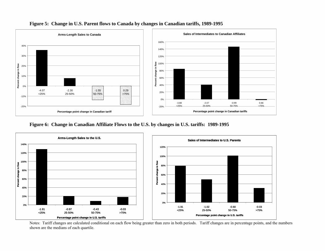