NBER WORKING PAPER SERIES

ACCOUNTING FOR PRICE ENDOGENEITY IN AIRLINE ITINERARY CHOICE MODELS: AN APPLICATION TO CONTINENTAL U.S. MARKETS

Virginie LurkinLaurie A. Garrow

Matthew J. HigginsJeffrey P. Newman

Michael Schyns

Working Paper 22730http://www.nber.org/papers/w22730

NATIONAL BUREAU OF ECONOMIC RESEARCH1050 Massachusetts Avenue

Cambridge, MA 02138October 2016

This research was supported in part by “Fonds National de la Recherche Scientifique” (FNRS - Belgium). We would also like to thank Angelo Guevara for his advice on instruments, Tulinda Larsen for providing us with schedule data, and Chris Howard and Asteway Merid of the Airlines Reporting Corporation for their patience and diligence in answering our many questions about their ticketing database. The views expressed herein are those of the authors and do not necessarily reflect the views of the National Bureau of Economic Research.

NBER working papers are circulated for discussion and comment purposes. They have not been peer-reviewed or been subject to the review by the NBER Board of Directors that accompanies official NBER publications.

© 2016 by Virginie Lurkin, Laurie A. Garrow, Matthew J. Higgins, Jeffrey P. Newman, and Michael Schyns. All rights reserved. Short sections of text, not to exceed two paragraphs, may be quoted without explicit permission provided that full credit, including © notice, is given to the source.

Accounting for Price Endogeneity in Airline Itinerary Choice Models: An Application to ContinentalU.S. MarketsVirginie Lurkin, Laurie A. Garrow, Matthew J. Higgins, Jeffrey P. Newman, and MichaelSchynsNBER Working Paper No. 22730October 2016JEL No. L11,L9,L93,M2

ABSTRACT

Network planning models, which forecast the profitability of airline schedules, support many critical decisions, including equipment purchase decisions. Network planning models include an itinerary choice model that is used to allocate air total demand in a city pair to different itineraries. Multinomial logit (MNL) models are commonly used in practice and capture how individuals make trade-offs among different itinerary attributes; however, none that we are aware of account for price endogeneity. This study formulates an itinerary choice model that is consistent with those used by industry and corrects for price endogeneity using a control function that uses several types of instrumental variables. We estimate our model using a database of more than 3 million tickets provided by the Airlines Reporting Corporation. Results based on Continental U.S. markets for May 2013 departures show that models that fail to account for price endogeneity overestimate customers’ value of time and result in biased price estimates and incorrect pricing recommendations. The size and comprehensiveness of our database allows us to estimate highly refined departure time of day preference curves that account for distance, direction of travel, number of time zones traversed, departure day of week and itinerary type (outbound, inbound or one-way). These time of day preference curves can be used by airlines, researchers, and government organizations in the evaluation of different policies such as congestion pricing.

Virginie LurkinHEC-Management School4000 Liege, Belgiumvirginie.lurkin@epfl.ch

Laurie A. GarrowSchool of Civil and Environmental Engineering Georgia Institute of TechnologyAtlanta, GA 30332laurie.garrow@ce.gatech.edu

Matthew J. HigginsScheller College of BusinessGeorgia Institute of Technology800 West Peachtree StreetAtlanta, GA 30308and NBERmatt.higgins@scheller.gatech.edu

Jeffrey P. NewmanSchool of Civil and Environmental Engineering 790 Atlantic DriveAtlanta, GA 30332-0355jpn@gatech.edu

Michael SchynsHEC-Management School4000 Liege, BelgiumM.Schyns@ulg.ac.be

4

1. Introduction and motivation

Network planning models, which are used to forecast the profitability of airline schedules,

support many important long- and intermediate-term decisions. For example, they aid airlines

in performing merger and acquisition scenarios, route schedule analysis, code-share scenarios,

minimum connection time studies, price-elasticity studies, hub location and hub buildup

studies, and equipment purchasing decisions (Garrow, et al. 2010).

Network planning models forecast schedule profitability by determining the number of

passengers who travel in an origin destination (OD) pair, allocating these passengers to

specific itineraries, and calculating expected costs and revenues. The passenger allocation

model is often referred to as an itinerary choice model because it represents how individuals

make choices among itineraries. Many airlines use discrete choice models to capture how

individuals make trade-offs among different itinerary characteristics, e.g., departure times,

elapsed times, the number of connections, equipment types, carriers, and prices (see Garrow,

et al., 2010 and Jacobs, et al., 2012 for reviews of itinerary choice models used in practice and

Coldren, et al., 2003 and Koppelman, et al., 2008 for specific studies conducted for United

Airlines and Boeing, respectively).

However, to the best of our knowledge, none of the itinerary choice models used in

practice account for price endogeneity. Price endogeneity occurs when prices are influenced

by demand, i.e., higher prices are observed when demand is high and lower prices are

observed when demand is low. Failure to correct for price endogeneity is critical, as it will

result in biased estimates and incorrect profitability calculations. Recent work has focused

attention on the importance of accounting for endogeneity in demand studies. For example

Guevara (2015) notes that “endogeneity often arises in discrete-choice models, precluding the

consistent estimation of the model parameters, but is habitually neglected in practical

applications.” Guevara (2015) provides several examples from the mode choice, residential

location, and intercity travel demand literatures that provide evidence of endogeneity due to

omission of attributes and reviews approaches researchers have been using to account for this

endogeneity. These studies include those by Wardman and Whelan (2011) and Tirachini et al.

(2013) for mode choice applications; Guevara and Ben-Akiva (2006, 2012) for residential

location applications and Mumbower et al. (2014) for intercity applications.

Our prior work in air travel demand modeling has found strong evidence of price

endogeneity. In Mumbower et al. (2014) we model flight-level price elasticities in four

markets using linear regression models and find striking differences in price elasticity

estimates between a model that ignores and a model that accounts for price endogeneity. The

5

model that ignores price endogeneity produces inelastic results (-0.58) whereas the model that

accounts for price endogeneity using a two-stage least squares (2SLS) approach produces

elastic (-1.32) results. In Hotle et al. (2015) we investigate the impact of airlines’ advance

purchase deadlines on individuals’ online search and purchase behaviors for 60 markets. Our

model, which is also based on a 2SLS method, finds strong evidence of price endogeneity.

This paper builds on prior research by showing how to correct for price endogeneity

for an itinerary choice model that is consistent with those used by industry. Unlike our

previous applications, our model incudes “all” Continental U.S. markets and is based on

discrete choice versus linear regression methods. Specifically, we follow the approach of

Coldren and colleagues (2003) described for United Airlines and use a multinomial logit

(MNL) to model itinerary choice for Continental U.S. markets. Results demonstrate the

importance of accounting for price endogeneity; failure to do so results in value of time

estimates that are too high, biased price estimates, and incorrect pricing recommendations.

The results are intuitive, and validation tests indicate that the corrected model outperforms the

uncorrected specification.

Our study is distinct from the majority of prior studies reported in the literature in that

we use a large database of individual tickets from multiple carriers for our analysis.

Specifically, we estimate our model using an analysis database of 3 million tickets provided

by the Airlines Reporting Corporation (ARC). We are uniquely positioned to examine the

potential of using the ARC ticketing database for itinerary choice modeling applications as we

are able to work with detailed price data whereas airlines cannot due to anti-trust regulations.

Our paper contributes to the literature in three key ways. First, we demonstrate the ability to

use the ARC ticketing database (in spite of its limitations) to replicate itinerary choice models

representative of those used in practice. Second, we find a valid set of instruments to correct

for price endogeneity for Continental U.S. markets. Third, due to the size of our analysis

database, we are able to estimate detailed departure time of day preference curves that are

segmented by distance, direction of travel, number of time zones traveled, day of week, and

itinerary type (outbound, inbound or one-way). To the best of our knowledge, these curves

represent the most refined publicly-available estimates of airline passengers’ time of day

preferences.

The remaining sections are organized as follows. Section 2 describes the data

processing assumption we used to create our analysis database and the variables used in our

study. Section 3 presents our methodology, with a particular focus on how we addressed price

endogeneity. Empirical results are presented in Section 4. We conclude by highlighting how

6

our model contributes to the literature and offering directions for future research, many of

which are based on the data limitations commonly faced by industry when estimating discrete

choice models for itinerary choice applications.

2. Data

This section describes the data and variables we used, explains the process we used to

generate choice sets, and assesses the representativeness of our analysis database.

2.1. Airlines Reporting Corporation ticketing database

The Airlines Reporting Corporation (ARC) is a ticketing clearinghouse that maintains

financial transactions for all tickets purchased through travel agencies worldwide. This

includes both online (e.g., Expedia) and brick-and-mortar agencies. Some carriers, most

notably Southwest, are under-represented in the database because the majority of their ticket

sales are through direct sales channels (e.g., southwest.com) that are not reported to ARC.

ARC has detailed information associated with each ticket. This includes the price paid

for the ticket (and associated taxes and currency), ticketing date, booking class, and detailed

information about each flight associated with the ticket, e.g., departure and arrival

dates/times; origin, destination, and connecting airports; total travel time; connecting times;

flight numbers; equipment types and associated capacities; and operating and marketing

carriers. ARC classifies tickets into five product categories: First, Business, Unrestricted

Coach, Restricted Coach, and Other/Unknown. This product classification is based on tables

provided by the International Air Transport Association (IATA) that associates booking

classes for each carrier with these five product categories.

The ticketing database provided by ARC contains tickets that have at least one leg that

departed in May of 2013. May was selected because it is a month with average demand that

falls between off-peak and peak seasons. Given the majority of these tickets are for travel that

originates and terminates within the Continental U.S., we restrict our analysis to these

markets. Only tickets with six or fewer legs representing simple one-way or round-trip

journeys were included in the analysis. More than 93% of all tickets in the ARC database can

be classified as simple one-way and round-trip tickets. A simple one-way ticket does not

contain any stops. A stop occurs when the time between any two consecutive flights is more

than six hours. A simple round-trip itinerary represents a journey in which the individual

starts and ends the journey in the same city and makes at most one stop in a different city.

Round-trip itineraries can include multiple airports that belong to the same city, e.g., an

7

individual who flies round-trip from San Francisco to Chicago can fly from San Francisco

(SFO) to Chicago O’Hare (ORD), make a stop in Chicago, and then fly from Chicago

Midway (MDW) to Oakland (OAK). We excluded tickets that had directional fares of less

than $50 to eliminate tickets that were (likely) purchased using miles or by airline employees.

We also calculated the 99.9th fare percentile for four product classes: First, Business,

Unrestricted Coach, Restricted Coach/Other and eliminated the top 0.1% of observations from

each product class. This process, which is consistent with that used by ARC, was done to

eliminate tickets that were (likely) charter flights.

Our final database used for model estimation contains 3,265,545 directional

itineraries, representing 10,034,935 passenger trips.

2.2. Variable definitions

Table 1 defines and describes the independent variables included in our final itinerary choice

models. Among those variables included in our models, the definitions and descriptions for

elapsed time, number of connections, equipment type, and carrier preference (also referred to

as carrier-specific constants) are straight-forward to interpret. Variables used to define direct

flights, departure time of day, price, and marketing relationships merit additional discussion.

[Insert Table 1 about here]

Direct itineraries

We include nonstop, direct, single connection, and double connection itineraries in our

analysis. Figure 1 can be used to visualize the distinctions among these different types of

itineraries. A nonstop flight consists of a single flight and does not have any stops. Both direct

and single connection itineraries consist of two flight legs and a single stop. For a single

connection itinerary, the flight numbers and aircraft used for each leg differ whereas for a

direct itinerary, the flight numbers for each leg are identical and the aircraft used for each leg

is (typically) the same. The airport in which the intermediate stop occurs (shown as “xxx” on

Figure 1) is not shown in the ticketing database; i.e., only a single ticketing coupon for the

direct flight UA 548 from ORG to DST is recorded. Coupons for customers traveling from

ORG to xxx on UA 548 and xxx to DST on UA 548 also appear in the database, which allows

us to identify that UA 548 from ORG to DST is a direct flight.

Although we recognize that the terminology of a “nonstop” and “direct” can be

confusing, this distinction is critical for practice. In particular, given the limited number of

flight numbers that can be assigned to a flight, airlines often need to create direct itineraries

(or “reuse” the same flight number). Given a direct itinerary is more attractive to customers

8

than a single connecting itinerary (as customers typically stay with the same aircraft and do

not need to disembark and reboard at the intermediate stop), it is important for the airline

industry to model how demand differs for direct versus single-connecting itineraries. For

these reasons, we follow the approach used by other researchers (e.g., see Coldren et al.

(2003), Coldren and Koppelman (2005a,b), Koppelman et al. (2008)) and distinguish between

single connection and direct itineraries.

[Insert Figure 1 about here]

Departure time of day preferences

There are multiple approaches that can be used to model departure time preferences. The first

approach uses a set of categorical variables to represent non-overlapping departure time

periods, e.g., one variable for each departure hour. However, the use of categorical variables

can be problematic for forecasting applications when the difference in coefficients associated

with two consecutive time periods is large (e.g., for the departure periods 9:00-9:59 AM and

10:00-10:59). In this case, moving a flight by a few minutes (e.g., from 9:58 AM to 10:02 AM

can result in unrealistic changes in demand predictions. The second approach overcomes this

limitation by using a continuous specification that combines sine and cosine functions. We

model time of day preferences using a continuous time of day formulation and follow the

approach originally proposed by Abou-Zeid et al. (2006) for intracity travel and adapted by

Koppelman, et al. (2008) for itinerary choice models by including three sine and three cosine

functions representing frequencies of 2𝜋, 4𝜋, and  6𝜋.1

For example, the sin2𝜋 term is given as:

sin2𝜋 = 𝑠𝑖𝑛 2𝜋×departure  time /1440

where departure time is expressed as minutes past midnight and 1440 is the number of

minutes in the day. Similar logic applies to the sin4𝜋, sin6𝜋, cos2𝜋, cos4𝜋, and  cos6𝜋  terms.

One of the main contributions of our paper (which is possible due to the size of our analysis

database) is that we allow departure time preferences to vary according to several dimensions

including the length of haul, direction of travel, number of time zones crossed, departure day

of week, and itinerary type (i.e., outbound, inbound and one-way itineraries). More precisely,

we create ten segments based on the length of haul, direction of travel and number of time

zones crossed. For each segment, we estimate separate time of day preferences for departure

1 Carrier (2008) uses four sine and four cosine functions to model departure time preferences for European markets.

9

day of week and itinerary type. Thus, our model includes 1260 departure time preference

variables.

In a related paper (Lurkin, et al, 2016a), we compared the use of a discrete time of day

formulation with two continuous time of day formulations: one that was based on a 24-hour

cycle and the other that was truncated (or less than 24-hours) based on observed flight

departures for a particular segment. The results from the three time of day formulations are all

similar. The discrete distribution fits the data slightly better, but results in a large increase in

the number of time of day parameters. This increase makes it prohibitive to estimate refined

time of day curves by day of week and type of itinerary. That is, whereas the number of time

of day parameters required for the continuous formulation is 1,260 (6 sine/cosine x 7 days of

week x 3 itinerary types x 10 segments), the number of time of day parameters using 18

discrete intervals would be 3,780. Given the continuous time of day specification provides a

similar model fit and provides more realistic forecasts, we use the continuous time of day

formulation for our itinerary choice models.

In developing a model for United Airlines, Coldren and colleagues (2003) estimated

16 separate MNL models for Continental U.S. markets, one for each time zone pair (e.g.,

itineraries that start and end in the Eastern time zone (EE), itineraries that start and end in the

Central time zone (CC), etc.) The authors note that, aside from time of day preferences, the

estimated coefficients for other itinerary characteristics were similar across these 16

segments. We modify the segmentation approach proposed by Coldren and colleagues to: (1)

distinguish between short and long distances within the same time zone; and, (2) combine

time zone pairs that correspond to the same direction of travel and number of time zones.

Descriptive statistics for our ten segments are shown in Table 2. The table provides

information about the total number of city pairs, choice sets, itineraries, and passengers

associated with each segment. The mean, minimum and maximum distance travelled in each

segment as well as the mean, minimum and maximum number of alternatives by choice set

are also shown. This detailed segmentation allows us to estimate time of day preferences that

vary as a function of distance, direction of travel, and the number of time zones traveled (in

addition to the itinerary type (outbound, inbound, or one-way) and the departure day of

week).

[ Insert Table 2 about here ]

10

Price

The ARC ticketing database contains ticket-level price information linked to specific

itineraries and the time of purchase. This price included on the ticket includes only the base

fare (which corresponds to the revenues the airline receives) and does not include information

on additional ancillary fees (such as fees for checking baggage or reserving a seat).

Information about taxes and fees applied to the base fare are included in the ARC ticketing

database. In the U.S., domestic air travel taxes and fees include four main categories: a

passenger ticket tax (7.5 percent of the base fare); a flight segment tax ($3.90 a flight

segment); a passenger facility charge (up to $4.50 a flight segment); and a federal security

fee, also called the Sept. 11 fee ($2.50 a segment). These taxes and fees are not revenues the

airline receives. The first two taxes go to the Airport and Airway Trust Fund, which finances

the Federal Aviation Administration. Passenger facility charges are passed on to airports and

security fees finance the Transportation Security Administration.

Our discussions with industry practitioners revealed differing (and often strong)

opinions as to whether the “price variable” included in itinerary choice models should include

or exclude these taxes and fees. We discovered that multiple U.S. airlines and aviation

consulting firms do not include these taxes and fees in their “price variable.” Two primary

reasons were offered for this practice: (1) these firms believed models that included taxes and

fees provided results similar to those that excluded taxes and fees; and, (2) these firms noted

that airlines receive revenues only from the base fare. Conversely, those firms that did include

taxes and fees in their “price variable” noted that: (1) including taxes is critical for

international itineraries, as the taxes and fees can be quite large and exceed the base fare; and,

(2) customers do not see the base fare, but rather the “total” price of the itinerary, thus models

that represent the “price variables” as the sum of the base fare, taxes, and fees better reflect

customer behavior.

As part of our modeling exercise, we estimated models that included taxes and fees

and compared them to models that excluded taxes and fees. Results were similar for the two

price formulations; however, the model that included taxes and fees fit the data slightly better.

We include a price variable that includes the base fare as well as taxes and fees in our

specifications as this variable better reflects the prices considered by consumers.

There are several other assumptions we used to create our price variable. Although we

have detailed, ticket-level data in our analysis database, it is important to note that due to

antitrust concerns, airlines do not have access to this same information for their competitors.

For example, the U.S. Department of Transportation’s Origin and Destination Survey

11

Databank 1A/1B (U.S. DOT, 2013) provides a 10% sample of route-level prices, i.e., the

actual price paid for a ticket is known but it is not linked to the time of purchase (number of

days in advance of flight departure) or specific itineraries (e.g., flight numbers and departure

times). Given our focus on demonstrating how we can address price endogeneity in itinerary

choice models representative of those used in practice, we include an “average” price variable

that is similar to that used by industry. Our price variable represents the average price paid by

consumers for a specific itinerary origin, destination, carrier, level of service (i.e.,

nonstop/direct, single connection, double connection), and product type (i.e., high-yield or

low-yield). Also, consistent with industry practice, for round-trip itineraries, we assume the

price associated with an outbound or inbound itinerary is the ticket price/2.

Marketing relationships

A codeshare is a marketing relationship between two airlines in which the operating airline

allows its flight to be sold by a different carrier. Codeshare relationships can be determined

from the ARC ticketing database using information about marketing and operating carriers.

Each flight leg in the ARC ticketing database has a marketing carrier, marketing flight

number, operating carrier and operating flight number. The marketing carrier is the carrier

that sold the flight. The operating carrier is the airline that physically operated the flight. A

codeshare itinerary is one that has the same marketing carrier for all legs, but different

operating carriers. As an example, consider a ticket purchased from US Airways for travel

from Seattle (SEA) to Dallas (DFW) through Phoenix (PHX); the first leg is sold as US flight

102 and is operated by US Airways (as US102) and the second leg is sold as US flight 5998

and is operated by American Airlines (as AA1840). In this example, the marketing carrier for

each leg is the same because two US Airways flight numbers are used to sell the ticket –

US102 and US5998, i.e., American and US Airways have established a marketing agreement

that allows US Airways to sell tickets on AA1840.

Individuals can also purchase an itinerary that has two operating carriers that do not

have a marketing relationship. We define an interline itinerary as one that has different

marketing carriers. An interline itinerary is less attractive than a codeshare itinerary because

there is no coordination – or joint responsibility – between the two operating carriers. For

example, if a bag is checked, the passenger will need to exit security at the connecting airport,

retrieve the bag, and re-check it on the airline operating the second leg. Unlike a codeshare, if

the first leg is delayed, the airline operating the second leg has no obligation to accommodate

the passenger on a later flight.

12

An itinerary that is neither a codeshare or interline itinerary is an online itinerary. An

online itinerary is one that has the same marketing and operating carrier for all legs of the

itinerary.

2.3. Construction of choice sets

The ARC database provides information on the itinerary that was purchased by an individual;

however, in order to model itinerary choices using discrete choice models, we also need to

know what other alternatives were available and not chosen by the individual. There are two

main approaches that are used in practice to generate the universal choice set. The first

method uses a schedule file (which contains the set of all flight legs) and constructs

connecting itineraries using minimum connection, maximum connection, circuity, and other

rules. Minimum and maximum connection rules determine the minimum and maximum

connection times between two consecutive flight legs, respectively; these rules often depend

on whether an international connection (that requires passenger to clear customs) is involved.

Circuity rules are used to prevent circuitous routing, e.g., if a nonstop flight operates between

New York JFK and Miami MIA airports and has a distance of 1,093 miles, a circuity rule of

“1.2” could be used to generate single connecting itineraries that have a distance of 1,093 x

1.2 = 1,312 miles or less (representing by the sum of distances for each flight leg). This helps

prevent unreasonable routings, such as flying from New York to London to Miami or New

York to San Francisco to Miami.

The second method used in practice to construct the universal choice set is to use the

set of observed purchases. It is generally assumed that any itinerary purchased on a particular

day of the week was available for purchase on all other similar days of the week in the month.

That is, if an itinerary was purchased during the second Monday of the month, it is assumed

that the itinerary is part of the universal choice set for all Monday departures in the month.

In both methods, it is common to use a “representative week” from each month to

evaluate schedule profitability, instead of daily schedules. Intuitively, this is to ensure that the

profitability of a given route (and decision whether to purchase an aircraft with a particular

capacity) does not depend on special events or peak periods. The same concept is frequently

used in the design literature, e.g., when determining how many lanes to build on a highway,

engineers do not design for the busiest travel day of the year but rather representative peak

periods. Designing for the busiest travel day would result in the highway being under-utilized

for many other days of the year. The same concept applies to our problem.

13

There are advantages and disadvantages associated with each method. The first

method is advantageous from a forecasting perspective, i.e., given a future flight schedule the

universal set of choices can be easily generated. However, the first method often results in a

large number of itineraries that are contained in the universal choice set, but have no

corresponding purchases in a booking or ticketing database. An analysis based on an itinerary

file we obtained from a major U.S. airline revealed that many the domestic U.S. itineraries

they generated for May 2013 departures had no corresponding purchases in our May 2013

ticketing database. For these reason (particularly when the underlying research objective is

focused on understanding behavioral relationships, as it is the case in our application), it is

common to use the set of observed choices to generate the universal choice set. From a

theoretical perspective, the first method is preferred as using observed choices to create the

choice sets could bias parameter estimates. However, this bias becomes less of a concern as

the size of the input dataset increases (as it is the case in our application), as the probability of

excluding infrequently-chosen alternatives from the choice set (and potentially biasing

results) becomes quite small. For these reasons, and because we did not have access to the

leg-level schedule files, we generated the universal choice set using observed choices.

Formally, we construct choice sets for each OD city pair that departs on day of week d

using the revealed preferences from the ARC ticketing database. We assume that any

alternative purchased on day of week 𝑑! ,𝑎 = {Monday,Tuesday,… , Sunday} was also

available for purchase for all a days in the month, e.g., if an itinerary was purchased on the

first Monday in May 2013 we assume that the itinerary was available on all Mondays in that

month. We need to select a representative Monday that we can use to populate schedule

attributes (except for marketing relationships). We follow the convention of United Airlines

(Garrow 2004) and define the representative week as the week beginning the Monday after

the ninth of the month. This corresponds to May 13 – May 19, 2013 in our data. If an itinerary

was not purchased during the representative week, we populate itinerary attributes (except for

marketing relationships) based on the first day of the week in the month the itinerary was

purchased. In our MNL model, the number of passengers who chose an itinerary represents

the total number of passengers who traveled on day of week 𝑑! in May 2013 on that itinerary.

We define a unique itinerary as follows: Given m legs, a unique itinerary departing on

day 𝑑! is defined by the {legm origin airport, legm destination airport, legm operating carrier,

and legm operating flight number} for m=1,…,3. We assume that if any of the itineraries

meeting this definition was sold as a codeshare during the month, that the unique itinerary is a

codeshare.

14

We performed a sensitivity analysis on each variable in the utility function to ensure

the assumptions we used to populate schedule attributes were reasonable and did not result in

large measurement errors due to using a representative week. The percentage of itineraries in

our analysis database that have a measurement error is small (we estimated these errors to be

less than 2 percent for any given schedule attribute.) An example of the process we used to

construct choice sets is included as an Appendix.

Finally, to improve computational efficiency, we only included OD pairs that had

more than 30 passengers in our analysis. We performed a sensitivity analysis on our MNL

model to ensure this assumption was innocuous. Specifically, we estimated a MNL model

based on itineraries with an origin in the Eastern time zone and a destination in the Western

time zone with all OD pairs and compared it to one that only included OD pairs with more

than 30 passengers. Excluding intercept terms, the parameter estimates between these two

models differed by at most 5 percent and did not impact behavioral interpretations.

2.4. Representativeness of data

The ARC database is a stratified sample of ticket purchase, where the stratification is based

on distribution channel. Specifically, our estimation database contains tickets purchased

through travel agencies. Brick-and-mortar agencies include firms such as Carlson Wagonlit

Travel and online travel agencies include firms such as Expedia as well as “ultra-low cost”

firms such as Priceline. Ticket sales made through direct channels for some carriers, such as

southwest.com and delta.com are not represented in the ARC database. As shown in Table 3,

which compares carrier market shares between the ARC and DB1B databases, the stratified

sample does result in some carriers (most notably Southwest) being underrepresented in the

analysis database; however, there are still observations from “all” major carriers in our

database, and we have no reason to believe that the customers who purchase through direct

sales channels (which include the carriers’ websites and phone reservation systems) have

different itinerary preferences than customers who purchase through other distribution

channels, with the possible exception of carrier preferences, which are explicitly accounted

for in our model.

[ Insert Table 3 about here ]

Although the sample is not representative of the population in every way, this is less

of a concern when the purpose of the sample is to uncover relationships among variables (as it

is here) than when it is purely to describe a population (Babbie, 2009; Groves, 1989, Chapter

1). For example, if we were using the sample to estimate the true share of various carriers in

15

the population it would be problematic, but a model based on the sample can properly predict

itinerary choice given distribution channel. In particular, when the model is a multinomial

logit model (MNL), Manski and Lerman (1977) showed that under certain conditions, the

MNL parameter estimates obtained from a stratified sample would be consistent and unbiased

relative to the MNL estimates obtained from a simple random sample. Thus, we do not expect

that parameter estimates for the variables shown in Table 1 will be impacted by the non-

representativeness of our estimation database.

3. Methodology

This section reviews the multinomial (MNL) logit model and describes how we used a control

function to account for price endogeneity.

3.1. Multinomial logit model

We model the itinerary choice 𝑦!" that an individual 𝑛 chooses alternative  𝑖:

𝑦!" =  1  𝑖𝑓  𝑖𝑛𝑑𝑖𝑣𝑖𝑑𝑢𝑎𝑙  𝑛  𝑐ℎ𝑜𝑜𝑠𝑒𝑠  𝑖𝑡𝑖𝑛𝑒𝑟𝑎𝑟𝑦  𝑖  

0  𝑜𝑡ℎ𝑒𝑟𝑤𝑖𝑠𝑒    

Each choice set is modeled as the set of all directional itineraries between each city-pair for

each day of week 𝑑. For example, all Monday itineraries between Atlanta and Chicago

constitute a choice set. This choice is a function of itinerary, carrier, and product

characteristics. We exclude socioeconomic information as we have no information about the

individual who purchased the ticket.

For cases where 𝑦!" represents discrete outcome, as in the current situation, it is

natural to model the probability that 𝑦!" takes on a given value, using a discrete choice model

such as the MNL (McFadden, 1974). The majority of prior studies have used MNL models

for itinerary choice applications, including those that describe models used in practice (e.g.,

see Coldren, et al., 2003). Given the focus of our study is on determining how we can correct

for price endogeneity and include price for representative itinerary choice models used in

practice, we thus follow this convention and use MNL models. In the MNL, the utility 𝑈 for

individual 𝑛 in choosing alternative 𝑖 from choice set 𝐽! is a linear function of 𝒙!" ,𝑈!"  =

 𝜷!!𝒙!"  +  𝜀!", where 𝒙!" comprises the itinerary, carrier and product variables described in

Table 1 and 𝜷!! is the transpose of the vector of coefficients associated with all variables. If

𝜀!" is distributed independently and identically with a Gumbel (or Extreme Value Type I)

distribution, the probability of individual 𝑛 choosing alternative i is given as:

16

𝑃 𝑦!  =  𝑖   𝒙!") =!𝜷!

!𝒙!"

!𝜷!!𝒙!"

!∈!!

 .

3.2. Price endogeneity

Many prior studies of airline demand have failed to properly address price endogeneity and

have assumed that prices are exogenous. Endogeneity occurs when correlation exists between

an explanatory variable and the error term (or unobserved factors) in a model. This correlation

means that the conditional expectation of the error term on the endogenous explanatory

variable will not equal zero, which violates a main assumption required to ensure estimator

consistency for most models (Greene, 2003).

In demand models, prices are endogenous because they are influenced by demand,

which is influenced by prices (often referred to as simultaneity of supply and demand). Many

empirical demand studies have shown that price coefficients are underestimated if

endogeneity is not corrected, including recent studies that estimate: demand for high speed

rail travel (Pekgün, et al., 2013), household choice of television reception options (Goolsbee

and Petrin, 2004; Petrin and Train, 2010), household choice of residential location (Guevara

and Ben-Akiva, 2006; Guevara-Cue, 2010), choice of yogurt and ketchup brands (Villas-Boas

and Winer, 1999), consumer-level choice of and aggregate product demand for the make and

model of a new vehicle (Berry et al, 1995, 2004; Train and Winston, 2007), and brand-level

demand for hypertension drugs in the U.S. (Branstetter et al., 2011).

There are multiple methods that can be used to correct for price endogeneity. Guevera

provides a nice overview of different methods to treat endogeneity in discrete choice models

(Guevera-Cue, 2010; Guevera 2015). He notes that the two-stage control function (2SCF)

method that accounts for endogeneity using instruments (Heckman, 1978, Hausman, 1996) is

particular relevant in applications, such as ours because it “corrects for endogeneity even

when it occurs at the level of each alternative, making it more practical … when compared to

the method proposed by Berry et. al. (1995) which can only correct for endogeneity when it

occurs at the level or markets or large sets of alternatives.”

An instrument is a variable that does not belong in the demand equation, but is

correlated with the endogenous price variable. Instruments that satisfy the following two

conditions will generate consistent estimates of the parameters, subject to the model being

correctly specified: (1) instruments should be correlated with the endogenous variable, and (2)

they should be independent of the error term in the model (Rivers and Vuong, 1988; Villas-

Boas and Winer, 1999). Therefore, we need to find instruments that are correlated with

17

airfares but not correlated with a customer’s purchase or choice of an itinerary. Validity tests

are used to statistically determine whether the instruments are correlated with airfares, but not

correlated with the error term of the demand model (i.e., customers’ purchase or choice of a

flight).

Mumbower et al. (2014) review instruments that have been or could potentially be

used in airline applications and classify these instruments into four main categories: (1) cost-

shifting instruments; (2) Stern-type measures of competition and market power; (3) Hausman-

type price instruments; and, (4) BLP-type measures of non-price characteristics of other

products. Cost-shifting instruments help explain why costs differ across geographic areas

and/or product characteristics. Stern-type measures of competition and market power focus on

the number of products in the market and also the time since a product (and/or firm) was

introduced into the market (Stern, 1996). Hausman-type price instruments are based on prices

of the same airline in other geographic contexts (Hausman et al., 1994; Hausman, 1996). BLP

instruments, introduced by Berry et al. (1995), are based on the average non-price

characteristics of other products.

We use two instruments to correct for endogeneity: the first is a Hausman-type price

instrument, the other a Stern-type competition instrument. The Hausman-type instrument is

calculated for itinerary i as the cube of the average price of all itineraries having the same

carrier as itinerary  𝑖. For Stern-type competition instrument, we use a measure of capacity,

i.e., the cube of monthly seats flown in an origin-destination pair by carrier and product type

(i.e., high-yield and low-yield).

The first-stage of our two-stage control-function (2SCF) model is an ordinary least-

square (OLS) regression, Equation 1, that uses price as the dependent variable. As noted by

Guevara and Ben-Akiva (2006), the purpose of the price equation is not to make a precise

forecast of the price but to correct for endogeneity. Explanatory variables include the set of

instruments along with all other exogenous regressors (except for price) used in the discrete

choice model. The residual, defined as the difference between the actual and predicted price

𝛿!" = 𝑝!" − 𝑝!",  from the first stage regression is introduced in the second-stage discrete

choice model regression, Equation 2. The first-stage regression model and second-stage

discrete choice model are formulated as follows:

Stage 1: Estimate price by ordinary-least-square (OLS)

𝑝!" = 𝛼!𝐼𝑉!"! +⋯+ 𝛼!𝐼𝑉!"!  + 𝜸!!𝒙!" + 𝛿!"     (1)

Stage 2: Estimate the choice model using the residuals from Stage 1

18

𝑈!"  =  𝛽!𝛿!" + 𝛽!𝑝!" +  𝜷!!𝒙!"  +  𝜀!"   (2)

where

𝑝!" is the average price associated with alternative i for individual n; all itineraries

that have the same origin and destination, product type (i.e., high-yield or low-

yield), carrier, and number of stops have the same average price. Note that

nonstops and directs have zero stops, single connection itineraries have one

stop, and two connection itineraries have two stops.

𝐼𝑉!"! is the kth instrumental variables included in the price equation for alterative i

for individual n.

𝛼!   is the coefficient associated with the kth instrumental variable.

𝜸 is the vector of coefficients associated with all exogenous regressors,

excluding price, from Stage 1.

𝛿!" is the difference between actual and predicted prices from Stage 1, 𝑝!" − 𝑝!".

𝛽!   is the coefficient associated with the difference between actual and predicted

prices from Stage 1.

𝛽!   is the coefficient associated with price from Stage 2.

𝜷 is the vector of coefficients associated with all other exogenous regressors,

excluding price, from Stage 2.

As noted by Guevera-Cue (2010), the estimation of 2SCF in two stages has two

important implications. First, estimates are in general inefficient which implies only the ratios

of coefficients can be interpreted. Second, “the standard errors cannot be calculated from the

inverse of the Fisher information matrix, which prevents the direct application of hypothesis

testing. The need for correcting the standard errors comes from the fact that the second stage

of the method treats the residuals of the first stage as if they were error free, which they are

not” (Guevera-Cue, 2010, p. 34). Guevera-Cue reviews methods that can be used to address

this problem and notes that bootstrapping the observations in the first stage is often the most

viable approach (2010). Given in our application the number of observations is quite large

(more than three million), the standard errors from an uncorrected model are similar to those

obtained from a model that corrects for standard errors using bootstrapping. We verified this

is the case by bootstrapping observations in the first stage using a reduce model specification

with six time of day parameters and conducting 100 bootstraps. The standard errors between

the corrected and uncorrected model differed by at most 0.001 units.

19

We performed several diagnostic tests that are used to verify that endogeneity is

present, that instruments are valid (i.e., correlated with price) and strong (i.e., not correlated

with itinerary choices). First, we test the null hypothesis that price can be treated as an

exogenous regressor using the t-statistic associated with the residual from Equation 2. If the t-

statistic is significant at the 0.05 level the null hypothesis is rejected, indicating that price

should be treated as endogenous (Rivers and Vuong, 1988). This is indeed the case for our

problem, the t-statistic associated with 𝜹 is 118.60 (which is significant at the 0.001 level),

which implies that endogeneity was present in our model.

Next, we use several diagnostic tests to verify that our instruments are valid. As shown

in Table 4, which reports the results of the first-stage OLS regression for the two price

instruments we used to control for endogeneity, the parameter estimates associated with both

instruments are significantly different from zero at the 99% confidence interval level (p-value

< 0.001). In addition, the F statistic (F-stat > 99,999), is well above the critical value of 10

recommended as a rule of thumb by Staiger and Stock (1997).2 Finally, the 𝑅! of the

regression is equal to 0.3699. We conclude from these statistical tests that both instruments

are valid.

Finally, we test the null hypothesis that the set of instruments are strong (uncorrelated

with the error term) and correctly excluded from the demand model using the Direct Test for

discrete choice models proposed by Guevara (Guevera and Ben-Akiva, 2006; Guevara-Cue,

2010). To use the Direct Test, an additional (or auxiliary) discrete choice model is estimated;

this auxiliary model is identical to the one used in Equation 2 but includes k-1 instruments.

The log-likelihood (LL) values between these two models is small, the null hypothesis is

rejected, indicating the instruments are valid. The intuition behind this test is as follows. If the

instruments are correlated with price but not demand, then the inclusion of any instrument as

an additional variable into the corrected Stage 2 model, Equation 2, should produce a non-

significant increase in the log-likelihood variable. Due to identification restrictions, only k-1

of the k instruments can be included in the auxiliary discrete choice model. Formally, given k

instruments,

𝑆!"#$%& = −  2   𝐿𝐿!"#$%! − 𝐿𝐿!"#$%$!&' ~𝜒!",!.!"!

2 Staiger and Stock (1997) have focused on the 2SLS method but Guevara and Navarro (2013) suggest that similar thresholds are applicable in the case of the CF in logit models.

20

where the number of restrictions (NR) is equal to k-1 and the significance level of 0.05 is

used. Given two instruments, the difference in log-likelihood values between the two discrete

choice models can be at most 3.84. For our data, we find that

𝑆!"#$%& = −  2   −26,232,323.64− −26,232,323.36 = 0.56 < 𝜒!,!.!"! =3.84.

We therefore conclude that our instruments are exogenous, or are strong instruments.

[ Insert Table 4 about here ]

4. Model results

Table 5 shows results for two MNL models. The first “uncorrected” model does not account

for price endogeneity whereas the second “corrected” model does. Our presentation of results

is organized into two sections. The first section provides behavioral interpretations for non-

price attributes and the second focuses on pricing results.

[ Insert Table 5 about here ]

4.1. Interpretation of non-price estimates

The results of the MNL itinerary choice model are intuitive, and overall the model performs

well. The 𝝆𝟐, which provides a measure of overall model fit, is 0.1966. This is reasonable,

particularly in light of the fact that the 𝝆𝟐 will be affected by the number of alternatives in the

choice set; in general, the greater the number of alternatives, the smaller the 𝝆𝟐. When

interpreting the results, it is important to note that the coefficients in Table 5 are not directly

interpretable because there is a change of scale (Guevara and Ben-Akiva, 2012) and,

therefore, the ratios of the coefficients and/or elasticities are the only valid means of

information (Tables 6 - 8).

From a behavioral perspective, individuals strongly prefer nonstop itineraries and have

a slight preference for direct itineraries compared to connecting itineraries as shown by the

direct itinerary parameter estimate of -2.3311 compared to the number of connections

parameter estimate of -2.5582 in the corrected model (nonstops are the reference category and

have a utility of 0). This is consistent with expectations, since nonstop itineraries do not have

any stops and although direct and single-connecting itineraries both have a single stop,

passengers traveling on to the final destination do not typically need to change planes at the

intermediate stop location for a direct itinerary. In terms of equipment type, individuals prefer

larger aircraft over regional jets and propeller aircraft. The marketing relationship variables

are also intuitive and reveal the benefits of code-share agreements. Itineraries sold by multiple

carriers via code share agreements are more likely to be purchased than itineraries sold by a

21

single airline (or as an online itinerary). In this sense the marketing relationships are capturing

a level of advertising presence. As expected, interline itineraries are the least preferred type of

itinerary (as these involve the lowest level of coordination in baggage, ticketing, and other

services across flight legs that are operated by different carriers).

Departure times of day preferences are also intuitive. Figures 2 and 3 show the results

of the departure times of day preferences for two (out of the ten) segments, specifically for:

(1) itineraries less than 600 miles that travel westbound and cross one time zone; and, (2)

itineraries that travel westbound and cross three time zones. The curves for Monday to Friday

departures show distinct morning and evening peak preferences for both segments. These

peaks differ depending on itinerary type. For example, the morning peak is strongest for

outbound departures (particularly for those on Monday, Tuesday, and Wednesday). The

afternoon peak is strongest for inbound itineraries (particularly for the Wednesday and

Thursday departures). These preferences are consistent with people who travel for business

(who can depart early in the morning, gain one hour after traveling westbound, and arrive to a

meeting early in the day and then return home later in the week). Departure time preferences

for Saturday are similar with a strong morning peak for outbound departures (likely

corresponding to the start of leisure trips). Departure time preferences for Sunday are the

weakest, but show a slight preference for Sunday evening departures (likely corresponding to

the return of leisure trips and/or the beginning of a weekly business trip). Finally, the time of

day preferences for one-way itineraries are not as strong as those for outbound and inbound

itineraries (and typically fall between the two curves). This is expected, as the one-way

itineraries may represent either the outbound or inbound portion of a trip (but is unknown to

the researcher). Similar patterns are observed for different segments, although the exact

interpretation and peak periods differ depending on the segment.

Also, it is interesting to note that the time of day preferences are in general stronger

for the segment representing short haul trips of 600 miles or less versus longer-haul trips of at

least 1,578 miles. That is, note that the scale of the y-axis for both Figures 2 and 3 are the

same. For the short-haul flights in Figure 2, the utility for the morning and afternoon peaks

often reaches (and in some cases exceeds) 1.250 whereas for the longer-haul flights in Figure

3, the utility for the morning and afternoon peaks is less, typically around 0.75 utils. This

suggests that time of day preferences are stronger in short-haul versus long-haul markets.

Intuitively, this makes sense given that individuals traveling longer distances effectively

“lose” most of the day traveling, and do not have as much time for participating in activities at

the destination during the travel day. For example, on short-haul flights an individual could

22

leave the origin city in the morning and arrive at the destination in time for a 9 AM or 10 AM

meeting, whereas this is likely not an option for a long-haul trip (particularly eastbound

flights).3

[Insert Figures 2 and 3 about here]

The carrier constants reflect sample shares in the estimation database. Major carriers

(who are larger and sell more tickets) including Delta, United, American and US Airways

have non-negative carrier constants whereas smaller carriers and/or low cost carriers have

negative carrier constants. Several additional variables related to carrier presence were also

included in the analysis but were not significant and excluded from the final model

specification. Several studies have found that increased carrier presence in a market leads to

increased market share for that carrier (Algers and Beser 2001; Benkard, et al. 2008; Cornia,

et al. 2012; Gayle 2008; Nako 1992; Proussaloglou and Koppelman 1999; Suzuki, et al.,

2001). In addition, several other studies of itinerary choice models (particularly those based

on stated preference surveys), have been able to include customer-level information, such as

frequent flyer affiliation. Unfortunately, this and other customer-level information was not

available for our study. Finally, as part of our modeling exercise, we estimated separate

models for high yield and low yield segments; however, aside from the price coefficients, the

results were similar. We attribute this to the fact that the high yield and low yield products do

not directly correspond to business and leisure travel purposes. Our findings are similar to

those reported by Coldren, et al. (2003). In that work they find that aside from time of day

preferences, the estimated coefficients for other itinerary characteristics were similar across

their 16 segments (which are similar to our 10 segments and account for distance, direction of

travel, and number of time zones travelled). Thus, our segmentation is similar to that found by

other researchers.

4.2. Interpretation of price estimates

Our itinerary choice model does not include a “no purchase” alternative. This is

because in practice, a separate forecasting module is used to predict market size, or the

number of customers who will travel by air during a certain time period (typically a month).

Thus, the elasticities reported in this section represent “market share” elasticities in the sense

that, given an exogenously-generated market size, the itinerary choice model predicts market

shares as a function of differences in relative prices across carriers.

3 See Lurkin et. al (2016b), which contains the results of all of the departure time of day preference (including parameter estimates and departure time of day charts for all segments).

23

Tables 6 – 8 demonstrate the importance of correcting for price endogeneity. Table 6

shows the value of times associated with the uncorrected model and the model that corrects

for price endogeneity using a control function. Values of time for the high-yield segment are

calculated using the formula below (note that because elapsed time is expressed in minutes,

the factor of 60 is used to convert from minutes to hours). Similar logic applies to the

calculation of values of time (VOT) for the low-yield segment.

𝑉𝑂𝑇!" =𝛽!"#$%!&  !"#$×60

𝛽!"#$!%#  !!"!  !"#$%  !"#$

The values of time are overestimated in the uncorrected model: $126.03/hr for high-

yield and $64.81/hr for low-yield products compared to $83.30/hr and $43.36/hr, respectively

in the corrected model. This overestimate can lead to sub-optimal business decisions. For

example, a carrier that uses the uncorrected itinerary choice model would overestimate

customers’ willingness to pay for a new aircraft that reduces flight times. This could, in turn,

lead to overinvestment in capital expenditures in new aircraft.

Tables 7 and 8 show price elasticity estimates for the high yield and low-yield

products, respectively, based on the mean fares for each segment (and the average across all

segments). Aggregate elasticities for the high yield segment are calculated using the formula

presented by Ben-Akiva and Lerman (1985):

𝐸!"#!" = 𝐸!!"#!!(!)

!

 𝑤!𝑃! 𝑖𝑤!𝑃!(𝑖)!

 

where

𝐸!!"#!!(!) is the disaggregate direct point elasticity with respect to variable 𝑥!",

𝑤! is the weight of individual 𝑛 in the sample,

𝑃!(𝑖) is the probability that individual 𝑛 chooses alternative 𝑖.

These differences are economically important. In Table 7, the segments for which

elasticity flips from inelastic (greater than -1.0) to elastic (less than -1.0), can lead to

completely opposite effects than which were intended by firms. For example, in the “Same

TZ, distance > 600 mi.” segment we report a mean low yield fare of $207.96 and an

uncorrected model elasticity of -0.7732. Using simple first principles and basic economic

theory, given this inelasticity a firm could raise price, quantity demanded would decline (as

would total costs) but total revenues would in fact increase. Such a move, with certainty,

would increase economic profits. However, results from the model that accounts for price

24

endogeneity indicate that low-yield products on that segment are in fact elastic. As such, a

price increase would cause total revenues to decline; quantity demand would also decline (as

would total cost). The resulting impact on economic profits is now uncertain.

Again, using first principles, managers should never lower price on inelastic

consumers, as this will, with certainty, lead to lower revenues. In contrast, lowering price on

elastic consumers will result in the opposite, increased revenues. In Table 7 eight segments

are incorrectly identified by the basic model as being inelastic when in reality low-yield

products are elastic. For these segments, managers would incorrectly assume that they should

not decrease price in those markets. We see similar trends in Table 8 with the “3 Time Zone

Westbound” and “3 Time Zone Eastbound” segments. In general, the results in Table 8

demonstrate that high-yield products are not as inelastic as predicted by the uncorrected

model. In other words, consumers are more price-sensitive. Again, these results are

economically meaningful. For example, the uncorrected model reports an average elasticity

for high yield product of -0.5877; a 10% increase in price will lead to a 5.88% decline in

quantity demanded. In contrast, results from the model that accounts for price endogeneity

shows an elasticity of -0.8307; a 10% increase in price will lead to a 8.31% decline in

quantity demanded. This suggests that managers or revenue models would underestimate the

impact on quantity demanded by approximately 2.43%.

[ Insert Tables 6 – 8 here ]

5. Limitations, contributions, and future research

To the best of our knowledge, this is the first study to control for price endogeneity for an

itinerary choice model that is representative of those currently used in practice. Our model

suffers from the same data limitations faced by industry. Our sample is non-representative in

the sense that certain distribution channels are under-represented. We are therefore implicitly

assuming that those customers who purchase tickets through direct sales channels (such as

southwest.com and delta.com) have similar itinerary preferences as those who purchase

through other distribution channels (such as travelocity.com, priceline.com, and brick-and-

mortar travel agencies). Our ticketing database provides no information about the customers

who purchased the ticket, preventing us from examining differences in preference based on

trip purpose and socio-economic factors. The lack of information about customers also

prevents us from modeling schedule delay, defined as the difference between an individual’s

preferred departure time and the scheduled departure time of an itinerary. We also assume that

25

customer preferences and competition among alternatives can be represented using a MNL

model (which is the most common model used in practice); however more advanced discrete

choice models that allow for random coefficients and different substitution patterns across

product dimensions are clearly desirable.

Nonetheless, our analysis provides an important contribution by demonstrating how

models representative of those currently used in practice can be enhanced to correct for price

endogeneity. Our results show that failure to account for price endogeneity leads to over-

estimation of customers’ value of time. This can lead to sub-optimal business decisions, e.g.,

a carrier that uses the uncorrected itinerary choice model would over-estimate customers’

willingness to pay for a new aircraft that reduces flight times (and potentially over-invest in

new aircraft). A second main contribution is that it is the first study to estimate highly refined

departure time of day preferences. The price elasticity and departure time of day preferences

results are not restricted to itinerary choice modeling applications, and can help support

evaluation of proposed airport fees and taxes, national departure and emission taxes, landing

fees, and congestion pricing policies.

There are several research extensions. As part of our analysis, we used an average

price variable similar to that used by industry. However, prior research has shown that

customers’ price sensitivities vary as a function of how far in advance a ticket is purchased.

Extending the analysis to include advance purchase effects is one area of future research.

Prior research (e.g., Coldren and Koppelman, 2005a) has also shown that there are potentially

many layers of correlation within and across product attributes, with relationships extending

across airline, time of day, level of service (e.g., nonstop versus connecting), and potentially

other dimensions. Replacing the MNL with a simple nested logit choice model or a more

complex but flexible generalized extreme value (GEV) model such as the network GEV (Daly

and Bierlaire, 2006; Newman 2007) is another potential research direction. In particular, it

would be interesting to compare if the substitution patterns observed by Coldren and

Koppelman (2005a) using data from 2001 are also observed on more recent data. It would

also be interesting to determine if other product dimensions they did not consider for nesting

(such as high-yield versus low-yield product distinctions) or that they found to be

insignificant (such as level of service) are important to incorporate for models based on more

recent data.

Finally, it would be interesting to compare the results from the corrected model we

developed in this paper that corrects for price endogeneity to one that incorporates advanced

modeling techniques found in the economic welfare estimation literature. For example,

26

Armantier and Richard (2008) propose a method to account for the non-random nature of data

available for estimating airline itinerary choice models using distributions from publicly

available data such as DB1B (US DOT, 2013). As always, much remains to be done.

Acknowledgements

This research was supported in part by “Fonds National de la Recherche Scientifique” (FNRS

- Belgium). We would also like to thank Angelo Guevara for his advice on instruments,

Tulinda Larsen for providing us with schedule data, and Chris Howard and Asteway Merid of

the Airlines Reporting Corporation for their patience and diligence in answering our many

questions about their ticketing database.

References

[1] Abou-Zeid, M.A., Rossi, T.F. and Gardner, B. (2006). Modeling time of day choice in the

context of tour and activity based models. Paper presented at the 85th annual meeting

of the Transportation Research Board, Washington, DC.

[2] Armantier, O. and Richard, O. (2008). Domestic airline alliances and consumer welfare.

The RAND Journal of Economics, 39(3): 875-904.

[3] Algers, S. and Beser, M. (2001) Modeling choice of flight and booking class – A study

using stated preference and revealed preference data. International Journal of Services

Technology and Management, 2(1/2), 28-45.

[4] Babbie, E. R., (2009) The Practice of Social Research, 12th Edition. Wadsworth

Publishing Company, Belmont, CA.

[5]  Ben-Akiva, M. E., & Lerman, S. R. (1985). Discrete choice analysis: theory and

application to travel demand (Vol. 9). MIT press, Cambridge, MA.

[6] Benkard, C., Bodoh-Creed, A., and Lazarev, J. (2008) The long run effects of U.S. airline

mergers. Working Paper, Yale University.

<http://economics.yale.edu/sites/default/files/ files/Workshops-Seminars/Industrial-

Organization/benkard-081106.pdf> (accessed 07.03.15).

[7] Berry, S., Levinsohn, J. and Pakes, A. (1995) Automobile prices in market equilibrium.

Econometrica, 63 (4), 841-890.

[8] Berry, S., Levinsohn, J. and Pakes, A. (2004). Differentiated products demand systems

from a combination of micro and macro data: The new car market. Journal of Political

Economy, 112 (1), 68-105.

27

[9] Branstetter, L., Chatterjee, C. and Higgins, M.J. (2011) Regulation and welfare: Evidence

from Paragraph-IV generic entry in the pharmaceutical industry. Working paper,

Carnegie Mellon University and Georgia Institute of Technology.

[10] Carrier, E. (2008) Modeling the Choice of an Airline Itinerary and Fare Product Using

Booking and Seat Availability Data, Ph.D. Dissertation, Department of Civil and

Environmental Engineering, Massachusetts Institute of Technology, Cambridge, MA.

[11] Coldren, G.M., Koppelman, F.S., Kasturirangan, K. and Mukherjee, A. (2003) Modeling

aggregate air-travel itinerary shares: Logit model development at a major U.S. airline.

Journal of Air Transport Management, 9(6), 361-69.

[12] Coldren, G.M. and Koppelman, F.S. (2005a) Modeling the competition among air-travel

itinerary shares: GEV model development. Transportation Research Part A, 39(4),

345-65.

[13] Coldren, G.M. and Koppelman, F.S. (2005b) Modeling the proximate covariance

property of air travel itineraries along the time of day dimension. Transportation

Research Record, 1915, 112-23.

[14] Cornia, M. Gerardi, K.S. and Shapiro, A.H. (2012) Price dispersion over the business

cycle: Evidence from the airline industry. The Journal of Industrial Economics,

60(3):347–373.

[15] Daly, A. and Bierlaire, M. (2006) A general and operational representation of generalized

extreme value models. Transportation Research Part B, 40(4), 285-305.

[16] Garrow, L.A. (2004) Comparison of Choice Models Representing Correlation and

Random Taste Variation: An Application to Airline Passengers’ Rescheduling

Behavior. Ph.D. Dissertation, Department of Civil and Environmental Engineering,

Northwestern University, Evanston, IL.

[17] Garrow, L.A., Coldren, G.M. and Koppelman, F.S. (2010). MNL, NL, and OGEV

models of itinerary choice. In Discrete Choice Modeling and Air Travel Demand:

Theory and Applications, ed. L.A. Garrow. Ashgate Publishing: Aldershot, United

Kingdom. pp. 203-252.

[18] Gayle, P.G. (2008) An empirical analysis of the competitive effects of the

Delta/Continental/Northwest code-share alliance. Journal of Law and Economics,

51(4):743–766.

[19] Goolsbee, A. and Petrin, A. (2004) The consumer gains from direct broadcast satellites

and the competition with cable TV. Econometrica, 72 (2), 351-381.

28

[20] Greene, W.H. (2003) Econometric Analysis ed Rod Banister, 5th ed. Prentice Hall,

Upper Saddle River, New Jersey.

[21] Groves, R. M. (1989) Survey Errors and Survey Costs. John Wiley & Sons, New York.

[22] Guevara-Cue, C.A. (2010) Endogeneity and sampling of alternatives in spatial choice

models. Doctoral Dissertation, Department of Civil and Environmental Engineering,

Massachusetts Institute of Technology, Cambridge, MA.

[23] Guevara, C.A (2015) Critical assessment of five methods to correct for endogeneity in

discrete-choice models. Transportation Research Part A, 82(4), 240-254

[24] Guevara, C.A. and Ben-Akiva, M. (2006) Endogeneity in residential location choice

models. Transportation Research Record: Journal of the Transportation Research

Board, 1977, 60-66.

[25] Guevara, C.A. and Ben-Akiva, M. (2012) Change of scale and forecasting with the

control-function method in logit models. Transportation Science, 46(3): 425-437.

[26] Guevara, C.A. and Navarro, P. (2013) Control-function correction with weak instruments

in logit models. Working paper, Universidad de los Andes, Chile.

[27] Hausman, J.A. (1996) Valuation of new goods under perfect and imperfect competition.

The Economics of New Goods eds Robert J. Gordon and Timothy F. Bresnahan, 207–

248. University of Chicago Press, Chicago.

[28] Hausman, J., Leonard, G. and Zona, J.D. (1994) Competitive analysis with differentiated

products. Annals of Economics and Statistics, 34, 159-180.

[29] Heckman, J. (1978), Dummy endogenous variables in a simultaneous equation system.

Econometrica, 46, 931-959.

[30] Hotle, S., Castillo, M., Garrow, L.A. and Higgins, M.J. (2015) The impact of advance

purchase deadlines on airline customers’ search and purchase behaviors.

Transportation Research Part A 82:1-16.

[31] Jacobs, T.L., Garrow, L.A., Lohatepanont, M., Koppelman, F.S., Coldren, G.M. and

Purnomo, H. (2012). Airline planning and schedule development. Quantitative

Problem Solving Methods in the Airline Industry: A Modeling Methodology

Handbook. Part of the Fred Hillier International Series on Operations Research and

Management Sciences. Vol. 169. Eds. C. Barnhart and B. Smith. New York: Springer.

pp. 35-100.

[32] Koppelman, F.S., Coldren, G.C. and Parker, R.A. (2008) Schedule delay impacts on air-

travel itinerary demand. Transportation Research Part B, 42(3), 263-73.

29

[33] Lurkin, V., Garrow, L.A., Higgins, M.J., Newman, J.P. and Schyns, M. (2016a). A

comparison of departure time of day formulations. (January 27, 2016). Available at

SSRN: http://ssrn.com/abstract=2723668.

[34] Lurkin, V., Garrow, L.A., Higgins, M. and Schyns, M. (2016b) Continuous departure

time of day preferences for Continental U.S. Airline markets segmented by distance,

direction of travel, number of time zones, day of week and itinerary type (January 27,

2016). Available at SSRN: http://ssrn.com/abstract=2721974.

[35] Manski, C. and Lerman, S. (1977) The estimation of choice probabilities from choice

based samples. Econometrica, 45, 1977-88.

[36] McFadden, D. L., 1974. Conditional Logit Analysis of Qualitative Choice Behavior. In:

Zarembka, P. (Ed.), Frontiers in Econometrics. Academic Press, New York, pp. 105–

142.

[37] Mumbower, S. and Garrow, L.A. and Higgins, M.J. (2014) Estimating flight-level price

elasticities using online airline data: A first step towards integrating pricing, demand,

and revenue optimization. Transportation Research Part A 66: 196–212.

[38] Nako, S.M. (1992) Frequent flyer programs and business travellers: An empirical

investigation. The Logistics and Transportation Review, 28(4), 395-414.

[39] Newman, J. (2007). Normalization of network generalized extreme value models.

Transportation Research Part B 42(10): 958-969.  

[40] Pekgün, P., Griffin, P.M. and Keskinocak, P. (2013) An empirical study for estimating

price elasticities in the travel industry. Working Paper, University of South Carolina.

[41] Petrin, A. and Train, K. (2010) A control function approach to endogeneity in consumer

choice models. Journal of Marketing Research, 47 (1), 3-13.

[42] Proussaloglou, K. and Koppelman, F.S. (1999) The choice of air carrier, flight, and fare

class. Journal of Air Transport Management, 5(4), 193-201.

[43] Rivers, D. and Vuong, Q.H. (1988) Limited information estimators and exogeneity tests

for simultaneous probit models. Journal of Econometrics, 39, 347-366.

[44] Staiger, D. and Stock, J.H. (1997) Instrumental variables regression with weak

instruments. Econometrica: Journal of the Econometric Society, 65, 557-586.

[45] Stern, S. (1996). Market definition and the returns to innovation: Substitution patterns in

pharmaceutical markets. Working paper, Sloan School of Management, Massachusetts

Institute of Technology.

30

[46] Suzuki, Y., Tyworth, J.E. and Novack, R.A. (2001) Airline market share and customer

service quality: A reference-dependent model. Transportation Research Part A, 35(9),

773-88.

[47] Tirachini, A., Hensher, D.A., and Rose, J.M. (2013) Crowding in public transport

systems: Effects on users, operation and implications for the estimation of demand.

Transportation Research Part A, 53: 36-52.

[48] Train, K.E. and Winston, C. (2007) Vehicle choice behavior and the declining market

share of U.S. automakers. International Economic Review, 48 (4), 1469-1496.

[49] U.S. Department of Transportation, Bureau of Transportation Statistics (Quarter 3, 2013)

Origin and Destination Survey Databank 1A/1B. <www.transtats.bts.gov> (accessed

01.18.2016).

[50] Villas-Boas, J.M. and Winer, R.S. (1999) Endogeneity in brand choice models.

Management Science, 45 (10), 1324-1338.

[51] Wardman, M. and Whelan, G. (2011). Twenty years of rail crowding valuation studies:

Evidence and lessons from British experience. Transportation Reviews, 31(3): 379-

398.

31

Appendix: Example of choice set generation process

An example illustrating the process we used to generate choice sets is shown in Tables A1

and A2. Table A1 contains five unique itineraries from ATL to SEA for Tuesday departures

in May of 2013. The final choice set, shown in Table A2, contains five itineraries. The rows

from Table A1 that were used to populate schedule attributes (with the exception of marketing

relationships and passenger counts) are highlighted. For itineraries 1, 2, and 4 the date falling

in the representative week (May 14) is used to populate schedule attributes whereas for

itineraries 3 and 5 the first date that itinerary was purchased is used since there are no

purchases that occurred on May 14.

[ Insert Tables A1 and A2 about here ]

The number of passenger and marketing type associated with itinerary q in the final

choice set are calculated using information from all rows in Table A1 associated with

itinerary q. For example, the total number of passengers who purchase itinerary 1 is 23. The

marketing type for itinerary 2 is online because the marketing carriers and operating carriers

are always the same for all rows associated with itinerary 2. The marketing type associated

with itinerary 1 in the final choice set is a codeshare, because two tickets for travel on May 28

for Alaska operated flight 938 were sold by AA. The marketing type for itinerary 4 is an

interline because the marketing carriers for leg1 and leg2 differ.

32

List of Figures and Tables

Figure 1: Nonstop, Direct, Single-Connection and Double-Connection Itineraries

Figure 2: Departure Time of Day Preferences: One TZ Westbound, distances ≤  600 miles

Figure 3: Departure Time of Day Preferences: Three TZ Westbound

Table 1: Independent Variables and Definitions Table 2: Descriptive Statistics by Segment

Table 3: Airline Market Shares in ARC and DB1B Data Table 4: First-stage OLS regression

Table 5: Model Results Table 6: Value of Time Results

Table 7: Price Elasticities for Low-Yield Products Table 8: Price Elasticities for High-Yield Products

Table A1: Example of Itineraries Departing on Tuesdays from ATL-SEA Table A2: Example of Choice Set for Itineraries Departing on Tuesdays from ATL-SEA

33

Figure 1: Nonstop, Direct, Single-Connection and Double-Connection Itineraries

ORG DST UA 829

ORG DST UA 548 xxx

UA 548

ORG DST UA 619

CNX1 UA 180

ORG CNX2 UA 830 CNX1

UA 19 DST

UA 702

Nonstop

Direct

Single connection

Double connection

1

Figure 2: Departure Time of Day Preferences: One TZ Westbound, distances ≤  600 miles

2

Figure 3: Departure Time of Day Preferences: Three TZ Westbound

3

Table 1: Independent Variables and Definitions

Variable Definition Travel Time, Number of Connections, Connection, and Equipment Attributes

Elapsed time

Elapsed time is defined as the difference between the arrival time at the itinerary destination and the departure time at the itinerary origin. All arrival and departure times are reported in Coordinated Universal Time (UTC), which accounts for time zone differences.

Number of connections Number of itinerary connections. A value of zero indicates a nonstop itinerary and a value of one (two) indicates a single (double) connection.

Direct flight A “direct flight” is one that has two flight legs. The operating carrier and operating flight number of the two flight legs are the same. A direct flight is defined to have zero connections.

Wide- or narrow-body Regional jet or propeller

Equipment types include two categories. The first includes wide-body and narrow-body aircraft (no regional jets). The second includes narrow-body regional jets and propellers. For itineraries with more than one leg, the smallest equipment type is used.

Departure Time of Day

Sin2pi_DOW!_TripType! … Cos6pi_DOW!_TripType!

Departure time preferences are modeled using 1260 terms. Three sin (sin2pi, sin4pi, sin6pi) and three cosin functions (cos2pi, cos4pi, cos6pi) apply to each departure day of week i=1,2,…,7 and three trip types j=outbound, inbound, one-way.

Price

Average high yield fare Average low yield fare

We calculate separate prices for high yield and low yield fare products. We include First, Business, and Unrestricted Coach products as high yield fares and the Restricted Coach and Other/Unknown products as low yield fares. We calculate average high yield and average low yield fares for each itinerary origin, destination, carrier, and level of service (nonstop/direct, single connection, and double connection).

Marketing Relationships

Online An online itinerary is one that has the same marketing and same operating carrier for all legs.

Codeshare A codeshare itinerary is one that has the same marketing carrier for all legs, but different operating carriers.

Interline An interline itinerary is one that has different marketing carriers. Only itineraries with two or more legs can be interline itineraries.

Carrier Preference

Carrier_1 Carrier_2 … Carrier_9

For k=1,2,…,9 the indicator variable Carrier_k =1 if the itinerary operating carrier associated with an itinerary is carrier k and 0 otherwise. The itinerary operating carrier is defined as the carrier that operates the longest flight leg. The first eight terms represent carriers that each have more than 1% market share in the estimation data. All other carriers are combined into the Carrier_9 term. .

4

Table 2: Descriptive Statistics by Segment

Segment City pairs

Choice sets Itins Pax

Distance Choice sets

Min Mean Max Min Alts

Mean Alts

Max Alts

Same TZ, distance ≤ 600 mi. 4,703 30,943 711,282 2,219,511 31 415.0 600 2 10.8 95

Same TZ, distance > 600 mi. 3,524 22,861 520,481 1,848,742 601 839.3 1,534 2 14.3 105

One TZ Westbound, distance ≤ 600 mi. 859 5,617 112,615 306,119 84 463.6 600 2 10.6 64

One TZ Westbound, distance > 600 mi. 3,864 24,820 498,999 1,466,815 601 993.9 1,925 2 15.1 127

One TZ Eastbound, distance ≤ 600 mi. 863 5,630 115,187 312,265 84 462.0 600 2 10.3 63

One TZ Eastbound, distance > 600 mi. 3,898 25,062 501,345 1,446,807 601 993.7 1,925 2 14.5 137

Two TZ Westbound 1,860 11,505 239,936 681,666 643 1,576.4 2,451 2 17.1 133

Two TZ Eastbound 1,823 11,267 233,113 684,627 643 1,571.4 2,451 2 15.3 93

Three TZ Westbound 1,121 6,732 165,428 509,346 1,578 2,203,3 2,774 2 21.3 156

Three TZ Eastbound 1,091 6,619 167,159 559,037 1,578 2,210.9 2,774 2 19.2 138

TOTAL 23,606 151,056 3,265,545 10,034,935

5

Table 3: Airline Market Shares in ARC and DB1B Data

Carrier ARC Mkt Share DB1B Mkt Share

Delta Air Lines (DL) 29.5% 23.4%

United Airlines (UA) 22.9% 17.1%

US Airways (US) 18.4% 10.0%

American Airlines (AA) 17.5% 19.0%

Alaska Airlines (AS) 3.3% 4.2%

JetBlue Airways (B6) 3.2% 3.0%

Frontier Airlines (F9) 2.2% 1.7%

AirTran Airways (FL) 1.4% 2.8%

Virgin America (VX) 1.3% 0.9%

Sun Country Airlines (SY) 0.3% 0.2%

Southwest Airlines (WN) 0.0% 17.7%

Total 100% 100%

6

Table 4: First-stage OLS regression

Variable Parameter Std Error T-statistic P-value Delta Air Lines (DL) (ref.) 0.000 - - - United Airlines (UA) 26.95 0.0141 1,909 0.0000 American Airlines (AA) 36.70 0.0153 2,391 0.0000 US Airways (US) 26.17 0.0140 1,873 0.0000 Alaska Airlines (AS) -1.448 0.0447 -32.43 0.0000 Jetblue Airways (B6) -17.96 0.0437 -411.1 0.0000 Frontier Airlines (F9) -35.88 0.0418 -858.3 0.0000 AirTran Airways (FL) -15.13 0.0420 -360.4 0.0000 Other airlines -7.710 0.0452 -170.4 0.0000 Elapsed time (min) 0.1642 0.0001 2,309 0.0000 Regional jet or propeller (ref.) 0.000 - - - Wide- or narrow-body -12.28 0.0102 -1,203 0.0000 Number of connections -32.17 0.0180 -1,790 0.0000 Direct flight -33.43 0.0501 -667.7 0.0000 Online (ref.) 0.000 - - - Codeshare 5.562 0.0176 315.7 0.0000 Interline 52.62 0.0454 1,160 0.0000 Stern-type instrument 0.0000 0.0000 -1,584 0.0000 Hausman-type instrument 0.0000 0.0000 11,000 0.0000 Constant term 192.8 0.0262 7,349 0.0000 F statistic > 99,999 𝑅! 0.3699

7

Table 5: Model Results

LL= log likelihood, Adj. 𝝆² = 1 – (Final LL - #Attributes) /  𝑳𝑳(𝟎)

Uncorrected Model Corrected Model

Variable Parameter t-statistic Parameter t-statistic

Delta Air Lines (DL) (ref.) 0 - 0 -

United Airlines (UA) -0.0411 -30.8 -0.0076 -5.53

American Airlines (AA) 0.3802 284 0.4308 306

US Airways (US) 0.1917 142 0.2002 148

Alaska Airlines (AS) -0.0189 -4.89 -0.0814 -20.9

Jetblue Airways (B6) -0.3048 -104 -0.3788 -127

Frontier Airlines (F9) -0.2950 -88.8 -0.4279 -122

AirTran Airways (FL) -0.9756 -278 -1.0632 -296

Other airlines -0.3656 -92.1 -0.4033 -101

Average high yield fare ($) -0.0025 -258 -0.0036 -265

Average low yield fare ($) -0.0049 -383 -0.0069 -327

Elapsed time (min) -0.0053 -503 -0.0050 -455

Number of connections -2.4892 -1,194 -2.5582 -1,179

Direct flight -2.2624 -375 -2.3311 -384

Regional jet or propeller (ref.) 0 - 0 -

Wide- or narrow-body 0.4150 384 0.3889 353

Online (ref.) 0 - 0 -

Codeshare 0.2742 208 0.2825 214

Interline -0.2342 -35.4 -0.1297 -19.4

𝜹 (residuals) - - 0.0020 118.6000

𝑳𝑳(𝟎) -32,652,846.05 -32,652,846.05

Final 𝑳𝑳 -26,239,664.32 -26,232,323.64

Adj. 𝝆𝟐 0.1964 0.1966

8

Table 6: Value of Time Results

Value of Time Uncorrected

Model Corrected

Model High-yield ($/hr) 126.03 83.30

Low-yield ($/hr) 64.81 43.36

9

Table 7: Price Elasticities for Low-Yield Products

Low-Yield Products

Segment Mean fare

Uncorrected elasticities

Corrected elasticities

Same TZ, distance ≤ 600 mi. 221.42 -0.8251 -1.1551

Same TZ, distance > 600 mi. 207.96 -0.7732 -1.0826

One TZ Westbound, distance ≤ 600 mi. 221.32 -0.8134 -1.1387

One TZ Westbound, distance > 600 mi. 248.76 -0.9413 -1.3180

One TZ Eastbound, distance ≤ 600 mi. 219.15 -0.8260 -1.1564

One TZ Eastbound, distance > 600 mi. 251.80 -0.9567 -1.3396

Two TZ Westbound 265.62 -0.9995 -1.3992

Two TZ Eastbound 263.82 -0.9975 -1.3963

Three TZ Westbound 289.58 -1.1161 -1.5618

Three TZ Eastbound 290.41 -1.1586 -1.6218

Average for All Segments 240.20 -0.8976 -1.2567

10

Table 8: Price Elasticities for High-Yield Products

High-Yield Products

Segment Mean fare

Uncorrected elasticities

Corrected elasticities

Same TZ, distance ≤ 600 mi. 290.73 -0.5281 -0.7459

Same TZ, distance > 600 mi. 293.41 -0.4949 -0.6936

One TZ Westbound, distance ≤ 600 mi. 320.53 -0.5757 -0.8111

One TZ Westbound, distance > 600 mi. 329.03 -0.5735 -0.8051

One TZ Eastbound, distance ≤ 600 mi. 315.33 -0.5769 -0.8112

One TZ Eastbound, distance > 600 mi. 344.59 -0.5929 -0.8330

Two TZ Westbound 364.98 -0.6243 -0.8828

Two TZ Eastbound 347.66 -0.5773 -0.8136

Three TZ Westbound 503.74 -0.8416 -1.2106

Three TZ Eastbound 498.00 -0.8646 -1.2423

Average for all Segments 343.60 -0.5877 -0.8307

11

Table A1: Example of Itineraries Departing on Tuesdays from ATL-SEA

Itin Leg 1 Leg 2

# # Pax Mkt Type Org Dst Op Carr Mkt Carr Op Flt Dept Date Dept Time Org Dst Op Carr Mkt Carr Op Flt Dept Time

1 6 Online ATL SEA AS AS 938 5/7 8:16

1 3 Online ATL SEA AS AS 938 5/14 8:16

1 6 Online ATL SEA AS AS 938 5/21 8:16

1 2 Online ATL SEA AS AS 938 5/28 8:16

1 6 CShare ATL SEA AS AA 938 5/28 8:16

2 8 Online ATL SEA DL DL 319 5/7 10:10

2 5 Online ATL SEA DL DL 319 5/14 10:15

2 3 Online ATL SEA DL DL 319 5/21 10:10

3 1 Online ATL JFK DL DL 688 5/7 8:05 JFK SEA DL DL 417 11:23

4 2 ILine ATL PHX DL DL 545 5/21 9:15 PHX SEA WN WN 2849 13:30

4 1 ILine ATL PHX DL DL 545 5/28 9:20 PHX SEA WN WN 2849 13:30

5 2 Online ATL SLC DL DL 1278 5/7 12:10 SLC SEA DL DL 784 15:25

5 1 Online ATL SLC DL AF 1278 5/14 12:20 SLC SEA DL AF 784 15:25

5 1 CShare ATL SLC DL KL 1278 5/21 12:20 SLC SEA DL KL 784 15:25

5 1 CShare ATL SLC DL DL 1278 5/28 12:10 SLC SEA DL DL 784 15:25

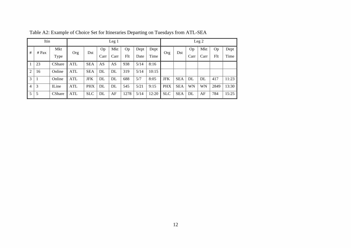
12

Table A2: Example of Choice Set for Itineraries Departing on Tuesdays from ATL-SEA

Itin Leg 1 Leg 2

# # Pax Mkt

Type Org Dst

Op

Carr

Mkt

Carr

Op

Flt

Dept

Date

Dept

Time Org Dst

Op

Carr

Mkt

Carr

Op

Flt

Dept

Time

1 23 CShare ATL SEA AS AS 938 5/14 8:16

2 16 Online ATL SEA DL DL 319 5/14 10:15

3 1 Online ATL JFK DL DL 688 5/7 8:05 JFK SEA DL DL 417 11:23

4 3 ILine ATL PHX DL DL 545 5/21 9:15 PHX SEA WN WN 2849 13:30

5 5 CShare ATL SLC DL AF 1278 5/14 12:20 SLC SEA DL AF 784 15:25