ACCIDENTS ON RURAL ROADS – FOR BETTER OR …starconference.org.uk/star/2010/accidents.pdf ·...

ACCIDENTS ON RURAL ROADS – FOR BETTER OR WORSE

Dr James Laird Institute for Transport Studies, University of Leeds

Russell Harris

RPS, Co Cork, Ireland

Dr Shujie Shen Institute for Transport Studies, University of Leeds

SUMMARY

This paper presents the results of a novel analysis of accident data on Ireland’s National Secondary Road network. This is a national network of single-carriageway A-roads. The results challenge the conventionally-held belief that a better-designed road is a safer road. .

ABSTRACT

Single-carriageway A-roads in rural areas are among the most dangerous routes on the network. Alongside journey time savings, safety improvements are therefore one of the main benefits claimed to result from quality improvements to rural single-carriageway roads. Existing appraisal methods support the engineers’ natural conviction that a better-designed road is a safer road. However, this contrasts with anecdotal evidence that as speeds and traffic flows increase, so does the likelihood of a fatal accident.

This paper examines the safety issue in more detail and presents a novel analysis of accident data on the National Secondary Road network in Ireland. The Irish national secondary network consists of 2,700 km of single-carriageway A-roads, complementing the national primary routes. The context is similar to Scotland – the two countries face similar challenges of accessibility to peripheral rural areas.

For this analysis, the 34 National Secondary routes have been broken up into 850 sections, each with a road quality score based on bendiness, carriageway width and gradient. Econometric analysis of accident rates and types by road quality identifies a number of interesting characteristics. As road quality improves, the overall accident rate falls. But the likelihood of a fatal accident increases, up to a certain threshold, before it begins to fall.

This more accurate modelling of accident rates leads to a situation where road quality improvements can result in an increase in the economic cost of accidents, with major implications for cost-benefit analysis of rural road improvement schemes.

© PTRC and Contributors 2010

1 INTRODUCTION

Single-carriageway A-roads in rural areas are among the most dangerous routes on the network. In Ireland for example the average historic accident rate on all rural 2 lane single-carriageway roads is almost 4 times that on motorways (National Roads Authority, 2008 Appendix 6). Alongside journey time savings, safety improvements are therefore one of the main benefits claimed to result from quality improvements to rural single-carriageway roads.

Existing appraisal methods support the engineers’ natural conviction that a better-designed road is no less safe than the unimproved road, and if anything safer. This is because appraisal methods typically promote the use of accident rates by road type for an improved road, with the rate for the unimproved road (the base situation) derived from local historic accident data. Typically this process will result in a reduction in the accident rate. However in some situations the observed rate on the unimproved road is lower than the ‘expected’ rate for the improved road, which would lead to a prediction of accident disbenefits. In such situations it is common practice to ensure no accident disbenefits by using the observed accident rate (from the unimproved road) for the improved road. The same economic cost per accident is attributed to both the before and after scenarios, unless there has been a change in road standard (e.g. from single-carriageway to dual-carriageway). The result is that an appraisal of a quality improvement to a rural single-carriageway road almost always generates safety benefits.

This expectation of a safety benefit contrasts with empirical evidence that as speeds increase, so does the likelihood of a fatal accident. As fatal accidents have the greatest weight in determining the economic cost of an average accident, it therefore becomes unclear whether a typical route improvement, which reduces the overall accident rate but increases the proportion of fatalities, will make the overall accident situation on rural roads better or worse – from an economic perspective.

Much literature exists that demonstrates accident rates are a function of traffic flow and geometric design standard. Hadi et al. (1993), for example, provide an extensive review of studies relating accidents to geometric and traffic characteristics. The general consensus is that increased traffic flow, curvature, gradient, poor pavement condition and the presence of intersections increase accident numbers, whilst increased lane widths and the presence of hard shoulders decrease accident numbers. Watters and O’Mahoney (2007) further identify that inconsistency in design standard between different sections of a route influences accident rates. Speed also has an important influence on the number and types of accident (fatal/serious or minor), with the proportion of fatal/serious accidents increasing with vehicle speed (Andersson and Nilsson, 1997). Variations in vehicle speed also increase the risk of an accident (Baruya et al,. 1999). More recently using English data Taylor, Baruya and Kennedy (2002) confirmed Andersson and Nilsson’s general findings that increased


speeds (all other geometric characteristics held constant) increase accident numbers. However, in contrast to Anderson and Nilsson they did not find a significant difference between the effects of speed on accident type. That is the impact of increasing vehicle speed on the number of accidents, where someone was killed or seriously injured, was statistically equivalent to its impact on the number of accidents where someone was only slightly hurt.

It is therefore clear that the main determinants of accident risk are well understood and have been so for quite some time.

Why therefore do not accident models used in appraisal reflect these characteristics? In part it is because there exists a complex non-linear relationship between accident rates (by accident type) and both road geometry and vehicle speeds, and in part because appraisals are often undertaken at quite a strategic level. From an appraisal perspective the challenge still remains - how best to incorporate the manner that accident rates and economic costs vary with the quality of the road network?

This paper adds to the literature on this topic; it not only revisits how accident rates (by type of accident) vary with road quality, but it does so within the context of a large cross-sectional study of a national single-carriageway road network. It adds value from a transport policy and appraisal perspective as new infrastructure simultaneously affects both road geometry and vehicle speed. By deriving a single relationship between road quality and accident rates and types, this paper demonstrates the manner that the economic cost of an accident varies non-linearly as the quality of a road is improved. It clearly demonstrates the fallacy that all road quality improvements will lead to safety benefits.

The paper has the following structure. Following this introductory section, Section 2 introduces the data, which relates to the National Secondary Road network in Ireland, whilst Section 3 describes the process of allocating a quality score to each part of this network. Section 4 describes the results of the empirical analysis, whilst Section 5 examines the implications of the models estimated for accident costs and safety benefits on rural single-carriageway roads. The final section, Section 6, presents the conclusions of the paper.

2 DATA

This study was focussed on the rural sections of the National Secondary Roads in Ireland (see Figure 1). These roads are part of a road classification system that is similar to that in Scotland – as illustrated in Table 1. They are broadly comparable to Scottish non-trunked A-roads in terms of function and quality. Whilst the classification is similar, one important difference between National Secondary Routes and Scottish non-trunked A-roads is that the National Roads Authority has defined responsibilities for the National Secondary Routes, which Transport Scotland does not share regarding the non-trunked A-roads.


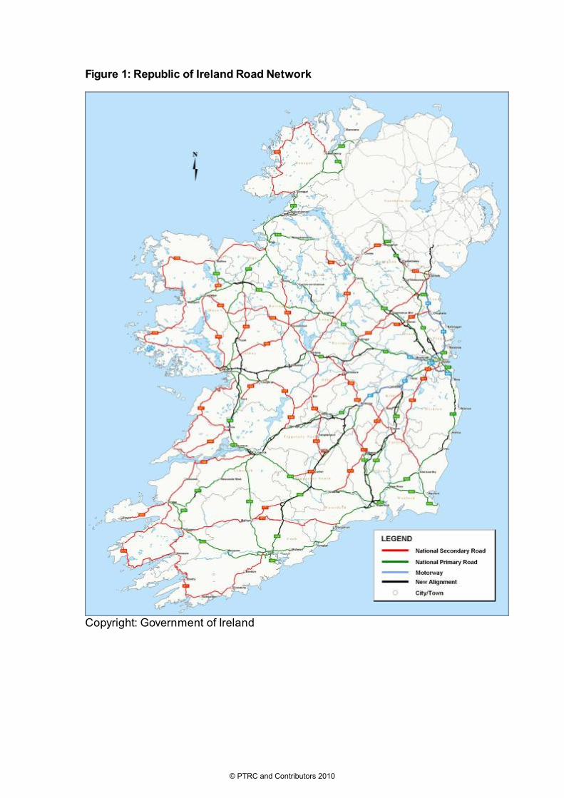
Figure 1: Republic of Ireland Road Network

Copyright: Government of Ireland


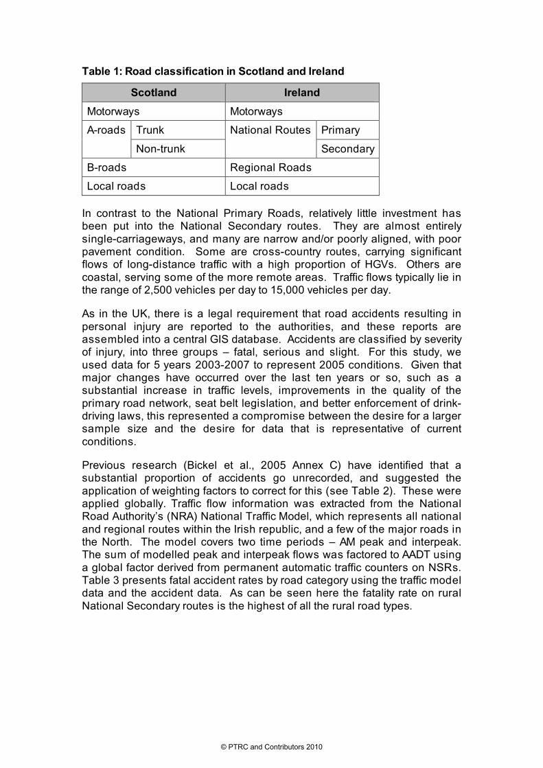
Table 1: Road classification in Scotland and Ireland

Scotland Ireland

Motorways Motorways

Trunk Primary A-roads

Non-trunk

National Routes

Secondary

B-roads Regional Roads

Local roads Local roads

In contrast to the National Primary Roads, relatively little investment has been put into the National Secondary routes. They are almost entirely single-carriageways, and many are narrow and/or poorly aligned, with poor pavement condition. Some are cross-country routes, carrying significant flows of long-distance traffic with a high proportion of HGVs. Others are coastal, serving some of the more remote areas. Traffic flows typically lie in the range of 2,500 vehicles per day to 15,000 vehicles per day.

As in the UK, there is a legal requirement that road accidents resulting in personal injury are reported to the authorities, and these reports are assembled into a central GIS database. Accidents are classified by severity of injury, into three groups – fatal, serious and slight. For this study, we used data for 5 years 2003-2007 to represent 2005 conditions. Given that major changes have occurred over the last ten years or so, such as a substantial increase in traffic levels, improvements in the quality of the primary road network, seat belt legislation, and better enforcement of drink-driving laws, this represented a compromise between the desire for a larger sample size and the desire for data that is representative of current conditions.

Previous research (Bickel et al., 2005 Annex C) have identified that a substantial proportion of accidents go unrecorded, and suggested the application of weighting factors to correct for this (see Table 2). These were applied globally. Traffic flow information was extracted from the National Road Authority’s (NRA) National Traffic Model, which represents all national and regional routes within the Irish republic, and a few of the major roads in the North. The model covers two time periods – AM peak and interpeak. The sum of modelled peak and interpeak flows was factored to AADT using a global factor derived from permanent automatic traffic counters on NSRs. Table 3 presents fatal accident rates by road category using the traffic model data and the accident data. As can be seen here the fatality rate on rural National Secondary routes is the highest of all the rural road types.


Table 2: Summary data for accident severity categories

Accident severity

Uncorrected rate per

million veh-kms on NSRs

Uncorrected proportion

Correction factor

Corrected rate

Corrected proportion

Fatal 0.009 8.3% 1.0 0.009 3.2%

Serious 0.016 15.5% 1.5 0.024 8.9%

Slight 0.079 76.2% 3.0 0.236 87.9%

All 0.103 N/A N/A 0.269 N/A

Table 3: Fatal accident rates by road type

Fatal accidents per million veh-km

Road category

0.0009 Motorway

0.0011 to 0.0025 Dual-carriageway

0.0067 National Primary (rural)

0.0084 Regional rural

0.0082 to 0.0133 Urban

0.0000 to 0.0141 National Secondary (rural)

3 THE QUALITY INDEX

Each rural National Secondary Road link within the model was allocated a route quality score. These scores were used to inform the choice of speed-flow curves for traffic modelling, and as the main independent variable in the accident analysis.

The following simplified version of the COBA formula was used:

Route Quality Index = 72.7 - .091 x bendiness (degrees per km) - .007 x hilliness (metres rise/fall per km) - .00063 x bendiness x hilliness + 1.8 x carriageway width (metres) + .99 x shoulder width (metres) + .3 x footpath & verge width (metres)

The speed of traffic may depend not only on route quality, but also on other factors such as speed limit, traffic flow, percentage of slow or heavy vehicles, and pavement condition. Nevertheless, for rural links, this index


was expected to be strongly correlated with free-flow speed, and this was borne out in the work to develop speed-flow curves.

3.1 Geographic resolution

The initial calculation of route quality was based on an NRA dataset consisting of separate data for the two directions of travel. The road was divided into “road lengths”, each of the order of 150m on average, with some road lengths very short (around 10m) and some substantially longer (around 2500m). Each road length came with “chainage” values, giving distance of each end of the road length from the start of the route corridor.

In order to improve the suitability of this network:

• Chainage values were recalculated, so that corresponding lengths in the two directions had comparable chainage values (if this is not done, one-way systems in urban areas can result in the two halves of the carriageway at a point being allocated to different lengths of road)

• Lengths were grouped together to give stretches of around 500m of road. Each stretch was given the average width values of its constituent lengths, weighted by distance. Each stretch was allocated the total metres rise and fall and the total degrees turned through of its constituent lengths.

For this calculation, bendiness of each length was capped at a maximum of 360 degrees of turn per kilometre, in order to limit the impact of a single bend on what would otherwise be a fairly straight section of road. Carriageway width of each length was capped at 5m per direction, on the basis that values beyond this were likely to be due to deceleration lanes or other localised features which have limited impact on overall speeds.

3.2 Identifying points of change of route quality

A spreadsheet-based method was developed to identify points of significant change in route quality. The spreadsheet process works on the 500m stretches imported from the NRN database into a GIS. Looking along the whole route corridor, the process iteratively finds the best place to split the corridor into sections. A combined average quality score is calculated for each section. The logic is summarised in Figure 2 – the following paragraphs explain each step in more detail.

For each stretch, the spreadsheet “looks ahead” to calculate a length-weighted average quality score for that stretch and the stretches ahead (stopping at a previous split-point or a total of 10 stretches or a distance of 3.3 km, whichever comes first). Similarly it “looks behind” to calculate the average quality score for the stretches in the other direction. Where this difference is greatest, that is considered the best place to split the route corridor into two sections.

If the difference is greater than a given threshold figure, then the split is considered worth making; the user accepts the split, and the spreadsheet


finds the new best place to split a link into two. If the difference is less than the chosen threshold, then the process has gone far enough. The average quality score for each link is exported from the spreadsheet back into the GIS.

An example of the results is shown in Figure 3, indicating how the 160km length of the N59 coastal route was split into sections of consistent quality, with an average length of around 5km.

Figure 2: Flowchart for identifying changes of route quality

3.3 The Route Quality Index

The resulting Route Quality Index has an observed maximum value of 810 for the highest-quality sections - wide, straight, flat, with good visibility. The lowest quality section is a place known as Corkscrew Hill on the N67 in north Clare - a steep, narrow road with hairpin bends; this has a score of 380, although this is an extreme case. Around 2% of the links in the network have scores below 500; the median score is 735.

The higher the quality score, the straighter, flatter and wider the road is. The highest scores are only achieved by roads built to full modern standards. In Ireland, such roads have a 2.5m hard shoulder each side. These are much

Within each route corridor

Find point of greatest difference

Difference >

threshold?

Split corridor at this point

Calculate average quality for each length

For each stretch, look ahead and behind


used by agricultural vehicles, and assist in reducing the need for dangerous overtaking manoeuvres.

It is estimated that the maximum quality score a single-carriageway could achieve is around 830. Such a road would be completely straight and flat, with wide lanes and a hard shoulder.

Figure 3: Quality scores at 500m resolution (blue) grouped into route sections of around 5km (pink)


Figure 4: Speed-flow curves for rural National Secondary Roads

Links were grouped into bands with similar quality scores, and a set of speed-flow curves derived to reflect the differences in speed between different qualities of road were assigned (see Figure 4). As can be seen from this figure, for a given traffic flow, vehicle speed increases with quality score. At the top end of the range, a car can easily do 100kph (the legal maximum) in good weather, and the average for all vehicles in all conditions was estimated at around 92kph. On the poorer-quality roads, flows are low, but average speeds as low as 50 to 60kph are not uncommon.

The links within the traffic model were split at the points where the route quality index changes. These links were then GIS-matched to the point data in the road accident database, to give a frequency of fatal, serious and slight accidents on each link.


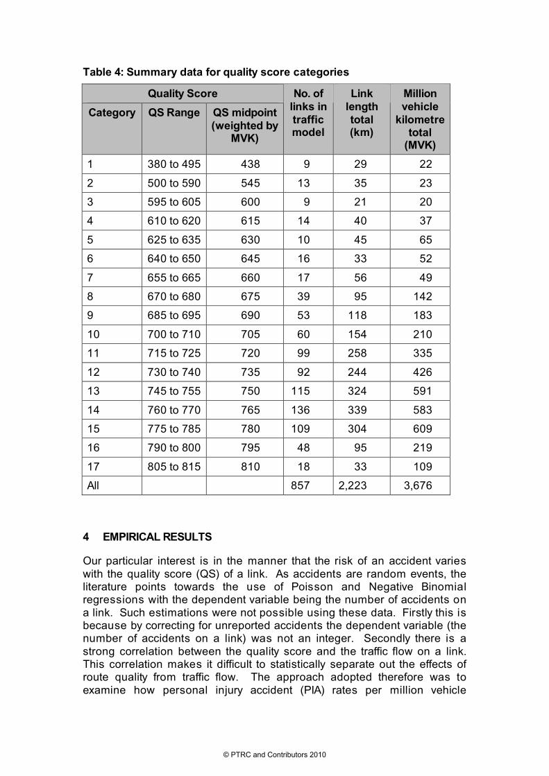
Table 4: Summary data for quality score categories

Quality Score

Category QS Range QS midpoint (weighted by

MVK)

No. of links in traffic model

Link length total (km)

Million vehicle

kilometre total

(MVK)

1 380 to 495 438 9 29 22

2 500 to 590 545 13 35 23

3 595 to 605 600 9 21 20

4 610 to 620 615 14 40 37

5 625 to 635 630 10 45 65

6 640 to 650 645 16 33 52

7 655 to 665 660 17 56 49

8 670 to 680 675 39 95 142

9 685 to 695 690 53 118 183

10 700 to 710 705 60 154 210

11 715 to 725 720 99 258 335

12 730 to 740 735 92 244 426

13 745 to 755 750 115 324 591

14 760 to 770 765 136 339 583

15 775 to 785 780 109 304 609

16 790 to 800 795 48 95 219

17 805 to 815 810 18 33 109

All 857 2,223 3,676

4 EMPIRICAL RESULTS

Our particular interest is in the manner that the risk of an accident varies with the quality score (QS) of a link. As accidents are random events, the literature points towards the use of Poisson and Negative Binomial regressions with the dependent variable being the number of accidents on a link. Such estimations were not possible using these data. Firstly this is because by correcting for unreported accidents the dependent variable (the number of accidents on a link) was not an integer. Secondly there is a strong correlation between the quality score and the traffic flow on a link. This correlation makes it difficult to statistically separate out the effects of route quality from traffic flow. The approach adopted therefore was to examine how personal injury accident (PIA) rates per million vehicle


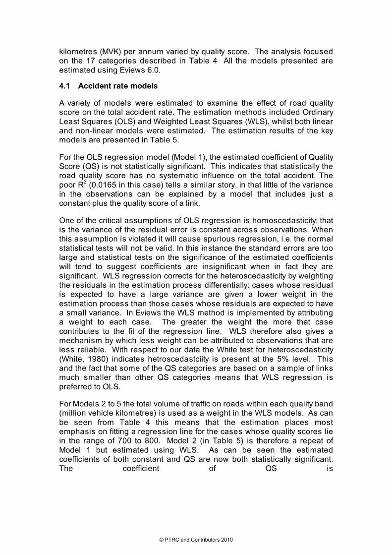
kilometres (MVK) per annum varied by quality score. The analysis focused on the 17 categories described in Table 4 All the models presented are estimated using Eviews 6.0.

4.1 Accident rate models

A variety of models were estimated to examine the effect of road quality score on the total accident rate. The estimation methods included Ordinary Least Squares (OLS) and Weighted Least Squares (WLS), whilst both linear and non-linear models were estimated. The estimation results of the key models are presented in Table 5.

For the OLS regression model (Model 1), the estimated coefficient of Quality Score (QS) is not statistically significant. This indicates that statistically the road quality score has no systematic influence on the total accident. The poor R2 (0.0165 in this case) tells a similar story, in that little of the variance in the observations can be explained by a model that includes just a constant plus the quality score of a link.

One of the critical assumptions of OLS regression is homoscedasticity: that is the variance of the residual error is constant across observations. When this assumption is violated it will cause spurious regression, i.e. the normal statistical tests will not be valid. In this instance the standard errors are too large and statistical tests on the significance of the estimated coefficients will tend to suggest coefficients are insignificant when in fact they are significant. WLS regression corrects for the heteroscedasticity by weighting the residuals in the estimation process differentially: cases whose residual is expected to have a large variance are given a lower weight in the estimation process than those cases whose residuals are expected to have a small variance. In Eviews the WLS method is implemented by attributing a weight to each case. The greater the weight the more that case contributes to the fit of the regression line. WLS therefore also gives a mechanism by which less weight can be attributed to observations that are less reliable. With respect to our data the White test for heteroscedasticity (White, 1980) indicates hetroscedastciity is present at the 5% level. This and the fact that some of the QS categories are based on a sample of links much smaller than other QS categories means that WLS regression is preferred to OLS.

For Models 2 to 5 the total volume of traffic on roads within each quality band (million vehicle kilometres) is used as a weight in the WLS models. As can be seen from Table 4 this means that the estimation places most emphasis on fitting a regression line for the cases whose quality scores lie in the range of 700 to 800. Model 2 (in Table 5) is therefore a repeat of Model 1 but estimated using WLS. As can be seen the estimated coefficients of both constant and QS are now both statistically significant. The coefficient of QS is


Table 5: Estimation results of the total accident rate models

Model 1 Model 2 Model 3 Model 4 Model 5 Average Weighted average

OLS WLS WLS WLS WLS

Constant 0.290663** (0.02297)

0.257063** (0.01028)

0.376339* (0.17236)

0.861357** (0.23818)

0.4432 (0.29176)

0.899959** (0.25594)

4.015706* (1.53215)

Quality Score -0.000126 (0.00025)

-0.000802* (0.00032)

-0.0000375 (0.00046)

-0.000854* (0.00034)

Quality Score in Logarithm

-0.567377*

(0.23128)

Vehicle Flow (AADT) -0.0000292

(0.00001)

If Quality Score>785:

Quality Score minus 785

0.001734

(0.00343)

2R (unweighted) 0.0165 N/A N/A N/A N/A

2R (weighted) N/A 0.3006 0.470 0.313 0.2863

Notes: the dependent variable is the total accident rate in all of the models. For the WLS models MVK by QS category was used as the weighting variable. * and ** indicate that the estimates are statistically significant at 5% and 1% levels respectively. Values in parentheses are standard errors.


significant at 5% significance level with negative sign. It implies that the total accidents rate will decrease when the quality of a road improves. The weighted R2 is 0.3006. This is not particularly large but it is a significant improvement over the OLS model.

In Model 3, AADT vehicle flow is included on the basis that higher vehicle flows may lead to a greater incidence of overtaking accidents. The model has a much higher R2, however, neither QS nor Vehicle Flow is statistically significant. This is not surprising given the high correlation between the two variables (0.8037). Model 2 is therefore preferred to this model. Models 4 and 5 present some non-linear variations to Model 2. The piecewise models were estimated by including a quality score interaction dummy variable for each quality score category (i.e. 16 interaction variables). These interaction variables were removed if their coefficients were not significant. Model 4 is the best performing of these piecewise models estimated. This model includes an interaction dummy variable that takes the value of zero up to a QS of 785 and the value of QS-785 for all higher values of QS. Unfortunately the interaction dummy variable is not statistically significant, thereby indicating that it has little explanatory power. Model 5 uses a semi-log form (only the independent variable QS is in logarithm). Similar to the results from Model 2 the QS variable is significant at 5% significance level with a negative sign. However, judged by the weighted R2 we consider the non logarithmic form (Model 2) to be the preferred model.

Overall, for the total accident rates we therefore consider Model 2 (the WLS model including QS) as the best model (see Figure 5). The QSM is statistically significant with expected sign and the R2 is relatively satisfactory. The average total accident rate and weighted total accident rate (million vehicle kilometres as weights) are also presented in Table 4 for comparison. The fact that accident rates decrease with quality score lends some support to the conviction that a better-designed road is a safer road. It also appears to suggest that on average the improved geometry of the roads with higher quality scores more than compensates, in a safety sense, for the increased accident risk from travelling at higher speeds.

4.2 Proportion of fatal accidents models

For the proportion of fatal accidents, a number of models were estimated of which seven are presented in Table 6. Once again these have been estimated using OLS and WLS. Models with and without constant terms have been estimated, as have piecewise models and semi-log and double log models. The estimation results are shown in Table 6, together with the average and weighted average values of proportion of fatal accidents.

The OLS model (Model 6) gives relatively high R2 (0.381). In the OLS model, the estimated coefficient of QS is statistically significant at 1% significance level with positive sign. The constant is almost significant at the 5% significance level. The model indicates that the road quality improvement will cause a significant increase in the proportion of fatal accidents. Given that road speeds increase with QS then this finding is consistent with that of Anderson and Nilsson (1997).


Figure 5: Total accident rates on NSRs

For the WLS model (Model 7), the QS variable is not significant and the R2 is very low. When the constant term is removed from the WLS model, as Model 8 shows, QS becomes significant at 1% significance level, with positive sign. However, the R2 is still very poor. By adding an interaction dummy variable into the model, as in Model 9, we obtain better estimation results. Model 9 is the best performing piecewise model with a single dummy interaction variable with QS. The coefficients on the QS and dummy variables are statistically significant at 1% and 5% significance level, respectively. The estimated coefficient for QS has positive sign whereas that for the interaction dummy is negative, with 740 as the change in gradient. This model suggests that for those roads with quality score no greater than 740 the improvement of road quality will result in an increase of proportions of fatal accidents. Improving the road beyond this level of quality significantly reduces the proportion of accidents that are fatal. This we note differs from Anderson and Nilsson’s finding on Swedish roads, in that an increase in speed for these road types is not leading to an increase in fatal accidents. Engineering design at these quality scores must be more than compensating for the increased fatality risk that higher speeds bring.

Model 10 is similarly a WLS piecewise model but includes two interaction dummy variables as independent variables. Both of the dummy variables are statistically significant at the significance level of 1%. The estimation results suggest that for any roads with quality score no greater than 605 the proportion of fatal accidents is zero. Those roads with a quality score of around 740 have the highest proportion of fatal accidents. This model shares a similar model form (and therefore policy implications) to Model 9 but has a much better fit to the data – both in terms of the significance of the coefficients and the R2 value.


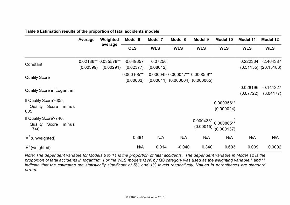
Table 6 Estimation results of the proportion of fatal accidents models

Model 6 Model 7 Model 8 Model 9 Model 10 Model 11 Model 12

Average Weighted average

OLS WLS WLS WLS

WLS WLS WLS

Constant 0.02186**

(0.00399)

0.035578**

(0.00291)

-0.049657

(0.02377)

0.07256

(0.08012)

0.222364

(0.51155)

-2.464387

(20.15183)

Quality Score 0.000105**

(0.00003) -0.000049 (0.00011)

0.000047** (0.000004)

0.000059** (0.000005)

Quality Score in Logarithm -0.028196 (0.07722)

-0.141327 (3.04177)



0.000356**

(0.000024)



-0.000438*

(0.00015)

-0.000865**

(0.000137)

2R (unweighted) 0.381 N/A N/A N/A N/A N/A N/A

2R (weighted) N/A 0.014 -0.040 0.340 0.603 0.009 0.0002

Note: The dependent variable for Models 6 to 11 is the proportion of fatal accidents. The dependent variable in Model 12 is the proportion of fatal accidents in logarithm. For the WLS models MVK by QS category was used as the weighting variable.* and ** indicate that the estimates are statistically significant at 5% and 1% levels respectively. Values in parentheses are standard errors.


For completeness, WLS models with semi-log and double log forms (Models 11 and 12) have been presented. For the WLS model in double log form both the dependent and independent variables are in logarithm. Neither of these two models has a good fit judged by the insignificant coefficients and the low R2s.

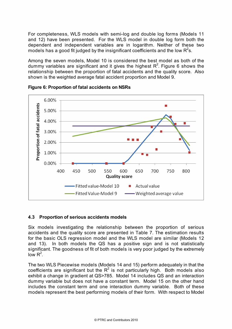
Among the seven models, Model 10 is considered the best model as both of the dummy variables are significant and it gives the highest R2. Figure 6 shows the relationship between the proportion of fatal accidents and the quality score. Also shown is the weighted average fatal accident proportion and Model 9.

Figure 6: Proportion of fatal accidents on NSRs

4.3 Proportion of serious accidents models

Six models investigating the relationship between the proportion of serious accidents and the quality score are presented in Table 7. The estimation results for the basic OLS regression model and the WLS model are similar (Models 12 and 13). In both models the QS has a positive sign and is not statistically significant. The goodness of fit of both models is very poor judged by the extremely low R2.

The two WLS Piecewise models (Models 14 and 15) perform adequately in that the coefficients are significant but the R2 is not particularly high. Both models also exhibit a change in gradient at QS>785. Model 14 includes QS and an interaction dummy variable but does not have a constant term. Model 15 on the other hand includes the constant term and one interaction dummy variable. Both of these models represent the best performing models of their form. With respect to Model


15, for example, none of the models that included QS interaction dummies with QS


Table 7: Estimation results of the proportion of serious accidents models

Model 12 Model 13 Model 14 Model 15 Model 16 Model 17 Average Weighted average

OLS WLS WLS

WLS WLS

WLS

Constant 0.088098**

(0.00924)

0.092967**

(0.00334)

0.08636

(0.06991)

0.084644

(0.09254) 0.094189**

(0.00304)

0.035034

(0.58929)

-4.509013

(7.14485)

Quality Score 0.0000026 (0.00010)

0.000011 (0.00012)

0.000125** (0.000004)

Quality Score in Logarithm

0.008745 (0.08895)

0.320255 (1.07852)



-0.002778*

(0.001052)

-0.002396*

(0.00107)

2R (unweighted) 0.000042 N/A N/A N/A N/A N/A

2R (weighted) N/A 0.00054 0.280 0.250 0.00064 0.0058

Note: The dependent variable for Models 12 to 16 is the proportion of serious accidents. The dependent variable in Model 17 is the proportion of serious accidents in logarithm. For the WLS models MVK by QS category was used as the weighting variable. * and ** indicate that the estimates are statistically significant at 5% and 1% levels respectively. Values in parentheses are standard errors.


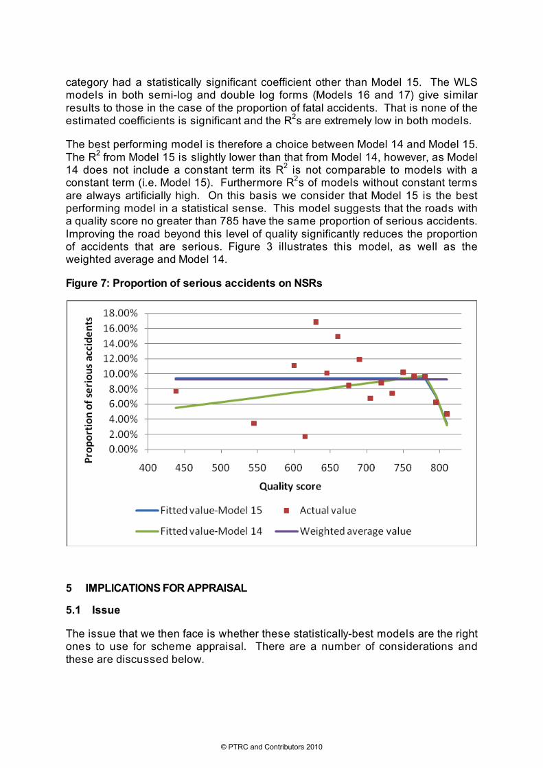
category had a statistically significant coefficient other than Model 15. The WLS models in both semi-log and double log forms (Models 16 and 17) give similar results to those in the case of the proportion of fatal accidents. That is none of the estimated coefficients is significant and the R2s are extremely low in both models.

The best performing model is therefore a choice between Model 14 and Model 15. The R2 from Model 15 is slightly lower than that from Model 14, however, as Model 14 does not include a constant term its R2 is not comparable to models with a constant term (i.e. Model 15). Furthermore R2s of models without constant terms are always artificially high. On this basis we consider that Model 15 is the best performing model in a statistical sense. This model suggests that the roads with a quality score no greater than 785 have the same proportion of serious accidents. Improving the road beyond this level of quality significantly reduces the proportion of accidents that are serious. Figure 3 illustrates this model, as well as the weighted average and Model 14.

Figure 7: Proportion of serious accidents on NSRs

5 IMPLICATIONS FOR APPRAISAL

5.1 Issue

The issue that we then face is whether these statistically-best models are the right ones to use for scheme appraisal. There are a number of considerations and these are discussed below.


Over our five year period there were no fatal accidents on any NSR with a quality score less than 610. Our statistically preferred piecewise linear model therefore has a modelled fatal proportion of zero. A valid question is, is this zero rate real, or is there some probability, albeit low, that such an accident will occur? That is are the observed zeros structural or sample related? We have taken the view that they are sample related, and as a consequence have kept the fatal accident rate constant below a quality score of 635.

The best accident rate model indicates very high accident rates at low quality scores. This results from the estimation process placing the most weight on providing a close fit to data points with quality scores between 700 and 800. It seems unrealistic that this rate should continue to increase for ever decreasing quality scores. We also must ask ourselves given the manner that the estimation process emphasises the fit around high quality scores, how representative the accident rate model is of the road network at low quality scores. We have taken the view that the accident rate model is not particularly representative at lower quality scores and have assumed a constant rate below a quality score of 635.

It is implausible to have a negative accident rate in reality. However, a statistical model may suggest a negative rate if that gives better fit to the data. So statistical fit has to be tempered by judgment - at least to an extent. For example, extrapolating the statistically-preferred serious proportion model to a quality score of 825, or the statistically-preferred fatal model to a quality score of 835, gives negative proportions of serious and fatal accidents. Is this an argument that undermines the validity of these models or is it the case that these models should only be applied over their own domain? We have taken the latter view. For quality scores which exceed those observed we suggest using the accident rates associated with a quality score of 810 (i.e. the maximum quality score observed).

Is it reasonable to suggest that the accident rate does not vary smoothly with the quality score, given that all the components of that score are continuous variables? The piecewise models demonstrate that we find statistically significant changes in gradient over different parts of the range, for both the fatal and the serious proportions models. Statistically we therefore reject the natural null hypothesis that there is no effect of quality (the horizontal lines in Figure 5, Figure 6 and Figure 7) on the accident rate. For the fatal and serious models we also reject the hypothesis that the effect of marginal change in quality is constant. Given the steepness of the gradient for high quality scores in both the serious and fatal models the question remains however, as to whether this effect is real or an artefact of the data. We have taken the view that is real, though the very sharp changes of gradient are a consequence of the model form (piecewise model). This view is based on both a human interpretation of the model fit, the use of a statistical method that places least weight on the least reliable datapoints, but also on the basis of an interpretation that as the road standard increases (i.e. quality score increases) then certain engineering characteristics also change such as improved overtaking opportunities and the provision of hard shoulders. Hard shoulders can for example reduce the incidences where agricultural and other slow moving vehicles impede other traffic thereby creating conflicts between users.


The human eye is excellent at pattern-recognition. But it finds it hard to deal with data that is of variable quality. Software applies rigorous statistical calculations. But lacks the imagination. The challenge for the analyst, as always, is how to combine the two optimally.

5.2 Application for scheme appraisal

The NRA’s Project Appraisal Guidelines give economic costs for fatal, serious and slight casualties, and the non-casualty costs of accidents. Using this data, and the data in the accident database on the number of casualties by type per category of accident, allows us to derive an economic cost for a fatal, serious and slight accident on the National Secondary Road network. By multiplying the cost per accident by the rate per million vehicle kilometres, we derive an economic cost of accidents per million veh km on roads of different quality. For the preferred models adjusted in the manner described in the previous section, this gives a cost curve of the form shown in Figure 8 and Figure 9. Given standard appraisal values of loss of life, the cost of a fatal accident is about ten times that of a serious accident, which is about seven times that of a slight accident. So the shape of the resulting curve is dominated by the model for proportion of fatal accidents.

Figure 8: Cost per accident by quality score

!0

!20,000

!40,000

!60,000

!80,000

!100,000

!120,000

!140,000

!160,000

400 450 500 550 600 650 700 750 800 850

Costs per accident (2002 prices and values)

Unadjusted rates Adjusted rates


Figure 9: Cost per Million Vehicle Kilometres by Quality Score

!0

!5,000

!10,000

!15,000

!20,000

!25,000

!30,000

!35,000

!40,000

!45,000

400 450 500 550 600 650 700 750 800 850

Costs per MVK in 2005 (2002 prices and values)

Unadjusted rates Adjusted rates Observed rates

It is immediately clear from this curve that modest road improvements of single-carriageway rural roads, where the quality of the existing route is below 730, are likely to create accident disbenefits. This is despite the total accident rate decreasing as the quality improves (see Figure 5). Once road quality reaches a score in the mid-700s, significant safety benefits can be delivered by improving it further.

The same calculation of total accident cost per million vehicle kilometres can be applied to the observed rates on each quality of road. This is a valuable check that the combination of the three models – for accident rate, fatal proportion and serious proportion – does not result in any systematic error which might not be apparent from looking at the models individually.

6 CONCLUSION

We draw several conclusions from this work:

The first is that the engineer’s confidence that improved roads are always safer seems misplaced. Whilst accident rates do fall with road quality, the nature of the accident changes. Roads that are part-way improved – like a half-blunt knife – can genuinely be substantially more dangerous than either new roads built to the highest modern standards or unimproved existing roads.


It is well known that fatality rate increases with speed; if fatal proportion increases faster than total rate declines, then there will be more fatal accidents. This result depends on the relative steepness of the two slopes in Figures 5 and 6, and the relative importance of fatal, serious, and slight accidents. We’re using standard economic appraisal values for a future year of 2025 to determine that relative importance.

More puzzling is why the proportion of fatal and serious accidents reduces again for the highest-quality roads. That conclusion rests on only a few data points, so it may be that subsequent studies with more and better data will find otherwise. Our conjecture at this stage is that roads with wide carriageways, hard shoulders and long straight sections reduce the variance of vehicle speed on the main carriageway, improve overtaking opportunities and reduce the risk that a crashing vehicle will hit an immovable object. These reductions in risk more than offset the increase in risk that improvements in speed have on the risk of a fatal or serious accident.

It follows that existing appraisal methods in the area of safety too often rely on over-simple relationships which can give substantially wrong answers, and there is a need for improvements in this area.

Roads policy is informed by many different considerations. Purely from the point of view of safety, putting in modest improvements to poor-quality roads may be counter-productive, while substantial improvements that would bring route quality up to the highest levels (on the right-hand side of the graph) may be unaffordable. An appropriate policy response might be to identify two categories of road:

• those where the flow is high enough to justify a high standard of carriageway provision

• those which should be left alone, or even have their best bits worsened to give a consistently low standard, combined with a lower speed limit - traffic-calmed rural main roads.

Finally, as in all empirical work there is a real tension between statistical and interpretive approaches to data analysis. On the one hand a mechanistic process which applies statistical tests without looking at the data is unlikely to give best models for use in scheme appraisal. On the other hand, fitting curves “by eye” can lead to bias due to over-reliance on data points with a high uncertainty. Both approaches, without appropriate sense checks, may also lead to implausible results (e.g. negative accident rates).

REFERENCES

ANDERSSON, G. and G. NILSSON. 1997. Speed Management in Sweden. Swedish National Road and Transport Research Institute (VTI), Linkoping.

BARUYA, A., D.J. FINCH, and P.A. WELLS. 1999. A speed–accident relationship for European single-carriageway roads. Traffic Engineering Control, 40(3), pp.135–139.


BICKEL, P. et al. 2006Proposal for harmonised guidelines. HEATCO deliverable 5. EU-project developing harmonised European approaches for transport costing and project assessment (HEATCO). Institut für Energiewissenschaft und Rationelle Energieanwendung, Stuttgart. Available at: http://heatco.ier.uni-stuttgart.de/

HADI, M.A., J. ARULDHAS, L.F. CHOW, and J.A. WATTLEWORTH. 1993. Estimating Safety Effects of Cross-Section Design for Various Highway Types Using Negative Binomial Regression. Transportation Research Record, 1500, TRB, National Research Council, pp.169–177.

NATIONAL ROADS AUTHORITY. 2008. Project Appraisal Guidelines. Dublin: National Roads Authority.

TAYLOR, M.C., A. BARUYA, and J.V. KENNEDY. 2002. The relationship between speed and accidents on rural single-carriageway roads. TRL Report TRL 511. Crowthorne: Transport Research Laboratory

WATTERS, P. and M. O’MAHONY. 2007. The relationship between geometric design consistency and safety on rural single-carriageway roads in Ireland. European Transport Conference, Noordwijkerhout, Netherlands, 17-19 October 2007. London: AET Transport.

WHITE, H., 1980. A heteroscedasticity-consistent covariance matrix estimator and a direct test of heteroscedasticity, Econometrica, 48, pp 817-838.

ACKNOWLEDGEMENTS

We are grateful to the National Roads Authority for the provision of the relevant databases that facilitated this research. All conclusions are however are own and do not necessarily represent the view of the National Roads Authority.

BIOGRAPHIC DETAILS

Dr James Laird

James is Senior Research Fellow at the Institute for Transport Studies in the University of Leeds. He has 16 years experience in both a consultancy and academic environment. His principal interests are in the economic appraisal of transport schemes with a specialisation in rural issues and wider economic impacts. He is based in Inverness.

Russell Harris

Russell is a professional transport modeller with multi-disciplinary consultants RPS. He previously worked for the UK Department for Transport in London, where


http://heatco.ier.uni-stuttgart.de



he looked after their National Transport Model and TEMPRO software, and helped develop DMRB modelling guidance.

Dr Shujie Shen

Shujie is a Research Fellow at the Institute for Transport Studies in the University of Leeds. Her main research interests include econometric modelling and forecasting, with particular interests in economic analysis of transportation demand and costs.


ACCIDENTS ON RURAL ROADS – FOR BETTER OR …starconference.org.uk/star/2010/accidents.pdf ·...

Documents

Transcript of ACCIDENTS ON RURAL ROADS – FOR BETTER OR …starconference.org.uk/star/2010/accidents.pdf ·...