Access to Markets and the Benefits of Rural Roads:A Nonparametric Approach

Hanan G. Jacoby*

June 1998

Abstract

Transport infrastructure plays a central role in rural development, yet little isknown about the size and especially the distribution of benefits from road investments.This paper develops and implements a method for nonparametrically estimating thebenefits from road projects at the household level using the relationship between the valueof farmland and its distance to agricultural markets. The empirical analysis, using datafrom Nepal, suggests that providing extensive road access to markets would confersubstantial benefits on average, much of these going to poor households. However, thebenefits would not be large enough or targeted efficiently enough to appreciably reduceincome inequality in the population.

Keywords: Rural Roads, Income Distribution, Nonparametric Regression

JEL Classification: O12, D31, C14

*Development Research Group, The World Bank, 1818 H Street N.W., Washington DC20433. The views expressed in this paper are those of the author and should not beattributed to the World Bank or affiliated organizations.

1

I. Introduction

Rural infrastructure is a major development priority (World Bank, 1994), yet little

is known about the size and especially the distribution of benefits from such investments in

LDCs. The distribution issue is salient, not only in the formulation of policy, but also in

understanding the political constraints on the allocation of infrastructure investment.

Rural roads are an important form of public infrastructure, providing cheap access to both

markets for agricultural output and for modern inputs. Given limited policy instruments

for reaching the remote rural poor, road-building would seem desirable on distributional

grounds. On the other hand, the benefits of infrastructure projects accrue mainly to

landowners, who are generally not among the very poor. Thus, the extent to which rural

road construction ameliorates income inequality is ultimately an empirical question.1

In this paper, I examine the distributional consequences of rural roads using data

from Nepal, a country with a largely agrarian economy, a sparse highway network, and

extremely difficult terrain. To this end, I develop an empirical methodology for

nonparametrically estimating the household-specific benefits from alternative road projects

using information on the value of farmland and distance to agricultural markets. If land

behaves like a standard asset, which is a testable assumption, then its value equals the

discounted stream of maximal profits from cultivation. Hence, the income gains from

lower transport costs should be capitalized in land values. With an estimate of the land

value-distance relationship in hand, it is possible to describe the joint distribution of

hypothetical road project benefits and household income.

1 Howe and Richards (1984) discuss some distributional aspects of rural roads and present case studies.Also, van de Walle (1996) uses micro-data and a profit function approach to examine the distribution ofbenefits from irrigation in Viet Nam.

2

In principle, road benefits could also be estimated from the relationship between

farm profits and distance to markets. However, there are several difficulties with this

approach, the most nettlesome of which is that survey data rarely, if ever, provide accurate

information on an essential component of profit, the cost of transporting goods and

agricultural inputs to and from markets. Another difficulty is that profit (or production)

functions assume a fixed technology and thus cannot easily account for potential

adaptations of farmers to greater remoteness from markets, such as substitution of

traditional for modern inputs or away from transport-intensive crops. The relationship

between land value and distance to market is immune from such difficulties.

To be sure, the idea of using land values to estimate the average benefits of

infrastructure investments in a population is hardly new, though it has not to my

knowledge been applied to rural transport. In any case, such estimates do not address the

primary question of this paper, which is a distributional one. The innovation here is to link

a household-level benefit estimate with a measure of household income. In doing so, I

take a nonparametric approach. While it is true that economic theory is largely silent on

the parametric form of hedonic price functions (see Stock, 1991), in practice, relaxing

parametric assumptions in hedonic models is much more likely to matter for distributional

questions than for questions about average benefits.

Theoretically, my analysis is based on the Ellet-Walters model of rural transport

(see Walters, 1968; Gersovitz, 1989), in which land rents decline with distance to markets

through the influence of distance on effective prices. The model, laid out in the next

section, provides a simple characterization of the potentially conflicting distributional

consequences of road projects.

3

Section III discusses the nonparametric or, more precisely, semi-nonparametric

estimation of the land value equation. Section IV describes the data, analyzes how farmer

behavior is influenced by distance to market, and tests the appropriateness of a standard

asset-pricing model for land. Section V presents the main empirical results, the analysis of

land values and of the distribution of benefits from hypothetical road projects. Section VI

concludes the paper.

II . Theoretical Framework

Basic Model

Farmers are assumed to cultivate a single crop using x kg per hectare of a modern

input, say chemical fertilizer, and l hours per hectare of labor. Crop yield y (kg per

hectare) is produced with a fixed technology represented by the neoclassical production

function y f x l= ( , ) . Let w be wage rate and ~v and ~p be the “effective” or farm gate

prices of output and fertilizer, respectively, discussed below. Per hectare land rent, ρ , is

defined as the maximal profit that can be earned on a hectare of land,

ρ( ,~, ~) max ~ ~,

w v p py wl vxl x

≡ − − (1)

and can be thought of as a long-run average.

Effective prices are determined by the economic geography, which is illustrated in

Figure 1. A highway of arbitrary length through the countryside runs through a large city

where all fertilizer is produced and output is purchased. The highway transects a series of

otherwise isolated mountain valleys along which all farms are located. This is a

convenient fiction, but not unlike the geography of Nepal. The total cost of transporting

4

goods between farms and the city has two components: a relatively large cost of

headloading goods (i.e., using human porters) between the farm and the road and a

relatively small cost of trucking goods along the road. All farmers trade agricultural

output and fertilizer in a competitive market center located at the road juncture with their

valley (markets at intermediate points up the valley are an inessential complication since

goods must still be headloaded from the main highway). From a given farm, it takes h

hours to walk to the market center and the portage cost of goods is b Rupees/(kg hours),

where b is proportional to the wage. If the money prices of fertilizer and output at a

particular market center are v and p , respectively, then the effective purchase price of

fertilizer is ~v v bh= + Rupees/kg and the effective selling price of output is ~p p bh= −

Rupees/kg. All labor can be obtained locally with zero transport costs.

Unprofitable land will not be cultivated, so the limit of cultivation in terms of

walking time to the market center, h* , is implicitly defined by ρ( ; , , )*h w p v = 0 . As

figure 1 illustrates, h* declines across valleys as one moves away from the city, because

p declines and v increases; ultimately, h* = 0 and all cultivation ends.

As to the relationship between land rent and travel time, by the envelope theorem

∂ρ∂

( , ~, ~) ( ) *w v ph

b y x h h= − + < for (2)

So, the negative rent gradient is just equal in magnitude to the total transport costs per

hour per hectare. Furthermore, by the convexity of the profit function in prices,

∂ ρ∂

2

2 0( , ~, ~) *w v ph

h h> < for (3)

Thus, along any given valley, the rent function is convex.

5

Notice that convexity of the rent function does not require that farmers both

purchase fertilizer and sell output at the same time (though nonparticipation in the latter

market means that rents depend upon the endogenous shadow price of output). However,

if one moves far enough away from a market center, farmers may stop selling output and

buying fertilizer altogether, and the rent gradient would be zero beyond this point (and

thus the rent function not strictly convex). Convexity is also robust to the assumption of a

single crop or production technology. Figure 2 shows how the rent function along one of

the valleys in Figure 1 reflects the profit maximizing choice of available crops or

technologies; as travel time rises, farmers may switch away from bulkier crops or from

agricultural practices that are intensive in modern inputs.

Roads and Welfare

Using the above framework, consider the welfare implications of building a road of

given length off of the main highway into a particular valley. The local scale of the project

ensures that it has no general equilibrium effects on wages or prices. To avoid specifying

the source of public finance, assume that the project is funded by earmarked foreign aid.

Let λ denote the length of the road in foot-travel (hours walking time) equivalents. By

enabling truck transport, the road effectively cuts portage costs by some fraction µ. The

new rent function, suppressing its dependence on prices and on µ,2 is

2 The parameter µ reflects road quality. I do not consider the welfare effects of variation in µ because, asa practical matter, the cost of upgrading road surface (from earth to gravel or asphalt) far outweighs thesmall reduction in vehicle operating cost, once truck transport is feasible (Beenhakker and Lago, 1983).Although improvements in road conditions, given surface type, can substantially reduce vehicle operatingcost, these cost-savings are likely to be small compared to those of a new road. Of course, in the extremecase where an existing road is impassible to trucks, a road improvement is tantamount to a new road.

6

σ λ ρ µ λρ λ µ λ

( , ) ( )( ( ))

h h hh h

= <= − − ≥

for for 1

(4)

Figure 3 illustrates the rise in land rents as a result of the project, along with the expansion

in the limit of cultivation h* .

An interesting policy question concerns the length of the road, specifically whether

it makes sense to build a lot of short roads or fewer long ones, given a fixed construction

budget. A key input into this decision is the marginal social benefit of road length, where

“society” in this case refers to the farmers in the typical valley. Suppose that household

income z is determined by farm profit (land rent) and labor earnings, the latter which is

assumed fixed across households for expository purposes; i.e., z h A e= +σ λ( , ) , where A

is total landholdings and e is earnings. Let G h A( , ) denote the joint cumulative

distribution function for distance from market center and landholdings. Finally, let ψ ( )z

be the increasing, strictly concave, indirect utility function. Assuming it is additive, the

social welfare function is

W h A e dG h Ah

A

( ) ( ( , ) ) ( , )*( )λ ψ σ λλ= +∫∫ 0

(5)

Notice that households already on a road do not benefit from its extension further up the

valley (i.e., σ λλ = <0 for h ), so that differentiating (5) with respect to λ yields

′ = ′∫∫W AdG h Ah

A

( ) ( , )*λ ψ σ

λ λ (6)

To illuminate the distributional issues, it is instructive to fix land area for the

moment and to decompose marginal social benefit as follows

[ ] [ ] [ ] [ ] ′ = − ′ > > + ′ >W A G A E A h E A h Cov A h A( , ) ( ) , , , ,λ λ ψ λ σ λ ψ σ λλ λ1 (7)

7

The first term in (7) is simply the fraction of households living off the road. The first term

in the curly brackets is the average marginal value of the road extension for these

beneficiaries, assuming their marginal utilities of income and appreciations in plot value are

uncorrelated. The second term in curly brackets accounts for this correlation, which must

be negative because ′′ >ψ σh A 0 and σλh < 0 . In other words, farther up the valley,

where land rents are low and thus households are poorer, rents rise by less due to the road

extension. The size of this “targeting inefficiency” depends crucially on the shape of the

rent function; indeed the covariance is zero if the rent function is linear in travel time. In

sum, the marginal social benefit of a road extension is higher when: (i) the fraction of the

population living off-road is higher; (ii) the average off-road household is poorer (i.e., has

a higher ′ψ ); (iii) the off-road rent gradient is steeper; and (iv) the targeting inefficiency

(the covariance term) is smaller.

With land area variable the distributional issue becomes cloudier. First, for any

given h, both the benefit from the road extension and household income are increasing in

landholdings.3 While this effect exacerbates inequality, there is also an effect working in

the opposite direction. It is often the case in developing countries, and Nepal is no

exception, that poorer households are found in more remote areas, perhaps because poor

migrants settle on the fringes of cultivation. If A and h are negatively correlated, then the

beneficiaries of a road extension (those off the original road) tend to be poorer, resulting

in a greater marginal social benefit than if A and h are uncorrelated. Allowing earnings, e,

to vary in the population complicates matters further, but the basic point remains, namely

3 Note that in this model renters do not benefit from road construction; their higher rent payments justoffset the greater profitability of the land.

8

that road construction has ambiguous distributional effects. The goal of the empirical

work is to resolve this ambiguity in the case of Nepal.

III. Econometric Specification

The theoretical analysis is framed in terms of rents, but my data are on land values

at the plot level. According to the standard asset-pricing model

log( ) log( ( ; , , )) log( )V h w p v r= −ρ (8)

where V is the present market value of a plot of land and r is the constant discount rate.4

Assume that this formula is valid, at least until it is tested in Section IV.

Besides negativity and convexity in h , economic theory imposes no restrictions on

the form of ρ . It is therefore desirable to estimate the rent function nonparametrically,

but this is not feasible when it includes many other variables besides h . For example, any

plot characteristic, such as soil quality, that shifts the production function f should also

shift the rent function ρ . Additionally, in the absence of accurate data on input and

output prices, geographic price variation can be swept out of the rent function by

including market center (regional) dummy variables.5 A within-market analysis also

ameliorates the problem of endogenous placement of roads and/or markets; in particular,

4 If farmers are risk neutral, then V E

rtt

t= +++=

∞∑ 0 1110

[ ]( )

ρ, where E0 is the expectations operator conditional

on today’s information set. If it is further assumed that profits per hectare follow a random walk so thatE t t0 1[ ]ρ ρ+ = , then the formula simplifies to V r= ρ , where ρ ρ= 0 (see Clark et. al, 1993).

5 Strictly speaking, this procedure is only an approximation. Since h enters effective prices linearly,log(ρ) cannot be additively separable in money prices. Even with accurate price data, it would be difficultto impose the full structure of the theoretical model in the estimation of the rent function. On the otherhand, given the relatively low cost of trucking, it is unlikely that price variation along the main highwayis sufficiently great to render this approximation inaccurate.

9

market centers may be located closer to more fertile land, where rents are higher. Given

these considerations, I take a semi-nonparametric approach by assuming that

log( ) log ( )ρ θ γ δ= + ′ + ′h X M , where θ is a nonparametric function, X is a vector of

plot characteristics, and M is a vector of regional dummy variables.

As to the dependent variable in (8), Colwell and Munneke (1997) warn against

using land value per-hectare because plot values may be nonlinear in area. If so, and if

parcel size is correlated with distance to market, then such a specification will lead to a

spurious correlation between land value and distance. Including the log of plot area, A ,

to account for this nonlinearity in the empirical specification of (8) gives

log( ) log ( ) log( )V h A X M u= + + ′ + ′ +θ β γ δ (9)

which nests the value per-hectare specification when β = 1 . Note, log ( )θ h absorbs

log( )r , and the error term, u , reflects unobserved attributes of the plot.

Following Robinson (1988) and Stock (1991), equation (9) can be estimated by

first using bivariate kernel regressions to “partial out” h from both sides. Since the

number of kernel regressions required equals one plus the dimensionality of ( A X M, , ),

this method is computationally very expensive, especially given the large sample. A much

cheaper approach uses the fact that h is a discrete valued regressor in the data with k

distinct values. In the first stage, I include a k − 1vector of dummy variables D in (9) for

each value of h ; i.e., I replace logθ with ω ξ==

−∑ jj

kjD

1

1. Applying ordinary least squares

(OLS) to this regression yields a consistent estimate of ( , , , )β γδξ . In the second stage, I

calculate ∃ω for each observation and run a nonparametric regression of this variable

against h to get a smoothed estimate of θ .

10

IV. Data and Preliminary Analysis

Nepal Living Standards Survey

The data for this study come from the 1995-96 Nepal Living Standards Survey

(NLSS), a nationwide multi-topic survey collected by the Central Bureau of Statistics

assisted by the World Bank (Central Bureau of Statistics, 1995). A stratified random

sample of around 3400 households was drawn from four zones: Mountains, urban Hills,

rural Hills, and Terai. In addition, a special sample of 1200 households was surveyed in

the Arun valley (rural Hills), which I include in my analysis.

The NLSS contains a detailed agricultural module including information on the use

of modern inputs, of which chemical fertilizer predominates, and on crop production and

sales. In addition, the survey provides a listing of all plots owned or leased in by the

household along with information on plot area, land quality, irrigation by season, net rent

received by season (if leased out), and, of course, value of owned plots. The question on

plot value reads as follows: “If you wanted to buy a plot exactly like this, how much

would it cost you?” One indication of farmers’ awareness of land values, besides the fact

that it is by far their most productive asset, is the frequency of land transactions, which is

surprisingly high in the sample.6 Among the 3,621 landowning households, 5 percent

bought land the previous year and 9 percent either bought or sold land. Moreover,

although 85 percent of all plots are inherited, 28 percent of the landowning households

purchased at least one of their current plots. Note also that any nonsystematic

6 Land transactions are sparse in most contexts. For this reason many hedonic studies use self-assessedland values (see, in particular, Mendelsohn, et al., 1994 and the citations in Colwell and Munneke, 1997)or housing values (see Bartik and Smith, 1987).

11

measurement error in plot values will not affect the coefficients of a regression in which

plot value is the dependent variable.

A unique feature of the NLSS questionnaire is that it collects information at the

household level on access to 14 different facilities. For each facility, the survey asks about

travel time (in minutes, hours, and days) and mode of transport; i.e., by foot (without

load), bicycle, motorcycle, car/bus, and mixed (foot+vehicle). Keep in mind that

collecting data on actual distance, even using satellite telemetry, would be of little value in

mountainous Nepal (except perhaps in the Terai). However, I do not use the household-

level travel time information directly. Instead, I take the median of travel times by

“wards” (in rural areas these are villages and environs) based on households that report

travel times by foot, which the great majority do. The advantage of this procedure is that

it standardizes travel times for mode of transport, which is potentially endogenous, and it

mitigates the measurement error that is likely to be present in household level travel times.

I focus on market centers and agricultural cooperatives, since these facilities are

the most likely to offer the opportunity to sell output and purchase modern inputs. In fact,

over two-thirds of the households who report using chemical fertilizers obtained them

from agricultural cooperatives, and most of the rest from private traders. My measure of

h is the minimum of ward- median travel times to the market center and agricultural

cooperative. Ideally, travel times to all relevant facilities should be considered separately,

but this would lead to multicollinearity problems, not to mention making nonparametric

estimation practically impossible. Median travel time to a market center or a cooperative

in the sample of 3,724 cultivating households is 2 hours (mean=2.8 hrs.). Median travel

12

times are shorter on the plains of the Terai (1.25 hrs.) than in the Hills (2 hrs.) or

Mountains (3 hrs.).

Finally, it is necessary to define a market area within which money prices (i.e., p ,

v , and w ) do not vary. I take each district to be a distinct market; 73 out of the 75

districts in the country are represented in the NLSS sample and there are on average about

4 wards in a district (except in the oversampled Arun valley where this number is much

higher). Though somewhat arbitrary, identifying a market by a district is consistent with

evidence from the village questionnaires attached to the NLSS. These data show that very

few villages have either market centers or agricultural cooperatives located in the same

ward; households living in several different wards share these facilities.

Analysis of Fertilizer Use and Crop Sales

If proximity to markets influences land values through the effective prices of

agricultural inputs and outputs, then purchases of modern inputs and sales of output

should decline with distance from the market center. According to the model, observed

fertilizer use per hectare, allowing for corner solutions, is x x w v p* max ( ,~, ~), = 0 . A

similar equation holds for observed total crop sales per hectare, s* , except that sales also

depend on household consumption decisions. Analyzing marketed surplus ( s* minus

consumption) is problematic because transport costs drive a wedge between selling and

purchase prices and net sellers respond differently to variation in these transport costs than

do net buyers (see, e.g., Omamo, 1998). Examining crop sales alone focuses on the

selling decision, which is my primary interest. It is also probably reasonable to assume

13

that for net sellers consumption is relatively unresponsive to transport costs, given that

income and substitution effects work in opposite directions.

Figures 4 and 5 plot nonparametric regression estimates of fertilizer use per

hectare and crop sales per hectare, respectively, against travel time. The econometric

specification is similar to equation (9) and the sample consists of 3,712 cultivating

households.7 Since both fertilizer use and crop sales are heavily censored at zero, I

estimate the first-stage models by tobit, in addition to OLS.8 For the tobits, I drop

observations with perfect classification; i.e., where all cases of a given value of h or of a

given district are censored (167 observations for fertilizer, 6 for crop sales).9 The second-

stage nonparametric regressions are estimated using the LOWESS smoother with

bandwidth=0.8. The choice of smoother is dictated by its robustness to outliers and by the

fact that the 60 successive values of h are not equally spaced, which can lead to biases in

kernel regressions (Fan, 1992).

The figures show that fertilizer purchases and crop sales per hectare decline

steadily beyond travel times of about one hour. It is unclear why the curves are increasing

for travel times of less than an hour, but one reason might be that cultivation is typically

less intensive near urban areas. Also, comparing the curves based on OLS and tobit first-

stage regressions indicates that accounting for censoring makes little substantive

7 Twelve households are dropped because they are uniquely identified by their district and their value of h.8 The first-stage parameter estimates are suppressed for brevity. To summarize, education of the head andthe set of district dummies are jointly significant in all regressions, and the demographic variables(number of adult males and females and male and female children), included only in the crop salesequation to capture consumption variation, are also jointly significant.9 The high rate of censoring within certain districts precludes the use of semiparametric methods that arerobust to deviations from normality. In particular, the censored LAD estimator fails to converge when

14

difference. In sum, this analysis supports the notion that transport costs influence farm

profits through input use and crop marketing decisions. The fertilizer result, in particular,

confirms the importance of the intensive margin of cultivation, implying that the farm

profit function, and hence the rent function, should be convex.

Analysis of Plot Values and Rents

Underlying the asset-pricing formula given by equation (8) are several strong

assumptions about land and credit markets,10 which may not hold in Nepal. To test

equation (8), along with the validity of self-reported plot values, I compare values with

rents received on plots that are leased out (mainly sharecropped). My analysis is based on

a sample of 381 plots that were either rented out during both agricultural seasons, or were

rented out in the wet (the main growing season) and left fallow in the dry. It should be

noted, however, that about twice this many plots (around six percent of all those owned)

were rented out during at least one season. Net rents are summed across both seasons,

and include the value of in-kind payments while netting out the cost of inputs provided to

tenants. The median rent to value ratio ( ρ V ) is 0.055, which can be viewed as an

estimate of the discount rate r. Formally, I run the regression

log( ) log( )V = + +η η ρ ζ0 1 (9)

and test whether η1 1= .

district dummies are included in the specifications. The overall rates of censoring in the samples are 43percent for fertilizer and 49 percent for sales.10 For example, where land is the sole form of collateral for loans, its price may reflect its collateral valuein addition to the capitalized value of the stream of rents (see Chalamwong and Feder, 1988).

15

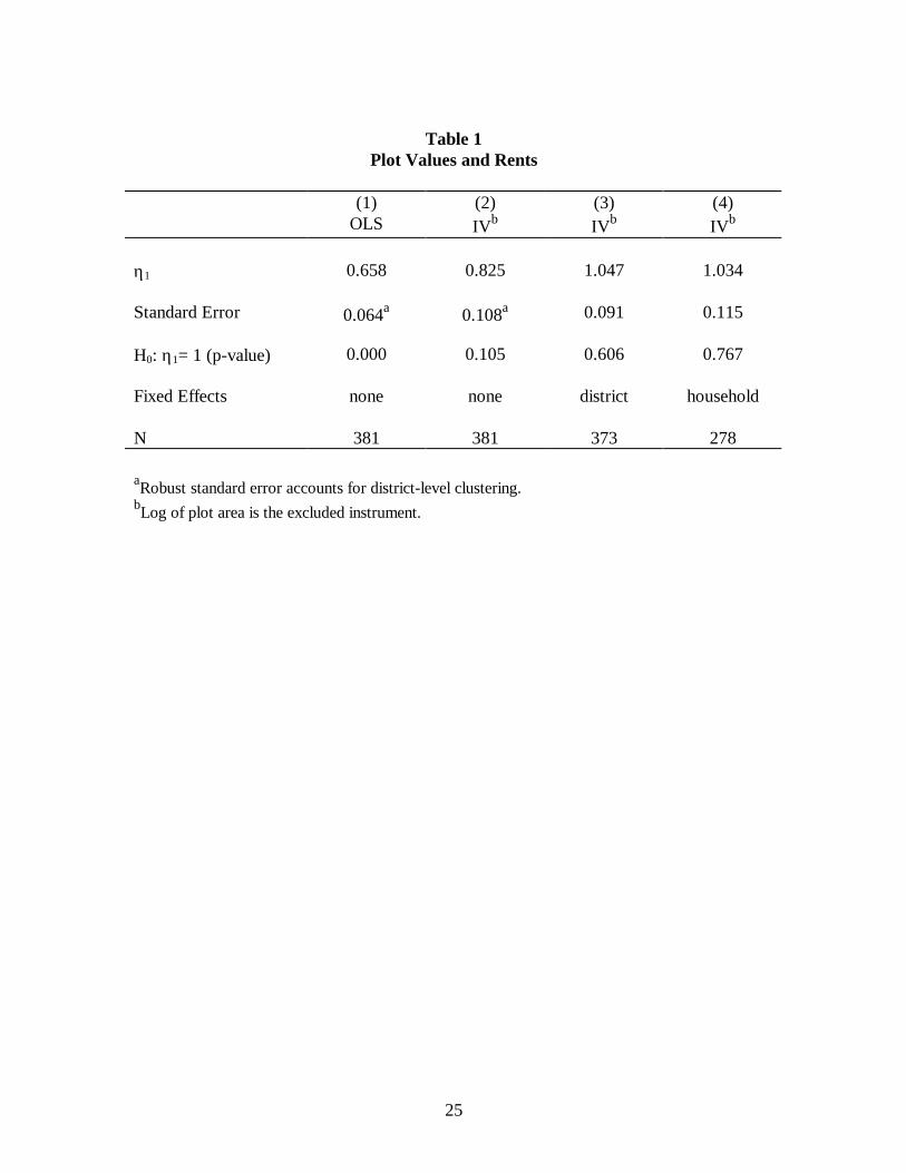
Table 1 reports a series of estimators of η1 that make progressively less restrictive

assumptions about the form of correlation between log( )ρ and the error term ζ . The

OLS estimate in column (1) assumes that log( )ρ and ζ are uncorrelated, and it falls well

short of unity. However, one reason for this low estimate could be attenuation bias due to

random measurement error in rents. Specification (2) thus instruments rents with plot

area, which does indeed raise the estimate of η1 , though it remains marginally below unity.

Specification (3) corrects for the possibility that credit market conditions (i.e., log( ))r and

rents might covary across markets by including district fixed effects (using only districts

that contribute more than one plot to the sample); η1 is still precisely estimated, but it is

no longer statistically different from unity. Finally, specification (4) includes household

fixed effects, using the 90 households that contribute more than one plot to the sample.

This estimator corrects for the possibility that household-specific interest rates and rents

are correlated, as well as for any selection bias induced by restricting the sample to those

households that rent out land. This last estimate of η1 is again indistinguishable from

unity, so that the maintained assumptions of the asset- pricing model and of no systematic

reporting bias in plot values cannot be rejected.

V. Main Results

Plot Values and Distance to Market

Information is available on a total of 13,672 plots owned by 3,621 households.

Plot characteristics include suitability for rice cultivation (khet land), whether irrigated,

and if so whether seasonally or year round, mode of irrigation (tubewell, canal, other),

16

system of irrigation (self-managed, agency managed, community managed), and the

“quality” of the plot based on a four grade classification used by the land revenue

department for tax assessments. Land value is missing for 13 plots and quality for 98

plots, so the plot value regressions are based on 13,651 observations. However, when

predicting plot values based on the regression results, these missing observations can be

recovered by imputing plot quality with its modal value.

Table 2 reports two specifications of the plot value regression. The first assumes

that θ( )h h= and the second performs the first-stage in the semi-nonparametric

estimation described in Section III. In both specifications, the plot characteristics have

significant and sensible coefficients; for example, plots that are suitable for rice, plots with

year round irrigation,11 high quality plots, and, of course, larger plots are more valuable.

However, the value per-hectare specification ( β = 1 in equation (9)) is resoundingly

rejected, which is important because plot size turns out to be negatively correlated with

distance to markets. Thus, restricting β to one would have led to an underestimate of the

rate of decline of land values with travel time (Colwell and Munneke, 1997). As it is,

travel time is strongly negatively associated with land values.

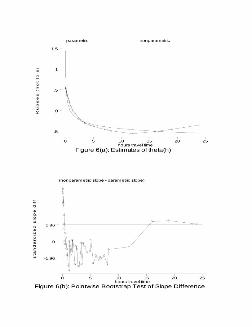
Figure 6(a) plots the ∃( )θ h derived from the two specifications in Table 2

(normalized by taking deviations from means). In the first case, ∃( )θ h h= − 0.222 , which is

obviously convex. The nonparametric estimate of θ( )h (LOWESS; bandwidth=0.8) is

also roughly convex, except that the function is increasing above travel times of 12 hours,

11 Since irrigation is an investment, which may be responsive to distance to market, I also ran the plotvalue regressions unconditional on the irrigation variables. In this case, the coefficient on log travel timeis − 0.225 (0.0217), which is almost identical to its value of –0.222 in specification (1) of Table 2.

17

though only 5 percent of plots are located this far from markets.12 To formally compare

the parametric and nonparametric models, I use the bootstrap, drawing 100 percent

random samples in two stages, first by sampling plots within households and then by

sampling households. On each replication, the two models are run and the difference in

the slope of ∃( )θ h is calculated at each value of h. As a test of whether the actual slope

differences in Figure 6(a) are significantly different from zero, Figure 6(b) plots, at each h,

the ratio of the actual slope difference to the standard deviation over the 100 bootstrap

replications. When the absolute value of this ratio exceeds 1.96, the equality of slopes can

be rejected at the 5 percent level. That this hypothesis is rejected near the endpoints is

perhaps not too surprising. However, the nonparametric estimate is also significantly

steeper (more negatively sloped) than the parametric estimate in much of the one to three

hour travel time range, where the data are most dense. Although other parametric models

might fit the data better, this test shows that there is sufficient power to reject a reasonable

parametric alternative, thus supporting a nonparametric approach.

Benefits and Distributional Consequences of Road Projects

The expected appreciation in value of a given plot as travel time falls from an

initial value of h0 to a value of h1 is

[ ] [ ] [ ]∃( ) ∃( ) exp ∃log( ) ∃ ∃ exp( ∃)θ θ β γ δh h A X M E u1 0− + ′+ ′ (10)

The last term in this expression takes into account unobserved heterogeneity in plot

values, and can be estimated nonparametrically as the average exponentiated residual from

12 Bandwidth choice is subjective, but the main features of the nonparametric fit are robust to bandwidth.

18

(9). Although nonparametric regression only provides an estimate of θ at actual values of

h , ∃( )θ h1 can be estimated by linear interpolation between known values of ∃θ . To

simulate the benefits from the road project discussed in Section II, let h h1 0= µ for

h0 < λ and h h1 0 1= − −λ µ( ) for h0 ≥ λ. I set the value of µ at 0.1 to reflect the fact

that the cost per ton-km of headloading in Nepal is roughly ten times the cost of

trucking.13 Total household (capitalized) benefit from the project is simply the sum of the

appreciations in value of each of the household’s plots.14

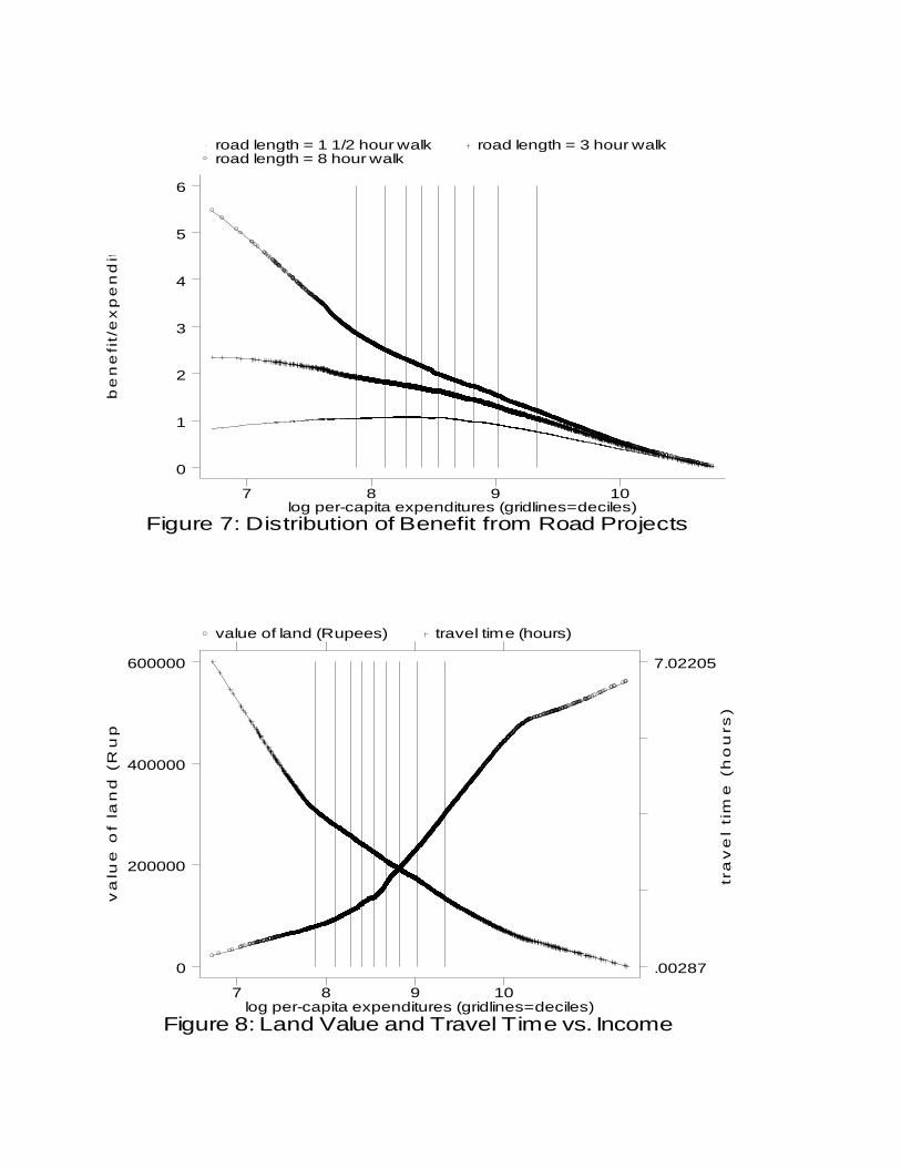
Following standard practice, I use total household consumption expenditures as a

measure of income and per-capita expenditures, adjusted for regional price differences, as

a measure of welfare. Let us say that a road project is progressively (regressively)

targeted if the ratio of benefit to total household expenditures, the benefit ratio, is

decreasing (increasing) in per-capita expenditures. Figure 9 plots nonparametric

regression curves (LOWESS; bandwidth=0.8) of benefit ratios against log per-capita

expenditures for three road projects, corresponding to three values of λ. The estimates

are based on the full sample of 4,573 households, which includes both households who do

not cultivate and those who do not own land.15

13 This number is based on information in Walters (1968), but it is still approximately valid according toWorld Bank transport economists familiar with Nepal.

14 In the few cases where the reduction in travel time occurs on the increasing portion of ∃θ , benefit is setto zero. Note that it is not possible to calculate benefits from the additional land brought under cultivation

as h* increases. However, as long as one considers a marginal road extension, these benefits are anenvelope phenomenon and hence are zero.15 All statistics reported for this sample (e.g., the expenditure deciles in Figure 7) are calculated usingpopulation weights to insure that they are nationally representative. Ninety-three percent of thehouseholds (on weighted basis) live in rural areas.

19

Figure 7 shows that as the road is extended farther up the “representative” valley,

benefits are targeted more progressively. Indeed, the distribution of benefits from a short

road, one that extends a mere 1.5 hours walking time up the valley, is slightly regressive.

Sixty percent of the sample would lie along such a road, whereas 85 percent would lie

along the 3-hour road and 98 percent would lie along the 8-hour road. The key factor

behind the increasing progressivity is the strong tendency for poorer households to live

farther away from markets, as confirmed by the nonparametric regression curve in Figure

8. Evidently, this factor dominates the opposing tendency of poorer households to have

less valuable landholdings, also illustrated in Figure 8.

While suggestive, Figure 7 does not address the question of whether the benefits of

a hypothetical road project are sufficiently large and distributed sufficiently progressively

to reduce overall income inequality. To tackle this question first requires converting the

capitalized benefits into a permanent income flow, which in turn requires an assumption

about the discount rate, r. Suppose that current household expenditures equal permanent

income. For a pure farm household, with no off-farm employment and which leases in no

land, permanent income equals rVTOTAL , where VTOTAL is the sum of the value of all plots

owned; more generally, income comes from other sources as well. Thus, in a regression

of total household expenditures on VTOTAL , the coefficient on VTOTAL should equal the

discount rate r, with other sources of income consigned to the residual. A slight

refinement of this regression, which includes ward (village) fixed effects and which

instruments VTOTAL for measurement error using total land area owned, gives ∃ .r = 0 058

20

with a standard error of 0.010.16 This estimate of the discount rate is remarkably close to

that derived earlier from the rent to value ratio (i.e., 0.055). In the calculations that

follow, I set r = 0 06. .

Denote household benefits per capita from a road of length λ by B( )λ . Per capita

expenditures (permanent income) as a function of road length is thus z z rB( ) ( )λ λ= +0 ,

where z0 is baseline per capita expenditures. Assuming that ψ ε( )z z= −1 , ε > 0 , the

social welfare function (see (5)) can be written as W z I( ) [ ( )( ( ))]λ λ λ ε= − −1 1 , where z is

mean per capita expenditures and I ∈ [ ]0,1 is Atkinson’s measure of inequality.17

Differentiating with respect to λ gives

′ ∝ ′ − ′−

WW

zz

II

( )( )

( )( )

( )( )

λλ

λλ

λλ1

(10)

In other words, the rate of increase in social welfare as the road is extended can be

decomposed into the rate of increase in mean income and the rate of increase in income

equality, 1 − I . An assessment of whether road building has important distributional

consequences can be made by comparing the magnitudes of these two components at

reasonable values of the inequality aversion parameter ε . Specifically, define

Ω ( ; )( ) ( ) ( )λε λ λ λ= − −

−− − −

−

I II

z zz

I II

0

0

0

0

0

01 1(11)

16 The OLS estimate of r, which does not account for measurement error, is substantially smaller at0.0076 (0.0007). These regressions are based on the sample of 3,621 households that own land.

17 Recall that ( )I Nzzi

N i= −

−

=

−

∑1 11

1

1 1ε ε( )

for ε ≠ 1where N is the number of individuals. When

ε = 1 , W z I( ) log[ ( )( ( ))]λ λ λ= −1 , where ( )I zzi

N Ni= − =∏1

1

1.

21

where the zero subscript denotes values prior to the road project. Ω ( ; )λε represents the

contribution of reduced income inequality to the increase in social welfare from the

building of a road of length λ.

Figure 9 plots Ω ( ; )λε using the Nepal data for λ’s ranging from 0.5 to 10 hours,

beyond which value practically every household is on the road so that ′ ≈W ( )λ 0 . Note

that putting all households in the sample on a road would raise z by ten percent, quite a

substantial gain in permanent income.18 Interestingly, at high values of inequality aversion

(ε = 4 ), building a short road actually increases income inequality (Ω < 0 ). For any value

of ε , the contribution of inequality reduction to the increase in social welfare rises with

the length of the road, again because of the strong tendency for the poor to live in more

remote areas. However, unless one chooses a value of ε above 2 or so, which is usually

considered rather large, the increase in social welfare is due overwhelmingly to higher

mean income. Rural road construction thus appears to be like a tide that lifts all boats

rather than a highly effective means of reducing income inequality.

VI. Conclusion

Transport infrastructure plays a central role in rural development, but the

distributional consequences of rural roads have not received adequate theoretical or

empirical attention. This paper develops and implements a method for nonparametrically

estimating the benefits from road projects at the household level and for examining the

distribution of these benefits across income classes. The findings for Nepal suggest that

18 Keep in mind that because I have weighted the sample to represent the population of Nepal, all of thesecalculations take proper account of the fact that population is less dense in more remote areas.

22

providing extensive road access to markets would confer substantial benefits on average,

much of these going to poor households. However, the benefits would not be large

enough or targeted efficiently enough to appreciably reduce income inequality in the

population (unless there is an exceptionally high degree of inequality aversion). Thus,

while my analysis may paint a more optimistic picture than the World Bank’s (1994, p. 80)

general assessment that infrastructure is “a blunt instrument for intervening directly on

behalf of the poor,” rural road construction is certainly not the magic bullet for poverty

alleviation.

Another lesson of this research is that data on land values and characteristics,

particularly at the plot level, can be extremely useful in measuring the benefits of

infrastructure investments in LDCs, and not just of rural roads. To be sure, land may not

always behave like a typical asset, so that benefit capitalization may be imperfect, but the

asset-pricing model can be tested to determine whether the methodology developed in this

paper is appropriate in a particular context.

Finally, it is important to mention the other benefits of rural roads besides cheaper

transport to and from agricultural markets, such as better access to schools and health

facilities and, more generally, to a greater variety of consumer goods. Insofar as farmers

prefer to live near their farms, at least some of these gains are likely to be capitalized in

farmland values. Separating out these distinct benefits of rural roads is left as a topic for

future research.

23

References

Bartik, Timothy J. and V. Kerry Smith. 1987. “Urban Amenities and Public Policy,”Chapt. 31 in Handbook of Regional and Urban Economics, Vol. II, ed. by EdwinMills. Amsterdam: North Holland.

Beenhakker, Henri L. and Armando M. Lago. 1983. Economic Appraisal of RuralRoads. World Bank Staff Working Papers No. 610. Washington: The WorldBank.

Central Bureau of Statistics. 1995. Nepal Living Standards Survey: InterviewersManual, June. Washington: The World Bank.

Chalamwong, Yongyuth and Gershon Feder. 1988. “The Impact of LandownershipSecurity: Theory and Evidence from Thailand,” World Bank Economic Review,2(2):187-204.

Clark, J. Stephen, Murray Fulton, and John T. Scott, Jr. 1993. “The Inconsistency ofLand Values, Land Rents, and Capitalization Formulas,” American Journal ofAgricultural Economics, February: 147-55.

Colwell, Peter F. and Henry J. Munneke. 1997. “The Structure of Urban Land Prices,”Journal of Urban Economics, 41:321-36.

Fan, Jianqing. 1992. “Design-adaptive Nonparametric Regression,” Journal of theAmerican Statistical Association, 87:998-1004.

Gersovitz, Mark. 1989. “Transportation, State Marketing, and the Taxation of theAgricultural Hinterland,” Journal of Political Economy, 97(5):1113-37.

Howe, John and Peter Richards. 1984. Rural Roads and Poverty Alleviation. London:Intermediate Technology Publications.

Mendelsohn, Robert, William D. Nordhaus, and Daigee Shaw. 1994. “The Impact ofGlobal Warming on Agriculture: A Ricardian Analysis,” American EconomicReview, 84(4):753-71.

Omamo, Steven Were. 1998. “Transport Costs and Smallholder Cropping Choices: AnApplication to Siaya District, Kenya,” American Journal of AgriculturalEconomics, forthcoming.

Robinson, P. M. 1988. “Root-N-Consistent Semiparametric Regression,” Econometrica,56(4):931-54.

24

Stock, James H. 1991. “Nonparametric Policy Analysis: An Application to EstimatingHazardous Waste Cleanup Benefits,” in William A. Barnett, James Powell, andGeorge Tauchen, eds., Nonparametric and Semiparametric Methods inEconometrics and Statistics. Cambridge: Cambridge University Press.

Walters, Alan A. 1968. The Economics of Road User Charges. World Bank StaffOccasional Papers No. 5. Washington: The World Bank.

World Bank. 1994. World Development Report 1994: Infrastructure for Development.New York: Oxford University Press.

van de Walle, Dominique. 1996. Infrastructure and Poverty in Viet Nam, LSMSWorking Paper, No. 21. Washington: The World Bank.

25

Table 1Plot Values and Rents

(1)OLS

(2)IVb

(3)IVb

(4)IVb

η1 0.658 0.825 1.047 1.034

Standard Error 0.064a 0.108a 0.091 0.115

H0: η1= 1 (p-value) 0.000 0.105 0.606 0.767

Fixed Effects none none district household

N 381 381 373 278

aRobust standard error accounts for district-level clustering.bLog of plot area is the excluded instrument.

26

Table 2Plot Value Regressions

Means (1) (2)

Log(hours travel time) 3.47(4.01)a

-0.222(10.3)

---

H0: ξ = 0 (p-value)b --- 0.0000

Log(area in hectares) 0.298(1.16)a

0.558(37.8)

0.547(37.4)

Suitable for rice (khet) 0.434 0.149(3.89)

0.144(3.84)

Irrigation: seasonal 0.175 0.341

(4.55)0.325(4.47)

year-round 0.138 0.497(6.29)

0.450(5.88)

canal 0.239 0.060(1.0)

0.052(0.88)

tubewell 0.030 -0.034(0.41)

-0.061(0.74)

self-managed 0.189 -0.082(1.664)

-0.051(1.09)

agency managed 0.018 -0.219(1.663)

-0.209(1.67)

Quality: dwaim 0.240 -0.250

(5.27)-0.226(5.02)

sim 0.304 -0.499(9.04)

-0.465(8.84)

chahar 0.365 -0.833(13.9)

-0.792(13.9)

District dummies (p-value) 0.0000 0.0000

R2 0.546 0.568

Notes: Robust t-values accounting for household-level clustering in parentheses. Omitted categories:pakho/bari (dry) for khet; non-irrigated for irrigation; other for irrigation mode; community managed forirrigation management; and awal (highest grade) for quality. Sample size is 13,561 plots belonging to3,586 households.

aStatistics are for levels. Standard deviations are in parentheses.

bJoint significance of the dummy variables for each of the 60 values of h.

Rupees (

not

to s

cale

)

Figure 6(a): Estimates of theta(h)hours travel time

parametric nonparametric

0 5 10 15 20 25

-.5

0

.5

1

1.5

(nonparametric slope - parametric slope)

sta

ndard

ized s

lope d

iffe

rence

Figure 6(b): Pointwise Bootstrap Test of Slope Differencehours travel time

0 5 10 15 20 25

-1.96

0

1.96

benefit/expenditure

s

Figure 7: Distribution of Benefit from Road Projectslog per-capita expenditures (gridlines=deciles)

road length = 1 1/2 hour walk road length = 3 hour walk road length = 8 hour walk

7 8 9 10

0

1

2

3

4

5

6

valu

e o

f la

nd (

Rupees)

Figure 8: Land Value and Travel Time vs. Incomelog per-capita expenditures (gridlines=deciles)

travel tim

e (

hours

)

value of land (Rupees) travel time (hours)

7 8 9 10

0

200000

400000

600000

.00287

7.02205

kg/h

ecta

re (

not to

scale

)

Figure 4: Fertilizer Use vs. Travel Timehours travel time

OLS first-stage Tobit first-stage

0 5 10 15 20

-.4

-.2

0

.2

Rupees/h

ecta

re (

not to

scale

)

Figure 5: Crop Sales vs. Travel Timehours travel time

OLS first-stage Tobit first-stage

0 5 10 15 20

-.4

-.2

0

.2

.4