Access to Destinations: How Close is Close Enough?

Estimating Accurate Distance Decay Functions for Multiple Modes and Different Purposes

Report # 4 in the series Access to Destinations Study

Report # 2008-11

Technical Report Documentation Page 1. Report No. 2. 3. Recipients Accession No. MN/RC 2008-11 4. Title and Subtitle 5. Report Date

May 2008 6.

Access to Destinations: How Close is Close Enough? Estimating Accurate Distance Decay Functions for Multiple Modes and Different Purposes 7. Author(s) 8. Performing Organization Report No. Michael Iacono, Kevin Krizek and Ahmed El-Geneidy 9. Performing Organization Name and Address 10. Project/Task/Work Unit No.

11. Contract (C) or Grant (G) No.

Hubert H. Humphrey Institute of Public Affairs University of Minnesota 301 19th Avenue South Minneapolis, Minnesota 55455

(c) 89261 (wo) 32

12. Sponsoring Organization Name and Address 13. Type of Report and Period Covered Final Report 14. Sponsoring Agency Code

Minnesota Department of Transportation 395 John Ireland Boulevard Mail Stop 330 St. Paul, Minnesota 55155 15. Supplementary Notes http://www.lrrb.org/PDF/200811.pdf Report #4 in the series: Access to Destinations Study 16. Abstract (Limit: 200 words)

Existing urban and suburban development patterns and the subsequent automobile dependence are leading to increased traffic congestion and air pollution. In response to the growing ills caused by urban sprawl, there has been an increased interest in creating more “livable” communities in which destinations are brought closer to ones home or workplace (that is, achieving travel needs through land use planning). While several reports suggest best practices for integrated land use-planning, little research has focused on examining detailed relationships between actual travel behavior and mean distance to various services. For example, how far will pedestrians travel to access different types of destinations? How to know if the “one quarter mile assumption” that is often bantered about is reliable? How far will bicyclists travel to cycle on a bicycle only facility? How far do people drive for their common retail needs?

To examine these questions, this research makes use of available travel survey data for the Twin Cities region. A primary outcome of this research is to examine different types of destinations and accurately and robustly estimate distance decay models for auto and non-auto travel modes, and also to comment on its applicability for: (a) different types of travel, and (b) development of accessibility measures that incorporate this information.

17. Document Analysis/Descriptors 18. Availability Statement Transportation planning Trip distance

Walking Bicycling Travel behavior

No restrictions. Document available from: National Technical Information Services, Springfield, Virginia 22161

19. Security Class (this report) 20. Security Class (this page) 21. No. of Pages 22. Price Unclassified Unclassified 76

Access to Destinations: How Close is Close Enough? Estimating Accurate Distance Decay Functions for

Multiple Modes and Different Purposes

Final Report

Prepared by:

Michael Iacono Research Fellow

Department of Civil Engineering University of Minnesota

Kevin Krizek

College of Architecture and Planning University of Colorado – Denver

Ahmed El-Geneidy

School of Urban Planning McGill University

May 2008

Published by:

Minnesota Department of Transportation Research Services Section

395 John Ireland Boulevard, MS 330 St. Paul, Minnesota 55155-1899

This report represents the results of research conducted by the authors and does not necessarily represent the views or policies of the Minnesota Department of Transportation and/or the Center for Transportation Studies. This report does not contain a standard or specified technique.

Acknowledgements The authors would like to thank members of the project technical advisory panel, including Sue Lodahl, Darryl Anderson and Cindy Carlsson. They would also like to acknowledge the valuable contributions of Ryan Wilson, Jessica Horning and Gavin Poindexter.

Table of Contents Chapter 1: Introduction ................................................................................................................... 1 Chapter 2: Literature Review.......................................................................................................... 2

The Importance of Distance Decay Functions............................................................................ 2 Distance Decay Function Development...................................................................................... 2 Applications of Distance Decay Concepts.................................................................................. 3 The Relationship to Accessibility ............................................................................................... 4 Distance Decay and Accessibility Measures .............................................................................. 5 Estimation of Distance Decay Functions.................................................................................... 6

Ordinary Least Squares........................................................................................................... 6 Maximum Likelihood Estimation ........................................................................................... 7

Current Application .................................................................................................................... 7 Chapter 3: Distance Decay Function Estimates.............................................................................. 9

Data Sources ............................................................................................................................... 9 Travel Behavior Inventory...................................................................................................... 9 Transit On-Board Survey...................................................................................................... 10 Trail User Survey.................................................................................................................. 10 Non-Motorized Pilot Program (NMPP) Survey ................................................................... 10

Statistical Summaries................................................................................................................ 11 Walking..................................................................................................................................... 12 Bicycling................................................................................................................................... 13 Transit ....................................................................................................................................... 14

Trip Purpose.......................................................................................................................... 14 Service Type ......................................................................................................................... 17

Auto........................................................................................................................................... 19 Drive Alone........................................................................................................................... 19 Shared Ride Trips ................................................................................................................. 20

Health Care Decay Function..................................................................................................... 20 Chapter 4: Travel Time Decay Functions..................................................................................... 22

Walking..................................................................................................................................... 22 Bicycling................................................................................................................................... 22 Transit ....................................................................................................................................... 23

Chapter 5: Discussion ................................................................................................................... 26 Limitations ................................................................................................................................ 26

Sample Size........................................................................................................................... 26 Focus on Home-Based Trips................................................................................................. 26 No Multi-Stop Trip Chains ................................................................................................... 27 Estimation of Distance Decay Functions.............................................................................. 27

Applications of the Distance Decay Functions......................................................................... 27 Chapter 6: Conclusion................................................................................................................... 32 References..................................................................................................................................... 34 Appendix A: Distance Decay Functions by Mode and Purpose Appendix B: Statistical Summaries of the Estimated Distance Decay Functions

List of Figures

Figure 1. Distance Decay Curves for Walking Trips ………………………………………………….………13 Figure 2. Distance Decay Curves for Bicycling Trips …………………………………………………….…..14 Figure 3. Distance Decay Curves for Transit Trips by Purpose …………………………………….……..15 Figure 4. Distance Decay Curves for Transit Trips by Purpose with Walk Access …………….…..16 Figure 5. Distance Decay Curves for Transit Trips by Purpose with Auto Access …………….…...17 Figure 6. Distance Decay Curves for Transit Trips by Service Type ……………………………………18 Figure 7. Distance Decay Curves for Single-Occupant Auto Trips ………………………………………19 Figure 8. Distance Decay Curves for Shared Ride Auto Trips …………………………………………….20 Figure 9. Distance Decay Curve for Health Care Trips ………………………………………………………21 Figure 10: Distance Decay Curves for Walking Trips (Travel Time) …………………………………...23 Figure 11. Distance Decay Curves for Bicycle Trips (Travel Time) …………………………………….24 Figure 12. Distance Decay Curves for Public Transit Trips (Travel Time) …………………………...25 Figure 13. Walk Accessibility to Restaurants ……………………………………………………………………29 Figure 14. Bicycle Accessibility to Shopping ……………………………………………………………………30

List of Equations

Equation 1 ………………………………………………………………………………………………….………..….……....3 Equation 2 ………………………………………………………………………………………………….………..…...……..4 Equation 3 ………………………………………………………………………………………………….………..….…..…..5 Equation 4 ………………………………………………………………………………………………….………..….…..…..6 Equation 5 ………………………………………………………………………………………………….……….…..…..…..6 Equation 6 ……………………………………………………………………………………………….………….…………..7 Equation 7 ……………………………………………………………………………………………….…………….………..7 Equation 8 ……………………………………………………………………………………………….…………….………..7 Equation 9 ……………………………………………………………………………………………….…………….………16 Equation 10 ……………………………………………………………………………………………………………..…….27

Executive Summary Existing urban and suburban development patterns and the subsequent automobile dependence that is associated with them are leading to increased traffic congestion and air pollution. In response to the growing ills caused by urban sprawl, there has been an increased interest in creating more “livable” communities in which destinations are brought closer to one’s home or workplace (that is, achieving travel needs through land use planning). While several reports suggest best practices for integrated land use-planning, little research has focused on examining detailed relationships between actual travel behavior and mean distance to various services. For example, how far will pedestrians travel to access different types of destinations? How can we know if the “one quarter mile assumption” that has become conventional wisdom in planning and designing communities is reliable? How far will bicyclists travel to cycle on a bicycle only facility? How far do people drive for their common retail needs? This research provides evidence on these and other closely related questions. The approach taken in this research is to estimate sets of distance-decay functions to describe the impedance of travel distance or time across the transportation network. The concept of distance-decay, used widely in geography and spatial interaction modeling, including many transportation forecasting models, can be interpreted as measuring either the impedance to travel through a network or the willingness of individuals to travel various distances to access opportunities. An important feature of this work is the explicit effort to extend the set of distance-decay functions to as many combinations of modes and trip purposes as available data permit. The set of modes that are considered of interest in this study are auto (single-occupant and shared ride), public transit, bicycling and walking. The data sets used in the analysis include a general-purpose travel survey for the Twin Cities region, an on-board survey of users of the regional public transit system, and a survey of users of joint-use trail facilities in Hennepin County. Together, these data sets allow for a fairly comprehensive look at travel behavior by various modes and trip purposes.

The findings of the research, particularly as they relate to non-motorized modes (walking and bicycling), provide evidence that can supplement existing rules-of-thumb for pedestrian and bicyclist behavior. The findings suggest, for example, that substantial shares of pedestrian travel (perhaps one-quarter to one-third) exceed the often-cited threshold of one-quarter mile. Moreover, this finding appears to be invariant to trip purpose. Unless the segment of the population who reported these pedestrian trips are substantially different from those who either did not make utilitarian trips by the pedestrian mode or did not think to report them, this may be a welcome finding for pedestrian planning as it indicates a greater willingness to walk than is generally thought to be the case.

Results for bicycle travel data reveal a substantial difference in travel distances by trip purpose. Primary activities such as work and school often involved very long bike trips (up to 20-30 KM) for those who chose this mode. In contrast, more discretionary trips (e.g. for shopping, entertainment or recreation purposes) tended to be substantially shorter in length. It would be desirable for future studies of these types of behavior to target bicycling specifically in order to provide a large enough sample to further substantiate these findings.

The public transit trips examined in this study reveal significant differences in travel behavior across several types of stratification. Type of service (local bus, express bus, light rail), access mode and trip purpose all appear to affect trip length. The origin-destination data examined in this study allowed for a disaggregation of trips by segment (access, egress, and line-haul), which presents opportunities to ask further questions about how travelers view the relative importance of different parts of their trip (e.g. access).

Lastly, an important purpose of this research is to demonstrate how the decay curves for different travel modes and trip purposes can be used to provide measures of accessibility. While the calculation of accessibility measures for auto and transit modes are relatively straightforward using conventional travel demand models, we show how the use of a more disaggregate zonal structure using Census geography can allow for the generation of non-motorized accessibility measures at a spatial scale more closely aligned with actual bicycle and pedestrian travel behavior. While the results reported here are restricted to a relatively small sample area, the techniques should be scalable to larger geographic areas given full spatial data sets and appropriate computational hardware.

1

Chapter 1 Introduction

At the heart of much contemporary interest in transportation and community planning is the notion that cities can and should be modified to influence travel behavior. More specifically, increases in the density and mix of activities at various locations, along with improvements to the provision and aesthetics of facilities for travel, are intended to foster greater use of public transit and non-motorized modes (bicycling and walking) of travel. In most large metropolitan regions these ideas have filtered through to practice in the form of planning documents and inclusion in ongoing planning processes. The Metropolitan Council of the Twin Cities, for example, has produced its own such document intended to provide a guide for local units of government seeking to produce transit-oriented forms of development (Guide for Transit-Oriented Development, 2006). Many of these documents proscribe the geometric dimensions of the development in terms of catchment areas for local retail and service establishments, typically defined in terms of a particular walking distance or time (e.g. ¼ to ½ mile or 5 to 8 minutes). Yet empirical evidence on which to substantiate these guidelines remains scarce. We do not know whether individuals might be willing to travel farther than these thresholds, implying a potentially larger catchment area, or how the barrier of distance affects the propensity to travel to desired local destinations. This study seeks to produce evidence of people’s actual travel behavior, especially with reference to travel by public transit and non-motorized modes. Travel behavior is examined for several types of trip purposes (work, school, shopping, restaurant trips, recreation, etc.) to understand individuals’ willingness to travel a given distance to reach common destinations. The tool to be used to understand individual’s willingness to travel is that of distance decay functions. Distance decay is a concept that is familiar to conventional transportation planning practice as an integral part of methods to model the distribution of trips throughout urban space. The key element of distance decay functions is a parameter that describes the spatial reach of trips by a particular mode for a particular purpose (e.g. home-based work trips by auto). This parameter is typically interpreted in terms of travelers’ willingness to travel a given distance, or alternatively as a measure of impedance to travel that characterizes transportation networks and the distribution of activities that they serve. In planning practice, trip purposes are highly aggregated in order to expedite the process of travel forecasting. Little is known, then, about how far people will travel to reach a variety of destinations, and whether there are potentially significant differences between types of destinations. The following sections of the study introduce the concept of distance decay in greater detail and survey some of the literature on travel by various modes and for specific purposes. Then, the data sources employed in the study are introduced and distance decay functions are estimated for auto (single-occupant and shared ride), walking, bicycling and public transit modes. Next, a discussion section identifies some of the study’s limitations and indicates the potential use of the results in terms of measuring accessibility by various modes. Lastly, a concluding section recaps the findings of the study and suggests some next steps.

2

Chapter 2 Literature Review

The Importance of Distance Decay Functions The study of distance decay functions for various transportation modes and destinations provides a good starting point for understanding travel behavior associated with each mode. The parameters of distance decay functions provide a measure of the spatial extent of travel that each mode provides. Disaggregating the modal trips by purpose permits comparison of the distribution of trips by work and various non-work purposes for each mode. Empirically estimated distance decay functions also provide evidence that can be used to examine various claims about travel behavior and support planning activities. For example, the recent interest in land use planning circles in creating “livable” communities has centered around loosely-held assumptions about individuals’ propensity to walk to reach certain destinations. A general rule of thumb is that people will walk up to one-quarter of a mile to reach most destinations (Untermann, 1984). Little information is available as to whether some people are willing to walk further and if so, how much further. Also, there is little evidence concerning the effect of distance relative to the type of activity being pursued, the attractiveness of the destination (or destinations) being considered, and characteristics of the trip makers themselves. Engaging in these direct behavioral inquiries leads naturally to another important application of distance decay functions, that is, their use as the basis for calculating measures of accessibility. Accessibility measures for motorized modes are often readily available, given the abundance of data on their use and their application to various planning activities. Similar measures are rarely calculated for walking and cycling trips since they are less frequent activities and represent a rather small share of overall urban travel. However, given data on the spatial distribution of trips and crude measures of attractiveness for various destinations, one could derive measures of accessibility provided by non-motorized modes. These types of measures could be used to illustrate the impacts of planning initiatives designed to promote the use of non-motorized modes or to increase the concentration of activities near a given location. The following sections outline the formulation and use of distance decay functions, including their connection to transportation planning models and the development of accessibility measures. Some empirical studies incorporating distance decay concepts are reviewed to give a sense of the variety of possible applications. The estimation of distance decay functions is then briefly discussed, along with the approach to be applied in the current study.

Distance Decay Function Development

Distance decay functions are of particular interest in transportation and land use planning activities because of their historic association with gravity models, a form of spatial interaction model conventionally used to forecast trip distribution in transportation planning models. In general, the unconstrained gravity model for forecasting interactions between zonal units (e.g. traffic analysis zones) in an urban region might take the form (Fotheringham & O' Kelly, 1989):

3

βαμ −= ijjiij cwkvT (1)

where Tij represents the number of trips between zones i and j, vi and wj are variables conveying information about the attraction or intensity of origin and destination zones, and cij is a function representing the cost of travel between zones. The function cij is the distance decay function component of the gravity model and represents the deterrence or impedance to travel or interaction between locations due to distance, when all other determinants of interaction are held constant (Fotheringham, 1981). In a distance decay function, the parameter β is of great importance, since it specifies the level of deterrence or impedance to travel created by distance. Alternatively, this parameter may be interpreted as the willingness of individuals to travel between locations, given the conditions of the transportation network and the distribution of activities. In the gravity model presented above, the distance decay function is presented as a power function. Alternatively, the function can be specified as the inverse of distance or with the more common specification of a negative exponential function exp(-bx), where x is a variable representing distance. Regardless of the mathematical expression used, the distance decay function is intended to convey the decline in interaction as spatial separation increases, hence the typical use of a monotonically decreasing function. For purposes of trip distribution modeling, analysts sometimes may simplify the gravity model by assuming that origins and destinations are known, which may be the case for some habitual types of trips (e.g. journey to work or school). This reduces the structure of the gravity model to the estimation of its decay or deterrence function. Separate functions will often be estimated for different trip purposes before being reintroduced to a forecasting model (Bates, 2000)

The distance decay parameter is often studied over time because of its characteristic of being dynamic and changing in response to transportation network development and changes in urban spatial structure. For example, Luoma, Mikkonen and Palomaki (1993) present evidence of the decline in the distance decay parameter over time as a result of increasing travel speeds and more fully-developed networks. Further work (Mikkonen & Luoma, 1999) sought to decompose the reasons for the observed change in gravity model parameters over time.

Applications of Distance Decay Concepts

Distance decay functions have found widespread use in transportation planning activities due to their relative simplicity and ability to describe a range of phenomena. Among the more common uses have been the empirical estimation of transit service areas via pedestrian access (Hsiao, Lu, Sterling, & Weatherford, 1997; Levinson & Brown-West, 1984; Lutin, Liotine, & Ash, 1981; Upchurch, Kuby, Zoldak, & Barranda, 2004; Zhao, Chow, Li, Ubaka, & Gan, 2003). as well as auto access (Farhan & Murray, 2006). Researchers studying pedestrian behavior in central business districts have also found distance decay relationships to be a useful organizing principle to describe pedestrian movement. Rutherford (Rutherford, 1979) estimated a gravity model of pedestrian trip distribution for the Chicago CBD using distance as an impedance factor, while Seneviratne (1985) used survey data from the Calgary CBD to estimate “critical distances” for walking in CBDs. Both of these studies are a bit dated, though they illustrate nicely the effects of distance on pedestrian travel patterns.

4

While the concept of distance decay is able to provide a rough proxy for the effect of travel cost on travel decisions, many researchers have noted the incomplete nature of distance as a predictor of spatial choice and travel behavior. Some attempts have been made to provide trip distribution models that account for the attraction characteristics of various destinations (Daly, 1982), (Bhat, Govindarajan, & Pulugurta, 1998), competition among destinations (Fotheringham, 1983), and intervening opportunities (Goncalves & Ulyssea-Neto, 1993). Others have sought to explain disaggregate spatial choices, such as consumers’ shopping choice behavior, in terms of aspatial, general attributes (McCarthy, 1980), (Wrigley & Dunn, 1984), (Timmermans, 1996). One particularly interesting study by Beckmann et al. (Beckmann, Golob, & Zahavi, 1983a), (Beckmann, Golob, & Zahavi, 1983b) attempts to explain the spatial distribution of trips as elliptical “travel probability fields”, which incorporate elements of urban spatial structure and the effects of residential location on travel patterns.

The results of many of these studies suggest that qualitative, aspatial factors may exert a significant amount of influence on travel behavior, interacting with the effects of urban structure to produce observed spatial choices and travel patterns. Individuals typically do not behave like physical objects, being drawn deterministically to the nearest activities. Nonetheless, given the limited policy tools available to change behavioral patterns, urban planners have stressed the importance of bringing potential destinations into greater proximity of residences. These measures seek to reduce overall travel or increase non-motorized mode shares by reducing the impedance of distance and increasing the quantity and variety of nearby destinations. Designing and testing such a strategy requires some formulation of the systematic relationship between transportation and land use. This relationship most often finds its expression in the form of the concept of accessibility.

The Relationship to Accessibility

The influence of distance on travel in urban areas is modified by the spatial structure of activities. This is the effect of accessibility, and it is believed to influence multiple dimensions of travel behavior, including the spatial distribution of trips. Defining an appropriate measure to capture the locational and behavioral aspects of accessibility has been a matter of much discussion in the transportation planning literature.

A review of accessibility measures by Handy and Niemeier (Handy & Niemeier, 1997) suggests three general categories of measures: gravity-based measures, cumulative opportunity measures, and behavioral measures. Gravity-based measures, as their name implies, are derived from the gravity model of spatial interaction. In deriving gravity-based measures of accessibility, destination opportunities, such as employment, are weighted by the cost of their interaction. This cost is usually specified by the distance decay function component of the gravity model, often taking on the familiar negative exponential form. Thus, a measure of Hansen (Hansen, 1959) accessibility (in reference to the seminar paper by Walter Hansen), which is based on the gravity model, could be specified as:

ij

jkjik fWA ∑= (2)

5

where i and j are subareas, Wk is a total population of opportunities, Wkj is a sub-population of opportunities (Harris, 2001). The function fij represents the cost of travel as an impedance to interaction, and can be specified as:

)exp( ijij bCf −= (3)

where f is the impedance function, with b as a non-negative parameter, and C a generalized cost variable, which can be replaced simply with distance or travel time. While this general formulation of accessibility is based on the unconstrained case of the gravity model, it can be easily extended to the single and double constraint varieties of the gravity model (Harris, 2001). The cumulative opportunity measure of accessibility, perhaps best characterized by Wachs and Kumagai (Wachs & Kumagai, 1973), seeks to describe the accessibility of a location in terms of the number of opportunities that can be reached within a specified period of time. This method of measurement does not, however, discount measures of opportunity over distance (Krizek, 2005), and it is sensitive to the choice of demarcation area (Baradaran & Ramjerdi, 2001). Despite these limitations, the cumulative opportunity measure continues to be used due to its ease of comprehension and less data-intensive structure. A third class of measures identified by Handy and Niemeier (Handy & Niemeier, 1997) are behavioral accessibility measures, alternatively referred to as a utility-based surplus approach (Baradaran & Ramjerdi, 2001). Based on utility theory and disaggregate travel choice models, behavioral measures allow for individual preference and perceived utility, as opposed to an aggregate approach with an assumption of uniform preferences across all individuals (Ben-Akiva & Lerman, 1979). Behavioral measures consider accessibility to be a function of the attributes of a destination and the cost of travel, as revealed by consumer choices. Since this measure of accessibility can be defined in terms of monetary units, it can be more easily used for comparison purposes. More recent attempts at measuring accessibility have emphasized a movement toward disaggregate measurement of accessibility and the incorporation of constraints on travel behavior. In particular, interest in activity-based analysis of travel and time geography have yielded accessibility measures that account for the temporal dimension of activities and multipurpose activity behavior through the use of space-time prisms. Accessibility measures based on these considerations are referred to as constraints-based measures (Baradaran & Ramjerdi, 2001).

Distance Decay and Accessibility Measures Distance decay functions are central to determining accessibility measures, particularly those based on gravity model formulations. Since these models specify access as a declining function of separation, the distance decay or impedance parameter will impact accessibility by either increasing or decreasing the degree of separation between two locations. Recall from equation (3) that travel impedance can be specified as a negative exponential function. Again, the variable Cij represents a generalized cost measure that can include time, money, distance or other forms of cost, and is modified by a parameter b. When b is relatively small, impedance is low and accessibility is high. The inverse of accessibility can then be viewed as an average cost (of access) and can be specified as:

6

bac ikik /)ln(−= (4)

where c is the average cost of accessing activity k from location i, given b. This average approaches 0 as b becomes large, and becomes large as b approaches 0. Therefore, b represents a measure of unwillingness to travel. Also, the b coefficient is negative, since Cij is a measure of disutility. Hence, it is analogous to accessibility derived from multinomial logit models, using the logsum approach (Harris, 2001). As a practical matter, public authorities with responsibility for transportation planning approach their work with the general goal of improving accessibility vis-à-vis mobility improvements. That is, they seek to lower the cost of travel by all modes, and hence the impedance to movement, by providing mobility-enhancing improvements to existing networks. However, Handy (Handy, 2005) argues that competition among travel modes and feedback mechanisms involved in modal investments (particularly those oriented toward auto travel) might imply that mobility improvements and accessibility improvements are not necessarily complementary. The implication is that while mobility by auto has generally improved over time, mobility, and hence accessibility, by non-auto modes has declined. If this assessment is in fact true, it most likely means that planning for accessibility will require different goals and methods than those currently in place.

As far as planning methods are concerned, a good place to start would be with a thorough understanding of individuals’ current travel behavior by all modes, drawn from observations of actual behavior. This information can form the foundation of more elaborate accessibility measures. It is here that the study of distance decay functions can be quite useful.

Estimation of Distance Decay Functions Like other transportation models, distance decay functions must be estimated from sample data. Similar to other spatial interaction models, there are two primary methods for estimating a distance decay function: linear regression using ordinary least squares on a transformed decay function and estimation of a nonlinear model using maximum likelihood estimation (MLE) techniques.

Ordinary Least Squares Consider again the unconstrained gravity model in equation (1). This model is in power function form, though an exponential decay or impedance function can just as easily be used and often is in practice. While these two model forms are inherently non-linear, they can be transformed into a linear-in-parameters form by taking the natural logarithm of both sides. The logarithmic transformation of equation (1) has the form (Fotheringham & O' Kelly, 1989):

ijjiij cwvkT lnlnlnlnln βαμ −++= (5) If we choose an exponential decay function, the model takes on the form:

7

ijjiij cwvkT βαμ −++= lnlnlnln (6) Furthermore, if we ignore the production and attraction variables and estimate the decay function directly, we get a simple expression of the form:

ijij ckT β−= lnln (7)

Each of these equations can be estimated by ordinary least squares methods. However, while the other parameters in the model will be unbiased and consistent, the estimate of k, produced as eln k, will be underestimated unless the model fit is perfect (Heien, 1968), (Haworth & Vincent, 1979). Fotheringham and O’Kelly (Fotheringham & O' Kelly, 1989) offer a procedure for correcting this bias.

Maximum Likelihood Estimation Gravity models and their associated decay functions can also be estimated without transformation by maximum likelihood estimation techniques. The unconstrained gravity model can be estimated via maximum likelihood if it is assumed that interactions are the outcome of a Poisson process (Flowerdew & Aitkin, 1982). Similar estimation examples are given by Sen (Sen, 1986) and Sen and Matuszewski (Sen & Matuszewski, 1991). Algorithms for maximum likelihood estimation include the Newton-Raphson procedure, among others (Batty, 1976).

Current Application In this study, the distance decay functions for various combinations of mode and trip purpose are used to relate the number of trips to distance, which serve as a proxy for travel cost. Most distance decay functions are estimated as part of a gravity model, such as the formulation in equation (6), with travel time or some other function of generalized cost as predictors, and the number of trips stratified by time duration interval as a dependent variable. The dependent variable used here is the percent of trips in each distance interval, with the percent of trips expressed as a function of increasing distance. Observations of distance values are taken by selecting the midpoint of each distance interval. The percent is computed by simply dividing the number of trips in each interval by the total number of trips by a given mode for a given purpose. Hence, the distance decay function for each mode and activity combination can be written as:

)exp( xPmk βα= (8)

where Pmk denotes the percentage of trips of mode m and purpose k at a given distance x. Using the percentage of trips, rather than the absolute number, allows for a more standardized comparison among activities within a given mode and ensures that the decay function will not be sensitive to the number of available observations. One may also note that using the percentage of trips instead of the number of trips as the dependent variable does not affect the impedance

8

parameter, β, since this only reflects a scale transformation of the decay function. The value of the α parameter is scaled accordingly, however. The following section provides empirical estimates of distance decay functions for each available mode and trip purpose.

9

Chapter 3 Distance Decay Function Estimates

Distance decay functions are estimated for five modes: walking, bicycling, public transit, single-occupant auto, and shared ride (defined as auto with two or more occupants). For each mode a subset of six different trip purposes are used, contingent upon data availability. The six trip purposes are work, shopping, school or school-related activities, restaurant trips, entertainment, recreation or fitness trips, and trail access trips, which are defined only for the bicycle mode. For each mode, a summary figure is produced, with all trip purposes for a single mode plotted on the same axes. Figures for individual combinations of mode and trip purpose are provided in Appendix A with estimated curves, sample sizes, and an R2 measure of goodness-of-fit. Note that the sample sizes listed on these figures do not correspond directly to the number of points plotted on each figure. This occurs because the distance decay curves are estimated from points representing the distance intervals for each mode and purpose, along with their associated trip frequencies. The number of points plotted to estimate a decay function for each mode is held constant across trip purposes, and is roughly proportional to the sample size for the trip purpose with the least number of observations. This explains why many of the curves for the auto modes are estimated with only 15 points, while there are typically several hundred observations for each trip purpose.

Data Sources

Travel Behavior Inventory The primary source of data for the estimation of distance decay functions was the Metropolitan Council’s 2000 Travel Behavior Inventory (TBI). Conducted approximately every 10 years, the TBI includes a home interview component, during which travel diary data are collected from participating households in additional to socioeconomic and demographic data. The primary purpose of the TBI is to collect travel data from which the submodels of the regional travel demand forecasting model system can be updated, though the data also supports many of the Council’s transportation planning activities. The home interview survey component of the TBI was conducted by telephone with a randomly selected set of households between April and September of 2001. Households were recruited from the seven core counties of the Twin Cities region, along with a smaller sample from the 13 adjacent ‘collar’ counties. The sample was stratified by geography in order to provide a proper geographic distribution of samples. Counties within the seven-county core of the region were sampled independently in order to maintain proportion with their 1990 U.S. Census household counts. Counties in the 13-county ‘collar’ were clustered and sampled together without distribution requirements. Sample selection was also managed to ensure adequate representation of households with respect to household size and vehicle ownership strata. A total of 8,961 households were recruited to participate in the survey, of which 6,219 provided complete 24-hour travel diaries. These travel diaries yielded data on over 40,000 trips, including travel by motorized and non-motorized modes. Trips were classified based on trip

10

purpose and data were collected regarding type of activity at each trip origin and destination, with 17 different activity types identified.

Transit On-Board Survey Given the relatively small percentage of travelers who use public transit modes (bus, rail and demand-response services), data from the TBI survey were rather limited in their ability to describe travel behavior by transit. Fortunately, a more detailed on-board survey of transit users was authorized by the Metropolitan Council and conducted in 2005. These data were collected primarily to update the mode choice submodel of the Council’s forecasting model system and include data on trip origins and final destinations, as well as points of access and egress from transit stops and stations. The inclusion of this data set allowed for a more highly disaggregated analysis of transit use, including stratification by trip purpose, access mode and type of service. The on-board survey was conducted with a stated goal of completing 22,000 valid surveys for the transit system. Targets were set to collect minimum samples based on service type (local, express, and commuter bus, light rail) and peak/off-peak strata. The on-board survey data were more limited in terms of their treatment of trip purpose, since the objective of the survey was simply to identify characteristics relevant to travel forecasting models. Trip purposes identified in the survey were limited to general purposes of work, school (K-12), college/university, shopping and ‘other’.

Trail User Survey Data on bicycle use reported in the TBI data were also rather limited, necessitating the use of supplementary data sources to either confirm the results produced from the TBI or to replace them where existing data were insufficient or missing. A survey of bicycle use conducted by Hennepin County along three major bicycle trails provided one such source of supplementary data. The trail user survey was an intercept survey administered by County staff located at 13 points along the Midtown Greenway, Kenilworth and Southwest LRT trails. In addition to user counts, staff collected survey data items concerning respondents’ activities on the trail, frequency of trail use, residential location, general activity level and satisfaction with the trail system. In all, approximately 3,000 surveys were collected. These data were particularly useful for calculating distance decay functions for bicycle access to major trail facilities.

Non-Motorized Pilot Program (NMPP) Survey An additional source of data covering travel by non-motorized modes was provided by a recent survey conducted by the Active Communities/Transportation (ACT) research team at the University of Minnesota as part of an evaluation of The Non-motorized Transportation Pilot Program (NMPP), a program to increase walking and bicycling authorized under the most recent federal surface transportation bill. The NMPP program authorized grants to four communities (Minneapolis, MN, Colubmia, MO, Sheboygan, WI, and Marin County, CA) to promote non-

11

motorized mode use and required a follow-up evaluation to determine the program’s efficacy. As part of the interim evaluation, a survey was conducted in each of the four communities along with a control community (Spokane, WA) between September 2006 and January 2007, to gauge rates of walking and cycling. Since the focus of the survey was on behavior by users of non-motorized modes and public transit, these groups were sampled using quota sampling techniques in order to ensure a minimum number of responses from each stratum. More frequent users of walking, cycling and public transit modes were identified through their responses to a question in a self-mailer that preceded the administration of the survey regarding elapsed time since their last instance of use of a particular mode. These respondents were then asked to participate in a longer telephone survey, during which much of the data regarding their travel behavior was collected. The survey also contained questions that asked about a recent “reference” trip, in which the respondent was asked to provide information about trip distance, destination type, user perception, and other trip-specific data. A total of approximately 1,500 complete surveys were returned, roughly 300 from each study region.

Statistical Summaries A set of statistical summaries for each distance decay function is provided in Appendix B. There are five tables, each covering a specific mode and providing estimation results for the set of decay functions relating to each trip purpose. For each trip purpose there is a set of three different estimates. Originally, the distance decay curves were fitted using Microsoft Excel’s curve fitting module and specifying an exponential form. The output from this module includes estimates of the relevant parameters, along with an (unadjusted) goodness-of-fit statistic, R2. While these summary measures are provided, along with a graphical display, there are no estimates of variance included for the fitted exponential function and no summaries of residuals from which to extract such information. It is important to note that the impedance parameters are estimated from sample data, and hence take on a sampling distribution. In many transportation planning applications, this uncertainty is ignored and is a source of forecast error. In the present study it is even more important to quantify this uncertainty, since the curves estimated for non-motorized modes are based on limited sample sizes and represent a cross-section of the population with varying propensities to bike or walk. To provide variance estimates for the decay function parameters and a check against the original estimates, two other sets of estimates are reported. The estimates labeled regression represent linear least-squares estimates of the distance decay functions, using the transformation described in equation (7). For this set of estimates, the α parameter is transformed using its natural logarithm, and must be exponentiated in order to provide the actual mean value estimate. The estimates labeled curve fitting represent parameter estimates obtained using the curve fitting module in SPSS version 13.0 statistical software. This module estimates the non-linear, exponential decay function directly, rather than the transformed version, which results in more precise estimates of the scaling (α) parameter. The curve-fitting module estimates the decay function by least-squares techniques using the Levenberg-Marquardt algorithm, a minimization algorithm that minimizes a function (e.g. the sum of squared residuals) over a space of the function’s parameters. The algorithm

12

interpolates between the Gauss-Newton algorithm and the gradient descent method (Marquardt, 1963). The sum of squared residuals is minimized by iteratively selecting a damping parameter, λ, to minimize a function representing the “neighborhood” around the vector of parameters. Convergence is usually assumed to have been achieved when the reduction in the sum of squares reaches some pre-defined limit. The algorithm requires the user to supply initial values for the estimates of the parameters. The regression and curve-fitting summaries provide parameter estimates along with their standard errors and associated t-statistics. In addition, model summaries for the bivariate regressions representing the decay functions are listed. These include the coefficient of determinantion (R2), the F-statistic for tests of overall model significance, and the sample size used to estimate distance decay functions for each mode and trip purpose.

Walking Distance decay curves for the walking mode are presented in Figure 1. From the figure it is apparent that most walking trips cover distances of less than 3 kilometers (km), or roughly 1.86 miles. The curves take on similar forms for work, shopping, and restaurant trips, while entertainment, recreation and fitness trips tend to cover longer distances. This result reflects the more discretionary nature of entertainment or recreation trips and their lack of strict time constraints within the course of an individual’s daily activity schedule. Curves fitted for recreation trips using TBI and NMPP data are summarized in Table 1 of Appendix B. The distance decay parameters derived from each data set are relatively similar (≈ -0.77 and -0.69), though the variance of the parameter estimated from the TBI data is marginally higher, due to a slightly smaller sample.

Curves fitted for individual trip purposes are provided in Figures A.1 through A.4 in Appendix A. These curves appear to fit the data quite well, according to the summary statistics provided with each curve. Impedances for walking trips are especially high, with impedances for all trip purposes except for entertainment, recreation and fitness falling within the range of -1.0 to -2.0. These impedances reflect the rather limited speeds attainable by pedestrian travel. However, an interesting result is that a surprising number of trips are made at distances up to and even exceeding 1 km (0.6 mile). This result is consistent across trip purposes, suggesting that individuals may be willing to walk considerably greater distances than the ¼ mile threshold considered a standard in planning practice, in order to pursue common activities such as shopping and restaurant trips.

13

0%

10%

20%

30%

40%

0 1 2 3 4 5 6 7

Distance (km)

Perc

ent o

f Tri

psWorkShoppingRestaurantEntertainmentExpon. (Work)Expon. (Entertainment)Expon. (Shopping)Expon. (Restaurant)

Figure 1. Distance Decay Curves for Walking Trips

Bicycling

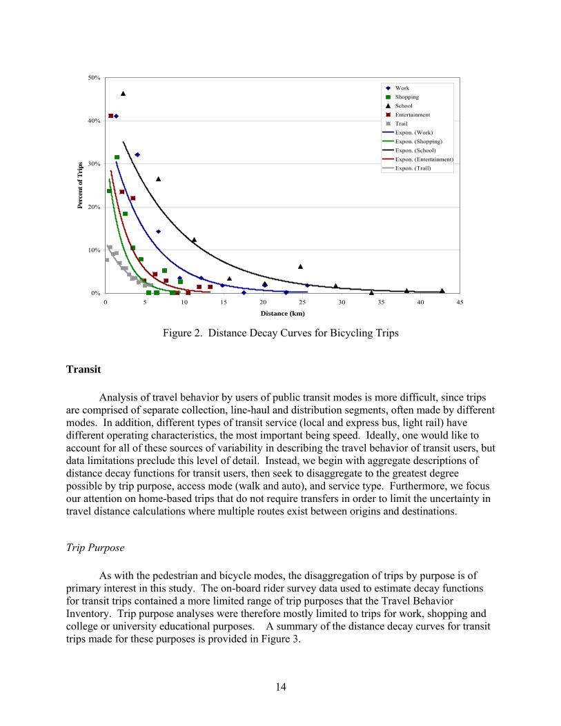
Distance decay curves for bike trips are provided in Figure 2. Bicyclists are willing to travel much longer distances than pedestrians, largely due to higher average speeds attainable by bicycle. Entertainment, recreation and fitness trips appear to cover the greatest average distances with some trips reaching 30 to 40 km (18.6 to 24.8 miles). Work trips by bike are the next longest type of trip, with most trips falling within a range of about 20 km. Bike trips for work, shopping, or access to bicycle trail facility tend to be shorter on average, with the majority of trips falling within 10 km (6.2 miles). Trip purpose is an important factor in determining the length individuals are willing to travel by bicycle.

Distance decay curves for individual trip purposes by bike are presented in Figures B.1 through B.5 in Appendix A. It becomes more clear that some of the curves estimated for the bicycle mode are constrained by limited data. Sample sizes for curves estimated for work, shopping, and entertainment, recreation and fitness trips are all below 70 observations. It is clear that bicycling trips are a rather rare behavior that is hard to capture and describe accurately within the context of general purpose travel surveys. In contrast, the distance decay function estimated for trail access trips has a much larger sample size, since the data upon which this curve was estimated come from a specialized survey of bicycle trail user behavior.

14

0%

10%

20%

30%

40%

50%

0 5 10 15 20 25 30 35 40 45

Distance (km)

Perc

ent o

f Tri

psWorkShoppingSchoolEntertainmentTrailExpon. (Work)Expon. (Shopping)Expon. (School)Expon. (Entertainment)Expon. (Trail)

Figure 2. Distance Decay Curves for Bicycling Trips

Transit Analysis of travel behavior by users of public transit modes is more difficult, since trips are comprised of separate collection, line-haul and distribution segments, often made by different modes. In addition, different types of transit service (local and express bus, light rail) have different operating characteristics, the most important being speed. Ideally, one would like to account for all of these sources of variability in describing the travel behavior of transit users, but data limitations preclude this level of detail. Instead, we begin with aggregate descriptions of distance decay functions for transit users, then seek to disaggregate to the greatest degree possible by trip purpose, access mode (walk and auto), and service type. Furthermore, we focus our attention on home-based trips that do not require transfers in order to limit the uncertainty in travel distance calculations where multiple routes exist between origins and destinations.

Trip Purpose As with the pedestrian and bicycle modes, the disaggregation of trips by purpose is of primary interest in this study. The on-board rider survey data used to estimate decay functions for transit trips contained a more limited range of trip purposes that the Travel Behavior Inventory. Trip purpose analyses were therefore mostly limited to trips for work, shopping and college or university educational purposes. A summary of the distance decay curves for transit trips made for these purposes is provided in Figure 3.

15

0%

10%

20%

30%

40%

50%

0 10 20 30 40 50 60

Distance (km)

Perc

ent o

f Tri

psWork

College

Shopping

Expon. (Work)

Expon.(Shopping)Expon. (College)

Figure 3. Distance Decay Curves for Transit Trips by Purpose

As one would expect, work trips tend to be longer-distance trips, covering distances of 50 or more KM with some regularity. Trips for shopping or college purposes were shorter and broadly similar in terms of responding to the effects of distance. Summaries of the fitted curves are provided in Table 3 of Appendix B, while the individual curves are displayed in Figures C.1 through C.3 of Appendix A. Using aggregate trip purpose data does obscure some of the underlying differences in the characteristics of travel for each purpose, though. On one hand, many of the transit users making trips identified as being for college or university purposes may include students, many of whom live relatively short distances from campus and make short daily commute trips by bus. These are counterbalanced by students (and some faculty or staff) who commute longer distances using the network limited-stop and express bus routes directly serving the university. These types of trips would show up as the less frequent observations in the long tail of the decay curve. A related issue is the effect of access mode and service type on trip length. Many transit work trips are longer than other types of transit trips because travelers are using higher-speed services such as express bus and light rail, allowing greater distance to be covered without much additional travel time. In addition, more of the users of these types of services are likely to use auto as an access mode, increasing overall trip speeds. This latter effect can be examined by disaggregating the trips by both access mode and trip purpose. Given the hypothesis that travelers have a more or less fixed budget of travel time, transit users who access transit by walking to a station or stop would be expected to make shorter trips, since they are in principle trading off access (and perhaps also egress) time against time

16

spent on the line-haul portion of the trip (i.e. time spent in-vehicle), thus generating shorter overall distances. This hypothesis is borne out by comparison of the distance decay parameters for trips with walk and auto access by trip purpose in Table 4 of Appendix B. One can also confirm these differences visually by examining the curves for trips by walk and auto access presented in Figures 4 and 5. Trips with walk access for shopping and college purposes are generally confined to distances of less than 20 KM, while work trips are as longer as 35 KM. By contrast, trips with auto access tend to be longer, with overall distances of up to 50 KM for college trips and nearly 60 KM for work trips.

0%

7%

14%

21%

28%

35%

42%

49%

0 5 10 15 20 25 30 35 40

Distance (km)

Perc

ent o

f Tri

ps

Work

Shopping

College

Expon.(College)Expon. (Work)

Expon.(Shopping)

Figure 4. Distance Decay Curves for Transit Trips by Purpose with Walk Access

Transit trips with auto access trips also appear to have a distance threshold (in the range of 5-10 KM) below which users will not use this combination of access and line-haul modes. This finding also indicates that a negative exponential curve is not appropriate for capturing the distance decay effect for this type of trip. Figure 5 plots the exponential curves in addition to points that trace out the shape of the curves using predictions from a more general decay function of the form:

)exp()()( xxxf βα μ −= (9)

17

0%

6%

12%

18%

24%

30%

0 10 20 30 40 50 60

Distance (km)

Perc

ent o

f Tri

psWorkCollegeWork (predicted)College (predicted)Expon. (Work)Expon. (College)

Figure 5. Distance Decay Curves for Transit Trips by Purpose with Auto Access

where α, μ and β are parameters to be estimated. This form has been referred to as a ‘combined’ function (Ortuzar & Willumsen, 2001). It is unimodal and approaches zero as the cost or impedance variable x does. The parameters of the fitted curves using this specification are listed in the Appendix B statistical summaries under the label “combined” for each trip purpose. The combined function appears to be a better fit for transit trips with auto access, and indeed is a suggested form for trip distribution functions applied to auto trips or any type of travel where short trips are not common (Kanafani, 1983).

Service Type Another useful way to disaggregate transit trips in order to isolate the effects of speed on distance is to stratify trips by service type. The detailed data available from the on-board survey of transit users permits this type of analysis. Users are stratified according to three major service types: express bus, light rail and local bus. The curves fit for transit trips by service type are shown in Figure 6. Again, there appear to be threshold effects for each of the service types, though they are more pronounced for express and light rail trips. The summaries for each of the fitted curves in Table 5 of Appendix B indicate that, particularly for express and light rail trips, the combined function again provides a markedly better fit to the data.

18

0%

10%

20%

30%

40%

50%

0 10 20 30 40 50 60 70

Distance (km)

Perc

ent o

f Tri

psExpressLocalLight RailExpon. (Express)Expon. (Light Rail)Expon. (Local)

Figure 6. Distance Decay Curves for Transit Trips by Service Type

The deviation of the data from the negative exponential curve form becomes more apparent when the individual curves are viewed in isolation (Figures C.4 through C.6 in Appendix A). Trips by local bus appear to be considerably shorter than express bus and light rail. This can be partly accounted for by the different operating speeds of the services, but also by the tendency of express bus services (and to a smaller extent, light rail services) to be used extensively for work trips, which tend to be longer than average regardless of mode.

While the negative exponential form does not fit the distribution of total trip distances very well, it does describe well the distance decay effect for access modes by themselves. Summaries of these curves disaggregated by service type are provided in Table 6 of Appendix B.

19

Auto

Drive Alone

As Figure 7 indicates, single-occupant trips by auto are considerably longer than trips by non-motorized modes and also longer than most transit trips. Decay curves for most trip purposes are strikingly similar, with the exception of work trips which, as one would expect, cover a greater distance. For non-work trip purposes by solo drivers, distances of up to 30 km or so are fairly common, while work trips appear to routinely extend beyond 40 km.

0%

10%

20%

30%

40%

50%

0 10 20 30 40 50 60 70

Distance (km)

Perc

ent o

f Tri

ps

WorkShoppingSchoolRestaurantEntertainmentExpon. (Work)Expon. (Shopping)Expon. (School)Expon. (Restaurant)Expon. (Entertainment)

Figure 7. Distance Decay Curves for Single-Occupant Auto Trips

Additional comparisons are permitted by examining the estimated impedance parameters (β) in Table 7 of Appendix B. While drive alone trips for non-work purposes tend to have impedance values slightly above 0.1 in magnitude, work trips tend to indicate a lower impedance, closer to 0.09. By contrast, impedance values for bike trips range from 0.12 for school-related trips to over 0.50 for shopping trips. As noted above, impedances for walking trips are greatest, with values ranging form 1.0 to 2.0. The relative magnitudes of these values indicate the importance of modal speeds in determining the spatial extent of travel by each mode.

20

Shared Ride Trips Shared ride trips describe all auto trips taken with two or more occupants. This includes regular carpools, as well as any other arrangement involving one or more occupants, such as parents taking their children along on shopping trips or to school. Figure 8 displays the distance decay curves for shared ride trips.

Estimates of impedance parameters for shared ride trips are largely similar to those for single-occupant auto trips, though there is not as much of a noticeable difference between work and non-work trips. Work and entertainment, recreation and fitness trips tend to be slightly longer on average than other types of trips, as is evident in Figure 8. Most trips cover distances of up to 30 km, with some work and recreation trips approaching and exceeding 40 km.

Health Care Decay Function In addition to the travel survey data collected to estimate decay functions for most trip purposes, a special data set was provided for clinic trips that allow for inferences regarding health care access-related travel. The data were collected from 32 clinics in the Twin Cities metropolitan area, representing over 170,000 clinic visits. A five percent random sample was

0%

10%

20%

30%

40%

0 10 20 30 40 50 60

Distance (km)

Perc

ent o

f Tri

ps

WorkShoppingSchoolRestaurantEntertainmentExpon. (Work)Expon. (Shopping)Expon. (School)Expon. (Restaurant)Expon. (Entertainment)

Figure 8. Distance Decay Curves for Shared Ride Auto Trips

21

drawn from these data, yielding over 8,500 observations. Each record contained the address of the clinic, along with the zip code of the trip maker, allowing for the calculation of a minimum distance path from the zip code centroid to the facility. A major limitation of these data, however, is the fact that no information was obtained on choice of mode. Therefore, the decay curves represent a pooling of trips by all modes, though the inclusion of a large number of longer-distance trips suggests a dominance by auto travel.

Figure 9 displays the negative exponential decay function fitted to the health care data. Overall, the fit is quite good, except for short distance trips (less than 10 km). The fit is improved slightly if the combined function is employed, allowing for the smaller number of trips that are made over very short distance (see Table 9 of Appendix B).

Figure 9. Distance Decay Curve for Health Care Trips

The fitted curve for the health care data indicates that the majority of health care-related trips are less than 20 km in length. The presence of a small number of very long trips probably represents individuals who either live at the metropolitan fringe, far from the nearest clinic, or require special treatment that can only be accessed at a few, highly specialized and geographically dispersed facilities. It should be noted, again, that these trips represent clinic visits, which are likely to represent more routine treatments. This is qualitatively different from access to hospitals, for which trip frequencies are likely to be less, but for which access is more critical.

22

Chapter 4 Travel Time Decay Functions

As a check against the accuracy of the distance decay functions estimated using data on trip distance, a second set of functions were estimated using travel time as the impedance variable. This is an important step, since our previous procedure involving travel distance does not allow for validation of either the chosen travel path (assumed to be minimum distance) or the trip speed. One drawback of using travel time data, however, is that the sample is limited to the Travel Behavior Inventory data, since the other data sets do not collect data on trip duration. Also, data on travel time is self-reported in the TBI, indicating that the accuracy of the data is subject to the bounds of human perception and cognition.

Walking A couple of things stand out when observing the distance decay functions for walking using travel time as an impedance measure. The first is the considerably smaller impedance parameter estimates, with all parameters taking values of 0.10 or less. This is merely a function of the units used in the analysis (minutes as opposed to kilometers), so the relative magnitudes of the parameter values should be roughly consistent across trip purposes. The second is the remarkable amount of consistency between trip purposes, which is indicated by the comparison of fitted curves in Figure 10. Only a small fraction of trips are longer than 30 minutes in duration, with an absolute upper limit near one hour. Trips for recreation, exercise and fitness purposes appear to have the greatest duration, followed closely by school and work-related trips. Shopping and restaurant trips tend to be the shortest, though not by much. Curves fitted for individual trip purposes are provided in Figures F.1 through F.5 in Appendix A, and statistical output for these curves is provided in Table 10 of Appendix B.

Bicycling

Distance decay curves for bicycle trips exhibit less uniformity and a weaker fit than those fitted for walking trips using travel time. Figure 11 contains the fitted curves and indicates that the simple negative exponential functions that fit the distance data reasonably well do not approximate as well the effect of travel time on the propensity to travel. In particular, the negative exponential curves tend to overpredict trips of a shorter duration, while underpredicting some of the longer trips in the 25 to 60 minute range. This is reflected in the fit of the individual curves, as shown in Figures G.1 through G.4 of Appendix A, and as summarized in Table 11 of Appendix B. Also suggestive is the improved explanatory power of the combined function, which allows for a non-monotonic shape and appears to better fit the distribution of travel time data. Work trips still appear to be the longest trips, followed by recreation, school and shopping trips, though this relationship is blurred by the poor fit of the curves at more extreme values. Again, most trips appear to be less than 30 minutes in length, with almost none greater than 60 minutes.

23

Figure 10: Distance Decay Curves for Walking Trips (Travel Time)

Transit

The lack of fit of the negative exponential curve to the travel time data becomes most apparent when trips taken by public transit are examined. The limited number of non-work trips by public transit in the data set restrict the analysis to work and shopping trips. The individual curves for each of these trip purposes are provided in Figures H.1 and H.2 of Appendix A. Imposing the negative exponential specification on these data result in an equation with almost no explanatory power; in fact, imposing an exponential curve form on the shopping trip data results in the estimation of a positive coefficient for the travel time variable, certainly a counterintuitive result.

24

Figure 11. Distance Decay Curves for Bicycle Trips (Travel Time)

The data for work and shopping trips by transit are plotted in Figure 12, along with curves for each trip purpose using predicted values from the combined function. While the transit data do exhibit a degree of variability that is not present for the other modes (particularly for work-related trips), the combined function provides a greatly improved fit, as can be visualized in Figure 12 and confirmed by the summaries in Table 12 of Appendix B. As was discussed in the interpretation of the distance-related transit decay functions, transit travel can vary on many dimensions, such as service type and access mode, which is then reflected in the more scattered nature of the travel time data for transit trips. Figure 12 also shows that there is a minimum threshold for the duration of transit trips of somewhat less than 10 minutes. This reflects the fact that transit trips incur a certain fixed time cost, relating to stop or station access and waiting times.

25

0%

5%

10%

15%

20%

25%

0 20 40 60 80 100 120Travel Time (min)

Perc

ent o

f Tri

ps

Work (actual)

Work (predicted)

Shopping (actual)

Shopping (predicted)

Figure 12. Distance Decay Curves for Public Transit Trips (Travel Time)

26

Chapter 5 Discussion

This section reviews some of the limitations the study faced and identifies further uses of the estimated distance decay functions.

Limitations

Sample Size

Perhaps the greatest limitation of the study was the inability to obtain workable sample sizes for various combinations of modes and trip purposes. General purpose travel surveys such as the TBI’s home interview survey tend to yield small numbers of trips by public transit and non-motorized modes, given the rarity of these behaviors. While this data source provided a large number of potential trip purposes (17 were identified in the data set), disaggregating trips by mode and purpose greatly limited the sizes of the samples that could be obtained from them. Public transit trips for purposes other than work were represented only in small numbers. Further limiting the sample sizes used in the analysis was the quality of the data available. Usable records in each data set had to be geocodable, including all trip origins and destinations. In addition, records in the transit on-board survey needed to have boarding and alighting points properly located and geocoded. Inaccurate or inappropriate survey responses, including reporting of unrealistic trip distances or speeds, further thinned the data sets. As a consequence, many of the parameters of the estimated decay functions retained high amounts of variance, as is reported in the statistical summaries.

The other three data sources used in the study were specialized surveys designed to capture behavior by specific modes. While these surveys were able to target certain modes and provide a larger number of observations, they also tended to be limited in terms of the trip purposes identified in the survey instrument. This was especially the case for the transit on-board survey, whose primary purpose was to collect data suitable for modeling purposes. It would seem that a study designed to provide greater depth than the current work would need to design and implement a special survey instrument, combined with specialized sampling techniques, rather than relying on existing secondary sources of data.

Focus on Home-Based Trips

Since emphasis in this study is placed on understanding how far individuals will travel to reach various destinations and how this might help to structure measures of accessibility, most interest is centered around individuals accessing activities relative to their home location. Thus, non-home based trips are not examined as extensively in this study. This may not be as much of a problem for travel by non-motorized modes, since multi-stop trips by these modes tend to be less common (Ye, Pendyala, & Gottardi, 2007). However, the treatment of transit trips

27

significantly limited our understanding of transit travel behavior. By constraining the trips used in the analysis to those that did not require transfers, a significant number of trips were missed. These excluded trips may have had characteristics dissimilar from those that were studied. One possibility is that they represented longer trips than those studied (in terms of time, distance or both). Another is that a significant number of light rail trips were missed, since many rail users must transfer at either their boarding or alighting point during a trip.

No Multi-Stop Trip Chains

Among the most fundamental concepts of travel behavior analysis is the idea that individuals’ travel behavior is structured in both space and time and faces numerous constraints (Ettema & Timmermans, 1997; McNally, 2000). Activities are typically organized into trip chains or tours in order to be carried out with reference to some primary activity (work, school, etc.). Since the secondary data sources used in the analysis all contain trip-based data sets, the resulting analysis must make the rather strong (and unrealistic) assumption that all trips are carried out independently of one another.

Estimation of Distance Decay Functions In more conventional analyses of travel demand or other applications where predictions of spatial interaction are required, distance decay functions are typically estimated as part of a more general gravity-type model (see Section 2) containing variables that represent the attractiveness of origins and destinations. The decay functions are estimated along with these terms because of the close relationship between the impedance parameter and the spatial structure of the study region (Sheppard, 1995). The impedance parameter is, in principle, a function of both the utility of the transportation network and the spatial distribution of activities around a given location. Hence, estimating distance decay functions without reference to these variables could introduce a considerable amount of bias into the decay function parameters. The possible extent of this bias is difficult to determine a priori.

Applications of the Distance Decay Functions

In addition to providing valuable information about the willingness of individuals to travel to reach various destinations, the distance decay functions estimated in this study can be used as inputs to further types of analysis. One possible application is the study of multimodal, multipurpose accessibility. Using the decay functions estimated for the various mode-purpose combinations, Song (1996) shows how the negative exponential function can be introduced into a gravity-type accessibility measure to yield an accessibility equation of the form:

E

xEA ij

j

i

∑≠

−=

)exp( β (10)

28

where Ai represents the accessibility at zone i, Ej is a measure of opportunities (here we can use employment) at zone j, E represents all opportunities available in the region, and the negative exponential decay function is as defined as before. In this manner, accessibility measures can be calculated for all modes, or as a single measure with a weighted sum to represent the probabilities of using each mode. In addition to calculating regional, gravity-based measures of accessibility, smaller-scale measures of neighborhood accessibility (Handy & Clifton, 2001; Krizek, 2003) can also be calculated using cumulative opportunities formulations (Wachs & Kumagai, 1973) and information about the range of each mode from the estimated distance decay curves. These types of measures have rarely been evaluated for non-motorized modes, hence the construction of such measures from the distance decay functions provided in this study represent a significant achievement.

To illustrate the procedures used to produce estimates of non-motorized accessibility, we completed some sample accessibility calculations for a small study area in South Minneapolis. The study area is bounded on the west by Lyndale Avenue, on the north by Franklin Avenue, on the east by the Mississippi River, and on the south by 50th Street. This area contains approximately 1,600 Census block groups, which represent the unit of analysis. The accessibility values calculated for each block group are integral accessibility measures (Song 1996), where the activities in each destination zone, discounted by their associated impedance value, are summed across destinations and normalized by dividing by the total activities in the study area. This method provides a measure that can be easily interpreted and compared across zones on the same zero to one scale. Thus, in each case, accessibility is expressed as a decimal indicating proximity to destinations in each location. In the case of each accessibility calculation, an attractiveness measure is constructed for each block group by summing the level of retail sales at each establishment within the block group. Impedance measures are introduced by calculating the shortest path through the network between each block group pair, then using this value to discount activities at the destination using the functional form described previously.

Figure 13 presents maps displaying measures of accessibility to restaurant destinations for the walking mode. Again, the maps show the same measures calculated using time and distance as alternate measures of travel impedance. Consistent with the findings described earlier, they show a high degree of correlation. Areas near clusters of restaurant destinations are shown to have high levels of accessibility, with a gradual decline as one moves away from these clusters.

Figure 14 presents a pair of maps showing accessibility to shopping destinations by bicycle with distance and time impedance measures. In this case, destinations are spread more evenly throughout the study area, leading to higher overall accessibility values in each zone. Retail establishments appear to align themselves along linear corridors, reflecting the historical network of streetcar routes in South Minneapolis. One particularly large corridor is found along Lake Street, a major east-west route that lies at the center of the swath of high accessibility shown in both maps. This high-accessibility location results from a combination of clustering of activities and proximity to the Midtown Greenway, a grade separated off-street bicycle facility highlighted in green on the map.

29

Figure 13. Walk Accessibility to Restaurants

30

Figure 14. Bicycle Accessibility to Shopping

31

These examples demonstrate the applicability of accessibility measures to non-motorized modes and the importance of spatial scale when measuring non-motorized accessibility. The use of block-level data allow for the identification of local clusters of activity, which translate into pockets of higher accessibility. With the same sets of data available at the regional level, it should be possible to scale these types of calculations up to produce region-wide measures of accessibility by non-auto modes.

32

Chapter 6 Conclusion

The evidence presented in this study is intended to address a perceived need in the field of transportation planning, especially with respect to non-auto modes, though relevant information about auto travel is also presented. The evidence focuses on one particular aspect of travel behavior, namely the spatial distribution of trips by mode and trip purpose. The findings are intended to supplement traditional rules-of-thumb regarding planning for travel by walking and bicycle modes. The findings suggest, for example, that substantial shares of pedestrian travel (perhaps one-quarter to one-third) exceed the often-cited threshold of one-quarter mile. Moreover, this finding appears to be invariant to trip purpose. These results are based on available reported trips from actual travel diaries. Unless the segment of the population who reported these pedestrian trips are substantially different from those who either did not make utilitarian trips by the pedestrian mode or did not think to report them, this may be a welcome finding for pedestrian planning. Results for bicycle travel data revealed a substantial difference in travel distances by trip purpose. Primary activities such as work and school often involved very long bike trips (up to 20-30 KM) for those who chose this mode. In contrast, more discretionary trips (e.g. for shopping, entertainment or recreation purposes) tended to be substantially shorter in length. It would be desirable to future studies of these types of behavior to target bicycling specifically in order to provide a large enough sample to further substantiate these findings. The public transit trips examined in this study reveal significant differences in travel behavior across several types of stratification. Type of service (local bus, express bus, light rail), access mode and trip purpose all appear to affect trip length. The origin-destination data examined in this study allowed for a disaggregation of trips by segment (access, egress, and line-haul), which presents opportunities to ask further questions about how travelers view the relative importance of different parts of their trip (e.g. access). As mentioned previously, though, the analysis of transit trips presented here was limited to those making one or fewer transfers. Future work should extend this to multiple-transfer trips using transportation planning packages with a significant transit travel modeling component. A notable finding across the different travel modes was that a range of functional forms can and should be used to measure travel impedance. We have suggested a couple of these alternatives in earlier sections; a thorough examination of the literature on the practice of travel demand modeling would likely turn up even more. Different modes tend to have different characteristics that are reflected in their decay or impedance functions. The most glaring examples are auto and transit travel, which both tend to have certain minimum thresholds in terms of travel time or distance. Thus, when comparing across modes or trip purposes, a good guideline to follow would be to fit multiple curves using different functional forms to find the most appropriate form. Lastly, we have also demonstrated how the decay curves for different travel modes and trip purposes can be used to provide measures of accessibility. While the calculation of accessibility measures for auto and transit modes are relatively straightforward using conventional travel demand models, we have shown how the use of a more disaggregate zonal structure using Census geography can allow for the generation of non-motorized accessibility

33

measures at a spatial scale more closely aligned with actual bicycle and pedestrian travel behavior. While our results were restricted to a relatively small sample area, the techniques should be scalable to larger geographic areas given full spatial data sets and appropriate computational hardware.

34

References

Baradaran, S., & Ramjerdi, F. (2001). Performance of accessibility measures in Europe. Journal of Transportation and Statistics, 4(2/3), 31-48.

Bates, J. J. (2000). History of demand modelling. In D. A. Hensher & K. J. Button (Eds.), Handbook of Transport Modelling (Vol. 1, pp. 11-33). Amsterdam: Pergamon Press.

Batty, M. (1976). Urban modelling: algorithms, calibrations, predictions (Vol. 3). Cambridge, UK: Cambridge University Press.

Beckmann, M. J., Golob, T. F., & Zahavi, Y. (1983a). Travel probability fields and urban spatial structure: 1. theory. Environment & Planning A, 15(5), 593-606.

Beckmann, M. J., Golob, T. F., & Zahavi, Y. (1983b). Travel probability fields and urban spatial structure: 2. empirical tests. Environment & Planning A, 15(6), 727-738.

Ben-Akiva, M. E., & Lerman, S. R. (1979). Disaggregate travel and mobility-choice models and measures of accessibility. In D. A. Hensher & P. R. Stopher (Eds.), Behavioural Travel Modelling. London: Croom Helm.

Bhat, C. R., Govindarajan, A., & Pulugurta, V. (1998). Disaggregate attraction-end choice modeling: formulation and empirical analysis. Transportation Research Record, 1645, 60-68.

Daly, A. J. (1982). Estimating choice models containing attraction variables. Transportation Research, Part B, 16B(1), 5-15.

Ettema, D., & Timmermans, H. J. P. (1997). Theories and models of activity patterns. In D. Ettema & H. J. P. Timmermans (Eds.), Activity-based approaches to travel analysis (pp. 1-36). Oxford, UK: Pergamon Press.

Farhan, B., & Murray, A. T. (2006). Distance decay and coverage in facility location planning. Annals of Regional Science, 40(2), 279-295.

Flowerdew, R., & Aitkin, M. (1982). A method of fitting the gravity model based on the Poisson distribution. Journal of Regional Science, 22, 191-202.

Fotheringham, A. S. (1981). Spatial structure and distance-decay parameters. Annals of the Association of American Geographers, 71, 425-436.

Fotheringham, A. S. (1983). A new set of spatial interaction models: the theory of competing destinations. Environment & Planning A, 15(1), 15-36.

Fotheringham, A. S., & O' Kelly, M. (1989). Spatial interaction models: formulations and applications. Boston: Kluwer.

Goncalves, M. B., & Ulyssea-Neto, I. (1993). The development of a new gravity-opportunity model for trip distribution. Environment & Planning A, 25(6), 817-826.

Handy, S. L. (2005). Planning for accessibility: In theory and in practice. In D. M. Levinson & K. J. Krizek (Eds.), Access to Destinations (pp. 131-147). Amsterdam: Elsevier.

Handy, S. L., & Clifton, K. J. (2001). Evaluating neighborhood accessibility: Possibilities and practicalities. Journal of Transportation and Statistics, 4(2/3), 67-78.

Handy, S. L., & Niemeier, D. A. (1997). Measuring accessibility: An exploration of issues and alternatives. Environment & Planning A, 29(7), 1175-1194.

Hansen, W. (1959). How accessibility shapes land use. Journal of the American Institute of Planners, 25(1), 73-76.

35

Harris, B. (2001). Accessibility: Concepts and Applications. Journal of Transportation and Statistics, 4(2/3), 15-30.

Haworth, J. M., & Vincent, P. J. (1979). The stochastic disturbance specification and its implications for log-linear regression. Environment & Planning A, 11(7), 781-790.

Heien, P. M. (1968). A note on log-linear regression. Journal of the American Statistical Association, 63, 1034-1038.

Hsiao, S., Lu, J., Sterling, J., & Weatherford, M. (1997). Use of geographic information system for analysis of transit pedestrian access. Transportation Research Record, 1604, 50-59.

Kanafani, A. K. (1983). Transportation demand analysis. New York, NY: McGraw-Hill. Krizek, K. J. (2003). Operationalizing neighborhood accessibility for land use-travel behavior

research and regional modeling. Journal of Planning Education and Research, 22(3), 270-287.

Krizek, K. J. (2005). Perspecives on Accessibility and Travel. In D. M. Levinson & K. J. Krizek (Eds.), Access to Destinations (pp. 109-130). Amsterdam: Elsevier.

Levinson, H. S., & Brown-West, O. (1984). Estimating bus ridership. Transportation Research Record, 994, 8-12.

Luoma, M., Mikkonen, K., & Palomaki, M. (1993). The threshold gravity model and transport geography: How transport development influences the distance-decay parameter of the gravity model. Journal of Transport Geography, 1(4), 240-247.

Lutin, J. M., Liotine, M., & Ash, T. M. (1981). Empirical models of transit service areas. Journal of Transportation Engineering, 107(4), 427-444.

Marquardt, D. (1963). An algorithm for least-squares estimation of nonlinear parameters. SIAM Journal of Applied Mathematics, 11(2), 431-441.

McCarthy, P. S. (1980). A study of the importance of generalized attributes in shopping choice behavior. Environment & Planning A, 12(11), 1269-1286.

McNally, M. G. (2000). The Activity-Based Approach. In D. A. Hensher & K. J. Button (Eds.), Handbook of Transport Modelling (Vol. 1, pp. 53-69). Amsterdam: Pergamon Press.

Metropolitan Council (Internet). Guide for Transit-Oriented Development, August 2006 (cited April 2006), http://www.metrocouncil.org/planning/tod/TOD_index_page.pdf

Mikkonen, K., & Luoma, M. (1999). The parameters of the gravity model are changing--how and why? Journal of Transport Geography, 7(4), 277-283.

Ortuzar, J. d. D., & Willumsen, L. G. (2001). Modelling transport (3rd ed.). Chichester, UK: John Wiley.

Rutherford, G. S. (1979). Use of the gravity model for pedestrian travel distribution. Transportation Research Record, 728, 53-59.

Sen, A. K. (1986). Maximum likelihood estimation of gravity model parameters. Journal of Regional Science, 26, 461-474.

Sen, A. K., & Matuszewski, Z. (1991). Properties of maximum likelihood estimates of gravity model parameters. Journal of Regional Science, 31, 469-486.

Seneviratne, P. N. (1985). Acceptable walking distances in central areas. Journal of Transportation Engineering, 111(4), 365-376.

Sheppard, E. S. (1995). Modeling and predicting aggregate flows. In S. A. Hanson (Ed.), The geography of urban transportation (2nd edition ed., pp. 100-128). New York, NY: Guilford Press.

Song, S. (1996). Some tests of alternative accessibility measures: a population density approach. Land Economics, 72(4), 474-482.

36

Timmermans, H. J. P. (1996). A stated choice model of sequential mode and destination choice behaviour for shopping trips. Environment & Planning A, 28(1), 173-184.

Untermann, R. K. (1984). Accommodating the pedestrian: adapting towns and neighborhoods for walking and bicycling. New York: Van Nostrand Reinhold.

Upchurch, C., Kuby, M., Zoldak, M., & Barranda, A. (2004). Using GIS to generate mutually exclusive service areas linking travel on and off a network. Journal of Transport Geography, 12(1), 23-33.

Wachs, M., & Kumagai, T. G. (1973). Physical accessibility as a social indicator. Socio-Economic Planning Sciences, 7(5), 437-456.

Wrigley, N., & Dunn, R. (1984). Stochastic panel-data models of urban shopping behaviour: 1. Purchasing at individual stores in a single city. Environment & Planning A, 16, 629-650.

Ye, X., Pendyala, R. M., & Gottardi, G. (2007). An exploration of the relationship between mode choice and complexity of trip chaining patterns. Transportation Research, Part B: Methodological, 41B(1), 96-113.

Zhao, F., Chow, L.-F., Li, M.-T., Ubaka, I., & Gan, A. (2003). Forecasting transit walk accessibility: Regression model alternative to buffer method Transportation Research Record, 1835, 34-41.

Appendix A

Distance Decay Functions by Mode and Purpose

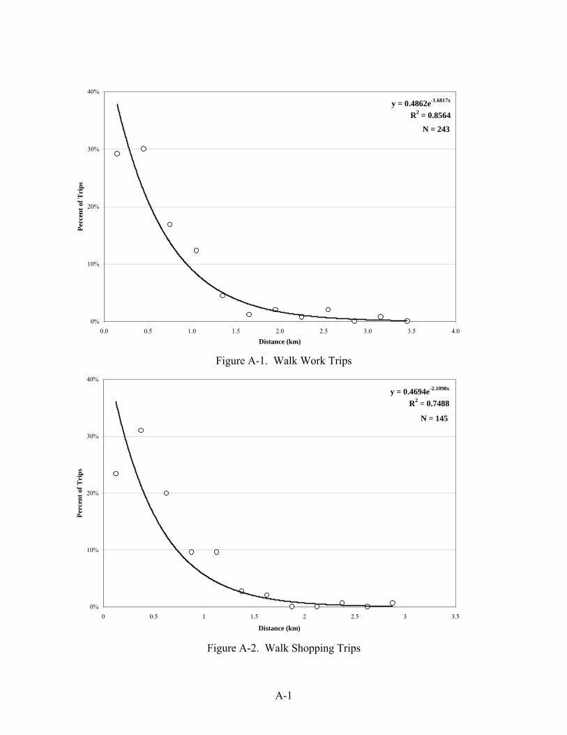
A-1

y = 0.4862e-1.6817x

R2 = 0.8564

0%

10%

20%

30%

40%

0.0 0.5 1.0 1.5 2.0 2.5 3.0 3.5 4.0

Distance (km)

Perc

ent o

f Tri

ps

N = 243

Figure A-1. Walk Work Trips

y = 0.4694e-2.1098x

R2 = 0.7488

0%

10%

20%

30%

40%

0 0.5 1 1.5 2 2.5 3 3.5

Distance (km)

Perc

ent o

f Tri

ps

N = 145

Figure A-2. Walk Shopping Trips

A-2

y = 0.3878e-1.3919x

R2 = 0.8499

0%

10%

20%

30%

40%

0 0.5 1 1.5 2 2.5 3 3.5 4

Distance (km)

Perc

ent o

f Tri

ps

N = 134

Figure A-3. Walk Restaurant Trips

y = 0.3238e-0.7655x

R2 = 0.6096

0%

10%

20%

30%

40%

0 1 2 3 4 5 6 7 8

Distance (km)

Perc

ent o

f Tri

ps

N = 156

Figure A-4. Walk Entertainment, Recreation and Fitness Trips

A-3

y = 0.4018e-0.203x

R2 = 0.6406

0%

10%

20%

30%

40%

50%

0 5 10 15 20 25 30

Distance (km)

Perc

ent o

f Tri

ps

N = 56

Figure B-1. Bike Work Trips

y = 0.3422e-0.5131x

R2 = 0.4303

0%

5%

10%

15%

20%

25%

30%

35%

0 1 2 3 4 5 6 7 8 9 10

Distance (km)

Perc

ent o

f Tri

ps

N = 38

Figure B-2. Bike Shopping Trips

A-4

y = 0.4651e-0.1236x

R2 = 0.7894

0%

10%

20%

30%

40%

50%

0 5 10 15 20 25 30 35 40 45

Distance (km)

Perc

ent o

f Tri

ps

N = 177

Figure B-3. Bike School or School-Related Trips

y = 0.3704e-0.3763x

R2 = 0.5836

0%

10%

20%

30%

40%

50%

0 2 4 6 8 10 12 14

Distance (km)

Perc

ent o

f Tri

ps

N = 68

Figure B-4. Bike Entertainment, Recreation and Fitness Trips

A-5

y = 0.1192e-0.3328x

R2 = 0.9274

0%

2%

4%

6%

8%

10%

12%

0 1 2 3 4 5 6

Distance (km)

Perc

ent o

f tri

ps

N = 1,967

Figure B-5. Bike Trail Access Trips

y = 0.6759e-0.0935x

R2 = 0.915

0%

7%

14%

21%

28%

35%

0 10 20 30 40 50 60

Distance (km)

Perc

ent o

f Tri

ps

N = 1,065

Figure C-1. Transit Work Trips

A-6

y = 0.3439e-0.0916x

R2 = 0.6404

0%

10%

20%

30%

40%

50%

0 5 10 15 20 25 30 35 40 45 50

Distance (km)

Perc

ent o

f Tri

ps

N = 65

Figure C-2. Transit Shopping Trips

y = 0.3927e-0.1145x

R2 = 0.8547

0%

10%

20%

30%

40%

50%

0 5 10 15 20 25 30 35 40 45 50

Distance (km)

Perc

ent o

f Tri

ps

N = 460

Figure C-3. Transit College and University Trips

A-7

y = 0.216e-0.0595x

R2 = 0.4792

0%

5%

10%

15%

20%

25%

0 10 20 30 40 50 60 70

Distance (km)

Perc

ent o

f Tri

ps

N = 871

Figure C-4. Transit Trips by Express Bus

y = 0.1276e-0.0457x

R2 = 0.2934

0%

5%

10%

15%

20%

25%

0 5 10 15 20 25 30 35 40 45 50

Distance (km)

Perc

ent o

f Tri

ps

N = 349

Figure C-5. Transit Trips by Light Rail

A-8

y = 0.4905e-0.1955x

R2 = 0.9398

0%

6%

12%

18%

24%

30%

0 5 10 15 20 25 30 35

Distance (km)

Perc

ent o

f Tri

ps

N = 1,316

Figure C-6. Transit Trips by Local Bus

y = 0.5279e-0.0905x

R2 = 0.9531

0%

5%

10%

15%

20%

25%

0 10 20 30 40 50 60 70

Distance (km)

Perc

ent o

f Tri

ps

N = 1,300

Figure D-1. Drive Alone Work Trips

A-9

y = 0.3859e-0.1178x

R2 = 0.9665

0%

10%

20%

30%

40%

50%

0 10 20 30 40 50 60

Distance (km)

Perc

ent o

f Tri

ps

N = 2,437

Figure D-2. Drive Alone Shopping Trips

y = 0.3737e-0.1227x

R2 = 0.6676

0%

5%

10%

15%

20%

25%

0 5 10 15 20 25 30 35 40 45

Distance (km)

Perc

ent o

f Tri

ps

N = 260

Figure D-3. Drive Alone School or School-Related Trips

A-10

y = 0.3129e-0.1178x

R2 = 0.9618

0%

10%

20%

30%

40%

0 5 10 15 20 25 30 35 40 45 50

Distance (km)

Perc

ent o

f Tri

ps

N = 745

Figure D-4. Drive Alone Restaurant Trips

y = 0.3388e-0.1035x

R2 = 0.9812

0%

5%

10%

15%

20%

25%

0 5 10 15 20 25 30 35 40 45 50

Distance (km)

Perc

ent o

f Tri

ps

N = 511

Figure D-5. Drive Alone Entertainment, Recreation and Fitness Trips

A-11

y = 0.2396e-0.0773x

R2 = 0.8883

0%

5%

10%

15%

20%

25%

30%

0 5 10 15 20 25 30 35 40 45 50

Distance (km)

Perc

ent o

f Tri

ps

N = 181

Figure E-1. Shared Ride Work Trips

y = 0.3756e-0.1286x

R2 = 0.9635

0%

10%

20%

30%

40%

0 5 10 15 20 25 30 35 40 45 50

Distance (km)

Perc

ent o

f Tri

ps

N = 959

Figure E-2. Shared Ride Shopping Trips

A-12

y = 0.1593e-0.0961x

R2 = 0.5884

0%

5%

10%

15%

20%

25%

30%

0 5 10 15 20 25 30 35

Distance (km)

Perc

ent o

f Tri

ps

N = 176

Figure E-3. Shared Ride School or School-Related Trips

y = 0.426e-0.1399x

R2 = 0.8695

0%

10%

20%

30%

40%

0 5 10 15 20 25 30 35 40 45 50

Distance (km)

Perc

ent o

f Tri

ps

N = 500

Figure E-4. Shared Ride Restaurant Trips

A-13

y = 0.3368e-0.0936x

R2 = 0.8907

0%

5%

10%

15%

20%

25%

30%

35%

0 10 20 30 40 50 60

Distance (km)

Perc

ent o

f Tri

ps

N = 369

Figure E-5. Shared Ride Entertainment, Recreation and Fitness Trips

y = 0.519e-0.10x

R² = 0.927N = 366

0%

10%

20%

30%

40%

0 10 20 30 40 50 60

Travel Time (min)

Perc

ent o

f Tri

ps

Figure F-1. Walking Work Trips

A-14

y = 0.523e-0.10x

R² = 0.600N = 105

0%

10%

20%

30%

40%

0 5 10 15 20 25 30 35 40 45 50

Travel Time (min)

Perc

ent o

f Tri

ps

Figure F-2. Walk School or School-Related Trips

y = 0.370e-0.09x

R² = 0.724N = 269

0%

7%

14%

21%

28%

35%

0 10 20 30 40 50 60

Travel Time (min)

Perc

ent o

f Tri

ps

Figure F-3. Walk Shopping Trips

A-15

y = 0.377e-0.09x

R² = 0.702N = 179

0%

10%

20%

30%

40%

0 10 20 30 40 50 60

Travel Time (min)

Perc

ent o

f T

rips

Figure F-4. Walk Restaurant Trips

y = 0.545e-0.09x

R² = 0.932N = 292

0%

10%

20%

30%

40%

0 5 10 15 20 25 30 35 40 45 50

Travel Time (min)

Perc

ent o

f Tri

ps

Figure F-5. Walk Entertainment, Recreation and Fitness Trips

A-16

y = 0.146e-0.03x

R² = 0.378N = 109

0%

5%

10%

15%

20%

25%

0 10 20 30 40 50 60 70 80

Travel Time (min)

Perc

ent o

f Tri

ps

Figure G-1. Bike Work Trips

y = 0.4225e-0.0998x

R2 = 0.5955N = 36

0%

10%

20%

30%

40%

0 10 20 30 40 50 60

Travel Time (min)

Perc

ent o

f Tri

ps

Figure G-2. Bike School or School-Related Trips

A-17

y = 0.432e-0.10x

R² = 0.697N = 64

0%

7%

14%

21%

28%

35%

0 10 20 30 40 50 60

Travel Time (min)

Perc

ent o

f Tri

ps

Figure G-3. Bike Shopping Trips

y = 0.294e-0.07x

R² = 0.589N = 131

0%

7%

14%

21%

28%

35%

0 10 20 30 40 50 60

Travel Time (min)

Perc

ent o

f Tri

ps

Figure G-4. Bike Entertainment, Recreation and Fitness Trips

A-18

y = 0.0323e-0.0102x

R2 = 0.0416N = 176

0%

5%

10%

15%

20%

25%

0 20 40 60 80 100 120

Travel Time (min)

Perc

ent o

f Tri

ps

Figure H-1. Transit Work Trips

y = 0.014e0.029x

R² = 0.045N = 22

0%

5%

10%

15%

20%

0 10 20 30 40 50 60

Travel Time (min)

Perc

ent o

f Tri

ps

Figure H-2. Transit Shopping Trips

Appendix B Statistical Summaries of the Estimated Distance Decay Functions

B-1

Table 1. Distance Decay Functions for Walking Trips by Trip Purpose

Distance Constant Model Fit β S.E. t sig. α S.E. t sig. (adj.) R2 F N Work Trips Excel -1.682 0.486 0.856 243 Regression -1.683 0.219 -7.685 0.000 -0.723 0.454 -1.593 0.143 0.841 59.284 243 Curve Fitting -1.683 0.219 -7.685 0.000 0.486 0.220 2.209 0.052 0.841 59.284 243 Shopping Trips Excel -2.110 0.469 0.749 Regression -2.106 0.388 -5.428 0.000 -0.756 0.671 -1.127 0.286 0.721 29.474 145 Curve Fitting -2.106 0.388 -5.428 0.000 0.469 0.315 1.489 0.167 0.721 29.474 145 Restaurant Trips Excel -1.392 0.388 0.850 134 Regression -1.397 0.186 -7.511 0.000 -0.946 0.385 -2.457 0.034 0.835 56.710 134 Curve Fitting -1.397 0.186 -7.511 0.000 0.388 0.150 2.587 0.027 0.835 56.710 134 Recreational Trips TBI Excel -0.766 0.324 0.610 156 Regression -0.769 0.193 -3.984 0.003 -1.119 0.803 -1.394 0.193 0.574 15.830 156 Curve Fitting -0.769 0.193 -3.984 1.003 0.327 0.262 1.248 0.241 0.574 15.830 156 NMPP Excel -0.688 0.499 0.797 104 Regression -0.687 0.122 -5.619 0.000 -0.695 0.529 -1.314 0.225 0.773 31.571 104 Curve Fitting -0.687 0.122 -5.619 0.000 0.499 0.264 1.891 0.095 0.773 31.571 104

B-2

Table 2. Distance Decay Functions for Bicycle Trips by Trip Purpose

Distance Constant Model Fit β S.E. t sig. α S.E. t sig. (adj.) R2 F N Work Trips Excel -0.203 0.402 0.641 56 Regression -0.203 0.054 -3.759 0.005 -0.910 0.838 -1.086 0.309 0.594 14.190 56 Curve Fitting -0.203 0.054 -3.759 0.005 0.402 0.337 1.193 0.267 0.594 14.190 56 Shopping Trips Excel -0.513 0.342 0.430 38 Regression -0.514 0.209 -2.459 0.039 -1.071 1.203 -0.890 0.399 0.360 6.059 38 Curve Fitting -0.514 0.209 -2.459 0.039 0.343 0.412 0.833 0.430 0.360 6.059 38 School Trips Excel -0.124 0.465 0.789 177 Regression -0.122 0.023 -5.304 0.001 -0.780 0.591 -1.320 0.223 0.756 28.854 177 Curve Fitting -0.122 0.023 -5.304 1.001 0.458 0.271 1.690 0.129 0.756 28.854 177 Recreational Trips TBI Excel -0.376 0.370 0.584 68 Regression -0.375 0.113 -3.319 0.011 -1.003 0.911 -1.101 0.303 0.527 11.034 68 Curve Fitting -0.375 0.113 -3.319 0.011 0.367 0.334 1.099 0.304 0.527 11.034 68 NMPP Excel -0.228 0.544 0.927 87 Regression -0.229 0.022 -10.387 0.000 -0.604 0.318 -1.899 0.094 0.922 107.892 87 Curve Fitting -0.229 0.022 -10.387 0.000 0.546 0.174 3.141 0.014 0.922 107.892 87 Trail Trips Excel 0.333 0.119 0.927 1967 Regression Curve Fitting

B-3

Table 3. Distance Decay Functions for Transit Trips by Trip Purpose

Distance (β) Constant (α) Shape (μ) Model Fit Coeff. S.E. t Coeff. S.E. t Coeff. S.E. t (adj.) R2 F N Work Trips Excel -0.094 0.676 0.915 1065 Regression -0.093 0.010 -9.467 -0.405 0.345 -1.174 0.908 89.633 1065 Curve Fitting -0.093 0.010 -9.467 0.667 0.230 2.902 0.908 89.633 1065 Combined -0.143 0.018 -7.875 -2.350 0.690 -3.406 1.110 0.369 3.012 0.954 94.564 1065 College Trips Excel -0.115 0.393 0.855 460 Regression -0.116 0.017 -6.953 -0.902 0.493 -1.828 0.840 48.343 460 Curve Fitting -0.116 0.017 -6.953 0.406 0.200 2.027 0.840 48.343 460 Combined -0.062 0.042 -1.483 0.675 1.205 0.560 -1.002 0.706 -1.419 0.858 28.241 460 Shopping Trips Excel -0.092 0.344 0.640 65 Regression -0.092 0.024 -3.811 -1.060 0.697 -1.522 0.600 14.527 65 Curve Fitting -0.092 0.024 -3.811 0.346 0.241 1.435 0.600 14.527 65

B-4

Table 4. Distance Decay Functions for Transit Trips by Access Mode and Trip Purpose Distance (β) Constant (α) Shape (μ) Model Fit Coeff. S.E. t Coeff. S.E. t Coeff. S.E. t (adj.) R2 F N Walk Access Work Trips Excel -0.139 0.588 0.869 747 Regression -0.138 0.019 -7.433 -0.544 0.406 -1.338 0.858 55.252 747 Curve Fitting -0.138 0.019 -7.433 0.581 0.236 2.461 0.858 55.252 747 Combined -0.248 0.026 -9.504 -2.446 0.470 -5.203 1.496 0.328 4.567 0.959 106.610 747 College Trips Excel -0.286 0.507 0.719 408 Regression -0.285 0.063 -4.509 -0.685 0.656 -1.045 0.682 20.327 408 Curve Fitting -0.285 0.063 -4.509 0.504 0.331 1.524 0.682 20.327 408 Combined -0.699 0.053 -13.132 -2.082 0.268 -7.768 2.662 0.316 8.412 0.967 134.184 408 Shopping Trips Excel -0.130 0.280 0.898 42 Regression -0.130 0.015 -8.379 -1.275 0.179 -7.139 0.885 70.207 42 Curve Fitting -0.130 0.015 -8.379 0.279 0.050 5.599 0.885 70.207 42 Combined -0.195 0.034 -5.712 -1.571 0.207 -7.586 0.469 0.226 2.075 0.919 51.755 42 Auto Access Work Trips Excel -0.034 0.146 0.184 263 Regression -0.033 0.025 -1.323 -1.937 0.882 -2.196 0.077 1.751 263 Curve Fitting -0.033 0.025 -1.323 0.144 0.127 1.134 0.077 1.751 263 Combined -0.188 0.031 -6.080 -7.892 1.175 -6.716 3.399 0.628 5.415 0.797 18.635 263 College Trips Excel -0.050 0.190 0.225 36 Regression -0.050 0.033 -1.522 -1.658 0.964 -1.721 0.128 2.317 36 Curve Fitting -0.050 0.033 -1.522 0.191 0.184 1.038 0.128 2.317 36 Combined -0.191 0.072 -2.641 -5.719 2.087 -2.740 2.579 1.223 2.109 0.390 3.881 36

B-5

Table 5. Distance Decay Functions for Transit Trips by Service Type

Distance (β) Constant (α) Shape (μ) Model Fit Coeff. S.E. t Coeff. S.E. t Coeff. S.E. t (adj.) R2 F N Local Bus Trips Excel -0.196 0.491 0.940 1316 Regression -0.186 0.014 -13.238 -0.799 0.272 -2.933 0.931 175.250 1316 Curve Fitting -0.186 0.014 -13.238 0.450 0.123 3.670 0.931 175.250 1316 Combined -0.243 0.031 -7.857 -1.539 0.442 -3.480 0.666 0.332 2.005 0.945 111.679 1316 Express Bus Trips Excel -0.060 0.216 0.479 871 Regression -0.062 0.018 -3.369 -1.492 0.738 -2.021 0.443 11.350 871 Curve Fitting -0.062 0.018 -3.369 0.225 0.166 1.354 0.443 11.350 871 Combined -0.199 0.012 -16.727 -7.717 0.530 -14.570 3.373 0.267 12.647 0.961 160.828 871 Light Rail Trips Excel -0.046 0.128 0.293 349 Regression -0.046 0.020 -2.258 -2.054 0.555 -3.703 0.240 5.099 349 Curve Fitting -0.046 0.020 -2.258 0.128 0.071 1.803 0.240 5.099 349 Combined -0.185 0.024 -7.755 -5.449 0.594 -9.175 2.326 0.364 6.398 0.824 31.498 349

B-6

Table 6. Distance Decay Functions for Transit Trips by Access Mode and Service Type

Distance (β) Constant (α) Shape (μ) Model Fit Coeff. S.E. t Coeff. S.E. t Coeff. S.E. t (adj.) R2 F N Walk Access Local Bus Excel -2.199 0.413 0.900 1120 Regression -2.150 0.258 -8.324 -0.912 0.447 -2.041 0.884 69.281 1120 Curve Fitting -2.150 0.258 -8.324 0.402 0.180 2.238 0.884 69.281 1120 Express Bus Excel -2.393 0.384 0.827 613 Regression -2.347 0.351 -6.684 -0.982 0.608 -1.616 0.799 44.673 613 Curve Fitting -2.347 0.351 -6.684 0.375 0.228 1.646 0.799 44.673 613 Light Rail Excel -1.919 0.591 0.850 185 Regression -1.932 0.280 -6.905 -0.511 0.484 -1.056 0.838 47.675 185 Curve Fitting -1.932 0.280 -6.905 0.600 0.290 2.065 0.838 47.675 185 Auto Access Local Bus Excel -0.175 0.421 0.668 40 Regression -0.175 0.044 -4.016 -0.866 0.627 -1.379 0.627 16.129 40 Curve Fitting -0.175 0.044 -4.016 0.421 0.264 1.594 0.627 16.129 40 Express Bus Excel -0.135 0.453 0.954 161 Regression -0.136 0.011 -12.785 -0.778 0.221 -3.524 0.948 163.448 161 Curve Fitting -0.136 0.011 -12.785 0.459 0.101 4.530 0.948 163.448 161 Light Rail Excel -0.113 0.375 0.834 140 Regression -0.113 0.018 -6.352 -0.972 0.340 -2.863 0.814 40.35 140 Curve Fitting -0.113 0.018 -6.352 0.378 0.128 2.945 0.814 40.35 140

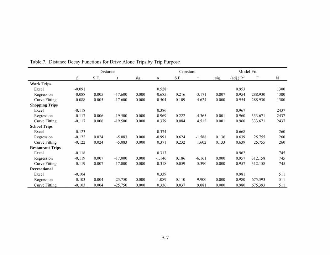
B-7

Table 7. Distance Decay Functions for Drive Alone Trips by Trip Purpose

Distance Constant Model Fit β S.E. t sig. α S.E. t sig. (adj.) R2 F N Work Trips Excel -0.091 0.528 0.953 1300 Regression -0.088 0.005 -17.600 0.000 -0.685 0.216 -3.171 0.007 0.954 288.930 1300 Curve Fitting -0.088 0.005 -17.600 0.000 0.504 0.109 4.624 0.000 0.954 288.930 1300 Shopping Trips Excel -0.118 0.386 0.967 2437 Regression -0.117 0.006 -19.500 0.000 -0.969 0.222 -4.365 0.001 0.960 333.671 2437 Curve Fitting -0.117 0.006 -19.500 0.000 0.379 0.084 4.512 0.001 0.960 333.671 2437 School Trips Excel -0.123 0.374 0.668 260 Regression -0.122 0.024 -5.083 0.000 -0.991 0.624 -1.588 0.136 0.639 25.755 260 Curve Fitting -0.122 0.024 -5.083 0.000 0.371 0.232 1.602 0.133 0.639 25.755 260 Restaurant Trips Excel -0.118 0.313 0.962 745 Regression -0.119 0.007 -17.000 0.000 -1.146 0.186 -6.161 0.000 0.957 312.158 745 Curve Fitting -0.119 0.007 -17.000 0.000 0.318 0.059 5.390 0.000 0.957 312.158 745 Recreational Trips Excel -0.104 0.339 0.981 511 Regression -0.103 0.004 -25.750 0.000 -1.089 0.110 -9.900 0.000 0.980 675.393 511 Curve Fitting -0.103 0.004 -25.750 0.000 0.336 0.037 9.081 0.000 0.980 675.393 511

B-8

Table 8. Distance Decay Functions for Shared Ride Trips by Trip Purpose

Distance Constant Model Fit β S.E. t sig. α S.E. t sig. (adj.) R2 F N Work Trips Excel -0.077 0.240 0.888 181 Regression -0.076 0.007 -10.857 0.000 -1.439 0.213 -6.756 0.000 0.884 107.508 181 Curve Fitting -0.076 0.007 -10.857 1.000 0.237 0.050 4.740 0.000 0.884 107.508 181 Shopping Trips Excel -0.129 0.376 0.964 959 Regression -0.130 0.007 -18.571 0.000 -0.965 0.202 -4.777 0.000 0.961 345.595 959 Curve Fitting -0.130 0.007 -18.571 0.000 0.381 0.077 4.948 0.000 0.961 345.595 959 School Trips Excel -0.096 0.159 0.588 176 Regression -0.096 0.022 -4.364 0.001 -1.833 0.380 -4.824 0.000 0.566 19.236 176 Curve Fitting -0.096 0.022 -4.364 1.001 0.160 0.061 2.623 0.021 0.566 19.236 176 Restaurant Trips Excel -0.140 0.426 0.870 500 Regression -0.140 0.015 -9.333 0.000 -0.853 0.416 -2.050 0.061 0.859 86.610 500 Curve Fitting -0.140 0.015 -9.333 1.000 0.426 0.177 2.407 0.032 0.859 86.610 500 Recreational Trips Excel -0.094 0.337 0.891 369 Regression -0.093 0.009 -10.333 0.000 -1.100 0.295 -3.729 0.003 0.883 106.367 369 Curve Fitting -0.093 0.009 -10.333 1.000 0.333 0.098 3.398 0.005 0.883 106.367 369

B-9

Table 9. Distance Decay Functions for Health Care Trips (no mode specified)

Distance (β) Constant (α) Shape (μ) Model Fit Coeff. S.E. t Coeff. S.E. t Coeff. S.E. t (adj.) R2 F N Health Care Excel -0.110 0.525 0.980 8,554 Regression -0.118 0.004 -29.256 -0.612 0.187 -3.275 0.978 855.913 8,554 Curve Fitting -0.118 0.004 -29.256 0.542 0.101 5.350 0.978 855.913 8,554 Combined -0.132 0.009 -14.636 -1.342 0.474 -2.833 0.374 0.225 1.663 0.980 471.291 8,554

B-10

 

Table 10. Distance Decay Functions for Walking Trips with Time Impedance

Travel Time (β) Constant (α) Shape (μ) Model Fit

Coeff. S.E. t Coeff. S.E. t Coeff. S.E. t (adj.) R2 F N

Work Trips

Excel -0.100 0.519 0.927 366

Regression -0.106 0.010 -10.853 -0.671 0.338 -1.983 0.914 117.782 366

Curve Fitting -0.106 0.010 -10.853 0.511 0.173 2.957 0.914 117.782 366

Combined -0.116 0.026 -4.480 -1.016 0.927 -1.096 0.202 0.502 0.403 0.906 54.037 366

Shopping Trips

Excel -0.090 0.370 0.724 269

Regression -0.094 0.018 -5.104 -0.999 0.635 -1.574 0.695 26.046 269

Curve Fitting -0.094 0.018 -5.104 0.368 0.234 1.576 0.695 26.046 269

Combined -0.063 0.048 -1.333 0.091 1.710 0.053 -0.638 0.926 -0.689 0.678 12.576 269

School Trips

Excel -0.100 0.523 0.600 105

Regression -0.106 0.031 -3.464 -0.645 0.880 -0.733 0.550 12.002 105

Curve Fitting -0.106 0.031 -3.464 0.524 0.461 1.136 0.550 12.002 105

Combined -0.231 0.069 -3.372 -4.114 1.907 -2.157 2.243 1.133 1.980 0.670 10.150 105

Restaurant

Excel -0.090 0.377 0.702 179

Regression -0.093 0.019 -4.804 -0.985 0.667 -1.477 0.667 23.076 179

Curve Fitting -0.093 0.019 -4.804 0.373 0.249 1.499 0.667 23.076 179

Combined -0.081 0.051 -1.588 -0.576 1.840 -0.313 -0.240 0.996 -0.241 0.633 10.480 179

Recreation

Excel -0.090 0.545 0.932 292

Regression -0.100 0.010 -10.264 -0.586 0.280 -2.096 0.921 105.352 292

Curve Fitting -0.100 0.010 -10.264 0.556 0.156 3.575 0.921 105.352 292

Combined -0.153 0.016 -9.261 -2.052 0.458 -4.478 0.947 0.272 3.481 0.967 131.933 292

B-11

Table 11. Distance Decay Functions for Bicycle Trips with Time Impedance

Travel Time (β) Constant (α) Shape (μ) Model Fit Coeff. S.E. t Coeff. S.E. t Coeff. S.E. t (adj.) R2 F N Work Trips Excel -0.030 0.146 0.378 109 Regression -0.040 0.014 -2.821 -1.922 0.609 -3.156 0.332 7.956 109 Curve Fitting -0.040 0.014 -2.821 0.146 0.089 1.642 0.332 7.956 109 Combined -0.088 0.032 -2.721 -4.317 1.574 -2.742 1.255 0.768 1.633 0.408 5.822 109 Shopping Trips Excel -0.100 0.432 0.697 64 Regression -0.107 0.022 -4.791 -0.836 0.776 -1.077 0.666 22.953 64 Curve Fitting -0.107 0.022 -4.791 0.434 0.336 1.288 0.666 22.953 64 Combined -0.182 0.053 -3.425 -3.542 1.912 -1.852 1.585 1.036 1.531 0.706 14.190 64 School Trips Excel -0.100 0.422 0.595 36 Regression -0.100 0.026 -3.845 -0.858 0.899 -0.954 0.556 14.785 36 Curve Fitting -0.100 0.026 -3.845 0.424 0.381 1.112 0.556 14.785 36 Combined -0.199 0.059 -3.370 -4.450 2.124 -2.095 2.104 1.150 1.829 0.640 10.799 36 Recreation Excel -0.07 0.294 0.589 131 Regression -0.071 0.019 -3.785 -1.226 0.645 -1.901 0.548 14.329 131 Curve Fitting -0.071 0.019 -3.785 0.293 0.189 1.551 0.548 14.329 131 Combined -0.105 0.048 -2.180 -2.465 1.727 -1.428 0.726 0.935 0.776 0.529 7.180 131

B-12

Table 12. Distance Decay Functions for Transit Trips with Time Impedance

Travel Time (β) Constant (α) Shape (μ) Model Fit Coeff. S.E. t Coeff. S.E. t Coeff. S.E. t (adj.) R2 F N Work Trips Excel -0.010 0.032 0.041 176 Regression -0.010 0.011 -0.908 -3.441 0.692 -4.974 0.008 0.825 176 Curve Fitting -0.010 0.011 -0.908 0.032 0.022 1.445 0.008 0.825 176 Combined -0.095 0.014 -6.702 -10.705 1.158 -9.244 3.210 0.482 6.659 0.682 23.475 176 Shopping Trips Excel 0.029 0.014 0.045 22 Regression 0.029 0.044 0.655 -4.252 1.402 -3.032 0.061 0.429 22 Curve Fitting 0.029 0.044 0.655 0.014 0.020 0.713 0.061 0.429 22 Combined -0.215 0.076 -2.826 -12.011 2.419 -4.966 4.760 1.368 3.480 0.525 6.535 22