ACCESS Numerical Weather Prediction resources for...

ACCESS Numerical Weather Prediction resources for the national research community

Michael NaughtonBureau of Meteorology R&D BranchEarth System Modelling Program Atmospheric Modelling Team

[email protected]

Reprising talk prepared by Gary Dietachmayerfor last week's Climate and Water Summer Institute

OzEWEX 3rd National WorkshopCanberra, 14-15 December 2016

mailto:[email protected]

Outline

• "ACCESS": the Australian Community Climate and Earth-System Simulator

– Focus here is on the NWP components of ACCESS

• Introduction to Numerical Weather Prediction (NWP)

• NWP at the BoM

• NWP and streamflow – WIRADA, Carlisle-flood examples

• Access to NWP data - NCI

Intro to NWP – towards an eqn set

• Many physical systems have prognostic equations that allow us to predict a future state from a past one.

– Driving to Canberra: dx/dt = v(x,t) – If v is constant (V) : x(new) = x(old) + V * time

• A significant component of atmospheric behaviour can be captured if we treat the atmosphere as an ideal gas.

– Three equations for momentum (u, v, w) - "Euler" / "Navier Stokes"– Conservation of mass– Conservation of energy– Equation of state relating thermodynamic variables

• In atmospheric modelling parlance, this is the "dynamics" of the model

Intro to NWP – the need for discretisation

• Dynamics eqns are a set of coupled, non-linear, partial-differential equations

– No general analytical solution

• Computers are dumb, but fast – can only do basic algebraic operations, but can do lots of them

• "Discretisation" is the process of replacing the original continuous equations by a set of algebraic ones whose solution is 'sufficiently close' to the original set.

• Chunk-up space into a regular array of small-volume "grid-cells" – analogous to pixels in an image

– Replace derivatives by differences.

• "Resolution" = width of a grid-cell

– Higher resolution is (mostly!) more accurate, but also more expensive

Intro to NWP – Discretisation via a lat/long grid

(Henderson-Sellers, 1985)

Intro to NWP – beyond N-S (moist processes!)

(Bauer et al, 2015)

Intro to NWP – need for parameterisation

(Arakawa &Schubert, 1974)

• Many important processes occur at scales of less than a grid-cell

• Can't simply ignore them

– Feed back onto the resolved scales– Often very impactful (eg., precip)

• Parameterise them – relate their average impact to variables on the model-grid scale

– E.g., if the model has ascent in an area of moist instability, assume convection will form, (latent) heating will occur, etc

• In modelling parlance, these parameterisedprocesses are referred to as "physics"

• "Dynamics" + "Physics" + Big-Computer = ability to project atmosphere forward in time

– but from what ……………………..

Intro to NWP – Data Assimilation (Intro)

The problem:

• The model state may consist of ~50 million grid points and 7 meteorological variables at each point - 350 million pieces of information …

• We may actually assimilate "only" 3 – 4 million individual observations

• We don't generally observe model variables (eg., grid-cell temperature versus top-of-cloud radiance)

• Obs coverage varies widely in time/space

• The observations aren't "truth"

Intro to NWP – Data Assimilation (Variational)

General idea is to minimise:

where

• xa is the "analysis" (model IC), xf is the short-term forecast ("background")

• y are the observations, H maps from observed to analysis (model) space

• B and R are forecast and observation error covariances

Lots of "tricks" applied here:

• Minimisation, with B term, resolves the insufficient data problem

– and effectively carries obs forward from previous times

• Use a descent method, based on grad-J

• Rescale/filter B term

Intro to NWP – Data Assimilation (the NWP cycle)

• OPS = Obs-processing

• VAR = DA step

• UM = model-forecast

• FG = First-Guess = Background

• Analysis is now a blend of model and observations

At this point we have established a good model to allow us to project forward in time, and a sound method to establish an initial-state to project forward from.

What could possibly be missing ………………….

Intro to NWP – Uncertainty and Ensembles

• The famous "butterfly effect" – even small differences in the initial-state can grow into significant differences in the forecast.

• Varies in space & time.

• Running an ensemble of FCs off perturbed initial-conditions, enables us to forecast forecast-accuracy (useful information!) or forecast probabilities

(K. Mylne, UKMO)

APS1 APS2

G 40 25

R 12 12

TC 12 12

C 4 1.5

Grid size (km)

70 vertical levels

• "APS" = Australian Parallel Suite

• "G2" = ACCESS-G, in APS2

• Darwin domain in C2

BoM NWP – Suite Configuration

Even with a Super-Computer, forecast timeliness demands a balance between: FC-length, model-domain, and resolution

BoM NWP – APS2 Increased Observations

• Aust-region• Winter• MSLP• Verif against

own analysis

• Comparable to UKMO

• G2 provides 6-8 hours more lead-time than G1

BoM NWP – APS2 ACCESS-G Verification

Caveats:

• In summer, G1, G2, UKMO are very similar.• Tropical performance of G2 is arguably worse but,

• Tropical analyses are not as reliable as mid-latitude• Australian surface-obs verif is very positive

• (Spring, G2 – G1 error, ie., negative is better, G2 much better at forecasting T-max)

BoM NWP – Performance of APS2 ACCESS-G

International Comparison: G1, G2, ECMWF, UKMO, US, JMA

BoM NWP – APS2 ACCESS-G Verification

BoM NWP – Global Ensemble, "GE2"

Currently running 12Z daily at 60 km, 70 levels (N216L70)

Scheduled for "limited" (mostly in terms of products) operational implementation in APS2.

24-member ensemble designed for medium-range forecasting

• Based on UKMO MOGREPS• Global ensemble to 10 days• Global ETKF for initial condition

perts• Stochastic model perturbations

ACCESS-G 40km (N320) – G2 25km (N512) ACCESS-GE 60km (N216)

ACCESS-R 12 km

ACCESS-CC1: 4km C2: 1.5km

BoM NWP – GE2 Verification

MSLP T850

Aust

NH

Trop

SH

ACCESS-GE-ControlE-MeanE-Spread

Ensemble mean skill better than deterministic ACCESS-G after first couple/few days

BoM NWP – GE2 Verification

ACCESS-GEECMWFJMANCEP

MSLP December 2014

SHEM TROP NHEM

BoM NWP – GE2 case-study ex-TC Oswald

This event followed the monsoon onset in mid-January. TC Oswald formed in the western part of Gulf of Carpentaria around 20 January. It existed briefly as TC until it made landfall and moved across the Cape York peninsula as a tropical low.

Ex-TC Oswald then progressed over the following week down the Queensland coast and through to the northern NSW as far as the Sydney region, before moving off to the east on 29 January.

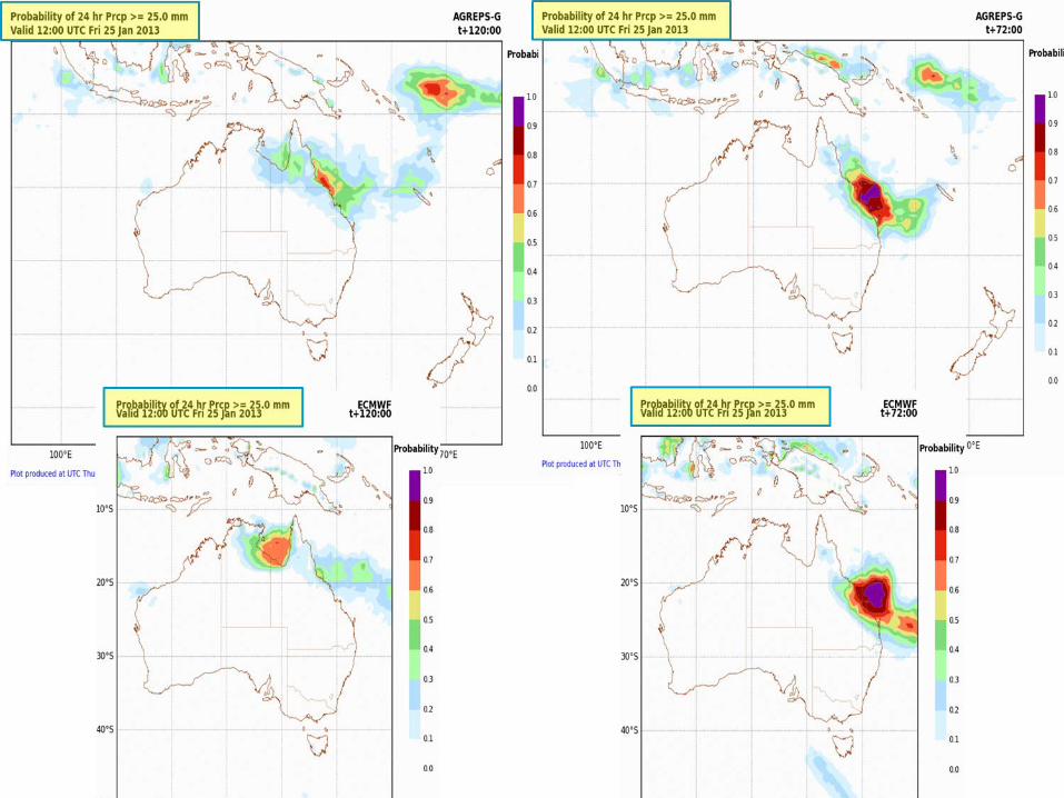
BoM NWP – GE2 case-study ex-TC Oswald

BoM NWP – GE2 application example

Volcanic ash dispersion• HYSPLIT dispersion model run from 24

ACCESS-GE ensemble members

Individual member 24-hour forecasts of ash concentrationin the 10-15 km layer.

Single control member Ensemble probability

Courtesy Richard Dare

BoM NWP – C2 (City) Upgrade Intro

• Inclusion of Darwin domain

• Upgraded components (UM, etc)

• Large increase in resolution (4.0km -> 1.5km), allows us to drop the grid-cell-bound convection-parameterisation – model now runs in "convection-permitting" mode

• Like C1, remains a down-scaler only – no DA of its own

(Focussing on 00Z run to capture initiation)

C2 – leftC1 – rightLight-rain: topHeavy-rain: bottom

BoM NWP – C2 Darwin Precip Stats


BoM NWP – C2 Brisbane Precip Stats


BoM NWP – C2 VicTas Precip Stats

C1-total

C2-total

Obs

BoM NWP – C1 rain "coastal locking"

(Jul-25, 2015: 24 hrc FC)

BoM NWP – Extreme rain event: Darwin, Nov-4 2013

12-hr

Start:7:00pm


The Centre for Australian Weather and Climate ResearchA partnership between CSIRO and the Bureau of Meteorology

24 Hr accum

C1

C2


33-hr

Start:1:30 pm

C2

C1

Melbourne Radar

01 Z 03 Z

03.5 Z 06 Z• 01 Z – Geelong region quiet

• 03 Z – Convection along coastline to SW of Geelong

• 03.5 Z – Consolidation, approaching Geelong

• 06 Z – Subsequent propagation to NE

BoM NWP – Geelong Storm, Jan-27 2016

07 Z / C2

07 Z / C1

06 Z / C2

Delayed timing – but this is forecast-only, no DA

ACCESS-C

Geelong Storm,Jan-27 2016

Operational ("C1", 4.5km, param), against APS2 ("C2", 1.5km, conv-perm)

BoM NWP – Geelong Storm, Jan-27 2016

06 Z / C1

DRAFT ONLY

• Need to constantly upgrade NWP to remain world-competitive

• Improved DA ("hybrid-VAR") for APS3+ - requires ensembles

• C3 includes RUC with radar-DA (ala SREP)

• City-ensembles (CE3) in APS3

• Flexible domain, "on-demand" systems – X and XE

BoM NWP – Timelines and Future

NWP & Streamflow – large-scale

The horizontal resolutions of NWP models are too coarse to resolve the small scale catchment variability

The post-processing is able to reproduce the spatial variation in mean rainfall

Rainfall total for period 12 h to 216 h

David Robertson – CSIRO/WIRADA

NWP & Streamflow – Direct/High-res NWP

Carlisle Flood, 2005Roberts et al UKMO, 2009

Gauge 12km

4km 1km

24-hour rain accumulations

• PDM riverflow FCs for a range of precip-sources

• dashed line – flood warning level

• 1km (red), 4km (blue), 12km (green)

• nowcasting (purple) , rain-gauge (orange)

• observed flow (black)

• note termination of precip sources

Access to BoM NWP data - NCI

• Bureau has a strong commitment to computing at the National Computational Infrastructure (NCI) in Canberra

– New NWP (and other) model systems are prototyped at NCI– Part of the "C for community" in "ACCESS"

• Provision of supported-experiments• ACCESS training courses and training materials• Supported by NeCTAR CWSLab funding

• Also contributes operational and near-operational NWP data to NCI, as a "nationally significant" dataset, in the RDS archive facility.

• Format of NWP data is steadily improving – from opaque grib to reasonably self-describing netCDF, and OPeNDAP is the goal in the future.

• Currently (Dec-2016) in the process of restructuring the data across multiple NCI projects.


http://nci.org.au/data-collections


• "lb4" is an NCI project

• Head to https://my.nci.org.au and log-on to make a request to be added to that project.

https://my.nci.org.au/


Operational, APS2, ACCESS-G model output, for a FC starting at 12Z on Dec-4, 2016. Surface ("sfc") fields shown.

netCDF files, one file per model variable, all forecast-times in the one file

float accum_prcp(time, lat, lon)

Summary

• NWP is built upon:

– Discretisation– Parameterisation– Data Assimilation– Uncertainty and Ensembles– All the above requiring very large obs/data, and very large computing

• BoM runs a suite of NWP systems covering a range of time/length-scales

– BoM systems are generally world-competitive– Underpin much of the Bureau's weather forecasting capability– Systems are continually improved, with convection-permitting and global-ensemble

systems imminent

• NWP feeds many downstream systems, including hydrological ones

– But care must be taken to mitigate NWP limitations too

• NCI is the first port of call for external users interested in BoM NWP data

Michael [email protected]

Thank you…

ACCESS Numerical Weather Prediction resources for...

Documents

Transcript of ACCESS Numerical Weather Prediction resources for...