Acceleration mechanisms: basic concepts

Erik Adli, University of Oslo, August 2016, Erik.Adli@cern.ch , v2.21

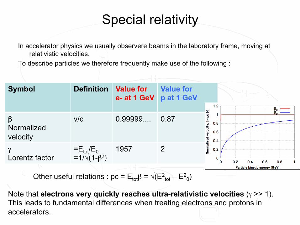
Special relativity

In accelerator physics we usually observere beams in the laboratory frame, moving at relativistic velocities.

To describe particles we therefore frequently make use of the following :

Symbol Definition Value for e- at 1 GeV

Value for p at 1 GeV

βNormalized velocity

v/c 0.99999.... 0.87

γ Lorentz factor

=Etot/E0 =1/√(1-β2)

1957 2

Note that electrons very quickly reaches ultra-relativistic velocities (γ >> 1). This leads to fundamental differences when treating electrons and protons in accelerators.

Other useful relations : pc = Etotβ = √(E2tot – E2

0)

Accelerators: circular and linear

•  FB ⊥ v : only FE does work and provides energy gain •  FE or FB for deflection? When v ≈ c , 1 T ~ 3⋅108 V/m. FB preferred

for high velocity particles.

BE FFBvqEqBvEqF!!!!!!!!!

+=×+=×+= )(

Purpose of particle accelerators: steer, shape and modulate energy of charged particle beams. Dynamics of motion governed by the Lorentz force equation :

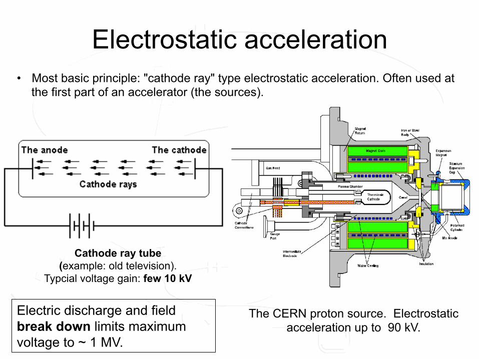
Electrostatic acceleration •  Most basic principle: "cathode ray" type electrostatic acceleration. Often used at

the first part of an accelerator (the sources).

The CERN proton source. Electrostatic acceleration up to 90 kV.

Cathode ray tube (example: old television).

Typcial voltage gain: few 10 kV

Electric discharge and field break down limits maximum voltage to ~ 1 MV.

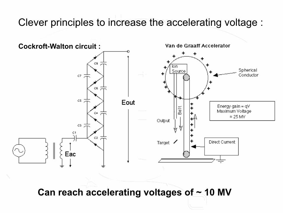
Clever principles to increase the accelerating voltage :

Cockroft-Walton circuit :

Can reach accelerating voltages of ~ 10 MV

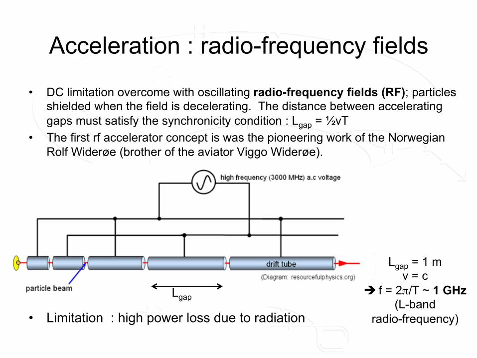
•  DC limitation overcome with oscillating radio-frequency fields (RF); particles shielded when the field is decelerating. The distance between accelerating gaps must satisfy the synchronicity condition : Lgap = ½vT

•  The first rf accelerator concept is was the pioneering work of the Norwegian Rolf Widerøe (brother of the aviator Viggo Widerøe).

•  Limitation : high power loss due to radiation

Acceleration : radio-frequency fields

Lgap = 1 m v = c

è f = 2π/T ~ 1 GHz (L-band

radio-frequency)

Lgap

Drift-tube linac (Alvarez structure)

The Alvarez structure (CERN linac)

Standing EM-wave (TM010-like mode) fills cavity The RF fields, with wavelengths on the order structure length, cannot enter small holes in drift tubes (shielding) Drift tubes are made of increasing length, adjusted to varying β : used for heavy particles where energy gain yields significant velocity gain up to several GeV.

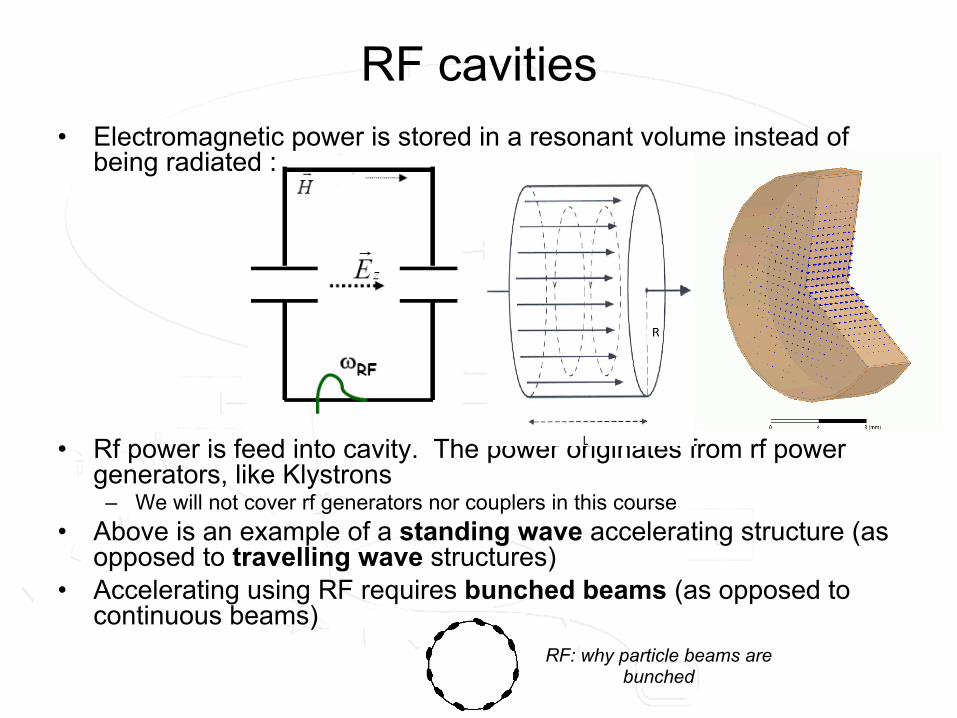
•  Electromagnetic power is stored in a resonant volume instead of being radiated :

•  Rf power is feed into cavity. The power originates from rf power generators, like Klystrons

–  We will not cover rf generators nor couplers in this course •  Above is an example of a standing wave accelerating structure (as

opposed to travelling wave structures) •  Accelerating using RF requires bunched beams (as opposed to

continuous beams)

RF cavities

RF: why particle beams are bunched

RF field break down High gradient limits : field levels of 10-100 MV/m.

From the PhD-thesis of Kyrre Sjøbæk.

Electrons in surface are emitted (field emission), vacuum arcs may form and the field breaks down. Eventually the break down processes may damage the structure.

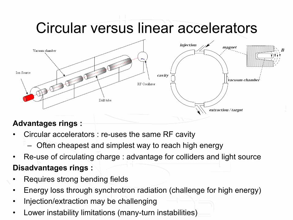
Circular versus linear accelerators

Advantages rings : •  Circular accelerators : re-uses the same RF cavity

–  Often cheapest and simplest way to reach high energy •  Re-use of circulating charge : advantage for colliders and light source Disadvantages rings : •  Requires strong bending fields •  Energy loss through synchrotron radiation (challenge for high energy) •  Injection/extraction may be challenging •  Lower instability limitations (many-turn instabilities)

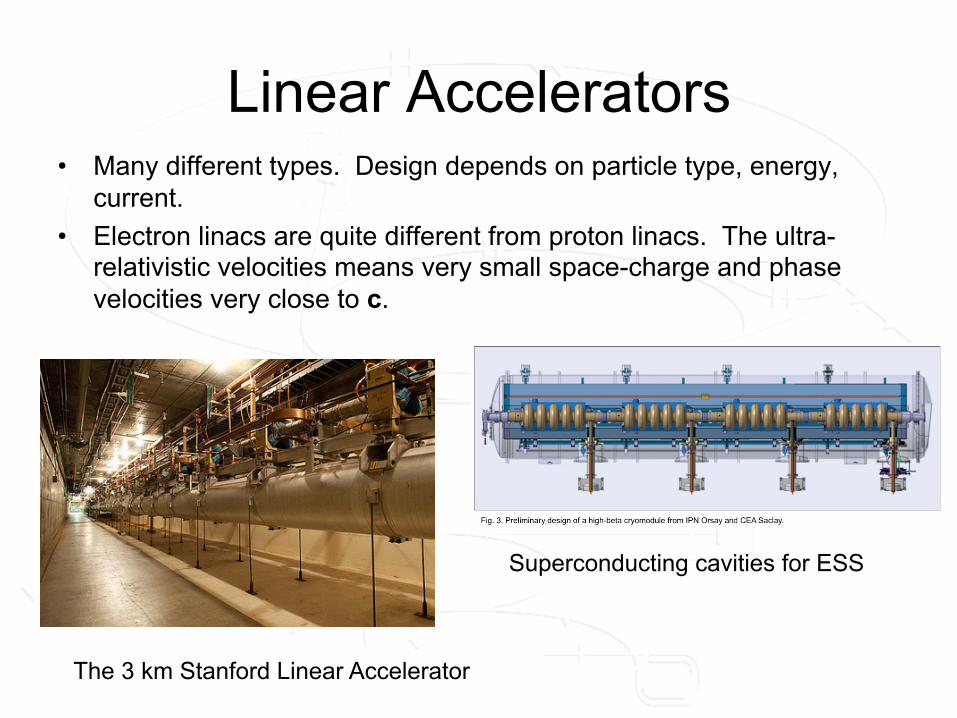
Linear Accelerators •  Many different types. Design depends on particle type, energy,

current. •  Electron linacs are quite different from proton linacs. The ultra-

relativistic velocities means very small space-charge and phase velocities very close to c.

The 3 km Stanford Linear Accelerator

Superconducting cavities for ESS

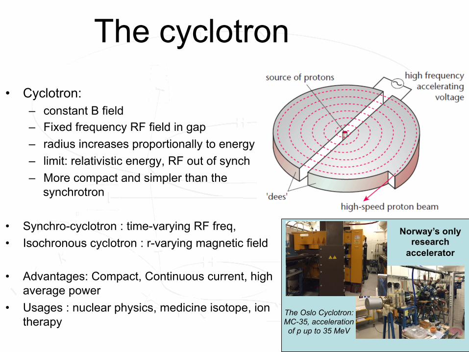
The cyclotron

•  Cyclotron: –  constant B field –  Fixed frequency RF field in gap –  radius increases proportionally to energy –  limit: relativistic energy, RF out of synch –  More compact and simpler than the

synchrotron

•  Synchro-cyclotron : time-varying RF freq, •  Isochronous cyclotron : r-varying magnetic field •  Advantages: Compact, Continuous current, high

average power •  Usages : nuclear physics, medicine isotope, ion

therapy

The Oslo Cyclotron: MC-35, acceleration of p up to 35 MeV

Norway’s only research

accelerator

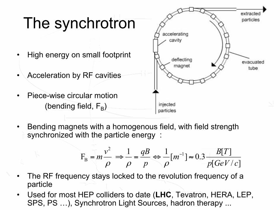
The synchrotron

•  High energy on small footprint

•  Acceleration by RF cavities

•  Piece-wise circular motion (bending field, FB)

•  Bending magnets with a homogenous field, with field strength synchronized with the particle energy :

•  The RF frequency stays locked to the revolution frequency of a particle

•  Used for most HEP colliders to date (LHC, Tevatron, HERA, LEP, SPS, PS …), Synchrotron Light Sources, hadron therapy ...

]/[][3.0][11 F 1

2

B cGeVpTBm

pqBvm ≈⇔=⇒= −

ρρρ

Accelerating cavities

The Maxwell Equations

Free space wave solution

n

Ei

No dispersion means that wave components of all frequencies propagate at speed of light; the shape of wave is preserved as it propagates.

Animation by E. Jensen

Pill-box cavity design Assume solution that have form with only Ez and Bθ components, and : Maxwell can then be written :

Resulting wave equation :

Length scales: R = 0.1 m

è f = ω/2π ~ 1 GHz (L-band radio-frequency)

Can be solved with boundary condition Ez(R) = 0

(Exercise set 1) Wille Ch. 5.2.

Pill-box cavity TM solution

•  RF power is oscillating (from the magnetic field to the electric field), at the mode frequency ω :

•  Ez is constant in space along the axis of acceleration, z, at any instant in time.

•  Solution for the fundamental transverse magnetic mode is :

The fundamental mode is named “TM01”

Electric field Magnetic field

Animation by Rolf Wegner

Pillbox cavity: field simulation

The E-field of the TM01-mode of a pill-box cavity, calculated by an eigenmode solver. Electromagnetic codes: allows for solving of arbitrary geometries. Prototyping and optimization of cavities. Examples, HFSS, CST Microwave studio, ACE3P.

Note how the electric and the magnetic field are 90 deg out of phase.

Simple models allows us to build and intuitive understanding of the fields and how they behave. Modes often bear resemblance to pill-box modes and same name conventions are often used. Real rf structure geometries : fields from numerical simulation.

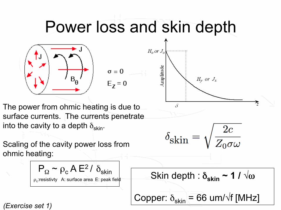
Power loss and skin depth

The power from ohmic heating is due to surface currents. The currents penetrate into the cavity to a depth δskin. Scaling of the cavity power loss from ohmic heating:

Skin depth : δskin ~ 1 / √ω Copper: δskin = 66 um/√f [MHz]

PΩ ~ ρc A E2 / δskin A: surface area ρc:resistivty E: peak field

(Exercise set 1)

Cavity losses and metrics

Due to finite conductivity and to radiation through cavity openings (e.g. for beam), the cavity energy U [J] will be lost over time, if not replenished. Power loss rate : P [W]. This can be written as :

where the cavity quality factor is Q = ωU / P : energy decay time in # of RF cycles. Typical Q for copper: 103 – 104. Q for superconducting cavities : 108 – 1010. Another key parameters is how much voltage gain do we get per power lost, defining the cavity shunt resistance Rs [Ω] = V2 / P. High Rs is favorable. A much used metric to define cavity design independent of material, depending only on cavity shape is Rs/Q [Ω] = V2 / ωU.

U(t) = U0exp(-tω/Q)

Time Transit Factor Fields change while the beam flies through the cavity. The beam not seeing

the peak electric field all the way through gives the transit time factor.

Electric field ti

zeEtE ω−=)(

Bunch tz c=

Electric field

T =VaccEz dz∫

=E(z)dz∫Ez dz∫

czt =

Definition of transit time

factor

zci

zeEzEω

−=)(

time evolving field

Field full and frozen

beam

Time Transit Factor

phase rotates by full 360° during time beam takes to

cross cavity

For example: L = λ / 2 gives T=0.64

T = sin (ωL/2c) / (ωL/2c)

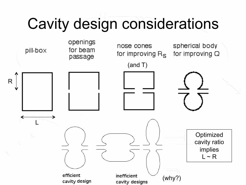
Cavity design considerations

(why?)

(and T)

Optimized cavity ratio

implies L ~ R

L

R

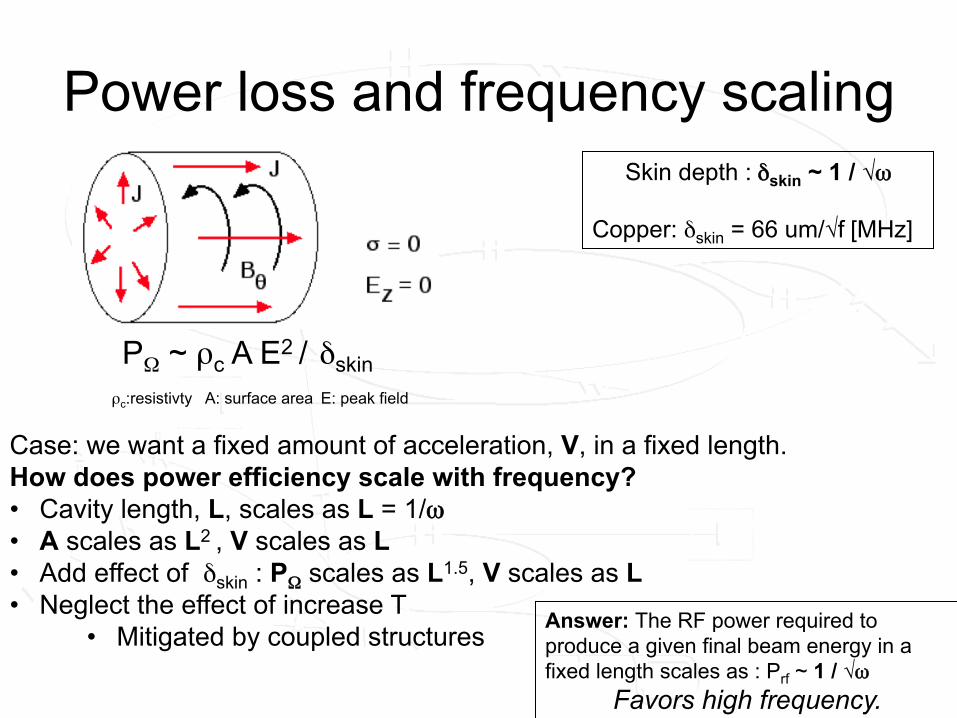
Power loss and frequency scaling Skin depth : δskin ~ 1 / √ω

Copper: δskin = 66 um/√f [MHz]

PΩ ~ ρc A E2 / δskin A: surface area ρc:resistivty E: peak field

Case: we want a fixed amount of acceleration, V, in a fixed length. How does power efficiency scale with frequency? •  Cavity length, L, scales as L = 1/ω •  A scales as L2 , V scales as L •  Add effect of δskin : PΩ scales as L1.5, V scales as L •  Neglect the effect of increase T

•  Mitigated by coupled structures

Answer: The RF power required to produce a given final beam energy in a fixed length scales as : Prf ~ 1 / √ω

Favors high frequency.

Cavity main metric

The main properties of an accelerating cavity are typically given by : •  ω : frequency•  Q : quality factor •  Rs/Q : “R over Q”, geometric factor representing the cavity design

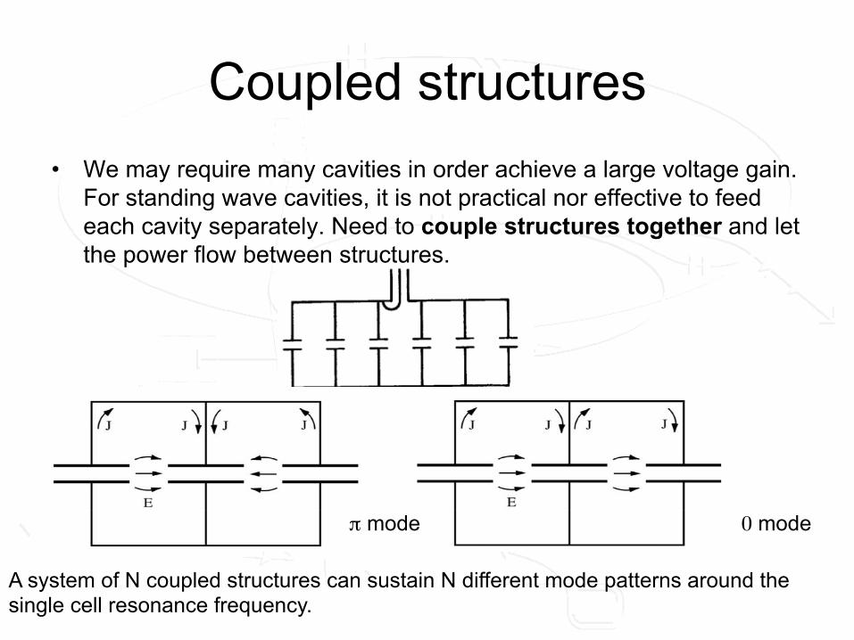
Coupled structures •  We may require many cavities in order achieve a large voltage gain.

For standing wave cavities, it is not practical nor effective to feed each cavity separately. Need to couple structures together and let the power flow between structures.

A system of N coupled structures can sustain N different mode patterns around the single cell resonance frequency.

π mode 0 mode

Travelling wave structures

Travelling wave structure

Power flow

electric field

magnetic field

power flow

power flow Rf fields at frequences higher than the cut-off ωc = cπ/a can propagate through wave guides, with phase velocity vp > c. Typical dimensions: ~1-100 cm. Cannot be used for acceleration, must slow down phase velocity to match particle velocities.

a

EM waves can propagate in wave guides, of different sizes and shapes.

Wille Ch. 5.1.

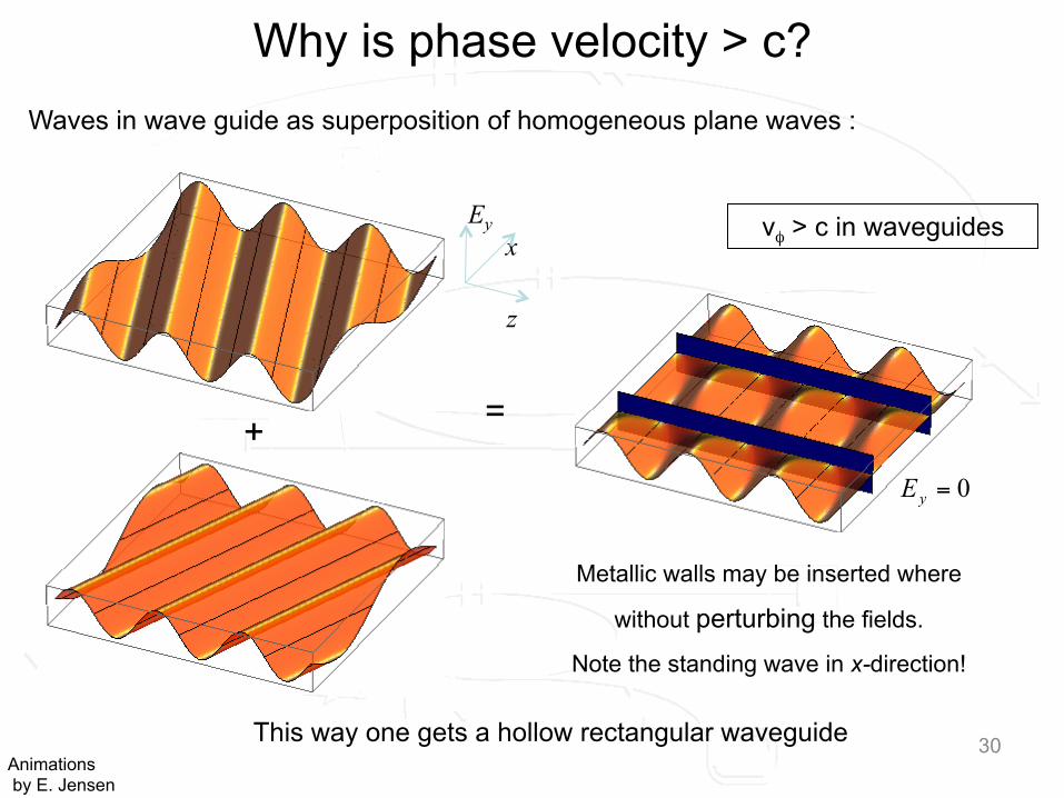
Why is phase velocity > c?

+ =

Metallic walls may be inserted where

without perturbing the fields.

Note the standing wave in x-direction!

z

x Ey

This way one gets a hollow rectangular waveguide

0=yE

30

vφ > c in waveguides

Waves in wave guide as superposition of homogeneous plane waves :

0=yE

Animations by E. Jensen

31

0 100 200 300 4000

5 109×

1 1010×

1.5 1010×

2 1010×

wavenumber k [1/m]

freq

uenc

y [H

z]

=k

201 ⎟⎠

⎞⎜⎝

⎛−=ωωω

ck

ck ω=

vφ = ω / k = c/√(1-(ωc /ω)2) > c

Wave guide: dispersion curve

vp = c

vp > c

Wille Ch. 5.1.

Electron linear accelerators Electron linear accelerators: vparticle = c. Travelling wave coupled structures can be

seen as a waveguide (vp > c) “disc-loaded” with irises to reduces the phase velocity of a mode to vp =c.

Often explained as particles surfing the electromagnetic waves.

The main linac of the Compact Linear Collider: 70% travelling wave structures

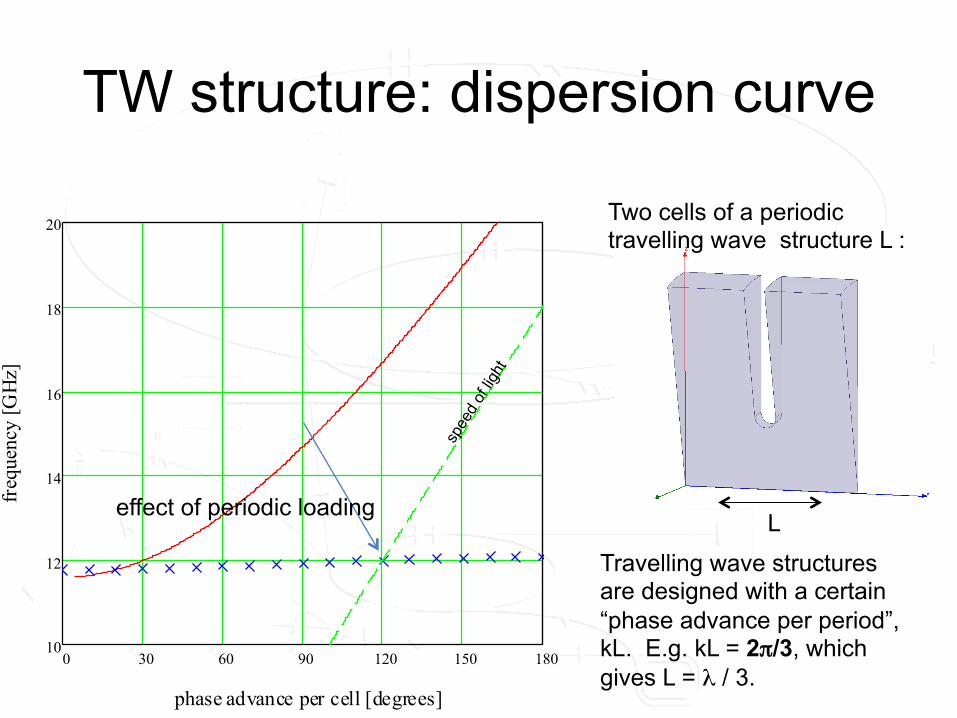
TW structure: dispersion curve

0 30 60 90 120 150 18010

12

14

16

18

20

phase advance per cell [degrees]

freq

uenc

y [G

Hz]

effect of periodic loading

Two cells of a periodic travelling wave structure L :

L

Travelling wave structures are designed with a certain “phase advance per period”, kL. E.g. kL = 2π/3, which gives L = λ / 3.

Traveling wave structure: field simulation

beam propagation direction

Animation by Rolf Wegner 2π/3 structure

Optimal beam phasing

Animation from Kyrre Sjøbæk, showing optimal phasing of a beam (red) in a periodic loaded structure.

CLIC travelling wave structure Total length ~ 22 cm.

Cell length = 8.3 mm.

Damping wave guides: required due to wake fields (treated in part about collective effects)

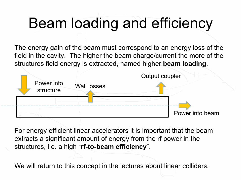
Beam loading and efficiency The energy gain of the beam must correspond to an energy loss of the field in the cavity. The higher the beam charge/current the more of the structures field energy is extracted, named higher beam loading. For energy efficient linear accelerators it is important that the beam extracts a significant amount of energy from the rf power in the structures, i.e. a high “rf-to-beam efficiency”. We will return to this concept in the lectures about linear colliders.

Wall losses

Output coupler Power into structure

Power into beam

?

Longitudinal dynamics

Longitudinal Dynamics: degrees of freedom tangential to the reference trajectory us: tangential to the reference trajectory, co-moving with the beam

Phase stability

•  RF phase observed by a particle in a cavity : φ = ωrf t = ωrf z/v. Energy gain per turn:

•  Linac : designed and tuned to accelerate a synchronous particle, with nominal momentum, at the same phase in each accelerating gap, φs

•  Other particles move in longitudinal phase space : –  z-position differs -> RF phase differs -> different voltage experienced –  momentum differs -> relative velocity differs

•  If φs is at the rising slope of cavity voltage, particles arriving late (back of beam) will see a larger voltage gain and v.v. This leads to longitudinal phase stability.

•  NB: ultra-relativistic particles in linacs : negligible Δvelocity / Δenergy –  -> frozen charge profile, ψ(z). Example: linear collider electron/positron linacs

s

φs t

Longitudinal phase-space Linac

Cavity voltage seen by a particle.

Beam from any source has a spread in the phase-space

ΔΕ = q Vmax sinφ

Wille Ch. 5.6.

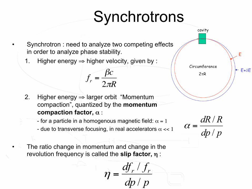
Synchrotrons •  Synchrotron : need to analyze two competing effects

in order to analyze phase stability. 1.  Higher energy ⇒ higher velocity, given by :

2.  Higher energy ⇒ larger orbit “Momentum compaction”, quantized by the momentum compaction factor, α :

- for a particle in a homogenous magnetic field: α = 1

- due to transverse focusing, in real accelerators α << 1

•  The ratio change in momentum and change in the revolution frequency is called the slip factor, η :

€

fr =βc2πR

pdpfdf rr

//

=η

pdpRdR//

=α

Calculating the slip factor

•  Logarithmic differentiation gives:

•  For a momentum increase dp/p: –  η>0: velocity increase dominates ( fr increases ) –  η<0: circumference increase dominates ( fr decreases ) €

dfrfr

=dββ−dRR

dpp

=dββ(1+

β 2

1−β 2) =

dββγ 2

⇒η =dfr / f rdp / p

=1γ 2−α

Phase stability in a synchrotron •  η>0: velocity increase dominates, fr increases

•  Synchronous particle stable for 0º<φs<90º –  A particle N1 arriving early with φ= φs-Δφ will get a lower energy kick, and arrive

relatively later next pass –  A particle M1 arriving late with φ= φs+Δφ will get a higher energy kick, and arrive

relatively earlier next pass •  η<0: stability for 90º<φs<180º •  η=0 at the transition energy. When the synchrotron reaches this

energy, the RF phase needs to be switched rapidly from φs to 180-φs

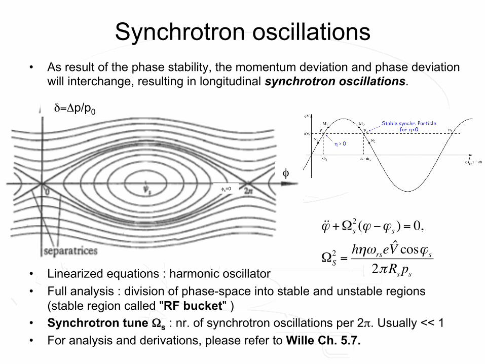
Synchrotron oscillations •  As result of the phase stability, the momentum deviation and phase deviation

will interchange, resulting in longitudinal synchrotron oscillations.

•  Linearized equations : harmonic oscillator •  Full analysis : division of phase-space into stable and unstable regions

(stable region called "RF bucket" ) •  Synchrotron tune Ωs : nr. of synchrotron oscillations per 2π. Usually << 1•  For analysis and derivations, please refer to Wille Ch. 5.7.

!!ϕ +Ωs2 (ϕ −ϕs ) = 0,

ΩS2 =

hηωrseV̂ cosϕs

2πRsps

φ

δ=Δp/p0

φs=0

Synchrotron: energy ramping

•  In a synchrotron, the synchronous particle energy is increasing synchronously with the bending magnet field strength, B :

•  or in momentum gain per turn :

•  Using the relation energy and momentum, we get energy gain per turn :

•  Thus, for a given dB/dt profile the synchronous phase is calculated as :

p’ = q ρ Β’

Δp / turn = 2πR/v q ρ Β’

ΔΕ = Δp v = 2πR q ρ Β’= q Vmax sinφs

sinφs= 2πR ρ Β’ / Vmax We distinguish: ρ : magnet bending radius 2πR : total circumference

Summary: longitudinal dynamics for a synchrotron

–  Particles arrive at a certain time and therefore a certain RF phase of the acceleration

–  To accelerate ramp up the magnetic field, and with automatic RF frequency modulation the synchronous particle will stay on the reference orbit

–  Due to the phase-stability, the particles in the phase-space vicinity of the synchronous particle will be captured by the RF and will also be accelerated at the same rate, undergoing synchrotron oscillations

φ

δ=Δp/p

φs=0

?

Acknowledgements

•  Pictures and animations taken from a large number of sources, including Walter Wuensch’ lectures on linear collider rf, Erk Jensen, Rolf Wegner’s and Kyrre Sjøbæk’s animations + Alex Chao’s USPAS lecture notes.