ACADEMIC PRESS INC. (LONDON) LTD Theory and Practice...
73
Theory and Practice of Scanning Optical Microscopy TONY WILSON Department of Engineering Science, University of Oxford with contributions from COLIN SHEPPARD Department uI Engineering Science, University uf Oxfurd 1984 ACADEMIC PRESS (Harcourt Brace Jovanovich, Publishers) London Orlando San Diego San Francisco New York Toronto Montreal Sydney Tokyo Sao Paulo ACADEMIC PRESS INC. (LONDON) LTD 24/28 Oval Road, London NWI United States Editiun published by ACADEMIC PRESS INC. (Harcourt Brace Jovanovich, Inc.) Orlando, Florida 32887 Copyright © 1984 by ACADEMIC PRESS INC. (LONDON) LTD All Rights Reserved No part of this book may be reproduced in any form by photostat, microfilm, or any other means, without written permission from the publishers British Library Cataloguing in Publication Data Wilson, T. Theory and practice of scanning optical microscopy. 1. Microscope and microscopy 1. Title II. Sheppard, C. J. R. 502'.8'2 QH205.2 ISBN 0-12-757760-2 LCCCN 83-73235 Filmset by Eta Services (Typesetters) Ltd, Beccles, Suffolk and printed in Great Britain by Thomson Litho Ltd., East Kilbride, Scotland
Transcript of ACADEMIC PRESS INC. (LONDON) LTD Theory and Practice...
Theory and Practiceof Scanning Optical
Microscopy
TONY WILSON
Department of Engineering Science, University of Oxford
with contributions from
COLIN SHEPPARD
Department uI Engineering Science, University uf Oxfurd
1984
ACADEMIC PRESS
(Harcourt Brace Jovanovich, Publishers)
London Orlando San Diego San Francisco New YorkToronto Montreal Sydney Tokyo Sao Paulo
ACADEMIC PRESS INC. (LONDON) LTD24/28 Oval Road,
London NWI
United States Editiun published byACADEMIC PRESS INC.
(Harcourt Brace Jovanovich, Inc.)Orlando, Florida 32887
Copyright © 1984 byACADEMIC PRESS INC. (LONDON) LTD
All Rights Reserved
No part of this book may be reproduced in any form by photostat, microfilm, or anyother means, without written permission from the publishers
British Library Cataloguing in Publication Data
Wilson, T.Theory and practice of scanning optical microscopy.1. Microscope and microscopy1. Title II. Sheppard, C. J. R.502'.8'2 QH205.2
ISBN 0-12-757760-2LCCCN 83-73235
Filmset by Eta Services (Typesetters) Ltd, Beccles, Suffolkand printed in Great Britain by
Thomson Litho Ltd., East Kilbride, Scotland


THEORY OF IMAGING 13
Chapter 2
Introduction to the Theory ofFourier Imaging
In order to appreciate the fundamental limitations of the resolution andimage formation properties of optical microscopes, it is necessary to begin bydiscussing the foundations of diffraction theory. We shall then carryon todiscuss the most important component of an optical imaging system-thelens-and finally combine our findings in a consideration of the role ofFourier analysis in the theory of coherent and incoherent image formation.
2.1 Kirchhoff diffraction and the Fresnel approximation
We take as our starting point the Kirchhoff diffraction formula, which is themathematical interpretation of Huygens' principle. For paraxial optics theelectromagnetic field may be expressed as a scalar field amplitude. If we areconcerned only with radiation of angular frequency w this may be written as
1J = Re {U eicot}, (2.1)
where U is the complex amplitude and Re { } denotes the real part.Kirchhoff's diffraction formula [2.1] gives the amplitude in the plane X2, Y2in terms of the distribution in the plane XI' YI (Fig. 2.1) as
+00
U2(X2,Yl) = JJj;RUI(Xl,YtleXp(-jkR)dXldYI, (2.2)
-00
where k is the wavenumber, given by k = 2rr./A, and Ais the wavelength. Thisexpression assumes that U I is slowly varying compared to the wavelength,and that both U I and U 2 are only appreciable in a region around the opticaxis which is small compared to the axial distance z. According to Huygens'
12
principle each element of the wavefront U 1 may be considered to give rise to aspherical wave with strength Proportional to U l' The double integral thenrepresents a summation over all elements of the wavefront.
Z
FIG. 2.1. Diffraction geometry.
If we impose a more rigid condition on the maximum values of Xl' YI andX2, Y2' we may replace the distance R in the denominator by z and expandthe R in the exponent by the binomial theorem to give the Fresnelapproximation
+00
It should be noted that the assumption that U 1 is slowly varying is necessaryfor paraxial optics, as a quickly varying amplitude will result in diffractionthrough large angles.
2.2 The Fraunhofer approximation
If z is large compared to the maximum of XI and Yl, the Fresnelapproximation to the diffraction integral may be used. However, if the morestringent condition that
z » tk(xf + yflmax (2.4)
is also. satisfied, we may make the further approximation of neglecting thett~rms mvolvmg xf and yf, to give the Fraunhofer approximation
exp (- jkz) jkU2(X2'Y2) = 'A exp --
2(x~+yD
J z z+00

14 THEORY AND PRACTICE OF SCANNING OPTICAL VlICROSCOPY THEORY OF IMAGING 15
The condition (2.4) may be written in terms of the Fresnel number N defined
as
so that if N « 1 the Fraunhofer form of the diffraction integral may be used.We now introduce the two-dimensional Fourier transform Oem, n) of
V (x, y) which we define as
N = n(xi + Yi)nm/AZ, (2.6)
after the aperture is simply the product of the illuminating amplitude and thetransmission of the aperture. This amounts to saying that the presence of theaperture does not affect the distribution in amplitude before the aperture,which corresponds to the Kirchhoff boundary conditions. Thus if arectangular aperture is illuminated with a uniform plane wave, the amplitudeV 1 is given by a rect function. The diffracted amplitude V z for a rectangularaperture of dimensions a and b may thus be written
(2.15)
(2.16)
(2.13)
(2.14)
r<l}r> 1,
circ (r) = 1,
= 0,
'"O(p) = f V (r)Jo(2rrpr)2rrr dr,
o
1(e "') _(ab)Z . .z (a sin e). z(b sin <P)z ,'I' - -;- smc -,- smc -.-'I.Z .Ie I.
the diffracted amplitude is given by
V () (jkd)_ exp(-jkz) 1[2J1 (2rrr l a//.z)]
1 rl exp - - rra .2z jAZ 2rrrla/;z
Here we have made use of the integral
where Jn is a Bessel function of the first kind of order n. If the originalamplitude is that of an evenly illuminated circular aperture radius a, writtenas circ (rda), where the circ function is defined
2.2.2 The circular aperture
If a function of two coordinates x, y is radially symmetric such that it is afunction of r only then its two-dimensional Fourier transform is also radiallysymmetric and may be written as a Fourier-Bessel (or Hankel) transform
Vz(x2,Yz)expjk (x~ + yn = exp ~ -jkz) ab sine (a:,z) sine (bYz).~ ~ ~ b
(2.12)
Defining the angles e, <p as sin -1 (xz/z), sin -1 (Yz/z), we may write for thediffracted intensity, which is merely the modules squared of the diffractedamplitude,
(2.8)
(2.7)
(2.11 )
(2.10)
. " sin (rr~)smc<,;=---·
rr~
+w
o(m, n) = JJVex, y) exp 2nj(mx + ny) dx dy;
+ ,x'
V(x, y) = JJOem, n) exp -2nj(mx + ny) dm dn.
-w
2.2.1 The rectangular aperture
We define the rectangular function rect (x) by [2.1J
rect x = 1, Ixl < ±}= o. Ixl >!
The Fourier transform of rect (x/a) is a sine (am), the sinc function beingdefined as
Then we can write (2.5) in the form
jk z z exp(-jkz) - .V 2 (x l ,Yz)exp-2 (Xl + Yl) = 'A V 1(Xl/I.Z,Yl/AZ), (2.9)
z J Z
The exponential term on the left-hand side of equation (2.9) shows that aFourier transform relationship between the original and diffracted field issatisfied on a spherical surface (to the paraxial approximation) centred on the
axial point of the Xl' Yl plane.We shall now give three examples of Fraunhofer diffraction which we shall
find important later.
the inverse relationship is
If an aperture in an opaque screen is illuminated with a plane wave, then,providing the dimensions of the aperture are large compared to thewavelength (as they must be for our paraxial approximation), the amplitude
1
JJ (2 )2 d - J1(2rrp) [2J 1 (2n p)]o rrpr rrr r - --- = rr .p 2rrp
o
(2.17)

16 THEORY AND PRACTICE 01 SCANNING OPTICAL MICROSCOPYTHEORY OF IMAGING 17
2.2.3 The annular aperture
For an evenly illuminated annular aperture, outer and inner radii a and yarespectively, the amplitude is given by (using 2.16)
(jkd ) exp(-jkz) 1
U (r ) exp - = --.-. -- - na1 2z J~z
x fl2J d2nrl~/AZ)j-l rYj (2nr lY;/i.Z)j}. (2.19)2nrla/J.z L 2nrlyaj AZ
In the limiting case of a thin annulus given by (1 - y) = s, with s small, the
amplitude is
The exponential factor represents a spherical wave convergent on the point atdistancefbeyond the lens. The amplitude in the plane at distance z away maybe calculated using equation (2.3), to give
It may be shown that a thin lens constructed from a dielectric medium withtwo spherical surfaces gives the required phase variations [2.1].
A real lens also has a finite physical size. The effect of this may be takeninto account by introducing the pupil function of the lens P(x, y), which isunity within the pupil and zero outside. In general, the pupil function can bea varying complex function of position to account for absorption in the lens,reflection at the surfaces, or variations which are purposely introduced.
Let us now illuminate the lens with a plane wave of unit strength. Theamplitude just after the lens may be written
(2.23)
(2.18)
where sin (J is rl/z.
The diffracted intensity may thus be written
_ (n~)ll2Jj(2na sin (J/A)jl,11 (1J) - . (J"AZ 2na sm / I.
(jkd ) eXp(-jkZ)J- )J(2 ")2 dU(r)exp - =--.-.- - o(rj-a 0 nrjrl/I.Z nsr j r j ,
1 2z JAZo
(2.20)
where 6 is the Dirac delta function, giving
(jkr~) exp ( - jkz). ..
U(r ) exp - = .' 2nwJo(2nr laIAZ).1 2z JAZ
(2.21)
Multiplying out the squared brakets, the terms in xf, yf will be seen to cancelif Z is equal to f. Then
exp (-jkf) -jk 1 2
U1(X2' Yz) = ji,f exp 2J (x 2 + Y2)
2.3 The thin lens
We shall now consider the effects of a thin lens, that is a lens which is so thinthat the rays do not experience a significant displacement upon traversing it.The lens produces a phase change proportional to the optical path, given bythe line integral of the refractive index along the ray. Restricting our analysIsto the quadratic approximation, we now consider a perfect thm l~ns, bywhich we mean a lens producing the quadratic phase change reqUired tocollimate a spherical wave diverging from a point at distance.f from the lensinto a plane wave. By considering equation (2.9), we see that the phasechange produced by the lens must be such as to multiply the amplitude by the
factor
(2.22)
+:xJ
X JJP(x j , yJl expj; (xjx l + YjYz) dX 1 dYI' (2.25)
The integral is the Fourier transform of the pupil function, which we denoteby h(Xl' Y2)' Thus we can write for the intensity in the focal plane of the lens
(2.26)
We are often concerned with radially symmetric pupils. Then the twodimensional Fourier transform may be written as a Fourier-Bessel transformand in the focal plane
00
U2(rl ) = exp jJkf) exp ( - ;7~) J t(rl)JOCn~rl )2nr1 dr j . (2.27)
o
18 THEORY AND PRACTICE OF SCANNING OPTICAL MICROSCOPY THEORY OF IMAGING 19
If the lens has a circular pupil radius a, then the amplitude is identical tothat written in equation (2.16) for Fraunhofer diffraction by a circularaperture. It is convenient to introduce a normalised optical coordinate v,
defined by
equation (2.21) gives for the amplitude in the focal plane
UAv) = -2jNEeXP(-jkf)exp(~~2)Jo(V). (2.32)
v = kr2 sin (J. .~ 2rrr2a/}J~ (2.28)
where sin (J. is the numerical aperture of the lens (assuming imaging in air).Then we can write for the focal amplitude
U2(v) = _jNeXP(_jkf)exp(~~2)[2J~(V)l (2.29)
where N is the Fresnel number given by
(2.30)
If N is large then the condition
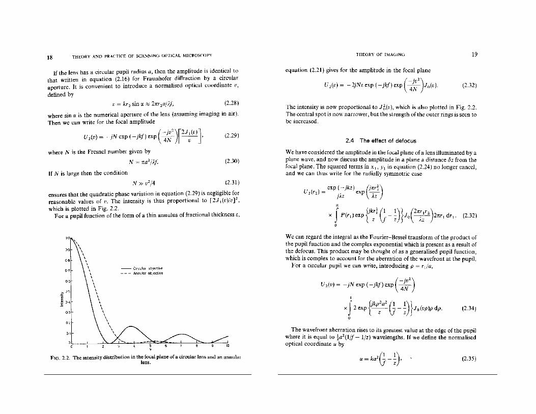
The intensity is now proportional to J6(v), which is also plotted in Fig. 2.2.The central spot is now narrower, but the strength of the outer rings is seen tobe increased.
2.4 The effect of defocus
We have considered the amplitude in the focal plane of a lens illuminated by aplane wave, and now discuss the amplitude in a plane a distance (jz from thefocal plane. The squared terms in XI' YI in equation (2.24) no longer cancel,and we can thus write for the radially symmetric case
N»v2 /4 (2.31)
ensures that the quadratic phase variation in equation (2.29) is negligible forreasonable values of v. The intensity is thus proportional to [2J I (v)/V]2,which is plotted in Fig. 2.2.
For a pupil function of the form of a thin annulus of fractional thickness E,
U )exp(-jkz) (jrrd)
2(r2 = ')' exp---,-----} z II.Z
00
f {jkrf (1 1)} (2rrr lr2)x P(rdexp-z-j-; Jo~2rrrldrl'
o
(2.32)
The wavefront aberration rises to its greatest value at the edge ofthe pupilwhere it is equal to ta2 (1/f - liz) wavelengths. If we define the normalisedoptical coordinate u by
We can regard the integral as the Fourier-Bessel transform of the product ofthe pupil function and the complex exponential which is present as a result ofthe defocus. This product may be thought of as a generalised pupil function,which is complex to account for the aberration of the wavefront at the pupil.
For a circular pupil we can write, introducing p = rda,0·&
0·7
0·6
C 0-5.~
".! 0·4.EO
0·3
02
0·1
-- Circular objecUve- - - Annular objective
U 2 (v) = -jNeXP(-jkf)exp(~~2)
I
f {jkp2a2 (1 1)}x 2 exp ~z- j -; Jo(vp)p dp.
o
(2.34)
FIG. 2.2. The intensity distribution in the focal plane of a circular lens and an annularlens.
(2.35)

20 THEORY AND PRACTICE OF SCANNING OPTICAL MICROSCOPY
the amplitude is
and u is linearly related to the distance from the focal plane. Then themaximum wavefront aberration is 2 bz sin2 (rx/2).
Along the optic axis we obtain for the amplitude
(2.36)
(2.42)
(2.41 )
(2.38)
(2.37)
(2.39)
(2.40)
1
qu, v) = f2 cos (tjup2)JO(Vp)p dp,
o1
S(u, v) = J2 sin (tjup2)JO(Vp)p dp.
o
(_jV
2)
U2(U,V)= -jN exp (-jkz)exp 4N
1
x f2exp(tjup 2 )Jo(vp)pdp.
o
(ju)[sin (U/4)]U2 (u, 0) = -jNexp (-jkz)exP "4 ~/4-'
These integrals may be evaluated numerically or expressed in terms ofLommel functions. The behaviour of the intensity in the focal region isillustrated in Fig. 2.3, which shows contours of constant intensity, normalised to unity at the focal point. The lines u = v correspond to the shadowedge given by geometrical optics for the paraxial case.
I[ the pupil function is a thin annulus, the integral in equation (2.32) maybe evaluated directly, to give for the amplitude
U 2(U, v) = -2jNE exp (-jkz) exp ( ~~2) exp (!;u)Jo(v).
I(u, 0) = Nz[sinu~~4)J'
In general the intensity may be written
I(u, v) = N 2[C 2(U, v) + S2(U, v)],
where qu, v) and S(u, v) are defined as [2.2]
Or for the intensity
If z = f + bz with bz small
u ~ k bza2/p ~ 4k bz sin2 (!X/2)

22 THEORY AND PRACTICE OF SCANNING OPTICAL MICROSCOPY THEORY OF IMAGING 23
-00
amplitude U2(X2' Y2) immediately behind the lens is found by applying theFresnel diffraction formula and multiplying by the pupil function and phasefactor for the lens, to give
(2.44)
(2.46)1 1 1-+-=
dl dz f
-00
-jk{ 2 Z}x exp 2d
l(X2 - Xl) + (Y2 - YI)
- jk { 2 2}X exp 2d
2(X3 - x 2) + (Y3 - Y2)
jk 2 zx exp 2j (X2 + Yz) dX I dy, dx z dY2
'kx exp ~~l (xi + yi)
- jk 2 2 {-jk ( 1 1 1) 2 Z }x exp 2d2
(X3 + Y3) exp -2- dl
+ d2-7 (X 2 + Yz)
. [ (Xl X3) (YI Y3)JX eXPlk Xz d; + dz
+ Yz d; + d3
dx, dYI dxz dyz·
(2.45)
If the condition known as the lens law
(2.43)
The amplitude U3(X3, Y3) in a plane at a distance d2 behind the lens is thengiven by a further application of equation (2.3)
I ~·!·)r----I,( X1,yl ) I (~3'Y3)-d1---j~ dz-----
FIG. 2.4. The image formation geometry.
2.5 Coherent imaging
Let us now assume we have a transparency which is sufficiently thin that itmay be described completely by a complex amplitude transmittance t(x, y),of which the variations in modulus represent the variations in absorption intraversing the transparency, whereas the variations in phase account for theoptical path travelled. If this is illuminated with an axial plane wave of unitstrength the amplitude after the transparency is similarly t(x, y). If thetransparency is placed at a distance d1 in front of a lens (Fig. 2.4), the
The important feature here is that the intensity variation with distance fromthe optic axis is independent of the value of u within the range of the Fresnelapproximation, that is the depth of focus is exceedingly large. As the beampropagates the radiation diffracts away from the axis, but power issimultaneously diffracted inwards from the strong outer rings. A beam withintensity distribution given by J ~(v) will propagate without spreading as aresult of this dynamic equilibrium: it is a mode of free space.
The imaging properties of lenses and mirrors with annular aperture havebeen the subject of considerable interest since the work of Airy [2.3J in 1841.In the annular lens the central peak is sharpened but at the expense ofincreasing the strength of the outer bright rings (Fig. 2.2). The intensity in thefocal plane and along the optic axis for an annulus of finite width has beencalculated by Steward [2.4, 2.5] who also showed [2.5J that the intensitydistribution along the optic axis is stretched out relative to that of a circularlens, that is, the depth of field is increased. This increased depth of field,however, is unfortunately not useful for examining extended objects in theconventional microscope [2.6], as the increase in brightness in the outerdiffraction rings results in a loss of contrast, and an n-fold increase in focaldepth involves an n-fold loss oflight. Because a laser is used as a light sourcein scanning microscopy this latter point, however, is not a serious drawbackin this case.

24 THEORY AND PRACTICE OF SCANNING OPTICAL MICROSCOPY THEORY OF IMAGING 25
(2.52)
is satisfied, and furthermore with
d2 = Md l ,
we obtain
(2.47)
as the intensity point spread function. For a circular pupil the intensity is(following equations 2.16, 2.29)
I(V)=[2J~(~J'
+CIJ
where the normalised coordinate v is given by
v = 2nr3a/Ad 1 (2.53)
+0()
and we have normalised the intensity to unity on the optic axis. Equation(2.52) represents the Airy disc, as shown in Fig. 2.2
If the lens law (2.46) is not satisfied then for small departures from the focalplane the amplitude point spread function is as given by the previous sectionon the effects of defocus. For a circular pupil we have
(2.54)h(u, v) = C(u, v) + jS(u, v),
where we have normalised to unity for u = v = 0, and u is given by
u = ka2 (J - :1 -d~} (2.55)
Introducing x' = Xl + x 3/M, y' = YI + Y3/M in equation (2.49) we have
-jkx exp 2Md
l(x3 + y3)
jk [( X3
) ( Y3)1x exp~ X2 Xl + M + Y2 Yl + M dXI dYI dX2 dY2.
(2.48 )
(2.49)
IIII -jk 2 2x P(X2'Yl) t(Xl'Yl)exp 2d
l(Xl + Yll
Performing the integral in x 2 , Y2 we have
where+00
(2.50)
is the Fourier transform of the pupil function, as introduced in equation(2.26). Suppose now that our object consists of a single bright point in anopaque background, so that
-0()
x exp ~i~ {(x' -~y + (Y' - ~r}h(X" y')dx' dy'.
(2.56)
For an imaging system of reasonable quality the spread function falls offquickly, so that x', y' are small. The exponential terms in X'2, y'2 and x'x3,
y'Y3 can therefore be replaced by unity to give
(2.51)
Then the amplitude is a constant times h(x3/M, Y3!M), and the latter is calledthe amplitude point spread function or impulse response of the opticalsystem. The distance X3/M represents a distance in the object plane, and M isthe linear magnification of the image. The intensity is given by the modulussquared of h(X3/M, Y3/M), again multiplied by a constant, and this is known
+00
X If t(x l , yIlh(~l + (:3/M , Yl + Y3/M ) dx, dYl'
(2.57)

26 THEORY AND PRACTICE OF SCANNING OPTICAL MICROSCOPY THEORY OF IMAGING 27
The image may thus be written
using equation (2.50) to giveThe integral is the convolution of the object transmittance with the pointspread function, the M's resulting in a magnification M in the image, and thepositive sign in the argument of the spread function corresponding to aninverted image. Of the two complex exponential terms in (2.57) the first is aconstant phase term which therefore does not affect the image.
The second phase factor in (2.57) represents a spherical phase variationwhich may also be neglected if we are concerned with small changes in x 3 , Y3'
In most of the following, however, we are interested in optical systems wherethe optical beam travels along the axis, in which case there is no phasevariation to worry about.
The intensity is clearly given by
+oc
-0:::'
+00
(2.61)
(2.62)
which is the convolution of th object transmittance and g(x,). The quantityg(x,) is called the line spread function, and is the amplitude image of a brightline.
H the pupil is radially symmetric, the line spread function is given byequation (2.62) as the one-dimensional Fourier transform of P(r2 ), ascompared with the point spread function, which is the Fourier-Bessel, ortwo-dimensional Fourier, transform of P(r2)' For a lens with Ixl :E; a
(2.65)
(2.64)
(2.63)
(sin v)=2a --
v
+a
+00
U3 (X 3 ,h) = },2~d1 f t(Xdg(x, + ~) dXl,
where (equation 2.28)(2.59)
(2.58)
2.6 Imaging of line structures in coherent systems
+00
13(x 3 , Y3) = A4~ 2di Iff t(x" ydh(x, + x 3/M, y, + hiM) dx, dy, 1
2
.
In the previous section we derived a general expression for the image in acoherent imaging system, and also considered the image of the single pointobject. An important class of objects are those in which the transmittance is afunction of one direction only, let us say t(xTl. Using equation (2.57) theimage is, disregarding the phase-terms,
Considering the integral y" we see that
+00 +00
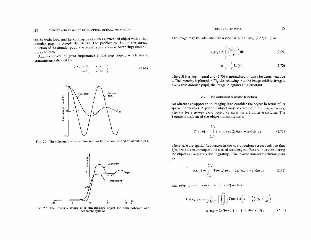
This is plotted in Fig. 2.5, where it is normalised to unity at the origin. Thisresult may also be derived by direct integration of the point spread functionas in (2.61). For a thin annular pupil, on the other hand, we have
f h(Xl+~'Yl+~)dYl= f h(Xl+~'Yl)dYl'-00
(2.60) (2.66)
with the result that, as we might expect, the image is independent of thecoordinate Y3' The integral may be written in terms of the pupil function,
= 2 cos v, (2.67)
which again is shown normalised in Fig. 2.5. The side-lobes are now as strong
28 THEORY AND PRACTICE OF SCANNING OPTICAL MICROSCOPY THEORY OF IMAGING 29
as the main lobe, and hence imaging of such an extended object with a thinannular pupil is completely useless. The problem is that in the spreadfunction of the annular pupil, the intensity in successive outer rings does not
decay to zero.Another object of great importance is the step object, which has a
transmittance defined by
t(xtl = 0,= 1,
(2.68)
The image may be calculated for a circular pupil using (2.63) to give
(2.69)
(2.70)
2.7 The coherent transfer function
where Si is a sine integral and (2.70) is normalised to unity for large negativev. The intensity is plotted in Fig. 2.6, showing that the image exhibits fringes.For a thin annular pupil, the image integrates to a constant.
An alternative approach to imaging is to consider the object in terms of itsspatial frequencies. A periodic object may be resolved into a Fourier series,whereas for a non-periodic object we must use a Fourier transform. TheFourier transform of the object transmittance is
(2.71)
+00
T(m, n) = ff t(x, y) exp 2nj(mx + ny) dx dy
c.2Uc~
1l~Q. 10Vl
OJc
::J
FIG. 2.5. The coherent line spread function for both a circular and an annular lens.
where m, n are spatial frequencies in the x, y directions respectively, so that11m, lin are the corresponding spatial wavelengths. We are thus consideringthe object as a superposition of gratings. The inverse transform relation givesus
-10 -5 10
+00
t(x, y) = ff T(m, n) exp -2nj(mx + ny) dm dn
and substituting this in equation (2.57) we have
+00
U3(X3,Y3) = A2~di ffffT~m, n)h(x 1 + ~'Yl + ~)
(2.72)
FIG. 2.6. The intensity image of a straight-edge object for both coherent andincoherent systems. (2.73)

30 THEORY AND PRACTICE OF SCANNING OPTICAL MICROSCOPY THEORY OF IMAGING 31
Performing the integrals in Xl' Yl using the inverse of equation (2.50) weobtain
+00
U3(X3,Y3) = ;'2~d~ ff T(m,n)c(m,n)
(2.81)
(2.82)
(2.83)
(2.80)
I(x 3) = Ic(OW + 2 Re {c*(O)c(v)b} cos 2nvx3 ,
and for the intensity
I(x 3 ) = Ic(OW + ilWle(vW + 2 Re {c*(O)c(v)b} cos 2nvx3
+ tlWlc(vW cos 4nvx 3
which is a linear image of the object amplitude transmittance. If thetransfer function is real, as it is for an aberration free pupil, and b is purelyimaginary, there is no image.
For an object which has a cosinusoidal variation in absorption coefficient,refractive index or thickness (or height in a reflection specimen) we can write
If the transfer function is even, we have for the image amplitude
U (x 3 ) = c(O) + bc(r) cos 2nvx,
where Re { } denotes the real part and * denotes the complex conjugate. Ifthe modulus of b is small such that we can neglect Ibl 2 this becomes
that is, it consists of only one pair of spatial frequency, one positive and onenegative. The Fourier transform of the object is
T(m, n) = [o(m) + ~ o(m - v) + ~ o(m + V)l b(n).
(2.75)
(2.74)2nj
x exp M (mX3 + nY3) dm dn.
-00
where the coherent transfer function c(m, n) is given by
The image may thus be found by resolving the object transmittance into itsFourier spectrum, multiplying by a coherent transfer function, which givesthe strength of the various Fourier components in the image, and theninverse transforming to give the image amplitude. We may thus write
The positive exponent in (2.75) indicates that the image is inverted. For thecase of a circular pupil we may further write
In this case there are an infinite series of spatial frequencies present, but if Iblis small we can expand as a power series
elm, n) = P(mAd l , nAdd· (2.76)t(X) = exp {b cos 2nvx}.
t(X) = 1 + b cos 2nvx + ib2 cos2 2nvx + ...
(2.84)
(2.85)
where m, nare normalised (dimensionless) spatial frequencies and a is the lensradius.
If we now consider a line structure for which n = 0, then the transferfunction is
elm, n) = P(ma, na)
2.8 The angular spectrum
The amplitude of a plane wave of unit strength at a point r is given by
If we can neglect terms in higher order than b, equation (2.85) reduces to(2.79) and the image is given by equation (2.83). If the term of order b inequation (2.83) is zero, however, then we must include terms of order b2 inequation (2.85), in which case equation (2.82) is no longer valid.
(2.86)U(r) = exp -j(k 'r)
(2.78)
(2.77)
Iml < I,}Iml> 1.
c(m, 0) = 1,
=0,
This spatial frequency cut-off corresponds to a spatial wavelength in theobject of vJ2n.
Let us consider an object which may be described by
where k is the wave vector such that ifthe direction cosines of the direction ofpropagation are IZ, ft, y, this may be wr!tten
t(x) = 1 + b cos 2nvx, (2.79)
-2njU(x, Y, z) = exp -;.- (IZX + fly + yz), (2.87)
32 THEORY AND PRACTICE OF SCANNING OPTICAL MICROSCOPY THEORY OF IMAGING 33
where IX, fJ and yare related by
If we illuminate an object with transmission t(x, y) we have, in terms of theFourier Spectrum of the object (equation 2.72),
(2.95)
2.9 Incoherent imaging
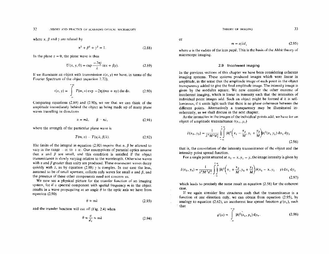
In the previous sections of this chapter we have been considering coherentimaging systems. These systems produced images which were linear inamplitude, in the sense that the amplitude image of each point in the objecttransparency added to give the final amplitude image. The intensity image isgiven by the modulus square. We now consider the other extreme ofincoherent imaging, which is linear in intensity such that the intensities ofindividual point images add. Such an object might be formed if it is selfluminous, if it emits light such that there is no phase coherence between thedifferent points. Alternatively a transparency may be illuminated incoherently, as we shall discuss in the next chapter.
As the intensities in the images of the individual points add, we have for anobject of amplitude transmittance t(x l , Yd
where a is the radius of the lens pupil. This is the basis of the Abbe theory ofmicroscope imaging.
or
(2.89)
(2.88)
(2.91)
(2.90)
13 = nA,IX = mA.,
+00
t(x, y) = f T(m, n) exp -2nj(mx + ny) dm dn.
In the plane z = 0, the plane wave is thus
-2njU(x, Y, 0) = exp -,- (IXX + f3y).
Ic
Comparing equations (2.89) and (2.90), we see that we can think of theamplitude immediately behind the object as being made up of many planewaves travelling in directions
The limits of the integral in equation (2.90) require that IX, fJ be allowed tovary in the range - co to + oc. Our assumptions of paraxial optics assumethat (l and fJ are small, and this condition is satisfied if the objecttransmittance is slowly varying relative to the wavelength. Otherwise waveswith IX and 13 greater than unity are produced. These evanescent waves decayquickly with z, as by equation (2.88) y is complex. In our case the lens,assumed to be of small aperture, collects only waves for small IX and 13, andthe presence of these other components need not concern us.
We now see a physical picture for the transfer function of an imagingsystem, for if a spectral component with spatial frequency m in the objectresults in a wave propagating at an angle IJ to the optic axis we have fromequation (2.90)
+00
(2.98)
+00
g'(x) = f IW(Xl' yIl dYl'
that is, the convolution of the intensity transmittance of the object and theintensity point spread function.
For a single point situated at x I = x, Yl = Y, the image intensity is given by
which leads to precisely the same result as equation (2.58) for the coherentcase.
If we again consider line structures such that the transmittance is afunction of one direction only, we can obtain from equation (2.95), byanalogy to equation (2.62), an incoherent line spread function g' (x1), such
. that
(2.92)
(2.94)
(2.93)lJ~mA.
T(m, n) = T(rx/A., fJj).).
where the strength of the particular plane wave is
and the transfer function will cut ofT (Fig. 2.4) when

34 THEORY AND PRACTICE OF SCANNING OPTICAL MICROSCOPY THEORY OF IMAGING 35
(2.99)
(2.100) (2.103 )
+00
W(x, y) = ffT(m, n) exp -2nj(mx + ny) dm dn.
Substituting into equation (2.9), we have
where H 0 is a zero order Struve function, and where we have used Struve'sintegral [2.7, p. 497J and normalised (2.102) to unity at large negative valuesof v. This is plotted in Fig. 2.6 and we see that the fringing whichcharacterised the coherent response is absent. It is also important to note thatthe apparent position of the edge is different in the two cases. If we assume(arbitrarily) that the edge occurs at the position of the half-intensity response,we would introduce a slight error in the coherent case. We now finallyconsider incoherent imaging in terms of spatial frequencies. Followingsection 2.7 we introduce the object intensity spectrum T(m, n), such thatwhich may be written as [2.7J
g'(v) = 3n H j (2v)8 v2
where H j is a first-order Struve function and where we have normalised tounity at the origin. The incoherent line spread function is illustrated in Fig.2.7.
We may also consider the image of the straight edge (equation 2.68) whichmay be calculated from equation (2.100), for a system using circular lenses, as
In general it is not possible to express this integral simply, in terms of thepupil function of the lens, as in the coherent case. However, by substitutingthe appropriate point spread function into equation (2.95), we obtain g'(xdby direct integration. For a circular lens we have
00
I(v) = 3n fH j(2z) dz8 Z2
r
1 {Hd2V ) fHo(z) }oc- -2- + --dz,n v z
2v
g'(v)
5 v 10
FIG. 2.7. The incoherent line spread function for a circular lens.
(2.101)
(2.102)
x T(m, n) exp -2nj(mx j + nYj) dm dn dX j dYj' (2.104)
Performing the integrals in Xj , Yj and using the inverse of equation (2.50)together with the convolution theorem (see e.g. reference 2.1, p. 10), we maywrite
+00
I(x3' Y3) = A4~ 2d; ff T(m, n)C(m, n) exp -~nj (mx3 + nY3) dm dn,
(2.105)
with
(2.106)
where ® denotes the convolution operation.This function may be called the incoherent transfer function. The similarity
between equations (2.105) and (2.75) should be noted.The incoherent transfer function is plotted in Fig. 2.8 for circular pupils.
We see that it is non-zero for line structures with normalised spatialfrequencies (m, Ii) less than two. This spatial frequency cut-off corresponds toa special wavelength in the object of vln, that is twice the spatial frequencybandwidth of the coherent system. The smooth gradual fall off of this transferfunction may be seen as the reason for the absence of ringing in the straightedge response.
36 THEORY AND PRACTICE OF SCANNING OPTICAL MICROSCOPY
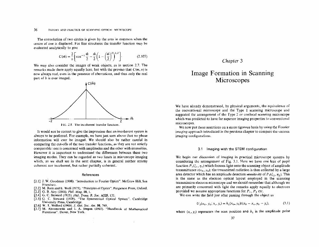
The convolution of two circles is given by the area in common when thecentre of one is displaced. For line structures the transfer function may beevaluated analytically to give
elm)
We may also consider the images of weak objects, as in section 2.7. Theremarks made there apply equally here, but with the proviso that C(m, n) isnow always real, even in the presence of aberrations, and thus only the realpart of b is ever imaged.
2[ - -( (-)2)l i2J' _ -1 m m mC (m) =; COS 2 ~2 1 - 2 . (2.107)
Chapter 3
Image Formation in ScanningMicroscopes
-_--':2~-------.L..----------"'"...2-- in
FIG. 2.8. The incoherent transfer function.
It would not be correct to give the impression that an incoherent system isalways to be preferred. For example, we have just seen above that no phaseinformation will ever be imaged. We should also be rather careful incomparing the cut-offs of the two transfer functions, as they are not strictlycomparable: one is concerned with amplitudes and the other with intensities.However it is important to understand the differences between these twoimaging modes. They can be regarded as two limits in microscope imagingwhich, as we shal1 see in the next chapter, is in general neither strictlycoherent nor incoherent, but rather partially coherent.
References
[2.1] J. W. Goodman (1908). "Introduction to Fourier Optics". McGraw Hill, SanFrancisco.
[2.2] M. Born and E. Wolf (1975). "Principles of Optics". Pergamon Press, Oxford.[2.3] G. B. Airy (1841). Phil. Mag. 18, 1.[2.4] G. C. Steward (1925). Phil. Trans. R. Soc. A225, 131.[2.5] G. C. Steward (1928). "The Symmetrical Optical System". Cambridge
University Press, Cambridge.[2.6] W. T. Welford (1960). J. Opt. Soc. Am. SO, 749.[2.7] M. Abramowitz and I. A. Stegun (1965). "Handbook of Mathematical
Functions". Dover, New York.
We have already demonstrated, by physical arguments, the equivalence ofthe conventional microscope and the Type 1 scanning microscope andsuggested the arrangement of the Type 2 or confocal scanning microscopewhich was predicted to have far superior imaging properties to conventionalmicroscopes.
We now put these assertions on a more rigorous basis by using the Fourierimaging approach introduced in the previous chapter to compare the variousimaging configurations.
3.1 Imaging with the STEM configuration
We begin our discussion of imaging in practical microscope systems byconsidering the arrangement of Fig. 3.1. Here we have one lens of pupilfunction P I(~I' tfl) which focuses light onto the scanning object of amplitudetransmittance t(xo, Yo); the transmitted radiation is then col1ected by a largearea detector which has an amplitude detection sensitivity of P2(~2' f/2)' Thisis the same as the electron optical layout employed in the scanningtransmission electron microscope and we should remember that although weare primarily concerned with light the remarks apply equal1y to electronsprovided we assume appropriate functions for PI' P 2 etc.
We can write the field just after passing through the object as
where (x" y,) represents the scan position and hi is the amplitude point
37


40 THEORY AND PRACTICE OF SCANNING OPTICAL MICROSCOPY IMAGE FORMATION IN SCANNING MICROSCOPES 41
interference term depends on g2 (2xct , 0), that is on the size of P2. If weconsider our two limiting cases we have for a vanishingly small detector
where the amplitude images add together and imaging is therefore coherent.Conversely for a large area detector
and the intensity images add together, as one would expect for incoherentimaging. Generalising, we may thus say that altering the size of the detectoralters the coherence of the system.
The question as to how close together the two points may come before theyare said to be no longer resolved is not easy to answer as various criteria havebeen proposed giving different results. The two most widely used criteria arethe Sparrow criterion which is concerned with the rate of change of the slopeof the image at the midpoint and the Rayleigh criterion which somewhatarbitrarily states that the two points will be just resolved when the intensity atthe midpoint is 0.735 times that at the points. The Rayleigh criterion wasintroduced for incoherent imaging with a circular aberation-free pupil, inwhich it corresponds to the condition that the first zero of the image of onepoint coincides with the position of the central peak of the image of thesecond point object. We will discuss two-point imaging a little further bysupposing that we have two circular aberration-free pupils such that
(3.19)
(3.20)
L(s) = 2vct,
1(0,0)I(v
d, 0) = 0·735
which is the distance in optical coordinates between two point objects suchthat the Rayleigh criterion
Thus we see that the image depends on the size of the detector relative to thatof the objective rather than the absolute size of the detector. The parameter sis called the coherence parameter. It is interesting to note that whenever 2sv
ctis a root of J 1(2svct ) = 0 the product term is absent and the image is the sameas would have been obtained if the object had been incoherently illuminated.In particular for equal pupils (s = 1) this will be the case when 2vct is a nonzero root of J 1 (2vd ) = 0 which means practically that the geometrical imagesof the pinholes are separated by a distance equal to the radius of any darkring of the Airy pattern of the objective. Thus if the two points are separatedby a distance such that the Rayleigh criterion is satisfied for an incoherentsystem, the Rayleigh criterion is also satisfied for a system with equalobjective and detector pupils. So the two-point resolution as given by theRayleigh criterion is identical in these two systems.
We can discuss the effect of the coherence parameter s on the two-pointresolution by introducing a function [3.1]
is satisfied.
This function is plotted in Fig. 3.2 and we can see that the separation forthe points to be just resolved for equal pupils or very large detector is 0.61optical units. The best resolving power is obtained with s - 1·5. We haveincluded in Fig. 3.2 the curve for a microscope employing a full circular
(3.12)
(3.13)
(3.14)
(3.15)
Pdr) = 1,
P2(r) = 1,
We further introduce a parameter s, defined by
(3.16)
The value s = 0 corresponds to coherent imaging and s -jo OJ to incoherentimaging. Using these definitions we can immediately write from equation(3.6)
(3.17)
10
09
fr'llsl07 ---
- - - TYPE 1 SCANNING MICROSCOPE_TWO CIRCULAR PUPilS
- T'l'P£ I SCANNING MICROSCOPE-ANNULAR COLLECTOR
FIG. 3.2. Two point resolution in a Type 1 scanning microscope.
where v is the normalised optical coordinate of equation (2.53). Equation(13.11) may now be rewritten as
I (v" 0) = (:211(vs + Vct))2 + (2J 1(vs - Vct ))2v, + Vd v, - Vd
+ 2(2J 1(2SVct ))(2J1(VS + Vd ))(2J1 (V, - Vd )). (3.18)2svct v, + Vd Vs - Vct
06
os::L0'01
o ! , •
o O-'j "s,.~ ( I ,
20

42 THEORY AND PRACTICE OF SCANNJ]';G OPTICAL MICROSCOPY IMAGF FORMATION IN SCANNING MICROSCOPES 43
+ <Xl
I(x" y,) = ffffffffhdxo, yo)h!(x~,y~)T(m. n)T*(p, q)-<Xl
where m, p are spatial frequencies in the x direction and n, q are similarlyspatial frequencies in the y direction. We have to introduce the spatialfrequencies p, q, which are dummy variables which disappear uponintegration of (3.22), in order to be able to write the product of (3.21) and(3.22) with the integral signs at the front.
Substituting equations (3.21) and (3.22) into (3.5) we obtain
This is in contrast to conventional microscopy where, as a complete objectfield must be imaged, Kohler illumination is preferred to give uniformillumination over the field.
The imaging of the Type 1 scanning microscope is still described byequations (3.5) and (3.6) but now P2(~2' 112) represents the pupil function ofthe collector lens if we assume that the detector has a uniform response. Wenow proceed to discuss the imaging in terms of spatial frequencies. Thisconcept was introduced in section (2.7) where we represented a non-periodicobject in terms of its Fourier transform or spectrum. Thus we can write(equation 2.72)
(3.21)
(3.22)
+(;0
-<Xl
t*(x, y) = ff T*(p, q) exp 2nj(px + qy) dp dq
+ <Xl
t(x, Y) = ff T(m, n) exp ~2nj(mx + ny) dm dn
and for the complex conjugate
3.2 The partially coherent Type 1 scanning microscope
Although the arrangement of Fig. 3.1 is employed in the scanningtransmission electron microscope it is usual in scanning optical microscopyto employ a second, collector lens to gather the radiation which has passedthrough the object and focus it onto the detector. Figure 3.3 shows twopossible configurations in which the detector collects all the light which isincident on P2 and so they both have exactly the same imaging properties aseach other and as the STEM configuration. In Chapter 1 we discussed howthe Type 1 scanning microscope is equivalent to the conventional microscope. In the scanning microscope of Fig. 3.3(a) the radiation is focused onto the detector, and as it is analogous to the critical illumination system inconventional microscopy it may be termed critical detection. In Fig. 3.3(b)on the other hand the detector is placed in the back focal plane of thecollector lens and we may call this Kohler detection, again by analogy withKohler illumination in conventional microscopy. The Kohler system relieson the response of the detector being uniform across the whole area and sothe preferred approach is the critical detection arrangement of Fig. 3.3(a).
objective lens and an infinitely narrow annular detector. For the particularcase of a two-point object the limiting resolution is improved by employingsuch a collector [3.2].
This may be written as
+:0
I(x" ys! = ffffC(m. II; P. q)!(m, n)T*(p, q)
x g2(XO - x~, Yo - Y~)
x exp - 2nj {m(xo - xJ - p(x~ - xs ) + n(yo - Ys) - q(y~ - Ys)}
x dm dn dpdq dxo dyo dx~ dy~. (3.23)
(3.24)
-00
x exp 2nj {(m - p)xs + (n - q)ys} dm dn dp dq,
(0)
(b)
FIG. 3.3. Two equivalent forms of the partially coherent Type 1 scanningmicroscope.

44 THEORY AND PRACTICE OF SCANNING OPTICAL MICROSCOPY IMAGE FORMATION IN SCANNING MICROSCOPES 45
with+oc
C(m, n; p, q) = ffffh1(xO' yo)hHx~, y~)g2(XO - X~, Yo - Yo)
representing P 1 centred on ( - mM, 0) and ( - pAd, 0), which also falls withinthe circle P2. This is illustrated in Fig. 3.4. There are two limiting cases ofinterest as the diameter of P2 is varied. When P2 is large we see that C(m; p)becomes a function of (m - p) only. This is in fact what one expects forincoherent imaging, and imaging is indeed incoherent for this limiting case as
x exp -2nj{mxo - px~ + nyo - qyo} dxo dyo dx~ dyo(3.25)
which using equations (3.6) and (3.2) may be recast as
+00P, (x+m,yl
This represents a very important result as we have been able to express theintensity variation in the image of an arbitrary specimen by equation (3.24) inwhich C(m, n; p, q), the partially coherent transfer function (sometimes alsocalled the transmission cross coefficient), is a function only of the opticalsystem and not the object. This is the real power of this approach whereby wecan introduce an imaging function which is common to all objects. We cansee from equation (3.24) that "perfect" imaging is obtained if the transferfunction C(m, n; p, q) is always unity; this is not possible in practice and theaim in microscope design is to make this function as smooth and great inextent as possible. It should be noted, however, that a "perfect" image doesnow show up phase variations, so that "perfect" imaging may not even bedesirable in practice.
In order to fix our ideas concerning the transfer function method let usnow consider a line structure which has detail in the x-direction only. Thetransfer function may now be contracted to
FIG. 3.4. The region of integration for C(m; pl.
(3.29)
(3.30)
C(m;p) = P 1(mU)P!(pM)
= c(m)c*(p),
/P2 (x,y I
and thus the image may be written as
discussed in section (2.9). On the other hand as P 2 becomes vanishingly smallwe find that
(3.26)X Pf(~2 + pM, '12 + qAd) d~2 d'12'
+00
= ff IP2(~2' '12)\2P1(~2 + mM, '12)P!(~2 + pAd, '12) d~ 2 d'12,
-oc(3.28)
and C(m; p) is the transfer function which gives the magnitude of the spatialfrequency component (m - p) in the intensity image.
We further consider the case where the microscope has aberration-freecircular pupils of the form of equations (3.14) and (3.15). We may graphicallycalculate the transfer function as the area of overlap of the two circles
which of course corresponds to the coherent imaging of section (2.7). Againthe positive exponent corresponds to an inverted image.
A practically important case is where the two pupils are of equal size.Under these circumstances the imaging is partially coherent and the C(m; p)function somewhat more complicated. It is shown in Fig. 3.5(b) in (m; p)space where it is seen to exhibit an 'hexagonal cut-off. It should beremembered that although m and p are plotted here in orthogonal directionsthey represent two spatial frequencies in the same direction. The symmetry of
C(m; p) = C(m, 0; p, 0) (3.27)+00
I (x,) = I f c(m)T(m) exp (2njmx,) dm 1
2
,
-00
(3.31 )
46 THEORY AND PRACTICE OF SCANNING OPTICAL MICROSCOPY IMAGE FORMATION IN SCANNING MICROSCOPES 47
(3.35)
(3.36)
(3.37)
+00
1(0,0) = Iff U2(~2' tl2) d~2~dtl2r,
3.3 The confocal scanning microscope
3.3.1 Introduction
which may be written for even spread functions
I (x" Ys) = Ih[h z ® t1 2,
As explained in section 1, the Type 1 scanning microscope has imagingproperties identical to those of conventional non-scanning microscopes. TheType 2, or confocal scanning microscope, on the other hand has completelydifferent imaging properties. The confocal microscope is formed by placing apoint detector in the detector plane of Fig. 3.3(a). We can write the field in thedetector plane (x z , yz) as the convolution of the amplitude in the object planewith the point spread function of the collector lens
U(X2, Y2; x" Ys)+00
= ffhdxo, yo)t(xo - x" Yo - y,)h2(~ - X O, ~ - Yo) dxo dyo·
-00 (3.33)
However if we employ a point detector at X2 = Y2 = 0 the detected intensityis
+00
I(x" Y,) = Iff h[(xo, yo)t(xo - x" Yo - ys)hz(-xo, - Yo) dxo dyo 1
2
,
-00
(3.34)
that is the microscope behaves as a coherent microscope with an effectivepoint spread function given by the product of those for the two lenses.
We have thus found that the combination of point detector and scanningconverts a convolution of the form (h[t) ® h2 (which is obtained for a Type 1scanning microscope (equation 3.16)) into one of the form (h[h 2 ) ® t.Another way of considering the confocal microscope is to calculate first theamplitude U in terms of U2,
so that if X2 = Y2 = 0
(3.32)Ivl < 2.
"(pip
---,f---+-~~- m
2 r (v) (v){ (v)Z-}[IZlA(v)=; cos-[ 2 - 2 1- 2 '
(0) (bl (01
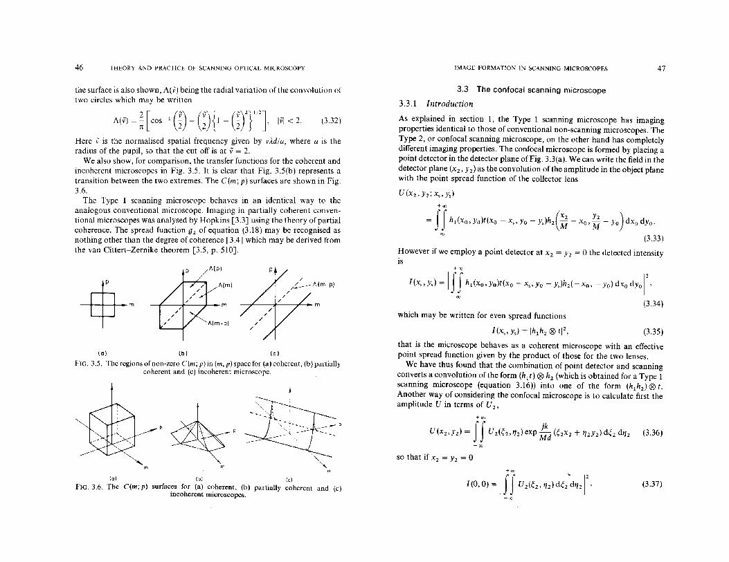
FIG. 3.6. The elm; p) surfaces for (a) coherent, (b) partially coherent and (c)incoherent microscopes.
m
(0) (b) (c)
FIG. 3.5. The regions of non-zero C(m; p) in (m, p) spacefor (aj coherent, (b) partiallycoherent and (c) incoherent microscope.
the surface is also shown, A(v) being the radial variation of the convolution oftwo circles which may be written
Here v is the normalised spatial frequency given by vAdla, where a is theradius of the pupil, so that the cut off is at v= 2.
We also show, for comparison, the transfer functions for the coherent andincoherent microscopes in Fig. 3.5. It is clear that Fig. 3.5(b) represents atransition between the two extremes. The C (m; p) surfaces are shown in Fig.3.6.
The Type 1 scanning microscope behaves in an identical way to theanalogous conventional microscope. Imaging in partially coherent conventional microscopes was analysed by Hopkins [3.3J using the theory of partialcoherence. The spread function gz of equation (3.18) may be recognised asnothing other than the degree of coherence [3.4J which may be derived fromthe van Cittert-Zernike theorem [3.5, p. 510].

48 THEORY AND PRACTICE OF SCANNING OPTICAL MICROSCOPY IMAGE FORMATION IN SCANNING MICROSCOPFS 49
with
FIG. 3.7. The image of a single point object.
We may now turn our attention to the Fourier imaging and substitutingequation (3.21) into (3.34) are able to write
- - - CONVENTIONAL MICROSCOPE
-- CONFOCAL MICROSCOPE-CIRCULAR PUPILS
--- CONFOCAL MICROSCOPE-ONE CiRCULAR AND ONEANNULAR PUPil
_ .• - CONFOCAL MICROSCOPE-TWO ANNULAR PUPILS
,. \
\\'\ \
" \:\ \\. \
:\ \I' \,\ "., \
\\ "~\ \
\\ ":' \
\\ \, \ \
\' \.. \ \\\ "°o!:--_L--_·.s·!,--"'::::"+'~"";:;:---J---':--="..:l=-=-=~_=-±==~----.L_-.......J10
07
02
03
+00
I (x" Ys) = Iff elm, n)T(m, n) exp 2nj(mx, + nys) dm dn IZ' (3.41)
-00
maxima of the spread function of the annulus coincide with the zeros of thatof the circular lens. The two-point resolution is now 28 % better than aconventional microscope with equal lens pupils.
For large values of v the intensity in the image of a single point in aconventional microscope falls off as v- 3. In a confocal microscope with twocircular lenses it falls off as v- 6, whereas with one annular lens it falls off asv-4. With two narrow annuli however it falls off as v - 2, that is the power insuccessive sidelobes only falls off as V-I and total normalised power does notconverge, so that such an arrangement is clearly unusable.
(3.39)
that is the effect of the point detector is to integrate the amplitude over thepupil p 2' This compares with the Type 1 scanning microscope where thedetector integrates the intensity over the pupil P2' Substituting for U 3 from(3.3) we obtain for the confocal ease
x expj: (XO~2 + YOt/2) dxo dyo d~2 dt/ 2IZ
. (3.38)
and using (3.2) to introduce hz we reproduce (3.34).The point detector integrates amplitude over the pupil P z: it therefore has
the same effect as the amplitude-sensitive detector used in acoustic microscopy [3 .6J. The scanning acoustic microscope is a confocal microscope andexhibits many of the properties of confocal microscopes.
+00
I(x" yJ = Iffff hl(xo, yo)I(Xo - x" Yo - y,)P2(~2' t/2)
3.3.2 Image formation in confocal microscopes
If the two lenses in a confocal microscope are circular and of equal numericalaperture the image of a point object is (from 3.35)
which is shown in Fig. 3.7, the central peak being sharpened up by 27%relative to the image in a conventional microscope (at half the peakintensity). The sidelobes are also dratically reduced, so there is thus amarked reduction in the presence of artefacts in confocal images.
If we calculate the image of two closely spaced point objects we find thatwhen the Rayleigh criterion is satisfied the points are separated by anormalised distance 2vd = 0·56. This is 32 % closer than in a conventionalcoherent microscope and 8 %closer than in a conventional microscope withequal lens pupils. The relative values are illustrated in Fig. 3.2. The fact thatthe sidelobes are weaker in confocal microscopy suggests that it should bepossible to use an annular lens in a confocal microscope. With one circularand one annular lens of equal radii the intensity is given by
(3.40)
so that the central peak is now even narrower (40 %narrower compared witha conventional microscope) and the sidelobes are extremely weak as the
(3.42)
w.here elm, n) is a coherent transfer function. For two circular pupils ofequalradii the coherent transfer function is identical to the incoherent transferfunction for an incoherent system (equation 2.106).

50 THEORY AND PRACTICE OF SCANNING OPTICAL MICROSCOPY IMAGE FORMATION IN SCANNING MICROSCOPES 51
(3.44)
coherent
v< 2.
c.£Uc::>-0·6
08
o 0'5Normalised spatial frequency
FIG. 3.10. The coherent transfer function for various microscope geometries.
the spatial frequency in the image. For the confocal microscope the responsefor the sum frequencies is improved, but for the difference frequencies isreduced as compared to the conventional microscope, Fig. 3.5(b). Thisaccounts for the fact that the imaging in confocal microscopy is generallyimproved even though the coherent transfer function in the confocal microscope is identical to the incoherent transfer function for a conventionalincoherent microscope. This coherent transfer function is compared with thatfor a conventional coherent microscopy in Fig. 3.10, the cut-off frequencybeing twice as great. The transfer function also falls off gradually and thus wedo not expect excessive fringing to be present in the image of a straight edge.Also shown is the transfer function for a confocal microscope with oneannular pupil, illustrating that the response for higher spatial frequencies isimproved. This transfer function is given by the radial variation of theconvolution of a circle with an annulus, given by
A(v) = ~COS-l (~)1l 2 '
This should be compared with equation (3.32) for the convolution of twocircles.
The confocal microscope with one annular pupil may be compared withthat with two circular pupils by studying the region of m, p space within
p
m-p
(3.43)
p
C(m; p) = c(m)c*(p)
(0) m lbl m
FIG. 3.9. The C(m; p) surfac~ for a confocal scanning microscope with (a) circularlenses 'and (b) WIth one annular lens and one circular lens.
(0)
FIG. 3.8. Contours of constant C(m; p) showing lines of normalised spatial frequency(m - p) for (a) circular lenses and (b) one annular and one circular lens in confocal
microscopes.
If we again restrict ourselves to considering the images of line structuresthe function of interest is elm; p) given by
for the confocal microscope.Figures 3.8(a) and 3.9(a) show the form of this transfer function for a
confocal microscope with equal pupils. For a given pair of spatial frequencymoduli the response is higher if they have the same sign (differencefrequencies) than if of opposite sign (sum frequencies). The m-p axis is shownin Figs 3.8(a) and 3.8(b): the greater the distance along the axis the higher
52 THEORY AND PRACTICE OF SCANNING OPTICAL MICROSCOPY IMAGE FORMATION IN SCANNING MICROSCOPES 53
3.4 Aberrations in scanning microscopes
3.4.1 Introduction
that is it depends only on C(v; 0). Imaging of weak objects in conventionaland confocal microscopes with circular pupils is thus identical. However, ifaberrations are present this is no longer the case and the confocal microscopemay behave very differently. (3.50)
_--.........2.0
where
3.4.2 Defocus in scanning microscopes
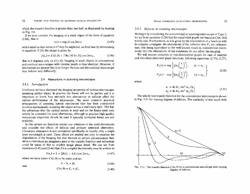
We begin by considering the conventional or scanning microscope of Type 1;we see from equation (3.28) that for equal sized pupils the function C(m; 0) iswholly real. Furthermore, as it is given by the convolution of a function withits complex conjugate, the aberrations of the collector lens P 2 are unimportant, this being equivalent to the well-known result in conventional microscopy that the aberrations of the condenser do not affect the imaging.
We will restrict ourselves to one-dimensional pupils for ease of analysisand introduce aberrated pupil functions, following equations (2.35), (2.37),
p](x) = exp {1jU](~r},
P2(x) = exp {!jU2(:J 2
},
FIG. 3.11. The transfer function C(m; 0) for a conventional microscope with varyingdegrees of defocus.
U t = 4k t5z 1 s~n22 (at/2),}u
2= 4k t5z
2sm (ad2). (3.51)
The wholly real transfer function for the conventional microscope is shownin Fig. 3.11 for varying degrees of defocus. The similarity of this result with
(3.48)
(3.49)
(3.47)
(3.46)I(xsl = C(O; 0) + 2 Re {bC(v; OJ} cos 2nvx"
and
I (x,) = 1 + 2(br Cr - bjCJ cos 2nvx"
where we have taken C(O; 0) to be unity and set
b = br + jb j
C(v; 0) = Cr + jCi .
Until now we have discussed the imaging properties of various microscopesassuming perfect lenses. In practice the lenses will not be perfect and it isimportant to know how seriously lens aberrations or defocus affect theoptical performance of the microscope. The most common practicalarrangement of scanning optical microscope that has been constructedinvolves mechanically scanning the object across a stationary spot. This hasthe advantage that the optical system is axial and so the lenses need onlystrictly be corrected for axial aberrations, although in practice high-qualitymicroscope objectives should be used if specially corrected lenses are notavailable.
In this section we therefore restrict our attention to the axial aberrationsand consider the effects of defocus and primary spherical aberration.Chromatic aberration is not considered specifically as usually only a singlelaser wavelength is used. These effects are studied not only to examine thedegradation of the imaging but also because in certain circumstances theyserve to introduce an imaginary part to the transfer function and advantagecould be taken of this to crudely image phase detail. We can see fromequations (3.45) and (3.46) that if b is complex the intensity may be written as
which the transfer function is greater than one half, as illustrated by shadingin Fig. 3.8.
If we now consider the imaging of a weak object of the form of equation(2.84), that is
t(x) = exp (b cos 2nvx) (3.45)
with b small so that terms in b 2 may be neglected, we find that by substitutingin equation (3.24) the image is given by
54 THEORY AND PRACTICE OF SCANNING OPTICAL MICROSCOPY IMAGE FORMATION IN SCANNING MICROSCOPES 55
that obtained by Hopkins [3.7] for full circular pupils justifies our onedimensional model. An imaginary part may be introduced into the transferfunction by stopping down the collector lens. It is found, however [3.8], thatthis lens must be stopped down considerably before phase imaging becomesappreciable which, with the associated reduction in spatial frequency cut-off,is the major reason why this method of obtaining phase contrast is not widelyused.
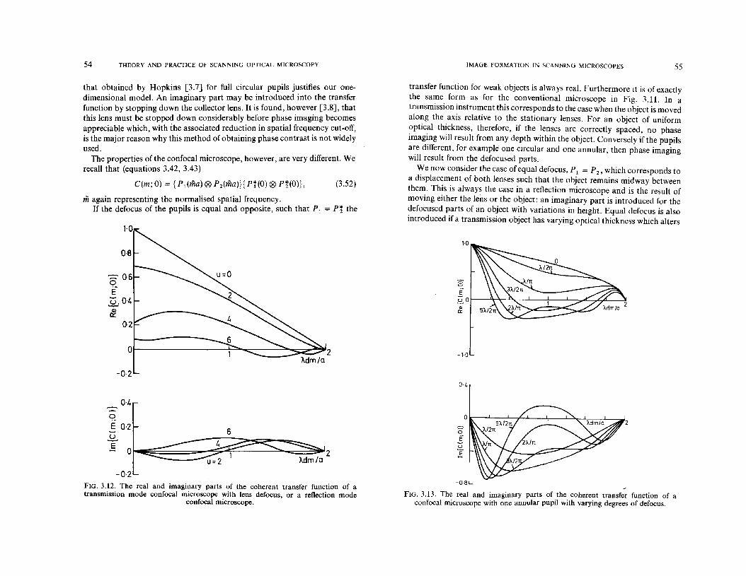
The properties of the confocal microscope, however, are very different. Werecall that (equations 3.42, 3.43)
C(m; 0) = { PI (ma) ® Pz(ma)}{ P!(O) ® PHO)}, (3.52)
magain representing the normalised spatial frequency.If the defocus of the pupils is equal and opposite, such that PI = P~ the
transfer function for weak objects is always real. Furthermore it is of exactlythe same form as for the conventional microscope in Fig. 3.11. In atransmission instrument this corresponds to the case when the object is movedalong the axis relative to the stationary lenses. For an object of uniformoptical thickness, therefore, if the lenses are correctly spaced, no phaseimaging will result from any depth within the object. Conversely if the pupilsare different, for example one circular and one annular, then phase imagingwill result from the defocused parts.
We now consider the case of equal defocus, PI = Pz, which corresponds toa displacement of both lenses such that the object remains midway betweenthem. This is always the case in a ref1ection microscope and is the result ofmoving either the lens or the object: an imaginary part is introduced for thedefocused parts of an object with variations in height. Equal defocus is alsointroduced if a transmission object has varying optical thickness which alters
0 2 -1·0Xdm/a
-0·2D·.
0·"-'?. 0
2E 0·2 6 =0..£ E'.§ ua ]"
u=2
-0·2FIG. 3.12. The real and imaginary parts of the coherent transfer function of atransmission mode confocal microscope with lens defocus, or a reflection mode
confocal microscope.
-08
FIG. 3.13. The real and imaginary parts of the coherent transfer function of aconfocal microscope with one annular pupil with varying degrees of defocus.
56 THEORY AND PRACTICE OF SCANNING OPTICAL MICROSCOPY IMAGE FORMATION IN SCANNING MICROSCOPES 57
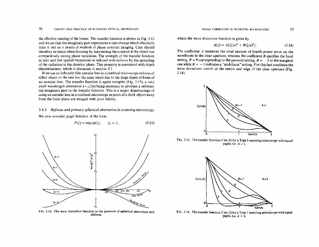
(3.54)
2
where the wave distortion function is given by
C(m;O)
The coefficient A measures the total amount of fourth-power error On thewavefronts in the clear aperture, whereas the coefficient B specifies the focalsetting, B = 0 corresponding to the paraxial setting, B = - 2 to the marginalone while B = -1 indicates a "mid-focus" setting. For this last condition thewave deviations vanish at the centre and edge of the clear aperture (Fig.3.14).
FIG. 3.15. The transfer function C(m; 0) for a Type 1 scanning microscope with equalpupils for A = 1.
>.dm/a
FIG. 3.16. The transfer function C(m; 0) for a Type 1 scanning micro~cope with equalpupils for A = 2.
(3.53 )
3.4.3 Defocus and primary spherical aberration in scanning microscopy
We now consider pupil function of the form
-1
FIG. 3.14. The wave distortion function in the presence of spherical aberration anddefocus.
the effective spacing of the lenses. The transfer function is shown in Fig. 3.12and we see that the imaginary part experiences a sign change which effectivelyrules it out as a practit al method of phase contrast imaging. Care shouldtherefore be taken when focusing by maximising the contrast if the object hascomparitively strong phase variations. The strength of the transfer functionat zero and low spatial frequencies is reduced with defocus by the spreadingof the radiation in the detector plane. This property is associated with depthdiscrimination, which is discussed in section 3.7.
If we use an infinitely thin annular lens in a confocal microscope defocus ofeither object or the lens has the same result due to the large depth of focus ofan annular lens. The transfer function is again complex (Fig. 3.13), a verysmall wavelength aberration (~)..j2n) being necessary to produce a substantial imaginary part to the transfer function. This is a major disadvantage ofusing an annular lens in a confocal microscope as parts of a thick object awayfrom the focal plane are imaged with poor fidelity.

58 THEORY AND PRACTICE OF SCANNING OPTICAL MICROSCOPY IMAGE FORMATION IN SCANNING MICROSCOPES 59
It should be noted that, unlike the case of pure defocus, the system is notsymmetrical in focal setting and that by making B negat~ve the effects of thespherical aberration may be to a certain extent be allevIated. W.e now .consider the effect of this pupil function on the performance of vanous mIcroscope types.
For the conventional microscope, C(m; 0) is wholly real and independentof the aberrations of the second lens. This has been evaluated numericallyand is plotted for various focal settings with degrees of sperical aberration
corresponding to A = 1 and 2 in Figs 3.15 and 3.16 again for a onedimensional model. The effect of the spherical aberration is drastically toreduce the mid- to higher spatial frequency components, but the effect isalmost focused out at B = -1, the mid-focus setting. Positive values of B, onthe other hand, reduce the performance and with higher degrees of sphericalaberration and defocus phase reversal occurs for some spatial frequencies.
A=2
2·5
2
'·5~
0
E
oS~ 0·5
0
-0,5
A='
2,5
2
~ 1·50
Eu.,0<:
0·5
0
-0·5
-1
,---" .." "-~/ " 8;-2, ,, ,.. ,.. ,.. ,
/ ,/ ,
/ \, \/ -...... \
-:,..::~.~__":.----.. . __ a '\\ { ......•.
~'- ,",\'" "" -i--~ \f........~,
Adm/a'!.. 2" ' .. '" ,........\. ·.........·.L__/l--.;.~ .....
\ ,._.•..•./
-0'5
-,
o·
.E-0·5
-,FIG. 3.17. The real and imaginary parts of the transfer function C(m;O) for aconfocal scanning microscope with equal lenses, A = 1. Defoci of both lenses are
equal.
............:...;-- .. 1--..... -'. ""~ 0 5 /<~;;;.;;>"/<.~< ....\. "., 0
~ /' .'.-'-' \E 0 ~!!!I!''''-::.:.::::.;2=::;:).=d:.:..m=/a~'-,..I..r.-.=-...~.-_-_----:..:~-j.'-:-=-.,.......;~
, \ -, y.••_.' ,/"i·. : ,/
\ . ./ ,, .... .,! /8=-2\... /
, ·•..•_ ...l "
" ,, ,, "'-"
FIG. 3.18. The real and imaginary parts of the transfer function C(m; 0) for aconfocal scanning optical microscope with equal lenses, A = 2. Defoci of both lenses
are equal.

60 THEORY AND PRACTICE OF SCANNING OPTICAL MICROSCOPY IMAGE FORMATION IN SCANNING MICROSCOPES 61
2
A=2, .•... -..... "-
.............. '.~1
. '-'-···•.....~2 ----__ ~--..... ..'"
Ol---------"··"-.:"------l..-==.....==.:..:.=:::;ll....",.,...----",.l.-•...__.-"1"""
0·5
3.4.4 Discussion
In the conventional or Type 1 scanning microscope with two equal pupils thetransfer function is purely real and although spherical aberration results in adegradation of the spatial frequency response the effect may be reduced byappropriate defocusing.
The results of using an annular objective in a confocal microscope [3.10Jare shown in Figs 3.21 and 3.22. These are equally applicable to conventional microscopes with an annular condenser. There is again no "aberrated"contribution from the annulus and so the curves apply equally to reflectionmicroscopy. We can see that for A = 1 and 2 the mid-focus setting, B = -1has almost cancelled out the effect of spherical aberration. However at highervalues of A it is more difficult to focus out these effects and so a confusedimage consisting of both amplitude and phase information would result.
"~.:.~~:-._. A=l....... ~1-._
'';,2'.-..- ~..=:::.:::-.:.~ »o;
':::::' 0·5oE~ 01-----:-:---:----+-------=--:1~ M~ 2
We now turn to confocal scanning microscopes [3.9]. Here the aberrationsof both lenses are important and the transfer function is in general complex.It is reasonable to assume that if two equal lenses are used that they wouldboth suffer from similar degrees of spherical aberration and we have assumedthat the coefficients A for the lenses are equal. We have plotted the transferfunction for two special cases. The first is when the lenses have equal degreesof defocus (corresponding to a change in the separation of the lenses). It isseen (Figs 3.17 and 3.18) that again the mid-focus setting almost cancels outthe effect of spherical aberration.
The second special case is that of equal and opposite defocus of the twolenses (corresponding to a movement of the specimen relative to the fixedlenses). The curves (Figs 3.19 and 3.20) indicate that defocus does not improve the high spatial frequency response and does not decrease the magnitude of the imaginary part. The curves for positive and negative defocus areidentical because of the commutative property of the convolution operation.
-0·5 -0'5
-1 -,
FIG. 3.20. Real and imaginary parts of the transfer function C(m;0) for a confocalscanning microscope with equal pupils, A = 2. Defocus of one lens is equal and
opposite to that of the other.
0·5
8=0 !10 1 ;;;;;;;::::;;;;::;~~~~~._~._.==.....~....~...~~ : : :........................ !2 Adm/Q 2
E-(}
-1
FIG. 3.19. Real and imaginary parts of the transfer function C(m; 0) for a confocalscanning microscope with equal pupils, A = 1. Defocus of one lens is equal and
opposite to that of the other.
~ 0·50
E~ 0
E
-0·5
-,
.....................- ......-.....
2

62 THEORY AND PRACTICE OF SCANNING OPTICAL MICROSCOPY IMAGE FORMATIO]\; IN SCANNING MICROSCOPES 63
In a confocal microscope, there is an imaginary part introduced. This maybe reduced by adjustment of the lens spacing but not by movement of theobject relative to the lenses. If the object transmittance exhibits both phaseand amplitude variations interpretation of the micrographs may provedifficult. Thus, in general, for a confocal microscope to operate properly it isimportant that the lenses should be well corrected for the laser wavelengthused, but, on the other hand, if the object is mechanically scanned off-axisaberrations are of course, unimportant. If the object is such that it exhibitsonly very small amplitude variations in transmittance the spherical aberrationcould result in useful phase imaging without this being associated with thedetrimental reduction in spatial frequency bandwidth introduced by stoppingdown the collector lens.
The scanning acoustic microscope has imaging properties similar to thoseof the confocal optical microscope and the imaging is characterised by acoherent transfer function identical to the C(m; 0) function of the confocalmicroscope. A typical figure for the maximum path error in an acousticmicroscope might be A/4. A value of A of unity corresponds to a maximumpath error of ;./6'3 and thus the spherical aberration in the acousticmicroscope could well give rise to phase imaging.
We should note that although in some cases the effect of aberrations on thereal part may be small care should be taken in the interpretation ofmicrographs especially if the phase delay in the object is appreciable.
-0 B
FIG. 3.22. Transfer function C(rn; 0) for a conventional microscOJIe with annularcondenser or confocal microscope with one annular lens in the presence of spherical
aberration, A = 2.
9-E
~ 0..a 0:
EuO..a:
-10
-1,0 OB
0'4B'- 2
B =- 2
(5_0 E9- 2 !d-
O
E ~u
E
-0-8
FIG. 3.21. Transfer function C(rn; 0) for a conventional microscope with annularcondenser or confocal microscope with one annular lens in the presence of spherical
aberration, A = 1.
64 THEORY AND PRACTICE OF SCANNING OPTICAL MICROSCOPY IMAGE FORMATION IN SCANNING MICROSCOPES 65
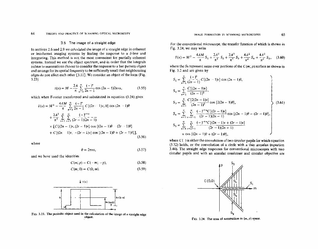
For the conventional microscope, the transfer function of which is shown inFig. 3.24, we may write
4AM 2A2 2A 2 4A 2 4A2lex) = M 2 - -- Sl + ~2 S2 + -2 S3 + -2 S4 + -2 S5' (3.60)
n n n n n
where the Ss represent sums over portions of the C(m; p) surface as shown inFig. 3.2 and are given by
00 (_)_
Sl = _~1 (2n _ 1) C{(2n - l)v} cos (2n - 1)8,
f C{ (2n - l)v}S2=_=1 (2n-l)2'
00 C{2(2n - l)v}S3 = L (2 _ )2 cos {2(2n - l)O}, (3.61)
"= 1 n 1
en 00 ( _ r+-c{(2r - l)v}S4 = _~1 r=~+l (2r _ 1)(2n _ 1) cos {(2n - 1)0 - (2r - 1)8},
00 00 (-r"C{(2n-l)v+(2r-l)v}S5 = I I
_=1 r=n+1 (2r -1)(2n -1)
x cos {(2n - 1)0 + (2r - l)e},
where C( ) is either the convolution of two circular pupils for which equation(3.32) holds, or the convolution of a circle with a thin annulus (equation3.44). The straight edge responses for conventional microscopes with twocircular pupils and with an annular condenser and circular objective are
(3.55)
(3.57)0= 2nvx,
where
and we have used the identities
2A a; (_)"
t(x) = M - - I -- cos (2n - 1)2nvx,n _=1 2n - 1
which when Fourier transformed and substituted in equation (3.24) gives
4AM a; (_)nl(x) = M 2 - -~ I -- C{(2n - l)v; O} cos (2n - 1)8
n _=1 2n - 1
2A 2 00 00 (_ r+n+ -2 I I --'---'---
n "=1 r=l (2r - 1)(2n - 1)
x [C{(2n - l)v, (2r - l)v} cos {(2n - 1)8 - (2r - 1)8}
+ C{(2n - l)v, -(2r - l)v} cos {(2n - 1)0 + (2r - l)e)],(3.56)
3.5 The image of a straight edge
In sections 2.6 and 2.9 we calculated the image of a straight edge in coherentor incoherent imaging systems by finding the response to a is-line andintegrating. This method is not the most convenient for partially coherentsystems. Instead we use the object spectrum, and in order that the integralsreduce to summations choose to consider the response to a bar pattern objectand arrange for its spatial frequency to be sufficiently small that neighbouringedges do not affect each other [3.11]. We consider an object of the form (Fig.3.23)
FIG. 3.23. The periodic object used in the calculation of the image of a straight edgeobject.
C(m;p)=C(-m; -p),
C(m; 0) = C(O; m).
t(x I
b
M=la+b
0'- -2-
x
(3.58)
(3.59)
c(O,O\~ s,-----....-:=====......&.__ m
~53
FIG. 3.24. The area of summation in (m, p) space.

66 THEORY AND PRACTICE OF SCANNING OPTICAL MICROSCOPY IMAGE FORMATION IN SCANNING MICROSCOPES 67
shown in Fig. 3.25 where the normalised distance v is given by equation(2.28). It should be noted that the image in the microscope with an annularcondenser is relatively poor. Turning now to the confocal microscope weobtain the much simpler result
l 2A 00 (-)"C {(2n - l)v} J2I(x) = M - --;- "~1 (2n _ 1) cos {(2n - l)O} (3.62)
when the object is defocused. There are thus advantages in using two equalpupils in a confocal microscope and we conclude this section by examiningthis case.
The impulse response for a confocal microscope with circular lenses hasvery weak side lobes. We know that the use of annular lenses results in asharper central peak and also an increase in the strength of the side lobes. It is
vFIG. 3.26. The straight edge image in a confocal microscope with equal annular
lenses.
3.6 The image of a phase edge
We have just discussed the image of a strong amplitude objec(and so we nowmove on to discuss the image of a strong phase object such as a phase edge
642o-2-4
11=0----
0·50·60708O·g0'96,
interesting to examine which of these two effects is dominant on the straightedge response for small central obscurations.
Figure 3.26 shows the results for various values of /" the ratio of the innerto the outer radii of the annuli [3.10]. Unfortunately, we can see that anyobscuration of the aperture degrades the performance. However the increasein depth of focus may warrant the use of a small obstruction. As the side lobeswith circular lenses are so small it still seems likely that there is someapodisation which would result in an improved straight edge response.
01
FIG. 3.25. The images of a straight edge object in various microscope arrangements.
>l-v;ZW
~
0·001 '-----!;3----!2~----!-1---!;0----!---:l:-2---!3---
v
0·01
The relevant responses are plotted in Fig. 3.25 and we see that the confocalmicroscope with two circular lenses gives a better image than a conventionalmicroscope but that a confocal microscope with one annular and one fullcircular lens gives the best response of all.
In a confocal microscope the use of two equal pupils results in anamplitude point spread function which is never negative and hence thestraight edge response under these conditions does not exhibit fringing even

68 THEORY AND PRACTICE OF SCANNING OPTICAL MICROSCOPY IMAGE FORMATION IN SCANNING MICROSCOPES 69
Following the methods of the previous section we are able to write for thepartially coherent conventional microscope [3.12]
where the phase change is abrupt and not small. The image of such an objectis of considerable importance in cell sizing and counting in biology andlinewidth measurement in integrated circuit technology, where the edge ofthe cell or the metallisation may be thought of as the phase step.
We consider an object whose amplitude transmittance is alternativelyexpjc/Jl and expj¢z, which may be written
[(1 + expjA¢) 2 00 (-)" 1
t(x) = expjc/Jl - ~ (1 - expj¢) I --cos (2n - 1)82 1t n=12n-1
(3.63)where A¢ = ¢z - ¢1 and () is as defined in equation (3.57).
(1 + cos A¢) 4 sin A¢ I {S}I(x) = C(O;O)- m I
2 1t
4- 2" (1 - cos A¢)[Sz + S3 + 2(S4 + S5)]
1t
where the Ss are given by equation (3.61).
(3.64)
.-__--n/4n/2n
'-0 ~__ n14
vFIG. 3.27. The intensity in the image of a phase edge in a conventional scanning
microscope.
~
FIG. 3.28. The intensity in the image of a phase edge in a confocal scanningmicroscope.
70 THEORY AND PRACTICE OF SCANNING OPTICAL MICROSCOPY IMAGE FORMATION IN SCANNING VlICROSCOPJCS 71
(3.65)
The expressions are again much simpler for the confocal microscope andmay be written
lex) = Ie -+:- e~pj~if; )QO) - [2(1 - e:pj~if;) SIJlz.
In a scanning microscope the intensity in the image depends on theproperties of both the objective lens and the collector lens. Assuming that theimpulse response of the latter is I1 z , the intensity is given by (equation 3.35)
(3.69)
which becomes smaller as ~if; increases as indicated in Fig. 3.28 reaching zerofor ~if; = re.
where hi is the impulse response of the lens and u, v the optical coordinates(equations 2.28 and 2.37), a constant multiplier being neglected. For the casewhen the lens has a circular pupil, Fig. 2.3 shows contours of equal intensityin the (u, v) plane. These results also show the intensity variation in the imageplane (v is now proportional to the distance in the image plane) of a pointobject placed a normalised distance u from the focal plane of the lens. For agiven object position the axial intensity in the image is given by
(3.70)
(3.71)
0) (sin U/4)4leu, = --- ,
u/4
oc
lm'(u) = 2re f l(u,l.')vdl.'.
o
which shows that if depth of field is defined in terms of the fall-off inmaximum intensity for a point image, the depth of field for the confocalmicroscope is reduced relative to that of a conventional microscope, thedifference not being very great.
There are, however, other associated properties which may be of practicalimportance. For instance we may investigate the variation in the integratedintensity for the image of our point source, which is a measure of the totalpower in the image [3.13]. This tells us how our microscope discriminatesagainst parts of the object not in the focal plane. We define the integratedintensity as
If both lenses are equal the intensity is simply the square of that in the Type 1microscope. For two circular pupils the contours of Fig. 2.3 arc still validexcept that the value of the intensity of the contour is squared. The axialintensity varies as
For the Type 1 microscope we know from Parseval's theorem that this isequal to the integral of the modulus squared of the effective (that is thedefocused) pupil function, and since the effect of the defocus is merely tointroduce a phase factor which disappears when the modulus is taken wecome to the conclusion that the integrated intensity does not fall off in theType 1 microscope. We may argue this equally from conservation of energy.Since our function leu, v) for the Type 1 microscope is the same as the intensity near the focus of a lens the integrated intensity is proportional to thepower crossing any plane perpendicular to the optic axis, and this must beconstant.
There is thus no discrimination of this kind in the Type 1 or conventionalmicroscopes, but this is not as bad as it seems as the d"focused imageeventually becomes a constant background which is rejected by the observer,although of course it does reduce contrast.
(3.67)
(3.66)
(3.68)
leu, v) = Il1du, vW
I (u, 0) = ei:/~4y.
3.7 Depth discrimination in scanning microscopes
A large depth of field is often a desirable property in a microscope, such aswhen observing rough surfaces. Equally, when observing thick biologicalspecimens in transmission it is often useful to limit the depth of field to avoidconfusion in interpretation of the micrographs.
If we observe the image of a single point in a conventional or Type Iscanning microscope as the object is taken out of the focal plane we find thatthe image broadens and that the axial intensity decreases. Either of thesequantities may be taken as an indicator of depth of field.
The intensity variation near the focus of a lens may be written as
The responses are plotted in Fig. 3.27 and 3.28. We see that the phase edgemanifests itself as a central dip in intensity which in all cases gives greatercontrast for the confocal microscope. The extreme case of a 1800 phase stepgives a limiting central intensity of 0·333 in the conventional microscopecompared with zero in the confocal instrument. The central intensity in theconfocal case may be written as
1(0) = cosz (~2if;)
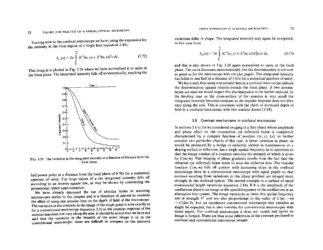
72 THEORY AND PRACTICE OF SCANNING OPTICAL MICROSCOPYIMAGE FORMATION IN SCANNING MICROSCOPES 73
FIG. 3.29. The variation in the integrated intensity as a function of distance from thefocal plane.
Turning noW to the confocal microscope we have, using the expression forthe intensity in the focal region of a single lens (equation 2.40),
This integral is plotted in Fig. 3.29 where we have normalised it to unity inthe focal plane. The integrated intensity falls off monotonically, reaching the
(3.73)I;nt(u) = 2n f (C 2 (u, v) + S2(U, v»)J6(v)u dv,
o
and this is also shown in Fig. 3.29 again normalised to unity at the focalplane. The curve decreases monotomically, but the discrimination is not nowso great as for the microscope with circular pupils. The integrated intensityhas fallen to one half at a distance of 1·05A for a numerical aperture of unity.
We have seen that using one annular lens in a confocal microscope reducesthe discrimination against objects outside the focal plane. If two annularlenses are used we would expect this discrimination to be further reduced. Inthe limiting case as the cross-section of the annulus is very small theintegrated intensity becomes constant as the impulse response does not thenvary .along the axis. !his is consistent with the claim of increased depth offield III a confocal microscope with two annular lenses [3.14].
3.8 Contrast mechanisms in confocal microscopy
In sections 3.1 to 3.6 we considered imaging of a thin object whose amplitudeand pha~e effect on the transmitted (or rel1ected) beam is completelycharactensed by a complex function of position t(x, y). Let us furtherconsider two particular objects of this type. A linear variation in phase, aswould be produced by a wedge of dielectric viewed in transmission or asloping surface in rel1ection, has a single spatial frequency in its spectrum sothat the image consists of a constant intensity the strength of which is givenby C(m, m). This imaging of phase gradients results from the fact that therefracted (or rel1ected) beam tends to miss the collector lens. The transferfunction C(m, m) falls off quicker with increasing slope in the confocalmicroscope than in a conventional microscope with equal pupils so thatcontrast ~esulting from variations in this phase gradient are imaged morestrongly In the confocal system. The second example is a surface of smallcosinusoidal height variations (equation 2.84). If h is the amplitude of theoscillations there is no image at the spatial frequency of the oscillations in anaberration free system. The image variations at twice this spatial frequencyare of strength b2 and are also proportional to the value of C(m; ~m)-. C(2m; 0). For an incoherent conventional microscope this vanishes asmight be ~xpected, but it also vanishes for conventional microscopes withequal pupils. For confocal microscopes it does not vanish and hence animage is formed. There are thus some differences in the contrast produced inconfocal and conventional microscope images.
varia.tions differ in shape. The integrated intensity may again be computed,III this case from
(3.72)
Type I
08
07
0·6:Z"'..
~ '".~0-5 t;:..
J!! '?:>..!:: ~." 0·4 'q.~ ~! 03
~
0·2
0·1
u
C1J
I;nt(u) = 2n f (C2(u, v) + S2(U, v)fv du.
o
half power point at a distance from the focal plane of 0'70). for a numericalaperture of unity. For large values of u the integrated intensity falls offaccording to an inverse square law, as may be shown by considering thegeometrical optics approximation.
We have already discussed the use of annular lenses in scanningmicroscopes earlier in this chapter and it is therefore of interest to examinethe effect of using one annular lens on the depth of field of the microscope.The variation in the intensity in the image of the single point is now exactly asfor a conventional microscope (equation 3.5) as the impulse response of theannular lens does not vary along the axis. It should be noted that we have notsaid that the variation in the breadth of the point image is as in theconventional microscope: these are difficult to compare as the intensity
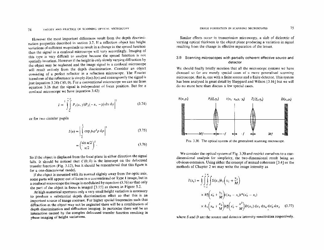
74 THEORY AND PRACTICE OF SCANNING OPTICAL MICROSCOPY IMAGE FORMATION IN SCANNING MICROSCOPES 75
However the most important differences result from the depth discrimination properties described in section 3.7. If a reflection object has heightvariations of sufficient magnitude to result in a change in the spread functionthen the signal in a confocal microscope will vary accordingly. Imaging ofthis type is very difficult to analyse because the spread function is notspatially invariant. However if the height is only slowly varying diffraction bythe object may be neglected and the image signal in a confocal microscopewill result entirely from the depth discrimination. Consider an objectconsisting of a perfect reflector in a reflection microscope. The Fouriertransform of the reflectance is simply b(m) b(n) and consequently the signal isjust (equation 3.24) C(O; 0). For a conventional microscope we can see fromequation 3.26 that the signal is independent of focus position. But for aconfocal microscope we have (equation 3.42)
Similar effects occur in transmission microscopy, a slab of dielectric ofvarying optical thickness in the object plane producing a variation in signalresulting from the change in effective separation of the lenses.
3.9 Scanning microscopes with partially coherent effective source anddetector
We should finally briefly mention that all the microscope systems we havedicussed so far are merely special cases of a more generalised scanningmicroscope, that is, one with a finite source and a finite detector. This systemhas been analysed in great detail by Sheppard and Wilson [3.16] but we willdo no more here than discuss a few special cases.
+00
I = Iff Pj(x, y)Pz( -x, - Y) dx dyr (3.74)D(X2.Y2)
~
or for two circular pupils
1
I(u)=\f eXP}UpZPdPr
a
(3.75)\1§l~c------Mf--- -f--'+-Of------ f--+~--Mf·-------l~
(3.76)FIG. 3.30. The optical system of the generalised scanning microscope.
So if the object is displaced from the focal plane in either direction the signalfalls. It should be noticed that C(O; 0) is the intercept on the defocusedtransfer function (Fig. 3.12), but it should be remembered that this figure isfor a one-dimensional model.
If the object is mounted with its normal slightly away from the optic axis,some parts will appear out offocus in a conventional or Type 1 image, but ina confocal microscope the image is modulated by equation (3.76) so that onlythe part of the object in focus is imaged [3.15] as shown in Figure 5.2.
At high numerical apertures only a very small height variation is necessaryto produce a substantial depth discrimination effect so that this is animportant source of image contrast. For higher spatial frequencies such thatdiffraction at the object may not be neglected there will be a combination ofdepth discrimination and diffraction imaging. In particular there will be aninteraction caused by the complex defocused transfer function resulting inphase imaging of height variations.
We consider the optical system of Fig. 3.30 and restrict ourselves to a onedimensional analysis for simplicity, the two-dimensional result being anobvious extension. Using either the concept of mutual coherence [3.4] or themethods of Chapter 2 we may write the image intensity as
+00
x hr(x~ + ~)t(xo - x,)t*(x~ - xJ
x I:z(XO + ~)h!(X~ + ~)D(Xz)dXl dXo~x~dxz (3.77)
where Sand D are the source and detector intensity sensitivities respectively.
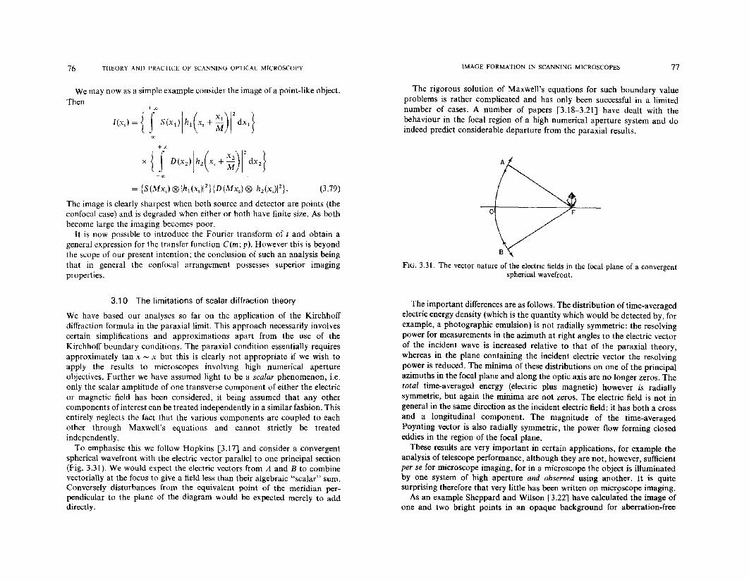
76 THEORY AND PRACTICE OF SCANNING OPTICAL MICROSCOPY IMAGE FORMATION IN SCANNING MICROSCOPES 77
We may now as a simple example consider the image of a point-like object.Then
+w
The rigorous solution of Maxwell's equations for such boundary valueproblems is rather complicated and has only been successful in a limitednumber of cases. A number of papers [3.18-3.21] have dealt with thebehaviour in the focal region of a high numerical aperture system and doindeed predict considerable departure from the paraxial results.
FIG. 3.31. The vector nature of the electric fields in the rocal plane of a convergentspherical wavefront.
+00
X {f D(X2)[h2(XS + ~)12 dX2}(3.79)
The image is clearly sharpest when both source and detector are points (theconfocal case) and is degraded when either or both have finite size. As bothbecome large the imaging becomes poor.
It is now possible to introduce the Fourier transform of t and obtain ageneral expression for the transfer function C(m; p). However this is beyondthe scope of our present intention; the conclusion of such an analysis beingthat in general the confocal arrangement possesses superior imagingproperties.
o F
3.10 The limitations of scalar diffraction theory
We have based our analyses so far on the application of the Kirchhoffdiffraction formula in the paraxial limit. This approach necessarily involvescertain simplifications and approximations apart from the use of theKirchhoff boundary conditions. The paraxial condition essentially requiresapproximately tan x ~ x but this is clearly not appropriate if we wish toapply the results to microscopes involving high numerical apertureobjectives. Further we have assumed light to be a scalar phenomenon, i.e.only the scalar amplitude of one transverse component of either the electricor magnetic field has been considered, it being assumed that any othercomponents of interest can be treated independently in a similar fashion. Thisentirely neglects the fact that the various components are coupled to eachother through Maxwell's equations and cannot strictly be treatedindependently.
To emphasise this we follow Hopkins [3.17] and consider a convergentspherical wavefront with the electric vector parallel to one principal section(Fig. 3.31). We would expect the electric vectors from A and B to combinevectorially at the focus to give a field less than their algebraic "scalar" sum.Conversely disturbances rrom the equivalent point of the meridian perpendicular to the plane of the diagram would be expected merely to adddirectly.
The important differences are as follows. The distribution of time-averagedelectric energy density (which is the quantity which would be detected by, forexample, a photographic emulsion) is not radially symmetric: the resolvingpower for measurements in the azimuth at right angles to the electric vectorof the incident wave is increased relative to that of the paraxial theory,whereas in the plane containing the incident electric vector the resolvingpower is reduced. The minima of these distributions on one of the principalazimuths in the focal plane and along the optic axis are no longer zeros. Thetotal time-averaged energy (electric plus magnetic) however is radiallysymmetric, but again the minima are not zeros. The electric field is not ingeneral in the same direction as the incident electric field; it has both a crossand a longitudinal component. The magnitude of the time-averagedPoynting vector is also radially symmetric, the power flow forming closededdies in the region of the focal plane.
These results are very important in certain applications, for example theanalysis of telescope performance, although they are not, however, sufficientper se for microscope imaging, for in a microscope the object is illuminatedby one system of high aperture and observed using another. It is quitesurprising therefore that very little has been written on microscope imaging.
As an example Sheppard and Wilson [3.22] have calculated the image ofone and two bright points in an opaque background for aberration-free

78 THEORY AND PRACTICE OF SCANNING OPTICAL MICROSCOPY
microscope systems at high numerical apertures. They find that the image ofa single point object remains radially symmetric even if the light source isplane polarised. For the conventional microscope the overall effects are quitesmall but the aperture of the condeser affects the image of the single point aswell as determining the degree of coherence in the imaging process. Theconfocal microscope is found to give a slightly broader image than thatpredicted by paraxial theory and the depth ofthe minima are reduced. This isin agreement with the practical observations of Brakenhoff et al. [3.23].
The general conclusion of this discussion is that further work on theelectromagnetic aspects of image formation would be immensely valuable butis likely to be very difficult. The fortunate fact is that for all its assumptionsthe scalar theory is able to predict to a surprising accuracy the effects that are
observed in practice.
Chapter 4
Imaging Modes of theScanning Microscope
References
-w
+w
I(x) = ff C(m; p)T(m)T*(p) exp 2nj(m - p)x dm dp (4.1)
as the intensity must be a real quantity.We now choose to ignore diffraction effects and consider an object whose
amplitude transmittance may be written as t(x) = a(x) exp N(x). If
4.1 General imaging considerations
It will be useful before we move on to discuss practical imaging schemes toreturn to our general partially coherent microscope of Chapter 3 and askwhat form the transfer function should take in order that the variations inimage intensity represent the required variation of object property. We recallthat for an object which varies only in the x-direction, the image intensitymay be written as
(4.3)
(4.2)
C(m;p) = 1
C(m; p) = C*(p; m)
then
from which we see that
[3.1] H. H. Hopkins and P. M. Barham (1950). Proc. Phys. Soc. 63, 72.[3.2] T. S. McKechenie (1972). Opt. Acta 19,729.[3.3] H. H. Hopkins (1953). Proc. R. Soc. A217, 408.[3.4] H. H. Hopkins (1951). Proc. R. Soc. A208, 263.[3.5] M. Born and W. Wolf (1975). "Principles of Optics." Pergamon, Oxford.[3.6] R. A. Lemons (1975). Ph.D. Thesis, Stanford University.[3.7] H. H. Hopkins (1955). Proc. R. Soc. A231, 91.[3.8] C. J. R. Sheppard and T. Wilson (1980). Phil. Trans. R. Soc. 295, 513.[3.9] C. J. R. Sheppard and T. Wilson (1979). Appl. Opt. 18, 7.
[3.10] C. J. R. Sheppard and T. Wilson (1979). Appl. Opt. 18, 3764.[3.11] T. Wilson and J. N. Gannaway (1979), Optik 54, 201.[3.12] T. Wilson (1981). Appl. Opt. 20, 3244.[3.13] C. 1. R. Sheppard and T. Wilson (1978). Opt. Lett. 3, 115.[3.14] C. J. R. Sheppard (1977). Optik 48,320.[3.15] D. K. Hamilton, T. Wilson and C. J. R. Sheppard (1981). Opt. Lett. 6, 625.[3.16] C. J. R. Sheppard and T. Wilson (1978). Opt. Acta. 25, 315.[3.17] H. H. Hopkins (1943). Proc. Phys. Soc. 55, 116.[3.18] B. Richards (1956). In "Symposium on Astronomical Optics and Related
Subjects" (Ed. Z. Kopal), p. 352. North Holland, Amsterdam.[3.19] B. Richards and E. Wolf (1956). Proc. Phys. Soc. B69, 854.[3.20] A. Boivin and E. Wolf (1965). Phys. Rev. B138, 1561.[3.21] A. Boivin, J. Dow and E. Wolf (1967). J. Opt. Soc. Am. 17, 1171.[3.22] C. J. R. Sheppard and T. Wilson (1982). Proc. R. Soc. A379, 145.[3.23] G. J. Brackenhoff, P. Blom and P. Barends (1979). J. Microsc. 117,219.
I(x)=W (4.4)
which is often referred to as a perfect amplitude image. On tpe other hand if
C(m;p) = mp
79
(4.5)
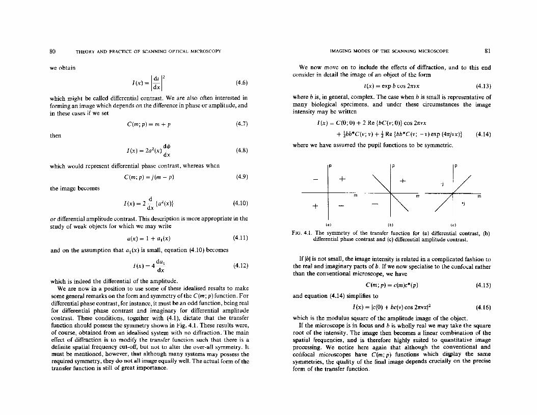
80 THEORY AND PRACTICE OF SCANNING OPTICAL MICROSCOPY IMAGING MODES OF THE SCANNING MICROSCOPE 81
We now move on to include the effects of diffraction, and to this endconsider in detail the image of an object of the form
we obtain
I
dt 1
2
[(X) = dx (4.6)t(x) = exp b cos 2nvx (4.13)
which might be called differential contrast. We are also often interested informing an image which depends on the difference in phase or amplitude, andin these cases if we set
where b is, in general, complex. The case when b is small is representative ofmany biological specimens, and under these circumstances the imageintensity may be written
C(m;p) = m + p
then
(4.7)
(4.8)
[(x) = C(O; 0) + 2 Re {bC(v; a)} cos 2nvx
+ tbb*C(v; v) + t Re {bb*C(v; -v)exp (4njvx)}
where we have assumed the pupil functions to be symmetric.
(4.14)
~~) +
or differential amplitude contrast. This description is more appropriate in thestudy of weak objects for which we may write
(4.15)
(4.16)
p
-j
m m
+j
(e)( bl
m
(0)
+
If Ibl is not small, the image intensity is related in a complicated fashion tothe real and imaginary parts of b. If we now specialise to the confocal ratherthan the conventional microscope, we have
C(m; p) = c(m)c*(p)
and equation (4.14) simplifies to
I (x) = Ic(O) + be(v) cos 2nvxl2
p p
which is the modulus square of the amplitude image of the object.If the microscope is in focus and b is wholly real we may take the square
root of the intensity. The image then becomes a linear combination of thespatial frequencies, and is therefore highly suited to quantitative imageprocessing. We notice here again that although the conventional andcOlifocal microscopes have C(m; p) functions which di!jplay the samesymmetries, the quality of the final image depends crucially on the preciseform of the transfer function.
FIG. 4.1. The symmetry of the transfer function for (a) differential contrast, (b)differential phase contrast and (c) differential amplitude contrast.
(4.12)
(4.10)
(4.11)
C(m; p) = j(m - p)
dI(x) = 2 dx {a 2 (x)}
which is indeed the differential of the amplitude.We are now in a position to use some of these idealised results to make
some general remarks on the form and symmetry ofthe C(m; p) function. Fordifferential phase contrast, for instance, it must be an odd function, being realfor differential phase contrast and imaginary for differential amplitudecontrast. These conditions, together with (4.1), dictate that the transferfunction should possess the symmetry shown in Fig. 4.1. These results were,of course, obtained from an idealised system with no diffraction. The maineffect of diffraction is to modify the transfer function such that there is adefinite spatial frequency cut-off, but not to alter the over-all symmetry. Itmust be mentioned, however, that although many systems may possess therequired symmetry, they do not all image equally well. The actual form of thetransfer function is still of great importance.
a(x) = 1 + a1(x)
and on the assumption that adx) is small, equation (4.10) becomes
da 1I(x)=4d:X
the image becomes
which would represent differential phase contrast, whereas when
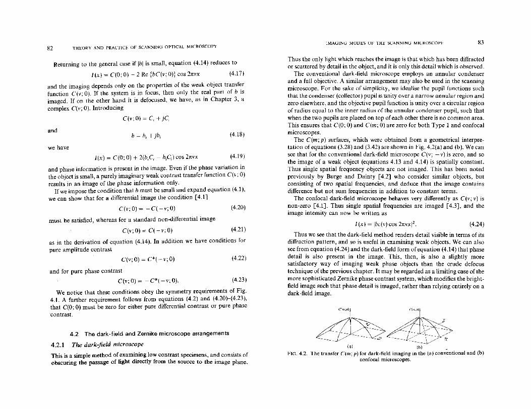
82 THEORY AND PRACTICE OF SCANNING OPTICAL MICROSCOPYIMAGING MODES OF THE SCANNING MICROSCOPE 83
as in the derivation of equation (4.14). In addition we have conditions forpure amplitude contrast
We notice that these conditions obey the symmetry requirements of Fig.4.1. A further requirement follows from equations (4.2) and (4.20}-(4.23),that C(O; 0) must be zero for either pure differential contrast or pure phasecontrast.
4.2 The dark-field and Zernike microscope arrangements
4.2.1 The dark-field microscope
This is a simple method of examining low contrast specimens, and consists ofobscuring the passage of light directly from the source to the image plane.
(4.24)l(x) = Ibc(v) cos 2nvxl 2•
Thus the only light which reaches the image is that which has been diffractedor scattered by detail in the object, and it is only this detail which is observed.
The conventional dark-field microscope employs an annular condenserand a full objective. A similar arrangement may also be used in the scanningmicroscope. For the sake of simplicity, we idealise the pupil functions suchthat the condenser (collector) pupil is unity over a narrow annular region andzero elsewhere, and the objective pupil function is unity over a circular regionof radius equal to the inner radius of the annular condenser pupil, such thatwhen the two pupils are placed on top of each other there is no common area.This ensures that C(O; 0) and C(m; 0) are zero for both Type 1 and confocalmicroscopes.
The C(m; p) surfaces, which were obtained from a geometrical interpretation of equations (3.28) and (3.42) are shown in Fig. 4.2(a) and (b). We cansee that for the conventional dark-field microscope C(v; -v) is zero, and sothe image of a weak object (equations 4.13 and 4.14) is spatially constant.Thus single spatial frequency objects are not imaged. This has been notedpreviously by Burge and Dainty [4.2] who consider similar objects, butconsisting of two spatial frequencies, and deduce that the image containsdifference but not sum frequencies in addition to constant terms.
The confocal dark-field microscope behaves very differently as C(v; v) isnon-zero [4.1]. Thus single spatial frequencies are imaged [4.3], and theimage intensity can now be written as
Thus we see that the dark-field method renders detail visible in terms of itsdiffraction pattern, and so is useful in examining weak objects. We can alsosee from equation (4.24) and the dark-field form of equation (4.14) that phasedetail is also present in the image. This, then, is also a slightly moresatisfactory way of imaging weak phase objects than the crude defocustechnique of the previous chapter. It may be regarded as a limiting case of themore sophisticated Zernike phase contrast system, which modifies the brightfield image such that phase detail is imaged, rather than relying entirely on adark-field image.
(Q) (b)_
FIG. 4.2. The transfer C(m; p) for dark-field imaging in the (a) conventional and (b)confocal microscopes.
(4.23)
(4.22)
(4.21 )
(4.20)
(4.19)
(4.18)b = br + jbi
l(x) = C(O; 0) + 2(brCr - biC;) cos 2nvx
C(v; 0) = C*( -v; 0)
and for pure phase contrast
C(v; 0) = - C*( -v; 0).
C(v;O) = -C(-v;O)
must be satisfied, whereas for a standard non-differential image
C(v; 0) = C( -v; 0)
and phase information is present in the image. Even if the phase v.ariation inthe object is small, a purely imaginary weak contrast transfer functIOn C(v; 0)results in an image of the phase information only.
If we impose the condition that b must be small and expand equation (4.1),we can show that for a differential image the condition [4.1]
we have
and
Returning to the general case if Ibl is small, equation (4.14) reduces to
1(x) = C(O; 0) + 2 Re {bC(v; O)} cos 2nvx (4.17)
and the imaging depends only on the properties of the weak object transf~r
function C(v; 0). If the system is in focus, then only the real part of b IS
imaged. If on the other hand it is defocused, we have, as in Chapter 3, acomplex C(v; 0). Introducing
C(v; 0) = Cr + jCi
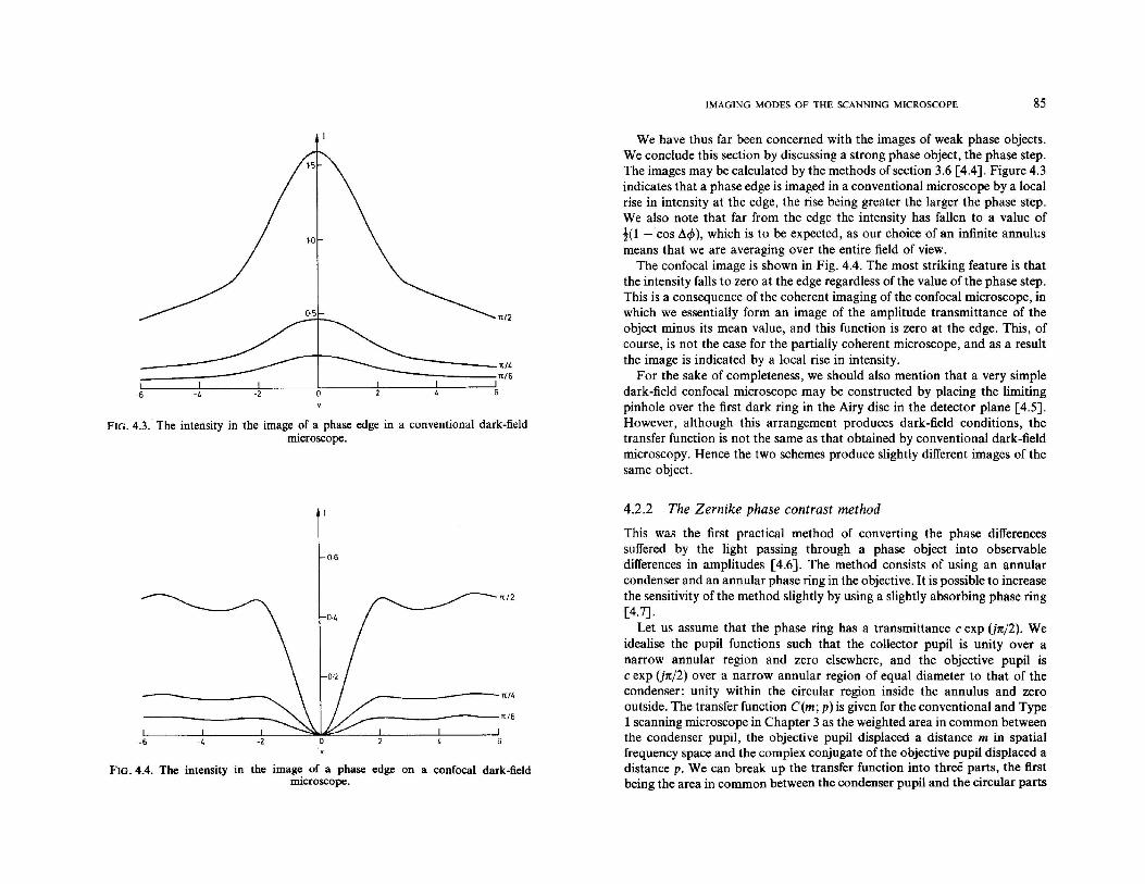
IMAGING MODES OF THE SCANNING MICROSCOPE 85
FIG. 4.3. The intensity in the image of a phase edge in a conventional dark-fieldmicroscope.
-6 -4 -2
n/2
------n/J,-------n/6
We have thus far been concerned with the images of weak phase objects.We conclude this section by discussing a strong phase object, the phase step.The images may be calculated by the methods of section 3.6 [4.4]. Figure 4.3indicates that a phase edge is imaged in a conventional microscope by a localrise in intensity at the edge, the rise being greater the larger the phase step.We also note that far from the edge the intensity has fallen to a value oft(1 - cos LlcP), which is to be expected, as our choice of an infinite annulusmeans that we are averaging over the entire field of view.
The confocal image is shown in Fig. 4.4. The most striking feature is thatthe intensity falls to zero at the edge regardless ofthe value of the phase step.This is a consequence of the coherent imaging of the confocal microscope, inwhich we essentially form an image of the amplitude transmittance of theobject minus its mean value, and this function is zero at the edge. This, ofcourse, is not the case for the partially coherent microscope, and as a resultthe image is indicated by a local rise in intensity.
For the sake of completeness, we should also mention that a very simpledark-field confocal microscope may be constructed by placing the limitingpinhole over the first dark ring in the Airy disc in the detector plane [4.5].However, although this arrangement produces dark-field conditions, thetransfer function is not the same as that obtained by conventional dark-fieldmicroscopy. Hence the two schemes produce slightly different images of thesame object.
0·6
n/2
_--------n/4..._---------n/6
-6 -4
FIG. 4.4. The intensity in the image of a phase edge on a confocal dark-fieldmicroscope.
4.2.2 The Zernike phase contrast method
This was the first practical method of converting the phase differencessuffered by the light passing through a phase object into observabledifferences in amplitudes [4.6]. The method consists of using an annularcondenser and an annular phase ring in the objective. It is possible to increasethe sensitivity of the method slightly by using a slightly absorbing phase ring[4.7].
Let us assume that the phase ring has a transmittance c exp U1t/2). Weidealise the pupil functions such that the collector pupil is unity over anarrow annular region and zero elsewhere, and the objective pupil isc exp U1t/2) over a narrow annular region of equal diameter to that of thecondenser: unity within the circular region inside the annulus and zerooutside. The transfer function C(m; p) is given for the conventional and Type1 scanning microscope in Chapter 3 as the weighted area in common betweenthe condenser pupil, the objective pupil displaced a distance m in spatialfrequency space and the complex conjugate of the objective pupil displaced adistance p. We can break up the transfer function into three parts, the firstbeing the area in common between the condenser pupil and the circular parts

86 THEORY AND PRACTICE OF SCANNI]'.;G OPTICAL MICROSCOPY IMAGING MODES OF THE SCANNING MICROSCOPE 87
of the objective pupils, the second between the condenser pupil and theannular parts of the objective pupils, and the third part between thecondenser pupil and the circular part of one objective pupil and the annularpart of the other. The first part is real and its form is shown in Fig. 4.5(a). Form = 0 or p = 0 the transfer function is zero, but for small values of m and P, ifthey are both of the same sign, it quickly rises to a value corresponding to halfthe area of the annulus. Thereafter, for small p, the transfer function falls offas cos -I (mAfI2a). If m and p are of opposite sign, the transfer function iszero. The second part of the transfer function is also real (Fig. 4.5(b)). Thethree annuli intersect only if two annuli are coincident, that is, along them = 0, p = 0, or m = p lines. The value at m = 0, p = 0 is eZ times the area ofthe annulus, this being normalised to unity in the diagrams. The third part ofthe transfer function is imaginary. In Fig. 4.5(c) we have shown thecontribution from the convolution of a circle and an annulus for m = 0 andp = O. There is also a very small non-zero value of the transfer function forother values of m and p if the width of the annulus is non-zero, but we haveneglected this for the sake of simplicity.
We consider imaging of a weak object of the form given by equation (4.13)
such that equation (4.19) applies. The zero spatial frequency component inthe image is taken to have a relative magnitude of unity, as given by Fig.4.5(b). The real part of the cosinusoidal component is imaged with a strengthgiven by the values of C(m; 0) in Fig. 4.5(b). Similarly, the imaginarycomponent is imaged with a strength given by the value of C(m; 0) in Fig.4.5(c). The properties of the image of a weak object are as follows:
i. The spatial frequency cut-off is the same as for a conventionalmicroscope with full illumination, but the spatial frequency response forphase information is better in the Zernike arrangement than for aconventional amplitude contrast microscope.ii. As Born and Wolf state, the intensity distribution produced in theimage is directly proportional to the phase changes introduced by theobject. This follows from equation (4.17), with the condition that the phasechange is small.iii. The contrast of the phase information is enhanced by a factor lierelative to the constant term.iv. Weak amplitude information is imaged poorly, with fringes and lowcontrast.
FIG. 4.5. The transfer function elm; p) for Zemike phase contrast imaging in aType 1 scanning microscope.
C(m; p) = {PZa(m) ® P If(m)}{ PZa(p) ® PIf(P) + {PZa(m) @ P la(m)}
X {PZa(p)@ P1a(p)} + j {PZa(m)@ P la (m)}{ PZa(p) ® PIf(P)}
- {PZa(m)@Plf(m)}{PZa(p)@Pla(P)}. (4.25)
The first two terms here representing the real part are shown in Fig. 4.6(a)and (b). We note that these pupil functions ensure that C(O; 0), C(m; 0),C(p; 0), etc. are all zero in Fig. 4.6(b). The imaginary part is also made up of
The Zernike method suffers from a number of disadvantages, although it isa very convenient way of showing up phase information. The ideal geometryof the phase plate depends on the particular form of the specimen, there beingfour variables to consider: the diameter and thickness of the annulus, and thetransmission and phase delay of the phase plate. De and Mondal [4.8] havediscussed the effect of varying the thickness of the annulus with constantouter diameter. As might be expected, the cut-off frequency increases as theannulus width decreases. Mondal and Slansky [4.9] have considered whathappens as the diameter of the annulus is varied with constant thickness. Thecut-off frequency is greater for larger diameter annuli, but contrast isreduced.
For the confocal microscope, the transfer function is again made up ofthree parts [4.1]. If we represent the annular collector pupil by PZa and theobjective PI by P If + jP la' where P If represents the full part and PIa theannular part, we can write
C(miP)
1C
C{miP)1-c2
C(m;p)
1
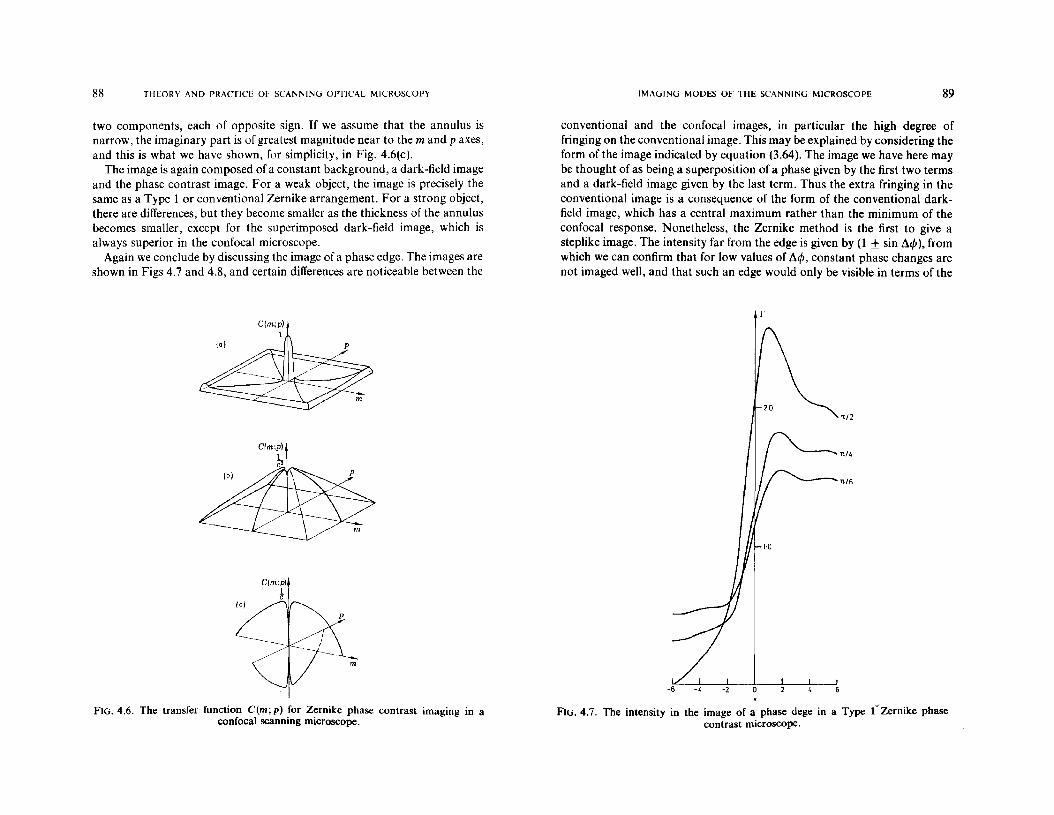
88 THEORY AND PRACTICE OF SCANNING OPTICAL MICROSCOPY IMAGING MODES OF THE SCANNING MICROSCOPE 89
two components, each of opposite sign. If we assume that the annulus isnarrow, the imaginary part is of greatest magnitude near to the m and p axes,and this is what we have shown, for simplicity, in Fig. 4.6(c).
The image is again composed of a constant background, a dark-field imageand the phase contrast image. For a weak object, the image is precisely thesame as a Type 1 or conventional Zernike arrangement. For a strong object,there are differences, but they become smaller as the thickness of the annulusbecomes smaller, except for the superimposed dark-field image, which isalways superior in the confocal microscope.
Again we conclude by discussing the image of a phase edge. The images areshown in Figs 4.7 and 4.8, and certain differences are noticeable between the
C(m;p)1
FIG. 4.6. The transfer function C(rn; p) for Zernike phase contrast imaging in aconfocal scanning microscope.
conventional and the confocal images, in particular the high degree offringing on the conventional image. This may be explained by considering theform of the image indicated by equation (3.64). The image we have here maybe thought of as being a superposition of a phase given by the first two termsand a dark-field image given by the last term. Thus the extra fringing in theconventional image is a consequence of the form of the conventional darkfield image, which has a central maximum rather than the minimum of theconfocal response. Nonetheless, the Zernike method is the first to give asteplike image. The intensity far from the edge is given by (1 ± sin /it/J), fromwhich we can confirm that for low values of /it/J, constant phase changes arenot imaged well, and that such an edge would only be visible in terms of the
Tt/2
Tt/~
"'---Tt/6
v
FIG. 4.7. The intensity in the image of a phase dege in a Type (Zernike phasecontrast microscope.

90 THEORY AND PRACTICE OF SCANNING OPTICAL MICROSCOPY IMAGING MODES OF THE SCANNING MICROSCOPE 91
fringing. We also note that, unlike the dark-field case, the method is sensitiveto the direction of change of phase, i.e. the sign of !'1cP is important. It isinteresting that in the limiting case of !'1cP = rr (where the average value of theamplitude is zero), the image is exactly the same as would be obtained in adark-field microscope.
- 20Tt/2
nf6
of the image [4.8]. All these methods have the disadvantage that the image ofa sharp discontinuity exhibits a distinct halo, which may extend for manyresolution elements [4.9]. The presence of this fringing is inherent in themethod, as absolute phase is not imaged. Thus a phase edge, for example,would not be visible without fringing. We might think that the fringing iscaused mainly by the annular region of the pupil, as might be expected forimaging with an annular lens, but in fact this is not the principal mechanism.
The haloes are produced irrespective of the degree of coherence of theimaging system. For the sake of clarity, then, we restrict ourselves to acoherent system, although this means that the results will generally not beapplicable near the edge [4.10].
A straight-edge object is defined to have an amplitude transmittance
t(x', y') = 1; x' > 0
= 0; x' < 0; \Jy' (4.26)
(4.30)
(4.28)
(4.29)
(4.27)
0< Iml < a
a < Iml < b
C(m) = d exp U1r/2)
= 1
for which
I(x) = ~ I c(O) +j~ fc~m) exp (21rjmx) dm 1
2
.
In a conventional coherent microscope, the coherent transfer function, C(m),is given by the pupil function of the lens which for a Zernike system may bewritten as
T(m, n) = ~ {l5(m) +~}2 Jrrm
and thus the image, which is only a function of x, becomes
and Si is the sine integral.The image now consists of a fine structure of fringes superimposed on a
slowly varying background, the scale of the fine structure being determinedby the outer radius of the lens pupil. The limiting case as b becomes muchlarger than (I describes the slowly varying background as
I(X)={I-~Si(2rraX)}\ x#O. (4.31)
where b is related to the outer radius of the lens and a to the radius of thecentral phase disc, which has a transmittance d. By setting d = 0, wereduce to the case of the dark-field microscope [4.11]. We therefore have
11 2 1
2
I(x) = 4 dj + -; {(dj - 1) Si (2rrax) + Si (21rbx)}
FIG. 4.8. The intensity in the image of a phase edge in a confocal Zernike phasecontrast microscope.
4.2.3 The halo effect in dark-field and Zernike phase contrast microscopy
Our discussion so far has been concerned exclusively with the images of weakphase objects. While such objects are representative of a great manybiological specimens, we must now turn our attention to strong objects, andthe phase edge in particular. This is not a pure abstraction: it may, forexample, reasonably model the edge of a biological cell.
The dark-field and Zernike schemes are two examples of a whole range ofimaging techniques which rely on the presence of a spatial filter in the Fouriertransform plane to remove or modify the zero spatial frequency component

92 THEORY AND PRACTICE OF SCANNING OPTICAL MICROSCOPY IMAGING MODES OF THE SCANNING MICROSCOPE 93
Intensity
(4.34)
where 0 and R refer to the object and reference beam respectively. Ifwe now
i. The annular source must be of sufficient area to provide a suitable levelof illumination. This is particularly important in conventionalmicroscopes.ii. The thickness of the annular phase ring must be sufficiently largecompared to the annular source to allow easy alignment.iii. There is a fundamental limit set by the requirement that the thicknessof the annuli must be large compared to the wavelength.
In practice, the dimensions are usually such that the halo does not fill theentire field of view.
In phase contrast or dark-field, we are imaging a change relative to someaverage background amplitude. The effects which we have discussed are aresult of the fact that the averaging is performed over some finite region of theobject. The principles are the same for the case of edge enhancement using asplit pupil in which one half experiences a phase change relative to the other,as the transition region must be of non-zero width and cannot be alignedexactly with the zero spatial frequency position. The Schlieren method, inwhich one half of the pupil is obscured, behaves similarly, as in practice it isimpossible to obscure the zero spatial frequency component without alsoobscuring some of the lower spatial frequencies.
4.3 Interference microscopy
The basic criterion for a source in a scanning optical microscope is that itshould be sufficiently bright to give a reasonable signal to produce a goodpicture. Hence a laser is now usually used. A further advantage of using alaser is that the coherence length of the beam makes the construction of aninterference microscope relatively easy, as the optical path lengths in the twoarms do not have to be made equal within such close tolerances.
We will begin by discussing the general scheme of Fig. 4.10, in which lighttransmitted through two dissimilar parallel optical paths illuminates twophotodiodes which are arranged to give signals corresponding to the sum anddifference of the amplitudes of the two beams [4.1]. The arrangement isanalogous to the Mach-Zehnder interferometer. Thus, each detector essentially gives
superimposed onto the halo, whereas if it is very narrow, we obtain imagingsomewhat similar to that in dark-field. If we choose to make the halo as wideas possible, this width is limited by three major factors:
(4.32)
~1/2b
t(x', y') = exp j1JI ; x' > 0
= expj1J2; x' < 0
- ~112a--1
2/d sinCH»)
X
FIG. 4.9. A sketch showing the variation in intensity in the image of a phase edge inthe Zernike phase contrast microscope.
The halo is therefore the result of diffraction by the finite size of the centraldisc. The extreme case of a tending to zero results in a halo that does notdecay within the extent of the image, which then becomes a central dip on auniform background. Ifwe now move on to consider a phase edge which maybe defined as
we can combine the previous results to obtain an expression for the halo, inthis case (when b » a) as
lex) = Icos e21J) + :d sin C~:)[(dj -1) Si (2nax) + ~JI2. (4.33)
The essential features are sketched in Fig. 4.9, where the fringes have beenomitted for clarity.
For the partially coherent Zernike arrangement employing an annularsource and phase ring, the fringes are almost absent, and they could befurther reduced by apodisation of the phase ring. The resolution is principallydetermined by the sum of the outer aperture of the annular source and theaperture of the objective. The width of the halo is determined by theminimum spatial frequency transmitted without change of phase, that is, bythe difference between the outer aperture of the annular source and the inneraperture of the phase ring (or vice versa). In practice, we should aim for thewidth of the halo to be either as wide or as narrow as possible. If it is verywide, the image gives an intensity change proportional to the change of phase
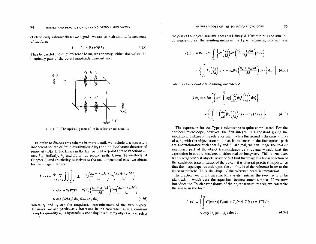
94 THEORY AND PRACTICE OF SCANNING OPTICAL MICROSCOPY IMAGING MODES OF THE SCANNING MICROSCOPE 95
electronically subtract these two signals, we are left with an interference termof the form
the part of the object transmittance that is imaged.lfwe subtract the sum anddifference signals, the resulting image in the Type 1 scanning microscope is
Thus by careful choice of reference beam, we can image either the real or theimaginary part of the object amplitude transmittance.
whereas for a confocal scanning microscope
1+ - L ~ Re (OR*) (4.35)
00
I(X)=4Re[{w* Jh!C~)h2*G~)dX~}
00
x{ JhIC~)h~C~)tI(X-Xo)dxo}J-x
(4.37)
(4.38)
The expression for the Type 1 microscope is quite complicated. For theconfocal microscope, however, the first integral is a constant giving themodulus and phase of the reference bcam, while the second is the convolutionof hlh~ with the object transmittance. If the lenses in the first optical pathare aberration-free such that hi and h'l are real, we can image the real orimaginary part of the object transmittance by choosing w such that theexpression in square brackets is either real or imaginary. This is true evenwith strong contrast objects, as is the fact that the image is a linear function ofthe amplitude transmittance of the object. It is of great practical importancethat the image depends only upon the amplitude of the reference beam at thedetector pinhole. Thus, the shape of the reference beam is immaterial.
In practice, we might arrange for the elements in the two paths to beidentical, in which case the equations become much simpler. If we nowintroduce the Fourier transforms of the object transmittances, we can writethe image in the form
FIG. 4.10. The optical system of an interference microscope.
In order to discuss this scheme in more detail, we include a transverselyincoherent source of finite distribution S(xd and an incoherent detector ofsensitivity D(X2)' The lenses in the first path have point spread functions hiand h~; similarly, h2 and h2 in the second path. Using the methods ofChapter 3, and restricting ourselves to the one-dimensional case, we obtainfor the image intensity
+00
-00
x t.(x - x )t'!'(x _ x' )hc(xo + X2/M)h"*(X~ + X 2/M)I 0 J 0, i.d J Ad
x S(xdD(X2) dX I dxo dx~ dX2 (4.36)
where t l and t2 are the amplitude transmittances of the two objects.However, we are particularly interested in the case when t 2 is a constantcomplex quantity w, as by carefully choosing this dummy object we can select
+w
x exp 2nj(m - p)x dm dp (4.39)
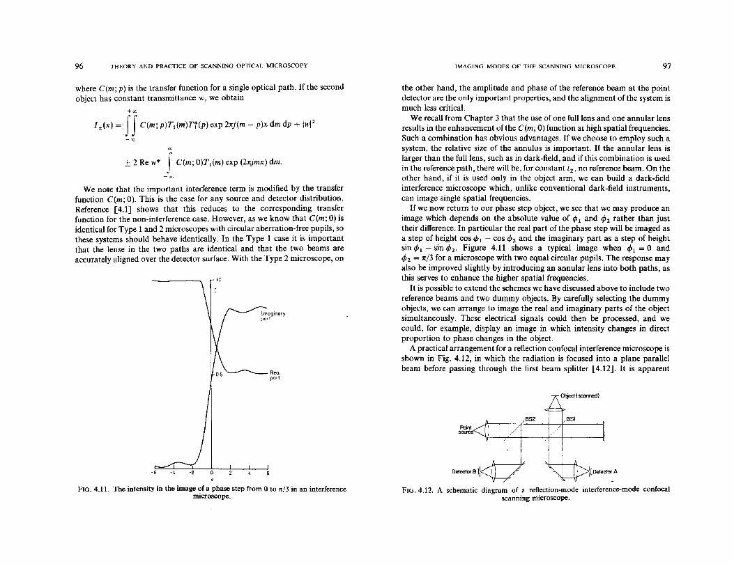
96 THEORY AND PRACTICE OF SCANNING OPTICAL MICROSCOPY IMAGING MODES OF THE SCANNING MICROSCOPE 97
BS2 BSI
Object (scanned)
:lDetector A
Pointsource
the other hand, the amplitude and phase of the reference beam at the pointdetector are the only important properties, and the alignment of the system ismuch less critical.
We recall from Chapter 3 that the use of one full lens and one annular lensresults in the enhancement of the C(m; 0) function at high spatial frequencies.Such a combination has obvious advantages. If we choose to employ such asystem, the relative size of the annulus is important. If the annular lens islarger than the full lens, such as in dark-field, and if this combination is usedin the reference path, there will be, for constant t2 , no reference beam. On theother hand, if it is used only in the object arm, we can build a dark-fieldinterference microscope which, unlike conventional dark-field instruments,can image single spatial frequencies.
If we now return to our phase step object, we see that we may produce animage which depends on the absolute value of 4JI and 4J2 rather than justtheir difference. In particular the real part of the phase step will be imaged asa step of height cos 4JI - cos 4J2 and the imaginary part as a step of heightsin 4JI - sin 4J2' Figure 4.11 shows a typical image when 4JI = 0 and4J2 = rc/3 for a microscope with two equal circular pupils. The response mayalso be improved slightly by introducing an annular lens into both paths, asthis serves to enhance the higher spatial frequencies.
It is possible to extend the schemes we have discussed above to include tworeference beams and two dummy objects. By carefully selecting the dummyobjects, we can arrange to image the real and imaginary parts of the objectsimultaneously. These electrical signals could then be processed, and wecould, for example, display an image in which intensity changes in directproportion to phase changes in the object.
A practical arrangement for a reflection confocal interference microscope isshown in Fig. 4.12, in which the radiation is focused into a plane parallelbeam before passing through the first beam splitter [4.12]. It is apparent
± 2 Re w* I C(m; 0)T1{m) exp (2rcjmx) dm.
+00
I ±(x) = iIIC(m; p)T1{m)Tf(p) exp 2rcj{m - p)x dm dp + Iwl2
-00
where C(m; p) is the transfer function for a single optical path. If the secondobject has constant transmittance w, we obtain
-6
We note that the important interference term is modified by the transferfunction C(m; 0). This is the case for any source and detector distribution.Reference [4.1] shows that this reduces to the corresponding transferfunction for the non-interference case. However, as we know that C{m; 0) isidentical for Type 1 and 2 microscopes with circular aberration-free pupils, sothese systems should behave identically. In the Type 1 case it is importantthat the lense in the two paths are identical and that the two beams areaccurately aligned over the detector surface. With the Type 2 microscope, on
FIG. 4.11. The intensity in the image of a phase step from 0 to 1[/3 in an interferencemicroscope.
FIG. 4.12. A schematic diagram of a reflection-mode interference-mode confocalscanning microscope.

98 THEORY ANO PRACTICE OF SCANNING OPTICAL MICROSCOPY IMAGING MOOES OF THE SCANNING MICROSCOPE 99
from equations (4.34) and (4.35) that the sum signal Is consists of the normalconfocal image 101 2 superimposed on a constant IRI 2
, while the differencesignal, 1o leaves a pure interference image. Because this signal can bebidirectional, an electronic offset is added to it, producing, for displaypurposes, a signal which is always positive-going.
Figure 4.13 shows the image of an area of a TEM grid formed just from thesignal 1A' showing a series of fringes representing variations in surface heightsuperimposed on the confocal image. Local deformations of the fringescorrespond to surface detail. Figure 4.14 shows a comparison confocal imageof the same region. A deep scratch is clearly visible in both images.
object, but it is also possible to use a reference beam which passes through thespecimen as well [4.1]. For example, in a differential interference microscopethe same optics are used to focus light simultaneously on two adjacent points,the beam being split into two and recombined using birefringent elements.Let us assume that the objects as seen by the displaced beams are
t](x) = t(x - .1); t 2(x) = t(x +.1) (4.40)
which, by applying the shift theorem give for the Fourier transforms gives
T](m) = T(m) exp (-2njm.1); T 2(m) = T(m) exp (2njm.1). (4.41)
FIG. 4.13. The single detector interference image, I" of part of a TEMgrid using a He-Ne (wavelength 632·8nm) laser and a 0'5 numerical aperture
objective.
FIG. 4.14. Confocal image of the same'region as Fig. 4.13.
FIG. 4.15. The sum image, Is, from thetwo-detector interference microscope.Note the similarity to Fig. 4.14 and [he
absence of fringes.
FIG. 4.16. Difference image, I D' fromthe two-detector interference microscope, showing the fringe pattern without the superimposed confocal image.
The images which have been shown so far have been produced using asingle detector. The effects of using the two-detector system will now bedescribed. The interference image, 1B , from the second detector is similar tolA' except that the fringes are displaced by half a period, so that the signal Isproduced by addition should exhibit no fringes. In practice small optimisations of the relative gains and pinhole alignments are needed to achieve theoptimum results shown in Fig. 4.15 which is, as predicted, similar to theconfocal images of Fig. 4.14. Figure 4.16 then records the image from thedifference signal 10' with no further adjustments made to the system, andshows the fringe pattern without the superimposed confocal image. Eventhough as equation (4.35) predicts, the brightness of the fringes is modulatedby the reflectivity of the object, their positions are now much more easilyobserved, allowing the surface topography to be deduced more precisely.
The arrangements discussed so far use a reference beam external to the
Substituting in equation (4.39), and assuming that the signals are added witha phase difference 2cP, we have
+oc
I(x) = fJC(m; p)T(m)T*(p) cos (2nm.1 ~ cP)
x cos (2np - cP) exp 2nj(m - p)x dm dp (4.42)
where w,e have neglected a constant phase factor. If .1 is very small, the casewhen cP IS zero reduces to the conventional image of t, whereas when cP = nl2we may write
+00
1(x) = ff C(m; p)T(m)T*(p)4n2 .12mp exp 2nj(m - p*x dm dp. (4.43)
-00

100 THEORY AND PRACTICE OF SCANNING OPTICAL MICROSCOPY IMAGING MODES OF THE SCANNING MICROSCOPE 101
This may be written in the form of an effective transfer function
This effective transfer function satisfies the conditions of equations (4.20),(4.23) and Fig. 4.1 for differential phase contrast imaging of weak objects. Onthe other hand, it also has the property that Ceff(m; 0) = 0, so that weakobjects are not imaged at all. The imaging of weak objects may be improvedby setting
+00
I(x) = ff Ceff(m; p)T(m)T*(p) exp 2nj(m - p)x dm dp
where
n,p=--b
2
which modifies the effective transfer function to
Ceff(m; p) = C(m; p)(2nt\m + b)(2nt\p + b)
(4.44)
(4.45)
(4.46)
(4.47)
unity magnitude. The image is then given by equation (4.39), and phaseinformation may be obtained by suitable choice of the relative phase of thetwo signals.
4.4 Differential microscopy
Although a great deal of useful information may be obtained by studying amicroscope image in which the contrast depends on the variation of either theamplitude (absorption) or phase ofthe amplitude transmittance of the object,it is often desirable to form an image which indicates how these quantitiesvary spatially across the object. This differential imaging is extremely useful,for example, in visualising the shape of an object or enhancing the contrastof point features.
There are many practical schemes of obtaining this contrast, and they maybe divided into two main types. In the first, the differentiation is achieved bydifferentially detecting the radiation which has probed the object, whilst inthe second a differential probe is employed.
4.4.1 Differentiation in the detector plane
We begin by describing a powerful scheme proposed initially by Dekkers andde Lang [4.13] to obtain phase information in the scanning transmissionelectron microscope without having to resort to the cruder methodsinvolving the defocus and spherical aberration of the electron lenses. Thebasic principle may be explained by considering a weak object of the form ofequation (4.13) in the STEM configuration of Fig. 4.17, such that the fieldjust after the object may be written as
The image of an object of the form
t(x) = 1 + jb; cos 2nvx
is given by
I(x) = 1 - 2b{2n:v) sin 2nvx + tbfC(v; V){ 1 +Cn:
vYl
+tbfC(v; -V){1-Cn:vYlcos4nvx.
For imaging over a wide range of spatial frequencies we may take
b = 2nt\v.
(4.48)
(4.49)
(4.50)
U(x, xo) = (1 + bcos 2nv(xo - x))h(xo) (4.51)
The weaker the object modulation, the greater is the range of spatialfrequencies that is imaged linearly. It is therefore important to provide somemeans for the fine tuning of the relative phase of the two beams in thedifferential interference microscope.
As a second example of a system with a reference beam which passesthrough the object, we should mention the method of axial separation, inwhich the reference· beam is focused at a point on the axis outside thespecimen. Because this reference beam is defocused as it traverses the object,we may assume that the effective specimen seen by the reference beam is of
-d-
FIG. 4.17. The STEM configuration.
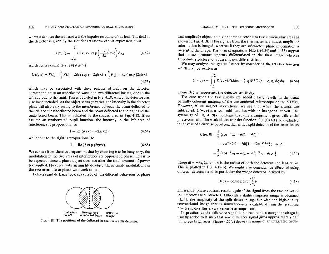
102 THEORY AND PRACTICE OF SCANNING OPTICAL MICROSCOPY IMAGING MODES OF THE SCANNING MICROSCOPE 103
where x denotes the scan and h is the impulse response of the lens. The field atthe detector is given by the Fourier transform of this expression, thus
b bU(~,x) = P(O + 2P(~ - Adv)exp (-2njvx) + 2P(~ + Adv)exp (2njvx)
(4.53)
00
f (-2nj)U (x, 0 = U (x, xu) exp -----;;t xu~ dxu
which for a symmetrical pupil gives
(4.52)
and amplitude objects to divide their detector into two semicircular areas asshown in Fig. 4.18. If the signals from the two halves are added, amplitudeinformation is imaged, whereas if they are subtracted, phase information ispresent in the image. The form of equations (4.23), (4.54) and (4.55) suggestthat phase structure appears differentiated in the final image whereasamplitude structure, of course, is not differentiated.
We may analyse this system further by considering the transfer functionwhich may be written as
+00
C(m; p) = ff D(~, I/)P(Adm -~, tj)P*(Adp -~, tj) d~ d'7 (4.56)
which may be associated with three patches of light on the detectorcorresponding to an undeflected wave and two diffracted beams, one to theleft and one to the right. This is depicted in Fig. 4.18, where the detector hasalso been included. As the object scans (x varies) the intensity in the detectorplane will also vary owing to the interference between the beam deflected tothe left and the undeflected beam and the beam deflected to the right and theundeflected beam. This is indicated by the shaded area in Fig. 4.18. If weassume an unaberrated pupil function, the intensity in the left area ofinterference is proportional to
where D(~, 1/) represents the detector sensitivity.The case when the two signals are added clearly results in the usual
partially coherent imaging of the conventional microscope or the STEM.However, if we neglect aberrations, we see that when the signals aresubtracted, C(m; p) is a real, odd function with an hexagonal cut-off. Thesymmetry of Fig. 4.19(a) confirms that this arrangement gives differentialphase contrast. The weak object transfer function C(m; 0) may be evaluatedin the case of a circular pupil together with a split detector of the same size as
Deflection Detector and Deflectionto left undeflected beam to right
FIG. 4.18. The positions of the deflected beams on a split detector.
We can see from these two equations that by choosing b to be imaginary, themodulation in the two areas of interference are opposite in phase. This is tobe expected, since a phase object does not alter the total amount of powertransmitted. However, with an amplitude object the intensity modulations inthe two areas are in phase with each other.
Dekkers and de Lang took advantage of this different behaviour of phase
1 + Re {b exp (-2njvx)}
while that to the right is proportional to
1 + Re {b exp (2njvx)}.
(4.54)
(4.55)
2C(m; 0) = - {cos- 1 m - m(1 _ m2)112
n
- cos- 1 2m - 2m[1 - (2m)2]1/2}; m < ~
2=;-{cos- 1 m-m(l-m2)112}; m>~ (4.57)
where m= m;.d/2a, and a is the radius of both the detector and lens pupil.This is plotted in Fig. 4.19(b). We might also consider the effects of usingdifferent detectors and in particular the wedge detector, defined by
D(O = const ~ circ (~} (4.58)
Differential phase contrast results again if the signal from the two halves ofthe detector are subtracted. Although a slightly superior image is obtained[4.14], the simplicity of the split detector together with the high-qualityconventional image that is simultaneously available during the scanningprocess makes this a very versatile arrangement.
In practice, as the difference signal is bidirectional, a consJant voltage isusually added to it such that zero difference signal gives approximately halffull screen brightness. Figure 4.20(a) shows the image of an integrated circuit

104 THEORY AND PRACTICE OF SCANNING OPTICAL MICROSCOPY
A
B
m
elm) 0.5(0)
(a)
p
FIG. 4.19. (a) The symmetry of the C(m; p) function indicating that differential phasecontrast imaging results. (b) The weak object transfer function for a split detector (A)
and a wedge detector (B).
formed by adding the signals from the detector halves. It is identical to aconventional image, the bright regions corresponding to metallisation whichstands up above the silicon surface. Figure 4.20(b) shows the differentialphase image formed by subtracting one of the two detected signals from theother. (Positive or negative contrast may be produced according to whichsignal is the subtrahend.) This image shows a pronounced effect of relief andconsiderable detail, particularly on the surface of the metallisation. The
FIG. 4.20. An integrated circuit viewed in reflection: (a) amplitude image, (b)differential phase image and (c) a similar region viewed in a conventional Zeiss
microscope using Nomarski Ole.

106 THEORY AND PRACTICE OF SCANNING OPTICAL MICROSCOPYIMAGING MODES OF THE SCANNING MICROSCOPE 107
+00
C(m; p) = ff FD(~~~;l}P2(~dI2PdAdP - ~1)
(4.63)
m
In both cases FD is an imaginary odd function, and so, from equation (4.59) isC(m; p). The symmetry is shown in Fig. 4.21, which indicates that thisscheme results in differential amplitude contrast. We also note that theimaging is no longer coherent in the two point detector case.
FIG. 4.21. The symmetry of the transfer function e(m; p) indicating that differentialamplitude contrast results.
p
4.4.2 Differentiation by a differential probe
In this approach, the optical arrangement in front of the object is modified inorder that the object may be probed with what might be termed a differentialspot. We have already discussed one such system in the section oninterferometry, where birefringent elements were used to produce spatiallyseparate spots to probe the object, thus producing differential phase contrast.
However, in this section we shall be more concerned with the effects ofusing lenses with coded pupil functions [4.14]. If the pupil function of theobjective were an amplitude wedge, then we would probe the object with thedifferential of the Airy disc. In practice, it might be easier to use a split pupil,in which case the object is probed by
h=H1(v)v
(4.60)
(4.59)
where FD is the Fourier transform of the detector sensitivity function, whichfor a split detector, if we subtract the signals, is given by
1FD(V)~j
V
image from just one half of the detector consists of a conventional image withdifferential phase contrast superimposed, again leading to an impression ofrelief. Figure 4.20(c) represents a comparison image obtained with aconventional microscope using the Nomarski differential contrast techniquedescribed in the last section. The same optics are used to focus lightsimultaneously on two adjacent points of the object, the beam being split intotwo and recombined using birefringent elements.
A detailed comparison of these two techniques has been carried out [4.15Jand the main differences are as follows. In the Nomarski technique, the imageis a complicated mixture of different contrast mechanisms, the relativestrengths of which can be altered by adjusting the compensator, while thesplit detector produces pure differential phase contrast. The Nomarskimethod also results in an asymmetrical response to phase gradients, unlikethe split detector method. Further the Nomarski technique is unsuitable forexamining birefringent objects.
It is, however, usual in scanning optical microscopy to include a lens afterthe object to collect the transmitted light onto a photodetector. We might askwhat kind of image would result from the use of a coded detector in this case.We recall from the discussion in Chapter 3 that the two detector distributionswhich prove useful are the split detectors, by analogy with the conventionalmicroscope. The two-point detector would consist of two pinholes placedsymmetrically about the optic axis of the microscope. The transfer functionfor a microscope with a point source may be written as
and again if we subtract the signals from a two-point detector
where f3 is a constant proportional to the spacing between the pointdetectors. If f3 is small then
FD(v) ~ j sin f3v (4.61 )
(4.62)
in the differentiating direction, where HI is a first-order Struve function.Figure 4.22 illustrates these two forms of illumination.
We may now ask what kind of contrast would result from the use of suchpupil functions. The easiest way to find out is to investigate the symmetry ofthe C(m; p) function. We can see from equation (3.28) that for a conventionalor Type 1 scanning microscope the transfer function is real and even

108 THEORY AND PRACTICE OF SCANNING OPTICAL MICROSCOPY IMAGING MODES OF THE SCANNING MICROSCOPE 109
We have already indicated in Chapter 3 that the performance of a confocalmicroscope may be improved by employing lenses with annular apertures.Thus we now calculate the transfer function c(m) for various combinations ofpupils. A combination of one split detector and one annular lens gives
irrespective of whether the condenser or objective is odd. Thus thesemicroscopes do not give any differential contrast.
The confocal arrangement, however, behaves differently. Recalling that
(4.64)
we find that c(m) is a real odd function and that the cut-off in (m; p) space is asquare with the symmetry shown in Fig. 4.23 which results in what we havetermed differential imaging. This is another instance of the power of coherentimaging in the confocal microscope: we have been able to incorporate thetools of coherent signal processing, but to a system having twice the spatialfrequency bandwidth than is usual with such systems.
2c(m) = - {cos - 1 m- cos - I 2m}; m< t
n
2= - cos - 1 m' m> t
n '
One full lens and one split annular lens gives
(4.65)
2.0
2c(m) = - cos- 1 msgn (m)
n(4.66)
while one full circular and one split circular lens has the transfer function ofequation (4.57). These functions are plotted in Fig. 4.24. We may alsocalculate similar curves for the case of wedge pupils [4.14].
In confocal microscopy, the detected amplitude may be written
elm)
(4.68)
(4.67)
m
A
U = h1hz ® t
and if one of the lenses has a wedge pupil function this becomes
U = h'lhz ® t5
A
B
p
- +m
+ -
FIG. 4.22. The dilTerential probe resulting from the use of a split pupil (A) and awedge pupil (B).
FIG. 4.23. The transfer function symmetry indicating that dilTerential imagingresults.
FIG. 4..24. The transfer function for a combination of one split P'Wil with one fullcircular pupil (A); one split pupil with one annular pupil (B); one full circular pupil
with one annular split pupil (C).

110 THEORY AND PRACTICE OF SCANNING OPTICAL MICROSCOPYIMAGING MODES OE THE SCANNING MICROSCOPE 111
(4.71)
(4.72)
(4.73)
FIG. 4.26. Schematic diagram of the resonant scanning microscope.
4.5 Resonant scanning optical microscopy
Ifwe p.lace an object within an optical resonator, we can construct a multiplebeam lllterference mIC~OSC?pe which is very sensitive to changes in opticalpath [4.1]. A schematIc dIagram of the method is shown in Fig. 4.26. Wecalculate the effect on the signal of introducing an object into the resonatorand a~sume.that the loss in the resonator is made up of a reflector power los~S 1 a dIffractIO~ loss S2' and that the power transmission factors of the inputand output mIrrors are S3 and S4 respectively. Let us assume that the system is
at resonance with no object, so that the electric fields at the first mirror addin phase. If the incident field is Eo, the circulating field after reflection fromthe input mirror is E, and the signal field is E,o, we have, noting that thepower loss per round trip is 2(SI + S2) + 8 3 + 84,
E 1/2 E{oS3 + 1 - (SI + S2 + S3/2 + S4/2)} = E
and
E = E{l _SI + S2} .1/2So 2 S4'
Taking
S3 = S4 = s' and SI + S2 = S
we have for the signal intensity, if S is small,
(4.69)
(4.70)
3
the prime denoting differentiation. However, for the special case ofhI = h2 = h, this becomes
-"'-----r---'-----~-----'t.c-----'------'-____;7'<---___,7'_-x
03
That is, we form an image of the differential of the amplitude transmittance ofthe object.
We finally consider the image of a single point. Figure 4.25 shows theamplitude image for the various practically important cases, all of which havebeen normalised such that they have the same slope at the origin. We recallthat in the non-differential coherent microscope a combination of oneannular and one full lens resulted in good imaging. The same is true here, butit is now important that the annular lens should be responsible for thedifferentiation. We have also plotted the ideal differential response with oneannular and one full lens in Fig. 4.25, that is
U = ~ (Jo(x) 2J 1 (x )) .ax x
Upon comparison, we see that it is reasonably similar to the wedge annuluscase.
Again, we may perform similar calculations for split pupils which displaysimilar trends, the preferred combination being one full and one split annularlens.
FIG. 4.25. The transfer function for a combination of lens 1 circular with lens 2annular (A); the ideal differential image (B); lens 1 annular with lens 2 circular (e);
two equal circular pupils (D).
I S'21=0
so -:-(s-+'---S-')--;'-2 (4.74)
Let us now assume that we have an object oftransmittance t in the resonator.The fields still add in phase to give
EoS~J2 + E {I - (81 + S2 + s3/2 + S4/2)}t 2 = E (4.75)

112 THEORY AND PRACTICE OF SCANNING OPTICAL MICROSCOPY IMAGING MODES OF THE SCANNING MICROSCOPE 113
(4.82){
VOir }
l/! = J o a(1 + f3(i - j)/M
This is the normal expression for the fringes in multiple beam interferometry[4.7]. Our typical value of s gives a fringe half-width that, with visible light,corresponds to a path length of the order of one nanometre.
So far we have not mentioned the spatial resolution that can be obtainedwith a resonant microscope. We can obtain some idea of this by calculatingthe field in the focal plane of a concentric resonator. Assuming that only thelowest-order mode is present, the higher-order modes being attenuated byhigher diffraction losses, an approximate expression for the amplitude at themirrors in Fig. 4.26 is
(4.78)
(4.76)
t=1-b
and
E, = E(1 _Sl; S2)S~/2t
whence, assuming s' = s and that s is small,
4t 2s2II, = {1 _ (1 _ ~:)t2}2 . (4.77)
A typical figure of s obtainable with multilayer dielectric reflectors [4.16] of2 x 10- 3 gives a signal which varies as shown in Fig. 4.27. The behaviour ishighly nonlinear, but for an almost transparent object
and so obtain a contrast enhancement of about 500 times. For a pure phaseobject where' is Riemann's zeta function, and M is related to the Fresnel number N
by
where VOl is the first zero of the zero-order Bessel function, a is the radius ofthe mirrors, f3 is given by
(4.83)f3 = - ~<t) = 0·824..jf[
(4.80)
(4.79)
t = expj(}
where b is very small. We can write for the intensity
In practice one would use a very high Fresnel number, for which equation(4.82) reduces to
we obtain from equation (4.77)
I,DI = ---,-----=---,---.-~,---;:;
s 1 + (1 - 2s)s 2 sin2 (}(4.81)
M 2 a2
-=N=-·8f[ 2Ad
(4.84)
As v ---> VOl both the numerator and denominator vanish and we obtain the
where v is the optical coordinate. This integral may be evaluated [4.17] togive
(4.87)
(4.85)
(4.86)
.l/!(v) = fJO(V01 ~)Jo(V)Vdv
o
In the focal plane we have an amplitude distribution given byI/Iso
FIG. 4.27. Signal intensity in the resonant microscope as a function of objecttransmittance.

114 THEORY AND PRACTICE OF SCANNING OPTICAL MICROSCOPYIMAGING MODES OF THE SCANNING MICROSCOPE 115
The focal plane intensity is shown in Fig. 4.28. It is somewhat wider than thecorresponding Airy disc, but exhibits extremely weak side lobes.
This then gives us an estimate of the resolution obtainable. If the objectstructu~e is ~oarse compared with this distribution, the radiation in theresonator will not be disturbed. However, to actually calculate the image of aparticular object, we must calculate the modes of the resonator with an objectpresent. The case of a microscope in which the radiation traverses the objecttwice is discussed in Chapter 6.
The resonant microscope has potential applications in studying smallphase variations, and also small changes in height of a reflecting specimen. Itis the coherence of the laser beam which allows the reflecting elements to beseparated by such large distances. This geometry allows a large numericalaperture to be employed as the beam strikes the mirrors of the resonatornormal to the coating.
limit by differentiation of these quantities
2 Jf(VOl)ILt(v~.otl = VOl --
4-'
1.0\~I'1\I'1\
0.8 \ "'I
\ \I .,
\\\ \\ \0.6,\ \\I
\II\ \\I
0.4 I \I\
\I
\I \I\ \0.2 I\\ \I
\ \ /\\
......>(.\ ,\ ,
0 2 6
(4.88)
4.6 Synthetic aperture imaging
It has long been known that by laterally displacing one of the lenses in amicroscope, the imaging properties are altered. This leads to easiervisualisation of certain features of certain classes of objects. In order tounderstand this effect we consider weak objects and the changes in theC(m; 0) function as the lens is moved. These functions are plotted in Fig.4.29, and we see that in the final case, the transfer function passes spatialfrequencies twice as high as in the in-line arrangement. This may be explainedphysically, as high spatial frequencies in the object result in large diffractionangles and as such will not be collected by the lens unless it is offset. The effectof this single sideband transfer function on the imaging is illustrated in Fig.4.30, where we have redrawn the weak object transfer function as the sum oftwo functions. These may be recognised as resulting in differential phasecontrast and dark-field images, but with the advantage of having twice theusual cut-off. Imaging of a similar form is obtained in the Schleiren system,where a knife edge is used to remove all the diffracted orders to one side of thezeroth, thereby resulting in a single sideband transfer function.
We might take advantage of the fact that the signal in a scanningmicroscope is obtained in an electrical form and can thus be processed beforebeing displayed. If we consider the arrangement of Fig. 4.31 where we haveone axial and two displaced lenses, we can combine the three signals to
Clm;Ol
-"'-----'----~ __ m
_fA.. m
FIG. 4.28. Focal plane intensity distribution for a concentric resonator (lowest-ordermode). FIG. 4.29. The effect on the transfer function of displacing an objective lens.

IMAGING MODES OF THE SCANNING MICROSCOPE 117
Clm;O)
C(m;OJ(bl
LA-2 iii 2
produce various pure contrast forms. These are illustrated in Fig. 4.32.Adding the outer two gives pure dark-field imaging, while subtraction resultsin pure differential phase contrast. Summing all three signals clearly results ina conventional image. The great advantage of this approach is that in allcases the resolution is twice as high as usual but there is no need to use veryexpensive, high numerical aperture lenses. Although we have limited ourdiscussion to three lenses it would be entirely possible to extend the argumentto include the use of a multi-element fly's eye lens.
We may now go on to consider the images of strong objects. Fig. 4.33indicates the form and symmetry of the C(m; p) function when one of theouter signals is subtracted from the other, and confirms that in generaldifferential phase contrast does result. However, recalling that C(m; p) is the
iii
C(m;O)
......,--------"7'"t'L------""-;;-iii +
FIG. 4.30. A geometrical construction to illustrate that single sideband imagingresults in differential phase contrast and dark-field imaging.
13
FIG. 4.31. Schematic diagram of a synthetic aperture imaging microscope.
-2
"~~ iii 2
FIG. 4.32. The transfer functions resulting from various combinations of 11 .12 and1
3, (a) Darkfield; (b) differential phase contrast; (c) coventional imaging.

118 THEORY AND PRACTICE OF SCANNING OPTICAL MICROSCOPY IMAGING MODES OF THE SCANNING MICROSCOPE 119
FIG. 4.33. The cut-off shapes in (m, p) space indicating the differences between (a)conventional and (b) confocal synthetic aperture imaging.
Pointsource
frequency cut-off for each semicircular pupil is 2 sin (IX/2)/1. rather than2 sin IX/A for the whole objective.
In the confocal microscope, however, the spatial frequency cut-off for areflection mode system with oblique illumination [4.19] is given by themaximum angle to the optic axis subtended at the object, rather than thesemi-angle subtended by the objective at the object as in a conventionalmicroscope. Thus if this instrument is used to examine an object, withsemicircular halves of the pupil being used to produce left- and right-handimages (Fig. 4.34), the spatial frequency cut-off in the resulting image ismaintained at 2 sin IX/A. Points of the object far away from the focal plane
Objective
+
(b)
--/+----+----/-I'---.m// '. //
/ X.// "
L- ~/ ,
// "-
//
//
//
/
//
/
(0)
____'--~~--,~---m
transfer function for the spatial frequency (m - p) in the image, we can seethat in the confocal case we have spatial frequencies twice as high as in theconventional and four times as high as in the non-offset coherent case. Thusthe confocal arrangement is to be prefered.
4.7 Stereoscopic microscopy
In a conventional stereoscopic microscope [4.18] the object is viewed fromtwo slightly different angles. The stereoscopic effect comes from a combination of mechanisms, the most important of which is the parallax effect. Thisresults in a lateral separation of the left- and right-hand images of each objectpoint, the magnitude of which depends on the axial distance from the focalplane. As a secondary mechanism, an inclined surface appears with differentintensity in the two images, resulting in highlighting. The shape of the objectalso differs in the two images according to the position in the object field andassociated with this is a variation in the lateral parallax shift over the field.
Stereoscopic microscopes have a limited resolution, as it is not possible toarrange for two high numerical aperture optical systems to be placed side byside. The maximum numerical aperture which may be achieved in principlewithout immersion using a single objective with the pupil split into twosemicircles, one being used for the left-hand image and the other for the right,is 0'707, rather than unity in a non-stereoscope microscope. In practice,however, it would be difficult to approach this limit closely. If a singleobjective with a numerical aperture ofsin IX is used in this way then the spatial
c=J Point detector
FIG. 4.34. Schematic diagram of a reflection confocal microscope with a half-planeobstruction.
undergo a lateral shift in the stereoscopic image pairs. The object may beboth illuminated and detected using semicircular pupils, or alternatively,illuminated and detected using one semicircular and one circular pupil or viceversa, the latter method resulting in a weaker stereoscopic effect. If twosemicircular pupils are employed, dark-field imaging results, so that inpractice the pupils are obscured by a segment slightly smaller than asemicircle. A compromise must be made between high-quality imaging and anoticeable stereoscopic effect.
Figure 4.35 shows a high magnification stereoscopic image pair producedusing a reflection microscope [4.20] and a semiconductor device as object.The objective had a numerical aperture of 0·5. The pair may be viewed byconventional methods, the separation being adjusted so that all objectheights appear to be a positive distance in front of the observer. Figure 4.36shows corresponding images produced with a large area detector. Thisarrangement is optically similar to a conventional stereoscopic microscope,except that in scanning methods there is no variation in object shape or in

parallax over the object field, as each point is brought to the centre of the fieldwhen imaged. In the resulting images, resolution is clearly much poorer thanin those produced by the confocal system.
The confocal stereoscopic pairs exhibit lateral shifts corresponding to theaxial distance from the focal plan. There is also a highlighting effect whichresults from a sensitivity to surface slope as shown in Fig. 4.37, where Ii is thefraction of the pupil radius obscured, adding to the stereoscopic sensation.The intensity detected for a surface whose normal is at an angle 8 to the opticaxis is given by
IMAGING MODES OF TIlE SCANNING MICROSCOPE
1(0) = c(~i~~)c* (s~n 8)sm rt. sm rt.
121
(4.90)
(4.91 )
m>O
1> m > 8/2
0< m < 8/2
0> m > -(1 - 8)
m<-(1-8).
10
=0;
c(m) = 0;
= A(m);
= A(m) - A(l - 8 + 2m);
= A(m) - A(l - Ii);
with
FIG 435 High magnification reflection stereoscopic image pair for2~ed using a. 'co~focal microscope. The area of each photograph IS 30l1m x 11m.
"0
A stereoscopic image pair formed witho.ut the detector pinhole, showingFIG. 4.36. much reduced resolutIOn.
10
[=0 or 1
0·8 10
0'6 0-8! •
m
E:: O-E
06
0·2 O·l
08
08-,:::
'u 06Eu
~0'4
w
0·2
0
a.u 0-£Iu
'0 02'00
0
FIG. 4.38. The transfer function for weak object modulation. The even part results inamplitude imaging and the odd part in differential phase contras!.
'---c±:::::::::::~-;--~=~-:;=O::::::*"=~)(l:i:-(O){6;--=CoFf811"10-10 -0,8 -0-6 -04sIn esin a;
I intensity for a perfect reflector at an angle e for variousFIG. 4.37. The signa obstructions 8.
122 THEORY AND PRACTICE OF SCANNING OPTICAL MICROSCOPY
The transfer function for weak object modulation is given by c(m)c*(O),which may be resolved into an even part, resulting in amplitude imaging, andan odd part giving rise to differential phase contrast. These are shown in Fig.4.38. The differential phase contrast gives opposite contrast in the twoimages, thus producing a confusing stereoscopic image. The method asdescribed so far is therefore only applicable for objects in which contrastcomes from variations in amplitude or surface slope. For a weak phaseobject, on the other hand, a stereoscopic pair may be formed by inverting thecontrast of one of the pair.
References
[4.1] C. J. R. Sheppard and T. Wilson (1980). Phil. Trans. R. Soc. 295, 315.[4.2] R. E. Burge and J. C. Dainty (1976). Optik 46, 229.[4.3] C. J. R. Sheppard and T. Wilson (1978). Opt. Acta 25,315.[4.4] T. Wilson (1981). App/. Opt. 20, 3238.[4.5] I. J. Cox, C. J. R. Sheppard and T. Wilson (1982). App/. Opt. 21, 778.[4.6] F. Zernike (1935). Z. Tech. Phys. 16,454.[4.7] M. Born and E. Wolf (1975). "Principles of Optics". Pergamon, Oxford.[4.8] M. De and P. K. Mondal (1965). J. Res. Nat. Bur. Stand. 69C, 199.[4.9] P. K. Mondal and S. Slansky (1970). Appl. Opt. 9,1879.
[4.10] T. Wilson and C. J. R. Sheppard (1981). Optik 59, 19.[4.11] K. G. Birch (1968). Opt. Acta 15, 113.[4.12] D. K. Hamilton and C. J. R. Sheppard (1982). Opt. Acta 29, 1573.[4.13] N. H. Dekkers and H. de Lang (1974). Optik 41, 452.[4.14] T. Wilson and C. J. R. Sheppard (1980). Proc. 1980 Int. Opt. Computing
Conf., SPIE, Vol. 232, p. 203.[4.15] D. K. Hamilton and C. J. R. Sheppard (1984). J. Microsc. 133, Pt 1,27.[4.16] C. J. R. Sheppard and R. Kompfner (1978). Appl. Opt. 17,2879.[4.17] L. A. Vainstein (1969). "Open Resonators and Open Waveguide". Golan
Press, Boulder, Colorado.[4.18] D. Birchon (1961). "Optical Microscopy Technique". Newnes, London.[4.19] J. P. J. Heemskerk, J. J. M. Braat and G. Bouwhuis (1981). JOSA 68, 1407.[4.20] C. J. R. Sheppard and D. K. Hamilton (1983). Appl. Opt. 22, 886.
Chapter 5
Applications of Depth Discrimination
5.1 Introduction
We have already seen in Chapter 3 that an inevitable consequence of thepoint detector of the confocal microscope is that the microscope imagesdetail only from the parts of the object around the focal plane. This depthdiscrimination property is not a feature of conventional or Type 1 scanningmicroscopes. The effect may be explained physically by considering the lightfrom outside the focal plane of the collector lens, which forms a defocusedspot at the detector plane (Fig. 5.1). The use of a central point detector resultsin a much weaker signal and so provides discrimination in the image againstdetail outside the focal plane.
The effect has been illustrated by deliberately mounting a planarmicrocircuit in a scanning optical microscope with its normal at an angle tothe optic axis [5.1]. Figure 5.2(a) shows the Type 1 microscope image: onlyone portion, running diagonally, is in focus. Figure 5.2(b) is the corresponding confocal image: here the discrimination against detail outside the focalplane is apparent. The areas which were out of focus in Fig. 5.1(a) have nowbeen rejected. Furthermore the confocal image appears to be in focusthroughout the width of the visible band, demonstrating that the depthdiscrimination effect is dominant over the depth of focus. This is important,as it means that any detail that is imaged efficiently in a confocal microscopewill be in focus.
5.2 Imaging with extended depth of field
For many purposes it is preferable to use a microscope with a small depth offield. One such application is the examination of a thick slice of biologicaltissue, where the section of interest may be surrounded by some transparent
123

124 THEORY AND PRACTICE OF SCANNING OPTICAL MICROSCOPY APPLICATIONS OF DEPTH IJISCRIMINATION 125
supporting medium. The depth discrimination property of the confocalscanning microscope makes it ideally suited for such applications. On theother hand a large depth of focus is often desirable, if, for example, we areinterested in imaging a rough metallographic surface. An increased depth offield may be obtained in a conventional instrument, but at the price of poorerresolution. It is possible, however, to take advantage of the depth discrimination property and combine this with axial scanning of the object toproduce a high resolution imaging instrument with vastly increased depth offield.
Objective Collector
confocal mode only the in-focus detail has been accepted by the microscope,thereby producing an image which appears in focus across the whole field ofview. This should be compared particularly with the conventional Type 1image of Fig. 5.2(a). The main merit of this approach is that by introducingaxial scanning we are able to produce "projected" images of rough specimenswith resolution comparable with that produced in a conventional microscopeby a high numerical aperture lens.
This technique is potentially extremely powerful, as it permits the depth offield in optical microscopy to be extended, in principle without limit, whilestill retaining high-resolution, dilTraction-limited imaging. An experimental
Oblect
FIG. 5.1. Depth discrimination in the confocal microscope. When the object is in thefocal plane (dashed lines) the transmitted light is focused on the pinhole. when theobject is out of the focal plane, a defocused spot is formed at the pinhole, and the
measured intensity is greatly reduced.
For example, if we had moved the specimen of Fig. 5.2 axially, we wouldhave obtained a corresponding pair of images, but with a dilTerent portion ofthe object brought into focus [5.1]. Thus we can produce the image of arough object such that all areas appear in focus by scanning the object in theaxial (z-direction) with a amplitude sufficiently large for every part of itssurface to pass through the focal plane. Needless to say, we must still scan inthe x- and y-directions. The required frequency for the z-scan is determinedfrom consideration of the horizonal (x-) and vertical (y-) resolution of theimage: the z-scan frequency must be high enough to ensure that each picturepoint passes through focus at least once. If the optical resolution is such thatthere are N picture points per line of the raster and if the line scan time is Tseconds, the axial scan frequency must be at least (Nj2T) Hz to meet thisrequirement. (Two picture points can pass through focus in each cycle ofaxial scan, one as the specimen travels each way.)
Figure 5.3(a), (b) shows the effect of mounting the microcircuit specimenon a piezoelectric biomorph and scanning it axially through a distance ofabout 20 ~m [5.2]. It is clear that with axial scanning the Type 1 microscopegives the expected confused, blurred, out of focus image, whereas in the
FIG. 5.2. (a) Conventional scanningmicroscope image of tilted specimen: theparts of the object out of the focal planeare blurred. (b) Confocal scanning microscope image of tilted specimen: onlythe part of the specimen in the focal planeis imaged strongly. 0·5 numerical aperture objective was used with a He-Ne(0'6328 11m wavelength) laser. A IO-llmdiameter pinhole was used in the con-
focal mode.
FIG. 5.3. (a) Conventional scanningmicroscope image of tilted specimen withaxial scan. (b) Confocal scanning microscope image of tilted specimen with
axial scan.
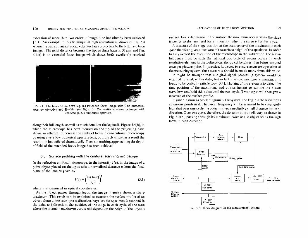
126 THEORY AND PRACTICE OF SCANNING OPTICAL MICROSCOPY APPLICATIONS OF DEPTH DISCRIMINATION 127
extension of more than two orders of magnitude has already been achieved[5.3]. An example of this technique at high resolution is shown in Fig. 5.4where the hairs on an ant's leg, with two hairs projecting to the left, have beenimaged. The axial distance between the tips of these hairs is 30 Ilm, and Fig.5.4(a) is an extended focus image which shows both excellently resolved
FIG. 5.4. The hairs on an ant's leg. (al Extended focus image with 0·85 numericalaperture objective and He-Ne laser light. (b) Conventional scanning image with
reduced (1/32) numerical aperture.
surface. For a depression in the surface, the maximum occurs when the stageis nearer to the lens, and for a projection when the stage is further away.
A measure of the stage position at the occurrence of the maximum in eachcycle therefore gives a measure of the surface height of the specimen. In ordcrto fully exploit the resolution of the microscope in the x-direction, the z-scanfrequency must be such that at least one cycle of z-scan occurs for eachresolution elemcnt in the x-direction: thc object height is then being sampledonce per picture point. In practice, however, to ensure accurate operation ofthe measuring system, the z-scan rate should be made many times this value.
It might be thought that a digital signal processing system would berequired to analyse this data, but in fact a simple analogue arrangement isfound to be perfectly satisfactory [5.4]. The aim of the system is to detect thetime position of the maximum, and at this instant to sample the z-scanwaveform and hold this value until the next cycle. This output will then give ameasure of the surface profile.
Figure 5.5 shows a block diagram of the system, and Fig. 5.6 the waveformsat various points in it. The z-scan frequency will be assumed to be sufficientlyhigh that over one cycle the object moves a negligibly small distance in the xdirection. Over one cycle, therefore, the detector output will vary as shown inFig. 5.6(b), passing through its maximum twice as the object scans throughfocus in each direction.
5.3 Surface profiling with the confocal scanning microscope
In the reflection confocal microscope, in the intensity I (u), in the image of apoint object placed on the optic axis a normalised distance u from the focalplane of the lens, is given by
where u is measured in optical coordinates.As the object passes through focus, the image intensity shows a sharp
maximum. This result can be exploited to measure the surface profile of anobject along a line scan (the x-direction, say). As the specimen is scanned inthe axial (z-) direction, the position of the stage in each cycle of the scanwhere the intensity maximum occurs will depend on the height of the object's
along their full length, as well as much detail on the leg itself. Figure 5.4(b), inwhich the microscope has been focused on the tip of the projecting hair,shows an attempt to increase the depth of focus in conventional microscopyby using a very low numerical aperture lens, but it is clear that as a result theresolution has suffered dramatically. Even so, nothing approaching the depthof field of the extended focus image has been achieved.
Penrecorder
~~f~tgt?~n ---------.----------------~system
FIG. 5.5. Block diagram of the measurement system.
(5.1 )(Sin (u/2 ))2
I(u)= --.u/2
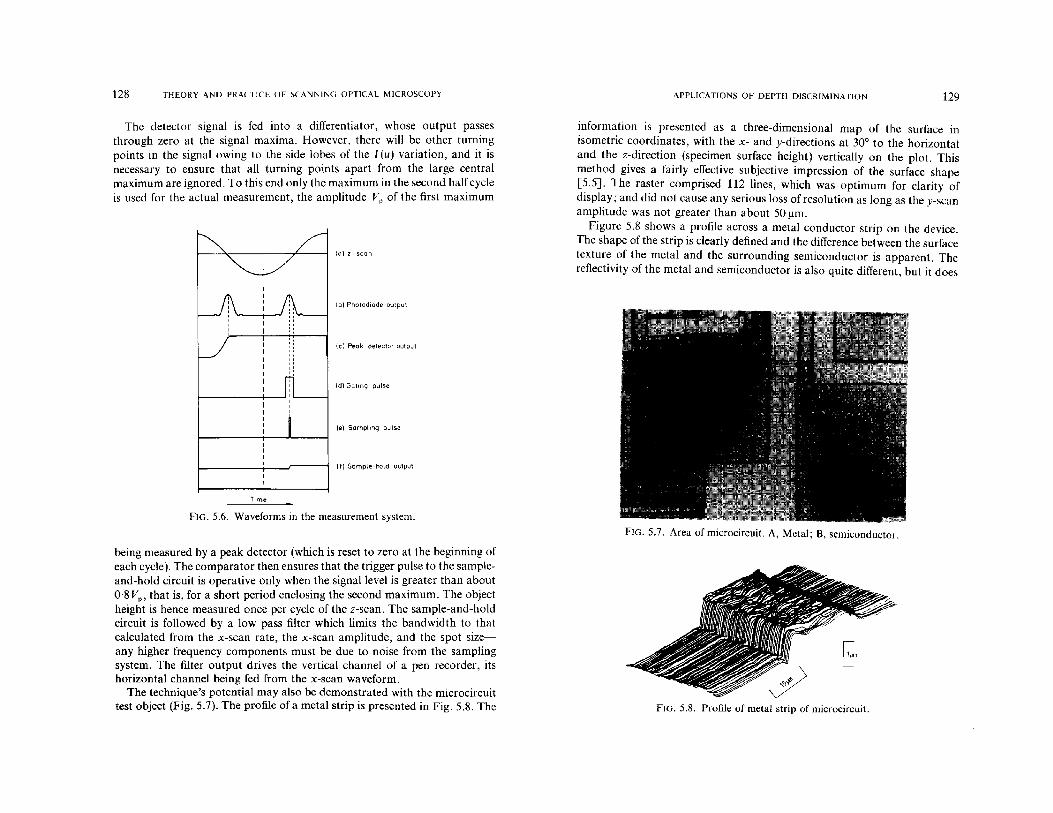
128 THEORY AND PRACTICE OF SCANNING OPTICAL MICROSCOPY APPLICATIONS OF DEPTH DISCRIMINATION 129
The detector signal is fed into a differentiator, whose output passesthrough zero at the signal maxima. However, there will be other turningpoints in the signal owing to the side lobes of the I (u) variation, and it isnecessary to ensure that all turning points apart from the large centralmaximum are ignored. To this end only the maximum in the second half cycleis used for the actual measurement, the amplitude Vp of the first maximum
(0) z- scan
(b) Photodiode output
{el Peal< detector outpul
(dl Galing pulse
(e) Sampling pulse
(f) Sample-hold oulput
Time
FIG. 5.6. Waveforms in the measurement system.
being measured by a peak detector (which is reset to zero at the beginning ofeach cycle). The comparator then ensures that the trigger pulse to the sampleand-hold circuit is operative only when the signal level is greater than about0·8 Vp , that is, for a short period enclosing the second maximum. The objectheight is hence measured once per cycle of the z-scan. The sample-and-holdcircuit is followed by a low pass filter which limits the bandwidth to thatcalculated from the x-scan rate, the x-scan amplitude, and the spot sizeany higher frequency components must be due to noise from the samplingsystem. The filter output drives the vertical channel of a pen recorder, itshorizontal channel being fed from the x-scan waveform.
The technique's potential may also be demonstrated with the microcircuittest object (Fig. 5.7). The profile of a metal strip is presented in Fig. 5.8. The
information is presented as a three-dimensional map of the surface inisometric coordinates, with the x- and y-directions at 30° to the horizontaland the z-direction (specimen surface height) vertically on the plot. Thismethod gives a fairly effective subjective impression of the surface shape[5.5]. The raster comprised 112 lines, which was optimum for clarity ofdisplay; and did not cause any serious loss of resolution as long as the y-scanamplitude was not greater than about 50 11m.
Figure 5.8 shows a profile across a metal conductor strip on the device.The shape of the strip is clearly defined and the difference between the surfacetexture of the metal and the surrounding semiconductor is apparent. Thereflectivity of the metal and semiconductor is also quite different, but it does
FIG. 5.7. Area of microcircuit. A, Metal; B, semiconductor.
FIG. 5.8. Profile of metal strip of microcircuit.
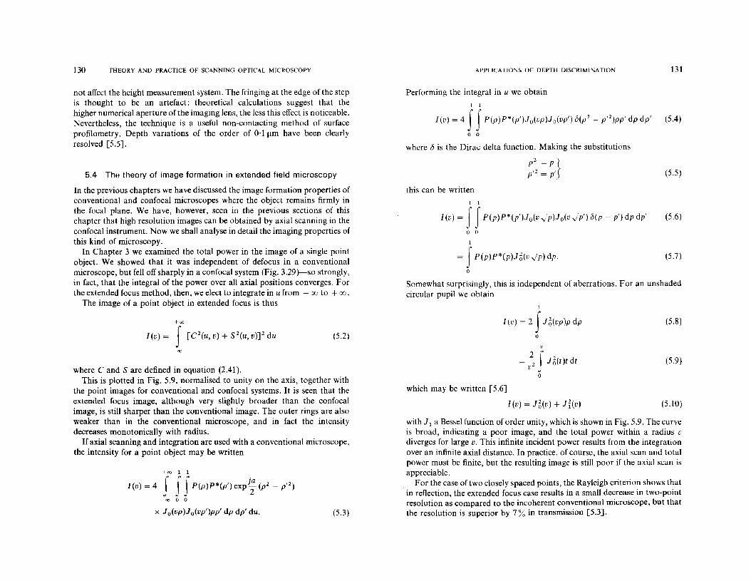
130 THEORY AND PRACTICE OF SCANNING OPTICAL MICROSCOPY APPLICATIONS OF DEPTH IJISCRIMINATION 131
not affect the height measurement system. The fringing at the edge of the stepis thought to be an artefact: theoretical calculations suggest that thehigher numerical aperture of the imaging lens, the less this effect is noticeable.Nevertheless, the technique is a useful non-contacting method of surfaceprofilometry. Depth variations of the order of 0·1 Jlm have been clearlyresolved [5.5].
Performing the integral in u we obtain
1 1
1(v) = 4 ffP(p)P*(p')Jo(rp)Jo(vp') b(p2 - p'2)pp' dp dp' (5.4)
o 0
where i5 is the Dirac delta function. Making the substitutions
where C and S are defined in equation (2.41).This is plotted in Fig. 5.9, normalised to unity on the axis, together with
the point images for conventional and confocal systems. It is seen that theextended focus image, although very slightly broader than the confocalimage, is still sharper than the conventional image. The outer rings are alsoweaker than in the conventional microscope, and in fact the intensitydecreases monotonically with radius.
If axial scanning and integration are used with a conventional microscope,the intensity for a point object may be written
5.4 The theory of image formation in extended field microscopy
In the previous chapters we have discussed the image formation properties ofconventional and confocal microscopes where the object remains firmly inthe focal plane. We have, however, seen in the previous sections of thischapter that high resolution images can be obtained by axial scanning in theconfocal instrument. Now we shall analyse in detail the imaging properties ofthis kind of microscopy.
In Chapter 3 we examined the total power in the image of a single pointobject. We showed that it was independent of defocus in a conventionalmicroscope, but fell off sharply in a confocal system (Fig. 3.29)-so strongly,in fact, that the integral of the power over all axial positions converges. Forthe extended focus method, then, we elect to integrate in u from - OCJ to + OCJ.
The image of a point object in extended focus is thus
this can be written
Somewhat surprisingly, this is independent of aberrations. For an unshadedcircular pupil we obtain
(5.9)
(5.8)
(5.10)
= 22r.I~(t)t dt
u Jo
1
l(v) = 2fJ~(vp)p dp
o
which may be written [5.6]
l(v) = .I6(v) + Ji(v)
1 1
l(v) = ffP(p)P*(p')Jo(v-lp).Io(v-lp') b(p - p') dp dp' (5.6)
o 0
1
= fP(p)P*(p)J~(u-lp) dp. (5.7)
o
p2 = p}p,2 = p' (5.5)
with.l 1 a Bessel function of order unity, which is shown in Fig. 5.9. The curveis broad, indicating a poor image, and the total power within a radius rdiverges for large v. This infinite incident power results from the integrationover an infinite axial distance. In practice, of course, the axial scan and totalpower must be finite, but the resulting image is still poor if the axial scan isappreciable.
For the case oftwo closely spaced points, the Rayleigh criterion shows thatin reflection, the extended focus case results in a small decrease in two-pointresolution as compared to the incoherent conventional microscope, but thatthe resolution is superior by 7 % in transmission [5.3].
(5.2)
(5.3)
+00
1(u) = f [C 2(u, v) + S2(U, V)]2 du
x J o(vp).Io(vp')pp' dp dp' duo
+ 00 1 1
1(u) = 4 JJJP(p)P*(p') expj; (p2 - p'2)
-00 0 0
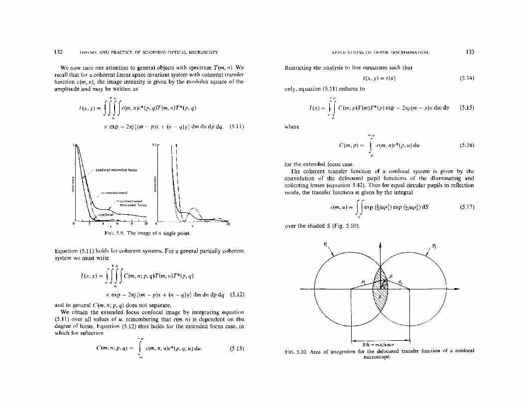
132 THEORY AND PRACTICE OF SCANNING OPTICAL MICROSCOPY APPLICATIONS OF DEPTH DISCRIMINATION 133
We now turn our attention to general objects with spectrum T(m, n). Werecall that for a coherent linear space invariant system with coherent transferfunction e(m, n), the image intensity is given by the modulus square of theamplitude and may be written as
Restricting the analysis to line structures such that
t(x, y) = t(x)
only, equation (5.11) reduces to
(5.14)
+00
J (x, y) = IIIIe(m, n)e*(p, q)T(m, n)T*(p, q)
+00
I(x)= II C(m;p)T(m)T*(p)exp-2nj(m-p)xdmdp (5.15)
x exp - 2nj{(m - p)x + (n - q)y} dm dn dp dq. (5.11) where
over the shaded S (Fig. 5.10).
(5.17)
(5.16)
+':.1)
elm; p) = I elm, n)c*(p, u) du
for the extended focus case.The coherent transfer function of a confocal system is given by the
convolution of the defocused pupil functions of the illuminating andcollecting lenses (equation 3.42). Thus for equal circular pupils in reflectionmode, the transfer function is given by the integral
elm, u) = IIexp (!jupi) exp (!jupD dS
s10
IiII\i\\i
0.1
10
,-convenllonal/ ex tended focus
~ conventional
/r-confoq.l extended focus
FIG. 5.9. The image of a single point.
Equation (5.11) holds for coherent systems. For a general partially coherentsystem we must write
+00
I(x, y) = IIIIC(m, n; p, q)T(m, n)T*(p, q)
x exp - 2nj{(m - p)x + (n - q)y} dm dn dp dq (5.12)
and in general C(m, n; p, q) does not separate.We obtain the extended focus confocal image by integrating equation
(5.11) over all values of u, remembering that elm, n) is dependent on thedegree of focus. Equation (5.12) thus holds for the extended focus case, inwhich for reflection
P,
pP,
+00
C(m, n; p, q) = f c(m, n, u)c*(p, q, u) duo (5.13 )2m = rnA/sin a
FIG. 5.10. Area of integration for the defocused transfer function of a confocalmicroscope.
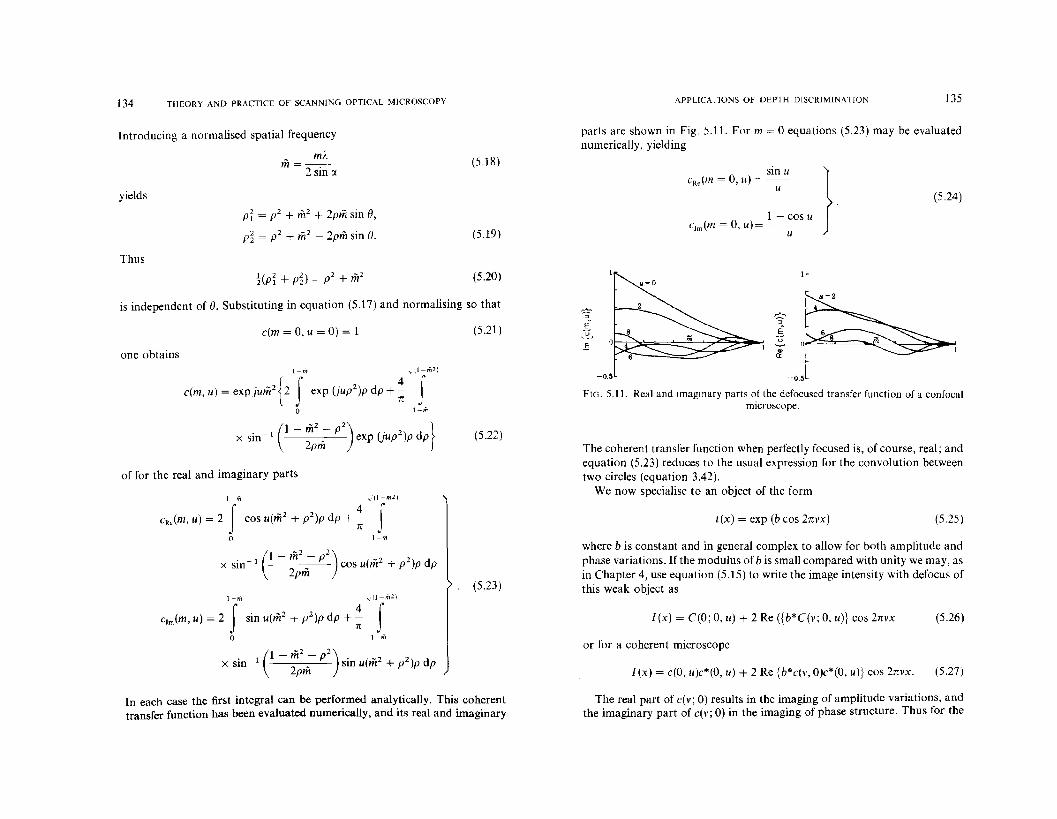
134 THEORY AND PRACTICE OF SCANNING OPTICAL MICROSCOPY APPLICATIONS OF DEPTH DISCRIMINATION 135
parts are shown in Fig. 5.11. For m = °equations (5.23) may be evaluatednumerically, yielding
Introducing a normalised spatial frequency
~ rnAm=--
2 sin ex
yields
pr = (12 + m2 + 2pm sin e,p~ = p2 + m2
- 2pm sin O.
(5.18)
(5.19)
sin ucRe(m = 0, u) =-
u
1 - cos Uc1m(m = 0, u)= .-
u
} (5.24)
Thus
is independent of O. Substituting in equation (5.17) and normalising so that
(5.21 )
(5.20)
c(m = 0, u = 0) = 1
one obtains
FIG. 5.11. Real and imaginary parts of the dcfocused transfer function of a confocalmicroscope.
I-m ,,(I-m 2)
c(m, u) = exPjUlii2
{ 2 f exp UU( 2)p dp + ~ fo I~m
-0.5 -0.5
I-m
The coherent transfer function when perfectly focused is, of course, real; andequation (5.23) reduces to the usual expression for the convolution betweentwo circles (equation 3.42).
We now specialise to an object of the form
where b is constant and in general complex to allow for both amplitude andphase variations. If the modulus of b is small compared with unity we may, asin Chapter 4, use equation (5.15) to write the image intensity with defocus ofthis weak object as
(5.26)
(5.27)
(5.25)t(x) = exp (b cos 2nvx)
lex) = C(O; 0, u) + 2 Re ({b*C(v; 0, u)} cos 2nvx
lex) = c(O, u)c*(O, u) + 2 Re {b*c(v, O)c*(O, u)} cos 2nvx.
or for a coherent microscope
(5.22)
(5.23)
. (1 -m2_ p2) . }x sm - 1 2pm exp UUp2)p dp
I-m ,/ll-ml)
Clm(m, U) = 2 f sin u(m2 + p2)p dp + ~ fo I-m
I-m ,.'(I-til 2 )
cRe(m, u) = 2 f cos u(m2 + p2)p dp + ~ fo
of for the real and imaginary parts
In each case the first integral can be performed analytically. This coherenttransfer function has been evaluated numerically, and its real and imaginary
The real part of c(v; 0) results in the imaging of amplitude variations, andthe imaginary part of c(v; 0) in the imaging of phase structure. Thus for the

136 THEORY AND PRACTICE OF SCANNING OPTICAL MICROSCOPYAPPLICATIONS OF DEPTH DISCRIMINATION 137
The real and imaginary parts of this weak object transfer function are shownin Fig. 5.12. It is seen that the real part is well behaved for values of u lessthan about six, by which time the magnitude of the real part is small anyway.The imaginary part, on the other hand, has a magnitude as large as 0·1
+1.1")
C(m; p) = f {cRe(m, u)cRe(p, u) + clm(m, u)crm(P, u)} du (5.29)
-00
around u = 2, which results in the image of phase variations, perhaps causedby specimen height variations. There are two completely different mechanisms whereby height variations may be imaged in confocal microscopy. Inthe first, the small variations in height are imaged by the transfer function,assumed constant over the corresponding part of the image. For example, ifthe transfer function is defocused by the presence of a constant displacementfrom the focal plane, small variations in height about this constant displacement are imaged by its imaginary part. In the second mechanism, the abso
.lute height variations are imaged by the optical sectioning property. It isdifficult to develop a theory which adequately incorporates both theseeffects, although it is apparent that the first mechanism results in contrastwhich is independent of numerical aperture, while the second becomesincreasingly more important at high numerical apertures.
If we now return to consider the transfer function of the extended focusconfocal microscope, we have from equation (5.16), for the weak objecttransfer function
(5.30)
that is, it is wholly real. Here we have made use of the relationship
cRe(m,-u)=cRe(m,u) }.crm(m, -u) = -clm(m, u)
Furthermore the relationships
(5.28)(
sin u) (1 -cos u) }CRe(v; 0, u) = ~u- '.J.,")" - -;;-- ',,(',"1 _
(sin u) (1 -cos u)
C1m(v; 0, u) = ~u- clm(v, u) - U cRe(v, u)
confocal microscope in reflection we have
-0.2
0.2
CRe ( -m, u) = cRe(m, u)}clm( -m, u) = c1m(m, u)
(5.31)
result in the symmetry conditions
8
oE
~.§
C(±m; ±p) = C(±p; ±m).
The weak object transfer function may be written
+00
C(m; 0) = f c(m, u)c*(O, u) du
(5.32)
(5.33)
where-0.2
FIG. 5.12. Real and imaginary parts of the defocused weak object transfer functionfor a confocal microscope.
c*(O, u) = L(exp - ju - 1).u
(5.34)
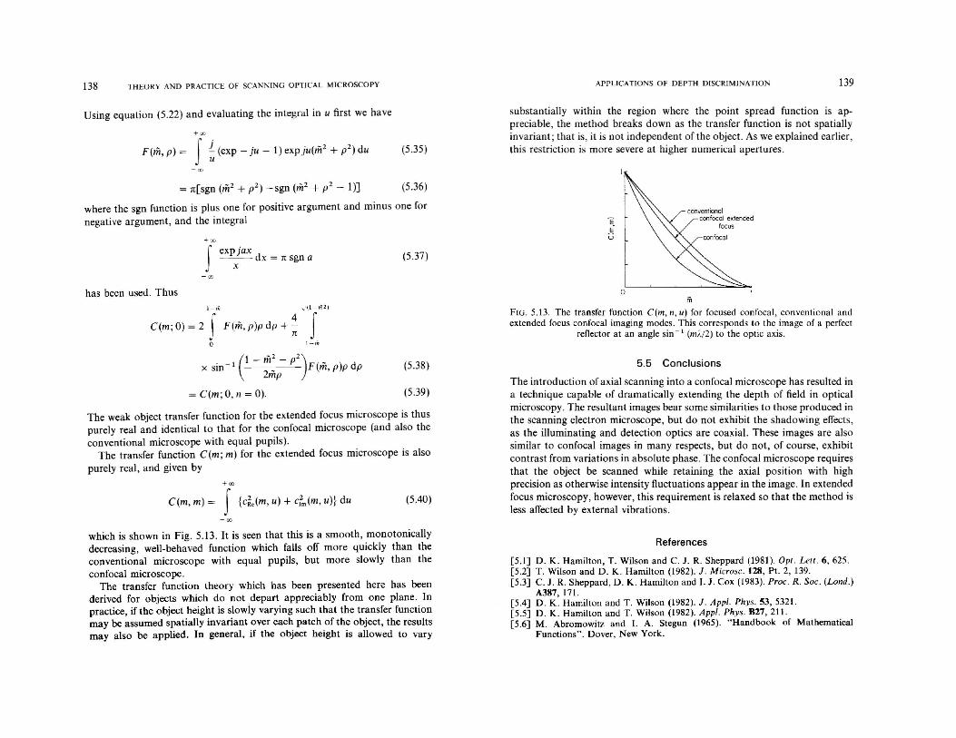
138 THEORY AND PRACTICE OF SCANNING OPTICAL MICROSCOPY APPLICATIONS OF DEPTH DISCRIMINATION 139
Using equation (5.22) and evaluating the integraJ in u first we have
+00
F(rn, p) = f f(exp - ju - 1) expju(rn2 + p2) du (5.35)
substantially within the region where the point spread function is appreciable, the method breaks down as the transfer function is not spatiallyinvariant; that is, it is not independent of the object. As we explained earlier,this restriction is more severe at higher numerical apertures.
where the sgn function is plus one for positive argument and minus one fornegative argument, and the integral
has been used. Thus
C(m; 0) = 2 T' F(rn, p)p dp + ~ .JIJ''''Io I-til
conventionalconfocal extended
focus
iiio
FIG. 5.13. The transfer function C(m, n, u) for focused confocal, conventional andextended focus confocal imaging modes. This corresponds 10 the image of a perfect
reflector at an angle sin - 1 (m}.(2) to the optic axis.
(5.37)
(5.36)
expjax--- dx = 'IT sgn a
x
+00
f-00
The weak object transfer function for the extended focus microscope is thuspurely real and identical to that for the confocal microscope (and also theconventional microscope with equal pupils).
The transfer function C(m; m) for the extended focus microscope is alsopurely real, and given by
x sin -I C-~;p- P2)F(rn, p)p dp
= C(m; 0, n = 0).
+00
C(m, m) = f {cie(m, u) + cfm(m, u)} du
(5.38)
(5.39)
(5.40)
5.5 Conclusions
The introduction of axial scanning into a confocal microscope has resulted ina technique capable of dramatically extending the depth of field in opticalmicroscopy. The resultant images bear some similarities to those produced inthe scanning electron microscope, but do not exhibit the shadowing effects,as the illuminating and detection optics are coaxial. These images are alsosimilar to confocal images in many respects, but do not, of course, exhibitcontrast from variations in absolute phase. The confocal microscope requiresthat the object be scanned while retaining the axial position with highprecision as otherwise intensity fluctuations appear in the image. In extendedfocus microscopy, however, this requirement is relaxed so that the method isless affected by external vibrations.
-00
which is shown in Fig. 5.13. It is seen that this is a smooth, monotonicallydecreasing, well-behaved function which falls off more quickly than theconventional microscope with equal pupils, but more slowly than theconfocal microscope.
The transfer function theory which has been presented here has beenderived for objects which do not depart appreciably from one plane. Inpractice, if the object height is slowly varying such that the transfer functionmay be assumed spatially invariant over each patch of the object, the resultsmay also be applied. In general, if the object height is allowed to vary
References
[5.1] D. K. Hamilton, T. Wilson and C. J. R. Sheppard (1981). Op!. Let!. 6, 625.[5.2] T. Wilson and D. K. Hamilton (1982). J. Microsc. 128, PI. 2, 139.[5.3] C. J. R. Sheppard, D. K. Hamilton and I. J. Cox (1983). Proc. R. Soc. (Land.)
A387,17t.[5.4] D. K. Hamilton and T. Wilson (1982). J. Appl. Phys. 53, 5321.[5.5] D. K. Hamilton and T. Wilson (1982). Appl. Phys. 827, 21t.[5.6] M. Abromowitz and I. A. Stegun (1965). "Handbook of Mathematical
Functions". Dover, New York.